
Technische Universitat Munchen
Wissenschaftszentrum Weihenstephan fur Ernahrung, Landnutzung und Umwelt
Fachgebiet fur Biostatistik
Statistical modeling of risk and trends in the life sciences with applications to forestry, plantbreeding, phenology, and cancer
Andreas Bock
Vollstandiger Abdruck der von der Fakultat Wissenschaftszentrum Weihenstephan fur Ernahrung,Landnutzung und Umwelt der Technischen Universitat Munchen zur Erlangung des akade-mischen Grades eines
Doktors der Naturwissenschaften
genehmigten Dissertation.
Vorsitzende: Univ.-Prof. Dr. Ch.-C. SchönPrufer der Dissertation:
1. Univ.-Prof. D. Pauler Ankerst, Ph.D.2. Univ.-Prof. Dr. A. Menzel
Die Dissertation wurde am 18.11.2013 bei der Technischen Universitat Munchen eingereichtund durch die Fakultat Wissenschaftszentrum Weihenstephan fur Ernahrung, Landnutzungund Umwelt am 17.04.2014 angenommen.


Statistical modeling of risk and trends in the lifesciences with applications to forestry, plant breeding,
phenology, and cancer
Andreas Bock


Danksagung
Danke sagen mochte ich . . .
. . . Donna Ankerst fur die außerst engagierte Betreuung und fachliche Unterstutzung.
. . . Chris-Carolin Schon und Yongle Li (Leo) fur die Einblicke in die Welt der Pflanzen-zucht und die Interaktion mit ihrem Lehrstuhl.
. . . Annette Menzel und Chiara Ziello fur das angenehme Zusammenspiel im Anwen-dungsbeispiel der Phanologie.
. . . Peter Biber und Jochen Dieler fur die begeisterte Aufklarung uber den Lebens-und Leidensweg der Baume.
. . . Hannes Petermeier fur fachlichen und freundschaftlichen Rat, gepaart mit tat-kraftiger Unterstutzung bei allen Problemen des Buro- und Campuslebens.
. . . Josef und Ulf fur ihre Hilfsbereitschaft und den kurzweiligen Buroalltag der letz-ten Jahre.
. . . Esther und Martina fur die Anmerkungen und Verbesserungsvorschlage zu dieserArbeit.
. . . meiner Familie.


Zusammenfassung
Empirische Belastbarkeit ist eine allgegenwartige Anforderung an die Forschung – auch
oder vor allem in den Lebenswissenschaften. In dieser Arbeit wird fur vier typische The-
mengebiete gezeigt, wie statistische Methodik eingesetzt wird um diesem Ziel gerecht zu
werden. Augenmerk liegt auf verschiedenen Stufen der statistischen Modellierung und dem
Verweis auf Uberschneidungen der eingesetzten Methodik zwischen den unterschiedlichen
thematischen Bereichen. Die Ergebnisse der statistischen Auswertungen werden anschaulich
prasentiert und in Bezug auf die inhaltliche Problemstellung interpretiert.
Im ersten Teil der Arbeit steht die Neuentwicklung eines Risikomodells fur die Forst-
wissenschaften im Fokus. Ziel ist es die Sterblichkeit einzelner Baume in Abhangigkeit
ihrer lokalen Konkurrenzsituation gegenuber anderen Baumen vorherzusagen. Die Modell-
entwicklung beginnt mit einer Bestandsaufnahme der vorhandenen Information, die sich in
Form der Stichprobe und der Literatur zu diesem Thema ausdruckt, und dem Definieren des
genauen Einsatzszenarios des zu erstellenden Modells. Mithilfe von Ergebnissen der deskrip-
tiven Auswertung im Bezug auf die beobachtete Sterblichkeit und den am Baum gemesse-
nen Großen, leiten wir daraus die Konsequenzen fur die statistische Modellbildung ab.
Eine geeignete Modellklasse wird vom zeitstetigen Coxmodell ausgehend unter Ausnutzung
der Gemeinsamkeit zum binaren Regressionsmodell hergeleitet. Zur Sterblichkeitsvorher-
sage dient die Verallgemeinerung des logistischen Regressionsmodells zur Klasse der gener-
alisierten additiven gemischten Modelle, die dem Stichprobendesign gerecht wird und eine
flexible Kombination von Kovariableneffekten ermoglicht. Fur die Variablenselektion inner-
halb dieser Klasse werden Maße zur Quantifizierung der Modellvorhersagegute eingefuhrt
und in einem Kreuzvalidierungsschema ausgewertet. Eine abschließende Vereinfachung der
Parametrisierung des Modells erlaubt eine unkomplizierte Anwendung und Implementierung.
Die im zweiten Teil dieser Arbeit betrachteten Versuchsreihen der Pflanzenzucht wurden
zum Zwecke einer Assoziationsstudie durchgefuhrt, von der Ruckschlusse fur die Zuchtung
robuster Roggenarten gezogen werden sollen. Aus statistischer Sicht stellen die Versuche sehr
gute Ausgangsbedingungen bereit, da es sich um geplante Experimente handelt, die mit Hilfe
von Randomisierung und Blockbildung die Einflusse von nicht beobachteten Bedingungen
quantifizierbar bzw. kontrollierbar machen. Ausgewertet werden die Beobachtungen mit-
tels eines gemischten linearen Modelles, das mehrere Ebenen des Verwandtschaftsgrades der
unterschiedlichen Arten zueinander berucksichtigt und den longitudinalen Aspekt der Ver-

Zusammenfassung
suchsreihen aufgreift. Die dafur eingesetzten Komponenten des Regressionsmodells werden
detailliert beschrieben. Zuletzt werden die genetischen Merkmale mit statistisch signifikan-
tem Zusammenhang zur Frosttoleranz prasentiert und eingeordnet.
Im Abschnitt aus dem Themengebiet der Phanologie wird untersucht wie sich die Blutezeit
verschiedener Arten im Laufe der letzten 30 Jahre geandert hat. Mit Techniken der Meta-
Analyse wird eine Vielzahl von lokal beobachteten Trends in ein statistisches Modell zusam-
mengefuhrt, und somit eine ubergreifende Betrachtung ermoglicht. Bei der Herangehensweise
wird die unterschiedliche Unsicherheit die den einzelnen Trends anhaftet berucksichtigt und
untersucht inwiefern der geographische Standort der Messstationen die Ergebnisse beein-
flusst. Unter anderem ließ sich beobachten, dass bei Arten, die ihre Pollen mithilfe des Windes
zu anderen Pflanzen ubertragen, der langjahrige Trend hin zu einem fruherem Blutebeginn
starker ausgepragt ist als bei Arten, die durch Insekten bestaubt werden. Nicht zuletzt sind
derartige Resultate fur die Allergologie relevant. Ob sich insgesamt auf eine langer werdende
Pollensaison schließen lasst, kann von den Ergebnissen der Studie nur indirekt angedeutet
werden. Es werden jedoch Ansatze aufgezeigt, wie sich diese Fragestellung mit ahnlichen
Daten empirisch untersuchen lasst.
Der Aspekt der Modellvalidierung wird im medizinischen Abschnitt erneut aufgegrif-
fen. Bestehende Risikomodelle fur Prostatakrebs werden auf ihren Nutzen hin bewertet.
Sie beruhen hauptsachlich auf dem prostataspezifischen Antigen und wurden entwickelt,
um Patienten und Arzten eine Hilfestellung zu geben, wann der mit Risiken verbundene
Eingriff einer Biopsie gerechtfertigt ist. Neben bereits eingefuhrter Maße zur Modellbew-
ertung wird ein weitere Große, welche die personlichen Umstande des Patienten mit ein-
bezieht, zur Beurteilung des Risikomodells herangezogen. Die Validierung findet an zehn
externen Kohorten statt, und gibt an ob das Risiko von Betroffenen, bei denen die Biopsie
nachtraglich tatsachlich einen Krebsbefund feststellen ließ, zuverlassig hoher bewertet wird
als bei Mannern ohne Prostatakrebsbefund. Wie auch das absolute Niveau der Risikovorher-
sage, das nur fur einen Teil der untersuchten Personen gut vorhersehbar ist, fallen die Resul-
tate gemischt aus, und hangen unter anderem von der unterschiedlichen Pravalenz/Inzidenz
in den Kohorten und den studienspezifischen Ablaufen ab.

Abstract
Empirical capacity is a ubiquitous claim for the research—even or especially in the life
sciences. In this work the use of statistical models to achieve this objective is presented in
four important areas of life science. The focus is on different stages of statistical modeling and
discussion of overlapping methodology in the diverse thematic areas. The results of statistical
analysis are presented vividly and interpreted in relation to the substantive problem.
The first part of this thesis focuses on the development of a risk model for the for-
est sciences aiming to predict the mortality of individual trees as a function of their local
competition from other trees. The model development starts with an inventory of existing
information, which is expressed in the form of the sample and literature on this topic, and
the definition of the exact deployment scenario of the model to be created. Together with
the results of descriptive analyses in relation to the observed mortality and measured tree
quantities the consequences for statistical modeling are derived. A suitable model meeting
the requirements is deduced from the continuous-time Cox model by exploiting the equiva-
lence to binary regression models when transitioning to the discrete case. For prediction of
mortality, the generalization of standard logistic regression models to the class of general-
ized additive mixed models is used allowing to map the sampling design and to include a
flexible combination of covariate effects. For purpose of variable selection within this class
metrics quantifying different aspects of the predictive quality of the model are presented and
evaluated in a cross-validation scheme. A parametrical simplification of the chosen model
ensures ease of use and implementation. The estimation of the proposed model is based
on over 14,000 individual observations in the experimental plots and a combination of four
competition indices.
The growing trials of plant breeding considered in this work were conducted for an associ-
ation study aiming to draw conclusions for breeding robust species of rye. From a statistical
point of view, these planned experiments are advantageous to quantify and control unob-
served conditions by means of randomization and blocking building. The trials are analyzed
using linear mixed models taking multiple levels of relationship between different varieties
of rye and longitudinal data structures into account. A detailed description of the individual
components of the regression models is made and the genetic characteristics with significant
association to frost tolerance are discussed.
The phenology section examines whether the flowering dates of different species have

Abstract
changed over the last 30 years. With techniques of meta-analysis, a variety of locally observed
trends is merged in a statistical model allowing for a powerful overarching assessment. In
this approach, the uncertainty that adheres to the individual trends is taken into account
and it is examined how the spatial variation has to be considered in the analysis of the
developments. Among other things, significant indications exist that for species relying on
the wind to carry their pollen to other plants, the long-term trend to flower earlier in the
year is more pronounced than for species pollinated by insects. Not least, such findings are
relevant for the field of allergology. Whether longer pollen seasons are to be expected in
the future may only be indirectly indicated by the results of the study. However, possible
modeling approaches on how to investigate this issue empirically on similar kinds of data
are given.
The focal point in the medical section is model validation. The usefulness of existing risk
models for prostate cancer is investigated; these models are mainly based on the prostate
specific antigen and designed to help patients and physicians to determine whether a biopsy
with its inherent risks is warranted. Besides established measures of model performance
another metric is introduced, which includes the personal circumstances of the patient in
the assessment of the risk model. The validation is implemented by means of ten external
cohorts, and indicates whether the risk of persons where the subsequently performed biopsy
actually detects cancer is predicted reliably higher than in men without prostate cancer
diagnosis. It is shown that the absolute level of risk predictions is calibrated only for a
part of the investigated persons and that the results vary depending on the cohort-specific
prevalence/incidence and study-specific procedures.

Publications
This thesis contains parts which have already appeared or will appear in publications
where discussed statistical methodology has been used. Those publications and the associated
author contributions are:
(1) A. Bock, J. Dieler, P. Biber, H. Pretzsch, and D. P. Ankerst (2013). Predicting tree
mortality for European Beech in Southern Germany using spatially explicit competition
indices. Forest Science. To appear.
A.B. derived the statistical concept, performed all data handling and statis-
tical analysis and wrote the paper. H.P. provided the data and P.B. and J.D.
advice on the data. D.A. provided supervision and helped with the paper
editing.
(2) Y. Li, A. Bock, G. Haseneyer, V. Korzun, P. Wilde, C.-C. Schon, D. P. Ankerst, and
E. Bauer (2011). Association analysis of frost tolerance in rye using candidate genes
and phenotypic data from controlled, semi-controlled, and field phenotyping platforms.
BMC Plant Biology 11, 146.
Y.L. and A.B. share first authorship; Y.L. carried out the candidate gene
and population structure analysis and drafted the manuscript, while A.B.
conceived the statistical models, performed the statistical analyses, including
relevant graphics, and drafted the methods and results sections concerning
statistics. G.H. participated in the molecular analyses and interpretation of
the results. D.A. reviewed all statistics. V.K. provided SSR marker data.
P.W. developed the plant material. E.B. and C.S. designed and coordinated
the study and interpreted the results. All authors edited the final manuscript.
(3) C. Ziello, A. Bock, N. Estrella, D. P. Ankerst, and A. Menzel (2012). First flowering
of wind-pollinated species with the greatest phenological advances in Europe. Ecogra-
phy 35 (11), 1017–1023.
C.Z. and A.M. conceived the analysis. Specifically, A.B. developed the idea
of applying weighted linear mixed models for the meta analysis of the COST
data, selected statistical methods and wrote R scripts. C.Z. performed the
analyses and wrote the paper. N.E., D.A. and A.M. edited the final paper.

(4) D. P. Ankerst, A. Bock, S. J. Freedland, I. M. Thompson, A. M. Cronin, M. J. Roobol,
J. Hugosson, J. Stephen Jones, M. W. Kattan, E. A. Klein, F. Hamdy, D. Neal, J. Dono-
van, D. J. Parekh, H. Klocker, W. Horninger, A. Benchikh, G. Salama, A. Villers, D. M.
Moreira, F. H. Schroder, H. Lilja, and A. J. Vickers (2012). Evaluating the PCPT risk
calculator in ten international biopsy cohorts: results from the prostate biopsy collab-
orative group. World Journal of Urology 30 (2), 181–187, and
(5) D. P. Ankerst, A. Bock, S. J. Freedland, J. Stephen Jones, A. M. Cronin, M. J. Roobol,
J. Hugosson, M. W. Kattan, E. A. Klein, F. Hamdy, D. Neal, J. Donovan, D. J. Parekh,
H. Klocker, W. Horninger, A. Benchikh, G. Salama, A. Villers, D. M. Moreira, F. H.
Schroder, H. Lilja, A. J. Vickers, and I. M. Thompson (2012). Evaluating the prostate
cancer prevention trial high grade prostate cancer risk calculator in 10 international
biopsy cohorts: results from the prostate biopsy collaborative group. World Journal of
Urology . To appear.
A.B. conceived the statistical plan and performed all statistical analysis. Due
to membership in the consortium D.A. was required to be first author and
wrote the manuscript. All other authors contributed data.

Contents
Introduction 1
1 Forestry 9
1.1 Introduction . . . . . . . . . . . . . . . . . . . . . . . . . . . . . . . . . . . . 9
1.2 Data and exploratory methods . . . . . . . . . . . . . . . . . . . . . . . . . . 11
1.2.1 Data source and mortality . . . . . . . . . . . . . . . . . . . . . . . . 11
1.2.2 Variables and risk factors . . . . . . . . . . . . . . . . . . . . . . . . . 12
1.2.3 Contrasting risk factors in mortality versus non-mortality periods . . 16
1.3 Model development . . . . . . . . . . . . . . . . . . . . . . . . . . . . . . . . 22
1.3.1 Exploratory results and implications for modeling . . . . . . . . . . . 22
1.3.2 Literature review for individual tree mortality models . . . . . . . . . 29
1.3.3 From Cox to GAMM . . . . . . . . . . . . . . . . . . . . . . . . . . . 33
1.3.4 Final model structure . . . . . . . . . . . . . . . . . . . . . . . . . . . 39
1.3.5 Selection of risk factors . . . . . . . . . . . . . . . . . . . . . . . . . . 40
1.3.6 Measures of model performance . . . . . . . . . . . . . . . . . . . . . 41
1.4 Mortality prediction model . . . . . . . . . . . . . . . . . . . . . . . . . . . . 42
1.4.1 Model equation . . . . . . . . . . . . . . . . . . . . . . . . . . . . . . 42
1.4.2 Contrasting performance . . . . . . . . . . . . . . . . . . . . . . . . . 46
1.5 Summary and outlook . . . . . . . . . . . . . . . . . . . . . . . . . . . . . . 47
2 Plant breeding 49
2.1 Introduction . . . . . . . . . . . . . . . . . . . . . . . . . . . . . . . . . . . . 49
2.2 Methods . . . . . . . . . . . . . . . . . . . . . . . . . . . . . . . . . . . . . . 50
2.2.1 Plant material and DNA extraction . . . . . . . . . . . . . . . . . . . 50
2.2.2 Phenotypic data assessment . . . . . . . . . . . . . . . . . . . . . . . 51
2.2.3 Obtaining genetic components for association model . . . . . . . . . . 52
2.2.4 SNP-FT association model . . . . . . . . . . . . . . . . . . . . . . . . 53
2.2.5 Phenotypic variation . . . . . . . . . . . . . . . . . . . . . . . . . . . 55
2.2.6 About the kinship matrix . . . . . . . . . . . . . . . . . . . . . . . . 56
2.2.7 Platform-specific model details . . . . . . . . . . . . . . . . . . . . . . 60
2.2.8 Haplotype-FT association model and gene×gene interaction . . . . . 62
2.2.9 Obtaining model-based results . . . . . . . . . . . . . . . . . . . . . . 62
2.3 Results . . . . . . . . . . . . . . . . . . . . . . . . . . . . . . . . . . . . . . . 63
2.3.1 Phenotypic data analyses . . . . . . . . . . . . . . . . . . . . . . . . . 63
2.3.2 Population structure and kinship . . . . . . . . . . . . . . . . . . . . 65
2.3.3 Association analyses . . . . . . . . . . . . . . . . . . . . . . . . . . . 65
2.4 Discussion . . . . . . . . . . . . . . . . . . . . . . . . . . . . . . . . . . . . . 71
CONTENTS
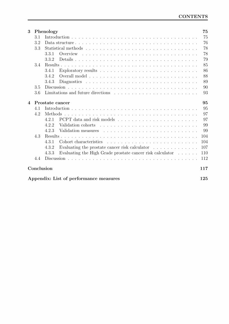
3 Phenology 753.1 Introduction . . . . . . . . . . . . . . . . . . . . . . . . . . . . . . . . . . . . 753.2 Data structure . . . . . . . . . . . . . . . . . . . . . . . . . . . . . . . . . . . 763.3 Statistical methods . . . . . . . . . . . . . . . . . . . . . . . . . . . . . . . . 78
3.3.1 Overview . . . . . . . . . . . . . . . . . . . . . . . . . . . . . . . . . 783.3.2 Details . . . . . . . . . . . . . . . . . . . . . . . . . . . . . . . . . . . 79
3.4 Results . . . . . . . . . . . . . . . . . . . . . . . . . . . . . . . . . . . . . . . 853.4.1 Exploratory results . . . . . . . . . . . . . . . . . . . . . . . . . . . . 863.4.2 Overall model . . . . . . . . . . . . . . . . . . . . . . . . . . . . . . . 883.4.3 Diagnostics . . . . . . . . . . . . . . . . . . . . . . . . . . . . . . . . 89
3.5 Discussion . . . . . . . . . . . . . . . . . . . . . . . . . . . . . . . . . . . . . 903.6 Limitations and future directions . . . . . . . . . . . . . . . . . . . . . . . . 93
4 Prostate cancer 954.1 Introduction . . . . . . . . . . . . . . . . . . . . . . . . . . . . . . . . . . . . 954.2 Methods . . . . . . . . . . . . . . . . . . . . . . . . . . . . . . . . . . . . . . 97
4.2.1 PCPT data and risk models . . . . . . . . . . . . . . . . . . . . . . . 974.2.2 Validation cohorts . . . . . . . . . . . . . . . . . . . . . . . . . . . . 994.2.3 Validation measures . . . . . . . . . . . . . . . . . . . . . . . . . . . 99
4.3 Results . . . . . . . . . . . . . . . . . . . . . . . . . . . . . . . . . . . . . . . 1044.3.1 Cohort characteristics . . . . . . . . . . . . . . . . . . . . . . . . . . 1044.3.2 Evaluating the prostate cancer risk calculator . . . . . . . . . . . . . 1074.3.3 Evaluating the High Grade prostate cancer risk calculator . . . . . . 110
4.4 Discussion . . . . . . . . . . . . . . . . . . . . . . . . . . . . . . . . . . . . . 112
Conclusion 117
Appendix: List of performance measures 125
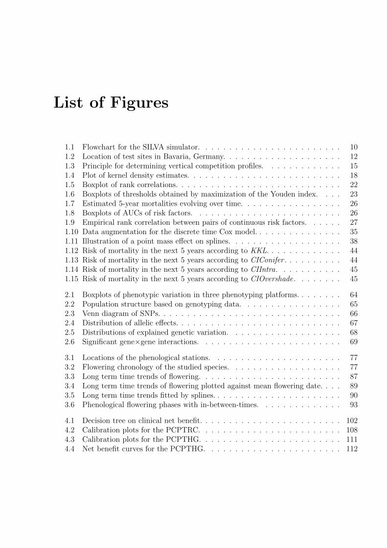
List of Figures
1.1 Flowchart for the SILVA simulator. . . . . . . . . . . . . . . . . . . . . . . . 101.2 Location of test sites in Bavaria, Germany. . . . . . . . . . . . . . . . . . . . 121.3 Principle for determining vertical competition profiles. . . . . . . . . . . . . 151.4 Plot of kernel density estimates. . . . . . . . . . . . . . . . . . . . . . . . . . 181.5 Boxplot of rank correlations. . . . . . . . . . . . . . . . . . . . . . . . . . . . 221.6 Boxplots of thresholds obtained by maximization of the Youden index. . . . 231.7 Estimated 5-year mortalities evolving over time. . . . . . . . . . . . . . . . . 261.8 Boxplots of AUCs of risk factors. . . . . . . . . . . . . . . . . . . . . . . . . 261.9 Empirical rank correlation between pairs of continuous risk factors. . . . . . 271.10 Data augmentation for the discrete time Cox model. . . . . . . . . . . . . . . 351.11 Illustration of a point mass effect on splines. . . . . . . . . . . . . . . . . . . 381.12 Risk of mortality in the next 5 years according to KKL. . . . . . . . . . . . . 441.13 Risk of mortality in the next 5 years according to CIConifer . . . . . . . . . . 441.14 Risk of mortality in the next 5 years according to CIIntra. . . . . . . . . . . 451.15 Risk of mortality in the next 5 years according to CIOvershade. . . . . . . . 45
2.1 Boxplots of phenotypic variation in three phenotyping platforms. . . . . . . . 642.2 Population structure based on genotyping data. . . . . . . . . . . . . . . . . 652.3 Venn diagram of SNPs. . . . . . . . . . . . . . . . . . . . . . . . . . . . . . . 662.4 Distribution of allelic effects. . . . . . . . . . . . . . . . . . . . . . . . . . . . 672.5 Distributions of explained genetic variation. . . . . . . . . . . . . . . . . . . 682.6 Significant gene×gene interactions. . . . . . . . . . . . . . . . . . . . . . . . 69
3.1 Locations of the phenological stations. . . . . . . . . . . . . . . . . . . . . . 773.2 Flowering chronology of the studied species. . . . . . . . . . . . . . . . . . . 773.3 Long term time trends of flowering. . . . . . . . . . . . . . . . . . . . . . . . 873.4 Long term time trends of flowering plotted against mean flowering date. . . . 893.5 Long term time trends fitted by splines. . . . . . . . . . . . . . . . . . . . . . 903.6 Phenological flowering phases with in-between-times. . . . . . . . . . . . . . 93
4.1 Decision tree on clinical net benefit. . . . . . . . . . . . . . . . . . . . . . . . 1024.2 Calibration plots for the PCPTRC. . . . . . . . . . . . . . . . . . . . . . . . 1084.3 Calibration plots for the PCPTHG. . . . . . . . . . . . . . . . . . . . . . . . 1114.4 Net benefit curves for the PCPTHG. . . . . . . . . . . . . . . . . . . . . . . 112
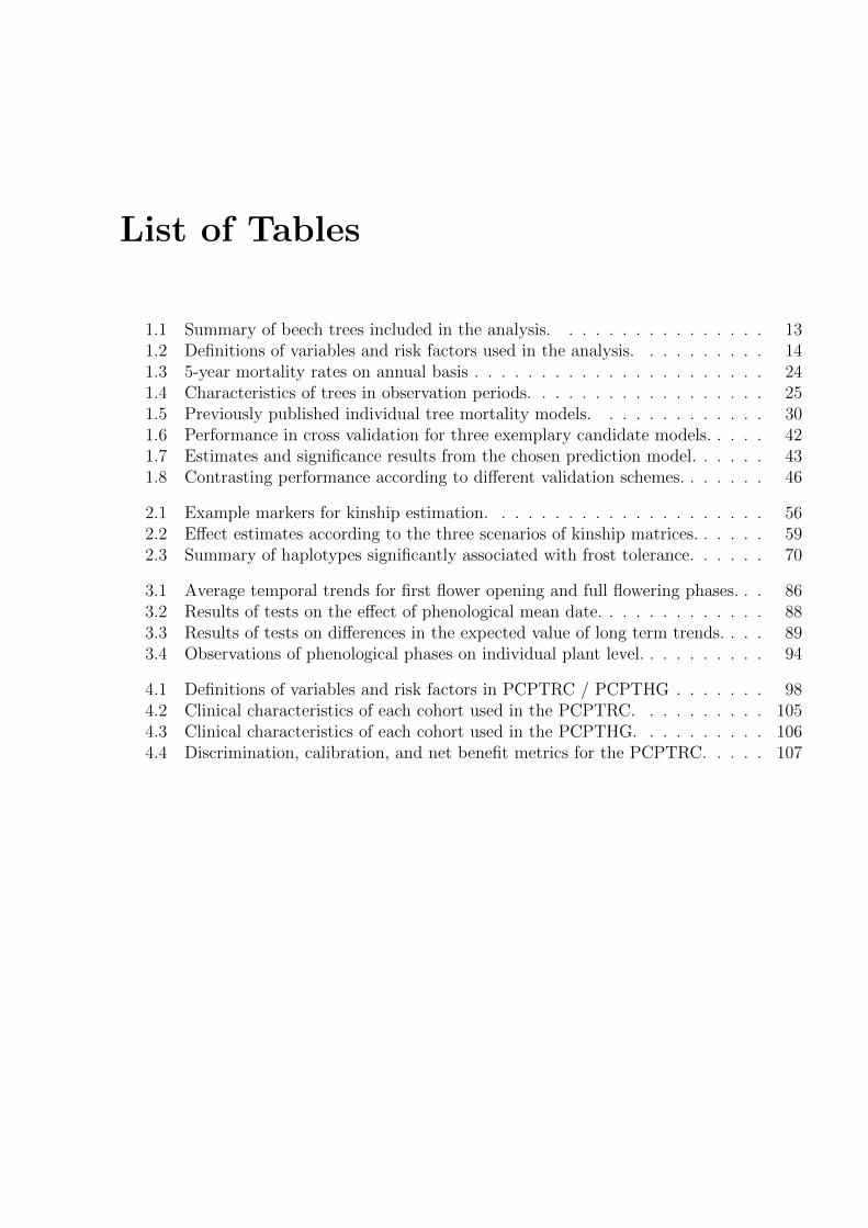
List of Tables
1.1 Summary of beech trees included in the analysis. . . . . . . . . . . . . . . . 131.2 Definitions of variables and risk factors used in the analysis. . . . . . . . . . 141.3 5-year mortality rates on annual basis . . . . . . . . . . . . . . . . . . . . . . 241.4 Characteristics of trees in observation periods. . . . . . . . . . . . . . . . . . 251.5 Previously published individual tree mortality models. . . . . . . . . . . . . 301.6 Performance in cross validation for three exemplary candidate models. . . . . 421.7 Estimates and significance results from the chosen prediction model. . . . . . 431.8 Contrasting performance according to different validation schemes. . . . . . . 46
2.1 Example markers for kinship estimation. . . . . . . . . . . . . . . . . . . . . 562.2 Effect estimates according to the three scenarios of kinship matrices. . . . . . 592.3 Summary of haplotypes significantly associated with frost tolerance. . . . . . 70
3.1 Average temporal trends for first flower opening and full flowering phases. . . 863.2 Results of tests on the effect of phenological mean date. . . . . . . . . . . . . 883.3 Results of tests on differences in the expected value of long term trends. . . . 893.4 Observations of phenological phases on individual plant level. . . . . . . . . . 94
4.1 Definitions of variables and risk factors in PCPTRC / PCPTHG . . . . . . . 984.2 Clinical characteristics of each cohort used in the PCPTRC. . . . . . . . . . 1054.3 Clinical characteristics of each cohort used in the PCPTHG. . . . . . . . . . 1064.4 Discrimination, calibration, and net benefit metrics for the PCPTRC. . . . . 107

Introduction
Empirical evidence forms the basis for inference in the life sciences. Accordingly, much
effort and cost are invested in performing trials, recording, collecting, and storing data.
Statistical methodology deals with finding optimal approaches in terms of planning, ascer-
tainment, and analysis. Therefore it is imperative to additionally involve the capabilities of
modern statistical methods to enhance subject matter understanding. The aim of this thesis
is to quantify the risk of certain threats in different fields of the life sciences in order to more
accurately predict the occurrence of these threats in the future. Therefore, risk models for
application in forestry, plant breeding, phenology, and oncology are developed and validated
using modern state-of-the-art statistical methodology.
One of the most basic statistical association models is linear regression and it is the fun-
dament for the analyses of the plant breeding experiments of Chapter 2 and the phenological
observations in Chapter 3. Through linear regression the impact of one or more exploratory
variables x on a metric quantity y can be statistically examined presuming the additive
relationship
y = β0 + β1 x1 + . . .+ βp xp.
Although called the linear model, nonlinear relationships can be accommodated by trans-
forming either the outcome or explanatory variables. As it is not realistic to assume a strictly
deterministic relationship between y and x and measurements do not have infinite accuracy,
the above equation is extended by a probabilistic term, here in an additive manner, leading
to a proposed model for a sample of n observations:
yi = β0 + β1i x1i + . . .+ βp xpi + εi = x′iβ + εi, i = 1, . . . , n.
For the distribution of ε an assumption is made, which should reflect the sample design
and accurately describe the distribution of the observed data, which can be checked in a
subsequent residual analysis. A standard choice is to assume independent and identically
distributed (iid) normal errors εiiid∼ N(0, σ2). This implies that the data y are randomly
collected, are independent, and are normally distributed given x, with equal variance (ho-
mogeneity of variance). No distributional assumption is made for the parameter vector β
in this model. Alternative assumptions for the error term allow to formulate advanced ap-

2 Introduction
proaches, with t-distributed errors yielding robust regression for the mean, and asymmetric
Laplace distributed errors yielding quantile regression for quantiles of the distribution, in
particular the median.
Whenever possible and meaningful the design of an experiment or data collection should
provide a metric outcome, since continuous metric data provide richer information than
categorical or grouped data. Coarsening by grouping into classes, such as by dichotomizing
size into small/medium/large, results in a loss of information in likelihood-based inference.
However, truly categorical outcomes, such as mortality (alive versus dead) must be modeled
on the categorical scale. Relating a dichotomous variable such as mortality to covariates
can be achieved by a statistical model that effectively inserts a metric variable in between.
An unobservable (latent) variable is postulated as being the driving force behind mortality.
The latent variable exists on a continuum (such as severity of bad health) and when it
reaches a threshold, the outcome of mortality is experienced. This is in fact the statistical
definition of the commonly used logistic regression model for binary events. Specifically, the
observed variable y assumes either value 0 or 1, such as corresponding to alive versus dead,
respectively. It connects to a latent variable y with threshold τ by the mechanism
y =
1 (dead) if y > τ
0 (alive) if y ≤ τ.
A probabilistic model is assumed for the latent variable conditional on observed covariates:
yi = β0 + β1i x1i + . . .+ βp xpi + εi, i = 1, . . . , n.
From this relationship, the probability of death for the ith individual, π, is
πi = P(yi = 1) = P(x′iβ + εi > τ) = 1− h(−x′iβ),
where h(.) is the cumulative density function assumed for ε. Specifying h(.) as the standard
logistic distribution
h(η) =exp(η)
1 + exp(η)
results in the logistic regression model for y on x:
P(yi = 1|xi) =exp(x′iβ)
1 + exp(x′iβ)i = 1, . . . , n.
In contrast to linear regression for metric outcomes, there is no free variance parameter in
the logistic error distribution. Its fixed value is needed for unique estimation of β1, . . . , βp.
Otherwise only the ratio of two β coefficients would be unambiguous. Another restriction
is made by specifying τ = 0 to obtain an identifiable intercept β0. Loosely speaking, these

Introduction 3
restrictions pay tribute to the fact that the scale of y is unknown and the sample of binary y
observations does not allow to extract information concerning dispersion in the underlying
vector of probabilities πi. Impacts which can be attributed to theses scale issues in comparison
to linear models are discussed in Mood (2010).
Logistic regression has become the most commonly used model for binary outcomes
and risk prediction in medical statistics (it is used in this context in Chapter 4). This
can be attributed to the fact that it provides meaningful interpretable effect estimates in
retrospective case control designs as well as in prospective cohort studies. A commonly
encountered example provides an illustration, which also introduces some basic metrics in
risk modeling. Of key interest in epidemiological studies is the quantification of the relative
risk (RR) of exposed individuals E (for example, smokers) compared to non-exposed E (non-
smokers) for developing a certain disease (lung cancer). This can be achieved by setting up
a cohort of healthy persons comprising both exposed and non-exposed individuals who are
followed over a time period of, say, 20 years. The data obtained from this kind of study
results in the following 2 by 2 table, where the letters a, b, c, d represent the observed counts:
Developed disease
Exposed D (yes) D (no)
E (yes) a b
E (no) c d
The risk of the disease for exposed individuals, πE, is estimated by a/(a + b), and for non-
exposed individuals, πE, by c/(c + d). The relative risk of the disease associated with the
exposure thus is
RR(D) =πEπE.
Another metric quantifying the impact of the exposure is the odds ratio (OR) (Szumilas,
2010). It begins with the odds (odds) in favor of an event, which is the ratio of the probability
that the event happens to the probability that the event does not happen:
odds(D|E) =πE
1− πE(odds in exposed),
odds(D|E) =πE
1− πE(odds in non-exposed),
OR(D) =odds(D|E)
odds(D|E),
which is estimated by
OR(D) =a · db · c
.
For a rare disease, when probabilities πE and πE to develop the disease are small for both
4 Introduction
exposed and non-exposed, respectively, the relative risk can be approximated by the odds
ratio, RR(D) ≈ OR(D). However, for rare diseases the prospective design of a cohort study
is not efficient. Hundreds of thousands of individuals must be followed for long periods
of time in order to capture sufficient numbers of diseased cases, incurring a prohibitive cost
burden. An alternative concept to circumvent this problem is to perform a case-control study
(Breslow et al., 1980). Here, individuals are not followed until outbreak of the disease, but
individuals suffering from the disease (cases) are selected from a population retrospectively,
such as through the scanning of hospital records. Suitable controls without the disease are
matched according to individual factors, such as being in similar age. The exposure status is
established afterwards. The case-control design is a leading competitor for modeling the rare
event of tree mortality in forests covered in Chapter 1. The limitation of the case-control
design is that it is not possible to infer the risk of disease as the counts of cases and controls
are artificially fixed. The advantage is that the odds ratio can still be used to approximate
the relative risk because odds ratios behave symmetrically in terms of switching disease and
exposure,
OR(E) =odds(E|D)
odds(E|D)=odds(D|E)
odds(D|E)= OR(D).
For the relative risk this is not valid in general: RR(D) 6= RR(E).
The parameters β1, . . . , βp of the logistic regression model parametrize the log odds ratio
with respect to a unit change in the according covariates x1, . . . , xp. Thus, logistic regression
can be used to estimate the odds ratio in the case-control design. If we set y = 1 for all
cases, y = 0 for all controls, x = 1 for all exposed individuals, x = 0 for the non-exposed,
and estimate the model
P(y = 1|x) =exp(β0 + β1x)
1 + exp(β0 + β1x).
then the odds ratio of disease with respect to exposure is
P(y = 1|x = 1)
1−P(y = 1|x = 1)
/ P(y = 1|x = 0)
1−P(y = 1|x = 0)= exp(β1).
One is able to retrieve useful effect estimates regardless of the base level of mortality. The
strength of using a model-based approach, such as logistic regression, over traditional epi-
demiological tabular methods, is the easy expandability to account for multiple risk factors
and confounders by including additional parameters. The ubiquitous use of logistic regression
is not confined to the medical context. It can be used whenever the objective is to quantify
the probability of occurrence of specific events or the presence of certain characteristics or
states. In forestry, it is the dominant model for the prediction of tree mortality (cf. Table
1.5). A peculiarity to be minded in this context is that the proportion of trees where mor-
tality was actually observed is very low (rare events). Consequences for the performance of
logistic regression are discussed in King and Zeng (2001).
Introduction 5
Alternatively, event data may be more finely modeled in terms of the time until the
event occurs. Time to event data are addressed by survival models. In practice, there is
often the situation that the time spans of observations are recorded only coarsely, leading
to discrete time survival models. Discrete survival time models may be approximated by
logistic regression models, as we will perform in our analyses of mortality of beech trees in
a German network that inspected trees only approximately every 5 years (Chapter 1).
If rich time-to-event data are available in metric form, Cox regression is a common choice,
since it accommodates censoring of observations, which occurs when individuals are known
to survive only up to a specific time point but not what happens afterwards, allows the
incorporation of covariates in terms of a linear predictor affecting a hazard ratio, and makes
no parametric assumptions on the baseline hazard (Cox, 1972). This model is not described
in more detail here since none of the outcomes in this thesis were of the continuous time-
to-event type, but issues and potential future directions would apply analogously as for the
other statistical models used here. Approaches towards survival models which make more
explicit use of the actually observed time spans than the Cox model, which only employs
the chronological order of the events, are dealt with in Kneib and Fahrmeir (2004) and
Carstensen (2005).
A central issue to all the statistical models that incorporate explanatory variables to
explain variation is how to incorporate random effects to account for residual heterogeneity
due to less tangible effects, such as by differences in geographic locations or by machine. The
term mixed models reflects the fact that the model comprises further random effects with
a distributional assumption in addition to fixed effects which are understood as unknown
but existent true (hence fixed) quantities (McCulloch and Searle, 2001). Mixed models have
made it into routine practice in virtually all fields of the life sciences including ecology (Zuur,
2009), medicine (Brown and Prescott, 2006), veterinary research (Duchateau et al., 1998),
agricultural sciences (Gbur et al., 2012), and animal breeding (Mrode and Thompson, 2005).
However, the application of mixed models is less motivated by the philosophy about inter-
preting quantities as random or fixed but more motivated by the pragmatism to flexibly
incorporate subjective understandings in the model. Furthermore, mixed models have their
frequentist counterpart in penalized estimation approaches. The connection of ridge regres-
sion with the normality assumption of random effects is the one example. The purposes of
random effects in mixed models range from accounting for the hierarchical structure of the
sample (trees organized in plots, measurements originating from phenological stations, block
building in growing trials), incorporating secondary information about the sample (related-
ness of genotypes, geographic coordinates), and achieving a data-driven selection of model
complexity (penalized splines, baseline mortality over time). The strength of generalized
mixed models is to allow rather any combinations of such building blocks in the systematic
part of the model independently from the outcome-specific distribution. By replacing a series
of repeated analyses (say over different trials) into a single analysis using random effects,
6 Introduction
multiple testing is more controllable, the power (effective sample size) of the experiment is
increased, and inference concerning global versus site-specific trends is permitted. For this
reason, mixed models are used in most of the applications in this thesis (Chapters 1–3).
Whatever the type of statistical model, external validation on a completely independent
data set is the proof of principle that the model can be used in practice. State-of-the art
approaches in the application and validation of statistical modeling for a variety of outcome
types and experimental settings are demonstrated in the remaining chapters of this thesis.
In Chapter 1 (Forestry) we examine the steps of model development, which involve de-
scriptive analyses, a literature review of similar studies, and the presentation of imposed
consequences. The final risk model is derived from a discrete approximation to the Cox
model and is refined to the class of generalized additive mixed models. The statistical tools
applied include nonparametric tests, function approximation using splines and the specifica-
tion of random effects reflecting spatial and temporal structures of dependency. Model selec-
tion is based on performance measures which were calculated in a cross validation scheme.
Accompanying graphs illustrate a way of communicating the results.
In Chapter 2 (Plant breeding), we present an association study with the objective of de-
ducting new breeding programs on robust kinds of rye. For this study growing trials on several
genotypes in three different platforms were designed and conducted employing techniques
of randomization and block-building. The results are related to the occurring variations of
genetic markers in the plant genome. These markers were selected in advance to cover re-
gions linked to frost tolerance as indicated by previous studies (candidate gene approach).
The statistical association model includes the genetic similarity of different genotypes ex-
plicitly and accounts for the particular sampling design. By application of this model several
genetic markers are identified, which are most promising across all three platforms in terms
of breeding purposes.
Chapter 3 (Phenology) covers a meta analysis on phenological data. The aim of the
analysis was to infer the developments in long-term trends for different species from the
records of flowering dates available in aggregated form in the COST (European Cooperation
in Science and Technology) network. In detail, we investigate potential evidence that flow-
ering dates of wind pollinated species have advanced more than insect pollinated plants and
whether the length of the flowering season within a calendar year has become longer in the
past decades, as pollen in the air are a major trigger for allergies. We demonstrate how to
treat observations which do not arise from a simple random sample and how to handle the
multiple testing problem arising when several hypotheses are examined on the same data.
Further, we show how a spatial correlation structure can be embedded in the model and use
bootstrap combined with spline methods for diagnostic purposes.
In Chapter 4 (Cancer) we assess the quality and benefit of model-based prostate cancer
predictions. Prostate cancer is one of the leading causes of cancer death in men in Western
Europe and the United States; more than 670,000 men are diagnosed with prostate cancer

Introduction 7
every year (European Randomized study of Screening for Prostate Cancer, 2013). Two ex-
isting prostate cancer risk calculators are validated using new external data not involved in
the preceding development stage. We introduce measures that evaluate the prediction per-
formance in terms of calibration and discrimination abilities. Further, we discuss whether
usage of these calculators can provide a clinical benefit for the considered validation cohorts.
Finally we conclude with a discussion on future research needed for the modeling of
outcomes of the type that have arisen in the four applications of this thesis.

8 Introduction
Chapter 1
Forestry
Parts of the following chapter will be published in “Predicting tree mortality for European
beech in southern Germany using spatially explicit competition indices” by A. Bock, J.
Dieler, P. Biber, H. Pretzsch, and D. P. Ankerst (accepted in Forest Science 2013). Figure
1.2 was provided by Jochen Dieler, Figure 1.3 by Peter Biber. Figures which are equivalent
to those of the article are indicated with “reproduced”, those which are similar but basing
on different data with “in style of”.
1.1 Introduction
Tree mortality prediction is an essential component of single tree-based forest growth
models, including the growth simulator SILVA (Pretzsch et al., 2002). The SILVA simulation
software was developed in 1989 and is since maintained by the Chair for Forest Growth and
Yield at the Technische Universitat Munchen (SILVA website, 2013). It allows the simulation
of forest growth for complex structured pure and mixed stands following an individualized
tree approach. A stand is seen as a system of single trees having different characteristics,
that mutually influence each other. Inter-tree relationships are derived from positions and
sizes of trees relative to each other, and used to calculate competition indices (CI), which
in turn enter the simulation model. The user can specify various scenarios for thinning con-
cepts and intensity up to a maximum simulation length of 145 years. The program updates
the forest profile at 5-year intervals. The results can be assessed in terms of timber produc-
tion, and economical and structural characteristics, which are useful for decision-making in
forest as well as landscape management, for educational purposes, and as leads to further
scientific enquiries. The general simulation procedure takes place in three steps: 1.) Set up
the management and site conditions, and, if needed, complete missing information via the
stand structure generator; 2.) Calculate the competition measures and apply the model for
mortality, thinning, and increment; 3.) Generate the various outputs.
10 Chapter 1. Forestry
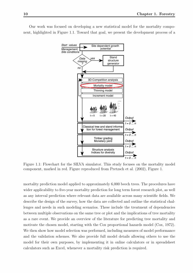
Our work was focused on developing a new statistical model for the mortality compo-
nent, highlighted in Figure 1.1. Toward that goal, we present the development process of a
Figure 1.1: Flowchart for the SILVA simulator. This study focuses on the mortality modelcomponent, marked in red. Figure reproduced from Pretzsch et al. (2002), Figure 1.
mortality prediction model applied to approximately 6,000 beech trees. The procedures have
wider applicability to five-year mortality prediction for long term forest research plot, as well
as any interval prediction where relevant data are available across many scientific fields. We
describe the design of the survey, how the data are collected and outline the statistical chal-
lenges and needs in such modeling scenarios. These include the treatment of dependencies
between multiple observations on the same tree or plot and the implications of tree mortality
as a rare event. We provide an overview of the literature for predicting tree mortality and
motivate the chosen model, starting with the Cox proportional hazards model (Cox, 1972).
We then show how model selection was performed, including measures of model performance
and the validation schemes. We also provide full model details allowing others to use the
model for their own purposes, by implementing it in online calculators or in spreadsheet
calculators such as Excel, whenever a mortality risk prediction is required.
1.2 Data and exploratory methods 11
1.2 Data and exploratory methods
1.2.1 Data source and mortality
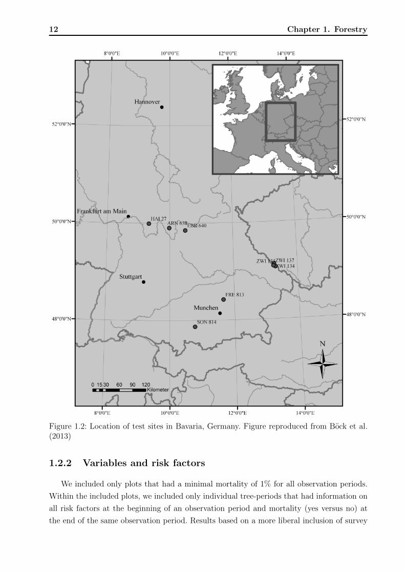
Data were collected from beech trees taken from multiple plots at eight test sites in
Bavaria, Germany that were undergoing surveillance from 1985 until 2007 (Figure 1.2).
Individual trees were observed between one to four observation periods during these years,
with observation periods ranging from three to ten years (most five years). Individual tree-
periods where the tree experienced mortality through man-made thinning or natural disasters
such as storms were excluded. Generally, the terms mortality and mortality rate are used
interchangeably, denoting the number of deaths by a certain cause occurring in a given
population at risk during a specified time period (World Health Organization, 2013). As
the observed mortality rates were based on time periods of different lengths, they only have
limited interpretability. Therefore we also calculated standardized 5-year mortality rates.
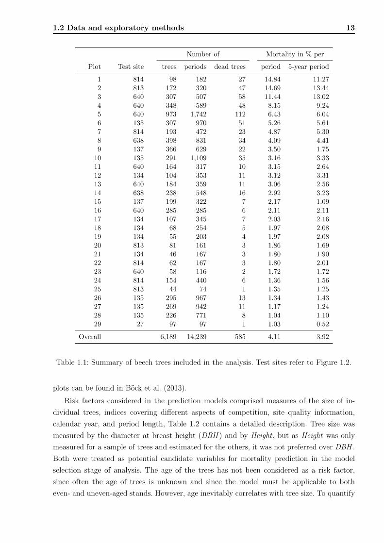
The inclusion criteria resulted in 6,189 beech trees and 14,239 tree-periods from 29 plots.
The data are summarized in Table 1.1.
12 Chapter 1. Forestry
Figure 1.2: Location of test sites in Bavaria, Germany. Figure reproduced from Bock et al.(2013)
1.2.2 Variables and risk factors
We included only plots that had a minimal mortality of 1% for all observation periods.
Within the included plots, we included only individual tree-periods that had information on
all risk factors at the beginning of an observation period and mortality (yes versus no) at
the end of the same observation period. Results based on a more liberal inclusion of survey
1.2 Data and exploratory methods 13
Number of Mortality in % per
Plot Test site trees periods dead trees period 5-year period
1 814 98 182 27 14.84 11.272 813 172 320 47 14.69 13.443 640 307 507 58 11.44 13.024 640 348 589 48 8.15 9.245 640 973 1,742 112 6.43 6.046 135 307 970 51 5.26 5.617 814 193 472 23 4.87 5.308 638 398 831 34 4.09 4.419 137 366 629 22 3.50 1.75
10 135 291 1,109 35 3.16 3.3311 640 164 317 10 3.15 2.6412 134 104 353 11 3.12 3.3113 640 184 359 11 3.06 2.5614 638 238 548 16 2.92 3.2315 137 199 322 7 2.17 1.0916 640 285 285 6 2.11 2.1117 134 107 345 7 2.03 2.1618 134 68 254 5 1.97 2.0819 134 55 203 4 1.97 2.0820 813 81 161 3 1.86 1.6921 134 46 167 3 1.80 1.9022 814 62 167 3 1.80 2.0123 640 58 116 2 1.72 1.7224 814 154 440 6 1.36 1.5625 813 44 74 1 1.35 1.2526 135 295 967 13 1.34 1.4327 135 269 942 11 1.17 1.2428 135 226 771 8 1.04 1.1029 27 97 97 1 1.03 0.52
Overall 6,189 14,239 585 4.11 3.92
Table 1.1: Summary of beech trees included in the analysis. Test sites refer to Figure 1.2.
plots can be found in Bock et al. (2013).
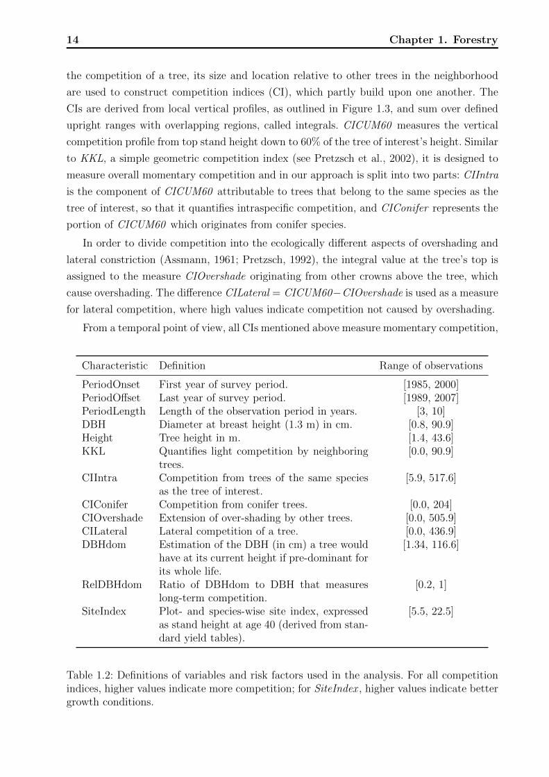
Risk factors considered in the prediction models comprised measures of the size of in-
dividual trees, indices covering different aspects of competition, site quality information,
calendar year, and period length, Table 1.2 contains a detailed description. Tree size was
measured by the diameter at breast height (DBH ) and by Height , but as Height was only
measured for a sample of trees and estimated for the others, it was not preferred over DBH .
Both were treated as potential candidate variables for mortality prediction in the model
selection stage of analysis. The age of the trees has not been considered as a risk factor,
since often the age of trees is unknown and since the model must be applicable to both
even- and uneven-aged stands. However, age inevitably correlates with tree size. To quantify
14 Chapter 1. Forestry
the competition of a tree, its size and location relative to other trees in the neighborhood
are used to construct competition indices (CI), which partly build upon one another. The
CIs are derived from local vertical profiles, as outlined in Figure 1.3, and sum over defined
upright ranges with overlapping regions, called integrals. CICUM60 measures the vertical
competition profile from top stand height down to 60% of the tree of interest’s height. Similar
to KKL, a simple geometric competition index (see Pretzsch et al., 2002), it is designed to
measure overall momentary competition and in our approach is split into two parts: CIIntra
is the component of CICUM60 attributable to trees that belong to the same species as the
tree of interest, so that it quantifies intraspecific competition, and CIConifer represents the
portion of CICUM60 which originates from conifer species.
In order to divide competition into the ecologically different aspects of overshading and
lateral constriction (Assmann, 1961; Pretzsch, 1992), the integral value at the tree’s top is
assigned to the measure CIOvershade originating from other crowns above the tree, which
cause overshading. The difference CILateral = CICUM60−CIOvershade is used as a measure
for lateral competition, where high values indicate competition not caused by overshading.
From a temporal point of view, all CIs mentioned above measure momentary competition,
Characteristic Definition Range of observations
PeriodOnset First year of survey period. [1985, 2000]PeriodOffset Last year of survey period. [1989, 2007]PeriodLength Length of the observation period in years. [3, 10]DBH Diameter at breast height (1.3 m) in cm. [0.8, 90.9]Height Tree height in m. [1.4, 43.6]KKL Quantifies light competition by neighboring
trees.[0.0, 90.9]
CIIntra Competition from trees of the same speciesas the tree of interest.
[5.9, 517.6]
CIConifer Competition from conifer trees. [0.0, 204]CIOvershade Extension of over-shading by other trees. [0.0, 505.9]CILateral Lateral competition of a tree. [0.0, 436.9]DBHdom Estimation of the DBH (in cm) a tree would
have at its current height if pre-dominant forits whole life.
[1.34, 116.6]
RelDBHdom Ratio of DBHdom to DBH that measureslong-term competition.
[0.2, 1]
SiteIndex Plot- and species-wise site index, expressedas stand height at age 40 (derived from stan-dard yield tables).
[5.5, 22.5]
Table 1.2: Definitions of variables and risk factors used in the analysis. For all competitionindices, higher values indicate more competition; for SiteIndex , higher values indicate bettergrowth conditions.
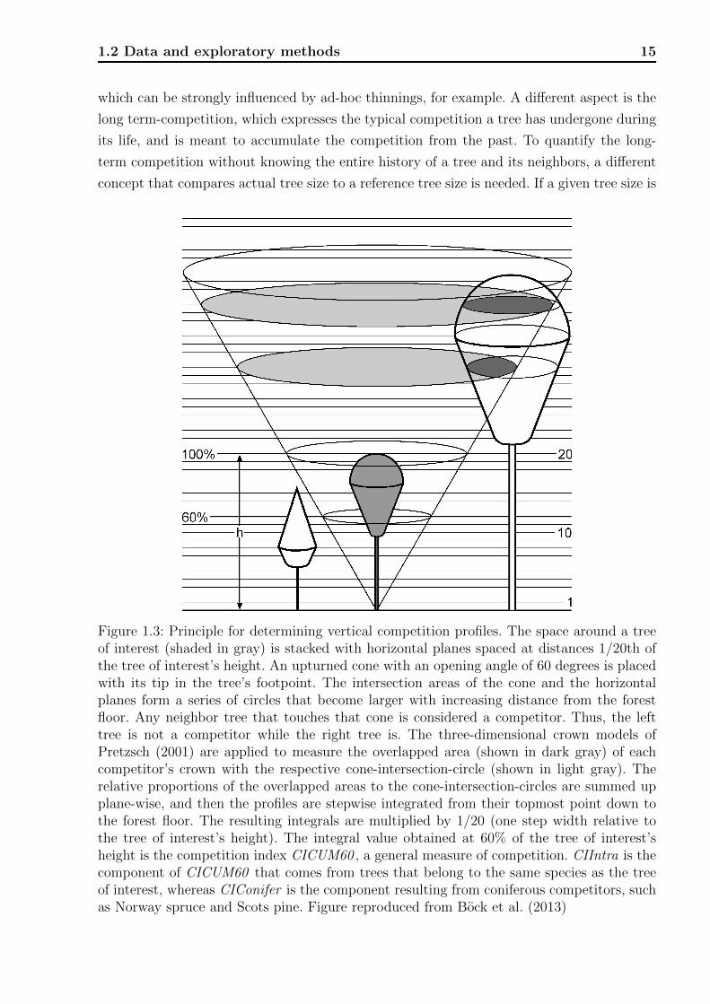
1.2 Data and exploratory methods 15
which can be strongly influenced by ad-hoc thinnings, for example. A different aspect is the
long term-competition, which expresses the typical competition a tree has undergone during
its life, and is meant to accumulate the competition from the past. To quantify the long-
term competition without knowing the entire history of a tree and its neighbors, a different
concept that compares actual tree size to a reference tree size is needed. If a given tree size is
Figure 1.3: Principle for determining vertical competition profiles. The space around a treeof interest (shaded in gray) is stacked with horizontal planes spaced at distances 1/20th ofthe tree of interest’s height. An upturned cone with an opening angle of 60 degrees is placedwith its tip in the tree’s footpoint. The intersection areas of the cone and the horizontalplanes form a series of circles that become larger with increasing distance from the forestfloor. Any neighbor tree that touches that cone is considered a competitor. Thus, the lefttree is not a competitor while the right tree is. The three-dimensional crown models ofPretzsch (2001) are applied to measure the overlapped area (shown in dark gray) of eachcompetitor’s crown with the respective cone-intersection-circle (shown in light gray). Therelative proportions of the overlapped areas to the cone-intersection-circles are summed upplane-wise, and then the profiles are stepwise integrated from their topmost point down tothe forest floor. The resulting integrals are multiplied by 1/20 (one step width relative tothe tree of interest’s height). The integral value obtained at 60% of the tree of interest’sheight is the competition index CICUM60 , a general measure of competition. CIIntra is thecomponent of CICUM60 that comes from trees that belong to the same species as the treeof interest, whereas CIConifer is the component resulting from coniferous competitors, suchas Norway spruce and Scots pine. Figure reproduced from Bock et al. (2013)

16 Chapter 1. Forestry
small compared to a reference tree size, the tree must have experienced strong competition in
the past and vice versa. As trees under competition suffer a reduction in diameter increment
more than in height increment, the DBHdom measure is used as a reference. This measure
is defined as the DBH a pre-dominant tree has at a given height and is estimated as follows.
From a subsample of the data the allometric relationship, DBHdom = 0.6553 ·Height1.327, is
estimated (assuming the units m for Height and cm for DHB) and used to estimate the DBH
a tree could have achieved at its current height under very low competition during its life
up until the present. Dividing the tree’s current DBH by the estimated DBHdom yields the
measure RelDBHdom. Low values of RelDBHdom indicate the tree has undergone stronger
long-term competition, while larger values near or even exceeding 1 indicate the tree has not
suffered much competition throughout its life. Finally, site quality (SiteIndex ) is expressed
through the expected mean stand height in m at age 40 years based on the yield table for
European beech by Schober (1967).
In addition to the tree-related characteristics, variables originating from the sampling
design were included in the analysis. The calendar years at the beginning and end of each
observation period are denoted as periodOnset and periodOffset , the time between those,
as periodLength. A description of all variables acting as candidates to be included in the
prediction model are summarized in Table 1.2.
To report mortality as a function of time we restructured the observations and calculated
the mortality rate on a calendar year basis. The mortality rate within a calendar year was
calculated by the ratio
Number of mortalities during calendar year
Number of observed trees at risk during the calendar year,
where number of trees at risk are those that were alive and in the study at the beginning
of the calendar year. The exact year of mortality of a specific tree is not known within its
period of observation and was therefore distributed uniformly during the respective period.
For example, a tree observed as dead at the end of the survey period from 1995 to 1998,
contributes 1/3 to the numerator, and 1 to the denominator for each of the three years.
Finally, the annual mortality rates were translated to 5-year rates by multiplying by 5 (van
Belle and Fisher, 2004, chap. 15). We present the 5-year mortality for each year, along with
95% confidence intervals obtained from a normal approximation to the binomial distribution,
as well as the number of deaths and exposure time. The course of mortality over the years,
which is smoothed owing to the calculation method, is also displayed as graph.
1.2.3 Contrasting risk factors in mortality versus non-mortality
periods
In a primary stage towards the prediction model we evaluated each risk variable sepa-
rately. The object of investigation was whether and how values of the risk factors differed
1.2 Data and exploratory methods 17
between tree-observation periods that resulted in mortality versus non-mortality. We pre-
ferred this by-period approach to an analysis at tree level, as the latter would require a
longitudinal analysis of the trees or a reduction of multiple observations of the same tree to
a single one. For this in turn, further assumptions are needed, it does not reflect the aspired
by-period prediction and moreover does not make use of the entire data set. Indeed, the sta-
tistical tests in the following paragraph rely on the assumption of independent observations
and we will discuss to what extent this assumption is justified in the model development
section.
By means of numerical statistical measures and tests we compared risk factors and obser-
vational characteristics between tree-observation periods with and without mortality using
means, standard deviations (SD), and ranges. As a measure of association between a con-
tinuous variable (risk factor) and a dichotomous variable (mortality) we report the area
underneath the receiver operating characteristic (ROC) curve (AUC)(Tom, 2006). Techni-
cally, the ROC curve is a graph of the false positive fraction (FPF) against the true positive
fraction (TPF) for all possible thresholds of a the risk factor. The FPF is the proportion of
alive subjects with a risk factor higher than the threshold, that means erroneously classi-
fied as dead and TPF is the proportion of dead subjects with a risk factor higher than the
threshold. Let x ∈ R be the risk factor, y ∈ {0; 1} the observed mortality being 1 for a dead
tree, 0 for a live tree, and cut the threshold, then the FPF and TPF are calculated as
FPFcut =
∑I(xi > cut)I(yi = 0)∑
I(yi = 0)
and
TPFcut =
∑I(xi > cut)I(yi = 1)∑
I(yi = 1),
respectively, where the sum includes all observations i = 1, . . . , n and the indicator func-
tion I() evaluates to 1 if the statement in its argument holds and 0 otherwise. The AUC
quantifies the ability of a risk factor to distinguish between mortality and non-mortality
periods. It equals the probability that for a randomly chosen pair of single tree observation
periods, where one observation period of the pair resulted in mortality and the other not,
the risk factor is higher for the period with mortality (if high values of the risk factor are
associated with mortality, lower otherwise). An AUC close to 100% indicates good discrim-
ination of the risk factor for mortality, while an AUC close to 50% indicates that the risk
factor exhibits no better discriminating ability between observation periods with mortality
versus non-mortality than flipping a coin. So, in its standard form AUC is reported as a
number between 0.5 and 1 and does not provide information about the direction in which a
risk factor acts, that is whether high values of the risk factor indicate mortality. We provide
this additional information when needed. As a rank-based measure the AUC is invariant to
18 Chapter 1. Forestry
monotone transformations, which means it leads to the same conclusion whether or not a
monotone transformation is applied to the risk factor. It can be shown that the Wilcoxon
0.00
0.01
0.02
0.03
0.04
0.05
0.06
0.07
0.08
0.09
0.10
0 10 20 30 40 50 60 70 80 90DBH
Den
sity
Status atend of period
alivedead
0.0
0.5
1.0
1.5
2.0
2.5
3.0
3.5
1.0 1.1 1.2 1.3 1.4 1.5 1.6 1.7 1.8 1.9 2.0
DBH3 20
Den
sity
0.00
0.01
0.02
0.03
0.04
0.05
0.06
0.07
0.08
0 5 10 15 20 25 30 35 40 45Height
Den
sity
0.00
0.05
0.10
0.15
0.20
0.25
1 2 3 4 5 6 7 8 9 10 11 12
Height2 3
Den
sity
0.00
0.05
0.10
0.15
0.20
0.25
0.30
0 10 20 30 40 50 60KKL
Den
sity
0.0
0.1
0.2
0.3
0.4
0.5
0.6
0.7
0.8
0.0 0.5 1.0 1.5 2.0 2.5 3.0 3.5 4.0
KKL1 3
Den
sity
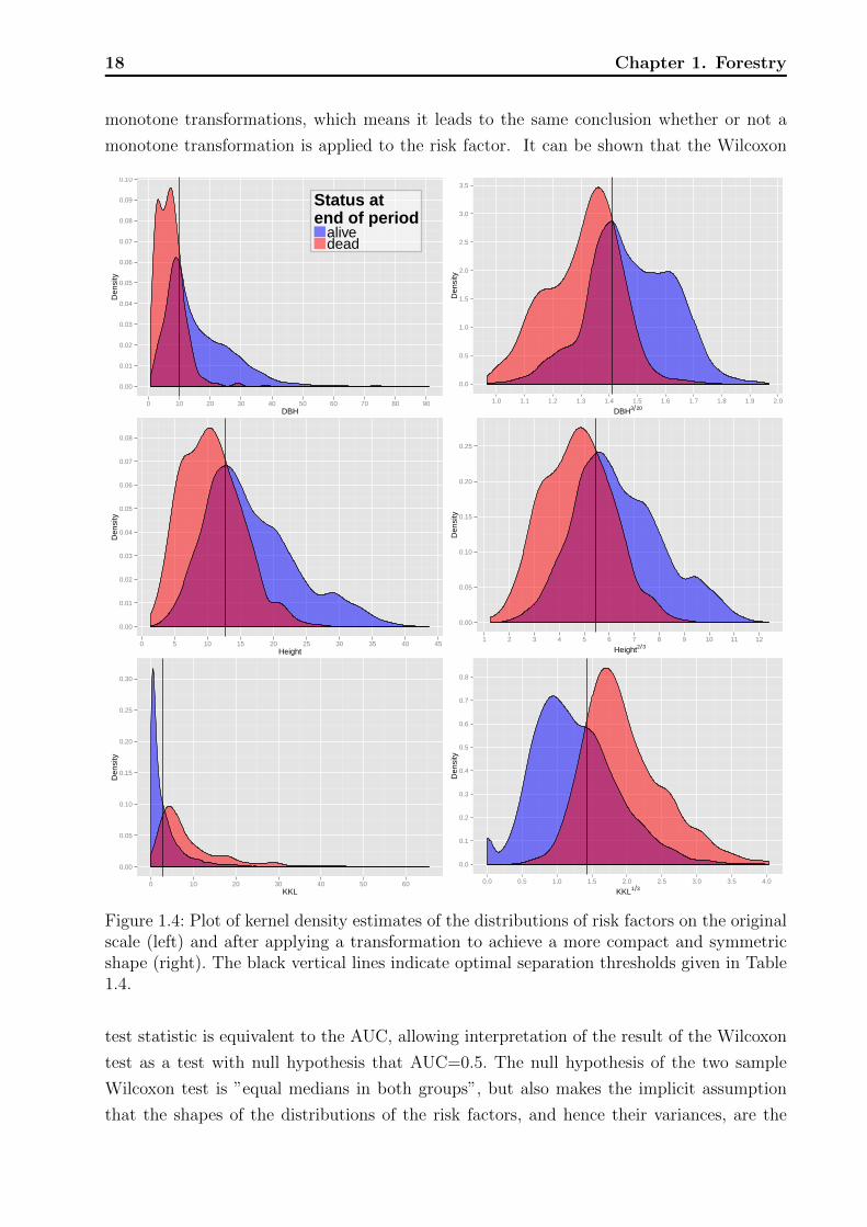
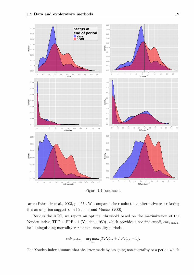
Figure 1.4: Plot of kernel density estimates of the distributions of risk factors on the originalscale (left) and after applying a transformation to achieve a more compact and symmetricshape (right). The black vertical lines indicate optimal separation thresholds given in Table1.4.
test statistic is equivalent to the AUC, allowing interpretation of the result of the Wilcoxon
test as a test with null hypothesis that AUC=0.5. The null hypothesis of the two sample
Wilcoxon test is ”equal medians in both groups”, but also makes the implicit assumption
that the shapes of the distributions of the risk factors, and hence their variances, are the
1.2 Data and exploratory methods 19
0.000
0.001
0.002
0.003
0.004
0.005
0.006
0.007
0.008
0 50 100 150 200 250 300 350 400 450 500CIIntra
Den
sity
Status at end of period
alivedead
0.00
0.02
0.04
0.06
0.08
0.10
0.12
0.14
0.16
0.18
0.20
2 4 6 8 10 12 14 16 18 20 22
CIIntra1 2
Den
sity
0.00
0.01
0.02
0.03
0.04
0.05
0.06
0.07
0 20 40 60 80 100 120 140 160 180 200CIConifer
Den
sity
0.0
0.1
0.2
0.3
0.4
0.5
0.6
0.7
0.8
0.0 0.5 1.0 1.5 2.0 2.5 3.0 3.5 4.0 4.5 5.0 5.5 6.0
CIConifer1 3
Den
sity
0.000
0.001
0.002
0.003
0.004
0.005
0.006
0 50 100 150 200 250 300 350 400 450 500CIOvershade
Den
sity
0.00
0.02
0.04
0.06
0.08
0.10
0.12
0 2 4 6 8 10 12 14 16 18 20 22
CIOvershade1 2
Den
sity
Figure 1.4 continued.
same (Fahrmeir et al., 2003, p. 457). We compared the results to an alternative test relaxing
this assumption suggested in Brunner and Munzel (2000).
Besides the AUC, we report an optimal threshold based on the maximization of the
Youden index, TPF + FPF - 1 (Youden, 1950), which provides a specific cutoff, cutY ouden,
for distinguishing mortality versus non-mortality periods,
cutY ouden = arg maxcut
{TPFcut + FPFcut − 1}.
The Youden index assumes that the error made by assigning non-mortality to a period which
20 Chapter 1. Forestry
0.00
0.05
0.10
0.15
0.20
0.25
0.30
0.35
0.40
0 50 100 150 200 250 300 350 400 450CILateral
Den
sity
Status at end of period
alivedead
0.0
0.1
0.2
0.3
0.4
0.5
0.6
0.7
0.8
0 1 2 3 4 5 6 7
CILateral1 3
Den
sity
0.000
0.005
0.010
0.015
0.020
0.025
0.030
0.035
0 10 20 30 40 50 60 70 80 90 100 110 120DBHdom
Den
sity
0.00
0.05
0.10
0.15
0.20
0.25
0.30
1 2 3 4 5 6 7 8 9 10 11
DBHdom1 3
Den
sity
0
1
2
3
4
5
6
0.2 0.3 0.4 0.5 0.6 0.7 0.8 0.9 1.0 1.1RelDBHdom
Den
sity
0
1
2
3
4
5
6
0.3 0.4 0.5 0.6 0.7 0.8 0.9 1.0 1.1
RelDBHdom2 3
Den
sity
Figure 1.4 continued.
actually ends in mortality is treated equally to the reverse error arising when mortality is
assigned to a period not ending in mortality. We provide the optimal threshold to enhance
the understanding of “what is high” and “what is low”, as the scales of the CIs hardly have
an intuitive meaning.
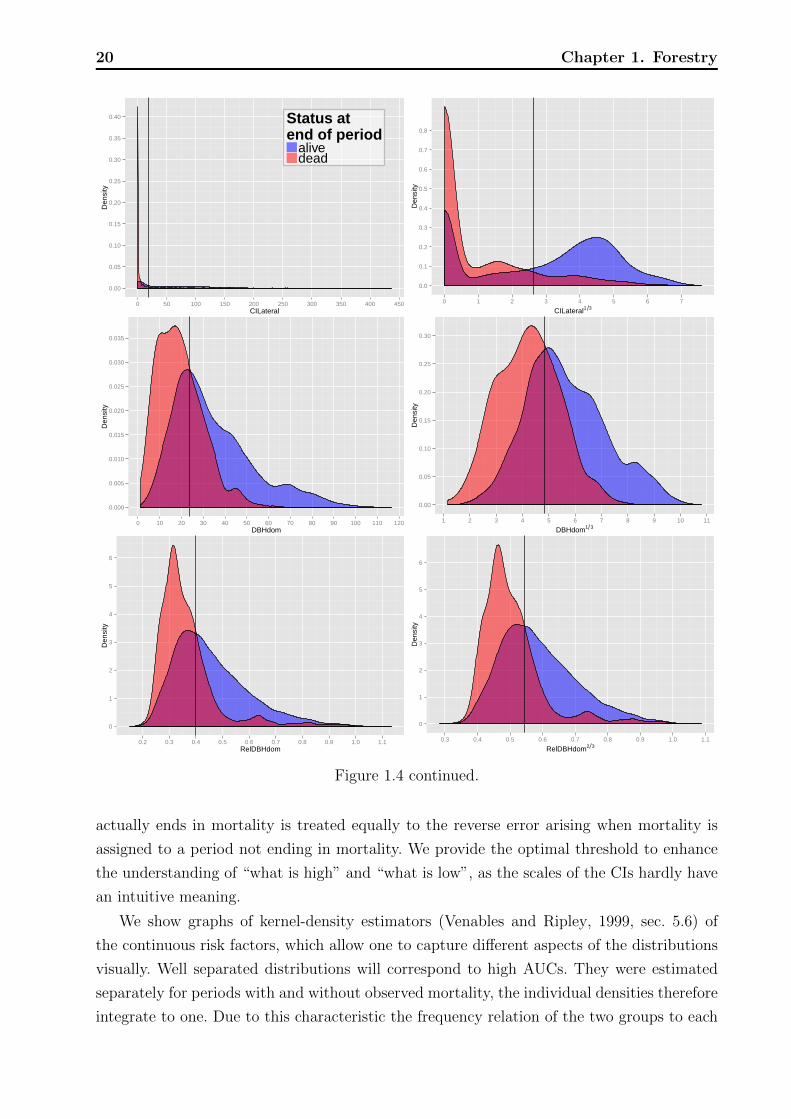
We show graphs of kernel-density estimators (Venables and Ripley, 1999, sec. 5.6) of
the continuous risk factors, which allow one to capture different aspects of the distributions
visually. Well separated distributions will correspond to high AUCs. They were estimated
separately for periods with and without observed mortality, the individual densities therefore
integrate to one. Due to this characteristic the frequency relation of the two groups to each

1.2 Data and exploratory methods 21
other is not evident, but the overlaid densities allow the following interpretation. For a
specific measurement of a risk factor, say DBH = 20 (see Figure 1.4 top left for an example)
the overlaid densities imply that there was a higher proportion of live rather than dead
trees. However, this interpretation assumes that mortality and non-mortality periods are
equally likely a priori and one has to keep in mind that the marginal density estimates of
risk the factors are aggregated over all plots, years, and other factors that might influence
mortality. Graphs with little overlap of the mortality- and non-mortality curves indicate
good discrimination in terms of the range of the risk factors. Vertical black lines indicate the
optimal thresholds of separation based on the Youden index, cutY ouden.
Concerning the growth of a tree it is obvious that variables such as DBH and Height are
strongly connected with each other, as both variables quantify the abstract concept of tree
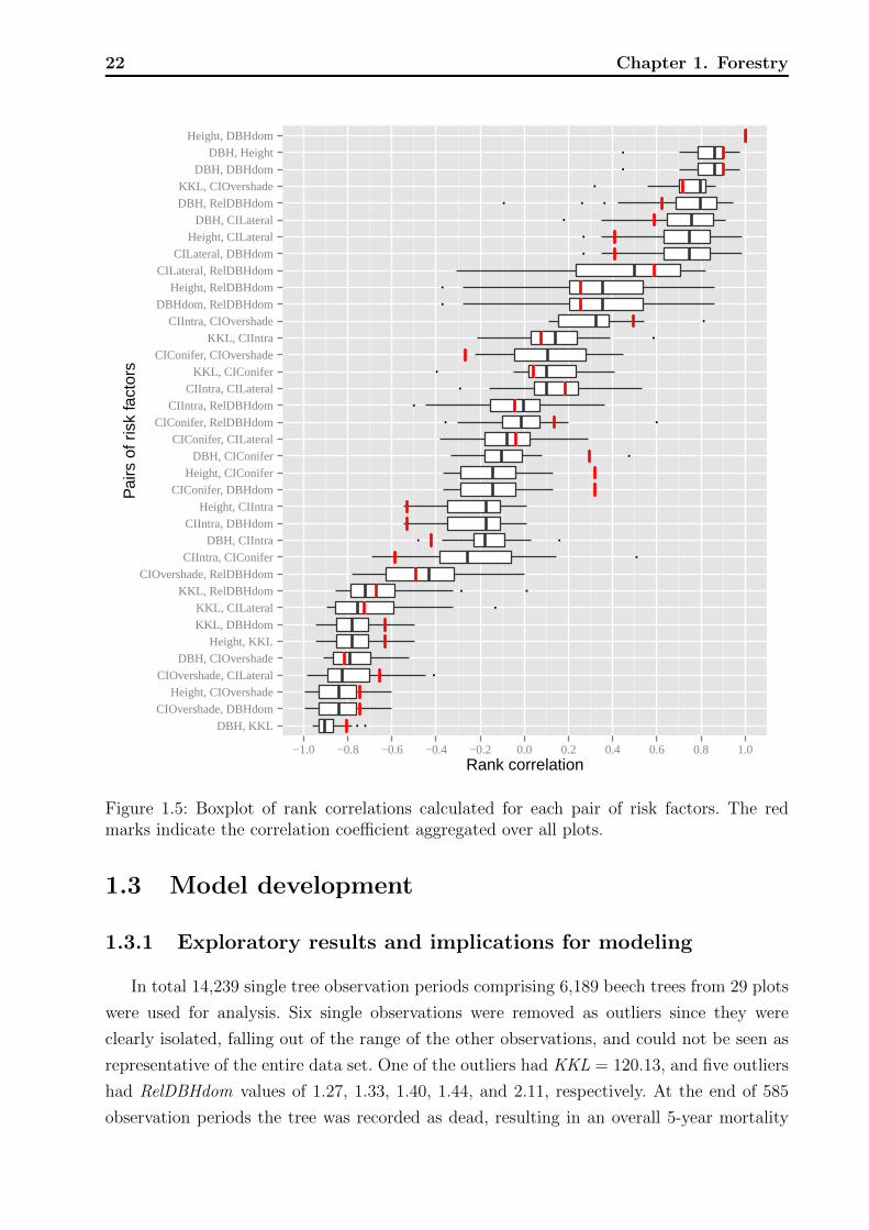
size. It is very likely that this connection can be seen in terms of empirical correlations in
the data set as well. Similarly, the way that CIs partly build upon one another likely leads
to strong inter-dependencies. We looked at rank correlations between pairs of risk factors,
which allowed us to empirically assess to what extent different CIs measure different aspects
of competition. Having the planned regression model for mortality in mind, where the risk
factors would act as independent variables, it was important to know which variables con-
tributed additional information not already present in others. Rank correlation as a measure
of association is limited by the fact that it only captures monotone relationships. Inspection
of scatter plots in addition to raw correlation values helps to overcome this shortcoming.
Non parametric loess smoothers (Cleveland et al., 1992) are overlaid in the graphs, which in-
dicate the shape of possible non-monotone dependence. Like for the AUC, rank correlations
are invariant against strictly monotone transformations, providing maximum generalizability
at this stage of model development.
In the descriptive methods presented so far we ignored the hierarchical structure of the
data. The statistical measures and graphs were calculated over all plots (stands), which
could either weaken or amplify the true effects of the risk factors. Assuming homogeneous
conditions across different plots we expect little variation on quantities such as the AUC,
correlations, and thresholds obtained within single plots compared to the aggregated calcu-
lation. We conducted a stratified analysis of the risk factors and compare results with the
aggregated analysis, allowing to investigate the potential impact of a hierarchical approach.
Plot specific rank correlations between risk factors, optimal thresholds, and AUCs are pre-
sented. We do not show the variables periodLength and periodOnset since they hardly vary
within a single plot, as well as the variable SiteIndex , which is a characteristic of the whole
plot and therefore cannot be explored at the plot level.
We present the results of the descriptive analysis in the following section, along with the
implications for the mortality model.
22 Chapter 1. Forestry
● ●
●
●
●●
●
●●
●
● ●
●
●
●
●
●
●
●
●
●
●
● ●●
●
●
●
DBH, KKLCIOvershade, DBHdom
Height, CIOvershadeCIOvershade, CILateral
DBH, CIOvershadeHeight, KKL
KKL, DBHdomKKL, CILateral
KKL, RelDBHdomCIOvershade, RelDBHdom
CIIntra, CIConiferDBH, CIIntra
CIIntra, DBHdomHeight, CIIntra
CIConifer, DBHdomHeight, CIConifer
DBH, CIConiferCIConifer, CILateral
CIConifer, RelDBHdomCIIntra, RelDBHdom
CIIntra, CILateralKKL, CIConifer
CIConifer, CIOvershadeKKL, CIIntra
CIIntra, CIOvershadeDBHdom, RelDBHdom
Height, RelDBHdomCILateral, RelDBHdom
CILateral, DBHdomHeight, CILateral
DBH, CILateralDBH, RelDBHdomKKL, CIOvershade
DBH, DBHdomDBH, Height
Height, DBHdom
−1.0 −0.8 −0.6 −0.4 −0.2 0.0 0.2 0.4 0.6 0.8 1.0Rank correlation
Pai
rs o
f ris
k fa
ctor
s
Figure 1.5: Boxplot of rank correlations calculated for each pair of risk factors. The redmarks indicate the correlation coefficient aggregated over all plots.
1.3 Model development
1.3.1 Exploratory results and implications for modeling
In total 14,239 single tree observation periods comprising 6,189 beech trees from 29 plots
were used for analysis. Six single observations were removed as outliers since they were
clearly isolated, falling out of the range of the other observations, and could not be seen as
representative of the entire data set. One of the outliers had KKL = 120.13, and five outliers
had RelDBHdom values of 1.27, 1.33, 1.40, 1.44, and 2.11, respectively. At the end of 585
observation periods the tree was recorded as dead, resulting in an overall 5-year mortality

1.3 Model development 23
●●29
DBH
5 10 15 20 25 30
29
Height
10 15 20 25
●29
KKL
2 4 6 8 10
●
●
9
20
CIIntra
50 100 150 200 250 300
11
11
CIConifer
0 20 40 60 80
● ●
1
28
CIOvershade
100 150 200
●●●28
1
CILateral
0 10 20 30 40 50 60
29
DBHdom
10 20 30 40 50 60
27
2
RelDBHdom
0.3 0.4 0.5 0.6
Figure 1.6: Boxplots of thresholds obtained by maximization of the Youden index in eachplot. The color indicates the direction: Red indicates values greater as the threshold areassociated with mortality, blue indicates smaller values as the threshold are associated withmortality. Thick vertical lines show the threshold calculated over all plots. The numbers nextto/within the boxplots count the plots where the risk factor acts in the particular direction.Counts do not add up to 29 within one risk factor if there are plots having the same valueof the risk factor for all periods.
rate of 3.9% (Table 1.3).
5-year mortality rates varied substantially between plots, with the highest at 13.44%
(Table 1.1). The lowest rate was observed in Plot 29 where each of the 97 trees contributed
a observation period of ten years (in sum 970 years of exposure time) and only one died,
resulting in a 5-year mortality rate of 0.52%. In Table 1.1 the plots are arranged decreasingly
by mortality per period which is not consistent with the order of the 5-year mortality.
The biggest difference is visible in Plot 9, having a mortality per period twice as high as
standardized to a 5-year period. The reason is because Plot 9 was surveyed strictly in ten
year intervals. The big divergence indicates that we need to consider the exposure time,
namely the length of the observation period, as part of the observed mortality rate instead
of as a risk factor, and use an approach which harmonizes the data. We addressed this issue
via an offset term in the mortality model.
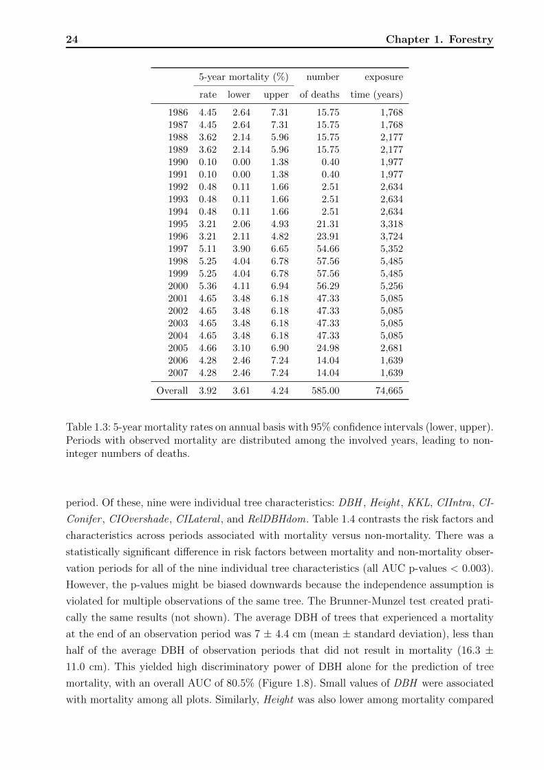
Between 1986 and 2007 the mortality rate ranged between 3% and 5.5% except for the
years 1990 to 1994 where the rate dropped below 1% (Table 1.3, Figure 1.7). Due to the way
that data were collected and restructured to calculate yearly mortality rates, it is hard to
assess the actual distribution of yearly test statistics with null hypotheses of equal mortality
rates. Nevertheless, the pointwise confidence intervals visualized in Figure 1.7, which ignore
these issues, support the impression that the low mortality rates between 1990 and 1994
did not only occur by chance. The foresters could not give any explanations for the 4% dip
during these years; neither explanations of natural kind, such as a change in the weather nor
of technical kind, such as a change in recording. Thus we left these years in the analysis but
addressed the temporal heterogeneity by a random effect for calendar year.
For each of the observation periods included in the analysis, measurements of 13 potential
risk factors for mortality listed in Table 1.2 were available at the beginning of the observation
24 Chapter 1. Forestry
5-year mortality (%) number exposure
rate lower upper of deaths time (years)
1986 4.45 2.64 7.31 15.75 1,7681987 4.45 2.64 7.31 15.75 1,7681988 3.62 2.14 5.96 15.75 2,1771989 3.62 2.14 5.96 15.75 2,1771990 0.10 0.00 1.38 0.40 1,9771991 0.10 0.00 1.38 0.40 1,9771992 0.48 0.11 1.66 2.51 2,6341993 0.48 0.11 1.66 2.51 2,6341994 0.48 0.11 1.66 2.51 2,6341995 3.21 2.06 4.93 21.31 3,3181996 3.21 2.11 4.82 23.91 3,7241997 5.11 3.90 6.65 54.66 5,3521998 5.25 4.04 6.78 57.56 5,4851999 5.25 4.04 6.78 57.56 5,4852000 5.36 4.11 6.94 56.29 5,2562001 4.65 3.48 6.18 47.33 5,0852002 4.65 3.48 6.18 47.33 5,0852003 4.65 3.48 6.18 47.33 5,0852004 4.65 3.48 6.18 47.33 5,0852005 4.66 3.10 6.90 24.98 2,6812006 4.28 2.46 7.24 14.04 1,6392007 4.28 2.46 7.24 14.04 1,639
Overall 3.92 3.61 4.24 585.00 74,665
Table 1.3: 5-year mortality rates on annual basis with 95% confidence intervals (lower, upper).Periods with observed mortality are distributed among the involved years, leading to non-integer numbers of deaths.
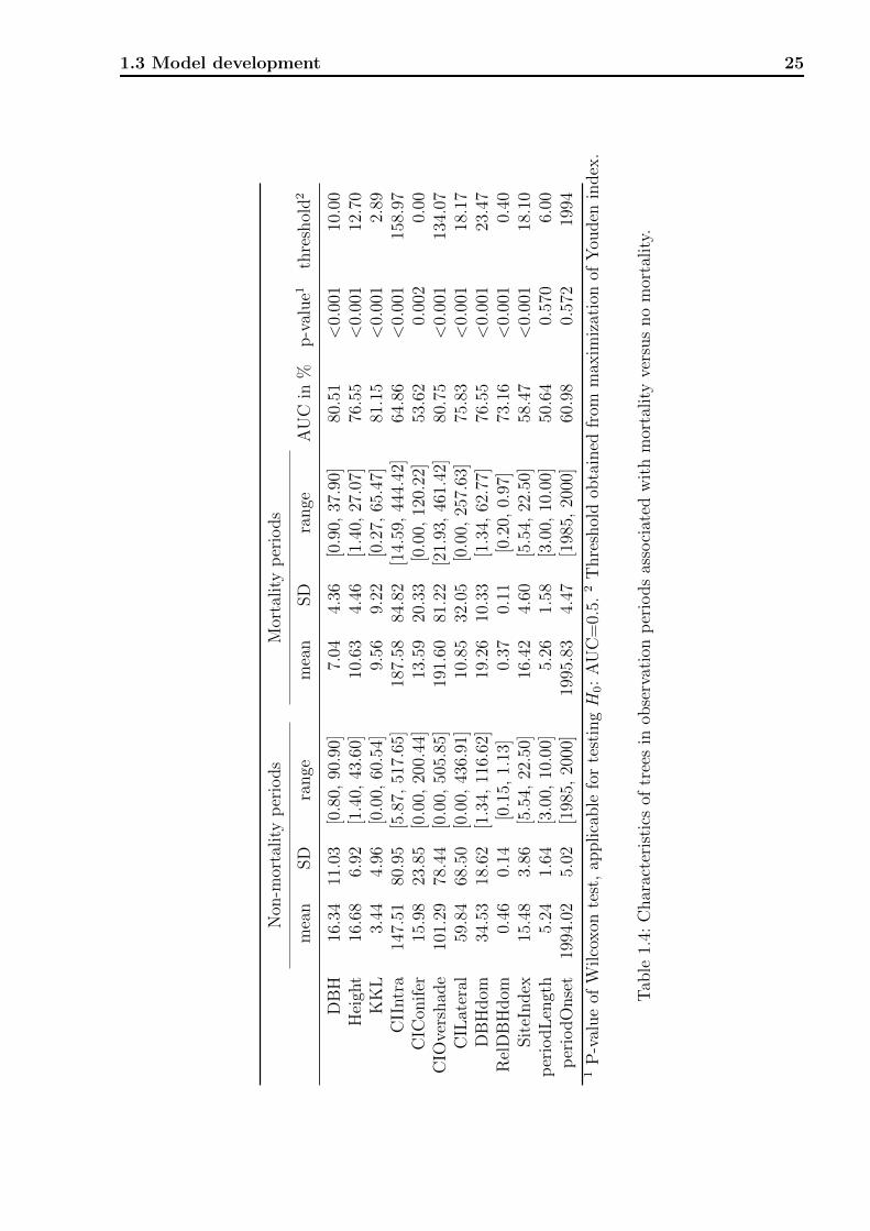
period. Of these, nine were individual tree characteristics: DBH , Height , KKL, CIIntra, CI-
Conifer , CIOvershade, CILateral , and RelDBHdom. Table 1.4 contrasts the risk factors and
characteristics across periods associated with mortality versus non-mortality. There was a
statistically significant difference in risk factors between mortality and non-mortality obser-
vation periods for all of the nine individual tree characteristics (all AUC p-values < 0.003).
However, the p-values might be biased downwards because the independence assumption is
violated for multiple observations of the same tree. The Brunner-Munzel test created prati-
cally the same results (not shown). The average DBH of trees that experienced a mortality
at the end of an observation period was 7 ± 4.4 cm (mean ± standard deviation), less than
half of the average DBH of observation periods that did not result in mortality (16.3 ±11.0 cm). This yielded high discriminatory power of DBH alone for the prediction of tree
mortality, with an overall AUC of 80.5% (Figure 1.8). Small values of DBH were associated
with mortality among all plots. Similarly, Height was also lower among mortality compared
1.3 Model development 25
Non
-mor
tality
per
iods
Mor
tality
per
iods
mea
nSD
range
mea
nSD
range
AU
Cin
%p-v
alue1
thre
shol
d2
DB
H16
.34
11.0
3[0
.80,
90.9
0]7.
044.
36[0
.90,
37.9
0]80
.51
<0.
001
10.0
0H
eigh
t16
.68
6.92
[1.4
0,43
.60]
10.6
34.
46[1
.40,
27.0
7]76
.55
<0.
001
12.7
0K
KL
3.44
4.96
[0.0
0,60
.54]
9.56
9.22
[0.2
7,65
.47]
81.1
5<
0.00
12.
89C
IIntr
a14
7.51
80.9
5[5
.87,
517.
65]
187.
5884
.82
[14.
59,
444.
42]
64.8
6<
0.00
115
8.97
CIC
onif
er15
.98
23.8
5[0
.00,
200.
44]
13.5
920
.33
[0.0
0,12
0.22
]53
.62
0.00
20.
00C
IOve
rshad
e10
1.29
78.4
4[0
.00,
505.
85]
191.
6081
.22
[21.
93,
461.
42]
80.7
5<
0.00
113
4.07
CIL
ater
al59
.84
68.5
0[0
.00,
436.
91]
10.8
532
.05
[0.0
0,25
7.63
]75
.83
<0.
001
18.1
7D
BH
dom
34.5
318
.62
[1.3
4,11
6.62
]19
.26
10.3
3[1
.34,
62.7
7]76
.55
<0.
001
23.4
7R
elD
BH
dom
0.46
0.14
[0.1
5,1.
13]
0.37
0.11
[0.2
0,0.
97]
73.1
6<
0.00
10.
40Sit
eIndex
15.4
83.
86[5
.54,
22.5
0]16
.42
4.60
[5.5
4,22
.50]
58.4
7<
0.00
118
.10
per
iodL
engt
h5.
241.
64[3
.00,
10.0
0]5.
261.
58[3
.00,
10.0
0]50
.64
0.57
06.
00p
erio
dO
nse
t19
94.0
25.
02[1
985,
2000
]19
95.8
34.
47[1
985,
2000
]60
.98
0.57
219
941
P-v
alue
ofW
ilco
xon
test
,ap
plica
ble
for
test
ingH
0:
AU
C=
0.5.
2T
hre
shol
dob
tain
edfr
omm
axim
izat
ion
ofY
ouden
index
.
Tab
le1.
4:C
har
acte
rist
ics
oftr
ees
inob
serv
atio
np
erio
ds
asso
ciat
edw
ith
mor
tality
vers
us
no
mor
tality
.
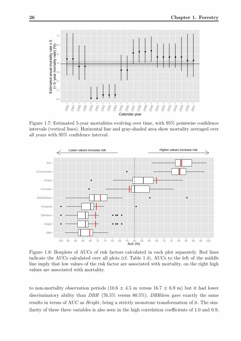
26 Chapter 1. Forestry
● ●
● ●
● ●
● ● ●
● ●
●● ●
●
● ● ● ● ●
● ●
0
1
2
3
4
5
6
7
1986
1987
1988
1989
1990
1991
1992
1993
1994
1995
1996
1997
1998
1999
2000
2001
2002
2003
2004
2005
2006
2007
Calendar year
Est
imat
ed a
nual
mor
talit
y ra
te x
5
(= 5
−ye
ar m
orta
lity
rate
) (%
)
Figure 1.7: Estimated 5-year mortalities evolving over time, with 95% pointwise confidenceintervals (vertical lines). Horizontal line and gray-shaded area show mortality averaged overall years with 95% confidence interval.
Lower values increase risk Higher values increase risk
●● ●●●
●● ●●●
●●
●●
●
●
●
DBH
Height
DBHdom
CILateral
RelDBHdom
CIConifer
CIIntra
CIOvershade
KKL
100 95 90 85 80 75 70 65 60 55 50 55 60 65 70 75 80 85 90 95 100AUC (%)
Figure 1.8: Boxplots of AUCs of risk factors calculated in each plot separately. Red linesindicate the AUCs calculated over all plots (cf. Table 1.4). AUCs to the left of the middleline imply that low values of the risk factor are associated with mortality, on the right highvalues are associated with mortality.
to non-mortality observation periods (10.6 ± 4.5 m versus 16.7 ± 6.9 m) but it had lower
discriminatory ability than DBH (76.5% versus 80.5%). DBHdom gave exactly the same
results in terms of AUC as Height , being a strictly monotone transformation of it. The sim-
ilarity of these three variables is also seen in the high correlation coefficients of 1.0 and 0.9,
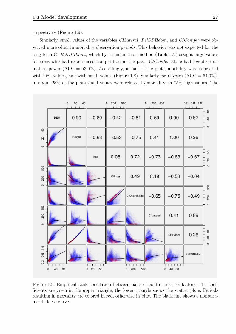
1.3 Model development 27
respectively (Figure 1.9).
Similarly, small values of the variables CILateral , RelDBHdom, and CIConifer were ob-
served more often in mortality observation periods. This behavior was not expected for the
long term CI RelDBHdom, which by its calculation method (Table 1.2) assigns large values
for trees who had experienced competition in the past. CIConifer alone had low discrim-
ination power (AUC = 53.6%). Accordingly, in half of the plots, mortality was associated
with high values, half with small values (Figure 1.8). Similarly for CIIntra (AUC = 64.9%),
in about 25% of the plots small values were related to mortality, in 75% high values. The
Figure 1.9: Empirical rank correlation between pairs of continuous risk factors. The coef-ficients are given in the upper triangle, the lower triangle shows the scatter plots. Periodsresulting in mortality are colored in red, otherwise in blue. The black line shows a nonpara-metric loess curve.

28 Chapter 1. Forestry
two risk factors CIConifer and CIIntra alone were of limited use for predicting mortality, at
least in a monotone fashion. However, relaxing that restriction and accounting for other CI
in parallel, they might still contribute valuable information in a mortality model. KKL and
CIOvershade were the CIs with highest AUCs (81.1% and 80.8%, respectively) and acted in
the expected direction, with high values associated with smortality. The plot-specific vari-
able SiteIndex was lower among non-mortality compared to mortality periods (AUC 58.46%),
which indicated better growth conditions in non-mortality periods at a first glance, but the
validity of that on single tree-period is not given due to the plot-specific character of the
variable, resulting in the same constant value of SiteIndex for all tree periods within a plot
at all observed calendar years. Finally, there was no statistical difference in the length of
observation periods between those associated with mortality and non-mortality (Table 1.4),
though this observation does not affect the importance of periodLength in the definition of
mortality rates. We observed that risk factors with good overall discriminatory capabilities
are available and that they might be further enhanced when we account for the hierarchical
structure (plot-specific AUCs often better than overall AUC, Figure 1.8).
Figure 1.4 shows the empirical distributions of risk factors in mortality and non-mortality
periods. Besides the quantities of location (mean) and variability (SD) already provided in
Table 1.4, the skewness and potential multimodel shape can be assessed by this figure. The
distributions of Height and RelDBHdom were unimodal with slight skewness towards larger
trees. The majority of tree heights were near 12 m, but a smaller group of trees had larger
heights near 30 m. The distribution of DBH indicated slight bimodality within mortality
periods, with a minority fraction of larger trees. For CIIntra and CIOvershade most of
threes within non-mortality periods had small values. The majority of trees were observed
in periods without light competition from neighboring trees (KKL = 0), competition from
conifer trees (CIConifer = 0), or lateral competition (CILateral = 0). We will refer to these
accumulations on a single value (here zero) as point masses in the next section. In particular
the extreme skewness of CILateral and KKL suggested that transformations are needed to
zoom into areas of interest, figuratively speaking.
The single threshold obtained by maximization of the Youden index (shown by a vertical
line in Figure 1.4) illustrates where the density of the risk factor in non-mortality periods
was significantly shifted from the density in mortality periods. For risk factors where the
densities overlap extensively, we cannot achieve good separation with a single threshold, as
seen in the case of CIConifer . The thresholds calculated in each plot are given in Figure
1.6. As for the AUC, orientation of the thresholds, that is, whether values above or below
thresholds are associated with mortality are indicated. For DBH all 29 plots had the same
orientation, meaning that values below the threshold were higher associated with mortality.
The same applied for Height and DBHdom, whereas for KKL, all plots consistently showed
association of mortality with values above the threshold. Again, CIConifer behaves most
extreme, in eleven plots values higher than the threshold indicate mortality, and in 11 plots,

1.3 Model development 29
values lower than the threshold. A threshold for the remaining 7 plots could not be calculated
as in these plots CIConifer was zero for all trees.
The empirical correlations, summarized in Figure 1.9, were strongly and statistically
significantly negative for the risk factor pairs DBH & KKL (-0.80), CIOvershade & DBHdom
(-0.75), Height & CIOvershade (-0.75), DBH & CIOvershade (-0.81), and KKL & CILateral
(-0.73). High correlations were observed for DBH & Height (0.90), DBH & DBHdom (0.90),
and KKL & CIOvershade (0.72). Height & DBHdom were in perfect rank correlation, being
a monotone transformation of each other. We found no relevant correlation of CIConifer &
CILateral (-0.04), RelDBHdom & CIIntra (-0.04), and KKL & CIConifer (0.04). Only the
relationship between CILateral and DBHdom (0.41) looked severely non-monotone according
to the loess smoother, but the variation was too large for inferring a meaningful functional
dependency (Figure 1.9). Comparison of correlation coefficients within single plots with
aggregated estimates painted a mixed picture. For strong correlations the overall estimates
were lower (in absolute value) except for the variables DBH and Height (or DBHdom), for
medium correlations the differences were bigger, but no general trend was obvious. The sign
of the correlation coefficient changed in 20 out of 36 pairs in at least one plot compared to
the aggregated coefficient.
In summary we list several implications to be considered in building a mortality model.
• Mortality is a rare event, present in only 4.11% of the observations in this data set.
• Mortality varies considerably over time.
• Mortality varies considerably between plots.
• Mortality is measured over different sized intervals and needs to be standardized.
• Risk factors differ in distribution between mortality and non-mortality periods.
• Multiple observation periods of the same tree are not necessarily independent.
• Multiple observations within one plot cannot be assumed to be independent, i.e. there
is spatial correlation.
• Risk factors have partly functional dependencies by definition and/or strong empirical
correlation between each other.
1.3.2 Literature review for individual tree mortality models
Before presenting our own individual tree mortality model we review modeling approaches
suggested and applied in the literature.
There have been various individual tree mortality models developed for many different
species of trees; Table 1.5 contains a list. All mortality models in the literature that we
have consulted included DBH or some measure of basal area, and logistic regression was by
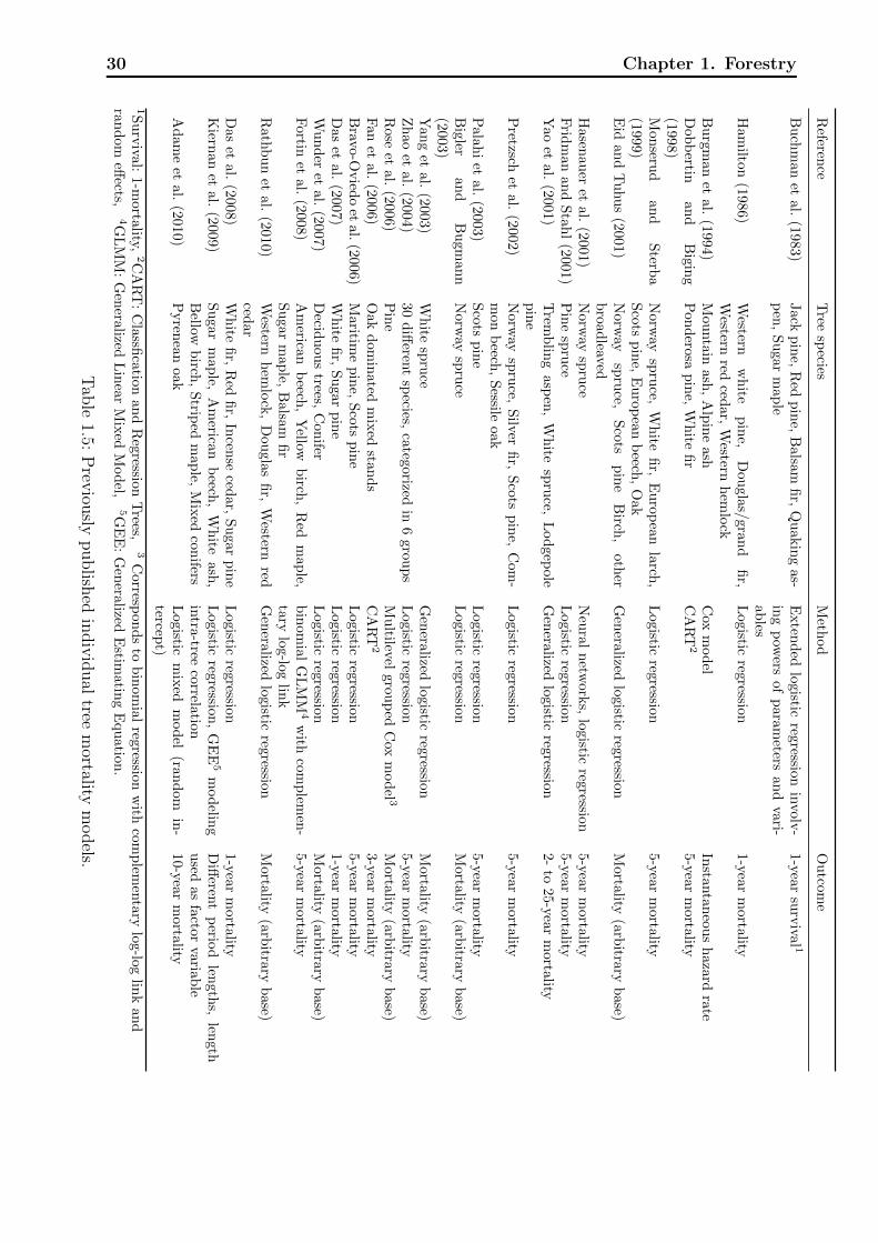
30 Chapter 1. ForestryR
eference
Tree
species
Meth
od
Ou
tcome
Bu
chm
an
etal.
(1983
)Jack
pin
e,R
edp
ine,
Balsa
mfi
r,Q
uakin
gas-
pen
,S
ugar
map
leE
xten
ded
logistic
regression
involv
-in
gp
owers
of
para
meters
and
vari-ab
les
1-yearsu
rvival 1
Ham
ilton
(1986
)W
esternw
hite
pin
e,D
ou
gla
s/gra
nd
fir,
Western
redced
ar,
Western
hem
lock
Logistic
regressio
n1-y
earm
ortality
Bu
rgm
anet
al.(19
94)
Mou
nta
inash
,A
lpin
eash
Cox
mod
elIn
stantan
eous
hazard
rateD
ob
bertin
and
Bigin
g(1
998)
Pon
derosa
pin
e,W
hite
fir
CA
RT
25-year
mortality
Mon
serud
and
Sterb
a(1
999)
Norw
aysp
ruce,
Wh
itefi
r,E
uro
pea
nla
rch,
Scots
pin
e,E
uro
pea
nb
eech,
Oak
Logistic
regressio
n5-y
earm
ortality
Eid
an
dT
uhu
s(200
1)
Norw
aysp
ruce,
Sco
tsp
ine
Birch
,oth
erb
road
leavedG
enera
lizedlo
gistic
regression
Mortality
(arbitrary
base)
Hasen
au
eret
al.
(2001
)N
orw
aysp
ruce
Neu
ral
netw
ork
s,lo
gistic
regression5-year
mortality
Frid
man
an
dS
tah
l(2
001)
Pin
esp
ruce
Logistic
regressio
n5-year
mortality
Yao
etal.
(2001)
Trem
blin
gasp
en,
Wh
itesp
ruce,
Lod
gep
ole
pin
eG
enera
lizedlo
gistic
regression
2-to
25-yearm
ortality
Pretzsch
etal.
(2002)
Norw
aysp
ruce,
Silver
fir,
Sco
tsp
ine,
Com
-m
on
beech
,S
essileoak
Logistic
regressio
n5-y
earm
ortality
Pala
hi
etal.
(2003)
Scots
pin
eL
ogistic
regressio
n5-year
mortality
Big
leran
dB
ugm
ann
(2003)
Norw
aysp
ruce
Logistic
regressio
nM
ortality(arb
itraryb
ase)
Yan
get
al.
(2003
)W
hite
spru
ceG
enera
lizedlo
gistic
regression
Mortality
(arbitrary
base)
Zh
aoet
al.(200
4)
30d
ifferen
tsp
ecies,ca
tegorized
in6
gro
up
sL
ogistic
regressio
n5-year
mortality
Rose
etal.
(2006)
Pin
eM
ultilevel
gro
up
edC
oxm
od
el 3M
ortality(arb
itraryb
ase)F
an
etal.
(2006
)O
ak
dom
inated
mix
edsta
nd
sC
AR
T2
3-yearm
ortalityB
ravo-Ovied
oet
al.
(2006)
Maritim
ep
ine,
Sco
tsp
ine
Logistic
regressio
n5-year
mortality
Das
etal.
(2007)
Wh
itefi
r,S
ugar
pin
eL
ogistic
regressio
n1-year
mortality
Wu
nd
eret
al.(20
07)
Decid
uou
strees,
Conifer
Logistic
regressio
nM
ortality(arb
itraryb
ase)F
ortin
etal.
(2008)
Am
ericanb
eech,
Yellow
birch
,R
edm
ap
le,S
ugar
map
le,B
alsa
mfi
rb
inom
ial
GL
MM
4w
ithcom
plem
en-
tary
log-lo
glin
k5-year
mortality
Rath
bu
net
al.
(2010)
Western
hem
lock
,D
ou
gla
sfi
r,W
esternred
cedar
Gen
eralized
logistic
regression
Mortality
(arbitrary
base)
Das
etal.
(2008)
Wh
itefi
r,R
edfi
r,In
cense
cedar,
Su
gar
pin
eL
ogistic
regressio
n1-year
mortality
Kiern
anet
al.(200
9)
Suga
rm
aple,
Am
erican
beech
,W
hite
ash
,B
ellowb
irch,
Strip
edm
ap
le,M
ixed
con
ifersL
ogistic
regressio
n,
GE
E5
mod
eling
intra
-treeco
rrelatio
nD
ifferen
tp
eriod
length
s,len
gthu
sedas
factorvariab
leA
dam
eet
al.(201
0)
Pyren
eanoak
Logistic
mix
edm
od
el(ran
dom
in-
tercept)
10-yearm
ortality
1Su
rvival:
1-morta
lity,2C
AR
T:
Classfi
cation
and
Reg
ression
Trees,
3C
orresp
on
ds
tob
inom
ial
regression
with
comp
lemen
tarylog-log
link
and
rand
om
effects,
4GL
MM
:G
enera
lizedL
inea
rM
ixed
Mod
el,5G
EE
:G
enera
lizedE
stimatin
gE
qu
ation
.
Tab
le1.5:
Prev
iously
publish
edin
div
idual
treem
ortalitym
odels.
1.3 Model development 31
far the most commonly used statistical model. The initial mortality model in SILVA was
presented by Pretzsch et al. (2002) and was based on a subset of the same data as for our
application. They also used logistic regression, but instead of using all observation periods,
they selected an equal-sized series of observation periods from trees that had survived to
observation periods where trees had died, mimicking the efficient case control designs used
for rare diseases in medicine. Their mortality model indicated an increased risk of mortality
for trees with smaller DBH, with lower ratios of heights to DBH, with larger values of a site
index (estimated stand top height at age 50 years), and with larger ratios of estimated tree
basal area growth over the next 5 years to DBH. Our findings for DBH and SiteIndex in the
exploratory univariate analyses were significant in the same direction. However, the ratio
Height/DBH was found to act in the opposite direction in the univariate analysis (AUC =
78.4%, p-value < 0.001, not shown in previous tables).
Monserud and Sterba (1999) used logistic regression to develop individual tree mortality
models for the six major forest species of Austria, one being European beech, using a single
5-year remeasurement period of a permanent plot network of the Austrian National Forest
Inventory. In addition for use in an individual tree stand growth simulator, their aim was
to provide a general mortality model to replace outdated yield tables that were still being
used at the time. Their inventory recorded an overall 5-year mortality rate for European
beech of 4.3%, which is very close to what was observed in our study (4.1%), and they
elucidated the obstacles present for accurately modeling rare events. In order to make their
model generally applicable in Austria, where they argued that most stands failed to meet
the definition of even-aged, they intentionally excluded site index and age of individual trees
from consideration in their model, arguing that tree size is already an integrated response to
these factors. In their introduction they outlined that the most popular statistical method
for modeling individual tree mortality is logistic regression, but that Weibull and Gamma
regression have also been applied. Further they stated that in their data, the nonparametric
approaches recursive partitioning and neural networks did not lead to significant improve-
ment in the ability to predict mortality compared to classical statistical methods, but were
applied successfully elsewhere (Monserud and Sterba, 1999).
Using permanent plot data from a mountainous region in Switzerland, Wunder et al.
(2007) focused on prediction models for European beech that distinguished between growth-
dependent and growth-independent mortality. The growth-dependent models used as a risk
factor the relative basal area increment between two measurement periods divided by the
basal area at the second measurement period. Location site and DBH were included as
growth-independent risk factors. Their data showed that trees that died experienced lower
relative growths in the period before death than comparable time periods among trees that
survived. A spline fit for the relationship of relative growth to survival revealed a nonlinear
relationship. The impact of growth on survival was stronger among trees with smaller relative
growths than among trees with higher relative growths. Among the two sites in their study,
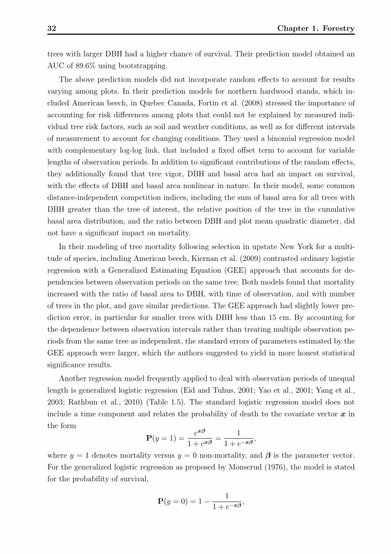
32 Chapter 1. Forestry
trees with larger DBH had a higher chance of survival. Their prediction model obtained an
AUC of 89.6% using bootstrapping.
The above prediction models did not incorporate random effects to account for results
varying among plots. In their prediction models for northern hardwood stands, which in-
cluded American beech, in Quebec Canada, Fortin et al. (2008) stressed the importance of
accounting for risk differences among plots that could not be explained by measured indi-
vidual tree risk factors, such as soil and weather conditions, as well as for different intervals
of measurement to account for changing conditions. They used a binomial regression model
with complementary log-log link, that included a fixed offset term to account for variable
lengths of observation periods. In addition to significant contributions of the random effects,
they additionally found that tree vigor, DBH and basal area had an impact on survival,
with the effects of DBH and basal area nonlinear in nature. In their model, some common
distance-independent competition indices, including the sum of basal area for all trees with
DBH greater than the tree of interest, the relative position of the tree in the cumulative
basal area distribution, and the ratio between DBH and plot mean quadratic diameter, did
not have a significant impact on mortality.
In their modeling of tree mortality following selection in upstate New York for a multi-
tude of species, including American beech, Kiernan et al. (2009) contrasted ordinary logistic
regression with a Generalized Estimating Equation (GEE) approach that accounts for de-
pendencies between observation periods on the same tree. Both models found that mortality
increased with the ratio of basal area to DBH, with time of observation, and with number
of trees in the plot, and gave similar predictions. The GEE approach had slightly lower pre-
diction error, in particular for smaller trees with DBH less than 15 cm. By accounting for
the dependence between observation intervals rather than treating multiple observation pe-
riods from the same tree as independent, the standard errors of parameters estimated by the
GEE approach were larger, which the authors suggested to yield in more honest statistical
significance results.
Another regression model frequently applied to deal with observation periods of unequal
length is generalized logistic regression (Eid and Tuhus, 2001; Yao et al., 2001; Yang et al.,
2003; Rathbun et al., 2010) (Table 1.5). The standard logistic regression model does not
include a time component and relates the probability of death to the covariate vector x in
the form
P(y = 1) =exβ
1 + exβ=
1
1 + e−xβ,
where y = 1 denotes mortality versus y = 0 non-mortality, and β is the parameter vector.
For the generalized logistic regression as proposed by Monserud (1976), the model is stated
for the probability of survival,
P(y = 0) = 1− 1
1 + e−xβ,
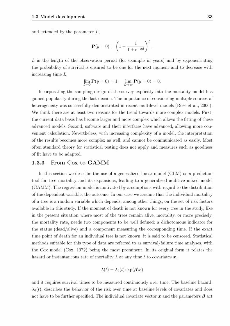
1.3 Model development 33
and extended by the parameter L,
P(y = 0) =
(1− 1
1 + e−xβ
)L.
L is the length of the observation period (for example in years) and by exponentiating
the probability of survival is ensured to be one for the next moment and to decrease with
increasing time L,
limL→0
P(y = 0) = 1, limL→∞
P(y = 0) = 0.
Incorporating the sampling design of the survey explicitly into the mortality model has
gained popularity during the last decade. The importance of considering multiple sources of
heterogeneity was successfully demonstrated in recent multilevel models (Rose et al., 2006).
We think there are at least two reasons for the trend towards more complex models. First,
the current data basis has become larger and more complex which allows the fitting of these
advanced models. Second, software and their interfaces have advanced, allowing more con-
venient calculation. Nevertheless, with increasing complexity of a model, the interpretation
of the results becomes more complex as well, and cannot be communicated as easily. Most
often standard theory for statistical testing does not apply and measures such as goodness
of fit have to be adapted.
1.3.3 From Cox to GAMM
In this section we describe the use of a generalized linear model (GLM) as a prediction
tool for tree mortality and its expansions, leading to a generalized additive mixed model
(GAMM). The regression model is motivated by assumptions with regard to the distribution
of the dependent variable, the outcome. In our case we assume that the individual mortality
of a tree is a random variable which depends, among other things, on the set of risk factors
available in this study. If the moment of death is not known for every tree in the study, like
in the present situation where most of the trees remain alive, mortality, or more precisely,
the mortality rate, needs two components to be well defined: a dichotomous indicator for
the status (dead/alive) and a component measuring the corresponding time. If the exact
time point of death for an individual tree is not known, it is said to be censored. Statistical
methods suitable for this type of data are referred to as survival/failure time analyses, with
the Cox model (Cox, 1972) being the most prominent. In its original form it relates the
hazard or instantaneous rate of mortality λ at any time t to covariates x,
λ(t) = λ0(t) exp(β′x)
and it requires survival times to be measured continuously over time. The baseline hazard,
λ0(t), describes the behavior of the risk over time at baseline levels of covariates and does
not have to be further specified. The individual covariate vector x and the parameters β act
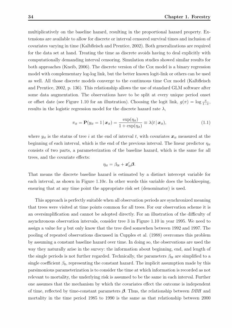
34 Chapter 1. Forestry
multiplicatively on the baseline hazard, resulting in the proportional hazard property. Ex-
tensions are available to allow for discrete or interval censored survival times and inclusion of
covariates varying in time (Kalbfleisch and Prentice, 2002). Both generalizations are required
for the data set at hand. Treating the time as discrete avoids having to deal explicitly with
computationally demanding interval censoring. Simulation studies showed similar results for
both approaches (Kneib, 2006). The discrete version of the Cox model is a binary regression
model with complementary log-log link, but the better known logit-link or others can be used
as well. All those discrete models converge to the continuous time Cox model (Kalbfleisch
and Prentice, 2002, p. 136). This relationship allows the use of standard GLM software after
some data augmentation. The observations have to be split at every unique period onset
or offset date (see Figure 1.10 for an illustration). Choosing the logit link, g(π) = log π1−π ,
results in the logistic regression model for the discrete hazard rate λ,
πit = P(yit = 1 |xit) =exp(ηit)
1 + exp(ηit)≡ λ(t |xit), (1.1)
where yit is the status of tree i at the end of interval t, with covariates xit measured at the
beginning of each interval, which is the end of the previous interval. The linear predictor ηit
consists of two parts, a parameterization of the baseline hazard, which is the same for all
trees, and the covariate effects:
ηit = β0t + x′itβ.
That means the discrete baseline hazard is estimated by a distinct intercept variable for
each interval, as shown in Figure 1.10c. In other words this variable does the bookkeeping,
ensuring that at any time point the appropriate risk set (denominator) is used.
This approach is perfectly suitable when all observation periods are synchronized meaning
that trees were visited at time points common for all trees. For our observation scheme it is
an oversimplification and cannot be adopted directly. For an illustration of the difficulty of
asynchronous observation intervals, consider tree 3 in Figure 1.10 in year 1995. We need to
assign a value for y but only know that the tree died somewhen between 1992 and 1997. The
pooling of repeated observations discussed in Cupples et al. (1988) overcomes this problem
by assuming a constant baseline hazard over time. In doing so, the observations are used the
way they naturally arise in the survey: the information about beginning, end, and length of
the single periods is not further regarded. Technically, the parameters β0t are simplified to a
single coefficient β0, representing the constant hazard. The implicit assumption made by this
parsimonious parameterization is to consider the time at which information is recorded as not
relevant to mortality, the underlying risk is assumed to be the same in each interval. Further
one assumes that the mechanism by which the covariates effect the outcome is independent
of time, reflected by time-constant parameters β. Thus, the relationship between DBH and
mortality in the time period 1985 to 1990 is the same as that relationship between 2000
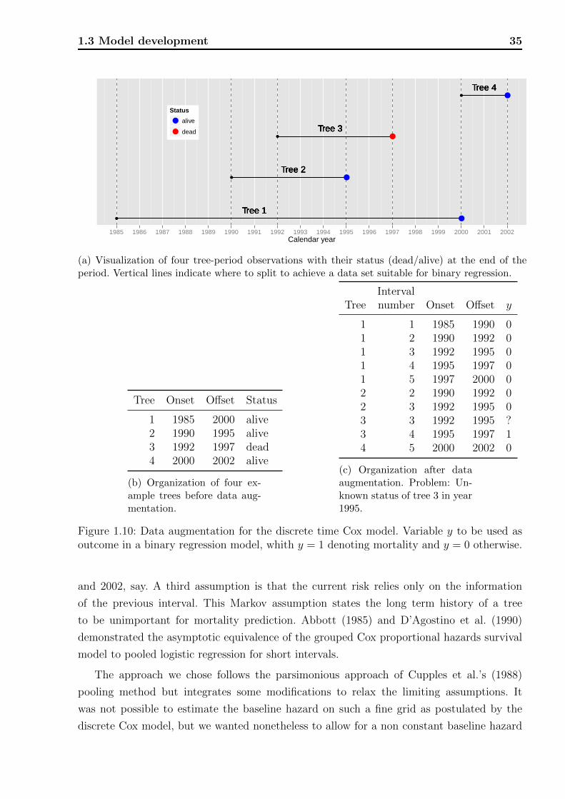
1.3 Model development 35
●
●
●
●
●
●
●
●
Tree 1Tree 1Tree 1Tree 1
Tree 2Tree 2Tree 2Tree 2
Tree 3Tree 3Tree 3Tree 3
Tree 4Tree 4Tree 4Tree 4
1985 1986 1987 1988 1989 1990 1991 1992 1993 1994 1995 1996 1997 1998 1999 2000 2001 2002Calendar year
Status
●
●
alive
dead
(a) Visualization of four tree-period observations with their status (dead/alive) at the end of theperiod. Vertical lines indicate where to split to achieve a data set suitable for binary regression.
Tree Onset Offset Status
1 1985 2000 alive2 1990 1995 alive3 1992 1997 dead4 2000 2002 alive
(b) Organization of four ex-ample trees before data aug-mentation.
IntervalTree number Onset Offset y
1 1 1985 1990 01 2 1990 1992 01 3 1992 1995 01 4 1995 1997 01 5 1997 2000 02 2 1990 1992 02 3 1992 1995 03 3 1992 1995 ?3 4 1995 1997 14 5 2000 2002 0
(c) Organization after dataaugmentation. Problem: Un-known status of tree 3 in year1995.
Figure 1.10: Data augmentation for the discrete time Cox model. Variable y to be used asoutcome in a binary regression model, whith y = 1 denoting mortality and y = 0 otherwise.
and 2002, say. A third assumption is that the current risk relies only on the information
of the previous interval. This Markov assumption states the long term history of a tree
to be unimportant for mortality prediction. Abbott (1985) and D’Agostino et al. (1990)
demonstrated the asymptotic equivalence of the grouped Cox proportional hazards survival
model to pooled logistic regression for short intervals.
The approach we chose follows the parsimonious approach of Cupples et al.’s (1988)
pooling method but integrates some modifications to relax the limiting assumptions. It
was not possible to estimate the baseline hazard on such a fine grid as postulated by the
discrete Cox model, but we wanted nonetheless to allow for a non constant baseline hazard
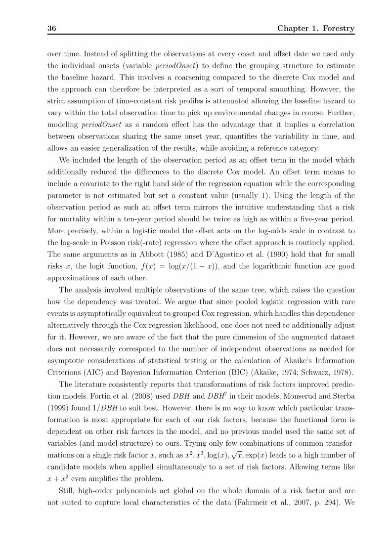
36 Chapter 1. Forestry
over time. Instead of splitting the observations at every onset and offset date we used only
the individual onsets (variable periodOnset) to define the grouping structure to estimate
the baseline hazard. This involves a coarsening compared to the discrete Cox model and
the approach can therefore be interpreted as a sort of temporal smoothing. However, the
strict assumption of time-constant risk profiles is attenuated allowing the baseline hazard to
vary within the total observation time to pick up environmental changes in course. Further,
modeling periodOnset as a random effect has the advantage that it implies a correlation
between observations sharing the same onset year, quantifies the variability in time, and
allows an easier generalization of the results, while avoiding a reference category.
We included the length of the observation period as an offset term in the model which
additionally reduced the differences to the discrete Cox model. An offset term means to
include a covariate to the right hand side of the regression equation while the corresponding
parameter is not estimated but set a constant value (usually 1). Using the length of the
observation period as such an offset term mirrors the intuitive understanding that a risk
for mortality within a ten-year period should be twice as high as within a five-year period.
More precisely, within a logistic model the offset acts on the log-odds scale in contrast to
the log-scale in Poisson risk(-rate) regression where the offset approach is routinely applied.
The same arguments as in Abbott (1985) and D’Agostino et al. (1990) hold that for small
risks x, the logit function, f(x) = log(x/(1 − x)), and the logarithmic function are good
approximations of each other.
The analysis involved multiple observations of the same tree, which raises the question
how the dependency was treated. We argue that since pooled logistic regression with rare
events is asymptotically equivalent to grouped Cox regression, which handles this dependence
alternatively through the Cox regression likelihood, one does not need to additionally adjust
for it. However, we are aware of the fact that the pure dimension of the augmented dataset
does not necessarily correspond to the number of independent observations as needed for
asymptotic considerations of statistical testing or the calculation of Akaike’s Information
Criterions (AIC) and Bayesian Information Criterion (BIC) (Akaike, 1974; Schwarz, 1978).
The literature consistently reports that transformations of risk factors improved predic-
tion models. Fortin et al. (2008) used DBH and DBH2 in their models, Monserud and Sterba
(1999) found 1/DBH to suit best. However, there is no way to know which particular trans-
formation is most appropriate for each of our risk factors, because the functional form is
dependent on other risk factors in the model, and no previous model used the same set of
variables (and model structure) to ours. Trying only few combinations of common transfor-
mations on a single risk factor x, such as x2, x3, log(x),√x, exp(x) leads to a high number of
candidate models when applied simultaneously to a set of risk factors. Allowing terms like
x+ x2 even amplifies the problem.
Still, high-order polynomials act global on the whole domain of a risk factor and are
not suited to capture local characteristics of the data (Fahrmeir et al., 2007, p. 294). We

1.3 Model development 37
chose spline functions in order to flexibly, and simultaneously model smooth functional re-
lationships for multiple covariates in a data driven way, which has been successfully applied
in many fields. Nevertheless we used transformations on the risk factors as a first step to
achieve symmetric and compact empirical distributions. That might not be absolutely nec-
essary, but in our opinion helped to stabilize the procedure and reduced the impact of the
knot locations of the spline. Three of the risk factors, KKL, CILateral , and CIConifer had
a disproportionately large number of zeros (point masses), these were removed for seeking
the optimal transform. The considered transformations were power transformations where
power could range from 0.01 to 1. The Kolmogorov-Smirnov (KS) test for normality was
used to find an optimal power transform with the transform corresponding to the smallest
value of the KS test statistic declared as optimal. The optimal power was rounded to the
next even fraction and the variable was transformed by this power for all further analyses,
including the spline construction. The resulting transformations along with their effect on
the shape of the empirical distributions are shown in Figure 1.4. The spline approach applied
to transformed risk factors x allows a more flexible modeling than a global polynomial. It
is intended to approximate the unknown functional relationship g(x) of a covariate to the
outcome y, by the spline s(x),
g(x) ≈ s(x).
The spline function s(x) is defined as follows: The domain of x is divided in intervals by
selecting a set of m knots. Within each interval the spline is parameterized as a polynomial
of degree l, pl(x),
pl(x) = γ0 + γ1x+ γ2x2 + . . .+ γlx
l.
Further, to ensure global smoothness, s(x) must be l − 1 times continuously differentiable
not only within the intervals, but also at the connection points between the intervals. For
estimation within a regression framework a constructive representation, which fulfills these
requirements, is needed. Basis functions, B, are utilized to parameterize the spline function,
s(x) =d∑j=1
δjBj(x),
where d = m+l−1 linear combinations of basis functions are needed when a l-degree B-spline
basis (Eilers and Marx, 1996) with m knots is used. The basis functions are recursively
defined, following (Fahrmeir et al., 2007, p. 304 ff.),
B0j (x) = I[κj ,κj+1)(x) =
1 κj ≤ x < κj+1,
0 otherwise,j = 1, . . . , d− 1,
B1j (x) =
x− κjκj+1 − κj
I[κj ,κj+1)(x) +κj+2 − x
κj+2 − κj+1
I[κj+1,κj+2)(x),
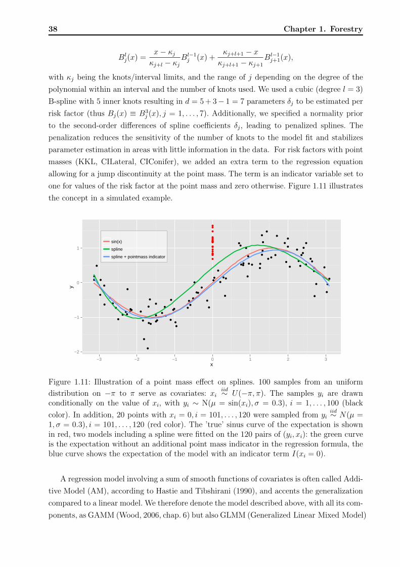
38 Chapter 1. Forestry
Blj(x) =
x− κjκj+l − κj
Bl−1j (x) +
κj+l+1 − xκj+l+1 − κj+1
Bl−1j+1(x),
with κj being the knots/interval limits, and the range of j depending on the degree of the
polynomial within an interval and the number of knots used. We used a cubic (degree l = 3)
B-spline with 5 inner knots resulting in d = 5 + 3− 1 = 7 parameters δj to be estimated per
risk factor (thus Bj(x) ≡ B3j (x), j = 1, . . . , 7). Additionally, we specified a normality prior
to the second-order differences of spline coefficients δj, leading to penalized splines. The
penalization reduces the sensitivity of the number of knots to the model fit and stabilizes
parameter estimation in areas with little information in the data. For risk factors with point
masses (KKL, CILateral, CIConifer), we added an extra term to the regression equation
allowing for a jump discontinuity at the point mass. The term is an indicator variable set to
one for values of the risk factor at the point mass and zero otherwise. Figure 1.11 illustrates
the concept in a simulated example.
●
●
●
● ●
●
●
●
●
●
●
●
●
●
●
●
●
●
●
●
●
●
●
●
●
● ●
●
●
●
●
●
●
●
●
●
●
●
●
●
●
●
●
●
●
●
●
●
●
●
●
●
●
●
●
●
●
●
●
●●
●
●
●
●
●
●
●
●
●●
●
●
●
●
●
●
●
●
●
●
●
●
●
●
●
● ●
●
●
●
●
●
●
●
●
●●
●
●
●
●
●
●
●
●
●
●
●
●
●
●●
●
●
●
●
●
●
●
−2
−1
0
1
−3 −2 −1 0 1 2 3x
y
sin(x)
spline
spline + pointmass indicator
Figure 1.11: Illustration of a point mass effect on splines. 100 samples from an uniform
distribution on −π to π serve as covariates: xiiid∼ U(−π, π). The samples yi are drawn
conditionally on the value of xi, with yi ∼ N(µ = sin(xi), σ = 0.3), i = 1, . . . , 100 (black
color). In addition, 20 points with xi = 0, i = 101, . . . , 120 were sampled from yiiid∼ N(µ =
1, σ = 0.3), i = 101, . . . , 120 (red color). The ’true’ sinus curve of the expectation is shownin red, two models including a spline were fitted on the 120 pairs of (yi, xi): the green curveis the expectation without an additional point mass indicator in the regression formula, theblue curve shows the expectation of the model with an indicator term I(xi = 0).
A regression model involving a sum of smooth functions of covariates is often called Addi-
tive Model (AM), according to Hastie and Tibshirani (1990), and accents the generalization
compared to a linear model. We therefore denote the model described above, with all its com-
ponents, as GAMM (Wood, 2006, chap. 6) but also GLMM (Generalized Linear Mixed Model)

1.3 Model development 39
is appropriate as the spline representation is still linear in its coefficients.
1.3.4 Final model structure
In sum, the steps above resulted in a GAMM with multiple risk factors, relating the
probability of death π of an individual tree within the observation period to risk factors
measured at the beginning of the observation period, the calendar year, the tree’s plot and
the length of the observation period as follows:
log
(πijk
1− πijk
)= β0 + offsetijk + γi + γj + s1(DBH
3/20ijk )+
s2(Height2/3ijk ) + s3(KKL
1/3ijk ) + s4(CIIntra
1/2ijk )
s5(CIConifer1/3ijk ) + s6(CIOvershade
1/2ijk ) + s7(CILateral
1/3ijk )+ (1.2)
s8(DBHdom1/3ijk ) + s9(RelDBHdom
2/3ijk ) + s10(SiteIndexijk)+
β1I(KKLijk = 0) + β2I(CILateralijk = 0) + β3I(CIConiferijk = 0).
The single components are:
πijk: Probability of death for tree k from plot j at the end of period i
(πijk = P(yijk = 1 | covariates )).
β0: Global intercept of model.
offsetijk:(log(periodLength
5
))ijk
.
γi: Random effect for periodOnset i, i =1985, 1987, 1989, 1991, 1994, 1995, 1996,
1997, 1999, 2000; with γi ∼ N(0, σperiodOnset).
γj: Random effect for plot j, j = 1, . . . , 29; with γj ∼ N(0, σplot).
s(x): Evaluation of spline function for covariate x; s(x) =∑d
l=1 δlBl(x), where δl are
the coefficients of the penalized spline and Bl the spline basis functions. The
penalization of coefficients is expressed by a regularization prior, δl ∼ N(0, σs).
The splines were set up separately for each risk factor. We used a spline of degree
3 with 5 inner knots resulting in d = 5 + 3− 1 = 7 parameters δl to be estimated
per risk factor (Fahrmeir et al., 2007, p.303).
β1, β2, β3: Coefficients according to the point mass effects, where I(KKLijk = 0) is meant
to evaluate to 1 if KKLijk = 0, and 0 otherwise. Similarly for CILateral and
CIConifer .
The model expression above implies that all of the risk factors (Table 1.2) appeared in the
final model, but we used model selection to pare down the model to an optimal parsimonious
model that is more likely to be accurate on external validation. This process is described
next.

40 Chapter 1. Forestry
1.3.5 Selection of risk factors
We followed the recommendations in Harrell et al. (1996) that no more than p = m/10
predictor degrees of freedom should be examined for fitting a model aiming for good predic-
tion, where degrees of freedom is understood as the number of coefficients in model fitting
in this context. In the case of a logistic regression model for mortality, or equivalently a
survival model, m is determined as the number of non-censored event times. In our data
that is the number of dead trees, m = 585, resulting in p ≈ 58 free parameters as the upper
limit to use in the prediction model. The model structure as stated in Model 1.2 involves 102
coefficients, but most of them are subject to restrictions due to normality assumptions (plot
and period effects) and penalization (smooth spline effects), leading to an effective number
considerably lower than that. However, we regarded Model 1.2 as the upper bound in terms
of complexity, and did not consider further effects such as interactions between risk factors.
For the actual selection of an optimal set of risk factors to include in the mortality
prediction model, we performed an internal cross-validation. The particular cross-validation
scheme reflected the hierarchical structure of the observations and the ultimate purpose
of the model, which would be to predict 5-year mortality for a tree in a new plot. For
median (or conditional) prediction the periodOnset and plot random effects would all be set
to zero (Skrondal and Rabe-Hesketh, 2009). We used k-fold cross validation with k = 29
to correspond to the 29 plots represented in the data. Each of the 29 plots served in turn
as a single test data set with the remaining 28 plots combined as a training set, resulting
in 29 internal cross-validations. For each training set, a set of candidate models were fit
and parameter estimates were used to predict the mortality for trees in the corresponding
validation set. To reduce the influence of multi-collinearity among the risk factors on stability
of the model selection process, the Spearman correlations among the transformed risk factors
(Figure 1.5 and 1.9) were assessed and models containing two risk factors with correlations
exceeding 0.75 in absolute value were dropped from further consideration.
Basically, we constructed the set of candidate models by building all subsets of smooth
terms (s1, . . . , s9) in Model 1.2, excluding those with pairs of high correlation as mentioned
above. Point mass effects were always included along with the according smoothed effect.
The global intercept, offset term, and the random effects for plot and periodOnset were
included in all of the candidate models at this stage. We investigated the performance of the
resulting 67 models and used the best ones as a basis for further investigation. For example,
if the functional form of a smooth effect looked linear, the term was replaced by a simple
linear term, and the modified model was again assessed by cross-validation. In stepwise
modifying, dropping and adding terms, we tried to further improve the performance and
where appropriate, simplify the model, basing all actions on cross-validation. At the end we
ran 142 models through this machinery and ultimately picked a final model among those

1.3 Model development 41
performing best. We will describe the measures of model performance in the following section.
1.3.6 Measures of model performance
Assessment of the predictive abilities of candidate models was an essential part in model
development. Considering the purpose of the tree mortality model, we based all calculations
on the predicted values y = π (0 ≤ y ≤ 1), corresponding to the predicted mortality from
the logistic regression model, and its relationship to the true outcome y ∈ {0; 1} in the
test data. Measures of model performance all deal with the distance of y to y but highlight
different aspects of performance. Our focus was on discrimination, which measures how
strong the predictions differ in n observations with y = 1 and y = 0, and calibration, which
measures the agreement between observed outcomes and predictions from a frequentist point
of view. If we predict a 20% risk of mortality for a tree, we should observe approximately 20
of 100 trees with such a prediction to experience mortality. Quantities combining different
aspects are said to measure overall performance (Steyerberg et al., 2010). An extensive list of
performance measures, along with their calculation rule and interpretation can be found in
the Appendix. For model selection we focused on the AUC (discrimination), the calibration
slope (calibration), and for overall model performance on R2 and Brier score (Steyerberg,
2009, p. 257). The AUC for a covariate x, as described in Section 1.2.3, also applies for the
case where x is a predicted probability of mortality, instead of a risk factor. Thus, y, such
as that arriving from a model fit to a training set of trees has same interpretation with the
difference that we assess the separation ability of the whole model, a combination of several
risk factors. The calibration slope (CS), is the estimated slope coefficient, β, of a logistic
regression model of true outcome y on the predicted risks y,
log
(P(y = 1)
1−P(y = 1)
)= α + β log
(y
1− y
),
CS ≡ β,
that is the model predictions y are transformed and used as the regressor variable in the
logistic model. A calibration slope for a perfectly calibrated model is 1, while coefficients
lower than 1 indicate that the predictions are too extreme. Too extreme means that the
observed mortality is higher than predicted for low-risk trees and lower than predicted for
high-risk trees (Steyerberg et al., 2001). The R2 is based on the binomial likelihood, and can
be interpreted in analogy to a linear regression model, as the proportion of variance explained
by the model. For logistic regression, Nagelkerke (1991) standardized the binomial likelihood-
based R2Lik with the theoretically maximal reachable R2, which depends on the proportion
of success (yi = 1) in the data set to ensure the value of 1 for a perfect fit, analogous to
linear regression. Log likelihoods of intercept-only and risk factor-based prediction models
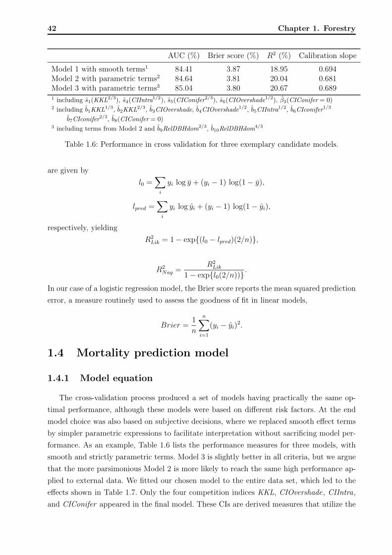
42 Chapter 1. Forestry
AUC (%) Brier score (%) R2 (%) Calibration slope
Model 1 with smooth terms1 84.41 3.87 18.95 0.694Model 2 with parametric terms2 84.64 3.81 20.04 0.681Model 3 with parametric terms3 85.04 3.80 20.67 0.6891 including s1(KKL2/3), s4(CIIntra1/2), s5(CIConifer2/3), s6(CIOvershade1/2), β3(CIConifer = 0)2 including b1KKL1/3, b2KKL2/3, b3CIOvershade, b4CIOvershade1/2, b5CIIntra
1/2, b6CIconifer1/3
b7CIconifer2/3, b8(CIConifer = 0)
3 including terms from Model 2 and b9RelDBHdom2/3, b10RelDBHdom4/3
Table 1.6: Performance in cross validation for three exemplary candidate models.
are given by
l0 =∑i
yi log y + (yi − 1) log(1− y),
lpred =∑i
yi log yi + (yi − 1) log(1− yi),
respectively, yielding
R2Lik = 1− exp{(l0 − lpred)(2/n)},
R2Nag =
R2Lik
1− exp{l0(2/n))}.
In our case of a logistic regression model, the Brier score reports the mean squared prediction
error, a measure routinely used to assess the goodness of fit in linear models,
Brier =1
n
n∑i=1
(yi − yi)2.
1.4 Mortality prediction model
1.4.1 Model equation
The cross-validation process produced a set of models having practically the same op-
timal performance, although these models were based on different risk factors. At the end
model choice was also based on subjective decisions, where we replaced smooth effect terms
by simpler parametric expressions to facilitate interpretation without sacrificing model per-
formance. As an example, Table 1.6 lists the performance measures for three models, with
smooth and strictly parametric terms. Model 3 is slightly better in all criteria, but we argue
that the more parsimonious Model 2 is more likely to reach the same high performance ap-
plied to external data. We fitted our chosen model to the entire data set, which led to the
effects shown in Table 1.7. Only the four competition indices KKL, CIOvershade, CIIntra,
and CIConifer appeared in the final model. These CIs are derived measures that utilize the
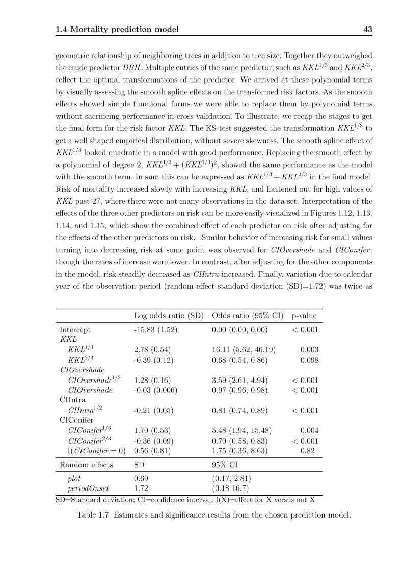
1.4 Mortality prediction model 43
geometric relationship of neighboring trees in addition to tree size. Together they outweighed
the crude predictor DBH . Multiple entries of the same predictor, such as KKL1/3 and KKL2/3,
reflect the optimal transformations of the predictor. We arrived at these polynomial terms
by visually assessing the smooth spline effects on the transformed risk factors. As the smooth
effects showed simple functional forms we were able to replace them by polynomial terms
without sacrificing performance in cross validation. To illustrate, we recap the stages to get
the final form for the risk factor KKL. The KS-test suggested the transformation KKL1/3 to
get a well shaped empirical distribution, without severe skewness. The smooth spline effect of
KKL1/3 looked quadratic in a model with good performance. Replacing the smooth effect by
a polynomial of degree 2, KKL1/3 + (KKL1/3)2, showed the same performance as the model
with the smooth term. In sum this can be expressed as KKL1/3 + KKL2/3 in the final model.
Risk of mortality increased slowly with increasing KKL, and flattened out for high values of
KKL past 27, where there were not many observations in the data set. Interpretation of the
effects of the three other predictors on risk can be more easily visualized in Figures 1.12, 1.13,
1.14, and 1.15, which show the combined effect of each predictor on risk after adjusting for
the effects of the other predictors on risk. Similar behavior of increasing risk for small values
turning into decreasing risk at some point was observed for CIOvershade and CIConifer ,
though the rates of increase were lower. In contrast, after adjusting for the other components
in the model, risk steadily decreased as CIIntra increased. Finally, variation due to calendar
year of the observation period (random effect standard deviation (SD)=1.72) was twice as
Log odds ratio (SD) Odds ratio (95% CI) p-value
Intercept -15.83 (1.52) 0.00 (0.00, 0.00) < 0.001KKL
KKL1/3 2.78 (0.54) 16.11 (5.62, 46.19) 0.003
KKL2/3 -0.39 (0.12) 0.68 (0.54, 0.86) 0.098CIOvershade
CIOvershade1/2 1.28 (0.16) 3.59 (2.61, 4.94) < 0.001CIOvershade -0.03 (0.006) 0.97 (0.96, 0.98) < 0.001
CIIntra
CIIntra1/2 -0.21 (0.05) 0.81 (0.74, 0.89) < 0.001CIConifer
CIConifer1/3 1.70 (0.53) 5.48 (1.94, 15.48) 0.004
CIConifer2/3 -0.36 (0.09) 0.70 (0.58, 0.83) < 0.001I(CIConifer = 0) 0.56 (0.81) 1.75 (0.36, 8.63) 0.82
Random effects SD 95% CI
plot 0.69 (0.17, 2.81)periodOnset 1.72 (0.18 16.7)
SD=Standard deviation; CI=confidence interval; I(X)=effect for X versus not X
Table 1.7: Estimates and significance results from the chosen prediction model.
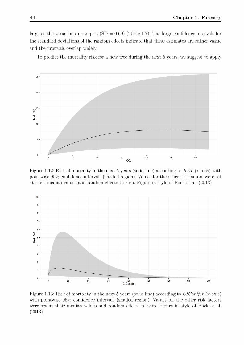
44 Chapter 1. Forestry
large as the variation due to plot (SD = 0.69) (Table 1.7). The large confidence intervals for
the standard deviations of the random effects indicate that these estimates are rather vague
and the intervals overlap widely.
To predict the mortality risk for a new tree during the next 5 years, we suggest to apply
Figure 1.12: Risk of mortality in the next 5 years (solid line) according to KKL (x-axis) withpointwise 95% confidence intervals (shaded region). Values for the other risk factors were setat their median values and random effects to zero. Figure in style of Bock et al. (2013)
Figure 1.13: Risk of mortality in the next 5 years (solid line) according to CIConifer (x-axis)with pointwise 95% confidence intervals (shaded region). Values for the other risk factorswere set at their median values and random effects to zero. Figure in style of Bock et al.(2013)
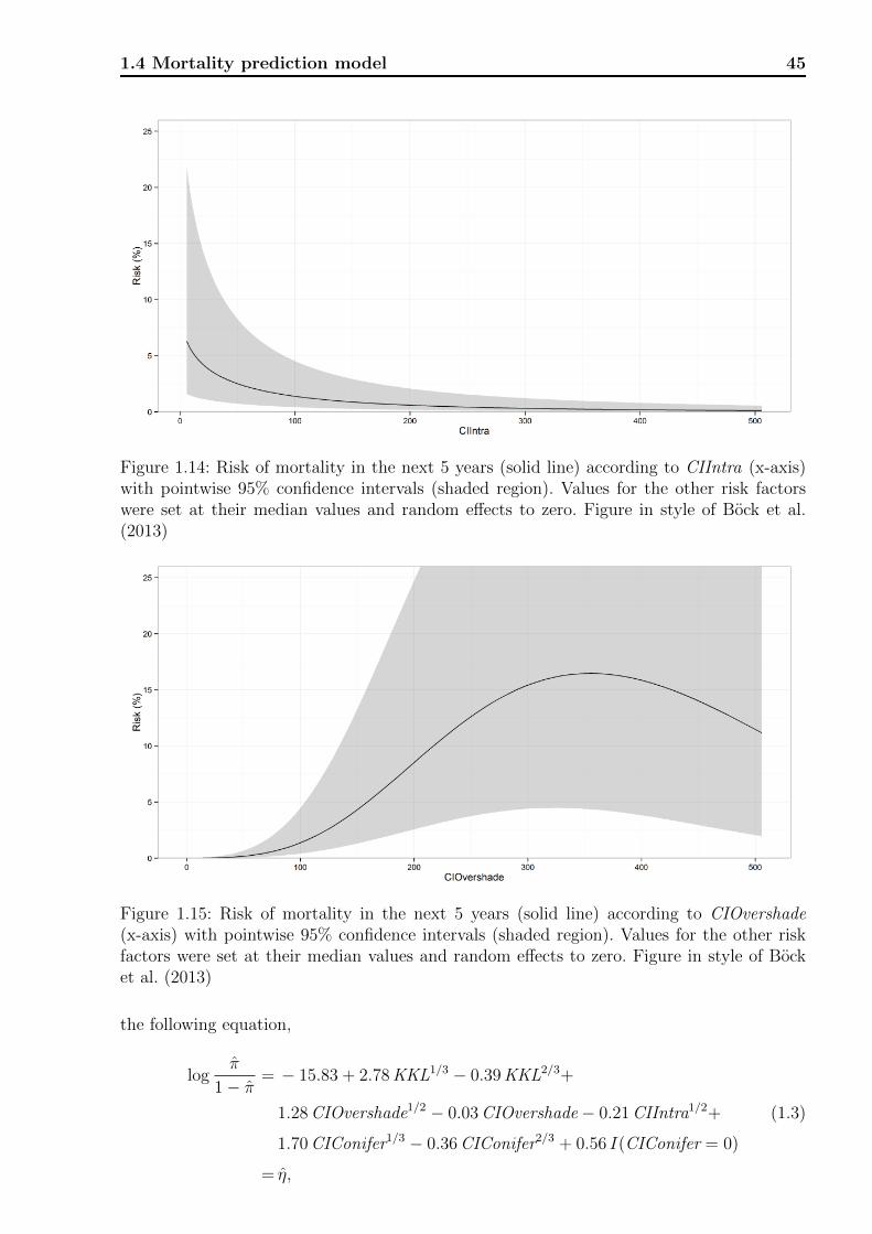
1.4 Mortality prediction model 45
Figure 1.14: Risk of mortality in the next 5 years (solid line) according to CIIntra (x-axis)with pointwise 95% confidence intervals (shaded region). Values for the other risk factorswere set at their median values and random effects to zero. Figure in style of Bock et al.(2013)
Figure 1.15: Risk of mortality in the next 5 years (solid line) according to CIOvershade(x-axis) with pointwise 95% confidence intervals (shaded region). Values for the other riskfactors were set at their median values and random effects to zero. Figure in style of Bocket al. (2013)
the following equation,
logπ
1− π= − 15.83 + 2.78 KKL1/3 − 0.39 KKL2/3+
1.28 CIOvershade1/2 − 0.03 CIOvershade− 0.21 CIIntra1/2+ (1.3)
1.70 CIConifer1/3 − 0.36 CIConifer2/3 + 0.56 I(CIConifer = 0)
= η,

46 Chapter 1. Forestry
AUC (%) Brier score (%) R2 (%) Calibration slope
Cross validation 84.64 3.81 20.04 0.681Internal validation 88.93 3.35 31.62 1.048
Table 1.8: Contrasting performance according to different validation schemes. Cross vali-dation: Leave-one-plot-out cross validation of final model. Internal validation: Final modelfitted on entire data (leading to Equation 1.3) is validated on the same data using all infor-mation of the fitted model, including random effect estimates.
where I(CIConifer = 0) equals 1 if CIConifer has the value 0 and equals 0 otherwise, and
the result η is transformed to the probability scale by π = exp(η)/(1 + exp(η)).
1.4.2 Contrasting performance
Finally, we want to contrast the performance measures according to internal and cross
validation using a model with the same set of covariates. Table 1.8 lists the AUC, Brier
score, pseudo R2, and calibration slope. The cross validation results are based on the model
structure which led to the final model, that is, included terms were the covariates from
Equation1.3, the random effects for plot and period and the offset term. To recall, in that
leave-one-plot-out cross validation the coefficients differed from those in the aforementioned
equation in each of the models fitted on the 29 training datasets. The actual coefficients
we suggest for use to obtain risk predictions are those from the model fitted to the entire
dataset. For this we show the internal validation: Model fitting and model assessment were
based on the same data, all information were used to obtain prediction, including random
effects coefficients.
Internal validation clearly had the best performance, mainly because internal predictions
are always well-calibrated. As our approach of cross validation is somewhere in between of
internal and external validation, it is reasonable to expect an AUC around 80%, a fairly good
separation ability, for similar but new data. The calibration slope was below unity, which
indicates some overfitting. That means we are not able to quantify the mortality risk very
accurately on average. A general shrinkage of the coefficients might overcome this. On the
other hand we observed an calibration slope above unity for the per definition well-calibrated
internal predictions. This effect was induced by the random effects in the model, as fixed
effects only models show perfect calibration in terms of average measures such as calibration
slope or calibration in the large, which contrast mean predictions against mean outcomes
(a fixed effects only model would obtain a calibration slope equal to unity). The fact that
random effects with normality assumption are somewhat lower in magnitude than their fixed
effects counterparts would be, finally leads to an underrating of actually high risks and the
overestimation of small risks. In other words, the shrinkage effect, which is desirable to correct
for overfitting, is seen in an underfitting tendency in the internal prediction performance.
Measures of goodness-of-fit, which represent a distance between the observed outcomes and

1.5 Summary and outlook 47
the predictions, showed a drop down of 12% (Brier score) and 35% (R2). We attribute this
discrepancy to the over-optimism of internal validation and the fact that, on principle, the
results of binomial regression models can hardly be generalized to different settings (Mood,
2010). However, the good separation ability seen on the AUC showed only a moderate decline
of 4.8%, giving occasion to believe that predictions on external data will also deliver valuable
information to identify trees which are particularly at risk.
1.5 Summary and outlook
The review of the literature combined with the results of this study show that a variety
of statistical methods have effectively been used for modeling the rare event of forest mortal-
ity. Forest mortality models are designed with specific objectives in mind, these objectives
determine the risk factors used in the model. In contrast to other models, mortality models
in this study were specifically designed to capitalize on the many geometrical and distance-
based competition indices that are calculated with detailed forest inventory data through the
SILVA simulator. As such, competition indices outweighed the effect of the crude predictor
DBH or other predictors of tree size. The mortality model presented here was developed for
European Beech, one of the largest of two species currently under observation as part of the
Bavarian forest network. A next step would be to move on to another common species, the
Douglas fir and to assess whether a similar risk profile for mortality holds.
In this study we focused on modeling the functional dependency of mortality on risk
factors, accounting for the peculiarities of the sampling design. A probabilistic model was
fitted using the maximum likelihood approach. McIntosh and Pepe (2002) show the optimal-
ity of such models in terms of AUC. However, it might be worth trying to directly optimize
measures of model performance which were used for now only for model assessment. This
would result in different loss functions than the one presently applied, the negative binomial
likelihood, and the discussion of proper scoring rules (Gneiting and Raftery, 2007).
Investigations concerning to relax the normality assumption of the random effects via
Dirichlet process priors (Kleinman and Ibrahim, 1998b; Wang, 2010) did not show enhance-
ments in terms of model performance. On the contrary, based on our examinations we found
the normality constraint to be rather helpful in rare-events logistic regression, having a stabi-
lizing effect. Further, the methods suggested in Pregibon (1981) and Landwehr et al. (1984)
for the detection of outliers were not expedient as they mainly sorted out the few trees where
mortality was observed. The computationally demanding model selection based on the cross
validation of a large set of candidate models was not contradictory to AIC/BIC procedures,
which could be obtained faster, but had two advantages: The dependency of the results on
the specification of the effective sample size (Zou and Normand, 2001) which is a quantity
needed in both criteria could be avoided. In our setting with longitudinal observations and
possibly multiple levels of random effects, it is somewhat unclear how to derive a suitable

48 Chapter 1. Forestry
quantity of effective sample size. Further, both AIC and BIC provide no support on the de-
cision about which type of risk predictions from a random effects model (conditional versus
marginal) should be used.
Chapter 2
Plant breeding
This chapter emphasizes the statistical methods used in the article “Association analysis
of frost tolerance in rye using candidate genes and phenotypic data from controlled, semi-
controlled, and field phenotyping platforms” (Y. Li, A. Bock, G. Haseneyer, V. Korzun, P.
Wilde, C.-C. Schon, D. P. Ankerst, and E. Bauer, 2011b), while shortening the biological
background and subject matter considerations. For those we refer to the original article and
its supplementary material, which provide more details. Figures in the original article were
produced by Li and partly recreated on the underlying data by the author of this thesis to
match the style of this dissertation (referenced with “recreated”).
2.1 Introduction
Frost stress, one of the important abiotic stresses, not only limits the geographic dis-
tribution of crop production but also adversely affects crop development and yield through
cold-induced desiccation, cellular damage and inhibition of metabolic reactions (Gusta et al.,
1997; Chinnusamy et al., 2007). Thus, crop varieties with improved tolerance to frost are of
enormous value for countries with severe winters. Frost tolerance (FT) is one of the most
critical traits that determine winter survival of winter cereals (Saulescu and Braun, 2001).
Among small grain cereals, rye (Secale cereale L.) is the most frost tolerant species and thus
can be used as a cereal model for studying and improving FT (Fowler and Limin, 1987;
Hommo, 1994). After cold acclimation where plants are exposed to a period of low, but
non-freezing temperature, the most frost-tolerant rye cultivar can survive under severe frost
stress down to approximately −30 ◦C (Thomashow, 1999). Tests for evaluating FT can be
generally separated into direct and indirect approaches. For direct approaches, where plants
are exposed to both cold acclimation and freezing tests, plant survival rate, leaf damage,
regeneration of the plant crown, electrolyte leakage, and chlorophyll fluorescence are often
used as phenotypic endpoints (Saulescu and Braun, 2001). For indirect approaches, where
plants are only exposed to cold acclimation, the endpoints of water content (Fowler et al.,
1981), proline (Dorffling et al., 1990), and cold-induced proteins (Houde et al., 1992) are
50 Chapter 2. Plant breeding
often used. The evaluation of FT can be conducted either naturally under field conditions
or artificially in growth chambers, with both methods associated with advantages and dis-
advantages. Under field conditions, plant damage during winter is not only affected by low
temperature stress per se, but also by the interaction of a range of factors such as snow
coverage, water supply, and wind. Therefore, measured phenotypes are the result of the full
range of factors affecting winter survival. Opportunities for assessing FT are highly depen-
dent upon temperature and weather conditions during the experiment. In contrast, frost
tests in growth chambers allow for a better control of environmental variation and are not
limited to one trial per year. However, they are limited in capacity and may not correlate
well with field performance. Therefore, it has been recommended to test FT under both
natural and controlled conditions whenever possible (Saulescu and Braun, 2001).
Identification of genes underlying traits of agronomic interest is pivotal for genome-based
breeding. Due to methodological advances in molecular biology, plant breeders can now select
varieties with favorable alleles through molecular markers, including single nucleotide poly-
morphisms (SNPs), identified in genes linked to desirable traits (Rafalski, 2002; Tester and
Langridge, 2010). Whole genome- and candidate gene-based association studies have identi-
fied large numbers of genomic regions and individual genes related to a range of traits (Harjes
et al., 2008; Malosetti et al., 2007; Thornsberry et al., 2001; Zhao et al., 2007). However, un-
derlying population structure and/or familial relatedness (kinship) between genotypes under
study have proven to be a big challenge, leading to false positive associations between molec-
ular markers and traits in plants due to the heavily admixed nature of plant populations
(Aranzana et al., 2005). In response, several advanced statistical approaches have been de-
veloped for genotype-phenotype association studies, including genomic control (Devlin and
Roeder, 1999), structured association (Pritchard et al., 2000), and linear mixed model-based
methodologies (Stich et al., 2008; Yu et al., 2006).
The main objective of this study was to identify SNP alleles and haplotypes conferring su-
perior FT through candidate gene-based association studies performed in three phenotyping
platforms: controlled, semi-controlled, and field.
2.2 Methods
2.2.1 Plant material and DNA extraction
Plant material was derived from four Eastern and one Middle European cross-pollinated
winter rye breeding populations: 44 plants from EKOAGRO (Poland), 68 plants from Petkus
(Germany), 33 plants from PR 2733 (Belarus), 41 plants from ROM103 (Poland), and 15
plants from SMH2502 (Poland). To determine the haplotype phase, a gamete capturing
process was performed by crossing between 15 and 68 plants of each source population to
the same self-fertile inbred line, Lo152. Each resulting heterozygous S0 plant represented
one gamete of the respective source population. S0 plants were selfed to obtain S1 families
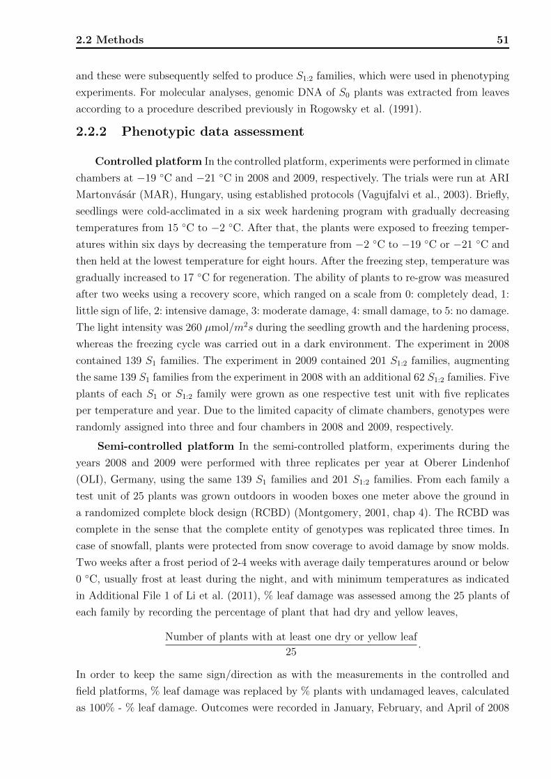
2.2 Methods 51
and these were subsequently selfed to produce S1:2 families, which were used in phenotyping
experiments. For molecular analyses, genomic DNA of S0 plants was extracted from leaves
according to a procedure described previously in Rogowsky et al. (1991).
2.2.2 Phenotypic data assessment
Controlled platform In the controlled platform, experiments were performed in climate
chambers at −19 ◦C and −21 ◦C in 2008 and 2009, respectively. The trials were run at ARI
Martonvasar (MAR), Hungary, using established protocols (Vagujfalvi et al., 2003). Briefly,
seedlings were cold-acclimated in a six week hardening program with gradually decreasing
temperatures from 15 ◦C to −2 ◦C. After that, the plants were exposed to freezing temper-
atures within six days by decreasing the temperature from −2 ◦C to −19 ◦C or −21 ◦C and
then held at the lowest temperature for eight hours. After the freezing step, temperature was
gradually increased to 17 ◦C for regeneration. The ability of plants to re-grow was measured
after two weeks using a recovery score, which ranged on a scale from 0: completely dead, 1:
little sign of life, 2: intensive damage, 3: moderate damage, 4: small damage, to 5: no damage.
The light intensity was 260 µmol/m2s during the seedling growth and the hardening process,
whereas the freezing cycle was carried out in a dark environment. The experiment in 2008
contained 139 S1 families. The experiment in 2009 contained 201 S1:2 families, augmenting
the same 139 S1 families from the experiment in 2008 with an additional 62 S1:2 families. Five
plants of each S1 or S1:2 family were grown as one respective test unit with five replicates
per temperature and year. Due to the limited capacity of climate chambers, genotypes were
randomly assigned into three and four chambers in 2008 and 2009, respectively.
Semi-controlled platform In the semi-controlled platform, experiments during the
years 2008 and 2009 were performed with three replicates per year at Oberer Lindenhof
(OLI), Germany, using the same 139 S1 families and 201 S1:2 families. From each family a
test unit of 25 plants was grown outdoors in wooden boxes one meter above the ground in
a randomized complete block design (RCBD) (Montgomery, 2001, chap 4). The RCBD was
complete in the sense that the complete entity of genotypes was replicated three times. In
case of snowfall, plants were protected from snow coverage to avoid damage by snow molds.
Two weeks after a frost period of 2-4 weeks with average daily temperatures around or below
0 ◦C, usually frost at least during the night, and with minimum temperatures as indicated
in Additional File 1 of Li et al. (2011), % leaf damage was assessed among the 25 plants of
each family by recording the percentage of plant that had dry and yellow leaves,
Number of plants with at least one dry or yellow leaf
25.
In order to keep the same sign/direction as with the measurements in the controlled and
field platforms, % leaf damage was replaced by % plants with undamaged leaves, calculated
as 100% - % leaf damage. Outcomes were recorded in January, February, and April of 2008
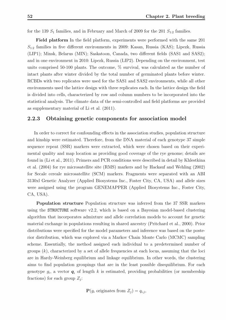
52 Chapter 2. Plant breeding
for the 139 S1 families, and in February and March of 2009 for the 201 S1:2 families.
Field platform In the field platform, experiments were performed with the same 201
S1:2 families in five different environments in 2009: Kasan, Russia (KAS); Lipezk, Russia
(LIP1); Minsk, Belarus (MIN); Saskatoon, Canada, two different fields (SAS1 and SAS2);
and in one environment in 2010: Lipezk, Russia (LIP2). Depending on the environment, test
units comprised 50-100 plants. The outcome, % survival, was calculated as the number of
intact plants after winter divided by the total number of germinated plants before winter.
RCBDs with two replicates were used for the SAS1 and SAS2 environments, while all other
environments used the lattice design with three replicates each. In the lattice design the field
is divided into cells, characterized by row and column numbers to be incorporated into the
statistical analysis. The climate data of the semi-controlled and field platforms are provided
as supplementary material of Li et al. (2011).
2.2.3 Obtaining genetic components for association model
In order to correct for confounding effects in the association studies, population structure
and kinship were estimated. Therefore, from the DNA material of each genotype 37 simple
sequence repeat (SSR) markers were extracted, which were chosen based on their experi-
mental quality and map location as providing good coverage of the rye genome; details are
found in (Li et al., 2011). Primers and PCR conditions were described in detail by Khlestkina
et al. (2004) for rye microsatellite site (RMS) markers and by Hackauf and Wehling (2002)
for Secale cereale microsatellite (SCM) markers. Fragments were separated with an ABI
3130xl Genetic Analyzer (Applied Biosystems Inc., Foster City, CA, USA) and allele sizes
were assigned using the program GENEMAPPER (Applied Biosystems Inc., Foster City,
CA, USA).
Population structure Population structure was inferred from the 37 SSR markers
using the STRUCTURE software v2.2, which is based on a Bayesian model-based clustering
algorithm that incorporates admixture and allele correlation models to account for genetic
material exchange in populations resulting in shared ancestry (Pritchard et al., 2000). Prior
distributions were specified for the model parameters and inference was based on the poste-
rior distribution, which was explored via a Markov Chain Monte Carlo (MCMC) sampling
scheme. Essentially, the method assigned each individual to a predetermined number of
groups (k), characterized by a set of allele frequencies at each locus, assuming that the loci
are in Hardy-Weinberg equilibrium and linkage equilibrium. In other words, the clustering
aims to find population groupings that are in the least possible disequilibrium. For each
genotype gi, a vector qi of length k is estimated, providing probabilities (or membership
fractions) for each group Zj:
P(gi originates from Zj) = qi,j,
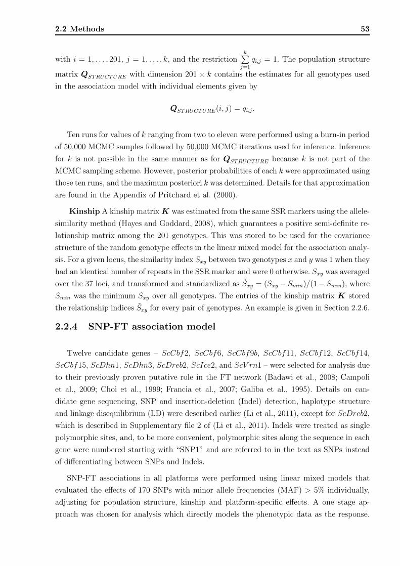
2.2 Methods 53
with i = 1, . . . , 201, j = 1, . . . , k, and the restrictionk∑j=1
qi,j = 1. The population structure
matrix QSTRUCTURE with dimension 201 × k contains the estimates for all genotypes used
in the association model with individual elements given by
QSTRUCTURE(i, j) = qi,j.
Ten runs for values of k ranging from two to eleven were performed using a burn-in period
of 50,000 MCMC samples followed by 50,000 MCMC iterations used for inference. Inference
for k is not possible in the same manner as for QSTRUCTURE because k is not part of the
MCMC sampling scheme. However, posterior probabilities of each k were approximated using
those ten runs, and the maximum posteriori k was determined. Details for that approximation
are found in the Appendix of Pritchard et al. (2000).
Kinship A kinship matrixK was estimated from the same SSR markers using the allele-
similarity method (Hayes and Goddard, 2008), which guarantees a positive semi-definite re-
lationship matrix among the 201 genotypes. This was stored to be used for the covariance
structure of the random genotype effects in the linear mixed model for the association analy-
sis. For a given locus, the similarity index Sxy between two genotypes x and y was 1 when they
had an identical number of repeats in the SSR marker and were 0 otherwise. Sxy was averaged
over the 37 loci, and transformed and standardized as Sxy = (Sxy −Smin)/(1−Smin), where
Smin was the minimum Sxy over all genotypes. The entries of the kinship matrix K stored
the relationship indices Sxy for every pair of genotypes. An example is given in Section 2.2.6.
2.2.4 SNP-FT association model
Twelve candidate genes – ScCbf2, ScCbf6, ScCbf9b, ScCbf11, ScCbf12, ScCbf14,
ScCbf15, ScDhn1, ScDhn3, ScDreb2, ScIce2, and ScV rn1 – were selected for analysis due
to their previously proven putative role in the FT network (Badawi et al., 2008; Campoli
et al., 2009; Choi et al., 1999; Francia et al., 2007; Galiba et al., 1995). Details on can-
didate gene sequencing, SNP and insertion-deletion (Indel) detection, haplotype structure
and linkage disequilibrium (LD) were described earlier (Li et al., 2011), except for ScDreb2,
which is described in Supplementary file 2 of (Li et al., 2011). Indels were treated as single
polymorphic sites, and, to be more convenient, polymorphic sites along the sequence in each
gene were numbered starting with “SNP1” and are referred to in the text as SNPs instead
of differentiating between SNPs and Indels.
SNP-FT associations in all platforms were performed using linear mixed models that
evaluated the effects of 170 SNPs with minor allele frequencies (MAF) > 5% individually,
adjusting for population structure, kinship and platform-specific effects. A one stage ap-
proach was chosen for analysis which directly models the phenotypic data as the response.

54 Chapter 2. Plant breeding
The general form of the linear mixed model for the three platforms was
y = 1β0 + xSNPβSNP + QSTRUCTUREβSTRUCTURE +
XPLATFORMβPLATFORM + ZPLATFORMγPLATFORM + (2.1)
ZGENOTY PEγGENOTY PE + ε.
More precise descriptions are given below, where for better readability the subscripts were
dropped if the context allowed. (platform-specific details are regarded afterwards):
y Vector of platform-specific phenotypes with dimension n×1.
1β0 Design vector with solely 1 entries 1 (n×1) and scalar intercept coefficient β0.
xSNPβSNP
Design vector xSNP (n×1) for bi-allelic SNP containing entries in dummy-coding: 0
for the reference allele (Lo152), 1 for the non-reference allele. Accordingly, βSNP is a
scalar fixed effect when switching from reference allele to non-reference allele.
QSTRUCTUREβSTRUCTURE
Design matrix Q (n×(k−1)), containing the first (k−1) membership fractions, which
were obtained from the STRUCTURE software. The k-th fraction is not used, as it is a lin-
ear combination of the others due to the sum-to-one constraint. Fixed effect coefficients
vector β with dimension (k − 1)× 1.
XPLATFORMβPLATFORM
Platform specific design matrix X (n× p) for fixed effects vector β (p× 1).
ZPLATFORMγPLATFORM
Platform specific design matrix Z (n×m) for random effects vector γ (m× 1). Ran-
dom effects are assumed to follow a multivariate normal distribution, γPLATFORM ∼N(0,D), with covariance matrix D.
ZGENOTY PEγGENOTY PE
Design matrix Z (n× l) for the random genotype effects and random effects vector γ
(l × 1). For the genotype effects the distributional assumption is
γ ∼ N(0, σ2gK),
where K is the kinship matrix and σ2g is the genotypic variation to be estimated. The
peculiarity of γ is its correlation structure given through the matrix K. The software
we used for model fitting only allowed some limited types of covariance matrices,
correlated random intercepts were not directly supported. That is, user input of a

2.2 Methods 55
correlation matrix was not possible. However, uncorrelated random intercepts, which
were supported, are equivalent to the use of an identity matrix instead ofK. In order to
still account for kinship in the estimation of genotype effects the correlation structure
was shifted in the design matrix Z, which was constructed as follows: The incidence
matrix Z, which links each observation to its genotype effect, was post-multiplied by
the transpose of the Cholesky-root of K, denoted by KT/2. The Cholesky-root is well-
defined for symmetric, positive semi-definite matrices, a property which is guaranteed
using the allele-similarity method from Hayes and Goddard (2008). That is,
K = KT/2K1/2,
with K1/2 being the right Cholesky-root, which is an upper-triangular-matrix, and
KT/2 the transpose of it, which is a lower-triangular-matrix. From γ ∼ N(0, σ2gI), it
holds that
Zγ ∼ N(0, σ2gZIZ
′).
From Z = ZKT/2, it holds that
σ2gZIZ
′ = σ2gZKZ
′,
which is the desired variance for ZGENOTY PEγGENOTY PE:
V(ZGENOTY PEγGENOTY PE) = σ2gZKZ
′.
Therefore ZGENOTY PE was set to ZKT/2 in the mixed model and γ ∼ N(0, σ2gI).
ε Residual error ε (n × 1), assumed to comprise independent and identically distributed
random normal errors with mean zero and variance σ2: ε ∼ N(0, Iσ2).
2.2.5 Phenotypic variation
To test phenotypic variation between genotypes, the same platform-specific models as
described for the SNP-FT association analyses were fitted for each platform omitting the
SNP and population structure fixed effects. Within the controlled platform, separate models
were fitted for each combination of temperature and year; for the semi-controlled platform,
separate models were fitted for each month of each year; and for the field platform, sepa-
rate models were fitted for each geographic location—altogether 15 subgroups in all three
platforms. Within this grouping, mean outcomes per genotype were calculated. That is, the
replicates of each genotype were averaged and summarized in boxplots.
Genetic variation was reported as the variance component corresponding to the random
genotype effect in each model, with a p-value computed using the likelihood ratio test (LRT),

56 Chapter 2. Plant breeding
Marker 1 Marker 2 Marker 3 Marker 4
Genotype 1 A A A AGenotype 2 A B B BGenotype 3 A C A B
Table 2.1: Example markers for kinship estimation.
a conservative estimate since the true asymptotic distribution of the LRT statistic is a
mixture of chi-square distributions (Fitzmaurice et al., 2004). This analysis aims to give an
overview of the measured variability in the trials and is therefore reported first in the results
section.
2.2.6 About the kinship matrix
The kinship matrix is supposed to express genetic similarity between different individuals
or genotypes. Regarding the kinship matrix as an empirical correlation matrix might be
misleading as it is not clear what the theoretical counterpart (the true underlying parameter)
is. However, in the mixed model it is used as a correlation or covariance matrix in the prior
distribution of the random genotype effects. The documentation of the kin() function in the
synbreed R-package (Wimmer et al., 2012) is a good starting point for further reading about
the different types of kinship estimation and their interpretation. The scale of the kinship
matrix, in terms of a scalar factor multiplied with the matrix K, is arbitrary for the fit of
the linear mixed model and also the inference is unaffected when the variance parameter
associated with K, σ2g , is estimated (and not fixed). Clearly, quantities such as heritability,
h2 =σ2g
σ2g+σ2 , highly depend on how the kinship matrix is derived. Balding (2013) shows recent
developments.
Below are some examples of how the entries of the kinship matrix K influence the
estimation in a linear mixed model. Suppose there are SSR markers from three homozygous
inbred lines at four loci, demonstrated in the following table: The simple matching coefficient
of Reif et al. (2005) in the standardized version of Hayes and Goddard (2008) is calculated
as
Sxy = (Sxy − Smin)/(1− Smin),
for genotype x and genotype y, with Sxy the proportion of loci with identical alleles, and Smin
the minimum S between all genotypes. As Genotype 1 and Gentoype 3 have two identical
alleles out of four, their coefficient is 2/4. The minimum between all three genotypes is 1/4,
leading to a similarity coefficient between Genotype 1 and Genotype 3 of
SGenotpye 1,Genotype 3 = S13 =24− 1
4
1− 14
= 1/3.
The coefficients for all pairs of the three genotypes in this example are stored in the kinship

2.2 Methods 57
matrix
K =
1 0 1/3
0 1 1/3
1/3 1/3 1
,where the rows and columns are ordered accordingly to Genotype 1, 2, and 3.
To illustrate how such a kind of correlation matrix affects the estimation of the random
effects γ, we consider the fixed artificial outcome vector y of six plants from three genotypes
and three different scenarios of kinship matrices. The data are coded as:
y Genotype
1 1
1 1
1 2
4 2
2 3
3 3
and Z =
1 0 0
1 0 0
0 1 0
0 1 0
0 0 1
0 0 1
.
For the mixed model
y = 1β0 +Zγ + ε, γ ∼ N(0, σ2gK), ε ∼ N(0, σ2I),
with given variance parameters σ2g = σ2 = 1, the variance of y is
V(y) = I +ZKZ ′ = V .
The estimates of the fixed effect β0 and the random effects γ are
β0 = (1′V −11)−11′V −1︸ ︷︷ ︸Hfix
y
and
γ = KZ ′V −1︸ ︷︷ ︸H
(y − 1β0)︸ ︷︷ ︸y
.
We present three matrices K, representing different grades of correlation between random
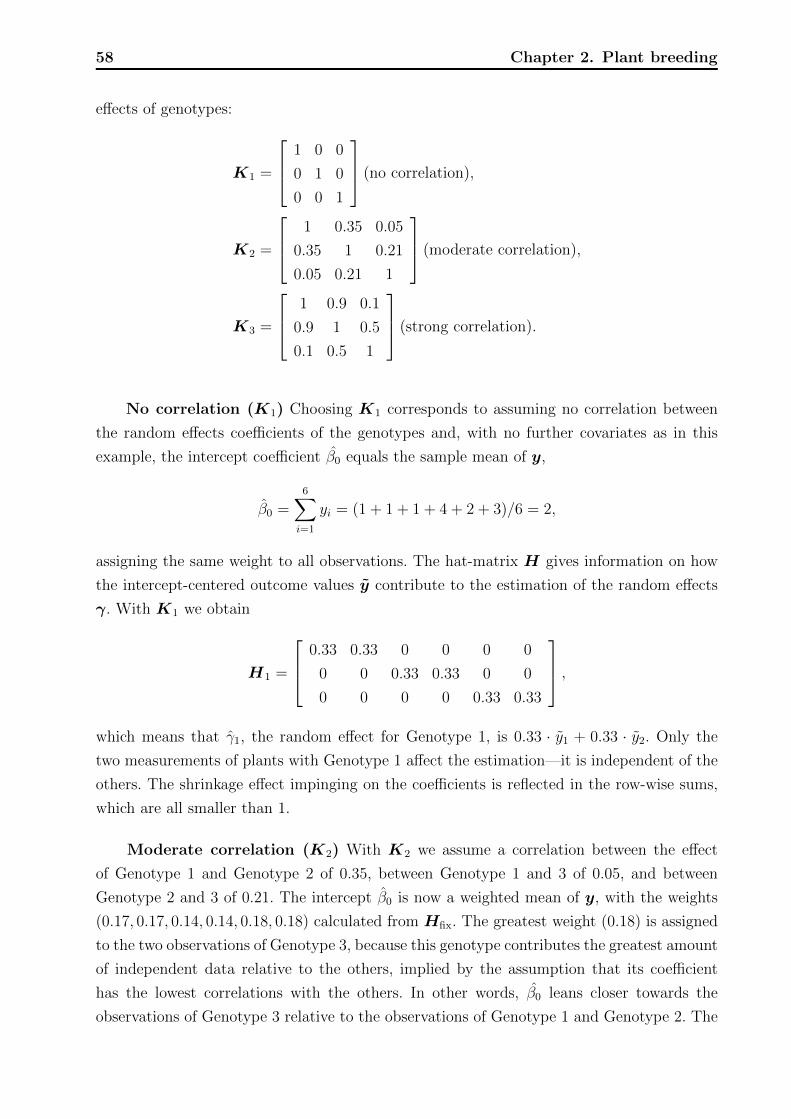
58 Chapter 2. Plant breeding
effects of genotypes:
K1 =
1 0 0
0 1 0
0 0 1
(no correlation),
K2 =
1 0.35 0.05
0.35 1 0.21
0.05 0.21 1
(moderate correlation),
K3 =
1 0.9 0.1
0.9 1 0.5
0.1 0.5 1
(strong correlation).
No correlation (K1) Choosing K1 corresponds to assuming no correlation between
the random effects coefficients of the genotypes and, with no further covariates as in this
example, the intercept coefficient β0 equals the sample mean of y,
β0 =6∑i=1
yi = (1 + 1 + 1 + 4 + 2 + 3)/6 = 2,
assigning the same weight to all observations. The hat-matrix H gives information on how
the intercept-centered outcome values y contribute to the estimation of the random effects
γ. With K1 we obtain
H1 =
0.33 0.33 0 0 0 0
0 0 0.33 0.33 0 0
0 0 0 0 0.33 0.33
,which means that γ1, the random effect for Genotype 1, is 0.33 · y1 + 0.33 · y2. Only the
two measurements of plants with Genotype 1 affect the estimation—it is independent of the
others. The shrinkage effect impinging on the coefficients is reflected in the row-wise sums,
which are all smaller than 1.
Moderate correlation (K2) With K2 we assume a correlation between the effect
of Genotype 1 and Genotype 2 of 0.35, between Genotype 1 and 3 of 0.05, and between
Genotype 2 and 3 of 0.21. The intercept β0 is now a weighted mean of y, with the weights
(0.17, 0.17, 0.14, 0.14, 0.18, 0.18) calculated from Hfix. The greatest weight (0.18) is assigned
to the two observations of Genotype 3, because this genotype contributes the greatest amount
of independent data relative to the others, implied by the assumption that its coefficient
has the lowest correlations with the others. In other words, β0 leans closer towards the
observations of Genotype 3 relative to the observations of Genotype 1 and Genotype 2. The
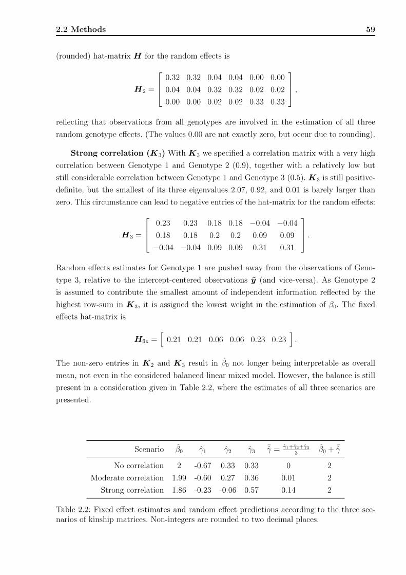
2.2 Methods 59
(rounded) hat-matrix H for the random effects is
H2 =
0.32 0.32 0.04 0.04 0.00 0.00
0.04 0.04 0.32 0.32 0.02 0.02
0.00 0.00 0.02 0.02 0.33 0.33
,reflecting that observations from all genotypes are involved in the estimation of all three
random genotype effects. (The values 0.00 are not exactly zero, but occur due to rounding).
Strong correlation (K3) With K3 we specified a correlation matrix with a very high
correlation between Genotype 1 and Genotype 2 (0.9), together with a relatively low but
still considerable correlation between Genotype 1 and Genotype 3 (0.5). K3 is still positive-
definite, but the smallest of its three eigenvalues 2.07, 0.92, and 0.01 is barely larger than
zero. This circumstance can lead to negative entries of the hat-matrix for the random effects:
H3 =
0.23 0.23 0.18 0.18 −0.04 −0.04
0.18 0.18 0.2 0.2 0.09 0.09
−0.04 −0.04 0.09 0.09 0.31 0.31
.Random effects estimates for Genotype 1 are pushed away from the observations of Geno-
type 3, relative to the intercept-centered observations y (and vice-versa). As Genotype 2
is assumed to contribute the smallest amount of independent information reflected by the
highest row-sum in K3, it is assigned the lowest weight in the estimation of β0. The fixed
effects hat-matrix is
Hfix =[
0.21 0.21 0.06 0.06 0.23 0.23].
The non-zero entries in K2 and K3 result in β0 not longer being interpretable as overall
mean, not even in the considered balanced linear mixed model. However, the balance is still
present in a consideration given in Table 2.2, where the estimates of all three scenarios are
presented.
Scenario β0 γ1 γ2 γ3¯γ = γ1+γ2+γ3
3β0 + ¯γ
No correlation 2 -0.67 0.33 0.33 0 2
Moderate correlation 1.99 -0.60 0.27 0.36 0.01 2
Strong correlation 1.86 -0.23 -0.06 0.57 0.14 2
Table 2.2: Fixed effect estimates and random effect predictions according to the three sce-narios of kinship matrices. Non-integers are rounded to two decimal places.

60 Chapter 2. Plant breeding
2.2.7 Platform-specific model details
In this section we provide details of the association models, which differed in the three
platforms and were not covered in Section 2.2.4.
Controlled platform analyses The outcome vector y was a recovery score, which
contained observations of n = 3360 test units, and the platform specific effect, βPLATFORM
included the two years of measurement 2008 and 2009 and two temperatures, −19 ◦C and
−21 ◦C. A common platform-specific random effect controlling for the seven chambers across
the two years 2008 and 2009 was included in the model, γPLATFORM ∼ N(0, Iσ2chamber), as
it provided a more parsimonious model with the same goodness-of-fit compared to a nested
random effect for chamber within year. No additional explicit generation adjustment for S1
versus S1:2 families was included in the statistical model, as these effects were confounded
with the fixed effect adjustment for year and the random chamber effects. In other words,
the generation effect was assumed implicitly adjusted for by other year effects in the model.
Within fixed effects coded by
Xcontrolled︸ ︷︷ ︸n×2
= [x1,x2] , βcontrolled = (β1, β2),
where the individual elements of x1 were 0 or 1 indicating whether an observation belongs
to the year 2008 or 2009, and x2 for temperature equal to −21 ◦C versus −19 ◦C. For the
random chamber effect, the design matrix Zcontrolled (n × 7) mapped each observation to
one of the seven chambers (three in 2008 and four in 2009) and thus to the random effects
γcontrolled (7 × 1). According to the notation in Section 2.2.4, D was an identity matrix of
dimension seven.
Semi-controlled platform analyses The outcome vector y was % plants with un-
damaged leaves measured repeatedly over three months (January, February, and April) in
2008 and two months (February, March) in 2009. The platform-specific fixed effects vector,
βPLATFORM , included three terms: a year effect, an overall linear trend in time for the three
months in 2008 and two months in 2009, and an interaction of year and linear trend in time,
coded by
Xsemi︸ ︷︷ ︸n×3
= [x1,x2,x3] , βsemi = (β1, β2, β3),
where elements of x1 were indicators for year 2009, the elements of x2 numeric representa-
tions of the month (0,1, or 2 for observations from 2008, and 0 or 1 for observations from
2009), and the elements of x3 were interactions of the years and months (1 for observations
from the second month (March) in 2009, and zero otherwise). This design permitted inter-
pretation of β1 as the change in % plants with undamaged leaves from 2008 to 2009, β2, the
change by month during 2008, and β2 + β3, the change by month during 2009.
The platform-specific random effects (vector γPLATFORM) consisted of three parts: 1.

2.2 Methods 61
replication, which was modeled as a blocking-factor (three replications in each of the two
years, leading to six blocks). 2. a random intercept and 3. a random trend according to month
for each plant group (the set of 25 plants where the outcome was determined). In principle
we had 1,020 of these plant groups originating from the 139 S1 families in 2008 and 201
S1:2 families in 2009, with three replications leading to 3 × (139 + 201) = 1, 020 outcomes.
For the analysis only 200 families in 2009 could be used, leading to 1,017 plant groups. The
replication random effect was assumed independent from the random intercept and trend,
and for the latter two random effects a correlation coefficient was estimated. Combining
the 1,251 observations from 2008 and 1,206 from 2009 led to n = 1, 251 + 1, 206 = 2, 457
observations in sum, and the design matrix Zsemi and random effects γsemi were constructed
as follows:
Zsemi︸ ︷︷ ︸n×2040
=
[Z1n×6
, Z2n×1017
, Z3n×1017
],
where Z1 was an incidence matrix mapping the outcomes to one of the six replications, Z2
was an incidence matrix mapping each observation to a plant group, and Z3 had the same
non-zero entries as Z2, but contained the numeric representation of the corresponding month
instead of an entry of 1 (same as x2 in the fixed effects design above). With γsemi we denote
the stacked vector of random effects,
γsemi1×2040
= (γ1,γ2,γ3),
where γ1 was a vector with six elements (γ11, . . . , γ16) = {γ1i}i=1,...,6, and both γ2 and γ3
were vectors with 1,017 elements each. The 2× 1 vector (γ2j, γ3j) contained j-th element of
each γ2 and γ3, which allows to define the distributional assumption as
γ1i ∼ N(0, σ2rep), i = 1, . . . , 6,
(γ2j, γ3j) ∼ N(0,D), j = 1, . . . , 1017,
where D is a 2 × 2 unstructured covariance matrix to be estimated. There were thus four
variance parameters to estimate.
Field platform analyses The outcome vector y was % survival and the platform-
specific fixed effect βPLATFORM included indicator variables for the six environments, five
environments in 2009 and one in 2010. In total n = 3, 216 outcomes could be considered in the
model. Platform-specific random effects included a block effect nested within environments
arising from the lattice design. That is, the fixed effects design matrix Xfield (n× 5) =
[x1,x2,x3,x4,x5] maps the observations to the environments (location in year), where Minsk
2009 is the reference category. From the lattice design there were 198 blocks (nested within
environments), modeled by a random intercept per block: Zfield (n× 198), with random
effects vector γfield, which was assumed to be normally distributed, with individual elements
62 Chapter 2. Plant breeding
γj ∼ N(0, σ2block), independent for j = 1, . . . , 198.
2.2.8 Haplotype-FT association model and gene×gene interaction
In addition to the effect of single SNPs in the association models, the effects of haplotypes
were estimated as well. A haplotype bundles the information of several markers from adjacent
locations and allows a categorization. From a statistical perspective they are categorical
variables defined by the interaction of other categorical variables. For example, if there is
information on three SNPs available, with two levels each, there are 23 = 8 haplotype phases
possible, with usually not each of these phases actually observed.
Here, haplotype phase was determined by subtracting the common parent Lo152 al-
leles and haplotypes were defined within each candidate gene using DnaSP v5.10 (Rozas
et al., 2003). Haplotype-FT associations were performed using candidate gene haplotypes
with MAF > 5%. The same platform-specific statistical models controlling for population
structure, kinship, and platform-specific effects were used to test associations between hap-
lotypes of the respective candidate genes and FT. For these analyses βhap replaced βSNP as
a measure of the haplotype effect of the non-reference, compared to the reference haplotype
Lo152. First, significant differences between haplotypes of one gene were assessed using the
LRT. If the overall statistic was significant, individual haplotype effects were tested against
the reference haplotype Lo152 via t-tests. Based on haplotype information gene×gene inter-
actions (= haplotype×haplotype intercations) were assessed using the likelihood ratio test,
comparing the full model with main effects plus interaction to the reduced model with main
effects only.
2.2.9 Obtaining model-based results
Analyses of marker-FT associations were conducted using the lme4 package (Bates and
Machler, 2010), implemented in R (R Core Team, 2012). The LRTs were performed as follows.
For a single term in the model (SNP or haplotype) and platform the available data were
determined, as missing values were different for every SNP and MAF-rule. Two mixed models
were fitted, a full model, which contained the marker effect of interest (xSNPβSNP , xhapβhap,
or xhap×hapβhap×hap), and a reduced model not containing that term. The reduced model to
test the gene×gene interaction was a model containing both genes in an additive way. The
test statistic was then calculated as D = 2 lfull−2 l0, where lfull and l0 were the log-likelihood
values of the full and reduced models, respectively. Under the null hypothesis of no effect
(or interaction), the test statistic asymptotically follows a χ2-distribution, Da∼ χ2(df), with
the degrees of freedom df being the difference in numbers of parameters of the two models,
which comes down to a 1 in a SNP-test, for example. The p-values were reported as the
probability mass above the observed test statistic: p-value = P(X > D), with X ∼ χ2(df).
Significance of individual haplotype effects β was assessed via the t-statistic performed at
the two-sided α = 0.05 level. The t-statistic was derived using the elements of the estimated
2.3 Results 63
variance-/covariance matrix available in the model output, t-value = β/V(β), and P-values
as p-value = 2 P(X > |t-value|), with X ∼ t(df). For the degrees of freedom we used
the number of observations minus the number of fixed effects in the model. A multiple
testing problem arises, which inflates the false positive rate of the study. A simple and
common way to handle this problem is the Bonferroni correction where the significance level
is divided by the number of tests. However, the Bonferroni correction is too conservative and
only suitable for independent tests, an assumption violated in this study due to a high LD
between some of the SNPs as previously shown (Li et al., 2011). Therefore, the less stringent
significance level of α = 0.05 was used in order to retain candidates for further validation
in upcoming experiments. The exact p-values are available in Supplementary file 3 of Li
et al. (2011) and can be adjusted for multiple testing. Empirical correlations between the
170 SNP-FT associations reported among the three phenotyping platforms were performed
using Pearson’s correlation, based on the t-values from the corresponding association tests.
The genetic variation explained by an individual SNP or haplotype was calculated as
100× ((σ2g − σ2
gSNP )/σ2g),
where σ2 are the estimates of the respective genetic variances, in the reduced model without
an individual SNP (σ2g), and in the model including an individual SNP, σ2
gSNP ) (Mathews
et al., 2008). This ad-hoc measure can result in negative estimates since variance components
of genetic effects do not automatically decrease with more adjustment in a model. Negative
estimates were truncated to zero.
2.3 Results
2.3.1 Phenotypic data analyses
Phenotypic assessments of FT were carried out in 12 environments from three different
phenotyping platforms. Phenotypic data was analyzed separately in each environment (Fig-
ure 2.1). Genotypic variation for FT was significant at both temperatures for both years
in the controlled platform (p < 0.001). Recovery scores ranged from a median near 2.5
(between intensive and moderate damage) at −19 ◦C in 2008 to a median near 1.0 (little
sign of life) at −21 ◦C in 2009. As expected, recovery scores were higher at −19 ◦C than
at −21 ◦C in the same year but were lower in 2009 than in 2008, probably due to differ-
ent generations of rye material (S1 vs S1:2 families). The high variability at −2 ◦C in 2008
might have been induced by substantial variation between chambers (there was significant
variation due to chamber (p < 0.01)). In the semi-controlled platform, genotypic variation
for FT was significant during all months for both years (p < 0.01). Linear decreasing trends
were observed during each year, which was expected since that was longitudinal data and
thus the damaged portions of plants increased during the progression of winter. In the field
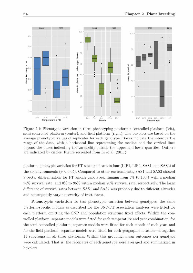
64 Chapter 2. Plant breeding
●
●
●
●
●
2008 2009
0.0
0.5
1.0
1.5
2.0
2.5
3.0
3.5
−21 −19 −21 −19Temperature in oC
Mea
n R
ecov
ery
Sco
re2008 2009
●
●
●
●
●
●
●
●
●●
●
30
40
50
60
70
80
90
100
Jan. Feb. Apr. Feb. Mar.Month
Mea
n %
pla
nts
with
und
amag
ed le
aves
2009 2010
●
●
●
●
●●●
●
●
●
●
0
20
40
60
80
100
KAS LIP1 MIN SAS1 SAS2 LIPEnvironment
Mea
n %
sur
viva
lFigure 2.1: Phenotypic variation in three phenotyping platforms: controlled platform (left),semi-controlled platform (center), and field platform (right). The boxplots are based on theaverage phenotypic values of replicates for each genotype. Boxes indicate the interquartilerange of the data, with a horizontal line representing the median and the vertical linesbeyond the boxes indicating the variability outside the upper and lower quartiles. Outliersare indicated by circles. Figure recreated from Li et al. (2011).
platform, genotypic variation for FT was significant in four (LIP1, LIP2, SAS1, and SAS2) of
the six environments (p < 0.05). Compared to other environments, SAS1 and SAS2 showed
a better differentiation for FT among genotypes, ranging from 5% to 100% with a median
75% survival rate, and 0% to 95% with a median 20% survival rate, respectively. The large
difference of survival rates between SAS1 and SAS2 was probably due to different altitudes
and consequently varying severity of frost stress.
Phenotypic variation To test phenotypic variation between genotypes, the same
platform-specific models as described for the SNP-FT association analyses were fitted for
each platform omitting the SNP and population structure fixed effects. Within the con-
trolled platform, separate models were fitted for each temperature and year combination; for
the semi-controlled platform, separate models were fitted for each month of each year; and
for the field platform, separate models were fitted for each geographic location—altogether
15 subgroups in all three platforms. Within this grouping, mean outcomes per genotype
were calculated. That is, the replicates of each genotype were averaged and summarized in
boxplots.
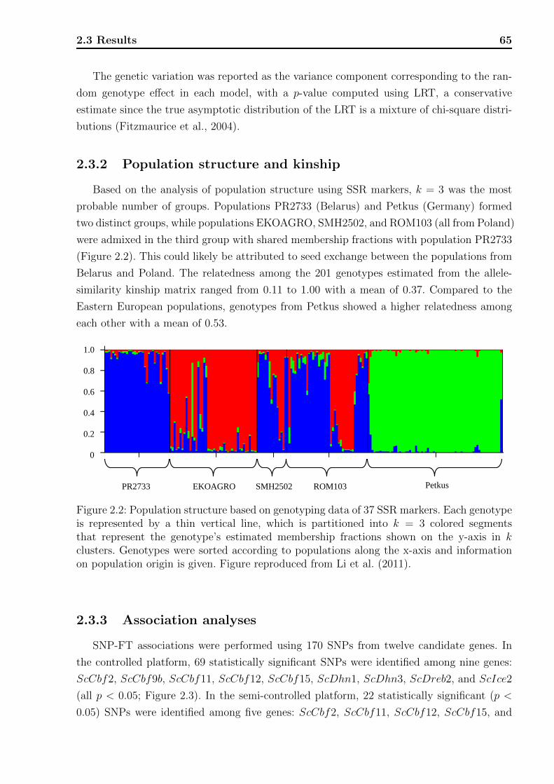
2.3 Results 65
The genetic variation was reported as the variance component corresponding to the ran-
dom genotype effect in each model, with a p-value computed using LRT, a conservative
estimate since the true asymptotic distribution of the LRT is a mixture of chi-square distri-
butions (Fitzmaurice et al., 2004).
2.3.2 Population structure and kinship
Based on the analysis of population structure using SSR markers, k = 3 was the most
probable number of groups. Populations PR2733 (Belarus) and Petkus (Germany) formed
two distinct groups, while populations EKOAGRO, SMH2502, and ROM103 (all from Poland)
were admixed in the third group with shared membership fractions with population PR2733
(Figure 2.2). This could likely be attributed to seed exchange between the populations from
Belarus and Poland. The relatedness among the 201 genotypes estimated from the allele-
similarity kinship matrix ranged from 0.11 to 1.00 with a mean of 0.37. Compared to the
Eastern European populations, genotypes from Petkus showed a higher relatedness among
each other with a mean of 0.53.
PR2733 ROM103SMH2502EKOAGRO Petkus
1.0
0.8
0.6
0.4
0.2
0
Figure 2.2: Population structure based on genotyping data of 37 SSR markers. Each genotypeis represented by a thin vertical line, which is partitioned into k = 3 colored segmentsthat represent the genotype’s estimated membership fractions shown on the y-axis in kclusters. Genotypes were sorted according to populations along the x-axis and informationon population origin is given. Figure reproduced from Li et al. (2011).
2.3.3 Association analyses
SNP-FT associations were performed using 170 SNPs from twelve candidate genes. In
the controlled platform, 69 statistically significant SNPs were identified among nine genes:
ScCbf2, ScCbf9b, ScCbf11, ScCbf12, ScCbf15, ScDhn1, ScDhn3, ScDreb2, and ScIce2
(all p < 0.05; Figure 2.3). In the semi-controlled platform, 22 statistically significant (p <
0.05) SNPs were identified among five genes: ScCbf2, ScCbf11, ScCbf12, ScCbf15, and
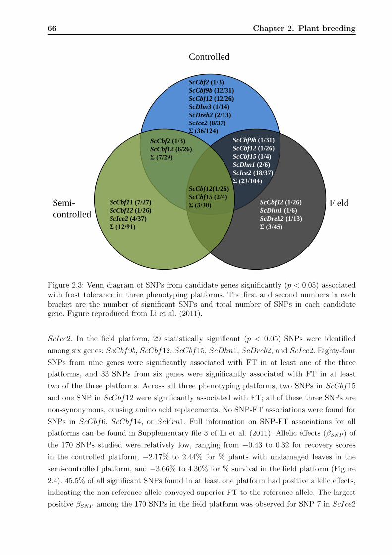
66 Chapter 2. Plant breeding
Controlled
Semi-
controlled
Field
ScCbf2 (1/3)
ScCbf9b (12/31)
ScCbf12 (12/26)
ScDhn3 (1/14)
ScDreb2 (2/13)
ScIce2 (8/37)
Σ (36/124)
ScCbf12(1/26)
ScCbf15 (2/4)
Σ (3/30)
ScCbf2 (1/3)
ScCbf12 (6/26)
Σ (7/29)
ScCbf9b (1/31)
ScCbf12 (1/26)
ScCbf15 (1/4)
ScDhn1 (2/6)
ScIce2 (18/37)
Σ (23/104)
ScCbf12 (1/26)
ScDhn1 (1/6)
ScDreb2 (1/13)
Σ (3/45)
ScCbf11 (7/27)
ScCbf12 (1/26)
ScIce2 (4/37)
Σ (12/91)
Figure 2.3: Venn diagram of SNPs from candidate genes significantly (p < 0.05) associatedwith frost tolerance in three phenotyping platforms. The first and second numbers in eachbracket are the number of significant SNPs and total number of SNPs in each candidategene. Figure reproduced from Li et al. (2011).
ScIce2. In the field platform, 29 statistically significant (p < 0.05) SNPs were identified
among six genes: ScCbf9b, ScCbf12, ScCbf15, ScDhn1, ScDreb2, and ScIce2. Eighty-four
SNPs from nine genes were significantly associated with FT in at least one of the three
platforms, and 33 SNPs from six genes were significantly associated with FT in at least
two of the three platforms. Across all three phenotyping platforms, two SNPs in ScCbf15
and one SNP in ScCbf12 were significantly associated with FT; all of these three SNPs are
non-synonymous, causing amino acid replacements. No SNP-FT associations were found for
SNPs in ScCbf6, ScCbf14, or ScV rn1. Full information on SNP-FT associations for all
platforms can be found in Supplementary file 3 of Li et al. (2011). Allelic effects (βSNP ) of
the 170 SNPs studied were relatively low, ranging from −0.43 to 0.32 for recovery scores
in the controlled platform, −2.17% to 2.44% for % plants with undamaged leaves in the
semi-controlled platform, and −3.66% to 4.30% for % survival in the field platform (Figure
2.4). 45.5% of all significant SNPs found in at least one platform had positive allelic effects,
indicating the non-reference allele conveyed superior FT to the reference allele. The largest
positive βSNP among the 170 SNPs in the field platform was observed for SNP 7 in ScIce2
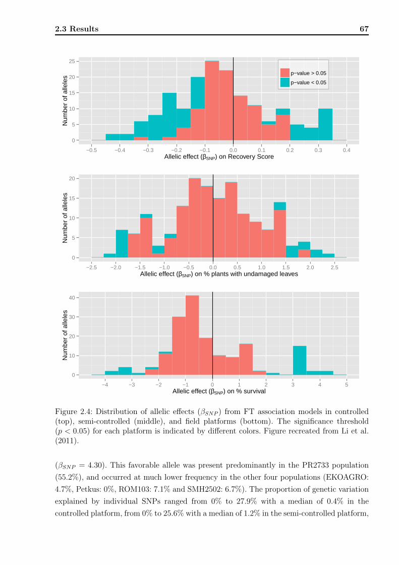
2.3 Results 67
0
5
10
15
20
25
−0.5 −0.4 −0.3 −0.2 −0.1 0.0 0.1 0.2 0.3 0.4Allelic effect (βSNP) on Recovery Score
Num
ber
of a
llele
sp−value > 0.05
p−value < 0.05
0
5
10
15
20
−2.5 −2.0 −1.5 −1.0 −0.5 0.0 0.5 1.0 1.5 2.0 2.5Allelic effect (βSNP) on % plants with undamaged leaves
Num
ber
of a
llele
s
0
10
20
30
40
−4 −3 −2 −1 0 1 2 3 4 5Allelic effect (βSNP) on % survival
Num
ber
of a
llele
s
Figure 2.4: Distribution of allelic effects (βSNP ) from FT association models in controlled(top), semi-controlled (middle), and field platforms (bottom). The significance threshold(p < 0.05) for each platform is indicated by different colors. Figure recreated from Li et al.(2011).
(βSNP = 4.30). This favorable allele was present predominantly in the PR2733 population
(55.2%), and occurred at much lower frequency in the other four populations (EKOAGRO:
4.7%, Petkus: 0%, ROM103: 7.1% and SMH2502: 6.7%). The proportion of genetic variation
explained by individual SNPs ranged from 0% to 27.9% with a median of 0.4% in the
controlled platform, from 0% to 25.6% with a median of 1.2% in the semi-controlled platform,
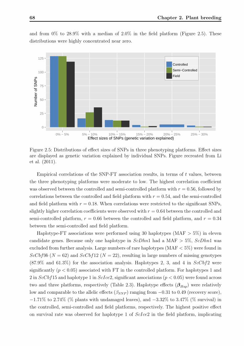
68 Chapter 2. Plant breeding
and from 0% to 28.9% with a median of 2.0% in the field platform (Figure 2.5). These
distributions were highly concentrated near zero.
0
25
50
75
100
125
0% − 5% 5% − 10% 10% − 15% 15% − 20% 20% − 25% 25% − 30%Effect sizes of SNPs (genetic variation explained)
Num
ber
of S
NP
s
Controlled
Semi−Controlled
Field
Figure 2.5: Distributions of effect sizes of SNPs in three phenotyping platforms. Effect sizesare displayed as genetic variation explained by individual SNPs. Figure recreated from Liet al. (2011).
Empirical correlations of the SNP-FT association results, in terms of t values, between
the three phenotyping platforms were moderate to low. The highest correlation coefficient
was observed between the controlled and semi-controlled platform with r = 0.56, followed by
correlations between the controlled and field platform with r = 0.54, and the semi-controlled
and field platform with r = 0.18. When correlations were restricted to the significant SNPs,
slightly higher correlation coefficients were observed with r = 0.64 between the controlled and
semi-controlled platform, r = 0.66 between the controlled and field platform, and r = 0.34
between the semi-controlled and field platform.
Haplotype-FT associations were performed using 30 haplotypes (MAF > 5%) in eleven
candidate genes. Because only one haplotype in ScDhn1 had a MAF > 5%, ScDhn1 was
excluded from further analysis. Large numbers of rare haplotypes (MAF < 5%) were found in
ScCbf9b (N = 62) and ScCbf12 (N = 22), resulting in large numbers of missing genotypes
(87.9% and 61.3%) for the association analysis. Haplotypes 2, 3, and 4 in ScCbf2 were
significantly (p < 0.05) associated with FT in the controlled platform. For haplotypes 1 and
2 in ScCbf15 and haplotype 1 in ScIce2, significant associations (p < 0.05) were found across
two and three platforms, respectively (Table 2.3). Haplotype effects (βHap) were relatively
low and comparable to the allelic effects (βSNP ) ranging from −0.31 to 0.49 (recovery score),
−1.71% to 2.74% (% plants with undamaged leaves), and −3.32% to 3.47% (% survival) in
the controlled, semi-controlled and field platforms, respectively. The highest positive effect
on survival rate was observed for haplotype 1 of ScIce2 in the field platform, implicating
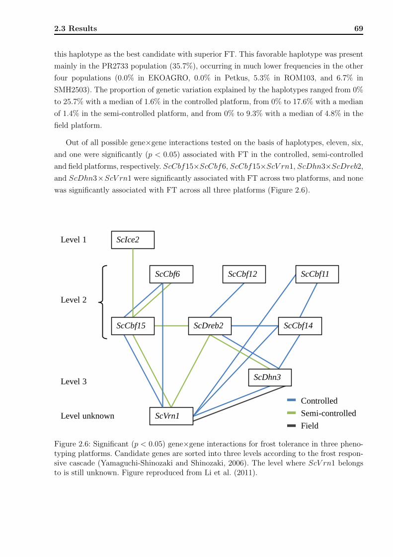
2.3 Results 69
this haplotype as the best candidate with superior FT. This favorable haplotype was present
mainly in the PR2733 population (35.7%), occurring in much lower frequencies in the other
four populations (0.0% in EKOAGRO, 0.0% in Petkus, 5.3% in ROM103, and 6.7% in
SMH2503). The proportion of genetic variation explained by the haplotypes ranged from 0%
to 25.7% with a median of 1.6% in the controlled platform, from 0% to 17.6% with a median
of 1.4% in the semi-controlled platform, and from 0% to 9.3% with a median of 4.8% in the
field platform.
Out of all possible gene×gene interactions tested on the basis of haplotypes, eleven, six,
and one were significantly (p < 0.05) associated with FT in the controlled, semi-controlled
and field platforms, respectively. ScCbf15×ScCbf6, ScCbf15×ScV rn1, ScDhn3×ScDreb2,
and ScDhn3×ScV rn1 were significantly associated with FT across two platforms, and none
was significantly associated with FT across all three platforms (Figure 2.6).
ScIce2
Controlled
Semi-controlled
Field
Level 1
Level 2
Level 3
ScCbf6
ScCbf15
ScVrn1
ScDhn3
ScDreb2 ScCbf14
ScCbf11ScCbf12
Level unknown
Figure 2.6: Significant (p < 0.05) gene×gene interactions for frost tolerance in three pheno-typing platforms. Candidate genes are sorted into three levels according to the frost respon-sive cascade (Yamaguchi-Shinozaki and Shinozaki, 2006). The level where ScV rn1 belongsto is still unknown. Figure reproduced from Li et al. (2011).
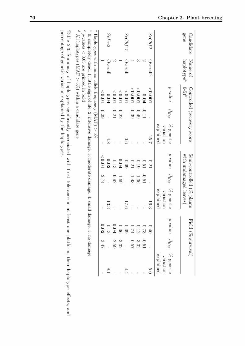
70 Chapter 2. Plant breeding
Can
did
ateN
ame
ofC
ontrolled
(recoveryscore
Sem
i-controlled
(%plan
tsF
ield(%
surv
ival)gen
ehap
lotyp
ea
0-5)b
with
undam
agedleaves)
p-value
cβHap
%gen
eticp-valu
eβHap
%gen
eticp-valu
eβHap
%gen
eticvariation
variationvariation
explain
edex
plain
edex
plain
ed
ScCbf
2O
verall d<
0.0
01
-25.7
0.21-
16.30.40
-5.0
20.0
4-0.11
-0.51
-0.51-
0.73-0.51
-3
<0.0
01
0.49-
0.191.36
-0.12
3.32-
4<
0.0
01
-0.39-
0.21-1.43
-0.74
0.57-
ScCbf
15O
verall<
0.0
1-
0.60.09
-17.6
0.09-
4.41
<0.0
1-0.22
-0.0
4-1.69
-0.06
-3.32-
2<
0.0
1-0.21
-0.13
-0.92-
0.0
4-2.59
-ScIce2
Overall
0.0
4-
4.80.0
2-
13.30.13
-8.1
1<
0.0
10.29
-<
0.0
12.74
-0.0
23.47
-a
Hap
lotyp
esw
ithm
inor
allelefreq
uen
cy(M
AF
)>
5%b
0:
com
pletely
dea
d.
1:
littlesig
nof
life.2:
inten
sived
amage.
3:m
od
erated
amage.
4:sm
alld
amage.
5:n
od
amage
cp-valu
es<
0.05are
prin
tedin
bold
dA
llh
ap
lotyp
es(M
AF>
5%
)w
ithin
acan
did
ategen
e
Tab
le2.3:
Sum
mary
ofhap
lotyp
essign
ifican
tlyasso
ciatedw
ithfrost
tolerance
inat
leaston
eplatform
,th
eirhap
lotyp
eeff
ects,an
dp
ercentage
ofgen
eticvariation
explain
edby
the
hap
lotyp
es.

2.4 Discussion 71
2.4 Discussion
FT is a complex trait with polygenic inheritance. While the genetic basis of FT has been
widely studied in cereals by bi-parental linkage mapping and expression profiling, exploitation
of the allelic and phenotypic variation of FT in rye by association studies has lagged behind
(Francia et al., 2007; Baga et al., 2007; Campoli et al., 2009). This study reports the first
candidate gene-based association study in rye examining the genetic basis of FT.
Statistically significant SNP-FT associations were identified in nine candidate genes hy-
pothesized to be involved in the frost responsive network among which the transcription
factor Ice2 is one of the key factors. Others are the Cbf gene family, the Dreb2 gene and
dehydrin gene family (Dhn). For a biological discussion of their role in the frost responsive
network and connections to findings in other studies, we refer to Li et al. (2011).
Effect sizes of markers, commonly expressed as percentage of the genetic variance ex-
plained by markers, are of primary interest in association studies since they are the main
factors that determine the effectiveness of subsequent marker assisted-selection processes.
Two hypotheses for the distribution of effect sizes in quantitative traits have been proposed:
Mather’s “infinitesimal” model and Robertson’s model (Mackay, 2001). The former assumes
an effectively infinitesimal number of loci with very small and nearly equal effect sizes; the
latter, an exponential trend of the distribution of effects, whereby a few loci have relatively
large effects and the rest only small effects. Findings in this study support the latter, with
distributions of SNP effect sizes (percentage of the genetic variance explained by individual
SNPs) highly concentrated near zero and few SNPs having large effects (maximum 28.8%
explained genetic variation). A similar distribution of haplotype effect sizes was observed.
A recent review summarizing association studies in 15 different plant species also impli-
cated Robertson’s model and further suggested that phenotypic traits, species, and types of
variants may impact distributions of effect sizes (Ingvarsson and Street, 2010).
Epistasis, generally defined as the interaction between genes, has been recognized for over
a century (Bateson, 1902), and recently it has been suggested that it should be explicitly
modeled in association studies in order to detect “missing heritabilities” (Phillips, 2008; Wu
et al., 2010). In this study, eleven, six, and one significant (p < 0.05) gene×gene interaction
effects were found in the controlled, semi-controlled and field platforms, respectively, suggest-
ing that epistasis may play a role in the frost responsive network. From the frost responsive
network, one might hypothesize that transcription factors interact with their downstream
target genes, for example, that ScIce2 interacts with the ScCbf gene family and the latter
interacts with COR genes, such as the dehydrin (Dhn) gene family. Indeed, significant inter-
actions were observed in ScIce2× ScCbf15, ScCbf14× ScDhn3, and ScDreb2× ScDhn3.
Some candidate genes in the same cascade level also interact with each other, such as mem-
bers of the ScCbf gene family, ScCbf6× ScCbf15 and ScCbf11× ScCbf14.
Similar interactions within the Cbf gene family were also observed in Arabidopsis where
72 Chapter 2. Plant breeding
AtCbf2 was indicated as a negative regulator of AtCbf1 and AtCbf3 (Novillo et al., 2004). In
this study, ScV rn1 was not significantly associated with FT but had significant interaction
effects with six other candidate genes, underlining the important role of ScV rn1 in the
frost responsive network. It is worth to point out that the power of detecting gene×gene
interaction might be low due to the relatively small sample size.
Low to moderate empirical correlations of SNP-FT associations were observed across the
three platforms reflecting the complexity of FT and thus the need for different platforms in
order to more accurately characterize FT. There are at least two reasons possibly explaining
the relatively low to medium empirical correlations of SNP-FT associations: 1) the different
duration and intensity of freezing temperature and 2) the different levels of confounding
effects from environmental factors, other than frost stress, per se. In the controlled platform,
plants were cold-hardened and then exposed to freezing temperatures (−19 ◦C or −21 ◦C)
in a short period of six days using defined temperature profiles. Recovery score in the con-
trolled platform represents the most pure and controlled measurement of FT among the three
platforms, since the effect of environmental factors other than frost stress is minimized.
In the semi-controlled platform, plants were exposed to much longer freezing periods with
fluctuating temperatures and repeated frost-thaw processes. In addition, a more complex
situation occurred in this platform, requiring plants to cope with other variable climatic
factors such as changing photoperiod, natural light intensity, wind, and limited water supply.
Thus, the measurement % plants with undamaged leaves in the semi-controlled platform
reflects the combined effect of various environmental influences and stresses on the vitality of
leaf tissue but does not mirror survival of the crown tissue as an indicator for frost tolerance.
In the field platform, winter temperatures were generally lower than in the semi-controlled
platform due to the strong continental climate in Eastern Europe and Canada.
The measurement % survival in the field is further confounded by environmental effects,
such as snow-coverage, soil uniformity, topography, and other unmeasured factors. The dif-
ferent experimental platforms permit the identification of different sets of genes associated
with FT, which might impact the correlations of SNP-FT associations across platforms. It is
worth pointing out that the correlation between the controlled and semi-controlled platform
was higher than between the semi-controlled and field platform. One possible explanation
is that plant growth in boxes in both controlled and semi-controlled platforms results in
a rather similar environment where roots are more exposed to freezing than in the field.
Several studies have suggested that different genes might be induced under different frost
stress treatments. A large number of blueberry genes induced in growth chambers were not
induced under field conditions (Dhanaraj et al., 2007).
In rye, Campoli et al. (2009) drew the conclusion that expression patterns of different
members of the Cbf gene family were affected by different acclimation temperatures and
sampling times. Most prior studies on FT have been conducted in controlled environments.
However, the relatively low to medium correlation among platforms in this study suggest

2.4 Discussion 73
that future studies should consider various scenarios in order to obtain a more complete
picture of the genetic basis of FT in rye.

74 Chapter 2. Plant breeding

Chapter 3
Phenology
This chapter emphasizes and extends the statistical methods used in the article “First
flowering of wind-pollinated species with the greatest phenological advances in Europe” (C.
Ziello, A. Bock, N. Estrella, D. P. Ankerst, and A. Menzel, 2012), while shortening the
biological background and subject matter interpretations. The author of this thesis was
second author and primary statistician of the forenamed article and performed all statistical
analyses.
3.1 Introduction
Phenology is the science of naturally recurring events in nature, such as leaf unfolding
and flowering of plants in spring, fruit ripening, as well as the arrival and departure of
migrating birds and the timing of animal breeding (Koch et al., 2009). It offers quantitative
evidence of climate change impacts on ecosystems, indicating an increasing advancement of
flowering phases in recent decades (Rosenzweig et al., 2007). A stronger tendency for winter
and spring phenological phases to advance, relative to summer phases, has been reported
in the literature (Lu et al., 2006; Menzel et al., 2006). Only few studies have assessed the
influence of plant traits on the response to global warming. A recent study in this direction
reported a greater temporal advancement among entomophilous (insect-pollinated) plants
compared to anemophilous (wind-pollinated) species (Fitter and Fitter, 2002).
Changes in the pollen season, particularly related to its timing, duration, and intensity,
are one of the most likely consequences of climate change (Huynen et al., 2003). A threat of
these changes to human health is the expected further increase of the worldwide burden of
pollen-related respiratory diseases (Beggs, 2004; D’Amato et al., 2007; D’Amato and Cecchi,
2008). Most research in this area has been addressed to observing and forecasting the phe-
nological behavior of single species characterized by a high allergenic effect, such as birch or
ragweed (Laaidi, 2001; Rasmussen, 2002; Rogers et al., 2006; Wayne et al., 2002). We expand
the research on climate change effects on phenology and present a statistical meta-analysis
based on a massive data set, permitting the quantification of differences in phenological tem-

76 Chapter 3. Phenology
poral trends due to pollination mode and woodiness, as well as yearly patterns of trends.
Ultimately, this leads to the identification of groups which are more likely to show changes
in their phenology and, hence, more likely to increase harm to humans.
3.2 Data structure
The analyzed phenological data consist of flowering records based on an abundant data
set, which covers dates of diverse phenological phases, and comprises more than 35,000 series
of flowering in Central Europe (Menzel et al., 2006). Most of these data are available at the
COST (European COoperation in the field of Scientific and Technical research) database,
collected within the in the meantime concluded COST Action 725 (Koch et al., 2009). We
selected series with a length of more than 15 years between 1971 and 2000, which were
available in aggregated form as a linear regression of the flowering time (coded as day of
year, doy) on calendar year (cy) for each series. The common linear regression was assumed:
doy = β0 + β1 cy + ε,
with ε ∼ N(0, σ2), the Normal distribution with mean 0 and variance σ2. For our statistical
analysis, we used the estimates β1i, se(β1i), and doyi of the i = 1, . . . , 5971 selected series of
flowering:
β1i Estimated regression slope of the ith series, interpreted as the average trend or time
shift of flowering time in days per year for an increase of one calendar year.
se(β1i) Standard error of β1i, a measure of how precisely the average trend was captured by
the linear regression model.
doyi Average flowering time across all years of study in series i, which carries equiva-
lent information as the estimated intercept β0i, when used along with β1i, because
β0 = doy− β1 cy.
The 5,971 analyzed series were measured in 983 phenological stations spread over 13
countries in Europe (list of countries by decreasing number of stations: Germany, Switzer-
land, Russia, Austria, Czech Republic, Slovenia, Latvia, Norway, United Kingdom, Croatia,
Finland, Estonia, and Slovakia) (Figure 3.1). The spatial information about the phenological
stations was recorded as geographic latitude and longitude, and the altitude above sea level.
Phenological aspects The study contains records on 28 different species, all an-
giosperms. They are listed in Fig. 3.2 ordered by mean flowering dates. The disparity in the
number of anemophilous (wind-pollinated) and entomophilous (insect-pollinated) species (7
versus 21) results from the low percentage (≈ 10%) of wind-pollinated species among the
angiosperms. Note that all considered wind-pollinated species are allergenic, that is they
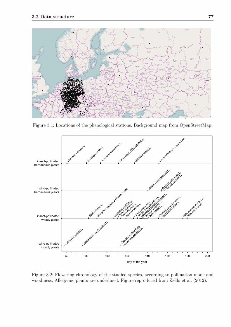
3.2 Data structure 77
6e+06
7e+06
8e+06
9e+06
0e+00 2e+06 4e+06 6e+06x
y
Figure 3.1: Locations of the phenological stations. Background map from OpenStreetMap.
Figure 3.2: Flowering chronology of the studied species, according to pollination mode andwoodiness. Allergenic plants are underlined. Figure reproduced from Ziello et al. (2012).

78 Chapter 3. Phenology
can cause a malfunction of the immune system, which leads to overproduction of antibodies.
Allergenicity is a characteristic also present among insect-pollinated species, but the pollen
of anemophilous plants is considerably higher in amount and aggressiveness, at least for an-
giosperms. This aspect allows consideration of wind-pollinated species as representatives of
allergenic species, so that the results of their monitoring can be used to reasonably estimate
the consequences of climate change on allergic human subjects.
The classification of allergenic plants follows the information available at the website of
the EAN (European Aeroallergen Network). Flowering phenophases available are first flower
opens and full flowering (50% of flowers open). Woodiness, which classifies plants in those
having a persistent woody stem or being a herb, is another trait linked to allergenicity. As
most sensitized subjects are allergic to grass pollen (i.e. pollen of non-woody plants) (Esch,
2004; Jaeger, 2008), these allergens together with the pollen of the plant genus Ambrosia
(McLauchlan et al., 2011; Ziska et al., 2011) are the most studied allergens in the literature.
Of similar importance is the allergenic effect of some tree species, such as birch (D’Amato
et al., 2007), whose pollen cause severe reactions in humans, particularly at northern latitudes
where it is predominant.
3.3 Statistical methods
3.3.1 Overview
In this section we provide an overview on the statistical methods used to analyze the
phenology data, with details in the next section. The influence of pollination mode and
woodiness on flowering trends (first flowering and full flowering) was assessed using weighted
linear mixed models, with weights chosen as the precision, i.e. the inverse of the variance
of the data regressions that were provided (Becker and Wu, 2007). Statistical significance
of results was assessed using 1,000 bootstrap samples (Efron and Tibshirani, 1994), and
goodness of fit was calculated by means of an R2 measure for mixed models based on the
likelihood (Xu, 2003). Bootstrap samples were also presented in graphs to reflect uncertainty.
Fixed effects considered were woodiness, pollination mode, and mean phenodate for each
series, which was also provided along with the estimated regression coefficient. A random
effect for stations was included, which implies correlation between observations from the
same station, and data from different stations were modelled independently. More advanced
spatial structures, such as the exponential correlation structure (Pinheiro and Bates, 2000,
p. 230) that uses the coordinate information of stations, were also considered, but did not
show any impact on the estimates of interest and were therefore rejected. Altitude above
sea level of stations was excluded as a fixed effect since it neither showed significance, nor
affected other estimates when included in the model, as similarly found in previous work
(Ziello et al., 2009).

3.3 Statistical methods 79
A series of model-based analyses was performed in duplicate for first flowering trends and
full flowering trends. In detail, the estimates β1 (subscript i suppressed) obtained from the
linear regressions of flowering time (first flowering and full flowering, respectively) for the
5,971 flowering series served as observations of the response variable “flowering trends” in unit
days per year (d/yr). First, univariate regressions of the effects of woodiness and pollination
on flowering trends were performed. Then, the linear effect of mean date (doyi) on trends was
assessed separately by pollination mode and woodiness, and by combinations of pollination
mode and woodiness in an overall model for both phenological phases. Finally, the linearity
constraint of the mean date effect was relaxed via a spline approach to evaluate the robustness
of the general conclusions drawn under assumption of a linear effect. Frayed ends of spline
curves arise mainly from arbitrary extrapolation of the spline when bootstrap samples do
not cover the whole time range, and should be used as natural limits for interpretation.
3.3.2 Details
Heterogeneity The outcome of interest, trend in flowering time, is not directly mea-
sured but results rather from an aggregation of observations by the pre-manufactured linear
regressions. We therefore conducted a meta-analysis, with procedures adjusted to the specific
situations. For example, comparison of the means of two groups with a t-test assumes that
observations within samples are identically distributed, which is not fulfilled by the flowering
trends. Every single trend, being an estimated coefficient, has its own variance and follows
asymptotically the large sample normal distribution: β1a∼ N(β1, se(β1)2), with β1 the esti-
mator of the trend and se(.) its standard error. As outlined in Becker and Wu (2007), we
used weights defined by the squared standard error, 1/se(β1)2, in our calculations to account
for different variances of the trend estimators. In practice, a pooled t-test adjusted with
such defined weights can be performed in a linear regression framework with heteroscedastic
errors, and fitted by weighted least squares. For ease of notation, let y be the combined
vector of outcomes, x a 0/1 vector indicating the membership to the two samples, and w
the vector of weights. All three vectors are of same length n = n1 + n2, with n1 the number
of observations in sample 1 and n2 the number of observations in sample 2. The two-sample
pooled t-test for equal means in both groups,
H0 : µ1 = µ2 versus HA : µ1 6= µ2,
is identical to the test of
H0 : β1 = 0 versus HA : β1 6= 0,
in the linear regression model
yi = β0 + β1 xi + εi, εi ∼ N(0, σ2), i = 1, . . . , n.
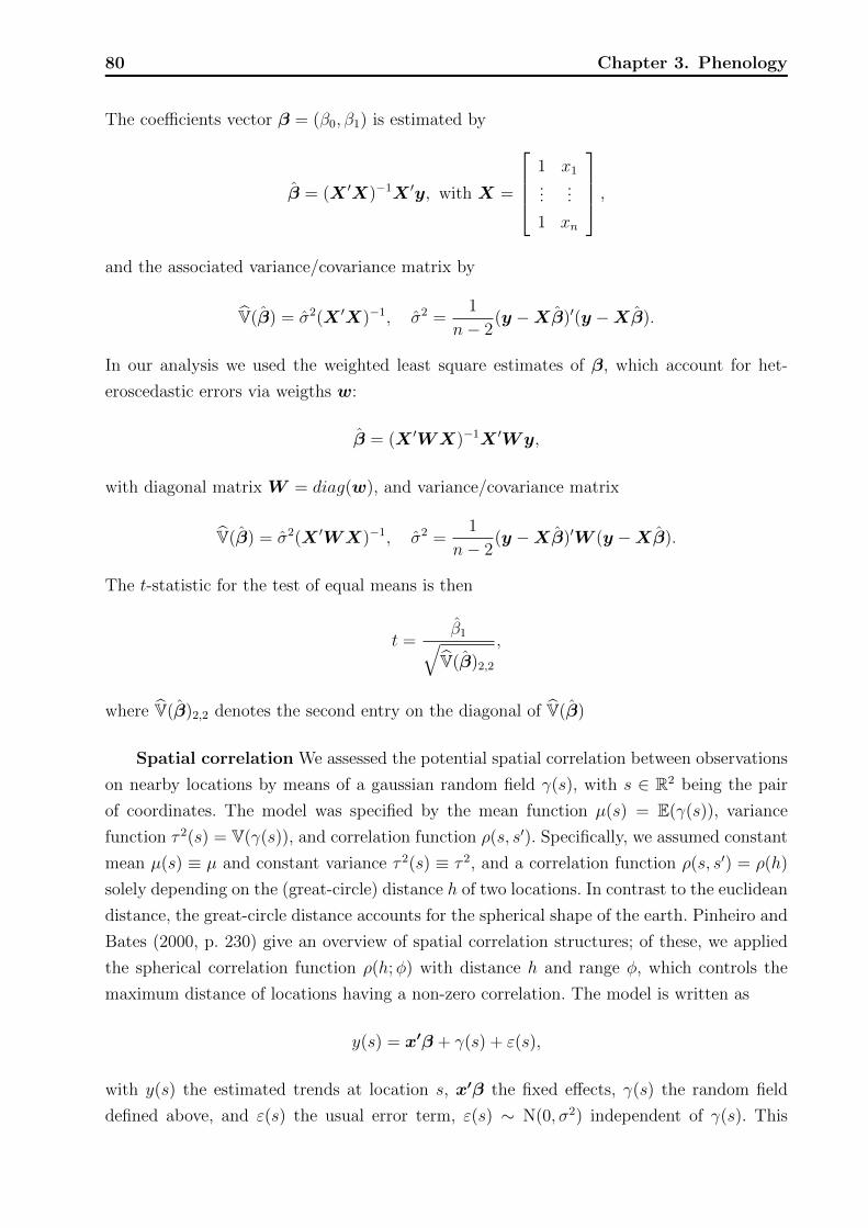
80 Chapter 3. Phenology
The coefficients vector β = (β0, β1) is estimated by
β = (X ′X)−1X ′y, with X =
1 x1
......
1 xn
,and the associated variance/covariance matrix by
V(β) = σ2(X ′X)−1, σ2 =1
n− 2(y −Xβ)′(y −Xβ).
In our analysis we used the weighted least square estimates of β, which account for het-
eroscedastic errors via weigths w:
β = (X ′WX)−1X ′Wy,
with diagonal matrix W = diag(w), and variance/covariance matrix
V(β) = σ2(X ′WX)−1, σ2 =1
n− 2(y −Xβ)′W (y −Xβ).
The t-statistic for the test of equal means is then
t =β1√
V(β)2,2
,
where V(β)2,2 denotes the second entry on the diagonal of V(β)
Spatial correlation We assessed the potential spatial correlation between observations
on nearby locations by means of a gaussian random field γ(s), with s ∈ R2 being the pair
of coordinates. The model was specified by the mean function µ(s) = E(γ(s)), variance
function τ 2(s) = V(γ(s)), and correlation function ρ(s, s′). Specifically, we assumed constant
mean µ(s) ≡ µ and constant variance τ 2(s) ≡ τ 2, and a correlation function ρ(s, s′) = ρ(h)
solely depending on the (great-circle) distance h of two locations. In contrast to the euclidean
distance, the great-circle distance accounts for the spherical shape of the earth. Pinheiro and
Bates (2000, p. 230) give an overview of spatial correlation structures; of these, we applied
the spherical correlation function ρ(h;φ) with distance h and range φ, which controls the
maximum distance of locations having a non-zero correlation. The model is written as
y(s) = x′β + γ(s) + ε(s),
with y(s) the estimated trends at location s, x′β the fixed effects, γ(s) the random field
defined above, and ε(s) the usual error term, ε(s) ∼ N(0, σ2) independent of γ(s). This

3.3 Statistical methods 81
model implies that the correlation between the observations y(s) and y(s′) is given by
Corr(y(s), y(s′)) = ρ(h;φ).
The same model can be expressed as a linear mixed model (see Fahrmeir et al., 2007, p. 327 ff),
y = Xβ +Zγ + ε,
with the following components:
y Vector of temporal flowering trends.
Xβ Fixed effect design matrix and effects, specifics provided later.
Z Design matrix for the random effects; an incidence matrix (entries of zero and one)
mapping each single observation to its phenological station.
R Correlation matrix derived from the correlation function ρ(h;φ) and the distance ma-
trix H , which contains the distance between every pair of phenological stations,
R[i, j] = ρ(H [i, j];φ),
with ρ(.) given by
ρ(h;φ) =
1− 32|h/φ|+ 1
2|h/φ|3 0 ≤ h ≤ φ,
0 h > φ.
γ Vector of multivariate normally distributed random station effects γ ∼ N(0, τ 2R).
ε Vector of independent but heteroscedastic errors,
ε ∼ N(0, σ2W−1),
where the weight matrix is specified as a diagonal matrix W = diag(w), with w the
inverse squared standard errors of the trend estimators. The strict diagonal structure
of W reflects the assumption of independent observations within a station given the
random station effect γ.
The impact of spatial correlation is to pull estimates of station effects towards their
neighbors, referred to as spatial smoothing. The amount of smoothing is controlled by the
variance parameter τ 2, estimated from the data during the model-fitting. For an illustration
of the involved matrices, we give an example on observations from four different stations in
Germany using a range parameter of φ = 50 (km):

82 Chapter 3. Phenology
Station Latitude Longitude y se(y)
1 51.7833 6.0167 -0.16196 0.28756
2 51.6333 6.1833 -0.04226 0.26424
3 51.0500 6.2333 -0.28621 0.27743
4 51.5833 6.2500 0.03426 0.29378
H =
0 20.27 82.91 27.48
20.27 0 64.95 7.23
82.91 64.95 0 59.31
27.48 7.23 59.31 0
, R =
1 0.43 0 0.26
0.43 1 0 0.78
0 0 1 0
0.26 0.78 0 1
,
Z =
1 0 0 0
0 1 0 0
0 0 1 0
0 0 0 1
, W =
12.09 0 0 0
0 14.32 0 0
0 0 12.99 0
0 0 0 11.59
.
The assumption of no spatial correlation between effects of different stations is expressed by
an identity matrix R. However, since this approach still induces correlation within obser-
vations of the same station due to the shared random effect, it is denoted as unstructured
spatial correlation.
Inference The aim of this study was to compare the temporal trends between the differ-
ent types of pollination and woodiness, as well as to asses how the trends differ with respect
to average flowering time in year, doy. As stated previously, we entered the categorical vari-
ables pollination (wind versus insect) and woodiness (woody versus non-woody) as factor
variables in the model matrix X. We estimated the different phenological phases (first flow-
ering and full flowering) in separate models, i.e. we applied the same model structure to the
two data subsets containing only first- and full flowering data, respectively. Subsequently, we
combined both phases in an overall model, using the complete dataset and an additional co-
variate, indicating the phenological phase. In an exploratory analysis we assessed the effects
of woodiness and pollination type in main effects models, while ignoring other effects. This
technically violates the principle of marginality (Nelder, 1977). We therefore used a more
complex model for inference, which simultaneously incorporated all variables. Initially, the
effect of average flowering time in year (variable doy) on the temporal trend was estimated

3.3 Statistical methods 83
linearly. More specifically, the generic form of Xβ contained the following terms,
Xβ =1β0 + βwoodyI(x1 = woody) + βwindI(x2 = wind)+
βwoody,windI(x1 = woody)I(x2 = wind)+
βdoydoy + βdoy,woodydoyI(x1 = woody)+
βdoy,winddoyI(x2 = wind)+
βdoy,woody,winddoyI(x1 = woody)I(x2 = wind),
where the indicator function I(x) of a vector is meant to act element-wise on x and returns
the evaluations as vector again. It evaluates to 1 if the x belongs to the specified category,
and to 0 otherwise. In other words this is a two-way interaction model. Again, we provide
an example:
Woodiness (x1) Pollination mode (x2) Average flowering time (doy)
woody wind 125.414
woody insect 113.414
non-woody wind 113.700
non-woody insect 114.034
results in the design matrix,
X =
1 1 1 1 125.414 125.414 125.414 125.414
1 1 0 0 113.414 113.414 0 0
1 0 1 0 113.700 0 125.414 0
1 0 0 0 114.034 0 0 0
,
and the associated vector of fixed effects,
β′ = (β0, βwoody, βwind, βwoody,wind, βdoy, βwoody,doy, βwind,doy, βdoy,woody,wind).
Later, to verify the linearity assumption, the constraint was relaxed, allowing a more flexible
relationship by means of a spline function. We applied polynomial splines on a B-spline basis,
as outlined in Section 1.3.3. We also assessed the effect of altitude above sea level using a
spline of that form.
Hypotheses tests Based on the coefficients β we formulated the hypotheses of interest.
The significance of the linear relationship between doy and flowering time for non-woody
& insect-pollinated plants (1), woody & insect-pollinated plants (2), non-woody & wind-
pollinated plants (3), and woody & wind-pollinated plants (4) can be assessed by tests of

84 Chapter 3. Phenology
the hypotheses
H1 : βdoy = 0
H2 : βdoy + βwoody,doy = 0
H3 : βdoy + βwind,doy = 0
H4 : βdoy + βwoody,doy + βwind,doy + βdoy,woody,wind = 0,
which can be expressed as tests of linear combinations c′jβ , j = 1, . . . , 4 of the coefficient
vector with C = (c′1, . . . , c′4)′ specified as
C =
0 0 0 1 0 0 0 0
0 0 0 1 0 1 0 0
0 0 0 1 0 0 1 0
0 0 0 1 0 1 1 1
.
For mixed models with unbalanced designs, as present here, the exact distribution of Cβ
under the null hypotheses is unknown. Approximations can be held using t-distributions
(Pinheiro and Bates, 2000, p. 90), with the degrees of freedom to be specified. As an al-
ternative, we applied a nonparametric bootstrap to asses the statistical significance of the
hypothesis tests. We drew B = 1, 000 bootstrap samples of the dataset, and fitted the model
for each sample leading to estimates β(b), b = 1, . . . , B. We estimated V(c′jβ) by its em-
pirical counterpart, the sample variance of (c′jβ(1), . . . , c′jβ(B)), denoted as s2B(c′jβ), for
j = 1, . . . , 4. p-values for the tests of the hypothesis
H0,j : c′jβ = 0 vs. HA,j : c′jβ 6= 0
are obtained as
p-value = 2 · (1− Φ(|zj|)),
with Φ(.) the standard normal distribution, and
zj =c′jβ√s2B(c′jβ)
.
Multiple tests on the same data require an adjustment to in order to control the overall level
of false-positive findings. Therefore, we calculated the p-values based on quantiles of the
joint (asymptotic) multivariate normal distribution of the vector of test statistics zj (Bretz
et al., 2011, chap. 3). We applied the multiple comparison adjustment for 17 hypotheses
tests, which are based on parameter estimates of the overall model. We tested for equal
slope parameters of the covariate doy for different categories of pollination and woodiness

3.4 Results 85
and assessed whether the flowering trends y were the same between these categories. For the
latter comparison we set the average flowering date to doy = 100. Therefore, the results are
to be interpreted for plants which flower on average at the 100th day of the year.
Additionally, we visualized the uncertainty of the estimates by plotting all bootstrap
samples using transparent colors, simultaneously showing the data on the original scale along
with model-based predictions of the flowering trends. Predictions are limited to regions of the
covariate-space in the data that were involved in the particular estimation. We recommend
to limit interpretation to these areas and not to extrapolate. The pseudo R2 for linear mixed
models discussed by Xu (2003) is based on the maximized log-likelihood of the full model,
l(β), containing all covariates, and the maximized log-likelihood of the null model, l(β0),
including only an intercept coefficient as fixed effect, with the same random effects structure
in both models. It is calculated as
R2 = 1− exp
(− 2
n(l(β)− l(β0))
),
with n the number of observations, and can roughly be interpreted as the proportion of
variance explained by the considered fixed effects.
Computational aspects We performed all analyses and graphs within the R environ-
ment (R Core Team, 2012). An implementation for the calculation of great-circle distances
is readily available in the sp package (Bivand et al., 2008), returning distances in kilometers.
For mixed models with a simple random effects structure, such as uncorrelated random in-
tercepts, we used the lme4 package (Bates and Machler, 2010) and and extensions thereof in
the gamm4 package, allowing for inclusion of splines (Wood, 2012). Models with structured
spatial correlations required specification of the design- and correlation matrices, which was
performed using mgcv (Wood, 2006) and regress (Clifford and McCullagh, 2012) packages.
For model-fitting the restricted log-likelihood was optimized and used for tests and parameter
estimates. Calculation of the pseudo R2 was done using maximum likelihood. Programs for
bootstrapping were taken from boot package (Canty and Ripley, 2010), for multiple testing
adjustment from the multcomp package (Hothorn et al., 2008).
3.4 Results
Model structure By using different values of the range parameter for the spherical cor-
relation function, φ = 50, 70, 100, 150 km, we observed no practical impact of the structured
spatial correlation on the fixed effects in the model. A random intercept for station specified
by an identity matrix R was kept in the model. Altitude above sea level did not affect other
estimated effects when included in the model and neither a linear relationship nor a spline
function for altitude was statistically significantly different from zero. These results confirm
findings by Ziello et al. (2009) observed in a related application.
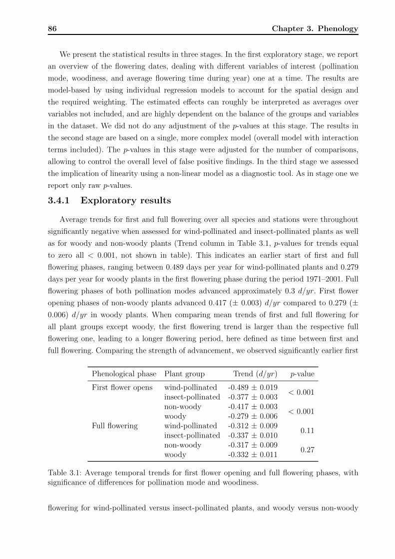
86 Chapter 3. Phenology
We present the statistical results in three stages. In the first exploratory stage, we report
an overview of the flowering dates, dealing with different variables of interest (pollination
mode, woodiness, and average flowering time during year) one at a time. The results are
model-based by using individual regression models to account for the spatial design and
the required weighting. The estimated effects can roughly be interpreted as averages over
variables not included, and are highly dependent on the balance of the groups and variables
in the dataset. We did not do any adjustment of the p-values at this stage. The results in
the second stage are based on a single, more complex model (overall model with interaction
terms included). The p-values in this stage were adjusted for the number of comparisons,
allowing to control the overall level of false positive findings. In the third stage we assessed
the implication of linearity using a non-linear model as a diagnostic tool. As in stage one we
report only raw p-values.
3.4.1 Exploratory results
Average trends for first and full flowering over all species and stations were throughout
significantly negative when assessed for wind-pollinated and insect-pollinated plants as well
as for woody and non-woody plants (Trend column in Table 3.1, p-values for trends equal
to zero all < 0.001, not shown in table). This indicates an earlier start of first and full
flowering phases, ranging between 0.489 days per year for wind-pollinated plants and 0.279
days per year for woody plants in the first flowering phase during the period 1971–2001. Full
flowering phases of both pollination modes advanced approximately 0.3 d/yr. First flower
opening phases of non-woody plants advanced 0.417 (± 0.003) d/yr compared to 0.279 (±0.006) d/yr in woody plants. When comparing mean trends of first and full flowering for
all plant groups except woody, the first flowering trend is larger than the respective full
flowering one, leading to a longer flowering period, here defined as time between first and
full flowering. Comparing the strength of advancement, we observed significantly earlier first
Phenological phase Plant group Trend (d/yr) p-value
First flower opens wind-pollinated -0.489 ± 0.019< 0.001
insect-pollinated -0.377 ± 0.003non-woody -0.417 ± 0.003
< 0.001woody -0.279 ± 0.006
Full flowering wind-pollinated -0.312 ± 0.0090.11
insect-pollinated -0.337 ± 0.010non-woody -0.317 ± 0.009
0.27woody -0.332 ± 0.011
Table 3.1: Average temporal trends for first flower opening and full flowering phases, withsignificance of differences for pollination mode and woodiness.
flowering for wind-pollinated versus insect-pollinated plants, and woody versus non-woody
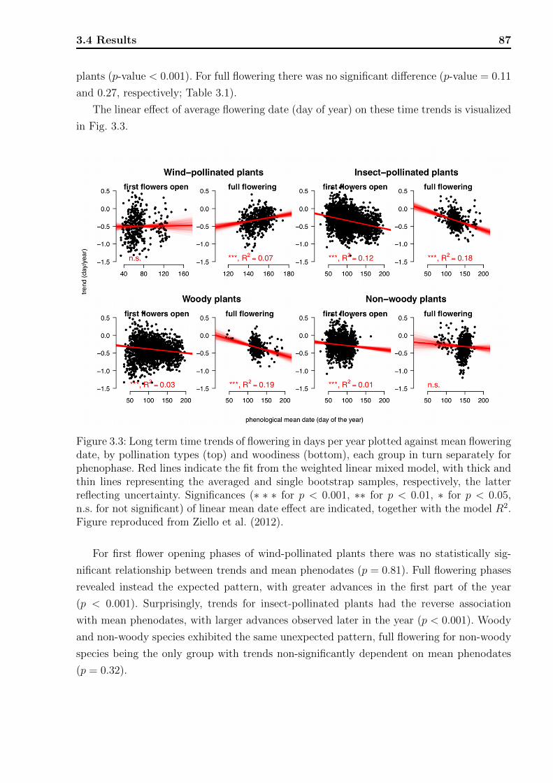
3.4 Results 87
plants (p-value < 0.001). For full flowering there was no significant difference (p-value = 0.11
and 0.27, respectively; Table 3.1).
The linear effect of average flowering date (day of year) on these time trends is visualized
in Fig. 3.3.
Figure 3.3: Long term time trends of flowering in days per year plotted against mean floweringdate, by pollination types (top) and woodiness (bottom), each group in turn separately forphenophase. Red lines indicate the fit from the weighted linear mixed model, with thick andthin lines representing the averaged and single bootstrap samples, respectively, the latterreflecting uncertainty. Significances (∗ ∗ ∗ for p < 0.001, ∗∗ for p < 0.01, ∗ for p < 0.05,n.s. for not significant) of linear mean date effect are indicated, together with the model R2.Figure reproduced from Ziello et al. (2012).
For first flower opening phases of wind-pollinated plants there was no statistically sig-
nificant relationship between trends and mean phenodates (p = 0.81). Full flowering phases
revealed instead the expected pattern, with greater advances in the first part of the year
(p < 0.001). Surprisingly, trends for insect-pollinated plants had the reverse association
with mean phenodates, with larger advances observed later in the year (p < 0.001). Woody
and non-woody species exhibited the same unexpected pattern, full flowering for non-woody
species being the only group with trends non-significantly dependent on mean phenodates
(p = 0.32).
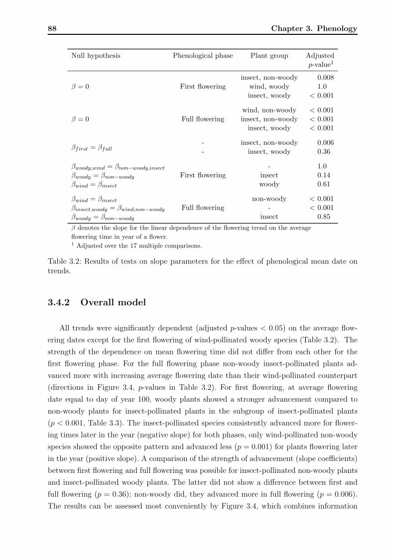
88 Chapter 3. Phenology
Null hypothesis Phenological phase Plant group Adjustedp-value1
β = 0 First floweringinsect, non-woody 0.008
wind, woody 1.0insect, woody < 0.001
β = 0 Full floweringwind, non-woody < 0.001insect, non-woody < 0.001
insect, woody < 0.001
βfirst = βfull- insect, non-woody 0.006- insect, woody 0.36
βwoody,wind = βnon−woody,insectFirst flowering
- 1.0βwoody = βnon−woody insect 0.14βwind = βinsect woody 0.61
βwind = βinsectFull flowering
non-woody < 0.001βinsect,woody = βwind,non−woody - < 0.001βwoody = βnon−woody insect 0.85
β denotes the slope for the linear dependence of the flowering trend on the average
flowering time in year of a flower.1 Adjusted over the 17 multiple comparisons.
Table 3.2: Results of tests on slope parameters for the effect of phenological mean date ontrends.
3.4.2 Overall model
All trends were significantly dependent (adjusted p-values < 0.05) on the average flow-
ering dates except for the first flowering of wind-pollinated woody species (Table 3.2). The
strength of the dependence on mean flowering time did not differ from each other for the
first flowering phase. For the full flowering phase non-woody insect-pollinated plants ad-
vanced more with increasing average flowering date than their wind-pollinated counterpart
(directions in Figure 3.4, p-values in Table 3.2). For first flowering, at average flowering
date equal to day of year 100, woody plants showed a stronger advancement compared to
non-woody plants for insect-pollinated plants in the subgroup of insect-pollinated plants
(p < 0.001, Table 3.3). The insect-pollinated species consistently advanced more for flower-
ing times later in the year (negative slope) for both phases, only wind-pollinated non-woody
species showed the opposite pattern and advanced less (p = 0.001) for plants flowering later
in the year (positive slope). A comparison of the strength of advancement (slope coefficients)
between first flowering and full flowering was possible for insect-pollinated non-woody plants
and insect-pollinated woody plants. The latter did not show a difference between first and
full flowering (p = 0.36); non-woody did, they advanced more in full flowering (p = 0.006).
The results can be assessed most conveniently by Figure 3.4, which combines information
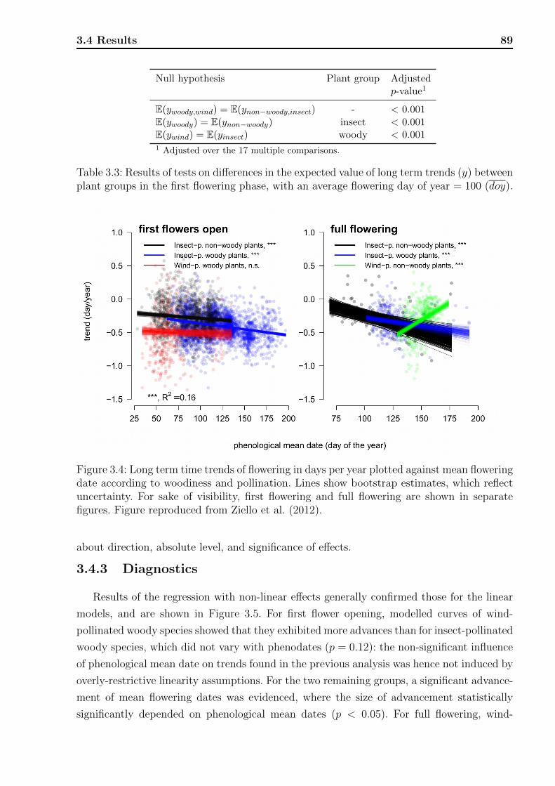
3.4 Results 89
Null hypothesis Plant group Adjustedp-value1
E(ywoody,wind) = E(ynon−woody,insect) - < 0.001E(ywoody) = E(ynon−woody) insect < 0.001E(ywind) = E(yinsect) woody < 0.0011 Adjusted over the 17 multiple comparisons.
Table 3.3: Results of tests on differences in the expected value of long term trends (y) betweenplant groups in the first flowering phase, with an average flowering day of year = 100 (doy).
Figure 3.4: Long term time trends of flowering in days per year plotted against mean floweringdate according to woodiness and pollination. Lines show bootstrap estimates, which reflectuncertainty. For sake of visibility, first flowering and full flowering are shown in separatefigures. Figure reproduced from Ziello et al. (2012).
about direction, absolute level, and significance of effects.
3.4.3 Diagnostics
Results of the regression with non-linear effects generally confirmed those for the linear
models, and are shown in Figure 3.5. For first flower opening, modelled curves of wind-
pollinated woody species showed that they exhibited more advances than for insect-pollinated
woody species, which did not vary with phenodates (p = 0.12): the non-significant influence
of phenological mean date on trends found in the previous analysis was hence not induced by
overly-restrictive linearity assumptions. For the two remaining groups, a significant advance-
ment of mean flowering dates was evidenced, where the size of advancement statistically
significantly depended on phenological mean dates (p < 0.05). For full flowering, wind-
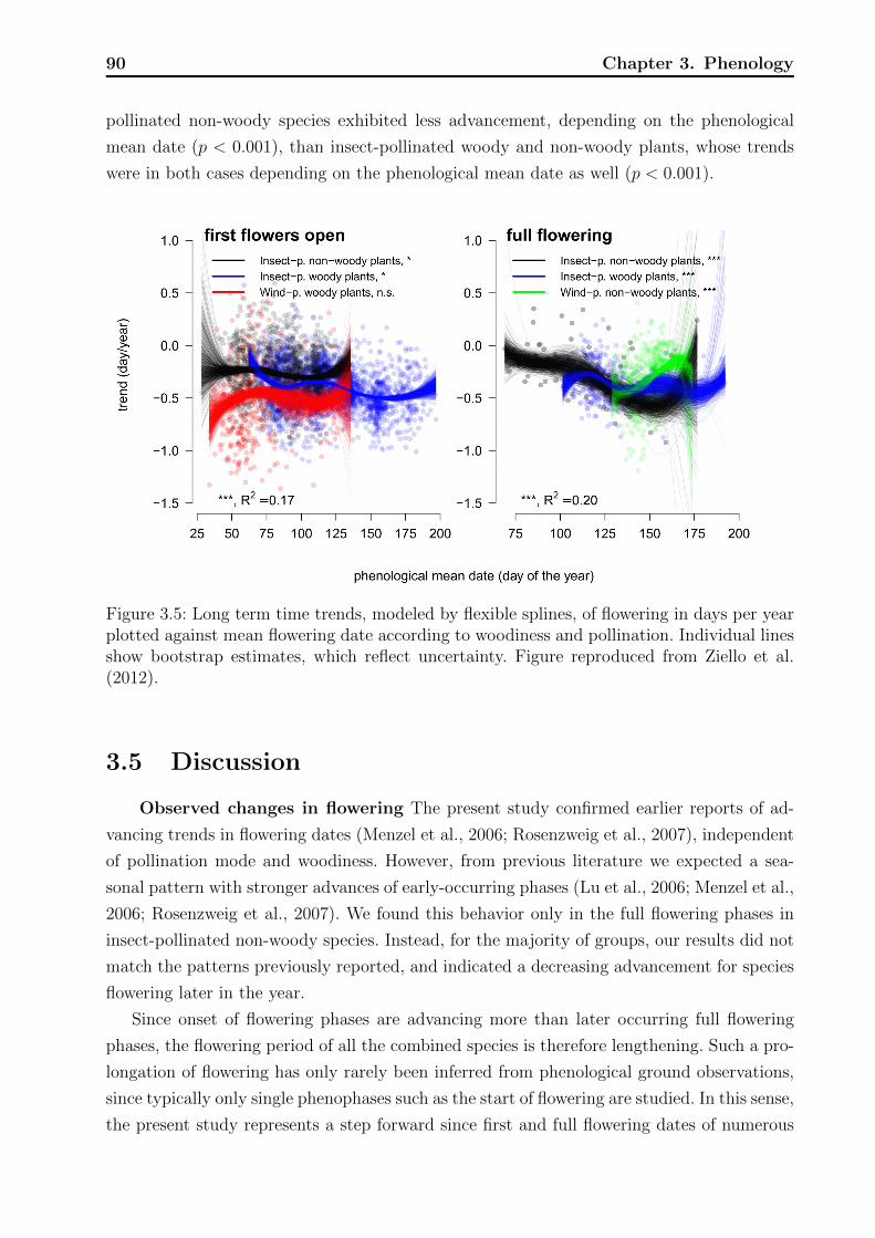
90 Chapter 3. Phenology
pollinated non-woody species exhibited less advancement, depending on the phenological
mean date (p < 0.001), than insect-pollinated woody and non-woody plants, whose trends
were in both cases depending on the phenological mean date as well (p < 0.001).
Figure 3.5: Long term time trends, modeled by flexible splines, of flowering in days per yearplotted against mean flowering date according to woodiness and pollination. Individual linesshow bootstrap estimates, which reflect uncertainty. Figure reproduced from Ziello et al.(2012).
3.5 Discussion
Observed changes in flowering The present study confirmed earlier reports of ad-
vancing trends in flowering dates (Menzel et al., 2006; Rosenzweig et al., 2007), independent
of pollination mode and woodiness. However, from previous literature we expected a sea-
sonal pattern with stronger advances of early-occurring phases (Lu et al., 2006; Menzel et al.,
2006; Rosenzweig et al., 2007). We found this behavior only in the full flowering phases in
insect-pollinated non-woody species. Instead, for the majority of groups, our results did not
match the patterns previously reported, and indicated a decreasing advancement for species
flowering later in the year.
Since onset of flowering phases are advancing more than later occurring full flowering
phases, the flowering period of all the combined species is therefore lengthening. Such a pro-
longation of flowering has only rarely been inferred from phenological ground observations,
since typically only single phenophases such as the start of flowering are studied. In this sense,
the present study represents a step forward since first and full flowering dates of numerous
3.5 Discussion 91
species have been analyzed and a prolongation of this flowering period has been inferred,
which is of paramount importance for those allergic individuals that could likely experience
a prolongation of their main suffering period. Due to the substantial lack of phenological
data for the end of flowering, changes in the dates of this phase, which could directly assess
the lengthening of the complete flowering period, can only be hypothesized. However, studies
of direct pollen measurements have also reported longer pollen seasons (Rosenzweig et al.,
2007), confirming the occurrence of longer flowering periods.
Differentiation of trends by pollination mode Phases related to the onset of flow-
ering of wind-pollinated species exhibited the greatest advances, providing evidence that the
phenology of anemophilous species may be more strongly affected by climate change, even
if showing the weakest changes by year among the analyzed groups (Figure 3.4, Table 3.2).
Compared to insect-pollinated species, wind-pollinated ones exhibited a larger prolonga-
tion of the flowering period, as inferred from the stronger advance of first flower opening
phases compared to full flowering phases. It could hence also be inferred that the combined
flowering period of all the species analyzed lengthened more for wind-pollinated than for
insect-pollinated plants, which is a finding of high importance for pollen-associated allergic
diseases.
Several studies have reported on differences in phenology and ecology between pollination
modes (Bolmgren et al., 2003; Rabinowitz et al., 1981). In contrast to the findings of this
study, Fitter and Fitter (2002) reported that in a recent context of general and fast phenolog-
ical changes in Great Britain, insect-pollinated species were more likely to flower early than
wind-pollinated species. In addition to a different geographical area, this discrepancy could
be due to different criteria for the selection of phenological series: they used records longer
than 23 years in the periods 1954-2000, requiring at least 4 years in the decade 1991-2000. In
the current study, we selected series covering a shorter period (1971-2000) and were exhaus-
tive as at least 29 out of 30 years were analyzed. Hence, in this study the years 1991-2000 are
much more represented and results may better mirror the effects of the pronounced warming
of such a decade. We identify this in the magnitudes of changes: the median advances found
by Fitter and Fitter (2002) are three to six days for five decades, equivalent to a trend of −0.1
and −0.12 days per year (d/yr). In the present study, the mean trends are all stronger than
−0.3 d/yr, reaching almost −0.5 d/yr. Another difference to Fitter and Fitter (2002) is in
contrast to our findings. We found trends of insect-pollinated species to be stronger later in
the season, they reported that insect-pollinated species that flowered early were much more
sensitive to warming than those that flowered later. We return to this later in the discussion.
Hypothesized reasons for stronger flowering responses of wind-pollinated
species Wind-pollination is a functional trait that can be preferentially found in specific
geographical conditions, such as high altitudes and latitudes, in open vegetation structures
such as Savannah, in habitats presenting seasonal loss of leaves such as northern temperate
deciduous forests, or in island floras (Ackerman, 2000; Regal, 1982; Whitehead, 1969). Among
92 Chapter 3. Phenology
the widespread angiosperms (≈ 230,000 plant species), around 18% of families are abiotically
pollinated, and at least 10% of species are wind-pollinated (Ackerman, 2000; Friedman and
Barrett, 2009). All of the strongest allergenic species included in this study (e.g. birch,
grasses) belong to this group.
We observed a stronger advance in first flowering dates for wind-pollinated compared
to insect-pollinated species, and hypothesized that in addition to their pollination syn-
drome (a set of characteristics that co-occur among plants using the same pollination agent)
anemophilous angiosperms have inherited a more rapid adaptedness, in other words a major
plasticity. Angiosperms in general show higher evolutionary rates since their first evolution-
ary stages than gymnosperms, having probably originated in an environment that favored
rapid reproduction (Regal, 1982). Fertilization periods, temporal gaps between pollination
and consequent fertilization, are in fact known to be shorter in angiosperms than in gym-
nosperms (Williams, 2008). The key to the huge success of angiosperms may be due to this
rapidity, even if the reasons for their fast and wide-step radiation are still not completely un-
derstood. Within angiosperms, wind-pollinated species may have changed their pollination
mode as a reaction to unfavorable environmental conditions, enabling more capability for re-
sponding to the variability of climate. This aptitude would make anemophilous angiosperms
particularly sensitive to environmental changes, and thus a group of strong responders to
global warming.
This enhanced sensitivity to warming is made more credible due to the absence of limiting
factors, such as the availability of pollinators. Entomophilous plants could be less free to react
to temperature variations because their pollinator strategies would not match those changes.
Hence, they would be less likely to change their ecological internal clock.
The effect of woodiness and time of the year As Table 3.1 might suggest, the onset
of flowering of non-woody species advanced more than that of woody species for the first
flowering phase. This effect needs to be relativized when looking at the significance tests in
Table 3.2, where pollination mode is considered. In addition, for full flowering the pollination
mode makes a difference for the effect of woodiness. However, when considering the seasonal
variation, the predominant effect of pollination mode over the trait of woodiness is clear. In
fact, advancements for woody and non-woody insect-pollinated species were quite similar in
both flowering phases. In light of the results of this study, the dependence of the observed
first flowering trends on the season seems to be more complex than previously reported. For
entomophilous species the former finding of smaller advances of phases occurring early in the
year is in contrast with the current study (Fitter and Fitter, 2002). This difference in intra-
annual patterns of changes could be due to differences in number of locations monitored,
as for example, only one station from Great Britain was available and 983 in continental
Europe.
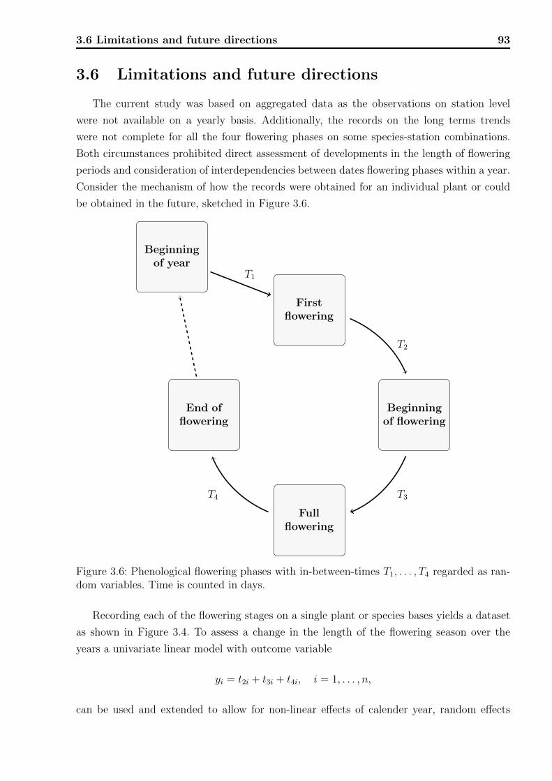
3.6 Limitations and future directions 93
3.6 Limitations and future directions
The current study was based on aggregated data as the observations on station level
were not available on a yearly basis. Additionally, the records on the long terms trends
were not complete for all the four flowering phases on some species-station combinations.
Both circumstances prohibited direct assessment of developments in the length of flowering
periods and consideration of interdependencies between dates flowering phases within a year.
Consider the mechanism of how the records were obtained for an individual plant or could
be obtained in the future, sketched in Figure 3.6.
Beginningof flowering
Firstflowering
End offlowering
Fullflowering
Beginningof year
T3T4
T2
T1
Figure 3.6: Phenological flowering phases with in-between-times T1, . . . , T4 regarded as ran-dom variables. Time is counted in days.
Recording each of the flowering stages on a single plant or species bases yields a dataset
as shown in Figure 3.4. To assess a change in the length of the flowering season over the
years a univariate linear model with outcome variable
yi = t2i + t3i + t4i, i = 1, . . . , n,
can be used and extended to allow for non-linear effects of calender year, random effects

94 Chapter 3. Phenology
Sojourn in flowering phase1 further covariates such as
Plant/species T1 = t1 T2 = t2 T3 = t3 T4 = t4 calendar year and location
i = 1 t11 t21 t31 t41 x1...
......
......
...i = n t1n t2n t3n t4n xn
1According to Figure 3.6 phases are: No flowering (beginning of year),
first flowering, beginning of flowering, full flowering, end of flowering.
Table 3.4: Observations of phenological phases on individual plant level.
for species, and spatial effects for station. A more sophisticated approach is the estimation
of a multivariate model, which explicitly accounts for (or models the) correlations between
observations of a plant within a calendar year. The vector-valued outcome variable,
yi = (t1i, t2i, t3i, t4i), i = 1, . . . , n,
is accordingly modeled as a function of the covariate vector xi, and again extensions for
random and spatial effects are possible (Timm, 2002, chap. 6).
However, the suggested models all assume normally distributed outcome variables T1, . . . , T4.
A natural alternative are time-to-event-models, motivated by the characteristic of time spans
to be non-negative. In detail, a multi-state model is appropriate, where the states (flowering
phases) occur progressively in time. The transitions between flowering phases are described
by hazard rates λ(t), a function of time t (see Section 1.3.3), and several ways to account for
the flowering history of a plant are possible. Completely ignoring the differences in flowering
phases and the flowering history leads to a common hazard rate for every kind of event
(phase). This results in a two-state survival model assuming all T1, . . . , T4 to be identically
distributed within a plant. In other words we expect the time to first flowering to be same
as the time between first flowering and beginning of flowering and so on. More realistic
seems a hazard rate which depends on the current state of plant and time. These models are
so-called Markovian if only depending on the current state and time without incorporating
previous states. Additional information, such as the sojourn time in the previous state or
the end of flowering in the previous year can be included as covariates. This implies some
rearrangement of the data set, outcome variables of earlier phases serve as covariates for the
current phase. Survival models extended for random effects so-called frailty models account
for heterogeneity between species or location (Hanagal, 2011, chap. 12).

Chapter 4
Prostate cancer
This chapter emphasizes the statistical methods used in the articles “Evaluating the
PCPT risk calculator in ten international biopsy cohorts: results from the prostate biopsy
collaborative group” (D.P. Ankerst, A. Boeck et al., 2012a) and “Evaluating the prostate
cancer prevention trial high grade prostate cancer risk calculator in 10 international biopsy
cohorts: results from the prostate biopsy collaborative group” (D.P. Ankerst, A. Boeck et al,
2012b). The author of this thesis was second author of the forenamed articles, responsible
for all statistical analyses and produced all figures and tables appearing in the articles and
this thesis.
4.1 Introduction
The Prostate Cancer Prevention Trial (PCPT) was a North American phase III random-
ized, double-blind, placebo-controlled study of the chemoprevention effects of finasteride
versus placebo on prostate cancer development. Study participation was limited to men
older than 54 years of age, who have a prostate-specific antigen (PSA) level less than or
equal to 3.0 ng/mL and have a normal digital rectal exam (DRE) result. They were annually
screened and referred to interim biopsy (six-core) whenever their PSA exceeded 4.0 ng/mL
or their DRE was abnormal. Follow-up time was seven years. At the end of this follow-up
time, all men were requested to undergo a prostate biopsy regardless of their current PSA
value and DRE result, or whether they had previously undergone a prostate biopsy that was
negative for prostate cancer. Data of 5,519 participants from the placebo arm of the PCPT
were used to develop a risk calculator for prostate cancer (PCPTRC) and a calculator for
predicting high-grade (Gleason grade ≥ 7) prostate cancer (PCPTHG). The PCPTRC and
PCPTHG were posted online on the websites of the Health Science Center in San Antonio,
a part of the University of Texas, in 2006. Since then it is used by patients and clinicians
worldwide as a counseling aid for the decision to undergo prostate biopsy.
In this work we present a study on the external validity of the PCPTRC (Ankerst et al.,
2012) and the PCPTHG (Ankerst et al., 2012) on multiple cohorts in order to identify

96 Chapter 4. Prostate cancer
potential populations where it may or may not be applicable. To that end, we highlight the
characteristics of the study populations used to build the calculators in comparison to those
used for the validation. Statistical measures which are suitable to quantify the performance
of the calculators as a prediction tool are discussed.
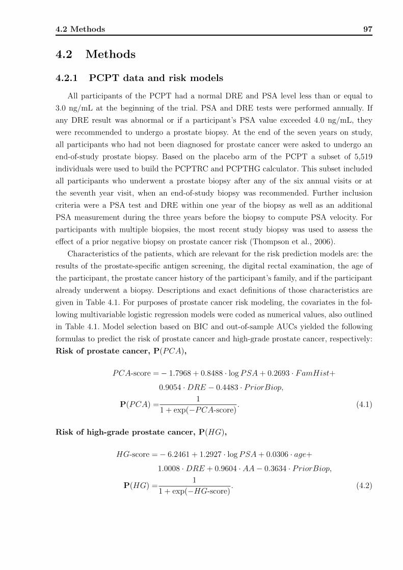
4.2 Methods 97
4.2 Methods
4.2.1 PCPT data and risk models
All participants of the PCPT had a normal DRE and PSA level less than or equal to
3.0 ng/mL at the beginning of the trial. PSA and DRE tests were performed annually. If
any DRE result was abnormal or if a participant’s PSA value exceeded 4.0 ng/mL, they
were recommended to undergo a prostate biopsy. At the end of the seven years on study,
all participants who had not been diagnosed for prostate cancer were asked to undergo an
end-of-study prostate biopsy. Based on the placebo arm of the PCPT a subset of 5,519
individuals were used to build the PCPTRC and PCPTHG calculator. This subset included
all participants who underwent a prostate biopsy after any of the six annual visits or at
the seventh year visit, when an end-of-study biopsy was recommended. Further inclusion
criteria were a PSA test and DRE within one year of the biopsy as well as an additional
PSA measurement during the three years before the biopsy to compute PSA velocity. For
participants with multiple biopsies, the most recent study biopsy was used to assess the
effect of a prior negative biopsy on prostate cancer risk (Thompson et al., 2006).
Characteristics of the patients, which are relevant for the risk prediction models are: the
results of the prostate-specific antigen screening, the digital rectal examination, the age of
the participant, the prostate cancer history of the participant’s family, and if the participant
already underwent a biopsy. Descriptions and exact definitions of those characteristics are
given in Table 4.1. For purposes of prostate cancer risk modeling, the covariates in the fol-
lowing multivariable logistic regression models were coded as numerical values, also outlined
in Table 4.1. Model selection based on BIC and out-of-sample AUCs yielded the following
formulas to predict the risk of prostate cancer and high-grade prostate cancer, respectively:
Risk of prostate cancer, P(PCA),
PCA-score =− 1.7968 + 0.8488 · logPSA+ 0.2693 · FamHist+
0.9054 ·DRE − 0.4483 · PriorBiop,
P(PCA) =1
1 + exp(−PCA-score). (4.1)
Risk of high-grade prostate cancer, P(HG),
HG-score =− 6.2461 + 1.2927 · logPSA+ 0.0306 · age+
1.0008 ·DRE + 0.9604 · AA− 0.3634 · PriorBiop,
P(HG) =1
1 + exp(−HG-score). (4.2)
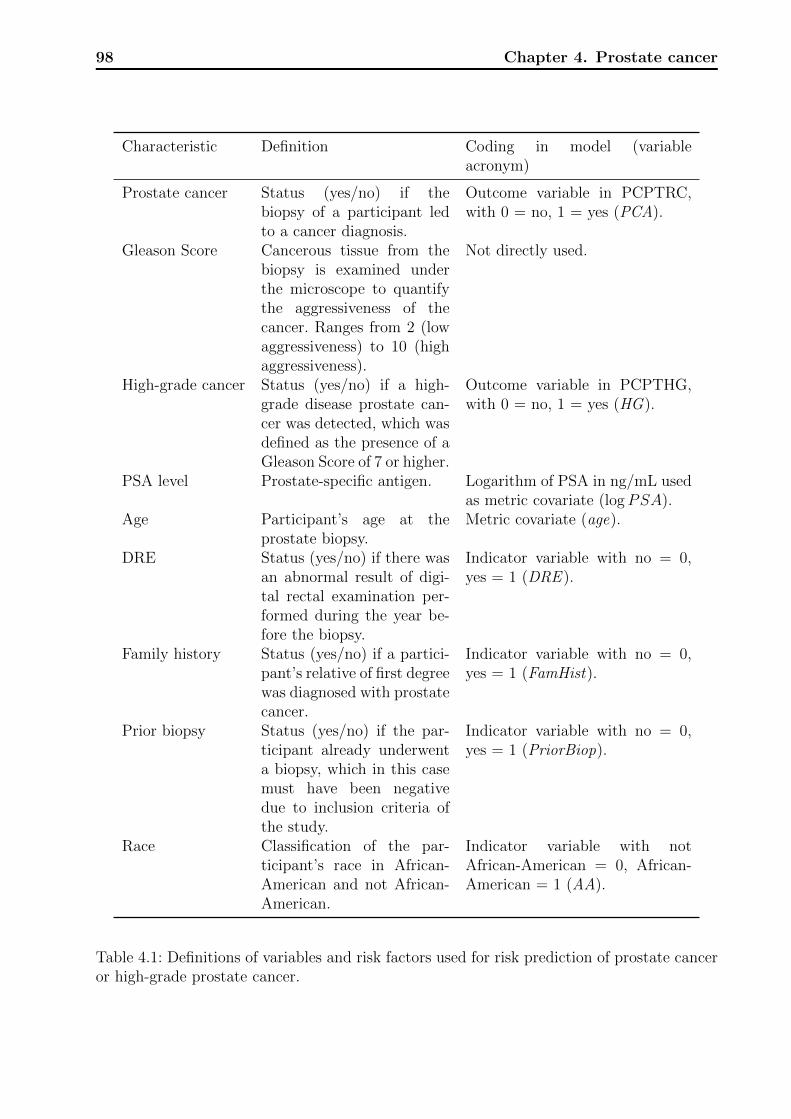
98 Chapter 4. Prostate cancer
Characteristic Definition Coding in model (variableacronym)
Prostate cancer Status (yes/no) if thebiopsy of a participant ledto a cancer diagnosis.
Outcome variable in PCPTRC,with 0 = no, 1 = yes (PCA).
Gleason Score Cancerous tissue from thebiopsy is examined underthe microscope to quantifythe aggressiveness of thecancer. Ranges from 2 (lowaggressiveness) to 10 (highaggressiveness).
Not directly used.
High-grade cancer Status (yes/no) if a high-grade disease prostate can-cer was detected, which wasdefined as the presence of aGleason Score of 7 or higher.
Outcome variable in PCPTHG,with 0 = no, 1 = yes (HG).
PSA level Prostate-specific antigen. Logarithm of PSA in ng/mL usedas metric covariate (logPSA).
Age Participant’s age at theprostate biopsy.
Metric covariate (age).
DRE Status (yes/no) if there wasan abnormal result of digi-tal rectal examination per-formed during the year be-fore the biopsy.
Indicator variable with no = 0,yes = 1 (DRE ).
Family history Status (yes/no) if a partici-pant’s relative of first degreewas diagnosed with prostatecancer.
Indicator variable with no = 0,yes = 1 (FamHist).
Prior biopsy Status (yes/no) if the par-ticipant already underwenta biopsy, which in this casemust have been negativedue to inclusion criteria ofthe study.
Indicator variable with no = 0,yes = 1 (PriorBiop).
Race Classification of the par-ticipant’s race in African-American and not African-American.
Indicator variable with notAfrican-American = 0, African-American = 1 (AA).
Table 4.1: Definitions of variables and risk factors used for risk prediction of prostate canceror high-grade prostate cancer.
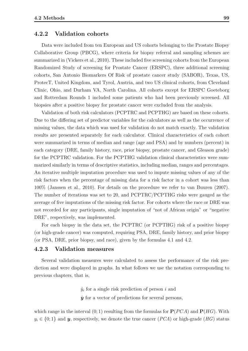
4.2 Methods 99
4.2.2 Validation cohorts
Data were included from ten European and US cohorts belonging to the Prostate Biopsy
Collaborative Group (PBCG), where criteria for biopsy referral and sampling schemes are
summarized in (Vickers et al., 2010). These included five screening cohorts from the European
Randomized Study of screening for Prostate Cancer (ERSPC), three additional screening
cohorts, San Antonio Biomarkers Of Risk of prostate cancer study (SABOR), Texas, US,
ProtecT, United Kingdom, and Tyrol, Austria, and two US clinical cohorts, from Cleveland
Clinic, Ohio, and Durham VA, North Carolina. All cohorts except for ERSPC Goeteborg
and Rotterdam Rounds 1 included some patients who had been previously screened. All
biopsies after a positive biopsy for prostate cancer were excluded from the analysis.
Validation of both risk calculators (PCPTRC and PCPTHG) are based on these cohorts.
Due to the differing set of predictor variables for the calculators as well as the occurrence of
missing values, the data which was used for validation do not match exactly. The validation
results are presented separately for each calculator. Clinical characteristics of each cohort
were summarized in terms of median and range (age and PSA) and by numbers (percent) in
each category (DRE, family history, race, prior biopsy, prostate cancer, and Gleason grade)
for the PCPTRC validation. For the PCPTHG validation clinical characteristics were sum-
marized similarly in terms of descriptive statistics, including median, ranges and percentages.
An iterative multiple imputation procedure was used to impute missing values of any of the
risk factors when the percentage of missing data for a risk factor in a cohort was less than
100% (Janssen et al., 2010). For details on the procedure we refer to van Buuren (2007).
The number of iterations was set to 20, and PCPTRC/PCPTHG risks were gauged as the
average of five imputations of the missing risk factor. For cohorts where the race or DRE was
not recorded for any participants, single imputation of “not of African origin” or “negative
DRE”, respectively, was implemented.
For each biopsy in the data set, the PCPTRC (or PCPTHG) risk of a positive biopsy
(or high-grade cancer) was computed, requiring PSA, DRE, family history, and prior biopsy
(or PSA, DRE, prior biopsy, and race), given by the formulas 4.1 and 4.2.
4.2.3 Validation measures
Several validation measures were calculated to assess the performance of the risk pre-
diction and were displayed in graphs. In what follows we use the notation corresponding to
previous chapters, that is,
yi for a single risk prediction of person i and
y for a vector of predictions for several persons,
which range in the interval (0; 1) resulting from the formulas for P(PCA) and P(HG). With
yi ∈ {0; 1} and y, respectively, we denote the true cancer (PCA) or high-grade (HG) status

100 Chapter 4. Prostate cancer
of a person.
ROC and AUC Discrimination was calculated via receiver operating characteristic
curves (ROC). Areas underneath the ROC curve (AUC) were calculated for predicted risks
and compared to those with PSA alone for each cohort. As already previously described in
Section 1.2.3, the AUC is applicable to assess the discrimination ability of both a metric
covariate, like PSA, and of risk predictions y. For the interpretation we refer to the afore-
mentioned section, where also calculation formulas are given. The rank-based Wilcoxon test
was used to infer the differences in AUCs of the y and PSA values in terms of statistical
significance.
Hosmer-Lemeshow test As a measure of calibration, the Hosmer-Lemeshow (HL)
goodness-of-fit test was used (Hosmer and Lemeshow, 2000, p. 147). A risk prediction model
shows good calibration if there is a strong similarity between observed outcomes y and
predicted risks y, which is described in more detail in Section 1.3.6. The test statistic of the
HL-test sums the squared differences of predictions and true outcomes over G = 10 groups.
The pair of vectors (y,y) is gathered in groups by deciles of the predicted risks y, that is,
the 10% smallest yi define a group, the next largest 10% define the second group, and so on.
This results in nearly equally-sized groups with n/10 pairs of (yi, yi), where n is the total
sample size. With ng we denote the particular sample size in group g, g = 1, . . . , 10. The
χ2-type test statistic is thus
HL =G∑g=1
(Og − ng ¯yg
)2
ng ¯yg(1− ¯yg),
with Og being the sum of observed cancers in group g,
Og =
ng∑i=1
yi,
and ¯yg being the average prediction risk in group g,
¯yg =1
ng
ng∑i=1
yi.
Applied on data from an external validation, under the null-hypothesis HL asymptotically
follows a χ2-distribution with nine degrees of freedom:
H0 : No difference between observed outcome and model-predicted risk,
HA : Observed outcome differs from prediction, and
HLa∼ χ2(df = 9).
Thus, for this test a p-value of p < 0.05 indicates a poor agreement between predicted

4.2 Methods 101
PCPTRC/PCPTHG risks and actual observed risk. However, it must be brought to attention
that the null hypothesis is of good calibration, which will result in low power to detect
miscalibration for small sample sizes, and we would only reject the null hypothesis if it was
very severe. Furthermore, even in a situation with a quite perfectly calibrated model, we
would reject the null hypothesis in a sufficiently large study (Steyerberg, 2009, p. 274 ff).
Calibration plot A visualization of the HL test and its decile-based categorization is
the calibration plot. In the graph, the ten average predicted risks ¯yg are laid out against the
actual observed risks yg = Og/ng of these categories. For an easier visual assessment, the
occurring points are connected by lines in order of the predicted risks (x-axis). Vertical lines
indicate Bonferroni adjusted 95% confidence intervals (CI) of the observed risks, based on
their standard errors,
se(yg) =
√yg(1− yg)
ng),
CIg = yg ± 2.08 se(yg).
The factor 2.08 in the above formula reflects the Bonferroni adjustment over G = 10 decile
groups to reach an overall confidence level of 95% (α = 0.05), and is the (1− α/210
) = 0.9975-
quantile of the standard normal distribution needed for a two-sided CI. Good calibration is
indicated when the line chart is close to the graph of an identity function, which corresponds
to a 45 ◦ line if both axis scales are isometric. The identity function graphs are drawn as ledger
lines. At least the confidence intervals should overlap that line for acceptable calibration.
Additionally, good discrimination of the model is indicated when the line chart is spread
out over the range of the x-axis, that is the risk predictions yi cover the whole interval of
possible values between 0 and 1.
For the PCPTHG a modified version of the calibration plot is shown, although it has the
same interpretation. It was not based on a hard grouping of the data by deciles, but using a
smoothing technique to soften the dependency on the arbitrarily chosen number of G = 10
groups. Steyerberg (2009) suggested the loess smoother as described in Cleveland et al.
(1992), but practically identical results were achieved using a smoothing-spline approach a
binomial GLM (see Section 1.3.3), with the advantage that 95% pointwise CIs were readily
available. In short, the observed outcomes y are modeled as a non-linear function of the
predicted risks y. Opposite to the decile-based calibration plot, the distribution, or spread,
of the predicted risks cannot be assessed immediately; a rug plot displaying the shape of the
distribution, similar to a histogram, is overlaid at the bottom of the graph to overcome this.
Net benefit The clinical net benefit (Vickers and Elkin, 2006; Rousson and Zumbrunn,
2011) aims to account for the consequences of a decision suggested by the prediction model.
Usually, decision-theoretic approaches attach utilities U to every possible option and seek for
optimal decision rules. However, for a concrete application some knowledge outside the data
at hand have to be present, which allow these utilities to be quantified. The idea of providing
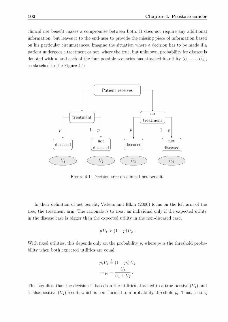
102 Chapter 4. Prostate cancer
clinical net benefit makes a compromise between both: It does not require any additional
information, but leaves it to the end-user to provide the missing piece of information based
on his particular circumstances. Imagine the situation where a decision has to be made if a
patient undergoes a treatment or not, where the true, but unknown, probability for disease is
denoted with p, and each of the four possible scenarios has attached its utility (U1, . . . , U4),
as sketched in the Figure 4.1:
Patient receives
treatment
p 1− p
diseased
U1
not
diseased
U2
no
treatment
p 1− p
diseased
U3
not
diseased
U4
Figure 4.1: Decision tree on clinical net benefit.
In their definition of net benefit, Vickers and Elkin (2006) focus on the left arm of the
tree, the treatment arm. The rationale is to treat an individual only if the expected utility
in the disease case is bigger than the expected utility in the non-diseased case,
pU1 > (1− p)U2 .
With fixed utilities, this depends only on the probability p, where pt is the threshold proba-
bility when both expected utilities are equal,
pt U1!
= (1− pt)U2
⇒ pt =U2
U1 + U2
.
This signifies, that the decision is based on the utilities attached to a true postive (U1) and
a false positive (U2) result, which is transformed to a probability threshold pt. Thus, setting

4.2 Methods 103
U1 = 1, which is just a standardization of the utilities, we can express U2 as a function of pt,
ptU1=1=
U2
1 + U2
⇒ U2 =pt
1− pt.
The net benefit for a prediction model is defined as the sum of all benefits minus the sum of
all costs. A benefit arises when a diseased person is treated, and is quantified with U1 = 1.
Costs arise when a non-diseased person is treated and is quantified with U2 = pt1−pt . The
expected net benefit as a function of pt (and therefore of U1 and U2) thus is
E (netben(pt)) = p · 1︸︷︷︸benefit
− (1− p) ·(
pt1− pt
)︸ ︷︷ ︸
costs
.
Replacing the unknown p by its empirical counterpart, the fraction of true positives, leads
to the estimated net benefit
netben(pt) =true positve count
n− false positive count
n
(pt
1− pt
),
where n is the number of all observations in the validation set. In the notation used through-
out this thesis, with yi as a individual risk prediction and yi as a true outcome, the formula
for the net benefit is
netbenmodel(pt) =1
n
n∑i=1
I(yi > pt)I(yi = 1)− 1
n
n∑i=1
I(yi > pt)I(yi = 0)
(pt
1− pt
). (4.3)
Besides the model-based strategy, the net benefit is calculated for two additional decision
strategies, which are rather extreme. They consist of not treating anyone and treating every-
one, regardless of their individual threshold probability. The net benefit for treating nobody
is constant zero,
netbentreat none(pt) = 0, (4.4)
while for treating everyone it is
netbentreat all(pt) =1
n
n∑i=1
I(yi = 1)︸ ︷︷ ︸prevalence
− 1
n
n∑i=1
I(yi = 0)︸ ︷︷ ︸1− prevalence
(pt
1− pt
), (4.5)
which is a decreasing function of pt, ranging from prevalence down to negative infinity. Fi-
nally, the net benefit graphs of the three functions 4.3, 4.4, and 4.5, are shown for a reasonable
104 Chapter 4. Prostate cancer
range of threshold probabilities, which reflect the different individual circumstances of an
individual.
In the context of this validation study, “treatment” corresponds to the decision whether a
person undergoes a prostate biopsy. The graph shows for which areas of personal probability
thresholds pt the prediction model is useful for the patients, or in other words, shows where
the benefit is higher compared to the other two strategies. The threshold serves a proxy how
the patient weighs the harms of a unnecessary biopsy compared to a delayed diagnosis of
prostate cancer. The scale of the net benefit has the following interpretation: A prediction
model with a net benefit of 0.12 (at a specific pt) is equivalent to a strategy that identifies
12 cancers in 100 patients with no unnecessary biopsies (Vickers, 2008).
4.3 Results
As mentioned above, patients within the cohorts used for the evaluation of the overall
cancer calculator and the high-grade cancer calculator differed slightly due to the different set
of missing values in the predictor variables. The tables and graphs are presented separately
for each of the evaluations.
4.3.1 Cohort characteristics
Among the PBCG cohorts used to evaluate the PCPTRC, age was fairly consistent with
a median in the early sixties (Table 4.2). Median PSA values ranged from 3.4 ng/ml in the
SABOR cohort to 5.2 ng/ml in the Durham VA cohort, and rates of abnormal DRE, from
a low of 10% in the Goeteborg Rounds 2–6 and Tyrol cohorts to a high of 31% in the Tarn
cohort. Family history of prostate cancer was only reported in half of the cohorts and those
reported all fell at or below 11% except for SABOR at 29%. This was an artifact of selection
bias for the SABOR cohort since its protocol included a family history substudy that offered
biopsies to men with PSA less than 4.0 ng/ml and a positive family history. African origin was
not reported in the European cohorts but could be presumed to be negligible. The Durham
VA cohort provided a contrast, with 45% of the individuals being of African origin. This
cohort also had the highest cancer rate of 47% exceeding all nine other cohorts where the
rates ranged from 26 to 39%. The Distribution of biopsy Gleason grades indicated a majority
of low-grade cancers (Gleason 6 or less) in the ERSPC and SABOR screening cohorts, but
only approximately half or less low-grade cancers were observed in the Tarn section of the
ERSPC and the more clinical cohorts, Cleveland Clinic and Durham VA cohorts.
High-grade prostate cancer rates ranged from 4% in Goeteberg Rounds 2–6 to 22% in the
Durham VA cohort, which was characterized by the highest percentage of men with African
origin (45%), one of the risk factors included in the PCPTHG (Table 4.3).
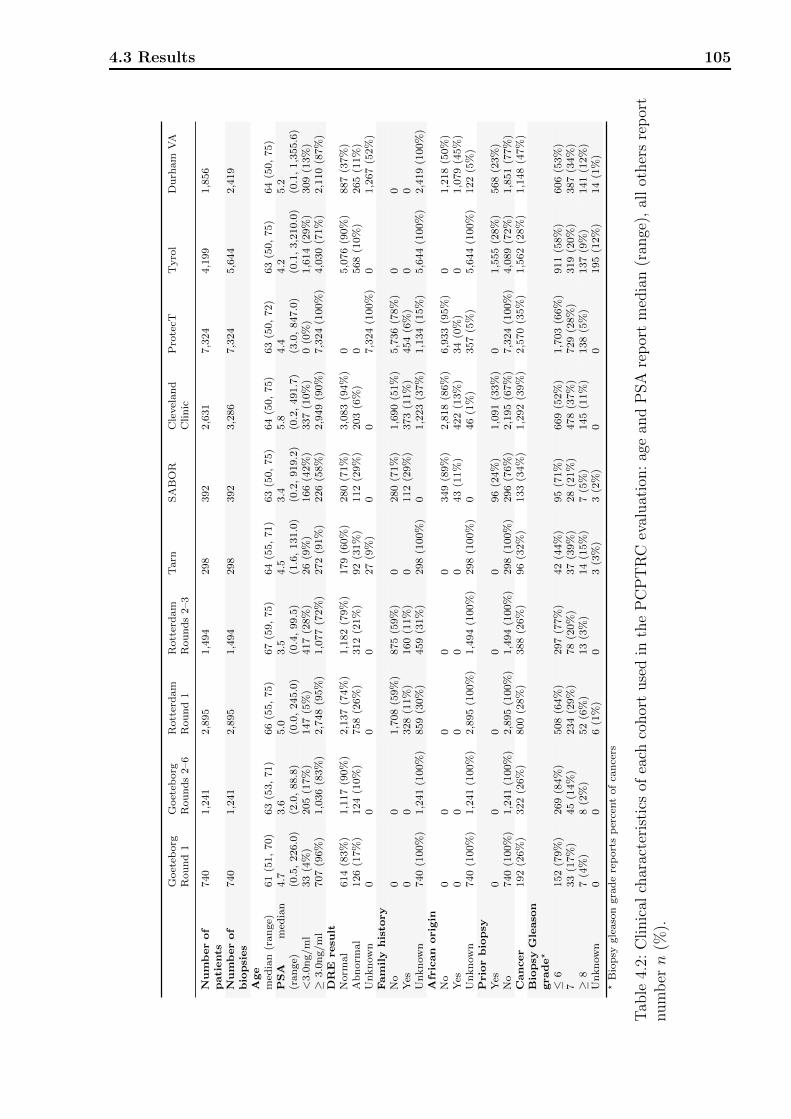
4.3 Results 105
Goet
eborg
Rou
nd
1G
oet
eborg
Rou
nd
s2–6
Rott
erd
am
Rou
nd
1R
ott
erd
am
Rou
nd
s2–3
Tarn
SA
BO
RC
level
an
dC
lin
icP
rote
cTT
yro
lD
urh
am
VA
Numberof
patients
740
1,2
41
2,8
95
1,4
94
298
392
2,6
31
7,3
24
4,1
99
1,8
56
Numberof
biopsies
740
1,2
41
2,8
95
1,4
94
298
392
3,2
86
7,3
24
5,6
44
2,4
19
Age
med
ian
(ran
ge)
61
(51,
70)
63
(53,
71)
66
(55,
75)
67
(59,
75)
64
(55,
71)
63
(50,
75)
64
(50,
75)
63
(50,
72)
63
(50,
75)
64
(50,
75)
PSA
med
ian
(ran
ge)
4.7
(0.5
,226.0
)3.6
(2.0
,88.8
)5.0
(0.0
,245.0
)3.5
(0.4
,99.5
)4.5
(1.6
,131.0
)3.4
(0.2
,919.2
)5.8
(0.2
,491.7
)4.4
(3.0
,847.0
)4.2
(0.1
,3,2
10.0
)5.2
(0.1
,1,3
55.6
)<
3.0
ng/m
l33
(4%
)205
(17%
)147
(5%
)417
(28%
)26
(9%
)166
(42%
)337
(10%
)0
(0%
)1,6
14
(29%
)309
(13%
)≥
3.0
ng/m
l707
(96%
)1,0
36
(83%
)2,7
48
(95%
)1,0
77
(72%
)272
(91%
)226
(58%
)2,9
49
(90%
)7,3
24
(100%
)4,0
30
(71%
)2,1
10
(87%
)DRE
resu
ltN
orm
al
614
(83%
)1,1
17
(90%
)2,1
37
(74%
)1,1
82
(79%
)179
(60%
)280
(71%
)3,0
83
(94%
)0
5,0
76
(90%
)887
(37%
)A
bn
orm
al
126
(17%
)124
(10%
)758
(26%
)312
(21%
)92
(31%
)112
(29%
)203
(6%
)0
568
(10%
)265
(11%
)U
nkn
ow
n0
00
027
(9%
)0
07,3
24
(100%
)0
1,2
67
(52%
)Fam
ily
histo
ry
No
00
1,7
08
(59%
)875
(59%
)0
280
(71%
)1,6
90
(51%
)5,7
36
(78%
)0
0Y
es0
0328
(11%
)160
(11%
)0
112
(29%
)373
(11%
)454
(6%
)0
0U
nkn
ow
n740
(100%
)1,2
41
(100%
)859
(30%
)459
(31%
)298
(100%
)0
1,2
23
(37%
)1,1
34
(15%
)5,6
44
(100%
)2,4
19
(100%
)African
origin
No
00
00
0349
(89%
)2,8
18
(86%
)6,9
33
(95%
)0
1,2
18
(50%
)Y
es0
00
00
43
(11%
)422
(13%
)34
(0%
)0
1,0
79
(45%
)U
nkn
ow
n740
(100%
)1,2
41
(100%
)2,8
95
(100%
)1,4
94
(100%
)298
(100%
)0
46
(1%
)357
(5%
)5,6
44
(100%
)122
(5%
)Priorbiopsy
Yes
00
00
096
(24%
)1,0
91
(33%
)0
1,5
55
(28%
)568
(23%
)N
o740
(100%
)1,2
41
(100%
)2,8
95
(100%
)1,4
94
(100%
)298
(100%
)296
(76%
)2,1
95
(67%
)7,3
24
(100%
)4,0
89
(72%
)1,8
51
(77%
)Cancer
192
(26%
)322
(26%
)800
(28%
)388
(26%
)96
(32%
)133
(34%
)1,2
92
(39%
)2,5
70
(35%
)1,5
62
(28%
)1,1
48
(47%
)Biopsy
Gleaso
ngrade?
≤6
152
(79%
)269
(84%
)508
(64%
)297
(77%
)42
(44%
)95
(71%
)669
(52%
)1,7
03
(66%
)911
(58%
)606
(53%
)7
33
(17%
)45
(14%
)234
(29%
)78
(20%
)37
(39%
)28
(21%
)478
(37%
)729
(28%
)319
(20%
)387
(34%
)≥
87
(4%
)8
(2%
)52
(6%
)13
(3%
)14
(15%
)7
(5%
)145
(11%
)138
(5%
)137
(9%
)141
(12%
)U
nkn
ow
n0
06
(1%
)0
3(3
%)
3(2
%)
00
195
(12%
)14
(1%
)?
Bio
psy
gle
aso
ngra
de
rep
ort
sp
erce
nt
of
can
cers
Tab
le4.
2:C
linic
alch
arac
teri
stic
sof
each
cohor
tuse
din
the
PC
PT
RC
eval
uat
ion:
age
and
PSA
rep
ort
med
ian
(ran
ge),
all
other
sre
por
tnum
bern
(%).
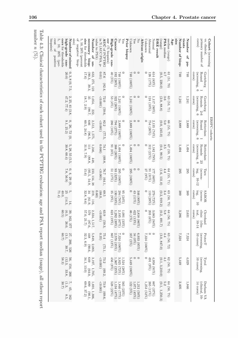
106 Chapter 4. Prostate cancer
Cohort
(screenin
gvs.
clinica
l,p
rimary
nu
mb
erof
cores)
ER
SP
Cco
horts
Goeteb
org
Rou
nd
1(screen
ing,
6co
res)
Goeteb
org
Rou
nd
s2-6
(screenin
g,
6co
res)
Rotterd
am
Rou
nd
1(screen
ing,
6co
res)
Rotterd
am
Rou
nd
s23
(screenin
g,
6co
res)
Tarn
(screen-
ing,
10-1
2co
res)
SA
BO
R(screen
-in
g,
10
cores)
Clev
elan
dclin
ic(clin
-ica
l,10-1
4co
res)
Pro
tecT(screen
ing,
10
cores)
Tyro
l(screen
ing,
10
cores)
Du
rham
VA
(clinica
l,10-
14
cores)
Number
of
pa-
tients
740
1,2
41
2,8
89
1,4
94
295
389
2,6
31
7,3
24
4,0
29
1,8
46
Numberofbiop-
sies
740
1,2
41
2,8
89
1,4
94
295
389
3,2
86
7,3
24
5,4
49
2,4
05
Age
med
ian
(ran
ge)
61
(51,
70)
63
(53,
71)
66
(55,
75)
67
(59,
75)
64
(55,
71)
63
(50,
75)
64
(50,
75)
63
(50,
72)
62
(50,
75)
64
(50,
75)
PSA
med
ian
(ran
ge)
4.7
(0.5
,226.0
)3.6
(2.0
,88.8
)5.0
(0.0
,245.0
)3.5
(0.4
,99.5
)4.4
(1.6
,131.0
)3.4
(0.2
,919.2
)5.8
(0.2
,491.7
)4.4
(3.0
,847.0
)4.1
(0.1
,3,2
10.0
)5.2
(0.1
,1,2
50.3
)DRE
resu
ltN
orm
al
614
(83%
)1,1
17
(90%
)2,1
35
(74%
)1,1
82
(79%
)177
(60%
)279
(72%
)3,0
83
(94%
)0
4,9
58
(91%
)887
(37%
)A
bn
orm
al
126
(17%
)124
(10%
)754
(26%
)312
(21%
)91
(31%
)110
(28%
)203
(6%
)0
491
(9%
)265
(11%
)U
nkn
ow
n0
00
027
(9%
)0
07,3
24
(100%
)0
1,2
53
(52%
)African
origin
No
00
00
0346
(89%
)2,8
18
(86%
)6,9
33
(95%
)0
1,2
12
(50%
)Y
es0
00
00
43
(11%
)422
(13%
)34
(0%
)0
1,0
71
(45%
)U
nkn
ow
n740
(100%
)1,2
41
(100%
)2,8
89
(100%
)1,4
94
(100%
)295
(100%
)0
46
(1%
)357
(5%
)5,4
49
(100%
)122
(5%
)Priorbiopsy
Yes
00
00
095
(24%
)1,0
91
(33%
)0
1,5
24
(28%
)565
(23%
)N
o740
(100%
)1,2
41
(100%
)2,8
89
(100%
)1,4
94
(100%
)295
(100%
)294
(76%
)2,1
95
(67%
)7,3
24
(100%
)3,9
25
(72%
)1,8
40
(77%
)Cancer
192
(26%
)322
(26%
)794
(27%
)388
(26%
)93
(32%
)130
(33%
)1,2
92
(39%
)2,5
70
(35%
)1,3
67
(25%
)1,1
34
(47%
)High-g
rade
can-
cer
(%b
iop
sies)40
(5%
)53
(4%
)286
(10%
)91
(6%
)51
(17%
)35
(9%
)623
(19%
)867
(12%
)456
(8%
)528
(22%
)
AUC
of
PC
PT
HG
in%
(AU
CP
SA
,p
-valu
eto
PS
A)
87.6
(82.4
,0.0
1)
72.0
(59.6
,<
0.0
01)
82.2
(77.5
,<
0.0
01)
74.1
(69.8
,0.0
46)
76.7
(64.1
,<
0.0
01)
69.5
(68.0
,0.6
0)
63.9
(59.3
,<
0.0
01)
75.4
(75.1
,0.3
5)
73.2
(69.2
,<
0.0
01)
73.9
(69.6
,<
0.0
01)
Number
of
un-
necessa
ry
biop-
sies
for
thresh
old
s5,
10,
20%
(percen
tof
neg
ativ
eb
iop
-sies)
632,
275,
123
(90.3
,39.3
,17.6
)
1,0
54,
222,
35
(88.7
,18.7
,2.9
)
2,5
12,
1,5
75,
646
(96.5
,60.5
,24.8
)
1,2
46,
448,
111
(88.8
,31.9
,7.9
)
233,134,38
(95.5
,54.9
,15.6
)
219,
116,
34
(61.9
,32.8
,9.6
)
2,3
34,1,5
17,
579
(87.6
,57.0
,21.7
)
5,8
49,
2,0
83,
448
(90.6
,32.3
,6.9
)
3,1
97,
1,7
05,
649
(64.0
,34.1
,13.0
)
1,6
91,1,3
06,
699
(90.1
,69.6
,37.2
)
Numberofm
issed
high-g
rade
can-
cers
for
thresh
old
s5,
10,
20%
(per-
cent
of
positiv
eb
iop
sies)
0,3,8
(0,7.5
,20.0
)2,25,41
(3.8
,47.2
,77.4
)0,
26,
72
(0,
9.1
,25.2
)5,28,55
(5.5
,30.8
,60.4
)0,
4,
29
(0,
7.8
,56.9
)5,
14,
25
(14.3
,40.0
,71.4
)
39,
162,
377
(6.3
,26.0
,60.5
)
27,
266,
526
(3.1
,30.7
,60.7
)
56,
154,
266
(12.3
,33.8
,58.3
)
7,
45,
162
(1.3
,8.5
,30.7
)
Tab
le4.3:
Clin
icalch
aracteristicsof
eachcoh
ortused
inth
eP
CP
TH
Gevalu
ation:
agean
dP
SA
report
med
ian(ran
ge),all
others
report
num
bern
(%).
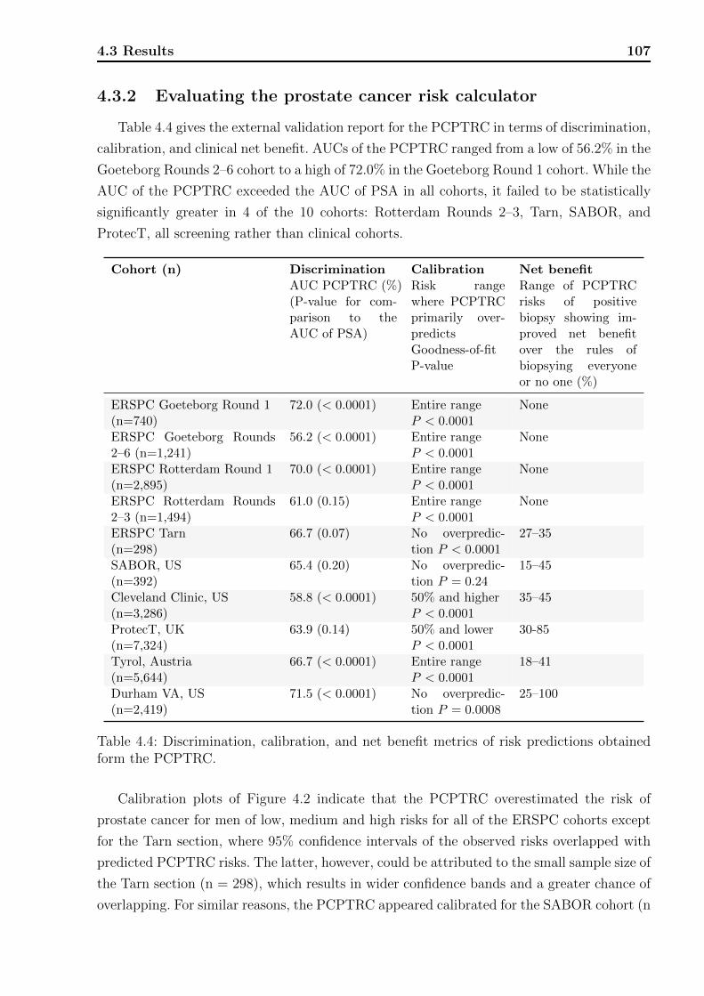
4.3 Results 107
4.3.2 Evaluating the prostate cancer risk calculator
Table 4.4 gives the external validation report for the PCPTRC in terms of discrimination,
calibration, and clinical net benefit. AUCs of the PCPTRC ranged from a low of 56.2% in the
Goeteborg Rounds 2–6 cohort to a high of 72.0% in the Goeteborg Round 1 cohort. While the
AUC of the PCPTRC exceeded the AUC of PSA in all cohorts, it failed to be statistically
significantly greater in 4 of the 10 cohorts: Rotterdam Rounds 2–3, Tarn, SABOR, and
ProtecT, all screening rather than clinical cohorts.
Cohort (n) DiscriminationAUC PCPTRC (%)(P-value for com-parison to theAUC of PSA)
CalibrationRisk rangewhere PCPTRCprimarily over-predictsGoodness-of-fitP-value
Net benefitRange of PCPTRCrisks of positivebiopsy showing im-proved net benefitover the rules ofbiopsying everyoneor no one (%)
ERSPC Goeteborg Round 1(n=740)
72.0 (< 0.0001) Entire rangeP < 0.0001
None
ERSPC Goeteborg Rounds2–6 (n=1,241)
56.2 (< 0.0001) Entire rangeP < 0.0001
None
ERSPC Rotterdam Round 1(n=2,895)
70.0 (< 0.0001) Entire rangeP < 0.0001
None
ERSPC Rotterdam Rounds2–3 (n=1,494)
61.0 (0.15) Entire rangeP < 0.0001
None
ERSPC Tarn(n=298)
66.7 (0.07) No overpredic-tion P < 0.0001
27–35
SABOR, US(n=392)
65.4 (0.20) No overpredic-tion P = 0.24
15–45
Cleveland Clinic, US(n=3,286)
58.8 (< 0.0001) 50% and higherP < 0.0001
35–45
ProtecT, UK(n=7,324)
63.9 (0.14) 50% and lowerP < 0.0001
30-85
Tyrol, Austria(n=5,644)
66.7 (< 0.0001) Entire rangeP < 0.0001
18–41
Durham VA, US(n=2,419)
71.5 (< 0.0001) No overpredic-tion P = 0.0008
25–100
Table 4.4: Discrimination, calibration, and net benefit metrics of risk predictions obtainedform the PCPTRC.
Calibration plots of Figure 4.2 indicate that the PCPTRC overestimated the risk of
prostate cancer for men of low, medium and high risks for all of the ERSPC cohorts except
for the Tarn section, where 95% confidence intervals of the observed risks overlapped with
predicted PCPTRC risks. The latter, however, could be attributed to the small sample size of
the Tarn section (n = 298), which results in wider confidence bands and a greater chance of
overlapping. For similar reasons, the PCPTRC appeared calibrated for the SABOR cohort (n
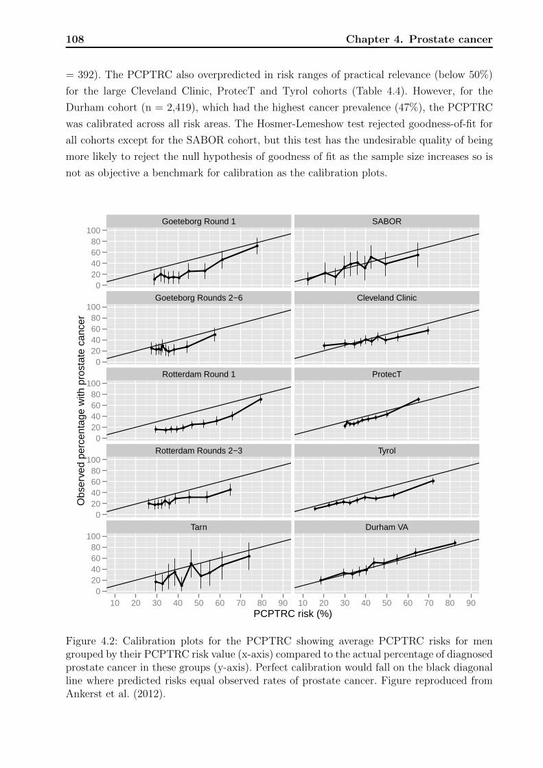
108 Chapter 4. Prostate cancer
= 392). The PCPTRC also overpredicted in risk ranges of practical relevance (below 50%)
for the large Cleveland Clinic, ProtecT and Tyrol cohorts (Table 4.4). However, for the
Durham cohort (n = 2,419), which had the highest cancer prevalence (47%), the PCPTRC
was calibrated across all risk areas. The Hosmer-Lemeshow test rejected goodness-of-fit for
all cohorts except for the SABOR cohort, but this test has the undesirable quality of being
more likely to reject the null hypothesis of goodness of fit as the sample size increases so is
not as objective a benchmark for calibration as the calibration plots.
●
●● ● ● ●
● ●
●
●
●
●●
●● ●
●
●
●
●
● ●●●●
●●
●●
●
●● ●
●● ●
●●
●
●
● ● ● ●●
● ●●
●
●
●●● ● ●
● ● ●●
●
● ● ●●●
●
● ● ●
●
●●
● ● ●●
● ●●
●
●●
●
●
●
●
●●
●
●
●
● ●● ●
● ●●
●
●
Goeteborg Round 1 SABOR
Goeteborg Rounds 2−6 Cleveland Clinic
Rotterdam Round 1 ProtecT
Rotterdam Rounds 2−3 Tyrol
Tarn Durham VA
020406080
100
020406080
100
020406080
100
020406080
100
020406080
100
10 20 30 40 50 60 70 80 90 10 20 30 40 50 60 70 80 90PCPTRC risk (%)
Obs
erve
d pe
rcen
tage
with
pro
stat
e ca
ncer
Figure 4.2: Calibration plots for the PCPTRC showing average PCPTRC risks for mengrouped by their PCPTRC risk value (x-axis) compared to the actual percentage of diagnosedprostate cancer in these groups (y-axis). Perfect calibration would fall on the black diagonalline where predicted risks equal observed rates of prostate cancer. Figure reproduced fromAnkerst et al. (2012).

4.3 Results 109
The last column of Table 4.4 shows the range of risk thresholds for which the PCPTRC
had higher clinical net benefit than the alternative strategies of biopsying all or none of the
men. A risk threshold is the minimum risk at which a patient and clinician would opt for
biopsy and varies between individuals due to personal preference. One reasonable threshold
is 20%, suggesting that it would be worth conducting no more than five biopsies to find one
cancer; a reasonable range of thresholds might be 15–30%. There was limited (ERSPC Tarn,
Cleveland Clinic, ProtecT) to no clinical benefit at all (other four ERSPC cohorts) to using
the PCPTRC to determine a subgroup of men to be biopsied compared to biopsying all of
those meeting cohort-specific criteria for biopsy. For the remaining three cohorts, SABOR,
Tyrol, and Austria, clinical benefit was observed at reasonable risk ranges: 15–45%, 18–41%,
and 25–100%, respectively (Table 4.4).
110 Chapter 4. Prostate cancer
4.3.3 Evaluating the High Grade prostate cancer risk calculator
Across the 25,512 biopsies from the ten cohorts combined, the AUC of the PCPTHG
was 74.6 %, a modest three percentage points increase over the AUC for PSA (71.5 %,
p < 0.0001). Use of PCPTHG risk thresholds of 5, 10 and 20 % as definitions of a positive
test for referral to biopsy would have resulted in 84.4, 41.7, and 15.0 %, respectively, of
all high-grade negative biopsies testing positive (percent unnecessary biopsies), and 4.7, 24.0
and 51.5 % missed high-grade prostate cancer cases, respectively. According to the individual
cohorts, these statistics are shown in Table 4.3.
Evaluation of the PCPTHG for ten- and higher-core biopsy schemes–compar-
ison with six-core The last six cohorts of Table 4.3 and Figures 4.3 and 4.4 implemented
ten- and higher-core schemes. The median AUC of the PCPTHG for high-grade disease
detection in the ten- and higher-core cohorts was 73.5 % (range 63.9 % - 76.7 %). Both
the median and range were lower than those for the four ERSPC cohorts that had six-core
biopsy schemes (median 78.1 %; range 72.0 % - 87.6 %). In two of the six ten- and higher-
core cohorts, the PCPTHG did not reach statistically significant improvement in direct
comparison to PSA for high-grade cancer discrimination (p-values > 0.05); in all four six-
core cohorts, the PCPTHG performed statistically significantly better than PSA (p value <
0.05) (Table 4.3). Of all cohorts included in the analysis, only the 10-core Cleveland Clinic
cohort showed clear evidence of underprediction, and this was restricted to risk ranges of less
than 15 % (Figure 4.3). The PCPTHG primarily overpredicted high-grade prostate cancer
in all six-core ERSPC screening studies. Clinical net benefit was not lower for the six higher-
core biopsy scheme cohorts compared with the six-core biopsy cohorts; in fact, it was often
higher (Figure 4.4). In three of the four six-core ESRPSC screening cohorts, there was no
clinical benefit to using the PCPTHG across all risk thresholds.
Comparison of the PCPTHG in healthy/screening versus clinically referred
populations Restricting attention to cohorts with ten- and higher-core biopsy schemes, the
four screening cohorts had PCPTHG AUCs of 76.7 % (Tarn), 69.5 % (SABOR), 75.4 %
(ProtecT) and 73.2 % (Tyrol), respectively, which overlapped with the AUCs observed in
the clinical cohorts, 63.9 % (Cleveland Clinic) and 73.9 % (Durham VA, USA). Of note is
the large 10-point difference between the Cleveland Clinic and Durham VA AUCs (Table
4.3). There were no obvious differences between calibrations or in clinical net benefits in the
higher-core screening cohorts compared with the higher-core clinical cohorts (Figs. 4.3, 4.4).
Comparison of the PCPTHG of US versus European populations Restricting
attention to cohorts with ten- and higher-core biopsy schemes, this comparison involves the
three US cohorts – SABOR (AUC = 69.5 %), Cleveland Clinic (63.9 %) and Durham VA
(73.9 %)–versus the three European cohorts–Tarn (76.7 %), ProtecT (75.4 %) and Tyrol
(73.2 %) (Table 4.3). The range of AUCs for the European cohorts is in fact shifted higher
than that for the US cohorts. The sample size of Tarn cohort is too low to make inference

4.3 Results 111
concerning calibration. For low levels of high-grade risk (<10 %) the PCPTHG appears
as good or better calibrated in the two remaining European higher-core cohorts (ProtecT
and Tyrol) compared with the US cohorts (Figure 4.3). The higher-core European screening
cohorts, Tarn, ProtecT and Tyrol, show comparable clinical net benefit to the US higher-
core cohorts, with the exception of the US Cleveland Clinic cohort, where the PCPTHG had
Figure 4.3: Calibration plots for the PCPTHG showing average PCPTHG risks for mengrouped by their PCPTHG risk value (x-axis) compared with the actual percentage with adiagnose of high-grade prostate cancer (y-axis). Shaded areas represent approximate 95 %confidence intervals. Perfect calibration would fall on the diagonal line where predicted risksequal observed rates of high-grade prostate cancer, and adequate calibration is indicatedwhere shaded regions overlap the diagonal lines. Vertical bars at the bottom are scaledhistograms depicting relative frequencies of participants obtaining specified PCPTHG risks.Figure reproduced from Ankerst et al. (2012).
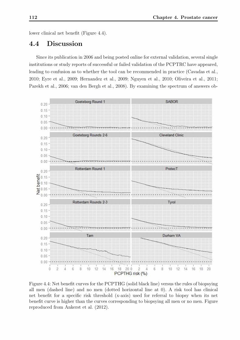
112 Chapter 4. Prostate cancer
lower clinical net benefit (Figure 4.4).
4.4 Discussion
Since its publication in 2006 and being posted online for external validation, several single
institutions or study reports of successful or failed validation of the PCPTRC have appeared,
leading to confusion as to whether the tool can be recommended in practice (Cavadas et al.,
2010; Eyre et al., 2009; Hernandez et al., 2009; Nguyen et al., 2010; Oliveira et al., 2011;
Parekh et al., 2006; van den Bergh et al., 2008). By examining the spectrum of answers ob-
Figure 4.4: Net benefit curves for the PCPTHG (solid black line) versus the rules of biopsyingall men (dashed line) and no men (dotted horizontal line at 0). A risk tool has clinicalnet benefit for a specific risk threshold (x-axis) used for referral to biopsy when its netbenefit curve is higher than the curves corresponding to biopsying all men or no men. Figurereproduced from Ankerst et al. (2012).

4.4 Discussion 113
tained in a wide variety of cohorts using three complementary validation metrics, this report
illuminates the inherent variability of results of external validation by cohort and chosen
metric. This variation is not unique to the PCPTRC, but would rather extend to valida-
tion studies of all risk-prediction tools and the rapidly increasing numbers of investigations
of new markers for enhancing prostate cancer, including the urine/blood markers PCA3,
AMACR, MMP-2, and GSTP1/RASSF1A methylation status (Ankerst et al., 2008; Prior
et al., 2010). Indeed, these results are a convincing demonstration that properties such as
“calibration [are] best seen not as a property of a prediction model, but of a joint property
of a model and the particular cohort to which it is applied” (Vickers and Cronin, 2010).
The AUC appears to be the most ubiquitous criterion implemented for validation in uro-
logic research, but even in the absence of a calculator, the AUC for PSA itself evaluated
across the ten cohorts of this study varied from no utility at all (AUC = 50.9%, Goete-
borg Rounds 2–6) to fairly decent performance (AUC = 67.0%, Goeteborg Round 1) (data
provided by Kattan). The AUC suffers an additional disadvantage because it is influenced
by the selection of patients for inclusion based on PSA: Including only patients with PSA
exceeding 3.0 ng/ml downwardly influences the AUC compared to an AUC based on a sam-
ple without such a restriction. The PCPTRC amounts to a weighted average of PSA along
with the dichotomous (yes versus no) risk factors of DRE, family history and prior biopsy,
and therefore its AUC typically tracks the one of PSA in the same cohort. Accordingly,
the AUC of the PCPTRC was also lowest in Goeteborg Rounds 2–6 (AUC = 56.2%) and
highest in Goeteborg Round 1 (AUC = 72.0%). In these two cohorts along with four others,
the AUC of the PCPTRC was statistically significantly higher than that of PSA. As noted
by Kattan (2011), the key for unbiased inference of markers or calculators is head-to-head
comparisons within cohorts and not across cohorts, as it is hard to control for unmeasurable
cohort differences.
Calibration plots confirmed an earlier PBCG observation that for most cohorts, the
PCPTRC tends to give prostate cancer risk predictions that are too high, overestimating
actual risks both in the PSA <4.0 ng/ml range, the range on which the PCPTRC was
largely developed, and grossly overestimating outside this range (Vickers et al., 2010). The
calibration plots revealed that the PCPTRC was better calibrated for cohorts with larger
prevalences of cancer, in particular the Durham VA clinical cohort. A limitation of all results
is that single imputation had to be performed for missing risk factors in several cohorts, and
this would affect calibration. For example, family history was not recorded in five of the ten
cohorts, therefore for these cohorts, the optimal value “no family history” was used for all
participants. Unfortunately even with the assumption of ”no family history” the PCPTRC
still overestimated the risk and would have been worse if the actual values of family history
were available. Additionally, because the lowest PCPTRC risks observed in many of the
cohorts fell near 30%, the current study provides no assessment of calibration of PCPTRC
for lower risks that might be of greatest interest for decision-making concerning a biopsy.
114 Chapter 4. Prostate cancer
Clinical net benefit is a more recently proposed validation metric that seeks to quantify
the net benefit to a patient for using a particular decision rule to opt for a prostate biopsy,
specifically, by choosing a threshold risk and deciding to undergo biopsy only if risk predicted
by the decision rule exceeds this value. For each possible threshold, the net benefit of using
the PCPTRC along with this threshold for referral to biopsy is assessed relative to just the
rule of referring everyone in the cohort for biopsy. However, this application of the net benefit
requires the underlying risk predictions to be well calibrated, which is property that is not
naturally given in external predictions. The five ERSPC cohorts had per protocol referral
of men for biopsy for PSA exceeding 3.0 ng/ml (4.0 ng/ml in some sections at some years),
and there was no observed benefit to using the PCPTRC for these men with primarily high
risks to begin with. In contrast, net benefit of using the PCPTRC at thresholds 15–45%
was observed in the SABOR cohort, a cohort with lower PSA values, and most similar in
nature to the PCPT cohort as described above. Among the remaining cohorts, there was
only limited net benefit at limited ranges of PCTPRC thresholds.
In sum, this study has shown that the PCPTRC may not be universally applicable, that
in the population of men with elevated PSA (above 3.0 ng/ml) who would most seriously
consider prostate biopsy; the PCTPRC may overestimate the risk of finding prostate cancer.
This result could be due to that the PCPTRC was fit on a different population of men,
primarily healthy men with PSA less than 3.0 ng/ml. The accuracy of the PCPTRC on such
a healthy population of men is not ruled out by the current validation study, since no cohorts
of this type were included.
The evaluation of the PCPTHG did not show decreased performance for contemporary
cohorts that use a higher number of cores compared to cohorts that had implemented six-
core biopsy schemes (used in the PCPT), in cohorts comprising clinical patients rather than
healthy patients undergoing screening, or in European versus US cohorts. Two primary
advantages of the PCPTHG are that it requires only easily obtainable patient parameters
that are part of a routine clinical exam (not including prostate volume) and that it is
available on the internet. On some populations and judged by some criteria, the PCPTHG
was no better than other screening methodologies; for example, in SABOR and ProtecT, the
AUC of the PCPTHG did not differ statistically significantly from PSA (Table 4.3). These
two cohorts implemented contemporary ten- and higher-core biopsy schemes. Extended core
sampling has been shown to increase both prostate cancer and high-grade disease detection
(Takenaka et al., 2006; O’Connell et al., 2004; Eskicorapci et al., 2004). Nevertheless, on
no population and according to no scale, was the PCPTHG worse than simpler screening
measures such as PSA, and this combined with the PCPTHG’s simplicity and availability
implies that it can be implemented as a complementary aid to the physician and patient
in their decision to go forward or not with prostate biopsy, without the expectation that it
could cause harm to the patient.
There are several limitations to the current study on risk calculation of high grade
4.4 Discussion 115
prostate cancer. The primary limitation is that comparison of cohorts that evolved under
different protocols as a means of assessing whether specific factors, such as 6- versus higher-
core biopsy schemes, affects performance characteristics of a risk tool is no substitution for
a single protocol analysis where individual factors, such as actual number of biopsy cores
taken, are recorded for each patient. Cohorts were classified according to the primary number
of cores used. Nevertheless, given this limitation, we believe a multiple external validation
of a risk tool gives a more balanced assessment of the operating characteristics of a risk tool
than a single evaluation study and can be more informative as to when and where the risk
tool works in practice.
Another limitation is that all men underwent prostate biopsy and thus had one or more
risk factors for prostate cancer. It was not possible to account for subtle differences in biopsy
technique that might have had significant impact on high-grade cancer detection rates, such
as choice of specific location to obtain cores independent of the number of cores. Furthermore,
a central pathology review was not achievable, so it is possible that variation in aggressiveness
in declaring biopsy specimens to have high-grade cancer might have occurred. The PCPTHG
was designed to predict high-grade disease defined as Gleason score of seven and higher, but
contemporary risk prediction typically focuses on clinically significant cancer, which may not
include a Gleason score of seven. The information on ethnicity needed for the race covariate,
a key risk factor in the PCPTHG, was entirely missing for 6 of the cohorts. Since these
cohorts were all European, it could be assumed that their African origin proportion was
negligible. DRE was not recorded for the ProtecT cohort and so assumed to be normal for
all participants in that cohort. This can alternatively be considered a bonus evaluation of
the robustness of the online PCPTHG, since it now allows use without DRE performed and
then defaults to normal. This feature followed a prior study on SABOR that revealed DRE
to be highly unstable, reverting to normal the year after an abnormal result in nearly 75 %
of incidences (Ankerst et al., 2009).
There are currently many online nomograms and risk calculators available for prostate
cancer, and it can be confusing figuring which calculator is optimal (Vickers and Cronin,
2010). Though novel biomarkers, such as %freePSA, and additional parameters, such as
prostate volume, could improve upon existing calculators, the cost of including a more-
difficult-to-obtain risk factor has to be weighed against a more widely applicable risk calcu-
lator. The rate of complications from prostate biopsy ranges from 2 to 4 %, and individual
patients and doctors will vary in their assessment of how high a risk of high-grade disease
needs to be to prompt them to biopsy (Thompson and Ankerst, 2012). Therefore, we rec-
ommend that PCPTHG risks in the range of 5-20 % be used depending on how much the
individual weights the harm of a missed high-grade cancer to the harm of an unnecessary
biopsy.
Findings of this study have implications for other risk-prediction tools beyond the PCP-
TRC and PCPTHG. It is typical in urologic research to declare definitive success or failure

116 Chapter 4. Prostate cancer
of a tool based on a single validation measure evaluated on data from a single institution.
However, if validation is a function of both the model and the cohort being studied, there are
two consequences. First, those proposing models must explore the properties of the model
in different cohorts, and investigate the aspects of a cohort that affect model performance.
Second, clinicians should be cautious in using a model unless it has been shown to provide
added value, such as benefit, in a very similar population to the one in which it is being used
clinically.
Conclusion
In this thesis, we presented the development and implementation of statistical models
in four different fields of recent research within the life sciences. The underlying data struc-
tures included the monitoring of tree stands over several decades, strictly planned growing
trials of rye, aggregated flowering trends from huge databases, and patient data from sev-
eral international clinical cohorts. Although the study aims varied, the flexible framework
of regression analysis could be employed as appropriate concept for most of the demands.
Still the common linear regression model is the workhorse of applied statistics and basis
for generalizations in all fields of research, with a long list of applications described in the
literature.
The generalizations we presented and need for future work include the use of random
effects structures (Chapters 1–3), multivariate analysis of correlated outcomes, and a move
towards integrated modeling of external information and outcome (Chapters 2–4), and splines
for flexible modeling of covariate effects (Chapters 1, 3).
Models for random effects In this thesis random effects were mainly used to account
for dependence within the outcomes originating from hierarchical structures or shared char-
acteristics. While the random spatial effects in the phenology application were motivated by
geographical locations, the random genotype effects in the rye study reflected the genetic
similarity of plants to each other. Both approaches define a measure of distance between two
sample units with larger distance inducing declining correlations. Consequently, the same
thoughts given on the kinship matrix also apply to the spatial aspects of the flowering dates:
In both cases sample units closer in terms of the distance measure provide less independent
information than distant ones for inference on flowering trends and SNPs, respectively, based
on the fixed effects of the model. For all of the above applications the distribution of random
effects was assumed to be normal. The estimation of the parameters of a normal distribution
is known to be sensitive to outliers, which could in turn also lead to biased estimates of the
fixed effects in the model. A robustification to that end is the use of t-distributions (Lange
et al., 1989). They have a higher mass on their tails compared to the normal distribution
allowing the estimate of the central tendency to be less influenced by single extreme obser-
vations. With the extension to skew-t distributions it is further possible to catch existing
skewness in the distribution of random effects (Ho and Lin, 2010). If the assumptions on
the random effects density p(.) should allow characteristics such as multimodality or non-

118 Conclusion
standard skewness, mixture distributions offer a sustainable way. The density of a mixture
distribution m(.) is a convex combination of K densities fk(.)
m(x;θ) =K∑k=1
wk fk(x;θk),K∑k=1
wk = 1,
where θ is the parameter vector of the mixture distribution comprising the parameters θk
of each mixture component and the non-negative weights wk: θ = (θk, wk, . . . ,θK , wK).
However, the estimation now also includes the number K of mixture components in addition
to the parameters in θ, which is much more demanding than estimation of a fixed number
parameters in the first place. This kind of model belongs to the class of variable dimension
models (Marin and Robert, 2007, p. 170). Standard optimization routines such as gradient
methods often fail on the non-trivial likelihood surface and need problem specific extensions.
From a Bayesian perspective, reversible jump Markov chain techniques (Green, 1995) allow
to infer the number of components simultaneously with the other parameters. Ideally, the use
of mixture models reveals interpretable clusters in the data. Although parametric, mixture
models can be seen as a step towards nonparametric density estimation (in our case for the
random effects) making very little assumptions on the shape of underlying distribution.
In a strictly nonparametric Bayesian approach p(.) is assumed to be a random unknown
quantity and a prior is needed over the infinite space of density or distribution functions.
Such random probability measures can be specified using Dirichlet processes (DP )(Ferguson,
1973). To obtain priors for continuous densities extensions to Dirichlet process mixtures
(DPM) (Antoniak, 1974) can be used (we refer to the references for a formal definition; here,
only a sketch is given). The distribution of the random effects vector bi for the ith out of N
groups is characterized hierarchically as
bi|θi∗∼ f(bi|θi) (∗distibuted not identically but independently, i.e. exchangeable),
θi|Giid∼ G, i = 1, . . . , N,
G ∼ DP (α,G0),
with θi the parameter vector of an arbitrary continuous density and G a random probability
measure defined through a DP with concentration parameter α and base measure G0, which
is also a distribution on the desired support of bi. Due to the cluster property of the involved
DP (MacEachern, 1994) the N θis are partitioned into k sets of clusters, with 0 < k ≤ N .
Since these random effects are defined for a group of observations, a single cluster comprises
of one or more of those groups. All observations in a cluster share an identical value of θi
but the random effects bi within a cluster are different because of the continuity of f(.). In
summary, this concept enables a very accurate prediction of the random effects, that is close
to the data, and clusters can still be identified by the parameters θi. Applications of DPM as

Conclusion 119
priors for random effects within generalized linear mixed models can be found in Kleinman
and Ibrahim (1998a), an implementation in R is provided by Jara et al. (2011).
Multivariate analysis of correlated outcome It is common to refer to a multivari-
ate (or multiple) outcome when for a single sample unit more than one random feature is
observed. A simple example is the collection of the height and weight of 100 individuals lead-
ing to a bivariate outcome for each of the 100 individuals. Also the monitoring of the same
outcome over multiple time points leads to multivariate outcomes, such as the longitudinal
observations of the percentage of damaged leaves in the growing trials (Section 2.2.1).
In principle, multivariate analyses are to be preferred over separate univariate analyses
since it carries several advantages: the correlation between the different outcomes is ex-
plicitly modeled and can be inferred, hypotheses of interest can be globally tested, that
is the aggregation of separate results is circumvented, and multiple testing which requires
adjustment can be avoided. Furthermore, an efficiency gain may be expected in the situation
of missing values and a more realistic assessment of the overall impact with respect to the
study aim is possible (McCulloch, 2008).
Whenever the multiple outcomes are commensurate, that is all outcomes share the same
scale, multivariate extensions of univariate GLMs can be applied. For m normally distributed
outcomes the multivariate linear model (MLM) is given by
Yn×m
= Xn×p
Bp×m
+ En×m
,
where Y is matrix with n oberservations (rows) on m outcomes (columns), X is the design
matrix derived from the predictor variables, B the matrix of coefficients, and E the matrix
of errors. In standard cases, the observations on different sample units are assumed to be
independent and a potential non-zero covariance is specified between the m outcomes within
a sample: ε′iiid∼ Nm(0,Σ), with ε′i the ith row of E and Nm(0,Σ) the m-dimensional normal
distribution with mean vector zero and covariance matrix Σ. There are m variance and
m(m− 1)/2 covariance parameters in Σ in this setup. However, a model definition equal to
the above equation can be obtained by specifying a formally univariate model. Therefore,
the rows of the matrices Y and B are stacked into vectors y and β, and the design matrix
X is inflated to dimension n ·m×m · p (see Izenman, 2008, p.162).

120 Conclusion
The model equation is then
ynm×1
= jXjnm×mp
βmp×1
+ jεjnm×1
,
where ε is normally distributed with mean vector zero and a block-diagonal covariance matrix
Cov(ε) =
Σ
m×m0 · · · 0
0 Σm×m
· · · 0
.... . .
...
0 · · · 0 Σm×m
.
This point on the equivalence is made for three reasons; a) the term “multivariate” cannot
be directly tied to the pure dimension of the statistical model but rather to the underlying
assumptions in the structure of the error term; b) the MLM is not bound to this rectangle
scheme. Not all entries in Y and X must be available, i.e. it is not mandatory to have
observations of all m outcomes on all n units to specify a multivariate model; the stacking
is still possible, and the regressors x need not to be equal for each of the outcomes; c)
a connection to mixed models is made, exemplary for a the random intercept model. For
the latter, more restrictive assumptions on the outcome variables/error terms are made:
Conditional on the regressors, the same variation in all m types of outcomes is assumed,
i.e. homoscedastic errors, and in addition the correlation between the outcomes is assumed
to be positive and constant between all m(m− 1)/2 pairs of outcomes. These are plausible
considerations for a model on repeated measures in longitudinal studies. Technically, the
covariance matrix Σ is therefore parametrized with two parameters, a variance σ2 on the
diagonal and a common covariance ρσ2 on the off-diagonals (ρ ≥ 0). Thus, when i indicates
the observation and j the outcome it holds that
Cov(yij, yi′j′) = σ2 for all i = i′ and j = j′ (= V(yij)),
Cov(yij, yi′j′) = ρσ2 for all i = i′ and j 6= j′,
Cov(yij, yi′j′) = 0 for all i 6= i′.
This however is equivalent to the marginal distribution of y in a linear mixed model with
random intercept
yij = x′ij β + γi + εij, i = 1, . . . , n, j = 1, . . . , ni,
εijiid∼ N(0, σ2),
γiiid∼ N(0, σ2
γ), γi, εij independent,
where V(yij) = σ2 + σ2γ corresponds to σ2 from the MLM and the covariance σ2
γ of obser-
vations sharing a random effect corresponds to ρσ2. Note that this restricted MLM and the

Conclusion 121
random intercept model are only equivalent in their marginal presentation. The conditional
specification of the random intercept model is more explicit. It makes specific additive as-
sumptions on the composition of the variance. As a consequence marginal inference in both
models is expected to provide similar but not identical results.
In conclusion, the mixed models extensively used throughout this thesis already represent
forms of multivariate and simultaneous inference. Further directions towards this goal of
analysis of the sojourn in flowering stages in the phenology chapter are indicated in Section
3.6. The situation of the growing trials of Chapter 2 is somewhat different and discussed in
the following paragraphs.
For the situation of multiple commensurate outcomes obtained on the same sample unit
the considerations of the previous section apply. However, the growing trials of Chapter
2 were run in three independent platforms (controlled, semi-controlled, open field) with
different outcomes (mean recovery score, % leaf damage, % survival). The analysis was
conducted in separate models with platform specific adjustments and in a second step the
results on SNP effects were bundled over the platforms using their p-values (Figure 2.3).
Understanding the genotypes as central entity with multiple outcomes nested in platforms,
trials, locations, years, blocks etc. one could construct a huge common multivariate model for
all observations at hand. In a first attempt on could build a model with interaction terms of
a platform indicator being created and the terms present in the three individual models. All
these interactions are needed as the outcomes—although all metric—are on different scales
and effect sizes (i.e. both fixed and random effects coefficients) depend on that scale. With
that overall model at hand it would be possible to formally test composite null hypotheses
such as “SNP1 has a positive effect on frost tolerance” by
H0 : βSNP1, platform i ≤ 0 ∀ i = 1, 2, 3, vs.
HA : βSNP1, platform i > 0 for at least one i,
within one single model. The conclusion however would coincide with those obtained by
separate models. Technically, this is due to the independence (zero covariance) of the ob-
servations between different platforms. The observations are uncoupled by the interaction
terms and the per-platform variances. Hence, the formal unified analysis as sketched above
does not provide advantages over separate analyses. To overcome this problem arising with
non-commensurate outcomes one would need to make more restrictive assumptions with re-
spect to the scales involved or the cross-outcome direction of the effects (omitting interaction
terms), or less restrictive assumptions with respect to the assumed dependence for elimina-
tion of structural zeros in the covariance matrix. One approach towards that end exists in
extending the random intercept model from above, which is presented conceptually here and
is described in more detail in McCulloch (2008).
For ease of notation only two non-commensurate outcomes y1, y2 are considered, but ideas

122 Conclusion
apply for multiple outcomes as well. Again, non-commensurate outcomes denote variables
measured on different scales including count data, binary data, or as in case of the grow-
ing trials metric outcomes on different ranges. Both outcomes must measure an underlying
quantity such as frost tolerance in the same direction, say, y1 on metric scale, y2 on binary
scale. They can be sampled under completely different circumstances, but their individual
observations can be classified coherently (such as by genotype). The class membership is
indicated by a random intercept γi in a conditional model for both outcomes
log
(P(y1ij|γi)
1−P(y1ij|γi)
)= x′1ij β1 + γi, (logistic regression for y1),
y2ij|γi = x′2ij β2 + λ γi + ε1ij, (linear regression for y2),
γiiid∼ G (distribution G to be specified),
where x1ij and x2ij are outcome-specific covariate vectors and ε1ijiid∼ N(0, σ2). Due to the
shared random effect γi the observation of the same class i are marginally correlated across
outcomes. The difference in scale is taken into account by the parameter λ, which, however,
assumes the random effects to act in the same direction in all settings (outcomes). McCul-
loch (2008) discusses consequences with distributions where the variance is a functional of
the mean such as Bernoulli distributions used with binary data. Since the outcomes of the
growing trials presented in this thesis are on metric scale this would not be an issue. To ac-
count also for the dependence between genotypes induced by the kinship the iid-assumption
of γi must be relaxed by specifying a suitable multivariate prior G for the vector γ com-
prising all single random genotype effects γi. In these models with shared random effect
across outcomes, the hypothesis of interest specified above could be tested simultaneously
for all platforms in a model based way. An alternative approach focusing on the marginal
distribution is suggested in Roy et al. (2003). Models for multivariate outcomes on different
scales using copulas are described in Joe (1997).
Flexible modeling of covariate effects Revealing the true functional form of the
association between outcome and covariates is a fundamental objective in statistical models.
Probably too ambitious, at least good approximations which fulfill the specific purpose of
the model are needed. The standard configuration of linear effects is a plausible choice when
a rather rough quantification of direction and strength of a suspected global trend is desired.
However, in situations where the association is more complex the linear approximation cannot
detect small scale deviations and can lead to biased estimates. Regression models can be
straightforwardly generalized by adding transforms of covariates to the predictor and allowing
interaction effects. The problem of variable selection rapidly becomes cumbersome when
several covariates are involved. The use of penalized splines as described in Section 1.3.3
is suitable to flexible model smooth relationships and is also able to capture small scale
effects if the knot-setup is chosen accordingly. The concept of penalization helps to prevent

Conclusion 123
overfitting due to wiggly function profiles.
In turn, the stochastic correspondent of the penalization approach fits perfectly in the
concept of random effects models whose merits have been broadly discussed. The underlying
constructive formulation of splines via basis functions can be extended in more dimensions
for the estimation of interaction surfaces and spatial effects. The equivalence of Kriging
and the use of radial basis functions should be noted here (Dubrule, 1984). Being linear in
their coefficients spline approximations can be represented as linear models allowing the use
of established numerical routines and also subject matter considerations on the functional
shape such as monotonicity can be embedded in the design matrices of the regression model
(Wood, 1994).
Even though statistical models can provide good approximations to unknown dependency
structures the final decision cannot be objective but rests with the researcher. Not least
because often a set of candidate models performs equally well. We experienced that in real
world examples the profitably complexity is relatively low compared to what is offered from
more theoretical research activities. Although simpler models are known to generalize better
on external data and in new situations it is challenging to set definitive limits of complexity
before an analysis. In particular, the analysis of designed experiments, which are less subject
to undesired ambient conditions, can demonstrate the limits of predictability of complex
(biological) systems—or provide fresh impetus.

124 Conclusion

List of performance measures
This appendix provides an overview of measures useful for assessing model performance.
The list contains both visual and numerical approaches. The notation used is y for the vector
of predictions/risks from a model, and y for the true status (0 or 1). The main goal is to
quantify the relationship between observed outcomes y and the corresponding estimation y.
Some of the measures require a cut-off value or grouping of y, which will be denoted by cut
(Tom, 2006).
relevant/concordant/discordant pairs The following terms describe the agreement of
observation-prediction pairs: ((yi, yi), (yj, yj)) (Tutz, 2000, p. 111ff).
N denotes the number of relevant pairs with different outcomes,
N =∑i,j
I(yi 6= yj)
= 2
(∑i
I(yi = 1)∑i
I(yi = 0)
).
Nc the number of concordant pairs,
Nc =∑i,j
(I(yi < yj)I(yi < yj)) +∑i,j
(I(yi > yj)I(yi ≥ yj)),
and Nd the number of discordant pairs,
Nd =∑i,j
I(yi < yj)I(yi > yj) +∑i,j
I(yi > yj)I(yi < yj).
Kendall’s τ
τ =Nc −Nd
n(n− 1)/2.
Goodman and Kruskal’s γ
γ =Nc −Nd
Nc +Nc
.
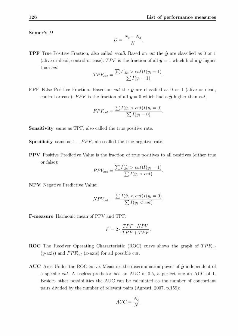
126 List of performance measures
Somer’s D
D =Nc −Nd
N.
TPF True Positive Fraction, also called recall. Based on cut the y are classified as 0 or 1
(alive or dead, control or case). TPF is the fraction of all y = 1 which had a y higher
than cut
TPFcut =
∑I(yi > cut)I(yi = 1)∑
I(yi = 1).
FPF False Positive Fraction. Based on cut the y are classified as 0 or 1 (alive or dead,
control or case). FPF is the fraction of all y = 0 which had a y higher than cut,
FPFcut =
∑I(yi > cut)I(yi = 0)∑
I(yi = 0).
Sensitivity same as TPF, also called the true positive rate.
Specificity same as 1− FPF , also called the true negative rate.
PPV Positive Predictive Value is the fraction of true positives to all positives (either true
or false):
PPVcut =
∑I(yi > cut)I(yi = 1)∑
I(yi > cut).
NPV Negative Predictive Value:
NPVcut =
∑I(yi < cut)I(yi = 0)∑
I(yi < cut).
F-measure Harmonic mean of PPV and TPF:
F = 2 · TPF ·NPVTPF + TPF
.
ROC The Receiver Operating Characteristic (ROC) curve shows the graph of TPFcut
(y-axis) and FPFcut (x-axis) for all possible cut.
AUC Area Under the ROC-curve. Measures the discrimination power of y independent of
a specific cut. A useless predictor has an AUC of 0.5, a perfect one an AUC of 1.
Besides other possibilities the AUC can be calculated as the number of concordant
pairs divided by the number of relevant pairs (Agresti, 2007, p.159):
AUC =Nc
N.

List of performance measures 127
Pseudo R2 (Veall and Zimmermann, 1996). For logistic regression, Nagelkerke (1991) stan-
dardized the binomial likelihood-based R2Lik with the theoretically maximal reachable
R2, which depends on the proportion of success (yi = 1) in the data set to ensure the
value of 1 for a perfect fit, analogous to linear regression. Log likelihoods of intercept-
only and risk factor-based prediction models are given by
l0 =∑i
(yi log y + (yi − 1) log(1− y)) ,
lpred =∑i
(yi log yi + (yi − 1) log(1− yi)) ,
respectively, yielding
R2Lik = 1− exp{(l0 − lpred)(2/n)},
and Nagelkerke’s R2Nag
R2Nag =
R2Lik
1− exp{l0(2/n))}.
Correlation Pearson correlation rPearson between y and y,
rPearson(y,y) =
∑(yi − ¯y)(yi − y)√∑
(yi − ¯y)2√∑
(yi − y)2,
is analogous to linear regression’s multiple correlation coefficient R. Its absolute value
has limited interpretation, nevertheless, rPearson is useful for comparing different pre-
dictions for the same outcome (Agresti, 2007, p.144).
Spearman correlation is a nonparametric alternative, which measures how good an
arbitrary monotone function can capture the relationship between the two variables.
The values yi and yi are replaced by their ranks rg(yi) and rg(yi) and the Pearson
correlation is calculated,
rSpearman(y,y) = rPearson(rg(y), rg(y)).
Ties are assigned the average of the ranks associated with the tied observations (van
Belle and Fisher, 2004, p. 327).
Wilcoxon statistic W The Wilcoxon rank-sum test and the Mann-Whitney-U test refer
to equivalent tests, in the literature the term Wilcoxon-Mann-Whitney test is also
used (Bergmann et al., 2000). The test statistic is based on the sum of ranks, rg(y),
for either yi = 1 or yi = 0 observations, with the ranks derived from the entire y vector.
Let n0 be the number of yi = 0, and n1 the number of yi = 1, (it holds n0 + n1 = n),

128 List of performance measures
then
W =n∑i=1
rg(yi)I(yi = 0)− n0(n0 + 1)
2,
or
W =n∑i=1
rg(yi)I(yi = 1)− n1(n1 + 1)
2,
which will be different in general, but lead to the same conclusions when used for
statistical testing. W is equivalent to the AUC (Hanley and McNeil, 1982),
AUC =W
n0n1
.
Again, ties are assigned the average of the ranks associated with the tied observations.
Hosmer-Lemeshow The Hosmer-Lemeshow-Test (Lemeshow and Hosmer Jr, 1982; Hos-
mer and Lemeshow, 1980, 2000, p.147) groups the observations by deciles (if G = 10)
of risks (y) and calculates a χ2 measure.
HL =G∑g=1
(Og − ng ¯yg
)2
ng ¯yg(1− ¯yg),
with Og being the sum of observed yi = 1 in group g,
Og =
ng∑i=1
yi,
and ¯yg is the average prediction risk in group g,
¯yg =1
ng
ng∑i=1
yi.
H0 : No difference between observed outcome and model-predicted risk,
HA : Observed outcome differs from prediction,
HLa∼ χ2(df = G− 1) when applied to an external validation dataset and
HLa∼ χ2(df = G− 2) for internal validation.
Brier Score or mean predicted squared error:
Brier =1
n
∑i
(yi − yi)2.

List of performance measures 129
A perfect prediction has a score of 0. The score of a non-informative model depends
on the proportion of sucesses (yi = 1) in the data set. As with Nagelkerke’s R2 it can
be scaled with its maximum Briermax for a given proportion,
Briersc = 1− Brier
Briermax,
with
Briermax = ¯y(1− ¯y)2 + (1− ¯y)¯y2 = ¯y (1− ¯y),
and ¯y being the arithmetic mean of y (Steyerberg, 2009, p.257). Briersc ranges between
zero and one. In opposite to R2Nag the scaling depends on the predictions y and not only
on the actual outcome y. This limits the use of the scaled version to assess different
models on external data.
Deviance residuals depend on assumed distribution. (McCullagh and Nelder, 1989, p.34,
p.39). For Bernoulli distributions, deviance residuals are given by
rDi = sign(yi − yi)
√2
(yi log
(yiyi
)+ (1− yi) log
(1− yi1− yi
)).
An overall measure of goodness-of-fit is the sum of squared deviance residuals∑
(rDi)2.
Pearson residuals also depend on the assumed distribution of y. They standardize the
difference between yi and yi by its standard deviation. In case of assuming a Bernoulli
distribution they are given by
rPi =yi − yi√yi(1− yi)
.
As overall measure of goodness-of-fit the squared sum is used:∑rP 2
i . Further stan-
dardized Pearson residuals exist, which use the leverage of observations and claim to
have unit variance (Hosmer and Lemeshow, 2000, p.173).
Discrimination slope denotes the absolute difference in average predictions between suc-
cesses and failures (Steyerberg, 2009, p.264),
|¯yy=0 − ¯yy=1|,
or in more computational notation,∣∣∣∣∣ 1
n0
n∑i=1
yiI(yi = 0)− 1
n1
n∑i=1
yiI(yi = 1)
∣∣∣∣∣ ,

130 List of performance measures
where n0 is the number of yi = 0 and n1 the number of yi = 1. Better models have a
larger discrimination slope.
t-statistic (for discrimination) Similar to the discrimination slope the test statistic of
the two sample t-test can be used to assess separation ability. The two samples are
formed on the outcome variable yi = 0 versus yi = 1. Again, larger values of the test
statistic imply better predictions.
Calibration-in-the-large compares the average predictions and the average outcome:
y − ¯y,
with ¯y = 1n
∑yi. Larger deviations from zero imply worse predictions, with nega-
tive sign corresponding to over-prediction (too high risks) and positive sign to under-
prediction.
t-statistic (for calibration) Similar to calibration-in-the-large the test statistic of the
paired t-test can be utilized, to assess the differences between predictions and out-
come,
t =yD
sd(yD),
with yD being the vector of differences y − y, yD its arithmetic mean and sd() the
empirical standard deviation.
Calibration slope CS is the estimated slope coefficient, β, in a logistic regression model
of true outcomes yi on the predicted risks yi, i=1, . . . , n,
log
(P (yi = 1)
1− P (yi = 1)
)= α + β log
(yi
1− yi
),
CS ≡ β,
that is, the model predictions yi are transformed and used as the regressor variable
in the logistic model. A calibration slope for a perfectly calibrated model is 1, while
coefficients lower than 1 indicate that the predictions are too extreme. Too extreme
means that the observed mortality is higher than predicted for low-risk observations
and lower than predicted for high-risk observations (Steyerberg et al., 2001). The cali-
bration slope is also linked to discrimination, higher slopes imply better discrimination
(Steyerberg, 2009, p.264).

Bibliography
Abbott, R. D. (1985). Logistic regresson in survival analysis. American Journal of Epidemi-
ology 121 (3), 465–471.
Ackerman, J. D. (2000). Abiotic pollen and pollination: Ecological, functional, and evolu-
tionary perspectives. Plant Systematics and Evolution 222 (1), 167–185.
Adame, P., M. d. Rıo, and I. Canellas (2010). Modeling individual-tree mortality in Pyrenean
oak (Quercus pyrenaica Willd.) stands. Annals of Forest Science 67 (8), 10.
Agresti, A. (2007). An introduction to categorical data analysis (2nd ed.). Hoboken NJ:
John Wiley & Sons.
Akaike, H. (1974). A new look at the statistical model identification. IEEE Transactions on
Automatic Control 19 (6), 716–723.
Ankerst, D. P., A. Bock, S. J. Freedland, J. Stephen Jones, A. M. Cronin, M. J. Roobol,
J. Hugosson, M. W. Kattan, E. A. Klein, F. Hamdy, D. Neal, J. Donovan, D. J. Parekh,
H. Klocker, W. Horninger, A. Benchikh, G. Salama, A. Villers, D. M. Moreira, F. H.
Schroder, H. Lilja, A. J. Vickers, and I. M. Thompson (2012). Evaluating the prostate
cancer prevention trial high grade prostate cancer risk calculator in 10 international biopsy
cohorts: results from the prostate biopsy collaborative group. World Journal of Urology .
Accepted on 22.04.2012.
Ankerst, D. P., A. Bock, S. J. Freedland, I. M. Thompson, A. M. Cronin, M. J. Roobol,
J. Hugosson, J. Stephen Jones, M. W. Kattan, E. A. Klein, F. Hamdy, D. Neal, J. Dono-
van, D. J. Parekh, H. Klocker, W. Horninger, A. Benchikh, G. Salama, A. Villers, D. M.
Moreira, F. H. Schroder, H. Lilja, and A. J. Vickers (2012). Evaluating the PCPT risk cal-
culator in ten international biopsy cohorts: results from the prostate biopsy collaborative
group. World Journal of Urology 30 (2), 181–187.
Ankerst, D. P., J. Groskopf, J. R. Day, A. Blase, H. Rittenhouse, B. H. Pollock, C. Tangen,
D. Parekh, R. J. Leach, and I. Thompson (2008). Predicting prostate cancer risk through
incorporation of prostate cancer gene 3. The Journal of Urology 180 (4), 1303–1308; dis-
cussion 1308.
131

132 BIBLIOGRAPHY
Ankerst, D. P., R. Miyamoto, P. V. Nair, B. H. Pollock, I. M. Thompson, and D. J. Parekh
(2009). Yearly prostate specific antigen and digital rectal examination fluctuations in a
screened population. The Journal of Urology 181 (5), 2071–2075; discussion 2076.
Antoniak, C. E. (1974). Mixtures of Dirichlet processes with applications to Bayesian non-
parametric problems. The Annals of Statistics , 1152–1174.
Aranzana, M. J., S. Kim, K. Y. Zhao, E. Bakker, M. Horton, K. Jakob, C. Lister, J. Moli-
tor, C. Shindo, and C. L. Tang (2005). Genome-wide association mapping in Arabidopsis
identifies previously known flowering time and pathogen resistance genes. PLOS Genet-
ics 1 (5), e60.
Assmann, E. (1961). Waldertragskunde: Organische Produktion, Struktur, Zuwachs und Er-
trag von Waldbestanden. Munchen: BLV Verlagsgesellschaft.
Badawi, M., Y. V. Reddy, Z. Agharbaoui, Y. Tominaga, J. Danyluk, F. Sarhan, and M. Houde
(2008). Structure and functional analysis of wheat ICE (inducer of CBF expression) genes.
Plant Cell Physiology 49 (8), 1237–1249.
Baga, M., S. V. Chodaparambil, A. E. Limin, M. Pecar, D. B. Fowler, and R. N. Chib-
bar (2007). Identification of quantitative trait loci and associated candidate genes for
low-temperature tolerance in cold-hardy winter wheat. Functional and Integrative Ge-
nomics 7 (1), 53–68.
Balding, D. (2013). Kinship and heritability: some recent developments. Presentation at the
5th Paris Workshop on Genomic Epidemiology . http://innovationcenter.netne.net/
paris_workshop/downloads/presentations/BaldingDavid_Paris2013.pdf. Accessed
on 30.07.2013.
Bates, D. and M. Machler (2010). lme4: Linear mixed-effects models using S4 classes. R
package version 0.999375-37.
Bateson, W. (1902). Mendel’s principles of heredity. University Press.
Becker, B. J. and M.-J. Wu (2007). The synthesis of regression slopes in meta-analysis.
Statistical Science 22 (3), 414–429.
Beggs, P. J. (2004). Impacts of climate change on aeroallergens: past and future. Clinical
and Experimental Allergy 34 (10), 1507–1513.
Bergmann, R., J. Ludbrook, and W. P. J. M. Spooren (2000). Different outcomes of the
Wilcoxon-Mann-Whitney test from different statistics packages. The American Statisti-
cian 54 (1), 72–77.

BIBLIOGRAPHY 133
Bigler, C. and H. Bugmann (2003). Growth-dependent tree mortality models based on tree
rings. Canadian Journal of Forest Research 33 (2), 210–221.
Bivand, R., E. J. Pebesma, and V. G. Rubio (2008). Applied spatial data: analysis with R.
New York: Springer.
Bock, A., J. Dieler, P. Biber, H. Pretzsch, and D. P. Ankerst (2013). Predicting tree mortality
for european beech in southern germany using spatially explicit competition indices. Forest
Science. Accepted.
Bolmgren, K., O. Eriksson, and H. P. Linder (2003). Contrasting flowering phenology and
species richness in abiotically and biotically pollinated angiosperms. Evolution 57 (9),
2001–2011.
Bravo-Oviedo, A., H. Sterba, M. del Rıo, and F. Bravo (2006). Competition-induced mor-
tality for Mediterranean Pinus pinaster Ait. and P. sylvestris L. Forest Ecology and Man-
agement 222 (1-3), 88–98.
Breslow, N. E., N. E. Day, et al. (1980). Statistical methods in cancer research. Vol. 1. The
analysis of case-control studies. Distributed for IARC by WHO.
Bretz, F., T. Hothorn, and P. Westfall (2011). Multiple Comparisons Using R. New York:
CRC Press.
Brown, H. and R. Prescott (2006). Applied mixed models in medicine. Hoboken NJ: John
Wiley & Sons.
Brunner, E. and U. Munzel (2000). The nonparametric Behrens-Fisher problem: Asymptotic
theory and a small-sample approximation. Biometrical Journal 42 (1), 17–25.
Buchman, R. G., S. P. Pederson, and N. R. Walters (1983). A tree survival model with
application to species of the great lakes region. Canadian Journal of Forest Research 13,
601–608.
Burgman, M., W. Incoll, P. Ades, I. Ferguson, T. Fletcher, and A. Wohlers (1994). Mortality
models for mountain and alpine ash. Forest Ecology and Management 67 (1-3), 319–327.
Campoli, C., M. A. Matus-Cadiz, C. J. Pozniak, L. Cattivelli, and D. B. Fowler (2009).
Comparative expression of Cbf genes in the Triticeae under different acclimation induction
temperatures. Molecular Genetetics and Genomics 282 (2), 141–152.
Canty, A. and B. Ripley (2010). boot: Bootstrap R (S-Plus) functions. R package version
1.2-43.

134 BIBLIOGRAPHY
Carstensen, B. (2005). Demography and epidemiology: Practical use of the lexis diagram
in the computer age. or: Who needs the cox-model anyway? Annual meeting of Finnish
Statistical Society . http://publichealth.ku.dk/sections/biostatistics/reports/
2006/.
Cavadas, V., L. Osorio, F. Sabell, F. Teves, F. Branco, and M. Silva-Ramos (2010). Prostate
cancer prevention trial and European randomized study of screening for prostate cancer
risk calculators: a performance comparison in a contemporary screened cohort. European
Urology 58 (4), 551–558.
Chinnusamy, V., J. Zhu, and J. K. Zhu (2007). Cold stress regulation of gene expression in
plants. Trends in Plant Science 12 (10), 444–451.
Choi, D. W., B. Zhu, and T. J. Close (1999). The barley (Hordeum vulgare L.) dehy-
drin multigene family: Sequences, allele types, chromosome assignments, and expression
characteristics of 11 Dhn genes of cv Dicktoo. Theoretical and Applied Genetics 98 (8),
1234–1247.
Cleveland, W. S., E. Grosse, and W. M. Shyu (1992). Local regression models. In J. M.
Chambers and T. Hastie (Eds.), Statistical models in S, pp. 309–376. New York: Chapman
and Hall/CRC.
Clifford, D. and P. McCullagh (2012). regress: The regress package. R package version 1.3-8.
Cox, D. R. (1972). Regression models and life-tables. Journal of the Royal Statistical Society.
Series B (Statistical Methodology) 34 (2), 187–220.
Cupples, L. A., R. B. D’Agostino, K. Anderson, and W. B. Kannel (1988). Comparison
of baseline and repeated measure covariate techniques in the Framingham Heart Study.
Statistics in Medicine 7 (1-2), 205–222.
D’Agostino, R. B., M. L. Lee, A. J. Belanger, L. A. Cupples, K. Anderson, and W. B. Kannel
(1990). Relation of pooled logistic regression to time dependent Cox regression analysis:
the Framingham Heart Study. Statistics in Medicine 9 (12), 1501–1515.
D’Amato, G. and L. Cecchi (2008). Effects of climate change on environmental factors in
respiratory allergic diseases. Clinical and Experimental Allergy 38 (8), 1264–1274.
D’Amato, G., L. Cecchi, S. Bonini, C. Nunes, I. Annesi-Maesano, H. Behrendt, G. Liccardi,
T. Popov, and P. Van Cauwenberge (2007). Allergenic pollen and pollen allergy in Europe.
Allergy 62 (9), 976–990.
Das, A., J. Battles, P. J. van Mantgem, and N. L. Stephenson (2008). Spatial elements of
mortality risk in old-growth forests. Ecology 89 (6), 1744–1756.

BIBLIOGRAPHY 135
Das, A. J., J. J. Battles, N. L. Stephenson, and P. J. van Mantgem (2007). The relationship
between tree growth patterns and likelihood of mortality: a study of two tree species in
the sierra nevada. Canadian Journal of Forest Research 37, 580–597.
Devlin, B. and K. Roeder (1999). Genomic control for association studies. Biometrics 55,
997–1004.
Dhanaraj, A. L., N. W. Alkharouf, H. S. Beard, I. B. Chouikha, B. F. Matthews, H. Wei,
R. Arora, and L. J. Rowland (2007). Major differences observed in transcript profiles of
blueberry during cold acclimation under field and cold room conditions. Planta 225 (3),
735–751.
Dobbertin, M. and G. S. Biging (1998). Using the non-parametric classifier CART to model
forest tree mortality. Forest Science 44 (4), 507–516.
Dorffling, K., S. Schulenburg, G. Lesselich, and H. Dorffling (1990). Abscisic acid and proline
levels in cold hardened winter wheat leaves in relation to variety-specific differences in
freezing resistance. Journal of Agronomy and Crop Science 165 (4), 230–239.
Dubrule, O. (1984). Comparing splines and Kriging. Computers & Geosciences 10 (2),
327–338.
Duchateau, L., P. Janssen, and J. Rowlands (1998). Linear mixed models. An introduction
with applications in veterinary research. ILRI (International Livestock Research Institute).
Efron, B. and R. Tibshirani (1994). An Introduction to the Bootstrap. New York: Chapman
and Hall/CRC.
Eid, T. and E. Tuhus (2001). Models for individual tree mortality in norway. Forest Ecology
and Management 154 (1-2), 69–84.
Eilers, P. and B. Marx (1996). Flexible smoothing with B-splines and penalties. Statistical
Science 11 (2), 89–121.
Esch, R. (2004). Grass pollen allergens. In R. Lockey, S. Bukantz, and J. Bousquet (Eds.),
Allergens and Allergen Immunotherapy, pp. 185–206. New York: Marcel Dekker.
Eskicorapci, S. Y., D. E. Baydar, C. Akbal, M. Sofikerim, M. Gunay, S. Ekici, and H. Ozen
(2004). An extended 10-core transrectal ultrasonography guided prostate biopsy protocol
improves the detection of prostate cancer. European Urology 45 (4), 444–449.
European Randomized study of Screening for Prostate Cancer (2013). Background to Study.
http://http://www.erspc-media.org/erspc-background/. Accessed on 10.10.2013.

136 BIBLIOGRAPHY
Eyre, S. J., D. P. Ankerst, J. T. Wei, P. V. Nair, M. M. Regan, G. Bueti, J. Tang, M. A.
Rubin, M. Kearney, I. M. Thompson, and M. G. Sanda (2009). Validation in a multiple
urology practice cohort of the Prostate Cancer Prevention Trial calculator for predicting
prostate cancer detection. The Journal of Urology 182 (6), 2653–2658.
Fahrmeir, L., T. Kneib, and S. Lang (2007). Regression: Modelle, Methoden und Anwendun-
gen. Berlin; Heidelberg: Springer.
Fahrmeir, L., R. Kunstler, I. Pigeot, and G. Tutz (2003). Statistik. Der Weg zur Datenanalyse
(4 ed.). Berlin: Springer.
Fan, Z., J. M. Kabrick, and S. R. Shifley (2006). Classification and regression tree based sur-
vival analysis in oak-dominated forests of Missouri’s Ozark highlands. Canadian Journal
of Forest Research 36, 1740–1748.
Ferguson, T. S. (1973). A Bayesian analysis of some nonparametric problems. The Annals
of Statistics , 209–230.
Fitter, A. H. and R. S. R. Fitter (2002). Rapid changes in flowering time in british plants.
Science (New York, N.Y.) 296 (5573), 1689–1691.
Fitzmaurice, G. M., N. M. Laird, and J. H. Ware (2004). Applied Longitudinal Analysis.
Wiley Series in Probability and Statistics. Hoboken NJ: John Wiley & Sons.
Fortin, M., S. Bedard, J. DeBlois, and S. Meunier (2008). Predicting individual tree mor-
tality in northern hardwood stands under uneven-aged management in southern Quebec,
Canada. Annals of Forest Science 65 (2), 205–205.
Fowler, D. B., L. V. Gusta, and N. J. Tyler (1981). Selection for winterhardiness in wheat.
III. screening methods. Crop Science 21 (6), 896–901.
Fowler, D. B. and A. E. Limin (1987). Exploitable genetic variability for cold tolerance in
commercially grown cereals. Canadian Journal of Plant Science 67 (1), 278–278.
Francia, E., D. Barabaschi, A. Tondelli, G. Laido, F. Rizza, A. M. Stanca, M. Busconi,
C. Fogher, E. J. Stockinger, and N. Pecchioni (2007). Fine mapping of a HvCBF gene clus-
ter at the frost resistance locus Fr-H2 in barley. Theoretical and Applied Genetics 115 (8),
1083–1091.
Fridman, J. and G. Stahl (2001). A three-step approach for modelling tree mortality in
swedish forests. Scandinavian Journal of Forest Research 16 (5), 455–466.
Friedman, J. and S. C. H. Barrett (2009). Wind of change: new insights on the ecology and
evolution of pollination and mating in wind-pollinated plants. Annals of Botany 103 (9),
1515–1527.

BIBLIOGRAPHY 137
Galiba, G., S. A. Quarrie, J. Sutka, A. Morgounov, and J. W. Snape (1995). RFLP mapping
of the vernalization (Vrn1) and frost resistance (Fr1) genes on chromosome 5A of wheat.
Theoretical and Applied Genetics 90 (7-8), 1174–1179.
Gbur, E. E., W. Stroup, K. McCarter, S. Durham, L. Young, M. Christman, M. West, and
M. Kramer (2012). Analysis of generalized linear mixed models in the agricultural and
natural resources sciences. Madison: American Society of Agronomy.
Gneiting, T. and A. E. Raftery (2007). Strictly proper scoring rules, prediction, and estima-
tion. Journal of the American Statistical Association 102 (477), 359–378.
Green, P. J. (1995). Reversible jump Markov chain Monte Carlo computation and Bayesian
model determination. Biometrika 82 (4), 711–732.
Gusta, L. V., R. Willen, P. Fu, A. J. Robertson, and G. H. Wu (1997). Genetic and en-
vironmental control of winter survival of winter cereals. Acta Agronomica Academiae
Scientiarum Hungaricae 45 (3), 231–240.
Hackauf, B. and P. Wehling (2002). Identification of microsatellite polymorphisms in an
expressed portion of the rye genome. Plant Breeding 121 (1), 17–25.
Hamilton, D. A. (1986). A logistic model of mortality in thinned and unthinned mixed
conifer stands of Northern Idaho. Forest Science 32 (4), 989–1000.
Hanagal, D. D. (2011). Modeling Survival Data Using Frailty Models. New York: Chapman
& Hall/CRC.
Hanley, J. A. and B. J. McNeil (1982). The meaning and use of the area under a receiver
operating characteristic (ROC) curve. Radiology 143 (1), 29–36.
Harjes, C. E., T. R. Rocheford, L. Bai, T. P. Brutnell, C. B. Kandianis, S. G. Sowinski,
A. E. Stapleton, R. Vallabhaneni, M. Williams, and E. T. Wurtzel (2008). Natural genetic
variation in lycopene epsilon cyclase tapped for maize biofortification. Science 319 (5861),
330–333.
Harrell, F., K. Lee, and D. Mark (1996). Tutorial in biostatistics multivariable prognostic
models: issues in developing models, evaluating assumptions and adequacy, and measuring
and reducing errors. Statistics in Medicine 15, 361–387.
Hasenauer, H., D. Merkl, and M. Weingartner (2001). Estimating tree mortality of Norway
spruce stands with neural networks. Advances in Environmental Research 5 (4), 405–414.
Hastie, T. and R. Tibshirani (1990). Generalized additive models. New York: Chapman and
Hall/CRC.

138 BIBLIOGRAPHY
Hayes, B. J. and M. E. Goddard (2008). Technical note: prediction of breeding values using
marker-derived relationship matrices. Journal of Animal Science 86 (9), 2089–2092.
Hernandez, D. J., M. Han, E. B. Humphreys, L. A. Mangold, S. S. Taneja, S. J. Childs,
G. Bartsch, and A. W. Partin (2009). Predicting the outcome of prostate biopsy: com-
parison of a novel logistic regression-based model, the prostate cancer risk calculator, and
prostate-specific antigen level alone. BJU International 103 (5), 609–614.
Ho, H. J. and T.-I. Lin (2010). Robust linear mixed models using the skew t distribution
with application to schizophrenia data. Biometrical Journal 52 (4), 449–469.
Hommo, L. M. (1994). Hardening of some winter wheat (Triticum aestivum L.), rye (Secale
cereals L.), triticale (Triticosecale Wittmack) and winter barley (Hordeum vulgare L.)
cultivars during autumn and the final winter survival in Finland. Plant Breeding 112 (4),
285–293.
Hosmer, D. and S. Lemeshow (1980). Goodness of fit tests for the multiple logistic regression
model. Communications in Statistics – Theory and Methods 9 (10), 1043–1069.
Hosmer, D. and S. Lemeshow (2000). Applied logistic regression. Hoboken NJ: John Wiley
& Sons.
Hothorn, T., F. Bretz, and P. Westfall (2008). Simultaneous inference in general parametric
models. Biometrical Journal 50 (3), 346—363.
Houde, M., R. S. Dhindsa, and F. Sarhan (1992). A molecular marker to select for freezing
tolerance in Gramineae. Molecular Genetics and Genomics 234 (1), 43–48.
Huynen, M., B. Menne, H. Behrendt, R. Bertollini, S. Bonini, R. Brandao, et al. (2003). Phe-
nology and human health: allergic disorders. Report of a WHO meeting, Rome, Italy 16,
17.
Ingvarsson, P. K. and N. R. Street (2010). Association genetics of complex traits in plants.
New Phytologist 189 (4), 909–922.
Izenman, A. J. (2008). Modern multivariate statistical techniques: regression, classification,
and manifold learning. New York: Springer.
Jaeger, S. (2008). Exposure to grass pollen in europe. Clinical and Experimental Allergy
Reviews 8 (1), 2–6.
Janssen, K. J. M., A. R. T. Donders, J. Harrell, Frank E, Y. Vergouwe, Q. Chen, D. E.
Grobbee, and K. G. M. Moons (2010). Missing covariate data in medical research: to
impute is better than to ignore. Journal of Clinical Epidemiology 63 (7), 721–727.

BIBLIOGRAPHY 139
Jara, A., T. E. Hanson, F. A. Quintana, P. Muller, and G. L. Rosner (2011). Dppackage:
Bayesian non-and semi-parametric modelling in R. Journal of Statistical Software 40 (5),
1–30.
Joe, H. (1997). Multivariate models and dependence concepts, Volume 73.
Kalbfleisch, J. D. and R. L. Prentice (2002). The Statistical Analysis of Failure Time Data
(2 ed.). Hoboken NJ: John Wiley & Sons.
Kattan, M. W. (2011). Factors affecting the accuracy of prediction models limit the compari-
son of rival prediction models when applied to separate data sets. European Urology 59 (4),
566–567.
Khlestkina, E. K., H. M. T. Ma, E. G. Pestsova, M. S. Roder, S. V. Malyshev, V. Korzun, and
A. Borner (2004). Mapping of 99 new microsatellite-derived loci in rye (Secale cereale L.)
including 39 expressed sequence tags. Theoretical and Applied Genetics 109 (4), 725–732.
Kiernan, D., E. Bevilacqua, R. Nyland, and L. Zhang (2009). Modeling tree mortality
in low-to medium-density uneven-aged hardwood stands under a selection system using
generalized estimating equations. Forest Science 55 (4), 343–351.
King, G. and L. Zeng (2001). Logistic regression in rare events data. Political Analysis 9 (2),
137–163.
Kleinman, K. P. and J. G. Ibrahim (1998a). A semi-parametric Bayesian approach to gen-
eralized linear mixed models. Statistics in Medicine 17 (22), 2579–2596.
Kleinman, K. P. and J. G. Ibrahim (1998b). A semiparametric Bayesian approach to the
random effects model. Biometrics 54 (3), 921.
Kneib, T. (2006). Mixed model-based inference in geoadditive hazard regression for interval-
censored survival times. Computational Statistics and Data Analysis 51 (2), 777–792.
Kneib, T. and L. Fahrmeir (2004). A mixed model approach for structured hazard regression.
SFB 386 Discussion Paper 400, University of Munich.
Koch, E., A. Donelly, W. Lipa, A. Menzel, and J. Nekovar (Eds.) (2009). Final Scientific Re-
port of COST 725: Establishing a European Dataplatform for Climatological Applications.
European Cooperation in the field of Scientific and Technical Research.
Laaidi, M. (2001). Regional variations in the pollen season of Betula in Burgundy: two
models for predicting the start of the pollination. Aerobiologia 17 (3), 247–254.
Landwehr, J. M., D. Pregibon, and A. C. Shoemaker (1984). Graphical methods for assessing
logistic regression models. Journal of the American Statistical Association 79 (385), 61–71.
140 BIBLIOGRAPHY
Lange, K. L., R. J. Little, and J. M. Taylor (1989). Robust statistical modeling using the t
distribution. Journal of the American Statistical Association 84 (408), 881–896.
Lemeshow, S. and D. Hosmer Jr (1982). A review of goodness of fit statistics for use in
the development of logistic regression models. American Journal of Epidemiology 115 (1),
92–106.
Li, Y., A. Bock, G. Haseneyer, V. Korzun, P. Wilde, C.-C. Schon, D. P. Ankerst, and E. Bauer
(2011). Association analysis of frost tolerance in rye using candidate genes and pheno-
typic data from controlled, semi-controlled, and field phenotyping platforms. BMC Plant
Biology 11, 146.
Li, Y. L., G. Haseneyer, C.-C. Schon, D. P. Ankerst, V. Korzun, P. Wilde, and E. Bauer
(2011). High levels of nucleotide diversity and fast decline of linkage disequilibrium in rye
(Secale cereale L.) genes involved in frost response. BMC Plant Biology 11, 6.
Lu, P., Q. Yu, J. Liu, and X. Lee (2006). Advance of tree-flowering dates in response to
urban climate change. Agricultural and Forest Meteorology 138 (1–4), 120–131.
MacEachern, S. N. (1994). Estimating normal means with a conjugate style Dirichlet process
prior. Communications in Statistics–Simulation and Computation 23 (3), 727–741.
Mackay, T. F. C. (2001). The genetic architecture of quantitative traits. Annual Review of
Genetics 35, 303–339.
Malosetti, M., C. G. van der Linden, B. Vosman, and F. A. van Eeuwijk (2007). A mixed-
model approach to association mapping using pedigree information with an illustration of
resistance to phytophthora infestans in potato. Genetics 175 (2), 879–889.
Marin, J.-M. and C. P. Robert (2007). Bayesian core: a practical approach to computational
Bayesian statistics. New York: Springer.
Mathews, K. L., M. Malosetti, S. Chapman, L. McIntyre, M. Reynolds, R. Shorter, and
F. Eeuwijk (2008). Multi-environment QTL mixed models for drought stress adaptation
in wheat. Theoretical and Applied Genetics 117 (7), 1077–1091.
McCullagh, P. and J. A. Nelder (1989). Generalized Linear Models (2 ed.). New York:
Chapman and Hall/CRC.
McCulloch, C. (2008). Joint modelling of mixed outcome types using latent variables. Sta-
tistical Methods in Medical Research 17 (1), 53–73.
McCulloch, C. E. and S. R. Searle (2001). Generalized, Linear and Mixed Models (1 ed.).
Hoboken NJ: Wiley & Sons.

BIBLIOGRAPHY 141
McIntosh, M. W. and M. S. Pepe (2002). Combining several screening tests: Optimality of
the risk score. Biometrics 58 (3), 657–664.
McLauchlan, K., C. Barnes, and J. Craine (2011). Interannual variability of pollen pro-
ductivity and transport in mid-North America from 1997 to 2009. Aerobiologia 27 (3),
181–189.
Menzel, A., T. H. Sparks, N. Estrella, E. Koch, A. Aasa, R. Ahas, K. Alm-Kubler, P. Bissolli,
O. Braslavska, A. Briede, F. M. Chmielewski, Z. Crepinsek, Y. Curnel, A. Dahl, C. Defila,
A. Donnelly, Y. Filella, K. Jatczak, F. Mage, A. Mestre, Ø. Nordli, J. Penuelas, P. Pirinen,
V. Remisova, H. Scheifinger, M. Striz, A. Susnik, A. J. H. Van Vliet, F.-E. Wielgolaski,
S. Zach, and A. Zust (2006). European phenological response to climate change matches
the warming pattern. Global Change Biology 12 (10), 1969–1976.
Monserud, R. A. (1976). Simulation of forest tree mortality. Forest Science 22 (4), 438–444.
Monserud, R. A. and H. Sterba (1999). Modeling individual tree mortality for Austrian
forest species. Forest Ecology and Management 113 (2-3), 109–123.
Montgomery, D. C. (2001). Design and analysis of experiments (5 ed.). Hoboken NJ: John
Wiley & Sons.
Mood, C. (2010). Logistic regression: Why we cannot do what we think we can do, and what
we can do about it. European Sociological Review 26 (1), 67–82.
Mrode, R. and R. Thompson (2005). Linear models for the prediction of animal breeding
values. Wallingford: CABI.
Nagelkerke, N. (1991). A note on a general definition of the coefficient of determination.
Biometrika 78 (3), 691–692.
Nelder, J. A. (1977). A Reformulation of Linear Models. Journal of the Royal Statistical
Society. Series A (Statistics in Society) 140 (1), 48–77.
Nguyen, C. T., C. Yu, A. Moussa, M. W. Kattan, and J. S. Jones (2010). Performance
of prostate cancer prevention trial risk calculator in a contemporary cohort screened
for prostate cancer and diagnosed by extended prostate biopsy. The Journal of Urol-
ogy 183 (2), 529–533.
Novillo, F., J. M. Alonso, J. R. Ecker, and J. Salinas (2004). CBF2/DREB1C is a negative
regulator of CBF1/DREB1B and CBF3/DREB1A expression and plays a central role in
stress tolerance in Arabidopsis. Proceedings of the National Academy of Sciences of the
United States of America 101 (11), 3985–3990.

142 BIBLIOGRAPHY
O’Connell, M. J., C. S. Smith, P. E. Fitzpatrick, C. O. Keane, J. M. Fitzpatrick, M. Behan,
H. F. Fenlon, and J. G. Murray (2004). Transrectal ultrasound-guided biopsy of the
prostate gland: value of 12 versus 6 cores. Abdominal Imaging 29 (1), 132–136.
Oliveira, M., V. Marques, A. P. Carvalho, and A. Santos (2011). Head-to-head comparison of
two online nomograms for prostate biopsy outcome prediction. BJU International 107 (11),
1780–1783.
Palahi, M., T. Pukkala, J. Miina, and G. Montero (2003). Individual-tree growth and mor-
tality models for Scots pine (Pinus sylvestris L.) in north-east Spain. Annals of Forest
Science 60 (1), 1–10.
Parekh, D. J., D. P. Ankerst, B. A. Higgins, J. Hernandez, E. Canby-Hagino, T. Brand, D. A.
Troyer, R. J. Leach, and I. M. Thompson (2006). External validation of the prostate cancer
prevention trial risk calculator in a screened population. Urology 68 (6), 1152–1155.
Phillips, P. C. (2008). Epistasis – the essential role of gene interactions in the structure and
evolution of genetic systems. Nature Reviews Genetics 9 (11), 855–867.
Pinheiro, J. C. and D. M. Bates (2000). Mixed Effects Models in S and S-Plus. Statistics
and Computing. New York: Springer.
Pregibon, D. (1981). Logistic regression diagnostics. The Annals of Statistics , 705–724.
Pretzsch, H. (1992). Modellierung der Kronenkonkurrenz von Fichte und Buche in Rein-
und Mischbestanden. Allgemeine Forst- und Jagdzeitung 163 (11/12), 203–213.
Pretzsch, H. (2001). Modellierung des Waldwachstums. Blackwell Wissenschafts-Verlag.
Pretzsch, H., P. Biber, and J. Dursky (2002). The single tree-based stand simulator SILVA:
construction, application and evaluation. Forest Ecology and Management 162 (1), 3–21.
Prior, C., F. Guillen-Grima, J. E. Robles, D. Rosell, J. M. Fernandez-Montero, X. Agirre,
R. Catena, and A. Calvo (2010). Use of a combination of biomarkers in serum and urine
to improve detection of prostate cancer. World Journal of Urology 28 (6), 681–686.
Pritchard, J. K., M. Stephens, N. A. Rosenberg, and P. Donnelly (2000). Association mapping
in structured populations. American Journal of Human Genetics 67 (1), 170–181.
R Core Team (2012). R: A Language and Environment for Statistical Computing. Vienna,
Austria: R Foundation for Statistical Computing.
Rabinowitz, D., J. K. Rapp, V. L. Sork, B. J. Rathcke, G. A. Reese, and J. C. Weaver (1981).
Phenological properties of wind- and insect-pollinated prairie plants. Ecology 62 (1), 49–56.

BIBLIOGRAPHY 143
Rafalski, A. (2002). Applications of single nucleotide polymorphisms in crop genetics. Cur-
rent Opinion in Plant Biology 5 (2), 94–100.
Rasmussen, A. (2002). The effects of climate change on the birch pollen season in Denmark.
Aerobiologia 18 (3), 253–265.
Rathbun, L. C., V. LeMay, and N. Smith (2010). Modeling mortality in mixed-species stands
of coastal British Columbia. Canadian Journal of Forest Research 40, 1517–1528.
Regal, P. J. (1982). Pollination by wind and animals: Ecology of geographic patterns. Annual
Review of Ecology and Systematics 13, 497–524.
Reif, J. C., A. E. Melchinger, and M. Frisch (2005). Genetical and mathematical proper-
ties of similarity and dissimilarity coefficients applied in plant breeding and seed bank
management. Crop Science 45 (1), 1–7.
Rogers, C. A., P. M. Wayne, E. A. Macklin, M. L. Muilenberg, C. J. Wagner, P. R. Epstein,
and F. A. Bazzaz (2006). Interaction of the onset of spring and elevated atmospheric
CO2 on ragweed (Ambrosia artemisiifolia L.) pollen production. Environmental health
perspectives 114 (6), 865–869.
Rogowsky, P. M., F. L. Y. Guidet, P. Langridge, K. W. Shepherd, and R. M. D. Koebner
(1991). Isolation and characterisation of wheat-rye recombinants involving chromosome
arm 1DS of wheat. Theoretical and Applied Genetics 82 (5), 537–544.
Rose, C. E., D. B. Hall, B. D. Shiver, M. L. Clutter, and B. Borders (2006). A multilevel
approach to individual tree survival prediction. Forest Science 52 (1), 31–43.
Rosenzweig, C., G. Casassa, D. J. Karoly, A. Imeson, C. Liu, A. Menzel, S. Rawlins, T. L.
Root, B. Seguin, P. Tryjanowski, et al. (2007). Assessment of observed changes and re-
sponses in natural and managed systems. In M. L. Parry (Ed.), Climate Change 2007:
Impacts, Adaptation and Vulnerability: Working Group II Contribution to the Fourth As-
sessment Report of the IPCC Intergovernmental Panel on Climate Change., pp. 79–131.
Cambridge University Press.
Rousson, V. and T. Zumbrunn (2011). Decision curve analysis revisited: overall net benefit,
relationships to ROC curve analysis, and application to case-control studies. BMC Medical
Informatics and Decision Making 11 (1), 45.
Roy, J., X. Lin, and L. M. Ryan (2003). Scaled marginal models for multiple continuous
outcomes. Biostatistics 4 (3), 371–383.
Rozas, J., J. C. Sanchez-DelBarrio, X. Messeguer, and R. Rozas (2003). DnaSP, DNA
polymorphism analyses by the coalescent and other methods. Bioinformatics 19 (18),
2496–2497.

144 BIBLIOGRAPHY
Saulescu, N. N. and H. J. Braun (2001). Cold tolerance. In M. P. Reynolds, J. Ortiz-
Monasterio, and A. McNab (Eds.), Application of Physiology in Wheat Breeding, pp. 111–
123.
Schober, R. (1967). Buchen-Ertragstafel fur maßige und starke Durchforstung. In
Die Rotbuche 1971, Volume 43/44 of Schriften der Forstlichen Fakultat Gottingen und
der Niedersachsischen Forstlichen Versuchsanstalt, pp. 333. Frankfurt am Main: JD
Sauserlander’s Verlag.
Schwarz, G. (1978). Estimating the dimension of a model. The Annals of Statistics 6 (2),
461–464.
SILVA website (2013). Chair for Forest Growth and Yield, Technische Universiat
Munchen. http://www.wwk.forst.tu-muenchen.de/research/methods/modelling/
silva/. Accessed on 28.02.2013.
Skrondal, A. and S. Rabe-Hesketh (2009). Prediction in multilevel generalized linear models.
Journal of the Royal Statistical Society. Series A (Statistics in Society) 172 (3), 659–687.
Steyerberg, E. W. (2009). Clinical prediction models: a practical approach to development,
validation, and updating. New York: Springer.
Steyerberg, E. W., F. E. Harrell Jr, G. J. Borsboom, M. Eijkemans, Y. Vergouwe, and J. F.
Habbema (2001). Internal validation of predictive models: Efficiency of some procedures
for logistic regression analysis. Journal of Clinical Epidemiology 54 (8), 774–781.
Steyerberg, E. W., A. J. Vickers, N. R. Cook, T. Gerds, M. Gonen, N. Obuchowski, M. J.
Pencina, and M. W. Kattan (2010). Assessing the performance of prediction models.
Epidemiology 21 (1), 128–138.
Stich, B., J. Mohring, H. P. Piepho, M. Heckenberger, E. S. Buckler, and A. E. Melchinger
(2008). Comparison of mixed-model approaches for association mapping. Genetics 178 (3),
1745–1754.
Szumilas, M. (2010). Explaining odds ratios. Journal of the Canadian Academy of Child
and Adolescent Psychiatry 19 (3), 227–229.
Takenaka, A., R. Hara, Y. Hyodo, T. Ishimura, Y. Sakai, H. Fujioka, T. Fujii, Y. Jo, and
M. Fujisawa (2006). Transperineal extended biopsy improves the clinically significant
prostate cancer detection rate: a comparative study of 6 and 12 biopsy cores. International
Journal of Urology 13 (1), 10–14.
Tester, M. and P. Langridge (2010). Breeding technologies to increase crop production in a
changing world. Science 327 (5967), 818–822.

BIBLIOGRAPHY 145
Thomashow, M. F. (1999). Plant cold acclimation: Freezing tolerance genes and regulatory
mechanisms. Annual Review of Plant Physiology 50, 571–599.
Thompson, I. M. and D. P. Ankerst (2012). The benefits of risk assessment tools for prostate
cancer. European Urology 61 (4), 662–663.
Thompson, I. M., D. P. Ankerst, C. Chi, P. J. Goodman, C. M. Tangen, M. S. Lucia, Z. Feng,
H. L. Parnes, and J. Coltman, Charles A (2006). Assessing prostate cancer risk: results
from the prostate cancer prevention trial. Journal of the National Cancer Institute 98 (8),
529–534.
Thornsberry, J. M., M. M. Goodman, J. Doebley, S. Kresovich, D. Nielsen, and E. S. Buck-
ler (2001). Dwarf8 polymorphisms associate with variation in flowering time. Nature
Genetics 28 (3), 286–289.
Timm, N. H. (2002). Applied Multivariate Analysis. New York: Springer.
Tom, F. (2006). An introduction to ROC analysis. Pattern Recognition Letters 27, 861–874.
Tutz, G. (2000). Die Analyse kategorialer Daten. Munchen, Wien, Oldenbourg: Oldenbourg
Wissenschaftsverlag.
Vagujfalvi, A., G. Galiba, L. Cattivelli, and J. Dubcovsky (2003). The cold-regulated tran-
scriptional activator Cbf3 is linked to the frost-tolerance locus Fr-A2 on wheat chromosome
5A. Molecular Genetics and Genomics 269 (1), 60–67.
van Belle, G. and L. Fisher (2004). Biostatistics: a methodology for the health sciences.
Hoboken NJ: John Wiley & Sons.
van Buuren, S. (2007). Multiple imputation of discrete and continuous data by fully condi-
tional specification. Statistical Methods in Medical Research 16 (3), 219–242.
van den Bergh, R. C. N., M. J. Roobol, T. Wolters, P. J. van Leeuwen, and F. H. Schroder
(2008). The prostate cancer prevention trial and European randomized study of screening
for prostate cancer risk calculators indicating a positive prostate biopsy: a comparison.
BJU International 102 (9), 1068–1073.
Veall, M. and K. Zimmermann (1996). Pseudo-r2 measures for some common limited de-
pendent variable models. Journal of Economic Surveys 10 (3), 241–259.
Venables, W. N. and B. D. Ripley (1999). Modern applied statistics with S-PLUS. New York:
Springer.

146 BIBLIOGRAPHY
Vickers, A. J. (2008). Decision curve analysis. Presentation at the International Sympo-
sium: Measuring the Accuracy of Prediction Models . http://www.lerner.ccf.org/qhs/
outcomes/documents/vickers.pdf. Accessed on 30.09.2013.
Vickers, A. J. and A. M. Cronin (2010). Everything you always wanted to know about
evaluating prediction models (but were too afraid to ask). Urology 76 (6), 1298–1301.
Vickers, A. J., A. M. Cronin, M. J. Roobol, J. Hugosson, J. S. Jones, M. W. Kattan,
E. Klein, F. Hamdy, D. Neal, J. Donovan, D. J. Parekh, D. P. Ankerst, G. Bartsch,
H. Klocker, W. Horninger, A. Benchikh, G. Salama, A. Villers, S. J. Freedland, D. M.
Moreira, F. H. Schroder, and H. Lilja (2010). The relationship between prostate-specific
antigen and prostate cancer risk: the prostate biopsy collaborative group. Clinical Cancer
Research 16 (17), 4374–4381.
Vickers, A. J. and E. B. Elkin (2006). Decision curve analysis: A novel method for evaluating
prediction models. Medical Decision Making 26 (6), 565–574.
Wang, J. (2010). A nonparametric approach using Dirichlet process for hierarchical gener-
alized linear mixed models. Journal of Data Science 8, 43–59.
Wayne, P., S. Foster, J. Connolly, F. Bazzaz, and P. Epstein (2002). Production of allergenic
pollen by ragweed (Ambrosia artemisiifolia L.) is increased in CO2-enriched atmospheres.
Annals of allergy, asthma and immunology: official publication of the American College of
Allergy, Asthma, & Immunology 88 (3), 279–282.
Whitehead, D. R. (1969). Wind pollination in the angiosperms: Evolutionary and environ-
mental considerations. Evolution 23 (1), 28–35.
Williams, J. H. (2008). Novelties of the flowering plant pollen tube underlie diversification
of a key life history stage. Proceedings of the National Academy of Sciences of the United
States of America 105 (32), 11259–11263.
Wimmer, V., T. Albrecht, H.-J. Auinger, and C.-C. Schoen (2012). synbreed: a framework
for the analysis of genomic prediction data using R. Bioinformatics 28 (15), 2086–2087.
Wood, S. (1994). Monotonic smoothing splines fitted by cross validation. SIAM Journal on
Scientific Computing 15 (5), 1126–1133.
Wood, S. (2012). gamm4: Generalized additive mixed models using mgcv and lme4. R package
version 0.1-6.
Wood, S. N. (2006). Generalized Additive Models: An Introduction with R. New York:
Chapman & Hall.

BIBLIOGRAPHY 147
World Health Organization (2013). Definitions of emergencies. http://www.who.int/hac/
about/definitions/en/index.html. Accessed on 28.02.2013.
Wu, X. S., H. Dong, L. Luo, Y. Zhu, G. Peng, J. D. Reveille, and M. M. Xiong (2010). A
novel statistic for genome-wide interaction analysis. PLOS Genetics 6 (9), e1001131.
Wunder, J., B. Reineking, J. F. Matter, C. Bigler, and H. Bugmann (2007). Predicting tree
death for fagus sylvatica and abies alba using permanent plot data. Journal of Vegetation
Science 18 (4), 525–534.
Xu, R. (2003). Measuring explained variation in linear mixed effects models. Statistics in
Medicine 22 (22), 3527–3541.
Yamaguchi-Shinozaki, K. and K. Shinozaki (2006). Transcriptional regulatory networks in
cellular responses and tolerance to dehydration and cold stresses. Annual Review of Plant
Biology 57, 781–803.
Yang, Y., S. J. Titus, and S. Huang (2003). Modeling individual tree mortality for white
spruce in Alberta. Ecological Modelling 163 (3), 209–222.
Yao, X., S. J. Titus, and S. E. MacDonald (2001). A generalized logistic model of individual
tree mortality for aspen, white spruce, and lodgepole pine in Alberta mixedwood forests.
Canadian Journal of Forest Research 31, 283–291.
Youden, W. (1950). Index for rating diagnostic tests. Cancer 3 (1), 32–35.
Yu, J. M., G. Pressoir, W. H. Briggs, I. V. Bi, M. Yamasaki, J. F. Doebley, M. D. Mc-
Mullen, B. S. Gaut, D. M. Nielsen, and J. B. Holland (2006). A unified mixed-model
method for association mapping that accounts for multiple levels of relatedness. Nature
Genetics 38 (2), 203–208.
Zhao, D., B. Borders, and M. Wilson (2004). Individual-tree diameter growth and mortality
models for bottomland mixed-species hardwood stands in the lower Mississippi alluvial
valley. Forest Ecology and Management 199 (2-3), 307–322.
Zhao, K., M. Aranzana, S. Kim, C. Lister, C. Shindo, C. Tang, C. Toomajian, H. Zheng,
C. Dean, and P. Marjoram (2007). An Arabidopsis example of association mapping in
structured samples. PLOS Genetics 3, e4.
Ziello, C., A. Bock, N. Estrella, D. P. Ankerst, and A. Menzel (2012). First flowering of wind-
pollinated species with the greatest phenological advances in Europe. Ecography 35 (11),
1017–1023.

148 BIBLIOGRAPHY
Ziello, C., N. Estrella, M. Kostova, E. Koch, and A. Menzel (2009). Influence of altitude on
phenology of selected plant species in the Alpine region (1971–2000). Climate Research 39,
227–234.
Ziska, L., K. Knowlton, C. Rogers, D. Dalan, N. Tierney, M. A. Elder, W. Filley, J. Shrop-
shire, L. B. Ford, C. Hedberg, P. Fleetwood, K. T. Hovanky, T. Kavanaugh, G. Fulford,
R. F. Vrtis, J. A. Patz, J. Portnoy, F. Coates, L. Bielory, and D. Frenz (2011). Recent
warming by latitude associated with increased length of ragweed pollen season in central
north america. Proceedings of the National Academy of Sciences 108 (10), 4248–4251.
Zou, K. H. and S.-L. T. Normand (2001). On determination of sample size in hierarchical
binomial models. Statistics in Medicine 20 (14), 2163–2182.
Zuur, A. F. (2009). Mixed effects models and extensions in ecology with R. New York:
Springer.