Advanced Reconstruction and Noise Reduction Techniques in Four- and Six-Dimensional X-ray Imaging Modalities Saeed Seyyedi PhD Thesis Supervisors: PD Dr. Tobias Lasser Prof. Dr. Franz Pfeiffer Asst. Prof. J. Webster Stayman July 2018

Welcome message from author
This document is posted to help you gain knowledge. Please leave a comment to let me know what you think about it! Share it to your friends and learn new things together.
Transcript
Advanced Reconstruction and Noise Reduction Techniques in Four- and Six-Dimensional X-ray Imaging Modalities
Saeed Seyyedi
PhD Thesis
Supervisors:PD Dr. Tobias Lasser
Prof. Dr. Franz PfeifferAsst. Prof. J. Webster Stayman
July 2018

Technische Universität MünchenInformatik Department
Advanced Reconstruction andNoise Reduction Techniquesin Four- and Six-Dimensional
X-ray Imaging Modalities
Saeed Seyyedi
Vollständiger Abdruck der von der Fakultät für Informatik der Technischen UniversitätMünchen zur Erlangung des akademischen Grades eines
Doktors der Naturwissenschaften (Dr. rer. nat.)
genehmigten Dissertation.
Vorsitzender: Univ.-Prof. Dr.-Ing. Darius Burschka
Prüfer der Dissertation: 1. Priv.-Doz. Dr. Tobias Lasser
2. Prof. Dr. Franz Pfeiffer
3. Assistant Prof. J. Webster Stayman, Ph.D.Johns Hopkins University, Baltimore, MD, USA
Die Dissertation wurde am 12.04.2018 bei der Technischen Universität München eingere-icht und durch die Fakultät für Informatik am 28.06.2018 angenommen.

Abstract
Modern imaging modalities have revolutionized our lives by offering a deeper under-standing of the nature. Discovery of x-rays however, allowed the exploration of differentstructures and to exploit a micro-scaled information of human bodies, industrial objectsand materials. In total, several imaging modalities became available using different typesof x-ray contrasts, namely, absorption, phase contrast and dark-field.
In this work, we study two modern x-ray imaging modalities and propose severaldata processing and analysis chains along with evaluation techniques to investigate theeffectiveness of proposed methods.
In the first part, we study X-ray Tensor Tomography, a novel imaging modality forthree-dimensional reconstruction of x-ray scattering tensors from dark-field imagesobtained in a grating interferometry setup. One of the main limitations of X-ray TensorTomography is the degradation of the measured two-dimensional dark-field images dueto the detector readout noise and insufficient photon statistics which is consequentlyaffecting the three-dimensional volumes reconstructed from this data.
In this study, we investigate different two- and three-dimensional noise reduction andregularized reconstruction methods based on Total Variation technique incorporated intothe XTT processing pipeline using different schemes. The quantitative and qualitativeevaluation based on datasets from several industrial material samples as well as a clinicalsample reveal both qualitative and quantitative improvements in noise reduction for allproposed methods compared to the method without denoising.
In the second part, we study Liver CT perfusion which is a novel x-ray imagingtechnique to enable the evaluation of perfusion metrics that can reveal hepatic diseasesand that can be used to assess treatment responses. Despite the several potentialapplications of CTP, associated x-ray radiation dose with hepatic CTP studies is significant,as it requires many CT datasets spread over about a minute of acquisition. Radiationdose issues limit the more widespread use of CT perfusion as a diagnostic tool. Severaltraditional image processing methods have been proposed to reconstruct individualtemporal samples. However, the sequential scans acquired in CT perfusion share a largeamount of anatomical information between temporal samples suggesting an opportunityfor improved data processing.
In this work, we adopted a prior-image-based reconstruction approach called Recon-struction of Difference to enable low-exposure data collections in CTP. Several simulationstudies have been performed using a four-dimensional digital anthropomorphic phantomwhich was derived from a combination of human models and measured time-attenuationcurves from animal studies. Several evaluations have been performed to assess thequality of temporal reconstructions and the accuracy of the estimated time-attenuationcurves, and to investigate the common perfusion metric maps including hepatic arte-rial perfusion, hepatic portal perfusion, hepatic perfusion index and time-to-peak. Thestudies suggest that Reconstruction of Difference enables significant exposure reductionsand can outperform both standard analytic reconstruction as well as more sophisticated
ii
model-based reconstruction.
iii
Zusammenfassung
Moderne Bildgebungsmodalitäten erlauben ein tieferes Verständnis der Natur undhaben dadurch unser Leben revolutioniert. Die Entdeckung von Röntgenstrahlen er-möglichte die Erforschung von verschiedenen Strukturen und die Ausnutzung vonInformationen über den menschlichen Körper, industrielle Objekte und Materialien aufMikroskalen. Insgesamt wurden mehrere Bildgebungsverfahren entwickelt, die ver-schiedene Röntgen-Kontrastmechanismen benutzen, insbesondere Absorption, Phasen-Kontrast und Dunkelfeld.
In dieser Arbeit untersuchen wir zwei moderne Röntgen-Bildgebungsmodalitäten undstellen mehrere Algorithmen für Datenverarbeitung und Datenanalyse vor, zusammenmit Auswertungstechniken um die Effektivität der vorgeschlagenen Methoden zu prüfen.
Im ersten Teil untersuchen wir „X-ray Tensor Tomography“, eine neue Bildgebungsmodalität zur drei-dimensionale Rekonstruktion von Röntgen-Streutensoren aus Bildern,die in einem Grating Interferometer aufgenommen wurden. Eine der größten Limita-tionen der X-ray Tensor Tomography ist die Verschlechterung der gemessenen, zwei-dimensionalen Dunkelfeld-Bilder durch Rauschen beim Auslesen des Detektors sowiedurch ungenügende Photonen-Statistiken, was in Folge in den von diesen Daten rekon-struierten drei-dimensionalen Volumen ebenfalls zu Artefakten aufgrund von Rauschenführt.
In dieser Arbeit untersuchen wir verschiedene zwei- und drei-dimensionale Meth-oden zur Reduktion von Rauschen sowie Regularisierungs-Methoden basierend aufder „Total Variation“ Technik, die auf verschiedene Arten in die XTT Bearbeitungs-Pipeline eingebunden werden. Die quantitative und qualitative Evaluation auf Basis vonDatensätzen von verschiedenen industriellen Materialproben und einer klinischen Mate-rialprobe zeigen Verbesserungen in der Rauschunterdrückung bei allen drei Methodenim Vergleich zu der Methode ohne Rauschunterdrückung.
Im zweiten Teil untersuchen wir Leber CT Perfusion (CTP), eine neue RöntgenBildgebungs-Technik, die die Evaluierung von Perfusions-Metriken erlaubt, wodurchhepatische Krankheiten entdeckt werden können, und womit der Behandlungserfolgeingeschätzt werden kann. Trotz einige potentieller Anwendungen von CTP ist diedamit assoziierte Röntgen Strahlendosis für hepatische CTP Studien signifikant hoch, damehrere CT Datensätze über eine Minute hinweg aufgenommen werden müssen. DasProblem der Strahlendosis beschränkt daher den weiteren, grösser angelegten Einsatzvon CTP als ein diagnostisches Hilfsmittel. Einige traditionelle Bildverarbeitungsmetho-den wurden bereits vorgeschlagen, um einzelne zeitliche Aufnahmen zu rekonstruieren.Allerdings teilen sich die sequentiellen Aufnahmen, die in CTP gemacht werden, einengroßen Anteil von anatomischen Informationen zwischen den einzelnen zeitlichen Auf-nahmen, was eine Gelegenheit bietet für verbesserte Bildverarbeitungsmethoden.
In dieser Arbeit adaptieren wir a-priori Informationen in die Rekonstruktionsmeth-ode, genannt „Reconstruction of Difference“, um CTP Aufnahmen mit einer geringenStrahlendosis zu ermöglichen. Verschiedene Simulations-Studien wurden durchge-
iv
führt anhand eines vier-dimensionalen anthropomorphischen Phantoms, das wir auseiner Kombination von menschlichen Modellen und gemessenen Abschwächungskurvenaus Tierstudien. Verschiedene Auswertungen wurden durchgeführt um die Qualitätder Rekonstruktionen zu beurteilen in Hinblick auf Zeit und Genauigkeit der Zeit-Abschwächungs-Kurven, und um die allgemeinen Perfusions-Metriken zu untersuchen,insbesondere die hepatische arterielle Perfusion, die hepatische Portal-Perfusion, denhepatischen Perfusions-Index und die Zeit bis zum Peak. Die Studien legen nahe,dass durch die „Reconstruction of Difference“-Methode signifikante Reduktionen in derStrahlendosis möglich sind, und dass die Methode sowohl die Standard-Methoden deranalytischen Rekonstruktion und andere, hoch-entwickelte Modell-basierte Methodenübertreffen kann.
v
Contents
Abstract i
Zusammenfassung iii
I. INTRODUCTION 1
1. Basics 2
2. X-ray based Imaging 42.1. X-radiation or Röntgen-rays . . . . . . . . . . . . . . . . . . . . . . . . . . . 42.2. Generation of X-rays . . . . . . . . . . . . . . . . . . . . . . . . . . . . . . . 5
2.2.1. X-ray Tubes . . . . . . . . . . . . . . . . . . . . . . . . . . . . . . . . 52.2.2. Synchrotron X-rays . . . . . . . . . . . . . . . . . . . . . . . . . . . . 6
2.3. Interaction of X-rays with Matter . . . . . . . . . . . . . . . . . . . . . . . . 62.4. Applications of X-rays . . . . . . . . . . . . . . . . . . . . . . . . . . . . . . 7
3. Computed Tomography 103.1. Background . . . . . . . . . . . . . . . . . . . . . . . . . . . . . . . . . . . . 103.2. Theory . . . . . . . . . . . . . . . . . . . . . . . . . . . . . . . . . . . . . . . 103.3. Applications . . . . . . . . . . . . . . . . . . . . . . . . . . . . . . . . . . . . 10
3.3.1. Clinical Applications . . . . . . . . . . . . . . . . . . . . . . . . . . . 113.3.1.1. Abdomen . . . . . . . . . . . . . . . . . . . . . . . . . . . . 113.3.1.2. Bone . . . . . . . . . . . . . . . . . . . . . . . . . . . . . . . 123.3.1.3. Head . . . . . . . . . . . . . . . . . . . . . . . . . . . . . . 123.3.1.4. Chest . . . . . . . . . . . . . . . . . . . . . . . . . . . . . . 12
3.3.2. Non-clinical Applications . . . . . . . . . . . . . . . . . . . . . . . . 123.4. Artifacts in CT . . . . . . . . . . . . . . . . . . . . . . . . . . . . . . . . . . . 13
4. Tomographic Reconstruction 144.1. Reconstruction Algorithms . . . . . . . . . . . . . . . . . . . . . . . . . . . 144.2. Analytical Reconstruction Methods . . . . . . . . . . . . . . . . . . . . . . 154.3. Iterative Reconstruction Techniques . . . . . . . . . . . . . . . . . . . . . . 16
4.3.1. Algebraic Reconstruction Technique (ART) . . . . . . . . . . . . . . 174.3.2. Simultaneous Iterative Reconstruction Technique (SIRT) . . . . . . 174.3.3. Simultaneous Algebraic Reconstruction Technique (SART) . . . . . 184.3.4. Conjugate Gradient (CG) . . . . . . . . . . . . . . . . . . . . . . . . 184.3.5. Maximum Likelihood Expectation Maximization (MLEM) . . . . . 204.3.6. Penalized Likelihood (PL) . . . . . . . . . . . . . . . . . . . . . . . . 204.3.7. Prior Image Registered Penalized Likelihood Estimation (PIRPLE) 224.3.8. Separable Paraboloid Surrogates (SPS) . . . . . . . . . . . . . . . . 22
4.4. Hybrid Algorithms . . . . . . . . . . . . . . . . . . . . . . . . . . . . . . . . 23
vi
Contents
4.5. Image Regularization and Noise Reduction . . . . . . . . . . . . . . . . . . 234.5.1. Tikhonov Regularisation . . . . . . . . . . . . . . . . . . . . . . . . . 234.5.2. Total Variation Regularization (TV) . . . . . . . . . . . . . . . . . . 23
4.6. Compressed Sensing and Sparse Regularization . . . . . . . . . . . . . . . 244.6.1. Prior Image Constrained Compressed Sensing (PICCS) . . . . . . . 244.6.2. Alternating Direction Method of Multipliers (ADMM) . . . . . . . 25
5. Four-Dimensional CT Imaging 265.1. CT Perfusion Imaging . . . . . . . . . . . . . . . . . . . . . . . . . . . . . . 265.2. Perfusion Analysis Techniques . . . . . . . . . . . . . . . . . . . . . . . . . 26
5.2.1. Compartmental Analysis . . . . . . . . . . . . . . . . . . . . . . . . 275.2.2. Deconvolution Analysis . . . . . . . . . . . . . . . . . . . . . . . . . 27
6. Grating Based Imaging 30
7. Other Imaging Modalities 327.1. Positron Emission Tomography (PET) . . . . . . . . . . . . . . . . . . . . . 327.2. Single-photon Emission Computed Tomography (SPECT) . . . . . . . . . 327.3. Magnetic Resonance Imaging (MRI) . . . . . . . . . . . . . . . . . . . . . . 337.4. Ultrasound . . . . . . . . . . . . . . . . . . . . . . . . . . . . . . . . . . . . . 33
8. Structure of this Thesis 36
II. X-RAY TENSOR TOMOGRAPHY 39
9. Introduction to X-ray Tensor Tomography 409.1. Overview . . . . . . . . . . . . . . . . . . . . . . . . . . . . . . . . . . . . . . 409.2. Background . . . . . . . . . . . . . . . . . . . . . . . . . . . . . . . . . . . . 409.3. XTT Setup and Acquisition . . . . . . . . . . . . . . . . . . . . . . . . . . . 419.4. XTT Forward Model . . . . . . . . . . . . . . . . . . . . . . . . . . . . . . . 439.5. XTT Reconstruction . . . . . . . . . . . . . . . . . . . . . . . . . . . . . . . . 44
10. XTT Evaluation Techniques 4810.1. Overview . . . . . . . . . . . . . . . . . . . . . . . . . . . . . . . . . . . . . . 4810.2. Tensor Orientation Evaluation . . . . . . . . . . . . . . . . . . . . . . . . . . 4810.3. Numerical Analysis . . . . . . . . . . . . . . . . . . . . . . . . . . . . . . . . 4910.4. Image Quality Assessment . . . . . . . . . . . . . . . . . . . . . . . . . . . . 49
11. XTT Reconstruction, Regularization and Noise Reduction 5011.1. Overview . . . . . . . . . . . . . . . . . . . . . . . . . . . . . . . . . . . . . . 5011.2. Block-parallel Regularized XTT Reconstruction Methods . . . . . . . . . . 50
11.2.1. ADMM Regularized XTT Reconstructions . . . . . . . . . . . . . . 5011.2.2. Total-Variation Regularized XTT Reconstruction . . . . . . . . . . . 51
11.3. Whole-System Regularized XTT Reconstruction Method . . . . . . . . . . 5211.4. Projection Domain Denoising . . . . . . . . . . . . . . . . . . . . . . . . . . 5311.5. Image Domain Denoising . . . . . . . . . . . . . . . . . . . . . . . . . . . . 5411.6. Experiments . . . . . . . . . . . . . . . . . . . . . . . . . . . . . . . . . . . . 55
11.6.0.1. Carbon Fiber Knot Sample . . . . . . . . . . . . . . . . . . 56
vii
Contents
11.6.0.2. Crossed Sticks Sample . . . . . . . . . . . . . . . . . . . . 5711.6.0.3. Femur Sample . . . . . . . . . . . . . . . . . . . . . . . . . 57
11.6.1. Regularization Techniques Investigation . . . . . . . . . . . . . . . 5711.6.2. Denoising Techniques Investigation . . . . . . . . . . . . . . . . . . 58
11.7. Results . . . . . . . . . . . . . . . . . . . . . . . . . . . . . . . . . . . . . . . 5811.7.1. Regularization Techniques Investigation . . . . . . . . . . . . . . . 5811.7.2. Denoising Techniques Investigation . . . . . . . . . . . . . . . . . . 62
11.7.2.1. Dark-Field Projection Denoising . . . . . . . . . . . . . . . 6211.7.2.1.1. Carbon Knot Sample . . . . . . . . . . . . . . . . 6211.7.2.1.2. Femur Sample . . . . . . . . . . . . . . . . . . . . 62
11.7.2.2. Reconstructed Components . . . . . . . . . . . . . . . . . 6311.7.2.2.1. Carbon Knot Sample . . . . . . . . . . . . . . . . 6311.7.2.2.2. Femur Sample . . . . . . . . . . . . . . . . . . . . 64
11.7.2.3. Components Quality Assessment . . . . . . . . . . . . . . 6611.7.2.4. Tensor Visualization . . . . . . . . . . . . . . . . . . . . . . 7011.7.2.5. Numerical Behavior . . . . . . . . . . . . . . . . . . . . . . 7011.7.2.6. Tensor Orientation Evaluation . . . . . . . . . . . . . . . . 70
11.8. Conclusion . . . . . . . . . . . . . . . . . . . . . . . . . . . . . . . . . . . . . 70
III. CT PERFUSION IMAGING 77
12. CT Perfusion Imaging of the Liver 7812.1. Overview . . . . . . . . . . . . . . . . . . . . . . . . . . . . . . . . . . . . . . 7812.2. Background . . . . . . . . . . . . . . . . . . . . . . . . . . . . . . . . . . . . 7812.3. Acquisition . . . . . . . . . . . . . . . . . . . . . . . . . . . . . . . . . . . . . 7812.4. Forward Model . . . . . . . . . . . . . . . . . . . . . . . . . . . . . . . . . . 7912.5. Reconstruction . . . . . . . . . . . . . . . . . . . . . . . . . . . . . . . . . . . 79
12.5.1. Feldkamp–Davis–Kress Reconstruction . . . . . . . . . . . . . . . . 8012.5.2. Penalized-Likelihood Reconstruction . . . . . . . . . . . . . . . . . 8012.5.3. Prior Image Penalized-Likelihood Estimation (PIPLE) . . . . . . . 80
12.6. Hepatic Perfusion Analysis . . . . . . . . . . . . . . . . . . . . . . . . . . . 80
13. Low-dose CT Perfusion Imaging 8413.1. Overview . . . . . . . . . . . . . . . . . . . . . . . . . . . . . . . . . . . . . . 8413.2. Background . . . . . . . . . . . . . . . . . . . . . . . . . . . . . . . . . . . . 8413.3. Data Generation . . . . . . . . . . . . . . . . . . . . . . . . . . . . . . . . . . 8713.4. Phantom Design . . . . . . . . . . . . . . . . . . . . . . . . . . . . . . . . . . 8813.5. Reconstruction of Difference . . . . . . . . . . . . . . . . . . . . . . . . . . . 8813.6. Experiments . . . . . . . . . . . . . . . . . . . . . . . . . . . . . . . . . . . . 89
13.6.1. Regularization Investigation . . . . . . . . . . . . . . . . . . . . . . 8913.6.1.1. Penalized-Likelihood Regularization . . . . . . . . . . . . 8913.6.1.2. Prior-Image Penalized-Likelihood Regularization . . . . . 9013.6.1.3. Reconstruction of Difference Regularization . . . . . . . . 90
13.6.2. Incident Fluence Investigation . . . . . . . . . . . . . . . . . . . . . 9113.6.3. Time-Attenuation Curves . . . . . . . . . . . . . . . . . . . . . . . . 9113.6.4. Perfusion Analysis . . . . . . . . . . . . . . . . . . . . . . . . . . . . 91
viii
Contents
13.7. Results . . . . . . . . . . . . . . . . . . . . . . . . . . . . . . . . . . . . . . . 9213.7.1. Regularization Investigation . . . . . . . . . . . . . . . . . . . . . . 92
13.7.1.1. Penalized-Likelihood Regularization . . . . . . . . . . . . 9313.7.1.2. Prior-Image Penalized-Likelihood Regularization . . . . . 9313.7.1.3. Reconstruction of Difference Regularization . . . . . . . . 94
13.7.2. Incident Fluence Investigation . . . . . . . . . . . . . . . . . . . . . 9513.7.3. Time-Attenuation Curves . . . . . . . . . . . . . . . . . . . . . . . . 9513.7.4. Perfusion Analysis . . . . . . . . . . . . . . . . . . . . . . . . . . . . 99
13.8. Conclusion . . . . . . . . . . . . . . . . . . . . . . . . . . . . . . . . . . . . . 99
14. Outlook 104
List of Figures 107
List of Tables 114
Acknowledgments 115
Publications Resulting from this Work 118
Bibliography 119
ix

Part I.
INTRODUCTION
1

1. Basics
Great discoveries are madeaccidentally less often than thepopulace likes to think.
A Shorter History of Science [Dam13]Sir William Cecil Dampier
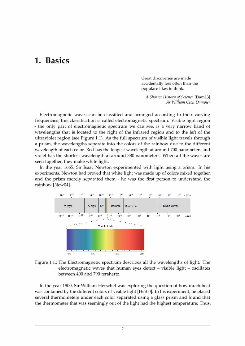
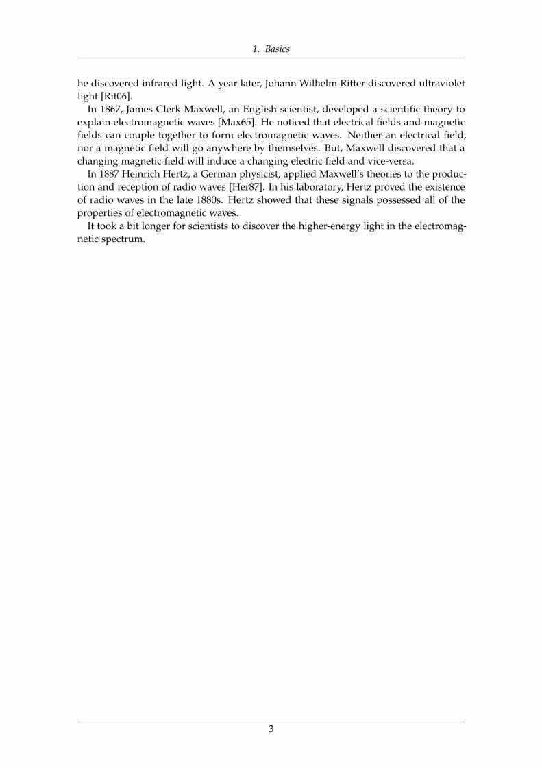
Electromagnetic waves can be classified and arranged according to their varyingfrequencies; this classification is called electromagnetic spectrum. Visible light region- the only part of electromagnetic spectrum we can see, is a very narrow band ofwavelengths that is located to the right of the infrared region and to the left of theultraviolet region (see Figure 1.1). As the full spectrum of visible light travels througha prism, the wavelengths separate into the colors of the rainbow due to the differentwavelength of each color. Red has the longest wavelength at around 700 nanometers andviolet has the shortest wavelength at around 380 nanometers. When all the waves areseen together, they make white light.
In the year 1665, Sir Isaac Newton experimented with light using a prism. In hisexperiments, Newton had proved that white light was made up of colors mixed together,and the prism merely separated them - he was the first person to understand therainbow [New04].
Figure 1.1.: The Electromagnetic spectrum describes all the wavelengths of light. Theelectromagnetic waves that human eyes detect – visible light – oscillatesbetween 400 and 790 terahertz.
In the year 1800, Sir William Herschel was exploring the question of how much heatwas contained by the different colors of visible light [Her00]. In his experiment, he placedseveral thermometers under each color separated using a glass prism and found thatthe thermometer that was seemingly out of the light had the highest temperature. Thus,
2
1. Basics
he discovered infrared light. A year later, Johann Wilhelm Ritter discovered ultravioletlight [Rit06].
In 1867, James Clerk Maxwell, an English scientist, developed a scientific theory toexplain electromagnetic waves [Max65]. He noticed that electrical fields and magneticfields can couple together to form electromagnetic waves. Neither an electrical field,nor a magnetic field will go anywhere by themselves. But, Maxwell discovered that achanging magnetic field will induce a changing electric field and vice-versa.
In 1887 Heinrich Hertz, a German physicist, applied Maxwell’s theories to the produc-tion and reception of radio waves [Her87]. In his laboratory, Hertz proved the existenceof radio waves in the late 1880s. Hertz showed that these signals possessed all of theproperties of electromagnetic waves.
It took a bit longer for scientists to discover the higher-energy light in the electromag-netic spectrum.
3
2. X-ray based Imaging
X-ray imaging has been proven to be an incredible component of several medical diagnos-tic and treatment techniques as well as many industrial Inspections of solid materials andproducts. X-ray technology is the oldest and most commonly used form of imaging thatuses ionizing radiation to produce images of the internal structure of different objects.Owing to the recent advances in computing power, several x-ray based imaging devicesand techniques have been developed and are in use in medical and non-medical applica-tions, including computed tomography (CT), mammography, interventional radiologyand digital radiography.
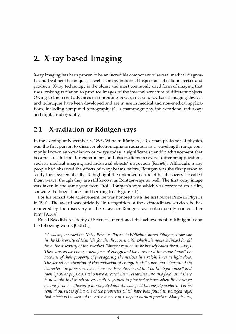
2.1 X-radiation or Röntgen-raysIn the evening of November 8, 1895, Wilhelm Röntgen , a German professor of physics,was the first person to discover electromagnetic radiation in a wavelength range com-monly known as x-radiation or x-rays today, a significant scientific advancement thatbecame a useful tool for experiments and observations in several different applicationssuch as medical imaging and industrial objects’ inspection [Rön96]. Although, manypeople had observed the effects of x-ray beams before, Röntgen was the first person tostudy them systematically. To highlight the unknown nature of his discovery, he calledthem x-rays, though they are still known as Röntgen-rays as well. The first x-ray imagewas taken in the same year from Prof. Röntgen’s wife which was recorded on a film,showing the finger bones and her ring (see Figure 2.1).
For his remarkable achievement, he was honored with the first Nobel Prize in Physicsin 1901. The award was officially "in recognition of the extraordinary services he hasrendered by the discovery of the x-rays or Röntgen-rays subsequently named afterhim" [AB14].
Royal Swedish Academy of Sciences, mentioned this achievement of Röntgen usingthe following words [Odh01]:
"Academy awarded the Nobel Prize in Physics to Wilhelm Conrad Röntgen, Professorin the University of Munich, for the discovery with which his name is linked for alltime: the discovery of the so-called Röntgen rays or, as he himself called them, x-rays.These are, as we know, a new form of energy and have received the name "rays" onaccount of their property of propagating themselves in straight lines as light does.The actual constitution of this radiation of energy is still unknown. Several of itscharacteristic properties have, however, been discovered first by Röntgen himself andthen by other physicists who have directed their researches into this field. And thereis no doubt that much success will be gained in physical science when this strangeenergy form is sufficiently investigated and its wide field thoroughly explored. Let usremind ourselves of but one of the properties which have been found in Röntgen rays;that which is the basis of the extensive use of x-rays in medical practice. Many bodies,
4
2. X-ray based Imaging
Figure 2.1.: The first x-ray projection was taken in 1895 from Prof. Wilhelm Röntgen’s wifewhich was recorded on a film, showing the finger bones and her ring [Kev98].
just as they allow light to pass through them in varying degrees, behave likewisewith x-rays, but with the difference that some which are totally impenetrable to lightcan easily be penetrated by x-rays, while other bodies stop them completely. Thus,for example, metals are impenetrable to them; wood, leather, cardboard and othermaterials are penetrable and this is also the case with the muscular tissues of animalorganisms... ."
2.2 Generation of X-raysX-rays are waves of electromagnetic energy. They behave in a similar way as light rays, butat much shorter wavelengths - in the range of 0.01-10 nm - and are capable of penetratingsome thickness of matter. There are three major ways that x-rays are generated. Themost common is the Bremsstrahlung process. Bremsstrahlung is a German term thatmeans "braking rays". It is an important phenomenon in the generation of x-rays whererays are produced by slowing down of the primary beam electrons by the electric fieldsurrounding the nuclei of the atoms in the sample [Low58].
Another method is K-shell emission, where a high energy electron knocks an electronfrom an inner orbit in an atom, and an x-ray is emitted with the replacement of thatelectron.
The third method occurs in a synchrotron, which is a subatomic particle acceleratorthat creates high intensity x-rays used for nuclear studies.
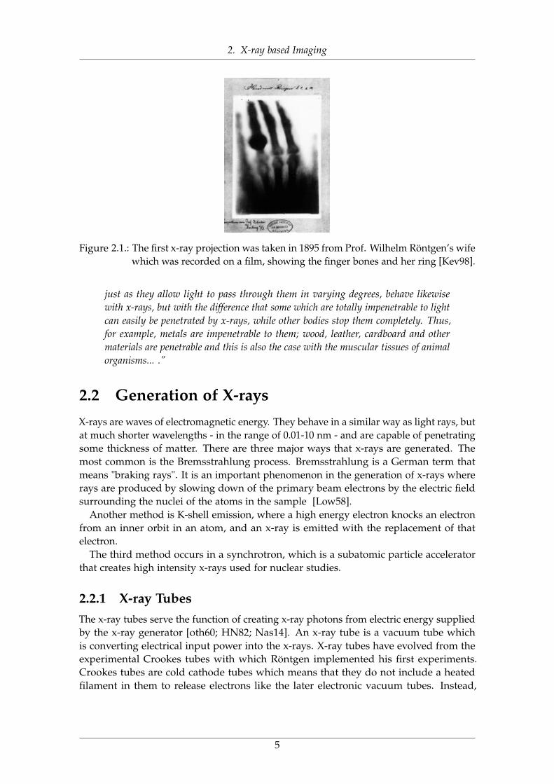
2.2.1 X-ray TubesThe x-ray tubes serve the function of creating x-ray photons from electric energy suppliedby the x-ray generator [oth60; HN82; Nas14]. An x-ray tube is a vacuum tube whichis converting electrical input power into the x-rays. X-ray tubes have evolved from theexperimental Crookes tubes with which Röntgen implemented his first experiments.Crookes tubes are cold cathode tubes which means that they do not include a heatedfilament in them to release electrons like the later electronic vacuum tubes. Instead,
5
2. X-ray based Imaging
Figure 2.2.: A diagram of a modern x-ray tube. This type of tube was devised by Coolidgein 1913 [SP08].
electrons are generated by the ionization of the residual air by a high DC voltage whichis applied between the electrodes [Beh15; Alb77].
In 1913, William Coolidge invented the Coolidge tube, an x-ray tube with an improvedcathode to be used in x-ray machines which enabled more intense visualization of deep-seated anatomy and tumors. Figure 2.2 illustrates basic parts of an original Coolidgetube including a spherical bulb with two cylindrical arms, cathode arm and the anodearm [Coo16].
2.2.2 Synchrotron X-raysX-ray photons can also be created under different conditions. A synchrotron is an ex-tremely powerful source of x-rays. The x-rays are produced by high energy electronswhich circulate around the synchrotron. Synchrotron x-rays can be used for traditionalx-ray imaging, phase-contrast x-ray imaging, and tomography. The Ångström-scale wave-length of x-rays enables imaging well below the diffraction limit of visible light [Win97;Wil91; Van79]. Extremely bright, short x-ray pulses which are tuned to selected wave-length regions, have several applications including the probing of chemical reactions onsurfaces, electronic structures of semiconductors and magnetic materials, the structureand function of proteins and biological macromolecules and also for photon activationtherapy, tomotherapy, microbeam radiation therapy [Lew97; AJ94; Bla05].
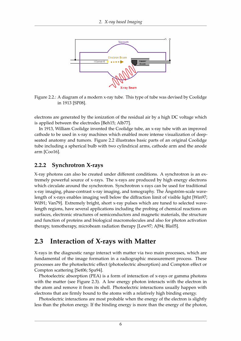
2.3 Interaction of X-rays with MatterX-rays in the diagnostic range interact with matter via two main processes, which arefundamental of the image formation in a radiographic measurement process. Theseprocesses are the photoelectric effect (photoelectric absorption) and Compton effect orCompton scattering [Set06; Spa94].
Photoelectric absorption (PEA) is a form of interaction of x-rays or gamma photonswith the matter (see Figure 2.3). A low energy photon interacts with the electron inthe atom and remove it from its shell. Photoelectric interactions usually happen withelectrons that are firmly bound to the atoms with a relatively high binding energy.
Photoelectric interactions are most probable when the energy of the electron is slightlyless than the photon energy. If the binding energy is more than the energy of the photon,
6
2. X-ray based Imaging
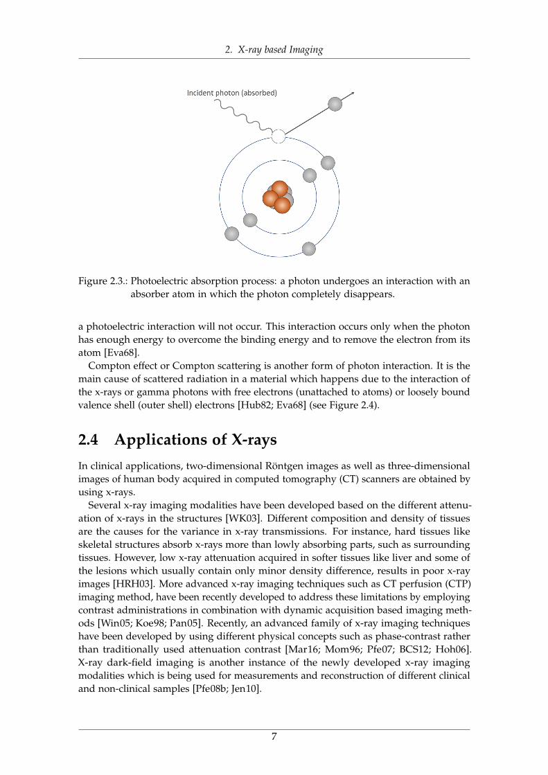
Figure 2.3.: Photoelectric absorption process: a photon undergoes an interaction with anabsorber atom in which the photon completely disappears.
a photoelectric interaction will not occur. This interaction occurs only when the photonhas enough energy to overcome the binding energy and to remove the electron from itsatom [Eva68].
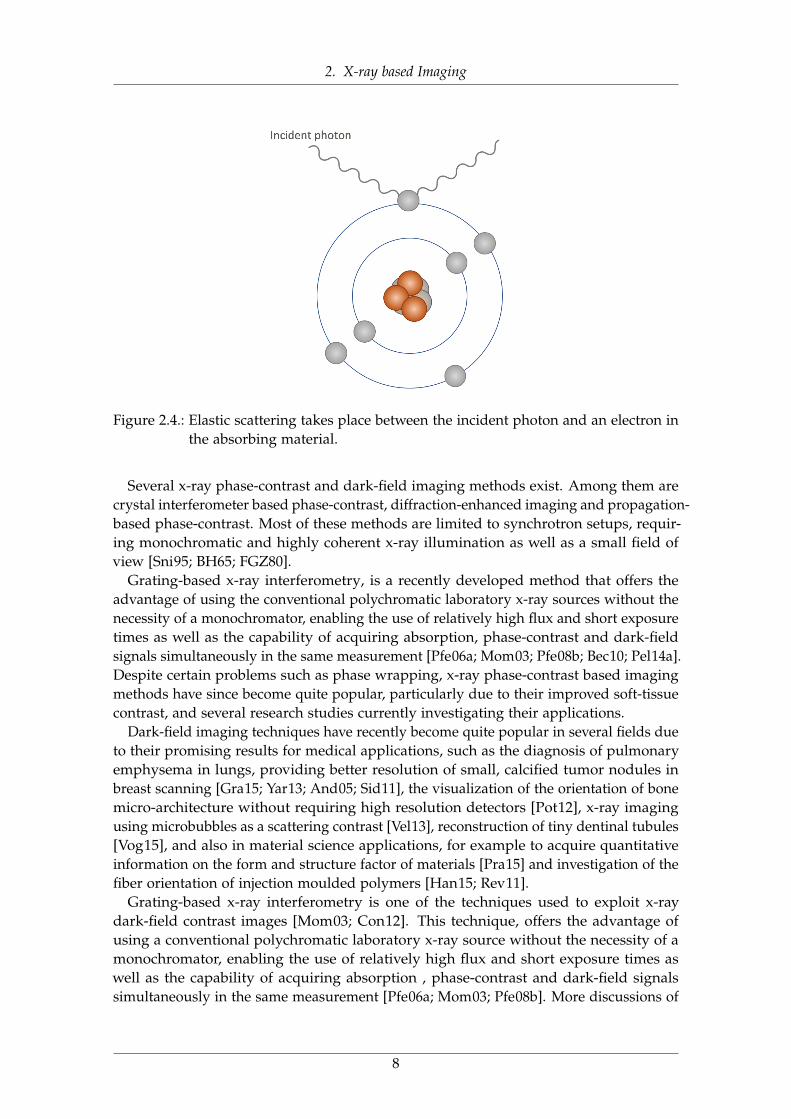
Compton effect or Compton scattering is another form of photon interaction. It is themain cause of scattered radiation in a material which happens due to the interaction ofthe x-rays or gamma photons with free electrons (unattached to atoms) or loosely boundvalence shell (outer shell) electrons [Hub82; Eva68] (see Figure 2.4).
2.4 Applications of X-raysIn clinical applications, two-dimensional Röntgen images as well as three-dimensionalimages of human body acquired in computed tomography (CT) scanners are obtained byusing x-rays.
Several x-ray imaging modalities have been developed based on the different attenu-ation of x-rays in the structures [WK03]. Different composition and density of tissuesare the causes for the variance in x-ray transmissions. For instance, hard tissues likeskeletal structures absorb x-rays more than lowly absorbing parts, such as surroundingtissues. However, low x-ray attenuation acquired in softer tissues like liver and some ofthe lesions which usually contain only minor density difference, results in poor x-rayimages [HRH03]. More advanced x-ray imaging techniques such as CT perfusion (CTP)imaging method, have been recently developed to address these limitations by employingcontrast administrations in combination with dynamic acquisition based imaging meth-ods [Win05; Koe98; Pan05]. Recently, an advanced family of x-ray imaging techniqueshave been developed by using different physical concepts such as phase-contrast ratherthan traditionally used attenuation contrast [Mar16; Mom96; Pfe07; BCS12; Hoh06].X-ray dark-field imaging is another instance of the newly developed x-ray imagingmodalities which is being used for measurements and reconstruction of different clinicaland non-clinical samples [Pfe08b; Jen10].
7
2. X-ray based Imaging
Figure 2.4.: Elastic scattering takes place between the incident photon and an electron inthe absorbing material.
Several x-ray phase-contrast and dark-field imaging methods exist. Among them arecrystal interferometer based phase-contrast, diffraction-enhanced imaging and propagation-based phase-contrast. Most of these methods are limited to synchrotron setups, requir-ing monochromatic and highly coherent x-ray illumination as well as a small field ofview [Sni95; BH65; FGZ80].
Grating-based x-ray interferometry, is a recently developed method that offers theadvantage of using the conventional polychromatic laboratory x-ray sources without thenecessity of a monochromator, enabling the use of relatively high flux and short exposuretimes as well as the capability of acquiring absorption, phase-contrast and dark-fieldsignals simultaneously in the same measurement [Pfe06a; Mom03; Pfe08b; Bec10; Pel14a].Despite certain problems such as phase wrapping, x-ray phase-contrast based imagingmethods have since become quite popular, particularly due to their improved soft-tissuecontrast, and several research studies currently investigating their applications.
Dark-field imaging techniques have recently become quite popular in several fields dueto their promising results for medical applications, such as the diagnosis of pulmonaryemphysema in lungs, providing better resolution of small, calcified tumor nodules inbreast scanning [Gra15; Yar13; And05; Sid11], the visualization of the orientation of bonemicro-architecture without requiring high resolution detectors [Pot12], x-ray imagingusing microbubbles as a scattering contrast [Vel13], reconstruction of tiny dentinal tubules[Vog15], and also in material science applications, for example to acquire quantitativeinformation on the form and structure factor of materials [Pra15] and investigation of thefiber orientation of injection moulded polymers [Han15; Rev11].
Grating-based x-ray interferometry is one of the techniques used to exploit x-raydark-field contrast images [Mom03; Con12]. This technique, offers the advantage ofusing a conventional polychromatic laboratory x-ray source without the necessity of amonochromator, enabling the use of relatively high flux and short exposure times aswell as the capability of acquiring absorption , phase-contrast and dark-field signalssimultaneously in the same measurement [Pfe06a; Mom03; Pfe08b]. More discussions of
8
2. X-ray based Imaging
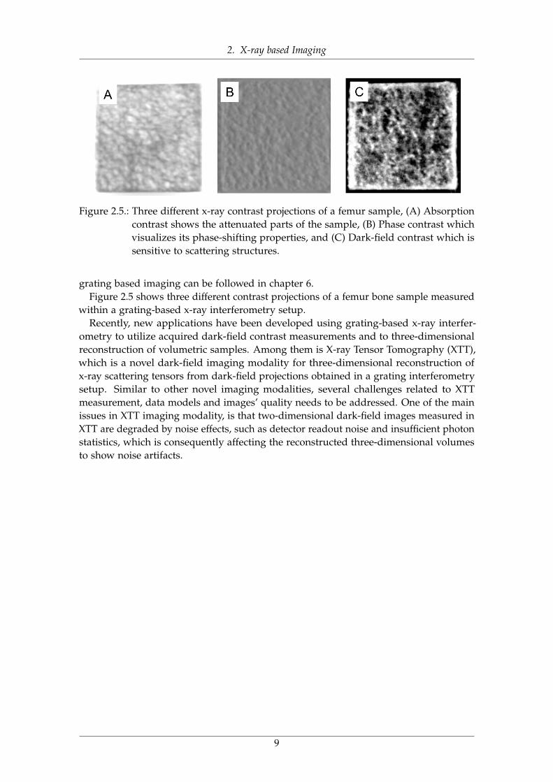
Figure 2.5.: Three different x-ray contrast projections of a femur sample, (A) Absorptioncontrast shows the attenuated parts of the sample, (B) Phase contrast whichvisualizes its phase-shifting properties, and (C) Dark-field contrast which issensitive to scattering structures.
grating based imaging can be followed in chapter 6.Figure 2.5 shows three different contrast projections of a femur bone sample measured
within a grating-based x-ray interferometry setup.Recently, new applications have been developed using grating-based x-ray interfer-
ometry to utilize acquired dark-field contrast measurements and to three-dimensionalreconstruction of volumetric samples. Among them is X-ray Tensor Tomography (XTT),which is a novel dark-field imaging modality for three-dimensional reconstruction ofx-ray scattering tensors from dark-field projections obtained in a grating interferometrysetup. Similar to other novel imaging modalities, several challenges related to XTTmeasurement, data models and images’ quality needs to be addressed. One of the mainissues in XTT imaging modality, is that two-dimensional dark-field images measured inXTT are degraded by noise effects, such as detector readout noise and insufficient photonstatistics, which is consequently affecting the reconstructed three-dimensional volumesto show noise artifacts.
9
3. Computed Tomography
In this section, we first introduce a brief history of computed tomography in section 3.1.Next, we will introduce a theoretical concept of computed tomography imaging in sec-tion 3.2 and finally will explain the tomographic reconstruction algorithms in section 4.1.
3.1 BackgroundComputed tomography (CT) is one of the well-established x-ray imaging modalitieswith wide spread applications from medical diagnosis to industrial non-destructivetesting [Kal06]. CT technology has seen remarkable innovations in the past decadeswhich have improved the performance of this modality in diagnosis and steadily increasedits clinical indications. The first successful practical implementation of the theory wasachieved in 1972 by Sir Godfrey Newbold Hounsfield [AH73], who played a vital role inthe development of CT by conducting several experiments based on the mathematicaltheories of Allan McLeod Cormack in 1964 [Cor63]. They received a Nobel Prize for theircontributions in the development of CT, and Hounsfield’s name was selected to be as astandard measurement unit for recorded x-ray attenuation.
3.2 TheoryA CT scanner combines a series of two-dimensional x-ray projections taken from differentangles and uses computer processing to create three-dimensional images, or slices, of amedical sample like bones, blood vessels and soft tissues inside the human body or someindustrial materials.
Due to the three-dimensional nature of CT scans, this modality provides more detailedinformation in comparison to a single x-ray image acquisition. In fact, conventional CTscanners are developed to acquire the absorption contrast projections. Due to this reason,CT imaging is one of the mostly used modalities for imaging of hard tissues like bonesrather than softer tissues. However, recent advances in x-ray imaging modalities such ascontrast enhanced imaging and introduction of phase and dark-field contrast imagingmethods have proved a potential for precise measuring and visualizing of softer tissueslike hepatic tumors, brain tissue and long nodules.
3.3 ApplicationsOwing to the recent advancements in mechanics, electronics and computing power, theCT scanning time has been reduced, resultant images have a better quality and readabilitywhich helps CT scanners to be chosen as a good non-invasive imaging technology forclinical and non-clinical studies.
10
3. Computed Tomography
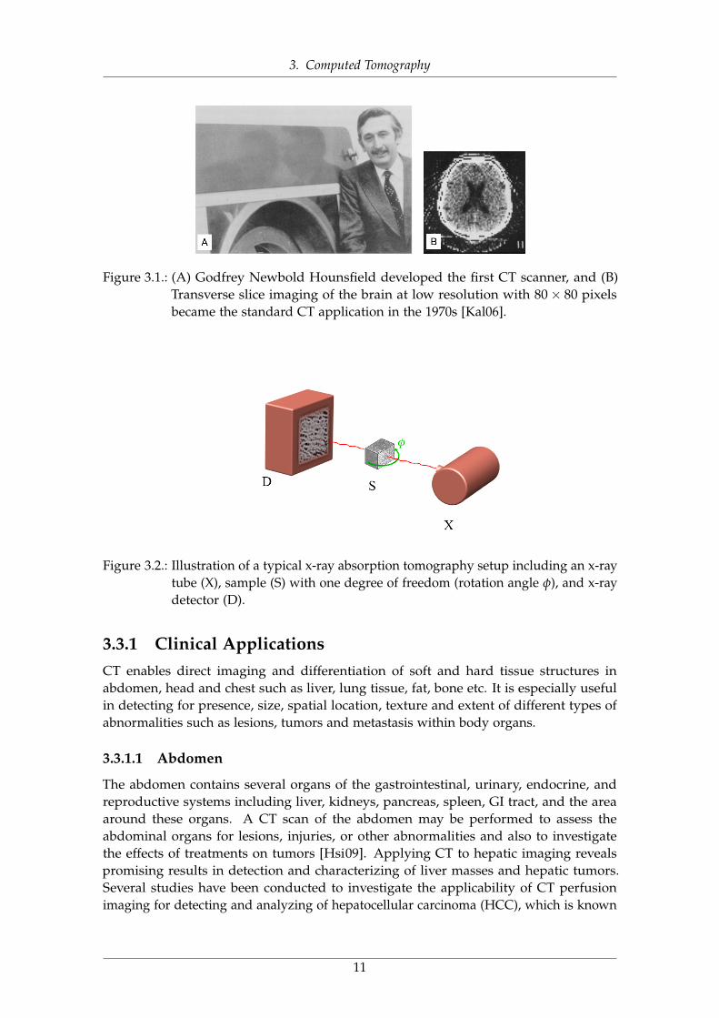
Figure 3.1.: (A) Godfrey Newbold Hounsfield developed the first CT scanner, and (B)Transverse slice imaging of the brain at low resolution with 80× 80 pixelsbecame the standard CT application in the 1970s [Kal06].
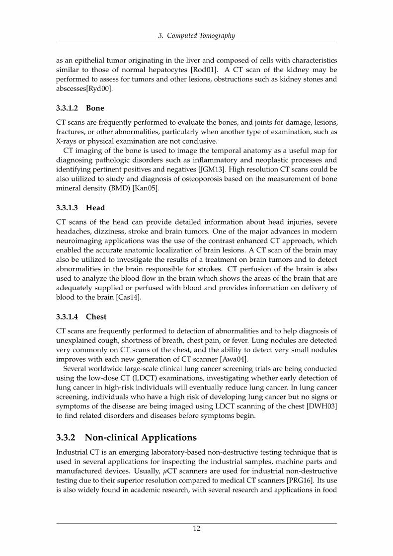
Figure 3.2.: Illustration of a typical x-ray absorption tomography setup including an x-raytube (X), sample (S) with one degree of freedom (rotation angle φ), and x-raydetector (D).
3.3.1 Clinical ApplicationsCT enables direct imaging and differentiation of soft and hard tissue structures inabdomen, head and chest such as liver, lung tissue, fat, bone etc. It is especially usefulin detecting for presence, size, spatial location, texture and extent of different types ofabnormalities such as lesions, tumors and metastasis within body organs.
3.3.1.1 Abdomen
The abdomen contains several organs of the gastrointestinal, urinary, endocrine, andreproductive systems including liver, kidneys, pancreas, spleen, GI tract, and the areaaround these organs. A CT scan of the abdomen may be performed to assess theabdominal organs for lesions, injuries, or other abnormalities and also to investigatethe effects of treatments on tumors [Hsi09]. Applying CT to hepatic imaging revealspromising results in detection and characterizing of liver masses and hepatic tumors.Several studies have been conducted to investigate the applicability of CT perfusionimaging for detecting and analyzing of hepatocellular carcinoma (HCC), which is known
11
3. Computed Tomography
as an epithelial tumor originating in the liver and composed of cells with characteristicssimilar to those of normal hepatocytes [Rod01]. A CT scan of the kidney may beperformed to assess for tumors and other lesions, obstructions such as kidney stones andabscesses[Ryd00].
3.3.1.2 Bone
CT scans are frequently performed to evaluate the bones, and joints for damage, lesions,fractures, or other abnormalities, particularly when another type of examination, such asX-rays or physical examination are not conclusive.
CT imaging of the bone is used to image the temporal anatomy as a useful map fordiagnosing pathologic disorders such as inflammatory and neoplastic processes andidentifying pertinent positives and negatives [JGM13]. High resolution CT scans could bealso utilized to study and diagnosis of osteoporosis based on the measurement of bonemineral density (BMD) [Kan05].
3.3.1.3 Head
CT scans of the head can provide detailed information about head injuries, severeheadaches, dizziness, stroke and brain tumors. One of the major advances in modernneuroimaging applications was the use of the contrast enhanced CT approach, whichenabled the accurate anatomic localization of brain lesions. A CT scan of the brain mayalso be utilized to investigate the results of a treatment on brain tumors and to detectabnormalities in the brain responsible for strokes. CT perfusion of the brain is alsoused to analyze the blood flow in the brain which shows the areas of the brain that areadequately supplied or perfused with blood and provides information on delivery ofblood to the brain [Cas14].
3.3.1.4 Chest
CT scans are frequently performed to detection of abnormalities and to help diagnosis ofunexplained cough, shortness of breath, chest pain, or fever. Lung nodules are detectedvery commonly on CT scans of the chest, and the ability to detect very small nodulesimproves with each new generation of CT scanner [Awa04].
Several worldwide large-scale clinical lung cancer screening trials are being conductedusing the low-dose CT (LDCT) examinations, investigating whether early detection oflung cancer in high-risk individuals will eventually reduce lung cancer. In lung cancerscreening, individuals who have a high risk of developing lung cancer but no signs orsymptoms of the disease are being imaged using LDCT scanning of the chest [DWH03]to find related disorders and diseases before symptoms begin.
3.3.2 Non-clinical ApplicationsIndustrial CT is an emerging laboratory-based non-destructive testing technique that isused in several applications for inspecting the industrial samples, machine parts andmanufactured devices. Usually, µCT scanners are used for industrial non-destructivetesting due to their superior resolution compared to medical CT scanners [PRG16]. Its useis also widely found in academic research, with several research and applications in food
12
3. Computed Tomography
science [Sch16], material science [MW14] as well as in geoscience applications [CB13].Recently, CT imaging has successfully entered the field of coordinate metrology as aflexible measurement technique for performing dimensional measurements on industrialparts [War16].
3.4 Artifacts in CTArtifacts can seriously degrade the quality of images in computed tomography scans,which could make them diagnostically unusable. To improve image quality, it is essentialto understand why artifacts occur and how they can be corrected or removed.
CT artifacts originate due to the range of reasons. Physics-based artifacts occur due tothe physical processes in the acquisition process of images. Patient related artifacts arehappening due to the several factors associated with patient movement or the presenceof metal part in or on the patient body. Scanner related artifacts result from issues inscanner functioning parts. However, in most of the cases, careful patient positioningand precise selection of scanner parameters are the most vital factors to prevent CTartifacts [Hsi09; BK04].
Noise, is one of the most commonly encountered artifact in CT images as a result ofthe statistical error of reduced photon counts, which results in several bright and darkstreaks appearing along the direction of greatest attenuation [Hsi09]. Several iterativereconstruction techniques associated with regularization and noise reduction methodshave been proposed to reduce the effect of this artifact [Nak05]. We will discuss moreabout this artifact and several pipelines including denoising methods and reconstructiontechniques to prevent reduced image quality in the next chapters (see part I,chapter 11).
Beam hardening and scattering are two other commonly existing types of artifactsthat produce dark streaks in the CT images. Iterative reconstruction and several post-processing approaches methods have been proposed to reduce the effect of this class ofartifacts [Van11; BF12; WFV00]. Its also proved that, dual energy CT imaging can reducethe effects of beam hardening artifact by scanning the target with two different energies.The acquired information can be used to derive virtual monochromatic images that donot suffer from beam hardening effects [AM76].
Metal artifacts are another commonly seen artifacts that occur due to the existence ofhigh density objects such as metal prostheses, surgical clips, or dental fillings which couldgenerate streak-like lines in CT images [De 99; De 00]. Several techniques have beenproposed to address the metal artifact reduction. Among them are iterative metal deletiontechnique [BF11], or a technique to determine the implant boundaries semi-automaticallyand to replace the missing projection data by linear interpolation [KHE87].
Recently, Stayman et. al. [Sta12] proposed a Known-Component reconstruction methodto reduce the artifacts such as noise and streaking due to the existing of metal implantsthat degrade the image quality. This method is integrating the already known shape andmaterial information of an object into the reconstruction problem benefiting a registrationstep for the known component [Xu17; Zha17].
13
4. Tomographic Reconstruction
While advances in CT hardware technology continue to overcome its physical limitations,recent updates in computing power have opened additional doors for improving theperformance of CT imaging via more advanced processing methods, such as tomographicreconstruction techniques.
Mathematically, computed tomography can be assumed as an inverse problem, sinceit recovers the attenuation coefficients of a measured sample from a set of transmissionvalues. As shown in Figure 3.2, rotation of a sample results in several number ofcoefficients of the two-dimensional Fourier transform for each sample slice. Tomographicreconstruction seeks to estimate a specific system from a finite number of projections.The mathematical fundamentals for tomographic imaging was described by JohannRadon [Rad86].
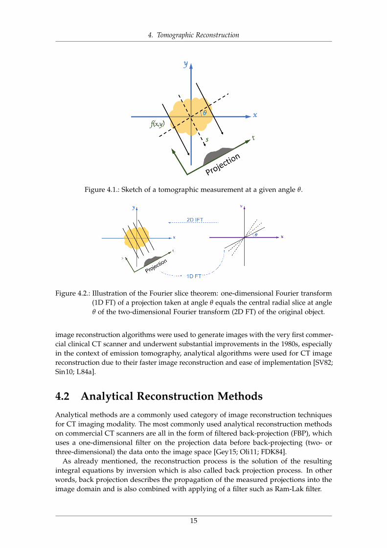
As shown in Figure 4.1, the projection of an object is a set of line integrals acquiredduring the measurement process at an arbitrary given angle such as θ.
Assuming the data collection process as a series of parallel rays, at position, across aprojection at angle θ, the computed tomography problem can be given according to theBeer-Lambert law [Buz08], which describes the absorption of x-rays as,
I = I0e−∫
µ(x,y)ds, (4.1)
where µ(x, y) refers to the attenuation coefficient which is specific to each material and Iand I0 denote the transmitted and incident intensities respectively.
In theory, the inverse Radon transformation would yield the original image. Fourierslice theorem states that the values along the one-dimensional Fourier transform ofa parallel projection of an object’s slice are equal to those along a line parallel to thedetector through the center of the slice’s two-dimensional Fourier transform. In otherwords, if we had an infinite number of one-dimensional projections of an object taken atan infinite number of angles, we could perfectly reconstruct the original object, f (x, y).However, in practical applications, there exist a finite number of projections available.
Figure 4.2 shows a visual illustration of the Fourier slice theorem.
4.1 Reconstruction AlgorithmsImage reconstruction in CT imaging is a mathematical process that generates tomographicimages from x-ray projection data acquired at many different angles around the patientand has fundamental impacts on image quality, radiation dose and therefore on diagnosisprocess.
Image reconstruction algorithms play a critical role in the quality and appearance oftomographic images. These methods are divided into two major categories, analyticalreconstruction methods and iterative reconstruction (IR) techniques. Although iterative
14
4. Tomographic Reconstruction
Figure 4.1.: Sketch of a tomographic measurement at a given angle θ.
Figure 4.2.: Illustration of the Fourier slice theorem: one-dimensional Fourier transform(1D FT) of a projection taken at angle θ equals the central radial slice at angleθ of the two-dimensional Fourier transform (2D FT) of the original object.
image reconstruction algorithms were used to generate images with the very first commer-cial clinical CT scanner and underwent substantial improvements in the 1980s, especiallyin the context of emission tomography, analytical algorithms were used for CT imagereconstruction due to their faster image reconstruction and ease of implementation [SV82;Sin10; L84a].
4.2 Analytical Reconstruction MethodsAnalytical methods are a commonly used category of image reconstruction techniquesfor CT imaging modality. The most commonly used analytical reconstruction methodson commercial CT scanners are all in the form of filtered back-projection (FBP), whichuses a one-dimensional filter on the projection data before back-projecting (two- orthree-dimensional) the data onto the image space [Gey15; Oli11; FDK84].
As already mentioned, the reconstruction process is the solution of the resultingintegral equations by inversion which is also called back projection process. In otherwords, back projection describes the propagation of the measured projections into theimage domain and is also combined with applying of a filter such as Ram-Lak filter.
15
4. Tomographic Reconstruction
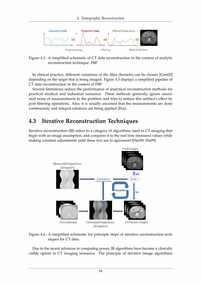
Figure 4.3.: A simplified schematic of CT data reconstruction in the context of analyticreconstruction technique: FBP.
In clinical practice, different variations of the filter (kernels) can be chosen [Gen02]depending on the target that is being imaged. Figure 4.3 displays a simplified pipeline ofCT data reconstruction in the context of FBP.
Several limitations reduce the performance of analytical reconstruction methods forpractical medical and industrial scenarios. These methods generally ignore associ-ated noise of measurements in the problem and tries to reduce this artifact’s effect bypost-filtering operations. Also, it is usually assumed that the measurements are donecontinuously and integral solutions are being applied [Fes].
4.3 Iterative Reconstruction TechniquesIterative reconstruction (IR) refers to a category of algorithms used in CT imaging thatbegin with an image assumption, and compares it to the real time measured values whilemaking constant adjustments until these two are in agreement‘[Her09; Hu99].
Figure 4.4.: A simplified schematic for principle steps of iterative reconstruction tech-niques for CT data.
Due to the recent advances in computing power, IR algorithms have become a clinicallyviable option in CT imaging scenarios. The principle of iterative image algorithms
16
4. Tomographic Reconstruction
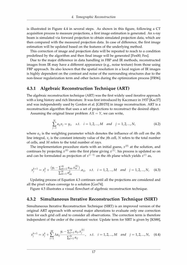
is illustrated in Figure 4.4 in several steps. As shown in this figure, following a CTacquisition process to measure projections, a first image estimation is generated. An x-raybeam is simulated via forward projection to obtain simulated projection data, which arethen compared with the measured projection data. In case of difference, the first imageestimation will be updated based on the features of the underlying method.
This correction of image and projection data will be repeated to reach to a conditionpredefined by the algorithm and then final image will be generated [Fes00; Fes].
Due to the major difference in data handling in FBP and IR methods, reconstructedimages from IR may have a different appearance (e.g., noise texture) from those usingFBP approach. Its also known that the spatial resolution in a local region of IR imagesis highly dependent on the contrast and noise of the surrounding structures due to thenon-linear regularization term and other factors during the optimization process [FR96].
4.3.1 Algebraic Reconstruction Technique (ART)The algebraic reconstruction technique (ART) was the first widely used iterative approachwith a long history and rich literature. It was first introduced by Kaczmarz in 1937 [Kac37]and was independently used by Gordon et al. [GBH70] in image reconstruction. ART is areconstruction algorithm that uses a set of projections to reconstruct the desired object.
Assuming the original linear problem AX = Y, we can write,
N
∑j=1
aijxj = yi, s.t. i = 1, 2, ..., M and j = 1, 2, ..., N, (4.2)
where aij is the weighting parameter which denotes the influence of ith cell on the jthline integral, xj is the constant intensity value of the jth cell, N refers to the total numberof cells, and M refers to the total number of rays.
The implementation procedure starts with an initial guess, x(0) at the solution, andcontinues by projecting x(0) onto the first plane giving x(1). his process is updated so onand can be formulated as projection of x(i−1) on the ith plane which yields x(i) as,
xk+1j = xk
j +(yi −∑N
m=1 aim.x(k)m )
∑Nm=1 a2
im
.aij, s.t. i = 1, 2, ..., M and j = 1, 2, ..., N, (4.3)
Updating process of Equation 4.3 continues until all the projections are considered andall the pixel values converge to a solution [Gor74].
Figure 4.5 illustrates a visual flowchart of algebraic reconstruction technique.
4.3.2 Simultaneous Iterative Reconstruction Technique (SIRT)Simultaneous Iterative Reconstruction Technique (SIRT) is an improved version of theoriginal ART approach with several major alterations to evaluate only one correctionterm for each grid cell and to consider all observations. The correction term is thereforeindependent of the order of the constant vector. Update term for SIRT is given by [KS88],
xk+1j = xk
j +M
∑i=1
λaijyi −∑N
j=1 aij.x(k)j
∑Ni=1 aij
, s.t. i = 1, 2, ..., M and j = 1, 2, ..., N, (4.4)
17
4. Tomographic Reconstruction
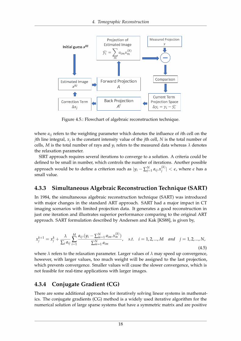
Figure 4.5.: Flowchart of algebraic reconstruction technique.
where aij refers to the weighting parameter which denotes the influence of ith cell on thejth line integral, xj is the constant intensity value of the jth cell, N is the total number ofcells, M is the total number of rays and yi refers to the measured data whereas λ denotesthe relaxation parameter.
SIRT approach requires several iterations to converge to a solution. A criteria could bedefined to be small in number, which controls the number of iterations. Another possibleapproach would be to define a criterion such as |yi − ∑N
j=1 aij.x(k)j | < ε, where ε has a
small value.
4.3.3 Simultaneous Algebraic Reconstruction Technique (SART)In 1984, the simultaneous algebraic reconstruction technique (SART) was introducedwith major changes in the standard ART approach. SART had a major impact in CTimaging scenarios with limited projection data. It generates a good reconstruction injust one iteration and illustrates superior performance comparing to the original ARTapproach. SART formulation described by Andersen and Kak [KS88], is given by,
xk+1j = xk
j +λ
∑i aij
M
∑i=1
aij.(yi −∑Nm=1 aim.x(k)m )
∑Nm=1 aim
, s.t. i = 1, 2, ..., M and j = 1, 2, ..., N,
(4.5)where λ refers to the relaxation parameter. Larger values of λ may speed up convergence,however, with larger values, too much weight will be assigned to the last projection,which prevents convergence. Smaller values will cause the slower convergence, which isnot feasible for real-time applications with larger images.
4.3.4 Conjugate Gradient (CG)There are some additional approaches for iteratively solving linear systems in mathemat-ics. The conjugate gradients (CG) method is a widely used iterative algorithm for thenumerical solution of large sparse systems that have a symmetric matrix and are positive
18
4. Tomographic Reconstruction
definite. CG approach was first proposed by Hestenes and Stiefel [HS52; Sti52] in 1952and has become a well-known method for its rapid convergence in several applicationareas [VV86].
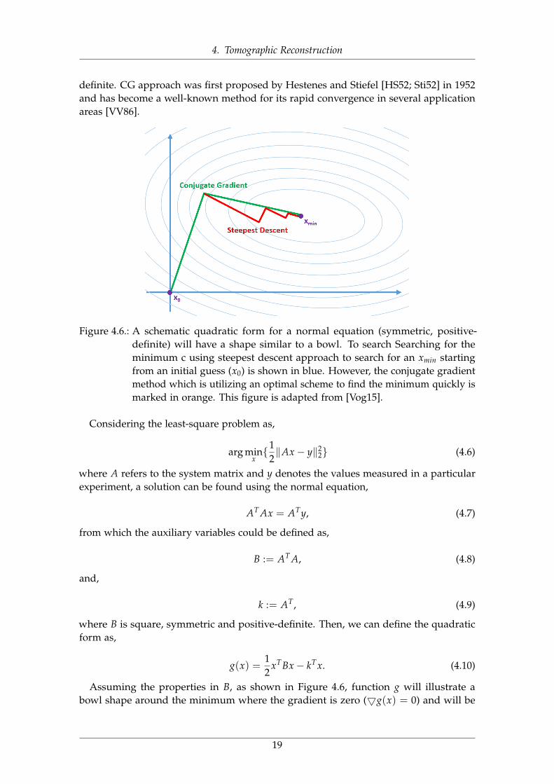
Figure 4.6.: A schematic quadratic form for a normal equation (symmetric, positive-definite) will have a shape similar to a bowl. To search Searching for theminimum c using steepest descent approach to search for an xmin startingfrom an initial guess (x0) is shown in blue. However, the conjugate gradientmethod which is utilizing an optimal scheme to find the minimum quickly ismarked in orange. This figure is adapted from [Vog15].
Considering the least-square problem as,
arg minx{1
2‖Ax− y‖2
2} (4.6)
where A refers to the system matrix and y denotes the values measured in a particularexperiment, a solution can be found using the normal equation,
AT Ax = ATy, (4.7)
from which the auxiliary variables could be defined as,
B := AT A, (4.8)
and,
k := AT, (4.9)
where B is square, symmetric and positive-definite. Then, we can define the quadraticform as,
g(x) =12
xTBx− kTx. (4.10)
Assuming the properties in B, as shown in Figure 4.6, function g will illustrate abowl shape around the minimum where the gradient is zero (5g(x) = 0) and will be
19
4. Tomographic Reconstruction
computed as,5 g(x) = Bx− k, (4.11)
which is simply describing the idea of relaxation approach. A vectorx which is solving alinear system Bx = k, will also minimize the quadratic form of g(x).
Assuming this relation, rather than solving the normal equation AT Acx = Bx = k =
ATy, it will be possible to to search for a minimum of the quadratic form g(x) whilecomputing a least-squares image reconstruction. since the minimization problem isnon-linear, steepest descent (gradient descent) would be one possible method to solveit [FP63].
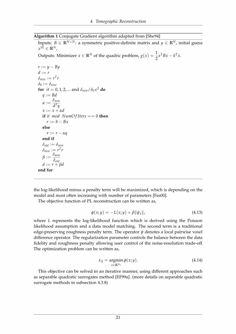
A simplified pseudo-code of CG approach is illustrated in 2. However, the concept ofCG is to restrict number of search directions, and to take the optimal step size such thata second search along the same direction is superfluous (see Figure 4.6).
CG approach, is initialized with an arbitrary location (x0), and evaluates the gradientto obtain a search direction. Then, a new estimate will be computed by moving along thissearch line to a close point to the solution with respect to the concept of B-orthogonalityas described in [AMS90; FR64]. One of the most important aspects in CG is the factthat there is an upper bound on the number of iterations, such that CG is guaranteedto find the optimal solution of the least-squares problem in as many steps as there aredimensions, utilizing the mutually B-orthogonal search directions combined with optimalstep lengths [GKR85].
A detailed overview of CG, its applications and generalizations to indefinite or non-symmetric matrices, can be found in [Saa03].
4.3.5 Maximum Likelihood Expectation Maximization (MLEM)The methods introduced so far are assuming well-posed problem with some goodmeasurements and none of them model the statistical properties of the measurementprocess.
Likelihood based approaches are another category of methods for photon-limitedconditions that are the standard since decades, in order to support low dose imaging.
The problem of image reconstruction can be formulated as a standard statisticalestimation problem. This leads to the following multiplicative update equation:
xk+1j = xk
j +1
∑i aij∑
i
yi
aTi x(k−1)
, s.t. i = 1, 2, ..., M and j = 1, 2, ..., N, (4.12)
where the variable k refers to the iteration index.As shown in Equation 4.19, MLEM approach is iteratively maximizing a likelihood
function which has several advantages over the conventional FBP techniques. Theseadvantages could be summarized as (1) MLEM methods do not require equally spacedprojection data, (2) they can be utilized for limited set of projection data, and (3) theyyields less artifacts [VSK85; L84a].
4.3.6 Penalized Likelihood (PL)Penalized likelihood (PL) estimation is a way to consider the complexity of a model whileestimating parameters of different models. In general, instead of applying a simple MLE,
20
4. Tomographic Reconstruction
Algorithm 1 Conjugate Gradient algorithm adapted from [She94]
Inputs: B ∈ RN×N : a symmetric positive-definite matrix and y ∈ RN , initial guessx[0] ∈ RN ,
Outputs: Minimizer x ∈ RN of the quadric problem, g(x) =12
xTBx− kTx.
r := y− Byd := rδnew := rTrδ0 := δnew
for it = 0, 1, 2, ... and δnew/δ0 ε2 doq := Bd
α :=δnew
dTqx := x + αdif it mod NumO f Iters == 0 then
r := b− Bxelse
r := r− αqend ifδold := δnew
δnew := rTr
β :=δnew
δoldd := r + βd
end for
the log-likelihood minus a penalty term will be maximized, which is depending on themodel and most often increasing with number of parameters [Fes00].
The objective function of PL reconstruction can be written as,
φ(x; y) = −L(x; y) + β‖ψx‖, (4.13)
where L represents the log-likelihood function which is derived using the Poissonlikelihood assumption and a data model matching. The second term is a traditionaledge-preserving roughness penalty term. The operator ψ denotes a local pairwise voxeldifference operator. The regularization parameter controls the balance between the datafidelity and roughness penalty allowing user control of the noise-resolution trade-off.The optimization problem can be written as,
x∆ = argminx∈RNx
φ(x; y). (4.14)
This objective can be solved in an iterative manner, using different approaches suchas separable quadratic surrogates method [EF99a]. (more details on separable quadraticsurrogate methods in subsection 4.3.8)
21
4. Tomographic Reconstruction
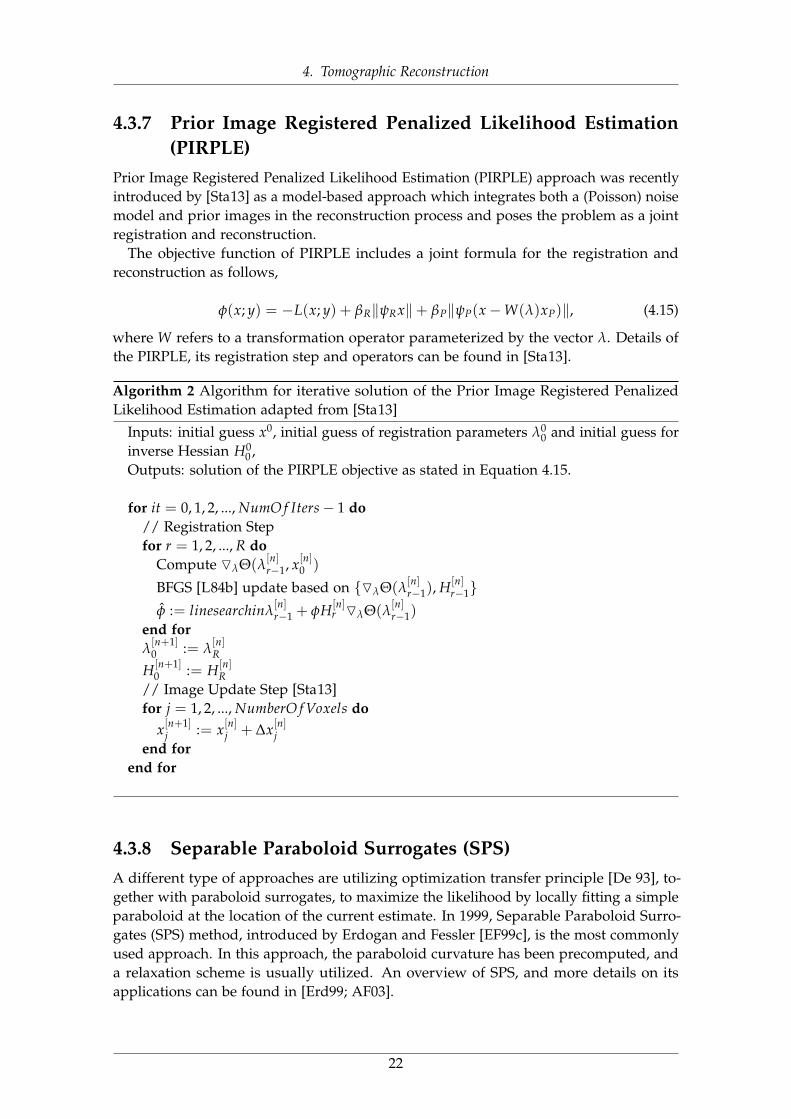
4.3.7 Prior Image Registered Penalized Likelihood Estimation(PIRPLE)
Prior Image Registered Penalized Likelihood Estimation (PIRPLE) approach was recentlyintroduced by [Sta13] as a model-based approach which integrates both a (Poisson) noisemodel and prior images in the reconstruction process and poses the problem as a jointregistration and reconstruction.
The objective function of PIRPLE includes a joint formula for the registration andreconstruction as follows,
φ(x; y) = −L(x; y) + βR‖ψRx‖+ βP‖ψP(x−W(λ)xP)‖, (4.15)
where W refers to a transformation operator parameterized by the vector λ. Details ofthe PIRPLE, its registration step and operators can be found in [Sta13].
Algorithm 2 Algorithm for iterative solution of the Prior Image Registered PenalizedLikelihood Estimation adapted from [Sta13]
Inputs: initial guess x0, initial guess of registration parameters λ00 and initial guess for
inverse Hessian H00 ,
Outputs: solution of the PIRPLE objective as stated in Equation 4.15.
for it = 0, 1, 2, ..., NumO f Iters− 1 do// Registration Stepfor r = 1, 2, ..., R do
Compute OλΘ(λ[n]r−1, x[n]0 )
BFGS [L84b] update based on {OλΘ(λ[n]r−1), H[n]
r−1}φ := linesearchinλ
[n]r−1 + φH[n]
r OλΘ(λ[n]r−1)
end forλ[n+1]0 := λ
[n]R
H[n+1]0 := H[n]
R// Image Update Step [Sta13]for j = 1, 2, ..., NumberO f Voxels do
x[n+1]j := x[n]j + ∆x[n]j
end forend for
4.3.8 Separable Paraboloid Surrogates (SPS)A different type of approaches are utilizing optimization transfer principle [De 93], to-gether with paraboloid surrogates, to maximize the likelihood by locally fitting a simpleparaboloid at the location of the current estimate. In 1999, Separable Paraboloid Surro-gates (SPS) method, introduced by Erdogan and Fessler [EF99c], is the most commonlyused approach. In this approach, the paraboloid curvature has been precomputed, anda relaxation scheme is usually utilized. An overview of SPS, and more details on itsapplications can be found in [Erd99; AF03].
22
4. Tomographic Reconstruction
4.4 Hybrid AlgorithmsHybrid algorithms combine both analytical and iterative methods using different arrange-ments. In one example, the initial image is generated by the use of analytical methods (e.g.FBP), and then iterative methods have been utilized in order to optimize several imagedomain characteristics, such as noise [Fun11]. In another example, an iterative algorithmcan be directly used in the reconstruction process to focus on image improvements of aninitial image estimate that is generated by an analytical method [VLR13; Wil13].
4.5 Image Regularization and Noise ReductionImages can be improved by considering more constraints e.g. fitting the input data subjectto a smooth shape. Mathematically, this can be expressed using Lagrange multipliers [La97]. General regularised reconstruction can be written as,
arg minx{T(x) + λV(x)} (4.16)
where T(x) refers to the data fidelity term, V(x) denotes a penalty function or regulariserand λ denotes the weight of the penalty term V, and thus its impact in comparison tothe data fidelity term T. The latter is minimised if the additional constraint is met.
4.5.1 Tikhonov RegularisationTikhonov regularization, named in honor of Andrey Tikhonov, is the most commonlyused method for regularization of ill-posed problems [Tik63]. The penalty can be writtenas,
VTikhonov(x) = ‖Lx‖22 (4.17)
where L denotes the Tikhonov matrix and can be utilized based on the specific application,and an operator mapping the coefficients into the Fourier domain can be used to levelthe frequencies of the image.
4.5.2 Total Variation Regularization (TV)Total Variation regularization (TV) is a most often used penalty in imaging and digitalimage processing, that has applications in noise removal. It is based on the principle thatsignals with excessive and possibly spurious detail have high total variation, that is, theintegral of the absolute gradient of the signal is high. Considering two-dimensional signalx, such as images, the TV norm proposed by Rudin, Osher and Fatemi in 1992 [ROF92]is,
V(x) = ∑i,j
√|xi+1,j − xi,j|2 + |xi,j+1 − xi,j|2 (4.18)
which is an isotropic and not differentiable. However, an anisotropic variation whichcould be also easier to minimize, is shown as,
23
4. Tomographic Reconstruction
Vanisotropic(x) = ∑i,j|xi+1,j − xi,j|2 + |xi,j+1 − xi,j|2 (4.19)
TV has been extensively used as a denoising method in imaging applications [SP08;Sey18c; Sey13a; SY14a]. Assuming the signal x corrupted by additive white Gaussiannoise,
y = x + n x, y, n ∈ R (4.20)
Standard TV denoising problem can be expressed as,
minx‖y− x‖22 + λV(x). (4.21)
where λ refers to the regularization parameter, controlling how much smoothing isperformed. Larger noise levels call for larger λ.
4.6 Compressed Sensing and Sparse RegularizationCompressed Sensing (CS) enables a potentially large reduction in the sampling andcomputation costs for sensing signals that have a sparse or compressible represen-tations [EK12]. While the Nyquist-Shannon sampling theorem states that a certainminimum number of samples is required in order to perfectly capture an arbitrary signal,when the signal is sparse in a known basis we can vastly reduce the number of measure-ments that need to be stored. Consequently, when sensing sparse signals we might beable to do better than suggested by classical results. This is the fundamental idea behindCS: rather than first sampling at a high rate and then compressing the sampled data, wewould like to find ways to directly sense the data in a compressed form.
In a recent work, Donoho, showed that a signal having a sparse representation canbe recovered exactly from a small set of linear, nonadaptive measurements. This resultsuggests that it may be possible to sense sparse signals by taking far fewer measurements,hence the name compressed sensing [Don06].
There are some significant factors in original CS method to be considered such as (1)the image must be sparse, (2) reconstruction of the image must be done using a nonlinearmethod, and (3) the standard linear reconstruction method should generate incoherentview aliasing artifacts by applying the sparsifying transform [EK12],
min‖ψx‖1 s.t. AX = Y, (4.22)
4.6.1 Prior Image Constrained Compressed Sensing (PICCS)Prior image constrained compressed sensing (PICCS) method considers a high qualityprior image xp to reconstruct the image x from an undersampled data set by solving thefollowing constrained minimization problem [CTL08a],
minx[α‖ψ1(x− xp)‖1 + (1− α)‖ψ2x‖1
]s.t. AX = Y, (4.23)
Here the sparsifying transforms, ψ1 and ψ2 refer to any transform and α denotes theregularization parameter.
24
4. Tomographic Reconstruction
4.6.2 Alternating Direction Method of Multipliers (ADMM)Alternating Direction Method of Multipliers (ADMM) approach has been proposedby [Boy11], to solve a linear combination of two convex functionals via variable splitting.The approach is to use two distinct variables while doing the optimization, where thefirst one is the minimizing of least-squares data fidelity term and the second one is thesparsity constraint.
Considering the optimization problem with an assumption of both data and regular-ization terms being convex as,
arg minx{1
2‖Ax− y‖2
2 + λ‖Tc‖1}, (4.24)
where operator T can be defined as analysis operator, transforming the pixel coefficientsinto the coefficients of the respective basis or frame.
Equation 4.25 can be transfered into an equivalent constrained optimization problemusing ADMM and decoupling data and regularization terms as below, [Boy11]
arg minx{1
2‖Ax− y‖2
2 + λ‖z‖1}, s.t. Tx = z. (4.25)
Considering the augmented Lagrangian Lp,
Lp(x, z, u) =12‖Ax− y‖2
2 + λ‖z‖1 + uT(Tx− z) +ρ
2‖Tx− z‖2
2, (4.26)
where the chosen parameter ρ couples Tx and z, and u refers to a Lagrange multiplier. Ingeneral, each iteration of ADMM has three distinct steps which involves two optimizationproblems and one pure update and can be solved as [Boy11],
(AT A + ρTTT)xp+1 = ATy + ρTTzp + up, (4.27)
where ρ ∈ R denotes the coupling parameter. Second, we perform,
zp+1 = Sλ/ρ(Txp+1 + up), (4.28)
where Sλ/ρ denotes the soft-thresholding operator. As the third step, we finally performthe update,
up+1 = up + Txp+1 − zp+1, (4.29)
where the first part is a linear problem which can be solved using the methods like CG(see chapter 11), and the second step minimizes the `1-penalty on the variable z and thelast step will be updating the Lagrange multiplier u [Wah12].
25
5. Four-Dimensional CT Imaging
Four-dimensional (4D) CT is an imaging technique to obtain and reconstruct multipleimages of the same target over time. 4D CT increasingly offers potential advantages asan alternative primary investigation and is a common second-line investigation [Hsi09].
4D CT can provide precise anatomic information and can help differentiate healthytissue and lesions. It includes image sets in three planes (axial, coronal, sagittal) andthe fourth dimension could be the perfusion information derived from multiple contrastphases. It is most commonly performed with three phases: non-contrast, arterial, anddelayed phase imaging [Hoa14].
5.1 CT Perfusion ImagingCT perfusion (CTP) is a functional imaging modality that measures the tissue blood-flowparameters through sequential CT scanning of the same tissue or organ over the time.Typically, an iodinated contrast agent is administered and projection images are acquiredbefore, during, and after injection of contrast to track temporal changes in CT attenuation.Several commercial software packages are available for calculating parametric mapslike blood volume, blood flow and time to peak values. Most of the available packageshowever, are using similar mathematical models to quantitatively asses the perfusionparameters. Most of these models are based on the maximum slope method (SM) tocalculate the perfusion parameters. The principle of the SM is quite simple which makes itvery attractive for brain and liver perfusion evaluation tasks [MHD93a; MHD93b]. Someother methods employ a deconvolution of the arterial input function (AIF). Algebraicdeconvolution approaches based on the singular value decomposition (SVD) are alsoused in some packages [Eas02; Ass16].
CT perfusion imaging has several application for visualization and investigation ofabnormalities in brain and liver indications. CTP of the brain, is critical in characterizingthe irreversibly infarcted brain tissue and the severely ischemic but potentially salvageabletissue [Kon09]. Liver CT perfusion provides valuable information on blood flow dynamicsas a valuable measurement for hepatic fibrosis in patients with chronic liver disease andalso in the evaluation of therapeutic effectiveness for liver cancer [KKW14; Qia10; Ass15].
5.2 Perfusion Analysis TechniquesTwo basic functional CT paradigms are measured from the acquired data: perfusionmeasurements and permeability studies [Mil99].
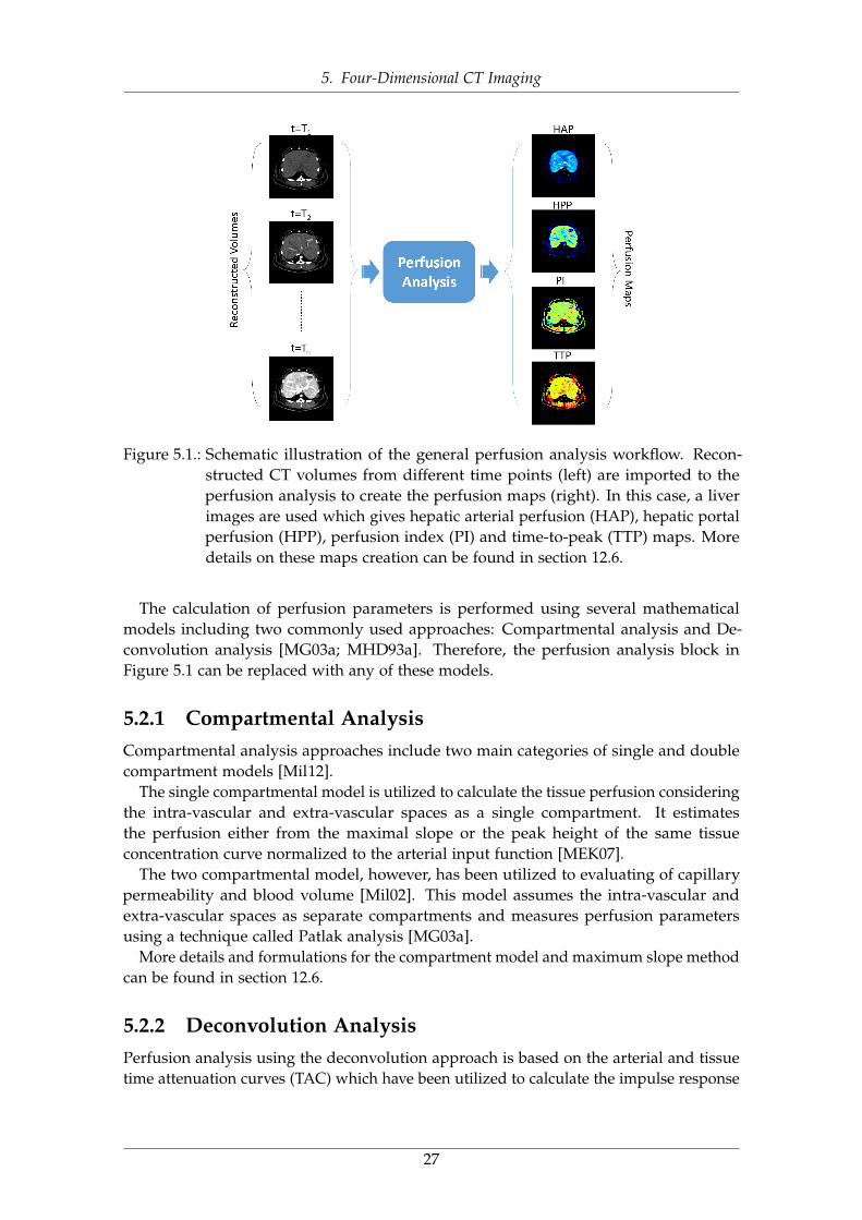
Figure 5.1 illustrates a general perfusion analysis workflow. As shown in this figure,reconstructed CT volumes from different time points (left) are imported to the perfusionanalysis to create the perfusion maps (right).
26
5. Four-Dimensional CT Imaging
Figure 5.1.: Schematic illustration of the general perfusion analysis workflow. Recon-structed CT volumes from different time points (left) are imported to theperfusion analysis to create the perfusion maps (right). In this case, a liverimages are used which gives hepatic arterial perfusion (HAP), hepatic portalperfusion (HPP), perfusion index (PI) and time-to-peak (TTP) maps. Moredetails on these maps creation can be found in section 12.6.
The calculation of perfusion parameters is performed using several mathematicalmodels including two commonly used approaches: Compartmental analysis and De-convolution analysis [MG03a; MHD93a]. Therefore, the perfusion analysis block inFigure 5.1 can be replaced with any of these models.
5.2.1 Compartmental AnalysisCompartmental analysis approaches include two main categories of single and doublecompartment models [Mil12].
The single compartmental model is utilized to calculate the tissue perfusion consideringthe intra-vascular and extra-vascular spaces as a single compartment. It estimatesthe perfusion either from the maximal slope or the peak height of the same tissueconcentration curve normalized to the arterial input function [MEK07].
The two compartmental model, however, has been utilized to evaluating of capillarypermeability and blood volume [Mil02]. This model assumes the intra-vascular andextra-vascular spaces as separate compartments and measures perfusion parametersusing a technique called Patlak analysis [MG03a].
More details and formulations for the compartment model and maximum slope methodcan be found in section 12.6.
5.2.2 Deconvolution AnalysisPerfusion analysis using the deconvolution approach is based on the arterial and tissuetime attenuation curves (TAC) which have been utilized to calculate the impulse response
27
5. Four-Dimensional CT Imaging
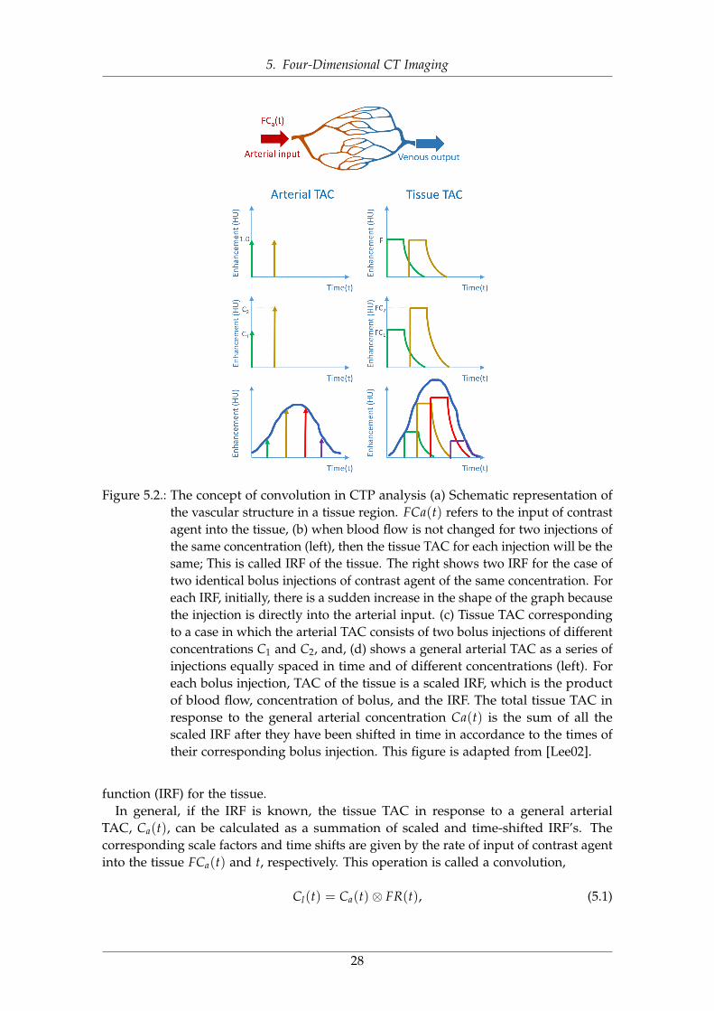
Figure 5.2.: The concept of convolution in CTP analysis (a) Schematic representation ofthe vascular structure in a tissue region. FCa(t) refers to the input of contrastagent into the tissue, (b) when blood flow is not changed for two injections ofthe same concentration (left), then the tissue TAC for each injection will be thesame; This is called IRF of the tissue. The right shows two IRF for the case oftwo identical bolus injections of contrast agent of the same concentration. Foreach IRF, initially, there is a sudden increase in the shape of the graph becausethe injection is directly into the arterial input. (c) Tissue TAC correspondingto a case in which the arterial TAC consists of two bolus injections of differentconcentrations C1 and C2, and, (d) shows a general arterial TAC as a series ofinjections equally spaced in time and of different concentrations (left). Foreach bolus injection, TAC of the tissue is a scaled IRF, which is the productof blood flow, concentration of bolus, and the IRF. The total tissue TAC inresponse to the general arterial concentration Ca(t) is the sum of all thescaled IRF after they have been shifted in time in accordance to the times oftheir corresponding bolus injection. This figure is adapted from [Lee02].
function (IRF) for the tissue.In general, if the IRF is known, the tissue TAC in response to a general arterial
TAC, Ca(t), can be calculated as a summation of scaled and time-shifted IRF’s. Thecorresponding scale factors and time shifts are given by the rate of input of contrast agentinto the tissue FCa(t) and t, respectively. This operation is called a convolution,
Cl(t) = Ca(t)⊗ FR(t), (5.1)
28
5. Four-Dimensional CT Imaging
where ⊗ denotes the convolution operator, Cl(t) refers to the TAC obtained from tissue,and FR(t) is the blood-flow scaled IRF [Lee02; Cue02].
A schematic overview of the convolution concept for CTP analysis is illustratedin Figure 5.2.
For the estimation of capillary permeability a distributed parameter model is usedwhich consists of an extended deconvolution model [Mil12]. More details and formula-tions of this approach can be found in [Lee02]
29
6. Grating Based Imaging
Modern Grating-based imaging (GBI) is a recently introduced approach to phase contrastand dark-field imaging which includes conventional laboratory sources and is basedon the use of a three-grating Talbot-Lau interferometer [Cla98; Pfe06b]. It has somesimilarities to the crystal interferometer [BH65] as it consists of a beam splitter and abeam analyzer, and is also similar to analyzer based imaging (ABI) [IB95] as it measuresthe first derivative of the phase front, and enables the dark-field imaging.
As shown in Figure 6.1, an ordinary setup of x-ray tube (X), specimen (S) and detector(D) has been extended by inserting a source grating (G0) after the tube, and two moregratings (G1, G2). The source grating G0 creates multiple sources with sufficiently highcoherence to allow for a periodic interference behind the phase grating G1. Finally theanalyzer grating G2 enables to measure the interference pattern with conventional x-raydetectors [Mom96].
Measurement process starts with several images that recorded while the relativelateral position of G2 is being shifted relatively to G1 which could be translated intothe interference pattern that is too small to be measured directly with a conventionaldetector.
A periodic function for each detector pixel can be described as [Wei05],
I(xg) ≈ a0 + a1cos(φ +2π
p2xg) (6.1)
where p2 refers to the period in G2, xg denotes the stepping and φ refers to the phase ofthe intensity curve.
As shown in Figure 6.2, from a scan Is with a sample located in the setup and also areference scan Ir without, multiple signals can be extracted. The different signals andtheir relation to the sample as well as the reference scan are illustrated in the same Figure.
These quantities are computed as [Pfe08b] described below. The absorption a iscalculated by the ratio of the mean intensity as,
a =a0,s
a0,r. (6.2)
Also the differential phase-contrast ∆φ can be calculated as
∆φ = φs − φr, (6.3)
and dark-field signal V will be extracted as,
V =a1,sa0,r
a0,sa1,r. (6.4)
where a∆,s and a∆,r refer to a. as in Equation 6.1 respectively for Is and Ir. The quotientsof a1,s and a0,s refer to the visibility Vs, with the reference visibility Vr defined accord-ingly [Bec10]. More detailed information on grating based imaging concept can be foundin [Bec09; Mom96; Pfe06a; Pfe08a; Wei05].
30
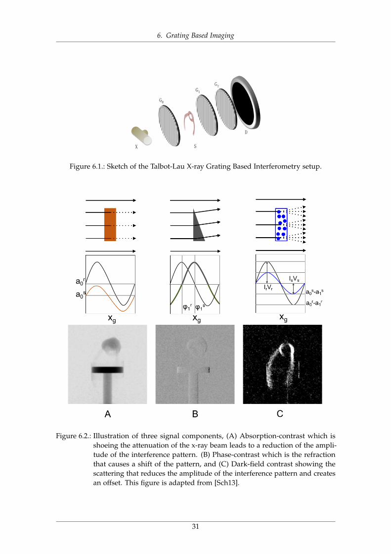
6. Grating Based Imaging
Figure 6.1.: Sketch of the Talbot-Lau X-ray Grating Based Interferometry setup.
Figure 6.2.: Illustration of three signal components, (A) Absorption-contrast which isshoeing the attenuation of the x-ray beam leads to a reduction of the ampli-tude of the interference pattern. (B) Phase-contrast which is the refractionthat causes a shift of the pattern, and (C) Dark-field contrast showing thescattering that reduces the amplitude of the interference pattern and createsan offset. This figure is adapted from [Sch13].
31
7. Other Imaging Modalities
In previous sections, We have discussed x-ray based imaging modalities and describedCT imaging modality including its physics, theory, reconstruction techniques, limitationsand challenges. However, several different types of medical imaging modalities are alsobeing used for clinical and non-clinical applications.
Positron emission tomography (PET) is a nuclear imaging technology that enables thevisualization of metabolic processes in the body. Another similar modality, Single-photonemission computed tomography (SPECT) is also using gamma rays and can providethree-dimensional information in the form of cross-sectional slice images of the patient.Some types of medical imaging modalities work without using ionizing radiation, forexample magnetic resonance imaging (MRI) and ultrasound imaging, and have beenutilized in diagnosis of several diseases.
In this section, we will briefly introduce some of these modalities by explaining theirtheory, structures and existing challenges.
7.1 Positron Emission Tomography (PET)A PET scan is a type of nuclear medicine imaging modality which is used to imagedifferent tissues to identify some conditions by looking at blood flow, metabolism, andoxygen use [Bai05].
PET imaging modality construct three-dimensional images by detecting gamma raysemitted when certain Radioactive tracers (radiotracers) are injected into a patient’s body.Radiotracers are absorbed by tissues with higher levels of metabolism (e.g., active tumors)than the rest of the body. Gamma rays are generated when a positron emitted from theradiotracer collides with an electron in tissue and results a pair of photons that emanatein opposite directions and are detected by detectors which are located around the patient.Unlike other anatomical imaging modalities such as CT and ultrasound, PET imagingprovides functional information of the imaging target [ABP12; Ter83; Ass17].
PET scans have been utilized to diagnose several diseases including heart disease, braintumors, stroke, cancer, head injuries, Parkinson’s disease, and many other disorders. Inneurology, PET has been used in a range of conditions, and in particular in severe focalepilepsy, where it may be used to compliment Magnetic Resonance Imaging [Gam02].
7.2 Single-photon Emission Computed Tomography(SPECT)
SPECT scanning is similar to PET, and is used to determine how organs inside the bodywork using the injection of a radioactive tracer; for the SPECT scan, the tracer will stay inthe bloodstream [Hol10].
32
7. Other Imaging Modalities
Similar to PET, the radiotracer starts emitting gamma rays, from the patient, whichcontrasts with the PET scans which emit positrons. Then, these rays are detected by thegamma camera that rotates through 360 degrees around the patient which enables thecross-sectional images to be assembled three-dimensionally similar to CT imaging. Thisenable the visualization of three-dimensional volumes or a series of two-dimensionalimages at the end [Kno83].
SPECT imaging has several different applications, which make this form of imagingconvenient for the medical tests. Cardiac SPECT scans can be used to inspect the bloodflow through the heart. SPECT scans can be also utilized to reveal hidden fractures inbone, such as shin splints and stress fractures because areas of bone healing usually lightup on the scans. It could be also used to inspect the parts of the brain that are affected byvarious disorders including Dementia, Epilepsy and head injuries [HT90].
7.3 Magnetic Resonance Imaging (MRI)Magnetic resonance imaging is a noninvasive imaging modality that allows for thevisualization of both structural and functional information of the scanned human body.
In 1938, Isidor Isaac Rabi described the NMR phenomenon for the first time by devel-oping a technique to measure the magnetic characteristics of atomic nucleus. Discoveryof Rabi, facilitated the development of MRI for use in clinical problems [ABP12]. In 1971,Raymond Damadian used NMR in medical applications by measuring T1 and T2 relax-ation times in rat tumors. Dr Damadian observed that a tumor tissue possessed longerT2 times than those of a normal tissue, a finding that was published in Science [Dam71].The first images of humans scanned in an MR machine were produced in 1977 whichis the crude images of the human thorax. In 1984, Michael Moseley established hiswork in diffusion imaging as a groundwork for fMRI techniques [WME84]. In the recentyears, diffusion tensor imaging (DTI) and fMRI using blood oxygenation level-dependent(BOLD) techniques were also introduced [Mos90].
Today, an MRI scanner consists of a large, powerful magnet in which the target lies.Signals will be sent to the body using a radio wave antenna and then received back.Returned signals are then converted into images. MR imaging has several applicationsincluding imaging of organs of the chest and abdomen such as heart, liver, biliary tract,kidneys, spleen, bowel, pancreas, and adrenal glands. It is also used to visualize thepelvic organs including the bladder and the reproductive organs such as the uterus andovaries in females and the prostate gland in males and also blood vessels [Le 92; ABP12].
7.4 UltrasoundIn Ultrasound imaging, also known as sonography, sound waves are used to be reflectedby organs and other interior body parts in real-time for image producing. An ultrasoundimage is produced based on the reflection of these waves off of the imaging targetstructures. The amplitude of the signal and the signal traveling time through the objectprovide the information to produce the images. Ultrasound imaging has been used forseveral years and has an excellent safety record. Unlike x-ray based imaging modalities,there is no ionizing radiation exposure associated with ultrasound modality [Sza04;MRA14]. However, diagnostic ultrasound has been one of the active research areas for
33
7. Other Imaging Modalities
last decade and several advancements have been reported in medical ultrasound imaging,elastography, ultrasound contrast agent imaging, super resolution imaging, and 2D arraytransducer [Lee17; SK17].
Ultrasound imaging has applications to evaluate the abnormalities in pregnancy,imaging of the heart and blood vessels and inspecting organs in the abdomen symptomsof pain [Shu15].
34
7. Other Imaging Modalities
35
8. Structure of this Thesis
Subject of this thesis is the advanced reconstruction and noise reduction techniques infour- and six-dimensional x-ray imaging modalities. We study two major research topicsorganized in two main parts, including Part (I) to study the six-dimensional x-ray tensortomography as a newly developed grating-based imaging modality which leveragesthe dark-field contrast projections to reconstruct volumes of medical and non-medicaltargets scanned. In this part, we will introduce XTT setup, theory and discuss theissues and limitations with using this modality for measuring of some medical andnon-medical specimens. We particularly, focus on the data processing chain of XTT,including image reconstruction and also noise reduction of XTT data and introduceseveral evaluation methods to assess the acquired data using these techniques. In thispart, we will investigate the best way to incorporate a denoising technique into the XTTreconstruction pipeline, in particular the popular total variation denoising technique.We will propose two different schemes of including denoising into the reconstructionprocess, one using a column block-parallel iterative scheme and one using a whole-systemapproach. Additionally, we will compare results using a simple denoising approach,applied either before or after reconstruction. Several experiments will be introduced andcorresponding results will be illustrated visually and quantitatively for both medical andnon-medical datasets.
Part (II) of this thesis, includes the low-dose CT perfusion imaging study of theliver and includes various advanced data processing, image reconstruction and analysisapproaches. In this part, we will introduce CT perfusion which is a recently developedCT imaging technique with several demonstrated clinical and pre-clinical utility in thedetection, staging, and analysis of treatment response for different applications such headand neck, liver, lung and colorectal imaging [Mil12]. CT perfusion has been successfullyemployed to assess the extent of salvageable tissue in acute stroke cases [SL05]. It hasalso been used in assessing tumor vascularity changes that result from chemotherapyand radiation therapy [Sah07]. CT perfusion of the liver can reveal hepatic diseases andthat can be used to assess treatment responses [LMS15]. More widespread adoption ofliver CTP in clinical trials to assess its potential as a biomarker as well as broader clinicaluse have been hampered by concerns over radiation exposure.
A variety of strategies have been proposed to limit radiation exposure includingthe individualization of scanning parameters, modification of tube current or voltagethroughout the observation period. However, decreasing the x-ray radiation dose reducesCT image quality with increased noise and possible streak artifacts which lowers theclinical and diagnosis utility of the scan.
In this part, we address the low-dose CT perfusion imaging of the liver by designing asimulation study based on the real animal data. Finally, we adapt a novel data processingchains including reconstruction of difference [Pou16] to investigate the reduction ofradiation dose level for CT perfusion studies.
we apply the RoD method to low-dose CTP data. The approach is investigated in
36
8. Structure of this Thesis
simulation studies using an anthropomorphic phantom with realistic time attenuationcurves (TACs) for different tissue types. We analyze imaging performance in individualreconstructions in the imaging sequence from contrast injection, through uptake, andwashout, and perform a perfusion analysis to compare several perfusion metrics includinghepatic arterial perfusion, hepatic portal perfusion, hepatic perfusion index and time-to-peak metrics. The RoD approach is compared with traditional FBP and penalized-likelihood (MBIR) reconstructions.
37
8. Structure of this Thesis
38

Part II.
X-RAY TENSOR TOMOGRAPHY
39

9. Introduction to X-ray Tensor Tomography
9.1 OverviewIn this chapter, we introduce X-ray Tensor Tomography (XTT), as a novel x-ray imagingmodality used for reconstruction of three-dimensional x-ray scattering tensors fromdark-field projections obtained in a grating-based interferometry setup. A detailedintroduction on the background of XTT imaging modality and previous related studieswill be discussed in section 9.2. An introduction of acquisition and forward model willfollow in sections 9.3 and 9.4. Finally, in 9.5, we explain the existing reconstructionmethod for XTT imaging.
9.2 BackgroundConventional x-ray imaging methods rely on the attenuation of x-rays when they passthrough an object. Recently, grating interferometer based approaches [Mom03; Pfe06a]have been proposed to extract the scattering and refraction of x-rays by the scanned objectin order to obtain phase and dark-field contrast. Dark-field contrast is a measurementof the ultra-small angle of x-rays deviating from their origin after interaction with sub-micron sized structures [Con12; Pel14b; Wan14]. The dark-field contrast obtained in agrating interferometry setup is an anisotropic signal, which means that the measuredsignal depends on the orientation of the scattering material with respect to the gratingsensitivity direction [Bay14a; Yas11]. This feature can be used to extract the informationabout the orientation of different materials from the variations in the dark-field signal.
Dark-field imaging techniques have recently become quite popular in several fields ofresearch by showing promising results not only in medical applications, such as the diag-nosis of pulmonary emphysema in lungs, providing better resolution of small, calcifiedtumor nodules in breast scanning [Gra15; Yar13; And05; Sid11], the visualization of theorientation of bone micro-architecture without requiring high resolution detectors [Pot12],x-ray imaging using microbubbles as a scattering contrast [Vel13], reconstruction of tinydental tubules [Vog15], but also in material science applications, for example to ac-quire quantitative information on the form and structure factor of materials [Pra15] andinvestigation of the fiber orientation of injection molded polymers [Han15; Rev11].
Jensen et al. [Jen10; Pot12] introduced directional two dimensional x-ray dark-fieldimaging or x-ray vector radiography (XVR) to reconstruct structure orientations from sev-eral projections acquired by rotating the sample around the beam propagation direction.
Malecki et al. [Mal14; Mal13] introduced a novel three-dimensional extension ofdirectional X-ray dark-field imaging, called X-ray Tensor Tomography (XTT), whichplaces the sample on an Eulerian cradle, which allows rotation of the sample with threedegrees of freedom to provide a three-dimensional reconstruction of x-ray scatteringtensors at each location of the scanned sample, revealing the local orientation and
40
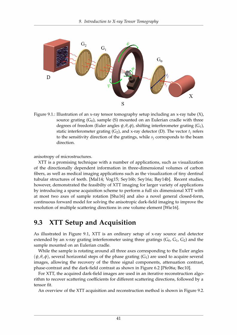
9. Introduction to X-ray Tensor Tomography
Figure 9.1.: Illustration of an x-ray tensor tomography setup including an x-ray tube (X),source grating (G0), sample (S) mounted on an Eulerian cradle with threedegrees of freedom (Euler angles ψ, θ, φ), shifting interferometer grating (G1),static interferometer grating (G2), and x-ray detector (D). The vector tj refersto the sensitivity direction of the gratings, while sj corresponds to the beamdirection.
anisotropy of microstructures.XTT is a promising technique with a number of applications, such as visualization
of the directionally dependent information in three-dimensional volumes of carbonfibers, as well as medical imaging applications such as the visualization of tiny dentinaltubular structures of teeth. [Mal14; Vog15; Sey16b; Sey16a; Bay14b]. Recent studies,however, demonstrated the feasibilty of XTT imaging for larger variety of applicationsby introducing a sparse acquisition scheme to perform a full six dimensional XTT withat most two axes of sample rotation [Sha16] and also a novel general closed-form,continuous forward model for solving the anisotropic dark-field imaging to improve theresolution of multiple scattering directions in one volume element [Wie16].
9.3 XTT Setup and AcquisitionAs illustrated in Figure 9.1, XTT is an ordinary setup of x-ray source and detectorextended by an x-ray grating interferometer using three gratings (G0, G1, G2) and thesample mounted on an Eulerian cradle.
While the sample is rotating around all three axes corresponding to the Euler angles(ψ, θ, φ), several horizontal steps of the phase grating (G1) are used to acquire severalimages, allowing the recovery of the three signal components, attenuation contrast,phase-contrast and the dark-field contrast as shown in Figure 6.2 [Pfe06a; Bec10].
For XTT, the acquired dark-field images are used in an iterative reconstruction algo-rithm to recover scattering coefficients for different scattering directions, followed by atensor fit.
An overview of the XTT acquisition and reconstruction method is shown in Figure 9.2.
41
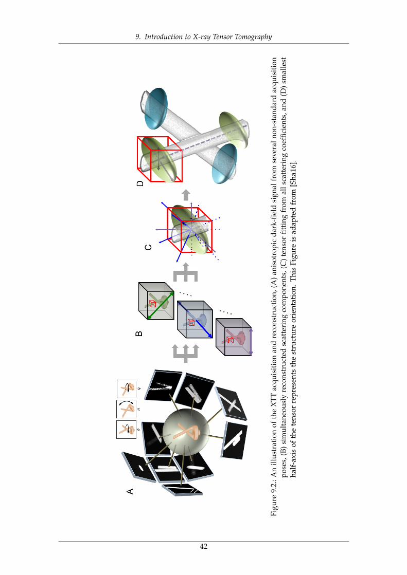
9. Introduction to X-ray Tensor Tomography
Figu
re9.
2.:A
nill
ustr
atio
nof
the
XTT
acqu
isiti
onan
dre
cons
truc
tion,
(A)
anis
otro
pic
dark
-fiel
dsi
gnal
from
seve
raln
on-s
tand
ard
acqu
isiti
onpo
ses,
(B)
sim
ulta
neou
sly
reco
nstr
ucte
dsc
atte
ring
com
pone
nts,
(C)
tens
orfit
ting
from
alls
catt
erin
gco
effic
ient
s,an
d(D
)sm
alle
stha
lf-a
xis
ofth
ete
nsor
repr
esen
tsth
est
ruct
ure
orie
ntat
ion.
This
Figu
reis
adap
ted
from
[Sha
16].
42
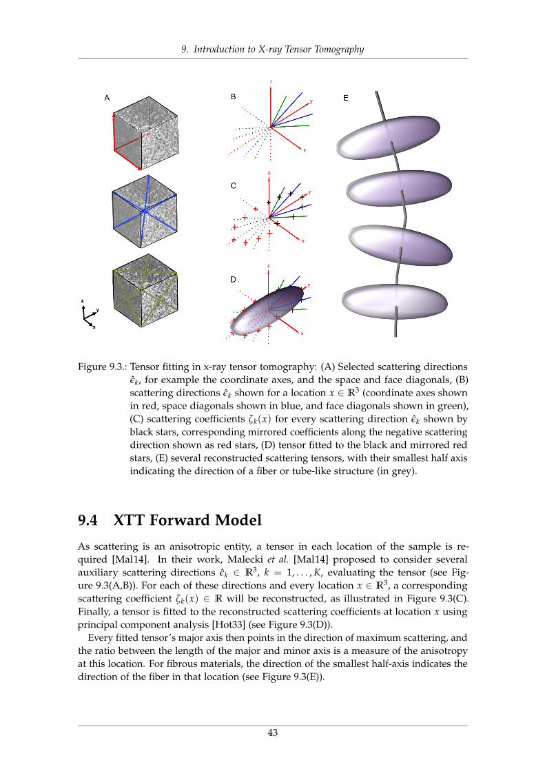
9. Introduction to X-ray Tensor Tomography
Figure 9.3.: Tensor fitting in x-ray tensor tomography: (A) Selected scattering directionsεk, for example the coordinate axes, and the space and face diagonals, (B)scattering directions εk shown for a location x ∈ R3 (coordinate axes shownin red, space diagonals shown in blue, and face diagonals shown in green),(C) scattering coefficients ζk(x) for every scattering direction εk shown byblack stars, corresponding mirrored coefficients along the negative scatteringdirection shown as red stars, (D) tensor fitted to the black and mirrored redstars, (E) several reconstructed scattering tensors, with their smallest half axisindicating the direction of a fiber or tube-like structure (in grey).
9.4 XTT Forward ModelAs scattering is an anisotropic entity, a tensor in each location of the sample is re-quired [Mal14]. In their work, Malecki et al. [Mal14] proposed to consider severalauxiliary scattering directions εk ∈ R3, k = 1, . . . , K, evaluating the tensor (see Fig-ure 9.3(A,B)). For each of these directions and every location x ∈ R3, a correspondingscattering coefficient ζk(x) ∈ R will be reconstructed, as illustrated in Figure 9.3(C).Finally, a tensor is fitted to the reconstructed scattering coefficients at location x usingprincipal component analysis [Hot33] (see Figure 9.3(D)).
Every fitted tensor’s major axis then points in the direction of maximum scattering, andthe ratio between the length of the major and minor axis is a measure of the anisotropyat this location. For fibrous materials, the direction of the smallest half-axis indicates thedirection of the fiber in that location (see Figure 9.3(E)).
43
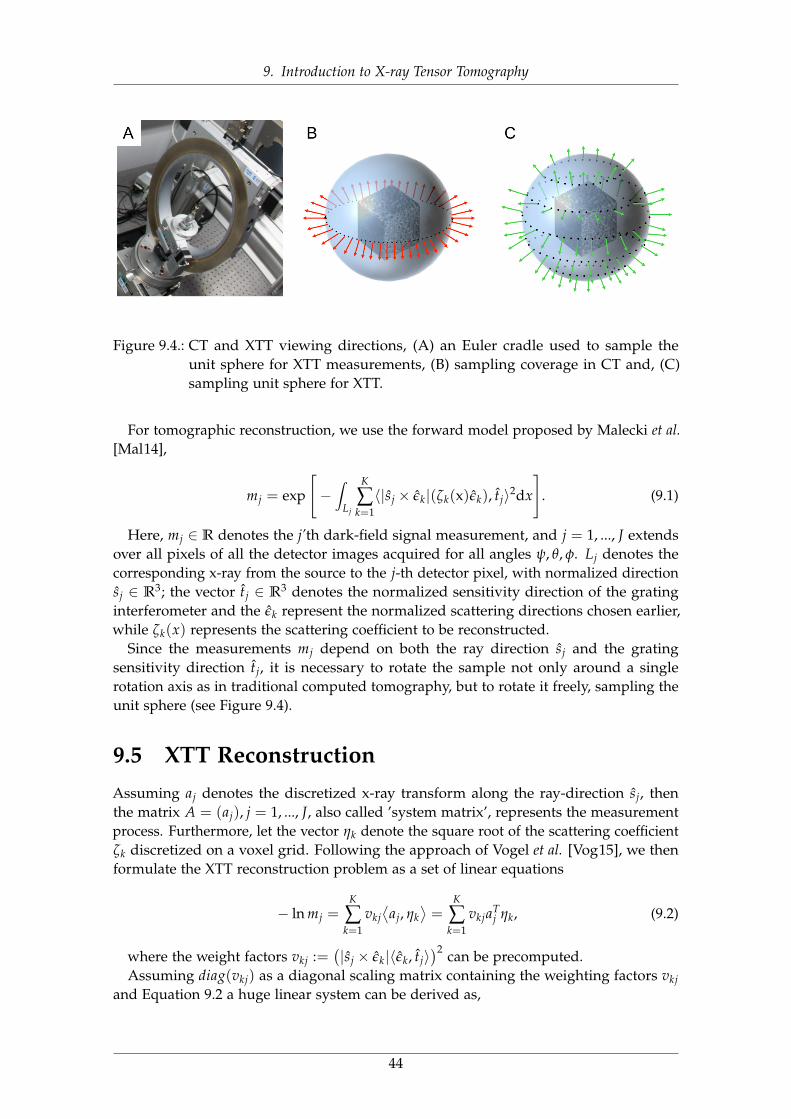
9. Introduction to X-ray Tensor Tomography
Figure 9.4.: CT and XTT viewing directions, (A) an Euler cradle used to sample theunit sphere for XTT measurements, (B) sampling coverage in CT and, (C)sampling unit sphere for XTT.
For tomographic reconstruction, we use the forward model proposed by Malecki et al.[Mal14],
mj = exp
[−∫
Lj
K
∑k=1〈|sj × εk|(ζk(x)εk), tj〉2dx
]. (9.1)
Here, mj ∈ R denotes the j’th dark-field signal measurement, and j = 1, ..., J extendsover all pixels of all the detector images acquired for all angles ψ, θ, φ. Lj denotes thecorresponding x-ray from the source to the j-th detector pixel, with normalized directionsj ∈ R3; the vector tj ∈ R3 denotes the normalized sensitivity direction of the gratinginterferometer and the εk represent the normalized scattering directions chosen earlier,while ζk(x) represents the scattering coefficient to be reconstructed.
Since the measurements mj depend on both the ray direction sj and the gratingsensitivity direction tj, it is necessary to rotate the sample not only around a singlerotation axis as in traditional computed tomography, but to rotate it freely, sampling theunit sphere (see Figure 9.4).
9.5 XTT ReconstructionAssuming aj denotes the discretized x-ray transform along the ray-direction sj, thenthe matrix A = (aj), j = 1, ..., J, also called ’system matrix’, represents the measurementprocess. Furthermore, let the vector ηk denote the square root of the scattering coefficientζk discretized on a voxel grid. Following the approach of Vogel et al. [Vog15], we thenformulate the XTT reconstruction problem as a set of linear equations
− ln mj =K
∑k=1
vkj⟨
aj, ηk⟩=
K
∑k=1
vkjaTj ηk, (9.2)
where the weight factors vkj :=(|sj × εk|〈εk, tj〉
)2 can be precomputed.Assuming diag(vkj) as a diagonal scaling matrix containing the weighting factors vkj
and Equation 9.2 a huge linear system can be derived as,
44
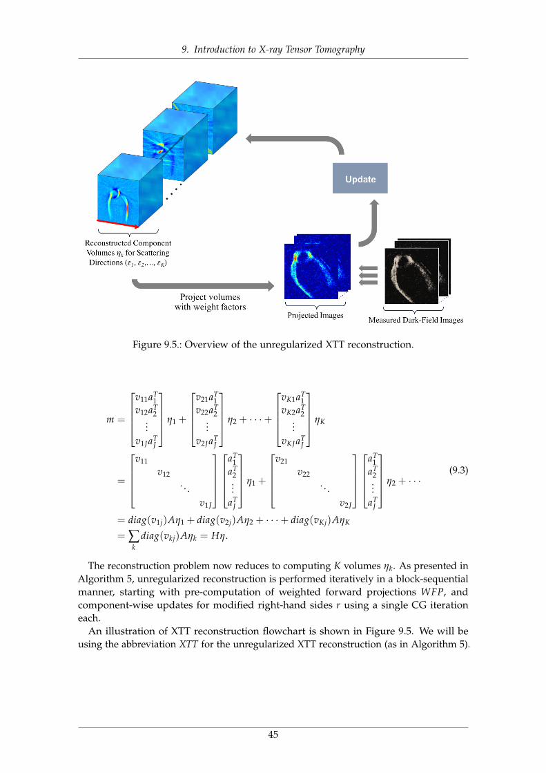
9. Introduction to X-ray Tensor Tomography
Figure 9.5.: Overview of the unregularized XTT reconstruction.
m =
v11aT
1v12aT
2...
v1JaTJ
η1 +
v21aT
1v22aT
2...
v2JaTJ
η2 + · · ·+
vK1aT
1vK2aT
2...
vKJaTJ
ηK
=
v11
v12. . .
v1J
aT1
aT2...
aTJ
η1 +
v21
v22. . .
v2J
aT1
aT2...
aTJ
η2 + · · ·
= diag(v1j)Aη1 + diag(v2j)Aη2 + · · ·+ diag(vKj)AηK
= ∑k
diag(vkj)Aηk = Hη.
(9.3)
The reconstruction problem now reduces to computing K volumes ηk. As presented inAlgorithm 5, unregularized reconstruction is performed iteratively in a block-sequentialmanner, starting with pre-computation of weighted forward projections WFP, andcomponent-wise updates for modified right-hand sides r using a single CG iterationeach.
An illustration of XTT reconstruction flowchart is shown in Figure 9.5. We will beusing the abbreviation XTT for the unregularized XTT reconstruction (as in Algorithm 5).
45
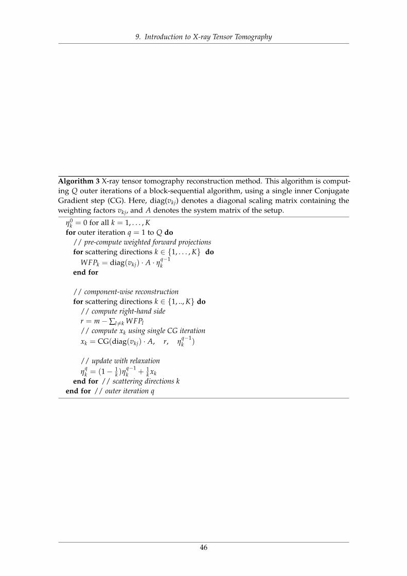
9. Introduction to X-ray Tensor Tomography
Algorithm 3 X-ray tensor tomography reconstruction method. This algorithm is comput-ing Q outer iterations of a block-sequential algorithm, using a single inner ConjugateGradient step (CG). Here, diag(vkj) denotes a diagonal scaling matrix containing theweighting factors vkj, and A denotes the system matrix of the setup.
η0k = 0 for all k = 1, . . . , K
for outer iteration q = 1 to Q do// pre-compute weighted forward projectionsfor scattering directions k ∈ {1, . . . , K} do
WFPk = diag(vkj) · A · ηq−1k
end for
// component-wise reconstructionfor scattering directions k ∈ {1, .., K} do
// compute right-hand sider = m−∑l 6=k WFPl// compute xk using single CG iterationxk = CG(diag(vkj) · A, r, η
q−1k )
// update with relaxationη
qk = (1− 1
k )ηq−1k + 1
k xkend for // scattering directions k
end for // outer iteration q
46
9. Introduction to X-ray Tensor Tomography
47
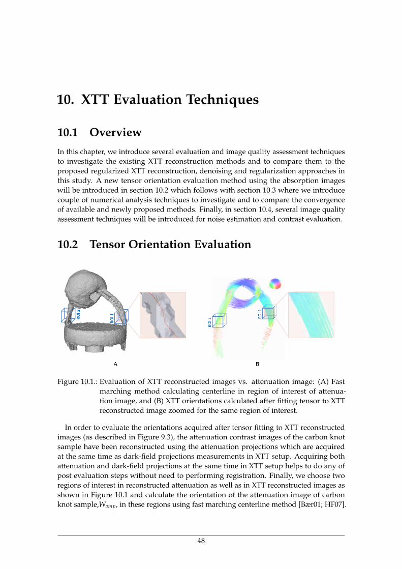
10. XTT Evaluation Techniques
10.1 OverviewIn this chapter, we introduce several evaluation and image quality assessment techniquesto investigate the existing XTT reconstruction methods and to compare them to theproposed regularized XTT reconstruction, denoising and regularization approaches inthis study. A new tensor orientation evaluation method using the absorption imageswill be introduced in section 10.2 which follows with section 10.3 where we introducecouple of numerical analysis techniques to investigate and to compare the convergenceof available and newly proposed methods. Finally, in section 10.4, several image qualityassessment techniques will be introduced for noise estimation and contrast evaluation.
10.2 Tensor Orientation Evaluation
Figure 10.1.: Evaluation of XTT reconstructed images vs. attenuation image: (A) Fastmarching method calculating centerline in region of interest of attenua-tion image, and (B) XTT orientations calculated after fitting tensor to XTTreconstructed image zoomed for the same region of interest.
In order to evaluate the orientations acquired after tensor fitting to XTT reconstructedimages (as described in Figure 9.3), the attenuation contrast images of the carbon knotsample have been reconstructed using the attenuation projections which are acquiredat the same time as dark-field projections measurements in XTT setup. Acquiring bothattenuation and dark-field projections at the same time in XTT setup helps to do any ofpost evaluation steps without need to performing registration. Finally, we choose tworegions of interest in reconstructed attenuation as well as in XTT reconstructed images asshown in Figure 10.1 and calculate the orientation of the attenuation image of carbonknot sample,Wamp, in these regions using fast marching centerline method [Bær01; HF07].
48
10. XTT Evaluation Techniques
For evaluation we use,
δ = tan−1(‖Wamp ×Wxtt‖
Wamp ·Wxtt
), (10.1)
where δ denotes the angle between Wamp, and corresponding Wxtt denoting the XTTdirection extracted after tensor fitting in the same region [Sey18c].
10.3 Numerical AnalysisIn order to study the numerical behavior of the proposed methods, we computed thenormalized residual norms,
r(q) :=‖m−∑k diag(vkj) · A · η
(q)k |2
‖m‖2, (10.2)
and also the normalized update,
M(q):=mean‖η(q)
k − η(q−1)k ‖2
‖η(q)k ‖2
. (10.3)
10.4 Image Quality AssessmentIn order to quantitatively measure the contrast in the images for the three differentmethods, we compute the contrast-to-noise ratio CNR() as,
CNR =|ηROI − ηBG|
σBG, (10.4)
where ηBG denotes the mean of the scattering signal of the all background (BG) areawhich is segmented and masked out using threshold mask.
Another qualitative evaluation metric that we use here is the signal-to-noise ratio(SNR),
SNR =ηROI
σBG, (10.5)
where ηROI denotes the mean of the scattering signal in a certain region of interest (ROI)of a component image η and σBG refers to the standard deviation of the background (BG)of each component.
To estimate noise levels, we use the median absolute deviation (MAD)[MT77],
MAD = median(|ηROI −median(ηROI)|
), (10.6)
49
11. XTT Reconstruction, Regularization andNoise Reduction
11.1 OverviewIn this chapter, we introduce several regularized reconstruction methods, noise reductionapproaches and post processing techniques for XTT imaging data . We propose variousregularized XTT reconstruction techniques such as parallel-block regularized XTT recon-struction technique in sections 11.2.2 and 11.2.1 and the whole-system regularized XTTreconstruction approach in section 11.3. Furthermore, two different noise reduction meth-ods will be introduced for incorporation of denoising step into the projection domainmeasurements and image domain data respectively in sections 11.2.1 and 11.2.2. Finally,in section 11.6, we will explain several conducted experiments to evaluate the proposedmethods and the corresponding results will be illustrated in section 11.7.
11.2 Block-parallel Regularized XTT ReconstructionMethods
Measured XTT data is always subject to signal fluctuations of various origins, which aregenerally and collectively referred to as "noise". The noise present in the recorded rawdark-field images will propagate through the reconstruction algorithm and influence thequality of the resulting images. Chabior et al.[Cha11] showed that the noise in dark-fieldcontrast images will always be higher than in attenuation-contrast images. Thus, the XTTimaging modality is very vulnerable to noise and should highly profit from denoising.
Total variation (TV) denoising is a well-known technique that was originally developedfor denoising images with additive Gaussian noise by Rudin, Osher and Fatemi [ROF92].Since then, TV methods have been successfully applied to a multitude of other imagedenoising problems, also within the computed tomography community[SP08; CTL08b;SY14b; Sey13b; Ert12; Sey14]. In particular, the TV denoising approach is often used inorder to recover images with a reduced noise level, while preserving the edges of theunderlying signal.[CL97; DS96].
In this section, we investigate the applicability of component based denoising approachin XTT modality by incorporating a TV denoising step into the XTT reconstruction usingtwo different pipeline designs and evaluate the best way to incorporate the TV noisereduction step for XTT data.
11.2.1 ADMM Regularized XTT ReconstructionsIn this section, we introduce a way to add a total variation (TV) regularization step whenupdating each XTT component ηk. For this purpose, we use several iterations of the
50
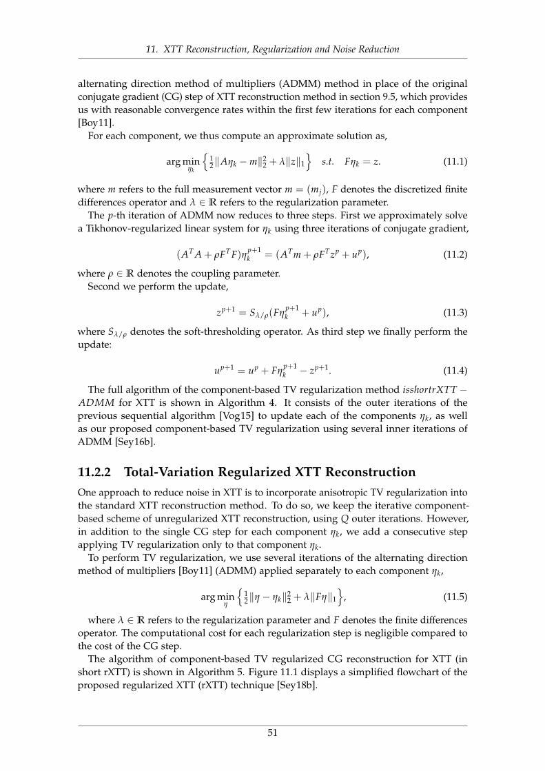
11. XTT Reconstruction, Regularization and Noise Reduction
alternating direction method of multipliers (ADMM) method in place of the originalconjugate gradient (CG) step of XTT reconstruction method in section 9.5, which providesus with reasonable convergence rates within the first few iterations for each component[Boy11].
For each component, we thus compute an approximate solution as,
arg minηk
{12‖Aηk −m‖2
2 + λ‖z‖1
}s.t. Fηk = z. (11.1)
where m refers to the full measurement vector m = (mj), F denotes the discretized finitedifferences operator and λ ∈ R refers to the regularization parameter.
The p-th iteration of ADMM now reduces to three steps. First we approximately solvea Tikhonov-regularized linear system for ηk using three iterations of conjugate gradient,
(AT A + ρFT F)ηp+1k = (ATm + ρFTzp + up), (11.2)
where ρ ∈ R denotes the coupling parameter.Second we perform the update,
zp+1 = Sλ/ρ(Fηp+1k + up), (11.3)
where Sλ/ρ denotes the soft-thresholding operator. As third step we finally perform theupdate:
up+1 = up + Fηp+1k − zp+1. (11.4)
The full algorithm of the component-based TV regularization method isshortrXTT −ADMM for XTT is shown in Algorithm 4. It consists of the outer iterations of theprevious sequential algorithm [Vog15] to update each of the components ηk, as wellas our proposed component-based TV regularization using several inner iterations ofADMM [Sey16b].
11.2.2 Total-Variation Regularized XTT ReconstructionOne approach to reduce noise in XTT is to incorporate anisotropic TV regularization intothe standard XTT reconstruction method. To do so, we keep the iterative component-based scheme of unregularized XTT reconstruction, using Q outer iterations. However,in addition to the single CG step for each component ηk, we add a consecutive stepapplying TV regularization only to that component ηk.
To perform TV regularization, we use several iterations of the alternating directionmethod of multipliers [Boy11] (ADMM) applied separately to each component ηk,
arg minη
{12‖η − ηk‖2
2 + λ‖Fη‖1
}, (11.5)
where λ ∈ R refers to the regularization parameter and F denotes the finite differencesoperator. The computational cost for each regularization step is negligible compared tothe cost of the CG step.
The algorithm of component-based TV regularized CG reconstruction for XTT (inshort rXTT) is shown in Algorithm 5. Figure 11.1 displays a simplified flowchart of theproposed regularized XTT (rXTT) technique [Sey18b].
51
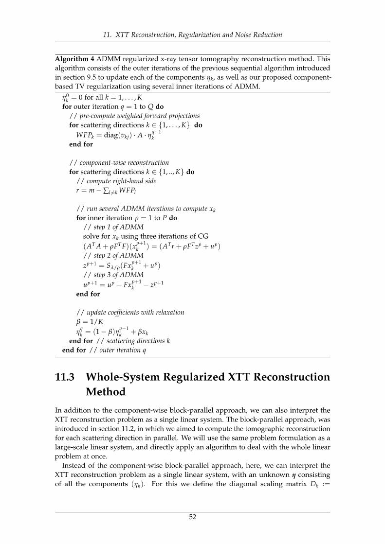
11. XTT Reconstruction, Regularization and Noise Reduction
Algorithm 4 ADMM regularized x-ray tensor tomography reconstruction method. Thisalgorithm consists of the outer iterations of the previous sequential algorithm introducedin section 9.5 to update each of the components ηk, as well as our proposed component-based TV regularization using several inner iterations of ADMM.
η0k = 0 for all k = 1, . . . , K
for outer iteration q = 1 to Q do// pre-compute weighted forward projectionsfor scattering directions k ∈ {1, . . . , K} do
WFPk = diag(vkj) · A · ηq−1k
end for
// component-wise reconstructionfor scattering directions k ∈ {1, .., K} do
// compute right-hand sider = m−∑l 6=k WFPl
// run several ADMM iterations to compute xkfor inner iteration p = 1 to P do
// step 1 of ADMMsolve for xk using three iterations of CG(AT A + ρFT F)(xp+1
k ) = (ATr + ρFTzp + up)
// step 2 of ADMMzp+1 = Sλ/ρ(Fxp+1
k + up)
// step 3 of ADMMup+1 = up + Fxp+1
k − zp+1
end for
// update coefficients with relaxationβ = 1/Kη
qk = (1− β)η
q−1k + βxk
end for // scattering directions kend for // outer iteration q
11.3 Whole-System Regularized XTT ReconstructionMethod
In addition to the component-wise block-parallel approach, we can also interpret theXTT reconstruction problem as a single linear system. The block-parallel approach, wasintroduced in section 11.2, in which we aimed to compute the tomographic reconstructionfor each scattering direction in parallel. We will use the same problem formulation as alarge-scale linear system, and directly apply an algorithm to deal with the whole linearproblem at once.
Instead of the component-wise block-parallel approach, here, we can interpret theXTT reconstruction problem as a single linear system, with an unknown η consistingof all the components (ηk). For this we define the diagonal scaling matrix Dk :=
52
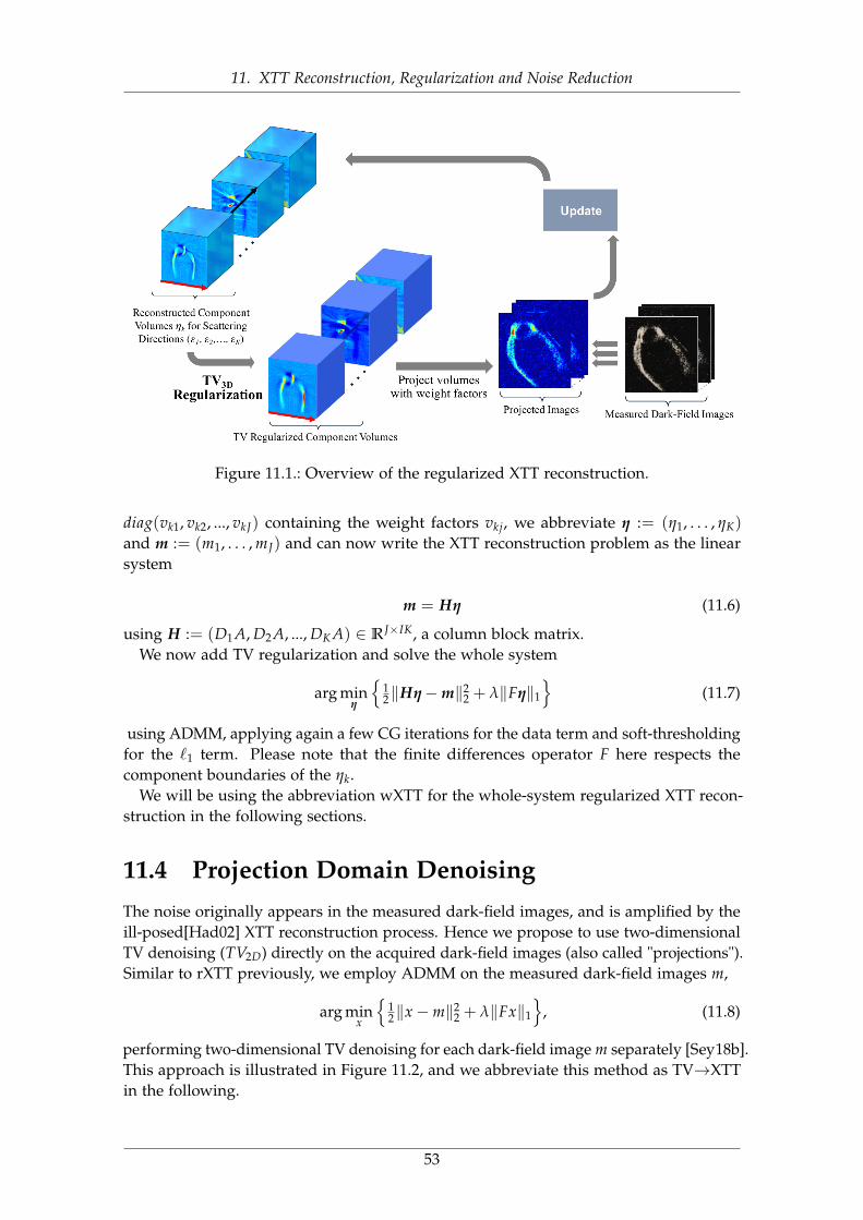
11. XTT Reconstruction, Regularization and Noise Reduction
Figure 11.1.: Overview of the regularized XTT reconstruction.
diag(vk1, vk2, ..., vkJ) containing the weight factors vkj, we abbreviate η := (η1, . . . , ηK)
and m := (m1, . . . , mJ) and can now write the XTT reconstruction problem as the linearsystem
m = Hη (11.6)
using H := (D1A, D2A, ..., DK A) ∈ RJ×IK, a column block matrix.We now add TV regularization and solve the whole system
arg minη
{12‖Hη−m‖2
2 + λ‖Fη‖1
}(11.7)
using ADMM, applying again a few CG iterations for the data term and soft-thresholdingfor the `1 term. Please note that the finite differences operator F here respects thecomponent boundaries of the ηk.
We will be using the abbreviation wXTT for the whole-system regularized XTT recon-struction in the following sections.
11.4 Projection Domain DenoisingThe noise originally appears in the measured dark-field images, and is amplified by theill-posed[Had02] XTT reconstruction process. Hence we propose to use two-dimensionalTV denoising (TV2D) directly on the acquired dark-field images (also called "projections").Similar to rXTT previously, we employ ADMM on the measured dark-field images m,
arg minx
{12‖x−m‖2
2 + λ‖Fx‖1
}, (11.8)
performing two-dimensional TV denoising for each dark-field image m separately [Sey18b].This approach is illustrated in Figure 11.2, and we abbreviate this method as TV→XTTin the following.
53
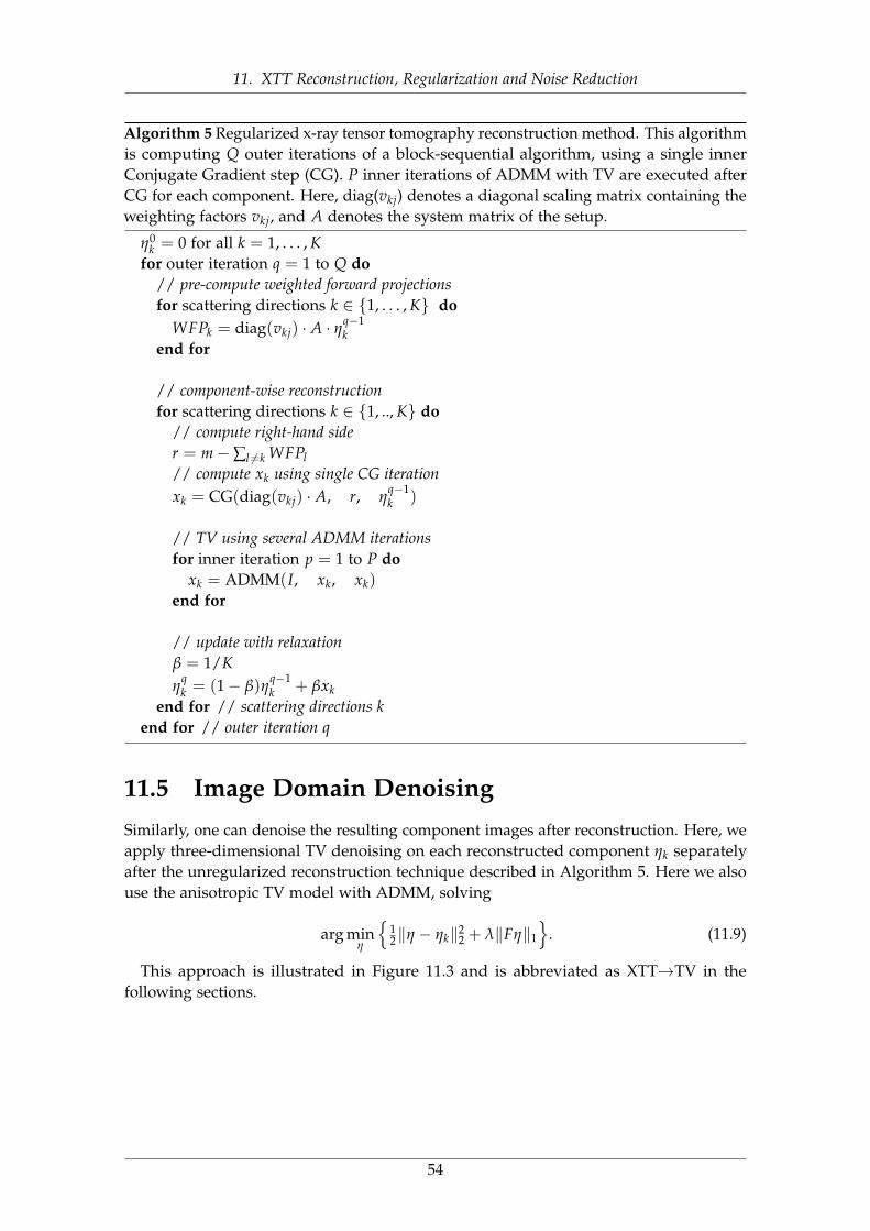
11. XTT Reconstruction, Regularization and Noise Reduction
Algorithm 5 Regularized x-ray tensor tomography reconstruction method. This algorithmis computing Q outer iterations of a block-sequential algorithm, using a single innerConjugate Gradient step (CG). P inner iterations of ADMM with TV are executed afterCG for each component. Here, diag(vkj) denotes a diagonal scaling matrix containing theweighting factors vkj, and A denotes the system matrix of the setup.
η0k = 0 for all k = 1, . . . , K
for outer iteration q = 1 to Q do// pre-compute weighted forward projectionsfor scattering directions k ∈ {1, . . . , K} do
WFPk = diag(vkj) · A · ηq−1k
end for
// component-wise reconstructionfor scattering directions k ∈ {1, .., K} do
// compute right-hand sider = m−∑l 6=k WFPl// compute xk using single CG iterationxk = CG(diag(vkj) · A, r, η
q−1k )
// TV using several ADMM iterationsfor inner iteration p = 1 to P do
xk = ADMM(I, xk, xk)
end for
// update with relaxationβ = 1/Kη
qk = (1− β)η
q−1k + βxk
end for // scattering directions kend for // outer iteration q
11.5 Image Domain DenoisingSimilarly, one can denoise the resulting component images after reconstruction. Here, weapply three-dimensional TV denoising on each reconstructed component ηk separatelyafter the unregularized reconstruction technique described in Algorithm 5. Here we alsouse the anisotropic TV model with ADMM, solving
arg minη
{12‖η − ηk‖2
2 + λ‖Fη‖1
}. (11.9)
This approach is illustrated in Figure 11.3 and is abbreviated as XTT→TV in thefollowing sections.
54
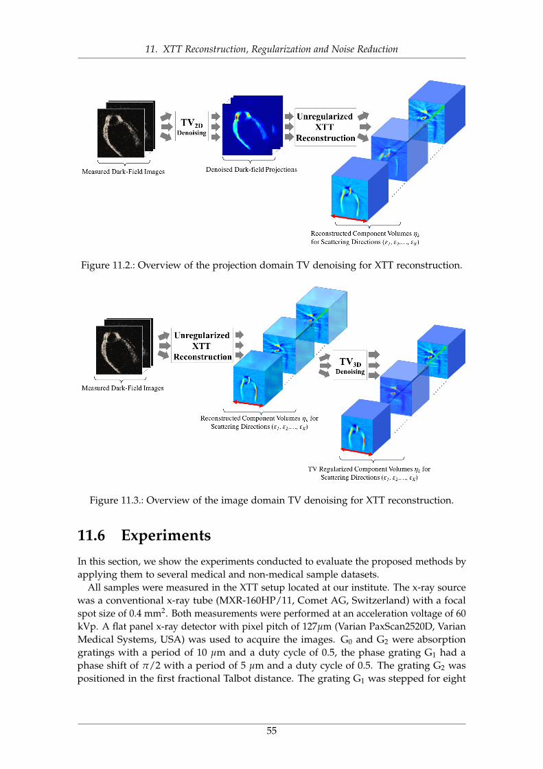
11. XTT Reconstruction, Regularization and Noise Reduction
Figure 11.2.: Overview of the projection domain TV denoising for XTT reconstruction.
Figure 11.3.: Overview of the image domain TV denoising for XTT reconstruction.
11.6 ExperimentsIn this section, we show the experiments conducted to evaluate the proposed methods byapplying them to several medical and non-medical sample datasets.
All samples were measured in the XTT setup located at our institute. The x-ray sourcewas a conventional x-ray tube (MXR-160HP/11, Comet AG, Switzerland) with a focalspot size of 0.4 mm2. Both measurements were performed at an acceleration voltage of 60kVp. A flat panel x-ray detector with pixel pitch of 127µm (Varian PaxScan2520D, VarianMedical Systems, USA) was used to acquire the images. G0 and G2 were absorptiongratings with a period of 10 µm and a duty cycle of 0.5, the phase grating G1 had aphase shift of π/2 with a period of 5 µm and a duty cycle of 0.5. The grating G2 waspositioned in the first fractional Talbot distance. The grating G1 was stepped for eight
55
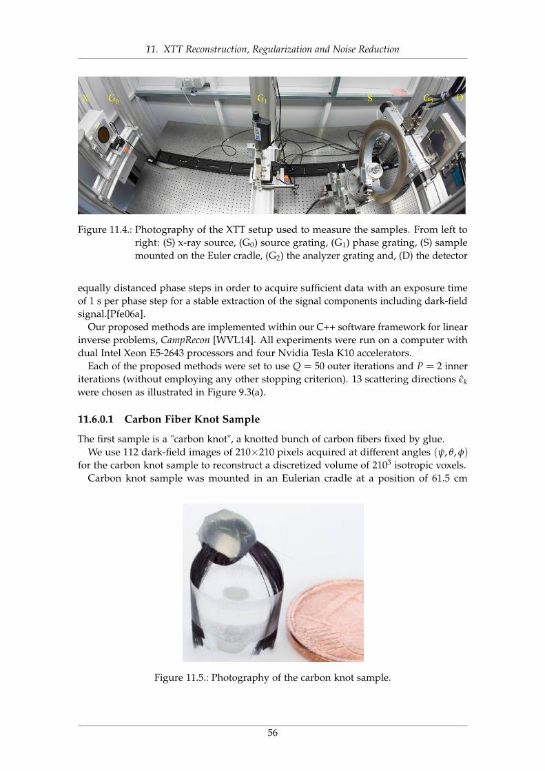
11. XTT Reconstruction, Regularization and Noise Reduction
Figure 11.4.: Photography of the XTT setup used to measure the samples. From left toright: (S) x-ray source, (G0) source grating, (G1) phase grating, (S) samplemounted on the Euler cradle, (G2) the analyzer grating and, (D) the detector
equally distanced phase steps in order to acquire sufficient data with an exposure timeof 1 s per phase step for a stable extraction of the signal components including dark-fieldsignal.[Pfe06a].
Our proposed methods are implemented within our C++ software framework for linearinverse problems, CampRecon [WVL14]. All experiments were run on a computer withdual Intel Xeon E5-2643 processors and four Nvidia Tesla K10 accelerators.
Each of the proposed methods were set to use Q = 50 outer iterations and P = 2 inneriterations (without employing any other stopping criterion). 13 scattering directions εkwere chosen as illustrated in Figure 9.3(a).
11.6.0.1 Carbon Fiber Knot Sample
The first sample is a "carbon knot", a knotted bunch of carbon fibers fixed by glue.We use 112 dark-field images of 210×210 pixels acquired at different angles (ψ, θ, φ)
for the carbon knot sample to reconstruct a discretized volume of 2103 isotropic voxels.Carbon knot sample was mounted in an Eulerian cradle at a position of 61.5 cm
Figure 11.5.: Photography of the carbon knot sample.
56
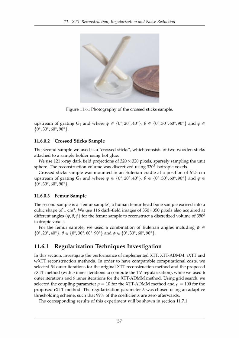
11. XTT Reconstruction, Regularization and Noise Reduction
Figure 11.6.: Photography of the crossed sticks sample.
upstream of grating G1 and where ψ ∈ {0◦, 20◦, 40◦}, θ ∈ {0◦, 30◦, 60◦, 90◦} and φ ∈{0◦, 30◦, 60◦, 90◦}.
11.6.0.2 Crossed Sticks Sample
The second sample we used is a "crossed sticks", which consists of two wooden sticksattached to a sample holder using hot glue.
We use 121 x-ray dark field projections of 320× 320 pixels, sparsely sampling the unitsphere. The reconstruction volume was discretized using 3203 isotropic voxels.
Crossed sticks sample was mounted in an Eulerian cradle at a position of 61.5 cmupstream of grating G1 and where ψ ∈ {0◦, 20◦, 40◦}, θ ∈ {0◦, 30◦, 60◦, 90◦} and φ ∈{0◦, 30◦, 60◦, 90◦}.
11.6.0.3 Femur Sample
The second sample is a "femur sample", a human femur head bone sample excised into acubic shape of 1 cm3. We use 116 dark-field images of 350×350 pixels also acquired atdifferent angles (ψ, θ, φ) for the femur sample to reconstruct a discretized volume of 3503
isotropic voxels.For the femur sample, we used a combination of Eulerian angles including ψ ∈{0◦, 20◦, 40◦}, θ ∈ {0◦, 30◦, 60◦, 90◦} and φ ∈ {0◦, 30◦, 60◦, 90◦}.
11.6.1 Regularization Techniques InvestigationIn this section, investigate the performance of implemented XTT, XTT-ADMM, rXTT andwXTT reconstruction methods. In order to have comparable computational costs, weselected 54 outer iterations for the original XTT reconstruction method and the proposedrXTT method (with 5 inner iterations to compute the TV regularization), while we used 6outer iterations and 9 inner iterations for the XTT-ADMM method. Using grid search, weselected the coupling parameter ρ = 10 for the XTT-ADMM method and ρ = 100 for theproposed rXTT method. The regularization parameter λ was chosen using an adaptivethresholding scheme, such that 99% of the coefficients are zero afterwards.
The corresponding results of this experiment will be shown in section 11.7.1.
57
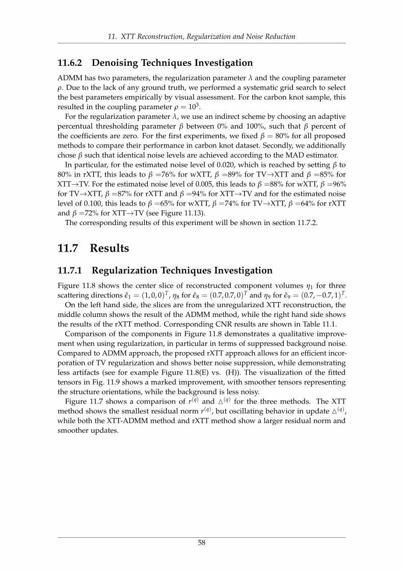
11. XTT Reconstruction, Regularization and Noise Reduction
11.6.2 Denoising Techniques InvestigationADMM has two parameters, the regularization parameter λ and the coupling parameterρ. Due to the lack of any ground truth, we performed a systematic grid search to selectthe best parameters empirically by visual assessment. For the carbon knot sample, thisresulted in the coupling parameter ρ = 103.
For the regularization parameter λ, we use an indirect scheme by choosing an adaptivepercentual thresholding parameter β between 0% and 100%, such that β percent ofthe coefficients are zero. For the first experiments, we fixed β = 80% for all proposedmethods to compare their performance in carbon knot dataset. Secondly, we additionallychose β such that identical noise levels are achieved according to the MAD estimator.
In particular, for the estimated noise level of 0.020, which is reached by setting β to80% in rXTT, this leads to β =76% for wXTT, β =89% for TV→XTT and β =85% forXTT→TV. For the estimated noise level of 0.005, this leads to β =88% for wXTT, β =96%for TV→XTT, β =87% for rXTT and β =94% for XTT→TV and for the estimated noiselevel of 0.100, this leads to β =65% for wXTT, β =74% for TV→XTT, β =64% for rXTTand β =72% for XTT→TV (see Figure 11.13).
The corresponding results of this experiment will be shown in section 11.7.2.
11.7 Results
11.7.1 Regularization Techniques InvestigationFigure 11.8 shows the center slice of reconstructed component volumes η1 for threescattering directions ε1 = (1, 0, 0)T, η8 for ε8 = (0.7, 0.7, 0)T and η9 for ε9 = (0.7,−0.7, 1)T.
On the left hand side, the slices are from the unregularized XTT reconstruction, themiddle column shows the result of the ADMM method, while the right hand side showsthe results of the rXTT method. Corresponding CNR results are shown in Table 11.1.
Comparison of the components in Figure 11.8 demonstrates a qualitative improve-ment when using regularization, in particular in terms of suppressed background noise.Compared to ADMM approach, the proposed rXTT approach allows for an efficient incor-poration of TV regularization and shows better noise suppression, while demonstratingless artifacts (see for example Figure 11.8(E) vs. (H)). The visualization of the fittedtensors in Fig. 11.9 shows a marked improvement, with smoother tensors representingthe structure orientations, while the background is less noisy.
Figure 11.7 shows a comparison of r(q) and M(q) for the three methods. The XTTmethod shows the smallest residual norm r(q), but oscillating behavior in update M(q),while both the XTT-ADMM method and rXTT method show a larger residual norm andsmoother updates.
58
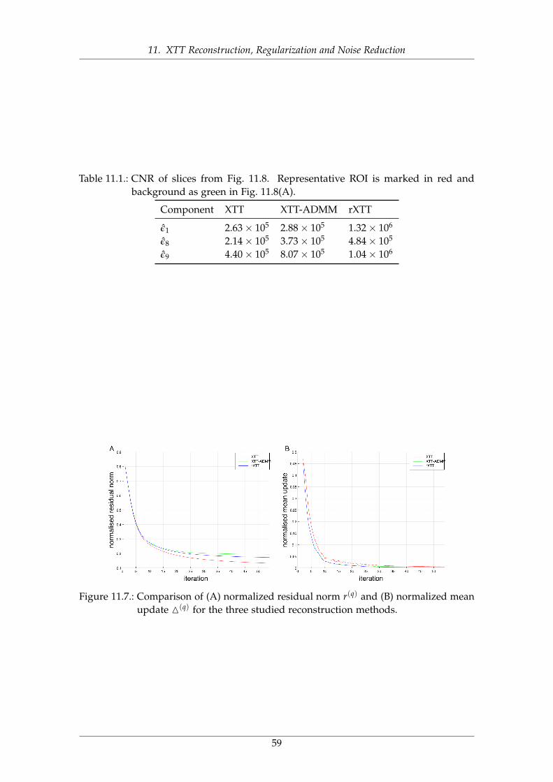
11. XTT Reconstruction, Regularization and Noise Reduction
Table 11.1.: CNR of slices from Fig. 11.8. Representative ROI is marked in red andbackground as green in Fig. 11.8(A).
Component XTT XTT-ADMM rXTT
ε1 2.63× 10⁵ 2.88× 10⁵ 1.32× 10⁶
ε8 2.14× 10⁵ 3.73× 10⁵ 4.84× 10⁵
ε9 4.40× 10⁵ 8.07× 10⁵ 1.04× 10⁶
Figure 11.7.: Comparison of (A) normalized residual norm r(q) and (B) normalized meanupdate M(q) for the three studied reconstruction methods.
59
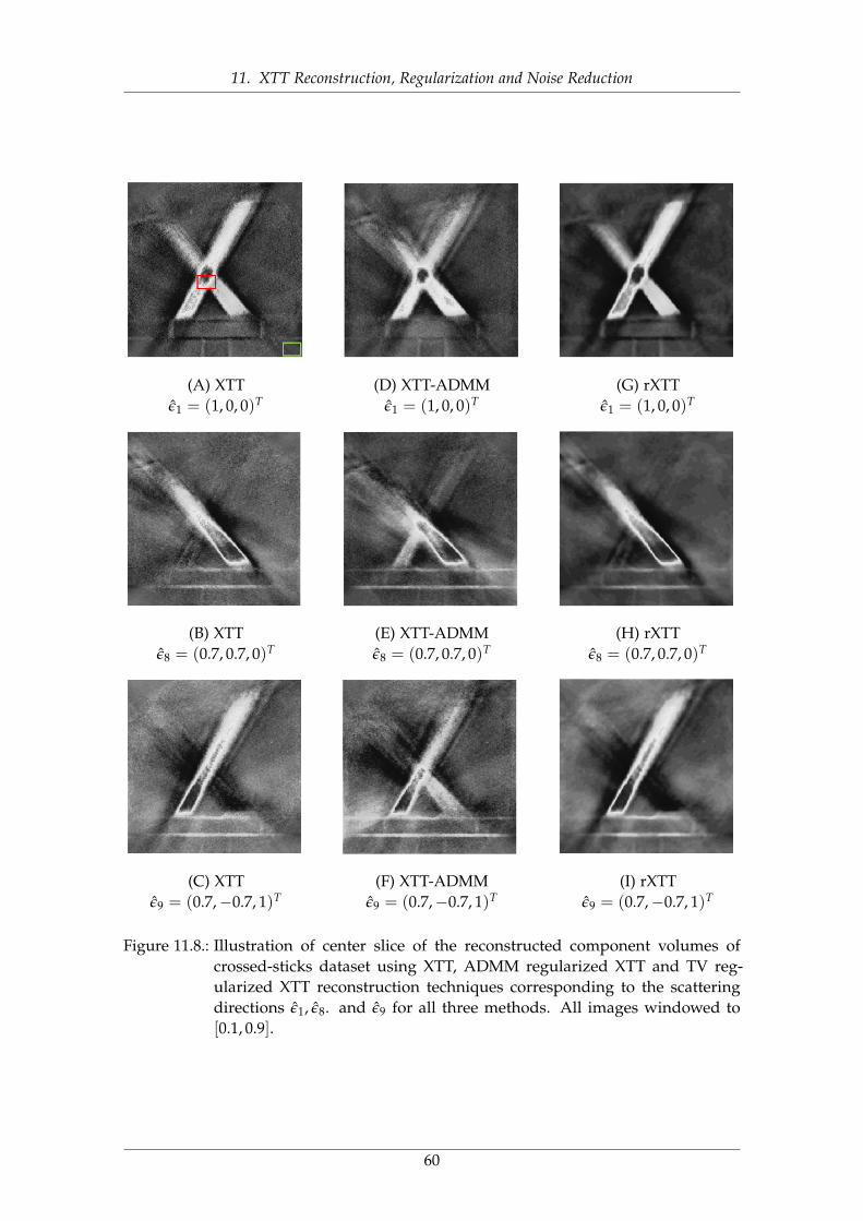
11. XTT Reconstruction, Regularization and Noise Reduction
(A) XTTε1 = (1, 0, 0)T
(D) XTT-ADMMε1 = (1, 0, 0)T
(G) rXTTε1 = (1, 0, 0)T
(B) XTTε8 = (0.7, 0.7, 0)T
(E) XTT-ADMMε8 = (0.7, 0.7, 0)T
(H) rXTTε8 = (0.7, 0.7, 0)T
(C) XTTε9 = (0.7,−0.7, 1)T
(F) XTT-ADMMε9 = (0.7,−0.7, 1)T
(I) rXTTε9 = (0.7,−0.7, 1)T
Figure 11.8.: Illustration of center slice of the reconstructed component volumes ofcrossed-sticks dataset using XTT, ADMM regularized XTT and TV reg-ularized XTT reconstruction techniques corresponding to the scatteringdirections ε1, ε8. and ε9 for all three methods. All images windowed to[0.1, 0.9].
60
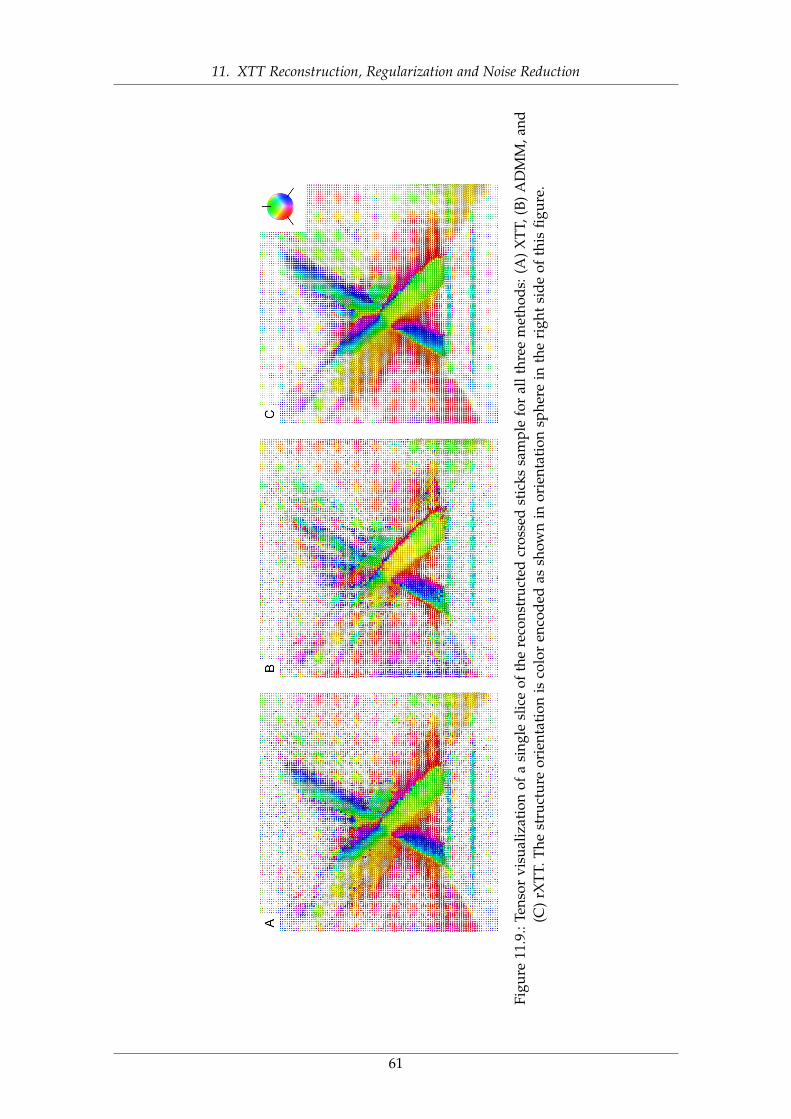
11. XTT Reconstruction, Regularization and Noise Reduction
Figu
re11
.9.:
Tens
orvi
sual
izat
ion
ofa
sing
lesl
ice
ofth
ere
cons
truc
ted
cros
sed
stic
kssa
mpl
efo
ral
lthr
eem
etho
ds:(
A)
XTT
,(B)
AD
MM
,and
(C)
rXTT
.The
stru
ctur
eor
ient
atio
nis
colo
ren
code
das
show
nin
orie
ntat
ion
sphe
rein
the
righ
tsi
deof
this
figur
e.
61
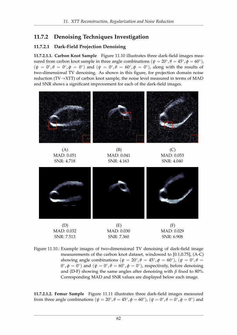
11. XTT Reconstruction, Regularization and Noise Reduction
11.7.2 Denoising Techniques Investigation
11.7.2.1 Dark-Field Projection Denoising
11.7.2.1.1. Carbon Knot Sample Figure 11.10 illustrates three dark-field images mea-sured from carbon knot sample in three angle combinations (ψ = 20◦, θ = 45◦, φ = 60◦),(ψ = 0◦, θ = 0◦, φ = 0◦) and (ψ = 0◦, θ = 60◦, φ = 0◦), along with the results oftwo-dimensional TV denoising. As shown in this figure, for projection domain noisereduction (TV→XTT) of carbon knot sample, the noise level measured in terms of MADand SNR shows a significant improvement for each of the dark-field images.
(A)MAD: 0.051SNR: 4.718
(B)MAD: 0.041SNR: 4.163
(C)MAD: 0.053SNR: 4.040
(D)MAD: 0.032SNR: 7.513
(E)MAD: 0.030SNR: 7.360
(F)MAD: 0.029SNR: 6.908
Figure 11.10.: Example images of two-dimensional TV denoising of dark-field imagemeasurements of the carbon knot dataset, windowed to [0.1,0.75], (A-C)showing angle combinations (ψ = 20◦, θ = 45◦, φ = 60◦), (ψ = 0◦, θ =
0◦, φ = 0◦) and (ψ = 0◦, θ = 60◦, φ = 0◦), respectively, before denoisingand (D-F) showing the same angles after denoising with β fixed to 80%.Corresponding MAD and SNR values are displayed below each image.
11.7.2.1.2. Femur Sample Figure 11.11 illustrates three dark-field images measuredfrom three angle combinations (ψ = 20◦, θ = 45◦, φ = 60◦), (ψ = 0◦, θ = 0◦, φ = 0◦) and
62
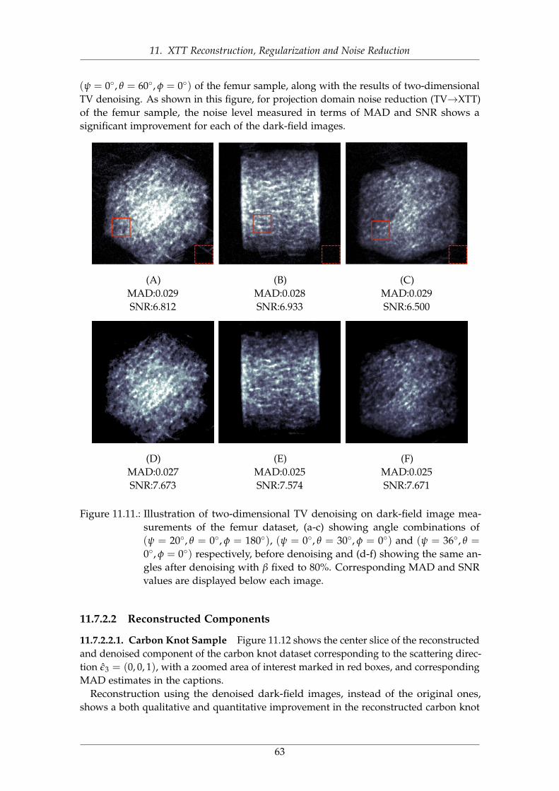
11. XTT Reconstruction, Regularization and Noise Reduction
(ψ = 0◦, θ = 60◦, φ = 0◦) of the femur sample, along with the results of two-dimensionalTV denoising. As shown in this figure, for projection domain noise reduction (TV→XTT)of the femur sample, the noise level measured in terms of MAD and SNR shows asignificant improvement for each of the dark-field images.
(A)MAD:0.029SNR:6.812
(B)MAD:0.028SNR:6.933
(C)MAD:0.029SNR:6.500
(D)MAD:0.027SNR:7.673
(E)MAD:0.025SNR:7.574
(F)MAD:0.025SNR:7.671
Figure 11.11.: Illustration of two-dimensional TV denoising on dark-field image mea-surements of the femur dataset, (a-c) showing angle combinations of(ψ = 20◦, θ = 0◦, φ = 180◦), (ψ = 0◦, θ = 30◦, φ = 0◦) and (ψ = 36◦, θ =
0◦, φ = 0◦) respectively, before denoising and (d-f) showing the same an-gles after denoising with β fixed to 80%. Corresponding MAD and SNRvalues are displayed below each image.
11.7.2.2 Reconstructed Components
11.7.2.2.1. Carbon Knot Sample Figure 11.12 shows the center slice of the reconstructedand denoised component of the carbon knot dataset corresponding to the scattering direc-tion ε3 = (0, 0, 1), with a zoomed area of interest marked in red boxes, and correspondingMAD estimates in the captions.
Reconstruction using the denoised dark-field images, instead of the original ones,shows a both qualitative and quantitative improvement in the reconstructed carbon knot
63
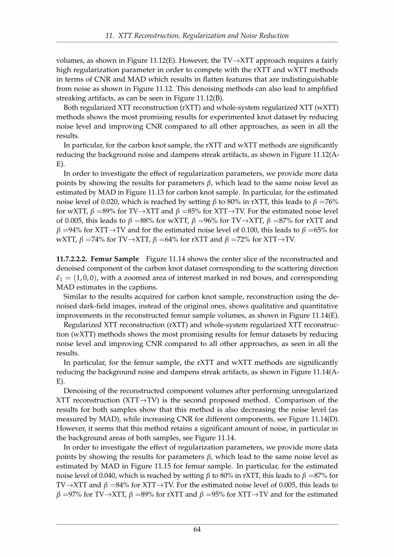
11. XTT Reconstruction, Regularization and Noise Reduction
volumes, as shown in Figure 11.12(E). However, the TV→XTT approach requires a fairlyhigh regularization parameter in order to compete with the rXTT and wXTT methodsin terms of CNR and MAD which results in flatten features that are indistinguishablefrom noise as shown in Figure 11.12. This denoising methods can also lead to amplifiedstreaking artifacts, as can be seen in Figure 11.12(B).
Both regularized XTT reconstruction (rXTT) and whole-system regularized XTT (wXTT)methods shows the most promising results for experimented knot dataset by reducingnoise level and improving CNR compared to all other approaches, as seen in all theresults.
In particular, for the carbon knot sample, the rXTT and wXTT methods are significantlyreducing the background noise and dampens streak artifacts, as shown in Figure 11.12(A-E).
In order to investigate the effect of regularization parameters, we provide more datapoints by showing the results for parameters β, which lead to the same noise level asestimated by MAD in Figure 11.13 for carbon knot sample. In particular, for the estimatednoise level of 0.020, which is reached by setting β to 80% in rXTT, this leads to β =76%for wXTT, β =89% for TV→XTT and β =85% for XTT→TV. For the estimated noise levelof 0.005, this leads to β =88% for wXTT, β =96% for TV→XTT, β =87% for rXTT andβ =94% for XTT→TV and for the estimated noise level of 0.100, this leads to β =65% forwXTT, β =74% for TV→XTT, β =64% for rXTT and β =72% for XTT→TV.
11.7.2.2.2. Femur Sample Figure 11.14 shows the center slice of the reconstructed anddenoised component of the carbon knot dataset corresponding to the scattering directionε1 = (1, 0, 0), with a zoomed area of interest marked in red boxes, and correspondingMAD estimates in the captions.
Similar to the results acquired for carbon knot sample, reconstruction using the de-noised dark-field images, instead of the original ones, shows qualitative and quantitativeimprovements in the reconstructed femur sample volumes, as shown in Figure 11.14(E).
Regularized XTT reconstruction (rXTT) and whole-system regularized XTT reconstruc-tion (wXTT) methods shows the most promising results for femur datasets by reducingnoise level and improving CNR compared to all other approaches, as seen in all theresults.
In particular, for the femur sample, the rXTT and wXTT methods are significantlyreducing the background noise and dampens streak artifacts, as shown in Figure 11.14(A-E).
Denoising of the reconstructed component volumes after performing unregularizedXTT reconstruction (XTT→TV) is the second proposed method. Comparison of theresults for both samples show that this method is also decreasing the noise level (asmeasured by MAD), while increasing CNR for different components, see Figure 11.14(D).However, it seems that this method retains a significant amount of noise, in particular inthe background areas of both samples, see Figure 11.14.
In order to investigate the effect of regularization parameters, we provide more datapoints by showing the results for parameters β, which lead to the same noise level asestimated by MAD in Figure 11.15 for femur sample. In particular, for the estimatednoise level of 0.040, which is reached by setting β to 80% in rXTT, this leads to β =87% forTV→XTT and β =84% for XTT→TV. For the estimated noise level of 0.005, this leads toβ =97% for TV→XTT, β =89% for rXTT and β =95% for XTT→TV and for the estimated
64
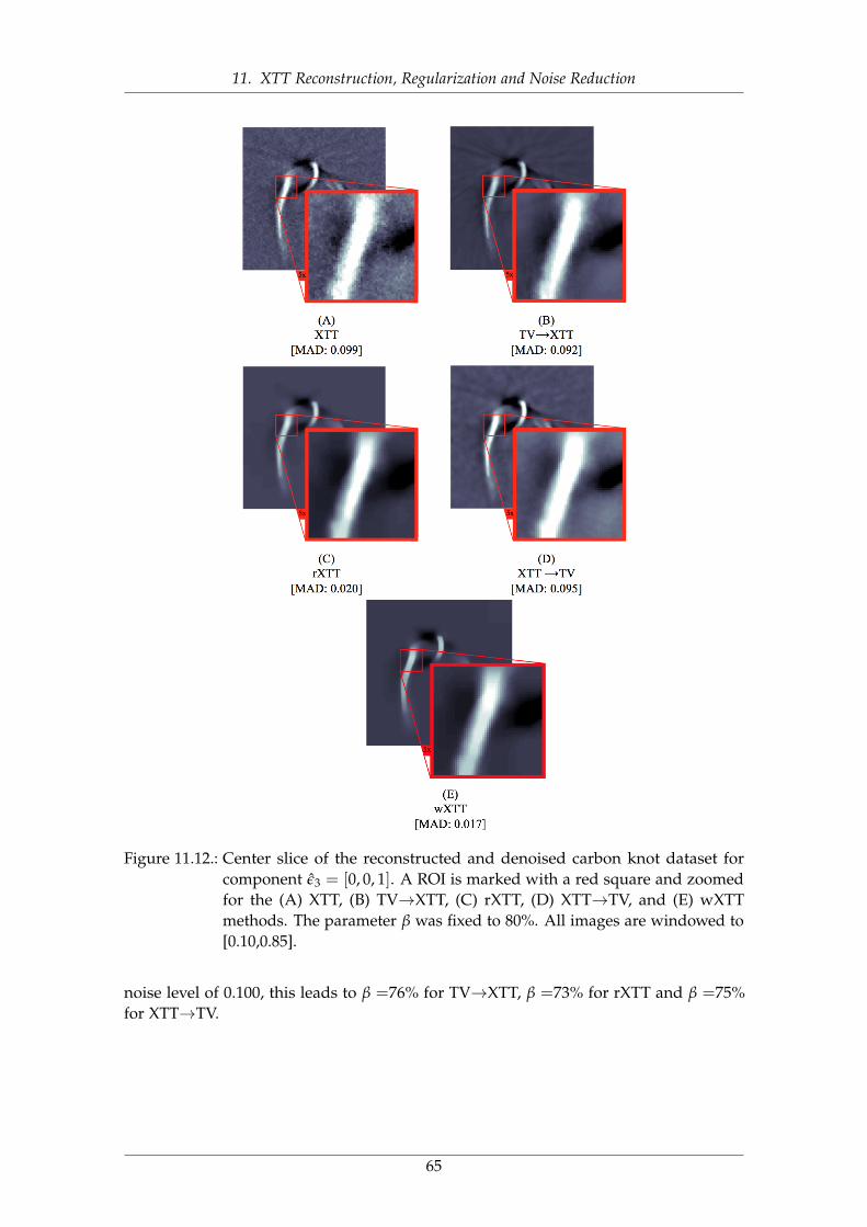
11. XTT Reconstruction, Regularization and Noise Reduction
Figure 11.12.: Center slice of the reconstructed and denoised carbon knot dataset forcomponent ε3 = [0, 0, 1]. A ROI is marked with a red square and zoomedfor the (A) XTT, (B) TV→XTT, (C) rXTT, (D) XTT→TV, and (E) wXTTmethods. The parameter β was fixed to 80%. All images are windowed to[0.10,0.85].
noise level of 0.100, this leads to β =76% for TV→XTT, β =73% for rXTT and β =75%for XTT→TV.
65
11. XTT Reconstruction, Regularization and Noise Reduction
Figure 11.13.: Zoomed area of interest of the images (see Figure 11.12) of the carbonknot dataset corresponding to the scattering direction ε3, windowed to[0.10,0.85]. The parameters β have been chosen such that the TV→XTT,rXTT and XTT→TV methods match in noise level as estimated by MAD.(A,E,I) TV→XTT, (B,F,J) rXTT, (C,G,K) XTT→TV, and (D,H,L) wXTT.
11.7.2.3 Components Quality Assessment
Illustration of MAD and CNR comparisons are shown in Figure 11.16, respectively, forthe reconstructed components of the scattering directions ε1, ε2 and ε3.
MAD and CNR comparisons for femur sample are shown in Figure 11.17, respectively,for the reconstructed components of the scattering directions ε1, ε2 and ε3.
66
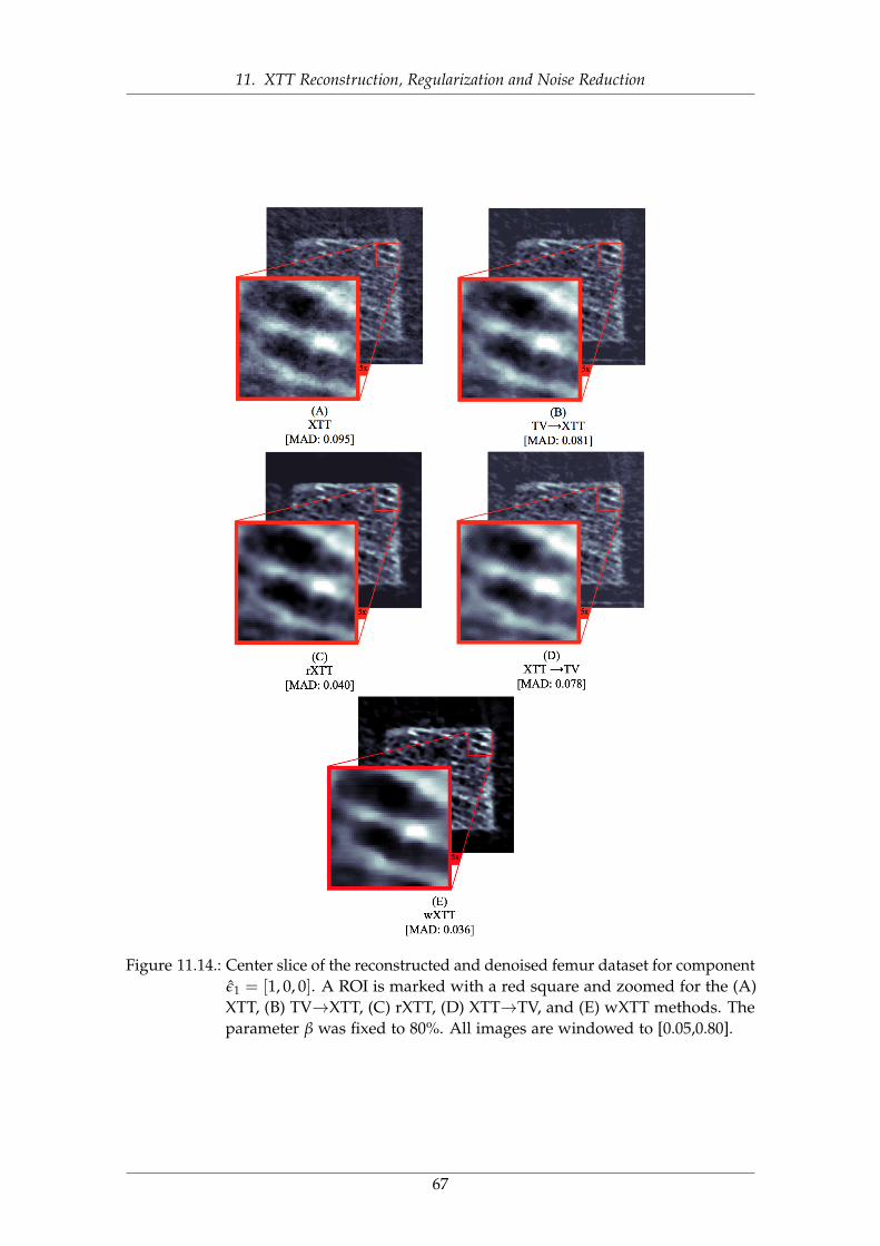
11. XTT Reconstruction, Regularization and Noise Reduction
Figure 11.14.: Center slice of the reconstructed and denoised femur dataset for componentε1 = [1, 0, 0]. A ROI is marked with a red square and zoomed for the (A)XTT, (B) TV→XTT, (C) rXTT, (D) XTT→TV, and (E) wXTT methods. Theparameter β was fixed to 80%. All images are windowed to [0.05,0.80].
67
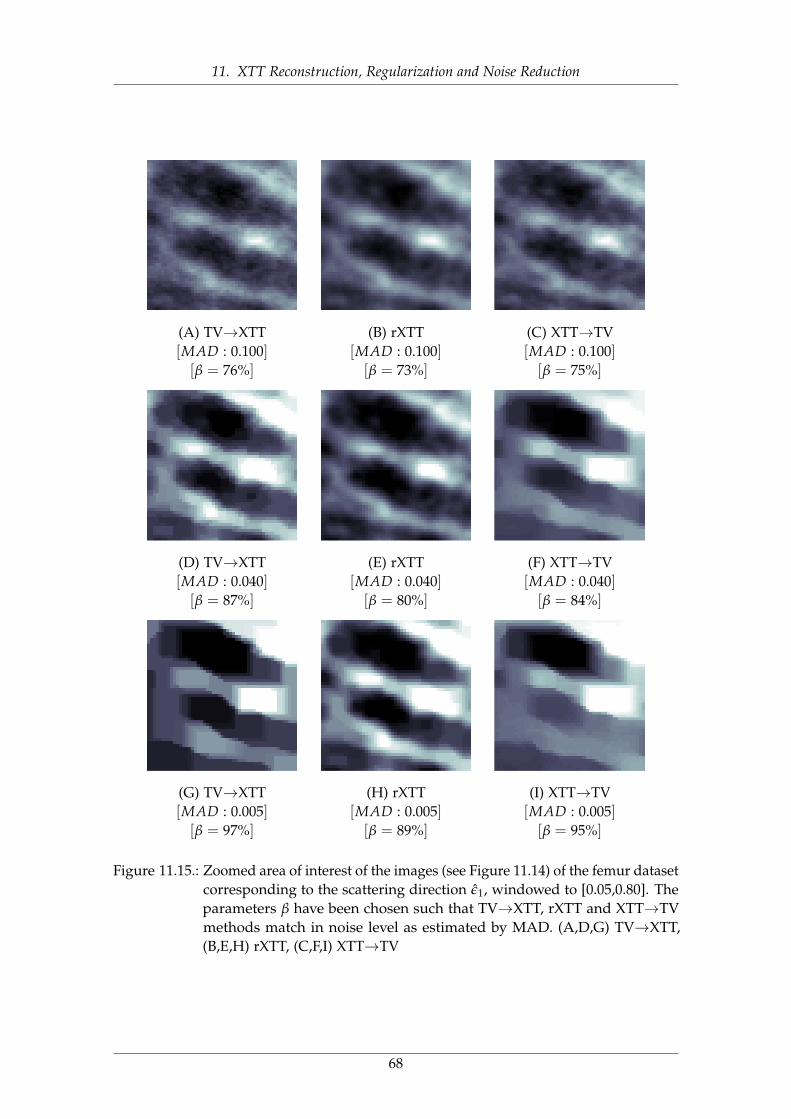
11. XTT Reconstruction, Regularization and Noise Reduction
(A) TV→XTT[MAD : 0.100][β = 76%]
(B) rXTT[MAD : 0.100][β = 73%]
(C) XTT→TV[MAD : 0.100][β = 75%]
(D) TV→XTT[MAD : 0.040][β = 87%]
(E) rXTT[MAD : 0.040][β = 80%]
(F) XTT→TV[MAD : 0.040][β = 84%]
(G) TV→XTT[MAD : 0.005][β = 97%]
(H) rXTT[MAD : 0.005][β = 89%]
(I) XTT→TV[MAD : 0.005][β = 95%]
Figure 11.15.: Zoomed area of interest of the images (see Figure 11.14) of the femur datasetcorresponding to the scattering direction ε1, windowed to [0.05,0.80]. Theparameters β have been chosen such that TV→XTT, rXTT and XTT→TVmethods match in noise level as estimated by MAD. (A,D,G) TV→XTT,(B,E,H) rXTT, (C,F,I) XTT→TV
68
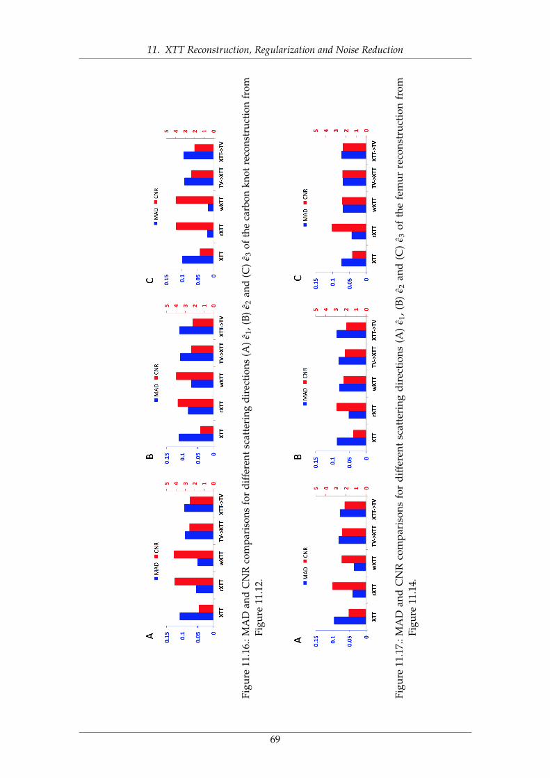
11. XTT Reconstruction, Regularization and Noise Reduction
Figu
re11
.16.
:MA
Dan
dC
NR
com
pari
sons
for
diff
eren
tsca
tter
ing
dire
ctio
ns(A
)ε 1
,(B)
ε 2an
d(C
)ε 3
ofth
eca
rbon
knot
reco
nstr
uctio
nfr
omFi
gure
11.1
2.
Figu
re11
.17.
:MA
Dan
dC
NR
com
par
ison
sfo
rd
iffe
rent
scat
teri
ngd
irec
tion
s(A
)ε 1
,(B
)ε 2
and
(C)
ε 3of
the
fem
ur
reco
nstr
uct
ion
from
Figu
re11
.14.
69
11. XTT Reconstruction, Regularization and Noise Reduction
11.7.2.4 Tensor Visualization
Figure 11.18 shows the center slice of the finally reconstructed tensors of carbon knotsample using all the scattering directions εk, visualized as tensors with the color encodingthe main structure orientation (see orientation color coding sphere in the center ofFigure 11.18).
Figure 11.19 shows the center slice of the finally reconstructed tensors of femur sampleusing all the scattering directions εk, visualized as tensors with the color encodingthe main structure orientation (see orientation color coding sphere in the center ofFigure 11.19).
11.7.2.5 Numerical Behavior
In order to study the convergence of proposed methods, a comparison of r(q) and ∆(q)
plots for the proposed methods was shown in Figure 11.20. The TV→XTT and XTTmethods show smaller residual norm r(q), but oscillating behavior in update ∆(q), whilerXTT and wXTT methods shows a larger residual norm and smoother updates. The rXTTand wXTT methods have been shown to produce considerably less noise artifact andvisually smoother, non-oscillating updates.
11.7.2.6 Tensor Orientation Evaluation
One of the limitations in XTT imaging assessment is the lack of any XTT groundtruth phantom to evaluate the proposed reconstruction and image denoising methods.However, In order to evaluate the XTT reconstruction and noise reduction methodsproposed in this paper, we introduced an approach based on the using of attenuationimages as a standard ground truth.
Figure 11.21(A,B) shows a histogram comparison of the angular differences δ of thefiber orientations for regular XTT and the two proposed methods rXTT and wXTT.A corresponding box plot is shown in Figure 11.21(C,D). As shown in this figure,comparison between the orientation information acquired from XTT reconstructionand noise reduction methods shows fairly small angles of deviations δ’s to the centerlineorientation of attenuation image while the proposed rXTT method exposes smallerdeviations comparing to the other methods.
11.8 ConclusionIn this chapter, we studied the best way to incorporate a denoising technique into the XTTreconstruction pipeline, in particular the popular total variation denoising technique. Weproposed two different schemes of including denoising into the reconstruction process,one using a column block-parallel iterative scheme and one using a whole-systemapproach. Additionally, we compared results using a simple denoising approach, appliedeither before or after reconstruction. As shown in the experiments and correspondingresults, all proposed methods show marked improvements in noise reduction for both ofour experimental datasets.
In order to study the convergence speed of the proposed methods, a comparison of r(q)
and ∆(q) plots was shown in Figure 11.20. The TV→XTT and XTT methods show smaller
70
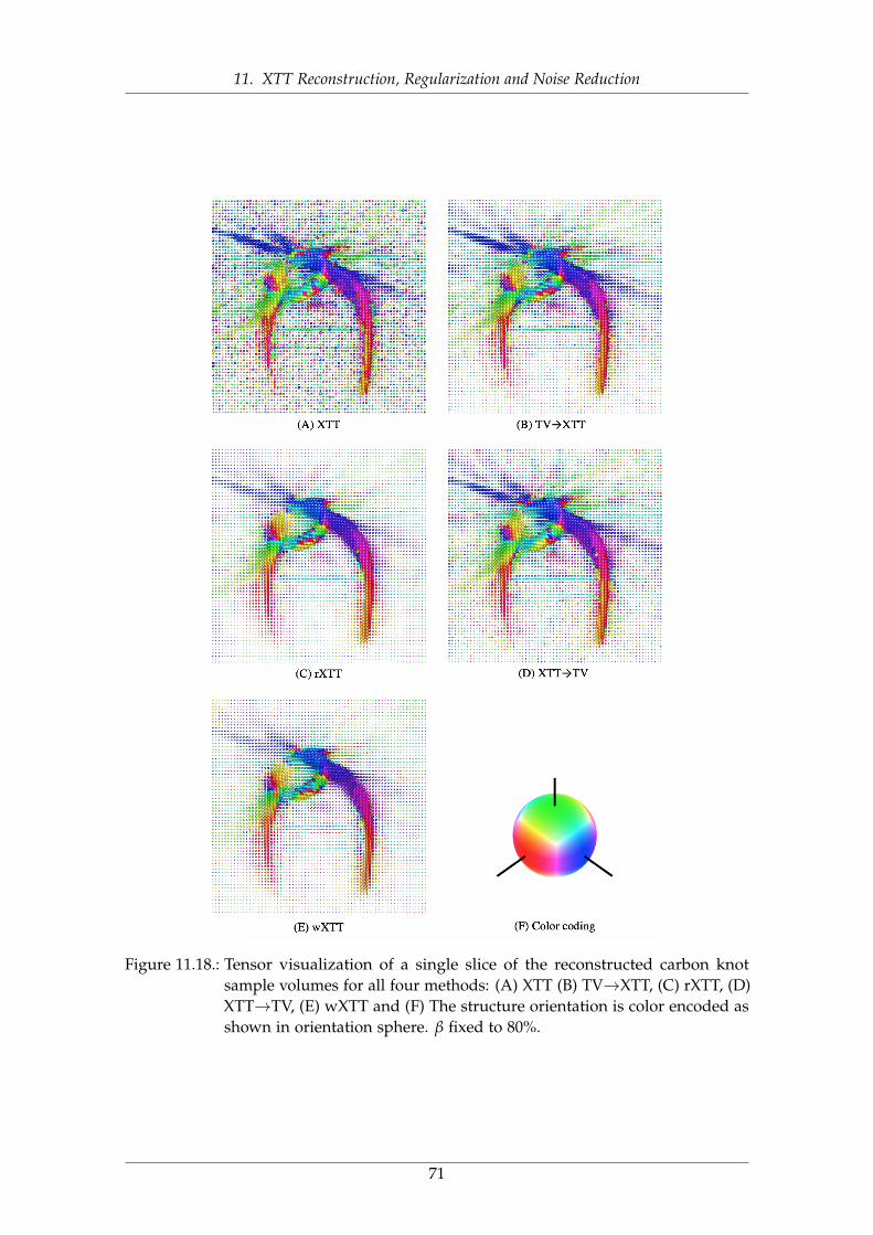
11. XTT Reconstruction, Regularization and Noise Reduction
Figure 11.18.: Tensor visualization of a single slice of the reconstructed carbon knotsample volumes for all four methods: (A) XTT (B) TV→XTT, (C) rXTT, (D)XTT→TV, (E) wXTT and (F) The structure orientation is color encoded asshown in orientation sphere. β fixed to 80%.
71
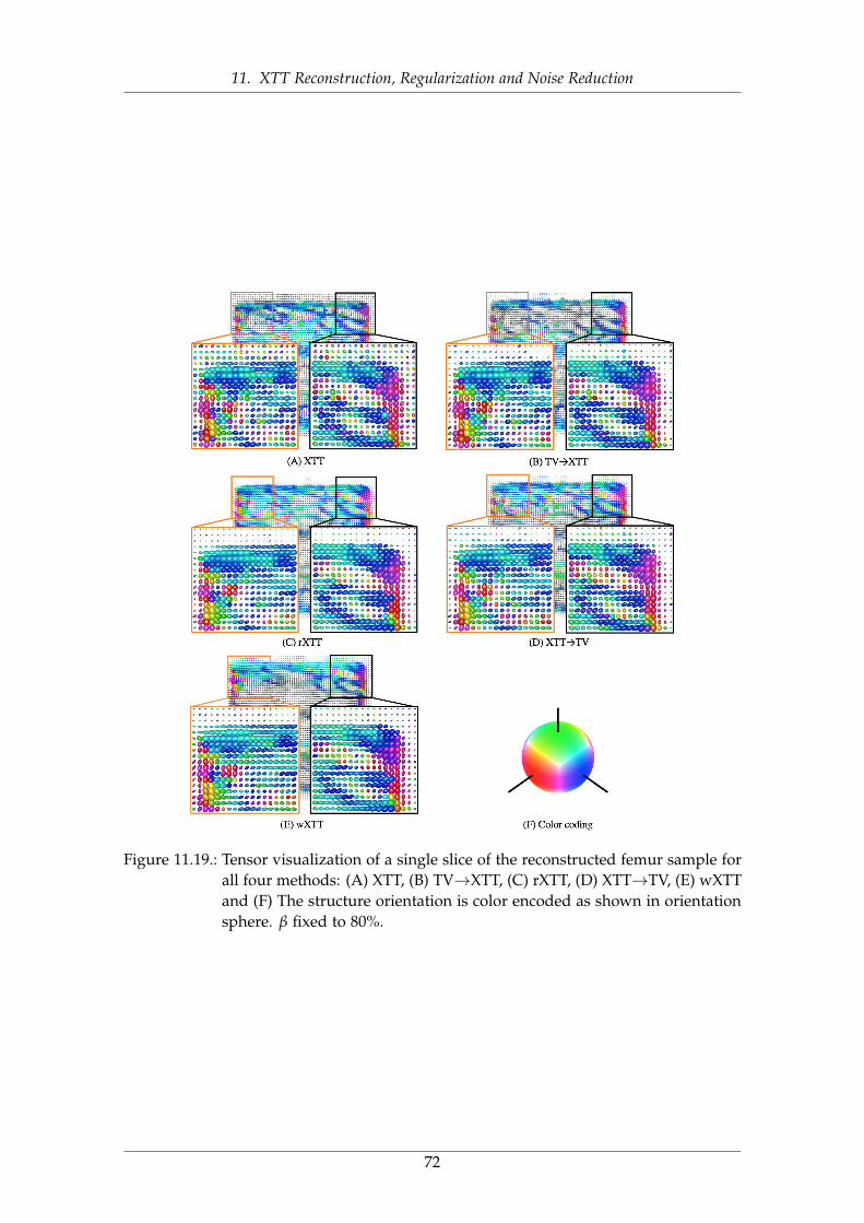
11. XTT Reconstruction, Regularization and Noise Reduction
Figure 11.19.: Tensor visualization of a single slice of the reconstructed femur sample forall four methods: (A) XTT, (B) TV→XTT, (C) rXTT, (D) XTT→TV, (E) wXTTand (F) The structure orientation is color encoded as shown in orientationsphere. β fixed to 80%.
72
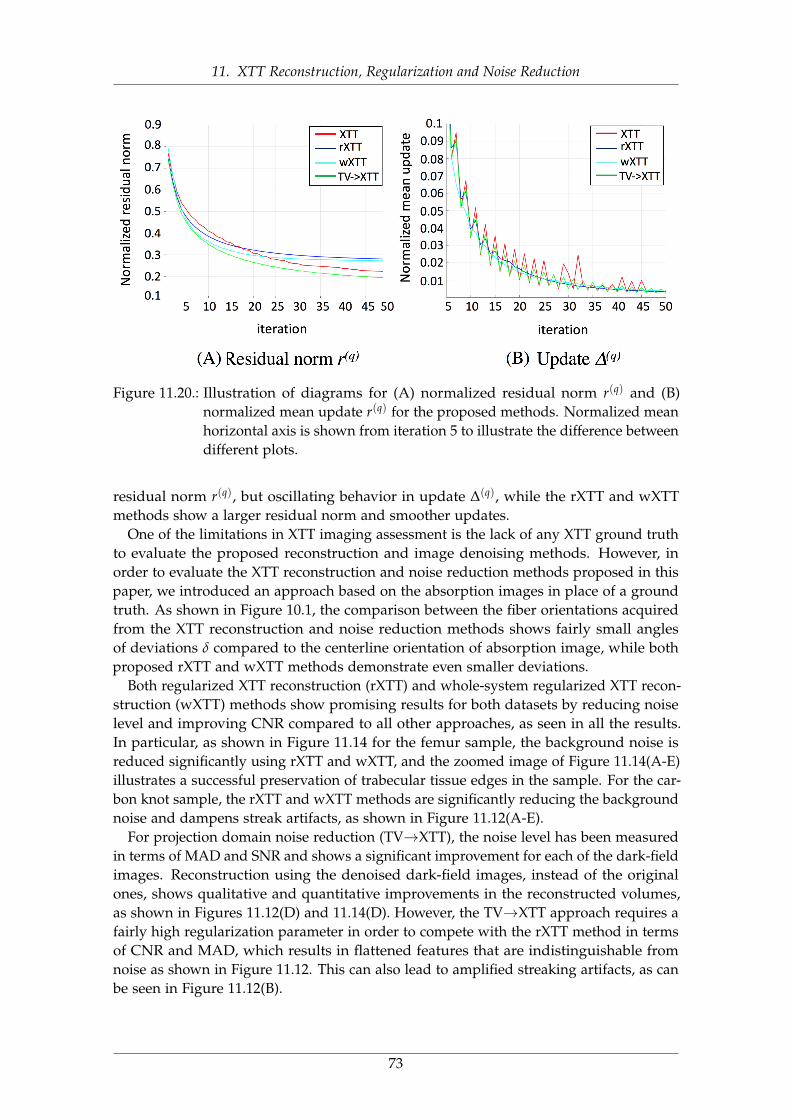
11. XTT Reconstruction, Regularization and Noise Reduction
Figure 11.20.: Illustration of diagrams for (A) normalized residual norm r(q) and (B)normalized mean update r(q) for the proposed methods. Normalized meanhorizontal axis is shown from iteration 5 to illustrate the difference betweendifferent plots.
residual norm r(q), but oscillating behavior in update ∆(q), while the rXTT and wXTTmethods show a larger residual norm and smoother updates.
One of the limitations in XTT imaging assessment is the lack of any XTT ground truthto evaluate the proposed reconstruction and image denoising methods. However, inorder to evaluate the XTT reconstruction and noise reduction methods proposed in thispaper, we introduced an approach based on the absorption images in place of a groundtruth. As shown in Figure 10.1, the comparison between the fiber orientations acquiredfrom the XTT reconstruction and noise reduction methods shows fairly small anglesof deviations δ compared to the centerline orientation of absorption image, while bothproposed rXTT and wXTT methods demonstrate even smaller deviations.
Both regularized XTT reconstruction (rXTT) and whole-system regularized XTT recon-struction (wXTT) methods show promising results for both datasets by reducing noiselevel and improving CNR compared to all other approaches, as seen in all the results.In particular, as shown in Figure 11.14 for the femur sample, the background noise isreduced significantly using rXTT and wXTT, and the zoomed image of Figure 11.14(A-E)illustrates a successful preservation of trabecular tissue edges in the sample. For the car-bon knot sample, the rXTT and wXTT methods are significantly reducing the backgroundnoise and dampens streak artifacts, as shown in Figure 11.12(A-E).
For projection domain noise reduction (TV→XTT), the noise level has been measuredin terms of MAD and SNR and shows a significant improvement for each of the dark-fieldimages. Reconstruction using the denoised dark-field images, instead of the originalones, shows qualitative and quantitative improvements in the reconstructed volumes,as shown in Figures 11.12(D) and 11.14(D). However, the TV→XTT approach requires afairly high regularization parameter in order to compete with the rXTT method in termsof CNR and MAD, which results in flattened features that are indistinguishable fromnoise as shown in Figure 11.12. This can also lead to amplified streaking artifacts, as canbe seen in Figure 11.12(B).
73
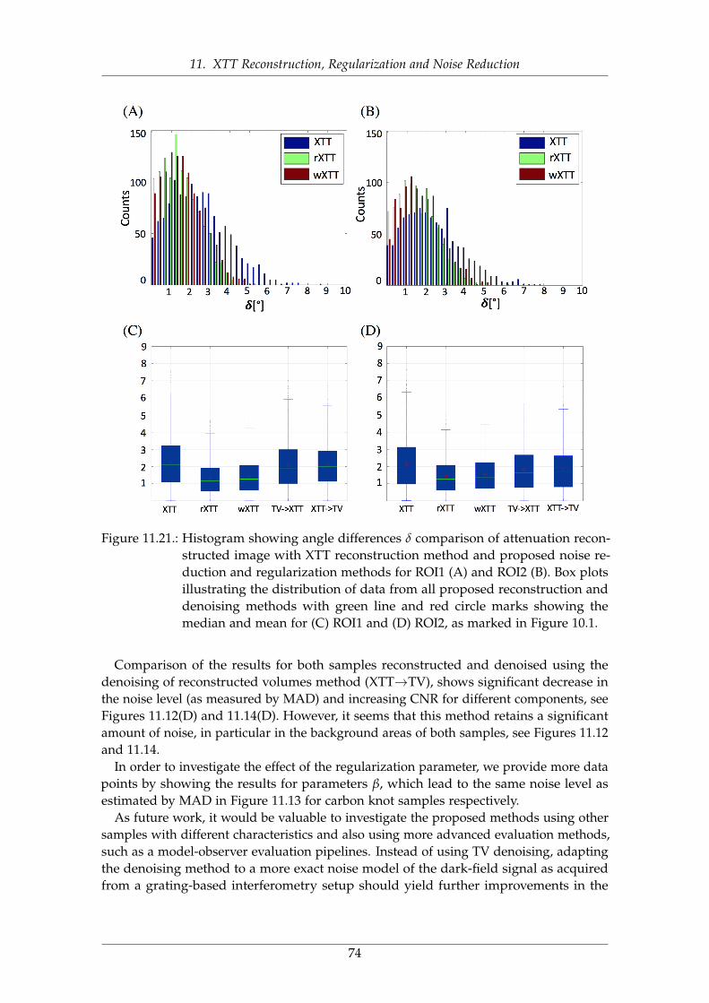
11. XTT Reconstruction, Regularization and Noise Reduction
Figure 11.21.: Histogram showing angle differences δ comparison of attenuation recon-structed image with XTT reconstruction method and proposed noise re-duction and regularization methods for ROI1 (A) and ROI2 (B). Box plotsillustrating the distribution of data from all proposed reconstruction anddenoising methods with green line and red circle marks showing themedian and mean for (C) ROI1 and (D) ROI2, as marked in Figure 10.1.
Comparison of the results for both samples reconstructed and denoised using thedenoising of reconstructed volumes method (XTT→TV), shows significant decrease inthe noise level (as measured by MAD) and increasing CNR for different components, seeFigures 11.12(D) and 11.14(D). However, it seems that this method retains a significantamount of noise, in particular in the background areas of both samples, see Figures 11.12and 11.14.
In order to investigate the effect of the regularization parameter, we provide more datapoints by showing the results for parameters β, which lead to the same noise level asestimated by MAD in Figure 11.13 for carbon knot samples respectively.
As future work, it would be valuable to investigate the proposed methods using othersamples with different characteristics and also using more advanced evaluation methods,such as a model-observer evaluation pipelines. Instead of using TV denoising, adaptingthe denoising method to a more exact noise model of the dark-field signal as acquiredfrom a grating-based interferometry setup should yield further improvements in the
74
11. XTT Reconstruction, Regularization and Noise Reduction
resulting image quality. The adapted denoising method could then be integrated intothe XTT reconstruction pipeline in the same way as suggested in this work for the TVdenoising method.
In summary, we have investigated several ways of incorporating a denoising approachinto the XTT reconstruction technique. In particular, we studied a component-basedregularized reconstruction technique, interleaving denoising with the regular block-parallel XTT reconstruction step in each iteration (rXTT), as well as a whole-systemapproach using regularization directly (wXTT). The results of the conducted experimentsshow a marked improvement in noise reduction for both experimental datasets, bothqualitatively and quantitatively, for all methods, when compared to the unregularizedXTT reconstruction technique. The two proposed approaches incorporating denoising intothe reconstruction process, rXTT and wXTT, perform markedly better than the simpledenoising of the raw dark-field images (TV→XTT) or the reconstructed componentimages (XTT→TV), with very slight advantages for the wXTT approach.
75
11. XTT Reconstruction, Regularization and Noise Reduction
76

Part III.
CT PERFUSION IMAGING
77

12. CT Perfusion Imaging of the Liver
12.1 OverviewThis chapter will provide an overview of CT perfusion (CTP) imaging and its applicationsfor liver imaging. First, a theoretical overview of the CTP data acquisition will bepresented in section 12.3. Next, in section 12.4, the forward model will be introduced.In section 12.5, we provide a review of several existing tomographic reconstructiontechniques for CTP imaging and finally, will explain perfusion data analysis techniquesin section 12.6.
12.2 BackgroundCT perfusion (CTP) is a functional imaging modality that requires the acquisition of abaseline image before injection of any contrast enhancement which will be followed by aseries of images acquired as a function of time following an intravenous bolus injectionof a conventional iodinated CT contrast material [Mil02; MG03b]. Thus, the temporalchanges in contrast enhancement effectively provide a time–attenuation curve (TAC), which can be analysed to quantify a range of parameters such as tissue blood-flowparameters that indicate the functional status of the vascular system within tumorsand adjacent tissues [May00; MEK07; Jai08]. Typically, an iodinated contrast agent isadministered and projection images are acquired before, during, and after the injectionof contrast to track temporal changes in CT attenuation [Gil01]. (see Figure 12.1)
With the availability of wide-area detectors (e.g. 256 slices or more), CT can cover wholeorgans which has facilitated CTP in a variety of applications including head and neck,liver, lung and colorectal imaging [Mil12; MG03a]. CTP has shown remarkable results indiagnosing malignant and non-malignant parotid lesions [Bis07] and in assessing tumorvascularity changes that result from chemotherapy and radiation therapy [Sah07].
Liver CT perfusion provides valuable information on blood flow dynamics in theassessment of liver damage or severity of hepatic fibrosis in patients with chronic liverdisease‘[Has06], in the evaluation of therapeutic effectiveness for liver cancer [KKW14],and in the assessment of hepatic perfusion changes after surgical and radiologicalinterventions [Qia10; Wei05]. Recent studies also revealed promising results of usingCTP as a viable biomarker for of hepatocellular carcinoma (HCC) tumor and pancreaticlesion detection and analysis [Sah07; Ipp12].
12.3 AcquisitionSeveral data acquisition protocols have been proposed for CTP imaging. In this study,however, we use a similar protocol to the animal model with denser sampling at thebeginning of the sequence [Bui11].
78
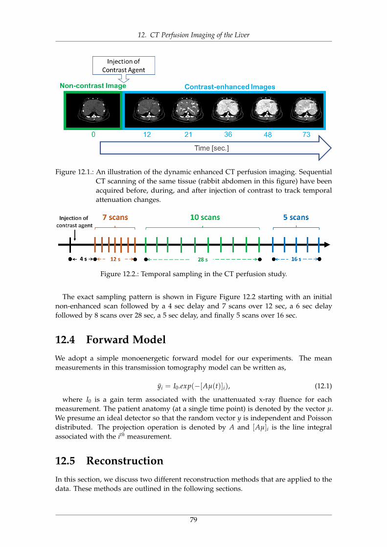
12. CT Perfusion Imaging of the Liver
Figure 12.1.: An illustration of the dynamic enhanced CT perfusion imaging. SequentialCT scanning of the same tissue (rabbit abdomen in this figure) have beenacquired before, during, and after injection of contrast to track temporalattenuation changes.
Figure 12.2.: Temporal sampling in the CT perfusion study.
The exact sampling pattern is shown in Figure Figure 12.2 starting with an initialnon-enhanced scan followed by a 4 sec delay and 7 scans over 12 sec, a 6 sec delayfollowed by 8 scans over 28 sec, a 5 sec delay, and finally 5 scans over 16 sec.
12.4 Forward ModelWe adopt a simple monoenergetic forward model for our experiments. The meanmeasurements in this transmission tomography model can be written as,
yi = I0.exp(−[Aµ(t)]i), (12.1)
where I0 is a gain term associated with the unattenuated x-ray fluence for eachmeasurement. The patient anatomy (at a single time point) is denoted by the vector µ.We presume an ideal detector so that the random vector y is independent and Poissondistributed. The projection operation is denoted by A and [Aµ]i is the line integralassociated with the ith measurement.
12.5 ReconstructionIn this section, we discuss two different reconstruction methods that are applied to thedata. These methods are outlined in the following sections.
79
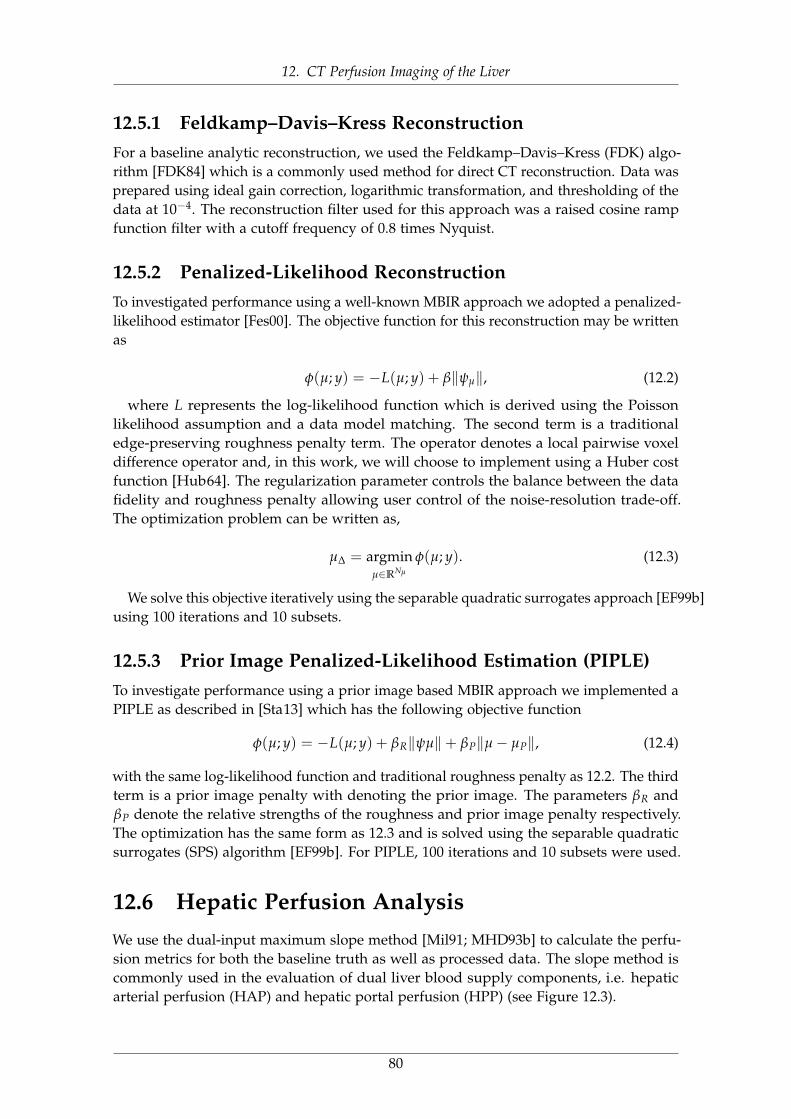
12. CT Perfusion Imaging of the Liver
12.5.1 Feldkamp–Davis–Kress ReconstructionFor a baseline analytic reconstruction, we used the Feldkamp–Davis–Kress (FDK) algo-rithm [FDK84] which is a commonly used method for direct CT reconstruction. Data wasprepared using ideal gain correction, logarithmic transformation, and thresholding of thedata at 10−4. The reconstruction filter used for this approach was a raised cosine rampfunction filter with a cutoff frequency of 0.8 times Nyquist.
12.5.2 Penalized-Likelihood ReconstructionTo investigated performance using a well-known MBIR approach we adopted a penalized-likelihood estimator [Fes00]. The objective function for this reconstruction may be writtenas
φ(µ; y) = −L(µ; y) + β‖ψµ‖, (12.2)
where L represents the log-likelihood function which is derived using the Poissonlikelihood assumption and a data model matching. The second term is a traditionaledge-preserving roughness penalty term. The operator denotes a local pairwise voxeldifference operator and, in this work, we will choose to implement using a Huber costfunction [Hub64]. The regularization parameter controls the balance between the datafidelity and roughness penalty allowing user control of the noise-resolution trade-off.The optimization problem can be written as,
µ∆ = argminµ∈RNµ
φ(µ; y). (12.3)
We solve this objective iteratively using the separable quadratic surrogates approach [EF99b]using 100 iterations and 10 subsets.
12.5.3 Prior Image Penalized-Likelihood Estimation (PIPLE)To investigate performance using a prior image based MBIR approach we implemented aPIPLE as described in [Sta13] which has the following objective function
φ(µ; y) = −L(µ; y) + βR‖ψµ‖+ βP‖µ− µP‖, (12.4)
with the same log-likelihood function and traditional roughness penalty as 12.2. The thirdterm is a prior image penalty with denoting the prior image. The parameters βR andβP denote the relative strengths of the roughness and prior image penalty respectively.The optimization has the same form as 12.3 and is solved using the separable quadraticsurrogates (SPS) algorithm [EF99b]. For PIPLE, 100 iterations and 10 subsets were used.
12.6 Hepatic Perfusion AnalysisWe use the dual-input maximum slope method [Mil91; MHD93b] to calculate the perfu-sion metrics for both the baseline truth as well as processed data. The slope method iscommonly used in the evaluation of dual liver blood supply components, i.e. hepaticarterial perfusion (HAP) and hepatic portal perfusion (HPP) (see Figure 12.3).
80
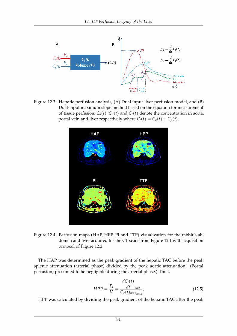
12. CT Perfusion Imaging of the Liver
Figure 12.3.: Hepatic perfusion analysis, (A) Dual input liver perfusion model, and (B)Dual-input maximum slope method based on the equation for measurementof tissue perfusion, Ca(t), Cp(t) and Cl(t) denote the concentration in aorta,portal vein and liver respectively where Cl(t) = Ca(t) + Cp(t).
Figure 12.4.: Perfusion maps (HAP, HPP, PI and TTP) visualization for the rabbit’s ab-domen and liver acquired for the CT scans from Figure 12.1 with acquisitionprotocol of Figure 12.2.
The HAP was determined as the peak gradient of the hepatic TAC before the peaksplenic attenuation (arterial phase) divided by the peak aortic attenuation. (Portalperfusion) presumed to be negligible during the arterial phase.) Thus,
HPP =Fa
V=
dCl(t)dt max
Ca(t)maxmax, (12.5)
HPP was calculated by dividing the peak gradient of the hepatic TAC after the peak
81
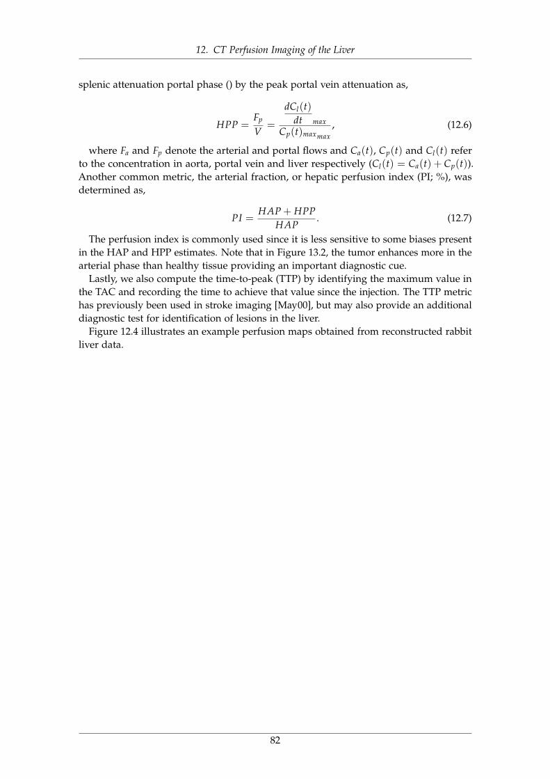
12. CT Perfusion Imaging of the Liver
splenic attenuation portal phase () by the peak portal vein attenuation as,
HPP =Fp
V=
dCl(t)dt max
Cp(t)maxmax, (12.6)
where Fa and Fp denote the arterial and portal flows and Ca(t), Cp(t) and Cl(t) referto the concentration in aorta, portal vein and liver respectively (Cl(t) = Ca(t) + Cp(t)).Another common metric, the arterial fraction, or hepatic perfusion index (PI; %), wasdetermined as,
PI =HAP + HPP
HAP. (12.7)
The perfusion index is commonly used since it is less sensitive to some biases presentin the HAP and HPP estimates. Note that in Figure 13.2, the tumor enhances more in thearterial phase than healthy tissue providing an important diagnostic cue.
Lastly, we also compute the time-to-peak (TTP) by identifying the maximum value inthe TAC and recording the time to achieve that value since the injection. The TTP metrichas previously been used in stroke imaging [May00], but may also provide an additionaldiagnostic test for identification of lesions in the liver.
Figure 12.4 illustrates an example perfusion maps obtained from reconstructed rabbitliver data.
82

12. CT Perfusion Imaging of the Liver
83
13. Low-dose CT Perfusion Imaging
13.1 OverviewOur aim in this chapter is to describe low-dose CT perfusion (CTP) imaging and tointroduce its applications in liver imaging scenarios. Next, we will provide an overviewof the data generation in section 13.3. Then, a detailed discussions on the phantomdesign and proposed reconstruction method to reduce the radiation dose in CTP examsfollows in sections 13.4 and 13.5 respectively. Next, in section 13.6, several experimentswill be introduced and the corresponding results will be illustrated in section 13.7.
13.2 BackgroundCT perfusion imaging of the liver enables the evaluation of perfusion metrics that canreveal hepatic diseases and that can be used to assess treatment responses. Despite thepotential clinical applications of the CTP, the excessive radiation dose exposed duringthe sequential scanning is a major drawback that limits more widespread use of CTP inclinical and research applications [Pan05; Ogu14]. Several techniques have been studiedto decrease the radiation exposures including patient-size-specific scanning parametermodifications and variation of exposure throughout the temporal scanning [Mur05;OKM11; Che09; Li14]. However, lowering x-ray exposure, inevitably reduces the qualityof the acquired images and can introduce noise and streak artifacts which, in turn,lowering the accuracy of the desired perfusion parameters.
Model-based iterative reconstruction (MBIR) techniques have been proposed as one ofthe solutions to improve the trade-off between radiation dose and acquired image quality.Recent studies on body CT scanning have demonstrated that such advanced processingmethods can improve image quality in a low exposure scan, thereby reducing theeffective dose exposed to the patient [Vor11; Har09]. Recent study of Negi et al. [Neg12]demonstrated that the adaptive iterative dose reduction (AIDR) reduced the image noisewhile maintaining hepatic perfusion parameters. However, most reconstruction methodstend to be applied in isolation, neglecting the large amount of shared information betweenscans.
In contrast, prior-image-based reconstruction (PIBR) approaches have been proposedto incorporate anatomical information found in previous scans. Prior information ismuch stronger than traditional assumptions of image smoothness and should allow forfurther reductions of noise and artifacts comparing to conventional MBIR regularization.
Example PIBR methods include prior-image-constrained compressed sensing () [CTL08b]and prior-image-registered penalized-likelihood estimation (PIRPLE) [Sta13]. Both ofthese techniques use a high quality prior image volume to help reconstruct low ex-posure or sparsely sampled projection data. PICCS has previously been investigatedfor small animal CTP [Net10]. A modification of PIRPLE with deformable registration
84
13. Low-dose CT Perfusion Imaging
has been used to reduce x-ray exposures in lung nodule surveillance by more than anorder of magnitude [Dan14]. Recently, Pourmorteza et al. [Pou16] proposed a novelReconstruction of Difference (RoD) technique that uses a penalized likelihood objectiveto directly reconstruct the difference between an already scanned prior image and thecurrent anatomy enabling direct reconstructions of anatomical change (analogous todigital sub- traction angiography) with reduced noise.
In this study, we investigate the feasibility of using RoD technique for liver CTP byproviding a digital simulations based on real time activity data and introduce severalevaluation and perfusion analysis techniques [Sey18a]. An illustration of the proposedacquisition and processing chain for liver CTP is shown in Figure 13.1.
Tomographic measurements (yn) are acquired over a range of time points n = 0 toN. These measurements cover a changing anatomy (µn) from an unenhanced volume(pre-iodine-injection) at n = 0, through uptake and washout of the contrast. A high-quality unenhanced baseline image (µ0) serves as a prior image (µp) for input into RoDto reconstruct difference image volumes (µ∆) for all subsequent low-dose sequentialdata. These difference images can be used to form estimates of the current imageanatomy (µ = µp + µ∆) at each time point. Subsequent perfusion analysis using standardcomputations on the entire image sequence is then used to create perfusion maps usingvarious metrics.
85
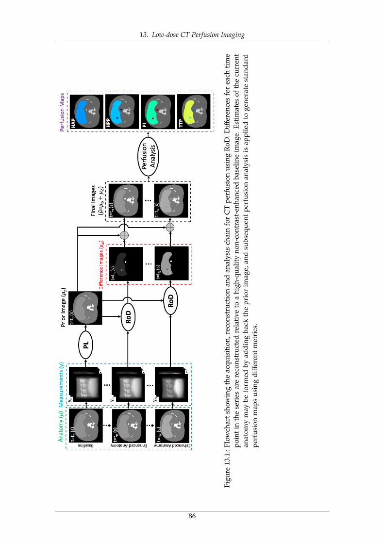
13. Low-dose CT Perfusion Imaging
Figu
re13
.1.:
Flow
char
tsh
owin
gth
eac
quis
itio
n,re
cons
truc
tion
and
anal
ysis
chai
nfo
rC
Tpe
rfus
ion
usin
gR
oD.D
iffe
renc
esfo
rea
chti
me
poin
tin
the
seri
esar
ere
cons
truc
ted
rela
tive
toa
high
-qua
lity
non-
cont
rast
-enh
ance
dba
selin
eim
age.
Esti
mat
esof
the
curr
ent
anat
omy
may
befo
rmed
byad
din
gba
ckth
epr
ior
imag
e,an
dsu
bseq
uent
perf
usio
nan
alys
isis
appl
ied
toge
nera
test
and
ard
perf
usio
nm
aps
usin
gdi
ffer
ent
met
rics
.
86
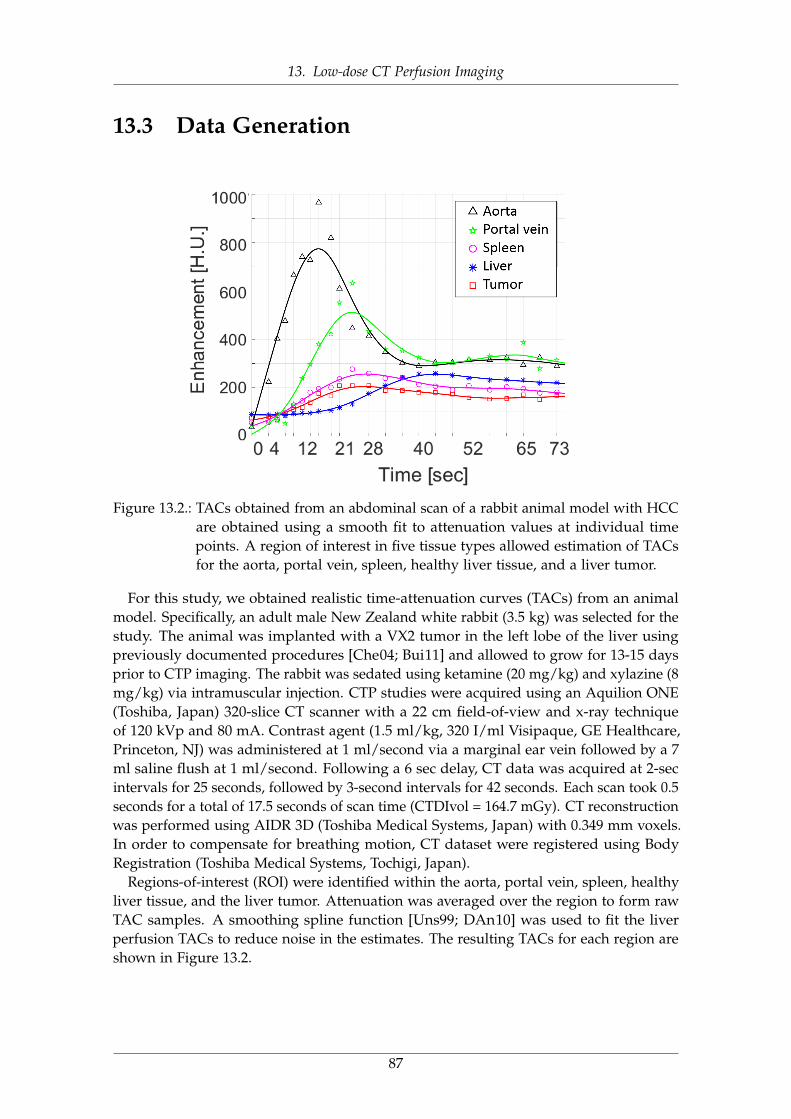
13. Low-dose CT Perfusion Imaging
13.3 Data Generation
Figure 13.2.: TACs obtained from an abdominal scan of a rabbit animal model with HCCare obtained using a smooth fit to attenuation values at individual timepoints. A region of interest in five tissue types allowed estimation of TACsfor the aorta, portal vein, spleen, healthy liver tissue, and a liver tumor.
For this study, we obtained realistic time-attenuation curves (TACs) from an animalmodel. Specifically, an adult male New Zealand white rabbit (3.5 kg) was selected for thestudy. The animal was implanted with a VX2 tumor in the left lobe of the liver usingpreviously documented procedures [Che04; Bui11] and allowed to grow for 13-15 daysprior to CTP imaging. The rabbit was sedated using ketamine (20 mg/kg) and xylazine (8mg/kg) via intramuscular injection. CTP studies were acquired using an Aquilion ONE(Toshiba, Japan) 320-slice CT scanner with a 22 cm field-of-view and x-ray techniqueof 120 kVp and 80 mA. Contrast agent (1.5 ml/kg, 320 I/ml Visipaque, GE Healthcare,Princeton, NJ) was administered at 1 ml/second via a marginal ear vein followed by a 7ml saline flush at 1 ml/second. Following a 6 sec delay, CT data was acquired at 2-secintervals for 25 seconds, followed by 3-second intervals for 42 seconds. Each scan took 0.5seconds for a total of 17.5 seconds of scan time (CTDIvol = 164.7 mGy). CT reconstructionwas performed using AIDR 3D (Toshiba Medical Systems, Japan) with 0.349 mm voxels.In order to compensate for breathing motion, CT dataset were registered using BodyRegistration (Toshiba Medical Systems, Tochigi, Japan).
Regions-of-interest (ROI) were identified within the aorta, portal vein, spleen, healthyliver tissue, and the liver tumor. Attenuation was averaged over the region to form rawTAC samples. A smoothing spline function [Uns99; DAn10] was used to fit the liverperfusion TACs to reduce noise in the estimates. The resulting TACs for each region areshown in Figure 13.2.
87
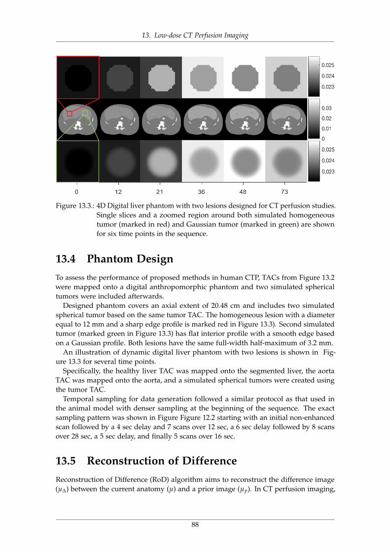
13. Low-dose CT Perfusion Imaging
Figure 13.3.: 4D Digital liver phantom with two lesions designed for CT perfusion studies.Single slices and a zoomed region around both simulated homogeneoustumor (marked in red) and Gaussian tumor (marked in green) are shownfor six time points in the sequence.
13.4 Phantom DesignTo assess the performance of proposed methods in human CTP, TACs from Figure 13.2were mapped onto a digital anthropomorphic phantom and two simulated sphericaltumors were included afterwards.
Designed phantom covers an axial extent of 20.48 cm and includes two simulatedspherical tumor based on the same tumor TAC. The homogeneous lesion with a diameterequal to 12 mm and a sharp edge profile is marked red in Figure 13.3). Second simulatedtumor (marked green in Figure 13.3) has flat interior profile with a smooth edge basedon a Gaussian profile. Both lesions have the same full-width half-maximum of 3.2 mm.
An illustration of dynamic digital liver phantom with two lesions is shown in Fig-ure 13.3 for several time points.
Specifically, the healthy liver TAC was mapped onto the segmented liver, the aortaTAC was mapped onto the aorta, and a simulated spherical tumors were created usingthe tumor TAC.
Temporal sampling for data generation followed a similar protocol as that used inthe animal model with denser sampling at the beginning of the sequence. The exactsampling pattern was shown in Figure Figure 12.2 starting with an initial non-enhancedscan followed by a 4 sec delay and 7 scans over 12 sec, a 6 sec delay followed by 8 scansover 28 sec, a 5 sec delay, and finally 5 scans over 16 sec.
13.5 Reconstruction of DifferenceReconstruction of Difference (RoD) algorithm aims to reconstruct the difference image(µ∆) between the current anatomy (µ) and a prior image (µp). In CT perfusion imaging,
88
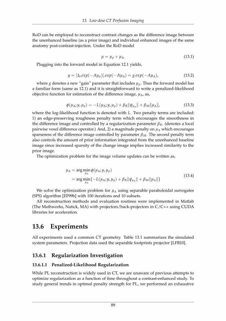
13. Low-dose CT Perfusion Imaging
RoD can be employed to reconstruct contrast changes as the difference image betweenthe unenhanced baseline (as a prior image) and individual enhanced images of the sameanatomy post-contrast-injection. Under the RoD model
µ = µp + µ∆. (13.1)
Plugging into the forward model in Equation 12.1 yields,
y = [I0.exp(−Aµp)].exp(−Aµ∆) = g.exp(−Aµ∆), (13.2)
where g denotes a new “gain” parameter that includes µp. Thus the forward model hasa familiar form (same as 12.1) and it is straightforward to write a penalized-likelihoodobjective function for estimation of the difference image, µ∆, as,
φ(µ∆; y, µp) = −L(µ∆; y, µp) + βR‖ψµ∆‖+ βM‖µ∆‖, (13.3)
where the log-likelihood function is denoted with L. Two penalty terms are included:1) an edge-preserving roughness penalty term which encourages the smoothness inthe difference image and controlled by a regularization parameter βR. (denotes a localpairwise voxel difference operator.) And, 2) a magnitude penalty on µ∆ which encouragessparseness of the difference image controlled by parameter βM. The second penalty termalso controls the amount of prior information integrated from the unenhanced baselineimage since increased sparsity of the change image implies increased similarity to theprior image.
The optimization problem for the image volume updates can be written as,
µ∆ = arg minµ∆
φ(µ∆; y, µp)
= arg minµ∆{−L(µ∆; y, µp) + βR‖ψµ∆‖+ βM‖µ∆‖}
(13.4)
We solve the optimization problem for µ∆ using separable paraboloidal surrogates(SPS) algorithm [EF99b] with 100 iterations and 10 subsets.
All reconstruction methods and evaluation routines were implemented in Matlab(The Mathworks, Natick, MA) with projectors/back-projectors in C/C++ using CUDAlibraries for acceleration.
13.6 ExperimentsAll experiments used a common CT geometry. Table 13.1 summarizes the simulatedsystem parameters. Projection data used the separable footprints projector [LFB10].
13.6.1 Regularization Investigation
13.6.1.1 Penalized-Likelihood Regularization
While PL reconstruction is widely used in CT, we are unaware of previous attempts tooptimize regularization as a function of time throughout a contrast-enhanced study. Tostudy general trends in optimal penalty strength for PL, we performed an exhaustive
89
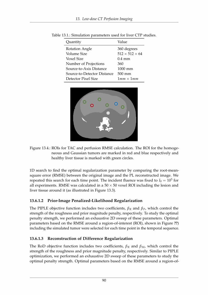
13. Low-dose CT Perfusion Imaging
Table 13.1.: Simulation parameters used for liver CTP studies.
Quantity Value
Rotation Angle 360 degreesVolume Size 512× 512× 64Voxel Size 0.4 mmNumber of Projections 360Source-to-Axis Distance 1000 mmSource-to-Detector Distance 500 mmDetector Pixel Size 1mm× 1mm
Figure 13.4.: ROIs for TAC and perfusion RMSE calculation. The ROI for the homoge-neous and Gaussian tumors are marked in red and blue respectively andhealthy liver tissue is marked with green circles.
1D search to find the optimal regularization parameter by comparing the root-mean-square error (RMSE) between the original image and the PL reconstructed image. Werepeated this search for each time point. The incident fluence was fixed to I0 = 103 forall experiments. RMSE was calculated in a 50× 50 voxel ROI including the lesion andliver tissue around it (as illustrated in Figure 13.3).
13.6.1.2 Prior-Image Penalized-Likelihood Regularization
The PIPLE objective function includes two coefficients, βR and βP, which control thestrength of the roughness and prior magnitude penalty, respectively. To study the optimalpenalty strength, we performed an exhaustive 2D sweep of these parameters. Optimalparameters based on the RMSE around a region-of-interest (ROI), shown in Figure ??)including the simulated tumor were selected for each time point in the temporal sequence.
13.6.1.3 Reconstruction of Difference Regularization
The RoD objective function includes two coefficients, βR and βM, which control thestrength of the roughness and prior magnitude penalty, respectively. Similar to PIPLEoptimization, we performed an exhaustive 2D sweep of these parameters to study theoptimal penalty strength. Optimal parameters based on the RMSE around a region-of-
90
13. Low-dose CT Perfusion Imaging
Figure 13.5.: Illustration of penalized-likelihood regularization parameter optimizationusing root-mean-square error (RMSE) change between iterations.
interest (ROI), shown in Figure 13.4) including the simulated tumor were selected foreach time point in the temporal sequence.
13.6.2 Incident Fluence InvestigationTo study the performance of RoD under different exposure conditions, we simulateddifferent levels of Poisson noise for noisy measurements with fluence ranging fromI0 = 5× 10³ to 105 (photons per pixel) in each of the time points. The prior image forRoD was produced by PL reconstruction of the t = 0 (unenhanced image volume) usingI0 = 5× 10³ photons.
13.6.3 Time-Attenuation CurvesTo study perfusion accuracy we conduct an analysis of TAC accuracy. For this study,TACs are reproduced for each reconstruction approach by averaging over healthy andtumor ROIs (shown in Figure 13.4). Errors are computed for each time point. RMSE isalso computed for healthy liver and tumor ROI.
To consider the effects of noise, five different noise realizations were generated andreconstructed for all comparisons. Standard deviations over noise realizations werecomputed for each time point to place error bars on TAC estimate curves and theircorresponding RMSE plots.
13.6.4 Perfusion AnalysisAnother study conducted to investigate the perfusion accuracy of each approach is toassess perfusion metric accuracy. For this study, the four different perfusion metrics iden-
91
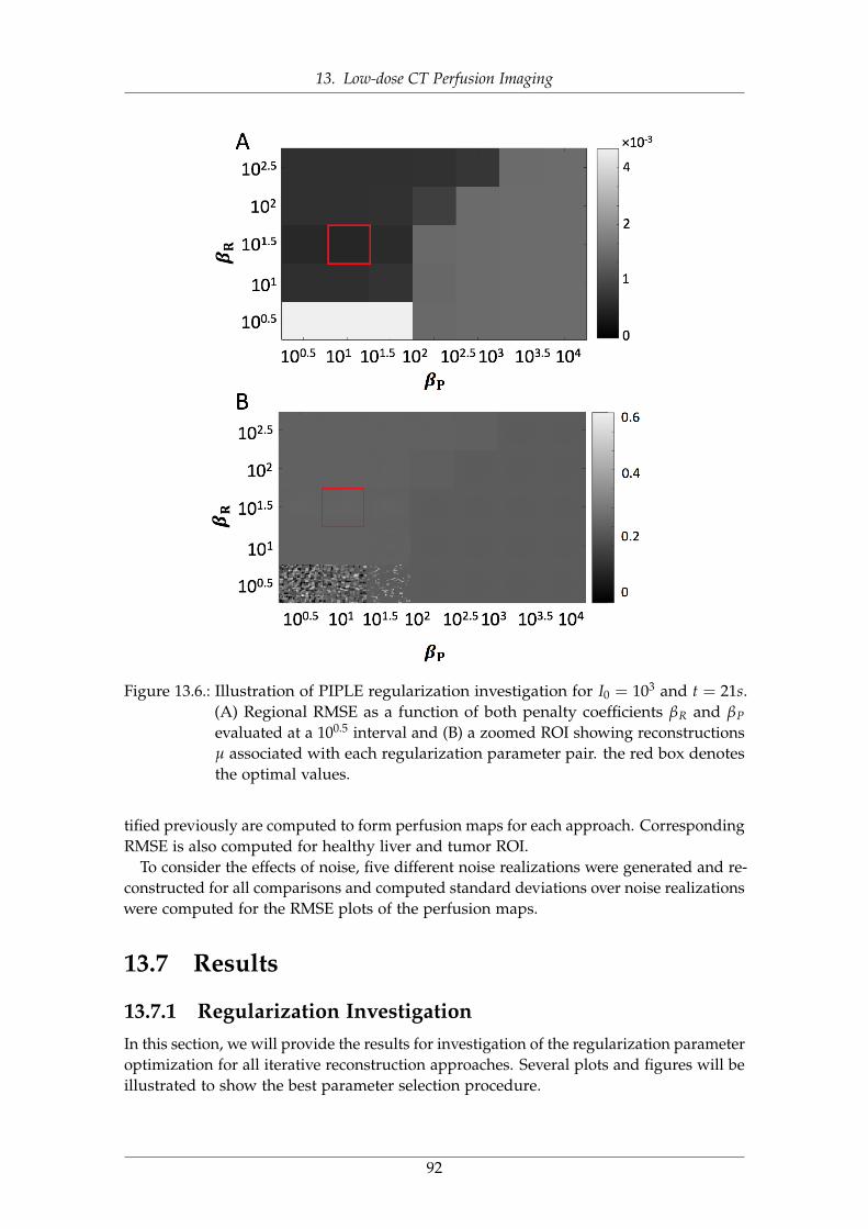
13. Low-dose CT Perfusion Imaging
Figure 13.6.: Illustration of PIPLE regularization investigation for I0 = 103 and t = 21s.(A) Regional RMSE as a function of both penalty coefficients βR and βP
evaluated at a 100.5 interval and (B) a zoomed ROI showing reconstructionsµ associated with each regularization parameter pair. the red box denotesthe optimal values.
tified previously are computed to form perfusion maps for each approach. CorrespondingRMSE is also computed for healthy liver and tumor ROI.
To consider the effects of noise, five different noise realizations were generated and re-constructed for all comparisons and computed standard deviations over noise realizationswere computed for the RMSE plots of the perfusion maps.
13.7 Results
13.7.1 Regularization InvestigationIn this section, we will provide the results for investigation of the regularization parameteroptimization for all iterative reconstruction approaches. Several plots and figures will beillustrated to show the best parameter selection procedure.
92
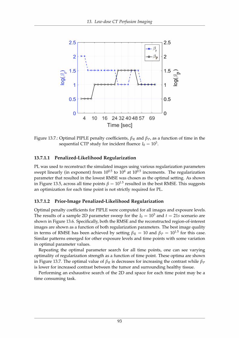
13. Low-dose CT Perfusion Imaging
Figure 13.7.: Optimal PIPLE penalty coefficients, βR and βP, as a function of time in thesequential CTP study for incident fluence I0 = 103.
13.7.1.1 Penalized-Likelihood Regularization
PL was used to reconstruct the simulated images using various regularization parametersswept linearly (in exponent) from 100.5 to 104 at 100.5 increments. The regularizationparameter that resulted in the lowest RMSE was chosen as the optimal setting. As shownin Figure 13.5, across all time points β = 101.5 resulted in the best RMSE. This suggestsan optimization for each time point is not strictly required for PL.
13.7.1.2 Prior-Image Penalized-Likelihood Regularization
Optimal penalty coefficients for PIPLE were computed for all images and exposure levels.The results of a sample 2D parameter sweep for the I0 = 103 and t = 21s scenario areshown in Figure 13.6. Specifically, both the RMSE and the reconstructed region-of-interestimages are shown as a function of both regularization parameters. The best image qualityin terms of RMSE has been achieved by setting βR = 10 and βP = 101.5 for this case.Similar patterns emerged for other exposure levels and time points with some variationin optimal parameter values.
Repeating the optimal parameter search for all time points, one can see varyingoptimality of regularization strength as a function of time point. These optima are shownin Figure 13.7. The optimal value of βR is decreases for increasing the contrast while βP
is lower for increased contrast between the tumor and surrounding healthy tissue.Performing an exhaustive search of the 2D and space for each time point may be a
time consuming task.
93
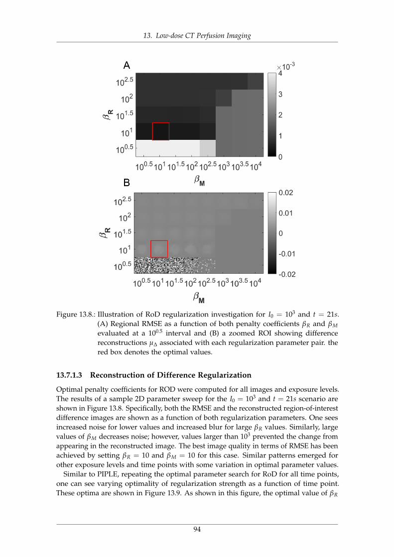
13. Low-dose CT Perfusion Imaging
Figure 13.8.: Illustration of RoD regularization investigation for I0 = 103 and t = 21s.(A) Regional RMSE as a function of both penalty coefficients βR and βM
evaluated at a 100.5 interval and (B) a zoomed ROI showing differencereconstructions µ∆ associated with each regularization parameter pair. thered box denotes the optimal values.
13.7.1.3 Reconstruction of Difference Regularization
Optimal penalty coefficients for ROD were computed for all images and exposure levels.The results of a sample 2D parameter sweep for the I0 = 103 and t = 21s scenario areshown in Figure 13.8. Specifically, both the RMSE and the reconstructed region-of-interestdifference images are shown as a function of both regularization parameters. One seesincreased noise for lower values and increased blur for large βR values. Similarly, largevalues of βM decreases noise; however, values larger than 103 prevented the change fromappearing in the reconstructed image. The best image quality in terms of RMSE has beenachieved by setting βR = 10 and βM = 10 for this case. Similar patterns emerged forother exposure levels and time points with some variation in optimal parameter values.
Similar to PIPLE, repeating the optimal parameter search for RoD for all time points,one can see varying optimality of regularization strength as a function of time point.These optima are shown in Figure 13.9. As shown in this figure, the optimal value of βR
94
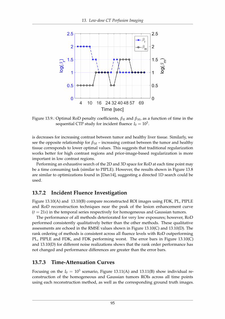
13. Low-dose CT Perfusion Imaging
Figure 13.9.: Optimal RoD penalty coefficients, βR and βM, as a function of time in thesequential CTP study for incident fluence I0 = 103.
is decreases for increasing contrast between tumor and healthy liver tissue. Similarly, wesee the opposite relationship for βM – increasing contrast between the tumor and healthytissue corresponds to lower optimal values. This suggests that traditional regularizationworks better for high contrast regions and prior-image-based regularization is moreimportant in low contrast regions.
Performing an exhaustive search of the 2D and 3D space for RoD at each time point maybe a time consuming task (similar to PIPLE). However, the results shown in Figure 13.8are similar to optimizations found in [Dan14], suggesting a directed 1D search could beused.
13.7.2 Incident Fluence InvestigationFigure 13.10(A) and 13.10(B) compare reconstructed ROI images using FDK, PL, PIPLEand RoD reconstruction techniques near the peak of the lesion enhancement curve(t = 21s) in the temporal series respectively for homogeneous and Gaussian tumors.
The performance of all methods deteriorated for very low exposures; however, RoDperformed consistently qualitatively better than the other methods. These qualitativeassessments are echoed in the RMSE values shown in Figure 13.10(C) and 13.10(D). Therank ordering of methods is consistent across all fluence levels with RoD outperformingPL, PIPLE and FDK, and FDK performing worst. The error bars in Figure 13.10(C)and 13.10(D) for different noise realizations shows that the rank order performance hasnot changed and performance differences are greater than the error bars.
13.7.3 Time-Attenuation Curves
Focusing on the I0 = 103 scenario, Figure 13.11(A) and 13.11(B) show individual re-construction of the homogeneous and Gaussian tumors ROIs across all time pointsusing each reconstruction method, as well as the corresponding ground truth images.
95
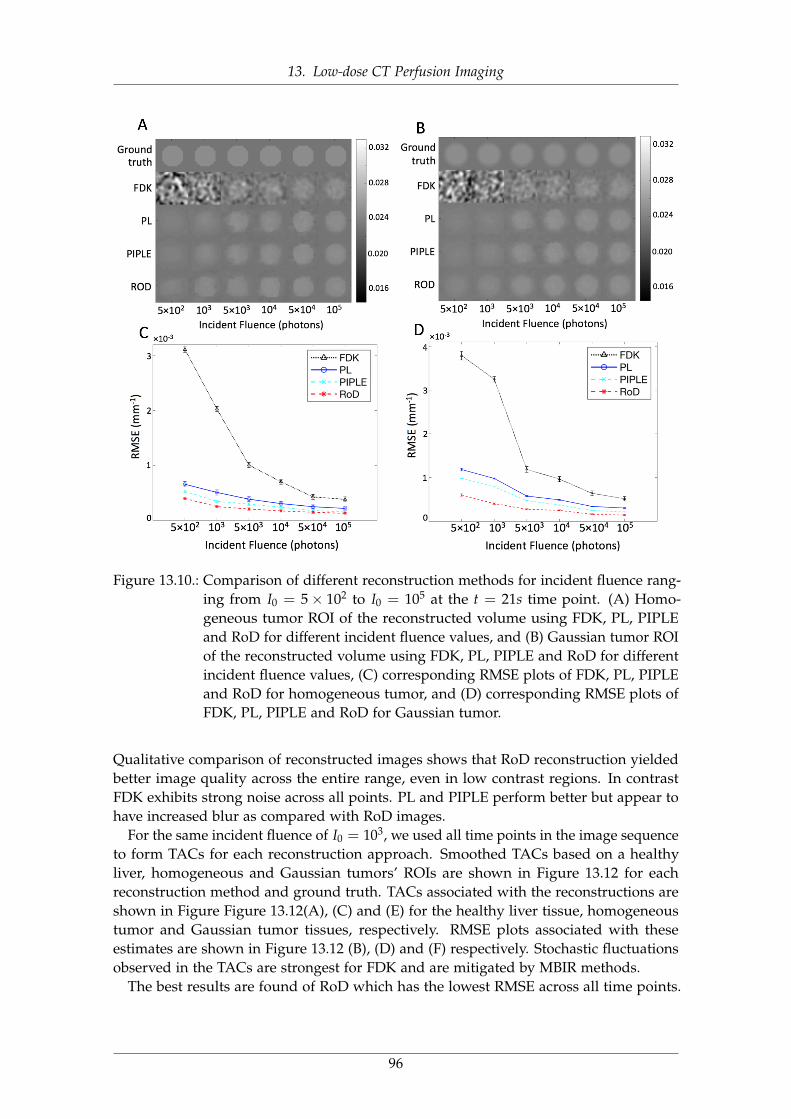
13. Low-dose CT Perfusion Imaging
Figure 13.10.: Comparison of different reconstruction methods for incident fluence rang-ing from I0 = 5× 10² to I0 = 105 at the t = 21s time point. (A) Homo-geneous tumor ROI of the reconstructed volume using FDK, PL, PIPLEand RoD for different incident fluence values, and (B) Gaussian tumor ROIof the reconstructed volume using FDK, PL, PIPLE and RoD for differentincident fluence values, (C) corresponding RMSE plots of FDK, PL, PIPLEand RoD for homogeneous tumor, and (D) corresponding RMSE plots ofFDK, PL, PIPLE and RoD for Gaussian tumor.
Qualitative comparison of reconstructed images shows that RoD reconstruction yieldedbetter image quality across the entire range, even in low contrast regions. In contrastFDK exhibits strong noise across all points. PL and PIPLE perform better but appear tohave increased blur as compared with RoD images.
For the same incident fluence of I0 = 103, we used all time points in the image sequenceto form TACs for each reconstruction approach. Smoothed TACs based on a healthyliver, homogeneous and Gaussian tumors’ ROIs are shown in Figure 13.12 for eachreconstruction method and ground truth. TACs associated with the reconstructions areshown in Figure Figure 13.12(A), (C) and (E) for the healthy liver tissue, homogeneoustumor and Gaussian tumor tissues, respectively. RMSE plots associated with theseestimates are shown in Figure 13.12 (B), (D) and (F) respectively. Stochastic fluctuationsobserved in the TACs are strongest for FDK and are mitigated by MBIR methods.
The best results are found of RoD which has the lowest RMSE across all time points.
96
13. Low-dose CT Perfusion Imaging
RoD produces TACs closest to the ground truth with a more substantial improvementfor the tumor ROI.
97
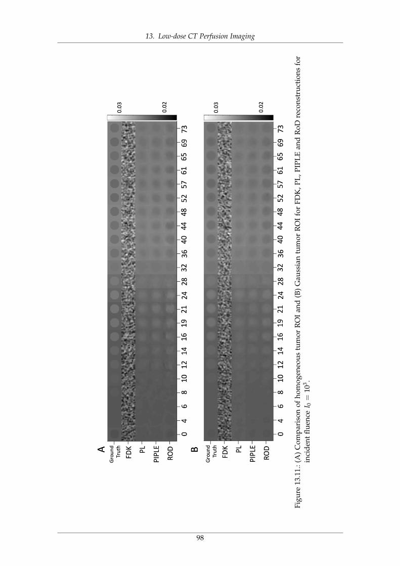
13. Low-dose CT Perfusion Imaging
Figu
re13
.11.
:(A
)C
ompa
riso
nof
hom
ogen
eous
tum
orR
OI
and
(B)
Gau
ssia
ntu
mor
RO
Ifo
rFD
K,P
L,P
IPL
Ean
dR
oDre
cons
truc
tion
sfo
rin
cide
ntflu
ence
I 0=
103 .
98
13. Low-dose CT Perfusion Imaging
13.7.4 Perfusion AnalysisFigure 13.13 shows the calculated perfusion maps including HAP, HPP, PI and TTP mapsfor different reconstruction techniques at an incident fluence of I0 = 103. Consistentwith previous results FDK exhibits increased noise as compared with other approaches.Similarly, the tumor does not appear in the TTP map. RoD outperforms the other methodswith better tumor PI contrast and a conspicuous tumor apparent in the TTP map. PLand RoD appear to perform comparably for the HAP and HPP maps. CorrespondingRMSE comparisons for these perfusion maps are presented in Figure 13.14 for both thehealthy liver and tumor ROIs. PL performs better than FDK, but increased blue in the PImap reduces conspicuity of the tumor. PIPLE performs better than FDK, PL and PIPLE,however the intensity of tumor region in the PI map is still lower than RoD and TTP mapalso shows a noisy appearance for the liver tissue.
Again, the quantitative results reinforce the qualitative observations with improvedperformance using RoD. As shown in this figure, the differences are greatest for PI andin the tumor ROI. Similar performance of PL and RoD in the tumor ROI is also noted.
13.8 ConclusionIn this chapter, a novel pipeline for acquisition, reconstruction and processing of sequen-tial CTP imaging data was presented. In particular, an initial high-quality baseline recon-struction of the unenhanced anatomy was used in a prior-image-based reconstructionmethod called Reconstruction of Difference to improve the image quality of subsequentreconstructions of low-exposure contrast-enhance CT data. The proposed RoD approachoutperformed both traditional approaches and another prior image method (PIPLE). Theimproved performance was demonstrated across a range of exposures for individualtime-point reconstructions, for time-attenuation curve estimates, and in the computationof common perfusion metric maps.
The experimental conditions used a high-quality baseline image volume acquired at afluence of 105 photons per detector element (which is a clinically relevant exposure in ourexperience). Using RoD suggests that this exposure could be dropped to 103 photons andretain useful perfusion images instead of repeating the 105 photon exposure over 20 times.In the low-exposure RoD case, the dose would be dominated by the initial baseline scanrepresenting a substantial dose reduction (e.g. a 20 times reduction). These preliminaryresults suggest the underlying methodology is a potentially powerful approach that canbe applied in sequential data reconstruction like CT perfusion. Moreover, such methodsmay enable techniques like liver CTP which have not found widespread clinical use dueto radiation dose concerns.
99
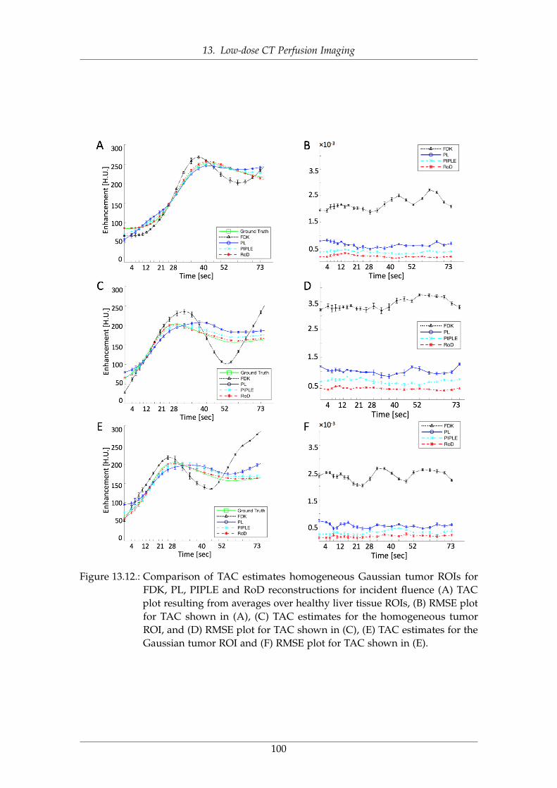
13. Low-dose CT Perfusion Imaging
Figure 13.12.: Comparison of TAC estimates homogeneous Gaussian tumor ROIs forFDK, PL, PIPLE and RoD reconstructions for incident fluence (A) TACplot resulting from averages over healthy liver tissue ROIs, (B) RMSE plotfor TAC shown in (A), (C) TAC estimates for the homogeneous tumorROI, and (D) RMSE plot for TAC shown in (C), (E) TAC estimates for theGaussian tumor ROI and (F) RMSE plot for TAC shown in (E).
100
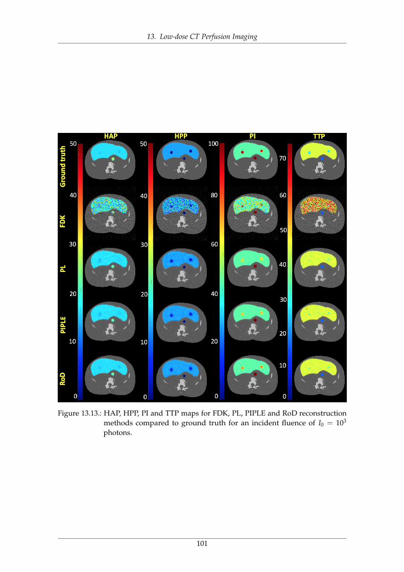
13. Low-dose CT Perfusion Imaging
Figure 13.13.: HAP, HPP, PI and TTP maps for FDK, PL, PIPLE and RoD reconstructionmethods compared to ground truth for an incident fluence of I0 = 103
photons.
101
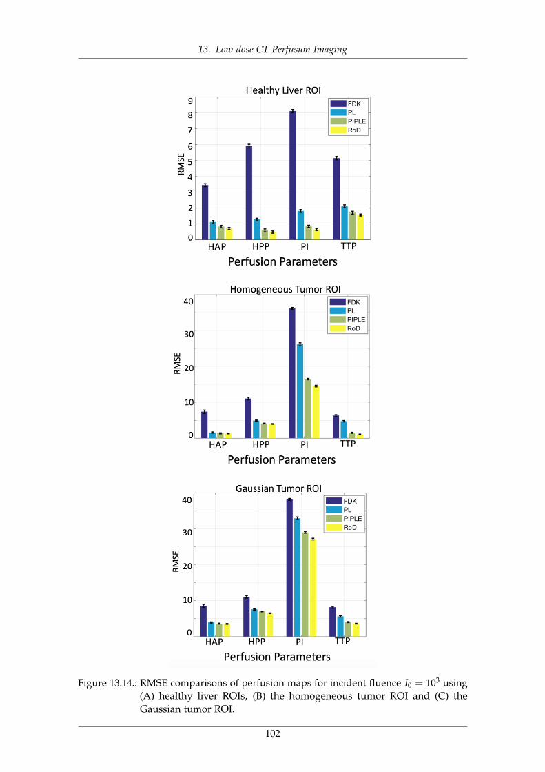
13. Low-dose CT Perfusion Imaging
Figure 13.14.: RMSE comparisons of perfusion maps for incident fluence I0 = 103 using(A) healthy liver ROIs, (B) the homogeneous tumor ROI and (C) theGaussian tumor ROI.
102
13. Low-dose CT Perfusion Imaging
103
14. Outlook
Do not fear to be eccentric in opinion,for every opinion now accepted wasonce eccentric.
Bertrand Russell
Medical imaging has advanced rapidly in the beginning of the twenty-first century.Diagnostic images captured at the right place and at the right time give physicians,surgeons, and researchers an important tool to help provide better patient care at a lowercost than before. The application of 3D and 4D imaging technologies have the potentialto create better images for improved diagnostics in radiology. Recent advances in imageacquisitions and formations, resulted in digital images rather than traditional non-digitaldata. Digital images are more than pictures; they offer sources of data which includeseveral information and solutions that are not easily traceable by human eyes.
Improvements in x-ray based imaging such as computed tomography, in the nextdecades, will result in reductions of radiation dose in a way where this issue will nolonger be of concern. Phase contrast x-ray imaging is also likely to be the next newimaging method to be explored more clinically and in the real applications area.
Until recently, all computed tomography systems reconstructed images using thefiltered back projection techniques due to its relatively short running time using oldercomputer systems. However, with recent improvements in computing power and thereduction in costs for the power itself, all the major imaging device vendors now includeand offer iterative image reconstruction techniques. New noise reduction, regularizationand artifact removal methods have been developed during last decade which enablesdiagnostic image clarity on low dose scans that was not possible before. This enables CTscanning at much lower doses that a decade ago.
In this thesis, we studied two novel four- and six-dimensional x-ray imaging modalitiesand investigated several data processing and analysis pipelines along with evaluationtechniques to assess the effectiveness of proposed methods.
Particularly, in the first part of this study, we focused on X-ray Tensor Tomography, anovel imaging modality developed for three-dimensional reconstruction of x-ray scatter-ing tensors from dark-field images obtained in a grating interferometry setup. In thispart, we addressed one of the main limitations of X-ray Tensor Tomography which isthe degradation of the measured two-dimensional dark-field images due to the detectorreadout noise and insufficient photon statistics affecting, which is consequently, affectingthe reconstructed three-dimensional volumes from these data showing noise artifacts.We investigated the best way to incorporate total variation denoising technique intothe reconstruction pipeline. Several different schemes for applying noise reductionmethods based on two- and three-dimensional TV regularization have been proposedto reduce the noise level before, during or after the reconstruction process and evaluatethe effectiveness and quality of images reconstructed and denoised using these schemes.
104
14. Outlook
The quantitative and qualitative evaluation based on datasets from different industrialand clinical samples show improvements in noise reduction for all proposed methodscompared to the method without denoising. The best results are achieved by the regular-ized reconstruction technique for x-ray Tensor Tomography, which aims in interleavingreconstruction and denoising.
In the second part, we studied the low-dose CT perfusion of the liver. Liver CTperfusion is a novel x-ray imaging technique that has demonstrated clinical utility in thedetection, staging, and analysis of treatment response in hepatic diseases by enablingthe evaluation of several perfusion metrics. We addressed the reduction of radiationexposures associated with hepatic CTP studies which is one the main limitations of CTperfusion tests by developing a novel scheme for acquiring and processing sequentialCT perfusion data. We proposed to adapt Reconstruction of Difference method whichestimates the difference between unenhanced baseline and subsequent scans. This use ofthe baseline as a prior image permits significant reductions in noise in reconstructions.Several experiments evaluating the performance of RoD relative to traditional analytic andmodel based iterative reconstruction methods suggest that proposed method producesbetter images, better quantification in the TACs, and better perfusion maps for commonlyused perfusion metrics. These results suggest the RoD processing can dramaticallyreduce exposure requirements. In this case, the exposure of all but the unenhancedbaseline scan was dropped by two orders of magnitude and accurate perfusion resultswere maintained.
Through all of this, exciting advances in diagnostic medical imaging, x-ray imagesprocessing and computed tomography can be expected. However, so much work isneeded to reach to that point by developing faster, clearer and safer imaging technologiesthat would be available for majority of the populations in the world. On a more positivenote, the future of medical imaging and image processing, will bring new capabilitiesand tools that have even greater medical values to improve humans’ lives. We will seeradiation dose in x-ray imaging modalities continue to drop and utilization of all imagingservices become more efficient, with lower costs and even fewer waste in healthcareresources, to the benefit of patients, physicians and everyone in the healthcare cycle.
105
14. Outlook
106

List of Figures
1.1. The Electromagnetic spectrum describes all the wavelengths of light. Theelectromagnetic waves that human eyes detect – visible light – oscillatesbetween 400 and 790 terahertz. . . . . . . . . . . . . . . . . . . . . . . . . . 2
2.1. The first x-ray projection was taken in 1895 from Prof. Wilhelm Röntgen’swife which was recorded on a film, showing the finger bones and herring [Kev98]. . . . . . . . . . . . . . . . . . . . . . . . . . . . . . . . . . . . . 5
2.2. A diagram of a modern x-ray tube. This type of tube was devised byCoolidge in 1913 [SP08]. . . . . . . . . . . . . . . . . . . . . . . . . . . . . . 6
2.3. Photoelectric absorption process: a photon undergoes an interaction withan absorber atom in which the photon completely disappears. . . . . . . . 7
2.4. Elastic scattering takes place between the incident photon and an electronin the absorbing material. . . . . . . . . . . . . . . . . . . . . . . . . . . . . 8
2.5. Three different x-ray contrast projections of a femur sample, (A) Absorptioncontrast shows the attenuated parts of the sample, (B) Phase contrast whichvisualizes its phase-shifting properties, and (C) Dark-field contrast whichis sensitive to scattering structures. . . . . . . . . . . . . . . . . . . . . . . . 9
3.1. (A) Godfrey Newbold Hounsfield developed the first CT scanner, and (B)Transverse slice imaging of the brain at low resolution with 80× 80 pixelsbecame the standard CT application in the 1970s [Kal06]. . . . . . . . . . . 11
3.2. Illustration of a typical x-ray absorption tomography setup including anx-ray tube (X), sample (S) with one degree of freedom (rotation angle φ),and x-ray detector (D). . . . . . . . . . . . . . . . . . . . . . . . . . . . . . . 11
4.1. Sketch of a tomographic measurement at a given angle θ. . . . . . . . . . 154.2. Illustration of the Fourier slice theorem: one-dimensional Fourier trans-
form (1D FT) of a projection taken at angle θ equals the central radial sliceat angle θ of the two-dimensional Fourier transform (2D FT) of the originalobject. . . . . . . . . . . . . . . . . . . . . . . . . . . . . . . . . . . . . . . . . 15
4.3. A simplified schematic of CT data reconstruction in the context of analyticreconstruction technique: FBP. . . . . . . . . . . . . . . . . . . . . . . . . . 16
4.4. A simplified schematic for principle steps of iterative reconstruction tech-niques for CT data. . . . . . . . . . . . . . . . . . . . . . . . . . . . . . . . . 16
4.5. Flowchart of algebraic reconstruction technique. . . . . . . . . . . . . . . . 184.6. A schematic quadratic form for a normal equation (symmetric, positive-
definite) will have a shape similar to a bowl. To search Searching for theminimum c using steepest descent approach to search for an xmin startingfrom an initial guess (x0) is shown in blue. However, the conjugate gradientmethod which is utilizing an optimal scheme to find the minimum quicklyis marked in orange. This figure is adapted from [Vog15]. . . . . . . . . . 19
107
List of Figures
5.1. Schematic illustration of the general perfusion analysis workflow. Recon-structed CT volumes from different time points (left) are imported to theperfusion analysis to create the perfusion maps (right). In this case, a liverimages are used which gives hepatic arterial perfusion (HAP), hepaticportal perfusion (HPP), perfusion index (PI) and time-to-peak (TTP) maps.More details on these maps creation can be found in section 12.6. . . . . . 27
5.2. The concept of convolution in CTP analysis (a) Schematic representationof the vascular structure in a tissue region. FCa(t) refers to the input ofcontrast agent into the tissue, (b) when blood flow is not changed for twoinjections of the same concentration (left), then the tissue TAC for eachinjection will be the same; This is called IRF of the tissue. The right showstwo IRF for the case of two identical bolus injections of contrast agent ofthe same concentration. For each IRF, initially, there is a sudden increasein the shape of the graph because the injection is directly into the arterialinput. (c) Tissue TAC corresponding to a case in which the arterial TACconsists of two bolus injections of different concentrations C1 and C2, and,(d) shows a general arterial TAC as a series of injections equally spaced intime and of different concentrations (left). For each bolus injection, TAC ofthe tissue is a scaled IRF, which is the product of blood flow, concentrationof bolus, and the IRF. The total tissue TAC in response to the generalarterial concentration Ca(t) is the sum of all the scaled IRF after they havebeen shifted in time in accordance to the times of their correspondingbolus injection. This figure is adapted from [Lee02]. . . . . . . . . . . . . . 28
6.1. Sketch of the Talbot-Lau X-ray Grating Based Interferometry setup. . . . . 316.2. Illustration of three signal components, (A) Absorption-contrast which
is shoeing the attenuation of the x-ray beam leads to a reduction of theamplitude of the interference pattern. (B) Phase-contrast which is therefraction that causes a shift of the pattern, and (C) Dark-field contrastshowing the scattering that reduces the amplitude of the interferencepattern and creates an offset. This figure is adapted from [Sch13]. . . . . 31
9.1. Illustration of an x-ray tensor tomography setup including an x-ray tube(X), source grating (G0), sample (S) mounted on an Eulerian cradle withthree degrees of freedom (Euler angles ψ, θ, φ), shifting interferometergrating (G1), static interferometer grating (G2), and x-ray detector (D).The vector tj refers to the sensitivity direction of the gratings, while sjcorresponds to the beam direction. . . . . . . . . . . . . . . . . . . . . . . . 41
9.2. An illustration of the XTT acquisition and reconstruction, (A) anisotropicdark-field signal from several non-standard acquisition poses, (B) simulta-neously reconstructed scattering components, (C) tensor fitting from allscattering coefficients, and (D) smallest half-axis of the tensor representsthe structure orientation. This Figure is adapted from [Sha16]. . . . . . . 42
108
List of Figures
9.3. Tensor fitting in x-ray tensor tomography: (A) Selected scattering directionsεk, for example the coordinate axes, and the space and face diagonals,(B) scattering directions εk shown for a location x ∈ R3 (coordinate axesshown in red, space diagonals shown in blue, and face diagonals shownin green), (C) scattering coefficients ζk(x) for every scattering directionεk shown by black stars, corresponding mirrored coefficients along thenegative scattering direction shown as red stars, (D) tensor fitted to theblack and mirrored red stars, (E) several reconstructed scattering tensors,with their smallest half axis indicating the direction of a fiber or tube-likestructure (in grey). . . . . . . . . . . . . . . . . . . . . . . . . . . . . . . . . 43
9.4. CT and XTT viewing directions, (A) an Euler cradle used to sample theunit sphere for XTT measurements, (B) sampling coverage in CT and, (C)sampling unit sphere for XTT. . . . . . . . . . . . . . . . . . . . . . . . . . . 44
9.5. Overview of the unregularized XTT reconstruction. . . . . . . . . . . . . . 45
10.1. Evaluation of XTT reconstructed images vs. attenuation image: (A) Fastmarching method calculating centerline in region of interest of attenuationimage, and (B) XTT orientations calculated after fitting tensor to XTTreconstructed image zoomed for the same region of interest. . . . . . . . . 48
11.1. Overview of the regularized XTT reconstruction. . . . . . . . . . . . . . . . 5311.2. Overview of the projection domain TV denoising for XTT reconstruction. 5511.3. Overview of the image domain TV denoising for XTT reconstruction. . . 5511.4. Photography of the XTT setup used to measure the samples. From left to
right: (S) x-ray source, (G0) source grating, (G1) phase grating, (S) samplemounted on the Euler cradle, (G2) the analyzer grating and, (D) the detector 56
11.5. Photography of the carbon knot sample. . . . . . . . . . . . . . . . . . . . 5611.6. Photography of the crossed sticks sample. . . . . . . . . . . . . . . . . . . 5711.7. Comparison of (A) normalized residual norm r(q) and (B) normalized
mean update M(q) for the three studied reconstruction methods. . . . . . . 5911.8. Illustration of center slice of the reconstructed component volumes of
crossed-sticks dataset using XTT, ADMM regularized XTT and TV reg-ularized XTT reconstruction techniques corresponding to the scatteringdirections ε1, ε8. and ε9 for all three methods. All images windowed to[0.1, 0.9]. . . . . . . . . . . . . . . . . . . . . . . . . . . . . . . . . . . . . . . 60
11.9. Tensor visualization of a single slice of the reconstructed crossed stickssample for all three methods: (A) XTT, (B) ADMM, and (C) rXTT. Thestructure orientation is color encoded as shown in orientation sphere inthe right side of this figure. . . . . . . . . . . . . . . . . . . . . . . . . . . . 61
11.10.Example images of two-dimensional TV denoising of dark-field imagemeasurements of the carbon knot dataset, windowed to [0.1,0.75], (A-C)showing angle combinations (ψ = 20◦, θ = 45◦, φ = 60◦), (ψ = 0◦, θ =
0◦, φ = 0◦) and (ψ = 0◦, θ = 60◦, φ = 0◦), respectively, before denoisingand (D-F) showing the same angles after denoising with β fixed to 80%.Corresponding MAD and SNR values are displayed below each image. . 62
109
List of Figures
11.11.Illustration of two-dimensional TV denoising on dark-field image mea-surements of the femur dataset, (a-c) showing angle combinations of(ψ = 20◦, θ = 0◦, φ = 180◦), (ψ = 0◦, θ = 30◦, φ = 0◦) and (ψ = 36◦, θ =
0◦, φ = 0◦) respectively, before denoising and (d-f) showing the sameangles after denoising with β fixed to 80%. Corresponding MAD and SNRvalues are displayed below each image. . . . . . . . . . . . . . . . . . . . . 63
11.12.Center slice of the reconstructed and denoised carbon knot dataset forcomponent ε3 = [0, 0, 1]. A ROI is marked with a red square and zoomedfor the (A) XTT, (B) TV→XTT, (C) rXTT, (D) XTT→TV, and (E) wXTTmethods. The parameter β was fixed to 80%. All images are windowed to[0.10,0.85]. . . . . . . . . . . . . . . . . . . . . . . . . . . . . . . . . . . . . . 65
11.13.Zoomed area of interest of the images (see Figure 11.12) of the carbonknot dataset corresponding to the scattering direction ε3, windowed to[0.10,0.85]. The parameters β have been chosen such that the TV→XTT,rXTT and XTT→TV methods match in noise level as estimated by MAD.(A,E,I) TV→XTT, (B,F,J) rXTT, (C,G,K) XTT→TV, and (D,H,L) wXTT. . . . 66
11.14.Center slice of the reconstructed and denoised femur dataset for compo-nent ε1 = [1, 0, 0]. A ROI is marked with a red square and zoomed for the(A) XTT, (B) TV→XTT, (C) rXTT, (D) XTT→TV, and (E) wXTT methods.The parameter β was fixed to 80%. All images are windowed to [0.05,0.80]. 67
11.15.Zoomed area of interest of the images (see Figure 11.14) of the femurdataset corresponding to the scattering direction ε1, windowed to [0.05,0.80].The parameters β have been chosen such that TV→XTT, rXTT and XTT→TVmethods match in noise level as estimated by MAD. (A,D,G) TV→XTT,(B,E,H) rXTT, (C,F,I) XTT→TV . . . . . . . . . . . . . . . . . . . . . . . . . 68
11.16.MAD and CNR comparisons for different scattering directions (A) ε1, (B)ε2 and (C) ε3 of the carbon knot reconstruction from Figure 11.12. . . . . 69
11.17.MAD and CNR comparisons for different scattering directions (A) ε1, (B)ε2 and (C) ε3 of the femur reconstruction from Figure 11.14. . . . . . . . . 69
11.18.Tensor visualization of a single slice of the reconstructed carbon knotsample volumes for all four methods: (A) XTT (B) TV→XTT, (C) rXTT, (D)XTT→TV, (E) wXTT and (F) The structure orientation is color encoded asshown in orientation sphere. β fixed to 80%. . . . . . . . . . . . . . . . . . 71
11.19.Tensor visualization of a single slice of the reconstructed femur sample forall four methods: (A) XTT, (B) TV→XTT, (C) rXTT, (D) XTT→TV, (E) wXTTand (F) The structure orientation is color encoded as shown in orientationsphere. β fixed to 80%. . . . . . . . . . . . . . . . . . . . . . . . . . . . . . . 72
11.20.Illustration of diagrams for (A) normalized residual norm r(q) and (B)normalized mean update r(q) for the proposed methods. Normalizedmean horizontal axis is shown from iteration 5 to illustrate the differencebetween different plots. . . . . . . . . . . . . . . . . . . . . . . . . . . . . . 73
11.21.Histogram showing angle differences δ comparison of attenuation re-constructed image with XTT reconstruction method and proposed noisereduction and regularization methods for ROI1 (A) and ROI2 (B). Boxplots illustrating the distribution of data from all proposed reconstructionand denoising methods with green line and red circle marks showing themedian and mean for (C) ROI1 and (D) ROI2, as marked in Figure 10.1. . 74
110
List of Figures
12.1. An illustration of the dynamic enhanced CT perfusion imaging. SequentialCT scanning of the same tissue (rabbit abdomen in this figure) have beenacquired before, during, and after injection of contrast to track temporalattenuation changes. . . . . . . . . . . . . . . . . . . . . . . . . . . . . . . . 79
12.2. Temporal sampling in the CT perfusion study. . . . . . . . . . . . . . . . . 7912.3. Hepatic perfusion analysis, (A) Dual input liver perfusion model, and (B)
Dual-input maximum slope method based on the equation for measure-ment of tissue perfusion, Ca(t), Cp(t) and Cl(t) denote the concentrationin aorta, portal vein and liver respectively where Cl(t) = Ca(t) + Cp(t). . 81
12.4. Perfusion maps (HAP, HPP, PI and TTP) visualization for the rabbit’sabdomen and liver acquired for the CT scans from Figure 12.1 with acqui-sition protocol of Figure 12.2. . . . . . . . . . . . . . . . . . . . . . . . . . . 81
13.1. Flowchart showing the acquisition, reconstruction and analysis chain forCT perfusion using RoD. Differences for each time point in the series arereconstructed relative to a high-quality non-contrast-enhanced baselineimage. Estimates of the current anatomy may be formed by adding backthe prior image, and subsequent perfusion analysis is applied to generatestandard perfusion maps using different metrics. . . . . . . . . . . . . . . 86
13.2. TACs obtained from an abdominal scan of a rabbit animal model withHCC are obtained using a smooth fit to attenuation values at individualtime points. A region of interest in five tissue types allowed estimation ofTACs for the aorta, portal vein, spleen, healthy liver tissue, and a liver tumor. 87
13.3. 4D Digital liver phantom with two lesions designed for CT perfusionstudies. Single slices and a zoomed region around both simulated homo-geneous tumor (marked in red) and Gaussian tumor (marked in green)are shown for six time points in the sequence. . . . . . . . . . . . . . . . . 88
13.4. ROIs for TAC and perfusion RMSE calculation. The ROI for the homoge-neous and Gaussian tumors are marked in red and blue respectively andhealthy liver tissue is marked with green circles. . . . . . . . . . . . . . . . 90
13.5. Illustration of penalized-likelihood regularization parameter optimizationusing root-mean-square error (RMSE) change between iterations. . . . . . 91
13.6. Illustration of PIPLE regularization investigation for I0 = 103 and t = 21s.(A) Regional RMSE as a function of both penalty coefficients βR and βP
evaluated at a 100.5 interval and (B) a zoomed ROI showing reconstructionsµ associated with each regularization parameter pair. the red box denotesthe optimal values. . . . . . . . . . . . . . . . . . . . . . . . . . . . . . . . . 92
13.7. Optimal PIPLE penalty coefficients, βR and βP, as a function of time in thesequential CTP study for incident fluence I0 = 103. . . . . . . . . . . . . . 93
13.8. Illustration of RoD regularization investigation for I0 = 103 and t = 21s.(A) Regional RMSE as a function of both penalty coefficients βR and βM
evaluated at a 100.5 interval and (B) a zoomed ROI showing differencereconstructions µ∆ associated with each regularization parameter pair. thered box denotes the optimal values. . . . . . . . . . . . . . . . . . . . . . . 94
13.9. Optimal RoD penalty coefficients, βR and βM, as a function of time in thesequential CTP study for incident fluence I0 = 103. . . . . . . . . . . . . . 95
111
List of Figures
13.10.Comparison of different reconstruction methods for incident fluence rang-ing from I0 = 5× 10² to I0 = 105 at the t = 21s time point. (A) Homo-geneous tumor ROI of the reconstructed volume using FDK, PL, PIPLEand RoD for different incident fluence values, and (B) Gaussian tumor ROIof the reconstructed volume using FDK, PL, PIPLE and RoD for differentincident fluence values, (C) corresponding RMSE plots of FDK, PL, PIPLEand RoD for homogeneous tumor, and (D) corresponding RMSE plots ofFDK, PL, PIPLE and RoD for Gaussian tumor. . . . . . . . . . . . . . . . . 96
13.11.(A) Comparison of homogeneous tumor ROI and (B) Gaussian tumor ROIfor FDK, PL, PIPLE and RoD reconstructions for incident fluence I0 = 103. 98
13.12.Comparison of TAC estimates homogeneous Gaussian tumor ROIs forFDK, PL, PIPLE and RoD reconstructions for incident fluence (A) TACplot resulting from averages over healthy liver tissue ROIs, (B) RMSE plotfor TAC shown in (A), (C) TAC estimates for the homogeneous tumorROI, and (D) RMSE plot for TAC shown in (C), (E) TAC estimates for theGaussian tumor ROI and (F) RMSE plot for TAC shown in (E). . . . . . . 100
13.13.HAP, HPP, PI and TTP maps for FDK, PL, PIPLE and RoD reconstructionmethods compared to ground truth for an incident fluence of I0 = 103
photons. . . . . . . . . . . . . . . . . . . . . . . . . . . . . . . . . . . . . . . 10113.14.RMSE comparisons of perfusion maps for incident fluence I0 = 103 using
(A) healthy liver ROIs, (B) the homogeneous tumor ROI and (C) theGaussian tumor ROI. . . . . . . . . . . . . . . . . . . . . . . . . . . . . . . . 102
112
List of Figures
113

List of Tables
11.1. CNR of slices from Fig. 11.8. Representative ROI is marked in red andbackground as green in Fig. 11.8(A). . . . . . . . . . . . . . . . . . . . . . . 59
13.1. Simulation parameters used for liver CTP studies. . . . . . . . . . . . . . . 90
114

Acknowledgments
This dissertation could not have been completed without the great support that I havereceived from so many people over the years. I wish to offer my most heartfelt thanks toall of them.
First, I would like to especially thank my academic advisor Dr. Tobias Lasser forhis guidance and for inspiring me with his deep understanding of several subjects inmy projects. I would also like to thank him for his forbearance and understandingduring some of the more difficult steps of my PhD studies and his endless supports andmotivating helps during last years.
I also would like to thank Prof. Dr. Franz Pfeiffer, my second supervisor from Physicsdepartment, for many supports during these years and for hosting me and providing allinfrastructures and facilities for my project.
I would like to thank Dr. J. Webster Stayman, my international supervisor from JohnsHopkins University, who was hosting me in his group. You taught me how the scientificcommunity functions, and I could always talk to you during my stay in your lab, nomatter if it was about ’the integral of all errors’ or anything beyond that.
I would like to acknowledge support via BERTI, European Commission funded projectunder Grant Agreement Number 605162, which was a great support for my researchduring last years. I would like to mention plenty of useful trainings and courses arrangedby BERTI office, which were motivation keys for me to continue my research and studiesin an optimum way.
I would like to express my special appreciation and thanks to Dr. Andrea Glogger,BERTI manager, Dr. Petra Dorfner and Katharina Lang from Graduate School of Bio-engineering for their greatest supports with all official and non-official issues regardingmy studies and my research in TUM and for arranging many of interesting events anduseful training during the time I was attending as an ESR in BERTI.
I also would like to thank Prof. Dr. Nassir Navab, for lots of opportunities he providedfor me throughout my PhD studies to have active interactions with his groups at bothTUM and JHU.
I thank Dr. Christina Cozzini my industrial mentor and Dr. Jonathan Sperl and Dr.Dirk Beque from GE-GRC in Munich for their contributions during several meetings andevents for my project with plenty of interesting suggestions and corrections for my work.
I want to express my gratitude to the people of both E17 and CAMP chairs, for makingme feel like being among friends rather than just colleagues. My special thanks to YashSharma, Matthias Wieczorek, Florian Schaff, Christoph Jud, Friedrich Prade and all otherPostdocs, Masters and PhD candidates in the group who helped me to develop and finishmy project and with whom I had lots of fruitful discussions regarding the problems andissues I was facing in my research.
List of Tables
I am very grateful to Dr. Martin Dierolf, Andreas Fehringer and all the others thatkeep the IT infrastructure at the chair running and patiently helped me with all networksand servers problem.
I want to thank all the people in AIAI and I-Star labs and Carnegie Center of Schoolof Medicine at Johns Hopkins University and specially Prof. Dr. Jeffrey Siewerdsen,Steven Tilley, Hao Dang, Dr. Hao Zhang, Dr. Grace Gang and Dr. Amir Manbachi whowere hosting me for my international research stay during my PhD studies and whom Ilearned plenty of new and amazing techniques and scientific stuff during that time.
116
List of Tables
117

Publications Resulting from this Work
Peer-Reviewed Papers1. S. Seyyedi, M. Wieczorek, F. Pfeiffer, and T. Lasser. (2018), "Incorporating a Noise
Reduction Technique into X-ray Tensor Tomography", IEEE Transactions on Computa-tional Imaging.
2. S. Seyyedi, E. Liapi, T. Lasser, R. Ivkov, R. Hatwar, and J. W. Stayman. (2018),"Low-Dose CT Perfusion of the Liver using Reconstruction of Difference", IEEETransactions on Radiation & Plasma Medical Science.
Co-authored
1. Y. Sharma, M. Wieczorek, F. Schaff, S. Seyyedi, F. Prade, F. Pfeiffer, T. Lasser.(2016), "Six dimensional X-ray Tensor Tomography with a compact laboratorysetup",Applied Physics Letters., Volume 109 (2016).
Peer-Reviewed Conference Proceedings1. S. Seyyedi, E. Liapi, T. Lasser, R. Ivkov, R. Hatwar, and J. W. Stayman. (2017), "Eval-
uation of Low-Dose CT Perfusion for the Liver using Reconstruction of Difference",Proceedings of International Conference on Fully Three-Dimensional Image Reconstructionin Radiology and Nuclear Medicine, Xi’an, China, 2017.
2. S. Seyyedi, M. Wieczorek, Y. Sharma, F. Schaff, C. Jud, F. Pfeiffer, and T. Lasser.(2016), “Component-based TV Regularization for X-ray Tensor Tomography”, Pro-ceedings of 13th IEEE International Symposium on Biomedical Imaging (ISBI), Prague,Czech Republic, 2016, (Accepted for oral presentation) .
3. S. Seyyedi, M. Wieczorek, C. Jud, F. Pfeiffer, and T. Lasser. (2016), “A RegularizedX-ray Tensor Tomography Reconstruction Technique”, Proceedings of InternationalConference on Image Formation in X-Ray Computed Tomography, Bamberg, Germany,2016.

Bibliography
[AB14] N. M. AB. The Nobel Prize in Physics 1901. 2014. url: http://www.nobelprize.org/nobel_prizes/physics/laureates/1901/ (visited on 10/15/2017).
[ABP12] M. Analoui, J. D. Bronzino, and D. R. Peterson. Medical imaging: principlesand practices. CRC Press, 2012.
[AF03] S. Ahn and J. A. Fessler. “Globally convergent image reconstruction foremission tomography using relaxed ordered subsets algorithms.” In: IEEETransactions on Medical Imaging 22.5 (2003), pp. 613–626.
[AH73] J. Ambrose and G. Hounsfield. “Computerized transverse axial tomogra-phy.” In: The British journal of radiology 46.542 (Feb. 1973), pp. 148–9. issn:0007-1285.
[AJ94] F. Anton and A. Jahnke. Synchrotron radiation source. US Patent 5,341,104.Aug. 1994.
[Alb77] R. D. Albert. Scanning X-ray source. US Patent 4,057,745. Nov. 1977.
[AM76] R. E. Alvarez and A. Macovski. “Energy-selective reconstructions in x-raycomputerised tomography.” In: Physics in Medicine & Biology 21.5 (1976),p. 733.
[AMS90] S. F. Ashby, T. A. Manteuffel, and P. E. Saylor. “A taxonomy for conju-gate gradient methods.” In: SIAM Journal on Numerical Analysis 27.6 (1990),pp. 1542–1568.
[And05] M. Ando, K. Yamasaki, F. Toyofuku, H. Sugiyama, C. Ohbayashi, G. Li, L.Pan, X. Jiang, W. Pattanasiriwisawa, D. Shimao, et al. “Attempt at visualizingbreast cancer with X-ray dark field imaging.” In: Japanese j. of app. phys. 44.4L(2005), p. L528.
[Ass15] S. Assili, A. F. Kazerooni, L. Aghaghazvini, H. S. Rad, and J. P. Islamian.“Dynamic contrast magnetic resonance imaging (DCE-MRI) and diffusionweighted MR imaging (DWI) for differentiation between benign and malig-nant salivary gland tumors.” In: Journal of biomedical physics & engineering5.4 (2015), p. 157.
[Ass17] S. Assili, L. Caldeira, P. Lehman, A. Shahbazi, C. Filss, N. J. Shah, and K.Langen. “Evaluation of 18 F-FET-PET and perfusion MRI texture features inbrain tumor grades.” In: (2017).
[Ass16] S. Assili. “Diffusion and Perfusion Magnetic Resonance Imaging:Fundamentalsand Advances.” In: ArXiv e-prints (Nov. 2016). arXiv: 1611.06826 [physics.med-ph].
[Awa04] K. Awai, K. Murao, A. Ozawa, M. Komi, H. Hayakawa, S. Hori, and Y.Nishimura. “Pulmonary nodules at chest CT: effect of computer-aideddiagnosis on radiologists’ detection performance.” In: Radiology 230.2 (2004),pp. 347–352.
119
Bibliography
[Bær01] J. A. Bærentzen. On the implementation of fast marching methods for 3D lattices.Tech. rep. 2001.
[Bai05] D. L. Bailey, D. W. Townsend, P. E. Valk, and M. N. Maisey. Positron emissiontomography. Springer, 2005.
[Bay14a] F. L. Bayer, S. Hu, A. Maier, T. Weber, G. Anton, T. Michel, and C. P. Riess.“Reconstruction of scalar and vectorial components in X-ray dark-fieldtomography.” In: Proceedings of the National Academy of Sciences 111.35 (2014),pp. 12699–12704.
[Bay14b] F. L. Bayer, S. Hu, A. Maier, T. Weber, G. Anton, T. Michel, and C. P. Riess.“Reconstruction of scalar and vectorial components in X-ray dark-fieldtomography.” In: Proceedings of the National Academy of Sciences 111.35 (2014),pp. 12699–12704.
[BCS12] A. Bravin, P. Coan, and P. Suortti. “X-ray phase-contrast imaging: frompre-clinical applications towards clinics.” In: Physics in medicine and biology58.1 (2012), R1.
[Bec10] M. Bech, O. Bunk, T. Donath, R. Feidenhans, C. David, and F. Pfeiffer.“Quantitative x-ray dark-field computed tomography.” In: Phys. in med. andbio. 55.18 (2010), p. 5529.
[Bec09] M. Bech. “X-ray imaging with a grating interferometer.” PhD thesis. Mu-seum Tusculanum, 2009.
[Beh15] R. Behling. Modern Diagnostic X-Ray Sources: Technology, Manufacturing, Relia-bility. CRC Press, 2015.
[BF11] F. E. Boas and D. Fleischmann. “Evaluation of two iterative techniquesfor reducing metal artifacts in computed tomography.” In: Radiology 259.3(2011), pp. 894–902.
[BF12] F. E. Boas and D. Fleischmann. “CT artifacts: causes and reduction tech-niques.” In: Imaging Med 4.2 (2012), pp. 229–240.
[BH65] U. Bonse and M. Hart. “An X-ray interferometer.” In: App. Phys. Lett. 6.8(1965), pp. 155–156.
[Bis07] S. Bisdas, M. Baghi, J. Wagenblast, R. Knecht, C. H. Thng, T. S. Koh, andT. J. Vogl. “Differentiation of benign and malignant parotid tumors usingdeconvolution-based perfusion CT imaging: Feasibility of the method andinitial results.” In: European Journal of Radiology 64.2 (2007), pp. 258–265. issn:0720048X. doi: 10.1016/j.ejrad.2007.02.032.
[BK04] J. F. Barrett and N. Keat. “Artifacts in CT: recognition and avoidance.” In:Radiographics 24.6 (2004), pp. 1679–1691.
[Bla05] H. Blattmann, J.-O. Gebbers, E. Bräuer-Krisch, A. Bravin, G. Le Duc, W.Burkard, M. Di Michiel, V. Djonov, D. Slatkin, J. Stepanek, et al. “Appli-cations of synchrotron X-rays to radiotherapy.” In: Nuclear Instruments andMethods in Physics Research Section A: Accelerators, Spectrometers, Detectors andAssociated Equipment 548.1 (2005), pp. 17–22.
120
Bibliography
[Boy11] S. Boyd, N. Parikh, B. P. E Chu, and J. Eckstein. “Distributed Optimizationand Statistical Learning via the Alternating Direction Method of Multipli-ers.” In: Found. and Tre. in Mach. Lea. 3.1 (2011), pp. 1–122. issn: 1935-8237.doi: 10.1561/2200000016.
[Bui11] M. Buijs, J. A. Vossen, J.-F. H. Geschwind, N. Salibi, L. Pan, V. P. Ventura,E. Liapi, K. H. Lee, and I. R. Kamel. “Quantitative proton MR spectroscopyas a biomarker of tumor necrosis in the rabbit VX2 liver tumor.” In: Journalof Vascular and Interventional Radiology 22.8 (2011), pp. 1175–1180.
[Buz08] T. M. Buzug. Computed tomography: from photon statistics to modern cone-beamCT. Springer Science & Business Media, 2008.
[Cas14] M. Castillo. “History and evolution of brain tumor imaging: insights throughradiology.” In: Radiology 273.2S (2014), S111–S125.
[CB13] V. Cnudde and M. N. Boone. “High-resolution X-ray computed tomographyin geosciences: A review of the current technology and applications.” In:Earth-Science Reviews 123 (2013), pp. 1–17.
[Cha11] M. Chabior, T. Donath, C. David, M. Schuster, C. Schroer, and F. Pfeiffer.“Signal-to-noise ratio in x ray dark-field imaging using a grating interferom-eter.” In: Journal of Applied Physics 110.5, 053105 (2011).
[Che04] J.-H. Chen, Y. Lin, Y. Huang, T. Chen, W. Lin, and K. Han. “Induction ofVX2 carcinoma in rabbit liver: comparison of two inoculation methods.” In:Laboratory animals 38.1 (2004), pp. 79–84.
[Che09] M.-L. Chen, Q.-Y. Zeng, J.-W. Huo, X.-M. Yin, B.-P. Li, and J.-X. Liu. “Assess-ment of the hepatic microvascular changes in liver cirrhosis by perfusioncomputed tomography.” In: World J Gastroenterol 15.28 (2009), pp. 3532–3537.
[CL97] A. Chambolle and P.-L. Lions. “Image recovery via total variation minimiza-tion and related problems.” In: Numerische Mathematik 76.2 (1997), pp. 167–188.
[Cla98] J. F. Clauser. Ultrahigh resolution interferometric x-ray imaging. US Patent5,812,629. Sept. 1998.
[Con12] W. Cong, F. Pfeiffer, M. Bech, and G. Wang. “X-ray dark-field imagingmodeling.” In: JOSA A 29.6 (2012), pp. 908–912.
[Coo16] W. D. Coolidge. Vacuum-tube. US Patent 1,203,495. Oct. 1916.
[Cor63] A. M. Cormack. “Representation of a Function by Its Line Integrals, withSome Radiological Applications.” In: Journal of Applied Physics 34.9 (Sept.1963), pp. 2722–2727. issn: 0021-8979. doi: 10.1063/1.1729798.
[CTL08a] G.-H. Chen, J. Tang, and S. Leng. “Prior image constrained compressedsensing (PICCS): a method to accurately reconstruct dynamic CT imagesfrom highly undersampled projection data sets.” In: Medical physics 35.2(2008), pp. 660–663. issn: 00942405. doi: 10.1118/1.2836423.
[CTL08b] G.-H. Chen, J. Tang, and S. Leng. “Prior image constrained compressedsensing (PICCS): a method to accurately reconstruct dynamic CT imagesfrom highly undersampled projection data sets.” In: Medical physics 35.2(2008), pp. 660–663.
121

Bibliography
[Cue02] C. A. Cuenod, I. Leconte, N. Siauve, F. Frouin, C. Dromain, O. Clément,and G. Frija. “Deconvolution technique for measuring tissue perfusionby dynamic CT: application to normal and metastatic liver.” In: Academicradiology 9.1 (2002), S205–S211.
[Dam13] W. C. Dampier. A shorter history of science. Cambridge University Press, 2013.
[Dam71] R. Damadian. “Tumor detection by nuclear magnetic resonance.” In: Science171.3976 (1971), pp. 1151–1153.
[DAn10] M. D’Antò, M. Cesarelli, P. Bifulco, M. Romano, V. Cerciello, F. Fiore, andA. Vecchione. “Study of different Time Attenuation Curve processing inliver CT perfusion.” In: Information Technology and Applications in Biomedicine(ITAB), 2010 10th IEEE International Conference on. IEEE. 2010, pp. 1–4.
[Dan14] H. Dang, A. Wang, M. S. Sussman, J. Siewerdsen, and J. W. Stayman. “dPIR-PLE: a joint estimation framework for deformable registration and penalized-likelihood CT image reconstruction using prior images.” In: Physics inmedicine and biology 59.17 (2014), p. 4799.
[De 00] B. De Man, J. Nuyts, P. Dupont, G. Marchal, and P. Suetens. “Reduction ofmetal streak artifacts in x-ray computed tomography using a transmissionmaximum a posteriori algorithm.” In: IEEE transactions on nuclear science47.3 (2000), pp. 977–981.
[De 99] B. De Man, J. Nuyts, P. Dupont, G. Marchal, and P. Suetens. “Metal streakartifacts in X-ray computed tomography: a simulation study.” In: IEEETransactions on Nuclear Science 46.3 (1999), pp. 691–696.
[De 93] A. R. De Pierro. “On the relation between the ISRA and the EM algorithmfor positron emission tomography.” In: IEEE transactions on Medical Imaging12.2 (1993), pp. 328–333.
[Don06] D. L. Donoho. “Compressed sensing.” In: IEEE Transactions on InformationTheory 52.4 (2006), pp. 1289–1306. issn: 00189448. doi: Doi10.1109/Tit.2006.871582.
[DS96] D. C. Dobson and F. Santosa. “Recovery of blocky images from noisy andblurred data.” In: SIAM Journal on Applied Mathematics 56.4 (1996), pp. 1181–1198.
[DWH03] S. Diederich, D. Wormanns, and W. Heindel. “Lung cancer screening withlow-dose CT.” In: European journal of radiology 45.1 (2003), pp. 2–7.
[Eas02] J. D. Eastwood, M. H. Lev, T. Azhari, T.-Y. Lee, D. P. Barboriak, D. M.Delong, C. Fitzek, M. Herzau, M. Wintermark, R. Meuli, et al. “CT perfusionscanning with deconvolution analysis: pilot study in patients with acutemiddle cerebral artery stroke.” In: Radiology 222.1 (2002), pp. 227–236.
[EF99a] H. Erdogan and J. A. Fessler. “Monotonic algorithms for transmissiontomography.” In: IEEE Transactions on Medical Imaging 18.9 (1999), pp. 801–814. issn: 02780062. doi: 10.1109/42.802758.
[EF99b] H. Erdogan and J. A. Fessler. “Monotonic algorithms for transmissiontomography.” In: IEEE transactions on medical imaging 18.9 (1999), pp. 801–814.
122
Bibliography
[EF99c] H. Erdogan and J. A. Fessler. “Ordered subsets algorithms for transmissiontomography.” In: Physics in Medicine & Biology 44.11 (1999), p. 2835.
[EK12] Y. C. Eldar and G. Kutyniok. Compressed sensing: theory and applications.Cambridge University Press, 2012.
[Erd99] H. Erdogan. Statistical image reconstruction algorithms using paraboloidal surro-gates for PET transmission scans. University of Michigan, 1999.
[Ert12] M. Ertas, A. Akan, K. Cengiz, M. Kamasak, S. Seyyedi, and I. Yildirim. “3-Dtomosynthesis image reconstruction using total variation.” In: BioMedicalComputing (BioMedCom), 2012 ASE/IEEE International Conference on. IEEE.2012, pp. 1–5.
[Eva68] R. D. Evans. “X-ray and γ-ray interactions.” In: Fundamentals (Second Edition).Elsevier, 1968, pp. 93–155.
[FDK84] L. Feldkamp, L. Davis, and J. Kress. “Practical cone-beam algorithm.” In:JOSA A 1.6 (1984), pp. 612–619.
[Fes] J. A. Fessler. “Image reconstruction: Algorithms and analysis.” In: ().
[Fes00] J. A. Fessler. “Statistical image reconstruction methods for transmissiontomography.” In: Handbook of medical imaging 2 (2000), pp. 1–70.
[FGZ80] E. Förster, K. Goetz, and P. Zaumseil. “Double crystal diffractometry forthe characterization of targets for laser fusion experiments.” In: Kristall undTechnik 15.8 (1980), pp. 937–945.
[FP63] R. Fletcher and M. J. Powell. “A rapidly convergent descent method forminimization.” In: The computer journal 6.2 (1963), pp. 163–168.
[FR64] R. Fletcher and C. M. Reeves. “Function minimization by conjugate gradi-ents.” In: The computer journal 7.2 (1964), pp. 149–154.
[FR96] J. A. Fessler and W. L. Rogers. “Spatial resolution properties of penalized-likelihood image reconstruction: space-invariant tomographs.” In: IEEETransactions on Image processing 5.9 (1996), pp. 1346–1358.
[Fun11] Y. Funama, K. Taguchi, D. Utsunomiya, S. Oda, Y. Yanaga, Y. Yamashita,and K. Awai. “Combination of a low tube voltage technique with the hybriditerative reconstruction (iDose) algorithm at coronary CT angiography.” In:Journal of computer assisted tomography 35.4 (2011), p. 480.
[Gam02] S. S. Gambhir. “Molecular imaging of cancer with positron emission tomog-raphy.” In: Nature Reviews Cancer 2.9 (2002), p. 683.
[GBH70] R. Gordon, R. Bender, and G. T. Herman. “Algebraic reconstruction tech-niques (ART) for three-dimensional electron microscopy and X-ray photog-raphy.” In: Journal of theoretical Biology 29.3 (1970), pp. 471–481.
[Gen02] K. Gentile. “The care and feeding of digital, pulse-shaping filters.” In: RFDESIGN 25.4 (2002), pp. 50–58.
[Gey15] L. L. Geyer, U. J. Schoepf, F. G. Meinel, J. W. Nance Jr, G. Bastarrika, J. A.Leipsic, N. S. Paul, M. Rengo, A. Laghi, and C. N. De Cecco. “State ofthe art: iterative CT reconstruction techniques.” In: Radiology 276.2 (2015),pp. 339–357.
123
Bibliography
[Gil01] J. Gillard, N. Antoun, N. Burnet, and J. Pickard. “Reproducibility of quanti-tative CT perfusion imaging.” In: The British journal of radiology 74.882 (2001),pp. 552–555.
[GKR85] R. Glowinski, H. Keller, and L. Reinhart. “Continuation-conjugate gradi-ent methods for the least squares solution of nonlinear boundary valueproblems.” In: SIAM journal on scientific and statistical computing 6.4 (1985),pp. 793–832.
[Gor74] R. Gordon. “A tutorial on ART (algebraic reconstruction techniques).” In:IEEE Transactions on Nuclear Science 21.3 (1974), pp. 78–93.
[Gra15] S. Grandl, K. Scherer, A. Sztrókay-Gaul, L. Birnbacher, K. Willer, M. Chabior,J. Herzen, D. Mayr, S. D. Auweter, F. Pfeiffer, F. Bamberg, and K. Hellerhoff.“Improved visualization of breast cancer features in multifocal carcinomausing phase-contrast and dark-field mammography: an ex vivo study.”In: European Radiology 25.12 (2015), pp. 3659–3668. issn: 1432-1084. doi:10.1007/s00330-015-3773-5.
[Had02] J. Hadamard. “Sur les problèmes aux dérivés partielles et leur significationphysique.” In: Princeton University Bulletin 13 (1902), pp. 49–52.
[Han15] C. Hannesschläger, V. Revol, B. Plank, D. Salaberger, and J. Kastner. “Fi-bre structure characterisation of injection moulded short fibre-reinforcedpolymers by X-ray scatter dark field tomography.” In: Case Studies in Non-destructive Testing and Evaluation 3 (2015), pp. 34–41. issn: 2214-6571. doi:http://dx.doi.org/10.1016/j.csndt.2015.04.001.
[Har09] A. K. Hara, R. G. Paden, A. C. Silva, J. L. Kujak, H. J. Lawder, and W.Pavlicek. “Iterative reconstruction technique for reducing body radiationdose at CT: feasibility study.” In: American Journal of Roentgenology 193.3(2009), pp. 764–771.
[Has06] K. Hashimoto, T. Murakami, K. Dono, M. Hori, T. Kim, M. Kudo, S.Marubashi, A. Miyamoto, Y. Takeda, H. Nagano, et al. “Assessment ofthe severity of liver disease and fibrotic change: the usefulness of hepaticCT perfusion imaging.” In: Oncology reports 16.4 (2006), pp. 677–684.
[Her00] W. Herschel. “Experiments on the refrangibility of the invisible rays of thesun. by william herschel, ll. dfrs.” In: Philosophical Transactions of the RoyalSociety of London (1800), pp. 284–292.
[Her09] G. T. Herman. Fundamentals of computerized tomography: image reconstructionfrom projections. Springer Science & Business Media, 2009.
[Her87] H. Hertz. “Ueber sehr schnelle electrische Schwingungen.” In: Annalen derPhysik 267.7 (1887), pp. 421–448.
[HF07] M. S. Hassouna and A. A. Farag. “Multistencils fast marching methods:A highly accurate solution to the eikonal equation on cartesian domains.”In: IEEE transactions on pattern analysis and machine intelligence 29.9 (2007),pp. 1563–1574.
[HN82] T. Hayashi and S. Nomura. X-ray tubes. US Patent 4,344,011. Aug. 1982.
124
Bibliography
[Hoa14] J. K. Hoang, W.-k. Sung, M. Bahl, and C. D. Phillips. “How to performparathyroid 4D CT: tips and traps for technique and interpretation.” In:Radiology 270.1 (2014), pp. 15–24.
[Hoh06] M. Hoheisel. “Review of medical imaging with emphasis on X-ray de-tectors.” In: Nuclear Instruments and Methods in Physics Research Section A:Accelerators, Spectrometers, Detectors and Associated Equipment 563.1 (2006),pp. 215–224.
[Hol10] T. A. Holly, B. G. Abbott, M. Al-Mallah, D. A. Calnon, M. C. Cohen, F. P.DiFilippo, E. P. Ficaro, M. R. Freeman, R. C. Hendel, D. Jain, et al. “Singlephoton-emission computed tomography.” In: Journal of nuclear cardiology17.5 (2010), pp. 941–973.
[Hot33] H. Hotelling. “Analysis of a complex of statistical variables into principalcomponents.” In: Journal of educational psychology 24.6 (1933), p. 417.
[HRH03] W. R. Hendee, E. R. Ritenour, and K. R. Hoffmann. “Medical imagingphysics.” In: Medical Physics 30.4 (2003), pp. 730–730.
[HS52] M. R. Hestenes and E. Stiefel. Methods of conjugate gradients for solving linearsystems. Vol. 49. 1. NBS Washington, DC, 1952.
[Hsi09] J. Hsieh et al. “Computed tomography: principles, design, artifacts, andrecent advances.” In: SPIE Bellingham, WA. 2009.
[HT90] B. L. Holman and S. S. Tumeh. “Single-photon emission computed tomog-raphy (SPECT): applications and potential.” In: Jama 263.4 (1990), pp. 561–564.
[Hu99] H. Hu. “Multi-slice helical CT: Scan and reconstruction.” In: Medical physics26.1 (1999), pp. 5–18.
[Hub64] P. J. Huber et al. “Robust estimation of a location parameter.” In: The Annalsof Mathematical Statistics 35.1 (1964), pp. 73–101.
[Hub82] J. Hubbell. “Photon mass attenuation and energy-absorption coefficients.”In: The International Journal of Applied Radiation and Isotopes 33.11 (1982),pp. 1269–1290.
[IB95] V. Ingal and E. Beliaevskaya. “X-ray plane-wave topography observation ofthe phase contrast from a non-crystalline object.” In: Jour. of Phys. & App.Phys. 28.11 (1995), p. 2314.
[Ipp12] D. Ippolito, C. Capraro, A. Casiraghi, C. Cestari, and S. Sironi. “Quantita-tive assessment of tumour associated neovascularisation in patients withliver cirrhosis and hepatocellular carcinoma: role of dynamic-CT perfusionimaging.” In: European radiology 22.4 (2012), pp. 803–811.
[Jai08] R. Jain, S. Ellika, L. Scarpace, L. Schultz, J. Rock, J. Gutierrez, S. Patel, J.Ewing, and T. Mikkelsen. “Quantitative estimation of permeability surface-area product in astroglial brain tumors using perfusion CT and correlationwith histopathologic grade.” In: American Journal of Neuroradiology 29.4 (2008),pp. 694–700.
[Jen10] T. H. Jensen, M. Bech, O. Bunk, T. Donath, C. David, R. Feidenhans’l, andF. Pfeiffer. “Directional x-ray dark-field imaging.” In: Physics in Medicine andBiology 55.12 (2010), p. 3317.
125
Bibliography
[JGM13] A. F. Juliano, D. T. Ginat, and G. Moonis. “Imaging review of the temporalbone: part I. Anatomy and inflammatory and neoplastic processes.” In:Radiology 269.1 (2013), pp. 17–33.
[Kac37] S. Kaczmarz. “Angenaherte auflosung von systemen linearer gleichungen.”In: Bull. Int. Acad. Sci. Pologne, A 35 (1937), pp. 355–357.
[Kal06] W. A. Kalender. “X-ray computed tomography.” In: Phys. Med. Biol 51 (2006),pp. 29–43. doi: 10.1088/0031-9155/51/13/R03.
[Kan05] J. A. Kanis, F. Borgstrom, C. De Laet, H. Johansson, O. Johnell, B. Jonsson,A. Oden, N. Zethraeus, B. Pfleger, and N. Khaltaev. “Assessment of fracturerisk.” In: Osteoporosis international 16.6 (2005), pp. 581–589.
[Kev98] B. Kevles. Naked to the bone: Medical imaging in the twentieth century. BasicBooks, 1998.
[KHE87] W. A. Kalender, R. Hebel, and J. Ebersberger. “Reduction of CT artifactscaused by metallic implants.” In: Radiology 164.2 (1987), pp. 576–577.
[KKW14] S. H. Kim, A. Kamaya, and J. K. Willmann. “CT Perfusion of the Liver:Principles and Applications in Oncology.” In: Radiology 272.2 (2014), pp. 322–44. issn: 1527-1315. doi: 10.1148/radiol.14130091.
[Kno83] G. Knoll. “Single-photon emission computed tomography.” In: Proceedingsof the IEEE 71.3 (1983), pp. 320–329.
[Koe98] M. Koenig, E. Klotz, B. Luka, D. J. Venderink, J. F. Spittler, and L. Heuser.“Perfusion CT of the brain: diagnostic approach for early detection of is-chemic stroke.” In: Radiology 209.1 (1998), pp. 85–93.
[Kon09] A. Konstas, G. Goldmakher, T.-Y. Lee, and M. Lev. “Theoretic basis andtechnical implementations of CT perfusion in acute ischemic stroke, part 1:theoretic basis.” In: American Journal of Neuroradiology 30.4 (2009), pp. 662–668.
[KS88] A. C. Kak and M. Slaney. Principles of computerized tomographic imaging. IEEEpress, 1988.
[L84a] K. Lange, R. Carson, et al. “EM reconstruction algorithms for emission andtransmission tomography.” In: J Comput Assist Tomogr 8.2 (1984), pp. 306–16.
[L84b] D. G. Luenberger, Y. Ye, et al. Linear and nonlinear programming. Vol. 2.Springer, 1984.
[La 97] J. L. de La Grange. Théorie des fonctions analytiques. 1797.
[Le 92] D. Le Bihan, R. Turner, P. Douek, and N. Patronas. “Diffusion MR imaging:clinical applications.” In: AJR. American journal of roentgenology 159.3 (1992),pp. 591–599.
[Lee17] H. Lee, H. Kim, H. Han, M. Lee, S. Lee, H. Yoo, J. H. Chang, and H. Kim.“Microbubbles used for contrast enhanced ultrasound and theragnosis: areview of principles to applications.” In: Biomedical Engineering Letters 7.2(2017), pp. 59–69.
[Lee02] T.-Y. Lee. “Functional CT: physiological models.” In: Trends in biotechnology20.8 (2002), S3–S10.
126
Bibliography
[Lew97] R. Lewis. “Medical applications of synchrotron radiation x-rays.” In: Physicsin medicine and biology 42.7 (1997), p. 1213.
[LFB10] Y. Long, J. A. Fessler, and J. M. Balter. “3D forward and back-projection forX-ray CT using separable footprints.” In: IEEE transactions on medical imaging29.11 (2010), pp. 1839–1850.
[Li14] H.-o. Li, C. Sun, Z.-d. Xu, F. Miao, D.-j. Zhang, J.-h. Chen, X. Li, X.-m. Wang,C. Liu, and B. Zhao. “Low-dose whole organ CT perfusion of the pancreas:preliminary study.” In: Abdominal imaging 39.1 (2014), pp. 40–47.
[LMS15] E. Liapi, M. Mahesh, and D. V. Sahani. “Is CT perfusion ready for livercancer treatment evaluation?” In: Journal of the American College of Radiology12.1 (2015), pp. 111–113. issn: 1558349X. doi: 10.1016/j.jacr.2014.10.007.
[Low58] F. Low. “Bremsstrahlung of very low-energy quanta in elementary particlecollisions.” In: Physical Review 110.4 (1958), p. 974.
[Mal13] A. Malecki, G. Potdevin, T. Biernath, E. Eggl, E. G. Garcia, T. Baum, P. B.Noël, J. S. Bauer, and F. Pfeiffer. “Coherent superposition in grating-baseddirectional dark-field imaging.” In: PloS one 8.4 (2013), e61268.
[Mal14] A. Malecki, G. Potdevin, T. Biernath, E. Eggl, K. Willer, T. Lasser, J. Maisen-bacher, J. Gibmeier, A. Wanner, and F. Pfeiffer. “X-ray tensor tomography.”In: EPL 105.3 (2014), p. 38002.
[Mar16] H. E. Martz, C. M. Logan, D. J. Schneberk, and P. J. Shull. X-ray imaging:Fundamentals, Industrial Techniques and Applications. CRC Press, 2016.
[Max65] J. C. Maxwell. “A dynamical theory of the electromagnetic field.” In: Philo-sophical transactions of the Royal Society of London 155 (1865), pp. 459–512.
[May00] T. E. Mayer, G. F. Hamann, J. Baranczyk, B. Rosengarten, E. Klotz, M.Wiesmann, U. Missler, G. Schulte-Altedorneburg, and H. J. Brueckmann.“Dynamic CT perfusion imaging of acute stroke.” In: American journal ofneuroradiology 21.8 (2000), pp. 1441–1449.
[MEK07] K. Miles, J. D. Eastwood, and M. Konig. Multidetector computed tomographyin cerebrovascular disease: CT perfusion imaging. CRC Press, 2007.
[MG03a] K. A. Miles and M. R. Griffiths. “Perfusion CT: A worthwhile enhancement?”In: British Journal of Radiology 76.904 (2003), pp. 220–231. issn: 00071285. doi:10.1259/bjr/13564625.
[MG03b] K. A. Miles and M. Griffiths. “Perfusion CT: a worthwhile enhancement?”In: The British journal of radiology 76.904 (2003), pp. 220–231.
[MHD93a] K. A. Miles, M. P. Hayball, and A. K. Dixon. “Functional images of hepaticperfusion obtained with dynamic CT.” In: Radiology 188.2 (1993), pp. 405–411.issn: 0033-8419, 1527-1315. doi: 10.1148/radiology.188.2.8327686.
[MHD93b] K. A. Miles, M. P. Hayball, and A. K. Dixon. “Functional images of hepaticperfusion obtained with dynamic CT.” In: Radiology 188.2 (1993), pp. 405–411.
127
Bibliography
[Mil12] K. A. Miles, T. Y. Lee, V. Goh, E. Klotz, C. Cuenod, S. Bisdas, A. M. Groves,M. P. Hayball, R. Alonzi, and T. Brunner. “Current status and guidelines forthe assessment of tumour vascular support with dynamic contrast-enhancedcomputed tomography.” In: European Radiology 22.7 (2012), pp. 1430–1441.issn: 09387994. doi: 10.1007/s00330-012-2379-4.
[Mil02] K. Miles. “Functional computed tomography in oncology.” In: EuropeanJournal of Cancer 38.16 (2002), pp. 2079–2084.
[Mil91] K. Miles. “Measurement of tissue perfusion by dynamic computed tomogra-phy.” In: The British journal of radiology 64.761 (1991), pp. 409–412.
[Mil99] K. Miles. “Tumour angiogenesis and its relation to contrast enhancementon computed tomography: a review.” In: European journal of radiology 30.3(1999), pp. 198–205.
[Mom03] A. Momose, S. Kawamoto, I. Koyama, Y. Hamaishi, K. Takai, and Y. Suzuki.“Demonstration of X-ray Talbot interferometry.” In: Japanese journal of appliedphysics 42.7B (2003), p. L866.
[Mom96] A. Momose, T. Takeda, Y. Itai, and K. Hirano. “Phase–contrast X–ray com-puted tomography for observing biological soft tissues.” In: Nature medicine2.4 (1996), pp. 473–475.
[Mos90] M. E. Moseley, Y. Cohen, J. Kucharczyk, J. Mintorovitch, H. Asgari, M.Wendland, J. Tsuruda, and D. Norman. “Diffusion-weighted MR imagingof anisotropic water diffusion in cat central nervous system.” In: Radiology176.2 (1990), pp. 439–445.
[MRA14] M. Mischi, N. Rognin, and M. Averkiou. “Ultrasound imaging modalities.”In: (2014).
[MT77] F. Mosteller and J. W. Tukey. “Data analysis and regression: a second coursein statistics.” In: Addison-Wesley Series in Behavioral Science: QuantitativeMethods (1977).
[Mur05] K. Murase, T. Nanjo, S. Ii, S. Miyazaki, M. Hirata, Y. Sugawara, M. Kudo,K. Sasaki, and T. Mochizuki. “Effect of x-ray tube current on the accuracy ofcerebral perfusion parameters obtained by CT perfusion studies.” In: Physicsin medicine and biology 50.21 (2005), p. 5019.
[MW14] E. Maire and P. J. Withers. “Quantitative X-ray tomography.” In: Internationalmaterials reviews 59.1 (2014), pp. 1–43.
[Nak05] Y. Nakayama, K. Awai, Y. Funama, M. Hatemura, M. Imuta, T. Nakaura,D. Ryu, S. Morishita, S. Sultana, N. Sato, et al. “Abdominal CT with lowtube voltage: preliminary observations about radiation dose, contrast en-hancement, image quality, and noise.” In: Radiology 237.3 (2005), pp. 945–951.
[Nas14] M. L. F. Nascimento. “Brief history of X-ray tube patents.” In: World PatentInformation 37 (2014), pp. 48–53.
128
Bibliography
[Neg12] N. Negi, T. Yoshikawa, Y. Ohno, Y. Somiya, T. Sekitani, N. Sugihara, H.Koyama, T. Kanda, N. Kanata, T. Murakami, et al. “Hepatic CT perfusionmeasurements: a feasibility study for radiation dose reduction using newimage reconstruction method.” In: European journal of radiology 81.11 (2012),pp. 3048–3054.
[Net10] B. E. Nett, R. Brauweiler, W. Kalender, H. Rowley, and G.-H. Chen. “Perfu-sion measurements by micro-CT using prior image constrained compressedsensing (PICCS): initial phantom results.” In: Physics in medicine and biology55.8 (2010), p. 2333.
[New04] I. Newton. “Opticks: Or a treatise of the reflexions, refractions, inflexionsand colours of light.” In: (1704).
[Odh01] C. Odhner. The Nobel Prize in Physics 1901. 1901.
[Ogu14] H. Ogul, M. Kantarci, B. Genç, B. Pirimoglu, N. Çullu, Y. Kizrak, Ö. Yilmaz,and N. Karabulut. “Perfusion CT imaging of the liver: review of clinicalapplications.” In: Diagnostic and Interventional Radiology 20.5 (2014), p. 379.
[OKM11] M. Okada, T. Kim, and T. Murakami. “Hepatocellular nodules in livercirrhosis: state of the art CT evaluation (perfusion CT/volume helical shuttlescan/dual-energy CT, etc.)” In: Abdominal imaging 36.3 (2011), pp. 273–281.
[Oli11] E. F. Oliveira, S. B. Melo, C. C. Dantas, D. A. Vasconcelos, and F. Cadiz.“Comparison among tomographic reconstruction algorithms with a limiteddata.” In: International Nuclear Atlantic Conference-INAC 2011. 2011.
[oth60] and others. X-ray tubes. US Patent 2,952,790. Sept. 1960.
[Pan05] P. V. Pandharipande, G. A. Krinsky, H. Rusinek, and V. S. Lee. “Perfusionimaging of the liver: current challenges and future goals 1.” In: Radiology234.3 (2005), pp. 661–673.
[Pel14a] G. Pelzer, A. Zang, G. Anton, F. Bayer, F. Horn, M. Kraus, J. Rieger, A. Ritter,J. Wandner, T. Weber, A. Fauler, M. Fiederle, W. S. Wong, M. Campbell,J. Meiser, P. Meyer, J. Mohr, and T. Michel. “Energy weighted x-ray dark-field imaging.” In: Opt. Express 22.20 (Oct. 2014), pp. 24507–24515. doi:10.1364/OE.22.024507.
[Pel14b] G. Pelzer, A. Zang, G. Anton, F. Bayer, F. Horn, M. Kraus, J. Rieger, A. Ritter,J. Wandner, T. Weber, et al. “Energy weighted x-ray dark-field imaging.” In:Optics express 22.20 (2014), pp. 24507–24515.
[Pfe06a] F. Pfeiffer, T. Weitkamp, O. Bunk, and C. David. “Phase retrieval and dif-ferential phase-contrast imaging with low-brilliance X-ray sources.” In: Nat.phys. 2.4 (2006), pp. 258–261.
[Pfe06b] F. Pfeiffer, T. Weitkamp, O. Bunk, and C. David. “Phase retrieval and differ-ential phase-contrast imaging with low-brilliance X-ray sources.” In: NaturePhysics 2.4 (2006), pp. 258–261. issn: 1745-2473. doi: 10.1038/nphys265.
[Pfe07] F. Pfeiffer, C. Kottler, O. Bunk, and C. David. “Hard x-ray phase tomographywith low-brilliance sources.” In: Physical review letters 98.10 (2007), p. 108105.
129
Bibliography
[Pfe08a] F. Pfeiffer, M. Bech, O. Bunk, P. Kraft, E. F. Eikenberry, C. Brönnimann, C.Grünzweig, and C. David. “Hard-X-ray dark-field imaging using a gratinginterferometer.” In: Nature Materials 7.2 (2008), pp. 134–137. issn: 1476-1122.doi: 10.1038/nmat2096.
[Pfe08b] F. Pfeiffer, M. Bech, O. Bunk, P. Kraft, E. F. Eikenberry, C. Brönnimann, C.Grünzweig, and C. David. “Hard-X-ray dark-field imaging using a gratinginterferometer.” In: Nat. mat. 7.2 (2008), pp. 134–137.
[Pot12] G. Potdevin, A. Malecki, T. Biernath, M. Bech, T. H. Jensen, R. Feidenhans’l,I. Zanette, T. Weitkamp, J. Kenntner, J. Mohr, P. Roschger, M. Kerschnitzki,W. Wagermaier, K. Klaushofer, P. Fratzl, and F. Pfeiffer. “X-ray vector radio-graphy for bone micro-architecture diagnostics.” In: Physics in Medicine andBiology 57.11 (2012), p. 3451.
[Pou16] A. Pourmorteza, H. Dang, J. Siewerdsen, and J. W. Stayman. “Reconstructionof difference in sequential CT studies using penalized likelihood estimation.”In: Physics in medicine and biology 61.5 (2016), p. 1986.
[Pra15] F. Prade, A. Yaroshenko, J. Herzen, and F. Pfeiffer. “Short-range orderin mesoscale systems probed by X-ray grating interferometry.” In: EPL(Europhysics Letters) 112.6 (2015), p. 68002.
[PRG16] A. du Plessis, S. G. le Roux, and A. Guelpa. “Comparison of medical andindustrial X-ray computed tomography for non-destructive testing.” In: CaseStudies in Nondestructive Testing and Evaluation 6 (2016), pp. 17–25.
[Qia10] L. J. Qian, Z. G. Zhuang, Y. F. Cheng, Q. Xia, J. J. Zhang, and J. R. Xu.“Hemodynamic alterations in anterior segment of liver graft after right-lobe living-donor liver transplantation: computed tomography perfusionimaging findings.” In: Abdominal imaging 35.5 (2010), pp. 522–527.
[Rad86] J. Radon. “On the determination of functions from their integral valuesalong certain manifolds.” In: IEEE transactions on medical imaging 5.4 (1986),pp. 170–176.
[Rev11] V. Revol, I. Jerjen, C. Kottler, P. Schütz, R. Kaufmann, T. Lüthi, U. Sennhauser,U. Straumann, and C. Urban. “Sub-pixel porosity revealed by x-ray scatterdark field imaging.” In: J. of App. Phys. 110.4 (2011), p. 044912.
[Rit06] J. W. Ritter. “Bemerkungen zu Herschel?s neueren Untersuchungen überdas Licht.” In: Physisch-Chemische Abhandlungen, in chronologischen Folge. IIBand. Leipzig: Reclam (1806), pp. 81–107.
[Rod01] A. Rode, B. Bancel, P. Douek, M. Chevallier, V. Vilgrain, G. Picaud, L.Henry, F. Berger, T. Bizollon, J.-L. Gaudin, et al. “Small nodule detection incirrhotic livers: evaluation with US, spiral CT, and MRI and correlation withpathologic examination of explanted liver.” In: Journal of computer assistedtomography 25.3 (2001), pp. 327–336.
[ROF92] L. I. Rudin, S. Osher, and E. Fatemi. “Nonlinear total variation based noiseremoval algorithms.” In: Phys. & Nonlin. Phen. 60.1 (1992), pp. 259–268.
[Rön96] W. C. Röntgen. “On a new kind of rays.” In: Science (1896), pp. 227–231.
130
Bibliography
[Ryd00] J. Rydberg, K. A. Buckwalter, K. S. Caldemeyer, M. D. Phillips, D. J. Conces Jr,A. M. Aisen, S. A. Persohn, and K. K. Kopecky. “Multisection CT: scanningtechniques and clinical applications.” In: Radiographics 20.6 (2000), pp. 1787–1806.
[Saa03] Y. Saad. Iterative methods for sparse linear systems. Vol. 82. siam, 2003.
[Sah07] D. V. Sahani, N.-S. Holalkere, P. R. Mueller, and A. X. Zhu. “Advancedhepatocellular carcinoma: CT perfusion of liver and tumor tissue–initialexperience.” In: Radiology 243.3 (2007), pp. 736–743. issn: 0033-8419. doi:10.1148/radiol.2433052020.
[Sch16] L. Schoeman, P. Williams, A. du Plessis, and M. Manley. “X-ray micro-computed tomography (µCT) for non-destructive characterisation of foodmicrostructure.” In: Trends in Food Science & Technology 47 (2016), pp. 10–24.
[Sch13] S. Schleede. “X-ray Phase-Contrast Imaging at a Compact Laser-Driven Syn-chrotron Source.” PhD thesis. München, Technische Universität München,Diss., 2013, 2013.
[Set06] A. Sethi. “X-Rays: Interaction with Matter.” In: Encyclopedia of Medical Devicesand Instrumentation (2006).
[Sey13a] S. Seyyedi, K. Cengiz, M. Kamasak, and I. Yildirim. “An object-orientedsimulator for 3D digital breast tomosynthesis system.” In: 2013 8th Inter-national Symposium on Image and Signal Processing and Analysis (ISPA). Sept.2013, pp. 262–267. doi: 10.1109/ISPA.2013.6703750.
[Sey13b] S. Seyyedi, K. Cengiz, M. Kamasak, and I. Yildirim. “An object-orientedsimulator for 3D digital breast tomosynthesis imaging system.” In: Computa-tional and mathematical methods in medicine 2013 (2013).
[Sey16a] S. Seyyedi, M. Wieczorek, C. Jud, F. Pfeiffer, and T. Lasser. “A RegularizedX-ray Tensor Tomography Reconstruction Technique.” In: 4th InternationalConference on Image Formation in X-Ray Computed Tomography. July 2016.
[Sey16b] S. Seyyedi, M. Wieczorek, Y. Sharma, F. Schaff, C. Jud, F. Pfeiffer, and T.Lasser. “Component-based TV regularization for X-ray tensor tomography.”In: Biomedical Imaging (ISBI), 2016 IEEE 13th International Symposium on. IEEE.2016, pp. 581–584.
[Sey18a] S. Seyyedi, E. Liapi, T. Lasser, R. Ivkov, R. Hatwar, and J. W. Stayman.“Low-Dose CT Perfusion of the Liver using Reconstruction of Difference.”In: IEEE Transactions on Radiation and Plasma Medical Sciences PP.99 (2018),pp. 1–1. issn: 2469-7311. doi: 10.1109/TRPMS.2018.2812360.
[Sey18b] S. Seyyedi, M. Wieczorek, F. Pfeiffer, and T. Lasser. “Incorporating a NoiseReduction Technique Into X-Ray Tensor Tomography.” In: IEEE Transactionson Computational Imaging 4.1 (Mar. 2018), pp. 137–146. doi: 10.1109/TCI.2018.2794740.
[Sey18c] S. Seyyedi, M. Wieczorek, F. Pfeiffer, and T. Lasser. “Incorporating a NoiseReduction Technique into X-ray Tensor Tomography.” In: IEEE Transactionson Computational Imaging (2018).
131
Bibliography
[Sey14] S. Seyyedi. “Sayısal Meme Tomosentezi Görüntülemenin Toplam DegisintiMinimizasyonu Kullanarak Sıkıstırılmıs Algılama Yöntemleri Temelli Ben-zetimi, Degerlendirmesi Ve Çalısması.” MA thesis. Fen Bilimleri Enstitüsü,2014.
[Sha16] Y. Sharma, M. Wieczorek, F. Schaff, S. Seyyedi, F. Prade, F. Pfeiffer, andT. Lasser. “Six dimensional X-ray Tensor Tomography with a compactlaboratory setup.” In: Applied Physics Letters 109.13 (2016), p. 134102.
[She94] J. R. Shewchuk et al. An introduction to the conjugate gradient method withoutthe agonizing pain. 1994.
[Shu15] K. K. Shung. Diagnostic ultrasound: Imaging and blood flow measurements. CRCpress, 2015.
[Sid11] S. Sidhu, G. Falzon, S. Hart, J. Fox, R. Lewis, and K. Siu. “Classificationof breast tissue using a laboratory system for small-angle x-ray scattering(SAXS).” In: Phys. in med. and bio. 56.21 (2011), p. 6779.
[Sin10] S. Singh, M. K. Kalra, J. Hsieh, P. E. Licato, S. Do, H. H. Pien, and M. A. Blake.“Abdominal CT: comparison of adaptive statistical iterative and filtered backprojection reconstruction techniques.” In: Radiology 257.2 (2010), pp. 373–383.
[SK17] J. Seo and Y.-s. Kim. Ultrasound imaging and beyond: recent advances in medicalultrasound. 2017.
[SL05] S. K. Shetty and M. H. Lev. “CT perfusion in acute stroke.” In: Neuroimagingclinics of North America 15.3 (2005), pp. 481–501.
[Sni95] A. Snigirev, I. Snigireva, V. Kohn, S. Kuznetsov, and I. Schelokov. “On thepossibilities of x-ray phase contrast microimaging by coherent high-energysynchrotron radiation.” In: Rev. of Sci. Ins. 66.12 (1995), pp. 5486–5492.
[SP08] E. Y. Sidky and X. Pan. “Image reconstruction in circular cone-beam com-puted tomography by constrained, total-variation minimization.” In: Physicsin medicine and biology 53.17 (Sept. 2008), pp. 4777–4807.
[Spa94] C. Sparks. Resonant anomalous X-ray scattering: theory and applications. NorthHolland, 1994.
[Sta12] J. W. Stayman, Y. Otake, J. L. Prince, A. J. Khanna, and J. H. Siewerdsen.“Model-based tomographic reconstruction of objects containing knowncomponents.” In: IEEE transactions on medical imaging 31.10 (2012), pp. 1837–1848.
[Sta13] J. W. Stayman, H. Dang, Y. Ding, and J. H. Siewerdsen. “PIRPLE: a penalized-likelihood framework for incorporation of prior images in CT reconstruc-tion.” In: Physics in medicine and biology 58.21 (2013), p. 7563.
[Sti52] E. Stiefel. “Über einige methoden der relaxationsrechnung.” In: Zeitschriftfür angewandte Mathematik und Physik ZAMP 3.1 (1952), pp. 1–33.
[SV82] L. A. Shepp and Y. Vardi. “Maximum likelihood reconstruction for emissiontomography.” In: IEEE transactions on medical imaging 1.2 (1982), pp. 113–122.
132
Bibliography
[SY14a] S. Seyyedi and I. Yildirim. “3D digital breast tomosynthesis image recon-struction using anisotropic total variation minimization.” In: 2014 36thAnnual International Conference of the IEEE Engineering in Medicine and BiologySociety. Aug. 2014, pp. 6052–6055. doi: 10.1109/EMBC.2014.6945009.
[SY14b] S. Seyyedi and I. Yildirim. “3D digital breast tomosynthesis image recon-struction using anisotropic total variation minimization.” In: Engineering inMedicine and Biology Society (EMBC), 2014 36th Annual International Conferenceof the IEEE. IEEE. 2014, pp. 6052–6055.
[Sza04] T. L. Szabo. Diagnostic ultrasound imaging: inside out. Academic Press, 2004.
[Ter83] M. M. Ter-Pogossian. “Positron emission tomography (PET).” In: DiagnosticImaging in Medicine. Springer, 1983, pp. 273–277.
[Tik63] A. Tikhonov. “Solution of incorrectly formulated problems and the regular-ization method.” In: Soviet Meth. Dokl. 4 (1963), pp. 1035–1038.
[Uns99] M. Unser. “Splines: A perfect fit for signal and image processing.” In: IEEESignal processing magazine 16.6 (1999), pp. 22–38.
[Van11] G. Van Gompel, K. Van Slambrouck, M. Defrise, K. J. Batenburg, J. de Mey,J. Sijbers, and J. Nuyts. “Iterative correction of beam hardening artifacts inCT.” In: Medical physics 38.S1 (2011).
[Van79] A. Van Steenbergen. “Synchrotron radiation sources.” In: IEEE Transactionson Nuclear Science 26.3 (1979), pp. 3785–3790.
[Vel13] A. Velroyen, M. Bech, A. Malecki, A. Tapfer, A. Yaroshenko, M. Ingrisch, C. C.Cyran, S. D. Auweter, K. Nikolaou, M. Reiser, and F. Pfeiffer. “Microbubblesas a scattering contrast agent for grating-based x-ray dark-field imaging.”In: Physics in Medicine and Biology 58.4 (2013), N37.
[VLR13] V. Vardhanabhuti, R. Loader, and C. A. Roobottom. “Assessment of im-age quality on effects of varying tube voltage and automatic tube currentmodulation with hybrid and pure iterative reconstruction techniques in ab-dominal/pelvic CT: a phantom study.” In: Investigative radiology 48.3 (2013),pp. 167–174.
[Vog15] J. Vogel, F. Schaff, A. Fehringer, C. Jud, M. Wieczorek, F. Pfeiffer, and T.Lasser. “Constrained X-ray tensor tomography reconstruction.” In: Opt. exp.23.12 (2015), pp. 15134–15151.
[Vog15] J. Vogel. “Tomographic Reconstruction beyond Classical X-ray CT.” PhDthesis. Technische Universität München, 2015.
[Vor11] G. A. Vorona, R. C. Ceschin, B. L. Clayton, T. Sutcavage, S. S. Tadros, andA. Panigrahy. “Reducing abdominal CT radiation dose with the adaptivestatistical iterative reconstruction technique in children: a feasibility study.”In: Pediatric radiology 41.9 (2011), pp. 1174–1182.
[VSK85] Y. Vardi, L. Shepp, and L. Kaufman. “A statistical model for positron emis-sion tomography.” In: Journal of the American statistical Association 80.389(1985), pp. 8–20.
[VV86] A. Van der Sluis and H. A. van der Vorst. “The rate of convergence ofconjugate gradients.” In: Numerische Mathematik 48.5 (1986), pp. 543–560.
133
Bibliography
[Wah12] B. Wahlberg, S. Boyd, M. Annergren, and Y. Wang. “An ADMM algorithmfor a class of total variation regularized estimation problems.” In: IFACProceedings Volumes 45.16 (2012), pp. 83–88.
[Wan14] Z. Wang, N. Hauser, G. Singer, M. Trippel, R. A. Kubik-Huch, C. W. Schnei-der, and M. Stampanoni. “Non-invasive classification of microcalcificationswith phase-contrast X-ray mammography.” In: Nature communications 5(2014).
[War16] J. M. Warnett, V. Titarenko, E. Kiraci, A. Attridge, W. R. Lionheart, P. J.Withers, and M. A. Williams. “Towards in-process x-ray CT for dimensionalmetrology.” In: Measurement Science and Technology 27.3 (2016), p. 035401.
[Wei05] C. Weidekamm, M. Cejna, L. Kramer, M. Peck-Radosavljevic, and T. R.Bader. “Effects of TIPS on liver perfusion measured by dynamic CT.” In:American Journal of Roentgenology 184.2 (2005), pp. 505–510.
[WFV00] G. Wang, T. Frei, and M. W. Vannier. “Fast iterative algorithm for metalartifact reduction in X-ray CT.” In: Academic radiology 7.8 (2000), pp. 607–614.
[Wie16] M. Wieczorek, F. Schaff, F. Pfeiffer, and T. Lasser. “Anisotropic X-Ray Dark-Field Tomography: A Continuous Model and its Discretization.” In: PhysicalReview Letters 117.15 (2016), p. 158101.
[Wil13] M. J. Willemink, P. A. de Jong, T. Leiner, L. M. de Heer, R. A. Nievelstein,R. P. Budde, and A. M. Schilham. “Iterative reconstruction techniques forcomputed tomography Part 1: technical principles.” In: European radiology23.6 (2013), pp. 1623–1631.
[Wil91] K. Wille. “Synchrotron radiation sources.” In: Reports on Progress in Physics54.8 (1991), p. 1005.
[Win05] M. Wintermark, M. Sesay, E. Barbier, K. Borbély, W. P. Dillon, J. D. Eastwood,T. C. Glenn, C. B. Grandin, S. Pedraza, J.-F. Soustiel, et al. “Comparativeoverview of brain perfusion imaging techniques.” In: Stroke 36.9 (2005),e83–e99.
[Win97] H. Winick. “Synchrotron radiation sources: Past, present and future.” In:Röntgen Centennial, X-rays in Natural and Life Sciences. World Scientific (1997),pp. 45–64.
[WK03] A. Webb and G. C. Kagadis. “Introduction to biomedical imaging.” In:Medical Physics 30.8 (2003), pp. 2267–2267.
[WME84] G. E. Wesbey, M. E. Moseley, and R. L. Ehman. “Translational molecularself-diffusion in magnetic resonance imaging. II. Measurement of the self-diffusion coefficient.” In: Investigative radiology 19.6 (1984), pp. 491–498.
[WVL14] M. Wieczorek, J. Vogel, and T. Lasser. “CampRecon - a software frameworkfor linear inverse problems.” In: TUM Technical Report (2014). doi: I1401.
[Xu17] S. Xu, A. Uneri, A. J. Khanna, J. Siewerdsen, and J. W. Stayman. “Polyener-getic known-component CT reconstruction with unknown material compo-sitions and unknown x-ray spectra.” In: Physics in Medicine & Biology 62.8(2017), p. 3352.
134
Bibliography
[Yar13] A. Yaroshenko, F. G. Meinel, M. Bech, A. Tapfer, A. Velroyen, S. Schleede,S. Auweter, A. Bohla, A. Ö. Yildirim, K. Nikolaou, et al. “Pulmonary em-physema diagnosis with a preclinical small-animal x-ray dark-field scatter-contrast scanner.” In: Radiology 269.2 (2013), pp. 427–433.
[Yas11] W. Yashiro, S. Harasse, K. Kawabata, H. Kuwabara, T. Yamazaki, and A.Momose. “Distribution of unresolvable anisotropic microstructures revealedin visibility-contrast images using x-ray Talbot interferometry.” In: PhysicalReview B 84.9 (2011), p. 094106.
[Zha17] C. Zhang, W. Zbijewski, X. Zhang, S. Xu, and J. Stayman. “Polyenergeticknown-component reconstruction without prior shape models.” In: MedicalImaging 2017: Physics of Medical Imaging. Vol. 10132. International Society forOptics and Photonics. 2017, 101320O.
135

Bibliography
136

Index
4D CT, 26
absorption, 8, 10, 31, 48, 55ADMM, 25, 51, 54AIDR, 84Analytical Reconstruction Methods, 15ART, 17arterial phase, 81
Bone Imaging, 12
CNR, 49Compressed Sensing, 24Compton, 7Conjugate Gradient, 18, 46, 51, 54Coolidge tube, 6Crookes tubes, 5CT, 7, 10, 78, 87CT Artifacts, 13CTP, 7, 26, 36, 78, 84, 87
dark-field, 7, 10, 31, 48, 56, 62, 63Dark-field imaging, 8, 9Deconvolution Analysis, 28denoising, 48, 50, 63
Fast Marching, 48FBP, 15, 37FDK, 80, 95
HAP, 80, 81HCC, 11, 78Head and Neck Imaging, 12HPP, 80, 81Huber, 80Hybrid Algorithms, 23
interferometry, 8Iterative Reconstruction, 16
liver CTP, 11, 85, 99low-dose CT perfusion, 84
low-dose CTP, 36Lung Imaging, 12
MAD, 62maximal Slope Method, 27MBIR, 37, 84, 96mean update, 49MLEM, 20
PEA, 6Penalized likelihood, 20penalized-likelihood, 37, 80perfusion index, 82phase-contrast, 8, 10, 31photoelectric, 6PI, 82, 99PIBR, 84PICCS, 24, 84PIPLE, 95PIRPLE, 22, 84PL, 91, 95, 99Poisson, 21, 80portal phase, 82prior-image-based reconstruction, 99
Röntgen, 4, 5Reconstruction of Difference, 88, 99regularization, 21, 48, 50, 80, 84residual norm, 49RMSE, 90RoD, 36, 85, 88, 91, 95, 99ROI, 49, 87, 90, 91rXTT, 57, 64
SART, 18scattering, 7SIRT, 17SNR, 49, 62SPS, 22, 89
TAC, 78, 81, 91
137
Index
Tensor Orientation Evaluation, 48Tikhonov regularization, 23time-attenuation curves, 87time-to-peak, 82Total variation, 50TTP, 82TV, 23, 50, 54, 62, 63
wXTT, 57
X-ray Tensor Tomography, 9, 40X-ray tube, 5XTT, 9, 40, 48, 50, 55XTT-ADMM, 57XVR, 40
138

Doctoral ThesisTechnical University of Munich
Department of InformaticsJuly 2018
Related Documents