Chapter Three Methodology
- 28 -
3.1 Introduction to CMG
Computer modeling group abbreviated as CMG, is a software company that produces
reservoir simulation programs for the oil and gas industry. It is based in Calgary,
Alberta, Canada with branch offices in Houston, Dubai, Caracas and London. The
company is traded on the Toronto Stock Exchange under the symbol CMG. The
company offers three simulators, a black oil simulator, called IMEX, a compositional
simulator called GEM and a thermal compositional simulator called STARS.
The company began in 1978 as an effort to develop a simulator by Khalid Aziz of
the University of Calgary's Chemical Engineering department, with a research grant
from the government of Alberta.
Builder is a MS-Windows based software tool that you can use to create simulation
input files (datasets) for CMG simulators. All three CMG simulators, IMEX, GEM and
STARS, are supported by Builder. Builder covers all areas of data input, including
creating and importing grids and grid properties, locating wells, importing well
production data, importing or creating fluid models, rock-fluid properties, and initial
conditions. Builder contains a number of tools for data manipulation, creating tables
from correlations, and data checking. It allows you to visualize and check your data
before running a simulation.
3.2 CMG component
3.2.1 Builder
Builder is CMG's Windows'" User Interface for preparing reservoir simulation
models. With the latest technology and a very efficient model preparation workflow,
Builder assists engineers in easily navigating the often complex process of preparing
reservoir Simulation models.
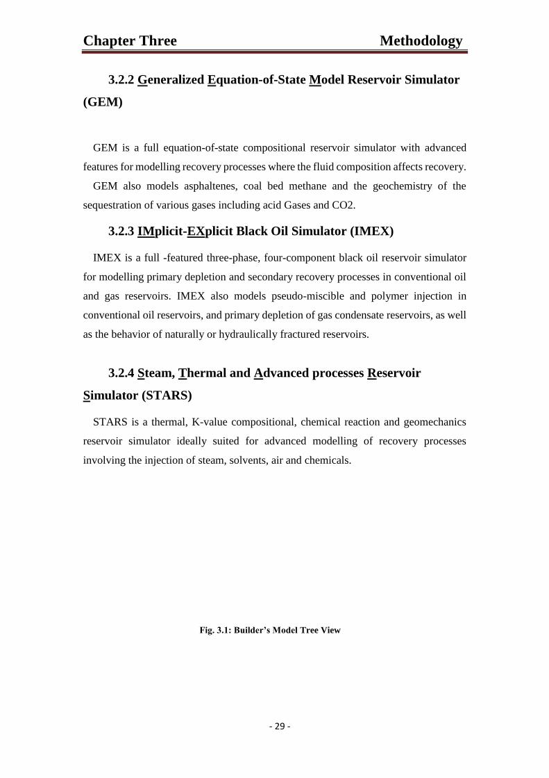
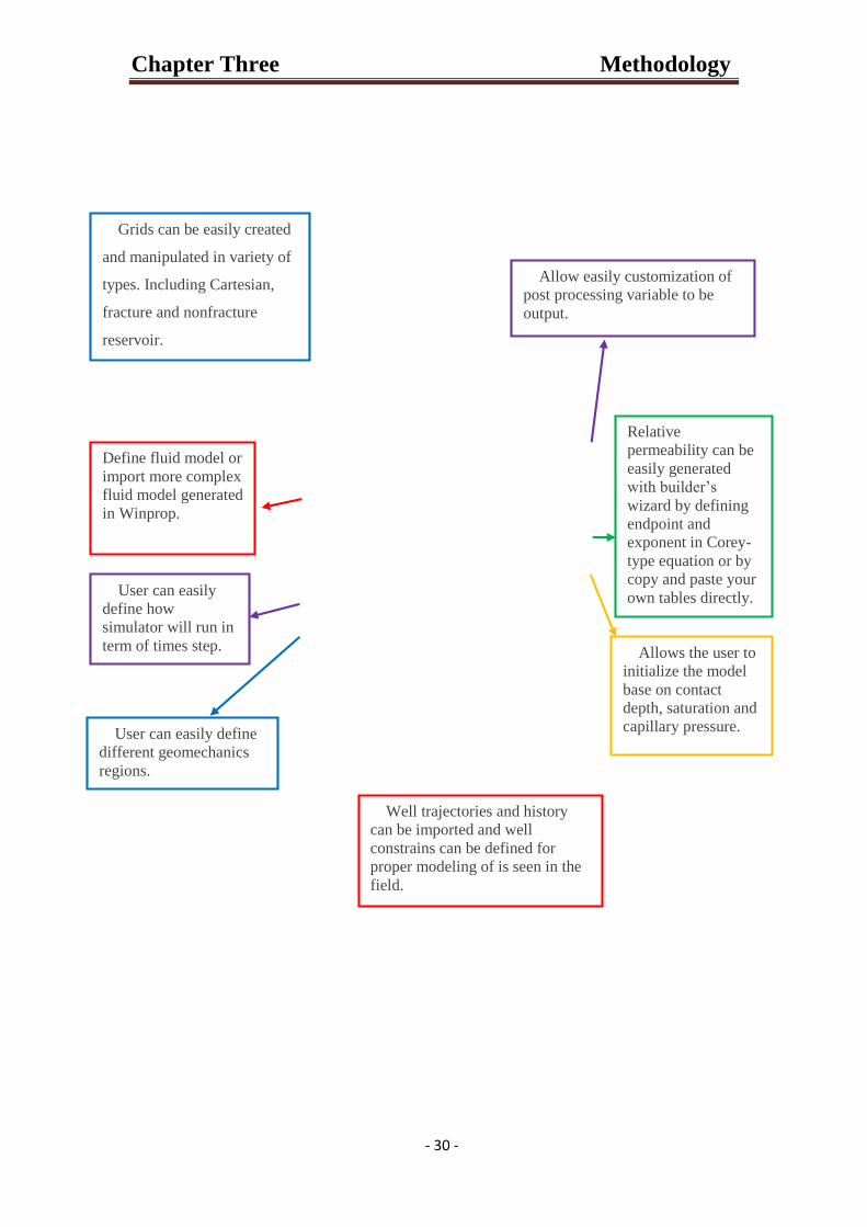
Figure 3.1 explains the six major components in builder’s tree view.
.
Chapter Three Methodology
- 29 -
3.2.2 Generalized Equation-of-State Model Reservoir Simulator
(GEM)
GEM is a full equation-of-state compositional reservoir simulator with advanced
features for modelling recovery processes where the fluid composition affects recovery.
GEM also models asphaltenes, coal bed methane and the geochemistry of the
sequestration of various gases including acid Gases and CO2.
3.2.3 IMplicit-EXplicit Black Oil Simulator (IMEX)
IMEX is a full -featured three-phase, four-component black oil reservoir simulator
for modelling primary depletion and secondary recovery processes in conventional oil
and gas reservoirs. IMEX also models pseudo-miscible and polymer injection in
conventional oil reservoirs, and primary depletion of gas condensate reservoirs, as well
as the behavior of naturally or hydraulically fractured reservoirs.
3.2.4 Steam, Thermal and Advanced processes Reservoir
Simulator (STARS)
STARS is a thermal, K-value compositional, chemical reaction and geomechanics
reservoir simulator ideally suited for advanced modelling of recovery processes
involving the injection of steam, solvents, air and chemicals.
Fig. 3.1: Builder’s Model Tree View
Chapter Three Methodology
- 30 -
Allow easily customization of
post processing variable to be
output.
Grids can be easily created
and manipulated in variety of
types. Including Cartesian,
fracture and nonfracture
reservoir.
Define fluid model or
import more complex
fluid model generated
in Winprop.
User can easily
define how
simulator will run in
term of times step.
User can easily define
different geomechanics
regions.
Well trajectories and history
can be imported and well
constrains can be defined for
proper modeling of is seen in the
field.
Relative
permeability can be
easily generated
with builder’s
wizard by defining
endpoint and
exponent in Corey-
type equation or by
copy and paste your
own tables directly.
Allows the user to
initialize the model
base on contact
depth, saturation and
capillary pressure.
Chapter Three Methodology
- 31 -
3.3 Steps to Get Results
Results Graph is typically used to plot curves of well properties that vary over time
(“Timeseries properties”). Examples of Timeseries property are Cumulative- Oil, Gas
and Water; Oil-, Gas- and Water Rates, etc. These Timeseries properties are read from
a simulation output file. The plot can contain as many wells, groups, sectors, leases, or
layers that vary with time as you wish data from several different files More than one
parameter versus time curves More than one parameter versus parameter curves.
Parameters from all those available in the selected simulation results files (SR2), field
history files (FHF) or PA Load Format files In addition, you can Plot spatial property
(e.g. oil saturation) versus distance curves. Currently you can specify three types of
distances: Along a well trajectory Along a well “path” (perforation-to-perforation as
defined in the simulation input file) and Between two blocks specified by their UBAs
(Universal Block Address, e.g. 5,3,2) Create “Special History” by reading spatial
property data at the available time records in the SR2 file. These parameters can then
be used just like any other Special History parameter that is output in the SR2 file.
Create “difference property” parameters. A difference property is created from two files
with identical property and well names. These parameters can be used just like any
other parameters to create curves.
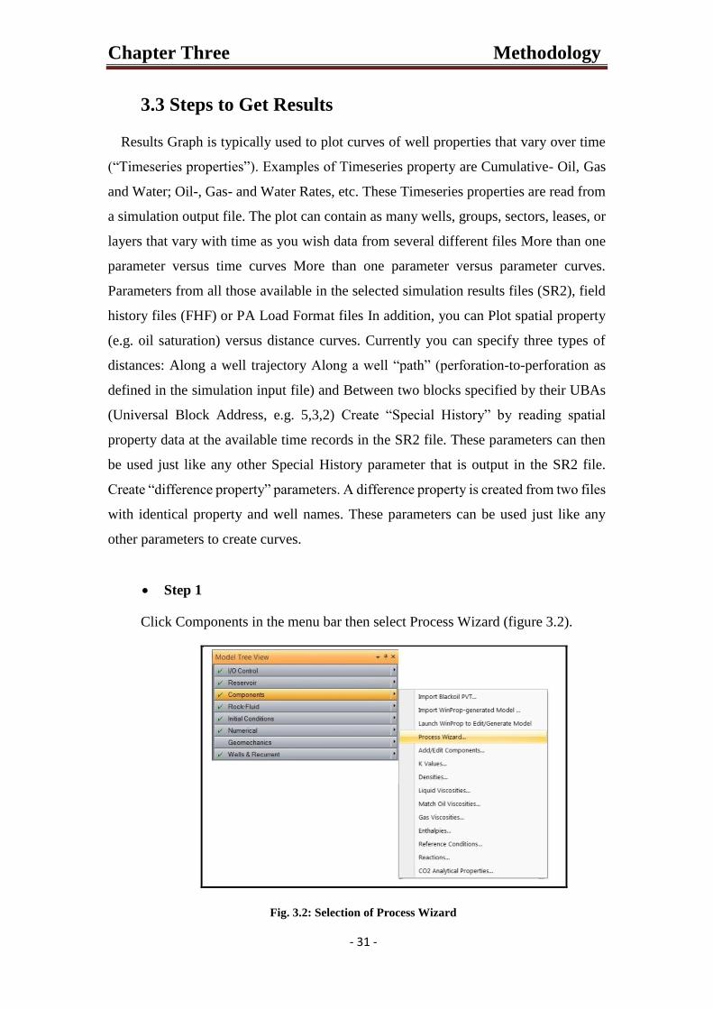
Step 1
Click Components in the menu bar then select Process Wizard (figure 3.2).
Fig. 3.2: Selection of Process Wizard
Chapter Three Methodology
- 32 -
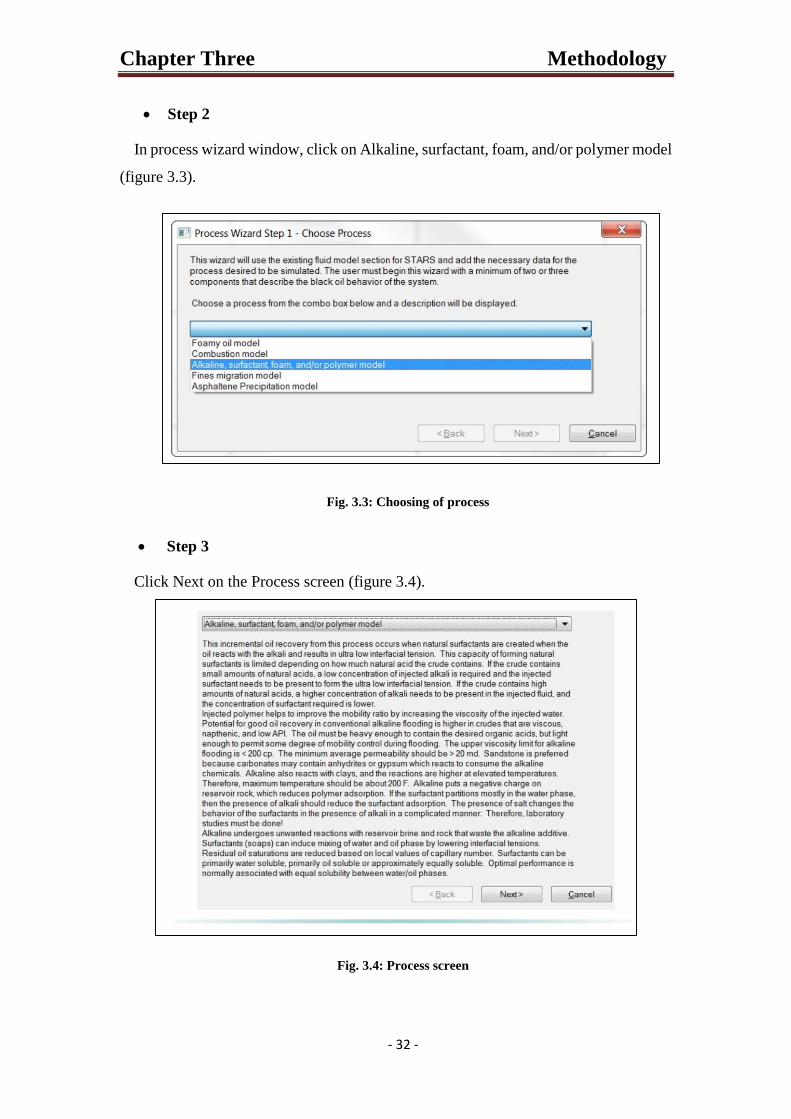
Step 2
In process wizard window, click on Alkaline, surfactant, foam, and/or polymer model
(figure 3.3).
Fig. 3.3: Choosing of process
Step 3
Click Next on the Process screen (figure 3.4).
Fig. 3.4: Process screen
Chapter Three Methodology
- 33 -
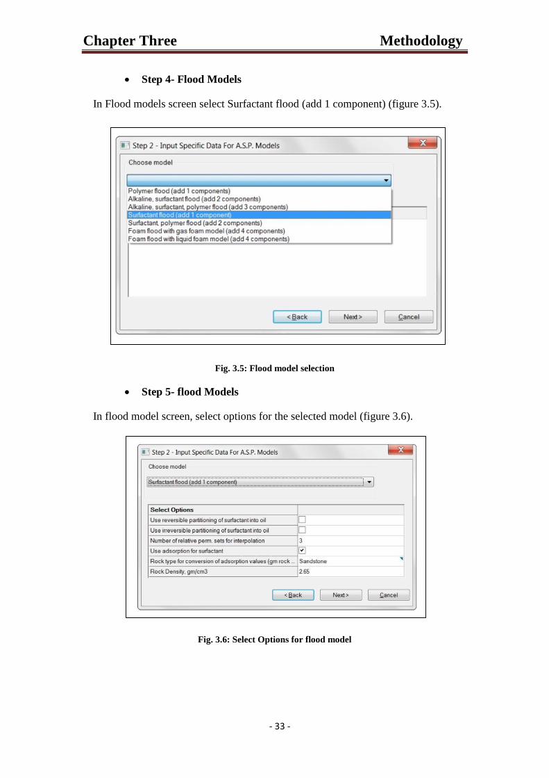
Step 4- Flood Models
In Flood models screen select Surfactant flood (add 1 component) (figure 3.5).
Fig. 3.5: Flood model selection
Step 5- flood Models
In flood model screen, select options for the selected model (figure 3.6).
Fig. 3.6: Select Options for flood model
Chapter Three Methodology
- 34 -
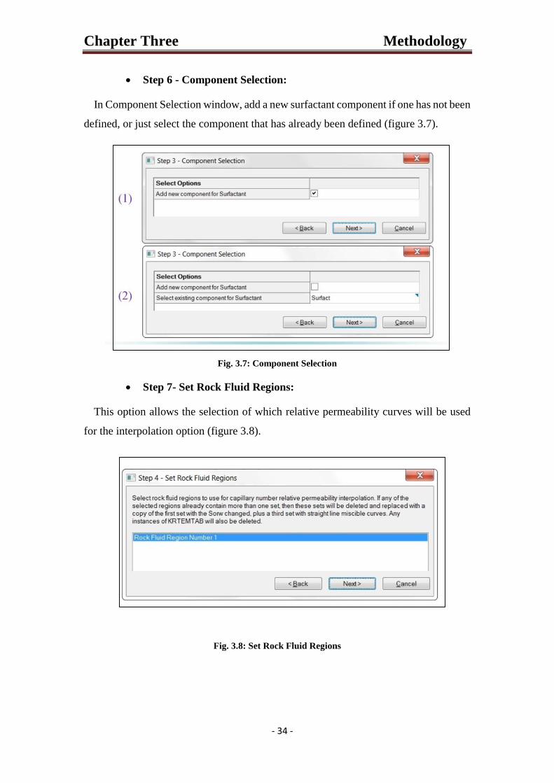
Step 6 - Component Selection:
In Component Selection window, add a new surfactant component if one has not been
defined, or just select the component that has already been defined (figure 3.7).
Fig. 3.7: Component Selection
Step 7- Set Rock Fluid Regions:
This option allows the selection of which relative permeability curves will be used
for the interpolation option (figure 3.8).
Fig. 3.8: Set Rock Fluid Regions
Chapter Three Methodology
- 35 -
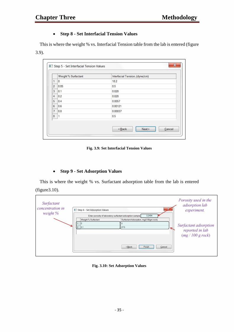
Step 8 - Set Interfacial Tension Values
This is where the weight % vs. Interfacial Tension table from the lab is entered (figure
3.9).
Fig. 3.9: Set Interfacial Tension Values
Step 9 - Set Adsorption Values
This is where the weight % vs. Surfactant adsorption table from the lab is entered
(figure3.10).
Fig. 3.10: Set Adsorption Values
Chapter Three Methodology
- 36 -
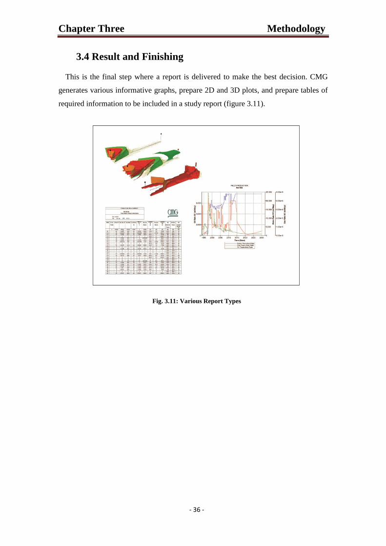
3.4 Result and Finishing
This is the final step where a report is delivered to make the best decision. CMG
generates various informative graphs, prepare 2D and 3D plots, and prepare tables of
required information to be included in a study report (figure 3.11).
Fig. 3.11: Various Report Types