RED: Robust Earliest Deadline Scheduling - CiteSeerX

RED: Robust Earliest Deadline Scheduling

�

Giorgio C. Buttazzo and John A. Stankovic

y

Scuola Superiore S. Anna

Via Carducci, 40 - 56100 Pisa, Italy

July 8, 1993

Abstract

In this paper we introduce a robust earliest deadline scheduling algorithm for deal-

ing with sporadic tasks under overloads in a hard real-time environment. The algorithm

synergistically combines many features including a very important minimum level of guar-

antee, dynamic guarantees, graceful degradation in overloads, deadline tolerance, resource

reclaiming, and dynamic re-guarantees. A necessary and su�cient schedulability test is

presented, and an e�cient O(n) guarantee algorithm is proposed. The new algorithm

is evaluated via simulation and compared to several baseline algorithms. The experi-

mental results show excellent performance of the new algorithm in normal and overload

conditions.

1 Introduction

Many real-time systems rely on the earliest deadline (EDF) �rst scheduling algorithm. This

algorithm has been shown to be optimal under many di�erent conditions. For example, for

independent, preemptable tasks, on a uni-processor EDF is optimal in the sense that if any

algorithm can �nd a schedule where all tasks meet their deadline then EDF can meet the

deadlines [Der 74]. Also, Jackson's rule [Jac 55] says that ordering a set of tasks by deadline

will minimize the maximum lateness. Further, it has also been shown that EDF is optimal

under certain stochastic conditions [Tow 91].

In spite of these advantageous properties, EDF has one major negative aspect. That is,

when using EDF in a dynamic system, if overload occurs, tasks may miss deadlines in an

unpredictable manner, and in the worst case, the performance of the system can approach zero

e�ective throughput [Loc 86]. This aspect of EDF is a well known fact and applies when using

EDF in a dynamic system. However, for a static collection of tasks we see by Moore's rule

[Moo 68], that to minimize the number of jobs which are late, simply order by earliest deadline

and drop the late jobs. By using EDF in a planning mode that performs dynamic guarantees,

�

This work was supported, in part, by NSF under grants IRI 9208920 and CDA 8922572, by ONR under

grant N00014-92-J-1048, by ESPRIT III TRACS Project #6373, by MURST 40%, and by CNR Special

Project on Robotics.

y

This work was performed while Prof. Stankovic was on sabbatical from the Computer Science Dept.,

Univ. of Massachusetts.

1

we can make use of a result similar to Moore's theorem, thereby avoiding the catastrophic

failure of EDF and making it more robust. Moreover, our approach synergistically combines

many nice scheduling features, further enhancing its robustness. The main contribution of

this paper is the development and the performance evaluation of a robust version of the EDF

algorithm, which has the following characteristics:

� it operates in normal and overload conditions with excellent dynamic performance and

avoids the major negative aspect of EDF scheduling;

� it is a priori analyzable together with o�ering certain minimum guarantees of system

performance;

� it is used in planning mode with additional on-line evaluative properties such as depict-

ing the size of the overload, when and where the overload will occur and dynamically

assessing the overall impact of this overload on the system;

� it includes extended timing semantics based on a deadline tolerance per task that is

suitable to certain applications such as robotics;

� it applies to simultaneously handling n classes of preemptable tasks where tasks can

have di�erent values;

� it is embedded in a general framework that:

{ is easily and cost e�ectively implementable (O(n) complexity),

{ separates guarantee, dispatching and rejection policies,

{ maintains a state view of the system that accurately depicts overload (to accom-

plish this required us a novel on-line calculation of overload with respect to varying

deadlines),

{ reclaims resources to improve performance, and

{ dynamically attempts re-guarantees when resources are reclaimed.

A performance study is accomplished via simulation. Our new algorithm is compared

against the standard earliest deadline algorithm and a guarantee based earliest deadline

algorithm [Ram 84]. We compare the algorithms under widely varying conditions with respect

to load, arrival rates, value distributions, allowed tolerances, and actual versus worst case

execution times. The new algorithm signi�cantly outperforms these baselines in all tested

situations.

The paper is organized as follows. Section 2 introduces terminology and basic concepts.

In Section 3 we state the main properties of the proposed approach, give the basic guarantee

algorithm, and present the e�cient calculation of system load. In Section 4 we deal with

overload conditions and present a new model for robust scheduling in overload. Section 5

discusses the problem of resource reclaiming, which adds exibility to our approach, and

presents a new framework in which all the parts of the algorithm synergistically integrate

into a general scheme. Section 6 presents the performance study. Section 7 discusses related

research, showing how this work is a signi�cant extension to the state of the art of EDF

scheduling. Section 8 summarizes the main results and presents the implications of the

proposed approach.

2

2 Terminology and Basic Concepts

In order to motivate and more easily understand the following de�nitions, proofs, and subse-

quent additions to the basic algorithm, we begin by presenting an overview of the dynamic

operation of the system. First, we assume that there are n known tasks given by T

1

; T

2

; :::; T

n

where each has a worst case computation time, a deadline relative to when the task is acti-

vated, and a speci�ed deadline tolerance level which indicates the amount of lateness allowed

for a given task (may be zero). Tasks are preemptable. Tasks are invoked dynamically, and

at any point in time the system could have zero, all, or an arbitrary subset of these n tasks

active.

When a task is activated at time t, it is inserted into an ordered list of tasks based on

an earliest deadline �rst policy and an analysis is performed to determine feasibility of the

entire set of currently active tasks, whether overload exists and, if so, where, when, for how

long, and which tasks are involved in the overload, and how the active tasks would operate

subject to allowed tolerances.

2.1 Minimum Levels of Guarantee

Static real-time systems are designed for worst case situations. Then, assuming that all

the assumptions made in the design and analysis are correct, all tasks always make their

deadlines. Theoretically, we can then say that the level of guarantee for these systems is

absolute. Unfortunately, static systems are not always possible because for many applications

the environment and system itself, being imperfect, violate their assumptions fairly often, or

because to develop a static design with absolute guarantees is too costly. When either or

both of these conditions exist, we �nd dynamic real-time systems. In these systems, absolute

guarantees are not attained. However, we believe that a necessary property of dynamic

systems must be a tradeo� between what is guaranteed and what is probabilistic. A property

of a dynamic real-time system should be a minimum level of guarantee together with best

e�ort beyond this minimum. For example, assume that we have an application with 2000

di�erent tasks and this application exists in a hostile environment. To statically design a

solution might be impossible, or if it were possible might require a very large number of

processors (say 100s of them). Now it may be known that only 20 of these 2000 tasks are

truly critical and that it is unlikely that more than 10 percent of the tasks are active at

the same time. A good dynamic system design would give an absolute guarantee to the 20

critical tasks and provide enough resources to also meet the deadlines of all other tasks likely

to be active at the same time, i.e., under normal loads. To achieve this may only require 5-6

processors. In other words, to build a system for a reasonable cost, we may miss deadlines

(rarely) on non-critical tasks.

Unfortunately, many algorithms used in dynamic real-time systems do not have good

minimum level of guarantee properties. For example, earliest deadline and rate monotonic

have very limited minimum guarantees. Our RED algorithm considers minimum levels of

guarantees at two di�erent times: a priori and at run time. For the a priori guarantee

of critical tasks, the designer applies all worst case assumptions, but only for the critical

tasks and knowing that the run time algorithm is RED. In this way, an absolute minimum

performance is guaranteed for the critical tasks. In the a priori analysis we show that using

3

RED all critical task deadlines are met, and that even in the presence of other real-time tasks

from other classes of jobs, that there is no way that these non-critical tasks can negatively

in uence the scheduling of the critical tasks. This is a simple yet important property of our

approach. Beyond this a priori analysis at run time, RED ensures that all critical and other

real-time tasks will make their deadline under normal loads, simply due to the optimality

feature of EDF scheduling. When overloads occur for non-critical tasks, RED still ensures

that critical tasks can execute and that there is a best e�ort at maximizing value of non-critical

tasks. Further, even if the load assumptions for the critical tasks are wrong and more critical

tasks arrive than planned for a priori, then RED still guarantees a high value by ensuring

that any critical task, once guaranteed, never misses its deadline. There is no domino e�ect.

In summary, by maintaining a pro�le, analyzing it, and using resource reclaiming, the value

output of the system is maintained at a high value. Catastrophic drops in value do not occur

and e�ective cpu utilization is also maintained at a high value.

2.2 Notations and Assumptions

Before we describe the guarantee algorithm, we �rst state our de�nitions, notations, and

assumptions.

De�nitions:

� A task is a sequence of instructions that will continuously use the processor until its

completion, if it is executing alone on the processor [Sha 90].

� A sporadic task is a task with irregular arrival times and minimum interarrival time.

� A task set is said to be feasibly scheduled by a certain algorithm if and only if all tasks

can complete their execution within their time constraints.

� A newly arrived task is said to be guaranteed to complete its execution before its deadline

if and only if a feasible schedule can be created for the newly arrived task and those

still active tasks that have been previously guaranteed, such that all tasks will meet

their timing constraints.

� We refer to the time interval between the �nishing time of a task and its absolute

deadline as a residual time.

For the proofs which provide a necessary and su�cient condition for the schedulability

of task sets at each task activation, we require a notation that identi�es the i

th

task in the

current ordered list at time t. For this we use the notation J

1

; J

2

; :::; J

m

where J

i

is the

task in the i

th

position. At the next task activation, the task in each position may change

completely due to the deadline of the new task and possible task completions since the last

task activation. On task completions the order does not change, but all tasks conceptually

move up one position. Further, at each task activation, once a task is inserted into the ordered

list, then each task in the list has a current scheduled start and �nish time. If a task completes

before its worst case execution time, then the cpu time will be reclaimed, essentially moving

all other still active tasks starting time forward. The time a task is dispatched is called the

4

actual starting time. Since tasks are preemptable, a given task may have multiple actual

start times, but only a single actual �nish time. At each new actual start time, a task only

requires its remaining execution time, not the full worst case time (in other words the task

is not restarted, just continued).

Notation:

J denotes a set of active sporadic tasks J

i

ordered by increasing deadline, J

1

being the task

with the shortest absolute deadline.

a

i

denotes the arrival time of task J

i

, i.e., the time at which the task is activated and becomes

ready to execute.

C

i

denotes the maximum computation time of task J

i

, i.e., the worst case execution time

(wcet) needed for the processor to execute task J

i

without interruption.

c

i

denotes the dynamic computation time of task J

i

, i.e., the remaining worst case execu-

tion time needed for the processor, at the current time, to complete task J

i

without

interruption.

d

i

denotes the absolute deadline of task J

i

, i.e., the time before which the task should com-

plete its execution, without causing any damage to the system.

D

i

denotes the relative deadline of task J

i

, i.e., the time interval between the arrival time

and the absolute deadline.

S

i

denotes the �rst start time of task J

i

, i.e., the time at which task J

i

gains the processor

for the �rst time.

s

i

denotes the last start time of task J

i

, i.e., the last time, before the current time, at which

task J

i

gained the processor.

f

i

denotes the estimated �nishing time of task J

i

, i.e., the time according to the current

schedule at which task J

i

should complete its execution and leave the system.

L

i

denotes the laxity of task J

i

, i.e., the maximum time task J

i

can be delayed before its

execution begins.

R

i

denotes the residual time of task J

i

, i.e., the length of time between the �nishing time of

J

i

and its absolute deadline.

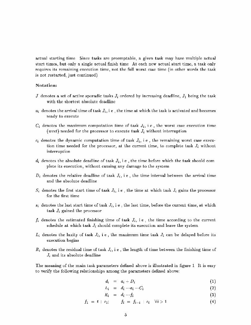
The meaning of the main task parameters de�ned above is illustrated in �gure 1. It is easy

to verify the following relationships among the parameters de�ned above:

d

i

= a

i

+D

i

(1)

L

i

= d

i

� a

i

� C

i

(2)

R

i

= d

i

� f

i

(3)

f

1

= t+ c

1

; f

i

= f

i�1

+ c

i

8i > 1 (4)

5

Figure 1: Task parameters

In our model, we assume that the minimum interarrival time of each sporadic task is

equal to its relative deadline D

i

, thus a sporadic task J

i

can be completely characterized by

specifying its relative deadline D

i

and its worst case execution time C

i

. Hence, a sporadic

task set will be denoted as follows: J = fJ

i

(C

i

; D

i

), i = 1 to ng.

Throughout our discussion, we assume that tasks are scheduled on a uniprocessor by the

Earliest Deadline First (EDF) scheduling algorithm, according to a preemptive scheduling

discipline, so that the processor is always assigned to the task whose deadline is the earliest.

We assume that tasks arrive dynamically and arrival times are not known a priori. EDF

algorithm is optimal in underload conditions, it is dynamic, it can be used for periodic and

aperiodic tasks, and it can be easily extended to deal with precedence constraints. Group of

tasks with precedence constraints can be scheduled with EDF by modifying their deadlines

and release times so that both deadlines and precedence relations are met [Bla 76] [Che 90].

Overheads are assumed to be zero, but how to account for overheads is discussed in the

conclusions.

3 Guarantee Algorithm

We formulate the dynamic, on-line, guarantee test in terms of residual time, which is a

convenient parameter to deal with both normal and overload conditions. We �rst present the

main results without the notion of deadline tolerance, and then we will extend the algorithm

by including tolerance levels and task rejection policy. The basic properties stated by the

following lemmas and theorems are used to derive an e�cient O(n) algorithm for analyzing

the schedulability of the sporadic task set whenever a new task arrives in the systems.

Lemma 1 Given a set J = fJ

1

; J

2

; :::; J

n

g of active sporadic tasks ordered by increasing

deadline, the residual time R

i

of each task J

i

at time t can be computed by the following

recursive formula:

R

1

= d

1

� t� c

1

(5)

R

i

= R

i�1

+ (d

i

� d

i�1

)� c

i

: (6)

Proof.

By the residual time de�nition (equation 3) we have:

R

i

= d

i

� f

i

:

6

By the assumption on set J, at time t, task J

1

is executing and cannot be preempted by

other tasks in the set J , hence its estimated �nishing time is given by the current time plus

its remaining execution time:

f

1

= t + c

1

and, by equation (3), we have:

R

1

= d

1

� f

1

= d

1

� t� c

1

:

For any other task J

i

, with i > 1, each task J

i

will start executing as soon as J

i�1

completes,

hence we can write:

f

i

= f

i�1

+ c

i

(7)

and, by equation (3), we have:

R

i

= d

i

� f

i

= d

i

� f

i�1

� c

i

=

= d

i

� (d

i�1

�R

i�1

)� c

i

= R

i�1

+ (d

i

� d

i�1

)� c

i

and the lemma follows. 2

Lemma 2 A task J

i

is guaranteed to complete within its deadline if and only if R

i

� 0.

Proof.

(If part): Suppose R

i

� 0. By the result obtained in Lemma 1 we can write:

R

i�1

+ (d

i

� d

i�1

)� c

i

� 0

that is, by equation (3):

d

i

� f

i�1

� c

i

� 0

which can be written as:

f

i�1

+ c

i

� d

i

and by equation (7):

f

i

� d

i

which means that J

i

completes its execution within its deadline, i.e., it is guaranteed.

(Only if part): Suppose task J

i

completes its execution within its deadline. This means that

f

i

� d

i

and since, by equation (7), f

i

= f

i�1

+ c

i

, we have

f

i�1

+ c

i

� d

i

:

By equation (3) we can write:

(d

i�1

�R

i�1

) + c

i

� d

i

� 0

and since, by equation (6) of Lemma 1,

(d

i�1

� R

i�1

) + c

i

� d

i

= �R

i

we have R

i

� 0 and the lemma follows. 2

7

Theorem 3 A set J = fJ

i

, i = 1 to ng of n active sporadic tasks ordered by increasing

deadline is feasibly schedulable if and only if R

i

� 0 for all J

i

2 J.

Proof.

It follows directly by applying Lemma 2 to each task of the set. 2

Notice that if we have a feasibly schedulable set J of n active sporadic tasks, and a new

task J

a

arrives at time t, to guarantee the new ordered task set J

0

= J [ fJ

a

g we only need

to compute the residual time of task J

a

and the residual times of tasks J

i

such that d

i

> d

a

.

This is because the execution of J

a

does not in uence those tasks having deadline less than

or equal to d

a

, which are scheduled before J

a

.

We now summarize the basic guarantee algorithm in the form of pseudo code. This basic

version is enhanced in later sections of the paper to produce the robust ED (RED) algorithm.

Algorithm GUARANTEE(J; J

a

)

begin

t = get current time();

R

0

= 0;

d

0

= t;

Insert J

a

in the ordered task list;

J

0

= J [ J

a

;

k = position of J

a

in the task set J

0

;

for each task J

0

i

such that i � k do f

R

i

= R

i�1

+ (d

i

� d

i�1

)� c

i

;

if (R

i

< 0) then return ("Not Guaranteed");

g

return ("Guaranteed");

end

Clearly, the above guarantee algorithm runs in O(n) time in the worst case. This makes

the proposed approach an e�cient schedulability test to run whenever a sporadic task arrives.

Now we introduce a new framework for handling real-time sporadic tasks under overload

conditions, and we propose a robust version of the Earliest Deadline algorithm. Before we

describe such a robust algorithm, we de�ne few more basic concepts.

3.1 Load Calculation

In some real-time environments, the workload of the system can be considered the same as the

processor utilization factor. For example, for a set of n periodic tasks with computation time

C

i

and period T

i

, with no resource con icts, the utilization factor can be easily computed, as

proposed in [Liu 73], by

U =

n

X

i=1

C

i

T

i

:

8

For sporadic tasks, the utilization factor could be computed by considering the minimum

interarrival time as a sort of period. However, this would lead to an overestimation of the

workload, since it would refer to the (very pessimistic) case in which all sporadic tasks have

the maximum arrival rate.

In a real-time environment with aperiodic tasks, a commonly accepted de�nition of work-

load refers to the standard queueing theory, according to which a load �, also called tra�c

intensity, represents the expected number of task arrivals per mean service time [Zlo 91].

This de�nition, however, does not say anything about task deadlines, hence it is not as useful

in a hard real-time environment.

A more formal de�nition has been proposed in [Bar 92], in which is said that a sporadic

real-time environment has a loading factor b if and only if it is guaranteed that there will

be no interval of time [t

x

; t

y

) such that the sum of the execution times of all tasks making

requests and having deadlines within this interval is greater than b(t

y

� t

x

). They use this

de�nition in order to prove worst case bounds on the performance of on-line algorithms in

the presence of overloads. Theoretically, this is �ne for bounds analysis. For practical use,

however, these intervals can be very numerous, requiring too much computation if used on-

line. Moreover, having only a single load value can easily be misleading. Although such a

de�nition is more precise than the �rst one, it is still of little practical use, since no on-line

methods for calculating the load are provided, nor proposed.

One main purpose of RED is to operate well even in overload conditions. However, it

is di�cult to develop a good measure of load in a real-time system because each task has a

unique start time and deadline. This gives rise to overloads occurring in speci�c intervals, even

when the total processor utilization is very low. For actual use on-line, we need an e�cient

mechanism to detect and react to overload. Our approach uses a technique that is very

similar to the o�-line iterative analysis done in rate monotonic scheduling; however, we use

it on-line and apply it to aperiodic tasks scheduled by earliest deadline rather than periodic

tasks scheduled by frequency of period. The idea is to iteratively identify the cpu utilization

required by all the tasks up to the i

th

task. For example, �rst we compute the utilization

required by the �rst task in the schedule. Then we compute the utilization required by the

�rst two tasks in the schedule, etc. As we show below, this iterative procedure is e�cient,

avoids needing to know the theoretically worst case load in any interval, and has many nice

properties including:

� a complete load pro�le is e�ciently created,

� the time (intervals) at which overloads might occur is predicted,

� the magnitude of the overload is identi�ed,

� the impact of the overload on the system as a whole is calculated, e.g., will only a few

tasks miss their deadlines or is it possible that many (all) tasks will miss their deadlines,

and

� many types of other analysis can be applied to the pro�le including

{ applying semantics of deadline tolerance levels (of speci�c tasks being late by

speci�c amounts)

9

{ shifting load by altering deadlines (possible, e.g., by slowing down operations in a

robotics application).

Before we explain our method of computing system load, we introduce the following

notation:

�

i

(t

a

) indicates the processor load in the interval [t

a

; d

i

), where t

a

is the arrival time of the

latest arrived task in the sporadic set,

�

max

indicates the maximum processor load among all intervals [t

a

; d

i

), i = 1 to n, where t

a

is the arrival time of the latest arrived task in the sporadic set.

In practice, the load is computed only when a new task arrives, and it is of signi�cant

importance only within those time intervals [t

a

; d

i

) from the latest arrival time t

a

, which is

the current time, and a deadline d

i

. Thus the load computation can be simpli�ed as:

�

i

(t

a

) =

P

d

k

�d

i

c

k

d

i

� t

a

:

Theorem 4 The load �

i

(t

a

) in the interval [t

a

; d

i

) can be directly related to the residual time

R

i

of task J

i

, according to the following relation:

�

i

= 1�

R

i

d

i

� t

a

(8)

Proof.

Since tasks are ordered by increasing deadline, after the arrival time t

a

, they will be executed

in such a way that f

1

= t

a

+ c

1

and f

i

= f

i�1

+ c

i

. Therefore, we can write:

X

d

k

�d

i

c

k

+ t

a

= f

i

and since, by equation (3),

f

i

= d

i

� R

i

we have:

X

d

k

�d

i

c

k

= (d

i

� t

a

)� R

i

:

Hence the load �

i

(t

a

) can be directly related to the residual time R

i

of task J

i

, as follows:

�

i

(t

a

) = 1�

R

i

d

i

� t

a

:

2

10

3.2 Load function

It is important to point out that, within the interval [t

a

; d

n

] between the latest arrival time

t

a

and the latest deadline of task J

n

, the processor work load is not constant, but it varies in

each interval [t

a

; d

i

). To express this fact, we de�ne the following load function:

�(t

a

; t) =

8

>

<

>

:

�

1

for t

a

� t < d

1

�

i

for t 2 [d

i�1

; d

i

)

0 for t � d

n

De�nition 1 Let �

max

be the maximum of the load function �(t

a

; t) in the interval [t

a

; d

n

].

We say that the system is underloaded if �

max

� 1, and overloaded if �

max

> 1.

De�nition 2 We de�ne Exceeding Time E

i

of a task J

i

as the time that task J

i

will execute

after its deadline, that is: E

i

= max

i

(0;�R

i

). We then de�ne Maximum Exceeding Time

E

max

the maximum among all E

i

in the tasks set, that is: E

max

= max

i

(E

i

).

Notice that, in underloaded conditions (�

max

� 1), E

max

= 0, whereas in overload condi-

tions (�

max

> 1), E

max

> 0.

Observation 1 Once we have computed the load factor �

i

for task J

i

, the next load factor

�

i+1

can be computed as follows:

�

i+1

=

�

i

(d

i

� t

a

) + c

i+1

d

i+1

� t

a

:

Proof.

By Theorem 4 we can write:

�

i+1

= 1�

R

i+1

d

i+1

� t

a

and by Lemma 1:

�

i+1

= 1�

R

i

+ d

i+1

� d

i

� c

i+1

d

i+1

� t

a

=

d

i

� t

a

� R

i

+ c

i+1

d

i+1

� t

a

:

Applying equation (8) we have:

(d

i

� t

a

� R

i

) = �

i

(d

i

� t

a

)

therefore we obtain:

�

i+1

=

�

i

(d

i

� t

a

) + c

i+1

d

i+1

� t

a

:

2

11

task a

i

C

i

d

i

J

0

7 4 12

J

1

0 14 16

J

2

3 4 21

J

3

5 5 28

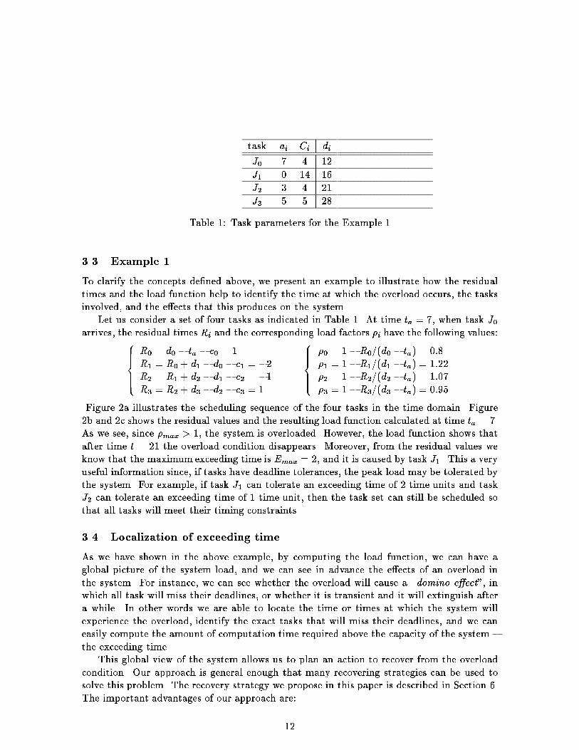
Table 1: Task parameters for the Example 1

3.3 Example 1

To clarify the concepts de�ned above, we present an example to illustrate how the residual

times and the load function help to identify the time at which the overload occurs, the tasks

involved, and the e�ects that this produces on the system.

Let us consider a set of four tasks as indicated in Table 1. At time t

a

= 7, when task J

0

arrives, the residual times R

i

and the corresponding load factors �

i

have the following values:

8

>

>

>

<

>

>

>

:

R

0

= d

0

� t

a

� c

0

= 1

R

1

= R

0

+ d

1

� d

0

� c

1

= �2

R

2

= R

1

+ d

2

� d

1

� c

2

= �1

R

3

= R

2

+ d

3

� d

2

� c

3

= 1

8

>

>

>

<

>

>

>

:

�

0

= 1� R

0

=(d

0

� t

a

) = 0:8

�

1

= 1� R

1

=(d

1

� t

a

) = 1:22

�

2

= 1� R

2

=(d

2

� t

a

) = 1:07

�

3

= 1� R

3

=(d

3

� t

a

) = 0:95

Figure 2a illustrates the scheduling sequence of the four tasks in the time domain. Figure

2b and 2c shows the residual values and the resulting load function calculated at time t

a

= 7.

As we see, since �

max

> 1, the system is overloaded. However, the load function shows that

after time t = 21 the overload condition disappears. Moreover, from the residual values we

know that the maximum exceeding time is E

max

= 2, and it is caused by task J

1

. This a very

useful information since, if tasks have deadline tolerances, the peak load may be tolerated by

the system. For example, if task J

1

can tolerate an exceeding time of 2 time units and task

J

2

can tolerate an exceeding time of 1 time unit, then the task set can still be scheduled so

that all tasks will meet their timing constraints.

3.4 Localization of exceeding time

As we have shown in the above example, by computing the load function, we can have a

global picture of the system load, and we can see in advance the e�ects of an overload in

the system. For instance, we can see whether the overload will cause a \domino e�ect", in

which all task will miss their deadlines, or whether it is transient and it will extinguish after

a while. In other words we are able to locate the time or times at which the system will

experience the overload, identify the exact tasks that will miss their deadlines, and we can

easily compute the amount of computation time required above the capacity of the system {

the exceeding time.

This global view of the system allows us to plan an action to recover from the overload

condition. Our approach is general enough that many recovering strategies can be used to

solve this problem. The recovery strategy we propose in this paper is described in Section 6.

The important advantages of our approach are:

12

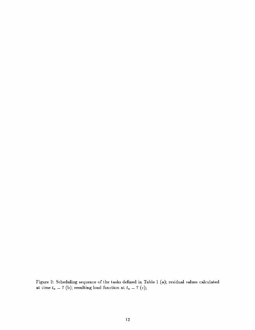
Figure 2: Scheduling sequence of the tasks de�ned in Table 1 (a); residual values calculated

at time t

a

= 7 (b); resulting load function at t

a

= 7 (c);

13

� it increases exibility in expressing time constraints via the deadline tolerance mecha-

nism,

� it makes the scheduling algorithm more robust in the sense of giving better and more

predictable performance under all loads; this is achieved via a combination of using

value, deadline tolerance, and resource reclaiming,

� it allows the integration of di�erent rejection policies for di�erent classes of tasks, and

� it provides a minimum guarantee even in overload conditions.

4 Deadline Tolerance

In many real applications, such as robotics, the deadline timing semantics is more exible

than scheduling theory generally permits. For example, most scheduling algorithms and ac-

companying theory treat the deadline as an absolute quantity. However, it is often acceptable

for a task to continue to execute and produce an output even if it is late { but not too late.

In order to more closely model this real world situation, we permit each task to be char-

acterized by a computation time, deadline, and deadline tolerance. The deadline tolerance

is then the amount of time by which a speci�c task is permitted to be late. Further, when

using a dynamic guarantee paradigm, a deadline tolerance provides a sort of compensation

for the pessimistic evaluation of using the worst case execution time. For example, without

tolerance, we could �nd that a task set is not feasibly schedulable, and hence decide to reject

a task. But, in reality, the system could have been scheduled because with the tolerance and

full assessment of the load we might determine that overload is simply for this task and it

is within its tolerance level. Another e�ect is that various tasks could actually �nish before

their worst case times so the resource reclaiming part of our algorithm could then compensate

and the guaranteed task with tolerance could actually �nish on time. Basically, our approach

minimizes the pessimism found in a basic guarantee algorithm.

Another real application issue is that once some task has to miss a deadline, it should

be the least valuable task. Again, many algorithms do not address this fact. In summary,

we modify our previous task model by introducing two additional parameters: a deadline

tolerance and a task value.

Notation:

m

i

denotes the deadline tolerance of task J

i

, i.e., the maximumtime that task J

i

may execute

after its deadline, and still produce a valid result.

v

i

denotes the task value, i.e, the relative importance of task J

i

with respect to the other

tasks in the set.

Moreover, we split real-time tasks into two classes:

� HARD tasks are those tasks that are guaranteed to complete within their deadline in

underload conditions;

14

� CRITICAL tasks are those tasks that are dynamically guaranteed to complete within

their deadline in underload conditions and in overload conditions. CRITICAL tasks

may also be guaranteed a priori for speci�ed loads (in both under and overloads) by

ensuring enough cpu power for them.

In our more robust model, a sporadic task J

i

is completely characterized by specifying its

class, its relative deadline D

i

, the deadline tolerance m

i

, the worst case execution time C

i

,

and its value v

i

. In the following, we assume that the task class can be derived from the task

value. For instance, tasks with maximum value v

i

= V

max

can be considered as CRITICAL.

In summary, a sporadic task set will be denoted as follows:

J = fJ

i

(C

i

; D

i

; m

i

; v

i

); i = 1 to ng

Within this framework, di�erent policies are used for handling sporadic tasks in a robust

fashion. In particular, tasks are scheduled based on their deadline, guaranteed based on

C

i

; D

i

; m

i

; v

i

, and rejected based on v

i

.

4.1 The general RED scheduling strategy

When dealing with the deadline tolerance factorm

i

, each Exceeding Time has to be computed

with respect to the tolerance factor m

i

, so we have: E

i

= max(0;�(R

i

+m

i

)).

To guarantee the execution time of CRITICAL tasks in overload conditions, the algo-

rithm uses a rejection strategy to reject tasks based on their values, to remove the overload

condition. Several rejection strategies can be used for this purpose. As discussed in the next

section on performance evaluation, two rejection strategies have been implemented and com-

pared. The �rst policy rejects a single task (the least value one), while the second strategy

tries to reject more tasks, but only if the newly arrived task is a CRITICAL task. In the

single task policy, since the algorithm knows the Maximum Exceeding Time E

max

and the

task J

w

which would cause such a time over ow, it tries to reject the least value task in

the sporadic set, whose execution time is greater than E

max

. The multiple task policy may

choose to reject more tasks such that

P

i

c

i

� E

max

and whose deadlines are less than the

deadline of the newly arrived CRITICAL task. Both of these options are evaluated in the

performance study. Another strategy for rejecting tasks is based on the concept of value

density, de�ned as the ratio v

i

=C

i

. According to this strategy, tasks with longer computation

times have lower value density and hence have more chances to be rejected. To be general,

we will describe the RED algorithm by assuming that, in overload conditions, some rejection

policy will search for a subset J

�

of least value (non critical) tasks to reject in order to make

the current set schedulable. If J

�

is returned empty, then the overload cannot be recovered,

and the newly arrived task cannot be accepted. Notice that CRITICAL tasks previously

guaranteed cannot be rejected.

If J

w

is the task causing the maximum exceeding time over ow, the rejectable tasks that

can remove the overload condition are only those tasks whose deadline is earlier than or equal

to d

w

. This means that the algorithm has to search only for tasks J

i

, with i � w.

15

Algorithm RED guarantee(J; J

a

)

begin

t = get current time();

E = 0; /* Maximum Exceeding Time */

w = 1; /* Exceeding task index */

R

0

= 0;

d

0

= t;

J

0

= J [ fJ

a

g; /* Insert J

a

in the ordered task list */

k = position of J

a

in the task set J

0

;

for each task J

0

i

such that i � k do f

R

i

= R

i�1

+ (d

i

� d

i�1

)� c

i

;

if (R

i

+m

i

< �E) then f

E = �(R

i

+m

i

);

w = i;

g

g

if (E = 0) then return (``Guaranteed");

else f Let J

�

be the set of least value tasks

selected by the rejection policy;

if (J

�

is not empty) then f

reject all task in J

�

;

return (``Guaranteed");

g

else return (``Not Guaranteed");

g

end

4.2 Example 2

To show how the RED algorithm works, we present an example on a set of �ve tasks, whose

parameters are given in Table 2. The rejection policy adopted in the example is to remove

the least value task, such that its execution time is greater than the maximum exceeding

time E

max

. The estimated scheduling sequence of the set at time t = 3, before J

0

arrives, is

shown in �gure 3a, while the situation at time t = 4 is illustrated in �gure 3b. When task J

0

arrives, the set is found not schedulable, because R

3

+m

3

= �2 < 0, meaning that task J

3

would exceed its (tolerant) time constraint by 2 units.

To make the set schedulable, some task has to be rejected, so that all residual times

become non negative. According to this strategy, the least value task in the set, task J

4

(with value 2) cannot be removed, since it would not recover the overload situation. The

next least value task, J

2

(with value 3) cannot be removed, because its computation time

(c

2

= 1) is not su�cient to remove the exceeding load. The �rst least value task that can be

removed is task J

1

, since its computation time (c

1

= 5) is greater than E

max

.

16

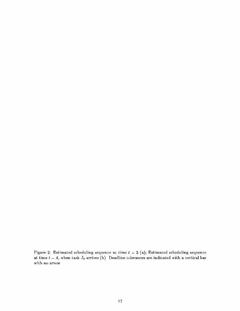
Figure 3: Estimated scheduling sequence at time t = 3 (a); Estimated scheduling sequence

at time t = 4, when task J

0

arrives (b). Deadline tolerances are indicated with a vertical bar

with no arrow.

17

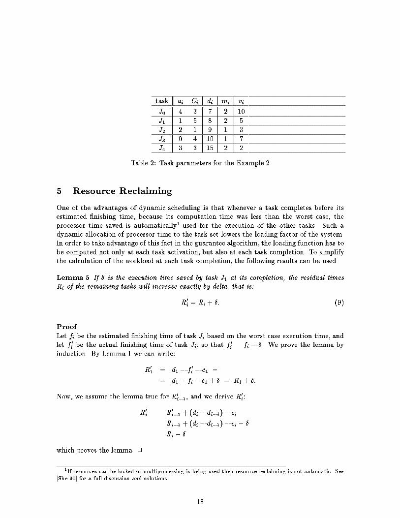
task a

i

C

i

d

i

m

i

v

i

J

0

4 3 7 2 10

J

1

1 5 8 2 5

J

2

2 1 9 1 3

J

3

0 4 10 1 7

J

4

3 3 15 2 2

Table 2: Task parameters for the Example 2

5 Resource Reclaiming

One of the advantages of dynamic scheduling is that whenever a task completes before its

estimated �nishing time, because its computation time was less than the worst case, the

processor time saved is automatically

1

used for the execution of the other tasks. Such a

dynamic allocation of processor time to the task set lowers the loading factor of the system.

In order to take advantage of this fact in the guarantee algorithm, the loading function has to

be computed not only at each task activation, but also at each task completion. To simplify

the calculation of the workload at each task completion, the following results can be used.

Lemma 5 If � is the execution time saved by task J

1

at its completion, the residual times

R

i

of the remaining tasks will increase exactly by delta, that is:

R

0

i

= R

i

+ �: (9)

Proof.

Let f

i

be the estimated �nishing time of task J

i

based on the worst case execution time, and

let f

0

i

be the actual �nishing time of task J

i

, so that f

0

i

= f

i

� �. We prove the lemma by

induction. By Lemma 1 we can write:

R

0

1

= d

1

� f

0

i

� c

1

=

= d

1

� f

i

� c

1

+ � = R

1

+ �:

Now, we assume the lemma true for R

0

i�1

, and we derive R

0

i

:

R

0

i

= R

0

i�1

+ (d

i

� d

i�1

)� c

i

=

= R

i�1

+ (d

i

� d

i�1

)� c

i

+ � =

= R

i

+ �

which proves the lemma. 2

1

If resources can be locked or multiprocessing is being used then resource reclaiming is not automatic. See

[She 90] for a full discussion and solutions.

18

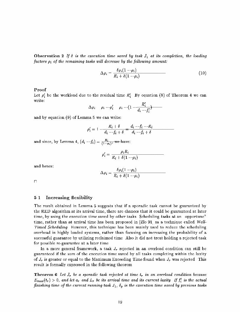
Observation 2 If � is the execution time saved by task J

1

at its completion, the loading

factors �

i

of the remaining tasks will decrease by the following amount:

��

i

=

��

i

(1� �

i

)

R

i

+ �(1� �

i

)

(10)

Proof.

Let �

0

i

be the workload due to the residual time R

0

i

. By equation (8) of Theorem 4 we can

write:

��

i

= �

i

� �

0

i

= �

i

� (1�

R

0

i

d

i

� f

0

i

)

and by equation (9) of Lemma 5 we can write:

�

0

i

= 1�

R

i

+ �

d

i

� f

i

+ �

=

d

i

� f

i

�R

i

d

i

� f

i

+ �

and since, by Lemma 4, (d

i

� f

i

) =

R

i

(1��

i

)

, we have:

�

0

i

=

�

i

R

i

R

i

+ �(1� �

i

)

and hence:

��

i

=

��

i

(1� �

i

)

R

i

+ �(1� �

i

)

2

5.1 Increasing exibility

The result obtained in Lemma 5 suggests that if a sporadic task cannot be guaranteed by

the RED algorithm at its arrival time, there are chances that it could be guaranteed at later

time, by using the execution time saved by other tasks. Scheduling tasks at an \opportune"

time, rather than at arrival time has been proposed in [Zlo 91] as a technique called Well-

Timed Scheduling. However, this technique has been mainly used to reduce the scheduling

overhead in highly loaded systems, rather than focusing on increasing the probability of a

successful guarantee by utilizing reclaimed time. Also it did not treat holding a rejected task

for possible re-guarantee at a later time.

In a more general framework, a task J

r

rejected in an overload condition can still be

guaranteed if the sum of the execution time saved by all tasks completing within the laxity

of J

r

is greater or equal to the Maximum Exceeding Time found when J

r

was rejected. This

result is formally expressed in the following theorem.

Theorem 6 Let J

r

be a sporadic task rejected at time t

r

in an overload condition because

E

max

(t

r

) > 0, and let a

r

and L

r

be its arrival time and its current laxity. If f

0

i

is the actual

�nishing time of the current running task J

1

, �

p

is the execution time saved by previous tasks

19

after t

r

, and �

1

is the execution time saved by J

1

, then the task set J

0

= (J � fJ

1

g) [ fJ

r

g

can be guaranteed at time f

0

i

if and only if

(f

0

i

� t

r

+ L

r

) and (� � E

max

)

where � = �

p

+ �

1

is the total execution time saved in the interval [t

r

, f

0

i

].

Proof.

Without loss of generality, we assume m

i

= 0 for all tasks.

(If part). If task J

r

was rejected, there was a task J

k

such that R

k

= �E

max

(t

r

) < 0 and

R

i

� R

k

for all task J

i

. Let � = �

p

+ �

1

be the total execution time saved in the interval [t

r

,

t

0

f

]. If � � E

max

, then at time t

0

f

, by Lemma 5, we have that

R

0

k

= � +R

k

= � �E

max

� 0 and

R

0

i

� R

0

k

for all tasks J

i

therefore:

R

0

i

� 0 for all tasks J

i

and by Theorem 1 the task set is feasibly schedulable.

(Only if part). Left to the reader. 2

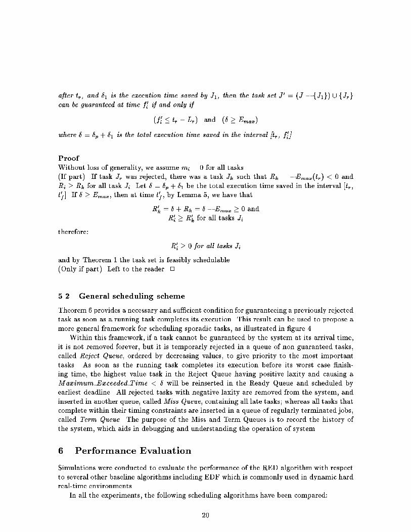
5.2 General scheduling scheme

Theorem 6 provides a necessary and su�cient condition for guaranteeing a previously rejected

task as soon as a running task completes its execution. This result can be used to propose a

more general framework for scheduling sporadic tasks, as illustrated in �gure 4.

Within this framework, if a task cannot be guaranteed by the system at its arrival time,

it is not removed forever, but it is temporarly rejected in a queue of non guaranteed tasks,

called Reject Queue, ordered by decreasing values, to give priority to the most important

tasks. As soon as the running task completes its execution before its worst case �nish-

ing time, the highest value task in the Reject Queue having positive laxity and causing a

Maximum Exceeded Time < � will be reinserted in the Ready Queue and scheduled by

earliest deadline. All rejected tasks with negative laxity are removed from the system, and

inserted in another queue, called Miss Queue, containing all late tasks; whereas all tasks that

complete within their timing constraints are inserted in a queue of regularly terminated jobs,

called Term Queue. The purpose of the Miss and Term Queues is to record the history of

the system, which aids in debugging and understanding the operation of system.

6 Performance Evaluation

Simulations were conducted to evaluate the performance of the RED algorithm with respect

to several other baseline algorithms including EDF which is commonly used in dynamic hard

real-time environments.

In all the experiments, the following scheduling algorithms have been compared:

20

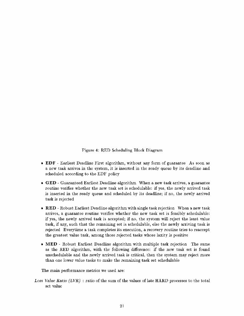
Figure 4: RED Scheduling Block Diagram

� EDF - Earliest Deadline First algorithm, without any form of guarantee. As soon as

a new task arrives in the system, it is inserted in the ready queue by its deadline and

scheduled according to the EDF policy.

� GED - Guaranteed Earliest Deadline algorithm. When a new task arrives, a guarantee

routine veri�es whether the new task set is schedulable: if yes, the newly arrived task

is inserted in the ready queue and scheduled by its deadline; if no, the newly arrived

task is rejected.

� RED - Robust Earliest Deadline algorithmwith single task rejection. When a new task

arrives, a guarantee routine veri�es whether the new task set is feasibly schedulable:

if yes, the newly arrived task is accepted; if no, the system will reject the least value

task, if any, such that the remaining set is schedulable, else the newly arriving task is

rejected. Everytime a task completes its execution, a recovery routine tries to reaccept

the greatest value task, among those rejected tasks whose laxity is positive.

� MED - Robust Earliest Deadline algorithm with multiple task rejection. The same

as the RED algorithm, with the following di�erence: if the new task set is found

unschedulable and the newly arrived task is critical, then the system may reject more

than one lower value tasks to make the remaining task set schedulable.

The main performance metrics we used are:

Loss Value Ratio (LVR) : ratio of the sum of the values of late HARD processes to the total

set value.

21

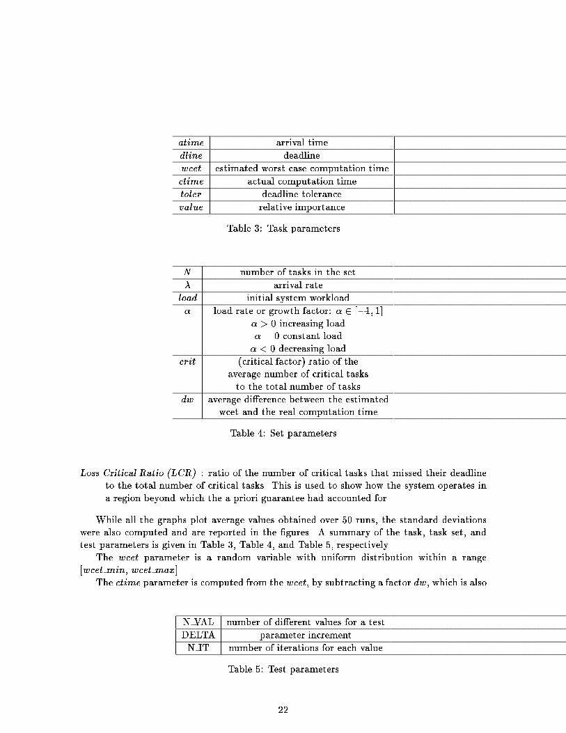
atime arrival time

dline deadline

wcet estimated worst case computation time

ctime actual computation time

toler deadline tolerance

value relative importance

Table 3: Task parameters

N number of tasks in the set

� arrival rate

load initial system workload

� load rate or growth factor: � 2 [�1; 1]

� > 0 increasing load

� = 0 constant load

� < 0 decreasing load

crit (critical factor) ratio of the

average number of critical tasks

to the total number of tasks

dw average di�erence between the estimated

wcet and the real computation time

Table 4: Set parameters

Loss Critical Ratio (LCR) : ratio of the number of critical tasks that missed their deadline

to the total number of critical tasks. This is used to show how the system operates in

a region beyond which the a priori guarantee had accounted for.

While all the graphs plot average values obtained over 50 runs, the standard deviations

were also computed and are reported in the �gures. A summary of the task, task set, and

test parameters is given in Table 3, Table 4, and Table 5, respectively.

The wcet parameter is a random variable with uniform distribution within a range

[wcet min, wcet max].

The ctime parameter is computed from the wcet, by subtracting a factor dw, which is also

N VAL number of di�erent values for a test

DELTA parameter increment

N IT number of iterations for each value

Table 5: Test parameters

22

a random variable with uniform distribution within a range [dw min, dw max]. Deadline

tolerances are also uniformly distributed in the interval [tol min, tol max].

Task arrival times are generated in sequence based on the arrival rate � speci�ed in the

set parameters. The arrival time of task i is computed as:

atime(i) = atime(i� 1) + r(1=�; �)

where r(a; b) is a Gaussian random variable with mean a and variance b

2

. Task deadline is

calculated according to the workload speci�cation given by the two parameters � and �:

d

i+1

= d

i

+

c

i+1

�

� r(�

c

i+1

�

; �):

Finally, the value of non critical tasks is de�ned as a random variable uniformly distributed

in the interval [1; N ]. The value of critical tasks is de�ned as CRIT VALUE, which is a value

greater than N . The number of critical tasks in the set is controlled by the crit parameter.

Default values were set at: N = 50, � = 0:2 (a task every 5 ticks), load = 0:9, � = 0:5,

crit = 0:2 (20 percent of critical tasks), wcet = 30, dw = 0, tol = 0.

6.1 Experiment 1: Critical Factor

In the �rst experiment, we tested the capability of the algorithms of handling critical tasks

in overload conditions. Figure 5a and 5b plot the Loss Critical Ratio (LCR) and the Loss

Value Ratio (LVR) obtained for the four algorithms as a function of the critical factor. In

this experiment, the initial workload was 0.9, with a growth factor � = 0:5. For each task,

the deadline tolerance was set to zero, and the computation time (ctime) was set equal to

the estimated wcet (dw = 0).

As shown in Figure 5, both LVR and LCR for EDF go over 0.9 as soon as the critical

factor become greater than 0.2. This is clearly due to the domino e�ect caused by the heavy

load. Although the guarantee routine used in the GED algorithm avoids such a domino e�ect

typical of the EDF policy, it does not work as well as RED nor MED, since critical tasks are

rejected as normal hard tasks, if they cause an overload. For example, when the percentage

of critical tasks is 50% (critical factor = 0.5) we see a gain of about 15% for RED and MED

over GED.

Another important implication from Figure 5 is that RED and MED are able to provide

almost no loss for critical tasks in overload conditions, until the number of critical tasks

in the set is above 50% of the total number of tasks; the LCR is practically zero for both

algorithms. Above this percentage, however, some loss is experienced and, by around 80% of

the load being critical tasks, we start to see the multiple task rejection policy used in MED

begin to be slightly more e�ective than RED.

To understand the behavior of RED and MED depicted in �gure 5a, remember that the

LVR is computed from the value of HARD tasks only, since CRITICAL tasks belong to a

di�erent class. Therefore, as the critical factor increases, RED and MED have to reject more

HARD tasks to keep the LCR value low, whereas GED does not make any dinstiction between

HARD and CRITICAL tasks.

As a matter of fact, an important result shown in this experiment is that for task sets in

which the number of critical tasks is less than the number of hard tasks, it is not worthwhile

23

Figure 5: LVR vs critical factor (a); LCR vs critical factor (b).

24

to use complicated rejection strategies. In this cases, the simple (O(n)) strategy used in

RED, in which the least value task is rejected, performs as well as more sophisticated and

time consuming policies.

Notice that in all experiments presented in this paper, no assumption has been made

on the minimum interarrival time of critical tasks. Therefore, even when the percentage of

critical tasks is low, there is always a (low) probability that a critical task can be rejected

with the MED algorithm, if it arrives just after another critical task and the deadlines of

both are close. Note that this condition is an overload.

6.2 Experiment 2: Load Rate

In this experiment, the number of critical tasks was 20 percent of the total number of tasks

(which means 10 in the average out of 50). The initial workload was 0.9, and the load growth

factor �, was varied from 0 to 0.75, with a step of 0.05. For each task, the deadline tolerance

was set to zero, and the computation time (ctime) was set equal to the estimated wcet (dw

= 0).

Figure 6a plots the loss value ratio (LVR) obtained with the four algorithms as a function

of the load growth factor �, and �gure 6b plots the loss critical ratio (LCR). When � = 0 the

system workload is maintained on the average around its initial value � = 0:9, therefore the

loss value is negligible for all algorithms. By increasing �, the load increases as new tasks

arrive in the system.

As it is clear from the �gure, the EDF algorithm without guarantee was not capable of

handling overloads, so that the loss in value increased rapidly towards its maximum (equal to

the total set value). At this level, only the �rst tasks were able to �nish in time, while all other

tasks missed their deadlines. Again, RED and MED did not show any signi�cant di�erence

between themselves during this test, but a very signi�cant improvement was achieved over

EDF and GED. For example, using a growth factor � = 0:5, which causes a heavy load,

the LVR is 0.98 with EDF, 0.17 with GED, and only 0.11 for both RED and MED. Notice

that the loss value obtained running RED and MED is entirely due to hard tasks, since from

�gure 5b we see that the number of critical tasks missing their deadlines is practically zero

for RED and MED.

6.3 Experiment 3: Arrival Rate

In the third experiment, we monitored the loss value by varying the task arrival rate. In this

case, task deadlines were generated in a slightly di�erent fashion. Task laxity was generated

�rst as a random variable uniformly distributed in the interval [lax min; lax max]. Then,

task deadline was computed as follows:

deadline = arrival time + wcet + laxity:

As shown in the graphs reported in �gure 7, the results of this test are consistent with

those discussed in the previous experiment. So the results hold over a wide range of system

conditions.

25

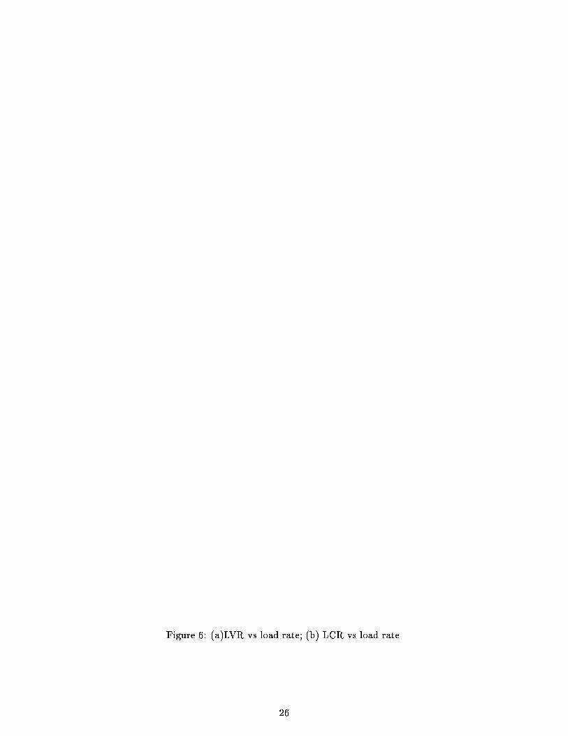
Figure 6: (a)LVR vs load rate; (b) LCR vs load rate.

26

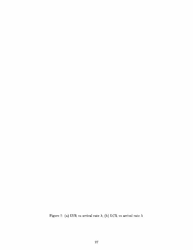
Figure 7: (a) LVR vs arrival rate �; (b) LCR vs arrival rate �.

27

Figure 8: (a) LVR vs dw; (b) LCR vs dw.

28

6.4 Experiment 4: Early Completion

Experiment 4 is intended to show the e�ectiveness of the recovery strategy used in the RED

(and MED) algorithm. When a task completes its execution before its estimated �nishing

time, the recovery strategy tries to reaccept rejected tasks (based on their values) until they

have positive laxity. This is a very important feature of RED since, due to the pessimistic

evaluation of the wcet, the actual computation time of a task may be very di�erent from its

estimated value. We call computation time error dw the di�erence between the estimated

wcet and the actual computation time of a task. Figure 8a and 8b show the loss value ratio

LVR and the loss critical ratio LCR as a function of dw. In this test, the initial load was

set to 0.9, with a growth factor � = 0:5. The number of critical tasks was 20 percent of the

total number, and computation time error dw varied from 0 to 15, with an estimated wcet

ranging from 30 to 40 time units.

Notice that, although EDF does not use any recovery strategy, EDF performs better than

GED for high values of dw. This is due to the fact that for high computation time errors,

the actual workload of the system is much less than the one estimated at the arrival time, so

EDF is able to execute more tasks. On the other hand, GED cannot take advantage of saved

time, since it rejects tasks at arrival time based on the estimated load. RED and MED also

reject tasks based on the current estimated workload, but the recovery strategy makes use

of saved execution time for reaccepting rejected tasks. Since tasks are reaccepted based on

their value, RED and MED perform as well as EDF for large computation time errors.

For example, with an average computation time error of dw = 5, the LVR obtained with

RED is about 3 times less than the one obtained with GED, and about 13 times less than

the one obtained with EDF. For large errors, say dw > 10, EDF shows about the same

performance of RED and MED, in terms of both LVR and LCR, whereas GED performs

almost as before.

6.5 Experiment 5: Deadline Tolerance

Experiment 5 shows the e�ect of having a deadline tolerance. Remember that a task with

deadline d

i

and tolerance m

i

is not treated as a task with deadline (d

i

+ m

i

): deadline is

used for scheduling, and tolerance is used for guarantee. This means that the algorithm

always tries to schedule all tasks to meet their deadlines; only in overload conditions there is

a chance that some task may exceed its deadline. In order to compare the four algorithms in

a consistent fashion, the concept of tolerance has been used also for EDF and GED. In this

experiment, the initial load was 0.9, with a growth factor � = 0:2. The number of critical

tasks was 70 percent of the total number (i.e., about 35 out of 50), and tolerance level was

varied from 0 to 15.

Figures 9a and 9b show the LVR and the LCR values for the four algorithms, as the

tolerance level varies from 0 to 15. LCR can be considered as the probability for a critical

task of missing its deadline. LCR values obtained with EDF were more than an order of

magnitude bigger than those obtained with the other algorithms. Notice that, as the number

of critical tasks in the set was relatively high, for low tolerance values, the MED algorithm

performs better than RED, whereas for higher values the two algorithms have the same

performance.

29

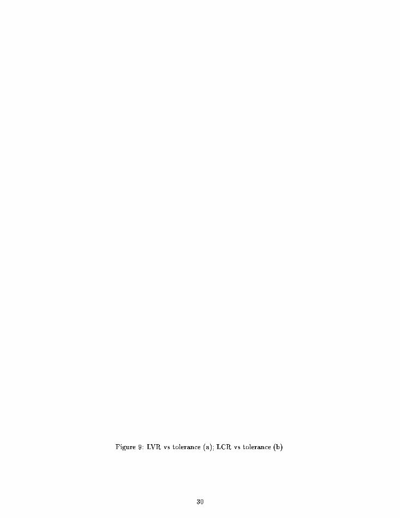
Figure 9: LVR vs tolerance (a); LCR vs tolerance (b).

30

For example, with a tolerance level of 5 units, the LCR factor is 0.62 with EDF, 0.042

with GED, 0.0014 with RED, and only 0.009 with MED. As we can see from the graph, for

tolerance values greater than 10, RED and MED cause no late critical tasks.

Note from �gure 9a that GED performs better than the other three algorithms in terms

of LVR. This is due to the fact that RED and MED reject more hard tasks than GED, to

keep the LCR as low as possible.

6.6 Performance Evaluation Summary

The performance results clearly show the poor performance of EDF scheduling in overload.

This fact has been often stated, but rarely shown with performance data. The results also

show the clear advantage of on-line planning (dynamic guarantee) algorithms under such con-

ditions. More importantly, the results also show that the new RED algorithm is signi�cantly

better than even the basic guarantee approach because it uses the entire load pro�le, dead-

line tolerance, and resource reclaiming. The better performance occurs across di�erent loads,

deadline distributions, arrival rates, tolerance levels, and errors on the estimates of worst case

execution time. RED also is signi�cantly better than EDF and better than GED in handling

unexpected overloads of critical tasks; an important property for safety critical systems. This

implies that RED keeps the system safe, longer, when unanticipated overloads occur. We

also see that the very simple rejection policy for RED su�ces in almost all conditions, and

that MED only improves RED in a small part of the parameter space.

7 Related Work

Earliest deadline scheduling has received much attention. It has been formally analyzed

proving that it is an optimal algorithm for preemptive, independent tasks when there is no

overload [Der 74], and proving that it is not optimal for multiprocessors [Mok 83]. It has

been used in many real-time systems, often assuming that overload will not occur. However,

it is now well known that earliest deadline scheduling has potentially catastrophically poor

performance in overload. Various research has been performed attempting to rectify this

problem. We brie y present EDF work related to overload as well as some general work on

overload in real-time systems.

Ramamritham and Stankovic [Ram 84] used EDF to dynamically guarantee incoming

work and if a newly arriving task could not be guaranteed the task was either dropped or

distributed scheduling was attempted. All tasks had the same value. The dynamic guarantee

performed in this paper had the e�ect of avoiding the catastrophic e�ects of overload on EDF.

In [Biy 88] the previous work was extended to tasks with di�erent values, and various policies

were studied to decide which tasks should be dropped when a newly arriving task could not

be guaranteed. However, the work did not fully analyze the overload characteristics, build a

pro�le, allow deadline tolerance, nor integrate with resource reclaiming and re-guarantee, as

we do in this paper.

Haritsa, Livny and Carey [Har 91] present the use of a feedback controlled EDF algorithm

for use in real-time database systems. The purpose of their work is to get good average per-

formance for transactions even in overload. Since they are working in a database environment

31

their assumptions are quite di�erent than ours, e.g., they assume no knowledge of transaction

characteristics, they consider �rm deadlines not hard deadlines, there is no guarantee, and no

detailed analysis of overload. On the other hand, for their environment, they produce a very

nice result, a robust EDF algorithm. The robust EDF algorithm we present is very di�erent

because of the di�erent application areas studied, and because we also include additional

features not found in [Har 91].

In real-time Mach [Tok 87] tasks were ordered by EDF and overload was predicted using

a statistical guess. If overload was predicted, tasks with least value were dropped. Je�ay,

Stanat and Martel [Jef 91] studied EDF scheduling for non-preemptive tasks, rather than the

preemptive model used here, but did not address overload.

Other general work on overload in real-time systems has also been done. For example, Sha

[Sha 86] shows that the rate monotonic algorithmhas poor properties in overload. Thambidu-

rai and Trivedi [Tha 89] study transient overloads in fault tolerant real-time systems, building

and analyzing a stochastic model for such a system. However, they provide no details on

the scheduling algorithm itself. Schwan and Zhou [Sch 92] do on-line guarantees based on

keeping a slot list and searching for free time intervals between slots. Once schedulability is

determined in this fashion, tasks are actually dispatched using EDF. If a new task cannot

be guaranteed, it is discarded. Zlokapa, Stankovic and Ramamritham [Zlo 91] propose an

approach called well-time scheduling which focuses on reducing the guarantee overhead in

heavily loaded systems by delaying the guarantee. Various properties of the approach are

developed via queueing theoretic arguments, and the results are a multi-level queue (based

on an analytical derivation), similar to that found in [Har 91] (based on simulation).

In [Loc 86] an algorithm is presented which makes a best e�ort at scheduling tasks based

on Earliest Deadline with a rejection policy based on removing tasks with the minimum value

density. He also suggests that removed tasks remain in the system until their deadline has

passed. The algorithm computes the variance of the total slack time in order to �nd the

probability that the available slack time is less than zero. The calculated probability is used

to detect a system overload. If it is less than the user prespeci�ed threshold, the algorithm

removes the tasks in increasing value density order. Consequently, detection of overload

is performed in a statistical manner rather than based on an exact pro�le as in our work.

This gives us the ability to perform speci�c analysis on the load rather than a probabilistic

analysis. While many features of our algorithm are similar to Locke's algorithm, we extend

his work, in a signi�cant manner, by the careful and exact analysis of overload, support n

classes, provide a minimum level of guarantee even in overload, allow deadline tolerance,

more formally address resource reclaiming, and provide performance data for the impact of

re-guarantees. We also formally prove all our main results.

Finally, Gehani and Ramamritham [Geh 91] propose programming language features to

allow speci�cation of deadline and a deadline slop factor (similar to our deadline tolerance),

but propose no algorithms for supporting this feature.

8 Conclusions

We have developed a robust earliest deadline scheduling algorithm for hard real-time envi-

ronments with preemptive tasks, multiple classes of tasks, and tasks with deadline tolerances.

32

We have formally proven several properties of the approach, developed an e�cient on-line

mechanism to detect overloads, and provided a complete load pro�le which can be usefully

exploited in various ways. A performance study shows the excellent performance of the al-

gorithm in both normal and overload conditions. Precedence constraints can be handled by

a priori converting precedence constraints to deadlines. A future extension we are working

on is to include resource sharing among tasks.

In this paper we assumed zero overheads for dynamic scheduling. This, of course, is not

true. Basically, there are two distinct and important aspects to scheduling overhead, one is

the cpu time it steals from application tasks, and two, is the latency it creates while making

the decision. We advocate the use of a scheduling chip that does the dynamic guarantees and

which runs in parallel with the application processor. This eliminates the �rst aspect of the

overhead, i.e., scheduling no longer steals cpu cycles from application tasks. A scheduling

chip would also minimize latency because it can be tailored to the scheduling function and

therefore be quite fast. However, the worst case latency must still be taken into account

and this can be accomplished by computing a cuto� line { a time equivalent to worst case

scheduling cost. Then the planning does not modify the application processor schedule prior

to the cuto� line. This two part approach to dealing with scheduling overhead works and

has been implemented in the Spring Kernel [Sta 91]. The technique is easily applied to the

algorithm in this paper.

References

[Bar 91] S. Baruah, G. Koren, B. Mishra, A. Raghunathan, L. Rosier, and D. Shasha,

\On-line Scheduling in the Presence of Overload," Proc. of IEEE Symposium on

Foundations of Computer Science, San Juan, Puerto Rico, October 2-4, 1991.

[Bar 92] S. Baruah, G. Koren, D. Mao, B. Mishra, A. Raghunathan, L. Rosier, D. Shasha,

and F. Wang, \On the Competitiveness of On-Line Real-Time Task Scheduling,"

Proceedings of Real-Time Systems Symposium, December 1991.

[Biy 88] S. Biyabani, J. Stankovic, and K. Ramamritham, \The Integration of Deadline and

Criticalness in Hard Real-Time Scheduling," Proceedings of the Real-Time Systems

Symposium, December 1988.

[Bla 76] J. Blazewicz, \Scheduling dependent tasks with di�erent arrival times to meet

deadlines" In E. Gelenbe, H. Beilner (eds), Modelling and Performance Evaluation

of Computer Systems, Amsterdam, North-Holland, 1976 pp 57-65.

[Che 90] H. Chetto, M. Silly, and T. Bouchentouf, \Dynamic Scheduling of Real-Time Tasks

under Precedence Constraints," The Journal of Real-Time Systems, 2, pp. 181-194,

1990.

[Der 74] M. Dertouzos, \Control Robotics: The Procedural Control of Physical Processes,"

Proceedings of the IFIP Congress, 1974.

[Geh 91] N. Gehani and K. Ramamritham, \Real-Time Concurrent C: A Language for Pro-

grammingDynamic Real-Time Systems," Real-Time Systems, 3, pp. 377-405, 1991.

33

[Har 91] J. R. Haritsa, M. Livny, and M. J. Carey, \Earliest Deadline Scheduling for Real-

Time Database Systems," Proceedings of Real-Time Systems Symposium, Decem-

ber 1991.

[Jac 55] J. Jackson, \Scheduling a Production Line to Minimize Tardiness," Research Re-

port 43, Management Science Research Project, University of California, Los An-

geles, 1955.

[Jef 91] K. Je�ay, D. Stanat, and C. Martel, \On Non-Preemptive Scheduling of Periodic

and Sporadic Tasks," Proceedings of Real-Time Systems Symposium, December

1991.

[Liu 73] C. L. Liu and J. Leyland, \Scheduling Algorithms for Multiprogramming in a Hard

Real-Time Environment," Journal of the ACM, 20, pp. 46-61, 1973.

[Loc 86] C. D. Locke, \Best E�ort Decision Making For Real-Time Scheduling," PhD The-

sis, Computer Science Dept., CMU, 1986.

[Mok 83] A. K. Mok, \Fundamental Design Problems of Distributed Systems for the Hard

Real Time Environment," PhD Dissertation, MIT, May 1983.

[Moo 68] J. Moore, \An n Job, One Machine Sequencing Algorithm for Minimizing the Num-

ber of Late Jobs," Management Science, Vol. 15, No. 1, pp. 102-109, September

1968.

[Ram 84] K. Ramamritham and J. Stankovic, \Dynamic Task Scheduling in Hard Real-Time

Distributed Systems," IEEE Software, pp. 65-75, July 1984.

[Sch 92] K. Schwan and H. Zhou, \Dynamic Scheduling of Hard Real-Time Tasks and Real-

Time Threads," IEEE Transactions on Software Engineering, Vol. 18, No. 8, pp.

736-748, August 1992.

[Sha 86] L. Sha, J. Lehoczky, and R. Rajkumar, \Solutions for Some Practical problems in

Prioritized Preemptive Scheduling," Proceedings of Real-Time Systems Symposium,

December 1986.

[Sha 90] L. Sha, R. Rajkumar, J. P. Lehoczky, \Priority Inheritance Protocols: An Ap-

proach to Real-Time Synchronization," IEEE Transactions on Computers, Vol.

20, No. 9, pp. 1175-1185, September 1990.

[She 90] C. Shen, K. Ramamritham, and J. Stankovic, \Resource Reclaiming in Real-Time,"

Proceedings of Real-Time Systems Symposium, December 1990.

[Sta 91] J. Stankovic and K. Ramamritham, \The Spring Kernel: A New Paradigm for

Real-Time Systems," IEEE Software, Vol. 8, No. 3, pp. 62-72, May 1991.

[Tha 89] P. Thambidurai, and K. S. Trivedi, \Transient Overloads in Fault-Tolerant Real-

Time Systems," Proceedings of Real-Time Systems Symposium, December 1989.

34

[Tok 87] H. Tokuda, J. Wendorf, and H. Wang, \Implementation of a Time-Driven Sched-

uler for Real-Time Operating Systems," Proceedings of the Real-Time Systems

Symposium, December 1987.

[Tow 91] D. Towsley and S. Panwar, \Optimality of the Stochastic Earliest Deadline Policy

for the G/M/c Queue Serving Customers with Deadlines," Univ. of Massachusetts

Technical Report, September 1991.

[Zlo 91] G. Zlokapa, J. A. Stankovic, and K. Ramamritham, \Well-Timed Scheduling: A

framework for Dynamic Real-Time Scheduling," Submitted to IEEE Transactions

on Parallel and Distributed Systems, 1991.

35