REPORT DOCUMENTATION PAGE Farm Approved QMS No. 0704-0138 ._ __ ,.„--,„„ ot inTerm.tion .1 «tunMM to «r-»o» 1 -ouf OB wn"». .«auoirvj m ami rar r^wmng ."«ruoom. >»ircim^ «jrrorvj oau lourcrv. »viO"< rroornnq suraw or tun cciirraonu „_,,„ lna „r^n :r» co(l«rcl>on at .nform.tion. S*f*l commtrra rr-irai«; 5ln Oure*o mm«» or »r», ctnw IUKI et inn 5»« 1 » ? »•"• <"» «»»""* "• °»" "!^:_„ ,or rwucinc urn ouram to «uwww» -»»ouinm ^rrvic«. Director«» for intorm.oon Ot«noom jna »«cons. 121 j Intnai 1. AGENCY USE ONLY (Leav» b/jn«; 2 - * E TÄ T f995 3. REPORT TYPE ANO DATES COVERED Final, 01 April 1992 - 15 May 1995 A. TITLE AND SUSTTTU Real-Time DOA Estimation of Wideband Signals with Multidimensional Arrays via Signal Subspace Techniques 6. AUTHOR(S) Dr. Michael D. Zoltowski 7. PERFORMING ORGANIZATION NAME(S) AND AOORESS(ES) Purdue University, W. Lafayette, IN 47907 5. FUNDING NUMBERS F49620-92-J-0198 9. SPONSORING/MONITORING AGENCY NAME(S) AND ADDRESS(ES) Air Force Office of Scientific Research 110 Duncan Avenue, Suite B115 Boiling AFB, DC 20332 3. PERFORMING ORGANIZATION REPORT NUMBER Purdue TR-EE-95 A 10. SPONSORING/MONITORING AGENCY BETM-"«- • — AFOSR-TR-95 11. SUPPLEMENTARY NOTES Ua. DISTRIBUTION/AVAILABIUTYpT^-g^feTjrio^ STATEMENT K Distribution Unlimited Anproved tor public leiecuH «i,-. Duttacutioo unlimited • -**> •) 13. ABSTRACT (Maximum 200 worm) cmr E:LECTE JUL 2 8 1995 ON COO 2D Unitary ESPRIT is developed as a closed-form 2-D angle estimation algorithm for use in conjunction with a uniform rectangular array (URA). In the final stage of the algorithm, the real and imaginary parts of the i-th eigenvalue of a matrix are one-to-one related to the respective direction cosines of the i-th source relative to the two major array axes. Reduced dimension beamspace implementations of 2D Unitary ESPRIT are developed along with adaptations for other array configurations including two. orthogonal linear arrays. A novel approach to angle estimation in beamspace is also developed based on the observation that beamspace noise eigenvectors may be transformed to vectors in the element-space noise subspace. The transformed noise eigenvectors are bandpass, facilitating multirate processing involving modulation to baseband, filtering, and decimation. As these operations are linear, the Root-MUSIC (ESPRIT) based algorithm merely premultiplies each beamspace noise (signal) eigenvector by a precomputed transformation matrix. Compared to previous beamspace implementations of Root-MUSIC or ESPRIT, this approach places no restrictions on the structure of the matrix beamformer. Extensions for the URA are developed based on Multidimensional multirate processing. DTM QUALITY INSPECTED 8 14. SUBJECT TERMS angle estimation, antenna arrays multirate processing, beamforming frequency estimation, direction finding 17. SECURITY CLASSIFICATION OF REPORT UNCLASSIFIED 18. SECURITY CLASSIFICATION OF THIS PAGE .UNCLASSIFIED 19. SECURITY CLASSIFICATION OF ABSTRACT UNCLASSIFIED 15. NUMBER OF PAGES 16. PRICE CODE 20. LIMITATION OF ABSTRACT UL NSN 75«KI1-280-5500 S;ancard Form 298 (Rev. 2-39) »'-tr-yra o» »V Sta Z21-'*

Welcome message from author
This document is posted to help you gain knowledge. Please leave a comment to let me know what you think about it! Share it to your friends and learn new things together.
Transcript
REPORT DOCUMENTATION PAGE Farm Approved
QMS No. 0704-0138
._ __ ,.„--,„„ ot inTerm.tion .1 «tunMM to «r-»o» 1 -ouf OB wn"». .«auoirvj m ami rar r^wmng ."«ruoom. >»ircim^ «jrrorvj oau lourcrv. »viO"< rroornnq suraw or tun cciirraonu „_,,„ lna „r^n :r» co(l«rcl>on at .nform.tion. S*f*l commtrra rr-irai«; 5ln Oure*o mm«» or »r», ctnw IUKI et inn 5»«1»™? »•"• <"»■«»»""* "• °»" "!^:_„ ,or rwucinc urn ouram to «uwww» -»»ouinm ^rrvic«. Director«» for intorm.oon Ot«noom jna »«cons. 121 j Intnai
1. AGENCY USE ONLY (Leav» b/jn«; 2- *ETÄTf995 3. REPORT TYPE ANO DATES COVERED
Final, 01 April 1992 - 15 May 1995
A. TITLE AND SUSTTTU
Real-Time DOA Estimation of Wideband Signals with Multidimensional Arrays via Signal Subspace Techniques
6. AUTHOR(S)
Dr. Michael D. Zoltowski
7. PERFORMING ORGANIZATION NAME(S) AND AOORESS(ES)
Purdue University, W. Lafayette, IN 47907
5. FUNDING NUMBERS
F49620-92-J-0198
9. SPONSORING/MONITORING AGENCY NAME(S) AND ADDRESS(ES)
Air Force Office of Scientific Research 110 Duncan Avenue, Suite B115 Boiling AFB, DC 20332
3. PERFORMING ORGANIZATION REPORT NUMBER
Purdue TR-EE-95
A
10. SPONSORING/MONITORING AGENCY BETM-"«- • —
AFOSR-TR-95
11. SUPPLEMENTARY NOTES
Ua. DISTRIBUTION/AVAILABIUTYpT^-g^feTjrio^ STATEMENT K
Distribution Unlimited Anproved tor public leiecuH
«i,-. Duttacutioo unlimited • -**>■•)
13. ABSTRACT (Maximum 200 worm)
cmr E:LECTE JUL 2 8 1995
ON COO
2D Unitary ESPRIT is developed as a closed-form 2-D angle estimation algorithm for use in conjunction with a uniform rectangular array (URA). In the final stage of the algorithm, the real and imaginary parts of the i-th eigenvalue of a matrix are one-to-one related to the respective direction cosines of the i-th source relative to the two major array axes. Reduced dimension beamspace implementations of 2D Unitary ESPRIT are developed along with adaptations for other array configurations including two. orthogonal linear arrays. A novel approach to angle estimation in beamspace is also developed based on the observation that beamspace noise eigenvectors may be transformed to vectors in the element-space noise subspace. The transformed noise eigenvectors are bandpass, facilitating multirate processing involving modulation to baseband, filtering, and decimation. As these operations are linear, the Root-MUSIC (ESPRIT) based algorithm merely premultiplies each beamspace noise (signal) eigenvector by a precomputed transformation matrix. Compared to previous beamspace implementations of Root-MUSIC or ESPRIT, this approach places no restrictions on the structure of the matrix beamformer. Extensions for the URA are developed based on Multidimensional multirate processing.
DTM QUALITY INSPECTED 8
14. SUBJECT TERMS angle estimation, antenna arrays multirate processing, beamforming frequency estimation, direction finding
17. SECURITY CLASSIFICATION OF REPORT
UNCLASSIFIED
18. SECURITY CLASSIFICATION OF THIS PAGE
.UNCLASSIFIED
19. SECURITY CLASSIFICATION OF ABSTRACT
UNCLASSIFIED
15. NUMBER OF PAGES
16. PRICE CODE
20. LIMITATION OF ABSTRACT
UL
NSN 75«KI1-280-5500 S;ancard Form 298 (Rev. 2-39) »'-tr-yra o» »V Sta Z21-'*

GENERAL INSTRUCTIONS FOR COMPLETING SF 298
Tne Report Documentation Page (RDP) is used in announcing and cataloging reports. It is important that this information be consistent with the rest of the report, particularly the cover and title pag Instructions for filling in each block of the form follow. It is important to stay within the lines to me- opt/ca/ scanning requirements.
e. eet
Slock 1. Aoencv Use Only (Leave blank).
Block 2. Report Date. Full publication date including day, month, and year, if available (e.g. 1 Jan 83). Must cite at least the year.
Block 3. Type of Report and Dates Covered. State whether report is interim, final, etc. If applicable, enter inclusive report dates (e.g. 10 Jun87-30Jun88).
Block 4. Title and Subtitle. A title is taken from the part of the report that provides the most meaningful and complete information. When a report is prepared in more than one volume, repeat the primary title, add volume number, and include subtitle forthe specific volume. On classified documents enter the title classification in parentheses.
Block 5. Funding Numbers. To include contra« and grant numbers; may include program element numbers), project number^}, task numbers), and work unit numbers). Use the following labeis:
C G PE
Contract Grant Program Element
PR TA WU
Project Task Work Unit Accession No.
Block S. Authoris). Name{s) of person(s) responsible for writing the report, performing the research, or credited with the content of the report. If editor or compiler, this should follow the name(s).
Block 7. Performing Organization Name(s) and Address(es). Seif-expianatory.
Block 8. Performing Organization Report Number. Enterthe unique alphanumeric report number(s) assigned by the organization performing the report.
Block 9. Soonsorino/Monitorino Aoencv Name(s) and Addressees). Seif-expianatory.
Block 10. Soonsoring/Monitorino Agency Report Number. (If known)
Block 11. Supplementary Notes. Enter information not included elsewhere such as: Prepared in cooperation with...; Trans, of...; To be published in When a report is revised, include a statement whether the new report supersedes or supplements the older report
Block 12a. Distribution/Availability Statement. Denotes public availability or limitations. Gte any availability to the public. Enter additional limitations or special markings in all capitals (e.g. NOFORN, REL, ITAR).
DOD
DOE - NASA- NT1S -
See DoDD 5230.24, 'Distribution Statements on Technical Documents." See authorities. See Handbook NHB 2200.2. Leave blank.
Block 12b. Distribution Code.
DOO DOE
NASA NT1S
Leave biank. Enter DOE distribution categories from the Standard Distribution for Unclassified Scientific and Technical Repo«*-J. Leave blank. Leave blank.
Block 13. Abstract. Include a brief (Maximum 200 words) factual summary of the most significant information contained in the report
Block 14. Subject Terms. Keywords or phrases identifying major subjects in the report
Block 15. Number of Paoes. Enter the total number of pages.
Block 16. Price Code. Enter appropriate price code (NTIS only).
Blocks 17.-19. Security Classifications. Self- explanatory. Enter U.S. Security Classification in accordance with U.S. Security Regulations (i.e., UNCLASSIFIED). If form contains classified information, stamp classification on the top and bottom of the page.
Block 20. Limitation of Abstract This block must be completed to assign a limitation to the abstract Enter either UL (unlimited) or SAR (same as report). An entry in this block is necessary if the abstract is to be limited. If blank, the abstract is assumed to be unlimited.
Standard form 298 Sack (fUv. 2-39)

REAL-TIME DIRECTION-OF-ARRIVAL ESTIMATION OF WIDEBAND SIGNALS WITH MULTIDIMENSIONAL
ARRAYS VIA SIGNAL SUBSPACE TECHNIQUES
Final Technical Report
Air Force Office of Scientific Research
Grant/Contract Number: F49620-92-J-0198
Period Covered: 01 April 1992-15 May 1995
Principal Investigator:
Michael D. Zoltowski
School of Electrical Engineering 1285 Electrical Engineering Building
Purdue University West Lafayette, IN 47907 USA e-mail: [email protected]
Phone: 317-494-3512 FAX: 317-494-0880
Program Director:
Jon A. Sjogren
AFOSR/NM 110 Duncan Ave., Suite B115
Boiling Air Force Base Washington, DC 20332
[email protected] Phone: 202-767-4940 FAX: 202-404-7496
A 99507210A2 Accesjon For
NTIS CRA&I DTIC TAB Unannounced Justification
By Distribution/
Availability Codes
Dist Avail and/or
Special

Summary of Efforts
Closed-Form 2D Angle Estimation with Rectangular Arrays
UCA-ESPRIT is a recently developed closed form algorithm for use in conjunction with a
uniform circular array (UCA) that provides automatically paired source azimuth and elevation
angle estimates. 2D Unitary ESPRIT is presented as an algorithm providing the same capabil-
ities for a uniform rectangular array (URA). In the final stage of the algorithm, the real and
imaginary parts of the i — th eigenvalue of a matrix are one-to-one related to the respective
direction cosines of the i — th source relative to the two major array axes. 2D Unitary ESPRIT
offers a number of advantages over other recently proposed ESPRIT based closed-form 2D an-
gle estimation techniques. First, except for the final eigenvalue decomposition of dimension
equal to the number of sources, it is efficiently formulated in terms of real-valued computation
throughout. Second, it is amenable to efficient beamspace implementations that will be pre-
sented. Third, it is applicable to array configurations that do not exhibit identical subarrays, e.
g., two orthogonal linear arrays. Finally, 2D Unitary ESPRIT easily handles sources having one
member of the spatial frequency coordinate pair in common. Simulation results are presented
verifying the efficacy of the method. Beamspace DOA Estimation Featuring Multirate Eigenvector Processing
A novel approach to angle of arrival estimation in beamspace has been developed. Beamspace
noise eigenvectors may be transformed to vectors in the element-space noise subspace. The
transformed noise eigenvectors are bandpass, facilitating multirate processing involving modu-
lation to baseband, filtering, and decimation. As these operations are linear, a matrix transfor-
mation applied to the eigenvectors may be constructed a priori. Incorporation of the technique
into either the Root-MUSIC or ESPRIT prescriptions provides a computationally efficient pro-
cedure. Compared to past efforts to adapt Root-MUSIC and ESPRIT to beamspace, this
approach circumvents the need for restrictive requirements on the form of the beamforming
transformation. An asymptotic theoretical performance analysis is also included to provide an
alternative to computationally intensive Monte-Carlo simulations. Simulation studies show the
validity of the performance predictive expressions and verify that the procedure, when incor-
porated into the Root-MUSIC/ESPRIT formulations, produces a direction finding technique
that nearly attains the Cramer-Rao bound. Multidimensional Multirate DOA Estimation in Beamspace
The ID multirate approach was extended to the more general case of 2D angle estimation
with a uniform rectangular array (URA) of sensors. Multidimensional multirate processing is
employed to ultimately yield a small order polynomial in two variables. Again, due to the
linearity of the 2D filtering and 2D decimation operations, the actual algorithm merely premul-
tiplies each beam space noise eigenvector by a precomputed transformation matrix. To avoid
the spectral search, despite the fact that the fundamental theorem of algebra does not hold
in 2D, we propose taking the orthogonal complement of the resulting transformed noise eigen-
vectors and applying a novel version of ESPRIT facilitating closed-form 2D angle estimation.
Simulations demonstrating the efficacy of the approach are presented along with theoretical
performance analysis.

Real-Time Frequency And 2-D Angle Estimation With Sub-Nyquist Spatio-Temporal Sampling An algorithm has been developed for real-time estimation of the frequency and azimuth and
elevation angles of each signal incident upon an airborne antenna array system over a very wide frequency band, 2-18 GHz, commensurate with electronic signal warfare. The algorithm pro- vides unambiguous frequency estimation despite severe temporal undersampling necessitated by cost/complexity of hardware considerations. The 2-18 GHz spectrum is decomposed into 1 GHz bands. The baseband output of each antenna is sent through two 250 MHz sampled channels where one is delayed relative to the other (prior to sampling) by .5 ns, the Nyquist interval for a 1 GHz bandwidth. Due to the high variance of the Direct ESPRIT frequency estimator, aliased frequencies are estimated via a simple formula and translated to the proper aliasing zone utilizing eigenvector information generated by PRO-ESPRIT. The algorithm also provides unambiguous 2-D angle estimation over the entire 2-18 GHz bandwidth despite se- vere spatial undersampling at the higher end of this band necessitated by mutual coupling considerations and resolving power requirements at the lower end of the band. Eigenvector information generated by PRO-ESPRIT is used to facilitate computationally simple estimation of azimuth and elevation angles automatically paired with corresponding frequency estimates despite aliasing. Simulations are presented demonstrating the capabilities of the algorithm.
'*
a

Contents
1 Closed-Form 2D Angle Estimation with Rectangular Arrays 1
1.1 Introduction 2 1.2 Real-Valued Processing with Uniform Linear Array 4
1.3 Unitary ESPRIT for Uniform Linear Array 6
1.4 DFT Beamspace ESPRIT for Uniform Linear Array 9 1.4.1 Relationship Between Unitary ESPRIT and DFT Beamspace ESPRIT . 11
1.4.2 Relationship Between DFT Beamspace ESPRIT and Beamspace ESPRIT 12
1.5 2D Unitary ESPRIT for Uniform Rectangular Array 13
1.5.1 2D Unitary ESPRIT vs. ACMP • • 17
1.6 2D DFT Beamspace ESPRIT for Uniform Rectangular Array 18
1.6.1 Reduced Dimension Example 20
1.6.2 Comparison with UCA-ESPRIT 21
1.7 2D DFT Beamspace ESPRIT for Cross Array 23
1.8 Simulations 25
1.9 Conclusions 27
1.10 References 28
1.11 Figures , 31
2 Beamspace DOA Estimation Featuring Multirate Eigenvector Processing 34
2.1 Introduction 35
2.2 Array Signal Model 37 2.3 Development of DOA Estimators Featuring Multirate Eigenvector Processing . . 39
2.3.1 Multirate Noise Eigenvector Processing • 39
2.3.2 Incorporation of Filter Deconvolution 43
2.3.3 Root-MUSIC Incorporating Multirate Eigenvector Processing 46
2.3.4 TLS-ESPRIT Incorporating Multirate Eigenvector Processing 48
2.3.5 Location of Extraneous Roots Created by Filtering 50
2.4 Theoretical Performance Analysis 51
2.4.1 Performance Analysis of Root-MUSIC Formulation 52
, 2.4.2 Performance Analysis of ESPRIT Formulation 53
2.5 Computer Simulations 54
2.6 Conclusions/Remarks 57
2.7 Appendix: Asymptotic Variance of ESPRIT Formulation 58
2.8 References 59
2.9 Figures 6!
3 Multidimensional Multirate DOA Estimation in Beamspace 66
3.1 Introduction 67
3.2 Array Geometry 69
3.3 Beamforming 73
m
3.4 Eigenanalysis 74 3.5 Multirate Processing of Beamspace Noise Eigenvectors 75 3.6 TLS-ESPRIT 78 3.7 Bandlimiting the Response 82 3.8 Further Reductions in Complexity 84
3.8.1 Real Covariance Processing 84 3.8.2 Orthogonal Complement 85
3.9 Algorithm Summary 86 3.10 Performance Analysis 86 3.11 Computer Simulations 88 3.12 Conclusions 91 3.13 Appendix: Characterizing the Asymptotic Error 92 3.14 References 96
Real-Time Frequency And 2-D Angle Estimation With Sub-Nyquist Spatio- Temporal Sampling 98 4.1 Introduction 99 4.2 Spatio-Temporal Sampling and Data Model 101 4.3 ESPRIT Based Frequency Estimation With Temporal Undersampling 105 4.4 2-D Angle Estimation With Spatial Undersampling Via PRO-ESPRIT and In-
teger Search Formulation 110 4.4.1 Estimation of the Array Manifold for Each Source 110 4.4.2 Prescription for Nonuniform Element Spacing Facilitating Nonambiguous
Angle Estimation Ill 4.4.3 Integer Search Algorithm for Direction Cosine Estimation 114
4.5 Simulation Examples 116 4.6 Final Comments 118 4.7 References 119 4.8 Computation of Cramer Rao Lower Bound for, Frequency and 2D Angle Estimationll9
4.9 Figures 122
IV

1 Closed-Form 2D Angle Estimation with Rectangular Arrays
UCA-ESPRIT is a recently developed closed form algorithm for use in conjunction with a uni-
form circular array (UCA) that provides automatically paired source azimuth and elevation
angle estimates. 2D Unitary ESPRIT is presented as an algorithm providing the same capabil-
ities for a uniform rectangular array (URA). In the final stage of the algorithm, the real and
imaginary parts of the i — th eigenvalue of a matrix are one-to-one related to the respective
direction cosines of the i — th source relative to the two major array axes. 2D Unitary ESPRIT
offers a number of advantages over other recently proposed ESPRIT based closed-form 2D an-
gle estimation techniques. First, except for the final eigenvalue decomposition of dimension
equal to the number of sources, it is efficiently formulated in terms of real-valued computation
throughout. Second, it is amenable to efficient beamspace implementations that will be pre-
sented. Third, it is applicable to array configurations that do not exhibit identical subarrays, e.
g., two orthogonal linear arrays. Finally, 2D Unitary ESPRIT easily handles sources having one
member of the spatial frequency coordinate pair in common. Simulation results are presented
verifying the efficacy of the method.
1.1 Introduction
1.2 Real-Valued Processing with Uniform Linear Array
1.3 Unitary ESPRIT for Uniform Linear Array
1.4 DFT Beamspace ESPRIT for Uniform Linear Array
1.4.1 Relationship Between Unitary ESPRIT and DFT Beamspace ESPRIT
1.4.2 Relationship Between DFT Beamspace ESPRIT and Beamspace ESPRIT
1.5 2D Unitary ESPRIT for Uniform Rectangular Array
1.5.1 2D Unitary ESPRIT vs. ACMP
1.6 2D DFT Beamspace ESPRIT for Uniform Rectangular Array
1.6.1 Reduced Dimension Example
1.6.2 Comparison with UCA-ESPRIT
1.7 2D DFT Beamspace ESPRIT for Cross Array
1.8 Simulations
1.9 Conclusions
1.10 References
1.11 Figures

1 Introduction
For ID arrays, if the elements are uniformly-spaced, Root-MUSICand ESPRIT1 [1] avert a spectral
search in determining the direction of arrival (DOA) of each incident signal. Instead, the DOA of
each signal is determined from the roots of a polynomial. For either Root-MUSIC or ESPRIT2, the
roots of interest ideally lie on the unit circle and are related one-to-one with each source as shown
in Figure 1.
For 2D (planar) arrays, the fact that the fundamental theorem of algebra does not hold in two
dimensions typically precludes a rooting type of formulation. Even for the highly regular uniform
rectangular array (URA), 2D MUSIC requires a spectral search of a multimodal two-dimensional
surface, while both Multiple Invariance ESPRIT [2, 3] and Clark & Scharf's 2D IQML [4] algorithm
involve nonlinear optimization. Now, it should be pointed out that a URA lends itself to separable
processing allowing one to decompose the 2D problem into two ID problems. That is, one can
estimate the DOA's with respect to one array axis via one set of calculations involving a MUSIC or
ESPRIT based polynomial formulation, and also do the same with respect to another array axis.
Coupling information may be employed to subsequently pair the respective members of the two sets
of ID angle estimates [5].
In the Algebraically Coupled Matrix Pencil (ACMP) method of van der Veen et al3 [6], eigen-
vector information is employed to pair the respective members of the two sets of ID angle estimates.
However, ACMP breaks down if two sources have the same arrival angle relative to either the z-axis
or the y-axis, assuming the URA to lie in the x-y plane.
In contrast, for a uniform circular array (UCA) the recently developed UCA-ESPRIT [7, 8]
algorithm provides closed-form, automatically paired 2D angle estimates as long as the azimuth
and elevation angle of each signal arrival is unique. As illustrated in Figure 2, in the final stage
of UCA-ESPRIT, the i-th eigenvalue of a matrix is of the form sin#t- ej0i, where fa and 0t- are the
azimuth and elevation angles of the i-th source. Note that sin/?,- e^{ = ut- + jvi, where u* and u,- are
the direction cosines of the i-th source relative to the x and y axes, respectively. The eigenvalue
for each source is thus unique such that UCA-ESPRIT does not have the aforementioned problem
1 ESPRIT may also be employed in the case of an array composed of at least two translationally invariant subarrays. 2In ESPRIT the DOA's are extracted from eigenvalues which are roots of the characteristic polynomial of a
matrix. 3van der Veen et al do not actually give their method a name. In a later paper Vanpoucke et al label their method
ACMP.
' A CMP has when two sources have the same u, or the same u;. We here develop a closed-form 2D
angle estimation algorithm for a URA that provides automatic pairing in a similar fashion. That
is, in the final stage of new algorithm, referred to as 2D Unitary ESPRIT, the real and imaginary
parts of the i-th eigenvalue of a matrix are one-to-one related to «,• and ut-, respectively.
2D Unitary ESPRIT is developed as an extension of the recently proposed Unitary ESPRIT
[9, 10] algorithm for a uniform linear array (ULA). Unitary ESPRIT exploits the conjugate centro-
symmetry of the array manifold for a ULA to formulate each of the three primary stages of ESPRIT
in terms of real-valued computations: (1) the computation of the signal eigenvectors, (2) the solution
to the system of equations derived from these signal eigenvectors, and (3) the computation of the
eigenvalues of the solution to the system of equations formed in stage 2. Note that Huarng k
Yeh [11] and Linebarger et al [12] previously exploited the conjugate centro-symmetry of the ULA
manifold to formulate the determination of the noise eigenvectors and subsequent spectral search
required by MUSIC in terms of real-valued computation. The ability to formulate an ESPRIT-
like algorithm for a ULA that only requires real-valued computations from start to finish, after an
initial sparse unitary transformation, is critically important in developing a closed-form 2D angle
estimation algorithm for a URA similar to UCA-ESPRIT for a UCA. Unitary ESPRIT is thus
reviewed in Section 3 after a brief overview in Section 2 of CN to $N transformations facilitated by
the conjugate centro-symmetry of the ULA manifold.
A reduced dimension beamspace version of Unitary ESPRIT is developed in Section 4. There are
a number of advantages to working in beamspace: reduced computational complexity [13], decreased
sensitivity to array imperfections [14], and lower SNR resolution thresholds [15]. In contrast to the
Beamspace ESPRIT [16] algorithm of Xu et al, the beamspace version of Unitary ESPRIT exploits
the real-valued nature of the beamspace manifold to formulate each of the three primary stages of
ESPRIT in terms of real-valued computations as in Unitary ESPRIT, but in a reduced dimension
space. Although the respective developments of Unitary ESPRIT and its beamspace counterpart
proceed along markedly different lines, there is an interesting relationship between the two presented
in Section 4.1. The relationship between Beamspace ESPRIT and the new beamspace version of
Unitary ESPRIT is examined in Section 4.2.
2D Unitary ESPRIT is developed in Section 5. In addition to the ability to handle sources
having the same arrival angle relative to either the x-axis or the y-axis, 2D Unitary ESPRIT offers
a number of advantages over other recently proposed ESPRITb&sed closed-form 2D angle estimation

techniques including ACMP. First, except for the final eigenvalue decomposition of dimension equal
to the number of sources, it is efficiently formulated in terms of real-valued computation throughout.
Second, it is amenable to a reduced dimension beamspace implementation. In Section 6, we develop
a beamspace version of 2D Unitary ESPRIT as an extension of the beamspace version of Unitary
ESPRIT presented in Section 4.
Another advantage of 2D Unitary ESPRIT over ACMP is that the former is applicable to array
configurations that do not exhibit identical subarrays, e. g., two noncollinear ULA's. In contrast,
A CMP requires an array of sensor triplets so that one can extract three identical subarrays from the
overall array. 2D Unitary ESPRIT only requires that the array exhibit invariances in two distinct
directions. In Section 7, we show how 2D Unitary ESPRIT may be simply adapted for the case of
two orthogonal ULA's having a common phase center. A CMP is not applicable with such an array
geometry.
Simulation results are presented in Section 8 verifying the efficacy of 2D Unitary ESPRIT and its
beamspace counterpart, and comparing their respective performances with the Cramer-Rao Lower
Bound.
2 Real-Valued Processing with a ULA
All of the developments in this paper rely on some well known aspects of real-valued processing
with a ULA which are quickly reviewed here [9, 10, 11, 12, 17]. Employing the center of the ULA as
the phase reference, the array manifold is conjugate centro-symmetric. For example, if the number
of elements comprising the ULA, N, is odd, there is a sensor located at the array center and the
array manifold is
V
3LN(/J,) ^(^i>,...,e-^,l,e^...,e^(^1HT, (1)
where \i = ^&xu with A equal to the wavelength, Ar is equal to the interelement spacing, and u
equal to the direction cosine relative to the array axis. The conjugate centro-symmetry of a^(^) is
mathematically stated as UN&N{P) = aÄr(/*)> wnere
1
UN = 1
€ %NxN. (2)
1
As the inner product between any two conjugate centro-symmetric vectors is real-valued, any matrix
whose rows are each conjugate centro-symmetric may be employed to transform the complex-valued

element space manifold, ajv(/j), into a real-valued manifold. As noted by a numerous authors
[9, 11, 12], the simplest matrices for accomplishing such are
Q2A' = ^
if N is even, or
Q 2/r+i 1
V2
IK j h<
IK 0 jIK
UK 0 -j UK
(3)
(4)
if TV is odd. Q$ is a sparse unitary matrix that transforms a^(/i) into an N x 1 real-valued manifold,
dj\r(/i) = Q^ajv(/i). For example, if the number of elements comprising the ULA is odd, the form
in (4) is used and
dN(p) = Q%3LN(H) = y/2 x cos (-J-M » -i cos(/i), l/\/2, - sin ^—/xj ,..., sin(/i) (5)
Let Rra; denote the N x N complex-valued element space sample covariance matrix. Since the
transformed manifold is real-valued, the signal eigenvectors required at the front end of ESPRIT
may be computed as the "largest" eigenvectors of TZe{Q^'R.xxQN}. Note that in addition to
the obvious computational reduction, taking the real part of the correlation matrix effects signal
decorrelation [17] in the case of highly correlated or coherent sources. Alternatively, if X denotes the
N xNs element space data matrix containing N3 snapshots as columns, the signal eigenvectors may
be computed as the "largest" left singular vectors of the real-valued matrix Q$[X, nwX*]M2jvs,
where I/va JIN, M2Ns = -L T VT • (6)
Since IIjvQiv = Q*Ni ^ follows that Q^[X,nNX*]M2JVs = V2[fte{Y},-Jm{Y}], where Y =
Q$X. From a numerical point of view, the latter is preferable due to computational efficiency and
robustness to dynamic range, especially if one employs an algorithm like the rank revealing URV
decomposition [18].
Note that pre-multiplication of an N x 1 vector by Q^ involves very little computation. In fact, it
involves no multiplications (the scaling by y/2 is unnecessary in computing the signal eigenvectors)
and only N additions. In Section 4, we also consider the use of the N pt. DFT matrix, with
appropriate scaling of the rows to make them each conjugate centro-symmetric [17], to transform
the data into a real-valued beamspace. Although FFT's are fast, this approach ostensibly involves
significantly more computation than the use of Q$. The utility of transforming to beamspace comes

into play when there is a-priori information on the general angular locations of the signal arrivals, as
in a radar application, for example. In this case, one may only apply those rows of the DFT matrix
that form beams encompassing the sector of interest. This yields a reduced dimension beamspace
and leads to reduced computational complexity [13, 14, 15, 17]. This is possible due to the physical
interpretation that the rows of the DFT matrix form beams pointed to different angles. There is
no such physical interpretation for the rows of Q$ thereby precluding the possibility to work in a
reduced dimension space.
Note that in this paper we do not address the problem of estimating the number of sources. We
will assume an estimate is available via a procedure such as that described by Xu et al in [19] which
explicitly exploits the conjugate centro-symmetry of the array manifold for a ULA.
3 Review of Unitary ESPRIT for ULA
As a precursor to developing an ESPRIT [1] based closed-form 2D angle estimation scheme for a
URA, we first briefly review the recently proposed Unitary ESPRIT [9] algorithm for a uniform
linear array (ULA) that only requires real-valued computations from start to finish after an initial
sparse unitary transformation by Q$. As discussed above, if X denotes the N x Ns element space
data matrix containing Ns snapshots as columns, the signal eigenvectors for Unitary ESPRIT may
be computed as the "largest" left singular vectors of the real-valued matrix [Jle{Y},Im{Y}],
where Y = Q$X. Assume that there are d < N signal arrivals. Asymptotically, the N x d
real-valued matrix of signal eigenvectors, E5, is related to the real-valued N x d DOA matrix,
D = [d(^i),d(/x2), ...,d(/id)], as Es = DT, where T is an unknown dx d real-valued matrix.
Since Q$ is unitary, it follows that asymptotically (as the number of snapshots becomes infinitely
large)
Q^E5 = AT, ' (7)
where. A = [a(/Ji),a(/*2), •••, »(/*<*)], the N x d complex-valued element space DOA matrix. For a
ULA, A satisfies the so-called invariance property [1]
JaA$M = J2A where: $„ = diag{eJ'"1, e^\ ..., e'""}, (8)
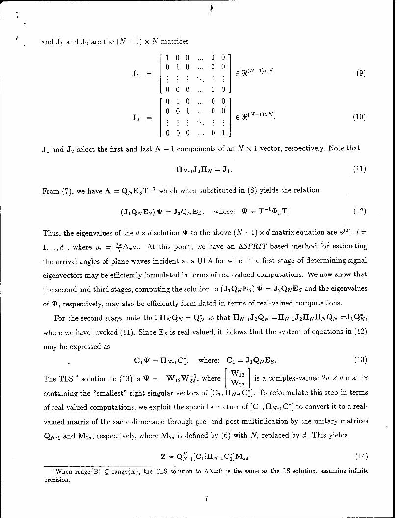
and Ji and J2 are the (N - 1) x N matrices
Ji =
1 0 0 .. . 0 0 0 1 0 .. . 0 0
0 0 0 .. . 1 0
0 1 0 .. . 0 0 0 0 1 .. . 0 0
0 0 0 .. . 0 1
<E &(*-V*N (9)
6 &N-V*N. (10)
Ji and J2 select the first and last N - 1 components of an N x 1 vector, respectively. Note that
IIN-I^II/V = Ji- (11)
From (7), we have A = QATEST-1 which when substituted in (8) yields the relation
(J1Q^ES)* = J2QTVES, where: * = T_1$MT. (12)
Thus, the eigenvalues of the dxd solution * to the above (N -l)xd matrix equation are ew, i =
1,...,d , where m = ^A^u,-. At this point, we have an ESPRIT based method for estimating
the arrival angles of plane waves incident at a ULA for which the first stage of determining signal
eigenvectors may be efficiently formulated in terms of real-valued computations. We now show that
the second and third stages, computing the solution to (JjQ^Es) * = J2Q;vEs and the eigenvalues
of \P, respectively, may also be efficiently formulated in terms of real-valued computations.
For the second stage, note that HNQN = Qjv so ^^ ^-N-I^^QN =n7v-1J2Il2vnArQjv =JIQAT>
where we have invoked (11). Since Es is real-valued, it follows that the system of equations in (12)
may be expressed as
d* = IIJV-IC*, where: C^ = JaQjvEs. (13)
W12
W22 is a complex-valued 2d x d matrix The TLS 4 solution to (13) is * = -Wi2Wj2\ where
containing the "smallest" right singular vectors of [C^IIjv-iCi]. To reformulate this step in terms
of real-valued computations, we exploit the special structure of [Cx, II^-iC*] to convert it to a real-
valued matrix of the same dimension through pre- and post-multiplication by the unitary matrices
Qjv-i and M2d, respectively, where M2(* is defined by (6) with Ns replaced by d. This yields
z = QjJ-i[c1iniv-1c;]M2d. (14)
4When range{B} C range{A}, the TLS solution to AX=B is the same as the LS solution, assuming infinite precision.

The fact that Z is real-valued is verified by alternatively expressing it as Z = V^[^e{G},-Im{G}],
where G = Qjv-ici- ft is easily shown that the right singular vectors of Z are simply related to those
of [CI,IIJV-IC;] through the unitary transformation M2d- Specifically, if
2d x d matrix containing the "smallest" right singular vectors of Z, then
V12
V22 is a real-valued
W12
w22
1
72 Id Id
jld -ßä
v12 v22
_L_
72 V12+jV22
V12 - jV22 (15)
This shows how the TLS solution * = -W^W^1 may be computed in terms of the right singular
vectors of the real-valued matrix Z in (14).
To formulate the final stage of ESPRIT in terms of real-valued computation, observe that
* = -WuWä1
= -(V12+jV22)(V12-iV22)-1
= - ((-v^) -fr) ((-v^v^1) +jidy1
= /(-Vx.V-1). (16)
where f(x) denotes the linear fractional transformation
x - j /(*) = x+j
(17)
It follows from the Cay ley-Hamilton theorem, that if u is an eigenvalue of the real-valued matrix
-V12VJ21, then f{u) - -(u-j)/(u+j) is an eigenvalue of -W^W^1 and the associated eigen-
vectors are the same. This shows how the desired complex eigenvalues of * = -Wi2Wj2 may be
determined in terms of the eigenvalues of a real-valued matrix.
Now, asymptotically, the eigenvalues of * = -W^W^1 are eJW, i = l,...,d. Let a;,- be an
eigenvalue of -V^V^1. It follows from the above development that eJW = -(w; - j)/{u>i + j).
Solving for u;,- yields
This reveals a spatial frequency warping identical to the temporal frequency warping incurred in
designing a digital filter from an analog filter via the bilinear transformation! Consider d = A/2
so that (i = ~/\xu = iru. In this case, there is a one-to-one mapping between -1 < m < 1,
corresponding to the range of possible values for a direction cosine, and -00 < w,- < 00. Unitary
ESPRIT is summarized below.

Summary of Unitary ESPRIT
1. Compute Es via the d' "largest" left singular vectors of [7?.e{Y},lm{Y}], where Y =
2. Compute V12
V22
where G = (Q# .1J1Qjv)Es
via the d "smallest" right singular vectors of Z = [Jle{G}, —Jm{G}],
3. Compute w,-, i = 1, ...,d, as the eigenvalues of the d x d real-valued matrix — V^V^1.
4. Compute the spatial frequency estimates as //,- = 2tan-1(u;{), i = l,...,d.
4 DFT Beamspace ESPRIT for ULA
As an alternative to Unitary ESPRIT, we here develop a version of ESPRIT for a ULA that works in
DFT beamspace. Similar to Unitary ESPRIT, and in contrast to the Beamspace ESPRIT algorithm
of Xu et al [16], the algorithm to be developed, referred to as DFT Beams-pace ESPRIT, involves
only real-valued computation from start to finish after the initial transformation to beamspace.
Reduced dimension processing in beamspace is facilitated when one has a-priori information on
the general angular locations of the signal arrivals, as in a radar application, for example. In this
case, one may only apply those rows of the DFT matrix that form beams encompassing the sector
of interest, thereby yielding reduced computational complexity. If there is no a-priori information,
one may examine the DFT spectrum and apply the algorithm to be developed to a small set of
DFT values around each spectral peak above a particular threshold. In a more general setting, one
may simply apply DFT Beamspace ESPRIT via parallel processing to each of a number of sets of
successive DFT values corresponding to overlapped sectors. Note, though, that in the development
to follow, we will employ all N DFT beams for the sake of notational simplicity and so that we can
relate DFT Beamspace ESPRIT to Unitary ESPRIT.
Applying the conjugate centro-symmetrized version of the m — th row of the N pt. DFT matrix
6vH = As-rir w; l,e" -''m$,e- ■j2mi
■ ,e -j(JV-l)m# (19)
the m — th component of the DFT beamspace manifold is
sin [f [fJ,-mN bm(/i) = w^aiV(/i)
sin
I (20)

Note that we can perform a front end FFT (effectively implementing the Vandermonde form of
the rows of the DFT matrix) and achieve conjugate symmetrized beamforming a-posteriori through
simple scaling of the DFT values (see (19)). The iV x 1 real-valued beamspace manifold is then
bff(n) = W%3LN{fi) = [bo(ii), 6i(/x),... , &JV-I (/*)]' (21)
where W$ denotes the conjugate centro-symmetrized N pt. DFT matrix whose rows are given by
(19).
Comparing bm+1 (/i) = ^1(^(1+1)1)] with bM in (20)'the numerator of WAOis observed
to be the negative of that of bm(p). Thus, two successive components of the beamspace manifold
are related as
sm 2TT\
2 l" ~ mU) bm(n) + sin
,2TT bm+i{/i) - 0. (22)
Trigonometric manipulations lead to
tan (|) {cos (m^j bm{jj,) + cos ((m+1)-^) WO*)} = sin (m^) U/O+sm (W1)^) WiM-
(23)
Compiling all N - 1 equations in vector form yields an invariance relationship for the beamspace
manifold similar to that for the element space manifold:
tan (0 rxb(/x) = rab(f0 (24)
where
Ti =
1 cos U
0 cos £
0
cos (f)
0
0
0
0
0
cos ((N-2)f) cos ((N-l)i) _
e &N-v*N (25)
To =
0 sinf^
0 sin(i) sin(f) 0
0
0
0 € &N-V*N (26)
0 0 0 ... sin((N-2)$) sin ((N-l)f)
With d sources, the beamspace DOA matrix is B = [b(/ii),b(/i2),...,b(^)]. The beamspace
manifold relation in (24) translates into the beamspace DOA matrix relation
r!BOM = r2B, where: fi„ = diag {tan \^-j ,..., tan (^j J . (27)
10

Now, the appropriate signal eigenvectors for the algorithm presently under development may be
computed as the "largest" left singular vectors of the real-valued matrix W$[X, II/VX*]M2JVS =
y/2[R.e{Y}i —Jm{Y}], where Y = W$X. Asymptotically, the N x d matrix of signal eigenvectors,
Es, satisfies Es = BT, where T is an unknown d x d real-valued matrix. Substituting B = EsT-1
into (27) yields
r!Es* = r2Es, where: # = T_11^T. (28)
Thus, the eigenvalues of the d x d solution * to the (N — 1) x d matrix equation above are
tan(/*;/2), i = l,...,d. The algorithm based on this development, DFT Beamspace ESPRIT, is
summarized below.
Summary of DFT Beamspace ESPRIT
1. Compute Es via the d "largest" left singular vectors of [Re{Y}, Jm{Y}], where Y =
W#X.
2. Compute * as the solution to the (N - 1) x d matrix equation (I\Es) * = (r2E5).
3. Compute Ui, i = 1,..., d, as the eigenvalues of the d x d real-valued matrix *&.
4. Compute spatial frequency estimates as m = 2tan-1(u;;), i — 1, ...,d.
4.1 Relationship Between Unitary ESPRIT and DFT Beamspace ES- PRIT
To relate Unitary ESPRIT and DFT Beamspace ESPRIT, consider the following sequence of ma-
nipulations:
bN(ii) = W§aN(n) = WNQNQNMP) = W#Q;vd,v(/i). (29)
Substituting (29) into (24), we find that d^(^), defined in (5), satisfies a relation similar to (24):
tan f -J YidiV(/u) = T2djv(^)
where Ti and T2 are the (JV — 1) x d real-valued matrices
Ti^WJjQtf and T2 = T2W%QN.
(30)
(31)
Thus, the second stage of the Unitary ESPRIT algorithm summarized at the end of Section 2
could be alternatively posed as finding *& as the solution to the (N — 1) x d matrix equation r v121
(TiEs)1^ = T2Es- Employing the TLS method of solution, one would compute ^r via the V 22
11

d "smallest" right singular vectors of the real-valued matrix [YiEs, Y2Es], and the rest of the
algorithm would be the same. Note, though, that Yi and Y2 are not sparse like either Ji and J2
or Ti and T2. For example, for N = 4 elements,
T1 =
1 3 -1 -1 1 -1 -1 1 1
and To =
-1 -1
1
1 -1 -1 1 1 -3
-1 1 -3
Ti cos &r2 = sm
This concurs with the previous assertion that because there is no physical interpretation of the rows
of Q$ in terms of forming beams pointed to different angles, one cannot work with a subset of the
rows of Q$.
Again, the utility of DFT Beamspace ESPRIT over Unitary ESPRIT is in scenarios where one
employs a subset of the rows of W$, the number of which depends on the width of the sector
of interest and may be substantially less than N, to transform from element space to beamspace.
Employing the appropriate subblocks of T1 and T2 as selection matrices, the algorithm is the same
as that summarized previously except for the reduced dimensionality. For example, if one employed
three successive rows of W$ associated with the DFT bin indices, m, m +1, and m + 2, respectively,
to form three beams in estimating the angles of two closely-spaced signal arrivals, as in the low-angle
radar tracking scheme described by Zoltowski and Lee [20], the appropriate 3x2 selection matrices
are
(m§) cosf(m+l)^ 0
0 cos ((m+l)$) cos ((m 4- 2)#) _
In this case, one would compute the d = 2 "largest" eigenvectors of a 3 x 3 real-valued matrix, solve
a 2 x 2 real-valued system of equations, and compute the 2 eigenvalues of the resulting 2x2 matrix
solution.
4.2 Relationship Between DFT Beamspace ESPRIT and Beamspace ESPRIT
■s
In [16], Xu etal develop a beamspace version of ESPRIT that is applicable whenever the Nb x N
beamforming matrix, FH, exhibits an invariance property similar to that exhibited by the element
space DO A matrix in (8). Here Nb denotes the number of beams. That is, if F satisfies JiF0 =
J2F, where 0 is an Nb x Nb diagonal matrix, then Xu etal provide prescriptions for constructing
(Nb - 1) x Nb matrices X^ and S2 satisfying eJ'"Sib(^) = S2b(/i), where b(/i) is the Nb x 1
beamspace manifold b(/x) = Fi7a(/i). This facilitates the use of ESPRIT in beamspace ultimately
(mff) sm({m+l)%) 0
0 sin((m+l)^) sin((m + 2):
12

yielding as eigenvalues the quantities eJß\ i = 1,..., d as in standard ESPRIT, except via processing
in a reduced dimensional space.
Xu etal note that a beamforming matrix FH composed of Nb rows of the N pt. DFT matrix
satisfies a relationship of the form JiFQ = J2F thereby facilitating the use of Beamspace ESPRIT.
To see the relationship between DFT Beamspace ESPRIT and Beamspace ESPRIT, substitute the
expression for tan(/f/2) in (18) into the invariance relationship for b(/i) in (24). This yields, after
some manipulation,
(e^ - l^bOO = j(e^ + l)r2b(/i). =» e^(rx - jT2)b(/i) = (rx + jT2)b(fi).
Thus, in the case where FH is composed of conjugate centro-symmetrized rows of the N pt. DFT
matrix, the appropriate matrices Si and £2 required in the execution of Beamspace ESPRIT are
Sx = Tt— jT2 and E2 = X^. For this case then, this provides an alternative method for constructing
Sa and S2 as opposed to the method prescribed by Xu et al in [16] which involves a singular value
decomposition.
Note, though, that even if through centro-symmetrization one determines the signal eigenvectors
via real-valued computation as discussed previously, the second and third stages of Beamspace
ESPRIT require complex-valued computation ultimately yielding as eigenvalues eJMi, i = l,...,d.
Aside from the increased computation complexity relative to DFT Beamspace ESPRIT, this does
not facilitate an extension for the URA yielding automatically paired azimuth and elevation angle
estimates.
5 2D Unitary ESPRIT for URA
We now-develop an extension of Unitary ESPRIT'for a uniform rectangular array (URA) of N x M
elements lying in the x-y plane and equi-spaced by &x in the x direction and Ay in the y direction.
In addition to \i = ^A^u, where u is the direction cosine variable relative to the x-axis, we define
the spatial frequency variable v = x^vu> where v is the direction cosine variable relative to the
y-axis.
In this development, in addition to representing the array manifold as an NM x 1 vector,
denoted a(^f, v), it will be convenient to represent it as an N x M matrix, denoted A(fJ., v), as well.
The two forms are related through the operators vec(-) and mat(-) as a(/i, v) = vec(A(fJ,,v)) and
A{p,v) = moi(a(/i, v)). The operator uec(-) maps anJVxM matrix to an NM x 1 vector by
13

stacking the columns of the matrix. The operator mat(-) performs the inverse mapping, mapping
an NM x 1 vector into an iV x M matrix such that that mat(vec(X)) = X. An important property
of the vec operator that will prove useful throughout the development is
vec(ABC) = (CT <g> A) vec(B), (32)
where ® denotes the Kronecker matrix product.
In matrix form, the array manifold may be expressed as
A(ii,!/) = 3LN(ii)a^{u), (33)
where aM(j/) is defined by (1) with N replaced by M and \i replaced by v. Recall that ajv(/x)
satisfies ejßJia.N(/j,) = J2ajv(/z), where Ji and J2 are the (N - 1) x N selection matrices defined in
(9) and (10), respectively. It follows that A{ß, v) in (33) satisfies the invariance relation
e^J1A(^u) = J2A(fi,u). (34)
Using the property of the vec operator in (32), we find that the NM x 1 array manifold in vector
form satisfies
e^JMla(^f/) = JM2a(Ai,z/) (35)
where JMl and Jß2 are the (iV - \)M x NM selection matrices:
J„i = IM ® Ji and 3ß2 =IM® J2- (36)
This represents (N - \)M equations obtained by comparing the respective phases of each adjacent
pair of elements parallel to the x-axis.
Similarly, to set up the invariance relation relative to the y-axis, observe that
e>"A(w)3l=A{w)3l, (37)
where the (M — l)xM matrices J3 and J4 select the first and last M — 1 components of an M x 1
vector, respectively, such that ej"J3a.M{v) = J4&M(V)- J3 and J4 are defined similar to (9) and
(10), except that they are (M - 1) x M. Using the property of the vec operator in (32), we find
that the NM x 1 array manifold in vector form satisfies the following invariance with respect to v.
e3V 3vl&(fi, v) = J„2a(/J, u), (38)
14

where J„i and J„2 are the N(M — 1) x NM selection matrices:
Jj/i = J3 ® Iiv and JI,2 = J4®IJV- (39)
This represents all possible N(M — 1) equations obtained by comparing the respective phases of
each adjacent pair of elements parallel to the y-axis.
Since ajv(/j) and &M{V) are both conjugate centro-symmetric, TLNA(H, V)HM = A*((i,v). Ap-
plying the vec operator to both sides of this relation and using the property in (32), we obtain
(UM ® IIjv)a(/j, v) = a*(/j, u). Recognizing that IIM ®TLN = TLNM, it follows that a(/x, v) is con-
jugate centro-symmetric. We may thus pre-multiply by the sparse unitary matrix QMN to obtain
the NM x 1 real-valued manifold
d(/x,I/) = Q^a(/x,i/). (40)
Let X be an NM x iVs matrix composed of Ns snapshots of data as columns. Viewing the
array output at a given snapshot as a matrix, we effectively apply the vec operator to form an
NM x 1 vector and place it as a column of X. Similar to the ID case, the NM x d matrix of
signal eigenvectors, Es, may be computed as the "largest" left singular vectors of the real-valued
matrix Q%M[X,nNMX*]M2N, = y/2[Re{Y},-Im{Y}], where Y = Q#MX. Asymptotically,
Es, is related to the real-valued NM x d DOA matrix, D = [d(^, z/i),d(/z2, u2), ...,d(fid,Vd)], as
Es = DT, where T is an unknown d x d real-valued matrix. Since QJVM 1S unitary, it follows that
asymptotically
QJVMES = AT, (41)
where A = [a(/Ji, vi), a(/j2, ^2), ■■■, a(/Jd, */<*)], the NM x d complex-valued element space DOA ma-
trix. From (35), it follows that
JMlA*„ = J„2A, where: $„ = diag{e^\ e^\ ..., e?»*}. (42)
Substituting A = QJVA/EST-1 into (42) yields the relation
(JMiQiVMEs)^ = J^QjvMEs, where: *M = T"X$MT. (43)
Continuing the development similar to the ID case, note that JMl and Jß2 satisfy a property
similar to (11): H.(N-\)M^U.2^-NM = J/ii- Invoking this relationship and the property UNMQNM =
15
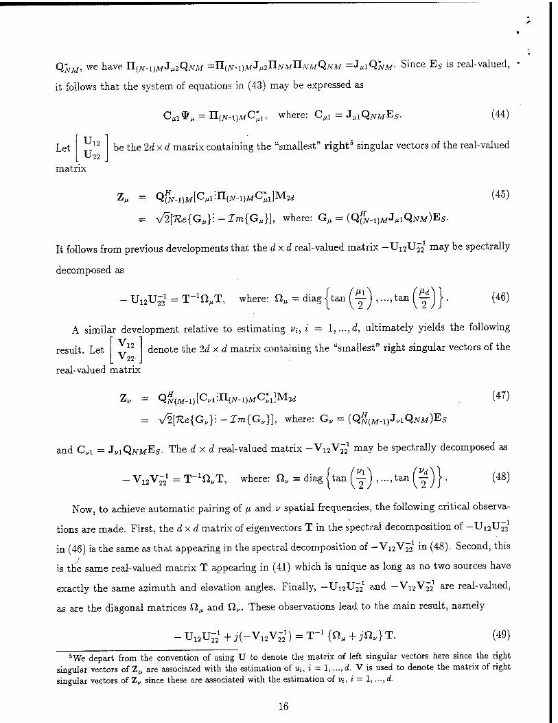
Q'NM, we have U^.^MJ^QNM =11(N-I)MJ^TINM^NMQNM =JMiQiVM- Since Es is real-valued,
it follows that the system of equations in (43) may be expressed as
Let U12
U22
matrix
ClllVli = n{N-1)MCl1, where: C^ = JMlQ^MEs- (44)
be the 2dxd matrix containing the "smallest" right5 singular vectors of the real-valued
= Q(AT-l)M[CMl:n(iV-l)MC*1]M2Ii
= ^e{G,}:-Im{GM}], where: GM = (Q^.1)MJ^IQ^M)E5.
(45)
It follows from previous developments that the d x d real-valued matrix -Ui2U22 may be spectrally
decomposed as
UnU^1 = T-^T, where: «M = diag {tan (^j ,..., tan (^) } (46)
A similar development relative to estimating i/t-, i = l,...,d, ultimately yields the following
denote the 2d x d matrix containing the "smallest" right singular vectors of the result. Let _, »22
real-valued matrix
Z„ = Q^(Af-i)[Cvi:n(jv-i)AfC^]M2d
= V2[Re{Gu}\ - lm{Gu}}, where: G„ = (Q#(M-I)J,IQJVM)ES
(47)
and C„i = J^IQJVWES- The </xd real-valued matrix -V12VM may be spectrally decomposed as
_ V12V2-2X = T-^.T, where: fl„ = diag {tan (y) ,..., tan (y J j. (48)
Nowj to achieve automatic pairing of /x and z/ spatial frequencies, the following critical observa-
tions are made. First, the d x d matrix of eigenvectors T in the spectral decomposition of -U^U^
in (46) is the same as that appearing in the spectral decomposition of -V^V^1 in (48). Second, this
is the same real-valued matrix T appearing in (41) which is unique as long as no two sources have
exactly the same azimuth and elevation angles. Finally, -U^U^1 and -V^V^1 are real-valued,
as are the diagonal matrices £lß and $V These observations lead to the main result, namely
UuUj.,1 +;(-Vi2V-21) = T-1 {0„ +Ä}T. (49)
5We depart from the convention of using U to denote the matrix of left singular vectors here since the right singular vectors of Z„ are associated with the estimation of u,-, i = 1, ...,d. V is used to denote the matrix of right singular vectors of Z„ since these are associated with the estimation of vt, i = l,...,d.
16

Thus, the eigenvalues of -U^U^1 +j(-Vi2V22
1) are tan(/z;/2) + j tan(i/,-/2), i - l,...,d. The
algorithm based on this development is referred to as 2D Unitary ESPRIT and is summarized
below.
Summary of 2D Unitary ESPRIT
1. Compute Es via the d "largest" left singular vectors of [Re{Y},Im{Y}], where Y =
2. Compute U12
U22
via the d "smallest" right singular vectors of
Zß = [Re{Gß},-lm{Gß}}, where Gß = (QfN_1)MJßlQNM)Es-
3. Compute _,12 via the d "smallest" right singular vectors of Z„ = [7£e{G„}, — Jm{G„}], L 22 J
where G^ = (Q^(M.1)JI/1Q^JW)ES.
4. Compute A,-, i = 1, ...,d, as the eigenvalues of the d x J matrix -U^U^1 + j(—V^V^1).
5. Compute spatial frequency estimates: //,- = 2tan_1(7?.e{At}), ^- = 2tan_1(Jm{A,}), i =
l,...,d.
Note that the maximum number of sources 2D Unitary ESPRIT can handle is minimum{M(iV —
1),N(M - 1)}, assuming that at least d + 1 snapshots are available. If only a single snapshot is
available, one can extract d + 1 or more identical rectangular subarrays out of the overall array to
get the effect of multiple snapshots, thereby decreasing the maximum number of sources that can
be handled.
5.1 2D Unitary ESPRIT vs. ACMP
Note that 2D Unitary ESPRIT provides closed-form, automatically paired 2D angle estimates as
long as the spatial frequency coordinate pairs (/x,-, Vi),i — 1,..., d, are distinct. That is, no additional
effort is needed if a pair or more of sources have the same m or V{. This is in contrast to the
Algebraically Coupled Matrix Pencil (ACMP) method of van der Veen et al which also provides
closed-form, automatically paired 2D angle estimates but breaks down if two sources have either
the same \i or v spatial frequency coordinate. Note that in order to avoid the same problem as
ACMP in this regard, one must solve the complex eigenvalue problem signified by (49). If one
attempts to compute the real eigenvalues of -U^U^1 alone, for example, there is a degeneracy in
the eigenvectors when two sources have the same fi spatial frequency coordinate thereby precluding
the ability to determine T.
17

Note that Vanpoucke et al propose a form of subarray averaging to overcome the problem of
ACMP occurring when two sources have either the same fj, or v spatial frequency coordinate, but
this decreases the maximum number of sources that can be handled and increases the computational
complexity significantly.
Note that ACMP requires an array of sensor triplets so that one can extract three identical
subarrays from the overall array. 2D Unitary ESPRIT only requires that the array exhibit invari-
ances in two distinct directions, as would be the case with two uniform linear arrays (ULA's), for
example. In Section 7, we show how 2D Unitary ESPRIT may be simply adapted for the case of
two orthogonal ULA's having a common phase center. ACMP is not applicable with such an array
geometry. Another advantage of 2D Unitary ESPRIT over ACMP is that 2D Unitary ESPRIT is
efficiently formulated in terms of real-valued computations, except for the final d x d eigenvalue
decomposition, while ACMP requires complex-valued computations throughout.
6 2D DFT Beamspace ESPRIT for URA
With 2D DFT beamforming (and attendant conjugate centro-symmetrization through simple scal-
ing), the components of the beamspace array manifold are separable real-valued patterns of the
form . . . , , . N, sing „-m» sinf , - ng)
fc»,.(e.") = —m OT- . r, /—~zw■ (50> sin j(^-mf)] Sin[l(,-nff)]'
Note that the matrix form of the beamspace manifold, denoted B(p, v), is related to the matrix form
of the array manifold via a 2D DFT as B(n, v) = W%A(n, v)WM, where W# denotes the conjugate
centro-symmetrized N pt. DFT matrix whose rows are given by (19) and W^ is defined similarly
with N replaced by M. Substituting the form of A(p,v) in (33) into B{n,v) = W%A(n,v)WM
yields
B{^u) = bN{ß)bJi(u)i (51)
where bN((j,) is defined in (21) and hM{v) is defined similarly with N replaced by M and \i replaced
by v. Given that bjv(^) satisfies the invariance relationship in (24), it follows that B((i, v) satisfies
tan (|) YlB{li,v) = Y2B{^v). (52)
18
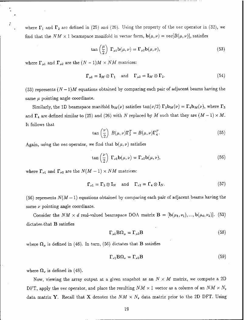
where I\ and T2 are defined in (25) and (26). Using the property of the vec operator in (32), we
find that the NM x 1 beamspace manifold in vector form, b(fi,u) = vec[B(fi,i/)], satisfies
tan (£) IVb(/z, u) = Tß2h{n, v), (53)
where TßX and T/i2 are the (N - l)M x NM matrices:
IVi = Ijif <8> Ti and rM2 = IM<8>r2. (54)
(53) represents (N -1)M equations obtained by comparing each pair of adjacent beams having the
same fj, pointing angle coordinate.
Similarly, the ID beamspace manifold bjv/(v) satisfies tan(i//2) T3bM(z/) = r4b]^(i/), where T3
and T4 are defined similar to (25) and (26) with N replaced by M such that they are (M -1) x M.
It follows that
tan (|) B{^u)Tl = B{^u)Tl. (55)
Again, using the vec operator, we find that b(fl, v) satisfies
tan(0 rvlb(/i,p) = rv2b(/x,i/), (56)
where TvX and Tv2 are the N(M - 1) x NM matrices:
Tul = T3 0 Ijv and T^ = T4 ® Ijv- (57)
(56) represents N(M — 1) equations obtained by comparing each pair of adjacent beams having the
same v pointing angle coordinate.
Consider the NM x d real-valued beamspace DOA matrix B = [b(jui, ut), ...,b(p,d, Vd)]. (53)
dictates .-that B satisfies
rMlBßM = r^B (58)
where Clß is defined in (46). In turn, (56) dictates that B satisfies
r.iBfi, = r„2B (59)
where Clv is defined in (48).
Now, viewing the array output at a given snapshot as an N x M matrix, we compute a 2D
DFT, apply the vec operator, and place the resulting NM x 1 vector as a column of an NM x Ns
data matrix Y. Recall that X denotes the NM x Ns data matrix prior to the 2D DFT. Using
19

the vec operator, the relationship between Y and X may be expressed as Y = (W^- <g> W$)X.
The appropriate NM x d matrix of signal eigenvectors, Es, for the algorithm presently under
development may be computed as the d "largest" left singular vectors of the real-valued matrix
[Jle{Y},Tm{Y}}. Asymptotically, Es = BT, where T is an unknown d x d real-valued matrix.
Substituting B = EST_1 into (58) and (59) yields the signal eigenvector relations
rMlEs*M = Tß2Es where: Vß = T^fi/T (60)
rvlEs9u = I\,2Es where: ¥„ = T^O/T. (61)
As in the extension of Unitary ESPRIT for a URA, automatic pairing of y. and v spatial frequency
estimates is facilitated by the fact that all of the quantities in (60) and (61) are real-valued. Thus,
*M + i*" may be spectrally decomposed as
^ß+j^, = T-1{Qß+jÜt/}T (62)
The algorithm based on this development, 2D DFT Beamspace ESPRIT, is summarized below.
Summary of 2D DFT Beams-pace ESPRIT
1. Compute a 2D DFT of the N x M matrix of array outputs at each snapshot (scale for conjugate centro-symmetrization), apply the vec operator, and place the result as a column
of Y.
2. Compute Es via the d "largest" left singular vectors of [Jle{Y},lm{Y}].
3. Compute ^fß as the solution to the (N - l)M x d matrix equation rMiEs*M = Fß2Es-
4. Compute \P„ as the solution to the N(M - 1) x d matrix equation T^Es^u = T^Es-
5. Compute A,-, i = 1,..., d, as the eigenvalues of the d x d matrix *M + ;'*„.
6. Compute spatial frequency estimates: m = 2tan_1(7?.e{At}), i/,- = 2tan_1(Jm{At}), i =
l,...,d.
6.1 Reduced Dimension Example
As in the ID case, the utility of 2D DFT Beamspace ESPRIT over 2D Unitary ESPRIT is in
scenarios where one works with a subset of 2D DFT beams that encompass some volume of space
of interest. In fact, the ability to work in a reduced dimension beamspace is even of more value in
the case of a URA since the total number of elements may be quite high. As an example, consider
a scenario, similar to the low-angle radar tracking problem, in which we desire to estimate the
20

respective azimuth and elevation angles of each of two closely-spaced sources. To this end, we form
four 2D DFT beams steered to the spatial frequency coordinate pairs (m|^,n||), ((m + l)^,n||),
(m^, (n + l)ff), and ((m + 1)^, (n + l)|f), respectively, as depicted in Figure 3. Recalling that
the components of the beamspace manifold have the form in (50), the 4x1 beamspace manifold
for this case is
b(/i, v) = [bm,n(n, u) , &m+i,n(/*, *>) , &m,n+l(A*i ") i &m+l,n+l(A*, ^)] • (63)
In this case, Es is 4 x 2 and may be constructed from the two "largest" eigenvectors of the real
part of the 4x4 matrix formed from the inter-beam correlations. The 2x2 matrices \£ß and
*BU would be computed as the corresponding solutions to the 4x2 respective matrix equations
IViEs#M = rM2Es and TulEsV,, = r„2Es, where
r„i =
rM2 —
r„i =
rv2
cos (mjj}
0
sin (m^)
0
cos (n§)
0
sin (n^)
0
cos
sin
(("»+1)$) 0
0
0 0
0
cos (n^j
0
cos
cos (mjj) cos ((m+l)j0 _
0 0
sin (m^) sin ((m+1)^) _
cos ((n+l)§) _ 0
smltn+1)^)
0
0
sin(n^) ' 0 sin((n+l)£)
In the final stage of the algorithm, tan(^/2) + j tan(j/,-/2), z = 1,2, would be computed as the
eigenvalues of a 2 x 2 matrix.
6.2 Comparison with UCA-ESPRIT
As discussed in Section 1, UCA-ESPRIT [7, S] is a recently developed closed-form 2D angle esti-
mation scheme for a uniform circular array (UCA). As indicated in Figure 2, in the final stage of
UCA-ESPRIT, the i-th eigenvalue of a matrix has the form Uj + jvi, where u,- and u; are the direc-
tion cosines of the i-th source relative to the x and y axes, respectively, assuming the UCA to lie in
the x-y plane. This is in contrast to 2D DFT Beamspace ESPRIT where there is spatial frequency
warping such that the final eigenvalues are of the form tan(/f;/2)+j tan(j/,-/2), i — 1,..., d. A notable
difference between the development of UCA-ESPRIT and that of 2D DFT Beamspace ESPRIT is
that in the former the sampled aperture pattern was assumed to be approximately equal to the
21

continuous aperture pattern [7, 8], while no such approximation was made in the latter case. We .
here briefly show that if a similar approximation is made in the development of 2D DFT Beamspace
ESPRIT, the final eigenvalues yielded by the resulting approximate 2D DFT Beamspace ESPRIT
algorithm are identical in form to those yielded by UCA-ESPRIT.
Aside from averting spatial frequency warping, this form of the eigenvalue has a nice geometrical
interpretation in that it may be expressed as u{ + jv{ = sin0t- e^S where & and 0,- are the azimuth
and elevation angles of the i-th source, respectively. This is illustrated in Figure 2. 0t- varies between
0° and 90° so that sin0t- varies between 0 and 1, while fc varies between 0° and 360°. Thus, one can
immediately glean the azimuth angle of the i-th source from the polar angle of the i-th eigenvalue.
The corresponding elevation angle is the arcsine of the magnitude of the i-th eigenvalue. If the
eigenvalue is at the origin, the source is at boresite. If the eigenvalue is on the unit circle, the
source is in the same plane as the array. Also, we may use the fact that an eigenvalue should be
located on or within the unit circle to screen out false alarms.
Assume the interelement spacing in either direction to be less than or equal to a half-wavelength. ill L i \ sintf ("-m¥)] sin[f ("-n&)l In this case, in the vicinity of the mainlobe and first few sidelobes, om,n(/z, v) « \r_m^\ —\/u_n2*\ ■
Substituting \i = ^f Axu and v = ^-Ayv, define
sin[f(fA,u-mf)]si.[f(yA8,-nf)]
*~M = i($*,u-m$) *(**.-»») ' ' ' This is the far field pattern that would result with a continuous rectangular aperture of dimension
NAX by MAy. The superscript a denotes approximate pattern. Similar to the development for the
sampled aperture pattern, observe that bamn{u,v) and b^+hn(u,v) are related as
(^ A,« - m%) %,B(«, v) + (^ A„« - (m + l)%) %+1>, v) = 0, (65)
(66)
which may be rearranged as
« {%>,«) + £+!,»(«>»)} = j^-{mbamJu,v) + (m + l)ba
m+1Ju,v)}.
Similarly, bamn{u,v) and ba
m^n+1(u,v) are related as
i^Ayv - n|) b°mJu,v) + (^Ayv - (n + 1)|) £tn+1(«, t,) = 0, (67)
which may be rearranged as
v {£>,«) + bam<n+l(u,v)} = -^{nba
mJu,v) + (n + l)bam^(u,v)}. (68)
1y
11

For the sake of brevity, consider again the case of four 2D DFT beams to estimate the respective
azimuth and elevation angles of each of two closely-spaced sources. In this case, the 4x1 beamspace r ]T
manifold is ha{u,v) = \b^in(u,v), bam+hn(u,v), ba^n+l{u,v), ba
m+hn+l(u,v)\ . Given the relations
above, it is readily deduced that uTaulb
a{u7v) = Tau2b
a{u,v) and vTavlb
a(u,v) = Tav2b
a(u,v), where
■pa 1 ul —
■pa L vl
1 1 0 0 ' 0 0 1 1
1 0 1 0 " 0 1 0 1
and Tau2
A
NAX
A and r", =
m (m+1) 0 0 0 0m (m+1)
n 0 (n+1) 0 On 0 (n+1)
Asymptotically, the 4 x 2 real-valued matrix of signal eigenvectors, Es, satisfies Es = BT, where
B = [b(wi,ui),b(u2,U2)] and T is an unknown 2 x 2 real-valued matrix. Expediting the development,
it follows that r^E5*u = Tau2Es, where #u = T-xfiuT and fiu = diag{ui,u2}. Also, I^Es*« =
r^2Es, where *„ = T-1ß„T and Qv = diag{u1,u2}- Thus, ux + jvi and u2 + jv2 are the two
eigenvalues of \PU + j^v.
The point is that with d < A/2 the sampled aperture pattern is very well approximated by the
continuous aperture pattern in the vicinity of the mainlobe and first few sidelobes. Thus, if only a
relatively small number of beams is selected, the modified version of 2D DFT Beamspace ESPRIT
sketched above yields the direction cosines directly without spatial warping.
T 2D DFT Beamspace ESPRIT for Cross Array
Consider an array composed of an N element ULA aligned with the x-axis and an M element ULA
aligned with the y-axis. The center of each leg is assumed to be at the origin so that they have
a common phase center. To ease the development and for the sake of notational simplicity, we
will assume M and N are both even so that the two legs do not share a common element at the
origin. However, with slight modification, the adaptation of 2D DFT Beamspace ESPRIT for a
cross array developed subsequently may also be employed when M and/or N are odd. Also, due to
space limitations, we here only present the appropriate adaptation of 2D DFT Beamspace ESPRIT.
2D Unitary ESPRIT may also be suitably adapted but would require a slightly more complicated
development.
Let x(£) and y(£) be the N x 1 and Mxl snapshot vectors output by the two respective legs
at time L The (N + M) x 1 composite snapshot vector is formed as z{€) = x(*)
y(4 These are
23

stacked as the columns of an (vV + M) x Ns matrix Z. The array manifold for such an array is
a(^,i/) aN(n)
(69)
where a.pj(p) and B.M{V) are each conjugate centro-symmetric as defined previously. Note that it
is only because the two legs have a common phase center that we are able to express the array
manifold in this form. If this is not the case, as with an L-shaped array, for example, either the
upper N x 1 or lower Mxl block of a(/x, v) would not be conjugate centro-symmetric and it would
not be possible to convert a(/j, v) to a real-valued manifold through a simple matrix transformation.
Transformation to beamspace is accomplished via
WN O
o WM (70)
bN(/j.)
bM(v) (71)
The beamspace manifold is
b(/i, v) = F"a(/i, u) =
where b^(fi) and b^(i/) are as defined previously. In practice, transformation to beamspace is
accomplished via an N pt. DFT of the x-axis leg and an M pt. DFT of the y-axis leg, with
a-posteriori conjugate centro-symmetrization via simple scaling of each DFT value.
Let Es be the (JV + M) x d matrix of signal eigenvectors computed as the d "largest" left sin-
gular vectors of [R,e{H}, Jm{H}], where H = F^Z. (Alternatively, Es may be determined as the d
"largest" eigenvectors of Ke{FHZZHF}.) Asymptotically, Es = BT, where B = [ty/n, ^i),-,b(/^,^)]
and T is an unknown d x d real-valued matrix. Define the following matrices:
Aßl = [T^ I ^OJ }N-I and Aß2 = [T^:. OJ}N-I
A„i = [O^ : JjJ }M-I and A„2 = [O^ : Tß }M-I
(72)
(73)
where T3 and T4 are defined similar to (25) and (26) with N replaced by M. The following signal
eigenvector relations follow quite readily from previous developments:
A^Es^ = A^Es where: ¥„ = T^n/T
A„iEs¥„ = A,*Es where: #„ = T^T.
(74)
(75)
As with 2D DFT Beamspace ESPRIT, automatic pairing of JJL and v spatial frequency estimates is
facilitated by the fact that all of the quantities in (74) and (75) are real-valued. Thus, \&M + j~9u
24
may be spectrally decomposed as
*M + j*, = T-1{fiM+Ä}T (76)
The algorithm based on these observations is similar in form to 2D DFT Beamspace ESPRIT for a
URA.
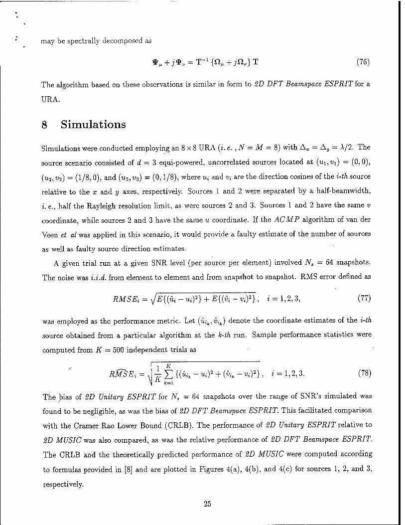
8 Simulations
Simulations were conducted employing an 8 x 8 URA (i. e. , N = M = 8) with Ax = Ay = A/2. The
source scenario consisted of d = 3 equi-powered, uncorrelated sources located at (ui,Vi) = (0,0),
(u2, v2) = (1/8,0), and (u3, v3) = (0,1/8), where m and u; are the direction cosines of the i-th source
relative to the x and y axes, respectively. Sources 1 and 2 were separated by a half-beamwidth,
i. e., half the Rayleigh resolution limit, as were sources 2 and 3. Sources 1 and 2 have the same v
coordinate, while sources 2 and 3 have the same u coordinate. If the ACMP algorithm of van der
Veen et al was applied in this scenario, it would provide a faulty estimate of the number of sources
as well as faulty source direction estimates.
A given trial run at a given SNR level (per source per element) involved Ns = 64 snapshots.
The noise was i.i.d. from element to element and from snapshot to snapshot. RMS error defined as
RMSEi = ^E{{üi - uif} + E{(vi - Viy} , i = 1,2,3, (77)
was employed as the performance metric. Let (üik,Vik) denote the coordinate estimates of the i-th
source obtained from a particular algorithm at the k-th run. Sample performance statistics were
computed from K = 500 independent trials as
1 K
RMSEi = . — J2 {(«••* - ui)2 + fa* - ^)2} , i = 1,2,3. \ Ä fc=i
(78)
The bias of 2D Unitary ESPRIT for Ns = 64 snapshots over the range of SNR's simulated was
found to be negligible, as was the bias of 2D DFT Beamspace ESPRIT. This facilitated comparison
with the Cramer Rao Lower Bound (CRLB). The performance of 2D Unitary ESPRIT relative to
2D MUSIC was also compared, as was the relative performance of 2D DFT Beamspace ESPRIT.
The CRLB and the theoretically predicted performance of 2D MUSIC were computed according
to formulas provided in [8] and are plotted in Figures 4(a), 4(b), and 4(c) for sources 1, 2, and 3,
respectively.
25
Note that 2D MUSIC essentially achieved the CRLB over the range of SNR's simulated so that
its theoretically predicted RMSE curve is coincident with the CRLB curve. Of course, 2D MUSIC
requires the localization of 3 peaks of a 2D spectrum. In element space, determining the value of
the 2D MUSIC spectrum at a given point involves the calculation of an inner product of the form
a-ff(//,^)PJ-a(//,i/), where P1 is 64 x 64. This kind of calculation has to be done repeatedly in
performing a localized Newton-Raphson search around each spectral peak.
The respective RMSE's of 2D Unitary ESPRIT and 2D DFT Beamspace ESPRIT for sources 1,
2, and 3 are plotted in Figures 4(a), 4(b), and 4(c), respectively. In accordance with the summary
of 2D Unitary ESPRIT at the end of Section 3.0, the computations required for a single run were:
(i) 64 additions per each of 64 snapshots to transform from complex-valued space to real-valued
space, (ii) calculation of the 3 "largest" left singular vectors of a 64 x 128 real-valued matrix, (iii)
calculation of the solution to two systems of equations of the form AX = B where A and B are
both 64 x 3 and real-valued, and (iv) calculation of the eigenvalues of a 3 x 3 complex-valued matrix.
The performance of 2D Unitary ESPRIT is observed to be very close to the CRLB for SNR's greater
than or equal to -6 dB, although it does not achieve the CRLB even at the rather high SNR level of
12 dB. (Keep in mind that there are 64 elements and that the SNR is that per element.) Observe
that on a logarithmic scale, the small gap between the performance of 2D Unitary ESPRIT and
the CRLB is fairly constant as a function of SNR for SNR's above -6 dB.
To demonstrate the efficacy of working in a reduced dimension beamspace, 2D DFT Beamspace
ESPRIT employed a 3 x 3 set of 9 beams with mainlobes rectangularly spaced in the u-v plane and
centered at (u, v) = (0,0). In accordance with the summary of 2D DFT Beamspace ESPRIT at the
end of Section 4.0, the computations required for a single run were: (i) 9 sets of 64 multiplications
and 63 additions for each of 64 snapshots to transform from element space to beamspace, (ii)
calculation of the 3 "largest" left singular vectors of a 9 x 128 real-valued matrix, (iii) calculation
of the solution to two systems of equations of the form AX = B where A and B are both 9x3
and real-valued, and (iv) calculation of the eigenvalues of a 3 x 3 complex-valued matrix. A scatter
plot of the 3 eigenvalues obtained from 2D DFT Beamspace ESPRIT for each of 200 independent
runs at an SNR of 3 dB is displayed in Figure 4(d). For SNR's greater than or equal to -6 dB,
the performance of 2D DFT Beamspace ESPRIT is observed to be only slightly worse than that of
2D Unitary ESPRIT despite the dramatic reduction in computational complexity. Similar to 2D
Unitary ESPRIT, the gap between the performance of 2D DFT Beamspace ESPRIT and the CRLB
26

is fairly constant as a function of SNR over the range of SNR's simulated.
An interesting observation is that for SNR's lower than -9 dB, 2D DFT Beams-pace ESPRIT
outperformed 2D Unitary ESPRIT. This is in accordance with observations made by Xu et al.
[16] in comparing the performance of their version of Beamspace ESPRIT with that of ESPRIT in
element space. At low SNR's Xu et. al. argued that the better performance of the former over that
latter is due to fact that Beamspace ESPRIT exploits a-priori information on the source locations
by forming beams pointed in the general directions of the sources. This argument is applicable here
as well.
The difference in performance between 2D Unitary ESPRIT or 2D DFT Beamspace ESPRIT
and the CRLB, and the fact that 2D MUSIC achieves the CRLB for the range of SNR's simulated,
suggests a strategy wherein the 2D angle estimates provided by either 2D Unitary ESPRIT or 2D
DFT Beamspace ESPRIT axe used as starting points for localized Newton searches of the 2D MUSIC
spectrum to achieve uniformly minimum variance unbiased estimates (UMVUE's). Note that the
computational burden of performing these localized searches of the 2D MUSIC spectrum may be
reduced substantially by operating in beamspace and exploiting the conjugate centro-symmetry of
the URA manifold.
9 Conclusions
2D Unitary ESPRIT is a closed form 2D angle estimation algorithm for use in conjunction with
a URA and is easily adapted for other dual invariance arrays including a cross array. 2D DFT
Beamspace ESPRIT is an efficient beamspace implementation of 2D Unitary ESPRIT facilitating
reduced dimension processing and attendant reduction in computational complexity. The 2D angle
estimates provided by either 2D Unitary ESPRIT or 2D DFT Beamspace ESPRIT may be used as
starting points for localized Newton searches of the 2D MUSIC spectrum, the ML algorithm, or the
Multiple Invariance ESPRIT algorithm. Due to space limitations, performance analysis of either
2D Unitary ESPRIT or 2D DFT Beamspace ESPRIT is not included here, but would follow in the
same vein as the performance analysis of UCA-ESPRIT in [22]. Note that 2D Unitary ESPRIT
may also be employed in a variety of applications other than 2D angle estimation including 2D
harmonic retrieval for image analysis, for example.
27

10 Bibliography
[1] R. Roy and T. Kailath, "ESPRIT-Estimation of signal parameters via rotational invariance
techniques," IEEE Trans. Acoust., Speech, Signal Processing, vol.37, pp.984-995, July 1989.
[2] A. L. Swindlehurst, B. Ottersten, G. Xu, R. H. Roy, and T. Kailath, "Multiple Invariance
ESPRIT", IEEE Trans. Signal Processing, vol. 40, pp. 867-881, Apr. 1992.
[3] A. L. Swindlehurst and T. Kailath, "Azimuth/elevation direction finding using regular array
geometries", IEEE Trans. Aerospace and Electronic Systems, vol. 29, pp. 145-156, Jan. 1993.
[4] M. P. Clark and L. L. Scharf, "Two-Dimensional Modal Analysis Based on Maximum Likeli-
hood", IEEE Trans. Signal Processing, vol. 42, pp. 1443-1452, June 1994.
[5] M. D. Zoltowski and D. Stavrinides, "Sensor Array Signal Processing via a Procrustes Rotations
Based Eigenanalysis of the ESPRIT Data Pencil," IEEE Trans. Acoustics, Speech, and Signal
Processing, vol. 37, pp. 832-861, Jun. 1989.
[6] A.J. van der Veen, P.B. Ober, E.D. Deprettere, "Azimuth and Elevation Computation in High
Resolution DOA Estimation", IEEE Trans. Signal Processing, vol. 40, pp. 1828-1832, July
1992.
[7] M.D. Zoltowski and C.P. Mathews, "Closed-Form 2D Angle Estimation with Uniform Circular
Arrays Via Phase Mode Excitation and ESPRIT," 27th Asilomar IEEE Conf. on Signals,
Systems, and Computers, vol. 1, pp. 169-173, Nov. 1993.
[8] C.P. Mathews and M.D. Zoltowski, "Eigenstructure Techniques for 2-D Angle Estimation
with Uniform Circular Arrays," scheduled to appear in IEEE Trans, on Signal Processing,
September 1994.
[9] ivi. Haardt and M.E. Ali-Hackl, "Unitary ESPRIT: How to Exploit Additional Information
Inherent in the Rotational Invariance Structure", Proc. IEEE Int. Conf. Acoust., Speech, Signal
Processing, Adelaide, Australia, Apr. 1994.
[10] M. Haardt and J.A. Nossek, "Unitary ESPRIT: How to Obtain Increased Estimation Accuracy
with a Reduced Computational Burden", Techincal Report No. TUM-LNS-TR-94-3, Institute
28

of Network Theory k Circuit Design, Technical University of Munich, D-80290 Munich, Ger-
many, May 1994.
[11] K.C. Huarng and C.C. Yeh, "A unitary transformation method for angle-of-arrival estimation",
IEEE Trans. Signal Processing, vol. 39, pp. 975-977, Apr. 1991.
[12] D.A. Linebarger, R.D. DeGroat, and E.M. Dowling, "Efficient Direction Finding Methods Em-
ploying Forward/Backward Averaging", scheduled to appear in IEEE Trans. Signal Processing,
1994.
[13] K. Buckley and X.-L. Xu, "Spatial-Spectrum Estimation in a Location Sector," IEEE Trans.
Acoust, Speech, Signal Process., vol. ASSP-38, no. 11, pp. 1842-1852, Nov. 1990.
[14] G. Bienvenu and L. Kopp, "Decreasing High Resolution Method Sensitivity by Conventional
Beamforming Preprocessing," in Proc. of 1984 IEEE Int'l Conf. on Acoust, Speech, and Signal
Process., pp. 33.2.1-33.2.4, April 1984.
[15] H. Lee and M. Wengrovitz, "Resolution Threshold of Beamspace MUSIC for Two Closely-
Spaced Emitters," IEEE Trans. Acoust., Speech, Signal Process., vol. 38, pp. 1545-1559, Sept.
1990.
[16] G. Xu, S.D. Silverstein, R. H. Roy, and T. Kailath, "Beamspace ESPRIT," IEEE Trans. Signal
Processing, vol. 42, pp. 349-356, Feb. 1994.
[17] M.D. Zoltowski, G.M. Kautz, and S.D. Silverstein, "Beamspace Root-MUSIC", IEEE
Trans. Signal Processing, vol. 41, pp. 344-364, Jan. 1993.
[18] K.JfR. Liu, D.P. O'Leary, G.W. Stewart, and Y.J.J. Wu, "An Adaptive ESPRIT Based on
URV decomposition", in Proc. IEEE Int. Conf. Acoust, Speech, Signal Processing, vol. IV,
pp. 37-40, Minneapolis, MN, Apr. 1993.
[19] G. Xu, R.H. Roy, and T. Kailath, "Detection of Number of Sources via Exploitation of Centro-
symmetry Property", IEEE Trans. Signal Processing, vol. 42, pp. 102-112, Jan. 1994.
[20] M. D. Zoltowski and T. Lee, "Maximum Likelihood Based Sensor Array Signal Processing in
the Beamspace Domain for Low-Angle Radar Tracking," IEEE Trans, on Signal Processing,
vol. 39, pp. 656-671, Mar. 1991.
29

[21] F. Vanpoucke, M. Moonen, and Y. Berthoumieu, "An Efficient Subspace Algorithm for 2-D
Harmonie Retrieval", Proc. IEEE Int. Conf. Acoust., Speech, Signal Processing, Adelaide,
Australia, Apr. 1994.
[22] C. P. Mathews and M. D. Zoltowski, "Performance Analysis of the UCA-ESPRIT Algorithm for
Circular Ring Arrays," scheduled to appear in IEEE Trans, on Signal Processing, September
1994.
30

CD
Hb c cd (-;
■4—»
=5
£ N cd
CO
X cd
>^ Ä
CD c
•T—I co O o ;-*
I! >
co
'x cd
i X
•4—> Ui
CD C
• <"■< co O o '—'
""Sb c cd C O • *-< cd >
13
©
CO • *-* X cd
■*—"
C o
CU o cd
'S« CO
cd u- u cd -t->
C • ^* co O O
II 3
2' ^, ^/ ^7
31
>^ cd
2 fc .2 03 «S
>SÖ 1 o 1 'S & § « &« 5 cd ü
° * Ö co O ^ w ^ -fi O >. ^
•- fcj > 13 * H f- t. ^H a« « 2 |§5 o-3Ö r- _ D C JS O
ja H £ — '—1 cd
slra
tii
A-E
S D
FT
= ÜQ M 3 C^
<N CD '■«
3 to £
■o £ co •;-< C £ ^ <Ö t-< "w*
_o t—i <D
o ^ = co CU « ~ CO >
O w CD ^ 'S ÖD
— O •<-; cd .. <U
^ co —■* ,—• +—> o 6 o
CD co e
gih
aria
C i >
llust
rati
ia R
oot
ingl
e in
>—1 r> CO
,-J D Ui 3 tß
*&«

SIS es
+ c 51Z CN|
TO A—0—w
<* x
< Jr.
s Cd X! <0
CO
X) VH
«2 00 C
• 1—4
Ä 00
•i—i
00
CO o cd Cu
Cd CO
X)
a. C
s eo
£ o
c E-> o &-J •zs pi 2 OH £ oo
«8 CO
c cd
«4-4 o c o
• 1-« *-> cd b Cfl 3
w CO
OH CO
cd
Q Q
h-<H
m eo 3 00 • *-*
32

IOV RMS Estimation Error for Source 1 at (u,v) - (0,0)
~Q— 2D DFT Beamspace ESPRIT - Exp. (9 beams)
—X— 2D Unitary ESPRIT - Experimental
2D MUSIC - Theoretical
.*•-. CR Lower Bound
«10' IT
10 ,-3
64 snapshots per run 8x8 rectangular array, \= &y= X/2 3 equi-power, uncorrelated sources 500 trial runs per SNR
101f
2 ui , M10' cc
-10 -5 0 SNR (dB)
10 10 ,-3
RMS Estimation Error for Source 3 at (u,v) =■ (0,1/8)
—Q— 2D OFT Beamspace ESPRIT - Exp. (9 beams) —X-- 2D Unitary ESPRIT - Experimental
20 MUSIC - Theoretical
CR Lower Bound
64 snapshots per run 8x8 rectangular array, &x= Ay= X/2 3 equi-power, uncorrelated sources 500 trial runs per SNR
-10 -5 0 SNR (dB)
10
Figure 4: (a) RMSE for source 1 in simulation example. Figure 4: (c) RMSE for source 3 in simulation example.
io-1r
«10 cr
10 v-3
RMS Estimation Error for Source 2 at (u,v) - (1/8,0)
—Q— 2D DFT Beamspace ESPRIT - Exp. (9 beams)
—X— 2D Unitary ESPRIT - Experimental
2D MUSIC - Theoretical
CR Lower Bound
64 snapshots per run 8x8 rectangular array, A= Ay= 3 equi-power, uncorrelated sources 500 trial/uns per SNR
-10 -5 0 SNR (dB)
10
0.25
0.2
0.15
0.1
0.05
■°-°§,
♦
.05
Scatter Plot of 2D OFT Beamspace ESPRIT Eigenvalues
200 trial runs overlaid 64 snapshots per run, SNR =■ 3 dB 8x8 rectangular array, Ax= Ay= \n 3 equi-power, uncorrelated sources
Idealform: z=tan(u/2) + jtan(v/2)
0.05 0.1 Re(2)
0.15 0.2 055
Figure 4: (b) RMSE for source 2 in simulation example. Figure 4: (d) Scatter plot of 2D DFT Beamspace ESPRIT eigenvalues.
33
2 Beamspace DO A Estimation Featuring Mult irate Eigen- vector Processing
A novel approach to angle of arrival estimation in beamspace is developed. Beamspace noise eigenvectors may be transformed to vectors in the element-space noise subspace. The trans- formed noise eigenvectors are bandpass, facilitating multirate processing involving modulation to baseband, filtering, and decimation. As these operations are linear, a matrix transformation applied to the eigenvectors may be constructed a priori. Incorporation of the technique into ei- ther the Root-MUSIC or ESPRIT prescriptions provides a computationally efficient procedure. Compared to past efforts to adapt Root-MUSIC and ESPRIT to beamspace, this approach cir- cumvents the need for restrictive requirements on the form of the beamforming transformation. An asymptotic theoretical performance analysis is also included to provide an alternative to computationally intensive Monte-Carlo simulations. Simulation studies show the validity of the performance predictive expressions and verify that the procedure, when incorporated into the Root-MUSIC/ESPRIT formulations, produces a direction finding technique that nearly attains
the Cramer-Rao bound.
2.1 Introduction
2.2 Array Signal Model
2.3 Development of DOA Estimators Featuring Multirate Eigen- vector Processing
2.3.1 Multirate Noise Eigenvector Processing
2.3.2 Incorporation of Filter Deconvolution
2.3.3 Root-MUSIC Incorporating Multirate Eigenvector Processing
2.3.4 TLS-ESPRIT Incorporating Multirate Eigenvector Processing
2.3.5 Location of Extraneous Roots Created by Filtering
2.4 Theoretical Performance Analysis
2.4.1 Performance Analysis of Root-MUSIC Formulation
2.4.2 Performance Analysis of ESPRIT Formulation
2.5 Computer Simulations
2.6 Conclusions/Remarks
2.7 References
2.8 Appendix: Asymptotic Variance of ESPRIT Formulation
34

1. Introduction
Beamspace formulations of the eigenstructure class of direction finding sensor array processing algo-
rithms offer a number of advantages over their element space counterparts. First, there is a computational
benefit realized in the processing of data of a much smaller dimension. Second, a practical implemen-
tation to current phased array technology is allowed. Third, beamspace formulations exhibit a reduced
sensitivity to sensor position perturbations and noise non-idealities [1]. Fourth, although suboptimal in
high SNR situations, the inherent concentration over a specific spatial region of interest leads to noise
reduction and, hence, enhanced ability for localization in the more critical case of low SNR [2, 3].
In the case of the Spectral MUSIC algorithm proposed by Schmidt [4], which is applicable to arbitrary
array geometries, the Vandermonde nature of the element space array response to a plane wave signal for
the common uniform linear-spaced array geometry facilitates a root-finding procedure for angle estimation
[5] as a computationally attractive alternative to the spectral search. The beamspace formulation of
Spectral MUSIC, however, does not directly offer a polynomial root-finding capability. By relating the
beamspace manifold to the element space direction vector, a beamspace Root-MUSIC capability can be
realized but the order of the resulting polynomial to be rooted is related to the number of sensors, N,
as 2JV — 2. This represents such a considerable computationally intensive task for large arrays so as to
preclude its use for the associated performance gains as noted in [6].
Recently, an efficient algorithm was proposed in [7] as a means of reducing the Root-MUSIC polyno-
mial to order 2JV& — 2, where Nb is the number of beams. This represents a tremendous computational
savings if only a relatively few number of beams are formed to probe a spatial subband (sector) for sources.
The approach in [7] was accomplished by requiring that the beamforming vectors possess common spatial
nulls. We point out that, like the beamspace Root-MUSIC formulation in [7], an adaptation of ES-
PRIT to beamspace in [8] also required significant restrictions on the form of the beamforming vectors.
Aside from this possibly over-restrictive requirement, two other problems associated with the beamspace
Root-MUSIC algorithm were observed. First, the technique didn't exploit the spatially-confined region
of operation in the rooting stage of the algorithm. That is, as the number of sensors comprising the array
increases, the spatial extent of the beamforming window decreases with constant Nb but, yet, the rooting
algorithm is still capable of localizing signals over all of visible space. Second, the approach involved the
use of an iVj, x Nb matrix transformation Q which was found to be highly ill-conditioned. For example,
35

the condition number of Q for an iV = 128 element array operated upon by a spatial Discrete Fourier
Transform (DFT) beamformer was computed for a varying number of beams and plotted in Figure 1. In
contrast, the other curve in the figure (Z transformation) corresponds to an alternative approach that is
the key result of this paper, having a similar implementation for the MUSIC setting but fundamentally
different to the approach in [7]. Whereas the condition number associated with the Z transformation is
relatively constant at a value near 3 for all beamspace dimensions, the corresponding value for the Q
transformation is large for even a small number of beams, e.g., for a beamformer comprised of Nb = 8
spatial DFT beams, the condition number is approximately 8 • 109.
The main purpose of this paper is to develop a processing methodology that is based on the trans-
formability of a beamspace noise eigenvector to an element-space counterpart as noted in passing in [3, 9].
In the intended application of beamspace processing, a spatial subband is probed so that the transformed
beamspace noise eigenvectors are naturally bandlimited in a spatial sense. This banded characteristic
allows for the application of classical multirate digital signal processing to isolate and spatially enlarge
the spatial subband of interest. Note that this methodology departs from classical multirate processing in
that the pertinent information lies in the in-band signal nulls instead of signal peaks. In the conventional
mode of multirate processing, one has to be concerned with spectral peaks outside the "basebanded" sub-
band being aliased into the subband thereby causing ambiguities. Lowpass filtering is implemented prior
to decimation to avoid this condition. However, in array processing at the sensor level, this pre-filtering
operation destroys the Vandermonde nature of the manifold thereby precluding rooting based DOA es-
timation techniques such as Root-MUSIC or ESPRIT. Here the goal is to preserve in-band signal nulls
and the development will show that the ability to root is easily maintained. In addition, with respect
to aliasing artifacts, out-of-band signals not sufficiently de-emphasized by the front-end beamforming
give rise to out-of-band signal nulls which actually serve to suppress aliasing contributions resulting from
decimation (see Figure 2 to be discussed shortly).
An important feature of this approach is that there are no restrictive requirements on the form of
the beamforming vectors. Another advantage of this technique is that the angular separation between
"in-band" signal roots is increased by the decimation factor, thereby easing the job of rooting. Another
major advantage is that the technique is computationally robust as the Z matrix transformation applied
to the beamspace noise eigenvectors is well conditioned, e.g., refer to Figure 1 where the condition number
36

of a Z transformation is shown for the same array length and a suitable decimation procedure.
As the eigenvector transformation-decimation procedure is general in nature, the technique may be
applied to any eigenstructure direction finding algorithm. We here consider the Root-MUSIC and ES-
PRIT [10] formulations as these techniques are fairly representative of the eigenstructure class of angle
estimators; application to other algorithms is straightforward.
The contents of this paper are as follows. Following a description of the data model, the beamspace
noise eigenvector transformation-decimation technique is developed and applied to Root-MUSIC and
ESPRIT ideology in Section 3. The theoretical performance of the MUSIC/ESPRIT formulations is de-
veloped, in terms of the estimation variance, in Section 4. Finally, the theoretical performance expressions
are validated in simulations and the optimality of the technique is observed through a comparison study
with the stochastic Cramer-Rao bound in a variety of experiments in Section 5.
2. Array Signal Model
The DO A estimation methodology described herein assumes a uniform linear array of sensors. An
extension to the two-dimensional array geometry composed of a rectangular lattice of sensors is readily
clear.
Assuming that K narrowband plane-wave signals, residing at a common center frequency, impinge
upon an N-sensor array, the complex basebanded data snapshot vector at the m'th sampling instant,
x(m), is expressed as a superposition of signals embedded in additive noise as
K x(m) = Yl *k(rn)aN(pk) + n(m) m = 1,...,M (1)
In the above equation, the amplitudes of the K signals, Sfc(-), k = 1,..., Ä", are modelled as zero-mean
jointly Gaussian random variables with non-singular covariance Ps, and n(-) is a zero-mean complex
gaussian noise vector with assumed covariance £ n(m)nH(m) = <T*1N- The array response to a unit-
amplitude signal arriving from the spatial location /x is represented by aw(/i), where \i = ^ d sin(ö),
d is the sensor spacing, A is the wavelength, and 9 is the conical angle of arrival. In accordance with a
uniform sensor placement, the structure of the array manifold vector has the form
Ml*) = {l,eJli,e^,...,e*N-^}. (2)
The associated sensor covariance matrix, assuming that the noise is uncorrelated with the signal set, is
37

simply
Rx = APSAH + a2
nIN, (3J
aN(fj,1): ajv(/i2): • • • : &N{IJ>K) In the where A is the matrix of element-space manifold vectors, A =
event that the noise exhibits a colored character, we assume that the noise correlation matrix is known.
The benefits of beamforming as a pre-processing operation prior to DOA estimation is well known in
the literature [1, 2, 3, 7]. Here we transform the element-space data to an Nb dimensional beamspace in
a digital or analog fashion. This operation is mathematically modelled as
y(m) = WHx(m) m = l,...,M (4)
where the columns of the JVxiV& beamforming matrix are orthonormalized so that WFW = INb. De-
noting the jVj-dimensional beamspace manifold vector as b(/z), the associated beamspace covariance, Rj,,
is
Ry = S \y{m)y(m)H] = WHRrW = BPSB" + <r2nINb, (5)
where B = b(/*x);b(/*2); ... \b(fiK)] andb(^) = WHa.N(fi).
As the ideal covariance matrix is not accessible in practice, an M-sample estimate is employed as
M
R* = £ y(m)yH(m), (6) m=l
where we assume that M > K. We also assume that Nb > K for proper operation of the DOA es-
timators. As the beamspace dimension, Nb, is usually chosen to be small in relation to N, to yield a
computationally attractive algorithm displaying enhanced localization performance of low SNR signals
[7, 9], the assumption K < Nb may seem too restrictive. However, through judicious selection of beam-
forming vectors, we merely assume that fewer than Nb signals are effectively present in the beamspace
data; signals that are not located within the spatial sector of interest are sufficiently de-emphasized by
the beamforming operation.
The eigendecomposition of Ky provides the signal and noise subspace descriptors as necessitated by
the DOA architectures considered in this paper. Notationally, R, is decomposed as (A^J where At-,
i—l,...,Nb, are the eigenvalues arranged in decreasing order, Ai > A2 > ... > Ajvfc > 0, with associated
eigenvectors e,-. Thus { e,-, i = 1, ...,K } span a ./^-dimensional (signal) subspace used as an estimate of the
true subspace spanned by the columns of B, and the remaining Nb - K eigenvectors span an estimate of
38
the orthogonal (noise) subspace. The number of signals, K, is assumed to be available, possibly estimated
via a procedure such as that described in [11].
An alternative procedure for the estimation of the noise or signal subspace is the decomposition of the
real part of Rj, as discussed in [7, 9]. By simply referencing the phase of the beamforming vectors and
the element space manifold to the array center, i.e., through the scaling of (2) by the multiplicative factor
exp (—jfJ'^f^j) and requiring a symmetric magnitude taper in the beamforming vectors, the beamspace
manifold b(/z) is real-valued. Thus Re{Rj,} = BRe{Ps}BT + cr$Nb- The advantages of processing
only the real part of Rj, are a computational savings and a signal decorrelation effect to improve the
angle estimation accuracy in correlated signal scenes [9]. Note that the forthcoming discussion of DOA
estimation employing eigenvector decimation places no restrictions on how the signal or noise eigenvectors
are estimated.
3. Development of DOA Estimators Featuring Multirate Eigenvector Pro-
cessing
In this section, we develop the beamspace Root-MUSIC and TLS-ESPRIT DOA estimators incorpo-
rating multirate eigenvector processing. In Section A, we discuss the basis of the multirate processing
technique of beamspace noise eigenvectors and present some computational reductions in Section B. Fi-
nally the techniques are applied to obtain Root-MUSIC and TLS-ESPRIT DOA estimation algorithms
in Sections C and D, respectively.
A. Multirate Noise Eigenvector Processing
The critical relation motivating the development of the algorithms presented in this paper is that a
beamspace noise eigenvector can be transformed to a noise eigenvector in element space as noted in [3, 9].
Defining
v,- = We,-, (7)
where et-, i > K, is a noise eigenvector of the ideal beamspace covariance, we see that v; is indeed an
eigenvector lying in the noise subspace of Rx as evidenced by
0 = B^e, = (W*Af et- = A" (We;) = A*v,- i > K. (8)
Since A is an NxK matrix composed of the element space direction vectors which collectively span the
signal subspace, v,- = W et-, i=üf+l,...,iV&, lies in the element space noise subspace. Also, given that e, is
39

unit-length, v,- is unit-length as guaranteed by the ortho-normality of the columns of W. Note, however,
that no direct relationship exists between the beamspace and element-space signal subspace eigenvectors"
and that the Nb - K transformed noise eigenvectors only partially describe the iV-dimensional element-
space noise subspace.
We now focus the development of the multirate eigenvector prescription to the MUSIC algorithm.
Employing the transformed noise eigenvectors which partially describe the element-space noise subspace,
the associated MUSIC null spectrum [4] is appropriately described as
Nb
KAO = E l4(/*)vfc|2. -7T</i<7r (9) ">MUK. .
k=k+\
For the structure of the array manifold given in (2), it is observed that each term in (9) simply has the
form of an iV-point spatial Discrete Time Fourier Transform (DTFT) of a transformed noise eigenvector,
VM = ajfoOvfc = E VfcWe'X"-1) -K < p < * (10) n=l
where Ufc(n) represents the n'th entry in the vector vfc.
By selecting the set of beamforming vectors to interrogate some sector of space while attenuating
signals that lie elsewhere, the spectrum of the transformed eigenvectors are naturally spatially band-
limited. This can be seen by viewing the null spectrum of a single transformed noise eigenvector as shown
in Figure 2. The parameters associated with the figure are as follows. iV=128 half-wavelength spaced
sensors were employed in conjunction with a spatial DFT beamformer consisting of eight consecutive
beams centered in space at sin 0 = 25/iV. For reference purposes, the spatial responses of the JVj, = 8
beams are plotted in Figure 3. There were two equi-powered signals located near mid-band at 10.6° and
11.5°; the locations are labelled on the figure. In addition, a high-strength signal was placed at a distant
location of sin 0 = 69/iV. A single beamspace noise eigenvector of the ideal covariance was employed to
generate the plot in Figure 2. Note that the "extraneous" null within the band will fill in when all of the
transformed noise eigenvectors are employed. Although in-band nulls are of interest, the main point of
the figure is that the spectrum exhibits an elevated response in the spatial region where the beams are
directed and a suppressed response in the region neighboring the distant signal.
The bandpass nature of the null spectra suggests a multirate procedure wherein the spatial band
surrounding sin 9 = 25/iV is spatially basebanded and the corresponding spatial sequence is decimated.
Consider decimation by an integer factor D that is less than or equal to the maximum allowable value.
40

For the example employing Nb spatial DFT beams, the maximum decimation factor is Dmax = N/Nb.2
The sequence associated with the fc'th decimated eigenvector is (recall vk = Wet)
v$\i + 1) = vk(Di + 1) i = 0,1,..., N/D - 1.
From classical multirate theory, the spatial spectrum associated with the fc'th decimated eigenvector is
Keep in mind the periodicity in the variable //, i.e., V(fi + 2irn) = V(fi) for integer n. Assuming that
the spectrum has negligible amplitude outside of the region of interest, i.e., Vk{n) « 0, \fi\ > ir/D, only
the £ = 0 term contributes to the sum leading to Vfi (fi) « Vk(fi/D) for -ir < ^ < ir.
In the usual application of multirate processing, one must be concerned with the aliasing of signals
into the band of interest; here we must insure that aliasing does not result in the "filling in" of signal
nulls within the band of interest. Note that signals that lie outside of the spatial band of interest do not
affect the spectrum, i.e., in fact, the reduced amplitude in the neighboring region as seen in Figure 2 will
result in a smaller aliasing contribution. However, the presence of the large distant signals may increase
the perceived dimension of the signal subspace, K, in the decomposition of the sample covariance matrix
so that their presence is undesired.
If the front-end beamformers have high sidelobes, a spatial filter prior to decimation might be necessary
to insure that the null spectrum is not distorted due to aliasing, i.e., the "signal" nulls are not lost or
shifted appreciably. The filter should incorporate a sufficient stopband attenuation to limit the degree of
aliasing. However, a larger stopband attenuation requires a larger filter length. As the ultimate intention
of multirate processing is to reduce the dimension of the transformed/decimated noise eigenvectors, a
shorter-length filter is desired. Note that the length of the noise eigenvectors after decimation is [ ^p'1 ],
where L is the filter length, D is the decimation factor which is less than or equal to Dmax = N/Nb, and
\ x] refers to the smallest integer greater than or equal to x.
As there is no need for a linear phase requirement, an IIR filter may be employed. The absence of
a linear phase requirement in IIR designs should result in a smaller filter length, L, where L is taken
as some appropriate effective length of the associated impulse response. Note, however, that the classic
IIR low-pass filter designs such as Butterworth, Chebyshev, Elliptic, etc., yield poles that are very near
2Although the terminology "sampling rate alteration" applies for non-integer Dmax, we will still refer to the rate conversion operation as decimation.
41

the unit circle so that the associated impulse responses are relatively long. It was determined that these
classic IIR designs offer little or no advantages in terms of lengths vs. band specifications as compared
to such FIR techniques as the Hamming, Hanning, or Blackman windowed low-pass filters (LPF). Also
note that a high degree of passband ripple may not pose a significant problem as there is a procedure, to
be discussed shortly, for the removal of the residual ripple after decimation.
A major factor in determining an appropriate filter length is the width of the transition band. The
simplest means of increasing the width of the transition band, and, hence, shortening the filter length,
is to decimate by a factor that is less than the maximum allowable limit Dmax. This would increase the
distance between the edges of the beamforming sector, i.e., the region encompassed by the mainlobes of
the Nb beams, and the spatial location \i = v/D, i.e., the location that is scaled-up to the spectral edge
(p = 7r) after decimation. Thus, by designing a filter with a transition band that lies within a spatial zone
that is exterior to the passband of the beamforming sector, the aliasing effects are essentially confined to
this region which is disregarded in the end.
Another approach is to simply allow the passband edge to extend within the beamforming sector as
it has been shown in [7, 9] that beamspace DO A architectures tend to perform rather poorly in terms
of estimation bias/variance at the edges of the beamforming sector. This effect is attributable to the
reduction in the total signal power, proportional to bH(/i) b(», as the signal nears the edge of the spatial
subband. Thus the transition band of the filter may be designed to encompass perhaps 25-50% of the total
beamforming sector in which case one would have to allow a corresponding overlap appropriate amongst
subbands probed in succession or in parallel. Due to the characteristic shape of the noise eigenvector
spectra, the aliasing effects primarily originate just outside of the pre-decimation subband defined over
^ e [-7T/D, ir/D]. Thus, specifying that the transition band of the filter be centered at 7r/D, the
aliasing will be primarily present in the edges of the beamforming window and this is disregarded.
Returning to the Nb = 8 beam example, an N = 128 element Hamming-windowed LPF with a
transition band defined over the region \i € [Q.5TT/N,9.5TT/N], where p = STT/N is both the edge of the
beamforming window and the edge of the pre-decimation subband, proved to be a reasonable design.
A sketch of the passband associated with this low pass filter design can be found in Figure 4. The
filter response is superimposed over the MUSIC null spectrum associated with the use of all spatially
basebanded transformed noise eigenvectors to show another feature of this filter selection: the interlacing
42

of the nulls which results in a dramatical reduction in the effects of aliasing. As the out-of-band nulls
of the basebanded beamspace MUSIC null spectrum are at known data-independent spatial positions
corresponding to the common null locations of the beam set of Figure 3, the filter parameters can be
selected to produce the null interlacing effect as seen in Figure 4. Also note that the use of all beamspace
noise eigenvectors in a MUSIC formulation resulted in the removal of the non-signal in-band spatial null
that was present in the single transformed noise eigenvector spectrum of Figure 2. The resulting filtered
eigenvector MUSIC null spectrum is shown in Figure 5 and the corresponding decimated MUSIC null
spectrum is shown in Figure 6.
With the modulation (spatial basebanding), filtering, and decimation operations notated by M, F,
and V, respectively, the decimated/transformed noise eigenvectors are then i/, = V ? M { W e; }, i > K.
As decimation, filtering, and modulation are linear operations, these may be performed a priori on the
Nb columns of W as evidenced in
( Nb ) Nb Nb
Ui = VTM E wfcei(fc) = £ PFM {wfc}] ei{k) = £ zke{{k) = Ze<, (12) U=l k=\ k=l
where
= VTM {W}. (13) zi: z2 : ... : zNb
Hence, a matrix Z of dimension NzxNb, where Nz = \ N+£~l ], may be computed a priori and applied
to the beamspace noise eigenvectors ei, i = K + 1, ...,Nb. In the more general case of sampling rate
conversion where the desired "decimation" factor is not an integer but can be expressed as a ratio of two
integers D = MD/MI, the corresponding matrix Z is computed as
Z = VMDF1MIM{W}, (14)
where VMD represents a decimation operation by a factor of MD and I'M/ refers to an interpolation
operation by a factor of Mi. Note that the filter frequency design specifications are appropriately modified
to reflect the positioning following the interpolator. Also, due to the modulation operation, the matrix
Z can be employed for a common beam set steered to any sector of space. In this mode of operation, the
estimates of the signal \i locations provided by the algorithm are relative to the center of the beamforming
sector.
B. Incorporation of Filter Deconvolution
43

As the inclusion of a properly designed filter will result in negligible aliasing effects, it is possible to
reduce the row-dimension of the matrix Z, and hence the order of the polynomial that ultimately needs
to be rooted. This computational advantage is accomplished through the deconvolution of the decimated
filter sequence from each column of Z as substantiated in this section.
Denoting the spatial DTFT of the i'th transformed and decimated beamspace noise eigenvector i/,-
defined in (12) as VJ?FM(p), we find, as similar to the form in Equation (10),
Nz
fc=i
The above form offers an alternative view of the decimation procedure where the spatial spectrum
V$FM{n) is expressed in terms of the respective DTFT's of the filter and the z'th modulated-transformed
eigenvector. Defining the DTFT's
TV
v£>(?) = E-SW^^ *>K (i6)
H(pi) = J2 h(k)e^k-V (17) k=\
where vj$ = M {We,-} = M {i/i} and h = [Ä(l), ■•-, h(L)f is an L x 1 vector composed of the
entries of the filter impulse response. One can express VfiFM(fi) as
Notice that the form of (18) implies an integer-valued decimation factor D. Modifications for the more
general cases where the sampling rate alteration is expressible as a non-reducible ratio of two integers,
D = MD/MI, are readily incorporated into the procedure and will be addressed later in this section.
Assuming that aliasing effects are negligible, the £ = 0 term (region surrounding baseband) dominates
so that the following approximations hold
v&M « ^(5)^(5 1_
D S'CT?: V5i?(£)- («)
Notice that the bracketted term in the latter approximation is simply the DTFT of the decimated impulse
response of the filter sequence, hD(k) = h(Dk). Acceptance of the above approximations suggests
that one is capable of removing the effects of the filter from the decimated null spectrum. Thus, we
44

may acquire the pertinent (signal) information associated with the eigenvector spectrum by viewing an
alternate spectrum, denoted VQ11DFM(/JL), given as
V{i) (,A ~ VDFM{V) . . V
G-*DFMW ~ D_! H(B-21i\- (20)
Equivalently, the spectral division can be accomplished by deconvolving the decimated filter sequence
out of the i'th decimated eigenvector, Ze,-. As the deconvolution operation is also linear, one can simply
deconvolve the decimated filter impulse response out from each column of Z in (13) to form a matrix Z'.
Denote the deconvolution operator as Q~l so that Z' = Q~XVTM. {W}. Recall that Z is an NzxNb
matrix where Nz = [" N+£~a ] ■ Assuming that the deconvolution is exact, the size of Z' is Nz>xNb,
where Nz> — \ N^~1 ] - [£] + 1. As the imperfect filtering introduces a small degree of aliasing, the
deconvolution is not exact. Therefore, there exists a remainder term that must be considered such that
the resultant process may not be causal. Numerically it is better to carry out the deconvolution by way of
spectral division. In this case, the DTFT of a given column of Z is divided, point-wise, by the DTFT of
the decimated filter sequence so that the inverse DTFT of the result provides the associated deconvolved
column of Z'. Depending upon the values of N and Nb, simulations have shown that possibly one or
two extra points on either side of the Nz> points should be appended to each column of Z'. A suitable
criterion employed in simulation studies is that all points whose magnitudes greater than 5-10% of the
maximum value should be included in Z'.
Returning to the example cited earlier where the beamforming matrix corresponding to an N = 128
element ULA with d = A/2 and Nb = 8 beams is operated on by an L = 128 length Hamming-windowed
LPF and then maximally decimated, the dimensionality of the Z matrix is NzxNb, Nz = r NfL-i -| _ -^
Assuming perfect deconvolution, the associated value of Nz, is 9. Adopting the 10% criteria in the
selection of the row-dimension of Z', it was found that one extra row was needed. By way of spectral
division employing the FFT/IFFT algorithms, the extra values were the last samples of the IFFT, which
were wrapped-around to form the first row of Z'.
In the case of non-integer decimation where the factor D is expressible as a ratio of two integers as
D = MD/MI, a similar procedure can be implemented. Referring to Equation (18), the spectrum V$(-)
is replaced by the pre-filtered spectrum V}^(-) defined by the DTFT of the i'th transformed, modulated,
and interpolated (Mi) noise eigenvector. The applicable decimation factor in (18) is then MD. Note that
the filter frequency-band specifications are selected to reflect the presence of the interpolation stage. As
45

a result, for the matrix Z defined by Z = VMD TXMl M { W }, the Nb columns of the matrix Z' are
found by deconvolving the decimated filter impulse response (decimated by the factor MD) out from the
corresponding columns of Z.
The reduced row dimension of Z' relative to that of Z ultimately results in a computational savings for
DOA estimation at the expense of a slight degradation in performance as will be shown in a subsequent
section. The application of multirate eigenvector processing to the MUSIC algorithm is analyzed in
Section C while an application to the TLS-ESPRIT algorithm is considered in Section D. The two
algorithms are considered as representative of the class of eigenstructure DOA estimators. Extensions to
other DOA estimation algorithms are easily accomplished.
C. Root-MUSIC Incorporating Multirate Eigenvector Processing
The multirate eigenvector technique is simply incorporated into the MUSIC algorithm of Schmidt [4].
As the transformed beamspace eigenvectors, We,-, i > K, are orthogonal to the element-space manifold
vectors corresponding to a signal arrival angle, ajv^fc), k < K, the following condition holds
Ze, = VTM { We,} J_ VTM { ajv(^) } i>K, k< K. (21)
Assuming that the filter is ideal with a cutoff at the spatial location p = T/D, it is easily observed that
the in-band signal nulls are preserved through the decimation operation such that
(VFM{Wei}f (VTM W/ife)}) = {Zeif *Nz{D fik) = 0 i>K,k<K. (22)
If the filter is properly designed to limit aliasing yet pass all in-band signals, Equation (22) is a reasonably
accurate approximation. Thus a suitable MUSIC null spectrum can be defined as
- UMU^)= E |a£z(ZV)(Ze,)| = ajJa(^)ZEnEfZffa^(I>/i), (23)
where the estimated noise eigenvectors comprise En = eK+\ ■ &K+2 ■ ••• -eNb and a.Nz{Dn) is an
iVVdimensional element space manifold vector, where Nz = fi^ril- Due to the Vandermonde
structure of RNz(Dp), the spectral search for the estimation of the DOA angles can be converted
to the rooting of polynomial a la Root-MUSIC. The true angles, 0fc, are then computed from zk via
9k = sin_1(arg{5fe}A/27r<fI>), k < K. The resulting algorithm is summarized below. Note that the
Root-MUSIC algorithm employing the deconvolved version of Z, Z' = g^VTM { W}, is defined in
a similar way where Z' and Nz> are substituted for Z and Nz, respectively.
46

Summary of Root-MUSIC Application Algorithm
1. form the Nz x Nb decimated-filtered-modulated beamforming matrix a-priori: Z = VT'M {W}
2. EVD of Ry = E!=I y{m)yH(m)/M, where y(m) = WHx{m) m=l,...,M.
3. estimate number of sources, K, and place Nb-K "smallest" eigenvectors as columns of En
4. with pk = Eto F(Nz -k + i,i + 1), k=0,l,...,i\^-l, where P = Z EnEf ZH, and construct
p(z) =Po+ pxz + ... + PNz-,zN^ + ... + p\z™^ + p5z™«-a
5. root p(z), select Ä" signal roots: 0fc = sin~1(&Tg{zk}\/2irdD) k = 1,2,..., Ä"
Comparing the above prescription to that delineated in [7], the Nz x Nb transformation Z replaces
an Nb x Nb matrix Q. The only disadvantage is a slight increase in computation as the polynomial to be
rooted is slightly higher in order. However, the dimension Nz can be selected to be only slightly larger
than Nb if the deconvolution operation, Q~x, is incorporated. The advantages of using the Z approach
over that of Q are robustness to the computational accuracy of the rooting algorithm (due to the increase
in angular separation between signal roots) and removal of the over-restrictive structural requirements of
the type of beamformer employed. In addition, the condition number of Q is astronomical, between 105
and 1025 for the array parameters employed in generating Figure 1 while Z is extremely well-conditioned.
The accuracy of the Z and Z' transformations was assessed by observing the signal root locations when
the ideal sample covariance is decomposed for use in the Root-MUSIC algorithm. The parameters of the
array, beamformer, and decimator are those presented earlier in the example of Figures 2-6. The resulting
root locations are shown in Figure 7 and the actual signal root locations for the two transformation types
are included in the figure. The extremely accurate signal-root placement associated with the use of Z
suggests-that the orthogonality criterion Ze; J_ a^z(DfXk), i > K, k < K, is valid. Also note that the
effects of the filter can be removed via deconvolution without appreciably affecting the performance of
the algorithm as indicated by the locations of the roots associated with the use of Z'.
To visualize the removal of the passband ripple as induced by the filter when deconvolution is em-
ployed, an example involving an FIR filter designed via the Parks-McClellan [12] algorithm with a "large"
passband ripple was analyzed. In addition, to verify the validity of the general multirate procedure, an
47

N = 90 sensor array with Nb — 6 beams was used in a scenario involving decimation by a non-integer
fraction D = 11.25 = 45/4 which is less than the maximum allowable value of Dmax = N/Nb = 15.
The filter was designed to be of length 270; note that the filtering is accomplished at the output of the
interpolator stage (Dj — 4). The sub-maximal decimation factor allowed for a wide filter transition
band, (l/4)(5/7V)7r < \i < (l/4)(ll/JV)7r, which, combined with a frequency band weighting favoring
a high stopband attenuation, resulted in a 67 dB stopband attenuation with a 1.8 dB passband ripple.
Plots of the spatial responses of the filter (dashed line) and interpolated beamformers (solid lines) are
presented in Figure 8. The beamforming weight vectors were interpolated, by a factor of 4, to allow a
visual comparison with the filter response curve.
Figure 9 shows the response of the Nb = 6 transformed, filtered, and decimated beamforming vectors
along with the spectrum of the decimated filter. Note that the decimated filter magnitude spectrum
(dashed curve) appears to follow the shape of the beam peaks.
The spectral MUSIC algorithm was employed with an ideal noise-only beamspace covariance matrix to
compare the effects of using Z or Z'. As this situation is effected using EnEf = I, the MUSIC spectrum
characterizes the imparted distortion to a white noise input spectrum by the inclusion of filtering or
filtering followed by deconvolution. Figure 10 shows the MUSIC spatial spectra for a noise-only input
employing the Z and Z' techniques. The results show that the deconvolution operation was effective
in removing the filter shape from the spectrum leaving only a slight ripple that is representative of the
finite spatial window associated with the beamformer. Again, the deviation at the edges of the spatial
spectrum from the anticipated constant level is expected: the beamforming sector does not extend to the
edge of the band at fi = r/D.
D. TLS-ESPRIT Incorporating Multirate Eigenvector Processing
As with a previous beamspace Root-MUSIC algorithm [7], the beamspace ESPRIT formulation of
Xu, et.al. [8] requires a rather restrictive specification on the form of the beamforming vectors. As we
will see in this section, the ULA geometry allows an ESPRIT application of the transformed-decimated
beamspace eigenvector approach of section B.
Given the Nb-K transformed and decimated noise eigenvectors, define an Nz x {[Nz - Nb] + K)
matrix Ezs whose columns form a subspace that is orthogonal to that formed from the vectors Zet-,
i > K. An efficient means of computing Ezs is by way of a QR decomposition of ZEn. Note that the
48
Standard ESPRIT approach employs a matrix whose K columns span an estimate of the signal subspace;
here we have a set of vectors in E^3 whose span encompasses the (decimated element-space) subspace,
since Nz > Nb. Assuming aliasing effects to be negligible, we have
span{ajvz(2tyfc), fc = l,-J<} C range { EZs } ■ (24)
Although beamspace signal eigenvectors are not transformable to their element space counterparts,
there is an alternative means of finding a set of vectors that are related to the beamspace signal eigenvec-
tors and also span the orthogonal subspace of span {Ze,-,z = K + 1,..., iVj,}. The NzxNb matrix trans-
formation Z has full column rank so that the orthogonal subspace of span{Ze,-,i = K + 1,..., Nb} is
expressible as a collection of Nz — Nb spanning vectors which are orthogonal to the columns of Z as well
as K vectors lying in the column space of Z. A permissable set of vectors which span the orthogonal
subspace are the columns of
Ez3 = Z(ZHZ)-1e1\ ...•:Z(ZHZ)-1eK-.ß1\ ...\ßNz_Nb , (25)
where \ ßi, ..-, ßw _w } 1S a se* OI" vectors that span the subspace orthogonal to the column space of
Z. Notice that the set of vectors in (25) are not orthogonal but still are adequate for use in ESPRIT.
In addition to the computational savings in avoiding a QR-decomposition, construction of Ez, according
to (25) also allows one to derive the theoretical angle estimation performance using available asymptotic
expressions for the beamspace eigenvector statistics as we shall see in Section 4.
We will return to the "over-specification" issue of the decimated signal subspace in this section and
show that judicious beamforming and filter design allows for proper operation of a suitably defined
ESPRIT algorithm. Assuming that the beamforming and filtering operations produce little aliasing effects
so that Equation (24) is a reasonably accurate approximation, we may define a TLS-ESPRIT procedure
to estimate the directions of the K signal arrivals based upon the Vandermonde form of a^z(-). The
algorithm is summarized as follows.
Summary of TLS-ESPRIT Application Algorithm
1. form Nz x JV& decimated-filtered-modulated beamforming matrix a priori: Z = VfM{W}.
Form a set of vectors, ß{, i = 1,..., Nz — Nb, that span a subspace orthogonal to range{ Z }.
2. EVD of Rj, = Em=i y{m)yH(m)/M, where y(m) = WHx{m), m = 1,..., M.
49

3. estimate number of sources, K, and form the matrix EZl composed of vectors which span the
estimated decimated signal subspace: EZs z^z)-1^! ... i Z{ZHZ)-Xek \ßx\...\ ßNz_Nb
4. form (Nz-l) x 2(NZ-Nb + K) matrix Exy = Ei | E2 where Ei and E2 are the first and last
Nz-l rows of Ez„ and compute the 2{NZ-Nb+K) x 2{NZ-Nb+K) EVD Ej,EE, = ESE"
5. partition E into (Nz-Nb+K) x (Nz-Nh + K) submatrices: E =
6. compute the {Nz-Nb + K) x (Nz-Nb+K) EVD -tix2E^ = T$T
En Ei2
E21 E22
7. for those Ä" nearly unit-magnitude eigenvalues A,- = $„, estimate the corresponding signal arrival
directions as 6k = sin'1 (angle{\i}\/2ivdD)
Location of Extraneous Roots Created by Filtering
A major concern is that the extra column dimension of EZs over the if-dimensional signal subspace will
result in the declaration of ambiguous signals. First of all, note that we've already at this point estimated
the number of signal arrivals. Here, an argument is presented that suggests that the extraneous roots
will not lie near the unit circle. This claim is also verified via a simulation example presented in Section
4.
First, note that in the case of ideal decimation where the filter exhibits a perfect low-pass nature,
Equation (24) applies. From the summary above, recall that the fc'th diagonal element of $ has unit
magnitude, $kk = ejDßk ■ Now consider the inclusion of a linear filter in the decimation operation. The
aliasing effects caused by decimation will result in an ESPRIT signal eigenvalue that will not have a unit
magnitude characteristic, even if the ideal beamspace covariance matrix is available. However, a judicious
filter and beamformer design will result in an approximate unit-magnitude eigenvalue characteristic.
In addition to ESPRIT eigenvalues directly corresponding to signals, assume that there is an extra-
neous unit magnitude eigenvalue, A», i.e.,
I?! EZs - A, T2 Ez, = 0.
This suggests that, in addition to the Vandermonde components arising from the true signals, a Vander-
monde vector corresponding to the angle D\i* also lies in the decimated signal subspace. Equivalently,
50

this implies a§z(Dfj,*) is orthogonal to the range of ZE^5, so that
a#z(ity.) [ZEnE^Z*] aNz(Dp.) = 0.
Thus the spectrum of every transformed and decimated beamspace noise eigenvector exhibits a null at the
spatial location Z?/z„. By design, there are no common in-band beamformer nulls and the filter response
is also non-zero across the spatial sector of interest so that A, must be an ESPRIT eigenvalue associated
with a signal arrival.
Refer to Figure 6 where a Hamming-weighted LPF was employed as the decimation filter applied
to noise eigenvectors generated from an A^ = 8 spatial DFT beamformer. The filter has an associated
spatial response that is relatively flat across the subband and there are no common in-band nulls in the
set of beamforming vectors. Note that the only nulls in the MUSIC null spectrum correspond to signal
arrival angles. The behavior at the edges of the band is expected from the presence of a root near -K at a
radius of 0.9 as shown in Figure 7. As a result of the relationship between the ESPRIT eigenvalues and
the roots generated from Root-MUSIC, it is anticipated that an extraneous ESPRIT eigenvalue will lie
in the complex plane near the unit circle at x and that all other non-signal eigenvalues will be sufficiently
displaced from the unit circle. This is acceptable since these eigenvalues are discarded anyway as a result
of previous discussion. In summary, an ESPRIT eigenvalue with a nearly unit magnitude suggests the
presence of a signal at an associated spatial angle as long as the filter and beamforming vectors are
judiciously designed.
4. Theoretical Performance Analysis
As noted in Section 2, the use of conjugate centro-symmetric beamforming architectures in conjunction
with uniformly-spaced linear arrays with phase referencing at the array center results in a purely real-
valued beamspace manifold. The real-valued property of the manifold allows one to decompose only the
real part of the sample covariance matrix to determine the signal or noise subspaces as noted in [7, 9]. In
addition to the obvious computational advantages of a real-valued decomposition, a performance benefit
is realized through the decorrelation of correlated signals as taking the real part of the beamspace sample
covariance matrix is equivalent to applying a single forward/backward average in element-space prior to
beamforming [7, 9]. In uncorrelated signal environments, the real and complex-valued procedures result in
similar performances in terms of estimation variance; however, the bias is, in general, smaller with the use
51

of real covariance processing. As a result of these advantages as well as the applicability of either approach
with regard to the Root-MUSIC and ESPRIT based procedures incorporating eigenvector decimation,
we derive the theoretical performance of the two algorithmic approaches for the case of real-covariance
processing. Extension for the case of complex processing is readily determined.
Define Ae; = et- - e,-, i = 1, ...,K, as the error in the z'th eigenvector due to the use of a sample
estimate of the covariance matrix where et- and e,- are the i'th eigenvectors obtained from the beamspace
sample covariance matrix and the ideal covariance, respectively, under some common uniqueness criterion.
The distribution of Ae; was shown to be asymptotically Gaussian with zero mean and covariance [9]
Nb Nb V ., '
S{M&ekAeJ} = £ EM ATfA A ) e"e"' M = l,-..,# (26) m=i „=i \Xk - Am){M ~ K)
Tmntk = - { AfcA^m^„jb + AfcAm5mn6M + (e^R/e/)(eJ'R/en)(l-^)(l-5fcn)
+ (e^R/cKef R/e,)(l - 6mn)(l - Ske) } (27)
R, = Im{R} = BIm{Ps}BT. (28)
To allow for the use of previous MUSIC [6, 9] and ESPRIT [15] performance analyses, it is assumed
that the aliasing effects are negligible. As noted earlier, the assumption is valid when the decimation
operation includes a judiciously designed filter or the use of front-end beamformers with very low out-
of-band responses. The condition may be verified by observing the placement of the (signal) MUSIC
roots/ESPRIT eigenvalues in the case of a known ideal covariance. Once again, the Root-MUSIC sig-
nal locations for the motivational example shown in Figure 7 confirm the validity of the assumption,
particularly in the case where deconvolution is not employed.
A. Performance Analysis of Root-MUSIC Formulation
The asymptotic variance of the Root-MUSIC estimator is readily obtained using available results
when assuming orthogonality between the transformed-filtered-decimated beamspace noise eigenvectors
and the decimated element-space manifold, i.e., Ze; JL a.Nz{6k) k = 1,...,K i = K + 1,...,^.
By observing that the spectral and Root-MUSIC formulations offer the same asymptotic performance in
terms of the variance as shown in [6], the expression for the spectral MUSIC estimate variance employing
real-covariance processing in [9] can be easily amended to the case at hand. Specifically, the null spectrum
52
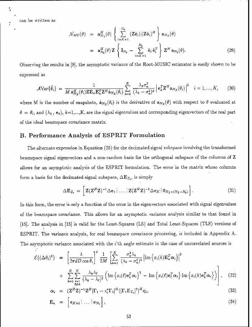
can be written as
MMU{9) = agz(0)i £ (Zei)(Zei)H \ aNx(6) { i=K+l )
I i=K+l I (29)
Observing the results in [9], the asymptotic variance of the Root-MUSIC estimator is easily shown to be
expressed as
AVax{0i} = 1 K
E h°l e^a^) » = !,...,#, (30) Me^z(9i)ZEnElZHkNz(ei) fx (A* - <Y
where M is the number of snapshots, ä.Nz(9i) is the derivative of ajvz(0) with respect to 9 evaluated at
9 = 6i, and (Ajt, e^), fc=l,...,K, are the signal eigenvalues and corresponding eigenvectors of the real part
of the ideal beamspace covariance matrix.
B. Performance Analysis of ESPRIT Formulation
The alternate expression in Equation (25) for the decimated signal subspace involving the transformed
beamspace signal eigenvectors and a non-random basis for the orthogonal subspace of the columns of Z
allows for an asymptotic analysis of the ESPRIT formulation. The error in the matrix whose columns
form a basis for the decimated signal subspace, AE^3, is simply
AEz3 Z(ZHZ)-1Aei; ... ■:Z(ZHZ)-1AeK-:0Nzx{Nz-Nb) (31)
In this form, the error is only a function of the error in the eigenvectors associated with signal eigenvalues
of the beamspace covariance. This allows for an asymptotic variance analysis similar to that found in
[15]. The analysis in [15] is valid for the Least-Squares (LS) and Total Least-Squares (TLS) versions of
ESPRIT. The variance analysis, for real beamspace covariance processing, is included in Appendix A.
The asymptotic variance associated with the i'th angle estimate in the case of uncorrelated sources is
£{(M)2} = A n2
2irdD cos 9{
1
2M
alh ■ K
.£ (A* - ^ Im{xt-(Ä;)E^at-}|
K K
+ EE AfcA kM
k=i t=i (A* - x() Im|x,(^)efat-} - Im[xt(£)efa,-j Im|x,-(A;)e^ai j
a, = (z^z)-1z^[r1-z;r2]^([r1EZ3]t^qj,
E„ *K+1 '■ ■ ■ ■ '■ eNb
, (32)
(33)
(34)
53

where f denotes pseudoinverse, x, and qt are the right and left eigenvectors associated with the i'th
(signal) eigenvalue of F = (r1EzJtr2Ez., and T1 and T2 are (Nz - 1) x Nz matrices that select the
first and last Nz - 1 rows of a matrix with Nz rows, respectively. Note that the expressions contained
in Appendix A may be applied to the more general case of correlated signals; only the result for the
uncorrelated signal scenario is summarized here due to its simpler form.
5. Computer Simulations
A number of computer simulations were conducted to assess the validity of the noise eigenvector
transformation/decimation techniques with regard to angle estimation. Specifically, the theoretical and
empirical standard deviations of the Root-MUSIC and TLS-ESPRIT estimators were compared in a
variety of source/processing scenarios. Also, the performance of the decimation approach was compared
to the stochastic Cramer-Rao Lower Bound [4, 16].
Common to all experiments, 600 trials were employed to derive the empirical results and only M = 16
snapshots were used to estimate the beamspace covariance matrix. Although this situation can hardly
be classified as asymptotic in the number of snapshots, the theoretical performance curves were observed
to compare rather closely to the derived experimental results.
The empirical standard deviations were computed in a variety of scenarios involving one or two
uncorrelated, closely-spaced signals. A MUSIC root or ESPRIT eigenvalue was classified as arising from
a signal if the root/eigenvalue location was within a 0.15 radial distance from the unit circle and lying in
an angular (decimated) region encompassing 85% of the unit circle, i.e., in the region [-0.857T, 0.857r]. All
trial runs, including those unresolved situations where only one signal was observed in the neighborhood
of a signal pair, were used to compute the location statistics.
Experiment 1: The simulation parameters of this experiment associated with the array, beamformer,
and decimation components are similar to those outlined in the example of Section 3, namely, an N =
128 element ULA with half-wavelength spacing was operated on with an Nb = 8 channel spatial DFT
beamformer. The spatial window was centered at broadside so that the spatial region -Nb/N < sin# <
Nb/N was probed. An L - 128 length Hamming-weighted low-pass filter was employed in the decimation
procedure configured for maximal decimation, i.e., D — N/Nb-
. Two half-Rayleigh spaced signals of equal power were embedded in additive complex Gaussian noise
so that a sensor level 10 dB SNR was achieved. To assess the effects of signal placement within the spatial
54

beamforming sector on the estimation variance, the center of the signal set was shifted from baseband
(sm6 = 0) to the edge of the window (sin9 = S/JV). The empirical standard deviation of the two Root-
MUSIC angle estimators, i.e., those formed using the matrix Z as well as the deconvolved version Z',
were computed. Note that the dimension of Z was 16 x 8 while Z' was formed by adding one additional
(remainder) row to the required (Nb + 1) x Nb matrix to form a 10 x 8 eigenvector transformation. The
results are shown, along with the theoretical prediction as obtained from Equation (30) and the stochastic
Cramer-Rao Lower bound [4, 16] in Figure 11.
Several comments relating to Figure 11 are in order. Although the number of snapshots is relatively
small, the theoretical performance curve is still a reasonably accurate representation of the empirically
derived result. The rippled nature of the variance curves is due to the limited number of beams that are
implemented in the approach. This characteristic is the result of a varying spatial power gain as similar
to that depicted in Figure 10. As noted in [7, 9], the degradation in performance near the band edge
suggests the need for sub-band overlap if one is interested in the detection and localization of all signals
across the visible spatial spectrum. The variance of the estimate at the extreme right edge is not shown
as the experimental and theoretical curves exhibit an exponential rise. In the central region of the band,
however, the eigenvector transformation-decimation technique is seen to produce an accurate estimate
in this Root-MUSIC formulation as evidenced by the closeness of the results to the Cramer-Rao Bound.
Note that the curves related to the theoretical variance associated with the use of Z and the Cramer-Rao
Bound overlap.
Experiment 2: Employing the same decimation transformations as in Experiment 1, the variance of
the Root-MUSIC estimators were observed for a varying SNR for two signals located at 10.6° and 11.5°,
as used in the motivational example of Figures 2 through 7. The empirical and theoretical standard
deviations were computed and are depicted in Figure 12.
Note that the theoretically derived curve, defined for the 16 x 8 transformation Z, closely tracks
the corresponding empirical counterpart at moderate to high SNR values. The deviation at the lower
SNR values is attributed to the signal-merging effects in the resolution threshold regime of operation as
noted in [9]. Although the stochastic Cramer-Rao Bound is based upon the statistics of the available
beamspace data and does not assume the presence of any sub-optimal techniques such as decimation,
the Root-MUSIC procedure incorporating decimation is readily observed to essentially offer the optimum
55

performance associated with un-biased estimators. Also, the similarity between the empirical variance
curves corresponding to the competing approaches (Z versus Z') suggests that the computational savings
associated with the smaller Root-MUSIC polynomial via the use of Z' is not obtained at the expense
of a higher estimation variance. In fact, simulations have shown that the estimation variance is usually
smaller for decimation architectures incorporating deconvolution. However, the imperfect deconvolution
usually results in an induced estimate bias as will be observed in Experiment 3.
Experiment 3: The main purpose of this experiment is to show that the filtering operation in the
decimator may not be warranted in certain situations. A single signal was positioned at 1° and the
bias performance was studied for the use of two beamforming architectures. In one situation, Nb = 6
DFT beams were formed from an N - 36 element ULA. The beamspace to element-space eigenvector
transformation was configured for maximal decimation, D = 6, with and without the use of a Parks-
McClellan equiripple FIR filter exhibiting approximately 50 dB attenuation in the stopband region. In the
other beamforming scenario, a practical application of Nb = 6 Taylor weighted beams [17], exhibiting a
50 dB sidelobe level, were spaced at the half-power points and employed in a similar scheme involving the
use/absence of additional filtering in the decimation operation. Note that the latter approach will produce
an angle estimate exhibiting a substandard resolution ability due to the attendant wider mainlobes relative
to DFT beams. However, this methodology is often required in practice to reduce the deleterious effects
of sidelobe clutter, i.e., the masking of signals within a given beam by a strong clutter signal in the
sidelobes of the beam. The beam spacing/aperture weighting associated with this case results in no
common spatial nulls amongst the beam set so that the application of past beamspace MUSIC [7] and
ESPRIT [8] formulations is precluded.
The empirically derived mean location estimates were determined for a varying SNR for various
schemes incorporating the two beamforming architectures and are plotted in Figure 13. Again, the
purpose ..here is not to compare the two beamforming approaches, rather, it is to observe the effects on
performance of the inclusion of a filter in the decimation operation. Also, the inclusion of a filter increases
the order of the polynomial to be rooted thereby increasing computation and creating extraneous roots.
With reference to Figure 13, note that the use of a filtering operation in the decimator with no additional
deconvolution stage results in essentially an unbiased estimator for both beamforming architectures.
As observed in the results, the Taylor-based sensor weighting provides sufficient attenuation so that a
56

negligible aliasing effect is incurred, i.e., the induced estimation bias is small. However, with the filter
incorporated into the decimation operation, the imperfect deconvolution stage imparts a small bias of
—0.02°. Thus the filtering operation is unnecessary as evidenced in the bias plot and a smaller standard
deviation should be realized on account of the smaller dimension of the resulting Root-MUSIC polynomial.
Essentially the opposite is observed for the case of unweighted spatial DFT beamforming. Here the
sidelobe levels are large so that aliasing effects are present as evidenced by the top curve indicating a
0.05° bias in the unfiltered mode of operation. With filtering as well as a deconvolution stage included
in the decimation operation, a smaller bias of 0.025° is realized. The need for filtering is evident from
observing the required dimension of the transformation Z'. Comparing the necessary row dimension
of the decimation transformation incorporating deconvolution, Z', for the unweighted DFT and Taylor
beamformers, the required sizes were 10 x 6 and 7x6, respectively. These required sizes were determined
according to the criteria discussed in Section 3.
Experiment 4: In this experiment, we test the validity of the TLS-ESPRIT formulation of the noise
eigenvector transformation-decimation procedure and verify the theoretical variance expression of Section
4i, Equation (32). The source/processing parameters are the same as those of Experiment 2.
The theoretical and empirical standard deviation were computed over a varying SNR and the results
are depicted in Figure 14. The results show that the performance predictor of Section 4 accurately
tracks the empirical results. Also, the variance associated with the decimation architecture incorporating
a filter deconvolution stage outperforms the "undeconvolved" counterpart. To verify the conjecture
that the quiescent locations of the extraneous eigenvalues are sufficiently away from the unit circle, the
ESPRIT eigenvalues were calculated in the absence of noise and plotted in Figure 15. Note that only the
eigenvalues, interior to the unit circle are plotted as the closest exterior eigenvalue is located at a radius
of 5.4 (associated with the Z transformation). Referring to Figure 15, in the absence of deconvolution,
two "signal" eigenvalues appear at the correct location and the eigenvalue closest to the unit circle of the
remaining is located at a radius of 0.62 and an angle very near IT. When deconvolution is incorporated,
the closest non-signal eigenvalue is located at T at a radius of 0.09. However, the signal eigenvalues
exhibit a small bias at the perceived (translated) angular locations of 10.587° and 11.465°.
6. Conclusions/Remarks
We have developed a novel approach to angle estimation in the beamspace domain. The approach
57

offers a computationally attractive and non-restrictive procedure relative to the type of beamformer
employed that is easily implemented in the MUSIC and ESPRIT algorithms. Theoretical expressions
for the estimate variance were obtained in an asymptotical analysis and confirmed in a variety of sim-
ulations. Although the technique was applied to the uniform linear array geometry, an extension to a
two-dimensional array to provide simultaneous azimuth/elevation angle estimates is evident and currently
under investigation.
Appendix: Asymptotic Variance of ESPRIT Formulation
Given that z,- is a (signal) unit-magnitude eigenvalue of the matrix
F = (r1E^)t(r2E2j = [(r1EzjH(r1Ezj]t(r1Ezj
ff(r2E^), (35)
with x,- and q, the corresponding right and left eigenvectors, Rao and Hari [15] showed that, to o(M *),
Azi = qf AFx,.
The error in F, AF, due to the finite sample estimation of the beamspace covariance matrix is
AF = {TiEzJiTtAEz.) - (TxEz.y(^AE^JF,
(36)
(37)
which is applicable to either the Least Squares (LS) or Total Least Squares (TLS) versions of ESPRIT.
Substituting the form of AEz3 in Equation (31) into Equation (36), one obtains
£{|A,;|2} = a?
(z*f£{ (A*)2} = of
J2Exz(k)x*(Z)£{AekAeJ} k=i t=i
J2J2 *,-(*) *,•(*)£{AejfeAeH k=i t=i
aci
«.->
(38)
(39)
where a and the signal eigenvector error statistics were stated in Equations (33) and (26), respectively.
Following [15], these quantities are then substituted into
£{ (A0;)2} = A
2irdD cos 0{
S{\Az^}-Re{(z*rS{(Azxy}} (40)
to yield the desired theoretical asymptotic estimation variance.
In the case of uncorrelated signals, the asymptotic error in the signal subspace eigenvectors become
_f . . T, Ski Ä Ai-A™ T (I — Si??) AtA £{ Aek Aej } = — }_,
2M t, (h ~ Am)2
m^k
e"iem
■kM T eeek. 2M (Afc - \e)2
(41)
58

After substituting and simplifying (the algebraic details are omitted here due to space limitations), the
asymptotic variance of the ESPRIT angle estimate for uncorrelated sources reduces to
£{(A*02} = A
T2
2xdD cos 9;
1 K ~2
£ 7I^IIm{^)E^} 2M |j=i (Afc - a\
K K AtA/ + £En lJIm{^eH -Im{x1-(/)e?,a,-}lm{xt-(*)efaI-}
fc=i i=i iAfc A^i v , (42)
where En is an Nb x (JV& - K) matrix composed of the noise eigenvectors associated with the ideal
beamspace covariance.
References [1] G. Bienvenu and L. Kopp, "Decreasing High Resolution Method Sensitivity by Conventional Beamforming
Preprocessing," in Proc. of 1984 IEEE Int'l Conf. on Acoust, Speech, and Signal Process., pp. 33.2.1-33.2.4,
April 1984.
[2] C. L. Byrne and A. K. Steele, "Sector-Focussed Stability for High-Resolution Array Processing," in Proc. of
1987 IEEE Int'l Conf. on Acoust, Speech, and Signal Process., pp. 54.11.1-54.11.4, April 1987.
[3] H. Lee and M. Wengrovitz, "Resolution Threshold of Beamspace MUSIC for Two Closely-Spaced Emitters,"
IEEE Trans. Acoust, Speech, Signal Process., vol. ASSP-38, no. 9, pp. 1545-1559, Sept. 1990.
[4] R. O. Schmidt, "A Signal Subspace Approach to Multiple Emitter Location and Spectral Estimation," Ph.D.
dissertation, Stanford University, Stanford, CA, 1981
[5] A. J. Barabell, "Improving the Resolution Performance of Eigenstructure-Based Direction Finding Algo-
rithms," in Proc. of 1983 IEEE Int'l Conf. on Acoust, Speech, and Signal Process., pp. 336-339, May 1983.
[6] B. D. Rao and K. V. S. Hari, "Performance Analysis of Root-MUSIC," IEEE Trans. Acoust, Speech, Signal
Process., vol. ASSP-37, no. 12, pp. 1939-1949, December 1989.
[7] M. D. Zoltowski, G. M. Kautz, and S. D. Silverstein, "Beamspace Root-MUSIC," IEEE Trans, on Signal
Processing, vol. 41, no. 1, pp. 344-364, Jan 1993.
[8] G. Xu, S. D. Silverstein, R. Roy, and T. Kailath, "Parallel implementation and Performance of Beamspace
ESPRIT;" in Proc. of 1984 IEEE Int'l Conf. on Acoust, Speech, and Signal Process., pp. 1497-1500, April
1991.
[9] G. M. Kautz and M. D. Zoltowski, "Performance Analysis of MUSIC Employing Conjugate Symmetric
Beamformers," Submitted to IEEE Trans, on Signal Processing, May 1993.
[10] A. Paulraj, R. Roy, and T. Kailath, "Estimation of Signal Parameters via Rotational Invariance Techniques
- ESPRIT," in Proc. 19-th Asilomar Conf. on Signals, Systems and Computers, pp. 83-89, Nov. 1985.
[11] M. Wax and T. Kailath, "Detection of Signals by Information Theoretic Criteria," IEEE Trans. Acoust,
Speech, Signal Process., vol. ASSP-33, pp. 387-392, April 1985.
[12] J. G. Proakis and D. G. Manolakis, Introduction to Digital Signal Processing, Macmillan, 1988.
[13] T. W. Anderson, An Introduction to Multivamate Statistical Analysis, Second ed., John Wiley k Sons, 1984.
59

[14] M. Kaveh and A. J. Barabell, "The Statistical Performance of the MUSIC and the Minimum-Norm Algo-
rithms in Resolving Plane Waves in Noise," IEEE Trans. Acoust., Speech, Signal Process., vol. ASSP-34, ncr.
2, pp. 331-341, April 1986.
[15] B. D. Rao and K. V. S. Hari, "Performance Analysis of ESPRIT and TAM in Determining the Direction
of Arrival Plane Waves in Noise," IEEE Trans. Acoust, Speech, Signal Process., vol. ASSP-37, no. 12, pp.
1990-1995, December 1989.
[16] P. Stoica and A. Nehorai, "Performance Study of Conditional and Unconditional Direction-of-Arrival Es-
timation," IEEE Trans. Acoust, Speech, Signal Process., vol. ASSP-38, no. 10, pp. 1783-1795, October
1990.
[17] T. T. Taylor, "Design of Line-Source Antennas for Narrow Beamwidth and Low Side Lobes," IRE Trans-
actions on Antennas and Propagation, pp. 16-28, January 1955.
60

Figure 1: Condition Number vs. Number of Beams
Sine of Bearing Angle
Figure 2: Spectrum of a Transformed Noise Eigenvector
Sin 10.6* Sin 11.5
0.15 0.2 Sine of Bearing Angle
Figure 3: Angular Responses of Eight Successive DFT Beamforming Vectors
61

*—>j Hamming Weighted LPF
-80 -0.1 -0.1 -0.05 0 0.05
Sine of Bearing Angle 0.15
Fiffure 4: Null Soectrum After Modulation and Filter Resnonse
-0.15 -0.1 -0.05 0 0.05 Sine of Bearing Angle
0.15
Figure 5: Null Snectrum After fTa,mminff Window Rased Baxidnass Filtering
-10
m-20 ■o
-40
-50-
-60
16(Sln(10.6") - 25/N)
16(Sin(11.5') - 25/N)
-0.8 -0.6 -0.4 -0.2 0 0.2 0.4 Sine of Bearing Angle
0.6 0.8
Figure 6: Null Spectrum After Decimation By Factor of 128/8 = 16
62
J7C16 (sin 11.5° - 25/N)
Signal Root Locations
Z Z
Mag. Angle
Mag. Angle
1.0000 10.6000"
1.0000 11.5000"
0.9907 10.5934'
0.9899 11.497/
jit16( Sin 10.6" - 25/N)
o' - Roots Associated with 16x8 Z 'x' - Roots Associated with 10 x 8 71
Figure 7: Roots Using Modulated-Filtered-Decimated Noise Eigenvectors (1/4)(11/N): Filter Stopband Edge (1/4)(8/N) : Po«t-Decimation Foldover Frequent (1/4)(5/N) : Filler Passband Edge
W-OT -0© • ÜXi) (-X0) (-Xs) Direction Sine
Figure 8: Spatial Responses of Equi-Ripple Filter and Interpolated Beam Set
Figure 9: Decimated Filter/Beamformer Spectra
63

Figure 10: Effects of Filter Deconvolution on White Noise MUSIC Spectrum
x10
Stochastic CRB & Theoretical Std Dev - Z: 16x8
Center of Subband : 0 Right Edge of Subband : 8 / N
1/N 5/N 6/N 2/N 3/N 4/N Signal Set Position Within Subband
Figure 11: Experiment 1: Left Signal Standard Deviation vs. Signal Set Location Within Subband
0.12-
0.1
0.08-
0.06
0.04-
0.02
-15 -10
-e— Empirical Std Dev - Z -«— Empirical Std Dev - Z ' Theoretical Std Dev - Z
Stochastic CRB
16x8 10x8 16x8
10 SNR (dB)
Figure 12: Experiment 2: Left Signal Standard Deviation vs. Source SNR
64

I.Ub
1.05
1.04
2.1-02 c o 1 1.01 o a.
DFTBeamforming —x— With Filtering, No Deconvolution - Z : 12x6 --*-- With Filtering and Deconvolution - Z : 10x6 --*•- No Filtering - Z : 6x6
Taylor Weighted Beamforming, 50 dB Sidelobe Level —e— With Filtering. No Deconvolution - Z : 11 x 6 "O" With Filtering and Deconvolution - Z : 7x6 . —o— No Filtering - Z : 6x6
50 0 5 10 15 20 25 30 35 40 45 SNR (dB)
Fieure 13: Experiment 3: Location Bias vs. Source SNR
Empirical Std Dev - Z : 16 x 8 Empirical Std Dev - Z' : 10x8 Theoretical Std Dev - Z : 16 x 8
15 20 25 SNR (dB)
Figure 14: Experiment 4: Left Signal Standard Deviation vs. Source SNR j*16(sin 11.5 -25/N)
js 16 (sin 10.6 -25/N)
'o' - Eigenvalues Associated with 16 x 8 Z 'x' - Eigenvalues Associated with 10x8 Z'
Figure 15: Experiment 4: Quiescent Locations of the ESPRIT Eigenvalues
65

3 Multidimensional Mult irate DO A Estimation in Beamspact
TThe ID multirate approach developed in the previous section is extended to the more general
case of 2D angle estimation with a uniform rectangular array (URA) of sensors. Multidimen-
sional multirate processing is employed to ultimately yield a small order polynomial in two
variables. Again, due to the linearity of the 2D filtering and 2D decimation operations, the
actual algorithm merely premultiplies each beam space noise eigenvector by a precomputed
transformation matrix. To avoid the spectral search, despite the fact that the fundamental
theorem of algebra does not hold in 2D, we propose taking the orthogonal complement of the
resulting transformed noise eigenvectors and applying a novel version of ESPRIT facilitating
closed-form 2D angle estimation. Simulations demonstrating the efficacy of the approach are
presented along with theoretical performance analysis.
3.1 Introduction
3.2 Array Geometry
3.3 Beamforming
3.4 Eigenanalysis
3.5 TLS-ESPRIT
3.6 Bandlimiting the Response
3.7 Further Reductions in Complexity
3.8 Algorithm Summary
3.9 Performance Analysis
3.10 Computer Simulations
3.11 Conclusions
3.12 , Appendix: Characterizing the Asymptotic Error
3.13 References
3.14 Figures
66

1 Introduction
The eigenstructure based Spectral Music Algorithm of Schmidt [1] has become the standard for
estimating the Direction of Arrival (DOA) of narrowband plane waves impinging upon a sensor array.
Unfortunately the required spectral search is a burdensome task for ID arrays and computationally
pohibitive for 2D arrays. Two well developed methods for reducing this complexity are beamforming
techniques [5] and Esprit [4] [6]. Beam space methods reduce the complexity from the number of
array sensor elements to the number of beams used to probe a given sector or subband. Furthermore,
in the case of a uniform linear array (ULA), beam space techniques yield an implementation (Beam
space Root-Music) that allows one to solve for the arrival angles by rooting a small order polynomial.
Alternatively, Esprit places a minor restriction on the array geometery and then determines the
arrival angles from the eigenvalues of a rotation matrix.
For maximum computational savings, a beam space formulation of Esprit has been de-
sired, but previous attempts have resulted in restrictive requirements on the beamformer. Recently
Zoltowski and Kautz [2] [3] developed a beam space formulation of Esprit for ID ULA's that works
with any type of front end beamformer. The new approach is based on the observation that beam
space noise eigenvectors may be transformed to vectors in the element space noise subspace, which
are bandpass and exhibit nulls at the location of inband sources. This facilitates multirate pro-
cessing involving modulation to baseband, filtering, and decimation. From the linearity of these
operations, the actual algorithm need only need premultiply each beam space noise eigenvector by
a simple transformation matrix that is computed apriori. The resulting "telescoped" noise eigen-
vectors yield a small dimensional element space noise subspace which is used to obtain a small
dimensional signal subspace where the Esprit algorthm can be applied.
With the combined advantages of beam space processing and Esprit, multidimensional DOA
67

estimation becomes computationally feasible. This paper extends the beam space approach to the
more general case of 2D angle estimation with a uniform rectangular array (URA). Multidimensional
multirate processing is employed to ultimately yield a small dimensional signal subspace. Again,
due to the linearity of the 2D filtering and 2D decimation operations, a simple transformation
matrix is computed apriori so that the actual algorithm need only premultiply each beam space
noise eigenvector by this matrix.
Directly applying the ID Esprit algorithm to the ÜRA would require two separate appli-
cations of Esprit, one for each direction. This estimates the two direction angles independently
and leads to the problem of how they can be paired. Alternatively, a novel version of Esprit is
developed that estimates the two directions from a singal eigenvalue eigenvector pair. Hence they
are automatically coupled.
The paper is organized as follows. The array geometry and data model are described in
Section 2 and the beamforming process is briefly reviewed in Section 3. The eigen characteristics
of the system are developed in Section 4 and multirate processing techniques are applied to the
eigenvectors in Section 5. The applicability of the Esprit algorithm is verified in Section 6. Section
7 addresses the issue of bandlimiting the beamformer response and Section 8 describes some further
reductions in computational complexity. Finally in Section 9 the proposed 2D Multirate Esprit
Algorithm is presented. A theoretical performance analysis is presented in Section 10 and computer
simulations are examined in Section 11. A few concluding remarks are included as Section 12.
The notation used in this paper indicates vectors by lower case bold letters and matrices by upper
case bold letters. The Hermitian, conjugate transpose, will be denoted by a superscript H and the
conjugate will be denoted by a superscript *.
68

2 Array Geometry
The array geometry considered in this paper is a rectangular array comprised of M elements in the
x direction and N elements in the y direction uniformly spaced by Ax = Ay = A„/2 (see Figure 1).
To specify the source directions, define x,y, and z to be unit vectors along the coordinate axes and
O.N-1
M-1.N-1
Figure 1: Array Geometry
ax, cty, az to be the angles between a vector and the respective coordinate axis. If pi is a unit vector
normal to a plane wave emanating from the ith source, then pi = cos^Jx + cos(ayi)y + cos(aZi)z.
These direction cosines are converted to azimuth, 9, and elevation, <j>, angles as cos aXi = cos 9i sin <j>i
and cosaVi. = sin 0,- sin fc (see Figure 2).
Define an arbitrary reference point to be r = (xr,yr,0) = (krAx,lTAy,0) and let fk,i be a
vector from r to the k, Ith sensor. Then rk,i = {k - kr) Axx + (l - lr) &yy. Assuming that the signals
are narrowband with common center frequency u>0, the response of the k, Ith sensor to the iih source
at time t can be written as
jf«' (t) = s-(i)e?Uo^?k'1*^ = Si.(i)eJ^Kfc-fc'-)AiCOSÖ>sill^+('-i'-)Avsinöisin*il. n\
Because sin(^) = sin(7r — <f>), a signal with direction angles (9, <f>) and a signal with direction angles
(0, -K — <f>) will have the same array response. This produces a directional ambiguity that is inherent
to uniform rectangular arrays (URA). To see how this ambiguity manifests itself notice that if <f>
69
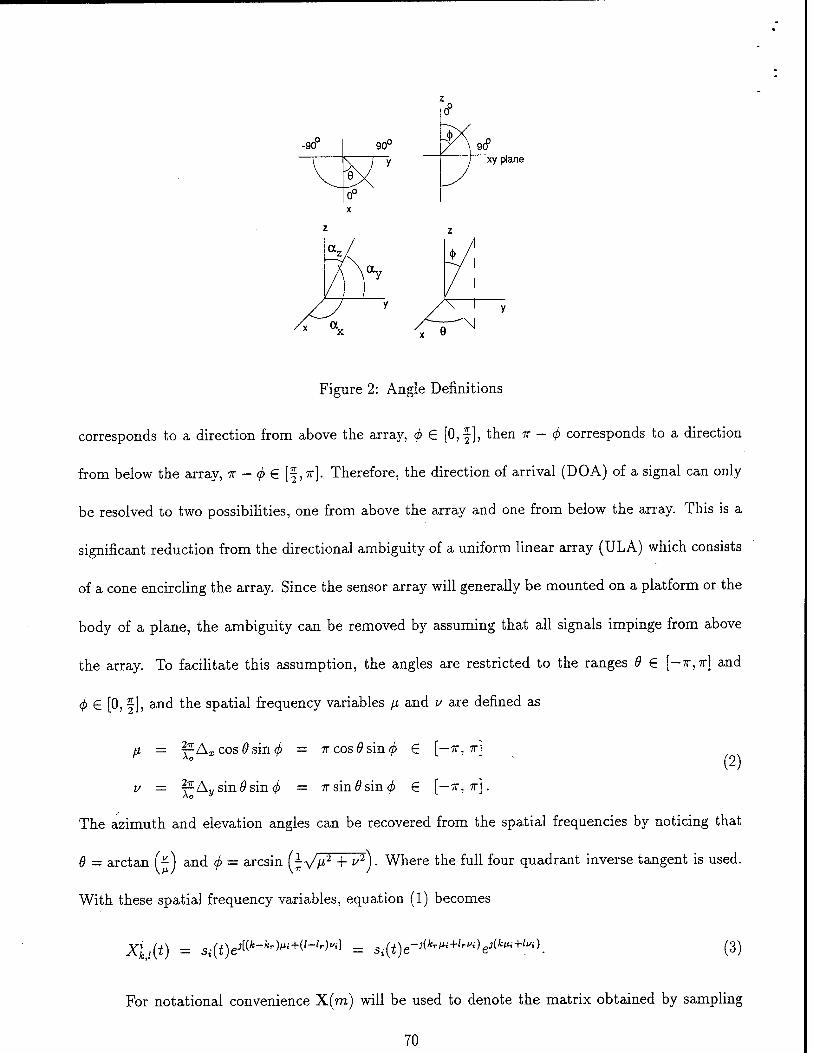
-90" 90u
xy plane
Figure 2: Angle Definitions
corresponds to a direction from above the array, <j> € [0,§], then ir — <f> corresponds to a direction
from below the array, ir - <j> € [f, ir].. Therefore, the direction of arrival (DOA) of a signal can only
be resolved to two possibilities, one from above the array and one from below the array. This is a
significant reduction from the directional ambiguity of a uniform linear array (ULA) which consists
of a cone encircling the array. Since the sensor array will generally be mounted on a platform or the
body of a plane, the ambiguity can be removed by assuming that all signals impinge from above
the array. To facilitate this assumption, the angles are restricted to the ranges 9 € [-ir,K] and
4> € [0, f], and the spatial frequency variables JJL and v are defined as
P T1
Ax cos 9 sin 6 = 7rcos#sin<^ € [—ir, r] (2)
v = ^Aysin^sin^ = TT sin 9 sin <f> € [—x, 7r].
The azimuth and elevation angles can be recovered from the spatial frequencies by noticing that
9 = arctan (-) and <j> = arcsin (^vV2 + 1/2)- Where the full four quadrant inverse tangent is used.
With these spatial frequency variables, equation (1) becomes
Xljit) = Si(t)e Jp-Mw+e-'r)"'] *(*)■
,-]{krlti+lrVi) „jikiti+ll/i) (3)
For notational convenience X(m) will be used to denote the matrix obtained by sampling
70

the array at time tm and X'(m) will denote the array response due to the ith signal at time tr
where m is the snapshot index. Using equation (3) X*(m) is given by
X'(m) = Si(tm)e-^i+l^
e3Vi
oJßi e3(ßi+V<)
„j(N-l)vi
Dj[w+(JV-l)".-i
ej(M-l)ßi ej[(M-l)M,+^] ... ej[(M-l)ßi+(N-l)i>i]
(4)
The term e""^fcrW+'r'/^ is an arbitrary phase common to all sensors, that is determined by the
reference point. Choosing the origin as reference point [kr = lr = 0), yields an element space
array manifold, i.e. the array response viewed as a function of fi and f, of the form A.MN{IJ-I V) =
aM(/i)a^(y). Where ajvf(/z) and &N{V) are defined to be the one dimensional uniform linear array
(ULA) manifold vectors.
aM(/x) = [l.e»*, ...,e^-^
The mth snapshot of the array due to all d impinging signals can now be written as
d-l
X(m) = Yl Si(m)AMN{fii, v%) + N(m) i=0
(5)
(6)
Where Nk,i(m) is measurement noise associated with the mth snapshot of the k, Ith sensor, and
N(m) is the M x N noise matrix.
It is useful to view the array response as an MN x 1 vector as well as an M x N matrix.
To facilitate conversions between these forms, consider the operator vec that maps an M x N
matrix to an MN x 1 vector by concatenating its columns, and the inverse operator, mat, that
maps an MN x 1 vector to an M x N matrix by using M consecutive elements of the vector for
each column of the resulting matrix. If Q is an arbitrary matrix with columns denoted q^, then
r i T uec(Q) = qf, q^, ..., qjj . If q is an arbitrary vector and q(k : /) denotes its kth through Ith
71

Table 1: Properties
PI: V]V ® x,w = = uec(xitfV^)
P2: XMVJ = = mat(vN ® XM)
P3: uec(ADB) = = (Br ® A)uec(D
P4: (A®B)T = = (AT®BT)
P5 : (A <g> B)(C <g> D) = = (AC)®(BD)
elements, then mat(q) = [q(0 : M - 1) | ... | q(MN - M : MN - 1) ]. The following example
illustrates these operators
/
vec
V
1 3 5
2 4 6
= [1,2,3,4,5,6]'
\J
mat ([I, 2, 3, 4, 5, 6, f) = 1 3 5
2 4 6
Some important properties of vec, mat, and the Kronecker product, <g>, are listed in Table 1 (see
also [9]). Most notably, Property 1 allows the array response to be written in vector form as
d-l
x(m) = uec(X(m)) = £} st-(m)aMivO;, Vi) + n(m) = >Ws(m) + n(m). (7) t=0
Where s(m) is the vector of signal amplitudes, aAfjv(^, ^) is the array manifold in vector form, and
the columns of AMN are the signal steering vectors, i.e., the array manifold evaluated at the spatial
frequencies corresponding to the signal directions.
s(m) = [s0(m), ..., Sd-i{m)]
SLMN(fi, v) = vec(AMN(lJ; v)) = a.N(v) ® ajw(//)
AMN = [a-MNincvo) I ••• I 3^(^-1,^-1)] •
(8)
(9)
(10)
The element space signal subspace is defined to be the column-space of AMN, Se = 'R {AMN}, and
72

the element space noise subspace is denned to be the orthogonal complement of <Se. Since AMN is
MN x d, Se is a d dimensional subspace of MN dimensional space.
3 Beamforming
Now consider the class of separable two dimensional beamformers. Let WM be an arbitrary M x Mb
beamforming matrix (with Mb < M) for the fi spatial frequency. The kth row of W^ denoted w^k
forms a beam for a specific frequency in the desired range. W„ is defined in a similar fashion for
the v spatial frequency. Using w^, in conjunction with w*( a beam is generated for a specific 2D
frequency in the subband of interest. Therefore, the Mb x Nb beam space snapshot matrix is formed
as Y(m) = W^X(m)W*, and the MbNb x 1 beam space snapshot vector is given by y = uec(Y).
Using Property 3 from Table 1 these can be written as
Y(m) = WfX(m)W; = £ Si(m)W« AMN{m, u{)W; + Wf N(m)W; »=o (11)
y(m) = vec(Y{m)) = [Wf <g> Wjj AMNs(m) + [Wf ® Wf J n(m).
Therefore, the beam space array manifold is described by
BO*,*) = WfAMiv(M,i/)W; (12)
b(p,v) = [wf0Wj]a^,y) = [Wf aiV(Z/)] ® [wf aM(^)] (13)
B = [b(ll0,V0) | ... | M/irf.!,^-!)]. (14)
Finally the beam space signal subspace, 5&, is defined to be the d dimensional subspace of MbNb
dimensional space that is spanned by the columns of S, and the MbNb — d dimensional beam space
noise subspace is defined to be the orthogonal complement of <Sf,.
At this time it should be noted that the beamformer need not be separable. This assumption
was made because the separable nature of the array structure leads directly to separable beamform-
73

ers. In vector form, nonseparable beamformers modify equation (11) by replacing W„ <g) Wß with
an arbitrary MN x MbNb matrix W6.
4 Eigenanalysis
Using equation (7) and assuming that the measurement noise is zero mean, uncorrelated between
sensors, and has equal power cr2, the MN x MN element space autocorrelation matrix is
R* = E {x(n)x(n)F} = ARSAH + a2I. (15)
It has been observed [4] that the eigenvectors of R^ corresponding to the d largest eigenvalues form
a basis for Se and the remaining eigenvectors of R^ form a basis for S^. Under the assumption of
orthonormal beams, the MbNb x MbNb beam space autocorrelation matrix has the form
Ry W? ® w H ARSAH [W„ ® W„] + <72I = BRsB
H + a2I. (16)
The eigenvectors of Rv are also divided into two sets, the "beam space signal eigenvectors" {f; :
i = 0, ...d- 1} that form a basis for Sb, and the "beam space noise eigenvectors" {f, : j =
d,... MbNb — 1} that form a basis for SbL.
If the number of signals, d, is unknown it can be estimated at this time using the AIC or
MDL methods of [10]. Therefore, in all further developments, it will be assumed that d is known.
Since the "beam space noise eigenvectors" lie in Sbx, they are orthogonal to the beam space
signal steering vectors, i.e., bH(m, i/,-)fj = 0 for all i - 0,... d - 1 and j = d,... MbNb - 1. Recalling
equation (13) yields the following important result.
H 0 = b*{(ja, ui)fj = [(Wf (8) Wf) ajwK/i,-, fij\ f, = *MN(^ ^ [(w<- ® WM) f.] (17)
This shows that the matrix W„ (8) WA maps the beam space noise eigenvectors, f,-, to the element
space noise subspace, S^ [3]. However, there are only MbNb - d beam space noise eigenvectors, so
74

this mapping does not yield a complete basis for <Sex.
The general Music algorithm exploits the orthogonality between the beam space noise eigen-
vectors and the signal steering vectors, by forming the beam space Music null spectrum Sß{ft, v).
MbNb-l MbNb-\ 2
SB(W) = E h'Wftl = E |a£(/x)WMF,Wja^)| (18) j=d j=d
Where Fj is defined to be the beam space noise eigenvector written in matrix form (Fj = mat(fj)).
Signal directions are then estimated from values of p and v corresponding to nulls in SB(P, V). TWO
well established problems with this method [4] are that the array manifold must be known and
stored, and the search over a two dimensional space can be computationally prohibitive.
5 Multirate Processing of Beam Space Noise Eigenvectors
In an effort to circumvent these problems, notice that the crux of the beam space Music null
spectrum are the M x N telescoped [3] beam space noise eigenvectors Gj = W^FjWj (j =
d,...,MbNb — 1) and GJ(IM,V) = aj^(//)Gja^(z/) is the two dimensional Discrete Space Fourier
Transform of Gj. Letting Fj(k, I) denote the k, Ith element of Fj yields
Mfc-1 Nb-\
G,(/i,u) = a^W^Wja^) = E E *)(*>0 [aS(^)w«<*NH] ■ (19) Jk=0 /=0
Since wMfc and w„( form a beam in the desired subband, aj^(//)"wMfcw^a^(i/) is a bandpass function
of fi and v for all k, I. Consequently Gj(n,v) is a bandpass function of \i and v. Without loss
of generality, assume that the M&iVj, beams encompass the spatial subband defined by — ir f-^J <
P < K \~M) an(l ~ir (iv ) — v — T \~N)
an<^ nave sufficiently low out of band sidelobes. Then the
beamformer response is negligible outside this subband, i.e., Gj(n, v) ~ 0 for ^-ir < \fi\ < r and
J£TT < | v | < 7T, so Gj can be decimated by dx = j^- and dy = jj- without incurring a significant
amount of aliasing. (Note: Gj can always be modulated to baseband and filtered to make this
assumption valid. See section 7).
75

The decimation process can be modeled mathematically as premultiplying Gj by Dx and
postmultiplying by D^ where Dx and Dy are the Mb x M and Nb x N decimation matrices. For
example if Mb = 2 and M = 6
Dr = 10 0 0 0 0
0 0 0 10 0
Therefore the decimated telescoped beam space noise eigenvectors are given by
H, = D.Gj-Dj1 = (D,W„) F,-(D,W„ (Mb x Nb) (20)
h,- = veciHj) = [(DyWv)®(DxWß)]fj (MbNb x 1)
for j = d,...,M6iVfe-l.
It is important to note that since decimation is a linear operation it can be performed apriori
on the telescoping matrices. Furthermore, fractional sampling rate alterations can be effected by
replacing Dx with DxFxlx, where I* represents an interpolation matrix and F* represents filtering.
The space spanned by the decimated telescoped beam space noise eigenvectors, hj, will be referred
to as as <Sj".
Since H, is Mb x Nb, it has a 2D-DSFT given by ^(/x, u) = a^(/*)H,a^(i/) where aMb(/0
and 3iNb{v) are defined analogously to equation (5). By standard Multirate analysis [13] the rela-
tionship between Hj(fi,v) and Gj(n,v) is
1 d*z* d^ (u-2-xp v - 27r<?\ Hj(fi,v) EEcf «s"y p=0 g=0 dr
(21)
Since the beamformer response is negligible outside the subband, Hj(p, v) « j^rGj (£, ^J for all
—7T < /i, i/ < 7T and therefore
Hj(dxfMi,dyi/i) 1 G,-0i,-,i/0 = ^Vb^^^Ofi = 0.
dx^y 0>xOiy
(22)
This shows that the decimation process preserves the in band source nulls and increases their
separation by a factor of dx and dy. Hence, the beam space Music null spectrum (18) could be
76
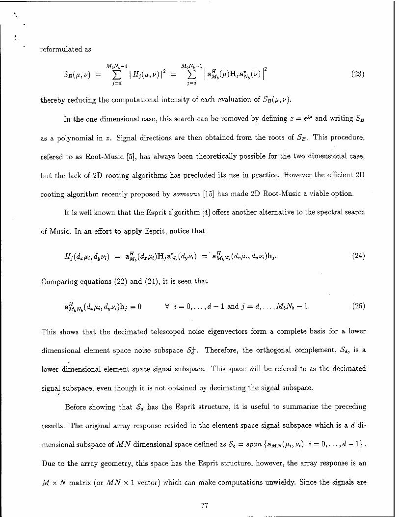
reformulated as
MbNb-l MbNh-\
SBM = £ |ffi(M,")i2 = E |a£»Hia^(i/)| (23)
thereby reducing the computational intensity of each evaluation of 5B(M5 Z/)-
In the one dimensional case, this search can be removed by defining z = tm and writing SB
as a polynomial in z. Signal directions are then obtained from the roots of SB- This procedure,
refered to as Root-Music [5], has always been theoretically possible for the two dimensional case,
but the lack of 2D rooting algorithms has precluded its use in practice. However the efficient 2D
rooting algorithm recently proposed by someone [15] has made 2D Root-Music a viable option.
It is well known that the Esprit algorithm [4] offers another alternative to the spectral search
of Music. In an effort to apply Esprit, notice that
Hj(dxfii,dyUi) = &Mb{dxßi)'H.j&*Nb{dyVi) = a.%lbNb(dxni,dyvi)h.j. (24)
Comparing equations (22) and (24), it is seen that
^MbNb(d^^ dvvi)hi = ° V i = 0,..., d - 1 and j = J,..., MbNb - 1. (25)
This shows that the decimated telescoped noise eigenvectors form a complete basis for a lower
dimensional element space noise subspace <Sj\ Therefore, the orthogonal complement, Sd, is a
lower dimensional element space signal subspace. This space will be refered to as the decimated
signal subspace, even though it is not obtained by decimating the signal subspace.
Before showing that Sd has the Esprit structure, it is useful to summarize the preceding
results. The original array response resided in the element space signal subspace which is ad di-
mensional subspace of MN dimensional space defined as Se = span {a-MN^i, ^t) i = 0,..., d — 1} .
Due to the array geometry, this space has the Esprit structure, however, the array response is an
M x N matrix (or MN x 1 vector) which can make computations unwieldy. Since the signals are
77

known to be in a certain subband, a beamformer is applied that imposes a bandpass characteristic
on the array response, which can then be decimated without incurring aliasing. This reduces the
signal space to a d dimensional subspace of an MbNb dimensional space and yields matrices that
are only i¥& x N},. However in the beamforming process the Esprit structure is lost. This structure
can be restored by decimating and telescoping in the noise subspace, then converting back to the
orthogonal complement (see Figure 3). It is important to notice that the element space signal eigen-
^i,dyvi)
Figure 3: Subspace Relations
vectors which are obtained directly from the element space correlation matrix cannot be decimated
because they are not bandlimited. The beam space signal eigenvectors are not telescoped because
this does not yield vectors in the element space signal subspace. Hence they will not have not have
the Esprit structure. However telescoping and decimating the beam space noise eigenvectors yields
a space that is the orthogonal complement to a smaller dimensional element space signal space.
6 TLS-Esprit
It remains to show that Sd does indeed have the Esprit structure. The Esprit algorithm requires
an array formed by "sensor doublets" that are separated by a constant displacment vector [4]. This
78

can be accomplished by viewing the Mb x Nb rectangular array as two overlapping Mb x (Nb - 1)
subarrays with Mb(Nb — 2) common elements (see Figure 4a). The resulting subarray manifolds are
AR
r. --.-,. "i
i
AR
~i_~
(a) (b)
Figure 4: Array Partitioning
given by the first and last Nb — 1 columns of AMbNb{(J; v). Mathematically this can be modeled as
AA^JV^/Z,:/)!?! and AMbNb{ß, v)T2, where Tx and T2 are the first and last Nb - 1 columns of the
Nb x Nb identity matrix. For example, if Nb = 3, I\ and T2 are as follows:
r1 =
1 0
0 1
0 0
r2 =
0 0
1 0
0 1
The vector form of the subarray manifolds are obtained by premultiplying by the Mb x Mb identity
matrix and applying Property 3 of Table 1. It is easily verified that the two subarray manifolds, in
matrix and vector form, are related as follows:
(26) AMbNb(v, v)T2 = e?v AMbNb{fi, v)Tx
■" 32&MbNb(v>,v) = eJ"JiaMöjV5(/^)-
Where Ji = Tj®lMb and J2 = rj®IA/6. Therefore, the signal steering vectors for the subarrays are
related by 223LMbNb(dxVi, dyfi) = e3dyVi3ia.MbNh{dxiii, dyUi) for all i = 0,..., d - 1 and consequently
^2^-MbNb = J\AMbNb~£v (27)
79

where Tu = diag^»"0,..., e3d,jl,d-1}. This can be generalized to an arbitrary basis, K = ^4M6JV6T,
for Sd by postmultiplying both sides by any d x d nonsingular matrix T and premultiplying T by
Id = TT-1.
hAMbNbT = Jx^^TT-^T (28)
J2K = JiK*. (29)
Where * = T_1TT. This relationship is the basis for the TLS-Esprit algorithm [4]. It shows that
the v spatial frequencies can be estimated from the eigenvalues of the matrix that rotates the first
Mb(Nb - 1) rows of K into the last Mb(Nb - 1) rows of K.
Alternatively, the array can be viewed as two overlapping (Mb - 1) x Nb subarrays with
(Mb - 2)Nb common elements (see Figure 4b). This yields subarray manifolds that are the first and
last Mb-l rows of AMbNb(p, v) an<i modelled by T3AMbNb(fJ; v) and T4AMbNb(n, v). In this case,
T3 and T4 are the first and last Mb - 1 rows of the Mb x Mb identity matrix and
J4-4M6;V6 = 2zAMbNb"£ß (30)
where Y„ = diag{e^M,..., e^*"--»}, J3 = IJV6 ® T3, and J4 = Ijv6 ® T4.
Therefore, if the array is divided in a row-wise fashion, the JJL spatial frequencies can be
estimated from the eigenvalues of the matrix that rotates J3K into J4K. However, if the p. and
v frequencies are obtained independently by applying Esprit to K in a row-wise and column-wise
fashion, there is no apparent way to pair the frequency components corresponding to a specific
signal.
In an effort to circumvent this problem, notice that as long as no two signals have the same \i
and v frequencies, JXK and J2K are rank d. Therefore, * always exists and has a full set of eigen-
values and linearly independent eigenvectors. Consider performing an eigenvalue decomposition of
* to obtain *=ETE-X.
80

If Vi is a distinct frequency, then 7,- is a distinct eigenvalue of \£ and the associated right
eigenvector is unique (to within a scalar multiple). Therefore, et- is the ith column of T_1 and the
ith signal steering vector can be obtained as
Ke, = ÄMbNbTei = aiaMbNb(dxHi,dyVi). (31)
To estimate the \i frequency from the steering vector recall equation (30), let 1^ = Ke„ and notice
that (J3l,)ff (J4I.O = {Mb - l)Nbe>d*ßi. Therefore, define p{ as
A Pi = L— (J310" (J4IO = ith^Tßi* = ifpi.- = «*". (32)
(Mb-l)Nbyö,J v"v * (Mb-l)Nb
So Hi is obtained as \i{ = -j-arg (pi). An important observation here is that the p, and v frequencies
for a signal are estimated from an eigenvalue-eigenvector pair and as such are automatically coupled.
Now consider the case where V{ is not a distinct frequency, say z/0 = ... = vv-\, then \£
has an eigenvalue of multiplicity p and the associated eigenvectors {e0,..., eP-i}, are not unique.
Therefore, et- is not the ith column of T-1 and
Ke, = [sLMbNb(dx{J,o, dyv0) \...\ a^^^/ip-i, dy^p-i)] Ci V i = 0,... p - 1 (33)
for some arbitrary p x 1 vector C;. In this case the eigenvector will not directly yield the [i frequency.
However, the matrix
K [e0 I • • • I ep_x] = [a.MbNb{dx/J.o, dyv0) \...\ aMbNb(dxßP-i, ^p-i)] C (34)
has the Esprit structure. Therefore, applying Esprit in a row-wise fashion will yield the \i frequen-
cies. Coupling the frequencies is not an issue because all of the corresponding u frequencies are
identical and already known.
Before proceeding, several aspects of the above development need to be emphasized. First,
K, the arbitrary basis for Sd, is obtained as the orthogonal complement of the decimated telescoped
noise eigenvectors h;-. Second, the matrix products JaK and J2K are the first and last Mb(Nb - 1)
81
rows of K, and can be effected without actually performing any matrix multiplies. Third, the matrix
* that rotates JiK into J2K is estimated by applying the Total Least Squares method of Golub
and Van Loan [11] [12] to equation (29) (as in [4]). Finally, equation (29) has a unique solution
for * provided that the number of rows exceeds (or equals) the number of columns in JiK. Since
JXK Mb(Nb -l)x(f, TLS-Esprit can determine up to Mb(Nb - 1) signal directions. It is also worth
mentioning that since Sd has the Esprit structure any type of Esprit algorithm, such as PRO-Esprit
[6], can be applied to K.
7 Bandlimiting the Response
Thus far it has been assumed that beamformer employed is comprised of MbNb beams that encom-
pass the subband defined by -TT ($) < [i < * (§) and -TT ($) < v < TT ($). If the beams
are insufficiently bandlimited or not centered at broadside, the beam space noise eigenvectors can
be modulated to baseband and filtered prior to decimation to make the assumption valid. It is
important to realize that the filtering process increases the length of the eigenvectors. In the one
dimensional case Kautz [2] showed that a decimated version of the filter can be deconvolved from
the decimated telescoped eigenvectors to remove most of this extra dimensionality. Furthermore
since filtering and deconvolution are linear operations they can also be performed apriori on the
telescoping matrix. For the ID case this yields telescoped eigenvectors that are (Mb + 1) x 1 and
a resulting decimated signal subspace that is a d + 1 dimensional subspace of Mb + 1 dimensional
space.
This extra dimensionality does not cause any problems for 2D Music. In fact, if the beam-
former employed has the common out of band nulls property then filter nulls can be positioned
to coincide with out of band peaks thereby effectively eliminating aliasing [5]. For ID Esprit, this
82

extra dimensionality produces a \I> matrix that is (d + 1) x (d + 1) and has an eigenvalue that is
not related to a signal direction. Kautz argued that this extraneous eigenvalue is far removed from
the unit circle, so it is easily identified and ignored. In the case of a rectangular array, the filter-
ing is two dimensional, so after deconvolution the resulting eigenvectors are (Mb + 1) x (Nb + 1).
This yields a d + Mb + Nb + 1 dimensional decimated signal subspace and * has Mb + Nb + 1
extra eigenvalues. Kautz's argument that these additional eigenvalues are far removed from the
unit circle is still valid, but now the eigenvalue decomposition is performed on a matrix that is
(d + Mh + Nb +1) x (d + Mb + Nb +1) instead of d x d. This is a nonnegligible increase in complexity
that can be easily circumvented by improving the front end beamformer.
An obvious choice for the beamformer is (Mb - 2) x (Nb - 2) Hamming weighted orthonormal
DFT beams centered at // = -ir(Mb-3)/M .. .x(M6-3)/M and v = -ir(Nb-3)/N .. .ir(Nb-3)/N
because they have low sidelobes and common out of band nulls [5]. However this yields an even larger
increase in complexity because the eigenvectors have length MbNb but there are only (Mb-2)(Nb-2)
of them. Therefore Sd is a d + 2Mb + 2Nb + A dimensional subspace and # has 2Mb + 2Nb + 4 extra
eigenvalues. So the beamformer employed must have Mb x Nb beams.
In section 11 several types of beamformers will be investigated to determine which ones
yield the best performance. For the moment, it is sufficient to point out a few properties that need
to be considered when choosing the beamformer. First, for the- Esprit formulation no filtering is
performed, so common out of band nulls are unnecessary. Second, larger main lobes are required to
reduce the sidelobe ripple, but this yields beams that may extend outside the desired subband (see
Figure 5). This is not a problem, since aliasing caused by these wider main lobes will only effect
signals at the band edge. It is a well established fact that performance decays at the band edge
even without aliaing, so subands should be overlapped. Third, orthogonal beams are required for
equation (16) to be valid, but this increases the ripple, and consequently the estimation error due
83

to aliasing. However, nonorthogonal beams introduce error because Ry = BHSBH + <r2W^W(,.
One way to reduce the error due to nonorthogonal beams is to "clean" the matrix Ry. This is
mentioned in [6] for use in cases where the noise is not spatially white. Notice that nonorthogonal
beams only cause a problem at low SNR.
8 Further Reductions in Complexity
In this section several remarkable computational savings that have been devloped for ID are ex-
tended to 2D. Since these are direct extensions of the ID case and are given a thorough treatment
elsewhere, the details will be omitted.
8.1 Real Covariance Processing
It has been observed [5] that for the ID ULA, placing the reference point in the center of the array
and making appropriate restrictions on the beamformer enables one to replace the EVD of Ry with
the EVD of TZe. {Ry}. This effects a considerable reduction in complexity and is readily extended
to the uniform rectangular array.
With the reference point in the center of the array, r = (^^A^, —jpA^O), the array
manifold'vectors have the form AMN{V-, V) — aA/(M)aN-(^) where
a„W = [e->m»,...,eW)f ^ '' awW = [e-^)V..,^>f.
These steering vectors have the following conjugate centrosymmetric property:
IMN*MN{PL, V) = (ijv ® IM) (a;v(z/) <g> aw(p)) = ajsr(i/) ® aJtf(/0 = aM7v(^ "). (36)
Where 1M is the M x M reverse permutation matrix, that "flips" the M x 1 column vector. Since
IM is its own inverse and IMN = IN ® IM, applying a conjugate centrosymmetric beamformer yields
84
real valued beam space steering vectors.
B = {W?®W*]A = [W? ®W?]iMNiMNA = [WJ®WJ]^* = B* (37)
Using this in equation (16) and taking the real part of the beam space correlation matrix yields
7&{RJ = ^{[wf^Wj^R^tW^W.l + a2!} = Bile {Rs} BT + <r2I. (38)
Therefore, the real part of the beam space correlation matrix has the desired eigen structure and
the TLS-Esprit algorithm can be applied to the real part, instead of the "full blown", correlation
matrix.
8.2 Orthogonal Complement
Recall that columns of K form a basis for Sd and have thus far been obtained as the orthogonal
complement of H = WtF„. This requires a computationally intensive SVD on.WtFn to find
K. Kautz [2] noticed that an alternate basis for Sd can be obtained by applying a simple linear
tranformation to Fs. To show this, let Z = Wt (wf Wt) and notice that
(Zfifhj = [w^Wfw/f^W^ = fff,- = 0. (39)
Hence the matrix Z maps a beam space signal eigenvector to element space (but not to its element
space counterpart). Therefore K can be determined as
" K = ZF, = [Zf0 | ... | Zfd_x]. (40)
In the event that filtering is employed, this transformation yields an insufficient basis for Sd- How-
ever the remaining basis vectors can be obtained by precomputing the orthogonal complement of
85

9 Algorithm
1. Precompute the beamforming matrix, Wj, and Z = Wt (Wf WtJ .
2. Store P snapshots of the array as the columns of X, and form Y = Wf X.
3. Compute the EVD of the real part of the beam space correlation matrix and form K.
1 MbNb-l
Ke{Ry} = --Re{YYH} = ]T A,-f,ff K = Z [f0 | ... | f^ ] " l'=0
4. Form K12 = [Ki | K2], where Ki and K2 are the first and last Mb(Nb — 1) rows of K, and
compute the EVD of Kf2K12 = QAQ-1.
5. Partition Q into d x d blocks and estimate \£ = — Q12 (Q22)- •
6. Compute the EVD of \£ to obtain T and estimate the v frequencies.
* = EYE-1 Y = diag{7o,..., 7^-1} Vi = -7- arg7,- dy
7. For distinct i/t- estimate the fx frequencies as //,- = j- arg/),-. Where p,- = if PI,-, 1,- = Ke;, and
* - (Mb-l)Nb
8. For repeated V{ form L = K [ei | ... | ep_i] and estimate the pi frequencies as fii = j- arg /),-.
Where p,- are the eigenvalues of the matrix that rotates the J3L into J4L (steps 4-6).
10 Performance Analysis
A large portion of the 2D performance analysis is identical to the ID analysis performed by Kautz
[7] and Rao and Hari [8], so their work will be followed as much as possible. The bulk of the error
analysis is included as Appendix A and the major results are presented in this section. To maintain
86

a consistent notation, estimated quantities will be denoted with a "hat", and the error between
estimated and actual quantities will be denoted with a "A" (e.g. Af, = f; — f,-).
The primary source of error in the proposed algorithm results from the finite snapshot
approximation of the beam space correlation matrix Rj,. Let Ry = R/ + JRQ and recall that R/ is
real, symmetric, and positive definite so its eigenvalues, A, are real and the associated eigenvectors,
f, can be chosen to be real. Kautz has shown [7] that the error in the signal eigenvectors is
asymptotically zero mean with with covariance
, MbNb-lMbNb-l r>
m^k n^l
k,l = 0,...,d-l (41)
Tmnlk = 2 [^kWmlSnk + h^m6mJkl + (^Q^l) (^kRQfn) (1 ~ M (1 " hn)
+ (f£RQfn) (fjRQf;) (1 - Smn) (1 - Skl)\ . (42)
It should be noted that the multiplicative factors of the form (1 - £..) can be removed. They are
only included to emphasize the fact that ffc Rgffc = 0.
This error propogates through to 7 and e, the eigenvalues and right eigenvectors of *, as
E{|A7t-|2} = c$ [EEe^K(0E{AffcAf;
T} L k=0 1=0
(7;)2E{(A7,-)
2} = c$\Y;Z«W«m{AfkM?}
fc=0 1=0
d-l d-l (
OLi
OL;
E{Ae,Aef} = E E 7" m=0 n=0 ^ V /»
(7.7-)
d-l d-l
7m) (7j - In)
inrtj) ^0 n=o I W« ~ 7m) (7i ~~ In)
am = Zff(J!-7;j/(Kf)\-
'd-l d-l <*i X)£«(*)«i(0E{AffcAff} aiB
^•=o /=o
E'{AeiAej} = EE «2. fi:i;ei(fc)Ci(0E{AffcAf?'}) «;„
(43)
(44)
(47)
The relationship between Aet- and A/ot- is given by
E{|A^|2} = efK^PKE{AeiAef}KffPTKet + efKHPTKE{AetAef}Ki?PKei
87

+2 % {ef K"PKE {Ae;Aef } KrPKe;} (48)
E{(APi)2} = efKHPKE{AeI-Aef}KrPTK*e* + efKTPrK*E{AeJAef}*K^PKet-
+2 7?e {ef KTPKE { Ae< Aef } KH PKe,-} (49)
r^r4). (so) (M6 - l)iVb "b
It remains to show how A# and A7; relate to A//,- and A//;. This was done by Rao and Hari [8].
, , E{|A7,|2}-^{(7,-)2E{(A7if}} E{(A^)} = ^ (51)
B{(W}. 4iMH-^yB{(A,m (52)
Combining equations 41 through 52 produces the desired asymptotic error characteristics
of the signal frequency estimates. However, This does not yield any insightful information. For
the case of d uncorrolated sources with equal signal power as and noise power an, the resulting
asymptotic error reduces to
11 Simulations
Various computer simulations were performed to verify the efficacy of the proposed 2D Esprit
algorithm. Unless stated otherwise, all experiments simulate a 32 x 32 array with half wavelength
spacing and 3 equal power sources, a23. The beam space correlation matrix is estimated from
32 snapshots of the array and 200 trials are executed for each particular point of interest. The
front end beamformer consists of 64 beams centered at broadside, so the subband being probed is
—f < (M^) < f; and the maximal decimation rate of dx = dy = 4 is used. To investigate the
effects mentioned in section 7, three separate types of beams are simulated, DFT beams, Hamming
beams, and Ortonormal Hamming beams (see Figure 5 for ID plots). Finally, it is important to
note that the error criterion used to evaluate the estimator is the average RMS error between the
88

d-1
actual signal frequencies and their estimates, rms = j^V^' ~ ^^ + (^ ~~ ^' anc* ^^ re^ers
i=0
to the per signal per element signal to noise ratio, SNR = 10 log |§-.
DFT Beams
-2 0 2 u spatial freq
Hamming Beams
ST-20 33. o -40 Q.
OT-60
-80
1 II
-2 0 2 u spatial freq
ON Hamming Beams
-2 0 2 u spatial freq
Dec DFT Beams Dec Hamm Beams
-2 0 2 u spatial freq
-2 0 2 u spatial freq
Dec ON Hamm Beams 0
-2 0 2 u spatial freq
Figure 5: Beams
Before simulating Esprit, it is worthwhile to simulate 2D Multirate Spectral Music (Eqn.
23). The three signals simulated had 0 dB SNR and spatial frequencies (a,-a), (-a,-a), and
(-a, a), ..where a = |f = 0.1963. Since the main lobe width of the Hamming beams is ||, these
signals are said to have 100% beam width separation (see Figure 6). These plots show that 2D
Multirate processing does indeed work, and the resulting spectral nulls are moved to (±dxa, ±dya) —
(±0.7852, ±0.7852). For comparison purposes, Esprit was simulated with the same parameters
and the results displayed as scatter plots (see Figure 7). Notice that the scatter plot verifies the
automatic coupling properties of the proposed Esprit algorithm, but shows that DFT beams have
a slight bias.
89

DFT Beams Hamming Beams
VFreq UFreq
ON Hamming
U Freq
VFreq
DFT
UFreq
Hamming
cr 2 CD
£ o >-2
• SO
CO
VF
req 2
0 -2
^=®
-2 0 2 UFreq
ON Hammin
-2 0 2 UFreq
a- 2 a> £ 0 >-2
#
-2 0 2 UFreq
Figure 6: Beam Space Music Null Spectrum for 3 sources with OdB SNR and 32 Array Snapshots
In section 7 it was stated that the orthogonality of the beamformer is only a consideration
at low SNR, and at high SNR the dominant factor is the height of the sidelobes. Figure 6 illustrates
this point. Hamming weighted beams have the lowest sidelobes and yield the deepest nulls. To
further investigate the SNR dependence of the estimator, the same three signals were simulated and
the SNR was varied from -30dB to OdB (see Figure 8 first row). This figure shows that for SNR
values below — lOdB measurement noise dominates so DFT beams perform better, but for SNR
values above — lOdB aliasing due to high sidelobess dominates so Hamming beams perform better.
In an effort to investigate the performance of 2D Esprit for closely spaced sources, this
90

Rect DFT Beams Hamming Beams
cr
0.2 M
0.1
0
-0.1
-0.2 X K
ON Hamming Beams
0.2
cr CD
0 0.2 UFreq
-0.2 0 0.2 UFreq
-0.2 0 0.2 UFreq
Figure 7: Scatter Plots: Esprit for 3 sources with OdB SNR and 32 Snapshots
simulation was repeated with the signal separation reduced to 50% of the beamwidth (a = jj =
0.0982) (see Figure 8 second row). The performance actually improved. To understand why this
happened, it is necessary to investigate the beamformer performance with respect to signal location.
It is a well established fact that the performance of ID beamformers decay near the band
edges. To see how the 2D beamformer performs, one signal was simulated and its position was
varied from the center of the band to the band edge along the // axis. This was repeated, varying
the signal along the ft = v diagonal (see Figure 9). The performance does indeed decay, hence
subbands should be overlapped.
Lastly the number of array snapshots was varied. The first row of Figure 10 depicts the
original 3 signals with 0 dB SNR, and the second row depicts the same three signals with -20 dB
SNR.
12 Conclusion
The proposed 2D Multirate Esprit Algorithm has been shown to work well. Let's submit this paper!
91

RMS Error RMS Error RMS Error
-30 -20 -10 SNR (dB)
0.3
0.2 i
I 0.1
0
A"" Hamming
\ VN
■\ ^
\ '5
30 -20 -10 SNR (dB)
-30 -20 -10 SNR (dB)
RMS Error 0.3
RMS Error 0.3
RMS Error
0.3 \
§0.2 LU
"S o0.1
u \*
\ \ \ V '^ N
0.2 o
S«.I \\ \ ^ ^
^*--^. ' -as« 1 1w -
.0.2 o w v.
-0.1
% -U3 0 -20 -10 SNR (dB)
0 -20 -10 SNR (dB)
0 -20 -10 SNR (dB)
Figure 8: RMS Error vs SNR: Esprit for 3 sources, OdB SNR, 32 Snapshots and 200 trials per SNR
value. Row 1 has 100% BW separation, and Row 2 has 50% BW separation.
A Characterizing the Asymptotic Error
A detailed characterization of the asymptotic error in the eigenvectors of the real part of the beam
space correlation matrix can be found in [7], so the current developement will begin by showing
how Af effects the estimate of *. Recall that K = [Zf0 | • • • | Zfr-i] = ZFS and K is divided into
Ki = JiK and K2 = J2K. The error in these matrices is given by
AK, = K, - Kt = JtK - JtK = JtZFs - JtZFs = J<ZAFS
Using Kx and K2, # is determined as the solution to K2 = Kx#. Therefore,
K2 + AK2 = (Kx + AKO^ + A*)
K2 + AK2 = K^ + KiA^ + AKx^ + AKiA*
AK2 « KxA^ + AKx*
i = 1,2. (53)
92
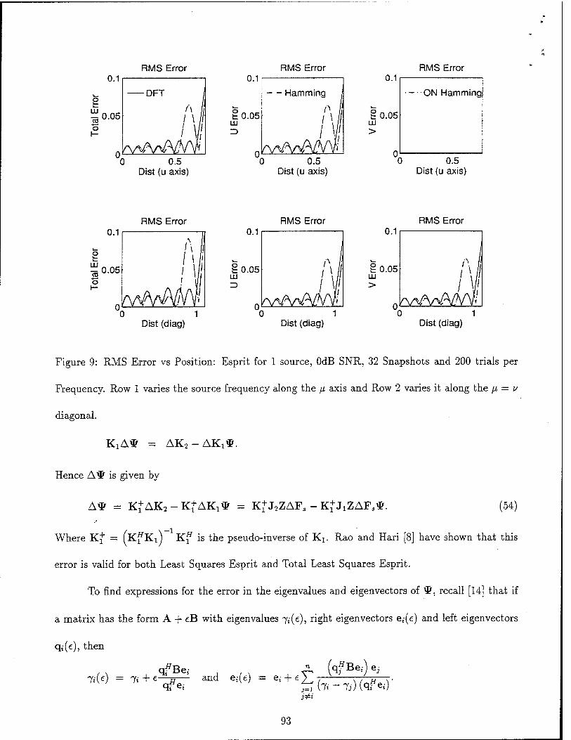
RMS Error RMS Error RMS Error
0 0.5 Dist (u axis)
LU 0.05
0 0.5 Dist (u axis)
0.1
2 0.05 LU >
ON Hamming
0 0.5 Dist (u axis)
LU -=0.05 CD
RMS Error RMS Error RMS Error
"0 1 Dist (diag)
tO.05 LU =>
0 1 Dist (diag)
2 0.05 LU >
Dist (diag)
Figure 9: RMS Error vs Position: Esprit for 1 source, OdB SNR, 32 Snapshots and 200 trials per
Frequency. Row 1 varies the source frequency along the \i axis and Row 2 varies it along the \i — v
diagonal.
KxA* = AK2-AKX#.
Hence A\£ is given by
A* = K+AKs-KfAKx* = K+J2ZAFS - K+JXZAFS*. (54)
Where Kf = (KfKij Kf is the pseudo-inverse of Ki. Rao and Hari [8] have shown that this
error is valid for both Least Squares Esprit and Total Least Squares Esprit.
To find expressions for the error in the eigenvalues and eigenvectors of *, recall [14] that if
a matrix has the form A + eB with eigenvalues 7,-(e), right eigenvectors e,-(e) and left eigenvectors
q,-(e), then
1.W = * + '-&T md -W = e' + £5(7,-7))(qfe,)-
93

RMS Error 0.015
20 40 60 Number of Snaps
RMS Error 0.015
20 40 60 Number of Snaps
RMS Error 0.015
o UJ
0.01
0.005
ON Hamming
\
20 40 60 Number of Snaps
RMS Error
20 40 60 Number of Snaps
RMS Error
0.2
5 0.15
UJ 0.1
0.05 n ■
20 40 60 Number of Snaps
RMS Error
0.2
§0.15
ÜJ 0.1
0.05
20 40 60 Number of Snaps
Figure 10: Performance vs Snapshots: Esprit with 3 sources, 32 Snapshots and 200 trials per
Frequency. Row 1 has OdB SNR and row 2 has -20dB SNR
In this case A = <P, B = A*, and qf e,- = 1, so the eignvalue error is given by
A7i = qf [K+AK2 - K+AKX*] e< = -7iqf K+(Jx - 7*J2) AKe< = -7iajf AFset.(55)
Where a,j has been defined as a^-
that
ZH(Ji-^J2f (Kf)H q,. From (55), it is easily verified
A7i a H AFseief AFf| a« = <*£££ e,(A:)e*(OAffcAf;ra
d-x d-i
Jfc=0 (=0
(A7i)2 = (7i)
2 af f AFse,-ef AFf I a*. = (7lf a? £ £ ^H-(0AffcAif < d-\ d-i
EE Jr=0 (=0
Now consider the right eigenvector.
Ae. =y(^h = ^/-7,«?AFse,:
j,=o wt — 7?'J >=o (7i - 7j)
(56)
(57)
(58)
94

Therefore
Ae,Aef = £ £ 'o i 1 (7i - 7m) (7i - 7n)
U-\ d-\
<*?m EE^M(0Af,Af^ uiB
d-1 d-1
Ae,-AeJ = EE (7i7i)
\jt=o ;=o
^d-1 d-l
emeffe9)
\jfe=0 /=o /
emel (60) lo n=0 I W»' 7m) (7j 7n;
Taking the expectation of equations (56, 57, 59, 60) yields equations (43 - 46). With the error in
the eigenvectors of ^ characterized, the error in /?,- can now be determined.
Pi = IfPli
Pi + A/n = (l + Al^Pd + Al,) = lfPl,- + lfPAl1- + AlfPl, + AlfPAli
Apt- « IfPA1, + AlfPI, = efK*PKAe,- + Ae?K^PKe, (61)
Equations (48 - 49) come directly from (61).
It remains to show how A7; and A/9,- effect Ai/; and A/^-. Recall that ideally 7; = ejdyUi, but
due to errors 7,- = r.-e-7^^' = fiejd!'('yi+A''''). Consider 7 = re-7^ and notice that
<97 = dre^y+jdyre^ydu = e^vdr + jdyld„
97i = ^«dri+jdyvd,,; = 7* (&<+;<*A)
Therefore
|d7i|2
(57,.)2
^{(7n2(ö7l)2}
A)2 + (dA)2
[A)2 - (4Af
and consequently
|A7,-|2-7^{(7;)2(A7,-)2} <*"> " 2(t? ■
(62)
This results differs slightly from that obtained by Rao and Hari [8]. They were concerned with the
direction angle 9 not the frequency v = sin0. Therefore, they had a (cos0) in the denominator
due to the fact that dv = COS#<9ö.
95

References
[1] R. 0. Schmidt, "A Signal Subspace Approach to Multiple Emitter Location and Spectral
estimation" Ph.D. dissertation, Stanford University, Stanford, CA, 1981
[2] G. M. Kautz and M. D. Zoltowski, "Beamspace DOA Estimation Featuring Multirate Eigen-
vector processing," Submitted to IEEE Trans, on Signal Processing, May. 1994.
[3] M. D. Zoltowski, J. V. Krogmeier, and G. M. Kautz, "Novel Multirate Processing of Beamspace
Noise Eigenvectors," Submitted to IEEE Signal Processing Letters, Jan. 1994.
[4] R. Roy and T. Kailath, "ESPRIT-Estimation of Signal Parameters Via Rotational Invariance
Techniques," IEEE Trans. Acoust., Speech, Signal Processing, vol. 37, no. 7, pp. 984-995, July
1989.
[5] M. D. Zoltowski, G. M. Kautz, and S. D. Silverstein, "Beamspace Root-MUSIC," IEEE Trans,
on Signal Processing, vol. 41, no. 1, pp. 344-364, Jan. 1993.
[6] M. D. Zoltowski and D. Stavrinides, "Sensor Array Signal Processing Via a Procrustes Rota-
tions Based Eigenanalysis of the ESPRIT Data Pencil," IEEE Trans. Acoust, Speech, Signal
Processing, vol. 37, no. 6, pp. 832-861, June 1989.
[7] G. M. Kautz and M. D. Zoltowski, "Performance Analysis of MUSIC Employing Conjugate
Symmetric Beamformers," Submitted to IEEE Trans, on Signal Processing, May. 1993.
[8] B. D. Rao and K. V. S. Hari, "Performance Analysis of ESPRIT and TAM in Determining the
Direction of Arrival of Plane Waves in Noise," IEEE Trans. Acoust., Speech, Signal Processing,
vol. 37, no. 12, pp. 1990-1995, Dec. 1989.
96

[9] J. W. Brewer, "Kronecker Products and Matrix Calculus in System Theory," IEEE Trans, on
Circuits and Systems, vol. cas-25, no. 9, pp. 772-781, Sept. 1978.
[10] M. Wax and T. Kailath, "Detection of Signals by Information Theoretic Criteria," IEEE Trans.
Acoust, Speech, Signal Processing, vol. ASSP-33, no. 2, pp. 387-392, April 1985.
[11] G. H. Golub and C. F. Van Loan, "An Analysis of the Total Least Squares Problem," SIAM
J. Numerical Anal., vol. 17, no. 6, pp. 883-893, Dec 1980.
[12] G. H. Golub and C. F. Van Loan, Matrix Computations. Baltimore. MD: Johns Hopkins Uni-
versity Press. 1984
[13] P. P. Vaidyanathan, Multirate Systems and Filter Banks, New Jersey: Prentice Hall, 1993.
[14] J. H. Wilkinson, The Algebraic Eigenvalue Problem. Clarendon Press Oxford 1965
[15] A. Nonymous, Zoltowski mentioned that someone at MIT has developed a 2-D rooting algorithm,
, but it has not been published and we have not seen it.
97

4 Real-Time Frequency And 2-D Angle Estimation With Sub-Nyquist Spatio-Temporal Sampling
An algorithm has been developed for real-time estimation of the frequency and azimuth and
elevation angles of each signal incident upon an airborne antenna array system over a very wide
frequency band, 2-18 GHz, commensurate with electronic signal warfare. The algorithm pro-
vides unambiguous frequency estimation despite severe temporal undersampling necessitated
by cost/complexity of hardware considerations. The 2-18 GHz spectrum is decomposed into
1 GHz bands. The baseband output of each antenna is sent through two 250 MHz sampled
channels where one is delayed relative to the other (prior to sampling) by .5 ns, the Nyquist
interval for a 1 GHz bandwidth. Due to the high variance of the Direct ESPRIT frequency
estimator, aliased frequencies are estimated via a simple formula and translated to the proper
aliasing zone utilizing eigenvector information generated by PRO-ESPRIT. The algorithm also
provides unambiguous 2-D angle estimation over the entire 2-18 GHz bandwidth despite se-
vere spatial undersampling at the higher end of this band necessitated by mutual coupling
considerations and resolving power requirements at the lower end of the band. Eigenvector
information generated by PRO-ESPRIT is used to facilitate computationally simple estimation
of azimuth and elevation angles automatically paired with corresponding frequency estimates
despite aliasing. Simulations are presented demonstrating the capabilities of the algorithm.
4.1 Introduction
4.2 Spatio-Temporal Sampling and Data Model
4.3 ESPRIT Based Frequency Estimation With Temporal Under- sampling
4.4 2-D Angle Estimation With Spatial Undersampling Via PRO- ESPRIT and Integer Search Formulation
4.4.1 Estimation of the Array Manifold for Each Source
4.4.2 Prescription for Nonuniform Element Spacing Facilitating Nonambiguous Angle Estimation
4.4.3 Integer Search Algorithm for Direction Cosine Estimation
4.5 Simulation Examples
4.6 Final Comments
4.7 References
4.8 Computation of Cramer Rao Lower Bound for Frequency and 2D Angle Estimation
4.9 Figures
98

1 Introduction
The problem under investigation is that of real-time estimation of the frequency and azimuth and eleva-
tion angles of each signal incident upon an airborne antenna array system over a very wide frequency band,
2-18 GHz, commensurate with electronic warfare. The problem is complicated by severe undersampling in
both the temporal and spatial domains necessitated by cost and complexity of hardware considerations [1].
To reduce the complexity of the overall receiver hardware, the bandwidth at the intermediate frequency
is chosen to be quite large equal to 1 GHz. Correspondingly, the entire 2-18 GHz spectrum is decomposed
into overlapping 1 GHz bands; each band is examined in succession or in parallel. The Nyquist temporal
sampling rate for digitization of a 1 GHz band is 2 GHz. Although A/D converters operating at 2 GHz rate
are available, they are very expensive and processing speed following the converter may limit the overall
operation of the receiver. In the prototype system pictured in Figure 1 [1], the receiver output, after conver-
sion to baseband, is sampled at a rate of 250 MHz, one-eighth of the Nyquist rate. This severe undersam-
pling leads to aliasing and attendant problems of ambiguity. The aliased frequency as a function of baseband
frequency with a sampling rate of 250 MHz is plotted in Figure 3.
Note that the aliasing function plotted in Figure 3 is for the case where only the in-phase channel is
sampled. Sampling of the quadrature channel represents additional hardware costs and overall doubles the
number of samples to be processed. Thus, in keeping with the overall goal of reduced complexity of
hardware and computation, it is assumed that only the in-phase component, a real-valued signal, is sampled
and input to the system. Note, it is typically necessary to generate the complex analytic signal in a direction
finding application to resolve a 180° ambiguity in the azimuth angle estimates. Again motivated by the
desire to keep the computational complexity low, the complex analytic signal is roughly approximated by
computing the DFT of the output of each antenna and throwing away the negative frequency portion of the
spectrum. This approach averts the need to pass the sampled signal through an FIR digital Hubert
Transformer which could possibly lead to edge effects or a reduced number of effective time samples
(depending on whether one includes all output points of the FIR digital Hilbert Transformer or just those out-
put points for which there were no zero entries in the FIR filter window.) The spatio-temporal signal model
is developed in Section 2.
The procedure for frequency estimation with Sub-Nyquist temporal sampling developed within may be easily adapted for narrowband direction-of-arrival estimation with two identical, collinear uniform linear arrays (ULA's). In this application, the displacement between the two arrays should be less than a half-wavelength but the interelement spacing for either array may be much greater than a half-wavelength to achieve a large aperture and, hence, increased resolution capability relative to a ULA of the same total number of elements but with half-wavelength spacing.
99-

In order to estimate the baseband frequency of each signal despite aliasing, the baseband output of each
antenna is sent through two 250 MHz sampled channels where one is delayed by x relative to the other (prior
to sampling) as indicated in Figure 1. The time-delay, x, is chosen less than or equal to the Nyquist sampling
interval for the baseband bandwidth, W, i. e., x ^ 1/(2W). In the prototype system depicted in Figure 1, W =
1 GHz and x = .5 ns = .5 x 10"9 s. ESPRIT [2,3] may then be applied to estimate the baseband frequencies in
any 1 GHz baseband bandwidth. To facilitate real-time implementation, ESPRIT is applied in DFT space.
In this mode of processing the steps are (i) compute an FFT of a block of samples, (ii) locate peaks via a sim-
ple peak-picking algorithm, and (iii) apply ESPRIT to a small set of DFT values around each peak.
In Section 3, we show that the Direct ESPRIT frequency estimator has a variance several orders of
magnitude greater than the Cramer Rao Lower Bound (CRB). An alternative approach referred to as Indirect
ESPRIT is presented that is computationally simple and achieves performance very close to the CRB.
Indirect ESPRIT makes novel use of eigenvector information generated by the PRO-ESPRIT algorithm [3]
to estimate the aliased frequency of each source via a simple formula and correctly translate it to the proper
aliasing zone where it is added to or subtracted from the appropriate integer of the sampling rate in accor-
dance with Figure 3.
Once the frequency of each signal is estimated, the next goal is to estimate the corresponding azimuth
and elevation angles. There are two problems here. First, each angle estimate must be correctly paired with
the proper frequency estimate. Second, in general, 2-D angle estimation is significantly more computation-
ally complex than 1-D angle estimation. Again, real-time implementation is an overriding factor. Now, since
the sources are at different frequencies, the filtering inherent in selecting only those DFT values around a
spectral peak should ideally be sufficient to isolate single source contributions and avoid the frequency-angle
pairing problem. However, aside from sidelobe leakage effects, this is not the case as sources well separated
in analog frequency may be aliased to very nearly the same digital frequency. In Section 4, eigenvector
information generated by PRO-ESPRIT is used to facilitate computationally simple estimation of azimuth
and elevation angles automatically paired with corresponding frequency estimates despite aliasing.
• In the case of a uniformly-spaced linear array, half-wavelength spacing between antennas is required to
avoid ambiguities in estimating the arrival angle of a signal. With half-wavelength spacing at the upper end
of the 2-18 GHz spectrum, the elements are too closely spaced at the lower end of the spectrum leading to
problems of mutual coupling and poor resolution. The resolution capability and estimator accuracy of any
arrival angle estimation algorithm is proportional to the aperture length measured in units of wavelengths.
To achieve a high degree of resolution power and estimator accuracy and yet avoid mutual coupling, the ele-
ments must be spaced nonuniformly over a large aperture.
-100-

The prototype system employs an L-shaped antenna array having nonuniformly spaced elements along
each leg as pictured in Figure 2. The interelement spacings along either axis is much greater than a half-
wavelength, particularly at 18 GHz. In Section 4, we develop (i) a prescription for interelement spacings for
nonambiguous angle estimation and (ii) an attendant algorithm for angle estimation that is computationally
simple for real-time implementation. Although there is a plethora of previous work on the design of nonuni-
form linear arrays [6-8], the development in Section 4 assumes a small number of antenna elements due to
cost and space limitations on the antenna platform attached to the aircraft. Also, high sidelobes is not as
much a problem since we are able to isolate the individual contribution of each source. In contrast to previ-
ous work [6-8], the prescription for interelement spacings is developed synergistically with a simple integer
based search algorithm for angle estimation. Section 5 presents simulations that demonstrate the power of
the overall frequency and 2-D angle estimation algorithm summarized in the flowchart presented in Figure 5.
2. Spatio-Temporal Sampling and Data Model
The parameters for the prototype sub-Nyquist spatio-temporal sampling system are indicated in Figure
1. We concentrate on signal parameter estimation for a particular 1 GHz baseband bandwidth. For the sake
of simplicity, the signals are modeled as RF pulsed waveforms. The development to follow, though, holds as
B L long as each signal satisfies the standard narrowband assumption — y cos8 < 1. For a given signal, B is
the bandwidth, fc is the carrier frequency, L is the length of the array, X is the wavelength, and cosQ is the
direction cosine relative to the array axis. Since the carrier frequencies here lie somewhere between 2 and 18
GHz, the narrowband assumption is satisfied almost always except for some extremely wideband signals.
We also assume that no two signals are at exactly the same RF frequency. Even if there is multipath propa-
gation between a given source and the airborne antenna array, the Doppler shift each multipath signal under-
goes is distinct as long as each multipath signal has its own distinct azimuth and elevation coordinates [9].
Let the sampling rate be denoted Fs. We are here assuming that Fs is well below the Nyquist rate lead-
ing to aliasing. For our prototype system, Fs = 250 MHz equal to one-eighth of the Nyquist rate (2 GHz for a
1 GHz baseband bandwidth). Consider sampling a single sinusoid of the form cos(2uFjt + <j>), where Fj is the
baseband frequency (0 ^ Fj ^ 1 GHz).
F- Fs cos(27cFjt + (!))|t;=IvFi=cos(2jt-^-n-i-(j)) = cos[2jrfjn + <!)] for (XFj«:-^- W
F: F; Fs = COSPJCC-^—l)n + <H = cos[27t(l-~-)n - <M = cos[2;tfjn - $] for — < Fj < Fs
101-
Fj Fs ' cos[27i(l—-*-)n + <H = cos[2jcfjn + $] for F, < Fj < 3—
p. p. F : COS[2TC(—-2)n + $] = COS[2JI(2—=r)n -<!>] = cos[27cfjn - <j>] for 3-^- < Fj < 2FS
Fs Fs 2
For each range of the analog baseband frequency, the corresponding digital frequency fj is between 0 and .5,
i. e., 0 < fj < .5. Continuing this development, we obtain the aliasing function g(F) plotted in Figure 3 for the
case of Fs = 250 MHz corresponding to our prototype system. With the aliasing function thus defined, the
digital frequency, fj, is related to analog baseband frequency, Fj, as fj =g(Fj)/Fs. The analog aliased fre-
quency is defined as Fj = fjFs = g(F); FJ is the frequency one would obtain if the analog sinusoidal signal
was reconstructed from its samples. An important observation is that when Fj is in a range where the slope
of the aliasing function g(F) is negative, the constant phase offset of the sampled sinusoid is the negative of
that associated with the continuous-time sinusoid.
In order to estimate the baseband frequency of each signal despite aliasing, the baseband output of each
antenna is sent through two 250 MHz sampled channels where one is delayed by x relative to the other (prior
to sampling). We here assume that the time-delay, x, is less than or equal to the Nyquist sampling interval
for the baseband bandwidth, W, i. e., x s 1/(2W). In the prototype system depicted in Figure 1, W = 1 GHz
and x = .5 ns = .5 x 10""9 s.
The sampled versions of the reference and time-delayed data sets, referred to as the X and Y data sets,
respectively, (one pair of data sets for each antenna) may be described as
xi(n)= £ JAe*V^(i) e^" + -X^e^® e^" 1 (2)
Yi(n) = Si —ej^Yioej^Y)(i) e"jx52ltFjT e"2^" + ^Le~jXiVj<,e"jK|YjCl) e^2*1^ e~j2^n I
where, for the moment, we are neglecting the effects of noise. The various quantities in (2) are described
below. J is the total number of signals in a particular 1 GHz baseband bandwidth. Aj is the amplitude of the
j-th signal while Yjo is the phase of j-th signal at the origin of the antenna array system. Yj(i) is the relative
phase of the j-th signal arrival at the i-th antenna. If the i-th antenna is at the x-y coordinate pair, (XJ , y{),
and the j-th source is at an azimuth angle of 9j and an elevation angle of fy,
102

Yj(i) = --5- (XicosejSin<|)j + yiSin9jSin(j>j) i=l,...,M (3)
where Xj is the wavelength of the j-th signal arrival and M is the total number of antennas comprising the
array. Kj is the slope of the aliasing function g(F) at F = Fj equal to either +1 or -1. In accordance with (1),
Kj takes into account the conjugation that occurs when Fj is in an interval where the aliasing function is
downward sloping. Note, in the prototype system the observation interval is .5 (i.s = .5 x 10-6 s yielding
roughly N = 128 samples for each of the M antennas.
As indicated in Figure 1, the first processing step is to compute an FFT of both the X and Y data sets at
each antenna output Ultimately ESPRIT [2,3] is applied to a small set of DFT values around each spectral
peak in the positive frequency portion of each of the 2M spectra. We are effectively using the DFT as a nar-
rowband passband filter. This is done for two reasons. First, by isolating only positive frequencies we are
able to resolve a 180° ambiguity in azimuth angle. Second, in processing a given peak, the eigenvalue
decompositions (EVD's) required are done on matrices of dimension equal to the number of DFT values
which is less than the number of antennas. Separate peaks may be processed in parallel. Recall that sources
well separated in baseband frequency may be aliased to very nearly the same digital frequency due to under-
sampling. Thus, several sources may be contributing to a given spectral peak.
The respective N pt. DFT's of the X and Y data sets for the i-th antenna are denoted Xi(k) and Yi(k),
i=l,...,M, and may be expressed as
Xi(k) = £ j^e**«^® sincNj(fr£) + ^e-^e-^(i) sincNj(fj+£)} (4)
Yi(k)-i|^*^® e^^sinc^f-l) + ^e-^e-^(i) ^2^sincNj(fj+|-)|
where Nj is the number of samples for which the j-th signal is "turned on" and the periodic sine function is
defined as sincwCf) = e"J,r(N"1)f sm^ . Note, in contrast to convention, we include the phase term sin(Ttf)
e-j7t(N-i)f m ^g definition of sincN(f) for the sake of notational simplicity.
The next processing step is to locate spectral peaks. We here assume that a simple peak-picking algo-
rithm is employed. Note that only coarse estimates of the peak locations are required for the algorithm to
perform well. The respective DFT spectra for the X and Y data set for each antenna, 2M DFT spectra all
together, should exhibits peaks at the same locations. At this point, we concentrate on a single peak in each
DFT spectrum at the same location located at or near the DFT value k = k,, without loss of generality.
103-

L = 2L'+1 DFT values around the corresponding peak in each DFT spectrum are collected to construct the
following set of 2M L x 1 vectors: (5)
Xi(ko) = [Xi(ko-L0,... .XiOfo) XiCko+L')]7 Yi(ko)=[Yi(ko-L0,... , Yi(ko) Yi(ko+L')]T
To give a perspective on the computational complexity, in the simulations presented in Section 6 we ran
cases where XiOO and YiOO are 4x1 and cases where Xt0O and Yt0O are 5x1. The governing factor is
that the number of DFT values selected around a peak should be at least one greater than the number of
sources making significant contributions to that peak, denoted J'.
Substituting (4) into (5), the Lxl vector of X DFT values around k<> may be expressed as
XiOO = £ j^V'^® d(fj) + Ae-™°e-™(i) dH) j (6)
where d(fj) is the Lxl vector
d(fj) = smew fj~ N , sincNj f-^ J N
, smcN kp+L'
N (7)
As long as the window of DFT values is not either near k=0 or near k=N/2, the DFT acts as a narrowband
bandpass filter such that d(-fj) is small enough relative to d(fj) to be negligible. To simplify the develop-
ment, we will neglect the contribution of d(-fj). If d(-fj) is not negligible then the algorithm to be
developed will indicate a source having a negative aliased frequency which potentially may be screened out.
Neglecting the negative frequency contributions, XiOO = E —ie^e^® d(fj) where J'< J is the j=i 2
number of sources making a significant contribution to the spectral peak at or near the digital frequency
ko/N. This expression describes the vector of DFT values around a peak in the DFT spectrum of a single
antenna. The DFT vectors from all M antennas are placed as the columns of an LxM matrix as
X = [Xi (ko); X2(ko); • • • ; XM(ko)]. X may be expressed in factored form as
x = I AJ e^* d(fj)aT(ej,(|)j,Kj) (LxM) (8) j=i
where A] = Aj/2 and aOj.^.xj) = [e*Yi(1), ejl™(2), • • • , ej^Yj(M)]T with YjG) defined by (3). aO^Kj) for
Kj = 1 is the Mxl array manifold vector for a signal incident from the (0j,<(>j) direction. The dependence on
Kj, the slope of the aliasing function at Fj, is introduced as a simplistic means of denoting a conjugation; it
allows us to avoid breaking the sum in (8) into terms for which the array manifold is conjugated and those
for which it is not conjugated.
-104-

Similarly, the corresponding DFT outputs from all M antennas for the Y (time-delayed) data is col-
lected as Y = [Y1(k0); Y2(ko); ••• • YM(k<,)]. Neglecting negative frequency components, Y may be
expressed as
Y = £ Aj e** e*2^ d(fj) aT(ej,(|)jf Kj) (L x M) (9)
Equations (8) and (9) represent the pure signal component of the spatio-temporal data model assumed
throughout. Again, KJ is the slope of the aliasing function g(F) in Figure 3 at F = Fj equal to either +1 or -1.
Kj is a notational tool that takes into account the conjugation that occurs when Fj is in an interval where the
aliasing function is downward sloping.
3. ESPRIT Based Frequency Estimation With Temporal Undersampling
Given the data model described by (8) and (9), the applicability of ESPRIT [2,3] is evident
Y - uX = £ Aj e** {e-*2^ - n)d(fj) aT(8j)(t)j,Kj) (10)
The critical observation for estimating Fj is that when u. = e~JKi2j: '\ the rank of Y - uX drops from V to J'-l
since the /-th term drops out of the sum. Thus, Uj = e"Jxi2,lF,\ j=l,... J', are J' distinct generalized eigenvalues
of the LxM rectangular matrix pencil {Y, X}.
The argument of the ESPRIT eigenvalue, arg{u.j} = -KJ27CFJT, is plotted as a function of the baseband
frequency Fj for Fs = 250 MHz in Figure 4. Recall that KJ is the slope of the aliasing function at F = Fj. Note
that certain ranges of phase within (-JI,JI) are not permissible as the argument of u.j. In fact, only half of the
2TC interval (-TC,JC) is permissible. For example, under ideal noiseless conditions, no value of phase in the
interval (-JC/8,-2JI/8) is permissible as the argument of Uj = c~iKi jT.
The PRO-ESPRIT [3] variant of ESPRIT is here employed as a "fast" implementation of ESPRIT for
estimating the phase factors, -Kj2jtFjX, j=l,...,J'. PRO-ESPRIT operates on the LxL autocorrelation and
cross-correlation matrices RM = ^•£Xi(k0)X[I(k0) = ^XXH and R^ = ^SYi(k0)X[I(k0) = ^YXH.
Note the number of DFT values selected around the peak at ko, L, may be as small as two if only a single
source is contributing to the peak. The algorithm is first summarized and then briefly justified.
First, compute an EVD of R„: RK u} = ^ u(, i = 1,...,L, where the eigenvalues are indexed in order of
decreasing magnitude. The number of complex sinusoids with aliased frequency components in the vicinity
of ko, J's J, may be determined from a number of techniques including statistical tests that examine the
eigenvalues such as AIC or MDL. With the Y < L largest (signal) eigenvalues and corresponding signal
eigenvectors, construct the J'xJ' diagonal matrix Zs and the LxJ' matrix Us as
-105-

Zs =diag{(X1-^nin)iy2,a2-Xtnin)
1/2)... ,(h'-K^)m) (11)
us = [ui: u2: • • • : uj-] (12)
The smallest eigenvalue, Amu,, is asymptotically equal to the noise power which affects the diagonal ele-
ments of the autocorrelation matrix RM. Note for a given antenna output, even if the noise is not white, i. e.,
the noise spectral density is not flat over the entire 1 GHz bandwidth, it can be shown that the noise contam-
inating a small set of successive DFT values is approximately i.i.d. The final major step is an EVD of
»F = Zi1 Us1 Ryx Us Zi1 (J'xJ') (13)
The eigenvalues of *¥ are estimates of Uj = e~J1<i j\ j=l,...,J'.
PROOF: Let X = UsZsVs be the SVD of X including only the J' nonzero singular values and correspond-
ing left and right singular vectors; Us is LxJ', Zs is J'xJ', and Vs is MxJ'. It follows from (8) and (9), that
range{Us} = range{Y} = span{d(fO ,... , d(fr)} and range{Vs} = range{YH} = span{a*(9i,<|)1,Ki)....
, a*(8j',<|)j',Kj')} such that Y = UsUs YVsVs* where UsUs and VsVs* are projection operators. Thus,
Y - uX = UsUs* Y VsVs1 - uUsZsVs1
= UsZs{Zi1UsIYVs-uIr}Vs
I
= UsZs{Zi,UsIYVsZsUsIUsZi1 -ulrJVs1
= USZS {Zi1UsIYXHUsZiI - pIr}V|? (14)
where we have used the fact that ZsUsUsZ^1 =Iy. Thus, the J' nontrivial generalized eigenvalues of the
LxM matrix pencil {Y, X} may be computed as the eigenvalues of the J'xJ' matrix Z^Us YXHUsZi1. The
proof is completed by recognizing that XXH = UsZ|Us. H
In the prototype system t = JxlO^s such that Fj may be estimated from the phase of the j-th ESPRIT
eigenvalue according to Fj = | arg{|ij }/2n | (2xl09) Hz, j=l,... J', where arg{z} is the phase angle of the com-
plex number z. Any error in arg{Uj} due to noise is grossly magnified due to the multiplication by 109, i. e.,
multiplication by a 1 GHz. Simulations presented in Section 6 reveal that the variance of the baseband fre-
quency estimates obtained from ESPRIT in this manner are on the order of 10 MHz while the Cramer Rao
Lower Bound (CRB) on the variance of any unbiased estimator of frequency is on the order of 10 KHz. This
extreme differential motivates us to see if we can obtain performance closer to the CRB without incurring
too much additional computation.
106

The above approach is referred to as the Direct ESPRIT approach. An alternative approach is referred
to as Indirect ESPRIT. The steps in Indirect ESPRIT are: (i) estimate the digital frequency fj, (ii) convert fj
to the aliased analog frequency via FJ = fj Fs, and (iii) translate Fj up to the proper aliasing zone using the
phase of the ESPRIT eigenvalue u.j, in conjunction with Figure 4, where FJ is either added to or subtracted
from an integer multiple of the sampling rate to estimate the actual baseband frequency. Two computation-
ally efficient, high-resolution algorithms for estimating the aliased frequencies using DFT values as input are
Beamspace Root-MUSIC [4] and Beamspace ESPRIT [5]. Recall high-resolution capability is necessary
since sources well separated in analog frequency may be very closely-spaced in digital frequency due to
aliasing. However, despite their relative computational efficiency, implementing either of these two algo-
rithms represents a substantial increase in computational complexity.
More important, though, is the data association problem wherein the aliased frequency estimates must
be paired with the correct ESPRIT eigenvalue so that it is translated to the proper alias zone. If the aliased
frequencies are estimated independently of the ESPRIT eigenvalues, this pairing problem is very difficult,
insurmountable when sources are closely-spaced in frequency after aliasing. Fortuitously, eigenvector infor-
mation provided by PRO-ESPRIT facilitates automatic pairing of the aliased frequency estimates with the
corresponding ESPRIT eigenvalues. In addition, the eigenvector information generated by PRO-ESPRIT
provides a means for isolating the individual contribution of each source despite aliasing. This facilitates
simple estimation of the aliased frequency associated with each source. It may be done on an individual
basis assuming a single source leading to a simple closed-form formula as shown shortly.
The j-th Mxl right generalized eigenvector, r}, of the LxM rectangular matrix pencil {Y,X} is that vec-
tor satisfying {Y - UJX}I-J = 0. Substituting the noiseless (ideal) forms of the X and Y data matrices:
JS Aj e*Yi° {e-jKW - ii) d(fj) a^Sj^j.Kj)! Fj = 0 (15)
When \L = e~iK,2nP'x, the /-th term d(f/) aT(8/,<|>/,iQ) drops out of sum such that aT(9/,<t),,K/)rj =0 for
/ = 1 J', I * j. Hence, r-j can be used to extract d(fj) to within a scalar multiple:
Xrjocd(fj) (Yrjocd(fj))
A key point is that the estimate of d(fj) obtained in this manner is automatically paired with the ESPRIT
eigenvalue that is an estimate of Uj = eT^2n?iX since rj is the right generalized eigenvector associated with Uj.
Thus, a frequency estimation algorithm that assumes a single source may be applied to d(fj) to estimate fj.
Note, we only desire r-j in order to compute X rj as our estimate of d(fj) to within a scalar multiple.
We can bypass the computation of Tj and construct Xrj directly from the J'xl right eigenvectors of f,
-107-

defined by (13), satisfying *Fßj = U-jßj, j=l,...J'. From (14) and (15), it follows that
d(fj)oeXrj = Us2:sft j=l.--.J* (16)
where Zs and Us are constructed from the J' largest eigenvalues and corresponding eigenvectors of R^
according to (11) and (12), respectively.
Next, we apply Beamspace ESPRIT [5] to d(fj) to estimate fj. After much algebraic manipulation, the
single source assumption leads to the following simple formula for estimating fj:
fj = -^ arg|dH(fj) A* Pi d(fj) t j=l,..,J' (17)
where d(fj) is computed as in (16) and Pi and A are each LxL matrices defined as
1 f k.-L' K ko+L' ] Pi=IL-lllT A = diag \-^-W- e-**TT :*"-N-4 (18)
i_ C ,...,C ,...,C I
«1 - where 1 is an Lxl vector composed of all ones. The aliased analog frequency is then estimated as Fj = Fsfj,
where F, = 250 MHz in our prototype system. Rather than develop the formula in (17) as a simplification of
the general Beamspace ESPRIT algorithm presented in [5], due to space limitations we here simply present a
proof that it works when d(fj) = d(fj).
PROOF: First, we need to define some quantities. Let W denote an LxN matrix whose rows are L succes-
sive rows of the NxN DFT matrix associated with the DFT indices, ko - L',..., k,,,..., ko + L'. Let Yix and
W2 be composed of the first and last N-l columns of W, respectively. Wj and W2 are each Lx(N-l) and
related as W2 = AWj. Finally, let wN denote the last column of W; wN = diag(AN_1), where diag (•) con-
verts the LxL diagonal matrix AN_1 to an Lxl column vector. Note, the first column of W is 1 such that
Pi W = [0L ; Pi W2] = [0L : Pi AWi ], where 0L is an Lxl vector composed of all zeroes.
Next, define v(f) as the Nxl Vandermonde vector v(f) = [ 1, ej2lrf , e** , • • • , ej(N-1)2,rf]T. Let
vj(f) and v2(f) be composed of the first and last N-l elements of v(f), respectively. vi(f) and v2(f) are each
(N-l)xl and related as v2(f) = Qi2vf\\(f). With these definitions and relationships, it follows that
dH(fj) A* Pi d(fj) = vH(fj) WH A* Pi W v(fj)
= ^(fj) WH A* Pi AWi Vl(fj) ej2,rf)
= {v?(fj) W? + e-j(N-1)2,rf' w|J} A* Pi AW! Vl(fj) e^
-108-

= v?(fj) W? A* Pi AW! vi(fj) ej27tf] + lTPi AW! Vl(fj)e J27tfi ^iTpi *w. v.^f.v-^-2^
= {v?(fj) W? A* Pi AW! Vl(fj)} ej2lrf<
where we have used the fact that w§ A* = diagH(AN_1)A* = diagH(AN-1A) = diagH(IL) = 1T. where
diagH(D) is intended to mean convert the diagonal matrix D to a column vector and conjugate transpose (in
that order).
Since v?(fj) W? A* Pi AWi vi(fj) is real-valued, it follows that arg{dH(fj) A* Pi d(fj)} = 2jrfj. 9
Comparing the Direct and Indirect ESPRIT methods, in the former the phase of the j-th eigenvalue of
Y is mulüplied by TCXIO9 while in the latter the phase of d (fj) A* Pi d(f-) is multiplied by 250X10
6/2TC.
The multiplicative factor in the latter is three orders of magnitude lower than that in the former. This is a
heuristic explanation as to why the performance of the Indirect ESPRIT method comes much closer to
achieving the Cramer Rao Lower Bound (CRB) than the Direct ESPRIT method.
The formula for translating Ff up to the proper aliasing zone is dictated by Figure 4 wherein the phase
of the ESPRIT eigenvalue u. = e~jK2*F\ where % = ^xlCT^s, is plotted as a function of the analog baseband
frequency, 0 s F ^ 1 GHz. Within the interval (-JC, it) are eight disjoint permissible intervals, each having a
width of TC/8 and a one-to-one correspondence with each of the eight aliasing zones depicted in Figure 3. If
the phase of the ESPRIT eigenvalue lies within one of these permissible intervals, Ff is translated to the
corresponding aliasing zone accordingly where it is either added to or subtracted from the appropriate integer
multiple of 250 MHz. If, due to noise, the phase of the ESPRIT eigenvalue lies within one of the impermis-
sible regions, it is projected into the nearest permissible region. This decomposes the interval (-TC, %) into
eight distinct intervals, each having a width of TC/4, and having a one-to-one correspondence with each of the
eight possible aliasing zones plotted in Figure 3. The baseband frequency of the j-th source, Fj, is ultimately
determined from the aliased frequency estimate, Fj, according to
Fj =
<a * arg{u.;}+rc/16 Fj -250xl06 round^ „ Hz for -15rc/16<arg{|ij}<JC (19)
Fj = lxl09-Fja Hz for -rc< arg{Uj} <-15ic/16
where round[x] is the nearest integer to x as denned previously.
As an example, if argfjij} is either in the impermissible region TC / 16 < arg{Uj} < JC / 8, the permissible "■a
region 7i / 8 < arg{jij} < 2% 18, or the impermissible region 2% / 8 < arg{Hj} < 5rc / 16, Fj is subtracted from
250 MHz to obtain Fj. Simulations presented in Section 6 reveal (19) to be a very robust formula for
translating F* to the proper aliasing zone. Note, that if we are off by one in selecting the correct aliasing
-109-

zone a very large error may be incurred. Two adjacent aliasing zones differ in that in one F* is added to nFs
while in the other it is subtraced from (n+l)Fs.
4. 2-D Angle Estimation With Spatial Undersampling Via PRO-ESPRIT and Integer Search
4.1 Estimation of the Array Manifold for Each Source
In Section 3, we saw that use of the right generalized eigenvectors of the LxM matrix pencil {Y,X}
facilitates a simple procedure for estimating the aliased frequency of a source that was automatically paired
with an ESPRIT eigenvalue thereby, in turn, facilitating simple translation up to the proper aliasing zone.
The left generalized eigenvectors of the LxM matrix pencil {Y,X} play a similar role in the problem of
estimating the azimuth and elevation angle of each source contributing to a given peak in the DFT spectrum.
Specifically, the j-th left generalized eigenvector of {Y,X} is used to extract from the X and Y data an esti-
mate of the array manifold for the j-th source, denoted a(8j,<t>j,Kj). Recall the inclusion of KJ in the definition
of the array manifold is a notational tool to reflect the fact that the array manifold is conjugated when the
baseband frequency is located on a downward sloping portion of the aliasing function.
The j-th Lxl left generalized eigenvector, lj, of the LxM rectangular matrix pencil {Y,X} is that vector
satisfying if {Y - |ijX} = 0. Substituting the noiseless (ideal) forms of the X and Y data matrices, we have
If JS AJ e** {e-*2"1^ - ujd(fj) a^Oj.^Kj) L 0 (20)
When u. = e"jKi2'rf'T, the l-th term d(f/)aT(e/,<)>/,K,) drops out of the sum such that if d(f,) = 0 for
/ = 1 J', / * j. Hence, lj can be used to extract a(8j,<t>j,Kj) to within a scalar multiple:
If X«aT(ej,<j.j,Kj) => XTlf - aOj.^Kj) if Y-a^Vcj) => YTlf ~ aOj.^.Kj) (21)
Thus, applying the j-th left generalized eigenvector allows us to extract an estimate of the array mani-
fold forthe j-th source which, in turn, may be operated upon to estimate the azimuth and elevation angles of
the j-th source. The latter problem is greatly simplified, specifically in cases where sources are very closely-
spaced in digital frequency due to aliasing, due to the ability to isolate a single source contribution. In addi-
tion, since lj is associated with the ESPRIT eigenvalue p.j = e~jX52,tFi\ the azimuth and elevation angle esti-
mates obtained by processing the estimate of a(0j,fy,Kj) are automatically paired with the estimate of Fj
obtained via the algorithm developed in Section 3. Knowledge of Fj is tantamount to knowledge of the
proper aliasing zone. This allows us to determine the value of Kj enabling us to resolve a 180° ambiguity in
the azimuth angle estimate (flipping the sign of KJ introduces a 180° change in azimuth angle).
-110-

Similar to the case with the right generalized eigenvectors, the j-th Lxl left generalized eigenvector, lj,
of the LxM rectangular matrix pencil {Y,X} may be efficiently computed from the J'xl j-th left eigenvector,
Oj, of Y in (13) satisfying aj1 *F = Ujaf, j=l,...,J'. From (14) and (20), it follows that
ljsUsIi1«! j=l,-..J' (22)
Recall Y is the number of sources making a nonnegligible contribution to a particular DFT spectral peak
which may be as small as one if sources are well separated in digital frequency.
In general, the problem of 2-D angle estimation is considerably more computationally complex than
the problem of 1-D angle estimation. Fortuitously, the isolation of single source components via PRO-
ESPRIT facilitates separable 2-D angle estimation given an appropriate array geometry. For example, con-
sider a 2-D array consisting of two orthogonal linear arrays, e.g., an L-shaped array. Since we've isolated a
single source component, we can determine the direction cosine of a source relative to each axis indepen-
dently. Each leg may be processed independently applying an appropriate 1-D angle estimation algorithm.
The x and y direction cosines are automatically paired with each other as well as with the corresponding fre-
quency estimate. Simple trigonometry may be invoked to convert the x and y direction cosines into azimuth
and elevation angle estimates.
42 Prescription for Nonuniform Element Spacing Facilitating Nonambiguous Angle Estimation
In accordance with the discussion in Section 1, to achieve a high degree of resolution power and esti-
mator accuracy and yet avoid mutual coupling, the elements of each leg of the L-shaped array are spaced
nonuniformly with interelement spacings much greater than a half-wavelength. The design problem is two-
fold: (i) development of a prescription for "good" interelement spacings for unambiguous angle estimation
relative to each array axis and (ii) development of a computationally simple algorithm for processing the
estimate of the array manifold provided by PRO-ESPRIT to estimate the direction cosine of a source with
respect to each axis. We here assume a small number of antenna elements due to cost and complexity of
hardware considerations and space limitations on the antenna platform attached to the aircraft
The L-shaped array geometry employed in the simulations presented in Section 6 is depicted in Figure
2. The corresponding array manifold is
a(ejf4>j,x$)= (23)
IT
JS2s3-v, j^2lC^0-v] jijto-^-v, JKjÄ-^-v, jnjÄ-J-n, jxj27t1-uj JKJ2K—5-U, ji^ai-j-n e *> ,e *» ,e ^ ,e ** ,l,e ^ , e ^ , e "> , e "»
where Uj and Vj are the direction cosines of the j-th source relative to x-axis and y-axis, respectively, and Xj
-111-

~X v/"=vj0 + /d /e"
ceiling -T-(l+Vjo) , floor h
d-Vjo) (28)
The objective is to choose d! and d2 so that alignment, i. e., vk = v/~, only occurs for k = / = 0.
Equating the expressions for vj: and vf
- A« ~&i vjo+k- = vjo + /-
d2_ = _T
di k (29)
d2 d2 d2 /' , This indicates that ambiguities may possibly arise if — is rational. Express — as — = p- , where / and
k' are relatively prime, i. e., have no common factors other than unity. The set of ambiguous angles is then
v - v + n k' _L = v:0 + n /' — for any n for which -1 < vn < 1. Consider the case of n=l. If we make ™ ->" di d2
X X; sure that either v^ + k7— or vio + /'— lies outside the visible region, i. e., is either less than -1 or greater
^ di d2
than +1, then there is no ambiguity. That is, within the visible region corresponding to direction cosines
with absolute value less than 1 there is only alignment at n=0 or k = / = 0.
Part of the design procedure then is to select di and d2 such that the relatively prime factors /' and k'
comply with one of the following conditions. Either
if* ceiling di
*j d+Vjo) , floor
*i (1-Vjo) r or l'*\ ceiling
d2 -—(l+vjo) A)
, floor d-Vjo)
These conditions depend on the direction cosine of the source. To remove the data dependence, we over-
specify and let Vj«, = 1 for the lower bound limit and vjo = -1 for the upper bound limit The goal then is to
select d! and d2 suchthat the relatively prime factors /' and k' comply with one of the following conditions.
if* <-floor 2d,
*i , floor
2d,
h or /' * -H
" ■•
-floor "2d2"
, floor "2d2l L^ J
«. -
(30)
d2 /' With —- = —, where k' and /' are relatively prime, if either of the conditions above are satisfied, then dj k'
within the visible region the ambiguities only align at true source direction cosine, VJQ.
Note that satisfying the condition above at 18 GHz guarantees that ambiguities may be resolved at
lower frequencies since Ik'^l = |k'max| = floor[2di /Xj] decreases with decreasing frequency (increasing \)
-113

as does |/'min| = \l'max\ = floor[2d2 / Xj].
As an illustrative example, for the simulations we chose di = 2.3 in and d2 = 5.3 in. Consider the upper
limit of the 2-18 GHz spectrum, 18 GHz, for which the wavelength is X, = 2/3 in. (30) dictates that at 18
GHz, k'<*{-6 , 6} and V* {-14 ,14}. Expressing d2/di as the ratio of two relatively prime numbers as
h- = — = — = — we see that k' = 23 4 f-6 , 6} and /'=53 4 {-14 , 14} so that both conditions in (30) di 2.3 23 k'
are satisfied and the direction cosine may be uniquely determined over the entire 2-18 GHz spectrum.
4J Integer Search Algorithm for Direction Cosine Estimation
We have shown that through judicious selection of the interelement spacings, it is theoretically possible
to uniquely determine the true source direction cosine. We now develop an algorithm to do such. With
• -, d> respect to Figure 2, element pairs 1-2 and 4-5 provide two measurements of \ft = arg{e ^ }. The candi-
date estimates of vjo in the "visible" region -1 < v s 1 are
4D = A_¥l+k^i k 2;tdi Y1 di ke-^ ceiling
di Vi X,j 2TC
, floor di Vi Xj 2%
(31)
Let k* be that for which vio = —^-yi + k* -j-. We will determine k* by stepping through the integers in J 2;tdi di
the range of k in (31), evaluating a metric for each corresponding v^, and selecting that value for which the
metric is minimum. An appropriate metric is developed below. Note, since di is the smallest interelement
spacing represented in the array, the number of ambiguous angles associated with the corresponding phase
measurement ^ is least This is in line with the overridding goal of keeping the computational load as small
as possible.
■ , dj
• J T"Vj° Element pairs 1-3 and 3-5 provide two measurements of y2 = arg{e ^ }. The candidate estimates
of Vjo in the "visible" region are
*-2^**£ " ceiling d2 ¥2
, floor d2 Y2I Xj 2K X,j 2%
(32)
Let I* denote that value of / such that vP = vjo. Equating the expressions for v£1} and vP} in (31) and (32),
respectively, yields -^-¥1 + k-?- = ^rVi + l~- Selecting d! and d2 in accordance with the prescrip- r 2Kdi di 2)id2 a2
tion developed previously, vP = vp} only when k=k* and 1=1 *. Solving for / yields
-114-

di dj 2K 2JC (33)
It follows that in stepping through the range of feasible integers k, (33) yields an integer value of / only when
k = k* for which/ = /*.
An algorithm for determining k* then is as follows. For each integer k in
{ceiling di Yi
, floor di Vi Xj 2;t Xj 2ie
}, compute the corresponding / according to (33). Select k* as that
for which | /-round[/] | is minimum, where round [ / ] is the integer closest to /. Although this is a rather
ad-hoc technique, it is computationally simple and simulations reveal that it performs very well with respect
to resolving the ambiguity.
So far we've only made use of the relative phase measurements associated with the interelement spac-
ings di and d2. Element pairs 2-3 and 3-4 provide two measurements of ^ = arg{e
X X vj/3 + m—-2— with the expression for v P and solving for m yields
J 2«—r Vj,,
}. Equating
v<3> = 2a<d2-d1) d2-di
d2-di d2-di vi V3 m = k—:— +
Relative to the prototype array in Figure 2,
di dj 2% 2%
<*2-di 3.0 30 m'
(34)
_ J±v_ _^__ (30) dictates that at 18 GHz di 2.3 23 k'
k'<* {-6 , 6} and m'<* {-8,8}. Since k'=23 and m'=30, the conditions are satisfied so that (34) only yields an
integer when k = k .
v(4> =
Similarly, element pairs 1-4 and 2-5 provide two measurements of ^4 = arg{e
\\r4 + n^ \ with the expression for v^!) and solving for n yields
gd,-d,) j2jl r Vfa
}. Equating
2re(2d2-<i1) 202-d!
2d2-d! 2d2-d! V! y4 n = k 1 -T—
dj di 2JC 2JI (35)
Relative to the prototype array in Figure 2, — = -^— = — = -77. (30) dictates that at 18 GHz dj 2.3 2.5 K
k'4 {-6 , 6} and n'<* {-22 ,22}. Since k'=23 and n'=83, the conditions are satisfied so that (35) only yields
an integer when k = k*.
A refined algorithm for determining k* is as follows. For each integer k in
{ceiling di ¥1
, floor "di vi
Xj 2% Xj 2« I, compute the corresponding values of /, m, and n, according to (33),
-115-

(34), and (35), respectively. Select k* as that for which |/-round[/]| + |m-round[m]| + |n-round[n]| is
minimum. Once k* is determined, compute 1*, m*. and n* by substituting k* into (33), (34), and (35),
respectively. Compute the corresponding estimates of the direction cosine according to
vpÄjL.¥l+„*£-, vjPasJL.Va + /*^Lf v^—i^+m*-^-, and 2jcdi di 2rcd2 d2 27t(d2-di) d2-di
v($ = -2 \i/d+n*—-—. The direction cosine relative to the vertical axis is estimated as a n 2ji(2d2-di)Y 2d2-di
weighted sum of these estimates. Each direction cosine estimate is weighted by the corresponding interele-
ment distance as the accuracy of the estimate increases with increasing distance, provided one can resolve
the ambiguity.
A similar procedure may be used to estimate the direction cosine relative to the horizontal axis. A
flowchart of the overall algorithm, including frequency estimation, is depicted in Figure 5. The computa-
tional simplicity is evident. Note, due to space limitations, the processing of the left eigenvectors indicated
in the flowchart is only relative to a single leg and needs to be repeated for each leg.
5. Simulation Examples
The performance of the frequency and 2-D angle estimation algorithm summarized in the flowchart in
Figure 5 was examined in two simulation examples. Example 1 involves two sources very closely-spaced in
frequency after sampling due to aliasing. Example 2 represents a very stressful signal environment involving
four sources very closely-spaced in frequency after sampling. In both cases simulations were conducted at
the lower and upper ends of the 2-18 GHz spectrum. This was done to show that the algorithm works prop-
erly over a very wide bandwidth using the same physical array, the M=9 element L-shaped array with
geometry depicted in Figure 2. Note, at 18 GHz the wavelength is roughly 2/3 in. such that the smallest
interelement spacing in the L-array, dt = 2.3 in, is roughly 7 times a half-wavelength. In general, both dt
and d2 are several times greater than a half-wavelength at all frequencies in the band 2-18 GHz.
The simulation parameters indicated in Figures 1 and 2 were common to all simulation runs. In all
cases, the signal scenario was composed of equi-powered RF pulsed signals (monochromatic planewaves)
that were "turned on" during the entire .5 us interval in which 128 samples were collected. White Gaussian
noise was added to the raw data samples output from each channel of each antenna, in accordance with the
raw data model described in Equations (36) and (37) of Appendix A, prior to computing the 128 pt DFT.
Finally, the Cramer Rao Lower Bound for a particular set of simulation parameters was computed according
to expressions developed in Appendix A.
116

Example 1. The parameters describing the two signal arrivals are listed in Table I. In the one set of
simulations the signals were in the 2-3 GHz band and the mixing frequency was 2 GHz, while in the other
the signals were in the 17-18 GHz band and the mixing frequency was 17 GHz. A typical DFT spectrum
representative of any of the 18 sampled channels (two channels for each of M=9 antennas) for either signal
band (2-3 GHz or 17-18 GHz), is plotted in Figure 8. Due to their relative proximity, the two signal arrivals
give rise to a single peak in the positive frequency portion of the spectrum. The frequency and 2-D angle
estimation algorithm was applied to the DFT values in the range 11-14. In each run, the major computations
were a 4x4 EVD followed by a 2x2 EVD. Sample statistics computed from 250 independent runs for each of
a number of different SNR's are plotted in Figures 6,7,9, and 10.
Figures 6 and 9 reveal the high variance of the Direct ESPRIT frequency estimates, three orders of
magnitude greater than the CRB, in accordance with the discussion in Section 3. The sample standard devia-
tions of the Indirect Beamspace ESPRIT frequency estimates are very close to the CRB, particularly for
SNR's greater than 4 dB. An important point to note is that despite how closely-spaced the two sources are
in frequency after aliasing, in all cases, i. e., for each source, for each SNR tested, and for each of 250
independent runs, the aliased frequency estimate obtained from Beamspace ESPRIT was translated to the
proper aliasing zone. This demonstrates the robustness of the translation formula in (19). Note that the
biases of the frequency estimates were always less than or equal to 1 MHz which is negligible relative to the
actual RF frequencies which are in the band 2-18 GHz.
Relative to the appropriate CRB, the performance of the angle estimation subroutine is not nearly as
good as that of the frequency estimation subroutine. The sample standard deviations of the angle estimates
obtained from the integer search algorithm are roughly two orders of magnitude greater than the CRB. This
is true for both azimuth and elevation angle estimation as evidenced in Figures 7 and 10, respectively, and
for both ends of the 2-18 GHz spectrum. Better performance may be achieved by using the angle estimates
from the integer search algorithm as starting points for localized Newton searches of a 1-D or 2-D MUSIC
spectrum or for initializing the expectation maximization algorithm, for example. However, imperfections in
the hardware implementation of the algorithm may preclude achieving the CRB which for the case where the
signals are in the 17-18 GHz band is roughly a thousandth of a degree. It may be very difficult to achieve
this kind of accuracy in practice even if it is achieved in simulation. Note, although the sample variances of
the angle estimates were large relative to the CRB, the sample biases were very small. Although not plotted,
the sample biases obtained in the 2-3 GHz range were less 0.1° in all cases, even at 0 dB SNR, while the
sample biases obtained in the 17-18 GHz range were less 0.01° in all cases, even at 0 dB SNR.
-117-

Again, for signals in the 17-18 GHz band, the smallest interelement spacing in the L-array employed is
roughly 7 times greater than a half-wavelength. For a given source in a given run and for a given leg of the
array, the integer search algorithm had to choose which of roughly seven possible angles is the correct one.
For all SNR's tested, the algorithm chose an angle in the vicinity of the actual angle in all 250 independent
runs despite how closely-spaced the two sources were in frequency after aliasing.
Note, whereas the performance of the frequency estimation phase of the algorithm did not vary
significantly from one end of the 2-18 GHz spectrum to the other, the performance of the angle estimation
phase of the algorithm did. The sample standard deviations of the angle estimates obtained in the 17-18 GHz
range are roughly an order of magnitude smaller than those for the corresponding sources in the 2-3 GHz
range. This is to be expected since the aperture length in terms of wavelengths at 18 GHz is roughly an order
of magnitude greater than that at 2 GHz.
Example 2. This simulation example is presented to demonstrate the power of the algorithm in light of
the stressful nature of the signal scenario. The parameters describing each of the four signal arrivals simu-
lated are listed in Table II. A typical DFT spectrum is plotted in Figure 13. The four signal arrivals give rise
to a single split peak in the positive frequency portion of the spectrum. The frequency and 2-D angle estima-
tion algorithm was applied to the DFT values in the range 24-28. In each run, the major computations are a
5x5 EVD followed by a 4x4 EVD. Sample statistics computed from 250 independent runs for each of a
number of different SNR's are plotted in Figures 11,12,14 and 15.
Despite the fact that the four sources were all aliased to within a 4 MHz range, performance similar to
that obtained in the much less stressful signal scenario of Example 1 was achieved. Relative to the 17-18
GHz simulation, for a given source in a given run and for a given leg of the array, the integer search algo-
rithm had to choose which of roughly seven possible angles is the correct one. For SNR's greater than or
equal to 5 dB, the algorithm chose an angle in the vicinity of the actual angle in all 250 independent runs. At
0 dB, ah erroneous angle was selected roughly 10% of the time. This yielded a very large sample variance
not plotted in either Figure 12,14 or 15. Bearing in mind the stressful nature of the signal environment, four
sources aliased to within a 4 MHz range, this is actually remarkable performance.
6. Final Comments
The frequency and 2-D angle estimation algorithm developed within and summarized in Figure 5 is not
able to handle sources that are aliased to exactly the same frequency. Examining Figure 3, this will occur if
(i) two sources are separated in frequency by nFs or (ii) one source is at nFs - AF while another source is at
nFs + AF, where n is an integer. The failure of the algorithm in this case is due to a rank deficiency in the X
and Y data matrices similar to the coherent signal problem encountered in array signal processing [9]. At the
-118
cost of a modest increase in computation, this deficiency may be overcome by working with spatial covari-
ance matrices, as opposed to frequency domain covariance matrices, and performing a single forward-
backward average when processing each leg of the L-array independently. The single forward-backward
average is facilitated by the symmetric placing of elements along an axis. A more general measure would be
to incorporate an additional sampled channel at a different rate, e. g., 225 MHz. This is the subject of ongo-
ing investigation.
References
[1] R. B. Sanderson, J. B. Y. Tsui and N. Freese, "Reduction of Ambiguities Through Phase Relations,"
IEEE Trans. Aerospace and Electronic Systems, Oct. 1992, pp. 950-956.
[2] R. Roy and T. Kailath, "ESPRIT - Estimation of Signal Parameters via Rotational Invariance Tech-
niques," IEEE Trans. Acoust., Speech, and Signal Process (ASSP), vol. 37, pp. 984-995, My 1989.
[3] M. D. Zoltowski and D. Stavrinides,'' Sensor Array Signal Processing via a Procrustes Rotations Based
Eigenanalysis of the ESPRIT Data Pencil," IEEE Trans. ASSP, vol. 37, June 1989, pp. 832-861.
[4] M. D. Zoltowski, G. M. Kautz, and S. D. Silverstein, "Beamspace Root-MUSIC," IEEE Trans, on Sig-
nal Processing, vol. 41, Jan. 1993, pp. 344-364.
[5] G. Xu, S. D. Silverstein, R. Roy and T. Kailath, "Parallel Implementation and Performance Analysis of
Beamspace ESPRIT," Proc. 1991 IEEE ICASSP, Apr. 1991, pp. 1497-1500.
[6] D. King, R. Packard, and R. K. Thomas, "Unequally-Spaced Broad-Band Antenna Arrays," IRE
Trans. Antennas Propagat., vol. 8, Sept. 1960, pp. 498-500.
[7] A. Ishimaru, "Theory of Unequally-Spaced Arrays," IRE Trans. Antennas Propagat., vol. 8, Nov.
1962, pp. 691-702.
[8] M. Skolnik, G. Nemhauser, and J. Sherman, "Dynamic Programming Applied to Unequally Spaced
Arrays," IRE Trans. Antennas Propagat., vol. 12, Jan. 1964, pp. 35-43.
[9] F. Haber and M. D. Zoltowski, "Spatial Spectrum Estimation in a Coherent Signal Environment Using
/ an Array in Motion," IEEE Trans. Antennas Propagat., vol. 34, Mar. 1986, pp. 301-310.
Appendix A. Computation of Cramer Rao Lower Bound for Frequency and 2-D Angle Esti-
mation
The data model used for calculating the CRB is the raw data output from the reference and time-
delayed channels of each of M antennas. By raw data, we mean that prior to any processing including the
FFT (or DFT). Let x(n) denote the Mxl vector the i-th component of which is the raw data output from the
reference channel of the i-th antenna, i=l,...,M, at the n-th sampling instant, n=0,l,...,N-l. Let y(n) be
-119-

V
defined similarly relative to the time-delayed channel at each antenna. From the initial development in Sec-
tion 2, it follows that x(n) and y(n) may be expressed as
x(n) = Re{AQnc}+nx(n) n = 0,l N-l (36)
y(n) = Re{AQnOc} + ny(n) n = 0,1,...,N-1 (37)
The various quantities in (36) and (37) are defined below. A is the MxJ DOA matrix
A = [a(8,M): a(92,(|)2): • • ■ : a(Mj)] (38)
where a(9j,(j)j) is denned by (23) with KJ = 1. c is the Jxl vector
c = [ci,C2, ...,Cj]T=c+jc (39)
where Cj = A^ is the complex amplitude of the j-th source at time n = 0 at the reference element, fl is the
JxJ diagonal matrix
Q = diag{ejCülT,ejü)jT,...,ejtülT} (40)
where oOj = 27cFj with Fj denoting the baseband analog frequency, and T is the sampling interval equal to the
reciprocal of the sampling rate, Fs. 4> is the JxJ diagonal matrix
O = diag{ejC0lt,ejWjX,...,ejt0,T} (41)
where x is the time delay equal to .5 ns = .5xl0"9 s in our prototype system. nx(n) and ny(n), n=0,l,...,N-l,
are i.i.d. multivariate Gaussian noise vectors, nx(n) ~ H0,cnIu) and ny(n) - 9^0,anIu)-
Given the Gaussian assumption on the respective distributions of nx(n) and ny(n), it follows that
x(n) - ^Re{Annc},o^IM) and y(n) - 5^Re{AQnOc},a^IM). The log-likelihood function is
lnL(a), 9, <j>, c, c, a„) = constant - NM lnc„ (42)
—TS l|x(n)-Re{AQnc}||2--V S ||y(n)-Re{AQnOc}||2
2C„ n=o 2<Jn „=o
Let a denote the set of parameters that the log-likelihood function depends on. a contains 5J+1 parameters
which we group as follows: <a = [<Bi ,a>2,..., coj]T, 8 = [9i ,92,..., 9j]T, $ = [<j>i ,fo,..., <j>j]T,
c = [A!COSYlo,..., AJCOSYJOL C = [Aisinyio,..., AjsinyJo], and o„ is the unknown noise power. Recall that
J is the total number of sources.
With the (5J+l)x(5J+l) Fisher Information Matrix defined as J = I(a) = E{Va(lnL) V£(lnL)}, the
CRB on any unbiased estimator of the i-th parameter cq is [J-1
]ü. *• e., the i-th diagonal element of the
inverse of J. Taking into account symmetry, the Fisher Information Matrix may be built up from the the
-120-

(1,1) element E
-^-(lnL)VT(lnL)
M (InL) MN the five lxJ blocks, E 3o2
(lnL)Vj(lnL)
,E da'
-(lnL)Vj(lnL) ,E del (lnL)Vj(lnL) , andE -^-(lnL)VT(lnL)
fan ,all
of which are equal to 0, and the JxJ blocks EtV^Vj], E[VsVj] E[V^Vj], EtV^Vj], E[VcV£], E[V<Vj],
E[VeVj], E[V-cVj], E[V-CV£], E[V9VS], E[VeVj], E[V8V£], E^V*], E[V+Vj], and E[V*V£], where it
is understood that the function that the gradient is operating upon in each case is the log-likelihood function
in (42). The derivation of each block is straightforward. Due to space limitations, it is not feasible to present
an expression for each of these fifteen JxJ blocks. As an example, though,
E[V9Vj] = \ £ Re{Q*nC*AJ?}Re{AtanC} + -y E Re{Q*nC*<&*AeI}Re{A^QnC} (43)
On n=0 an n=0
where C, Ae, and Aa are defined below.
C = diag{ci ,c2 ,... , cj} (44)
Afl = äe^« ,j=i,...j (e^MMj)
A^ = a<!> a(9,<!)) 0=1,...J (8,<t.He],<t>j)
(45)
-121-

A/D: 250 MHz rate
Xj(ll) T=0.5 (is block N=128pt. FFT
Xj(k)
RF
BW =
2GHz<
BPF
= 1 GHz
fc< 18 GH;
Mix to Baseband
0-1 GHz \>- ys(n) Yj(k) Delay
T=. 5 ns A/D: 250 MHz rate 'iv '
T=0.5 |is block N=128pt. FFT
Figure 1: Receiver module and front end signal processing for i-th antenna in prototype system.
yt • 1
• 2
wavelength at 2 GHz= 6 inches wavelength at 18 GHz = 2/3 inches
d2
L Array Configuration 3 d1 =2.3 in.
d2 = 5.3 in.
8 §r Figure 2: L-shaped antenna array employed in simulations for azimuth/elevation angle estimation over 2-18 GHz spectrum. Each leg is symmetric about its center.
122

0 125 250 375 1000 F (MHz)
Figure 3: Aliasing function: aliased frequency as a function of baseband frequency after sampling at 250 MHz with real processing (no I and Q).
7C
7K/8
671/8
571/8
7C/2
37U/8
27C/8
71/8
0
-7t/8
-27C/8
-37U/8
-7C/2
-57U/8
-67U/8
-77C/8
-K
arg {p.}
2t0 3''5 5(0 625 750 875 1000 F(MHz)
Figure 4: Phase of ESPRIT eigenvalue as a function of analog baseband frequency with 250 MHz sampling rate.
123

With 1<L<6 DFTvalues centered at a DFT spectral peak in both X and Y data at i-th antenna, i=l,...,M, construct Lxl DFT vectors (L' = floor [ (L-l)/2 ]):
X. (y = [ X Ofc- L-),...,X(ko),...^.(ko+L') ]T Y .(y = [ Y (V La...,Y(k) Y(ko+L>) ]T
I Form LxL covariance and cross-covariance matrices:
M H M H R = I X.(k)X.(k)/M R = X Y (k)X (k)/M
XX • 1 1 0 1 0 yX . , 1 0 1 0 XX i=1
T Compute EVD of R . Determine no. of sources, J, (1<J<L) contributing to spectral peak at 1^ by applying statistical test (e.g., AIC) to eigenvalues.
1/2 ^ Z =diag{(Xi- X^U.Oj- \±1)>(JxJ); Us= ^...^(LxJ)
eigenvalues, (i.
left eigenvectors,
I Compute EVD of ^Z^U R U E~ (JXJ) . L a. ^^*r^ s S yx S JS__J—^ nght
eigenvalues, \i J
eigenvectors, ß.
for each source, j=l,...,J, estimate analog baseband frequency, F , and direction cosine, v.,: J J
i for each interelement spacing, d- , i=l,...,I,
represented in leg, estimate corr. phase differential:
V arg („^ ^0)»S<«J}'2 * m-th and n-th antennas are separated by d j dj is smallest interelement spacing in leg
T determine n as that integer in range
ndJceilingf-d^Xj-cpJ floor[d1/A,j-q>1 ]}
I for which £
i=2 n .-round [n.]
l l is minimum
where:" n. = (d./d^ (n + <p ) - <p. i=2,...,I
aliased freq. estimate (0 < F: < 125 MHz):
F = latgtßrSU ^UI ß.}.F j 2 7C 6 l Kj S S I S S] s
baseband freq. estimate (0 < Fj < l GHz): arg{u.j}+ ic/16 A
F.= J
Aa F.— F • round
J S 7C/4
I
1 K. =-sign {arg {p..} }
J J A A (i) *• i m * /v I
_ , v = if +n.—J J J Ii=1 j ' j d- i l d
A 1 I A(i) v.= K. J_X v
A A,:
1
F. and v. automatically paired- J J
estimate of wavelength: A . RF A . A. • = c / (Fmix + Fi ' c: speed of light
mixer frequency: 2 < F ^ < 17 GHz mix
r~" defined quantities (computed a-priori):
Fs = 250 MHz wN= exp[- j2«/N] k0-L' v k_+L'
J. 1 T
A=diag|wN ? WN ;...,WN ]
i i T ; = 1 -—11 (1: Lxl composed of ones)
ILL i
5. Flowchart of frequency and 2-D angle estimation algorithm.

j Fj(RF) (GHz) (MHz)
F? (MHz)
*,■ =
128F?/f. (deg.) (deg.) 1 (2/17).227 227 23 11.8 20 40 2 (2/17).275 275 25 12.8 50 30
Table I. Signal Parameters for Simulation Example 1.
20 40 60 80 100 120 140
10 frequency Estimates (2-3 GHz band)
10
o 6 .2 10
io-
10
io-
=:=*=:= Mr'
Direct
ESPRIT
+227 MHz source o 275 MHz source
======*=:=:=.:..:. ==::*
Indirect
*"'".„„ Beamspace ESPRIT
CRB~ *■ =====*
0 2 4 6 8 10 12 14 16 SNR(dB)
Figure 8: Sample DFT spectrum of X data for Ex. 1.
Frequency Estimates (17-18 GHz band) 10
10
lid5
•äio-
io-
i i
Direct
ESPRIT
+227 MHz source o 275 MHz source
Indirect S;». Beamspace ESPRIT
0 2 4 6 8 10 12 14 16 SNR(dB)
Figure 6: Frequency estimation performance for Example 1 with signals in 2-3 GHz band.
Figure 9: Frequency estimation performance for Example 1 with signals in 17-18 GHz band.
Azimuth Estimates (2-3 and 17-18 GHz bands)
+227 MHz source o 275 MHz source
Elevation Estimates (2-3 and 17-18 GHz bands)
10
CRB: 17 GHz
0 2 4 6 8 10 12 14 16 SNR(dB)
10
10
+227 MHz source o 275 MHz source
6 8 10 12 14 16 SNR(dB)
Figure 7: Azimuth estimation performance for Example 1. Figure 10: Elevation estimation performance for Ex. 1.
125

j Fj(RF) (GHz) (MHz)
F? (MHz) 128^,7/,
9j (deg.) (deg.)
1 (2/17).952 952 48 24.6 120 15
2 (2/17).049 49 49 25.1 20 40
3 (2/17).700 700 50 25.6 50 30
4 (2/17).303 303 53 27.1 200 45
Table II. Signal Parameters for Simulation Example 2.
450 r
400
350-
300-
250
200
150
100
50
0
24- 28
A/W~
20 40 60 80 100 120 140
Figure 13: Sample DFT spectrum of X data for Ex. 2.
Frequency Estimates (2-3 GHz band) 10
10
X
£10'
10"
Direct + 49 MHz sourc« o 700 MHz sourc«
ESPRIT
m—
x 952MHz sourc» • 303MHz sour»
Indirect Beamspace ESPRIT
6 8 10 12 14 16 SNR (dB)
in8 Frequency Estimates (17-18 GHz band)
10 ' +49 MHz source Direct o 700 MHz source
107
g--.._ ESPRIT * 952 MHz source
""■■»•■■»BJ
g ~ .* 0 6 310° ■
<a
1 'S 5 Indirect ^io5
1
m4
"" Beamspace ESPRIT
CRB - ■ ZL______^
,„3 i i ....i._. 1 :—i
8 10 12 SNR (dB)
14 16
Figure 11: Frequency estimation performance for Example 2 with signals in 2-3 GHz band.
Figure 14: Frequency estimation performance for Example 2 with signals in 17-18 GHz band.
10
§10
Azimuth Estimates (2-3 and 17-18 GHz bands)
simulations: 2 GHz
+49 MHz source : o700MHzsource:
1952MHz source \ «303MHz source
x— ^simulations: ITGEÖf-
10
3 10
10
10 ■
Elevation Estimates (2-3 and 17-18 GHz bands)
simulations: 2 GHz
+49 MHz source ; 0700 MHz source; x 952 MHz source^ * 303 MHz source;
^ simulations: 17 GHz
__ CRB: 17 GHz
6 8 10 SNR (dB)
12 14 16
Figure 12: Azimuth estimation performance for Example 2. Figure 15: Elevation estimation performance for Ex. 2.
126
Related Documents