2mhhhhhhhhhl - DTIC

AD-A119 410 STANFORD UNIV CA DEPT OF STATISTICS F/6 12/1

SEQUENTIAL STOCHASTIC CONSTRUCTION OF RANDOM POLYGONS(U)JUN 02 E I GEOR6E NOOOIlt-76-C-O475

UNCLASSIFIED TR-320 NL2mhhhhhhhhhlIIIIIIIEEEEEEEIEIIIIIIIIEEEEIIIIIIIIIIIIII

EllllllllllllI

let

SEP 2 1 1982

A

SEQUENTIAL STOCHASTIC CONSTRUCTION

OF RANDOM POLYGONS

BYEdward Ian George

TECHNICAL REPORT NO. 320

JUNE 10, 1982

Prepared Under Contract

NOOO1 4-76-C-0475 (NR-042-267)

For the Office of Naval Research

Herbert Solomon, Project Director

Reproduction in Whole or in Part is Permittedfor any Purpose of the United States Government S% E LA

A

DEPART14ENT OF STATISTICSS TANFORD UNIVERSITY This document has been aPprovedSTANFORD, CALIFORNIA for Public release adsaeisdistribution Is uuln ndtale;it

TABLE OF CONTENTS

INTRODUCTION . . . . . . . . . . 1

0.1. Motivation * * . * . ............ 1

0.2. Recent Research . . . .. .. .. . . . . . . . .. 3

0.3. The Present Work. . . . . . . . . . . .. . . . . . .. . . 4

CHAPTER 1POISSON LINE PROCESSES ...................... 6

1.1. Poisson Fields of Lines . ......... . . . . . . . . 6

1.2. The Basic Theorems . . . . . . . . . . . . ........ 13

CHAPTER 2THE CURLING PROCESS....... ... . . . . . . . . . . . . . 22

2.1. Which Distributions? . . . . . o . . . . o o . . . o 22

2.2o Notation . . . . o. . . . . . . .. . . . . . . . .. .. 24

2.3. The Curling Process Conceptually . . . . . . . . . . . . . . 26

2.4. The Joint Distribution of 0 and 91 - Picking a Polygon

Randomly . . . o . o . . . . . .. . . . . . . . ... . . . 29

2.5. The Conditional Distribution for General (OIz(n-1)) . . . 32

2.6. The Conditional Distribution for General (Znle(n-1)) . . . 34

2.7. The Joint Density of Z(n) - The Curling Process . . . . . . 40

CHAPTER 3POLYGON DISTRIBUTIONS . . . . . . . . . . . . . . . . . . . . . . 42

3.1. The Polygon Formed by the Curling Process . . . . . . . . . 42

3.2. The Event (N- n . . . . . 4 ... .. ... . . ... .. 44

3.3. The Joint Density of Z(N) of Polygons .. ........ 47

3.4. The Polygon Density In Isotropicp ............ 31

I

. .. . .. .. . . . . . .. ... . . . . . , m . . .. . .. i1 .. . . . .. . . :. . . .. . .. . ~ i i

a l, . .. . . . . . . .. . . -- . . .

3.5. The Distribution of Polygon Characteristics In Isotropice** . . . . . . , . .6 0 0. .. . . . 0 .. .. . . . .. . 52

3.6. The Polygon Densities for FamLlies of Aulsotropic pc* . . 56

3.7. Extensiona of the Curling Process . . ... . 62

CBAPTER 4MT CARLO STMULAT( T OF POLYGON CONSTRUCTION . . . . . . . . . 64

4.1. Previous Studies . . . . . . . . .... 64(Z ca I ) J ( n ) 7

4.2. Fast Simulation of (zeOD 1 j ) . . . . . . . . . . . . 70

4.3. Some Simulation Techiiques . . . . . . . . . . . . . . . . 79

4.4. The Simlated Curling Process . . . . . . . . . . .... 82

4.5. Simulation Results . . . . . . . . . . . . . . . . . . . . 85

4.5.1. The Isotropic Case . . . ... . . . ..... 85

4.5.2. Anisotropic Cases Induced by C . . . . . . . . . . 91

4.5.3. Anisotroplc Cases induced by QD . . . . . . . . . . 105

APPENDIX A.1 . . . . . . . . . . . 115

APP EN IX A.2 . . . . . . . . . . . . . . 117

APPMIDIX A.3 . . . . . ..................... 123

APPENDIX A.4 . . . . . ..................... 125

yoogOES ..... e . ... . . . . . .. 128

R IFC .i .... . . . . .3

LIST OF TABLIS

4.1 Monte Carlo Study by S. Dugout ... . ....... .

4.2 Same Moute Carlo Estiuatea of Craiu and Mile .. .. .. . 69

4.3 Isotropic G(0)

a) Sample Percentiles . . . . . . . . . . . . . . . 88

b) Sample Ments . o . . . . . . . . . . .o. . . . o . . . 89

c) The Large Polygons .. ................. 90

4.4 Anisotropic G(2,0,1,1,w/2,0,0)

a) Sample Percentile a .... ............... 93

b) Sample Moments . o . . . . . . . . . . . . . . . . . . 0 94

c) The Large Polygons ................... 95

4.5 Anisotropic G(2,012,1,2.0,0)

a) Sample Percentiles ................... 96

b) Sample Moments . . . . . o . ... . . . . . . . . . . . 97

c) The LargePolygons . . . . . . 98

4.6 Anisotropic G(2,0,4,1,8/3,0,0)

a) Sample Percentiles ................... 99

b) Sample Moments o . . . . . . . . . . . . . . . . . . 100

c) The Large Polygons . . . . . . . . . . . . . 0 . ... . 101

4.7 Anisotropic C(2,4,4,1,1,0,7/3 )

a) Sample Percentiles ................... 102

b) Sample Moments . . . . o . . . . . . . . . . . . . . . 103

C) The Large Polygons ................... 104

4.8 Anisotroplc 5 Point Discrete Uniform

a) Sample Perctls ...................... 106

b) Sample Noments o o . . . . . . . . . . . o . 107

c) L, ge, @l,, o ................... o

LI! ii

4. 9 Auiotropic 10 Point Discrete Uniform

a) Sample Percentles . .................. 109

b) Samle NaMts . . . . . . . . . . . . . 110

c) The Large Polons .. . ... ............ 111

4.10 MAisotropic 20 Point Discrete Unifom

a) Sugle Percentiles .................. . 112

b) Smple )ments . . . . . o . o o . . .. . .. 113

c) The Larg Polygons . .................. 114

iv

i4

WITRDUCTION

0.1. Motivation.

Research on the Idea of random polygons formed by random lines

in the plane, the subj ect of the present thesis, was first motivated

in the literature by the physicist Goudsmit (1945).- Concerned with

the positioning of particle tracks In early cloud-chamber experiments,

Goudamit wanted to know if the distribution of these tracks was random.

He considered the general model of "a plane cover- th straight

lines distributed at random in position and direct ".Observing that

these lines subdivide or tessellate the plane in 4 polygons, see Figure

0.1, he posed the pro'-ane of finding the probability distribution of

the areas of these fragments. Presumably, if he could measure the

areas of the polygons formed between the tracks, knowledge of these

distributions would pave the way for statistical investigations of the

actual positioning process.

Polygon

Figure 0.1.

... . . . . . - . .. .. . .. • .. .. ... . . . .. . .. . .7 . . . ... .. - - -• . . ... .. -,• , .. . . . .. ... . . . . .1..

E!

Rather than attack the general problem, Goudsit considered three

easier problems. He first solves the problem for the simplified case

where lines are limited to two perpendicular directions. He next con-

siders the idealized problem on a sphere with random great circles

replacing lines, "in order to avoid difficulties with infinity". By

counting arguments he obtains the mean area, and observes that as the

diameter of the sphere is increased whlUe the density of lines is held

constant, the tessellation characteristics approach those in the planr

case. Finally, Goudsmit finds the mean square area for polygons with

a clever ad hoe teclique, reminiscent of the method of Crofton. For

a comprehensive account of Goudsmit's work, including extensions and

generalizations, see Solomon (1978).

2

0.2. Recent Research

By far the most significant contriobutor to research on this prob-

lea has been R. E. Miles. Miles (1964) reports on the findings of his

(unpublished) Ph.D. dissertation in which he lists the essential pro-

perties of the models on which the present work is based. Modelling

random lines in the plane by homogeneous Poisson fields of lines (see

Section 1.1) [1], Miles investigates the distribution of other polygon

characteristics besides A, the area, such as N, the number of sides, S,

the perimeter, and D, the in-circle diameter [2]. Though he presents

(without proof) many impressive partial results and alludes to others,

he concludes by stating that

"The central open questions are clearly the determinationin the isotropic case of the distributions of N, S, and(especially) A. ... Failing exact methods, a Monte Carlostudy would seem to offer an excellent way of approximatingthis particular distribution and others."

Miles (1971) generalizes the problem to higher dimensions and establishes

the ergodic theory for future work. Miles (1973) derives the explicit

form of certain ergodic distributions, establishes relationships between

different polygon populations in the tessellation, and suggests stochastic

constructions for polygons similar in spirit to the one developed here

[3]. Miles (1974) develops some sampling theory pertinent to methods

used in the Monte Carlo study by Crain and Miles (1976).

Concise summaries and extensive bibliographies of recent work on

generalizations of this problem and related probleqs can be found in

Moran (1966, 1969), Little (1974), and Baddeley (1977). General random

line processes are discussed at length in Harding and Kendall (1974).

3

0.3. The Present Work

This dissertation develops a different point of view as to the

genesis of aggregates of polygons formed by Poisson fields of random

lines. When seen as resulting from a tessellation, the polygon aggre-

gate is a secondary formation in the sense that it is not determined

until the entire field of lines has been realized. However, the reali-

zation of each polygon is a random event in its own right. A sequential

stochastic point process, called the curling process, is constructed.

It is distinct from the Poisson line process and generates polygons one

at a time. In effect, this process can select an independent and iden-

tically distributed sample of polygons from the polygon aggregate in a

Poisson field of lines.

As well as lending insight Into the dynamics of polygon formation,

the curling process is a fruitful tool for the investigation of the dis-

tributions of polygon characteristics. In particular, it yields a high

speed computer simulation technique for Monte Carlo studies of these

characteristics. Furthermore, the curling process is specified in the

general translation invariant context. Hence, it can be used to explore

anisotropic alternatives in addition to the isotropic (rotationally

invariant) case.

The outline of this work is as follows. Chapter 1 defines the

Poisson line processes that are used to model random lines n the plane.

Basic results which are required to develop the curling process are

proved there. Chapter 2 defines the curling process and develops its

distributional characteristics. Chapter 3 contains derivations of the

polygon distributions from the curling process and explores methods for

deriving distributions of polygon characteristics. it also contains

definitions of useful families of anisotropic alternatives to isotropy.

Chapter 4 contains a Monte Carlo study of the distributions of polygon

characteristics over a wide range of Poisson line distributions. Therein

are established some theorems which enable the use of a high speed ver-

sion of the curling process for simulation.

A

5

' I ' Ir Ii ii I

CHAPTER 1

POISSON LINE PROCESSES

1.1. Poisson Fields of lines.

We parametrize each line in the plane by (p,8) where p (

is the (signed) perpendicular distance of the line from the origin 0,

and e c [0,7') (4] is the northeast angle that this line makes

with the horizontal, see Figure 1.1.

p0 \ horizontal

Figure 1.1.

A set of lines

( 1 .1 ) x - { ( p , ,e ) , i - 0 , ± , _ 2 ,. .. .

is said to be a Poisson field of lines if

(1.2) i) -< "< P-1 < PO < Pl < P2 <''" < c is

a realization of a linear Poisson process of

constant intensity T > 0. (See the appendix)

for definitions of the Poisson process).

6

(1.3) ii) a are realizations of Indepenudet and Identically

distributed random variables with arbitrary distribu-

tion G(M), 0 C [0,). Furthermore the angles {e

are independent of the distances {P I

A poisson line process is that random process whose realization is

a Poisson field of lines.

The (p,8) parametrization makes clear the bijective correspon-

2dence between lines in R and the cylinder

(1.4) C {(p,8): pC(---,-) , B[0, ) 1

Equivalently we can define a Poisson line process to be a two-dimensional

Poisson point process N on C. More precisely, N is a non-negative

integer-valued random Borel measure on C [5] which satisfies for

disjoint Borel Al,...,$A on C and some T > 0,

(1.5) Pr n (N(A) - n)) II (m(AI)) /n }where

(1.6) m(A) - fA dp dG(O) . [6]

(For consistency with (1.3) we choose G suitably normalized to be a

probability distribution.)

7

It should be pointed out that there are several equivalent ways

of generating a Poisson field of lines. We shall however, regard the

process N on C defined by (1.5) and (1.6) as our starting point

end use it to prove many of the basic results in Section 1.2.

We now proceed to show how m(A) in (1.6) arises solely from

invariance considerations. Let 47 be the group of translations of

R2 . Let Z be the group of motions on C induced by 3*. For the

following results it wil be convenient to consider the angle * that

the perpendicular from 0 to a line makes with the origin. See

Figure 1.2.

0 N 0

Figure 1.2.

In terms of 6 we have

e + fore e 0..)

(.- ) for [Ce 7r

The relationship between (p.6) and the cartesian coordinates (x,y)

of its points in s2 i then

(1.8) x cos +y sin -p- 0.

8

I is clearly geerated by notions of the form

T (x,y) 1-+ (Xz* * for (x* y C 2" .

This notion sends (1.8) into

x coo * + y sin *- (p-x coo -y sin ) = 0

Thus Z is generated by motions of the form

(1.9) T y,): (p, e) 1-* (p-x coo y sinf, 8), for (x .y )c 2

(x y

with * related to e by (1.7). It Is interesting to note that. (1.9)

is a shear and not a translation of C. In fact, U contains no trans-

lations.

Theorem 1.1.1. Every positive Borel measure m on C Invariant under

Z is expressible, up to positive factors, in the form (1.6).

Proof. We shall prove the theorem for the case where m is expressible

in the form

) n(A) A f(p,O) dp defA

for all Borel A on C.

If m is invariant under we have from (1.9)

9

... . .. .. .- i.l J l .f I I I .

' " ' li t . ... ...[I -- " I Ir .. . . . . . ..

2

(1.11) ,(A)- (* ,y ) ( ,y a(z ,S

where

(1.12) T y * A- {(pO): T - 1 (p, e ) £ A)

But (1.10), (1.11) and (1.12) lply that V (x ,y )cR 2

f (p, e) dp d J f (p,e) dp dO

A IT A~-x

f Pxcos -y 81n@ ,)dp deA

-> f(p,8) - f(p-x *os - y 'in e) (x**) X2.

Hence, f(pe) - S(G) say, is a function of e only and

m(A) - JA S(0) dp dO A 4p dG(0) •

Theorem 1.1.1 illustrates how (p,0) (or (p,)) is a natural

parsmetrisation of lines In the plane vith respect to translation

Invariant measures.

We say that a line process is hooieneous If the distribution of

the process is translation Invariant, i.e. the distribution of the

process is Invariant under the actions of

10

Theorem 1.1.2. The Poisson line process Is homogeneous 1ff (1.6) holds

for the characterizing point process N defined by (1.5).

Proof.* If the Poisson line process In hoeeo, then NIis Invariant

on C under JT. But then so Is ENCA) - TnCA) Invariant under 5for

aUl A on C. It follow from Theorem 1.1.1 that for suitably chosen

,r>O0, (1. 6) holds.

The reverse Implication follow directly from the demonstrated

invariance of m(A) - f Adp dG(e) derived in Theorem 1.1.1. 11

The special case of homogeneity of most Interest is that where

the group of motions Is enlarged to include rotations. We denote this

enlarged group by M~ , and the group of induced notions on C by l1A.

Davidson (1974) shoved that U&~ on Cis generated by motions of the

form

Ra): (p,Oe) ->(p, e+o) , for M [O,Wr)

and

S: (p,6) -4(p+ corn*s for a E KR

analogous to (1.9).

We also have the veil known analogue of Theorem 1.1.1.

Theorem 1.1.3. (Crof ton (1885), Santalo (1953)). There is, up to

positive factors, a unique positive florel measure on C invariant

under th, and this measure (which we shall denote by mIn), is of

the form

1 ((1.13) dp de for all arel A on C.

(The factor 1 appears in (1.13) for consistency with the definition

of G In (1.3) as a probability distribution.)

We say that a line process is homogeneous and isotropic if the

process is translation and rotation invariant, i.e. the distribution

of the process is invariant under the actions of he . We have the

following analogue of Theorem 1.1.2 which is proved with the same

argument replacing Theorem 1.1.1 by Theorem 1.1.3.

Theorem 1.1.4. The Poisson line process is homogeneous and isotropic

ff (1.13) holds for the characterizing point process N defined by

(1.5).

Throughout the sequel we shall only concern ourselves with homo-

geneous Poisson line processes. We call those line processes which

are not Isotropic, anisotropic. By a slight abuse of terminology,

we will refer to isotropic and anisotropic Poisson fields of lines

vhen the line process generating them has those properties.

12

1.2. The Basic Theorems.

In this section we derive the probability distributions of certain

types of events in a Poisson field of lines. These are known results

which can be derived in a variety of ways. We use the following Idea.

By expressing each event as the realization of points in a particular

set A on C our results follow directly from (1.5) once we have

found m(A) or aI(A).

We shall find it convenient to allow e, the orientation angle,

to be in the range [-w,2w]. It is to be understood that such a e

refers to a line with orientation 8 mod w. We generalize the

distribution G(e) by

(1.14) dG(e) - dG(e mod 70

The following theorems concern intersections of a Poisson field

with a line. Let 10 be an arbitrary line in 2 with orientation

00(C[0,7r)). For definiteness, we define the angle of intersection of

another line with to by t o -- 00, where lines are now parametrized

by (p,O) with 80 S 0 < 80 + 7r understood in the sense above.

Fix a segment C of length c on 10 and define

(1.13) AC(a) {(p,e): the line (p,O) intersects C and 0 < ( 0-e) <(a)

13

Theorms 1.2.1.

(1.16) a3(AC (.0) - ce J in(04 0 dG(e)

Proof. By translation Invariance, ye may locate C with the souther-

most end at the origin, 0. Consider an arbitrary line (p.8) Inter-

secting C at length a from 0. See Figure 1.3.

C

~0

Figure 1. 3.

Reparametrizing (p,O) by (sO), we have

p a sin(6 0 ) dp dG(9) -sin(O-8 0 )do dG(0)

Hence,

z(A coo)) fA C61) dp dG(O)

- fo0)Jsin(O-e )do dG(8)00

000

C c sn(O-%) dG(O)00

04

144

In the isotropic case dG(e) eS- de, and

(1.17) ,(()) - C fw sin(O-0o)do - f ,1 6 do0

The above results are the building block* of the following theorems.

Theorem 1.2.2. Points of Intersection of £ with t 0 are realizations

0of a linear Poison process of constant intensity rA (%0 ) uwhre

(1.18) X(6o) . ° sin(e o) dG(O) - f !sin(e8 °)dc() "e o r

The result holds conditionally for I0 E Z

Proof. It follows from Theorem 1.2.1 that for any set of intervals

Cl,...,Cn of lengths ci,....c n ,

(1.19) u(Ac, ()) (8 0 )c I

(1.5) Implies that intersections of Z with Ci have a Poisson din-

tribution with sean TX(e 0 )cI. Furthermore, if the C,' are disjoint,

intersections with C1, ... ,Cn are autually independent. This Is suffi-

cient to characterize the linear Poisson process along L0 of (constant)

intensity TX( O ) (sea characterization (A.1) in the appendix).

Finally, the result holds conditionally on Z0 r. Z because 10

we arbitrary. II

15

For isotropic Z, Theorem 1.2.2 bold@ with

(1.20) )e):2

since from (1.17)

(1.21) a, (AC (7r)) 0 in 2 ci -

Theorem 1.2.3. In Theorem 1.2.2, the angles associated with points of

intersection are independent and identically distributed with comaon

distribution

(1.22) H 0 (6)) - (.(e) fe J w sin(8- 0 ) dG(e)0

for 0£ (0,7r). These angles are also Independent of the pi's associated

with the Intersecting lines.

Proof. Consider again the interval C on lo.

Conditional on n Intersections with C, i.e. N(%()) - n, let

f ~r'±'d)1-1 denote the (ralludeed) parametrizations of the Intersecting

lines.

It follows from (1.5) that [71

{(P *e) IN(AC(w)) -n jm

are Independent and Identically distributed with comn density

WmA ()))- dp dG(O) n (p.O) C A(W) (a

Thus, since C is arbitrary,

16

H e (a) -P{(P,e) CA ())IN(A(I))) > 01

- (a(AC(l)))' '()dp dG (8)

m(Ac(W))

c I" sin (e-e0 ) dG (e)Ace0

by (1.16) and (1.18).

Independence of angles among disjoint intervals is imaediate from

(1.5). The Independence of the angles from the pi's is Immediate

from the absence of piin (1.22). 1Results in the isotropic case are again much simpler where Theorem

1.2.3 holds with

(1.23) H 0(W) - 2 sin(O-e )dG - Jsine de

independent of 8 as we should expect.0

It follows jImmediately from (1.22) that the density of the

angles of lines intersecting it0 in

(1.24) dFe1q (8) - (( 0 Yj~~-0 joe

Using the convention (1.14), the support of (1.23) can be any Interval

of length iT.

17

Lf

In the Isotropic case (1.23) Is just

(1.25) d70 (e) - i an 8 dO

Theorem 1.2.4. Consider T an arbitrary triangle with aides T1 9T2 IT

of lengths t l.t 2 .t 3 and orientations 8 1'82'03 respectively. Then

the number of intersections of Z with T has a Poisson distribution

with mean

(1.26) ( ~ Xe+tM

The number of intersections of X with T which do not Intersect side

T3 has a Poisson distribution with mean

3I

Proof. Let

B - {(p,e): (p.0) intersects T)

and

B - ((p.0): (p,6) Intersects T but not T 3

Since each line Intersecting T Intersects two sides, we have In the

notation of (1.15)

32&(B) -Im%()

and

2m (B) a m(A% (w)) + m(AB2(7r)) -m(A 3 (,r))

But as in (1.19),

m(AT t)) - tA(ei)i

Hence the desired assertions follow from (1.5). II

We remark that by (1.20), Theorem 1.2.4 holds in the isotropic case

with (1.26) replaced by

(1.28) (t1 + t2 + €3)

and (1.27) replaced by

(1.29) (t.+t-t

The next result involves the distributions of angles of inter-

sections of members of £. As opposed to our use of integral geometry

to evaluate the measure of sets above, we find a conditional probability

argument simpler now.

Theorem 1.2.5. Angles of intersection between members of £ have

the marginal distribution

(1.30) H(w) - )1 J J Isin(l-eO)I dG(e 1 ) dG(0 0 )

0< 1e1-e01 5

eo¢ [0,w)

19

where

(1.31) " 0 (e 0) d(e 0 )

and c c (0,wr).

Proof. By unconditioning (i.e. integrating over the range of 00) the

result of Theorem 1.2.3, we obtain

H s(n() 1t-6f0) dG(8 1) dG(0)

which is identical with (1.30) using (1.14). ) is then the correct

normalizing constant. 11

Notice that in the isotropic case, since (1.23) does not depend

on 80, we have immediately that

(1.32) H(w) - f sin 0 dO for a)e (0,7?)

It follows iimediately from (1.22) that the Joint density of the

angles of lines at intersection points is

(1.33) dH(e0e) - x-Isin(e1 -e0 )Id(e1 )dG( 0)

Using (1.14), the support of (1.33) is the direct product of any two

intervals, each of length W.

20

In the isotropic case (1.33) is just

(1.34) dH(00,81) - l sin(61-%)IdO deo

The result (1.34) is somewhat counterintuitive since lines In an

isotropic field would seem to meet at uniformly distributed angles.

(1.34) reflects the fact that angles far from perpendicular are 'shifted'

out towards "infinity'.

21

CHAPTER 2

THE CURLING PROCESS

Every realization of a Poisson line process subdivides the plane

into a set of non-overlapping polygons. Borrowing from the notation of

Miles (1973), we denote the aggregate of polygons from a single reali-

zation by p*. P* refers to the general case; we use the terms iso-

tropic p* and anisotropic P* to refer to the polygon aggregate in

the isotropic and anisotropic cases, respectively. In this chapter we

develop a sequential stochastic process, which we shall hereafter call

the curling process, capable of generating an independent and identi-

cally distributed sample of polygons from the population of polygons

equivalent to any V* up to translation. [9] The reduction of members

of p* by invariance is an advantage since virtually all of the polygon

characteristics of interest are invariant under the groups of motion

considered.

2.1. Which Distributions?

As is discussed in the introduction, of substantial interest to

research workers in this area, has been the distributional properties

of certain characteristics of members of p*, principally N, the

number of sides, S, the perimeter, and A, the area. Two questions

come to mind as to what is meant by the distribution of characteris-

tics here. Namely, how does one define a distribution for a single

realization P*, and is the distribution the same for all p*? The

prior work of Miles (1964, 1973) answers these questions. By exploit-

ing the homogeneity of the Poisson line process Miles is able to

22

I

demonstrate the existence of erSodic distributions an the limits of

empirical distributions of polygons contained in a disc of radius q

as q 4'.. These ergodic distributions are the same for all p* (v.p.1).

Miles even obtains explicit forms for certain characteristics, though

not for the ones mentioned.

The distribution of polygons obtained by the curling process

turns out to be exactly the ergodic distribution obtained by Miles

though we do not base our derivation on ergodic results. All of the

probabilistic results in Section 1.2 are based on the population of

all realizations of a Poisson line process. The curling process is

derived from these results and hence is based on the distribution of

of all polygons obtained from all P*'s. We shall devote this super-

population by P**. However, the eventual agreement with Miles'

results shows that our results apply equally well to the population

of polygons in a single P*.

23

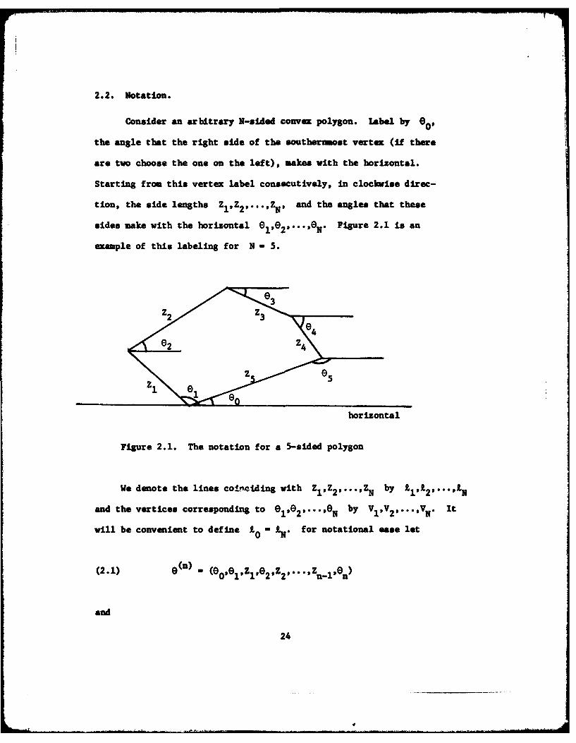
2.2. Notation.

Consider an arbitrary N-sided convex polygon. Label by 0o

the angle that the right side of the southernmost vertex (if there

are two choose the one on the left), makes with the horizontal.

Starting from this vertex label consecutively, in clockwise direc-

tion, the side lengths Z1,Z2,...,Z , and the angles that these

sides make with the horizontal e ,e 2 ,...,ON . Figure 2.1 is an

example of this labeling for N - 5.

3 e3

e4

z1 G

horizontal

Figure 2.1. The notation for a 5-sided polygon

We denote the lines coinciding with Zl,Z2 ,...,ZN by 1,L 2 ,..LN

and the vertices corresponding to el,e 2 ,...,ON by VlV 2 9... ,VN. It

will be convenient to define to0- %. for notational ease let

(2.1) e(n) (e0,el,zl,e 2 ,z2 ,...9Zn- 1 .en)

and

24

. . .. .-

(2.2) z( ) - ( ( n ) , z )

Since

N N(2.3) eN=e 0 -w , 7 z i sine 1 = 0, 0 z cos e = 0-

1-1 -1

N and ( are sufficient to specify any polygon in p** up

to translation. For isotropic pes. we will force e0 B 0, in which

case N and e(N-1) are sufficient to specify a polygon up to

translation and rotation.

We denote the perimeter by S where

N(2.4) S M i ,

i-i

which can be reduced to a function of e(N-1) by (2.3).

If we also consider the polygon to be located in the Cartesian

plane with the origin located at vl, we find the Cartesian coordi-

nates of the vertices useful. These may be related to the e's and

Z's by

i i(Xi,Yi) ( zj cos Z , sin 0

iinl(2.5)

(X0 ,Y0 ) - (0,0)

We denote the area by A. By considering successive areas of triangles

25

and quadrilaterals formed by consecutive sides over the x-axis we

obtain the following convenient expression for A.

2 (I.

This can be related to the O's and Z's by (2.5), and further reduced

by (2.3).

In the sequel we shall be treating much of the above notation

as representing random variables.

2.3. The Curling Process Conceptually

We now proceed to describe very generally the curling process.

Each realization of the curling process is an infinite alternating

sequence of angles and side lengths. As will be seen, from each of

these realizations we can extract one polygon, so that polygons are

a by-product of the curling process Just as they are a by-product of

the line process. However, although our construction of the curling

process is based on the properties of the Poisson line process derived

n Section 1.2, it is Important to regard the two processes as separate

entities.

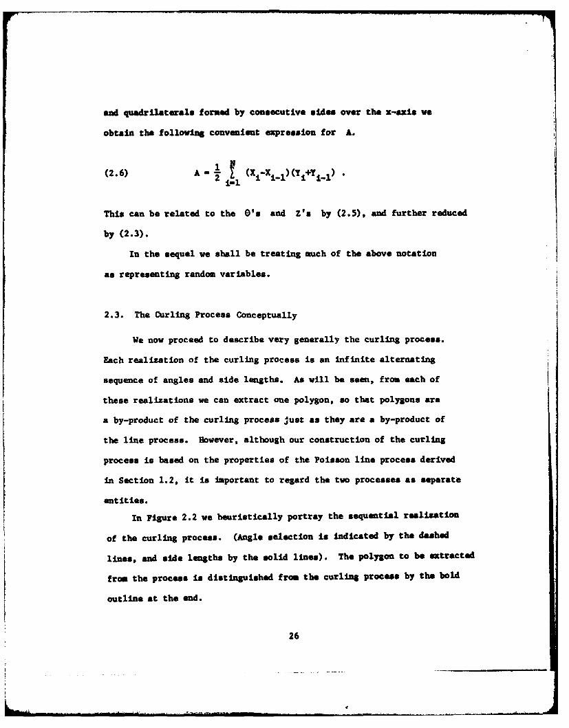
In Figure 2.2 we heuristically portray the sequential realization

of the curling process. (Angle selection is indicated by the dashed

lines, and side lengths by the solid lines). The polygon to be extracted

from the process Is distinguished from the curling process by the bold

outline at the end.

26

S tart OP I~ P lo - dpO o o

POLYGOM

Bad

Figure 2.2

As Figure 2.2 demonstrates, the polygon and the curling process

coincide initially. Because of this coincidence we use essentially

the sane notation for each. That is, the curling process is denoted

by the same sequence

e 0 , e 1 , Z19 e2 ,Z2 ,e3 ,Z3 , ...

corresponding to the polygon notation developed in Section 2.2. It

should be clear from the context which coordinates we are referring

to. Rowever, when ambiguity might arise, or it is necessary to

distinguish between the two, we will put '' over the symbol when

expressly referring to the curling processes. For townple, given

that the polygon to be extracted as N sides, one can conclude from

Figure 2.2 that i-1 is the first coordinate of the curling process

which might depart from the corresponding coordinate %- 1 of the

polygon formed. Specifically, we will define W (or more precisely

27

. . . . . . . ... . ... .. . .. . -. .. .. . . . . ". . . . .. . II N Iii

R-1) as a stopping time so that the first 2N-2 coordinates of the

curling process coincide with the first 2N-2 coordinates of the

polygon, .(N- l) Since the remaining polygon coordinates are deter-

mined through (2.3), the polygon distribution Is obtained from the

distribution of the first 2N-1 coordinates of the curling process.

Just as in Figure 2.2, our development and specification of the

curling process will be sequential. This point of view is simpler,

clearer, and greatly facilitates Monte Carlo simulation. As the

process in highly dependent, ve condition on the past at each step

using conventional conditional probablity arguments. In particular,

we regard the past as a realized sequence pei aining to the selection

of a polygon. The joint distribution of the curling process is obtained

as the product of the derived conditional probabilities. The stopping

time N is determined by the first side length to cross 10. Thus, the

polygon coinciding with the curling process has as its last vertex VNt

the intersection of the curling process with J0* Though the curling

process conceptually continues forever, we will not concern ourselves

with its behavior beyond this stopping time.

In 'he remainder of this chapter we develop the sequential and

joint distributional properties of the curling process. The joint

distribution yields expressions concerning the distributions

of characteristics of members of p'e, which we explore in Chapter 3.

The sequential distributions are the basis of the Monte Carlo siaala-

tion studies in Chapter 4. There we derive some results concerming

simulation of these sequential distributions which are equivalent yet

faster computationally. In this sense the final curling process we

use is defined in that chapter.

28

-±k .. . .. ... .

2.4. The Joint Distribation of 0 and 0 1 - Picking a Polylon Eandomly.

0 1 - (60,91) determies the orientation and size of the southern-

most angle of a polygon. The following proposition apparently first

observed by M. Stone (Wles (1964)), links the distribution of this

angle to the distribution of certain intersection angles, and enables

us to ample a member of p**.

Proposition. In any realization of a line process, there exists a

bijective map between the pointsof intersection of lines and ambers

of the polygon aggregate induced.

Proof. Associate with each polygon, that intersection point corres-

ponding to the vertex which is southernmost. If there are two, choose

the one on the left. This choice is unique. Similarly, associate with

each intersection point that polygon which lies entirely above it. If

there are two, choose the one on the right. This choice is unique. H

(Note that the choice of south is arbitrary here).

Hence to sample a polygon from P**, we need only ample southern-

most vertices which, by the proposition, correspond to sampling northern-

most angles at intersection points. It follows that the joint distribution

of 0 and 0e can be obtained from (1.32) by a symetry argument as

2(2.7) deo Oel(eo,91) - sin(el- 0o ) dG(e 1) dG(8)

for 0 < O < 1 < .

29

As we are interested in specifying the curling process sequen-

tially, we need the marginal distribution of 00 which can be

computed (in principle) for specific nstances of G fron

2.8) F O) A dG(e O) sine O) dG(O)

(2.8) dF 0 x6o 0 sneo

for 00 C [0,W).

Next, givan 0O. 01 Is selected from the conditional density

(2.9) d,1 0 (81) [A sin(-ej )dG(e)] .sin(0 1 -e) dG(e 1 )

for 0<0 < el <I

In the isotropic case, the actual value of 00 will be unimportant

because of the rotational invariance. In this case we begin the curling

process with the angle (O1-0O). The marginal distribution of

0 - (01-01) for isotropic P** is derived from (2.7) as (X - 2w

from (1.34))

dP(O) - sin 0 d6 d6eO - - s in 6 de

Thus, for isotropic P*, without loss of generality we asinine 0 0 0

and begin the curling process by selecting 81 from the density

w-e0

(2.10) dye(81) 6 sin 01 de1

for 0< e01 .

30

4

It Is Interesting to compare this choice of 81 with the naive

gues drF (01) -.1 sin 01 dO1 . This Is tantamount to choosing an

arbitrary vertm In the plane. The sample of polygons so chosen will

be weighted by the number of vertices. This particular aggregate of

polygons are the N-polygons described by Miles (1973).

31

- ....... .. ... ...... .i _ ' -- .. ... --... .... ... .. . : = :I

2.5. The Conditional Distribution for General (nW n').

From (1.24) we know that the conditional density of (enj(n-l))

is proportional to

dnlz (n-l) (n) [in nn- 1 ) Ide n )

(ni

However, the range of support is tricky. (n z(n-1)) is the angle

of Zno the line on which Zn, the next side of the polygon, will

lie. The information conditioned on is that z ( n - l) is already part

of the polygon. This restricts the range of (0njz(n-1)) to be that

where £ does not cut back through the polygon.n

Define d to be the diagonal from v to Vn, and a ton-l n-1

be the angle from d to the horizontal at v . See Figure 2.3.n-1 n

z v

v1 horizontal

Figure 2.3.

32

d n-I

. . . . . . . . ... . . : - . : : . - s . . . .zi 00-00

The range of support is then

(2.11) 0e~ £e n-~n [101

The density on this range is

(2.12) dF (1(e) dF8 I e (8eIzl)n n-(ai

nq -1-i n-)W sin(e - -8)dG(O d

where

(.2.13) q(z U 1 , 0 (n-1)) f 0 jn-1 si( n8) d'(0)OLn-i

and

(2.14) a -tan - n- in x n

where ( ,yn) are the Cartesian coordinates of v n+l given by

(2.5).

(Note: We have written q as a function of two argudents for convenience

in our use of it later).

33I

2.6. The Conditional Distribution for General (ZnJe(n-1)).

We now derive the conditional distribution of the side lengths

in the curling process. We begin with the simple but Illuminating case

of (ZlJ8(1)). By Theorem 1.2.2 and characterization (A.2) (appendix),

the distances between points of intersections along a line in Z, are

independent and identically exponentially distributed with parameter

SX(e), where 6 is the orientation of the line. Thus, the distribu-

tion of Z1I8(n - l) is

(2.15) dF ()(z 1) - TX(81) exp{-rX(8 1)z1)dz1

where z£ [0,-) and x(0 1 ) is given by (1.18).

For the more complicated general case, consider the triangle T

with side lengths dnl, z and d with angle orientation an_l, 0 n

and a respectively. See Figure 2.4.

n-1

Figure 2.4.

34

By Theorem 1.2.4, the number of lines hitting T but not side

d n_ has a Poisson distribution with mean

(zn(n) + dX(c)- dn X ( a n -1 ) )

from (1.27) and using (1.18) and (2.14)

Hence, (see Snyder (1975), Chapter 2), the number of hits along

, the line coincident with z, not crossing dnl is a non-

homogeneous (linear) Poisson process with intensity *(z) where

*(z) satisfies

rz(2.16) r_ tzX(en) +dX (a)-dn I(n1)] a(z)dz

This implies

(2.17) )(z) + [( n ) +I

since d and a are functions of z, and dX() evaluated at z = 0

is equal to dnlX(tn1) .

It now follows immediately from the above, (see Snyder (1975)),

that (zn16(n)), the distance until a first hit through Ln not

intersecting dnl, has density

(2.18) dFznle(n) (zn) = (Z n)exp(- n (z)dzldzn

T [( n) + z ]exp{- j [zx(0n ) +dnX(a. ) - dn_iX(cA ]dznn

with support on z n (0,C).

35

4

We now derive a useful and surprising fact, namely that

ad L(e n)(n(2.19) (zn 2 - X(e) + z I - Tq(z n

where q(z 6~) is defined in (2.13) as the measure of the set ofnP

lines in R 2crossing Z at z n which do not cross dn1l* (2.19)

says that the intensity of the nonhomogeneous Poisson process of hits

along I is proportional to q(z~ e(n ) the measure of 'availablen n

lines at nr

We now proceed to derive (2.19). We begin vith the trigonometric

reduction

-1 Ysil(O-an) sin(6-tan (-) + V)

n

-1 Y-a-in(e-tan (=-))

n

y ncosO -xnsin 0

N2 +y2)1/2

which combined with d~ - (x2 +y2 )1/2 yed

(2.20) d nx (e ) - dnfn sin(e-aa) Ge

n

az +Iw

.- (yncos0 -xnuin 8) dG(e)

By the chain rule,

36

adnX (a) ad n X(a) actn adn.a) n( n3y n d (a ) axn

az a a a axtn n n U n n n

Evaluating the partial derivatives of d n (Z) above via (2.20), we

have

'- n% (yncos e - x sin O)dG(O) n cos e - x sin ejdG(e)

=0

-(ycos - s )dG(e) -f cos 0 dG(O)Y n n n n

et f7

.-- Jn (y cos 8 - x sin e)dG(e) - sin e dG(6)ftn Jct

n CIn nl

where the last two partials follow by Leibnitz's rule. From (2.5) we

have

yz sin On , n cos n

Combining the above we obtain

ad X(c) a+wn - (sin e cos e - cos 6 sin O)dG(O)

= sin(On-8) dG(8) .

37

9-

But then

ad X (ot)*(z) - (A n) +

n

"- [ sin(8-0n)dG(e) + sin(6 -e)dG(e)J2 n n8 +W (8

n nT q- n[+i sin(e-e)dG() +i( ed(~

- 13n

n= q(Z n, e(n) ) ,

which verifies (2.19).

Combining (2.18) with (2.19) we obtain another useful expression

for the density of (ZnO(n)), namely

(2.21) dF (zn) - t ex- 1 [zn A (0 ) + d X V) - dn ) dz

(2.21) fits nicely with the angle density (2.!2) to provide, as we will

see, a substantially simplified joint density.

We rewrite (2.18) one more way which will be extremely useful in

deriving fast algorithms for simulating the curling process in Chapter

4. By (2.18) and (2.19) again,

(2.22) dF (z) T ' q(z ,0 (n)exp{-T Q(z 0 )dzz le(n) n naZn

38

4

where

(2.23) Q(Z q (n) f r' q(z,0O12))dzf

We remind the reader that the support of (2.21) and (2.22) in

39

Owl" I

2.7. The Joint Density of Z (n- The Curling Process.

We summarize and conclude this chapter with the Joint density

of Z .t) This is obtained simply as the product of the conditional

densities

... e F e n i z * dY ( 1 )(n) dF ( 1) (n)

Summarizing the previous results, we have from (2.7)

(2.24) dFO (e 9 si~ -6 2 dG(O ) d0'01 1. si( 1 0) d0 0

on 0< 0< 0 1 <

from (2.12)

(2.25) dFe 1 3jz(n-l)(0fl - (q(z U 1 11 (n-1) ))- sin(O -0n) dG(O n)

on "n-1 < n < 6n

and from (2.21)

(2.26) dF Z e()(z n- ~zn (n))

ezp{( -1 (a X(e ) + d X(O-dX(xn)fldzn

on 0<:z <

40

Thus,

(2.27) dF (n) n') )= -i ( "i(e 1 -e 1 1))

ji-1n

- q(zn, ~n))( dG(ei))( 1 dz i )1-0 i-i

on the set

(2.28) iz(n): 0 < e0 < el < 1r,

O i-I < e l < e i_ 1 i - 2,...,n

0 <- <- .

The support (2.28) can be expressed in different useful ways as will

be seen in Chapter 3.

41

CHAPTER 3

POLYGON DISTRIBUTIONS

In this chapter we take the constructed curling process, and use

it to derive expressions for the distribution of polygon characteris-

tics. As was described in Section 2.3, we use a stopping time to

extract polygons from the curling process. This procedure turns out

to be mathematically convenient as well as efficient for the simula-

tions in Chapter 4. We also define some general families of anisotropic

distributions which are particularly appropriate for the general distri-

butional forms obtained. Finally, in the last section, we suggest some

alternative approaches to obtaining distributional information from the

curling process.

3.1. The Polygon Formed by the Curling Process.

(Here and in the rest of this chapter we shall find it necessary

to distinguish in our notation between the curling process and the

polygon formed. We shall do so by placing a over the curling

process coordinates as described in Section 2.4.)

Selecting 01 and 00 at the beginning of the curling process

is tantamount to selecting t1 and to " N N the two lines coinci-

dent with the first and last edges, a1 and z., of the polygon sampled.

However, whereas the curling process 'travels' over t1 , there is

42

no edge of the curling process on t o . The polygon 'formed' by the

curling process has as its boundary the curling process realization

up to the first Intersection with t o , together with the length along

1 from v 1 to this intersection point. This point becomes the last

vertex of the polygon vN , and the last side of the polygon r.,

becomes this length along t0 from v1 to vN . See Figure 3.1.

-- - v

zl

horizontalv v1

0

Figure 3.1.

4

A 43

I

3.2. The Event {N-n).

N, the number of sides of the polygon formed, is one more than

the index of the first side length of the curling process to cross

1 0* That is,

n--(3.1) N - inffn: z Z sin(G1-. ) < 01

i-i

Precisely, N-1 is a stopping time of the curling process (in the

sequence {(n ,Zn )) of angle and side pairs).

The event {N- ni can be usefully expressed as

(3.2) {N-n) - {N > n-i and Zn-i crosses 1 0

- {N > n-i and 0n-i < 00 and Z"n-l > UU-1

where we define

~ k-i(3.3) Uk - -sec(Ok-GO) i Zi sin(OfG)

i-i

The requirement that in-i < 00 in (3.2) is necessary and sufficientfor Zn-1 to cross t0 when Z n- > Un-l"

We can use (3.2) and the joint density (2.27) to find, in principle,

the distribution of N by

(3.4) PfN ,nl - (-(n)) .

f 4n) Z

44

This integration, as e will see, is in ost cases, prohibitively

difficult to carry out.

We now proceed to describe each set [N-n) in terms of an explicit

range of Z(n-i) (actually wh2 erl) whee the integration in (3.4)

might be carried out. For a - 2,...,n-1, define

(3.5) D t(n) 00 (n):O < i < _1, 0 < zi < for i-,...,.-I

and a1 < 0, 0 < z < um

and < 03<o 0 < z < u for j-m+l,...,n-i

and n-1 < n <0 11

and

(3.6) D(n) O {(n) 0 < e, < e,_l, 0< z, < for i-1,...,n-1

and an < O <61

and

(n1 -1l n1(3.7) D(n_) - D(n-)m-2

(Note: ak is as in (2.14) and uk corresponds to Uk n (3.3)).

45

.1#

Thus

(3.8) {N-n) - D(nl) {(n-1) -1 - zn-1 <

(3.8) follow from (3.2) as can be verited by induction.

An immediate observation from this section is the result that the

distribution of N is in general invariant under changes in the intensity

parameter T. This follows by observing that transforming z! ' Tzi ,

i -1,...,n in (2.27) yields a density not depending on T. Further-

more, the sets N- n) are unchanged by such a transformation as can

be seen by examination of (3.5) and (3.6). The result then follows

from (3.4).

We might remark here about our future notational use of N as an

index. Any variable indexed by N is defined to be that variable

indexed by n on the set [N= n). For example,

(3.9) ( N- 1) = (n-1) * I{N= n)n-3

46

4 ..

3.3. The Joint Density of Z(N) of Polygons.

It was pointed out in Section 2.2 that N and e(N'4) specify

a polygon up to translation since the last three polygon coordinates

ZNl, N and ZN are determined by 9 (N- l) via the relationships

in (2.3). Hence, the distribution of 0 (N-l) is equivalent to that

of Z(N) . We now derive the distribution of 0 (Nl) from the curling

process.

Figure 3.1 illustrates quite clearly that the curling process

coordinates and the polygon coordinates are identical until the

curling process crosses lt at which point they depart. More

precisely we have,

(3.10) (-1) - e(N-) but zN-1 y ZN-1 (w.p.1)

By (3.9) and (3.10), we can specify the density of 0(N-l) by

the densities of 0(nl) on the sets fN-n}. Expressing {N-n}

by (3.8) we obtain

(3.11) dF (8(n-l)) ( J dF (nzl)(z(n-i))(N1) u 0z 1)0n 1 <Z_ < z

n-1l- n-i

(n-1)with support on D

By (2.19) and (2.27) the right side of (3.11) is

47

#I

2 - -(3.12) - - -2

n-2 n-i n-2

* z 1X(0 1i)(. dG( 1))(e dzi)2 - 1 i-O i-i

+ a dn 1 'X(an-I)

Tunl2 ~'n-l + zn-- n-l + n1n-i

The definite integral on the right side of (3.12) is evaluated as

(3.13) -exp{- j [ZniX(6n_) + dnix(en)III,U 1n-

= expf- j [zNIX(eN_)+-.(eN)]}

since

(3.14) on {Nn} , Uni " zN 1 , dn = zN and n-i M eN"

Combining (3.11)-(3.13), we have on {N- nl

(3.15) dF ( (n1) 2 nn1 sin(1-Sil))Tn - 2

(. d( - 1) ( n - i-i

n n-i n-2Mxpf- [ z1 X(ei))l( dG(6))( 1 dzi )

i 1 O i- i

with support on D(n - ).

48

We nov exteud (3.15) to define a general density on IR

which correspords to the density of polygons in p*. This is

simply done by establishing a correspondence between cylinder sets of

R and the events {N-nl. We then obtain dF (N) as dF (N-1) on

those sets and zero elsewhere.

More precisely, let z - (80,e 1 ,ZlO 2 9 z 2,...) denote a point in

CO (n) WDefine Z c NR such that

(n) (n-1) (n-1)(n(3.16) Z(n) {z: 8 (n l) D and z (n satisfies (2.3)1}

Since Z( n ) n Z(m * for n 0 m, and since {N-n} - Z(n), we

have from (3.9),

(3.17) dFz(N)(z) - dF (N-1)(6(n-1)(

That (3.17) contains differential elements of varying length 2N-2

may seem awkward. However, it does express very nicely that the

dimension of the density dFz(N) is varying over the cylinder sets(n)

Z s . This is simply a restatement of the fact that an N sided poly-

gon is determined (up to translation) by 2N-2 coordinates.

We summarize the results of this section by combining (3.15)-(3.17)

into

2 N1N-2(3.18) dF (N)(Z) 2 -Il sin(i-Oi-l))T

Z i-l

N N-1 N-2exp(-- C ( ziX(ei)]1( R dG(Oi))( I dzi)

i-l i4O i9O

49

where z C Z 01 N n.d (N)(z is taken to have support only onz

(n)z-M U Zn-3

We observe an Immediate fact from (3.18) concerning the distribution

of S and A Under Changes in T. The transformation z- M ZLP

i - 1,...,N, yields the distribution of polygons for T - .if we

denote by S(T) and A(T), the distributions of S and A under

intensity T, then this transformation coupled with (2.4) and (2.6)

yields S(T) - 5(1) and A(T) - T2 A(l). Thus, the distribution of

S(T) and A(Tr) are easily obtainable from the distributions of S(1)

and A(l).

50

3.4. The Polygon Density in Isotropic p

For isotropic p *, we have dG(e) - de, from (1.13), and

X(e) E-1 from (1.20). As we mentioned in Section 2.4, we take

90 - 0 and use the marginal density in (2.10) for dFO1. Thus,

the density (3.18) becomes

-O1 N-1 N-2(3.19) dF z (N)(z) = -- ) 1 sin( i-l -ei))

N-2exp{- 1 s)( R deidzi)dN_1i-1

nwith support on Z. (s I iZ as in (2.4)).

By suitable reparametrization the isotropic density (3.19) can

be shown to be the same as the isotropic ergodic density derived by

Miles (1973) [11]. This agreement means that independent realizations

of the curling process yield the equivalent of an i.i.d. sample of

polygons from the ergodic distribution. We should remark that

ergodicity of the Poisson line process implies that the ergodic

distribution of polygons is the same in any p (w.p.1). Hence the**

distribution of polygons in p will necessarily be identical with

the ergodic distribution of polygons in any P* (w.p.1) if the ergodic

distribution is suitably defined.

51

3.5. The Distribution of Polygon Characteristics in Isotropic p,

Before demonstrating how one can (in principle) derive the

distributions of N, S and A in isotropic p*, we remark that

some of the moments of these distributions are known. Some of these

are

E[N] - 4 E[S] = 2T/W E[A] - /T 2

E[N 2] (r 2+24)/2

(3.20) E[SN] - r(w2 +8)/2- E[S 2 ] =2 (i2 +4)/22

E[AN] 7 3/2T2 E[AS] = 4/2T3 E[A 2] W4 /2T4

E[NA2]= w4(8 2 _21)/21T4 E[SA2] = 8w7/21T5 E[A 3] - 4v7/7T 6

(3.20) and other moment results have been derived by R. Miles, D. G.

Kendall, P. I. Richards and H. Solomon with ad hoc techniques. Miles

(1973) and Solomon (1978) contain explicit illustrations of some of

these derivations. Generalizing these techniques to find higher order

moments unfortunately seems to yield irreducible integral formulas. An

example of such difficulty is provided in Appendix A.2 where the author

has derived an integral formula for E[A 4 . It is interesting to note

that E[N], E[A] and E[A2 ] above, agree (after normalization) with

the results derived by Goudemit (1945).

The reasonably simple closed form expressions in (3.20) lead one

to believe that similarly simple analytical expressions exist for the

Joint and marginal distrihations of' N, S and A. To date, as far as

the author knows, no one has succeeded in finding them. We now carry

52

out explicitly some of the 'nanipulations of the density (3.19) to

demonstrate some of what is nown about these distributional forms.

Having already carried out the integration of (3.4) over

in- in (3.13), the distribution of N is expressed from (3.19)

as

(3.21) P{N-nln) dFZ(N)(z)

z (n)

For n - 3, (3.21) becomes

(3.22) P{N-3) - T i 0 1W--O ) sin e1 sin(Ol-1e 2 )

T1 + Cos 2)eXP{- 1 -+]o e sn dz deld .7 -z 1[l+cos 01 sinB 1( sin 82

The exponent in (3.22) is arrived at by the relationship

N N-2 l+cos eN-1(3.23) s - zi = z,[Il+cos ei-sin e1( sin eN '

I=1 I--1

derivable from (2.3) when 80 " 0.

By Fubini, we elect to first integrate out z in (3.22) to

obtain

I 0 sin Olsin e2sin(Ol-e2)

(3.24)sin 2 -sin Ol-sin(6-e2 de2del

Simplification of the integrand in (3.24) requires the trigonometric

identities

53

.. ., . ... . .. . . . . . .

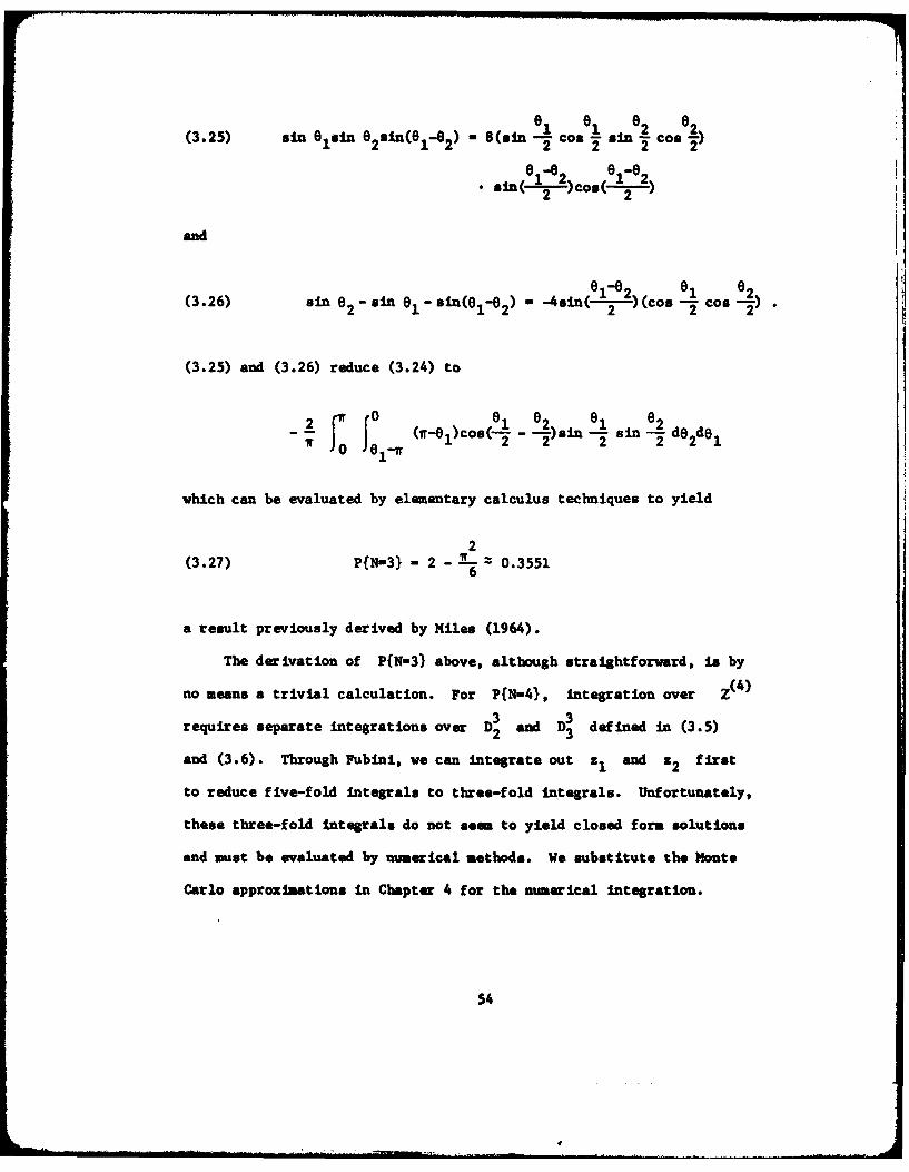
e 1 e2 e2(3.25) sin 8 sn e2 sin(-- 2) - 8(sin - cos e sin i Cos S)

sin co 2 - 1co)81l82 18

and

sin -2 si 2 - 1

(3.26) sin -sin e 1 -sin(e- 2 ) = -4sin(-- -- ) (cos - cos

(3.25) and (3.26) reduce (3.24) to

2 jW JO el 2 1 2

- J(T-el)c°8( -2sin - 2 sin -2 de 2de 1

which can be evaluated by elementary calculus techniques to yield

2(3.27) P{N-3} - 2 - L- = 0.3551

6

a result previously derived by Miles (1964).

The derivation of P{N-31 above, although straightforward, is by

no means a trivial calculation. For P{N-4}, ntegration over Z(4 )

requires separate integrations over D3and D3defined In (3.5)

and (3.6). Through Fubini, we can integrate out z and z2 first

to reduce five-fold Integrals to three-fold Integrals. Unfortunately,

these three-fold integrals do not seem to yield closed form solutions

and must be evaluated by numerical methods. We substitute the Monte

Carlo approximations in Chapter 4 for the numerical integration.

54

The distributions of S and A should be obtainable (in principle)

from (3.19) with appropriate transformations involving tne expressions

(2.4) and (2.6). The author however, has not yet found a transformation

that yields a tractable integral. Miles (1973) is able to derive a

partial result in this direction. He suggests the transformation

5 - * z 2 +t E1 = 2,...,N

which in our case reduces (3.19) to

N-2 N-3 a w-8 N-1(3.28) [(a) s a ds][(-- 1 )( r1 sin(e -

7r W i-l

sin ON-1 N-i N

(2cos e(sin e2 +cot eN-c°S 82) )i3 dei)(- 1 d i)I

Let - (63 ,...,6N_,C 2....,N), so that 0 determines the 'shape'

of the polygon. Given N, the ranges of S and * do not depend on

each other. Thus (3.28) implies that given N, 2TS/w is X2 distri-

buted with 2(N-2) degrees of freedom. Miles also observes that given

N, S and * are independent, inotherwords the perimeter and the shape

are independent within each class of polygons of a fixed number of

sides.

We are able to make one more conclusion from (3.28). Since the

intensity T does not appear on the right, then given N, the distri-

bution of * does not depend on T. But we know from Section 3.2 that

the distribution of N does not depend on T. We conclude that the,*

distribution of 'shapes' of polygons, ip, in isotropic p , i invariant

under changes in the intensity parameter T.

55

. . . . .. .II l l . .. ... . . I I .

I : I :: +" 1' '+ + , -

MIT-

3.6. The Polygon Densities for Families of hnisotropic

Specification of the density of polygons (3.18) for particular

anisotropic P requires dG(O) and )JO) for 6e [0O*f). Given

G, the calculation of ).(e*) is as follows. From (1.18),

xe -Lo Iusin(e-e*) IdG (a)

r8*M Jo (-cos e* sin ()+sin 6* cos e) do~e)

+ J (Cos ~*sin e)-sin e)* cos e) dG(e)e*

Tbus for the indefinite integral

(3.29) F(e) - (coo 6* sin 6- sin 6* cos 6) dG(6)

we have

(3.30) X(OC) -F(1r) + F(0) -2F(e*)

Obtaining F and hence X(O*) in closed form from (3.29) and (3.30)

is not always an easy matt. (121

CWe now propose a family Q of continuous densities on [0,w) which

are general, interpretable and yield X(O*) in closed form. Simple,

expressions for X(O*) give us simpler Polygon densities and make for

simpler, faster and more accurate simulations of the curling process,

56

as we viii see in Chapter 4. Define

(3.31) -{G: G Is of the form (3.32)1

(3.32) dO (6) 1 K i8lain (0-a ) I dO

for e E (0,w), where

(n,m,ct,$) - nm,..Vnlq..Vno'.O)

M c {O,1,2,.o.

(3.33) 1- *. 2 2

iC (0,-)

n

i- i

12rwhere K - sinGe dO J1 O-

m r(d+l1)

The interpretation of G (nm(,)is as a mixture of

n pulses in [O.w) with

tmi -sharpness of the i th pulse

(334 i + i location of the ith ls

01 relative size of th~e i th pulse

Notice that (a .. -a (O, ...O") yields isotropic G. We wite

G 0 for such C.

57

The intuitive interpretability (3.34) suggests that Q-G( 0 ) is

a useful family of alternatives to isotropy, especially for statis-

tical analysis. We show in A.2 of the appendix that q is dense in

the class of continuous probability densities on [0,1] so that

essentially contains all alternatives. Finally, the functions X(6*)

obtained from maembers of q are in closed form as we show below.

Define for general G C Q

(3.35) X (U'U'CL0) (0*) - r0 lain(e-e*)IdG (n'U'L'O) (6)

and for the special case

(3.36) XI(8*) - (1,2.O,1)(0*)

The following relationship substantially reduces the computational

effort for finding general X.

(3.37) 7(n,mQ,B)(6,). - imi

We derive (3.37) as follows

58

i4

K- iO Jsin(6-8*) 1( 0 "sin (0-0t1 )J)d8

" K7I i Bi sin(-e*)llsin i(8-a)l dO

K7 lsin(-(8*-t))lsin ' d6

-K1 n K . (e*-ci)K i K i i

A (m *) and hence general X can be calculated by elementary methods3

from (3.29) and (3.30). (This is a long calculation for large m).

For example,

1 ?(3.38) X1 (:*) " . [(2 - 0*)cos e* + sin 0*]

(3.39) X2 (0*) (cos 2 * + 1)

and

(3.40) X4(6*) - 1- (1 + 2 cos 2 * -_ cos e*)

We also propose the family q D of discrete alternatives to iso-

tropy defined by

(3.41) D _ {G: G has a p.m.f. g of the form (3.42))

(3.42) g(O) P, for i - l,...,I and 0£ £ [0,w)

Consisting of a finite number of discrete pulses or atoms in [0,),

we note that

59

• , 1I

G(i, ,**, ,Lz, 0 1,..., 0],p 1,*...,pz)(e) £ QI '

D

ji m, • • •

so that members of Q D are (pointwise) limits or extremes of members

of Q C. Thus, investigation into anisotropic e* generated by

members of QP is another way of gaining insight into which alterna-

tives to isotropy should be considered. Preliminary modelling by

members of qD would be a strategy to the eventual fitting of members

of 9C.

Calculation of X(O*) for members g c QD is done directly from

(1.18). Because the angles of the curling process pertain only to

intersections between members of S, we need only evaluate x(8*)

at the atoms of g. We have, for g of the form (3.42),

I

(3.43) X( ) - i11 Pitsin(ei-oj) , j - 1,..., I.

1Notice that for the discrete uniform case, (i.e. where pi - for

i 1,...,Z), A(8 ) - X() for all i, j in (3.43). For computer

simulation of the curling process induced by g Q D, we first

compute and store the I necessary values of X(B*) specified by

(3.43).

In Chapter 4, we carry out a simulation study of anisotropic

**C Dp induced by some of the simpler members of Q and D

60

We close this section by remarking that analogous to the moment

results In (3.20), Miles (1964) provides the following known first

and second order moments of N, S, and A in the general anisotropic

case.

E[N] - 4 E[S] - 4/XT E[A] - 2/XT2

(3.44) E[N 2] - An +12 E[A 2 ] - 4/XT2

E[SN] - 2(Xn+4)/AT E[AN] = 2nl/T 2 E[AS] - 4rn/Ar 3

where

(3.45) A o - (e) dG(e)

as in (1.31) and,

(3.46) = o [A()]-2 dO

61

3.7. Extensions of the Curling Process.

As we have seen in this chapter, the integral expressions obtained

for the joint distribution of the angles and side lengths in the general

case (3.18) and even in the much simpler isotropic case (3.19) are

too unwieldy for deriving the distributions of N, S or A. The approxi-

mate answers obtained by the simulation in Chapter 4 are a partial solution

to this difficulty. However, it seems that more tractable expressions

may be obtainable by exploiting the curling process in alternative ways.

We mention some of these alternatives in this section, and suggest possi-

ble directions for future work.

The most obvious extension of the curling process is to use other

stopping times. For example, by stopping at the crossing of 1 (after

it), the curling process samples two adjacent random polygons. Other

stopping times sample more complicated combinations of polygons. Inves-

tigation of these related polygons would yield information concerning the

association among polygons. Furthermore, the unions of adjacent polygons

form other polygon aggregates. Miles (1973) has shown that the distribu-

tions of polygon characteristics in these aggregates correspond to certain

weightings of the distributions in p . [12] Different stopping times

for the curling process enable us to explore these aggregates.

Another alternative is to skip selection of the initial angle,

(0 in the anisotropic case and 01 in the isotropic case), and to

begin the curling process with the next variable, (01 in the aniso-

tropic case and Z in the isotropic case). Indeed, careful examination

of the conditional densities of angles and sides in (2.25) and (2.26)

62

reveals that these densities are independent of the initial angle. The

distribution of 0, or 01 in the isotropic case, applied to this

process would yield relationships among the probabilities in the distri-

bution of N. Presumably, these relationships would be similar to the

recursive integral equations alluded to by Miles (1964, 1973).

Finally we mention a method to exploit the invariance of the

distribution of N under changes in the intensity T. In the appendix,

we show that this invariance yields a relationship between the distribu-

tion of N and the probabilities of splitting a random N-sided polygon

by a random secant into a J-sided and an (N+4-j)-sided polygon. If

the procedure to select a random secant could be incorporated into the

curling process, it would be a valuable tool for the investigation of

these splitting probabilities.

63

CHAPTER 4

MONTE CARLO SIMULATION OF POLYGON CONSTRUCTION

As we saw in Chapter 3, the expressions derived for the distribu-

tions of polygons in 63" are not manageable enough to obtain useful

forms for the distributions of polygon characteristics of main interest

namely N, S and A. In this chapter we demonstrate the real strength

of the curling process, to efficiently select an independent and

identically distributed sample of polygons from P*.

4.1. Previous Studies.

Two previous Monte Carlo studies by Dufour [14] and Crain and

Miles (1976) have been aimed at approximating the distributions of

N, S and A in the isotropic case. Some of the estimates from

these studies are presented in Tables 4.1 and 4.2 at the end of this

section. In both of these studies, the simulation consisted of first

simulating a Poisson field of lines in a fixed bounded region, and then

extracting the polygons circumscribed by the lines in this region. For

comparisons, we shall refer to this type of construction as the grouped

method, and to the curling process construction as the sequential method.

In this section we discuss how several drawbacks of the grouped

method are successfully avoided by the sequential method. We first

compare speed and efficiency, and then examine some estimation issues.

Crain and Miles also address these estimation issues and deal with them

as effectively as possible within their constraints. They even point

out how some of the stochastic constructions of polygons described

in Miles (1973), which possess the independent identically distributed

sampling properties of the sequential method, would avoid these

problems.

64

First of all, the sequential method is substantially faster and

requires far less computer memory than the grouped method. Dufour's

analysis processes 947 polygons formed by 65 random lines. The

information concerning Dufour's effort is unavailable, but the small

number of polygons he analyzed suggests his methods were slow. The

analysis by Crain and Miles processed 200,000 polygons in 66 sample

discs. [15] They used about 15 hours of computer time on an IBM 360/50,

a processing rate of about 200 per minute. They also required 180K

bytes of memory just to store the information on each sampled disc.

With the sequential method, we are able to process, in the isotropic

case 2,500,000 polygons on a PDP 10/KI in just 4.76 hours, a rate of

8745 per minute. Furthermore, storage is minimal because polygons can

be dispensed with as soon as they are processed. Adjusting these

figures for the machine differences [16], we estimate that compared

to the method of Crain and Miles our method is about 22 times faster

while requiring virtually no storage. These differences in effi-

ciency are probably due to the fact that the grouped method algorithms

spend the bulk of their time searching for polygons, while the sequen-

tial method algorithms compute each polygon quickly as it is needed.

It is interesting to note that Crain and Miles surmise that the sto-

chastic constructions they suggest would require the same magnitude

of computer effort per polygon as the grouped method.

The next comparisons concern estimation. The polygons generated

by the grouped method are dependent in each region sampled. As a

result, assessment of the precision of estimates is nontrivial since

65

the dependency is rather difficult to assess. The curling process

on the other hand, by providing an i.i.d. sample, enables straight-

forward estimates of accuracy based on standard statistical methods.

It can be argued that the grouped method provides more information

such as estimates of the rate of ergodic convergence or the amount

of dependency. Some of this information could be provided by the

extensions of the curling process discussed in Section 3.7. However,

due to the complexity of this type of information, we do not pursue

it further.

Another problem that the grouped method must contend with is

edge effects. That is, the boundary of the region sampled will

necessarily intersect those polygons lying at the edge. The portions

of these polygons lying outside the region are unobserved. To deal

with this problem, one can undersample: exclude those polygons 4rom

the sample; or one can oversample: include those polygons together

with estimates of their unseen properties. Crain and Miles use under-

sampling, and devise sophisticated techniques for weighting the ample

to overcome bias (see Miles (1974)). There are no boundary constraints

on the sequerttial method.

The last estimation issue we look at concerns the relationship

of estimates to the intensity of the process. The grouped method

essentially samples a Poisson field in a fixed bounded region as follows.

First n, the number of hits, is selected from a Poisson distribution

with intensity r. Then n uniform random secants through this region

are selected.

66

A subtle conceptual estimation problem is involved with this method.

Namely, given n, the lines are more likely to case from a Poisson

line process with the intensity of the maxinm likelihood estimate

of T. The question then arises as for which intensity of a Poisson

line process does the sampled region give the best estimates? This

problem affects distributional estimates for S and A, whereas

the distribution of N, as we shoved in Section 3.2, is invariant under

intensity changes. We do not face this problem with the sequential

methods.

Probably because of the computer effort involved with the grouped

method, previous Monte Carlo studies have focused exclusively on the case

of most interest, isotropic p . The amount of extra computer effort

required to extend the sequential method to the anisotropic case is

small. The processing rate decreases to 5708 per minute in the slowest

case we analyzed. The value of estimating the distributions of polygon

characteristics in anisotropic p** is that these distributions are

the alternatives to isotropy which must be considered when devising

statistical techniques for analysis.

67

Ii

TABLE 4. 1

MONTE CARLO STUDY DY S. DUDFOUR

ISOTROPIC POISSOIN FIELD SAMPLE SIZE 947INTENSITY T-1

SAMPLE PERCENT ILES

PROB(N -n)

1= 3 4 5 6 7

.36 .38 .19 .054 .010

PROD(S < %)

sm .5000 1.000 2.500 5.000.05 .11 .26 .51

s-7.500 10.00 15.00 20.00.67 .79 .92 .98

PROD(A < a)

-. 5000Q-1 . 1000 . 2500 . 5000 . 7500.13 .18 .27 .38 .45

a 1.000 2.500 5.000 10.00 15.00.50 .67 .90 .90 .95

68

TABLE 4.2

SOWE MONTE CARLO ESTIMATES OF CRAIN AND MILES C163

ISOTROPIC POISSON FIELD SAMPLE SIZE 200000

VARIOUS ESTIMATES OFPROB(N - n)

n- 3 4 5 6 7*STD .3541 .3781 .1923 .0589 .0132+STD .3558 .3759 .1889 .06075 .01296

*WTD .35561 .37790 .19183 .05922 .01318

WTD .35514 .37774 .18896 .6075 .01294GRF .355066 .381374 .189829 .058653 .012714

CRF .355066 .379904 .190732 .059129 .012607

no 8 9 10 11 12*STD .00188 .000262 .000015+STD .00210 .000297 .000025 .0000032 .0000024*WTD .001958 .000248 .000038

+WTD .00208 .000291 .000024 .0000024 .0000025QRF .002071 .000265 .000027 .0000024 .00000017CRF .001958 .000230 .000021 .0000015 .000000086

69

.ini *~ i

4.2. Fast Simulation of (Z,'e)n+ ) IS •

(Note: We now drop the '-' notation for the curling process).

In this section we derive a simple and fast procedure for samula-

ting the conditional random variables Z nlen and 0 n+l z(n) in the

curling process. This procedure is not only the basis for the efficiency

of our simulation, but also lends substantial insight into the process

of conditional hits in a Poisson field. To derive it from the curling

process, we use the following theorem which shows quite clearly how

linear Poisson processes of varying intensity arise from random censor-

ing of linear Poisson processes of constant intensity.

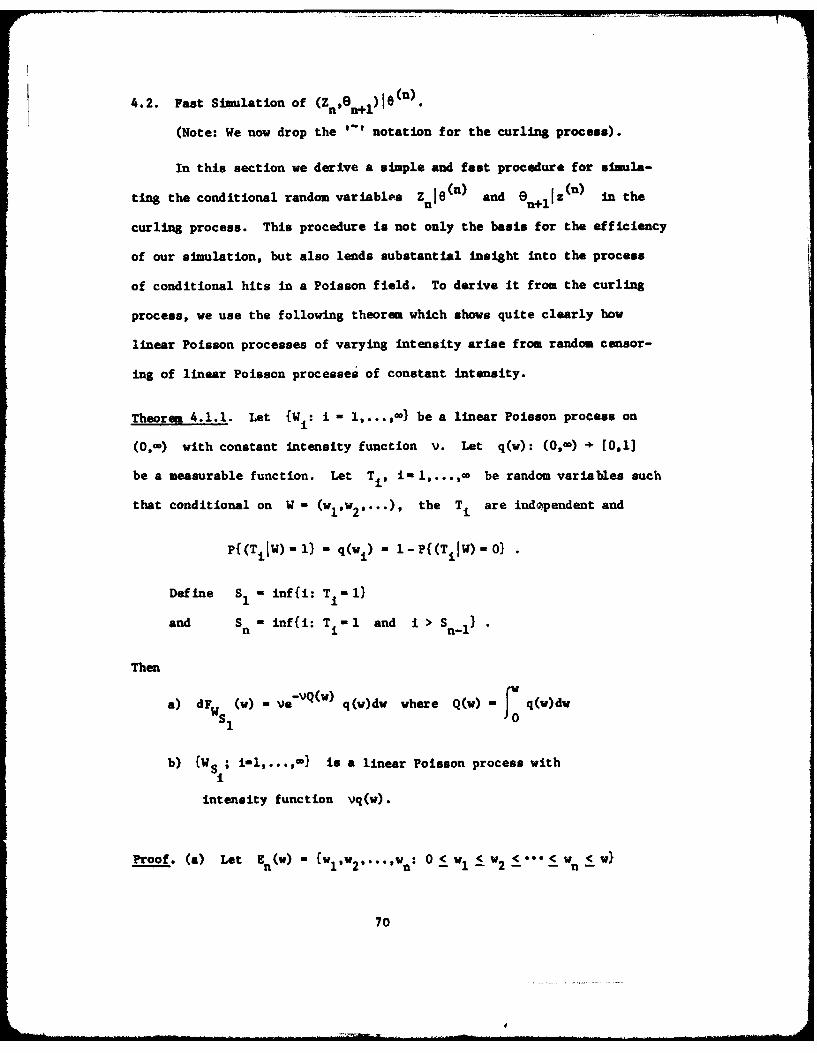
Theorem 4.1.1. Let {Wt: i - l,...,0 be a linear Poisson process on

(0,M ) with constant intensity function V. Let q(w): (0,-) 4. [0,1]

be a measurable function. Let Ti, i l,...,oo be random variables such

that conditional on W - (wlW 2 ,...), the Ti are independent and

P{(TiJW)"=l) - q(w1 ) - 1-P{(TilW)=O}

Define SI - inf{i: Tim 1}

and Sn - inf{i: Ti m 1 and i > S_1)

Then

a) dFW () - Ve- VQ(w) q(w)dw where Q(w) " q(w)dwS1

b) {WS i; i-l,...,} is a linear Poisson process with

intensity function vq(w).

Proof. (a) Let En(w) 1 fWlV2,...,n : 0 < wI < w2 wn < w}

70

()- P[S1.n and W < w)

ni r()il re- v- 1 )1~ q dlv)"

where we define wo 0. By the Fubini theorem, we have

rV~nn-l n-i

ve q(w)n1 1- wdnmi 0 N) fE -l ( TI l-qi w) )dvldw2... n1 w

By symmetry,

wr-xVW n-ie nI qI V

- l 0~v n~~ (n-i)!

n-iTI (l-q(w 1 ))dw 1dw 2 -*dwni ldw n10<W <w i-i

Again using Fubini,

1n~ (w ye n ) Lni-:( 10 (1-q(w ))dw 1)dw

Ve' q(w) [(ivw~)l

By monotone convergence (and replacing the dummy variable w n by v

for visual ease),

71

0 v n-0 j

TO f V , q(v) eVv-Vq (v) dv

- -VQ v) 0 ieVQ W)

(a) follows by differentiating.

(c) By exploiting the independence of the WHi's (Bee (A. 2)), and

the conditional independence of the T i'a, the argument in (a)

generalizes to yield the joint density for

o (W S***.Hs

as

nn -VQ(v 5dFW (w W v(I q~w )e n dw(n

(n)) a- a n

the desitad joint density. ~

Now recall that the conditional density of (nie (n) ), (side

length in the curling process), was derived in Section 2.6, (2.23),

as

(4.1) dF nj(n) (z) d Tq(z,.e (n) )exp{-17Q(z U.80n))1dz n

72

where q(z ,n ) and Q(zn e(n)) are defined in (2.13) and (2.24)

respectively. Referring to Figure 3.1, intuitively z is the dis-

tance from vn along Iu to v n+ given that ZU+l does not cross

back through the polygon being formed.

n /./7 -" n+l

horitzontal

Figure 3.1.

We make the following tidentifications with Theorem 4.1.1. Let

W } correspond to the point process of hits along £u starting

I n

from v unconditionally, i.e. as if i n were an arbitrary line

in Z. By Theorem 1.2.2, (W1) is a linear Poisson point process

with constant intensity

(4.2) v r( n)

73

Associate with each point W i the angle 0 1 that 9, makes

with the intersecting line. The angles 0 1 are i.i.d. with the

density

(4.3) dF($ i) - (A (O ) sin(e n-O)dG(O) for *c (e n-w,e n)

given by (1.22) from Theorem 1.2.3. From Section 2.5, would be

a 'legal' candidate for 8 +1 if *i (C NPO) where a i corresponds

to the angle of the diagonal from v1 to W i as ini (2.11) and (2.14).

I %.

I ~l

011

v horizontal

Figure 3.2.

For exaple in Figure 3.2, 01 is not 'legal' but * 2 is.

Def ine {1 if 0 iE (aitin)Ti if 01i (Mi'On)

74

Then from (4.3) and (2.13), P{TLIW} - q(wI) where

(4.4) q(wi) " )(en)-i J dF( i)

(w.O (n) )

x .(0 n)•

Combining (4.2) and (4.4) with Theorem 4.1.1(a), we observe that

(4.5) dFw (w) - V exp{-VQ(w)lq(w)dwSI

- Tq(w,B (n) )expf-TQ(we (n) )}dw

which is precisely the same density as dF in (4.1). Further-

more, the independence of the O.'s allows us to infer that

-3.

(4.6) dF OIva 1s( ) - ((q(ws ' (n))) sin(en- )dG(O)

for *C (atson), precisely the density dF (n) given by

(2.12). n+11

We summarize the above results in the following theorem.

75

Theorem 4.1.2. Let VV2.. be i.i.d. with exponential density

(4.7) dF(v) - TA(0n)eXpf-TX(8n )v)dv , ve (0,0) .

Let 1,02.... be i.i.d. (and independent of the Vi's) with density

(4.8) dF( ) = ((0n))-i sin(O n-)dG(0) , * (6 -w,0n)

Let

T - inf{i: 0 C (CL, n)}.

TThen Zn " i and On+, - OT have the bivariate conditional densityi-1 +

(4.9) dF (znn+) = T sin(n -n+)z n E) (n) n n+l n n+l

(nexpf-TQ(z(n ) 6 dG(O n+l)dz

onz (0,-), (anOnn n~l n nononl Zn £(,0, 0+1 nen:.

(Note that the joint density appearing in (4.9) is obtained as the pro-

duct of (2.12) and (2.22)).

In the following flow diagram we illustrate the ease with which

Theorem 4.1.2 enables us to simulate Z and n+1 . The particular

techniques for simulating V, and 0, in the middle steps are dis-

cussed in the next section.

76

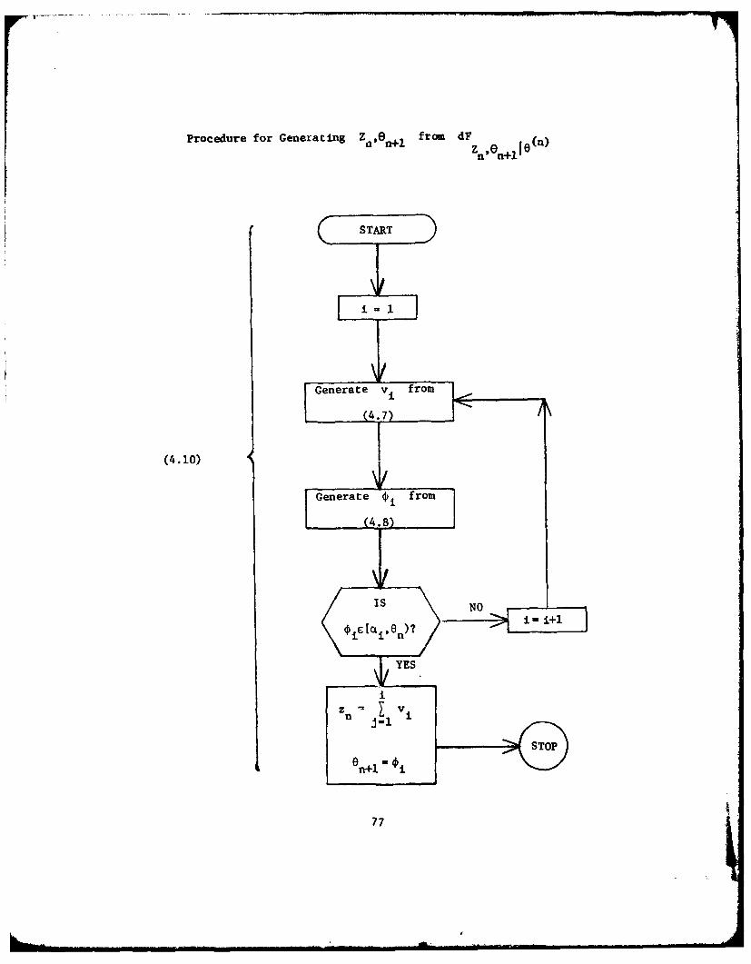
Procedure for Generating Z a0 , from dF n l ()

Gee t e v~ from

(4.10)

)eerate4fo]

IS NO

n )? i-Mi+1

YES

STOP

0 n+1 '

77

We remark that a particularly nice programming feature of the

procedure (4.10) is that we require only xn-lyn~-v (see (2.5)),

and 0n from O(n) for the calculation of X(On ) and the bounds

(CiOn), (see (2.14)). As discussed in Section 4.4, this information

is easily and necessarily stored sequentially during execution of the

main program.

78

4.3. Some Simulation Techniques.

Our computer system provides, as do most computer systems, a fast

routine for generating an independent sequence of uniform [0,1] random

variables, which we shall denote by ElE2, . [17] To generate a

general independent sequence of random variables fl,n2 ,... with distribu-

tion function F, it is well known that we can simply take i F

How well this works in practice depends on the ease with which we can

invert F.

To generate Vi in (4.10) we simply take V, = (TX(n))-I log

as the exponential distribution (4.7) is easy to invert. The difficulty

of simulating Zn! 8 (n) directly from the distribution induced by the

density (2.18) should be apparent. Inevitably it would require evalua-

t(on of A-(E) where A(z) - [zX(en)+dnX(a n)-dn i( nal)],

calculation hopeless by analytical methods and very long by numerical

methods.

The generation of 0 in (4.10) takes a bit more doing. Although

in the isotropic case the distribution (4.8) is easy to invert, in the

anisotropic case this is not generally true. To get around this problem,

we resort to an old-fashioned simulation method, the general rejection

technique. An informative discussion of this technique, apparently

introduced by von Neumann, appears in Butler (1956).

We describe our application of the rejection technique to the

simulation of 01 with the flow diagram below. We first need the

following notation. Rewrite the density (4.8) of 0 as

79

- , = T ' '

: . . . . .. . . . .. .

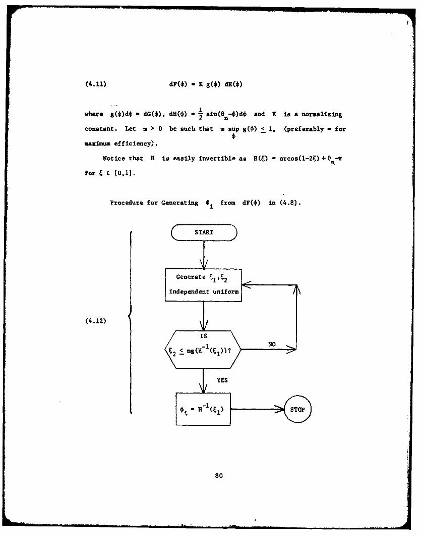
(4.11) dF(O) - K g(O) dH(O)

1

where g(O)dO = dG(O), dH(O) --I sin(On-)dO and K is a normalizing

constant. Let m > 0 be such that m sup g(O) <1 , (preferably - for

maximum efficiency).

Notice that H is easily invertible as H(E) - arcos(1-2E)+ 8 -w

for C C [0,11.

Procedure for Generating 0 from dF() in (4.8).

Generate Ei,2

independent uniform

(4.12) 4/is

-l NOt21 mg(H-1(El))?' 0 "

-1-H STOP

80

This technique seems to work quite well as long as g - dG is not

too variable. However, if it is very variable and G"1 is readily

obtainable, we can reverse the roles of H and G in (4.9) to

achieve greater efficiency.

To show that the density of the fi generated by (4.12) is correct

simply notice that

PE 2 < mg(H- (Y))l ) cc g(k-l(al)) .

Since E is uniform on [0,1], the density of -1 ( ) is

dF(f) - g( ) dH(f)

agreeing with (4.11).

We use the same general ideas for generating 00 and 61 from

the joint density dF8 0,6 appearing in (2.7). First we generate

n0 with density dG, by taking G-1 () if C-1 is easily obtainable,

or by (4.12) with dH S 1. Then we generate T11 by (4.12) with

H-( ) - arcos(1-2E) + n0 . Finally, we obtain eo - min(noPq) and01 imx(n0,ni).

81

As -

4.4. The Simulated Curling Process.

We present in this section the flow diagram out.Ujing the pro-

gramming steps for the generation of each random polygon by the curling

process. The steps at which 00,01 and (Zn' n+l) are generated,

incorporate the methods developed in Sections 4.2 and 4.3. We Implement

these methods as subroutines in our program.

As each polygon is generated we need to output N, S and A for

computing the statistics we tabulate. Each of these polygon characteris-

tics can be obtained by incrementing partial sums as each side length

and angle (z n, n+) is generated. In the flow diagram we will use

the following notation for formulas required to compute and save partial

information during execution. This notation corresponds to (2.4), (2.5),

(2.6), (3.1) and (3.3) which are necessary for the calculation of N, S

and A.

nxn z cos E IiUl

nYn" I zisin0en

n-i(4.13) Un " -sec(en-o) isin(e0'eo)

nn il Zn

a n (yi-_ ) (X ,YO ) (0,0)1-8

82

II

In the last branch of the construction, after N has been obtained,

we compute z: 1_, 6 N and zN from (4.13) via (2.3) as

zN-i N- U

8N -e 0 -76N 60

2 +2 1/2

83

I54~

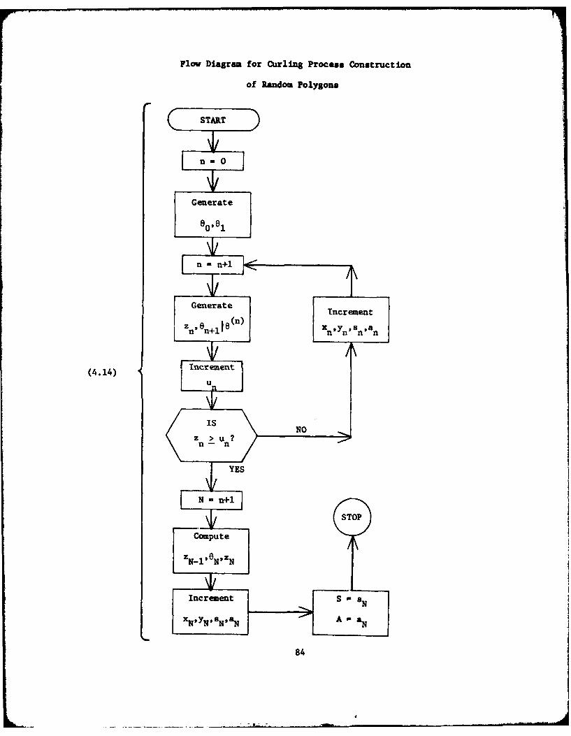
Flow Diagram for Curling Process Construction

of Random Polygons

START

n-O0

Generate

(4.14)Inrmt

u8

4.5. Simulation Results.

In this final section the results of a Monte Carlo investigation

of the distributions of N, S, and A in various p by simulation

of the curling process, are presented In three subsections consisting

of the isotropic case, some anisotropic cases induced by members of

C d sorpcDnd some anisotropic cases induced by members of D The

intensity of the Poisson field is kept at T - 1 in all the simula-

tions. The related distributions for different intensities follow

immediately from the observations made at the end of Sections 3.2 and

3.3.

Three tables are presented for each case. The first table presents

sample percentiles. The second presents sample moments, the estimated

standard error of the estimates, and the numerical values for some of

the known moments given in (3.20) and (3.38). These are provided for

an assessment of the numerical accuracy of our computing facilities.

The last table lists characteristics of the twenty five largest polygons

(in area) sampled. Included in this list is the isoperimetric ratio

I - S J4A for each of these polygons. The well known isoperimetric

inequality states that I > 1, with equality holding only for a circle.

Thus I is a measure of the circularity of a polygon.

4.5.1. The Isotropic Case.

Tables 4.3a-c present the results for the isotropic case. Being

the case of primary interest in the literature, a sample size of 2,500,000

polygons was simulated with the goal of obtaining the most precise esti-

mates of the unknown distributional characteristics to date. Fortunately,

85

the simulation rate of 8745 polygons per minute, was the fastest of

the simulations. This was probably due to the fact that angle simula-

tion here did not require the somewhat inefficient rejection technique

discussed in Section 4.3.

The width of the 99Z confidence band about the sample distribution

function induced by the percentile estimates in Table 4.3a is obtained

from the familiar Kolmogorov statistic as .00103. (Hence the band for

the N probabilities given is .00206). The estimates for N provided

by Dufour, and Crain and Miles in Tables 4.1 and 4.2 are close but not

always within these limits. It is comforting to compare the estimate

.3552 of P{N- 3} with the known theoretical value of .3551 derived

in (3.27).

The sample moments presented in Table 4.3b seem to be extraodinarily

accurate. Indeed, the estimates of the known moments are in every case

within half of a standard error of the true value! Thus, there is every

reason to believe that the estimates of the unknown moments are similarly

accurate and can perhaps be useful in the pursuit of the theoretical

values.

The largest polygons (in area) sampled are listed in Table 4 .3c.

The initial motivation for providing this list of extreme values was

to investigate a conjecture by D.G. Kendall 119] that IIA 1 as

A - - , that the largest polygons in area tend to be circular. The

isoperimetric ratios in the table do not appear to be getting smaller

though it is perhaps unreasonable to expect that this sample size

emulates what happens near infinity. What this facinating conjecture

does bring to mind however, is whether or not the large polygons are

86

many sided. It is interesting to note that of the 53 polygons with

10 or more sides in the sample, none appeared in this list. Finally,

if idall's conjecture is false, the next question to ask is, to

what value does IIA converge as A + m if it converges at all?

87

!I

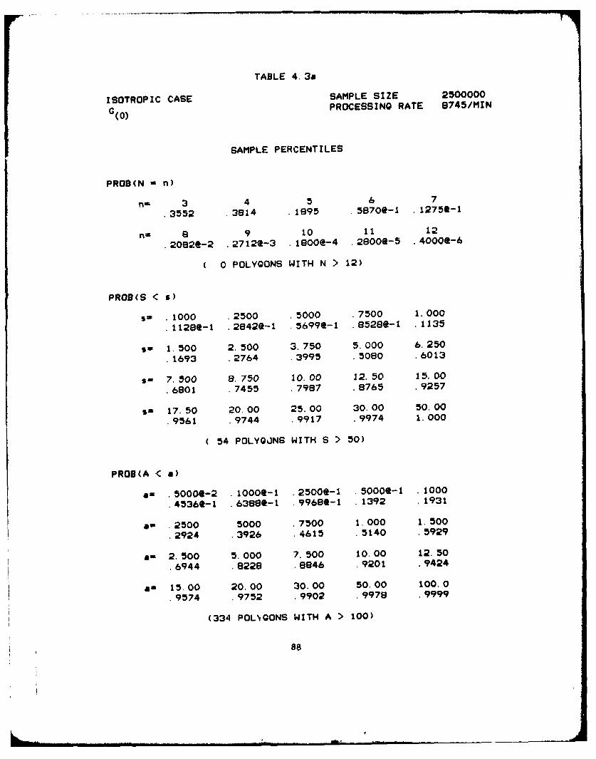
TABLE 4. 3a

ISOTROPIC CASE SAMPLE SIZE 2500000

(0) PROCESSING RATE 8745/MIN

SAMPLE PERCENTILES

PROB(N - n)

n= 3 4 5 6 7

.3552 .3814 .1895 .5870*-1 .12750-1

n 6 e 9 10 11 12

.2082@-2 .27122-3 .1800@-4 .28000-5 .40000-6

( 0 POLYGONS WITH N > 12)

PROD(S '< £)

s- 1000 .2500 .5000 .7500 1.000

.1128-l .28422-1 .5699e-1 .8528-1 .1135

s- 1.500 2.500 3.750 5.000 6.250

.1693 .2764 .3995 .5080 .6013

s- 7.500 8.750 10.00 12.50 15.00

.6801 7455 .7987 .8765 .9257

s- 17.50 20.00 25.00 30.00 50.00

.9561 .9744 .9917 .9974 1.000

54 POLYGONS WITH S > 50)

PROB(A < a)

a- .50000-2 . 1000t-1 .25000-1 .50000-1 .1000

.4536Q-1 .63880-1 .99680-1 .1392 .1931

a- .2500 5000 .7500 1.000 1.500

.2924 .3926 .4615 .5140 .5929

a- 2.500 5.000 7. 500 10.00 12. 50

.6944 .8228 .8846 .9201 .9424

a- 15.00 20.00 30.00 50.00 100.0

.9574 .9752 .9902 .9978 .9999

(334 POLNGONS WITH A > 100)

88

TABLE 4.3b

ISOTROPIC CASE SAMPLE SIZE 2500000G(0) PROCESSING RATE 8745/MIN

SAMPLE MOMENTS

N S A

IST MOMENT = 3.99980 6.28409 3.14061(STD ERR) .6116e-3 .34010-2 .39340-2

2ND MOMENT = 16.9336 68.4150 48.5634(STD ERR) .54902-2 .77040-1 .2052

3RD MOMENT = 76.0337 1028.67 1718.34(STD ERR) .39776-1 2.073 23.32

4TH MOMENT - 362.110 19520.2 107669.(STD ERR. .2768 66. 18 4225.

5TH MOMENT - 1826.58 444941. .103294@8

(STD ERR) 1.954 2665. .9695@6

6TH MOMENT = 9735.80 .11801608 .136291@10(STD ERR) 14.32 1192@6 .248309

KNOWN MOMENTS

N S A

IST MOMENT - .00000 6.28319 3. 14159

2ND MOMENT - 16.9356 68.4438 48.7045

3RD MOMENT - unknown unknown 1725.88

89

TABLE 4.3c

ISOTROPIC CASE SAMPLE SIZE 2500000G(0) PROCESSING RATE 8745/MIN

THE 25 LARGEST POLYGONS (IN AREA)

I =ISOPERIMETRIC RATIO

RANK N S A I

1 8.000 64.71 285.0 1.1692 6.000 61.95 243.8 1.2523 9.000 59.18 219.1 1. 2724 7.000 55.94 206.1 1.2085 6.000 54.77 203.0 1.1766 6.000 57.20 199.3 1.3067 8.000 55.2 193.4 1.2558 8.000 54.20 192.6 1.2129 6.000 57.89 187.6 1.42110 7.000 51.27 185.8 1.12611 8.000 53.92 184.6 1.25312 9.000 53.65 181.2 1.26413 9.000 50.17 180.3 1.11114 6.000 62.70 177.4 1.76315 6.000 52.98 172.2 1.29716 6.000 58.73 171.2 1.60317 7.000 50.21 170.8 1.17418 9.000 53.00 169.4 1.31919 8.000 50.50 168.4 1.20520 8.000 52.30 166.7 1.30621 7.000 53.74 165.6 1.38622 8.000 53.02 165.2 1.35423 7.000 48.07 163.9 1.12224 7.000 54.43 160.9 1.46525 5.000 49.71 159.0 1.237

90

I ~~SEQUENTIAL STOCHASTIC CONSTRUCTION OF RANDOM POLYGONS AS b STNODUIV C ETOFSAITCS) e1/

IJUN 82 E I GEORGE N00014-76-C-0475

UNCLASSIFIED TR-32 0 NL

I ImhhhhhmhEhEEEEEEE2 E".'

C!4.5.2. Anisotropic Cases Induced by QC

Tables 4.4a through 4.7c present the sioulation results for

anisotropic cases induced by the following four members of QC.

dG(2 oll, 2 0 ,)(e) - (2w)-l(1 +1 sin O)de

d(2,0,2,1,2,0,0) (8) - (2w)- (1 + 2 sin 28)dO

dG(2 0 4 1 8 / 3 0 0 )(0) - (21r)- (1+ (8/3)sin4e)dO

dG(2 4,4 0 , 3 )(e) _ 1 (sin4e + sin4(e d8

The first three distributions are mixtures of the uniform with

progressively sharper pulses. In each case the pulses are weighted

so as to contribute half of the total probability to the mixture.

The last case is a mixture of two sharp pulses located at a distance

of 7r/3 from each other. The functions X(e) for each of the

distributions are obtained from (1.20) and (3.37)-(3.40).

The purpose of these simulations was exploratory so that sample

sizes were kept to 100,000, far smaller than the 2,500,000 for the

isotropic case. The simulation rate for the first case was 7211

polygons per minute and decreased to 5708 per minute in the last case.

Ostensibly, this decreasing rate was primarily due to increased Ineffi-

ciency of the rejection technique for simulating the angle distribution

with sharper pulses. Nonetheless, this slowest case is still quite

fast as it took only a total of 17.52 minutes of cpu time.

Turning Immediately to the tables of sample moments in each of

these cases, we see that the accuracy of the simulation is breaking

91

4E

down. For example, estimates of EN] are underestimated by several

standard errors In every case. Extensive investigation into this

discrepancy revealed that the problem is due to numerical rounding

error which accumulates in the less stable anisotropic cases.

Correction of this Inaccuracy would require the use of a more accu-

rate programing language. [20]

In light of these numerical problems, the high precision from

our sample size is Irrelevant. Nonetheless, the estimates themselves

are close enough to the true values so that general information about

the nature of the distributions of N, S, and A in these anisotropic

cases can be gleaned from the results. Also, the Inaccuracies are less

severe for the estimates with S and A. Rather than go nto a lengthy

analysis of these results, we observe that none of these cases differ

markedly from the isotropic case.

92

TABLE 4. 4a

ANISOTROPIC CASE SAMPLE SIZE 100000G(2 ,0,1,1,w/ 2 ,0,0) PROCESSING RATE 7211/MIN

SAMPLE PERCENTILES

PROB(N - n)

n- 3 4 5 6 7.3580 . 3815 .1892 . 56610-1 . 1224t-1

8, a 9 10 11 12.20500-2 .33000-3 .50008-4 .0000 .0000

( 0 POLYGONS WITH N > 12)

PROB(S < s)

s- .1000 .2500 .5000 .7500 1.000.10690-1 .27062-1 .55160-1 .83780-1 .1122

s, 1.500 2.500 3.750 5.000 6.250.1668 .2734 .3943 .5018 . 5944

s- 7.500 8.750 10.00 12.50 15.00.6731 .7394 .7930 .8714 .9225

s- 17.50 20.00 25.00 30.00 50.00.9534 .9728 .9907 .9971 1.000

( 4 POLYGONS WITH S > 50)

PROB(A < a)

an .50000-2 .10000-1 .25000-1 .50000-1 . 1000.43760-1 .62690-1 . 99580-1 . 1389 . 1920

an .2500 .5000 .750 1.000 1.500.2900 .3902 .4589 .5115 .5903

an 2.500 5.000 7.500 10.00 12.50.6919 .9208 .s32 .9192 .9416

am 15. 00 20. 00 30. 00 50. 00 100. 0.9566 .9746 .9901 .9978 .9999

15 POLYGONS WITH A > 100)

93

L " *L .... .* , -- r ". .. . .. 1 1 . . . . ... ....Il I I1 I i " i l .. .. .. . f l I . .. .. .... .. . . . . .. .. ... " .... .... ..

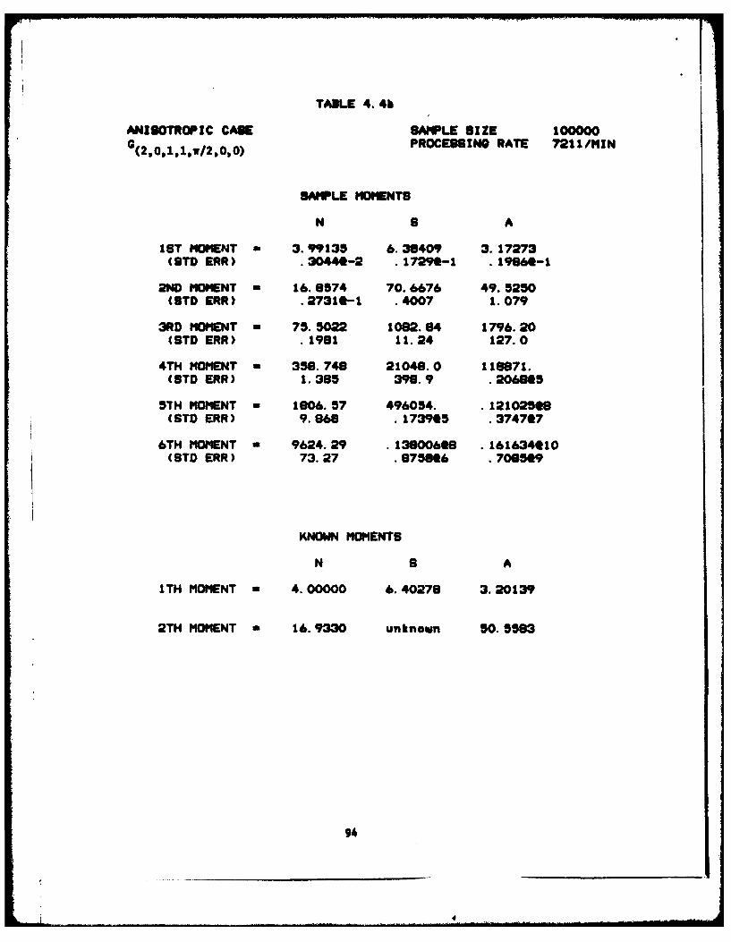
TABLE 4. 4b

ANISOTROPIC CAME SAMPLE 8IZE 100000a (2,0,1,1,r/2,0,O) PROCESSING RATE 7211/MIN

SAMPLE MOMENTS

N 8 A

1ST MOMENT - 3. 99135 6. 38409 3. 17273(STD ERR) .30440-2 . 1729-1 . 1986-1

2ND MOMENT - 16. 8574 70. 6676 49. 5250(STD ERR) .27310-1 .4007 1.079

3RD MOMENT - 75. 5022 1082. 64 1796. 20(STD ERR) .1981 11.24 127.0

4TH MOMENT - 358.748 21048.0 118871.(STD ERR) 1.385 398.9 .206805

5TH MOMENT - 1808. 57 496054. . 12102509(STD ERR) 9. 968 . 173915 .374707

6TH MOMENT - 9624. 29 . 13 00609 . 161634010(STD ERR) 73.27 .875806 .708509

KNOWN MOMENTS

N 9 A

1TH MOMENT - 4. 00000 6. 40278 3. 20139

2TH MOMENT - 16. 9330 unknown 50. 55S3

94

TABLE 4. 4c

ANISOTROPIC CASE NPLE SIZE 100000G(2,0,1,1,w/2,0,0) PROCESSING RATE 7211/MIN

THE 25 LARGEST POLYGONS (IN AREA)I -ISOPERIMETRIC RATIO

RANK N 8 A I

1 6.000 55.86 199. 8 1.2422 7.000 52.36 167.1 1.3063 4.000 52.74 163.7 1.3524 6.000 45.74 134.6 1.2375 7.000 47.20 128.6 1.3786 6.000 45.62 125.7 1.3177 6.000 45.78 121.4 1.373a 7.000 42.63 120.3 1.2029 8.000 39.86 115.8 1.09210 7.000 42.59 111.2 1.29911 6.000 45.60 109.8 1.50812 8. 000 42.38 105.6 1.35413 7.000 48.99 104.9 1.82114 7.000 42.99 103.5 1.42115 6.000 41.18 102.0 1.32316 6.000 62.47 98.57 3.15117 9.000 37.07 97.13 1.12619 6.000 39.39 95.57 1.29219 8.000 40.67 95.01 1.38520 5. 000 40.14 91.83 1.39621 7.000 36.87 90.47 1.19622 8.000 40.37 99.26 1.45323 6.000 37.00 87.25 1.24924 7.000 42.20 86.17 1.64525 6. 000 47.24 86.09 2. 063

95

._ r

TABLE 4.5a

ANISOTROPIC CASE SAMPLE SIZE 100000PROCESSING RATE 7159/MIN

SAMPLE PERCENTILES

PROB(N " n)

3 4 5 6 7.3603 .3810 .1877 .56752-1 .12152-1

n- 8 9 10 11 12.17500-2 . 35004-3 .30002-4 .0000 .0000

0 POLYGONS WITH N > 12)

PROI(S < 0)

sm .1000 .2500 .5000 .7500 1.000.10722-1 .26830-1 .55034-1 .83274-1 .1106

sm 1.500 2.500 3.750 5.000 6.250.1666 .2716 .3914 .4957 . 5981

ga 7. 500 8. 750 10. 00 12. 50 15. 00.6661 .7306 .7953 .8656 .9173

a" 17. 50 20. 00 25. 00 30.00 50. 00.9499 . 9704 .9097 . 9962 1. 000

C 4 POLYGONS WITH 8 > 50)

PROB(A C a)

a- . 50000-2 . 10000-1 .25000-1 .50000-1 . 1000.44540-1 . 6300-1 .98500-1 . 1384 . 1923

a- .2500 .5000 .7500 1.000 1. 500.2922 .3910 .4590 .5111 .5690

a- 2.500 5.000 7.500 10.00 12.50.6904 .6192 .8923 .9162 .9406

a- 15. 00 20. 00 30. 00 50.00 100.0.9564 .9744 .9900 .9975 .999

C 14 POLYGONS WITH A > 100)

96

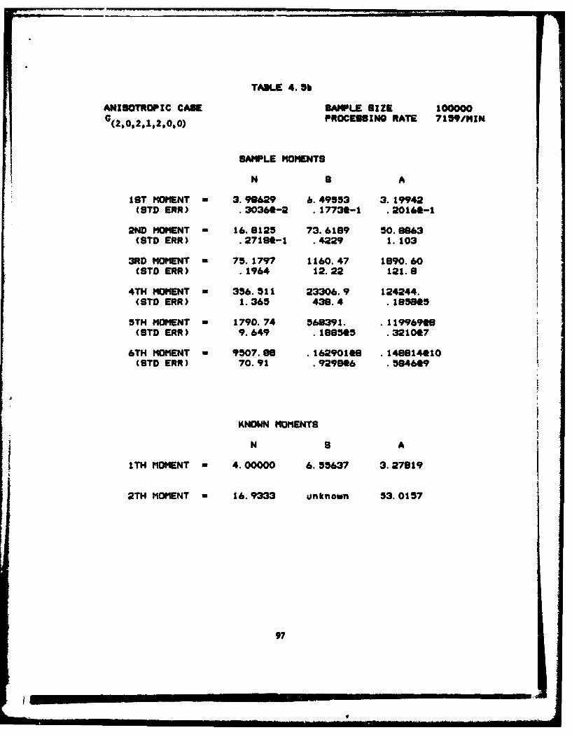
TALE 4. 5b

ANISOTROPIC CASE SAMPLE SIZE 1000000 (2.0.2.1.2,0,0) PROCESSING RATE 7159/MIN

SAMPLE MOMENTS

N a A

1ST MOMENT - 3. 9629 . 49553 3. 19942(STD ERR) .30360-2 . 17730-1 .20160-1

2ND MOMENT - 16.8125 73. 6199 50.963(STD ERR) .27180-1 .4229 1.103

3RD MOMENT - 75. 1797 1160.47 1890.60(ST0 ERR) .1964 12.22 121.8

4TH MOMENT - 356.511 23306.9 124244.(STD ERR) 1.365 439.4 . 18565

5TH MOMENT - 1790. 74 566391. .11996909(STD ERR) 9.649 .188545 .3210t7

6TH MOMENT - 9507.8 . 1629018 . 149814010(STD ERR) 70.91 .929806 .584649

KNOWIN MOMENTS

N s A

ITH MOMENT - 4. 00000 6. 55637 3. 27819

2TH MOMENT - 16.9333 unknown 53. 0157

97

TABLE 4. 5c

AN13OTROPIC CASE SAMPLE SIZE 100000

(2.0,2,1,2,0,0) PROCESSING RATE 7159/MIN

THE 25 LARGEST POLYGONS (IN AREA)

I -ISOPERIMETRIC RATIO

RANK N S A I

1 8.000 61.59 193.9 1.5572 8.000 46.90 154.7 1.1323 6.000 59.65 153.7 1.8434 7.000 51.00 149.9 1.3815 7.000 49.39 142.3 1.3646 7.000 43.06 120.5 1.2247 5.000 47.54 113.2 1.589a 5.000 43.01 108.0 1.3639 6.000 43.95 107.5 1.43110 7.000 42.34 104.9 1.36111 6.000 40.12 103.8 1.23312 7.000 51.59 101.5 2.08713 6.000 40.54 101.1 1.29414 4.000 41.49 101.0 1.35615 8.000 40.49 98.96 1.31816 6.000 39.35 98.32 1.25417 7.000 40.39 97.79 1.32819 7.000 44.10 97.39 1.59519 6.000 41.04 97.09 1.38120 5.000 41.75 96.35 1.44021 8.000 41.41 96.30 1.41722 5.000 42.49 96.24 1.49223 6.000 40.90 95.34 1.39624 4.000 43.94 95.02 1.61725 7.000 38.01 94.96 1.211

98

TABLE 4.6a

ANISOTROPIC CASE SAMPLE SIZE 100000G(2,0,4,1,8/3.0,0 ) PROCESSING RATE 862/MIN

SAMPLE PERCENTILES

PROB(N - n)

n- 3 4 5 6 7.3635 .3834 .1836 .5612t-1 .11430-1

n- a 9 10 11 12•1780*-2 .1500-3 .2o00-4 .1000*-4 .0000

( 0 POLYGONS WITH N > 12)

PROB(S < s)

s 1000 .2500 .5000 .7500 1.000.10660-1 .2725t-1 .54220-1 .80840-1 .1078

sm 1.500 2.500 3.750 5.000 6.250.1619 .2633 .3820 .4865 .5743

im 7.500 8.750 10.00 12.50 15.00.6521 .7179 .7734 .8545 .9079

s- 17.50 20.00 25.00 30.00 50.00.9422 .9645 .9870 .9951 1.000

( 4 POLYGONS WITH S > 50)

PROB(A < a)

a- .50000-2 .1OOOe-1 .2500-1 . 50000-1 .1000.44430-1 .6308-1 .98240-1 .1373 .1908

am .2500 .5000 .7500 1.000 1.500.2889 .3897 .4561 .5082 .5860

a- 2.500 5.000 7.500 10.00 12.50.6862 .8154 .8785 .9149 .9373

a- 15.00 20.00 30.00 50.00 100.0.9532 .9726 .9889 .9972 .9999

(15 POLYGONS WITH A > 100)

99

I II I III~ llI Il I I I I I I II

TABLE 4.6b

ANISOTROPIC CASE SAMPLE SIZE 100000G (2,0,4,1,8/3,00) PROCESSING RATE 6282/MIN

SAMPLE MOMENTS

N S A

1ST MOMENT a 3.97474 6.72080 3.29444(STD ERR) .3012Q-2 .18480-1 .20690-1

2ND MOMENT - 16.7058 79.3305 53.6550(STD ERR) .2685Q-1 .4602 1.061

3RD MOMENT a 74.4005 1307.63 1944.86(STD ERR) . 1928 13.78 95.11

4TH MOMENT a 351.152 27472.4 115541.(STD ERR) 1.329 500.0 .108705

5TH MOMENT = 1754.04 698314. .93224107(STD ERR) 9.304 .209205 .138807

6TH MOMENT m 9251.63 .20698108 . 90831009(STD ERR) 67.99 .965406 .1882t9

KNOWN MOMENTS

N S A

ITH MOMENT - 4.00000 6.79264 3.39632

2TH MOMENT - 16.9346 unknown 56.9205

100

,.......

TABLE 4.6c

ANISOTROPIC CASE SAMPLE SIZE 100000G(2 , 0 ,4, 1 , 8 / 3 , 0 ,0) PROCESSING RATE 6262/PIN

THE 25 LARGEST POLYGONS (IN AREA)

I -ISOPERIMETRIC RATIO

RANK N a A I

1 7.000 58.34 154.1 1.7572 6.000 48.53 135.1 1.3873 6.000 48.8w 131.6 1.4464 5.000 46.52 130.6 1.3195 5.000 49.43 128.0 1.5196 6.000 43.69 123.2 1.2327 7.000 45.95 123.2 1.364a 7.000 49.98 121.5 1.6379 6.000 45.17 115.3 1.408

10 5.000 43.33 110.9 1.34711 6.000 42.36 108.7 1.31412 6.000 45.49 107.3 1.53513 7.000 54.30 105.7 2.21814 7.000 54.72 105.2 2.26515 7.000 40.35 103.2 1.25616 7.000 42.49 99.72 1.44117 6.000 42.50 99.70 1.44118 8.000 39.72 98.94 1.26919 7.000 40.82 97.86 1.35520 5.000 45.27 97.67 1.67021 6.000 40.58 96.68 1.35522 8.000 43.24 96.27 1.54623 6.000 42.19 95.81 1.47824 5.000 40.24 94.62 1.36225 7.000 43.39 93.55 1.602

101

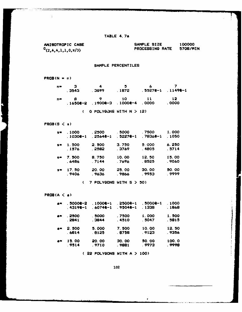
TABLE 4.7a

ANISOTROPIC CASE SAMPLE SIZE 100000G(2 4 4 ,1,1,0,w/ 3) PROCESSING RATE 5708/MIN

SAMPLE PERCENTILES

PROD(N - n)

n- 3 4 5 6 7.3543 .3899 . 1872 .55270-1 .11490-1

n 9 a 9 10 11 12.16500-2 .19000-3 .10000-4 .0000 .0000

( 0 POLYGONS WITH N > 12)

PROB(S < $)

s- .1000 .2500 .5000 .7500 1.000.10300-1 .25640-1 .52270-1 .78360-1 .1050

i 1.500 2.500 3.750 5.000 6.250.1576 .2582 .3769 .4805 .5714

s- 7.500 8.750 10.00 12.50 15.00.6486 .7144 .7696 .8525 .9060

t 17.50 20.00 25.00 30.00 50.00.9406 .9636 .9866 .9953 .9999

7 POLYGONS WITH S > 50)

PROB(A < a)

a- .50o-2 .10000-1 .25000-1 .5000-1 . 1000.43190-1 .60740-1 .95040-1 .1338 .1868

am .2500 .5000 .7500 1.000 1.500.2841 .3844 .4510 .5047 .5815

a- 2.500 5.000 7.500 10.00 12.50

.6814 .8125 .8758 .9123 .9356

am 15.00 20.00 30.00 50.00 100.0.9514 .9710 .9881 .9973 .9998

( 22 POLYGONS WITH A > 100)

102

=- -sI

TABLE 4. 7b

ANISOTROPIC CASE SAMPLE SIZE 100000G ( 2 , 4 4 ,1 ,1 0 .W/ 3 ) PROCESSING RATE 57018/MIN

SAMPLE MOMENTS

N S A

1ST MOMENT - 3. 98548 6. 790583 3. 36630(STD ERR) .2996t-2 .1850t-1 .21240-1

2ND MOMENT - 18. 7914 80. 2053 56. 4374(STD ERR) . 26690-1 . 4577 1. 239

3RD MOMENT - 74. 7903 1317. 46 2209. 25(STD ERR) .1913 13.45 146.7

4TH MOMENT - 352.826 27381.3 156815.(STD ERR) 1.313 480.1 .222005

5TH MOMENT - 1759. 49 683733. . 18480209(STD ERR) 9. 102 . 199505 .362107

6TH MOMENT - 9254. 11 . 19836109 . 215716010(STD ERR) 65.05 .919906 .6087e9

KNOWN MOMENTS

N S A

ITH MOMENT a 4. 00000 6. 79264 3. 39632

2TH MOMENT - 16. 9175 unknown 56. 7235

103

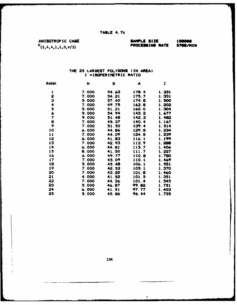
TAILE 4.7c

ANISOTROPIC CASE @MLE IZElG(2 ,4, 4 ,1,1,0,W/ 3 ) PNOXMIN RATE I ITtIIN

THE 25 LARGEST POLYGONS (IN AREA)

I -ISOPERIMIETRIC RATIO

RANW N S A I

1 7.000 54.63 178.4 1.3312 7.000 54.21 175.7 1.3313 5.000 57.40 174.8 1.5004 7.000 49.75 163.8 1.2025 5.000 51.21 160.0 1.3046 5.000 54.94 143.2 1.6777 9.000 51.48 142.3 1.482a 7.000 45.37 140.4 1.1679 7.000 51.50 139.4 1.51410 6.000 44.86 129.8 1.23411 7.000 44.09 124.8 1.23912 6.000 41.83 116.1 1. 19913 7.000 42.93 113.9 1.2914 6.000 44.81 113.7 1.40615 8.000 41.50 111.7 1.22716 6.000 49.77 110.8 1.79017 7.000 45.09 110.1 1.46919 5.000 45.48 106.1 1.55119 7.000 42.53 105.1 1.37020 7.000 43.22 101.8 1.46021 4.000 41.52 101.5 1.35122 7.000 44.36 101.4 1.54523 5.000 46.87 99.82 1.75124 6.000 41.51 97.77 1.40325 5.000 45.86 96.44 1.735

104

V

4.5.3. Anisotropic Cases Induced by .

Tables 4.8a through 4.10c present the simulation results for

the anisotropic cases induced by the three discrete uniform distribu-

tions in Q with atoms at 5, 10 and 20 points respectively. The

functions X(O) tur each of these distributions are obtained from

(3.43).

As in the previous anisetropic simulations, the purpose here was

exploratory so that sample sizes were also kept to 100,000. Simula-

tion rates were still high, between 8275 and 6787 polygons per minute.

Unfortunately, these cases were affected, though not so severely, by

the same numerical problems discussed in the last subsection. Nonethe-

less, the general tendency for these cases to progressively approximate

the isotropic case is readily apparent as expected. A deeper investiga-

tion into this convergence may well provide the key to obtaining the

elusive analytic distributions of N, S, and A in the isotropic case.

Ji

105

.1;

TABLE 4.8a

ANISOTROPIC CASE SAMPLE SIZE 1000005 POINT DISCRETE UNIFORM PROCESSING RATE 8275/MIN

SAMPLE PERCENTILES

PROB(N - n)

n- 3 4 5 6 7.3124 .4434 .1876 .48170-1 .75900-2

nu 8 9 10 11 12.85000-3 .40000-4 .0000 .0000 .0000

( 0 POLYGONS WITH N > 12)

PROB(S C s)

Sm .1000 .2500 .5000 .7500 1.000.89900-2 .2353t-I .48970-1 .7498-1 .1005

So 1.500 2.500 3.750 5.000 6.250.1526 .2553 .3772 .4873 .5820

s- 7.500 8.750 10.00 12.50 15.00.6638 .7316 .7873 .8697 .9219

Sm 17.50 20.00 25.00 30.00 50.00.9540 .9735 .9907 .9971 1.000

1POLYGONS WITH 8 ) 50)

PROB(A < a)

am .50000-2 .10000-1 .,25000-1 .50000-1 .1000.36060-1 .5258-1 .85110-1 .1214 .1735

am .2500 .5000 .7500 1.000 1,500.2714 .3731 .4436 .4976 .5701

am 2. 500 5. 000 7. 500 10. 00 12. 50.6824 .8155 .8905 .9168 .9406

an 15.00 20. 00 30.00 50. 00 100.0.9561 ,9740 .991 .9"76 .99

12 POLYGONS WITH A > 100)

106

Vi

TABLE 4.8b

ANISOTROPIC CASE SAMPLE SIZE 1000003 POINT DISCRETE UNIFORM PROCESSING RATE 8275/NIN

SAMPLE MOMENTS

N 8 A

18T MOMENT - 3. 99792 6. 50949 3. 26471(STD ERR) .27850-2 .17160-1 .20100-1

2ND MOMENT - 16.7589 71.8088 51.0454(STD ERR) .24410-1 .3951 .9927

3RD MOMENT - 73.7311 1088.00 1774.38(STD ERR) .1710 10. 64 98.86

4TH MOMENT - 340. 442 20764.2 101147.(STD ERR) 1. 136 340. 1 .1090e5

5TH MOMENT - 1648. 46 474312. .79976707(STD ERR) 7. 554 .123905 .155507

6TH MOMENT 8 9359. 11 .12504408 .79280909(STD ERR) 51.30 .494506 .237309

KNOWN MOMENTS

N 8 A

ITH MOMENT - 4.00000 6.49839 3.24920

2TH MOMENT - 17. 1038 unknown 53. 9825

107

TABLE 4. 8c

ANISOTROPIC CASE SAMPLE SIZE 100000S POINT DISCRETE UI1FORM PROCESSING RATE 6275/MIN

THE 25 LARGEST POLYGONS (IN AREA)

I -ISOPERrIETRIC RATIO

RANK N S A I

1 9.000 48.44 165.2 1.1312 7.000 51.31 145.6 1.4393 7.000 44.56 129.9 1.2144 6.000 43.36 111.6 1.2615 6.000 43.22 116.4 1.2776 7.000 44.55 110.5 1.4297 6.000 41.82 110.1 1.264a 5.000 45.12 10.3 1.5259 7.000 43.45 105.0 1.431

10 6.000 41.57 104.8 1.31211 6.000 44.59 103.3 1.53112 6.000 39.67 103.2 1.21313 5.000 39.05 97.75 1.24114 7.000 39.52 96.85 1.28415 5.000 39.08 94.47 1.28716 9.000 38.32 91.76 1.27417 6.000 39.55 91.24 1.29619 7.000 37.01 91.13 1.19519 6.000 38.57 90.52 1.30820 8.000 36.84 89.99 1.20021 6.000 41.81 88.16 1.57822 7.000 37.10 88.04 1.24423 9.000 36.72 87.88 1.22124 5.000 39.16 87.24 1.39925 5.000 38.03 86.30 1.333

106

I

TABLE 4.9a

AI4ISOTROPIC CASE SAMPLE SIZE 10000010 POINT DISCRETE UNIFORM PROCESSING RATE 7142/MIN

SAMPLE PERCENTILES

PROB(N m n)

n- 3 4 5 6 7.3462 .3977 .1861 .56144-1 .1194*-1

n 8 9 10 11 12.16400-2 .19006-3 .30006-4 .0000 .0000

( 0 POLYGONS WITH N > 12)

PROB(s < s)

sm .1000 .2500 .5000 .7500 1.000.1079 -1 . 27010-1 .55402-1 .82016-1 .1098

sm 1.500 2.500 3.750 5.000 6.250.1644 .2722 .3945 .5035 . 598

sm 7.500 8.750 10.00 12.50 15.00.6776 .7432 .7972 .8742 .9247

s- 17. 50 20.00 25.00 30.00 50.00.9555 .9743 .9918 .9973 1.000

( 0 POLYGONS WITH 8 > 50)

PROB(A C a)

O- .5000*-2 .10006-1 .25000-1 . o0000-1 .1000.42140-1 .59976-1 .94626-1 .1334 .1870

a- .2500 .5000 .750 1.000 1.500.2871 .3881 .4570 .5101 .5911

a- 2.500 5.000 7.500 10.00 12.50.693S .8214 .8836 .9188 .9406

am 15.00 20.00 30.00 50.00 100.0.9565 .9748 .9900 .9976 .999

15 POLYGONS WITH A > 100)

109

___,__.. . ..... . . .. ... ... ... . _ _

TABLE 4.9b

ANISOTROPIC CASE SAMPLE SIZE 10000010 POINT DISCRETE UNIFORM PROCESSING RATE 7142/MIN

SAMPLE MOMENTS

N 8 A

1ST MOMENT - 3. 99568 6.33138 3. 16962(STD ERR) .2994t-2 .1704t-1 .19910-1

2ND MOMENT - 16.8619 69. 1134 49.2739(STD ERR) .26750-1 .3867 .9910

3RD MOMENT - 75. 2963 1040. 33 1723. 58(STD ERR) .1925 10.34 88.94

4TH MOMENT - 355. 871 19730. 5 100635.(STD ERR) 1.327 330.5 .102705

5TH MOMENT - 1778. 18 448133. . 810163*7(STD ERR) 9.265 . 120605 . 1330e7

6TH MOMENT - 9374.35 .11772409 .79408109(STD ERR) 66.95 .480906 .193009

KNOWN MOMENTS

N S A

17H MOMENT - 4. 00000 6. 33538 3. 16769

2TH MOMENT - 16. 9759 unknown 49. 9284

110

. . . . . . .. .. .. . . ... .. . a , ,ia| | . . . . . . - ,, l . . . .

TABLE 4.9c

ANISOTROPIC CASE SAMPLE SIZE 10000010 POINT DISCRETE UNIFORM PROCESSINO RATE 7142/IlN

THE 25 LARGEST POLYGONS (IN AREA)

I -ISOPERIIETRIC RATIO

RANK N 8 A I

1 8.000 49.24 154.7 1.1972 7.000 49.50 134.3 1.4523 6.000 46.57 134.1 1.2884 6.000 44.75 130.1 1.2255 7.000 44.15 124.2 1.2486 7.000 46.05 119.9 1.4087 7.000 44.04 115.5 1.3368 8.000 41.41 114.0 1.1979 7.000 43.80 111.6 1.36810 8.000 41.42 108.0 1.26511 10.00 38.58 105.2 1.12712 8.000 47.09 104.9 1.68313 5.000 46.93 104.4 1.67914 7.000 42.27 102.3 1.39015 6.000 40.33 100.1 1.29316 8.000 38.55 98.64 1.19917 7.000 44.38 96.85 1.81818 7.000 41.14 95.65 1.40819 7.000 40.26 94.78 1.36120 8.000 42.48 94.61 1.51821 6.000 38.97 94.11 1.28422 6.000 37.62 92.39 1.21923 6.000 37.19 91.78 1. 19924 7.000 39.40 91.50 1.35025 6.000 42.91 90.23 1.624

111

II |I I II

4

TABLE 4. 10.

ANISOTROPIC CASE SAMPLE SIZE 10000020 POINT DISCRETE UNIFORM PROCESSING RATE 6707/1MN

SAMPLE PERCENTILES

PROB(N n)

n, 3 4 5 6 7.3526 .3863 . 1879 . 5775*-1 . 1316k-1

n 8 9 10 11 12* 19704-2 .31000-3 .0000 .0000 .0000

0 POLYGONS WITH N > 12)

PROB(8 C s)

.1000 .2500 .5000 .7500 1.000

.11550-1 .28260-1 .57049-1 .845"-1 .1127

1.500 2.500 3.750 5.000 6.250.1684 .2769 .3998 .5070 .6025

7.500 8.750 10.00 12.50 15.00. 804 .7451 .7989 .8755 . 9253

5- 17.50 20.00 25.00 30.00 50.00.9565 .9752 .9917 .9974 1.000

I POLYGONS WITH S > 50)

PROI(A < a)

am . 50000-2 . 10000-1 . 25000-1 . 5000/I-1 . 1000* 4417t -1 .63094-1 .99130-1 . 1360 . 1916

a- .2500 .5000 .7500 1.000 1. 500.2926 .3931 .4617 .5145 . 941

a- 2. 500 5.000 7.500 10.00 12.50.6960 .8220 .8040 .9200 . 942

a, 15. 00 20. 00 30. 00 50. 00 100.0.9377 .975 .9900 .9979 .VM96

18 POLYQONi WITH A > 100)

112

, - l .. . . . . .

TABLE 4.10b

ANISOTROPIC CASE SAMPLE SIZE 10000020 POINT DISCRETE UNIFORM PROCESSING RATE 6787/MIN

SAMPLE MOMENTS

N S A

18T MOMENT - 3. 99967 6.28806 3.13505(STD ERR) .30486-2 .1701t-1 .19620-1

2ND MOMENT - 16.9266 68.4676 48.3149(STD ERR) .27370-1 .3854 1.005

3RD MOMENT - 75.9519 1029.46 1696.74(STD ERR) .1982 10.36 102.4

4TH MOMENT - 361.425 19540.3 103363.(STD ERR) 1.377 336.6 .145765

5TH MOMENT - 1821.48 445572. .919135t7(STD ERR) 9.669 .126205 .2397e7

6TH MOMENT - 9698.74 .118015t8 . 105159010(STD ERR) 69.95 .521406 .4198*9

KNOWN MOMENTS

N S A

1TH MOMENT - 4.00000 6.29614 3.14807

2TH MOMENT - 16.9450 unknown 49.0064

113

.. . . . . . . ... . .i . . .

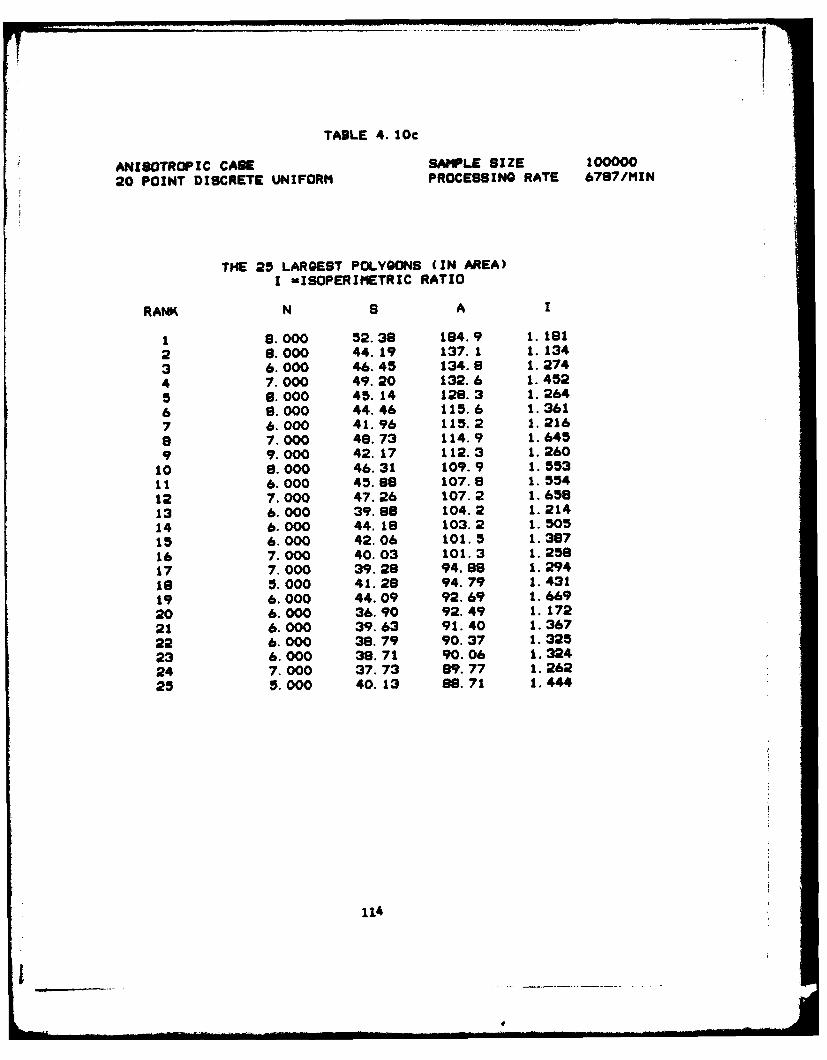
TABLE 4.10c

ANISOTROPIC CASE SAMPLE SIZE 100000

20 POINT DISCRETE UNIFORM PROCESSING RATE 6787/MIN

THE 25 LARGEST POLYGONS (IN AREA)

I -ISOPERIMETRIC RATIO

RANK N S A I

1 8.000 52.38 194.9 1.181

2 8.000 44.19 137.1 1.134

3 6.000 46.45 134.8 1.274

4 7.000 49.20 132.6 1.452

5 6.000 45.14 128.3 1.264

6 9.000 44.46 115.6 1.361

7 6.000 41.96 115.2 1.216

a 7.000 48.73 114.9 1.645

9 9.000 42.17 112.3 1.260

10 8.000 46.31 109.9 1.553

11 6.000 45.88 107.8 1.554

12 7.000 47.26 107.2 1.658

13 6.000 39.88 104.2 1.214

14 6.000 44.18 103.2 1.505

15 6.000 42.06 101.5 1.387

16 7.000 40.03 101.3 1.258

17 7.000 39.28 94.88 1.294

19 5.000 41.28 94.79 1.431

19 6.000 44.09 92.69 1.669

20 6.000 36.90 92.49 1.172

21 6.000 39.63 91.40 1.367

22 6.000 38.79 90.37 1.325

23 6.000 38.71 90.06 1.324

24 7.000 37.73 89.77 1.262

25 5.000 40.13 88.71 1.444

114

APPENDIX

A.l. Characterizations of the Linear Poisson Process of (Constant)Intensity T (lppT).

A realization of a linear point process is a set of points on

R. It is well known that any of the following conditions is suffi-

cient to completely characterize this process as an LppT.

(A.1) (Counting Specification). Let N be a nonnegative integer-

valued random Borel measure on R. Then for k arbitrary

disjoint Borel sets Al9..,A k' k - 1,2,..., the random vari-

ables N(Al),...,N(k) have independent Poisson distributions

with means m(A1 ),..., m(Ak), where m is Lebesgue measure.

(Note that it is sufficient to specify this property for

intervals A,..,%1.

(A.2) (Interval Specification). If 0 is an arbitrary time origin

and the process points are labelled according to the defini-

tion ... <T-2 <T_I <T o <0 <T, <_T2 < ., then the inter-

vals TI-T_2 , To-T_1 , -To, T1 , T2-T1,... are a sequence of

iid exponentially distributed random variables with parameter

T.

(A.3) (Local Intensity Specification). As in (A.1) let N be a

nonnegative integer-valued random Borel measure on 1R. Let

A(t) denote the history of the processes at time t. Then as+ ,

115

....... .........

P{N(t,t+6) - llM(t)} - TS + 0(S)

and

P{N(t,t+6) > 1Mi(t)} - o() .

(Note that the second condition here virtually excludes the

possibility of multiple occurrences.)

There are several other known ways of characterizing a £ppT.

For a list of these, together with references, see Cox and Isham (1980).

116

A.2. An Integral Formula for E[A 4 ]

We here derive an integral formula for the fourth moment of A

in isotropic 1A. We proceed by exact .analogy with the derivation of

E[A 2 ] in Coudsmit (1945) and the generalization for deriving E[A 3

in Solomon (1978). The basic idea is to derive two expressions for

the probability that four random points in a large area D lie inside

the same polygon. We shall denote this probability by P4 . The two

expressions are then equated, the area D+-, and our formula is obtained.

The first expression for P4 is obtained as follows. Let h(a)

be the probability density of A. Let M be the numbe- of polygons in

D. Then the probability that a random point in D lies inside a poly-

gon of area between a and a + da is approximately

aoh(a)do/D .

The probability that three more random points lie inside this same

3polygon is (o/D) . Thus we obtain

(A.4) P4 - J T 4 h(a)da " - E[ 4A 4

The second expression is obtained by averaging over all positions

of four random points, the probability that no line in £ passes through

the convex hull, denoted by C, of these four points. This is equivalent

to their lying in the same polygon.

We denote the four points by xl, x2, x3, and x4 . Without loss

of generality, we orient the horizontal axis so that x1 is at the

117

..

origin and x2 lies along the axis In the positive direction. Let

r,- xi+1 - x3 j, ± - 1,2,3. Let 81 be the angle between r1 and

r2 and 82 the angle between r1 and r3 . See Figure A.l.

X3

14 r

81

x 1 r 1 x2

Figure A.1

We write r - (rl, r2, r3, el, 02) and let p(r) be the peri-

meter of C. We have by an easy generalization of Theorem 1.2.4 that

the probability that no line of £ crosses C is

(A.5) e-TP(r)/ w .I

Notice that when the line segments joining the four points xl, x2,

Xy3 X4 form a reentrant quadrilateral, C is a triangle. Otherwise,

C is a convex quadrilateral.

In terms of differentials, the probability that a particular

orientation lies between r and r + dr is

21r r1 r2 T3 dr/D3

the ratio of the differential 0olume element to the total volume.

Combining this with (A.5) yields

118

I

(A.6) P4 11(g)/D 3 + o(l)

where

(A.7) a()-2w JJJJJ)/ *" ? r I K2 r3 dr

and

{-(r: 0<r<a, 1-1.2,3 and 0' <2w, j -1.2)

is the set of all positions of the four points in the plane. The ters

o(l) - 0 as D0- in (A.6) accounts for the part of E not included

in D. That this is the correct order term follows by noting that

p(r) > r,, i - 1,2,3.

Equating (A.4) and (A. 6 )we have as D'

(A.8) ERA 4 ] = 11D(E)D-1

TT 2~ P(E)

2since lir D/M - E /A] wiT . (See Solomon (1978)).

We now proceed to reduce E by symmetry arguments. First1

)I(El) - P(E)

where

E " E (I {r: o< < <2w) .

Next observe that the integration in (A.7) is the same for

regions of E1 where x2 x3 . z4 all lie in the same half-plane.

Hence,

119

E

1( 2 ) - 1 (3) - (E4)

where

Z3 -E I n {r: o <e1 < e 2 <2, )

4 - , n f{r: o<e 1 ,i e < 27r)

Finally let

5 %1 - o e 0 < e3. < 2 )

so that

El - E2 U E3 U E4 U E5

Combining the above we have

(A.9) I (E) - 6V (E2 ) + 211(E 5 )

We nov proceed to express p(r) explicitly on the sets E2 and

E5. Define

5. I

(A.10) h(r) - 3 or coo0Cos e + sin el 1' si 2 2

I~1 sin 02

h(r) is the distance along the line coitLIdent with r 2 , from xI

to the line connecting x2 and x4 .

3x

h(r)

X2

120

L [i

Let

1- 2 n (r: r2 h(r))

1 E7 2 (I (r- r2 > h(r))

Notice that r C E6 Implies C Is a triangle and r e P7 Implies C

is a quadrilateral.

For notational convenience, write the distance a - J as

d(r~rj) - (r2 + r2 - 2rr Cos 1/2

%12 e 1- '13"w62 %'23 " e4 2 •e

Then

+ 3 + d("-"3) o6(A.11) p (r) d-~ 3 nrCE

{rI + r3 + d(rl,r2) + d(r 2 ,r 3 ) on r e 7

Also since r C E5 Implies C is a triangle we have

(A.12) p(r) - d(rl,r2) + d(r2 ,r3) + d(r13 r3) on r c 15

Coabining this reduction with (A.8) and (A.9) we obtain

(A.13) E[A 6 + 5)]

where

VE 2w JJJ *-'p(r)Iw r r r3 dr

II

and

121

EMM

96 - {r: 0 r <a, 0< r2 h(r), 0< r3 < %

0 < < 0 2 < T)

17 - (r:0 < 1 << -,. h(r) < r 2 < -' 0 < r3 <-

0<81 <82-<W

95 " {r: 0<r i < to i - 1,2,3 and

0 < 01 < w < 02 < _ 1 <2w)

Writing out (A.13) more explicitly we have the integral formula

(A.14)2 -i-[ frJ2 ff(h(r) --I(r+rj4,d(r1 , 3 )

--(r 4+3 ( d(r.r) d r 2 3 )\+ eh(r) r 2 dr2 ) rr 3dridr 3 dOldO2 j

+ I: -d

r 2 r 3 dr1dr 2 dr 3 de1 de 2 }]

where h(r) is defined in (A.10).

122

L

CA.3. A Theorem on the Richness of Q

Theorem. Q C defined in (3.31) is dense In the class 6 of con-

tinuous probability densities on [Ow].

Proof. Let f C 4 and pick e > 0. f is uniformly continuous

so a 8 > 0 A:

(A.15) If(1) - f( 2) 4 if I el-e2I < 26.

Let M - max f(O). Then a a0 An V e,

(A.16) 6 Isine0(eO-W) IA4( >1 -je8 Y'n0 4M

(see (3.33) for definition of K ).

Combining (A.15) and (A.16), we have uniformly in e

(A.17) 7J f W 1 -lain (6-w) J- - f(e)

0 --o

< 1(1 - -L +e.M--< I

Def ine

0-Loh(e) - F 7J( Si .U ( - -)-i

and

SM . () in (

K n n30 j 1 n

123

We can choose N large eanough so that . 8

(hX(e) - o10 (B-.)) & <&_0O 4

by direct Riemana approxmation, and

(A.19) h ()

because

N I f(O) de- 1.

Combining (A.17), (A.18), and (A.19) we have V 0

Igm(o) - f(e)l < C

Buc

S N O = G( ,, , , ) ( 0 ) C q C ,

where n-N and for i 1,...,N, a1- "0. "- and

124j ____________

h.__ _______

A.4. Splitting ?robabilities ad the Distribution of N.

Consider & random seant through an 3-sided polygon In isotropic

p,° That is, let the secant coincide with a line whoes coordinates

(P.8) are distributed proportionally to dpde over the set of lines

hitting the polygon. This secant 'splits' the polygon into left and

right polygons which we define as lying to the left and right respe.-

tively of the lover intersection of the secant with the polygon . see

Figure A.2.

left polygon SECANT

right polygon

Figure A.2

Define the left splitting probability p*1, where i - 3,4,..., and

j - 3,...,i+1, to be the probablity that a random secant through a

random i-sided polygon in p yields a J-sided left polygon.

The following system of equations expresses the interrelation

between the distribution of N and the splitting probabilities.

Knowledge of either set of probabilities should enable us to solve

this system for the other.

(A.2 o) p(U-u - (1-2) {f-i)p*_ 3.4. ....

125

t _

We shel outline a derivation of (A2) which is based on the

luvariance of the distribution of N under changes in the Itnasity

T of the Foison line process. Consider a random secant tbrouag

the portion of e contained In a Uarge disc of radius q. As In

the proof of Theorem 1.2.4 It is easily shoa that the probability

that this secant hits a polygon with perimeter a is proportional

to a. Deflne pq to be the probability density that this secanti's

hits an i-sided polygon with perimeter a. Then,

oP:L, a a dPq{S- *,N- i]

where P {S- a,N- 1} is the Joint density of S and N in the disc.q

Now let q . so that the random secant will correspond to a new

line resulting from an infintesimal Increase in the Intensity T

of the Poisson line process. Then p q . p H the probability

density of i-aided polygons vith perimeter a along the new line.

Furthermore, since P q(S S,N- t] 4- P(S - s,N- i) the ergodic density,

we have

R

(A.21) PHi a a cS-a.," )

Define pi to be the probalblity density of I-sided polygons along

the new line. Integrating (A.21) we obtain

Pi a dP(S -,N- 1)

6J'adP(S-9IN- ) • P{I-i)

fsjIN-I) • P*,{, i)

126

But from Section 3.5 we have z(SIw- - (i-2) and Z[N] - 4, so

that

pi ""(i-2) • #(N- i)

Finally, this now line creates two polygons for every one it hits.

However, because of the invariance of the distribution of N under

the addition of one more line, the distribution of N of the new polygons

must be this same distribution. By the syetry between left and right

new polygons, we have for a - 3,4,...

P(N-. a) 2 - p pH piNi-m-l uN

0 (1-2) PfN- i1}p

We remark that a little more simplification of (A.20)is possible because

Pin = Pi(i+4-) by symetry.

127

FOOTNOTES

[1] The agreement of some of his results with those of Goudemit

(vhen suitably normalized) suggests that Goudsait had in mind

this very model.

[21 The in-circle of a convex polygon is the largest circle it

contains. While it may not be unique, its diameter is. We

shall not investigate this ch racteristic further as it seems

to be less Important than N, S, or A.

[31 The particular paper, Miles (1973), came to the attention of

the author after the bulk of the present york had been carried

out. His stochastic constructions seem not to be of the sequen-

tial nature of the construction developed here, although both

processes begin with a similar step. Apparently, his construc-

tions are not very efficient for simulation studies as he chose

a different method in his later Monte Carlo study with Crain.

Furthermore, as he does not elaborate on the details of his con-

struction, it is hard to see the mathematical potential, although

he does allude to some recursive integral equations for the dis-

tributions of polygon characteristics. Finally, his constructions

are given for the isotropic case whereas the sequential construc-

tion here is developed in the general translation invariant con-

text. The essential overlap of Miles? contribution with the

present paper is that both constructions yield sets of polygons

equivalent to an independent and identically distributed Sample of

polygons from a Poisson field of lines.

128

(4] Some researchers in the line processes consider directed lines and use

this parametrization with e £ [0, 2r). We will be concerned

only with undirected lines.

[5] C is endowed with the ordinary ruclidean topology.

[6] Some researchers (Davidson (1974)) consider the more general doubly

stochastic Poisson line process. The equivalent point process

on C then has the same distributional form as (1.5) with m

replaced by a random Borel measure A. We shall not consider

this generalization here.

[7] It actually takes a little doing to establish this from (1.5).

A possible derivation establishes a characterization like (A.3)

for multivariate Poisson processes from which a joint conditional

density can be derived, we do not carry out the details as this

seems to be a well known property.

(8] We use the term density throughout this work to refer to the

differential element of the measure referred to. For example,

if U is a measure, then we refer to dV as the density where

P(A) - fA dp. Note that contrary to common usage, we include

the differential element of the carrier measure.

[9] For isotropic AV* the curling process can be modified to select

a sadmple from a population equivalent up to translation and

rotation.

[10] We condition on the open interval (n-l' 8n-l) here. When the

distribution G of 8 is continuous, it trivially does not

matter. However, this restriction is essential if G has an

129

.

atom at either a_ or 0 Any such value would violate then-l n-i'

property that the Poisson point process on C has no multiple

points (a property similar to (A.3)).

11] See formula (5.19) in Miles (1973). Miles uses a different para-

metrization of the angles, but his side lengths Li are the same

as our Zi .

(121 For example, a natural candidate would be the circular normal

distribution where the density is proportional to exp(-K cos 201,

see Mardia (1972). The reader can verify that a closed form

expression for F in (3.29) is unobtainable.

[13] The Monte Carlo study of Crain and Miles (1976) exploits informa-

tion from one of these aggregates, the perimeter welghted+ polygons,

(see also footnote [15]).

[14] Result communicated to H. Solomon in unpublished memo. See

Solomon (1978), p. 54.

[15] Actually Crain and Miles consider two types of polygons,

* polygons which are the same as ours, and +polygons which

rre the unions of pairs of adjacent polygons. They simulated

100,495 *polygons and 95,485 + polygons in 45 and 21 sample

discs, respectively. The distributions of +polygon charac-

teristics correspond to a perimeter weighting of those * polygons.

Table 4.2 presents some estimates of the distribution of N based

on +polygons, (see also footnote (171). In particular, extreme

values of N, S, and A are more likely in the + polygon popula-

tion so that more precise estimates of the tails are available.

130

[16] The computer operators at the IMSSS facility, Stanford, Ca.,

estimate that our machine, the PDPXO/KI is about twice as

fast as the IBM 360/50 used by Crain and Miles. They added

however that the comparison is difficult.

[17] We present in this table the different estimates that Crain

and Miles obtain for the distribution of N. *STD and +STD

estimates are ordinary sample averages using *polygons and

+polygons respectively, (see footnote [15]). *WTD and +WTD

are the corresponding weighted estimates compensating for the

edge effects. QRF and CRF refer to quadratic and cubic

ratio fits obtained by fitting polynomial expressions for

ratios of probabilities to the data and known values. Crain

and Miles present histograms rather than percentile estimates

for S and A, together with various types of moment estimates.

[18] We programmed the Monte Carlo simulations in the programming

language SAIL (Stanford Artificial Intelligence Laboratory).

This language includes as a standard subroutine a pseudo-random

number generator called RAN.

119] Private communication to H. Solomon.

120] Our programming language SAIL is basically an algorithmically

oriented language for programming ease. The variables used hold

at most eight significant digits rendering it somewhat inaccurate

for sophisticated numerical work. Apparently a new extended

precision version of SAIL will soon be available. Alternatively,

the extended precision capability of FORTRAN makes it an ideal

language for this type of simulation. The author plans to carry

131

41

out more extensive simulations of these sensitive anisotropic

cases with a more numerically precise programming language

In the future.

132

IEFIERUCES

Baddeley, A. (1977), "A Fourth Note on Recent Research in GeometricalProbability," Adv. Appl. Prob. 9, 824-860.

Butler, J. W. (1954), "Machine Sampling f-om Given Probability Dis-tributions," in Meyer, H. A. (ed.), Symposium on Monte CarloMethods. Wiley, N.Y.

Cowan, R. (1978), "The Use of Ergodic Theorems in Random Geometry,"Suppl. Adv. Appl. Prob. 10, 47-57.

Cox, D. R. and Isham, V. (1980), Point Processes, Chapman and Hall,London.

Crain, I. K. and Miles, R. E. (1976), "Monte Carlo Estimates of theDistributions of the Random Polygons Determined by Random Linesin a Plane," J. Stat. Comp. 4, 293-325.

Crofton, M. W. (1885), "Probability," Encyclopedia Britannica, 9th ed.,Vol. 19, 768-788.

Davidson, R. (1974), "Constructing of Line Processes: Second OrderProperties," in Harding and Kendall (eds.), Stochastic Geometry,Wiley, N.Y., 55-75.

Dwight, H. B. (1961), Tables of Integrals and Other Mathematical Data,Macmillan, N.Y.

Goudsmit, S. A. (1945), "Random Distribution of Lines in a Plane,"Rev. Mod. Phys. 17, 321-322.

Hammersley, J. M. and Handscomb, D. C. (1964), Monte Carlo Methods,Metheun, London.

Harding, E. F. and Kendall, D. G. (1974), Stochastic Geometry, Wiley,N.Y.

Little, D. V. (1974), "A Third Note on Recent Research in GeometricalProbability," Adv. Appl. Prob. 6, 103-130.

Mardia, K. V. (1972), Statistics of Directional Data, Academic Press,N.Y.

Miles, R. E. (1964), "Random Polygons Determined by Random Lines in aPlane," Proc. Nat. Acad. Sci. (USA), Part I 52, 901-907; Part II52, 1157-1160.

Miles, R. E. (1971), "Poisson Flats in Euclidean Spaces. II," Adv.Appl. Prob. 3, 1-43.

133

..

r

Miles, R. E. (1974), "On the Elimination of Edge Effects in PlanarSampling," in Harding and Kendall (eds.), Stochastic Geometry,Wiley, N.Y., 227-247.

Miles, R. E. (1973), "The Various Aggregates of Random PolygonsDetermined by Random Lines n a Plane," Adv. Math. 10, 256-290.

Moran, P. A. P. (1966), "A Note on Recent Research in GeometricalProbability," J. Appl. Prob. 3, 453-463.

Moran, P. A. P. (1969), "A Second Note on Recent Research in Geometri-cal Probability," Adv. Appl. Prob. 1, 73-89.

Santalo, L. A. (1953), Introduction to Integral Geometry, Hermann,Paris (Act. Sci. Indust. No. 1198).

Santalo, L. A. (1976), "Integral Geometry and Geometric Probability,"Encyclopedia of Mathematics and Its Applications, Vol. 1,Addison-Wesley, MA.

Solomon, H. and Wang, P. (1972), "Nonhomogeneous Poisson Fields ofRandom Lines with Applications to Traffic Flow," Proc. SixthBerkeley Symp. Math. Statist. Prob. 3, 383-400.

Solomon, H. (1978), Geometrical Probability, SIAM Publications (CBMS-NSF 28), PA.

Solomon, H. and Stephens, M. A. (1980), "Approximations to Densitiesin Geometrical Probabiligy," J. Appl. Prob. 17, 145-153.

Snyder, D. L. (1975), Random Point Processes, Wiley, N.Y.

134

UNCLASSIFIEDS9CUONTV CLASSIICATION OF THIS PAGE (11110 1040heue

REPORT DOCMAENTATION PAGE at nuvocm1. REPORT WNDMER IS. GOT ACCESSONO e RaCIPOEUVS CATAL.OG AuIm

320 LAD-.4i i' _ _ _ _ _ _ _ _T. TITLE (anSW IM101 S. TYPE OF REIPORT a PEROD COV648O

SEQUENTIAL STOCHASTIC CONSTRUCTION OF TECHNICAL REPORTRANDOM POLYGONS S mr~eo E@Tnmi

.AUTHORM~S CONTRACT ON GRAT 00111EWO

Edward Ian George NOOO1 4-76-C-0475

9- PERFORMING ORGANIZATION HAMS AND ADDRES 10-I RO P ROJ PT AK

Department of Statistics NREA042-267RStanford University N-4-6Stanford, CA 94305

11. CONTROLLING OFFICE NAME AND ADDRESS I2. REPoORT DATE

Office Of Naval Research June 10, 1982Statistics & Probability Program Code 4iisp IS. NUMBER orPAGESArl i nton.GV 2221 134

14, MONITORING AGGWAY NAME & ADORISS(11 au.1"el, tomus Con.Iliad 053. IS. SEUIYCLS.(1le. ispinl

UNCLASSIFIED

14416 DECL ASSIICATI8NIOOWNGRAOIN41

16. DISTRIBUTION STATEMENT (of if A5 flpe )

APPROVED FOR PUBLIC RELEASE: DISTRIBUTION UNLIMITED.

17. DISTRIBUTION STATEMENT (*Ios the a ~int i~e in Wleek 20. 19 [email protected] bmeet )

IS. SUPPLEMENTARY NOTES

I9. KCEY WORDS (Cowl.. - deof rev* old* it nrnaw m dsd for 10" bla u&)

Poisson fields of lines; distributions of sides, parameter and area

of random polygons; isotropic and anisotropic cases.

20. AtOS1 RACT (Centme a.o rowas old. Of nteearin ME Idesoft IF Slee MMnS.)

PLEASE SEE REVERSE SIDE.

O 12 1473 EDITION OP, I NOv 5515 OBSOLETE UNCLASSIFIEDSf N 0 102- L9- 11.-6601 SEItY CLASSIFICATION OF T041S PAGE (SSO.se O& .

UM CLASSIFIE0I NTUYV CLAUPICATION OP TWiS PaSS m* Rk*

#320

Homogeneous Poisson fields of lines divide the plane Into non-

overlapping convex polygons. Of Interest to researchers in geometrical

probability have been the distributions of characteristics of the poly-

gons induced by the distributions of the lines, especially N, the

number of sides, S, the perimeter, and A, the area. A sequential

stochastic process is developed from which an Independent and identically

distributed sample of polygons can be extracted with a stopping time. It

is shown that the distribution of polygons so obtained is identical to

the distribution of polygons in the Poisson field. The stochastic process

is developed in full gnezality and can be applied to anisotropic cases

as well as the case of most interest, the Isotropic case. Useful families

of anisotropic distributions for this problem are defined.

The sequential stochastic process is used to derive general analytical

expressions for polygon distributions for the investigation of the unknown

distributions of N, S and A. Methods are also developed which provide

the basis for very fast computer slmulation of the process. A Monte Carlo

study of the distributions of N, S, and A in various cases is presented.

In particular, a ample of 2,500,000 polygons in the isotropic case provides

the most precise results to date.

s . " " UNCLASSIFIED