Ehmihmimhhhhum. - DTIC

AD0A0797648 CORPS OF ENGINEERS BUFFALO N Y BUFFALO DISTRICT F/B 6/6PHOSPHORUS TRANSPORT IN RIVERS.(U)NOV 7B F H VERHOFF. 0 A MELFT. 0 B BAKER

UNCLASSIFIED Mh u2

Ehmihmimhhhhum.

c/;2t

434v Ru

~~~ PIAW

A"A

~W,

MA'

4~*5

SECU. :LASStFICATION OF THIS PAGE ("oin Date Entered)___________________

(DTL a rid btitle)ker

* VAhophru 26505;or ief-~n Cors ofna ErrBl

1776~~~ROR_ NigaaStetBfflERY140

1. AUTIBTO STT.EN CofAC ORi RRATport)~a

Approaved for puliMel 0Sease; ituin unlimited.N/

9.1 SPLEMENT0OAY ATO MOTESADRS 0 PORMELMNPOJCT

Springfied, VA 22161 . V nv. ogatwVA.KE 26ORDS (ContiU on r Cofp n ofea En s idntfbblok numser

akerer QaiyLbHeleErie Drainge BasfinO45

Water Quality AlgaeNCE-H ov7

1776 NiTagar SCctthereered Bufalo NY 14207w e97dnif ybocub

The. researchI wor AE C Nt&ainReSd ifrnthi freponrtlcnOfcen the transport CAS(of tiotl

niquoe for analing datease obt uifo leiEredt.uaierreetd

Thpes calcuvlaon werm developed Teternicanfhourceiof thviepopou

and tEYORD quantifye threre iu itocr the lake.tf The slonumreadqa)t fpopou

Lake ~ ~ ~ ~ i Eri LaeEreDaiaeaiWate 1473it AlgaNOIMV65~ OOe TEUcas

PEhIosphorus~O F HS AE Ntm ot ntrd

SECURITY CLASSIFICATION OF THIS PAGE(Whn Data Euted) - a-

must be determined if successful pollution abatement stratigies are to bedevfsed f#r Lake Erie.

The first section of this report presents the basic concepts, mass balances(that applied to the water and that applied to the phosphorus), and forcerelationships.

The second section of this report concerns the quantification of totalphosphorus input to Lake Erie from river basins and shoreline sources. A com-putational method called the Flow Interval Method was devised to permit the

calculation of total phosphorus influx without measuring the total phosphorusconcentration for the entire year.

Another important aspect of reducing total phosphorus influx from river basinsis the understanding of the transport processes in rivers. The third sectionof this report concerns the transport of total phosphorus during storm events.

The fourth section of this report presents the derivation of the necessaryequations used to calculate the distance of the travel density function frommeasurements of the water flow rate and the total phosphorus concentrations ata point in the stream.

A calculational technique used to analyze upstream point source inputs is pre-sented in Section Five of this report.

SECURITY CLASSIFICATION OF THIS PAGE(Wen Data Entered)

PHOSPHORUS TRANSPORT IN RIVERS

by

FRANK H. VERHOFFDepartment of Chemical Engineering

West Virginia UniversityMorgantown, WV 26505

DAVID A. MELFIand

STEPHEN M. YAKSICHLake Erie Wastewater Management Study

U. S. Army Corps of EngineersBuffalo, NY 14207

DAVID B. BAKERWater Quality Laboratory

Heidelberg CollegeTiffin, OH 44156

Lake Erie Wastewater Management StudyU. S. Army Corps of Engineerss, Buffalo District

1776 Niagara StreetBuffalo, NY 14207

November, 1978 . -

its.

TABLE OF CONTENTS

Page

LIST OF FIGURES iv

LIST OF TABLES vii

LIST OF SYMBOLS viii

INTRODUCTION 1

EQUATIONS 4Eulerian Point of View 4Lagrangian Point of View 5

Summary 6

II THE ESTIMATION OF NUTRIENT TRANSPORT IN RIVERS 8

Acknowledgement 9Introduction 10Phosphorus Dynamics in Rivers 13Estimation Procedure for Measured Basins 18Application to the Maumee and Sandusky Rivers 21Regional Phosphorus Load Model 24Application of the Phosphorus Load Model to Lake

Erie Tributaries 30

Least Squares Utilization of the Data 30

Conclusions 33References 34

III TOTAL PHOSPHORUS TRANSPORT DURING STORM EVENTS 35Introduction 36Observed Data from Rivers 36Mass Balance Model 38Results of the Simulation 40Conclusion and Summary 42References 44

IV STORM TRAVEL DISTANCE CALCULATIONS FOR TOTALPHOSPHROUS AND SUSPENDED MATERIALS IN RIVERS 45Abstract 46

Introduction 47Methodology 48Summary and Conclusions .--- c - 62References 63

.. L

i '/ .. .. .. .

"i .". "

TABLE OF CONTENTs (Cont'd)

MOMENT METHODS FOR ANALYZING RIVER MODELSWITH APPLICATION TO POINT SOURCE PHOSPHORUS 64

Abstract 65Introduction 66Literature Reviev 67Theoretical Development 68Method of Moments 70Discussion of Theoretical Results 73Data from the Sandusky River in Ohio 77Calculations of the Moments fromExperimental Data 82

Model Discrimination and Parameter Estimationfor the Sandusky River 84

Conclusions 85References 87

iii

-?

LIST OF FIGURES

page

SECTION I EQUATIONS

1 Discharge vs. Flow Cross-sectional Area 7

SECTION II THE ESTIMATION OF NUTRIENT TRANSPORT IN RIVERS

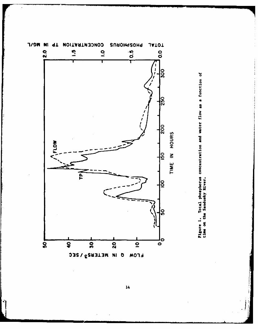
1 Total Phosphorus Concentration and Water Flow asa Function of Time on the Sandusky River 14

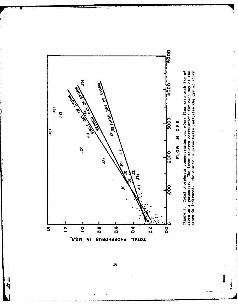
2 Total Phosphorus Concentration vs. River Flow Rate withDay of Storm as a Parameter 16

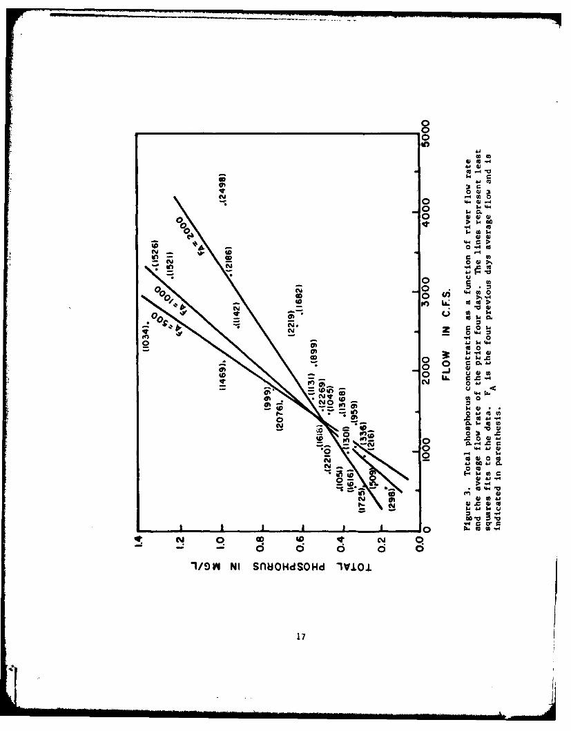
3 Total Phosphorus Concentration as a Function ofRiver Flow Rate and the Average Flow Rate of thePrior Four Days 17

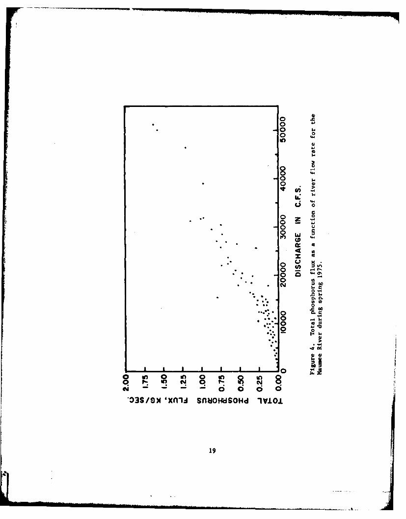
4 Total Phosphorus Flux as a Function of RiverFlow Rate for the Maumee River During Spring 1975 19

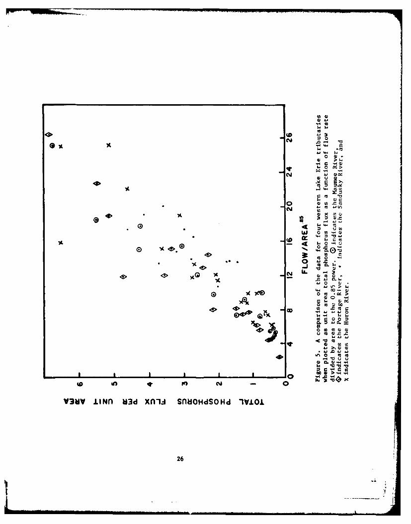
5 A Comparison of the Data for Four Western Lake ErieTributaries when Plotted as Unit Area TotalPhosphorus Flux as a Function of Flow RateDivided by Area to the 0.85 Power 26

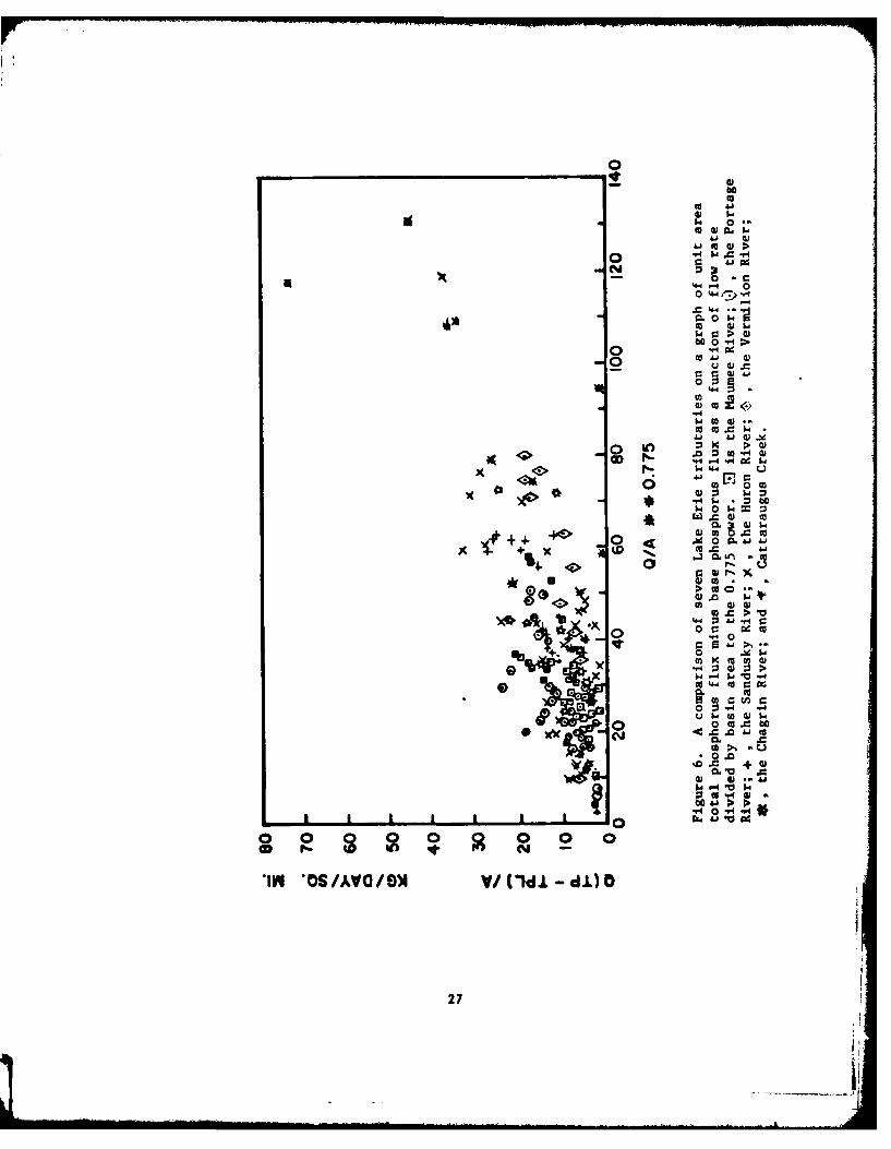
6 A Comparison of Seven Lake Erie Tributaries ona Graph of Unit Area Total Phosphorus Flux MinusBase Phosphorus Flux as a Function of Flow RateDivided by Basin Area to the 0.775 iower 27

SECTION 111,TOTAL PHOSPHORUS TRANSPORT DURING STORM EVENTS

I Hydrograph and Chemograph at the USGS Gaging Stationon Tymochtee Creek at Crawford, Ohio 37

2 Discharge vs. Area Curve for Stations in theSandusky River Basin 39

3 Model Results 41

4 Time vs. Distance Downstream of the Hydrographand Chemograph Peaks 43

iv

LIST OF FIGURES (Cont'd)

SECTION IV STORM TRAVEL DISTANCE CALCULATIONS FOR TOTALPHOSPHORUS AND SUSPENDED MATERIALS IN RIVERS

I Hydrograph and Chemograph (Total Phosphorus) forthe Sandusky River near Fremont, Ohio 49

2 Discharge vs. Area Curves for Stations in theSandusky River Basin 50

3 A Plot of Area or Discharge as a Function ofAxial River Distance Showing the Storm Waveat Two Different Times with the AssociatedPosition of a Water Parcel 52

4 Total Phosphorus Concentration in a Water Parcelas a Function of Water Parcel Travel Distance 55

5 Illustrations of the Average Travel Distance forTotal Phosphorus 56

6 Graphical Construction for the Calculation ofDistribution of Total Phosphorus Travel Distances

From the Total Phosphorus Chemograph 58

7 Distribution of Travel Distances for TotalPhosphorus in the Sandusky River at Fremont 60

8 Cumulative Probability of Travel Distances atVarious Stations in the Sandusky River Basin 61

SECTION V NONENT METHODS FOR ANALYZING RIVER MODELS WITHAPPLICATION TO POINT SOURCE PHOSPHORUS

I A Plot of the Zeroth Moment Ratio, AH , as aFunction of the Reaction Parameter, I/B, forVarious Values of the Dispersion Paramiter, I/A 74

2 A Plot of the First Moment, MI , as a Functionof the Reaction Parameter, I/, for VariousValues of the Dispersion Parameter, I/A 75

3 The Resulting Linear Plot of the First Moment,M i, as a Function of the Adsorption CapacityParameter, Am, for Various Values of theReaction Parameter, 1/1 76

v I

I

LIST OF FIGURES (Cont'd)

Page4 Dependency of the Second Moment on the Dispersion

Parameter, I/A, for Various Values of theReaction Parameter, I/B 78'

5 Ortho Phosphorus Concentrations and Dye Dumps asa Function of Time at the Kestetler Station 79

6 Ortho Phosphorus and Dye Concentrations as aFunction of Time at the Denzer Station 80

7 Ortho Phosphorus and Dye Concentrations as aFunction of Time for the Mt. Zion Station 81

8 Examples of the Least Squares Fitting of theOrtho Phosphorus Concentration to a NormalDistribution Function at Kestetler and Denzer 83

vi

LIST OF TABLES

page

SECTION II THE ESTIMATION OF NUTRIENT TRANSPORT IN RIVERS

I Phosphorus Flux Estimates Based Upon Populationor Land Area 12

2 Comparison of Load Calculation Methods 22

3 Comparison of Sampling Strategies with FlowInterval Method 23

4 Least Squares Fit Results 29

5 Comparison of Total Phosphorus Flux for LakeErie Tributaries Measured vs. PhosphorusLoad Model 31

6 Unit Area Contributions of Total Phosphorus 32

SECTION V MOMENT METHODS FOR ANALYZING RIVER MODELS WITHAPPLICATION TO POINT SOURCE PHOSPHORUS

I Moments for Phosphorus Peaks 83

2 Dispersion Coefficients 84

vii

Llo

I

LIST OF SYMBOLS

SECTION II THE ESTIMATION OF NUTRIENT TRANSPORT IN RIVERS

A = Drainage basin area above a gaging station in square miles.

ai - Arbitrary Constant

CTP 0 Total phosphorus concentration on a viven day in mg/I as P.

D - Total number of days in a given time period.

d- The number of days in a given time interval in which the flow ratewas in the "i" interval.

FA " Average of the four previous days daily averaged flows in cfs.

i a "i" interval

i i "o point in "i" interval

ki a Number of data points in the "i" interval.kr = Factor for r percent confidence interval based upon the normal

distribution with man zero and minus one.

L - Flux values for the "k" data point in the "i" interval.

Lij = Flux values for the "k" data point in the "i" interval.

L = Average daily total phosphorus flux for a given time period.

Li - Average total phosphorus flux for interval "i" for a given timeperiod.

n a Exponent power for the drainage basin area.

P - Total phosphorus concentration in mg/I as P.

- Probability that flow occurs in the "i" interval during a givenperiA of time.

PL = Low total phosphorus concentration for a given stream in ag/I as P.

Q - Instantaneous flow at time P was measured in cfs.

viii

2" I A.

LIST OF SYMBOLS (Cont'd)

Q Length of each flow segment.

Qi Maximum instantaneous flow rates for the "i" interval.

2 Standard error for the mean for interval "i."

Si = Variance

V = Variance for the estimated average daily flux.

cK- Y - intercept of the least square equation.

,3- Slope of the least square equation.

SECTION III TOTAL PHOSPHORUS TRANSPORT DURING STORM EVENTS

A - stream discharge area ft2 (m2)C - total phosphorus stream concentration, ppm (mg/l)Cin- total phosphorus inflow concentration, ppm (mg/l)f a function of A and defines Qf a derivative of fq - influx volume rate per axial distance, cfa t (T3 /sec/m)Q a volumetric flow rate of the stream, cfs (m sec)

t a time, secTP a total phosphorus concentration, ppm (mg/l)u - velocity, ft/sec (m/sec)x a axial variable, ft (m)n a increment of

ac - proportionality constant

Subscripts

i - ith station in the numerical solutionj - jth time in the numerical solution

ix

INTRODUCTION

The research work contained in this report concerns the transport of totalphosphorous and orthophosphorus to Lake Erie. The various calculationaltechniques for analyzing data obtained from Lake Erie tributaries are pre-sented. These calculations were developed to determine the source of thephosphorus and to quantify the input to the lake. The source and quantity ofphosphorous must be determined if successful pollution abatement strategiesare to be devised for Lake Erie.

Under Public Law 92-500 the U. S. Congress directed the Corps of Engineers todevelop a management plan which would rehabilitate Lake Erie. The BuffaloDistrict of the Corps was specifically assigned the task. Thus, the LakeErie Wastewater Management Study was formed.

From its conception, the basic goal of the study has been to develop a mana-gement plan which would reduce or reverse the eutrophic status of the lake.Probably, the two most obvious indicators of Lake Erie eutrophication are theanaerobic hypolimnium in the Central Basin and excessive algal growth. Themanagement plan should reduce the area of anaerobic hypolimnium and diminishthe peak concentrations of algae in the lake.

Many researchers have concluded that the majority of Lake Erie's problems canbe attributed to excessive nutrient inputs to the lake. These nutrients sti-mulate the phytoplankton (algae) growth which yields excess growth. Theexcess algae settle and decompose in the hypolimnium. The decomposition pro-cess consumes oxygen which is responsible for the anaerobic hypolimnium. Theanaerobic hypolimnium reduces the concentration of desirable fish species inthe Central Basin. Since the onset of Lake Erie's eutrophication problems,cowercial fishing has declined markedly. Further undesirable consequencesof excessive nutrients are taste and odor problems in drinking water forlakeshore comunities and polluted beaches unfit for recreation.

The excessive nutrients entering Lake Erie include the macronutrients of car-bon, nitrogen, and phosphorus and the micronutrients of iron, copper, etc.Mathematical models indicate that of these nutrients, phosphorus is con-sidered to be the limiting nutrient affecting algae growth. Experiments haveshown that phosphorous additions to Lake Erie will stimulate algae growth andorthophosphorus concentrations decrease to nearly zero during summer algalblooms. Further, phosphorus is the only macronutrient which is not a consti-tuent of the atmosphere. Thus, it is concluded that since phosphorus is thenutrient which limits the growth of algae in Lake Erie, reducing the input ofphosphorus to the lake would be the best procedure for reducing excessivealgae growth and consequently reversing lake eutrophication.

In order to reduce the phosphorus influx to Lake Erie it is necessary todetermine the sources of phosphorus and the methods by which it istransported to the lake. Basically, there are five sources of phosphorusinto the lake; atmospheric fallout shoreline erosion, direct point sources,river basin sources, and bottom seJiments. No attention is given toatmospheric inputs because these are small and uncontrollable. The shorelineerosion inputs of phosphorus are ignored because the phosphorus contained

'F

in these materials is considered unavailable for algal growth. Inputs frombottom sediments will essentially cease if the hypolimnium of the Centralbasin does not become anaerobic. Thus, the two important sources ofphosphorus are the point sources along the lake shoreline and inputs fromriver basins.

Experimental data are required for the calculational techniques developedherein. These calculations permit quantative understandings of the sourcesof phosphorus and an understanding of the processes involved in the transportof this phosphorus to the lake. The experimental data for the shorelinepoint sources includes the records of various treatment plants along LakeErie and the Detroit River. The experimental data for the river basins arecomposed of the measured river flow and the ortho and total phosphorus con-centrations at the river mouths' confluence with Lake Erie. Additionalexperimental data were taken downstream from a point source which was locatedin the Sandusky River, a Lake Erie tributary. This point source, located atBucyrus, Ohio, was investigated to distinguish between the point sourceinputs to river basins and those emanating from fields, forests, and othernonpoint sources.

Different computational methodologies were developed using the experimentaldata. The first section of this report presents the basic concepts, massbalances, and force relationships used in the proceeding sections of thereport. There are two basic mass balances; that applied to the water andthat applied to the phosphorus. These mass balances are time dependent sincemuch of the transport occurs during storm water flows in the river basins.Further, the force relationship is considered in the form of flow versusstream cross sectional area dependency. With these basic conceptsestablished, the remaining sections of the report can be understood.

The second section of this report concerns the quantification of totalphosphorus input to Lake Erie from river basins and shoreline sources. A -computational method called the Flow Interval Method was devised to permitthe calculation of total phosphorus influx without measuring the totalphosphorus concentration for the entire year. The data requirements for thismethod are discussed, and it is concluded that a good estimate could beachieved if high flow storms were included in the data. The methodology wasextended further to river basins with few total phosphorus measurements.This extension was called the Regional Total Phosphorus Model. It was shownto apply to all river basins with substantial total phosphorus measurementsand it was presumed to apply to other basins. The study conclusions indicatethat basin inputs were significant and would have to be reduced if eutrophi-cation was to be lessened.

Another important aspect of reducing total phosphorus influx from riverbasins is the understanding of the transport processes in rivers. The thirdsection of this report concerns the transport of total phosphorus duringstorm events. basically, the unsteady water mass balance indicates that thewater velocity should be slower than the storm wave velocity.

However, it was noted that the total phosphorus peak always preceeded thewater peak. The computations in the third section demonstrate that the only

2

feasible explanation of this phenomena is for there to be a resuspension anddeposition of the total phosphorus from the banks and bottoms of the streamsduring storm events.

The fourth section of this report presents the derivation of the necessaryequations used to calculate the distance of the travel density function frommeasurements of the water flow rate and the total phosphorus concentrationsat a point in the stream. From this information, the average travel distancefor total phosphorus can be calculated and the fraction of material carried agiven distance can also be obtained. In general, it was found that for largestorms the total phosphorus was transported greater distances than smallstorms. It was also found that the travel distance was shorter in theupstream tributaries than in the downstream mainstem stations. It must beemphasized that these calculations only apply at the point of measurement.

The above calculations indicate that a considerable portion of the totalphosphorus in transport during a storm event never reaches the lake. Thus,the question has been raised as to the fate of point source phosphorusentering the river at some upstream point. A calculational technique used toanalyze upstream point source inputs is presented in Section Five of thisreport. This analysis applies during steady flow in contrast to all theother analysis which were performed on storm events. The computational tech-niqui uses the method of moments to determine the rate of disappearance oforthophosphorus from the water column, presumably into the sediments duringsteady flow. A least squares method for fitting the diurnal peak oforthophosphorus concentrations coming from the treatment plant was devised.This analysis indicated that the orthophosphorus coming from the treatmentplant at Bucyrus, Ohio, did not discharge directly into Lake Erie but ratherit was deposited into the sediments of the Sandusky River. Presumably, thenext storm event which passed through the river basin resuspended thisphosphorus as total phosphorus and carried it toward the lake. This analysisillustrates that the point source phosphorus in the upstream reaches of theriver basin apparently has significantly less impact on Lake Erie than thepoint sources along the shoreline.

This introduction shows the importance of phosphorus in relation to therestoration of Lake Erie. The various computational techniques presentedherein aid in the understanding of total phosphorus transport from riverbasins in Lake Erie. This understanding will be used in the development ofmanagement strategies for the restoration of Lake Erie.

3

EQUATIONS

The basic hydrodynamic principles as used for the calculational procedures inthe following sections will be reviewed. In particular, the conservation ofmass for both the water and the nutrient of interest will be given. Also, adiscussion of the slow versus cross sectional relationship, as it applies tothe solution of the mass balance equations, will be presented.

Eulerian Point of View

The usual mass balance on water flowing in a stream is formed on an incremen-tal distance and change in time and is the Eulerian point of view. The deri-vation can be found in many texts (1) and the resulting equation expressingthis conservation of water mass is given below:

a - q ()'t ax

where A - water cross sectional slow area at x & tQ - volumetric flow rate at x & tx - distance downstreamt - timeq - net volumetric water inflow per unit river length at

x&t

This equation contains two dependent variables Q and A, and two independentvariables x and t. Since there are two dependent variables and only oneequation, this equation cannot be solved by itself. The additional rela-tionship will be discussed later. Also, the net inflow must be specified asa function of time and distance; thus, net inflow includes such phenomena astributary or sheet flow inputs and ground water inflow or efflux.

In addition to the mass balance on the water, a mass balance on the nutrientof interest, mainly total phosphorus, must be made. Following the same pro-cedure as used for the water, the equation describing the conservation ofmass for total phosphorus can be derived and is given below:

3A 2c - qC1 (2)

where C - concentration of substance at x and tC1 - inflow concentration q substance at x and t

Performing the differentiation of the products gives the following:

at+ at ~ ax ax 1 (3)

4

'IA

Substituting the mass balance on the water (Eq. 1) in Equation (3) yields thefollowing simpler equation which was used on all the Eulerian analysis:

*- . qci

A C+Q LC+ j +3Q iat axat ax/

A + Q L q(Cl - c)

This equation gives an additional relationship, but it also adds anotherdependent variable, C. Now there are two equations (0 and 4) to solve forthree variables Q, A, and C. To complete these differential equations, it ispresumed that q and C, are known as functions of distance and time and thatthe initial and boundary conditions are known for each of the two equations.Also, it should be noted that the dispersion term is neglected from Equation2 and hence Equation 4. This was done for two reasons; first, most of thetime these equations are used for unsteady flow for which there are fewvalues for dispersion coefficients, and second, the equations are solvednumerically which introduces some dispersion into the solution.

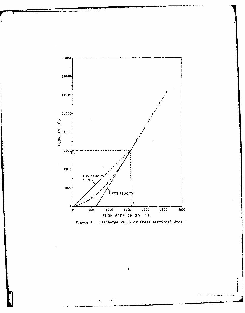
Even if the initial conditions, the boundary conditions, and the inflow func-tions, q and Cl are known, it is still not possible to solve these equationswithout another relationship. Normally, this is provided by a force (or asit is sometimes called momentum) balance. In many instances this forcebalance is dominated by the friction term; in such instances there exists aunique relationship between the river volumetric flow and the cross sectionalarea. Thus, instead of using an empirical relationship such as the Chezyequation, the measured relationship of Q vs A as obtained from the riverpoint of interest is used. This relationship is shown in Figure 1.

Mathematically, Figure I can be expressed as

A - f(Q) or Q - f(A) (5)

Now, it is possible to solve Equations 1, 4, and 5 with known initial con-ditions, boundary conditions, and input functions. When the transport ofnutrients is considered from the Eulerian point of view, these are theequations used. The assumptions involved in deriving equations must beremembered when results derived from them are interpreted. In particular,the assumption of no dispersion, the assumption of a unique flow vs. arearelationship should be checked.

Lagrangian Point of View

In addition to the Eulerian point of view, the following sections sometimesutilize the Lagrangian point of view, i.e., the observer moves with theflowing water instead of being fixed in space. For Langrangian con-siderations, we are interested in the location of a water parcel, S, as afunction of time and this relationship is given below.

5

dodt vW (6)

where S = position of water relative to fixed surroundingsvu water velocity

The water velocity is obtained as the chord of the Q vs. A curve as shown inFigure 1.

In addition to the relationship of the water parcel position to the fixedsurroundings (which have a velocity of zero), interest is focused on the

*position of the water parcel relative to the water wave (hydrograph) in thestream. This position is described by the following relationship.

dz . vw - Vdt (7)

where Z - position of water parcel relative to waterwave in river

v = wave velocity

The wave velocity is determined as the tangent to the Q vs. A curve as shownin Figure 1.

Summary

The basic equations to be used in the following sections are the conservationof mass for both the water and the nutrient and the Q vs. A curve in itsmeasured form. These equations are derived for both the Eulerian andLagrangian point of view. Their solution requires a knowledge of boundaryconditions, initial conditions, and/or input flows and concentrations.Sometimes these equations are turned around to calculate the input functions,sometimes they are linearized, but always the principles of conservation of amass is applied.

6

32000

28000

24000 /

200001J /

z lecool

12000 J-

8000-

FLOW V'ELOCIT

4000-

WAVE VELOCITY

,,A

00 560 1000O 15 00 2060 2500 30*00

FLOW AREA IN SO. FT.

Figure 1. Discharge vs. Flow Cross-sectional Area

, oo 7

__ _ _ _ _ _

THE ESTIMATION OF NUTRIENT TRANSPORT IN RIVERS

by

F. H. Verhoff

Department of Chemical EngineeringWest Virginia University

Morgantown, West Virginia 26505

and

S. M. Yaksich

andD. A. Melfi

Lake Erie Wastewater Management StudyU. S. Army Corps of Engineers

Buffalo, New York 14207

8

Acknowledgment

This work vas entirely supported by the U.S. Army Corps of Engineers. BuffaloDistrict in conjunction with their Lake Erie Wastewater Management Study.The water quality data was collected and analyzed by David S. Baker and J.W. Kramer of Heidelberg College.

Introduction

The eutrophication of many lakes and the decline of water quality in rivershas been attributed to the increase in phosphorus concentration in thesewaters by human activity. Abatement schemes to reduce phosphorus inputs havebeen implemented to alleviate the water quality problems in these lakes andstreams. However, the quantitative effect of these point source phosphorusremoval projects on the downstream receiving rivers and lakes is not knownbecause the dynamics of phosphorus transport in rivers is not understood.The efficacy of the abatement is determined by improvement in the quality ofthe receiving water after the treatment implementation. One quantitative andfaster measure of phosphorus abatement would be the reduction of phosphorustransport by the river into which the abated point sourced emptied.

Further, there have been many mathematical models of rivers and lakes whichpurport to predict future water quality. Most of these models are for lakesor downstream segments of rivers and they use the nutrient loadings of tribu-taries and upstream river segments as inputs to the models. These loadingsare often estimated based upon factors which are supposedly correlated withthe population or land area of the given river basin. The literature clearlyindicates that these correlation factors vary by as much as a factor of fiveand hence the models are only good to this accuracy.

In order to better understand and hence manage our water resources, it isimperative that the nutrient dynamics in rivers be understood. This paperaddresses the problem of posphorus dynamics, presents a calculated techniqueby which the phosphorus loadings can be estimated from experimental data, andapplies the procedure to tributaries of Lake Erie. In addition, this tech-nique is extended to the estimation of phosphorus loadings in rivers withminimal measurements of total phosphorus concentration.

Previous Investigations

The general problem of phosphorus flux determination for a given river basinwould appear to involve land use, rainfall, temperature, and other parametersintrinsic to the basin. Various facets of the relationship of phosphorusconcentration and flux to these parameters have been investigated in thepast. Generally, one can say that of all the factors influencing phosphorusflux, the flow rate of the river dominates.

Wang and Evans (13) determined the concentration of various nutrientsincluding soluble orthophosphate at a one meter depth in nine different sta-tions in the Illinois River during 1967. They found an inverse relationshipbetween orthophosphate concentration and flow; this relationship is commonlyreferred to as the dilution effect. Inviro Control (3) examined the time andflow records of 142 sampling stations on different rivers throughout theUnited States and found that orthophosphate predominately exhibited the dilu-tional effect. However, total phosphorus concentration generally increasedwith increasing flow rate. Since orthophosphate was a small percentage ofthe total phosphorus, the major portion of phosphorus transport in riveroccurs during high flow rate periods, i.e., during storms. Kemp (6) attri-buted the increasing phosphorus concentration to scouring of bottom sediments

10

during increased flow. He also states that a significant amount of phosphateaccumulation occurs in the sediments during low flows as caused by theabsorption on clay materials and by assimilation by periphyton. Otherinvestigators have found correlations between flow and other nutrient con-centrations (Johnson (5) and Fuha (4)).

The fact that total phosphorus concentration depends upon river flow rate hasnot been used in the calculation of total yearly phosphorus flux for rivers.One procedure often used is based on the loading factor as a function of thepopulation in the upstream river basin or the land area above the point ofloading estimation in the river. To illustrate the variability in these fac-tors, the literature values of loading per unit area are shown in Table 1.It can be seen that these factors can vary by several orders of magnitude.Thus, by judiciously choosing these factors based on area or population or acombination of both, it is possible to calculate different levels ofphosphorus fluxes and to reach variant conclusions for the same river. Forexample, by choosing high population factors and low agricultural factors itcan be concluded that most of the total phosphorus is of municipal origin.The variability of these factors for the rivers considered in this study willbe emphasised later.

Further procedures for the calculation of the river flux involves use ofactual total phosphorus concentrations and river flows taken at the riverpoint of interest. The first calculational procedure uses the product of theaverage flow tines the average concentration to estimate the total phosphorusflux. The second procedure essentially calculates the average of the productof the flow and the concentration. In the third procedure, the flux iscalculated from the flow weighted average concentration tines the total flowfor the given river for the time period of interest. Baker and Kramer (1)discuss these procedures and conclude that considerable variability exists inthese techniques. This variability results from the dependency of totalphosphorus concentration upon river flow rate. In the Lake Erie Report (8),it was concluded that to properly estimate total phosphorus fluxes, high flowevents must be sampled and that as many as 48 total phosphorus measurements ayear in a given stream could be insufficient to yield a good estimate of theflux if high flow events were missed.

The general conclusion resulting from the survey of the literature suueststhat the present techniques for phosphorus load estimation are deficient.Hence, a better loading calculation method is needed which also yields anestimate of the error associated with the flux estimate.

Goal of the Present Work

Since certain facts are known about the dynamics of phosphorus transport inrivers and since phosphorus fluxes in rivers are important data for eval-uation of phosphorus abatement programs and prediction of eutrophicationpotential of water bodies, it would seen logical to try to utilise knownriver properties in the estimation of loadings. This paper contains adescription of the methodology developed and used for the estimation of thetotal phosphorus loading into Lake Erie. To make these estimates, there aretwo fundamental but related problems to be attacked. First, since it was

11

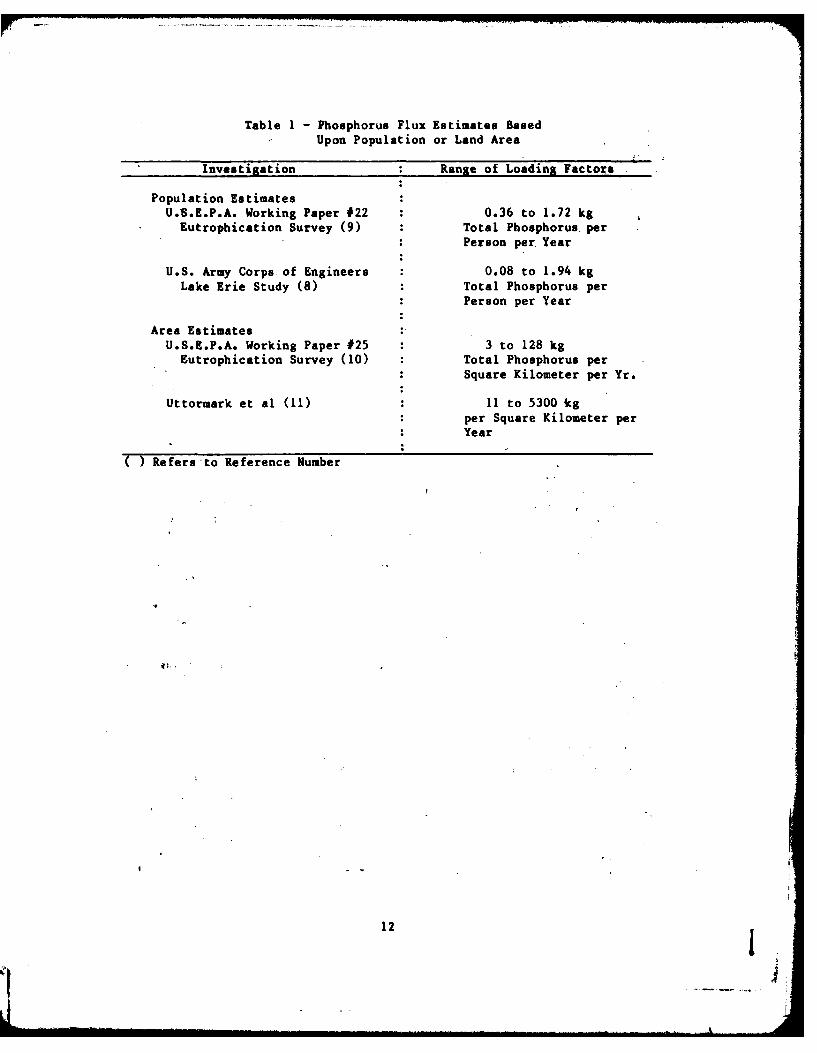
Table I - Phosphorus Flux Estimates Based

Upon Population or Land Area

Investigation Range of Loading Factors

Population EstimatesU.S.E.P.A. Working Paper #22 0.36 to 1.72 kg

Eutrophication Survey (9) Total Phosphorus, per

: Person per Year

U.S. Army Corps of Engineers 0.08 to 1.94 kgLake Erie Study (8) : Total Phosphorus per

: Person per Year

Area EstimatesU.S.E.P.A. Working Paper #25 3 to 128 kg

Eutrophication Survey (10) Total Phosphorus per: Square Kilometer per Yr.

Uttormark et al (11) * 11 to 5300 kg: per Square Kilometer per* Year

( ) Refers to Reference Number

12

- - -* v

impossible to sample and analyze a river at time intervals frequent enough toaccurately integrate the product of the concentration and the flow over thecourse of a year, some procedure for the estimation of the total yearly fluxof phosphorus from a limited number of samples must be devised. Secondly, itwas also impossible to institute a sampling program in all the rivers whichevpty into Lake Erie, and thus there was needed a scheme for the estimationof phosphorus fluxes from river basins in which a minimum of phosphorus con-centration data was available.

Herein is presented an estimation scheme for the expected value of thephosphorus flux in a particular river and for the standard error associatedwith the expected value. The procedure essentially involves the experimentalestablishment of a relationship (either a curve or a group of data) betweenthe flow rate and the phosphorus flux (flow times concentration). This curveis then employed in conjunction with flow data for the entire year to esti-mate the flux and the standard error. Thus, this procedure required alimited sampling program for the establishment of the flux flow curve.

For the rivers in which no phosphorus measurements were made, a similar pro-cedure was used except that the curve relating phosphorus flux to river flowrate had to be generalized such that it would apply to all rivers of the LakeErie basin. The only experimental data required for the rivers with littlephosphorus information was the daily flow data, the base phosphorus con-centration from the historical record, and the area of the watershed. All ofthis information was readily available for all the important streams flowinginto Lake Erie.

Phosphorus Dynamics in Rivers

The procedure for phosphorus flux estimation developed in this report isbased upon a knowledge of the dynamics of phosphorus in river basins. Fromprevious research studies, it has been documented that phosphorus con-centrations generally increase with increasing flow. Cahill (2) reportedthat for the Brandywine River the phosphorus concentration definitely peaksbefore the water flow rate reaches its maximum. Some data taken on theSandusky River as an integral part of this study also indicates this samecharacteristic. This data is shown in Figure 1. If one is to use this phe-nomena in phosphorus flux estimation, then the correlation should take intoaccount the time as well as the flow rate of the river. The relationshipbetween flux and the two variables, river flow, and time into the storm wereinvestigated.

In the development of a correlation, the flow rate of the river can be quan-tified from the stage reading. In our calculations we will be using instan-taneous flow for the correlations and daily average in the flux calculations.There may be some error introduced by this procedure, however, it should beminor compared with other errors because of the large river basin studied.The ideal situation would be to have both data in terms of instantaneous flowrate, but that data is not historically available. Walling (12) has shownthat the use of daily average flow measured to estimate sediment flux canlead to large errors on small rivers.

13

,/OVI NI di NOI1VVIN33NO3 snkWoldSOHd IVJ.OJ

0 00

000

CY4

c'I

0U0

S'.

00

ILI

0 1

-4

144

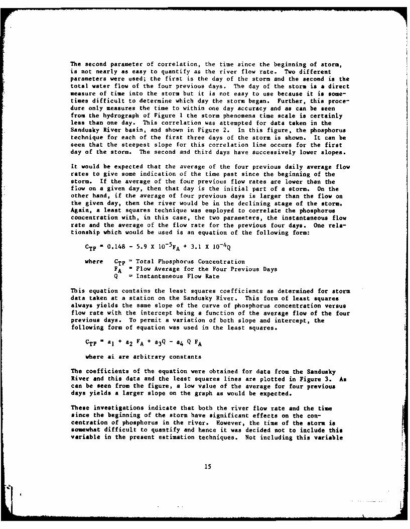
The second parameter of correlation, the time since the beginning of storm,is not nearly as easy to quantify as the river flow rate. Two differentparameters were used; the first is the day of the storm and the second is thetotal water flow of the four previous days. The day of the storm is a directmeasure of time into the storm but it is not easy to use because it is some-times difficult to determine which day the storm began. Further, this proce-dure only measures the time to within one day accuracy and as can be seenfrom the hydrograph of Figure 1 the storm phenomena time scale is certainlyless than one day. This correlation was attempted for data taken in theSandusky River basin, and shown in Figure 2. In this figure, the phosphorustechnique for each of the first three days of the storm is shown. It can beseen that the steepest slope for this correlation line occurs for the firstday of the storm. The second and third days have successively lower slopes.

It would be expected that the average of the four previous daily average flowrates to give some indication of the time past since the beginning of thestorm. If the average of the four previous flow rates are lower than theflow on a given day, then that day is the initial part of a storm. On theother hand, if the average of four previous days is larger than the flow onthe given day, then the river would be in the declining stage of the storm.Again, a least squares technique was employed to correlate the phosphorusconcentration with, in this case, the two parameters, the instantaneous flowrate and the average of the flow rate for the previous four days. One rela-tionship which would be used is an equation of the following form:

CTp = 0.148 - 5.9 X 10-5 FA + 3.1 X 10- 4Q

where CTP f Total Phosphorus ConcentrationFA = Flow Average for the Four Previous DaysQ = Instantaneous Flow Rate

This equation contains the least squares coefficients as determined for stormdata taken at a station on the Sandusky River. This form of least squaresalways yields the same slope of the curve of phosphorus concentration versusflow rate with the intercept being a function of the average flow of the fourprevious days. To permit a variation of both slope and intercept, thefollowing form of equation was used in the least squares.

CTP a1 + a2 FA + a3Q - a4 Q FA

where ai are arbitrary constants

The coefficients of the equation were obtained for data from the SanduskyRiver and this data and the least squares lines are plotted in Figure 3. Ascan be seen from the figure, a low value of the average for four previousdays yields a larger slope on the graph as would be expected.

These investigations indicate that both the river flow rate and the timesince the beginning of the storm have significant effects on the con-centration of phosphorus in the river. However, the time of the storm issomewhat difficult to quantify and hence it was decided not to include thisvariable in the present estimation techniques. Not including this variable

15

00____ ___ ___ ___ ____ ___ _ _CC_ %0

0

* 4.

> 00 0

0 0

0~ 0 0JO

(14 4 .6V

-'S 0 04* O~ 41 4a'o 4a W0

0 S'0w

0 -;

vow Ni *nOdS~ IV

16mo

0 0

0 ed.41. 44

>ot

oy 0 0

010

-00

cy. 0 14

co4 0

00 0

0 00 LL. 0IL4 01.1-

'44:3W

WE4 Ca 0..0 00

00064

in .010 r

000

N 0 461

171

0 oto"

0 O.C

c; ci 0

does not necessarily imply that the phosphorus fluxes calculated will be less

accurate, rather it implies that the variance associated with the estimationtechnique (for a given number of experimental measurements) will be larger.Hence, the equivalent accuracy can be achieved by ignoring the time into the

storm, if more experimental data points are used in the correlation of flow

versus concentration, that would be used in concentration versus flow and

flow average of the previous four days. For this estimation of phosphorusflux into Lake Erie, the only parameter considered important will be the flowrate.

Estimation Procedure for Measured Basins

The flux estimation procedure for each river basin in which concentration andflow measurements have been made is based upon a technique called the flowinterval method. Baker and Kramer (1) and Porterfield (7) used the basicidea of the interval method previously. This method essentially involves theplotting of the product of the total phosphorus concentration times the flow

rate (i.e., the total phosphorus flux) as a function of the river flow rate.This dependency of flux with river flow rate is then used with the dailyaverage river flow records to calculate the yearly total phosphorus flux.

An example of the data used in the phosphorus flux estimation is shown inFigure 4. This river data illustrates the quadratic character of the data

when plotted as total phosphorus flux as a function of river flow rate. If

the total phosphorus concentration were plotted versus river flow, a linear

relationship would result. This graph of total phosphorus flux versus riverflow rate is then used in the estimation technique by dividing the maximum

flow rate (Q.) into n equal segments. The length of each segment is then

Q -QM/n'

If Qi = i x 0, then the "i" flow interval contains all river flows greaterthan Qi-l and less than Qi. In each of the "i" intervals there are ki data

points whose flux values are given by Li3 . The average flux value for eachinterval is then calculated by the following formula.

ki- .-Lijin

The standard error of the mean then can be calculated for each interval basedupon the following formula.

S i 2 =j=I(j-,;,)2

k i (ki-0)

Although it is known that L1 is distributed normally and that Si is chi-

squared and that any confidence interval for the "i" flow interval should

involve the students t distribution, other known and unaccounted errors in

the system mitigate against expending the extra effort to carry the exactstatistics through the problem. Thus, for these calculations it will be

18

C.'

U:4-

* 0 w

z) o

0 0 U

* II* 0 -

0 a0

0. - cc .

* 4

*00.0 0,

C ~~*. 0 PI

'03S/S- xni. 1.4~S~dIV

194

jpresumed that the average for each interval is distributed normally with manLi and variance TO"

In order to compute the total phosphorus flux for a year or ay other periodof time, it is necessary to determine the number of days during the timeperiod that the flow was in each flow interval on the graph. The probabil-ity, Pi, that the flow occurs in the "i" interval, is given by the followingformula.

Pi .d.

D

where Pi a The probability that flow occurs in the "i" intervalduring a given period of time.

d i - The number of days in the given time interval in which

the flow rate was in the "i" interval.

D a The total number of days in the given tine period.

The average daily flux of total phosphorus for the given time period is thencalculated from the following formula:

n

L Li Pii-I

An approximation for the variance associated with this estimated averagedaily flux is calculated by the equation below.

2V. B~ i

i-I

Since it was presumed that the average total phosphorus flux for each flowinterval was distributed normally, the weighted sum of this random variablewill again be distributed normally. Thus, the confidence interval for theaverage daily total phosphorus flux will be given by the following formula.

L Lkr FR

here kr is the factor for r percent confidence interval based upon the nor-mal distribution with mean zero and variance one.

It must be remembered that the assumption of the normal distribution insteadof the students t distribution in each of the flow intervals will tend toreduce the estimated confidence interval. However, for a reasonably largenumber of measurements, the estimates based upon the normal distributionapproaches these from the students t distribution.

In order to calculate the total flux of total phosphorus for the given periodof time, the average daily total phosphorus flux is multiplied by the number

20

of days in the time period. Similarly the confidence interval is calculated

by multiplying the daily variability by the number of days.

Application to the Maumee and Sandusky Rivers

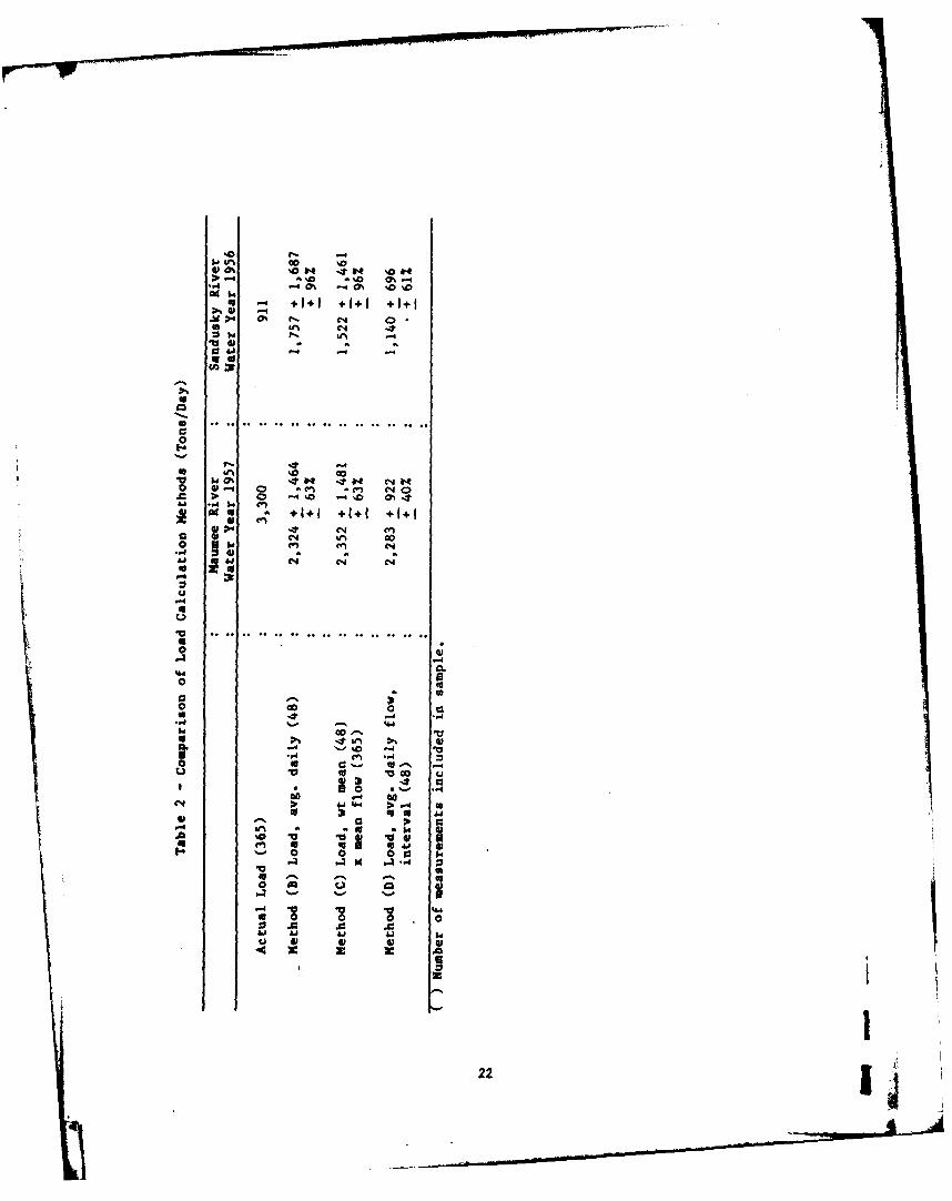
In this section, the flow interval method of total flux estimation will becompared with three other estimation schemes. Also, the amount and type ofconcentration data which are required to obtain good flux estimates will bediscussed. For water years 1956 on the Sandusky River and 1957 on the MaumeeRiver, 48 measurements (four per month) of suspended sediment concentrationand water flow rate were randomly selected from daily concentration and flowdata. Four different methods for the estimation of the total phoaporus fluxwere used. (Table 2). Method A was the multiplication of the average flowtimes the average concentration for the 48 measurements. Method B simplyinvolves the calculation of the flux for each day and then averaging thesefluxes. Method C obtains an estimate of the average daily flux bymultiplying the flow weighted average concentration times the average dailyflow. Method D is the flow interval method presented in the previous sec-tion. No comparisons will be made for Method A since it will obviouslyunderestimate the suspended sediment flux since the concentration increaseswith increasing flow.

Comparison of the suspended sediment loads for the Maumee River show thateach of the three methods calculate an average flux which is less than theactual flux of 3,300 tons/day based on 365 measurements. However, the errorestimate for the flow interval method is 40 percent versus 63 percent foreach of the other methods. The reason for the low flux estimate is that notenough high flows were included in the sample of 48.

Comparion of the flux data for the Sandusky River for water year 1956 showsthat the flow interval method yields a better estimate and smaller error thanMethods (B) or (C). The Sandusky estimate using the flow interval method isbetter than the Maumee estimate using the same method because the day whichcarried the highest sediment load was included in the Sandusky sample.

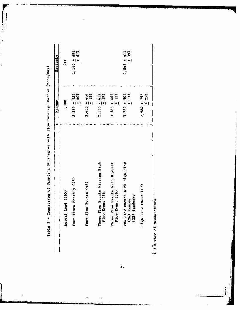
Table 3 illustrates the ability of the flow interval method for estimatingthe entire year average flux from limited concentration information with awell defined flux versus flow curve. For the Maumee River, 48 samplesselected uniformly were compared with 48 samples selected during the fourmajor flow events. It can be seen from the table that the selection of theevent information yielded a better estimate (3,453 + 464 tons/day) andsmaller error (13 percent) than the four times monthly strategy (2,283 + 922tons/day) and (40 percent error) when compared to the actual load, (3,310tons/day).

When only three flow events (36 samples) were included with the high flowevent omitted, a poorer estimate (2,136 + 412 tons/day) was obtained, eventhough the error estimate was small. When three flow events which includedthe high flow were selected (36 measurements) a good flux estimate (3,486 +

467 tons/day, 13 percent error) was obtained. Including only the two high7-flow events (24 measurements) again yielded good flux (3,789 + 502 tons/day)and error estimate (13 per cent). Using only the high flow event

21

Ii.

00% OH 'tH %OV.0 40% 00.

U ~+1+1 + 14l +1~

C4 e

00

I.'t**

'tH 49P4 e4H

A 0 -4 0 '0 0%4"

-t C.4

O I. 41 4)

q44

U2

+ - + +1 ++

eq %0 0 C.)0% 44 4T L -

cn 0" 0 %0n U) co ODc

C1 nU

4) 0.4 4~G 4- .44 i IC

z .to

-4 W tzt

w~' 4 F14 C4 1.d.4 C-I A ~ .0

4-W4

.00

J23

(17 measurements) also gave a good flux estimate (2,984 + 757 tons/day),however, the error estimate increased to 25 percent.

Comparison of sampling strategies for the Sandusky River shown that samplingthe two high flow events (22 measurements) yields a better flux estimate(1,045 + 411 tons/day) and error estimate (39 percent), than 48 measurementsmade four times monthly (1,140 + 696 tons/day and 61 percent error estimate)when compared to the actual flux (365 measurements) of 911 tons/day.

The reason a better flux estimate and smaller error estimate is obtained forthe Maumee River than for the Sandusky River is that a flow event lasts 10 to14 days on the Maumee. On the Sandusky, a flow event lasts only five to ninedays. Therefore, 12 measurements over the hydrograph averages one measure-ment per day for the Maumee. For the Sandusky, daily measurements are notenough. To obtain good definition for the Sandusky, measurements should betaken at least every 12 hours, or 12 measurements in six days. For a streamwhich rises and falls in one day, measurements should be taken about everytwo hours.

In summary then, it is concluded that the flow interval method will yieldgood estimates of the flux if the high flow portion of the flux versus flowcurve is defined.

Regional Phosphorus Load Model

In a previous section, it was shown that the flow interval method yields goodestimates of the flux if enough high flow measurement points are included inthe data base. Thus, to estimate the phosphorus flux for a given river basinit is only necessary to measure the phosphorus flux as a function of flowrate for several high flow events and then utilize the daily average flowrecord to calculate the total flux. Hence this procedure could be used forall the basins in which sampling was performed during this study.

However, the sampled river basins only constituted one third of the totaldrainage area into Lake Erie. To complete a phosphorus flux estimate intothe lake, it is necessary to calculate the fluxes from the other two thirdsof the land area. In other words, a methodology had to be developed whichwould permit the computation of the phosphorus fluxes for many river basinswhich had a very limited chemical sampling history and had the flow recordfrom a stream gaging station.

Since the previous calculations indicated the importanoe of measuring highflow events in a river basin and since no historical records contain thesemeasurements, it was necessary to attempt an extrapolation from the basinsmeasured during this study into those unmonitored rivers. The extrapolationneed only involve the relationship between phosphorus flux and river flowrate, because once this information is known, the flow interval method can beemployed using the stream flow data from the gage. The problem then is thedetermination of the general relationship between phosphorus flux and riverflow rate which will apply to all rivers in the Lake Erie basin.fortunately, the sampling program involved rivere from the far west to theeast of the lake encompassing most terrain and soil types. Thus if a general

24

pmI

relationship for the phosphorus flux as a function of flow rate could befound for these rivers it probably would apply to all the rivers of the LakeErie basin.

The initial attempts to achieve this general correlation focused on the fourmonitored rivers of western Lake Erie, i.e., the Maumee, the Portage, theHuron, and the Sandusky Rivers. These rivers had the same range ofphosphorus concentration although the flows were quite different because ofdifferent land areas. The first task was to find some function of area whichwould reduce these four rivers to the same flow rate scale. Often the unitarea contribution is considered important and this concept would suggest that

the flow rate of the river be divided by the area of the river basin.However, the most important time periods of phosphorus flux are the storms.During storms, according to partial area hydrology, only the fraction of the

total basin area near the stream contributes to the actual flow observed.For partial area hydrology, the length of the river might be more nearly thecharacteristic dimension. Since the river length is related somewhat to the

square root of the basin area, partial area hydrology then leads to a flowparameter which involves the flow rate divided by the area to a power betweenone half and one. After plotting the data for the four rivers using dif-

ferent power fractions, it was found that the best fit was approximately the0.85 power. Figure 3 shows the plot based upon the parameter of flow ratedivided by area to the 0.85 power.

Although only a portion of the river basin is contributing to storm flow andphosphorus, the river bottom is contributing phosphorus which is transportedduring the storms. Hence, on the ordinate in Figure 5, is plotted the totalphosphorus flux divided by the total area of the river basin. From thisfigure it can be seen that all four of these basins are indistinguishable,i.e., this graph could be employed for the prediction of the phosphorus fluxof any of these rivers. It appeared that this correlation could be used forall the rivers of western Lake Erie.

If the data from Cattaraugus Creek in eastern Lake Erie is plotted on Figure5, it is imediately apparent that this data lies significantly below that of

the western Erie rivers. Upon further inspection of the data one finds thatthe total phosphorus concentration of the Cattaraugus is much lower than thatfound in the Maumee for example. However, the difference between high andlow values were about the same. In other words, the Cattaraugus and theMaumee were similar in the increase of total phosphorus concentration withincreased flow. They differed in the base value of phosphorus concentrationduring low flow time periods. This fact suggested that maybe the Cattaraugus

and other eastern Erie rivers could be made similar to the western Erierivers if the base total phosphorus concentration were subtracted from the

total phosphorus concentration found during high flow periods and this fluxdifference plotted against the flow rate parameter.

Figure 6 contains this new flux parameter, the flow times the differencebetween the total phosphorus concentration and the total phosphorus con-centration during base flow divided by the basin area, graphed as a functionof the flow parameter. As can be seen from this graph the data from sevenrivers (Naumee, Portage, Sandusky, Huron, Chagrin, Vermilion, and

25

0 0 j>.J

N 0 ad

4.14. to

a -4 t

L. m$z4 0 -40 4 QJ4

00

0 C3

U0 -4 Q)

00 M > ..

(0P4 " 0.0

cc 0 '4

CLa

$w 41 4. 0L

LM 0

4 4441

VUV~~~~1.- 2.2.U.i. n8~SO d l~

2600

00co

00S 4.1

41 9

0 *

441

o 90

0 -

0 u ..

lt0.1 0

_0 W 0-H

9P.- w0 44

x 0 w1.' 0 w' 0

+ 4. 0.

4. .CY

0 0 94t4 0

4. 0 >44K04

X. 0

NO- -

0 ,-40 0ad

0O. 04449.4 -4 . -

27

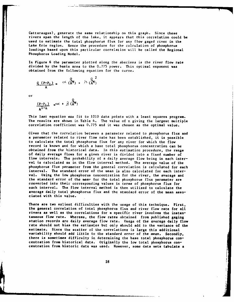
Cattaraugus), generate the same relationship on this graph. Since theserivers span the length of the lake, it appears that this correlation could beused to estimate the total phosphorus flux for any flow gaged river in theLake Erie region. Hence the procedure for the calculation of phosphorusloadings based upon this particular correlation will be called the RegionalPhosphorus Loading Model.

In Figure 6 the parameter plotted along the abscissa is the river flow ratedivided by the basin area to the 0.775 power. This optimal exponent wasobtained from the following equation for the curve.

Q (PP,) AC(~Tr) +

A

or

Al-n

This last equation was fit to 1010 data points with a least squares program.The results are shown in Table 4. The value of n giving the largest multiplecorrelation coefficient was 0.775 and it was chosen as the optimal value.

Given that the correlation between a parameter related to phosphorus flux anda parameter related to river flow rate has been established, it is possibleto calculate the total phosphorus flux for any river for which the flowrecord is known and for which a base total phosphorus concentration can beobtained from the historical data. In this estimation procedure, the rangeof daily average flows for a given river is divided into a fixed number offlow intervals. The probability of a daily average flow being in each inter-val is calculated as in the flow interval method. The average value of thephosphorus flux parameter from the general correlation is calculated for eachinterval. The standard error of the mean is also calculated for each inter-val. Using the low phosphorus concentration for the river, the average andthe standard error of the mear for the total phosphorus flux parameter areconverted into their corresponding values in terms of phosphorus flux foreach interval. The flow interval method is then utilized to calculate theaverage daily total phosphorus flux and the standard error of the mean asso-ciated with this value.

There are two salient difficulties with the usage of this technique. First,the general correlation of total phosphorus flux and river flow rate for allrivers as well as the correlations for a specific river involves the instan-taneous flow rate. Whereas, the flow rates obtained from published gagingstation records are daily average flow rate. Usage of the average daily flowrate should not bias the estimates but only should add to the variance of theestimate. Since the scatter of the correlations is large this additionalvariability should add little to the standard error of the mean. Secondly,there is sometimes difficulty in determining the base total phosphorus con-centration from historical data. Originally the low total phosphorus con-centration from historic data was used. However, some data sets tabulate a

28

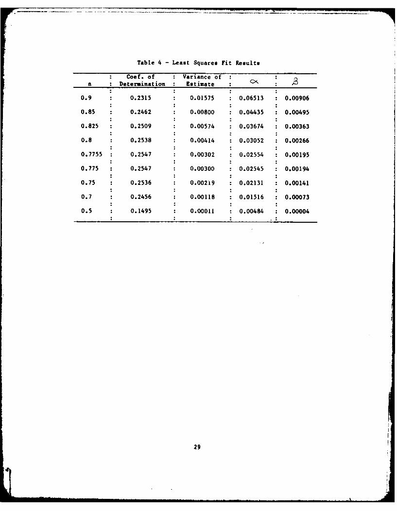
Table 4 - Least Squares Fit Results

Coef. of : Variance of

n Determination : Estimate : >

0.9 0.2315 0.01575 0.06513 0.00906

0.85 0.2462 0.00800 0.04435 0.00495

0.825 0.2509 0.00574 0.03674 0.00363

0.8 0.2538 0.00414 0.03052 0.00266

0.7755 0.2547 0.00302 0.02554 0.00195

0.775 0.2547 0.00300 0.02545 0.00194

0.75 0.2536 0.00219 0.02131 0.00141

0.7 0.2456 0.00118 0.01516 0.00073

0.5 0.1495 0.00011 0.00484 0.00004

29

I.

single total phosphorus concentration which is significantly lower than allothers measured (zero for example). The question arose as to whether thatvalue was a true measurement or whether it is an experimental error. As ageneral rule it was best to choose as the low phosphorus concentration thelowest value which occurs two or preferably three times in the historicaldata set. Close examination of the data revealed that the low totalphosphorus concentrations occurred when the flow rate was in the range of 0.5to 2.0 cubic feet per second divided by area to the 0.775 power. The basephosphorus concentration was then calculated by averaging the concentrationswhich were measured with flows in this range.

Application of the Phosphorus Load Model to Lake Erie Tributaries

To test the efficacy of the Phosphorus Load Model (PLM) for the prediction ofphosphorus loadings for rivers of the Lake Erie basin, internal comparisonswere made on the seven rivers whose data comprised the general correlation.Predictions of the total phosphorus loads were computed for all seven riversusing the PLM. Then the data from each river was used separately with theflow interval method to calculate the phosphorus flux of each river. A com-parison of the values is shown in Table 5. As can be seen the PLM predictsvalues which are within the expected errors for all the rivers. The mostsignificant deviation in 1975 occurs in the Cattaraugus, but the intervalsoverlap and statistically one would expect this type of deviationoccassionally. It must be remembered that the deviation interval is 90 per-cent probable. The conclusion drawn from this table is that the PLM pre-dicts the phosphorus flux almost as accurately as the measured data using thebest calculational technique, i.e., the flow interval method. The PLM wasthus utilized in all the total phosphorus flux estimates for primarily ruralriver basins.

The phosphorus load model was applied to most of the tributaries of Lake Eriewith the resulting phosphorus transport per unit area listed in Table 6. Itcan be seen that the unit area loading varies by a factor of three. Further,subtraction of the point source (either reported or on a population basis)does not improve the similarity of the loading factors for these basins.Thus it appears that factors beyond area or population determine the outflowof total phosphorus and that these factors are not easy to discern.

Least Squares Utilization of the Data

Inste~d of using the actual data points themselves in the flow intervalmethod it is possible to employ the least squares best fit of this data alongwith the river flow information to estimate the total phosphorus transport.This procedure has been investigated with certain assumptions about thedistribution of the random variable contained in the data. The estimation ofthe daily average flux of total phosphorus is quite straight forward and canbe done if so desired from the least squares equation listed in Table 4. Thecalculation of the variance associated with this estimate is more difficultand requires certain assumptions.

Overall, the use of the least squares does not reduce the effort since themeasured river data must be first analyzed on the computer to obtain the

30

1

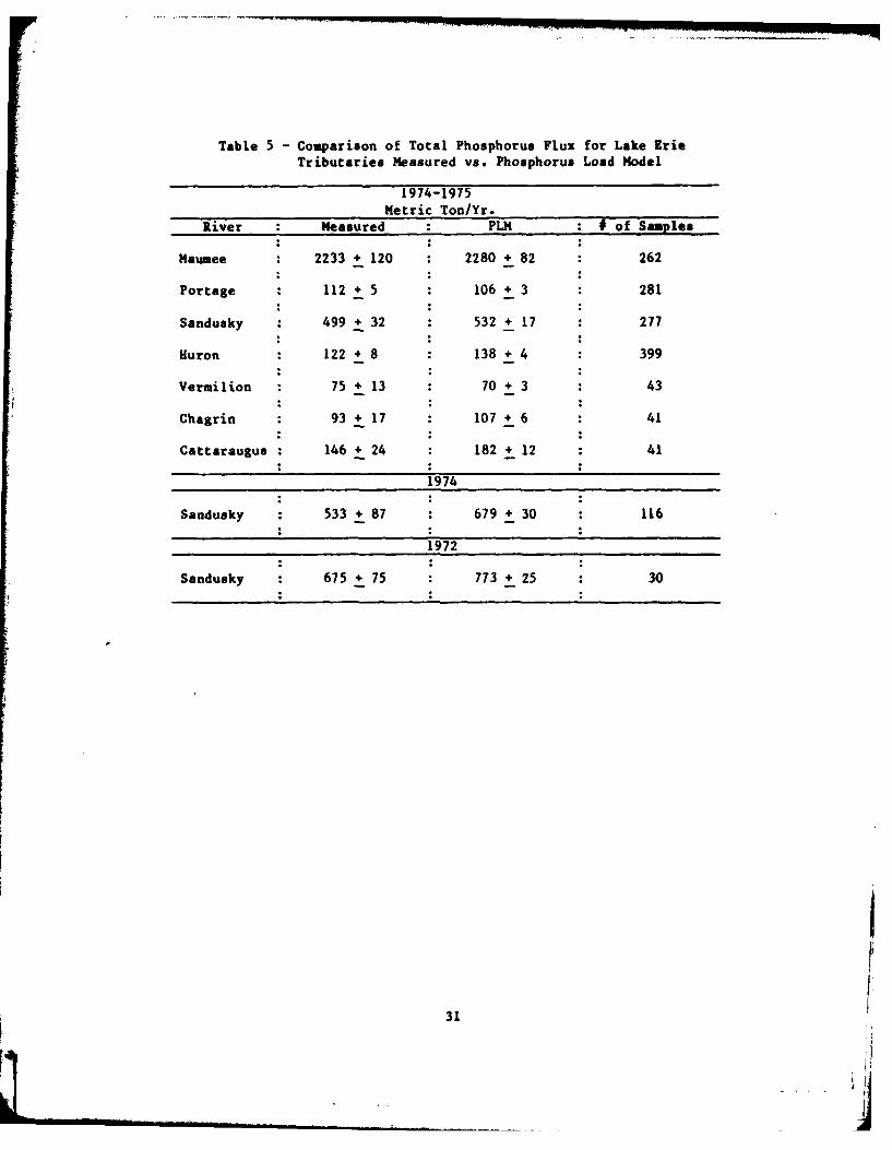
Table 5 - Comparison of Total Phosphorus Flux for Lake ErieTributaries Measured vs. Phosphorus Load Model

1974-1975

Metric Ton/Yr.River Measured PLM # of Samples

Maumee 2233 + 120 2280 + 82 262

Portage 112 + 5 106 + 3 281

Sandusky 499 + 32 532 + 17 277

Huron 122 + 8 138 + 4 399

Vermilion 75 + 13 70 + 3 43

Chagrin 93 4 17 107 + 6 41

Cattaraugus 146 + 24 182 + 12 41

1974

Sandusky 533 + 87 679 + 30 116

1972

Sandusky 675 + 75 773 + 25 30

31

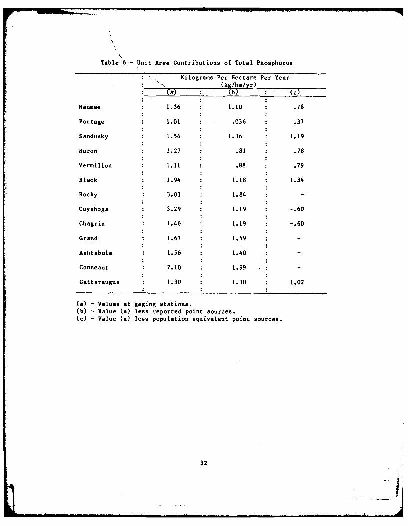
Table 6-- Unit Area Contributions of Total Phosphorus

: . Kilograms Per Hectare Per Year

(kg/ha/yr): (') :(b) (c)

Maumee 1.36 1.10 .78

Portage 1.01 .036 .37

Sandusky 1.54 1.36 1.19

Huron 1.27 .81 .78

Vermilion 1.11 .88 .79

Black 1.94 1.18 1.34

Rocky 3.01 1.84 -

Cuyahoga 3.29 1.19 -.60

Chagrin 1.46 1.19 -.60

Grand 1.67 1.59

Ashtabula 1.56 1.40 -

Conneaut 2.10 : 1.99 -

Cattaraugus 1.30 : 1.30 1.02

(a) - Values at gaging stations.(b) - Value (a) less reported point sources.(c) - Value (a) less population equivalent point sources.

32'i Jir

least squares equation. Since the data is already on the computer, it isexpedient to proceed immediately to the flow interval method rather thanbother with the fitting equation.

If a quick estimate of the loading of a given river is needed, it is possibleto use the least squares fit of the regional phosphorus load model. However,it must be remembered that this model was shown to be useful for tributariesof Lake Erie only. Any extrapolation to other river systems is precarious.

Conclusions

A flow interval method for the estimation of total phosphorus transport ratein rivers is developed. This method requires some measurements of totalphosphorus concentration and the daily river flow records. In a comparisonwith previous methods the flow interval method is shown to be superior.

This method is generalized to all tributaries in the Lake Erie basin. Thisregional phosphorus load model is shown to be useful for all the nonurbantributaries of the lake. This model was applied to several rivers and theresulting total phosphorus transport was used to calculate the unit area andunit population contributions for these basins. There was considerablevariation in the unit contributions among river basins which appeared similarin most respects.

The method as applied in this paper is restricted to total phosphorus.However, it has application to any substance whose concentration is a func-tion of river flow rate. In a previous report, the Corps of Engineers usedthis technique for calculations of chloride, ammonia, organic and nitrite-nitrate nitrogen, orthophosphorus, silica, and suspended solids transport.

33

Mo --- -

References

1. Baker, D. B., and J. W. Kramer, "Phosphorus Sources and Transport in anAgricultural River Basin of Lake Erie," Proc. 16th Conf. Great Lakes Res.,Internat. Assoc. Great Lakes Res., 1973, pp. 858-871.

2. Cahill, T. H., P. Imperato, and F. H. Verhoff, "Evaluation of PhosphorusDynamics in a Watershed" Journal of Environmental Engineering, ASCE Vol. 100,No. EEZ, April 1974, pp. 439-458.

3. Enviro Control Inc., "National Assessment of Trends in Water Quality,"Report to Council of Environmental Quality, NTIS, Springfield, VA, 1972.

4. Fuhs, G. W., "The Chemistry of Streams Tributary to Lake George, NewYork," Environmental Health Report No. 1, NYS Dept. of Health, Albany, NY,Sept. 1972.

5. Johnson, N. M., et. al., "A Working Model for the Variation in StreamWater Chemistry at the Hubbard Brook Experimental Forest, New Hampshire,"Water Resources Research, Vol. 5, 1969, p. 1353.

6. Kemp, L. E., "Phosphorus in Flowing Streams," Water Research, Vol. 2,1968, p. 373.

7. Porterfield, G., "Com'*putation of Fluvial-Sediment Discharge,"Applications of Hydraulics, Book 3, Chapter 13, Techniques of Water ResourcesInvestigations of the United States Geological Survey. 1972.

8. U. S. Army Corps of Engineers, "Lake Erie Wastewater Management Study,Preliminary Feasibility Report" Vol. 3, Buffalo, NY, December 1975.

9. U. S. Environmental Protection Agency, "Nitrogen and Phosphorus inWastewater Effluents," Working Paper No. 22, National Eutrophication Survey,Corvallis, OR, Aug. 1974.

10. U. S. Environmental Protection Agency, "Relationships Between DrainageArea Characteristics and Non-Point Source Nutrients in Streams," WorkingPaper No. 25, National Eutrophication Survey, Corvallis, OR, August 1974.

11. Uttormark, P. D., J. D. Chapin, and K. M. Green, "Estimating NutrientLoadings of Lakes from Non-Point Sources," Report to National EnvironmentalResearch Center, NTIS, Springfield, VA, August, 1974.

12. Walling, D. E., Limitations of the Rating Curve Technique for EstimatingSuspended Sediment Loads, with Particular Reference to British Rivers,"Erosion and Solid Matter Transport in Inland Waters-Symposium, IAHS - AISHPublication No. 122, 1977, pp. 34-48.

13. Wang, W. C. and R. L. Evans, "Dynamics of Nutrient Concentrations in theIllinois River," Journal Water Pollution Control Federation, Vol. 42, 1970,p. 2117.

34

TOTAL PHOSPHORUS TRANSPORT DURING STORM EVENTS

by

F. H. Verhoff

Department of Chemical EngineeringWest Virginia UniversityMorgantown, WV 26505

and

D. A. Melfi

Lake Erie Wastewater Management StudyU. S. Army Corps of Engineers

Buffalo, New York 14207

Presented at the Twentieth Conference on Great Lakes Research, The Universityof Michigan, Ann Arbor, Michigan, 1977

35

Introduction

It is known that the total phosphorus concentration increases with increasingriver flow rate during storm events for many rivers. Cahill et al. (1) foundthis to be the case for the Brandywine River in eastern Pennsylvania and theCorps of Engineers (3) found this same phenomena in the rivers of westernOhio which drain into Lake Erie. In further work on Lake Erie, the questionarose as to the origin of the total phosphorus passing a given downstreampoint in the river during the storm event. Keup (2) suggested that thistotal phosphorus comes from the river bottom, banks, and flood plains duringthe storm event. Others proposed that the source of this total phosphorus ata downstream river station is runoff water which comes from some part of theland area of the basin.

The two views of phosphorus transport which during storms can be sumarizedas follows. The continuous flow theory envisions the total phosphorus to bewashed from the land, through the river system, and into the receiving waterbody during one storm event. The discontinuous theory would propose that thephosphorus is moved from the land and through the stream by a series of floodwaves. The first wave would carry the material from the land into the riverbed. The second wave would pick up the total phosphorus, carry it somedistance, and redeposit it in the river again. This process would continueuntil the total phosphorus reaches the receiving water body. By eithertransport scheme the total phosphorus originates from the land surface andends in the receiving water body.

The goal of this research is to determine which of the two theories is themore plausible. The methodology to be employed is to derive mass balancesfor the water and the total phosphorus, to use these models to simulate thetransport of total phosphorus in a river system with inflow and sometimeswith a resuspension input, and to compare the results of these simulationswith the known characteristics of total phosphorus concentrations and flowrates during storms in the rivers of western Ohio. If the simulation withinflow alone correctly predicts the hydrograph and chemograph charac-teristics, the effect of resuspension of total phosphorus from the sedimentswill be assumed negligible. However, if only the resuspension mechanism iscapable of generating the required characteristics of the measured che-mograph, then it will be presumed that this mechanism is prime means by whichtotal phosphorus is transported.

Observed Data From Rivers

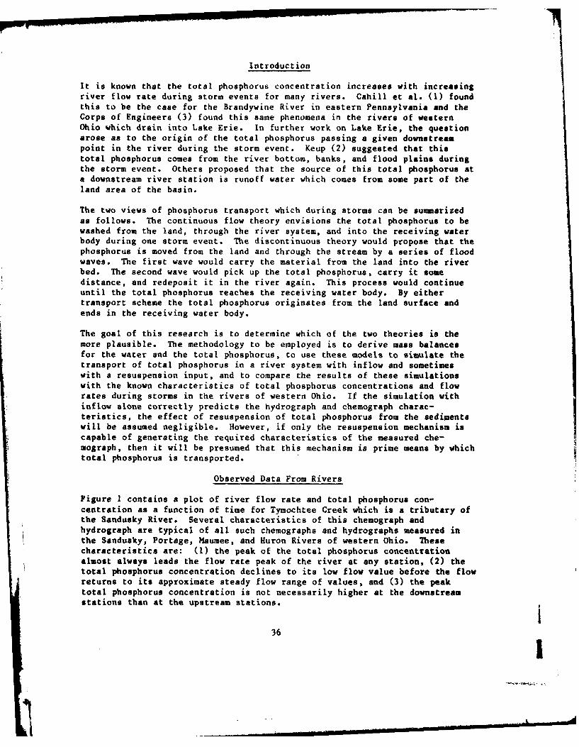
Figure I contains a plot of river flow rate and total phosphorus con-centration as a function of time for Tymochtee Creek which is a tributary ofthe Sandusky River. Several characteristics of this chemograph andhydrograph are typical of all such chemographs and hydrographs measured inthe Sandusky, Portage, Maumee, and Huron Rivers of western Ohio. Thesecharacteristics are: (1) the peak of the total phosphorus concentrationalmost always leads the flow rate peak of the river at any station, (2) thetotal phosphorus concentration declines to its low flow value before the flowreturns to its approximate steady flow range of values, and (3) the peaktotal phosphorus concentration is not necessarily higher at the downstreamstations than at the upstream stations.

36 I

1/OI'I NI di f1OlIV~JLN])NO:) sfHOIIJSOrd IVIOI

a 00

0 VooM

-0

00

0. 0

w Og33S/tH310 NI0M0.

37U

These three characteristics will be used to discern the correctness of the

two different theories for phosphorus transport in river reaches.

Mass Balance Model

The mass balance model used to simulate the hydrograph is the differential

mass balance over an increment in the axial direction and an increment intime.

aAqit ax

where A - discharge area of the streamQ - volumetric flow rate of the streamq - influx volume rate per axial distancex - axial variablet - time

This equation contains two dependent variables, A and Q. In order to solvethis equation, another relationship between these two variables mustbefound; usually it is a force balance over an infinitesimal axial distance andtime. However, to simplify simulation, the rating curve (flow-as function ofstage) will be formulated such that Q, flow rate, is a function of A, streamdischarge area. The normal dispersion term in the force and mass balanceswill be absent from this formulation: however, dispersion will not affectany of the characteristics of hydrograph and chemograph with which a com-parison will be made since dispersion will not change the position of thetotal phosphorus peak and will tend to spread the phosphorus peak.

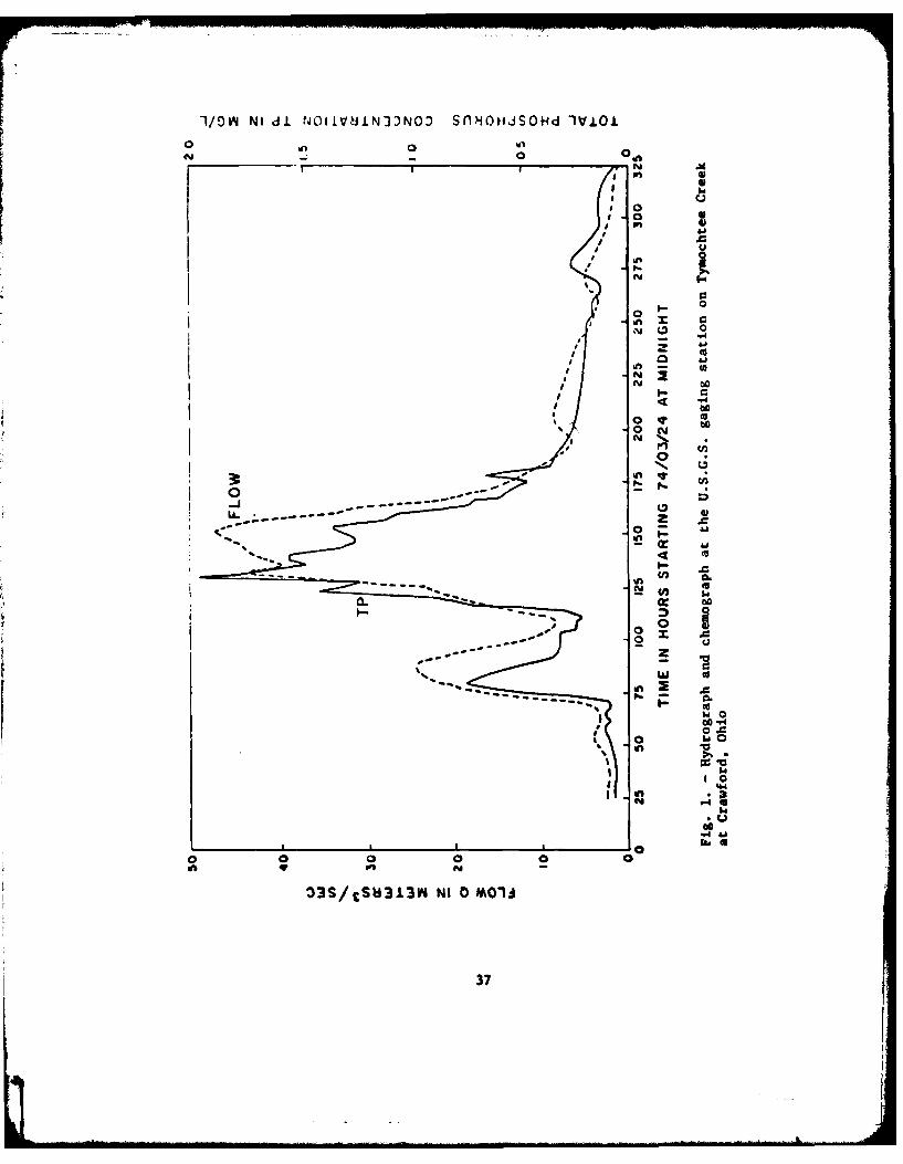
The relationshipbetween the discharge and area is determined from field data

and typical curves for the Sandusky River are shown in Figure 2. The rela-tionship between Q and A is similar for all four stations. The influence ofwater slope on this relationship has been shown to be negligible.Calculations indicate that the flow is about four percent higher during therising stage than that predicted by the Q vs. A curve.

Two different formulations of the mass balance are required for this study.One considers only the inflow and transport of total phosphorus and isderived from a mass balance on total phosphorus for an incremental distance

and incremental time in the stream.

8 A C + q C j

at ax

or expanding

ac ac+___ 4rz + qC -qCi

38

mo 5 3 1 2 4

r W

6000-

1g

40002 l00C

I

.oo

5 0," 1000 15,O0 2 0, C. 2.CO

OISCHARGE AREA IN S 'A;E FEET

Fig. 2. - Discharge vs. area curves for stations

in the Sandusky River basin at U.S.G.S. gaging

stations: 1 - Sandusky River near Bucyrus;

2 - Sandusky River near Upper Sandusky; 3 =

Tyaochtee Creek at Crawford; 4 - Sandusky River nearMexico; 5 - Sandusky River near Fremont

3,

where

C concentration of total phosphorus in the streamCi = concentration of total phosphorus in the influx flow

For the case of significant resuspension and deposition of total phosphorusduring flow the mass balance takes the following form.

AaC + gaC + qC = qC1 + C<a Cat axa

where

u velocity in the streamproportionality constant

The resuspension and deposition phenomena is presumed to be dependent uponthe rate of change of velocity with time. Thus when the velocity isincreasing there is a net input into the water column and when the velocityis decreasing there is a deposition from the water. Although the functionalform of this phenomena may be different than that proposed, the generalcharacteristics are similar to what actually is occurring in the stream. Thecoefficient, , can be varied to obtain reasonable total phosphorus con-centration profiles.

Because of the variability of q and the desire to introduce some dispersion,the equations were solved numerically. The hydrographs and chemographs thatare calculated are derived from information obtained at one point in theriver and hence the assumption that the whole stretch of river is similar tothe measured point is implied. The finite difference approximation for thewater balance is shown below.

Ai~~+ Ai~~ + Ai,j+ 1 t + qAt

1+ f, At

thx

where

f - function of A and defines Qf'= derivitive of f

Results of the Simulation

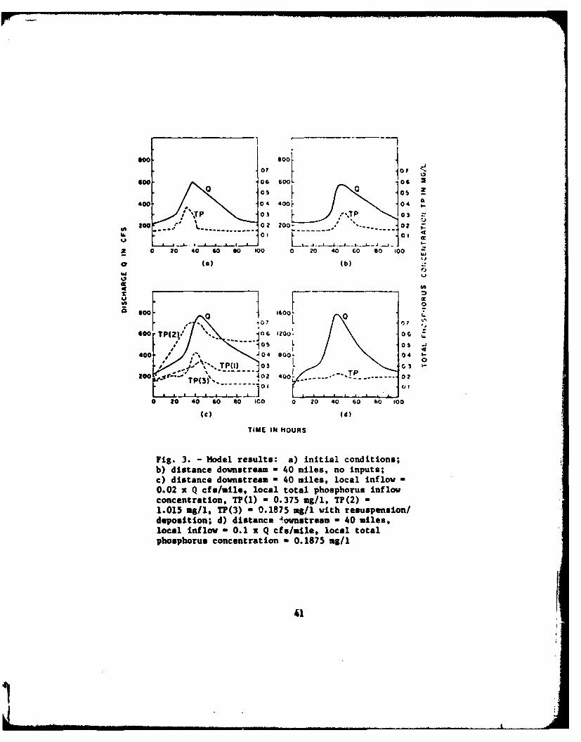
All the simulations were started with steady state stream conditions withrespect to flow and concentration. The input hydrograph and chemograph are Ishown in Figure 3(a). The results in Figure 3(b) indicate that after 40

40

I

600 [00 1407

107S00 ,06 600 j06 2

400. 04 -04

T ItJ oo ... 02 200 ,02 O

. L L- O-

Z 0 20 40 so so 100 0 20 40 60 so 100 z-wLi

a (.) (b)F u

go 100

1

Jo 0

too 04000 0

-0 C -

P. .. -.. .... ..o. O fE " " 1,

0 o 40 60 60 100 0 20 40 60 to 00

(€) Cd)

TIME IN HOURS

Fig. 3. - Model results: a) initial conditions;b) distance downstream - 40 miles, no inputs;c) distance downstream - 40 miles, local inflow =0.02 x Q cfa/mile, local total phosphorus inflowconcentration, TP(l) - 0.375 mg/l, TP(2) a1.015 mg/l, TP(3) - 0.1875 mg/1 with resuspension/deposition; d) distance 4ovnstream - 40 uiles,local Inflow - 0.1 x Q cfs/mile, local totalphosphorus concentration - 0.1875 mg/l

41

miles downstream with no water or chemical input, the peak of totalphosphorus has moved behind the peak of water flow. Note that the numericalmethods introduce some dispersion into the system.

Figure 3(c) contains the plot of the output hydrograph and several relatedchemographe for the condition in which the inflow rate was equal to two per-cent of the upstream flow rate per mile. When the inflow total phosphorusconcentration was equal to the initial peak concentration, the peak in thetotal phosphorus concentration lagged behind the hydrograph peak and thetotal phosphorus concentration did not return to the low flow value withinthe time frame of the hydrograph. This is not in agreement with observedfacts. The total phosphorus concentration peak did remain ahead of thehydrograph peak for input concentrations equal to three times the initialpeak concentration; however, in contrast to field observations the con-centration did not decline with the decline in the hydrograph and the peak ofconcentration constantly increased as the flood wave moded downstream.Figure 3(d) exhibits the hydrograph and chemograph for an increased inputflow rate. Again the total phosphorus peak falls behind the water peak andthe inflow is so large that the total phosphorus is diluted. Many otherinputs were considered and none yielded results which were in conformity withreality.

Only when the resuspension and deposition term was included in the totalphospho-is mass balance did the downstream hydrograph and chemograph possessthe observed field characteristics as shown in Figure 3(c). The peak intotal phosphorus concentration remained ahead of the hydrograph peak and thetotal phosphorus concentration declined with the declining hydrograph. Thepeak of total phosphorus concentration did not necessarily increasedownstream but its variability depended upon the value of the constant,in the resuspension functionality.

The relative position of the total phosphorus peak, to the discharge peak isshown in Figure 4. Almost all conditions which were simulated with onlytotal phosphorus input resulted in the total phosphorus peak eventuallylagging behind the flow peak. If the input concentration were made largeenough, the total phosphorus peak would approach the water peak and then moveahead again. Only when the resuspension term was included did the relativeposition of total phosphorus peak to the water peak remain stationary.

Conclusion and Summary

The flow of water and total phosphorus was simulated in a stream with dif-ferent types of total phosphorus transport mechanisms. The results of thesimulations were compared with known properties of observed hydrographe andchemographs. It is concluded that the major mechanism required to explainthe observed results is one which postulates the resuspension and depositionof total phosphorus from the reaches of the river. Thus most of the totalphosphorus moves through a river reach by moving a finite distance with eachhigh flow event passing through the river.

I42

I n I I I I I i ii U iii ,, , , -- ' , .. . ' " . . .. .... ... ... . I I I [ i - .. ..I

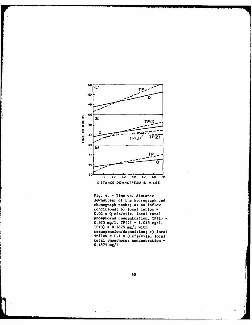
o (C ' T p , - " 0

4060

0 TP()-TP3z SO'

so-T -

2 - - -

40 "7J30

10 20 30 40 50 60 T0

DISTANCE DOWNSTREAM IN MILES

Fig. 4. - Time vs. distancedownstream of the hydrograph andchemograph peaks; a) no inflowconditions; b) local inflow =0.02 x Q cfs/mile, local totalphosphorus concentration, TP(l)0.375 mg/i, TP(2) - 1.015 mg/i,TP(3) - 0.1875 mg/i with

resuspension/deposition; c) localinflow - 0.1 x Q cfs/mile, localtotal phosphorus concentration

0.1875 mg/i

43

References

1. Cahill, T.H., Imperato, P. and F.H. Verhoff, "Evaluation of PhosphorusDynamics in a Watershed", J. Environmental Eng., Division ASCE, 100, 39-52(1974)

2. Kemp, L.E., "Phosphorus in Moving Streams", Water Research, 2, 373-385(1968)

3. U. S. Army Corps of Engineers, Buffalo District, "Lake Erie WastevaterManagement Study Preliminary Feasibility Report", December 1975

44

STORK TRAVEL DISTANCE CALCULATIONS

FOR TOTAL PHOSPHORUS AND SUSPENDEDMATERIALS IN RIVERS

by

Frank H. VerhoffDepartment of Chemical Engineering

West Virginia UniversityMorgantown, West Virginia 26505

and

David A. Helfiand

Stephen M. YaksichLake Erie Wastewater Management Study

U. S. Army Corps of Engineers

Buffalo, Nev York 14207

45

Abstract

From previous work it appears that total phosphorus is transported throughrivers by a series of storm events. This paper presents a method for calcu-loting the average distance of travel during any given storm event. Themethod uses the hydrograph, chemograph, and flow characteristics at a pointin the river. Comparisons were made between storm events at the same stationin a river, between different stations in the same river basin, and betweenstations in different rivers. Results show the distance of travel is depen-dent upon the magnitude and duration of the storm event, but not on themagnitude of the total phosphorus concentration.

46

Introduction

Most of the total phosphorus in streams appears to be transported duringstorm events and is associated with suspended solids transport. Severalother pollutants such as some pesticides are also transported in conjunctionwith the suspended material. Materials transported in this manner exhibitseveral characteristics. The concentration of the total phosphorus,suspended solids, etc. increases with increasing discharge (see U. S. ArmyCorps of Engineers (1975), Walling (1977), Verhoff, Melfi, and Yaksich(1978)). Also during any storm event the peak in total phosphorus orsuspended solids concentration occurs before the peak in discharge. Verhoffand Melfi (1978) have used these facts to show that total phosphorus istransported from the land surface to the receiving water body by a series ofstorm events. Each storm event picks up the total phosphorus from the streambottom, banks, and flood plains, transports it some distance downstream, anddeposits it in the stream again. This mechanism was suggested by Keup (1968)and again discussed by an Enviro Control Report (1972).

A major question to be answered concerning this mechanism is what is theaverage distance of travel for the total phosphorus during any given stormevent. This question is also an important one in sediment transport. N.G.Wolman (1977) discusses the various aspects of sediment transport includingthe wash load, the bed load, and the many complications related to yield. Inhis introductory paragraph he cites the ruling of Judge R. H. Kroninger in acontroversy over logging in a redwood forest. The Judge writes, "Whilenumerous expert witnesses in the fields of geology, forestry, engineering,and biology were presented, their conclusions and the opinionsthey derivedfrom them are hopelessly irreconcilable on such critical questions as howsuch and how far solid particles will be moved by any given flow of surfacewater. They were able to agree only that sediment will not be transportedupstream" (State of California, Marin County, versus E. Righetti et.al.,(1%9)). This paper will discuss the critical question of travel distance.A method for the calculation of distance of travel for total phosphorus andsuspended solids for a given flow of surface water will be presented. A pre-vious paper (Verhoff, Melfi, and Yaksich (1978)) discusses the calculation ofthe amount of total phosphorus transported past a given point in a stream.Both of these techniques are based upon data taken from that point in thestream.

Little prior work has been done in trying to understand the intermittenttransport of total phosphorus; however, there have been many papers writtenon the subject of suspended solids transport. Nordin divides the modelingefforts into two categories; (1) sediment movement modeled by computationaldeterministic hydrology (e.g. Bennett (1974), lagnold (1977), and Thomas g.Prasuhm (1977)); and (2) stochastic models used to simulate the movement ofparticles (e.g., Cheong and Shen (1976), and Todorovic and Nordin (1975)).These efforts have followed the same basic procedure. First, the deter-ministic model is proposed based upon force balances or the stochastic modelis proposed based upon some jump probabilities. The predictions of thesemodels are then compared with experimental data to assess the accuracy of theoriginal proposed models.

47

4'"

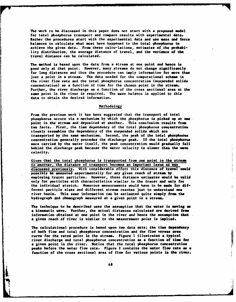
The work to be discussed in this paper does not start with a proposed modelfor total phosphorus transport and compare results with experimental data.Rather the procedures start with the experimental data and use mss and forcebalances to calculate what must have happened to the total phosphorus toachieve the given data. From these calcu-lations, estimates of the probabi-lity distribution, the average distance of travel, and the variance of thetravel distance can be calculated.

The method is based upon the data from a stream at one point and hence isgood only at that point. However, many streams do not change significantlyfor long distances and thus the procedure can imply information for more thanjust a point in a stream. The data needed for the computational scheme isthe river flow rate and the total phosphorus concentration (suspended solidsconcentration) as a function of time for the chosen point in the stream.Further, the river discharge as a function of the cross sectional area at thesame point-in the river is required. The mass balance is applied to thisdata to obtain the desired information.

Methodology

From the previous work it has been suggested that the transport of totalphosphorus occurs via a mechanism by which the phosphorus is picked up at onepoint in the stream and deposited at another. This conclusion results fromtwo facts. First, the time dependency of the total phosphorus concentrationclosely resembles the dependency of the suspended solids which aretransported by the same mechanism. Second, the peak of the total phosphorusconcentration generally precedes the discharge peak. If the total phosphoruswere carried by the water itself, the peak concentration would gradually fallbehind the discharge peak because the water velocity -is slower than the wavecelerity.

Given thbt the total phosphorus is transported from one point in the Streamto another, the distance of transport becomes an important issue as wasdiscussed previously. With considerable effort this distance of travel couldpossibly be measured experimentally for any given reach of Strem byemploying tracer particles. However, these distance estimates would be validonly for particles with characteristics similar to the tracer and only forthe individual stretch. Numerous measurements would have to be made for dif-ferent particle sizes and different stream reaches just to understand oneriver basin. This same information can be estimated quite simply from thehydrograph and chtemograph measured at a given point in a stream.

The technique to be described uses the assumption that the water is moving aa kinematic wave. Further, the actual distances calculated are derived frominformation obtained at one point in the river and hence the assumption thata given reach of river is similar to the measurement point is implied.

The calculational procedure is based upon two data sets; the time dependencyof both flow and total phosphorus concentration and the flow versus areacurve for the rated point in the stream. Figure 1 illustrates a typicalriver discharge and total phosphorus concentration as a function of time fora given point in the river. Notice that the total phosphorus concentrationpeaks before the water flow rate. Figure 2 contains the water flow rate as a

function of the cross sectional area of flow for various points in the river.

48

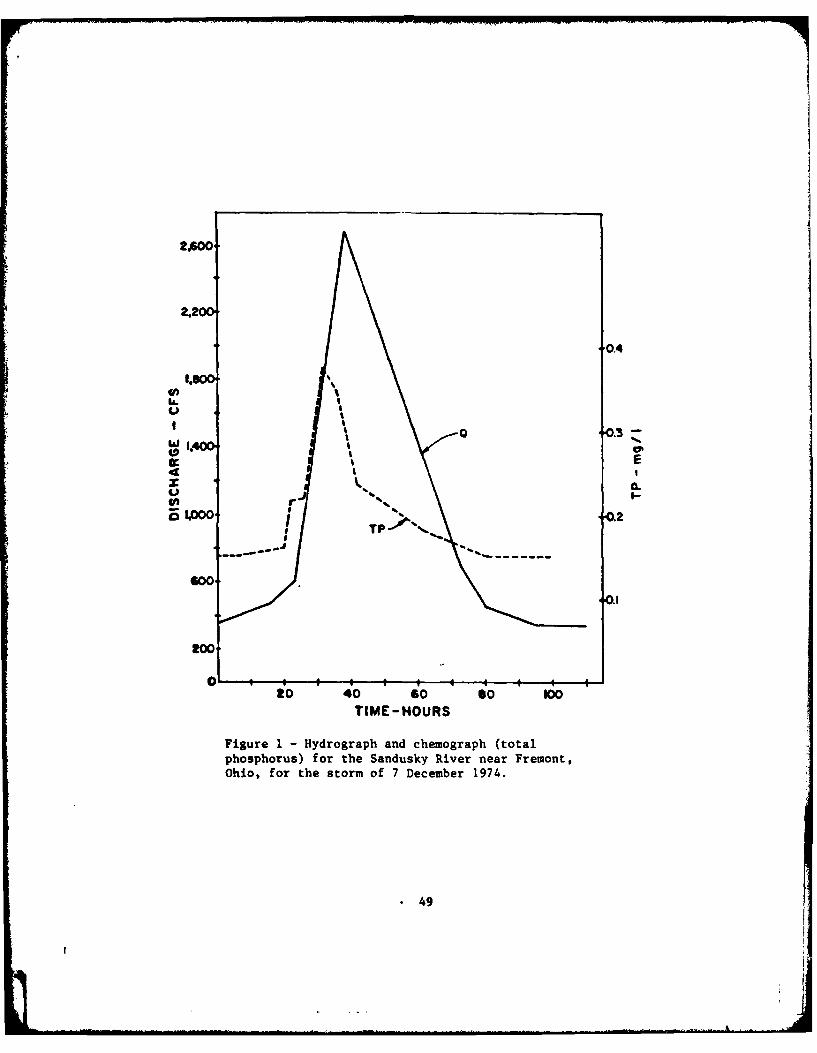
2,20

0.4

1.900

E

in r* .2

GOO.-

0

g0 40 60 so 10TIME-HOURS

Figure 1 -Hydrograph and chemograph (totalphosphorus) for the Sandusky River near Fremont,Ohio, for the storm of 7 December 1974.

49

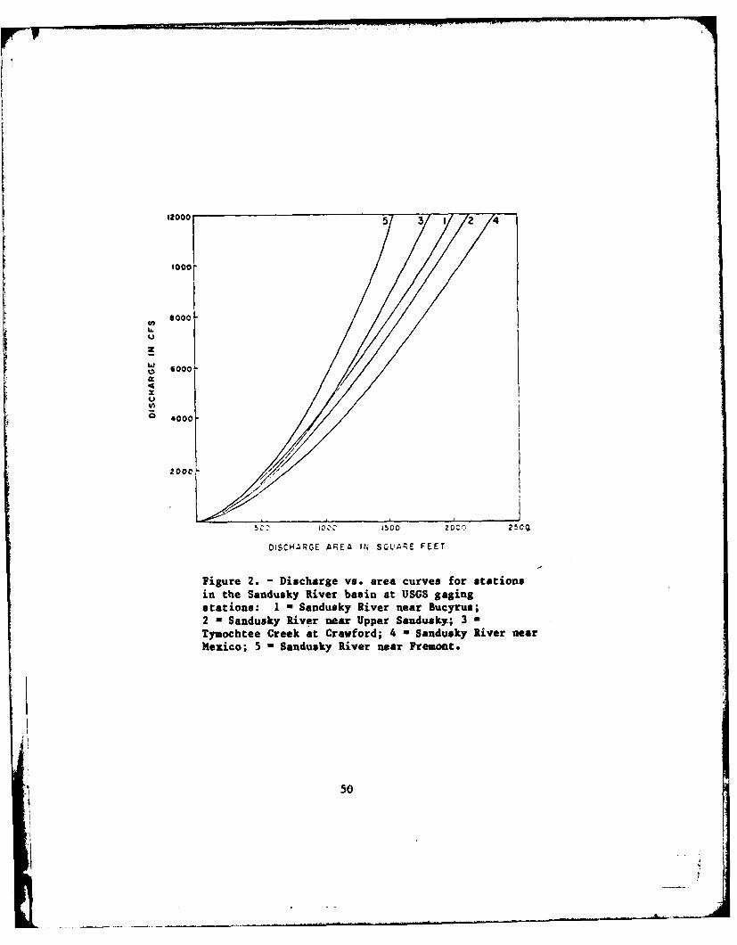
12000f 5 3 1 4

1000[E 0000-

IL

S40001

2000 "

DiSCH4ARGE AREA IN~ SC;L:A:E FEET

Figure 2. - Discharge vs. area, curves for stationsin the Sandusky River basin at USGS gagingstations: 1 a Sandusky River near Bucyrus;2 - Sandusky River near Upper Sanduskyt;-3 aTymochtee Creek at Crawford; 4 = Sandusky River nearMexico; 5 -Sandusky River near Fremont.

50

P '

The kinematic wave theory for river flow indicates that the wave moves fasterdownstream than the water itself for subcritical flow. Hence, if the infor-mation contained in Figure I was also measured at an incremental distancedownstream, it would appear approximately the same except that the wateritself would be slightly shifted in the hydrograph because of its slowervelocity than the wave celerity. Since the water itself is moving slowerthan the wave, a particular volume of water would appear to be moving fromleft to right through the hydrograph and chemograph shown in Figure I as thiswave proceeds downstream. As a volume of water moves through the hydrograph,the total phosphorus concentration of this water gradually increases asmaterial is picked from the river banks and bottom and after the con-centration peak is reached the concentration decreases again as this materialis deposited. Thus, if the position of the volume of water in the hydrographcould be related to its position in the stream, it would be possible todetermine the total phosphorus concentration of the volume of water as afunction of distance downstream (see Figure 3).

To obtain these necessary relationships, the flow versus cross- sectionalarea curve is employed. This relationship is plotted in Figure 2 and can berepresented by the following equation.

Q - g(A) (1)

where Q - river flow rate

A - cross-sectional area

According to the kinematic theory of hydrologic events, the wave celerity isquantitatively determined by the slope of the curve, and the velocity of thewater itself is found by dividing the flow rate by the area. The water andwave velocities are indicated in Figure 3.

vw g'(A) (2)v g(A)/A (3)

where v water velocityvw wave celerity

Now for any time increment, the incremental distance traversed by the water

volume is determined by the water velocity as shown below.

ds/dt u v (4)

where s a distance downstream of water volume

t - real time

However, as the distance downstream of the water volume, a, changes the posi-tion of the water in the hydrograph shifts. The problem is to relate theposition in the hydrograph of the given volume of water with the distancedownstream that the water has moved.

51

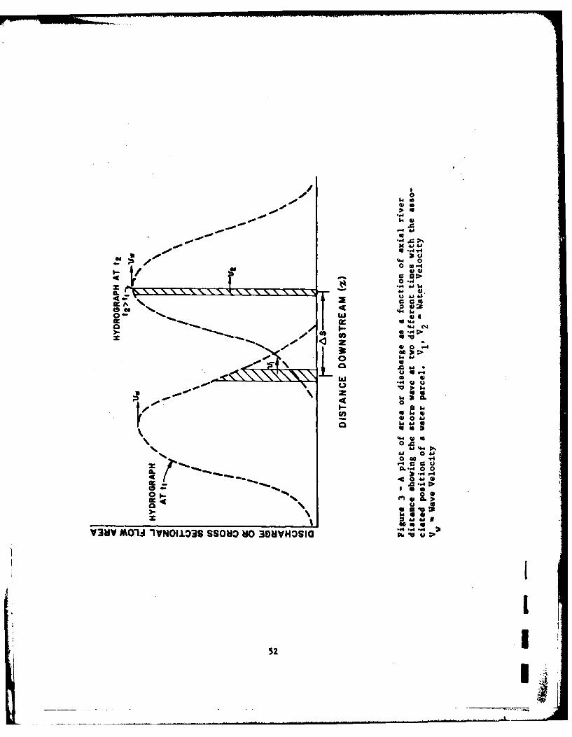
- 0

-41

c

0. 0-

o0.-0.. 1

44

I&I1" 4

I. >

4004

0 0 4

U0h

00 .41

r O*. .0 0

40"

V38V MOW IVN0110O3S SSOHO 80 398VHDSIG

52

To obtain the desired relationship it is necessary to consider the dynamicsof a wave form in a river. If only short distances are considered such thatno appreciable change in the hydrograph shape has occurred this wave formsatisfies the following relationship. This implies the wave velocity isapproximately constant and that there is little inflow into the stream.These assumptions are usually rea sonable since the wave velocity, dQ/dA, isnearly constant for high flows and tributary input is not considered.

f (to-X/vw) C C (5)

where C = constantto = time

X = axial coordinate downstream

This equation states that if an observer is moving at the velocity of thewave, there will be no change in the hydrograph at the observation point. Ifthe observer is not moving with the wave, then a positive change in thevariable to is equivalent to a positive change in the variable X/vw . Thiscan be written in differential form as the following equation assuming vw isnearly constant.

dto f dX/vw (6)

To perform the desired transformation as discussed above, it is necessary toconsider the change in position of a given parcel of water relative to thewave as the wave proceeds downstream.

dX/dt = vw-v (7)

where X - axial position of water parcelrelative to the wave

This then can be transformed into a time into the hydrograph by using theproperties of waves discussed above.

dX/vw = dt- 1 - v/vw (8)dt dt

This differential equation then relates the time into the hydrograph to realtime during the water movement downstream. It is then a simple matter ofrelating the position of the water parcel downstream to its position in thehydrograph.

dsds dt v (9)dt dto dt

or ds -v 1

dto vw-v 1- (10)V VW [

53

4

or ds g'(A) g(A)dto g'(A)A-g( (II)

This differential equation then relates the distance traversed by the parcelof water downstream to its position in the hydrograph as designated by timeinto the hydrograph. But from the hydrograph and chemograph data the totalphosphorus concentration is also known as a function of time into thehydrograph. Thus by integrating the differential equation from some zerodistance at the beginning of an event in the hydrograph, it is possible toobtain the concentration of total phosphorus in a given parcel of water as afunction of the distance that parcel has traveled downstream. This can berepresented by the following relationship.

CTP Cp(s) (12)

where CTp = total phosphorus concentration

A typical example of the relationship is shown in Figure 4. This figureindicates that as the particular volume of water enters the hydrograph, its

total phosphorus concentration increases indicating there is a net resuspen-sion of material presumably from the material in contact with the water. Ata certain point downstream, the total phosphorus concentration reaches amaximum and further progression downstream causes the net total phosphorus ofthe given volume of water to be reduced. Presumably during this time periodthe material is being deposited along the banks and the stream bottom.

The information in Figure 4 can be used to calculate the average distance

that the total phosphorus has been moved downstream during a given hydrologi-cal event. To help understand the process, a simple example will bediscussed. Figure 5a illustrates a graph of CTP versus downstream distancein which the transport distance is obviously So. A more complicated exampleis depicted in Figure 5b. The average distance traversed by the totalphosphorus concentration is given by the following formula.

Say = SoCo+SICI (13)Co +C

This equation can be generalized for the curve shown in Fig. 4. The formula

to be employed is as follows.

max sdc S cds (14)

S Cmin minav

fMax Cmax mi ndc

54

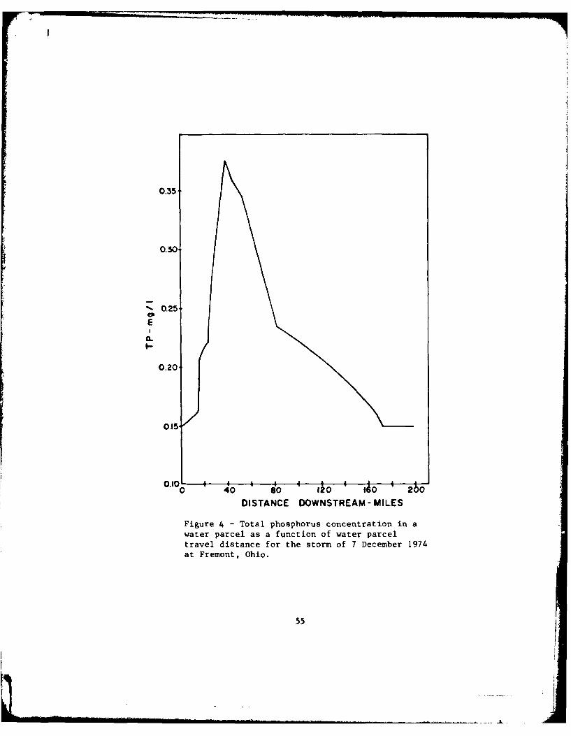
0.35'

0.30

0.25CPEa.

I-

0.20

0.15"

0.10 I 0 I I I - ,0 40 so 120 I0o 2 o

DISTANCE DOWNSTREAM- MILES

Figure 4 - Total phosphorus concentration in awater parcel as a function of water parcel

travel distance for the storm of 7 December 1974at Fremont, Ohio.

55

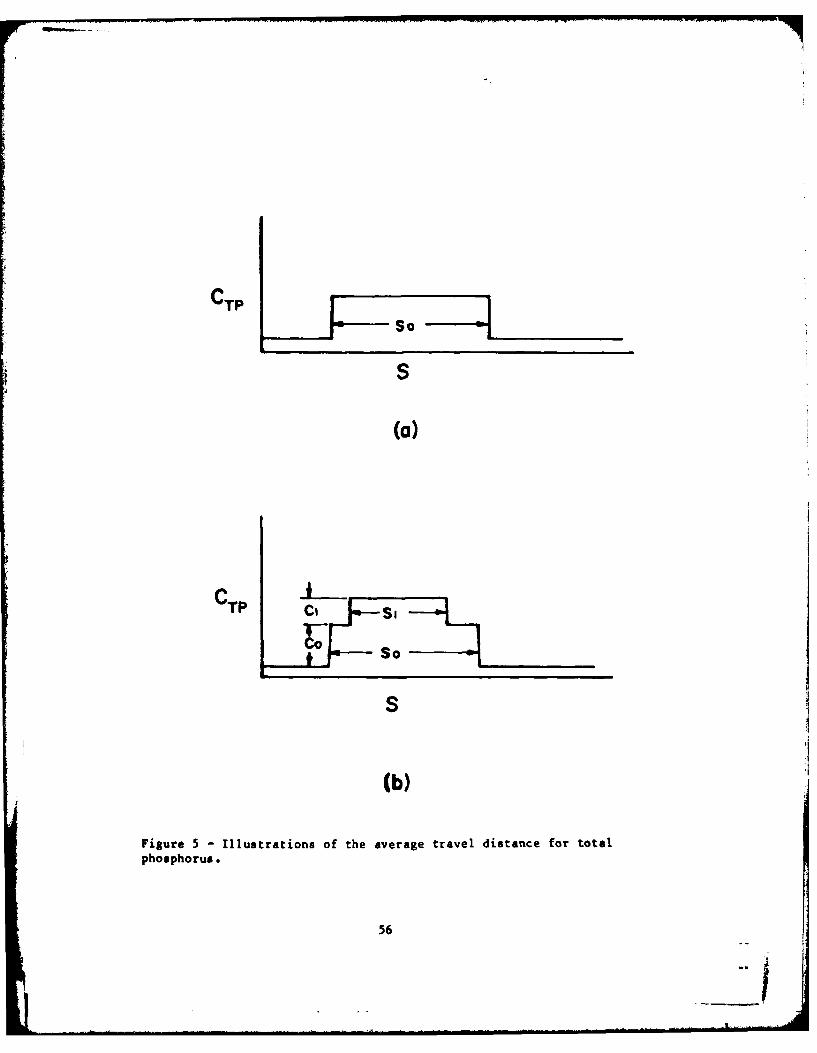
CTPSo

(a)

CTP- CO

So

(b)

Figure 5 - Illustrations of the average travel distance for totalphosphorus.

56

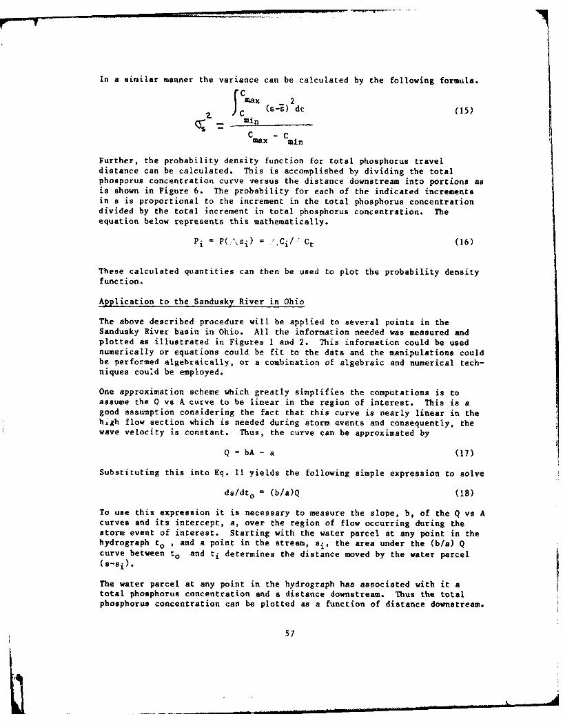
In a similar manner the variance can be calculated by the following formula.(Cmx 2

C (s-:i) dc (15)

z. Cmax min

Further, the probability density function for total phosphorus traveldistance can be calculated. This is accomplished by dividing the totalphosporus concentration curve versus the distance downstream into portions asis shown in Figure 6. The probability for each of the indicated incrementsin s is proportional to the increment in the total phosphorus concentrationdivided by the total increment in total phosphorus concentration. Theequation below represents this mathematically.

Pi = P(!^Xsi) = '.Ci/ Ct (16)

These calculated quantities can then be used to plot the probability density

function.

Application to the Sandusky River in Ohio

The above described procedure will be applied to several points in theSandusky River basin in Ohio. All the information needed was measured andplotted as illustrated in Figures 1 and 2. This information could be usednumerically or equations could be fit to the data and the manipulations couldbe performed algebraically, or a combination of algebraic and numerical tech-niques could be employed.

One approximation scheme which greatly simplifies the computations is toassume the 0 vs A curve to be linear in the region of interest. This is agood assumption considering the fact that this curve is nearly linear in thehigh flow section which is needed during storm events and consequently, thewave velocity is constant. Thus, the curve can be approximated by

Q = bA - a (17)

Substituting this into Eq. 11 yields the following simple expression to solve

ds/dt o - (b/a)Q (18)

To use this expression it is necessary to measure the slope, b, of the Q vs Acurves and its intercept, a, over the region of flow occurring during thestorm event of interest. Starting with the water parcel at any point in thehydrograph to , and a point in the stream, si, the area under the (b/a) Qcurve between to and ti determines the distance moved by the water parcel(s-si).

The water parcel at any point in the hydrograph has associated with it atotal phosphorus concentration and a distance downstream. Thus the totalphosphorus concentration can be plotted as a function of distance downstream.

57

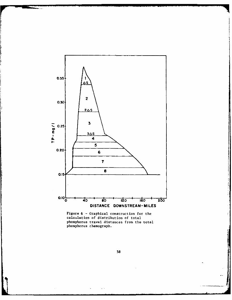
Ias

2

~.0.25

0.20.

0.15

0.101 i i0 40 so I;0 Ito 26b0

DISTANCE DOWNSTREAM- MILES

Figure 6 - Graphical construction for thecalculation of distribution of totalphosphorus travel distances from the totalphosphorus chemograph.

58

These procedures were applied to the information shown in Figure 1 for theSandusky River at Fremont. The Qvs A curve for Fremont from Figure 2 wasused and the resulting total phosphorus concentration as a function ofdistance is shown in Figure 4.

The average net distance of travel and the variance of this travel then canbe calculated using Eqs. 14 and 15. For this point in the stream the averagenet distance of travel was 64 miles and the stan dard deviation for this tra-vel was 45 miles. The stream with the characteristic Q vs A curve at Fremontwas transporting the total phosphorus an average distance of 64 miles as thestorm was passing that point. It must be emphasized that these calculatedvalues only apply at the measurement point.

Further then, the probability distribution of distance transported can becalculated. Figure 6 demonstrates the construction procedures required toobtain the approximate distance of travel. The resulting probability distri-bution is shown in Figure 7. This probability distribution was typical ofthe several which were calculated. In some instances it appeared thatdistribution definitely had two peaks and in others the distribution lookedPoisson in nature. Given that the distribution is bi-modal, it is possibleto speculate that two different total phosphorus transport mechanisms areoperative. One fraction of total phosphorus may be absorbed to dense clayparticles and have a short travel distance. Other total phosphorus may beassociated with less dense biological materials such as bacterial or fungalcells and these may be transported greater distances.

In some previous work, the yearly flux of total phosphorus from the SanduskyRiver into Lake Erie was calculated using the measurements at Fremont. Itwas presumed that all of the material passing Fremont went into Lake Erie 15miles away. The probability distribution in Figure 7 indicates that about 90percent of the material will be transported this distance if the riverremains similar to the flow characteristics at Fremont. Since the river pro-bably resuspends some material in the last 15 miles, the estimate of totalflux obtained at Fremont probably is reasonable for that entering the lake.

The important point to note is that the computations apply only at a point.However, points in a stream can differ in two regards, in the Q vs A curve orin the hydrograph and chemograph. Figure 2 shows the Q vs A curve at variousstations on the Sandusky River. There are no great differences in thesecurves and hence the major differences must lie in the hydrograph and che-mograph.

This travel distance estimation procedure was applied at several other sta-tions in the Sandusky River Basin for the storm of 7 December 1974. Thecumulative distributions of distance traveled is shown in Figure 8. It canbe seen that for this storm, three main stem Sandusky River stations atFremont, Bucyrus, and Upper Sandusky all give approximately the same distri-bution of travel. Only the station at Mexico yields a significantly greaterdistance of travel. This primarily results from a different chemograph,which may have been influenced by the dam upstream from the Mexico station.Further, the distance of travel at Crawford on Tymochtee Creek, a tributaryof the Sandusky River, is significantly less than for the main stem reaches.

59

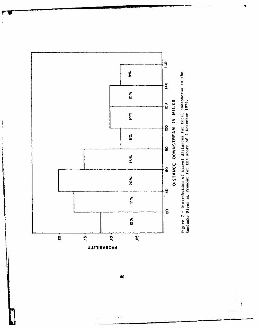
10

.0

0

____ ___ ___ _ CD ot o -0

Cn w

4-

(n0CY 0 9

U, ~-4WG.0

cc

0 02to

60

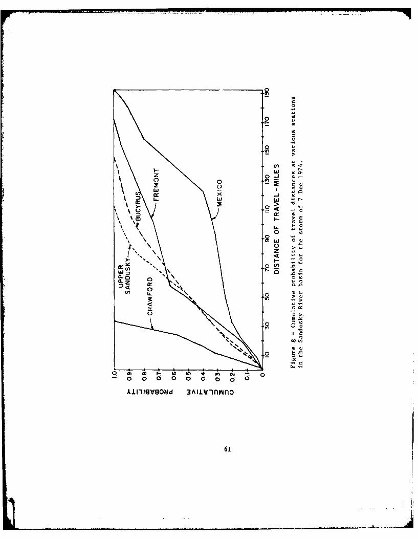
cc

0

0

0i

*j IA.

Li.!w 0 .t

'ii 00 -o

o o w14.

k 4-

ZT Z

o-Go

-r4

611

It appears that in the upper reaches of river basins the distance of travelmight be much shorter because the duration of the hydrograph is much less.

The travel distances were calculated for another much larger storm on the

Sandusky River. The average travel distances were correspondingly larger.At Fremont on the Sandusky River with a maximum flow of 15,000 cfs for thestorm of 22 February 1975 the travel distance was 2,256 miles. Since Fremontis 15 miles from Lake Erie, almost all of the total phosphorus measuredpassing Fremont gets into Lake Erie. In order to show that the actual magni-tude of the total phosphorus concentration has little effect on the distanceof travel, the calculations were performed for this same storm with exactlyone-half of the concentration. The average distance of travel is 2,257miles. However, the magnitude of the concentration directly affects theamount of transport. In contrast, the magnitude of the water flow rate has asignificant effect on the distance of travel.

This calculation procedure was performed for storm events on the Maumee Riverand the Cattaraugus Creek in the Lake Erie basin. The average distance oftravel for three different storms on the Maumee River at Waterville were 403,470, and 1,161 miles and the associated maximum flow was 18,700, 31,200, and50,400 cfs, respectively. This result indicates that the distance of travelincreases with increasing maximum flow for a given station. The storm of 29January 1975 on the Cattaraugus Creek had a maximum flow rate of 15,000 cfsyet the distance of travel for total phosphorus was only 49 miles. TheCattaraugus Creek Basin has a much higher slope and the stream events have ashorter duration; thus it would appear that short duration storm events pro-duce smaller travel distances for the total phosphorus. This again corro-borates the measurements at Crawford in Tymochtee Creek.

Summary and Conclusions

In this paper is developed a calculational procedure for estimating thedistance of travel for total phosphorus, suspended sediment, and other asso-ciated materials. The procedure is based upon the characteristics of thestream at a point and requires a knowledge of the hydrograph and the che-mograph for the substance of interest. Further, the river flow as a functionof river cross sectional area is needed for the point in the stream.

The calculational procedure is based upon the difference in the wave celerityand the water velocity. The calculated distances of travel for totalphosphorus appear to be reasonable. This calculation for distance of travelis far simpler than any experimental technique which could be devised toobtain the same information.

The distance of travel for total phosphorus was calculated at various pointson the Sandusky and Maumee Rivers, and Cattaraugus Creek. The distance oftravel increases with increasing maximum flow rate at a given point in thestream and it increases with increasing storm duration. For a given stormevent the distance of travel in the upper reaches of a tributary is less thanat the main stem stations. The channel slope apparently influences distanceof travel. Finally such stream alterations such as dams or channeling alsoinfluence the distance of travel for total phosphorus.

62

References

1) Bagnold, R.A., "Bed Load Transport by Natural Rivers," Water ResourcesResearch, Volume 13, April 1977, Number 2, p. 303.

2) Bennett, J.P., "Concepts of Mathematical Modeling of Sediment Yield,"Water Resources Research, Volume 10, June 1974, Number 3, p. 485.

3) Cheong, Hin Fatt, and Hsieh Wen Shen, "Stochastic Characteristics ofSediment Motions," Journal of the Hydraulics Division, ASCE, Vol. 102, No.HY7, July 1976, p. 1035.

4) Enviro Control Inc., "National Assessment of Trends in Water Quality,"Report to Council of Environmental Quality, NTIS, Springfield, VA, 1972.

5) Keup, L.E., "Phosphorus in Flowing Streams," Water Research, Vol. 2, 1968,p. 373.

6) Nordin, C., "Sediment Storage in Remobilization Characteristics ofWatersheds," Proceedings of the Workshop on Fluvial Transport, Eds. H. Shemand A.E.P. Watson, International Joint Commission, Kitchner, Ontario, October1976, p. 151.

7) State of California, Marin County, versus E. Righetti et. al., Decision ofthe Superior Court of California, Alameda, No. 393, 850, 1969.

8) Thomas, W.A. and A.L. Prasuhn, "Mathematical Modeling of Scour andDeposition," Journal of the Hydraulics Division, ASCE, Vol. 103, No. HY8,August 1977, p. 851.

9) Todorovic, Petar and C.F. Nordin, "Evaluation of Stochastic ModelsDescribing Movement of Sediment Particles on Riverbeds," Journal of Researchof the U.S. Geological Survey, Volume 3, Number 5 September-October 1975,p. 13.

10) U. S. Army Corps of Engineers, Buffalo District, Lake Erie WastewaterManagement Study - Preliminary Feasibility Report, December 1975.

11) Verhoff, F.H., and D.A. Melfi and S.M. Yaksich, "The Estimation ofNutrient Transport in Rivers," submitted for publication.

12) Verhoff, F.H., and D.A. Melfi, "Total Phosphorus Transport During StormEvents," Journal of the Environment Division, ASCE, Vol. 104, p. 1021, 1978.

13) Walling, D.E., "Assessing the Accuracy of Suspended Sediment RatingCurves for a Small Basin," Water Resources Research, Volume 13, June 1977,Number 3, p. 531.

14) Wolman, M. Gordon, "Changing Needs and Opportunities in the SedimentField," Water Resources Research, Volume 13, February 1977, Number 1, p. 50.

63

MOMENT METHODS FOR ANALYZING RIVER MODELSWITH APPLICATION TO POINT SOURCE PHOSPHORUS

by

F.H. VerhoffDepartment of Chemical Engineering

West Virginia UniversityMorgantown, WV 26506

and

David B. Baker

Water Quality LaboratoryHeidelberg College

Tiffin, OH 44156

64

'*1

Abstract

Quantitive analysis of the fate of point source pollutants in streams can beachieved by using moment analysis if the input concentration is periodic.The moment analysis permits the .discrimination among various proposed modelsand permits the estimation of the parameters in the selected model fordescribing the fate of the substance in a river.

Ortho phosphorus enters the Sandusky River from the Bucyrus, Ohio, sewagetreatment plant with a diurnal periodic concentration change. Moment analy-sis is used to discriminate between reversible adsorption in the sedimentsand the irreversible precipitation or microbial utilization in the sediments.The parameters for the irreversible model are calculated. These include thereaction rate constant and the dispersion in the river.

65

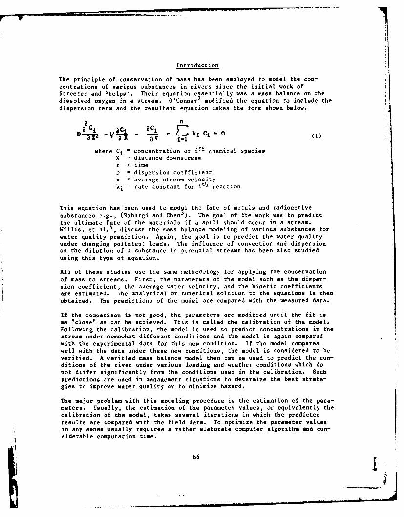
Introduction

The principle of conservation of mass has been employed to model the con-centrations of variYus substances in rivers since the initial work ofStreeter and Phelps . Their equation essentially was a mass balance on thedissolved oxygen in a stream. O'Conner 2 modified the equation to include thedispersion term and the resultant equation takes the form shown below.

2 na c ac ki - (1)

D Vx -aj -X at

where Ci = concentration of ith chemical speciesX = distance downstreamt = time

D = dispersion coefficientv = average stream velocityk i = rate constant for ith reaction

This equation has been used to model the fate of metals and radioactive

substances e.g., (Rohatgi and Chen 3 ). The goal of the work was to predictthe ultimate fate of the materials if a spill should occur in a stream.Willis, et al. 4, discuss the mass balance modeling of various substances forwater quality prediction. Again, the goal is to predict the water qualityunder changing pollutant loads. The influence of convection and dispersionon the dilution of a substance in perennial streams has been also studiedusing this type of equation.

All of these studies use the same methodology for applying the conservationof mass to streams. First, the parameters of the model such as the disper-sion coefficient, the average water velocity, and the kinetic coefficientsare estimated. The analytical or numerical solution to the equations is thenobtained. The predictions of the model are compared with the measured data.

If the comparison is not good, the parameters are modified until the fit isas "close" as can be achieved. This is called the calibration of the model.Following the calibration, the model is used to predict concentrations in thestream under somewhat different conditions and the model is again comparedwith the experimental data for this new condition. If the model compareswell with the data under these new conditions, the model is considered to beverified. A verified mass balance model then can be used to predict the con-ditions of the river under various loading and weather conditions which donot differ significantly from the conditions used in the calibration. Suchpredictions are used in management situations to determine the best strate-gies to improve water quality or to minimize hazard.

The major problem with this modeling procedure is the estimation of the para-meters. Usually, the estimation of the parameter values, or equivalently thecalibration of the model, takes several iterations in which the predictedresults are compared with the field data. To optimize the parameter valuesin any sense usually requires a rather elaborate computer algorithm and con-siderable computation time.

66

This paper presents a different approach for the estimation of parameters andfurther suggests that the mass balance equation (Equation 1) can be used withdata to compare different mechanisms for concentration change. The proce-dure is to use natural or artificial time varying inputs into the streamalong with moment analysis derived from the conservation equations to esti-mate constants and compare mechanisms. The particular application to bediscussed in this paper involves the transport and reactions of phosphorusdownstream from a municipal outfall. The time variation in this instance ische natural diurnal oscillation of phosphate concentration from a sewagetreatment plant.

Literature Review

Measurements downstream from a sewage treatment outfall have been made innu-merable times but in most cases the prime variables of interest have beendissolved oxygen and BOD. The measurements of ortho or total phosphorusdownstream are not that extensive. However, there have been enough measure-ments to indicate what the dynamics of phosphorus might be.

It has been thought for some time that total and ortho phosphorus is removedfrom the water column during low flow conditions and carried out of thewatershed during high flow events. This idea was suggested by Keup5 pri-marily as an explanation for the increasing total phosphorus concentrationswith increasing flows. Connell 6 also observed a significa!tt removal oftotal phosphorus during low flows and a subsequent increase in totalphosphorus concentration at the beginning of a storm event. McKee et al. 7

has measured significant nutrient concentrations in river sediments. Thus,it might be concluded that during low flows the ortho phosphorus is removedfrom the water column and accumulated in the sediments. The mechanisms bywhich this occurs might be adsorption on clay particles or accumulation bymicroorganisms.

The understanding of the phosphorus removal process is complicated by the

diurnal variations in the phosphorus concentrations. This diurnal variationcould be caused by the input of sewage treatment plants as shown in thispaper or it could have other origins such as discussed by Cahill et al. 8 .There are other documentations of this temperal oscillation. Thus, if onewishes to use Equation 1 to estimate the first order rate constant for thedisappearance of phosphorus in a given reach of stream from measurements atboth ends of the reach one must contend with the oscillations. Since theoscillations are not approximated by any function, estimation procedureswould involve numerical simulations and comparisons.

However, these temperal variations suggest a very easy method of analysis,i.e., the method of moments. The municipal sewage treatment plant creates aninput of phosphorus 4oncentration which resembles a probability distributionin time. It is possible to calculate the temporal moments of this distribu-tion at both the upstream station and the downstream station. The change inmoments between the two stations is related to the parameters in Equation Iby the method of moments.

67

• A

The method of moments has been used for years to determine the dispersoncoefficient in tubes as presented by Aris 9 . Some of this methodology hasbeen applied to rivers to determine the dispersion coefficient therein (seefor example ParkerlO). The most recent research on dispersion coefficientmeasurement has concentrated on the initial development of the moments fromgiven injection conditions and on the time to reach the normal distributionof concentration after the dye injection. However, there has been littleinvestigation in which the method of moments has been used to estimate kine-tic parameters in a stream.

The basic concepts for the use of the method of moments for the simultaneousestimation of dispersion coefficients and kinetic constants have beendeveloped by workers in the area of chromatography. The equation describingthe mass balance processes in a chromatograph are exactly the same as thosefor a river, e.g., the equations for chromatography are equivalent toEquation I. Yamaoka and Nakagawa 11-13 in a series of papers discuss theapplication of the method of moments to a set of equations similar toEquation 1. They present the mathematical details of the process, but theydo not investigate the details of the actual application to experimentalchromatograms. In particular, they do not attempt to use the various methodsfor numerically calculating moments from the experimental data nor do theydiscuss the sensitivity of parameter estimation.

Theoretical Development

There are various models that can be attempted for understanding the disper-sion and reaction of ortho phosphorus downstream from a municipal sewagetreatment plant. These models all differ in the form of the reaction term inthe equation. Sometimes these models entail another differential equationbut always the equations are linear or approximated by linear functions suchthat the Laplace Transform can be obtained. In this section, the mathemati-cal derivations will be obtained for two different models which couldpossibly describe the ortho phosphorus dynamics.

The first model to be considered involves the adsorption and desorption of

ortho phosphorus from the sediments. The equations which describe the dyna-mics in this situation are listed below.

D2S+ v - - I --aZ + k (C-C) - 0 (2)

ax ct(~si

,t " k (C-CO) (3)

where C.M concentration of ortho phosphate in the water adja-cent to river sediments

k mass transfer coefficientm - adsorption capability of sediments

68

This model essentially assumes that the rate of adsorption and desorption of

ortho phosphorus to the sediments is mass transfer limited.

The boundary conditions associated with these equations then are determined

by the input from the sewage plant, which is a diurnal oscillatory functionwith the rise in concentration occurring in the afternoon. This input then

is a sequence of normal-shaped curves. Since the model is linear, each oneof these normal-shaped curves can be considered separately. The total output

can be obtained by summing the output of each normal curve. The boundary

conditions associated with the passage of each normal-shaped curve is as

follows.

@ t - 0 C = Cs = 0 (4)

@ x = 0 c = Co(t) (5)

@ x = L dC@X dd 0(6)ds

where L = distance between sample points in stream

Co(t) - ortho phosphorus concentration in the stream as

caused by an afternoon input from a plant

The following dimensionless variables are defined.

/=vt/L R=d/L (7)

Pe = vd/D = Peclet Number

Th = dk/D= Thiele Modulus

mv

Am kd

where d = characteristic length e.g., river wetted perimeter.

Substituting these quantities into the equation then yields the

following.

2 2

ac c R2CL Th 2(C-C = 0 (8)9e Ec Pe .c2 PeR

Am T s (C-c s) (9)

69

There really are three parameters to be determined from these equations;

Am, A = Ripe, and B - Th2/PeR.

The second model to be considered is simpler than the first in thatphosphorus is presumed to disappear from the stream by a first order kine-

tics. This model would correspond to such phenomena as microbial uptake.

The equation for this case is given below.

3C + C -D2C+ kc - (10)

The boundary conditions given by Equations 4, 5 and 6 apply here also.

Using the same dimensionless variables, this equation can be written thus.

2ac c c-_ -A + BC- 0C (11)ao ac ac

In this equation, there are two parameters to be determined; A and B. This

in effect will determine the Peclet Number and a Thiele Modulus.

Method of Moments

The goal of the analysis is to obtain parameters A, B and Am for Equations 8and 9 or to evaluate parameters A and B of Equation 11. These numbers are tobe estimated from experimental concentration measurements at the beginningand end of the stream reach of interest by the method of moments.

A good description of the mathematical procedures to be sketched here is

given by J.M. Douglas 14. The mathematics will be derived for the simplermodel (Equation 11) and the results will be stated for the more complicatedmodel (Equations 8 and 9).

First, the Laplace transform is taken of Equation 11 using boundary condition

(Equation 4).

2

at+ T- - A d + BC - 0 (12)

where s = Laplace variable

C = concentration in Laplace domain

70

This equation is integrated to obtain

C - Al exp [(1/ + M) E/A] + A2 exp [(1/2 - M) e/A] (13)

where M - F/4+ B(s + A)

The boundary conditions (Equations 5 and 6) are used to evaluateconstants A, and A2 . Equation 6 can be replaced with a more con-venient condition. (see Friedly

15 )

E - C - 0 (14)

In the Laplace domain then the solution is

c =o exp [(I/ - M) E/A] (15)

where C0 = Laplace transform of COt)

Evaluate the function at C = I (X = L) and obtains a relationshipbetween the Laplace tranform of the concentration at each end of theriver reach.

C1 Co exp [(1/2 - M)/Aj = H(s) (16)

The method of moments is based upon the expansion of the Laplacetransformed concentration functions into the series of moments.

C0 - (-1) S Moi (17)j-0 TF

C. _ (-1) s Mlj (18)

where 1.lOj = jth time moment of the function at -0hMj - jth time moment of the function at C w 1

71

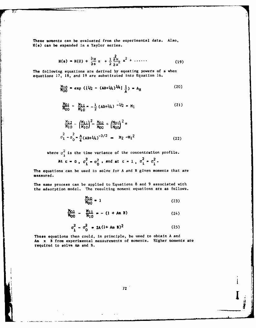
These moments can be evaluated from the experimental data. Also,H(s) can be expanded in a Taylor series.

2H(s) - H(O) + as +---1 2 . ...... (19)

The following equations are derived by equating powers of s whenequations 17, 18, and 19 are substituted into Equation 16.

0MIO - exp (11/2 - (AB+/4)'/4! ) - AH (20)IR60 A

o -1/2 (21)

I - (AB+1/4) - Hj

Mo0 2 O

2 2 A0l O0 (AB+1/4) 3 /2

- M2 -M 2 (22)

where 02 is the time variance of the concentration profile.1

At c 0O a 2 a2,andat Cal, a 2 a a2.1 0: o I

The equations can be used to solve for A and B given moments that are

measured.

The same process can be applied to Equations 8 and 9 associated with

the adsorption model. The resulting moment equations are as follows.

MOO (23)

o - , -f! (I + An ) (24)Mo- "10

a 2 y2 .2A(+Am B) 2 (25)1 0

These equations then could, in principle, be used to obtain A andAm x B from experimental measurements of moments. Higher moments arerequired to solve Am and B.

7272 '

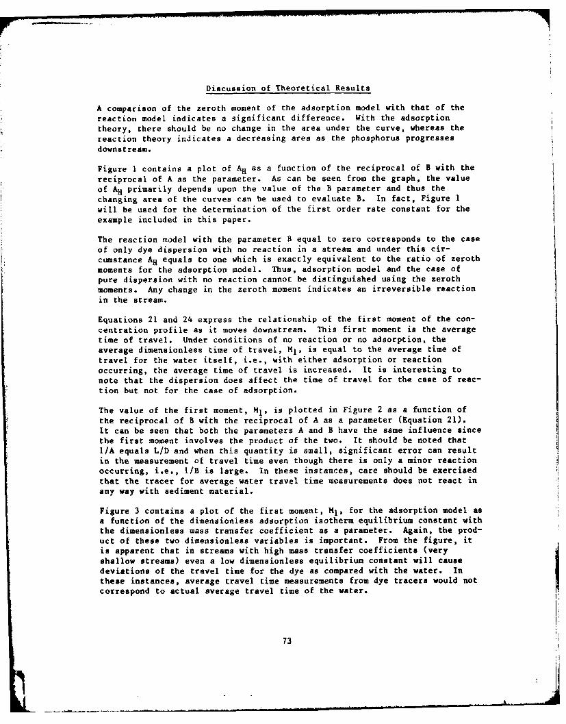
Discussion of Theoretical Results

A comparison of the zeroth moment of the adsorption model with that of the

reaction model indicates a significant difference. With the adsorptiontheory, there should be no change in the area under the curve, whereas the

reaction theory inJicates a decreasing area as the phosphorus progresses

downstream.

Figure I contains a plot of AH as a function of the reciprocal of B with the

reciprocal of A as the parameter. As can be seen from the graph, the value

of AH primarily depends upon the value of the B parameter and thus the

changing area of the curves can be used to evaluate B. In fact, Figure 1

will be used for the determination of the first order rate constant for theexample included in this paper.

The reaction model with the parameter B equal to zero corresponds to the caseof only dye dispersion with no reaction in a stream and under this cir-

cumstance AH equals to one which is exactly equivalent to the ratio of zeroth

moments for the adsorption model. Thus, adsorption model and the case ofpure dispersion with no reaction cannot be distinguished using the zerothmoments. Any change in the zeroth moment indicates an irreversible reaction

in the stream.

Equations 21 and 24 express the relationship of the first moment of the con-

centration profile as it moves downstream. This first moment is the averagetime of travel. Under conditions of no reaction or no adsorption, theaverage dimensionless time of travel, Ml , is equal to the average time oftravel for the water itself, i.e., with either adsorption or reactionoccurring, the average time of travel is increased. It is interesting tonote that the dispersion does affect the time of travel for the case of reac-tion but not for the case of adsorption.

The value of the first moment, Ml , is plotted in Figure 2 as a function ofthe reciprocal of B with the reciprocal of A as a parameter (Equation 21).It can be seen that both the parameters A and B have the same influence sincethe first moment involves the product of the two. It should be noted thatI/A equals L/D and when this quantity is small, significant error can resultin the measurement of travel time even though there is only a minor reactionoccurring, i.e., 1/B is large. In these instances, care should be exercised

that the tracer for average water travel time measurements does not react in

any way with sediment material.

Figure 3 contains a plot of the first moment, Ml, for the adsorption model as

a function of the dimensionless adsorption isotherm equilibrium constant withthe dimensionless mass transfer coefficient as a parameter. Again, the prod-uct of these two dimensionless variables is important. From the figure, itis apparent that in streams with high mass transfer coefficients (very

shallow streams) even a low dimensionless equilibrium constant will cause

deviations of the travel time for the dye as compared with the water. Inthese instances, average travel time measurements from dye tracers would not

correspond to actual average travel time of the water.

73

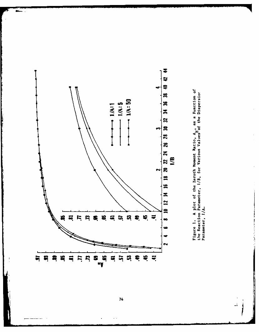
000

-in An 40 DC

P-40

I.IV

4>

0-

C4i

p4 4

OS.'40

004

41-

p44

..

1

"V

-t 74 -

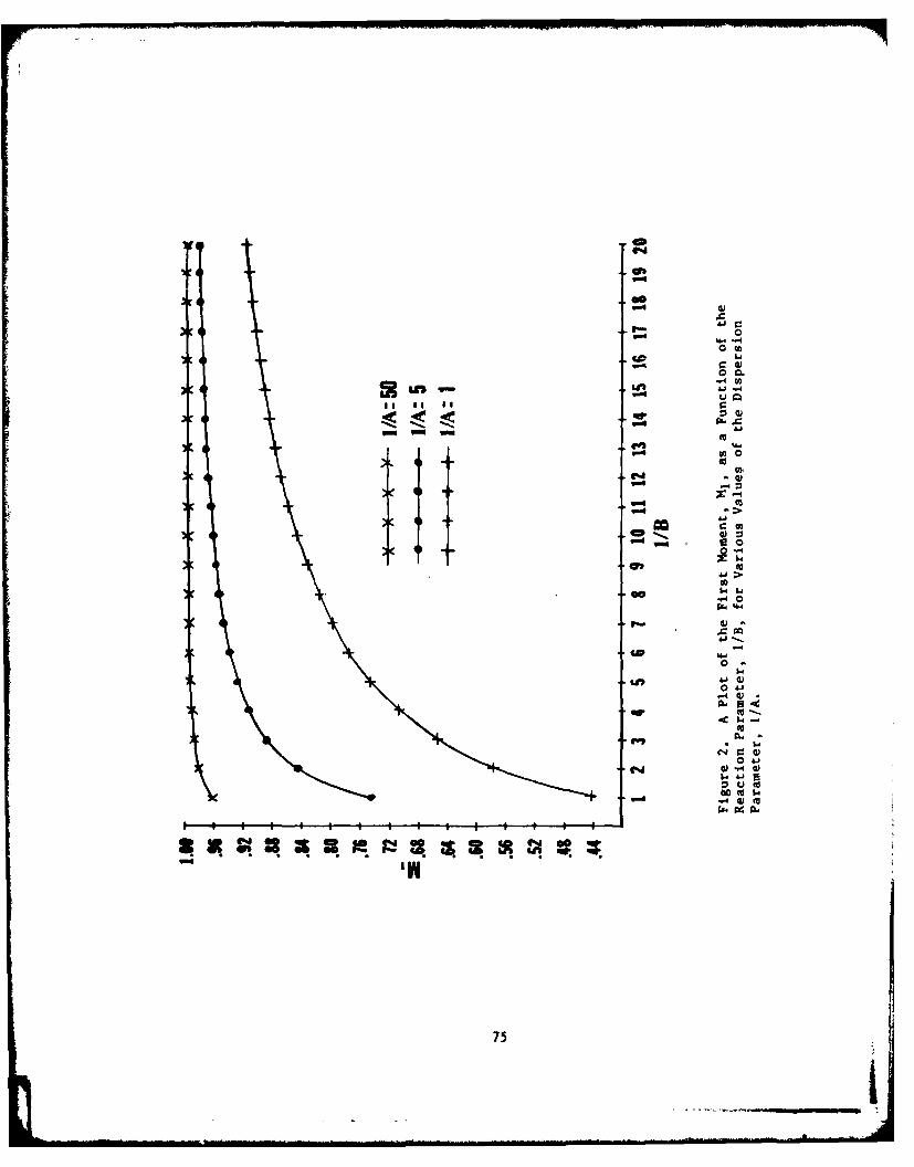
- 0

0 CLIn-4 W~

-n LI 414

)IC)CID

40 '4

-- 0

Ln $41.').0 A

a.- 41

4w4

0

4

75.

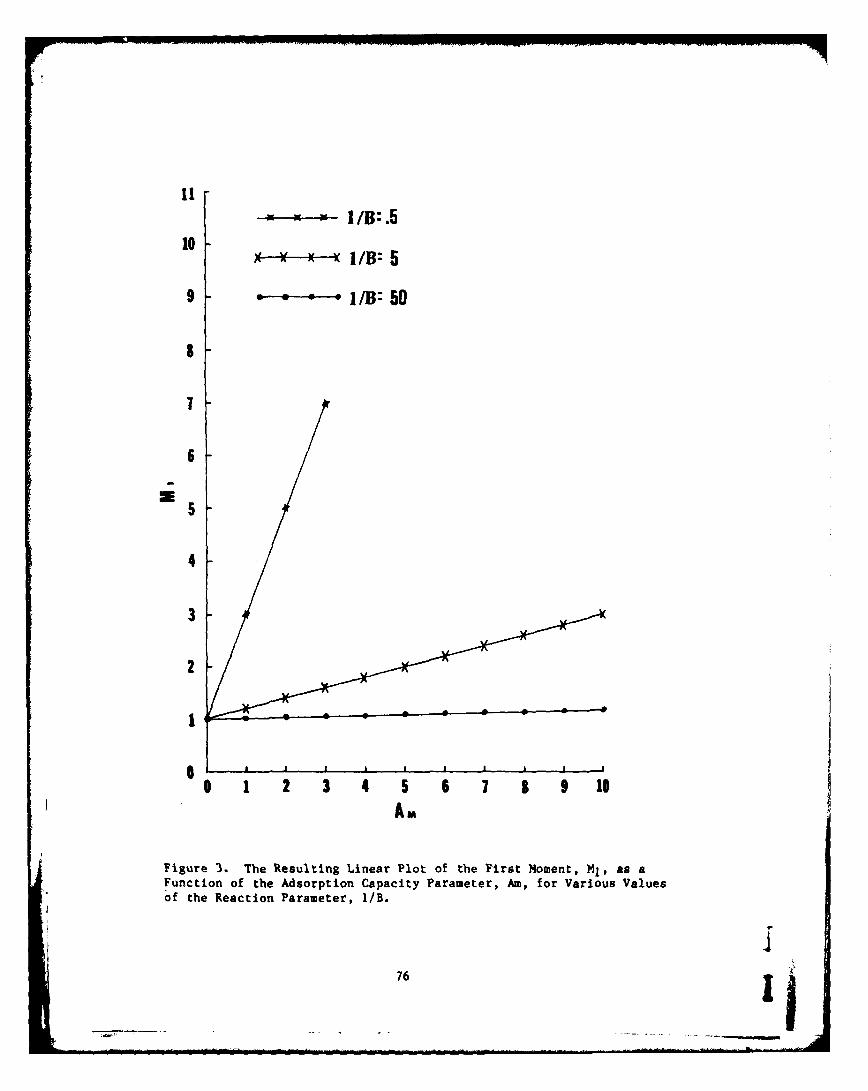
N N ~I1/B: .5

10*-*--*-I I/B: 5

9 1 / IB: 5D

4

3

2

S 1 2 3 4 5 6 7 8 9 10Am

Figure 3. The Resulting Linear Plot of the First M4oment, MI as aFunction of the Adsorption Capacity Parameter, Am, for Various Valuesof the Reaction Parameter, 1/B.

76

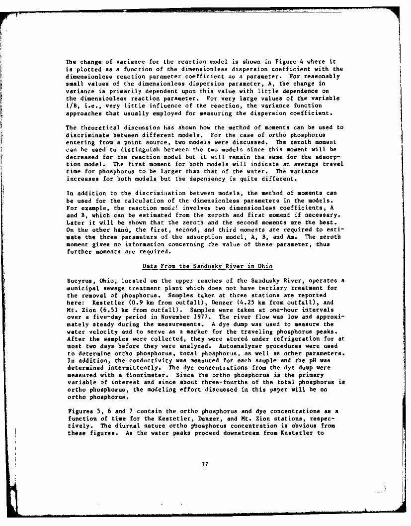
The change of variance for the reaction model is shown in Figure 4 where itis plotted as a function of the dimensionless dispersion coefficient with thedimensionless reaction parameter coefficient as a parameter. For reasonablysmall values of the dimensionless dispersion parameter, A, the change in

variance is primarily dependent upon this value with little dependence onthe dimensionless reaction parameter. For very large values of the variable1/B, i.e., very little influence of the reaction, the variance function

approaches that usually employed for measuring the dispersion coefficient.

The theoretical discussion has shown how the method of moments can be used to

discriminate between different models. For the case of ortho phosphorusentering from a point source, two models were discussed. The zeroth momentcan be used to distinguish between the two models since this moment will bedecreased for the reac.tion model but it will remain the same for the adsorp-tion model. The first moment for both models will indicate an average traveltime for phosphorus to be larger than that of the water. The varianceincreases for both models but the dependency is quite different.

In addition to the discrimi %ation between models, the method of moments canbe used for the calculation of the dimensionless parameters in the models.For example, the reaction model involves two dimensionless coefficients, Aand B, which can be estimated from the zeroth and first moment if necessary.Later it will be shown that the zeroth and the second moments are the best.On the other hand, the first, second, and third moments are required to esti-mate the three parameters of the adsorption model, A, B, and Am. The zerothmoment gives no information concerning the value of these parameter, thusfurther moments are required.

Data From the Sandusky River in Ohio

Bucyrus, Ohio, located on the upper reaches of the Sandusky River, operates a

municipal sewage treatment plant which does not have tertiary treatment forthe removal of phosphorus. Samples taken at three stations are reportedhere: Kestetler (0.9 km from outfall), Denzer (4.25 km from outfall), andMt. Zion (6.53 km from outfall). Samples were taken at one-hour intervalsover a five-day period in November 1977. The river flow was low and approxi-mately steady during the measurements. A dye dump was used to measure thewater velocity and to serve as a marker for the traveling phosphorus peaks.After the samples were collected, they were stored under refrigeration for at

most two days before they were analyzed. Autoanalyzer procedures were usedto determine ortho phosphorus, total phosphorus, as well as other parameters.In addition, the conductivity was measured for each sample and the pH was

determined intermittently. The dye concentrations from the dye dump weremeasured with a flourimeter. Since the ortho phosphorus is the primaryvariable of interest and since about three-fourths of the total phosphorus is

ortho phosphorus, the modeling effort discussed in this paper will be onortho phosphorus.

Figures 5, 6 and 7 contain the ortho phosphorus and dye concentrations as a

function of time for the Kestetler, Denzer, and Mt. Zion stations, respec-tively. The diurnal nature ortho phosphorus concentration is obvious from

these figures. As the water peaks proceed downstream from Kestetler to

77

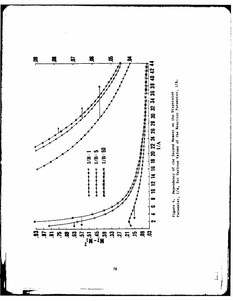
6wl -cmC=

Goo

GD U

o

cmd

V2, 0 4

C)0

0

ccJ

0w

N-)-

7 U11 ,

>ta

CCS

...cm-m

IN-Za

78

05

00610060

- - -O U

CUU.

E - OOLT ,

Lai OOLOu co

C3 4T* UUM

0 w

0)

OdOId..4

I'J

,,j

79

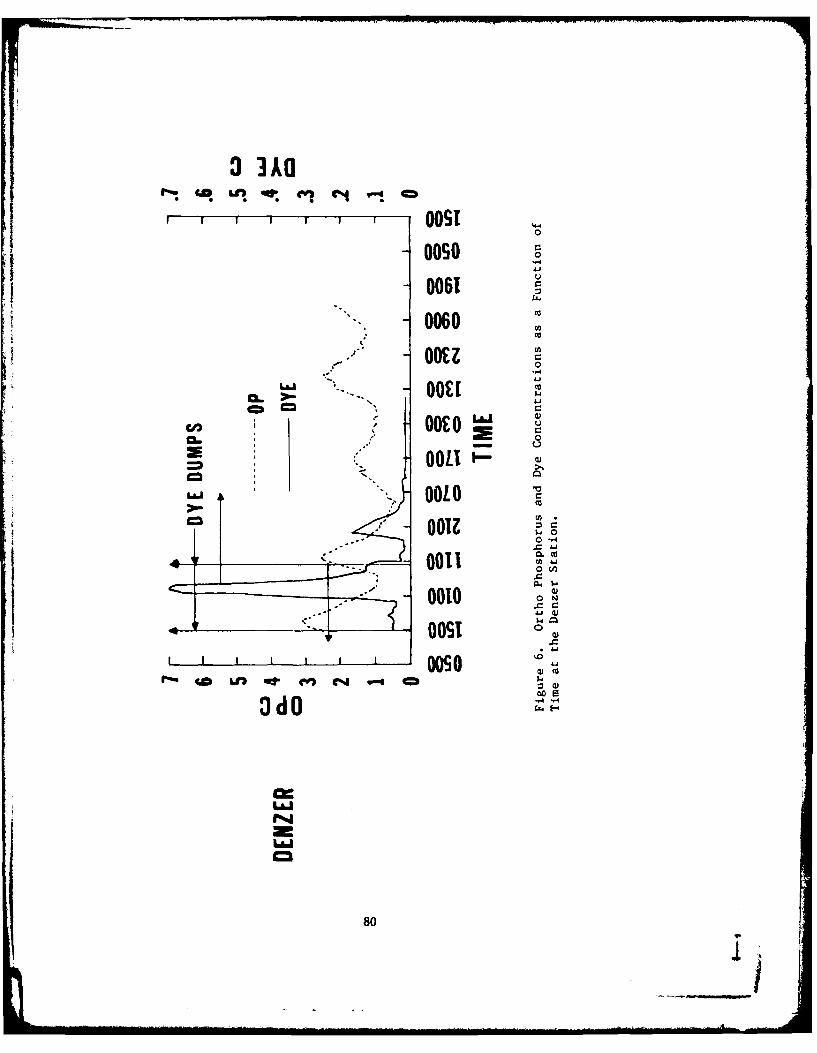
p I I I I OST 4

0

0060'1 0060

CL :I-, C0E

CmC

OUT w

OOLI'

I joo

0010 (4.c

OdD .

80

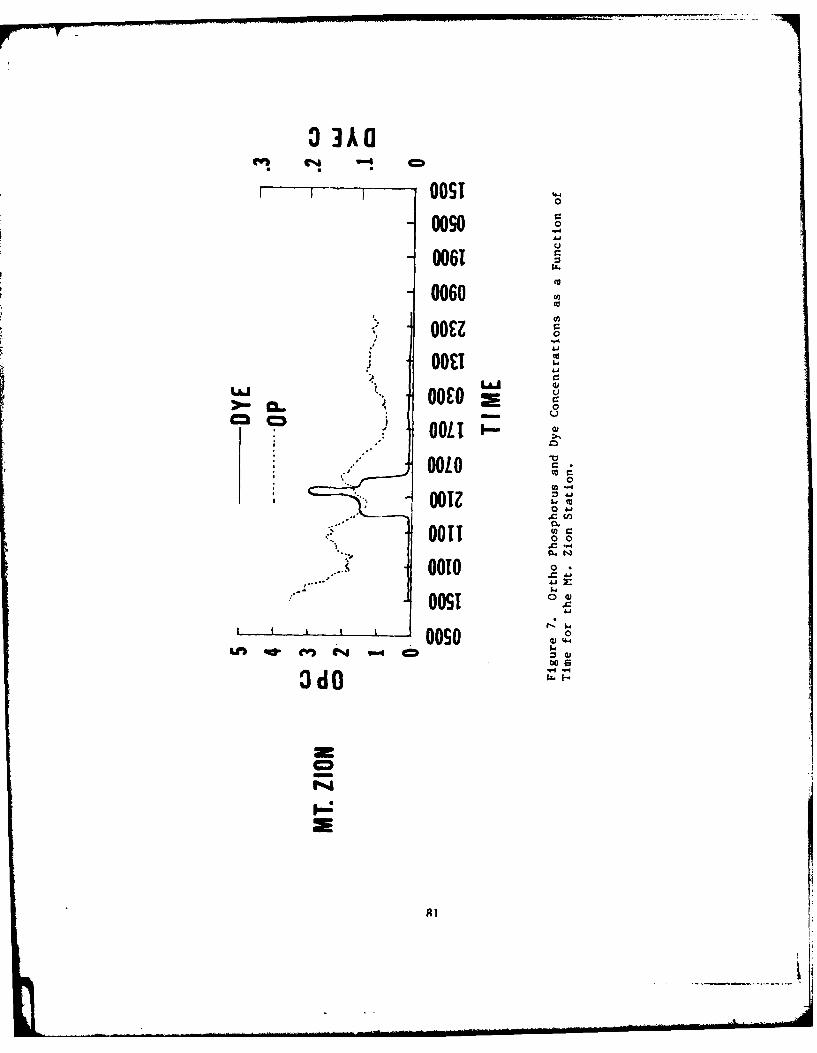
flF~T0061

0090

OUT

o006

0060

00~ g.;000 =

UOU

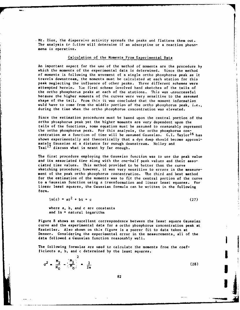
Mt. Zion, the dispersive activity spreads the peaks and flattens them out.The analysis to fcllow will determine if an adsorptive or a reaction pheno-mena is operative.

Calculation of the Moments From Experimental Data

An important aspect for the use of the method of moments are the procedure bywhich the moments of the experimental data is determined. Since the methodof moments is following the movement of a single ortho phosphorus peak as ittravels downstream, the moments must be calculated at each station for thispeak neglecting the influence of other peaks. Three different schemes wereattempted herein. lie first scheme involved hand sketches of the tails ofthe ortho phosphorus peaks at each of the stations. This was unsuccessfulbecause the higher moments of the curves were very sensitive to the assumedshape of the tail. From this it was concluded that the moment informationwuld have to come from the middle portion of the ortho phosphorus peak, i.e.,during the time when the ortho phosphorus concentration was elevated.

Since the estimation procedures must be based upon the central portion of theortho phosphorus peak yet the higher moments are very dependent upon thetails of the functions, some equation must be assumed to reasonably representthe ortho phosphorus peak. For this analysis, the ortho phosphorus con-centration as a function of time will be assumed Gaussian. G.I. Taylor 16 hasshown experimentally and theoretically that a dye dump should become approxi-matel5 Gaussian at a distance far enough downstream. Holley andTsail! discuss what is meant by far enough.

The first procedure employing the Gaussian function was to use the peak valueand its associated time along with the one-half peak values and their asso-ciated time values. This method provided to be better than the curvesketching procedure; however, it was very sensitive to errors in the measure-ment of the peak ortho phosphorus concentration. The third and best methodfor the estimation of the moments was to fit the central portion of the curveto a Gaussian function using a transformation and linear least squares. Forlinear least squares, the Gaussian formula can be written in the followingform.

ln(c) - at2 + bt + c (27)

where a, b, and c are constantsand In - natural logarithm

Figure 8 shows an excellent correspondence between the least square Gaussiancurve and the experimental data for a ortho phosphorus concentration peak atKestetler. Also shown on this figure is a poorer fit to data taken atDenzer. Considering the experimental error in the measurements, all of thedata followed a Gaussian function reasonably well.

The following formulas are used to calculate the moments from the coef-ficients a, b, and c determined by the least squares.

2 M2 '2 ' 1 (28)

W0 o/ 2a3

82, 02 __22.' M I =d (28

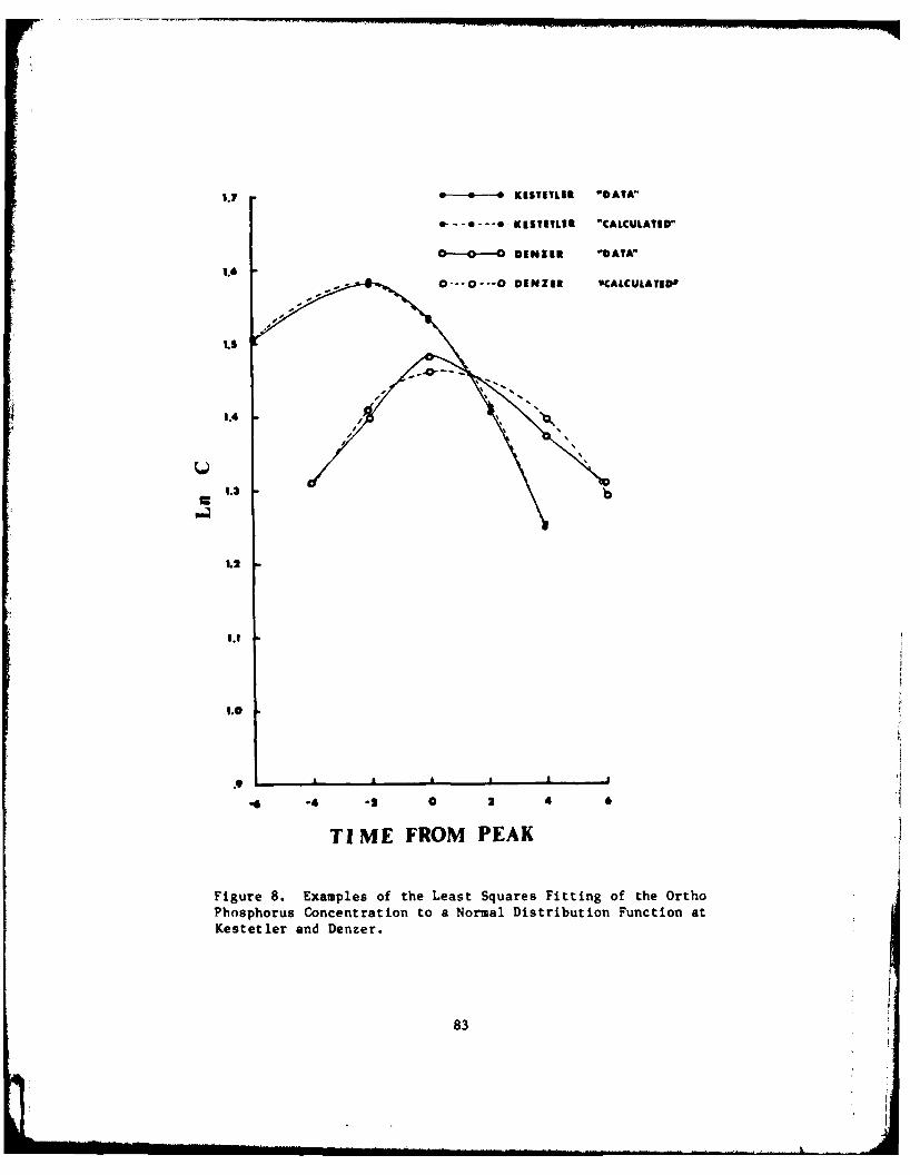
l*7 -4----KISTTLER 'DATA"

--- KSTTL9S "CALCULATED"

0 ------- O DENIER "DATA"

1.60---O---0 DINZIR SCALCULAFDW

1.4

re1.3

L.2

I.1

4 -4 -2 0 2 4

TI ME FROM PEAK

Figure 8. Examples of the Least Squares Fitting of the OrthoPhosphorus Concentration to a Normal Distribution Function atKestetler and Denzer.

83

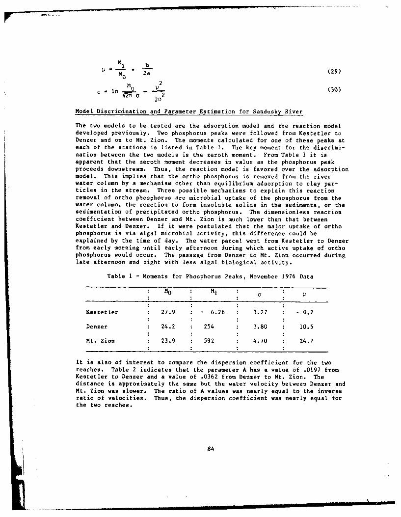
M bM 2a (29)

2O - (30)

20

Model Discrimination and Parameter Estimation for Sandusky River

The two models to be tested are the adsorption model and the reaction modeldeveloped previously. Two phosphorus peaks were followed from Kestetler toDenzer and on to Mt. Zion. The moments calculated for one of these peaks ateach of the stations is listed in Table 1. The key moment for the discrimi-nation between the two models is the zeroth moment. From Table I it isapparent that the zeroth moment decreases in value as the phosphorus peakproceeds downstream. Thus, the reaction model is favored over the adsorptionmodel. This implies that the ortho phosphorus is removed from the riverwater column by a mechanism other than equilibrium adsorption to clay par-ticles in the stream. Three possible mechanisms to explain this reactionremoval of ortho phosphorus are microbial uptake of the phosphorus from thewater column, the reaction to form insoluble solids in the sediments, or thesedimentation of precipitated ortho phosphorus. The dimensionless reactioncoefficient between Denzer and Mt. Zion is much lower than that betweenKestetler and Denzer. If it were postulated that the major uptake of orthophosphorus is via algal microbial activity, this difference could beexplained by the time of day. The water parcel went from Kestetler to Denzerfrom early morning until early afternoon during which active uptake of orthophosphorus would occur. The passage from Denzer to Mt. Zion occurred duringlate afternoon and night with less algal biological activity.

Table I - Moments for Phosphorus Peaks, November 1976 Data

Kestetler 27.9 - 6.26 3.27 - 0.2

Denzer 24.2 254 3.80 10.5

Mt. Zion 23.9 592 : 4.70 24.7

It is also of interest to compare the dispersion coefficient for the tworeaches. Table 2 indicates that the parameter A has a value of .0197 fromKestetler to Denzer and a value of .0362 from Denzer to Mt. Zion. Thedistance is approximately the same but the water velocity between Denzer andMt. Zion was slower. The ratio of A values was nearly equal to the inverseratio of velocities. Thus, the dispersion coefficient was nearly equal forthe two reaches.

84

kAD-A07 9 648 CORPS OF ENGINEERS BUFFALO0 N I BUFFALO DISTRICT F/G 6/6I POSPHORULS T RAN SPORT I N R"'E R S. IU)I S NOV0 T. F . VERHDFF, D A MELFI, 0 B BAKERUNCLASSIFIED ML

NONffllE~8

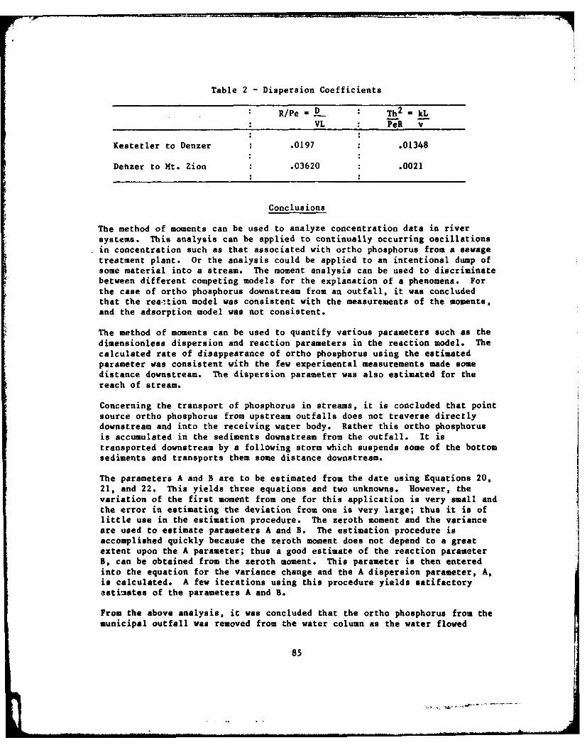
Table 2 - Dispersion Coefficients

R/Pe - R: Th 2 - kLVL PeR v

Kestetler to Denzer .0197 .01348

Dehzer to Mt. Zion .03620 .0021

Conclusions

The method of moments can be used to analyze concentration data in riversystems. This analysis can be applied to continually occurring oscillationsin concentration such as that associated with ortho phosphorus from a sewagetreatment plant. Or the analysis could be applied to an intentional dump ofsome material into a stream. The moment analysis can be used to discriminatebetween different competing models for the explanation of a phenomena. Forthe case of ortho phosphorus downstream from an outfall, it was concludedthat the reaction model was consistent with the measurements of the moments,and the adsorption model was not consistent.

The method of moments can be used to quantify various parameters such as thedimensionless dispersion and reaction parameters in the reaction model. Thecalculated rate of disappearance of ortho phosphorus using the estimatedparameter was consistent with the few experimental measurements made somedistance downstream. The dispersion parameter was also estimated for thereach of stream.

Concerning the transport of phosphorus in streams, it is concluded that pointsource ortho phosphorus from upstream outfalls does not traverse directlydownstream and into the receiving water body. Rather this ortho phosphorusis accumulated in the sediments downstream from the outfall. It istransported downstream by a following storm which suspends some of the bottomsediments and transports them some distance downstream.

The parameters A and B are to be estimated from the date using Equations 20,21, and 22. This yields three equations and two unknowns. However, thevariation of the first moment from one for this application is very small andthe error in estimating the deviation from one is very large; thus it is oflittle use in the estimation procedure. The zeroth moment and the varianceare used to estimate parameters A and B. The estimation procedure isaccomplished quickly because the zeroth moment does not depend to a greatextent upon the A parameter; thus a good estimate of the reaction parameterB, can be obtained from the zeroth moment. This parameter is then enteredinto the equation for the variance change and the A dispersion parameter, A,is calculated. A few iterations using this procedure yields satifactoryestimates of the parameters A and B.

From the above analysis, it was concluded that the ortho phosphorus from themunicipal outfall was removed from the water column as the water flowed

85

downstream. From the estimate of the reaction rate parameter B, it ispossible to estimate the distance downstream the water must move before mostof the phosphorus has been removed. This calculation assumes that the rateof removal remains constant throughout the stream reach. The first order ofreaction implies the following equation.

dC - kc (31)

dt

This equation is converted to the following form.

dc v (32)

The dimensionless time constant in this equation is simply theparameter B, i.e. (33)

B kLv

Since the distance between Kestetler and Denser is about 3.35 kilometers anda dimensionless distance of about 14 will correspond to about 90 percentremoval, it is expected that this 90 percent removal would be achieved about50 kilometers downstream, if the stream velocity remains constant. Actually,the velocity decreases and the phosphorus is removed more rapidly thandistance. Measurements 16 km downstream indicate that more than three-fourths of the ortho phosphorus has been removed at this point which is con-sistent with the model.

86

4 p

References

I. Streeter, N.W. and E.B. Phelps, "A Study of the Pollution and NaturalPurification of the Ohio River, III, Factors Concerned in the Phenomena ofOxidation and Reaeration." U.S. Public Health Service, Public HealthService, Public Health Bulletin No. 146, p. 75, February 1925.

2. O'Conner, D.J. "Oxygen Balance of an Estuary" ASCE J of San. Eng. Div.86, 35 (1960).

3. Rohatgi, N.K. and A.M. Chen "Fate of Metals in Wastewater Discharges toOcean" ASCE, J Env Engr. 102, 675 (1976).

4. Willis, R,; D.R. Anderson, and J.A. Dracup "Steady State Water QualityModeling To Streams" J. Env. Engr. ASCE 101, 245 (1975).

5. Keup, L.E., "Phosphorus in Flowing Streams," Water Research, Vol. 2,(1968), p. 373.

6. Connell, C.H., "Phosphates in Texas Rivers and Reservoirs," WaterResearch News No. 73, Southwest Water Research Council, Fort Worth, TX,(1965).

7. McKee, G.D., et. al., "Sediment-Water Nutrient Relationships, Part 2,"Water and Sewage Works, Vol. 177, (1970), p. 1047-1053.

8. Cahill, T.H.; Imperato, P.; and F.H. Verhoff, "Evaluation of Phosphorusin a Watershed" J. of Env. Eng. ASCE 100, 439 (1974).

9. Aris R. "On the dispersion of a solute in a fluid flowing through a tube"Proc. Roy Soc. Ser. A. 235, 67 (1956)

10. Parker, F.L. "Eddy Diffusion in Reservoirs and Pipelines" J. HydraulicsDivision ASCE 87, 475 (1961)

11. Yamaoka, K. and T. Nakaqawa "Application of Numerical LaplaceTransformation to Chromatograph Peak Anaysib J. of Chromat, 92, 213 (1974).

12. Yamaoka, K. and T. Nakagawa "Moment Analysis of Multiple PhaseChromatography" J. of Chromat. 105, 225 (1975).

13. Yamaoka, K. and T. Nakagawa "Moment Analysis for ReactionChromatography" J. of Chromat, 117, 1 (1976).

14. Douglas, J.M., Process Dynamics and Control Vol. 1, Prentice-HallEngelwood Cliffs, NJ, (1972), pp. 255-259.

15. Friedly, J.C. Dynamic Behavior of Processes, Prentice-Hall EngelwoodCliffs, NJ (1972), pp. 357-359.

87

16. Taylor, G.I. (1954) "The Dispersion of Hater in Turbulent Flov Through aPipe" Proceedings Royal Society of London 221A, 446 (1954).

17. Holley, E.R. and Y.H. Tsai "Conment on 'Longitudinal Dispersion inNatural Channels' by Terry J. Day" Water Resources, 13, 505 (1977).

88

,. .i i