Operations Research Unit 7
Sikkim Manipal University Page No. 136
Unit 7 Integer Programming Problem
Structure:
7.1 Introduction
Learning Objectives
7.2 All and Mixed Integer Programming Planning
7.3 Gomory’s all IPP Method
Construction of Gomory’s constraints
7.4 All IPP Algorithms
7.5 Branch and Bound Technique
Branch and bound algorithm
7.6 Summary
7.7 Terminal Questions
7.8 Answers to SAQs and TQs
Answers to self assessment questions
Answers to terminal questions
7.9 References
7.1 Introduction
Welcome to the seventh unit on Integer Programming Problem in
Operations Research Management. The Integer Programming Problem
(IPP) is a special case of Linear Programming Problem (LPP), where all or
some variables are constrained to assume non-negative integer values. You
can apply this problem to various situations in business and industry where
discrete nature of the variables is involved in many decision-making
situations. For instance, in manufacturing, the production is frequently
scheduled in terms of batches, lots or runs; in distribution, a shipment must
involve a discrete number of trucks or aircrafts or freight cars.
Learning objectives
By the end of this unit, you should be able to:
Write an integer programming problem (IPP)
Solve an integer programming problem (IPP) using Gomory’s method
Apply the branch and land technique
Operations Research Unit 7
Sikkim Manipal University Page No. 137
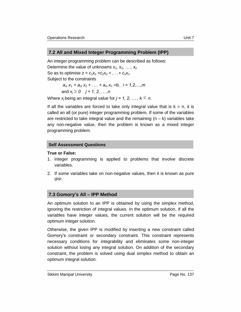
7.2 All and Mixed Integer Programming Problem (IPP)
An integer programming problem can be described as follows:
Determine the value of unknowns x1, x2, … , xn
So as to optimise z = c1x1 +c2x2 + . . .+ cnxn
Subject to the constraints
ai1 x1 + ai2 x2 + . . . + ain xn =bi , i = 1,2,…,m
and xj 0 j = 1, 2, … ,n
Where xj being an integral value for j = 1, 2, … , k n.
If all the variables are forced to take only integral value that is k = n, it is
called an all (or pure) integer programming problem. If some of the variables
are restricted to take integral value and the remaining (n – k) variables take
any non-negative value, then the problem is known as a mixed integer
programming problem.
Self Assessment Questions
True or False:
1. Integer programming is applied to problems that involve discrete
variables.
2. If some variables take on non-negative values, then it is known as pure
IPP.
7.3 Gomory’s All – IPP Method
An optimum solution to an IPP is obtained by using the simplex method,
ignoring the restriction of integral values. In the optimum solution, if all the
variables have integer values, the current solution will be the required
optimum integer solution.
Otherwise, the given IPP is modified by inserting a new constraint called
Gomory’s constraint or secondary constraint. This constraint represents
necessary conditions for integrability and eliminates some non-integer
solution without losing any integral solution. On addition of the secondary
constraint, the problem is solved using dual simplex method to obtain an
optimum integral solution.

Operations Research Unit 7
Sikkim Manipal University Page No. 138
If all the values of the variables in the solution are integers, then an optimum
inter-solution is obtained, or else a new constraint is added to the modified
LPP and the procedure is repeated till the optimum solution is derived. An
optimum integer solution will be reached eventually after introducing enough
new constraints to eliminate all the superior non-integer solutions. The
construction of additional constraints, called secondary or Gomory’s
constraints is important and needs special attention.
7.3.1 Construction of Gomory’s constraints
Consider a LPP or an optimum non–integer basic feasible solution. With the
usual notations, let the solution be displayed in the following simplex table.
Table 7.1: Simplex table
The optimum basic feasible solution is given by
xB = [x2, x3 ] = [y10, y20]; max z = y00
Since xB is a non-integer solution, we can assume that y10 is fractional. The
constraint equation is
y10 = y11 x1 + y12 x2 + y13 x3+ y14 x4 0xx 41
It reduces to
y10 = y11 x1 + x2 + y14 x4 0xx 41 _____ (1)
Because x2 and x3 are basic variables (which implies that y12 = 1 and
y13 = 0). The above equation can be rewritten as
x2 = y10 - y11 x1 - y14 x4
This is a linear combination of non-basic variables.
Now, since y10 0 the fractional part of y10 must also be non-negative. You
can split each of yij in (1) into an integral part Iij , and a non-negative
fractional part, f1j for j = 0,1,2,3,4. After the breakup (1) above, you can write
it as:
I10 + f10 = (I11 + f11) x2 + (I14 + f14) x4
Or
f10 - f11 x2 - f14 x4 = x2 + I11 x1 + I14x4 - I10 _____ (2)
yB xB y1 y2 y3 y4
y2 y10 y11 y12 y13 y14
y3 y20 y21 y22 y23 y24
y00 y01 y02 y03 y04
Operations Research Unit 7
Sikkim Manipal University Page No. 139
If you compare (1) and (2), you will see that if you add an additional
constraint in such a way that the left-hand side of (2) is an integer; then you
will be forcing the non-integer y10 towards an integer.
The desired Gomory’s constraint is
f10 – f11 x1 – f11 x4 ≤ 0
It is possible to have f10 – f11 x1 – f11 x4 = h where h > 0 is an integer. Then
f10 = h + f11 x1 + f14 x4 is greater than one. This contradicts that 0 < fij < 1 for j
= 0, 1, 2, 3, 4.
Thus Gomory’s constraint is
10sla
4,1j
jij
4,1j
10jij
4,1j
jig
f)1(Gxfor
fx.forfxf10
Where Gsla (1) is a slack variable in the above first Gomory’s constraint
The additional constraint to be included in the given LPP is towards
obtaining an optimum all integer solution. After adding the constraint, the
optimum simplex table looks like table 7.2 given below.
Table 7.2: Optimum simplex table
yB xB y1 y2 y3 y4 Gsla(1)
y1 y10 y11 y12 y13 y14 0
y2 y20 y21 y22 y23 y24 0
Gsla(1) – f10 – f11 0 0 – f14 1
y00 y01 y02 y03 y04 y05
Since – f10 is negative, the optimal solution is unfeasible. Thus the dual
simplex method is to be applied for obtaining an optimum feasible solution.
After obtaining this solution, the above referred procedure is applied for
constructing second Gomory’s constraint. The process is to be continued till
all the integer solution has been obtained.
Self Assessment Questions
Fill in the blanks:
3. An optimum solution to IPP is first obtained by using ______________.
4. With the addition of Gomory’s constraint, the problem is solved by
______ ______ ________.
Operations Research Unit 7
Sikkim Manipal University Page No. 140
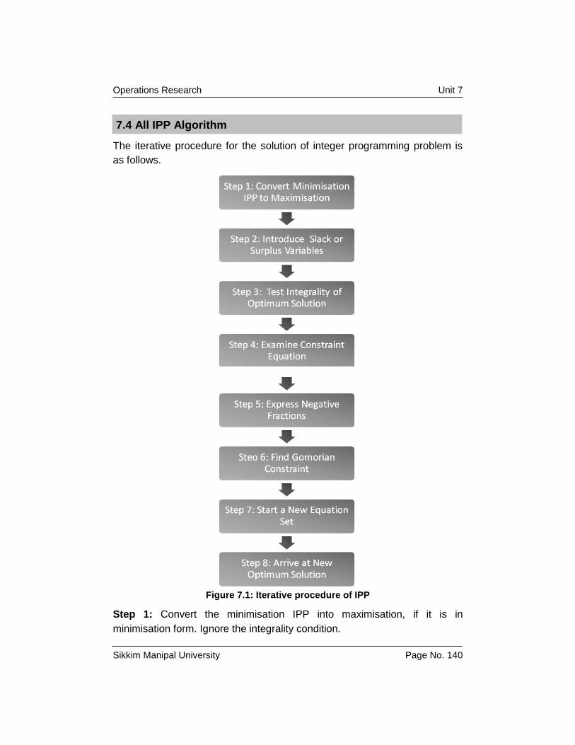
7.4 All IPP Algorithm
The iterative procedure for the solution of integer programming problem is
as follows.
Figure 7.1: Iterative procedure of IPP
Step 1: Convert the minimisation IPP into maximisation, if it is in
minimisation form. Ignore the integrality condition.
Operations Research Unit 7
Sikkim Manipal University Page No. 141
Step 2: Introduce the slack or surplus variables, if needed to convert the
inequations into equations and obtain the optimum solution of the given LPP
by using simplex algorithm.
Step 3: Test the integrality of the optimum solution
a) If the optimum solution contains all integer values, an optimum basic
feasible integer solution has been obtained.
b) If the optimum solution does not include all integer values, then proceed
to the next step.
Step 4: Examine the constraint equations corresponding to the current
optimum solution. Let these equations be represented by
)m........,,2,1,0i(,bx,y 1
ij
1n
0jij
Where n denotes the number of variables and m the number of
equations. Choose the largest fraction of bis to find iibi
max
Let it be i
1k
b or write is as o
kf
Step 5: Express the negative fractions if any, in the kth row of the optimum
simplex table as the sum of a negative integer and a non-negative fraction.
Step 6: Find the Gomorian constraint
1n
0j
kojkjfx,f
And add the equation
1n
0jjkjkosla x.ff)1(G
To the current set of equation constraints
Step 7: Start with a new set of equation constraints. Find the new optimum
solution by dual simplex algorithm so that Gsla (1) is the initial leaving basic
variable.
Operations Research Unit 7
Sikkim Manipal University Page No. 142
Step 8: If the new optimum solution for the modified LPP is an integer
solution, it is also feasible and optimum for the given IPP. If it is not an
integer solution, then return to step 4 and repeat the process until an
optimum feasible integer solution is obtained.
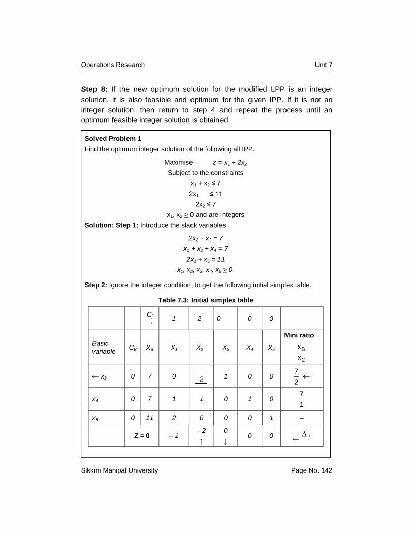
Solved Problem 1
Find the optimum integer solution of the following all IPP.
Maximise z = x1 + 2x2
Subject to the constraints
x1 + x2 ≤ 7
2x1 ≤ 11
2x2 ≤ 7
x1, x2 > 0 and are integers
Solution: Step 1: Introduce the slack variables
2x2 + x3 = 7
x1 + x2 + x4 = 7
2x1 + x5 = 11
x1, x2, x3, x4, x5 > 0.
Step 2: Ignore the integer condition, to get the following initial simplex table.
Table 7.3: Initial simplex table
Cj →
1 2 0 0 0
Basic variable
CB XB X1 X2 X3 X4 X5
Mini ratio
2
B
x
x
← x3 0 7 0 2 1 0 0 2
7
x4 0 7 1 1 0 1 0 1
7
x5 0 11 2 0 0 0 1 –
Z = 0 – 1 – 2
↑
0
↓ 0 0
← j
Operations Research Unit 7
Sikkim Manipal University Page No. 143
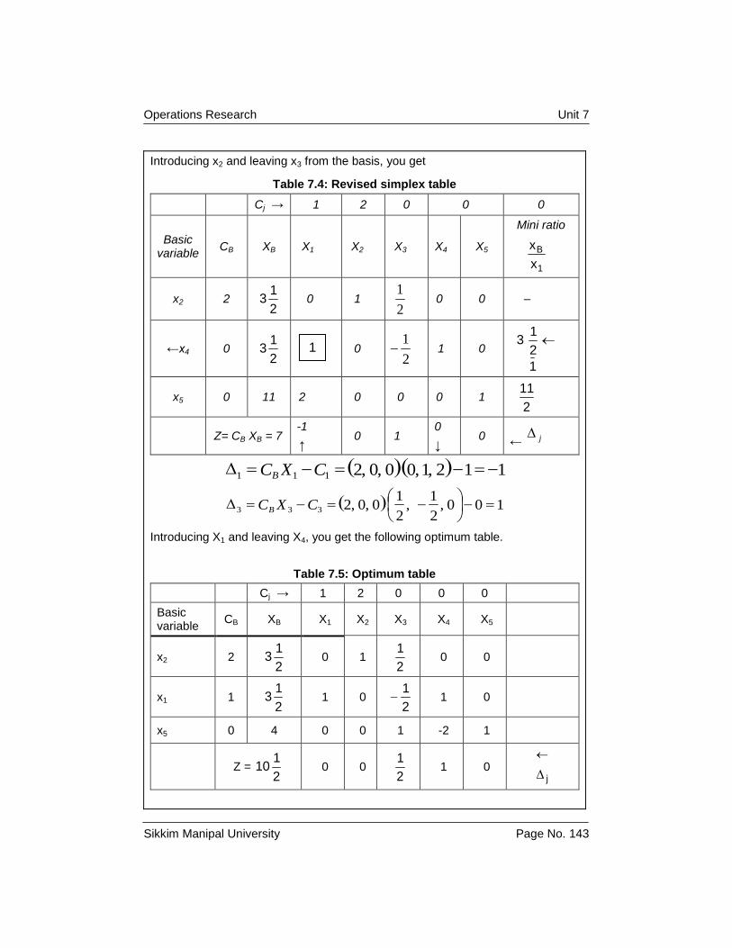
Introducing x2 and leaving x3 from the basis, you get
Table 7.4: Revised simplex table
Cj → 1 2 0 0 0
Basic variable
CB XB X1 X2 X3 X4 X5
Mini ratio
1
B
x
x
x2 2 2
13 0 1
2
1
0 0 –
←x4 0 2
13
0 2
1
1 0
1
2
13
x5 0 11 2 0 0 0 1 2
11
Z= CB XB = 7 -1
↑ 0 1
0
↓ 0
← j
112,1,00,0,2111 CXCB
100,2
1,
2
10,0,2333
CXCB
Introducing X1 and leaving X4, you get the following optimum table.
Table 7.5: Optimum table
Cj → 1 2 0 0 0
Basic variable
CB XB X1 X2 X3 X4 X5
x2 2 2
13 0 1
2
1 0 0
x1 1 2
13 1 0
2
1 1 0
x5 0 4 0 0 1 -2 1
Z = 2
110 0 0
2
1 1 0
j
1
Operations Research Unit 7
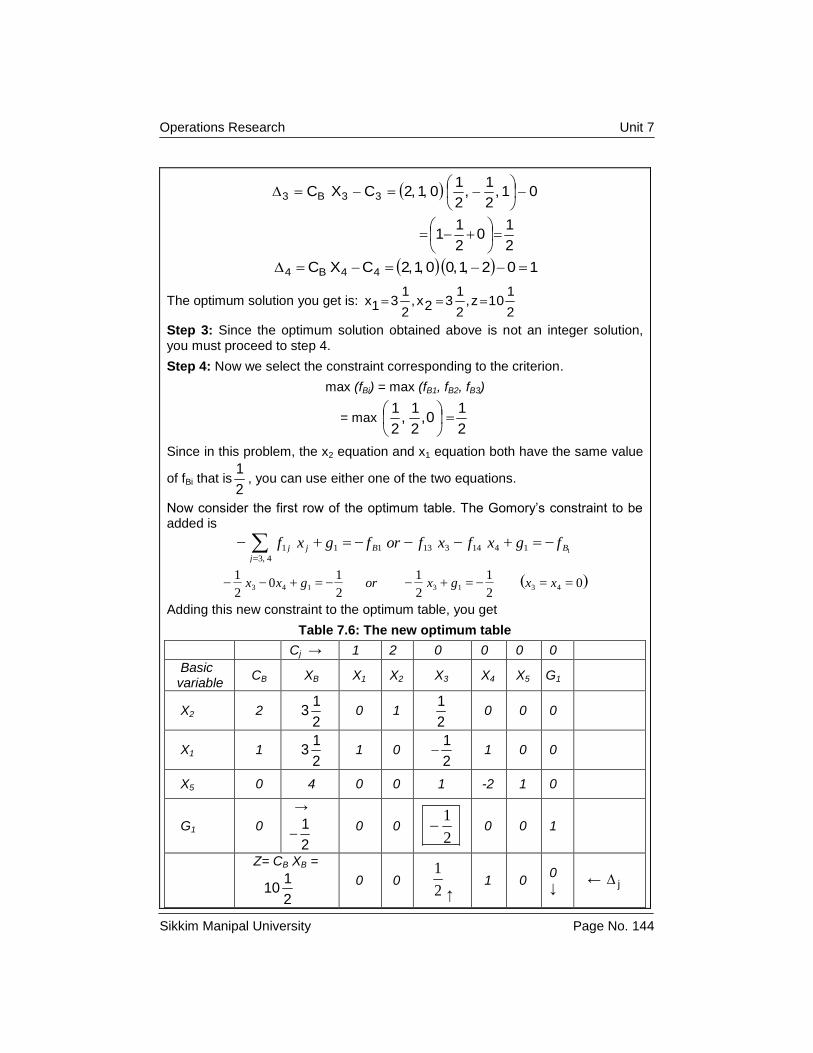
Sikkim Manipal University Page No. 144
01,2
1,
2
10,1,2CXC 33B3
2
10
2
11
102,1,00,1,2CXC 44B4
The optimum solution you get is: 2
110z,
2
132x,
2
131x
Step 3: Since the optimum solution obtained above is not an integer solution, you must proceed to step 4.
Step 4: Now we select the constraint corresponding to the criterion.
max (fBi) = max (fB1, fB2, fB3)
= max 2
10,
2
1,
2
1
Since in this problem, the x2 equation and x1 equation both have the same value
of fBi that is2
1, you can use either one of the two equations.
Now consider the first row of the optimum table. The Gomory’s constraint to be added is
4,3
1414313111 1
j
BBjj fgxfxforfgxf
02
1
2
1
2
10
2
14313143 xxgxorgxx
Adding this new constraint to the optimum table, you get
Table 7.6: The new optimum table
Cj → 1 2 0 0 0 0
Basic variable
CB XB X1 X2 X3 X4 X5 G1
X2 2 2
13 0 1
2
1 0 0 0
X1 1 2
13 1 0
2
1 1 0 0
X5 0 4 0 0 1 -2 1 0
G1 0
→
2
1
0 0 2
1
0 0 1
Z= CB XB =
2
110
0 0 2
1
↑ 1 0
0 ↓
← j
Operations Research Unit 7
Sikkim Manipal University Page No. 145
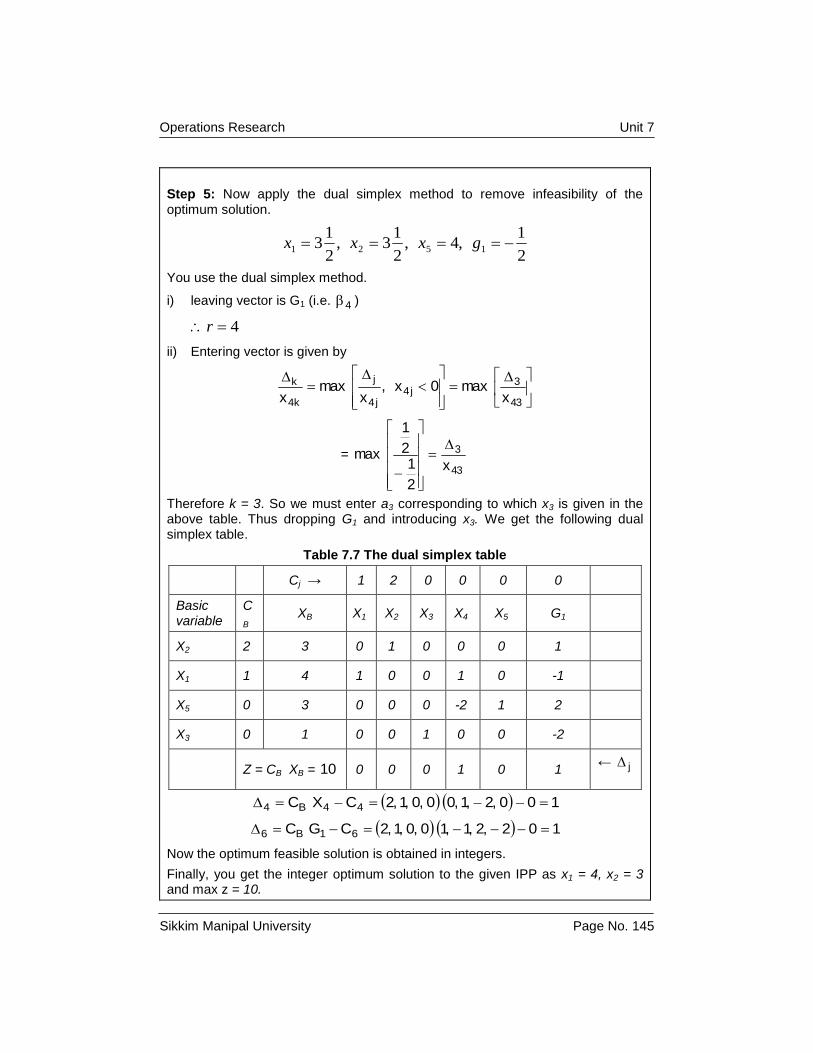
Step 5: Now apply the dual simplex method to remove infeasibility of the optimum solution.
2
1,4,
2
13,
2
13 1521 gxxx
You use the dual simplex method.
i) leaving vector is G1 (i.e. 4 )
4r
ii) Entering vector is given by
43
3j4
j4
j
k4
k
xmax0x,
xmax
x
= 43
3
x
2
12
1
max
Therefore k = 3. So we must enter a3 corresponding to which x3 is given in the above table. Thus dropping G1 and introducing x3. We get the following dual simplex table.
Table 7.7 The dual simplex table
Cj → 1 2 0 0 0 0
Basic variable
C
B XB X1 X2 X3 X4 X5 G1
X2 2 3 0 1 0 0 0 1
X1 1 4 1 0 0 1 0 -1
X5 0 3 0 0 0 -2 1 2
X3 0 1 0 0 1 0 0 -2
Z = CB XB = 10 0 0 0 1 0 1 ← j
100,2,1,00,0,1,2CXC 44B4
102,2,1,10,0,1,2CGC 61B6
Now the optimum feasible solution is obtained in integers.
Finally, you get the integer optimum solution to the given IPP as x1 = 4, x2 = 3 and max z = 10.
Operations Research Unit 7
Sikkim Manipal University Page No. 146
Self Assessment Questions
True or False:
5. Do you select the variable for Gomory’s constraint whose fractional
value is more?
6. Optimum values in an pure IPP can be x=2 and y=3.5.
7.5 Branch and Bound Technique
Sometimes a few or all the variables of an IPP are constrained by their
upper or lower bounds or by both. The most general technique for a solution
of such constrained optimisation problems is the branch and bound
technique. The technique is applicable to both all (or pure) IPP as well as
mixed IPP. The technique for a maximisation problem is discussed below:
Let the IPP be
Maximise
n
1j
jj xcz –––––––––––––––––––––––––––– (1)
Subject to the constraints
m....,,2,1ibxan
1j
ijij
––––––––––––––––––– (2)
xj is integer valued , j = 1, 2, …….., r (< n) –––––––––––––––––- (3)
xj > 0 …………………. j = r + 1, …….., n ––––––-––––––––––––––– (4)
Further let us suppose that for each integer valued xj, we can assign lower
and upper bounds for the optimum values of the variable by
Lj ≤ xj ≤ Uj j = 1, 2, …. r –––––––––––––––––––––––––– (5)
This is the main idea behind “the branch and bound technique”.
Consider any variable xj, and let I be some integer value satisfying Lj I Uj
– 1. Then clearly an optimum solution (1) through (5) also satisfies either
linear constraint.
x j I + 1 –––––––––––––––––––––––––––––– (6)
Or the linear constraint xj ≤ I –––––––––––––––––––––––––––––– (7)
To explain how this partitioning helps, let’s assume that there were no
integer restrictions (3), and it yields an optimal solution to LPP – (1), (2), (4)
and (5). This indicates x1 = 1.66 (for example).
Then you formulate and solve two LPPs each containing (1), (2) and (4). But
(5) for j = 1 is modified to be 2 ≤ x1 ≤ U1 in one problem and L1 ≤ x1 ≤ 1 in the
other. Further to each of these problems, process an optimal solution
satisfying integer constraint (3).
Operations Research Unit 7
Sikkim Manipal University Page No. 147
Then the solution having the larger value for z is clearly the optimum for the
given IPP. However, it usually happens that one (or both) of these problems
have no optimal solution satisfying (3), and thus some more computations
are required. Now let us discuss, step wise, the algorithm that specifies how
to apply the partitioning (6) and (7) in a systematic manner to finally arrive at
an optimum solution.
Let’s start with an initial lower bound for z, say z(0) at the first iteration, which
is less than or equal to the optimal value z*. This lower bound may be taken
as the starting Lj for some xj.
In addition to the lower bound z(0), you also have a list of LPPs (to be called
master list) differing only in the bounds (5). To start with (the 0th iteration)
the master list contains a single LPP consisting of (1), (2), (4) and (5). Let us
now discuss the procedure that specifies how the partitioning (6) and (7) can
be applied systematically to eventually get an optimum integer-valued
solution.
7.5.1 Branch and bound algorithm
At the tth iteration (t = 0, 1, 2 …), apply the following steps to get an optimum
integer.
Step 0: If the master list is not empty, choose an LPP from it. Otherwise
stop the process, go to step 1.
Step 1: Obtain the optimum solution to the chosen problem. If either
i) It has no feasible solution or
ii) The resulting optimum value of the objective function z is less than
or equal to z(t), then let z(t+1) = z(t) and return to step 0; otherwise go
to step 2
Step 2: If the obtained optimum solution satisfies the integer constraints (3)
then record it. Let z(t+1) be the associated optimum value of z; return to step
0. Otherwise move to step 3.
Step 3: Select any variable xj, j = 1, 2, …., p. that does not have an integer
value in the obtained optimum solution to the LPP, chosen in step 0. Let *jx
denote this optimal value of xj. Add two LPPs to the master list. These LPPs
are identical to the LPPs chosen in step 0, except that, the lower bound on
xj is replaced by
*jx + 1. Let z(t+1) = z(t); return to step 0.
Operations Research Unit 7
Sikkim Manipal University Page No. 148
Note: At the termination of the algorithm, if a feasible integer valued solution
yielding z(t) has been recorded, it is optimum, or else no integer valued
feasible solution exists.
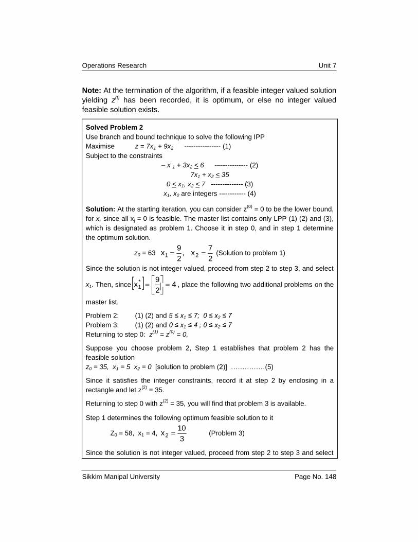
Solved Problem 2
Use branch and bound technique to solve the following IPP
Maximise z = 7x1 + 9x2 ---------------- (1)
Subject to the constraints
– x 1 + 3x2 < 6 -–------------ (2)
7x1 + x2 < 35
0 < x1, x2 < 7 -------------- (3)
x1, x2 are integers -–--------- (4)
Solution: At the starting iteration, you can consider z(0)
= 0 to be the lower bound,
for x, since all xj = 0 is feasible. The master list contains only LPP (1) (2) and (3),
which is designated as problem 1. Choose it in step 0, and in step 1 determine
the optimum solution.
z0 = 63 2
7x,
2
9x 21 (Solution to problem 1)
Since the solution is not integer valued, proceed from step 2 to step 3, and select
x1. Then, since 42
9x *
1
, place the following two additional problems on the
master list.
Problem 2: (1) (2) and 5 ≤ x1 ≤ 7; 0 ≤ x2 ≤ 7
Problem 3: (1) (2) and 0 ≤ x1 ≤ 4 ; 0 ≤ x2 ≤ 7
Returning to step 0: z(1)
= z(0)
= 0,
Suppose you choose problem 2, Step 1 establishes that problem 2 has the
feasible solution
z0 = 35, x1 = 5 x2 = 0 [solution to problem (2)] ……………(5)
Since it satisfies the integer constraints, record it at step 2 by enclosing in a
rectangle and let z(2)
= 35.
Returning to step 0 with z(2)
= 35, you will find that problem 3 is available.
Step 1 determines the following optimum feasible solution to it
Z0 = 58, x1 = 4, 3
10x2 (Problem 3)
Since the solution is not integer valued, proceed from step 2 to step 3 and select
Operations Research Unit 7
Sikkim Manipal University Page No. 149
x2. Then 33
10*xx
. Then add the following additional problems on the
master list:
Problem 4: (1) (2) and 72x4;41x0
Problem 5: (1) (2) and 0 ≤ x1 ≤ 4; 0 ≤ x2 ≤ 3
Returning to step 0 with z(3)
= z(2)
= 35, choose problem 4 from step 1, as you
know that problem 4 has no feasible solution, you again return to step 0 with z(4)
=
z(3)
= 35. Only problem 5 is available in the master list. In step 1, you again
determine the following optimum solution to this problem.
z0 = 55 x1 = 4 x2 = 3 (solution to problems) ---------- (6)
Since this satisfies the integer constraints, record it at step 2 by enclosing inside a
rectangle and let z(5)
= 55.
Returning to step 0, you will find that the master list is empty; and thus the
algorithm terminates.
Now on termination, you will find that only two feasible integer solutions namely
(5) and (6) have been recorded. The best of these gives the optimum solution to
the given IPP. Hence the optimum integer solution to the given IPP is Z0 = 55, x1
= 4, x2 = 3.
Figure 7.2: Tree diagram of the above example
Operations Research Unit 7
Sikkim Manipal University Page No. 150
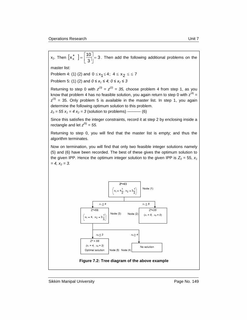
Table 7.8: Solution table
Node Solution Additional
Constraints Type of solution
x1 x2 z*
(1) 2
9
2
7
63 __
Non-integer (Original problem)
(2) 5 0 35 5x1 Integer ← z*
(1)
(3) 4 3
10
58 4x1 Non-integer
(4) …… …….. …….. 4x,4x 21 No solution
(5) 4 3 55 3x,4x 21 Integer ←z*(2)
(Optimal)
Self Assessment Questions
True or False:
7. Branch and bound technique is applied when some variables have
upper or lower bounds.
8. We start the technique with lower bound.
7.6 Summary
This chapter examines the programming model in which the assumption of
divisibility is weakened. This unit also describes two algorithms to determine
the optimal solution for an integer programming problem. One is the cutting
plane algorithm devised by Gomory and the other is the branch and bound
algorithm developed by Land Doig.
7.7 Terminal Questions
1. Use Branch and Bound technique to solve the following problem
Maximise z = 3x1 + 3x2 + 13 x3
Subject to
– 3x1 + 6x2 + 7x3 ≤ 8
6x1 – 3x2 + 7x3 ≤ 8
0 ≤ xj ≤ 5
And xj are integer j = 1, 2, 3
Operations Research Unit 7
Sikkim Manipal University Page No. 151
2. What is integer programming?
3. Explain the Gomory’s cutting plane all integer algorithm of an IPP?
7.8 Answers to SAQs and TQs
Answers to Self Assessment Questions
1. True
2. False
3. Simplex method
4. Dual simplex method
5. Correct
6. Wrong
7. True
8. False
Answers to Terminal Questions
1. At the end of the 8th iteration we get the optional solution to the I.P.P. is
x1 = x2 = 0, x3 = 1, z* = 13.
2. Refer to Section 7.2
3. Refer to Section 7.3
7.9 References
No external sources have been referred for this unit.