UNIVERSITÀ DEGLI STUDI DI SIENA
Dipartimento di Ingegneria dell’Informazione
Ph.D. Thesis - Ciclo XXI – May 13th, 2009
New techniques for steganography
and steganalysis in the pixel domain
Author: Ing. Giacomo Cancelli
Supervisor: Prof. Mauro Barni
Jury:
Prof. Andrea Abrardo Università degli Studi di Siena Prof. Jean-Luc Dugelay Institut Eurécom Prof. Alessandro Piva Università degli Studi di Firenze
Reviewers:
Dr. Gwenaël Doërr University College London Dr. Andreas Westfeld Technische Universität Dresden

Contents
1 Introduction 11.1 Contributions of the thesis . . . . . . . . . . . . . . . . . . . . . . 5
1.1.1 ALE . . . . . . . . . . . . . . . . . . . . . . . . . . . . . . 6
1.1.2 Comparative Methodology in Steganalysis . . . . . . . . . 6
1.1.3 MPSteg-color . . . . . . . . . . . . . . . . . . . . . . . . . 7
1.2 Thesis organization . . . . . . . . . . . . . . . . . . . . . . . . . . 7
I ±1 embedding steganalysis 9
2 Steganalysis: a classification problem 112.1 Training . . . . . . . . . . . . . . . . . . . . . . . . . . . . . . . . 12
2.2 Testing . . . . . . . . . . . . . . . . . . . . . . . . . . . . . . . . . 15
2.2.1 Cross validation . . . . . . . . . . . . . . . . . . . . . . . 15
2.2.2 Performance measures . . . . . . . . . . . . . . . . . . . . 15
2.3 Fisher Linear Discriminant Analysis . . . . . . . . . . . . . . . . . 20
3 ±1 embedding: state of art 233.1 ±1 embedding steganography . . . . . . . . . . . . . . . . . . . . 23
3.2 ±1 embedding steganalyzers . . . . . . . . . . . . . . . . . . . . . 24
3.2.1 High Order Statistics of the Stego Noise (WAM) . . . . . . 24
i
Contents
3.2.2 Center of Mass of the Histogram Characteristic Function(2D-HCFC) . . . . . . . . . . . . . . . . . . . . . . . . . . 26
4 Amplitude of Local Extrema 294.1 Improving previous work on histogram domain . . . . . . . . . . . 29
4.1.1 Removing Interferences at the Histogram Borders . . . . . . 30
4.2 Considering 2D Adjacency Histograms . . . . . . . . . . . . . . . 31
4.3 Performances of ALE . . . . . . . . . . . . . . . . . . . . . . . . . 33
4.3.1 Setup . . . . . . . . . . . . . . . . . . . . . . . . . . . . . 33
4.3.2 Results . . . . . . . . . . . . . . . . . . . . . . . . . . . . 35
4.4 Hybrid Algorithm . . . . . . . . . . . . . . . . . . . . . . . . . . . 37
4.5 Discussion . . . . . . . . . . . . . . . . . . . . . . . . . . . . . . . 37
5 Experimental comparison among ±1 embedding steganalysis 395.1 Databases . . . . . . . . . . . . . . . . . . . . . . . . . . . . . . . 39
5.2 Experimental Procedure . . . . . . . . . . . . . . . . . . . . . . . . 41
5.3 Experimental Results . . . . . . . . . . . . . . . . . . . . . . . . . 42
5.3.1 Impact of the source of imagery . . . . . . . . . . . . . . . 42
5.3.2 Impact of the embedding rate . . . . . . . . . . . . . . . . 46
5.3.3 Performances of the steganalyzers with prior information aboutthe source of imagery . . . . . . . . . . . . . . . . . . . . . 49
5.3.4 Performances of the steganalyzers without prior informationabout the source of imagery . . . . . . . . . . . . . . . . . 51
5.4 Conclusions . . . . . . . . . . . . . . . . . . . . . . . . . . . . . . 53
6 Steganalysis: remarks and future works 55
II MPSteg-color: a new steganographic technique 57
7 Steganography at higher semantic level 597.1 Introduction to MP image decomposition . . . . . . . . . . . . . . 60
7.2 Embedding a message in the MP domain . . . . . . . . . . . . . . . 62
ii
Contents
8 An MP tailored for steganographic application 658.1 Dictionary . . . . . . . . . . . . . . . . . . . . . . . . . . . . . . . 658.2 MP selection and update rules . . . . . . . . . . . . . . . . . . . . 66
9 A closer look at the new MP domain 73
10 MPSteg-color 7710.1 Embedding Rule . . . . . . . . . . . . . . . . . . . . . . . . . . . 7910.2 Improving undetectability . . . . . . . . . . . . . . . . . . . . . . . 8010.3 Increasing the payload . . . . . . . . . . . . . . . . . . . . . . . . 81
11 MPSteg-color: experimental results 8311.1 Image Database . . . . . . . . . . . . . . . . . . . . . . . . . . . . 83
11.2 Effectiveness of the proposed MP decomposition . . . . . . . . . . 8411.2.1 Interband correlation of decomposition path . . . . . . . . . 8411.2.2 Effectiveness of the decomposition refinement step . . . . . 84
11.3 Undetectability analysis . . . . . . . . . . . . . . . . . . . . . . . . 8511.3.1 Targeted steganalyzers . . . . . . . . . . . . . . . . . . . . 8511.3.2 State-of-art steganalyzers . . . . . . . . . . . . . . . . . . . 8711.3.3 Steganalysis Results . . . . . . . . . . . . . . . . . . . . . 8811.3.4 Computational Complexity . . . . . . . . . . . . . . . . . . 92
12 MPSteg-color: remarks and future works 99
13 Final remarks 101
Bibliography 105
iii

List of Figures
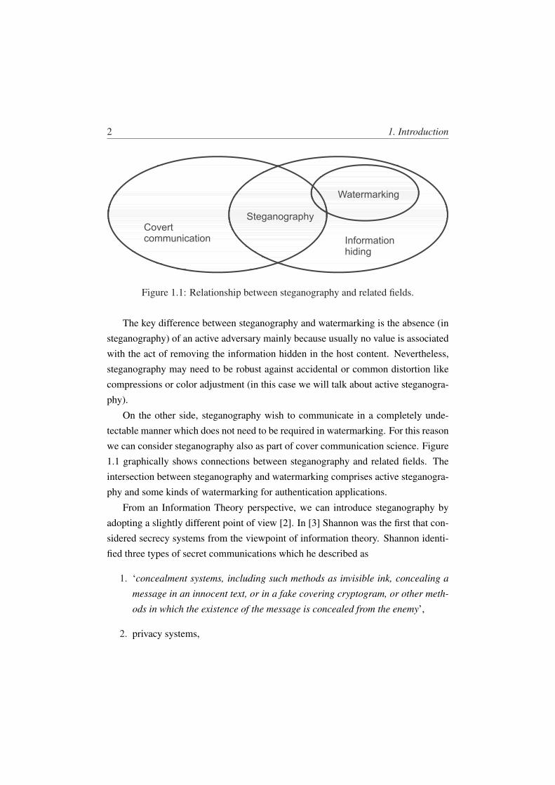
1.1 Relationship between steganography and related fields. . . . . . . . 2
2.1 Example Receiver Operating Characteristic (ROC) curve. . . . . . . 18
2.2 k = 5 individual ROC curves. . . . . . . . . . . . . . . . . . . . . 18
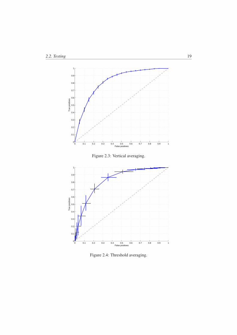
2.3 Vertical averaging. . . . . . . . . . . . . . . . . . . . . . . . . . . 19
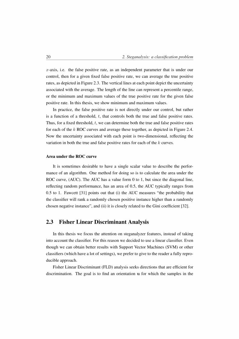
2.4 Threshold averaging. . . . . . . . . . . . . . . . . . . . . . . . . . 19
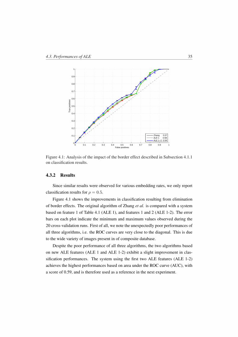
4.1 Analysis of the impact of the border effect described in Subsec-tion 4.1.1 on classification results. . . . . . . . . . . . . . . . . . . 35
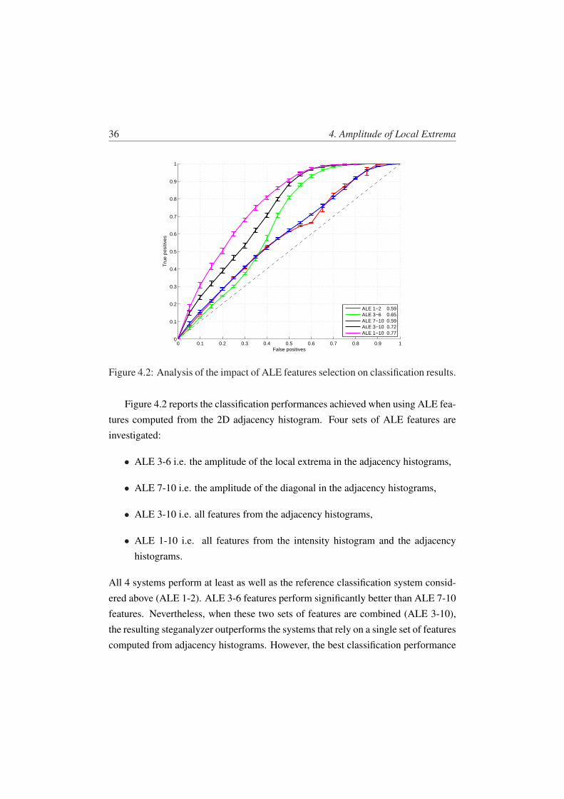
4.2 Analysis of the impact of ALE features selection on classificationresults. . . . . . . . . . . . . . . . . . . . . . . . . . . . . . . . . . 36
5.1 Impact of the source of imagery on classification performances. Theembedding rate has been fixed both during the training and testingphase and set equal to 0.5 bpp. The label of the rows indicates thedatabase used for training while the label of the columns representsthe dataset used during the testing phase. . . . . . . . . . . . . . . . 43
v

List of Figures
5.2 Impact of the embedding rate on classification performances. Thesource of imagery during both the training and testing phase is theCombined dataset. The label of the rows indicates the embeddingrate used for training while the label of the columns represents theembedding rate used during the testing phase. . . . . . . . . . . . . 47
5.3 Classification performances when prior information about the sourceof imagery is available. Training is done with stego contents ob-tained with embedding rates uniformly distributed across 0.2, 0.5and 1 bpp. The label of the rows indicates the source of imageryused both during training and testing. On the other hand, the labelof the columns represents the embedding rate used during the testingphase. . . . . . . . . . . . . . . . . . . . . . . . . . . . . . . . . . 50
5.4 Classification performances when no prior information about thesource of imagery is available. Training is done with the Com-bined database and stego contents obtained with embedding rates
uniformly distributed across 0.2, 0.5 and 1 bpp. The label of therows indicates the source of imagery used during testing, while thelabel of the columns represents the embedding rate used also duringthe testing phase. . . . . . . . . . . . . . . . . . . . . . . . . . . . 52
8.1 A subset of the atoms the dictionary consists of. . . . . . . . . . . . 66
8.2 The Selection Rule. . . . . . . . . . . . . . . . . . . . . . . . . . . 68
9.1 Comparison between the compaction property of the DCT and MPdomains. . . . . . . . . . . . . . . . . . . . . . . . . . . . . . . . . 74
9.2 Original gray-scale image. . . . . . . . . . . . . . . . . . . . . . . 74
9.3 Reconstructed image by using the first 2 DCT coefficients in a zig-zag ordering for each 4× 4 block. . . . . . . . . . . . . . . . . . . 75
9.4 Reconstructed image by using 2 atoms for each 4× 4 block. . . . . 75
11.1 For each block the numbers Z ′ = |A + D − B − C| and Z ′′ =|E + H − F −G| are computed. . . . . . . . . . . . . . . . . . . . 86
vi
List of Figures
11.2 Comparison between coefficients histogram of a cover image (dashedline) and a stego MPSteg-color image (solid line). . . . . . . . . . . 87
11.3 Comparison between BD (a) and MPHA (b) steganalyzers: the firstwindow size reported in the figure indicates the window size used bythe steganalyzer, the second one the size of the blocks used by theembedder to partition the image. The payload is 0.3159 bpp. . . . . 89
11.4 Perceptual invisibility of the stego-message. The cover (a) and the
stego (b) images can not be distinguished (payload = 0.3158 bpp,4× 4 partition, 51.40dB). . . . . . . . . . . . . . . . . . . . . . . . 94
11.5 Comparison between MPSteg-color with window 4 × 4 (solid line)and ±1 embedding (dashed line) with 3 different steganalyzers at0.3159 bpp of payload. . . . . . . . . . . . . . . . . . . . . . . . . 95
11.6 Comparison between MPSteg-color with window 5 × 5 (solid line)and ±1 embedding (dashed line) with 3 different steganalyzers at0.2002 bpp of payload. . . . . . . . . . . . . . . . . . . . . . . . . 95
11.7 Comparison between MPSteg-color with window 6 × 6 (solid line)and ±1 embedding (dashed line) with 3 different steganalyzers at0.1391 bpp of payload. . . . . . . . . . . . . . . . . . . . . . . . . 96
11.8 MPSteg-color detection performance on ALE at fixed embeddingrate (0.1391 bpp). . . . . . . . . . . . . . . . . . . . . . . . . . . . 96
11.9 MPSteg-color detection performance on WAM at fixed embeddingrate (0.1391 bpp). . . . . . . . . . . . . . . . . . . . . . . . . . . . 97
11.10MPSteg-color detection performance on 2D-HCFC at fixed embed-ding rate (0.1391 bpp). . . . . . . . . . . . . . . . . . . . . . . . . 97
vii


List of Tables
2.1 Binary classification outcomes. . . . . . . . . . . . . . . . . . . . . 16
4.1 Table of ALE features . . . . . . . . . . . . . . . . . . . . . . . . . 33
11.1 PSNR values (dB) for different payload and settings. . . . . . . . . 9011.2 Average execution time in seconds of embedding phases for images
512× 512 of size, window 4× 4 and full payload (0.32 bpp). . . . . 92
ix


Acknowledgements
I have a lot of acknowledgements to do for this thesis, specially because if I’marrived to be who I am is thanks to all the people that have been around me, fromthose close to my desktop to those which fill up my free time.
First of all, I would like to thank my Ph.D. supervisor Mauro Barni, for hissupport, for his guidance and constructive criticism during these three years and halfof my Ph.D.
Special thanks are due to Dr. Gwenaël Doërr and Prof. Ingemar J. Cox, who,in 2007, kindly received me in the Adastral Park Postgraduate Campus at UniversityCollege London through the European Exchange Program Erasmus, for their atten-
tion and enlightening discussions. I would like to acknowledge the review effortsfrom Dr. Gwenaël Doërr for his precious comments on the initial manuscript of thisthesis which have enabled to significantly enhance its clarity and quality and fromDr. Andreas Westfeld for his appreciation of my work.
Next, I would like to thank all the people who have been involved more or lessclose to my work. I want to thanks my colleague Angela, especially for her patienceduring our animate discussions, Guido for his generosity, and Sara for the Thursdaycurry dinners in the nicest Ipswich pub during my Erasmus period. Moreover, Icannot discard Riccardo, Pierluigi and Fabio for attending me for the coffe breakand for any kind of break too. I also thankful to all students that during this periodhave enjoyed my work with their wired and uncomprehensible questions about their
xi
List of Tables
thesis.I also thank all my friends who have helped me to relax during my free time and I
apologize to everyone for having neglected them by spending several weekends andholidays at work: you weren’t less important than my work! Moreover I appreciatemy Bands, Siena and Ipswich, because they have been the melody of my studies andI thanks my Contrada which underlined this period by winning a Palio.
At the end, really special thanks are due to my brother Matteo, my dad Fabrizio,
and my mum Loredana for their immeasurable support during ups and down of mylife and the Ph.D. award is mainly due to their help.
I’m almost sure that I’m missing someone so... thanks to all the people whoselove me too!
xii
Chapter 1
Introduction
Steganography is the art of invisible communication. The term invisible is notlinked to the meaning of the communication, as in cryptography in which the goalis to secure communications from an eavesdropper, on the contrary it refers to hid-
ing the existence of the communication channel itself. The general idea of hidingmessages in common digital contents, interests a wider class of applications thatgo beyond steganography. The techniques involved in such applications are collec-tively referred to as information hiding [1]. For example, while it is possible to addmetadata about an image in special tags (exif in JPEG standard) or file headers, thisinformation will be lost when the image is printed, because metadata inserted in tagson headers are tied to the image only as long as the image exists in digital form andare lost as soon as the image is printed. By using information hiding techniques, itis possible to fuse the digital content within the image signal regardless of the fileformat and the status of the image (digital or analog).
In this thesis we will refer to cover Work or equivalently to cover image, orsimply cover to indicate the images that do not yet contain a secret message, whilewe will refer to stego Work, or stego images, or stego object to indicate an image
with an embedded secret message. Moreover, we will refer to the secret message asstego-message or hidden message.
Depending on the meaning and goal of the embedded metadata, several infor-mation hiding fields can be defined, even though in literature the term ‘informationhiding’ is often used as a synonym for steganography. In digital watermarking, forinstance, the information is used for copy prevention, copy control, and copyrightprotection. In this case the embedded data should be robust to malicious attacks inorder to preserve its goal.
2 1. Introduction
Covertcommunication
Steganography
Watermarking
Informationhiding
Figure 1.1: Relationship between steganography and related fields.
The key difference between steganography and watermarking is the absence (insteganography) of an active adversary mainly because usually no value is associatedwith the act of removing the information hidden in the host content. Nevertheless,steganography may need to be robust against accidental or common distortion likecompressions or color adjustment (in this case we will talk about active steganogra-phy).
On the other side, steganography wish to communicate in a completely unde-tectable manner which does not need to be required in watermarking. For this reasonwe can consider steganography also as part of cover communication science. Figure1.1 graphically shows connections between steganography and related fields. Theintersection between steganography and watermarking comprises active steganogra-phy and some kinds of watermarking for authentication applications.
From an Information Theory perspective, we can introduce steganography byadopting a slightly different point of view [2]. In [3] Shannon was the first that con-sidered secrecy systems from the viewpoint of information theory. Shannon identi-fied three types of secret communications which he described as
1. ‘concealment systems, including such methods as invisible ink, concealing a
message in an innocent text, or in a fake covering cryptogram, or other meth-
ods in which the existence of the message is concealed from the enemy’,
2. privacy systems,

3
3. cryptographic systems.
With regards to concealment systems, i.e. steganography, Shannon stated that such‘systems are primarily a psychological problem’ and did not consider them further.
Afterwards the concept of steganography was recovered by Simmons [4] in hisfamous explanation of steganography described by mean of the prisoners’ problem.According to the prisoners’ scenario two accomplices in a crime have been arrestedand are about to be locked in widely separated cells. Their only means of com-munication after they are locked up is by way of messages conveyed for them bytrustees - who are known to be agents of the warden. The warden is willing to allowthe prisoners to exchange messages. However, since he has every reason to suspectthat the prisoners want to coordinate an escape plan, the warden will only permitthe exchanges to occur if the information contained in the messages is completelyopen to him and presumably innocuous. The prisoners, on the other hand, are will-ing to accept some risk of deception in order to be able to communicate at all, since
they need to coordinate their plans. To do this they have to deceive the warden byfinding a way of communicating secretely in the exchanges, i.e., of establishing anhidden channel between them in full view of the warden, even though the messagethemselves contain no secret (to the warden) information.
Today steganography is also seen as a way of ensuring freedom of speech inmilitary dictatorship countries or connected to homeland security. Steganographyhas also been supposed to be used by terrorists to design terroristic attacks. Exampleabout the terrorism are the technical jihad manual [5] that is part of a terrorist manualand the color of the Osama Bin Laden’s beard in its clips: military investigators thinkthat secret messages are associated each color of the beard to coordinate terroristcells.
Another topical target of steganography is computer warfare. New worms andspywares stole a lot of information about users and then they have to find a way tocarry out this data by preventing any suspicion of transmission existence by antivirus,firewall or data stream analysis.
From a different viewpoint, we sometimes know that there are some forbiddentransmissions [6] and we want to know who is sending secret information, for ex-
4 1. Introduction
ample, to the press. Apparently, during the 1980’s, British Prime Minister MargaretThatcher became so irritated at press leaks of cabinet documents that she had theword processors programmed to encode the identity of secretaries in the word spac-ing of documents, so that disloyal ministers could be traced. Later, steganographyhas being used by some HP and Xerox printers [7] which embed small yellow dotsduring the printing phase, by writing a coded message in which the serial numberof the printer and the print time is embedded. This security has been initially forced
onto printer manufacturers by the Federal Government because American dollar billswere easily forged with such printers (one of the weakest currency at the time).
During the last few years image steganography research has raised an increas-ingly interest. A variety of techniques have been proposed especially for a givenimage file format like gif, jpeg or images represented in the pixel domain. In fact,the main idea behind steganography undetectability is: less embedding changes tothe cover Work means a less detectable stego object. Even though this statement isnot completely true (as it shown in [8]), it represents a good starting point to developand to improve initial steganographic techniques proposed in the literature. More-over, new channel coding techniques have been proposed to reduce the embedding
changes as the introduction of matrix embedding [9, 10] and Wet Paper Coding [11].Other techniques [12, 13], specially in JPEG domain, use a subset of support to adjustin some way image statistics that are changed by the message embedding. Recentlyin [14] authors try to estimate the payload upperbound for a perfect undetectabilityby using common JPEG steganalysis.
The dual goal of steganography pertains to steganalysis whose goal is to dis-cover the presence of secret communication channels (secret messages) establishedby steganography. For each steganographic method, several techniques (i.e. target
steganalysis) [15, 16, 17, 18, 19] have been proposed, however the current state of
art is moving to blind steganalysis [20, 21, 22, 15], i.e. techniques that are designedto detect the widest possible range of steganography.
Modern steganalyzers summarize the image by a set of features which are ableto reveal the presence or the absence of a secret message embedded within the Work,then these features are used to train a classifier like a Linear Discriminant classifier
1.1. Contributions of the thesis 5
or a Support Vector Machine. After the training phase, the whole system based ona feature extraction and a classification step is ready to use. This feature summa-rization is highly dependent on the image itself, so it depends on image source andhence pre-embedding processing and experimental settings of a technique should becarefully described. The high dependence between steganalysis and images used inexperimental results can be explained by the follow considerations. Some stegan-alyzers which work on high order statistics are highly dependent on high support
frequencies, but these frequencies change a lot depending on image source (cam-era CCD, or scanner CCD) and the presence of lossy compression, i.e. a low passfiltering, that can be applied to the image before the potential steganography [23].
The detectability of a hidden message highly depends on the payload, i.e. theratio between the length of the secret message and the size of the cover in whichit is embedded. In a real case we should consider that no a priori information isgiven about the message length that could be embedded within the analyzed Work.Moreover, in [24, 25], authors show that the detectability of a stego image is linkedto square root ratio between the payload and the image size.
When a new steganalyzer is proposed, all the above issues should be take into ac-count. Moreover, authors should share all their experimental settings, including theimage database used for the test, to permit to validate and to make their work repro-ducible. Unfortunately, steganographic literature usually lacks good comparisonsand reproducible research, so in this thesis we tried to adopt a fully reproduciblemethodology applied both to steganography and steganalysis. In the next section, adetailed description of the main contributions of the thesis is given.
1.1 Contributions of the thesis
The contribution of this thesis is threefold. From a steganalysis point of viewwe introduce a new steganalysis method called ALE1 which outperforms previouslyproposed pixel domain method. As a second contribution we introduce a compar-ative methodology for the comparison of different steganalyzers and we apply it
1Amplitude of Local Extrema
6 1. Introduction
to compare ALE with the state-of-art steganalyzers. The third contribution of thethesis regards steganography, since we introduce a new embedding domain and acorresponding method, called MPSteg-color, which outperforms, in terms of unde-tectability, classical embedding methods. Next, we briefly describe each contribu-tion.
1.1.1 ALE
Recently Zhang et al. [26] have introduced an algorithm for the detection of ±1LSB steganography in the pixel domain based on the statistics of the amplitudes oflocal extrema in the grey-level histogram. Experimental results demonstrated perfor-mance comparable or superior to other state-of-the-art algorithms. In this thesis, wedescribe improvements to Zhang’s algorithm (i) to reduce the noise associated withborder effects in the histogram, and (ii) to extend the analysis to amplitude of localextrema in the 2D adjacency histogram.
Experimental results on a composite database of 7125 images, averaged overa 20-fold cross validation, with classification based on Fisher linear discriminants,demonstrated that the improved algorithm exhibits significantly better performancefor the given dataset. The new algorithm, called ALE, uses 10 features derived in avery efficient way from the 1D and 2D histograms, so it is also executable in a realscenario in which the steganalysis results have to be given in realtime.
1.1.2 Comparative Methodology in Steganalysis
As a second contribution we discuss a variety of issues associated with compar-ison of different steganalyzers and highlight some of these issues with a case studycomparing four steganalysis algorithms designed to detect ±1 embedding. In par-ticular, we discuss issues related to the creation of the training and testing sets. Weemphasize that for steganalysis, it is very unlikely that the assumptions used to cre-ate the training set will match conditions used during deployment. Consequently,it is imperative that testing also investigates how performance degrades as the testset deviates from the training data. The subsequent empirical evaluation of four al-gorithms on four different test sets revealed that algorithm performance is highly
1.2. Thesis organization 7
variable, and strongly dependent on the training and test imagery. Experimental re-sults clearly demonstrate that the performance is strongly image-dependent, and thatfurther work is needed to establish more comprehensive databases. It is also commonto assume that the embedding rate is known during testing and training, but this isunlikely to be the case in practice. Once again, significant performance degradationis observed. Experimental results also suggest that the common practice of trainingat a low embedding rate in order to deal with a wide range of embedding rates during
testing is not as effective as training with a mixture of embedding rates.
1.1.3 MPSteg-color
The third contribution regards steganography for color images. Specifically, wepropose a new steganographic method that tries to use the fail-safe of steganalyzersto improve the undetectability of the stego-message. In fact, although steganalyzersdo not know the hidden message, they rely on a statistical analysis to understandwhether a given signal contains hidden data or not. However this analysis disregardsthe semantic content of the cover signal. We argue that, from a steganographic pointof view it is preferable to embed the secret message at higher semantic levels of theimage, e.g. by modifying structural elements of the cover image like lines, edges orflat areas.
By the above consideration, we propose a new steganographic method, calledMPSteg-color, that hides the stego-message into some selected coefficients obtainedthrough a high redundant basis decomposition of the color image. The decompo-sition is efficiently obtained by using a Matching Pursuit (MP) algorithm. In thisway the hidden message is embedded at a higher semantic level and hence it is moredifficult for a steganalyzer to detect it.
1.2 Thesis organization
This thesis is organized in two parts regarding steganalysis and steganography inthe pixel domain. The first part deals with steganalysis by introducing it as classi-fication problem in Chapter 2 and by showing the state-of-art of steganalysis in the
8 1. Introduction
pixel domain in Chapter 3. Moreover, in Chapter 3 we describe a simple steganogra-phy benchmark called ±1 embedding. In Chapter 4 we propose a new steganalyzer,called ALE, which improves the±1 embedding detection especially for images withhigh frequency noise in the histogram. Chapter 5 investigates experimental issuein steganalysis by proposing a methodology to fully compare steganalyzer perfor-mances. In the same chapter, we also compare the ALE steganalyzer with otherthree state-of-art steganalyzers. Some considerations and future works are drawn in
Chapter 6.In Part II we develop a new steganography which is less detectable than ±1
steganography. To do so we embed the message at a higher semantic level withrespect to the pixel domain by using the high redundant basis domain describedin Chapter 7. Due to the impossibility to use the MP algorithm as it is used inimage compression, we define an MP suitable approach for steganalysis in Chapter8 and we fully describe the proposed technique, MPSteg-color, in Chapter 10. Theundetectability of MPSteg-color is investigated in Chapter 11 both against target andgeneral purpose steganalyzers. Chapter 12 presents some conclusions and futureworks on MPSteg-color.
Part I
±1 embedding steganalysis

Chapter 2Steganalysis: a classification problem
In this part of the thesis we will consider the steganalysis of±1 embedding tech-nique by introducing some steganalysis concepts and by describing the steganalyzersthat are available in literature. Moreover we propose a new steganalyzer and we com-pare it with the state-of-art steganalyzers in the pixel domain. While performing thiscomparison we also describe a full benchmark methodology.
A steganalysis algorithm receives a Work and must decide whether it is a coveror stego Work. Some steganalysis algorithms go further, attempting to estimate thesize of the embedded message and even the content of the message. In this thesis,we are only concerned with the first decision step, and as such, we view steganalysisas a binary classification problem, i.e. the Work is, or is not a stego Work.
Classification has a long history and we assume that the reader is familiar withthe basics of classification. It is not our intention to provide a detailed tutorial on thesubject of classification and the reader is directed to [27] for further information.
Blind steganalysis refers to algorithms that do not assume knowledge of the un-derlying steganographic algorithm [28]. As such, these algorithms are intended todetect the presence of a hidden message embedded with a wide variety of algorithms,perhaps including unknown algorithms. Conversely, targeted steganalysis assumesknowledge of the underlying steganographic algorithm, and as such, is intended for
the detection of a specific steganographic algorithm [28]. In this thesis, we are con-cerned with targeted steganalysis, specifically the detection of ±1 embedding.
As said, steganalysis is a classification problem, hence, building a steganalyzercan be viewed as a three step procedure:
1. For each image in a training set containing both cover and stego Works, extracta feature vector,
12 2. Steganalysis: a classification problem
2. With the available training feature vectors, train a binary classifier for the clas-sification of stego and non-stego Works,
3. Vary the decision parameters of the classifier, e.g. a threshold, to obtain thereceiver operating characteristic (ROC) curve for the training data and set the
value of this parameter to achieve the desired performance in terms of falsepositive or true positives.
Most steganalysis algorithms can be described by (i) their feature set, and (ii) theassociated classification algorithm. The feature set is often handcrafted, and may bederived from an analysis of one or more steganographic algorithms. In this Chapter,we assume that the feature set is given and focus our attention on general issuesrelated to classification, while the problem of define a significant set of features willbe addressed in the next chapter. We do not consider the relative merits of variousclassification algorithms, e.g. k-nearest neighbors (k-NN), Fisher linear discriminant(FLD) analysis, support vector machines (SVM), etc. Instead, we consider genericissues that are applicable to all classification algorithms. Specifically, we considertwo phases in the design of a classification system, namely the training phase andthe test phase. We now consider each in turn.
2.1 Training
During the training phase, the classification algorithm is presented with a set oflabeled data, i.e. images that are known to be either stego Works or cover Works.The classification algorithm uses this information to adjust its associated parametersin order to minimize the number of false positives and false negatives it classifies.
In steganalysis, a false positive corresponds to classifying a cover Work as a stegoWork. Similarly, a false negative corresponds to classifying a stego Work as a coverWork. Both errors are important, but the relative cost of each error may depend on theapplication. For example, if steganalysis is applied to the detection of covert terroristcommunication, a false negative may be more costly than a false positive. Such anapplication may therefore accept a higher false positive rate, in order to ensure a
2.1. Training 13
lower false negative rate. Of course, resources must then be available to analyze thedata classified as stego Works, and more resources will be needed because of thehigher level of false positive. If resources are severely constrained, as for examplemay be the case for police surveillance of hidden child pornography1, then a differentcompromise may be sought that seeks to reduce the number of false positives, eventhough this will be at the expense of increasing the number of false negatives, i.e.failing to detect actual cases.
Labeled examples of both cover images and stego images are needed. Coverimages are in abundance. They are available from cameras, the Internet and stan-dardized databases. However, in order for experimental results to be reproducible,the dataset must be publicly available. And for the experimental results to be com-
parable, it is necessary to use the same database for various algorithms, otherwisevariations in performance may be attributable to variations in the database rather thanin the algorithm. The steganalysis community has recognized this and a number ofdatabases have become de facto standards for experimentation. These databases aredescribed in Chapter 5.
The type of imagery contained in these databases varies considerably. It is de-rived from a variety of sources, i.e. cameras, outdoor scenes, indoor scenes, etc,and is stored in a variety of different formats, i.e. images may have never beencompressed or have been compressed using a number of lossy compression algo-rithms that introduce a variety of statistical artifacts. The effect of these variationshas not been discussed in detail. However, experimental results described in Chap-ter 5 clearly indicate that the performance of a single algorithm can vary greatly,depending on the database.
Since performance is so affected by the database, it is imperative to (i) charac-terize each database and understand what characteristics affect performance, (ii) teston multiple standardized databases in order to quantify the variation in performancedue to the dataset, and (iii) develop new databases that contain a wider variety oftraining imagery.
1Note that while child pornography is often cited as an application for steganalysis, we are unawareof any documented case of this. To the best of our knowledge, the closest case is the “twirl face”pedophile in Thailand [29] which is a long shot away from any kind of steganography.
14 2. Steganalysis: a classification problem
For targeted steganalysis, the labeled stego images are usually generated from thecover images by applying the known steganographic algorithm to the cover images.For blind steganalysis, a set of known steganographic algorithms can be used togenerate a labeled training set. In this case, the hope is that the resulting classifierwill at least learn to classify stego Works generated by this set of algorithms. Andperhaps will even generalize to previously unseen algorithms. Alternatively, one cantry to devise a model of cover content and detect whenever the content under test
deviates from this model [30].
Even in the case of target steganalysis, generation of the labeled set is not straight-forward. In particular, every steganographic algorithm will have a variety of param-eter setting. What values should be used to generate the stego images? There is no
definitive answer to this question. Rather, it depends on the particular applicationscenario. In an ideal situation, the steganalyst would have information about the pa-rameter settings used by the adversary. However, such a scenario is very unlikely. Inthe absence of this knowledge, it is necessary to deal with all possibilities.
Let us consider the embedding rate, which is a parameter common to all stegano-
graphic algorithms. The embedding rate, also referred to as the relative messagelength, is the ratio of the covert message length (in bits) to the number of samplesin the cover Work. It is well-known that the lower the embedding rate, the moredifficult it is to reliably detect a stego Work. Despite the fact that the embedding rateis unknown and also likely to vary, it is common to train using a single embeddingrate (and to test with the same). Clearly this represents a best-case scenario that isunlikely to be achieved in practice. However, if sufficient resources are available,then it may be possible to run multiple steganalysis algorithms, each trained for aspecific set of parameter settings. If the number of parameters is small, this may bepractical. If not, then it is necessary to train (and test) using a range of parametersettings2.
2This issue is examined further in Chapter 5.
2.2. Testing 15
2.2 Testing
Once the training phase is complete, the classification system must be tested.Clearly, the test data must be different from the training data. After all, when thesteganalysis system is deployed, it will be analyzing previously unseen data. Wetherefore need to be confident that the system does not suffer from over-learning.Testing on the training set does not provide us with this confidence (surprisingly,a number of papers on steganalysis do not follow this rule and classification ratessometimes are only reported on the training data).
2.2.1 Cross validation
A database of images must be divided into both a training and a test set. Ide-ally, this partitioning should be made by randomly assigning images to one or other
of the two sets, in order to avoid any bias. The size of the two sets does not needto be equal. To simulate real world conditions, it may be desirable to have a muchsmaller training set to account for the fact that there is much more content availableworldwide than any database being used in a lab. Of course, this may introducestrong performance variations depending on the content selected for training. To ad-dress this problem, it is a common practice to repeat the training and testing multipletimes. This is referred to as k-fold cross validation. One can then assess the stabilityof the steganalysis system by analyzing the detection performances statistics.
2.2.2 Performance measures
There are a number of performance measures that are of interest in steganalysis.The most common measures are the false positive and false negative rates. Sincethese two measures are intimately coupled, it is also common to depict these ratesin the form of a receiver operating characteristic (ROC) curve. A limitation of suchmeasures is that they do not provide a single numerical figure of merit. To addressthis, the area under the ROC curve is occasionally used as such.

16 2. Steganalysis: a classification problem
Table 2.1: Binary classification outcomes.True Class
p n
Hypothesized p true positives (TP ) false positives (FP )
Class n false negatives (FN ) true negatives (TN )
Column totals: P N
False positives and negatives
The steganalysis problem is a binary classification problem - is or isn’t the testinstance (image) a stego image? As such, there are four possible outcomes, whichare illustrated in Table 2.1. These are:
1. True positives, i.e. test instances that are correctly labeled as stego Works;
2. True negatives, i.e. test instances that are correctly labeled as non-stego Works;
3. False negatives, i.e. test instances that are incorrectly labeled as non-stegoWorks;
4. False positives, i.e. test instances that are incorrectly labeled as stego Works.
If P and N denote the real number of positive and negative instances, and TP andFP denote the predicted number of true positives and false positives, respectively,then the true positive rate, tp is defined as
tp =TP
P, (2.1)
and the false positive rate, fp as:
fp =FP
N. (2.2)
2.2. Testing 17
Common performance metrics which can be derived from these include preci-sion, recall, accuracy and F-measure:
Precision =TP
TP + FP, (2.3)
Recall =TP
P, (2.4)
Accuracy =TP + TN
P + N, (2.5)
F−measure =2
1/precision + 1/recall. (2.6)
Receiver Operating Characteristic
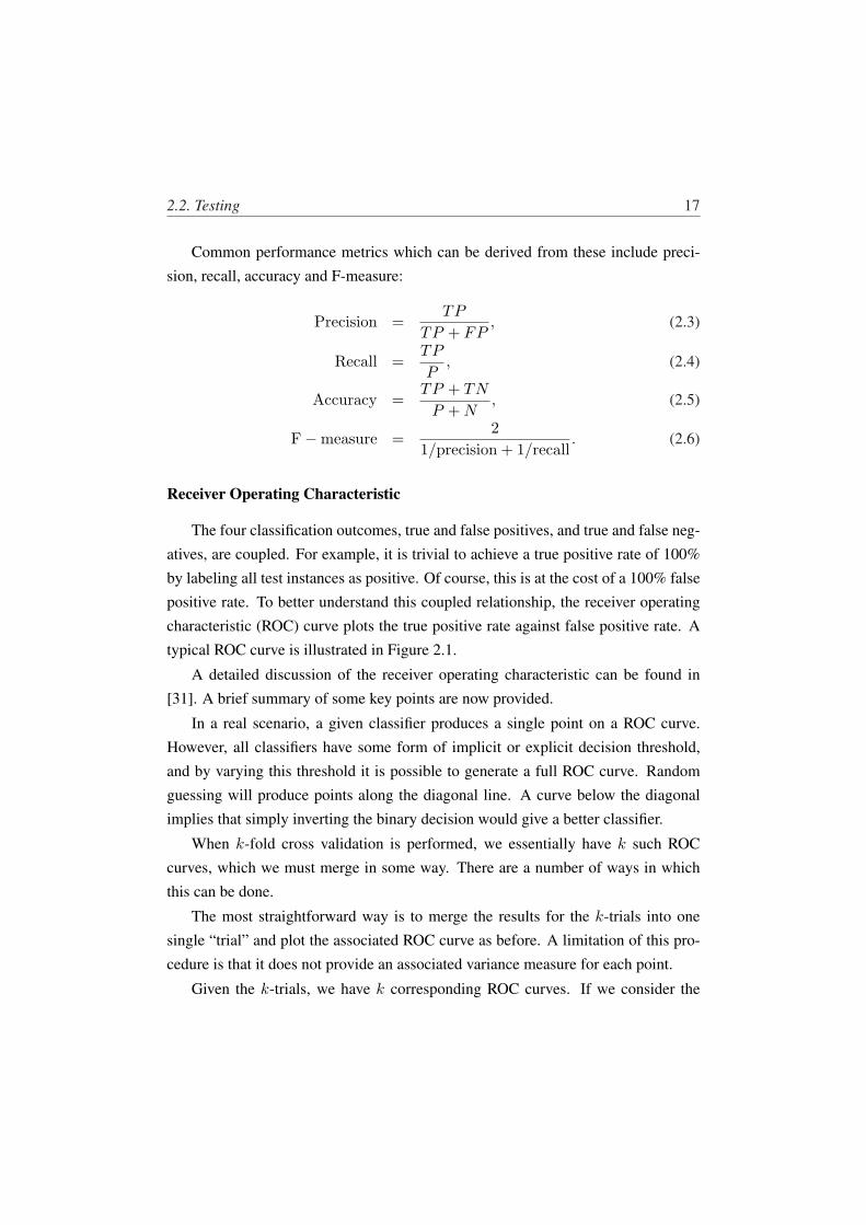
The four classification outcomes, true and false positives, and true and false neg-atives, are coupled. For example, it is trivial to achieve a true positive rate of 100%by labeling all test instances as positive. Of course, this is at the cost of a 100% falsepositive rate. To better understand this coupled relationship, the receiver operatingcharacteristic (ROC) curve plots the true positive rate against false positive rate. Atypical ROC curve is illustrated in Figure 2.1.
A detailed discussion of the receiver operating characteristic can be found in[31]. A brief summary of some key points are now provided.
In a real scenario, a given classifier produces a single point on a ROC curve.However, all classifiers have some form of implicit or explicit decision threshold,
and by varying this threshold it is possible to generate a full ROC curve. Randomguessing will produce points along the diagonal line. A curve below the diagonalimplies that simply inverting the binary decision would give a better classifier.
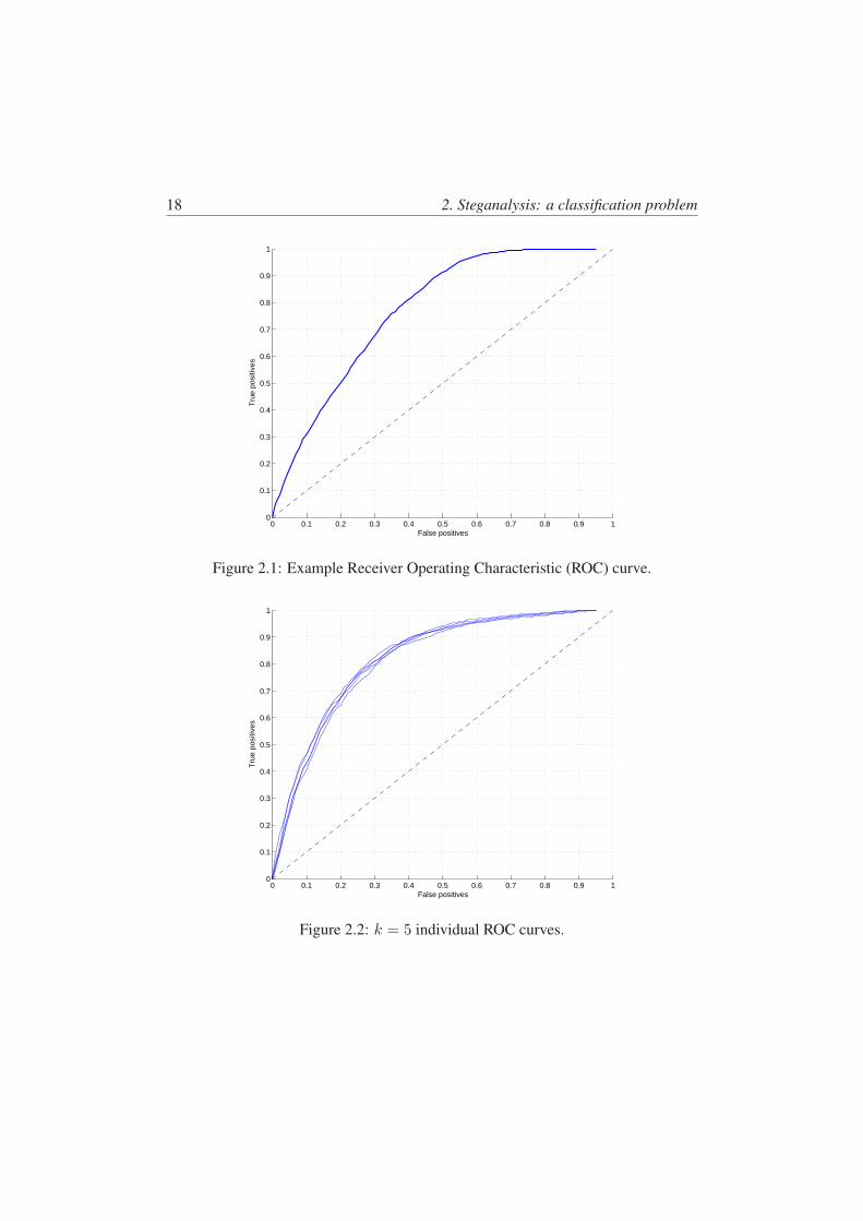
When k-fold cross validation is performed, we essentially have k such ROCcurves, which we must merge in some way. There are a number of ways in whichthis can be done.
The most straightforward way is to merge the results for the k-trials into onesingle “trial” and plot the associated ROC curve as before. A limitation of this pro-cedure is that it does not provide an associated variance measure for each point.
Given the k-trials, we have k corresponding ROC curves. If we consider the
18 2. Steganalysis: a classification problem
0 0.1 0.2 0.3 0.4 0.5 0.6 0.7 0.8 0.9 10
0.1
0.2
0.3
0.4
0.5
0.6
0.7
0.8
0.9
1
False positives
Tru
e po
sitiv
es
Figure 2.1: Example Receiver Operating Characteristic (ROC) curve.
0 0.1 0.2 0.3 0.4 0.5 0.6 0.7 0.8 0.9 10
0.1
0.2
0.3
0.4
0.5
0.6
0.7
0.8
0.9
1
False positives
Tru
e po
sitiv
es
Figure 2.2: k = 5 individual ROC curves.
2.2. Testing 19
0 0.1 0.2 0.3 0.4 0.5 0.6 0.7 0.8 0.9 10
0.1
0.2
0.3
0.4
0.5
0.6
0.7
0.8
0.9
1
False positives
Tru
e po
sitiv
es
Figure 2.3: Vertical averaging.
0 0.1 0.2 0.3 0.4 0.5 0.6 0.7 0.8 0.9 10
0.1
0.2
0.3
0.4
0.5
0.6
0.7
0.8
0.9
1
False positives
Tru
e po
sitiv
es
Figure 2.4: Threshold averaging.
20 2. Steganalysis: a classification problem
x-axis, i.e. the false positive rate, as an independent parameter that is under ourcontrol, then for a given fixed false positive rate, we can average the true positiverates, as depicted in Figure 2.3. The vertical lines at each point depict the uncertaintyassociated with the average. The length of the line can represent a percentile range,or the minimum and maximum values of the true positive rate for the given falsepositive rate. In this thesis, we show minimum and maximum values.
In practice, the false positive rate is not directly under our control, but ratheris a function of a threshold, t, that controls both the true and false positive rates.Thus, for a fixed threshold, t, we can determine both the true and false positive ratesfor each of the k ROC curves and average these together, as depicted in Figure 2.4.Now the uncertainty associated with each point is two-dimensional, reflecting thevariation in both the true and false positive rates for each of the k curves.
Area under the ROC curve
It is sometimes desirable to have a single scalar value to describe the perfor-mance of an algorithm. One method for doing so is to calculate the area under theROC curve, (AUC). The AUC has a value form 0 to 1, but since the diagonal line,reflecting random performance, has an area of 0.5, the AUC typically ranges from0.5 to 1. Fawcett [31] points out that (i) the AUC measures “the probability thatthe classifier will rank a randomly chosen positive instance higher than a randomly
chosen negative instance”, and (ii) it is closely related to the Gini coefficient [32].
2.3 Fisher Linear Discriminant Analysis
In this thesis we focus the attention on steganalyzer features, instead of takinginto account the classifier. For this reason we decided to use a linear classifier. Eventhough we can obtain better results with Support Vector Machines (SVM) or other
classifiers (which have a lot of settings), we prefer to give to the reader a fully repro-ducible approach.
Fisher Linear Discriminant (FLD) analysis seeks directions that are efficient fordiscrimination. The goal is to find an orientation u for which the samples in the
2.3. Fisher Linear Discriminant Analysis 21
dataset, once projected onto it, are well separated. Let us assume that a dataset D ismade of N d-dimensional samples x1, . . . ,xN , N1 being in a subsetD1 correspond-ing to one class and N2 being in a subset D2 corresponding to the other class. Thefirst step of FLD analysis consists in computing the d-dimensional sample mean ofeach class:
mi =1Ni
∑
x∈Di
x. (2.7)
Next, the scatter matrix SW = S1 + S2 is computed using the following definitions:
Si =∑
x∈Di
(x−mi)(x−mi)t. (2.8)
Finally, the direction of projection u is given by:
u = S−1W (m1 −m2). (2.9)
This vector u defines a linear function y = utx which yields the maximum ratioof between-class scatter to within-class scatter. The interested reader is redirectedto [27] for further details (pp. 117–121).

Chapter 3±1 embedding: state of art
In this chapter we describe the scenario this thesis is working on. Mainly weintroduce a common steganographic algorithm known as±1 embedding, also calledLSB matching, which is a common used technique to embed messages in the pixeldomain. Due to its simplicity, its efficiency, and its undetectability,±1 embedding isoften used as a benchmark for steganalysis and steganography. This simple evolution
from classical LSB is highly undetectable specially when the length of the embeddedmessage is smaller than the length of the embedding support.
We also introduce two state of art steganalyzers, by describing their feature ex-traction method. The first one is a blind method, while the second steganalyzer is asimple feature steganalyzer developed by analyzing artifacts specific to ±1 embed-ding.
3.1 ±1 embedding steganography
The simplest technique used in steganography is the Least Significative Bit (LSB)also called LSB replacement. To illustrate LSB replacement, let us consider grayscaleimages with pixels values in the range 0 . . . 255 as cover Works. LSB steganographyreplaces the least significant bit of each pixel value in the image with the correspond-ing bit of the message to be hidden. When LSB flipping is used, an even-valued pixelwill either retain its value or be incremented by one. However, it will never be decre-mented. The converse is true for odd-valued pixels. This asymmetry introducesa statistical anomaly into the intensity histogram – pairs of intensity values, specifi-cally 0-1, 2-3 etc., will, on average, exhibit the same frequency if the image is a stegoWork. This can be exploited for steganalysis purposes, as described in [33, 34, 35].

24 3. ±1 embedding: state of art
LSB matching, also known as ±1 embedding is a slightly more sophisticatedversion of least significant bit (LSB) embedding. Rather than simply replacing theLSB with the desired message bit, the corresponding pixel value is randomly in-cremented or decremented whenever the LSB value needs to be changed1. By sodoing, the asymmetry present in LSB flipping is almost eliminated2. Luckily forthe steganalyzer, other statistical anomalies are created that still permit discrimina-tion between cover and stego Works. However, these anomalies are more subtle and
discrimination accuracy is significantly lower than for LSB embedding.In formulas, ±1 embedding can be described as follows:
ps =
pc + 1, if b 6= LSB(pc) and(κ > 0 or pc = 0
)
pc − 1, if b 6= LSB(pc) and(κ < 0 or pc = 255
)
pc, if b = LSB(pc)
(3.1)
where κ is an i.i.d. random variable with uniform distribution in {−1, +1}, and pc
and ps are respectively the pixel value of the cover and the pixel value of the stegoimage. This process can be applied to all the pixels in the image or only for a pseudo-randomly chosen image portion, when the embedding rate, ρ, is less than one, i.e.the length of the hidden message is less than the number of pixels in the image.
3.2 ±1 embedding steganalyzers
The next sections describe a blind and a target steganalyzer which are the stateof art of steganalysis in the pixel domain.
3.2.1 High Order Statistics of the Stego Noise (WAM)
Since ±1 embedding is simply a matter of adding or subtracting 1 to a subsetof pixel values, it can be modeled as the addition of high frequency noise. In [10],
1Note that this strategy may affect bit-planes other than the LSB plane. For example, if the secretbit is a “0”, and the original 8-bit pixel value is 01111111, then incrementing this value results in10000000.
2The ±1 embedding has asymmetries only for 0 and 255 pixel values in which no random choicecan be applied due the lowerbound and upperbound borders.
3.2. ±1 embedding steganalyzers 25
Goljan et al. suggested estimating the stego noise and characterizing it with somecentral absolute moments. While their algorithm is a blind steganalysis algorithm,i.e. it is not designed to specifically detect ±1 embedding, it seems well suited to doso.
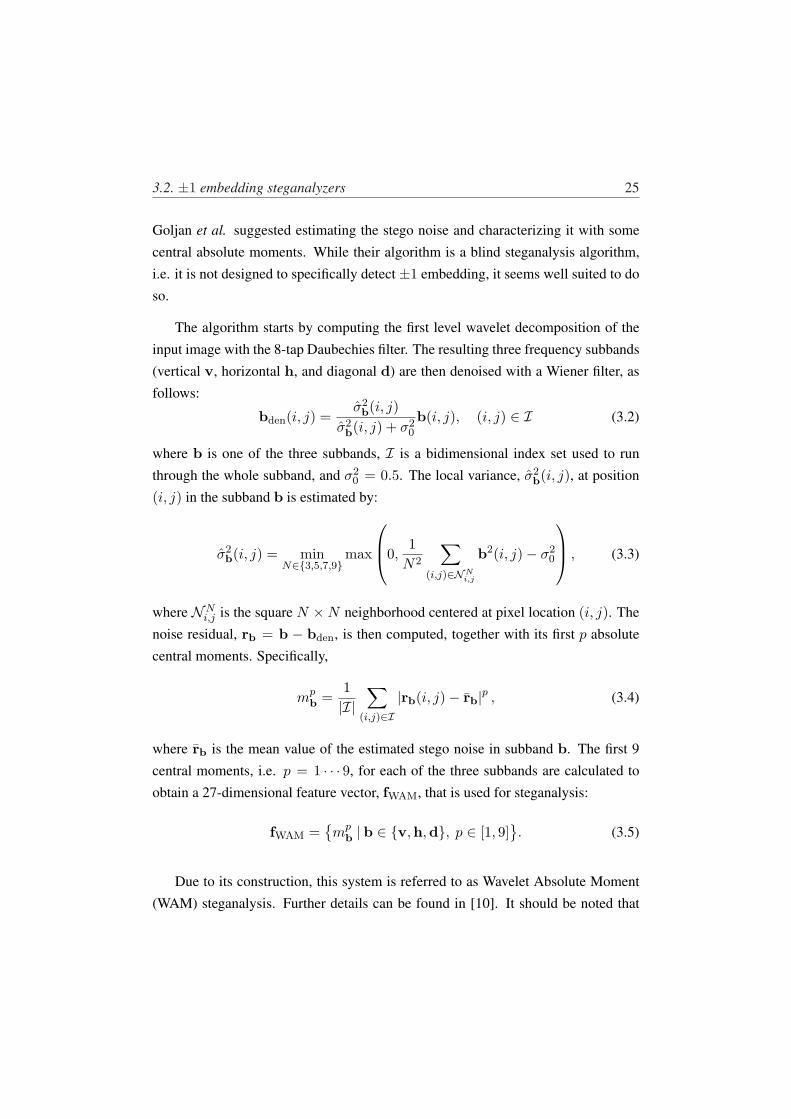
The algorithm starts by computing the first level wavelet decomposition of theinput image with the 8-tap Daubechies filter. The resulting three frequency subbands(vertical v, horizontal h, and diagonal d) are then denoised with a Wiener filter, asfollows:
bden(i, j) =σ2b(i, j)
σ2b(i, j) + σ2
0
b(i, j), (i, j) ∈ I (3.2)
where b is one of the three subbands, I is a bidimensional index set used to runthrough the whole subband, and σ2
0 = 0.5. The local variance, σ2b(i, j), at position
(i, j) in the subband b is estimated by:
σ2b(i, j) = min
N∈{3,5,7,9}max
0,
1N2
∑
(i,j)∈NNi,j
b2(i, j)− σ20
, (3.3)
where NNi,j is the square N ×N neighborhood centered at pixel location (i, j). The
noise residual, rb = b − bden, is then computed, together with its first p absolutecentral moments. Specifically,
mpb =
1|I|
∑
(i,j)∈I|rb(i, j)− rb|p , (3.4)
where rb is the mean value of the estimated stego noise in subband b. The first 9central moments, i.e. p = 1 · · · 9, for each of the three subbands are calculated toobtain a 27-dimensional feature vector, fWAM, that is used for steganalysis:
fWAM ={mp
b | b ∈ {v,h,d}, p ∈ [1, 9]}. (3.5)
Due to its construction, this system is referred to as Wavelet Absolute Moment(WAM) steganalysis. Further details can be found in [10]. It should be noted that
26 3. ±1 embedding: state of art
this method is not specific to ±1 steganography and can therefore be used to detectother steganographic techniques. Authors shows in [10] that by using a 0.5bpp ofpayload, WAM produces only 1.77% false positives at 50% of detection rate, and theAUC value is above 0.95.
Even though WAM algorithm provides a rather good classification accuracy, ithas main three weaknesses. The first one is that it looks for a fingerprint of thesteganography in the noisy region of the image. For a good detection, the ratio be-tween the steganography fingerprint and the image noise should be high. The secondone is that the feature vector has 27 elements, but for a given scenario (i.e. by ana-lyzing images that come from a specific source and by using the same steganography
with a fixed payload) only a subset of these are useful to detect stego image. More-over, by changing the scenario, it changes the feature subset too. This behavior is notgood when the steganalyzer works in a real scenario in which there is no knowledgeabout the images under analysis. The last one is the computational complexity forthe feature extraction, i.e. a wavelet full frame decomposition and the calculationof several high order statistics on an huge amount of wavelet coefficients. When asteganalysis system have to work with a big image database or an Internet imagestreaming, it is onerous to apply a real time analysis by using WAM.
3.2.2 Center of Mass of the Histogram Characteristic Function (2D-HCFC)
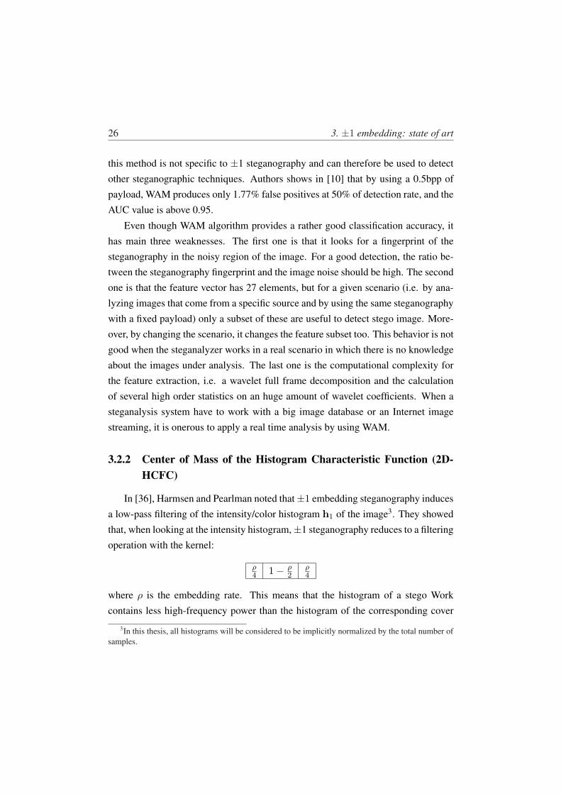
In [36], Harmsen and Pearlman noted that±1 embedding steganography inducesa low-pass filtering of the intensity/color histogram h1 of the image3. They showedthat, when looking at the intensity histogram,±1 steganography reduces to a filteringoperation with the kernel:
ρ4 1− ρ
2ρ4
where ρ is the embedding rate. This means that the histogram of a stego Workcontains less high-frequency power than the histogram of the corresponding cover
3In this thesis, all histograms will be considered to be implicitly normalized by the total number ofsamples.
3.2. ±1 embedding steganalyzers 27
image. In other words, the Fourier transform H1 of the intensity histogram, also re-ferred to as the Histogram Characteristic Function (HCF), is likely to be significantlyaffected by ±1 embedding steganography. In fact, its center of mass, defined as
c1(H1) =∑127
k=0 k‖H1(k)‖∑127k=0 ‖H1(k)‖ (3.6)
will be shifted toward the origin. In eq.(3.6) summations are from k = 0 to 127to avoid the symmetric parts of the Fourier transform. This approach can be ex-tended to multidimensional signals, e.g. RGB images, by using a multidimensionalFourier transform and computing a multidimensional center of mass. Experimentalresults [23] have shown that the HCF strategy performs better with RGB images thanwith grayscale images.
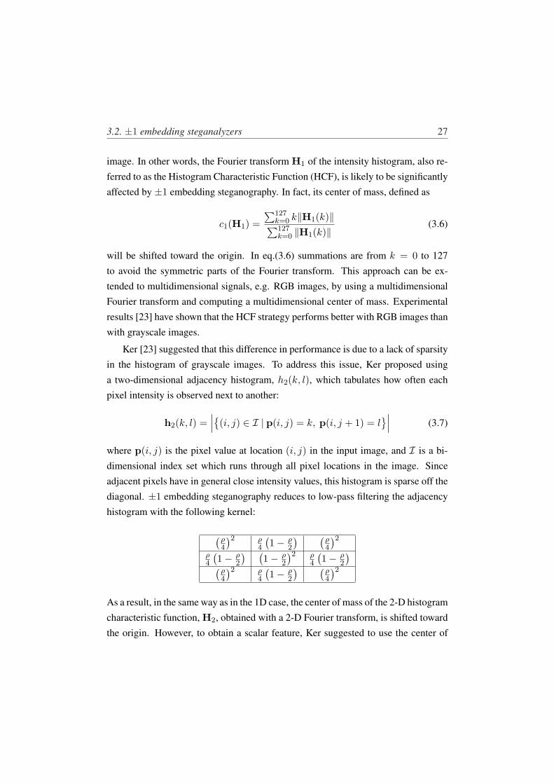
Ker [23] suggested that this difference in performance is due to a lack of sparsityin the histogram of grayscale images. To address this issue, Ker proposed usinga two-dimensional adjacency histogram, h2(k, l), which tabulates how often eachpixel intensity is observed next to another:
h2(k, l) =∣∣∣{(i, j) ∈ I | p(i, j) = k, p(i, j + 1) = l
}∣∣∣ (3.7)
where p(i, j) is the pixel value at location (i, j) in the input image, and I is a bi-dimensional index set which runs through all pixel locations in the image. Sinceadjacent pixels have in general close intensity values, this histogram is sparse off thediagonal. ±1 embedding steganography reduces to low-pass filtering the adjacencyhistogram with the following kernel:
(ρ4
)2 ρ4
(1− ρ
2
) (ρ4
)2
ρ4
(1− ρ
2
) (1− ρ
2
)2 ρ4
(1− ρ
2
)(ρ
4
)2 ρ4
(1− ρ
2
) (ρ4
)2
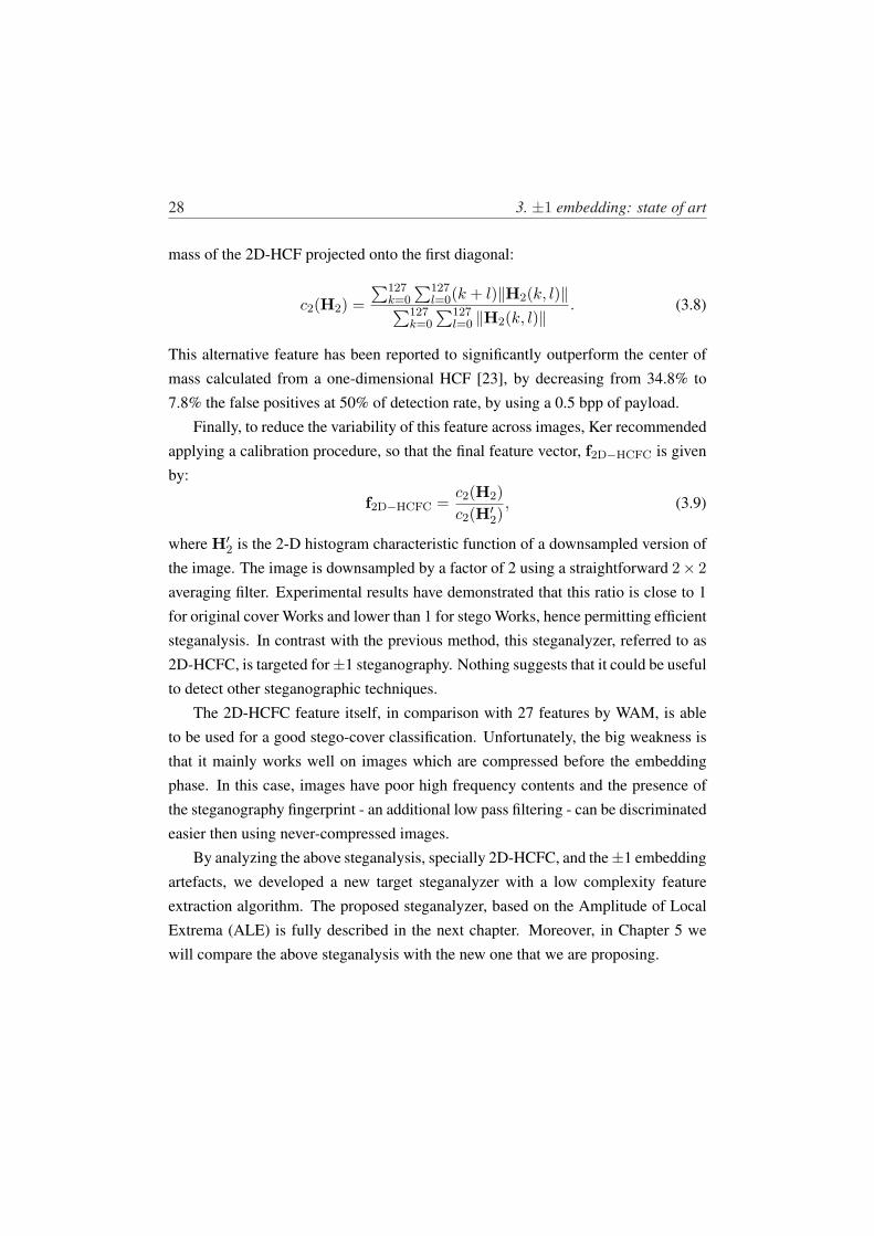
As a result, in the same way as in the 1D case, the center of mass of the 2-D histogramcharacteristic function, H2, obtained with a 2-D Fourier transform, is shifted towardthe origin. However, to obtain a scalar feature, Ker suggested to use the center of
28 3. ±1 embedding: state of art
mass of the 2D-HCF projected onto the first diagonal:
c2(H2) =∑127
k=0
∑127l=0(k + l)‖H2(k, l)‖∑127
k=0
∑127l=0 ‖H2(k, l)‖ . (3.8)
This alternative feature has been reported to significantly outperform the center ofmass calculated from a one-dimensional HCF [23], by decreasing from 34.8% to7.8% the false positives at 50% of detection rate, by using a 0.5 bpp of payload.
Finally, to reduce the variability of this feature across images, Ker recommendedapplying a calibration procedure, so that the final feature vector, f2D−HCFC is givenby:
f2D−HCFC =c2(H2)c2(H′
2), (3.9)
where H′2 is the 2-D histogram characteristic function of a downsampled version of
the image. The image is downsampled by a factor of 2 using a straightforward 2× 2averaging filter. Experimental results have demonstrated that this ratio is close to 1for original cover Works and lower than 1 for stego Works, hence permitting efficientsteganalysis. In contrast with the previous method, this steganalyzer, referred to as2D-HCFC, is targeted for±1 steganography. Nothing suggests that it could be usefulto detect other steganographic techniques.
The 2D-HCFC feature itself, in comparison with 27 features by WAM, is ableto be used for a good stego-cover classification. Unfortunately, the big weakness isthat it mainly works well on images which are compressed before the embeddingphase. In this case, images have poor high frequency contents and the presence ofthe steganography fingerprint - an additional low pass filtering - can be discriminatedeasier then using never-compressed images.
By analyzing the above steganalysis, specially 2D-HCFC, and the±1 embeddingartefacts, we developed a new target steganalyzer with a low complexity featureextraction algorithm. The proposed steganalyzer, based on the Amplitude of Local
Extrema (ALE) is fully described in the next chapter. Moreover, in Chapter 5 wewill compare the above steganalysis with the new one that we are proposing.
Chapter 4Amplitude of Local Extrema
In this chapter, we describe a new steganalysis algorithm that significantly im-proves upon previous results. It is based on work by Zhang et al. and it works onthe statistical properties of the amplitudes of local extrema (ALE). The extensionto the algorithm presented in [26] is described in Section 4.1. Specifically, we firstdescribe a modification to the algorithm that reduces noise associated with border ef-fects, i.e. pixel values with intensities of either 0 or 255. Section 4.2 then describesthe extension of the amplitudes of local extrema to 2D adjacency histograms. Theseenhancements result in a collection of 10 features whose classification performances
are evaluated in Section 4.3 through experimental validation. The results clearlydemonstrate significantly improved classification compared to the original stegana-lyzer by Zhang et al. [26]. Moreover in Section 4.4 we design a Hybrid steganalyzerthat takes into account state-of-art and ALE steganalyzers. At the end of the chapter,in Section 4.5, some consideration are drawn.
4.1 Improving previous work on histogram domain
In [36], the authors noted that ±1 embedding steganography induces a low-passfiltering of the intensity/colour histogram h1 of the image. Indeed, it is easy to showthat, when looking at the intensity histogram, ±1 steganography is equivalent to afiltering operation with the kernel:
ρ4 1− ρ
2ρ4
where ρ is the embedding rate. This implies that the histogram of a stego Workcontains less high-frequency power than the histogram of the corresponding coverimage.
30 4. Amplitude of Local Extrema
Based on this idea, Zhang et al. [26] proposed to observe what happens in thesurrounding of local extrema of the histogram [26]. Since ±1 embedding is equiv-alent to low pass filtering the intensity histogram, then the filtering operation willreduce the amplitude of local extrema (ALE). This motivated the introduction of anew feature, which is basically the sum of the amplitudes of local extrema in theintensity histogram, as defined below:
A1(h1) =∑
n∈E1
∣∣2h1(k)− h1(k − 1)− h1(k + 1)∣∣ (4.1)
where E1 ⊂ [1, 254] is the set of local extrema in the histogram given by:
k ∈ E1 ⇔(h1(k)− h1(k − 1)
)(h1(k)− h1(k + 1)
)> 0. (4.2)
Experimental results reported in [26] confirmed that the feature A1 is statisticallylarger for original cover Works than for stego Works. Moreover, using this feature inconjunction with a classifier based on Fisher linear discriminant (FLD) [27] analysis,resulted in much better classification results compared with other state-of-the-artsteganalyzers, such as WAM [10] or HCF-COM [36, 23].
4.1.1 Removing Interferences at the Histogram Borders
Embedding based on Equation (3.1) introduces a minor asymmetry: 0-valuedpixels will always be changed to 1 if their LSB needs to be modified. Similarly,255-valued pixels will always be changed to 254. This asymmetry in the histogramcan cause interferences with the extracted feature in eq. (4.1). To avoid this problem,Equation (4.1) is modified, as follows:
A1(h1) =∑
n∈E ′1
∣∣2h1(k)− h1(k − 1)− h1(k + 1)∣∣ (4.3)
where the set of local extrema E ′1 is now reduced to be within [3, 252]. In otherwords, the positions {1, 2, 253, 254} are not considered as potential local extrema.Nevertheless, to account the bound values of the histogram, the following additional
4.2. Considering 2D Adjacency Histograms 31
feature is defined:
d1(h1) =∑
k∈E∗1
∣∣2h1(k)− h1(k − 1)− h1(k + 1)∣∣ (4.4)
where E∗1 ⊂ {1, 2, 253, 254} is a set of local extrema as defined by Equation (4.2).
4.2 Considering 2D Adjacency Histograms
Inspired by [23], the analysis of local extrema has been extended to 2D adjacencyhistograms [37], h2(k, l), which tabulates how often each pixel intensity is observednext to another in the horizontal direction h2(k, l), as defined in Equation (3.7).Since adjacent pixels have, in general, close intensity values, this histogram is sparseoff the diagonal. It should be noted that the histogram defined by Equation (3.7)can be slightly modified to obtain 3 other adjacency histograms for other directions(vertical, main diagonal, and minor diagonal). For clarity we will use the apex h,v, D, d, respectively for horizontal, vertical, main diagonal, minor diagonal, to theadjacency function h2(k, l) in order to specify, if necessary, the kind of adjacency,otherwise h2(k, l) is referred to a generic kind of adjacency matrix. In particular, we
define again the four kinds of adjacency matrix:
hh2(k, l) =
∣∣∣{(i, j) ∈ I | p(i, j) = k, p(i, j + 1) = l
}∣∣∣ (4.5)
hv2(k, l) =
∣∣∣{(i, j) ∈ I | p(i, j) = k, p(i + 1, j) = l
}∣∣∣ (4.6)
hD2 (k, l) =
∣∣∣{(i, j) ∈ I | p(i, j) = k, p(i + 1, j + 1) = l
}∣∣∣ (4.7)
hd2(k, l) =
∣∣∣{(i, j) ∈ I | p(i, j) = k, p(i + 1, j − 1) = l
}∣∣∣ (4.8)
where p(i, j) is the pixel value at location (i, j) in the input image, and I is a bi-dimensional index set which runs through all pixel locations in the image.
Moreover, we can extend previous considerations about the ±1 embedding arte-facts on the histogram domain by using the adjacency matrix. In this case, by using

32 4. Amplitude of Local Extrema
±1 embedding with payload ρ, we obtain a 2-D low pass filtering with the followingkernel:
(ρ4
)2 ρ4
(1− ρ
2
) (ρ4
)2
ρ4
(1− ρ
2
) (1− ρ
2
)2 ρ4
(1− ρ
2
)(ρ
4
)2 ρ4
(1− ρ
2
) (ρ4
)2
Consequently, it should also be possible to distinguish between cover and stegoWorks by examining local amplitude extrema in the 2D adjacency histogram. Theset of local extrema in an adjacency histogram E2 ⊂ [0, 255]2 is defined as:
p = (k, l) ∈ E2 ⇔{∃ε ∈ {−1, 1}, ∀n ∈ N+
sign(h2(p)− h2(p + n)
)= ε
(4.9)
whereN+ = {(−1, 0), (1, 0), (0,−1), (0, 1)} is used to define a cross-shaped neigh-borhood and h2(·) is the generical adjacency matrix. However, many of these ex-trema have a small amplitude and are thus highly sensitive to changes of the coverWork. To achieve higher stability, this set is further reduced to:
p = (k, l) ∈ E ′2 ⇔ (k, l) ∈ E2 and (l, k) ∈ E2 (4.10)
In other words, only pairs of extrema symmetrical with respect to the main diagonalare retained. Empirical observations have revealed that such extrema have signifi-cantly higher amplitude and are thus more stable. The resulting generical feature isdefined by,
A2(h2) =∑
p∈E ′2
∣∣∣4h2(p)−∑
n∈N+
h2(p + n)∣∣∣ (4.11)
which is the sum of the amplitude of extrema located at positions in E ′2.
In addition to eq. 4.11 feature, empirical experiments have demonstrated thatthe sum of all the elements on the diagonal of a 2D adjacency histogram, defined asfollows:
d2(h2) =255∑
k=0
h2(k, k) (4.12)

4.3. Performances of ALE 33
1 A1(h1)2 d1(h1)3 A2(hh
2) (horizontal direction)4 A2(hv
2) (vertical direction)5 A2(hD
2 ) (main diagonal direction)6 A2(hd
2) (minor diagonal direction)7 d2(hh
2) (horizontal direction)8 d2(hv
2) (vertical direction)9 d2(hD
2 ) (main diagonal direction)10 d2(hd
2) (minor diagonal direction)
Table 4.1: Table of ALE features
could also be exploited to improve classification results. Indeed, ±1 steganographydecreases the value of this feature and its variations can be used in the decisionprocess.
Altogether, the above observations result in a collection of 10 features featureswhich are listed in Table 4.1.
4.3 Performances of ALE
In this Section we describe a number of experiments that we carried out to inves-tigate the impact of the various features on classification performance.
4.3.1 Setup
The experiments were run on a database composed of images originating fromthree different sources. Specifically:
• 2,375 images from the NRCS Photo Gallery [38].The photos are of naturalscenery, e.g. landscape, cornfields, etc. There is no indication of how thesephotos were acquired. This database has been previously used in [23].
• 2,375 images captured using 24 different digital cameras (Canon, Kodak, Nikon,Olympus and Sony) previously used in [10]. They include photographs of nat-
34 4. Amplitude of Local Extrema
ural landscapes, buildings and object details. All images have been stored in araw format i.e. the images have never undergone lossy compression.
• 2,375 images from the Corel database [39]. They include images of naturallandscapes, people, animals, instruments, buildings, artwork, etc. Althoughthere is no indication of how these images have been acquired, they are verylikely to have been scanned from a variety of photos and slides. This databasehas been previously used in [26].
The above image sets result in a composite database of 7125 images. Where nec-
essary, all images have been converted to grayscale. Moreover, a central croppingoperation of size 512×512 was applied to all images to obtain images of the same di-mension across all three source databases. Cropping was preferred over resamplingwith interpolation, in order to avoid any interference with the source signal.
The motivation for using more than one source database is to account for thevariability in steganalyzers’ performances across different databases [40, 41]. In thenext chapter we fully investigate this variability across image sources. It is hoped thatthis set of databases will become a reference for subsequent works in steganalysisresearch.
Given the composite database, the stego images are built by using±1 embeddingat 0.5 bpp of payload, thus obtaining the stego database. Then, for every image ALEfeatures are extracted and we randomly separated the cover-features database DALE
and stego features database D∗ALE into a training set (20% of the database size),and a test set (the remaining 80% of the database) and we built a ROC curve byusing Fisher Discriminant classifier on a training set and by projecting all the testfeature vectors onto the trained projection vector u. To apply a cross validationon the obtained results, we repeat 20 times the above procedure with a different
randomization of the train and test datasets. At the end we joined the 20 ROCs bythe vertical averaging scheme described in Chapter 2 .
The overall performance of the steganalyzer is then measured by computing thearea under the ROC curve (AUC).
4.3. Performances of ALE 35
0 0.1 0.2 0.3 0.4 0.5 0.6 0.7 0.8 0.9 10
0.1
0.2
0.3
0.4
0.5
0.6
0.7
0.8
0.9
1
False positives
Tru
e po
sitiv
es
Zhang 0.57ALE 1 0.58ALE 1−2 0.59
Figure 4.1: Analysis of the impact of the border effect described in Subsection 4.1.1on classification results.
4.3.2 Results
Since similar results were observed for various embedding rates, we only reportclassification results for ρ = 0.5.
Figure 4.1 shows the improvements in classification resulting from eliminationof border effects. The original algorithm of Zhang et al. is compared with a systembased on feature 1 of Table 4.1 (ALE 1), and features 1 and 2 (ALE 1-2). The errorbars on each plot indicate the minimum and maximum values observed during the20 cross-validation runs. First of all, we note the unexpectedly poor performances ofall three algorithms, i.e. the ROC curves are very close to the diagonal. This is due
to the wide variety of images present in of composite database.
Despite the poor performance of all three algorithms, the two algorithms basedon new ALE features (ALE 1 and ALE 1-2) exhibit a slight improvement in clas-sification performances. The system using the first two ALE features (ALE 1-2)achieves the highest performances based on area under the ROC curve (AUC), witha score of 0.59, and is therefore used as a reference in the next experiment.
36 4. Amplitude of Local Extrema
0 0.1 0.2 0.3 0.4 0.5 0.6 0.7 0.8 0.9 10
0.1
0.2
0.3
0.4
0.5
0.6
0.7
0.8
0.9
1
False positives
Tru
e po
sitiv
es
ALE 1−2 0.59ALE 3−6 0.65ALE 7−10 0.59ALE 3−10 0.72ALE 1−10 0.77
Figure 4.2: Analysis of the impact of ALE features selection on classification results.
Figure 4.2 reports the classification performances achieved when using ALE fea-tures computed from the 2D adjacency histogram. Four sets of ALE features areinvestigated:
• ALE 3-6 i.e. the amplitude of the local extrema in the adjacency histograms,
• ALE 7-10 i.e. the amplitude of the diagonal in the adjacency histograms,
• ALE 3-10 i.e. all features from the adjacency histograms,
• ALE 1-10 i.e. all features from the intensity histogram and the adjacencyhistograms.
All 4 systems perform at least as well as the reference classification system consid-ered above (ALE 1-2). ALE 3-6 features perform significantly better than ALE 7-10features. Nevertheless, when these two sets of features are combined (ALE 3-10),the resulting steganalyzer outperforms the systems that rely on a single set of featurescomputed from adjacency histograms. However, the best classification performance
4.4. Hybrid Algorithm 37
is achieved when all ALE features are combined (ALE 1-10). Compared to the orig-inal steganalyzer [26], the area under the ROC curve (AUC) value increases from0.57 to 0.77, which is a significant improvement.
4.4 Hybrid Algorithm
Experimental issues in steganalysis usually reveal that when the experimentalsetup is not ideally built in the lab, i.e. no information about payload, image sourcesand image preprocessing are known, no algorithm has a superior performance overall scenarios. Consequently, we also implemented a hybrid steganalysis system thatcombines the features from all three previously described algorithms.
Let us assume that there are S different steganalyzers {S1, . . . , SS} available toperform ±1 embedding steganalysis. Each steganalyzer Si relies on some featurevector fi, which may have different dimensionality depending on the consider ste-ganalyzer. A commonly used strategy to combine this collection of systems consistsin merging all information available, e.g. by concatenating all feature vectors in asingle meta feature vector f as follows:
f = f1|f2| . . . |fS (4.13)
where | denotes the concatenation operation.
Then applying a classifier on this meta feature vector is expected to increaseclassification performances. For instance, combining WAM (Chapter 3.2.1), 2D-HCFC (Chapter 3.2.2) and the above ALE results in a 38-dimensional feature vectorf .
4.5 Discussion
Now it could be interesting to evaluate the performance of ALE in a wider sce-nario. Unfortunately in steganalysis no evaluation benchmark has ever been designedto this aim as, for example, Stirmark benchmark [42] makes for watermarking appli-
38 4. Amplitude of Local Extrema
cations. However, every proposed steganalyzer1 should be fully evaluated especiallyon a real case scenario, by using comparisons with the current state-of-art stegan-alyzers and the advanced steganography. Unfortunately common comparisons aremade between old techniques or specific lab tests in which the image database andthe a priori steganalyzer knowledge as used payload or used dataset is really far awayfrom the practical case in which nothing is known. Usually, it could be that a stegan-alyzer seems to be the best because it obtains good accuracy classification scores in
the proposed experimental settings, but at the same time it could be the worst if weuse different comparison settings. These considerations are obviously true even forour steganalyzer.
Even though ALE seems to behave very well, an appropriate comparison pro-cedure should be designed to compare ALE behavior against state-of-art classifiers.Specifically, we should investigate how ALE performance vary by changing the ex-perimental conditions by changing both the image database and the payload. Dueto the importance of experimental settings and comparison with other steganalyzerslike WAM and 2D-HCFC, we will investigate the ALE performance and comparisonin the next chapter.
The performance variation across databases, or more in general, a full analysisabout ALE and its comparison with the state-of-art steganalysis is shown in Chapter5. Moreover, the next Chapter describes a new methodology approach for steganal-ysis comparisons which should be take into account in further steganalysis works.
1Similar considerations should be done for steganographic methods.
Chapter 5Experimental comparison among ±1 embedding
steganalysis
In this chapter we fully investigate ALE performances in comparison with WAMand 2D-HCFC (see Chapter 3). To do so, we define a new benchmark methodology
which takes into account the widest possible experimental setting. In this way theobtained results should be as close as possible to a real work steganalysis scenario.
Detection of ±1 embedding is known to be much more difficult than detectingLSB replacement. Nevertheless, a number of algorithms have been developed forthis purpose. Unfortunately, in literature experimental issues did not receive enough
attention and often authors do not consider the real constraints set by scenarios thatare completely different from those applying to steganalysis or steganography work-ing on a predefined image set or with a predefined payload. An additional problem isthat sometimes such a highly controlled scenario may not be reproducible speciallywhen the image database is not shared or it is not carefully described. In these biasedsituations results are not significant and no comparison between techniques can bemade.
In this chapter we would like to propose a comparative steganalysis methodologyby showing how results change when the experimental setup changes. To do so weuse a FLD classifier and we test ALE, WAM, 2D-HCFC and Hybrid steganalyzers.
5.1 Databases
In our study we used three different databases that have been previously usedin the context of steganography and watermarking. The three databases not onlycontain different images, but, more importantly, the image sources are significantly
40 5. Experimental comparison among ±1 embedding steganalysis
different, as discussed shortly. The motivation for using more than one database wasto determine any variability in performance across databases. A fourth database wascreated as the concatenation of these three primary databases. It is hoped that this setof databases will become a reference for subsequent works in steganalysis research1.
The four image databases are:
1. NRCS Photo Gallery: This image database is provided by the United StatesDepartment of Agriculture [38]. It contains 2,375 photos related to naturalresources and conservation from across the USA, e.g. landscape, cornfields,etc. Typically, the image formats are in 32-bit CMYK space color and in highresolution, i.e. 1500×2100. Unfortunately, there is no indication of how thesephotos were acquired. This image database has first been used in [23].
2. Camera Images: This image database is a collection of 3,164 images cap-tured using 24 different digital cameras (Canon, Kodak, Nikon, Olympus andSony). It includes photographs of natural landscapes, buildings and object de-tails. All images have been stored in a raw format i.e. the images have not
undergone lossy compression. A subset of these images was previously usedin [10].
3. Corel database: The Corel image database consists of a large collection ofuncompressed images [39]. They include natural landscape, people, animals,instruments, buildings, artwork, etc. Although there is no indication of howthese images have been acquired, they are very likely to have been scannedfrom a variety of photos and slides. Moreover, a close inspection of thegrayscale histogram of several pictures tend to suggest that the images havebeen submitted to some kind of histogram equalization technique. This pro-cess introduced significant artifacts in the histogram which, as a by-product,significantly boost the performances of the ALE steganalyzer as will be de-
tailed late. A subset of 8,185 images has been extracted from the databasewith dimension 512× 768.
1To encourage the use of this database, it is accessible on the website [43].

5.2. Experimental Procedure 41
4. Combined database: A fourth database was created by concatenating 2,375randomly selected images from each of the three databases.
Where necessary, all images have been converted to 8-bit depth grayscale. More-over, a central cropping operation of size 512 × 512 was applied to all images toobtain images of the same dimension across all three databases. Cropping was pre-ferred over resampling with interpolation, in order to avoid introducing artifacts dueto signal processing.
5.2 Experimental Procedure
For each one of the four databases (NRCS, Camera, Corel, Combined), the fol-lowing procedure was performed for every steganalyzer under study (WAM, 2D-HCFC, ALE, Hybrid):
1. Apply LSB embedding with embedding rate ρ to all images in the database Dto obtain the database of stego images D∗;
2. Separate both databases into a training set, {D(U),D∗(U)}, and a test set,{D(Uc),D∗(Uc)}, where U is a subset of the image indexes and Uc is its com-plement. The size of the training set was set to be equal to 20% of the databasesize;
3. For the steganalyzer under test, compute the associated feature vector for allimages in the training set and perform FLD analysis to obtain the trained pro-jection vector u;
4. For the steganalyzer under test, compute the associated feature vector for allimages in the test set, and project the feature vector onto u;
5. Compare the resulting scalar values to a threshold τ and record the probabil-ities of false positives and true positives for different values of the thresholdin order to obtain the Receiver Operating Characteristic (ROC) curve of thesystem.
42 5. Experimental comparison among ±1 embedding steganalysis
Steps 2 to 5 were repeated 20 times for cross-validation [27] and the ROC curvesvertically averaged. That is, for a fixed false positive value, the corresponding truepositive rates for each curve were averaged. The confidence level at each false posi-tive point depicted in the resulting curves indicates the minimum and maximum truepositive rates form the set of ROC curves.
Thresholding averaging of the ROC curves is also possible, as previously dis-cussed. For example, for the ALE algorithm and a given threshold, we obtain k = 20points corresponding to the true and false positive rates for the k-trials, and thesepoints lie in reasonably close proximity to one another. However, for the WAM al-gorithm, and consequently the hybrid algorithm as well, these k = 20 points are
dispersed across the ROC curve, i.e. the variances are very large.
Although we have not considered them in our study, alternative performancesmetrics have been suggested in the literature e.g. the detection reliability which issimply derived from the AUC [44], the false positive rate at 50% (80%) detection
rate [10], and others.
5.3 Experimental Results
In an attempt to obtain a better understanding of the different steganalyzers understudy, we first examine the impact of the source of imagery used during training andtesting, and in particular the consequences of using mismatching imagery. Next, weinvestigate the influence of the embedding rate depending on the testing conditions.Based on this analysis, we then further detail the performances of the individualsteganalyzers depending on whether or not some prior about the source of imagery isavailable before the steganalyzer is run. Such a priori information could for instancebe obtained thanks to forensic tools.
5.3.1 Impact of the source of imagery
In the first batch of experiments, the embedding rate is fixed and set equal toρ=0.5 bit per pixel (bpp), both during training and testing. Similar behavior wasobserved for other embedding rates but data is omitted for brevity and clarity. Each
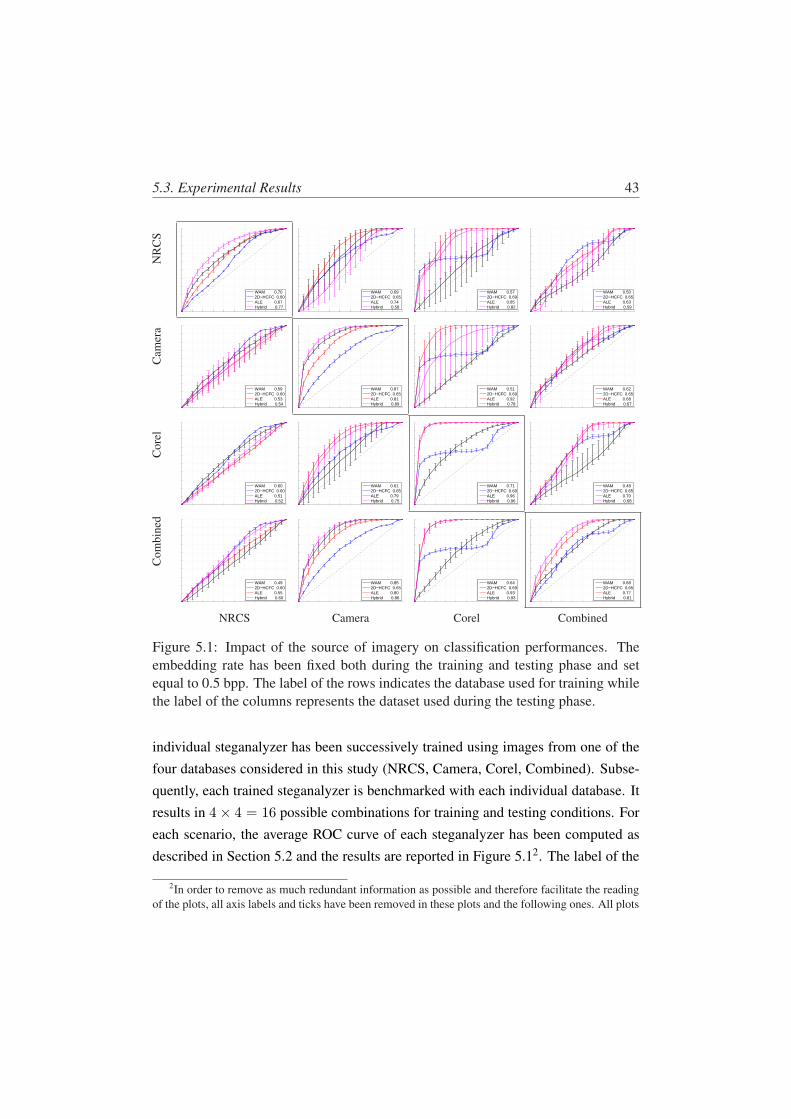
5.3. Experimental Results 43
NR
CS
WAM 0.702D−HCFC 0.60ALE 0.67Hybrid 0.77
WAM 0.692D−HCFC 0.65ALE 0.74Hybrid 0.58
WAM 0.572D−HCFC 0.69ALE 0.85Hybrid 0.82
WAM 0.502D−HCFC 0.65ALE 0.63Hybrid 0.59
Cam
era
WAM 0.592D−HCFC 0.60ALE 0.53Hybrid 0.54
WAM 0.872D−HCFC 0.65ALE 0.81Hybrid 0.89
WAM 0.512D−HCFC 0.69ALE 0.92Hybrid 0.78
WAM 0.622D−HCFC 0.65ALE 0.68Hybrid 0.67
Cor
el
WAM 0.602D−HCFC 0.60ALE 0.51Hybrid 0.52
WAM 0.612D−HCFC 0.65ALE 0.79Hybrid 0.75
WAM 0.712D−HCFC 0.69ALE 0.96Hybrid 0.96
WAM 0.482D−HCFC 0.65ALE 0.70Hybrid 0.68
Com
bine
d
WAM 0.492D−HCFC 0.60ALE 0.55Hybrid 0.60
WAM 0.852D−HCFC 0.65ALE 0.80Hybrid 0.86
WAM 0.642D−HCFC 0.69ALE 0.93Hybrid 0.93
WAM 0.682D−HCFC 0.65ALE 0.77Hybrid 0.81
NRCS Camera Corel Combined
Figure 5.1: Impact of the source of imagery on classification performances. Theembedding rate has been fixed both during the training and testing phase and setequal to 0.5 bpp. The label of the rows indicates the database used for training whilethe label of the columns represents the dataset used during the testing phase.
individual steganalyzer has been successively trained using images from one of thefour databases considered in this study (NRCS, Camera, Corel, Combined). Subse-quently, each trained steganalyzer is benchmarked with each individual database. Itresults in 4× 4 = 16 possible combinations for training and testing conditions. Foreach scenario, the average ROC curve of each steganalyzer has been computed asdescribed in Section 5.2 and the results are reported in Figure 5.12. The label of the
2In order to remove as much redundant information as possible and therefore facilitate the readingof the plots, all axis labels and ticks have been removed in these plots and the following ones. All plots
44 5. Experimental comparison among ±1 embedding steganalysis
rows indicates the database used for training and the label of the columns the oneused for testing. As a result, plots on the diagonal have matching training and testingconditions. They have been framed to clearly highlight them.
Let us first focus on the 3 × 3 block of figures in the top left corner. Accordingto expectation, the best performances are achieved when the training and testingconditions match (plots on the diagonal). However, even in these conditions, it isclear that the absolute performance of the four algorithms varies considerably acrossthe three primary image databases. Additionally, the relative performance is alsoseen to vary. For the NRCS and Camera testsets, the WAM algorithm exhibits bestperformance. However, even across these two testsets, the absolute performancevaries significantly. For example, we observe that for a false positive rate of 10%,the WAM algorithm has a true positive rate of 30% and 60% for NRCS and Camerarespectively. There are similar variations for the other two algorithms. For the Corel
testset, the ALE algorithm performs much better. Also, interestingly, we observea very strange behavior from the 2D-HCFC algorithm, where the true positive rateremains almost constant as the false positive rate increases from 20% to 70%. Asmight be expected, the hybrid algorithm exhibits the best performance for each ofthe three individual databases.
As soon as we deviate from the diagonal, i.e. when training and testing con-
ditions no longer match, we observe drastic performance degradation for all fouralgorithms and significant increase in variability. This indicates that each individ-ual database is specific and is not representative of the other two databases. As aresult, it illustrates the importance of training with a dataset that is representativeof the classes of images that will be observed in real life. If this is not done, thenthe performance of algorithms is likely to be worse than expected. For instance, ifthe Hybrid algorithm is trained with NRCS images whereas it will only encounterCamera images, then its performances is significantly reduced compared to if it hasbeen trained with Camera images, with an AUC score reducing from 0.89 to 0.58.As a matter of fact, it no longer the best performing algorithm, but is in fact the
share the same axis, i.e. false positive vs. true positive with all axis running from 0 to 1 with a linearscale.
5.3. Experimental Results 45
worse performer. This may sound rather counter-intuitive at first. Indeed, one wouldexpect that the hybrid system performs at least as well as the others e.g. by takingthe projection vector used for the best performing steganalyzer and padding it withzeros. And this is true! However, the projection vector used for classification is givenby the FLD analysis described in Chapter 2.3. During this process, two parametersare optimized at the same time: the within-class scatter (SW ) and the between-classscatter (SB). In other words, the optimization process for the within-class scatter
may come into the way of maximizing the separability between the two classes,hence resulting in degraded classification performances. This is clearly a limitationof FLD analysis which has motivated the use of Support Vector Machines (SVM) inrecent steganalysis systems.
Additionally, the increased variability of the ROC curve observed during cross-validation clearly indicates that there is no guaranteed performances with such mis-matching training strategies. As a result, a straightforward rule of thumb is ‘if youknow the source of imagery (whatever this means) that you will encounter in yourapplication, you should train with it’.
Now, let us assume that the steganalyzers have been trained with a single sourceof imagery but that they actually have to deal with a variety of images in practice (3
first rows of the last column). Since there is still a significant mismatch between thetraining and testing conditions, we observe a significant reduction of performancesand a huge increase of variability. As a result, this calls for training the classifierswith a variety of images (last row). Such strategy usually slightly hampers perfor-mances when testing on individual databases compared to the classification resultsachieved with matching training and testing conditions. This seems to be particu-larly true for the NRCS database where, for instance, the WAM steganalyzer sees itsAUC value drop from 70% to 49%, i.e. nearly random guessing. Still, the variabilityof the ROC curves during cross-validation is now significantly reduced compared tothe situation where the training and testing databases do not match. This low vari-ability is crucial in order to be able to guarantee performances. Moreover, the figurein the bottom right corner clearly shows that training steganalyzers on the Combineddatabase achieves superior performances, for all steganalyzers, when the system ac-
46 5. Experimental comparison among ±1 embedding steganalysis
tually encounters varied sources of imagery in practice.
In summary, the previous observations clearly indicate that, if the steganalyst hassome a priori information about the source of imagery that the system will encounterin practice, the steganalyzer should be trained with that specific source of imagery.For instance, one could imagine that a forensics module could be placed at the be-ginning of the system to accurately switch to the most appropriate steganalyzer foreach input test image. On the other hand, if the steganalyst has no a priori knowl-edge, then the system should be trained with the most varied sources of imagery aspossible in order to maintain performances.
5.3.2 Impact of the embedding rate
The previous results refer to the case where both training and testing were con-ducted for a known, fixed embedding rate of ρ=0.5 bpp. In practice, the steganalyst isunlikely to have knowledge of the embedding rate used by the steganographer. Thus,it is necessary to design a steganalysis algorithm that performs well for a variety ofembedding rates.
In the second round of experiments, both training and testing have been con-ducted by using the Combined database, since the previous observations strongly
hinted that it was the most relevant training strategy. Each individual steganalyzerhas been successively trained using stego content obtained with an embedding rate ρ
equal to 0.2, 0.5, 1 bpp3 or a uniform mix of these embedding rates. Subsequently,each trained steganalyzer is benchmarked with stego content obtained, again, withan embedding rate equal to 0.2, 0.5, 1 bpp or uniform mix of these embedding rates.It results in 4 × 4 = 16 possible combinations for training and testing conditions.For each scenario, the average ROC curve of each steganalyzer has been computedas described in Section 5.2 and the results are reported in Figure 5.2. The label ofthe rows indicates the embedding rate used for training and the label of the columnsthe one used for testing. As a result, plots on the diagonal have matching trainingand testing conditions. They have been framed to clearly highlight them.
3More exhaustive tests were conducted over a wider range of embedding rates. However, the be-havior is the same.
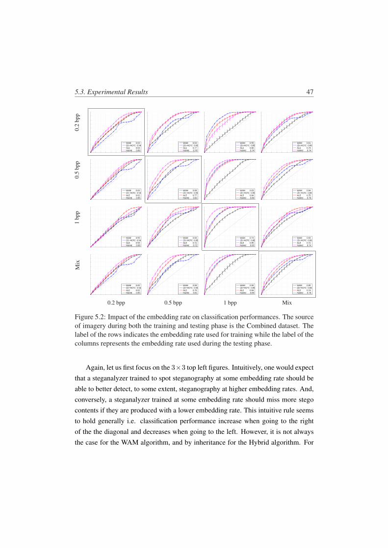
5.3. Experimental Results 47
0.2
bpp
WAM 0.632D−HCFC 0.54ALE 0.64Hybrid 0.69
WAM 0.642D−HCFC 0.65ALE 0.77Hybrid 0.78
WAM 0.552D−HCFC 0.85ALE 0.80Hybrid 0.74
WAM 0.612D−HCFC 0.68ALE 0.74Hybrid 0.74
0.5
bpp
WAM 0.602D−HCFC 0.54ALE 0.62Hybrid 0.65
WAM 0.682D−HCFC 0.65ALE 0.77Hybrid 0.82
WAM 0.632D−HCFC 0.85ALE 0.84Hybrid 0.89
WAM 0.642D−HCFC 0.68ALE 0.75Hybrid 0.79
1bp
p
WAM 0.552D−HCFC 0.54ALE 0.59Hybrid 0.58
WAM 0.602D−HCFC 0.65ALE 0.72Hybrid 0.72
WAM 0.742D−HCFC 0.85ALE 0.85Hybrid 0.93
WAM 0.632D−HCFC 0.68ALE 0.72Hybrid 0.74
Mix
WAM 0.602D−HCFC 0.54ALE 0.62Hybrid 0.65
WAM 0.682D−HCFC 0.65ALE 0.76Hybrid 0.81
WAM 0.662D−HCFC 0.85ALE 0.84Hybrid 0.89
WAM 0.652D−HCFC 0.68ALE 0.74Hybrid 0.78
0.2 bpp 0.5 bpp 1 bpp Mix
Figure 5.2: Impact of the embedding rate on classification performances. The sourceof imagery during both the training and testing phase is the Combined dataset. Thelabel of the rows indicates the embedding rate used for training while the label of thecolumns represents the embedding rate used during the testing phase.
Again, let us first focus on the 3×3 top left figures. Intuitively, one would expectthat a steganalyzer trained to spot steganography at some embedding rate should beable to better detect, to some extent, steganography at higher embedding rates. And,conversely, a steganalyzer trained at some embedding rate should miss more stegocontents if they are produced with a lower embedding rate. This intuitive rule seemsto hold generally i.e. classification performance increase when going to the rightof the the diagonal and decreases when going to the left. However, it is not alwaysthe case for the WAM algorithm, and by inheritance for the Hybrid algorithm. For
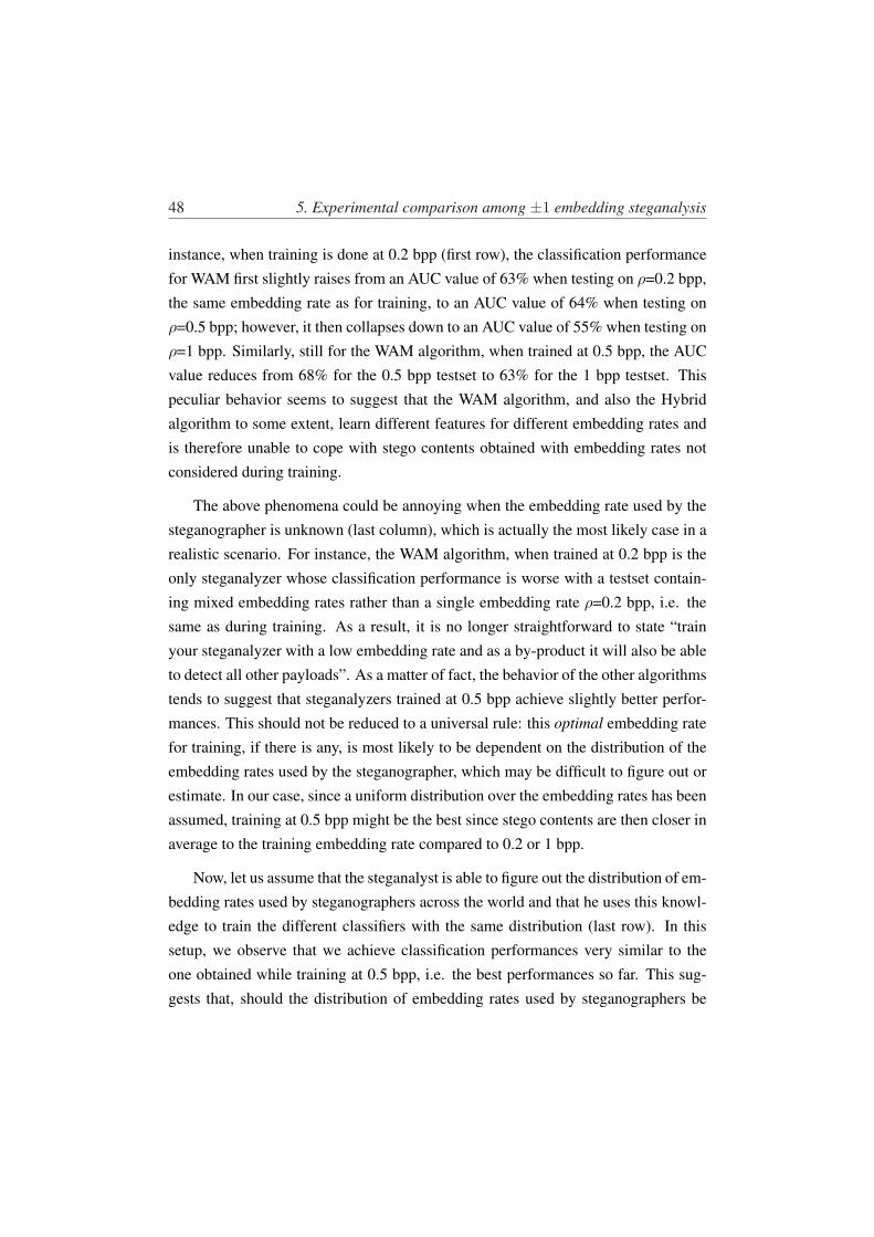
48 5. Experimental comparison among ±1 embedding steganalysis
instance, when training is done at 0.2 bpp (first row), the classification performancefor WAM first slightly raises from an AUC value of 63% when testing on ρ=0.2 bpp,the same embedding rate as for training, to an AUC value of 64% when testing onρ=0.5 bpp; however, it then collapses down to an AUC value of 55% when testing onρ=1 bpp. Similarly, still for the WAM algorithm, when trained at 0.5 bpp, the AUCvalue reduces from 68% for the 0.5 bpp testset to 63% for the 1 bpp testset. Thispeculiar behavior seems to suggest that the WAM algorithm, and also the Hybrid
algorithm to some extent, learn different features for different embedding rates andis therefore unable to cope with stego contents obtained with embedding rates notconsidered during training.
The above phenomena could be annoying when the embedding rate used by thesteganographer is unknown (last column), which is actually the most likely case in arealistic scenario. For instance, the WAM algorithm, when trained at 0.2 bpp is theonly steganalyzer whose classification performance is worse with a testset contain-ing mixed embedding rates rather than a single embedding rate ρ=0.2 bpp, i.e. thesame as during training. As a result, it is no longer straightforward to state “trainyour steganalyzer with a low embedding rate and as a by-product it will also be ableto detect all other payloads”. As a matter of fact, the behavior of the other algorithmstends to suggest that steganalyzers trained at 0.5 bpp achieve slightly better perfor-mances. This should not be reduced to a universal rule: this optimal embedding ratefor training, if there is any, is most likely to be dependent on the distribution of the
embedding rates used by the steganographer, which may be difficult to figure out orestimate. In our case, since a uniform distribution over the embedding rates has beenassumed, training at 0.5 bpp might be the best since stego contents are then closer inaverage to the training embedding rate compared to 0.2 or 1 bpp.
Now, let us assume that the steganalyst is able to figure out the distribution of em-bedding rates used by steganographers across the world and that he uses this knowl-edge to train the different classifiers with the same distribution (last row). In thissetup, we observe that we achieve classification performances very similar to theone obtained while training at 0.5 bpp, i.e. the best performances so far. This sug-gests that, should the distribution of embedding rates used by steganographers be
5.3. Experimental Results 49
known, it should be exploited during the training of the steganalysis algorithms.
5.3.3 Performances of the steganalyzers with prior information aboutthe source of imagery
Although the experimental results of the previous section clearly suggest that
training should be performed with the same distribution of embedding rates as theone encountered during testing, it is still not clear how a steganalysis algorithmshould be trained in general. Should we use a single source of imagery or a combina-tion of all known sources? As already mentioned, the answer it heavily depends onwhether or not, during the testing phase, we have some additional tools, e.g. multi-media forensics techniques, which gives some a priori information about the sourceof imagery of the tested content. In such a case, the steganalyst can switch to therelevantly trained classifier accordingly. In this section, we will assume that we dohave access to such a priori information and will review the detailed performancesof the different algorithms under study.
Each steganalyzer is trained on each of the three available databases (NRCS,Camera and Corel). The stego contents used for training are obtained using em-bedding rates uniformly distributed across 0.2, 0.5 and 1 bpp as suggested by priorfindings. Since we do assume to have prior information, we then test each classifierwith contents taken from the same database as the one using during training. Still,to get a better understanding of their classification performances, the steganalyzersare successively tested with stego contents obtained with an embedding rate equalto 0.2, 0.5, 1 bpp or a uniform mix of these. It results in 3 × 4 training and testingscenarios and, for each one of them, the average ROC curve of all steganalyzers hasbeen computed as described in Section 5.2. All the plots have been gathered in Fig-ure 5.3. The label of the rows indicates the database used both during training andtesting and the label of the columns the embedding rate used for testing.
Intuitively, one could expect that, for some training conditions i.e. for a givenrow, stego contents obtained with large embedding rates should be detected moreeasily than those with smaller ones. This rule seems to hold in most cases except,again, for the WAM algorithm on the Camera database. For this particular dataset,
50 5. Experimental comparison among ±1 embedding steganalysisN
RC
S
WAM 0.582D−HCFC 0.53ALE 0.58Hybrid 0.62
WAM 0.672D−HCFC 0.60ALE 0.67Hybrid 0.75
WAM 0.762D−HCFC 0.72ALE 0.76Hybrid 0.87
WAM 0.672D−HCFC 0.62ALE 0.66Hybrid 0.75
Cam
era
WAM 0.732D−HCFC 0.55ALE 0.63Hybrid 0.75
WAM 0.862D−HCFC 0.65ALE 0.80Hybrid 0.89
WAM 0.802D−HCFC 0.81ALE 0.91Hybrid 0.90
WAM 0.802D−HCFC 0.67ALE 0.79Hybrid 0.85
Cor
el
WAM 0.632D−HCFC 0.67ALE 0.82Hybrid 0.84
WAM 0.712D−HCFC 0.83ALE 0.96Hybrid 0.96
WAM 0.802D−HCFC 0.97ALE 0.97Hybrid 0.97
WAM 0.722D−HCFC 0.82ALE 0.92Hybrid 0.93
0.2 bpp 0.5 bpp 1 bpp Mix
Figure 5.3: Classification performances when prior information about the source ofimagery is available. Training is done with stego contents obtained with embeddingrates uniformly distributed across 0.2, 0.5 and 1 bpp. The label of the rows indicatesthe source of imagery used both during training and testing. On the other hand, thelabel of the columns represents the embedding rate used during the testing phase.
the AUC value indeed raises from 73% for 0.2 bpp to 86% for 0.5 bpp before de-creasing down to 80% for 1 bpp. The fact that this behavior is only observed for theCamera databases may be due to the fact that this dataset is actually composed ofimages taken with different cameras i.e. different sources of imagery strictly speak-ing. In any case, it does highlight the extreme sensitivity of the WAM algorithm.The plots for mixed payload give some kind of average of the ROC curves alongthe rows. However, these plots completely mask specific behaviors for different em-bedding rates. For instance with the NRCS database, efforts should be focused ondetecting low embedding rates since performances are really bad in that case. Itmight indeed be easier to raise the AUC of really poor ROC curves than further en-hance not so bad ROC curves. This calls for reporting more than only the averagecurve (mix) to get a better understanding of the system.
5.3. Experimental Results 51
Also worth mention, classification performances appear to be heavily dependenton the source of imagery. In average for instance, the AUC value of the best per-forming algorithm is equal to 75% for NRCS, 85% for Camera and 93% for Corel,hence clearly that some type of images might be more difficult to tackle than others.Additionally, setting apart the Hybrid algorithm, the best performing steganalysis al-gorithm seems to change from one dataset to the other. ALE definitely outperformsthe others on the Corel database, being matched by 2D-HCFC only for high embed-
ding rates. With the Camera dataset, the situation is more contrasted: WAM is betterfor low embedding rates but is being outmatched by ALE for high embedding rates.Finally, WAM and ALE are side by side for the NRCS database. Still, even in thatcase, combining the feature sets of both algorithms succeeds to significantly improveperformances hence demonstrating the complementarity of these two systems.
5.3.4 Performances of the steganalyzers without prior information aboutthe source of imagery
In contrast with the previous subsection, we now assume that the steganalyst isunable to figure out the source of the content which is to be tested. In other words,he can no longer switch pertinently between several specifically trained classifiers.This scenario is significantly more realistic in practice since one can hardly tell howmany sources of imagery should be considered to be close to the real world. As aresult, we conducted a final batch of experiments to address this specific situation.
In this scenario, the steganalyst trains the different steganalysis systems with theCombined database and stego contents obtained with an embedding rate uniformlydistributed across 0.2, 0.5 and 1 bpp. Still, the obtained classifiers are benchmarkedfor individual databases (NRCS, Camera, Corel, combined) and individual embed-ding rates (0.2, 0.5, 1 bpp and mixed payloads). It results in 4× 4 testing scenarios.For each of them, the average ROC curve of all steganalyzers has been computed asdetailed in Section 5.2 and the resulting plots are depicted in Figure 5.4. The labelof the rows indicates the dataset used for testing and the label of the columns the
embedding rate.
Again, classification performances improve when the embedding rate increases.
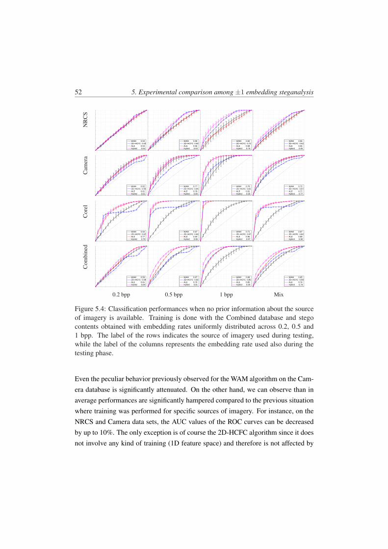
52 5. Experimental comparison among ±1 embedding steganalysisN
RC
S
WAM 0.532D−HCFC 0.53ALE 0.53Hybrid 0.54
WAM 0.552D−HCFC 0.60ALE 0.56Hybrid 0.63
WAM 0.602D−HCFC 0.72ALE 0.58Hybrid 0.76
WAM 0.562D−HCFC 0.62ALE 0.55Hybrid 0.65
Cam
era
WAM 0.622D−HCFC 0.55ALE 0.61Hybrid 0.61
WAM 0.772D−HCFC 0.65ALE 0.79Hybrid 0.80
WAM 0.762D−HCFC 0.81ALE 0.91Hybrid 0.90
WAM 0.722D−HCFC 0.67ALE 0.77Hybrid 0.77
Cor
el
WAM 0.642D−HCFC 0.67ALE 0.77Hybrid 0.79
WAM 0.672D−HCFC 0.83ALE 0.94Hybrid 0.95
WAM 0.712D−HCFC 0.97ALE 0.96Hybrid 0.97
WAM 0.672D−HCFC 0.82ALE 0.89Hybrid 0.90
Com
bine
d
WAM 0.592D−HCFC 0.54ALE 0.61Hybrid 0.64
WAM 0.672D−HCFC 0.65ALE 0.76Hybrid 0.81
WAM 0.682D−HCFC 0.85ALE 0.85Hybrid 0.90
WAM 0.652D−HCFC 0.68ALE 0.74Hybrid 0.78
0.2 bpp 0.5 bpp 1 bpp Mix
Figure 5.4: Classification performances when no prior information about the sourceof imagery is available. Training is done with the Combined database and stegocontents obtained with embedding rates uniformly distributed across 0.2, 0.5 and1 bpp. The label of the rows indicates the source of imagery used during testing,while the label of the columns represents the embedding rate used also during thetesting phase.
Even the peculiar behavior previously observed for the WAM algorithm on the Cam-era database is significantly attenuated. On the other hand, we can observe than inaverage performances are significantly hampered compared to the previous situationwhere training was performed for specific sources of imagery. For instance, on theNRCS and Camera data sets, the AUC values of the ROC curves can be decreasedby up to 10%. The only exception is of course the 2D-HCFC algorithm since it doesnot involve any kind of training (1D feature space) and therefore is not affected by
5.4. Conclusions 53
this change of training setup. Additionally, we can observe a mild increase in thevariability of the ROC curves, thus indicated increased instability for the differentsteganalysis systems. This drop of performances suggests that it might be utopian totrain a single classifier to address all situations and that it might be more relevant topertinently switch between specifically trained classifiers.
One could argue that the only relevant plot is the one in the bottom right corneras it reports the performances of the different steganalysis system in conditions closeto the real world. In that case, one would realize that classifications performancesare average at best. One could also be surprised by the suggested ranking of thedifferent classifier, the well-known WAM being the worst (most likely due to its lossof stability) and the underrated 2D-HCFC scoring not so badly. However, focusingon this single plot kind of hide the most important information: where should effortsbe targeted to further improve these performances. It is clear for instance that verylittle improvement is likely to be achieved on the Corel dataset. On the other hand,the NRCS dataset offers huge room for further improvement even at high embeddingrate.
5.4 Conclusions
We compared four steganalysis algorithms applied to the detection of ±1 em-bedding.
We stressed out that during training, it is necessary to provide a labeled set ofcover and stego Works. The stego Works are usually derived from the application ofknown steganographic algorithms. However, even for the case of targeted steganal-ysis there are a range of free parameters available to the steganographer, but usuallyunknown to the steganalyst. The most common such parameter is the embeddingrate. It is quite usual to report results assuming exact knowledge of the embeddingrate, i.e. training and testing are for a fixed embedding rate. Even though there aresome works that try to estimate the message length [45, 46, 47, 48], in practice, no-body will know the embedding payload. If training and testing are conducted overa range of embedding rates, we can expect performance to degrade. Our study also
54 5. Experimental comparison among ±1 embedding steganalysis
revealed this. It is common to train with a low embedding rate in order to cope witha wide range of embedding rates used during testing. However, experimental resultssuggest that this is less effective than training with a mixture of embedding rates.
In summary, our experiments revealed that (i) the performance of all algorithmsvaried significantly depending on the database, (ii) no one algorithm was superioracross all databases. In particular, we have seen that training in real world conditions,e.g. mixed embedding rates (and combined database), may have a significant impact
on performances compared to tightly controlled situation.

Chapter 6Steganalysis: remarks and future works
In the first part of the thesis we have discussed steganalysis in the pixel domain
by proposing the steganalyzer ALE and a methodology to experimentally evaluatethe performance of a steganalysis algorithms.
With regard to ALE, we modified the algorithm by Zhang et al. to deal with(i) border effects associated with the 1D intensity histogram, and (ii) extended it toinclude statistics associated to the amplitude of local extrema in the 2D adjacencyhistogram.
Experimental results demonstrated the positive impact of eliminating the bordereffects and showed substantial improvements in classification accuracy when fea-
tures derived from the 2D adjacency histogram were included. Moreover, the pro-posed steganalysis system proved to outperform other state-of-the-art steganalyzerssuch as WAM [10] and 2D-HCFC [23].
As future works, we could improve further the performances of ALE by using acalibrated version of the features as suggested by Ker in [23].
We have also discussed a number of issues in training and testing steganalysisalgorithms and illustrated these issues by comparing four algorithms for the detection
of ±1 embedding.
While the community recognizes the importance of standardized training andtest sets, it is clear that current databases are inadequate. In particular, we observedvery significant variations in performance across the four databases used in the testfor all the algorithms under evaluation. This indicates that no one database is cur-rently sufficiently representative of the variety of imagery that may be encounteredin the real world. More research is needed to (i) understand how various databasesdiffer from one another, and (ii) develop more comprehensive databases that better
56 6. Steganalysis: remarks and future works
represent the variation in real world imagery.Performance results are usually reported in the form of a receiver operating char-
acteristic curve, and we have followed this convention. Cross-fold validation gener-ates a family of ROC curves which must be merged. Vertical averaging and thresholdaveraging are two approaches for doing so. Both have the advantage of providing ameasure of the uncertainty associated with the ROC values. In our analysis, we ob-served an extreme range of uncertainty when attempting to apply threshold averaging
to the WAM (and hybrid) algorithms. Consequently, we chose to perform verticalaveraging. Probably this uncertainty is due directly to the cardinality of features. Asteganalysis open question regards about the best feature strategy: is a big amount offeatures [49, 50, 51] preferred to few features [52, 53, 54] in a real scenario?
Future works should investigate this more closely and it would be beneficial ifthe community agreed to standardize on one or other approach.
In many situations, it is useful to summarize the performance of an algorithmwith a single scalar value. One such value is the area under the ROC curve (AUC).While this is a common measure for summarizing ROC performance, further discus-sion is needed to decide whether the AUC is adequate and/or sufficient for comparingsteganalysis algorithms.
Part II
MPSteg-color: a newsteganographic technique

Chapter 7Steganography at higher semantic level
Common steganalyzers like those described in Chapter 3 and Chapter 4 rely on astatistical analysis to understand whether a given signal contains hidden data or not,however, this analysis disregards the semantic content of the cover signal. For thisreason it may be argued that, from a steganographic point of view, it is preferable toembed the stego-messages at the highest possible semantic level, e.g. by modifyingstructural elements of the host signal like lines, edges or flat areas in the case of stillimages.
Following a similar need arising from image compression applications1 [55, 56],a new class of image representation methods has been recently developed that relieson redundant bases decomposition. In practice, a dictionary with a large numberof elementary signals (called atoms) is built, trying to ensure that, for each image(or image block), a subset of few atoms exists that permits to represent the imageefficiently. The main problems with redundant basis decomposition of images arethe construction of the dictionary and, more importantly, the definition of an effi-
cient procedure to select the best subset of atoms for each image. The most commonapproach to solve the latter problem, consists to resort to Matching Pursuit (MP)techniques, that use a greedy algorithm to select a subset of atoms capable of repre-senting the to-be-decomposed image efficiently [57].
As a main result MP schemes permit to decompose images efficiently by de-scribing the main features of picture’s semantic.
Similar ideas about the usage of a semantic layer as message support are widelyinvestigated in watermarking field [58, 59, 60] in which the robustness and the invis-
1As a matter of fact, the goal of any compression algorithm is to describe the main semantic featuresof the image without considering noise-like details.
60 7. Steganography at higher semantic level
ibility of the watermark is required.
We propose a new steganographic method, called MPSteg-color, that hides thestego-message into some selected coefficients of the MP representation of the covercolor image. In this way the hidden message is embedded at a higher semantic leveland hence it should be more difficult for a steganalyzer to detect it. To actually builda steganographic technique based on MP decomposition several problems need tobe solved including: i) the choice of a suitable dictionary, ii) the setting up of MPrules which permit to correctly embed and extract the message in the MP domain,iii) the implementation of security aspects in order to prevent the detectability of theproposed technique.
In the sequel we show how we investigates and solved all the above problems.
7.1 Introduction to MP image decomposition
Given a vector space V , a high redundant basis is a set of elements of V whosenumber greatly exceeds the dimension of V . The main idea behind the use of redun-dant basis for signal representation is that for any given signal it is likely that we canfind a small subset of elements within the basis which are enough to represent thesignal up to a certain accuracy level. Indeed, the more elements are contained in thebasis the more likely the representing set will be small. Of course, since the number
of signals in the basis exceeds the size of the space the host signal belongs to, theelements of the basis will no longer be orthogonal as in standard signal decomposi-tion. At the same time, the availability of many degrees of freedom in the design ofthe redundant basis permits to include signals with specific semantic meaning.
In the following, the elements of the redundant basis will be called atoms, andthe redundant basis the dictionary. The dictionary is usually indicated as D:
D = {gk}k∈1,...,N , (7.1)
where gk is the k-th atom. If I is a generic signal (hereafter an image), we can
7.1. Introduction to MP image decomposition 61
describe it as the sum of a subset of elements of D:
I =N∑
k=1
ckgk, (7.2)
where ck is the specific weight of the k-th atom, and where as many ck as possibleare zero. There are no particular requirements concerning the dictionary: in fact,the main advantage of this approach is the complete freedom in designing D whichcan then be efficiently tailored to closely match signal structures. Due to the non-orthogonality of the atoms, the decomposition in equation (7.2) is not unique, hence
one could ask which is the best possible way of decomposing I. Several meaningscan be given to the term best decomposition. In compression applications, for in-stance, it is necessary that a suitable approximation in terms of human perceptibledistortion of the image I is obtained. In this case, it is convenient to restate the de-composition problem as follows. Let γ = {γ1, γ2 . . . γN} be a decomposition path,with γk indicating the index of the k-th atom of the decomposition. Let us also de-fine the residual signal Rn as the difference between the original image I and theapproximation obtained by considering only n atoms of the dictionary. We have:
In =n∑
k=1
ckgγk, (7.3)
Rn = I − In, (7.4)
where γk ties the atom identifier to the k-th position of the decomposition sum.
Given the above definitions, the best approximation problem can be restated asfollows:
minγ,ck:‖Rn‖2≤ε
n (7.5)
where ε is suitable approximation error. Unfortunately, the above minimization isan NP-hard problem, due to the non-orthogonality of the dictionary [61]. MatchingPursuit is a greedy method that, by looking for a suboptimal solution, permits toovertake the above NP problem with a polynomial complexity algorithm [61], by
62 7. Steganography at higher semantic level
looking for a step by step minimization of the current residual Rk. While MP findsthe best solution at each step, it generally does not find the global optimum.
In the following, we find convenient to rephrase MP as a two-step algorithm.The first step is defined through a selection function that, given the residual Rk−1,selects the appropriate element of D and its weight:
[ck, gγk] = S(Rk−1,D), (7.6)
where S(·) is a particular selection operator. At the second step, the residual isupdated
Rk = U(Rk−1, ck, gγk). (7.7)
As it can be seen, for a complete definition of the MP framework several specifi-cations must be given including the definition of the dictionary, the selection and theupdate rules. To do so, we must first investigate the requirements set by the particularframework in which we will apply the MP algorithm, i.e. image steganography.
7.2 Embedding a message in the MP domain
Given the representation formula
I =n∑
k=1
ck · gγk+Rn, (7.8)
there are different ways of embedding a message within I. In [62], for instance, thestego-messages is hidden in the particular decomposition path used to represent theimage, whereas in [57] and [8], the message is hidden by modifying the decomposi-tion coefficients ck. In this thesis, we adopt the latter approach, due to the difficultiesof applying the former strategy in a blind detection framework (indeed the schemedescribed in [62] requires non-blind detection). However, this strategy requires sev-eral problems to be addressed.
First of all, it is necessary that the transition from the pixel domain to the MPdomain and then back to the pixel domain does not introduce approximation errors
7.2. Embedding a message in the MP domain 63
that could prevent the correct decoding of the stego-messages. The easiest way ofachieving this result consists in requiring that all the operations are performed ininteger arithmetic with no need to quantize the stego image when the transformationfrom the MP to the pixel domain is performed.
The second requirement stems from the very goal of all our work, that is toembed the stego-message at as high semantic level as possible, hence the dictionaryshould be as semantically meaningful as possible.
The third and the most fundamental requirement, regards the stability of the MPdecomposition. MP instability has two different facets:
• Decomposition path instability: this source of instability is due to the factthat the insertion of the message may change the order in which the atoms arechosen by the MP algorithm. As a matter of fact, if this is the case, the decoderwill fail to read the hidden message correctly (note that in image compression,where the image is reconstructed from a list of weighed atoms, the fact that asuccessive decomposition generates a different list of atoms is not a problem).
• Coefficient instability: the second source of instability derives from the non-orthogonality of the dictionary: if we modify one single coefficient ck∗ , re-construct the modified image and apply the MP algorithm again, even if wedo not change the order in which the atoms are selected, it may well be thecase that all the coefficients will have different values. Even worse, there is no
guarantee that the coefficient of the k∗-th atom will be equal to the value weset it to. It is easy to show that this is the case, for example, if the selectionand update rules are based on the classical projection operator.
As a last observation, we note that, even though MP decreases the decomposi-tion problem to polynomial complexity, the computational burden may still be pro-hibitive, especially if MP is applied to large image blocks. For this reason we decidedto apply MP to small non-overlapping blocks rather than to consider the whole im-age. Note, however, that in principle, the subsequent discussion can be indifferentlyapplied to the whole host image or to subparts of it.
In the next two chapters we describe how the above constraints are satisfied by

64 7. Steganography at higher semantic level
MPSteg color. We first describe the dictionary, then we introduce new selection andupdate rules explicitly designed to avoid coefficient instability.
Chapter 8An MP tailored for steganographic application
In this chapter we introduce the MP domain in which we will embed the message.To do so we introduce the used dictionary, and we define proper selection and updaterules. The designed domain is then analyzed from the embedding point of view -by defining constraints which permit to correctly extract the embedded message -and the semantic point of view describing performances to validate the theoretical
semantic approach.
8.1 Dictionary
There are several ways of building the dictionary. Discrete- or real-valued atomscan be used and atoms can be generated manually or by means of a generating func-tion. In classical MP techniques, applied to still images [55], the dictionary is builtby starting from a small set of generating functions that generate real-valued atoms.A problem with real-valued atoms is that when the modified coefficients are used toreconstruct the image in the pixel domain, non-integer values may be produced, thusresulting in a quantization error when the grey levels are expressed in the standard8-bit format. This is a problem in steganographic applications where the hidden mes-sage is so weak that the quantization error may prevent its correct decoding. For thisreason, and to prevent instability problems, we decided to work with binary-valued
atoms for which only the 0 and 1 values are allowed.
The most important property of the dictionary is that it should be able to describeeach type of image with a linear combination of few atoms. To simplify the construc-tion of the dictionary and to keep the computational burden of the MP decompositionlow, we decided to work on a block by block basis, applying the MP algorithm to
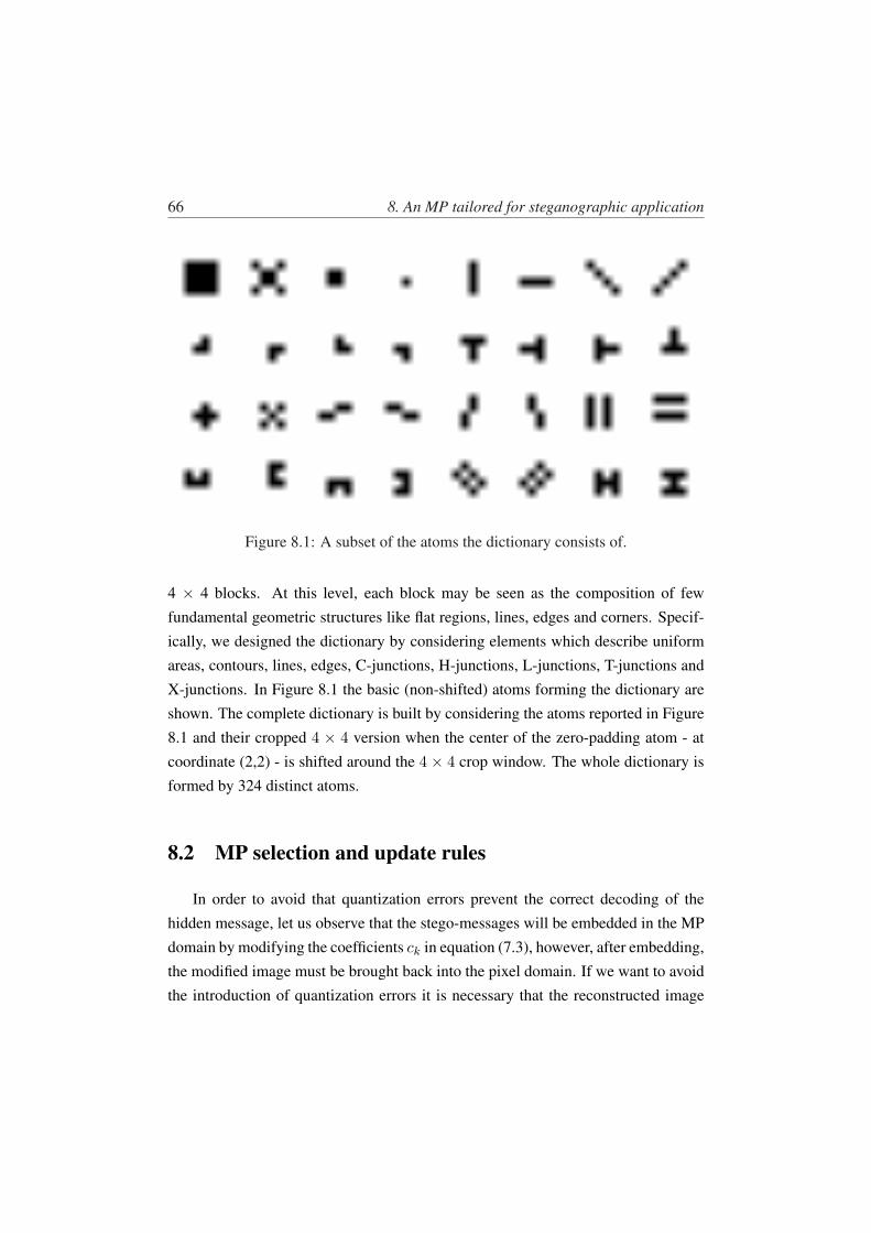
66 8. An MP tailored for steganographic application
Figure 8.1: A subset of the atoms the dictionary consists of.
4 × 4 blocks. At this level, each block may be seen as the composition of few
fundamental geometric structures like flat regions, lines, edges and corners. Specif-ically, we designed the dictionary by considering elements which describe uniformareas, contours, lines, edges, C-junctions, H-junctions, L-junctions, T-junctions andX-junctions. In Figure 8.1 the basic (non-shifted) atoms forming the dictionary areshown. The complete dictionary is built by considering the atoms reported in Figure8.1 and their cropped 4 × 4 version when the center of the zero-padding atom - atcoordinate (2,2) - is shifted around the 4 × 4 crop window. The whole dictionary isformed by 324 distinct atoms.
8.2 MP selection and update rules
In order to avoid that quantization errors prevent the correct decoding of thehidden message, let us observe that the stego-messages will be embedded in the MPdomain by modifying the coefficients ck in equation (7.3), however, after embedding,the modified image must be brought back into the pixel domain. If we want to avoidthe introduction of quantization errors it is necessary that the reconstructed image
8.2. MP selection and update rules 67
belongs to the Image class. The Image class is defined by the following property:
Property 1. Let I be a generic gray image1 in the pixel domain and let n ×m be
its size. Let I(x, y) be the value of the image I at x-row and y-column. We say that
I belongs to the Image class if:
∀x ∈ 1, . . . , n,∀y ∈ 1, . . . , m
0 ≤ I(x, y) ≤ 255 and I(x, y) ∈ N,
the value 255 is used by considering an 8 bit color depth for each color band.
The necessity of ensuring that at each step the approximated image and the resid-ual belong to the Image class already suggested us to consider binary-valued atoms,now we also impose that atom coefficients take non-negative integer values. In this
way, we ensure that the reconstructed image belongs to the Image class2
Coefficient instability is more difficult to deal with, especially when coupledwith the requirement that the decomposition path includes atoms matching the struc-tural content of the image. MPSteg-color achieves the above result by defining theselection rule as follows. At each decomposition step k let
S(Rk−1,D) = [c∗k, gγ∗k ] (8.1)
with
γ∗k = arg minγk∈{1,2,...,|D|}
∑
i,j
‖Rkγk
(i, j)‖2 (8.2)
and
Rkγk
= Rk−1 − c∗kgγk, (8.3)
1It is possible to extend this definition to RGB images by considering each color band as a grayimage.
2Actually we must also ensure that no underflow or overflow errors occur. We will consider thisproblem later on in Chapter 10.
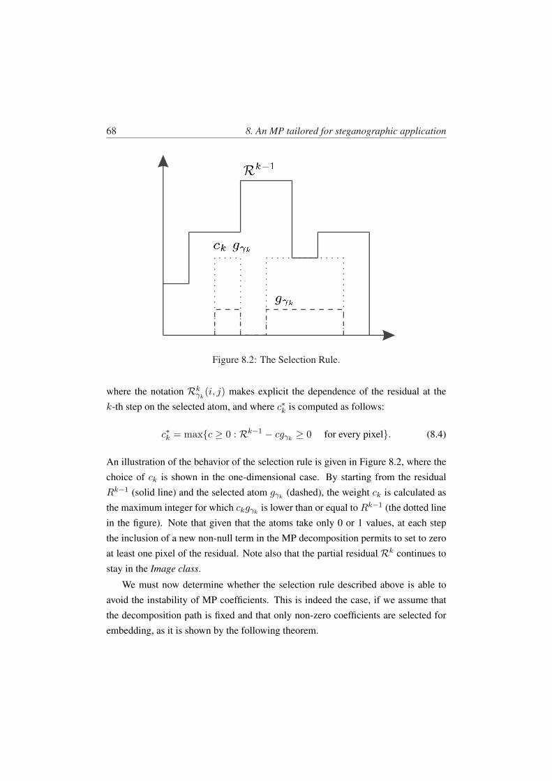
68 8. An MP tailored for steganographic application
Figure 8.2: The Selection Rule.
where the notation Rkγk
(i, j) makes explicit the dependence of the residual at thek-th step on the selected atom, and where c∗k is computed as follows:
c∗k = max{c ≥ 0 : Rk−1 − cgγk≥ 0 for every pixel}. (8.4)
An illustration of the behavior of the selection rule is given in Figure 8.2, where thechoice of ck is shown in the one-dimensional case. By starting from the residualRk−1 (solid line) and the selected atom gγk
(dashed), the weight ck is calculated asthe maximum integer for which ckgγk
is lower than or equal to Rk−1 (the dotted linein the figure). Note that given that the atoms take only 0 or 1 values, at each stepthe inclusion of a new non-null term in the MP decomposition permits to set to zero
at least one pixel of the residual. Note also that the partial residual Rk continues tostay in the Image class.
We must now determine whether the selection rule described above is able toavoid the instability of MP coefficients. This is indeed the case, if we assume thatthe decomposition path is fixed and that only non-zero coefficients are selected forembedding, as it is shown by the following theorem.
8.2. MP selection and update rules 69
Theorem 1. Let I = R0 be an image and let ~gγ = (gγ1 , . . . , gγn) be a decompo-
sition path. We suppose that the atoms are binary valued, i.e. they take only values
0 or 1. Assume that the MP decomposition coefficients are computed iteratively by
means of the following operations:
ck = max{c ≥ 0 : Rk−1 − cgγk≥ 0
for every pixel} (8.5)
Rk = Rk−1 − ckgγk, (8.6)
and let ~c = (c1, c2, . . . , cn) be the coefficient vector built after n iterations. Let ck
be an element of ~c with ck 6= 0, and let ~c ′ be a modified version of ~c where ck has
been replaced by c′k. If we apply the MP decomposition to the modified image
I ′ =n∑
i=1,i 6=k
ci · gγi + c′kgγk+Rn (8.7)
by using the decomposition path ~gγ , we re-obtain exactly the same vector ~c ′ and the
same residual Rn.
Proof. To prove the theorem we introduce some notations. We indicate by S(gγk)
the support of the atom (γk)3. This notation, and the fact that
gγk(x, y) ∈ {0, 1} ∀(x, y),
permits us to rewrite the rule for the computation of ck as follows:
ck = min(x,y)∈S(gγk
)Rk−1(x, y). (8.8)
We indicate by jk the coordinates for which the above minimum is reached, i.e.:
jk = arg min(x,y)∈S(gγk
)Rk−1(x, y). (8.9)
3The support of an atom is defined as the set of coordinates (x, y) for which gγk (x, y) 6= 0
70 8. An MP tailored for steganographic application
Note that after the update we will always have Rk(jk) = 0. We also find it usefulto define the set Jk =
⋃ki=1 ji, with J0 = ∅. In the following we will indicate
with R the residuals computed by applying the decomposition path ~gγ to I, whilewe will indicate with R′ the residuals obtained by applying the same decompositionpath to I ′. A similar notation applies to the other symbols we have defined. Letnow ck be a non-zero element of ~c. We surely have S(gγk
) ∩ Jk−1 = ∅ sinceotherwise we would have ck = 0. Let us show first that by applying the MP to I ′ the
coefficients of the atoms gγhwith h < k do not change. Without loss of generality
let h be the first element for which ch may have changed. Two cases are possible:S(gγk
) ∩ S(gγh) = ∅ or S(gγk
) ∩ S(gγh) 6= ∅. In the first case it is evident that the
weight ch can not change, since a modification of the weight assigned to gγkcannot
have any impact on (8.8) given that the minimization is performed on S(gγh).
When the intersection between S(gγh) and S(gγk
) is non-empty the proof is splitin two parts, the former considers the case c′k > ck, the latter the case c′k < ck. Whenc′k > ck some of the values in R′h−1 are increased, however R′h−1(jh) does notchange since S(gγk
)∩Jk−1 = ∅, hence leaving the choice of jh and the computationof the weight ch unchanged.
If c′k < ck, some values in R′h−1 are decreased while leaving R′h−1(jh) un-changed. However, ∀(x, y) ∈ S(gγk
) ∩ S(gγh) we have Rk−1(x, y) ≤ Rh(x, y)
since due to the particular update rule we adopted, at each iteration the values in theresidual cannot increase. For this reason at the h-th selection step, the modification ofthe k-th coefficient cannot decrease the residual by more thanRh−1− ch (remember
that ch = Rh−1(jh)). In other words, R′h−1(x, y) computed on the modified imageI ′ will satisfy the relation R′h−1(x, y) ≥ R′h−1(jh) hence ensuring that c′h = ch.
We must now show that the components h ≥ k of the vector ~c do not changeas well. Let us start with the case h = k. Since no coefficient has changed untilposition k, when the MP is applied to the image I ′ we have
c′′k = min(x,y)∈S(gγk
)
[Rk−1(x, y) + (c′k − ck)gγk
(x, y)]. (8.10)

8.2. MP selection and update rules 71
From equation (8.10) it is evident that
c′′k = c′k = min(x,y)∈S(gγk
)Rk−1(x, y), (8.11)
since the term (c′k − ck)gγkintroduces a constant bias on all the points of S(gγk
).As to the case h > k it is trivial to show that c′h = ch given that the residual after
the k-th step will be the same for I and I ′.
Theorem 1 can be applied recursively to deal with the case in which more thanone coefficient in ~c is changed. In the following we show how the stability resultstated in Theorem 1 can be used to build the MPSteg-color algorithm.

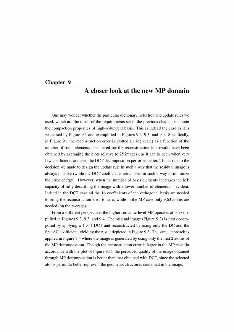
Chapter 9A closer look at the new MP domain
One may wonder whether the particular dictionary, selection and update rules weused, which are the result of the requirements set in the previous chapter, maintainthe compaction properties of high-redundant basis. This is indeed the case as it iswitnessed by Figure 9.1 and exemplified in Figures 9.2, 9.3, and 9.4. Specifically,in Figure 9.1 the reconstruction error is plotted (in log scale) as a function of thenumber of basis elements considered for the reconstruction (the results have beenobtained by averaging the plots relative to 25 images), as it can be seen when veryfew coefficients are used the DCT decomposition performs better. This is due to the
decision we made to design the update rule in such a way that the residual image isalways positive (while the DCT coefficients are chosen in such a way to minimizethe error energy). However, when the number of basis elements increases the MPcapacity of fully describing the image with a lower number of elements is evident.Indeed in the DCT case all the 16 coefficients of the orthogonal basis are neededto bring the reconstruction error to zero, while in the MP case only 9.63 atoms areneeded (on the average).
From a different perspective, the higher semantic level MP operates at is exem-plified in Figures 9.2, 9.3, and 9.4. The original image (Figure 9.2) is first decom-posed by applying a 4 × 4 DCT and reconstructed by using only the DC and thefirst AC coefficient, yielding the result depicted in Figure 9.3. The same approach isapplied in Figure 9.4 where the image is generated by using only the first 2 atoms ofthe MP decomposition. Though the reconstruction error is larger in the MP case (inaccordance with the plot of Figure 9.1), the perceived quality of the image obtainedthrough MP decomposition is better than that obtained with DCT, since the selectedatoms permit to better represent the geometric structures contained in the image.
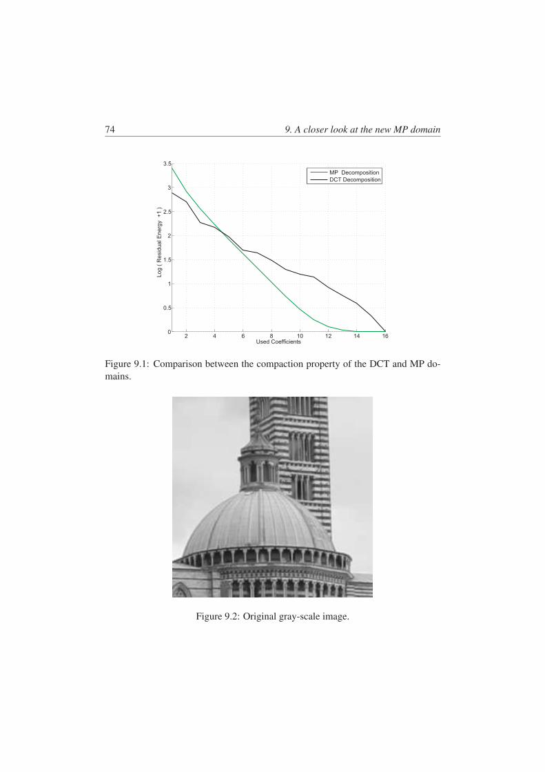
74 9. A closer look at the new MP domain
Figure 9.1: Comparison between the compaction property of the DCT and MP do-mains.
Figure 9.2: Original gray-scale image.
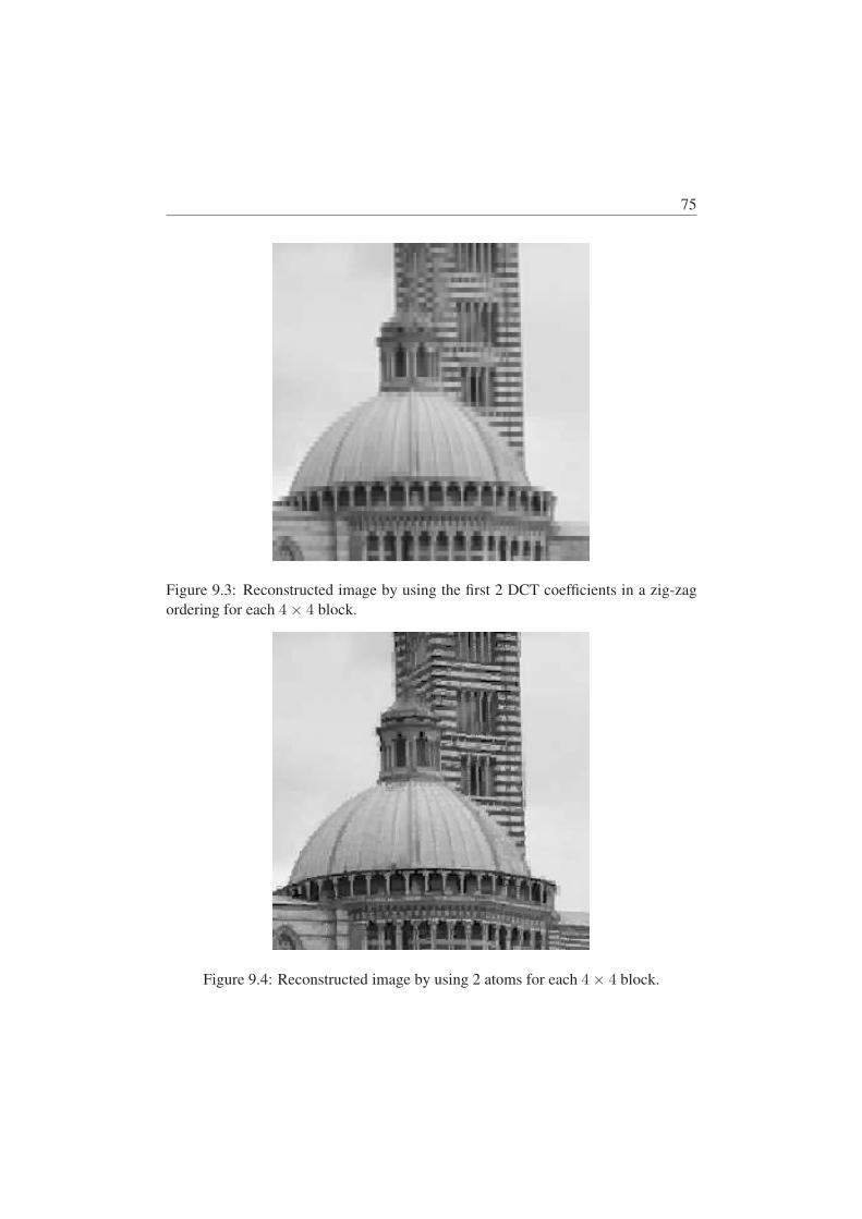
75
Figure 9.3: Reconstructed image by using the first 2 DCT coefficients in a zig-zagordering for each 4× 4 block.
Figure 9.4: Reconstructed image by using 2 atoms for each 4× 4 block.

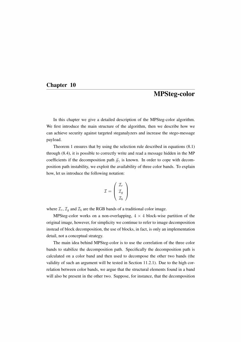
Chapter 10MPSteg-color
In this chapter we give a detailed description of the MPSteg-color algorithm.We first introduce the main structure of the algorithm, then we describe how wecan achieve security against targeted steganalyzers and increase the stego-messagepayload.
Theorem 1 ensures that by using the selection rule described in equations (8.1)through (8.4), it is possible to correctly write and read a message hidden in the MPcoefficients if the decomposition path ~gγ is known. In order to cope with decom-position path instability, we exploit the availability of three color bands. To explainhow, let us introduce the following notation:
I =
Ir
Ig
Ib
where Ir, Ig and Ib are the RGB bands of a traditional color image.
MPSteg-color works on a non-overlapping, 4 × 4 block-wise partition of theoriginal image, however, for simplicity we continue to refer to image decompositioninstead of block decomposition, the use of blocks, in fact, is only an implementationdetail, not a conceptual strategy.
The main idea behind MPSteg-color is to use the correlation of the three colorbands to stabilize the decomposition path. Specifically the decomposition path iscalculated on a color band and then used to decompose the other two bands (thevalidity of such an argument will be tested in Section 11.2.1). Due to the high cor-relation between color bands, we argue that the structural elements found in a bandwill also be present in the other two. Suppose, for instance, that the decomposition
78 10. MPSteg-color
path is computed on the Ir band, we decompose the original image as follows
I =
n∑
k=1
cr,k · gγr,k+Rn
r
n∑
k=1
cg,k · gγr,k+Rn
g
n∑
k=1
cb,k · gγr,k+Rn
b
(10.1)
where gγr,kare the atoms selected on the red band, cr,k,cg,k and cb,k are the atom
weights of each band and Rnr ,Rn
g and Rnb are the partial residuals. By using eq.
(10.1) we do not obtain the optimum decomposition of I for the green and bluebands, but this decomposition has a good property: if the red band is not modified
then the decoder may apply the selection function S(·) to the red band and use itto retrieve the decomposition path used by the embedder to hide the message in theother two bands.
In Section 10.2 we cope with the security aspect by adding for each block arandom choice between the reference and embeddable bands.
By assuming, for instance, that the decomposition path is computed on the redband, then MPSteg-color can embed the stego-message by operating on the vectorwith the decomposition weights of the green and blue bands, i.e. the vector
~cgb = (cg,1, cb,1, . . . , cg,n, cb,n). (10.2)
According to Theorem 1, we know that the stego-messages can be correctly embed-ded by changing the coefficients of the MP decomposition vector ~cgb, however, forthis result to hold it is necessary that only non-zero coefficients are modified. In fact,given that the decomposition path is computed on one band and the message embed-ded in the other two, it may be the case that the coefficients of some atoms of thedecomposition path are zero, i.e. the vector ~cgb may contain some null coefficients.This issue will be considered in the next section, where the embedding rule used byMPSteg-color is described.
10.1. Embedding Rule 79
10.1 Embedding Rule
We now describe the embedding rule used to embed the stego-message within~cgb. Given that the coefficients of ~cgb are non-negative integers, we can apply anymethod that is usually applied to embed a message in the pixel domain. However, wemust consider that the embedder cannot modify zero coefficients (due to Theorem1 assumptions), but in principle it could set to zero some non-zero coefficients. Ifthis is the case a de-synchronization would be introduced between the embedderand the decoder since the decoder will not know which coefficients have been usedto convey the stego-message. In the steganographic literature this is known as thechannel selection problem, for which an elegant solution exists, namely the WetPaper Code strategy introduced by Fridrich et al. in [11]. However, our aim was to
analyze the capability of the MP domain as a cover domain, hence will not considerany procedure to redirect the embedding changes of the basic MPSteg algorithm1.In fact, the same procedures could be applied to pixel domain methods, and are notrelated to the particular domain in which the message is embedded.
For this reason, we adopted the standard ±1 embedding, that is described inChapter 3.1, to embed the message in the non-null weights.
In order to avoid the channel selection problem, we add 2 to all the coefficientsfor which the ±1 embedding rule yields a null value. By indicating with
~cwgb = (cw
g,1, cwb,1, . . . , c
wg,n, cw
b,n)
the marked coefficient vector, then we build the stego image Is:
Is =
n∑
k=1
cr,k · gγr,k+Rn
r
n∑
k=1
csg,k · gγr,k
+Rng
n∑
k=1
csb,k · gγr,k
+Rnb
. (10.3)
1Similarly we will not consider matrix embedding [10], since it can be used to boost the perfor-mance of any steganographic scheme, regardless of the embedding domain.
80 10. MPSteg-color
While the application of ±1 embedding rule to MP coefficients guarantees that themodified coefficients lie in the [0,255] interval, it is possible that some pixels of thereconstructed image exceed the 255 limit. If this happens, the coefficients larger than2 are decreased by 2 until the overflow error disappears. In this way the embeddingdistortion is slightly augmented, however, such an effect is completely negligiblesince overflow errors are extremely rare.
10.2 Improving undetectability
While the undetectability of the above scheme against general purpose stegana-lyzers can be easily proved [8], undetectability against targeted steganalysis may bea problem. First of all, if the dictionary is assumed to be known, a steganalyzer maylook for specific artifacts introduced by MPSteg-color directly in the MP domain.Secondarily, even if the dictionary is kept secret, the particular nature of atoms andthe application of the MP algorithm at a block level, may introduce blocking arti-facts that could be used by a targeted steganalyzer to detect the presence of a stego-message. As it will be shown in section 11.3 this is indeed the case, hence somecountermeasures need to be taken.
First of all we decided to avoid using the first decomposition coefficient as sup-port of the secret message. Usually such a coefficient is able to describe most of theimage energy compared to the remaining atoms. For this reason, any modification tothe first atom is likely to introduce significant blocking artifacts, hence we decide tokeep such an atom unchanged.
The second and more important countermeasure we took, is randomization of
the embedding process. Randomization is applied at two different levels. At the firstlevel randomization affects the image decomposition into blocks. By following anapproach similar to that proposed by Solanki et al. in [63], the image is partitionedinto disjoint and contiguous windows of size 5 × 5 or 6 × 6, and MP decomposi-tion is applied to 4 × 4 blocks randomly chosen within the larger 5 × 5 (or 6 × 6)windows2. By doing so, we reduce and randomize the blocking artifacts introduced
2Randomization is achieved by changing the offset of the 4x4 window within the larger 5x5 or 6x6
10.3. Increasing the payload 81
by MPSteg-color that will be more difficult to detect. In addition, even by know-ing the MP dictionary, the MP domain used by a possible adversary will be spatiallyde-synchronized with respect to the one used by the embedder, thus making steganal-ysis in the MP domain more difficult. Of course a compromise between payload andundetectability must be found here, given that the larger the window size the betterthe undetectability at the expense of payload (given that the number of pixels nottouched by MPSteg-color will increase).
The second randomization level regards the choice of the reference color band
that is used to calculate the MP decomposition path. Specifically, a secret key is usedas a seed for a random number generator that decides on a block by block basis whichcolor band is used to calculate the decomposition path. The MP decomposition isapplied to the chosen band, while the secret message is embedded within the otherbands.
As it will be seen in Chapter 11, through randomization, especially block posi-tion randomization, it is possible to resist to attacks brought by targeted steganalysis.
10.3 Increasing the payload
An undesirable effect of block position randomization is that the payload is(slightly) decreased, all the more that the capacity3 of MP domain is intrinsicallylower than that of the spatial domain (see [57, 8]). A possible way to improve(slightly) the payload of messages hidden by MPSteg-color stems from the obser-vation that though the color bands are highly correlated, the decomposition pathcalculated on one of them in general is not able to lead to a zero residual on theother two bands. For some of the atoms selected in the reference band, in fact, anull coefficient is obtained in the other bands, thus diminishing the number of coef-ficients available for embedding. For this reason, after that the decomposition pathcomputed on the reference band is applied to the other two bands, the residual ofone of the these two bands is further decomposed to provide an additional list of
window.3We are using the term capacity in a loose sense, without any reference to the corresponding infor-
mation theoretic concept.

82 10. MPSteg-color
atoms that are used on the remaining band to provide additional coefficients to em-bed some more bits. In the sequel we will refer to this second decomposition stepas the decomposition refinement step. The actual payload increase obtained thanksto the decomposition refinement step will be evaluated experimentally in the nextchapter.
Chapter 11
MPSteg-color: experimental results
In this chapter we report experimental results that demonstrate the undetectabil-ity of the new MPSteg-color algorithm and validate the main assumptions behind it.First of all in Section 11.1 the image database used for the experiments is described.Afterwards, in Section 11.2 we take a closer look at the MP domain to support thehypothesis that the decomposition path calculated in one color band can be used withlittle loss for the other bands. We also evaluate the gain in terms of payload that isbrought by the decomposition refinement step.
After that, in Section 11.3, we carefully analyze the undetectability of the pro-posed technique, with particular attention to the effectiveness of partition randomiza-tion as a countermeasure to targeted steganalysis. For this reason the undetectabilityof the stego-message is tested first again two targeted steganalyzers explicitly devel-oped to detect MPSteg-color messages, then against general purpose steganalyzers.
11.1 Image Database
For the experimental validation we used a database of 2564 raw color images of512 × 512 size, which is a color version subset of the camera database described in5.1.
Images are the cropped version of the original ones which are taken in a RAWformat from several kinds of common cameras. The images in the database showa wide range of scenarios including countryside, houses, people, faces, man-madeobjects, etc.
84 11. MPSteg-color: experimental results
11.2 Effectiveness of the proposed MP decomposition
We first validate the conjecture that, due to the correlation between RGB colorbands, computing the decomposition path on one band and using it on the othertwo does not impair the capability of the MP algorithm to extract the most importantfeatures of image blocks. Moreover we give a measure of the payload allowed by theMP domain and the payload gain allowed by the decomposition refinement step. Onone side this is a good result showing a high degree of correlation, on the other sideit shows that the decomposition path calculated on one band is not capable of fullydescribe the content of the other bands, thus justifying the resort to a decompositionrefinement step.
11.2.1 Interband correlation of decomposition path
MPSteg-color relies on the assumption that the color bands are highly corre-lated. To experimentally validate the above conjecture, we decomposed a randomcolor band until a null residual is obtained, then with the same decomposition pathwe decomposed one of the remaining bands. After this second decomposition, we
usually obtain a non-null residual that will be null only if the decomposition pathcalculated on the first band fits the content of the second band. At this point we ap-plied a matching pursuit decomposition to the non-null residual and we measured itslength. By averaging the results obtained on all the images of the test database, wefound that about 3.7 additional atoms are needed to decompose the second and thethird band residuals whose energy is about 40,80dB (while about 9.63 atoms werenecessary for the reference band).
11.2.2 Effectiveness of the decomposition refinement step
The goal of the decomposition refinement step is to decompose the residuals ofthe two remaining bands after that the decomposition path computed on the referenceband is applied to them. In this way some extra non-zero coefficients are obtainedthus contributing to increase the payload of MPSteg-color. Specifically, we foundthat the number of available coefficients for embedding is increased by 12.29% on
11.3. Undetectability analysis 85
average. In terms of payload this means that if we embed one bit per non-null co-efficient then we are able to increase the size of the secret message by a 12.29%factor.
11.3 Undetectability analysis
The most important requirement for any steganographic technique is undetectabil-ity. In this section, we report the results that we obtained by applying four state-of-the-art steganalyzers to detect±1 embedding applied in the MP domain and the pixeldomains. Before doing that, however, we test the effectiveness of block partition ran-domization to combat targeted steganalyzers. In the following, we briefly describethe steganalyzers we used by grouping them into two main sets.
The first set comprises target steganalyzers. It will be used to show the weak-ness of MPSteg-color without the block-windows randomization. The second set ofsteganalyzers is composed by steganalyzers proposed until now.
All the steganalyzers are used as feature extractors, however, we decide to alwaysuse a simple linear classifier, namely the Fisher Linear Discriminant (FLD) that isdescribed in Chapter 2.3, to compare the goodness of each tool even though in theoriginal version some of them are associated with an SVM classifier. We choseto compare all the steganographic algorithms by using a FLD classifier in order tohighlight the capability of the various types of features to detect the presence of ahidden MPSteg message.
11.3.1 Targeted steganalyzers
The first targeted steganalyzer we used is built on the simple blocking artifactsdetector (BD) described in [64]. This technique was originally developed for detect-ing JPEG block artifacts, however, we adapted it to detect the artifacts introduced byMPSteg-color and use them as a feature to detect the presence of a stego-message.The algorithm is very simple: we split the image into blocks whose size should bematched to that used by the MP algorithm. Regardless of the block partition strategythe steganalyzer assumes that blocks are located on a grid aligned with the top-left

86 11. MPSteg-color: experimental results
B
C D
A
HG
FE
Figure 11.1: For each block the numbers Z ′ = |A + D − B − C| and Z ′′ = |E +H − F −G| are computed.
corner of the image. For each block we calculate Z and Z ′ as follows:
Z ′ = |A + D −B − C|Z ′′ = |E + H − F −G|
where A, B, C, D, E , F , G and H are taken as shown in Figure 11.1 in the caseof 4 × 4 blocks, the extension to larger blocks being trivial. Next the normalizedhistograms vectors h′(n) and h′′(n) are computed respectively for Z ′ and Z ′′ andthe following feature is calculated:
fBD =255∑
n=0
|h′(n)− h′′(n)|.
The above procedure is repeated for the three color bands producing a three-dimensionalfeature vector that is given as input to the FLD classifier.
The second steganalyzer we developed relies on the knowledge of the histogramof MP coefficients. For this to be possible, we assume that the steganalyzer knowsthe MP dictionary but it does not know the reference band that is used to calculate thedecomposition path (hence a random band is used as a reference by the steganalyzer).Figure 11.2 shows a typical histogram of a cover image and a stego MPSteg-color
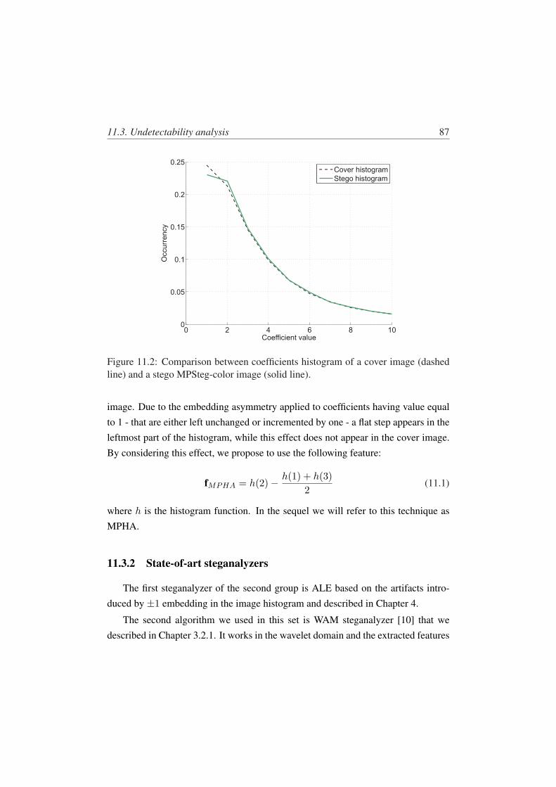
11.3. Undetectability analysis 87
0 2 4 6 8 100
0.05
0.1
0.15
0.2
0.25
Coefficient value
Occurr
ency
Cover histogram
Stego histogram
Figure 11.2: Comparison between coefficients histogram of a cover image (dashedline) and a stego MPSteg-color image (solid line).
image. Due to the embedding asymmetry applied to coefficients having value equalto 1 - that are either left unchanged or incremented by one - a flat step appears in theleftmost part of the histogram, while this effect does not appear in the cover image.By considering this effect, we propose to use the following feature:
fMPHA = h(2)− h(1) + h(3)2
(11.1)
where h is the histogram function. In the sequel we will refer to this technique asMPHA.
11.3.2 State-of-art steganalyzers
The first steganalyzer of the second group is ALE based on the artifacts intro-duced by ±1 embedding in the image histogram and described in Chapter 4.
The second algorithm we used in this set is WAM steganalyzer [10] that wedescribed in Chapter 3.2.1. It works in the wavelet domain and the extracted features
88 11. MPSteg-color: experimental results
are central moments that are calculated in the three detail bands of first order waveletdecomposition. This steganalyzer is a blind steganalyzer because it is not explicitlydeveloped to detect any particular kind of messages.
The third steganalyzer is 2D-HCFC algorithm introduced by Ker in [23] anddescribed in Chapter 3.2.2. It builds on some considerations made in [36] aboutartifacts generated in the histogram domain by ±1 embedding. In particular weused the concatenated features from the histogram analysis and the adjacency matrixanalysis.
Starting from the initial gray scale steganalyzers, we implemented a color versionby joining the 3 RGB band feature vectors in a unique vector with triple components.In this way we worked with 30 features for ALE, three features for 2D-HCFC and
81 features for WAM.
11.3.3 Steganalysis Results
For our experiments we embedded in each image a random message by using asecret unique key.
For MPSteg-color we used three window sizes in the experimental tests: 4 × 4,5 × 5 and 6 × 6. The comparison between different methods was always made byusing the maximum payload allowed by the techniques involved in the comparison,for instance when comparing MPSteg-color versions with different window sizes thepayload imposed by the largest window is used 1.
The cover and stego images produced as described above were used to build atraining and a test set, both containing 50% cover and 50% stego images. The sizeof the training set was equal to 20% of the 2564 images, the remaining 80% formingthe test set. The training and the test sets were built randomly, however, to avoid any
dependence of the results upon the specific training and test sets, the experimentswere repeated 20 times, each time with a different training and test set. In this waywe obtained 20 ROC curves that were vertically averaged to produce the final plotsshown in the following. In the plots the minimum and maximum bound of the beamof ROC curves is shown.
1The payload is expressed in bit per pixel, by considering 512× 512× 3 the number of the pixels.
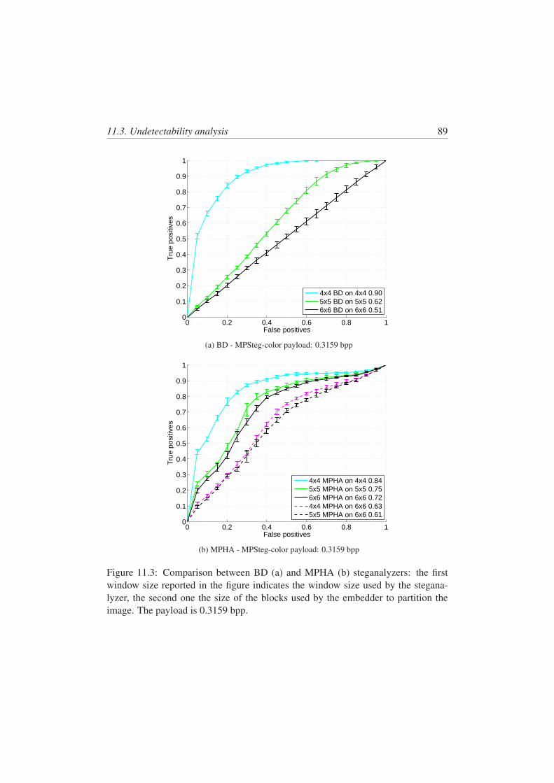
11.3. Undetectability analysis 89
0 0.2 0.4 0.6 0.8 10
0.1
0.2
0.3
0.4
0.5
0.6
0.7
0.8
0.9
1
False positives
Tru
e po
sitiv
es
4x4 BD on 4x4 0.905x5 BD on 5x5 0.626x6 BD on 6x6 0.51
(a) BD - MPSteg-color payload: 0.3159 bpp
0 0.2 0.4 0.6 0.8 10
0.1
0.2
0.3
0.4
0.5
0.6
0.7
0.8
0.9
1
False positives
Tru
e po
sitiv
es
4x4 MPHA on 4x4 0.845x5 MPHA on 5x5 0.756x6 MPHA on 6x6 0.724x4 MPHA on 6x6 0.635x5 MPHA on 6x6 0.61
(b) MPHA - MPSteg-color payload: 0.3159 bpp
Figure 11.3: Comparison between BD (a) and MPHA (b) steganalyzers: the firstwindow size reported in the figure indicates the window size used by the stegana-lyzer, the second one the size of the blocks used by the embedder to partition theimage. The payload is 0.3159 bpp.
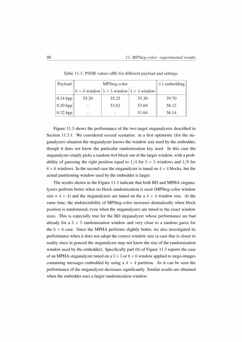
90 11. MPSteg-color: experimental results
Table 11.1: PSNR values (dB) for different payload and settings.
Payload MPSteg-color ±1 embedding
6× 6 window 5× 5 window 4× 4 window
0.14 bpp 55.20 55.25 55.30 59.70
0.20 bpp - 53.62 53.69 58.12
0.32 bpp - - 51.64 56.14
Figure 11.3 shows the performance of the two target steganalyzers described inSection 11.3.1. We considered several scenarios: in a first optimistic (for the ste-ganalyzer) situation the steganalyzer knows the window size used by the embedder,
though it does not know the particular randomization key used. In this case thesteganalyzer simply picks a random 4x4 block out of the larger window, with a prob-ability of guessing the right position equal to 1/4 for 5 × 5 windows and 1/9 for6× 6 windows. In the second case the steganalyzer is tuned on 4× 4 blocks, but theactual partitioning window used by the embedder is larger.
The results shown in the Figure 11.3 indicate that both BD and MPHA stegana-lyzers perform better when no block randomization is used (MPSteg-color window
size = 4 × 4) and the steganalyzers are tuned on the a 4 × 4 window size. At thesame time, the undetectability of MPSteg-color increases dramatically when blockposition is randomized, even when the steganalyzers are tuned to the exact windowsizes. This is especially true for the BD steganalyzer whose performance are badalready for a 5 × 5 randomization window and very close to a random guess forthe 6 × 6 case. Since the MPHA performs slightly better, we also investigated itsperformance when it does not adopt the correct window size (a case that is closer toreality since in general the steganalyzer may not know the size of the randomizationwindow used by the embedder). Specifically part (b) of Figure 11.3 reports the caseof an MPHA steganalyzer tuned on a 5× 5 or 6× 6 window applied to stego-imagescontaining messages embedded by using a 4 × 4 partition. As it can be seen theperformance of the steganalyzer decreases significantly. Similar results are obtainedwhen the embedder uses a larger randomization window.
11.3. Undetectability analysis 91
We now turn the attention to non-targeted steganalysis and to the comparisonbetween MPSteg-color and ±1 embedding applied in the pixel domain
Before presenting the ROC curves, it is instructive to consider the PSNR obtainedby applying ±1-steg in the pixel and in the MP domains. Such results are given inTable 11.1 for different MPSteg-color window sizes and different payloads. Theaverage PSNR is obtained by taking the average on the linear quantities and thenpassing to the logarithmic scale. As expected, by considering that the atoms of theMP decomposition has a support larger than a single pixel, MPSteg-color results ina lower PSNR, hence suggesting that any advantage in terms of undetectability (ifany) will be due to the better hiding properties of the MP domain.
Despite the lower PSNR, the presence of the stego-messages can not be noticedperceptually as it is exemplified in Figure 11.4 where the stego-image (right) cannotbe distinguished from the original one (left) even if the largest possible payload isused (0.3687bpp) for a PSNR of 51.22dB.
Figures 11.5, 11.6, and 11.7 compares the detectability of MPSteg-color withthat of ±1 embedding, for three different window sizes (and different payloads). Inthe legend, the Area Under Curve (AUC) value is also given for each steganalyzer asan overall measure of classification accuracy.
We can see that WAM and ALE are capable to distinguish the stego-images witha significant level of accuracy. In WAM case, though, the message embedded in theMP domain is less detectable than the one embedded in the pixel domain, while ALEworks better with MPSteg-color than ±1 embedding.
We can see that WAM is the only steganalyzer capable to distinguish the stego-images with a significant level of accuracy. Even in this case, though, the messageembedded in the MP domain is less detectable than the one embedded in the pixeldomain.
Slightly better results (from the steganalyzer point of view) are obtained for a 4×4 window (larger payload), however, the general behavior of the various algorithmsdoes not change.
In order to evaluate the dependence of MPSteg-color detectability on the size ofthe randomization window, the ROC curves obtained for different sizes are plotted
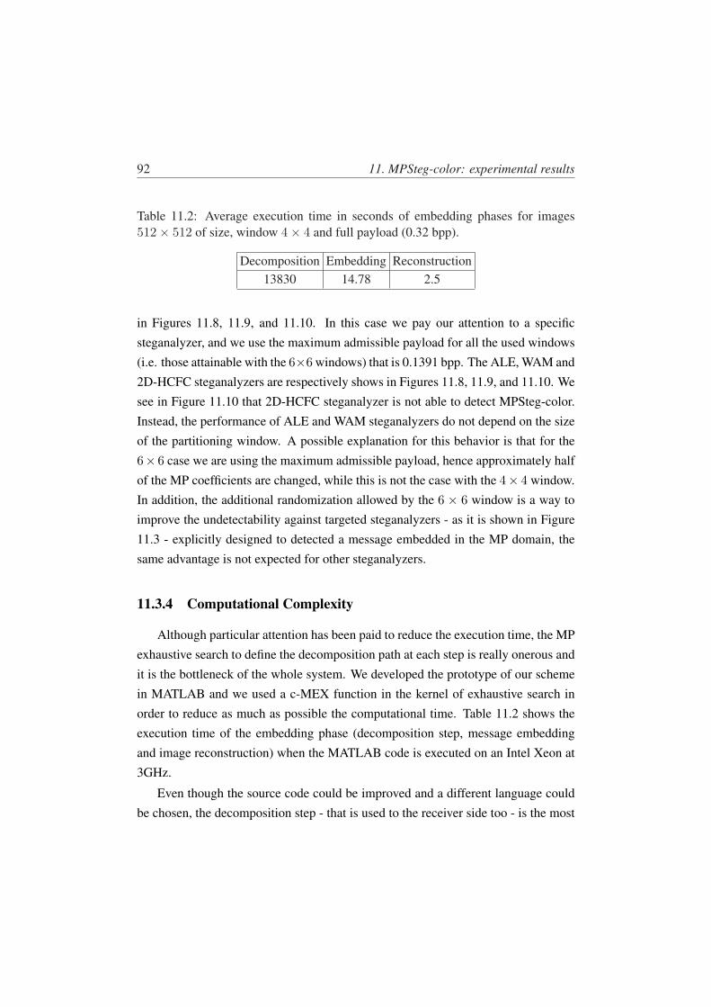
92 11. MPSteg-color: experimental results
Table 11.2: Average execution time in seconds of embedding phases for images512× 512 of size, window 4× 4 and full payload (0.32 bpp).
Decomposition Embedding Reconstruction13830 14.78 2.5
in Figures 11.8, 11.9, and 11.10. In this case we pay our attention to a specificsteganalyzer, and we use the maximum admissible payload for all the used windows(i.e. those attainable with the 6×6 windows) that is 0.1391 bpp. The ALE, WAM and2D-HCFC steganalyzers are respectively shows in Figures 11.8, 11.9, and 11.10. Wesee in Figure 11.10 that 2D-HCFC steganalyzer is not able to detect MPSteg-color.Instead, the performance of ALE and WAM steganalyzers do not depend on the sizeof the partitioning window. A possible explanation for this behavior is that for the
6× 6 case we are using the maximum admissible payload, hence approximately halfof the MP coefficients are changed, while this is not the case with the 4× 4 window.In addition, the additional randomization allowed by the 6 × 6 window is a way toimprove the undetectability against targeted steganalyzers - as it is shown in Figure11.3 - explicitly designed to detected a message embedded in the MP domain, thesame advantage is not expected for other steganalyzers.
11.3.4 Computational Complexity
Although particular attention has been paid to reduce the execution time, the MPexhaustive search to define the decomposition path at each step is really onerous andit is the bottleneck of the whole system. We developed the prototype of our schemein MATLAB and we used a c-MEX function in the kernel of exhaustive search in
order to reduce as much as possible the computational time. Table 11.2 shows theexecution time of the embedding phase (decomposition step, message embeddingand image reconstruction) when the MATLAB code is executed on an Intel Xeon at3GHz.
Even though the source code could be improved and a different language couldbe chosen, the decomposition step - that is used to the receiver side too - is the most

11.3. Undetectability analysis 93
critical part of the proposed steganography.
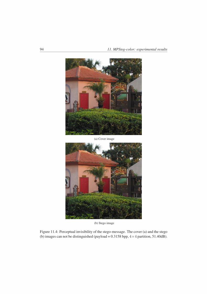
94 11. MPSteg-color: experimental results
(a) Cover image
(b) Stego image
Figure 11.4: Perceptual invisibility of the stego-message. The cover (a) and the stego(b) images can not be distinguished (payload = 0.3158 bpp, 4×4 partition, 51.40dB).
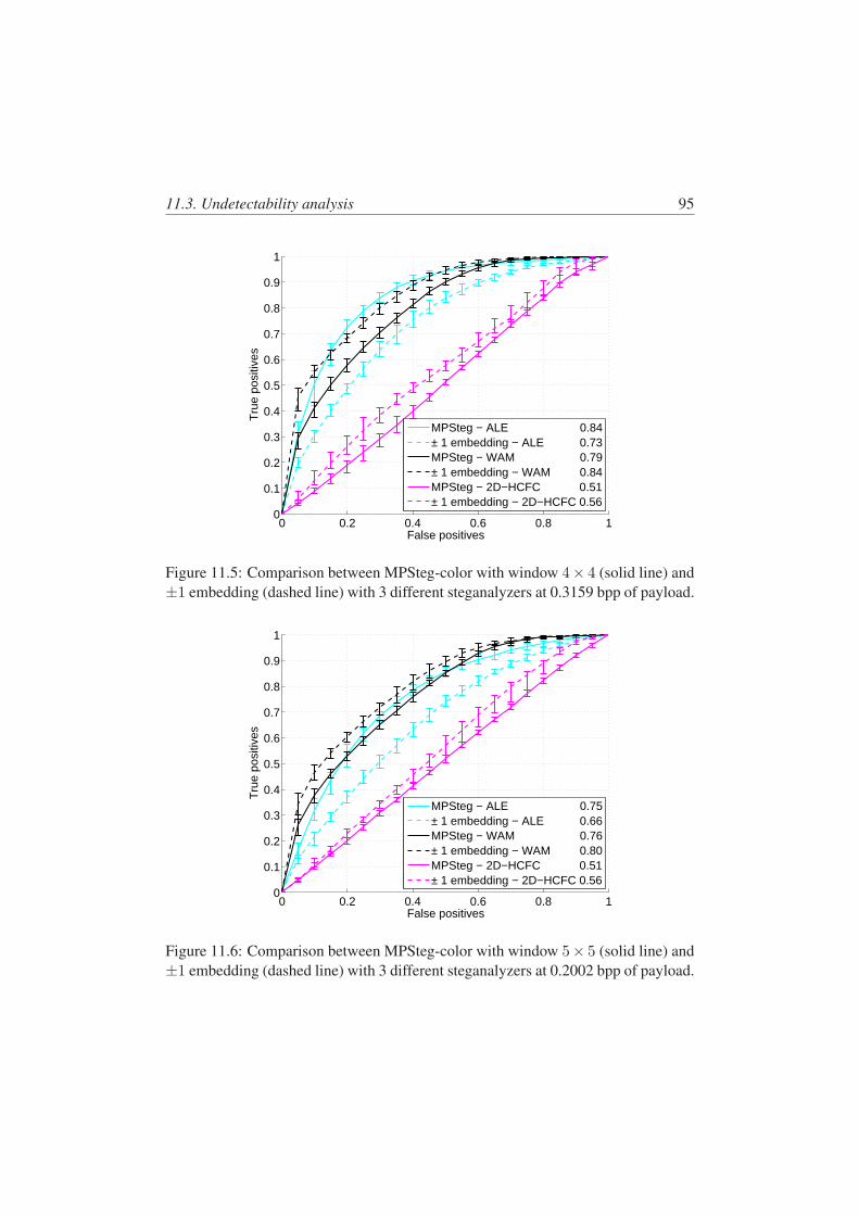
11.3. Undetectability analysis 95
0 0.2 0.4 0.6 0.8 10
0.1
0.2
0.3
0.4
0.5
0.6
0.7
0.8
0.9
1
False positives
Tru
e po
sitiv
es
MPSteg − ALE 0.84± 1 embedding − ALE 0.73MPSteg − WAM 0.79± 1 embedding − WAM 0.84MPSteg − 2D−HCFC 0.51± 1 embedding − 2D−HCFC 0.56
Figure 11.5: Comparison between MPSteg-color with window 4× 4 (solid line) and±1 embedding (dashed line) with 3 different steganalyzers at 0.3159 bpp of payload.
0 0.2 0.4 0.6 0.8 10
0.1
0.2
0.3
0.4
0.5
0.6
0.7
0.8
0.9
1
False positives
Tru
e po
sitiv
es
MPSteg − ALE 0.75± 1 embedding − ALE 0.66MPSteg − WAM 0.76± 1 embedding − WAM 0.80MPSteg − 2D−HCFC 0.51± 1 embedding − 2D−HCFC 0.56
Figure 11.6: Comparison between MPSteg-color with window 5× 5 (solid line) and±1 embedding (dashed line) with 3 different steganalyzers at 0.2002 bpp of payload.
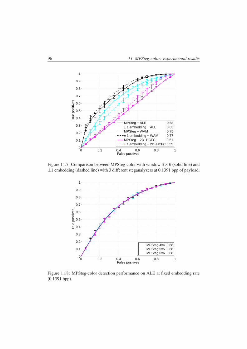
96 11. MPSteg-color: experimental results
0 0.2 0.4 0.6 0.8 10
0.1
0.2
0.3
0.4
0.5
0.6
0.7
0.8
0.9
1
False positives
Tru
e po
sitiv
es
MPSteg − ALE 0.68± 1 embedding − ALE 0.63MPSteg − WAM 0.75± 1 embedding − WAM 0.77MPSteg − 2D−HCFC 0.51± 1 embedding − 2D−HCFC 0.55
Figure 11.7: Comparison between MPSteg-color with window 6× 6 (solid line) and±1 embedding (dashed line) with 3 different steganalyzers at 0.1391 bpp of payload.
0 0.2 0.4 0.6 0.8 10
0.1
0.2
0.3
0.4
0.5
0.6
0.7
0.8
0.9
1
False positives
Tru
e po
sitiv
es
MPSteg 4x4 0.68MPSteg 5x5 0.68MPSteg 6x6 0.68
Figure 11.8: MPSteg-color detection performance on ALE at fixed embedding rate(0.1391 bpp).
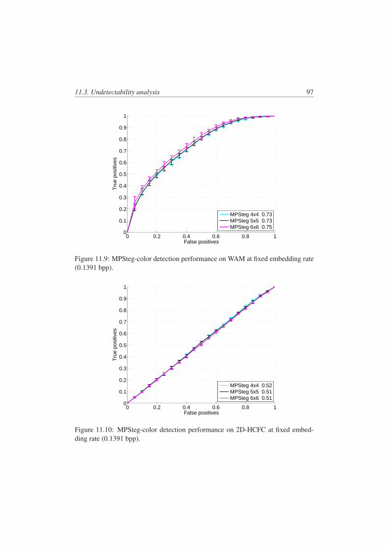
11.3. Undetectability analysis 97
0 0.2 0.4 0.6 0.8 10
0.1
0.2
0.3
0.4
0.5
0.6
0.7
0.8
0.9
1
False positives
Tru
e po
sitiv
es
MPSteg 4x4 0.73MPSteg 5x5 0.73MPSteg 6x6 0.75
Figure 11.9: MPSteg-color detection performance on WAM at fixed embedding rate(0.1391 bpp).
0 0.2 0.4 0.6 0.8 10
0.1
0.2
0.3
0.4
0.5
0.6
0.7
0.8
0.9
1
False positives
Tru
e po
sitiv
es
MPSteg 4x4 0.52MPSteg 5x5 0.51MPSteg 6x6 0.51
Figure 11.10: MPSteg-color detection performance on 2D-HCFC at fixed embed-ding rate (0.1391 bpp).

Chapter 12MPSteg-color: remarks and future works
In the second part of the thesis a new algorithm for embedding a stego-messageinto color images represented by means of high redundant basis decomposition hasbeen presented. The problems of previous schemes proposed in this sense have beensolved, with particular attention to undetectability against targeted steganalyzers.
Indeed, we have shown that without proper countermeasures, messages hidden inthe MP domain are easily detectable.
The undetectability of MPSteg-color has been extensively tested against bothtargeted and general purpose steganalyzers, showing the validity of the proposed ap-proach. In particular, the good hiding properties of the MP domain are demonstratedby comparing the undetectability of a±1 embedding message embedded in the pixel
with that of a ±1 embedding message embedded in the MP domain, with the latterbeing less detectable than the former despite a higher embedding distortion.
Further experimental investigations are needed in order to apply the full method-ology benchmark proposed in the first part of the thesis. Actually, we have not beenable to build a full MPSteg-color dataset with several payloads, due to the computa-tional complexity of the proposed technique.
Some further studies can consider the role of the dictionary, by analyzing the un-detectability dependence on the used atoms in order to design a powerful dictionarywhich is more able to make MPSteg-color undetectable. By enlarging the cardinalityof the dictionary, we could also study a randomized dictionary, i.e. a subset of a verybig dictionary, which can be unknown to the steganalyzer. In fact, a weakness ofMPSteg-color is that the steganalyzer knows the dictionary in which the message is
embedded and this fact can help in the design of a targeted method.
Another weakness of the proposed approach is that we are loosing one band just

100 12. MPSteg-color: remarks and future works
to correctly recover the decomposition path. In this way we lose about 1/3 of coeffi-cients which cannot be used as embedding support and the MPSteg-color maximumpayload goes down. As future works it could be possible to develop a new schemewith a blind decomposition path recovery or by embedding the message within theatom indexes instead of the atom weights. In this scenario, a great attention shouldbe given to synchronizing problems.
A few additional improvements of the proposed scheme are possible, either to
augment the payload or diminish the detectability. Specifically, the wet paper codingapproach may be applied to remove the constraint that message embedding cannotproduce zero coefficients, and matrix embedding can be applied to decrease the em-bedding distortion.
Chapter 13
Final remarks
In this thesis we have taken into account steganography and steganalysis in thepixel domain. Pixel domain steganography has been deeply investigated by manyresearch groups the last ten years so we can consider it as a rather mature field.
Several application scenarios could be interested to use either steganographies orsteganalysis techniques for digital images especially thanks to the widest connectioninfrastructure: Internet. Even though steganography is usually linked to malevolentapplications such as industrial espionage or coordination between terroristic cellsand steganalysis as a benevolent tool thought to reinforce homeland security, theseare not the unique application scenarios. For example in countries suffering frommilitary dictatorship, steganography can be seen as the only way of ensuring free-dom of speech while steganalysis becomes a tool to limit this freedom. We can saythat steganography and steganalysis need each other to avoid the supremacy of theadversary and for this reason research has lately been directed towards the investiga-tion of the ultimate limits of these techniques [45].
Today several steganographic and steganalysis methods ensure good results es-pecially in controlled scenarios with fixed payload, image sources, and image sizes
but they usually do not extend these good performance to practical case. Moreover,in the literature the performance of steganographic techniques are rarely based on atest set never analyzed by the classifier. In the last years, to obtain undetectabilitythe steganographic methods have been mainly concerned with the minimization ofembedding changes, but this methodology is not the unique possible strategy andresearchers should investigate other strategies as well.
In the above framework, the contribution of this thesis is threefold. The firstone is a new ±1 embedding steganalyzer, called ALE, which is able to detect ±1
102 13. Final remarks
embedding artifacts. The second one is the proposal of a comparison methodology tobe applied to fairly benchmark the merits and drawbacks of different steganalyzers.Finally, the last one is a new steganographic method, called MPSteg-color whichshows how embedding the hidden message at a higher semantic level could resultin a less detectable stego message than a strategy that minimizes the embeddingchanges without takes into account the embedding domain.
The first part of the thesis focuses on the importance of reproducible researchin terms of performance validation and weakness analysis. A lot of works describesteganography and steganalysis tools in a good way, however the reader has alwaysdifficulties to implement again these tools especially because the experimental re-sults are not obtained by using a standard procedure. We have shown in this thesisthat a proper design of the image database is a crucial path to obtain reproducibleresults. Moreover, recent studies [25] show that by fixing the payload, the resultschange through a square root law depending on image size and could be interesting
to extend our analysis by taking into account the image size.
Our analysis has also shown that when a steganalyzer does not know the payload,its performance in terms of AUC are far from those obtained in the best case in whichthey are known and this fact constitutes a big weakness of the current state of art. Inpractical applications, in fact, a steganalysis system can check the image size, andby using a forensic tool it can get information about the image sources (camera orscanner), but it never knows the message length.
Besides, we have shown that concatenating good features in a new steganalyzer,as hybrid steganalyzers do, it is usually a good way to improve performances, butif we do not know the practical scenario, i.e. the steganalyzer is trained with atrain set which is very different than the future test set, the concatenation may notbe the best strategy: it just increases the classification uncertainty. The ALE, thesteganalyzer proposed in this thesis, seems to be more stable in terms of overallAUC performances than WAM, which is the current state of art steganalyzer in the
pixel domain thanks to the low number of features it uses which are about one thirdof those used by WAM.
In the second part of this thesis we considered the steganography point of view
103
by showing that the weakness of steganalyzers could be used by steganographers todevelop more efficient and secure techniques. Specifically, we have proposed a newtechnique based on high redundant basis decomposition that shows how a embed-ding the message at a higher semantic level could result in a less undetectable stegomessage, when the steganalyzer is based on high-order statistics analysis. Of course,the proposed technique is just a prototype, however it clearly shows that embeddingmessages at a more semantic level could be a good way to achieve undetectability.
In the future, we could extend our research by fully analyzing the MP embeddingdomain, especially by investigating the relationship between detectability and thedesign and cardinality of the dictionary.

Bibliography
[1] M. Kharrazi, H. Sencar, and N. Memon, “Image Steganography: Concepts and Prac-tice,” Lecture Note Series, Institute for Mathematical Sciences, National University ofSingapore, 2004.
[2] I. Cox, T. Kalker, G. Pakura, and M. Scheel, “Information transmission and steganog-raphy,” Lecture Notes in Computer Science, vol. 3710, p. 15, 2005.
[3] C. Shannon, “Communication Theory of Secrecy Systems,” Bell System technical Jour-nal, vol. 28, pp. 656–715, 1954.
[4] G. J. Simmons, “The prisoners’ problem and the subliminal channel,” in Advances inCryptology: Proceedings of CRYPTO’83. Plenum Pub Corp, 1984, pp. 51–67.
[5] R. Givner-Forbes, “Steganography: Information Technology in the Service of Jihad,”The international Centre for Political Violence and Terrorism Research, March 2007.[Online]. Available: www.pvtr.org
[6] R. Anderson, “Stretching the limits of steganography,” Lecture Notes in Computer Sci-ence, vol. 1174, pp. 39–48, 1996.
[7] WikipediA The Free Encyclopedia. [Online]. Available:http://en.wikipedia.org/wiki/Printer_steganography
[8] G. Cancelli and M. Barni, “MPSteg-color: A new steganographic technique for colorimages,” Information Hiding: 9th International Workshop, Ih 2007, Saint Malo,France, June 11-13, vol. 4567, pp. 1–15, 2007.
106 BIBLIOGRAPHY
[9] A. Westfeld, “F5-a steganographic algorithm: High capacity despite better steganal-ysis,” in Information Hiding: 4th International Workshop, IH 2001, Pittsburgh, PA,USA, April 25-27, 2001: Proceedings. Springer, 2001, p. 289.
[10] M. Goljan, J. Fridrich, and T. Holotyak, “New blind steganalysis and its implications,”Proceedings of SPIE, vol. 6072, pp. 1–13, 2006.
[11] J. Fridrich, M. Goljan, P. Lisonek, and D. Soukal, “Writing on wet paper,” IEEE Trans-actions on Signal Processing, vol. 53, no. 10 Part 2, pp. 3923–3935, 2005.
[12] J. Fridrich, M. Goljan, and D. Hogea, “Attacking the outguess,” in Proc. of the ACMWorkshop on Multimedia and Security, 2002.
[13] P. Sallee, “Model-based methods for steganography and steganalysis,” InternationalJournal of Image and Graphics, vol. 5, no. 1, pp. 167–189, 2005.
[14] J. Fridrich, T. Pevny, and J. Kodovsky, “Statistically undetectable jpeg steganography:dead ends challenges, and opportunities,” in Proceedings of the 9th workshop on Mul-timedia & security. ACM New York, NY, USA, 2007, pp. 3–14.
[15] B. Roue and J. Chassery, “Improving LSB steganalysis using marginal and joint prob-abilistic distributions,” in Proceedings of the 2004 workshop on Multimedia and secu-rity. ACM New York, NY, USA, 2004, pp. 75–80.
[16] S. Dumitrescu, X. Wu, and Z. Wang, “Detection of LSB steganography via samplepair analysis,” IEEE transactions on Signal Processing, vol. 51, no. 7, pp. 1995–2007,2003.
[17] J. Fridrich and M. Long, “Steganalysis of LSB encoding in color images,” in 2000IEEE International Conference on Multimedia and Expo, 2000. ICME 2000, vol. 3,2000.
[18] A. Ker, “Quantitative evaluation of pairs and RS steganalysis,” Security, Steganogra-phy, and Watermarking of Multimedia Contents VI, vol. 5306, pp. 83–97, 2004.
[19] P. Lu, X. Luo, Q. Tang, and L. Shen, “An improved sample pairs method for detectionof LSB embedding,” in Proc. 6th Information Hiding Workshop, vol. 3200. Springer,2004, pp. 116–127.
[20] S. Lyu and H. Farid, “Steganalysis using higher-order image statistics,” IEEE Transac-tions on Information Forensics and Security, vol. 1, no. 1, pp. 111–119, 2006.
BIBLIOGRAPHY 107
[21] R. Bohme and A. Westfeld, “Exploiting preserved statistics for steganalysis,” in SixthWorkshop on Information Hiding, Toronto, Canada (2004, May). Springer, 2004.
[22] J. Fridrich, M. Goljan, D. Hogea, and D. Soukal, “Quantitative steganalysis of digitalimages: estimating the secret message length,” Multimedia Systems, vol. 9, no. 3, pp.288–302, 2003.
[23] A. D. Ker, “Steganalysis of LSB matching in grayscale images,” IEEE Signal Process-ing Letters, vol. 12, no. 6, pp. 441–444, 2005.
[24] A. Ker, T. Pevny, J. Kodovsky, and J. Fridrich, “The square root law of steganographiccapacity,” in Proceedings of the 10th ACM workshop on Multimedia and security.ACM New York, NY, USA, 2008, pp. 107–116.
[25] T. Filler, A. Ker, and J. Fridrich, “The square root law of steganographic capacity forMarkov covers,” in Proceedings of SPIE, vol. 7254, 2009, p. 725408.
[26] J. Zhang, I. J. Cox, and G. Doërr, “Steganalysis for LSB Matching in images withhigh-frequency noise,” IEEE 9th Workshop on Multimedia Signal Processing (MMSP),2007, pp. 385–388, 2007.
[27] R. Duda, P. Hart, and D. Stork, Pattern classification. Wiley-Interscience, 2000.
[28] I. J. Cox, M. Miller, J. Bloom, J. Fridrich, and T. Kalker, Digital watermarking andsteganography. Morgan Kaufmann, 2007.
[29] M. Tran, “Thai police name suspected web paedophile,” The Gardian, October 2007.
[30] T. Pevny and J. Fridrich, “Novelty detection in blind steganalysis,” in Proceedings ofthe 10th ACM workshop on Multimedia and security. ACM New York, NY, USA,2008, pp. 167–176.
[31] T. Fawcett, “ROC graphs: Notes and practical considerations for researchers,” Techni-cal Report HPL-2003-4, 2003.
[32] L. Breiman, Classification and Regression Trees. Chapman & Hall/CRC, 1998.
[33] M. Goljan, J. Fridrich, and T. Soukal, “Higher-order statistical steganalysis of paletteimages,” Proceedings of SPIE, vol. 5020, pp. 178–190, 2003.
[34] O. Dabeer, K. Sullivan, U. Madhow, S. Chandrasekaran, and B. S. Manjunath, “De-tection of hiding in the least significant bit,” IEEE Transactions on Signal Processing,vol. 52, no. 10, pp. 3046–3058, October 2004.
108 BIBLIOGRAPHY
[35] A. D. Ker, “A general framework for structural analysis of LSB replacement,” Pro-ceedings of the 7th Information Hiding Workshop, LNCS, vol. 3727, pp. 296–311, June2005.
[36] J. Harmsen, “Steganalysis of additive noise modelable information hiding,” Ph.D. dis-sertation, Ph.d. thesis at Rensselaer Polytechnic Institute, 2003.
[37] G. Cancelli, G. Doerr, I. J. Cox, and M. Barni, “Detection of ±1 LSB steganographybased on the amplitude of histogram local extrema,” in Image Processing, 2008. ICIP2008. 15th IEEE International Conference on, 2008, pp. 1288–1291.
[38] U. S. D. of Agriculture, “Natural Resources Conservation Service photo gallery,”2002. [Online]. Available: http://photogallery.nrcs.usda.gov
[39] C. Corporation, “Corel Stock Photo Library 3,” Ontario, Canada.
[40] G. Cancelli, G. Doërr, M. Barni, and I. J. Cox, “A comparative study of±1 steganalyz-ers,” Multimedia Signal Processing, 2008 IEEE 10th Workshop on, pp. 791–796, Oct.2008.
[41] G. Cancelli, G. Doërr, M. Barni, and I. J. Cox, “Comparing steganalyzers: A case studywith ±1 steganography,” IEEE Transactions on Information Forensics and Security,vol. submitted for publication, 2009.
[42] F. Petitcolas, R. Anderson, and M. Kuhn, “Attacks on copyright marking systems,” inProceedings of the Second International Workshop on Information Hiding. Springer,1998, pp. 218–238.
[43] G. Doërr, “Image database for steganalysis studies.” [Online]. Available:http://www.adastral.ucl.ac.uk/ gwendoer/steganalysis
[44] J. Fridrich, “Feature-based steganalysis for JPEG images and its implications for futuredesign of steganographic schemes,” in Information Hiding, 6th International Work-shop, vol. 3200. Springer, 2004, pp. 67–81.
[45] T. Pevny, J. Fridrich, and A. Ker, “From blind to quantitative steganalysis,” in Proceed-ings of SPIE, vol. 7254, 2009, p. 72540C.
[46] C. Liu and S. Liao, “High-performance JPEG steganography using complementaryembedding strategy,” Pattern Recognition, 2008.
[47] M. Kharrazi, H. Sencar, N. Memon et al., “Benchmarking steganographic and steganal-ysis techniques,” EI SPIE San Jose, CA, 2005.
BIBLIOGRAPHY 109
[48] D. Lou, C. Liu, and C. Lin, “Message estimation for universal steganalysis using multi-classification support vector machine,” Computer Standards & Interfaces, vol. 31,no. 2, pp. 420–427, 2009.
[49] T. Pevny and J. Fridrich, “Towards multi-class blind steganalyzer for JPEG images,”Lecture notes in computer science, vol. 3710, p. 39, 2005.
[50] T. Pevny and J. Fridrich, “Merging Markov and DCT features for multi-class JPEGsteganalysis,” IS&T/SPIE EI, vol. 6505, 2007.
[51] T. Pevny and J. Fridrich, “Multiclass Detector of Current Steganographic Methods forJPEG Format,” IEEE Transactions on Information Forensics and Security, vol. 3, no. 4,pp. 635–650, 2008.
[52] Y. Miche, P. Bas, A. Lendasse, C. Jutten, and O. Simula, “Reliable Steganalysis Usinga Minimum Set of Samples and Features,” EURASIP Journal on Information Security,2009.
[53] C. Jutten and O. Simula, “Advantages of Using Feature Selection Techniques on Ste-ganalysis Schemes,” in Computational and Ambient Intelligence 9th InternationalWork-Conference on Artificial Neural Networks, IWANN 2007, San Sebastian, Spain,June 20-22, 2007: Proceedings. Springer, 2007, p. 606.
[54] Y. Miche, B. Roue, A. Lendasse, and P. Bas, “A feature selection methodology forsteganalysis,” Lecture Notes in Computer Science, vol. 4105, p. 49, 2006.
[55] P. Vandergheynst and P. Frossard, “Image coding using redundant dictionaries,” Docu-ment And Image Compression, p. 207, 2006.
[56] R. i Ventura, P. Vandergheynst, and P. Frossard, “Low-rate and flexible image cod-ing with redundant representations,” IEEE Transactions on Image Processing, vol. 15,no. 3, 2006.
[57] G. Cancelli, M. Barni, and G. Menegaz, “Mpsteg: hiding a message in the matchingpursuit domain,” in Proceedings of SPIE, vol. 6072, 2006, p. 60720P.
[58] T. Hien, I. Kei, H. Harak, Y. Chen, Y. Nagata, and Z. Nakao, “Curvelet-Domain ImageWatermarking Based on Edge-Embedding,” Lecture Notes in Computer Science, vol.4693, p. 311, 2007.
[59] S. Lee, C. Yoo, and T. Kalker, “Reversible image watermarking based on integer-to-integer wavelet transform,” IEEE Transactions on Information Forensics and Security,vol. 2, no. 3 Part 1, pp. 321–330, 2007.
110 BIBLIOGRAPHY
[60] X. Zhang and K. Li, “Comments on" An SVD-based watermarking scheme for protect-ing rightful Ownership,” IEEE Transactions on Multimedia, vol. 7, no. 3, pp. 593–594,2005.
[61] S. Mallat and Z. Zhang, “Matching pursuit with time-frequency dictionaries,” IEEETransactions on Signal Processing, vol. 41, no. 12, pp. 3397–3415, 1993.
[62] P. Jost, P. Vandergheynst, and P. Frossard, “Redundant image representations in secu-rity applications,” International Conference on Image Processing (ICIP), 2004, vol. 4,2004.
[63] K. Solanki, A. Sarkar, and B. Manjunath, “YASS: yet another steganographic schemethat resists blind steganalysis,” Information Hiding: 9th International Workshop, IH2007, Saint Malo, France, June 11-13, vol. 4567, pp. 16–31, 2007.
[64] Z. Fan and R. de Queiroz, “Identification of bitmap compression history: JPEG detec-tion and quantizer estimation,” IEEE Transactions on Image Processing, vol. 12, no. 2,pp. 230–235, 2003.