1
Final Report
On the
Implementation of Image Processing Techniques for Target Detecting Robot using OpenCV
Project Supervisor
Dr. Haroon Attique Babri
Submitted By Jahanzeb Nasir 05-Elect-37
M. Usman Saeed 05-Elect-35
M. Mohsin Butt 05-Elect-40
M. Basit Shahab 05-Elect-294
Department Of Electrical Engineering
University Of Engineering And Technology
Lahore.
i
ABSTRACT
Digital Image Processing is one of the many fields that have seen large enhancements in
recent years. Applications ranging from home security cameras to military grade search bots,
cameras to ultra high resolution spectroscopes and what not are some of the application where
DIP is used. The purpose of this project was dual- faceted: educational and also to devise some
method other than what students normally use. MATLAB, with its two immensely popular
toolboxes naming “Data Acquisition Toolbox” and “Image Processing Toolbox” is the
conventional Image Processing tool being used now-a-days. We tried to use some other method
and after a lot of research, we found another tool “OpenCV”. So, in the project we used OpenCV
libraries and functions to perform the Image Processing.
The following report begins with the most basic information about Image Processing
System. The project consisted of three phases. First part was to design a base for the robot and
the interesting part about the base, well actually about the robot is that it was completely made
from wooden scales. The second part was to test the camera on PC and devise the algorithm for
Image Processing. The Image Processing process includes capturing frames, detecting the object
and then telling the robot where the object actually is. The final part was to design the complete
circuitry for the robot and its interface with the PC.
2
TABLE OF CONTENTS
Abstract…………………………………………………………..1
Table of Content………………………………………………....2
List of Figures…………………………………………………....4
Acknowledgements……………………………………………....5
Dedication………...……………………………………………....6
Project Overview…………………………………………………7
1.1 Basic Idea………………………………………………………………...7 1.2 Design Goals……………………………………………………………..7 1.3 Design Parameters for the Robot………………………………………...7
1.4 Design Phases…………………………………………………………….8 1.4.1 Design of Robot structure…………………………………....8
1.4.2 Image Processing……………………………………………..8 1.4.2 Control of the Robot…………………………………………..8
1.5 Report content………………………………………………………....8
Design of Robotic Structure……………………………………10
2.1 Basic Design…………………………………………………………….10 2.2 Arm Design…………………………………………………………......11 2.3 Complete Robotic Structure Design…………………………………….12
2.3.1 Rear Motor Assembly……………………………………......12 2.3.2 Front Motor Assembly……………………………………….13
2.3.3 Arm Motor Assembly……………………………………......13 2.4 Changes made at the final moments……………………………………13
Digital Image Processing………………………………………14
3.1 Digital Image Processing………………………………………………..14 3.2 Image Processing Fundamentals…………………………………….....14 3.2.1 CCD Camera…………………………………………………15
3.2.1.1 Image Sensor in a CCD Camera………………..15 3.2.2 The video Norm……………………………………………...15
3.2.2.1 The Interlace process…………………………...16
3.2.3 Color Camera………………………………………………...16
3.2.3.1 Single chip color cameras……………………….16
3.2.3.2 Three chip color cameras……………………….17
3
\ 3.3 What is Color?...........................................................................................17 3.4 Color management and Color transformation……………………………18
3.5 Color Spaces…………………………………………………………......18 3.5.1 RGB Color space……………………………………………18
3.5.2 Grayscale Color Space……………………………………...19 3.5.2.1 Converting Color Image to Grayscale…………..19 3.5.3 CIEL*a*b* Color space…………………………………….20
3.5.3.1 RGB and CMYK conversions to LAB………….21 3.5.3.2 Range of L*a*b* coordinates……………...….…21
3.6 Steps involved in Digital Image Processing……………………….……21 3.6.1 Capture the image……………………………………….….21 3.6.2 Color space Transformation……………………………......21
3.6.3 Color extraction……………………………………..……...21 \ 3.6.4 Identify an object of specific shape………………………...22
3.7 MATLAB as Image Processing Tool……………..……………………..22 3.7.1 Capture the image………………………………….………22 3.7.2 Color space Transformation………………………………..23
3.7.3 Color extraction…………………………………….………23 3.7.4 Identify an object of specific shape………………………..23
3.8 Open CV as Image Processing Tool………………………………..…...23 3.8.1 Capture the image……………………………………….…24 3.8.2 Color space Transformation……………………………….24
3.8.3 Color extraction……………………………………………24 3.8.4 Identify an object of specific shape……………………….25
Open CV as Image Processing Tool…………………………..26
4.1 Introduction……………………………………………………………..26 4.2 Why Open CV…………………………………………………………..26
4.3 Integrating Open CV with Microsoft Visual C++ 6.0…………………26 4.3.1 Setting up the system PATH environmental variable……….27
4.3.2 Specifying Directories in Visual C++ 6.0………………….27 4.3.3 Setting for new Projects in Microsoft Visual C++ 6.0…….27 4.4 Important Data types and Functions Used ……………………………..27
4.4.1 IPL Image Data Structure……………………………….....28 4.4.2 cvCvtColor………………………………………………..…..30
4.4.3 Memory Storage……………………………………………...30 4.4.3.1 cvSeq Sequence………………………………....31
4.5 Accessing Image Elements……………………………………………....32
4.5.1Direct access using a pointer…………………………………....33 4.6 Displaying Images……………………………………………………….33
4.7 Video I/O………………………………………………………………....36 4.7.1 CvCapture……………………………………………………...36 4.7.2 Capturing Frames……………………………………………....36
4.8 Circular Hough Transform……………………………………………….36 4.8.1 Parametric Representations……………………………………..37
4
4.8.2 Accumulator…………………………………………………….38 4.8.3 Circular Hough Transform Algorithm………………………….39
4.8.4 CHT in OpenCV………………………………………………..40
4.9 The Ball detection and retrieval algorithm……………………………….41
Control System Design………………………………………..46 5.1 Introduction…………………………………………………………….46
5.2 Algorithm Consideration……………………………………………….46 5.3 Control Simulation……………………………………………………...47
5.4 Control Code…………………………………………………………....49
Future Recommendations…………………………………….50 6.1 Circular Hough Transform Hardware……………………………………50 6.2 UART Interface…………………………………………………………51 6.3 Sobel Module……………………………………………………………51
6.4 Laplace Filtering…………………………………………………………52 6.5 Compact Module………………………………………………………....52
6.6 Circle Module…………………………………………………………….52 6.7 Draw Module……………………………………………………………..52
Appendix A-Matlab Code……………………………………...53
Appendix B-OpenCV Code…………………………………….56
Appendix C-Datasheets……………………………………...…70
Refrences………………………………………………………...
5
LIST OF FIGURES
Figure Title Page
2.1 Base Design ………………………………………………………….................10 2.2 Arm Design…...……………………………………………………....................11
2.3 Complete Robot Design………………………………………………................12 3.1 Image Processing System………….…………………………………................14 3.2 Interlace Process: two fields make a frame…………………………...…….......16
3.3 Image Produced by one chip camera…………………………............................17 3.4 Incoming light is divided into its basic components……………………………17
3.5 color images & their corresponding grayscale.....………………………………19 3.6 L*a*b* Color Space………………………………………………….................20 4.1 Input Image……………………………………………………………………..42
4.2 Multiple Circle Detection………………………………………………………42 4.3 Red Color Detection……………………………………………………………43
4.4 Blue Color Detection…………………………………………………………...43 4.5 Green Color Detection………………………………………………………….44 4.6 Input Image to Function and Output Image…………………………………….44
5.1 Control of DC Motor……………………………………………………...…….47 5.2 Control of Stepper Motor………………………………………………………47
5.3 Microcontroller Circuit………………………………………………………...48 5.4 Power Supply Unit……………………………………………………………...48 5.5 Serial Port Circuit..……………………………………………………………...49
6.1 Block Diagram of System………………………………………………………51

vi
ACKNOWLEDGEMENTS
We would like to thank all our teachers who taught us at UET because it was just because
of their efforts, we succeeded in achieving our goal.
Special thanks to the advisor, Dr. Haroon Attique Babri for his indispensable advice at
the most crucial steps of the project.
Many thanks to Sir Fahad Zubair, for he was there whenever we needed him. He was
very much helpful in the project and it would be a remiss if we don‟t mention that actually the
whole project was his idea. We wish him Good luck for his future plans.
Last, but not the least, we would like to thank Sir Asif Rehmat for his expertise and
helping us set the direction of the project.
Sincerely,
The Project Team.
7
DEDICATION
We dedicate this project to our Parents and Teachers for it is just because of their
prayers that we were able to complete our goals.
8
PROJECT OVERVIEW
1.1 Basic Idea
The idea behind the project was to develop a robot that can assist in search and
retrieval of a specified object. For that, we decided to set up a game plan for the robot
where there will be balls of different colors and the robot will search and retrieve a ball of
specific color. The searching part was done using a webcam that was interfaced to PC
serially. The retrieval process start once the ball is found.
1.2 Design Goals
Most of the robots that are being built now-a-days have metallic body. That
makes the robot heavy and if not that, expensive and difficult to design. So the first goal
was to come up with a new design and the idea that came up was to use only wooden
scales. The goal was to make the robot strong enough to carry all the motors, battery and
other stuff and on the other hand it should be lighter than the robots having metallic body.
After processing the image on PC, the second goal was to establish a serial link
between the robot and PC that will tell the robot when and where the ball actually is.
1.3 Design Parameters for the Robot
At the kick-off meeting, we decided how the project would be approached. At
this meeting, we decided several general design goals based on what has already been
done on such kind of project. By reviewing the pros and cons of the previous attempts
that were made to construct a robot with Image Processing capability, we finalized our
design goals and started work on finalized design.
The design goals of the robot were to reduce the cost and weight of the robot and
to devise an optimized method for the arm that will pick up the ball. Specific design
parameters are as follows:
2 degrees of freedom (1 for the arm, 1 for the gripper)
One DC motor for rear movement.

9
One bipolar stepper motor for front movement.
A single DC motor for both arm and gripper.
1.4 Design Phases
The whole design was divided in three phases.
1. Design of Robotic Structure.
2. Image Processing.
3. Control of the robot.
1.4.1 Design of Robotic Structure
The very first phase was to design the robotic structure. Like mentioned before,
the structure was made using wooden scales.
1.4.2 Image Processing
In this phase, we used a webcam to capture the image to the PC and then used
different image processing techniques to find the ball in the image. The image processing
tools used were OpenCV and MATLAB.
1.4.3 Control of the robot
This final phase was to implement a control circuitry on the robot which was
interfaced to the PC serially. After the ball is found, the PC sends a signal to the robot
about the location of the ball and then the robot works accordingly.
1.5 Report Contents
The report breakdown is outlined in the table of contents and list of figures. The
report moves forward in exact order of design phases. The first part consists of the
Robotic structure design. After that comes the Digital Image Processing chapter in which
basic concepts of DIP are explained. Also, this chapter includes an overview of our
methodology of performing Image Processing. Image Processing with the help of
MATLAB is explained and the code for frame extraction, color space transformation and
image segmentation is given in the appendix. After that the same procedure is explained
10
using OpenCV. Then comes the main chapter of “Image Processing Using OpenCV” in
which the image processing process is explained step by step. After that the “Design of
Control System” for the robot is explained. The appendices include code for Image
Processing using MATLAB, Image Processing using OpenCV and code for the control
circuit. The appendix also includes future recommendation for the project. The
information presented in the appendices is a supplement to this report, intended to aid
future designers who work on a similar robotic manipulator project (for example, use the
programs for design optimization).
11 | P a g e
Design of Robotic Structure
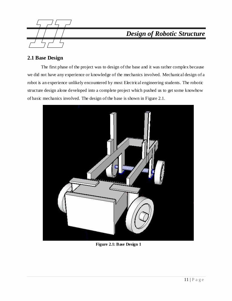
2.1 Base Design
The first phase of the project was to design of the base and it was rather complex because
we did not have any experience or knowledge of the mechanics involved. Mechanical design of a
robot is an experience unlikely encountered by most Electrical engineering students. The robotic
structure design alone developed into a complete project which pushed us to get some knowhow
of basic mechanics involved. The design of the base is shown in Figure 2.1.
Figure 2.1: Base Design 1
12 | P a g e
The base was designed keeping following factors in mind.
The base should be rigid enough to hold the motors and other stuff aboard.
The size of the base was designed so that it was large enough to accommodate everything
that was needed on board.
The front part was extended to accommodate the webcam.
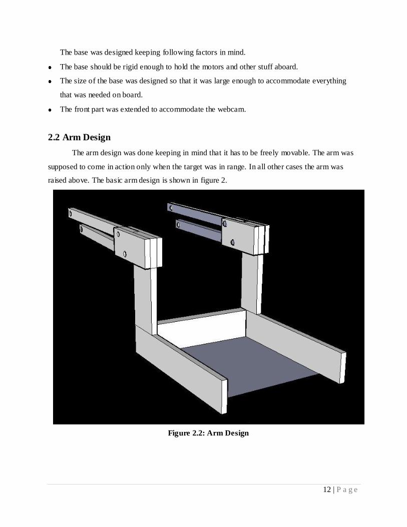
2.2 Arm Design
The arm design was done keeping in mind that it has to be freely movable. The arm was
supposed to come in action only when the target was in range. In all other cases the arm was
raised above. The basic arm design is shown in figure 2.
Figure 2.2: Arm Design
13 | P a g e
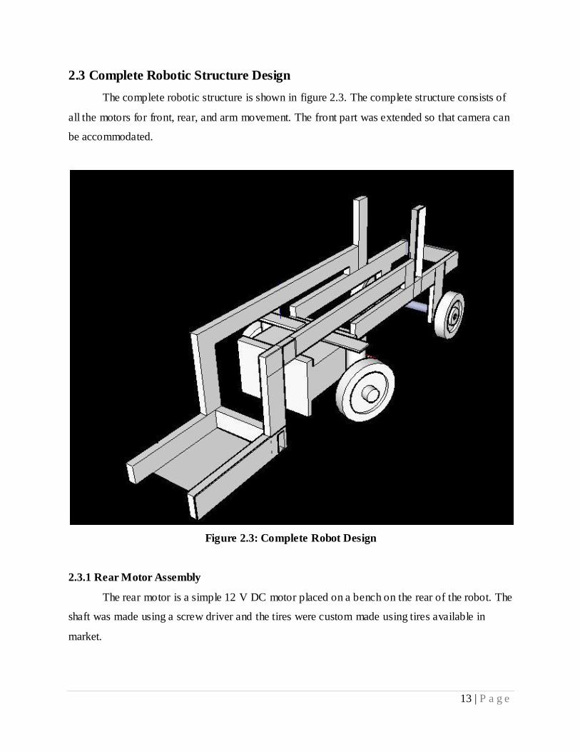
2.3 Complete Robotic Structure Design
The complete robotic structure is shown in figure 2.3. The complete structure consists of
all the motors for front, rear, and arm movement. The front part was extended so that camera can
be accommodated.
Figure 2.3: Complete Robot Design
2.3.1 Rear Motor Assembly
The rear motor is a simple 12 V DC motor placed on a bench on the rear of the robot. The
shaft was made using a screw driver and the tires were custom made using tires available in
market.
14 | P a g e
2.3.2 Front Motor assembly
The Front motor is a unipolar stepper motor with step size of 7.5 degree. The motor was
mounted on the wooden base. The front wheels turning capability is achieved using a rotary to
linear motion gear system.
2.3.3 Arm Motor Assembly
The arm motor is also placed on the base of the robot. It is a simple DC motor. The gears
attached have a very large gear ratio which helps the arm to retain its position and also helps it to
pick up large loads.
2.4 Changes made at the final moment
We had to do an important change in the arm at the final moment. The problem was that
when the designed arm was tested in actual environment, it was unable to hold the ball. So we
had to install some additional hardware for that. A door type arrangement was made. As we had
already accommodated three motors onboard, so we had to devise an arrangement such that only
one motor controls both the arm and the doors. The change made was that we add a pulley on the
top of the robot and the doors were pulled out by elastic bands. The doors were pulled in by a
wire which was pulled by the motor instead. So when the ball is in place and motor starts pulling
up, the doors close first and then the arm is raised.
15 | P a g e
Digital Image Processing
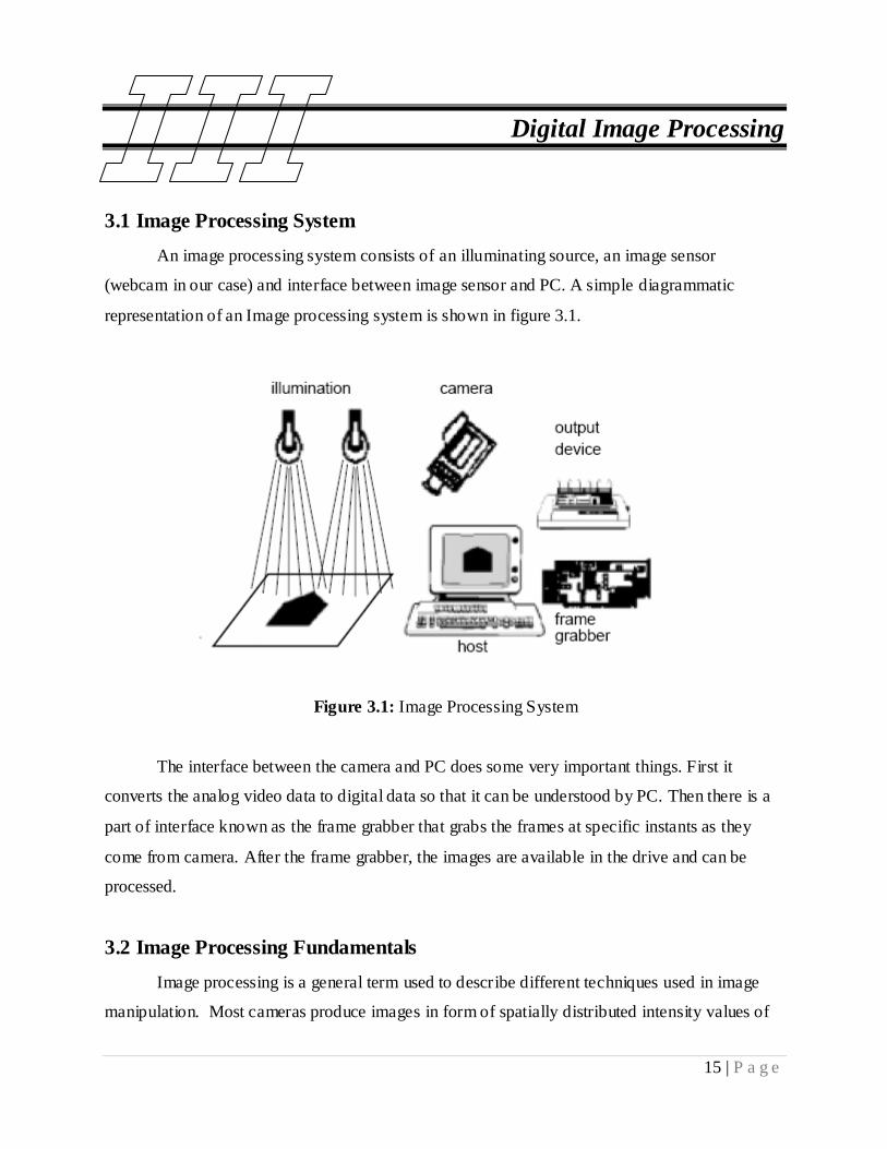
3.1 Image Processing System
An image processing system consists of an illuminating source, an image sensor
(webcam in our case) and interface between image sensor and PC. A simple diagrammatic
representation of an Image processing system is shown in figure 3.1.
Figure 3.1: Image Processing System
The interface between the camera and PC does some very important things. First it
converts the analog video data to digital data so that it can be understood by PC. Then there is a
part of interface known as the frame grabber that grabs the frames at specific instants as they
come from camera. After the frame grabber, the images are available in the drive and can be
processed.
3.2 Image Processing Fundamentals
Image processing is a general term used to describe different techniques used in image
manipulation. Most cameras produce images in form of spatially distributed intensity values of
16 | P a g e
electromagnetic radiations which can be digitized and stored in RAM. This helps in the
processing of the image.
Many image processing systems are used depending on the application used. They differ
in their acquisition principle, speed, resolution, sensor system and range.
Image sensors can be classified according to their sensitivity ranges. Electromagnetic
sensors for gamma radiation, X-rays, visual spectrum, infrared spectrum and radio wave
spectrum are available and are used in different applications.
3.2.1 CCD Cameras
In a film camera, a photo sensitive film is moved in front of the lens, exposed to light,
and then mechanically transposed to be stored in a film roll.
A CCD camera on the other hand has no mechanical parts. Incoming light falls on a CCD
(Charge Coupled Device) sensor which is actually a large number of light sensitive
semiconductors which we call “pixels”.
3.2.1.1 Image Sensor in a CCD Camera
Image sensor is the heart of a CCD camera. The physics behind the sensor is the inner
photo effect. This means that the incoming photons produce electrons in the semi-conductor
material, which are separated in the photo diode and are stored in a capacitor. This capacitor is
connected to the surrounding electrical circuit via a MOS transistor, which acts like a light
switch. If it opens, the charges will be collected by the capacitor (that explains the word
“integrated”) and will be transported when the switch is closed.
3.2.2 The Video Norm
Real time systems are usually based on video norms, which mean that the image
acquisition as well as the conversion of digital data into a video signal and vice versa have to
conform to international standards. In Europe, this norm is defined by the “Comite Consultaif
International des Radiocommunications (CCIR)”; in the USA, the norm is called RS-170
Standard and was defined by the Electronics Industries Association (EIA). The PAL (Phase
Alternation Line) and SECAM (Sequential Couleur a Memoire) color standards are based on
17 | P a g e
CCIR while the color system based on RS-170 is NTSC (National Television System
Committee).
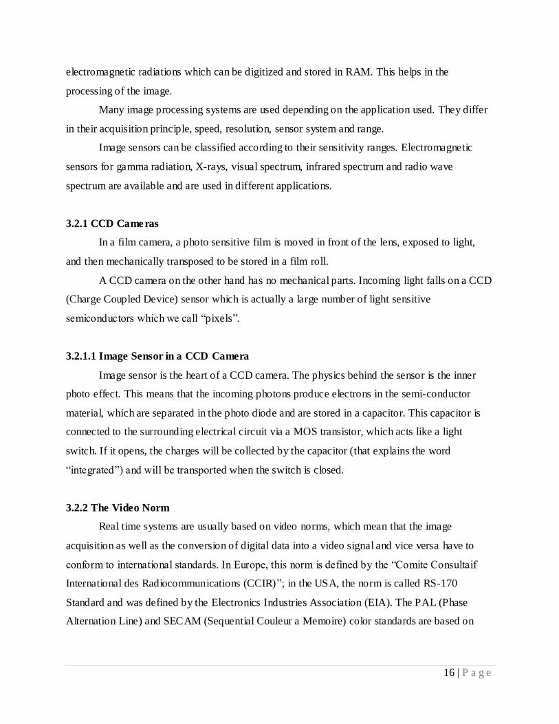
3.2.2.1 The Interlace Process
Both norms require a process which is required for the image on the screen to by non-
flickering. This is called the “Interlace Process”. The complete image (frame) is divided in two
half images (fields). One consists of the odd lines and the other consists of even lines of the
images. The interlace process is shown in figure 3.2
Figure 3.2: Interlace Process: two fields make a frame
3.2.3 Color Cameras
Color cameras produce a color image which consists of three parts: Red, green and blue.
By additive color mixture and intensity variations in the different parts, almost any color can be
produced.
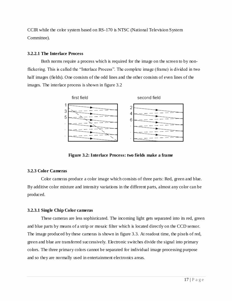
3.2.3.1 Single Chip Color cameras
These cameras are less sophisticated. The incoming light gets separated into its red, green
and blue parts by means of a strip or mosaic filter which is located directly on the CCD sensor.
The image produced by these cameras is shown in figure 3.3. At readout time, the pixels of red,
green and blue are transferred successively. Electronic switches divide the signal into primary
colors. The three primary colors cannot be separated for individual image processing purpose
and so they are normally used in entertainment electronics areas.
18 | P a g e
Figure 3.3: Image Produced by one chip camera
a) Mosaic filter
b) Stripe filter
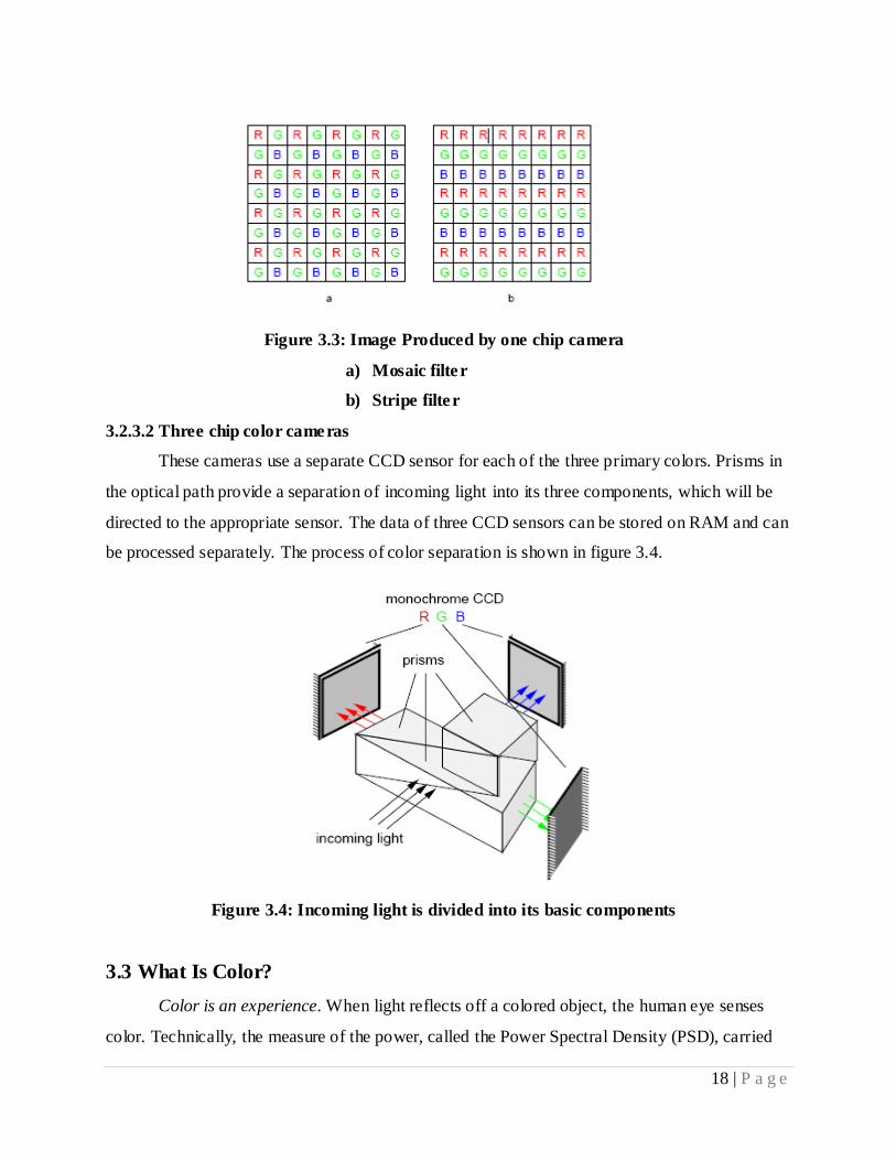
3.2.3.2 Three chip color cameras
These cameras use a separate CCD sensor for each of the three primary colors. Prisms in
the optical path provide a separation of incoming light into its three components, which will be
directed to the appropriate sensor. The data of three CCD sensors can be stored on RAM and can
be processed separately. The process of color separation is shown in figure 3.4.
Figure 3.4: Incoming light is divided into its basic components
3.3 What Is Color?
Color is an experience. When light reflects off a colored object, the human eye senses
color. Technically, the measure of the power, called the Power Spectral Density (PSD), carried
19 | P a g e
by each frequency or “color” in a light source (illuminant) and the colored object (colorant)
combine to produce reflected light with a particular PSD. This light interacts with the three types
of color-sensitive cones in the human eye to produce nerve impulses that the brain interprets as a
specific color.
Spectral color is useful for unambiguously describing a color, but it can be unwieldy for
describing large numbers of colors. It is much more common to use a color space transformation
that helps in getting device independent colors. In the case of RGB, the received images are
device-dependent combinations of red, green, and blue light. For color systems such as XYZ and
L*a*b* these images become device-independent and are modeled on aspects of the human
visual system.
3.4 Color Management and Color Transformations
Color management is an essential part of the image acquisition, image processing, and
image output workflow. Most cameras give images in RGB or YUV. So the color appearance
and format of pixels change if we change the camera. So we use color transformation to
transform the received color space in a known color space to make the received images device
independent.
3.5 Color Spaces
Some important color spaces like RGB, Grayscale and LAB are described below.
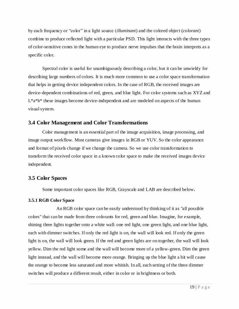
3.5.1 RGB Color Space
An RGB color space can be easily understood by thinking of it as "all possible
colors" that can be made from three colorants for red, green and blue. Imagine, for example,
shining three lights together onto a white wall: one red light, one green light, and one blue light,
each with dimmer switches. If only the red light is on, the wall will look red. If only the green
light is on, the wall will look green. If the red and green lights are on together, the wall will look
yellow. Dim the red light some and the wall will become more of a yellow-green. Dim the green
light instead, and the wall will become more orange. Bringing up the blue light a bit will cause
the orange to become less saturated and more whitish. In all, each setting of the three dimmer
switches will produce a different result, either in color or in brightness or both.
20 | P a g e
3.5.2 Grayscale Color Space
A grayscale image is an image in which the value of each pixel is a single sample, that is,
it carries only intensity information. Images of this sort, also known as black-and-white, are
composed exclusively of shades of gray, varying from black at the weakest intensity to white at
the strongest. Grayscale images are also called monochromatic, denoting the absence of any
chromatic variation.
3.5.2.1 Converting Color image to Grayscale
To convert any color to a grayscale representation of its luminance, first one must obtain
the values of its red, green, and blue (RGB) primaries in linear intensity encoding. Then, add
together 30% of the red value, 59% of the green value, and 11% of the blue value (these weights
depend on the exact choice of the RGB primaries, but are typical). Regardless of the scale
employed (0.0 to 1.0, 0 to 255, 0% to 100%, etc.), the resultant number is the desired linear
luminance value.
To convert a gray intensity value to RGB, simply set all the three primary color
components red, green and blue to the gray value, correcting to a different gamma if necessary.
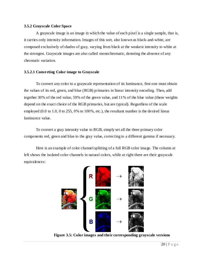
Here is an example of color channel splitting of a full RGB color image. The column at
left shows the isolated color channels in natural colors, while at right there are their grayscale
equivalences:
Figure 3.5: Color images and their corresponding grayscale versions
21 | P a g e
The reverse is also possible: to build a full color image from their separate grayscale
channels. By mangling channels, offsetting, rotating and other manipulations, artistic effects can
be achieved instead of accurately reproducing the original image.
3.5.3 CIE L*a*b* Color Space
CIE L*a*b* (CIELAB) is the most complete color space specified by the International
Commission on Illumination (Commission Internationale d'Eclairage, hence its CIE initials). It
describes all the colors visible to the human eye and was created to serve as a device independent
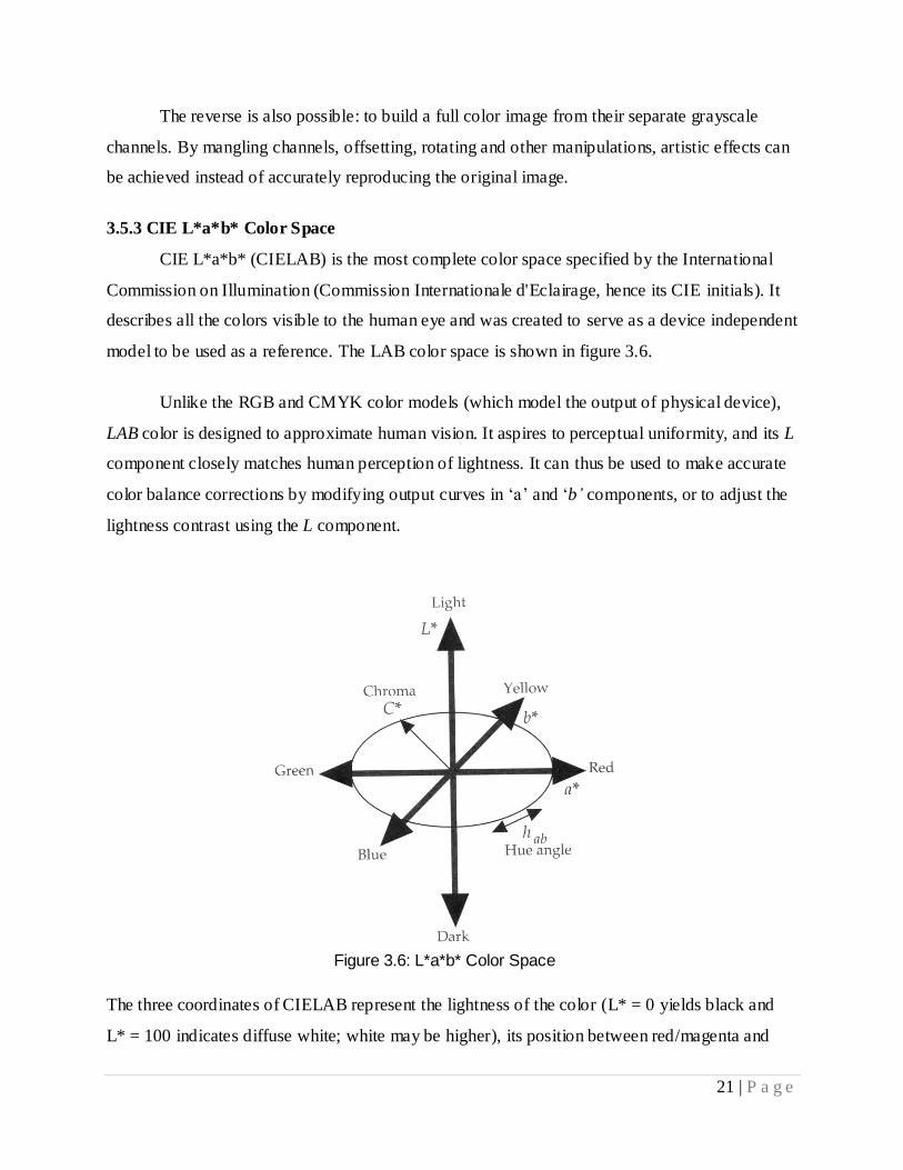
model to be used as a reference. The LAB color space is shown in figure 3.6.
Unlike the RGB and CMYK color models (which model the output of physical device),
LAB color is designed to approximate human vision. It aspires to perceptual uniformity, and its L
component closely matches human perception of lightness. It can thus be used to make accurate
color balance corrections by modifying output curves in „a‟ and „b’ components, or to adjust the
lightness contrast using the L component.
The three coordinates of CIELAB represent the lightness of the color (L* = 0 yields black and
L* = 100 indicates diffuse white; white may be higher), its position between red/magenta and
Figure 3.6: L*a*b* Color Space
22 | P a g e
green (a*, negative values indicate green while positive values indicate magenta) and its position
between yellow and blue (b*, negative values indicate blue and positive values indicate yellow).
3.5.3.1 RGB and CMYK conversions to LAB
There are no simple formulas for conversion between RGB or CMYK values and L*a*b*,
because the RGB and CMYK color models are device dependent. The RGB or CMYK values
first need to be transformed to a specific absolute color space, such as sRGB. This adjustment
will be device dependent, but the resulting data from the transform will be device independent,
allowing data to be transformed into L*a*b*.
3.5.3.2 Range of L*a*b* coordinates
As mentioned previously, the L* coordinate ranges from 0 to 100. The possible range of a* and
b* coordinates depends on the color space that one is converting from. For example, when
converting from sRGB, the „a*‟ coordinate range is [-0.86, 0.98], and the „b*‟ coordinate range
is [-1.07, 0.94].
3.6 Steps Involved in Digital Image Processing
The following steps were involved in the image processing.
3.6.1 Capture the image
The camera gives a video feed at 15fps. The first step is to get a frame from that video
feed and store the image in the hard disk.
3.6.2 Color space transformation
The frame captured is in a color space that is device dependant. So to get a color
representation of the image that is device independent, we transform the color space.
3.6.3 Color extraction
After the transformation, we search the image for some specific color; extract the image
after replacing that specific color with white and the remaining frame with black color and save
the resulting image as an intermediate image.
23 | P a g e
3.6.4 Identify an object of specific shape
After this, we find the boundaries of all the remaining objects in white and find out of the
shape of the boundary. This will tell us what the robot is looking at.
3.7 MATLAB as Image Processing Tool
MATLAB has two versatile toolbox used in image processing system. These are “Image
Acquisition Toolbox” and “Image Processing Toolbox”. In order to perform the image
processing, we proceed as follows.
3.7.1 Capture the image
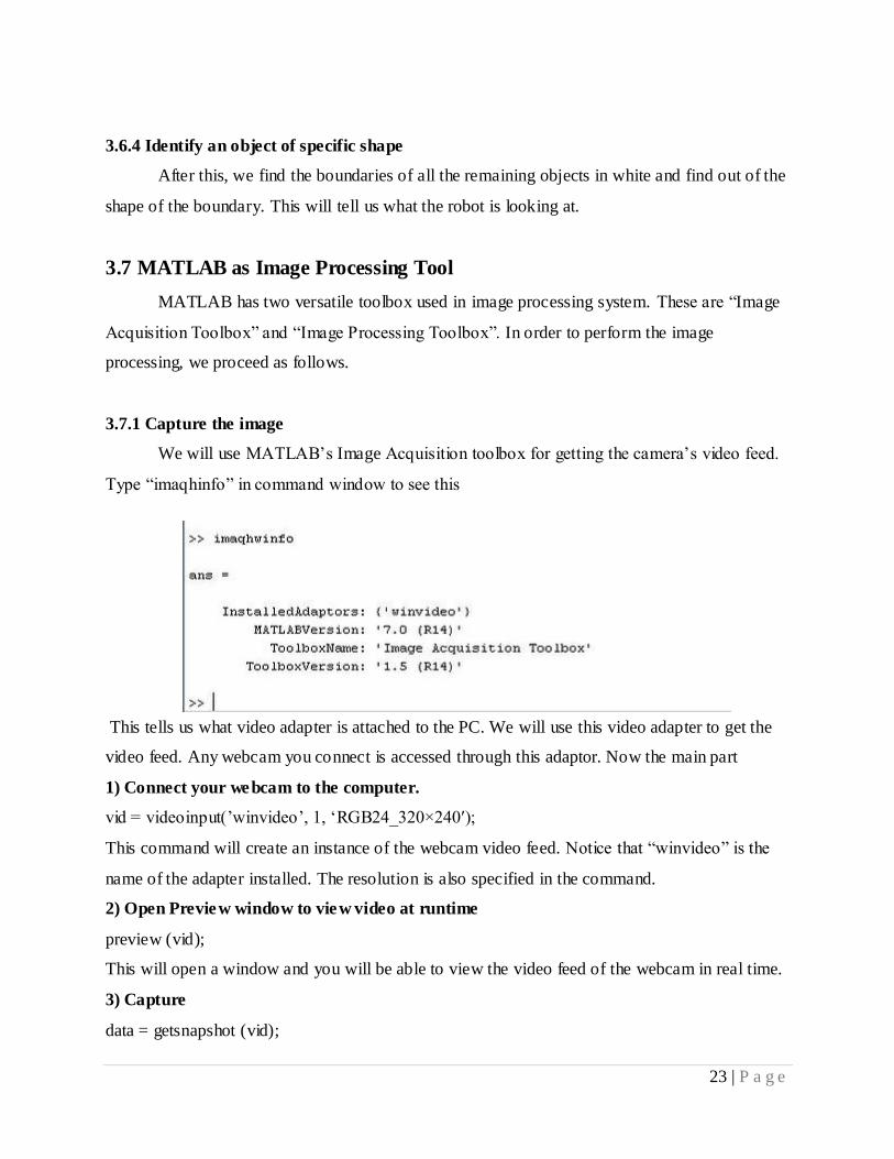
We will use MATLAB‟s Image Acquisition toolbox for getting the camera‟s video feed.
Type “imaqhinfo” in command window to see this
This tells us what video adapter is attached to the PC. We will use this video adapter to get the
video feed. Any webcam you connect is accessed through this adaptor. Now the main part
1) Connect your webcam to the computer.
vid = videoinput(‟winvideo‟, 1, „RGB24_320×240′);
This command will create an instance of the webcam video feed. Notice that “winvideo” is the
name of the adapter installed. The resolution is also specified in the command.
2) Open Preview window to view video at runtime
preview (vid);
This will open a window and you will be able to view the video feed of the webcam in real time.
3) Capture
data = getsnapshot (vid);
24 | P a g e
This command will store the image of that instant into the variable data in a matrix of 320X240.
3.7.2 Color space transformation
The image captured from the camera is in RGB color space. We convert it in L*a*b*
color space. We use two function of image processing toolbox to perform this.
cform = makecform ('srgb2lab');
lab_fabric = applycform (fabric, cform);
The complete code for this step is given in Appendix B.
3.7.3 Color extraction
In this step, we have an image that is transformed to L*a*b* color space. Each color
marker now has an „a*‟ and a „b*‟ value. You can classify each pixel in the actual image by
calculating the Euclidean distance between that pixel and each color marker. The smallest
distance will tell you that the pixel most closely matches that color marker. For example, if the
distance between a pixel and the red color marker is the smallest, then the pixel would be labeled
as a red pixel. The complete code for this step is given in Appendix B.
3.7.4 Identify an object of specific shape
After the last step, we start the identification of a specific object. We convert the image to
grayscale and then threshold it. Then the boundaries of the objects are calculated. Then an object
of a specific shape can be found using a shape metric. The complete code for this step is given in
Appendix B.
3.8 OpenCV as Image Processing Tool
OpenCV (Open Source Computer Vision) is a library of programming functions mainly
aimed at real time computer vision.
OpenCV is becoming a very good tool in image processing applications as it has libraries
that help in different applications like Object Identification, Segmentation and Recognition,
Motion Tracking etc.
25 | P a g e
3.8.1 Capture the image
In order to capture the image from the camera, we first create an instance of type
“CvCapture*” that will be used to get image from any device attached. We write
“CV_CAP_ANY” to tell that frame is to be captured from any device that is connected.
CvCapture* capture = cvCaptureFromCAM ( CV_CAP_ANY );
After that, we retrieve the frame using “cvRetrieveFrame” and store in a variable of type
“IplImage*”.
IplImage* frame=cvRetrieveFrame(capture);
After that the frame is ready to be processed.
3.8.2 Color space transformation
OpenCV is quite versatile in providing all the different functionalities in simple
MATLAB like format for example to convert RGB image to LAB color space, simply use a
command CV_RGB2LAB and we get the result.
3.8.3 Color extraction
In order to extract colors using OpenCV, we make use of a simple fact that all the RGB
images consists of 3 different channels naming Red, Green and Blue channel. So we use a simple
condition based upon the color we need to extract. The factor “29” is random and is dependent
on the device used. For example, for extraction of red color, which is the third channel in the
image, the condition is somewhat like this,
if(((data[i*step+j*channels+2]) > (29+data[i*step+j*channels]))
&& ((data[i*step+j*channels+2]) > (29+data[i*step+j*channels+1])))
datar[i*stepr+j*channelsr]=255;
else
datar[i*stepr+j*channelsr]=0;

26 | P a g e
3.8.4 Identify an object of specific shape
After the last step, we start the identification of a specific object. In this step, we use a
technique named “Hough Transform” to detect an object of circular shape. In OpenCV we use
Hough Gradient Method to detect circles.
27 | P a g e
OpenCV as Image Processing Tool
4.1 Introduction
The Intel Open Source Computer Vision Library, or just OpenCV, is a library of image
processing and computer vision algorithms. It‟s open source so anybody can contribute to it.
OpenCV utilizes Intel‟s Image Processing Library (IPL), which is a set of low-level image
processing functions. OpenCV uses DirectX, which is a set of APIs developed by Microsoft for
creating multimedia applications and games. OpenCV is portable and very efficient. It is
implemented in C/C++.
4.2 Why OpenCV
The Open CV Library is a way of establishing an open source vision community that will
make better use of up-to-date opportunities to apply computer vision in the growing PC
environment. The software provides a set of image processing functions as well as image and
pattern analysis functions. The functions are optimized for Intel architecture processors and are
particularly effective in taking advantage of Intel MMX technology.
OpenCV is quickly gaining popularity for developing real-time computer vision
applications. Some examples of applications include face recognizers, object
recognizers, and motion trackers, just to name a few. The library has especially gained popularity
in the computer vision research community. It allows researchers to get demos or research
projects up and running quickly, and take advantage of the large collection of algorithms that are
already available.
4.3 Integrating OpenCV with Microsoft Visual C++ 6.0
The OpenCV software runs on personal Computers that are Intel architecture based and
running Microsoft Windows. First of all DirectX 9.0 SDK and OpenCV Libraries must be
installed in the PC. The OpenCV integrating procedure with Microsoft Visual C++ 6.0 is given
below.
28 | P a g e
4.3.1. Setting Up the System PATH Environmental Variable
Add the path of the OpenCV “bin” folder “C:\ProgramFiles\OpenCV\bin” in the
Environment variables tab in System properties. Restart the computer for the PATH variable to
be updated.
4.3.2. Specifying Directories in Visual C++ 6.0
Visual C++ 6.0 must be able to find files such as include, source, executable, and library
files. We need to go in and manually tell the IDE where to find the ones it needs.
Start Microsoft Visual C++ 6.0. Goto tools > options > Directories tab. You can switch to other
file types such as library files by clicking the arrow under “Show directories for”.
In “Show directories for” ”include files” tab add the following paths.
“C:\ProgramFiles\OpenCV\cv\include”
“C:\ProgramFiles\OpenCV\cxcore\include”
“C:\ProgramFiles\OpenCV\otherlibs\highgui”
“C:\Program Files\Microsoft DirectX SDK (November 2008)\Include”
In “Show directories for” ”Executable files” tab add the following paths.
“C:\ProgramFiles\OpenCV\bin”
In “Show directories for” ”Library files” tab add the following paths.
“C:\ProgramFiles\OpenCV\lib”
“C:\Program Files\Microsoft DirectX SDK (November 2008)\lib\x86”
4.3.3. Settings for New Project in Microsoft Visual C++ 6.0
Whenever a new project is created goto Project Settings Links tab.
Under “Object/library Modules” add the following libraries
“cv.lib cxcore.lib srmbase.lib highgui.lib”
4.4 Important Data types and Functions Used
There are a few fundamental types OpenCV Operates on, and a several helper data types
that are introduced to make OpenCV API more simple and uniform. Some of the fundamental
data types and functions are discussed below:
29 | P a g e
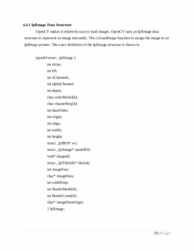
4.4.1 IplImage Data Structure
OpenCV makes it relatively easy to load images. OpenCV uses an IplImage data
structure to represent an image internally. The cvLoadImage function to assign the image to an
IplImage pointer. The exact definition of the IplImage structure is shown in
typedef struct _IplImage {
int nSize;
int ID;
int nChannels;
int alphaChannel;
int depth;
char colorModel[4];
char channelSeq[4];
int dataOrder;
int origin;
int align;
int width;
int height;
struct _IplROI* roi;
struct _IplImage* maskROI;
void* imageId;
struct _IplTileInfo* tileInfo;
int imageSize;
char* imageData;
int widthStep;
int BorderMode[4];
int BorderConst[4];
char* imageDataOrigin;
} IplImage;
30 | P a g e
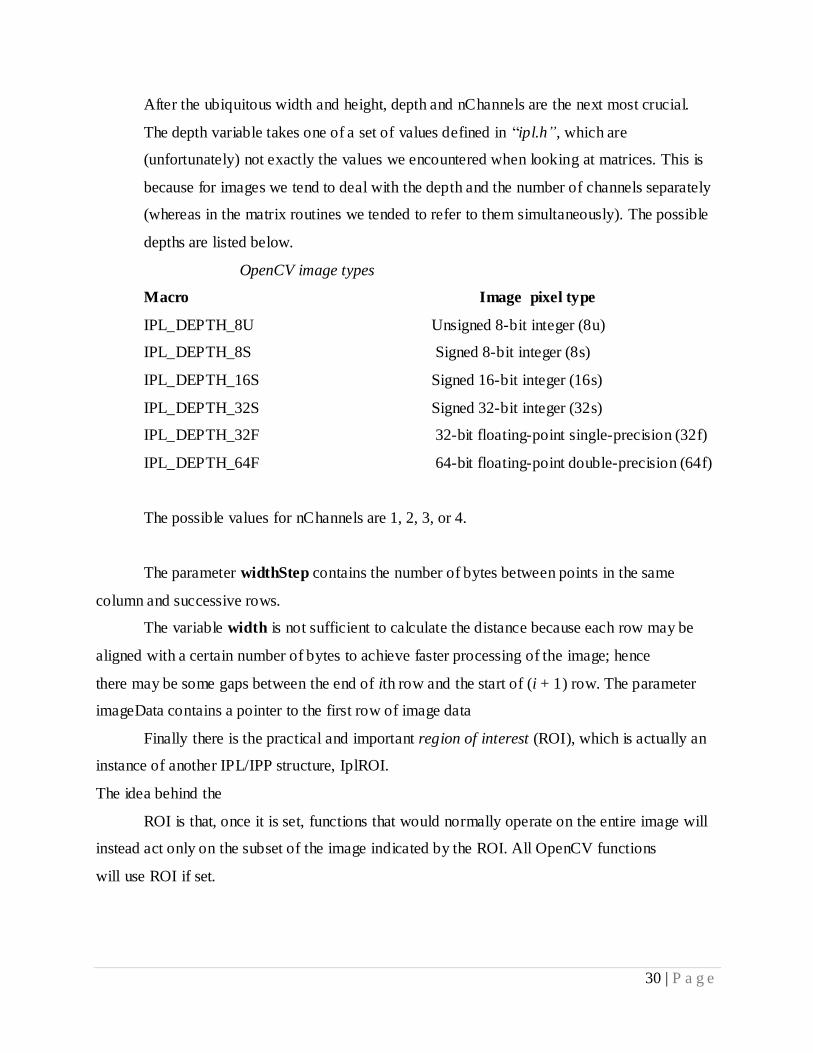
After the ubiquitous width and height, depth and nChannels are the next most crucial.
The depth variable takes one of a set of values defined in “ipl.h”, which are
(unfortunately) not exactly the values we encountered when looking at matrices. This is
because for images we tend to deal with the depth and the number of channels separately
(whereas in the matrix routines we tended to refer to them simultaneously). The possible
depths are listed below.
OpenCV image types
Macro Image pixel type
IPL_DEPTH_8U Unsigned 8-bit integer (8u)
IPL_DEPTH_8S Signed 8-bit integer (8s)
IPL_DEPTH_16S Signed 16-bit integer (16s)
IPL_DEPTH_32S Signed 32-bit integer (32s)
IPL_DEPTH_32F 32-bit floating-point single-precision (32f)
IPL_DEPTH_64F 64-bit floating-point double-precision (64f)
The possible values for nChannels are 1, 2, 3, or 4.
The parameter widthStep contains the number of bytes between points in the same
column and successive rows.
The variable width is not sufficient to calculate the distance because each row may be
aligned with a certain number of bytes to achieve faster processing of the image; hence
there may be some gaps between the end of ith row and the start of (i + 1) row. The parameter
imageData contains a pointer to the first row of image data
Finally there is the practical and important region of interest (ROI), which is actually an
instance of another IPL/IPP structure, IplROI.
The idea behind the
ROI is that, once it is set, functions that would normally operate on the entire image will
instead act only on the subset of the image indicated by the ROI. All OpenCV functions
will use ROI if set.
31 | P a g e
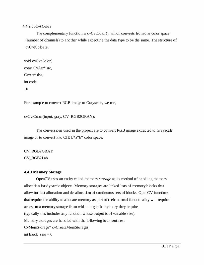
4.4.2 cvCvtColor
The complementary function is cvCvtColor(), which converts from one color space
(number of channels) to another while expecting the data type to be the same. The structure of
cvCvtColor is,
void cvCvtColor(
const CvArr* src,
CvArr* dst,
int code
);
For example to convert RGB image to Grayscale, we use,
cvCvtColor(input, gray, CV_RGB2GRAY);
The conversions used in the project are to convert RGB image extracted to Grayscale
image or to convert it to CIE L*a*b* color space.
CV_RGB2GRAY
CV_RGB2Lab
4.4.3 Memory Storage
OpenCV uses an entity called memory storage as its method of handling memory
allocation for dynamic objects. Memory storages are linked lists of memory blocks that
allow for fast allocation and de-allocation of continuous sets of blocks. OpenCV functions
that require the ability to allocate memory as part of their normal functionality will require
access to a memory storage from which to get the memory they require
(typically this includes any function whose output is of variable size).
Memory storages are handled with the following four routines:
CvMemStorage* cvCreateMemStorage(
int block_size = 0

32 | P a g e
);
void cvReleaseMemStorage(
CvMemStorage** storage
);
To create a memory storage, the function cvCreateMemStorage() is used. This function
takes as an argument a block size, which gives the size of memory blocks inside the
store. If this argument is set to 0 then the default block size (64kB) will be used. The
function returns a pointer to a new memory store.
The cvReleaseMemStorage() function takes a pointer to a valid memory storage and then
de-allocates the storage. This essentially equivalent to the OpenCV de-allocations of
images, matrices, and other structures
4.4.3.1cvSeq Sequence
One kind of object that can be stored inside memory storage is a sequence. Sequences are
themselves linked lists of other structures. OpenCV can make sequences out of many different
kinds of objects. In this sense you can think of the sequence as something similar to the generic
container classes (or container class templates) that exist in various other programming
languages. The sequence construct in OpenCV is actually a de-queue, so it is very fast for
random access and for additions and deletions from either end but a little slow for adding and
deleting objects in the middle.
The sequence structure itself (see Example 8-1) has some important elements that you
should be aware of. The first, and one you will use often, is total. The total number of points or
objects in the sequence. The next four important elements are pointers to other sequences:
h_prev, h_next, v_prev, and v_next. These four pointers are part of what are called
CV_TREE_NODE_FIELDS; they are used not to indicate elements inside of the sequence but
rather to connect different sequences to one another. Other objects in the OpenCV universe also
contain these tree node fields. Internal organization of CvSeq sequence structure is written
below.
typedef struct CvSeq {
int flags; // miscellaneous flags
int header_size; // size of sequence header
33 | P a g e
CvSeq* h_prev; // previous sequence
CvSeq* h_next; // next sequence
CvSeq* v_prev; // 2nd previous sequence
CvSeq* v_next // 2nd next sequence
int total; // total number of elements
int elem_size; // size of sequence element in byte
char* block_max; // maximal bound of the last block
char* ptr; // current write pointer
int delta_elems; // how many elements allocated
// when the sequence grows
CvMemStorage* storage; // where the sequence is stored
CvSeqBlock* free_blocks; // free blocks list
CvSeqBlock* first; // pointer to the first sequence block
}
A sequence is created like this:
CvSeq* yourvariable = cvCreateSeq(int seq_flags, int header_size, int elem_size,
CvMemStorage* storage.
Individual elements in a sequence can be accessed with
char* cvGetSeqElem( seq, index ).
A sequence can be used as a stack with functions like push and pop.
char* cvSeqPush( CvSeq* seq, void* element = NULL)
char* cvSeqPop( CvSeq* seq, void* element = NULL)
to see the total elements in a sequences
seq->total
4.5 Accessing Image Elements.
Assume that you need to access the -th channel of the pixel at the i- th row and j-th column.
The row index “i” is in the range [0, height-1]. The column index j is in the range [0, width-1] .
The channel index is in the range [0 ,nchannels – 1].
34 | P a g e
4.5.1Direct access using a pointer: (Simplified and efficient access under limiting assumptions)
o For a single-channel byte image:
o IplImage* img = cvCreateImage(cvSize(640,480),IPL_DEPTH_8U,1);
o int height = img->height;
o int width = img->width;
o int step = img->widthStep/sizeof(uchar);
o uchar* data = (uchar *)img->imageData;
o data[i*step+j] = 111;
o For a multi-channel byte image:
o IplImage* img = cvCreateImage(cvSize(640,480),IPL_DEPTH_8U,3);
o int height = img->height;
o int width = img->width;
o int step = img->widthStep/sizeof(uchar);
o int channels = img->nChannels;
o uchar* data = (uchar *)img->imageData;
o data[i*step+j*channels+k] = 111;
o For a multi-channel float image (assuming a 4-byte alignment):
o IplImage* img = cvCreateImage(cvSize(640,480),IPL_DEPTH_32F,3);
o int height = img->height;
o int width = img->width;
o int step = img->widthStep/sizeof(float);
o int channels = img->nChannels;
o float * data = (float *)img->imageData;
data[i*step+j*channels+k] = 111;
4.6 Displaying Images
OpenCV provides utilities for reading from a wide array of image file types as well as
from video and cameras. These utilities are part of a toolkit called HighGUI, which is
included in the OpenCV package. We will use some of these utilities to create a simple
program that opens an image and displays it on the screen. See Example 2-1.
35 | P a g e
#include “highgui.h”
int main( int argc, char** argv ) {
IplImage* img = cvLoadImage( argv[1] );
cvNamedWindow( “Example1”, CV_WINDOW_AUTOSIZE );
cvShowImage( “Example1”, img );
cvWaitKey(0);
cvReleaseImage( &img );
cvDestroyWindow( “Example1” );
}
When compiled and run from the command line with a single argument, this program
loads an image into memory and displays it on the screen. It then waits until the user
presses a key, at which time it closes the window and exits. Let‟s go through the program
line by line and take a moment to understand what each command is doing.
IplImage* img = cvLoadImage( argv[1] );
This line loads the image.* The function cvLoadImage() is a high- level routine that
determines
The file format to be loaded based on the file name; it also automatically allocates
the memory needed for the image data structure. Note that cvLoadImage() can read a
wide variety of image formats, including BMP, DIB, JPEG, JPE, PNG, PBM, PGM, PPM,
SR, RAS, and TIFF. A pointer to an allocated image data structure is then returned.
This structure, called IplImage, is the OpenCV construct with which you will deal
the most. OpenCV uses this structure to handle all kinds of images: single-channel,
multichannel, integer-valued, floating-point-valued, et cetera. We use the pointer that
cvLoadImage() returns to manipulate the image and the image data.
cvNamedWindow( “Example1”, CV_WINDOW_AUTOSIZE );
Another high- level function, cvNamedWindow(), opens a window on the screen that can
contain and display an image. This function, provided by the HighGUI library, also assigns
36 | P a g e
a name to the window (in this case, “Example1”). Future HighGUI calls that interact
with this window will refer to it by this name. The second argument to cvNamedWindow()
defines window properties. It may be set either to 0 (the default value) or to
CV_WINDOW_AUTOSIZE. In the former case, the size of the window will be the same
regardless of the image size, and the image will be scaled to fit within the window. In the latter
case, the window will expand or contract automatically when an image is loaded so as to
accommodate the image‟s true size.
cvShowImage( “Example1”, img );
Whenever we have an image in the form of an IplImage* pointer, we can display it in an
existing window with cvShowImage(). The cvShowImage() function requires that a named
window already exist (created by cvNamedWindow()). On the call to cvShowImage(), the
window will be redrawn with the appropriate image in it, and the window will resize
itself as appropriate if it was created using the CV_WINDOW_AUTOSIZE flag.
cvWaitKey(0);
The cvWaitKey() function asks the program to stop and wait for a keystroke. If a positive
argument is given, the program will wait for that number of milliseconds and then continue
even if nothing is pressed. If the argument is set to 0 or to a negative number, the
program will wait indefinitely for a key press.
cvReleaseImage( &img );
Once we are through with an image, we can free the allocated memory. OpenCV expects
a pointer to the IplImage* pointer for this operation. After the call is completed,
the pointer img will be set to NULL.
37 | P a g e
cvDestroyWindow( “Example1” );
Finally, we can destroy the window itself. The function cvDestroyWindow() will close the
window and de-allocate any associated memory usage (including the window‟s internal
image buffer, which is holding a copy of the pixel information from *img). For a simple
program, you don‟t really have to call cvDestroyWindow() or cvReleaseImage() because all
the resources and windows of the application are closed automatically by the operating
system upon exit, but it‟s a good habit anyway.
4.7 Video I/O
Following functions and methodology is used for Video I/O.
4.7.1 CvCapture
This structure contains all of the information about the AVI files being read, including
state information. The CvCapture structure is initialized to the beginning of the AVI
4.7.2 Capturing Frames
Following are the basic structures used to capture frames from a US B camera.
CvCapture* capture = cvCaptureFromCAM( CV_CAP_ANY );
This command initializes capturing from any video capture device that is connected to the pc.
After that, we retrieve the frame using “cvRetrieveFrame” or “cvQueryframe” and store in a
variable of type “IplImage”. NULL is returned is returned if no frames are available.
cvReleaseCapture(&capture) is used at the end of program to release the resources that was used
by the camera.
4.8 Circular Hough Transform
A commonly faced problem in computer vision is to determine the location, number or
orientation of a particular object in an image. One problem could for instance be to determine the
straight roads on an aerial photo, this problem can be solved using Hough transform for lines.
Often the objects of interest have other shapes than lines, it could be parables, circles or ellipses
38 | P a g e
or any other arbitrary shape. The general Hough transform can be used on any kind of shape,
although the complexity of the transformation increase with the number of parameters needed to
describe the shape. In the following we will look at the Circular Hough Transform (CHT).
4.8.1Parametric Representations
The Hough transform can be described as a transformation of a point in the x, y-plane to
the parameter space. The parameter space is defined according to the shape of the object of
interest. A straight line passing through the points (x1,y1) and (x2,y2) can in the x, y-plan is
described by:
y = ax+b
This is the equation for a straight line in the Cartesian coordinate system, where a, b
represent the parameters of the line. The Hough transform for lines do not use this representation
of lines, since lines perpendicular to the x-axis will have an “a” value of infinity. This will force
the parameter space a, b to have infinite size. Instead a line is represented by its normal which
can be represented by an angel q and a length r.
r = x cos(q)+y sin (q)
The parameter space can now spanned by q and r, where q will have a finite size,
depending on the resolution used for q. The distance to the line r will have a maximum size of
two times the diagonal length of the image. The circle is actually simpler to represent in
parameter space, compared to the line, since the parameters of the circle can be directly transfer
to the parameter space. The equation of a circle is
r^2 = (x−a)^2+(y−b)^2
As it can be seen the circle got three parameters, r, a, b. Where a, b are the center of the
circle in the x and y direction respectively and where r is the radius. The parametric
representation of the circle is
x = a+r cos(q)
y = b+r sin (q)
Thus the parameter space for a circle will belong to R^3 whereas the line only belonged
to R^2. As the number of parameters needed to describe the shape increases as well as the
dimension of the parameter space R increases so do the complexity of the Hough transform.
39 | P a g e
Therefore is the Hough transform in general only considered for simple shapes with parameters
belonging to R^2 or at most R^3.
4.8.2 Accumulator
The process of finding circles in an image using CHT is that first we find all edges in the
image. This step has nothing to do with Hough Transform and any edge detection technique of
your desire can be used. At each edge point we draw a circle with center in the point with the
desired radius. This circle is drawn in the parameter space, such that our x axis is the a - value
and the y axis is the b value while the z axis is the radii.
At the coordinates which belong to the perimeter of the drawn circle, we increment the
value in our accumulator matrix which essentially has the same size as the parameter space. In
this way we sweep over every edge point in the input image drawing circles with the desired
radii and incrementing the values in our accumulator. When every edge point and every desired
radius is used, we can turn our attention to the accumulator. The accumulator will now contain
numbers corresponding to the number of circles passing through the individual coordinates. Thus
the highest numbers (selected in an intelligent way, in relation to the radius) correspond to the
center of the circles in the image.
4.8.3 Circular Hough Transform Algorithm
The algorithm for Circular Hough Transformation can be summarized as,
Find edges.
Begin CHT.
For each edge point, Draw a circle with center in the edge point with radius r and
increment all coordinates that the perimeter of the circle passes through in the
accumulator.
Find one or several maxima in the accumulator
End CHT.
Map the found parameters (r, a, b) corresponding to the maxima back to the original
image.
40 | P a g e
4.8.4 CHT in OpenCV
With all of that in mind, let‟s move on to the OpenCV routine that does all this for us:
CvSeq* cvHoughCircles(
CvArr* image,
void* circle_storage,
int method,
double dp,
double min_dist,
double param1 = 100,
double param2 = 300,
int min_radius = 0,
int max_radius = 0
);
The Hough circle transform function cvHoughCircles() has similar arguments to the
line transforms. The input image is again an 8-bit image. The cvHoughCircles() function will
automatically perform edge detection on the input image, so you can provide a more general
grayscale image.
The circle_storage can be either an array or memory storage, depending on how you
would like the results returned. If an array is used, it should be a single column of type
CV_32FC3; the three channels will be used to encode the location of the circle and its
radius. If memory storage is used, then the circles will be made into an OpenCV sequence
and a pointer to that sequence will be returned by cvHoughCircles(). The method argument must
always be set to CV_HOUGH_GRADIENT.
The parameter „dp‟ is the resolution of the accumulator image used. This parameter
allows us to create an accumulator of a lower resolution than the input image. (It makes sense
to do this because there is no reason to expect the circles that exists in the image to fall
naturally into the same number of categories as the width or height of the image itself.)
If dp is set to 1 then the resolutions will be the same; if set to a larger number (e.g., 2),
then the accumulator resolution will be smaller by that factor ( in this case, half). The
value of dp cannot be less than 1.
41 | P a g e
The parameter „min_dist‟ is the minimum distance that must exist between two circles in
order for the algorithm to consider them distinct circles.
For the (currently required) case of the method being set to CV_HOUGH_GRADIENT,
the next two arguments, param1 and param2, are the edge threshold and the accumulator
threshold, respectively. Canny edge detector actually takes two different thresholds itself. When
cvCanny() is called internally, the first (higher) threshold is set to the value of param1 passed
into cvHoughCircles(), and the second (lower) threshold is set to exactly half that value. The
parameter param2 is the one used to threshold the accumulator and is exactly analogous to the
threshold argument of cvHoughLines().
The final two parameters are the minimum and maximum radius of circles that can be
found. This means that these are the radii of circles for which the accumulator has a
representation.
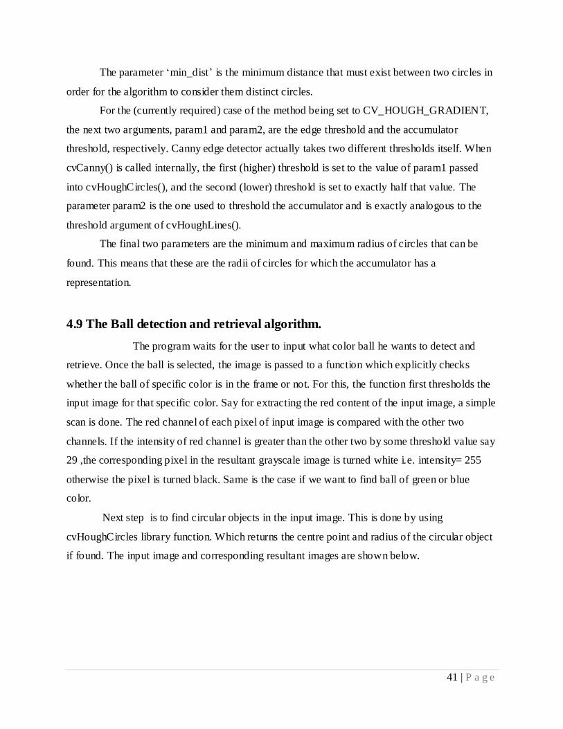
4.9 The Ball detection and retrieval algorithm.
The program waits for the user to input what color ball he wants to detect and
retrieve. Once the ball is selected, the image is passed to a function which explicitly checks
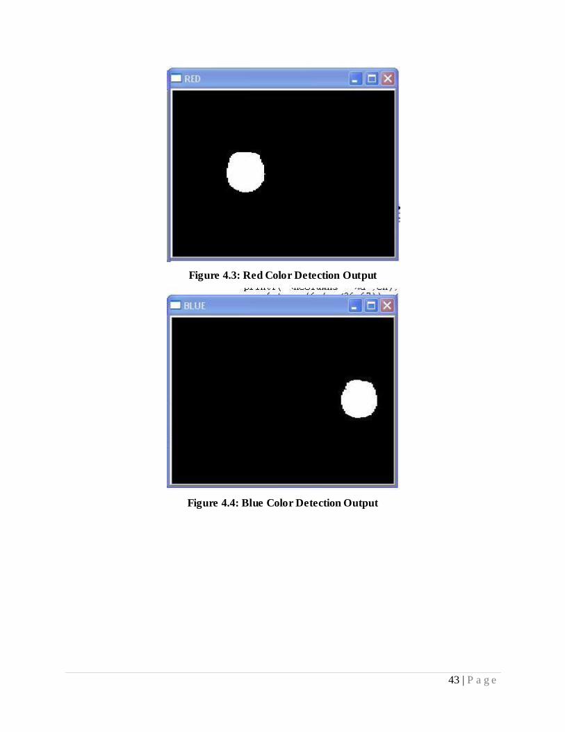
whether the ball of specific color is in the frame or not. For this, the function first thresholds the
input image for that specific color. Say for extracting the red content of the input image, a simple
scan is done. The red channel of each pixel of input image is compared with the other two
channels. If the intensity of red channel is greater than the other two by some threshold value say
29 ,the corresponding pixel in the resultant grayscale image is turned white i.e. intensity= 255
otherwise the pixel is turned black. Same is the case if we want to find ball of green or blue
color.
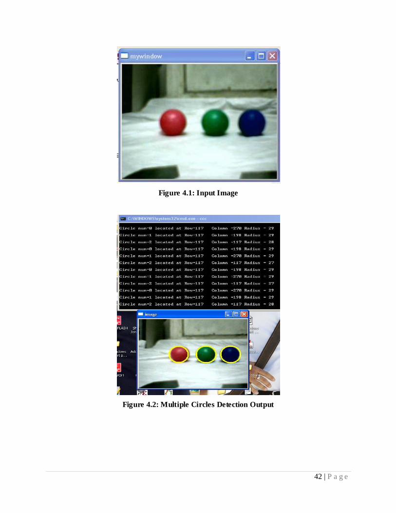
Next step is to find circular objects in the input image. This is done by using
cvHoughCircles library function. Which returns the centre point and radius of the circular object
if found. The input image and corresponding resultant images are shown below.
42 | P a g e
Figure 4.1: Input Image
Figure 4.2: Multiple Circles Detection Output
43 | P a g e
Figure 4.3: Red Color Detection Output
Figure 4.4: Blue Color Detection Output
44 | P a g e
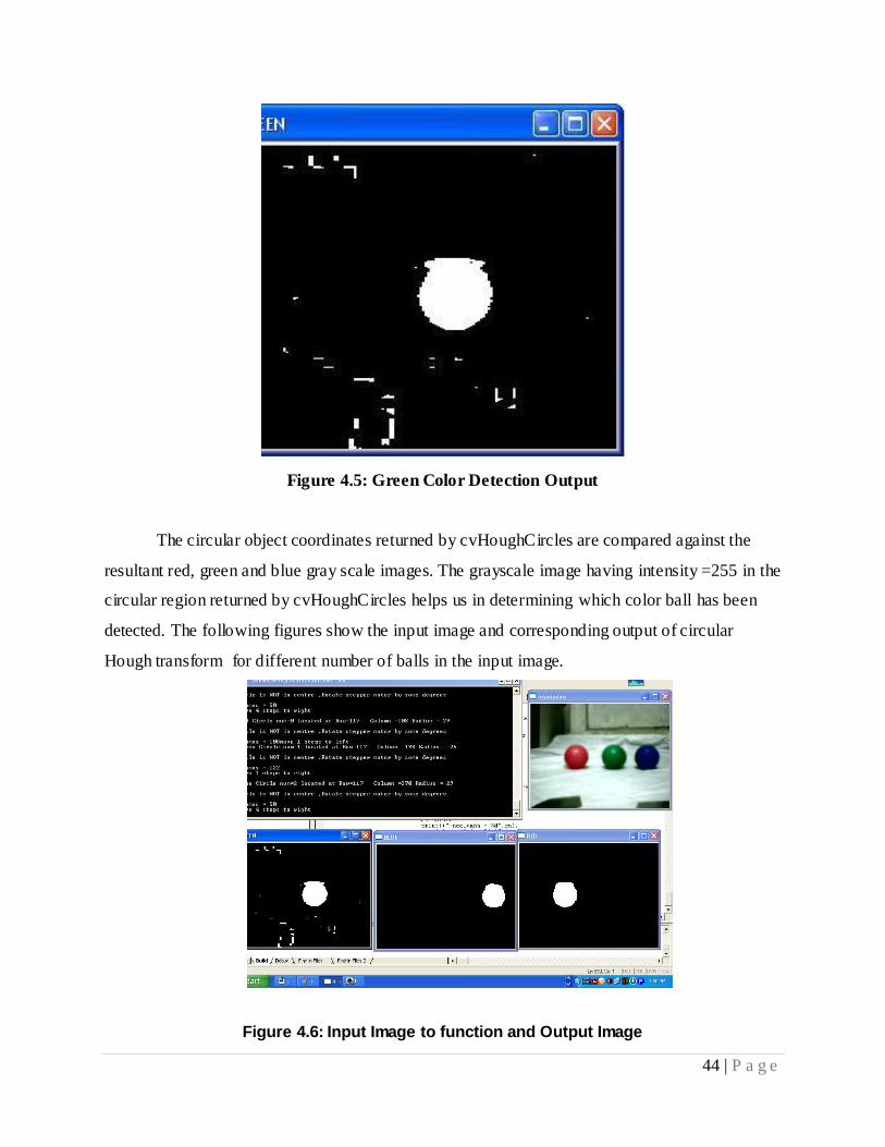
Figure 4.5: Green Color Detection Output
The circular object coordinates returned by cvHoughCircles are compared against the
resultant red, green and blue gray scale images. The grayscale image having intensity =255 in the
circular region returned by cvHoughCircles helps us in determining which color ball has been
detected. The following figures show the input image and corresponding output of circular
Hough transform for different number of balls in the input image.
Figure 4.6: Input Image to function and Output Image
45 | P a g e
After finding the ball of the specified color, control signals are sent serially to the robot.
If the ball is not in center, the signals sent are such that the robot turns some unit such that the
ball comes in center. Once the ball is in center, another control is sent telling the robot to move
forward. Once the robot is near the ball (this is found by continuously monitoring the radius
returned by cvHoughCircles), another control signal is sent telling the robot to lower its arm and
then start moving forward to retrieve the ball.
46 | P a g e
CONTROL SYSTEM DESIGN
5.1 Introduction
Control system design for the robot was the final phase of the project. Basic idea was to
keep the design simple yet complete in its working. The design considerations are listed below.
The actual control mechanism must be simple and so we made the control of the robot just
like an actual being in search of something.
While the arm is moving, the robot must not be able to move. This does not mean a locking
of the wheels, but control of the robot‟s movement must not occur simultaneously with that
of the arm.
5.2 Algorithm Considerations
Normal human day-to-day functioning is an automatic process – almost involuntary. The
thought pattern required for what most consider simple movements are actually incredibly
complex and intricate procedures. Consider you want to retrieve an object; the thought process
can be outlined in a few steps:
Locate the object.
Go to the object.
Retrieve it.
Now if we want our robot to perform these tasks, we would have to write pages and
pages of computer code as the processing for these very simple looking steps is quite immense,
even for the human brain (not that we notice it). The robot must have a vision system that can see
and locate the object. After the object is located, the motor control must be activated so that
robot can move to the object. After the object is reached, the robotic arm control is activated for
the retrieval of the object.
47 | P a g e
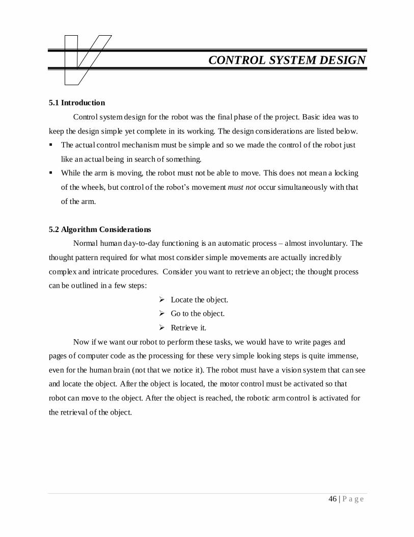
5.3 Controls Simulation
It is obvious that for successful operation of the project some method of checking control
algorithm and user interface is required, since doing direct construction could prove expensive in
terms of both money and time. To avoid this, we used Proteus as a simulation tool and all the
circuits were simulated first and after that hardware was made. The simulations of the control are
shown in figure 5.1.
Figure 5.1 control of dc motor
Figure 5.2 control of stepper motor
48 | P a g e
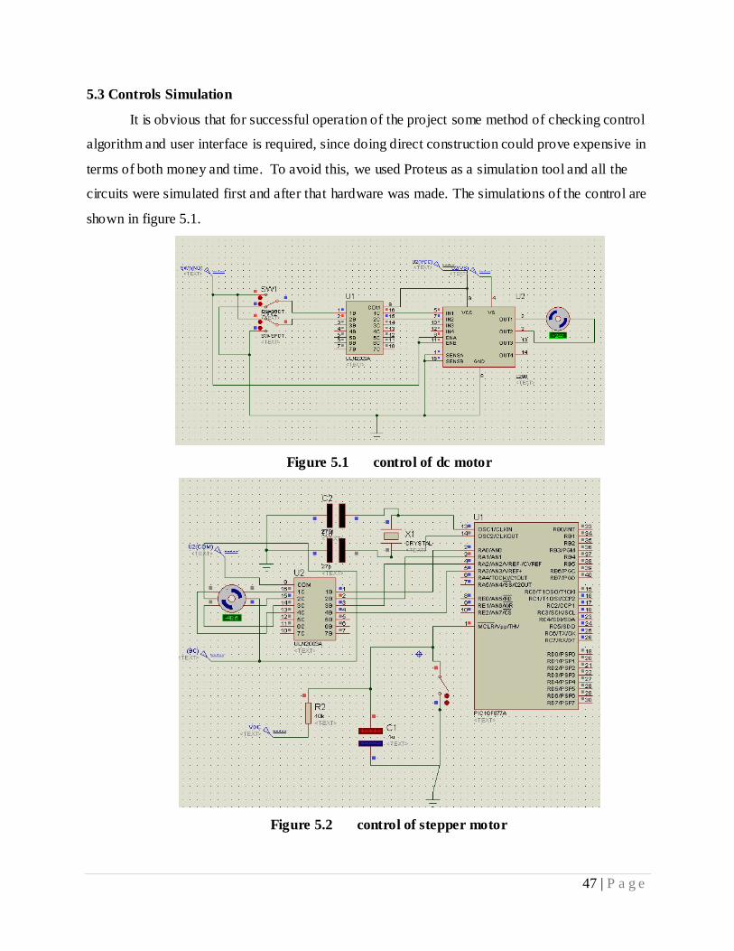
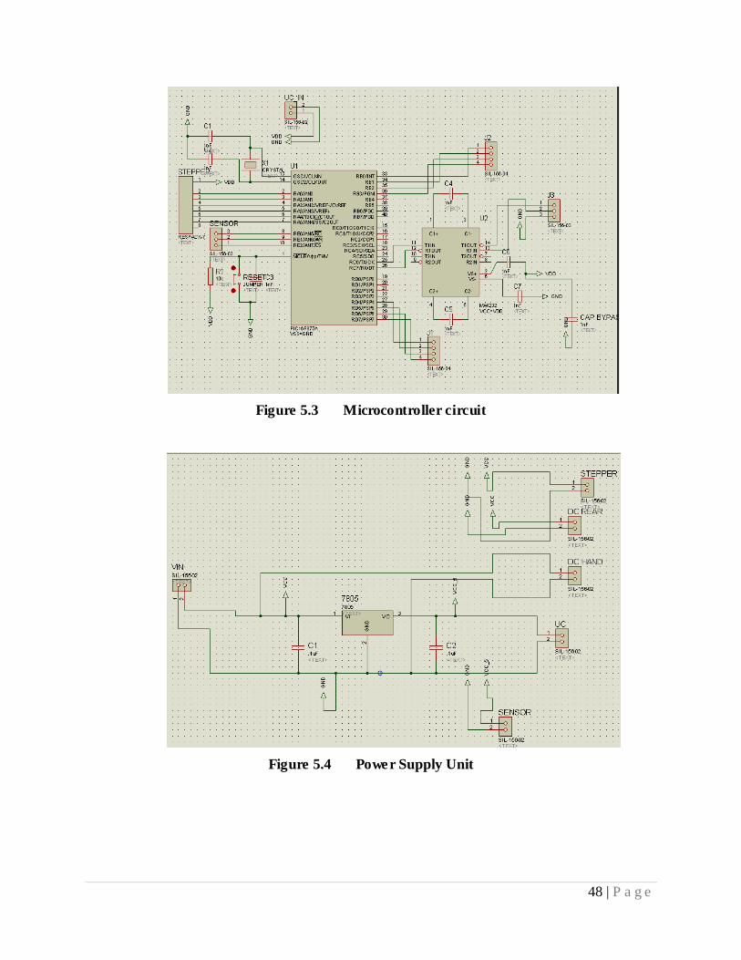
Figure 5.3 Microcontroller circuit
Figure 5.4 Power Supply Unit
49 | P a g e
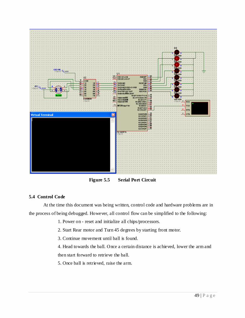
Figure 5.5 Serial Port Circuit
5.4 Control Code
At the time this document was being written, control code and hardware problems are in
the process of being debugged. However, all control flow can be simplified to the following:
1. Power on - reset and initialize all chips/processors.
2. Start Rear motor and Turn 45 degrees by starting front motor.
3. Continue movement until ball is found.
4. Head towards the ball. Once a certain distance is achieved, lower the arm and
then start forward to retrieve the ball.
5. Once ball is retrieved, raise the arm.
50 | P a g e
FUTURE RECOMMENDATIONS
6.1 Circular Hough Transform Hardware
The Hough Transform (Hough, 1962) has been used to characterize analytic features. It
was first applied to the recognition of straight lines, and later extended to circles, ellipses and
arbitrary shaped objects. Its main disadvantage is the computational and storage requirements
increase as a power of the dimensionality of the curve. It is not difficult to implement Circular
Hough Transform (CHT) algorithm (which is in R^3) on modern personal computer. However,
we want to use FPGA or ASIC to perform CHT. Modern FPGAs are capable of performing high
speed operation and have large amount of embedded memory. The whole CHT circuitry with
accumulator array excluded on a FPGA chip which has more than 1Mb RAM embedded.
For implementing the image processing algorithm on hardware, we need the code to be
efficient. For that reduce the image size, say image size is set to 256pixels * 256pixels, which
means 16bit address are enough for X-axis and Y-axis arithmetic. If we use trigonometry, then
the implementation will not be that efficient for hardware implementation. So do not use
trigonometric function to implement fast and efficient CHT. Not to use trigonometric function
means no tangent (gradient information) and no floating point arithmetic. We only need to
compute the integer radius and center location on FPGA and then use external accumulators to
get the results.
A FPGA or ASIC having more than 1 M-Bits embedded memory can serve our purpose
which can be used as our RAM buffer. Three 256*256*8 bit embedded memory (RAM1, RAM2
and RAM3) are required for edge detection and Laplace filtering. Images can be read from or
written to the RAM‟s using clock i.e. the FPGA use synchronous memory. Synchronous memory
in FPGA has better performance in writing than asynchronous memory. The block diagram of
the system is shown in Figure 6.1. The following paragraph describes the architecture more
detailed.
51 | P a g e
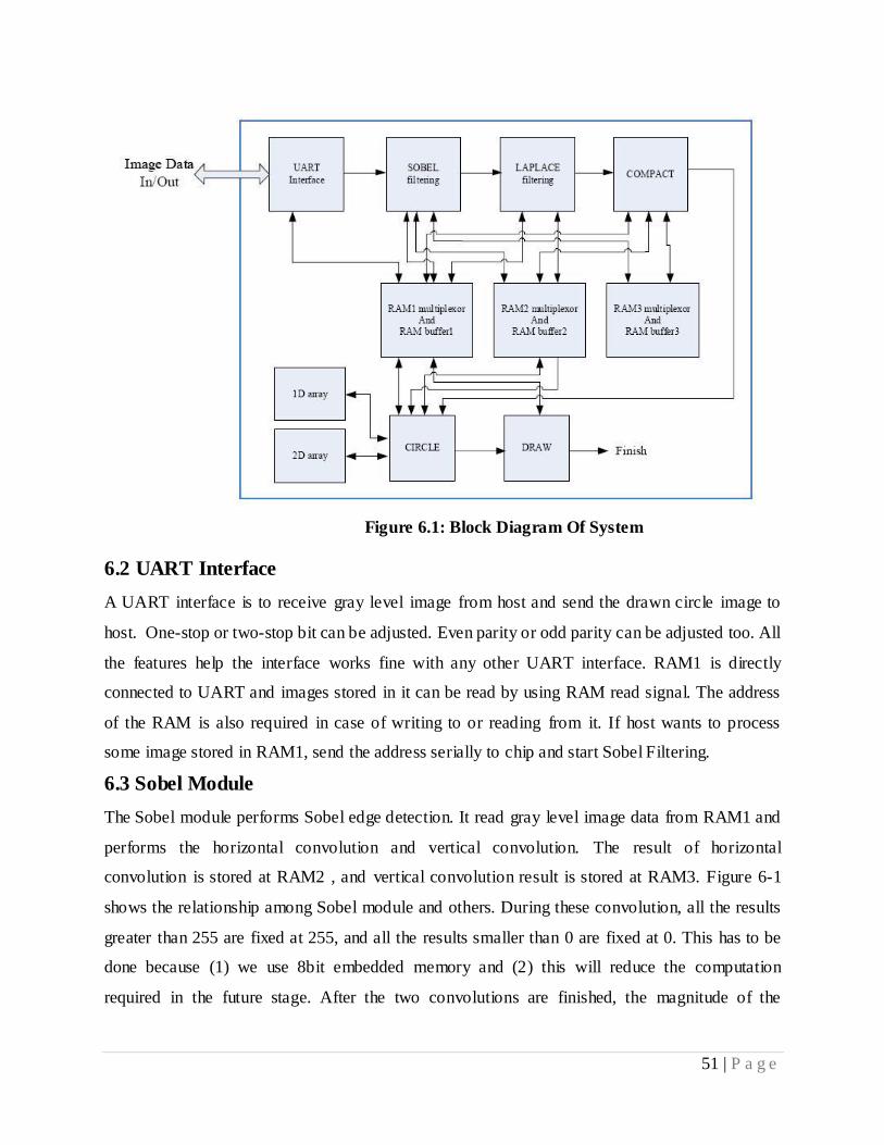
Figure 6.1: Block Diagram Of System
6.2 UART Interface
A UART interface is to receive gray level image from host and send the drawn circle image to
host. One-stop or two-stop bit can be adjusted. Even parity or odd parity can be adjusted too. All
the features help the interface works fine with any other UART interface. RAM1 is directly
connected to UART and images stored in it can be read by using RAM read signal. The address
of the RAM is also required in case of writing to or reading from it. If host wants to process
some image stored in RAM1, send the address serially to chip and start Sobel Filtering.
6.3 Sobel Module
The Sobel module performs Sobel edge detection. It read gray level image data from RAM1 and
performs the horizontal convolution and vertical convolution. The result of horizontal
convolution is stored at RAM2 , and vertical convolution result is stored at RAM3. Figure 6-1
shows the relationship among Sobel module and others. During these convolution, all the results
greater than 255 are fixed at 255, and all the results smaller than 0 are fixed at 0. This has to be
done because (1) we use 8bit embedded memory and (2) this will reduce the computation
required in the future stage. After the two convolutions are finished, the magnitude of the
52 | P a g e
gradient can be calculated and stored into RAM1. A threshold is again set to examine the
magnitude which makes the Sobel edge detection generate binary image.
6.4 Laplace Filtering
Some image have better result if we performance the Laplace filtering after Sobel edge detection,
and some don‟t. We can set a control bit to bypass Laplace filtering whenever we want. This will
reduce the computation time.
6.5 Compact Module
The extracted edge pixels in the result are randomly located in the image buffer RAM1 or
RAM2. We need to perform a defragmentation so that the performance of improves. So we need
to rearrange the edge pixels and place them in the RAM buffer in sequence to reduce searching
time in the center and radius calculation stage. The effect of compacting edge pixel locations is
remarkable and center and radius calculation time can be reduced by a great amount. This will
greatly reduce total detection time. If it is a valid edge pixel, the address of the data will be
written into RAM.
6.6 Circle Module
The Circle module calculate radius and center location according to the address stored in the
RAM.
6.7 Draw Module
The Draw module draw circle according to the detected radius and center location. Only the
circle with local maximum radius and center histogram is to be drawn or otherwise processing
time and memory required will increase. RAM contains the exact location of circle we detected.
The content of RAM can be read through UART interface.
53 | P a g e
APPENDIX A – MATLAB Code
fabric = imread('C:\Documents and Settings\Jahanzeb\My Documents\MATLAB\sample.jpg');
figure(1), imshow(fabric), title('fabric');
load regioncoordinates;
nColors = 6;
sample_regions = false([size(fabric,1) size(fabric,2) nColors]);
for count = 1:nColors
sample_regions(:,:,count) = roipoly(fabric,region_coordinates(:,1,count),...
region_coordinates(:,2,count));
end
imshow(sample_regions(:,:,2)),title('sample region for red');
cform = makecform('srgb2lab');
lab_fabric = applycform(fabric,cform);
a = lab_fabric(:,:,2);
b = lab_fabric(:,:,3);
color_markers = repmat(0, [nColors, 2]);
for count = 1:nColors
color_markers(count,1) = mean2(a(sample_regions(:,:,count)));
color_markers(count,2) = mean2(b(sample_regions(:,:,count)));
end
color_labels = 0:nColors-1;
54 | P a g e
a = double(a);
b = double(b);
distance = repmat(0,[size(a), nColors]);
for count = 1:nColors
distance(:,:,count) = ( (a - color_markers(count,1)).^2 + ...
(b - color_markers(count,2)).^2 ).^0.5;
end
[value, label] = min(distance,[],3);
label = color_labels(label);
clear value distance;
rgb_label = repmat(label,[1 1 3]);
segmented_images = repmat(uint8(0),[size(fabric), nColors]);
for count = 1:nColors
color = fabric;
color(rgb_label ~= color_labels(count)) = 0;
segmented_images(:,:,:,count) = color;
end
%imshow(segmented_images(:,:,:,2)), title('red objects');
%imshow(segmented_images(:,:,:,3)), title('green objects');
imshow(segmented_images(:,:,:,6)), title('purple objects');
x=segmented_images(:,:,:,2);
x=rgb2gray(x);
z=edge(x);

55 | P a g e
figure(2),imshow(z),title('edge');
56 | P a g e
APPENDIX B – OpenCV Code
#include"math.h" #include"conio.h"
#include"cv.h" #include"highgui.h"
#include"stdio.h" #include <windows.h> #include <iostream>
IplImage* redcheck(IplImage* input); IplImage* greencheck(IplImage* input); IplImage* bluecheck(IplImage* input);
void serialsend(int send,int stps);
int status = 0; int ball=0; int main()
{ /////////////////////////Wait for User Input ////////////////////////////
printf("\n Enter the colour of the ball to detect:\n 0: Red
\n1:Blue\n2:Green\n3:exit\n");
scanf("%d",&ball);
///////////////////////////////////////////////////////////////////////// /////////////////////Initializing dvices and images//////////////////////
int key=0; IplImage* frame=0;
CvCapture* capture = cvCaptureFromCAM( CV_CAP_ANY ); if( !capture ) {
fprintf( stderr, "ERROR: capture is NULL \n" ); getchar();
return -1; }
/////////////////////////Start capturing frames//////////////////////////
for (;;)
57 | P a g e
{
frame = cvQueryFrame( capture ); if( !frame ) {
fprintf( stderr, "ERROR: frame is null...\n" ); getchar(); break;
}
IplImage *red=redcheck(frame); IplImage *green=greencheck(frame); IplImage *blue=bluecheck(frame);
cvNamedWindow( "mywindow", CV_WINDOW_AUTOSIZE ); cvShowImage( "mywindow", frame );
////////////////////////Show Resultant Images//////////////////////////// switch(ball) {
case 0: cvNamedWindow( "RED", CV_WINDOW_AUTOSIZE );
cvShowImage( "RED", red); break; case 2:
cvNamedWindow( "GREEN", CV_WINDOW_AUTOSIZE );
cvShowImage( "GREEN", green); break; case 1:
cvNamedWindow( "BLUE", CV_WINDOW_AUTOSIZE );
cvShowImage( "BLUE", blue); break; }
key=cvWaitKey(10); if (key == 27){ printf("\n\n done! \n\n");
break; }
} ////////////////////////Destroy Windows and Devices//////////////////////////// switch(ball)
{ case 0:
cvDestroyWindow("RED"); break;
58 | P a g e
case 2: cvDestroyWindow("GREEN");
break; case 1:
cvDestroyWindow("BLUE"); break; }
cvReleaseCapture( &capture );
cvDestroyWindow( "mywindow" ); return (0); }
IplImage* redcheck(IplImage* input) {
IplImage *result=cvCreateImage( cvGetSize(input), 8, 1 );
//////////////////////Access Image Data Using pointers////////////////////// int i,j,k; int height,width,step,channels;
int stepr, channelsr; int temp=0;
uchar *data,*datar; i=j=k=0; height = input->height;
width = input->width; step =input->widthStep;
channels = input->nChannels; data = (uchar *)input->imageData;
stepr=result->widthStep; channelsr=result->nChannels; datar = (uchar *)result->imageData;
for(i=0;i < (height);i++) { for(j=0;j <(width);j++)
{ /* CHANNELS +2 ==RED CHANNEL.Select pixels which are more red
than any other color. Select a difference of 29(which again depends on the scene)*/
59 | P a g e
if(((data[i*step+j*channels+2]) > (25+data[i*step+j*channels])) && ((data[i*step+j*channels+2]) >
(25+data[i*step+j*channels+1]))) {
datar[i*stepr+j*channelsr]=255; } else
datar[i*stepr+j*channelsr]=0; }
} IplImage* gray = cvCreateImage(cvGetSize(input), 8, 1);
CvMemStorage* storage = cvCreateMemStorage(0); cvCvtColor(input, gray, CV_RGB2GRAY);
cvSmooth(gray, gray, CV_GAUSSIAN, 9, 9); CvSeq* circles = cvHoughCircles(gray, storage, CV_HOUGH_GRADIENT, 9, gray->height/25, 200, 100);
int numofsteps=0;
int left=0; int right=0; int cn=0;
for (int x = 0; x < circles->total; x++)
{ float* p = (float*) cvGetSeqElem(circles, x); int radius=cvRound(p[2]);
int column=cvRound(p[0]); int row=cvRound(p[1]);
if (ball==0 && status == 0) {
if (datar[cvRound(p[1])*stepr+cvRound(p[0])*channelsr]==255) {
printf("\n Red Circle num=%d located at Row=%d Column =%d Radius = %d\n",x,cvRound(p[1]),cvRound(p[0]),cvRound(p[2]));
if (radius>=62) printf("\ncircle is too near move backward\n");
else if (radius>=50 && radius<=70) {
printf("\ncircle is ready to be picked\n"); // 0000 0 0 1 1 0000 0000
serialsend(3,0); status = 3;
60 | P a g e
}
else if (radius<=49) {
if (column > ((gray->width/2)-20) && column <
((gray->width/2)+20))
{ printf ("\ncircle is in centre ,Move
forward.\n"); //0000 0 0 1 0 serialsend(2,0);
status = 2; }
else { printf ("\ncircle is NOT in centre ,Rotate
stepper motor by some degrees \n"); if (column>(gray->width/2))
{ right=1; left=0;
cn=320-column; printf("\ncolumns = %d",cn);
numofsteps=(6-(cn/26.67)); printf("\n move %d steps to
right\n",numofsteps);
//0000 0 1 1 0 serialsend(6,numofsteps);
status = 1; } else
{ right=0;
left=1; cn=column; printf("\ncolumns = %d",cn);
numofsteps=(6-(cn/26.67)); printf("move %d steps to
left",numofsteps); //0000 1 0 1 0 serialsend(10,numofsteps);
status = 1; }
} }
61 | P a g e
}
} if (ball == 0 && status == 1){
if (column > ((gray->width/2)-20) && column < ((gray->width/2)+20))
{
printf ("\ncircle is in centre ,Move forward.\n"); serialsend(2,0);
status = 2; } }
if (ball == 0 && status == 2){
//check whether in centre or not.if yes than pickup the balll..///// if ((radius>=55 && radius<=70) && status == 2) {
printf("\ncircle is ready to be picked\n"); serialsend(3,0);
status = 3; }
} }
return result; }
IplImage* greencheck(IplImage* input) {
IplImage *result=cvCreateImage( cvGetSize(input), 8, 1 );
///////////////////Accessing Image Data//////////////////////////// int i,j,k; int height,width,step,channels;
int stepr, channelsr; int temp=0;
uchar *data,*datar; i=j=k=0;
height = input->height; width = input->width;
step =input->widthStep; channels = input->nChannels;
62 | P a g e
data = (uchar *)input->imageData;
stepr=result->widthStep; channelsr=result->nChannels; datar = (uchar *)result->imageData;
for(i=0;i < (height);i++) {
for(j=0;j <(width);j++) {
/* CHANNELS +1 ==GREEN CHANNEL.Select pixels which are more red than any other color.
Select a difference of 29(which again depends on the scene)*/
if(((data[i*step+j*channels+1]) > (25+data[i*step+j*channels])) && ((data[i*step+j*channels+1]) >
(25+data[i*step+j*channels+2]))) datar[i*stepr+j*channelsr]=255;
else datar[i*stepr+j*channelsr]=0;
} }
IplImage* gray = cvCreateImage(cvGetSize(input), 8, 1); CvMemStorage* storage = cvCreateMemStorage(0);
cvCvtColor(input, gray, CV_RGB2GRAY); cvSmooth(gray, gray, CV_GAUSSIAN, 9, 9); CvSeq* circles = cvHoughCircles(gray, storage, CV_HOUGH_GRADIENT, 9,
gray->height/25, 200, 100);
int numofsteps=0; int left=0; int right=0;
int cn=0; for (int x = 0; x < circles->total; x++)
{ float* p = (float*) cvGetSeqElem(circles, x); int radius=cvRound(p[2]);
int column=cvRound(p[0]); int row=cvRound(p[1]);
if (ball==2 && status == 0)
63 | P a g e
{ if (datar[cvRound(p[1])*stepr+cvRound(p[0])*channelsr]==255)
{ printf("\n Green Circle num=%d located at Row=%d
Column =%d Radius = %d\n",x,cvRound(p[1]),cvRound(p[0]),cvRound(p[2])); if (radius>=62)
printf("\ncircle is too near move backward\n"); //circle is too near.... move backward.
else if (radius>=50 && radius<=70) { printf("\ncircle is ready to be picked\n");
serialsend(3,0); status = 3;
} else if (radius<=49) {
if (column > ((gray->width/2)-10) && column <
((gray->width/2)+10)) { printf ("\ncircle is in centre ,Move
forward.\n"); serialsend(2,0);
status = 2; } else
{ printf ("\ncircle is NOT in centre ,Rotate
stepper motor by some degrees \n"); if (column>(gray->width/2)) {
right=1; left=0;
cn=320-column; printf("\ncolumns = %d",cn); numofsteps=(6-(cn/26.67));
printf("\n move %d steps to right\n",numofsteps);
serialsend(6,numofsteps); status = 1; }
else {
right=0; left=1;
64 | P a g e
cn=column; printf("\ncolumns = %d",cn);
numofsteps=(6-(cn/26.67)); printf("move %d steps to
left",numofsteps); serialsend(10,numofsteps); status = 1;
} }
} } }
if (ball == 2 && status == 1){ if (column > ((gray->width/2)-20) && column < ((gray-
>width/2)+20)) { printf ("\ncircle is in centre ,Move forward.\n");
serialsend(2,0); status = 2;
} }
if (ball == 2 && status == 2){ if ((radius>=55 && radius<=70) && status == 2)
{ printf("\ncircle is ready to be picked\n"); serialsend(3,0);
status = 3;
} } }
return result; }
IplImage* bluecheck(IplImage* input)
{ IplImage *result=cvCreateImage( cvGetSize(input), 8, 1 );
int i,j,k; int height,width,step,channels;
int stepr, channelsr;
65 | P a g e
int temp=0;
uchar *data,*datar; i=j=k=0;
height = input->height; width = input->width;
step =input->widthStep; channels = input->nChannels;
data = (uchar *)input->imageData;
stepr=result->widthStep;
channelsr=result->nChannels; datar = (uchar *)result->imageData;
for(i=0;i < (height);i++)
{ for(j=0;j <(width);j++) {
/* CHANNELS +0 ==Blue CHANNEL.Select pixels which are
more red than any other color. Select a difference of 29(which again depends on the scene)*/
if(((data[i*step+j*channels]) > (25+data[i*step+j*channels+2])) && ((data[i*step+j*channels]) > (25+data[i*step+j*channels+1])))
{ datar[i*stepr+j*channelsr]=255;
}
else datar[i*stepr+j*channelsr]=0; }
}
IplImage* gray = cvCreateImage(cvGetSize(input), 8, 1); CvMemStorage* storage = cvCreateMemStorage(0); cvCvtColor(input, gray, CV_RGB2GRAY);
cvSmooth(gray, gray, CV_GAUSSIAN, 9, 9);
CvSeq* circles = cvHoughCircles(gray, storage, CV_HOUGH_GRADIENT, 9, gray->height/25, 200, 100);
66 | P a g e
int numofsteps=0; int left=0;
int right=0; int cn=0;
for (int x = 0; x < circles->total; x++) { float* p = (float*) cvGetSeqElem(circles, x);
int radius=cvRound(p[2]); int column=cvRound(p[0]);
int row=cvRound(p[1]); if (ball==1 && status == 0) {
if (datar[cvRound(p[1])*stepr+cvRound(p[0])*channelsr]==255) {
printf("\n Blue Circle num=%d located at Row=%d Column =%d Radius = %d\n",x,cvRound(p[1]),cvRound(p[0]),cvRound(p[2]));
if (radius>=62)
printf("\ncircle is too near move backward\n");
else if ((radius>=50 && radius<=70) ) { printf("\ncircle is ready to be picked\n");
serialsend(3,0); status = 3;
} else if (radius<=49)
{
if (column > ((gray->width/2)-10) && column < ((gray->width/2)+10))
{
printf ("\ncircle is in centre ,Move forward.\n");
serialsend(2,0); status = 2; }
else {
printf ("\ncircle is NOT in centre ,Rotate stepper motor by some degrees \n");
if (column>(gray->width/2)) {
right=1; left=0;
67 | P a g e
cn=320-column; printf("\ncolumns = %d",cn);
numofsteps=(6-(cn/26.67)); printf("\n move %d steps to
right\n",numofsteps); serialsend(6,numofsteps); status = 1;
} else
{ right=0; left=1;
cn=column; printf("\ncolumns = %d",cn);
numofsteps=(6-(cn/26.67)); printf("move %d steps to
left",numofsteps);
serialsend(10,numofsteps); status = 1;
} } }
} }
if (ball == 1 && status == 1){ if (column > ((gray->width/2)-20) && column < ((gray-
>width/2)+20))
{ printf ("\ncircle is in centre ,Move
forward.\n"); serialsend(2,0); status = 2;
} }
if (ball == 1 && status == 2){ if ((radius>=55 && radius<=70) && status == 2)
{ printf("\ncircle is ready to be picked\n");
serialsend(3,0); status = 3;
} }
}
68 | P a g e
return result; }
void serialsend(int send,int stps) {
///////////////////////////////////////////////////// /////////////////Opening the serial port/////////////////
HANDLE hSerial= CreateFile("COM3", GENERIC_READ|GENERIC_WRITE,
NULL, NULL,
OPEN_EXISTING, FILE_ATTRIBUTE_NORMAL, NULL);
if(hSerial==INVALID_HANDLE_VALUE){ printf("invalid handle.\n");
} /////////////////////////////////////////////////////
/////////////////Setting Parameters///////////////// DCB dcbSerialParams = {0};
dcbSerialParams.DCBlength=sizeof(dcbSerialParams); if (!GetCommState(hSerial, &dcbSerialParams)) { printf("error occured at getCommState\n");
} dcbSerialParams.BaudRate=CBR_115200;
dcbSerialParams.ByteSize=8; dcbSerialParams.StopBits=ONESTOPBIT; dcbSerialParams.Parity=NOPARITY;
///////////////////////Writing data //////////////////////
char buff1[2]; buff1[0]=char(send); buff1[1]=char(stps);
int siz1 = sizeof(buff1);
DWORD dwBytesRead = 0; for(int t=0;t<siz1;t++){
WriteFile(hSerial, buff1, siz1, &dwBytesRead, NULL); printf("\nsending data to serial port\n");
}

69 | P a g e
//////////////////////Closing down////////////////// CloseHandle(hSerial);
}
70 | P a g e
APPENDIX C – DataSheets
71 | P a g e
REFRENCES
[1] Gary Rost Bradski, Adrian Kaehler. Learning OpenCV. New York: O‟reilly Publishing,
2008. ISBN 13: 9780596516130
[2] OpenCV Installation and Getting Started Guide
http://www.scribd.com/
[3] Rafael C. Gonzalez & Richard E. Woods Digital Image Processing (3rd Edition) Prentice
Hall Publishing, ISBN : 9780131687288.
[4] Ying Bai The Windows Serial Port Programming Handbook ISBN-10: 0849322138
[5] Image Acquisition Toolbox 3.2 Manual
http://www.mathworks.com/
[6] Rafael C. Gonzalez & Richard E. Woods Digital Image Processing Using Matlab Prentice
Hall Publishing, ISBN : 9780130085191.