CRANFIELD UNIVERSITY
IZZATI IBRAHIM
ILLUMINATION INVARIANCE AND SHADOW COMPENSATION ON HYPERSPECTRAL IMAGES
CRANFIELD DEFENCE AND SECURITY
Academic Year: 2009-2013
Supervisor: Dr Peter Yuen January 2013


CRANFIELD UNIVERSITY
CRANFIELD DEFENCE AND SECURITY
PhD
Academic Year 2009 - 2013
IZZATI IBRAHIM
ILLUMINATION INVARIANCE AND SHADOW COMPENSATION ON HYPERSPECTRAL IMAGES
Supervisor: Dr Peter Yuen
January 2013
© Cranfield University 2013. All rights reserved. No part of this publication may be reproduced without the written permission of the
copyright owner.


i
ABSTRACT
To obtain intrinsic reflectance of the scene by hyperspectral imaging systems
has been a scientific and engineering challenge. Factors such as illumination
variations, atmospheric effects and viewing geometries are common artefacts
which modulate the way of light reflections from the object into the sensor and
that they are needed to be corrected. Some of these factors induce highly
scattered and diffuse irradiance which can artificially modify the intrinsic spectral
reflectance of the surface, such as that in the shadows.
This research is attempted to compensate the shadows in the hyperspectral
imagery. In this study, three methods known as the Diffuse Irradiance
Compensation (DIC), Linear Regression (LR) and spectro-polarimetry technique
(SP) have been proposed to compensate the shadow effect. These methods
have various degrees of shadow compensation capabilities, and their pros and
cons are elucidated within the context of their classification performances over
several data sets recorded within and outside of the laboratory. The spectro-
polarimetry (SP) technique has been found to be the most versatile and
powerful method for shadow compensation, and it has achieved over 90% of
classification accuracy for the scenes with ~30% of shadow areas.
Keywords:
Hyperspectral, diffuse, direct irradiance, polarizer, illumination invariance,
shadow

ii
LIST OF PUBLICATION
Journal Paper
Illumination invariance and shadow compensation via spectro-polarimetry
technique. Ibrahim, I., Yuen, P., Hong, K., Chen, T., Soori, U., Jackman, J.
and Richardson, M. 10, Bellingham, WA : SPIE, 2012, Optical Engineering
(OE), Vol. 51.
Shadow compensation and illumination invariance on hyperspectral images.
Ibrahim, I., Yuen, P., Hong, K., Chen, T., Soori, U., Jackman, J. and
Richardson, M. 2012, under review of Imaging Science Journal.
Shadow compensation using spectro-polarimetry technique on hyperspectral
images, Ibrahim, I., Yuen, P., Hong, K., Soori, U., Chen WT and Richardson,
M. Paper to be submitted to the Int. Journal of Remote Sensing.
Conference and Poster Paper
Illumination independent object recognitions in hyperspectral imaging. Ibrahim,
I., Yuen, P., Tsitiridis, A., Hong, K., Chen, T., Jackman, J., James, D. and
Richardson, M. Touluse, France : SPIE, 2010. Proceedings of the SPIE 7838.
Vol. 7838, pp. 78380O-1-12 .
Shadow compensation on hyperpsectral imageries. Ibrahim, I., Yuen, P.,
Soori, U., Chen, T., Hong, K., Tsitiridis, A., Jackman, J. and Richardson, M.
Shrivenham, Swindon : Defence Academy of the United Kingdom, 2012. 10th
Electro-optics & Infrared Conference.
Enhanced object recognition in cortex-like machine. Tsitiridis, A., Yuen, P. W.
T., Ibrahim, I., Soori, U., Chen, T., Hong, K., Wang, Z., James, D. and
Richardson, M. Corfu : IEEE/EANN, 2011. 12th EANN / 7th AIAI Joint
Conference on Engineering Application.

iii
Colour invariant target recognition in multiple camera CCTV surveillance. Soori,
U., Yuen, P. W. T., Ibrahim, I., Tsitiridis, A., Hong, K., Chen, T., Jackman, J.,
James, D. and Richardson, M. Prague : SPIE, 2011. Proceedings of the SPIE.
Vols. 8189A-24.
Assessment of tissue blood perfusion in-vitro using hyperspectral and thermal
imaging techniques. Chen, T., Yuen, P. W. T., Hong, K., Ibrahim, I., Tsitiridis,
A., Soori, U., Jackman, J., James, D. and Richardson, M. Wuhan, China :
IEEE, 2011. 5th International Conference on Bioinformatics and Biomedical.
Bulletin Paper
Ibrahim, I., Yuen, P., Tsitiridis, A., Hong, K., Chen, T., Jackman, J., James,
D. and Richardson, M. Spectral constancy on hyperspectral imageries.
Defence S&T Technical Bulletin. 2011, Vol. 4, 1, pp. 19-30.
Yuen, P., Ibrahim, I., Hong, K., Chen, T., Tsitiridis, A., Jackman, J., Kam, F.,
Jackman, J., James, D. and Richardson, M. Classification enhancements in
hyperpsectral remote sensing using atmospheric correction preprocessing
technique. Defence S&T Technical Bulletin. 2009, Vol. 2, 2, pp. 91-99.


v
ACKNOWLEDGEMENTS
I would like to thank Dr Yuen for his supervision, support and valuable guidance
during my PhD study. I also would like to thank Prof. Dr. Richardson for taking
time out of his busy schedules to assists me in my research and my journal
paper. I am also grateful to the Malaysian Ministry of Science, Technology and
Innovation and Malaysian Science Technology Research Institute for Defence
for sponsoring and giving me an opportunity to do my PhD study. Finally, I
would like to thank my family especially Haniff Zaid, Dr Ismaeel and my lovely
children, Hafiff and Haifa for their patience and supports during my PhD course.

vii
TABLE OF CONTENTS
ABSTRACT ......................................................................................................... i LIST OF PUBLICATION ...................................................................................... ii ACKNOWLEDGEMENTS................................................................................... v LIST OF FIGURES ............................................................................................. ix
LIST OF TABLES ............................................................................................. xiv LIST OF EQUATIONS ...................................................................................... xiv 1 HYPERSPECTRAL IMAGING SYSTEMS (HSI) ....................................... 17
1.1 Motivation of Research ........................................................................ 17 1.2 Aim ...................................................................................................... 19
1.3 Introduction to HSI............................................................................... 19 1.3.1 HSI and Other Imaging Systems .................................................. 20
1.3.2 Hyperspectral Images ................................................................... 23 2 AN OVERVIEW OF DETECTION AND CLASSIFICATION ALGORITHMS 27
2.1 Detection Overview ............................................................................. 27
2.1.1 Anomaly Detection ........................................................................ 27 2.1.2 Spatial Subsetting ......................................................................... 28
2.1.3 Target Removal ............................................................................ 29 2.1.4 Spectral Subsetting ....................................................................... 30 2.1.5 Matched Filter Detection ............................................................... 30
2.1.6 Performance Measure .................................................................. 31 2.2 Classification Overview ....................................................................... 33
2.2.1 Parametric Classifier via Bayes’ Theorem .................................... 34 2.2.2 Quadratic Likelihood Classifier (QD) ............................................. 36 2.2.3 Fisher Linear Discriminant (FD) .................................................... 37
2.2.4 Minimum distance Classifier (MD) ................................................ 38 3 RADIOMETRIC DISTORTION .................................................................. 39
3.1 Atmospheric Effects ............................................................................ 39 3.2 Atmospheric Correction ....................................................................... 44
3.2.1 Empirical Line Method (ELM)........................................................ 44 3.2.2 Flat Field Conversion .................................................................... 46 3.2.3 Internal Average Relative Reflectance (IARR) .............................. 47
3.2.4 Atmosphere Removal program (ATREM) ..................................... 47 3.2.5 Atmospheric and Topographic Correction (ATCOR) ..................... 48
3.2.6 Quick Atmosphere Correction (QUAC) ......................................... 51 4 ILLUMINATION EFFECT AND SHADOW ................................................. 52
4.1 Illumination Geometry ......................................................................... 52
4.1.1 Shading ........................................................................................ 54 4.1.2 Shadow ......................................................................................... 55
4.2 Previous Work on Shadow Compensation .......................................... 58 5 HSI EQUIPMENT ...................................................................................... 61
5.1 HSI Camera ........................................................................................ 61 5.2 Radiometric Calibration ....................................................................... 65
6 DIFFUSE IRRADIANCE COMPENSATION (DIC) METHOD FOR SHADOW COMPENSATION ........................................................................... 66

viii
6.1 Experiment Setup ................................................................................ 66
6.2 Low Reflectance and Shadow Mask ................................................... 70 6.3 DIC Shadow Compensation Method ................................................... 73 6.4 Assessments Methods ........................................................................ 75 6.5 DIC Shadow Compensation Results ................................................... 78
6.5.1 10 different coloured t-shirt data ................................................... 78
6.5.2 Previous work on shadow compensation: Normalization and band ratio 82 6.5.3 DIC Method for 5 t-shirts data ....................................................... 86 6.5.4 Conclusion .................................................................................... 93
7 COLOUR TRANSFER LINEAR REGRESSION METHOD ....................... 95
7.1 Linear Regression Method .................................................................. 95 7.2 Experimental Setup ............................................................................. 96 7.3 Linear Regression Result .................................................................. 100
7.3.1 Ten T-Shirt Indoor Data .............................................................. 100 7.3.2 Five T-Shirt Indoor Data ............................................................. 104 7.3.3 Outdoor Data set ........................................................................ 108
7.4 Conclusion ........................................................................................ 113 8 SPECTRO-POLARIMETRY METHOD (SP) ........................................... 115
8.1 Introduction and background ............................................................. 115 8.2 Spectro-Polarimetry Technique (SP) for shadow compensation ....... 117 8.3 Experimental Setup ........................................................................... 120
8.4 Scaled SAM Result ........................................................................... 124 8.5 Spectro-polarimetry (SP) Method Assessments ................................ 130
8.5.1 Indoor scene ............................................................................... 130 8.5.2 Outdoor scene ............................................................................ 138
8.6 Conclusion ........................................................................................ 143
9 CONCLUSIONS AND FUTURE WORK .................................................. 145
9.1 Diffuse Irradiance Compensation Method (DIC) ................................ 145
9.2 Linear Regression Method (LR) ........................................................ 146 9.3 Spectro-polarimetry Technique (SP) ................................................. 147
9.4 Future Work ...................................................................................... 148 REFERENCES ............................................................................................... 149 APPENDICES ................................................................................................ 161
Appendix A Reflectance for shadow and direct pixels of 10 different coloured t-shirt data .................................................................................... 161
Appendix B Reflectance for shadow and direct pixels of 5 different coloured t-shirt data 167 Appendix C Classification accuracy for each class before and after correction 171

ix
LIST OF FIGURES
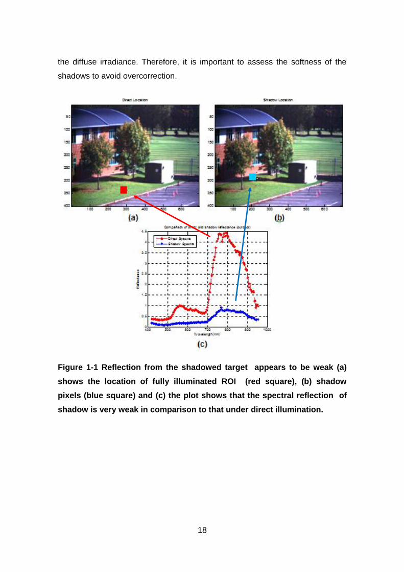
Figure 1-1 Reflection from the shadowed target appears to be weak (a) shows the location of fully illuminated ROI (red square), (b) shadow pixels (blue square) and (c) the plot shows that the spectral reflection of shadow is very weak in comparison to that under direct illumination. ........................ 18
Figure 1-2 The spectral properties of the lawn at various locations of an outdoor scene. Note that different locations of the shadow regions exhibit different apparent reflectance values as estimated by Empirical Line Method (ELM). This is due to the various degrees of self shadowing effects. ................... 19
Figure 1-3 Shows (a) RGB image, (b) location, (c) classification map of a specific probability of detection and (d) reflectance graph (reflectance versus wavelength (μm)) in Visible-near infrared (VNIR) of three look-alike red Astra car panels. The hyperspectral imaging system is capable to distinguish three different panels by exploiting more detailed spectral information other than the RGB bands. ..................................................... 22
Figure 1-4 A sample of a 3D HSI cube consists of spatial pixels in the axis x and y with spectra channels in the z direction. (b) The comparison of the ‘reflectance’ of a sample collected by MSI (top) and HSI (bottom) (9). ..... 24
Figure 1-5 Each pixel in the image can be plotted as the reflectance of targets in each waveband. This reflectance or spectral signature of targets can then be interpreted for target detection or classification (9). ............................. 24
Figure 1-6 An example of spectral signature for soil, water and vegetation (50). .................................................................................................................. 25
Figure 1-7 Typical variation of reflectance for vegetation (50) due to the variability of natural materials. ................................................................... 25
Figure 2-1 Graphical presentation of spatial subsetting in HSI images. ........... 29
Figure 2-2 shows an example of displaying the detected pixels over that of the ground truth target maps at a specific PFA. .............................................. 32
Figure 2-3 shows an example of (a) pixel based ROC and (b) indicates the target based ROC. .................................................................................... 32
Figure 2-4 The role of classification in labelling the hyperspectral data (22). ... 33 Figure 2-5 Diagram of classification taxonomy (22). ........................................ 34 Figure 2-6 The effect of the a priori probability on class probability density
function (49). ............................................................................................. 35 Figure 2-7 shows the discriminant function for the Bayes optimal partition
between 2 classes and the probability of error (49). .................................. 36 Figure 3-1 The energy structure for molecule (25). .......................................... 40 Figure 3-2 Diagram of the atmospheric windows – spectral regions in which
solar radiation is able to transmit through the Earth’s atmosphere. Chemical notation indicates the gas molecules that are responsible for the atmospheric absorption at particular wavelength (27). .............................. 40
Figure 3-3 Represents three types of scattering; Rayleigh scattering, Mie scattering and Geometrical optic model (25). ............................................ 42
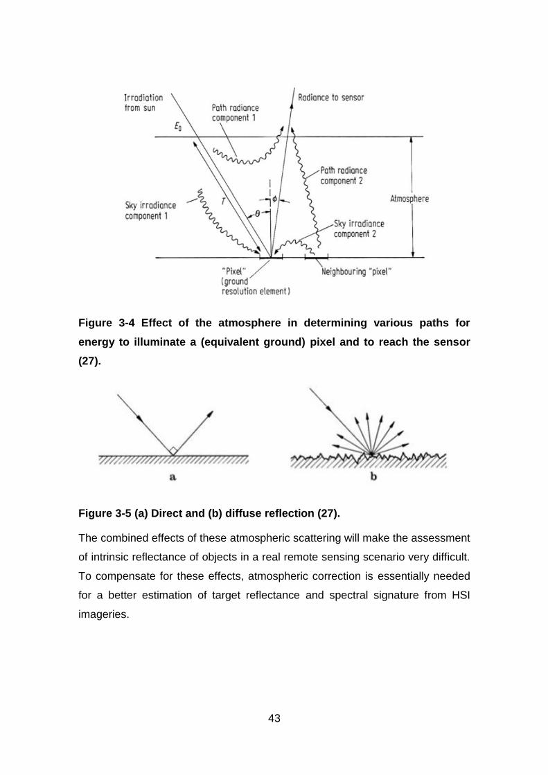
Figure 3-4 Effect of the atmosphere in determining various paths for energy to illuminate a (equivalent ground) pixel and to reach the sensor (27). ......... 43
Figure 3-5 (a) Direct and (b) diffuse reflection (27). .......................................... 43

x
Figure 3-6 ELM representation (21). ................................................................ 46
Figure 3-7 Illumination and viewing geometry (ATCOR) (45). .......................... 49 Figure 3-8 Schematic sketch of solar radiation components as seen by the HSI
system (45). .............................................................................................. 51 Figure 4-1 Illustration of steradian (25). ............................................................ 53 Figure 4-2 Depiction of the BRDF nomenclature (25). ..................................... 54
Figure 4-3 Shows (a) Lambertian surface and (b) specular surface. ................ 55 Figure 4-4 Sketch of cloud shadow geometry (34). .......................................... 55 Figure 4-5 (a) red square and (b) blue square represent the location extracted
from the image of fully illuminated pixels and shadow pixels respectively, (c) the spectral shape of direct and shadowed pixel are the same due to homogeneous background and that the sky is misty white, (d) normalised spectra of direct and diffused irradiated grass. .......................................... 56
Figure 4-6 (a) red square and (b) blue square represent the location extracted from the image for fully illuminated pixel and shadow pixels respectively, (c) the spectra shaped of shadowed pixel changed due to the complicated background (d) normalised spectra showing completely different spectral shapes between the directed and diffusely irradiated surfaces. ................ 57
Figure 5-1 Picture of (a) The Headwall Visible Near Infra-red (VNIR) imaging system and (b) the Specim & Xenics Short Wave Infra-red (SWIR) imaging system. ...................................................................................................... 61
Figure 5-2 Holospec™ Spectrograph (77). ....................................................... 62
Figure 5-3 Diagram of the ImSpector™ camera (78). ...................................... 63 Figure 5-4 Diagram of an Offner Imaging Spectrometer and photo of the
Headwall Photonics’ spectrograph Hyperspec (78). ................................. 63 Figure 5-5 The rotating mirror system made by our lab (78). ........................... 64 Figure 5-6 Pictures of the GUI for (a) VNIR_2.0 and (b) SWIR_2.0 program
(78). ........................................................................................................... 64
Figure 5-7 The calibrated panels used in this PhD research: top- gray panel (50% reflectance), bottom left- white panel (98% reflectance) bottom right- black panel (2% reflectance). .................................................................... 65
Figure 6-1 Shows (a) the data of 10 coloured t-shirts under uniform illuminations by light sources placed at the front of the scene denoted as C and D in the figure and (b) the RGB image of the experimental set-up showing the light blocker at both ends for shadows simulation............................................. 67
Figure 6-2 Shows (a) under oblique illumination casting self shadows in parts of the 10 coloured t-shirts (b) the RGB image of the complete scene under oblique illumination. ................................................................................... 68
Figure 6-3 Shows (a) the RGB image of 5 coloured t-shirts under uniform illumination (labelled from 1 to 5) and (b) when it is under oblique illumination casting shadows on part of the targets. .................................. 69
Figure 6-4 Shows the flow chart to obtain the final mask. ................................ 70 Figure 6-5 The low variance mask calculated from the image under oblique
illumination; (a) the false colour variance map and (b) the threshold of (a) used as the flat reflectance mask. This threshold map shows low variance target (indicated by scale equal to 0). ....................................................... 71
Figure 6-6 The procedure for obtaining the final shadow mask: (a) the RGB image under oblique illumination, (b) threshold (0.26) of the spectral mean

xi
of the image which represents the low reflectance pixels in the scene (c) final shadow mask (bright areas) after the flat reflectance pixels are removed. White scale colour on the final shadow map (c) indicates the shadow pixels whereas black scale colour represents the direct illumination pixels. ........................................................................................................ 72
Figure 6-7 Shows the (a) flat reflectance mask (black areas) for the 5 coloured t-shirt experiment, (b) low reflectance pixels in the scene (black areas) and (c) final shadow mask (bright areas). Note that although .......................... 73
Figure 6-8 Shows the RGB image of the experimental set up for assessing Edir and Ediff. ..................................................................................................... 74
Figure 6-9 Shows (a) spectral characteristics of Edir and Ediff in DN values and (b) to highlight the difference in the spectral characteristics of the Edir and Ediff. ............................................................................................................ 74
Figure 6-10 Shows (a) the RGB image of 10 different t-shirts data under direct illumination and (b) the RGB image of 5 different t-shirt data and the yellow box depicts where the training data pixels are extracted for classification. 76
Figure 6-11 Shows the target map in false colours for (a) 10 different colours t-shirts and (b) 5 different colours t-shirts. These target maps are used to evaluate the accuracy of classification. ..................................................... 77
Figure 6-12 Shows RGB images of (a) Raw data, (c) RW data, (b) and (d) are the false colour image of the classification results for the respective Raw and RW data. The overall accuracies in these cases are respectively 38% & 68%, and note the large misclassifications in the classes 1 and 2 in the Raw data as shown in (b). ......................................................................... 80
Figure 6-13 Shows (a) RGB image and (b) the classification result after DIC shadow compensation exhibit 70% of classification accuracy. Note that the DIC has achieved the best overall accuracy in comparison to that of the Raw and RW results. ................................................................................ 81
Figure 6-14 Shows the RGB images of the image taken at oblique illumination (a) after normalisation (RW Norm), and (b) the false colour classification results of RW Norm. Note that target classes 1, 2 and 4 have been substantially misclassified in the RW Norm data. ...................................... 83
Figure 6-15 Shows (a) the RGB image and (b) the false colour classification result of RW R870 giving 62% accuracy. ................................................. 84
Figure 6-16 Shows (a) RGB image and (b) the false colour classification result of RW RAdj giving 62% accuracy. ............................................................. 85
Figure 6-17 Shows the classification result of (a) the raw data and (b) RW data of 5 different coloured t-shit. ...................................................................... 87
Figure 6-18 Shows (a) the RGB image of RW Norm for the 5 different coloured t-shirts and (b) its classification result exhibiting 35% accuracy. .............. 88
Figure 6-19 Shows the RGB image of (a) RW R870 and (c) RW RAdj data of 5 different coloured t-shirt data together with their classification results shown in ((c) and (d)) respectively. ...................................................................... 90
Figure 6-20 Shows (a) the RGB image of the 5 different coloured t-shirts after DIC correction and (b) its classification result with 58% accuracy. Note that the correction is far from perfect as it can be seen from the RGB image. . 91
Figure 6-21 Shows the spectral plot of the apparent reflectance of the shadowed targets: without correction (RW) in blue, after correction by DIC

xii
in green, and comparison with that under direct illumination in red for (a) blue t-shirt (target 1), (b) red t-shirt (target 2) and (c) black t-shirt (target 4). .................................................................................................................. 93
Figure 7-1 Shows the final shadow mask (bright areas) (a) for the 10 coloured t-shirt indoor data, (b) the 5 coloured t-shirt indoor data and (c) the outdoor scene data. ................................................................................................ 98
Figure 7-2 Shows the RGB image of a hyperspectral data with 88 spectral bands that consists of 10 different coloured t-shirts indoor data used in the LR experiment. This data set is similar to that used in the DIC experiment. .................................................................................................................. 99
Figure 7-3 Shows the RGB image of a hyperspectral data with 88 bands that consists of 5 different coloured t-shirts indoor data used in the LR experiment. This data set is again similar to that in the DIC experiment. .. 99
Figure 7-4 Shows the hyperspectral data of outdoor scene with 102 spectral bands taken at a range of ~100m on a clear and sunny day on the 2nd October 2011 at 2 pm GMT. .................................................................... 100
Figure 7-5 Shows the RGB image of the 10 coloured t-shirt data after LR compensation. ......................................................................................... 101
Figure 7-6 Shows the false colour images of the classification result for the 10 coloured t-shirt data (a) after RW correction with 68% accuracy, (b) after DIC compensation with 70% accuracy and (c) after LR compensation with 75% accuracy. ......................................................................................... 102
Figure 7-7 Shows the spectral plot of shadowed pixels for two targets of (a) light green t-shirt (target 7) and (b) dark green t-shirt target 10) obtained from i) apparent reflectance without correction (RW in blue), ii) after correction via DIC (DIC in green)), iii) after LR (in light blue) iv) under direct illumination(in red). .................................................................................. 103
Figure 7-8 Shows the RGB image of the 10 coloured t-shirts data after LR operation. ................................................................................................ 104
Figure 7-9 Shows the false colour classification result of the 5 coloured t-shirt data set after (a) RW with 43% accuracy, (b) DIC compensation with 58% accuracy and (c) LR correction with 97% accuracy. ............................... 106
Figure 7-10 Shows the the spectral plot of the shadowed pixels from (a) blue t-shirt (target 1), (b) red t-shirt (target 2) and (c) black t-shirt (target 4) after i) no correction (RW in blue), ii) after correction by DIC (in green), iii) after LR (in light blue) and iv) the same targets under direct illumination. ...... 108
Figure 7-11 Shows the RGB image of an outdoor scene (a) before and (b) after correction by the LR method. .................................................................. 109
Figure 7-12 Shows the apparent reflectance of various targets (a) grass (b) bunker, (c) red bricks and (d) the lawn of the golf course before (in blue) and after (in green) correction by LR and to compare with that under direct illumination (in red). ................................................................................. 112
Figure 8-1 Shows the polarization set up in our system: a polarizer is is placed on the top of the camera’s objective lens. ............................................... 119
Figure 8-2 Shows the plot of the mean spectra from the white standard panel taken without and with (90degree) polarizer filter. ................................... 119

xiii
Figure 8-3 Shows the RGB picture of (a) the illumination Halogen lamp and the background, (b) the 4 t-shirt target and the shadow casted by a piece of cardboard placed at the left hand side of the targets. ............................. 121
Figure 8-4 Shows the RGB image of the 10 coloured t-shirt scene. ............... 121 Figure 8-5 (a) Shows the RGB picture of the lawn that was taken on clear and
sunny day at 1 pm and (b) shows the sky condition during the experiment. ................................................................................................................ 122
Figure 8-6 (a) Shows the RGB image of the bunker that was taken on a clear and sunny day at 1 pm and (b) shows the environment condition of the scene. ..................................................................................................... 123
Figure 8-7 Shows the RGB images (a) without polarizer (INP), (b) with polarizer (IP) and (c) the false colour scaled_SAM result of these two images for the indoor scene. ........................................................................................... 125
Figure 8-8 Shows the RGB images (a) without polarizer (INP), (b) with polarizer (IP) and (c) the false colour scaled_SAM result of these two images for the10 coloured t-shirt indoor data. Note that the shadow is identified in blue. ........................................................................................................ 127
Figure 8-9 Shows the RGB images (a) without polarizer (INP), (b) with polarizer (IP) and (c) the false colour scaled_SAM result of these two images for the lawn outdoor scene. Note that all trees and part of the lawn have been identified as shadows correctly. .............................................................. 128
Figure 8-10 Shows the RGB image (a) without polarizer (INP), (b) with polarizer (IP) and (c) the false colour map of the scaled_SAM result for the bunker outdoor scene. Note that the near side of the bunker and the cars have been identified as shadows correctly. ..................................................... 130
Figure 8-11 (a) Shows the RGB image of the baseline scene under direct illumination, and the yellow box depicts where the training data pixels are extracted from; (b) the ground truth target map in false colours. ............. 132
Figure 8-12 Shows the false colour map of the QD result (a) no correction by RW with accuracy 48%, (b) after correction by SP with 98% classification accuracy. ................................................................................................. 133
Figure 8-13 Shows the spectral plot of (a) Green t-shirt 1 (b) Red t-shirt 2 (c) Yellow t-shirt 3 and (d) Blue t-shirt 4 for the pixels i) no shadow compensation (RW in blue), ii) after SPT correction (in green) and iii) direction comparison with that under direct illumination (in red). ............. 135
Figure 8-14 Shows the false colour QD results (a) before correction by RW with accuracy of 57%, (b) after correction by SP with 90% accuracy. ............ 136
Figure 8-15 Shows the spectral plot of (a) t-shirt 1 (Orange), (b) t-shirt 5 (Blue), (c) t-shirt 7 (Light Green) and (d) t-shirt 10 (Dark Green) after i) no shadow compensation by RW (in blue), ii) after SPT correction (in green) and iii) comparison with that under direct illuminations. ...................................... 138
Figure 8-16 shows the the RGB images (a) before correction (INP), (b) the RGB after correction by SPT and (c) the spectral plot of the shadow pixels of the lawn before (in blue) and after correction by SPT (in green) with respect to that under direct illumination (in red). ...................................................... 140
Figure 8-17 shows the (a) the RGB image before correction (INP), (b) the RGB image after correction by SP technique and (c) the spectral plot of the shadow target before (in blue) and after correction by SPT (green) with

xiv
respect to that under direct illumination (in red) for the bunker outdoor data. The edge of shadow shape in (b) is seen to have a mixed pixel problem due to the bad pixels resolution of the camera. ......................... 142
LIST OF TABLES
Table 6-1 Summary of the classification results. .............................................. 94 Table 7-1 The SAM of the outdoor data with respected to that under direct
illumination. ............................................................................................. 110 Table 7-2 The distance similarity for outdoor data. ......................................... 110 Table 7-3 The overall result of classification accuracy. .................................. 114 Table 8-1 shows the spectra similarity of the shadow targets before and after
correction by SP technique with respected to that under direct illumination for the lawn data set. ............................................................................... 140
Table 8-2 shows the spectra similarity of the shadow targets before and after correction by SP technique with respected to that under direct illumination for the bunker data set. ........................................................................... 141
Table 8-3 The overall result of classification accuracy. .................................. 144
LIST OF EQUATIONS
(2-1) .................................................................................................................. 28 (2-2) .................................................................................................................. 28
(2-3) .................................................................................................................. 28 (2-4) .................................................................................................................. 31 (2-5) .................................................................................................................. 31 (2-6) .................................................................................................................. 31 (2-7) .................................................................................................................. 34
(2-8) .................................................................................................................. 34 (2-9) .................................................................................................................. 35
(2-10) ................................................................................................................ 36 (2-11) ................................................................................................................ 36 (2-12) ................................................................................................................ 37
(2-13) ................................................................................................................ 37 (2-14) ................................................................................................................ 37
(2-15) ................................................................................................................ 38 (2-16) ................................................................................................................ 38
(3-1) .................................................................................................................. 39 (3-2) .................................................................................................................. 45 (3-3) .................................................................................................................. 45 (3-4) .................................................................................................................. 45 (3-5) .................................................................................................................. 46
(3-6) .................................................................................................................. 46 (3-7) .................................................................................................................. 47

xv
(3-8) .................................................................................................................. 48
(3-9) .................................................................................................................. 48 (3-10) ................................................................................................................ 49 (3-11) ................................................................................................................ 50 (3-12) ................................................................................................................ 50 (3-13) ................................................................................................................ 50
(4-1) .................................................................................................................. 52 (4-2) .................................................................................................................. 53 (4-3) .................................................................................................................. 53 (4-4) .................................................................................................................. 53 (4-5) .................................................................................................................. 54
(4-6) .................................................................................................................. 54 (4-7) .................................................................................................................. 58 (4-8) .................................................................................................................. 59
(4-9) .................................................................................................................. 60 (6-1) .................................................................................................................. 75 (7-1) .................................................................................................................. 96
(7-2) .................................................................................................................. 96 (7-3) .................................................................................................................. 96
(7-4) .................................................................................................................. 97 (7-5) .................................................................................................................. 97 (8-1) ................................................................................................................ 117
(8-2) ................................................................................................................ 117 (8-3) ................................................................................................................ 118
(8-4) ................................................................................................................ 118 (8-5) ................................................................................................................ 118
GLOSSARY
AD Anomaly detection AMF Adaptive matched filter ATCOR Atmospheric and topographic correction ATREM Atmosphere removal algorithm BRDF Bidirectional reflectance distribution function DIC Diffuse irradiance compensation DN Digital number ED Euclidean distance classifier ELM Empirical line method EM Electromagnetic EO Electro-optic FD Fisher linear discriminant classifier FF Flat Field FLAASH Fast line-of-sight atmospheric analysis of spectral hypercubes FOV Field of view GLRT Generalized likelihood ratio test GMM Gaussian mixture model

xvi
GMRX Global Mean RX GRX Global RX HATCH High-accuracy atmospheric correction for hyperspectral data HSI Hyperspectral imaging IAR Internal average reflectance IGRX Iterated global RX LR Linear regression LRX Local RX LWIR Long wave infrared (8 to 14 μm) MD Minimum distance classifier MF Matched filter MODTRAN Moderate resolution atmosphere radiance and transmittance
model MSI Multispectral imaging MWIR Mid wave infrared (3 to 5 µm) PFA Probability of false alarm PoD Probability of detection QD Quadratic likelihood classifier QUAC Quick atmosphere correction RGB Red green blue ROC Receiver operating characteristic ROI Region of interest RX Iriving Reed and Xiaoli Yu SEM Stochastic expectation maximization SP Spectro-polarimetry SS Single spectrum method SWIR Short wave infrared (1 to 2.4 μm) TI Thermal imager VNIR Visible to near infrared
17
1 HYPERSPECTRAL IMAGING SYSTEMS (HSI)
1.1 Motivation of Research
Hyperspectral imaging (HSI) is a technique that allows the intrinsic electro-optic
(EO) properties, such as the reflectance and emissions of objects in the scene,
to be acquired remotely. This information can then be used for a variety of
applications including target detection and classification. The ultimate
usefulness of the technology relies very much on whether the reflectance and
emissions of the objects in the scene can be accurately retrieved from the
image as observed by the HSI system. If a flat landscape of scenery is
uniformly illuminated within the normal plane of the surface then it is possible to
deduce the reflectance of the scene accurately. This is possible only if the
viewing and illumination geometries are close to the normal plane and that the
atmospheric parameters are known. However, this is not the case in general,
partly due to the adjacency multiple diffuse scattering caused by nearby objects
in the scene.
Objects under shadows exhibit rather different EO properties compared to
objects that under direct illuminations. The reflected energy recorded by an
imaging system from a shadowed object usually consists of only diffuse
irradiance scattered by sky lights and adjacency surroundings objects.
Therefore, the digital number (DN) value of shadowed target is always lower
and it appears to look dark in the image, as shown in Figure 1-1.
The other issue when dealing with shadows in hyperspectral imageries is the
softness of the shadow which can be represented by the ratio between the
intensity of the shadow pixels with respected to that under direct illumination.
The softness of shadows is scene dependent as shown in Figure 1-2. When a
target is in hard shadow in which the direct illumination is completely blocked
(i.e. no direct illumination), the apparent reflectance spectrum appears to be
very weak approaching to almost zero. This is quite different for a target that is
in partial shadow. The partially shadowed target will have non-zero reflection of
18
the diffuse irradiance. Therefore, it is important to assess the softness of the
shadows to avoid overcorrection.
Figure 1-1 Reflection from the shadowed target appears to be weak (a)
shows the location of fully illuminated ROI (red square), (b) shadow
pixels (blue square) and (c) the plot shows that the spectral reflection of
shadow is very weak in comparison to that under direct illumination.

19
Figure 1-2 The spectral properties of the lawn at various locations of an
outdoor scene. Note that different locations of the shadow regions exhibit
different apparent reflectance values as estimated by Empirical Line
Method (ELM). This is due to the various degrees of self shadowing
effects.
1.2 Aim
It is evident that objects under shadow exhibit significant changes in the
reflected energy and spectral shape. This will cause a considerably negative
effect in target detection and classification. Therefore, the aim of this research is
to develop a method to compensate shadow effects in hyperspectral imagery.
The methodology adopted in this study involves:
1. Segmentation of direct and diffuse irradiance pixels from the
hyperspectral images
2. Correction of apparent reflectance of the shadowed objects using
information when the same object is under direct irradiance.
1.3 Introduction to HSI
Hyperspectral Imaging System (HSI) has been widely used in various
applications especially when more information apart from textural and
broadband RGB colours are required for the identification and discrimination of
objects. Hyperspectral imaging system offers high resolution of spectral
20
information and it has been deployed in many applications, including agriculture
(1, 2), surveillance (3), remote sensing (4, 5), medical (6, 7) and military (8).
The HSI system takes hundreds or more of contiguous wavebands ranging
from visible to near infrared (VNIR) region (0.4 to 0.95 μm) through the short
wave infrared (SWIR) (1 to 2.4 μm), mid wave infra-red (MWIR) (3 to 5 µm) and
up to long wave infrared (LWIR) (8 to 14 μm) region. Each waveband occupies
very narrow slice of electromagnetic (EM) spectrum of approximately 5 to 20 nm
wide, allowing the analysis to be performed on each individual waveband or a
subset of a selection of them to maximise the spectral contrast between the
target and the clutter background. For instance, HSI is able to distinguish
targets of similar colours by exploiting slices of spectral information in a wide
region as illustrated in Figure 1-3. Other conventional imaging systems such as
broadband digital RGB will be unable to discriminate these look-alike targets.
1.3.1 HSI and Other Imaging Systems
Historically, much of the success in defence surveillance and reconnaissance
has relied upon expert (human) interpretation such as by visual examination of
the imagery data. Conventional imaging systems, namely panchromatic and
broadband colour RGB, integrate the complete spectral range or broad
bandwidths in the order of ~100-200nm. These systems are not capable to
provide enough spectral information for target acquisition and can only provide
spatial information of the scene.
Advanced imaging technology, such as a thermal imager (TI), capture
emissions from targets rather than reflected light to form an image. The spectral
range of the thermal imaging systems are mostly in the Middle Wave Infrared
region (MWIR) 3 to 5 µm and Long Wave Infrared (LWIR) 8 to 14 µm. The
advantage of using thermal imaging systems is that they can operate in an
environment of total darkness and do not depend on the light of a scene as they
capture thermal energy emitted from the targets. Most TI systems are less
capable to sample IR radiations in narrow bandwidths and as a result, two
different objects which emit the same integrated thermal energy would exhibit

21
similar radiance intensity in the thermal band. It is even more difficult to use the
conventional TI system to detect targets that incorporate thermal camouflage
techniques by concealing the thermal radiation to blend into the surrounding.
(a)
(b)

22
(c)
(d)
Figure 1-3 Shows (a) RGB image, (b) location, (c) classification map of a
specific probability of detection and (d) reflectance graph (reflectance
versus wavelength (μm)) in Visible-near infrared (VNIR) of three look-alike
red Astra car panels. The hyperspectral imaging system is capable to
distinguish three different panels by exploiting more detailed spectral
information other than the RGB bands.

23
HSI systems represent an evolution in imaging technology from earlier
multispectral imaging (MSI) systems. Multispectral imaging systems commonly
employ about 10-20 discrete bands covering visible, Near Infrared (NIR), SWIR,
MWIR and LWIR regions. As these systems employ discrete bands, and
therefore they are not able to produce detailed signatures of targets due to the
insufficient spectral resolution.
HSI systems have been developed through the advancement in sampling the
reflective electromagnetic spectrum spanning from visible region (VIS) all the
way to LWIR region in narrow contiguous bands (about 10 to 30 nm wide) in
every pixel of a scene. HSI differs from MSI in that the number of bands
utilized in HSI is much higher (about 100 or more) and that the spectral bands
are contiguous.
1.3.2 Hyperspectral Images
HSI image cube consists of spatial and spectral information as illustrated in
Figure 1-4. Spatial information is normally presented in the x and y axis and the
spatial width are dependent on the field of view (FOV) of the system (9).
Spectral information is presented in the z axis and the resolution is dependent
on the spectral sampling capability of the system (9). One way to present
hyperspectral data is to make a composite image using three carefully chosen
spectral bands. However, choosing the most appropriate three channels from
HSI cube is not a straightforward task. Nevertheless, a set of three bands
similar to those used in the conventional RGB images are often adopted for
simple display of hyperspectral imageries (10). After appropriate processing, the
spectral vector in each pixel can be used for target detection and classification
as shown in Figure 1-5.

24
Figure 1-4 A sample of a 3D HSI cube consists of spatial pixels in the axis
x and y with spectra channels in the z direction. (b) The comparison of the
‘reflectance’ of a sample collected by MSI (top) and HSI (bottom) (9).
Figure 1-5 Each pixel in the image can be plotted as the reflectance of
targets in each waveband. This reflectance or spectral signature of targets
can then be interpreted for target detection or classification (9).
The ultimate goal of HSI is to detect and classify any interesting objects in the
scene based on the spectral characteristics of the target reflectance signature.
An overview of detection and classification methods will be outlined in Chapter
2. Suppose that there are 3 types of classes consisting of soil, water and
vegetation with spectral signatures within the visible to near infrared region as
given in Figure 1-6. However, the spectral signature of a given objects is not

25
represented by a single spectra but by a family of spectra as shown in Figure
1-7 due to the variability of natural substances. This variability is partly due to
the atmospheric and sensor effects that hamper the retrieval of target
reflectance accurately. All these factors make the separation of classes much
more difficult in practice. Hence pre-processing algorithm to compensate all
these factors is needed in order to improve the integrity of the spectral
characteristics of HSI data thus to improve the detection and classification
accuracy. This pre-processing step will be briefly reviewed in Chapter 3.
Figure 1-6 An example of spectral signature for soil, water and vegetation
(50).
Figure 1-7 Typical variation of reflectance for vegetation (50) due to the
variability of natural materials.

26
Apart from the factors as mentioned above, illumination effects such as
shadowing also affect the accuracy of retrieving intrinsic spectral property such
as reflectance of objects from the scene in remote sensing. Shadow effects
distort the intrinsic optical characteristic and therefore it is crucially important to
compensate this undesired shadowing effect in order to improve the target
detection and classification (10). This is the main concern of this research.
Three new methods of shadow compensation, namely Diffuse Irradiance
Compensation (DIC), Linear Regression (LR) and Spectro-polarimetry (SP)
technique have been proposed. The details of each method are outlined in
Chapter 6, 7 and 8.
27
2 AN OVERVIEW OF DETECTION AND
CLASSIFICATION ALGORITHMS
This chapter presents an overview of the theoretical and practical issues of
detection and classification algorithms for hyperspectral imagery processing.
The basic idea of HSI stems from the fact that different materials will exhibit
variable amounts of wavelength dependent reflection, absorption or emission
(11). This spectral characteristic can be used as signature for the detection and
classification of the scene.
2.1 Detection Overview
There are two main types of detection algorithms in HSI processing, namely
anomaly detection (AD) and matched filter (MF) detection. The former is the
detection technique that identifies pixels different from the background without
prior information (12). The latter is a detection technique based on prior
information of targets, i.e. spectral signatures of targets. This type of detection
aims to locate the pixel vectors that match the targets signature as much as
possible (13).
2.1.1 Anomaly Detection
Anomaly detection is a technique that locates and identifies the uncommon
pixel vector compared to the ‘norm’ of the background model. If an observed
pixel spectra differs from the ‘norm’ of the background then the deviation is
measured using a distance metric to represent the degree of anomaly. The
distance metric normally used in anomaly detection was derived by Iriving Reed
and Xiaoli Yu (RX) in 1990 (13). Yu and Reed developed the algorithm under
the Generalized Likelihood Ratio Test (GLRT) framework for multidimensional
image data. This assumes that the spectrum of the target and the covariance of
the background are Gaussian distributed and that they are generally unknown
(13-15).
28
By denoting a background model as B, a distance measure as d(.) and a
threshold as t, pixel x is regard as an anomaly if (16):
txxtBxdBxDRX ˆˆˆ, (2-1)
Where
N
n
nxN 1
1 (2-2)
and
N
n
Tnxnx
N 1
1 (2-3)
In equation (2-1) the distance between each pixel signature to the background
signature is calculated using Mahalanobis distance (16) in the RX formulation.
Here, the background is modelled as a multivariate Gaussian distribution (16).
Hence, in AD it is the model of the background which is needed for the
identification of uncommon pixels. There are various techniques reported for
characterizing the background, such as the employment of local or global
windowing, target removal or clustering.
2.1.2 Spatial Subsetting
The employment of local or global windowing has been one of the simplest
methods for background characterization and it is commonly known as spatial
subsetting. There are two types of local windowing: one is the local spatial
subset and the second is the spatial scene subset (globally) (17) as shown in
Figure 2-1. The local mode is commonly implemented using two concentric
sliding windows. The mean and covariance of the background are extracted
from the outer window while excluding the inner one. This is called Local RX
(LRX) (6). The global mode denoted as Global RX (GRX) which uses one
sliding window that takes large section of the imagery (13) and the Mahalanobis
29
distance of every test pixel is evaluated sequentially according to equation
(2-1). Global Mean RX (GMRX) models the background by utilizing the whole
image to calculate the mean and covariance of the background and it is more
suitable for real time detection work than LRX method.
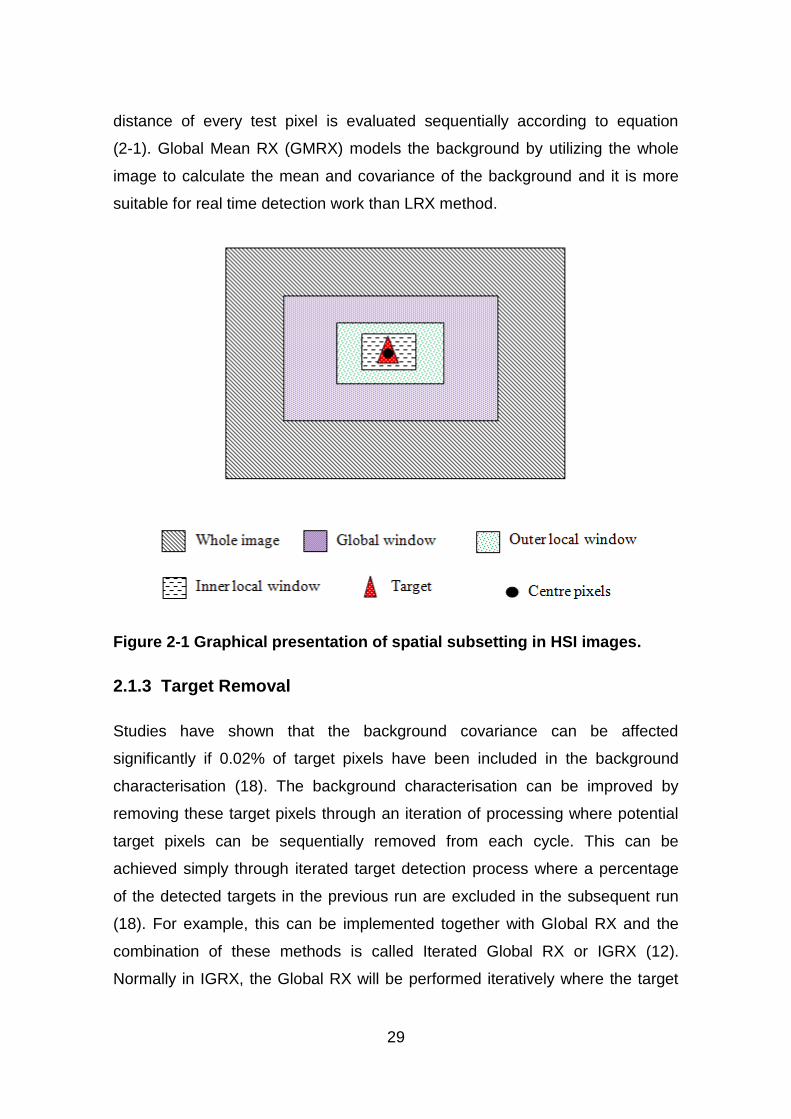
Figure 2-1 Graphical presentation of spatial subsetting in HSI images.
2.1.3 Target Removal
Studies have shown that the background covariance can be affected
significantly if 0.02% of target pixels have been included in the background
characterisation (18). The background characterisation can be improved by
removing these target pixels through an iteration of processing where potential
target pixels can be sequentially removed from each cycle. This can be
achieved simply through iterated target detection process where a percentage
of the detected targets in the previous run are excluded in the subsequent run
(18). For example, this can be implemented together with Global RX and the
combination of these methods is called Iterated Global RX or IGRX (12).
Normally in IGRX, the Global RX will be performed iteratively where the target

30
pixels will be detected by loosely thresholding the GRX in the first few rounds of
detection (12). Then, these target pixels are subsequently excluded in the next
iteration of detection. This process will be repeated until the IGRX detection
performance does not change significantly with respect to the previous run.
Alternatively, the target pixels can be found by using other algorithms, such as
spectral unmixing (19), as the first round of target detection.
2.1.4 Spectral Subsetting
All the detection algorithms mentioned in the above sections are based on the
assumption that the HSI data conforms to multivariate Gaussian distribution.
However, it is found that the real world HSI imagery generally consists of fat tail
containing high order statistics (12, 18). One way to circumvent this is to classify
the non-Gaussian HSI data into more Gaussian-like clusters. This can be
achieved by using Gaussian Mixture Model classification such as K-means
clustering or Stochastic Expectation Maximization (SEM) classification (18). K-
means technique is applied by classifying or grouping the objects based on the
spectral features into K classes. The feature refers to the mean of the class and
is calculated by minimizing the sum of squares of distances between each pixel
to the corresponding mean. While for SEM, the features refer to the mean and
the covariance of the classes. Both K-means and SEM aim to generate class or
cluster maps for the scene. Then, the detection is applied by finding the
anomalous pixels that is least likely to fall into each class (20).
2.1.5 Matched Filter Detection
Matched filter detection is a well-developed technique that uses a known target
spectral signature or target probe to search for the presence of that spectrum in
a scene (21). It attempts to detect and locate pixels containing a target
signature by modelling the scene background as unstructured or stochastic.
This takes the form of first and second order spectral statistics (mean, and
covariance, ) estimated from the HSI data of the scene like that performed in
the anomaly detection.

31
The adaptive matched filter (AMF) is a detector that models and suppresses a
background (21) and then uses a known target spectrum, denoted as s, to
search for that in the scene. The pixel x is classified as target classes, C if (16)
t
ss
xst
s
xsCBxD
T
TT
AMF
1
1
2~
~~,
(2-4)
This detector is optimum only when the target and background follow a
Gaussian distribution and in real applications this is highly unlikely (16).
The adaptive coherence or cosine detectors model the target variability by
measuring the angle between the target pixels to the target spectrum. The pixel
x is classified as a target pixel if (16):
ttxx
xPxCBxD
T
S
T
ACE
2cos~~
~~~, (2-5)
Where SP~
is the projection and reconstruction operator onto the target subspace
~
s , that is
T
SS
T
SSSP ~~~~~ 1
(2-6)
and is the angle between the target subspace and the test vector.
2.1.6 Performance Measure
The performance of the detection in remote sensing is commonly assessed
through a projection of detection result onto a map as illustrate in Figure 2-2,
which displays the detected pixels over the ground truth target map for a
specific probability of detection and the associated probability of false alarm
rate. This will provide the reader with an intuitive image of the detection result.
Alternatively, the Receiver Operating Characteristic (ROC) has been another
and more effective way to present the performance of the detector. The ROC
can be assessed in Pixel Based Graph (as in Figure 2-3 (a)) that counts every

32
detected pixel for various false alarm rates, while the Target Based Graph (as in
Figure 2-3 (b)) counts the number of the detected target. The ROC graph shows
the detector performance by plotting the probability of detection (PoD) versus
Probability of False Alarm (PFA), where the ideal case is to have the highest
PoD with the lowest PFA. By using both pixel based and target based ROC, the
efficiency of the detector can be assessed more accurately.
(a) (b)
Figure 2-2 shows an example of displaying the detected pixels over that of
the ground truth target maps at a specific PFA.
(a) (b)
Figure 2-3 shows an example of (a) pixel based ROC and (b) indicates the
target based ROC.

33
2.2 Classification Overview
Classification on hyperspectral imageries normally adopts a non-literal
processing which exploits mostly spectral information rather than spatial (21).
Each pixel in each band of the HSI imageries consists of specific reflectance or
radiance which can be labelled into specific classes by matching the distance
between the characteristics of each pixels with respected to the training data, as
shown in Figure 2-4. The assignment of a pixel into any particular class is
commonly based on the statistical intelligent which is associated with the
probability of error. There are two types of classification, namely supervised and
unsupervised. Supervised classification is a discriminate classifier that uses
class information whereas unsupervised classification clusters the groups
without the class information (22). For the purpose of this thesis we will
concentrate on supervised classification using a parametric classifier via Bayes’
theorem. Figure 2-5 shows a diagram of the classification taxonomy.
Figure 2-4 The role of classification in labelling the hyperspectral data
(22).

34
Figure 2-5 Diagram of classification taxonomy (22).
2.2.1 Parametric Classifier via Bayes’ Theorem
Parametric classifier utilises a statistical approach to classify the object of
interest to specific classes based on their spectral properties. These specific
classes that contains known spectral signature are associated with a specific
label. An important assumption in a statistical approach to classification is that
each spectral class can be described by a probability distribution in spectral
space such as normal or Gaussian distribution (22).
Given L number of training data, a posteriori probabilities that the pixel x
belongs to class i can be calculated with Bayes Rule:
xp
ipixpxip (2-7)
Where
L
ii
ipixpxp (2-8)
A decision rule to assign pixel x to one of the L number of classes can be
achieved using equation (2-7). For example, based on the Figure 2-6, let the
number of class is equal to 2, the Bayes decision rule can easily be interpreted
such that (49):

35
a pixel x belongs to class 1 if 2211 pxppxp
a pixel x belongs to class 2 if 1122 pxppxp
a decision cannot be made if 2211 pxppxp
The equation (2-7) is also called as discriminant function and is denoted as ig .
This discriminant function can be rewritten in a logarithmic form (22):
ipixpg i loglog (2-9)
The error of the classification is given by the area under the overlapping
portions of the posteriori probability as in Figure 2-7. Note that in this figure, the
crossover line indicate the decision boundary; which to the right indicate the
pixel x belongs to class 2 and to the left the decision favour class 1.
Figure 2-6 The effect of the a priori probability on class probability density
function (49).

36
Figure 2-7 shows the discriminant function for the Bayes optimal partition
between 2 classes and the probability of error (49).
2.2.2 Quadratic Likelihood Classifier (QD)
In hyperspectral images that consist of N number of bands, the probability
functions, ixp becomes a multivariate functions, iXp . The general
multivariate form for N-dimensional normal distribution is given as (49):
ii
T
i
i
NmXmXiXp 1
2
1
22
1exp
2
1
(2-10)
Where X = pixel feature vector
im = mean vector for class i
Σi = NN symmetric covariance matrix for class i
So the Bayes discriminant function for class i is then (49):
ii
T
iii mXmXN
ipg 1
2
1log
2
12log
2log (2-11)
The Quadratic Likelihood Classifier class partition is defined by equation (2-11)
and the decision is depended on the relations between the means and

37
covariance matrices of different classes. The values for and are estimated
from a set of training sample, given as N
jn xxx ,......1
Therefore,
N
i
ii xN
m1
1 (2-12)
And
N
i
T
iiiii mxmxN 1
1 (2-13)
As this classifier measures both the mean and the covariance it has been
proven to be one of the most effective classification methods within the HSI
community. However, the sample size of the training data must be sufficiently
large enough to achieve a well characterised covariance for each class to
minimise misclassifications (22).
2.2.3 Fisher Linear Discriminant (FD)
The minimum distance classifier assign the feature vector X to class whose
mean vector, im , is closest to X. If we assume that the covariance matrix are
equal for all classes, i.e. 0 ji and the a priori probabilities are equal, i.e.
0pjpip , the discriminate function of equation (2-11) becomes (49):
i
T
ii mXmXxg 1
02
1 (2-14)
Equation 2-14 is known as Mahalanobis Distance or Fisher Linear Discriminant
classifier (FD). A pattern is classified by finding the minimum distance from the
normalised mean.

38
2.2.4 Minimum distance Classifier (MD)
If the covariance matrices of all classes are assumed to be diagonal and have
equal variance along each feature axis, i.e.
2
2
2
00
00
00
i
Therefore, the covariance is merely 2 times the identity matrix, I (22), i.e.
Ii
2 and Ii
2
1 1
. So the discriminant function becomes:
2
2
2log
i
i
mXipXg
(2-15)
The quantity 2
imX is a scalar that can be expanded as:
N
n
inni mxd1
2
,
2 (2-16)
This scalar is simply the square of the Euclidean distance between vector X and
the mean, im . Therefore this of classifier is called the Minimum Distance
Classifier (MD) or Euclidean distance classifier (ED).

39
3 RADIOMETRIC DISTORTION
The radiant energy that is sensed by a hyperspectral system can generally be
separated into two components: one is the radiant energy reflected or
transmitted by objects due to irradiance sources such as solar or artificial light;
and the second one is the radiant energy due to self-emissions from the objects
(24). These radiant energies propagate through the atmospheric medium before
reaching the sensor. Therefore, it is important to measure all these components
in order to obtain accurate reflectance or spectral signatures of targets. This is
especially the case when dealing with electromagnetic propagation and
transmission through the atmosphere. Factors such as atmospheric scattering
and absorption, direct and diffuse solar irradiance, reflectance of adjacent
targets and bidirectional reflection differential effect may distort the assessment
of absolute reflectance.
3.1 Atmospheric Effects
When solar radiation propagates through the atmosphere it is affected by two
important mechanisms: absorption and scattering. Absorption by molecules in
the atmosphere is a quantum process that changes the molecules internal
state, increasing the energy and resulting in a temperature change (25). Figure
3-1 shows the energy structure of a molecule. For a photon to be absorbed by a
molecule, the photon energy, Ephoton must be higher than the molecular energy
bandgap, Eg. The energy of photon is given by Einstein equation:
hvE (3-1)
Where E is the energy of the photon, h is the Planks’ constant (6.626 x 10⁻³⁴ J-
sec) and is the frequency of the incident light. Because of this quantum
mechanism, the absorption is not significant within the visible band except for
H2O absorption between 0.65 and 0.85 um. However, absorption has a strong
affect within the thermal infrared region. There are approximately 30 different
species of gases in atmosphere but only 7 of them, namely water vapour (H2O),
carbon dioxide (CO2), ozone (O3), nitrous oxide (N2O), carbon monoxide (CO),

40
methane (CH4) and oxygen (O2), produce appreciable absorption features in the
thermal region (26). The spectral regions in which absorption does not occur
due to these gases are called atmospheric windows. Several atmospheric
windows exist in the range between 0.4 and to 2.5 µm (26), as shown in Figure
3-2. In the absence of atmospheric absorption the radiation transmittance
should be 100% but this is not generally the case. Hyperspectral data should be
collected within these atmospheric windows because outside these windows the
radiation transmittance will be significantly reduced due the atmospheric
absorption.
Figure 3-1 The energy structure for molecule (25).
Figure 3-2 Diagram of the atmospheric windows – spectral regions in
which solar radiation is able to transmit through the Earth’s atmosphere.
Chemical notation indicates the gas molecules that are responsible for the
atmospheric absorption at particular wavelength (27).

41
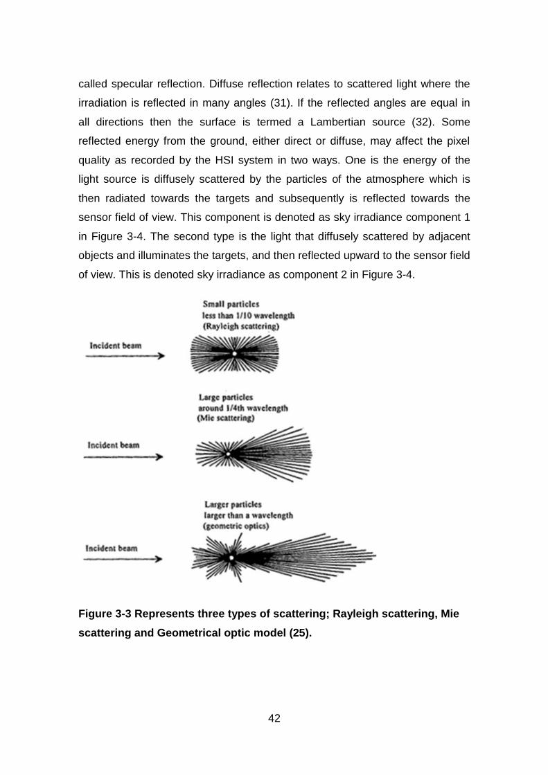
In the visible wavelengths the major scattering in the atmosphere is due to gas
molecules and water vapour. There are three forms of atmospheric scattering:
Rayleigh scattering, Mie scattering and Geometric optics model as illustrated in
Figure 3-3. Rayleigh scattering occurs when the solar radiation interacts with
molecules that have size less than one-tenth of the EM wavelength (25).
Example of such particles could be air molecules and haze particles or some of
the molecules of atmospheric gas such as nitrogen (N2) and oxygen (O2) (52).
Rayleigh scattering is wavelength dependant and is inversely proportional to the
fourth power of wavelength function. Therefore scattering is much higher at
shorter wavelengths.
Mie scattering or aerosol scattering occurs when the particles are comparable in
size to the radiation wavelength, such as dust, pollen, smoke and fog droplets.
Like that of the Rayleigh scattering, Mie scattering also influence a broad range
of wavelengths in the visible spectrum. However, this scattering tends to be the
greatest in the lower atmosphere where large particles are abundant.
The third type of scattering is non-selective and it is also known as Geometric
optics model scattering that occurs when the particles are larger than the
wavelength such as the rain drops (25). This scattering causes the light to be
scattered primarily in the forward direction. Because of these scattering effects,
the radiation may reach the sensor field of view before it reaches the ground.
This radiation component is called path radiance and can also be caused by the
diffuse reflectance from the ground to the sensor. Figure 3-4 shows the path
radiation, component 1, which scatters along the path up to sensor field of view
and component 2, which is the light scattered and reflected from the ground.
After the light passes through the atmosphere it will reach the surface of targets
and will be reflected in two ways: directly or diffusely as illustrated in Figure 3-5.
The surface or targets will reflect the radiation partially in the form of direct
reflection and partially in the form of diffuse reflection, regardless of the
direction of the incoming radiation (29). Direct reflection is when the incoming
radiation angle is normal to the plane of the reflected radiation angle and is
reflected only in a single direction (30). This type of reflection is sometimes
42
called specular reflection. Diffuse reflection relates to scattered light where the
irradiation is reflected in many angles (31). If the reflected angles are equal in
all directions then the surface is termed a Lambertian source (32). Some
reflected energy from the ground, either direct or diffuse, may affect the pixel
quality as recorded by the HSI system in two ways. One is the energy of the
light source is diffusely scattered by the particles of the atmosphere which is
then radiated towards the targets and subsequently is reflected towards the
sensor field of view. This component is denoted as sky irradiance component 1
in Figure 3-4. The second type is the light that diffusely scattered by adjacent
objects and illuminates the targets, and then reflected upward to the sensor field
of view. This is denoted sky irradiance as component 2 in Figure 3-4.
Figure 3-3 Represents three types of scattering; Rayleigh scattering, Mie
scattering and Geometrical optic model (25).
43
Figure 3-4 Effect of the atmosphere in determining various paths for
energy to illuminate a (equivalent ground) pixel and to reach the sensor
(27).
Figure 3-5 (a) Direct and (b) diffuse reflection (27).
The combined effects of these atmospheric scattering will make the assessment
of intrinsic reflectance of objects in a real remote sensing scenario very difficult.
To compensate for these effects, atmospheric correction is essentially needed
for a better estimation of target reflectance and spectral signature from HSI
imageries.

44
3.2 Atmospheric Correction
Atmospheric correction aims to compensate for the effects of atmospheric
absorption and scattering, as well as illumination angle artefacts on
hyperspectral imageries, by converting the radiance at the sensor to the
reflectance of the target surface (20). There are three types of atmospheric
correction methods (33, 34, 35 and 36): scene based empirical approach,
model based and hybrid based. Scene based empirical approach was the first
atmospheric correction that was developed during 1980s. Several examples of
scene based empirical methods are the Internal Average Reflectance (IAR) (37,
38), Flat Field (FF) (39, 40), Single Spectrum Method (SS) (41) and Empirical
Line Method (ELM) (42, 43 and 44).
In the late 1980s the first model based correction method, called Atmosphere
Removal Algorithm (ATREM), was introduced (26). This was then followed by
Atmospheric and Topographic Correction (ATCOR) (45), the Fast Line-of-Sight
Atmospheric Analysis of Spectral Hypercubes (FLAASH) (46) and High-
Accuracy Atmospheric Correction for Hyperspectral Data (HATCH) (47). For the
hybrid approach, researchers have used combinations of radiative modelling
approaches together with empirical approaches to estimate the surface
reflectance on HSI imageries (36, 48), such as the combination of ATCOR and
ELM (45). The selection of the atmospheric correction method depends on the
data quality, availability of radiometric calibration and atmospheric parameters,
a priori knowledge of the scene and ground spectral measurements (37). For
the purpose of this study several methods of empirical approach and model
based correction method, such as ATCOR, will be explained in more detail.
3.2.1 Empirical Line Method (ELM)
The Empirical Line Method (ELM) employs field reflectance measurements of
the scene to calculate the targets apparent reflectance. The word ‘apparent’
used in the ELM approach does not consider other possible effect, such as the
topography of the scene, for the estimation of target reflectance. Given an at

45
sensor raw image as DN, the linear equation for the radiance conversion is
given by
)( 1
2 DNccdL o (3-2)
Where oc and 1c are the calibration coefficients for the offset and slope
respectively, d is the distance between the light source and the target and it is
commonly assumed to be 1, DN is the digital number of the at sensor
measurement. When the downwelling radiance and the reflectance of two
standard calibration panels are presented in the scene, the two coefficients oc
and 1c can be found. To measure the offset and slope, at least two calibration
panels (white and black spectralon) are placed in the scene. From the mean
spectra of both calibration panels the ELM method generates the linear fit to
solve for gain and offset according to equation (3-2) and schematically as
shown in Figure 3-6. The reflectance, , for at-sensor radiance, L , can be
computed for each pixel in each band using (27)
01 cLc (3-3)
The term of 1c is equal to the atmospheric effect. This method will yield poor
result if the standard calibration panels do not represent the ‘true’ radiance of
the scene. Very often equations 3-2 and 3-3 are combined into one step:
bb BADN (3-4)
where Ab and Bb are the multiplicative and additive terms which comprises of
atmospheric transmission and instrumental factors.
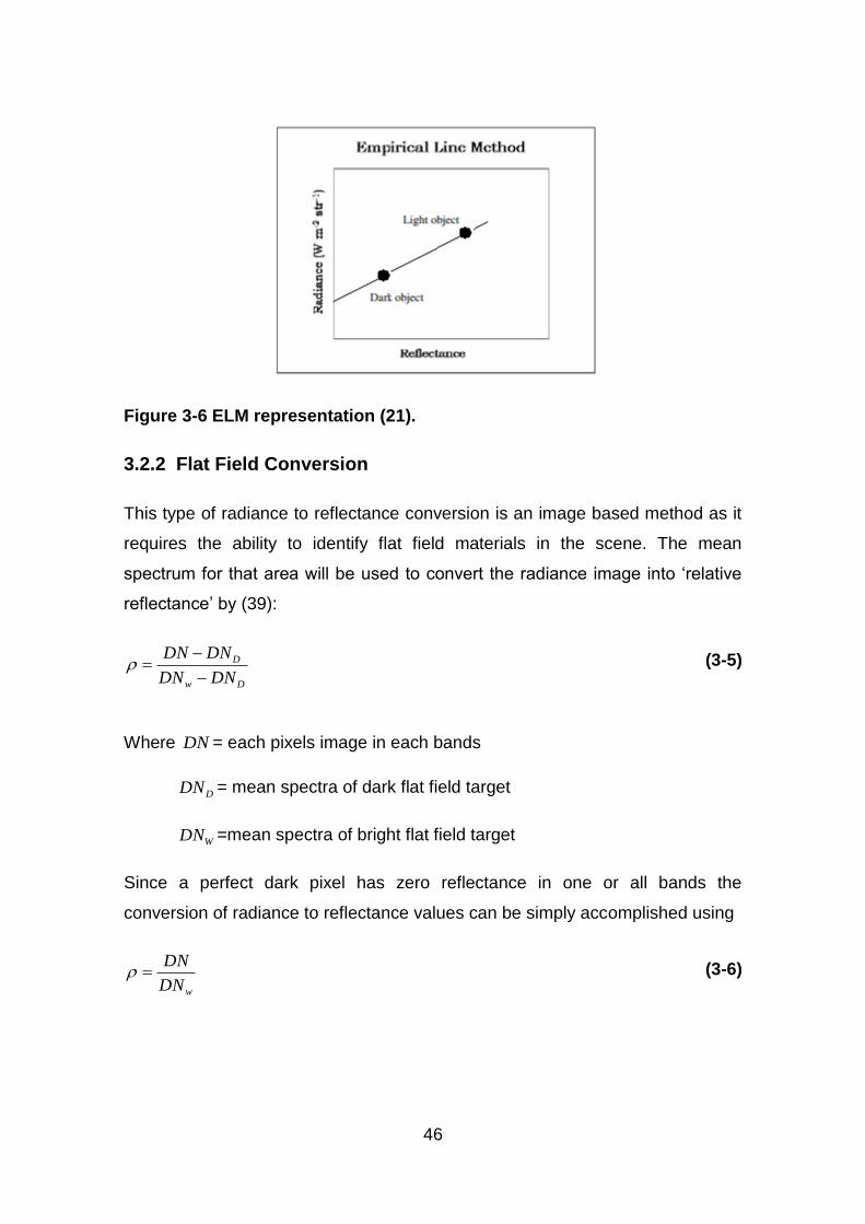
46
Figure 3-6 ELM representation (21).
3.2.2 Flat Field Conversion
This type of radiance to reflectance conversion is an image based method as it
requires the ability to identify flat field materials in the scene. The mean
spectrum for that area will be used to convert the radiance image into ‘relative
reflectance’ by (39):
Dw
D
DNDN
DNDN
(3-5)
Where DN = each pixels image in each bands
DDN = mean spectra of dark flat field target
WDN =mean spectra of bright flat field target
Since a perfect dark pixel has zero reflectance in one or all bands the
conversion of radiance to reflectance values can be simply accomplished using
wDN
DN (3-6)
47
3.2.3 Internal Average Relative Reflectance (IARR)
Internal Average Relative Reflectance (IARR) extracts the spectral information
from the raw data by measuring the mean spectrum of the whole image (37).
Every pixel vector is normalised by this global spectral mean to produce a
‘relative reflectance’ image. Given x as the pixels, i*j is the image coordinate
location, n is the number of bands and µn is the global spectral mean of the
whole image for each band, Internal Average Relative Reflectance (IARR)
correction method can be defined as:
n
njix
,* (3-7)
This correction method is normally employed when the atmospheric parameters
and ground spectral measurements of the scene is unavailable. Some artifacts
which may be mis-interpreted as real spectral features can induce large errors
in this atmospheric correction method. Ben-Dor et. al. have suggested to
employ subsets of the scene for the mean estimation to avoid inducing
artefacts (37).
3.2.4 Atmosphere Removal program (ATREM)
Atmosphere Removal program or ATREM retrieves the scaled surface
reflectance from hyperspectral image based on the radiative transfer model
(51). This program was developed in the late 1980s by the University of
Colorado. First, the solar zenith angle is derived based on the image acquisition
time, date and geographic location. Then, this program extracts the water
vapour column for every pixels based on the water vapour absorption band
between 940 nm and 1140 nm from the image. Then, it assesses the
transmission of other atmospheric gases such as water vapour, carbon dioxide,
ozone, nitrous oxide, carbon monoxide, methane and oxygen by using Malkos
narrow band model based on the ‘look-up’ table generate from the absorption of
water vapour through the Moderate Resolution Atmosphere Radiance and

48
Transmittance Model called MODTRAN. The apparent reflectance spectra are
obtained based on the equation given as (51):
cosRTLL suno (3-8)
Where oL = observed radiance at sensor
sunL = solar radiance above atmosphere
T = total atmospheric transmittance
R = surface reflectance
= incidence angle
This code, however, is rarely employed for hyperspectral analysis due to its
inefficiency for atmospheric correction (51). Advanced features such as spectral
smoothing, topographic correction and adjacency effects have not been
considered in the ATREM model (37).
3.2.5 Atmospheric and Topographic Correction (ATCOR)
Similar to other model based approaches, Atmospheric and Topographic
Correction (ATCOR) uses the MODTRAN atmospheric propagation model to
estimate the surface reflectance of the scene on a pixel-by-pixel basis. Given
the surface radiance for flat terrain background (Figure 3-7) (45)
s
ELL
r
g
vvsvp)1
0
(,,
(3-9)
Where L = at-sensor radiance for surface reflectance,
pL = path radiance
v = total ground-to-sensor atmospheric transmission

49
gE = global flux of horizontal surface, sum of direct irradiance ( directE )
and diffuse irradiance ( diffuseE )
r = large scale reference background reflectance determining the
effective global flux
s = spherical albedo of the atmosphere, accounts for atmospheric
backscattering to the ground
Figure 3-7 Illumination and viewing geometry (ATCOR) (45).
MODTRAN computes the atmospheric transmittance, v , direct and diffuse
solar flux, gE , and path radiance, pL as functions of viewing and illumination
geometry and the solar irradiance (45). The path radiance calculated by
MODTRAN is given by
s
gdiffuse
pathpath
ELL
1
/00 (3-10)
By setting 0 and 15.0r , the direct and diffuse solar flux and spherical
albedo can be estimated. The result is then stored in a precompiled look-up
table (LUT) for further reference. The at-sensor radiance as shown in Figure 3-8
consists of the following components
1L = scattered radiance or path radiance
50
2L = reflected energy from the target pixel itself which consists of
global flux that is the sum of direct and diffuse irradiance
3L = radiation reflected from the neighbouring pixel and scattered
into the field of view of the sensor, i.e. the adjacency effect that include
the atmospheric backscattering and volume scattering.
So the total radiance signal L received by the sensor can be written as (45)
321 LLLL (3-11)
In this case, the surface properties of the target pixels are given by component
2L and 1L and 3L are needed to be removed during the atmospheric correction.
2L is given by
DNccdLL o 1
2
2 (3-12)
The radiance of the scene can be estimated using the Empirical Line Method
(ELM) approach where 0c and 1c are the calibration coefficients (offset and
slope). Then the final surface reflectance can be obtained by combining
equation (3-12) into (3-9):
gv
po
E
LDNccd
1
2
(3-13)
Where pL = path radiance, 1L
gE = diffusedirect EE
2d = the sun to earth distance (in astronomical units)
which is taken as 1 in the atmospheric correction (ATCOR)
software (45).
It is seen that the scene based empirical approach has been a simple way for
the estimation of surface reflectance in remote sensing. However, this approach

51
relies on accurate spectral calibration for the estimation of calibration
coefficients. To achieve better assessment of surface reflectance the angle
dependent path radiance, atmospheric and topographic effects should be taken
into account.
Figure 3-8 Schematic sketch of solar radiation components as seen by the
HSI system (45).
3.2.6 Quick Atmosphere Correction (QUAC)
Quick Atmosphere Correction (QUAC) is an advanced method for atmospheric
correction (90, 91). This method converts the radiance data to reflectance by
locating the near-zero reflectance target to determine the offset or baseline.
This baseline is subtracted from the data and the remaining data is used to
determine the gain spectrum. The relative gain spectrum is calculated by
ratioing the spectral mean of all the endmembers to the spectral mean of each
endmember. QUAC will apply the offset and gain linearly such as ELM to derive
the reflectance data.
The method only uses information directly from the scene to allow the retrieval
of target reflectance even when the data does not have proper radiometric or
wavelength calibration, or when the solar illumination intensity is unknown. The
underlying assumption of this approach is that there must be a sufficiently low
non-zero reflectance for better estimation of baseline. Also, at least 10 diverse
materials should be selected in the scene for calculating a reasonable value for
the gain.

52
4 ILLUMINATION EFFECT AND SHADOW
In remote sensing the estimations of upwelling and path radiance have been
important factors for the assessment of surface reflectance of the scene.
Generally, solar irradiance is the main source of illumination in the outdoor
remote sensing applications, while artificial sources such as tungsten or
halogen lamps have been commonly deployed for the indoor work. Different
types of illumination sources exhibit different spectral power density across the
spectrum.
The power density of the illuminations can be assessed directly by using a
standard calibration panel such as spectral on which can then be used for
reflectance estimation. Spectralon can be made by materials which exhibit
diffuse reflectance spanning from zero to 1 independent of the viewing angle.
4.1 Illumination Geometry
The rate at which photons strike a surface is called radiant flux, which is
measured in Watts. This unit measures the energy delivered to a surface per
unit of time (52). The irradiance of an object is defined as the radiation per unit
time (power) impinging on the surface, normalized to the surface area (Wm-2).
Radiance is the normalization of irradiance to the solid angle of the observation
of the reflected light (Wm-2
sr-1) (9). Solid angle is the angle subtended at the
centre of sphere by an area on the surface of sphere as shown in Figure 4-1.
The steradian is defined as (25),
2
2
22
2
)(
)(
r
r
mr
mA (4-1)

53
Figure 4-1 Illustration of steradian (25).
Given the sun as the source of illumination, the illumination spectral power
distribution, E (Wm-2
sr-1) is given by,
iSE cos (4-2)
Where S = Solar Spectral Irradiance (Wm-2
sr-1
)
i = solar zenith angle (as shown in Figure 4-2)
When the solar radiation hits the surface of an object, the bidirectional
reflectance distribution function (BRDF) is given as the ratio of the reflected
radiance to incident irradiance (27),
)/(,
)/(,)(
2
2
1
srmWE
mWLsrBRDF
ii
rr
(4-3)
The relationship between the spectral reflectance ρ and BRDF is,
rriirrii BRDF ,,,,,, (4-4)
Combining equations (4-2), (4-3) and (4-4) gives
r

54
iS
L
cos (4-5)
Equation 4.5 has shown that the illumination and viewing angle can affect the
surface reflectance assessment rather significantly.
Figure 4-2 Depiction of the BRDF nomenclature (25).
4.1.1 Shading
Shading is a phenomenon caused by the geometry of the object as well as the
topology of the scene (32). This effect only appears on Lambertian surface
targets such as paints, cloths and wood, not shiny mirror-like objects (25).
Shading is defined as the intensity change as a function of the incident In and
reflected rays, Ir with respected to the surface normal as illustrated in (Figure
4-3 (a))
cosnr II (4-6)
Note that from equation (4-6) the intensity decreases with increasing angle.
For non-Lambertian (specular) surfaces the light is reflected in a single direction
as shown in Figure 4-3 (b). This specular reflection angle defines the optimum
position for viewing the scene.
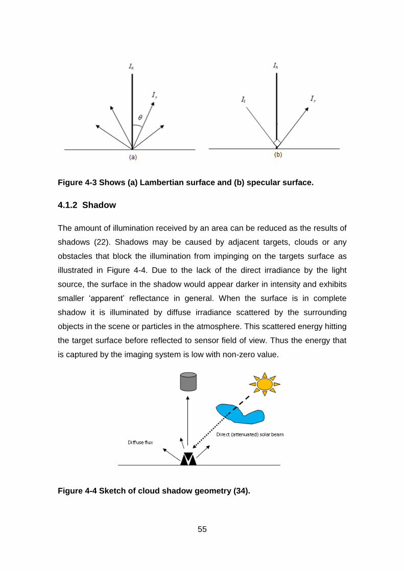
55
Figure 4-3 Shows (a) Lambertian surface and (b) specular surface.
4.1.2 Shadow
The amount of illumination received by an area can be reduced as the results of
shadows (22). Shadows may be caused by adjacent targets, clouds or any
obstacles that block the illumination from impinging on the targets surface as
illustrated in Figure 4-4. Due to the lack of the direct irradiance by the light
source, the surface in the shadow would appear darker in intensity and exhibits
smaller ‘apparent’ reflectance in general. When the surface is in complete
shadow it is illuminated by diffuse irradiance scattered by the surrounding
objects in the scene or particles in the atmosphere. This scattered energy hitting
the target surface before reflected to sensor field of view. Thus the energy that
is captured by the imaging system is low with non-zero value.
Figure 4-4 Sketch of cloud shadow geometry (34).

56
Shadow effects do not merely exhibit a lower energy of the reflected light; they
also induce a change of the spectral shape when compared with the same
object under direct irradiance. The extent of the change is dependent on the
surroundings such as the atmosphere and the background of the scene. For
scenes that contain homogenous and uniform background and that when the
sky is misty white, the change of spectral shape due to diffuse irradiance is not
an important issue, as shown in Figure 4-5.
Figure 4-5 (a) red square and (b) blue square represent the location
extracted from the image of fully illuminated pixels and shadow pixels
respectively, (c) the spectral shape of direct and shadowed pixel are the
same due to homogeneous background and that the sky is misty white,
(d) normalised spectra of direct and diffused irradiated grass.

57
However, for the scene that contains many different types of surfaces crowded
together in small area such as that in an indoor scene which consists of
coloured wall (magnolia), desk or boxes, the spectral shape change due to
diffuse irradiance appears to be very significant. This is illustrated in Figure 4-6
which depicts significant change of spectral shape of the shadowed surface
illuminated by diffuse irradiance with respected to that under direct illumination.
Figure 4-6 (a) red square and (b) blue square represent the location
extracted from the image for fully illuminated pixel and shadow pixels
respectively, (c) the spectra shaped of shadowed pixel changed due to the
complicated background (d) normalised spectra showing completely
different spectral shapes between the directed and diffusely irradiated
surfaces.

58
4.2 Previous Work on Shadow Compensation
Previous work by Franklin et al. (53) and Ranson and Daughetry (54) have
shown that shadow can influence classification accuracy significantly. Several
methods have been developed for correcting the shadows in hyperspectral
remote sensing. One de-shadowing method has been implemented in the
ATCOR atmospheric correction by Rolf Ritcher and Andreas Muller (55). This
technique detects shadows using several spectral bands that are sensitive to
shadows and then matched filter detection is employed to segment the
shadows from the scene. However, there are some restrictions on
implementations of this method. It is restricted to outdoor environments with
cloud cover of less than 25%; therefore it is more suitable for satellite or
airborne hyperspectral imaging. Other works that employ the matched filter
concept have also been reported (56) with slightly different rescaling methods
for shadow compensation. For MF method, sufficient number of bands is
required for better estimation of the covariance metric.
Another popular method in shadow removal applications is the band ratio
approach (57, 58 and 59). Band ratioing is an enhancement process in which
the DN values of one band is divided by that of any other band (58) or adjacent
bands (59). Given B1 and B2 are two different spectral bands of hyperspectral
data, band ratioing is deployed as,
yxB
yxBRatioBand
,
,
2
1 (4-7)
where B2 may be either an adjacent band of B1 or any other band that is not
similar to B1. When B1 and B2 have similar radiance or reflectance values, the
resulting band ratio will be close to 1. The disadvantage of this method is that
two different targets may exhibit similar reflectance after ratioing even though
they are completely different materials and therefore this method may not be
always applicable.
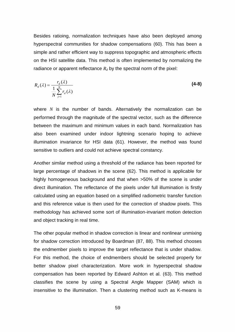
59
Besides ratioing, normalization techniques have also been deployed among
hyperspectral communities for shadow compensations (60). This has been a
simple and rather efficient way to suppress topographic and atmospheric effects
on the HSI satellite data. This method is often implemented by normalizing the
radiance or apparent reflectance Rd by the spectral norm of the pixel:
N
j
d
d
d
rN
rR
1
)(1
)()(
(4-8)
where N is the number of bands. Alternatively the normalization can be
performed through the magnitude of the spectral vector, such as the difference
between the maximum and minimum values in each band. Normalization has
also been examined under indoor lightning scenario hoping to achieve
illumination invariance for HSI data (61). However, the method was found
sensitive to outliers and could not achieve spectral constancy.
Another similar method using a threshold of the radiance has been reported for
large percentage of shadows in the scene (62). This method is applicable for
highly homogeneous background and that when >50% of the scene is under
direct illumination. The reflectance of the pixels under full illumination is firstly
calculated using an equation based on a simplified radiometric transfer function
and this reference value is then used for the correction of shadow pixels. This
methodology has achieved some sort of illumination-invariant motion detection
and object tracking in real time.
The other popular method in shadow correction is linear and nonlinear unmixing
for shadow correction introduced by Boardman (87, 88). This method chooses
the endmember pixels to improve the target reflectance that is under shadow.
For this method, the choice of endmembers should be selected properly for
better shadow pixel characterization. More work in hyperspectral shadow
compensation has been reported by Edward Ashton et al. (63). This method
classifies the scene by using a Spectral Angle Mapper (SAM) which is
insensitive to the illumination. Then a clustering method such as K-means is
60
used to identify the shadow pixels from the image. The correction is carried out
on the shadow pixels by subtracting the mean from each class based on the
equation,
sc
jiSCjiNSC
cjiji
wwxx
)1(()('
,,
,,, (4-9)
where jix ,' = current pixel with classification c
SC = mean vector for all shadow pixels in class c
NSC = mean vector for all non-shadow pixels in class c
jiw , = weight mask at pixel (i, j)
The only limitation for this method is that the user needs to have a prior
knowledge of target class before correcting the shadow pixels based on the
assign class.
The latest work has been reported by Friman et al. that combines passive and
active imaging for illumination and shadow compensation on hyperspectral
imageries (89). This work segments the illumination invariance map using the
Digital Surface Model (DSM) generated from an airborne LIDAR (Light
Detection and Ranging). Upon the establishment of the map, the shadow pixel
is identified and corrected using the non-linear squares estimation. Similar work
has been done by Nischan et al. that also combines passive and active imaging
for illumination and shadow compensation on hyperspectral imageries (92). A
laser illuminator such as white laser source is attached on the front of the
hyperspectral camera. By placing an illuminator in front of the imaging system,
this technique is able to eliminate illumination and viewing angle factors for
retrieving target reflectance of pixels that are under the shadow. Although the
method has shown good result in shadow compensation it requires
hyperspectral images to be combined together with images captured by a
LIDAR system.

61
5 HSI EQUIPMENT
5.1 HSI Camera
Two types of hyperspectral imaging systems have been used for image
acquisition during the course of this PhD research: a Headwall spectrograph for
Visible Near Infra-red (VNIR) wavebands and a Specim spectrograph for Short
Wave Infra-red (SWIR) spectral range as shown in Figure 5-1. The Headwall
VNIR camera has a spectral sensitivity between 400 and 1000 nm and it is
capable to deliver excellent image quality through a high sensitive silicon
charge couple device (CCD) detector. This type of photon detector converts
absorbed photon energy from incident light to an electrical signal. The changes
in the electrical signal determine the amount of the incident optical power. The
SWIR camera utilises an infrared thermal detectors, Hg1-xCdxTe (Mercury
Cadmium Telluride - MCT) combined with a high performance thermo electrical
cooler (TEC) for data collection within the 900 to 2500 nm spectral range.
Figure 5-1 Picture of (a) The Headwall Visible Near Infra-red (VNIR)
imaging system and (b) the Specim & Xenics Short Wave Infra-red (SWIR)
imaging system.
In the heart of the hyperspectral imaging system is a spectrograph which
provides the spatial and spectral information simultaneously. The spectrograph
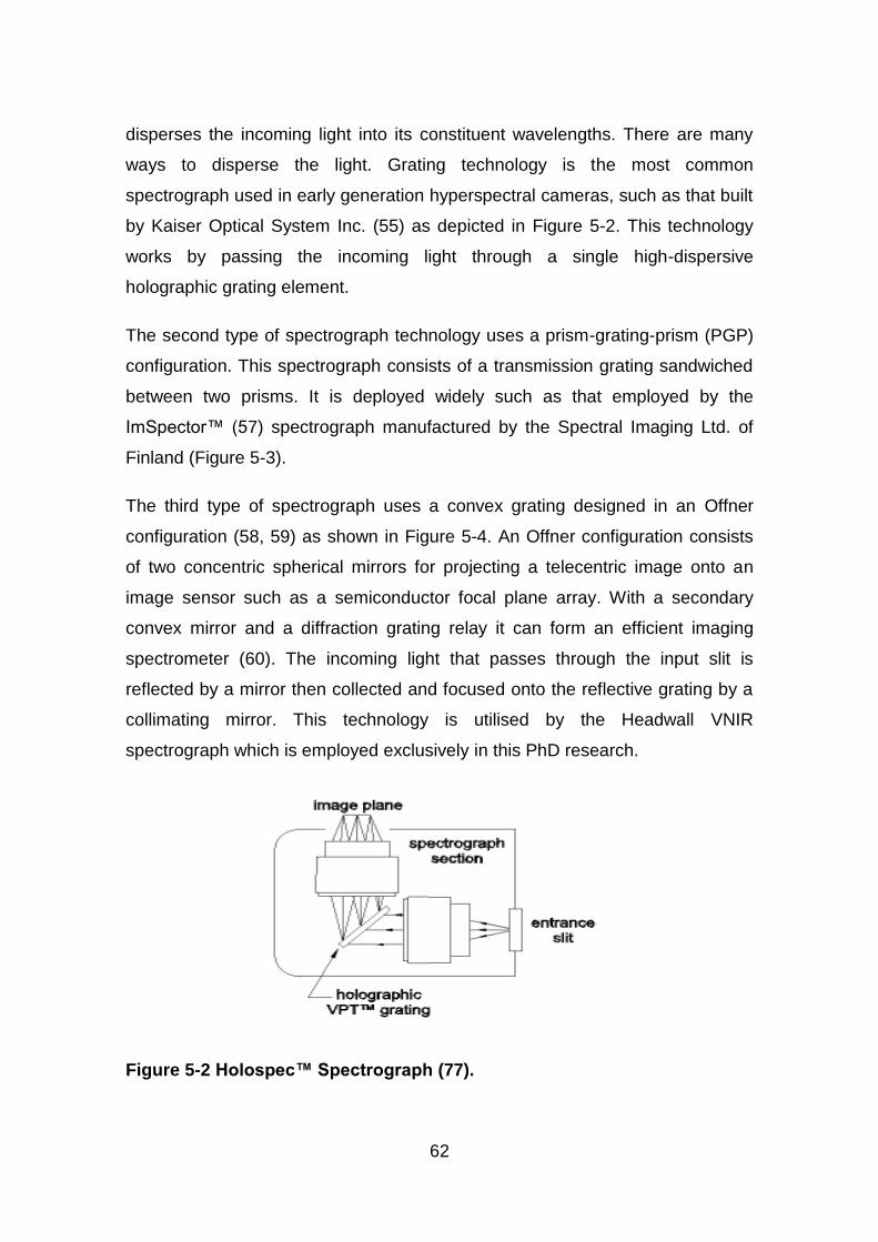
62
disperses the incoming light into its constituent wavelengths. There are many
ways to disperse the light. Grating technology is the most common
spectrograph used in early generation hyperspectral cameras, such as that built
by Kaiser Optical System Inc. (55) as depicted in Figure 5-2. This technology
works by passing the incoming light through a single high-dispersive
holographic grating element.
The second type of spectrograph technology uses a prism-grating-prism (PGP)
configuration. This spectrograph consists of a transmission grating sandwiched
between two prisms. It is deployed widely such as that employed by the
ImSpector™ (57) spectrograph manufactured by the Spectral Imaging Ltd. of
Finland (Figure 5-3).
The third type of spectrograph uses a convex grating designed in an Offner
configuration (58, 59) as shown in Figure 5-4. An Offner configuration consists
of two concentric spherical mirrors for projecting a telecentric image onto an
image sensor such as a semiconductor focal plane array. With a secondary
convex mirror and a diffraction grating relay it can form an efficient imaging
spectrometer (60). The incoming light that passes through the input slit is
reflected by a mirror then collected and focused onto the reflective grating by a
collimating mirror. This technology is utilised by the Headwall VNIR
spectrograph which is employed exclusively in this PhD research.
Figure 5-2 Holospec™ Spectrograph (77).

63
Figure 5-3 Diagram of the ImSpector™ camera (78).
Figure 5-4 Diagram of an Offner Imaging Spectrometer and photo of the
Headwall Photonics’ spectrograph Hyperspec (78).
As a commercial hyperspectral imaging system is normally extremely expensive
and our lab has chosen to develop our own hyperspectral imaging systems by
assembling spectrographs, scanners, and related driver circuits (Figure 5-5) for
a more economic and yet efficient HSI system. The optical scanner consists of

64
a rotating mirror which guides the light through the slit into the camera head.
Two software systems, VNIR_2.0 and SWIR_2.0 (Figure 5-6) have been
produced as controllers for the scanners of the Headwall VNIR and SWIR
hyperspectral imaging systems for image acquisitions respectively.
Figure 5-5 The rotating mirror system made by our lab (78).
Figure 5-6 Pictures of the GUI for (a) VNIR_2.0 and (b) SWIR_2.0 program
(78).
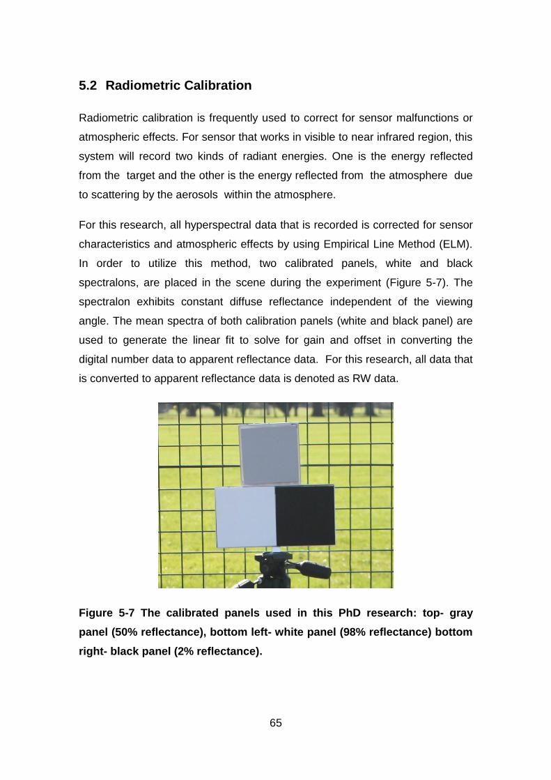
65
5.2 Radiometric Calibration
Radiometric calibration is frequently used to correct for sensor malfunctions or
atmospheric effects. For sensor that works in visible to near infrared region, this
system will record two kinds of radiant energies. One is the energy reflected
from the target and the other is the energy reflected from the atmosphere due
to scattering by the aerosols within the atmosphere.
For this research, all hyperspectral data that is recorded is corrected for sensor
characteristics and atmospheric effects by using Empirical Line Method (ELM).
In order to utilize this method, two calibrated panels, white and black
spectralons, are placed in the scene during the experiment (Figure 5-7). The
spectralon exhibits constant diffuse reflectance independent of the viewing
angle. The mean spectra of both calibration panels (white and black panel) are
used to generate the linear fit to solve for gain and offset in converting the
digital number data to apparent reflectance data. For this research, all data that
is converted to apparent reflectance data is denoted as RW data.
Figure 5-7 The calibrated panels used in this PhD research: top- gray
panel (50% reflectance), bottom left- white panel (98% reflectance) bottom
right- black panel (2% reflectance).

66
6 DIFFUSE IRRADIANCE COMPENSATION (DIC)
METHOD FOR SHADOW COMPENSATION
Most work within the HSI community commonly assumed full illumination of the
scene. The irradiance due to diffuse light (Ediff) and multiple scattering by the
background have been ignored or treated as a very minor factor. This approach
will lead to errors on the assessment of shadows which normally result in
exhibiting lower ‘apparent’ reflectance values than that of the same target under
directed illumination. Consequently, the same target can be mistakenly
classified into two different classes heavily jeopardises the classification
accuracy.
The diffuse irradiance in the outdoor case behaves quite differently from that of
the indoor one due to the different scatters and scattering mechanisms. In the
outdoor case it is the particles and air (O2) molecules in the atmosphere
dominates the scattering events particularly in the blue region (400 ~ 550 nm)
which gives an effective bluer spectrum in the diffuse irradiance. In the indoor
case, multiple scattering of the NIR wavelength by the surroundings in the room
is more effective, inducing a higher proportion of NIR spectrum in the diffuse
irradiance. Unlike in the outdoor case where the concentration of the particles in
the atmosphere remains fairly constant, the diffuse irradiance of the indoor case
is strongly dependent on the exact background surroundings as well as the
distributions of the objects or targets in the scene. It is impossible to model the
diffuse irradiance in the indoor case without prior information of the
environment. The purpose of this work is to develop a method to compensate
the shadow effect for the indoor hyperspectral scenario by modelling the diffuse
irradiance of the indoor scene.
6.1 Experiment Setup
The experiment was recorded by using the Headwall VNIR hyperspectral
imaging system within a laboratory environment of predominantly white and
yellow background. Two sets of data with 88 bands that consists of different
coloured t-shirts have been chosen to represent multiple targets. Figure 6-1
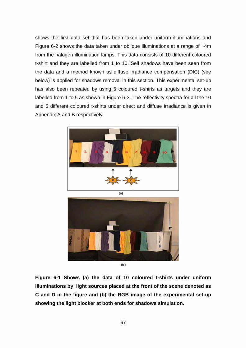
67
shows the first data set that has been taken under uniform illuminations and
Figure 6-2 shows the data taken under oblique illuminations at a range of ~4m
from the halogen illumination lamps. This data consists of 10 different coloured
t-shirt and they are labelled from 1 to 10. Self shadows have been seen from
the data and a method known as diffuse irradiance compensation (DIC) (see
below) is applied for shadows removal in this section. This experimental set-up
has also been repeated by using 5 coloured t-shirts as targets and they are
labelled from 1 to 5 as shown in Figure 6-3. The reflectivity spectra for all the 10
and 5 different coloured t-shirts under direct and diffuse irradiance is given in
Appendix A and B respectively.
Figure 6-1 Shows (a) the data of 10 coloured t-shirts under uniform
illuminations by light sources placed at the front of the scene denoted as
C and D in the figure and (b) the RGB image of the experimental set-up
showing the light blocker at both ends for shadows simulation.

68
Figure 6-2 Shows (a) under oblique illumination casting self shadows in
parts of the 10 coloured t-shirts (b) the RGB image of the complete scene
under oblique illumination.

69
Figure 6-3 Shows (a) the RGB image of 5 coloured t-shirts under uniform
illumination (labelled from 1 to 5) and (b) when it is under oblique
illumination casting shadows on part of the targets.

70
6.2 Low Reflectance and Shadow Mask
The irradiance of a target under shadow is difficult to assess due to the various
degree of the softness of the shadows throughout the scene. The only signal
that is seen by the sensor from the target under complete shadow is the small
reflected energy due to the diffuse irradiance from the adjacent targets,
background or environment. The direct illumination is completely blocked by
clouds or objects that cast the shadow.
Since shadow pixels have lower reflection intensity it is necessary to
differentiate them from the low reflectance objects that may be present in the
scene. In both cases the digital number (DN) of these pixels appears to be
small; however, it is the shadow pixels and not the low reflectance objects that
are needed to correct. In order to differentiate between low reflectance target
and shadow pixels two different masks using spectral variance and spectral
means, have been utilized for the classification of low reflectance objects and
the shadowed pixels respectively. Figure 6-4 shows the flow chart to obtain the
final mask.
Figure 6-4 Shows the flow chart to obtain the final mask.
Figure 6-5 shows the spectral variance map of 10 coloured t-shirt data with the
scale 0 to 0.7 to represent the value of variance. A low value of scale
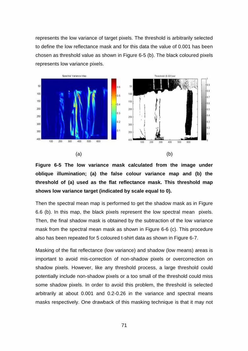
71
represents the low variance of target pixels. The threshold is arbitrarily selected
to define the low reflectance mask and for this data the value of 0.001 has been
chosen as threshold value as shown in Figure 6-5 (b). The black coloured pixels
represents low variance pixels.
(a) (b)
Figure 6-5 The low variance mask calculated from the image under
oblique illumination; (a) the false colour variance map and (b) the
threshold of (a) used as the flat reflectance mask. This threshold map
shows low variance target (indicated by scale equal to 0).
Then the spectral mean map is performed to get the shadow mask as in Figure
6.6 (b). In this map, the black pixels represent the low spectral mean pixels.
Then, the final shadow mask is obtained by the subtraction of the low variance
mask from the spectral mean mask as shown in Figure 6-6 (c). This procedure
also has been repeated for 5 coloured t-shirt data as shown in Figure 6-7.
Masking of the flat reflectance (low variance) and shadow (low means) areas is
important to avoid mis-correction of non-shadow pixels or overcorrection on
shadow pixels. However, like any threshold process, a large threshold could
potentially include non-shadow pixels or a too small of the threshold could miss
some shadow pixels. In order to avoid this problem, the threshold is selected
arbitrarily at about 0.001 and 0.2-0.26 in the variance and spectral means
masks respectively. One drawback of this masking technique is that it may not

72
be able to identify the shadows pixels correctly for the shadows in the low
variance materials (Figure 6.7(c)).
(a) (b)
(c)
Figure 6-6 The procedure for obtaining the final shadow mask: (a) the
RGB image under oblique illumination, (b) threshold (0.26) of the spectral
mean of the image which represents the low reflectance pixels in the
scene (c) final shadow mask (bright areas) after the flat reflectance pixels
are removed. White scale colour on the final shadow map (c) indicates the
shadow pixels whereas black scale colour represents the direct
illumination pixels.
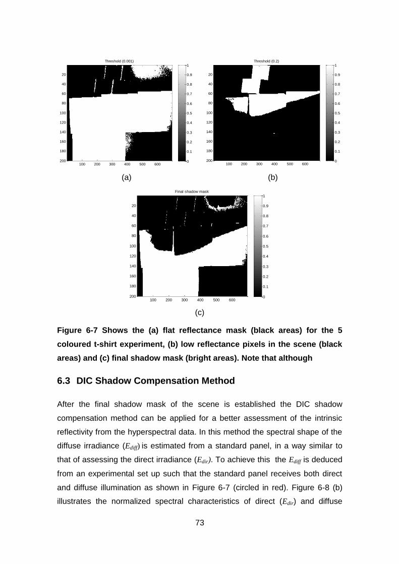
73
Threshold (0.001)
100 200 300 400 500 600
20
40
60
80
100
120
140
160
180
200 0
0.1
0.2
0.3
0.4
0.5
0.6
0.7
0.8
0.9
1
Threshold (0.2)
100 200 300 400 500 600
20
40
60
80
100
120
140
160
180
200 0
0.1
0.2
0.3
0.4
0.5
0.6
0.7
0.8
0.9
1
(a) (b)
Final shadow mask
100 200 300 400 500 600
20
40
60
80
100
120
140
160
180
200 0
0.1
0.2
0.3
0.4
0.5
0.6
0.7
0.8
0.9
1
(c)
Figure 6-7 Shows the (a) flat reflectance mask (black areas) for the 5
coloured t-shirt experiment, (b) low reflectance pixels in the scene (black
areas) and (c) final shadow mask (bright areas). Note that although
6.3 DIC Shadow Compensation Method
After the final shadow mask of the scene is established the DIC shadow
compensation method can be applied for a better assessment of the intrinsic
reflectivity from the hyperspectral data. In this method the spectral shape of the
diffuse irradiance (Ediff) is estimated from a standard panel, in a way similar to
that of assessing the direct irradiance (Edir). To achieve this the Ediff is deduced
from an experimental set up such that the standard panel receives both direct
and diffuse illumination as shown in Figure 6-7 (circled in red). Figure 6-8 (b)
illustrates the normalized spectral characteristics of direct (Edir) and diffuse

74
irradiance (Ediff) estimated from this scene; the difference of the spectral
characteristics between these two is quite apparent. The shadow compensation
is carried out in the following procedure:
(a) The digital numbered (DN) values of the pixels inside the shadow mask
are ratioed with the Ediff.
(b) For pixels outside of the shadow mask, which are directly illuminated,
their DN values are ratioed with Edir.
Figure 6-8 Shows the RGB image of the experimental set up for assessing
Edir and Ediff.
(a) (b)
Figure 6-9 Shows (a) spectral characteristics of Edir and Ediff in DN values
and (b) to highlight the difference in the spectral characteristics of the Edir
and Ediff.
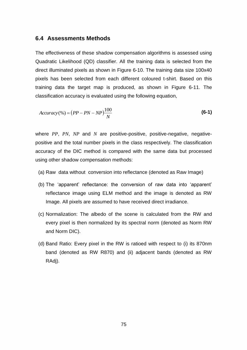
75
6.4 Assessments Methods
The effectiveness of these shadow compensation algorithms is assessed using
Quadratic Likelihood (QD) classifier. All the training data is selected from the
direct illuminated pixels as shown in Figure 6-10. The training data size 100x40
pixels has been selected from each different coloured t-shirt. Based on this
training data the target map is produced, as shown in Figure 6-11. The
classification accuracy is evaluated using the following equation,
N
NPPNPPAccuracy100
(%) (6-1)
where PP, PN, NP and N are positive-positive, positive-negative, negative-
positive and the total number pixels in the class respectively. The classification
accuracy of the DIC method is compared with the same data but processed
using other shadow compensation methods:
(a) Raw data without conversion into reflectance (denoted as Raw Image)
(b) The ‘apparent’ reflectance: the conversion of raw data into ‘apparent’
reflectance image using ELM method and the image is denoted as RW
Image. All pixels are assumed to have received direct irradiance.
(c) Normalization: The albedo of the scene is calculated from the RW and
every pixel is then normalized by its spectral norm (denoted as Norm RW
and Norm DIC).
(d) Band Ratio: Every pixel in the RW is ratioed with respect to (i) its 870nm
band (denoted as RW R870) and (ii) adjacent bands (denoted as RW
RAdj).
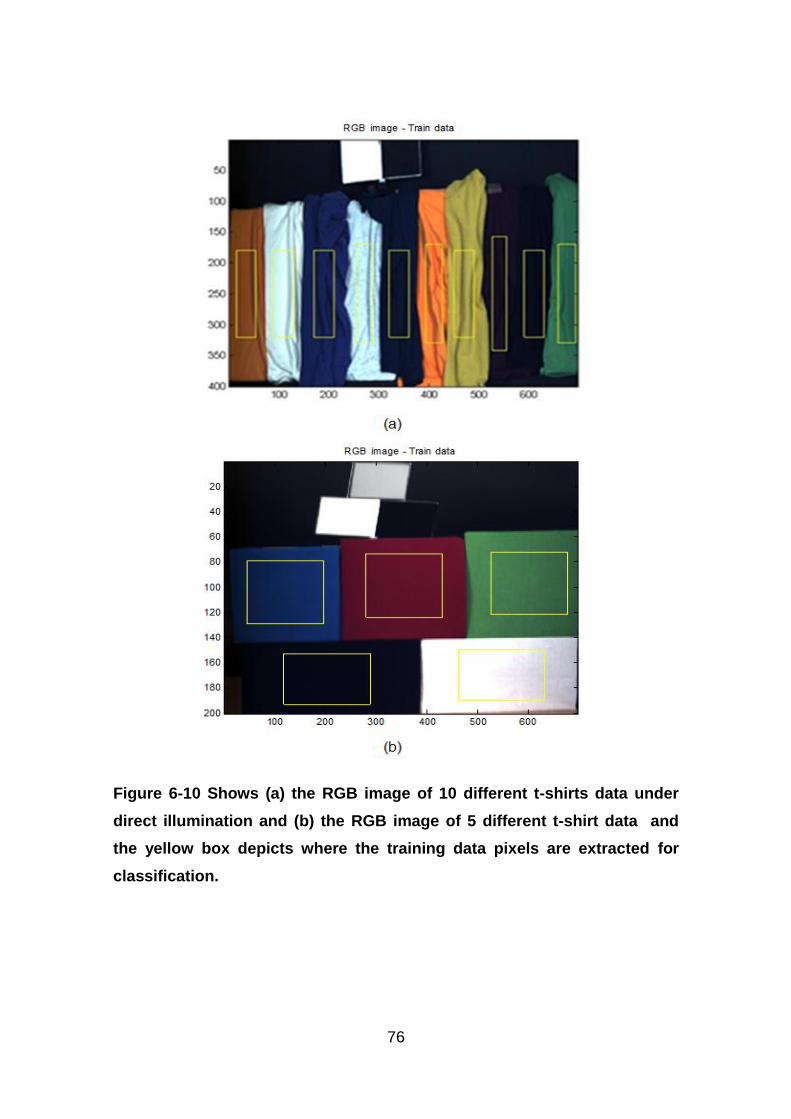
76
Figure 6-10 Shows (a) the RGB image of 10 different t-shirts data under
direct illumination and (b) the RGB image of 5 different t-shirt data and
the yellow box depicts where the training data pixels are extracted for
classification.

77
Figure 6-11 Shows the target map in false colours for (a) 10 different
colours t-shirts and (b) 5 different colours t-shirts. These target maps are
used to evaluate the accuracy of classification.

78
6.5 DIC Shadow Compensation Results
6.5.1 10 different coloured t-shirt data
Previous work has reported that affine transformations of data, such as that
using ELM method, will not affect the separability and classification efficiency
when using Quadratic classifier methods (62, 63). However, other studies (27,
64) have shown an improvement in inter-class separabilities when reflectance
data is used. Figure 6-12 shows the classification results for the raw (DN) data
together with the same image but transformed into ‘apparent reflectance’ via
ELM based method (RW). DN data achieved 38% classification accuracy
whereas the RW data attained 68% accuracy. Note the substantial
misclassifications in the DN data particularly in classes 1 and 2. By transforming
the raw data into apparent reflectance data, it helps to remove the sensor
characteristics and to compensate some of the illumination artefacts, resulting
in a better classification due to the enhancement of inter-class separation.
The classification result of DIC method is shown in Figure 6-13. It is seen that
the DIC method has achieved the best overall classification accuracy of 70%
compared to that of the RW image (68%). It is also perceived that most
shadows, particularly those in the deep shade, can be compensated by the DIC
method. However, it falls short for the lightly shadowed regions such as that in
class 1. This is mainly caused by the deficiency of the present method which
corrects all shadows by using the same Ediff.

79
80
Figure 6-12 Shows RGB images of (a) Raw data, (c) RW data, (b) and (d)
are the false colour image of the classification results for the respective
Raw and RW data. The overall accuracies in these cases are respectively
38% & 68%, and note the large misclassifications in the classes 1 and 2 in
the Raw data as shown in (b).

81
Figure 6-13 Shows (a) RGB image and (b) the classification result after
DIC shadow compensation exhibit 70% of classification accuracy. Note
that the DIC has achieved the best overall accuracy in comparison to that
of the Raw and RW results.
82
6.5.2 Previous work on shadow compensation: Normalization and
band ratio
Pixel vector normalisation has been a popular method for ‘flattening’ the
illumination artefact within the HSI community (37, 59, 60 and 67). It is shown
here that normalisation is not sufficient for this purpose and in many cases,
such as indoor situations, the diffused irradiance is strongly affected by the
background in the scene. Figure 6-14 shows the (a) RGB image of the targets
taken under oblique illumination after normalisation (RW Norm) and (b) its
classification result. This method results in large classification errors particularly
in the shadow regions after the data is normalized. The classification accuracy
is reduced from 68% (by RW) to 50% after the image is normalised,
demonstrating the inefficiency of pixel vector normalisation for shadow
mitigation in HSI processing. The DIC result is also compared with RW ratioed
with band 870 (RW R870) and ratioed with adjacent band (RW RAdj). The band
ratioing methods (RW R870 and RW RAdj) achieve only 62% of classification
accuracy as shown in Figure 6-15 and Figure 6-16. This has shown that DIC
method has achieved the best classification accuracy in comparison to the
normalization and the two band ratioing methods which have been commonly
adopted by the HSI community for shadow compensation.

83
Figure 6-14 Shows the RGB images of the image taken at oblique
illumination (a) after normalisation (RW Norm), and (b) the false colour
classification results of RW Norm. Note that target classes 1, 2 and 4 have
been substantially misclassified in the RW Norm data.
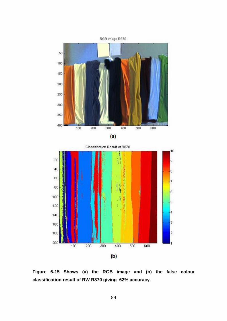
84
Figure 6-15 Shows (a) the RGB image and (b) the false colour
classification result of RW R870 giving 62% accuracy.
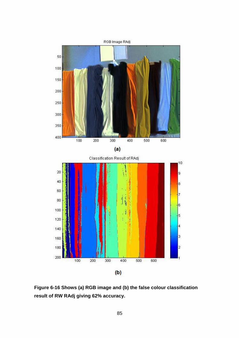
85
Figure 6-16 Shows (a) RGB image and (b) the false colour classification
result of RW RAdj giving 62% accuracy.

86
6.5.3 DIC Method for 5 t-shirts data
In this section the DIC method has been applied on the 5 different coloured t-
shirt data to check for reproducibility. As depicted in Figure 6-17, it is seen that
the raw data can only achieve 31% of classification accuracy whereas the RW
has attained 43% of accuracy. Similar to the previous result, the affine
transformed data set after RW exhibit ~30% better than that using the raw data
for the classification. This may suggest that by removing the sensor and
atmospheric transfer functions one can achieve much better target recognitions
from HSI imagery.
Classification result of raw data
100 200 300 400 500 600
10
20
30
40
50
60
70
80
90
100
110
1
1.5
2
2.5
3
3.5
4
4.5
5
(a)

87
Classification result of RW
100 200 300 400 500 600
10
20
30
40
50
60
70
80
90
100
110
1
1.5
2
2.5
3
3.5
4
4.5
5
(b)
Figure 6-17 Shows the classification result of (a) the raw data and (b) RW
data of 5 different coloured t-shit.
The results for the normalization and band ratio techniques also exhibit large
errors with only 35% classification accuracy as shown in Figure 6-18 and Figure
6-19, respectively. These results thus suggest that previous illumination
flattening methods such as the normalization and band ratio techniques in fact
do not perform very well for shadow eliminations in HSI imagery.
On the other hand, the DIC method has produced the best result with 58%
classification accuracy for this 5 coloured t-shirt data as shown in Figure 6-20.
This result thus shows that the DIC method is capable to compensate the
shadow artefact in hyperspectral processing much better than other techniques
reported in the literature. Figure 6-21 shows the plot of the apparent reflectance
for 3 selected shadowed targets before correction (RW), after correction via DIC
method and to compare with that under direct illumination. From these plots it
can be seen that the DIC method can help to restore ~80% of shadows

88
producing much better apparent reflectance characteristics of targets and to
enhance classification accuracy rather significantly
RGB image of RW Norm
100 200 300 400 500 600
20
40
60
80
100
120
140
160
180
200
(a)
Claasification result of RW Norm image
100 200 300 400 500 600
10
20
30
40
50
60
70
80
90
100
110
1
1.5
2
2.5
3
3.5
4
4.5
5
(b)
Figure 6-18 Shows (a) the RGB image of RW Norm for the 5 different
coloured t-shirts and (b) its classification result exhibiting 35% accuracy.

89
RGB image of RW R870
100 200 300 400 500 600
20
40
60
80
100
120
140
160
180
200
(a)
Classification result of RW R870
100 200 300 400 500 600
10
20
30
40
50
60
70
80
90
100
110
1
1.5
2
2.5
3
3.5
4
4.5
5
(b)

90
RGB image of RW Radj
100 200 300 400 500 600
20
40
60
80
100
120
140
160
180
200
(c)
Classification result of RW RAdj
100 200 300 400 500 600
10
20
30
40
50
60
70
80
90
100
110
1
1.5
2
2.5
3
3.5
4
4.5
5
(d)
Figure 6-19 Shows the RGB image of (a) RW R870 and (c) RW RAdj data
of 5 different coloured t-shirt data together with their classification results
shown in ((c) and (d)) respectively.

91
RGB image of DIC
100 200 300 400 500 600
20
40
60
80
100
120
140
160
180
200
(a)
Classification result of DIC
100 200 300 400 500 600
10
20
30
40
50
60
70
80
90
100
110
1
1.5
2
2.5
3
3.5
4
4.5
5
(b)
Figure 6-20 Shows (a) the RGB image of the 5 different coloured t-shirts
after DIC correction and (b) its classification result with 58% accuracy.
Note that the correction is far from perfect as it can be seen from the RGB
image.

92
450 500 550 600 650 700 750 800 850 9000
0.1
0.2
0.3
0.4
0.5
0.6
0.7
Wavelength(nm)
Reflecta
nce
Reflectance T-shirt 1 (Blue)
Direct Spectra
Shadow Spectra
via DIC
(a)
450 500 550 600 650 700 750 800 850 9000
0.2
0.4
0.6
0.8
1
1.2
1.4
Wavelength(nm)
Reflecta
nce
Reflectance T-shirt 2 (Red)
Direct Spectra
Shadow Spectra
via DIC
(b)
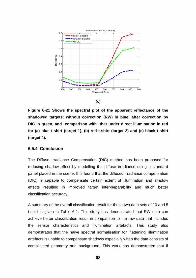
93
450 500 550 600 650 700 750 800 850 9000
0.1
0.2
0.3
0.4
0.5
0.6
0.7
Wavelength(nm)
Reflecta
nce
Reflectance T-shirt 4 (Black)
Direct Spectra
Shadow Spectra
via DIC
(c)
Figure 6-21 Shows the spectral plot of the apparent reflectance of the
shadowed targets: without correction (RW) in blue, after correction by
DIC in green, and comparison with that under direct illumination in red
for (a) blue t-shirt (target 1), (b) red t-shirt (target 2) and (c) black t-shirt
(target 4).
6.5.4 Conclusion
The Diffuse Irradiance Compensation (DIC) method has been proposed for
reducing shadow effect by modelling the diffuse irradiance using a standard
panel placed in the scene. It is found that the diffused irradiance compensation
(DIC) is capable to compensate certain extent of illumination and shadow
effects resulting in improved target inter-separability and much better
classification accuracy.
A summary of the overall classification result for these two data sets of 10 and 5
t-shirt is given in Table 6-1. This study has demonstrated that RW data can
achieve better classification result in comparison to the raw data that includes
the sensor characteristics and illumination artefacts. This study also
demonstrates that the naive spectral normalisation for ‘flattening’ illumination
artefacts is unable to compensate shadows especially when the data consists of
complicated geometry and background. This work has demonstrated that if
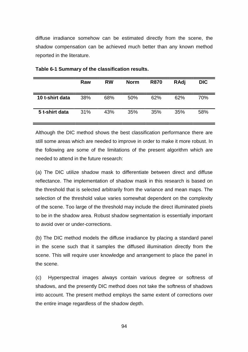
94
diffuse irradiance somehow can be estimated directly from the scene, the
shadow compensation can be achieved much better than any known method
reported in the literature.
Table 6-1 Summary of the classification results.
Raw RW Norm R870 RAdj DIC
10 t-shirt data 38% 68% 50% 62% 62% 70%
5 t-shirt data 31% 43% 35% 35% 35% 58%
Although the DIC method shows the best classification performance there are
still some areas which are needed to improve in order to make it more robust. In
the following are some of the limitations of the present algorithm which are
needed to attend in the future research:
(a) The DIC utilize shadow mask to differentiate between direct and diffuse
reflectance. The implementation of shadow mask in this research is based on
the threshold that is selected arbitrarily from the variance and mean maps. The
selection of the threshold value varies somewhat dependent on the complexity
of the scene. Too large of the threshold may include the direct illuminated pixels
to be in the shadow area. Robust shadow segmentation is essentially important
to avoid over or under-corrections.
(b) The DIC method models the diffuse irradiance by placing a standard panel
in the scene such that it samples the diffused illumination directly from the
scene. This will require user knowledge and arrangement to place the panel in
the scene.
(c) Hyperspectral images always contain various degree or softness of
shadows, and the presently DIC method does not take the softness of shadows
into account. The present method employs the same extent of corrections over
the entire image regardless of the shadow depth.
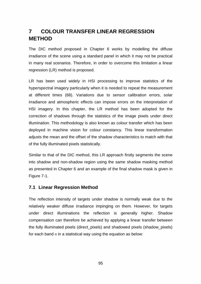
95
7 COLOUR TRANSFER LINEAR REGRESSION
METHOD
The DIC method proposed in Chapter 6 works by modelling the diffuse
irradiance of the scene using a standard panel in which it may not be practical
in many real scenarios. Therefore, in order to overcome this limitation a linear
regression (LR) method is proposed.
LR has been used widely in HSI processing to improve statistics of the
hyperspectral imagery particularly when it is needed to repeat the measurement
at different times (68). Variations due to sensor calibration errors, solar
irradiance and atmospheric effects can impose errors on the interpretation of
HSI imagery. In this chapter, the LR method has been adopted for the
correction of shadows through the statistics of the image pixels under direct
illumination. This methodology is also known as colour transfer which has been
deployed in machine vision for colour constancy. This linear transformation
adjusts the mean and the offset of the shadow characteristics to match with that
of the fully illuminated pixels statistically.
Similar to that of the DIC method, this LR approach firstly segments the scene
into shadow and non-shadow region using the same shadow masking method
as presented in Chapter 6 and an example of the final shadow mask is given in
Figure 7-1.
7.1 Linear Regression Method
The reflection intensity of targets under shadow is normally weak due to the
relatively weaker diffuse irradiance impinging on them. However, for targets
under direct illuminations the reflection is generally higher. Shadow
compensation can therefore be achieved by applying a linear transfer between
the fully illuminated pixels (direct_pixels) and shadowed pixels (shadow_pixels)
for each band n in a statistical way using the equation as below:

96
nnnn cpixelsshadowmshadowCorrected _*_ (7-1)
In this equation mn is defined as,
n
nn
pixelsshadowdeviationstd
pixelsdirectdeviationstdm
__
__ (7-2)
and cn as,
nnnn pixelsshadowmeanmpixelsdirectmeanc __
(7-3)
7.2 Experimental Setup
The data sets used for this experiment is the same as that used for the DIC
experiments. To recall, the hyperspectral data with 88 bands of 10 and 5
different coloured t-shirts have been used as targets as shown in Figure 7-2 and
Figure 7-3 in this experiment. In addition a 102 bands hyperspectral outdoor
data set without the ground truth information is also included as shown in Figure
7-4. This data set was taken on a clear and sunny day on 2nd October 2011 at 2
pm.
QD classification has been employed here for the evaluation of the shadow
removal performance and the training data and the ground truth are obtained
from the data set of the same scene under direct illumination as explained in
Chapter 6. Since the ground truth image is not available for outdoor data, the
effectiveness of the shadow compensation using LR method is evaluated using
the angle and distance metric of the apparent reflectance obtained before and
after shadow correction with respected to that of the same targets under direct
illuminations. Given 2 spectra vector, v1 and v2, the spectral angle mapper
(SAM) metric can be defined as (22),

97
2/1
2
,2
2/1
2
,1
,2,1
1cosN
n
n
N
n
n
N
n
nn
vv
vv
angle where n=band 1,....,N (7-4)
Equation (7-4) involves normalization by the norm of the vectors thus making
SAM to be insensitive to their magnitudes (72). Therefore, this SAM metric is
normally used for the evaluation of the similarity between two vector spectra.
The degree of dissimilarity in spectral shape is measure by the increase of the
angle between the two vectors.
Euclidean Distance (ED) has also been employed for assessing the magnitude
similarity of two vector spectra and it is given by (22),
2/1
2
,2,121,
N
n
nn vvvvED where n=band 1,....,N (7-5)
A small distance represents a close match between the two vector spectra.
(a)
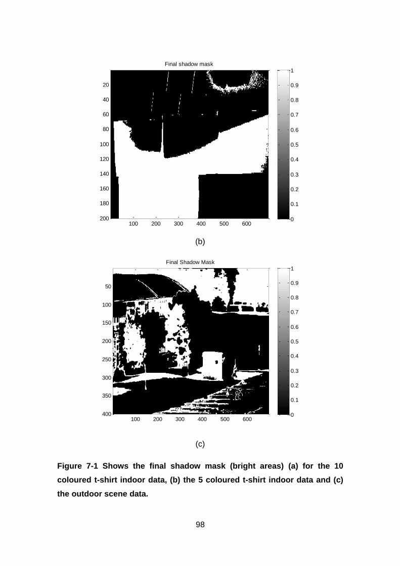
98
Final shadow mask
100 200 300 400 500 600
20
40
60
80
100
120
140
160
180
200 0
0.1
0.2
0.3
0.4
0.5
0.6
0.7
0.8
0.9
1
(b)
Final Shadow Mask
100 200 300 400 500 600
50
100
150
200
250
300
350
400 0
0.1
0.2
0.3
0.4
0.5
0.6
0.7
0.8
0.9
1
(c)
Figure 7-1 Shows the final shadow mask (bright areas) (a) for the 10
coloured t-shirt indoor data, (b) the 5 coloured t-shirt indoor data and (c)
the outdoor scene data.
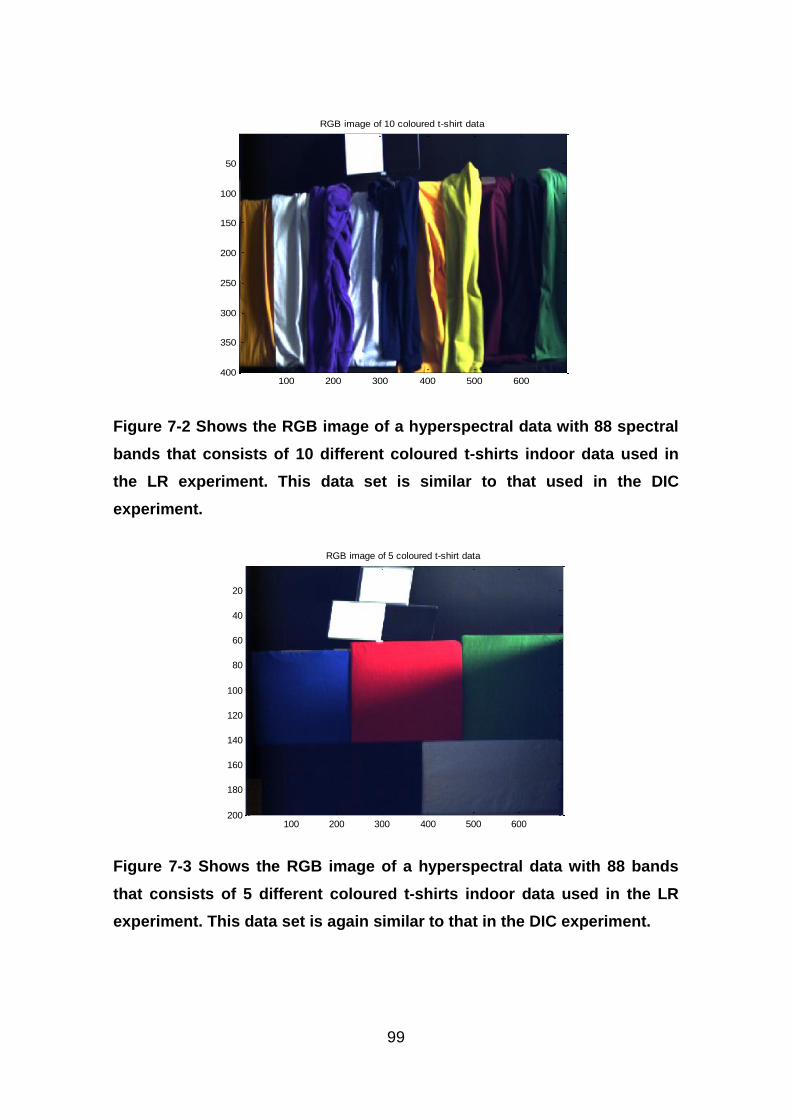
99
RGB image of 10 coloured t-shirt data
100 200 300 400 500 600
50
100
150
200
250
300
350
400
Figure 7-2 Shows the RGB image of a hyperspectral data with 88 spectral
bands that consists of 10 different coloured t-shirts indoor data used in
the LR experiment. This data set is similar to that used in the DIC
experiment.
RGB image of 5 coloured t-shirt data
100 200 300 400 500 600
20
40
60
80
100
120
140
160
180
200
Figure 7-3 Shows the RGB image of a hyperspectral data with 88 bands
that consists of 5 different coloured t-shirts indoor data used in the LR
experiment. This data set is again similar to that in the DIC experiment.

100
RGB of outdoor data
100 200 300 400 500 600
50
100
150
200
250
300
350
400
Figure 7-4 Shows the hyperspectral data of outdoor scene with 102
spectral bands taken at a range of ~100m on a clear and sunny day on the
2nd October 2011 at 2 pm GMT.
7.3 Linear Regression Result
7.3.1 Ten T-Shirt Indoor Data
The RGB image of the shadow compensation via LR method is shown in Figure
7-5. Recall that the classification accuracies of RW and DIC have achieved 68%
(Figure 7-6 (a)) and 70% (Figure 7-6 (b)) respectively for this data set. However,
it is seen that the LR method for shadow compensation has achieved 75%
classification accuracy as shown in Figure 7-6 (c).
Figure 7-7 shows the spectral plot of 2 shadowed targets before correction RW
(in blue), after correction via DIC (in green), LR (in light blue) methods and
compared with that under direct illumination (in red). It is seen that the shadow
compensated spectra by the LR method is closely resemble to that by the DIC
correction. However, one advantage of using the LR method is that it is easier
and simpler to apply in practise as it does not require prior knowledge of the
diffuse irradiance. In the DIC method it requires the standard panel to be in the

101
scene while the LR uses the statistics to compensate for shadow effect on the
hyperspectral images. However this may also mean that the LR method may be
sensitive to the statistics of the scene, for example, the proportions of the
shadowed and non-shadowed regions and the variability of targets in these
regions.
Figure 7-5 Shows the RGB image of the 10 coloured t-shirt data after LR
compensation.
(a)
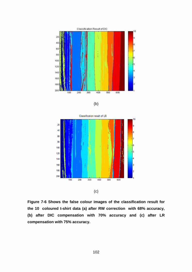
102
(b)
(c)
Figure 7-6 Shows the false colour images of the classification result for
the 10 coloured t-shirt data (a) after RW correction with 68% accuracy,
(b) after DIC compensation with 70% accuracy and (c) after LR
compensation with 75% accuracy.

103
450 500 550 600 650 700 750 800 850 9000
0.2
0.4
0.6
0.8
1
1.2
1.4
Wavelength(nm)
Reflecta
nce
Reflectance of T-shirt 7 (Light Green)
Direct Pixel
Shadow Pixel
Via DIC
Via LR
(a)
450 500 550 600 650 700 750 800 850 9000
0.1
0.2
0.3
0.4
0.5
0.6
0.7
0.8
Wavelength(nm)
Reflecta
nce
Reflectance of T-shirt 10 (Dark Green)
Direct Pixel
Shadow Pixel
Via DIC
Via LR
(b)
Figure 7-7 Shows the spectral plot of shadowed pixels for two targets of
(a) light green t-shirt (target 7) and (b) dark green t-shirt target 10)
obtained from i) apparent reflectance without correction (RW in blue), ii)
after correction via DIC (DIC in green)), iii) after LR (in light blue) iv)
under direct illumination(in red).

104
7.3.2 Five T-Shirt Indoor Data
Figure 7-8 shows the RGB image of the 5 t-shirt data after LR compensation.
From the previous chapter it is recalled that the classification accuracy of RW
and DIC methods have achieved 43% (Figure 7-9 (a)) and 60% ( Figure 7-9 (b))
for this data set respectively. Half of the target class 2 (red t-shirt) has been
misclassified as target class 5 in the untreated RW result. However, the QD
classifier is capable to classify the target class 2 correctly after the DIC
operation. The only error in this classification occurs in target 4. However,
almost all targets can be classified correctly after the LR compensation (Figure
7-9 (c)). The LR method has achieved 97% of classification accuracy which
demonstrates the effectiveness of LR method for shadow compensation.
RGB image of 5 coloured t-shirt after correction via LR
100 200 300 400 500 600
20
40
60
80
100
120
140
160
180
200
Figure 7-8 Shows the RGB image of the 10 coloured t-shirts data after LR
operation.
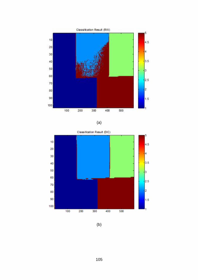
105
(a)
(b)

106
(c)
Figure 7-9 Shows the false colour classification result of the 5 coloured t-
shirt data set after (a) RW with 43% accuracy, (b) DIC compensation with
58% accuracy and (c) LR correction with 97% accuracy.
Figure 7-10 shows the spectral plot of 3 selected shadowed targets before
correction (RW), after correction via DIC and LR methods and a direct
comparison with that of under direct illumination. From this graph, it is seen that
the target reflectance under shadow has been improve after the correction and
it is seen to be closer to the target reflectance under direct illumination than
before the correction. Also, it is observed from this plot that the performance of
the shadow compensations by the LR is very close to that of the DIC and more
tests using a range of different data sets will be needed for a thorough
understanding of the exact potential of the LR method.

107
450 500 550 600 650 700 750 800 850 9000
0.1
0.2
0.3
0.4
0.5
0.6
0.7
Wavelength(nm)
Reflecta
nce
Reflectance T-shirt 1 (Blue)
Direct Pixel
Shadow Pixel
Via DIC
Via LR
(a)
450 500 550 600 650 700 750 800 850 9000
0.2
0.4
0.6
0.8
1
1.2
1.4
Wavelength(nm)
Reflecta
nce
Reflectance T-shirt 2 (Red)
Direct Spectra
Shadow Spectra
via DIC
via LR
(b)

108
450 500 550 600 650 700 750 800 850 9000
0.1
0.2
0.3
0.4
0.5
0.6
0.7
Wavelength(nm)
Reflecta
nce
Reflectance T-shirt 4 (Black)
Direct Pixel
Shadow Pixel
Via DIC
Via LR
(c)
Figure 7-10 Shows the the spectral plot of the shadowed pixels from (a)
blue t-shirt (target 1), (b) red t-shirt (target 2) and (c) black t-shirt (target 4)
after i) no correction (RW in blue), ii) after correction by DIC (in green),
iii) after LR (in light blue) and iv) the same targets under direct
illumination.
7.3.3 Outdoor Data set
The SAM and the ED distance metrics have been used as the performance
metric to evaluate the shadow compensation for the outdoor data set due to the
lack of the target map information for this data set. Figure 7-11 shows the RGB
image of the outdoor data after correction by using LR method, Table 7-1 and
Table 7-2 show the SAM and the ED distance metric of the shadowed pixels
before and after LR operation with respected to that under direct illumination.
The smaller of the angle and distances may represent a better shadow
compensation performance.
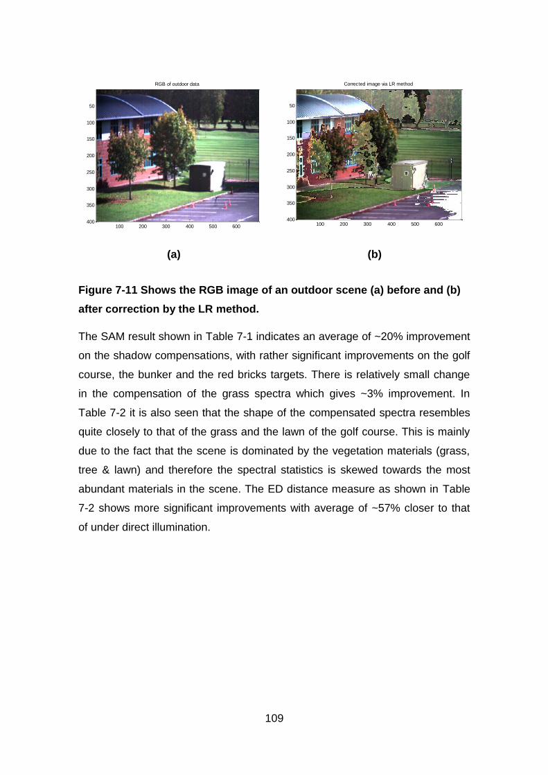
109
RGB of outdoor data
100 200 300 400 500 600
50
100
150
200
250
300
350
400
Corrected image via LR method
100 200 300 400 500 600
50
100
150
200
250
300
350
400
(a) (b)
Figure 7-11 Shows the RGB image of an outdoor scene (a) before and (b)
after correction by the LR method.
The SAM result shown in Table 7-1 indicates an average of ~20% improvement
on the shadow compensations, with rather significant improvements on the golf
course, the bunker and the red bricks targets. There is relatively small change
in the compensation of the grass spectra which gives ~3% improvement. In
Table 7-2 it is also seen that the shape of the compensated spectra resembles
quite closely to that of the grass and the lawn of the golf course. This is mainly
due to the fact that the scene is dominated by the vegetation materials (grass,
tree & lawn) and therefore the spectral statistics is skewed towards the most
abundant materials in the scene. The ED distance measure as shown in Table
7-2 shows more significant improvements with average of ~57% closer to that
of under direct illumination.
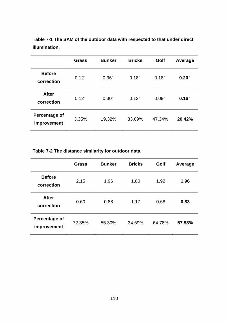
110
Table 7-1 The SAM of the outdoor data with respected to that under direct
illumination.
Grass Bunker Bricks Golf Average
Before
correction 0.12 0.36 0.18 0.18 0.20
After
correction 0.12 0.30 0.12 0.09 0.16
Percentage of
improvement 3.35% 19.32% 33.09% 47.34% 20.42%
Table 7-2 The distance similarity for outdoor data.
Grass Bunker Bricks Golf Average
Before
correction 2.15 1.96 1.80 1.92 1.96
After
correction 0.60 0.88 1.17 0.68 0.83
Percentage of
improvement 72.35% 55.30% 34.69% 64.78% 57.58%

111
This enhancement can also been seen from the spectra plot depicted in Figure
7-12. The value and shape of reflectance that is under shadow almost match
the direct reflectance as we can see in Figure 7.12 (a) and (d). However, from
Figure 7.12 (b) and (e), although the shadow reflectance has been improved the
shape tends to follow the major materials in the scene which is grass. The
changes of the shape after the correction can be clearly observed within the
band 500 to 700. This is due to the fact that this method is based on the statistic
approach which is sensitive to the statistical distributions of objects in the
shadow and non-shadow portions of the scene.
500 550 600 650 700 750 800 850 900 950 10000
0.5
1
1.5
2
2.5
3
3.5
4
4.5
5
Wavelength(nm)
Ref
lect
ance
Grass
Direct
Shadow
LR
(a)
500 550 600 650 700 750 800 850 900 950 10000
0.5
1
1.5
2
2.5
3
Wavelength(nm)
Ref
lect
ance
Bunker
Direct
Shadow
LR
(b)

112
500 550 600 650 700 750 800 850 900 950 10000
0.5
1
1.5
2
2.5
3
Wavelength(nm)
Ref
lect
ance
Red Bricks
Direct
Shadow
LR
(c)
500 550 600 650 700 750 800 850 900 950 10000
0.5
1
1.5
2
2.5
3
3.5
4
4.5
Wavelength(nm)
Ref
lect
ance
Golf
Direct
Shadow
LR
(d)
Figure 7-12 Shows the apparent reflectance of various targets (a) grass (b)
bunker, (c) red bricks and (d) the lawn of the golf course before (in blue)
and after (in green) correction by LR and to compare with that under
direct illumination (in red).

113
7.4 Conclusion
The DIC method has shown some improvements for shadow compensation in
hyperspectral processing. This method requires a standard panel to probe the
diffuse irradiance from the scene which is difficult to realise in practise.
Alternatively, a new method which transfers statistics from the non-shadow
region into the shadow region through Linear Regression (LR) method has been
proposed to achieve illumination invariance and shadow compensation for
hyperspectral imagery processing. Since this method is based on statistics the
performances will be sensitive to the statistical distributions of objects in the
shadow and non-shadow portions of the scene.
Preliminary classification results for two indoor data sets are given in Table 7-3
and it is found that:
(a) The LR shadow compensation improves classification accuracy by ~7% and
~5% better that of the RW and DIC method for the 10 coloured t-shirt indoor
data respectively.
(b) The LR method is found to improve ~54% and ~39% with respected to the
RW and the DIC method for the 5 different coloured t-shirt indoor data
respectively.
(c) The LR method attains on average of about 0.04 degree better than the RW
over 4 targets in an outdoor scene which is dominated by trees and lawn.
(d) The LR method reduces the distance by ~57% over 4 targets in the outdoor
scene
Although the LR method shows the best classification accuracy from these few
data sets without the need of the diffuse irradiance information, there are
limitations of the technique which will be addressed in the future work:
(a) This method utilizes the same shadow masking technique which requires
threshold in the variance and the spectral means as in the DIC method.
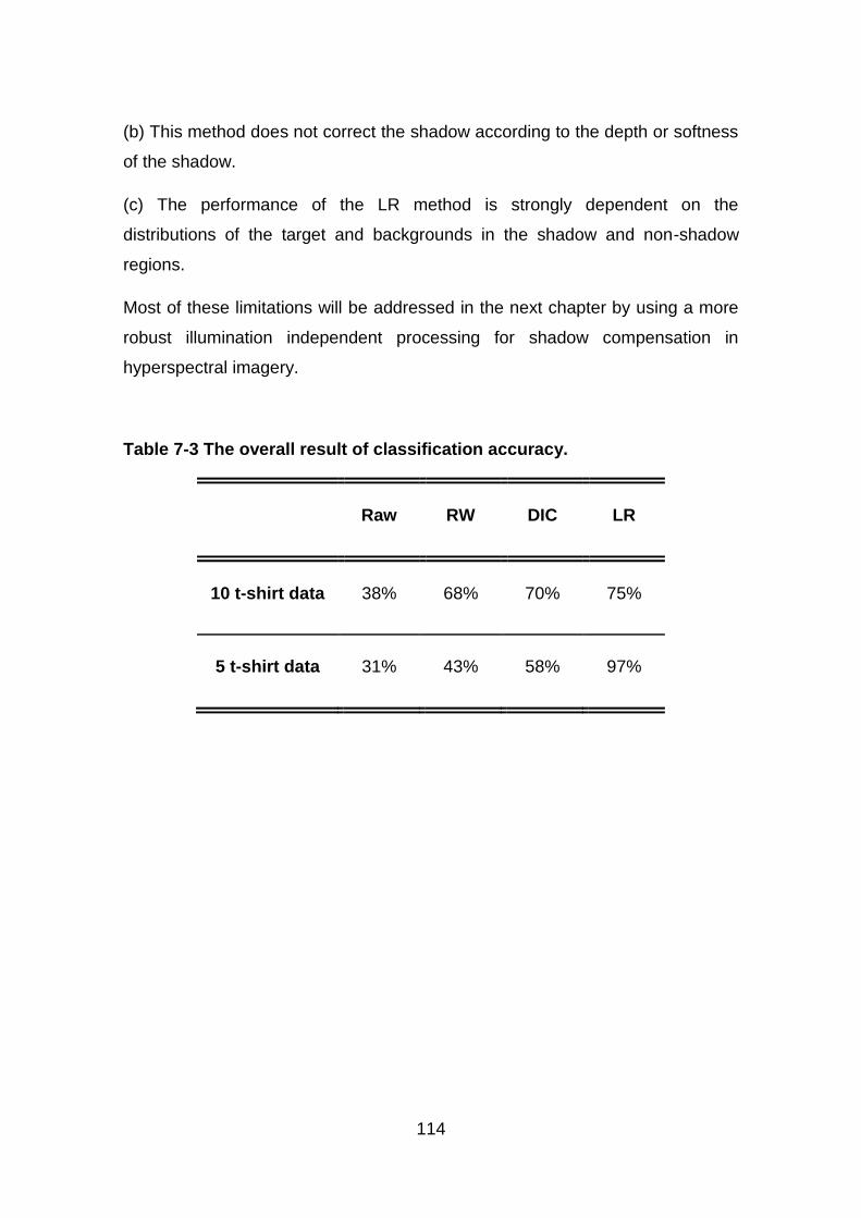
114
(b) This method does not correct the shadow according to the depth or softness
of the shadow.
(c) The performance of the LR method is strongly dependent on the
distributions of the target and backgrounds in the shadow and non-shadow
regions.
Most of these limitations will be addressed in the next chapter by using a more
robust illumination independent processing for shadow compensation in
hyperspectral imagery.
Table 7-3 The overall result of classification accuracy.
Raw RW DIC LR
10 t-shirt data 38% 68% 70% 75%
5 t-shirt data 31% 43% 58% 97%

115
8 SPECTRO-POLARIMETRY METHOD (SP)
Most of the previous effort on shadow compensation has been based on image
processing techniques. In this work we have attempted a new approach of
shadow compensation for hyperspectral imagery by employing a mixture of
Electro-optical (EO) hardware and image processing methods. The EO
hardware method is based on the spectral polarization and it is also known as
spectro-polarimetry technique (SP). Spectro-polarimetry can be deployed in a
system which polarises the light for the illumination and samples the properties
of the reflected light over some defined polarised spectral regions (79). In this
work we have adopted the illumination by a single light source and the reflected
light is collected under a range of polarisation angles. This technique does not
require the standard panel to sample the diffuse irradiance, and the shadow
mask can be deduced more accurately by using two HSI images with and
without polarizer.
The principle underlying in this work makes use of the fact that the reflections
from objects under diffuse irradiance is relatively more unpolarised than that
under direct illumination. We have employed Spectral Angle Mapper (SAM)
algorithm to differentiate between the shadowed and fully illuminated pixels.
SAM measures the spectral angle for each pixel between the non-polarized and
polarized images. These SAM values represent the fraction of the diffuse
irradiance across the images and they are then used for correcting shadows of
the hyperspectral images. This method is evaluated using QD classification and
spectral similarity measure, such as angle and distance metric. The results of
indoor and outdoor tests have shown that the direct and diffuse irradiated pixels
can be differentiated by using the SP technique.
8.1 Introduction and background
Hyperspectral imaging systems collects the spectral energy which is emitted or
reflected from the target in hundreds or more contiguous spectral channels.
However, by combining spectral and polarimetric techniques, more information
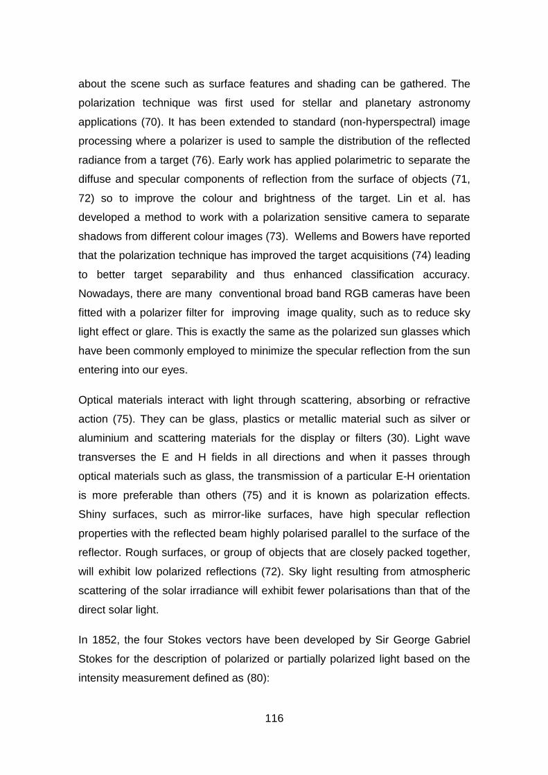
116
about the scene such as surface features and shading can be gathered. The
polarization technique was first used for stellar and planetary astronomy
applications (70). It has been extended to standard (non-hyperspectral) image
processing where a polarizer is used to sample the distribution of the reflected
radiance from a target (76). Early work has applied polarimetric to separate the
diffuse and specular components of reflection from the surface of objects (71,
72) so to improve the colour and brightness of the target. Lin et al. has
developed a method to work with a polarization sensitive camera to separate
shadows from different colour images (73). Wellems and Bowers have reported
that the polarization technique has improved the target acquisitions (74) leading
to better target separability and thus enhanced classification accuracy.
Nowadays, there are many conventional broad band RGB cameras have been
fitted with a polarizer filter for improving image quality, such as to reduce sky
light effect or glare. This is exactly the same as the polarized sun glasses which
have been commonly employed to minimize the specular reflection from the sun
entering into our eyes.
Optical materials interact with light through scattering, absorbing or refractive
action (75). They can be glass, plastics or metallic material such as silver or
aluminium and scattering materials for the display or filters (30). Light wave
transverses the E and H fields in all directions and when it passes through
optical materials such as glass, the transmission of a particular E-H orientation
is more preferable than others (75) and it is known as polarization effects.
Shiny surfaces, such as mirror-like surfaces, have high specular reflection
properties with the reflected beam highly polarised parallel to the surface of the
reflector. Rough surfaces, or group of objects that are closely packed together,
will exhibit low polarized reflections (72). Sky light resulting from atmospheric
scattering of the solar irradiance will exhibit fewer polarisations than that of the
direct solar light.
In 1852, the four Stokes vectors have been developed by Sir George Gabriel
Stokes for the description of polarized or partially polarized light based on the
intensity measurement defined as (80):

117
LR
yxyx
yxyx
yx
yx
II
II
II
II
EEiEEi
EEEE
EE
EE
s
s
s
s
S13545
900
900
**
**
22
22
3
2
1
0
(8-1)
In this equation, 0s is the total intensity of light, 1s is the difference between
horizontal and vertical polarization, 2s is the difference between linear and non-
linear polarization and 3s is the difference between right and left polarization, the
E(x,y) denote the electric field at (x,y). Note that the polarization of the reflected
light is dependent on the propagation of radiation from the source to the scene
and the scatter of the light by objects to the sensor. The exact content of the
atmosphere, the illumination and viewing geometries may affect the polarization
of the reflected beam. Multiple scattering by nearby objects of the scene can
also affect the polarization of the reflected beam that ultimately sensed by the
camera. To measure the entire Stokes polarization parameter one will need
several sets of polarizer to incorporate with the HSI system.
8.2 Spectro-Polarimetry Technique (SP) for shadow
compensation
The HSI system senses the reflections from both the diffuse irradiance, Ediffuse
and the direct irradiance, Edirect. The total flux of illumination is the sum of the
direct and diffuse irradiance,
diffusedirectg EEE (8-2)
Polarisation of light can be sensed through a polarizer (82) and this is set up in
our hyperspectral imaging system as shown in Figure 8-1. At a certain
polarisation angle this polarizer filters the reflections due to the direct
illumination Edirect. Shown in Figure 8-2 are the mean spectra of the white
standard panel taken with and without polarizer. The polariser is set at 90

118
degree and it is seen that the polarisation varies non-linearly as functions of
wavelength.
Two hyperspectral data, indoor data with 88 bands and outdoor data with 102
bands, are taken with and without the polarizer filter. The basic assumption in
this experiment is that there is a difference in the polarization properties
between direct and diffuse illumination. Therefore, the spectral contrast
between the non-polarized and polarized images, denoted by INP and IP
respectively, can be evaluated by using measures such as Spectral Angle
Mapper (SAM). Let x be the pixel vector for images INP and IP for N bands, then
the SAM algorithm is given as,
2/1
2
2/1
2
1
)()(
cos)(N
n
nP
N
n
nNP
N
n
nPnNP
xIxI
xIxI
xSAM where n=band 1,...,N
(8-3)
SAM measures the spectral contrast between the non-polarized images, INP,
with respected to the polarized image, IP. This value is then normalised over the
scene such as:
)max()min(
)min()(1)(_
SAMSAM
SAMxSAMxSAMScaled
(8-4)
This Scaled_SAM values represents the extent of the reflections due to the
diffuse irradiance in each pixels of the scene. Thus the shadow pixels for n
bands can be corrected by re-scaling the scene by the Scaled_SAM values
together with brightness compensation:
nxnx
x
nx
nx imagePimageNPSAMScaled
imageNPshadowCorrected ,,
,
,_
_ (8-5)

119
Figure 8-1 Shows the polarization set up in our system: a polarizer is is
placed on the top of the camera’s objective lens.
Figure 8-2 Shows the plot of the mean spectra from the white standard
panel taken without and with (90degree) polarizer filter.

120
8.3 Experimental Setup
Two types of data sets, indoor and outdoor set, have been used for this
experiment. The indoor data involves two sets data with 4 and 10 coloured t-
shirts as targets, and two outdoor data sets with the lawn and a bunker as
targets. All data sets have been taken without and with polarizer at various
angles of polarization in this experiment. Figure 8.3 (a) shows the illumination
source for taking the indoor data and (b) the 4 coloured t-shirts targets. The
shadow is casted by an object placed between the target and the light source
which is illuminated from one side of the scene. The shadow is casted such that
it is deeper at the far left (on the green t-shirt) and softer towards the right (on
the red t-shirt). The experimental set-up for the 10 coloured t-shirts data is
similar to that in the previous DIC and LR experiments. The RGB images of 10
coloured t-shirts data is given in Figure 8-4.
Figure 8-5 and Figure 8-6 depict the RGB images of the outdoor lawn and
bunker data sets which were taken on a clear and sunny day. The shadow of
the lawn data is casted by the trees. The back side of the bunker is in the shade
and the colour cannot be seen clearly from the raw data. Three standard panels
consisting of the white and black spectralons, are also placed in both the indoor
and outdoor scene for the Edirect estimation.
(a)
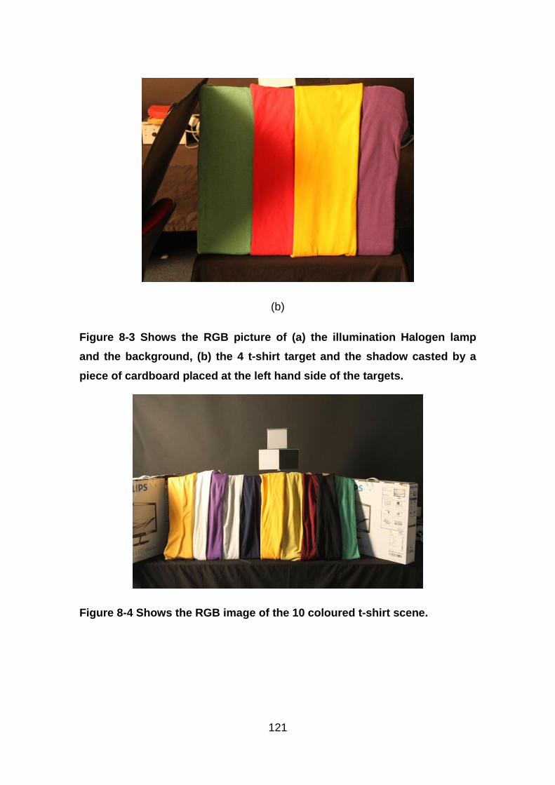
121
(b)
Figure 8-3 Shows the RGB picture of (a) the illumination Halogen lamp
and the background, (b) the 4 t-shirt target and the shadow casted by a
piece of cardboard placed at the left hand side of the targets.
Figure 8-4 Shows the RGB image of the 10 coloured t-shirt scene.

122
(a)
(b)
Figure 8-5 (a) Shows the RGB picture of the lawn that was taken on clear
and sunny day at 1 pm and (b) shows the sky condition during the
experiment.
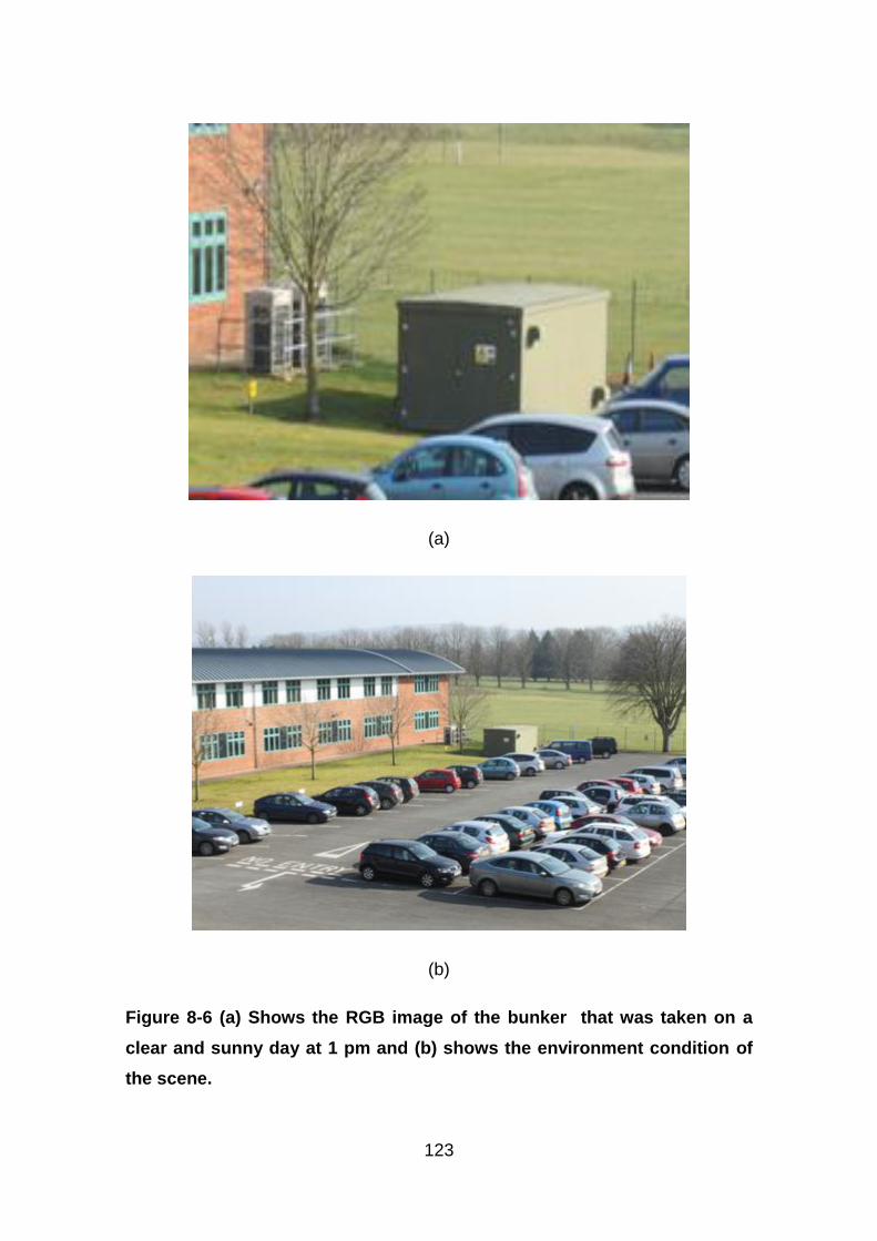
123
(a)
(b)
Figure 8-6 (a) Shows the RGB image of the bunker that was taken on a
clear and sunny day at 1 pm and (b) shows the environment condition of
the scene.

124
8.4 Scaled SAM Result
The first step in the SP technique is the evaluation of the Spectral Angle
Mapper (SAM) between the INP and IP. Figure 8-7 shows the RGB images (a)
without polarizer (INP), (b) with polarizer (IP) and (c) the scaled_SAM map
between INP and IP for the 4 coloured t-shirts image. The scaled_SAM map
shows a range of values in which the deep shadow is indicated by very small
scale and it is presented in blue in the figure. While those pixels under direct
illumination is presented by high SAM values shown in red colour in the figure. It
is also perceived that the SAM of the polarized image is capable to detect the
shadow pixels from the 10 coloured t-shirt data as shown in Figure 8-8. Note
that this method can detect minute shadows such as the self-shadow due to
wrinkles on t-shirt which can also easily be detected by this technique.
The same method also can detect shadows for the outdoor scene, as shown in
Figure 8-9 and Figure 8-10. The pixels that are illuminated by the sky light is
presented in blue colour on the SAM scaled map. A similar result has also been
seen from the bunker data in which the back side of the bunker, and the near
side of the car image, have been identified as shadows.
RGB image of indoor data (without polarizer)
100 200 300 400 500 600
50
100
150
200
250
300
(a)

125
RGB image of indoor data (with polarizer)
100 200 300 400 500 600
50
100
150
200
250
300
(b)
Scaled SAM
100 200 300 400 500 600
50
100
150
200
250
300 0
0.1
0.2
0.3
0.4
0.5
0.6
0.7
0.8
0.9
1
(c)
Figure 8-7 Shows the RGB images (a) without polarizer (INP), (b) with
polarizer (IP) and (c) the false colour scaled_SAM result of these two
images for the indoor scene.

126
RGB image without polarizer
100 200 300 400 500 600
50
100
150
200
250
(a)
RGB image with polarizer
100 200 300 400 500 600
50
100
150
200
250
(b)

127
Scaled SAM
100 200 300 400 500 600
50
100
150
200
2500.1
0.2
0.3
0.4
0.5
0.6
0.7
0.8
0.9
1
(c)
Figure 8-8 Shows the RGB images (a) without polarizer (INP), (b) with
polarizer (IP) and (c) the false colour scaled_SAM result of these two
images for the10 coloured t-shirt indoor data. Note that the shadow is
identified in blue.
RGB image outdoor data (without polarizer)
100 200 300 400 500 600
50
100
150
200
250
300
350
400
(a)

128
RGB image outdoor data (with polarizer)
100 200 300 400 500 600
50
100
150
200
250
300
350
400
(b)
Scaled SAM
100 200 300 400 500 600
50
100
150
200
250
300
350
400
0.1
0.2
0.3
0.4
0.5
0.6
0.7
0.8
0.9
1
(c)
Figure 8-9 Shows the RGB images (a) without polarizer (INP), (b) with
polarizer (IP) and (c) the false colour scaled_SAM result of these two
images for the lawn outdoor scene. Note that all trees and part of the lawn
have been identified as shadows correctly.

129
RGB image without polarizer
50 100 150 200 250
20
40
60
80
100
120
140
(a)
RGB image with polarizer
50 100 150 200 250
20
40
60
80
100
120
140
(b)

130
Scaled SAM
50 100 150 200 250
20
40
60
80
100
120
140 0
0.1
0.2
0.3
0.4
0.5
0.6
0.7
0.8
0.9
1
(c)
Figure 8-10 Shows the RGB image (a) without polarizer (INP), (b) with
polarizer (IP) and (c) the false colour map of the scaled_SAM result for the
bunker outdoor scene. Note that the near side of the bunker and the cars
have been identified as shadows correctly.
8.5 Spectro-polarimetry (SP) Method Assessments
To evaluate the effectiveness of the shadow compensation using polarization
technique, the QD classifier has been employed for the 4 and 10 coloured t-shirt
data sets. The angle and distance metric have been deployed for assessing the
spectral similarity of the shadowed pixels with respected to that under direct
illumination before and after correction by the SP.
8.5.1 Indoor scene
Figure 8-11 shows the training data and the ground truth map for the 4 coloured
t-shirt indoor data. It can be seen from Figure 8-12 that the classification
accuracy is almost 2 times better than that using the RW method which
assumes the complete scene receives Edirect only. The QD result after the SPT
correction has achieved ~98% accuracy far better than that by the RW (48%).

131
Figure 8-13 shows the spectral plots of the apparent reflectance of the
shadowed pixels for the 4 coloured t-shirts to compare with that before (RW)
and after correction by the SP method. It is seen that the SP corrected spectra
(in green curves) have improved rather remarkably and they are a close
resemblance to that under direct illuminations.
The QD result after SP correction image has achieved 90% classification
accuracy for the 10 coloured t-shirt indoor data as shown in Figure 8-14. The
spectral plots of the apparent reflectance of the shadowed pixels for the 4
selected t-shirt targets before and after compensation are given in Figure 8-15.
It is seen that the corrected spectra by SP (in green curves) have improved
substantially and they are a close resemblance to that under direct
illuminations.
Train data
100 200 300 400 500 600
50
100
150
200
250
300
(a)

132
Ground Truth Map
100 200 300 400 500 600
50
100
150
200
250
300 1
1.5
2
2.5
3
3.5
4
(b)
Figure 8-11 (a) Shows the RGB image of the baseline scene under direct
illumination, and the yellow box depicts where the training data pixels are
extracted from; (b) the ground truth target map in false colours.
QD result (RW)
100 200 300 400 500 600
50
100
150
200
250
300 1
1.5
2
2.5
3
3.5
4
(a)

133
QD result after correction via SPT
100 200 300 400 500 600
50
100
150
200
250
300 1
1.5
2
2.5
3
3.5
4
(b)
Figure 8-12 Shows the false colour map of the QD result (a) no correction
by RW with accuracy 48%, (b) after correction by SP with 98%
classification accuracy.
450 500 550 600 650 700 750 800 850 9000
0.1
0.2
0.3
0.4
0.5
0.6
0.7
Wavelength(nm)
Reflecta
nce
T-shirt No 1(Green)
Direct Spectra
Shadow Spectra
Corrected Spectra
(a)

134
450 500 550 600 650 700 750 800 850 9000
0.1
0.2
0.3
0.4
0.5
0.6
0.7
0.8
0.9
Wavelength(nm)
Reflecta
nce
T-shirt No 2(Red)
Direct Spectra
Shadow Spectra
Corrected Spectra
(b)
450 500 550 600 650 700 750 800 850 9000
0.2
0.4
0.6
0.8
1
1.2
1.4
Wavelength(nm)
Reflecta
nce
T-shirt No 3(Yellow)
Direct Spectra
Shadow Spectra
Corrected Spectra
(c)

135
450 500 550 600 650 700 750 800 850 9000
0.1
0.2
0.3
0.4
0.5
0.6
0.7
Wavelength(nm)
Reflecta
nce
T-shirt No 4(Blue)
Direct Spectra
Shadow Spectra
Corrected Spectra
(d)
Figure 8-13 Shows the spectral plot of (a) Green t-shirt 1 (b) Red t-shirt 2
(c) Yellow t-shirt 3 and (d) Blue t-shirt 4 for the pixels i) no shadow
compensation (RW in blue), ii) after SPT correction (in green) and iii)
direction comparison with that under direct illumination (in red).
QD classification result of shadow image
100 200 300 400 500 600
20
40
60
80
100
120
140
160
180
200
220
1
2
3
4
5
6
7
8
9
10
(a)
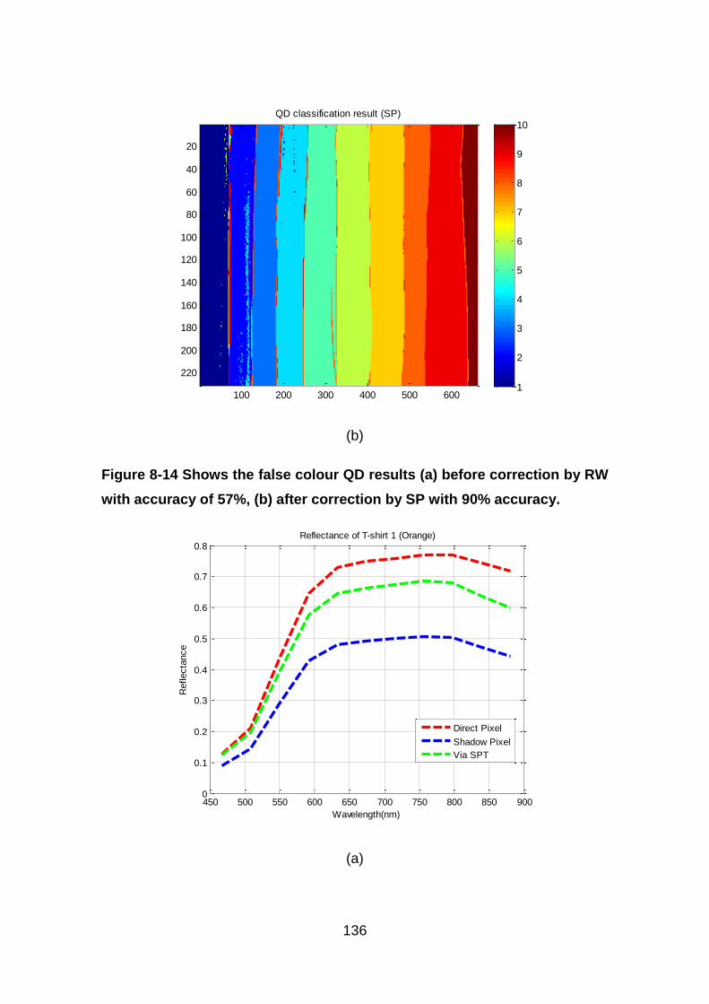
136
QD classification result (SP)
100 200 300 400 500 600
20
40
60
80
100
120
140
160
180
200
220
1
2
3
4
5
6
7
8
9
10
(b)
Figure 8-14 Shows the false colour QD results (a) before correction by RW
with accuracy of 57%, (b) after correction by SP with 90% accuracy.
450 500 550 600 650 700 750 800 850 9000
0.1
0.2
0.3
0.4
0.5
0.6
0.7
0.8
Wavelength(nm)
Reflecta
nce
Reflectance of T-shirt 1 (Orange)
Direct Pixel
Shadow Pixel
Via SPT
(a)

137
450 500 550 600 650 700 750 800 850 9000
0.2
0.4
0.6
0.8
1
1.2
1.4
Wavelength(nm)
Reflecta
nce
Reflectance of T-shirt 5 (Blue)
Direct Pixel
Shadow Pixel
Via SPT
(b)
450 500 550 600 650 700 750 800 850 9000.1
0.2
0.3
0.4
0.5
0.6
0.7
0.8
0.9
1
Wavelength(nm)
Reflecta
nce
Reflectance of T-shirt 7 (Light Green)
Direct Pixel
Shadow Pixel
Via SPT
(c)

138
450 500 550 600 650 700 750 800 850 9000
0.1
0.2
0.3
0.4
0.5
0.6
0.7
0.8
Wavelength(nm)
Reflecta
nce
Reflectance of T-shirt 10 (Darkgreen)
Direct Pixel
Shadow Pixel
Via SPT
(d)
Figure 8-15 Shows the spectral plot of (a) t-shirt 1 (Orange), (b) t-shirt 5
(Blue), (c) t-shirt 7 (Light Green) and (d) t-shirt 10 (Dark Green) after i) no
shadow compensation by RW (in blue), ii) after SPT correction (in green)
and iii) comparison with that under direct illuminations.
8.5.2 Outdoor scene
The result of the shadow correction for the lawn scene is shown in Figure 8-16
and it is seen that the RGB images have shown remarkable improvements after
the shadow compensation, with substantial enhancements on the spectral
integrity as shown in Figure 8-16 (c). Table 8-1 and Table 8-2 show the spectral
similarities of the shadow pixels before and after correction by SP technique for
the lawn and bunker data sets. From the table, the angle and distance measure
after correction have shown better similarities compared to before the
correction. It is seen that the SP technique has shown to be an effective
shadow compensation technique which can compensate shadows without the
need of choosing threshold parameters.
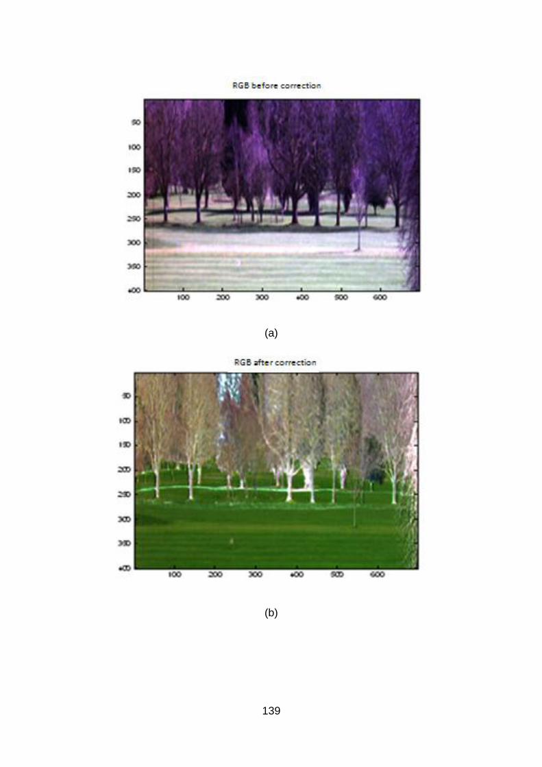
139
(a)
(b)
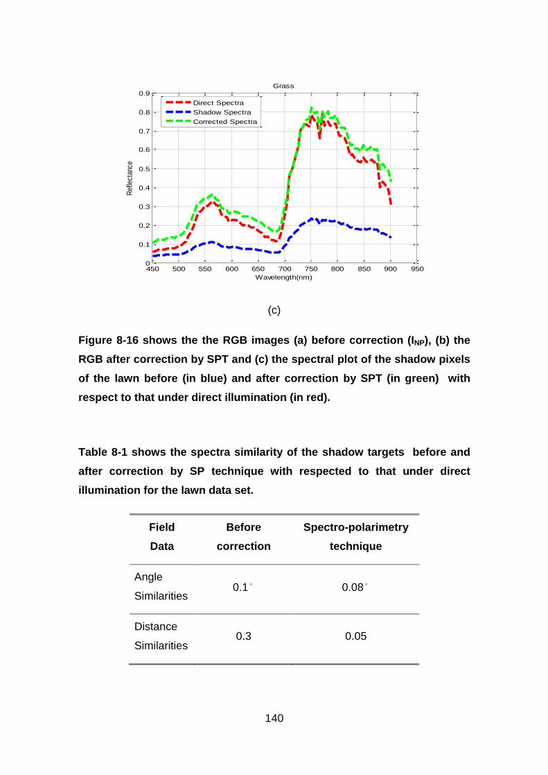
140
450 500 550 600 650 700 750 800 850 900 9500
0.1
0.2
0.3
0.4
0.5
0.6
0.7
0.8
0.9
Wavelength(nm)
Ref
lect
ance
Grass
Direct Spectra
Shadow Spectra
Corrected Spectra
(c)
Figure 8-16 shows the the RGB images (a) before correction (INP), (b) the
RGB after correction by SPT and (c) the spectral plot of the shadow pixels
of the lawn before (in blue) and after correction by SPT (in green) with
respect to that under direct illumination (in red).
Table 8-1 shows the spectra similarity of the shadow targets before and
after correction by SP technique with respected to that under direct
illumination for the lawn data set.
Field
Data
Before
correction
Spectro-polarimetry
technique
Angle
Similarities 0.1 0.08
Distance
Similarities 0.3 0.05
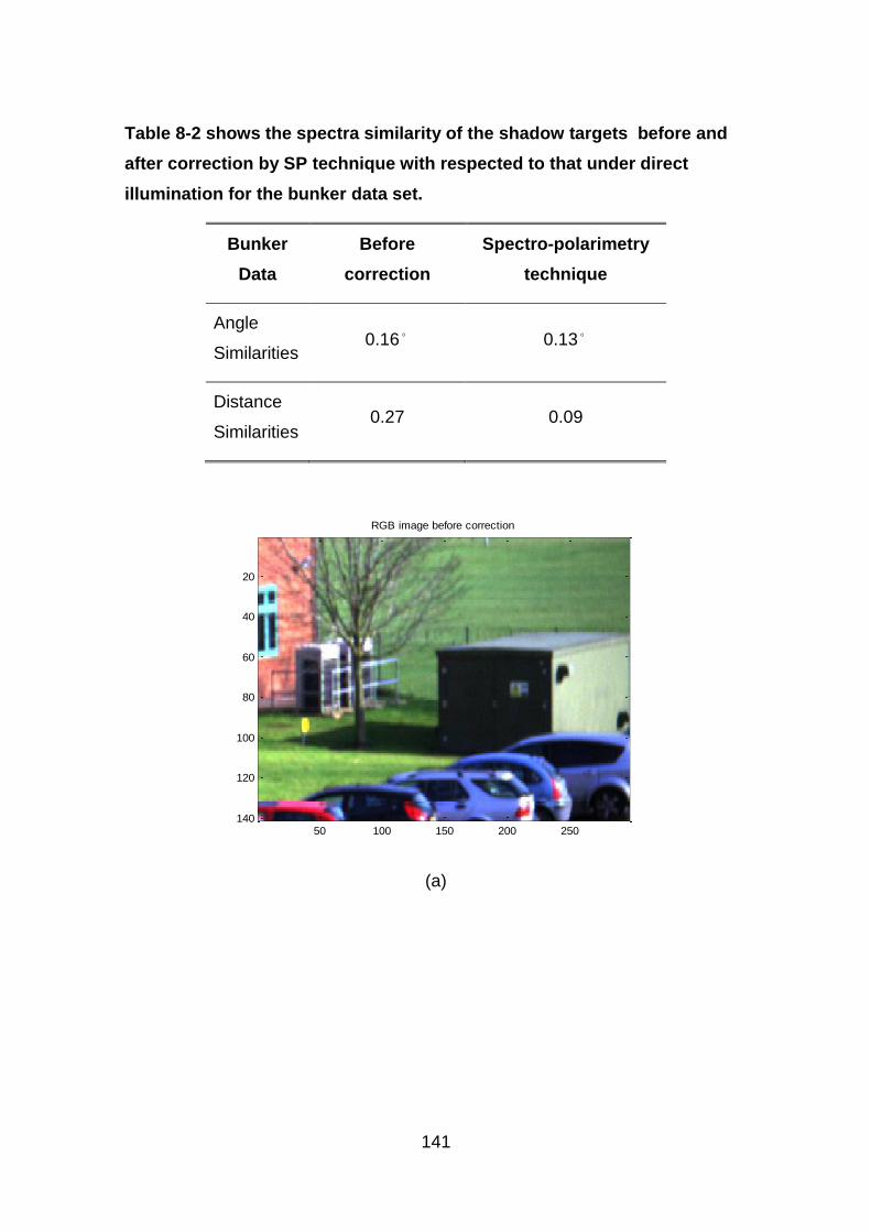
141
Table 8-2 shows the spectra similarity of the shadow targets before and
after correction by SP technique with respected to that under direct
illumination for the bunker data set.
Bunker
Data
Before
correction
Spectro-polarimetry
technique
Angle
Similarities 0.16 0.13
Distance
Similarities 0.27 0.09
RGB image before correction
50 100 150 200 250
20
40
60
80
100
120
140
(a)

142
RGB image after correction
50 100 150 200 250
20
40
60
80
100
120
140
(b)
450 500 550 600 650 700 750 800 850 900 9500
0.5
1
1.5
2
2.5
Wavelength(nm)
Ref
lect
ance
Grass
Direct Spectra
Shadow Spectra
Corrected Spectra
(c)
Figure 8-17 shows the (a) the RGB image before correction (INP), (b) the
RGB image after correction by SP technique and (c) the spectral plot of
the shadow target before (in blue) and after correction by SPT (green)
with respect to that under direct illumination (in red) for the bunker
outdoor data. The edge of shadow shape in (b) is seen to have a mixed
pixel problem due to the bad pixels resolution of the camera.

143
8.6 Conclusion
In this chapter a new method using spectro-polarimetry has been presented for
illumination invariance and shadow correction on hyperspectral imageries. The
spectro-polarimetry technique (SP) is capable to segment the shadow and non-
shadow regions based on the degree of polarization using simple Spectral
Angle Mapper (SAM) processing. The present result has shown that pixels
under direct and diffuse irradiance can be estimated using the polarization
technique.
The overall classification result for using different shadow compensation
methods is summarised in Table 8-3 :
(a) The SP technique achieves better classification accuracy with about a
factor of two better than that by the RW as it is evidenced by both the 4 and 10
coloured t-shirts data sets.
(c) The proposed SP method has improved the angle match ~25% and 18%
better than that of the RW method for the lawn and bunker shadows
respectively, with respected to that under direct illuminations.
This SP technique method has overcome most of the disadvantages in DIC and
LR method such as:
(a) There is no need to establish shadow masks using elaborate threshold
method in the SPT.
(b) The SPT does not require the standard panel to model the diffuse
irradiance.
(c) The SPT compensates shadows according to the depth of the shadow:
larger value of correction will be given for the deeper shadow.

144
Table 8-3 The overall result of classification accuracy.
Raw RW DIC LR SPT
10 t-shirt data 38% 68% 70% 75% 90%
5 t-shirt data 31% 43% 58% 97% -
4 t-shirt data - 48% 73% 86% 98%

145
9 CONCLUSIONS AND FUTURE WORK
The main objective of this research is to establish a method for the
compensation of illumination artefacts such as shadows in order to achieve
spectral constancy so to improve object recognitions. This chapter summarises
all the achievements during the course of this PhD programme entitled
‘Illumination invariance and shadow compensation on hyperspectral images’.
Three different types of algorithms have been developed for shadow
compensation and illumination invariance on hyperspectral images in this work.
Indoor and outdoor data has been selected as test data to assess the algorithm
performance. Three types of performance metric, Quadratic classifier (QD),
spectral angle and distance metrics have been used to evaluate algorithms
achievements. All algorithms are written in MATLAB to allow future work
modifications.
9.1 Diffuse Irradiance Compensation Method (DIC)
It is found from this study that the classification accuracy after converting the
data into ‘apparent’ reflectance denoted by RW, is about a factor of 2 better
than that using the raw DN data which includes the sensor characteristics and
illumination artefacts. The study also demonstrates that spectral normalisation
for ‘flattening’ illumination artefacts will result in a reduction of classification
accuracy by about 30% compared to RW data.
This work has also shown that the shadow compensation can be achieved if the
diffuse irradiance can be estimated from the scene. The Diffuse Irradiance
Compensation (DIC) method has been proposed for reducing shadow effect. It
is found that:
(a) The diffused irradiance compensation (DIC) enhances the target
classification accuracy over the RW method by about ~2% to 15% for the data
sets investigated in this study.

146
The DIC method requires the standard panel to be placed in the scene for
sampling the diffuse and direct irradiance. In real scenarios this method may be
hard to implement. Hyperspectral images may contain various degrees of
shadows and the DIC method compensates all shadows by the same amount
without taking the softness of the shadows into account. The other limitations in
DIC method is the establishment of the shadow mask which requires hard
thresholds to segment the scene into shadow and non-shadow regions. The
optimum threshold value is scene dependent and the methodology for finding
this value in a principled way is still lacking.
9.2 Linear Regression Method (LR)
The DIC method has exhibited some improvements for shadow compensation
but it is difficult to implement in practise. Alternatively, a Linear Regression (LR)
method which transfers statistics from the non-shadow region into the shadow
region has been proposed for illumination invariant of hyperspectral processing.
The achievements and limitations of LR method have been found as follows:
(a) The LR treated data has achieved classification accuracy of ~7% to 54%
better than that of the RW treatment for the data sets investigated in this study.
(b) The LR method is found to be ~5% to 39% better than that of the DIC
method over the data sets investigated in this work.
(c) The performance of the LR method is strongly dependent on the
distributions of the target and backgrounds in the shadow and non-shadow
regions.
Although the LR method has exhibit some improvements over the RW and DIC
methods, this methodology is prone to outliers and the distributions of targets in
the shadow and non-shadow regions. This method is optimum only if the
abundance of the objects is equally distributed in both the shadow and non-
shadow regions.

147
9.3 Spectro-polarimetry Technique (SP)
A new method which is based on spectra-polarimetry has been proposed for
shadow compensation in HSI imagery. The principle underlying this work makes
use of the fact that the reflections from objects under diffuse irradiance are
relatively more unpolarised than that under direct illumination. A Spectral Angle
Mapper (SAM) has been employed to assess the extent of the direct and diffuse
irradiances based on two images taken with and without polarizer for the same
scene. This SAM value is then re-scaled for the shadow compensation.
Although the polarization technique has been used in the conventional broad
band image processing for shadow compensation, this technique is believed to
be the first study for spectral invariance in hyperspectral image processing.
(a) The SP technique achieves better classification accuracy with about a factor
of two better than that by the RW as it is evidenced by both the 4 and 10
coloured t-shirts data sets.
(b) The proposed SP method has improved the angle match ~25% and 18%
better than that of the RW method for the lawn and bunker shadows
respectively, with respect to that under direct illuminations.
(e) This SPT method has overcome most of the disadvantages in DIC and LR
method such as:
1. There is no need to establish shadow masks using elaborate threshold
method in the SP method.
2. The SP technique does not require the standard panel to model the
diffuse irradiance.
3. The SP technique compensates shadows according to the depth of the
shadow: larger value of correction will be given for the deeper shadow.
148
The only drawback of this method is that it will require two sets of the same
scene to be acquired, with and without polarization. Hence this methodology
may be more difficult to be applied to real time applications.
9.4 Future Work
Although the SP technique has shown remarkably good results for shadow
compensation, more future work is needed especially for the design of the push
broom type hyperspectral camera as the scanning mirror will impose some
polarizations to the reflected beam. The design of a hyperspectral polarization
sensitive imaging system may help to overcome the limitation of the presently
SP method that requires two sets of the same scene to be acquired, with and
without polarization.
Other than that, one should attempt to apply the SP technique for the SWIR
region. The polarization within the visible to near infrared region is dominated by
the reflection properties of the surface. However, the polarization in the short
wave infrared region is complicated by the emission properties. The different
polarisations in these two regions may help to improve the effectiveness of the
SP technique in the future.
Polarization on shadow surface also would be changed during the different time
in the day. This technique can also be improved by experimenting it at different
time during the same day to see the changes on the polarization properties from
the reflectance of target under shadow. Also, the degree of polarisation will be
sensitive to sun-target-sensor geometry as a generalisation of the time of day.
Furthermore, the shadow compensation algorithm derived in this work has been
a non-principled method and a more rigorous physics based approach should
be the next step of work.

149
REFERENCES
1. Use of airborne hyperspectral imagery to map soil properties in tilled
agriculture fields. Hively W. D., McCarty G. W., Reeves III J. B., Lang M. W.,
Oesterling R. A. and Delwiche S. R. s.l. : Hindawi Publsiing Corporation,
2011, Applied and Environmental Soil Science, Vol. 2011, pp. 1-13.
2. A review of hyperspectral remote sensing and its application in vegetation
and water resource studies. Govender, M., Chatty, K. and Bulcock, H. 2,
South Africa : South Africa Water Research Commision, 2007, Water SA, Vol.
33, pp. 145-152.
3. Airborne infrared hyperspectral imager for intelligence, surveillance and
reconnaissance applications. Puckrin., E., Turcotte, C. S., Gagnon, M.,
Bastedo, J., Farley, V. and Chamberland, M. Baltimore, Maryland : SPIE,
2012. Vol. 8360.
4. Use of hyperspectral remote sensing for crop stress detection : Ground
Based Studies. Ray, S. S., Singh, J. P. and Panigrahy, S. 8, 2010,
International Archives of the Photogrammetry, Remote Sensing and Spatial
Information Science, Vol. XXXVIII, pp. 562-567.
5. Hyperspectral remote sensing technology and applications in China. Tong,
Q., Zhang, B., and Zheng, L. Frascati, Italy : European Space Agency (ESA),
2004. Proc. of the 2nd CHRIS/Proba Workshop. Vols. SP-578, pp. 1-10.
6. Multispectral and hyperspectral imaging: Applications for medical and
surgical diagnostic. Freeman, J., Downs, F., Marcucci, L., Lewis, E. N.,
Blume, B. and Rish, J. Chicago, USA : Institute of Electrical and Electronics
Engineers (IEEE), 1997. Engineering in Medicine and Bi Proceedings of the
19th Annual International Conference of the IEEE IEEE Engineering in Medicine
and Biology Society. Vol. 2, pp. 700 - 701.
7. Hyperspectral imaging applied to medical diagnosis and food safety.
Carrasco, O., Gomez, R. B, Chainani, A. and Roper, W. E. Orlando, FL :

150
SPIE, 2003. Proc. SPIE 5097, Geo-Spatial and Temporal Image and Data
Exploitation III. Vol. 5097, pp. 215-221.
8. Hyperspectral algorithm development for military applications: A multiple
fusion approach. Yuen, P. W. T. and Bishop, G. Edinburgh : Electro Magnetic
remote Sensing (EMRS) Defence Technoly Centre (DTC), 2006. 3rd EMRS
DTC Technical Conference. Vol. B20, pp. B20-1-6.
9. Spectral imaging for remote sensing. Shaw, G. and Burke, H. 1, 2003,
Lincoln Laboratory Journal, Vol. 14, pp. 3-28.
10. Richards, J.A. and Jia, X. Remote sensing digital image analysis: An
introduction. Berlin, Heidelberg, Germany : Springer, 2006.
11. Hyperspectral image processing for automatic target detection applications.
Manolakis, D., Marden, D., and Shaw, G. A. Lincoln Laboratory Journal : MIT,
2003, Vol. 14, pp. 79-116 .
12. Hyperspectral multiple approach fusion for the long range detection of low
observable objects:MUF2. Yuen, P. W. T. and Bishop, G. Europe : SPIE,
2006. Proceedings of the SPIE: Electro-Optical Remote Sensing II. Vol. 6396.
13. Alhberg, J., Chevalier, T., Andersson, P. and Klasen, L. Target detection
in multispectral imagery. Sweeden : Swedish Defence Research Agency, 2004.
14. Adaptive multiple-band CFAR detection of an optical pattern with unknown
spectral distribution. Reed, I. S. and Yu, X. October 1990, IEEE Transaction on
Acoustic. Speech. and Signal Processing, pp. 1760-1770.
15. Algorithms for the detection of sub-pixels targets in multispectral imagery.
Ashton, E. A. and Schaum, A. 7, s.l. : American Society for Photogrammetry
and Remote Sensing (ASPRS), July 1998, Photogrammetic Engineering &
Remote Sensing, Vol. 64, pp. 723-731.
16. Ahlberg, J. and Renhorn, I. Multi-and hyperspectral target and anomaly
detection. Linkoping : FOI Swedish Defence Research Agency, 2004.

151
17. Stein, D. W. J., Beaven, S. G., Hoff, L. E., Winter, E. M., Schaum, A. P.
and Stocker, A. D. Anomaly detection from hyperspectral imagery. IEEE Signal
Processing Magazine. January 2002, Vol. 19, 1, pp. 58-69.
18. Adaptive feature extraction techniques for subpixel target detections in
hyperspectral remote sensing. Yuen P. W. T. and Bishop, G. London, UK. :
SPIE, 2004. Proc. of SPIE Military remote sensing. Vol. 5613.
19. The effectiveness and limitations of geometric and statistical spectral
unmixing techniques for subpixel target detection in hyperspectral remote
sensing. Yuen P. W. T., Blagg. A. and Bishop, G. Bruges, Belgium : SPIE,
2005. Proc. of SPIE: Electro-Optical Remote Sensing. Vol. 5988.
20. West, J. E. . Matched filter stocastic background characterization for
hyperspectral target detection. s.l. : Rochester Institute of Technology, 2005.
21. Chang, C-I. Hyperspectral Imaging: Techniques for Spectral Detection and
Classification. New York, USA. : Kluwer Academic/Plenum Publisher, 2003.
22. Webb, A. Statistical pattern recognition. United Kingdom : A Hodder Arnold
Publication. , 1999.
23. Duda, R. O., Hart, P. E., Stork, D. G. Pattern Classification 2nd Edition.
New York : John Wiley & Sons, Inc, 2001.
24. Seyrafi, K. and Hovanessian, S. A. Introduction to electro-optic imaging
and tracking system. Norwood, MA 0206, USA : Artech House, Inc. , 1993.
25. Driggers, R.G., Cox, P. and Edwards, T. Introduction to Infrared and
Electro-Optical Systems. Norwood, MA, USA : Artech Hous, 1999.
26. Derivation of Scaled Surface Reflectances from AVIRIS Data. Gao, B.,
Heidebrecht, K. B. and Goetz, A. F. H. s.l. : Elsevier, 1993, Remote Sens.
Environ, Vol. 44, pp. 165-178.
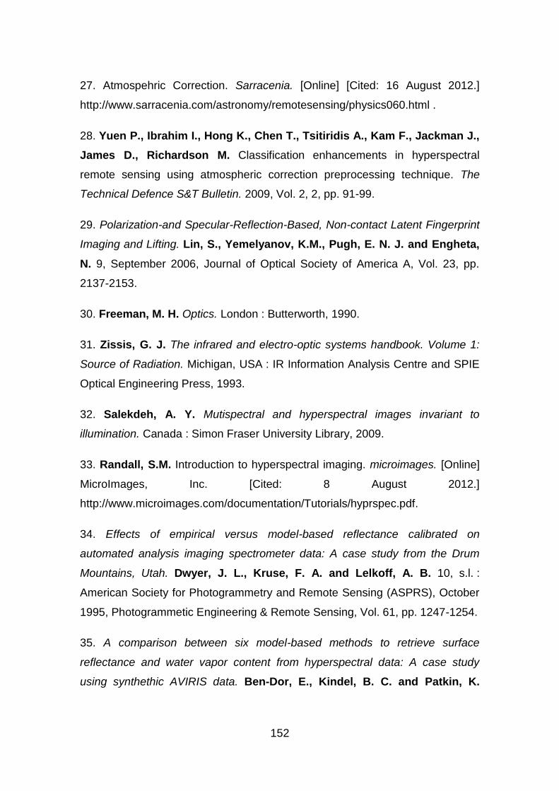
152
27. Atmospehric Correction. Sarracenia. [Online] [Cited: 16 August 2012.]
http://www.sarracenia.com/astronomy/remotesensing/physics060.html .
28. Yuen P., Ibrahim I., Hong K., Chen T., Tsitiridis A., Kam F., Jackman J.,
James D., Richardson M. Classification enhancements in hyperspectral
remote sensing using atmospheric correction preprocessing technique. The
Technical Defence S&T Bulletin. 2009, Vol. 2, 2, pp. 91-99.
29. Polarization-and Specular-Reflection-Based, Non-contact Latent Fingerprint
Imaging and Lifting. Lin, S., Yemelyanov, K.M., Pugh, E. N. J. and Engheta,
N. 9, September 2006, Journal of Optical Society of America A, Vol. 23, pp.
2137-2153.
30. Freeman, M. H. Optics. London : Butterworth, 1990.
31. Zissis, G. J. The infrared and electro-optic systems handbook. Volume 1:
Source of Radiation. Michigan, USA : IR Information Analysis Centre and SPIE
Optical Engineering Press, 1993.
32. Salekdeh, A. Y. Mutispectral and hyperspectral images invariant to
illumination. Canada : Simon Fraser University Library, 2009.
33. Randall, S.M. Introduction to hyperspectral imaging. microimages. [Online]
MicroImages, Inc. [Cited: 8 August 2012.]
http://www.microimages.com/documentation/Tutorials/hyprspec.pdf.
34. Effects of empirical versus model-based reflectance calibrated on
automated analysis imaging spectrometer data: A case study from the Drum
Mountains, Utah. Dwyer, J. L., Kruse, F. A. and Lelkoff, A. B. 10, s.l. :
American Society for Photogrammetry and Remote Sensing (ASPRS), October
1995, Photogrammetic Engineering & Remote Sensing, Vol. 61, pp. 1247-1254.
35. A comparison between six model-based methods to retrieve surface
reflectance and water vapor content from hyperspectral data: A case study
using synthethic AVIRIS data. Ben-Dor, E., Kindel, B. C. and Patkin, K.

153
Dehradun, India : The Optical Society of India, 2005. International Conference
on Optics & Optoelectronics (ICOL).
36. A review of atmospheric correction techniques for hyperpsectral remote
sensing of land surfaces and ocean color. Gao, B., Davis, C. O. and Goetz, A.
F. H. Washington, DC : IEEE, 2006. Conference on Geoscience and Remote
Sensing Symposium (GARSS).
37. The relationship between size of spatial substes of GER 63 channel
scanner data and the quality of the internal average relative reflectance (IARR)
atmospheric correction. Ben-dor, E. and Kruse, F. A. 3, United Kingdom :
Taylor & Francis, 1994, International Journal Remote Sensing, Vol. 15, pp. 683-
690.
38. Use of airborne imaging spectrometer data to map minerals associated with
hydrothermally altered rocks in the Northern Grapevine Mountains, Nevada and
California. Kruse, F. A. New York, USA. : Elsivier, 1985, Remote Sensing of
Environment , pp. 2431-51.
39. Computing radiances, reflectance and albedo from DN’s . Yale University.
[Online] [Cited: 10 September 2012.]
http://www.yale.edu/ceo/Documentation/ComputingReflectanceFromDN.pdf.
40. Automatic flat field algorithm for hyperspectral image calibration. Zhang, X.,
Zhang, B., Geng, X., Tong, Q. and Zheng, L. Wuhan, China : SPIE, 2003.
Symposium on Multispectral Image Processing and Pattern Recognition. Vol.
5286, pp. 636-639.
41. Evaluations of airborne visible/infrared imaging spectrometer data of the
Mountain Pass, California Carbomatite Complex. Crowley, J., Rowan, L. and
Podwysocki, M. Jet Propulsion Lab., California Inst. of Tech : Proceedings of
the Airborne Visible/Infrared Imaging Spectro, 2006.
42. Calibration of airborne imaging spectrometer data to percent reflectance
using field spectral measurements. Roberts, D.A., Yamaguchi, Y., and Lyon,

154
R.J.P. Ann Arbor, Michigan : Environmental Research Institute of Michigan,
Canada Centre for Remote Sensing, 1985. Proceedings Nineteenth
International Symposium on Remote Sensing of Environment. pp. 679-688.
43. Airborne Imaging Spectrometer-2: Radiometry and a comparison of
methods for the recovery of ground reflectance. Conel, J.E., R.O. Green,
G.Vane, C.J. Brueege and R.E. Alley. Pasadena, California : Jet Propulsion
Laboratory, 1987. Proceedings Airborne Imaging Spectrometer Data Analysis
Workshop. Vol. 21987, pp. 18-47.
44. Mineral mapping at Cuperite, Nevada, with a 63 channel imaging
spectrometer. Kruse, F. A., Kieren-Young, K. S., and Boardman, J. W. 56,
Maryland, USA : The American Society for Photogrammetry and Remote
Sensing (ASPRS) , 1990, Photogrammetric Engineering & Remote Sensing, pp.
83-92.
45. Richter, R. and Muller, A. Atmospheric/Topographic Correction for Satellite
Imagery (ATCOR 2/3 User Guide). German : German Aerospace Center, 2005.
pp. 3137-3148. Vol. 6.1.
46. Comparison of FLAASH versus Empirical Line Approach for atmospheric
correction of OMIS-II imagery. Zhang, X., Yang, H. and Shuai, T. Rio de
Janeiro, Brazil : IEEE, 2009. Asian Association on remote Sensing on IEEE
Conference on Agriculture/ Soil/Others.
47. The high accuracy atmospheric correction for hyperpsectral data (HATCH)
model. Qu, Z. 6, Colorado, USA : IEEE, June 2003, IEEE Transactions on
Geoscience and Remote Sensing, Vol. 41, pp. 1223-1231.
48. Using ground spectral irradiance for model correction of AVIRIS data.
Goetz, A. F. H., Heidebrecht, K. B., Kindel, B. and Boardman, J. W.
Pasadena, CA. : Jet Propulsion Laboratory, 1998.
49. Schowengerdt, R. A. Techniques for image processing and classification in
remote sensing. London : Academis Press, 1983.
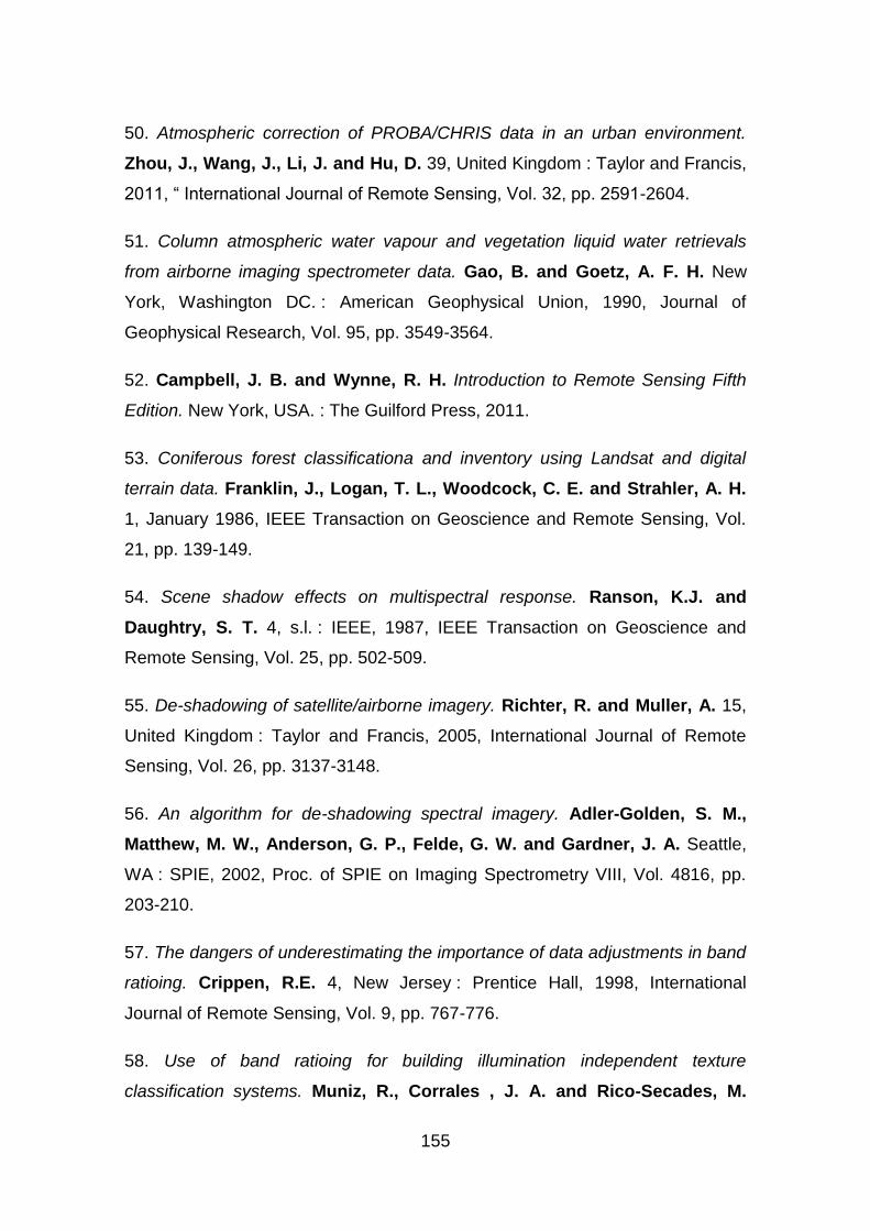
155
50. Atmospheric correction of PROBA/CHRIS data in an urban environment.
Zhou, J., Wang, J., Li, J. and Hu, D. 39, United Kingdom : Taylor and Francis,
2011, “ International Journal of Remote Sensing, Vol. 32, pp. 2591-2604.
51. Column atmospheric water vapour and vegetation liquid water retrievals
from airborne imaging spectrometer data. Gao, B. and Goetz, A. F. H. New
York, Washington DC. : American Geophysical Union, 1990, Journal of
Geophysical Research, Vol. 95, pp. 3549-3564.
52. Campbell, J. B. and Wynne, R. H. Introduction to Remote Sensing Fifth
Edition. New York, USA. : The Guilford Press, 2011.
53. Coniferous forest classificationa and inventory using Landsat and digital
terrain data. Franklin, J., Logan, T. L., Woodcock, C. E. and Strahler, A. H.
1, January 1986, IEEE Transaction on Geoscience and Remote Sensing, Vol.
21, pp. 139-149.
54. Scene shadow effects on multispectral response. Ranson, K.J. and
Daughtry, S. T. 4, s.l. : IEEE, 1987, IEEE Transaction on Geoscience and
Remote Sensing, Vol. 25, pp. 502-509.
55. De-shadowing of satellite/airborne imagery. Richter, R. and Muller, A. 15,
United Kingdom : Taylor and Francis, 2005, International Journal of Remote
Sensing, Vol. 26, pp. 3137-3148.
56. An algorithm for de-shadowing spectral imagery. Adler-Golden, S. M.,
Matthew, M. W., Anderson, G. P., Felde, G. W. and Gardner, J. A. Seattle,
WA : SPIE, 2002, Proc. of SPIE on Imaging Spectrometry VIII, Vol. 4816, pp.
203-210.
57. The dangers of underestimating the importance of data adjustments in band
ratioing. Crippen, R.E. 4, New Jersey : Prentice Hall, 1998, International
Journal of Remote Sensing, Vol. 9, pp. 767-776.
58. Use of band ratioing for building illumination independent texture
classification systems. Muniz, R., Corrales , J. A. and Rico-Secades, M.

156
Florida, USA : International Association for Pattern Recognition (IAPR), 2008.
9th International Conference on Pattern Recognition.
59. A band ratio approach for classification in shaded area. Kao, H. and Ren,
H. Beijing, China : Asian Association on Remote Sensing (AARS), 2009. 30th
Asian Conference on Remote Sensing. Vol. 2, pp. 658-662.
60. Development of vegetation index using radiant spectra normalized by their
arithmetic mean. Ono, A., Kajiwara, K., Honda, Y. and Ono, A. Japan : Nihon-
Rimōto-Senshingu-Gakkai, 2006. Proceedings of the Conference of the Remote
Sensing Society of Japan. Vol. 40.
61. Colour constancy form Hyper-spectral data. Gevers, T., Stokman, H.M.G
and Van de Weijer, J. Bristol, UK. : The British Machine Vision Association and
Society for Pattern Recognition, 2000. Proceedings of British Machine and
Vision Conference (BMVC).
62. Hyperspectral video for illumination-invariant tracking. Banerjee, A.,
Burlina, P. and Broadwater, J. Grenoble : IEEE, 2009. Hyperspectral Image
and Signal Processing: Evolution in Remote Sensing, 2009. WHISPERS '09.
First Workshop on.
63. A novel method for illumination suppression in hyperspectral images.
Ashton, E. A., Wemett, B.D., Leathers, R. A. and Downes, T. V. Orlando,
FL : SPIE, 2008. Proc. SPIE 6966, Algorithms and Technologies for
Multispectral, Hyperspectral, and Ultraspectral Imagery XIV. Vol. 6966, pp.
69660C-69660C-8 .
64. Effect of radiance-to-reflectance transformation and atmosphere removal on
maximum likelihood classification accuracy of high-dimensional remote sensing
data. Joseph, P. H. and David, A. L. Pasadena, CA : IEEE, 1994. Proceedings
of the 14th Annual International Geoscience and Remote Sensing Symposium
IGARSS.

157
65. Classification and Change detection using LandSat TM Data: When and
how to correct atmospheric effect. Song, C., Woodcock, C. E., Seto, K. C.,
Lenney, M. P. and Macomber, S. A. MO, USA : Elsivier, 2001, Remote
Sensing of Environment Journal, Vol. 75, pp. 230-244.
66. The atmospheric effect on the separability of field classes measured from
satellites. Kaufman, Y. J. MO, USA. : Elsevier, 1985, Remote Sensing of
Environment, Vol. 18, pp. 21-34.
67. An examination of spectral band ratioing to reduce topographic effect on
remotely sensed data. Holbern, B. and Justice, C. MO, USA : Elsivier, 1981,
Remote Sensing Environment, Vol. 2, pp. 115-133.
68. Comparison of relative radiometric normalization techniques. Yuan, D. and
Elvidge, C.D. MO, USA : Elsevier, 1996, ISPRS Journal of Photogrammetry
and Remote Sensing, Vol. 51, pp. 117-126.
69. A New Approach to Change Vector Analysis Using Distance and Similarity
Measures. Carvalho Junior, O. A., Guimaraes, R. F., Gillespie, A. R., Silva,
N. C. and Gomes, R. A. T. 11, Basel, Switzerland : Multidisciplinary Digital
Publishing Institute (MDPI), 2011, International Journal of Remote Sensing, Vol.
3, pp. 2473-2493.
70. Egan, W. G. Photometry and polarization in remote sensing. MO, New
York : Elsevier, 1985.
71. Using polarization to separate reflection components. Wolff, L.B. San
Diego, CA : Institute of Electrical and Electronics Engineers (IEEE), 1989.
Proceedings of IEEE Computer Society Conference on Computer Vision and
Pattern Recognition. Vol. 10, pp. 363-369.
72. Dark target retroreflection increase. Egan, W. G. Denver, CO, USA. : SPIE,
1999. Proc of SPIE: Polarization: Measurement, Analysis, and Remote Sensing
II. Vol. 3754.

158
73. Separation and contrast enhancements of overlapping cast shadow
components using polarization. Lin, S., Yemelyanov, K.M., Jr, E. N. P. and
Engheta, N. 16, Washington, DC, USA : Optical Society of America, August
2006, Optics Express, Vol. 14, pp. 7099-7108.
74. Improved hyperspectral imagery using diffuse illumination or a polarizer.
Wellems, D. and Bowers, D. San Diego, CA : SPIE, 2008. Proc of SPIE:
Reflection, Scattering, and Diffraction from Surfaces. Vol. 7065.
75. Ray tracing with polarization parameters. Wolff, L. B. and Kurlander, D. J.
6, 1990, IEEE computer Graphics and Applications, Vol. 10, pp. 44-55.
76. Improved diffuse reflection models for computer vision. Wolff, L., Nayar, S.
K. and Oren, M. 1, New York, USA : Springer, 1998, International Journal of
Computer Vision, Vol. 30, pp. 55-71.
77. Raman Spectrocopy. Holographic Imaging Spectrograph. [Online] Kaiser
Optical System, Inc. [Cited: 18 September 2012.]
http://www.kosi.com/Raman_Spectroscopy/holoSpecf18.php?ss=600.
78. Kam, F. Classification Technique for Hyperspectral Remote Sensing.
Swindon : Cranfield University, 2009. Mphil Tesis.
79. Review of passive imaging polarimetry for remote sensing applications.
Tyo, J. S., Goldstein, D. L., Chenault, D. B. and Shaw, J. A. 22, Washington,
DC. : Optical Society of America, 2006, Applied Optics, Vol. 45.
80. Brosseau, C. Fundamentals of Polarized Light. Toronto : John Wiley &
Sons, Inc., 1998.
81. Goldstein, D. Polarized light, revised and expanded (optical engineering).
New York : Marcer Decker AG, 2003.
82. Visual Behavior Based Bio-Inspired Polarization Techniques in Computer
Vision and Robotics. Shabayek, A. E., Morel, O. and Fofi, D. . In M. Pomplun,

159
& J. Nantes, France : Institue of Physics (IOP) Publishing, 2011. International
Workshop on Bio-inspired Robots.
83. Illumination invariance and shadow compensation via spectro-polarimetry
technique. Ibrahim, I., Yuen, P., Hong, K., Chen, T., Soori, U., Jackman, J.
and Richardson, M. 10, Bellingham, WA : SPIE, 2012, Optical Engineering
(OE), Vol. 51.
84. Ibrahim, I., Yuen, P., Tsitiridis, A., Hong, K., Chen, T., Jackman, J.,
James, D. and Richardson, M. Spectral constancy on hyperspectral
imageries. Defence S&T Technical Bulletin. 2011, Vol. 4, 1, pp. 19-30.
85. Illumination independent object recognitions in hyperspectral imaging.
Ibrahim, I., Yuen, P., Tsitiridis, A., Hong, K., Chen, T., Jackman, J., James,
D. and Richardson, M. Touluse, France : SPIE, 2010. Proceedings of the SPIE
7838. Vol. 7838, pp. 78380O-1-12 .
86. Shadow compensation on hyperpsectral imageries. Ibrahim, I., Yuen, P.,
Soori, U., Chen, T., Hong, K., Tsitiridis, A., Jackman, J. and Richardson, M.
Shrivenham, Swindon : Defence Academy of the United Kingdom, 2012. 10th
Electro-optics & Infrared Conference.
87. Automated Spectral Unmixing of AVIRIS Data Using Convex Geometry
Concepts. Boardman, J. W. Fourth JPL Airborne Geoscience Workshop 93-
26 : JPL Publication, 1993. Vol. 1.
88. Comparative study between a new nonlinear model and common linear
model for analysing laboratory simulated-forest hyperspectral data. Fan, W.,
Hu, B., Miller, J. and Li, M. 2009, International Journal of Remote Sensing, pp.
2951 - 2962.
89. Illumination and shadow compensation of hyperspectral images using a
digital surface model and non-linear least squares estimation.” 2011. Friman,
O., Tolt, G. and Ahlberg, J. s.l. : SPIE, 2011. Image and Signal Processing for
Remote Sensing. Proc. of SPIE. Vols. 81800Q-1: 8.

160
90. A new method for atmospheric correction and aerosol optical property
retrieval for VIS-SWIR multi- and hyperspectral imaging sensors: QUAC (QUick
atmospheric correction). Bernstein, L. S., Adler-Golden, S. M., Sundberg, R.
L., Levine, R. Y., Perkins, T. C., Berk, A., Ratkowski, A. J., Felde, G. and
Hoke, M. L. Seoul, Korea : IEEE, 2005. Geoscience and Remote Sensing
Symposium, 2005. IGARSS '05. Proceedings. 2005 IEEE International. pp.
3549 - 3552
91. In-scene-based atmospheric correction of uncalibrated VISible-SWIR (VIS-
SWIR) hyper- and multi-spectral imagery. Bernstein, L. S., Adler-Golden, S.
M., Sundberg, R. L. and Ratkowski, A. J. Cardiff, Wales, United Kingdom :
SPIE, 2008. Proc. SPIE 7107, Remote Sensing of Clouds and the Atmosphere
XIII, 710706.
92. Active Spectral Imaging. Nischan, M. L., Joseph, R. M., Libby, J. C and
Kerekes, J. P. 1, 2003, Lincoln Laboratory Journal, Vol. 14, pp. 131-144.

161
APPENDICES
Appendix A Reflectance for shadow and direct pixels
of 10 different coloured t-shirt data
The reflectance of a target under shadow is difficult to measure by optical
sensors due to an insufficient radiation component in the signal reflected by the
target. The signal captured by the sensor is always small but non-zero due to
the diffuse irradiance which still remains on the scene, although the direct
illumination is completely blocked by clouds or objects that cast the shadow.
This diffuse irradiance is resulted from the scattered energy from the adjacent
targets, background or environment. This appendix would show the comparison
between direct and diffuse reflectance from the same targets of 10 different
coloured t-shirt data.
Figure A- 1 shows the RGB of 10 different coloured t-shirts data.

162
450 500 550 600 650 700 750 800 850 9000
0.05
0.1
0.15
0.2
0.25
0.3
0.35
0.4
Wavelength(nm)
Ref
lect
ance
Reflectance of T-shirt 1 (Orange)
Direct Pixel
Shadow Pixel
Figure A- 2 shows the plot of direct and shadow pixels for t-shirt 1.
450 500 550 600 650 700 750 800 850 900
0.2
0.25
0.3
0.35
0.4
0.45
0.5
0.55
0.6
0.65
Wavelength(nm)
Ref
lect
ance
Reflectance of T-shirt 2 (White)
Direct Pixel
Shadow Pixel
Figure A- 3 shows the plot of direct and shadow pixels for t-shirt 2.
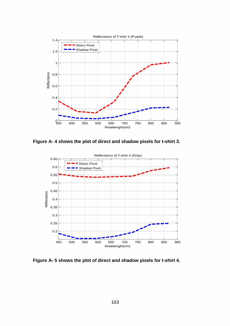
163
450 500 550 600 650 700 750 800 850 9000
0.2
0.4
0.6
0.8
1
1.2
1.4
Wavelength(nm)
Ref
lect
ance
Reflectance of T-shirt 3 (Purple)
Direct Pixel
Shadow Pixel
Figure A- 4 shows the plot of direct and shadow pixels for t-shirt 3.
450 500 550 600 650 700 750 800 850 900
0.2
0.25
0.3
0.35
0.4
0.45
0.5
0.55
0.6
0.65
Wavelength(nm)
Ref
lect
ance
Reflectance of T-shirt 4 (Gray)
Direct Pixel
Shadow Pixel
Figure A- 5 shows the plot of direct and shadow pixels for t-shirt 4.

164
450 500 550 600 650 700 750 800 850 9000
0.2
0.4
0.6
0.8
1
1.2
1.4
Wavelength(nm)
Ref
lect
ance
Reflectance of T-shirt 5 (Blue)
Direct Pixel
Shadow Pixel
Figure A- 6 shows the plot of direct and shadow pixels for t-shirt 5.
450 500 550 600 650 700 750 800 850 9000
0.2
0.4
0.6
0.8
1
1.2
1.4
1.6
1.8
2
Wavelength(nm)
Ref
lect
ance
Reflectance of T-shirt 6 (Yellow)
Direct Pixel
Shadow Pixel
Figure A- 7 shows the plot of direct and shadow pixels for t-shirt 6.

165
450 500 550 600 650 700 750 800 850 9000
0.2
0.4
0.6
0.8
1
1.2
1.4
1.6
1.8
2
Wavelength(nm)
Ref
lect
ance
Reflectance of T-shirt 7 (Light Green)
Direct Pixel
Shadow Pixel
Figure A- 8 shows the plot of direct and shadow pixels for t-shirt 7.
450 500 550 600 650 700 750 800 850 9000
0.2
0.4
0.6
0.8
1
1.2
1.4
Wavelength(nm)
Ref
lect
ance
Reflectance of T-shirt 8 (Red)
Direct Pixel
Shadow Pixel
Figure A- 9 shows the plot of direct and shadow pixels for t-shirt 8.

166
450 500 550 600 650 700 750 800 850 9000.02
0.03
0.04
0.05
0.06
0.07
0.08
Wavelength(nm)
Ref
lect
ance
Reflectance of T-shirt 9 (Black)
Direct Pixel
Shadow Pixel
Figure A- 10 shows the plot of direct and shadow pixels for t-shirt 9.
450 500 550 600 650 700 750 800 850 9000
0.1
0.2
0.3
0.4
0.5
0.6
0.7
0.8
0.9
1
Wavelength(nm)
Ref
lect
ance
Reflectance of T-shirt 10 (Dark Green)
Direct Pixel
Shadow Pixel
Figure A- 11 shows the plot of direct and shadow pixels for t-shirt 10.

167
Appendix B Reflectance for shadow and direct pixels
of 5 different coloured t-shirt data
This appendix shows the comparison plot between direct and shadow
reflectance from the same targets of 5 different coloured t-shirt data. Although
the targets is label in colour as in 10 different coloured t-shirt data, the material
of the t-shirt targets in different compared to the 10 different coloured t-shirt
data. Figure B- 2 shows the RGB image of the 5 different coloured t-shirt data.
Figure B- 1 shows the RGB of 10 different coloured t-shirts data.

168
450 500 550 600 650 700 750 800 850 9000
0.05
0.1
0.15
0.2
0.25
0.3
0.35
0.4
0.45
Wavelength(nm)
Ref
lect
ance
Reflectance T-shirt 1 (Blue)
Direct Pixel
Shadow Pixel
Figure B- 2 shows the plot of direct and shadow pixels for t-shirt 1.
450 500 550 600 650 700 750 800 850 9000
0.1
0.2
0.3
0.4
0.5
0.6
0.7
0.8
Wavelength(nm)
Ref
lect
ance
Reflectance T-shirt 2 (Red)
Direct Pixel
Shadow Pixel
Figure B- 3 shows the plot of direct and shadow pixels for t-shirt 2.

169
450 500 550 600 650 700 750 800 850 9000
0.1
0.2
0.3
0.4
0.5
0.6
0.7
Wavelength(nm)
Ref
lect
ance
Reflectance T-shirt 3 (Green)
Direct Pixel
Shadow Pixel
Figure B- 4 shows the plot of direct and shadow pixels for t-shirt 3.
450 500 550 600 650 700 750 800 850 9000
0.1
0.2
0.3
0.4
0.5
0.6
0.7
Wavelength(nm)
Ref
lect
ance
Reflectance T-shirt 4 (Black)
Direct Pixel
Shadow Pixel
Figure B- 5 shows the plot of direct and shadow pixels for t-shirt 4.
170
450 500 550 600 650 700 750 800 850 9000.1
0.2
0.3
0.4
0.5
0.6
0.7
0.8
0.9
Wavelength(nm)
Ref
lect
ance
Reflectance T-shirt 5 (White)
Direct Pixel
Shadow Pixel
Figure B- 6 shows the plot of direct and shadow pixels for t-shirt 5.

171
Appendix C Classification accuracy for each class
before and after correction
This appendix shows the Quadratic Classification (QD) result of each t-shirt for
10 different coloured t-shirts data before and after correction using DIC, LR and
SP technique. This result has been compared with 2 other different
classification methods such as Fisher Linear Classifier (FD) and Minimum
Distance Classifier (MD).
Table C- 1 shows QD classification result for each t-shirt of 10 different
coloured t-shirts data.
Yellow White Purple Gray Blue Orange Green Red Black Dark
Green Average
RW 33% 63% 99% 28% 62% 42% 95% 41% 39% 60% 56%
DIC 68% 70% 89% 48% 87% 12% 84% 47% 96% 99% 70%
LR 71% 84% 89% 74% 88% 20% 83% 49% 96% 99% 75%
SP 99% 83% 96% 75% 98% 96% 98% 79% 81% 93% 90%
Table C- 2 shows FD classification result for each t-shirt of 10 different
coloured t-shirts data.
Yellow White Purple Gray Blue Orange Green Red Black Dark
Green Average
RW 93% 52% 68% 53% 61% 51% 61% 76% 100% 98% 71%
DIC 82% 79% 93% 57% 53% 38% 82% 89% 100% 99% 77%
LR 88% 79% 93% 77% 42% 24% 84% 82% 100% 98% 77%
SP 100% 80% 100% 66% 100% 98% 98% 90% 100% 90% 92%
Table C- 3 shows MD classification result for each t-shirt of 10 different
coloured t-shirts data.
Yellow White Purple Gray Blue Orange Green Red Black Dark
Green Average
RW 81% 28% 17% 27% 42% 31% 16% 35% 100% 60% 44%
DIC 71% 59% 60% 39% 71% 10% 54% 60% 100% 85% 61%
LR 72% 59% 49% 39% 71% 11% 54% 60% 100% 89% 60%
SP 90% 82% 99% 79% 68% 90% 94% 75% 100% 91% 87%

172
The SP correction technique has shown substantial improvements in
classification accuracy compared to that of the raw data and and after
corrections by DIC and LR methods. In general the QD classifier exhibits the
best classification performance as it involves both the mean and covarince for
classification. The FD assumes the same covariance for all classes, while the
MD does not involve covariance for classification and therefore, these
classifiers have shown an inferior performance compared to that of the QD as it
can be seen in the above tables.
The SP technique also shows consistently better results for the majority of
colours, apart from black and dark green, as can be seen in Table C-1. When
comparing similar colours, such as yellow and orange, the SP technique
produces consistent results. However, this is not the case for the DIC and LR
methods due to the fundamental drawbacks in them. This discrepency could be
another topic of future work on spectral constancy in hyperspectral imaging.