39
CHAPTER 3
RESEARCH METHODOLOGY
3.1 GENERAL
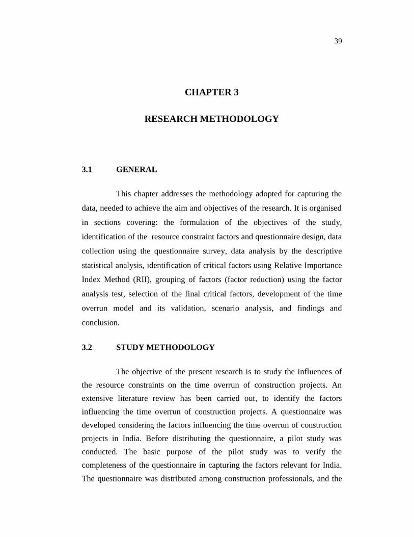
This chapter addresses the methodology adopted for capturing the
data, needed to achieve the aim and objectives of the research. It is organised
in sections covering: the formulation of the objectives of the study,
identification of the resource constraint factors and questionnaire design, data
collection using the questionnaire survey, data analysis by the descriptive
statistical analysis, identification of critical factors using Relative Importance
Index Method (RII), grouping of factors (factor reduction) using the factor
analysis test, selection of the final critical factors, development of the time
overrun model and its validation, scenario analysis, and findings and
conclusion.
3.2 STUDY METHODOLOGY
The objective of the present research is to study the influences of the resource constraints on the time overrun of construction projects. An extensive literature review has been carried out, to identify the factors influencing the time overrun of construction projects. A questionnaire was developed considering the factors influencing the time overrun of construction projects in India. Before distributing the questionnaire, a pilot study was conducted. The basic purpose of the pilot study was to verify the completeness of the questionnaire in capturing the factors relevant for India. The questionnaire was distributed among construction professionals, and the
40
data was collected. The data collected was analysed, using statistical methods, such as the descriptive statistics analysis, relative importance index analysis, Spearman rank order correlation test and factor analysis. Using the factor reduction technique, five factors were extracted out of the thirty three resource constraint factors originally considered. After the factor reduction, an equation for estimating the time overrun of construction projects was developed using structural equation modeling method. A scenario analysis was conducted, and finally the findings and conclusions are presented.
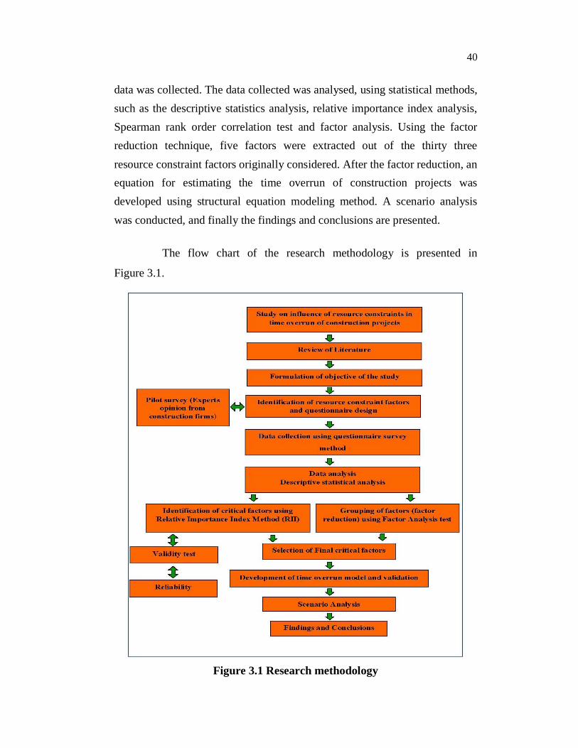
The flow chart of the research methodology is presented in
Figure 3.1.
Figure 3.1 Research methodology

41
3.2.1 Concerning Objective One: (To Identify the Factors Affecting
the Time Overrun of Construction Projects)
The literature about time overrun was reviewed (Frimpong et al
2003; Koushki et al 2005; Ogunsemi & Jagboro 2006; Fong et al 2006; Lo et al
2006; Assaf & AL-Hejji 2006; Sambasivan & Soon 2007; Alghbari et al 2007) to
identify the factors influencing the time overrun of construction projects. In
addition, there are other local factors that have been added, as recommended
by local experts.
33 factors influencing the time overrun of construction projects are
selected. These factors are grouped under four heads, namely, man power,
material, equipment and finance. Each factor is given a label. Manpower is
represented by MP, material by MA, equipment by EQ and finance by FI. Out
of the thirty three factors considered, 11 factors are man power related, 10
factors are material related, 7 factors are equipment related and 5 factors are
finance related. The factors which are considered in the questionnaire are
summarized and presented in Table 3.1.
Table 3.1 List of factors identified, grouped under four heads
Group Label of
each factor
Factors
Man Power
MP 01 Shortage of labour MP 02 Lack of skilled labour MP 03 Migrant labour MP 04 Labour injuries, disputes and strikes MP 05 Unqualified work force team MP 06 Personal conflicts among labour MP 07 Obtaining permits for migrant labour MP 08 Motivation MP 09 Communication MP 10 Mobilization MP 11 Absenteeism of labour
42
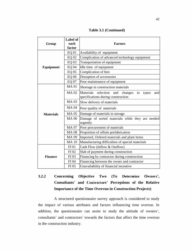
Table 3.1 (Continued)
Group Label of
each factor
Factors
Equipment
EQ 01 Availability of equipment EQ 02 Complication of advanced technology equipment EQ 03 Transportation of equipment EQ 04 Idle time of equipment EQ 05 Complication of hire EQ 06 Disruption of accessories EQ 07 Poor maintenance of equipment
Materials
MA 01 Shortage in construction materials MA 02 Materials selection and changes in types and
specifications during construction MA 03 Slow delivery of materials MA 04 Poor quality of materials MA 05 Damage of materials in storage MA 06 Damage of sorted materials while they are needed
urgently MA 07 Poor procurement of materials MA 08 Proportion of offsite prefabrication MA 09 Imported, Ordered materials and plant items MA 10 Manufacturing difficulties of special materials
Finance
FI 01 Cash Flow (Inflow & Outflow) FI 02 Slab of payment during construction FI 03 Financing by contractor during construction FI 04 Financing between the owner and contractor FI 05 Unavailability of financial incentive
3.2.2 Concerning Objective Two (To , Consultants and erceptions of the Relative Importance of the Time Overrun in Construction Projects)
A structured questionnaire survey approach is considered to study the impact of various attributes and factors influencing time overrun. In addition, the questionnaire can assist to study the attitude of owners , consultants and contractors towards the factors that affect the time overrun in the construction industry.
43
The relative importance index method (RII) is used here to
determine the owners , consultants and contractors perceptions of the
relative importance of the factors influencing time overrun in Indian
construction projects. The relative importance index is computed, as
presented in Section 3.4.1.
3.2.3 Concerning objective three (To identify the most significant
factors causing time overrun of construction projects)
The relative importance index method (RII) is also used to
determine the most significant factors influencing the time overrun of
construction projects in India.
The factor analysis is employed to establish which of the variables
could be the measuring aspects of the same underlying dimensions. Based on
the factor analysis, the thirty three factors identified as the most significant
factors influencing the time overrun of construction projects in India are
clustered under five components, and the details regarding the factor analysis
are presented in Section 3.5.
3.2.4 Concerning Objective Four (To Evaluate the Degree of
Agreement/Disagreement between , and
the Ranking of the Factors causing
Time Overrun of Construction Projects)
The degree of agreement between parties regarding the ranking of
factors is determined, according to the Spearman rank correlation
Coefficient. The degree of agreement is determined, as presented in Section
3.4.3.
44
3.2.5 Concerning Objective Five (To Test the Hypothesis to Verify
the Association between the Ranking of the ,
and
Overrun)
To test the hypothesis that there is no significant difference of
opinion between the three parties, regarding factors influencing time overrun.
The Spearman rank correlation coefficient is used according to two
hypotheses. This hypotheses are (Sambasivan & Soon 2007):
Null Hypothesis: H0: There is insignificant degree of agreement
among the owners, contractors and consultants.
Alternative Hypothesis: H1: There is significant degree of
agreement among the owners, contractors and consultants.
3.2.6 Concerning Objective Six (To Develop a Model to Depict the
Relationship between Resource Constraints and Time Overrun)
Structural Equation modeling (SEM) is adopted to analyse the
factors influencing the time overrun of construction projects. The SEM
method is suitable for exploring relationships among the variables. In this
study, a component based analysis is used, as it is more advisable when the
causal relation (Hair et al 2011) is studied. A model is developed to depict the
relationship between the influential resource constraint factors and the time
overrun. A case study for the validation of the proposed model is presented in
Section 6.9.
45
3.2.7 Concerning Objective Seven (To Formulate the
Recommendations to Reduce the Time Overrun of
Construction Projects so as to Improve the Performance of
Construction Projects)
The practices concerning the time overrun such as time, cost,
project owner satisfaction and the safety checklists are analyzed, in order to
know the main practical problems of projects time overrun in India and, then
to formulate the recommendations to reduce the time overrun of construction
projects in India.
3.3 DATA COLLECTION
3.3.1 Questionnaire Design
A questionnaire was developed to assess the perception of clients,
consultants, and contractors on the relative importance of factors influencing
the time overrun of construction projects in India. The questionnaire was
divided into two parts. The first part consisted of general information about
the respondent. The second part of the questionnaire focused on the resource
constraint factors, causing the time overrun of construction projects in India.
3.3.2 Data Measurement
In order to be able to select the appropriate method of analysis, the
level of measurement must be understood. For each type of measurement,
there is/are an appropriate method/s that can be applied, and not others. In this
research, ordinal scales were used. The ordinal scale, as shown in Table 3.5, is
a ranking or a rating scale, that normally uses integers in the ascending or
descending order. The numbers assigned as important (1, 2, 3, 4, 5) do not
indicate that the interval between scales are equal, nor do they indicate
46
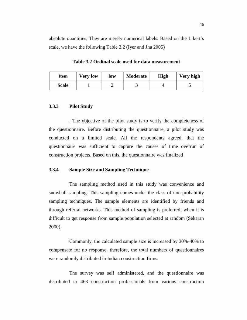
absolute quantities. They are merely numerical labels. Based on the Likert
scale, we have the following Table 3.2 (Iyer and Jha 2005)
Table 3.2 Ordinal scale used for data measurement
Item Very low low Moderate High Very high
Scale 1 2 3 4 5
3.3.3 Pilot Study
. The objective of the pilot study is to verify the completeness of
the questionnaire. Before distributing the questionnaire, a pilot study was
conducted on a limited scale. All the respondents agreed, that the
questionnaire was sufficient to capture the causes of time overrun of
construction projects. Based on this, the questionnaire was finalized
3.3.4 Sample Size and Sampling Technique
The sampling method used in this study was convenience and
snowball sampling. This sampling comes under the class of non-probability
sampling techniques. The sample elements are identified by friends and
through referral networks. This method of sampling is preferred, when it is
difficult to get response from sample population selected at random (Sekaran
2000).
Commonly, the calculated sample size is increased by 30%-40% to
compensate for no response, therefore, the total numbers of questionnaires
were randomly distributed in Indian construction firms.
The survey was self administered, and the questionnaire was
distributed to 463 construction professionals from various construction
47
organizations in India. Before handing over the questionnaires, all the
questions were explained to the respondents, so that they could fill the
questionnaire easily and properly. The responses were collected and analyzed.
Out of 463 copies of the questionnaire distributed to respondents 155 were
retrieved and analyzed.
3.3.5 Descriptive Statistics
The questionnaire was distributed to 463 construction
professionals, out of which 155 responses were received and thus, the
response rate of 33 details of the samples,
like gender, designation, working experience, types of organization, project
annual turnover and types of projects are explained using descriptive statistics
in Chapter 4.
3.4 STATISTICAL METHODS OF ANALYSIS
The statistical methods of analysis employed in this study other
than descriptive statistics, are the relative importance index analysis,
Spearman rank order correlation test, factor analysis, and multi - variate
analysis.
3.4.1 Relative Importance Index (RII) Method
The relative importance index method is used to determine the
relative importance of the various causes of time overrun. The same method
was adopted in this study within various groups (i.e. clients , consultants or
contractors ). The five-point scale ranging from 1 (not important) to 5
(extremely important) was adopted, and transformed to relative importance
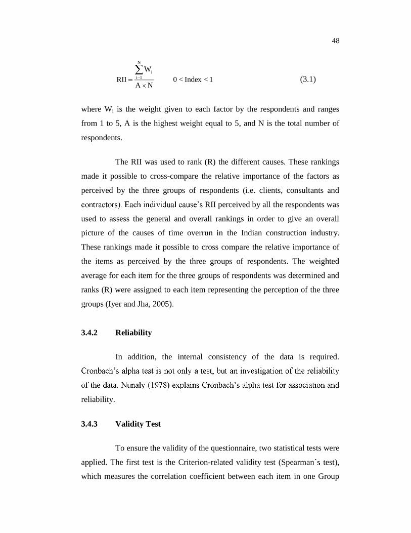
indices (RII) for each factor as follows:
48
1<Index <0
NA
WRII
N
1ii
(3.1)
where Wi is the weight given to each factor by the respondents and ranges
from 1 to 5, A is the highest weight equal to 5, and N is the total number of
respondents.
The RII was used to rank (R) the different causes. These rankings
made it possible to cross-compare the relative importance of the factors as
perceived by the three groups of respondents (i.e. clients, consultants and
RII perceived by all the respondents was
used to assess the general and overall rankings in order to give an overall
picture of the causes of time overrun in the Indian construction industry.
These rankings made it possible to cross compare the relative importance of
the items as perceived by the three groups of respondents. The weighted
average for each item for the three groups of respondents was determined and
ranks (R) were assigned to each item representing the perception of the three
groups (Iyer and Jha, 2005).
3.4.2 Reliability
In addition, the internal consistency of the data is required.
reliability.
3.4.3 Validity Test
To ensure the validity of the questionnaire, two statistical tests were
applied. The first test is the Criterion-related validity test (Spearman test),
which measures the correlation coefficient between each item in one Group
49
and the whole Group. To test the criterion related validity test, the correlation
coefficient for each item of the group factors and the total of the field, is
achieved. The significance (p-values) are less than 0.01, and the correlation
; therefore, it can be said
that the paragraphs of each field are consistent and valid to measure what it
was set for. The second test is the structure validity test (Spearman test) that
was used to test the validity of the questionnaire structure, by testing the
validity of each field and the validity of the whole questionnaire. It measures
the correlation coefficient between one field and all the fields of the
questionnaire that have the same level of a similar scale.
3.5 FACTOR ANALYSIS
In the absence of any standard lists of selection factors, there was a
considerable risk of the analysis of the responses yielding diverse results.
Thus, in establishing the list of factors, it was considered important to ensure
that the factors are of adequate relevance, and were also independent. The
response were therefore further analysed, by grouping them using the factor
analysis.
The appropriateness of employing the factor analysis was first
confirmed by a number of tests including Kaiser-Meyer-Olkin (KMO), the
measure of sampling adequacy and Bartlett test of sphericity. The principal
component analysis was then employed to extract the group factors with
eigenvalues greater than 1, suppressing all other factors with eigenvalues less
than 1,
clarify the factor pattern so as to ensure that each variable loads high on one
group factor, and very minimal on all other group factors, the variables were
the varimax orthogonal rotation method.
50
3.5.1 Kaiser Meyer Olkin (KMO) Test and Bartlett's Test of
Sphericity
The KMO statistic varies between 0 and 1. A value of 0 indicates
that the sum of partial correlations is large, relative to the sum of correlations,
indicating diffusion in the pattern of correlations (hence, the factor analysis is
likely to be inappropriate). A value close to 1 indicates that patterns of
correlations are relatively compact, and so, the factor analysis should yield
distinct and reliable factors. Kaiser (1974) recommended values greater than
0.5 as acceptable. Furthermore, values between 0.5 and 0.7 are medium,
values between 0.7 and 0.8 are good, values between 0.8 and 0.9 are very
good, and values greater than 0.9 are excellent. For these data, the values are
greater than 0.9, which falls in the range of being excellent; so it should be
clear that the factor analysis is appropriate for these data.
correlation matrix is an identity matrix. For the factor analysis to work, it
needs some relationship between the variables and if the R- matrix, were an
identity matrix then all correlation coefficients would be zero. So this test has
to be significant (Significance value less than 0.05). A significant test
identifies that the R-matrix is not an identity matrix; therefore, there are some
relations <
0.001), and the factor analysis is appropriate.
3.5.2 Communalities
Communalities indicate the amount of variance in each variable
that is accounted for. The initial communalities are estimates of the variance
in each variable accounted for by all the components or factors. Extraction
communalities are estimates of the variance in each variable, accounted for by
the factors (or components) in the factor solution. Small values (< 0.4)
51
indicate variables that do not fit well with the factor solution, and should
possibly be dropped from the analysis.
3.5.3 Extraction of Factors
The total number of common factors that can be extracted from any
factor analysis is equal to or less than the number of variables involved. The
important factors are those whose Eigen values are greater than or equal to 1,
because an Eigen value is a measure of how a standard variable contributes to
the principal components. A component with an Eigen value of less than 1 is
considered less important than such an observed variable, and can be ignored
(Kim and Mueller 1994).
3.5.4 Rotated Component Matrix
Rotation is a method used to simplify the interpretation of a factor
analysis. The rotated component matrix is a matrix of the loading for each
variable onto each factor.
3.6 DEVELOPMENT OF MODEL FOR TIME OVERRUN
After the factor analysis is carried out the structural equation
modelling is done for time overrun. Hence, the SEM model is the prediction
of the complicated process that has been attempted to be modelled. SEM is a
collection of statistical techniques that allows a set of relations between one or
more Independent Variables (IVs), either continuous or discrete, and one or
more Dependent Variables (DVs), either continuous or discrete, to be
examined. Both IVs and DVs can be either measured variables (directly
observed), or latent variables (unobserved, not directly observed). SEM is
also referred to as causal modeling, causal analysis, simultaneous equation
modeling, and analysis of covariance structures, path analysis, or
52
confirmatory factor analysis (Kline 1998; Mueller 1996). Structural Equation
Modeling (SEM) is superior to other methods, since it combines a
measurement model (confirmatory factor analysis), and a structural model
(regression or path analysis) in a single statistical test. It recognizes the
measurement error, and also offers an alternative method for measuring the
prime variables of interest through the inclusions of the latent variables and
surrogate variables. The major aim of these models was to fit and cover the
relevant research characteristics such as time overrun, in the resource
schedule performance measures and indicators in this research.
3.6.1 Limitations of the Structural Equation Model
The models are constructed for fitting the sample covariance
instead of the sample values themselves. This leads to the elimination of
much valuable information about the data, such as the means, skewness and
kurtosis. Yet, sample covariance is only one of the many characteristics of the
data, and is not sufficient enough to understand the total structure of the data.
Since the results of SEM are subject to sampling or selection
effects, with respect to at least three aspects of a study, viz, individuals,
measures, and occasions, the generalizability of the findings is also a
limitation of SEM. Researchers should specify the population of interest in
their hypothesis, and acknowledge that the conclusions derived from the
model cannot be generalized, except for that population. The indicators which
represent the latent variables should be chosen very carefully, because the
nature of the construct can shift with the choice of indicators, which in turn,
can influence the results and their interpretation. The findings can show
changes over time; therefore, the effect of one variable on another cannot be
identified as a single true effect, unless the variables do not change over any
time period of interest.
53
Another important limitation is the necessity of large sample sizes,
in order to maintain power and obtain stable parameter estimates and standard
errors. Some methods are developed for parameter estimation of small sample
size, after all estimates settle down at the smallest sample sizes, whereas
standard errors are determined still according to a larger number of samples
(Bentler 2006). A chi-square test which is the most common fit measure is
only recommended with moderate samples; in addition, coefficient alpha, the
most common measure of reliability, has several limitations; for instance,
coefficient alpha wrongly assumes that all items contribute equally to
reliability.
3.6.2 Model Specification
Model specification involves using all of the available relevant
theory, research, and information, and developing a theoretical model. Thus,
prior to any data collection or analysis, the researcher specifies a specific
model that should be confirmed with the variance and covariance data. In
other words, the available information is used to decide which variables to
include in the theoretical model, and how these variables are related
(Schumacker & Lomax 2004).
3.6.3 Model Identification
Identification refers to the amount of information available in the
covariance matrix, relative to the number of parameters that a researcher
extracts from these data.
The parameters in a model can be specified either as free, fixed, or
constraint. A free parameter is one that is unknown, and therefore needs to be
estimated. A fixed parameter is one that is not free, but is fixed to a specified
value, typically 0 or 1. A constraint parameter is one that is unknown, but is
54
constrained to equal one or other parameters (Schumacker & Lomax 2004). In
addition, model identification depends on the designation of parameters as
fixed, free, or constraint, due to its effect on the number of parameters that
require to be identified.
The aim of SEM is to specify a model as over identified; therefore,
the model has positive degrees of freedom that allow the testing/confirming
the validity of the model.
3.6.4 Model Estimation
observed population covariance matrix, sample covariance matrix (S), with
the residual matrix (the difference between
equal zero, 2 = 0; it means that it is a perfect model fit to the data. There
are different methods available for the estimation of the model; however, the
widely used models are the maximum likelihood (ML), generalized least
squares (GLS), least squares (LS), asymptotic distribution free (ADF), and
robust.
Maximum Likelihood (ML): is the most popular method among all
estimation methods, because it provides unbiased, consistent estimates of
population parameters; in addition, admissible model solutions and stable
parameter estimates can be obtained, in the case of small sample sizes. ML
methods are scale free, which means that the output of this method obtained
by the transformation of the scale of one or more of the observed variables,
and the output of the untransformed output are related (Schumacker & Lomax
2004). However, ML assumes multivariate normality, and non-normality in
the data can potentially lead to seriously misleading results. Nonetheless, ML
55
is also determined as quite robust against the mild violation of the normality
assumption (Bentler 1995).
Generalized Least Squares (GLS): GLS is an adaptation of least squares to
minimize the sum of the differences between the observed and predicted
covariance. It is probably the second-most common estimation method after
ML. GLS assumes multivariate normality like ML. The GLS estimation
process requires much less computation than ML; however, this should not be
accepted as an advantage, due to the powerful desktop computers with well-
constructed SEM programs. Olsson et al (2000) evaluated the parameter
estimates and overall fit of ML and GLS under different model conditions,
including non-normality, and concluded that ML could provide more realistic
indices of the overall fit and less biased parameter estimates for paths, than
the GLS under different misspecifications. In addition, ML performs better
for small samples; therefore, ML should generally be preferred for small
samples.
Asymptotic Distribution Free (ADF): Unlike the other methods, this
method does not require the multivariate normality assumption.
Unfortunately, this method is data-intensive; in other words, this methodology
requires really large sample sizes, to obtain model convergence and stable
parameter estimates. However, Yuan & Bentler (1997) found out that ML is
much less biased than ADF estimators for all distributions and sample sizes,
but when the sample size is large, ADF can compete with ML.
Robust: The strength of this method is that normality is not a requirement. In
this method, the estimates provided from the methods are accepted, but the
chi-square and standard errors are corrected to the non-normality situation.
The chi-square test is corrected in the conceptual way described by
Bentler (1996). Also, robust standard errors developed by Bentler (1996) are
provided as an output of the robust analysis, and they are correct in large
56
samples, even if the distributional assumption regarding the variables is
wrong (Bentler 2006). Although these robust statistics are computationally
demanding, they have been shown to perform better than the uncorrected
statistics, where the assumption of normality fails to hold and performs better
than the ADF. One important caveat regarding the use of robust statistics is
that, they can be computed only from raw data (Byrne 2006).
3.6.5 Model Testing
After the determination of the parameter estimates for a specified
SEM model, the model should be examined to see how well the data fit the
data; in other words, how well the theoretical model is supported by the
obtained sample data should be determined. Different fit indices are
developed for that purpose, namely, the chi-square, Normed Fit Indices
(NFI), Non-Normed Fit Indices (NNFI), Comparative Fit Indices (CFI),
Bollen Fit Indices (IFI), McDonald fit indices (MFI), Goodness of fit indices
(GFI) and Root Mean-Square Error of Approximation (RMSEA).
3.6.6 Model Fit Indices
In order to evaluate the model fit, model fit indices are used. There
are dozens of model fit indices described in the SEM literature, and new
indices are being developed all the time. It is up to the properties of the data
to decide, as to which particular indices and which values to report (Kenny &
McCoach 2003; Marsh et al 2004). Described next is a minimal set of fit
indices that is going to be reported and interpreted, when reporting the results
of SEM analysis of this research. The fit indices that are least affected by the
sample size were selected. These statistics include (1) Chi-square; (2) the root
mean square error of approximation (RMSEA; Steiger 1990) with its 90%
confidence level; (3) Comparative fit index (CFI; Bentler 1990); (4) Non-
Normed Fit Index (NNFI); and (5) Bollen Fit Indices (IFI).
57
3.6.7 2)
The value of 2 for a just identified model generally equals zero and
has no degrees of freedom. If 2= 0, the model perfectly fits the data. As the
value of 2 increases, the fit of an over identified model becomes increasingly
worse. The only parameter of a central Chi-square distribution is its degrees
of freedom (Kline 2005).
3.6.8 Normed Fit Indices
The NFI indicate the proportion in the improvement of the overall
fit of the developed model to a null model. The NFI range from zero to one
with higher values indicating a better fit; however, in small samples, it may
not reach 1.0 when the model is correct (Bentler 2006). A rule of thumb for
this index is that, 0.95 is indicative of a good fit relative to the baseline model,
while values greater than 0.90 may be interpreted as an acceptable fit
(Schermelleh-Engel et al 2003). The most important disadvantage of this
index is that, it is affected by sample size.
3.6.9 Non-Normed Fit Indices
NNFI is also known as Tucker-Lewis index (Bentler 2006). NNFI
generally ranges from zero to one, with higher values indicating a better fit;
but, since this index is not normed, values can fall outside the range 0-1. This
index is also affected by the complexity of the model; in other words, by
increasing the complexity of the model, the values of this index decrease. The
most important advantage of this index is that, it is one of the fit indices less
affected by the sample size (Bentler 1990).

58
3.6.10 Comparative Fit Indices
The CFI is one of a class of fit statistics, known as incremental or
comparative fit indices, which are among the most widely used in SEM. All
these indices assess the relative improvement in the
model compared with a baseline model. It is developed by Bentler (1990) for
avoiding the underestimation of fit in small samples. CFI is derived from the
comparison between the hypothesized and the independent models. The CFI
ranges from zero to one, with higher values indicating a better fit. A rule of
thumb for this index is that 0.95 is indicative of a good fit, relative to the
independence model, while values greater than 0.90 may be interpreted as an
acceptable fit (Byrne 2006).
3.6.11 Bollen Fit Indices
It is developed to address the issues related to parsimony and
sample size. IFI is computed basically by using the same procedure as that of
NFI, except that degrees of freedom are considered (Byrne 2006). A rule of
thumb for this index is that 0.95 is indicative of a good fit relative to the
independence model, while values greater than 0.90 may be interpreted as an
acceptable fit (Meehan and Stuart 2007).
3.6.12 Goodness of Fit Indices (GFI):
GFI is the measure of how much better the model fits, as compared
to the null model (Schermelleh-Engel et al 2003). The GFI ranges from zero
to one with higher values indicating a better fit, but in some cases the values
of GFI can fall outside the range 0-1. A rule of thumb for this index is that
0.95 is indicative of a good fit relative to baseline model, while values greater
59
than 0.90 may be interpreted as an acceptable fit (Schermelleh- Engel et al
2003).
3.6.13 Root Mean-Square Error of Approximation
The RMSEA is a parsimony-adjusted index, in that its formula
includes a built-in correction for model complexity. The RMSEA measures
the error of approximation. The value of zero indicates the best fit, and higher
values indicate a worse fit. The RMSEA estimates the amount of error of
approximation per model degree of freedom, and takes the sample size into
a close approximate
fit, values between 0.05 and 0.08 suggest reasonable error of approximation,
a poor fit (Browne & Cudeck 1993); this can be
provided by utilizing interpretative guidelines (Hu & Bentler 1999; Hu &
Bentler 1998); finally and most importantly, a confidence level is obtained as
an output. RMSEA values smaller than 0.05 indicate a good fit, values
between 0.05 and 0.08 indicate an adequate fit, and values between 0.08 and
0.10 indicate a mediocre fit, whereas values larger than 0.10 indicate that the
model should not be accepted (Schermelleh-Engel et al 2003). However,
when the sample size is small, this index tends to over-reject the true
population models (Hu & Bentler 1999).
3.6.14 Normality
Most of the estimation methods assume normal distributions for
continuous variables. Non-normal data can occur because of the scaling of
variables or limited sampling of subjects, and the normality can be on two
levels; univariate and multivariate normality. Univariate normality concerns
the distribution of the individual variables. The normality of a variable can be
evaluated according to the standard error of skewness and kurtosis. The
standard error of skewness is calculated by the ratio of skewness to its
60
standard error; values of standard error of skewness between -2 and 2 indicate
the normality of the variable. A large positive value of skewness indicates a
long right tail; an extreme negative.
3.7 SCENARIO ANALYSIS
The s
is to changes in the value of the parameters of the model and to changes in the
structure of the model. Scenario analyses focus on the variation impact between
two parameters. Parameter sensitivity is usually performed as a series of tests in
which the modeler sets different parameter values, to see how a change in the
parameter causes a change in the dynamic behavior of the time overrun. By
showing how the model behavior responds to changes in parameter values, the
scenario analysis is a useful tool in model building as well as in model
evaluation.
3.8 SUMMARY
An outline of the research methodology adopted for carrying out this
research is presented in this chapter.