ProQuest Dissertations - Rice Scholarship Home

RICE UNIVERSITY

Molecular Modeling the Microstructure and Phase Behavior of Bulk and Inhomogeneous Complex Fluids

By

ADAM BYMASTER

A THESIS SUBMITTED IN PARTIAL FULFILLMENT OF THE REQUIREMENTS FOR THE DEGREE

DOCTOR OF PHILOSOPHY

APPROVED, THESIS COMMITTEE

Dr. Walter G. Chapman, Chair William W. Akers Professor

Chemical and Biomolecular Engineering

'** / /**?*+'* 4**-

Dr. George J. Hirasaki A. J. Hartsook Professor

Chemical and Biomolecular Engineering

Dr. Enrique V. Barrera Professor

Mechanical Engineering and Materials Science

HOUSTON, TEXAS

APRIL 2009

UMI Number: 3362135

Copyright 2009 by Bymaster, Adam

INFORMATION TO USERS

The quality of this reproduction is dependent upon the quality of the copy

submitted. Broken or indistinct print, colored or poor quality illustrations

and photographs, print bleed-through, substandard margins, and improper

alignment can adversely affect reproduction.

In the unlikely event that the author did not send a complete manuscript

and there are missing pages, these will be noted. Also, if unauthorized

copyright material had to be removed, a note will indicate the deletion.

®

UMI UMI Microform 3362135

Copyright 2009 by ProQuest LLC All rights reserved. This microform edition is protected against

unauthorized copying under Title 17, United States Code.

ProQuest LLC 789 East Eisenhower Parkway

P.O. Box 1346 Ann Arbor, Ml 48106-1346

Copyright

Adam Bymaster

2009

To Kristen

Abstract

Molecular Modeling the Microstructure and Phase Behavior of

Bulk and Inhomogeneous Complex Fluids

By

Adam Bymaster

Accurate prediction of the thermodynamics and microstructure of complex fluids is

contingent upon a model's ability to capture the molecular architecture and the specific

intermolecular and intramolecular interactions that govern fluid behavior. This

dissertation makes key contributions to improving the understanding and molecular

modeling of complex bulk and inhomogeneous fluids, with an emphasis on associating

and macromolecular molecules (water, hydrocarbons, polymers, surfactants, and

colloids). Such developments apply broadly to fields ranging from biology and medicine,

to high performance soft materials and energy.

In the bulk, the perturbed-chain statistical associating fluid theory (PC-SAFT), an

equation of state based on Wertheim's thermodynamic perturbation theory (TPT1), is

extended to include a crossover correction that significantly improves the predicted phase

behavior in the critical region. In addition, PC-SAFT is used to investigate the vapor-

liquid equilibrium of sour gas mixtures, to improve the understanding of

mercaptan/sulfide removal via gas treating.

For inhomogeneous fluids, a density functional theory (DFT) based on TPT1 is

extended to problems that exhibit radially symmetric inhomogeneities. First, the

influence of model solutes on the structure and interfacial properties of water are

investigated. The DFT successfully describes the hydrophobic phenomena on

microscopic and macroscopic length scales, capturing structural changes as a function of

solute size and temperature.

The DFT is used to investigate the structure and effective forces in nonadsorbing

polymer-colloid mixtures. A comprehensive study is conducted characterizing the role of

polymer concentration and particle/polymer size ratio on the structure, polymer induced

depletion forces, and tendency towards colloidal aggregation.

The inhomogeneous form of the association functional is used, for the first time, to

extend the DFT to associating polymer systems, applicable to any association scheme.

Theoretical results elucidate how reversible bonding governs the structure of a fluid near

a surface and in confined environments, the molecular connectivity (formation of

supramolecules, star polymers, etc.) and the phase behavior of the system.

Finally, the DFT is extended to predict the inter-and intramolecular correlation

functions of polymeric fluids. A theory capable of providing such local structure is

important to understanding how local chemistry, branching, and bond flexibility affect

the thermodynamic properties of polymers.

Acknowledgements

This dissertation was made possible through the support and contributions of many.

First and foremost, I thank God, for it is under His grace that we live, learn, and flourish.

He has blessed my life in more ways than I deserve.

I am grateful to Professor Walter Chapman, who, as my thesis advisor and mentor,

introduced me to the world of complex fluid behavior and statistical mechanics. I thank

him for his support and contributions to this work, as well as his direction throughout this

thesis, which exposed me to a wide variety of topics and sciences.

I thank Professor George Hirasaki and Professor Enrique Barrera for serving on my

thesis committee and for providing critical evaluation and input to this dissertation.

I thank Professor Ken Cox for sharing his valuable ideas, insight, and advice during

group discussions and presentations.

I wish to thank Scott Northrop and Tim Cullinane for their fruitful discussions and

guidance of the sour gas modeling. I would also like to thank ExxonMobil for granting

permission to publish my internship work in this thesis.

A number of professional contacts also provided helpful discussions. I gratefully

acknowledge Felix Llovell and Professor Lourdes Vega, as well as Professor Dong Fu for

their helpful discussions about modeling phase behavior in the critical region. I also wish

to thank Professor Hank Ashbaugh for his stimulating discussions about hydrophobic

hydration and Juan Carlos Araque for his insight into the behavior of polymer-particle

mixtures.

vi

To my research group, I am grateful for our friendship and for the experiences we

shared. I acknowledge Aleksandra Dominik and thank her for her patience in answering

all my questions about the theory early in my research. I am indebted to Shekhar Jain,

whose own work and ideas had great influence on this research. To Clint Aichele, who

turned out to be an alright cowboy, and an even better friend; I thank him for his

friendship and our discussions on research and life. In addition, I thank Francisco

Vargas, Chris Emborsky, and Zhengzheng Feng for their comments during our group

discussions.

Last, but not least, I would like to thank my family for their love and support over the

years. I especially wish to thank my parents, Mark and Telesa Bymaster, who have been

tremendous influences on my life and work ethic. To my wife Kristen, I dedicate this

thesis. I owe you much, not only for your love, encouragement, and sacrifices, but also

for making me a better person.

The financial support for this work was provided by the Robert A. Welch Foundation

(Grant No. CI241) and by the National Science Foundation (CBET-0756166). This work

was supported in part by the Shared University Grid at Rice funded by the NSF under

Grant EIA-0216467, and a partnership between Rice University, Sun Microsystems, and

Sigma Solutions, Inc.

Table of Contents

CHAPTER 1: Introduction 1

1.1 Motivation and challenges 1

1.1.1 Bulk fluids 3

1.1.2 Inhomogeneous fluids 5

1.2 Laying the ground work: Wertheim's TPT1 for associating fluids 8

1.3 Scope of the thesis 12

CHAPTER 2: Renormalization-group corrections to a perturbed chain statistical associating fluid theory for pure fluids near to and far from the critical region 15

2.1 Introduction 15

2.2 Background on renormalization-group methods 17

2.3 PC-SAFT outside the critical region 19

2.4 Recursive relations 23

2.5 Results and discussion 27

2.5.1 Applying RG theory to PC-SAFT 27

2.5.2 Reproducing Llovell et al.'s Soft-SAFT results 31

2.5.3 Reproducing Fu et al. 's PC-SAFT results 32

2.5.4 Improving PC-SAFT+RG 33

2.6 Conclusions 42

CHAPTER 3: A thermodynamic model for sour gas treating 44

3.1 Introduction and motivation 44

3.2 Theoretical model 48

3.2.1 Model selection 48

3.2.2 PC-SAFT for associating mixtures 50


3.3.1 Parameter fitting for the mercaptans and sulfides 54

3.3.2 Hydrocarbon/FliS binary mixtures 58

3.3.3 Hydrocarbon/sulfide binary mixtures 60

3.3.4 HiS/sulfide binary mixtures 63

3.3.5 Solvent/'sulfide binary mixtures 64

3.3.6 Multicomponent mixtures 67

viii

3.3.7 Mercaptan physical solubility versus mercaptan chemical solubility 69

3.4 Conclusions 71

3.5 Future work and recommendations 72

CHAPTER 4: Density functional theory 76

4.1 Introduction and background 76

4.2 A general density functional formalism 78

4.3 Approximations for the free energy functional 82

4.3.1 Atomic fluids 83

4.3.2 Polyatomic fluids 85

4.4 Notable density functional theories 86

4.4.1 Chandler, McCoy and Singer 86

4.4.2 Density junctionals based on TPT1 87

4.4.2.1 Kierlik and Rosinberg 88

4.4.2.2 Segura, Chapman and Shukla 89

4.4.2.3 Yu and Wu 92

4.4.2.4 Chapman and coworkers 95

CHAPTER 5: Hydration structure and interfacial properties of water near a hydrophobic solute from a fundamental measure density functional theory 101

5.1 Introduction 101

5.2 Theory 106

5.2.1 Model.. .106

5.2.2 Density functional theory 109


5.4 Conclusions 125

CHAPTER 6: Microstructure and depletion forces in polymer-colloid mixtures from an /SAFTDFT 128


6.2 iSAFT model 135

6.2.1 Free energy Junctionals 136

6.2.2 Free energy functional derivatives 140

6.2.3 Equilibrium density profile and grand free energy 141


ix

6.3.1 Local structure 143

6.3.2 Polymer mediated forces 150

6.3.3 Second virial coefficient 156

6.3.4 A preliminary study: Effect of attractive interactions 159

6.4 Conclusions 164

CHAPTER 7: An iSAFT density functional theory for associating polyatomic molecules 168


7.2 Theory 174

7.2.1 Model 174

7.2.2 iSAFT density functional theory 177

7.2.2.1 Free energy Junctionals 178

7.2.2.2 Free energy functional derivatives 181


7.3.1 Associating polymers near a wall 184

7.3.2 Self-assembly of associating polymers into inhomogeneous phases 188

7.4 Conclusions 195

CHAPTER 8: An iSAFT density functional theory for the intermolecular and intramolecular correlation functions of polymeric fluids 196


8.2 iSAFT model 199

8.2.1 Inter- and intramolecular correlation functions 199

8.2.2 Free energies 202

8.2.3 Free energy derivatives 202

8.2.4 Equilibrium density profiles 203


8.4 Conclusions 212

CHAPTER 9: Concluding remarks 213

£Q\ ex,assoc

APPENDIX A: Derivation of e / \ (For Chapter 7) 220

X

APPENDIX B: Solving for X\ ( r i ) (For Chapter 7) 227

References 229

List of Figures

Figure 1.1: Qualitative features of the microstructure of a fluid adsorbed at a surface at high density (blue) and low density (green) 5

Figure 1.2: Schematic of the association interaction potential model, in the framework of TPT1 8

Figure 1.3: Bonding constraints between two associating molecules in TPT1 9

Figure 2.1: (a) Temperature-density diagram for n-octane before modification of the perturbing potential function (L=2o and ^=18.75). (b) Pressure-temperature diagram for w-octane before modification of the perturbing potential function (L=2a and ^=18.75). Circles are experimental data,85 the solid line represents PC-SAFT+RG, and the dotted line is PC-SAFT 30

Figure 2.2: PC-SAFT crossover (RG) parameter dependence on molecular weight 36

Figure 2.3: (a) Temperature-density diagram for n-octane using the modified perturbing potential function, (b) Pressure-temperature diagram for n-octane using the modified perturbing potential function. Symbols and lines defined as in Figure 2.1 38

Figure 2.4: (a) Temperature-density diagram and (b) pressure-temperature diagram for select light n-alkanes (C3, C5, andC7) 39

Figure 2.5: Phase equilibria predictions for heavy n-alkanes (C20, C24, C36). The circles represent simulation data,93and critical points from experiments.86 40

Figure 2.6: (a) Critical temperatures and (b) critical pressures for n-alkanes, from C2 to C36 as predicted by PC-SAFT +RG (solid lines) and PC-SAFT (dashed lines). Symbols represent experimental critical points.86'88'91'92 40

Figure 2.7: In (a), calculation of fi critical exponent. The circles are calculated results and the solid line is a power fit used to determine /?. In (b), calculation of 3 critical exponent. The filled circles are calculated results below the critical density and the open circles are calculated results above the critical density. The solid line is a power fit used to determine S 41

Figure 3.1: Simplified schematic of the absorption/stripping process for removal of sour gas impurities 46

Figure 3.2: Temperature-density diagram for methane and the sulfide series. The pure component parameters were regressed to the saturated liquid densities of each component 55

Xll

Figure 3.3: Pressure-temperature diagram for methane and the sulfide series. The pure component parameters were regressed to the vapor pressures of each component 56

Figure 3.4: Pure component parameter trends for the sulfide series. Other compound families demonstrate similar trends with molecular weight 58

Figure 3.5: P-x diagram for alkane+E^S mixtures. Symbols are experimental data, lines represent predictions from the PC-SAFT model: (a) CH4+H2S mixture, where symbols are experimental data,126 ky=0.055, (b) C2H6+H2S mixture, where symbols are experimental data,127 ky=0.07, and (c) C3H8+H2S mixture, where symbols are experimental data,128 ky=0.08 59

Figure 3.6: P-x diagram for (a) CH4+MSH (methyl mercaptan) mixture, where symbols are experimental data ,13M33 lines represent predictions from the PC-SAFT model (kij=0.04), and (b) CHt+EtSH (ethyl mercaptan) mixture, where symbols are experimental data ,131133 lines represent predictions from the PC-SAFT model (kij=0.037) 61

Figure 3.7: P-x diagram for (a) CH4+DMS (dimethyl sulfide) mixture, where lines represent predictions from the PC-SAFT model (kjj=0.03), and (b) CH4+EMS (methylethyl sulfide) mixture where lines represent predictions from the PC-SAFT model (kij=0.035). Symbols represent experimental data.131"133 62

Figure 3.8: P-x diagram for (a) CfrHH+MSH (methyl mercaptan) mixture, where lines represent predictions from the PC-SAFT model (kij=0.035), and (b) C4Hio+PrSH (propyl mercaptan) mixture, where lines represent predictions from the PC-SAFT model (ky=0.025). Symbols represent experimental data.131"133 62

Figure 3.9: P-x diagram for (a) H2S+COS (carbonyl sulfide) mixture, where symbols are experimental data,1 1 , m lines represent predictions from the PC-SAFT model (ky=0.045), (b) H2S+DMS mixture, where symbols are experimental data,131'132 lines represent predictions from the PC-SAFT model (ky=-0.015), and (c) HfeS+EMS mixture, where symbols are experimental data,131'132 lines represent predictions from the PC-SAFT model (kij=0.00). The T-x-y diagram for the H2S+MSH mixture is shown in (d), where symbols are experimental data,134 and lines represent predictions from the PC-SAFT model (kij=0.06) 63

Figure 3.10: P-x diagram for (a) H2O+MSH mixture, where symbols represent experimental data ,13 and lines represent predictions from the PC-SAFT model (ky=-9.01157E-5*T(K) + 5.46720E-2), (b) H20+EtSH mixture, where symbols are experimental data,137 and lines represent predictions from the PC-SAFT model (ky=-6.66667E-5*T(K) - 6.54333E-3), (c) H20+ H2S mixture, where symbols are experimental data,138 and lines represent predictions from the PC-SAFT model (kjj=0.025), and (d) H2O+ MDEA mixture, where symbols are experimental data135

(correlated using Raoult's law), and lines represent predictions from the PC-SAFT model (kij=-0.055) 65

xiii

Figure 3.11: Effect of temperature and molecular weight of mercaptan on the Henry's constant. As HRSH increases, the solubility or pickup of mercaptan in the liquid solvent decreases. Symbols are experimental data137 taken over a range of pressures. For comparison, lines represent predictions from the PC-SAFT model at a total pressure of P=2.5bar 66

Figure 3.12: In (a), P-x diagram for MSH + H20+ MDEA mixture. The aqueous amine solution is 50 wt% MDEA. Symbols are experimental data,108"110 lines represent predictions from the PC-SAFT model. The binary interaction parameters for MSH/H2O and MDEA/H20 were the same as before for the binary systems. The binary interaction parameter for MSH/MDEA was determined to be ky=0.085. From (b), P-x diagram for MSH + H2O+ MDEA mixture. The mass percent of MDEA in the aqueous amine solution is varied from 0%, 35 wt%, 50wt%, 75wt%, respectively 67

Figure 3.13: Effect of temperature and molecular weight of mercaptan on the Henry's constant in the ternary mixture RSH-MDEA-H2O (no acid gas loading). The aqueous amine solution is 50 wt% MDEA. As HRSH increases, the solubility or pickup of mercaptan in the liquid solvent decreases. Symbols are experimental data,108" 10 lines represent predictions from the PC-SAFT model. The PC-SAFT predictions shown are at P=1.0bar 68

Figure 3.14: Effect of temperature and molecular weight of mercaptan on the Henry's constant in the mixture RSH-toluene. Opposite to the aqueous amine solutions, the solubility increases as the size of the mercaptans increase. The ky for MSH/toluene and EtSH/toluene were fit to experimental VLE data,137 and were determined to be ky=0.01 and 0.0025, respectively 70

Figure 3.15: Effect of temperature and solvent choice on the solubility of the mercaptan. The physical solvents (hexane and toluene) show considerably more RSH pickup when compared to pure water or the aqueous amine solution (50wt% MDEA). The ky value for MSH/hexane was determined by experimental VLE data,137 and determined to be ky=0.035 71

Figure 3.16: Effect of temperature and acid gas loading on the solubility of the mercaptan. Symbols are experimental data.1 8"110 74

Figure 4.1: Schematic of chain formation from a mixture of associating spheres 96

Figure 5.1: Water represented using the four site model (4[2,2]) accounts for the two electron lone pairs (e) and the two hydrogen sites (H1") of the water molecule 107

Figure 5.2: The association interaction potential model. From the theory, if molecule 1 is oriented within the constraints given in eq. (5.6) with respect to molecule 2, then a

xiv

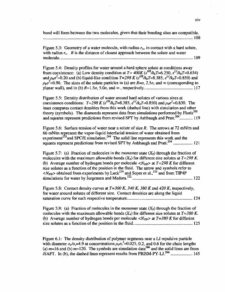
bond will form between the two molecules, given that their bonding sites are compatible. 108

Figure 5.3: Geometry of a water molecule, with radius rw, in contact with a hard solute, with radius rs. R is the distance of closest approach between the solute and water molecule 109

Figure 5.4: Density profiles for water around a hard sphere solute at conditions away from coexistence: (a) Low density condition at T= 400K (eHB/kbT=6.250, eu/kbT=0.634) and/W=0.20 and (b) liquid-like condition T=298 K (ePB/kbT=S.3S5, eu/kbT=0.S50) and pba

3=0.90. The sizes of the solute particles in (a) are R=o, 2.5<r, and oo (corresponding to planar wall), and in (b) i?=1.5<r, 5.0<r, and co , respectively 117

Figure 5.5: Density distribution of water around hard solutes of various sizes at coexistence conditions: T=298 K (ew%J=8.385, eu/kbT=O.S50) and/W=0.830. The inset compares contact densities from this work (dashed line) with simulation and other theory (symbols). The diamonds represent data from simulations performed by Floris205

and squares represent predictions from revised SPT by Ashbaugh and Pratt.204..... 119

Figure 5.6: Surface tension of water near a solute of size R. The arrows at 72 mN/m and 66 mN/m represent the vapor-liquid interfacial tension of water obtained from experiment and SPC/E simulation.244 The solid line represents this work and the squares represent predictions from revised SPT by Ashbaugh and Pratt.204 121

Figure 5.7: (a) Fraction of molecules in the monomer state (Xo) through the fraction of molecules with the maximum allowable bonds (X4) for different size solutes at T=298 K. (b) Average number of hydrogen bonds per molecule <NHB> at T=298 K for different size solutes as a function of the position in the fluid. The arrow and symbols refer to <NHB> obtained from experiments by Luck234 and Soper et al.,235 and from TIP4P simulationsi forwater by Jorgensen and Madura.222 122

Figure 5.8: Contact density curves at T=300 K, 340 K, 380 K and 420 K, respectively, for water around solutes of different size. Contact densities are along the liquid saturation curve for each respective temperature 124

Figure 5.9: (a) Fraction of molecules in the monomer state (Xo) through the fraction of molecules with the maximum allowable bonds (X4) for different size solutes at T=380 K. (b) Average number of hydrogen bonds per molecule <NHB> at T=380 K for different size solutes as a function of the position in the fluid 125

Figure 6.1: The density distribution of polymer segments near a LJ repulsive particle with diameter aJa^=A.9 at concentrations pbas =0.025, 0.2, and 0.6 for the chain lengths (a) m=16 and (b) m=120. The symbols are simulation data266 and the solid lines are from iSAFT. In (b), the dashed lines represent results from PPJSM-PY-LJ.266 145

XV

Figure 6.2: The fraction of end segment density to middle segment density (fe(r)) normalized to the bulk value (fe,buik) as a function of distance from the surface of a LJ repulsive colloidal particle (<7</cr,s=4.9). Results are presented for the case of m=16 at densities pi,os

3=0.025 and 0.6. In the inset, the normalized contact fraction is plotted as a function of chain length (m=16 and m=120) and density. The symbols are simulation results266 and the solid lines are from /SAFT 147

Figure 6.3: The density distribution of polymer segments near isolated hard particles of size ac/(Ts=5,15, and oo are shown and represented by solid, dashed, and dotted lines, respectively. In all panels the chain length of m=1000 is used. The concentrations are (a) pbas

3=0.00l, (b)/>6or/=0.1, and (c) pba3=Q.5, respectively 149

Figure 6.4: Depletion forces between two interacting particles of size (ac/as=5) as a function of colloidal separation. Solid lines denote i'S AFT results and symbols denote simulation data.269 Results are presented forpbOs

3=Q.\ and m=30 (a),pb<Js3=0.225 and

m=20 (o), and/)fc<r/=0.3 and m=l0 (0). The inset shows the corresponding potential of mean force (PMF) 152

Figure 6.5: Effect of concentration on (a) the potential of mean force (PMF) between two interacting particles (<7</<7j=4.9; m=16), and (b) the depletion force between two interacting particles (<TC/<TS=5; m=20). In (a), solid lines represent the /SAFT predictions and symbols denote MC simulations.265 The particle-polymer interaction is modeled via a LJ repulsive potential, consistent with the simulation data. The concentration is varied pbas

3=0.1(n), 0.2(0), and 0.3(o). In (b), solid lines represent the iSAFT predictions and symbols denote MC simulations.269 All nonbonded interactions are of hard-sphere type, consistent with the simulation data. The concentration is varied: pbas

3=0.225 (•), 0.3 (o), and 0.45 (0). The inset shows the corresponding PMF 153

Figure 6.6: Effect of (a) chain length and (b) colloid/segment size ratio (oi/oi) on the depletion forces between two interacting particles. In (a), interacting particles are of size (p(/os=5). The bulk segment density is pbas

3=03 and the chain length of the polymer chain is varied: m=\, 4, 10, and 100, respectively, from bottom to top at contact. In (b), the bulk segment density is pbas

3=Q.?> and the chain length of the polymer chain is m=50. The size ratio is varied: a,/(Ts=2.5, 5, and 10, respectively. The corresponding PMFs are shown in each inset 155

Figure 6.7: Second-virial coefficient as a function of bulk density ipb^s) for different chain lengths. iSAFT predictions are represented by the solid lines; the thin red solid line represents the case ajas =5, m=20 while the thick solid lines represent cases a,Jos =4.9, m=16 (red) and m=120 (blue), respectively. Symbols represent simulation data from Doxastakis et al.,265 o,/as =4.9, m=16 (o) and m=120 (•), and from Striolo et al.,269 a,/as

=5, m=20 (A). PRISM-PY predictions (dashed lines) for o<Jos =5, m=20 (red, Patel et al.180) and ajas =4.9, m=120 (blue, Doxastakis et al.265) are included for comparison.. 157

xvi

Figure 6.8: Second-virial coefficient for varying size ratios (a,/as=2.5, 5, 7.5, 10) as a function of (a) chain length and (b) bulk polymer density. In (a) the bulk density is constant at pbOs

3=03, while in (b) the chain length is constant at m=20 159

Figure 6.9: The density distribution of polymer segments near an attractive particle with diameter 0(/as =5, at a concentration/jftcr/=0.7, with polymer chain length m=20. The temperature was chosen to be T*=1.33. All non-bonded interactions are modeled using a truncated and shifted U potential. The symbols represent MD simulation results,299

whereas the solid lines represent iSAFT predictions for ecs/£ss=l (blue, A) and ZcJ^=2 (red, n) 162

Figure 6.10: The density distribution of polymer segments near an attractive particle with diameter Oc/as =5, at a concentration pbOs =0.7, with polymer chain length m=20. The temperature is varied (T*=1.0, T*=1.33, and T*=3.33) for (a) a weakly attractive polymer-colloid system, and (b) a strongly attractive polymer-colloid system 163

Figure 7.1: Dlustration of associating schemes used in this work: (a) end associating functional groups (terminal associating segment with one site) and (b) schemes capable of forming a star polymer architecture (3 arms, N=\6) at high association strengths.... 183

Figure 7.2: Effect of varying bonding strength (eassoc) on the structure of an associating fluid (associating scheme from Figure 7.1 (a)) near a smooth hard surface. Here dispersion interactions are neglected, eu=Q. Lines represent theoretical results using the inhomogeneous association free energy functional (solid lines) and the weighted bulk form association free energy functional (dashed lines, provided for comparison at highest association energies). In (a), a dimerizing hard sphere fluid is presented at/}fr0

,?=O.1999 and # ^ = 1 4 (right vertical axis), and at = 0 . 4 8 6 8 and # ^ = 1 1 (left vertical axis). Symbols represent simulation data.30 In (b), the structure of an associating polymer fluid (m=4) is presented at Pb<f =0,2 (right vertical axis) and pho =0.5 (left vertical axis). Here, symbols represent results for a nonassociating 4mer (0) and 8mer (a) 185

Figure 7.3: The density distribution of a star polymer (3 arms, iV=16) between two hard walls separated at a distance H=l6a (profile only given near one wall) at rfavg=0.2>, 0.2, and 0.1. A high population of star polymers is formed in the melt at high bonding strengths (e.g., Peassoc=30) using any of the association schemes given in Figure 7.1 (b). Symbols represent simulation data from Yethiraj and Hall341 and lines represent results from iSAFT. The density profiles are normalized to the bulk value 187

Figure 7.4: Phase diagram for an associating polymer mixture. The binary mixture is at a total segment density of 0^=0.85 and is symmetric (mci=S and mc2=8, equal concentrations, association scheme from Figure 7.1 (a)). Three distinct phases are present in the phase diagram: a homogeneous disordered phase, a 2 phase macrophase, and a lamellar microphase 189

xvii

Figure 7.5: (a) Example of a typical density profile for a liquid-liquid macrophase separation, (b) Example of a typical density profile for a lamellar microphase separation. A lamellar phase can form at higher association strengths where a higher concentration of copolymer exists in the mixture. The lamellar period for this example structure is L=8o. The equilibrium lamellar period (Le) for the microphase is determined via the grand free energy (See Figure 7.6; changing the bonding energy or the dispersion energy affects the equilibrium spacing of the lamellar structure) 190

Figure 7.6: Grand free energy per volume as a function of the computational domain at given association and dispersion energies (mc/=8, mC2=8, iV=16). The equilibrium spacing is determined as the width at which a minimum in the free energy occurs. Similar results and trends are predicted under other sets of conditions and chain lengths.

191

Figure 7.7: Phase diagram for associating polymer mixtures (iV=16 and #=100) highlighting the effect of chain length and temperature on the phase behavior. Three distinct phases are present in the phase diagram: a homogeneous disordered phase (DIS), a macrophase (2 phase), and a lamellar microphase (LAM). Reentrant behavior is observed (DIS-2 phase-DIS and LAM-DIS-LAM) upon raising/lowering the temperature.

192

Figure 8.1: Schematic of the test particle model used in this work. Here a middle segment from a hard-sphere chain of 8 segments is fixed at the origin. The inter- and intramolecular segment-segment correlation functions are calculated from the density distributions of the tethered segments (Ti and T2) and of the free molecules (F) around the fixed segment at the origin 199

Figure 8.2: In (a-c), the intermolecular site-site distribution functions of freely jointed hard-sphere 4mers are given at the overall packing fractions of 77=0.1,0.2, and 0.34: (a) gn(r), gn(r), and (c) g22(r). The corresponding average pair correlation function g(r) is given in (d). Symbols represent simulation data from Yethiraj et al.361 208

Figure 8.3: In (a-c), the intermolecular site-site distribution functions of freely jointed hard-sphere 8mers are given at the overall packing fractions of ^=0.05, 0.25, and 0.35: (a) gn(r), gu(r), and (c) g44(r). The corresponding average pair correlation function g(r) is given in (d). Symbols represent simulation data from Yethiraj et al.361 209

Figure 8.4: The average correlation functions of freely-jointed 4mers at ^=0.0524, 0.2618, and 0.4189. The average intermolecular correlation function is presented in (a), and the average nonbonded intramolecular correlation function is presented in (b). Symbols represent simulation data from Chang and Sandler.358 210

Figure 8.5: The average correlation functions of freely-jointed 8mers at //=0.0524, 0.2618, and 0.4189. The average intermolecular correlation function is presented in (a), and the average nonbonded intramolecular correlation function is presented in (b). Symbols represent simulation data from Chang and Sandler.358 211

List of Tables Table 2.1: Molecular parameters and crossover (RG) parameters </>, L, and £ 35

Table 2.2: Critical constants for light n-alkanes, compared with experimental data ' ' 37

Table 2.3: Critical constants for heavy n-alkanes, compared with experimental data86'91

39

Table 3.1: Pure component parameters for the components considered in this study. All components are main constituents typically found in natural gas mixtures or in the solvents used in treating 57

Table 5.1: Molecular parameters for water 116

1

CHAPTER

Introduction

This dissertation makes key contributions to improving the understanding and

molecular modeling of complex bulk and inhomogeneous fluids, with an emphasis on

associating and macromolecular molecules (e.g., water, hydrocarbons, polymers,

surfactants, and colloids). Such developments apply broadly to fields ranging from

biology and medicine, to high performance soft materials and energy. In this chapter, the

motivation, objectives, and outline of this research will be identified and introduced.

1.1 Motivation and challenges

Understanding the microscopic structure and macroscopic properties of complex

fluids from a molecular perspective is central to chemical process and material design.

Over the past several decades, accurate methods have been developed for describing the

thermodynamic behavior of fluids composed of simple molecules. Simple fluids are

characterized by their near spherical molecular shape and weak attractive forces, where

the structure of the liquid is dominated by geometric packing constraints. The attractive

forces contribute little to fluid structure and thus the fluid is a function of a single length

scale, in this case, the size of the molecules. Nevertheless, a great number of fluids do

not fall within this simple class. In contrast to simple fluids, much is left to be

2

investigated and understood for complex fluid behavior. The molecular thermodynamics

of complex fluids is dependent on multiple length scales. In addition to molecular size

and shape, the behavior of the fluid can also be dependent on molecular flexibility, polar

interactions, and other specific molecular interactions such as hydrogen bonding.

Associating fluids, polymers, surfactants, colloids, liquid crystals, gels, and biomolecules

all belong to this class of fluids.

Physical experiments are essential to advancing our knowledge and understanding of

complex fluid behavior, but unfortunately can be difficult to perform under certain

conditions (e.g., critical property measurements for heavier components), and can be

hampered by the large parameter space involved in such systems (e.g., material design).

Molecular theories can be applied in tandem with experiments to accelerate the

understanding of complex fluid behavior and material design. Still, modeling these

systems is not an easy task, due to the multiple length scales involved in such problems.

Accurate prediction of the thermodynamics and microstructure of a complex fluid is

contingent upon a model's ability to capture the molecular architecture and the specific

intermolecular and intramolecular interactions that govern fluid behavior, all while

satisfying thermodynamic consistency and remaining computationally tractable.

Unfortunately, even the more sophisticated existing theories fail in meeting such

challenges. This research is motivated by the need to fill this void. The primary focus of

this work is accurate prediction of the equilibrium phase behavior, thermodynamics, and

microstructure of complex fluids. The research has two components: bulk fluids and

inhomogeneous fluids.

3

1.1.1 Bulk fluids

The van der Waals equation of state (EOS), proposed in 1873, was the first equation

to predict vapor-liquid coexistence of a bulk fluid. Even today, many conventional

engineering equations of state are variants on the van der Waals equation. Such

equations of state represent repulsive interactions via a hard-sphere reference term, and

long-range attractions via a mean-field term. The commonly used EOSs (e.g., Redlich-

Kwong, Peng-Robinson ) improve the accuracy of the van der Waals equation by

introducing improvements to the hard-sphere and/or the mean field terms. The

advantages of using these equations include their easy implementation and their ability to

represent the relation between temperature, pressure, and phase compositions in binary

and multicomponent mixtures. However, such models are only suitable for simple

molecules (e.g., low molecular weight hydrocarbons, simple inorganics). In addition, it is

well known that such equations are restricted to the prediction of vapor pressure and

suffer invariably in estimating saturated liquid densities.3

For polyatomic molecules, a more appropriate reference fluid must be chosen to

account for the molecular size and shape. Advances in statistical mechanics have led to

the development of more fundamental, molecular based equations of state. In the mid

1980s, Wertheim4"7 proposed a thermodynamic perturbation theory of first order (TPT1)

to describe the phase behavior and thermodynamic properties of a fluid of hard spheres

with multiple association sites. Such work formed the basis for a number of equations of

state for chain fluids, most notably the statistical associating fluid theory (SAFT)

developed by Chapman et al.8"12 Chapman et al. extended TPT1 to mixtures of

associating atomic fluids and derived an EOS for hard chain fluids by taking the limit of

4

complete association between the spheres. Additional contributions such as dispersion

attractions, polarity and permanent dipole moments, to name a few, can be included as

additional perturbations to the reference fluid to mimic real fluid behavior. For example,

polarity is an important consideration for ketones, alcohols, esters, and water, where

permanent dipole moments are induced by imbalances in the electron density around a

molecule. Several SAFT versions are available today, as the SAFT approach has become

a standard equation for engineering purposes, especially for larger macromolecular fluids

with complex inter- and intramolecular interactions. One of the more prominent versions

of SAFT, perturbed-chain SAFT (PC-SAFT), is presented in chapters 2 and 3, along with

a brief review of other versions of SAFT and alternative bulk theories.

Despite years of work and development, even the more sophisticated and more

versatile equations of state still suffer from shortcomings. Some of the problematic

issues of bulk equations of state include the inability to accurately predict thermodynamic

properties in the critical region for fluids, as well as capture anomalous behavior in

aqueous systems. Some of these problems are not trivial and have been under

investigation for some time. Improving the predicted thermodynamic properties in the

critical region is a specific objective in this research and is addressed in chapter 2. In

addition, the SAFT equation of state is still finding wide use and application in the study

of new systems and more complex mixtures. Chapter 3 presents new results using PC-

SAFT to predict the phase behavior of mixtures containing constituents found in sour gas

treating services.

5

1.1.2 Inhomogeneous fluids

An inhomogeneous fluid is characterized by its non-uniformity in density with

respect to spatial coordinates. Figure 1.1 illustrates a simple example of the

microstructure of a fluid near a surface. In this example, the inhomogeneity in the

density profile occurs in one dimension, normal to the surface. The normal distance (r) is

scaled by the segment diameter (a) and the total segment density is scaled by the bulk

value ipb). As shown in the figure, fluids at interfaces or confined in pores have

properties qualitatively different from their bulk counterparts. At higher densities,

density enhancement and oscillations can occur near the surface, while at lower densities

depletion from the surface can occur. Far from the surface, the density reaches its bulk

limit, where the effects of the surface are no longer felt. Inhomogeneous structure is a

1 Inhomogeneous Region Bulk l (non-uniform density) (uniform density) -

/ #0^J>°..: 0 1 2 3 4 5 6

via

Figure 1.1: Qualitative features of the microstructure of a fluid adsorbed at a surface at high density (blue) and low density (green).

6

consequence of the interactions of the fluid molecules with a solid surface and/or the

interactions between the fluid itself. An understanding of such behavior is important as

fluid-wall and fluid-fluid interactions can compete against each other, thus leading to

surface driven phase behavior (e.g., layering, wetting) that is not present in bulk

systems.13 Such non-uniformity occurs in many natural systems such as at interfaces, in

confined spaces, and in self-assembling systems, thereby providing a great interest to the

chemical, oil and gas, pharmaceutical, and biological industries. Specific technological

processes where such work is important include processes involving oil recovery, paints

and coatings, detergents and shampoos, food production, pharmaceutical suspensions,

self-healing materials, affinity based separations, chemically modified surfaces for

sensors, drug delivery and medical diagnostics, and performance/smart materials.

Understanding the physics (surface forces, varying dimensionality, and interplay of

multiple length scales) behind such systems is a very challenging problem. Experimental

studies continue to provide many insights into inhomogeneous systems, yet can become

hampered by the inability to understand behavior on a molecular scale and, as previously

mentioned, by the inefficiency of studying the broad parameter space involved.

Theoretical models therefore play an important role in understanding and aiding the

experimental design of these complex systems. Still, these models have limitations and

must be chosen carefully. Early scaling and mean field theories do not provide detailed

microstructure information accurately and are often limited to specific systems.

Examples include the scaling theory of deGennes14 for polymer brushes and the

Asakura-Oosawa (AO) theory15'16 for athermal polymer-colloid suspensions. More

sophisticated approaches have been used extensively and have found wide success, most

7

notably self-consistent field theory (SCFT)17'18 and integral equation theory (IET).19'20

Still even these more sophisticated approaches suffer from limitations, as will be

discussed in more detail in later chapters. For example, SCFT is not suitable for studying

denser polymer fluids near surfaces or in confined nanoslits,21'22 where local density

fluctuations and liquid-like ordering become important, and IET can be very sensitive to

the particular closures employed within the theory, often giving unreliable results.

Molecular simulations have played an important role; however, due to the overwhelming

amount of information that is retained in these computations, simulations can become

computationally expensive, especially when considering supramacromolecules composed

of long polymeric chains.

Density functional theory (DFT) has emerged as a valuable tool that can be used to

better understand the microstructure, thermodynamics, and phase behavior of

inhomogeneous fluids. Rather than the coarse-grained representation of polymers used in

mean field theories and SCFT, density functional theory retains the microscopic details of

a macroscopic system, at a computational expense significantly lower than simulation. In

addition, the theory provides a single framework for predicting both bulk and interfacial

properties. A thorough review of classical DFT is given by Evans, while many

applications of DFT are discussed by Wu.27'28 A basic formalism and literature review of

density functional theory is given in chapter 4. The focus of this review, as well as the

developments in this dissertation, are density functional theories based on TPT1.

Because Wertheim's TPT1 serves as an important precursor for all the work in this thesis,

both for bulk and inhomogeneous fluid modeling, the key features of Wertheim's theory

of association is presented in the section below.

8

1.2 Laying the ground work: Wertheim's TPT1 for associating fluids

As mentioned, Wertheim derived a first order perturbation theory (TPT1) to describe

the short-ranged, highly anisotropic attractions that govern the structure and phase

behavior of associating fluids.4"7 The theory has been successfully utilized to study both

homogeneous and inhomogeneous systems, serving as an important basis and framework

for the development of equations of state and density functional theory. Wertheim

initially developed the theory for molecules with one associating site, and later

generalized the theory to account for any number of associating sites on the surface of the

molecules. In later work, Chapman12 extended Wertheim's TPT1 to mixtures of

associating fluids. The key features of the theory are discussed here using Chapman's

notation.

Figure 1.2: Schematic of the association interaction potential model, in the framework of TPT1.

Two associating molecules (represented as hard spheres with off-centered, short-

ranged, and highly directional associating sites on the surface, as illustrated in Figure 1.2)

can interact through the potential of interaction, given as the sum of the hard core

contribution, the anisotropic attractive contribution, and the association contribution.

"(ri2-«>Pto2) = " r e /(r,2)+ZZMrr(r1 2 ,co1 ,»2) (1.1) A B

9

where uref represents the reference fluid (hard core+ attractive) contribution, uassoc is the

directional contribution, rn is the distance between segment 1 and segment 2, coj and a>2

are the orientations of the two segments, and the summations are over all association sites

in the system. The association contribution is modeled via off centered sites that interact

through a square-well potential of short range rc. The interaction between site A on one

segment and site B on another segment are modeled using the following association

potential,

UAB {ri2><ai><°2) = ) r k . . (1-2) [0, otherwise

where 0AI is the angle between the vector from the center of segment 1 to site A and the

vector Tj2, and 0a2 is the angle between the vector from center of segment 2 to site B and

the vector Tn, as previously illustrated in Figure 1.2.

Figure 1.3: Bonding constraints between two associating molecules in TPT1.

Within the theory, only bonding between compatible sites is permitted (two

incompatible sites A and B have a bonding energy of zero, e"^ = 0). Additional

10

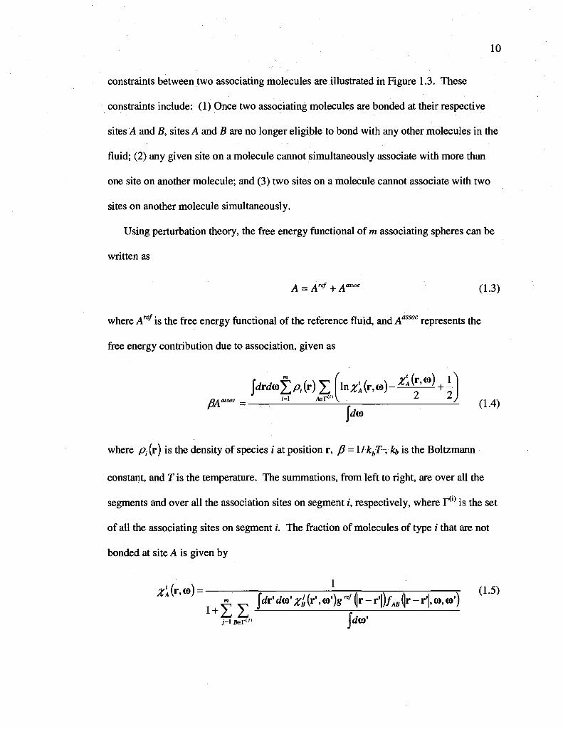
constraints between two associating molecules are illustrated in Figure 1.3. These

constraints include: (1) Once two associating molecules are bonded at their respective

sites A and B, sites A and B are no longer eligible to bond with any other molecules in the

fluid; (2) any given site on a molecule cannot simultaneously associate with more than

one site on another molecule; and (3) two sites on a molecule cannot associate with two

sites on another molecule simultaneously.

Using perturbation theory, the free energy functional of m associating spheres can be

written as

A = Aref+Aassoc (1.3)

where Are/is the free energy functional of the reference fluid, and Aassoc represents the

free energy contribution due to association, given as

\*dm±pt{v) I f l n ^ ( r , « ) - ^ f c ^ + i i=l Aer(,)

^

2 , [dm

(1.4)

where p, (r) is the density of species rat position r, P = \lkbT ,kt, is the Boltzmann

constant, and T is the temperature. The summations, from left to right, are over all the

segments and over all the association sites on segment i, respectively, where T(1) is the set

of all the associating sites on segment i. The fraction of molecules of type i that are not

bonded at site A is given by

y' (r co) = - (1 5) AK' ' - _ [dr'da'zi(r\<o')gr^r-r'\)fAB<\r-r'\,<o,<o') l + ZT<- rr,

j-i B=r»» ja<0

11

In the above expression, grefis the radial distribution function of the reference hard sphere

fluid, and /AB is the Mayer/-function for the association potential given as

/AB=[exp(-^Tc)-lJ-

One challenge in the area of molecular thermodynamics is the development of a

model capable of predicting both interfacial and bulk properties within a single

framework. As one can see from the above expressions, and as noted by Chapman,12

Wertheim's theory is formulated for inhomogeneous fluids and serves as the basis for

developing theories for both bulk and inhomogeneous associating fluids. In addition, the

theory can be extended to chain-like molecules by imposing the limit of complete

association between the different associating species in the mixture. To arrive at the free

energy expressions for a homogeneous bulk fluid (e.g., SAFT), the position dependence

of the density is ignored. As will be illustrated in chapters 2 and 3, such an equation of

state can be used to describe the phase behavior and thermophysical properties of real

fluids (after including additional perturbations such as dispersion attractions). By

preserving the position dependence of all variables in the system, the free energy is

suitable for use in an inhomogeneous environment. Eqs. (1.4) and (1.5) can be simplified

by relaxing and averaging over all orientations, therefore reducing the free energy

expressions as a functional of position r only. Segura et al.29"31 used this approach in the

development of a density functional theory based on TPT1 for associating spheres at a

hydrophobic wall. In addition, a density functional theory for chain fluids known as

inhomogeneous SAFT (/SAFT) was later developed on this basis.32"34 These works are

presented in chapter 4 and serve as important precursors to the research presented in this

dissertation (chapters 5-8).

12

1.3 Scope of the thesis

As mentioned, this research is devoted to the development of molecular theories

based on statistical mechanics to investigate the structural and thermodynamic properties

of bulk and inhomogeneous complex fluids. The foundation of this research comes from

Wertheim's first order thermodynamic perturbation theory (TPT1). A number of

equations of state based on TPT1 have been developed in an effort to meet the challenges

of modeling the fluid-phase-equilibria of larger molecules with more complex molecular

interactions. Despite such advancements, much work still remains, including addressing

theoretical shortcomings and meeting the challenges of predicting the phase behavior of

complex mixtures and polymer solutions. Chapter 2 extends the perturbed-chain

statistical associating fluid theory (PC-SAFT) to include a crossover correction using

renormalization-group theory. The crossover PC-SAFT equation of state significantly

improves the predicted phase behavior of the n-alkane family in the critical region in

comparison with available vapor-liquid equilibrium (VLE) experimental data. Chapter 3

presents new work using PC-SAFT as a predictive tool for investigating the phase

behavior of natural gas mixtures, aimed specifically at improving the understanding of

mercaptan/sulfide removal via gas treating. The model is validated against available

VLE mixture data.

The heart of the dissertation is the development and application of density functional

theory. Chapter 4 provides the background, a basic formalism of the theory, and a

literature review of important work that is relevant to this research. Chapters 5-8 provide

new theoretical developments which are validated with available simulation and/or

experimental data. In these chapters, the new developments of the theory are used to

13

investigate some of the more challenging problems of today involving interfacial and

inhomogeneous fluids.

In chapter 5, an atomic density functional theory is used to investigate the influence

of model solutes on the structure and interfacial properties of water. Results indicate that

hydrogen bonding is depleted near the surface of larger solute particles, thus leading to a

drying effect of the solvent at the surface of the non-polar solute and to long-ranged

hydrophobic attraction. The fundamental aspects of hydrophobic phenomena for such a

model system is important in understanding the role of hydrophobic interactions in more

complex systems, including surfactant self-assembly, protein folding, and the formation

of biological membranes.

In chapter 6, the inhomogeneous statistical associating fluid theory (/SAFT), a

polyatomic density functional theory, is used to investigate nonadsorbing polymer-colloid

mixtures. Such systems are of interest to a wide range of fields, from biology and

medicine to the design of property specific materials. However, many challenges still

remain for both experimentalists and theoreticians. The broad parameter space and

multiple length scales involved make the behavior of such a system difficult to

understand and model. Here, /SAFT is used to characterize the role of polymer

concentration and particle/polymer size ratio on the structure, polymer induced depletion

forces, and colloidal interactions.

While chapter 5 extends the previous work of Segura et al.29"31 for associating spheres

to investigate the radially symmetric (in inhomogeneities) water/solute problem, the

extension of molecular association to polyatomic systems is more challenging as it can

involve complex associating schemes (multiple associating sites located on different

14

polymer segments). Chapter 7 extends the inhomogeneous form of the association

functional to associating polymer systems. Results elucidate the importance of this

development, highlighting how reversible bonding governs the structure of a fluid near a

surface and in confined environments, the molecular connectivity (formation of

supramolecules, star polymers, etc.) and the phase behavior of the system (including

reentrant order-disorder phase transitions).

The iSAFT DFT is extended to predict the inter- and intramolecular correlation

functions of polymeric fluids in chapter 8. Correlation functions play a central role in

conventional liquid state theories. Knowledge of the inter- and intramolecular structure

can be used to enhance our understanding of the effect of local chemistry, bond

flexibility, and chain branching on the thermodynamic properties of polymers.

Finally, chapter 9 summarizes the key achievements of this dissertation. Attention is

also given to future applications and development of the density functional theory.

15

CHAPTER

Renormalization-group corrections to a perturbed chain statistical associating fluid theory for pure

fluids near to and far from the critical region

2.1 Introduction

The development of an equation of state that is accurate in describing thermodynamic

properties of fluids both near to and far from the critical region is of much interest in the

chemical industry. Accurate prediction of the phase envelope, particularly in the near

critical region, is essential in modeling processes encountered in natural gas and gas-

condensates production and processing, supercritical extraction, and fractionation of

petroleum. A multitude of equations of state have been developed that describe very well

the fluid properties away from the critical region, some of which include the cubic

equations of state, such as Peng-Robinson (PR) and Redlich-Kwong-Soave (SRK), as

well as molecular theory-based equations of state such as the statistical associating fluid

theory (SAFT). Unfortunately, no classical equation of state can describe properties near

to and far from the critical point with a single set of parameters. When fit to properties

away from the critical region, these equations of state provide very poor descriptions of

fluid behavior in the critical region. Alternatively, when fit to the critical point, a

classical equation of state gives poor results away from the critical region. Classical

equations of state assume that a Taylor series in density and temperature can be used to

16

expand the free energy about the critical point. Since the critical point is a non-analytic

point for the free energy, no such expansion is possible. By ignoring this effect, classical

equations of state produce a liquid-vapor coexistence curve that is quadratic near the

critical point. This quadratic behavior disagrees with experiment.

The true thermodynamic behavior in the critical region is a consequence of long-

range density/concentration fluctuations.35'36 Classical equations of state perform well in

the region where the correlation length is small (far from the critical region), where only

correlations between a few molecules make significant contributions to the free energy.

However, as the critical point is approached, the correlation length increases and larger

numbers of molecules make significant contributions to the free energy. Here, the large

correlation lengths imply that the system is not homogenous near the critical point and

the long-wavelength density fluctuations become important. Mean-field theories are not

capable of accurately describing correlations between large numbers of molecules. As a

result, long-wavelength density fluctuations are neglected, providing the reason why

these classical equations fail near the critical point.

To predict thermodynamic properties over the entire fluid region, a method that

incorporates the accuracy of these classical equations of state away from the critical

region, but is augmented with a correction to correctly describe behavior near the critical

region must be implemented. The crossover treatment discussed in this chapter provides

the needed corrections due to density fluctuations as the critical point is approached, and

reduces to the original classical equation of state (in the case studied here PC-SAFT,

described later) far from the critical region. This crossover treatment is based on

renormalization-group (RG) arguments.

17

2.2 Background on renormalization-group methods

Renormalization-group (RG) theory has proven to successfully describe the fluid

properties near the critical region. There are many approaches that apply the method to

account for the long-wavelength density fluctuations, some of which include work by

Chen, Albright, and Senger37'38 as well as White, Zhang, and Salvino.39"43 Chen et al.

describes the free energy of a fluid near its critical point through an Ising-like singularity,

written as a Landau expansion that contains an analytic contribution as well as a

contribution from the singularity due to long-range molecular correlations. The singular

contribution is represented by a scaling function of the reseated temperature (temperature

modified by a crossover function) and density, and is incorporated in the critical region.

Away from the critical region, the Helmholtz free energy reduces to the classical

expansion. Kiselev and Ely 44,45 also apply a method based on the renormalized Landau

expression to a classical equation of state, and actually use Chen et al's37 scaling

function near the critical point. Adidharma and Radosz ^ and McCabe and Kiselev 47

have applied Kiselev's method to SAFT and have shown improved results in the critical

region. The equation of state developed by Kiselev has the advantage that it is in a closed

form (does not require to be solved numerically). Unfortunately, these theories based on

the renormalized Landau expansion have the disadvantage of requiring many adjustable

parameters to fit experimental data.

White et al.'s work is an extension of the theory developed by Wilson 48'49, who

incorporated density fluctuations in the critical region using the phase-space cell

approximation. Here, White employs a recursive procedure that modifies the free energy

for a non-uniform fluid, thereby accounting for fluctuations in density. The subsequent

18

recursive steps account for longer and longer wavelength fluctuations. White and co

workers extended the range beyond the critical region, but was only accurate within 20%

of the critical temperature. Lue and Prausnitz50'51 and Tang52 independently improved

this region of accuracy and extended White's RG theory to general mean field theories.

Lue and Prausnitz incorporated a first-order mean spherical approximation with White's

RG method to provide an equation of state for simple square-well fluids and fluid

mixtures. Jiang and Prausnitz53,54 further applied Lue's work to an equation of state for

chain fluids (EOSCF) to describe the pure n-alkane family and chain mixtures. Tang, on

the other hand, combined White's RG transformation with a density functional theory

and the superposition approximation for a Lennard-Jones (LJ) fluid. The work of

Prausnitz and co-workers and Tang demonstrate that White's RG mechanisms can be

applied to achieve accurate equations of state that grasp the global behavior of different

fluids. The advantage of White's method is the addition of only two parameters, thereby

making the theory more predictive than the model devised by Chen et al. and Kiselev et

al. The main disadvantage is that the crossover method used can only be solved

numerically and does not lead to explicit expressions for the equation of state.

This work applies White's crossover treatment, while incorporating the improved

approximations developed by Lue and Prausnitz,50'51 to the perturbed-chain SAFT (PC-

SAFT) equation of state. Llovell et al.55'56 have also applied an approach based on Lue

and Prausnitz's work with success to a Soft-SAFT equation of state. Recently, Fu et al.57

presented results using the same renormalization procedure with the PC-SAFT equation

of state. In the following sections, a brief overview of the PC-SAFT equation of state is

given, followed by a description of the recursive relations from White's work. Previous

19

results from Llovell et al.55 and Fu et al.57are discussed, with special emphasis on the

approximations and methods (not previously documented) used to obtain their results.

Differences between results from Fu et al. and the results reported in this chapter are

discussed in terms of the approximations made. Results from this work are then

presented. From this work, it is found that when using this RG method, coupled with PC-

SAFT, the proposed crossover equation of state does not accurately predict properties in

the critical region for longer chain molecules. However, excellent results near to and far

from the critical region are obtained by modifying the renormalization scheme with an

additional parameter.

As previously noted, the work of Lue and Prausnitz extended the region of accuracy

(White's work) beyond the critical region. However, when applying the work of Lue and

Prausnitz to other equations of state, other authors have demonstrated that it is sometimes

necessary to alter the equation of state parameters to improve results obtained in the

critical region.53'55 When these changes are made, the equation of state cannot accurately

describe the coexistence curve far away from the critical point. In this work, the original

molecular parameters from PC-SAFT58 are used so that an accurate description of the

fluid can be predicted over the entire range of conditions, from the triple point to the

critical point. This is advantageous as one can use the original PC-SAFT molecular

parameters over the entire range of conditions without concern as to what parameters to

use for the given region of interest.

2.3 PC-SAFT outside the critical region

SAFT is one of the most widely used equations of state for calculating phase

equilibria for a wide variety of complex polymer systems. The theory's success comes

20

from its strong statistical mechanics foundation, which allows for physical interpretation

of the system. It was first derived by Chapman et al.,8"10 and is based on Wertheim's

first-order thermodynamic perturbation theory.4"7 There are several SAFT versions in

common use today, including LJ-SAFT,11'59"64 in which Lennard-Jones spheres serve as a

reference for chain formation, CK-SAFT which was suggested by Huang and Radosz 65'66

who applied a dispersion term developed by Chen and Kregleqski,67 SAFT-VR which

uses a square-well of variable range developed by Gil-Villegas et al.,68 and PC-SAFT

which uses a perturbed-chain dispersion term developed by Gross and Sadowski.58 In this

work, the crossover treatment will be applied to PC-SAFT, as described below. Just

recently, Dominik, Jain, and Chapman developed SAFT-D, an improved version of PC-

SAFT based on a dimer reference fluid.69

PC-SAFT applies Barker and Henderson's70'71 second-order perturbation theory to a

hard-chain reference fluid, resulting in a dispersion term that is dependent on the chain

length of a molecule. Here the main features of PC-SAFT relevant to this work are

described. For details, the reader is referred to the work of Gross and Sadowski.58 For

simplicity, the reduced Helmholtz free energy a(=A/Nki,T) is used throughout this work,

where N is the total number of molecules, k\, is the Boltzmann constant, and T is the

temperature. For non-associating chain systems, the total residual Helmholtz free energy

is written as

where the superscripts he and disp refer to the respective hard-chain and dispersion

contributions. The hard-chain contribution to the free energy is written in terms of the

21

hard-sphere (hs) free energy, the chain length (m), and the radial distribution function of a

fluid of hard spheres (ghs),s

a"0 =ahs+(l-m)\nghs. (2.2)

The hard-sphere interaction, given below, was developed by Carnahan and Starling

a =m-

.72

( I -?) 2 ' (2.3)

where r\ represents the packing fraction defined by

rj = . f }m r f S (2.4)

Here, p represents the number density of molecules, and d is the temperature-dependent

segment diameter, defined as67

d = o\ l-0.12exp ' - * A vVy

(2.5)

The dispersion term developed by Gross and Sadowski is a sum of contributions of the

first and second-order, given by

a" -Inp Iêa3 -npmCxI2m2eai, (2.6)

where the parameters e and a are the well-depth of the potential and temperature-

independent segment diameter, respectively, and C; is from the local compressibility

approximation of Barker and Henderson, written in terms of the hard-chain contribution

to the compressibility factor.

22

( Cx = i+zhc+P

dz he \

\ dp

(2.7)

The integrals h and h in eq. (2.6) are given as

/, = \u(x)ghc m;x— \x r ^ d)

zdx

/ a = — dp

p \u(x)2ghc\ m;—\x2dx

(2.8)

(2.9)

where u is the pair potential, and x is the reduced radial distance between two segments.

The above integrals are fit by simple power series in density r\

i=0

(2.10)

h{v,m)=Yjbi(nC>rli> i=0

(2.11)

where the coefficients a,- and bi are dependent on chain length according to

/ \ m-\ m-lm-2 «,. (m) = a0i + au + ,

m m m

(2.12)

, / \ , m-l. m-lm-2, b, M = b0i + bu + 6,

m m m (2.13)

The model constants a,-,- and bji are fit to experimental data of n-alkanes, and are reported

by Gross and Sadowski.58

The PC-SAFT equation of state has been applied with great success to a wide variety

of systems including associating and non-associating molecules,58'73'74 polar

, 73,75,76 . 76-79 80,81 . systems, ' ' polymer systems, " as well as other complex systems. ' The EOS

23

requires few parameters that scale well within a homologous series, making it a powerful

tool for systems where little experimental data is available. Despite its improved

accuracy in the critical region (compared to other equations of state), PC-SAFT still

experiences inaccuracies of thermodynamic properties as the critical point is approached,

and would benefit from a crossover correction.

2.4 Recursive relations

Using the renormalization method of White,39"43 the long-wavelength fluctuations to

the free energy density are included. The theory consists of recursive relations that

account for the fluctuations as the critical region is approached, and exhibits a crossover

between the classical equation of state (in this case PC-SAFT) and the universal scaling

behavior in the near-critical region.

This work follows Lue and Prausnitz's50'51 implementation of White's RG method,

who transformed the grand canonical partition function for simple fluids into a functional

integral. The interaction potential consists of a reference contribution and a perturbative

contribution, [u(r)=urej(r) + u'(r)]. The reference contribution is due mainly to the

repulsive interactions, while the perturbative contribution is due mainly to the attractive

part of the potential. Since the reference term contributes mainly with density

fluctuations of very short-wavelengths, renormalization is only applied to the attractive

part of the potential. The attractive part of the potential consists of short and long-

wavelength contributions. It is assumed that the mean-field theory can accurately

evaluate contributions from fluctuations of wavelengths less than a certain cutoff length L

(one of the added parameters). It is also assumed that the approach can be applied to

molecules made of chains of spherical segments.

24

The functional F5 below accounts for the contribution from short-wavelength

fluctuations, estimated using a local-density approximation

Fs(p)=lfs(p)dr, (2.14)

where fs is the Helmholtz energy density for a homogenous system with molecular

(number) density p ;fs can be calculated using the PC-SAFT equation of state, or any

other mean-field theory. It is important to note that/* should only include short-

wavelength fluctuations. Therefore, the long-wavelength fluctuations from the PC-SAFT

equation must be subtracted using the van der Waals approximation -a(mp)2. The factor

of m2 appears since there are m2 segment-segment interactions between a pair of

molecules. As a result,/4 is described as

fs=f"+a{mp)\ (2.15)

where a, the interaction volume (units of energy volume), is given by

a = --\u\r)dr. (2.16)

The total free energy,/'0', can be described as follows

f""=fid+fres, (2.17)

where the ideal82 and residual contributions are defined

fid=pkbT[\n{p)-l] (2.18)

fres = pkbTares . (2.19)

25

The zero-order solution, fo, is evaluated using the saddle point approximation.83 The

saddle point approximation neglects all density fluctuations of all wavelengths that are

not already accounted for by the reference fluid.

f0=fs-a(mp)2 (2.20)

Combining with eq. (2.15), the following is obtained

/<,=/"*• (2.21)

The contributions of the long-wavelength density fluctuations are accounted for using the

following recursive relations for the Helmholtz free energy density of a system at density

p.

fn(P) = fn-l(P) + %n(P)- (2-22)

In the above equation,/„ represents the Helmholtz free energy density and 3f„ the term

that corrects for long-wavelength fluctuations, given by

dfn{p) = -Kn\ry^^-, Q<p<PmJ2 (2.23) - A . (P) •

$m(p) = 0, PnJ2<P<Pmax (2 .24)

where Q? and Q^ refer to the density fluctuations for the short-range attraction and the

long-range attraction. The coefficient K„ is defined by

k T Kn = - ^ (2.25)

n 2 3 n L 3

at temperature T and cutoff length L. The procedure for calculating the density

fluctuations uses the following integral,

26

&/(P) = JexP Pi

G" (P'X) \dx (2.26) K„

where,

GHP,x)=llS£±±^llSPllllSBzA. (2.27)

Above, /? refers to both the short (s) and long (/) range attraction, respectively, and Gr

depends on the function / , calculated below,

Tn\p) = fn-l(P) + oc{mpf (2.28)

T (P) = /„-! (P) + (Amp)2 - 0 g • (2.29)

Above, îs an adjustable parameter (the other added critical scaling parameter,

representative of the average gradient of the wavelet84) and w represents the range of the

attractive potential, defined

w2 =-—\r2u'(r)dr. (2.30) 3a J

In the above procedure, £2„'refers to density fluctuations for the long-range attractive

potential, while Qns refers to the density fluctuations for the short-range attractive

potential. Referring to eq. (2.29), note that less of the initial attractive contribution is

subtracted out as the longer and longer fluctuation wavelengths are included (at

successive recursive steps). The procedure above can therefore be interpreted as the

calculation of the ratio of non-mean-field contributions to mean-field contributions as the

wavelength increases. From eqs. (2.23) and (2.24), it can be seen that the long-

wavelength fluctuations are only relevant when the density is less than half the maximum

27

density. Mentioned above, / w is the maximum molecular density allowed in the

system. To obtain this value, recall the basic relation for the packing fraction given by

eq. (2.4). Values of TJ > 0.7405 [= #/(3V2)j have no physical relevance since they

represent packing fractions greater than the closest packing of segments.58 If the

maximum value of the packing fraction allowed is then the maximum

molecular density can be described in the following way,

P™=^dT'^J2=~^2- (2'31)

In theory, the above recursive procedure should be carried out until n approaches infinity,

therefore obtaining the final full free energy density in the infinite order limit

/ = lim/„. (2.32)

However, as other authors have observed,50'51'53" 6 the thermodynamic properties become

stable after just a few iterations (n=5). The integral in eq. (2.26) is evaluated numerically

using the simple trapezoid rule. It was found that a density step of max was sufficient

in terms of accuracy. The resulting free energy was fit using a cubic spline function and

derivatives of this spline fit were then used to compute the chemical potential and

pressure.

2.5 Results and discussion

2.5.1 Applying RG theory to PC-SAFT

As mentioned earlier, in the framework of PC-SAFT, the dispersion interaction is a

result from a fitting to experimental data for the n-alkanes. Before obtaining the pure

28

CO

component parameters for the n-alkane components, Gross and Sadowski took an

intermediate step where they assumed a Lennard-Jones perturbing potential. If we

assume that the perturbation potential for this system is that of a Lennard-Jones-like fluid,

the constants or and w2 can be obtained. The reference potential is approximated using a

hard-sphere potential, given by,

Uref<j) = -°o r<a 0 r>a

(2.33)

and the perturbation potential is approximated by

«'W = 0

4e <o^

\r

f<i*

\r)

(2.34)

The constants or and w2 for the fluid are therefore given as

1 °° a = — \4m-2u'(r)dr = \67tea

9~ (2.35)

w = -L]4m.>u<{r)r2dr = — y.al w • 7

(2.36)

The added parameters ând L are adjusted to fit the critical properties. When fitting

the parameters, the critical point is evaluated from the standard critical criteria:

dP_

rd2P"

= 0

= 0

(2.37)

29

In previous work, Lue and Prausnitz51 fixed 0to a particular value (^=10) and used L as

an adjustable parameter to fit the critical temperature of square-well fluids. However, for

simple mixtures,50 they changed this criteria, fixing L (L=2a) and using </> as the

adjustable parameter to fit the critical temperature. Jiang and Prausnitz53 also fixed L and

used 0as the adjustable parameter to fit the critical temperature for real chain fluids.

However, they fixed L to a constant value (L=l 1.5A). Llovell, Pamies, and Vega55'56

were the first to make both 0and L adjustable to better systematize the fitting procedure

and optimize results.

When coupling RG theory with the PC-SAFT equation of state, all the above

approaches were considered. While the method proved successful in improving the

temperatures in the critical region, a major drawback of the method was realized as the

pressures in the critical region were overestimated by a large margin of error. Figure 2.1

illustrates the influence of the crossover treatment in the phase envelope for n-octane,

first in the temperature-density diagram and then in the pressure-temperature diagram.

The circles are experimental data,85 the dotted lines represent results from the PC-SAFT

equation, and the solid line comes from the PC-SAFT + RG. From Figure 2.1 (b), it is

seen that the pressures in the critical region are overestimated. Alternative solutions were

investigated and it was found that reasonable results could be obtained by going to high

values of L. However, these values of L may not represent physical values and therefore

were not considered further. The other alternative is to alter the molecular parameters so

that the pressures agree with the experimental values in the critical region. However, this

approach cannot describe the behavior of the fluid globally. We have developed an

alternative approach to provide global descriptions of the phase behavior. This approach

30

is presented below. While studying why poor results were initially obtained, we found

that several applications of White's theory are not as they appear in the literature,

(a) (b)

600

550

500

g

450

400

350

0 1 2 3 4 5 6 200 250 300 350 400 450 500 550 600

p (mol/L) T (K) Figure 2.1: (a) Temperature-density diagram for n-octane before modification of the perturbing potential function (L=2o and 0=18.75). (b) Pressure-temperature diagram for w-octane before modification of the perturbing potential function (L=2o and 0=18.75). Circles are experimental data,85 the solid line represents PC-SAFT+RG, and the dotted line is PC-SAFT.

As mentioned earlier, previous published results using this renormalization technique

coupled with other equations of state apparently do not suffer from inaccurate predictions

of the pressure in the critical region. To verify that the renormalization schemes used in

this work were correct and consistent with the schemes implemented previously by other

groups, we attempted to reproduce the published work by several groups including

Llovell et al.55 and later Fu et al.57 Although we have not successfully reproduced the

results of all groups, we have reproduced the results of Llovell et al. and Fu et al. after

considerable input from the authors. It is now clear that several groups using White's

approach have introduced additional numerical and, in some cases, empirical

approximations. Both groups use the same renormalization-group approach discussed in

3.2

2.8

2.4

2

1.6

1.2

0.8

0.4

11 I

! jo

It If

jo

f

31

section 2.4 and apply it to versions of the SAFT equation of state. Specifically, Llovell et

al.55 use a Soft-SAFT equation of state, while Fu et al.57 use PC-SAFT, as in this work.

In the next two subsections, the approximations used from both of these groups are

identified and discussed. Section 2.5.4 proposes modifications needed to overcome the

shortcomings mentioned in this section and presents the improved results.

2.5.2 Reproducing Llovell et al. 's Soft-SAFT results

As discussed previously, Llovell et al.55 applied White's RG method to the Soft-

SAFT equation of state with impressive results. To verify that the problems we were

experiencing (as outlined in the previous section) were specific to PC-SAFT, and that the

schemes implemented were correct and consistent, we attempted to reproduce the results

from Llovell et al.55 When applying this method to the Soft-SAFT equation of state, we

found that very good results could be obtained using the expressions and schemes

presented previously in section 2.4, thereby suggesting that our recursive schemes were

correct and consistent with previous work. However, to reproduce the results by Llovell

et al. exactly, it was realized after a discussion with Llovell and Vega that additional

approximations were introduced in their approach. For the values of the free energy

density at previous recursive steps needed in eqs. (2.28-29), Llovell et al. use the value of

/ „_ / and f n_xs instead of /„_, for all steps greater than one, thus introducing the

approximation,

32

fn'(P) = fn-i(P) + a{™PY . 2

/ . ' (P) = fn-i U» + <x(™p)2 TJT

Tnl(p) = JJ(p) + a{mp)2

Tn\p) = ln-ls(p) + a(mpf +*

forn = l

(2.38)

for n > 1 2n+l T2

Using this approximation, along with the published molecular and RG parameters

used by Llovell et al.,55 we were able to successfully reproduce their results. It should be

noted that we did find that good results could be obtained without using this

approximation (using expressions from section 2.4) and without altering the original

molecular parameters. This occurs because Soft-SAFT with the original parameters

underestimates the vapor pressure at the critical temperature. The critical scaling tends to

increases the pressure to produce good agreement with the experimental critical pressure.

2.5.3 Reproducing Fu et al. 's PC-SAFT results

Similar to this work, Fu et al.57 recently published results demonstrating White's RG

method coupled with the PC-SAFT equation of state. From their paper, Fu et al.57 use a

square-well perturbation potential to calculate the interaction volume, a, and the range of

the attractive potential, w; however, the expressions are not documented. It might be

assumed that the perturbation potential is the same as in earlier works.51'53 Regarding the

RG parameters, Fu et al. declare both to be constant, using L=2.0a and <j> = 13.5 .

Unfortunately, we were unable to reproduce Fu et al.'s results using the above parameter

values with potential expressions from earlier work.51'53 It was soon realized after a

discussion with Fu that there existed some significant differences between the recursive

33

expressions published and those implemented to obtain their results. The following

identifies these differences.

First, Fu et al. use a slightly modified form of the interaction volume from the form

used by Lue and Prausnitz51 and Jiang and Prausnitz.53 Here «takes the form

a = -±£a4xr2{-e)dr = ^[{A*y -a3]. (2.39)

To be consistent, the range of the attractive potential should also be modified over a

similar range of the square-well potential. However, in Fu et al.'s calculations, they used

the following

w2= — (Aaf. (2.40) 45v '

Further, Fu et al. multiply the free energy density to be renormalized by a factor of m

\j0 = mpkbTa""); however, they express the long-wavelength fluctuations using the

same mean-field approximation used by other groups (- can2p2) that is not scaled by an

additional factor of m. Justification for the inconsistent scaling of the free energy and the

long wavelength contribution was not stated. Still, using these inconsistent expressions,

Fu et al. obtain excellent correlations of the phase behavior. In section 2.5.4, we present

a modified scaling approach to improve the behavior of the PC-SAFT+RG equation of

state.

2.5.4 Improving PC-SAFT+RG

We applied scaling relations to improve the behavior of the PC-SAFT equation of

state simultaneously and independently of Fu et al. As discussed previously, in the PC-

SAFT equation of state the dispersion interaction is a result from a fitting procedure to

34

real substances. The perturbation part of the potential is therefore not well defined.

Thus, a slightly different approach is taken. A third adjustable parameter £ is introduced

to modify the Lennard-Jones potential used above in section 2.5.1 in the calculation of «

and w2. Therefore the new perturbing potential takes on the form

ii *(r) = £«•(/•) (2.41)

and a and w2 are now defined as

a = -^[4û'(r)dr=1-^^- (2.42)

w2= — Unr2^ u'(r)r2dr = — . (2.43) 3\a*> w 7

Using these relations, the parameters <j>, L, and £ can be adjusted to optimize the predicted

properties in the critical region. For a given alkane, the parameter 0is used to fit the

critical temperature at designated values of L and £ The parameters L and £ can be

adjusted accordingly to match the critical pressure and critical density.

For low molecular weight n-alkanes (up to C9H20) the critical properties are well

known from experiment. However, for heavier n-alkanes, critical property measurements

are impeded since the critical temperatures exceed the temperature of the onset of thermal

decomposition.86 Teja and coworkers87'88 and Nikitin et al.89,90 represent the few to

successfully make critical property measurements for heavier alkanes, but the

experimental error of these critical values can be quite large. For these reasons, in this

work the crossover parameters were fit, using the procedure described above, for C2-C8

and for C12 and Ci6.

35

Table 2.1: Molecular parameters and crossover (RG) parameters $ L, and £

n -alkane QHe C3H8

C4H10

C5H12

Q H ^

C7H16

QHjg

CnH26

C16H34

m 1.6069

2.0020

2.3316

2.6896

3.0576

3.4831

3.8176

5.3060

6.6485

0 (A) 3.5206

3.6184

3.7086

3.7729

3.7983

3.8049

3.8373

3.8959

3.9552

s/kb (K) 191.42

208.11

222.88

231.20

236.77

238.40

242.78

249.21

254.70

4> 15.38

20.37

23.43

25.30

33.25

38.10

42.06

49.21

56.56

L/o 1.40

1.63

1.75

1.83

2.24

2.35

2.63

2.77

2.95

% 0.520

0.397

0.304

0.261

0.205

0.173

0.155

0.142

0.136

The critical parameters were found to correlate well with molecular weight. The

values of the optimized parameters are presented in Table 2.1, and Figure 2.2 illustrates

the optimized parameter trends with molecular weight for C2-C16. As observed in

previous work,33'55 m<f> and mUa show linear behavior with respect to molecular weight.

The parameter <f also follows a well-defined trend with molecular weight. When

extrapolating to heavier w-alkanes, the proposed correlations (correlated from Table 2.1)

for the new parameters are

m(j) = 1.8316MW -47.947 (2.44)

mLI a = 0.091MW - 0.9085 (2.45)

g/m2 =318A2MW~2H11. (2.46)

The original PC-SAFT equation needs three molecular parameters: m the chain

length, crthe temperature independent segment diameter, and e the interaction energy.

Gross and Sadowski58 have already regressed these three parameters without

36

renormalization for several chain-like molecules, including the n-alkane family (C1-C20).

It is important to emphasize that the original molecular parameters m, a, and e proposed

by Gross and Sadowski58 were used and remained unaltered in all calculations. By using

these original parameters, the crossover equation can reduce to and maintain the good

behavior of the original PC-SAFT equation outside the critical region. It is known that

these three molecular parameters can be correlated as functions of molecular weight,58

providing extrapolative abilities for the heavier n-alkanes. Altogether, the three molecular

parameters, coupled with the new crossover parameters, are enough to describe all

thermodynamic properties.

I 10

s

50 100 150 200 250

MW (g/mol)

Figure 2.2: PC-SAFT crossover (RG) parameter dependence on molecular weight.

37

Table 2.2: Critical constants for light n-alkanes, compared with experimental data

n -alkane

QHe

C3H8

C4H10

CjH^

C6H14

C7H16

QHig

C12H26

C16H34

Exp.

305.3

369.8

425.1

469.7

507.3

540.2

568.7

658.0

722.4

TC(K) PC-SAFT+RG

305.3

369.8

425.1

469.7

507.3

540.2

568.7

658.0

722.4

PC-SAFT

309.0

375.1

432.5

479.3

519.3

552.6

583.1

673.3

737.6

Exp.

4.87

4.25

3.80

3.37

3.03

2.74

2.49

1.83

1.40

Pc (MPa)

PC-SAFT+RG

4.88

4.25

3.80

3.37

3.03

2.78

2.52

1.88

1.49

PC-SAFT

5.10

4.55

4.16

3.77

3.50

3.24

2.98

2.24

1.77

Exp.

6.75

4.92

3.92

3.22

2.72

2.34

2.03

1.33

1.00

p,.(mol/L)

PC-SAFT+RG

6.75

4.92

3.92

3.22

2.72

2.36

2.07

1.37

1.00

PC-SAFT

6.39

4.73

3.77

3.10

2.65

2.32

2.03

1.34

0.98

Table 2.2 gives the experimental, PC-SAFT, and PC-SAFT + crossover (RG) critical

constants Tc, Pc, and/JC for n-ethane to n-hexadecane. As already noted, PC-SAFT

overestimates Tc and Pc, while giving a very good estimate for the critical density pc. The

predictions of the critical constants made by the crossover PC-SAFT equation are much

improved. By fitting the three critical parameters, all three critical constants Tc, Pc, and

pc are matched with their respective experimental values. In cases where the critical

pressures and densities deviate slightly, the values given are still within experimental

error. In regard to the critical densities predicted by the crossover PC-SAFT equation,

other authors were unable to predict the critical densities as closely. Jiang and

Prausnitz,53 as well as Llovell et al.,55 observed over-predictions of the critical density in

their work, most likely due to changing the original molecular parameters.

Figure 2.3 illustrates the influence of the crossover treatment in the phase envelope

for w-octane, first in the temperature-density diagram and then in the pressure-

temperature diagram. The circles are experimental data,85 the dotted lines represent

results from the PC-SAFT equation, and the solid line comes from the PC- SAFT + RG.

These diagrams support the data in Table 2.2, illustrating an overestimation in critical

38

temperature and critical pressure from the PC-SAFT equation, but excellent results from

the PC-SAFT + RG equation. Note the improved results in the critical region of Figure

2.3 versus Figure 2.1.

(a) (b)

600

550

500

g H

450

400

350

0 1 2 3 4 5 6 200 250 300 350 400 450 500 550 600

p(mol/L) T(K)

Figure 2.3: (a) Temperature-density diagram for w-octane using the modified perturbing potential function, (b) Pressure-temperature diagram for n-octane using the modified perturbing potential function. Symbols and lines defined as in Figure 2.1.

Figure 2.4 (a) shows vapor-liquid coexistence curves for some select light n-alkanes

(C3, C5, C7) and Figure 2.4 (b) shows vapor pressures for the same group considered. The

results are in excellent agreement with experimental data and are representative of all n-

alkanes considered in this work. This is due to the PC-SAFT + RG equation's ability to

correct the inadequacies of the PC-SAFT equation by accounting for the density

fluctuations in the critical region. Outside the critical region, the PC-SAFT + RG reduces

to PC-SAFT, where PC-SAFT is accurate and reliable.

(a) (b)

39

g H

euu

500

400

300

200

100

- £ - .

f -swÂ

|

•

•

o ^ l

%

0 5 10 15 20 100 200 300 400 500 600

p(mol/L) T(K)

Figure 2.4: (a) Temperature-density diagram and (b) pressure-temperature diagram for select light n-alkanes (C3, C5, and C7).

The previously given correlations (eqs. 2.44-46) for <f>, L, and £ coupled with the

correlations given by Gross and Sadowski58 for m, a, and e, are tested for select heavy n-

alkanes (C20, C24, C30, and C36). Table 2.3 and Figure 2.5 elucidate the remarkable ability

to predict the critical behavior for the heavy members using these correlations, when

compared with simulation data93 and available experimental data.86'87'91 Figure 2.6 shows

the critical temperature Tc, and critical pressure Pc as a function of carbon number before

and after renormalization corrections.

Table 2.3: Critical constants for heavy n-alkanes, compared with experimental data 86,91

n -alkane

C20H42

C24H50

Q0H62

C36H74

Exp.

767.5

803.2

843.5

873.6

TC(K) PC-SAFT+RG

765.6

803.6

845.2

877.8

PC-SAFT

785.0

824.8

868.6

902.8

Exp.

1.10

0.90

--—

Pc (MPa) PC-SAFT+RG

1.16

0.96

0.72

0.56

PC-SAFT

1.45

1.23

0.97

0.78

Exp.

---__

p,.(mol/L) PC-SAFT+RG

0.79

0.62

0.50

0.42

PC-SAFT

0.77

0.63

0.49

0.39

40

Figure 2.5: Phase equilibria predictions for heavy n-alkanes (C20, C24, C36). The circles represent simulation data,93and critical points from experiments.86

(a) (b)

g o

I-

900

800

700

500

400

300

0 5 10 15 20 25 30 35 40

Carbon number

0 5 10 15 20 25 30 35 40

Carbon number

Figure 2.6: (a) Critical temperatures and (b) critical pressures for n-alkanes, from C2 to C36 as predicted by PC-SAFT +RG (solid lines) and PC-SAFT (dashed lines). Symbols represent experimental critical „ • »„ 86,88,91,92

points.

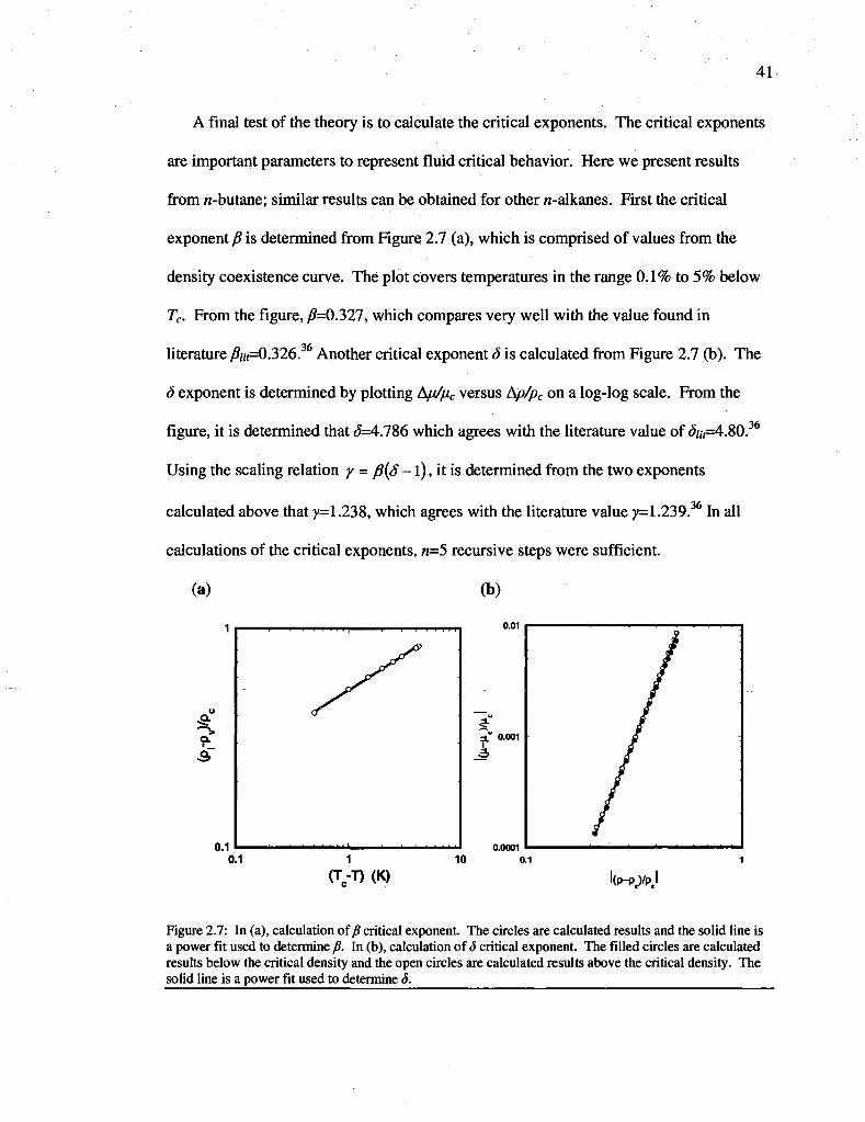
41

A final test of the theory is to calculate the critical exponents. The critical exponents

are important parameters to represent fluid critical behavior. Here we present results

from n-butane; similar results can be obtained for other n-alkanes. First the critical

exponent p is determined from Figure 2.7 (a), which is comprised of values from the

density coexistence curve. The plot covers temperatures in the range 0.1% to 5% below

Tc. From the figure, /?=0.327, which compares very well with the value found in

literature /?/ir=0.326.36 Another critical exponent d is calculated from Figure 2.7 (b). The

d exponent is determined by plotting A/j//ic versus tsp/pc on a log-log scale. From the

figure, it is determined that ^=4.786 which agrees with the literature value of J/,<=4.80.

Using the scaling relation y = {}{S -1), it is determined from the two exponents

calculated above that y=1.238, which agrees with the literature value y=1.239.36 In all

calculations of the critical exponents, n=5 recursive steps were sufficient.

(a) (b)

36

0.01

(Tc-T) (K) ko-pp/pj

Figure 2.7: In (a), calculation of fi critical exponent. The circles are calculated results and the solid line is a power fit used to determine /?. In (b), calculation of d critical exponent. The filled circles are calculated results below the critical density and the open circles are calculated results above the critical density. The solid line is a power fit used to determine <5.

42

2.6 Conclusions

As demonstrated, PG-SAFT, when coupled with renormalization-group theory, is

capable of accurately describing fluid properties both near to and far from the critical

region. Outside the critical region, where the correlation length is small, the PC-SAFT +

crossover (RG) equation reduces to the original PC-SAFT equation, where the latter is

already accurate and reliable. Inside the critical region, the crossover PC-SAFT equation

accounts for long-wavelength density fluctuations and reduces the inaccuracies of PC-

SAFT in this region (that are due to its mean-field nature).

The theory presented requires a parameter <f to account for the non-ideal perturbing

potential since the PC-SAFT dispersion term is fit to real n-alkane data, and also two

renormalization-group parameters 0and L. All crossover parameters are adjusted to fit

the experimental critical temperature, critical pressure, and critical density. As with the

original molecular parameters from PC-SAFT (m, <r, and e), the critical parameters also

exhibit relationships with molecular weight, thus providing the ability to correlate

parameters for heavier alkanes where little experimental data is available. The only

limitation to the theory is that it must be implemented numerically. Future applications

include applying the theory to simple fluid mixtures50'54'56'94 and within a density

functional construct.52'95'96

Although it is assumed that there are m2 segment-segment interactions between a pair

of molecules (used in the van der Waals approximation- am2p2), both the scaling

procedure presented in this work, particularly the added parameter £ and the additional m

factor in the approximation implemented by Fu et al. suggest the possibility mat the

intermolecular dispersion energy may go as mx where x<2. Such an effect may occur due

to screening effects, where a given segment on a chain could be surrounded by other

segments on the same chain, and therefore prevent the segment from interacting with

other segments in the fluid. This would have a larger effect on longer molecules than

shorter molecules. Such ideas are not trivial and thus require further consideration.

44

CHAPTER

A thermodynamic model for sour gas treating

3.1 Introduction and motivation

Hydrogen sulfide (H2S), carbon dioxide (CO2) and mercaptan (methyl-mercaptan,

ethyl-mercaptan, etc.) gases are common components encountered in natural gas,

synthesis gas and various refinery process streams. Typical concentrations of the above

components in the host gas stream can range anywhere from several parts per million to

50 percent by volume. The removal of acid gas impurities is a significant operation in

gas processing due to the highly corrosive and toxic nature of such components. In

addition, the removal of CO2 is highly desirable to avoid pumping any extra volume of

gas (which leads to high transportation costs) and because CO2 reduces the heating value

of the gas. For natural gas production, typical pipeline specifications require less than

4ppm by volume H2S;97'98 sales gas specification for natural gas typically requires the

CO2 to be less than 1-2% and feed quality for liquefaction into LNG require less than

50ppm by volume CO2.97'98 Total concentration of all sulfur species in the purified gas

stream typically must be less than 20-50ppm by volume.98

Research interests have therefore focused on developing highly economical and

selective gas treating methods to meet the increasing strict environmental regulations, and

45

to exploit poorer quality crude and natural gas. One example is the Controlled Freeze

Zone (CFZ™) technology invented at ExxonMobil Upstream Research Company"

which achieves the removal of CO2 and H2S from natural gas in a single step via

cryogenic distillation. Such a process is particularly advantageous for handling natural

gas mixtures of high CO2 and H2S content. An alternative to the CFZ™ technology and

a more conventional method used for removal of CO2, H2S, and other sulfur species is via

absorption and regeneration. Such processes are solvent-based, which generally capture

the acid gas and other sulfur impurities via a chemical, physical, or hybrid solvent.

Figure 3.1 shows a simplified schematic of a typical absorption/regeneration process.

The main constituents of a sour gas mixture typically involve hydrocarbons (Ci-C„),

nitrogen (N2), hydrogen sulfide (H2S), carbon dioxide (CO2), and components of the

other sulfides (carbonyl sulfide, carbon disulfide, dimethyl sulfide, methyl-ethyl sulfide,

methyl mercaptan, ethyl mercaptan, etc.). The sour gas mixture enters the absorber and is

contacted countercurrently with the lean solvent, which absorbs the acid gases and other

sulfur impurities to produce a sweetened gas stream as a product and a rich solvent (rich

in impurities). The rich solvent is then sent through a heat recovery exchanger and then

into the regenerator (a stripper with a reboiler). The heated reboiler (steam) provides the

high temperature needed to reverse the absorption process and regenerate the solvent,

which is then recycled for reuse in the absorber. The desorbed gases are then either sent

to a sulfur recovery unit (SRU) which involves a Claus process to generate elemental

sulfur, or to an acid gas injection (AGI) site for geosequestration or enhanced oil

recovery. Typical operating ranges are 35-50 °C and 5-200 bar for the absorber, and

115-125 °C at reduced pressure (~1.5 bar) for the stripping unit.100

46

Sour Natural Gas c,-cn

K fH2S\

I COS (parbonyl Sulfide)

. CS2(darbon Disulfide)

ORSfr (Mercaptans)

To be removed by lean solvent

__ Sweet Gas - Acid gases and sulfurspecies removed

Rich Solvent

Absorber Contactor

Lean Solvent

Acid Gases HzS co2

+ cos cs2 RSR

Stripping Gas (strips acid gases from rich solvent)

Stripper Regenerator

Figure 3.1: Simplified schematic of the absorption/stripping process for removal of sour gas impurities.

This research is specifically aimed at improving the understanding of

mercaptan/sulfide removal from sour gas mixtures. Knowledge of the vapor-liquid

equilibria (VLB) behavior of sour gas mixtures with different solvents is required for the

design of gas treating systems. For example, the equilibrium solubility of acid gases and

sulfur impurities in different solvents (maximum capacity of the solvent for the acid

gases and sulfur impurities) can be used to determine what solvent works best given the

inlet feed gas quality and final specifications, and to determine optimal operating

conditions (e.g., operating temperature, pressure, and the required circulation rate of the

solution to treat the supplied sour gas stream and meet product gas specifications).

The objective of this work was to build a simple model to estimate the pickup of

mercaptans by different amines in gas treating services. The model would then be

validated against available data. Experimental data for the vapor-liquid equilibria (VLE)

47

of mixtures containing the primary acid gases (H2S and CO2) in aqueous amines is

readily available in the literature101"106 and covers a wide range of concentrations and

temperatures. However, fewer experiments have been done to quantify the VLE behavior

containing the mercaptan and other sulfide components. The available data107"110

encompasses only a few mercaptans (methyl-, ethyl-, and propyl-mercaptans), at one

concentration for the lean solvent (50 wt% MDEA, 35 wt% DEA), over a very small

temperature range. Therefore the development of a model capable of accurately

capturing the solubility of mercaptans in aqueous amine solutions over a wide range of

conditions is a very challenging problem. Popular models used in industry include semi-

empirical methods, quasi-chemical and group-contribution methods, and the classical

cubic equations of state. While all these models have been used successfully to model

simple fluids such as hydrocarbon mixtures, none of these models are suited ideally for

the system of interest in this study. As mentioned previously, there is little data available

for the mercaptan solubilities in amine solutions, and such systems involve molecules

with large degrees of asymmetry in molecular size and complex molecular interactions

(hydrogen bonding species). For these reasons, a more sophisticated approach must be

used. In this work, a molecular based equation of state (EOS) was chosen, the perturbed-

chain statistical associating fluid theory (PC-SAFT) equation of state. The PC-SAFT

equation of state is designed to account for the effects of molecular association (hydrogen

bonding), the molecular size and shape, and the repulsive and dispersion interactions. It

is therefore well suited for nonideal phase behavior, typical of the mixtures encountered

in sour gas treating.

48

This chapter is organized as follows. The model selection and the theory of the PC-

SAFT EOS are discussed in detail in section 3.2. The results and discussion are found in

section 3.3. PC-SAFT has not been used to model many of the components and mixtures

of the sulfides and mercaptans. To validate the model, the theory was tested against

available VLE data for binary mixtures of constituents typically found in sour gas

treating services (hydrocarbons/H2S, hydrocarbons/sulfides*, H2S/sulfides*,

solventVsulfides*). The aforementioned systems provide a tough test of the theory,

involving a wide range of conditions and a wide variety of phase behavior. Finally,

sections 3.4 and 3.5 highlight the conclusions from the project, and discuss ideas and

recommendations for future work.

3.2 Theoretical model

3.2.1 Model selection

As previously discussed, building a model to predict the phase behavior for sour gas

treating applications is a challenging task and a difficult test for many models. Because

of the lack of data for mercaptans, the use of semi-empirical methods, quasi-chemical and

group-contribution methods (NRTL*, UNIQUAC£, and UNIFACf) m~114 would most

likely not be reliable, especially over a wide range of concentrations and temperatures.

Use of such activity coefficient models are typically coupled with equations of state

(which model the vapor phase), can be complex and involve many parameters that must

be fitted to match experimental data, and are often accurate over a very limited range of

* Includes mercaptans f Includes water and alkanolamines (e.g., MDEA, MEA, DEA) * Nonrandem Two Liquid Model £ Universal Quasi Chemical Approach F Universal Functional Activity Coefficient Model

49

conditions, especially for cases where experimental data is scarce as considered here.

The classical cubic equations of state (EOS) such as Peng-Robinson (PR)2 and Soave-

Redlich-Kwong (SRK)115 face many challenges in modeling such mixtures as well. The

PR and SRK EOS have been used with much success to model simple molecules (e.g.,

hydrocarbons). The advantages of using these equations include their easy

implementation and their ability to represent the relation between temperature, pressure,

and phase compositions in binary and multicomponent mixtures. Unfortunately, they do

not represent well systems with large degrees of asymmetry in molecular size and/or

molecular interactions. Therefore, they are not best suited for mixtures involving large

molecules with complex interactions (e.g., hydrogen bonding, polarity, etc.); the chemical

and physical solvents typically used in gas treating involve large molecules (amines,

glycols, etc.) and molecules with hydrogen bonding capabilities (water, amines, glycols,

alcohols, etc.). In addition, it is well known that PR and SRK are restricted to the

prediction of vapor pressure and suffer invariably in estimating saturated liquid

densities.3 One alternative for modeling such systems is to use a molecular based

equation of state. Examples include the equation of state for chain fluids (EOSCF)116 and

the perturbed-chain statistical associating fluid theory (PC-SAFT) equation of state.58 In

this work, the PC-SAFT EOS is chosen because it is well developed and has been applied

successfully to a wide range of systems. As discussed in chapter 2, the PC-SAFT

equation of state is derived from statistical mechanics and is designed to account for the

effects of molecular association (hydrogen bonding), the molecular size and shape, and

the repulsive and dispersion interactions. It is a predictive model with a strong

theoretical basis, requires few parameters (that are fit to pure component data, discussed

50

later), and requires no input mixture data. It is well suited for nonideal phase behavior,

typical of the mixtures encountered in sour gas treating. Detailed reviews on the above

mentioned models are available in the literature.3'117"119

3.2.2 PC-SAFTfor associating mixtures

In chapter 2 (section 2.3), the background and theoretical formulation for the PC-

SAFT equation of state was given for a nonassociating, pure component fluid. In this

section, the extension of PC-SAFT to mixtures is described, and an additional association

contribution to the free energy is included. Again, for simplicity, the reduced Helmholtz

free energy a(=A/NkbT) is used, where N is the total number of molecules, fa is the

Boltzmann constant, and T is the temperature. For associating chain systems, the total

residual Helmholtz free energy is written as

„res he . „disp . _assoc /i i\

a = a + a + a , (->•!)

where the superscripts he, disp, and assoc refer to the respective hard-chain, dispersion,

and association contributions. Additional contributions can be added as perturbations

(when applicable), including free energy contributions due to polarity and ionic

interactions. In this work, these contributions can be neglected for simplicity. The hard-

chain contribution to the free energy is written in terms of the hard-sphere (hs) free

energy, the chain length (m), and the radial distribution function of a fluid of hard spheres

(A

a t e = ^ t e + X j t , . ( l - m 1 . ) l n ^ f o , ) - (3-2) I

where i is the Ith component of the mixture, JC, is the mole fraction of component /, and

51

m = ^Jc,m, . The free energy for the hard-sphere fluid and the pair correlation function i

of hard spheres was extended to mixtures by Boublik120 and Mansoori et al.,121 given by

a = 4

H& Vol ti (1-6) m-^1

• + / ; 3 A

ln(l-6) (3.3)

where %n is defined as

^ f ^ E w C «e{0,l,2,3}. (3.4)

Here, /? represents the number density of molecules, and d is the temperature-dependent

segment diameter, defined as67

d, = a. l-0.12exp k T

V Kbl J

(3.5)

The dispersion term developed by Gross and Sadowski58 is a sum of contributions of the

first and second-order, given by

adisp =-2np Iêcry-np mCJ2mleai,

where the parameters e and a are the well-depth of the potential and temperature-

independent segment diameter, respectively, and

k T

f e.. V V

(3.6)

m 'eo* =Y^Lxiximimj 1 J

m 'e2<T3 =TJHxixJmimj

' J

(3.7)

(3.8)

52

Ci is from the local compressibility approximation of Barker and Henderson, written in

terms of the hard-chain contribution to the compressibility factor.

C,= l + Zhc +p azM dp

(3.9)

The integrals Ij and h in eq. (3.6) are given as

A = ju(x)g he (_ a

l>=tP

m;x— \x dx V d

p\u(x)2ghc m;—\x2dx

(3.10)

(3.11)

where u is the pair potential, and JC is the reduced radial distance between two segments.

The above integrals are fit by simple power series in density r\

Il^],m)=Yjai{m)r]i

1=0

I1{r],m)=Yabi{m)rii, 6

L 1=0

where the coefficients a, and bj are dependent on chain length according to

(3.12)

(3.13)

f—\ m-\ ai[m)=a0i+-^-ali +

m

m-\ m-lm-2 — — a2

m m

(3.14)

*iW=*k m-\, m-\ m-2, •—hi • o , + — K +

m m m (3.15)

The model constants a,,- and bp are fit to experimental data of n-alkanes, and are reported

by Gross and Sadowski.58

53

The association term, derived by Chapman et al.8"10 is based on the first order

thermodynamic perturbation theory (TPT1) of Wertheim.47 Chapman et al. showed that

by using Wertheim's theory, there is a relationship between the fraction of molecules not

bonded at a particular association site and the Helmholtz energy contribution due to

association. This relationship is given by9'10'65,66

-I* I At

lnX,*--2 '

(3.16)

where M,- is the number of association sites on species i. The fraction of molecules of

component i not bonded at site A is calculated as

X* = l + pZZxtflf' J Bj

(3.17)

The association strength can be approximated as

AAB'=^W exp ykbT - 1 (*}*"') (3.18)

Although each association site can have its own value for e^/kb and /fB, a common

simplification is to assume that all sites on a segment have the same volume ffB and

interaction energy e^/kb, thus leading to closed form solutions for X/\65'66

For mixtures, common mixing rules are applied. The Lorentz-Berthelot combining

rules for mixing are employed

eu=Jeft<X-kv) (3.19)

54

* , = ^ « + " y ) (3-2°)

where ky is the binary interaction parameter obtained from fitting binary vapor-liquid

equilibrium data. For cross-associating systems (e.g., water + alkanolamine, water +

methanol, water + glycol, etc.) the following combining rules were used, as suggested by

Wolbach and Sandler122

e^=Â'B'+eA'B') (3.21)

K**' =ylicA>B'icA<Bi\ 2fe»°* (VH+V*)

(3.22)

PC-SAFT, similar to the other forms of the SAFT family, is not strongly dependent

on the values of the binary interaction parameters. Molecular interactions responsible for

inducing non-ideality in the system are explicitly included in the equation of state per the

TPT1 framework. As mentioned previously, the PC-SAFT equation of state has been

applied with great success to a wide variety of systems including associating and non-

associating molecules,58'73'74 polar systems,73,75'76 polymer systems,76~79 the phase

behavior of asphaltenes80 and the thermodynamic inhibition of gas hydrates.123 The EOS

requires few parameters that scale well within a homologous series, making it a powerful

tool for systems where little experimental data is available.


3.3.1 Parameter fitting for the mercaptans and sulfides

While there is a large database of PC-SAFT parameters for pure components

available in the literature, the parameters for the mercaptans and sulfides considered in

55

this work have not been studied and are not available. Therefore, the pure component

parameters for this series were regressed against available saturated liquid density and

vapor pressure data for each component. The experimental data was taken from the

DIPPR* database124 (large database with data for over 2,000 components). Figures 3.2

and 3.3 illustrate the accuracy of the PC-SAFT equation of state in describing the phase

behavior of some of the pure components considered in this study, namely the sulfides,

first in the temperature-density diagram and then in the pressure-temperature diagram.

600

w 300

0 0.005 0.01 0.015 0.02 0.025 0.03

p (mol/cm3) Figure 3.2: Temperature-density diagram for methane and the sulfide series. The pure component parameters were regressed to the saturated liquid densities of each component.

The circles are experimental data124 and the lines represent results from the PC-SAFT

equation of state. As can be seen, the equation of state does very well in describing the

phase behavior, especially away from the critical point. Compared to other equations of

state, PC-SAFT also does very well in describing the critical region. Any error in this

* Design Institute for Physical Properties, Sponsored by AIChE © 2005; 2008 Design Institute for Physical Property Data/AIChE

56

j 125 region can be corrected (see chapter 2), however this is not necessary for the purposes

of this study, as the predictions from the original equation of state are assumed to be

sufficient in this region, and critical conditions are not expected to be encountered.

100

90

80

70

^ 60 i_ <o £ , 50

°" 40

30

20

10

0

-

-

-

CH4

/ J

.HjS

/ f08

H™^ ,

MSH

/ EtSH 4 .I DMS

( $ ,EMS

i

100 200 300 400 T(K)

500 600

Figure 3.3: Pressure-temperature diagram for methane and the sulfide series. The pure component parameters were regressed to the vapor pressures of each component.

Table 3.1 lists the regressed parameters considered in this work. For the sulfide

series, while there is a small degree of hydrogen bonding that is present (from the -SH

group), these energies are very low when compared to other hydrogen bonding fluids,

such as water, alcohols, or alkanolamines. Therefore, for simplicity, the association

contributions to the free energy for the sulfide series were neglected. These terms can be

included, although the improvement would most likely be negligible. Figure 3.4

illustrates the predictability of the PC-SAFT equation of state. From the figure, one can

see that the parameters for the sulfide series follow well-defined trends with molecular

weight. Other series (e.g., alkanes, alcohols, etc.) follow similar trends with molecular

57

weight. As a result, correlations for each series can be used to extrapolate for any

unknown/unfitted components and used with confidence in predicting the phase behavior

accurately. The alkanolamine methyldiethanolamine (MDEA) was also fitted for this

study. All other parameters (alkanes, water, etc.) can be found in the literature.58'74

Table 3.1: Pure component parameters for the components considered in this study. All components are main constituents typically found in natural gas mixtures or in the solvents used in treating.

Species

Hydrogen sulfide

Dimethyl sulfide

Methyl ethyl sulfide

Methyl mercaptan

Ethyl mercaptan

Propyl mercaptan

Carbonyl sulfide

Methane

Ethane

Propane

Butane

Pentane

Hexane

Toluene

Water

MDEA

Molecular Formula

H2S

C2H6O

C3H8S

CH4S

CaHeS

CaHsS

cos

CH4

C2H6

C3H8

C4H10

C5H12

CeHi4

C7H8

H20

C5H)3N02

m

1.6575

2.2330

2.4912

1.8791

2.2687

2.5355

1.6426

1.0000

1.6069

2.0020

2.3316

2.6896

3.0576

2.8149

1.0656

3.9019

a(A)

3.0404

3.4786

3.6243

3.3345

3.4667

3.6045

3.4141

3.7039

3.5206

3.6184

3.7086

3.7729

3.7983

3.7169

3.0007

3.5502

e/MK)

229.51

270.42

274.09

275.17

265.01

272.28

234.64

150.03

191.42

208.11

222.88

231.20

236.77

285.69

366.51

281.50

K*8

--

---"

-

-" -----

0.034868

0.068780

e^/MK)

-------

-

------

2500.70

1501.95

In the following sections, the model's ability to predict the phase behavior of

complex, multicomponent natural gas mixtures will be tested by comparing with

available binary mixture data (consisting of main constituents of natural gas mixtures).

This provides insight into the properties and structure of the multicomponent systems,

and tests the theory's ability to model the intermolecular forces involved that are

responsible for driving the thermodynamic behavior.

58

'•SHIKSF*

o

125

100

6 so

25

0

750

500 i

250

y = 7.03r»*»13S.45 5' = 0.MS6

20 40 60 80

MW(g/mol)

Figure 3.4: Pure component parameter trends for the sulfide series. Other compound families demonstrate similar trends with molecular weight.

3.3.2 HydrocarbonlHiS binary mixtures

As mentioned previously, hydrogen sulfide exists in many natural gas reservoirs. To

sweeten the gas, this acid gas must be removed. Therefore accurate knowledge of the

phase behavior of hydrogen sulfide with other components in a natural gas mixture is

very important. Figure 3.5 illustrates PC-SAFT's ability to accurately reproduce

available binary mixture data for CH4+H2S, C2H6+H2S, and C3H8+H2S, respectively.

59

(a) (b)

XC2H6' ^C2H6

(c)

0.2 0.4 0.6 0.8 1

XC3H8'^C3H8

Figure 3.5: P-x diagram for alkane+H2S mixtures. Symbols are experimental data, lines represent predictions from the PC-SAFT model: (a) CH4+H2S mixture, where symbols are experimental data,126

kjj=0.055, (b) C2H6+H2S mixture, where symbols are experimental data,127 kjj=0.07, and (c) C3H8+H2S mixture, where symbols are experimental data,128 kjj=0.08.

As can be seen from the figure, the different hydrocarbons behave differently in respect

to their phase behavior with H2S. For the CH4+H2S system, we see a "closed-looped"

like behavior, which is a characteristic of type III phase behavior according to the

60

classification scheme of Scott and van Konynenburg,129'130 and is most likely dominated

by large regions of liquid-liquid immiscibility. Referring back to Table 3.1, one sees that

this behavior is associated with a large disparity in the intermolecular forces involved

between the two components in the mixture (high disparity in the dispersion energy

parameter (£)). In contrast, for the mixtures involving ethane and propane, another

interesting phenomena, azeotropic behavior, is observed. Again, the molecular size and

interactions of the constituents in the system are responsible for such behavior. For these

components, the chain length (m) and dispersion energy (e) are close enough (when

compared to the parameters of H2S) so that the volatility of these components are similar

to the volatility of the hydrogen sulfide, thus leading to the observed azeotrope. PC-

SAFT predicts well this complex behavior with the available experimental data, over a

wide range of temperatures. Longer hydrocarbons do not demonstrate azeotropic

behavior.

3.3.3 Hydrocarbon/sulfide binary mixtures

Figures 3.6-3.8 illustrate the predictions of PC-SAFT against available experimental

data of isothermal dew and bubble curves for several hydrocarbon/sulfide (including

mercaptan) systems. Note how the phase behavior of mercaptans in methane (Figures 3.6

and 3.7) are qualitatively different than those observed for the heavier hydrocarbons

(Figure 3.8). Again such behavior is due to the compatibility of the two components in

the mixture for each other, which is driven by the differences in the size of the molecules

and intermolecular dispersion energies.

(a)

1000

2

800

.-. 600

400 V

200

CO

.a

100

80

A s 60

40

20

T=243K T=258K T=273K T=293K

CH./MSH

ZOOM

0.05 0.1 0.15

CH4' yCH4

(b)

500

400

^ 300

a

200

100

(bar

)

Q.

120

100

80

60

40

20

ni

• — ' 1 ' i

T=273K T=294 K T=313K

J9°

V l i . j 1_

i 1 ' 1 i A CH /EtSH / /

4 jSar

iS^P "

^Jr

-

ZOOM

— • - i J . . - - 1 . _ i

0.05 0.1 0.15 0.2 0.25

X V CH4' JCH4

Figure 3.6: P-x diagram for (a) CH4+MSH (methyl mercaptan) mixture, where symbols are experimental data ,131"133 lines represent predictions from the PC-SAFT model (1^=0.04), and (b) CHt+EtSH (ethyl mercaptan) mixture, where symbols are experimental data ,131133 lines represent predictions from the PC-SAFT model (kij=0.037).

62

(a) (b)

T=248 K CH./EMS

^ ^ ^ ^ ^ ^ ^ ^ ^ ^ ^ ^ ^ ^ ^ ^ ^ j ^ ^ ^ ^ ^ ^ ^ ^ ^ ^

0.05 0.1 0.15 0.2 0.25

CH4 CH4

Figure 3.7: P-x diagram for (a) CH4+DMS (dimethyl sulfide) mixture, where lines represent predictions from the PC-SAFT model (kij=0.03), and (b) CH4+EMS (methylethyl sulfide) mixture where lines represent predictions from the PC-SAFT model (k,j=0.035). Symbols represent experimental data.131'133

(a) (b)

C4H10' ^C4H10

Figure 3.8: P-x diagram for (a) CeH^+MSH (methyl mercaptan) mixture, where lines represent predictions from the PC-SAFT model (ky=0.035), and (b) dH^+PrSH (propyl mercaptan) mixture, where lines represent predictions from the PC-SAFT model (kjj=0.025). Symbols represent experimental data.131"133

63

3.3.4 HzS/sulfide binary mixtures

(a) (b)

i i T=253K

XH2S' ^H2S

0.2 0.4 0.6 0.8 1 XH2S' ^H2S

(c) (d)

0.2 0.4 0.6 0.8

XH2S, ^H2S

0.75 0.8 0.85 0.9 0.95 1 XH2S' ^H2S

Figure 3.9: P-x diagram for (a) H2S+COS (carbonyl sulfide) mixture, where symbols are experimental data,131132 lines represent predictions from the PC-SAFT model (1^=0.045), (b) H2S+DMS mixture, where symbols are experimental data,131132 lines represent predictions from the PC-SAFT model (ky=-0.015), and (c) H2S+EMS mixture, where symbols are experimental data, ' lines represent predictions from the PC-SAFT model (kjj=0.00). The T-x-y diagram for the H2S+MSH mixture is shown in (d), where symbols are experimental data,134 and lines represent predictions from the PC-SAFT model (kjj=0.06).

Figure 3.9 illustrates the predictions of PC-SAFT against available experimental

data for several hydrogen sulfide/sulfide (including mercaptan) systems. In Figure 3.9

64

(a), azeotropic behavior occurs for the H2S+COS system. Referring back to Table 3.1,

one sees that the size of the molecules (m) and dispersion energies (e) between the two

species are very similar, which, as discussed previously, drives such behavior.

3.3.5 Solvent/sulfide binary mixtures

Of course, to fully test the theory, one must also validate the model against available

binary data for the constituents of the natural gas with solvents (e.g., water and MDEA).

Figure 3.10 demonstrates the accuracy of the model in predicting the behavior with water

and methyldiethanolamine (MDEA). Capturing the correct behavior is very challenging

for the other conventional equations of state (PR, SRK, etc.), largely due to complex

intermolecular forces involved. As one can see, PC-SAFT is capable of correctly

describing such behavior, accounting for the hydrogen bonding capabilities and the larger

molecular sizes typically involved in absorption solvents. In Figure 3.10 (d),

experimental data by Xu et al.135 showed that Raoult's law does a very good job in

correlating the vapor pressures. Therefore to fit optimal ky values, instead of using the

scatter data by Xu et al., we used Raoult's law to provide isothermal predictions of the

vapor pressure

xtP? = ytP (3.23)

where i= water or MDEA, P°is the vapor pressure of pure component i, and P is the total

pressure or in this case the vapor pressure of the solution. The vapor pressure of water

was calculated using the correlation of Saul and Wagner,136 while the MDEA vapor

pressures were correlated using the Clausius-Clapeyron equation135

65

In P«MDEA= 26.29418 7657.862

(3.24)

where P is in Pascals (Pa) and T is in Kelvin (K).

(a) (b)

<5 3

o.5 2

(c)

T=323K HQ/MSH T=353K T=373K

• i . . . i . . . i

•"l"T"^"T"^^^^T^"P^^^^"l»l,"P,p!^^^,"!"l"PT-^

T=323K H_(VEtSH

0.002 0.004 0.006 0.008 0.01

X MSH

(d)

^ ^ ^ ^ ^ ^ ^ 0.001 0.002

XEtSH

0.003

1.2

1

0.8

D 0.6

0.4

0.2

0

H 0/MDEA T=298 K 2 T=313 K

T=343K T=373K

^ - b « I . ^ M £ ^ i • ° - • » • - * *

0.1 0.2 0.3

H2S MDEA

Figure 3.10: P-x diagram for (a) H20+MSH mixture, where symbols represent experimental data ,137 and lines represent predictions from the PC-SAFT model (k^-9.01157E-5*T(K) + 5.46720E-2), (b) H20+EtSH mixture, where symbols are experimental data,137 and lines represent predictions from the PC-SAFT model (kij=-6.66667E-5*T(K) - 6.54333E-3), (c) H20+ H2S mixture, where symbols are experimental data,138 and lines represent predictions from the PC-SAFT model (kjj=0.025), and (d) H20+ MDEA mixture, where symbols are experimental data135 (correlated using Raoult's law), and lines represent predictions from the PC-SAFT model (kji=-0.055).

66

800

700

200

o

320 340 360

T(K)

380

Figure 3.11: Effect of temperature and molecular weight of mercaptan on the Henry's constant. As HRSH increases, the solubility or pickup of mercaptan in the liquid solvent decreases. Symbols are experimental data137 taken over a range of pressures. For comparison, lines represent predictions from the PC-S AFT model at a total pressure of P=2.5 bar.

Above in Figure 3.11, one can see that the Henry's constant for the mercaptans in

water are calculated from the model. As the temperature increases, the solubility of the

gases decrease, as demonstrated by the increasing value of the Henry's constant. The

explanation for such behavior is similar to the reason why the vapor pressure increases

with temperature. As the temperature increases, higher temperatures increase the kinetic

energy of the molecules, causing them to break intermolecular bonds and to escape to the

vapor phase, away from the liquid solution. Another interesting observation from Figure

3.11 is the decrease in solubility for the longer chain mercaptans, therefore indicating a

relationship between the molecular size and the solubility. However, as will be discussed

later in section 3.3.7, more important is the compatibility between the solute and the

solvent.

67

3.3.6 Multicomponent mixtures

Finally, after validating the model versus available binary mixture data (consisting of

the many constituents found in natural gas mixtures and the typical solvents that treat the

sour gas), it is desirable to apply the model to some multicomponent mixtures. Of

course, such calculations are much more challenging. Previous experimental work108"110

indicated that the effect of system pressure on MSH solubility is within the experimental

uncertainty. For this reason, and to simplify the problem, the methane that was used in

the experiments to maintain the system pressure was not included here in the model. It

was therefore assumed that the system pressure and methane solubility had a negligible

effect on the solubility of the mercaptan species. Any such effect can, for now, be

accounted for through the ktj interaction parameter. It is suggested that this effect be

included in the future for more exact calculations.

(a) (b)

10 T=313K T=343K

IB

U

0.H

0.01

0.001

MSH/H O/MDEA

llllaUU!M^H^MaUU!_^HâaMl

10

a 0.1

0.01

100% HO 2

35wt%MDEA 50wt%MDEA 75wt%MDEA

10** 0.0001 0.001 0.01

MSH

0.001 0.1 10

Increasing solubility] of MSH

MSH/H O/MDEA 2

0.0001 0.001 0.01 0.1

MSH

Figure 3.12: In (a), P-x diagram for MSH + H20+ MDEA mixture. The aqueous amine solution is 50 wt% MDEA. Symbols are experimental data,108"110 lines represent predictions from the PC-SAFT model. The binary interaction parameters for MSH/H20 and MDEA/H20 were the same as before for the binary systems. The binary interaction parameter for MSH/MDEA was determined to be ky=0.085. From (b), P-x diagram for MSH + H20+ MDEA mixture. The mass percent of MDEA in the aqueous amine solution is varied from 0%, 35 wt%, 50wt%, 75wt%, respectively.

68

In Figure 3.12 (a), PC-S AFT accurately predicts the partial pressure of methyl

mercaptan as a function of the amount absorbed in the solvent. Figure 3.12 (b)

demonstrates the effect of changing the concentration of the MDEA in the aqueous amine

solution. Clearly, as illustrated by the figure and predicted from the model, the solubility

or amount of mercaptan picked up by the solution increases for higher wt% MDEA

solutions. Other studies139 have indicated the pickup of mercaptan in aqueous amines to

be pH dependent, suggesting that more basic solutions will better dissolve the

mercaptans. The results here are consistent with that work, although a more

comprehensive study could be conducted to include other amine solutions. Such

chemical absorption is discussed further in the next section. Finally, in Figure 3.13,

similar to the solubility trends presented in Figure 3.11 for the mercaptan-water system,

400

350

300

« 250

150

100

50

RSH/H 0/MDEA 2

-

.

^ ^

^

EtSH ^ S ^

MSH ^ * *

i

a -D D

O : e O

O -

1

315 330

T(K)

345

Figure 3.13: Effect of temperature and molecular weight of mercaptan on the Henry's constant in the ternary mixture RSH-MDEA-H20 (no acid gas loading). The aqueous amine solution is 50 wt% MDEA. As HRSH increases, the solubility or pickup of mercaptan in the liquid solvent decreases. Symbols are experimental data,108"110 lines represent predictions from the PC-S AFT model. The PC-SAFT predictions shown are at P=1.0 bar.

69

the Henry's constant increases for increasing chain length of the mercaptan, and with

increasing temperature (therefore indicating a decrease in solubility).

3.3.7 Mercaptan physical solubility versus mercaptan chemical solubility

In the previous sections, the mercaptan solubility in water and in aqueous solutions of

amines was demonstrated. The experimental data and model confirmed an increased

solubility of the mercaptans in the aqueous amine solutions. Also, as demonstrated by

the model, a higher degree of mercaptan removal is achieved for the more basic MDEA

solutions. Finally, lower molecular weight mercaptans with higher acidities will exhibit

larger chemical solubilities than longer mercaptans in amine solutions.

While there is chemical solubility taking place between the amine and the mercaptan,

there is also a degree of physical absorption taking place, as indicated by the case with

the pure water solvent. In fact, it is the physical absorption that is dominating the

behavior as demonstrated by the decrease in solubility for the higher molecular weight

mercaptans. Water is a polar solvent. If one thinks about the molecular structure of a

mercaptan component, it is the sulfide group (-SH) that encourages solubilization of the

gas in the liquid solution. Here the affinity, or the hydrogen bonding, between the -OH

part of the water and the -SH part of the mercaptan enable the two molecules to intermix.

Much like nonpolar hydrocarbons (that do not mix with water), when the alkyl part of the

mercaptan gets longer, the hydrogen bonding becomes less pronounced and less able to

encourage the mercaptan to stay in the solution.

Future work entails conducting a detailed study on the physical solubility of

commercial physical solvents typically used in gas treating services (e.g., Selexol,

Rectisol, Purisol, and/or solfolane). Such solvents are typically used at high pressure

70

conditions for bulk removal of acid gases. To understand the effect that a physical

organic (nonamine) solvent might have on the pickup of mercaptans, Figure 3.14 and

Figure 3.15 show the solubility of mercaptan in n-hexane and toluene. It is evident that

considerably more RSH dissolves in the organic solvent compared to water or the

aqueous amine solutions (HR$H decreases by an order of magnitude). In addition, the

solubility increases as the size of the mercaptan increases (opposite trend to that of the

aqueous solutions and pure water). Such results suggest that physical solvents or hybrid

solvents (mixtures of amines with physical solvents) are perhaps better suited for

mercaptan pickup. By replacing the water with a physical solvent in amine solutions,

hybrid solvents should allow for the same lean amine reactions (with CO2, H2S, and

mercaptans) plus greater sustained physical solubility at higher loading of acid gas.

14

12 1°

-C 8 (0 •Q Wx 6

(0

XC 4

2

0

-2 320 340 360 380

T(K) Figure 3.14: Effect of temperature and molecular weight of mercaptan on the Henry's constant in the mixture RSH-toluene. Opposite to the aqueous amine solutions, the solubility increases as the size of the mercaptans increase. The ley for MSH/toluene and EtSH/toluene were fit to experimental VLE data,137 and were determined to be ky=0.01 and 0.0025, respectively.

71

1000

100

I I

X 10

1 300 320 340 360 380

T(K)

Figure 3.15: Effect of temperature and solvent choice on the solubility of the mercaptan. The physical solvents (hexane and toluene) show considerably more RSH pickup when compared to pure water or the aqueous amine solution (50wt% MDEA). The k,j value for MSH/hexane was determined by experimental VLE data,137 and determined to be kij=0.035.

3.4 Conclusions

The recovery of sulfur compounds is a very important and challenging problem for

sour gas treating processes, as indicated by the dependence on many variables including

temperature, pressure, gas composition, solvent choice, and final specifications. In the

recovery of such compounds, it is important to understand the phase behavior for sour

gas components (and solvents) for more efficient design and operation. Experimental

data for the VLE of mixtures containing the primary acid gases (H2S and CO2) in

aqueous amines is readily available in the literature and covers a wide range of

concentrations and temperatures. However, fewer studies have been done to quantify the

VLE behavior containing the mercaptan and other sulfide components. The aim of this

work was to improve the understanding of mercaptan/sulfide removal from sour gas

1 1 ' 1 1

MSH/H20 MSH/H20/MDEA MSH/Hexane MSH/Toluene

1 • ' •

72

mixtures. In this work, it was demonstrated how PC-SAFT can be used as a predictive

tool for natural gas mixtures, to aid in the understanding of the complex phase behavior

involved, and in the design and operation of more efficient removal processes. The

theory was tested over a wide range of conditions, capturing the correct, diverse phase

behavior that can occur, in agreement with available experimental VLE data.

From the results shown, the phase behavior of natural gas mixtures is very sensitive

to the constituents involved (due to differences in molecular size and interactions). The

solubility of the sulfides and mercaptan species increase as the temperature decreases (in

all solvents). Results from the model suggest that mercaptan solubilities are pH

dependent, as more basic amine solutions yield higher RSH solubilities. Further, as

expected, solvent choice is crucial to mercaptan pickup in gas treating. Results from this

work suggest an increased solubility in organic (nonamine, physical) solvents, compared

to water and aqueous amine solutions. While aqueous chemical solvents demonstrate an

increased solubility trend for smaller mercaptans, organic physical solvents show an

increased solubility for larger mercaptans (and also hydrocarbons, although available

experiments139"142 demonstrate that the hydrocarbon solubilities are much lower than

those of the mercaptan). A more detailed investigation should be carried out on the

performance of commercial physical solvents in the future.

3.5 Future work and recommendations

This work demonstrated the capability of PC-SAFT to be used as a predictive tool for

research on sour gas treating services. More detailed calculations can be continued for

this study. First, in this study, the alkanolamine MDEA was investigated. Other

alkanolamines typically used in gas treating include diethanolamine (DEA),

73

monoethanolamine (MEA), and diglycolamine (DGA). Calculations could be extended

for these cases to quantify which amine performs best in mercaptan pickup. It is

expected that similar Henry's constants (high compared to the physical solvents) will be

obtained. Similarly, the work could also be extended to conduct a detailed analysis on

the performance of commercial physical solvents (e.g., Selexol, Rectisol, Purisol, and/or

solfolane) as well as select hybrid solvents at different temperatures and pressures. While

it may not be possible to model these commercial solvents exactly, the main constituents

found in these solvent mixtures could be included in the model. For studying the

physical solvents, the following references are recommended.139"142

Next, the model could be further used for multicomponent mixtures. In this work,

results were presented for binary and ternary mixtures. It would be interesting to study

the solubility of mercaptans in different solvents, while quantifying the effect of acid gas

(CO2 and H2S) loadings on the pickup of mercaptans. Limited experimental data108"110

suggest that acid gas loadings will hinder the pickup of mercaptans, as illustrated in

Figure 3.16. Further calculations could be done to quantify the degree of such an effect.

The acid gases (H2S and CO2) are more acidic than the mercaptans, and therefore it is

believed that the chemical solubility will be greatly reduced at high acid gas loadings

since these components react much faster with the amine solvent.

Of course, the solubility of all compounds in the natural gas mixture should be

investigated. In particular, how is the pickup of the acid gases (H2S and CO2) affected in

relation to the pickup of mercaptan? Also, it is known that physical solvents suffer from

the disadvantage of cosolubility of the hydrocarbons.139"142 The mercaptans should be

74

much more soluble in the organic solvents than the hydrocarbons, however it would be

useful to know how much hydrocarbon is being lost in the absorption process.

There are emerging technologies that can be investigated. Dow Chemical has been

testing new mercaptan removal agents (MRAs) that provide another reactive means for

increasing mercaptan removal.143 The MRAs can be added in different quantities to the

typical amine blends used in acid gas removal to achieve various degrees of mercaptan

removal. Modeling such MRAs or using the model to determine MRAs would be an

interesting investigation.

1000

CO

go, """^ 100

<a u

X 10

0 0.2 0.4 0.6 0.8 1

C02 + H2S

Figure 3.16: Effect of temperature and acid gas loading on the solubility of the mercaptan. Symbols are experimental data.108 u 0

Finally, the program written for this work works well for binary and ternary mixtures,

and can be applied further for multicomponent mixtures. However, such calculations can

become difficult, especially in regard to solution convergence. Any additional

modifications would require knowledge of the theory and experience in the FORTRAN

language environment. There are available software tools that incorporate the PC-SAFT

50 wt%M DEATH O 2

_ i _ _ i _ ^ _ _ | _ ^ _ _ i _ a i _ ^ _ ^ _ _ l _ ^ _ _ l _ ^ _ _ i _ ^ _ ^ _ _ ^ ^ _

75

equation of state into a user friendly environment. Such software include VLXE

(http://www.vlxe.com) and InfoChem's Multiflash (http://www.infochemuk.com). Both

of these are available as Microsoft Excel Add-In Software, and provide many benefits:

- Easy to use, handles multicomponent mixtures well

- Includes equation of state (cubics, PC-SAFT, etc.), activity coefficient,

and transport property models

- Performs wide variety of calculations (thermodynamic and transport

properties)

- Interoperability with Aspen+, Proll, gPROMS and HYSYS

Individual licenses for this software can be obtained on an individual basis, or as part of a

network, with full support.

http://www.vlxe.com

http://www.infochemuk.com

76

CHAPTER

Density functional theory

4.1 Introduction and background

The past quarter century has experienced a sharp learning curve in the understanding

of homogeneous (bulk) fluids. On the other hand, much of the understanding of

inhomogeneous fluids has yet to be discovered. Some might attribute the shortcomings

of the molecular modeling of bulk fluids also to our lack of understanding of

inhomogeneous fluids - that our understanding of homogeneous fluids is incomplete

without first an understanding of inhomogeneous fluids. This gives reason why much

research has shifted focus to inhomogeneous liquids, where a great industrial and

scientific interest exists in regard to technological processes involving interfaces and

confined spaces (e.g., oil recovery and colloidal stability).

An important theoretical tool to the theory of inhomogeneous fluids is the density

functional (DF) method. DF methods have advantages over alternative learning tools

such as experimental methods and molecular simulation in the study of inhomogeneous

fluids. Experimental methods are difficult to apply on a microscopic level, therefore

making it near impossible to distinguish from what theoretical contributions a given

system's behavior is driven (difficult to isolate competing effects). Molecular

77

simulations can work on this level, however they are very expensive computationally,

and therefore are limited to systems of small-to-moderate molecules (too expensive to

simulate long polymeric molecules). Like experimental results, results obtained from

simulations often require analytic methods to explain the underlying physics of the

problem. In contrast, density functional theory offers a much less computationally

demanding method that can be applied to a wide variety of systems, including long

molecules, under a wider range of conditions. The explanation for this is that molecular

simulations focus on an overwhelming amount of data generated by all constituent

particles in the simulation, whereas DF methods center on the direct connection between

free energy and density profiles (molecular structure).

The last two decades have seen much growth in the use of density functional

methods to predict microstructure and thermodynamics of both atomic (simple) and

molecular (polymeric) bulk and inhomogeneous fluids. Density functional theory (DFT)

has two approaches - the quantum approach developed by Hohenberg and Kohn 144 and

Kohn and Sham,145 and the classical approach first applied by Ebner, Saam, and

Stroud.146 The work of Kohn and co-workers is based on quantum chemistry, and their

DF treatment was originally developed to describe the electronic structure for a ground

state of an inhomogeneous electronic liquid. Their work has formed and still forms much

of the basis of density functional techniques used today, and eventually evolved and led

to the application to a classical system made by Ebner et al. to model the interfacial

properties of a Lennard-Jones (LJ) fluid. The classical approach forms the basis for

much of the work presented here, as it centers its attention on constructing theories for

inhomogeneous fluids. Any subsequent references to the term density functional theory

78

therefore refer to the classical version. Evans13 offers a detailed background and

mathematical description of the classical DFT for the interested reader.

Density functional theory has a statistical mechanics foundation, with the underlying

motive to express the free energy of an inhomogeneous system in terms of its density

field functional (with spatial variation) p(r). Once this functional is obtained, it can be

used to calculate the structure and thermodynamic functions such as phase behavior,

interfacial properties, surface forces, and molecular structure. Because density functional

can be used to model a wide variety of physical systems based on functionals, it should

be emphasized that DFT is more a framework with which to work in rather than a theory

as its name implies. The research in this thesis involves investigations to both atomic and

polyatomic systems. This chapter consists of a description of the basic structure of the

theory, followed by approximations for the free energy functional and recent

developments important to this work for both atomic and polyatomic systems.

4.2 A general density functional formalism

In this .section, the basic structure of density functional theory will be summarized for

a one-component atomic (monatomic) fluid. In general, the molecules can, of course, be

polyatomic chains, of like or different species. These more complex scenarios can be

incorporated into the theory; however the basic formalism remains the same. It may be

important to note that the discussion below assumes that the reader has a knowledge of

elementary statistical mechanics (see standard texts by McQuarrie147 and/or Huang148).

Consider the above monatomic fluid of volume V, comprised of iV molecules at a

temperature T. The Hamiltonian for the fluid of N molecules, each of mass m, consists of

79

contributions due to kinetic energy (K), potential energy (U), and the external potential

(£). In that order, the iV-molecule Hamiltonian is defined as

N In I2 i N N /. ,\ N

*.-$t+%Zo.b-'frZvrw, (4,, =K+U+E

where /», is the momentum of molecule i, r,- and r,- are position coordinates for molecules i

andj, uij is the intermolecular potential between molecules i andy, and V/"1 is the external

potential at position r,-. The grand canonical ensemble has fixed V, T, and /i (chemical

potential) and proves to be convenient to work in. The grand canonical partition function

(S) written in terms of the Hamiltonian HN is

In the above function, fi is defined as the inverse temperature P = 1 ^

kBT; , h is the

Plank's constant (with units = momentum x distance) and k\, represents the Boltzmann's

constant. It follows that the grand potential Q is the natural logarithmic of this function,

defined as

Q. = -kbT In S . (4.3)

In the grand canonical ensemble, different phases with different densities will coexist if

their grand potentials are equal (equal grand potentials imply equality of pressures, which

when coupled with equality of /i and Tfrom the grand canonical ensemble, warrant phase

coexistence).

80

In the above expressions, the Hamiltonian and thus the grand potential is a functional

of V'* (r,) and therefore of the combination

m = lM-Vex'(T)]. (4.4)

The thermal de Broglie wavelength is A = [h212n mkbTp . Combining this with eq.

(4.4) and integrating over the momentum coordinates leads to the following

simplification of eq. (4.2)

Here it is appropriate to introduce the microscopic density operator,

p{T) = f4S(T-rt), (4.6) i=i

where d signifies the multi-dimensional Dirac-delta function. The average over the

ensemble (()) below represents the equilibrium density of monomers

p(r) = <p(r)>. (4.7)

The previous two equations can be used to develop the thermodynamic potentials in

terms of p(r). Using the operator given in eq. (4.6) leads to the simplification of eq. (4.5)

Functional differentiation leads to

- ^ = t-^nr f ^ ( r * K ^ > f U . -ZJfi U{v)p{T)dr\ (4.9) sfc) hw.A™ J i f ' ^ ( r ^ J w '

81

Since

W = ^(\<P(r)p(r)dr) (4.10)

then it follows after applying the definition of the ensemble average (given above) that

sa{f)

This equation demonstrates the dependence of the field #r) on the grand potential Q. In

order to determine the fluid structure and thermodynamics, a function needs to be written

in terms of the density field p(r). This can be done using a Legendre transformation of

A[p(r)] = -kbTlnS + kbTldf^4f) J <WJ (4.12)

= Q\p{r)\+ldfp{f) </>{?)

where the second equality comes from eq. (4.11) and A represents the Helmholtz free

energy.

The functional A|/?(r)] above is defined as the equilibrium free energy of the system

in an external field V ^ r ) , with an equilibrium density p(r). The functional presented

in eq. (4.13) is very similar, only here the functional is expressed in terms of an arbitrary

non-equilibrium density fieldp{x).

Q\P{T)]= A[p{rj\- \dt p{t)<l>{f) (4.13)

82

It can be shown that Q is the minimum value of Q (the functional Q is minimized at

constant <j)(r) by the equilibrium density),150 thereby giving rise to the following relations

fifflr)] #(r)

Q.\p(r)] = Q,

= 0 (4.14)

Therefore, eq. (4.14) results in approximations to the equilibrium density and grand

potential. This comes from first approximating the free energy functional A[/5(r)] and

thus Q, and then following the above variational principle to minimize the Q with

respect to the equilibrium density field.

Since the exact form of A[/5(r)] is known only for an ideal monatomic fluid in two

and three dimensions, how one approximates this quantity for all other systems is what

distinguishes one DFT from another. Approximations vary and can be based on

computer simulations or theoretical models, as discussed in the next section.

4.3 Approximations for the free energy functional

As touched on at the conclusion of the last section, any application of the density

functional theory to a realistic physical problem requires an approximation to the free

energy functional. The formulation of an effective free energy functional is guided by

the specific intermolecular interactions in the considered system. Such interactions

typically include contributions to the free energy from short range repulsions (due to

molecular excluded volumes), long range van der Waals attractions, Coulomb

interactions, and hydrogen bonding. Additionally, it is important to reflect the

macromolecular architectures of the constituent molecules in the model. This includes

83

considerations such as the molecular shape, connectivity, and conformation. Once the

free energy functional is obtained, the equilibrium density field and the grand potential of

the system can be determined. Below is a summary of the approaches followed for

atomic and polyatomic fluids.

4.3.1 Atomic fluids

Any fluid whose structure and thermodynamics can be described by considering the

individual molecules as rigid entities with no internal degrees of freedom can be

classified as an atomic fluid. Examples include small molecular systems such as water

and carbon dioxide. The main objective in approximating the free energy functional for

atomic fluids lies in the contribution to the free energy due to the excluded volume

effects (the excess free energy functional). This is logical since the free energy of an

ideal monatomic system is known explicitly,151 and a common strategy toward

approximating A[/5(r)] is to write as a sum of ideal and excess contributions

A\fk)] = Au\p{T)]+Aa\fi(T)]. (4.15)

Above, the excess contribution results from intermolecular interactions. For pure

monatomic fluids, A'd[p(r)] in its exact form is given by151

/3Aid[p{r)] = j<Mr)[Mr)-l] . (4.16)

It is not uncommon for the ideal functional form to include A3 (A representing the de

Broglie wavelength) inside the logarithmic function. This term has been dropped here

since it is not density dependent, and hence does not affect the fluid structure or the

residual properties (i.e., it makes no direct contribution to the density profiles or the

phase behavior).

84

Evans 13 addresses several approaches for approximating the above excess free

energy functional. One of the more popular methods chosen is based on weighted-

density approximations (WDA) because of its highly accurate scheme and ability to adapt

to most systems.13 WDA methods are capable of describing systems with strong density

oscillations much better than other methods based on Taylor series expansions since it

does not correspond to any finite order density expansion of the excess free energy

functional Aex[p(r)]. Because of its versatility and accuracy, the weighted-density

approximation is the main approximation method described below.

The development of weighted-density approximations originates as a modification of

the local density approximation (LDA). The LDA approximates the value of the free

energy in the inhomogeneous system, a'nhom(r), at a point r in the inhomogeneous system

with density field p(r), by the free energy in the bulk abulk[p(r)], evaluated at p(r). Thus

the excess free energy functional is given by

/S4"Co(r)]^/?fdr/o(r)flfata-(r)

, • (4.17)

The disadvantage of this method is that for largely inhomogeneous fluids, the local

density p(r) may exceed that for close packing for pronounced peaks in the oscillatory

profile. As a result, the bulk free energy, abulk(p), at such densities gives unphysical

values. The theory therefore cannot be used to describe pronounced oscillatory density

profiles, which are significant in representing fluids in confined environments and at

surfaces. Despite this drawback, the theory can still be used to provide good descriptions

of the interfacial properties of systems, most notably vapor-liquid interfaces. Ultimately,

however, since WDA based DFTs can provide the best description of inhomogeneous

85

fluids, especially strongly inhomogeneous fluids, the work in this thesis will utilize such

a DFT over the alternative LDA based DFT.

WDA constructs a weighted (also referred to as smooth or course grained) density

p(r) that prevents unphysical values of the free energy. Here the smoothed density is

constructed as a weighted average of the density field p(r) over a local volume, which is

determined by the range of intermolecular forces. Therefore, the functional A a using the

WDA has the same form as for the LDA, but with the bulk free energy per particle

abulk(p) now evaluated at the weighted-density.

PAex\p{r)] = p\drp{r)abulk[p{T)} (4.18)

where,

p{r)= \dfp{f)4r-f\;p{r)). (4.19)

In the above expression, the different versions of WDA correspond to different formulas

for the weighting function co. The weighting function is usually chosen such that the

inhomogeneous fluid reduces to the form of the bulk system in the homogeneous limit.

Evans 13 discusses some of the more common approximations to hard-sphere systems,

some of which include work by Tarazona,152'153 Curtin-Ashcroft,154 Rosenfeld,155'156 and

Meister-Kroll.157

4.3.2 Polyatomic fluids

Unlike an atomic fluid, for a molecular system, intramolecular energetics (bonding

constraints between the polymer segments constituting a chain) govern behavior, even for

the ideal chain state. The existing DF methods for polyatomic systems differ in whether

the intramolecular interactions are accounted for in the ideal functional contribution

86

(AM [/?(r)]), the excess contribution (A** \p(r)]), or a combination of both. Further, a

polyatomic DFT can be formulated in terms of molecular density or segment density, and

can require additional input from other theories or simulations. Each therefore has its

own advantages and disadvantages in regard to accuracy and computational expense.

Some of the more popular and well established density functional theories, and how they

differ in regard to their formulations and approximations, are discussed in section 4.4. As

in the case for atomic fluids, weighted-density approximations are popular methods for

estimating the free energy functionals in polyatomic fluids. The application of these

approximations follows much the same procedure as in the case for atomic fluids.

4.4 Notable density functional theories

Today, most applications of DFT follow one of two routes:27 (1) the theory developed

by Chandler, McCoy, and Singer,158"160 or (2) Wertheim's first-order thermodynamic

perturbation theory (TPT1).4"7 A brief review of these density functional theories are

presented below. Most of the work discussed here focuses on polyatomic DFTs. The

work by Segura et al. for associating atomic fluids is also included due to its important

role in the development of recent polymer DFTs, as well as its role in the work of this

dissertation (see chapter 5 and chapter 7).

4.4.1 Chandler, McCoy and Singer

Classical density functional theory was first applied to polymeric systems in 1986 by

Chandler, McCoy, and Singer (CMS-DFT).158"160 Their theory is formulated on the basis

of segment density functionals. In the CMS-DFT, all intramolecular interactions are

accounted for in the ideal functional, while all intermolecular interactions are included in

87

the excess contributions. As a result, their ideal functional is very accurate and is exact

for an ideal chain system. However, the intramolecular correlation functions come at the

expense of a single-chain Monte Carlo simulation (a demanding iteration procedure that

requires a single-chain simulation for each step). In addition, this approach requires input

from the polymer integral equation theory (PRISM)161 for the direct correlation functions,

leading to inconsistencies between the bulk and the interface (the CMS-DFT does not

satisfy the wall contact theorem that relates the bulk pressure of a fluid to its contact

density at a hard wall). Similar to integral equation theory, the CMS-DFT is also very

sensitive to the particular closures employed, thus giving rise to potential complications

and unreliable results under specific conditions (e.g., inability to describe phase

transitions such as liquid-vapor coexistence).

4.4.2 Density junctionals based on TPT1

A density functional theory based on thermodynamic perturbation theory holds a

great value to this work. Wertheim's theory has been utilized for a wide range of

applications and systems. Most notable is the development of the statistical associating

fluid theory (SAFT) by Chapman et al.8'10 in 1988, which is very popular within industry

in describing complex fluid properties in the bulk. Chapman8 was the first to recognize

that Wertheim's TPT1 for association was written in general form for inhomogeneous

fluids. Kierlik and Rosinberg162"164 then applied Chapman's idea and became the first to

introduce a density functional theory based on Wertheim's theory. The main forms of

DFT based on Wertheim's theory include work by Kierlik and Rosinberg,162"164 Chapman

et al.,29-31.33,34,165-168 W u e { a l . ,169-172 B f y k S o k o l o w s k i e t ^173-178 p ^ m d

Egorov,179'180 and Jackson et al.181'182 These developments are discussed below.

88

4.4.2.1 Kierlik and Rosinberg

Kierlik and Rosinberg162"164 were the first to introduce a density functional theory for

polyatomic fluids based on Wertheim's theory. Kierlik and Rosinberg's density

functional is formed on the basis of molecular density functionals. The free energy

functional, in the limit of complete association, is exact for ideal chains as it retains

information about bond connectivity. Their excess functional accounts for all non-

bonded intra- and inter-molecular forces, expressing chain connectivity in terms of a

first-order perturbation theory, and the short-range correlations in terms of their own

density-independent weighted free energy functional.155'183 An important attribute to the

DFT developed by Kierlik and Rosinberg is that the intramolecular correlations in the

inhomogeneous fluid agree with the bulk, and such correlations and density profiles are

obtained in a self-consistent manner. As already discussed in section 4.4.1, this is not the

case for the CMS-DFT, which relies on PRISM and suffers from inconsistencies between

the bulk and the interface.

Kierlik and Rosinberg have applied their perturbation density functional theory to

model rigid molecules,162 flexible molecules,163 and freely-jointed chains in slit-like

pores.164 The theory performs well when compared with simulation,184 although it

overestimates chain enhancement near a wall at high densities, and underestimates the

depletion of chain sites near a wall at low densities.164 Although this polyatomic DFT is

superior to other theories (e.g., the integral equation theory and polymer self-consistent

field theory) in terms of describing the structure and thermodynamics of a system with

complex (non-bonded) intermolecular interactions, it does have drawbacks. The free

energy functional is written in terms of the molecular density, PM(R). Here the

89

multidimensional vector R=(ri, r2, r^,... rm>) denotes positions of all m monomers on a

given polymer molecule. The multi-point-based molecular density formalism of the

theory result in m* order implicit integral equations for the density profile. Kierlik and

Rosinberg162164 employ numerical methods to solve the higher order implicit integral

equations. However, these numerical techniques prove even more expensive than

simulation techniques.185

4.4.2.2 Segura, Chapman and Shukla

In 1997, Segura, Chapman, and Shukla29 introduced a density functional theory for

describing atomic associating fluids. The work of Segura et al. is based on Wertheim's

perturbation theory, and is important to the discussion here as it introduced new ideas to

the later development of polyatomic DFTs.

In the theory developed by Segura et al., the Tarazona ' weighted density

approximation for hard-spheres is employed, and intermolecular association effects can

be included through two perturbative approaches, both of which are discussed and

demonstrated with success by Segura et al. Both of these approaches will be discussed

here, as it is important to understand the basis for later developed theories, and will have

application in this thesis work. The two approaches are (1) application of Wertheim's

associating fluid functional as a perturbation to a reference fluid functional (in Segura's

case, the Tarazona hard-sphere free energy functional), and (2) application of a weighted-

density functional theory to the bulk equation of state for associating fluids.

In the first method outlined by Segura, the excess free energy functional can be

written as8

Aex Lo(r)] = AexM \p{r)]+A"-™00 \p{r)] (4.20)

90

where the hard-sphere and association contributions are denoted as hs and assoc,

respectively. The Carnahan and Starling72 equation of state is used for the hard-sphere

contribution, approximated at a weighted density using Tarazona weighting

functions,152,153

0AaJ" Lo(r)] = p\dTP{r)ahs [/?(r)] (4.21)

The association free energy functional for spherical molecules is given as4"8'10

PT~° Wr )1 = I \f*A In XM~ ^ +11*, (4-22)

where XA(r) is the fraction of molecules at position r, not bonded at site A, defined as

XA (r,) = , A f / w u • (4-23)

The derivation of this expression is not included here, but can be found in Segura's

work,29'186 as derived from Wertheim's theory.4"7 Above, it is assumed that the pair

correlation function for the inhomogeneous fluid can be approximated by the hard-sphere

pair correlation function at contact in the bulk (y/"((r,pbuik))> given in the expression below

*«4mcy'u{<r,pMk)f (4.24)

where/is the Mayer/-function defined in terms of the site bonding energy (eassoc)

/ = e x p ( pOSSOC ^

- 1 . (4.25)

In eq. (4.24), K is a constant geometric factor29 that accounts for the volume available for

bonding between molecules 1 and 2.

91

In the second method proposed by Segura et al., it is assumed that the hard-sphere

and association interactions are of similar range, so it is reasonable to apply a weighted

DFT to the bulk equation of state. Therefore, a weighted-density can be used for both the

hard-sphere and association free energy functionals. Again the hard-sphere terms are

obtained by the Carnahan and Starling72 equation of state, while the bulk SAFT

association relations are used for the association free energy functional29

where

pa^\pir)]=Yi^zAr)-^-+\ ABT

(4.27)

In eq. (4.27), the weighted-density and weighted fraction of molecules not bonded at site

A are substituted by the bulk terms of Wertheim's theory.5"8,10 By using the bulk

equations of this method, versus the inhomogeneous form of Wertheim's theory, the

computational time can be greatly reduced.

Both methods above have been used with success in DFTs for atomic associating

fluids. The first method introduced by Segura et al. demonstrates how Wertheim's

associating fluid functional can be used as a perturbation to a reference fluid free energy

functional. Although the second method is simpler and used by Segura and Chapman in

later work (as well as others, discussed below), the importance of the first method shows

up later in a polyatomic DFT developed by Tripathi and Chapman.33'34'187 This work is

discussed in section 4.4.2.4. The second method has been applied with varying forms of

weighting functions, but the basis of expressing this functional in terms of the bulk

equation of state remains the same. This includes work studying the effects of various

92

confinements on the interfacial properties and phase behavior of associating fluids by

Segura and Chapman,29"31 Sokolowski et al.177'178 (who apply a modified Meister-

.K r o l lIS7.188-190 w e i g h t i n g ) ^ W u e t ai.95,172 ( w h ( ) a p p l y R o s e n f e l d 1 5 5 , 1 5 6 w e i g h t i n g ) 5 m d

Tripathi and Chapman166"168 (who also apply Tarazona152'153 weighting). In addition,

Jackson and co-workers181,182 have demonstrated how such an approach can be applied

within a local density approximation (LDA, discussed previously in section 4.3.1), to

successfully describe the vapor-liquid interfacial properties, such as surface tension, of

inhomogeneous associating fluids. Method 2 also forms the basis for the polyatomic

DFT developed by Yu and Wu,172 which is briefly discussed in section 4.4.2.3. All tests

of the theory (for both methods) are in good agreement with Monte Carlo molecular

simulation.

It should be noted that the polyatomic DFTs mentioned that were later developed as

extensions to Segura et al.'s work, consider the formation of chains in the limit of

complete association, where all molecules are bonded. In contrast, the atomic DFT of

Segura considers the full range of molecular association as a function of temperature, an

important characteristic of hydrogen-bonding fluids. Work in this thesis incorporates

such molecular interactions to study the effects of full range molecular association, first

in a molecular model for water around a hydrophobic solute (chapter 5), and then to

associating polymeric fluids (chapter 7).

4.4.2.3 Yu and Wu

As mentioned in the previous section, one of the density functional methods proposed

by Segura et al.29 for atomic associating fluids forms the basis for a polyatomic DFT

developed by Yu and Wu.172 This DFT, similar to a DFT for associating atomic fluids

93

also developed by Yu and Wu,171 combines Wertheim's perturbation theory with the

weighted-densities of Rosenfeld's fundamental measure theory (FMT).155

The Helmholtz free energy functional for hard-sphere chains is expressed as the sum

of an ideal gas term A'd [pM (R)] and an excess term Aex[pM (R)] due to intra- and

intermolecular interactions.

A\pM (R)] = Aid \pM (R)]+ Aa \pM (R)] (4.28)

Here the multidimensional vector R=(rj, ri, r?,... rm) of the molecular density denotes

positions of all m monomers on a given polymer molecule. Yu and Wu use the same

exact ideal free energy functional as used by Woodward,191

/?AWMR)]= ldRpM(R)[lnpM{R)-l]+j3ldRpM{R)Vb{R) (4.29)

where dR = drxdr2..drm represents the set of differential volume, and Vb(R) is the

bonding potential which accounts for bonding connectivity, given by

e x p ( - ^ ( R ) ) = n * ^ ± ^ (4.30) i-i Ana

Above, the ideal chain is composed of fully flexible, non-interacting monomers, held at a

fixed bond length of a (the diameter of any given monomer). The excess free energy is

derived in terms of the segment densities

PAex = |rfr(ofo(K(r)})+0>cto"(K(r)})) (4.31)

where Ofa({na(r)})and OcAa,"({na(r)}) represent the excess free energy density due to

hard-sphere repulsion and chain connectivity, respectively. The set of weighted densities

is given by na(r), and both na(r) and O1" {{na(r)}) are computed from FMT155 (detailed

94

expressions can be found in given reference or in chapters 5-8). The above equation

implies that the effect of chain connectivity on the intramolecular interactions can be

accounted for using the segment densities. Yu and Wu assume (similar to the approach

by Segura et al.) that the chain connectivity can be formulated on the basis of a bulk

equation of state. From SAFT, the chain connectivity for a bulk fluid is given by

O **•*"* = —— pb In yhsMk (a) (4.32) m

where pb is the bulk density and yhsJmlk (a) is the bulk cavity correlation function

between segments, evaluated at contact. Yu and Wu extended this bulk form to the

inhomogeneous region by using the weighted densities of FMT.

1 » " ( k ( r ) } ) = — « o r i n ^ ( ^ k ( r ) } ) (4-33) m

where

>-(<r,K}) = ri - + - ^ + - ^ T (4.34)

l - n 3 4 ( l -n 3 ) 72(l-n3)

and na are the same weighted densities as given by FMT, and £ = 1 - nv2 • nv2 / n\. One

disadvantage of this formalism is its restriction that all chain segments must be of the

same size. Like the model of Kierlik and Rosinberg, the DFT developed by Yu and Wu

requires solving m'h order implicit integral equations due to the many- bonded nature of

the ideal chain free energy functional (expressed in terms of molecular density).

This new polyatomic DFT has been tested with the same Monte Carlo simulations184

as Kierlik and Rosinberg.164 Like the predictions of Kierlik and Rosinberg, Yu and Wu's

results underestimate chain depletion at the surface, though with better agreement than

95

Kierlik and Rosinberg. Kierlik and Rosinberg are able to give slightly better density

distributions for the end and middle segments. Yu and Wu attribute this to Kierlik and

Rosinberg's use of the inhomogeneous cavity correlation function for representing chain

connectivity, whereas they rely on Wertheim's first-order perturbation theory for a bulk

fluid to represent chain connectivity.

Wu and coworkers have applied their theory to mixtures of polymeric fluids,172 block

co-polymers near selected surfaces,169 and semi-flexible polymers.170 Other work

following the approach of Wu et al. includes work by Bryk, Sokolowski, and co-workers.

They have studied adsorption,175 surface phase transitions,17 and capillary

condensation174 in polymer systems, and have also applied the theory to star polymer

fluids.176 In addition, Patel and Egorov,179'180 similar to Wu and coworkers, have

employed a DFT based on a weighted free energy functional for chain fluids (using a

bulk equation of state) to study polymer-colloid mixtures (using a different weighted

formalism).

4.4.2.4 Chapman and coworkers

In 2005 Tripathi and Chapman33'34 developed a new density functional theory,

interfacial statistical associating fluid theory (iSAFT), for inhomogeneous polyatomic

fluids. This work extended the first method of Segura et al.29 The chain contribution to

the free energy functional was derived from Wertheim's TPT1 (similar to SAFT) by

considering a mixture of associating atomic spheres that form a fluid of chains in the

complete bonding limit (see Figure 4.1). This self-consistent DFT reduces to SAFT8'10'12

in the bulk and therefore offers all the features of SAFT, along with the ability to predict

the microstructure of an inhomogeneous system. The theory uses a segment-based

96

formalism while offering an accuracy that compares well and exceeds that of the

molecular density based and simulation dependent theories. The theory developed by

Tripathi and Chapman33'34 served as an important precursor to the current version of

iSAFT and to the work in this dissertation.

Figure 4.1: Schematic of chain formation from a mixture of associating spheres. • _ _

First, the total Helmholtz free energy of this associating mixture can be expressed as

A [pt (r)] = Aid [p, (r)] + MaJa [Pi (r)] + A A * " [p{ (r)] + AA"*-"" [Pl (r)] (4.35)

where the superscripts above, in order of appearance, represent the contributions to the

free energy due to the ideal gas free energy of the atomic mixture, excluded volume of

the monomer segments, association between segments in the mixture, and long-range

attraction. The subscript i represents the i'h molecule on a chain of m segments. The

ideal functional is defined

m

fiAu\pt(r)]= J*£ A ( r ) [ ln /> , ( r ) - l ] (4.36) 1=1

AexM is calculated using Rosenfeld's FMT,155156 while AejtfliiOCcan be derived from

TPT1. From Wertheim's theory for finite association, the association contribution to the

free energy can be written as previously done by Segura et al.29

m [A}( vi I. \ i

i=1 /l V I L

97

(4.37)

where the summations, in order, are over all the segments on a given chain, and over all

the association sites on segment i. x\ (r) represents the fraction of segments i not bonded

at association site A, defined as

^ f o K r, ,/• Lt \ t v (4-38)

Note the above expression is defined as in eq. (4.23). In the limit of complete

association, all the chains form and thus %'A (r) —> 0. In regard to this condition, Tripathi

and Chapman assumed that each association site on a given molecule reaches its

complete bonding limit at the same rate, i.e., XB (r2 ) ~ %\ (ri) • Tim simplifies eq. (4.38)

to the following33,34

In the above expressions,

A» (r, ,r2)=y'j (r, ,r2 )F« (r, ,r2 )K (4.40)

where yli is the cavity correlation function between segment i and its neighbor,/, and K is

a constant geometric factor29 that accounts for the volume available for bonding between

two segments. The Mayer function is expressed as

Fy(r1,r2) = e x p ^ ^ - ^ ( r x , r 2 ) ) ] - l (4.41)

98

where eassoc represents the association energy of interaction between two segments, and

V/ (ij,r2) is the energy of the bond (such as harmonic bonding potential for bond

vibration). By taking the limit of complete association, (forcing %'A{r)~> 0 as

£assoc ^ oo) the chain functional is obtained upon dropping all constant contributions to

the chemical potential, i.e., fieassoc and In K (these density independent contributions are

the same in the bulk and in the inhomogeneous region and can be discarded for the same

reason the thermal de Broglie wavelength was dropped from the ideal functional in

section 4.3.1).33'34

- ± l n \dv2 exp^^/ ( r 1 , r a ) ]y«(r 1 , r a )^( r a ) + i

(4.42)

Above, since the correlation function for an inhomogeneous system is not known, it is

assumed that it can be approximated by the hard-sphere pair correlation function at

contact in the bulk, evaluated at a coarse-grained (weighted) density. Finally, the long-

range attraction is included using the mean field approximation

A^\pM=\YZ fa*i<^-*&PM)pM (4-43)

The DFT developed by Tripathi and Chapman performs very well in comparison to

the DFTs developed by Kierlik and Rosinberg164 and Yu and Wu.172 It accurately

captures the density distributions for entire chains as well as end and middle segments in

the chain, despite the fact that the other theories have an exact ideal chain free energy

functional. This is due to better approximations for the excluded volume effects. The

theory developed by Tripathi and Chapman requires only the solving of a set of first-

P*Achain = \dvX A ( r , ) £ 1=1 i

99

order integral equations that does not depend on the chain length m. Such calculations

can be performed using elementary numerical methods as commonly used in atomic

T w j y 29-31,166-168

Tripathi and Chapman have applied their theory to inhomogeneous solutions and

blends of linear and branched chains. Branching is allowed in the theory by designating

the backbone chain to have additional association sites to which the branch segments can

form bonds (Figure 4.1). In addition, Tripathi and Chapman have also demonstrated

successful application of the theory to lipids in solution and lipid bilayers. Dominik et

al.165 extended the theory to real systems, calculating the surface tension of n-alkanes and

polymer melts. In this study, Dominik et al. showed how the bulk phase behavior and

interfacial properties could be described using one set of parameters, thereby

demonstrating how both systems can be studied within the single framework of iSAFT.

In the derivation of iSAFT, Tripathi and Chapman assumed that the theory satisfied

stoichiometry (overall stoichiometry is satisfied if the average segment density of all

segments on a molecule in the system are equal). However, it was later realized that this

original form of iSAFT does not constrain all the segments in the system to satisfy

stoichiometry, not even for the simple case of homonuclear chains (chains where all

segments are identical). The approximation that each association site on a given

molecule reaches its complete bonding limit at the same rate, i.e., %'B (r2) = x\ (ri )> does

not constrain stoichiometry (while both x\ (ri) a n ^ ZB (r2) do approach zero in the

complete bonding limit, they do not approach this limit at the same rate). This limitation

becomes more pronounced when the theory is applied to heteronuclear chains. In the

original iSAFT, each segment along a chain only retains information about its

100

neighboring segment. As a result, homonuclear systems still yield accurate results in

comparisons with simulation data, despite not satisfying stoichiometry. However, for

heteronuclear chains, it becomes essential to possess such information. It becomes

important, for example, for segments in a molecular system to know if other segments are

tethered to a surface, or in a diblock copolymer, for segments on one block to know

information about the segments on its neighboring block. Recently, a modified version

of iSAFT was introduced by Jain et al.32 that enforces stoichiometry and extends the

theory to complex heteronuclear systems. The theory performs well for a wide range of

systems, including copolymers in confinement192 and near selective surfaces,32 tethered

polymers,193 branched polymers,194 polymer colloid mixtures,195 and associating

polyatomic systems196 (the last two examples being work in this thesis). In the following

chapters, the modified version of iS AFT is presented along with the developments of this

research.

101

CHAPTER

Hydration structure and interfacial properties of water near a hydrophobic solute from a

fundamental measure density functional theory

5.1 Introduction

Water is a unique solvent, not only because of its thermodynamic anomalies and

complex hydrogen-bonding structure, but because it is also one of the few liquids found

in nature that possesses the attractive force imbalances that drive hydrophobic behavior.

The hydrophobic interactions in aqueous solutions play a significant role in many facets

of chemistry and biology, most notably in self-assembly processes such as the formation

of membranes and micelles in surfactant solutions, and the folding of proteins into stable,

10T 10S

functional complexes. ' A s mentioned, hydrophobic phenomena typically involve

complicated amphiphilic macromolecules that are part hydrophobic and part hydrophilic.

In order to study hydrophobic effects exclusively, researchers have focused on model

hydrophobic hard sphere solutes, neglecting all other interaction effects. Using this

approach, a better understanding of the molecular mechanisms behind hydrophobic

hydration has been achieved, and valuable insight has been gained in the interactions that

stabilize membranes, micelles, and proteins.

When a non-polar solute (e.g. a hydrocarbon) is immersed in water, the local structure

of the liquid around the solute is altered. Hydrophobic hydration describes these

102

structural changes that bulk water undergo when a non-polar molecule is dissolved in it.

Over three decades ago (1973), Stillinger199 presented an improved scaled particle theory

(SPT), from the classic SPT of Reiss et al.200'201 and Pierotti,202 that introduced new ideas

on the application of SPT to hydrophobic hydration of a hard sphere solute in water.

Stillinger theorized that the density of water molecules at the surface of a hard solute was

not a monatomic function of the radius of the solute particle, and hence suggested that the

hydration mechanisms at a molecular scale differ from those at a macroscopic scale. He

further predicted that near a large solute, water behaves much like that of a free vapor-

liquid interface. Results from theory and simulation have since confirmed a crossover in

the hydration of water between small and large length scales for hard sphere solutes.203"208

For small solute particles, the density of the water molecules at the surface is greater than

the bulk density of water; for larger solute particles, a drying transition occurs, as

predicted by Stillinger,199 and in the limit of an infinitely large particle, a vapor-liquid

like interface is formed (for water at ambient conditions).

Such behavior is dictated by a crossover in entropic and energetic dominance, and

therefore a theory capable of describing the hydrophobicity on both scales is of great

interest to describing more complex phenomena. While Monte Carlo simulations have

played a significant role in the progress and understanding of the structure of water

around a hydrophobic solute, their application to describing hydrophobic interactions of

large macromolecules can be computationally expensive. Lum, Chandler, and Weeks

(LCW)208 were the first to propose a unified theory capable of describing the

hydrophobic effects on both length scales for water. Their theory involves a two-step

process, where the density profile is comprised of a slowly varying part and a rapidly

103

varying part. The advantage of their theory is that it is not as computationally expensive

as simulation.

Density functional theory (DFT) is a tool with a statistical mechanics foundation that

can be used to study inhomogeneous fluids, such as the case considered here. Like the

theory of LCW, it offers a much less computationally demanding method when compared

to simulation. This is advantageous because it imposes no limitations for later studies

involving macromolecular fluids. When constructing a density functional theory, the

physics and molecular interactions between solute and solvent molecules are used to

express the free energy of the system as a functional of the density p(r). Once this

functional is obtained, it can be used to calculate the equilibrium molecular structure and

thermodynamic functions such as phase behavior, interfacial properties, and surface

forces. Unlike the LCW theory, density functional theory does not involve a two-step

process, but instead everything is calculated from the same free energy functional. This

provides for a more practical method and simplifies calculations. Sun209 constructed a

DFT based not on a water-water intermolecular potential, but rather experimental

observed liquid structure and thermodynamic data. Sun demonstrated that such a density

functional theory could capture the qualitative behavior predicted by simulation.210'211

Reddy and Yethiraj compared results from a density functional theory for a Yukawa

fluid with results from simulation, and they too demonstrated the structural anomalies of

their solvent around a solute particle of varying size. In addition, they also compared the

results for a Yukawa fluid from their DFT to those predicted by the theory of LCW, and

demonstrated that their DFT was in more quantitative agreement with simulation than the

LCW theory.

104

In this chapter, we investigate the interfacial properties and structure of water around

a solute particle as a function of the size of the solute. We extend a density functional

theory originally proposed by Segura et al. over 10 years ago, which was used for

describing associating (hydrogen-bonding) atomic fluids near a hydrophobic hard wall.

In the work of Segura et al., the Tarazona152'153 weighted density method for hard spheres

was employed and the well-established association free energy based on Wertheim's first

order thermodynamic perturbation theory (TPT1) ~7 was used to account for

intermolecular hydrogen-bonding interactions. The Segura et al. approximation has been

applied by numerous groups using different forms of weighting functions to study

structure, phase behavior, and interfacial properties of associating fluids (both in confined

environments and at vapor-liquid and solid-liquid interfaces). This includes work by

Segura et al.,29"31 Patrykiejew et al.177 and Pizio et al.178(applied a modified Meister-

Krolli57,i88-i9o w e i g h t i n g ) 5 Yu and Wu171 (applied Rosenfeld155 weighting), and Tripathi

and Chapman166"168 (also applied Tarazona weighting). Results from the above theories

were compared with molecular simulations29 and found to be in excellent agreement. In

this work, we use Rosenfeld's formalism155 for hard spheres, and improve the water

model suggested by Segura et al. to include long-range attractions. In addition, the

theoretical model is modified from the planar wall case to the spherically symmetric case

studied here.

Since this DFT accounts for the hydrogen bonding interactions, we expect results

similar to real water and available simulation data. The theory provides an added

advantage (over previous density functional theories used to study this case) as the

influence of a solute particle on the hydrogen-bonding structure of water can be evaluated

105

as a result of varying solute size. Further, the theory can be used to study the temperature

effects on the properties and structure of the system. This is important as hydrophobicity

is temperature dependent and can therefore affect the function and stability of aqueous

solutions and biological structures. For example, protein folding is one of the most

extensively characterized self-assembly processes in aqueous solutions, a behavior that is

highly temperature dependent and dictates whether the protein exists in a globular state or

an unfolded state. All molecular parameters incorporated into the model have values that

agree well with simulation data and experimental spectroscopic data for water.

Of course, the model used here for water is not complete, as multipolar interactions

and solute-water van der Waals attractions are not included. Still it will be shown that

the model used provides a good approximation to the real fluid behavior, capturing the

distinguishing fluid structure and interfacial properties as a function of the size of the

solute. Including attractions between the solute particle and the water molecules can

have a notable effect. Simulation results from Hummer and Garde214 and Ashbaugh et

al. ' ' suggest the dewetting behavior for large solutes becomes less pronounced

when the attractive solute-water interactions are included. For smaller solutes, there is

little difference in the wetting behavior of water when solute-water attractions are present

or absent. Huang and Chandler206 predicted similar results using a theory based on the

approach of Lum et al.,208 demonstrating how the drying interface is translated for larger

solutes. Solute-water attractions therefore affect the position of an interface, but are too

weak to affect the existence of the interface formed for very large solute particles.

5.2 Theory

5.2.1 Model

In this work, we consider a hard sphere solute particle in a pure associating water

solvent. Most models used in simulation treat water as a rigid molecule and make use of

point charges placed strategically on the molecules to mimic the effects of hydrogen-

bonding. Examples include the ST2 water model developed by Stillinger and

Rahman,216'217 the SPC model by Berendsen et al.,218,219 and the TIP model by

Jorgensen. While such models are useful for molecular simulations, point charge

models possess long-range Coulomb forces that are difficult to model within theory.223

In the work here, the water molecule is represented as a hard spherical repulsive core

with diameter ow and four square-well bonding sites placed in tetrahedral symmetry, a

model originally proposed by Bol.224 This model has proven to be a good alternative to

the above mentioned point charge models, and has been used successfully in simulation

studies by Kolafa and Nezbeda,225 and Ghonasgi and Chapman,226 and in theoretical

studies ' in conjunction with Wertheim's Theory. " The association sites mimic the

directional interactions characterized by hydrogen bonds, which play a dominating role in

determining the physical properties of aqueous systems. Using the notation of Yarrison

and Chapman81 (NSites[NProton acceptors, proton donors]), the four site model (4[2,2]) accounts

for the two electron lone pairs (e) and the two hydrogen sites (H+) of the water molecule,

as shown in Figure 5.1. The two electron lone pairs (e) are designated as type A,

whereas the two hydrogen sites (H+) are designated as type B. Using the (4[2,2]) model,

each water molecule is capable of forming up to four hydrogen bonds.

107

Figure 5.1: Water represented using the four site model (4[2,2]) accounts for the two electron lone pairs (e) and the two hydrogen sites (H*) of the water molecule.

The intermolecular potential between any two molecules consists of a reference fluid

contribution uref and a directional contribution uassoc

"(ri2'°>Pw2) = " re /(ri2)+ZZ<BOC(ri2î.«>2) (5.1) A B

where rn is the distance between molecules 1 and 2, coi and ©2 are the orientations of the

two molecules, and the two summations are over all hydrogen-bonding sites on the

molecules. The reference fluid potential Mre/can be described as the sum of repulsive and

attractive contributions

uref{r12) = uhs{rl2) + uatt{rn) (5.2)

where the hard sphere repulsion is given by

10, rn > aw

The attractive contribution uses a cut-and-shifted Lennard-Jones potential, with a Weeks,

\A.I 001 "yjft \it\

Chandler, and Andersen separation ' ' at rmm=2 aw

uatt{rn) = mm

uU{rn)-uU{rcut), rmin < rn < rcut . (5.4)

0, rn>rcl cut

where,

108

u"{rl2) = 4eu (a V2

\rn J

<o„ V

V r i27 (5.5)

JJ. where s is the molecular interaction energy and rcut is the position of the potential cut

off for the LJ potential, taken to be rcut - 3.0aw. The association potential between an

electron donor (e") site on molecule 1 and a hydrogen (H*) site on molecule 2 is given

as' 29

<r ( r , 2 ><Op<02) :

,HB

0,

rn<re;0Ai<Oc;OB2<0e

otherwise (5.6)

where dAi is the angle between the vector from the center of molecule 1 to site A and the

vector ri2, and 0B2 is the angle between the vector from the center of molecule 2 to site B

and the vector rn, as illustrated in Figure 5.2. As in the work from Segura et al.,29 only

bonding between an electron donor site and a hydrogen site are allowed, with a

hydrogen-bonding energy of ^B= e?A= eHB. Bonding of like sites have a bonding energy

of zero 0^*= ^B=0). The radial limits of square-well association were set to rc=1.05<rw

and the angular limit to 0C=27°.

n2 Figure 5.2: The association interaction potential model. From the theory, if molecule 1 is oriented within the constraints given in eq. (5.6) with respect to molecule 2, then a bond will form between the two molecules, given that their bonding sites are compatible.

109

In addition to the pair potential on the molecules, the hard solute particle introduces

an external field Vext (r) into the system, given by

V-(r) = h r < \ (5.7) W [0, r>R

In eq. (5.7), r is the center-to-center distance of a given water molecule with radius rw

from the solute particle with radius rs. R is the distance of closest approach between the

solute and water molecule, R - rs + rw, as illustrated in Figure 5.3.

- ^ -

Figure 5.3: Geometry of a water molecule, with radius rw, in contact with a hard solute, with radius rs. R is the distance of closest approach between the solute and water molecule.

5.2.2 Density functional theory

The underlying motive behind density functional theory is to develop an expression

for the grand potential Q|/>(r)] as a functional of the equilibrium density profile p(r) of

the fluid. From this, the desired thermodynamic and structural properties of the system

can be determined. The grand potential is related to the Helmholtz free energy functional

A[/?(r)] through the Legendre transform13

Q[p(r)] = A[p{r)]- J r f r ^ - V ^ r O H r ' ) (5-8)

110

where p(r) denotes the equilibrium density at position r, n represents the chemical

potential of the bulk fluid, and Vext (r) is the external field imposed on the system. The

density profile is obtained by minimizing the grand potential of the system

Sp{r) = 0 . (5.9)

equilibrium

The total Helmholtz free energy functional can be decomposed into an ideal and excess

contribution,

A[p(r)] = Au [p{r)] + AexM \p{r)] + Aex'°" \p(r)] + Aejr,assoc \p(r)] (5.10)

where the excess contribution consists of changes in the free energy due to excluded

volume (hs), long-range attraction (att), and association (assoc) over the ideal gas state.

The ideal functional is known exactly from statistical mechanics

0Aid[p(r)]= ldrp{r)[lnp{r)-l] (5.11)

where the temperature-dependent term (the de Broglie wavelength A) has been dropped

since it is not density dependent and hence does not affect the structure of the fluid.

When a solute particle is placed in a solvent, the excluded volume can create density

gradients and induce strong density oscillations in the system. Therefore, to approximate

Aex,hs, a weighted density formalism is an appropriate choice since it is capable of

describing such systems. Various accurate models are available,1"'1""1"'"' and in this

work, Aex'hs is represented using Rosenfeld's formalism.155 Rosenfeld's fundamental

measure theory (FMT) excess free energy for hard spheres was postulated to have the

form

I l l

0Aa*\p(r)] = j(M>aJ"[nl(r)] (5.12)

where ( ^ [ ^ ( r ) ] is the excess Helmholtz free energy density due to the hard core

interactions. oexfa [n. (r)] is assumed to be a function of only the system averaged

fundamental geometric measures, n,(r), of the particles, given by (for a pure fluid)

n,(r)= ^ ( r y ^ r - r ^ r ' (5.13)

where /=0,1,2,3,V1,V2, representative of the scalar and vector weighted densities. The

weight functions co(i) characterize the geometry of the water molecules. The three

independent functions are155

a,W = S{rw - r}, aP = e{rw - r); JV2) = -S(rw - r). (5.14)

The remaining functions are proportional to the above geometric functions155

0)(*)=JO. fl,(i)=_®_. dyx)=&_ . ( 5 . 1 5 )

An r.. An r An r

In eq. (5.14), S{f) is the Dirac delta function, and 0{f) is the Heaviside step function. For

this study, inhomogeneities occur only in the r direction and the density profile of pure

water around a hard solute particle has a spherical symmetry. Because of this symmetry,

the weighted densities are given by229"231

/ x nAr) n2(r)

rw An r„,

Inr „2(r) = ^ f V r V ( r ' )

"3 {r) = - V'"dr'r' [rw2 - (r - r')2 ] p(r')

r *-r-

112

_ ^ _ \ _ n V 2 ( r )

An r,

nV2(r) = -^rdr'r'[r2-r"+rw2]p(r') (5.16)

In the FMT formalism, $"•*•[n,(r)] has the form

<E-to [n, (r)] = -n0 ln(l - n3) + *• "2 " " " ' " " + ^ " 3 " 2 % 2 ' ! " y a . (5.17) 1 - n3 24^(1 - n3)

The density distribution, in the limit of a homogeneous fluid, becomes the bulk density

p(r) = pb. The vector-weighted densities vanish in the limit of a uniform fluid, whereas

the scalar quantities of the bulk fluid take the form

"o

n\

<

<

= Pb

= rwPb

= *nrw2pb

4 3 = ^ * rw Pb

(5.18)

Segura et al.29 previously introduced and successfully demonstrated two approaches

to include intermolecular association. The first applies Wertheim's associating fluid

functional as a perturbation to a reference fluid functional, while the second approach

expresses the functional in a weighted fashion, using the bulk equation of state. In this

work, we adopt the second method of Segura et al. so that the association contribution to

the Helmholtz free energy is expressed in the following weighted form

113

where <ba'aaoc[nl{r)] is the Helmholtz free energy density due to association for the

inhomogeneous fluid. This free energy density uses the bulk relations derived by

Ghonasgi and Chapman,226 expressed in the weighted density form171

^ x , a s s o c ^ n ^ = 4n^ l n ^ ( r ) - ^ l + i M ' 2 2

(5.20)

where the vector-weighted densities are accounted for in the term £ = 1 - nv2 • nv21 n2 .

The weighted fraction of molecules at position r not bonded at site A is represented by

XA and is given as29'226

* » = „ .—/ UAB, v (5-21)

where AAB (r) = ATK vfa {aw, ni )fAB . The geometric factor29

K = 0.25(l -cos(#c ))2<rw

2(rc -crw) accounts for the volume available for bonding

between molecules 1 and 2, fAB -1 is the Mayer/-function defined in

terms of the hydrogen-bonding energy {eHB), and y1" is an approximation of the

inhomogeneous hard sphere pair correlation function72'171

y v ? w n i ) = - — + ^ r ^ z — v + ~T\ 7 ^ — \ T - (5-22)

l - n 3 2 2(1-n3) ^ 2 ) 18(1-w3)

The final contribution, the free energy due to the long-range attraction, is included

within the mean field approximation147

A-~\p] = U dridr2u°"(\r2 - r . D x ^ r X r J . (5.23) Z 1r2 - rl | ><T»

114

Once the equilibrium density profile is obtained iteratively by solving eq. (5.9), the

surface tension can be calculated and the hydrogen-bonding network can be evaluated.

The surface tension of the fluid is calculated from

y=Q Qbulk (5.24)

where Qbuik is the bulk grand potential and A is the interfacial area. The bulk grand

potential is defined Q.bulk - -pV, where/? is the pressure of the fluid and Vis the solvent

accessible volume. In this work, A is defined as the solvent accessible surface area,

A=4nR2, where R = rs + rw. To ensure consistency in the theory for planar symmetry,

one can use the well-known sum rule for a flat wall, i.e. p+ = ftp, where p+ is the density

at contact. For a spherical wall, the sum rule is given as232

0\^) = 4nR>p(R) . (5.25) SR

Combing eq. (5.24) with eq. (5.25), the sum rule can be expressed in relation to the

surface tension

<n-*+?«$).T

where at large R, eq. (5.26) reduces to the sum rule for a flat wall.

To evaluate the hydrogen-bonding network, the fraction of molecules XA must be

determined. We use the formalism of Wertheim's theory to obtain an iterative equation

for the fraction of molecules not bonded at site A, following a similar procedure as the

planar case previously done by Segura et al.29'186

115

ZAM(r) = p — l—— (5-27)

rcr„, *-a~

where AAB is defined as before. In this approach, the orientation dependence of the

fraction of molecules not bonded at site A is neglected. Further, Wertheim's first order

perturbation theory4"7 neglects steric hindrances and assumes that all four association

sites are available for bonding, regardless of the distance from the surface of the solute.

Under these assumptions, Ghonasgi and Chapman226 derived the following equations for

the fraction of molecules bonded at n sites at distance r from a hard surface:

Zoir) = ZA*{r)

Z1(r) = 4Â3(r)[l-jA(r)]

Z2(r) = 6ZA2{r)[l-ZA(r)]2

Z3{r) = 4zMl-XA{r)Y

Z*(r)=b-ZA(rW- (5-28)

When using these expressions with theory, these fractions as a function of distance from

a hard wall were found to be in very good agreement with molecular simulation.186 Using

these expressions, we can study how the hydrogen-bonding network changes, as a

function of the distance from the surface of the solute, as the size of the solute particle is

varied.


For this model, four parameters are defined: the association geometric factor K, the

hydrogen-bonding energy eHB, the dispersion energy eu, and the diameter of the water

116

molecule aw. All parameter values selected were chosen to represent physical quantities

that agree with values used previously in molecular simulation and obtained by

experimental spectroscopic data for water. The same geometric factor used previously by

Segura et al.29 is used in this work. When determining the energy parameters, it is

assumed that for ambient water around a large hard sphere solute particle, the surface

tension closely resembles that of the vapor-liquid interfacial tension of water from

experiment (y°° ~ 72 mN/m).233 In addition, the association energy is chosen so that the

average number of hydrogen bonds per molecule in the bulk, <NHB>, agrees well with

simulation and experiment (<JV//B>~3.5).222,234'235 Past reports of the hydrogen-bonding

energy for water range from 3 to 8 kcal/mol.222'234'236240 In this work, the hydrogen-

bonding energy is taken to be 4.97 kcal/mol, which is equivalent to eHB lkb= 2500 (K).

The dispersion energy chosen was eu lkb = 253.5 (K), also within the range of previous

theoretical studies on water. The diameter of the water molecule, ow, was taken to be 2.8

A. Table 5.1 provides a summary of the parameter values used for water in this work.

All results presented and discussed below were obtained using this single set of

parameters.

Table 5.1: Molecular parameters for water.

ow(A) K/ow3 eHB/kb(K) eU/kb(K)

2.80 1.4849E-04 2500 253.5

117

At ambient conditions, water is naturally near to liquid-vapor coexistence. Before

elucidating the distinguishing fluid behavior at this natural state, the effect of varying

solute sizes are studied at single-phase state points away from coexistence. Figure 5.4

demonstrates the density profiles of water around a solute particle of varying size at a

low-density condition and at a liquid-like condition, both away from their respective

saturated liquid densities. In Figure 5.4 (a), depletion effects play the dominant role in

determining the structure of the fluid. Here the attractions between the solvent molecules

draw the molecules away from the surface of the solute particle towards the bulk, where

the molecules can experience greater nearest neighbor interactions. In contrast, Figure

5.4 (b) illustrates liquid-like ordering in the structure of the fluid at the surface, where

packing effects dominate and favor density enhancement (excluded volume

considerations force the solvent molecules to pack at the surface of the solute).

(a) (b)

& i. Q.

1.1

1

0.9

0.8

0.7

0.6

0.5

0.4

0.3

R = ° . ^ > w ^ r

X/' / * v / '' . ' Si / / / ' / * .' /

' »

/ *

*m' -

i

' - " ^ • ^

^

R=»

" •

-

2 3

(r-R)/o

I

0.5 1 1.5 2 (r-R)/o

2.5

Figure 5.4: Density profiles for water around a hard sphere solute at conditions away from coexistence: (a) Low density condition at T= 400K (.(PB/kbT=6.250, e"/fc6r=0.634) and pÔ.20 and (b) liquid-like condition T=298K(îB/kbT=%3%5, e^/tÔ.^850) and/jÔ.90. The sizes of the solute particles in (a) are R=a, 2.5a, and oo (corresponding to planar wall), and in (b) R=1.5a, 5.0<r, and oo , respectively.

118

Away from coexistence, the structure of a fluid at a surface is primarily dictated by

the fluid density in the bulk - depletion (dewetting) at low densities and enhancement

(wetting) at high densities. However, at coexistence conditions, either depletion or

density enhancement at the surface can occur, depending on the size of the solute particle.

This indicates a crossover in the free energy of the system from the changing entropic

and enthalpic contributions. From the theory, the coexisting liquid and vapor densities

for a given temperature, T, are found by satisfying the following criteria on the chemical

potential (/*) and pressure in both the vapor (g) and liquid (/) phases:

8 . (5.29) [Pg=Pi

Figure 5.5 illustrates how the hydration mechanisms differ on a molecular scale from

those on a macroscopic scale at coexistence conditions. From the figure, the solid curves

show the density distribution of molecules around a solute particle for different solute

radii. The dashed curve shows the density of molecules in contact with solute particles of

different radii. For an infinitely small solute particle (R/aw=Q), the structure of the

solvent around the solute will resemble that of its bulk counterpart, and the density at the

surface will therefore agree with the bulk value. This is because the solute is too small to

alter the structure of the fluid around it. As the size of the solute particle increases, the

fluid can reorganize around the solute and wet the surface (increasing solute size

encourages more efficient packing of the water molecules around the solute), giving rise

to a liquid-like structure with oscillations in the density profile. However, as illustrated

by the figure, this behavior is not a monatomic function of the solute size R, and a

crossover in the hydration structure of water around a solute particle induces a drying

119

transition as the solute size is increased. This behavior was first envisioned by Stillinger

over 30 years ago,19 but has just recently been confirmed by molecular

simulation. ' ' A t this crossover, packing effects no longer dominate the structure of

the fluid. Instead, the hydration network is forced to break more hydrogen bonds as the

molecules cannot reorganize themselves efficiently around the surface of the particle.

Further, energetic effects begin to play a more prominent role, pulling these water

molecules away from the surface where they can more effectively pack themselves. This

is evident in Figure 5.5 for larger 7?, where the density at contact decreases and the

oscillations dampen, and depletion sets in. As predicted by Stillinger199, for solutes

approaching the size of a planar interface (R=oo), the behavior of the density of molecules

at the surface resembles that at a free vapor-liquid interface. In the macroscopic limit

(/?—*oo), the contact density continues to decrease until it reaches a value very close to the

coexisting vapor density {psaw3=4A9 X 10"4).

*

Figure 5.5: Density distribution of water around hard solutes of various sizes at coexistence conditions: T=298 K (eHB/kbT=&.3&5, eu/kbT=0.850) and = 0 . 8 3 0 . The inset compares contact densities from this work (dashed line) with simulation and other theory (symbols). The diamonds represent data from simulations performed by Floris205 and squares represent predictions from revised SPT by Ashbaugh and Pratt.

204

120

The inset of Figure 5.5 demonstrates how this density functional theory compares in

predicting this crossover behavior with other theory and simulation. The symbols

represent the contact densities at various R calculated from the revised SPT by Ashbaugh

and Pratt,204 and simulation data from Floris.205 As illustrated in the inset, the density

functional theory captures the correct crossover qualitatively. The quantitative difference

may be attributed to the mean-field approximation used in the density functional theory

to account for the attractive interactions between the water molecules. Previous

studies242'243 for non-associating fluids have demonstrated that the mean-field

approximation can be quantitatively inaccurate in comparison to simulation data.

Possible techniques to improve the long-range attraction term include adopting non-

mean-field prescriptions that describe the attractive interactions using the first order mean

spherical approximation developed by Tang and Wu, 42 or using a weighted density

approximation developed by Muller et al.213 and demonstrated by Reddy and Yethiraj.212

These approaches will require additional development of the theory and will be the focus

of future work. However, despite using the mean-field approximation in the work here,

the DFT is still able to capture the distinguishing crossover behavior in the correct region.

This is an important measure of the theory as it illustrates that this DFT is capable of

correctly describing the behavior of the fluid on both the microscopic and macroscopic

length scales.

Figure 5.6 shows how the surface tension varies with the size of the solute in

comparison with results obtained by revised SPT by Ashbaugh and Pratt.204 The surface

tension was calculated using eq. (5.24). Note that the calculations for surface tension are

dependent on the location of the dividing surface. Here, the dividing surface is assumed

121

to be located at r=R, the radius where the density profile first becomes nonzero. The

results from Figure 5.6 are at the coexistence conditions at 298 K. As shown in the

figure, the results from this work are in good agreement with the results obtained by

Ashbaugh and Pratt, demonstrating the correct surface tension behavior over a range of

solute sizes. For smaller solute sizes, the surface tension is a rapidly varying function of

R, growing linearly with the size of the solute. For larger R, the correct asymptotic

behavior is predicted. The surface tension for macroscopic solutes (~70 mN/m) compares

well with the vapor-liquid interfacial tension of water obtained from experiment233 (72

mN/m) and the SPC/E244 model for water (66 mN/m).

100

80

| 60

~ 40

20

0 0 1 2 3 4 5

R/a w

Figure 5.6: Surface tension of water near a solute of size R. The arrows at 72 mN/m and 66 mN/m represent the vapor-liquid interfacial tension of water obtained from experimentând SPC/E simulation.244

The solid line represents this work and die squares represent predictions from revised SPT by Ashbaugh and Pratt.204

As previously discussed, the structure of water around a solute particle changes as the

particle size is increased, therefore suggesting the breaking of hydrogen bonds at the

surface for large R. The density functional theory developed and used in this chapter can

i i i i i

D O "o n - n

1 • '

122

monitor these changes in the hydration structure as the size of the solute particle changes.

First, Figure 5.7 (a) illustrates how the fraction of molecules in contact with the solute

particle that form n hydrogen bonds changes as a function of the size of the solute at 298

K. Note at this temperature how the majority of molecules experience a high degree of

hydrogen bonding, with most molecules having 3 and 4 hydrogen bonds. At the surface,

the fraction of molecules with 0,1, and 2 bonds (Xo, Xi, and Xi) increases monotonically

(for the sizes considered) with increasing solute size R, whereas the fraction of molecules

bonded 4 times (X4) decreases monotonically with increasing R. As one might expect,

the fraction of molecules bonded 3 times (X3) initially benefits from the hydrogen bonds

broken from the molecules with 4 hydrogen bonds, but for very large R, lower degrees of

surface curvature force these molecules to also give up hydrogen bonds,

(a) (b)

0.7 ->—1—1—1—1—1—r—r I I I I I ' I I I

10

Figure 5.7: (a) Fraction of molecules in the monomer state (Xo) through the fraction of molecules with the maximum allowable bonds (X4) for different size solutes at T=298 K. (b) Average number of hydrogen bonds per molecule <NHB> at T=298 K for different size solutes as a function of the position in the fluid. The arrow and symbols refer to <NHB> obtained from experiments by Luck234 and Soper et al.,235 and from TIP4P simulations for water by Jorgensen and Madura.222

123

Similarly, the disruption of the hydrogen-bond network (from increasing R) that

leads to an increase in the number of molecules with fewer hydrogen bonds is also

quantified in Figure 5.7 (b). For a very small solute particle (R=0.law) the hydrogen-

bonding pattern, and thus the average number of hydrogen bonds, <NHB>, near the

surface is very similar to that in the bulk. However, consistent with Figure 5.7 (a), near

larger solutes hydrogen bonds are lost. This is due to the solute extending a surface with

a lower degree of curvature for larger R, thus making it difficult for the molecules

adjacent to the surface to maintain their hydrogen-bonding network. As a result,

hydrogen bonds are broken at the surface of larger solutes. These results are in

qualitative agreement with molecular simulations done by Predota et al.245 In addition,

the results presented here indicate the average number of bonds in the bulk obtained at

298 K to be <iV//g>=3.51. This result is in very good agreement with the experimental

values </VHB>~3.55 obtained from IR data by Luck,234 and <iV#B>~3.57 from neutron

diffraction studies performed by Soper et al.235 Jorgensen and Madura222 also report the

average number of bonds for water at ambient conditions to be <NHB>~3.59 from their

TIP4P simulation model for water.

While being able to correctly describe hydration structure and identifying a length

scale associated with maximum hydrophobicity is important, it is also essential to have a

model that can quantify the effects of temperature on the hydrophobicity of the system.

Since hydrogen bonding is a function of temperature and is incorporated into this model,

this DFT can capture temperature effects on the behavior of the system. This is important

as hydrophobic interactions are temperature dependent and can therefore affect the

function and stability of aqueous solutions and biological structures. Figure 5.8

124

demonstrates how temperature affects the contact densities, and additionally, how these

temperature signatures are affected according to changing solute size. From the figure,

the curves are very similar to each other qualitatively. Temperature effects are observed

as the contact densities decrease with increasing temperature, and also the length

associated with the maximum of each curve decreases with increasing temperature.

Some theories, such as the original SPT, fail in describing such temperature

dependencies. Ashbaugh and Pratt204 recently presented a revised version of SPT that

corrects for this problem and gives results qualitatively consistent with the results

presented here.

Figure 5.8: Contact density curves at T=300 K, 340 K, 380 K and 420 K, respectively, for water around solutes of different size. Contact densities are along the liquid saturation curve for each respective temperature.

Figure 5.9 illustrates the effect of increasing the temperature on the hydrogen-

bonding network. As one might expect, as the temperature of the system is raised, more

hydrogen bonds are broken and more molecules with fewer bonds are present in the fluid.

125

This is evident when comparing Figure 5.9 (a), which is at its saturated liquid density at

T=380 K, to Figure 5.7 (a), which is at its saturated liquid density at T=29S K. Note the

increased fraction of molecules present at the surface with 0, 1, and 2 bonds from before.

As expected, Figure 5.9 (b) is qualitatively similar to Figure 5.7 (b), again demonstrating

a lower average bonding per molecule for larger solute particles. However, the average

number of hydrogen bonds per molecule in the bulk decreases from <NHB> =3.51

to<NHB> =2.64 as a result of the increased temperature,

(a) (b)

(0 8 "55 c tS •o a> •o c o

I

0.4

0.3

0.2

0.1

O

X

*%S^ ^ * ""~~* J. '""^ J\ ^ ^ X ~ ^ ^ ^ y

/ *» '** " ~~~—«i

« ' \ / J *

«

X ' * * » *''*

A ,- :" :-.. x.

^v^* ' , ' ' " ' ^ ^ > * * " ^ , ^ _ X

z v

2 3 4 5

R/o r/o

Figure 5.9: (a) Fraction of molecules in the monomer state (X0) through the fraction of molecules with the maximum allowable bonds (X4) for different size solutes at T=380 K. (b) Average number of hydrogen bonds per molecule <NHB> at T=380 K for different size solutes as a function of the position in the fluid.

5.4 Conclusions

In this work, we have presented a density functional theory that captures the

anomalous behaviors associated with the structure of water around a hydrophobic solute.

The density functional theory is based on Rosenfeld's formalism for hard spheres and

further accounts for hydrogen-bonding interactions by applying the same weighting

functions to Wertheim's bulk first-order perturbation theory. Attractive intermolecular

interactions are treated through a mean-field approximation.

Away from coexistence conditions, the fluid displays depletion from the solute at

lower densities. At high densities, packing effects dominate and an ordered, liquid-like

structure is displayed. Under conditions where the liquid density coexists with its vapor

(water at ambient conditions), a crossover occurs in the structure of the solvent at the

surface as predicted by Stillinger.199 For small solutes, an ordered, liquid-like structure is

observed; however, for larger macroscopic solutes, more hydrogen bonds are broken at

the surface and molecules are pushed away from the surface toward the bulk, leading to a

drying transition. The DFT can successfully described the surface tension with varying

solute size, capturing the rapidly varying behavior for small solutes and asymptotic

behavior for large solutes in quantitative agreement with the vapor-liquid interfacial

tension of water. The incorporation of hydrogen-bonding interactions into the theory has

several advantages. First, the theory can characterize the hydrogen-bonding network and

the changes it experiences when placed near different size solutes. Further, since

hydrogen bonding and hydrophobic interactions are temperature dependent, the theory

can capture the effects of temperature on the hydrogen-bonding structure of the fluid and

further the hydrophobicity of the system.

The density functional theory presented in this chapter for this fundamental case

remains to be demonstrated in elucidating the role of hydrophobic effects in more

complex cases. Recently, Tripathi and Chapman33'34 developed a polyatomic density

functional theory, interfacial statistical associating fluid theory (i-SAFT), which retains

the form of the atomic DFT presented in this work. The theory i-SAFT, in its short

127

existence, has proven to provide an accurate modeling framework for studying polymeric

fluids at considerably moderate computational expense.32"34'165'192"196 Many of the same

ideas manifested in this work can be transferred to study the role of hydrophobic effects

in macromolecular fluids, where molecular size and shape, hydrogen-bonding forces, and

intramolecular interactions affect the strength of hydrophobic interactions. Examples of

such intramolecular processes include the formation of micelles in surfactant solutions

and protein folding.

128

CHAPTER

Microstructure and depletion forces in polymer-colloid mixtures from an iSAFT DFT

6.1 Introduction

Colloidal particles dispersed in dilute or concentrated polymer solution represent an

important area of research today, as these systems are encountered and play an integral

role in many everyday processes and products. Nanocolloid-polymer systems have

attracted interests from a wide array of disciplines, ranging from biological and medical

applications (drug delivery and medical diagnostics) to the design of materials with

specific optical, electronic and mechanical properties (polymer-particle nanocomposites

and self-healing materials).246"250 Despite the multidisciplinary interests that surround

these systems, many challenges still remain for both experimentalists and theoreticians to

understand the interplay of forces and microstructure with the multiple length scales and

broad parameter space involved. The interaction between colloidal particles in polymer

solution or melt, as well as the surrounding fluid structure, is dictated by a number of

molecular parameters, including the particle/polymer size ratio, polymer chain length and

concentration, and the nature of the polymer-particle interaction.

An important starting point to understanding such phenomena is to consider the

simplest and most fundamental model of a colloidal suspension. The fundamental model

129

consists of a nonadsorbing polymer solution, characterized solely by hard-core repulsive

interactions between all species (between colloidal particles and polymer molecules;

solvent molecules are typically much smaller in size and are generally not considered

explicitly). Although purely entropic in nature, the behavior of such a system is very rich

and complex, dependent on the particle/polymer segment size ratio, polymer chain

length, and the concentration of the polymer solution. At low polymer concentrations,

molecules are depleted in the vicinity of an impenetrable colloidal particle. The range of

this depletion layer exhibits two different length scales, decreasing with increasing

polymer concentration. In the dilute regime, the depletion layer thickness is roughly on

the order of the polymer radius of gyration Rg; in the semidilute regime, the depletion

layer thickness converges to a value of one polymer segment (one bond length). As the

polymer concentration reaches the melt regime, polymer molecules will accumulate at the

surface of the colloidal particles due to packing effects. Quantifying such depletion and

packing effects have provided valuable insight into understanding the effective

interactions between colloidal particles in polymer-particle mixtures. As two particles in

polymer solution approach each other at dilute and semidilute concentrations, the chain

molecules are expelled from the region between the two particles. When this occurs, an

imbalance in the pressure exerted by the polymers on the outer walls of the interacting

particles induces an effective attraction between the particles in solution. Such attraction

is responsible for destabilization and flocculation of a colloidal suspension. However, at

higher concentrations where packing effects play a significant role, a high value of

osmotic pressure hinders the expulsion of chains from the region between the interacting

particles. In such cases, a repulsive barrier can form and potentially lead to

restabilization of the colloidal dispersion.

Asakura and Oosawa15'16 recognized the importance of understanding such polymer-

mediated forces by developing the first theory for athermal polymer-colloid suspensions.

The Asakura-Oosawa (AO) theory15'16 is a geometry-based model that makes several

simplifications, yet still addresses the entropy induced depletion attraction between two

hard spheres dissolved in a polymer solution. First the polymer chains are treated as hard

spheres in their interactions with the large colloids, therefore ignoring the internal

structure of the chain. In addition, all polymer-polymer interactions and correlations are

neglected; therefore the polymer chains are represented as ideal gas particles. Despite its

simplicity, the AO theory captures the depletion force between two colloids in fair

agreement with simulation and experiments in dilute solutions. The downfall of the

theory is that the polymer-mediated potential of mean force (PMF) predicted increases

monotonically with increasing polymer concentration and is therefore always attractive

and fails to reproduce a repulsive barrier between colloidal particles at high polymer

concentrations.

A number of investigations have been performed trying to resolve the shortcomings

of the AO theory using theoretical approaches such as scaling theory,251"255 mean-field

approximations, " self-consistent field theory (SCFT), ' integral equation theory

(IET),23"25'262'263 and simulation techniques.264"269 Despite the enormous amount of work

done in this area, even the more sophisticated approaches such as SCFT and IET still

suffer from limitations. SCFT has been applied to compute depletion forces in dilute and

semidilute polymer solutions, yet is not applicable to studying denser polymer fluids

131

where local density fluctuations and liquid-like ordering become important. Polymer

Reference Interaction Site Model (PRISM) IET can provide accurate descriptions of

fluids at a microscopic level. However it has been shown to be very sensitive to the

particular closures employed, and to give unreliable results (both quantitatively and

qualitatively) at moderate to high polymer densities and for cases when the colloid size is

much larger than the radius of gyration of the polymer.23"26'180 Furthermore,

considerations of future problems that entail complex intermolecular interactions pose

significant challenges and difficulties for even the more sophisticated theoretical

approaches such as SCFT and IET. Here SCFT does not retain the segment level details

needed to describe such interactions, and standard closure approximations employed in

IET cannot properly capture such non-hard-core phenomena.27'262 While simulations can

follow more involved intermolecular interactions, they can often become computationally

expensive, especially for polymer-particle mixtures where a wide range of particle size

ratios and length scales are involved in the problem. As a result, applications are often

limited to either the nanoparticle limit (where the polymer radius of gyration Rg is much

larger than the particle radius Rc) or to the colloid limit (where the colloid is much larger

than the polymer radius and can be represented by a planar wall). In addition to the

above limitations, conflicting results have arisen between the different theoretical

techniques. For example, in the nanoparticle regime, results from de Gennes252 and

Turner et al.270'271 predict that the colloid-colloid second virial coefficient remains

positive under dilute polymer conditions (ideal chains), in disagreement to field

theoretic256 and PRISM niT25'262 predictions. Thus, describing even this fundamental

model presents a major challenge to all theories and much is left to be understood.

Recently density functional theory ' has emerged as a powerful tool to

investigate the microstructure and interaction in polymer-particle mixtures, and can

provide valuable insight to the understanding of polymer-colloid solutions. Density

functional theory (DFT) is a tool with a statistical mechanics foundation that can adopt

complex segment level interaction force descriptions, while retaining the microscopic

details of a macroscopic system at a computational expense significantly lower than

simulation methods. Density functional theory has been applied to calculate the hard

chain distribution near flat hard walls34'275 and spherical hard particles276 in good

agreement with simulation data. Calculating the colloidal forces between two planar

walls is straightforward within a DFT framework; however, calculating the force between

spheres is a more challenging problem due to the curvature effects and multidimensional

density distribution of the polymers around the colloidal particles. Within density

functional theory, there are several prescriptions that can be used to calculate the

polymer-mediated forces between interacting particles. Patel and Egorov180 used a two-

dimensional density functional theory to calculate the interaction between two dilute

colloidal particles in an athermal polymer solution. This brute force approach is very

accurate in comparison to simulation studies, but comes at high computational cost.

Other methods attempt to circumvent the numerical challenges of the multidimensional

calculations via the Kirkwood superposition approximation277'278or the Derjaguin

approximation.279 The superposition approximation was found to be very accurate when

calculating colloidal interactions in a hard-sphere solvent;280"282 however, the accuracy of

the method breaks down rapidly as the polymer chain length is increased.180'272 The

Derjaguin approximation relates the forces between two colloid particles to that between

two planar surfaces but has been proven unreliable for the calculation of depletion forces

between two particles in both hard-sphere and polymeric fluids. ' " Recently, a

method of investigating the depletion forces between colloidal particles via an insertion-

route has proven valuable and accurate. The approach, developed by Roth et al.,285 is

based on the potential distribution theorem and links the depletion force between two

colloidal particles to the density profile of solvent around a single isolated particle. The

insertion-route approach avoids the numerical challenges and limitations of the

aforementioned techniques. The method has been applied successfully within density

functional theory to calculate the depletion potential in athermal binary hard-sphere

mixtures,285 and recently to polymer-colloid mixtures.272"274

All the aforementioned DFT work180'272"274 on polymer-colloid systems are

formulated on the basis of Wertheim's thermodynamic perturbation theory (TPT1).4"7

Each express the inhomogeneous free energy due to excluded-volume effects and chain

connectivity by using the free energy of a homogeneous (bulk) fluid evaluated at a

weighted density. In such DFTs, the weighted free energy due to chain connectivity only

accounts for indirect intramolecular interactions due to volume exclusion. Therefore the

intramolecular interactions due to the direct bonding potential are accounted for in the

ideal free energy functional, which is based on the multi-point molecular density pM ( R ) ,

where R(= {r(.}, i = 1, m) denotes the positions of all the segments on a polymer chain of

m segments, as given by Woodward.185'286 The many body nature of the molecular

density and the bonding constraints result in m* order implicit integral equations for the

density profile, which can make computations demanding for long chains. Recently,

another version of DFT based on TPT1, labeled interfacial (or inhomogeneous) statistical

associating theory (iS AFT), was developed by Tripathi and Chapman ' using a

segment-based formalism. This version of DFT offers accuracy comparable to the

molecular based theories, but at a computational expense of an atomic DFT. The

objective of this work is to demonstrate the applicability of /SAFT to describe the

phenomena associated with polymer-particle mixtures through comparisons with model

systems from simulations. /SAFT has already been successfully applied to study polymer

melts, solutions, and blends confined in slit-like pores by Tripathi and Chapman,33'34 and

it was also extended to real systems to calculate interfacial properties of n-alkanes and

polymers by Dominik et al.165 Recently, a modified version of /SAFT was introduced by

Jain et al.32 that is better suited for complex heteronuclear systems and performs well for

a wide variety of systems, including lipid and copolymer molecular systems32,192 and

tethered polymers.193 Although this work compares with simulations involving

homonuclear polymers, we employ the /SAFT version by Jain et al. because of its

potential to investigate a wider range of systems such as biomaterials, polyelectrolytes,

surfactant-like molecules, and other molecules possessing heteronuclear architectures.

Such will be the focus of future work.

In the next section, the /SAFT approach is presented and discussed. In section 6.3,

we present a comprehensive study for nonadsorbing polymer-particle mixtures,

discussing the structure of polymer segments near an isolated colloidal particle, the

effective interactions between two particles in polymer solution (adopting the insertion-

route developed by Roth et al.287), and the colloid-colloid osmotic second virial

coefficient. /S AFT predictions are shown to be in excellent agreement with simulation

data and to quantify the influence of polymer chain length, polymer solution density, and

135

the colloid/polymer segment size ratio on the behavior and stability of the colloidal

dispersion. In addition, a preliminary investigation for an attractive polymer-particle

system is presented and discussed. Here, the packing of polymer molecules at the surface

of a particle, and hence the depletion forces between interacting particles, are no longer

dictated by entropic effects exclusively, but also by enthalpic effects. Finally, concluding

remarks and future work are discussed in section 6.4.

6.2 iSAFT model

In this work, we consider spherical colloidal particles in the one and two particle limit

in a polymer solution composed of fully flexible polymer chains. Each chain consists of

m tangentially bonded segments. The starting point of the density functional theory is the

development of an expression for the grand free energy, Q, as a functional of the

equilibrium polymer density profile p{t). From this, the desired thermodynamic and

structural properties of the system can be determined. Working in the grand canonical

ensemble, which has fixed volume (V), temperature (7), and chemical potential (jS) of the

molecules, the grand free energy, Q, of a polymer chain composed of m segments, can be

related to the Helmholtz free energy functional A[/?(r)] through the Legendre

transform,13

0 |A(r ) ]=AU(r) ] -5 ;J* 'U-V | - ( r*)Vi l ( r ' ) (6.1)

where /?, (r) denotes the density of segment i on the polymer chain at position r, //, is the

chemical potential of segment i, and V)°* (r) is the external field acting on segment i. The

136

equilibrium density profile of the segments is obtained by minimizing the grand potential

of the system with respect to the density of segments

* , W = 0 Vi = l,m . (6.2)

The total Helmholtz free energy functional can be decomposed into an ideal and excess

contribution,

A\pt (r)] = A" \pt (r)] + Aaju \p, (r)] + Aa*" [pt (r)] + Aa"" \pt (r)] (6.3)


volume (hs), chain connectivity {chain), and long-range attraction (att), over the ideal gas

state of the atomic mixture.

6.2.1 Free energy Junctionals

The ideal gas functional is known exactly from statistical mechanics

m

M'dk(r)]= J * J > , ( * » A ( ' ) - I ] (6-4)


since it is not density dependent and hence does not affect the structure or

thermodynamics of the fluid. The inverse temperature is represented by fi = llkbT,

where kb is the Boltzmann's constant. The free energy due to excluded volume/short

range repulsion, Aex,hs, is calculated using Rosenfeld's fundamental measure theory

(FMT),155156 postulated to have the form

0AaJU \p, (r)] = j r f r O ^ k (r)] (6.5)

137

where <&ac,hs [na(r)] is the excess Helmholtz free energy density due to the hard core

interactions. <êxhs [na (r)] is assumed to be a function of only the system averaged

fundamental geometric measures, na(r), of the particles, given by

m m

na (r) = I naJ (r) = £ \pt (r') af> (r - r' )dr> (6.6) !=1 1=1

where a=0,1, 2, 3, Vi, V2, representative of the scalar and vector-weighted densities.

The weight functions /^characterize the geometry of the segments. The three

independent functions are155

tff> =<?(#,.-r); ^ 3 ) = 0 ( / ? , - r ) ; flf»>=-<?(*,-r) . (6.7)

155 whereas the remaining functions are proportional to the above geometric functions

m{1) Q)(2) m(V2)

fflf^; a,m=-î— • ^ = - 3 . (6.8) 4zR, \nRt AnR,

In eq. (6.7), d(r) is the Dirac delta function, 0(r) is the Heaviside step function and

/?,-(= oj/2) is the radius of segment i on the chain. In the FMT formalism, 0<*'fa [na (r)]

has the form

. r , ., n,n2-nv -nv n2 -3n2nv -nv ^• f ak(r] = -n0ln(l-n3)+ \ Vl ^ + \ 2 * * . (6.9)

l - n 3 24tf(l -n 3 )

The free energy due to the long-range attraction can be included within the mean field

.147 approximation

1 m m

A—fe(r)] = Z I r,>. * i*2»r(k2 -r, |)A(r,)p ;(r2). (6.10) l ,=1 ;=1 l'2 W'i

138

Previous studies179'288 have demonstrated that using the mean field approximation for

polymeric fluids to treat for attractive interactions performs very well in comparison with

simulation data. Attractive interactions are neglected for the majority of this work, but

are included in a preliminary study for attractive polymer-particle mixtures in section

6.3.4.

The free energy chain functional, Aex'cham, of m segments is derived from Wertheim's

thermodynamic perturbation theory (TPT1)4"7 as the polyatomic system is formed from a

mixture of associating atomic spheres in the limit of complete association. The

association free energy functional was originally proposed by Chapman12 on the basis of

TPT1

/a—«W=J*I2A(«i)2;fin^(«i)-:^+^l • (6-11) i=l A E P "

The summations, from left to right, are over all the segments and over all the association

sites on segment i, respectively, where r(1) is the set of all the associating sites on segment

12,29 i. tfA is the fraction of segments of type i that are not bonded at site A, given by

*lW"i+j*,*ik)tffe..ikfe)' (612)

where V denotes the neighboring segment that will bond to segment /, and

A" (r,, r2) = KF" (r,, r2 )y" (r,, r2) . Here K is a geometric constant that accounts for the

volume available for bonding between segments, and

F" (r,,r2) = [expê,, - Pvlond{rvr2))-\\ represents the association Mayer/-function. For

tangentially bonded spheres, the bonding potential is given as

139

exp[-/ft>^nd(r1,r2)J=—^—,2' ,2—-. The cavity correlation function / ' ( r , , r 2) is 4x{crw)

approximated by

y^rJ-b^MYy'^fcMW1 (6.13)

where yu''bulk represents the bulk cavity correlation function72 evaluated at contact and

Pjir,) represents the weighted density of segment j at position ri. In this work, the

simple weighting is used

where ay represents the diameter of segment,/ on the chain.

Originally, the chain functional in iSAFT was derived by taking eq. (6.11), and

forcing the complete bonding limit (;^(r)—» 0 as the bonding energy e0 —> °°) while

using the approximation that each site undergoes its complete bonding limit at the same

rate, i.e. ^ ( r z ) - ^ ^ ) . 3 3 ' 3 4 This assumes that all segments are identical and, thus, the

approximation is most accurate for homonuclear chains. Recently, a modified version of

iSAFT was introduced by Jain et al.32 This version of iSAFT solves self-consistently for

the z'A(r) and the segment densities to minimize the free energy. Thus, the model is

accurate for heteronuclear molecules. The infinite bonding energy is an additive

contribution to the chemical potential that is identical in the bulk and interface.

Therefore, the Kexp(/3e0) in the expressions for A(rj,r2) can be neglected. All the

functional derivatives are essential in solving the Euler-Lagrange equations (from eq.

(6.2)), which give the density profile. These expressions are presented below.

140

6.2.2 Free energy functional derivatives

Recalling eq. (6.2), to solve for the density profile, we obtain the following Euler-

Lagrange equation

SPj(r) SPj(r) SPj(r) SPj(r) " ^ V> [T)) ( 6 J 5 )

The functional derivatives are given as

| ^ = ln^ ( r ) (6.16)

S0A^_ = [ SV*[nM SPj(r) J*1 SPj(r) ( 6 > 1 7 )

§ [ a l U w h W - (6.18)

To arrive at the chain functional derivative, we follow Jain et al.'s approach by

manipulating the inhomogeneous association chemical potential (association functional

derivative) with the law of mass action (eq. (6.12)) and further applying the limit of

complete association (e0 —» °°), thereby giving

o / x = Z l n ^ r ) - T Z Z J A ( « I -—L-, xvi/î- (6-19) %>M) A^» 2tTirJ SPj{r)

where {&'} is the set of all segments bonded to segment k . Here stoichiometry is

enforced via the term %{. For the work considered here, each chain is comprised of m

segments, with each end segment having one bonding site (A), and each middle segment

141

having two bonding sites (A and B), respectively. For each segment,/', the fractions^

and ^ are given as32

j( \ 1 , _ _ _ ^ _ ^ _ _ J e x p ^ + 1 + juj+2 + ...+/im))j...jdrj+ldrj+2...drm exp[DJ+1(r,+1)-/?^(iv+1)

+ Dj+2{rj+2)-/3v;:2{rjJ+... + Dm{rJ-^

(6.20)

and

z j L ) = • . 1 • j expfÛ + A +... + //._1))J...jrfr1rfr2...rfr,-1exp[D1(r1)-^r(rI)

(6.21)

where D-(r) is given by

^ W ^ Z S j A l O - ^ ^ - ^ - ^ ^ - ^ ^ . (6.22)

6.2.3 Equilibrium density profile and grand free energy

To obtain the equilibrium density profile, the functional derivatives of the free

energies are substituted into the Euler-Lagrange (eq. (6.15)) to give

- | i | i A ( r , ) ^ ^ * , = ^ - r W ) (6-23)

142

This equation can be written to give the density profile

/7 ;.(rJ.)=exp(^)exp[^(r ;)-^,-'(r ;.)J/w(r j)/2J(r ;.) (6.24)

f m \ where // M = jUj is the bulk chemical potential of the chain, and /, . and I2j

\ J=1 J

represent the following multiple integrals, solved in a recursive fashion

and

(6.25)

(6.26)

(6.27)

Finally, the equilibrium grand free energy in this form is given by

where n(p^) represents the total number of associating sites on a given segment j .


In this work, we consider a polymer-particle mixture, where we first investigate the

distribution of polymer segments near an isolated colloidal particle of diameter oc, in a

good solvent. While the theory can easily handle heteronuclear chains, to compare with

simulations, the polymers are represented as homonuclear chains comprised of m

segments, where all segments have a diameter <ys. First, we examine systems governed

by excluded-volume interactions, where entropic effects determine the structure of the

fluid. Results for the polymer-mediated mean force between two dilute colloids and the

colloid-colloid osmotic second virial coefficient are also presented. In this

comprehensive study, the theoretical predictions are shown to be in excellent agreement

with simulation data, and the effects of varying polymer chain lengths, polymer solution

densities, and colloid/polymer-segment size ratios on the behavior of the system are

quantified and discussed. Finally, some preliminary calculations are presented for an

attractive polymer-particle system, where all non-bonded interactions are described by

Lennard-Jones (LJ) potentials. In such a system, the fluid structure and behavior are no

longer dictated by entropic effects exclusively, but also by enthalpic effects.

6.3.1 Local structure

First, we examine the structure of polymers in the vicinity of a single isolated

nanoparticle, where polymer segment-segment and polymer-particle attractions are

neglected. Recently, Doxastakis et al.266 investigated this case via Monte Carlo (MC)

simulations, treating the polymer molecules as bead-spring chains and all nonbonded

interactions with repulsive Lennard-Jones (LJ) interactions, truncated and shifted at the

position of the potential minimum r ^ = 21'6 a5. Doxastakis et al.266 performed their

simulations at a temperature (T* = kbTIe = 1.50579) so that the effective diameter (ds)

was equivalent to the hard-sphere diameter (as). To compare with these simulations, in

iSAFT the polymer is represented as a hard-sphere chain (for the segment-segment

interactions, the repulsive part of the LJ potential can be approximated by a hard-sphere

potential with an effective diameter). Similar to the simulations, polymer-particle

interactions are treated with repulsive LJ interactions, truncated and shifted at the

minimum of the potential

144

Vf(r) = K ( r ) + * - r~Rcs<^ (6.28) [0, r-Rcs>rniD

where, Rcs is the offset distance from the particle center to the center of the U interaction

site inside the particle and r is the center-to-center distance between a given polymer

segment and the particle. Here Rcs =((7c-crs)/2 and thereforeRcs = 1.95crs for a

particle of size a,Jas =4.9, as in the simulations. The parameter ecs represents the energy

strength between the colloidal particle and polymer segments, and the LJ potential ufs is

given by

uu =4e ( a. V2

\.r~RcS) r~RcsJ

(6.29)

Figure 6.1 shows the distribution of polymer chains near a particle of diameter a,/as

=4.9, in comparison with simulations from Doxastakis et al.266 In the figure, chain lengths

of m=16 and m=120 are studied at a range of concentrations, from the dilute regime

(pba\ = 0.025) to the melt regime (pba\ = 0.6). In the dilute regime (pba] = 0.025),

the polymer is depleted from the surface of the particle due to a decrease of accessible

chain conformations. When comparing results at this concentration for the chain lengths

m=16 and m=120, it is evident that the range of depletion is dependent on chain length.

Here the range of depletion increases with chain length, and as predicted by the AO

theory,15 the thickness of the depletion layer is roughly on the order of the radius of

gyration Rg . For chain lengths of w=16 and 120, the radius of gyration at infinite

dilution is estimated to be Rg /as = 2.35 and 8.27, respectively, using the correlation for

hard-sphere chains given by MC simulations from Dautenhahn and Hall289

145

ln(Rg las) = 0.6241 ln(m) - 0.8753 (6.30)

The thickness of the depletion layer decreases substantially as the concentration is

increased (pbcr3s = 0.2) and becomes essentially independent of the length of chain.

Here the polymer concentration approaches (for m=16) and surpasses (for m=l20) the

overlap density of polymer segments (pOL = 2>ml A7lR3g; represents crossover from dilute

to semidilute regime), and the thickness of the depletion layer becomes comparable to the

polymer segment diameter.251'290 In the melt regime (pbcr3s = 0.6), the polymer

accumulates at the surface of the particle due to excluded-volume (packing) effects. As

illustrated by the oscillations and peaks present at integer bond lengths, at high

concentrations the polymer segments form layers around the particle.

(a) (b)

^ ^ ^ ^ T ^ ^ ^ ^ T ^ ^ ^ ^ T ^ ^ ^ ^ T " ^ ^ ^ ^ ^

ms120; o/o =4.9 J e s I

(r-ojto

Figure 6.1: The density distribution of polymer segments near a LJ repulsive particle with diameter <Ty<Ts=4.9 at concentrations p^/=0.025,0.2, and 0.6 for the chain lengths (a) m=16 and (b) m=120. The symbols are simulation data266 and the solid lines are from iSAFT. In (b), the dashed lines represent results fromPRISM-PY-U 266

146

From Figure 6.1, the predictions from iSAFT are in excellent agreement with the

simulation data, especially at the intermediate and concentrated polymer densities. The

slight shift in the peak densities between iSAFT and the simulations is due to using a

slightly different chain model in /SAFT, where the bond length was designated as as (a

bond length of 1.12 oi was used in the bead-spring model from simulations). For

comparison, the predictions from /SAFT were compared to predictions from the well-

established and widely used polymer integral-equation theory, specifically the polymer

reference interaction site model (PRISM).161'291,292 Here we compare with PRISM

calculations from Doxastakis et al.266 The PRISM calculations employ a Percus-Yevick

(PY) closure293 with a short-range Lennard-Jones repulsive colloid and hard-sphere

interactions between polymer segments. As seen from the figure, the predictions from

/SAFT are superior to the PRISM calculations266 at high and intermediate densities.

However, PRISM performs better in the dilute regime because /SAFT is based on first-

order thermodynamic perturbation theory (TPT1) and therefore neglects long-range

intrachain correlations beyond the nearest neighbor that are important at such a

concentration. It should be noted, however, that such a case is not truly representative of

a real, dilute polymer-colloid system as these results employ an implicit solvent.

As discussed in the theory, /SAFT can, in general, solve for the density distribution of

each segment in the chain since the theory possesses the ability to track and retain

information about each segment. Considering the previous system, it is interesting to

examine the effect of preferential packing between end and middle segments on a chain

near a surface. Figure 6.2 illustrates for a chain length of m=16, the preferential packing

of end segments over middle segments as a function of distance from the surface of a

147

particle, for the dilute (pb(T3

s = 0.025) and high density concentrations (pbozs = 0.6). As

seen from the figure, chain ends always prefer to be near the surface of the particle

compared to the middle segments due to the higher entropic penalty of the middle

segments. At pba\ = 0.025, an end segment is more than twice as likely to be in contact

with the particle in comparison to a middle segment. Of course, this effect becomes less

pronounced as the density is increased (due to packing effects), as seen at pba\ = 0.6 in

the figure, and in the inset. As observed in simulations,266'294 from the inset the

preferential packing of end segments increases as the concentration of chain end

segments decreases in the bulk (as the chain length of the polymer chain is increased).

2.5

2

iT" 1

0.5

0 0 1 2 3 4 5

(r-o )/o x cs' s

Figure 6.2: The fraction of end segment density to middle segment density (fe(r)) normalized to the bulk value (feûik) as a function of distance from the surface of a LJ repulsive colloidal particle (<r/a^=4.9). Results are presented for the case of m= 16 at densities pbaf=0.025 and 0.6. In the inset, the normalized contact fraction is plotted as a function of chain length (m=16 and m=120) and density. The symbols are simulation results266 and the solid lines are from iSAFT.

Although a simple case, this example illustrates the ability of /SAFT to distinguish and

treat each segment differently in excellent agreement with simulation. This is a clear

148

advantage over existing theories, such as PRISM, where all segments on a chain are

treated as equivalent. While such an effect may not be important in this case (as

distinguishing end segments from middle segments will not affect the results presented in

Figure 6.1), such a contribution can play a significant role in more complex heteronuclear

systems, such as polymers with functional or hydrogen-bonding groups, polyelectrolytes,

and branched polymers.

In Figure 6.3, we demonstrate the ability of the theory to handle long polymeric

chains 0w=1000) near hard-sphere particles ranging in size from the nanoparticle

(protein) limit (Rc « Rg) to the colloid limit (Rc » Rg). Here, the external field

introduced into the system by the hard-sphere particle is given by

V«(r) =

oo, r <

0, r >

V + < T ^

; ; (6.3i)

V

where the potential is separated at the distance of closest approach between the particle

and a given polymer segment. For simulations, such calculations become substantially

expensive for long chains, and studies are usually limited to investigating either small

particles (with a diameter close to the size of the polymer segments) or to large particles

(where a colloid particle can be represented by a planar wall). iSAFT is not constrained

by such limitations. Again, we investigate a range of concentrations, from the dilute

regime (p6<xs3 = 0.001) to the melt regime (pba] = 0.5). Similar to Figure 6.1, depletion

effects are captured at dilute and semidilute concentrations, and packing effects increase

the accumulation of polymer at the surface as the concentration is increased. From

149

Figure 6.3, note that for cases where the depletion at the surface is present (phcr\ = 0.001

and pba\ =0.1), the range of depletion is not largely affected by varying the particle

size. This is in agreement with Figure 6.1 and previous studies that demonstrate the

range of depletion to be mainly dependent on the radius of gyration Rg and concentration.

(a) (b)

0.8

A " 0.6

0.4

0.2

^^.X

f , / /

/ / / #

/ / / '

• / ' /

1 >''

V* / / '«'

/ /

* *

0 »

t

>

S* S* 0

§

alts**

m=1000

. . . . . . .

- * * " •

•

•

" -

•

•

.

-

-pjj'^Sttl

0 5 10 15 20 25 30

(r-aj/o,

I I 111111111111111111111111II 1111

0 0.5 1 1.5 2 2.5 3 3.5 4

(r-ocs)/os

(C)

1.5

1.4

1.3

# 1-2

1.1

\ala =5

a / a * \ A

ms1G00;pbos3=05

.

0.5 1.5

(r-ojto

Figure 6.3: The density distribution of polymer segments near isolated hard particles of size <T/<TJ=5, 15, and oo are shown and represented by solid, dashed, and dotted lines, respectively. In all panels the chain length of m=1000 is used. The concentrations are (a)pftff/=0.001, (b)/9jo-/=0.1, and (c) pyuf=0.5, respectively.

150

However, the particle size does have a substantial effect on the amount of depletion at the

surface, increasing the surface deficit as the particle size increases. At high

concentrations (pbo] = 0.5), the density profiles are nearly identical for all size ratios,

except at contact and one polymer segment diameter away from the particle. For all

concentrations, the contact density is higher for smaller particles than for larger colloids

(for the size ratios considered). Such effects can be attributed to the polymer segments'

ability to more efficiently pack at the surface of smaller particles. Here, as the particle

increases in size from the nanoparticle limit to the colloid limit, surface curvature

decreases and therefore hinders the polymer segments to efficiently pack at the surface.

It is also noteworthy to mention that polymer chains near smaller particles are more likely

to wrap around the particle, which may also contribute to the higher contact density

obtained for smaller particles.

6.3.2 Polymer mediated forces

As discussed previously, there are several theoretical prescriptions used to calculate

the polymer-mediated forces between interacting particles, some of which include brute

force two-dimensional calculations,180 the superposition approximation,180 and the

Derjaguin approximation.295 The following results apply the insertion-route developed by

Roth et al.,287 which combines the potential distribution theorem232 with a density

functional theory for a mixture. This approach allows the potential distribution theorem

to be combined with J'SAFT and circumvents the numerical challenges of a

multidimensional problem by linking the potential of mean force between two colloidal

particles to the local distribution of polymer around a single particle. Roth et al.287 first

applied this method to calculate the depletion potential of binary hard-sphere mixtures

151

(mixture of big and small hard-sphere particles); however, the techniques they developed

are a general approach that is valid for an arbitrary number of components and

interparticle potentials. The approach has been applied successfully to calculate

depletion forces between nonspherical objects,296 as well as for the colloid/polymer

systems ' ' considered here. Following this approach, a colloid particle can be fixed

at the origin so that it acts as an external potential to the polymer solution. In response to

the external field imposed on the system, the polymer molecules acquire an

inhomogeneous density distribution near the particle, as illustrated and discussed in the

previous section. The second step involves inserting the second colloidal particle at

position r in this inhomogeneous density field. The depletion potential, or potential of

mean force, between the two particles can be written in terms of the one-body direct

correlation function c^ (r) = -fidA** 18pc (r),

pW{r) = c?{r-*«>)-c?{r) (6.32)

The above expression states that the reversible work required to bring two particles to a

separation distance r is equal to the difference in the work required to insert one particle

near a second particle (fixed at the origin) from that of the work required to insert the

particle in the bulk fluid. It is noted that the direct correlation function used above in eq.

(6.32) is dependent only on the equilibrium density profile before the second particle is

inserted. The depletion force is then defined from the potential of mean force W(r),

F(r) = ~W(r) (6.33) or

In Figure 6.4 and Figure 6.5, calculated depletion interactions via the insertion-

approach (coupled with iSAFT) are compared with recent MC simulations by Striolo et

152

al.269 and Doxastakis et.al.265 In these figures, the polymer-mediated depletion forces and

depletion potentials between two interacting particles are calculated at different

concentrations and chain lengths of the polymer. As one can tell from the figures, the

insertion method captures both the particle attractive force at short separations and the

mid-range repulsion (present at higher polymer concentrations), with good agreement

with simulation. The quantitative differences at contact and near the repulsive barrier

may be attributed to iSAFT being based on TPT1, as discussed previously, as well as the

sensitivity of the insertion approach to the weight functions and free energy expressions

employed.

0.5

0

-0.5

& -1.5

-2

-2.5

-3 0 0.5 1 1.5 2 2.5 3

(r-«c)/os

Figure 6.4: Depletion forces between two interacting particles of size (a/o^S) as a function of colloidal separation. Solid lines denote iSAFT results and symbols denote simulation data.269 Results are presented forpjff/=0.1 and m=30 (a), ptcr/^0.225 and m=20 (o), and/W=0.3 and m=10 (0). The inset shows the corresponding potential of mean force (PMF).

Figure 6.5 demonstrates the effect of polymer concentration on the depletion

interactions between two colloids. In Figure 6.5 (a), the effect of density on the potential

of mean force (PMF) is investigated for a size ratio o<Jos =4.9 and chain length m=16 and

i i i > i ' < i ' < ' ' i ' ' ' ' i '

o o

153

is compared to simulation data from Doxastakis et al. As in the previous section, to

compare with simulations, the polymer-particle interaction was modeled via a LJ

repulsive interaction and the polymer as a hard chain (simulation employed LJ repulsion

for all nonbonded interactions). Quantitative differences may be attributed in part to the

different chain models used in /S AFT and the simulations, discussed in the previous

section. Figure 6.5 (b) illustrates the effect of density on the polymer-mediated force

(a) (b)

-0.5

CO.

^ ^ ^ ^ ^ ^ ^ ^ ^ ^ ^ f e ^ ^ ^ B ^ ^ ^ *

0 0.5 1 1.5 2 2.5 3

<r?A 0.5 1 1.5 2

(r-o^M

Figure 6.5: Effect of concentration on(a) the potential of mean force (PMF) between two interacting particles (a/a^4.9; m=16), and (b) the depletion force between two interacting particles (<T/<TJ=5; m=20). In (a), solid lines represent the iSAFT predictions and symbols denote MC simulations.265 The particle-polymer interaction is modeled via a LJ repulsive potential, consistent with the simulation data. The concentration is variedpyos

3=Q.\(n), 0.2(0), and 0.3(o). In (b), solid lines represent the iSAFT predictions and symbols denote MC simulations.269 All nonbonded interactions are of hard-sphere type, consistent with the simulation data. The concentration is varied: ptffÔ.225 (•), 0.3 (o), and 0.45 (0). The inset shows the corresponding PMF.

between two colloidal particles of size a<Jos =5 and chain length m=20. The inset shows

the corresponding PMF. Here all nonbonded interactions are modeled via a hard-sphere

potential, consistent with simulations from Striolo et al.269 In Figure 6.5, the depletion

potential and depletion force show similar behavior to one another. As the polymer

154

concentration increases, the attractive strength at contact increases. This entropic

attraction occurs as the two particles approach each other and the polymer chains are

expelled from the region between the two particles. As the concentration is increased, the

osmotic pressure of the polymer solution exerted on the outer walls of the colloidal

particles also increases, thus increasing the attractive force between particles at small

separations. In addition, as the polymer concentration increases, the range of depletion

attraction decreases, and a repulsive barrier forms at intermediate separations. The

repulsive barrier forms at higher concentrations since higher osmotic pressures hinder the

expulsion of the chains from the region between the particles into the bulk. Here the

length scale for the colloidal interaction is determined by the polymer radius of gyration

at low densities (maximum occurs ~ ac + Rg) and by the polymer segment diameter at

high densities (maximum occurs ~ ac + as) as a result of packing effects.

Comparing Figures 6.4 and 6.5 (b), as the chain length increases (at fixed

concentration and colloid/segment size ratio), colloid-colloid repulsion decreases and is

shifted to large separations due to excluded volume effects of the polymer chains. The

effect of chain length on the colloid-colloid interaction is more evident in Figure 6.6 (a)

at fixed concentration (pbcr3s = 0.3) and colloid/segment size ratio (<7/<7j =5.0). Because

of entropic penalty, longer polymer chains are excluded from the region between the

interacting particles, and therefore do not exhibit a mid-range repulsive barrier when the

polymers are sufficiently large. Thus, as the length of the polymer is increased, the range

of the depletion attraction becomes longer. This is reflected in both the depletion force

and depletion potential. In addition, it is observed from the figure that the strength of the

attractive force at contact decreases with increasing chain length m. This is expected

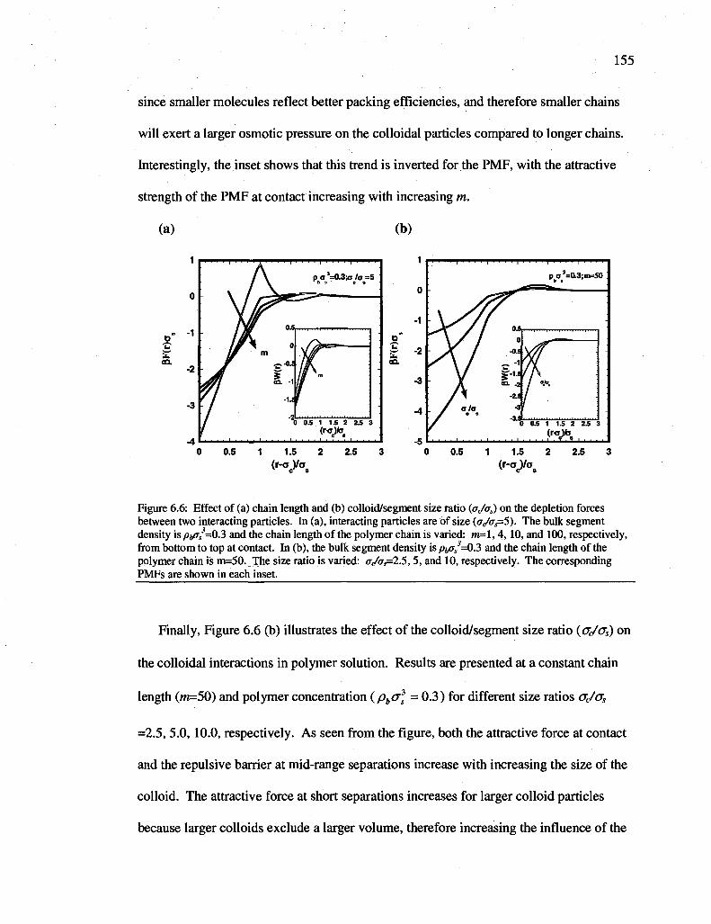
155

since smaller molecules reflect better packing efficiencies, and therefore smaller chains

will exert a larger osmotic pressure on the colloidal particles compared to longer chains.

Interestingly, the inset shows that this trend is inverted for the PMF, with the attractive

strength of the PMF at contact increasing with increasing m.

(a) (b)

Figure 6.6: Effect of (a) chain length and (b) colloid/segment size ratio (<T</<TJ) on the depletion forces between two interacting particles. In (a), interacting particles are of size (0/0^=5). The bulk segment density isp4ff/=0.3 and the chain length of the polymer chain is varied: w=l, 4,10, and 100, respectively, from bottom to top at contact. In (b), the bulk segment density is p^rs

3=Q3 and the chain length of the polymer chain is m=50. The size ratio is varied: oJos=25,5, and 10, respectively. The corresponding PMFs are shown in each inset.

Finally, Figure 6.6 (b) illustrates the effect of the colloid/segment size ratio (<rc/(Ts) on

the colloidal interactions in polymer solution. Results are presented at a constant chain

length (m=50) and polymer concentration ipbcr] = 0.3) for different size ratios cr</crs

=2.5, 5.0, 10.0, respectively. As seen from the figure, both the attractive force at contact

and the repulsive barrier at mid-range separations increase with increasing the size of the

colloid. The attractive force at short separations increases for larger colloid particles

because larger colloids exclude a larger volume, therefore increasing the influence of the

156

osmotic pressure exerted by the polymer solution on the outer walls of the colloidal

particles. Also, the probability of finding polymer segments in the region between

interacting colloids decreases with increasing colloid size, thus leading to a larger

attractive force. The increasing height of the repulsive barrier with increasing size ratio

reflects the greater tendency of the polymer to pack around the larger spheres. Similar

behavior is reflected in the inset for the PMF.

6.3.3 Second virial coefficient

In the previous section, it was illustrated that the polymer mediated colloid-colloid

force description can consist of attractive and repulsive regions. Such forces can compete

against one another to determine the stability of the colloidal dispersion. The colloid-

colloid osmotic second virial coefficient captures the net effect between such

competition. Using the iSAFT results for W(R), we compute the second virial coefficient

(Z?2) through the relation

B2 = -no] + In [" r2[l -exp(- 0W(r))] dr (6.34) 3 hc

where the first term is the hard-sphere contribution and the second term is the polymer

mediated contribution, respectively. Positive values of B2 indicate a stable colloid

dispersion (effective colloid-colloid repulsion), while negative values signify

destabilization of the colloidal dispersion (effective colloid-colloid attraction). It should

be noted that an accurate prediction for W(r) is essential in the calculation of B2, as

indicated by the integration of the quadratic term in eq. (6.34).

Figure 6.7 shows the density dependence of B2. Results from iSAFT are compared to

simulation and PRISM-PY data by Doxastakis et al.265 (m=16,120; aj as =4.9). In

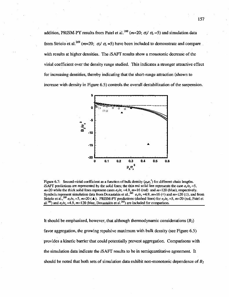
157

addition, PRISM-PY results from Patel et al.180 (m=20; aj as=5) and simulation data

from Striolo et al.269 (m=20; acl as =5) have been included to demonstrate and compare

with results at higher densities. The iSAFT results show a monotonic decrease of the

virial coefficient over the density range studied. This indicates a stronger attractive effect

for increasing densities, thereby indicating that the short-range attraction (shown to

increase with density in Figure 6.5) controls the overall destabilization of the suspension.

5

o

-5

V m

-10

-15

-20

0 0.1 0.2 0.3 0.4 0.5 0.6 b s

Figure 6.7: Second-virial coefficient as a function of bulk density ipyas3) for different chain lengths.

iSAFT predictions are represented by the solid lines; the thin red solid line represents the case ajas =5, m=20 while the thick solid lines represent cases ajas =4.9, m=l6 (red) and m=120 (blue), respectively. Symbols represent simulation data from Doxastakis et al.,265 ajas =4.9, m=l6 (o) and w=120 (•), and from Striolo et al.,269 ajas =5, m=20 (A). PRISM-PY predictions (dashed lines) for ajas =5, m=20 (red, Patel et al.180) and ajas =4.9, m=120 (blue, Doxastakis et al.265) are included for comparison.

It should be emphasized, however, that although thermodynamic considerations (fii)

favor aggregation, the growing repulsive maximum with bulk density (see Figure 6.5)

provides a kinetic barrier that could potentially prevent aggregation. Comparisons with

the simulation data indicate the /SAFT results to be in semiquantitative agreement. It

should be noted that both sets of simulation data exhibit non-monotonic dependence of #2

^ ^ ^ ^ ^ ^ ^ ^ ^ ^ ^ ^ ^ ^ ^ ^ ^ ^ ^ ^ ^ ^ ^ ^

^ ^ i ^ ^ ^ ^ ^ ^ ^ X ^ 1 • • • •

158

for the smaller chains considered (data for m=120 not available at higher densities). Still,

both iSAFT and simulations from Striolo et al.269 indicate a net attraction at higher

densities, although iSAFT does seem to underestimate this attraction (this is due to over

predicting the repulsive maximum of the PMF by i'S AFT at higher densities). In contrast,

results from PRISM-PY180'265 yield second virial coefficients that are positive for all

densities and become density independent at higher densities. This is consistent with

previous studies demonstrating PRISM-PY to be unreliable at higher densities (for all

chain lengths and size ratios) as B2 approaches the same finite limiting value (B2 /4).

Such behavior has been attributed to the poor performance of PRISM-PY in calculating

the potential of mean force (fails quantitatively and qualitatively at moderate to high

polymer concentrations).26'180 The performance of PRISM IET has been shown to yield

substantial improvements at moderate to high densities by employing a hyper-netted

chain (HNC) closure instead of the PY closure.23'24,26

While /SAFT indicates a decrease in the second virial coefficient as the chain length

is increased (from m=16 to m=120), the magnitude of this effect is not captured

quantitatively at very low densities (for m=120) in comparison to the simulation data.265

As discussed in previous sections, this may be attributed to iSAFT being based on TPT1,

resulting in the dilute and semidilute regimes of long chains not being described as

accurately. Still Bj decreases with increasing chain length, consistent with the simulation

and PRISM-PY results. Therefore colloids in solution of longer chains display a greater

propensity towards aggregation. This effect is again emphasized in Figure 6.8 (a). Here

B2 falls very rapidly for small m, but then appears to approach saturation for longer

chains. This is consistent with Figure 6.6 (a), which demonstrated a diminishing effect of

159

chain length on the effective force and an increasing attractive strength of the PMF at

contact with increasing chain length. Figure 6.8 illustrates the size ratio (oi/Os)

dependence of the colloid-colloid second virial coefficient (S2) as a function of (a) chain

length and (b) bulk polymer density. From the figure one sees that larger colloidal

particles encourage attraction and a greater tendency towards aggregation, especially at

higher concentrations, in accordance with the behavior in Figure 6.6 (b).

(a) (b)

DO

Figure 6.8: Second-virial coefficient for varying size ratios (a/as=2.5,5,7.5,10) as a function of (a) chain length and (b) bulk polymer density. In (a) the bulk density is constant atpbas

3=0.3, while in (b) the chain length is constant at m=20.

6.3.4 A preliminary study: Effect of attractive interactions

While the fundamental model provides valuable insight to nonadsorbing colloidal

suspensions, real polymer-colloid mixtures observed experimentally can involve

complicated (non-hard-core) interactions such as van der Waals attractions, Coulomb

forces, and/or specific polymer-particle attractive interactions. In such cases, the system

is no longer dictated by entropic effects exclusively, but also by enthalpic effects that can

influence the packing of polymer molecules at the surface of a particle. Fewer studies

have attempted to quantify the effects of including polymer-particle attractions. Hooper

et al.26 employed PRISM IET to investigate the effects of such attractions, capturing the

correct behavior in qualitative agreement with simulation studies.299'300 Recently Patel

and Egorov179 extended their density functional theory from the hard-core polymer-

particle system180 to the attractive polymer-particle system, investigating the case where

all non-bonded interactions were described by Lennard-Jones (LJ) potentials.

In this section, we test the ability of the /SAFT DFT to accurately describe attractive

polymer-particle mixtures. In this preliminary study, the structure of polymer molecules

near the surface of an attractive particle is compared with available simulation data299 to

study how the temperature and the nature of the interactions between the particle and

polymer matrix influence the behavior of the system. In this study all non-bonded

interactions are modeled using a truncated and shifted Lennard-Jones interaction

potential, similar to the simulation study by Bedrov et al.299 The polymer-particle

interactions can be represented by

vr«W =

r<Rcs

""(0-«eY(CX Rcs<r<C (6.35)

0, r>C

where Rcs is defined as before, Rcs ={ac-as)l2 ,r is the center-to-center distance

between a given polymer segment and the particle, and rc™' is the cutoff distance of the

LJ potential, set to r™' = 4.5crs (consistent with the simulations from Bedrov et al.299).

The LJ potential ufs (r) is given by eq. (6.29). Similarly, the interactions between

polymer segments are described

161

<(ru) =

£ss Uss Vss h

0,

°s < rn ^ rt

min

min

< r < rcut

^ M2 ^ 'ss

rn ^ rss

12

cut

(6.36)

where,

««foa) = 4*« fa.^

\rn J

12 (ay \rn J

(6.37)

and e^ is the molecular interaction energy between polymer segments, rs™' is the

position of the potential cutoff for the LJ potential taken to be rsc"' = 2.5as (consistent

with the simulations299), and the minimum of the potential is located at rmin=2mos. In the

previous work of Patel and Egorov,179 several methods of treating attractive

interactions 213,301,302 were tested to study the structure and nanoparticle interactions in

polymer-particle mixtures. Interesting results from their work indicated the simple mean-

field approximation provided the most accurate results, in quantitative agreement with

molecular dynamics (MD) simulations.299'300 Here we also employ the mean field

prescription to describe segment-segment attractive interactions using eqs. (6.10) and

(6.18). The temperature-dependent diameter (ds) is used to calculate the weighted

densities used in the hard-sphere and chain contributions to the free energy. The

temperature-dependent diameter of the polymer segments (ds) can be approximated

using 303

d = 1 +0.2977 (T*)

1 + 0.33163 (T*) + 0.00104771 {T *) 2 « (6.38)

where T* = kbT I ess.

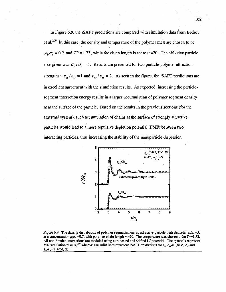
162

In Figure 6.9, the /SAFT predictions are compared with simulation data from Bedrov

et al.299 In this case, the density and temperature of the polymer melt are chosen to be

pbo\ = 0.7 and T* = 1.33, while the chain length is set to m=20. The effective particle

size given was ac\' as = 5. Results are presented for two particle-polymer attraction

strengths: ecs I ess =1 and scs I ess - 2. As seen in the figure, the j'SAFT predictions are

in excellent agreement with the simulation results. As expected, increasing the particle-

segment interaction energy results in a larger accumulation of polymer segment density

near the surface of the particle. Based on the results in the previous sections (for the

athermal system), such accumulation of chains at the surface of strongly attractive

particles would lead to a more repulsive depletion potential (PMF) between two

interacting particles, thus increasing the stability of the nanoparticle dispersion.

5

4

* 3

1

o

2 3 4 5 6 7 8 9

r/o s

Figure 6.9: The density distribution of polymer segments near an attractive particle with diameter ajas =5, at a concentration pyas =0.7, with polymer chain length m=20. The temperature was chosen to be r*=1.33. All non-bonded interactions are modeled using a truncated and shifted LJ potential. The symbols represent MD simulation results,299 whereas the solid lines represent /SAFT predictions for scs/ess=l (blue, A) and £ , ^ = 2 (red, • ) .

1 ' i ' '

I n n

E =2e CS 88

pbO9'=0.7,T*=1.33

m=20, o la =5

a n n q q g D P a a n a

(shifted upward by 2 units)

j>l|iift|'LAi ^ 1 1 * 1 ^ ^ |*| |ft| |ft| £ i jflt ^ 2^1 I

•MM*fek**^*JL

163

Previous work179 has indicated that increasing the temperature of the polymer

solution promotes destabilization of the colloidal dispersion. Interestingly, results

indicate the repulsive barrier formed at intermediate particle separations increases with

temperature for a weakly attractive system, and decreases with increasing temperature for

a strongly attractive system. The results presented in Figure 6.10 explain such behavior

by considering the temperature effects on the polymer-segment density around a single

isolated colloidal particle, first for a weakly attractive particle-polymer system (Figure

6.10 (a)), and then for a strongly attractive particle-polymer system (Figure 6.10 (Jo)). To

(a) (b)

*

111111111111 II111111111 M 1 1 I I 1 1 i i 1 1 i i i

Weakly attractive system e =0.0

po8=0.7

^ ^ ^ * * * * X * * r i a f c l * * * * J * r i

*

i i i .i I i i i i I i i i i I i i i i I i i i i I i i i i I i i i i I i i i i

Strongly Attractive System e =2e

Pb«;=o.7

m=20, o la =5 O 8

M M ^ * M I M M 1 M M I M M

5.5 6 6.5 7

r/o

3 3.5 4 4.5 5 5.5 6 6.5 7

r/o

Figure 6.10: The density distribution of polymer segments near an attractive particle with diameter ajas

=5, at a concentration/jfcff/=0.7, with polymer chain length m=20. The temperature is varied (T*=1.0, r*=1.33, and T*=3.33) for (a) a weakly attractive polymer-colloid system, and (b) a strongly attractive polymer-colloid system.

study temperature effects exclusively, again the density was chosen as pba] = 0.7, the

chain length was set to m=20, and the effective particle size was chosen as ac I as =5.

Different behavior is observed in each case. In Figure 6.10 (a), for the weaker interacting

system with ea = 0, an increase in T* increases the accumulation of polymer segments

near the surface of the colloid particle (thereby increasing steric stabilization). However,

in Figure 6.10 (b), for the strongly attractive system withfcs less = 2, an increase in T*

reduces the accumulation of polymer segments near the surface of the colloid (thereby

reducing steric stabilization).

Although, one can qualitatively visualize how the stability of a colloid dispersion is

affected with changing the nature of the polymer-particle interaction or with changing the

temperature (as briefly discussed above), a more complete study could be conducted on

the polymer-mediated forces involved in the above attractive systems. It would be

interesting to see how accurate the insertion-route (employed for the athermal polymer-

colloid system) would be in predicting the particle-particle interactions. The additional

perturbation of the mean field attraction may make the approach less accurate. As

mentioned previously in the chapter, the insertion approach is sensitive to the weight

functions and free energy expressions employed. Therefore, it may be necessary to use a

more sophisticated attraction term than the ones used in eqs. (6.10) and (6.18). Another

alternative approach is to calculate the depletion forces of interacting particles by brute

force.179 Of course, this approach requires a two-dimensional DFT and comes at a high

computational cost. Still, it would be of interest to understand completely the effects of

including attractive interactions in the system, including quantifying the competition

among contact aggregation, bridging effects, and steric stabilization.

6.4 Conclusions

In this work, we have demonstrated the ability of iSAFT density functional theory to

successfully describe the structure and effective force interactions in polymer-colloid

mixtures. A comprehensive comparison between theory and simulation was performed

165

for nonadsorbing mixtures, elucidating the roles of the broad parameter space involved in

such systems: the particle/polymer segment size ratio, polymer chain length and polymer

concentration.

For nonadsorbing polymer-colloid mixtures, the structure of polymers around a single

isolated particle was investigated under a wide range of conditions. The theory's

versatility was demonstrated under a tough test of conditions, from the nanoparticle limit

to the colloid limit in different concentration regimes. Under dilute and semidilute

concentrations, polymer segments are depleted from the surface of a particle. Here

iSAFT correctly captures a depletion layer on two different length scales, one on the

order of the segment diameter (semidilute regime), and the other on the order of the

polymer radius of gyration (dilute regime). The range of depletion is relatively

independent of the colloid size; however the total amount of depletion is dependent on

the particle size as the surface deficit increases with increasing particle size. At higher

concentrations, packing effects result in an accumulation of polymer segments near the

colloidal surface. In this concentration regime, the effect of particle size and chain length

on the density distribution of polymer segments diminishes significantly.

The theory captures the main characteristics of the polymer induced depletion

interaction between colloidal particles, quantifying the effects of polymer density,

polymer chain length, and particle/polymer-segment size ratio. Increasing the

concentration of the polymer solution encourages the particle-particle attractive force at

contact to increase, while decreasing the range of depletion attraction. Further, at high

concentrations a repulsive barrier can form at intermediate separations. Increasing

polymer chain length decreases the strength of the attractive force at contact, while

increasing the range of the depletion attraction. Both the attractive force at contact and

the repulsive barrier at mid-range separations increase with increasing the size of the

colloid.

The /SAFT results indicate the colloid-colloid second virial coefficient to decrease

monotonically with increasing the polymer density, thereby indicating that net repulsion

between colloids at low polymer densities gives way to net attraction at higher densities.

The net attraction predicted at higher densities is in agreement with available simulation

data.269 Further, the second virial coefficient decreases with increasing polymer chain

length and/or increasing colloid size. Such effects indicate a higher tendency towards

colloidal aggregation for larger colloids in solutions of longer chains.

Finally, a preliminary study was conducted for an attractive polymer-colloid system,

demonstrating excellent agreement between the /SAFT predictions and available

simulation data. In such a system, the fluid structure and behavior are no longer dictated

by entropic effects exclusively, but also by enthalpic effects. Calculations were

performed to quantify how the structure of polymer near a colloidal particle is affected by

the temperature and the nature of the polymer-colloid interaction. Results suggest that

increasing the particle-polymer attraction strength stabilizes the dispersion, as indicated

by the aggregation of polymer segments to the surface of the particle. Previous work179

has demonstrated that increasing the temperature of the polymer solution promotes

destabilization. Still, it is interesting to note that the repulsive barrier formed at

intermediate particle separations increases with temperature for a weakly attractive

system, and decreases with increasing temperature for a strongly attractive system. The

preliminary results presented in this chapter explain such behavior by considering the

167

temperature effects on the polymer structure around an isolated colloidal particle. An

increase in temperature increases the accumulation of polymer segments near the surface

of a colloid particle in a weak attractive polymer-colloid system (thereby increasing steric

stabilization), whereas the opposite behavior is observed for the stronger interacting

system. A more complete study could be conducted for the attractive polymer-colloid

system to investigate the polymer mediated forces involved as well as the colloid-colloid

second virial coefficient, to quantify the competition among contact aggregation, bridging

effects, and steric stabilization.

168

CHAPTER

An I'SAFT density functional theory for associating polyatomic molecules

7.1 Introduction

Unfavorable interactions between unlike species play an important role in the phase

behavior and microstructure of polymer systems, often leading to self-assembly of novel

nano-structures or to undesirable macrophase separation in polymer blends. In recent

years, macromolecules containing functional groups capable of forming reversible

noncovalent bonds (via hydrogen bonding or ionic interactions) have attracted much

attention from both experimentalists and theoreticians. The introduction of hydrogen-

bonding or ionic interactions found in such associating macromolecules are important to

the field of self-organizing soft materials, providing self-assembling mechanisms for a

polymer blend that can potentially lead to the production of new, highly functional

polymeric materials. Because of the reversible nature of such components, temperature

can be used to control molecular connectivity, and hence the phase behavior (polymer-

polymer miscibility, macrophase separation, and the self-assembly into mesostructures)

and the unique material properties (physical properties and processability) of the system.

Current and potential applications where such technology can be utilized include

biosensors, separation devices, controlled drug delivery,304 thermal manipulation of the

169

viscosity,305 and the development of "smart materials" with novel chemical, electrical,

mechanical, and optical (light emitting) properties,306"314 where the functionality of the

material can be switched on and off via temperature controlled phase transitions.

Experimental studies have provided many insights into associating polymers (e.g.,

surfactants, oligomers, copolymers, and biomolecules). Given the right conditions, or the

right balance between the association forces and repulsive forces between polymer

segments, experiments have observed some interesting phase behaviors and material

properties. For example, the design of supramacromolecules varying in size and

architecture (linear, comb, star, etc.) derived from hydrogen bonding has become an area

of great interest in macromolecular science, due to the interesting morphologies and

physical properties present in such systems. " Xiang et al. investigated AB and CD

copolymers blended in good solvent and demonstrated how micellar aggregates can form

in solution when B and D are able to interact via hydrogen bonding interactions.

Ruokolainen and coworkers312 demonstrated how hydrogen bonding interactions can

control functional properties and lead to hierarchical structural formation in block

copolymer/low molecular weight associating polymer blends (microphase separated

lamellar morphology, re-entrant closed loop macrophase separation, and high

temperature macrophase separation). Pan et al.316 investigated hydrogen bonding AB/CD

diblock copolymer blends and observed three phase structures, and Asari et al.306"308

demonstrated how block copolymers (blends of diblock/diblock and diblock/triblock

copolymers) can self-assemble into several complex Archimedean tiling patterns in the

bulk via hydrogen bonding interactions. In addition, many applications of these materials

involve interactions with solid surfaces or colloidal particles and in confined geometries

(adhesion, lubrication and friction, nanocomposites, blood flow and drug delivery, etc.).

For this reason, a number of experiments have also investigated associating polymer

solutions or melts in confined geometries and near surfaces, measuring the polymer

mediated forces involved. The aforementioned experimental studies are just a few

examples of how associating/hydrogen bonding polymers can form complex molecular

architectures, interesting phase transitions, and unique self-assembled patterns and

microstructures. Unfortunately, although valuable, results from such studies are often

confined to the specific system studied, leaving many unanswered questions.

Theoretical models will, without a doubt, play an important role in understanding and

aiding the experimental design of more complex systems due to their ability to cover a

wide parameter space that characterizes the polymer architectures and molecular weights,

chemical incompatibilities, and bonding strengths between associating species in

multicomponent polymer mixtures. One of the early theories for reversible bonding was

developed by Tanaka and coworkers,322'323 who used the random phase approximation

(RPA) to study the microphase and macrophase separation transitions in systems of

supramolecular diblock and comblike polymers. A shortcoming of the theory is its

inability to examine the mesophase structure and stability since the free energy of the

ordered microstructure is not considered (limited to investigating the stability of

'X'yA "SOS

homogeneous phases). Later, ten Brinke and coworkers ' were able to examine the

mesophase structure and stability for graft and diblock copolymer systems using a higher

order RPA, although the model is very laborious and restricted to the weak segregation

limit. More recently, Feng et al.326 and Lee et al.327 have recast the field-theoretic

description of supramolecular polymers to handle all segregation strengths, applying the

171

numerical self-consistent field theory (SCFT) within this framework to investigate the

self-assembly of associating supramolecular polymers. Unfortunately, mean field

theories and SCFT are not accurate in describing cases of macromolecules near solid

surfaces or in confined nanoslits,21,22 where local density fluctuations and liquid-like

ordering play a significant role. Molecular simulations have played an important role in

the investigation of associating polymers for problems related both in the bulk " and

in confined geometries.334"336 However, due to the overwhelming amount of information

that is retained in these computations, simulations can become computationally

expensive, especially when considering supramacromolecules composed of long

polymeric chains. Despite the success of all the aforementioned theoretical work, it is

desirable to have a theory that is computationally efficient and capable of investigating

associating polymer systems at any segregation strength and fluid density, as well as

capable of providing structural and thermodynamic information not only for bulk

microstructures, but also for fluids near surfaces or in confined environments, which are

important to many applications, as mentioned previously.

Recently, density functional theory (DFT) has emerged as a powerful theoretical tool

to investigate inhomogeneous polymer systems.27 Density functional theory is a tool with

a statistical mechanics foundation that includes more physics than mean field theories and

SCFT, retaining statistical segment length-level information rather than a coarse-grained

representation of the polymers, at an expense significantly lower than simulation

methods. As mentioned, mean-field theories and SCFT neglect fluid fluctuations that

become especially important near surfaces and in confined environments.21'22 Density

functional theory, on the other hand, is formulated in the grand canonical ensemble where

172

the fluctuations in the number of polymer chains in the system maintain a constant

chemical potential. Therefore, the system is compressible and phase transitions can

include fluctuations in the density of the system, which is key especially near surfaces

and in confined environments, where packing effects become important.

Chapman12 was the first to suggest that Wertheim's first order thermodynamic

perturbation theory (TPT1)4"7 free energy could be used naturally within a DFT

formalism for inhomogeneous associating fluids. The first DFT for associating fluids

within this framework was developed by Segura et al.,29 who described associating

atomic spheres near a hydrophobic hard wall. Segura et al.29 introduced and successfully

demonstrated two approaches to include intermolecular association between atomic

species. The first applies an association free energy functional based on Wertheim's

TPT1 as a perturbation to a reference fluid functional, while the second approach

approximates the association free energy functional using the bulk equation of state at an

effective density. The second (and more simple) approach has been applied with great

success by numerous groups using various local or weighted density formalisms to study

structure, phase behavior, and interfacial properties of associating atomic fluids (both in

confined environments and at vapor-liquid and solid-liquid interfaces).29"31'168'177'178 The

developments in density functional theory have lead to the advancement of our ability to

understand and investigate complex polymer systems. More recently the second

approach of Segura et al. has been extended to associating polyatomic fluids, specifically

to study the structure of associating molecules at liquid-vapor interfaces,95'337"339 in slit-

like pores, and at solid surfaces. In these studies, simple association schemes were

adopted based on the appropriate bulk free energy expressions for a polymer segment

173

with one association site. Such an approach, using the bulk free energy due to

association, is dependent on the accuracy of the weighting functions used and may not

produce the correct free energy in the limit of strong association.

In this chapter, we introduce an extension to the interfacial statistical associating fluid

theory (iSAFT)32 for associating polymer systems. The /SAFT density functional theory

is an extension to TPT1, where the contribution to the free energy due to chain formation

is derived from the inhomogeneous free energy for association for a mixture of

associating spheres, taken at the complete bonding limit. The theory has already been

successfully applied to study a wide range of complex polymer systems. Tripathi and

Chapman33'34applied iSAFT to study polymer melts, solutions, and blends confined in

slit-like pores and Dominik et al.165 applied the theory to real systems, calculating

interfacial properties of n-alkanes and homopolymers. Recently, an extension of /SAFT

was introduced by Jain et al.32 that corrects approximations in the original theory and

extends the theory to complex heteronuclear systems. For heteronuclear systems, iSAFT

has been applied successfully to investigate block copolymers in confinement192 and near

selective surfaces,32 tethered polymers,193 and polymer-colloid mixtures.195 The work in

this chapter for associating polymers is based on Segura et al.'s work for associating

spheres, where the first approach of Segura et al. (using the inhomogeneous form of the

association functional) is extended to polyatomic molecules. This approach is consistent

with the iSAFT approach for chains, reducing exactly to the iSAFT chain functional in

the infinite bonding limit. The resulting free energy expressions that are derived are

capable of modeling complex associating systems, where the full range of association can

174

be investigated for any association scheme (for molecules having any number of

association sites on any segment along a polymer chain).

In the next section, the iSAFT approach is presented and discussed, along with the

new theoretical developments for associating chains. In section 7.3, we demonstrate the

applicability of the theory to associating polymers through various examples. The ability

of the theory to handle associating polymers near surfaces and in the bulk will be

demonstrated over a wide range of conditions. Further, the importance of such a theory

will be elucidated through the complex behaviors observed for even the simple

associating molecules chosen in tins study, including the thermal reversible nature of

forming larger supramolecules and molecules with complex architectures, and the

resulting effect on the structure and phase behavior of the fluid (2 phase macroseparation

and microphase separated lamellar morphologies, and reentrant order-disorder transitions,

as observed by experiments). Finally, concluding remarks are discussed in section 7.4.

7.2 Theory

7.2.1 Model

The objective of this work is to study the full range of association for a fluid mixture

composed of associating, fully flexible polymer chains. Each chain consists of m

tangentially bonded spherical segments, where any number of association sites can be

placed on any segment along the chain. For simplicity, in this work all the segments have

the same diameter a, although the theory is capable of defining each segment to be

different. Here we consider linear chains, but the theory can also be applied to

associating branched chains (for the theoretical formulation for branched chains, the

reader is referred to the work by Jain and Chapman194). The polymer segments can

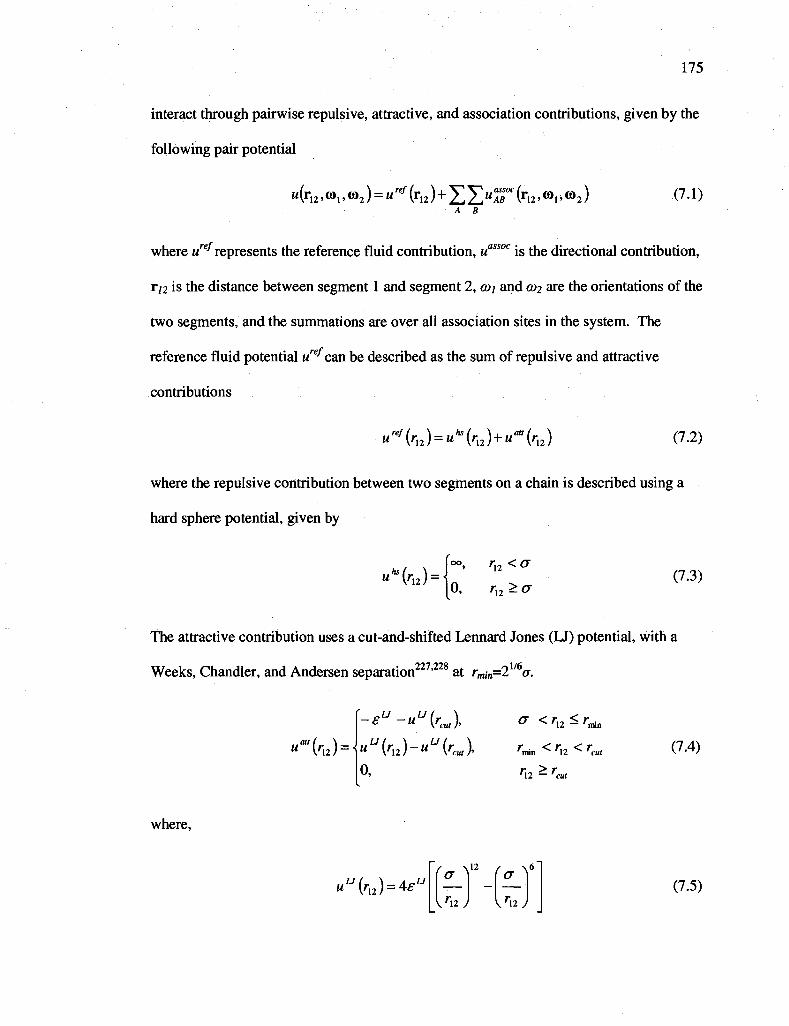
175

interact through pairwise repulsive, attractive, and association contributions, given by the

following pair potential

M(r12.,a»I,m2) = ii^(r1 2)+22«^0 C .(f1 2 ,a) l i©2) (7.1) A B

where uref represents the reference fluid contribution, uassoc is the directional contribution,

r/2 is the distance between segment 1 and segment 2, a>i and a>2 are the orientations of the

two segments, and the summations are over all association sites in the system. The

reference fluid potential wre/can be described as the sum of repulsive and attractive

contributions

«"{ra) = H*{ra) + u~{ra) (7.2)

where the repulsive contribution between two segments on a chain is described using a

hard sphere potential, given by

«fa(r12) = |oo, rn<a

0, rn>a (7.3)

The attractive contribution uses a cut-and-shifted Lennard Jones (LJ) potential, with a

Weeks, Chandler, and Andersen separation227'228 at rm,„=21/6<r.

um(ra) =

-eu-uu{rcut),

uu{rn)-uu{rcut),

o,

° <ri2^rBia

rmin < rU < rcut

ru * rcu,

(7.4)

where,

u»{rn) = Ae» (* V2 ffT \

\rn J \rnJ (7.5)

176

where su is the molecular interaction energy and rcut is the position of the potential cutoff

for the LJ potential, taken to be rCHf=3.5<7. Any segment along a chain can have multiple

association sites capable of interacting with other sites on other polymer segments. The

association contribution (important to the iSAFT chain functional and the full range

association functional) is modeled via off centered sites that interact through a square-

well potential of short range rc. The interaction between site A on one segment and site B

on another segment are modeled using the following association potential,

UAB \VX2^X^2)-\n , . ( 7 - 6 )

[0, otherwise

where OAI is the angle between the vector from the center of segment 1 to site A and the

vector Tn, and 9B2 is the angle between the vector from center of segment 2 to site B and

the vector r/2, as illustrated previously in Figure 5.2. Of course, only bonding between

compatible sites is permitted (two incompatible sites A and B have a bonding energy of

zero, e™g0C = 0). The radial limits of square-well association were set to rc=1.05crand

the angular limit to 0C=27°.

In addition to the pair potential between segments, an additional external field may be

imposed on the system. In this work, results are presented for both bulk fluids and fluids

near a hard surface. The external field introduced into the system by the hard wall is

given by

Vex,{z) =

where z is the distance normal to the surface.

a z< —

2 (7.7) 0, otherwise

177

7.2.2 iSAFT density functional theory

The density functional theory is formulated in the grand canonical ensemble, which

has a fixed volume (V), temperature (7), and chemical potential (//). The starting point of

the density functional theory is the development of an expression for the grand free

energy, Q, as a functional of the equilibrium polymer density profile p(r). From this, the

desired thermodynamic and structural properties of the system can be determined. In this

work, we consider associating fluid mixtures composed of polymeric components (Ci,

C2,...C„). The grand free energy can be related to the Helmholtz free energy functional

A[p(r)] through the Legendre transform,13

^kC1)(r),A(C2)(r),..]=AU(C1,(r),A(C2)(r),.J

^ r , . <„,,! „ „ / . * \ (7-8) X EK^'HrOk-^lr1)) /=C1,C2... 1=1

where /?/" (r) is the density of the ith segment on chain / at position r, pit/ is the chemical

potential of that segment, and V^ is the external field acting on that segment. The first

summation is over all chains I in the mixture (Cj, C2,...C„), and the second summation is

over all segments on chain /. Since j'SAFT is a segment-based DFT that treats each

segment differently, we can simplify this notation by combining these two sums to an

equivalent sum over all segments (TV) in the system, where N = mci+mC2+-~mcn- At

equilibrium, the following condition is satisfied

SO,

SPi (') = 0 V i = l , A T (7.9)

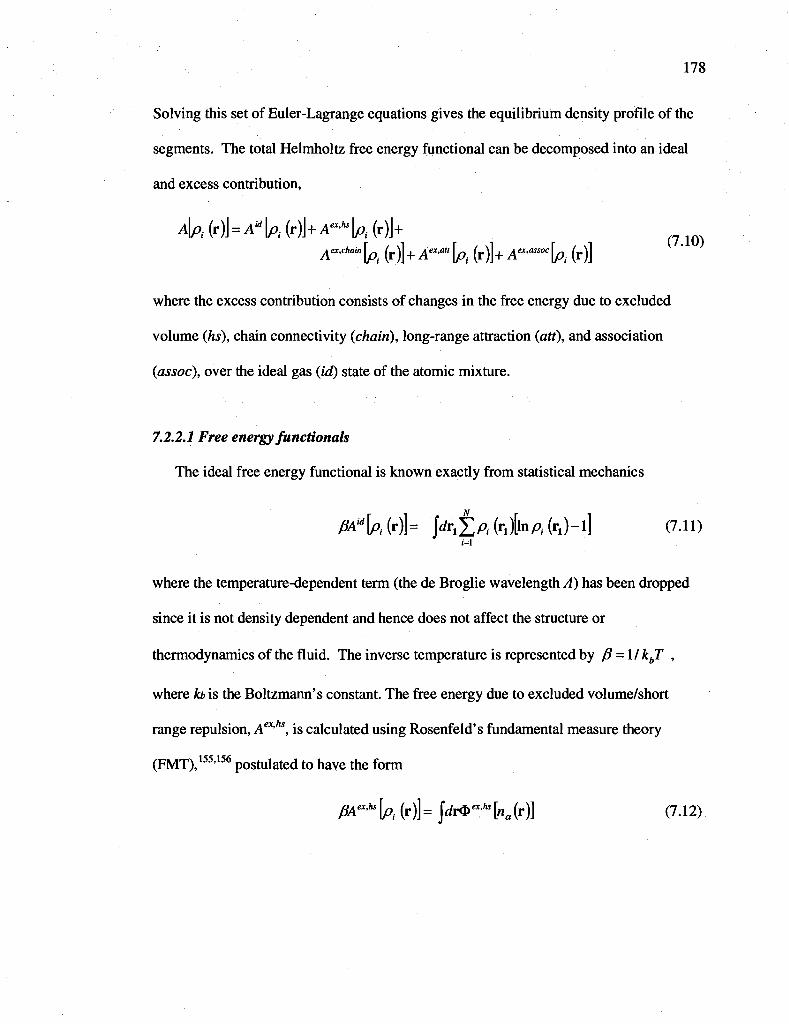
178

Solving this set of Euler-Lagrange equations gives the equilibrium density profile of the

segments. The total Helmholtz free energy functional can be decomposed into an ideal

and excess contribution,

Ap, (r)J = A* U (r)J+ A ^ \ p t (r)J+ Aex,chain ^ ( f ) ] + £v* ^ (f j ]+ ^ x , ^ ^ (,.)]


volume (hs), chain connectivity (chain), long-range attraction (att), and association

(assoc), over the ideal gas (id) state of the atomic mixture.

7.2.2.1 Free energy functionals

The ideal free energy functional is known exactly from statistical mechanics

A4"U(r)]= J A k Z A f c t n ^ f e J - l ] (7.11)


since it is not density dependent and hence does not affect the structure or

thermodynamics of the fluid. The inverse temperature is represented by /? = 1/ kbT ,

where h is the Boltzmann's constant. The free energy due to excluded volume/short

range repulsion, Aex'hs, is calculated using Rosenfeld's fundamental measure theory

(FMT),155156 postulated to have the form

0AaJU\p, (r)]= jdr<!>exhs[na{r)] (7.12)

179

where &aJa[na(r)] is the excess Helmholtz free energy density due to the hard core

interactions. ^"''"[naCr)] is assumed to be a function of only the system averaged

fundamental geometric measures, na (r), of the particles, given by

».(') = I Z»..W = Z/A(riVi ( a ,(r-r> I (7.13) /=C1,C2,... i=l 1=1

where a = 0,1, 2, 3, VI, V2, representative of the six scalar and vector weight functions

used in Rosenfeld's formalism.155,156 In the FMT formalism, <3>exhs [na(r)] has the form

a»--^nJr)] = - n 0 l n ( l - n 3 ) + " 1 " 2 - n - ' - n - +W 2 3 J 3 " ^ ; 2

1 1 - 2 (7.14) l - n 3 24^(1-n3)

The free energy due to long-range attraction can be included within the mean field

147

approximation

A - f l " U ( r ) ] = | i Z jrfr1c/r2Ml°ir2-r1|)A(r1)p;.(r2) (7.15) '=' M |r2-r, XT„

The association functional was originally developed by Chapman12'29 by extending TPT1.

Below the association functional is given for an associating polyatomic mixture

/il"*~h(r)]= jAiiXii) X f to2 i ( r , ) - ^ + l (7.16) =i iier*"

The first summation is over all segments (on all chains in the mixture) and the second

summation is over all the associating sites on segment i of chain /. x\ (ri) represents the

fraction of segments of type i which are not bonded at their site A. This fraction

unbonded is given by

180

\ (7.17)

1+ \dr2^pk{r2) 2>B(r2)A'*B(r„r2) k=\ B e r ( "

The degree of association is controlled by the term

A'L(r1,r2) = 4 e x p ^ ^ ) - 1 t ' 1 r i ' r 2 ) (7-18)

Here K represents a geometric constant (accounts for the entropic cost associated with the

orientations and bond volume of the associating segments), £™*°Bck is the associating

energy between compatible sites A and B on segments i and k, and y'k (rt, r2) is the cavity

correlation function for the inhomogeneous hard sphere reference fluid. The cavity

correlation function can be approximated using its bulk value72 evaluated at contact using

a weighted density33'34

y*fa2,«i,r2)« {o^MW^MV <7-19)

where pj (r,) represents the weighted density of segment j at position ri. In this work,

the simple weighting is used

?>')=i^L~ "'^ <7-20)

It has already been demonstrated how the association free energy functional based on

Wertheim's first order thermodynamic perturbation theory can be used in the limit of

complete association to form a polyatomic fluid (tangentially bonded chains) from a

mixture of associating spheres. ' ' In this chapter we demonstrate how, starting from

the same form of the inhomogeneous association free energy functional, the full range of

181

association can be investigated. When deriving the chain contribution to the free energy,

eassoc-> oo and an additional bonding potential vfond (r,, r2 )for tangentially bonded

segments is included in the above expression.32"34'165'193'195

7.2.2.2 Free energy functional derivatives

All the functional derivatives are essential in solving the Euler-Lagrange equations

(from eq. (7.9)), which give the density profile. The functional derivative of the free

energies are given

' | ^ v = l n p , ( r ) (7.21)

gpr* _ , • » - » [ n , . ( r , ) ] s ( \ ~ |«ri J—T\ (722>

exfitt N

f ( ^ = |i,K*,Klr-.lk(0 (7.23)

^Z - IlnziW-itl! U , ^ P * , (7.24)

In the above chain functional derivative, all association sites considered in this expression

are representative of the sites responsible for the molecular connectivity of the chains in

the mixture, which are formed by applying the limit of complete association ({k'} is the

set of all segments bonded to segment k on chain /). Details regarding the above

functional derivatives are given in earlier works. ' ' Below, the functional derivative

for the full range of association is given. Details of this derivation can be found in the

Appendix.

182

/=1 *=1 4er" * y ( r ) .

The above expression is the final form for associating chains. The term

(7.25)

only contributes for segments k with association sites that are eligible to bond to sites

located on segment i. Substituting the functional derivatives of the free energies in the

Euler-Lagrange (eq. (7.9)) allows for the solution of the equilibrium density profile of the

polymer segments. For complete details of the density profile expressions, the reader is

referred to previous work32'193195 and chapter 6 (section 6.2.3).


The primary focus of this section is to establish the capability of the theory to handle

a wide range of associating polymer systems. In this section, results are presented for

associating mixtures near surfaces and in the bulk, over a wide range of conditions in

comparison with available simulation and experimental data. The associating schemes

and mixtures investigated in this work are illustrated in Figure 7.1. First the theory is

validated near a hard wall, illustrating the effect of varying the association strength on the

behavior of the fluid (neglecting dispersion interactions). Next, an associating mixture is

considered at high association strengths, showing how different association schemes can

result in complex molecular architectures or supramolecules (see Figure 7.1 (b)). These

results are compared and agree very well with available simulation results for a star

polymer confined between two hard surfaces from Yethiraj and Hall.341 Finally, the

183

theory is demonstrated for a challenging problem of interest, a bulk associating mixture

of two homopolymers with end functional segments capable of reversibly bonding to

form supramolecular diblock copolymers. For this system, we systematically explore the

phase diagram, demonstrating how competing effects (chain length, chemical

incompatibilities, and bonding energies) can result in unique polymer morphologies

(microphase lamellar separation, two phase macrophase separation) and complex phase

behavior (regions of reentrant order-disorder transitions in the phase diagram, as

observed in experiments). These examples elucidate the ability of the theory to correctly

model and capture the complex fluid behavior for associating polymer systems. Such a

theory is important to the understanding and development in many problems and

applications (discussed in the Introduction) where temperature can be used to control the

reversible bonding, phase behavior, and material properties of the system.

Figure 7.1: Illustration of associating schemes used in this work: (a) end associating functional groups (terminal associating segment with one site) and (b) schemes capable of forming a star polymer architecture (3 arms, N=16) at high association strengths.

7.3.1 Associating polymers near a wall

First, we apply the proposed theory to a simple model of associating molecules and

investigate the structure of the fluid near a hard surface. As discussed previously in

section 7.1, there are two approaches to include association. The inhomogeneous

approach (the proposed approach, outlined in section 7.2) and the weighted approach

(included below) are compared in Figure 7.2. The second approach approximates the

association free energy functional using the bulk equation of state evaluated a weighted

density

>\P,(T)]= fatnMZ [**zM-^+± (7.26) i=l Aer(" 2

V J

where the fraction of segments of type i which are not bonded at their site A is given by

X-A (r,.) = — — 1 + Z Pk (r2) Z XB (r2 )A'L fo, r2) (7.27)

and A^fo . r J is defined as before in eq. (7.18). The accuracy of the weighted approach

is dependent on the weight functions used. For comparison, the same weighted density

used in the calculation of the cavity correlation function in eqs. (7.19) and (7.20) is used

in the second approach. The functional derivative can be found in previous work.31

Figure 7.2 captures the effect of varying the association strength on the structure of a

pure associating fluid near a hard wall. Depletion from the surface is captured at low

concentrations, while packing effects increase the accumulation of segments at the

surface at higher densities (dispersion interactions are neglected here, e"=0). In Figure

7.2 (a), the simple case of a dimerizing hard sphere fluid is presented at pb<f '=0.1999 and

185

eassoc/kbT=14 (right vertical axis), and at pb(/=0AS6S and easS0C/kbT = 11 (left vertical

axis), in comparision with simulation data.30 From these results, it is clear that at lower

densities and high association energies, the weighted approach is unable to capture the

correct structure of the fluid even qualitatively (these results are consistent with the

results found previously by Segura et al.30 using the Tarazona152'153 weight functions). In

contrast, the inhomogeneous form provides a more accurate expression for the free

energy of association and is able to capture the correct structure of die fluid at these

conditions. At higher densities, the weighted approach is much improved, however the

inhomogeneous approach is still superior and in better quantitative agreement with the

simulations. In Figure 7.2 (b), the model assumes a pure homopolymer (m=4) where a

(a) (b)

2.5

2.0

§ 1.5

1.0

' I ' I

Assa i l

i , i

• i i i i i *

j , pbo'=0.1999

6e"~=14

pbos=0.4868-

Pe""°=11 .

1.5

1.0

- 0.50

0.75

0.50 '—'—i—•—'—•—'—'—'—'—'—'—' 0.0 0.50 1.0 1.5 2.0 2.5 3.0 3.5

z/a

0.50

0.25

Figure 7.2: Effect of varying bonding strength (e"11"0) on the structure of an associating fluid (associating scheme from Figure 7.1 (a)) near a smooth hard surface. Here dispersion interactions are neglected, £"=0. Lines represent theoretical results using the inhomogeneous association free energy functional (solid lines) and the weighted bulk form association free energy functional (dashed lines, provided for comparison at highest association energies). In (a), a dimerizing hard sphere fluid is presented at/)jtfJ=0.1999 and pe°s*>c_n ( r i gn t v e r t i c a i axis^ a n d at ^ = 0 . 4 8 6 8 and pdasoc= 11 (left vertical axis). Symbols represent simulation data.30 In (b), the structure of an associating polymer fluid (m=4) is presented atpi/^=0.2 (right vertical axis) and p^'=0.5 (left vertical axis). Here, symbols represent results for a nonassociating 4mer (0) and 8mer (•).

186

a single association site is located on one of the terminal segments of the chain and is

able to bond with other chains in the fluid (see the association scheme presented in Figure

7.1 (a)). In Figure 7.2 (b), the symbols represent iSAFT results for a nonassociating 4mer

(0) and 8mer (•), while the lines represent /SAFT results for the associating 4mers. The

weighted approach is included for comparison at the highest association strengths

(dashed lines). In Figure 7.2 (b), the results indicate that both approaches capture the

correct behavior at high and low densities for associating chains, though there are some

minor quantitative differences (hard to distinguish in figure). Such results suggest that

the weighted approach may be sensitive to the concentration of associating segments in

the system. In this example, as the chain length increases, the effect of association

decreases and the concentration of bonding segments in the fluid decreases, scaling as

1/m. In comparing parts (a) and (b) of Figure 7.2, both approaches are accurate for lower

concentrations of associating segments (Figure 7.2 (b)), but give inaccurate structure

under certain conditions (high association strengths at lower densities) for systems with a

higher concentration of associating segments (Figure 7.2 (a)). All remaining results

presented are therefore based on the inhomogeneous form of the association functional,

because of its versatility and ability to handle any association scheme, especially for more

complex heteronuclear systems that may involve many associating segments. From

Figure 7.2 (b), as expected, the behavior of an associating linear chain (with one

associating site on a terminal segment) varies between that of a nonassociating chain of

the same length (in this case a 4mer) and that for a nonassociating chain twice as large

(8mer). When the association energy is low (eassoc/ki,T=Y), the profiles are similar to the

nonassociating 4mer. As the association energy increases, the concentration of 8mers in

the mixture also increases and approaches the behavior of a pure nonassociating 8mer.

Higher association energies result in higher concentrations of longer chains, which lead

to lower contact densities at the surface due to conformational entropic effects.

Of course, more involved association schemes, where the polymer molecule may

involve multiple associating segments and/or multiple sites, can lead to more complex

polymer architectures (at high association strengths). Figure 7.3 demonstrates such an

example, again considering only association interactions. Here we consider a polymer

mixture using any of the schemes presented in Figure 7.1 (b). High bonding strengths

(results in Figure 7.3 use eassoc/kbT>30) create a large population of star polymers (3 arms,

N=16) in the melt, so that we are able to compare the structure of the fluid confined

between two hard surfaces (separated at distance H=l6a) with available simulation data

by Yethiraj and Hall.341 The agreement between the theory and the simulation results are

- i 1 1 1 1 1 r 1 1 1 1-

f

2.0 t-

1.5

1.0

0 . 5 0

0.0

, ° 1 =01 awg

J 1 l_

0 . 5 0 1.0 1.5 2.0 2.5 3.0 3.5

z/o

Figure 7.3: The density distribution of a star polymer (3 arms, N=16) between two hard walls separated at a distance H=\6a (profile only given near one wall) at 7/^=0.3, 0.2, and 0.1. A high population of star polymers is formed in the melt at high bonding strengths (e.g., fieassoc=30) using any of the association schemes given in Figure 7.1 (b). Symbols represent simulation data from Yethiraj and Hall341 and lines represent results from /SAFT. The density profiles are normalized to the bulk value.

188

good, capturing the competition between packing and entropic effects at different average

packing fractions (rjavg) of the fluid in the confined space. Symbols represent simulation

data, while solid lines represent iSAFT results. In the figure, the density profiles are

normalized to their bulk value (/?&). Because the profiles are symmetric about the middle

of the confinement, only the profiles near one of the surfaces are shown. In our model,

the concentration of star polymer formed in the melt, and thus the fluid structure at the

surface, can be controlled by the temperature (or varying reversible bonding energy).

Differences in the contact density can be attributed to inaccuracies in the bulk equation of

state (which over predicts the pressure). Even more complex association schemes can be

applied to multicomponent mixtures to form star and comb polymers with arms of

arbitrary lengths.

In this section, the ability of the /SAFT DFT to capture compressibility effects and

the local structure of associating macromolecules near surfaces and in confined

environments was demonstrated. Future studies using iSAFT could provide interesting

insights into some of today's more challenging problems involving associating polymers

near surfaces and in confined environments, including lubrication and friction, adhesion,

nanocomposites, blood flow and drug delivery.

7.3.2 Self-assembly of associating polymers into inhomogeneous phases

In this section, we consider a binary mixture of two homopolymers of equal

concentrations and chain lengths. Homopolymer C; is assigned one association site (site

A) on a terminal bead (see association scheme Figure 7.1 (a)) that is allowed to reversibly

bond to a similar site (site B) on the other component in the mixture (C2). All systems

considered in this section have a melt-like, total segment density of pb<f =0.85. In this

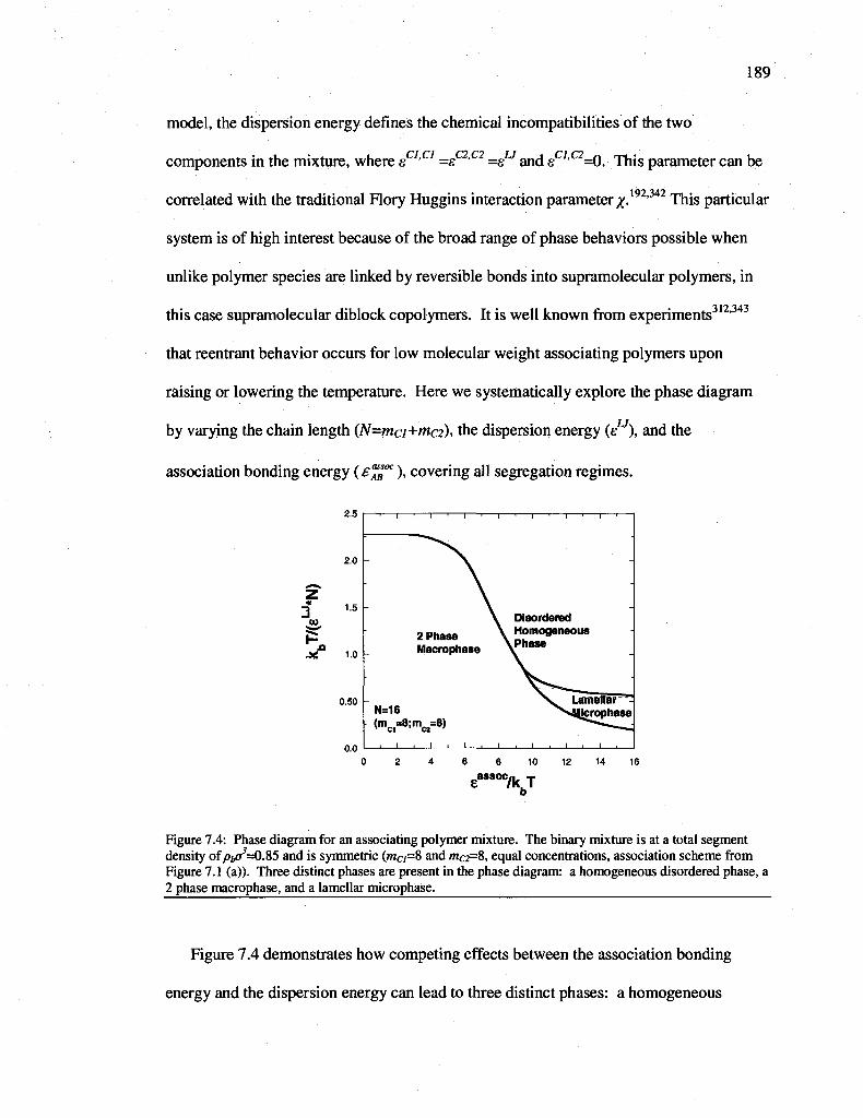
189

model, the dispersion energy defines the chemical incompatibilities of the two

components in the mixture, where scl'cl =eC2,C2 =eu and ecl,C2=0. This parameter can be

correlated with the traditional Flory Huggins interaction parameter/.192'342 This particular

system is of high interest because of the broad range of phase behaviors possible when

unlike polymer species are linked by reversible bonds into supramolecular polymers, in

this case supramolecular diblock copolymers. It is well known from experiments312'343

that reentrant behavior occurs for low molecular weight associating polymers upon

raising or lowering the temperature. Here we systematically explore the phase diagram

by varying the chain length (N=ma+mc2), the dispersion energy (eu), and the

association bonding energy (f^soc), covering all segregation regimes.

2.5

2.0

1.5

1.0

0.50

0.0

"1 ' I ' I ' I ' T ' I ' V

N=16

<mc,=8;mc2=8>

2 Phase Macrophase

Disordered Homogeneous

k Phase

6 8 10 12 14 16

e a s s o c / k T

b

Figure 7.4: Phase diagram for an associating polymer mixture. The binary mixture is at a total segment density of pyt/-0.%5 and is symmetric (/nC/=8 and /nC2=8, equal concentrations, association scheme from Figure 7.1 (a)). Three distinct phases are present in the phase diagram: a homogeneous disordered phase, a 2 phase macrophase, and a lamellar microphase.

Figure 7.4 demonstrates how competing effects between the association bonding

energy and the dispersion energy can lead to three distinct phases: a homogeneous

190

u

disordered phase (where Ci and C2 are miscible), a macrophase separation (liquid-liquid

immiscibility), and a microphase lamellar separation. From the figure, low dispersion

energies (low degree of incompatibility between the two components) and low

association energies lead to a homogeneous disordered phase (DIS). Upon increasing e'

at low association energies, a phase transition from the disordered state to a macrophase

separation (2 phase) occurs. This occurs due to the increased incompatibility between the

two components in the mixture and the low concentration of copolymer present in the

system. Note that increasing eu at fixed eaMOC does not correspond to decreasing the

temperature, since eassoc is also temperature dependent (addressed below). An example of

macrophase separation is illustrated in Figure 7.5 (a), characterized by the C\ and C2 rich

phases. However, as the association strength is increased, the concentration of diblock

(a) (b)

1.0

0.80

*-* 0.60 N

0.40

0.20

0.0

i — ' — 1 — ' — 1 — • — — Polymer C

— Polymery

I 1 I =

25 30

Figure 7.5: (a) Example of a typical density profile for a liquid-liquid macrophase separation, (b) Example of a typical density profile for a lamellar microphase separation. A lamellar phase can form at higher association strengths where a higher concentration of copolymer exists in the mixture. The lamellar period for this example structure is L=8<r. The equilibrium lamellar period (Le) for the microphase is determined via the grand free energy (See Figure 7.6; changing the bonding energy or the dispersion energy affects the equilibrium spacing of the lamellar structure).

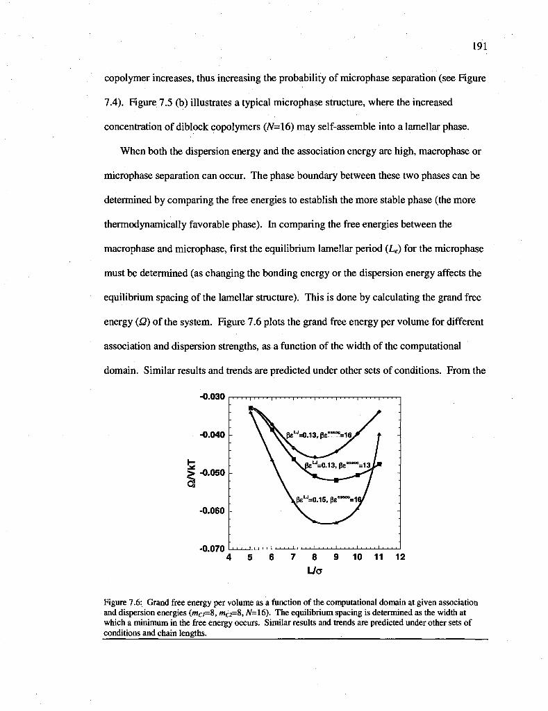
191

copolymer increases, thus increasing the probability of microphase separation (see Figure

7.4). Figure 7.5 (b) illustrates a typical microphase structure, where the increased

concentration of diblock copolymers (N=16) may self-assemble into a lamellar phase.

When both the dispersion energy and the association energy are high, macrophase or

microphase separation can occur. The phase boundary between these two phases can be

determined by comparing the free energies to establish the more stable phase (the more

thermodynamically favorable phase). In comparing the free energies between the

macrophase and microphase, first the equilibrium lamellar period (Le) for the microphase

must be determined (as changing the bonding energy or the dispersion energy affects the

equilibrium spacing of the lamellar structure). This is done by calculating the grand free

energy (Q) of the system. Figure 7.6 plots the grand free energy per volume for different

association and dispersion strengths, as a function of the width of the computational

domain. Similar results and trends are predicted under other sets of conditions. From the

-0.030

-0.040

> -0.050

-0.060

-0.070

4 5 6 7 8 9 10 11 12 Ua

Figure 7.6: Grand free energy per volume as a function of the computational domain at given association and dispersion energies (wC;=8, /nc2=8, N=16). The equilibrium spacing is determined as the width at which a minimum in the free energy occurs. Similar results and trends are predicted under other sets of conditions and chain lengths.

I I I I | I I I I | I I I I | I •! I I | I I I I | I I I I | I I I I | I I I I

, , , , I I . . . . I i . . i I i . i . I i i i i I . . . ,

192

figure, the equilibrium spacing is determined as the width at which a minimum in the free

energy occurs. For the lamellar phases, at a given association energy, the equilibrium

lamellar period increases and the equilibrium free energy decreases as the dispersion

energy becomes larger (the increasing incompatibility between the two components

promotes a decreasing number of interfaces to minimize the number of contacts between

Ci and Ci). At fixed dispersion energy, decreasing the association energy results in a

larger Le (and decreases the equilibrium free energy). Both trends encourage macrophase

separation, as the lamellar phase transitions into a liquid-liquid phase as reflected in the

phase diagram in Figure 7.4.

2.5

2.0

£ 1.5

* 3

w

I 1.0

0.50

0.0

0 5 10 15 ea s s o c / (eL J*N)

Figure 7.7: Phase diagram for associating polymer mixtures (N=16 and #=100) highlighting the effect of chain length and temperature on the phase behavior. Three distinct phases are present in the phase diagram: a homogeneous disordered phase (DIS), a macrophase (2 phase), and a lamellar microphase (LAM). Reentrant behavior is observed (DIS-2 phase-DIS and LAM-DIS-LAM) upon raising/lowering the temperature.

While Figure 7.4 highlights important features of the phase diagram, it does not show

a clear dependence on temperature (as both coordinates are temperature dependent).

Figure 7.7 provides the phase diagram after scaling the thermal energy (fc/,7) and the

193

bonding energy (eassoc) by the total dispersion interaction energy of the diblock chain

(eu*N). This provides a dimensionless temperature versus dimensionless bonding energy

to demonstrate the effect of changing the temperature at a fixed ratio of {eassoc /eu*N).

When looking at this phase diagram, one notices regions where reentrant behavior occurs.

First, for N=\6, it is obvious that reentrant behavior occurs upon raising/lowering the

temperature over a large band of higher energy ratios (eassoc /eu*N~ 7.90-12.25),

predicting a sequence of transitions from disordered to macrophase to disordered phases.

Here, such reentrant behavior is due to hydrogen-bonding interactions (similar behavior

drives closed loop LL immiscibility, which is unique to unlike, associating mixtures). At

low temperatures, the unlike pairs permit association and complete mixing (association

between unlike species in the mixture result in the low temperature miscibility of the

system, as indicated by the low temperature DIS). As the temperature is increased, many

of these association bonds are broken, leading to immiscibility (2 phase separation).

Increasing the temperature further leads to increased kinetic motion in the fluid, which

results in increased miscibility and complete mixing (high temperature DIS). A more

narrow band (e^™ /eu*N~ 7.45-7.9) displays transitions from lamellar to disordered to

lamellar phases upon raising and lowering the temperature. Similar bands of reentrant

behavior are also predicted in Figure 7.7 for longer diblock chains (N=100).

Homogeneous reentrant behavior has been observed experimentally. ' To our

knowledge, no experiments have demonstrated reentrant behavior of an inhomogeneous

phase in a supramolecular polymer system, although recent theoretical results (SCFT) by

Feng et al.326 do predict inhomogeneous reentrant behavior involving a lamellar phase,

consistent with the results presented here. It will therefore be interesting to see if such

194

reentrant inhomogeneous behavior can be observed in future experiments, based on these

results. Finally, Figure 7.7 also highlights the effect of increasing the chain length in the

associating mixture. As the chain length increases, the concentration of bonding

segments in the mixture decreases (scales as l/N). As a result, for increasing N, a higher

bonding energy is required to increase the concentration of copolymer in the mixture

(needed to encourage microphase separation and a homogeneous disordered phase) and

thus the two phase region becomes larger.

The iSAFT results presented in this section highlight the capabilities of the theory to

correctly capture hydrogen bonding/association interactions in polyatomic systems. Even

the fundamental case of associating homopolymers considered in this section challenges

the theory to capture the presence and absence of mesophases and liquid-liquid phase

behavior, as well as intriguing reappearing phases in the phase diagram. More detailed

extensions of this study can be conducted, specifically to study and understand more

complex, self-assembling associating polymer systems in the bulk. Such work includes

multicomponent (ternary and higher) polymer blends, asymmetric cases (unequal

concentrations and/or unequal chain lengths of the polymers), and multiple bonding sites

on multiple polymer segments of varying size (leading to other supramolecular

architectures beyond the diblock copolymer considered in this work). As the architecture

becomes more complicated, the self-assembly of more complex, hierarchical

morphologies can arise (for example, the self-assembly of Archimedean tiling patterns306"

308'310). Future studies of iSAFT to such challenging problems could aid in the

development and production of high performance soft materials and separation

applications.

7.4 Conclusions

The iSAFT density functional theory has been extended to associating polyatomic

molecular systems, using the inhomogeneous form of the association functional. The

approach provides a very accurate method for modeling a wide range of complex

associating polyatomic systems, capable of investigating the full range of association for

any bonding scheme. In this work, the ability of the theory to model associating

polymers near surfaces and in the bulk over a wide range of conditions was

demonstrated. Even for the fundamental associating polymers chosen in this work, the

results highlight a wide range of complex behaviors, demonstrating how reversible

bonding governs the structure of a fluid near a surface (in good agreement with available

simulation data), the molecular connectivity (formation of supramolecules and complex

architectures), and the phase behavior of the system (including reentrant order-disorder

phase transitions). The introduction of hydrogen bonding interactions thus leads to a new

class of self-assembling, highly functional materials. It is evident that iSAFT could

significantly aid in the understanding and experimental design of more complex,

associating polymer systems, with applications to the fields of biomolecules, separations,

high performance soft materials, polymer mediated adhesion and lubrication, and

polymer-inorganic nanocomposites.

196

CHAPTER 8 An /SAFT density functional theory for the

intermolecular and intramolecular correlation functions of polymeric fluids

8.1 Introduction

There is considerable interest in developing theories capable of accurately predicting

the microscopic liquid structure of polymeric fluids. Knowledge of the local structure

provides information about how molecules pack against one another, as well as how

thermodynamic properties of polymers are affected by bond angles (intramolecular

stiffness and flexibility), chain branching, and local chemistry. Integral equation theory

(IET) has long been used as the conventional method for predicting the correlation

functions of chain fluids. Curro and Schweizer19'20 developed the polymer reference

interaction site model (PRISM) theory for linear chain molecules by extending the RISM

theory of Chandler et al.344'345 The intermolecular correlation functions are calculated

for a given set of intramolecular correlation functions after the Ornstein-Zernike (OZ)

equation is formulated (and coupled with a closure relation). The PRISM theory has

been successfully applied to describe the microscopic structure of a broad range of

polymeric systems, including polymer melts,346 polyelectrolytes,347"349 polymer

blends,350'351 and liquid crystals.352 Unfortunately, the PRISM approach does suffer from

shortcomings. As mentioned, knowledge of the intramolecular correlation functions is

required to solve the intermolecular correlation functions (except for rigid molecules that

have only one configuration and the inter- and intramolecular correlation functions are

therefore not functionals of each other). Because the intramolecular correlations

functions are typically unknown, self-consistency between inter- and intramolecular

correlation functions are achieved via a single chain molecular simulation. As previously

discussed in chapter 6, the PRISM IET has been shown to be very sensitive to the

particular closures employed. For example, using standard closure approximations,

PRISM IET predicts short-range structural correlations for rigid and semiflexible

polymers, in the rod limit, that are qualitatively inaccurate.353'354 In addition, various

closures to the PRISM equation often give different results, thereby making the

development of closure approximations, especially for new situations, very difficult.

Finally, the theory is very inaccurate at low densities.355 Since all routes to the

thermodynamic properties of polymers require reliable structural properties from low to

high densities, the integral equation approach is not best suited for phase diagram

calculations.

Alternative theories based on Wertheim's theory for associating fluids4"7 have been

developed as new liquid state theories for polymers. Kierlik and Rosenberg162'163

developed a density functional theory (DFT) for polymeric fluids based on Wertheim's

thermodynamic perturbation theory (TPT), where a fluid of chains is formed from a

system of associating monomers. The approach gives reasonable intermolecular

correlation functions for short chains at high densities. However, the theory is not suited

for long chains at semi-dilute and dilute conditions. In the theory, Kierlik and Rosenberg

neglect intramolecular excluded volume effects (intramolecular structure factor is that of

198

an ideal freely jointed chain). As a result, the theory is unable to predict the nonideal

behavior of intramolecular correlation functions of polymeric fluids. Alternatively,

integral equation approaches based on Wertheim's theory have also been applied by

numerous groups.356"358 These approaches fail to predict the nonideal behavior of

intramolecular correlation functions even qualitatively, failing to correctly capture the

packing effects on the intramolecular structure.

More recently, the Percus test-particle method has been used to investigate the

correlation functions in polymeric fluids. From this idea,269 the structure of a fluid can be

represented by the local inhomogeneous density profile around an arbitrary fixed particle.

Yethiraj et al.359 applied this method and extended this idea to polymers. Using a density

functional theory, Yethiraj et al. demonstrated how the intermolecular correlation

functions could be calculated from the density profile of the fluid in the external field of a

single polymer molecule fixed at the origin. The theory is very accurate in comparison

with simulation data for hard-sphere chains. The drawback of the theory is that it is very

computationally intensive and requires a two-molecule simulation as input.359 Unlike a

monotomic fluid, the application of Percus' method to a fixed polymer molecule involves

a complex external field that depends on the positions of all segments on the fixed

molecule.

Alternatively, Yu and Wu360 also apply the Percus test-particle method using density

functional theory, but circumvent the computational expense and the required molecular

simulation input. Instead of fixing an entire polymer chain at the origin, Yu and Wu fix

one segment at the origin. The inter- and intramolecular correlation functions are then

calculated directly from the density distributions of segments around the fixed segment,

199

from the tethered chains (as part of the molecule containing the fixed segment) and from

the free polymer chains.

In this chapter, Percus' test-particle method is applied to the /SAFT density functional

theory using the extended approach from Yu and Wu.360 In the next section, the theory

and model for this work are discussed. Results are presented in section 8.3 and compared

with available simulation data for hard-sphere chains. Concluding remarks are then

presented in section 8.4.

8.2 iSAFT model

8.2.1 Inter- and intramolecular correlation functions

In this work, we consider a polymeric fluid consisting of tangentially connected hard-

sphere chains. Using the extended test-particle method proposed by Yu and Wu,360 we

allow one segment from an arbitrary selected chain to be fixed at the origin. The system

considered is equivalent to a mixture of 3 polymeric components (F, 7/ and T2) in a

Fixed segment at origin

Figure 8.1: Schematic of the test particle model used in this work. Here a middle segment from a hard-sphere chain of 8 segments is fixed at the origin. The inter- and intramolecular segment-segment correlation functions are calculated from the density distributions of the tethered segments (T! and T2) and of the free molecules (F) around the fixed segment at the origin.

200

spherically symmetric external field due to the fixed segment, as depicted in Figure 8.1.

From the figure, the free molecules are represented by F composed of m? segments,

while the tethered fragments are represented by Ti and T2 composed of mn and mn

segments, respectively. As demonstrated in previous chapters, the starting point of the

density functional theory is the development of an expression for the grand free energy,

Q, as a functional of the equilibrium density profile in an external field. In the above

model, the external field is a single, fixed polymer segment at the origin. The grand free

energy can be related to the Helmholtz free energy A|/>(r)] through the Legendre

transform,13

&\pr to pr (r), pr w]=A\P<T W Pr H Pr w]

l=F,Tl,T2 i=l

(8.1)

where /?/" (r) is the density of the ith segment on chain / at position r, ///° is the

chemical potential of that segment, and V£ is the external field acting on that segment.

The first summation is over all chains / in the mixture (F, Tj: Ti), and the second

summation is over all segments on chain /. The external field of the fixed segment

exerted on a segment directly bonded to the fixed segment (segments T of Ti and T2 in

Figure 8.1) is the segment-segment interaction plus the bonding energy (vbond)-

V»(r) = \V~ 'I* (8.2) 00 r <o

201

where l=Ti, T2. The external field of the fixed segment on all other segments in the

system is equal to the segment-segment interaction energy.

v«w=L- >~ (83)

0 r>a

By minimizing the grand free energy with respect to the density profiles, the density

distribution of the free polymer segments and the tethered polymer segments can be

determined.

^ * > ^ =0 . (8.4)

The segment distribution of the free molecules (F) around the fixed segment is related to

the intermolecular site-site correlation function

where p\Fy (r) is the density profile of segment i on molecule F around the fixed segment

j . The distribution of segments from fragments fj and T2 are related to the intramolecular

correlation function

«>«{') = Pu(r). (8.6)

where pfj (r) is the density of segment i on the tethered chain (7/ or Ti) from the fixed

segment j . There is only one tethered polymer chain (one Ti and/or one Ti), therefore the

following normalization condition is satisfied

\PP{r)dT = \ (8.7)

202

From the site-site correlation functions, we calculate the average intermolecular

correlation

1 mF mF

nip ,=i ,= i F i=l J=l

and the average intramolecular correlation function is given as

4r) = —lf^j(r). (8.9) mF M M

8.2.2 Free energies

The total Helmholtz free energy functional can be decomposed into an ideal and

excess contribution,

(8.10)


volume (hs), chain connectivity (chain), and long-range attraction (att), over the ideal gas

state of the atomic mixture. In this work, long-range attractions are neglected. For

brevity, the above expressions are not included here, but can be found in previous

chapters (chapters 6 and 7).

8.2.3 Free energy derivatives

Recalling eq. (8.4), to solve the density profiles of all segments in the mixture, we

obtain the following Euler-Lagrange equation,

f S ^ ^ ^ - M t f - ^ w ) . *»> * J ( r ) * J ( r ) * ; ( r ) * J ( r )

203

Again, for brevity, the above expressions are not included in the text here. For complete

details, the reader is referred back to previous chapters (chapters 6 and 7).

8.2.4 Equilibrium density profiles

Details regarding the expressions and procedure for solving the equilibrium density

profiles are given in chapter 6 (section 6.2.3). For completeness, these expressions are

reviewed again, with special emphasis on the new theory for the tethered chains. To

obtain the equilibrium density profile, the functional derivatives of the free energies are

substituted into the Euler-Lagrange equation (eq. (8.11)) to give

V <„/ \ SpAexM SpAexa" V l , , n

ln"" ( r )+ifw+*fw+5 ln^' ( r )

Z 9=F,n,T2 *=1 k' °Pj \r)

(8.12)

where {k'} is the set of all segments bonded to segment k . This equation can be written

to give the density profile

p j ' ^ J ^ e x p f ^ J e x p l D f W - ^ ^ l l / S ^ l / S f i - ) (8.13)

( «L ^

where /i„ = 2]//j-° is the bulk chemical potential of chain / and //'] (r;) and 1%) (r,) v ;=i J

represent the multiple integrals. Recall from chapter 6 (section 6.2.2), Dj° (r) is given by

D«>(r) = ! Y ff [p^(v)3XnykkMlk{r']'* _W?L_WZL ( 8 1 4 ) j [ ) 2qM„h¥Pk{x) 8pf{v) * ' 8pf{r) # « ( , ) • (8 '14)

204

In this problem, since all inhomogeneities are spherically symmetric, the density

distribution of both free (F) and tethered (Tj and Ti) polymer segments vary only in the

radial direction. Therefore, the total density profile can be expressed as

P?tFj)=P?(rj) (8-15)

and eq. (8.13) thus simplifies to

^ > ( 0 ) = exp(^M|)eXPlDf (i>)-/3Ki'(0)J/g(r,)/S(ry) (8.16)

where l=F, Tl and T2. In this work, only homonuclear chains are considered, therefore

all segments on all chains have a hard-sphere diameter of a. The multiple integrals,

•/,*'] \Tj) and I2] [rj), are solved in a recursive fashion and are given below for each

polymer chain. The following multiple integrals are given for the free polymer chains

(l=F):

(8.17)

^ W = j / ^ 1 ( - > x p f e ( , 0 - « ; i a ^ ) ] ^ + 1 ( r , r ' ) r,6>(<T-|r'-r|)>)

dr' J (8.18)

where A(^ (r,, r2) is defined as in chapter 6, A^ (r,, r2) = KFP (r,, r2)yf (rt, r2). Here K

is a geometric constant that accounts for the volume available for bonding between

segments, and FP (rj,r2) = |exp(/fe0 -'yft'w(r1, r2)).- lj represents the association Mayer

/-function. For tangentially bonded spheres, the bonding potential is given as

205

exp

o./j - I

[— fi>i„d (r,, r2)] = ' ,\2— • The cavity correlation function yf {vx, r2) is

defined as in earlier chapters.

When considering the tethered chains (l=Ti, T2), the following recurrence relations

are given:

/g ( r ) = exp [D«W- /^ ( f l r ) ]A«(« r ) (ae(cr-\r-o\))

CW=J^.MâM-/û'H]A%J(r'>) V'^(c^-|r'-r|) ,

rfr'

(8.19)

r'0(<7-| r'-r|)' rfr'

' 2 M = J / J J M e x p [ ^ ) M - / » ^ M ] ASfe r') r'0(<7-| r '-a|) '

rfr'

(8.20)

The chemical potential (HMF) needed in eq. (8.16) for solving the density profiles of the

free molecules (F) is obtained directly from Wertheim's TPT1 bulk equation of state for

hard-sphere chains. The chemical potentials of the tethered fragments (Ti and Ti) can be

determined using the normalization conditions

$4nr2pp(r)dr = l

J47tr2pf2){r)dr = l (8.21)

where j=\, 2, 3, ...mi, for l=Tj or T2. ThereforeHMTI and/z^ro can be solved by

combining eq. (8.16) with eq. (8.21), using any of the segments 7=1, 2, 3, ...mi. (This

206

also serves as a good check as using the expressions for any of the segments on a given

chain should yield the same chemical potential for the chain). For the first tethered

segment (segment T of l=Tj or T2)

\\7tr2{exp(/^ )<*p(Dr(r))exp(- 0V» W) C fo) ' S (rj ) \ d r = 1' <8-22)

which yields

exp(#/M,) = __ , (f), vW(ll/ v w n / v (8.23) exp^WM/SM

Using other segments yield equivalent results for //M/- Combining eq. (8.23) with eq.

(8.16) thus gives

A (n )W = A(r2)W = 4 ^ (8-24)

which matches the known condition for the tethered segment. Solving for the other

segments (j=2, 3,...mi) gives

The density profiles of the free polymer and of the tethered fragments around a fixed

segment of a polymer chain are used to calculate the inter- and intramolecular correlation

functions. The segments of a polymer chain are fixed one by one. Due to symmetry,

mF/2 calculations are required if mF is even, and (mp +l)/2 calculations are required if mF

is odd. Calculations can be simplified for very long polymers by assuming that all

middle segments have similar site-site correlation functions, and therefore only

correlations related to end and middle segments need be calculated.


The radial distribution functions for fully flexible hard-sphere chains of length m=4

and m=8 were calculated and compared with available simulation data. In this model, the

tangent hard-sphere freely jointed chain molecules are represented as a string of hard

spheres with fixed bond lengths equal to the hard-sphere diameter. There are no

additional torsional or bending potentials. In the calculations, the overall packing

fraction r\ is defined as 77 = 7tpb(r316, where pb is the number density of polymer

segments. Figures 8.2 and 8.3 compare /SAFT predictions for the site-site and average

intermolecular correlation functions for hard-sphere 4mers and 8mers with simulation

data from Yethiraj et al.361 The theory is in good agreement with the simulation results at

both high and low densities. The depletion of intermolecular segments at low density is

due to the chain connectivity, while packing effects lead to the opposite effect at higher

densities. The cusp at r=2o is related to the fixed bond length. The theory does tend to

overestimate the values of the distribution functions at contact, more specifically for the

end-middle and middle-middle segment radial distribution functions. From the figures,

one can also see that the correlation hole between the middle segments is more

pronounced than that involving the end segments (end-middle and end-end segments), in

agreement with simulation. It is expected that the middle segments are more sensitive to

multi-body correlations because of the close connectivity with neighboring segments.

Improvement might be possible by introducing the multi-body correlation functions in

the chain-connectivity contribution to the free energy.

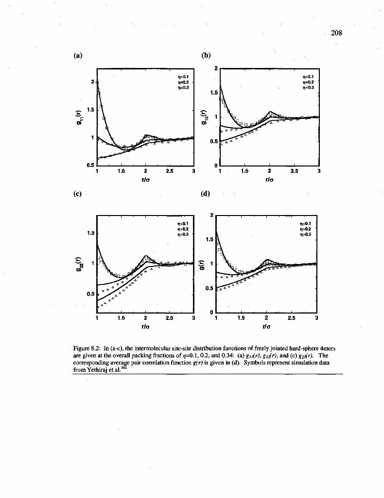
208

(a) (b)

(c) (d)

Figure 8.2: In (a-c), the intermolecular site-site distribution functions of freely jointed hard-sphere 4mers are given at the overall packing fractions of jpO.l, 0.2, and 0.34: (a) gu(r), giM, and (c) g2i(r). The corresponding average pair correlation function g(r) is given in (d). Symbols represent simulation data fromYethirajetal.361

209

(a) (b)

(c) (d)

1.5

o>

0.5

A • \

>o u * ^

tf"0 . / ^ oftf ^r A

Bfir ^^ *^ Bf / A

s& X A

11=0.05 11=0.25 T)=0.35

-r"*-*"

1 1.5 2 2.5 3 3.5 4

r/o

Figure 8.3: In (a-c), the intermolecular site-site distribution functions of freely jointed hard-sphere 8mers are given at the overall packing fractions of tj=0.05,0.25, and 0.35: (a) gu(r),gu(r), and (c) g^r). The corresponding average pair correlation function g(r) is given in (d). Symbols represent simulation data from Yethiraj et al.361

Figures 8.4 and 8.5 compare the average inter- and intramolecular correlation

functions predicted by iSAFT with simulation data by Chang and Sandler358 for 4mers

and 8mers. Figure 8.4 (a) and Figure 8.5 (a) present accurate predictions of the average

210

pair distribution functions g(r) by the theory. The theory does slightly overestimate the

value of g(r) at contact at higher densities. For the systems considered in this work, the

iSAFT density functional theory provides slightly more accurate intermolecular

correlation functions than Wertheim's multi-density integral equation theory,356"358'362

especially at low densities as the chain length is increased. The theory also provides

improvements in the intermolecular correlation functions in comparison to the density

functional theory by Yu and Wu,360 especially for longer chains at higher densities.

(a) (b)

11=0.0524 11=0.2618 i|=0.4189

Figure 8.4: The average correlation functions of freely-jointed 4mers at tj=0.0524,0.2618, and 0.4189. The average intermolecular correlation function is presented in (a), and the average nonbonded intramolecular correlation function is presented in (b). Symbols represent simulation data from Chang and Sandler.358

Figure 8.4 (b) and Figure 8.5 (b) present the corresponding average nonbonded

intramolecular radial distribution functions An r2Q)(r). Unlike the alternative

approaches in the literature (mentioned in the Introduction, integral equation

approaches356"358 and the DFT by Kierlik and Rosenberg162,163), the iSAFT density

211

functional theory is able to correctly capture the nonideal behavior of intramolecular

correlation functions, specifically the packing effects on the intramolecular structure.

(a)

2.5

2

1.5

TO 1

0.5

0 1

Figure 8.5: The average correlation functions of freely-jointed 8mers at //=0.0524,0.2618, and 0.4189. The average intermolecular correlation function is presented in (a), and the average nonbonded intramolecular correlation function is presented in (b). Symbols represent simulation data from Chang and Sandler.358

From part (b) of the figures, a discontinuity occurs at r=2a due to the direct interaction of

nearest neighbors along the polymer chain. At low densities, the intramolecular

correlation function increases in a monotonic fashion for separations r<2a. At higher

densities, a minimum occurs at approximately r=l.5a. For r>2a, the theory predicts the

essential features of nonmonotonic decay of the intramolecular correlation functions.

Unfortunately, the agreement between the theory and the simulation results is only semi

quantitative, especially at the contact values. The discrepancy between the theory and the

simulation results is most likely due to the use of two-body correlation functions in the

free energy expressions for chain connectivity. When a segment is fixed at the origin, the

intramolecular structure is sensitive to multi-body correlations among the segments

(b)

11=0.0524 tl=0.2618 11=0.4189

212

belonging to the same molecule. The DFT by Yu and Wu360 also predicts intramolecular

structure that is semi-quantitative with simulation. The /SAFT density functional theory

overestimates the intramolecular structure at contact, whereas the DFT by Yu and Wu

underestimates the structure at contact. This suggests that the intramolecular structure

may be sensitive to the weighting functions used in the chain free energy contributions.

8.4 Conclusions

A density functional theory based on Wertheim's theory is presented for the

correlation functions of polymeric liquids. The theory uses an extension of Percus' test

particle method, where the external field is a fixed polymer segment at the origin. The

iSAFT DFT is able to predict both the inter- and intramolecular correlation functions. In

comparison with alternative approaches found in the literature, the structural and

thermodynamic properties can be solved in a self-consistent manner, and the theory

requires no simulation data as input. In addition, the theory is able to capture the

nonideal behavior of intramolecular correlation functions. Improvements to the theory

include the use of multi-body correlations among the segments, and more sophisticated

weighted functions in the chain contribution.

213

CHAPTER

Concluding remarks

This thesis work has been devoted to the development of molecular modeling with

emphasis and application in molecular thermodynamics. The statistical associating fluid

theory (SAFT) and inhomogeneous SAFT (iSAFT) were extended to study the phase

behavior and microstructure of various complex systems. The key advances and findings

from this work are discussed below:

• The perturbed-chain SAFT (PC-SAFT) equation of state was extended to include a

crossover correction. In the critical region, the improved crossover equation of state

provides the correct nonclassical critical exponents. Away from the critical region,

the crossover equation reduces to the original PC-SAFT equation, therefore

maintaining the accuracy of PC-SAFT in this region. No modifications to the original

PC-SAFT molecular parameters were necessary. Excellent agreement with vapor-

liquid equilibrium experimental data for the n-alkane family was obtained inside and

outside the critical region, and all critical constants Tc, Pc, andpc were calculated

within their respective experimental errors. Future applications of this development

include applying the theory to simple fluid mixtures50'54'56'94 and within a density

functional construct.52'95'96

PC-SAFT was used as a predictive tool for natural gas mixtures, to aid in the

understanding of the complex phase behavior involved, and in the design and

operation of more efficient removal processes. The theory was tested against

available VLE data for binary mixtures of constituents typically found in sour gas

treating services (hydrocarbons/F^S, hydrocarbons/sulfides, H2S/sulfides,

solvent/sulfides). The theory performed very well over a wide range of conditions,

capturing the wide variety of phase behavior in comparison with available

experimental data. Multicomponent mixtures were discussed, with a comparison (of

mercaptan solubility) between aqueous amine solutions and physical solvents.

Results suggest an increased solubility in organic (nonamine, physical) solvents,

compared to water and aqueous amine solutions. A more detailed investigation could

be carried out on the performance of commercial physical solvents in the future.

Using a density functional theory (DFT) based on Rosenfeld's formalism for hard

spheres, the influence of model solutes of different sizes on the structure and

interfacial properties of water was investigated. In the theory, water was modeled as

a spherical hard core with four highly anisotropic square-well association or

hydrogen-bonding sites. The hydrogen-bonding interactions were accounted for

using the association free energy based on Wertheim's first order thermodynamic

perturbation theory. Long-range attractions were accounted for using a mean-field

approximation. From the DFT, the distinguishing fluid structure and interfacial

properties as a function of solute size were captured, demonstrating the ability of the

theory to successfully describe hydrophobic phenomena on both microscopic and

macroscopic length scales. In addition, details of structural changes in the hydrogen-

215

bonding network of water due to increasing solute size were quantified and discussed.

The temperature effects were also investigated, which are known to play an important

role in determining the hydrophobicity of the system.

• Using /S AFT, the structure and effective forces in nonadsorbing polymer-colloid

mixtures were investigated. The theory was tested under a wide range of conditions

and performed very well in comparison to simulation data. A comprehensive study

was conducted characterizing the role of polymer concentration, particle/polymer-

segment size ratio, and polymer chain length on the structure, polymer induced

depletion forces, and the colloid-colloid osmotic second virial coefficient. The theory

correctly captures a depletion layer on two different length scales, one on the order of

the segment diameter (semidilute regime), and the other on the order of the polymer

radius of gyration (dilute regime). The particle/polymer-segment size ratio was

demonstrated to play a significant role on the polymer structure near the particle

surface at low polymer concentrations, but this effect diminishes at higher polymer

concentrations. Results for the polymer-mediated mean force between colloidal

particles shows that increasing the concentration of the polymer solution encourages

particle-particle attraction, while decreasing the range of depletion attraction. At

intermediate to high concentrations, depletion attraction can be coupled to a mid-

range repulsion, especially for colloids in solutions of short chains. Colloid-colloid

second virial coefficient calculations indicate that net repulsion between colloids at

low polymer densities gives way to net attraction at higher densities, in agreement

with available simulation data. Furthermore, results indicate a higher tendency

towards colloidal aggregation for larger colloids in solutions of longer chains.

• The /SAFT DFT was extended to associating polyatomic molecular systems, using

the inhomogeneous form of the association functional. Such a development provides

a very accurate method for modeling complex associating polyatomic systems,

capable of investigating the full range of association for any bonding scheme.

Theoretical results demonstrate the ability of the theory to model problems near

surfaces and in the bulk over a wide range of conditions. The examples elucidate the

importance of this theoretical development, highlighting how reversible bonding

governs the structure of a fluid near a surface and in confined environments, the

molecular connectivity (formation of supramolecules, star polymers, etc.) and the

phase behavior of the system (including reentrant order-disorder phase transitions).

• The iSAFT DFT was extended to predict the inter-and intramolecular correlation

functions of polymeric fluids using Percus' test particle method. Results from the

theory for the inter- and intramolecular distribution functions, as well as the site-site

correlation functions, are in good agreement with available simulations for flexible,

hard chain fluids. Unlike the integral equation approaches and alternative density

functional theories, no molecular simulation is required as input. The method is

general and applicable to other polymeric fluids with more involved intermolecular

interactions. Knowledge of the inter- and intramolecular structure can be used to

enhance our understanding of the effect of local chemistry, bond flexibility, and chain

branching on the thermodynamic properties of polymers.

While the last few years have seen much growth and advancement to the iSAFT

density functional theory, the theory is still young, possessing opportunity for further

development and broader application. In addition, several problems involving

217

inhomogeneous fluids in 2/3 dimensions await (see applications discussed in chapter 5-

7), thus requiring the use of more efficient numerical methods and algorithms. A brief

description of potential future research utilizing these molecular tools, namely /SAFT, is

included below.

Broad application of polyatomic association

The work in this dissertation extended /SAFT to include hydrogen-bonding

interactions on polyatomic molecules, where the full range of molecular association as a

function of temperature can be considered. Chapter 7 demonstrated how hydrogen

bonding can play a key role in determining molecular connectivity and the minimization

of the grand free energy of the system (the driving force behind the self-assembly and

stabilization of mesostructures). Broader application of the theory can be used to

investigate more complex molecular systems, with more involved association schemes

(the theory was derived to account for any association scheme, with any number of

association sites on any polymer segment). This extension of the theory is important to

many industrial and biological processes, most notably in self-assembly processes such as

the formation of membranes and micelles in surfactant solutions, and the folding of

proteins into stable, functional complexes. Chapter 7 also listed additional applications

involving complex associating polymers that can self-assemble into hierarchical

morphologies (e.g., the self-assembly of Archimedean tiling patterns306"308'310). The

application of iSAFT to such challenging problems could aid in the development and

production of high performance soft materials, separation devices, and other smart

materials.

218

Improving long-range dispersion interactions

Results in this work account for long-range dispersion interactions via a mean-field

Lennard-Jones treatment. Although effective, it is still desirable to develop a more

sophisticated long-range attraction term. As mentioned briefly in chapter 5, possible

techniques to improve the long-range attraction term include adopting non-mean-field

prescriptions that describe the attractive interactions using the first order mean spherical

approximation developed by Tang and Wu,242 or using a weighted density approximation

developed by Muller et al. and demonstrated by Reddy and Yethiraj. A density

functional theory with a more sophisticated dispersion term that reduces to the dispersion

term incorporated in an equation of state (e.g., PC-SAFT) is of high interest. As

previously discussed, /SAFT shares a common basis with SAFT. Such self-consistency

is significant because while bulk properties of solutions are experimentally accessible,

fewer experimental results for interfacial properties are readily available. Dominik et

al.165 have already demonstrated how /SAFT can be used to simultaneously model the

bulk phase behavior and the interfacial properties of n-alkanes and polymer melts. In this

work, Dominik et al. used a mapping procedure to determine the appropriate DFT

attractive energies from the PC-SAFT attractive energies. Ideally, no parameter mapping

of the dispersion energies would be necessary, and parameters used in the bulk equation

of state could be transferred directly to the /SAFT model.

Intramolecular flexibility and stiffness

Research in this dissertation is presented for fully flexible chains. While sufficient for

capturing the essential physics of polyatomic systems, the ability to account for chain

flexibility or stiffness is important in determining the structure and properties of many

219

systems, including polymer solutions and melts,364"366 as well as some lipid/surfactant

molecules. Previous work developed the effect of an intramolecular bonding potential on

the bulk properties of polyatomic molecules.367 The theory accurately predicted the

difference in bulk properties between linear, bent, and cyclic molecules. The theory for

intramolecular bonding can be redeveloped in the form of density functional theory to

account for the effects of chain flexibility or stiffness, and tested versus molecular

simulation for semiflexible chains.364"366 In addition to the hard sphere models, the DFT

can be used to model particles/molecules varying in size and shape (e.g., rods, discs, etc.)

using alternative formalisms of the fundamental measure theory.

Dynamic density functional theory

The development of a time-dependent form of the density functional theory presented

in this thesis would extend the ability of the theory to predict non-equilibrium, dynamic

behavior and transport properties.372"376 Applications include supercooled liquids, and

time-dependent copolymer and surfactant mesostructures.

220

APPENDIX A SfiA ex,assoc

Derivation of 8 <\ (For Chapter 7)

Here we include the details of the polyatomic full range association functional

derivative. We begin by first writing the associating contribution to the free energy. This

is arrived at by working within the framework an extension12'29 of Wertheim's theory of

A. i io oo i an

association. " As Segura et al. ' ' previously introduced and successfully

demonstrated (for spherical molecules), there are two approaches to include

intermolecular association. The first applies Wertheim's associating fluid functional as a

perturbation to a reference fluid functional,

2 2^ Z=C1,C2 i=l Aer (0V

(A.1)

The first summation is over all chains / in the mixture (Cy, C2,...), the second

summation over all segments on chain /, and the final summation is over all the

associating sites on segment i of chain /. tf£ (i^) represents the fraction of segments of

type i on chain / which are not bonded at their site A. We simplify this notation by

combining the first two sums to an equivalent sum over all segments (iV) in the system.

221

/&~""h(r)]= j A i S A f c ) ^ f l n ^ ( r 1 ) - ^ ^ + (=1 AeP' 2 2

The fraction of unbounded segments i at site A is given by

ZiA(r1) = -

1 + \dr2 ]T pk (r2) £ ^ (r2) A*B (rx, r2) k=l BeV'

(A.2)

(A.3)

To solve the Euler-Lagrange equation for the density profile, the functional derivative is

needed. This is given as

#>» ^ ' \ 2 2 )

ZJ*.A(I)Z i=l Aer(i)

1 1 V

. ^ A ( 1 ) 2.

frlfti) (A.4)

We can manipulate the functional to remove the functional derivative

Such an algebraic manipulation was demonstrated for bulk systems by Michelson and

Hendricks.377 A similar approach was used to derive the chain free energy functional.32

The derivation begins by rearranging the definition of the fraction of unbonded

segments (eq. (A.3)) to give

1 — - ^ = 1+ f* 2 2> 4 ( r 2 ) 2>f l ( r 2 K B ( r P r 2 ) ZA\F\) J t=i iter'"

Differentiating this with respect to p} (r) gives

(A.5)

222

=( Z. (rK.(p1.r)l+ jAiSAfe) I f f ^ W ^ )

+ Jrfr2|;A(r2)2 *=i Ber '

• # »

*k( r , .» i ) \?M)

(A.6)

Multiplying both sides by - J<friZ A( ri) Z / ^ ( r i ) 1=1 A=r(1

i=i *=i A=r(,>Ber<*> {dPj\r)J

- J J * i * a Z i A ( r , k ( r a ) Z Z ^ ( ^ ( r 2 f ^ ^

(A.7)

Rearranging,

1=1 Aer1 =-HZA(*v)Zto Z^M^M

i=i /ter<0 Vser 0 '

- J* ,ZAfc) Z f ¥ W ] J * i Z A f c ) Izi(r IW,(r1,r1) *=i B6r<'>^Âr/J «•=> AEr"»

-JJ*i*aZZA(r,k(ra)Z ^MxkB{4^f^

We know from equation (A.3) that

(A.8)

f

223

(A.9)

Substitution of expression (A.9) into (A.8) gives us,

>/„ / ^ ( r . . r » P ^ p O ) ggpCt)

(A.10)

We can replace the dummy variables on the second term (RHS): B, k, T2 by A, i, r/

fatpfo) Z f y r n T ^ ] = - / * . £ A f c ) Z U ( l ) ( Z ^ W A % ( r „ r ) .=1 iter«>Âi rJAdÂ riJ '=1 A=r«> W ( J )

-f*J>.(oz. i=l AeP

^ ( r x ) v 1 A —1

Spj{r) J^zM

J J ^ Z Z A M A W Z Z^^kMri^T1^ .=1 *=i Aer<"fler»' ^ dPj\r) J

(A.11)

Collecting like terms and multiplying by (1/2) gives us

H^&feb-i. V J S J L ^

#W = 4 J*iZAfc)ZUi(l)( Z ^ A ^ r ) v * » y /=! Aer") Ber">

1 jjAi zz ciKfc) z s^^^^(^|rj 1=1 t=i Aer<" Ber*"

(A.12)

Substituting this into expression (A.4) in the functional derivative gives

224

SPA— = y ( j ZM + 1?

# » i 4 * " 2 +2, 4 JîZ^WZUiWf Z^frWuife.r)

1 1=1 A=r<'> V s e r U )

2 J J ^ t = i AEr">fcr<»> V W r /

(A.13)

r i ^ * Again recognizing that — T T T - 1 = feY A(ri) Z^( r i )AAB( r i ' r) • We can simplify

#>;(r) A ^ > l n ^ i ( r ) - ^ + |

(Zi(r) 0 I 2 2j

Af AT

4 JJ*i*aZZA(r,)A(r,) Z Z^Mi^^HT I*'1 ,=r t=i i=r<0 t r i l l I Opj\T) i=l t=l Aer" sen"

(A.14)

which, after changing the indices in term 2 of the RHS (from B to A), terms cancel and

the expression simplifies further to give

*U /<?AAB(r„r2)l

)

The degree of association is controlled by the term

(A.15)

(A.16)

225

Here K represents a geometric constant, £%*°Bck is the associating energy, and y'k is the

cavity correlation function for the inhomogeneous hard sphere reference fluid.

Calculating the derivative of expression (A. 16) needed for expression (A. 15)

Â'UrprJ _ tt , ^ l n y t t ( r p r 2 ) SPj(r) -*»**> SPj(r)

(A.17)

We approximate v '*^ ,^) to be at contact, and further by its bulk counterpart evaluated

at a weighted density py, so that

lnyik{rl,r2) = ^[\nyik(a,pj{rl))+lnyik(c7,pJ{r2

(A.18)

We are left with

SPj(r) - 2A ^ r > ' r M spfc) SPj(r)

Finally, we can substitute expression (A. 19) into expression (A. 15)

(A.19)

4 J J '=!*=• AEr">fcr<» [ dPj\r)

i=l k=l Aer ( , )Ber ( t ) # »

(A.20)

226

Fur ther us ing ., > - 1 = fdr2 J T pk ( r 2 ) £ ^ (r2 )A'* B (r,, r2) in the second term and

1 ^ f N

-T7-\~l\= J r f riZA('i),Zî(«'i)A«(r1,r2) in the third term (RHS) i=l /ten'

*n(r) = ZKtfO-))-7j*iZZ A(r,)Z fr-aifo), — z r p * > »

4 t=1 I=1 Ber(t> opMrJ

(A.21)

which is equivalent to

\L M = Zlln^(r))--ZZ foiAfc) Z l1-^^). „ A

dPj\T) Aer<» 2 I=i t=1 Aer«> <*>A<7

(A.22)

The above expression is the final form for associating chains (eq. (7.25) in the text). The

term only contributes for segments k with association sites that are

eligible to bond to sites located on segment i.

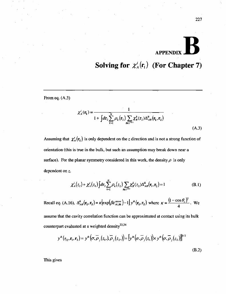
227

APPENDIX

Solving for ZAM (For Chapter 7)

From eq. (A.3)

ti(*x) = — • 1+ p r 2 ] > » 2 ) £;rf(r2)A'k(r1 ,r2)

k=\ Bel"1"

(A.3)

Assuming that x\ (ri) is o m y dependent on the z direction and is not a strong function of

orientation (this is true in the bulk, but such an assumption may break down near a

surface). For the planar symmetry considered in this work, the density/? is only

dependent on z-

^ H ^ W / ^ E A W E^(z2)4(r„r2)=l (B.l)

Recalleq.(A.16), A'*B(r1,r2) = 4 e x p ^ ^ ) - l J / ( r 1 , r 2 ) where < f = ( 1 " c ^ ^ ) , We

assume that the cavity correlation function can be approximated at contact using its bulk

counterpart evaluated at a weighted density33'34

y* fa.^)=yik (<r>Pj(zvYpj{z2,))= \yik (<^,(zi))x yik (^pji^f2

(B.2)

This gives

228

(B.3)

Given the position zi of segment i, we can integrate over the range of positions for

segment k that allow bonding. We perform the following change of variables

J*2 = f d(/>[dcoselr?2drn ^

Under our assumption, r12 y* (r12, Zj, z2) ~ <r2.y'* (<r, zuz2) over the range of bonding.

Neglecting the change in zi as rn goes from a to rc, we integrate f <ir12 = (rc - <r) and

f rfcos# = f d(z2 - Zi) = f <fe2' which after substitution lead to

ZiA{z,)+2îca2{rc -a)tfA{zi)\ X p ^ x

2 > « («2>{ M / & E S ) " i t * ( < ^ , fc O^y fc .))}&2 = 1 (B-5) flEP"

Rearranging, we are left with

l + 2 W ( r c - < x ) f j A f c ) - Z ^ < * » > { W ^ K j - l ^ ^ . ^ f c ^ ^ M k i 1 *=i Ber<'>

(B.6)

The above equation is applicable to a polyatomic fluid in planar geometry, with any

number of association sites (the expression is similar to the expression derived by Segura

et al.186 for a four site associating sphere). From this %\ can be solved in an iterative

fashion.

References

229

(1) Redlich, 0,; Kwong, J. N. S. Chemical Reviews 1949, 44, 233-244.

(2) Peng, D. Y.; Robinson, D. B. Ind. Eng. Chem. Fundam. 1976,15, 59.

(3) Wei, Y. S.; Sadus, R. J. AIChE Journal 2000, 46, 169-196.

(4) Wertheim, M. S. J. Stat. Phys. 1984,35,19.

(5) Wertheim, M. S.J. Stat. Phys. 1984, 35, 35.

(6) Wertheim, M. S. J. Stat. Phys. 1986,42,459.

(7) Wertheim, M. S.7. Stat. Phys. 1986, 42, All.

(8) Chapman, W. G., K.E. Gubbins, G. Jackson Mol. Phys. 1988, 65,1057.

(9) Chapman, W. G., K. E. Gubbins,G. Jackson, M. Radosz Ind. Eng. Chem. Res. 1990, 29, 1709.

(10) Chapman, W. G., K. E. Gubbins,G. Jackson Mol. Phys. 1988, 65, 1.

(11) Chapman, W. G. J. Chem. Phys. 1990, 93, 4299.

(12) Chapman, W. G., Ph.D. Thesis. Cornell University, 1988.

(13) Evans, R. In Fundamentals of Inhomogeneous Fluids; Henderson, D., Ed.; Marcel-Dekker: New York, 1992, p 85-175.

(14) Degennes, P. G. Macromolecules 1980,13, 1069-1075.

(15) Asakura, S.; Oosawa, F. J. Polym. Sci. 1958, 33,183.

(16) Asakura, S.; Oosawa, F. J. Chem. Phys. 1954, 22,1255.

(17) Edwards, S. F. Proceedings of the Physical Society of London 1965, 85, 613.

(18) Degennes, P. G. Reports on Progress in Physics 1969, 32, 187.

(19) Curro, J. G.; Schweizer, K. S. Journal of Chemical Physics 1987, 87, 1842-1846.

(20) Schweizer, K. S.; Curro, J. G. Physical Review Letters 1987, 58, 246-249.

(21) Geisinger, T.; Muller, M.; Binder, K. Journal of Chemical Physics 1999, 111, 5241-5250.

(22) Geisinger, T.; Muller, M.; Binder, K. Journal of Chemical Physics 1999, HI, 5251-5258.

(23) Chatterjee, A. P.; Schweizer, K. S. Journal of Chemical Physics 1998,109, 10464-10476.

(24) Chatterjee, A. P.; Schweizer, K. S. Journal of Chemical Physics 1998,109, 10477-10488.

(25) Fuchs, M.; Schweizer, K. S. Physical Review E 2001, 64, 021514.

(26) Hooper, J. B.; Schweizer, K. S.; Desai, T. G.; Koshy, R.; Keblinski, P. Journal of Chemical Physics 2004,121, 6986-6997.

(27) Wu, J. AIChE J. 2006, 52, 1169-1193.

(28) Wu, J. Z.; Li, Z. D. Annual Review of Physical Chemistry 2007, 58, 85-112.

(29) Segura, C. J.; Chapman, W. G.; Shukla, K. P. Molecular Physics 1997, 90, 759-771.

(30) Segura, C. J.; Vakarin, E. V.; Chapman, W. G.; Holovko, M. F. Journal of Chemical Physics 1998,108, 4837-4848.

(31) Segura, C. J.; Zhang, J.; Chapman, W. G. Molecular Physics 2001, 99, 1-12.

(32) Jain, S,; Dominik, A.; Chapman, W. G. Journal of Chemical Physics 2007,127, 244904.

(33) Tripathi, S.; Chapman, W. G. Physical Review Letters 2005, 94, 087801.

(34) Tripathi, S.; Chapman, W. G. Journal of Chemical Physics 2005,122, 094506.

(35) Sengers, J. M. H. L. Supercritical Fluid Technology Reviews in Modern Theory and Applications; CRC, 1991.

(36) Sengers, J. V.; Sengers, J. M. H. L. Annu. Rev. Phys. Chem 1986, 37, 189.

(37) Chen, Z. Y., P.C. Albright, J.V. Senger Phys. Rev. A 1990,41, 3160.

(38) Chen, Z. Y., A. Abbaci, S. Tang, J.V. Senger Phys. Rev. A 1990, 42, 3370.

(39) Salvino, L. W., J.A. White /. Chem. Phys. 1992, 96, 4559.

White, J. A. Fluid Phase Equilib. 1992, 75, 53.

White, J. A., S. Zhang J. Chem. Phys. 1993, 99, 2012.

White, J. A., S. Zhang 7. C/iem. Phys. 1995, 705, 1922.

White, J. A. J. Chem. Phys. 1999, 111, 9352.

Kiselev, S. B. Fluid Phase Equilib. 1998, 747, 7.

Kiselev, S. B., J.F. Ely Ind. Eng. Chem. Res. 1999, 38, 4993.

Adidharma, H., M. Radosz /. Chem. Phys. 1998, 37, 4453.

McCabe, C, S. B. Kiselev Ind. Eng. Chem. Res. 2004, 43, 2839.

Wilson, K. G. Phys. Rev. B 1971, 4, 3174.

Wilson, K. G., ME. Fisher Phys. Rev. Lett. 1972, 28, 240.

Lue, L.; Prausnitz, J. M. AlChEJ. 1998,44,1455.

Lue., L., J.M. Prausnitz J. Chem. Phys. 1998,108, 5529.

Tang, Y. J. Chem. Phys. 1998, 709, 5935.

Jiang, J., J.M. Prausnitz J. Chem. Phys. 1999, 777, 5964.

Jiang, J.; Prausnitz, J. M. AIChE J. 2000, 46, 2525.

Llovell, F., Josep C. Pamies, Lourdes F. Vega. /. Chem. Phys. 2004, 727, 10715.

Llovell, F.; Vega, L. F. J. Phys. Chem. B. 2006, 770, 1350.

Fu, D.; Li, X.-S.; Yan, S.; Liao, T. Ind. Eng. Chem. Res. 2006, 45, 8199-8206.

Gross, J., G. Sadowski Ind. Eng. Chem. Res. 2001, 40, 1244.

Banaszak, M., Y.C. Chiew, R. O'Lenick, M. Radosz J. Chem. Phys. 1994, 700, 3803.

Bias, F. J., L.F. Vega. Mol. Phys. 1997, 92, 135.

Ghonasgi, D., W.G. Chapman. AIChE J. 1994,40, 878.

232

(62) Ghonasgi, D.; Llano-Restrepo, M.; Chapman, W. G. J. Chem. Phys. 1993, 98, 5662.

(63) Johnson, J. K., E.A. Miiller, K.E. Gubbins. J. Phys. Chem. 1994, 98, 6413.

(64) Muller, E. A.; Vega, L. F.; Gubbins, K. E. Mol. Phys. 1994, 83, 1209.

(65) Huang, S. H., M Radosz. Ind. Eng. Chem. Res. 1990, 29, 2284.

(66) Huang, S. H., M Radosz. Ind. Eng. Chem. Res. 1991, 30, 1994.

(67) Chen, S. S., A. Kreglewski Ber. Bunsen-Ges 1977, 81(10), 1048.

(68) Gil-Villegas, A.; Galindo, A.; Whitehead, P. J.; Mills, S. J.; Jackson, G. J. Chem. Phys. 1997,106,4168.

(69) Dominik, A.; Jain, S.; Chapman, W. G. Ind. Eng. Chem. Res. 2007, 46, 5766-5774.

(70) Barker, J., D. Henderson /. Chem. Phys. 1967, 47, 2857.

(71) Barker, J., D. Henderson J. Chem. Phys. 1967,47, 4714.

(72) Carnahan, N. F., K.E. Starling J. Chem. Phys. 1969, 51, 635.

(73) Gross, J., G. Sadowski Supercritical Fluids as Solvents and Reaction Media 2004, 295-322.

(74) Gross, J., G. Sadowski Ind. Eng. Chem. Res. 2002, 41, 5510.

(75) Dominik, A., W.G. Chapman Ind. Eng. Chem. Res. 2005, 44(17), 6928.

(76) Ghosh, A. J. B., P.K. Jog,W.G. Chapman Macromolecules 2005, 38, 1025.

(77) Dominik, A., W. G. Chapman Macromolecules 2005, 38(26), 10836.

(78) Gross, J., G. Sadowski Ind. Eng. Chem. Res. 2002, 41, 1084.

(79) Tumakaka, F., J. Gross, G. Sadowski Fluid Phase Equilib. 2002,194-197, 541-551.

(80) Gonzalez, D. L., D.P. Ting, G. J. Hirasaki, W.G. Chapman Energy & Fuels 2005,19(4), 1230.

(81) Yarrison, M., W.G. Chapman Fluid Phase Equilib. 2004, 226, 195.

233

(82) Lee, L. L. Molecular Thermodynamics ofNonideal Fluids; Butterworth: Boston, 1988.

(83) Negele, J. W., H. Orland Quantum Many-Particle Systems; Addison-Wesley: Redwood City, CA, 1988.

(84) Battle, G. Recent Advances in Wavelet Analysis; Academic: Boston, 1994.

(85) http://webbook.nist. gov/.

(86) Amoros, J. Phys. Chem. Liq. 2002, 40, 269.

(87) Rosenthal, D. J.; Teja, A. S. AIChE J. 1989, 35, 1829.

(88) Teja, A. S.; Lee, R. J.; Rosenthal, D. J.; Anselme, M. J. In 5th IUPAC Conference on Alkanes andAlkanols Gfadisca, 1989.

(89) Nikitin, E. D.; Pavlov, P. A.; Bessonova, N. V. /. CHem. Thermodyn. 1994, 26, 177.

(90) Nikitin, E. D.; Pavlov, P. A.; Popov, A. P. Fluid Phase Equilib. 1997,141, 155.

(91) Ambrose, D.; Tsonopoulos, C. J. Chem. Eng. Data 1995, 40, 531.

(92) Rosenthal, D. J.; Teja, A. S. AIChE Journal 1989, 35, 1829-1834.

(93) Nath, S. K.; Escobedo, F. A.; Pablo, J. J. d. J. Chem. Phys. 1998,108, 9905.

(94) Cai, J., J.M. Prausnitz Fluid Phase Equilib. 2004, 219, 205.

(95) Fu, D.; Wu, J. Ind. Eng. Chem. Res. 2005, 44, 1120.

(96) Fu, D.; Zhao, Y. Chinese Journal of Chemistry 2005, 23, 386.

(97) Astarita, G.; Savage, D.; Bisio, A. Gas Treating with Chemical Solvents; John Wiley and Sons: New York, 1983.

(98) Cullinane, J. T.; Northrop, P. S., Private Communication.

(99) Valencia, J. A.; Denton, R. D.; Exxon Production Research Co. (Houston, TX) United States, 1985.

(100) Kohl, A. L.; Riesenfeld, F. Gas Purification; Gulf Publishing Company: Houston, TX, 1985.

http://webbook.nist

(101) Huang, S. H.; Ng, H. J. Gas Processors Association Research Report RR-155 1998.

(102) Jou, F. Y.; Carroll, J. J.; Mather, A. E.; Otto, F. D. Journal of Chemical and Engineering Data 1993, 38, 75-77.

(103) Jou, F. Y.; Mather, A. E.; Otto, F. D. Industrial & Engineering Chemistry Process Design and Development 1982, 21, 539-544.

(104) Jou, F. Y.; Otto, F. D.; Mather, A. E. Industrial & Engineering Chemistry Research 1994, 33, 2002-2005.

(105) Jou, F. Y.; Otto, F. D.; Mather, A. E. Journal of Chemical and Engineering Data 1996,47,1181-1183.

(106) Sidi-Boumedine, R.; Horstmann, S.; Fischer, K.; Provost, E.; Furst, W.; Gmehling, J. Fluid Phase Equilibria 2004, 218, 85-94.

(107) Awan, J. A.; Chareton, A.; Valtz, A.; Dieu, F.; Coquelet, C; Richon, D. Gas Processors Association Status Report, GPA Project 037. March 2008.

(108) Jou, F. Y.; Mather, A. E.; Ng, H. J.; Elsevier Science Bv: 1999, p 933-938.

(109) Jou, F. Y.; Mather, A. E.; Schmidt, K. A. G.; Ng, H. J. Journal of Chemical and Engineering Data 1999, 44, 833-835.

(110) Ng, H. J.; Jou, F. Y.; Mather, A. E. Gas Processors Association Research Report RR-164 1998.

(111) Abrams, D. S.; Prausnitz, J. M. AIChE Journal 1975, 21, 116-128.

(112) Fredenslund, A.; Gmehling, J.; Rasmussen., P. Vapor-Liquid Equilibria using UNIFAC; Elsevier: Amersterdam, 1977.

(113) Prausnitz, J. M.; Lichtenthaler, R. N.; Azevedo, E. G. d. Molecular Thermodynamics of Fluid-Phase Equilibria.; 3rd ed.; Prentice Hall: Englewood Cliffs, NJ, 1999.

(114) Renon, H.; Prausnit.Jm AIChE Journal 1968,14, 135.

(115) Soave, G. Chemical Engineering Science 1972, 27, 1197-&.

(116) Hu, Y.; Liu, H. L.; Prausnitz, J. M. Journal of Chemical Physics 1996,104, 396-404.

(117) Economou, I. G. Industrial & Engineering Chemistry Research 2002, 41, 953-962.

(118) Economou, I. G.; Donohue, M. D.; Elsevier Science Bv: 1996, p 518-529.

(119) Muller, E. A.; Gubbins, K. E. Industrial & Engineering Chemistry Research 2001,40,2193-2211.

(120) Boublik, T. Journal of Chemical Physics 1970, 53, 471.

(121) Mansoori, G. A.; Carnahan, N. F.; Starling, K. E.; Leland, T. W. Journal of Chemical Physics 1971, 54,1523.

(122) Wolbach, J. P.; Sandler, S. I. Industrial & Engineering Chemistry Research 1998, 57,2917-2928.

(123) Li, X. S.; Wu, H. J.; Englezos, P. Industrial & Engineering Chemistry Research 2006,45,2131-2137.

(124) Design Institute for Physical Properties, Sponsored by AIChE; 2008 Design Institute for Physical Property Data/AIChE.

(125) Bymaster, A.; Emborsky, C; Dominik, A.; Chapman, W. G. Industrial & Engineering Chemistry Research 2008, 47, 6264-6274.

(126) Kohn, J. P.; Kurata, F. AIChE Journal 1958, 4, 211-217.

(127) Kalra, H.; Robinson, D. B.; Krishnan, T. R. Journal of Chemical and Engineering Data 1977, 22, 85-88.

(128) Carroll, J. J.; Mather, A. E. Fluid Phase Equilibria 1992, 81, 187-204.

(129) Scott, R. L.; Royal Soc Chemistry: 1999, p 4225-4231.

(130) Vankonynenburg, P. H.; Scott, R. L. Philosophical Transactions of the Royal Society of London Series a-Mathematical Physical and Engineering Sciences 1980, 298, 495-540.

(131) Guilbot, P.; Fischer, K.; Valtz, A.; Theveneau, P.; Baba-Ahmed, A.; Richon, D. Fluid Phase Equilibria 2007, 260, 49-59.

(132) Guilbot, P. F., K.; Valtz, A.; Theveneau, P.; Baba-Ahmed, A. and D. Richon. Gas Processors Association RR-170 June 2000 .

(133) Privat, R.; Jaubert, J. N.; Mutelet, F. The Journal of Chemical Thermodynamics 2008, 40, 1331-1341.

236

(134) Lee, J. I.; Mather, A. E.; Otto, F. D. Journal of Chemical and Engineering Data 1978,23,78-79.

(135) Shuo, X.; Qing, S. J.; Zhen, Z. S.; Zhang, G. F.; Carroll, J. J. Fluid Phase Equilibria 1991, 67, 197-201.

(136) Saul, A.; Wagner, W. Journal of Physical and Chemical Reference Data 1987, 76,893-901.

(137) Kilner, J.; McBain, S. E.; Roffey, M. G. Journal of Chemical Thermodynamics 1990, 22, 203-210.

(138) Kuranov, G.; Rumpf, B.; Maurer, G.; Smirnova, N.; Elsevier Science Bv: 1997, p 147-162.

(139) Bedell, S. A.; Miller, M. Industrial & Engineering Chemistry Research 2007, 46, 3729-3733.

(140) Henni, A.; Tontiwachwuthikul, P.; Chakma, A. Journal of Chemical and Engineering Data 2006, 51, 64-67.

(141) Nassar, V. L. B., J.A.; and L.G. Lyddon. Bryan Research and Engineering, Inc. - Technical Papers. 2006.

(142) Nassar, V. L. B., J.A.; and L.G. Lyddon. Bryan Research and Engineering, Inc. - Technical Papers. 2008.

(143) Bedell, S. A.; Pirtle, L. L.; Griffin, J. M. Hydrocarbon Processing 2007, 86, 49-50.

(144) Hohenberg, P.; Kohn, W. Phys. Rev. 1964,136, B864.

(145) Kohn, W.; Sham, L. J. Phys. Rev. 1965,140, Al 133.

(146) Ebner, C.; Saam, W. F.; Stroud, D. Phys. Rev. A. 1976,14, 2264.

(147) McQuarrie, D. A. Statistical Mechanics; Unversity Science Books: Sausalito, CA, 2000.

(148) Huang, K. Statistical Mechanics; John Wiley and Sons: New York, 1987.

(149) McMullen, W. E.; Freed, K. F. J. Chem. Phys. 1990, 1413-1426.

(150) Evans, R. Adv. Phys. 1979, 28, 143.

237

151

152

153

154

155

156

157

158

159

160

161

162

163

164

165

166

167

168

169

170

171

172

Vanderlick, T. K.; Scriven, L. E.; Davis, H. T. J. Chem. Phys. 1989, 90, 2472.

Tarazona, P. Phys. Rev. A 1985,31, 2672.

Tarazona, P. Phys. Rev. A 1985, 32, 3148.

Curtin, W. A.; Ashcroft, N. W. Phys. Rev. Lett. 1986, 56, 2775.

Rosenfeld, Y. Phys. Rev. Lett. 1989, 63, 980.

Rosenfeld, Y. Phys. Rev. A. 1990, 42, 5978.

Meister, T. R; Kroll, D. M. Phys. Rev. A 1985, 31, 4055.

Chandler, D.; McCoy, J. D.; Singer, S. J. J. Chem. Phys. 1986, 85, 5971.

Chandler, D.; McCoy, J. D.; Singer, S. J. /. Chem. Phys. 1986, 85, 5977.

McCoy, J. D.; Singer, S. J.; Chandler, D. /. Chem. Phys. 1987, 87,4853.

Schweizer, K. S.; Curro, J. G. Phys. Rev. Lett. 1988, 60, 809.

Kierlik, E.; Rosinberg, M. L. J. Chem. Phys. 1992, 97, 9222.

Kierlik, E.; Rosinberg, M. L. J. Chem. Phys. 1993, 99, 3950.

Kierlik, E.; Rosinberg, M. L. J. Chem. Phys. 1994,100, 1716.

Dominik, A.; Tripathi, S.; Chapman, W. G. Industrial & Engineering Chemistry Research 2006, 45, 6785-6792.

Tripathi, S.; Chapman, W. G. J. Chem. Phys. 2003, 779, 12611.

Tripathi, S.; Chapman, W. G. Condensed Matter Physics 2003, 6, 523.

Tripathi, S.; Chapman, W. G. Journal of Chemical Physics 2003,118, 7993-8003.

Cao, D.; Wu, J. Macromolecules 2005, 38, 971.

Cao, D.; Wu, J. /. Chem. Phys. 2004,121, 4210.

Yu, Y.-X.; Wu, J. J. Chem. Phys. 2002, 776, 7094.

Yu, Y.-X.; Wu, J. /. Chem. Phys. 2002, 777, 2368.

(173) Bryk, P.; Bucior, K.; Sokolowski, S.; Zukocinki, G. J. Phys. Chem. B. 2005,109, 2977.

(174) Bryk, P.; Pizio, O.; Sokolowski, S. J. Chem. Phys. 2005,122, 194904.

(175) Bryk, P.; Sokolowski, S. J. Chem. Phys. 2004,121, 11314.

(176) Malijevsky, A.; Bryk, P.; Sokolowski, S. Phys. Rev. E. 2005, 72, 032801.

(177) Patrykiejew, A.; Sokolowski, S.; Henderson, D. Molecular Physics 1998, 95, 211.

(178) Pizio, O.; Patrykiejew, A.; Sokolowski, S. J. Chem. Phys. 2000,113, 10761.

(179) Patel, N.; Egorov, S. A. Journal of Chemical Physics 2005,123, 144916.

(180) Patel, N.; Egorov, S. A. Journal of Chemical Physics 2004,121, 4987-4997.

(181) Bias, F. J.; Rio, E. M. D.; Miguel, E. D.; Jackson, G. Molecular Physics 2001, 99, 1851.

(182) Gloor, G.; Bias, F. J.; Rio, E. M. d.; Miguel, E. d.; Jackson, G. Fluid Phase Equilib. 2002,194-197, 521.

(183) Kierlik, E.; Rosinberg, M. L. Phys. Rev. 1990, 42, 3382.

(184) Yethiraj, A.; Hall, C. K. Macromolecules 1990, 23, 1865.

(185) Yethiraj, A.; Woodward, C. E. J. Chem. Phys. 1995,102, 5499.

(186) Segura, C. J.; Chapman, W. G. Molecular Physics 1995, 86, 415-442.

(187) Tripathi, S., Ph.D. Thesis. Rice University, 2004.

(188) Calleja, M.; Rickayzen, G. Mol. Phys. 1993, 79, 809.

(189) Groot, R. D. Mol. Phys. 1987, 60, 45.

(190) Marsh, P.; Rickayzen, G.; Calleja, M. Mol. Phys. 1995, 84, 799.

(191) Woodward, C. E. Journal of Chemical Physics 1991, 94, 3183-3191.

(192) Jain, S.; Chapman, W. G. Molecular Physics 2009,107, 1-17.

(193) Jain, S.; Jog, P.; Weinhold, J.; Srivastava, R.; Chapman, W. G. Journal of Chemical Physics 2008,128.

239

(194

(195 13.

(196

(197

(198 Membranes; 2nd. ed.; Wiley: New York, 1980.

(199

(200

(201

(202

(203

(204;

(205

(206

(207

(208

(209;

(210

(211

(212

(213

(214

Jain, S.; Chapman, W. G- Molecular Physics 2009, Submitted.

Bymaster, A.; Jain, S.; Chapman, W. G. Journal of Chemical Physics 2008,128,

Bymaster, A.; Chapman, W. G. In preparation. 2009.

Kauzmann, W. Adv. Protein Chem. 1959,14, 1.

Tanford, C. The Hydrophobic Effect: Formation of Micelles and Biological

Stillinger, F. H. J. Solution Chem. 1973, 2, 141.

Reiss, H. Adv. Chem. Phys. 1965, 9, 1.

Reiss, H.; Frisch, H. L.; Lebowitz, J. L. J. Chem. Phys. 1959, 31, 369.

Pierroti, R. A. J. Chem. Phys. 1965, 69, 281.

Ashbaugh, H. S.; Paulaitis, M. E. J. Am. Chem. Soc. 2001,123, 10721.

Ashbaugh, H. S.; Pratt, L. R. Reviews of Modern Physics 2006, 78, 159.

Floris, F. /. Phys. Chem. B. 2005,109, 24061.

Huang, D.; Chandler, D. J. Phys. Chem. B. 2002,106, 2047.

Huang, D.; Geissler, P. L.; Chandler, D. /. Phys. Chem. B. 2001,105, 6704.

Lum, K.; Chandler, D.; Weeks, J. 7. Phys. Chem. B. 1999,103, 4570.

Sun, S. X. Phys. Rev. E. 2001, 64, 021512.

Floris, F. M.; Selmi, M.; Tani, A.; Tomasi, J. J. Chem. Phys. 1997,107, 6353.

Hummer, G.; Garde, S.; Garcia, A. E.; Pohorille, A.; Pratt, L. R. Proc. Natl. Acad. Sci. U.S.A. 1996,95,8951.

Reddy, G.; Yethiraj, A. /. Chem. Phys. 2004,121, 4203.

Muller, M.; MacDowell, L. G.; Yethiraj, A. J. Chem. Phys. 2003,118, 2929.

Hummer, G.; Garde, S. Phys. Rev. Lett. 1998, 80, 4193.

(215) Ashbaugh, H. S.; Pratt, L. R.; Paulaitis, M. E.; Clohecy, J.; Beck, T. L. /. Am. Chem. Soc. 2m5,127, 2808.

(216) Stillinger, F. H.Adv. Chem. Phys. 1975, 31, 1.

(217) Stillinger, F. H.; Rahman, A. J. Chem. Phys. 1974, 60, 1545.

(218) Berendsen, H. J. C; Grigera, J. R.; Straatsma, T. P. J. Phys. Chem. 1987, 91, 6269.

(219) Berendsen, H. J. C; Postma, J. M. P.; van Gunsteren, W. F.; Hermans, J. In Intermolecular Forces; Pullman, B., Ed.; D. Reidel: Dordrecht, 1981, p 331.

(220) Jorgensen, W. L. J. A. Chem. Soc 1981,103, 335.

(221) Jorgensen, W. L. J. Chem. Phys. 1982, 77, 4156.

(222) Jorgensen, W. L.; Madura, J. D. Mol. Phys. 1985, 56, 1381.

(223) Muller, E. A.; Gubbins, K. E. Ind. Eng. Chem. Res. 1995, 34, 3662.

(224) Bol, W. Mol. Phys. 1982, 45, 605.

(225) Kolafa, J.; Nezbeda, I. Mol. Phys. 1991, 61, 161.

(226) Ghonasgi, D.; Chapman, W. G. Mol. Phys. 1993, 79, 291.

(227) Chandler, D.; Weeks, J. D. Phys. Rev. Lett. 1970, 25, 149.

(228) Weeks, J. D.; Chandler, D.; Andersen, H. C. J. Chem. Phys. 1971, 54, 5237.

(229) Groh, B.; Mulder, B. Phys. Rev. E. 2000, 61, 3811.

(230) Warshavsky, V. B.; Song, X. Phys. Rev. E. 2004, 69, 061113.

(231) Yu, Y.; Wu, J. J. Chem. Phys. 2002,117, 10156.

(232) Henderson, J. R. Mol. Phys. 1983, 50,1A\.

(233) Pallas, N. R.; Harrison, Y. Colloids and Surfaces 1990, 43, 169-194.

(234) Luck, W. A. P. Discussions of the Faraday Society 1967, 115.

(235) Soper, A. K.; Bruni, F.; Ricci, M. A. Journal of Chemical Physics 1997,106, 247-254.

(236) Bondarenko, G. V.; Gorbaty, Y. E. Molecular Physics 1991, 74, 639-647.

(237) Jackson, G.; Chapman, W. G.; Gubbins, K. E. Molecular Physics 1988, 65, 1-31.

(238) Joesten, M. D.; Schaad, L. Hydrogen Bonding; Dekker: New York, 1974.

(239) Suresh, S. J.; Naik, V. M. Journal of Chemical Physics 2000,113, 9727-9732.

(240) Zielkiewicz, J. Journal of Chemical Physics 2005,123.

(241) Huang, D.; Chandler, D. Phys. Rev. E. 2000, 61, 1501.

(242) Tang, Y.; Wu, J. Phys. Rev. E. 2004, 70, 011201.

(243) Tang, Z.; Scriven, L. E.; Davis, H. T. J. Chem. Phys. 1991, 95, 2659.

(244) Alejandre, J.; Tildesley, D. J.; Chapela, G. A. Journal of Chemical Physics 1995, 702,4574-4583.

(245) Predota, M.; Nezbeda, I.; Cummings, P. T. Mol. Phys. 2002,100, 2189.

(246) Lee, J. Y.; Buxton, G. A.; Balazs, A. C. /. Chem. Phys. 2004,121, 5531.

(247) Sinani, V.; Kokysh, D. S.; Yun, B.-G.; Marts, R. L.; Pappas, T. C; Motamedi, M.; Thomas, S. N.; Kotov, N. A. Nano Lett. 2003, 3, 1177.

(248) Smith, K. A.; Tyagi, S.; Balazs, A. C. Macromolecules 2005, 38, 10138.

(249) Spoerke, E.; Stupp, S. J. Biomed. Mater. Res. 2003, 67A, 960.

(250) White, S.; So Hos, N. R.; Geubelle, P. H.; Moore, J. S.; Kessler, M. R.; Sriram, S. R.; Brown, E. N.; Viswanathan, S. Nature 2001, 409, 794.

(251) deGennes, P. Scaling Concepts in Polymer Physics; Cornell University Press: Ithaca, 1979.

(252) deGennes, P. G. C.R. Acad. Sci., Paris B 1979, 288, 359.

(253) Joanny, J. R.; Leibler, L.; Gennes, P. G. D. J. Poly. Sci., Polym. Phys. Ed. 1979, 17, 1073.

(254) Sear, R. P. Eur. Phys. J. B. 1999,1, 313.

(255) Sear, R. P. /. Chem. Phys. 2001,115,575.

(256) Eisenriegler, E. J. Chem. Phys. 2000,113, 5091.

242

(257) Maassen, R.; Eisenriegler, E.; Bringer, A. J. Chem. Phys. 2001,115, 5292.

(258) Surve, M.; Pryamitsyn, V.; Ganesan, V. J. Chem. Phys. 2005,122, 154901.

(259) Tuinier, R.; Fleer, G. J. Macromolecules 2004, 37, 8764.

(260) Scheutjens, J. M. H. M.; Fleer, G. J. Adv. Colloid Interface Sci. 1982,16, 361.

(261) Yang, S.; Yan, D.; Tan, H.; Shi, A. C. Phys. Rev. E. 2006, 74, 041808.

(262) Fuchs, M.; Schweizer, K. S. Journal of Physics-Condensed Matter 2002,14, R239-R269.

(263) Yethiraj, A.; Hall, C. K.; Dickman, R. Journal of Colloid and Interface Science 1992,757,102-117.

(264) Dickman, R.; Yethiraj, A. J. Chem. Phys. 1994,100, 4683.

(265) Doxastakis, M.; Chen, Y.-L.; de Pablo, J. J. J. Chem. Phys. 2005, 725, 034901.

(266) Doxastakis, M.; Chen, Y.-L.; Guzman, O.; de Pablo, J. J. J. Chem. Phys. 2004, 720, 9335.

(267) Louis, A. A.; Bolhuis, P. G.; Meijer, E. J. J. Chem. Phys. 2002, 776, 10547.

(268) Louis, A. A.; Bolhuis, P. G.; Meijer, E. J.; Hansen, J. P. J. Chem. Phys. 2002, 777, 1893.

(269) Striolo, A.; Colina, C. M.; Gubbiris, K. E.; Elvassore, N.; Lue, L. Molecular Simulation 2004,30,431.

(270) Tuinier, R.; Lekkerkerker, H. N. W.; Aarts, D. G. A. L. Phys. Rev. E. 2002, 65, 060801.

(271) Tuinier, R.; Vliegenthart, G. A.; Lekkerkerker, H. N. W. J. Chem. Phys. 2000, 113, 10768.

(272) Chen, X.; Cai, J.; Liu, H.; Hu, Y. Molecular Simulation 2006, 32, 877-885.

(273) Kim, S. C; Leez, S. H. Molecular Physics 2006,104, 1487-1495.

(274) Li, Z. D.; Wu, J. Z. Journal of Chemical Physics 2007,126, 1449041.

(275) Woodward, C. E.; Yethiraj, A. J. Chem. Phys. 1994,100, 3181.

(276) Freasier, B. C; Woodward, C. E. Comput. Theor. Polym. Sci. 1999, 9, 141.

(277) Hansen, J. P.; McDonald, I. R. Theory of Simple Liquids; 3rd ed.; Academic Press: San Diego, CA, 2006.

(278) Kirkwood, J. G. J. Chem. Phys. 1935, 3, 300.

(279) DerjaguhvB. V. Kolloid-Z. 1934, 69,155.

(280) Attard, P. J. Chem. Phys. 1989, 91, 3083.

(281) Biben, T.; Bladon, P.; Frenkel, D. J. Phys.: Condens. Matter 1996, 8, 10799.

(282) Louis, A. A.; Allahyarov, E.; Lowen, H.; Roth, R. Phys. Rev. E. 2002, 65, 061407.

(283) Gotzelmann, B.; Evans, R.; Dietrich, S. Physical Review E1998, 57, 6785-6800.

(284) Mao, Y.; Cates, M. E.; Lekkerkerker, H. N. "W.Physica A 1995, 222, 10-24.

(285) Roth, R.; Evans, R.; Dietrich, S. Physical Review E 2000, 62, 5360-5377.

(286) Woodward, C. E. J. Chem. Phys. 1991, 94, 3183.

(287) Roth, R.; Evans, R.; Dietrich, S. Phys. Rev. E. 2000, 62, 5360.

(288) Li, Z. D.; Cao, D. P.; Wu, J. Z. Journal of Chemical Physics 2005, 722.

(289) Dautenhahn, J.; Hall, C. K. Macromolecules 1994, 27, 5399.

(290) Bolhuis, P. G.; Meijer, E. J.; Louis, A. A. Phys. Rev. Lett. 2003, 90, 068304.

(291) Schweizer, K. S.; Curro, J. G. Adv. Polym. Sci. 1994,116, 319.

(292) Schweizer, K. S.; Curro, J. G. Adv. Chem. Phys. 1997, 98, 1.

(293) Percus, J.; Yevick, G. Phys. Rev. 1958,110, 1.

(294) Picu, R. C; Ozmusul, M. S. /. Chem. Phys. 2003,118, 11239.

(295) Li, Z.; Wu, J. J. Chem. Phys. 2007,126, 1449041.

(296) Konig, P. M.; Roth, R.; Dietrich, S. Phys. Rev. E. 2006, 74, 0414041.

(297) Chen, X.; Cai, J., J.M. Prausnitz; Hu, Y. Molecular Simulation 2006, 32, 877.

(298) Kim, S. C; Lee, S. H. Mol. Phys. 2006,104, 1487.

244

(299) Bedrov, D.; Smith, G. D.; Smith, J. S. Journal of Chemical Physics 2003,119, 10438-10447.

(300) Smith, J. S.; Bedrov, D.; Smith, G. D. Composites Science and Technology 2003, 63,1599-1605.

(301) Patra, C. N.; Yethiraj, A. J. Chem. Phys. 2000,112, 1579.

(302) Patra, C. N.; Yethiraj, A. J. Chem. Phys. 2003,118,4702.

(303) Cotterman, R. L.; Schwarz, B. J.; Prausnitz, J. M. AIChE Journal 1986, 32, 1787-1798.

(304) Li, J.; Li, X.; Ni, X. P.; Wang, X.; Li, H. Z.; Leong, K. W. Biomaterials 2006, 27, 4132-4140.

(305) Sijbesma, R. P.; Beijer, F. H.; Brunsveld, L.; Folmer, B. J. B.; Hirschberg, J.; Lange, R. F. M.; Lowe, J. K. L.; Meijer, E. W. Science 1997, 278, 1601-1604.

(306) Asari, T.; Arai, S.; Takano, A.; Matsushita, Y. Macromolecules 2006, 39, 2232-2237.

(307) Asari, T.; Matsuo, S.; Takano, A.; Matsushita, Y. Macromolecules 2005, 38, 8811-8815.

(308) Asari, T.; Matsuo, S.; Takano, A.; Matsushita, Y. Polymer Journal 2006, 38, 258-263.

(309) Beck, J. B.; Rowan, S. J. Journal of the American Chemical Society 2003,125, 13922-13923.

(310) Matsushita, Y. Macromolecules 2007, 40, 771 -776.

(311) Noro, A.; Matsushita, Y.; Lodge, T. P. Macromolecules 2008, 41, 5839-5844.

(312) Ruokolainen, J.; Makinen, R.; Torkkeli, M.; Makela, T.; Serimaa, R.; ten Brinke, G.; Ikkala, O. Science 1998, 280, 557-560.

(313) Ruokolainen, J.; Saariaho, M.; Ikkala, O.; ten Brinke, G.; Thomas, E. L.; Torkkeli, M.; Serimaa, R. Macromolecules 1999, 32, 1152-1158.

(314) Shen, J. G.; Hogen-Esch, T. Journal of the American Chemical Society 2008,130, 10866.

(315) Dai, J.; Goh, S. H.; Lee, S. Y.; Siow, K. S. Polymer Journal 1994, 26, 905-911.

(316) Pan, J.; Chen, M. R; Warner, W.; He, M. Q.; Dalton, L.; Hogen-Esch, T. E. Macromolecules 2000, 33, 7835-7841.

(317) Xiang, M. L.; Jiang, M.; Zhang, Y. B.; Wu, C; Feng, L. X. Macromolecules 1997,30, 2313-2319.

(318) Dai, L. M.; Toprakcioglu, C. Macromolecules 1992, 25, 6000-6006.

(319) Kim, H. S.; Lau, W.; Kumacheva, E. Macromolecules 2000, 33, 4561-4567.

(320) Kim, S. D.; Torkelson, J. M. Macromolecules 2002, 35, 5943-5952.

(321) Ruths, M.; Granick, S. Journal of Physical Chemistry B 1999,103, 8711-8721.

(322) Tanaka, F.; Ishida, M. Macromolecules 1997, 30, 1836-1844.

(323) Tanaka, F.; Ishida, M.; Matsuyama, A. Macromolecules 1991, 24, 5582-5589.

(324) Angerman, H. J.; ten Brinke, G. Macromolecules 1999, 32, 6813-6820.

(325) Dormidontova, E.; ten Brinke, G. Macromolecules 1998, 31, 2649-2660.

(326) Feng, E. H.; Lee, W. B.; Fredrickson, G. H. Macromolecules 2007, 40, 693-702.

(327) Lee, W. B.; Elliott, R.; Katsov, K.; Fredrickson, G. H. Macromolecules 2007,40, 8445-8454.

(328) Ayyagari, C ; Bedrov, D.; Smith, G. D. Polymer 2004, 45, 4549-4558.

(329) Guo, L.; Luijten, E. Journal of Polymer Science Part B-Polymer Physics 2005, 43,959-969.

(330) Huh, J.; Dckala, O.; tenBrinke, G. Macromolecules 1997, 30, 1828-1835.

(331) Huh, J.; ten Brinke, G. Journal of Chemical Physics 1998,109, 789-797.

(332) Koga, T.; Tanaka, F. European Physical Journal E 2005,17, 115-118.

(333) Sung, B. J.; Yethiraj, A. Journal of Chemical Physics 2003,119, 6916-6924.

(334) Chen, C. C; Dormidontova, E. E. Macromolecules 2006, 39, 9528-9538.

(335) Malvaldi, M.; Allegra, G.; Ciardelli, F.; Raos, G. Journal of Physical Chemistry B 2005,109, 18117-18126.

246

(336) Malvaldi, M; Bruzzone, S.; Raos, G.; Allegra, G. Journal of Physical Chemistry B 2007, 111, 4141-4149.

(337) Bryk, P.; Sokolowski, S.; Pizio, O. Journal of Chemical Physics 2006,125, 024909.

(338) Gloor, G. J.; Jackson, G.; Bias, F. J.; del Pvio, E. M.; de Miguel, E. Journal of Physical Chemistry C 2007, i i i , 15513-15522.

(339) Gloor, G. J.; Jackson, G.; Bias, F. J.; del Rio, E. M.; de Miguel, E. Journal of Chemical Physics 2004,121, 12740-12759.

(340) Bucior, K.; Fischer, J.; Patrykiejew, A.; Tscheliessnig, R.; Sokolowski, S. Journal of Chemical Physics 2007,126, 094704.

(341) Yethiraj, A.; Hall, C. K. Journal of Chemical Physics 1991, 94, 3943-3948.

(342) Frischknecht, A. L.; Curro, J. G.; Frink, L. J. D. Journal of Chemical Physics 2002,117, 10398-10411.

(343) Walker, J. S.; Vause, C. A. Scientific American 1987, 256, 98-&.

(344) Chandler, D. Journal of Chemical Physics 1973, 59, 2742-2746.

(345) Chandler, D.; Andersen, H. C. Journal of Chemical Physics 1972, 57, 1930.

(346) Schweizer, K. S.; Curro, J. G. In Advances in Chemical Physics, Vol 98 1997; Vol. 98, p 1-142.

(347) Shew, C. Y.; Yethiraj, A. Journal of Chemical Physics 1999,110, 11599-11607.

(348) Yethiraj, A. Journal of Chemical Physics 1999, 111, 1797-1800.

(349) Yethiraj, A.; Shew, C. Y. Physical Review Letters 1996, 77, 3937-3940.

(350) Schweizer, K. S.; Curro, J. G. Journal of Chemical Physics 1989, 91, 5059-5081.

(351) Schweizer, K. S.; Yethiraj, A. Journal of Chemical Physics 1993, 98, 9053-9079.

(352) Pickett, G. T.; Schweizer, K. S. Journal of Chemical Physics 1999,110, 6597-6600.

(353) Yethiraj, A. Journal of Chemical Physics 1994,101, 9104-9112.

(354) Yethiraj, A.; Dickman, R.; Szamel, G.; Kierlik, E.; Rosinberg, M. L. Molecular Physics 1994, 82, 937-955.

(355) Yethiraj, A.; Hall, C. K. Journal of Chemical Physics 1992, 96, 797-807.

(356) Kalyuzhnyi, Y. V.; Cummings, P. T. Journal of Chemical Physics 1995,103, 3265-3267.

(357) Chang, J.; Kim, H. Journal of Chemical Physics 1998,109, 2579-2587.

(358) Chang, J. E.; Sandler, S. I. Journal of Chemical Physics 1995,102, 437-449.

(359) Yethiraj, A.; Fynewever, H.; Shew, C. Y. Journal of Chemical Physics 2001,114, 4323-4330.

(360) Yu, Y. X.; Wu, J. Z. Journal of Chemical Physics 2003,118, 3835-3842.

(361) Yethiraj, A.; Hall, C. K.; Honnell, K. G. Journal of Chemical Physics 1990, 93, 4453-4461.

(362) Wertheim, M.S. Journal of Chemical Physics 1987, 87, 7323-7331.

(363) Frink, L. J. D.; Salinger, A. G.; Sears, M. P.; Weinhold, J. D.; Frischknecht, A. L. Journal of Physics-Condensed Matter 2002,14, 12167-12187.

(364) Fynewever, H.; Yethiraj, A. J. Chem. Phys. 1998,108, 1636-1644.

(365) Kumar, S. K.; Yethiraj, A.; Schweizer, K. S. J. Chem. Phys. 1995,103, 10332-10346.

(366) Yethiraj, A.; Fynewever, H. Mol. Phys. 1998, 93, 693-701.

(367) Ghonasgi, D.; Perez, V.; Chapman., W. G. J. Chem. Phys. 1994,101, 6880-6887.

(368) Schmidt, M. Physical Review E 2001, 63, 4.

(369) Esztermann, A.; Reich, H.; Schmidt, M. Physical Review E 2006, 73, 16.

(370) Bryk, P.; Roth, R. Physical Review E 2005, 71, 8.

(371) Hansen-Goos, H.; Mecke, K. Physical Review Letters 2009,102, 4.

(372) Frink, L. J. D.; Thompson, A.; Salinger, A. G. Journal of Chemical Physics 2000, 772,7564-7571.

(373) Matuszak, D.; Aranovich, G. L.; Donohue, M. D. Journal of Non-Equilibrium Thermodynamics 2006, 31, 355-384.

(374) Zvelindovsky, A. V.; Sevink, G. J. A.; van Vlimmeren, B. A. C; Maurits, N. M.; Fraaije, J. Physical Review E1998, 57, R4879-R4882.

(375) Morita, H.; Kawakatsu, T.; Doi, M.; Yamaguchi, D.; Takenaka, M.; Hashimoto, T. Macromolecules 2002, 35, 7473-7480.

(376) Chakrabarti, J.; Dzubiella, J.; Lowen, H. Europhysics Letters 2003, 61, 415-421.

(377) Michelsen, M. L.; Hendriks, E. M. Fluid Phase Equilibria 2001,180, 165-174.

ProQuest Dissertations - Rice Scholarship Home

Documents