ProQuest Dissertations - UCL Discovery

A High Performance, MicroChannel Plate Based, Photon Counting Detector For Space Use

Michael Leonard Edgar

Milliard Space Science Laboratory

Department of Physics and Astronomy

University College London

Submitted to the University of London

for the degree of Doctor of Philosophy

February, 1993

ProQuest Number: 10105611

All rights reserved

INFORMATION TO ALL USERS The quality of this reproduction is dependent upon the quality of the copy submitted.

In the unlikely event that the author did not send a com plete manuscript and there are missing pages, th ese will be noted. Also, if material had to be removed,

a note will indicate the deletion.

uest.

ProQuest 10105611

Published by ProQuest LLC(2016). Copyright of the Dissertation is held by the Author.

All rights reserved.This work is protected against unauthorized copying under Title 17, United States Code.

Microform Edition © ProQuest LLC.

ProQuest LLC 789 East Eisenhower Parkway

P.O. Box 1346 Ann Arbor, Ml 48106-1346

AbstractThis thesis describes the development of a microchannel plate (MCP) based photon

counting detector using the Spiral Anode (SPAN) as a readout. This detector was one of

two being evaluated for use in the Optical Monitor for ESA’s X-ray Multi Mirror satellite.

Throughout this thesis, where possible, the underlying physical processes, particularly those

of the MCP, have been identified and studied separately.

The first chapter is an introduction to photon counting detectors and includes

a review of the various readouts used with MCPs. The second chapter provides a more

detailed review and analysis of cyclic, continuous-electrode, charge-division readouts, of

which SPAN is an example.

The next two chapters describe the technique for measuring the radial distribution

of the MCP charge cloud, which can significantly affect detector imaging performance .

Results are presented for various operating conditions. The distribution consists of two

parts and the size is dependent on the operating voltages of the MCP stack.

The fifth and sixth chapters describe the procedure for operating a SPAN read

out and the decoding necessary for converting the ADC readings into a two dimensional

coordinate. Various methods are described and their limitations evaluated. The cause of problems associated with the SPAN readout, such as “ghosting” and fixed patterning and

methods of reducing them are discussed in detail. Results are presented which demonstrate

the performance of the anode.

The seventh chapter discusses and evaluates the interaction between channels in

MCPs and the long range effects an active pore has on the surrounding quiescent pores.

This represents the first time that these effects have been measured. The importance of

this phenomenon for imaging detectors is discussed and possible mechanisms evaluated.

The last chapter presents the conclusions of this work and discusses the suitability

of SPAN detectors for use on satellites.

To my parents,

without whom Fd only have had two chances;

Buckley *s and none.

And ye shall hear of wars and rumours of wars, see that you he not troubled, for all of these

things must come to pass, but the end is not yet.

For nation shall rise against nation and kingdom against kingdom: and there shall be

famines, and pestilences, and earthquakes in diverse places.

All these are the begining of sorrows.

Then shall they deliver you up to be afflicted, and shall kill you:...

And then shall many be offended, and shall betray one another, and shall hate one another.

And many false propets shall rise, and shall decieve many.

And because iniquity shall abound, the love of many shall wax cold.

But he that shall endure unto the end, the same shall be saved.

Matthew 24 : 6-13

C ontents

A b stra c t 2

L ist o f F igures 9

L ist o f Tables 15

1 R eview o f Tw o D im ensional P h o to n C oun ting D etec to rs 161.1 MicroChannel Plate, Secondary Electron M u ltip lie rs ...................................... 19

1 .1 . 1 Electron Multiplication in M C P s ........................................................... 231 .1 . 2 Ion F eedback ............................................................................................. 251.1.3 Saturation................................................................................................... 281.1.4 Gain Depression with Count R a t e ........................................................ 31

1 . 2 MCP Based Photom ultipliers.............................................................................. 351.2.1 EUV and X-Ray Pho tom ultip liers........................................................ 351 .2 . 2 Optical/UV Photom ultipliers................................................................. 35

1.3 MCP Position R ead o u ts ....................................................................................... 391.3.1 Light Amplification D etectors................................................................. 391.3.2 Charge Measurement D etectors.............................................................. 45

1.4 An Optical Monitor for the XMM S a te l l i te ..................................................... 591.4.1 Detectors...................................................................................................... 60

2 Cyclic C ontinuous E lec trode C harge M easu rem en t D evices 632 . 1 Fine P o s it io n .......................................................................................................... 65

2.1.1 Analysis of Sinusoidal E lectrodes........................................................... 652.1.2 The Effect of the Phase Angle .............................................................. 6 6

2 . 2 Coarse P o sitio n ............................... 712 .2 . 1 The Double Diamond C a th o d e .............................................................. 712.2.2 The Vernier A node.................................................................................... 732.2.3 The Spiral Anode (SPA N )....................................................................... 73

2.3 Practical A n o d e s .................................................................................................... 76

3 Techniques for M easuring th e Size and S pa tia l D is trib u tio n o f E lec tronC louds From M icroChannel P la te s 793.1 Introduction. The Interaction of MCP Charge Clouds with Readouts . . . . 79

3.2 The Split Strip A n o d e .......................................................................................... 813.3 The Experimental S e tu p .................................................... .................................. 83

3.3.1 Electronics and Data Acquisition............................................................ 873.4 Analysis of the S curve......................................................................................... 87

3.4.1 The Probability Density Distribution of the One Dimensional Integrated Charge C lo u d 87

3.4.2 The Structure and Reduction of the S curve.......................................... 8 8

3.4.3 Qualitative Discussion of the Charge Cloud Using p { c p ) .................... 923.5 Determining The Radial Distribution of the Charge C lo u d ........................... 95

3.5.1 Necessary Conditions for Determining the Radial Distribution of theCharge C loud .............................................................................................. 95

3.5.2 The Inversion............................................................................................... 953.5.3 The Least Squares P ro b lem ...................................................................... 1 0 0

3.5.4 The Linear Least Squares S o lu tio n ......................................................... 1013.5.5 The Radial Probability D is trib u tio n ...................................................... 1 0 2

3.6 The Nonlinear Leaat Squares P ro b le m ............................................................. 1033.6.1 A Manual Search In Three D im ensions............................................... 1033.6.2 Methods for Minimizing a V ariable......................................................... 1053.6.3 Powell’s Method of Conjugate Directions ............................................. 106

3.7 Practical Considerations...................................................................................... 1083.7.1 Accuracy and Stability ............................................................................... 109

M easu rem en ts o f th e R adial D is trib u tio n o f th e C harge C loud. 1134.1 Range of M easurem ents...................................................................................... 113

4.1.1 Range of Measurements at an MCP Anode Gap of 6.2 m m .............. 1134.1.2 Range of Measurements at an Anode Gap 3.0 m m ............................. 115

4.2 The General Form of the Radial Distribution of the Charge C lo u d ........... 1154.2.1 The Two Component Nature of The Radial D istribution..................... 1154.2.2 The Form of the Central Com ponent...................................................... 1184.2.3 The Form of the Wing C om ponent......................................................... 119

4.3 The Size of the Radial D istribution..................................................................... 1254.3.1 The Fit Parameters and the Radial D is tr ib u tio n ................................ 1254.3.2 The Fit Parameters at an Anode Gap of 6 . 2 mm................................... 1264.3.3 The Fit Parameters at an Anode Gap of 3.0 mm................................... 1314.3.4 A Simple Ballistic M o d e l ......................................................................... 1314.3.5 Space C h arg e ............................................................................................... 138

4.4 The Variation of Charge Cloud Size with MCP Operating Conditions. . . . 1384.4.1 The Effects of Gain on Charge Cloud S iz e ............................................. 1384.4.2 The Effects of Eg on Charge Cloud S iz e ................................................ 1444.4.3 Plate Bias V oltage.................................................................................... 1444.4.4 Comparison of the Measurements for the Two Gaps............................. 1494.4.5 The Effect of the Inter-plate Gap V o ltag e ............................................. 152

4.5 Charge Cloud Sym m etry...................................................................................... 1534.5.1 EU ipticity ..................................................................................................... 1534.5.2 Skewness ..................................................................................................... 159

5 O p era tin g th e S p iral A node 1615.1 Spiral T ransfo rm ..................................................................................................... 161

5.1.1 Coordinate R o ta tio n .................................................................................. 1615.1.2 Transformation to Cylindrical Polar C oord inates................................ 1635.1.3 Normalization With Respect to Pulse H e ig h t ....................................... 1655.1.4 Spiral Arm Assignment by Linear Discriminant Analysis..................... 1665.1.5 G hosts........................................................................................................... 169

5.2 Radius as a Function of Pulse H eight.................................................................. 1695.2.1 The Cause of Variation of Radius with Respect to Pulse Height . . 1745.2.2 Correction of Radius W ith Respect to Pulse Height .......................... 1805.2.3 Limitations on the Correction.................................................................. 182

5.3 Determining Spiral Constants ............................................................................ 1825.3.1 Line Finding by Edge D e te c t io n ............................................................ 1855.3.2 The Hough T ransform ............................................................................... 1925.3.3 Com parison.................................................................................................. 1995.3.4 Variation of Spiral C o n s ta n ts .................................................................. 203

5.4 Spiral Arm Assignment by Statistical Distribution of p In Hough Space . . 2065.5 Applications for Other D e tec to rs ........................................................................ 2085.6 How the Algorithm is Implemented..................................................................... 2115.7 SPAN Imaging Perform ance.................................................................................. 213

5.7.1 Pulse Height Related Position S h if ts ...................................................... 2135.7.2 Positional Linearity and Resolution......................................................... 214

6 T h e Effects o f D ig itiza tion for th e SPA N R eadou t 2206 . 1 The Effects of Anode Design Parameters on Fixed P a tte rn in g ....................... 2256 . 2 The Effects of User Defined Parameters on Fixed P a t te r n in g ...........................226

6.2.1 Pulse Height Related Vignetting............................................................... 2296.3 Fixed Reference A D C s........................................................................................... 2306.4 Ratiometric A D C s ................................................................................................. 2376.5 A lia sin g .................................................................................................................... 2406 . 6 Chicken Wire D isto rtion ........................................................................................ 2436.7 Possible Techniques for Reducing Fixed P a tte rn in g ......................................... 243

7 T h e Long R ange In te rac tio n B etw een P ores 2487.1 Introduction.............................................................................................................. 248

7.1.1 A djacency..................................................................................................... 2487.1.2 Effects of Gain Depression......................................................................... 251

7.2 Experimental P rocedu re ........................................................................................ 2527.2.1 MCP C onfigura tion .................................................................................. 2547.2.2 Readout and Electronics............................................................................ 2557.2.3 Software........................................................................................................ 255

7.3 The Spatial Extent of Gain Depression............................................................... 2567.4 Measurements of the Long Range Effects of Gain D ep ress io n ....................... 260

7.4.1 Further Measurements with the Pin H o l e ............................................. 2617.4.2 Measurements with a R i n g ...................................................................... 262

7.5 Dynamic, Long Range Gain D ep ress io n ........................................................... 2637.5.1 Measurements of the Dynamic, Long Range Gain Depression with the

R in g ............................................................................................................. 2697.6 Long Term, Long Range Gain D epression ........................................................ 271

7.6.1 The Variation of Long Term, Long Range Gain Depression with Time 2767.6.2 The Variation of Long Term, Long Range Gain Depression with Plate

V o lta g e ....................................................................................................... 2827.6.3 Image Distortions Due to the Long Term Effects of Long Range Gain

Depression ................................................................................................. 2857.7 Possible Mechanisms for Long Range Gain D epression.................................. 289

7.7.1 Dynamic, Long Range Gain D ep ress io n ............................................... 2897.7.2 Long Term, Long Range Gain D epression ............................................ 2947.7.3 C on clu sio n ................................................................................................. 299

8 C onclusions and F u tu re W ork 3008 . 1 The Size of the Charge C lo u d ............................................................................. 3008 . 2 The Interaction Between P o r e s .......................................................................... 3028.3 The Spiral A node................................................................................................... 304

8.3.1 Problems with SPAN .............................................................................. 3058.3.2 Proposed Real Time Operating S ystem s............................................... 3068.3.3 The Analogue Front E n d ........................................................................ 3108.3.4 The Suitability of SPAN for Use in S p a c e ............................................ 310

B ib liog raphy 313

A cknow ledgem ents 324

List o f Figures

1 . 1 Spatial and energy resolution for various two dimensional photon counters. 171 . 2 Schematic diagram of an MCP............................................................................... 2 0

1.3 The variation of element composition with depth in the glass material after reduction.................................................................................................................... 2 2

1.4 The variation in the yield of secondary electrons with varying primary electron energy for the glass after reduction.............................................................. 2 2

1.5 The relation between gain and Vd ........................................................................ 261 . 6 Universal gain curve of an MCP............................................................................ 261.7 Schematic diagram of a Chevron pair MCP configuration combined with a

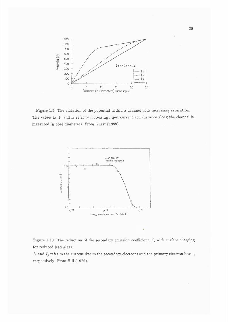
Wedge and Strip Anode.......................................................................................... 291 . 8 PHDs demonstrating different levels of saturation............................................. 291.9 The variation of the electric field within a channel with increasing saturation. 301 . 1 0 The reduction of the secondary emission coefficient, 6 , with surface charging

for reduced lead glass.............................................................................................. 301.11 PHDs exhibiting various degrees of gain depression with variation on count

rate............................................................................................................................. 321.12 Gain depression with count rate with high resistance plates............................ 341.13 UV Quantum Efficiency of MCP material........................................................... 361.14 Quantum Efficiency of an S20 photocathode....................................................... 361.15 Schematic diagram of a sealed tube...................................................................... 381.16 Proximity focussing PSF FWHM.......................................................................... 381.17 Schematic diagram of the PAPA detector............................................................ 411.18 Three and five point centroiding for the MIC detector...................................... 441.19 Schematic Diagram of the MAMA detector........................................................ 481 . 2 0 Resolution versus MCP gain for a Wedge and Strip Anode.............................. 511 . 2 1 Schematic diagram and readout electronics for a transmission, line delay line

readout......................... 541 . 2 2 Schematic diagram of a WSA....................................................... 58

2 . 1 Schematic diagram of sinusoidal, continuous, cyclic electrodes and the resultant Lissajous figure................................................................................................. 64

2 . 2 Demonstration that a homogeneous polynomial f { x , y , z ) describes a cone with an apex at the origin...................................................................................... 67

10

2.3 The Euler angles for a rotation through three dimensions............................... 672.4 Schematic diagram of the Double Diamond readout. .................................. 722.5 Schematic diagram of the Vernier anode............................................................. 722 . 6 The evolution of the spiral with movement along the anode.............................. 752.7 The differential increase of arc length for a curve.............................................. 762 . 8 Schematic diagram of the one dimensional SPAN readout for the SOHO

satellite....................................................................................................................... 782.9 Schematic diagram of a two dimensional SPAN................................................. 78

3.1 An example of measured and simulated modulation for a WSA..................... 803.2 Measured S-distortion for a WSA......................................................................... 823.3 Output from the double diamond cathode showing the effects of the convo

lution of the charge cloud with the geometry of the electrodes........................ 823.4 Schematic diagram of the Split Strip anode........................................................ 843.5 Schematic diagram of the general layout of the detector.................................. 853.6 The S curve returned by the Split Strip anode.................................................. 8 6

3.7 The probability density distribution of the integrated one dimensional distribution, p{cp) of the charge cloud obtained from the data represented in Figure 3.6.................................................................................................................. 89

3.8 The variation in the S curve with varying pulse height.................................... 903.9 Selected cross sections through the S curve........................................................ 913.10 The effect of electric field strength in the anode gap on the charge cloud.. . 933.11 The effect of plate bias voltage on the charge cloud.......................................... 943.12 The p{cp) curve displayed in Figure 3.7, overlayed with its reflection about

its centre.................................................................................................................... 963.13 Two overlayed p{cp) curves obtained with the pore bias angle aligned normal

and parallel to the split........................................................................................... 973.14 The annular regions of the charge cloud corresponding to the three terms in

Equation 3.5.............................................................................................................. 993.15 The vector between two minima xi and X2 obtained by minimizing along the

vector V from two initial points, is conjugate to v ............................................. 1073.16 Example of Powell’s method for finding the minimum by using conjugate

directions................................................................................................................... 1073.17 The distribution of F obtained with the automatic search routine................ I l l

4.1 Comparison of typical fits to a mean S curve, S{cp)......................................... 1174.2 Comparison of the success of fits with exponential and Gaussian central com

ponents..................................... 1 2 0

4.3 The one dimensional integrated probability density distributions obtainedfor g = 6 . 2 mm, Vg = 400 V, %. = 2.9 kV for both chevron bias angle/split orientations............................................................................................................... 1 2 1

4.4 An example of a flat wing..................................................................................... 1234.5 An example of severe modulation........................................................................ 1244.6 Radial probability distributions and associated uncertainties as determined

from the fit parameters........................................................................................... 127

11

4.7 The fit parameters obtained with g = 6 .2 mm and the chevron bias anglealigned parallel to the anode split...................................... 129

4.8 The fit parameters obtained with g = 6 .2 mm and the chevron bias anglealigned perpendicular to the anode split................................................ 130

4.9 The fit parameters obtained at an anode gap of 3.0 mm.................................. 1334.10 The output energy distribution from one single thickness MCP...................... 1354.11 Energy distribution of output electrons at various output angles for a single

MCP............................................................................................................. 1354.12 Horizontal distance travelled by output electrons while traversing the MCP-

anode gap for a simple ballistic model with various combinations of anglesand output kinetic energies...................................................................... 137

4.13 Horizontal distance travelled by a single electron in a given time due to Coulomb repulsion..................................................................................... 139

4.14 The PHD of the large data set showing the edges of the multiple gain intervals. 1414.15 The variation of the size of the charge cloud with varying gain....................... 1434.16 The variation of radii containing fixed fractions of the charge cloud with Eg. 1454.17 The variation of radii containing fixed fractions of the charge cloud with

approximate electron time of flight......................................................... 1464.18 The variation of radii containing fixed fractions of the charge cloud with

varying for = 3.0 mm........................................................................ 1474.19 The variation of radii containing fixed fractions of the charge cloud with

varying Vcfoi g = 6.2 mm...................................................................................... 1484.20 Comparison of ri for the two anode gaps versus Eg........................................... 1504.21 Comparison of r/ for the two anode gaps with respect to t / ............................. 1514.22 The affect of the inter-plate voltage on the fit parameters................................ 1544.23 The variation of r/ with gain due to the variation of the inter-plate gap voltage. 1554.24 The ratio of the average limiting radii for both the bias angle/split orientations. 1574.25 The difference between the two estimates for the centre channel, Acc for the

28 data sets................................................................................................. 160

5.1 Summary of the five steps necessary to transform the three ADC values intothe one dimensional output...................................................................... 162

5.2 An example of data that haa undergone the coordinate rotation........................1645.3 Ideal, three arm spiral represented in r/<j> space................................................ 1675.4 A family of ideal spirals on a continuous series of planes, sectioned by the

plane x = y .................................................................................................. 1675.5 An example of ghosting.......................................................................................... 1705.6 A corrected version of Figure 5.5......................................................................... 1715.7 The same as Figure 5.6 except that the LLD has been set to a higher value,

as shown by the PHD in the bottom left comer................................... 1715.8 Radius that has been normalized with respect to pulse height, r„ plotted

against <f>...................................................................................................... 1725.9 A similar diagram to Figure 5.8 except that it represents the subset of that

data that has a flat PHD.......................................................................... 1735.10 The non normalized radius r plotted against the pulse height h*........175

12

5.11 The same data as in Figure 5.10, but plotting the normalized radius against pulse height............................................................................ 175

5.12 The simulated variation of the radius of a Lissajous circle with respect to charge cloud size....................................................................................................... 176

5.13 The gradient of r„(h '), a , as a function of ...................................................... 1765.14 The Variation of a with anode gap voltage........................................................ 1785.15 The variation of a with plate voltage and anode gap electric field strength. 1795.16 As for Figure 5.9 after radius dependent correction........................................... 1815.17 As for Figure 5.11 after radius dependent correction......................................... 1815.18 As for Figure 5.9 after radius independent correction....................................... 1835.19 As for Figure 5.11 after radius independent correction...................................... 1835.20 The nonlinearity of the radius/pulse height relationship................................. 1845.21 As for Figure 5.16 after use of a northeast compass mask ED, as described

by Equation 5.28...................................................................................................... 1875.22 As for Figure 5.16 after use of a pseudo-compass mask ED, as described by

Equation 5.30............................................................................................................ 1875.23 As for Figure 5.16 after use of a Sobel ED. The three figures show the effect

of varying the threshold level................................................................................. 1895.24 Fragmentation of the spiral due to errors in spiral arm assignment................ 1905.25 Fits to the whole spiral........................................................................................... 1935.26 The Hough transform.............................................................................................. 1955.27 The Hough transform of the ideal spiral. Figure 5.3.......................................... 1965.28 As for Figure 5.27, except the side histogram shows the variation of with

0 and the bottom histogram shows the distribution of p along the line 0 = 6m .1965.29 The HT of Figure 5.16............................................................................................ 1985.30 The reduced angle range for the HT determined by the r„ intensity distribution . 2 0 0

5.31 Comparison of the Sobel ED and the HT............................................................ 2025.32 The variation of the spiral constants with anode gap voltage.......................... 2045.33 The variation of the spiral constants with plate voltage................................... 2055.34 An example of spiral arm assignment by statistical distribution of p in Hough

space........................................................................................................................... 2075.35 An example of the results obtained with spiral arm assignment by using the

statistical distribution of p..................................................................................... 2095.36 iag plotted against (f>\, demonstrating that these two values define a spiral. 2105.37 An example of pulse height related shifts in <!> and r„ ....................................... 2155.38 An example of positional shifts due to pulse height variation.......................... 2165.39 Image of an array of 50 pm pinholes demonstrating the linearity of the SPAN

readout....................................................................................................................... 2185.40 Image of a 37 pm bar mask in which the individual pores are clearly resolved. 219

6 . 1 The cubic lattice defined by the digitization levels of the three ADCs, produces a hexagonally packed lattice when sectioned by the z-j-y-fz = c, wherec is a constant........................................................................................................... 2 2 1

6 . 2 The variation of the number of lattice points lying within windows of constant finite width in both radius and phase angle......................................................... 223

13

6.3 The Axed patterning produced when all the possible lattice points have beenilluminated once and only once.............................................................................. 224

6.4 The effects of variation in the anode design parameters on fixed patterning. 2276.5 The effects of variation of user defined variables on fixed patterning.......2286 . 6 The variation of rum with h' for 8 bit ADCs...................................................... 2316.7 This diagram is similar to Figure 6 . 2 except that all of the lattice points from

all of the pulse height planes have been projected into one plane........................2326 . 8 The variation of fixed patterning with gain depression for fixed reference ADCs.2346.9 Simulation of the variation of fixed patterning with varying levels of digiti

zation for fixed reference ADCs............................................................................. 2356 . 1 0 Simulation of fixed patterning with varying levels of digitization with ratio-

metric ADCs............................................................................................................. 2396 . 1 1 The shift of the spiral origin with pulse height in a system using ratiometric

ADCs......................................................................................................................... 2416.12 Aliasing between 1 1 fim pixels and pores on 15 fj,m centres as measured with

a MIC detector......................................................................................................... 2426.13 Simulation of aliasing between 9fim pixels and pores on 15 fim centres. . . . 2446.14 Simulation of aliasing between 9/zm pixels and pores on 8 /xm centres. . . . 2446.15 An example of chicken wire distortion................................................................... 2456.16 Simulated fixed patterning due to the interaction between 8 bit digitized

inputs and the 2048 pixels. The image represents a flat field over 5% of the detector width located at the approximate centre.............................................. 247

6.17 Simulated fixed patterning with 3 random, extension bits on each of the inputs. The image was generated under the same conditions as Figure 6.16but with 11 bit inputs, of which the 3 least significant bits are random. . . 247

7.1 The effects of adjacency on gain depression.......................................................... 2507.2 The variation of pulse current to strip current with count rate and size of

illuminated area........................................................................................................ 2507.3 The Experimental Arrangement............................................................................. 2537.4 Mean MCP gain for each annulus, G(r) ................................................................ 2577.5 Relative mean gain versus annuli radius, G '(r).................................................... 2577.6 G'(r) for radii up to 1.5 mm................................................................................... 2587.7 Normalized count rates per annulus for the curves in Figure 7.6..........................2587.8 Pulse Height Distributions at selected radii......................................................... 2597.9 The intrinsic variation of the mean gain with radial distance, G (r), from the

centre of the pinhole for 3 plate voltages. The curves represent flat fields, i.e.the MCP was illuminated only by the diffuse X ray source.................................. 264

7.10 The variation of normalized average gain with radial distance from the centreof the pinhole, C '(r), for 3 plate voltages............................................................. 265

7.11 Examples of linear regression fits for data obtained at UV fluxes of 300 and 4500 Hz for a 3.0 kV plate voltage........................................................................ 267

7.12 The gradient and offset terms from the linear regression fits for 15 data sets, including data presented in Figure 7.10............................................................... 268

14

7.13 Gradient and offset terms for linear regression fits for 4 data sets obtainedat UV count rates of 500 and 900 Hz with a plate voltage of 3.0 kV.................. 268

7.14 The variation of G '(r) and relative total event rates for three UV count rates,as measured with the ring....................................................................................... 270

7.15 Variation of G '(r) with relative total count rates............................................... 2727.16 Flat fields obtained at various stages of the experiment.................................... 2747.17 Details of the UV illumination of the ring........................................................... 2787.18 The variation of the magnitude of long term LRGD with time............................2807.19 The data presented in 7.18 plotted linearly with respect to time.........................2817.20 The PHDs acquired for various different regions approximately 1 0 0 hours

after the last UV exposure of the ring.................................................................. 2837.21 Variation in gain for flat fields obtained at various chevron voltages after

prolonged UV illumination of the ring.................................................................. 2847.22 Image distortions in a two dimensional image produced by long term LRGD. 2867.23 Image distortions similar to those in Figure 7.22 after the MCP stack has

been rotated by 1 2 0 ° with respect to the readout.............................................. 2887.24 The equivalent circuit of the last dynode............................................................. 2917.25 Schematic diagram and equivalent circuit of coupling by lateral capacitance

between N active pores and Nq quiescent pores................................................. 2917.26 The variation of modal gain as a function of the inclination between the

electric field the channel axis.................................................................................. 2917.27 The reduction in secondary emission coefficient for reduced lead glass with

progressive electron bombardment........................................................................ 2977.28 Auger spectrum of regions of reduced lead glass that are unexposed figure a,

and that have undergone intense electron bombardment, figure b ................... 2977.29 Variation in the secondary emission coefficient for reduced lead glass with

varying Potassium concentration in the surface layer........................................ 297

8 . 1 Schematic diagram of a proposed realtime decoding system based on theHough transform...................................................................................................... 308

15

List o f Tables

1 . 1 Properties of various MCPs.................................................................................... 2 0

1 . 2 Performance characteristics of two dimensional MCP readouts........................ 62

3.1 Example of the information returned by the automatic search routine. . . . 110

4.1 Summary of operating voltages and typical gains for measurements with an anode gap of 6.2 mm............................................................................................... 114

4.2 Summary of operating voltages and typical gains for measurements with an anode gap of 3.0 mm............................................................................................... 116

4.3 Comparison of two exponential and three exponential fits.................................. 1184.4 The fit parameters for the radial distribution as measured at 6.2 mm for both

anode orientations.................................................................................................... 1284.5 The fit parameters for the radial distribution obtained at a gap of 3.0 mm. 1324.6 Fit parameters determined for the gain intervals as indicated in Figure 4.14. 1404.7 The ratio of the fit parameters for the two pore bias angle/anode split orien

tations and the difference between the two estimates of the centre channel. 156

7.1 Fit parameters for relative mean gain versus radius curves in Figure 7.6 parameters are the same as in Equation 7.4........................................................ 260

7.2 Total UV exposure and the intervals between the times at which the curvesin Figure 7.16 were acquired.................................................................................. 275

16

Chapter 1

R eview o f Two D im ensional

P h oton C ounting D etectors

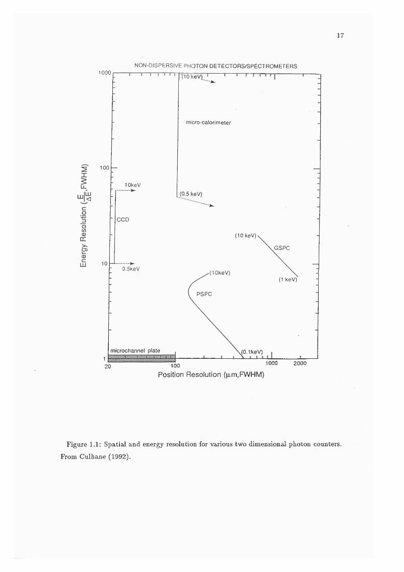
Figure 1 . 1 summarizes the performance characteristics of various two dimensional,

photon counting, X-ray detectors. Rear illuminated charge coupled devices (CCDs) can

be used directly as imaging, X-ray, photon counting detector^without the need of any

photon conversion or electron multiplying device. The microcalorimeter also detects an

X-ray photon directly, by detecting its thermal energy in a similar manner to an infrared

bolometer. At present, these detectors can only be used for photon energies greater than

~ 500 eV (Culhane, 1992 and references therein).

In the most widely used types of photon counting detectors, the incoming photon

produces at least one electron by either interacting with a gas, in gas proportional counters,

or a photocathode in photomultipliers. In the later case, this photo-electron is then multi

plied by a cascade of processes producing secondary electrons. If the gain is « 1 0 ® e“ or

larger, a current or light pulse large enough to be measured individually is produced when

the secondary electrons aie collected by an anode or phosphor.

In the position sensitive gas-filled proportional counter (PSPC), electron multipli

cation takes place in the gas, such as either a Xe/CH4 or Ar/CH 4 mixture, in the region of

a high electric field near an anode wire. The generation of a cloud of positive ions near the

anode wire induces charge on one or two cathodes which allows the centre of gravity of the

resulting charge cloud to be determined.

17

NON DISPERSIVE PHOTON DETECTORS/SPECTROMETERS1000

micro-calorimeter

1 0 0

lOkeV

(0.5 keV)|LUl<

CCD

(lOkeV)

GSPCO)

O.SkeV(lOkeV)

(1 keV)

PSPC

microchannel plate to. Ike V)

1000 20001 0 0

Position Resolution (p.m,FWHM)20

Figure 1.1: Spatial and energy resolution for various two dimensional photon counters.

From Culhane (1992).

18t I CC c t f (A mr%fft.+Woe(e ^ p ® f'o r f f Aftl f P C M ( # W/ »t t

photon’s energy. The cathodes are configured as either a crossed wire grid, a wire grid

combined with a one dimensional, planar cathode readout such as the “backgammon” or a

two dimensional, electrode readout such as the “Wedge and Strip”. These and other types

of position readout are discussed below.

The gas scintillation proportional counter (GSPC), avoids the need for electron

multiplication. Instead photo-electrons are created in a noble gas and pass into a region

where the electric field is high enough to cause gas scintillation, producing UV photons,

but the gas is not ionized. The number of photons is proportional to the number of photo

electrons and therefore, incident photon energy. By omitting the electron avalanche an

improvement in energy resolution of a factor ~ 2 can be achieved. Position is determined

by using an array of photomultiplier tubes or a two dimensional photomultiplier (Smith &

Bavdaz, 1992)

The most widely used secondary electron multiplier in image intensifiers are the

discrete dynode chain photomultiplier tubes (PMTs). Discrete dynode PMTs can produce

sufficient gain. However, only mesh dynode PMTs can provide two dimensional images and

the resolution is limited to approximately 300 ^m FWHM (Kume et oZ., 1986).

Since about the mid 1960s, position-sensitive photomultipliers have been used in

photon counting detectors for astronomical applications. In these detectors, sometimes

referred to as first generation image intensifiers, the photo-electrons from a photocathode

on the input window, are accelerated by a high voltage, approximately 10 kV, and then

electrostatically or magnetically focussed onto a phosphor screen (Baum, 1966). The energy

gained by the electrons’ traversal of the electric field is converted to a photon pulse. If

the phosphor is “sandwiched” together with another photocathode, the photon pulse will

produce more photo-electrons. Each sandwich can produce an electron gain of « 100 for a

10 kV potential (Randall, 1966).

Gains of up to 10® can be obtained by cascading four such stages together, requiring

40 kV. The original Imaging Photon Counting System (IPGS), used on several ground based

telescopes and as the Faint Object Camera on the Hubble Space telescope was a 4 stage

tube, using a TV camera as the position readout for the optical pulses.

MicroChannel plate (MCP) based devices are similar in concept, with the four

stage tube being replaced by a MCP electron multiplier. These devices are discussed in

detail in the next section.

The gas-filled detectors’ spatial resolutions are ultimately limited by the diffusion

19

of the photo-electrons whereas the other detectors’ ultimate resolutions are dependent on

their manufacturing processes. Although gas-filled detectors only have moderate spatial

resolutions, Figure 1 .1 , they are widely used because of their good energy resolution. The

photomultipliers offer no intrinsic energy resolution, however only the CCD has a spatial

resolution comparable with the MCP. Also, only image intensifiers are sensitive to photons

with energies < 1 0 0 eV and so can be used for EUV and UV/ Optical detectors as well as

X-rays.

1.1 MicroChannel P la te , Secondary E lectron M ultipliers

An MCP is a secondary electron multiplier consisting of an array of millions of

glass tubes, called channels or pores, fused into a disk about 1 mm thick and typically

25 mm diameter. A typical MCP would have cylindrical pores with an internal diameter

of 12.5 /xm. The pores are hexagonally packed with a spacing of approximately 15 fim.

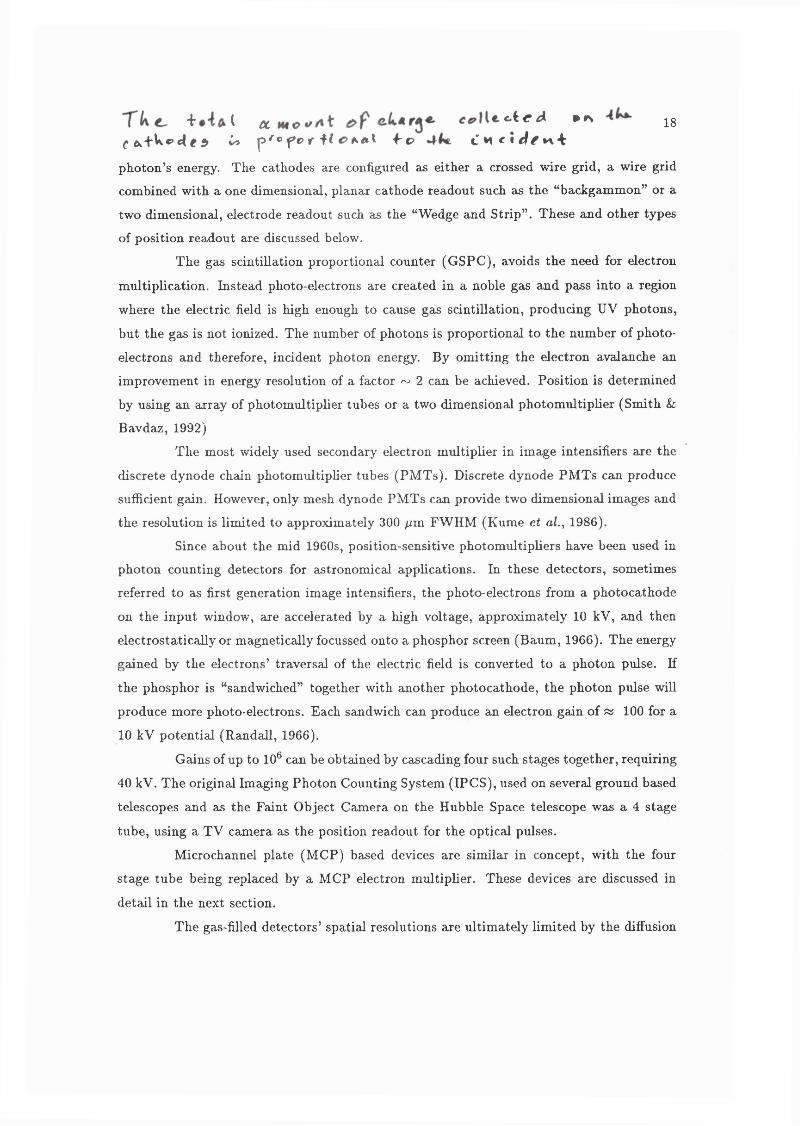
Figure 1 . 2 shows a schematic representation of an MCP and Table 1 . 1 shows the wide range

of the properties of a selection of MCPs available from just one manufacturer.

Washington et al. (1971) describe the manufacturing process of MCPs. The

material consists basically of silica glass into which is incorporated Pb and Bi oxides which

are then reduced to their metallic form by baking in a hydrogen atmosphere. This produces

a high resistance surface layer. Alkali ions are also introduced into the glass to give it the

required malleability and annealing temperatures. The electrical properties of metal oxide

glasses have been discussed in detail by Trap (1971).

Hill (1976) has carried out Auger analysis on the surface layer of this type of

bulk glass that has been treated in the same manner as MCPs during manufacture. Auger

analysis can only examine approximately the top nanometre of a surface but by ablating

the surface with an argon ion beam, the composition of the material with increasing depth

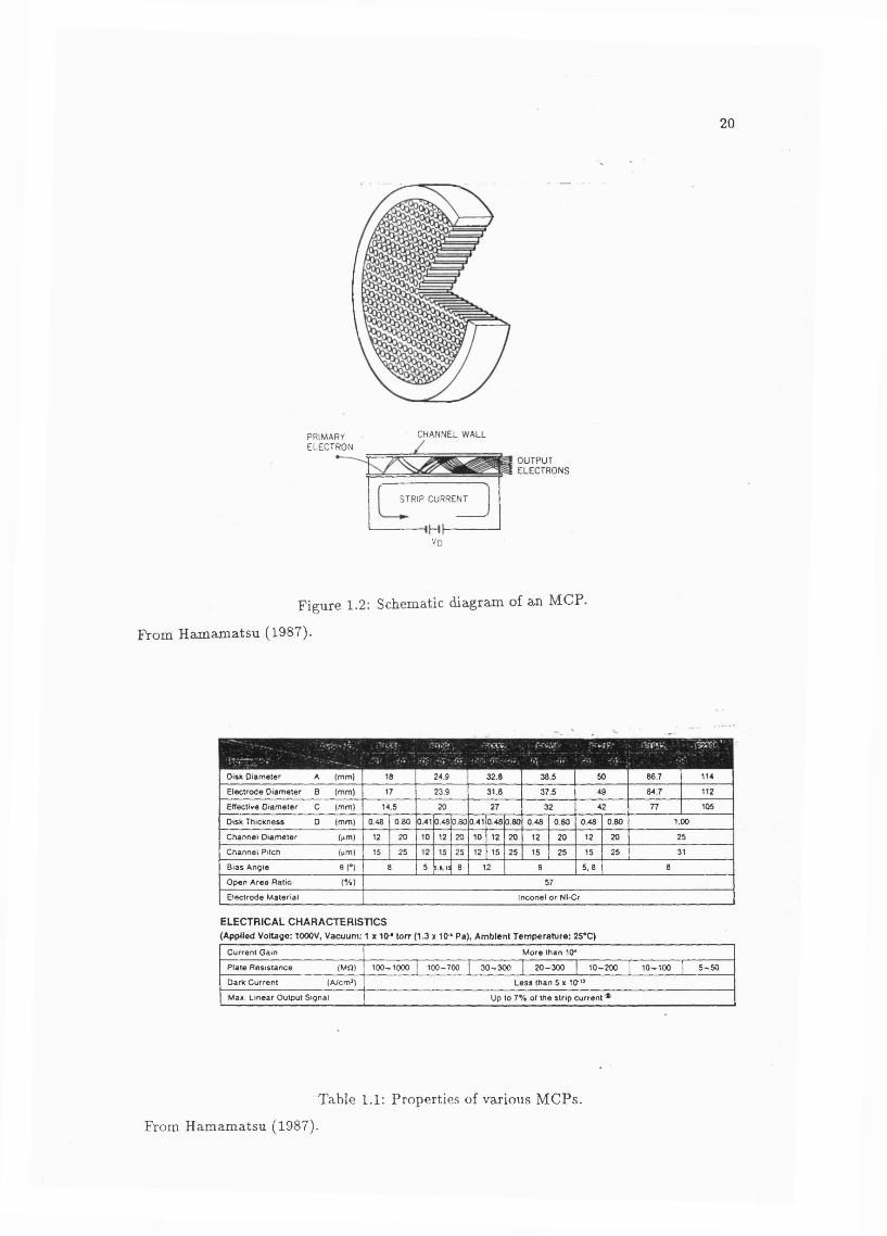
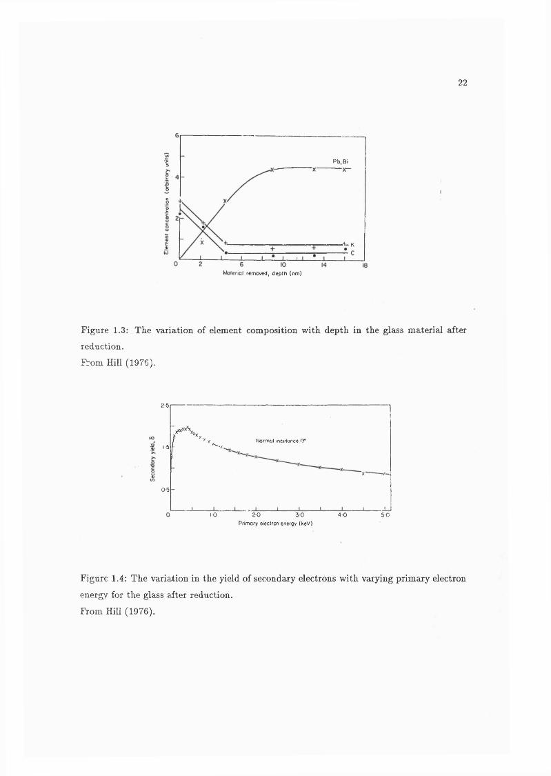
could be probed. Figure 1.3 shows this element composition as a function of depth. The

surface region has a high concentration of K but almost no Pb or Bi. The C is a surface

contaminant and other contaminants such as S and Ca were also present. The Pb and Bi

do not appear until about 1 0 to 2 0 nm below the surface. During heat treatment, K is

thought to occupy positions at the surface that would normally be occupied by Pb and Bi.

The resistivity was also measured with varying depth. The conducting layer was

located from 10 to 20 nm below the surface, which correlated with the appearance of Pb and

20

CHANNEL WALLPRIMARYELECTRON

OUTPUTELECTRONS

STRIP CURRENT

Vo

Figure 1.2: Schematic diagram of an MCP.

From Hamamatsu (1987).

Disk Diameter A (mm) 18 24.9 32.8 38.5 50 86.7 114

Electrode Diameter B (mm) 17 23.9 31.8 37.5 49 84.7 112

Effective Diameter C (mm) 14.5 20 27 32 42 77 105

Disk Thickness D (mm) 0.48 0.80 0.4l|0.48 0.80 0.41 0.48 0.80 0.48 0.80 0.48 0.80 1.00

Channel Diameter (jim) 12 20 10 12 20 10 12 20 12 20 12 20 25

Channel Pitch (nm) 15 25 12 15 25 12 15 25 15 25 15 25 31

Bias Angle 0 (•) 8 5 U d 8 12 8 5.8 8

Open Area Ratio (%) 57

Electrode Material Inconel or Nl-Cr

ELECTRICAL CHARACTERISTICS(Applied Voltage: 1000V, Vacuum: 1 x 10 lorr (1.3 x 10 Pa), Ambient Temperature: 25*0)

Current Gain More than 10*

Plate Resistance (MfJ) 100-1000 1 100 - 700 1 3 0 - 300 1 2 0 - 300 | 10- 200 ] 10-100 1 5 -50

Dark Current (A/cm') Less than 5 x 10-"

Max. Linear Output Signal Up to 7% of the strip current *

Table 1.1: Properties of various MCPs.


21

Bi. This conducting layer is approximately 2 0 0 nm deep. The surface layer consists basically

of silica and the resistance of this layer is approximately twice that of the conducting layer.

Figure 1.4 shows the secondary emission coefficient, S, for the reduced glass mate

rial. The shape of the curve is characteristic for all materials. As primary electron energy

increases, more energy is available to produce secondary electrons within the escape depth

of the material. However, if the primary energy is increased too much, secondary electrons

are produced much deeper in the material so that many do not have enough energy to

escape.

Hill (1976) has calculated that the escape depth of the reduced material is ap

proximately 3.3 nm. Therefore, the secondary electrons come from the layer that consists

mainly of silica. Also, the emissive layer is separated from the conducting layer by a high

resistance region several nanometers thick.

When the interior of a channel is reduced, the channel surface behaves as a con

tinuous dynode and the channel wall contains the conducting layer, through which current

flows, providing electrons to the thin emissive layer at the channel surface. The conducting

layer has quite high resistance so the channel wall behaves as a dynode resistance chain.

The two faces of the MCP are coated with an evaporated layer of conductor such

as Nichrome or Inconel. These conductive layers serve as the input and output electrodes

and connect all of the pores in parallel. The total resistance between the two electrodes is

the parallel combination of the resistance for each channel and is of the order of 1 0 0 Mft.

MCPs are high gain devices which are physically small and require relatively small

voltages, compared to first generation image intensifiers, and power, ^ 10 mW. These factors

make them particularly well suited for space use apart from their fragility and cleanliness

requirements. Spatial resolution is limited only by pore spacing, which has been realized

by some readouts (see below), and as they can be used for photon counting they have good

temporal resolution. As well as electrons, MCPs are sensitive to ions, UV and X-rays. Thick

MCPs, ~ 5 mm, have good have good quantum efficiencies (QE) for 7 -rays (Wiza, 1979),

possibly up to 511 kV (McKee et of., 1991). They can be provided in almost any shape in

sizes up to 10 X 10 cm, with square pores (Fraser et oZ., 1991a) and with a spherical shape

(Siegmund et aL, 1990). MCPs have also been operated at temperatures as low as 14 K

(Schecker et aL, 1992). This versatility has led to the extensive use of MCPs in a wide

variety of applications. They have even been used as passive elements in a large aperture

collimator for an X-ray spectrometer (Turner et a i, 1981 and Yamaguchi et aL, 1987) and

22

Pb.B iI

2

O12

IÜJ -+ -K

Molerial removed, depth (nm)

Figure 1.3: The variation of element composition with depth in the glass material after

reduction.

From Hill (1976).

2 5

15

0 5

r - " . . flormat incidonco (T

10__J_______ L

2 0 3 0Primory electron energy (keV)

4 0 5 0

Figure 1.4: The variation in the yield of secondary electrons with varying primary electron

energy for the glass after reduction.

From Hill (1976).

23

theoretical studies indicate that they could be used to focus hard X-rays with an efficiency

of up to 48 % (Wilkins et al.., 1989 and Chapman et a i, 1991).

1 .1 .1 E le c tro n M u ltip lic a tio n in M C P s

If we take each pore in isolation it behaves in the same manner as a Channel

Electron Multiplier (CEM) (Goodrich & Wiley, 1962 and Adams & Manley, 1966). How

ever, this is an approximation as it has been found that individual pores do interact with

their neighbours. In the following discussion, only isolated channels are described. The

interaction between pores will be discussed in detail in Chapter 7.

When a voltage, Vd , of the order of 1 kV, is applied to the end electrodes, an

electric held, E , is established which is parallel to the pore axis. The strip current, t,, is

given by

Is - V d I R cH , (1-1)

where Rch is the resistance of a single channel. When an electron collides with the channel

wall, secondary electrons may be produced. These electrons follow a parabolic trajectory,

dehned by their initial energy, eV, and E, and before colliding with the channel wall again,

see Figure 1 .2 .

Electron gain is a complicated cascade of statistical processes, which produce a

wide variation in the number of electrons in individual pulses. The magnitude of the gain

also depends on the energy and angle of incidence of the incoming particle. It can only be

properly described statistically, e.g. Lombard & Martin (1961) and Guest (1971). In the

following discussion only the average behaviour will be considered.

The average time t and distance 5 between collisions for a straight channel with

diameter, d, is given by

t~ ‘ V 2 e^ ’

5 = , (1.3)2 m '

where we assume that the electrons have been emitted normally from the wall with energy

Vn- The electrons will collide with the wall with an energy

Vc = E S , (1.4)

" 4 Î ^ ’

24

where a is the length to diameter ratio for the pore. MCPs with a = 40 are often referred

to as “single thickness plates” while if a = 80 they are called “double thickness plates”

There will be n collisions along the length of the pore where

n = ^ . (1 .6 )

As there are a finite number of wall collisions with approximately constant separation,

continuous dynode multipliers can be described as a conventional discrete dynode secondary

electron multiplier (Goodrich & Wiley, 1961, Adams & Manley, 1966 and Eberhardt, 1979,

1981). This discrete separation is not seen in practice, due to the statistical nature of

multiplication and the variable penetration depths of incident particles. One important

consequence of this model is that most of the electrons in the output pulse will originate

from the same region of the channel, the last dynode.

The number of secondary electrons produced in each collision is dependent on the

change in voltage and 6

S = V k K V , (1.7)

= . (1-8)

where & is a constant. Guest (1988) has determined that this is a good approximation of

the low energy collision typical of multiplication processes.

The increase in current along a finite length, A/ of channel is given by

At = t ( 6 — 1)— , (19)

and the overall gain G is given by

G = ^ , (1.10)

= , (1.11)

where t'o and i f are the initial and final currents respectively and G is sufficiently small

(Guest, 1988).

Adams & Manley (1966) and Loty (1971) have described models in which increas

ing E will increase the number of electrons emitted per collision by Equation 1 . 8 but by

Equation 1.3, the number of dynodes will be reduced. Therefore, for a given length, as the

25

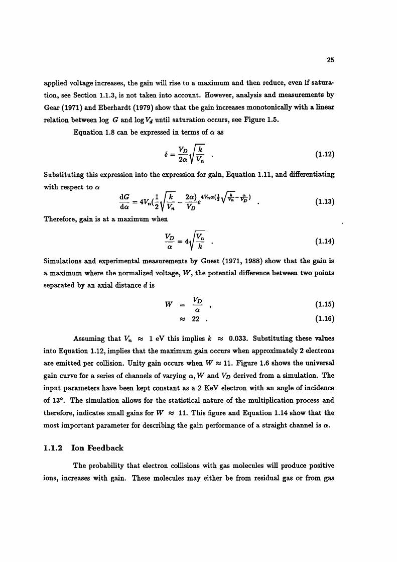
applied voltage increases, the gain will rise to a maximum and then reduce, even if satura

tion, see Section 1.1.3, is not taken into account. However, analysis and measurements by

Gear (1971) and Eberhardt (1979) show that the gain increases monotonicaUy with a linear

relation between log G and logVj until saturation occurs, see Figure 1.5.

Equation 1 . 8 can be expressed in terms of a as

_ V d f k 2 a VK, •

(1.12)

Substituting this expression into the expression for gain. Equation 1.11, and differentiating

with respect to a

Therefore, gain is at a maximum when

- ( . . . . )

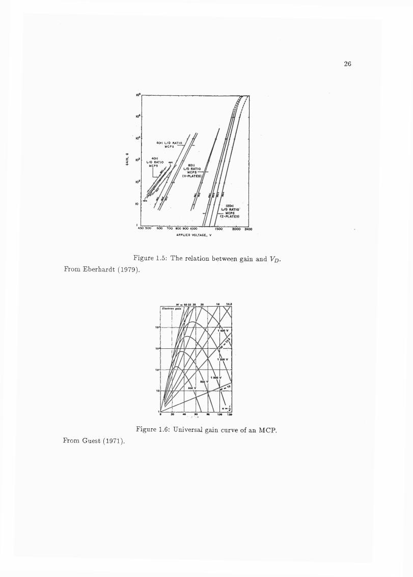
Simulations and experimental measurements by Guest (1971, 1988) show that the gain is a maximum where the normalized voltage, W, the potential difference between two points

separated by an axial distance d is

W = — , (1.15)a

% 2 2 . (1.16)

Assuming that Vn « 1 eV this implies k « 0.033. Substituting these values

into Equation 1 .1 2 , implies that the maximum gain occurs when approximately 2 electrons

are emitted per collision. Unity gain occurs when W » 1 1 . Figure 1 . 6 shows the universal

gain curve for a series of channels of varying a , W and Vd derived from a simulation. The

input parameters have been kept constant as a 2 KeV electron with an angle of incidence

of 13°. The simulation allows for the statistical nature of the multiplication process and

therefore, indicates small gains for W % 1 1 . This hgure and Equation 1.14 show that the

most important parameter for describing the gain performance of a straight channel is a.

1 .1 .2 Io n F eed b ack

The probability that electron collisions with gas molecules wiU produce positive

ions, increases with gain. These molecules may either be from residual gas or from gas

26

«0*1 L /0 RATIO MCPS

L / 0 RATIO M CPS3

450 500 GOO TOO n o *00 wooA P P U E O VOLTAGE, V

1500

Figure 1.5: The relation between gain and Vd . From Eberhardt (1979).

«00 V

Figure 1 .6 : Universal gain curve of an MCP.From Guest (1971).

27

desorbed from the channel wall during electron bombardment. Adams & Manley (1966)

have estimated that the number of ions produced, iV, is

N = 6 rieP , (1.17)

where n* is the number of electrons in a region of width u; at a pressure p Torr.

These ions can collide with the channel walls near the channel input producing

another pulse. For sealed tubes (see below) ions can hit the photocathode, poisoning it

and drastically reducing the tube lifetime (Oba &: Rehak, 1981 and Norton et of., 1991).

They may also produce secondary electrons from the photocathode generating another

event in another channel for a MCP. In this case, there will be two events occurring within

nanoseconds of each other, which will be treated as simultaneous and will produce errors

in position encoding in many readouts. These extra events could result in a regenerative

feedback situation, which in extreme cases could lead to the destruction of some channels.

The need to avoid ion feedback limits the maximum electron gain that a single straight

channel can supply to 10® (Wiza, 1979).Ion feedback can be overcome in CEMs by bending or curving the tubes as the

heavy ions have much longer trajectories than the secondary electrons. MCPs can also be

manufactured with curved channels, a “C plate”, (Timothy, 1974). The gain expression for a curved channel is different to that for a straight channel due to the effect of wall curvature

on the electron trajectories (Adams & Manley, 1966). Whereas a is the parameter that

determines the applied voltage/gain characteristics of a straight channel, the most important

parameter for a curved channel is the included angle of the curve. There is a limit to the

maximum included angle practicable for curved channels in MCPs which limits the gain to

w 10® e~ for a C plate (Wiza, 1979)

Another widely used method is to use two or more plates with straight channels

and with the pores inclined at an angle to the normal to the MCP face. Colson et al.

(1973) demonstrated that if these bias angles point in opposite directions, the shape of the

effective channel is bent, reducing ion feedback. They called this arrangement the Chevron

Shaped Electron Multiplier (CSEM). It is sometimes called a two stage detector, “V plate”

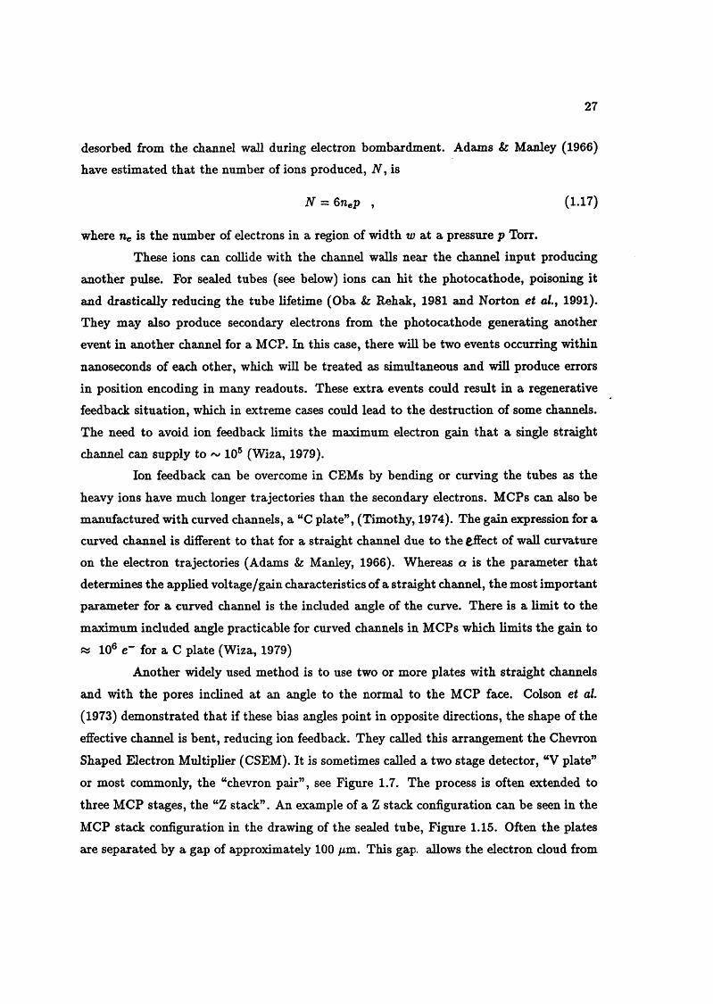
or most commonly, the “chevron pair” , see Figure 1.7. The process is often extended to

three MCP stages, the “Z stack”. An example of a Z stack configuration can be seen in the

MCP stack configuration in the drawing of the sealed tube. Figure 1.15. Often the plates

are separated by a gap of approximately 100 pm. This gap, allows the electron cloud from

28

the first MCP to expand and so Are several pores in the bottom plate, increasing the overall

gain. The inter-plate gap is discussed in Section 4.4.5. Using these configurations, gains of

1 0 — 1 0 ® e~ are obtainable with straight plates.

1 .1 .3 S a tu ra t io n

Due to the statistical nature of the gain process a pulse height distribution (PHD)

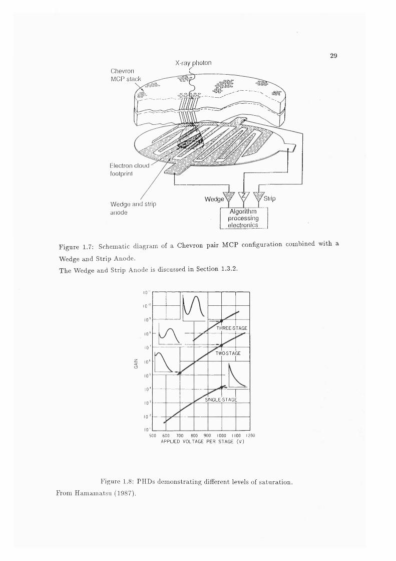
is produced. At low gains, the PHD has a negative exponential shape. However, as gains

increase the PHD is no longer a quasi-exponential but a pseudo-Gaussian (see Figure 1.8).

This effect is known as saturation.

There are two likely processes that can cause saturation.

1 . The space charge of electrons in the channel is sufficient to drive secondaries back into the wall before they can acquire enough energy from the electric field to produce

more secondaries (Bryant & Johnstone, 1965).

2 . There is a limit on the maximum rate at which electrons can be supplied through

the channel wall to the emissive layer. If more electrons are extracted than can be

supplied a positive charge will build up. As the wall resistance is very high, the time

constant is of the order of milliseconds while the total length of the electron pulse is

of the order of 1 0 ps. Therefore, the positive charge cannot be neutralized during the

pulse (Evans, 1965).

Experiment and simulation have determined that the dominant process in satura

tion is space charge for curved channels (Adams & Manley, 1966 and Schmidt & Hendee,

1966) and wall charging for straight channels (Adams & Manley, 1966, Loty, 1979 and

Guest, 1988).

At low enough gains, the electric field along the pore is uniform. As gain increases

and saturation begins, the potential distribution along the length of the pore changes. As

most electrons are extracted from the bottom of the channel, the potential of the bottom is

raised producing a low field region. This reduces the energy of the electrons colliding with

the wall in this region reducing 6. As shown in Figure 1.9, E decreases near the end of the

pore but increases at the start. At some point, E reaches a value that corresponds to unity

incremental gain. Also, the positive charge on the surface can reduce 6 directly, as some

of the lower energy secondary electrons cannot escape from the surface, and a high enough

charge can produce a region with close to unity gain (Hill, 1976), i.e. « 1 , see Figure 1 .1 0 .

29X-ray photon

Chevron MOP slack

m

Electron cloud footprint

StripW edgeW ed ge and strip an ode Algorithm

processingelectronics

Figure 1.7: Schematic diagram of a Chevron pair MCP configuration combined with a

Wedge and Strip Anode.The Wedge and Strip Anode is discussed in Section 1.3.2.

1 0 "

1 0 ' “

THREE-STAGE10*

1 0 ’

TWOSTAGE

1 0 *

^ SINGLE-STAGE

1 0 '

500 600 700 800 900 1000 1100 1200APPLIED VOLTAGE PER STAGE (V )

Figure 1.8: PHDs demonstrating different levels of saturation.


30

900800700

^ 600 500

300I0<<I1<<I2

g200100

0 5 10 15 2520Distance (h Diameters) from Input

Figure 1.9: The variation of the potential within a channel with increasing saturation.

The values Iq, Ii and I2 refer to increeising input current and distance along the channel is

measured in pore diameters. From Guest (1988).

2 0

I 5

f p : 3 0 0 eV noffnol incidence

X----- X—X--- !—^X

X

\

1 0 j :_L j__10"' 10'

Log,Qsomple current ( / s - /p ) ( A )

Figure 1.10: The reduction of the secondary emission coefficient, <5, with surface charging

for reduced lead glass.

Is and Ip refer to the current due to the secondary electrons and the primary electron beam,

respectively. From Hill (1976).

31

Increasing Vd increases saturation and moves the region of unity gain further up

the pore, reducing the length of pore that contributes effectively to gain. Eventually, the

region of unity gain extends along most of the length of the channel. The region near the

input then has a much larger E than in the unsaturated case and is the only region making

an effective contribution to the gain.

Saturated PHDs are a problem for image intensifiera being used in the proportional

mode, in which the output current is proportional to the input current. Saturation places

an upper limit on the output current and therefore output image intensity. In order to

maintain proportionality, the MCPs are operated in the low gain regime with a negative exponential PHD.

In a photon-counting detector, it is only necessary to obtain one pulse per input

photon. The pulse amplitude is not important, so long as it is above a threshold defined by

the signal to noise ratio (SNR) required by the position readout. In practice, a lower level

discriminator (LLD) is used to reject events lying below that treshold. A PHD with the

largest percentage of points lying above the LLD is necessary to ensure the best photometric

linearity of the detector. It can be seen from the PHDs in Figure 1 . 8 that the higher the

saturation, the higher the percentage of points with large amplitudes. Therefore, high

saturations are desirable in photon counting detectors.

Saturated PHDs are described by two parameters, the modal gain, i.e. the gain

which represents the mode of the PHD and the gain resolution or saturation, the ratio of

the PHD FWHM to the modal gain.

1 .1 .4 G ain D ep ression w ith C ount R a te

As described above, the neutralization of the positive wall charge takes a finite

time, of the order of milliseconds, due to the time constant of the channel. If another cascade

occurs in the channel before the wall charge is neutralized, the electric field will be still be

reduced at the bottom of the channel and this region will not make an effective contribution

to the gain. This depresses the modal gain (Loty, 1971, Timothy, 1981, Neischmidt et a l,

1982, Siegmund et a l, 1985), and moves the PHD to lower values. Zombeck & Fraser,

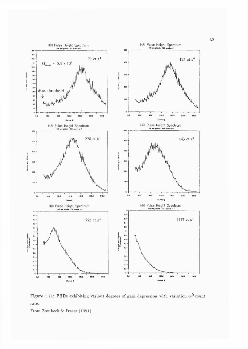
(1991) have presented PHDs for various count rates. Figure 1 .1 1 .

As the local count rate increases, the counting linearity of the detector degrades as

larger and larger proportions of the PHD fall below the LLD. Eventually, at a high enough

32HRI Pulse Height Spectrum

to o mm •m M 4 M mml i > - l

a a -

71 ct s= 5.9 X 10’140 -

1i1 disc, threshold

0.0

OwwW IHRI Pulse Height Spectrum

to o vm n o courrit • * !

IHRI Pulse Height Spectrum

to o am 77% cmwit m-1

HRI Pulse Height Spectrum

220 ct s500

200

too

0

tZOA400

772 ct s

h

00

124 ct s'« 0 -

I1

400

CKMHlfHRI Pulse Height Spectrum

too

443 ct s'500 -

I

tlOO ZOOOCtaiMl I

HRI Pulse Height Spectrum1117 MwiU i - l

1117 ct s'

n

1100

CMMkd I

Figure 1.11: PHDs exhibiting various degrees of gain depression with variation o^ count

rate.

From Zombeck & Fraser (1991).

33

local count rate, most of the PHD will fall below the LLD, effectively paralysing the pore. This process is the ultimate limit on the point source count rates for all MCP detectors.

Most position readouts can achieve point source count rates at this limit. In MCPs with

an individual channel resistance, Rcht of « 1 0 ^ D, significant gain depression can occur at

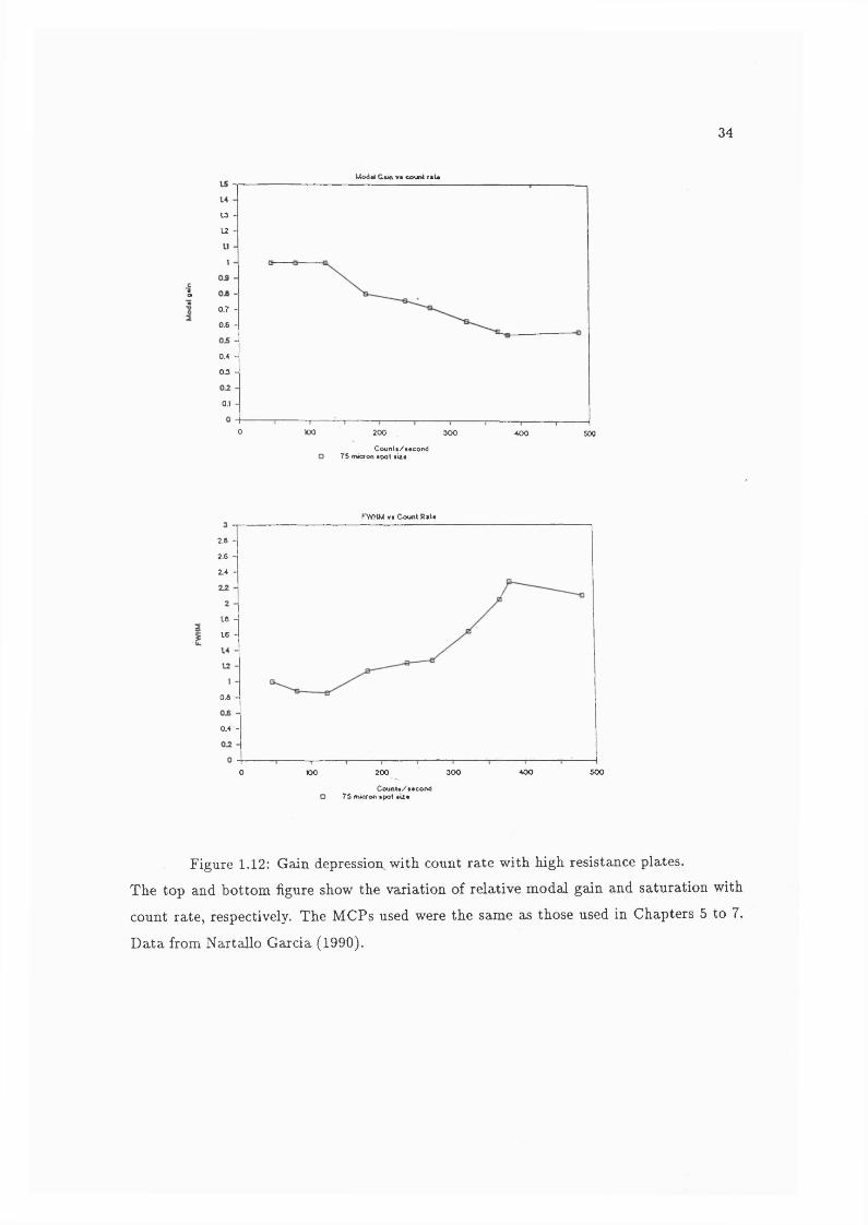
count rates as low as « 1 Hz.pore"^, (Fraser et oZ., 1991b and Nartallo Garcia, 1990), see

Figure 1.12.

Note that in the Figure 1.11 the absolute width of the PHD does not vary signifi

cantly as the gain is depressed. This is also shown in the saturation graph in Figure 1.12.

Saturation is a relative measurement of the PHD width with respect to the modal gain. The

variation in saturation in this diagram is due in the main part to the reduction in modal

gain rather than an increase in the absolute width of the PHD.

As the count rate is limited by the time constant of the pores, the photometric

linearity can be increased by reducing the resistance of the pores. Evaluation of lower

resistance MCPs have shown that countrates of % 40 and 500 Hz.pore~^ are sustainable

with minimal gain depression with Rch % 1 0 ^ and 1 0 ^ D, respectively, (Siegmund et oZ., 1991 and Slater & Timothy, 1991).

However, Rf^ cannot be made arbitrarily small and these values represent the

approximate limit for conventional, stable operation of MCPs. The resistance of the chan

nels has a negative temperature coefficient and Joule heating by the strip current running

through the walls will raise temperatures. Thermal runaway will occur for power densities

above 0 . 1 W.cm“ ^. A 25 mm diameter plate will be unstable with a resistance less than

roughly 5 MQ. This corresponds to a limiting count rate of several times 1 0 ® Hz.cm"^

(Feller, 1991). Assuming that the plate has 12.5 /im pores on 15 /im centres, there are

« 5 X 10® pores.cm"^. This limiting count rate corresponds to several hundred Hz.pore”"

for Rch « 1 0 ® Ü.

In conventional MCP mounts, almost all the heat must be removed radiatively

as there is poor lateral conduction through the plate edges. Feller (1991) found that by

connecting one MCP face directly to a heat sink. Joule heating was removed far more

efficiently by conduction and power dissipations of up to 3 W.cm“ ® could be maintained.

This allowed the continuous, stable use of a 25 mm, 750 kft, i.e Rch % 10 ® ft, plate at

1.7 kV with a maximum output rate of 1 2 k H z . p o r e " A t a voltage above 1.75 kV, the

plate once more became thermally unstable.

Although conductive cooling increases the MCP point source count rate perfor-

34

Modtl G «in V* count raU

U -U -

I0.7 -

0.6 -

0.4 -

OJ -

0.1 -

0 100 200 300 400 500

Coun(«/»«con<j 75 micfon «pot «ix*

rwHM v« Count Ra(«

Z 6 -

2.6 -

2.4 -

16 -

1.6 -

0.8 -

0.4 -

400 5000 200 300100

Counlt/M cond 75 micron spot *tz«

Figure 1.12: Gain depression with count rate with high resistance plates.

The top and bottom figure show the variation of relative modal gain and saturation with

count rate, respectively. The MCPs used were the same as those used in Chapters 5 to 7.

Data from Nartallo Garcia (1990).

35

mance dramatically, it requires a direct connection to the MCP face. However, it is not applicable to large format, high resolution imagers as all of the current readouts that pro

duce this performance require a gap between the MCP and the readout of at least 1 0 0 /zm

and in some cases millimetres, see Section 1.3.2.

1.2 M C P Based Photom ultipliers

1.2 .1 E U V and X -R ay P h o tom u ltip liers

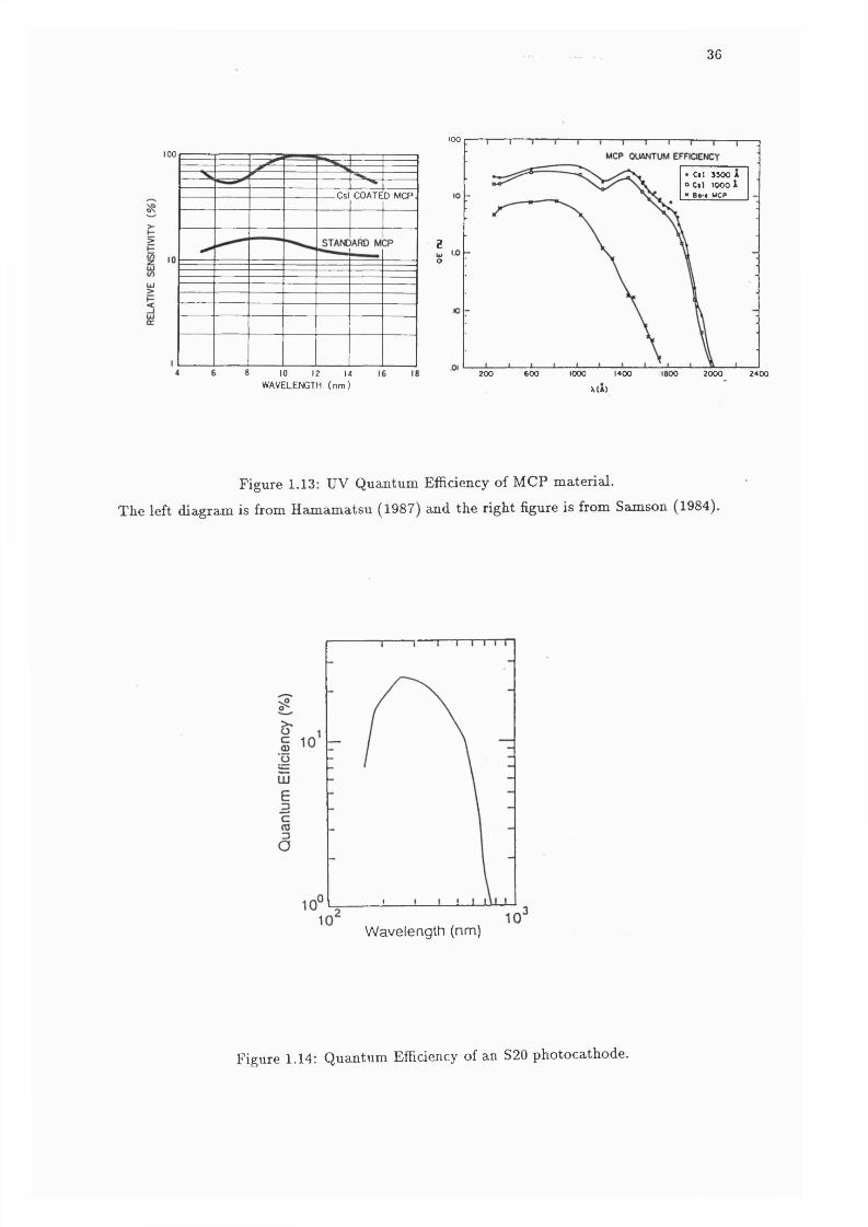
The quantum efficiency (QE) of an uncoated MCP in the UV is shown in Fig

ure 1.13. The QE at these and soft X ray wavelengths can be enhanced by depositing a

photocathode, for example Csl or MgF2 directly onto the MCP face. The sensitivity of an

MCP can also be extended into the hard X ray region by using a 1 0 0 /im Au photocathode

mounted directly onto the front of an MCP. Detected quantum efficiencies of « 0 . 2 % have

been achieved for 1 MeV X-rays (Veaux et al., 1991).In operation, the whole MCP stack and the readout are open to vacuum, so these

detectors are often called open-window detectors. These types of detectors have flown on many X-ray/EUV satellites, e.g. Einstein, EXOSAT and ROSAT (2k>mbeck & Fraser,

1991 and references therein) and are to be used on the Extreme Ultraviolet Explorer (Sieg

mund et al., 1985) &nd Solar and Heliospheric Observatory (SOHO) (Breeveld et al., 1992a)

satellites.

1 .2 .2 O p tic a l/U V P h o to m u ltip liers ^

For wavelengths from about 200 to 600 nm, the QE of a bare MCP falls of rapidly,

so a photocathode is necessary. A typical photocathode for these wavelengths is the multi

alkali S2 0 , see Figure 1.14.

There are a number of practical reasons why these photocathodes are not deposited

directly onto the MCP surface. The photo-electrons liberated from the microchannel plate

would have relatively low energies and those created other than within the channels would

probably be lost. Also, during the deposition of the photocathode it might prove impossible

to prevent a slight separation of photocathode constituents. These could end up deep inside

the pores which could lead to “switched on channels” .

Normally the photocathode is deposited on the surface of a UV/ Optical transpar-

36

100

-Csl COATED MCP

8 10 12 14WAVELENGTH (nm)

too

• C il 3500 A oC»l wool" Bor, MCP

2o

6 00 1000 1400 1800 2000 2400200

X(A)

Figure 1.13: UV Quantum Efficiency of MCP material.

The left diagram is from Hamamatsu (1987) and the right figure is from Samson (1984).

Wavelength (nm)

Figure 1.14: Quantum Efficiency of an S20 photocathode.

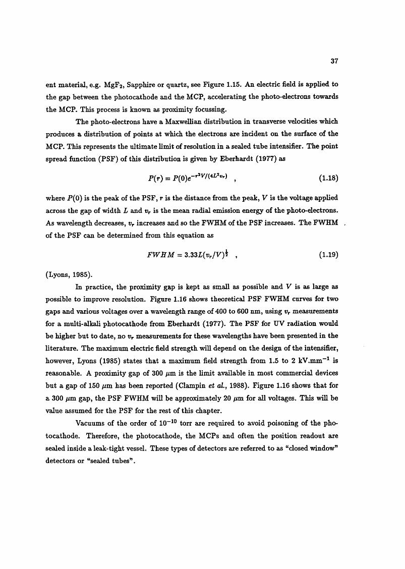
37

ent material, e.g. MgFg, Sapphire or quartz, see Figure 1.15. An electric field is applied to

the gap between the photocathode and the MCP, accelerating the photo-electrons towards

the MCP. This process is known as proximity focussing.The photo-electrons have a Maxwellian distribution in transverse velocities which

produces a distribution of points at which the electrons are incident on the surface of the

MCP. This represents the ultimate limit of resolution in a sealed tube intensifier. The point

spread function (PSF) of this distribution is given by Eberhardt (1977) as

P (r) = , (1.18)

where P(0) is the peak of the PSF, r is the distance from the peak, V is the voltage applied

across the gap of width L and is the mean radial emission energy of the photo-electrons.

As wavelength decreases, Vr increases and so the FWHM of the PSF increases. The FWHM

of the PSF can be determined from this equation as

F W H M = 3.33L{Vr/V)i , (1.19)

(Lyons, 1985).

In practice, the proximity gap is kept as small as possible and V is as large as

possible to improve resolution. Figure 1.16 shows theoretical PSF FWHM curves for two

gaps and various voltages over a wavelength range of 400 to 600 nm, using Vr measurements

for a multi-alkali photocathode from Eberhardt (1977). The PSF for UV radiation would

be higher but to date, no Vr measurements for these wavelengths have been presented in the

literature. The maximum electric field strength will depend on the design of the intensifier,

however, Lyons (1985) states that a maximum field strength from 1.5 to 2 kV.mm""^ is

reasonable. A proximity gap of 300 /xm is the limit available in most commercial devices

but a gap of 150 //m has been reported (Clampin et a l, 1988). Figure 1.16 shows that for

a 300 fjLm gap, the PSF FWHM will be approximately 2 0 fim for all voltages. This wiU be

value assumed for the PSF for the rest of this chapter.

Vacuums of the order of 1 0 ” ® torr are required to avoid poisoning of the pho

tocathode. Therefore, the photocathode, the MCPs and often the position readout are

sealed inside a leak-tight vessel. These types of detectors are referred to as “closed window”

detectors or “sealed tubes” .

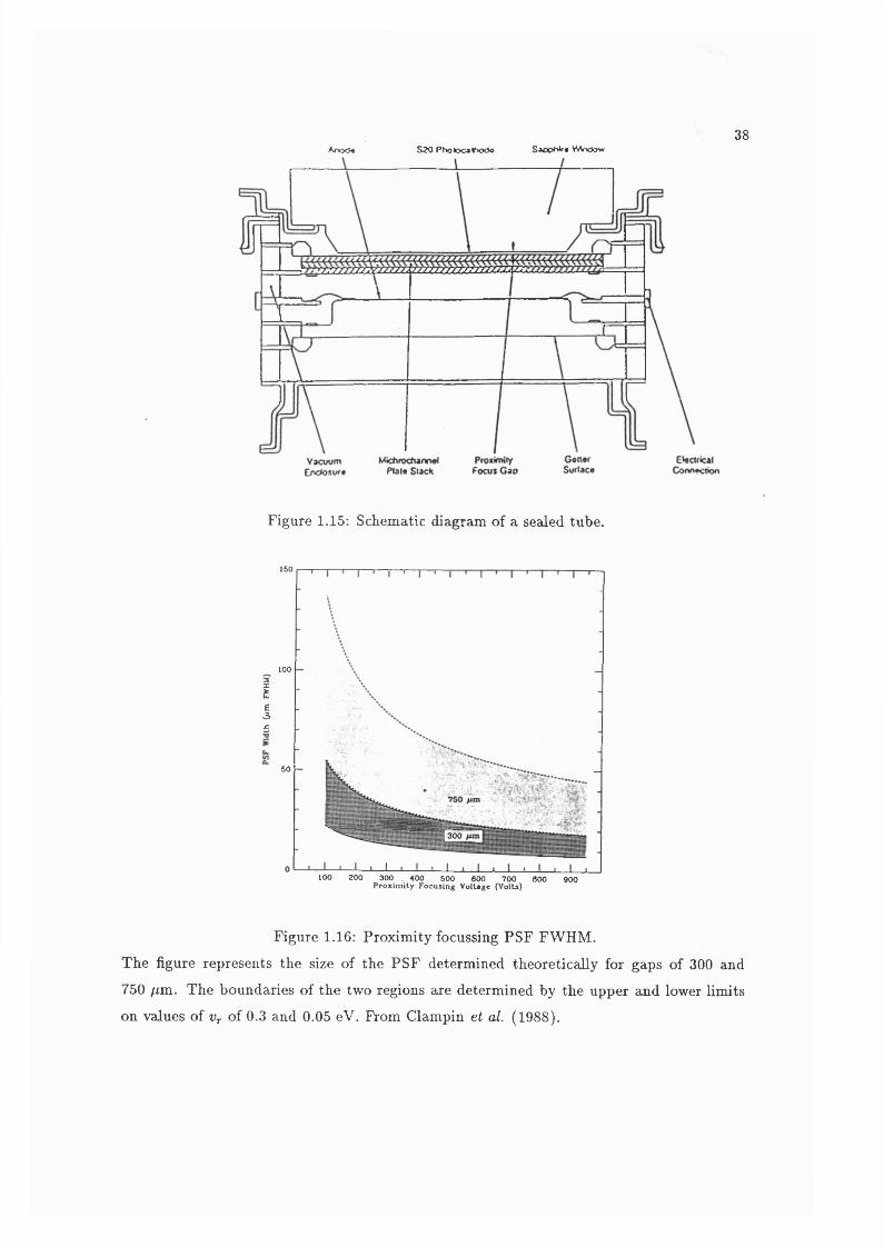
38AjxxV» 520 Phoiocaihodc S a o p W f # V W x Jo w

Figure 1.15: Schematic diagram of a sealed tube.

150

100SX£

I£

50

300

100 200 300 400 500 600 700 800P ro x im ity Focusing V oltage (Volts)

900

Figure 1.16: Proximity focussing PSF FWHM.

The figure represents the size of the PSF determined theoretically for gaps of 300 and

750 /xm. The boundaries of the two regions are determined by the upper and lower limits

on values of Vr of 0.3 and 0.05 eV. From Clampin et a i (1988).

39

1.3 M C P Position R eadouts

MCP baaed detectors can be divided into two major types.

1 . Light amplification detectors, in which the electron cloud produced by the MCP is

incident upon a phosphor producing a large pulse of photons which are optically

coupled to the detector, usually a CCD.

2. Charge measurement detectors, in which the centroid of the charge cloud is directly

measured by a series of electrodes. The positional readouts used in these detectors tn

can be used MCP and gas proportional detectors.A

1.3 .1 L ight A m p lification D etec to rs

There are two basic types of Light Amplification Detectors.

1 . Direct Readout Detectors.

In direct readout detectors, the position of the intensified events is immediately read

out and the detector performs no integration of events, e.g. PAPA.

2 . Scanned Readout Detectors.In scanned readout detectors the event is captured and stored by a detector and read

out later when the whole or part of the detector is scanned. Examples of this type of

detector are the vidicon camera, the Self-scanned PhotoDiode array (SPD) and the

Charge Coupled Device (CCD).

PAPA

In the Precision Analog Photon Address (PAPA) (Papaliolios et of., 1985) detec

tor the photon pulse from the phosphor is imaged by a system of lenses onto an array of

Gray coded or binary masks, as shown in Figure 1.17. Light transmitted by the masks is

then imaged onto a set of photomultipliers via an array of field lenses. One photomulti

plier, known as the strobe channel, looks at the whole output image without a mask and

determines whether an event has occurred in the field. A second photomultiplier looking

through a half clear, half opaque mask determines whether the event occurred in the left or

right section of the field. The light received by successive photomultipliers passes through

40

a set of progressively finer Gray coded masks, with the spatial frequency of the finest mask

determining pixel size.

It is possible, using a set of 9 photomultipliers and their respective masks to

determine the photon event position in the x direction to one of 512 positions. A similar

arrangement is implemented in the y direction using another 9 photomultiplier tubes and

a set of masks mounted orthogonally to the original set.

Using all 19 outputs from the above photomultipliers an 18 bit (z, y) address can

be generated which represents the arrival position of each detected photon. Therefore, 19

amplifier channels each consisting of a preamp and a discriminator are required.

At present, PAPA can provide up to 512 x 512 pixels, although formats of up to

4000 X 4000 pixels have been proposed (Papaliolios et oZ., 1985). PAPAs have been built

with 25 mm active diameters (Norton, 1990). Assuming an 18 X 18 mm square, 512 pixels,

20 fim defocussing in the proximity gap and a pore spacing of 15 /xm, the resolution will be

approximately equal to the quadratic sum of these components, i.e.

PSF FWHM = V 3 5 2 + 202 ^ 1 5 2 (1.20)

« 44 fim . (1.21)

The MCP charge cloud is incident on a P47 phosphor which has an extremely

short decay time of 2 0 0 ns. This implies a deadtime of 1 fjis per event (Norton, 1990).

In a paralysable detector, a subsequent event arriving within the initial event’s deadtime,

will extend the nonreceptive period of the detector by a further deadtime. In PAPA an

other event occurring during the phosphor decay time will lead to a wrong address being

returned. The detector will not return a correct address for a third event, until after the

deadtime associated with the second event has expired. PAPA can therefore be described

as a paralysable detector. Given the relation for a paralysable detector (Lampton & Bixler,

1985),

R' = Re~’ '’ , (1.22)

where R is the mean rate at the input, R' is the mean rate at the output and r is the

deadtime, then there will be a 1 0 % counting loss at a random arrival rate of 1 0 ® Hz. The

maximum point count rate for PAPA will be ultimately set by the channel recovery time of

the MCP.

In a nonparalysable detector, subsequent events do not extend the deadtime and

41

THERMOELECTRIC COOLER /

LENS m a s k s ARRAY ^

tINCOMINGPHOTON

COLLIMATOR/

FIELDLENSES

__________Q [) Channel 0

0 D Channel 2E BE D 0 I) s t r o b eI I 0 Channel 3

A / D EO 0 D C h a n n e l 1t

FIELDFLATTENINGLENSES

PM Ts

BINARY CODE GRAY CODE X-POSITION MASKS MASKS DATA CHANNEL

NO NO 0

YES YES

YES NO

DETECTED AND INTENSIFIED PHOTON

Figure 1.17: Schematic diagram of the PAPA detector.

The figure shows the arrangement of the optics, PMTs and examples of the Gray coded

masks. From Sams (1991).

the reduced mean rate is given by

42

(Lampton & Bixler, 1985). In this case, a random arrival rate of 10 Hz, will also cause a

10 % counting loss. All count rates quoted in this work correspond to this level of counting

loss.

The PAPA detector requires that the mechanical alignment of the optics system

with the coded masks be extremely precise. Sub-micron shifts in the mask position intro

duces serious fixed patterning noise in the final output image (Norton, 1990), i.e. some

pixels detect higher intensities than others under constant illumination.

Scanned Readout Detectors

The vidicon (generic name) has a dense array of reverse biased diodes on a silicon

substrate. An incident photon is converted into electron-hole pairs which locally discharge

the diodes. The wafer is then raster scanned with an electron beam and the current required

to recharge each diode reflects the intensity at that point. Vidicons are slow devices, intense

signals can spill over into the next diode and more than one scan of the electron beam may

be required to readout intense signals (Richter & Ho, 1986).

A SPD consists of an array of photodiodes connected to an output signal line

via switches. A shift register sequentially recharges each diode which effectively measures

the stored signal. The CCD stores signal in a similar way. The charge is transported by

an analog shift register. The SPD and CCD have very similar operational characteristics.

However, the CCD does have some advantages over the SPD, it is easier to construct two

dimensional CCDs and the CCD’s lower output capacitance means it can be clocked faster

and have lower noise (Richter & Ho, 1986). The CCD is therefore the detector used in most

modern scanned readout systems.

CCD Based Detectors

In CCD based detectors the pulse of photons is optically coupled to one or more CCDs

through a fibre-optic bundle. The small areaa of CCDs 1 cm^ compared to MCPs can be

overcome by using a fibre-optic bundle to couple to several CCDs, e.g. the Photon Counting

Array (PCA) which uses four (Rodgers et a/., 1988). The fibre-optic bundle can also be

tapered, producing an optical demagnification, to couple the phosphor to a single CCD.

43

For example the MCP Intensified CCD (MIC) detector (Fordham et al., 1989) uses a 3.8:1

fibre-optic taper.

When combined with the demagnification, CCD pixel sizes, 2 0 /im would

produce pixel sizes of 80 fim as seen at the photocathode. This large pixel size can

be overcome by spreading the photon pulse over a few pixels and centroiding which can

produce sub-pixel accuracy (Carter et oZ., 1990). Centroiding can be carried out over

the pixel with the peak intensity and the intensities in the closest CCD pixels in each of

the cardinal directions, 3 point centroiding, or the two closest pixels in each direction, 5

point centroiding (see Figure 1.18). Intensities are determined by digitizing the charge

accumulated in each pixel by an 8 bit ADC. As the CCD can transfer charge from pixel

to pixel, only one preamp and ADC are required. Three point centroiding can subdivide a

CCD pixel into up to 128^ subpixels (Carter et uZ., 1991).

W ith division to 1/32 nd. of an 8 8 fim CCD pixel, as seen at the photocathode,

the individual pores on the front MCP, 1 2 /xm pores on 15 /xm centres, can be resolved (Read et oZ., 1990). The PSF of the centroiding has been measured as % 2 /xm using 128

subpixels (Carter et aZ., 1991) and the overall resolution has been measured as 25 /xm. This

approximately represents the combination of an assumed proximity gap PSF of 2 0 /xm and

the pore spacing. IrjjThe point source countrate is limited the decay time of the output phosphor,

A% 2 /xs for a P 2 0 phosphor (Carter et aZ., 1991) and the frame rate. The size of the region

to be read out can be selected and as there are fewer pixels in a smaller region, faster frame

rates are possible. The maximum linear count rate for a flat field is % 2 X 10 Hz. The

maximum point source count for a 10.6x84/xm pixel is 38 Hz (Fordham, 1990) at a frame

rate of about 1.5 ms.

If two photons arrive at the same position during one frame they could be counted

as one photon. By operating the CCD in analog mode and measuring the amount of charge

it is possible to determine if more than one event has occurred at the point. This data can

be discarded or counted as two events. However, this method is very sensitive to depression

of the MCP gain at high local count rates (Richter &: Ho, 1986).

Great care must be also taken to ensure that overlapping events are properly

identified and discarded. This places further limitations on the point source count. W ith

3 point centroiding, the optical pulse must cover at least an area of at least 3 x 3 CCD

pixels. An overlapping event will result if a subsequent event occurs with its centre lying in

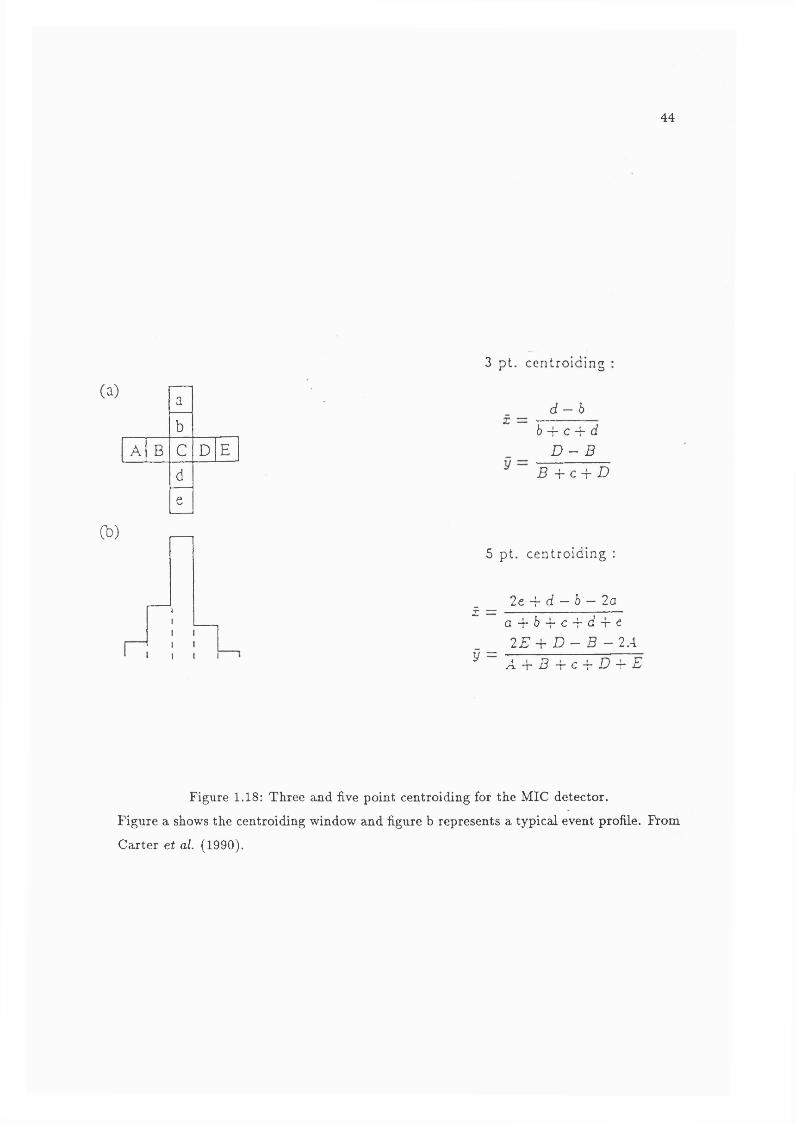
44

(a) a

bA B C D E

de

Cb)

3 pt. centroid ing

d — h 6 -f c + d

D - BB 4 - C 4 - D

5 pt. centroid ing :

2e -f d — 6 — 2aX ~

y =

a + 6 - r C - f d - T - e

2 E D - B - 2A

A - r B - r C - r E - v - t ^

Figure 1.18: Three and five point centroiding for the MIC detector.

Figure a shows the centroiding window and figure b represents a typical event profile. From

Carter et al. (1990).

45

one of, at the least «20 CCD pixels surrounding the central pixel of the first event, within

one frame time (Carter, 1991a). Therefore, a single event can effectively paralyse an area

containing approximately 1300 image pixels, assuming division into 8 x 8 subpixels, for the

whole frame time.The optical demagnification of a tapered fibre-optic introduces barrel distortion.

The higher the taper ratio, the worse the distortion. A taper of 3.8:1 produces a distortion

of « 1 % of the active diameter, i.e. « 300 iim (Read, 1990). It is possible that low

distortion tapers may be obtained, which would reduce this effect.

A ctive P ixel Image Sensors

Active pixel image sensors are a family of devices recently developed for use in high definition

television. These devices have not yet been used as positional readouts for MCPs, but

potentially they could. Although there are several different types of device, they all

consist of an array of pixels each containing a phototransistor as the light sensitive element

(Yusa et al., 1986, Hynecek, 1988, Tanaka et al., 1990 and Nakamura & Matsumoto, 1992).

For example, in the Charge Modulation Device (CMD) (Nakamura & Matsumoto,

1992), photons incident on a photoFET produce a population of holes near the gate. During

readout the magnitude of the source current is modulated by the number of holes. Readout

is carried out by varying the gate voltage and is nondestructive. The gates of all pixels in a

row are connected together so that a whole row is read out simultaneously. All the drains

of the FETs in one column are connected together and to one capacitor. Therefore, one

row at a time can be read with the source current charging capacitors in each column. The

capacitors are then clocked serially to a preamp. Each row can be read out individually

and in any sequence. All pixels can be reset simultaneously.

CMDs have been made with up to 2 million, « 7.5 /zm square pixels, t.e.l920xl036.

Data can be read out at 75 MHz, i.e. each pixel can be read out at «30 Hz if the whole

image is being read. The CMD has slightly better performance than the other active pixel

sensors and compares favourably to that of a CCD. It would be most interesting to evaluate

this chip as a MCP position readout.

1.3 .2 C harge M easu rem en t D etecto rs

The positional readouts in charge measurement detectors can also be divided into

two broad categories:

46

1 . Discrete Electrode Readouts, in which many anode electrodes, either pads or wires,

are used. These devices produce a digital code for the centroid position and the pixel

size is directly determined by the spacing of the electrodes.

2. Continuous Electrode Readouts, in which the output signal from the anode is a contin

uous function of the spatial position of the centroid. The continuous signal is digitized

by an ADC and the pixel size is determined by the ADC quantization.

D iscrete E lectrode Readouts

An example of a discrete electrode readout is the Coded Anode Converter (CO- DACON) (Me Clintock et uZ., 1982). The charge from the MCP is deposited on a series

of parallel strips, called charge spreaders, on one side of a dielectric substrate. These elec

trodes induce a charge on a set of orthogonal electrodes, called code tracks, on the other

side of the dielectric. The thickness of the code tracks varies along the length so the charge

induced is proportional to that area. Each charge spreader’s position is then represented

by a Gray code. This detector can provide 2" pixels with n amplifier channels. Only one

dimensional readouts have been constructed at this stage.

M A M A ’S

The most developed of the discrete electrode readouts are the Multi-Anode MicroChannel

Array (MAMA) readouts. There are two basic types of MAM As; the discrete-anode array

and the coincident-anode array (Timothy eZ a/., 1981).

1. The Discrete-Anode Array.

The discrete anode array consists of of an array of n X m anodes, insulated from each

other. Each channel must be read out with an individual electronic channel consisting

of a preamplifier and a discriminator. Therefore, n x m channels are required.

2 . The Coincidence-Anode Array.

The simplest coincidence-anode consists of two orthogonal planes of electrodes, sep

arated by an insulating layer, mounted on a substrate (Timothy & Bybee, 1975b).

Each plane consists of a series of linear 25 //m electrodes on 50 /im centres. In oper

ation, the MCP pulse is divided between the row and column electrodes at the point

of incidence. If a pulse occurs on both the row and column electrodes within a finite

47

time (~ 100 ns), the position of these two electrodes is taken to be the position of the

charge pulse. The coincidence anode allows an n x m array to be read out with n-{-m

discriminating channels.

The coincidence technique can be extended to further reduce the number of electronics

channels (Timothy et al., 1981). Figure 1.19 shows a Coincidence MAMA where 16

positions are encoded by 16 anodes and 8 amplifier channels. Every other anode,

call these the even anodes for convenience, is connected to one of four fine position

amplifiers. This indicates that an event is on any 4 out of 16 electrodes. Assuming

that the charge cloud only covers two electrodes, by connecting the odd anodes to

another set of 4 amplifiers, the coarse amplifiers, the pair of electrodes the MCP pulse

straddles is determined. Comparing signal intensities on the coarse and fine channels

determines if the centroid of the pulse is closer to the odd or even electrode.

All events that stimulate more than 4 electrodes or those that stimulate non-adjacent

electrodes are rejected. The events that are coincident on 2 or 3 adjacent electrodes

are identified and stored as addresses in the decoding electronics. This provides in

formation from 32 pixels. Adjacent two-fold and three-fold events are then summed

giving the required information for 16 pixels.

This process can be extended to more fine and coarse position channels. A 1024x1

pixel array requires 32 fine and coarse channel, i.e. 64 channels per axis. A 1024x1024

array can be manufactured by depositing another set of orthogonal electrodes, sepa

rated by an insulator, over the first set.

The deadtime associated with the analogue and the decoding electronics is 100 ns per

coincidence. . ».

Pixel size is determined by the size of the electrodes ani^S /xm have been achieved

(Timothy & Bybee, 1975a). Assuming a 20 /xm FWHM defocussing in the photocathode

MCP gap and 15 /xm pore spacing, the overall resolution would be % 35 /xm. As MAMA

only requires discrimination to determine position, they do not require as high a SNR as

readouts using charge measurement, e.g. continuous electrode readouts (see below) and

gains of approximately 10 electrons are sufficient. This can be provided by a single C

plate. Also, the gain depression caused by high local count rate does not have a great affect

on the resolution. However, when gain is depressed below the discriminator threshold, the

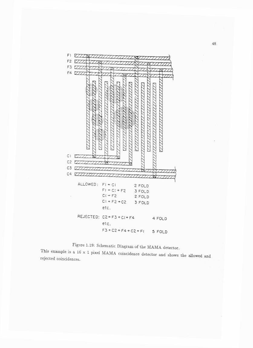
48

FI EZZ7F2 ZZZ72F3 r7777F4 u y y /.

if

22ZZZZ2ZZZZ2ZZZZSaZZZZZZZZZZZZZ3S

J

Cl rrr/,‘ .K

I €

ZZ2Z2ZZZ2ZZZà

2ZZ

zzC2 C 2 2 7 y / ,V / / .Z 2 a

Ns

1

zzzzz

1 5

ZT7 y

ts

z z z

a i l-ysK

trf

\sS5

\\\\

A

N5\\\5\W

E Z

y y / ; y y y- yy, ; / T -C4

222222

Z ZZZZ^

Z 2 7 Z

ALLOWED : FI -*■ Cl FI + Cl + F2 Cl 4- F2

Cl + F 2 + C 2

etc.

2 f o l d3 FOLD2 FOLD3 FOLD

4 FOLDREJECTED: 0 2 + F 3 + C I 4 - F 4

etc .

F3 4-C2 + F4 + C24-FI 5 FOLD

Figure 1.19: Schematic Diagram of the MAMA detector.

This example is a 16 x 1 pixel MAMA coincidence detector and shows the allowed andrejected coincidences.

49

photometric linearity will still be affected.The spatial extent of the MCP charge doud must be approximately the same size

as one of the electrodes for a discrete anode. This requires that the gap between the MCP

and the anode is small, 100 /im. Coinddence anodes require that the charge doud is

spread over at least two but not more than four dectrodes, so they require similar sized

anode gaps.

Continuous Electrode Readouts

In continuous dectrode readouts the charge from the inddent MCP pulse is par

titioned between a number of amplifiers, typically 2 per axis. There are two basic types of

these readouts.

1. The resistive anode, dday lines and crossed wire grid are Charge Division Readouts

in which charge is divided by a resistive or capadtive network.

2 . In Charge Sharing Readouts the charge is collected by a few dectrodes which are

insulated from each other. Ideally, the dectrodes are not coupled together and the

amount of charge collected on each dectrode depends soldy on its area. Therefore, the

total charge from the MCP is shared between the dectrodes according to th d r areas

at a given point. Two well known examples of these readouts are the Backgammon

and Wedge and Strip readouts.

W ith the exception of the Quadrant Anode and Resistive Anodes, charge division

and sharing readouts consist of a repeated pattern of dectrodes. The pitch of the pattern

is typically of the order of 1 mm. To avoid distortion, the spatial size of the charge doud

must cover several of these pitches, see the discussion in the Wedge and Strip section and

references therdn. A substantial gap, typically several millimetres, is needed between the

bottom of the MCP stack and the anode to ensure that the charge doud can expand to the

necessary size.

The resolution of the device depends on the accuracy of the charge measurement.

Therefore, good SNR is necessary for good resolution. As the dectronic noise is independent

of pulse height, a larger charge pulse will have a better SNR than a smaller one. Also, these

readouts are subject to partition noise. This noise is due to the quantum nature of the charge

carriers and their random arrival on one of the electrodes (Martin et o/., 1981). Partition

50

noise decreases with increasing pulse height, e„p oc . Therefore, a higher gain in the

MCP produces a higher SNR and better resolution. Figure 1.20 shows an example of how

resolution varies with MCP gain.As the MCP produces a PHD, the resolution of the ADCs must be at least equal to

the product of the desired position resolution and the pulse height dynamic range. Practical

limitations on the anode design limit the dynamic range. Gain depression caused by high

local count rates will move the PHD to lower levels, reducing the digitization of the measured

values and decreasing the SNR. Images must also be oversampled, i.e. the size of the pixel

defined by the ADC digitization must be smaller than the desired resolution. Otherwise, a

fixed patterning noise is produced (Clampin et oZ., 1988). As a result, in practice, at least

12 bit ADCs are required to produce a 1024 x 1024 pixel array.

R esistive Anodes

The resistive anode (Stiimpel et oZ., 1973 and Lampton & Paxesce, 1974) has the widest commercial availability of the MCP readout devices. It consists of an area of uniform

resistance, typically 10® — 1 0 ®IÎ/D. This area can have many different shapes (Fraser,

1989). The circular arc terminated resistive anode is one of the most successful designs

for eliminating image distortions (Gear, 1969). Resistive anodes require two electronics

channels, located on opposite sides of the resistive area, per axis.

Timing was the original method of determining the spatial position for the resistive

anode (Stiimpel et oZ., 1973). The times of the signal zero crossing point in the amplifiers

are measured. The electronics necessary for this method are similar to those used in delay

lines, see below. In this mode, changes in the anode temperature will produce a zooming

effect in the image (AUington-Smith & Schwarz, 1984 and Clampin et oZ., 1988) and charge

measurement is the most widely used method at present.

For charge measurement, each channel consists of a charge sensitive preamp, am

plifier and ADC. The centroid position is determined either by measuring the magnitude

of the current pulse, Q for each channel. The x and y coordinates are determined by the

equations,

" = QA + Q t ^ Q c + Qo '

^ " Qa + q I W c + Q d •

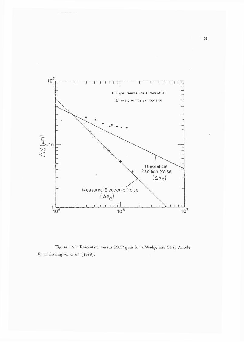
51

■ E iperim en ta l Data from MCP

Errors given by symbol size

10X

Theoretical Partition Noise

(AXn)

Measured Electronic Noise

Figure 1.20: Resolution versus MCP gain for a Wedge and Strip Anode.

From Lapington et al. (1988).

52

The anode will only operate linearly in the dc limit, i.e. a long filter time constant with respect to the anode time constant (Fraser & Mathieson, 1981), typically a few microseconds but as low as 0.5 //s giving a 6 //s deadtime (Clampin et a/., 1984).

The major limiting factor in the performance of resistive anodes is the Johnson noise associated with the resistive anode,

, (1.26)

where k is Boltzman’s constant, T is the temperature, r is the time constant of the

i rC m t R Co f Le

Resistive anodes have traditionally had problems With non-uniformity of the res

olution across the active area of the detector, the resolution at the edges being typically y/2 worse than that at the center, ~ 50/zm FWHM over a 25 mm diameter, (Lampton & Paresce, 1974, Clampin & Edwin, 1987 and F/oryan & Johnson, 1989). Firmani et al. (1984) and Clampin et al. (1988), however, have demonstrated a uniform resolution across the whole image of 40 /zm at 650 nm at 12 bits digitization. This resolution includes the contribution of the pore spacing. The diameters of the pores are quoted as 13 fim so the spacing should be ~ 15 /zm. The latter group report a PSF of 22 /zm FWHM from a proximity focussing gap of 300/zm with an applied voltage of 300 V. If we assume that the defocussing is reduced to 20 /zm, the resolution would improve marginally to « 39 /zm. Clampin et al. (1988) also report deviations from positional linearity of < 2 1 /zm.

Fraser (199 1 ^h ^êp o rted imaging 85 /zm square pores on 100 /zm centres,

achieving a best r ^ ôf 13.5 /zm over a 5 mm image, with a resistive anode. However,A

they do not describe the size of the detector or the electronics.Delay Lines

When the MCP charge pulse is incident on a delay line, it divides into two pulses that propagate in opposite directions. The centroid position is determined by measuring the difference in the arrival time of the pulses at opposite ends of the delay line. A separate delay line is required for each dimension.

There are three basic types of delay lines:

53

1 . Solid State Delay LinesThe charge from the MCP is collected on individual parallel strips which are connected

to taps in a solid state delay line. However, this system so distorts the MCP pulse

shape that the resolution is limited to 250 /im FWHM ( Keller et al.y 1987).

2. Planar Delay Lines

These delay lines have been produced by etching a zig-zag pattern in copper on a

hbreglass substrate (Siegmund et a/.,1989a). At present, only one dimensional delay

lines can be manufactured but the authors suggest that an anode consisting of crossed

delay lines may be possible. The operating characteristics are similar to those of a

transmission line delay line, so most of the following discussion is relevant to planar

devices as well.

3. Transmission Line Delay Lines

Figure 1 . 2 1 shows the schematic layout of a transmission line delay line (Williams &

Sobottka, 1989). Each delay line consists of two 2 0 0 /xm bare Cu wires wrapped, with

a 1 mm pitch, around a Cu centre. The wires are insulated from the Cu centre by ceramic spacers. One wire is wound halfway between the other wire so that the two

windings form a two wire transmission line. A second set of windings is wrapped in an

orthogonal direction to produce the second delay line. The two sets of windings axe

separated by a gap so that they are insulated from each other. Different DC voltages

are applied to each of the 4 wires and the Cu centre, to ensure that 50 % of the MCP

charge pulse goes to each of the delay lines and that all of the charge on one delay

line is collected on only one of the wires (Sobottka & Williams, 1988).

A schematic diagram of the electronics required for each delay line is shown in Fig

ure 1 .2 1 . The signals from opposite ends of the two wires are fed into differential

amplifiers. The outputs from these are then passed through two constant action

timing discriminators (CFD). A delay Td is added to one channel and then the two

channels are input to a time to analogue converter (TAC). The analogue TAC output

is digitized by an ADC. Therefore, only one ADC is required per axis. In practice,

the TAC and ADC could be replaced by a time to digital converter (TDC). The pla

nar delay line has a very similar electronic setup except that delay line only has one

component and uses two preamps instead of two differential amplifiers.

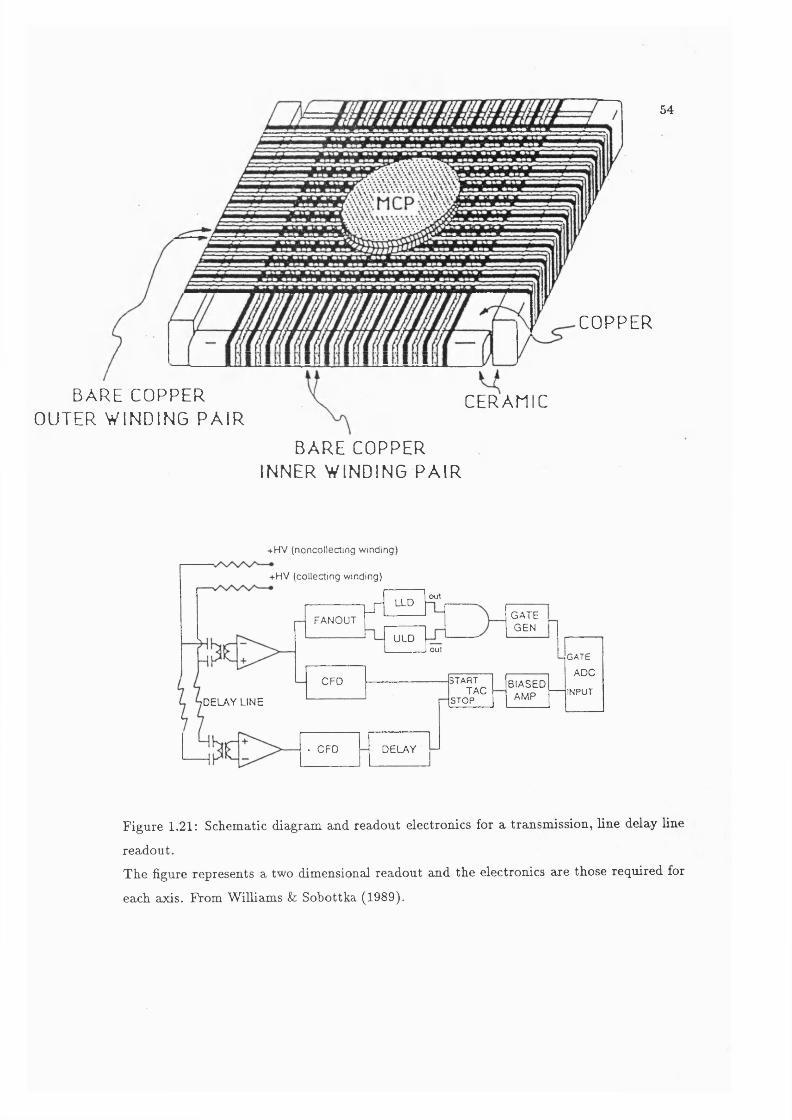
54

BARE COPPER OUTER WINDING PA IR

COPPER

CERAMIC

BARE COPPER INNER WINDING PAIR

►•HV (noncollecting winding)

+HV (collecting winding)

lTFANOUT

LLDout

ULDout

7DELAY LINE

. CFD DELAY

GATEGEN

C FD STARTTAC

STOP

GATE

ADCBIASED

AMP INPUT

Figure 1.21: Schematic diagram and readout electronics for a transmission, line delay line

readout.The figure represents a two dimensional readout and the electronics are those required for

each axis. From Williams Sz Sobottka (1989).

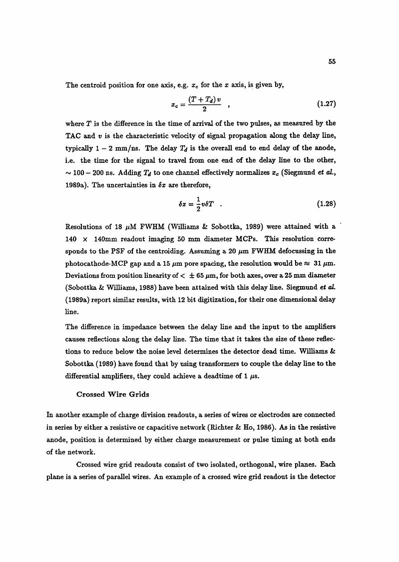
55

The centroid position for one axis, e.g. Xc for the x axis, is given by,

, (1.27)

where T is the difference in the time of arrival of the two pulses, as measured by the

TAC and v is the characteristic velocity of signal propagation along the delay line,

typically 1 — 2 mm/ns. The delay Td is the overall end to end delay of the anode,

i.e. the time for the signal to travel from one end of the delay line to the other,

rv 100 — 200 ns. Adding Td to one channel eflfectively normalizes Xc (Siegmund et nZ.,

1989a). The uncertainties in 6x are therefore,

6x = ^v6T . (1.28)

Resolutions of 18 /xM FWHM (Williams & Sobottka, 1989) were attained with a

140 X 140mm readout imaging 50 mm diameter MCPs. This resolution corre

sponds to the PSF of the centroiding. Assuming a 2 0 /xm FWHM defocussing in the

photocathode-MCP gap and a 15 /xm pore spacing, the resolution would be % 31 /xm. Deviations from position linearity of < ± 6 5 /xm, for both axes, over a 25 mm diameter

(Sobottka & Williams, 1988) have been attained with this delay line. Siegmund et al.

(1989a) report similar results, with 12 bit digitization, for their one dimensional delay

line.

The difference in impedance between the delay line and the input to the amplifiers

causes reflections along the delay line. The time that it takes the size of these reflec

tions to reduce below the noise level determines the detector dead time. Williams &

Sobottka (1989) have found that by using transformers to couple the delay line to the

differential amplifiers, they could achieve a deadtime of 1 /xs.

Crossed W ire Grids

In another example of charge division readouts, a series of wires or electrodes are connected

in series by either a resistive or capacitive network (Richter & Ho, 1986). As in the resistive

anode, position is determined by either charge measurement or pulse timing at both ends

of the network.

Crossed wire grid readouts consist of two isolated, orthogonal, wire planes. Each

plane is a series of parallel wires. An example of a crossed wire grid readout is the detector

56

used in High Resolution Imager (HRI), used on the Einstein Observatory and ROSAT

(Fraser, 1989).In the HRI readout, each of the wire planes consists of 1 0 0 /im wires on 200 fim

centres. For a 25 mm diameter image, this corresponds to 125 wires per axis. The planes

are held approximately at —300 V with respect to the rear of the MCP stacks. A small

bias voltage between the two planes ensures that the MCP charge pulse is divided evenly

between the two planes. The wires are coupled together with 1 0 kO resistors. Every eighth

channel is connected to a charge sensitive preamp, called a tap. Therefore, 17 amplifier

chains are required for each axis. The event position x is determined by a coarse and fine

position measurement, Xc and a;/, respectively,

x = Xc + Xf . (1.29)

The coarse position is equal to the position, x,*, of the tap, i, that has collected the largest

charge, Q,-, from the grid. The fine position is determined by a centroiding algorithm using

Qi and the charge on the adjacent taps,

" Q .Î+ Q .% + 1 ’(Chappell & Murray, 1989).

For a 25 mm diameter image a crossed grid readout is capable of 2 0 /xm FWHM

resolution at a linear count rate of 500 Hz (Fraser, 1989). Assuming that this resolution

includes the contribution from a pore spacing of 15 fim but not the proximity focussing

PSF, the overall resolution would be « 28 fim .

W edge and Strip Anodes

In charge sharing readouts, the anode is divided into a few conductive electrodes of finite

width, deposited on a substrate and insulated from each other. These types of anodes are

sometimes called progressive geometry encoders. The amount of charge collected on each

electrode depends on the area of that electrode. The electrodes usually have areas that vary

linearly across the anode. At any one point, the ratio of the electrode areas will be unique.

As a result, the ratios of the amount of charge collected on each electrode at any given point

will also be unique. Examples of this type of anode are the Four Quadrant Anode (Lampton

& Malina, 1976 and Purshke et oZ., 1987), the Backgammon Anode (Allemand & Thomas,

1976) and the Sickle and Ring Anode (Knibbeler et a l, 1987).

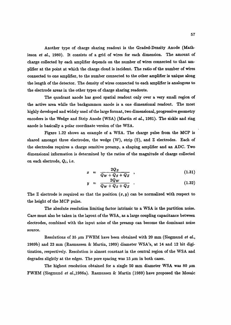
57

Another type of charge sharing readout is the Graded-Density Anode (Math

ieson et al. 1980). It consists of a grid of wires for each dimension. The amount of

charge collected by each amplifier depends on the number of wires connected to that am

plifier at the point at which the charge cloud is incident. The ratio of the number of wires

connected to one amplifier, to the number connected to the other amplifier is unique along

the length of the detector. The density of wires connected to each amplifier is analogous to

the electrode areas in the other types of charge sharing readouts.

The quadrant anode has good spatial readout only over a very small region of

the active area while the backgammon anode is a one dimensional readout. The most

highly developed and widely used of the large format, two dimensional, progressive geometry

encoders is the Wedge and Strip Anode (WSA) (Martin et oZ., 1981). The sickle and ring

anode is basically a polar coordinate version of the WSA.

Figure 1 . 2 2 shows an example of a WSA. The charge pulse from the MCP is

shared amongst three electrodes, the wedge (W), strip (S), and Z electrodes. Each of

the electrodes requires a charge sensitive preamp, a shaping amplifier and an ADC. Two

dimensional information is determined by the ratios of the magnitude of charge collected

on each electrode, Qi, i.e.

* " Qw + ^ s + Q z '

^ " Qw + q I + Qz •

The Z electrode is required so that the position (x,y) can be normalized with respect to

the height of the MCP pulse.

The absolute resolution limiting factor intrinsic to a WSA is the partition noise.

Care must also be taken in the layout of the WSA, as a large coupling capacitance between

electrodes, combined with the input noise of the preamp can become the dominant noise

source.

Resolutions of 35 fim. FWHM have been obtained with 2 0 mm (Siegmund et al.,

1989b) and 23 mm (Rasmussen & Martin, 1989) diameter WSA’s, at 14 and 1 2 bit digi

tization, respectively. Resolution is almost constant in the central region of the WSA and

degrades slightly at the edges. The pore spacing wa^ 15 fim in both cases.

The highest resolution obtained for a single 50 mm diameter WSA was 80 fim

FWHM (Siegmund et a/.,1986a). Rasmussen & Martin (1989) have proposed the Mosaic

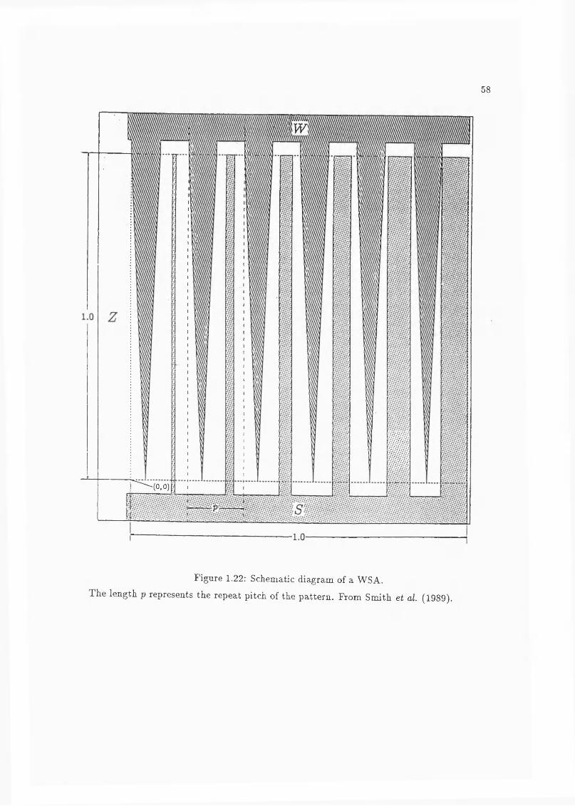
58

g

mmr ^ ( o ,o )

Figure 1.22: Schematic diagram of a WSA.

The length p represents the repeat pitch of the pattern. From Smith et ai (1989).

59

Wedge and Strip readout. Basically, nine 23 mm square, WSAs would be butted together, requiring 29 channels of electronics, 9 x 3 plus 2 extra channels for border sampling elec

trodes. They estimate this would produce < 30 ^m resolution over a 50 mm diameter. They

have demonstrated that it is possible to butt two WSAs together with positional linearities

of 50-100 /zm across the boundaries.

Assuming a 2 0 /zm FWHM defocussing in the photocathode-MCP gap, a resolution

of 35 /zm without defocussing would correspond to an overall resolution of w 41 /zm.

Variations in the size of the MCP charge cloud can introduce severe distortions in

WSA images (Smith et oZ., 1989 and Vallerga et aZ., 1989). These distortions are discussed

in Chapter 3. The spatial distribution of the charge cloud and its size have been measured

for various operating conditions and are discussed in Chapter 4.1. The distortion of the

position linearity for a WSA can be < 0.5 % of a 50 mm diameter image, i.e., 125 /zm

(Siegmund et al., 1986b). Using a correction map generated by image calibration, the

distortion could be reduced to approximately 25 /zm (Vallerga et al., 1989).

The limiting factor on the speed of a WSA is usually the time constant of the

shaping amp. Rasmussen & Martin (1989) used 5 /zs shaping times while obtaining 35 /zm

resolution.Cyclic Continuous Electrode Readouts

These types of readout include a novel form of MCP readout being developed at MSSL and

are analyzed in detail in the next chapter. The operation of one example is discussed in

Chapter 5.

1.4 A n O ptical M onitor for th e XM M Satellite

In order to best understand the nature of high energy sources it is necessary that

correlated observations are made over many wavelengths. During the operation of previous

X-ray astronomy satellites such as EXOSAT, large amounts of ground based and lUE (In

ternational Ultraviolet Explorer) observing time were devoted to correlated observations of

approximately 60% of the X-ray targets (Briel et al., 1987).

As most X-ray sources exhibit high variability over very short timescales, it is

also important that the multi-frequency observations be carried out simultaneously. It is

difhcult to coordinate ground based observations with those of a satellite, given the vagaries

60

of time allocation and the weather.Including an optical/UV telescope on an X-ray satellite would facilitate correlated

multi-frequency observations and would guarantee their simultaneity. This capability would

be very important in the study of important astronomical subjects, e.g. the relationship

between X-ray and optical variability in AGN, X-ray bursters and transient outbursts.

Interstellar extinction in the direction of X-ray sources can be determined by car

rying out broadband photometry in the U,B,V bands and bands not observable by ground

based telescopes, such as in the UV at 2500 A and the far UV at 1500 A. Narrow band

photometry can also be carried out in lines common to X-ray objects, e.g. the H/? line is

typically in emission from cataclysmic variables (CV) and QSO nuclei; the [Om] A = 5007 A line, characteristic of AGN, QSO and nebulae; and He II A = 4686 A, found in almost all

X-ray binaries, is particularly strong in CV and WR stars.

Due to the obvious versatility of such a system, the European Space Agency has

decided to include a small Optical/UV telescope, the Optical Monitor, on its X-ray Multi

Mirror (XMM) satellite. This will be the first time that an X-ray satellite has carried an

optical telescope.

1.4 .1 D etec to rs .

The optical monitor will have two detectors. The blue detector will be a photon

counting, sealed tube MCP intensifier with a S20 photocathode to cover the approximate

wavelength range 150 to 650 nm. The red detector consists of a CCD for the range 550 to

10000 nm.

The main performance requirements for the blue detector are:

1. Active Area: 18 x l8 mm square, which corresponds to a 16 x 16 arcmin field of view.

2. Number of pixels: 2048, i.e. « 9 /xm pixels.

3. Maximum countrate over the entire active area, defined by the Zodiacal Light: 2 x

10® Hz.

4. Point Spread Function: 18 /xm

5. Maximum Point Source Countrate: lO^Hz

6. Maximum Point Source Countrate with defocussing to twice the PSF: 10 Hz.

61

These axe demanding requirements especially when combined with a proposed ten

year lifetime and a total radiation dose of more than 100 krad.

Table 1.2 summarizes the performance of existing two dimensional detectors re

viewed in the previous section. None of the detectors actually meet the specification. As

MIC is limited only by the pore spacing and the proximity focussing PSF, it would appear

that the resolution requirement is optimistic. Only MIC, the crossed wire grid, the delay

line and MAMA have resolutions within a factor of two of the requirement. It should also

be remembered that 30 /zm represents the Nyquist limit of an image sampled by pores with

15 iim pore spacing. The proximity focussing PSF probably cannot be significantly reduced,

especially at wavelengths shorter than 400 nm. Using a smaller pore spacing would produce

some improvement in resolution. For example, using a 8 /xm pore diameter could reduce the

overall resolution of MIC to 22 /xm. The resolutions of the other detectors would improve

by a similar amount.

The crossed wire grid is too slow to meet the full field countrate The delay line is

a factor of two slower than required but this probably could be overcome. MIC just meets

the requirement while MAMA satisfies it easily.

The delay line’s and MAMA’s point source count rate is limited by the dynamic

performance of the MCP while MIC is limited by the frame rate of the CCD and the need to avoid of overlapping events. Therefore, it is unlikely that MIC could attain the high

point source countrates that low resistance MCPs would allow.

In Chapters 2 and 5, I discuss a novel type of charge division readout developed at MSSL and evaluate its performance with respect to the Optical Monitor’s blue detector

requirements.

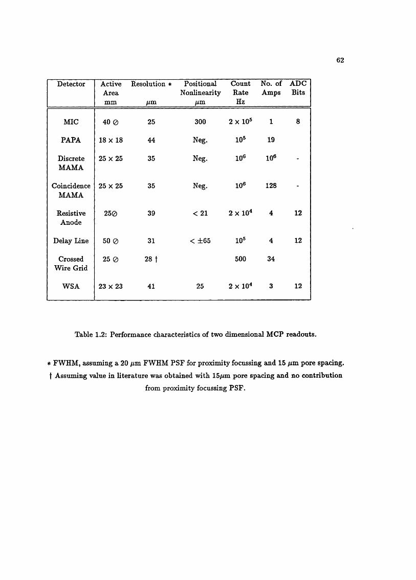
62

Detector ActiveAreamm

Resolution *

/xm

PositionalNonlinearity

/xm

CountRateHz

No. of Amps

ADCBits

MIC 4 0 0 25 300 2 X 10® 1 8

PAPA 18 X 18 4 4 Neg. 10® 19

DiscreteMAMA

25 X 25 35 Neg. 10® 10® -

CoincidenceMAMA

25 X 25 35 Neg. 10® 128 -

ResistiveAnode

2 5 0 39 < 21 2 X 1 0 ^ 4 12

Delay Line 50 0 31 < ± 6 5 10® 4 12

Crossed Wire Grid

25 0 28 t 500 3 4

WSA 23 X 23 41 25 2 X 10^ 3 12

Table 1.2: Performance characteristics of two dimensional MCP readouts.

* FWHM, assuming a 20 /im FWHM PSF for proximity focussing and 15 p,m pore spacing,

t Assuming value in literature was obtained with 15^m pore spacing and no contribution

from proximity focussing PSF.

63

Chapter 2

C yclic C ontinuous E lectrode

Charge M easurem ent D evices

An idealized example of a cyclic continuous electrode is shown in Figure 2.1. It

consists of three electrodes, the sum of whose widths is constant, w. The widths of the

electrodes at a given point p is given by

X = rcosp + c , (2.1)

z = r cos(p -\-(f>) + c , (2.2)

y = w - (x-\r z) . (2.3)

The offset c must be greater than the amplitude r to ensure that the electrodes are contin

uous and it is typically w/3. The phase shift <f> is constant along the whole anode.

The position p of an event is determined by a combination of two parts, a coarse

and fine position. The fine position is determined by the value of the phase angle $ within

a cycle of the repeated pattern, that satisfies Equations 2.1 and 2.2 The coarse position is

found by determining in which cycle an event occurs. If n is the number of the cycle, then

p cx 2n7T -f 0 . (2.4)

The advantage of cyclic electrodes is that the full dynamic range of the ADCs

is used in determining the fine position within a single cycle which is repeated several

times across the pattern. In other types of charge measuring readouts, e.g. the WSA and

delay lines, the ADC dynamic range can be used only once across the whole active area of

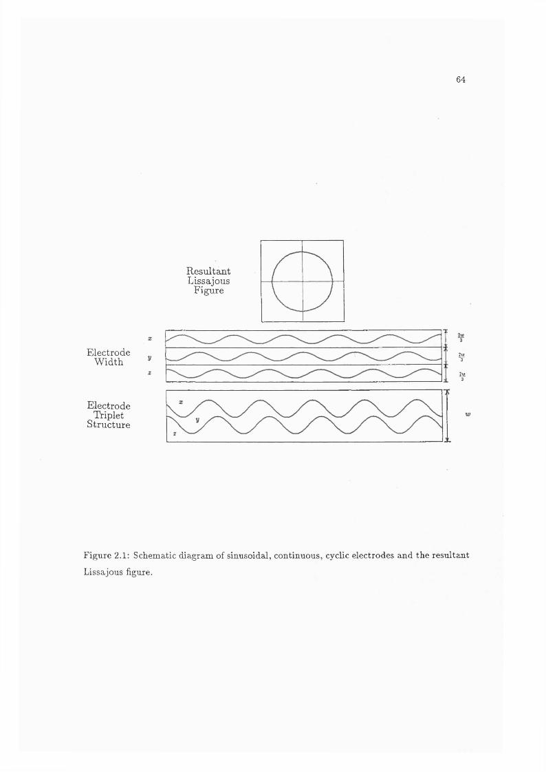
64

ElectrodeW idth

ElectrodeTriplet

Structure

ResultantLissajous

Figure

¥

¥

Figure 2.1: Schematic diagram of sinusoidal, continuous, cyclic electrodes and the resultant

Lissajous figure.

65

the detector. Therefore, for a given digitization level, continuous readouts offer, to a first

order approximation, an improvement in resolution by a factor directly proportional to the

number of cycles.

2.1 Fine Position

2 .1 .1 A n alysis o f S inusoidal E lectrod es

Let us represent the electrodes as oscillators, exhibiting simple harmonic motion,

with the same frequency and unit amplitude such that

x{t) = cos(wt) , (2 .5 )

z(t) = cos(wt + <f>) , (2.6)

y{t) = w - (x{t) + z{t)) . ( 2 .7 )

where 0 < < < oo .

By treating the electrodes as orthogonal oscillators we can describe their output in terms

of Lissajous figures.

For convenience I shall change the notation to the form

X = x(t) , (2 .8 )

0 = 6^t) = u t . (2 .9 )

Expanding Equation 2 .6 and substituting for x

z = cos cos — sin sin , (2.10)

= a: cos ^ + \ / l - sin , (2.11)

regrouping the term and squaring we obtain

z^ x^ — 2zx cos <l> — sin^ <f> = 0 . (2.12)

Including the condition that the sum of of the three oscillators is constant Equation 2.7

gives the polynomial / (x , y, z) such that

/(x ,y , z) = + x^ - 2zx cos <f> - , (2.13)

= 0 . (2.14)

66

As f ( x , y, z) satisfies

by Euler’s theorem, it is a homogeneous polynomial of order 2 in z, y, z (Massey & Kestdy

man, 1964). As f{ x ^y ,z ) is homogeneous and by Equation 2.14, / ( z ,y ,z ) = 0, Equa

tion 2.13 describes a cone with its vertex at the origin (Massey & Kestelman, 1964).

Figure 2.2 illustrates why this is the case. If a function / ( z ,y ,z ) is homogeneous and

f { x ,y ,z ) = 0 for a point P(^, t7,C), then f(x ^ y ,z ) = 0 for all points for all

numbers t. Therefore, all points on the line joining P to the origin also lie on the surface

of the cone.Therefore, for oscillators with a constant amplitude, the resulting locus is a conic

section. Continuously varying the amplitude of the oscillations would produce the cone.

2 .1 .2 T h e E ffect o f th e P h ase A n gle

As the cone surface is sectioned by various planes, a family of conic sections is

produced. Two sets of planes are of particular interest.Firstly the planes in which y is a constant, i.e. the planes parallel to the xz

plane. The equation of this section is given by Equation 2.12. This equation is the general

form of equation for Lissajous figures obtained from two orthogonal oscillators with equal

amplitudes and frequencies (Massey & Kestclman, 1964). If the condition that the phase

difference <l> = 90° is imposed, this equation reduces to

x^ + z^ = 1 , (2.16)

the unit circle centred on the origin. For successive cycles of the oscillators, the same locus

will be produced, so with only this information, it is impossible to determine during which

cycle an event occurred. Therefore, the time t at which a given event occurred is unknown,

only its phase.

The unit circle is produced by the ideal simple harmonic oscillators. Replacing

these by the equations for the actual electrodes. Equations 2.1-2.3 we obtain by the same

process

(x - c)^ + (z - c)^ = , (2.17)

a circle of radius r centred at (c,c). The fine position, is determined in a straight forward

67

Figure 2.2: Demonstration that a homogeneous polynomial f {x ,y^z) describes a cone with

an apex at the origin.

The symbols are explained in the accompanying text. From Massey & Kestleman (1964).

Z

y

Figure 2.3: The Euler angles for a rotation through three dimensions.

manner by6 = arctan X — c

z — c

68

(2.18)

The other conic section of particular interest is defined by the condition that the

sum of amplitudes be a constant, i.e. the section defined by the plane x y -\r z = w.

The equation of this section is given by Equation 2.13. It is on this plane that the locus

described by the three oscillators lies. The image in the xz plane is the projection of this

locus into two dimensions.

A coordinate system where one of the coordinates will be a constant, simplifying

the equation of the locus, can be obtained by changing the axes. Let this new constant

coordinate be z \ the obvious vector to use for the z' axis is the vector normal to the plane

and running through the origin, i.e. (1,1,1). This is achieved by rotating the axes.

A rotation can be completely described as a series of three rotations through the

Euler angles < ,0 and ^ (Corben & Stehle, 1974).

1. A rotation through an angle of (f) about the z axis. The matrix for this rotation is

cos sin< 0 ^

— sin 4> cos <j> 0

0 0 1

(2.19)

2. A rotation through an angle of 0 about the new y axis, the line O P,

Se =

0 0

0 cos 9 sin 6

0 — sin ^ cos 6

(2.20)

3. A rotation through an angle of ^ about the new z axis, z \

S,i, =

cosrjj sin^ 0 ^

— sin cos 0

0 0 1

(2 .21)

69

These rotations are shown in Figure 2.3.

The rotation matrix, S, such that

= S (2.22)

is given by

5 = S,pS$S^ . (2.23)

Only the first two rotations are required to carry out the transformation such that

the z* axis lies along the vector (1,1,1). For convenience, at this stage, we can impose the

condition ip = 0. The rotation matrix reduces to

m e fk a\rt /h 0 ^

S =COS( f ) sin<^

— cos 0 sin (}> cos <f> cos 9 sin 0

sin 0siiL<l> — sin 0 cos (f> cos 0 j

Therefore, the equations for the transformation are

z' = cos 4>x sin (j> y

y' = — cos 0 sin <f>x cos 0 cos (p y + sin 0 z

z' = sin 0 sin <p = —45° .

(2.24)

(2.25)

(2.26)

(2.27)

(2.28)

(2.29)

Substituting <P into Equation 2.26 and applying the condition of Equation 2.28 gives

V 2 cos 0 = — sin 0 , (2.30)

cos^ 0 + sin^ ^ = 1, so

3 cos^ 0 = 1 . (2.31)

70

with, reference to Equation 2.30

^ = -5 4 °4 4 '8 .2 ” , (2.32)

This is the so called “magic angle”, which is the angle between the body diagonal of a cube

and each of its faces (Klinowski, 1990). Substituting 0 and <j> into Equations 2.25-2.27 gives

the equations of the transformation

(2.33)

y = (z + y - 2z) (2.34)

z‘ = ^ ( a r + y + z) . (2.35)

Combining the electrode equations with the rotation equations and applying the

condition that a = y we obtain

x' = - ^ ( 2 z + z — 3c) , (2.36)

= ^ ( rc o s é ? + 2r cos(0 + 0)) , (2.37)

y' = ^ ( 3 z - 3c) , (2.38)

= y ^ (rc o s^ ) . (2.39)

Substituting y' into Equation 2.37 and expanding we obtain

x' = V ^(rcos0cos0—rsiné?sin0) + - ^ y ' ,V3

(2.40)

= y/2r cos 0 cos 0 — ^ 2 r^ (l — cos 0) sin 0 + -ÿ^y^ . (2.41)

Substituting y' and regrouping

v' / 2x^x ' - -^ {2 c o s0 + 1) = - r ^ l — sin< , (2.42)

by squaring both sides it can be shown that

0 1 ^ 2 X V o «Ï

x'^ + — (4r cos 0 + 5 ) -----7='(4r cos 0 + 2) = 2r sin 0 . (2.43)3 v 3

If cos 0 = i.e. 0 = —60° or 120°2

+ y'2 = 3r , (2.44)

71

a circle centred on the z* axis is produced. The fine position, 0 is determined by

x'9 = arctan — , (2.45)y

Therefore, the phase shift determines what type of coordinate transform is neces

sary and in which plane the conic section will be a circle. This is far the most convenient

curve to use, and it ha^ important implications for the Spiral Anode, which is discussed in

the Section 2.2.3.

2.2 Coarse Position

Various methods have been proposed for determining in which cycle an event has

occurred.

2.2 .1 T h e D o u b le D iam on d C ath od e

This readout has not been used in a MCP based detector but in large, metre scale,

drift chambers for particle physics detectors such as OPAL (OPAL Collaboration, 1991).

However, it represents an example of a cyclic, continuous electrode readout that could in

principle be used for MCPs.Figure 2.4 shows the basic form of this readout (Allison €é^d985). The electrodes

above the wire in the drift chamber are 90° out of phase with those below. Although the

waveform is triangular, the analysis described in the previous section will be true for all

of its Fourier components, and a square rather than circular locus would be produced

(Allison et aL, 1991).Fine position is determined with a triangular pattern of wavelength 171 mm and is

proportional to arctan , where e, and €c are values returned the cathodes above and

below the wire, respectively. The method for calculating the e values is shown in Figure 2.4.

The coarse position is determined in a similar way with a triangular waveform

with a wavelength 10 times longer. Allison et al. (1991), call this the medium position.

Determining on which of the 1710 mm wavelengths an events occurs is determined by arrival

time of events at either end of the wire or an extra series of electrodes. Resolutions of 1.5 mm

have been achieved for a wire 10.4 m long, using 8 bit ADCs.

For an MCP based system, 4 channels would be required per dimension, each

consisting of a preamp and an ADC.

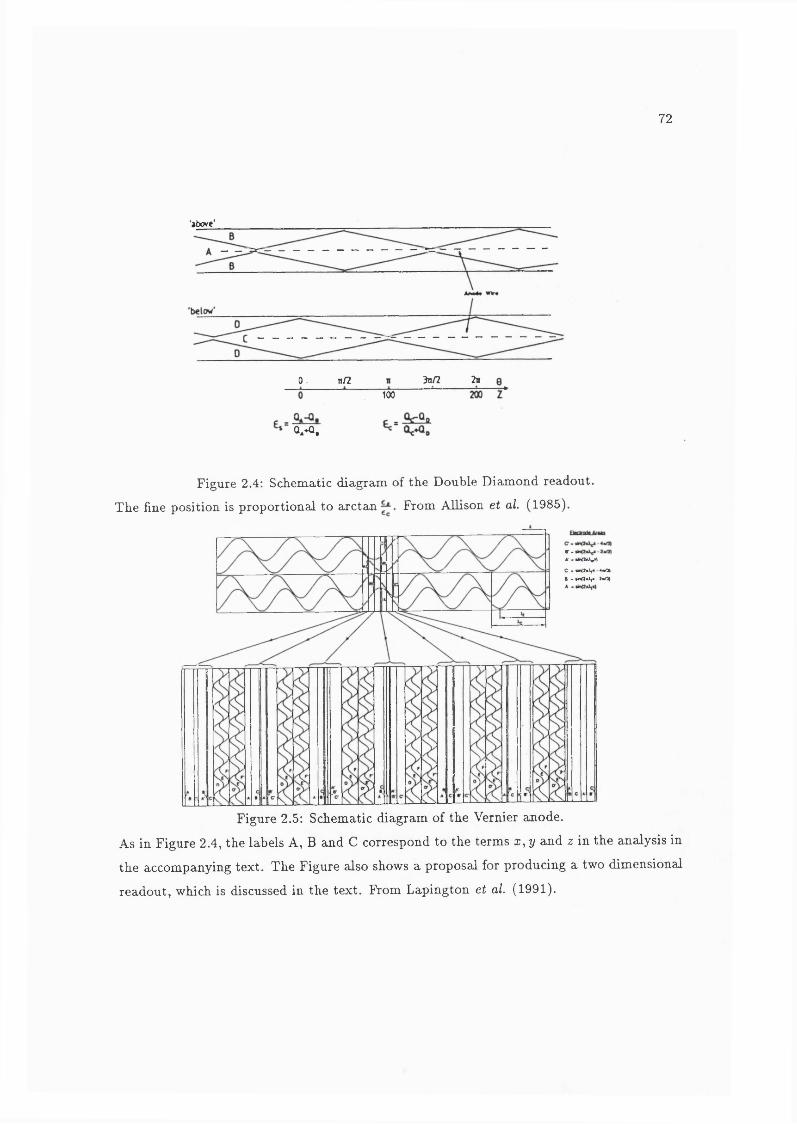
72

'above'

2n3n/2n/20100

Q, Q,

Figure 2.4; Schematic diagram of the Double Diamond readout.

The fine position is proportional to arctan From Allison et al. (1985).

>

>

r -A-.rtO-V»C -» ln (2 iiy -4W H ft - Sln(2«XfK . Imnn

Figure 2.5: Schematic diagram of the Vernier anode.

As in Figure 2.4, the labels A, B and C correspond to the terms x, y and z in the analysis in

the accompanying text. The Figure also shows a proposal for producing a two dimensional

readout, which is discussed in the text. From Lapington et al. (1991).

73

2 .2 .2 T h e V ernier A n od e

An example of the Vernier Anode is shown in Figure 2.5. The vernier anode uses

two triplets of sinusoidal electrodes similar to those in Figure 2.1 and so would require six

charge measuring channels per dimension. Both triplets have the same phase difference

between the x and z electrodes but the two triplets have slightly different wavelengths

(Lapington et a/., 1990, Lapington et aZ., 1991). The coarse position is the difference

between the phase angles returned from the two triplets.

Figure 2.5 also shows a proposal for producing a two dimensional readout. The

position in the vertical direction is encoded by the six continuous sinusoidal electrodes

in that direction. Horizontal position is determined by the other set of electrodes whose

widths vary from pitch to pitch so as to represent the width ratios determined by sinusoidal

electrodes at discrete intervals. These discrete and continuous axes represent an early

proposal for producing a two dimensional detector but in practice a method similar to that

described in Section 2.2.3 would probably be used.

2 .2 .3 T h e Spiral A n od e (S P A N )

Unlike the other two examples, SPAN does not require any extra electrodes to de

termine the coarse position but achieves this by modulating the amplitude of the sinusoidal component of the electrode widths. Therefore, it requires only three channels of charge

measuring electronics per axis.

If the amplitude of the sinusoidal electrode is directly proportional to the position

along the length of the anode p then the widths of the electrodes are

X = c-\-kp cos p , (2.46)

z = c + kpcos(p + (f>) , (2.47)

y = Zc — (x + z) , (2.48)

assuming a phase difference of 120°, although it would be equally true for 90°, and following

the procedure described in Equations 2.36-2.44

x'^ + y'^ = 3 (k p f , (2.49)

or converting into polar coordinates

r = y/Zkp , (2.50)

74

which is the equation for an Archimedean Spiral. Figure 2.6 shows the evolution of the

spiral as the position moves along the electrodes.

The fine position is determined by by the phase angle 0 in the usual manner and

the coarse position is determined by calculating which spiral arm an event lies on. The

position is therefore,

pcc O' = 2mr + 0 , (2.51)

where n is the spiral arm number.

If p is made directly proportional to 0' the resolution of the detector will vary as

the spiral evolves, i.e. along the length of the anode. As shown in Figure 2.6, the wavelength

decreases as the amplitude decreases. This is to ensure the change of spiral arc length is

approximately constant for equal lengths along the anode. If the spiral arc length is chosen

as the measure of position, rather than O', varying the wavelength can keep the resolution

constant across the width of the detector (Lapington et al., 1990 and Lapington et a/.,1991).

Figure 2.7 shows an increment in the arc length of the spiral, 5 for a small incre

ment of the angle 0. From this figure we can see that

= {r60 f + . (2.52)

Given the general equation of a spiral in polar coordinates

we can express 6S^

dO

The general solution to an integral of the form

r = kO , (2.53)

= k \e ^ + i)se^ , (2.54)

= t ( f + l ) i . (2.55)

IS

» = 2

y = J{x + a)^dx , (2.56)

xy/x'^ 4- a + log (x -f J (2.57)

(Weast, 1966). Therefore,

5 = ^ [ e V F T i + log {e + + 1) ] . (2 .5 5 )

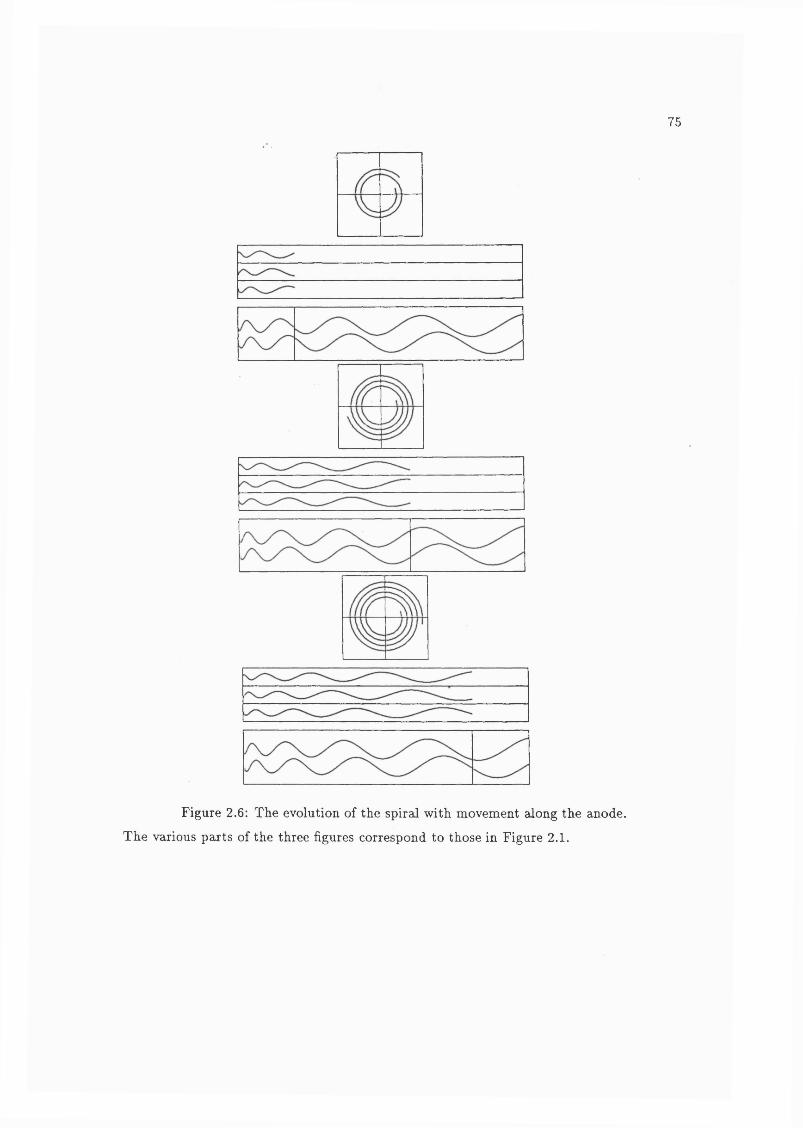
75

Figure 2.6: The evolution of the spiral with movement along the anode.

The various parts of the three figures correspond to those in Figure 2.1.

76

ds

Figure 2.7: The difFerential increase of arc length for a curve.

If we substitute Equation 2.55 with

then we can express the condition that the rate of change of S with position p as

^dp dO dp ’

(2.59)

(2.60)

(2.61)

therefore to keep the rate of change of arc length with position approximately constant

requires that

1 = 1 •

2.3 P rac tica l Anodes

So far, only SPAN has been used as a MOP readout. However the techniques used

in constructing a SPAN readout could be also used for the double diamond and the vernier.

Figure 2.8 shows a portion of the a one dimensional SPAN readout which is cur

rently being developed for the Coronal Diagnostic Spectrograph (CDS) on ESA’s SOHO

mission (Breeveld et oZ., 1992a). The anode consists of a periodic repetition of the triplet of

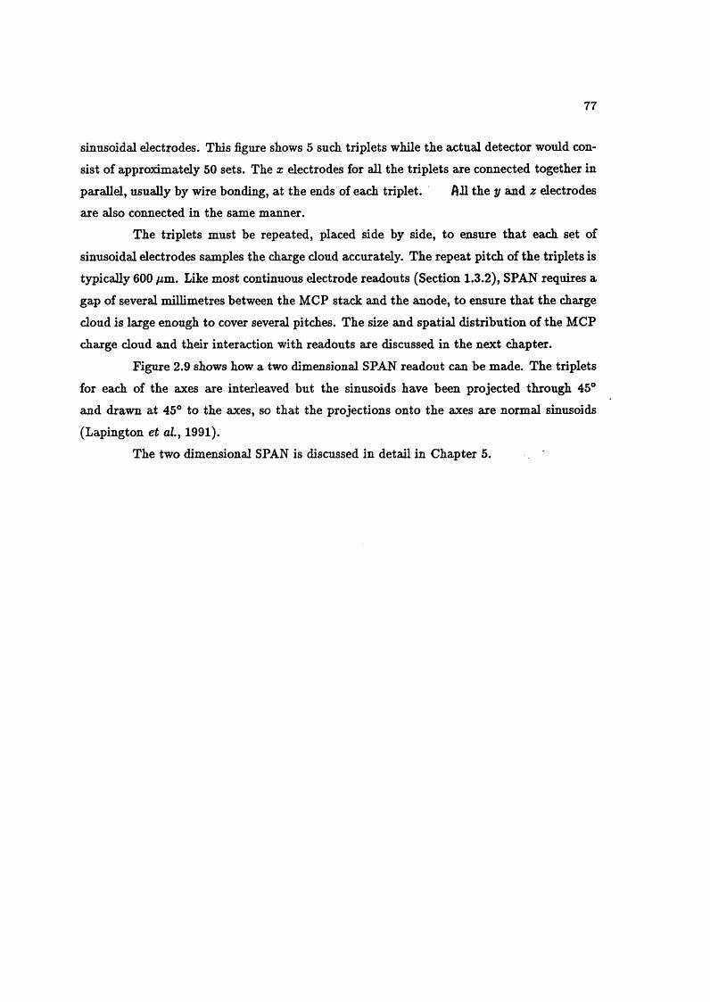
77

sinusoidal electrodes. This figure shows 5 such triplets while the actual detector would con

sist of approximately 50 sets. The x electrodes for all the triplets are connected together in

parallel, usually by wire bonding, at the ends of each triplet. AH the y and z electrodes

are also connected in the same manner.

The triplets must be repeated, placed side by side, to ensure that each set of

sinusoidal electrodes samples the charge cloud accurately. The repeat pitch of the triplets is

typically 600 /im. Like most continuous electrode readouts (Section 1.3.2), SPAN requires a

gap of several millimetres between the MCP stack and the anode, to ensure that the charge

cloud is large enough to cover several pitches. The size and spatial distribution of the MCP

charge cloud and their interaction with readouts are discussed in the next chapter.

Figure 2.9 shows how a two dimensional SPAN readout can be made. The triplets

for each of the axes are interleaved but the sinusoids have been projected through 45°

and drawn at 45° to the axes, so that the projections onto the axes are normal sinusoids

(Lapington et uZ., 1991).

The two dimensional SPAN is discussed in detail in Chapter 5.

78

Figure 2.8: Schematic diagram of the one dimensional SPAN readout for the SOHO satellite.

The width of the electrode triplets has been expanded by a factor of 10 for clarity. From Breeveld et al. (1992b).

Figure 2.9: Schematic diagram of a two dimensional SPAN.

The labels A, B and C correspond to the terms x, y and z in the ajialysis in the text. From

Lapington et al. (1992).

79

Chapter 3

Techniques for M easuring th e Size

and Spatial D istribution o f

E lectron Clouds Prom

MicroChannel P lates

3.1 In troduction . The In teraction of M C P Charge Clouds w ith R eadouts

In all MCP readouts with a repeat pitch, it is necessary that the pitches oversample

the charge cloud. If the charge cloud is too small with respect to the pitch, the charge

cloud is undersampled and an effect analogous to aliasing, called modulation or differential

nonlinearity, is introduced. This effect has been studied experimentally and by computer

simulation for the WSA (Smith et oL, 1989, Vallerga et aL, 1989). Figure 3.1 shows an

example of modulation.

Modulation can be overcome by allowing the charge cloud to spread over a larger

area. However, if the cloud is too large, charge will be lost off the edge of the anode

introducing another distortion. For the WSA, this is known as “S distortion” , see Figure 3.2.

Therefore, the anode design places constraints on the charge cloud size or a given cloud size

will place constraints on the anode design.

The spatial distribution of the charge cloud also affects the continuous cyclic elec-

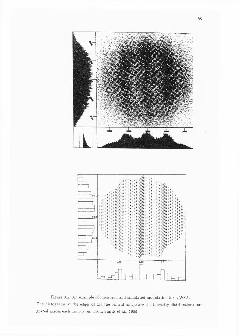
80

i l i f

Figure 3.1: An example of measured and simulated modulation for a WSA.

The histograms at the edges of the the central image are the intensity distributions inte

grated across each dimension. From Smith et al., 1989.

81

trodes discussed in the previous chapter as the charge cloud will behave as a spatial, band

pass filter. Convolution with the charge cloud will reduce the magnitude of any spatial

frequency component. Any continuous, cyclic detector which contains more than one spa

tial frequency component in its electrode structure , i.e. any type that produces an ideal

Lissajous figure other than a circle, will have the magnitudes of those components reduced

by varying amounts depending on their frequency. Therefore the resultant Lissajous figure

will be distorted. Such effects have been observed in the double diamond cathode, see Fig

ure 3.3. The extent of this distortion will be dependent on the size and distribution of the

charge cloud as this defines the filter response.

Carter et al. (1990) have modelled the affect of varying event width on the cen-

troiding for the MIC detector, see Section 1.3.1. They find positional shifts of the order of

10 /zm due to undersampling for too small an event and a loss of signal outside the 5 or 9

pixels used in centroiding if the event is too wide. They suggest that a detailed knowledge of

the spatial distribution of the charge cloud would enable these shifts to be removed during

calibration.All of these studies assumed a charge cloud distribution, usually a Gaussian as was

suggested by the group at Berkeley (Martin et a/.,1981). However, the same group found

that the charge cloud was not quite Gaussian but the core was sharper and the wings more extended (Jelinsky, 1979). Both of the WSA studies (Smith et oZ., 1989, Vallerga et uZ., 1989)

found that a quantitative prediction of a charge division readout’s performance depends

sensitively on the assumed charge cloud distribution. A detailed knowledge of the charge

cloud for a given set of MCP operating conditions allows the simulation of the operation of

an anode and characterization of the effects of modulation. It should also allow selection

of anode designs that will minimize the effects of modulation for that set of operating

conditions.

3.2 T he Split S trip Anode

Lapington et al. (198 g) developed the Split Strip Anode specifically to measure

the spatial distribution of the charge cloud. Figure 3.4 shows a simplified version of the

anode. The anode is a Strip and Strip detector with an insulating gap down the middle, i.e.

a split. The position, along the x axis, of the centroid of the charge cloud and the fraction

of charge falling on one side of the split can be measured simultaneously, for each event.

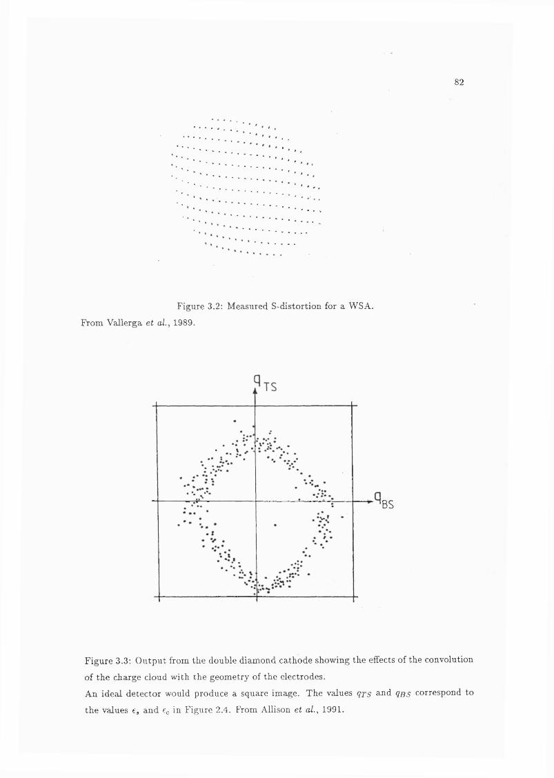
82

Figure 3.2: Measured S-distortion for a WSA.

From Vallerga et aZ., 1989.

'BS

Figure 3.3: Output from the double diamond cathode showing the effects of the convolution

of the charge cloud with the geometry of the electrodes.

An ideal detector would produce a square image. The values qxs a-nd qbs correspond to

the values e, and Cc in Figure 2.4. From Allison et al. 1991.

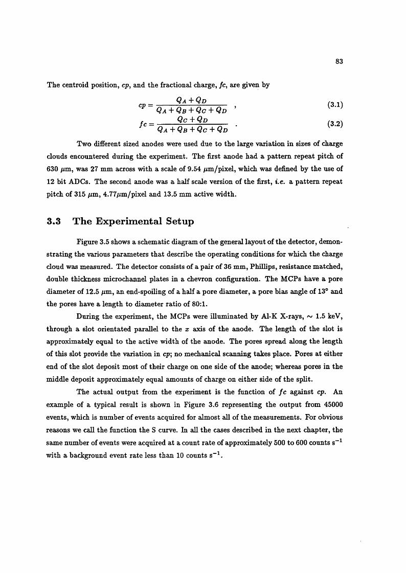
83

The centroid position, cp, and the fractional charge, /c, are given by

_______ Q a + Q d _________ / o 1 \

Q a + Q b + Q c Q d

f r - Q c + Q d / o

^ Q a + Q b + Q c + Q d ’ ^

Two different sized anodes were used due to the large variation in sizes of charge

clouds encountered during the experiment. The first anode had a pattern repeat pitch of

630 pm, was 27 mm across with a scale of 9.54 pm/pixel, which was defined by the use of

12 bit ADCs. The second anode was a half scale version of the first, i.e. a pattern repeat

pitch of 315 pm, 4.77pm/pixel and 13.5 mm active width.

3.3 T he E xperim ental Setup

Figure 3.5 shows a schematic diagram of the general layout of the detector, demon

strating the various parameters that describe the operating conditions for which the charge

cloud was measured. The detector consists of a pair of 36 mm, Phillips, resistance matched, double thir.1cT ip.RR microchannel plates in a chevron configuration. The MCPs have a pore

diameter of 12.5 pm, an end-spoiling of a half a pore diameter, a pore bias angle of 13° and

the pores have a length to diameter ratio of 80:1.

During the experiment, the MCPs were illuminated by Al-K X-rays, ^ 1.5 keV,

through a slot orientated parallel to the x axis of the anode. The length of the slot is

approximately equal to the active width of the anode. The pores spread along the length

of this slot provide the variation in cp; no mechanical scanning takes place. Pores at either

end of the slot deposit most of their charge on one side of the anode; whereas pores in the

middle deposit approximately equal amounts of charge on either side of the split.

The actual output from the experiment is the function of fc against cp. An

example of a typical result is shown in Figure 3.6 representing the output from 45000

events, which is number of events acquired for almost all of the measurements. For obvious

reasons we call the function the S curve. In all the cases described in the next chapter, the

same number of events were acquired at a count rate of approximately 500 to 600 counts s“

with a background event rate less than 10 counts s“ ^.

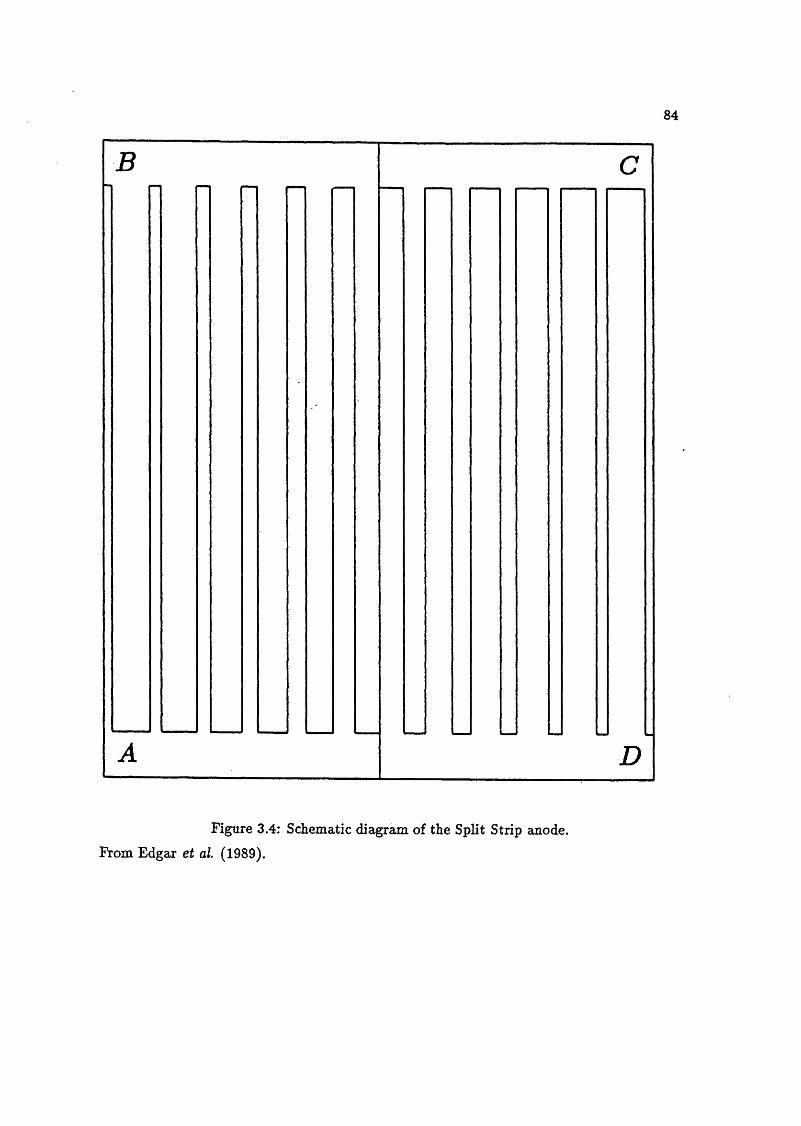
84

Figure 3.4: Schematic diagram of the Split Strip anode. From Edgar et a l (1989).

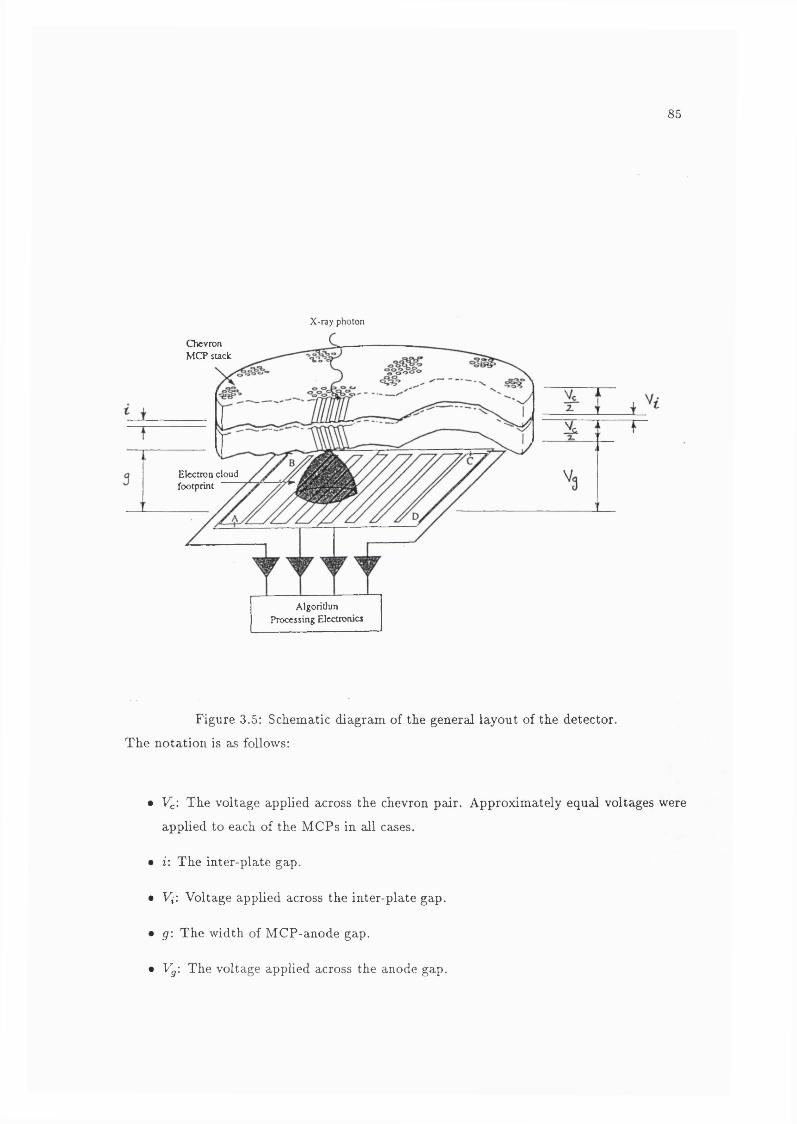
85

X-ray photon

Chevron MCP suck

Electron cloud footprint “

Algorithm Processing Electronics

Figure 3.5: Schematic diagram of the general layout of the detector.

The notation is aa follows:

• Vc: The voltage applied across the chevron pair. Approximately equal voltages were

applied to each of the MCPs in all cases.

• i: The inter-plate gap.

• Vi'. Voltage applied across the inter-plate gap.

• g: The width of MCP-anode gap.

• Vg-. The voltage applied across the anode gap.

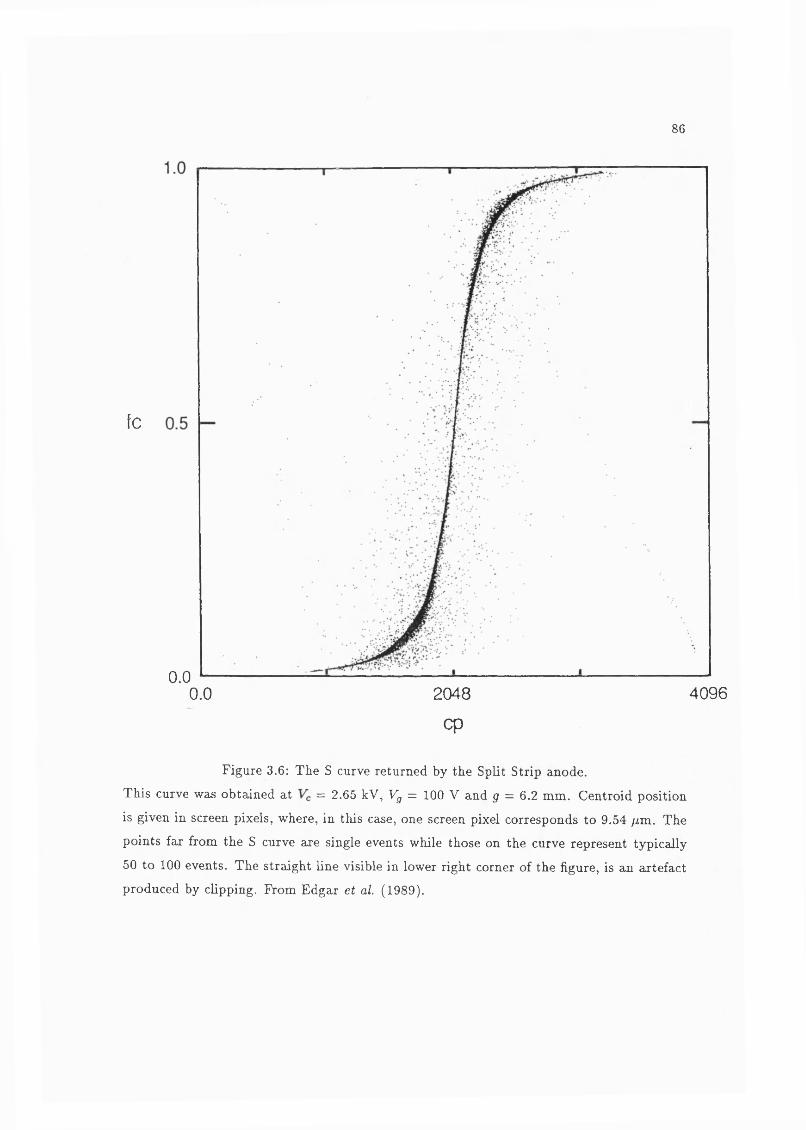
86

fc

0.02048 40960.0

cp

Figure 3.6: The S curve returned by the Split Strip anode.

This curve was obtained at = 2.65 kV, Vg = 100 V and g = 6.2 mm. Centroid position

is given in screen pixels, where, in this case, one screen pixel corresponds to 9.54 /zm. The

points far from the S curve are single events while those on the curve represent typically

50 to 100 events. The straight line visible in lower right corner of the figure, is an artefact

produced by clipping. From Edgar et al. (1989).

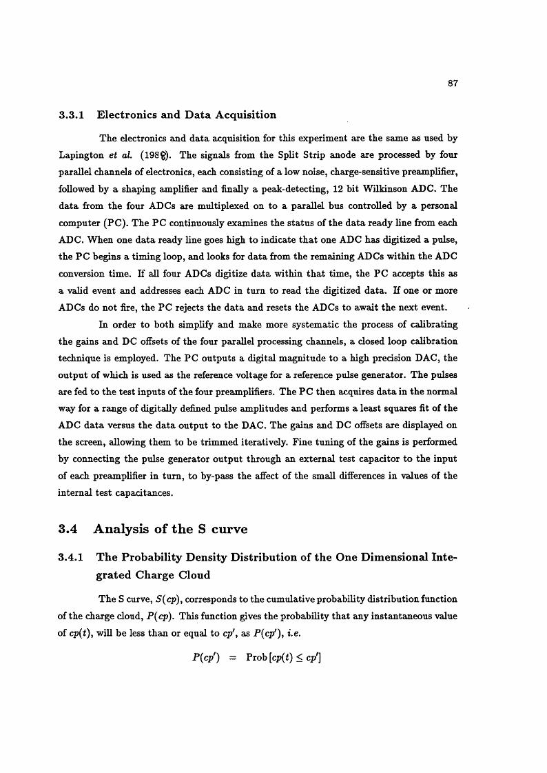
87

3 .3 .1 E lectron ics and D a ta A cq u isition

The electronics and data acquisition for this experiment are the same as used by

Lapington et al. (198^). The signals from the Split Strip anode are processed by four

parallel channels of electronics, each consisting of a low noise, charge-sensitive preamplifier,

followed by a shaping amplifier and finally a peak-detecting, 12 bit Wilkinson ADC. The

data from the four ADCs are multiplexed on to a parallel bus controlled by a personal

computer (PC). The PC continuously examines the status of the data ready line from each

ADC. When one data ready line goes high to indicate that one ADC has digitized a pulse,

the PC begins a timing loop, and looks for data from the remaining ADCs within the ADC

conversion time. If all four ADCs digitize data within that time, the PC accepts this as

a valid event and addresses each ADC in turn to read the digitized data. If one or more

ADCs do not fire, the PC rejects the data and resets the ADCs to await the next event.

In order to both simplify and make more systematic the process of calibrating

the gains and DC offsets of the four parallel processing channels, a closed loop calibration

technique is employed. The PC outputs a digital magnitude to a high precision DAC, the

output of which is used as the reference voltage for a reference pulse generator. The pulses

are fed to the test inputs of the four preamplifiers. The PC then acquires data in the normal way for a range of digitally defined pulse amplitudes and performs a least squares fit of the

ADC data versus the data output to the DAC. The gains and DC offsets are displayed on

the screen, allowing them to be trimmed iteratively. Fine tuning of the gains is performed

by connecting the pulse generator output through an external test capacitor to the input

of each preamplifier in turn, to by-pass the affect of the small differences in values of the

internal test capacitances.

3.4 Analysis of th e S curve

3.4 .1 T h e P rob ab ility D en sity D istr ib u tio n o f th e O ne D im en sion a l In te

gra ted C harge C loud

The S curve, 5(cp), corresponds to the cumulative probability distribution function

of the charge cloud, P{cp). This function gives the probability that any instantaneous value

of cp(f), will be less than or equal to cp', as jP(cp'), i.e.

P(cp') = Prob [cp{t) < cp']

88

/ P(cp)d{cp) , (3.3)J — O O

where p{cp) is the probability density function (Bêndat and Piersol, 1966). Therefore,

p{cp) can be determined by

As the Split Strip anode has translational symmetry parallel to the split, i.e. the y

axis, it can only produce one dimensional information about the charge cloud. The function

S(cp) represents the charge distribution integrated along the y axis. Therefore, the function

p{cp) corresponds to the probability density distribution of the one dimensional integrated

charge cloud. It represents the percentage of the charge cloud lying within a window of cp

with a constant, finite width. Figure 3.7 shows an example of p{cp).

It must be stressed that the Split Strip anode measures the probability distribution

of the charge cloud. It does not represent the number of electrons collected at any one point

but the fraction of the total charge cloud. The number of electrons can be determined if

the gain is known. In this and the next chapter, when I discuss the size of the charge cloud, I am always referring to the width of the probability distribution. This allows direct

comparisons between the radial distributions of charge clouds containing a large variation

in the total number of electrons.

3 .4 .2 T h e S tru ctu re and R ed u ction o f th e S curve

The S curve is reduced to a curve consisting of the average fc for a given cp. The

mean is determined over the whole range of fc for bins of cp 30 pixels wide, i.e. the sections

along which fc is determined, are always parallel to the f c axis.

The S curve consists of contributions from the charge clouds of tens of thousands of

events with pulse heights spread across the entire PHD. Figure 3.8 shows how the variation

in pulse height affects the shape of the S curve. In the linear region and at the edge of the

curve, there is no appreciable variation. However in the region of high curvature there is a

marked spectrum produced by the varying pulse height. It appears that this region is most

sensitive to a variation of charge cloud size with pulse height.

Figure 3.9 shows cross sections through the S curve, parallel to the fc axis at

a selection of points. In the central, linear region the cross sections are approximately

Gaussian. The cross sections through the regions of high curvature have the same general

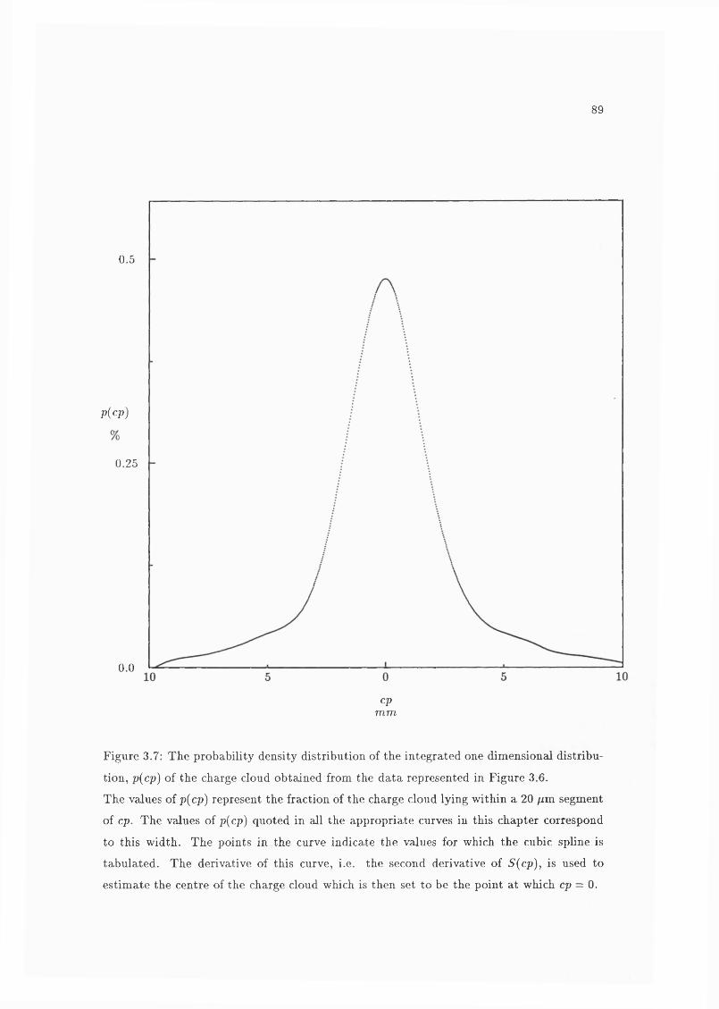
89

0.5

p(cp)

0.25

0.0

cpmm

Figure 3.7: The probability density distribution of the integrated one dimensional distribu

tion, p(cp) of the charge cloud obtained from the data represented in Figure 3.6.

The values of p{cp) represent the fraction of the charge cloud lying within a 20 pm segment

of cp. The values of p{cp) quoted in all the appropriate curves in this chapter correspond

to this width. The points in the curve indicate the values for which the cubic spline is

tabulated. The derivative of this curve, i.e. the second derivative of S(cp), is used to

estimate the centre of the charge cloud which is then set to be the point at which cp = 0.

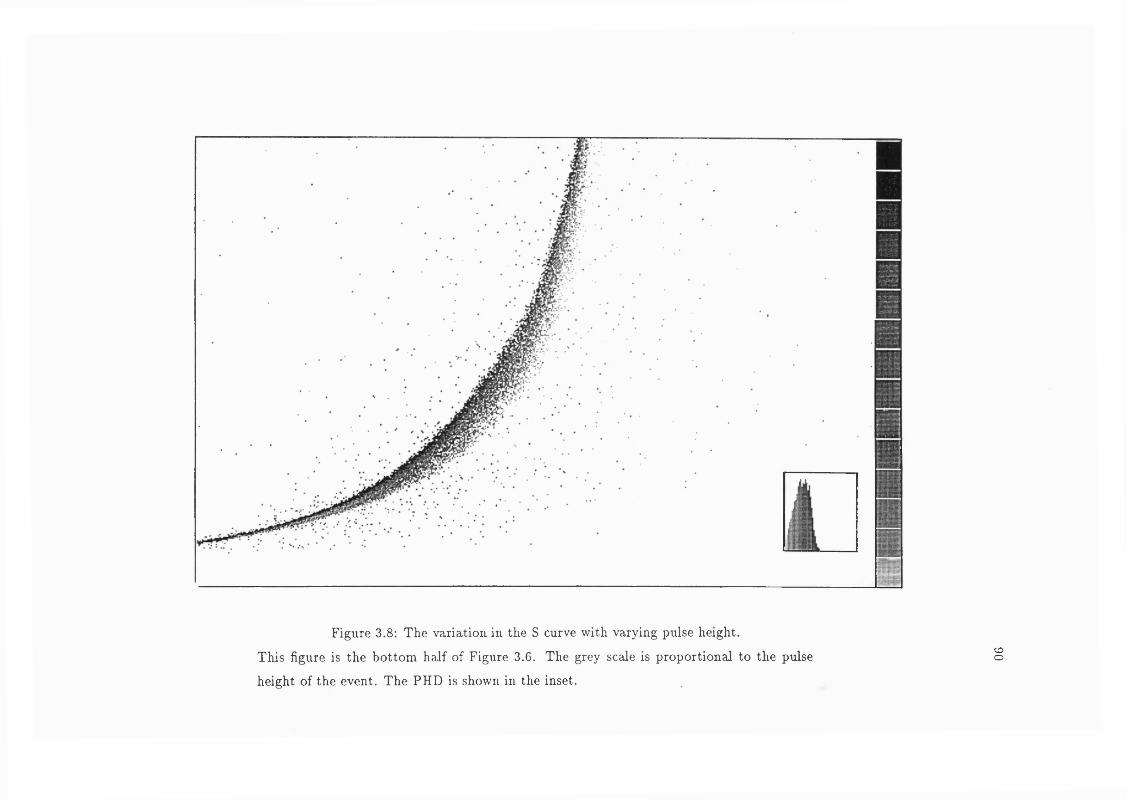
Figure 3.8: The variation in the S curve with varying pulse height.

This figure is the bottom half of Figure 3.6. The grey scale is proportional to the pulse

height of the event. The PHD is shown in the inset.

<£>O

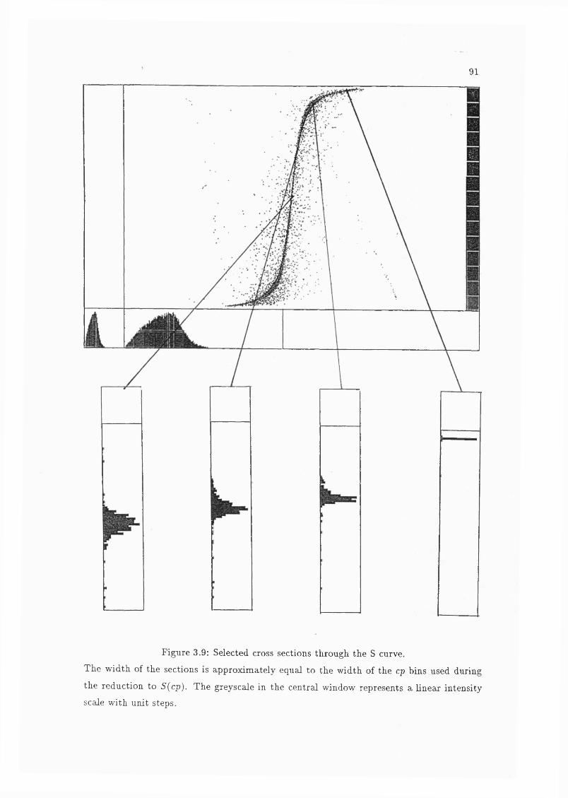
91

Figure 3.9: Selected cross sections through the S curve.

The width of the sections is approximately equal to the width of the cp bins used during

the reduction to S{cp). The greyscale in the central window represents a linear intensity

scale with unit steps.

92

shape as the PHD. So in these regions it is reasonable to assume that the cross sections

normal to the S curve are proportional to the PHD, and the cross sections in Figure 3.9 are

the projections of these normal sections onto a line parallel to the f c axis. As the PHDs

are approximately Gaussian, so are the cross sections parallel to the f c axis. Therefore, the

data points are approximately normally distributed about the mean S curve.

These cross sections are symmetric about the centre of the curve. The lower

pulse height events are always on the outside of the curve, i.e. further from the centre

indicating a tighter S curve. This behaviour was observed in every S curve obtained during

the experiment. This suggests that charge cloud size is a function of gain, with lower gain

events producing smaller charge clouds.

After reduction, the mean S curve, 5(cp), consists of on average 80 points with

coordinates (cp,-, fci ± or,), where Oj is one standard deviation for the ith. bin.

In practice, p(cp) is determined from the derivative of 5(cp). As differentiation

enhances noise, a smoothing, cubic spline (Me Kinley, 1986) was used to produce the p(cp)

curves. The spline contains 2000 data points across the width of S(cp).

3 .4 .3 Q u a lita tiv e D iscu ssio n o f th e C h a rg e C lo u d U sin g p{cp)

The distribution p(cp) is useful in describing the gross behaviour of the charge cloud (Edgar et al. 1989, Chappel & Murray, 1989, Rasmussen & Martin, 1989). Figure 3.10

shows an example of the effects of varying the electric field strength in the MCP anode gap.

Both curves show indications of at least two components. At low electric fields there is a

broad central core with extensive wings. At high electric fields, most of the charge cloud is

concentrated in a small, well defined peak with only small wings.

Figure 3.11 shows the affect of the voltage across the chevron, 1^, on the charge

cloud. There is little difference in the behaviour of the edges of the distribution but the

lower Vc produces a more well defined peak with a larger percentage of charge concentrated

in it.

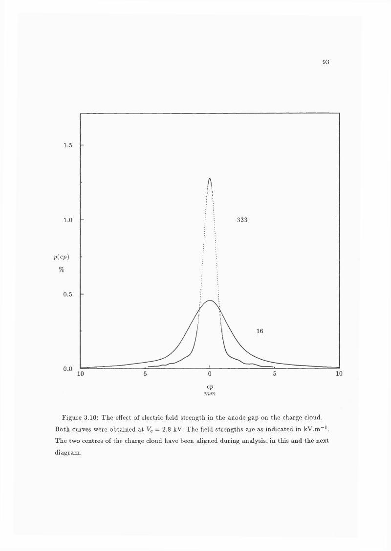
93

1.5

3331.0

p{cp)

0.5

0.0

cpmm

Figure 3.10: The effect of electric field strength in the anode gap on the charge cloud.

Both curves were obtained at = 2.8 kV. The field strengths are as indicated in kV.m“ .

The two centres of the charge cloud have been aligned during analysis, in this and the next

diagram.

94

1.0

2.8

p{cp)3.0

0.5

0.02.52.5

cpmm

Figure 3.11: The effect of plate bias voltage on the charge cloud.

Both curves were obtained with 200 V applied across a 3 mm anode gap, i.e. 67 kV.m“ ,

95

3.5 D eterm ining The Radial D istribu tion of th e Charge Cloud

The models developed to study modulation both require the radial distribution

of the charge doud, rather than just the integrated distribution. (Smith et al., 1989, Val

lerga et al., 1989). The radial distribution also presents a simpler, more general description

of the charge doud and would overcome any ambiguity introduced by integration, inherent

in p{cp).

In order to discuss the data quantitatively, it is necessary to obtain a best fit to

the data. We chose to fit directly to the mean S curve, S{cp) rather than p{cp) in which

the data has already undergone significant manipulation.

3 .5 .1 N ecessa ry C on d ition s for D eterm in in g th e R adial D istr ib u tio n o f

th e C harge C loud

As no mechanical scanning takes place, the S curve does not represent the charge

doud from one group of pores in the bottom MCP. It is the aggregate of all of the charge douds distributed across the anode. The spatial distribution can be determined without

mechanical scanning only if the form of the charge doud remains constant along the length

of the slot. Figure 3.12 demonstrates that regions equi-distant from the approximate centre

of the slot have similar charge cloud distributions. Therefore, it is a reasonable assumption

that the general form of the charge doud is constant along the length of the slot.

As the S curve represents the charge cloud integrated along the f c axis, deter

mining the radial distribution from the S curve requires the assumption that the charge

doud has azimuthal symmetry. A possible source of asymmetry is the orientation of the

pore bias angle with respect to the anode split. Figure 3.13 compares the distributions

from the two orientations. The similarity between the two indicates only a small degree of

asymmetry in the distribution and so, to a first order approximation, the charge doud is

radially symmetric. The topic of charge cloud symmetry is discussed further in Section 4.5.

3 .5 .2 T h e Inversion

The methods for carrying out the inversion and determining the linear least squares

solution, see Section 3.5.4, described here, in Edgar et al. (1989) and Lapington & Edgar

96

0.5

0.25

0.01010 0 55

cpmm

Figure 3.12: The p{cp) curve displayed in Figure 3.7, overlayed with its reflection about its

centre.

97

0.5

p{cp)

0.25

0.0

cpmm

Figure 3.13: Two overlayed p{cp) curves obtained with the pore bias angle aligned normal

and parallel to the split.

The curve obtained with the bias angle normal to the split is the same as is shown in

Figure 3.7.

98

(1989) follows that determined by Kessel (1988).

Let the spatial distribution be represented by a radial distribution, iV(r); the

measured S curve, 5(cp), is produced by the convolution of N{r) with the Split Strip. The

radial distribution can be determined by carrying out an inversion, i.e. find an expression

for N (r) that generates S{cp). The S curve is expressed as a function of N(r) by

c/ \ 2TjQ^rN{r)dr + 2 - arccos(^)]riV(r)dr

where rumit is the radius containing all of the charge. In the analysis, this radius

is taken to be equal to the half-width of the anode. Figure 3.14 shows the areas of the

charge cloud corresponding to each of the three terms.

The second term in the numerator of Equation 3.5 isrnimit C D

2 1 [tt - arccos(-)]riV (r)dr . (3.6)Jcp

As only one of the limits of this integral is fixed, inverting this expression for N(r) is a

Volterra problem of the first kind (Arfken, 1970), i.e.

/ ( x ) = f K{x,t)(f>(t)dt , (3.7)Ja

where K (x j t ) is a known function called the kernel and 4>(t) is the unknown function.

Expressions such as Equation 3.7 can be sometimes solved for the unknown function <f>{x)

as a function of f ( x ) and K {x,t) . In this case the kernel is

K(cp, r) = r(7T - arccos(^)) (3.8)

and the unknown function is the radial distribution N{r).

If the kernel is separable, i.e. K {xjt) can be expressed as a sum of of n terms

K {x,t) = '£ M i i x ) N i ( t ) , (3.9)3=1

where n is a finite number, the integral can be replaced by a finite series of simultaneous

algebraic equations. Then the unknown function (f>{x) can be expressed as the sum of a

finite number of terms. However, in this case the kernel

K{cp,r) = r(?r - arccos(—)) ,r

99

nimit

S p l i t

Figure 3.14: The annular regions of the charge cloud corresponding to the three terms in

Equation 3.5.

The first integral in the numerator is the charge inside the circle of radius cp. The second

integral in the numerator is the charge within the backwards ‘C’ shaped region outside the

first region and to the right of the split. The denominator is the total charge within the

circle of radius rnmit- From Edgar et al. (1989).

100

This cannot be expressed as a finite sum of terms of the form of Equation 3.9. Therefore,

the unknown function, N{r), would have to be expanded as an infinite Neuman series and

this would only be successful if that series converged. This method is not practical as it

would have to be carried out for each different S curve and there is no guarantee that an

analytical solution exists in every case. As a result, we decided to carry out a numerical

procedure based on the Least Squares Fit to determine N{r).

3 .5 .3 T h e L east Squares P roblem

The radial charge distribution can be modelled as the sum of n terms

N{r) = aiNi{r) + a2N2{r) + • ' ‘ + anNn{r) , (3.11)

where ai, 0 2 ,.. are the weights of the components which make up the radial charge

distribution. For computational ease we impose the normalization condition, ai + 0 2 H h

= 1. An S curve is generated by substituting each of the terms in Equation 3.11 into

Equation 3.5, producing a series of basis functions. The integrals in this expression are

evaluated by a numerical method based on cautious Romberg integration (de Boor 1970,

1971).

The generated S curve is the sum of these basis functions,

S{cp) = a[Si(cp) + a'2S2(cp) + • • • + aj,5„(cp) . (3.12)

This S curve is then compared to the measured, mean S curve, which is expressed by the

coordinates (cp,-,/c,- it a,). We use the weighted as a figure of merit for the fit which is

computed in the standard way as

\fci - s(cp,r(TV

(3.13)

where m is the number of points in the measured S curve, typically m ^ 80. Substituting

Equation 3.12 into this equation gives2

/c i - E ?(3.14)

If we define a m x n matrix containing the set of basis functions such that

. (3-15)

101

this is known as the design matrix (Press et al. 1986), and we also define vectors a ' and b,

such that a! is the vector containing the set of a'- and

hi = ^ , (3.16)

a'.a i = — , (3.17)

1then we can rewrite Equation 3.14 as

= (b - Aa')^ . (3.18)

The Least Squares problem is two fold:

1. The Linear Least Squares Problem.

Find the vector &' that minimizes for a given matrix.

2. The Nonlinear Least Squares Problem.

Find the design matrix A that minimizes x >

3 .5 .4 T h e L inear L east Squares S olu tion

If a function has a quadratic form such as

/(x ) = a + b^ + i x ^ , (3.19)

we can use the singular value decomposition method (Press et at., 1986) to find a solution

to the Linear Least Squares Problem. There is also a normalization condition on the basis

function weights of the form + Og -|------\-a„ = 1. If this condition is not satisfied, then the

fitted S curve is not symmetric about its centre and cannot be obtained from Equation 3.5.

Hence, the sum of a i,(i2 »• • provides a test of the least squares fitting program. In

practice, the sum of the weights was always within 0.1 % of 1.

For the weights determined with the least squares fit to be useful, a relationship

between the coefficients of Equation 3.11 and Equation 3.12 is needed. There is a specific

normalization condition on the Nj{r) of Equation 3.11 which yields = ai, = C2 , • .. .

Substitution of Equation 3.12 into Equation 3.5 yields

5(/c) = ai2x/o^riVi(r)dr + 2 [r - arccos(^)]riVi(r)dr

27rJJ‘*“‘*riVi(r)dr + 27t /Q*'™‘ri\r2(r)dr H----

27tjQ^rN2{r)dr -f- 2 [x — arccos(^)]riV2(r)drj 27t / o **'"**r i V i ( r ) d r + 27r/o'^‘‘™‘*riNr2( r ) d r + • • * ' ^ ^ ^

102

Notice that if2tt I rNj{r)dr = 1 (3.21)

Jofor all then the denominator in each term on the right hand side of Equation 3.20 is 1.

This results in the required equality between the coefficients.

The radial distribution which satisfies this normalization condition for an expo

nential is

Nexp{r, To) = ’■« ,

or for a Gaussian it isNgau{r,a)= 2 (a) .

3 .5 .5 T he R adial P rob ab ility D istr ib u tio n

If a radial distribution N(r) satisfies the normalization condition, Equation 3.21,

the radial cumulative probability distribution, P (r), is

P (r) = 27t / rN{r)dr , (3.22)Jo

and so the radial probability density distribution, p{r) is

p(r) = 2xriV(r) , (3.23)

which represents the fraction of the total charge lying on the circumference of a circle with

radius r.

The general form of the radial charge distribution consisting of, for example, an

exponential core and a Gaussian wing, that satisfies the normalization condition is given by

where Oc is the weight in the centre component, 0 , is the weight in the outer or wing

component, a„, = 1 — Uc.

The program developed to carry out the linear least squares solution, requires the

values for roc &nd row for the two components. It tahes approximately 2 minutes of Vax

11-780 equivalent CPU time to evaluate the two beisis functions, calculate the weights that

produce a minimum for those functions and return the weights and the minimum of

the fit.

103

3.6 The N onlinear Least Squares P roblem

The Nonlinear Least Squares Problem requires an iterative solution. A search is

made for the set of radial functions that produces the minimum

As the inversion program assumes azimuthal symmetry, the S curve is taken to

be symmetric about the point at which the fractional charge is equal to 0.5. The centroid

position of this point, i.e. the centre channel (cc), should be located at channel 2048 but,

in practice, the actual centre channel for any given S curve, is randomly distributed about

channel 2047, with <r = 6. The minimum and the beisis functions obtained for any fit are very sensitive to the chosen cc and, therefore, a search must be made to find this value.

As at least two terms were always found necessary to successfully model the radial

distribution of the charge cloud (see Section 4.2.1), a search for the minimum must take

place through, at least, a three dimensional space.

3 .6 .1 A M anual Search In T hree D im en sion s

A minimum exists for a two term fit for any value of cc. The minimum value of

is very sensitive to cc and an uncertainty of less than 1 % in the centre channel can produce

an uncertainty in the scale parameters of approximately 5 %. Therefore, the first stage in

a search is to determine a good estimate of cc.

A standard set of basis functions was chosen with 5 exponential terms, each with a

To that is kept constant and 2 Gaussian terms of constant g . Only cc is varied on successive

runs of the inversion program, until a minimum of the reduced (i.e. Xv = where1/ is the number of degrees of freedom) is found. This value of Xu ^dso represents a useful

first order approximation of the absolute minimum x^ obtainable for a given data set.

In the next stage of data reduction, the estimate of the centre channel is kept

constant, a new set of basis functions is chosen and their parameters varied until a new

x2 minimum is found. Then, keeping the basis function parameters constant, the adjacent

values of the centre channel are inserted into the fit to verify that the present x3 minimum

is the true minimum. If it is not, a further search is necessary. The function of x3 against

centre channel does not have any localized minima and the centre channel that produces

the true minimum is usually located within 3-4 channels of the seven element estimate. Al

though small adjustments may be necessary to the baîs function parameters when varying

the centre channel, a search over such a small scale is reasonably straight forward.

104

In order to fit a combination of two basis functions, for example an exponential

and a Gaussian, as in Equation 3.24,1 first selected a constant value for one parameter (e.g.

To = Tofc) and minimize x i along that line by varying a. The function x i ( ‘"'ok <) was found to contain no localized minima and was basically parabolic. The search for the value of a

(<7 = that produces the minimum x i for a, given rojt (x l = xtk) therefore, straight

forward and can be carried out by a Golden Ratio Search (Press et al., 1986). The end

result is the three dimensional co-ordinate {rok7<^k,XÎk)'The above process should be repeated several times for a spread of values of ro,-,

until the minimum is bracketted, i.e. there are three points, j , k and /, such that;

x l t < x l j , (3.25)

and Xrk < xli . (3-26)

where Voj < rok < roi . (3.27)

The plot of x^k ^Lg dnst rojt also has a parabolic nature without any localized minima.

The plot of rok against cTk is a monotonically increasing curve for increasing ro*.

It is, therefore, possible to interpolate between any two known values, e.g. roj and Voi,and obtain a good estimate of (7k for any given Vok lying between them. This significantly

reduces the number of iterations required. The search procedure then is almost reduced to

a normal minimum search in a well defined, two dimensional “valley” .

The total fitting procedure, including finding the centre channel and basis function

parameters, typically required 70 to 80 iterations, with approximately 2 minutes of Vax 11-

780 equivalent CPU time required per iteration.

Given the amount of time necessary to find the point that produces the minimum

Xy, a program that carried out an automated search was obviously desirable especially if

more than two terms are included in the fit. Also, carrying out the manual search for

charge clouds obtained over a range of MCP operating conditions, approximately 30 data

sets, showed that the x t surface was continuous and contained no localized minima above

levels of 0.1%. Therefore, an automatic search routine is a suitable method for finding the

global minimum.

105

3 .6 .2 M e th o d s fo r M in im iz in g a V a ria b le

Most methods of minimizing an N dimensional function rely on the existence of an

algorithm to minimize along a given vector. If we start at the point P in an Æ dimensional

space, then the function of iV-variables, /(x ) , can be minimized along a vector n by one

dimensional methods. These vector minimization routines require the input vectors x and

n, and find the scalar A such that / ( x + An) is a minimum. The routine then replaces x

with X + An and n with A n. The N dimensional methods only vary in the manner in which

they choose the vector n to be minimized along.

Most general purpose minimization routines depend on the function behaving as a

quadratic, a t least within the neighbourhood of the minimum. During the manual search,

it was found that the x ï function was approximately quadratic, so these methods are

applicable. A quadratic expression can be expanded in the form

/(x ) = a + b^x + ix ^ M x , (3.28)

where x and b are vectors and M is a n x n positive definite matrix. The gradient of the

function is thereforeV / = b + M x , (3.29)

and the condition for a minimum along a vector v is

v^(b + M x) = 0 , (3.30)

(Kowalik & Osborne, 1968).

Many methods for minimizing a function depend on evaluating v / for each step

in the iterative procedure, in order to determine the next direction to minimize along.

Widely used examples of these methods are the conjugate gradient, variable metric and the

Maxquadt methods. The last example is the usual method used in nonlinear least squares

problems (Press et of., 1986). However, the non-separable kernel in the second term in

the expression for the S curve. Equation 3.5, will also be non-sepaxable in the derivative.

Therefore, determining the partial derivatives of the function. Equation 3.14, would also

require a numerical approximation for each partial derivative. Each approximation would

be expected to take as long aa evaluating Equation 3.5, i.e. approximately 2 minutes. These

methods would take too long.

106

There are methods which can minimize a function without determining v / • Themost widely used of these is Powell’s Method of conjugate directions which is discussed in

detail in the next section.

3 .6 .3 P ow ell’s M eth od o f C onjugate D irection s

Two vectors, u and v are said to be conjugate with respect to a positive definite

matrix M ifu^M v = 0 . (3.31)

If d i, dg ,.. .d„ are a set of vectors mutually conjugate with respect to the positive definite

matrix M then the minimum of the quadratic form

/(x ) = a + b^x -f- ix ^ M x , (3.32)

can be found from any arbitrary initial point xq by minimizing along each each of the

vectors d,-, only once (Kowalik & Osborne, 1968). The order in which the vectors are used

is unimportant.Powell’s method attempts to find the set of mutually conjugate vectors. It is based

on the observation that if the minimum is determined along the vector v from two different

initial points then the vector joining the minima, x% and X2 (see Figure 3.15), is conjugate

to V . This can be demonstrated by

v^(M xi + b) = 0 , (3.33)

v^(M x2 + b) = 0 , (3.34)

by the definition of a minimum along a vector. Equation 3.30; subtracting these two equa

tions gives

v^M (xi — X2 ) = 0 , (3.35)

which by Equation 3.31 shows the vector (xi — X2 ) is conjugate to v.

Powell’s method extends this result. If the search for each minimum is made along

p conjugate directions then the join of these minima is conjugate to all of those vectors.

The basic algorithm (Kowalik & Osborne, 1968), who also include a proof, for n

independent vectors d i , . . . , d„

1. Let Ao minimize /(x(°) -|- Ad„) and set

x(^) = x(°) 4- Aod„ . (3.36)

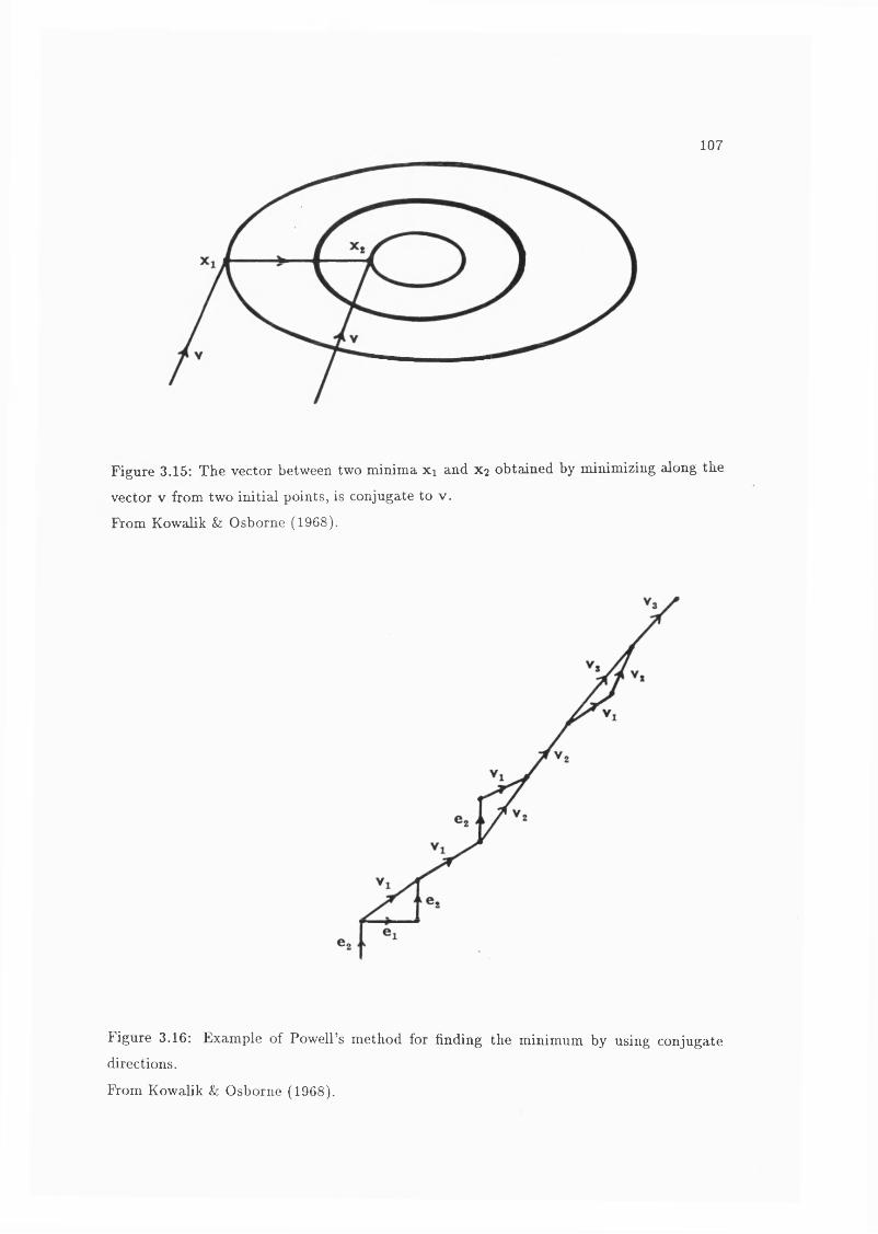
107

Figure 3.15: The vector between two minima x i and X2 obtained by minimizing along the

vector V from two initial points, is conjugate to v .

From Kowalik & Osborne (1968).

Figure 3.16: Example of Powell’s method for finding the minimum by using conjugate

directions.

From Kowalik & Osborne (1968).

108

2. For t = 1 , . . . , n compute A,-, to minimize /(%(') + Ad,) and set

xO+i) = x(') + A,d, . (3.37)

3. Sst d | — * *. ) 7% " X«

4. Set d„ = x ”" — x(*), x(°) =

5. Repeat (1).

Figure 3.16 shows an example of Powell’s method in two dimensions using the

basis vectors as the initial vector set, i.e. n = 2 and d,- = e,-. At the end of the first sweep

the vectorvi = x("+^) - x(^) (3.38)

is conjugate to d„, i.e. the vector 0 2 . After the second iteration the vector

V2 = — x(^) (3.39)

is conjugate to the vectors d„ and d„_i, i.e. v i and 0 2 . And so the process continues.

Powell (1964) showed that for a quadratic function such as Equation 3.28, after k

iterations a set of vectors is produced such that the last k members are mutually conjugate.Therefore, n iterations will exactly minimize a n dimensional function of quadratic form.

The coordinates of the minimum describe the basis functions and will generate the

elements of the design matrix A for least squares problem. Equation 3.15. This represents

the solution to the nonlinear least squares problem, i.e. the matrix that minimizes in

Equation 3.18.

3.7 P ractical Considerations

The automated search routine (ASR) that was developed was based on Powell’s

method as described by Press et al. (1986). However, the line minimization routines they

use were replaced by routines written by the author which minimize along vectors and not

the cardinal directions. These routines are based on those described by Press et at. (1986)

for Brent’s method and bracketting a minimum. Also when a minimum along a vector

is determined, the four closest neighbours are examined, to determine if the search has

109

converged to a local minimum because of the noisy nature of the surface. If one of the

neighbours is smaller the search then walks in that direction until a new minimum is found.

The whole width of the anode is 4096 pixels, defined by the digitization level of

the ADCs. All units of the ASR are defined in these pixels. The ASR is constrained so

that the components of the distribution are kept within a reasonable range of sizes. These

constraints are determined by the anode, all components must have a scale parameter, i.e.

(T or ro, less than half the anode width and must be larger than 10 pixels. If the central

peak of a charge cloud was so small that it was sampled by such a small number of pixels,

the transitional region in the S curve would appear as a very steep straight line and the

curve would be better described as a step function rather than an S curve.

The ASR is written in FORTRAN and is approximately 3000 lines long, 2000 lines

are devoted to the nonlinear least squares problem and the rest deals with the linear least

squares and the inversion. The ASR takes from 2 to 4 Vax 11-780 equivalent CPU hours to

determine a centre channel estimate and a two component fit.

Table 3.1 shows the information returned from the ASR. The uncertainties on the

weights are those returned by the Single Value Decomposition. The probability quoted is

probability that a random sample of n values, where n is the number of data points, would

have a larger than that returned by the fit.

If further information is needed, all of the vectors, the coordinates and for every

point for which W2is evaluated are included in a log file.

3.7 .1 A ccuracy and S ta b ility

The smallest step of the ASR is 0.5 pixels. The small uncertainties this produces in

the centre channel, affect the values of the scale parameters and can introduce an uncertainty

of less than 1 % in the centre term but up to 5 % in the wing term. When using the ASR,

measurements of several data sets taken with the same operating conditions showed that the

uncertainties associated with the central components are 3 %, 5 % for the wing components

and 2 % for the weight of the central component.

The value of x ï returned by a nine element fit used for estimating cc and the

result from the two element fit provide two independent values of x î- The value is a

measure of discrepancy between the estimated function and the parent function as well as

the deviations between the data and the parent function. By carrying out an F test with

110

filenam e: a l00p265.als

no. of v a lid d a ta p t s . :

2 exponentials

95

0 gaussians

I .P . :

2060.36 100.00 300.00

Nine element reduced ch isq : 1.258037

At cen tre channel: 2060.360

19 vecto rs ( to ta l )

6 powel i te r a t io n s

non b a s is vecto rs

min p t : p ix e ls

cen. chan ro ro

2060.16 108.90 372.47min p t : mm

1.04 3.55weights zuid t h e i r u n c e r ta in t ie s

0.69 0.31

0.00 0.00

Reduced Chi S q .: 1.187718

P ro b a b ility : 0.1045723

Table 3.1: Example of the information returned by the automatic search routine.

This example is for a two exponential fit to the data shown in Figure 3.6, the actual fit

itself is shown in Figure 4.1. This value of the reduced is approximately the average of

those returned for all of the data sets.

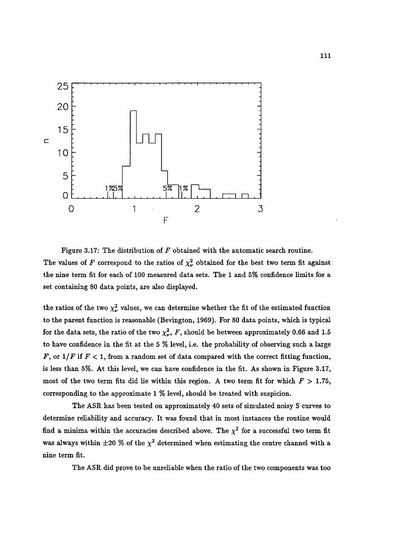
I l l

25

20

c

5%

0 2 3F

Figure 3.17: The distribution of F obtained with the automatic search routine.

The values of F correspond to the ratios of x t obtained for the best two term fit against

the nine term fit for each of 100 measured data sets. The 1 and 5% confidence limits for a

set containing 80 data points, are also displayed.

the ratios of the two x l values, we can determine whether the fit of the estimated function

to the parent function is reasonable (Bevington, 1969). For 80 data points, which is typical

for the data sets, the ratio of the two F , should be between approximately 0.66 and 1.5

to have confidence in the fit at the 5 % level, i.e. the probability of observing such a large

F , or 1 /F if F < 1, from a random set of data compared with the correct fitting function,

is less than 5%. At this level, we can have confidence in the fit. As shown in Figure 3.17,

most of the two term fits did lie within this region. A two term fit for which F > 1.75,

corresponding to the approximate 1 % level, should be treated with suspicion.

The ASR has been tested on approximately 40 sets of simulated noisy S curves to

determine reliability and accuracy. It was found that in most instances the routine would

find a minima within the accuracies described above. The for a successful two term fit

was always within ±20 % of the determined when estimating the centre channel with a

nine term fit.

The ASR did prove to be unreliable when the ratio of the two components was too

112

small, i.e. less th.au a factor of about 2, and most of the power was in the wings. In this

instance the search routine would attribute almost all of the power to a component whose

scale parameter was approximately half way between the two components.

Care must be taken in the selecting the initial point of the search. In some instances

the search will not converge to a minimum. The search routine will halt if a minimum has

not been found along vector after 25 iterations of the Brent method, or after four times

as many Powell iterations as needed for a n dimensional search. Another problem is that

the search may converge to a local minimum very quickly. This usually occurs when the

Powell algorithm does not select a new set of vectors but keeps using the original set of

basis functions, i.e. the orthogonal vectors in the direction of centre channel and the charge

cloud component scale parameters. In this instance, the search “folds up” on itself and

converges to a minima quite quickly afi it can only search along the original vector set.

Another problem, similar to the resolution problem discussed above, is that if the scale

parameters come too close together in size, the ASR will begin to treat them as one term,

either assigning equal weights to both terms or all the weight to one term.

If any of these problems occur, they can usually be overcome by selecting a new

initial point and starting again. I have found that the best selection for an initial point is

to choose the two scale parameters at the outside of the available set, i.e. 50 and 500 pixels.

If problems persist, the centre channel value can be set at a value a long way from the best

estimate. This is almost guaranteed to move the search around and ensure that non-basis vectors are used.

113

Chapter 4

M easurem ents o f th e R adial

D istribution o f the Charge Cloud.

4.1 R ange of M easurem ents

The radial distribution of the charge cloud was determined for over 80 different

operating conditions. The parameters describing the operating parameters in this chapter

are the same as those displayed in Figure 3.5. The measurements were made at 4 different chevron voltages, at 11 anode gap voltages, Vg, across two anode gaps, p, corresponding

to 15 electric field strengths. Eg, two orientations of the pore bias angle and with varying

inter-plate gap voltage, Vi.

4 .1 .1 R an ge o f M easu rem en ts at an M C P A n o d e G ap o f 6 .2 m m

Table 4.1 shows a summary of the operating voltages for which the charge cloud

was determined with g = 6.2 mm. Severe modulation prevented obtaining a measurement

for Vg = 800 V and Vc = 2.9 kV. In each case, the two MCPs were separated by a lOOfim

thick conducting spacer, therefore V{ was always zero.

Measurements were taken for all of the voltage combinations with the MCP pore

bias angle aligned both perpendicular and parallel to the split in the anode. These results

were presented by Edgar et ai (1989).

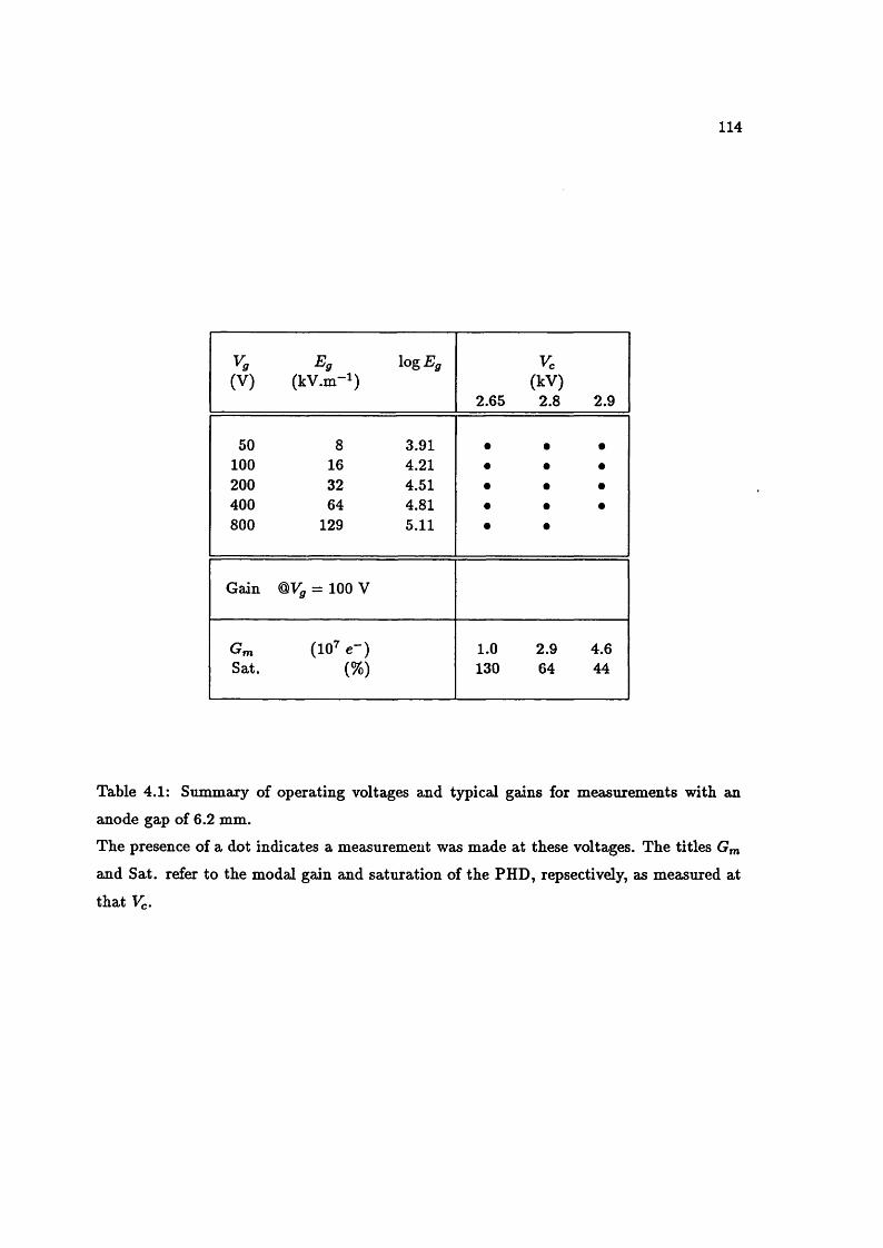
114

Vo(V)

^9(kV.m-1)

logoff

2.65

Vc(kV)

2.8 2.9

50 8 3.91 • • •100 16 4.21 • • •200 32 4.51 • • #400 64 4.81 • • •800 129 5.11 • •

Gain ÛVg = 100 V

Gm (10^ €-) 1.0 2.9 4.6Sat. (%) 130 64 44

Table 4.1: Summary of operating voltages and typical gains for measurements with an

anode gap of 6.2 mm.

The presence of a dot indicates a measurement was made at these voltages. The titles

and Sat. refer to the modal gain and saturation of the PHD, repsectively, as measured at

that Vc.

115

4 .1 .2 R an ge o f M easu rem en ts at an A n od e G ap 3 .0 m m

Table 4.2 summarizes the voltages at which measurements of the charge cloud

were made with g — 3.0 mm. The maximum values for Vg for = 3.0 and 3.1 kV is due

to the rather prosaic condition that the high voltage supply I used could not supply 4 kV.

Measurements were not made for Vg > 600 V at %= = 3.2 kV because of severe modulation,

see Figure 4.5. The small variation in the minimum value of Vg with Vc is due to the high

voltage pulling up Vg.

Some of these measurements were described by Lapington & Edgar (1989). In this

set of measurements, the two MCPs were separated by an 80 /zm thick insulator. Therefore,

a potential difference could be applied across the inter-plate gap. In all the measurements

described in Table 4.2, Vi = 0. The pore biaa angle was always aligned perpendicular to

the anode split.

At a single, fixed combination of Vg and V , Vi was varied through a range of

±30 V. These measurements are discussed in Section 4.4.5.

4.2 T he G eneral Form of th e R adial D istribu tion of th e Charge Cloud

Only Gaussian, exponential and constant offset basis functions were examined during the experiment.

4 .2 .1 T h e T w o C om p on en t N atu re o f T h e R ad ia l D istr ib u tio n

Figure 4.1 compares the best fit to a typical S curve obtained with a single exponen

tial a single Gaussian and two exponential terms. Clearly a single function is unsatisfactory.

In all cases, two terms were required to successfully fit the data. The general form of these

components is a narrow central peak containing the majority of the charge and a broad

diffuse wing component typically three times larger than the peak.

As shown in Figure 3.17, of the 100 two term fits, 16 lie outside the 5% confidence

limits when compared to the nine term fits. The addition of a third term in these cases,

does reduce their x î significantly, so that the corresponding values of F lie within that

confidence region. However, in all but six cases at least one of the terms has a negative

weight. Negative weights imply that the third term was mainly cancelling contributions

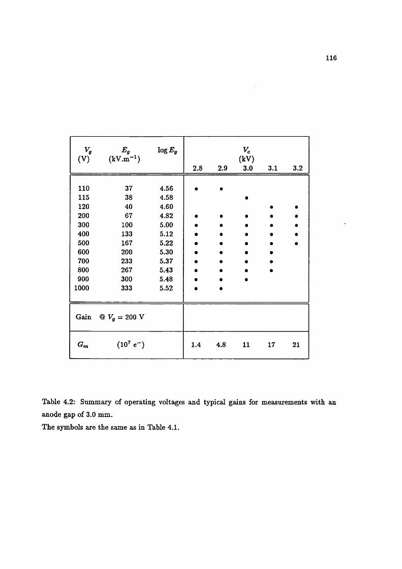
116

logE^(kV)

3.02.8 2.9 3.23.1

110115120200300400500600700800900

1000

4.564.584.604.825.005.125.225.305.375.435.485.52

40

100133167200233267300333

Gain Va = 200 V

4.81.4m

Table 4.2: Summaxy of operating voltages and typical gains for measurements with an

anode gap of 3.0 mm.

The symbols are the same as in Table 4.1.

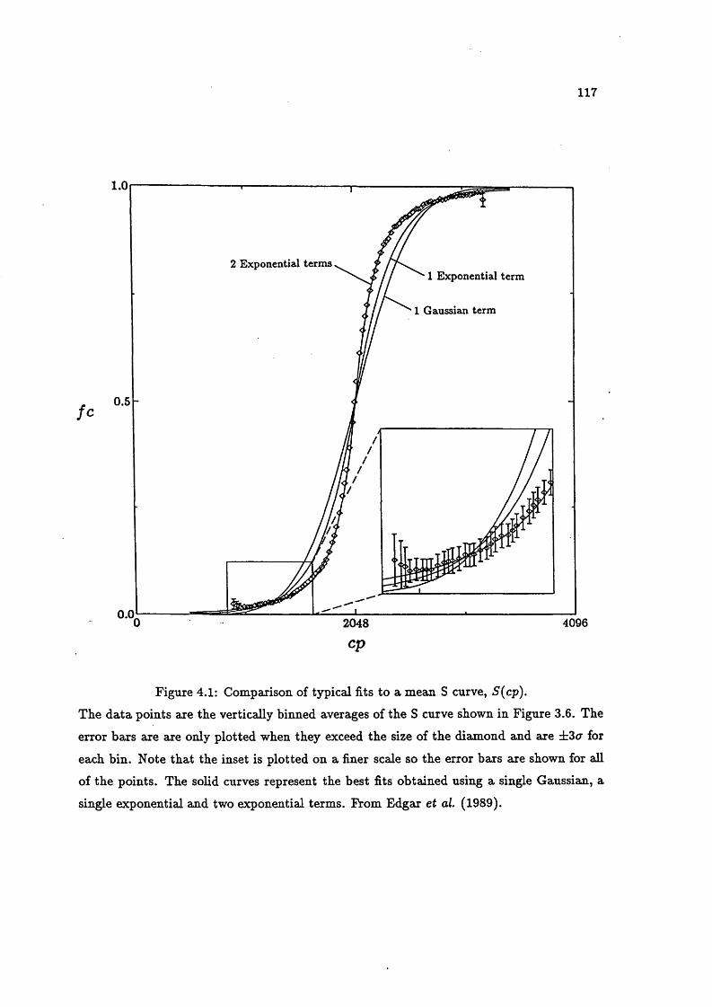
117

1.0

2 Exponential terms1 Exponential term

1 Gaussian term

0.5

0 .0,2048 4096cp

Figure 4.1: Compajison of typical fits to a mean S curve, 5(cp).

The data points are the vertically binned averages of the S curve shown in Figure 3.6. The

error bars are are only plotted when they exceed the size of the diamond and are ±3<r for

each bin. Note that the inset is plotted on a finer scale so the error bars are shown for all

of the points. The solid curves represent the best fits obtained using a single Gaussian, a

single exponential and two exponential terms. From Edgar et al. (1989).

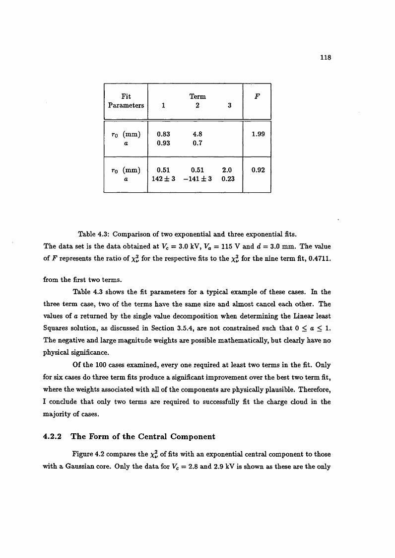
118

Fit Term FParameters 1 2 3

ro (mm) 0.83 4.8 1.99a 0.93 0.7

To (mm) 0.51 0.51 2.0 0.92a 142 ± 3 -141 ± 3 0.23

Table 4.3: Comparison of two exponential and three exponential fits.

The data set is the data obtained at = 3.0 kV, VJ, = 115 V and d = 3.0 mm. The value

of F represents the ratio of Xu for the respective fits to the x î for the nine term fit, 0.4711.

from the first two terms.

Table 4.3 shows the fit parameters for a typical example of these cases. In the

three term case, two of the terms have the same size and almost cancel each other. The

values of a returned by the single value decomposition when determining the Linear least

Squares solution, as discussed in Section 3.5.4, are not constrained such that 0 < a < 1.

The negative and large magnitude weights are possible mathematically, but clearly have no

physical significance.

Of the 100 cases examined, every one required at least two terms in the fit. Only

for six CEises do three term fits produce a significant improvement over the best two term fit,

where the weights associated with all of the components are physically plausible. Therefore,

I conclude that only two terms are required to successfully fit the charge doud in the

majority of cases.

4 .2 .2 T h e Form o f th e C entral C om pon en t

Figure 4.2 compares the x î of fits with an exponential central component to those

with a Gaussian core. Only the data for = 2.8 and 2.9 kV is shown as these are the only

119

two voltages for which measurements were made at all of the electric field strengths.

The figure demonstrates that there is a trend in the difference between the quality

of the fits obtained with the two types of cores with varying Eg. At low electric fields, the

two exponential fits are superior to the Gaussian and exponential combinations, the value

of F decreases progressively with Eg and the Gaussian core fits are superior at high fields.

From the F test for 80 data points for two fits with the same number of degrees

of freedom, as discussed in Section 3.7.1, the boundary for the 5 % and 1 % confidence

limits are | log F |« 0.16 and | log f |« 0.23, respectively. Only at the extremes of the

ranges of Eg, do a significant proportion lie outside of these confidence limits. Figure 4.2

also shows the large scatter in F obtained for the six data sets measured at %, = 2.8 kV

where Eg « 16 kV.m"^. These two factors, taken in conjunction, indicate there is not a

significant difference between the success of the fits with the two different forms of core for

the majority of values of Eg.

4 .2 .3 T h e Form o f th e W in g C om pon en t

In some instances, there is a slight variation in the quality of the fit between fits

with Gaussian and exponential wing terms. The exponential fit usually produced the better

fit but the differences in are much less than those obtained by changing the form of the

core term. When the weight associated with the wing was less than 20%, there was no

significant difference in the quality of the fit for the two types of terms.

F la t T erm s and M odulation

In other instances unreasonably large sizes of the wing were returned by the search

routine, for example 12 mm at %= = 2.9 kV, Vg = 400 V, gf = 6.2 mm and the chevron

plane parallel to the split. Figure 4.3 shows the charge cloud does not have a component

this large. A fit consisting of a single exponential and a constant term is as successful as

the two exponential case for both chevron plane orientations. This suggests that the large

Tow is not a physical result, but is instead an artefact of the fitting procedure trying to fit

to an essentially flat term.

These large terms appear at the onset of modulation, as shown in the behaviour of

wings in Figure 4.3. I tried to investigate the flat terms and the onset of modulation with

measurements at = 3.0 mm. Figure 4.4 and 4.5 show examples of an essentially flat wing

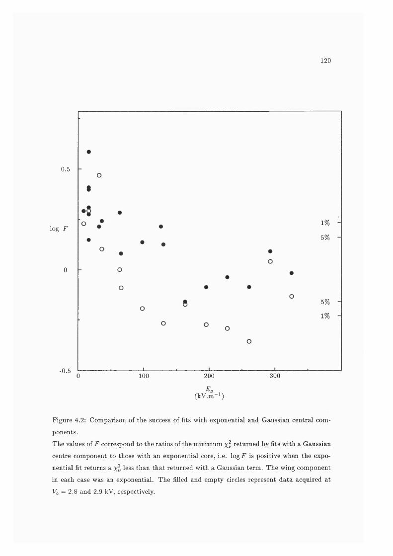
120

0.5

1%log F

5%

5%

-0.53000 100 200

E.(kV.m-i)

Figure 4.2: Comparison of the success of fits with exponential and Gaussian central com

ponents.The values of F correspond to the ratios of the minimum x l returned by fits with a Gaussian centre component to those with an exponential core, i.e. log F is positive when the expo

nential fit returns a x ï less than that returned with a Gaussian term. The wing component in each case was an exponential. The filled and empty circles represent data acquired at

Vc = 2.8 and 2.9 kV, respectively.

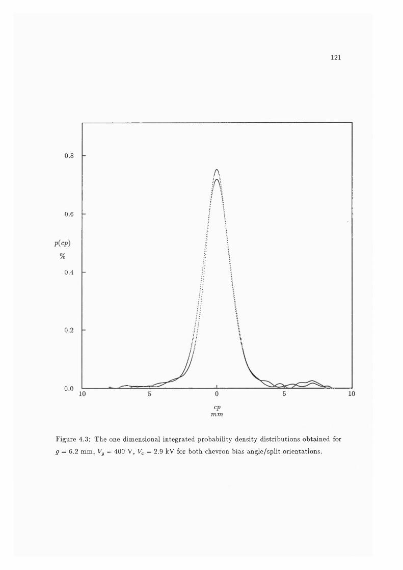
121

0.8

0.6

0.4

0.2

0.0

cpmm

Figure 4.3: The one dimensional integrated probability density distributions obtained for

g = 6.2 mm, Vg = 400 V, Vc = 2.9 kV for both chevron bias angle/split orientations.

122

component and an example of severe modulation obtained at the smaller gap.The p{cp) plot in Figure 4.4 was obtained just before the onset of modulation; when

Vg was increased by 100 V, modulation similar in magnitude to that seen in Figure 4.3 was

evident. As for g = 6.2 mm, the presence of the flat term and modulation appeared only at

for the highest plate voltages, for g = 3.0 mm = 3.1 and 3.2 kV. Fits to these S curves

would only converge if a constant offset wing was used and not with an exponential wing

term. The search would converge with Gaussian terms more often, but these were always

unfeasibley large.

The modulation increased in severity as Vg increased. Significant modulation was

not present in any of the 3.0 kV data sets but it becomes evident for Vg > 500 V and

Vg > 300 V for 3.1 and 3.2 kV, respectively. Figure 4.5 suggests that the 3.2 kV charge

cloud is larger than the corresponding 2.8 kV case. The values of roc returned by the search

routine for 3.1 kV were on average, 20% larger than those returned for the corresponding

values of Vg at 3.0 kV, and 25% larger for 3.2 kV.

This data shows that modulation occurs in larger charge clouds before it appears

in smaller ones. Therefore, the modulation is not purely a function of the charge cloud

size. It is possible that the flat term is responsible for this as it could introduce high spatial frequency components in to the charge cloud distribution. However, the flat term may itself

be an artefact of modulation, as it only appears on the verge of modulation.

Unfortunately at 3.1 kV and 3.2 kV, there was significant ion-feedback and clipping

of the front-end of the preamp, which makes data obtained at these voltages extremely

unreliable. This data is not discussed further in this chapter, but the onset of modulation

and the presence of the flat wings and their association with higher values of warrants

further detailed study.

It would be very interesting to carry out a large series of measurements on a finely

spaced mesh of Vc and Vg values, in the transitional region between no modulation and

severe modulation. In order that modulation can be induced without requiring that Vc

should be so large that ion-feedback occurs, the anode should have a larger repeat pitch, g

should be larger or higher values of Vg should be used.

As the Split-Strip anode consists of a repetitive structure, it is susceptible to

modulation but it can simultaneously return information about the charge cloud size. It

therefore provides a unique capability to study modulation in situ.

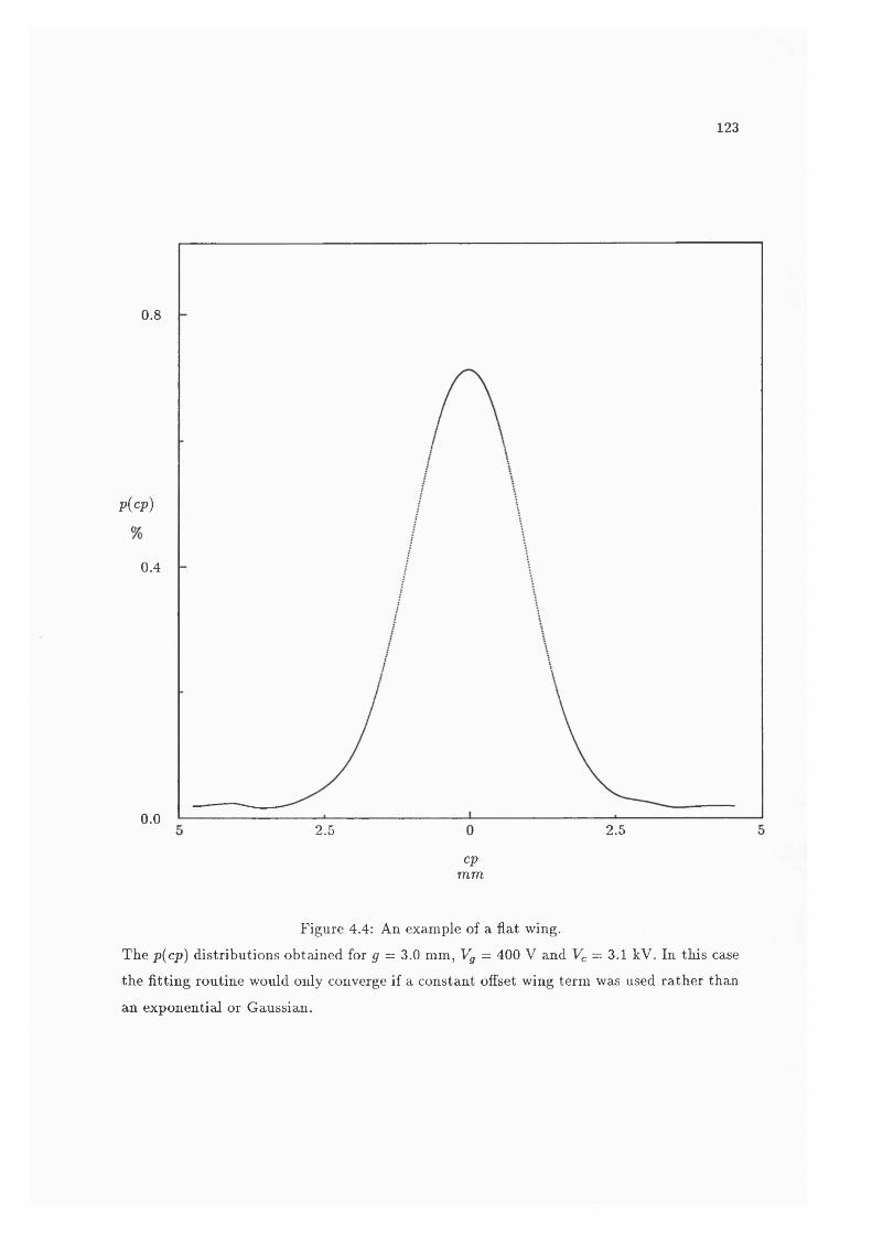
123

0.8

p{cp)

0.4

0.02.5 2.5

cpmm

Figure 4.4: An example of a flat wing.The p{cp) distributions obtained for g = 3.0 mm, Vg = 400 V and Vc = 3.1 kV. In this case the fitting routine would only converge if a constant offset wing term was used rather than

an exponential or Gaussian.

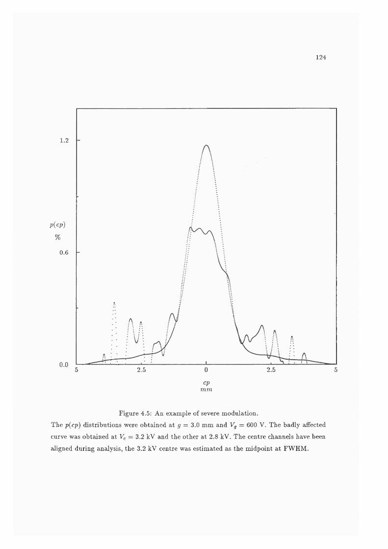
124

1.2

p{cp)

0.6

0.02.5 2.5

cpmm

Figure 4.5: An example of severe modulation.The p{cp) distributions were obtained at ^ = 3.0 mm and Vg = 600 V. The badly affected

curve was obtained at Vc = 3.2 kV and the other at 2.8 kV. The centre channels have been

aligned during analysis, the 3.2 kV centre was estimated as the midpoint at FWHM.

125

4.3 The Size of the R adial D istribution

4 .3 .1 T h e F it P aram eters and th e R adial D istr ib u tio n

The radial distributions presented in this chapter are the best fits to the mean

charge cloud obtained with either two exponential terms, as presented in Edgar et al. (1989)

and Lapington & Edgar (1989), or, as in approximately a dozen cases, a combination of an

exponential and a constant basis function.

The three fit parameters provide a convenient method of describing the form of

the charge cloud but do not provide a direct measure of the amplitude of the charge cloud

at given radius. It is necessary to use the radial probability distributions to describe the

fraction of charge present at a given radius or contained within an annulus.

The general form of the probability density function for the radial distribution

for the charge cloud is derived similarly to the example in Section 3.5.5 and is given by Equations 3.24 and 3.23

y \ / Û C ^ , (1 — d c ) ---p{r) = r ( — e ’•«c + — -— '-e ow J , (4.1)\ oc ôw /

where üc is the weight associated with the central component. To is the scale parameter and

the subscripts c and w refer to the core and wing components, respectively.

In the two exponential case, the total fraction of charge lying within a finite annulus

bounded by and rg is given by

P(Ar) = + +

+ ( l - a , ) [ e - ^ ( l + ^ ) - e - ^ 5 r ( l + ^ ) ] , (4.2)

where T2 > ri. The fraction of of charge lying within a limiting radius, r/ is given by

P (n ) — dc 1 — c ’“«c ^1 H + (1 ~ Oc) 1 “ c ^1 H ^ I • (4.3)

I shall use the quantities r/ and P to describe the size of the charge cloud as determined

from the fit parameters.

Figure 4.6 shows the radial probability density and cumulative distributions ob

tained from a set of fit parameters. Also shown is the uncertainty on F (r), (jp, which

assuming the errors are not correlated, are determined by

2 / S P Ÿ f à P Ÿ ( S P Ÿ

126

where (Jrocy are the uncertainties on the fit parameters. Multiple data sets were

taken at the same operating conditions as the data presented in this figure, for both pore

bias/split orientations and the fractional uncertainties were found to be

< roc = 3% , (4.5)

= 5% , (4.6)

(To, = 2% . (4.7)

These were the only operating conditions for which the uncertainties were determined and

I have assumed that they are also true for the other operating conditions when calculating

errors.

The three partial derivatives for the two exponential case are

, (4.8)6Toc foe

owc»'" , (4.9)

£ =The uncertainty in P produces an uncertainty in r/ whi(di is also shown in Fig

ure 4.6

(Trj = 1 (4.11)dPdpP

4 .3 .2 T h e F it P aram eters at an A n od e G ap o f 6 .2 m m .

(4.12)

The fit parameters obtained at p = 6.2 mm are listed in Table 4.4 and are shown

in Figures 4.7 and 4.8 as a function of Eg and These figures show that the size of

the charge cloud decreases with increasing Eg. The gap voltage is the predominant factor

in determining the size of the (karge cloud. As Eg increases and the size of the charge

cloud decreases, more charge is concentrated in the central component. At = 50 V, the

distributions have roc values of 0.9 to 1.4 mm and Tqw values of typically 4.0 mm, with

approximately equal weights. At 800 V, Vqc has reduced to approximately 0.5 mm while

row has dropped to approximately 3 mm.

There is relatively little difference between the charge clouds obtained at %; = 2.65

and 2.80 kV across the range in Vg. However, at %= = 2.90 kV there is a marked difference.

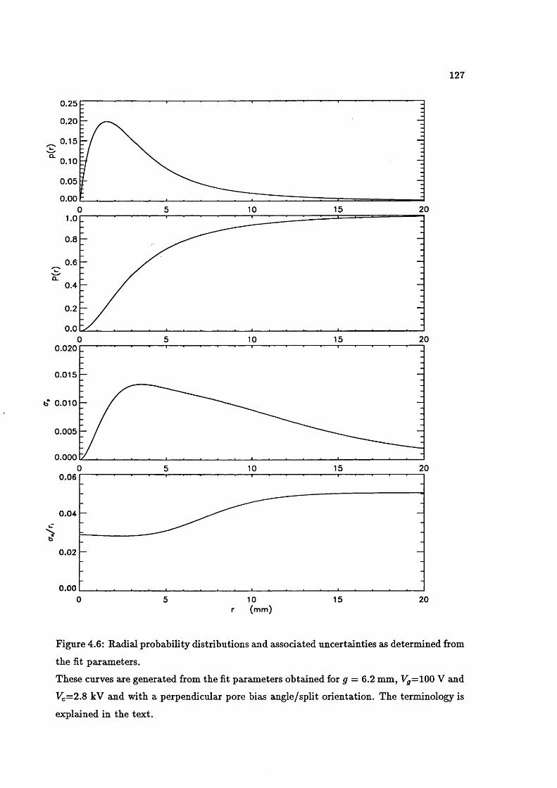
127

0.25

0.20

^ 0.15 C'CL

0.10

0.05

0.0020155 100

0.8

0.6Q.

0.4

0.2

0.0205 150 10

0.020

0.015

b 0.010

0.005

0.000200 15105

0.06

0.04iT>

0.02

0.000 15 205 10

(m m )

Figure 4.6: Radial probability distributions and associated uncertainties as determined from

the fit parameters.

These curves are generated from the fit parameters obtained for g = 6.2 mm, V^=100 V and

%;=2.8 kV and with a perpendicular pore bias angle/split orientation. The terminology is

explained in the text.

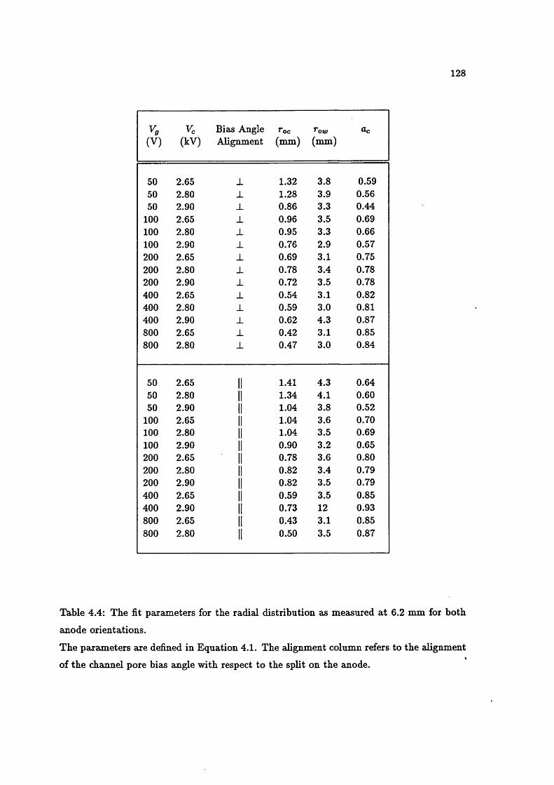
128

(V)Vc

(kV)Bias Angle Alignment

roc(mm)

ow(mm)

ttc

50 2.65 ± 1.32 3.8 0.5950 2.80 ± 1.28 3.9 0.5650 2.90 ± 0.86 3.3 0.44

100 2.65 _L 0.96 3.5 0.69100 2.80 ± 0.95 3.3 0.66100 2.90 _L 0.76 2.9 0.57200 2.65 ± 0.69 3.1 0.75200 2.80 ± 0.78 3.4 0.78200 2.90 0.72 3.5 0.78400 2.65 _L 0.54 3.1 0.82400 2.80 _L 0.59 3.0 0.81400 2.90 0.62 4.3 0.87800 2.65 _L 0.42 3.1 0.85800 2.80 _L 0.47 3.0 0.84

50 2.65 II 1.41 4.3 0.6450 2.80 II 1.34 4.1 0.6050 2.90 II 1.04 3.8 0.52

100 2.65 II 1.04 3.6 0.70100 2.80 II 1.04 3.5 0.69100 2.90 II 0.90 3.2 0.65200 2.65 0.78 3.6 0.80200 2.80 II 0.82 3.4 0.79200 2.90 II 0.82 3.5 0.79400 2.65 II 0.59 3.5 0.85400 2.90 II 0.73 12 0.93800 2.65 II 0.43 3.1 0.85800 2.80 II 0.50 3.5 0.87

Table 4.4: The fit parameters for the radial distribution as measured at 6.2 mm for both

anode orientations.

The parameters are defined in Equation 4.1. The alignment column refers to the alignment

of the channel pore bias angle with respect to the split on the anode.

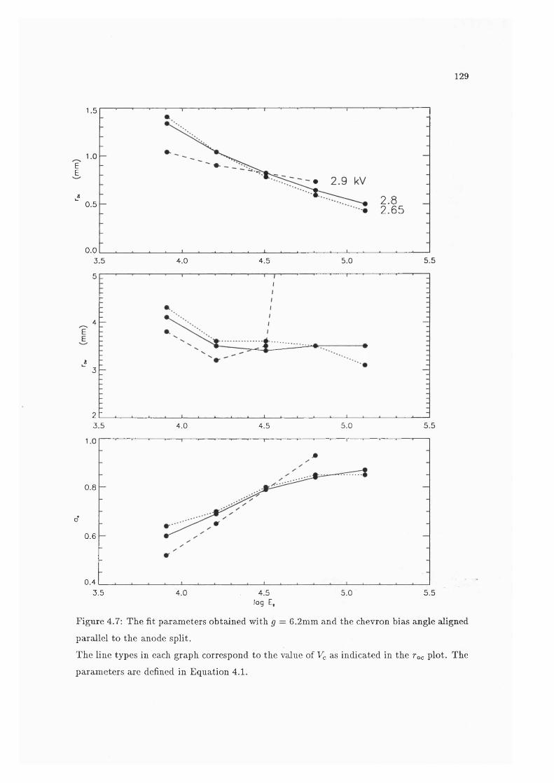
129

1.5

EE

J 2 .82 .650.5

0.05.0 5.53 .5 4.0 4.5

5

4

è3

2t_3.5 4.0 5.0 5.54.5

0.8

o*

0.6

0.43.5 5.0 5.54.0 4.5

log E,

Figure 4.7: The fit parameters obtained with g = 6.2mm and the chevron bias angle aligned

parallel to the anode split.

The line types in each graph correspond to the value of Vc ais indicated in the foe plot. The

parameters are defined in Equation 4.1.

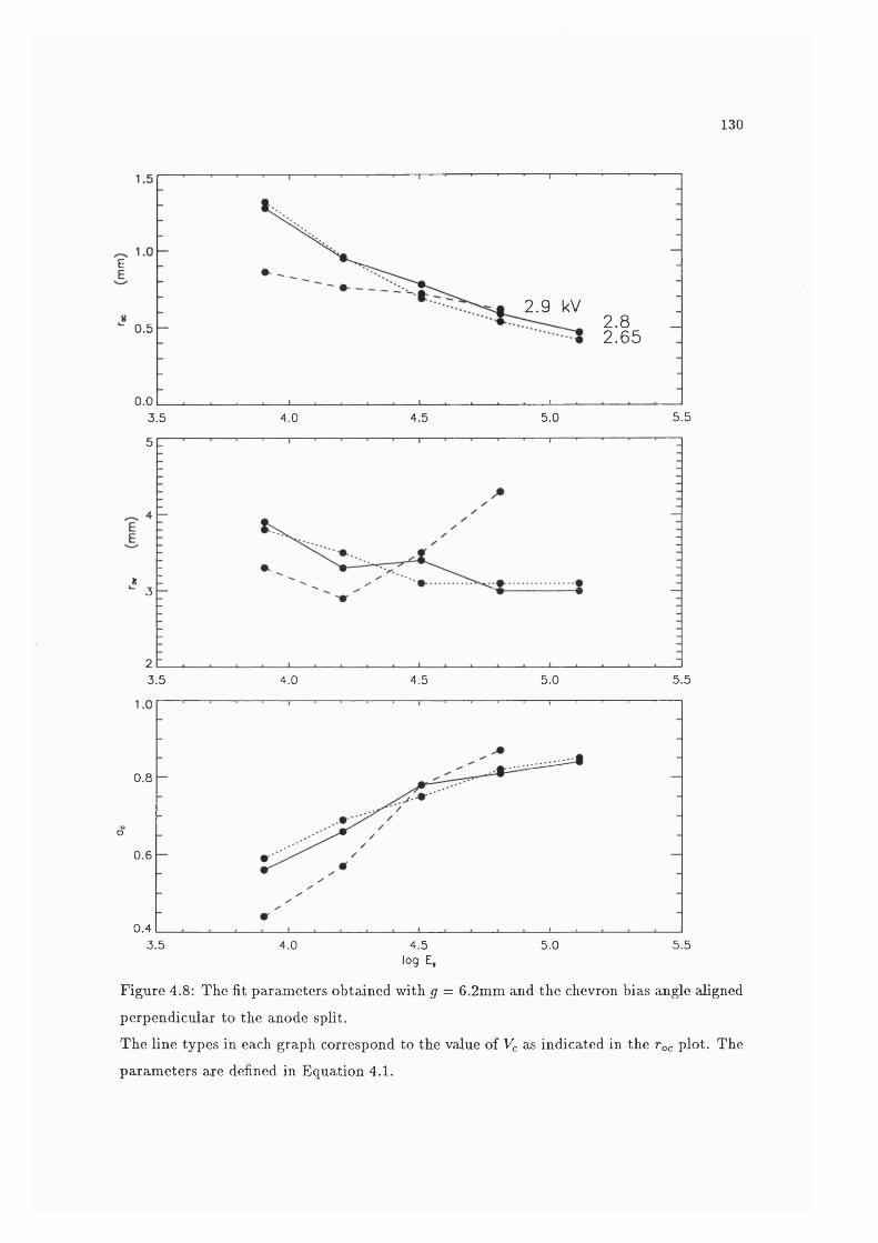
130

E

2.9 kV2 .82 .650.5

0.05.55.03 .5 4.0 4.5

5

4

S3

2L3.5 5.0 5 .54.0 4.5

0.8

o

0.6

0.43.5 5.0 5.54.0 4.5

log E,

Figure 4.8: The fit parameters obtained with g = 6.2mm and the chevron bias angle aligned

perpendicular to the anode split.

The line types in each graph correspond to the value of Vc as indicated in the Tqc plot. The

parameters are defined in Equation 4.1.

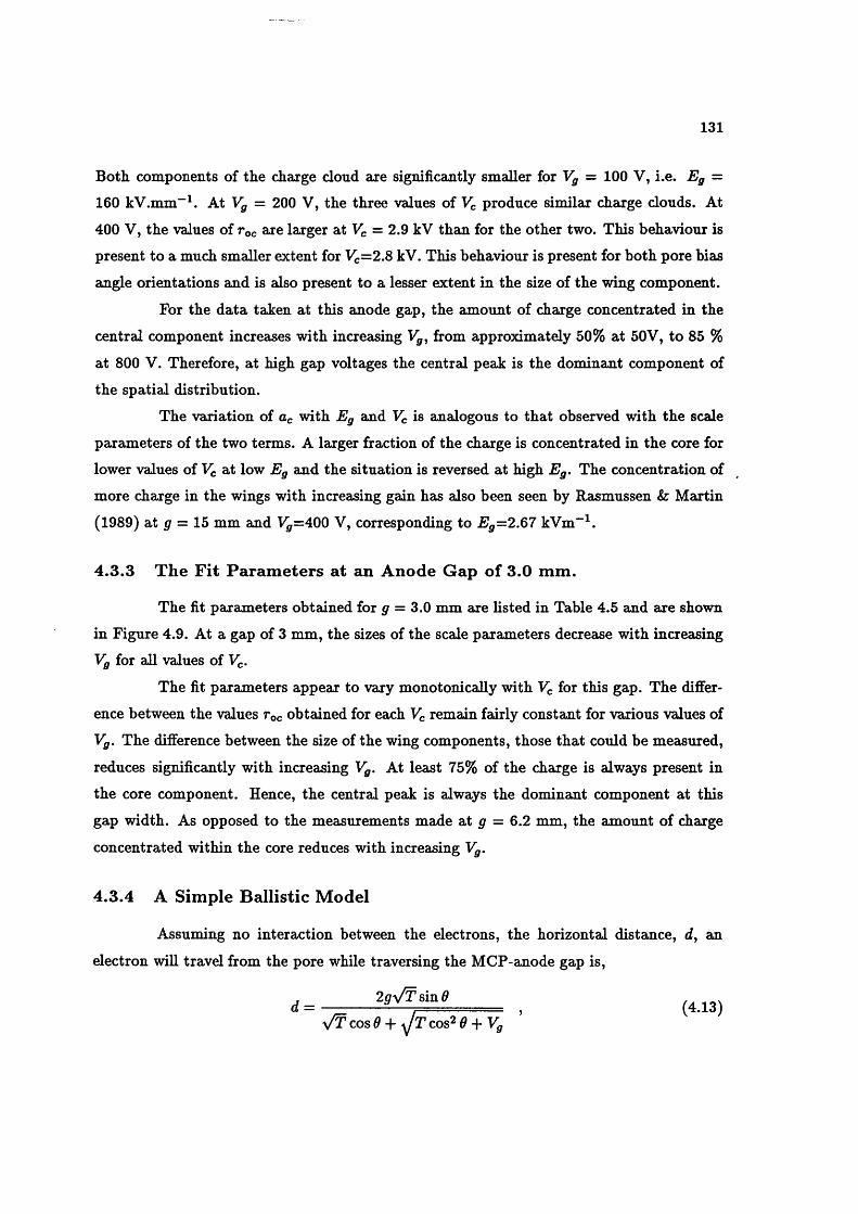
131

Both components of the charge cloud are significantly smaller for Vg = 100 V, i.e. Eg =

160 kV.mm"^. At = 200 V, the three values of Vc produce similar charge clouds. At

400 V, the values of Tqc are larger at %; = 2.9 kV than for the other two. This behaviour is

present to a much smaller extent for V^=2.8 kV. This behaviour is present for both pore bias

angle orientations and is also present to a lesser extent in the size of the wing component.

For the data taken at this anode gap, the amount of charge concentrated in the

central component increases with increasing Vgj from approximately 50% at 50V, to 85 %

at 800 V. Therefore, at high gap voltages the central peak is the dominant component of

the spatial distribution.

The variation of Uc with Eg and Vc is analogous to that observed with the scale

parameters of the two terms. A larger fraction of the charge is concentrated in the core for

lower values of Vc at low Eg and the situation is reversed at high Eg. The concentration of

more charge in the wings with increasing gain has also been seen by Rasmussen & Martin

(1989) at = 15 mm and 1^=400 V, corresponding to Eg=2.67 kVm~^.

4 .3 .3 T h e F it P aram eters at an A n od e G ap o f 3 .0 m m .

The fit parameters obtained for g = 3.0 mm are listed in Table 4.5 and are shown

in Figure 4.9. At a gap of 3 mm, the sizes of the scale parameters decrease with increasing Vg for all values of Vc.

The fit parameters appear to vary monotonically with Vc for this gap. The differ

ence between the values Tqc obtained for each Vc remain fairly constant for various values of

Vg. The difference between the size of the wing components, those that could be measured,

reduces significantly with increasing Vg. At least 75% of the charge is always present in

the core component. Hence, the central peak is always the dominant component at this

gap width. As opposed to the measurements made at flr = 6.2 mm, the amount of charge

concentrated within the core reduces with increasing Vg.

4 .3 .4 A S im ple B a llis tic M od el

Assuming no interaction between the electrons, the horizontal distance, d, an

electron will travel from the pore while traversing the MCP-anode gap is,

d = — , (4.13)y /T COS 6 + y T c o s ^ 6 -\-Vg

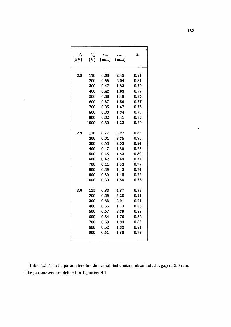
132

Vc(kV) (V)

I'oc(mm)

Tow(mm)

ÛC

2.8 110 0.68 2.45 0.81200 0.55 2.04 0.81300 0.47 1.83 0.79400 0.42 1.63 0.77500 0.38 1.49 0.75600 0.37 1.59 0.77700 0.35 1.47 0.75800 0.33 1.34 0.73900 0.32 1.41 0.73

1000 0.30 1.33 0.70

2.9 110 0.77 3.27 0.88200 0.61 2.35 0.86300 0.53 2.03 0.84400 0.47 1.59 0.78500 0.45 1.63 0.80600 0.42 1.49 0.77700 0.41 1.52 0.77800 0.39 1.43 0.74900 0.39 1.40 0.75

1000 0.39 1.50 0.76

3.0 115 0.83 4.87 0.93200 0.69 3.20 0.91300 0.63 2.91 0.91400 0.56 1.73 0.83500 0.57 2.39 0.88600 0.54 1.76 0.82700 0.53 1.94 0.83800 0.52 1.82 0.81900 0.51 1.80 0.77

Table 4.5: The fit parameters for the radial distribution obtained at a gap of 3.0 mm.

The parameters are defined in Equation 4.1

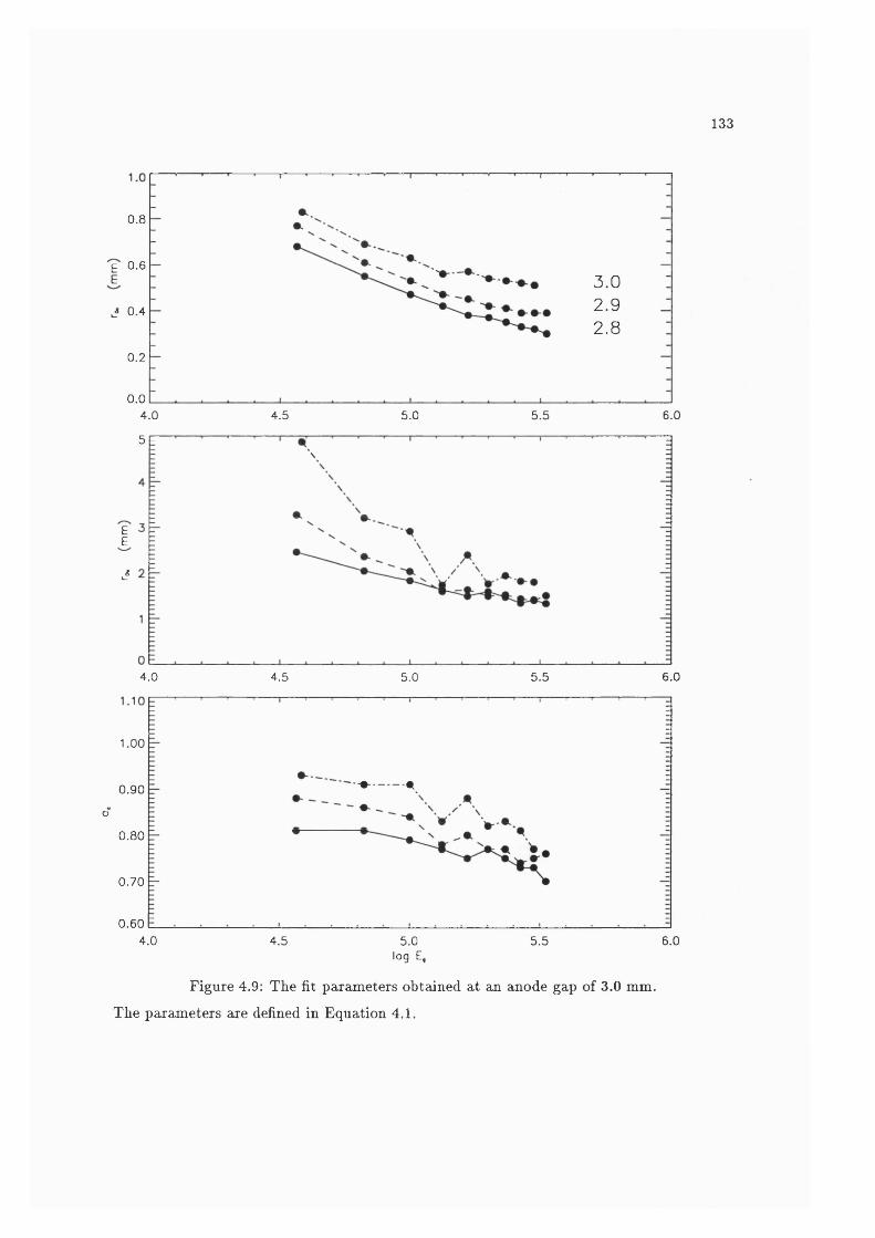
133

0.8

E 0.63.02.92 .8

a 0 .4

0.2

0.06.04 .0 4 .5 5 .0 5 .5

5 F

EE

J

6.04 .0 4 .5 5 .0 5 .5

1.00

"# it0 .9 0

o

0 .8 0

0 .7 0

0 .6 0

4 .0 4 .5 5 .0 5 .5 6.0log E,

Figure 4.9: The fit parameters obtained at an anode gap of 3.0 mm.

The parameters are defined in Equation 4.1.

134

where T is the output kinetic energy of the electron and d is the angle between the MCP velocity vector and the normal to MCP face. A ballistic model requires knowledge of the

angle and energy distributions.

Energy and Angular D istribution o f the Output Electrons

The energy distribution of output electrons for a single, single thickness MCP has

been measured by Koshida & Hosobuchi (1985) and Koshida (1986). They find that the

energy distribution has a peak at about 5 eV and a long exponential tail with energies

exceeding 100 eV, see Figure 4.10. As shown in this diagram, in unsaturated mode the

majority of electrons have an energy > 50 eV. As saturation increases the number of high

energy electrons decrease. Approximately 80% of the electrons lie equally distributed be

tween the two lower energy ranges. They determine that the low energy peak is caused

by electrons produced in the region of constant potential caused by the end-spoiling while

the high energy tail originates from regions further up the pore. The authors attribute the

shift to low energy electrons with increasing saturation to the charging of the channel wall

producing a nonlinear electric field inside the pore, as discussed in Section 1.1.3.

As electrons with different output energies appear to originate from different re

gions within the channel, the energy and angle distributions of the electrons cannot be

treated independently. Low energy electrons originating on the end-spoiling should have a

broader output angle distribution than the high energy electrons originating further up the

channel.

Bronshteyn et al. (1980) have measured the angular distribution of the electrons

from a single MCP. They found that the distribution is approximately Gaussian with a

half-width of 10 — 20° and a peak at an inclination to the MCP normal equal to the bias

angle. They also measured the energy distribution of electrons at a given output angle and

found that the range of energies is much larger for electrons with low inclination angles

than for those with relatively high inclinations, see Figure 4.11. However, the authors do

not discuss saturation. Given that they measured increasing electron energy with increasing

plate bias voltage, as opposed to what Koshida & Hosobuchi (1985) described for increasing

saturation, it is most likely that the MCPs are operated in the linear mode.

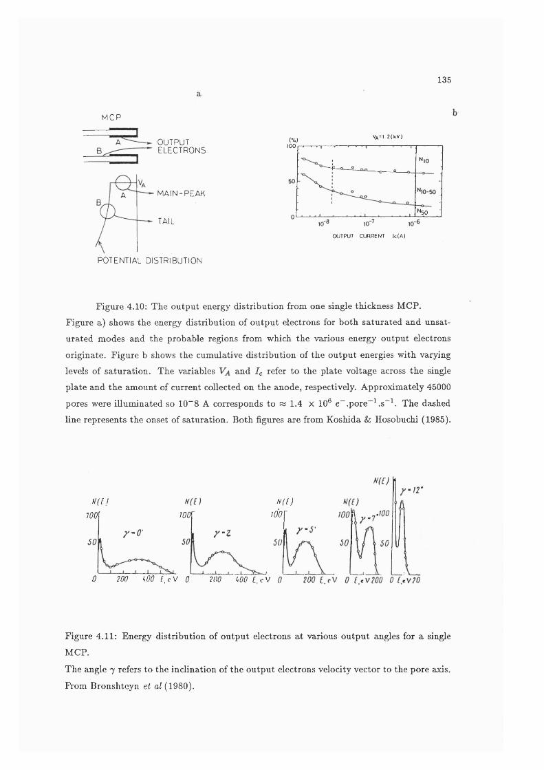
135

MCP

OUTPUTe l e c t r o n s

MAIN-PEAK

TAIL

POTENTIAL DISTRIBUTION

(V .)VA=l.2(kV)

100

' 5 0

OUTPUT CU RREN T lc{A )

Figure 4.10: The output energy distribution from one single thickness MCP.Figure a) shows the energy distribution of output electrons for both saturated and unsaturated modes and the probable regions from which the various energy output electrons originate. Figure b shows the cumulative distribution of the output energies with varying levels of saturation. The variables and Ic refer to the plate voltage across the single plate and the amount of current collected on the anode, respectively. Approximately 45000 pores were illuminated so 1 0 “ 8 A corresponds to % 1.4 x 10® e“ .pore“^.s“ ^ The dashed line represents the onset of saturation. Both figures are from Koshida & Hosobuchi (1985).

f/ff/ fÛ)100WOWO

200 m E.cV0 200 wo f.cV 0

Figure 4.11: Energy distribution of output electrons at various output angles for a single MCP.

The angle 7 refers to the inclination of the output electrons velocity vector to the pore axis.

From Bronshteyn et al (1980).

136

The M aximum Size o f the Charge Cloud Due Solely to Ballistic Effects

Figure 4.12 shows the horizontal distance an electron can travel while traversing

the MCP-anode gap for various combinations of output angles and energies, as determined

by using Equation 4.13. Electrons with energies less than 10 eV are assumed to be emitted

from the end-spoiling, undergo no acceleration in the channel and have no constraints on

their output angles.

Electrons with higher energies are assumed to come from the wall of the channel

beyond the end-spoiling. They are assumed to be emitted from the wall with no energy so

that all the kinetic energy comes from acceleration within the chaimel. The electric field

within the pore is assumed to be linear, i.e. the gradient of the potential along the channel

is linear until the end-spoiling is reached. The constraint on the angles is determined by

the straight line between the point from which the electron is assumed to be emitted and

the opposite edge of the channel. As the output angles of these electrons are assumed to

be constrained but those with low energies are not, there is a discontinuity in the model at

10 eV.

These constraints represent the upper limit of the possible output angles as the

electric field within the channel will cause the electrons to follow parabolic trajectories, and

so inclinations to the pore axis will be less than in the straight line case. The presence of

an electrostatic lens at the pore output will tend to further collimate the electrons (Guest,

1978).Figure 4.12 shows that relatively low energy electrons at high inclinations to the

pore axis travel the greatest horizontal distance. Although the output angle is the most

important variable for determining the horizontal distance, the variation of electron energy

for a given angle can produce differences in the distance travêd , particularly for low energy

electrons.

Given that the peak of the angular distribution occurs at the pore bias angle and

almost all the electrons have an energy less than 50 eV, the peak of the charge cloud would

be expected to lie within 1 mm of the pore. I shall take it to be located at a distance of

0.5 mm.

Even though the maximum value for the output angle for a given energy is almost

certainly overestimated, those electrons that have travelled the furthest from the pore have

not reached a distance of 4.0 mm, i.e. a radius of 3.5 mm. The average values of the fit

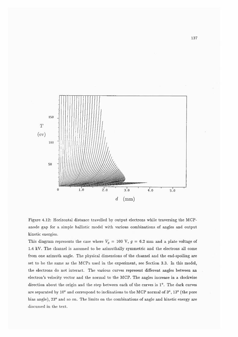
137

150

T

(ev)

100

1.0 2.0 3 .0 4 .0 5 .0

d (mm)

Figure 4.12: Horizontal distance travelled by output electrons while traversing the MCP- anode gap for a simple ballistic model with various combinations of angles and output kinetic energies.This diagram represents the case where Vg = 100 V, g = 6.2 mm and a plate voltage of

1.4 kV. The channel is assumed to be azimuthally symmetric and the electrons all come from one azimuth angle. The physical dimensions of the channel and the end-spoiling are

set to be the same as the MCPs used in the experiment, see Section 3.3. In this model, the electrons do not interact. The various curves represent different angles between an electron’s velocity vector and the normal to the MCP. The angles increase in a clockwise

direction about the origin and the step between each of the curves is 1°. The dark curves

are separated by 10° and correspond to inclinations to the MCP normal of 3°, 13° (the pore bias angle), 23° and so on. The limits on the combinations of angle and kinetic energy are

discussed in the text.

138

parameters for Vg — 100 V from Table 4.4 are; Tqc = 0.94 mm, rou, = 3.4 mm and ûc = 0.66 . Combining these values with Equation 4.3, I estimate over 30% of the total charge cloud

lies outside a radius of 3.5 mm. With a limit on the combination of angle and energy

comparable to that measured by Bronshteyn et al. (1980), i.e. 10° and 20 eV, the limiting

radius is approximately 1.0 mm which contains only about 20% of the charge cloud. Also,

as seen in Figure 3.7, a significant number of electrons have been collected at radii of up

to 10 mm. Even if an electron was emitted parallel to the MCP face, it would require an

initial energy of approximately 65 eV to travel 10 mm horizontally while traversing the gap.

Although a simple ballistic model can produce distributions with sizes comparable

to the size of the core, it is totally inadequate for describing the size of the wing component.

4 .3 .5 Sp ace C harge

Figure 4.13 shows the horizontal distance travelled by an electron due to the

coulomb repulsion between it and a single particle with a massive negative charge for typical

output electron time of flights. A t g — 6.2 mm and Vg = 100 V, it would take approximately

2.0 ns for an electron with zero initial velocity to cross the MCP-anode gap. The diagram

shows that a charge of only a few percent of the total charge within the electron cloud,

» 6.4 X 10® g, is needed to accelerate the electrons to the horizontal velocity needed to

reach a distance of 10 mm. Therefore, space charge effects can explain the relatively large

size of charge cloud.

The large variation in electron velocities will make a detailed model of the interac

tion between electrons extremely complex. Only a detailed Monte-Carlo simulation could

produce realistic predictions. Detailed knowledge of the electric fields at the pore exit would

also be necessary to determine an initial distribution of charge.

4.4 T he V ariation of Charge Cloud Size w ith M C P O perating Conditions.

4 .4 .1 T h e E ffects o f G ain on C harge C loud Size

As discussed in Section 3.7.1, multiple data sets were acquired at constant operat

ing conditions. Some of these data sets were concatenated to produce a data set containing

3.6 X 10® events. The data were binned into 10 intervals of gain each containing approxi-

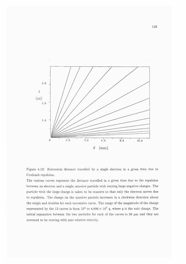
139

t

(ns)

3.0

2.0

1.0

2.0 4 .0 6.0 10.0

d (m m )

Figure 4.13: Horizontal distance travelled by a single electron in a given time due to

Coulomb repulsion.

The various curves represent the distance travelled in a given time due to the repulsion

between an electron and a single, massive particle with varying large negative charges. The

particle with the large charge is taken to be massive so that only the electron moves due

to repulsion. The charge on the massive particle increases in a clockwise direction about

the origin and doubles for each successive curve. The range of the magnitude of the charge

represented by the 13 curves is from lO'* to 4.096 x 10 q, where q is the unit charge. The

initial separation between the two particles for each of the curves is 50 //m and they are

assumed to be moving with zero relative velocity.

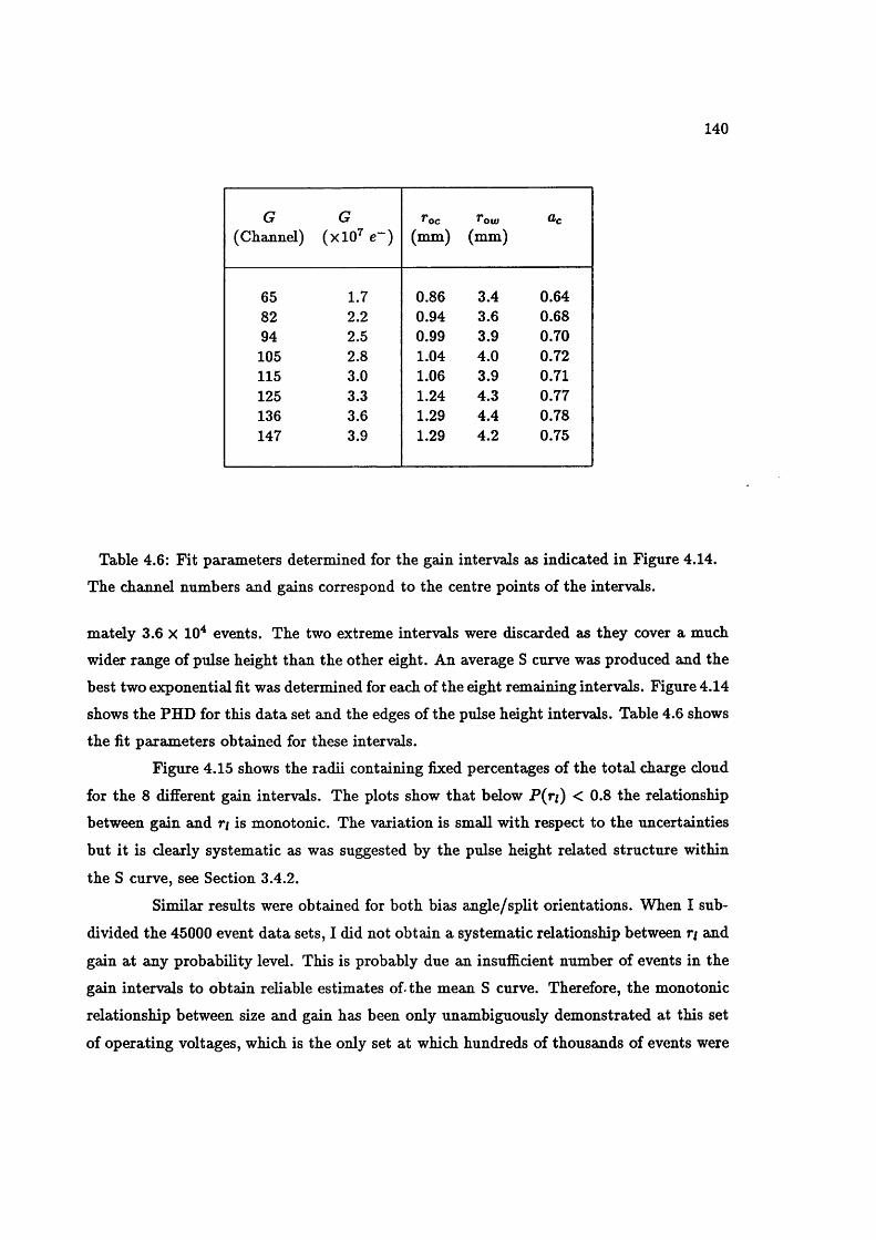
140

G(Channel)

G(xlO^ e“ )

Toe(mm)

7* oto(mm)

ac

65 1.7 0.86 3.4 0.6482 2.2 0.94 3.6 0.6894 2.5 0.99 3.9 0.70105 2.8 1.04 4.0 0.72115 3.0 1.06 3.9 0.71125 3.3 1.24 4.3 0.77136 3.6 1.29 4.4 0.78147 3.9 1.29 4.2 0.75

Table 4.6: Fit parameters determined for the gain intervals as indicated in Figure 4.14.

The channel numbers and gains correspond to the centre points of the intervals.

mately 3.6 X 10 events. The two extreme intervals were discarded as they cover a much

wider range of pulse height than the other eight. An average S curve was produced and the

best two exponential fit was determined for each of the eight remaining intervals. Figure 4.14

shows the PHD for this data set and the edges of the pulse height intervals. Table 4.6 shows

the fit parameters obtained for these intervals.

Figure 4.15 shows the radii containing fixed percentages of the total charge cloud

for the 8 different gain intervals. The plots show that below P (n ) < 0.8 the relationship

between gain and r/ is monotonie. The variation is small with respect to the uncertainties

but it is clearly systematic as was suggested by the pulse height related structure within

the S curve, see Section 3.4.2.

Similar results were obtained for both bias angle/split orientations. When I sub

divided the 45000 event data sets, I did not obtain a systematic relationship between r/ and

gain at any probability level. This is probably due an insufficient number of events in the

gain intervals to obtain reliable estimates of-the mean S curve. Therefore, the monotonie

relationship between size and gain has been only unambiguously demonstrated at this set

of operating voltages, which is the only set at which hundreds of thousands of events were

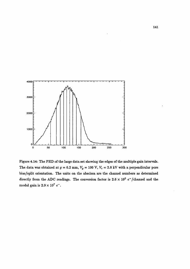
141

40 00

3000 -

2000

1000

250 3000 50 100 150 200

Figure 4.14: The PHD of the large data set showing the edges of the multiple gain intervals.

The data was obtained at gr = 6.2 mm, Vg = 100 V, = 2.8 kV with a perpendicular pore

bias/split orientation. The units on the abscissa are the channel numbers as determined

directly from the ADC readings. The conversion factor is 2.6 x 10® e~/channel and the

modal gain is 2.9 x 10^ e~.

142

acquired during the experiment. However, as Figure 4.15 confirms the existence of a sys

tematic relationship, suggested by the pulse height related structure within the S curve and

this structure was observed in all data sets, the gain/size relationship must be expected to

exist under all operating conditions.

The fits obtained for S curves consisting of the whole PHD, as displayed in Fig

ure 4.15 and Table 4.6, describe smaller charge clouds than those obtained for the gain

intervals containing the mode, mean or median of the PHD. This is most probably caused

by bias towards the low gain events when determining the average S curve. Figure 3.8 shows

that in some regions of the measured S curve, there is a much larger variation in the curve

for low gain events than for the larger events. This larger variation might provide a larger

“moment” when determining the mean, biasing the average to a lower level.

Therefore, the affect of varying charge cloud size on the Split Strip Anode itself is

of importance as the fitting procedure returns smaller charge clouds than would be expected,

when the whole PHD is used. Although in this instance, the biasing and the variation of

radius with gains are comparable to the uncertainties produced by the fit parameters, it

is not known how significant it would be under other operating conditions. Both of these

effects should be examined in detail in future experiments to determine how significant they

are and how they vary with operating conditions. This would require data sets containing

several hundred thousand events as 45,000 event data sets have proved inadequate to achieve

reliable fits for determining the variation of the S curve with gain. The gain intervals that I

used had sharp edges, so the cross sections through the S curve could not be approximated

by Gaussians. The statistic assumes implicitly that the errors in a distribution are

normally distributed. Ideally, a few million events should be acquired and subdivided into

a series of gain intervals with a Gaussian intensity distribution.

All of the other fits described in this chapter were made using the full PHD. As

nothing is known about the biasing of the mean S curve for the other operating conditions,

there is inevitably some degree of ambiguity when comparing data obtained under different

conditions. For the rest of the chapter I have assumed that this biasing always behaves in

a similar manner and that any variation is only comparable to the uncertainties observed

for this set of operating conditions.

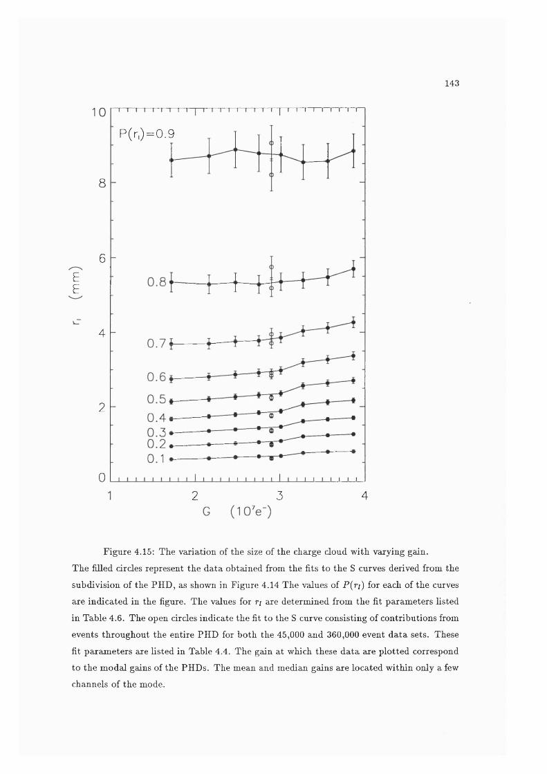
143

EE

1

p ( n ) = 0 . 9

8

6

4

2

0

42 3

Figure 4.15: The variation of the size of the charge cloud with varying gain.

The filled circles represent the data obtained from the fits to the S curves derived from the

subdivision of the PHD, as shown in Figure 4.14 The values of P(r/) for each of the curves

are indicated in the figure. The values for r/ are determined from the fit parameters listed

in Table 4.6. The open circles indicate the fit to the S curve consisting of contributions from

events throughout the entire PHD for both the 45,000 and 360,000 event data sets. These

fit parameters are listed in Table 4.4. The gain at which these data are plotted correspond

to the modal gains of the PHDs. The mean and median gains are located within only a few

channels of the mode.

144

4 .4 .2 T h e E ffects o f Eg on C harge C loud S ize

Figure 4.16 shows the variation of r/ for various levels of P{ri) with increasing Eg.

As the plot is log/log, a power law between radius and electric field strength would appear

as a straight line. As all the curves show significant curvature, there is no straight forward

power law relationship. There is also very little variation between the form of the curves

for the different P{ri) levels of the charge cloud from the 10% to the 90% levels.

Approximating the data at Eg < 100 kV.m~^ to a straight line, the approximate

index of the power law is -0.3. The time of flight, t / , for an electron with zero initial kinetic

energy, across the MCP-anode gap can be determined from Equation 4.13,

where rrie is the electron mass. A charge cloud in which the size evolved ballistically

would follow a power law with an index of -0.5 and one in which the electrons continuously

underwent a constant acceleration would have an index of -0.25.Figure 4.17 shows the variation of r/ with t f and gives some indication of the

expansion rate of the charge cloud. It is clear that the cloud expands at different rates at different levels and that it is not expanding at a constant velocity but being continuously

accelerated. The acceleration is highest at the radii containing the most charge which is as

expected for Coulomb repulsion.

4 .4 .3 P la te B ias V oltage

Figure 4.18 shows the variation of r/ with Eg for three separate values of Vc at

four probability levels for g — 3.0 mm. They indicate a monotonie relationship between

ri and Vc for P{ri) < 0.9. However, as shown in Figure 4.19, this situation does not hold

for g = 6.2 mm in which at low field strengths and at up to the 50% probability level the

2.9 kV charge cloud is significantly smaller than the 2.8 kV case. The data obtained at the

two gaps are compared in the next section.

Therefore, Vc does aflFect the size of the charge cloud but not in an easily predictable

manner and the size of the charge cloud is not driven solely by the gain. Therefore, space

charge alone is insufficient to explain the variation of the charge cloud with Vc.

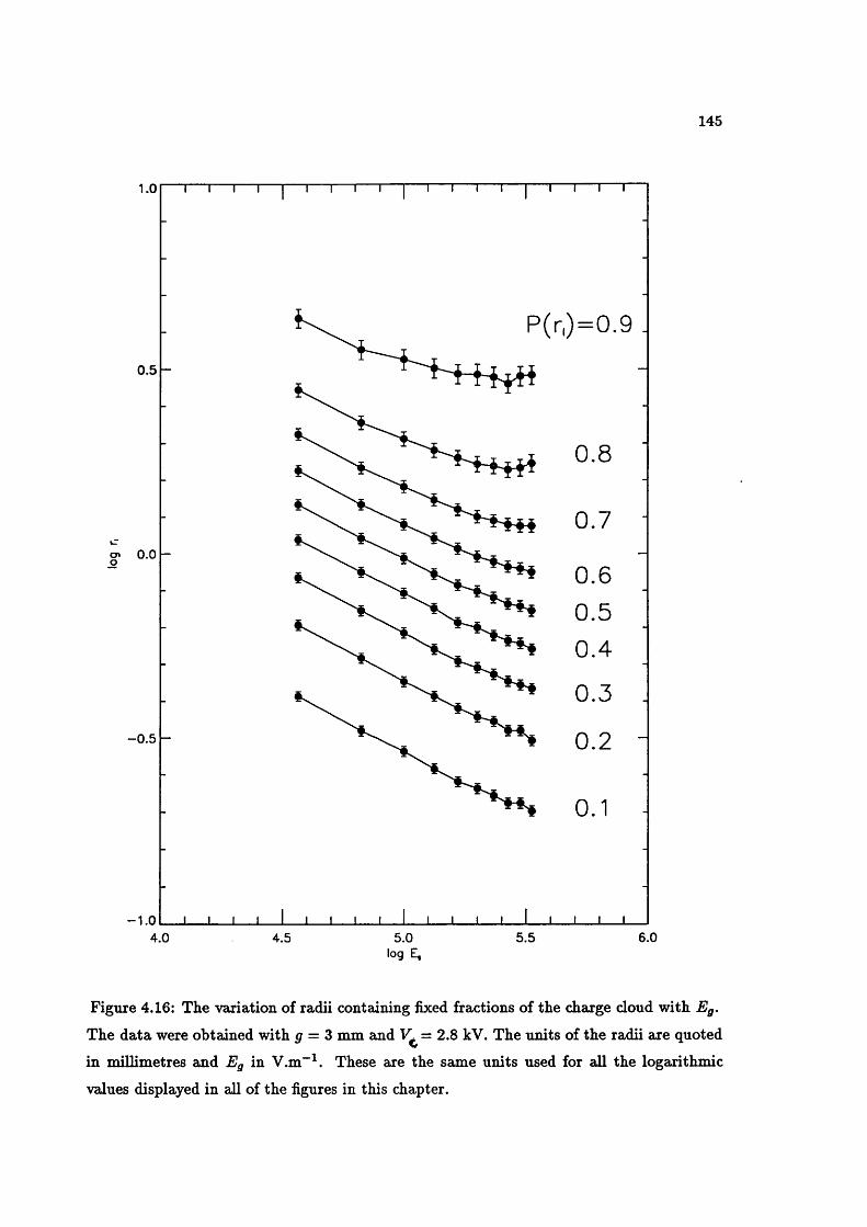
145

1.0

P(n)=o

0.5

0 . 8

0.7enO

0 . 6

0 .50 .4

0 .3

0 . 2-0 .5

-1.05.5 6.04.0 5.04.5

log E,

Figure 4.16: The variation of radii containing fixed fractions of the charge cloud with Eg.

The data were obtained with g = 3 mm and = 2.8 kV. The units of the radii are quoted

in millimetres and Eg in V.m~^. These are the same units used for all the logarithmic

values displayed in all of the figures in this chapter.

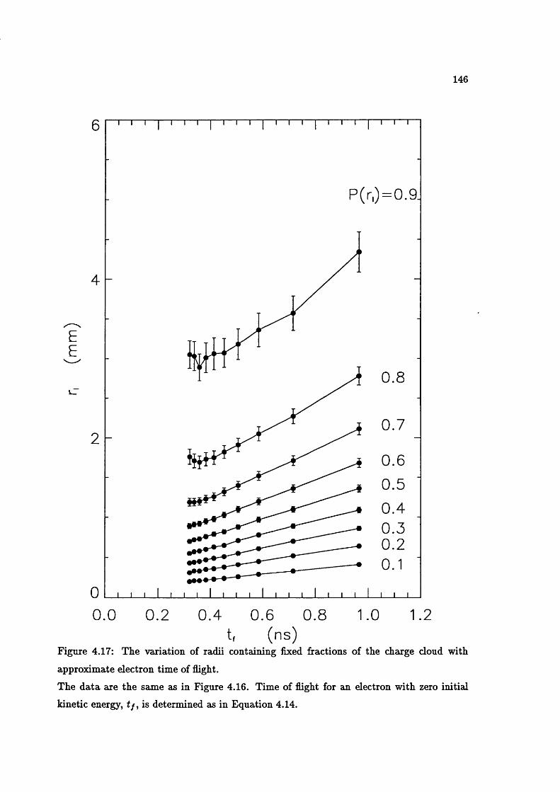
146

6

E E

0

P(r,) = 0 .9

0 . 8

0 .7

0 . 6

0 .50 .40 .30 . 2

J _ i I I I I I I 1 IJ__ L

0 .0 0 .2 0 .4 0 .6 0 .8 1.0 1.2t, (ns)

Figure 4.17: The variation of radii containing fixed fractions of the charge cloud with

approximate electron time of flight.

The data are the same as in Figure 4.16. Time of flight for an electron with zero initial

kinetic energy, t f , is determined as in Equation 4.14.

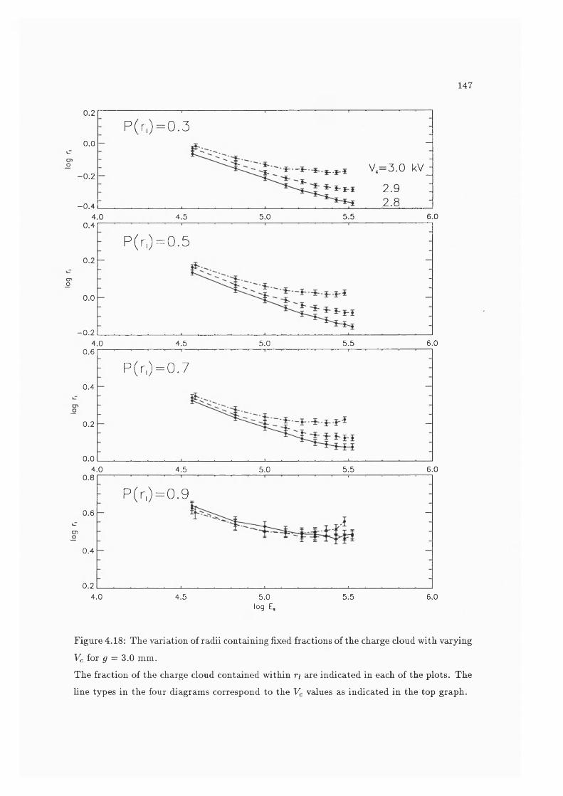
147

0.2

0.0

g'- 0.2

- 0 .44.0

O 'o

P(r,) = 0.3

•■ï— Vg—3 . 0 kVJ

2 . 92.8

4.5 5.0 5.5 6.00.4

P(r,) = 0.50.2

0.0

-0.24.5 5.0 5.5 6.04.0

0.6

P(r,) = 0.70.4

0.2

0.04.0 5.5 6.04.5 5.0

0.8

P(r,) = 0.90.6

CD

0.4

0.26.04.0 4.5 5.0 5.5

log E,

Figure 4.18: The variation of radii containing fixed fractions of the charge cloud with varying

Vc for g — 3.0 mm.

The fraction of the charge cloud contained within r\ are indicated in each of the plots. The

line types in the four diagrams correspond to the Vc values as indicated in the top graph.

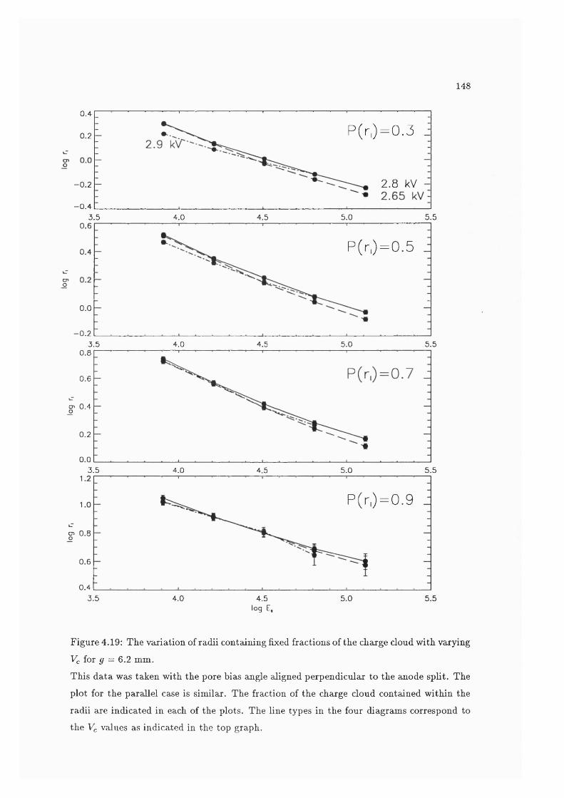
148

0.4

P(r,) = 0.30.2

2 . 8 kV -- 0.2

- 0 .43.5 4.5 5.0 5.54.0

0.6

P(r,) = 0.50.4

cr>o

0.0

- 0.25.53.5 4.0 4.5 5.0

0.8

0.6

cn 0.4

0.2

0.03.5 5.54.0 4.5 5.0

P(r,)=0.9

cn 0.8

0.6

0.43.5 4.0 5.54.5 5.0

log E,

Figure 4.19: The variation of radii containing fixed fractions of the charge cloud with varying Vc foT g = 6.2 mm.This data was taken with the pore bias angle aligned perpendicular to the anode split. The

plot for the parallel case is similar. The fraction of the charge cloud contained within the radii are indicated in each of the plots. The line types in the four diagrams correspond to the Vc values as indicated in the top graph.

149

4 .4 .4 C om parison o f th e M easurem en ts for th e T w o G aps.

Figure 4.20 directly compares r/ for the 2.8 and 2.9 kV data obtained for the

two MCP-anode gaps with respect to Eg. Of the 14 different combinations of Vg and g, 8

correspond to values of Eg lying within a region in which the data sets for the two gaps

overlap. The figure shows that at P (r/) < 0.9 the two curves fall on top of each other,

within errors, for most of the values of Eg in the overlapping region. For P (n ) > 0.9 the

discontinuity observed at the 90% level becomes larger.

Figure 4.21 compares the data obtained at the two gaps with respect to t f . Un

fortunately, there is a smaller degree of overlap between the two data sets for t f than for

Eg. The curves show a clear discontinuity between the two gaps for P (r/) < 0.9. The

intersection of the curves at the 90% level is probably coincidental as at higher levels the

discontinuity is present again, but in the opposite sense to that observed at lower levels, i.e.

the radii for g = 3.0 mm axe less than those for g = 6.2 mm.

Figures 4.20 and 4.21 indicate that the size of the majority of the charge cloud most probably scales with the anode gap electric field strength rather than with the electron

time of flight.

An interesting feature in Figure 4.20 is that at the 30% level, the 2.9 kV radii

are significantly smaller than those for 2.8 kV for log Pg < 4.5, approximately equal for

4.5 < logPg < 5.2 and significantly larger where Eg > 5.2. This does not appear to be a

function of the gap as the radii at these chevron voltages can be seen to be approximately

equal within the intermediate range of Eg in Figures 4.18 and 4.19 but it appears to be a

function of Eg.

As described in the previous section, the relationship between r/ and Vc is not

a straightforward function of the increased gain due to increased Vc. However, the gain

related structure within the S curves indicates that there is probably a direct relationship

between gain and charge cloud size for a constant set of operating conditions. Therefore,

the varying ratio of r/ at 2.9 kV to r/ at 2.8 kV is probably due to the variation of the

applied voltage itself and the interaction with Eg, not the associated gain variation. The

most likely mechanism for this behaviour involves the electrostatic lens present at the end

of the pore formed by the electric field within the channel due to Vc and its interaction with

Eg which penetrates into the channel. As Eg increases it will penetrate further into the

channel, changing the electrostatic lensing.

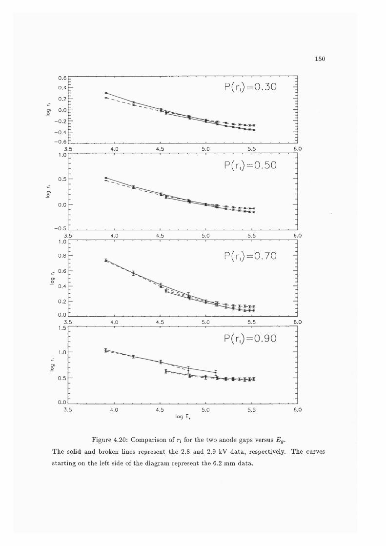
150

0.6

P(r,)=0.300.4

0.2

0.0

- 0.2

- 0 .4

- 0.66.03.5 4.0 4.5 5.0 5.5

P(r,) = 0 .500.5

cnO0.0

- 0 .55.0 5.5 6.03.5 4.0 4.5

P(r,) = 0 .700.8

0.6

“ 0.4

0.2

0.06.03.5 4.5 5.0 5.54.0

1.5

1.0

CD

0.5

0.03.5 4.0 4.5 5.0 5.5 6.0

log E,

Figure 4.20: Comparison of r/ for the two anode gaps versus Eg.

The solid and broken lines represent the 2.8 and 2.9 kV data, respectively. The curves

starting on the left side of the diagram represent the 6.2 mm data.

151

3

P(r,) = 0 .32

1

03 40 1

T2

P(r,) = 0.7

15

P(n)10

5

00 2 31 4

t, (ns)

Figure 4.21: Comparison of r/ for the two anode gaps with respect to t f .

The solid and broken lines represent the 2.8 and 2.9 kV data, respectively. The curves

starting on the left side of the diagram represent the 3.0 mm data.

152

Guest (1978) has modelled the electrostatic lens at the pore exit, with an esti

mated initial electron velocity distribution. However, the model does not tahe into account

saturation or interaction between electrons as he modelled the situation for linear operation

of a single plate illuminating a phosphor. A model of the affect of Vc in the present situation

in which a chevron pair is being used in the saturated mode with a charge division readout,

would have to take into account lensing as well as the variation of initial energy/angle dis

tributions due to saturation and the effects of space charge. It would also probably need to

take into account the time variation of the electric field inside the pore while firing including

the influence of the electric field rotation (Gatti et al.j 1983). Such a model is far beyond

the scope of this discussion.

4 .4 .5 T h e E ffect o f th e In ter-p la te G ap V oltage

The Effect on Gain

The effect of Vi on the gain of a chevron pair has been studied by Wiza et al. (1977),

Fraser et al. (1983) and Smith & AUington-Smith, (1986). They find that the variation of gain with VJ, where VJ* > 0, can be explained by considering the varying number of pores

illuminated in the bottom MCP by a single pore in the top MCP. The last authors used

the same set of MCPs as those used in this experiment and the discussion that follows is

based on their analysis.

The number of pores illuminated in the bottom plate is calculated using a simple

ballistic model. As the number of electrons leaving the first plate is much less than those

exiting the rear plate, interaction between electrons is disregarded. Adding the radius of the

pore to Equation 4.13, produces a equation similar to that presented in Fraser et. al. (1983)

which can be used to calculate the illuminated area.

The maximum angle between the velocity vector and the MCP normal was deter

mined, for this set of MCPs, to be 10 ± 5° and the average energy was assumed to be 3 eV

(Smith & AUington-Smith, 1986). Using these values, the gain would be a maximum for

Vi• = 0 when approximately 7 pores are illuminated in the bottom plate and reduce as Vi

increases: at +30 V only 3 pores would be illuminated.

A negative Vi applies a retarding potential and so the low energy electrons are

collected on the front MCP electrode. As low energy electrons represent a large proportion

of the output from the first plate, the gain is significantly reduced.

153

The Effect on Charge Cloud Size

Figure 4.22 shows the variation of the fit parameters with Vi and is compared to

the variation of gain. The saturation reduced by about 25 % at the extremes of the VJ

range from the maximum at Vi = 0 and, given the large systematic error on saturation

estimates of 10%, no significant difference between the positive and negative voltages was

observed. Note that the maximum size of row and Oc are offset by approximately +5 V

from the maximum value of Voc at V; = 0.

Figure 4.23 shows the variation of r/ with modal gain. It shows that the size of

the charge cloud is fairly insensitive to the variation in gain for VJ > 0 at all probability

levels but is very sensitive to gain variations when Vi < 0. This again demonstrates that

variation in gain alone is insufficient to explain variations in charge cloud sizes.

4.5 Charge Cloud Sym m etry

4 .5 .1 E llip tic ity

The values of Tq returned by the fitting procedure for the two chevron plane ori

entations indicate that the charge cloud is not azimuthally symmetric. In all cases, the

values Toe and Vow obtained with the pore bias angle parallel to the split are greater than,

or equal to those obtained with the bias angle and split orthogonal. Table 4.7 shows the

ratios of the fit parameters obtained for the two bias angle orientations. Excluding the case

where Vc = 2.9 kV and Vg = 400 V, in which anomalously large wing components were

obtained, the average difference in the size of the fit parameters over all the cases is 9%.

Figure 4.24 shows that on average, the charge clouds obtained with the parallel alignment

are significantly larger at almost all P(r/).

From the MCP pore geometry, it is reasonable to expect that the charge cloud will

exhibit either azimuthal or elliptical symmetry depending on the influence of the pore bias

angle. Our experiments show that, to a first order approximation, the charge cloud can

be regarded as being azimuthally symmetric. The variations between Tq values for the two

chevron plane orientations show that a function with elliptical symmetry presents a more

accurate description of the charge cloud. The fitting procedure we have described returns

a radial distribution. However, the translational symmetry of the anode also allows it to

measure an elliptical charge cloud. The fitting procedure returns the charge distribution

154

Toc , microns

2 0600

00

80

- 60

- 40

- 20

40020 400-40 -20

202800

002600 -

802400 -

602 2 0 0 -

2000 - 40

- 20800

60040-40 -20 0 20

ocmodal gain

— modal gain

a c , percent

95 20

00

90 - 80

- 60

85 - - 40

- 20

80-40 -2 0 0 20 40

Inteiplate Gap Voltage

3------ 3 c

>— modal gain

Figure 4.22: The affect of the inter-plate voltage on the fit parameters.

The voltages Vg and Vc were held at constant values of 400 V and 3.0 kV, respectively. The

modal gain is plotted in units such that 100 corresponds to 1.5 x 10® e~. The fit parameters

are defined in Equation 4.1. From Lapington & Edgar, (1989).

155

0.80

P(r,)=0.300.70

0.60

0.5020150 5 10

1.20

P(r,) = 0 .50

^ 1.00

0.90

0.80205 10 150

P(r,) = 0 .70

4.0

P(r,) = 0 .903.5

^ 3.0

2.5

2.00 5 15 2010

G. 10" e-

Figure 4.23: The variation of r/ with gain due to the variation of the inter-plate gap voltage.

The data in this figure is determined from the parameters presented in Figure 4.22. The

broken and solid lines correspond to > 0 and Vj- < 0, respectively.

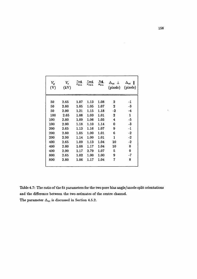
156

(V)Vc

(kV)

Ocll Acc J- (pixels)

Acc II (pixels)

50 2.65 1.07 1.13 1.08 2 -150 2.80 1.05 1.05 1.07 2 -350 2.90 1.21 1.15 1.18 -2 -4100 2.65 1.08 1.03 1.01 2 1

100 2.80 1.09 1.06 1.05 4 -5100 2.90 1.18 1.10 1.14 0 -3200 2.65 1.13 1.16 1.07 9 -1200 2.80 1.05 1.00 1.01 6 -2200 2.90 1.14 1.00 1.01 1 -2400 2.65 1.09 1.13 1.04 10 -2400 2.80 1.08 1.17 1.04 10 0400 2.90 1.17 2.79 1.07 5 0800 2.65 1.02 1.00 1.00 9 -7800 2.80 1.06 1.17 1.04 7 8

Table 4.7: The ratio of the fit parameters for the two pore bias angle/anode split orientations

and the difference between the two estimates of the centre channel.

The parameter Acc is discussed in Section 4.5.2.

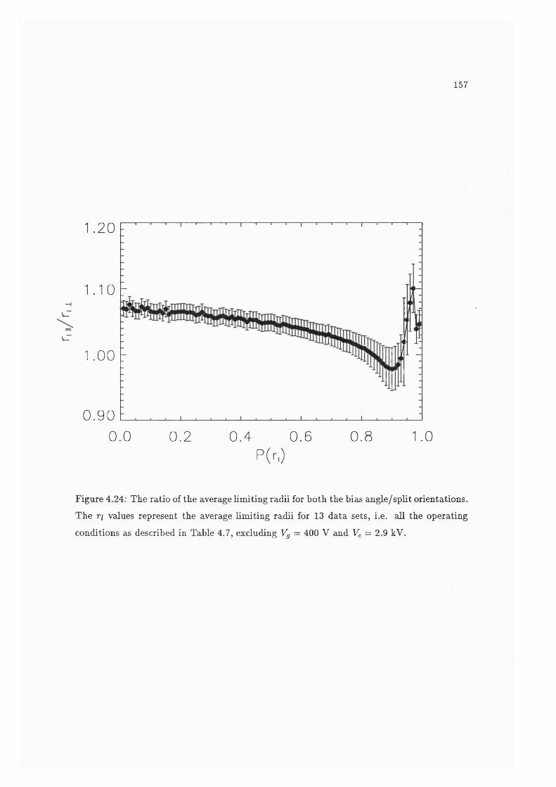
157

1 . 2 0 F

1.10 r

1.00 r

0 .900.0 0.2 0 .4 0.6 0 .8

P(n)1.0

Figure 4.24: The ratio of the average limiting radii for both the bieis angle/split orientations. The ri values represent the average limiting radii for 13 data sets, i.e. all the operating

conditions as described in Table 4.7, excluding Vg = 400 V and Vc = 2.9 kV.

158

for a section along the major or minor axis provided that axis is perpendicular to the

split direction. In the experiments, the chevron plane w2ls aligned with an anode axis to

within 10°. Assuming one of the axes is aligned with this plane, the distributions returned

represent the major and minor axes of the charge cloud.

As we are fitting to the charge cloud integrated across one axis, we would expect

that the values of ellipticity we measured to represent the lower limit. The ellipticity has

been measured for MIC type detectors, as described in Section 1.3.1 by direct imaging of

the light output from the phosphor. The major axis was on average 25% larger than the

minor axis for measurements over a wide range of operating conditions (Kawakami, 1992).

If the charge doud is elliptical, the major axis should be in the direction of the pore

bias angle, assuming that the energy and angle distributions of the output are constant with

azimuthal angle around the pore and using a purely ballistic model. Therefore, broader one dimensional integrated distributions should be observed when the pore bias angle is aligned

normal to the anode split. However, we observe precisely the opposite, indicating that the

major axis is perpendicular to the pore bias angle.

Bronshteyn et of (1980) report that the angular distribution of the output electrons

varies with the channel azimuth angle and that the distribution can be twice as wide for

electrons emitted normally to the plane of the channels as that for electrons emitted within

the plane. They also find that all the electrons have energies < 50 eV, independent of the

emission angle.

If the anode split is aligned parallel to the pore bias angle and assuming purely

ballistic behaviour, the angular spread of electrons emitted within the plane of the channels

will be preferentially spread across the cp axis. Those emitted normally to the channel plane

will be distributed along the /c axis. As shown in Figure 4.12, if the maximum emission

angle relative to the channel axis is doubled from « 10° to 20°, even if the energy is < 50 eV,

the electrons will travel a significantly larger distance than higher energy electrons emitted at

smaller angles. Therefore, even though the electron velocity distribution is not azimuthally

symmetric, a ballistic model would still predict that the major axis of the charge be aligned

along the pore bias axis.

However, I have already shown that the ballistic model is inadequate for predicting

the size of the charge cloud. Space charge, the initial electron distribution on exiting the

pore, the complex electric fields at the pore exit or a combination of any of these factors,

are all plausible mechanisms for the counter-intuitive orientation of the axes.

159

4 .5 .2 Skew ness

The centre channel of the S curve is the centroid position of the curve’s inflexion

point, which corresponds to the position of the peak of the integrated charge cloud distri

bution. Its value {ccad) can be obtained from the zero intercept of the second derivative

of the S curve. This measurement is independent of any symmetry assumptions. The fit

ting procedure also returns a value for the centre channel (cc/,f). This represents the best

estimate of the point about which the experimental S curve is rotationally symmetric.

The centre point should be located at 2048.0, but ccfn is randomly distributed

about channel 2048, o’ = 6, and ccgd about channel 2046, a — 1. The similarity between

the two distributions indicates that, as a group, there are no obvious differences between

the two centre channel estimates. However, for each individual S curve, differences between

cc/it and cc,j are evident. The values of this difference (Acc = cc/,f — cc,j) for the 28 data

sets are listed in Table 4.7 and are shown in Figure 4.25. When the chevron plane is aligned

parallel to the split, Acc is negative for 10 of the 14 cases and when the chevron plane is

aligned perpendicular to the split, 12 of the values of Acc positive. The average values of

Acc for the five data sets taken for each chevron plane orientation, at a constant combination of voltages, Vg — 100 V and = 2.80 kV, are; with chevron plane perpendicular to split,

Acc = 4 , <7 = 1, and with chevron plane parallel to split, Acc — —3, a = 1. As the values

of Acc &re small, less than 0.5 % of the centre channel, and the uncertainties are large,

the differences appear to be just on the edge of detection. However, the systematic nature

of the differences and their opposite signs for the two chevron plane orientations suggest

strongly that the previous symmetry assumptions are invalid at scales of the order of 1%.

The assumption of azimuthal symmetry appears to be valid for a first order approx

imation of the charge cloud. Variations between measurements of Tq show that, to second

order, a more accurate representation assuming elliptical symmetry is valid. At even higher

orders of accuracy, the systematic differences between the centre channel estimates, Acc,

imply that the charge cloud distribution is skew. At this level, the charge cloud can only

be characterized by taking data at many orientations of the chevron plane with respect to

the anode split.

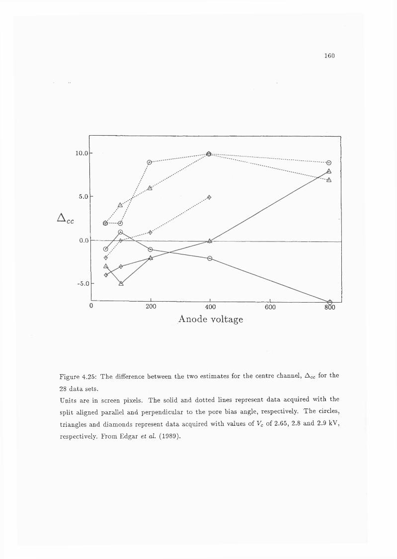
160

10.0

5.0

0.0

-5.0

200 400

Anode voltage600

Figure 4.25: The difference between the two estimates for the centre channel, Acc for the

28 data sets.

Units are in screen pixels. The solid and dotted lines represent data acquired with the

split aligned parallel and perpendicular to the pore biais angle, respectively. The circles,

triangles and diamonds represent data acquired with values of Vc of 2.65, 2.8 and 2.9 kV,

respectively. From Edgar et al. (1989).

161

Chapter 5

O perating the Spiral A node

All the data presented in this chapter was acquired with a similar experimental

setup to that described in Section 3.3, except there were six channels of electronics instead

of four. New software was required to implement the decoding algorithm for SPAN, and

this is discussed briefly in Section 5.6.

The MCPs are similar to those used in the charge doud experiments, as described

in that section but they are not the same set. The MCPs and configuration used in this

chapter are discussed in detail in Section 7.2.1.

5.1 Spiral Transform

Figure 5.1 summarizes the five steps necessary to transform the digitized mea

surements of the charge deposited on each of the three electrodes, into a one dimensional

coordinate.

In a two dimensional detector, the two coordinates are determined independently

so we can limit our discussion to one dimension.

5 .1 .1 C oord in ate R o ta tio n

The geometries of the three electrodes, for any given anode, define two conditions

on the coordinate transformation specific to that anode. For the anodes developed at MSSL

so fax these conditions are:

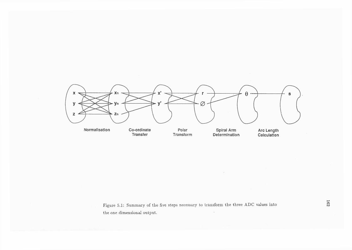
Xn

Zn

Normalisation Co-ordinateTransfer

PolarTransform

Spiral Arm Determination

Arc Length Calculation

Figure 5.1: Summary of the five steps necessary to transform the three ADC values into

the one dimensional output.

163

1. The radius of the angle, 0, increases as the spiral rotates about the three axes in the

order xzy, i.e. clockwise in Figure 5.2.

2. In polar coordinates, the line ^ = 0 must intercept the x axis.

The first condition is imposed for convenience in the decoding, as a spiral evolving

in an anti-clockwise direction can be transformed into one evolving clockwise simply by

interchanging the x and z electrodes. In order to satisfy this condition, it can be shown

from the equations of the coordinate transform as derived in Chapter 2, i.e. Equations 2.33

and 2.34,thatx'

^ = arctan —- . (5.1)yl

Using this equation the ^ = 0 line intercepts the —z axis. After a rotation through —60®

about the 2/ axis, this line will intercept the x axis. Therefore, the third Euler angle is

V» = -60° . (5.2)

The three Euler angles have now been determined and the full rotation matrix, S, is.

S = 0 73

-7 = ^ ^V 6 V 6 V 6, ^ 1 ,\ \/3 ^ ^ /

(5.3)

The set of equations for the transformation is now

x' = , (5-4)

y' = (2x ~ (y + z)) , (5.5)

z' = -ÿ= (x y + z) . (5.6)

Figure 5.2 shows an example of data that has undergone this coordinate rotation.

5 .1 .2 T ransform ation to C ylindrical Polar C oord in ates

The transformation to cylindrical polar coordinates (r, h) is straight forward

after the coordinates have been rotated.

r = + , (5.7)

x'(f> — arctan — , (5.8)

h = z ' . (5.9)

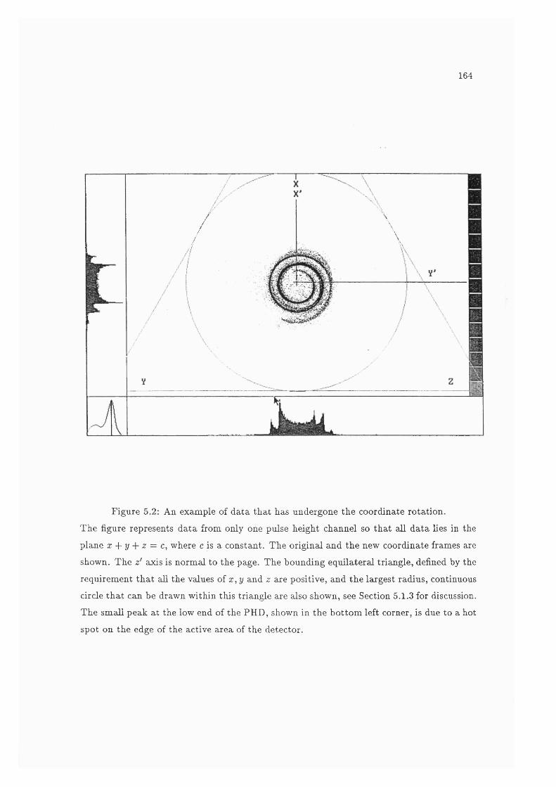
164

//

\

\

Figure 5.2: An example of data that has undergone the coordinate rotation.

The figure represents data from only one pulse height channel so that all data lies in the

plane x + y z = c, where c is a constant. The original and the new coordinate frames are

shown. The z' axis is normal to the page. The bounding equilateral triangle, defined by the

requirement that all the values of x, y and z are positive, and the largest radius, continuous

circle that can be drawn within this triangle are also shown, see Section 5.1.3 for discussion.

The small peak at the low end of the PHD, shown in the bottom left corner, is due to a hot

spot on the edge of the active area of the detector.

165

By fax the most convenient way to display the spiral is in r / ^ space, i.e. plotting

the radius and the phase angle as Cartesian coordinates. As r = k9^ we would expect a

straight line relationship in this space. However, as arctan will only return angles between

0 and 27T a series of parallel lines representing each of the spiral arms, will be produced.

Figure 5.3 shows an example of this space for an ideal spiral. Any departure from the ideal

spiral, e.g. due to eccentricity or olFset of the centre, will be apparent as a deviation from a

straight line. It is much easier to spot such deviations if the data is plotted in this manner

rather than as a spiral.

5 .1 .3 N orm aliza tion W ith R esp ec t to P u lse H eigh t

The cylindrical polar coordinate h is directly proportional to the amount of charge

collected on the three electrodes z, y and z. For convenience let us define a new variable h' such that

h' = y/3h , (5.10)

= y/3z' , (5.11)

= X + y + z . (5.12)

If the integers and z are constrained to be positive, as is the case for ADC

outputs, then all the points that lie on a plane such that h' is a constant, will be bound by

an equilateral triangle with vertices at (0,0, h'), (0, h \ 0) and (0,0, h'). Also, the maximum

radius of a continuous circle that can be drawn within this triangle is

Him — • (5.13)

An example of the limiting triangle and a circle with radius rum axe shown in Figure 5.2. In

order for an anode to produce points lying on this circle, would require that the amplitude

of the sinusoid would have to be equal to the whole width of the electrode, see Section 2.1.1,

i.e. at some point the width of the electrode would go to 0 and the electrode would not be

continuous. A continuous spiral must always have r < rum.

A series of spirals exist on parallel planes defined by the pulse height of the event.

Figure 5.4 shows a section through a family of ideal spirals on a continuous series of planes.

It is appaxent that the spiral constant k and therefore the radius are functions of pulse

height, r(h ') = k{h')9. Normalizing with respect to pulse height, will project the spirals in

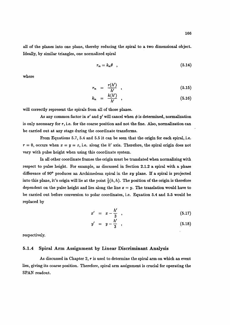
166

all of the planes into one plane, thereby reducing the spiral to a two dimensional object.

Ideally, by similar triangles, one normalized spiral

r„ = kn9 , (5.14)

where

T„ = , (5.15)

= ^ . (5.16)

will correctly represent the spirals from all of those planes.

As any common factor in x' and y' will cancel when <f> is determined, normalization

is only necessary for r, i.e. for the coarse position and not the fine. Also, normalization can

be carried out at any stage during the coordinate transforms.

From Equations 5.7, 5.4 and 5.5 it can be seen that the origin for each spiral, i.e.

r = 0, occurs when x = y = i.e. along the h' axis. Therefore, the spiral origin does not

vary with pulse height when using this coordinate system.

In all other coordinate frames the origin must be translated when normalizing with

respect to pulse height. For example, as discussed in Section 2.1.2 a spiral with a phase

difference of 90° produces an Archimedean spiral in the xy plane. If a spiral is projected

into this plane, i t ’s origin will lie at the point \{h , h). The position of the origin is therefore

dependent on the pulse height and lies along the line x = y. The translation would have to

be carried out before conversion to polar coordinates, i.e. Equation 5.4 and 5.5 would be replaced by

x’ = X - J , (5.17)

y' = y - y , (5.18)

respectively.

5 .1 .4 Spiral A rm A ssign m en t by L inear D iscrim in an t A n alysis

As discussed in Chapter 2, r is used to determine the spiral arm on which an event

lies, giving its coarse position. Therefore, spiral arm assignment is crucial for operating the

SPAN readout.

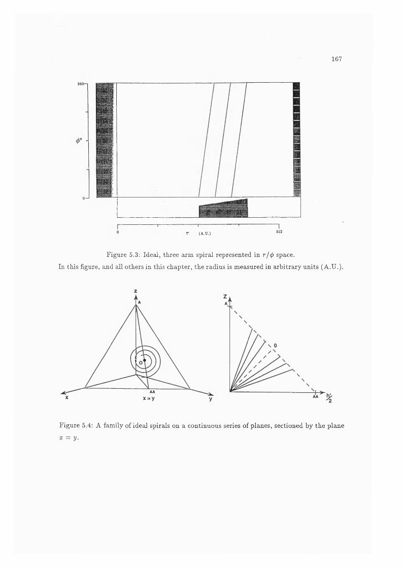
167

360-1

0-J

r (A.U.)

Figure 5.3: Ideal, three arm spiral represented in r /0 space.

In this figure, and all others in this chapter, the radius is measured in arbitrary units (A.U.).

AAx = y

Figure 5.4: A family of ideal spirals on a continuous series of planes, sectioned by the plane

X = y.

168

In the ideal caê represented by Figure 5.3, it is a straight forward procedure to

determine the true angle, i.e.

0 = 2mr + <j> , (5.19)

where n is the spiral number. For any point, provided the spiral constant k is known,

^ = — . (5.20)

If the lines in Figure 5.3 had a finite width, the problem would be more involved.

A spread in r, for any given fc, will return an incorrect value of 9.

However, if Equations 5.19 and 5.20 are combined,

" = ’ (S.21)

the quotient of n, Uquot’, is the number of the inner arm of the two arms that bracket the

point. The remainder, nrem, is the fractional distance of the point from the inner arm

relative to the separation of two spiral arms. We use Urcm to determine which of the two

bracketting arms the point will be mapped to. The true angle 6 is given by

9 = <2'riqyiQ'K "I” (f) if fl/rem ^ 0.5

2(ng„ot + 1)7T + </> if Tlrem > 0.5 • (5.22)

0 if rtrem — 0.5

Setting 0 to 0, effectively discards the point as this is the spiral origin. This would require

that the areas of the three electrodes would be equal, which never occurs in practice.

Therefore, any data at this point is spurious.

In practice, there is an interval of finite width, 2w, in which all points are discarded,

as it is assumed that points lying in this region cannot be confidently assigned to either of

the bracketting arms. Therefore, the previous equation becomes

9 = <IT'quot 4" ^ If f^rem ^ W

^(riquot + 1 )t + if Tlrem > 1 ~ W • (5.23)

0 if u ; < T lrem < I — W

Once the point has been assigned to a spiral arm, conversion to the arc length S

is a straight forward process as 5 « as described in Section 2.2.3.

169

5 .1 .5 G h osts

If the spiral arms are wide with respect to their separation, events associated

with one of the bracketting spiral arms may be mistakenly mapped onto the other arm. If

events are assigned to the incorrect arm there will be an error in their coarse position of

one cycle. Therefore there will be an error in S of producing a spurious image or

a “ghost” . As an example of what can occur, Figure 5.5, shows the result of spiral arm

assignment failing in both axes for a two dimensional image, compared to Figures 5.6 and

5.7 which are corrected images.

Therefore, every effort must be made to minimize deviations from the ideal spiral

arms and ensure that the width of the arms is small with respect to their spacing.

5.2 R adius as a Function of Pulse H eight

Figure 5.8 shows an example of the r„/<^ plot for actual data that has been nor

malized with respect to pulse height. This clearly indicates that the width of the spiral

arms cannot be ignored and that Equation 5.20 is invalid. The arms are so wide that severe

ghosting is produced, Figure 5.5 is the image produced from this data. The situation is

worse than the diagram suggests. The two bright spots in the image are from a “hot spot”

on the MCP and are actually associated with the centre spiral arm. Also the brighter cen

tral regions of the arms are due to the convolution of the pulse height distribution (PHD)

with the radial variation. The severity of the problem can be better appreciated if a flat

PHD is used.

Figure 5.9 shows a subset of the data in Figure 5.8. The 256 channel PHD has

been subdivided into 16 channel windows with approximately equal numbers of events in

each window. The region containing the hot spots haa been masked out as the hot spots’

PHDs consist almost entirely of low pulse height events and so these points would be over

represented in a flat PHD image of the whole MCP.

Figure 5.10 shows a section through the continuous sets of non-normalized spirals,

similar to the ideal case in Figure 5.4 for a 30° wide slice in <j) for the data displayed in

Figure 5.8. The wide slice is needed to provide enough data for a reasonable graph. As the

radius varies continuously with the phase angle, the width of the three curves is exaggerated

and is not the cause of the wide spiral arms in Figures 5.8 and 5.9. The wide linear arms are

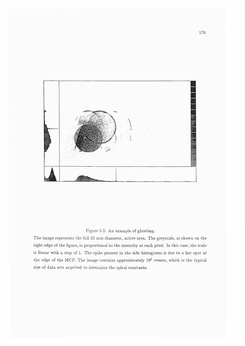
170

A ' # # ,

m m

Figure 5.5: An example of ghosting.

The image represents the full 25 mm diameter, active area. The greyscale, as shown on the

right edge of the figure, is proportional to the intensity at each pixel. In this case, the scale

is linear with a step of 1. The spike present in the side histograms is due to a hot spot at

the edge of the MCP. The image contains approximately 10 events, which is the typical

size of data sets acquired to determine the spiral constants.

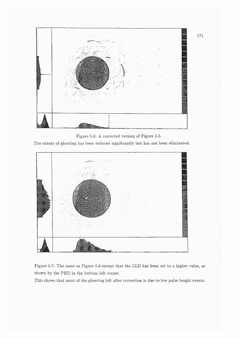
171

Figure 5.6: A corrected version of Figure 5.5.

The extent of ghosting has been reduced significantly but has not been eliminated.

Figure 5.7: The same as Figure 5.6 except that the LLD has been set to a higher value, as

shown by the PHD in the bottom left corner.

This shows that most of the ghosting left after correction is due to low pulse height events.

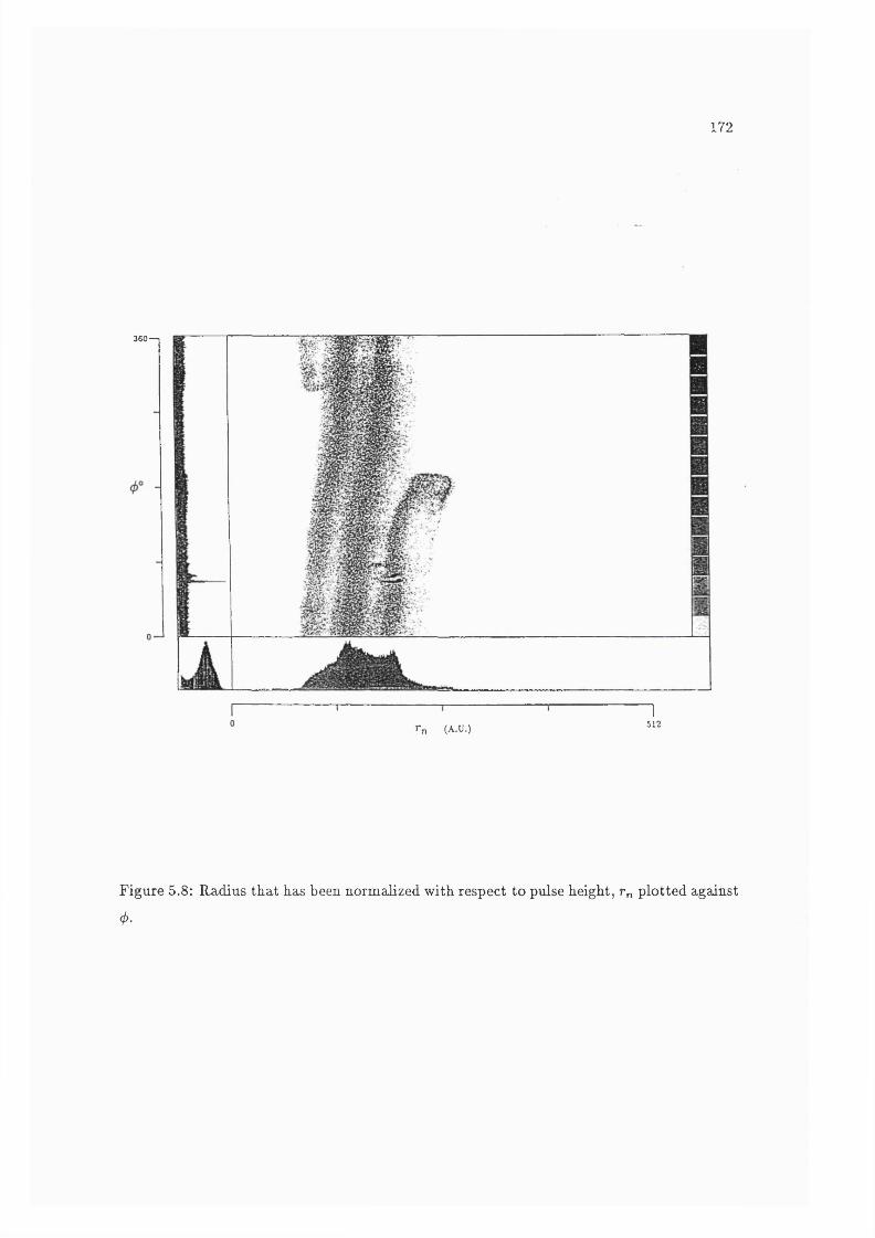
172

360-1

r „ (A.U.)I

512

Figure 5.8: Radius that has been normalized with respect to pulse height, r„ plotted against

4>.

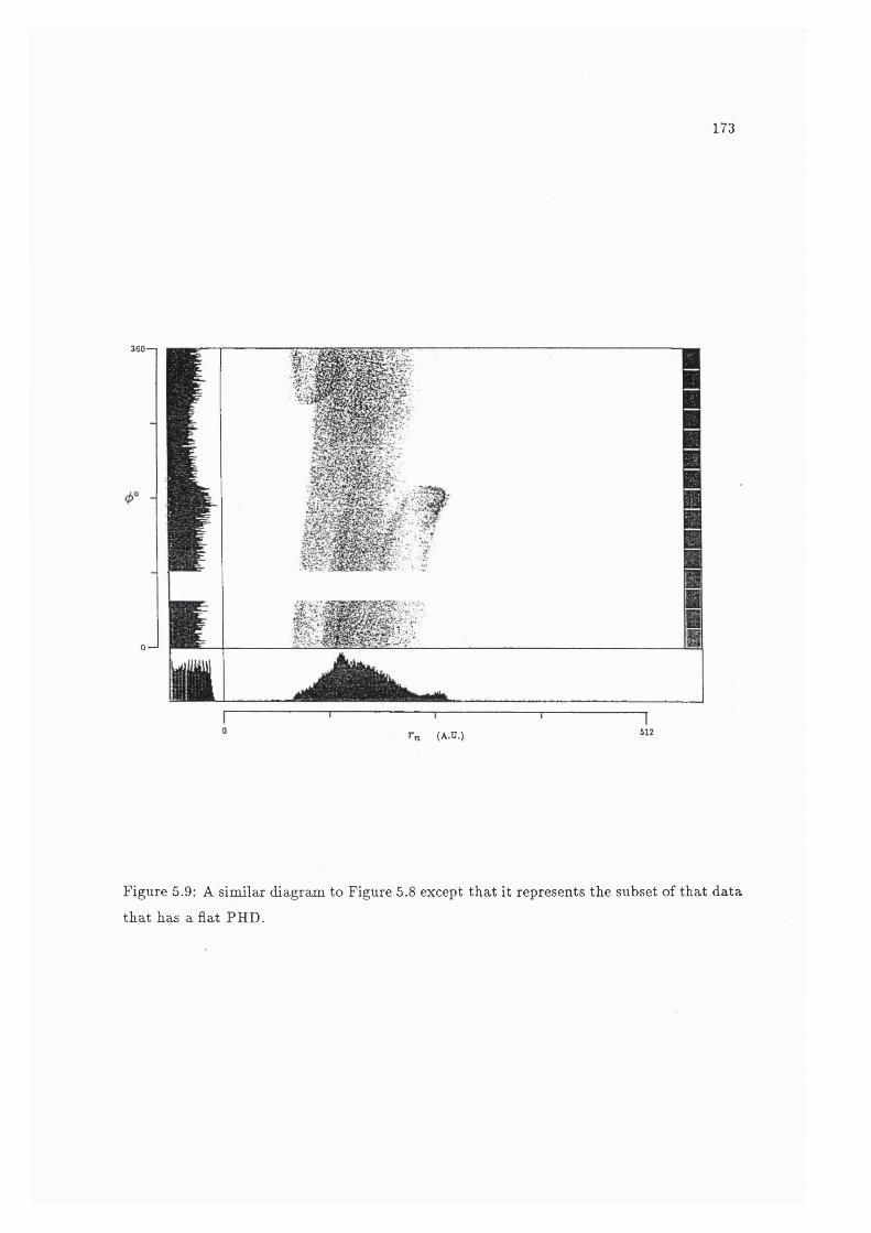
173

360—

0—' m

(A.U.) 512

Figure 5.9: A similar diagram to Figure 5.8 except that it represents the subset of that data

that has a flat PHD.

174

produced by the deviation of the radius/pulse height function, r(h ') from the ideal linear

behaviour as illustrated in Figure 5.4. This is more clearly illustrated by the r„ /h ' curve

in Figure 5.11, which shows the variation of the normalized radius plotted against pulse

height for a section of Figure 5.8. The lines would be horizontal if there was no variation

of the radius with h'. The side histogram on the r„ axis shows the intensity distribution

along the r„ axis for a 30® wide section of (f) in Figure 5.8

5 .2 .1 T h e C ause o f V ariation o f R adius w ith R esp e c t to P u lse H eigh t

Simulated charge cloud distributions, based on the measurements from the previ

ous chapter, have been convolved with a triplet of sinusoidal electrodes, see Section 2.1.1, by

Breeveld (Breeveld et al., 1992b). The amplitudes of the electrodes were not damped but

were constant so that the resultant Lissajous figure was a circle. As shown in Figure 5.12,

the radius of the Lissajous figure is a function of charge cloud size. The best fit to the

relationship between the two is

Rr « 3.9 — mm, (5.24)

where Rr is the radius of the Lissajous figure and R(cc) is the limiting radius that contains

99% of the total charge in the doud. In terms of the values described in Chapter 4.1,

Rcc corresponds to ri where as P{r{) = 0.99. The relationship is also linear for the radii

containing 68% and 95% of the total charge.

As discussed in Section 4.4.1, for a given set of operating voltages there is signifi

cant variation of the size of the charge doud with the gain of the event. This is probably the

case for all operating conditions. Variation of the charge doud size with gain is a probable

mechanism for the variation of radius with pulse height. However, nonlinearities in the

electronics or cross talk are also plausible mechanisms.

Figure 5.13 shows that a , the gradient of r„(h') as determined from the lines in

Figure 5.11, is not correlated with the phase angle of the spiral. The method for determining

this gradient is discussed in Section 5.3.3. This method is statistical in nature, the error bar

in the figure corresponds the bin size in the distribution used to determine a. The FWHM

of these distributions are 10 to 20 bins wide, i.e. the same size as a. The scatter of data in

this figure is typical of that observed for all the other data sets, so the bin width is a better

indicator of the uncertainty associated with a given measurement of a than the FWHM.

The same size bins were used for all measurements of a .

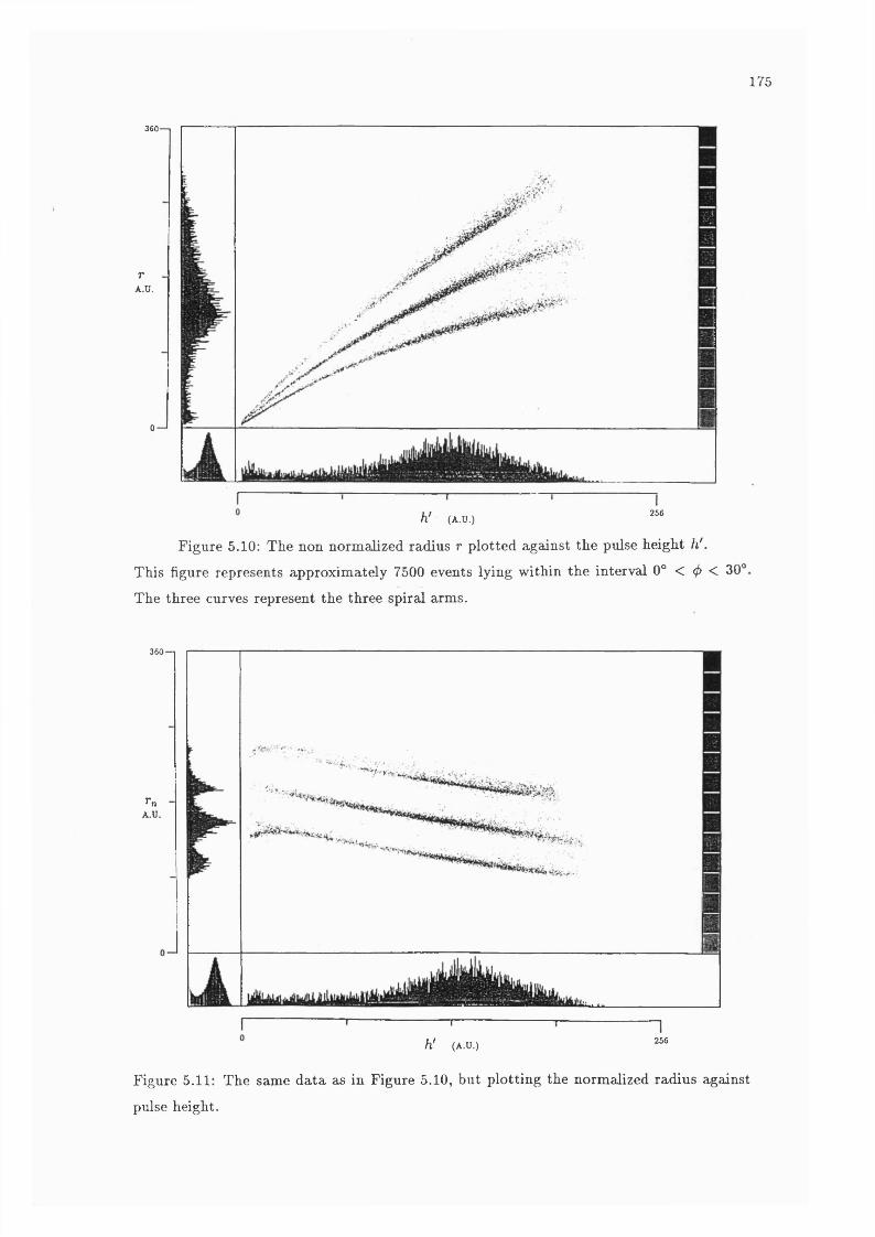
175

360—

rA.ü.

0-

256h* (A.U.)

Figure 5.10: The non normalized radius r plotted against the pulse height h'.This figure represents approximately 7500 events lying within the interval 0° < 0 < 30'

The three curves represent the three spiral arms.

3 6 0 - '

rnA.U.

h' (A.U.) 256

Figure 5.11: The same data as in Figure 5.10, but plotting the normalized radius against

pulse height.

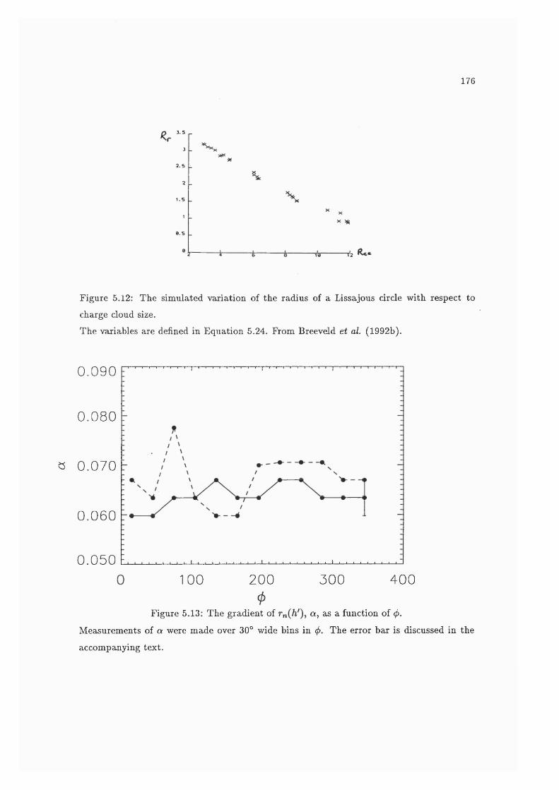
176

3 . 5

3

2 . 5

21 . 5

1

0 . 5

■V2

Figure 5.12: The simulated variation of the radius of a Lissajous circle with respect to charge cloud size.The variables are defined in Equation 5.24. From Breeveld et al. (1992b).

0.090

0.080

« 0.070

0.060

0.0504001 0 0 200 300

Figure 5.13: The gradient of a, as a function of <f>.

Measurements of a were made over 30° wide bins in (p. The error bar is discussed in the accompanying text.

177

Figure 5.14 shows the variation of a with Vg and shows significant reduction with

increasing voltage. The PHD also varies with increasing Vg. However, at high voltages, a

still varies significantly while the PHD parameters remain approximately constant. This

suggests that a depends on the electric field strength rather than varying PHD.

Figure 5.15 shows the variation of a with G„i obtained at different Vc values at

constant Eg. It shows that a is insensitive to Gm at high field strengths. As was observed

with the charge cloud size, the electric field strength appears to be the critical factor in

determining a rather than the gain.

As Vg increases, the charge cloud size decreases and so does a. It is interesting

that at a low Eg, there is a large variation in a with with the largest a at the lowest

Vc. This is the general behaviour of the charge cloud size observed at = 6.0 mm, see

Section 4.4.3, although in Figure 5.15 the electric field strengths are significantly higher.

The strongest fields are comparable to those obtained with g = 3 mm in which the charge

cloud increased with increasing %=, while in this case there is no significant variation.

As a is insensitive to PHD variations, it is unlikely to be due to nonlinearities

or offsets in the electronics. Cross talk is also unlikely, due to this PHD insensitivity and

the insignificant variation with <f>. The electric field strength is the dominant factor in

determining the size of a . It also appears that a is correlated with the average charge

cloud size and behaves in a similar manner with respect to gain variations due to varying

operating voltages. The most probable cause for the variation of radius with pulse height

is the variation in charge cloud size with gain, for a constant set of operating voltages.

Irrespective of the cause, the magnitude of the r„ /h ' variation can be varied by

the operating voltages. It also depends on the actual anode. Breeveld (1992) has measured

a for the one dimensional SPAN detector for the SOHO CDS. She finds the values of a also

vary with Vg and are smaller than those displayed in Figure 5.14. The maximum value of a

was 0.05 and the minimum was -0.02. By tuning Vg and plate voltage, data sets with a = 0

could be reliably achieved.

Therefore, on some detectors the effect can be removed totally but this may not be

possible for all detectors. Generally, the highest Eg practicable should be used to minimize

this effect. However, there will have to be a compromise between obtaining narrow spiral

arms and imaging performance.

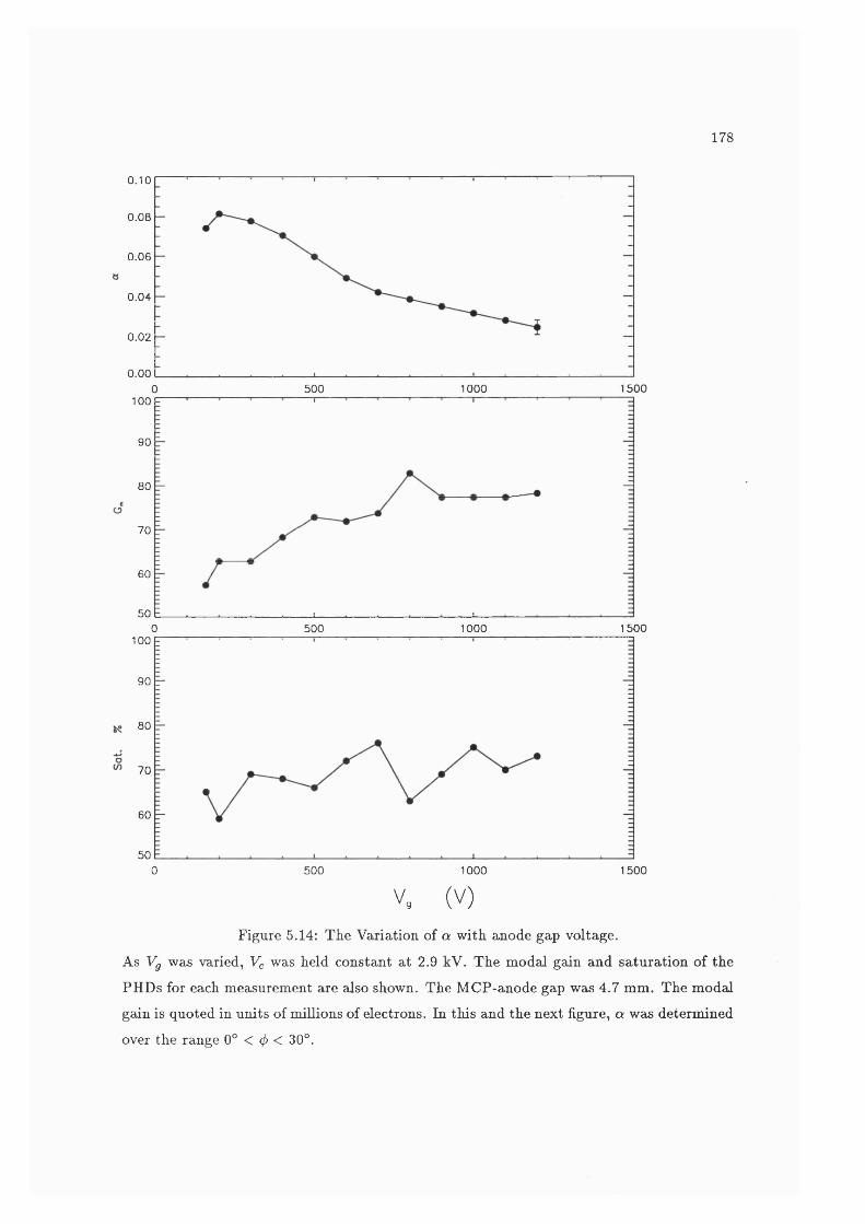
178

0.10

0.08

0.06

0.04

0.02

0.00500 1000 15000

100

90

80

70

60

501000 15000 500

100

90

80

70

60

500 500 1000 1500

V g ( V )

Figure 5.14: The Variation of a with anode gap voltage.

As Vg was varied, Vc was held constant at 2.9 kV. The modal gain and saturation of the

PHDs for each measurement are also shown. The MCP-anode gap was 4.7 mm. The modal

gain is quoted in units of millions of electrons. In this and the next figure, a was determined

over the range 0° < </> < 30°.

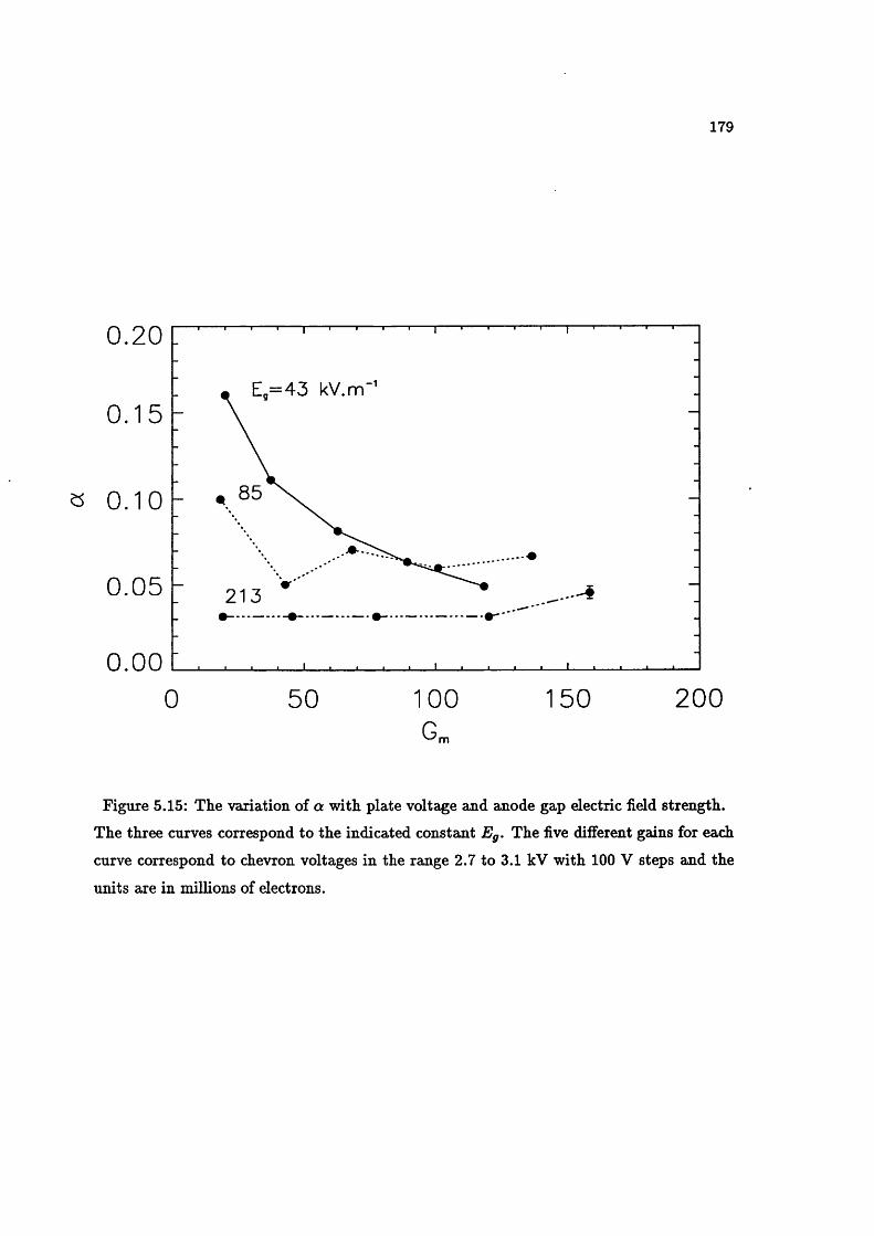
179

0.20

E.=43 kV.m"

85

0.05 213

0.000 50 1 0 0

G„150 200

Figure 5.15: The variation of a with plate voltage and anode gap electric field strength.

The three curves correspond to the indicated constant Eg. The five different gains for each

curve correspond to chevron voltages in the range 2.7 to 3.1 kV with 100 V steps and the

units are in millions of electrons.

180

5.2 .2 C orrection o f R adius W ith R esp ec t to P u lse H eigh t

When correcting for pulse height efiects, a flat PHD should be used. The correction

is based on a best flt to the gradient of the r{K) function. A correction for a peaked PHD

will be biased towards the modal gain and will only be the best fit for that particular PHD.

This does not represent a problem for low count rates but at higher rates, gain depression

will occur reducing the modal gain. A correction optimized for the original PHD will no

longer be ideal for the new PHD. Given that an astronomical detector will probably observe

some relatively bright point sources, there is little point in optimizing the detector for a

difluse, low level illumination. If the best fit is determined for a fiat PHD it should be

equally applicable for all likely PHDs.

Radius D ependent Correction by Quadratic Norm alization

The nonlinear behaviour of r(h '), as shown in Figure 5.10 strongly suggests that

the normalization should include second or higher order terms of the pulse height. Fig

ure 5.16 and Figure 5.17 show the and r„ /h ' plots for the fiat PHD data in Figure 5.9,

respectively, where

= ft'(l + afe') •This technique has the advantage that as it consists solely of a division, it can be carried out,

like normalization, at any stage during the coordinate transform. However, the divergence

of the Tn/h lines, as shown in Figure 5.17, gives rise to the variation in the widths of the

spiral arms in Figure 5.16. This shows that this radius correction is of limited efficiency.

Radius Independent Correction

Figures 5.18 and 5.19 are similar to Figures 5.16 and 5.17, respectively except that

r„ = ^ + ah’ , (5.26)

where a once again is constant and the gradient in Figure 5.11.

The fact that the lines in Figure 5.19 are parallel and with approximately zero

gradient gives rise to the narrow spiral arms in Figure 5.18 and indicates that this method

is superior to the radius dependent correction. The parallel lines also indicate that the

normalized spiral constant is independent of pulse height but that the efiect of pulse

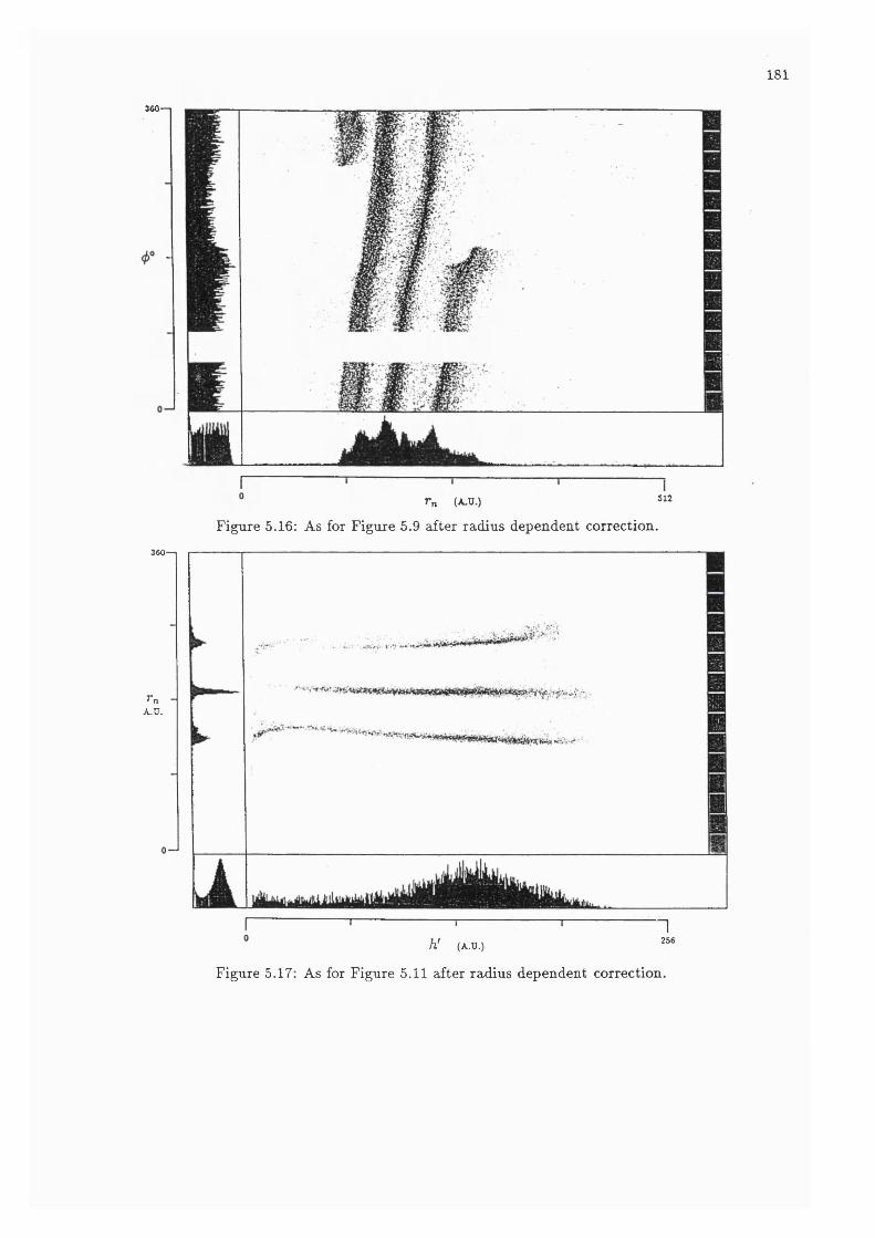
181

360—1

-

360—1

rnA.U.

r„ (A.U.)

Figure 5.16; As for Figure 5.9 after radius dependent correction.

512

h' (A.U.)

Figure 5.17: As for Figure 5.11 after radius dependent correction.

I256

182

height is a constant reduction in r„ with increasing pulse height. However, as the correction consists of an addition to r„, it can only be carried out after conversion to polar coordinates.

5 .2 .3 L im ita tion s on th e C orrection

The methods described for correcting the r„ /h ' variation assume that the function

is a simple linear relationship. As shown in Figure 5.20, this is not always the case. At

low pulse heights the relationship is clearly nonlinear and the curves actually intersect.

Although the lower digitization of these smaller events tends to produce wider arms when

normalized with respect to pulse height, it does not produce such significant broadening

nor can it explain the phenomenon in which the events tends to concentrate in one or two

relatively narrow bands. No simple method will be able to reliably resolve the spiral arms

below a pulse height, in this diagram, of channel 16. Above this level the charge relationship

can be reasonably approximated as a linear relationship.

The linearity of the relationship defines the point at which the LLD should

be set. Gain depression will produce events in the nonlinear region of the relationship, where the corrections are not accurate and there is a significant chance that ghosting will occur.

In practice a compromise would have to be set between reduced photometric linearity and

an increased risk of ghosting.

5.3 D eterm ining Spiral C onstants

In the linear discriminant analysis as described by Equation 5.23, the sole criterion

for assigning a point to either bracketting spiral is which of the arms is closer. It is therefore

absolutely essential to have good estimates of the positions of the arms and determining

the spiral constants is an integral part of spiral arm assignment.

In r„/<^ space, assuming that the arms are parallel, the position of the arms can

be described by A;„, the gradient, and the intercept of the first arm with the r„ axis. By the

equation of an Archimedean spiral, this offset can be represented by an angle so that for

any phase angle 4> the positions of the zth. spiral arm (r„;, <f)) can be determined from the

two spiral constants,

Tni = fc„(2î7T + V>) , (5.27)

For the same reasons aa discussed above for the radius/pulse height correction, a

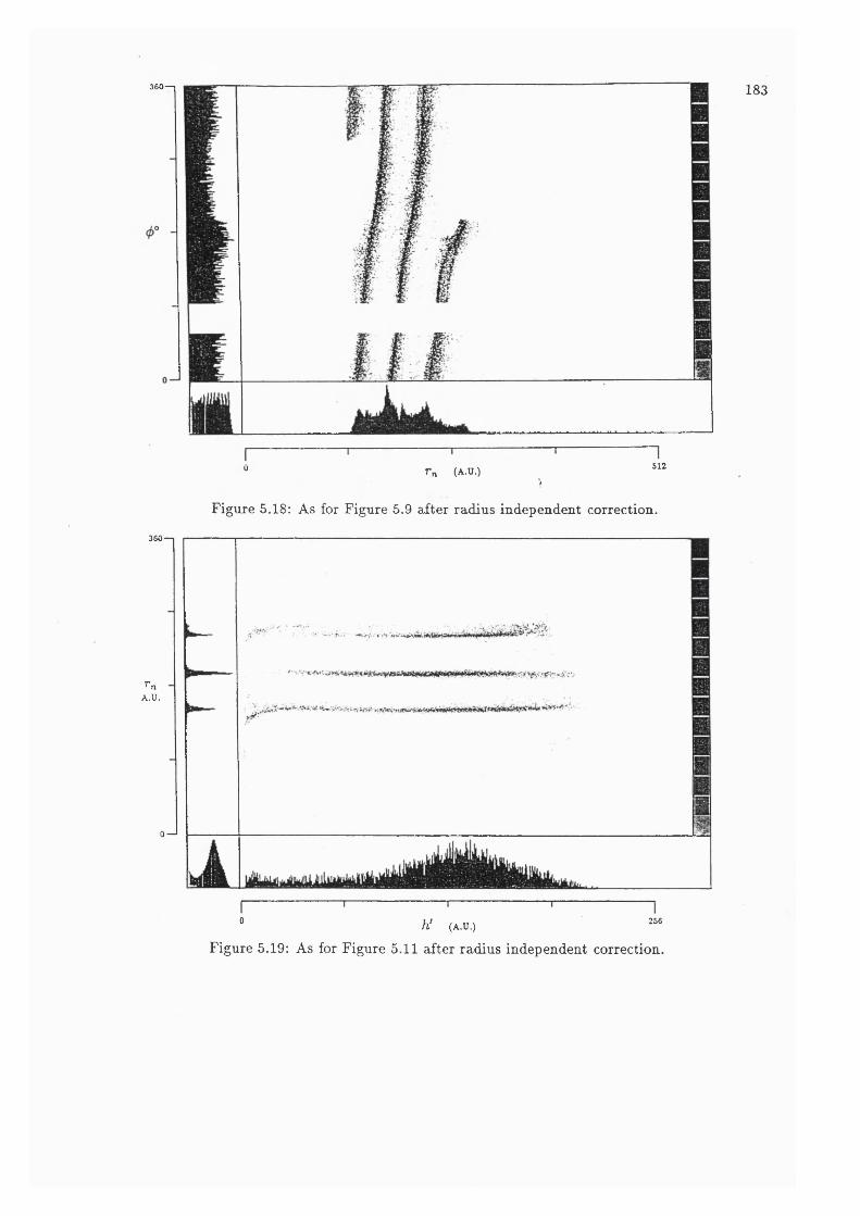
360—1 183

" Tn (A.U.)>

Figure 5.18: As for Figure 5.9 after radius independent correction.

512

360—1

rnA.U.

0 — 1

■

256° h' (A.U.)

Figure 5.19: As for Figure 5.11 after radius independent correction.

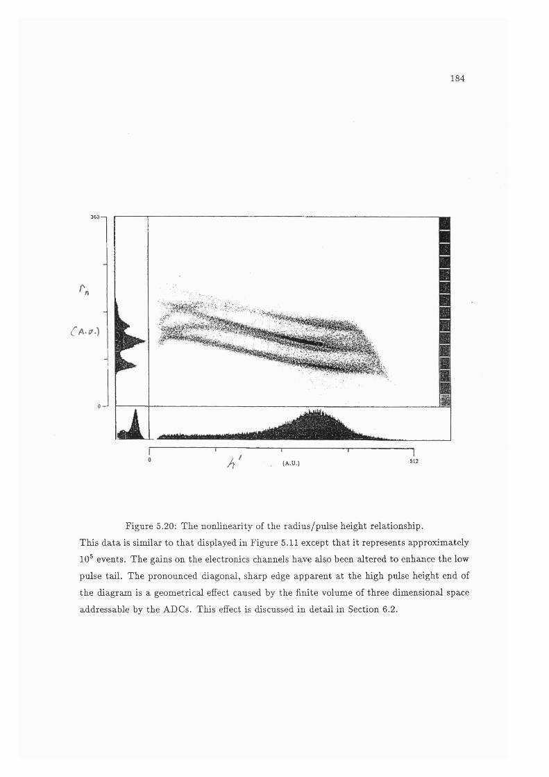
184

360—1

L

0 — '

/ I ' (A.U.) 512

Figure 5.20: The noniinearity of the radius/pulse height relationship.

This data is similar to that displayed in Figure 5.11 except that it represents approximately

10 events. The gains on the electronics channels have also been altered to enhance the low

pulse tail. The pronounced diagonal, sharp edge apparent at the high pulse height end of

the diagram is a geometrical effect caused by the finite volume of three dimensional space

addressable by the ADCs. This effect is discussed in detail in Section 6.2.

185

flat PHD should be used for determining the spiral constants so that the constants have the

most general applicability and have not been optimized for a narrow range of PHDs.

While evaluating methods of determining the spiral constants I have concentrated

on procedures that could be highly automated and require a minimal supervision by the

operator.

5.3 .1 L ine F in d in g by E dge D e tec tio n

In this method, I try to determine which points are associated with each of the

spiral arms, without making any assumptions about the spiral constants. When the spiral

arms have been identified, they are connected together to form one continuous line. The

gradient and offset are then determined for this line.

The first stage is to determine which points are connected to the spiral arms and

discard those that are not. I evaluated several edge detection algorithms for this purpose.

The edge detector (ED) algorithm returns a value for each point. In most image processing

applications this value is retained rather than the original intensity distribution, J(r„ ,0 ).

However, in this application I only wish to determine which points are associated with the

spiral arms and retain as much of the original distribution as possible. If the value returned

by the ED lies above a threshold, the intensity at that point, / ( r „ , is retained, if not the

intensity is set to zero. Ideally, isolated points will return a result below the threshold and

be discriminated against.

Compass Masks

Figure 5.21 shows the result of a northeast compass mask ED (P ratt, 1978) when

applied to the r„ /0 data produced by the radius dependent pulse height correction shown

in Figure 5.16. This is a good example to use as the wide arms represent a worst case for

EDs which are more suited to narrow lines such as the central arm. The results obtained

for radius independent correction are similar to those obtained for the central arm.

The northeast compass mask is the 3x3 matrix

/ 1 1 1

- 1 - 2 1 . (5.28)

y - 1 - 1 1 y

(5.29)

186

It is called the northeast mask because when convolved with J(r„ , edges with inclinations

to the y axis of w 45° will return the highest values. As the gradients in Figure 5.16 are

quite steep, a north compass mask waa used as well. The matrix for this mask is

/ 1 1 1 \1 - 2 1

—1 —1 —1 j

The results obtained with the north mask were almost indistinguishable from those for the

northeast mask.

For all of the compass masks, the maximum value an isolated point will return is

/( r„ ,0 ) , however, the point will be represented at five connected points after convolution.

Also, the sum of the elements is zero, so that regions of constant intensity will return zero.

This is a problem with the wide spiral arms when using a flat PHD, as 7 (r„ ,^) varies

slowly over the 3 pixel width of the mask. This leads to the fragmentation of the arms

and suppression of the centres. Fragmentation is exacerbated if 7(r„, <f>) has been smoothed

with a filter. If the spiral arm is fragmented, it severely complicates assignment of points

to individual arms.

A pseudo-compass mask of my own devising is

/ 0 1 0 \1 0 1

0 1 0V

(5.30)

/

This mask retains the edge enhancing feature but as the sum of the elements is non-zero

it does not return zero in regions of constant intensity and so reduces fragmentation. The

behaviour for isolated points is similar to compass masks producing a characteristic diamond

shape as seen in Figure 5.22.

N onlinear Edge D etection

Nonlinear EDs use a nonlinear combination of pixels to enhance edges before

thresholding the returned value (P ratt, 1978) An example of such a method is the Sobel

ED, in which the value returned for each point (i, j ) is given by

s{i,j) =where

(5.31)

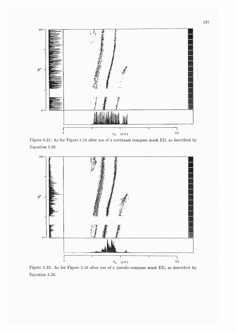
187

360—

0 —

•••) g

1512

I---------------- '------------- '--------------'° r„ (A.U.)

Figure 5.21: As for Figure 5.16 after use of a northeast compass mask ED, as described by Equation 5.28.

360 —

0 —

° r „ (A.U.) 512

Figure 5.22: As for Figure 5.16 after use of a pseudo-compass mask ED, as described by Equation 5.30.

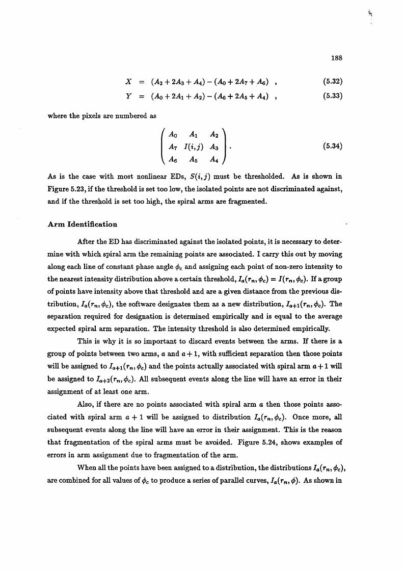
188

X — ( ^ 2 + 2A a + A 4 ) — (Aq + 2 A 7 + Aq) , ( 5.32)

Y — (Ao + 2Ai -}- A 2 ) — (A g + 2 A 5 4" A4 ) , ( 5 .3 3 )

where the pixels are numbered as

Ao Ai A2 ^(5.34)

yiQ Ji.1

At I ( i J ) As A& A5 A4 j

As is the case with most nonlinear EDs, S{i^j) must be thresholded. As is shown in

Figure 5.23, if the threshold is set too low, the isolated points are not discriminated against,

and if the threshold is set too high, the spiral arms are fragmented.

Arm Identification

After the ED has discriminated against the isolated points, it is necessary to deter

mine with which spiral arm the remaining points are associated. I carry this out by moving

along each line of constant phase angle &nd assigning each point of non-zero intensity to

the nearest intensity distribution above a certain threshold, /a(»*nj <f>c) = -f(^n> <l>c)- If a group of points have intensity above that threshold and are a given distance from the previous dis

tribution, Ia(rnj4>c)i the software designates them as a new distribution, ia+i(»*n»^c)- The separation required for designation is determined empirically and is equal to the average

expected spiral arm separation. The intensity threshold is also determined empirically.

This is why it is so important to discard events between the arms. If there is a

group of points between two arms, a and a + 1 , with sufficient separation then those points

will be assigned to /a+i(»*n? <l>c) and the points actually associated with spiral arm a + 1 will

be assigned to Ia+2(i'n, All subsequent events along the line will have an error in their

assignment of at least one arm.

Also, if there are no points associated with spiral arm a then those points asso

ciated with spiral arm a + 1 will be assigned to distribution /a(î'n><^c)- Once more, all

subsequent events along the line will have an error in their assignment. This is the reason

that fragmentation of the spiral arms must be avoided. Figure 5.24, shows examples of

errors in arm assignment due to fragmentation of the arm.

When all the points have been assigned to a distribution, the distributions Ja(r„, c)>

are combined for all values of <f>c to produce a series of parallel curves, Ja(»*n> <!>)• As shown in

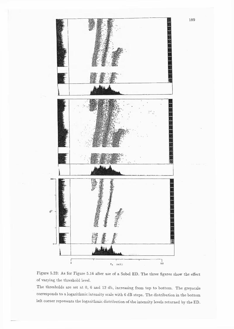
189

(A .U .)

Figure 5.23: As for Figure 5.16 after use of a Sobel ED. The three figures show the effect of varying the threshold level.

The thresholds are set at 0 ,6 and 12 db, increasing from top to bottom. The greyscale

corresponds to a logarithmic intensity scale with 6 dB steps. The distribution in the bottom

left corner represents the logarithmic distribution of the intensity levels returned by the ED.

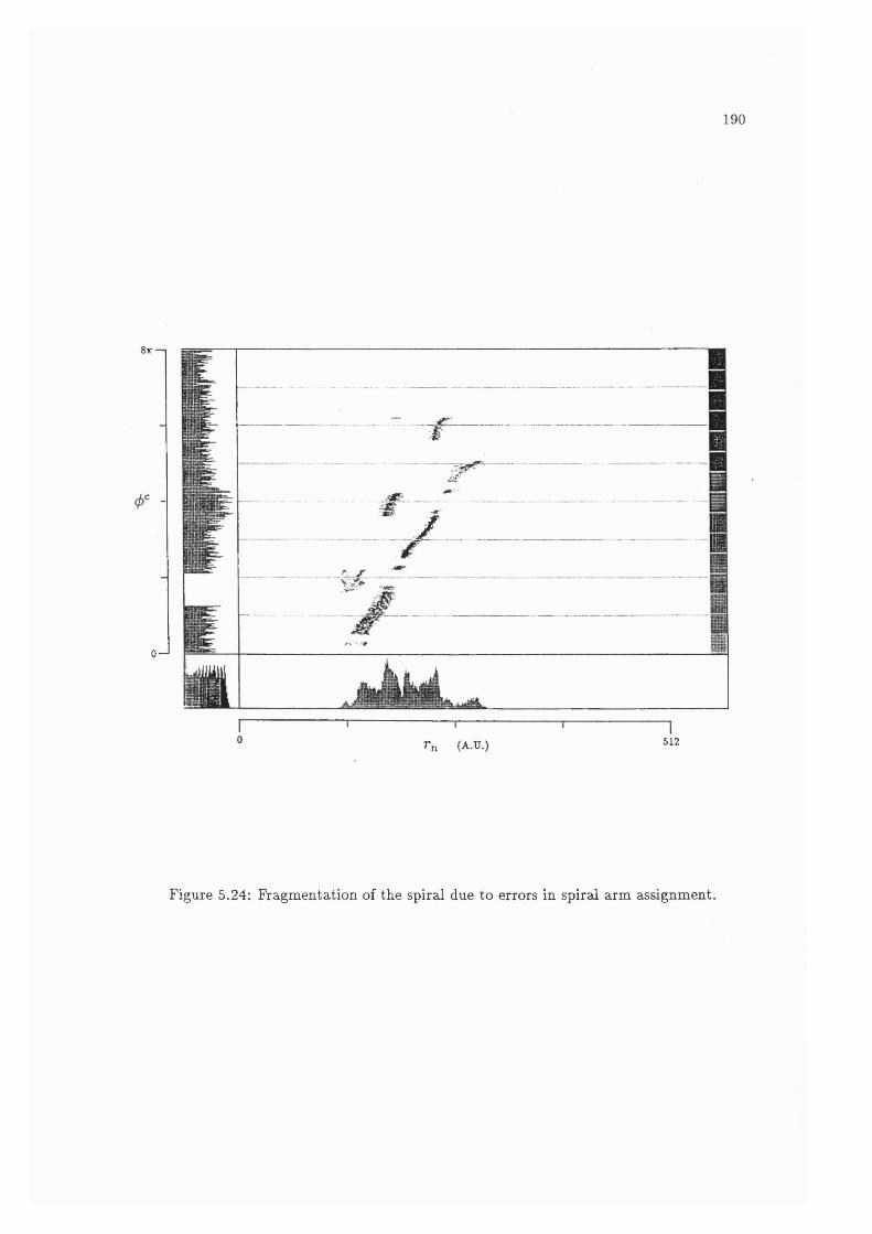
190

8ir-

-

0 — '

/

r n (A .U .) 512

Figure 5.24: Fragmentation of the spiral due to errors in spiral arm eussignment.

191

the rnj<f> plots, the start and end of the spiral do not correspond to the line ^ = 0. There

fore, the distribution numbers assigned by the software, even when the errors described

above don’t occur, will not correspond exactly to the spiral arm number for all values of

<j). The discontinuity in the distribution caused by the presence of a partial spiral arm, is

found by evaluating ^ where

where m is the number of pixels with non-zero intensity in the Ja(r„ ,^ ) distribution for

a constant value of (f>. Points with values of <f> greater than the discontinuity are assigned

the same spiral arm number as the distribution number a, while those points below the

discontinuity are deemed to belong to spiral arm a — 1.

It is necessary to use this discontinuity method because if the length of the first

spiral arm is small, as is the case with this dataset, the values of r for the end of the first

arm will overlap with the beginning second arm. So the J (r) distribution cannot be relied on to detect the start of the spiral. Also, as the phase angle at which the spiral starts is

not correlated with the angle at which the spiral ends, any sudden variation in /(^ ) , even

assuming that the spiral is continuous, cannot be used as an indicator of the start of the

spiral. By a similar argument, any sudden variation in over the full width of the detector

does not indicate the start of the spiral. Therefore, the one dimensional and the full two

dimensional intensity distributions cannot be guaranteed to correctly detect the start of the

spiral.

Determining the location of the discontinuity is the stage of the procedure that

is most susceptible to errors in the assignment of points to distributions. If errors have

occurred, discontinuities in the distributions will be present, comparable in magnitude to

those produced by the partial spiral arm. The software will reject any discontinuity that

is not present in all of the intensity distributions, excluding the last distribution. However,

if the first spiral arm is fragmented, no data may be present in the first distribution for a

finite range of <l>. This missing data will also produce a discontinuity in all distributions.

The data can be smoothed if too many discontinuities occur. However, as the operator has

to inspect the data to determine if the correct discontinuity was found, the procedure is not

wholly automatic and the operator should probably just choose the start point of the spiral

by eye.

When the spiral arms have been identified, they are all joined at their ends, making

192

one continuous line, Figure 5.25. This figure is the data from the flat PHD with radius

independent correction, Figure 5.18, as an ED causes too much fragmentation of the arms

with the radius dependent correction. The spiral constants are then estimated by taking

the line of best fit to the continuous line.

Line F itting by Robust Estim ation

Given that errors can occur in in the assignment of points to spiral arms and that

the continuous line has significant deviations from the ideal straight line particularly at the

ends, a line fitting routine is necessary that is robust, i.e. insensitive to outlying points.

Press et al. (1986) provide a more robust routine than the linear least squares which fits a

line by minimizing the absolute deviation, i.e.N

Y ^ \ y i - a - b x i \ , (5.36)t=i

where

y = a + bx , (5.37)

is the equation of the line. The algorithm carries out an iterative search by bracketting and

bisection to find the minimum. The initial point for the search the line fit parameters are

returned by a linear least square algorithm. In my software both the linear least squares and the robust estimates are returned so that the operator can compare and choose the

best fit.

At present this method of determining the spiral constants takes approximately

5.5 minutes on our PC, described below in Section 5.6, the time being approximately equally

divided between the ED and the line fitting.

5 .3 .2 T h e H ough Transform

The Hough transform (HT) is a well known method for line-finding in image analy

sis (P ratt, 1978 and references therein). It involves the transformation of a line in Cartesian

coordinates into polar coordinates. As shown in Figure 5.26, a straight line may be para

metrically described as

p = X cos 0 y sin 0 , (5.38)

where p is the normal distance of the line from the origin and 0 is the inclination of the

normal to the x axis. N .B . This 0 bears no relation to the spiral angle, but I have called it

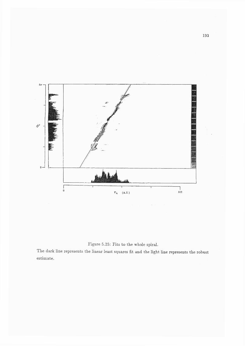
193

8 r —

4> -

rn (A.U.)1

512

Figure 5.25: Fits to the whole spiral.

The dark line represents the linear least squares fit and the light line represents the robust estimate.

194

0 to be consistent with the literature on the HT. The transform maps the line onto a single

point in Hough space with coordinates, {p,0).

The family of all lines passing through a given point (z, y), maps onto a continuous sinusoidal curve in Hough space, as shown in Figure 5.26. This curve consists of the values

of p and 0 that satisfies Equation 5.38 for a given value of x and y. It is only necessary to

evaluate Equation 5.38 for 0 < ^ < tt as the curve is symmetric around 0 = tt.

If we consider three co-lineax points, the HT of the family of lines passing through

each point will produce three curves. The intersection of these three curves in Hough space

at (po jô)) defines the line passing through those three points.Figure 5.27 shows the HT of the radial/phase plot for an ideal spiral, see Figure 5.3.

For each point (r,-, the curve that represents all the possible lines passing through that

point is determined. If n of these curves intersect at a given point in the Hough space,

( p , 0), then the intensity at that point is set as the sum of the intensities at the n points in

r/<f> space, i.e.

I{p^^) = + + I{f'n,n) • (5.39)

Therefore, the points in Figure 5.27 with the highest intensities, describe the lines in r/<f>

space on which most points lie.

This is precisely what we are trying to determine when obtaining the best fit for

k. As 9 in Hough space parametrically describes the gradient k in r/<^ space, we wish to

find the value of 6 ^ ’, that produces the most intense peaks. As we have defined that the

spiral evolves in a clockwise direction. Section 5.1.1, we know that p need only be evaluated

for the fourth quadrant, i.e. — < ^ < 0. In Figure 5.27, p has been calculated for each of

the 360 image pixels along the 9 axis, so each pixel represents As the gradient of the

lines is quite steep, 9m will be a small negative angle. In order to illustrate the variations

of J ( p , 9) around 9m, the HT has been carried out over the range ^ < 9 < ^.

As shown by the flat intensity distribution I (9), in the side histogram in Fig

ure 5.27, the total intensity integrated along any line of constant 9, is approximately con

stant. This indicates that almost all of the curves in Hough space for each of the points

(r,-,< î) will have positive values of p at angles sufiiciently close to 9m• So almost every

point m rjcf) space will be represented and the total number of points will be constant for

each value of 9 in this region. The intensity distribution for the value of 9 which contains

the points with the maximum intensity, 7( p , will have the maximum modulation. The

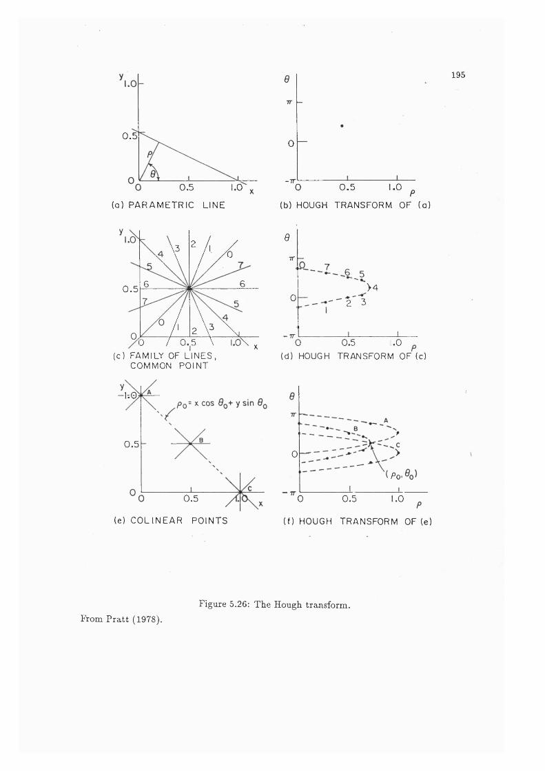
0 .5

1.00.5

(a) P A R A M E T R I C LINE

0 .5

a

\3 / yX \ / y

/ y6 6

/\

2 V X3 / 0. 5 \ l . 0 \ ,

(c) FAMILY OF LI NE S, COMMON POINT

-L 0 '

0 .5

0 .5

(e) C O L I N E A R P O IN TS

7T

0

-TT

195

0 0 .5 .0

(b) HOUGH TRANSFORM OF (a )

eTT

0

- 7T

>42 3

0 0.5 1 .0(d) HOUGH TRANSFORM OF (c)

0

— TT

'( Po-

0 0.5 .0

(f) HOUGH TRANSFORM OF (e)

Figure 5.26: The Hough transform.From Pratt (1978).

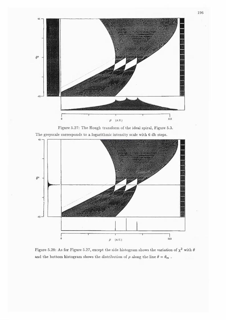
19645 -1

•45“ '

512p (A.U.)

Figure 5.27: The Hough transform of the ideal spiral, Figure 5.3

The greyscale corresponds to a logarithmic intensity scale with 6 db steps.45 —

-45-J

m m #

P (A.U.)n512

Figure 5.28: As for Figure 5.27, except the side histogram shows the variation of with 6

and the bottom histogram shows the distribution of p along the line 9 = On ■

197

degree of modulation can be found by determining the

I { e y ^

»=1 m(5.40)

where m is the number of pixels along the p axis. Therefore, the value of 0 that returns

the largest is the value that produces maximum modulation and represents the best fit

of the spiral constant k.

Figure 5.28 shows the variation of for Figure 5.27, in the side histogram. The

section along the line ^ I{,py ^m) is shown in the bottom histogram. This distribution shows the number of points lying on all the lines of gradient k in r / ^ space. The spiral phase

shift angle xj) can be estimated by correlating a set of delta functions with this distribution.

The spacing of the delta functions is determined by the value of 0m- The point at which

there is a maximum correlation between these delta functions and I{pj0m) represents the

best estimate of xjj.

Figure 5.29 shows the HT of the r„ /^ plot shown in Figure 5.16 and demonstrates

the information returned from the HT software. Of particular interest is how well the

spiral arms are defined in the section along 0 = 9m and how pronounced the peak is.

In the situation where the radius has been modified with radius independent correction.

Figure 5.18, the definition of the arms is slightly improved on that for the central arm in

this image.

The offset angle xj) has been estimated by the correlation of a 50% duty cycle square

wave, of frequency determined by 0m with l{p,0m)- A 50% width was chosen as the larger

the duty cycle used in the correlation, the less modulation of the result will be produced but

larger fractions would be used in practice. The estimate of xp returned by the correlation

determines directly whether the envelope for accepting data, should be symmetrical around

the spiral arm or should be skewed to one side.

Evaluating the HT over 90° takes approximately 5 minutes. The majority of this

time is used for calculating values of p, for the 360 values of 0, for each point. By limiting

the range of 0 over which p is evaluated, the HT can be sped up significantly.

The width of the r„ histogram in the r „ /^ plots gives a direct approximation of

0m- If we assume that there is at least one spiral arm in the image and not more than the

maximum number of arms defined by the anode design, m, then the range of 0 is such that

— < t a n ^ < ’ (5.41)xv xv^{m + 1)

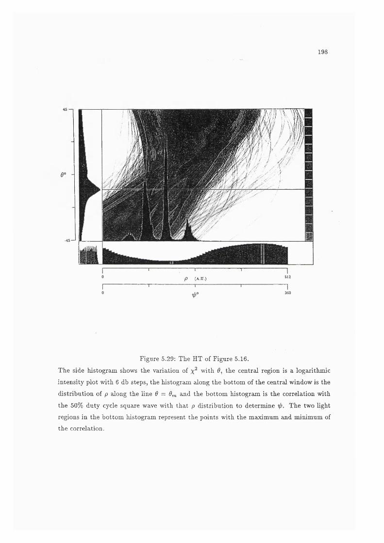
198

m m

p (A.U.) 512

360

Figure 5.29: The HT of Figure 5.16.

The side histogram shows the variation of with 6, the central region is a logarithmic

intensity plot with 6 db steps, the histogram along the bottom of the central window is the

distribution of p cdong the line 9 = 6m and the bottom histogram is the correlation with

the 50% duty cycle square wave with that p distribution to determine The two light

regions in the bottom histogram represent the points with the maximum and minimum of

the correlation.

199

where Wr and are the widths of the r„ and <f> histograms, respectively, and m + 1 is used

to make allowance for the finite widths of the spiral arms.

Figure 5.30 shows the HT of Figure 5.16 over the reduced range in ^ as determined

by Equation 5.41, where Wr is the width of /( r„ ) at the J(r„) level and is the total length

of the <j> axis, i.e. 360°. Both widths are in units of pixels. The range of 0 is approximately

15° wide and the HT takes only 80 seconds. In this case the range of 0 corresponds roughly

to the FWHM of the modulation distribution, in the side histogram, and should be enough

to demonstrate that the software has correctly located Om •

The HT could be sped up further by increasing the step in 9 to more than

However with our computer, the algorithm could not be made to take less than approxi

mately 40 seconds due to the time it takes to access the disk (approximately 400 kB must

be read) and to plot the intensity distribution, both of which must be carried out twice.

Various other methods have been proposed to reduce the number of calculations

in the HT (Ben-Tzvi &: Sandler, 1990 and references therein) but given the limited gains to

be made due to the computer speed, it is beyond the scope of this work to evaluate them.

The determination of Om and ^ take only an extra 15 seconds, so the spiral con

stants can be determined in approximately 1.5 minutes.

5 .3 .3 C om parison

The edge detection scheme is sensitive to noise, which can only be overcome by

thresholding of the values returned by the ED. As the spiral arms are not edges but lines

of finite width of almost constant intensity, thresholding will lead to fragmentation of the

arms. This can lead to assigning points to the wrong spiral arm, although robust estimation

of the line gradient can cope with this problem if it is not too severe.

The ED will only be successful if most of the points are assigned to the correct

spiral arm in order to determine the correct position of that spiral arm. However, assigning

points to arms is the very problem we are trying to overcome by determining the arm

positions. So it is a rather circular technique.

The ED scheme is not stable enough to be used in a purely automatic manner but

will require close supervision by the operator. The envelope containing the points that can

be confidently assigned to either arm, as described by Equation 5.23, is symmetric about

the centre of the spiral arms. However, this is not necessarily the best solution and an

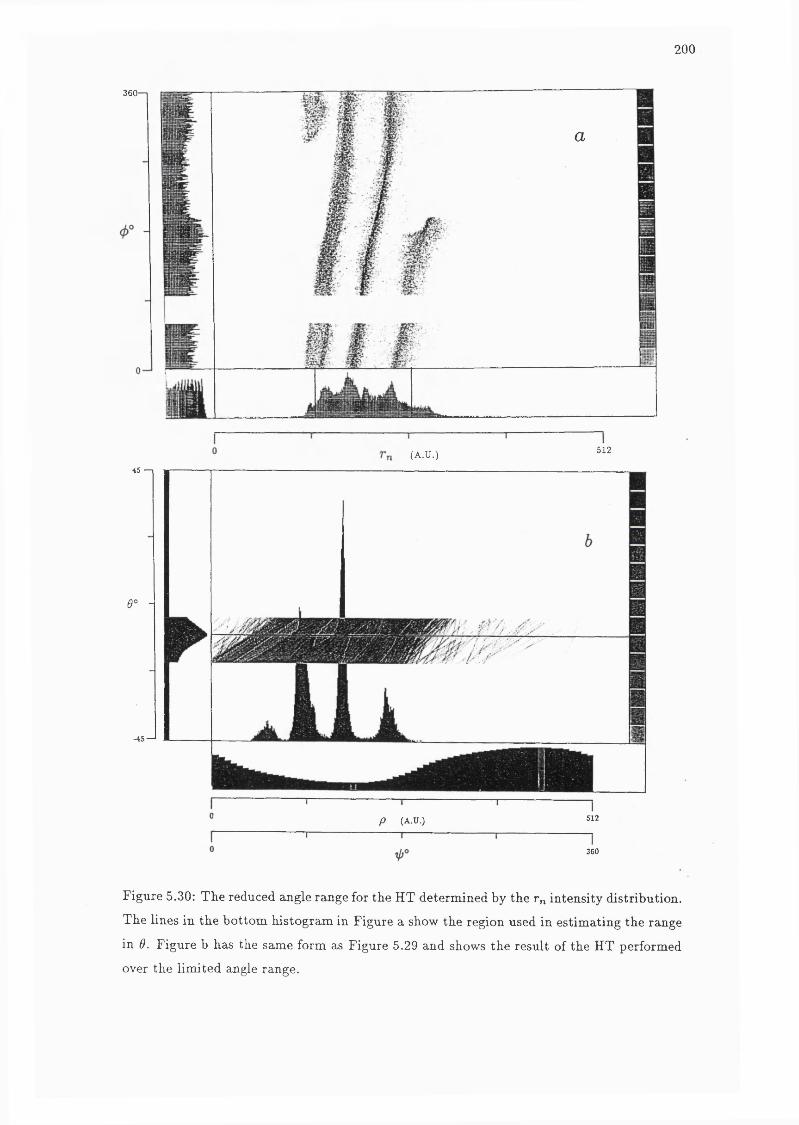
200

360-1

45 — I

e° -

-45—J

(A.U.)

a

512

P (A.U.) 512

360

Figure 5.30: The reduced angle range for the HT determined by the r„ intensity distribution.

The lines in the bottom histogram in Figure a show the region used in estimating the range

in d. Figure b has the same form as Figure 5.29 and shows the result of the HT performed

over the limited angle range.

201

envelope skewed to one side might be better. Another convolution with the whole J(r„ ,

distribution is necessary to determine where the centre of the envelope should lie. This

takes approximately 2.5 minutes, giving a total computation time of 8 minutes.

As noise is uncorrelated in position, it won’t be correlated in Hough space and

for a given value of 0, noise will be spread over a wide range of p. The points associated

with the arms are correlated in position and so will be concentrated into a smaller range

of p than the noise. As each point in the image is represented for each value of 9 in Hough

space, the SNR will be improved as the entire two dimensional image will be integrated

into one dimension. As 9 more closely corresponds to the gradient of the spiral arm, the

signal from the arms will be concentrated into smaller regions of p but the distribution of

the uncorrelated noise will not be significantly affected. The SNR will therefore increase

along with the definition of the spiral arms. The best SNR and arm definition will occur at

9m-

As example of the enhancement of SNR, Figure 5.31 compares the Sobel ED

with the HT for determining the gradient, a , of the r(h) function, see Section 5.2.1 and

Figure 5.11. As this is only a thin slice of the r„ /^ plot and the data is spread across 512

channels there are very few counts in each channel. EDs are suited for narrow lines such

as these but as there are so few counts in each energy channel, the arms are fragmented

again. More data are necessary for the ED to work and the problem still remains of how

to determine which arm is which. The HT, however, has clearly resolved the three arms

present and a ha^ been determined once more by the modulation of 7(p, ^).

Given the HT’s tolerance of noise it is suitable for use in a highly automated

procedure. It also takes one sixth of the time of the ED and has the potential for some

speed improvement, while the ED cannot be improved very easily. Also, the author finds it

particularly satisfying, philosophically, that the positions to which points are to be assigned,

can be determined without actually having to first assign points to some distribution.

The HT however will only work if the r„ /0 plot consists of a series of curves which

can be approximated by straight lines. If this is not the case, the ED method would have to

be used. The continuous curve, consisting of all the parallel curves joined together, would

then have to be fitted with a cubic spline because the curve could not be fitted with a

straight line.

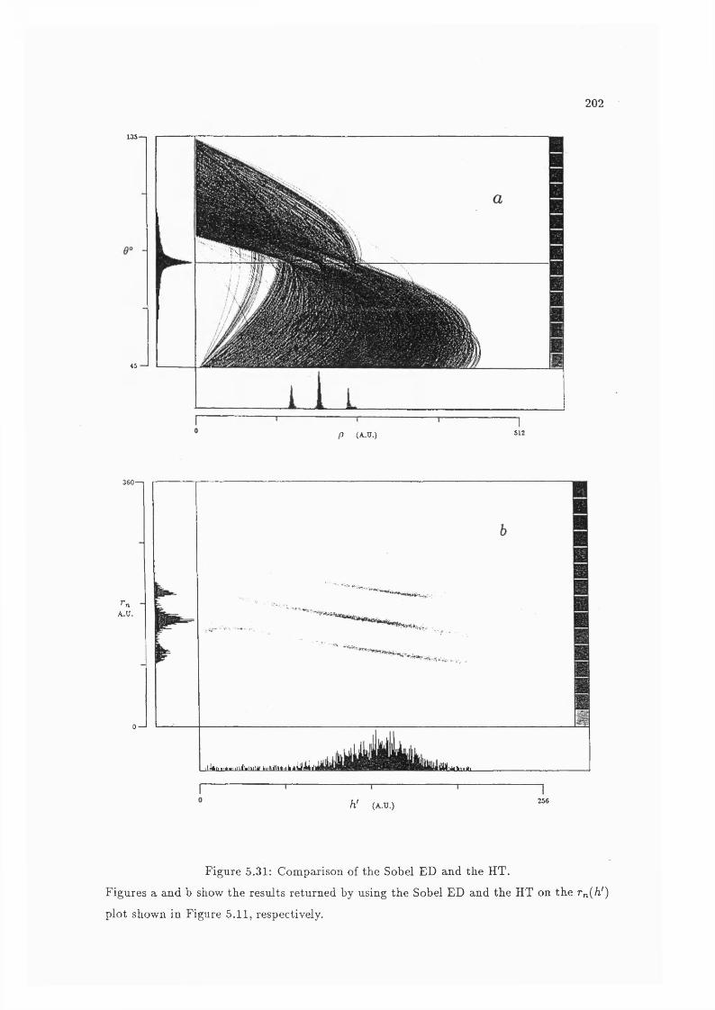
202

135—I

45

' - M

P (A.U.)I

512

360—1

TnA.U.

0—1

ilkli üÈmüdklLM luLAlÊilhAÜAllI .ÜHlJtlmUi.

h' (A.U.) 256

Figure 5.31: Comparison of the Sobel ED and the HT.

Figures a and b show the results returned by using the Sobel ED and the HT on the r„(/i')

plot shown in Figure 5.11, respectively.

203

5 .3 .4 V ariation o f Spiral C onstants

Although the two spiral fit parameters are constant for any given anode design, the

measured parameters vary with the plate operating conditions. As discussed in Section 5.2.1,

the radius of the Lissajous figure produced by the three electrodes, is dependent on the

charge cloud size. Any variation in that radius must significantly vary and The spiral

fit parameters are actually only constants for a constant set of operating conditions. For

consistency’s sake, I shall still refer to them as constants, although the variation of constants

is a somewhat oxymoronic concept.

The constants presented in this section were all measured with the Hough trans

form, as discussed in Section 5.3.2. The uncertainty in k corresponds to the bins in the distribution in Hough space, this corresponds to « ±0.05 in the arbitrary units of k.

The FWHM of the peaks is typically 5° corresponding to a width in fc of « 1.0 which is

much larger than the observed k variations.

The distribution obtained by the correlation of the square wave with /(p , is

very broad which makes ^ prone to large uncertainties. The full width at the point half way

between the maximum and minimum correlation is typically 180 — 240°. Also, all though k

and are quoted in units that suggest they are orthogonal, they are not: ij) is sensitively dependent on k.

Figure 5.32 shows how the constants vary with Vg. At the higher values of

only small variations in k still occur, but there are still significant, progressive variations

in The sizefof these shifts are large enough that if they were not corrected for, a large

fraction of events would be mapped into the region between the spiral arms and discarded,

severely degrading photometric linearity. Shifts in ^ larger than 90° can produce chronic ghosting.

Figure 5.33 shows how the constants vary with Vc. Once again there is relatively

little variation in k at the higher values of Vg but significant variations in ^ occur in all

cases.

Whenever photometric linearity is a consideration, new spiral constants should

be calculated if varying the MCP operating conditions produces a significant variation in

charge cloud size. As seen in Chapter 4.1, this occurs almost every time any of the operating

conditions are changed.

The constants are sensitive to operating conditions but they appear to be reason-

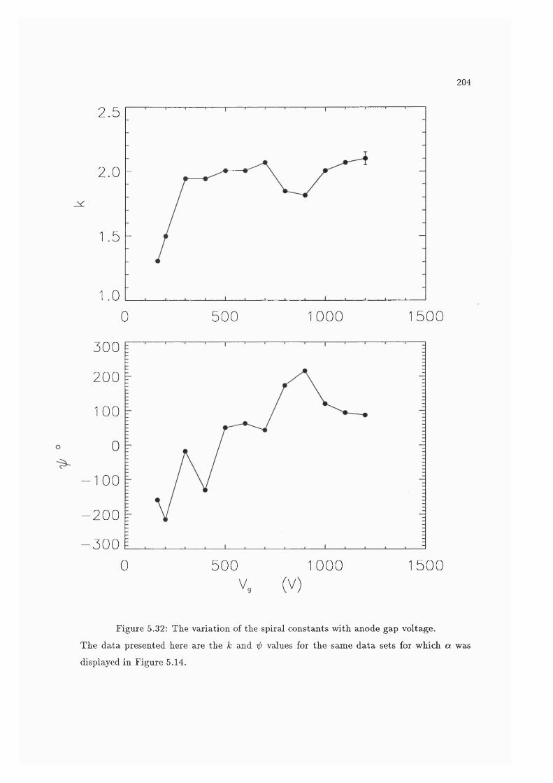
204

2.5

2.0 -

1.5 -

1.00 500 1000 1500

300

200

1 0 0

- 1 0 0

- 2 0 0

- 3 0 00 500 1000 1500

V , (V)

Figure 5.32: The variation of the spiral constants with anode gap voltage.

The data presented here axe the k and rf) values for the same data sets for which a was displayed in Figure 5.14.

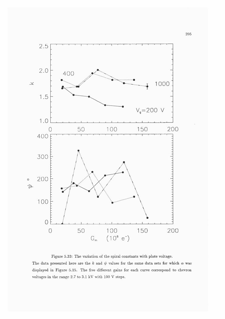
205

2.5

2.0 4 0 01 0 0 0 .

V = 2 0 0 V

0

0

50 1 0 0 150 200400

300

200

1 0 0

50 100 150Gm ( 1 0 ^ e - )

200

Figure 5.33: The variation of the spiral constants with plate voltage.

The data presented here are the k and 'if) values for the same data sets for which a was displayed in Figure 5.15. The five different gains for each curve correspond to chevron voltages in the range 2.7 to 3.1 kV with 100 V steps.

206

ably stable with time. Although no detailed investigation of time variation has been carried out, I have used the same constants at constant plate operating conditions continuously for up to a month, without any appreciable degradation in photometric linearity or increase in ghosting.

5.4 Spiral Arm Assignment by Statistical D istribution of p

In Hough Space

One further benefit of using the HT is that the distribution I{p^6m)-, see Figure 5.29, directly corresponds to the intensity distribution across the width of each spiral arm, for the whole length of each arm, i.e. every point associated with each arm is represented in the distribution.

This provides a convenient method of carrying out the spiral arm assignment. The operator need only select an intensity threshold in the distribution. The points above the threshold will be assigned to the appropriate spiral arm, those below wiU be discarded. Some care would have to be taken in the threshold selection, as partial spiral arms will have fewer counts in them, as shown in Figure 5.29. Alternatively, an acceptable width may be selected.

In either case, the operator may chose a scheme that wiU either eliminate theDM

chance of “ghosting”, retain the maximum number of events or a comprise between the two. Use of /(p , Om) would immediately allow a quantitative evaluation of the effectiveness of any decision criteria, such as percentage count loss or probability of ghosting.

The assignment could be implemented as a look-up-table (LUT) with the p value as input and the spiral arm number, a as output. The full width of the Hough transform

plots, in this chapter, is always 550 pixels. Therefore, a 9 bit address should be adequate

to describe the vast majority of possible p values. The memory could be configured as 4 bits deep, giving a total size of 256 bytes for the LUT. Figure 5.34 shows an example of I(p,Om) where data in between the spiral arms has been discriminated against and a representation of the values in the corresponding LUT. The rejected regions were chosen by eye. This image is presented only as an example and can in no way be claimed to represent an optimum case.

After the normalized data has been converted into polar space, (r„,0), it is trans-

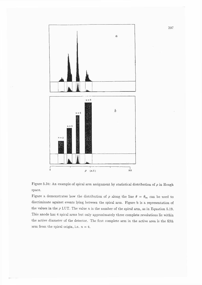
207

P (A.U.)I

512

Figure 5.34: An example of spiral arm cissignment by statistical distribution of p in Hough

space.

Figure a demonstrates how the distribution of p along the line d = Om can be used to

discriminate against events lying between the spiral arm. Figure b i s a representation of

the values in the p LUT. The value n is the number of the spiral arm, a in Equation 5.19.

This anode has 4 spiral arms but only approximately three complete revolutions lie within

the active diameter of the detector. The first complete arm in the active area is the fifth

arm from the spiral origin, i.e. n = 4.

208

ferred into Hongh. space (p, Û). Since 0^ has already been determined from the flat PHD

image, the data can be immediately projected into the line (p, 0m) by Equation 5.38

p = Tn cos 0m-\- sin • (5.42)

Figure 5.35 shows an example of an image obtained using this assignment method.

5.5 Applications for O ther D etectors

These techniques for spiral arm assignment are not just useful for SPAN alone.

They are applicable for any cyclic readout in which the variable used for determining coarse

position varies linearly and continuously with position across the detector, p.

For example, in the vernier anode. Section 2.2.2, coarse position is determined by

the difference in the phase angles returned from the two sets of triplets, or the phase lag

angle

^lag{p) = (f>2-<t>i » (5.43)

= p(w2 — Wi) , (5.44)

where W2 and wi are the different angular frequencies associated with the two electrode

triplets. From Equation 5.44 it can be seen that <f>iag varies linearly and continuously across

the detector as long as 0 iag repeats itself.

Figure 5.36 shows the plot of (f>i versus <f>iag for a simulated vernier anode where

W2 = l.lw i. It can be seen that it has the same general form as the r „ /^ plots for SPAN.

If <f>i and <f>iag were plotted in polar coordinates with (f>iag corresponding to the radius, the

resultant curve is a spiral. Therefore, the technique of spiral arm assignment is applicable

for the vernier anode.

In the case of double diamond readout. Section 2.2.1, the coarse position, (f>c is

given by

c - P^c (5.45)

and

(jJc = O.lw/ . (5.46)

where Wc and w/ are the angular frequencies of the triplets encoding the coarse and fine

positions (^ /) , respectively. The function <t>c{p) is linear and continuous over the range.

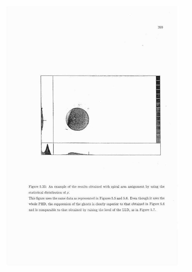
209

Figure 5.35: An example of the results obtained with spiral arm assignment by using the

statistical distribution of p.

This figure uses the same data as represented in Figures 5.5 and 5.6. Even though it uses the

whole PHD, the suppression of the ghosts is clearly superior to that obtained in Figure 5.6

and is comparable to that obtained by raising the level of the LLD, as in Figure 5.7.

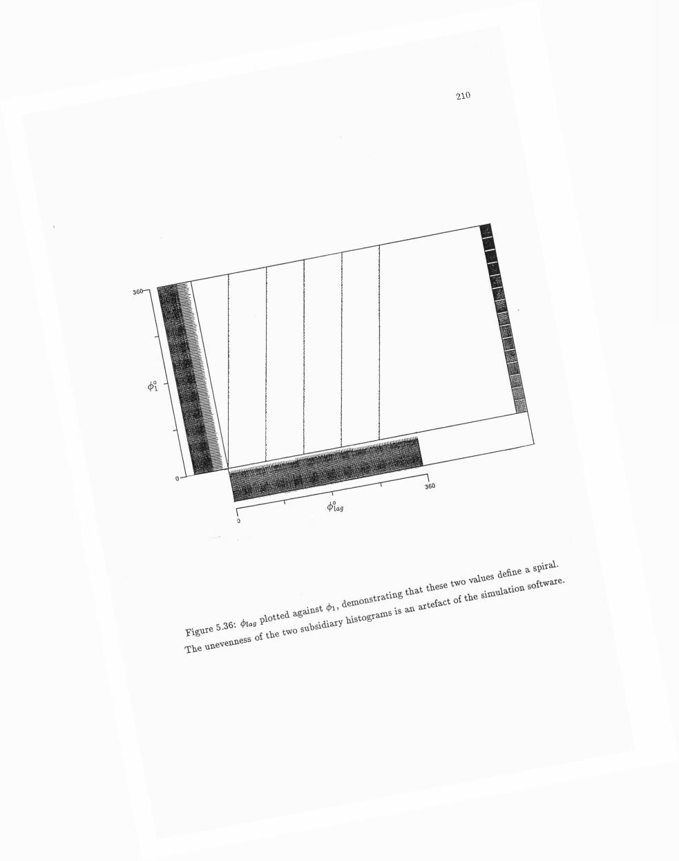
2 1 0

0

211

0 < p < Even though the Lissajous figure produced by the triangular electrodes is

a square, the double diamond readout will define a spiral if &re plotted as polar

coordinates.Spiral arm assignment should also be applicable for any readout in which the

coarse position variable, c, varies continuously, provided c{p) can be transformed into a

linear, monotonie relationship.

5.6 How th e A lgorithm is Im plem ented

At present, all of the decoding for SPAN is carried out in software. The software

runs on a Research Machines VX/2, PC compatible. This is an Intel 80386 based 16 MHz,

IBM PC compatible computer with a 80387 maths co-processor. The 80386 is always oper

ated in the “Real Mode”. The software is written under the Microsoft MS-DOS operating system. The display standard is VGA, 640 x 480 pixels with 16 colours. The software is

completely PC compatible and will run on any machine using MS-DOS 3.3, or later, and

supporting VGA graphics.Almost all of the software is written by the author in C and is approximately

3500 lines long. It is all written in the small memory mode and fits in the default data

and code segments and therefore uses < 128 kB when loaded. However, in operation it

uses a dynamically allocated array, 550 x 360 x 2 bytes deep, i.e. 396 kB. This array plus

the default data and code segments add up to approximately 540 kB of the 640 kB RAM

available under MS-DOS. Care must be taken in determining how much of this RAM other

software packages on the machine use.

At present, data acquisition is carried out by 6 ADCs controlled through a Pe

ripheral Interface Adapter by a routine written in assembler. Assembler was chosen for this

phase because of its speed. This assembler routine is the only hardware specific part of the

software.

Approximately 1000 events are acquired at a time and loaded into an array in

the default data segment. Control is then returned to the main C calling routine and the

decoding algorithm is carried out on the 1000 events, the pulse height of each event displayed

and a histogramming memory for each pixel is incremented. Then another 1000 events are

acquired and the process repeated.

At this stage the program is limited by the fact that the CPU has to control

212

data acquisition. As a result, data cannot be acquired and processed simultaneously and

the results are only displayed in “pseudo-realtime” . The decoding algorithm and the real

time display of events require much more time than the acquisition, limiting the speed of

operation of the software to approximately 600 counts.s"^

An important feature of the software is that the incoming digital data is converted

into floating point numbers immediately after it has been read in. This is necessary to

ensure that no spurious aliasing or fixed patterning is caused by roundoff errors during

integer arithmetic.

The data is displayed in a central window of the VGA screen, with dimensions of

550 X 360 pixels. When the acquisition is complete the pulse height distribution is plotted

in a small window (64 x 64 pixels). The integrated intensity across the x and y image axes

can be plotted in two side windows 550 x 64 and 360 x 64 pixels, respectively. Any

point on the screen can be interrogated by the mouse and the coordinates, the number of

counts per pixel, per energy channel or per line is displayed on the screen. A zoom feature

is available so any selected region of an image may be displayed using the full 550 x 360

array of pixels in the central window.

There are several modes of operation for the software :

1. Data can be displayed as it is acquired or from a stored image.

Most of the following options are available for both modes.

2. The number of bits of digitization for the ADC can be varied but only for events that

are actually being acquired.

3. A constant multiplication factor can be applied to individual channels for fine tuning

of the image. This is only used while testing electronics.

4. The cartesian coordinates in the plane of the spiral, e.g. Figure 5.2, the r „ /^ space,

for either dimension, or the two dimensional image can be displayed. Displaying the

one dimensional data is necessary for spiral arm assignment. The plane of the spiral

display is only used when investigating the gross shape of the spiral. It is sometimes

easier to visualise the cause of gross distortions from the spiral in this mode than in

the r/<f) mode.

5. The pulse height of each event can be displayed in realtime. This is particularly useful

213

when high local count rates depress the gain of the MCP. A selection can be made

either to display the cumulative total over all frames or just each individual frame.

6. The ratio of the total number of events plotted to the total number acquired is always

displayed in real time. When acquiring two dimensional data, this provides a measure

of the proportion of events that are not being mapped correctly to one of the valid

spiral arms.

7. The cumulative count per pixel can be displayed in real time or after acquisition is

complete. Intensity is shown with a 16 colours palette. The scale for the false colours

can be selected to be either logarithmic or linear and step sizes and offsets are also

selectable. The maximum number of counts per pixel is 64 k.

8. The whole active diameter or a selected region can be viewed in realtime. Similarly,

the range of event pulse heights to be displayed can be selected.

9. The 6 ADC values, at 12 bytes per event, the decoded position and pulse height,

10 bytes per event, or just the histogrammed memory can be saved to disk. Files

containing the 6 ADC values are used as inputs to a separate program to produce the

r{h) plots as in Figures 5.11. The histogrammed memory files are used as inputs to

the Hough transform and edge detection spiral constant determining programmes.

5.7 SPAN Im aging Perform ance

The diagrams in this section were obtained with an open faced detector, the config

uration of which is discussed in Section 7.2.1. They represent the best results obtained with

a SPAN to date. Lapington et al. (1992) have presented examples of recent performance

measurements with a two dimensional SPAN in a sealed tube detector.

The grey scales in all the diagrams in this section, correspond to intensity values

with zero offset and unit steps.

5.7 .1 P u lse H eigh t R e la ted P osition Sh ifts

Figure 5.37 shows that there is a pulse height related shift in ^ as well as in r„.

No correction for pulse height has been made on the radius in both figures, so that on each

spiral arm, the lower pulse height events have the larger radii.

214

In the data plotted in the plane of the spiral, the low pulse height data always precedes the high pulse height data, i.e. <!> is largest for the lowest values of W. This is also

apparent in the r„ /^ plot. If there was no variation of <j> with h \ the individual smears

would be parallel to the r„ axis. Also, the gradient, does not vary significantly through

360°.

The cause of this shift is not known at present but the author thinks they are

probably another charge cloud effect. If the variation in <f> was due to a h' dependent shift

of the spiral origin, the gradient would vary with angle and would have opposite signs for

points separated by 180°, so this cannot be the explanation. Also, although the magnitude

of the gradient is often not the same for each of the triplets, the sign always is. The data in

this diagram are those obtained from the second triplet of electrodes of the two dimensional

SPAN anode. The <^/r„ gradient for the first triplet is much smaller.

As the <j> is used to determine the fine position, any A' related variation in <f>

will induce pulse height related position shifts in a two dimensional image. Figure 5.38

shows an example of two dimensional images produced with varying proportions of the

PHD. The effect causes the low intensity tails extending in the positive y direction in the

figure consisting of events distributed throughout the entire PHD. These tails are not visible where a smaller range of pulse heights are used. Also, the tails extend much further in the

y direction than in the x which follows the behaviour of the 0 /r„ gradients for the two

triplets. The size of the pinhole images in the figure with the reduced pulse height ranges

have diameters of « 60 //m and the length of the tails are comparable. All though the shift

in 4> with pulse height is small, it can translate into significant positional shifts.

5 .7 .2 P o sitio n a l L inearity and R eso lu tion

Figure 5.39 shows an image of a pinhole array covering the whole active diameter

of the MCP. It demonstrates the excellent spatial linearity of SPAN. In all but the extreme

edges of the image, the maximum deviation from the expected position of the peak of the

images is 30 //m across the active region. The best resolutions obtained were at voltages

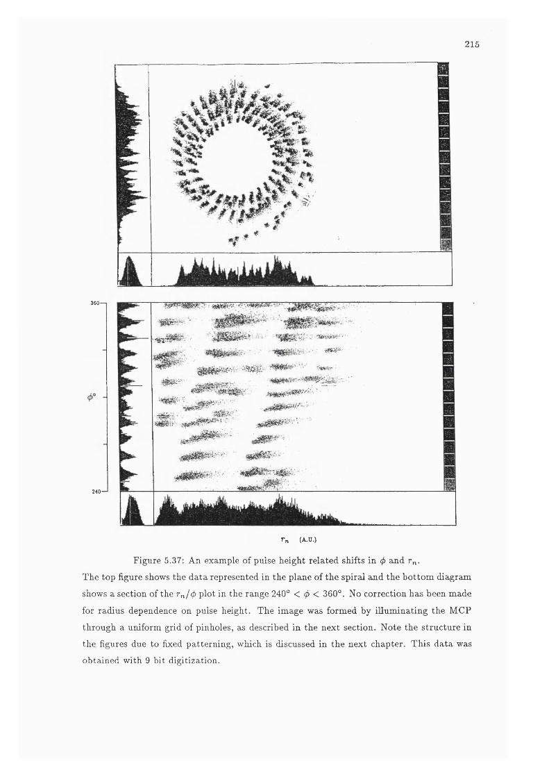
215

360—1

240—'

y ^ ç rg » * ? -; ••

. .1''-:' :%&$r .

jïèâfe/t.v, ■

r„ (A-u.)

Figure 5.37: An example of pulse height related shifts in </> and r„.

The top figure shows the data represented in the plane of the spiral and the bottom diagram

shows a section of the r„ /0 plot in the range 240° < 4> < 360°. No correction ha.s been made

for radius dependence on pulse height. The image was formed by illuminating the MCP

through a uniform grid of pinholes, as described in the next section. Note the structure in

the figures due to fixed patterning, which is discussed in the next chapter. This data was

obtained with 9 bit digitization.

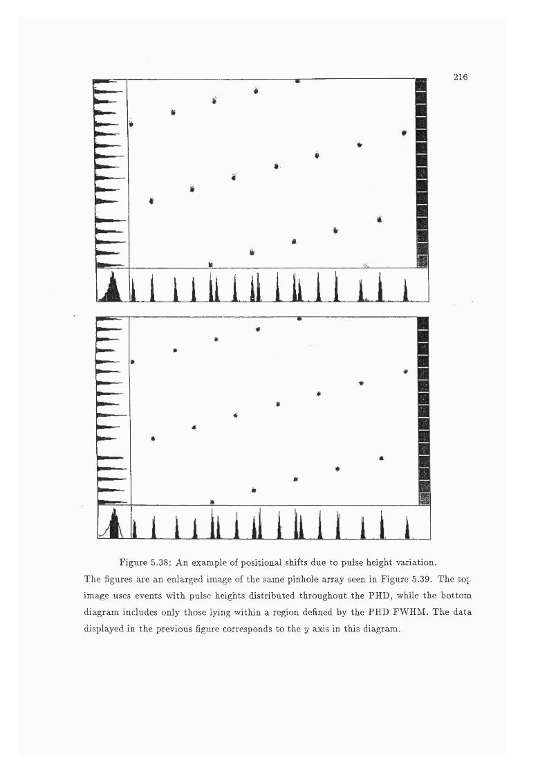
216

I l 1 1 l u i l l i l l

Figure 5.38: An example of positional shifts due to pulse height variation.

The figures are aji enlarged image of the same pinhole array seen in Figure 5.39. The top

image uses events with pulse heights distributed throughout the PHD, while the bottom

diagram includes only those lying within a region defined by the PHD FWHM. The data

displayed in the previous figure corresponds to the y axis in this diagram.

217

of = 2.9 kV and Vg = 400 V. Figure 5.40 shows an image obtained at these operating

conditions in which the MCP pores are visible. The image was acquired only using a limited

range of pulse heights, 6 ± 1 x 10ê“ , in order to overcome the h' related positional shifts.

The resolution is approximately 17 /zm FWHM which represents the centroiding PSF of the

readout.

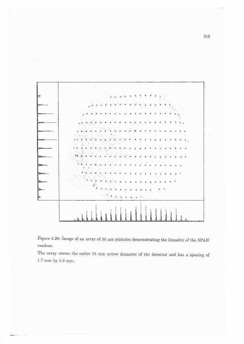
218

Figure 5.39: Image of an array of 50 /im pinholes demonstrating the linearity of the SPAN readout.

The array covers the entire 25 mm active diameter of the detector and has a spacing of 1.7 mm by 1.0 mm.

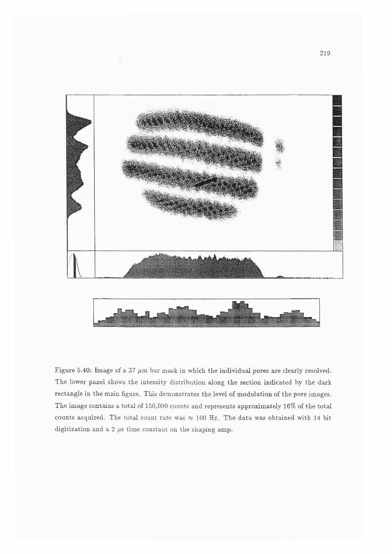
219

i

Figure 5.40; Image of a 37 /zm bar mask in which the individual pores are clearly resolved.

The lower panel shows the intensity distribution along the section indicated by the dark

rectangle in the main figure. This demonstrates the level of modulation of the pore images.

The image contains a total of 150,000 counts and represents approximately 16% of the total

counts acquired. The total count rate was % 100 Hz. The data was obtained with 14 bit

digitization and a 2 /iS time constant on the shaping amp.

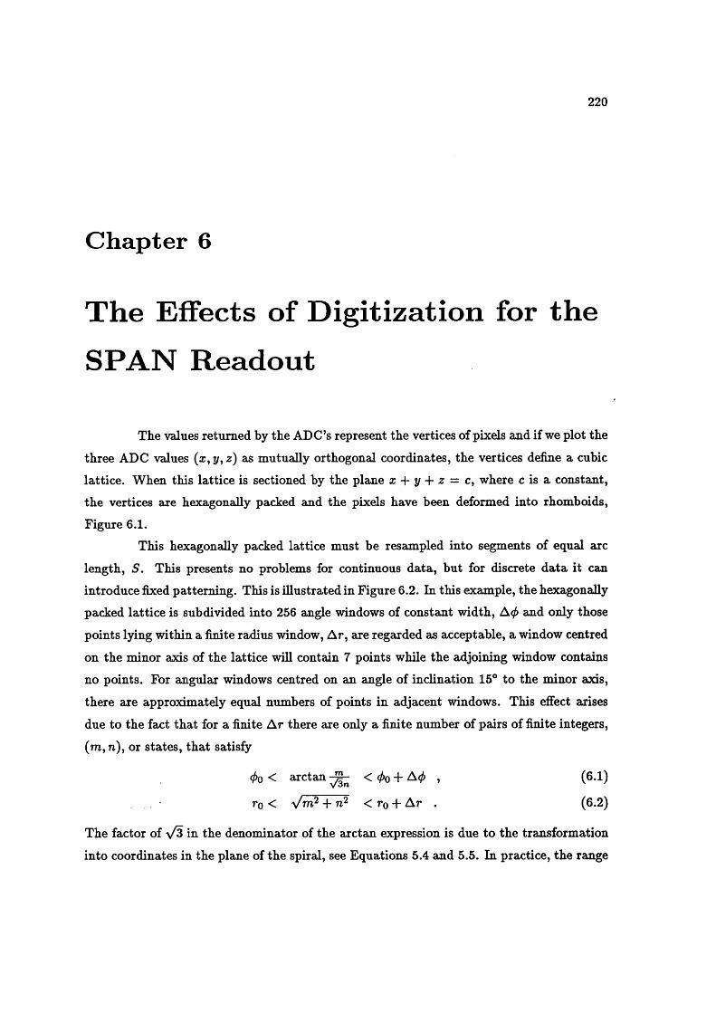
220

Chapter 6

T he Effects o f D ig itization for the

SPA N R eadout

The values returned by the ADC’s represent the vertices of pixels and if we plot the

three ADC values {x^y^z) as mutually orthogonal coordinates, the vertices define a cubic

lattice. When this lattice is sectioned by the plane z + y + z = c, where c is a constant,

the vertices are hexagonally packed and the pixels have been deformed into rhomboids.

Figure 6.1.This hexagonally packed lattice must be resampled into segments of equal arc

length, S. This presents no problems for continuous data, but for discrete data it can

introduce fixed patterning. This is illustrated in Figure 6.2. In this example, the hexagonally

packed lattice is subdivided into 256 angle windows of constant width, and only those

points lying within a finite radius window, A r, are regarded as acceptable, a window centred

on the minor axis of the lattice will contain 7 points while the adjoining window contains

no points. For angular windows centred on an angle of inclination 15° to the minor axis,

there are approximately equal numbers of points in adjacent windows. This effect arises

due to the fact that for a finite A r there are only a finite number of pairs of finite integers,

(m, n), or states, that satisfy

(f)Q < arctan < <o + A< , (6.1)

tq < y/rn? ri < ro + A r . (6.2)

The factor of y/Z in the denominator of the arctan expression is due to the transformation

into coordinates in the plane of the spiral, see Equations 5.4 and 5.5. In practice, the range

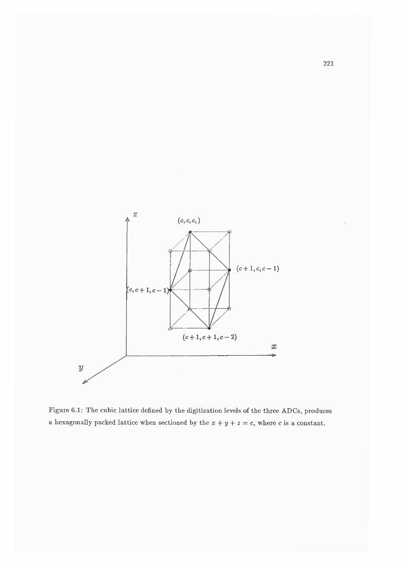
221

(c+ l ,c ,c - 1)

Figure 6.1: The cubic lattice defined by the digitization levels of the three ADCs, produces

a hexagonally packed lattice when sectioned by the a; + y + 2: = c, where c is a constant.

222

of m and n is limited by the number of digitization levels of the ADCs used.This effect presents itself as a variation in the sensitivity, s(t), from one pixel,

z, to another. Figure 6.3 shows a simulation of the variation in s(t) for a spiral anode

containing three arms in the active region of the detector. The active region commences at

the beginning of the fourth spiral arm, i.e.

Tla = 3 , (6.3)

n, = 4 , (6.4)

=> Stt < 0 < 147r . (6.5)

This is the approximate configuration of the spiral in the active area of the detectors eval

uated so far. There is only a phase shift of about 70° between this configuration and that

displayed in Figure 5.18, etc. Every possible state lying within a radius envelope, with a

relative width, Wr, half the spiral arm separation, i.e.

A r = Wr2k{h')7T , (6.6)

= k{h')TT , (6.7)

and centred on the centre of the spiral arms, has been illuminated just once.

The s(z) values correspond only to data from one pulse height plane, i.e. the plane,

h' = —256 , (6.8)

= 384 . (6.9)

Choosing only one plane also constrains the values of fc,

A;(384) = 2.1 , (6.10)

which corresponds to

kn = t(256) , (6.11)

= 1.4 , (6.12)

which is typical of the spiral constants for the anodes that have been evaluated so far.

The inputs r , y and z have been digitized to 8 bits, d = 8 and the arc length, 5,

defined by this range of 6 has been divided up into 2048 pixels. Tip, of equal width. This

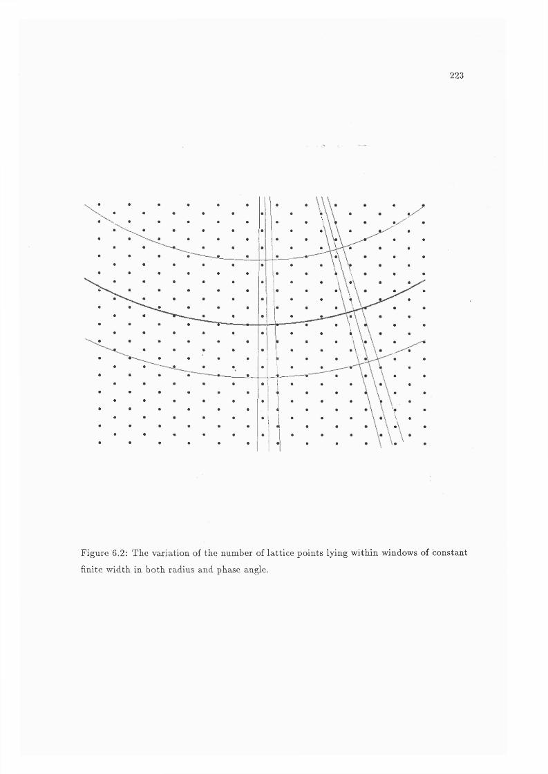
223

Figure 6.2: The variation of the number of lattice points lying within windows of constant

finite width in both radius and phase angle.

224

elUiUh*.

Mo p i x : Z048 n n : 2 .5 4 s d : 1 .1 1 4 , n o . 0 108 max p 5 pmax 130p

Figure 6.3: The fixed patterning produced when all the possible lattice points have been

illuminated once and only once.

The vertical lines represent s{i) for each of the pixels and the distribution on the bottom

left corner represents the distribution in s(i). There are 512 pixels represented in each of

the horizontal lines. The mean and variance are quoted in the bottom panel together with

the number of dead pixels, 108, the maximum value of 5(z), 5, and the number of pixels

with that value, 130.

225

represents the baseline requirements for the Optical Monitor (CM) detector. Even though

the pixels are of equal width in arc length, they behave effectively as though the width

varies from pixel to pixel, i.e. they have a finite differential nonlinearity. The magnitude of

the fixed patterning has a clearly defined cycle, becoming most prominent every 60° of

This occurs when a radial lies along one of the axes of the lattice, as along these lines, the

separation of the states is at a minimum and so more points exist in a finite A r and there

are no points in the adjacent angle windows.

The intensity distribution of s(t) varies between Poisson and Gaussian distribu

tions, depending on average sensitivity, s. The ratio of the standard deviation of s,- to s

provides a useful measurement of the degree of fixed patterning and does not require a priori

assumptions about the form of the distribution.

From the above description it can be seen that even in an ideal case, the ratio =

heis seven degrees of freedom,

— = 3 (^0 » Wr, h , d, 7%p) , (6.13)

which for the baseline configuration

| ( 3 , 4,2.1,0.5,384,8,2048) = 0.42 . (6.14)

The first three parameters in Equation 6.13 are defined by the pattern design while the last

four are defined by the user and the electronics.In this chapter, the fixed patterning is modelled assuming that all the electronic

components behave ideally. Another model has been developed in which the performance

of the readout is estimated for the presence of various effects such as noise and crosstalk.

Results from this model are presented in Breeveld et al., (1992b).

6.1 T he Effects of Anode Design P aram eters on Fixed P a t

tern ing

Even though the ratio f is a useful measure of the degree of fixed patterning, it

does not take into account the absolute limit set by s(i) = 0 . Figure 6.4 shows the simulated

variation of the ratio and p(0 ), the measured probability of a pixel having zero sensitivity,

i.e. a dead pixel, for variations of each of the three spiral parameters from the baseline

specification described above. Also, as fixed patterning is produced by a combination of

226

allowable pairs of integers, the ratio = will not be systematic over small ranges, indeed it

could be described as “pathologically unsystematic” . It is useful for a qualitative discussion

or for describing gross variations but not for detailed predictions.

Increasing any of these parameters reduces the fixed patterning as the arc length

is increased, i.e.

A5 « , (6.15)

« 2fc(h')7T^((na + UaŸ ~ , (6.16)

« 2k{h')'K‘ (n\ + 2naTig) . (6.17)

As described in Section 5.1.3 the radius of the largest that can be drawn

inside the equilateral triangle defined by the ADCs is given by

riim = ^ ^ • (6.18)

Therefore, a continuous spiral electrode has the constraint that

k{h')2T:{ria 4- + —) < , (6.19)

=> k{h')(na + 71, + j ) < 25 , (6.20)

where h' — 384. The | term is included to allow for the finite width of the spiral arms.

Equation 6.20 shows that the options for improving the fixed patterning are lim

ited. Figure 6.4 shows that for A;(384) = 2.1, if the total number of arms is greater than 12,

the magnitude of the fixed patterning increases rapidly. This is due to some parts of the

simulated spirals having radii greater than rum and so the spiral is no longer continuous. A

similar situation occurs when A;(384) > 3.5 if all other parameters are set at their baseline

levels.

6.2 T he Effects of User Defined P aram eters on Fixed P a ttern ing

Figure 6.5 is similar to Figure 6.4 and shows the variation in fixed patterning for

variation in the four user defined parameters. These four parameters h \w ,d ,n p vary the

number of lattice points included in each of the pixels.

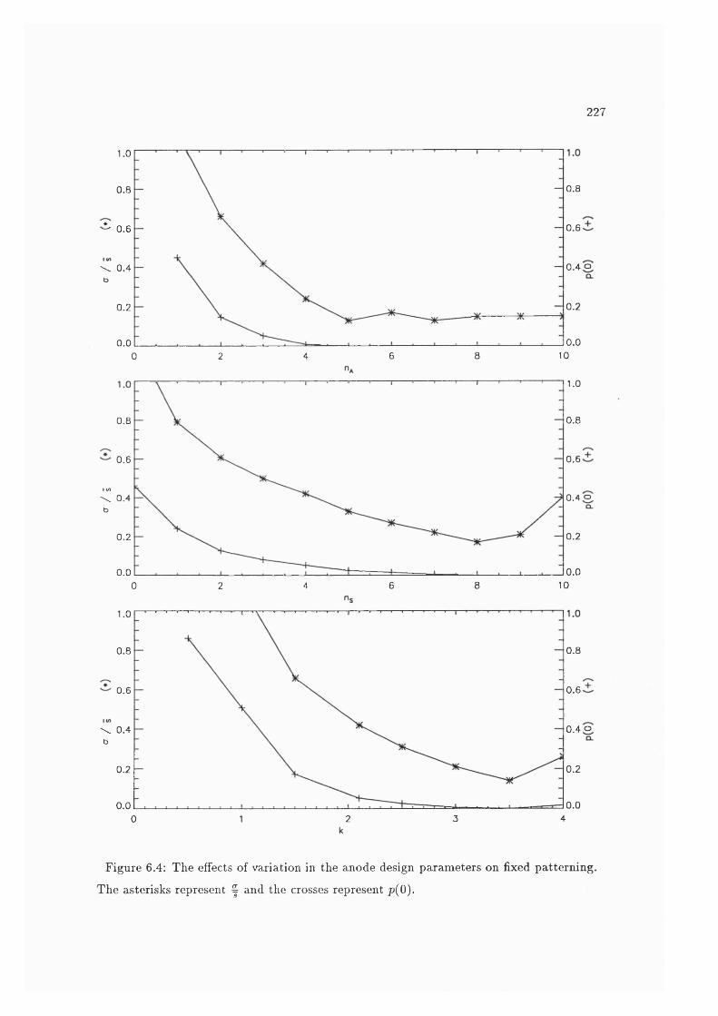
227

1.0

0.80.8

^ 0.6 0.6

0 .4 o\ 0 .4b

0.20.2

0.00.08 100 2 64

1.0

0.80.8

0.60.6

ll/I0 .4 o\ 0 .4

b

0.20.2

0.00.0106 80 2 4

1.0

0.80.8

0.60.6

0 .4 o\ 0 .4b

0.20.2

0.00.03 40 2

Figure 6.4: The effects of variation in the anode design parameters on fixed patterning.

The asterisks represent | and the crosses represent p(0).

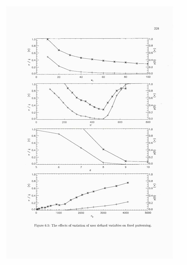
228

1.01.0

0.80.8

0.60.6

0.4 - 0.4

b0.20.2

0.00.010040 60 8020

f

1.01.0

0.80.8

0.60.6

0.4 0.4

b0.20.2

0.00.08000 200 400 600

1.0

0.80.8

0.60.6

0.4 0.4

b0.20.2

0.00.0105 6 7 8 9

0.8 0.8

0.60.6

0.4 0.4

b0.20.2

0.00 1000 2000 3000 4000

Figure 6.5: The effects of variation of user defined variables on fixed patterning.

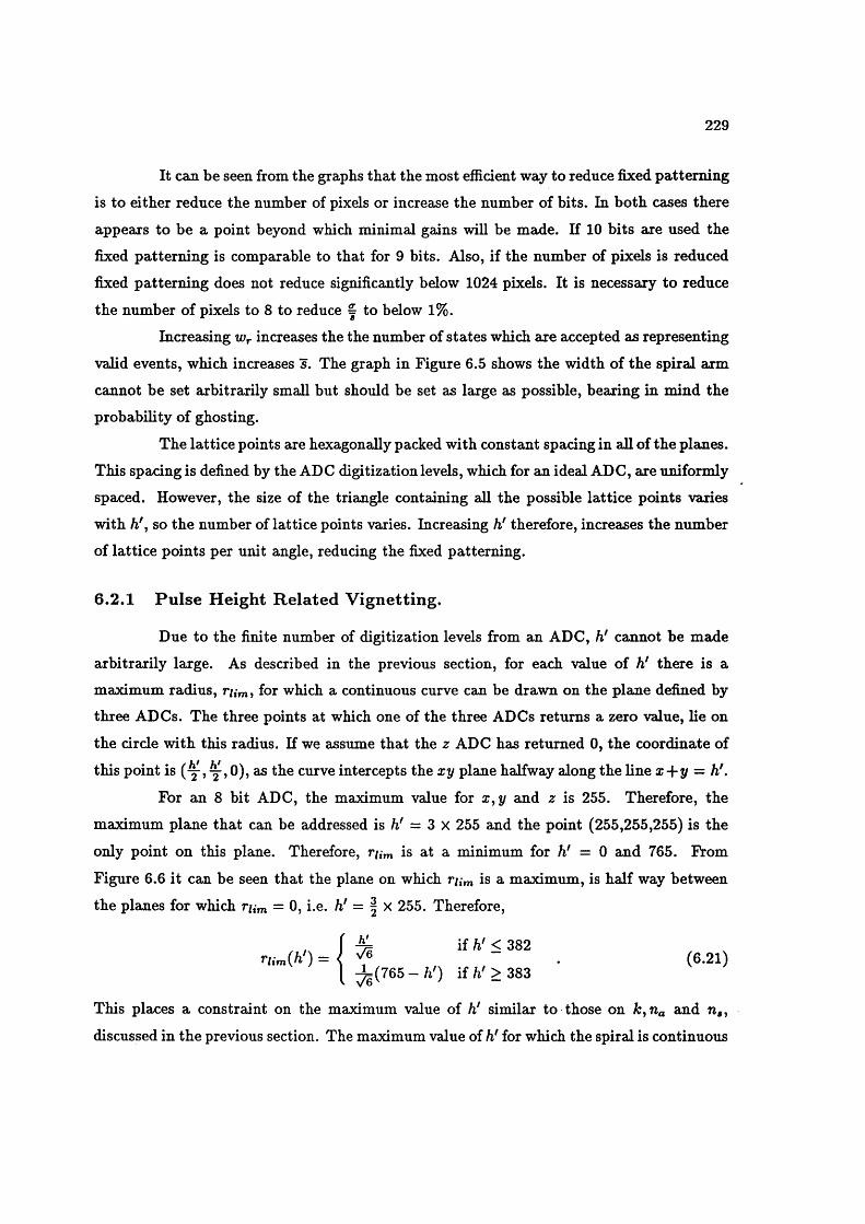
229

It can be seen from the graphs that the most efficient way to reduce fixed patterning

is to either reduce the number of pixels or increause the number of bits. In both cases there

appears to be a point beyond which minimal gains will be made. If 10 bits are used the

fixed patterning is comparable to that for 9 bits. Also, if the number of pixels is reduced

fixed patterning does not reduce significantly below 1024 pixels. It is necessary to reduce

the number of pixels to 8 to reduce = to below 1%.

Increasing Wr increases the the number of states which are accepted as representing

valid events, which increases s. The graph in Figure 6.5 shows the width of the spiral arm

cannot be set arbitrarily small but should be set as large as possible, bearing in mind the

probability of ghosting.

The lattice points are hexagonally packed with constant spacing in all of the planes.

This spacing is defined by the ADC digitization levels, which for an ideal ADC, are uniformly

spaced. However, the size of the triangle containing all the possible lattice points varies

with h', so the number of lattice points varies. Increasing h' therefore, increases the number

of lattice points per unit angle, reducing the fixed patterning.

6 .2 .1 P u lse H eight R ela ted V ig n ettin g .

Due to the finite number of digitization levels from an ADC, h’ cannot be made

arbitrarily large. As described in the previous section, for each value of h' there is a

maximum radius, for which a continuous curve can be drawn on the plane defined by

three ADCs. The three points at which one of the three ADCs returns a zero value, lie on

the circle with this radius. If we assume that the z ADC has returned 0, the coordinate of

this point is ( y , y , 0), as the curve intercepts the xy plane halfway along the line x-\-y = A'.

For an 8 bit ADC, the maximum value for and z is 255. Therefore, the

maximum plane that can be addressed is A' = 3 x 255 and the point (255,255,255) is the

only point on this plane. Therefore, rum is at a minimum for A' = 0 and 765. From

Figure 6.6 it can be seen that the plane on which rum is a maximum, is half way between

the planes for which r/,„, = 0, i.e. A' = | x 255. Therefore,

| ( 7 6 5 - V ) if f t '> 383 •

This places a constraint on the maximum value of h' similar to those on A, and n ,,

discussed in the previous section. The maximum value of A' for which the spiral is continuous

230

is actually dependent on the three anode parameters, i.e. by Equation 6.19

A;(h')27r(Tia + n , + i ) < ru m {h !) , (6 .2 2 )

inserting the values from the baseline configuration, maximum value of h* is given by

2.1— X 90 « -4 = (7 6 5 -h ') , (6.23)384 ^

h' % 500 . (6.24)

As pulse height increases beyond this level, the ADCs will be able to address

smaller fractions of the spiral plane, i.e. the spiral wiU be vignetted. This effect can be seen

in Figure 5.20 showing the hard limit on radius with pulse height and is demonstrated in

Figure 6.5 by the rapid increase in the non-uniformity of s for h' > 512.

This effect wiU tend to filter out multiple, simultaneous events as these will usually

be much larger than normal events. Very large events wiU only be addressable at small

values of r„ and if these radii are significantly smaller than the radius of the first spiral

arm, they will be effectively ignored. However, large events can also be incorrectly mapped

into the active region of the normalized spiral plain, producing spurious events that will be accepted. It is thought that this is the cause of the extra noise apparent for large pulse

heights in Figure 5.20. Therefore, extreme care must be taken in matching the PHD with

the reference voltage when using fixed reference ADCs.

6.3 Fixed Reference ADCs

In conventional ADCs the reference voltage is fixed and the digital output is pro

portional to that fixed reference. Therefore, aa the pulse heights vary, a series of planes is

produced. After normalization with respect to h‘ (see Section 5.1.3), the areas of each of

these planes are the same. Therefore, as the number of lattice points varies with data

from lower planes will produce a larger lattice spacing in the normalized plane and data

from higher planes will produce a smaller spacing.

If the lattice spacings are different, the states are not aligned and so there will be

many more states in any finite area of the plane, reducing fixed patterning. Figure 6.7 is

similar to Figure 6.3 but represents the effect of projecting many planes of different h ' and

constant lattice spacing into one plane. It is readily apparent that there are many more

states in some areas of finite angular and radial width compared to Figure 6.3.

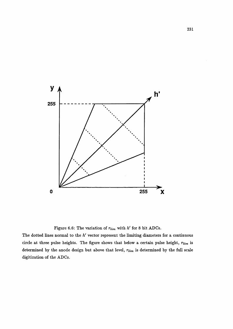
231

y

255

0 255 X

Figure 6.6: The variation of r/,„, with h' for 8 bit ADCs.

The dotted lines normal to the h' vector represent the limiting diameters for a continuous

circle at three pulse heights. The figure shows that below a certain pulse height, rum is

determined by the anode design but above that level, rum is determined by the full scale

digitization of the ADCs.

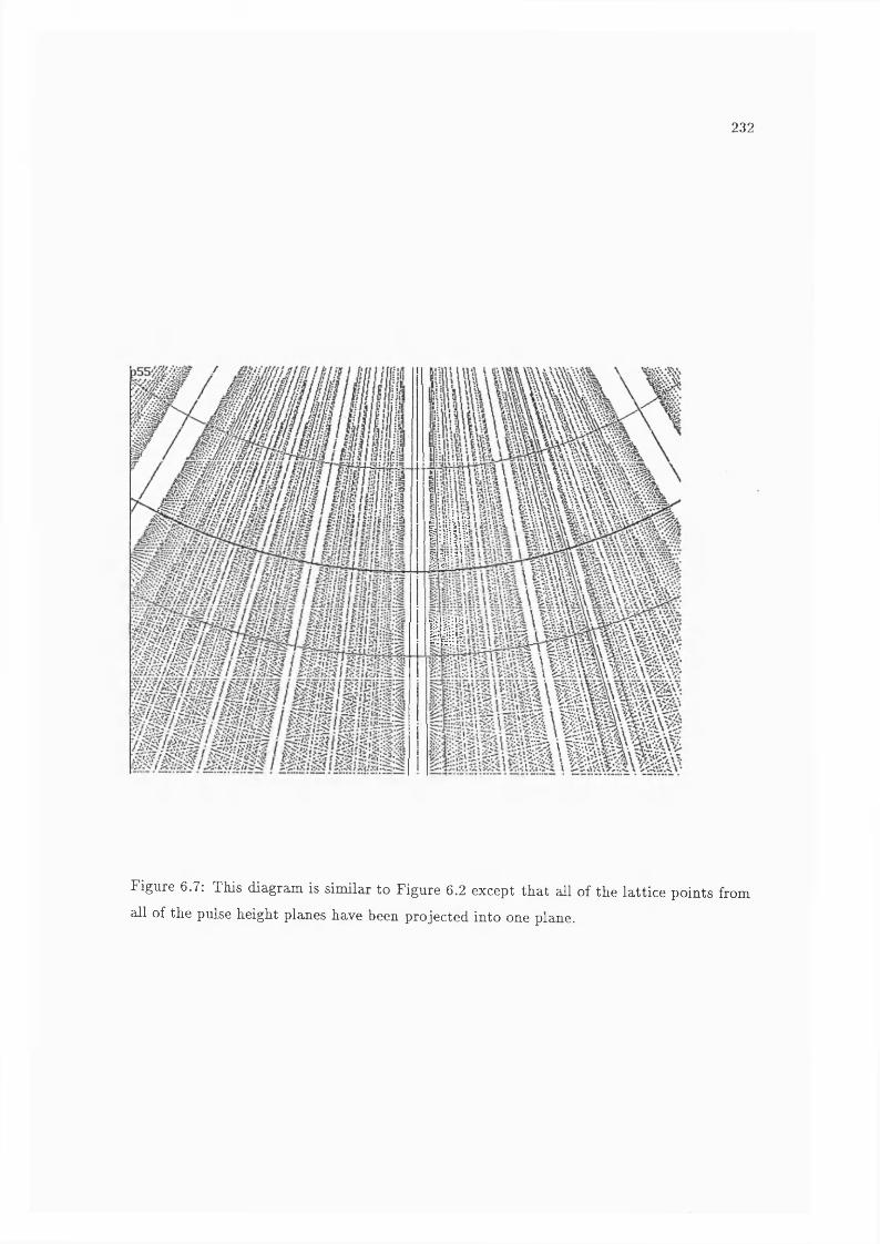
232

a ia # :]ÿtV-'V.

■ I

Figure 6.7: This diagram is similar to Figure 6.2 except that aü of the lattice points from

aU of the pulse height planes have been projected into one plane.

233

However, even thongh the spacing varies the orientation of the lattice axes does

not. The position along the axes vary for points from different planes, but the radial along

which they lie does not. This gives rise to the variation of number of states with angle,

which will produce variation in s(i). So even though fixed patterning could be reduced in

some areas, it is still a problem at precisely the same points that fixed patterning is most

severe for data from a single plane.

Fixed reference ADCs do not digitize all events to the full dynamic range of the

ADC. For example, an 8 bit ADC will only digitize an event with a pulse height of half

the reference value to 7 bits. Given that even a well saturated MCP PHD has a saturation

of the order of 50% and assuming that the PHD is Gaussian then there is a factor of 4

difference in the magnitude of the pulse height between ±3cr and magnitude of the modal

gain would be only approximately 60% of the +3<j point. Therefore, a 9 bit ADC would be necessary to obtain the full 8 bit digitization at the modal gain without clipping the top

half of the PHD.

Given that the gain will be depressed at high point source count rates, at least a

10 bit ADC is necessary to maintain the level of fixed patterning at that of the baseline

configuration, as discussed in the previous section. Figure 6.8 shows an example of gain

depression increasing the fixed patterning. The data was obtained with 9 bit Wilkinson

ADCs. Data digitized at the full 9 bits would occupy the extreme right of the PHD display.

As the PHD lies only in the left half of the display, the data has been digitized at less than

8 bits. The data at the lower count rate already shows severe variations in s(i) but as the

count rate increases the gain is depressed, leading to increased fixed patterning and almost

total fragmentation of the image.

Figure 6.9 shows the results from a simulation of varying the number of bits dig

itization for a fixed reference ADC. The actual data was acquired with 14 bit Wilkinson

ADCs, i.e. d = 14, and is also displayed. The other images are produced by the same data

using only the d most significant bits of the original 14 bit data. The data has not been

resampled into pixels of equal arc length but is the direct output as calculated by 5 =

Each of the pixels in the image represents approximately 4 //m which is about

half of the pixel width required by the OM. The SPAN used for these measurements has a

diameter of 36 mm and contains 4 spiral arms. Only w 3 arms lie in the 25 mm diameter

of the MCPs. The OM requires an 18 mm square active area. Assuming that a pattern

can be made with 4 spiral arms in this area, the fixed patterning for a given physical pixel

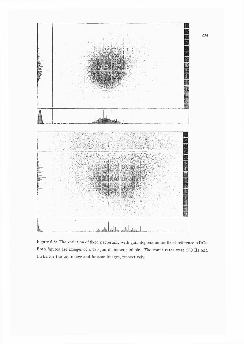
234

# # # # # # # * #til

Figure 6.8: The variation of fixed patterning with gain depression for fixed reference ADCs.

Both figures are images of a 180 //m diameter pinhole. The count rates were 250 Hz and

1 kHz for the top image and bottom images, respectively.

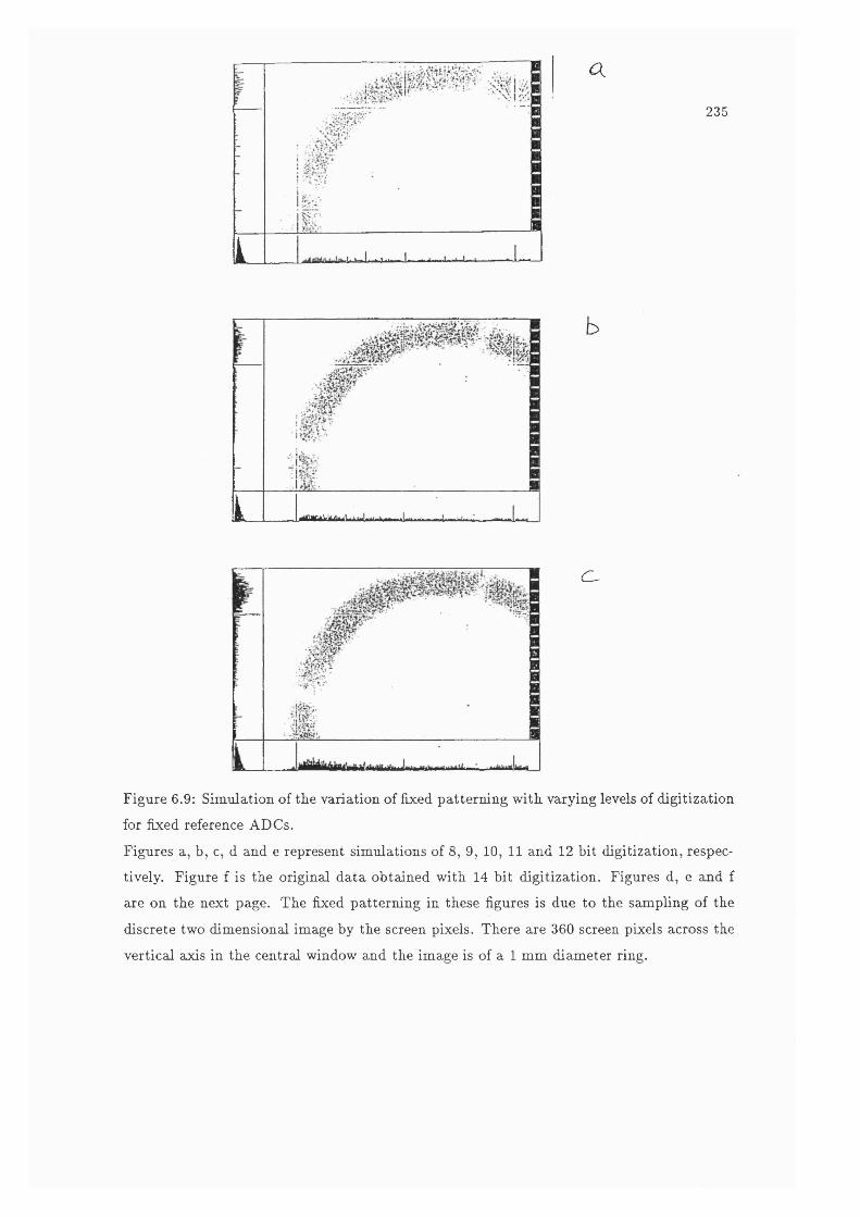
I th ill k * l , ^ I »i«— I ,

a

235

I iHllTdr ikilii V. .1

b

c .

Figure 6.9; Simulation of the variation of fixed patterning with varying levels of digitization

for fixed reference ADCs.

Figures a, b, c, d and e represent simulations of 8, 9, 10, 11 and 12 bit digitization, respec

tively. Figure f is the original data obtained with 14 bit digitization. Figures d, e and f

are on the next page. The fixed patterning in these figures is due to the sampling of the

discrete two dimensional image by the screen pixels. There are 360 screen pixels across the

vertical axis in the central window and the image is of a 1 mm diameter ring.

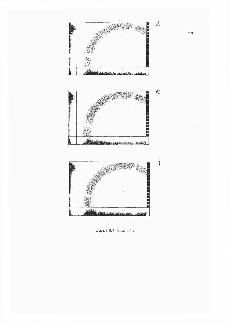
LM ______

236

’èM k

!

Figure 6.9 continued.

237

size should be reduced by a factor of two. Therefore, the fixed patterning displayed in

Figures 6.9 and 6.10 is from 2 to 4 times worse than that for an anode designed specifically

for the OM. These images should therefore be regarded as worse caê scenarios.

The images demonstrate that although the fixed patterning varies in severity, its

position remains constant. They also show that 12 bits are necessary to achieve a fixed

patterning level similar to the original data.

6.4 R atio m etric ADCs

In ratiometric ADCs, the reference is driven by a varying voltage. The digital

output is directly proportional to the ratio of the magnitude of the input to the magnitude

of the varying reference signal at the time of conversion.

Ratiometric ADCs offer a potential major advantage over fixed reference ADCs for fixed patterning. If the reference is driven with the sum oi x, y and z, then the data will

be immediately normalized with respect to pulse height and all the data will be projected

into one pulse height plane. This has four important consequences.

1. Fixed reference ADCs require that the normalization is carried out after digitization

by a division by the sum of the three ADCs. At present, this is carried out in software

as a floating point operation. In an actual realtime system used on the satellite,

this division would most probably be carried out as a integer division. This would

require either an Arithmetic Logic Unit (ALU) or look-up-table (LUT). In either

case, it represents extra electronics that are not required for ratiometric ADCs. Also

normalization by division with digitized values is itself, a source of fixed patterning

(Koike & Hasegawa, 1988, Geesman et al., 1991 and Phillips, 1992).

2. The number of lattice points will be constant for events with differing pulse heights,

so fixed patterning should be independent of the PHD and count rate.

3. The data can be normalized into a plane of the user’s choice by multiplying the

reference by a constant factor. For example, consider an 8 bit ADC, if

Qre/ = Qx + Qy-\r Qz , (6.25)

X + y + z = 255 , (6.26)

however, if

238

Qref — + Qy + Qz) j (6.27)

X + y z = 382 , (6.28)

where Qx is the output of the preamp for the x electrode etc. and Qref is the signal

driving the reference. As discussed in Section 6.2, selecting a plane with a higher h'

will reduce the fixed patterning. The limit on h' will be defined by the SNR on Qref

or Tiirf i .

4. If we substitute h’ into the expressions for the coordinate rotation, Equations 5.4 and

5.5, we obtain

^ - (z + 2y)) , (6.29)

y' — —ÿ=(3z — h') . (6.30)V6

As ratiometric ADCs normalize with respect to pulse height, h' is a constant. There

fore, for an ideal spiral, only 2 ratiometric ADCs are necessary per axis.

Figure 6.10 is similar to Figure 6.9 except that a ratiometric ADC has been sim

ulated with the original 14 bit data. In each case the normalized plane is

h’ = ^ 2 ^ - 1) . (6.31)

From the diagram it can be seen that a 10 bit ADC is needed to overcome fixed patterning.

This represents a 2 bit improvement over the fixed reference ADC, which corresponds to

the approximate expected pulse height dynamic range of 4.

The speed at which they can operate is limited by the analog bandwidth of the

reference bandwidth. The one dimensional SPAN detector for SOHO is evaluating Micro

Power Systems (1989) MP7683 8 bit, fiash ADCs in the ratiometric mode (Breeveld et al.,

1992). These are low power chips, «100 mW, and space qualified. SOHO’s count rate

requirement is 100 kHz, approximately half that of the OM. At this stage it appears that

these ADCs will meet the SOHO requirements but not the OM’s.

Ratiometric, 8 bit ADCs are available with higher reference analog bandwidths, for

example TRW’s (1991) TDC 1058 is rated at 5 MHz, and Analog Devices’ (1988) AD9002 at

10 MHz. These chips have higher power consumption, 600 mW and 750 mW, respectively

and it is not known if they are space qualified but they do demonstrate that ratiometric

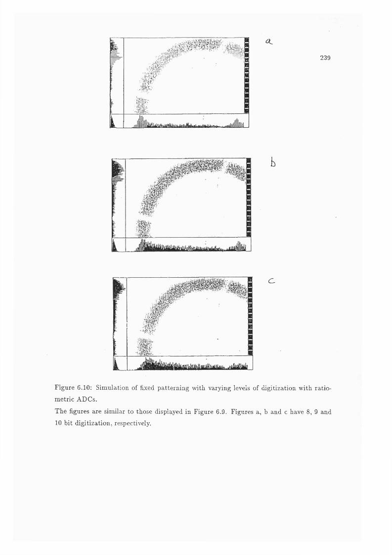
I

,irn

, inl

239

L

C

Figure 6.10: Simulation of fixed patterning with varying levels of digitization with ratio-

metric ADCs.

The figures are similar to those displayed in Figure 6.9. Figures a, b and c have 8, 9 and

10 bit digitization, respectively.

240

ADCs can meet the OM specification of 200 kHz, random. At present it appears that 8 bits

is the maximum for a fast, ratiometric capable ADC. However, the MP7683 and AD9002

have overflow signals so it is possible to combine two chips to obtain 9 bit digitization.

If the reference input is not linear with respect to pulse height, it will produce

variations in radius with respect to pulse height. It may be possible to overcome this

variation in a similar manner as described in Section 5.2.2. However, if only 2 ADCs are

used, the three dimensional xyz data has effectively been projected into the xy plane and is

therefore susceptible to the pulse height proportional shift of the spiral origin, as discussed

in Section 5.1.3. Figure 6.11 shows a simulation of nonlinear behaviour of the reference.

Using two ratiometric ADCs, this or any other pulse height related phenomenon

cannot be corrected. If pulse height related effects are significant and need to be corrected,

a third ADC is required. This ADC has to have a fixed reference in order to provide pulse

height information from the sum of QxiQy and Qg. In the software the pulse height has

always been divided into 256 channels which has always been sufficient to correct any pulse

height related effects. Therefore the third ADC requires a maximum of 8 bits.

6.5 Aliasing

In MCP based detectors, the image is hexagonally sampled by the MCP pores in

the front plate. This produces a resolution limit of approximately twice the pore spacing,

i.e. the Nyquist Limit. Any variation in the image with a spatial frequency higher than

this limit will cause aliasing.

A gap between two MCPs allows the charge cloud from the first MCP to spread

out and excite several pores in the back plate. Therefore, the charge cloud distribution from

the front plate is sufficiently sampled by the rear plate so that aliasing between the MCPs

does not occur.

Carter (1991a) has presented results of aliasing between 11 ^m pixels and pores

with a 15 ^m spacing, see Figure 6.12. As the SPAN detector is capable of resolving

the pores in the front plate and the dimensions are similar, aliasing could be a problem.

However, the degree of modulation of the fringes is dependent on the PSF of the centroiding

of the charge cloud. A finite PSF acts as a filter, reducing the power in the higher spatial

frequencies of an image and therefore, the power aliased into the Nyquist frequency range.

Figures 6.13 and 6.14 show results of a computer model of fringing between pores

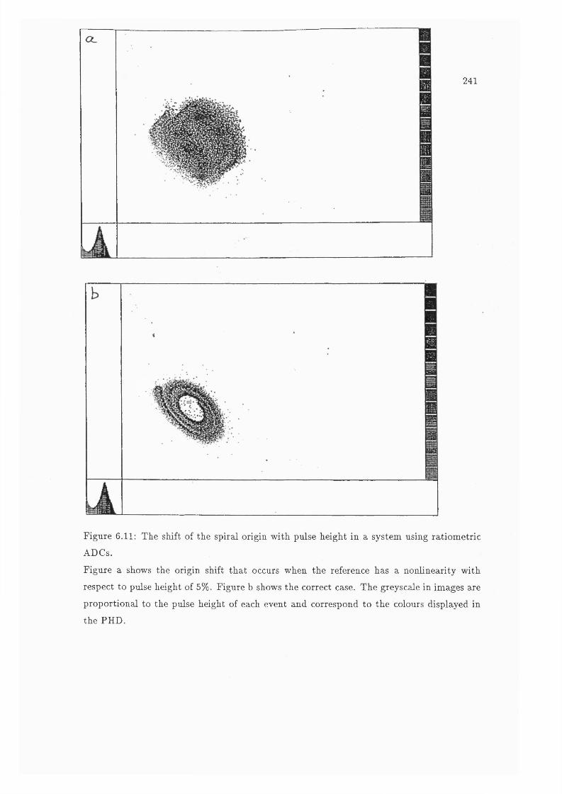
241

Figure 6.11: The shift of the spiral origin with pulse height in a system using ratiometric

ADCs.

Figure a shows the origin shift that occurs when the reference has a nonlinearity with

respect to pulse height of 5%. Figure b shows the correct case. The greyscale in images axe

proportional to the pulse height of each event and correspond to the colours displayed in

the PHD.

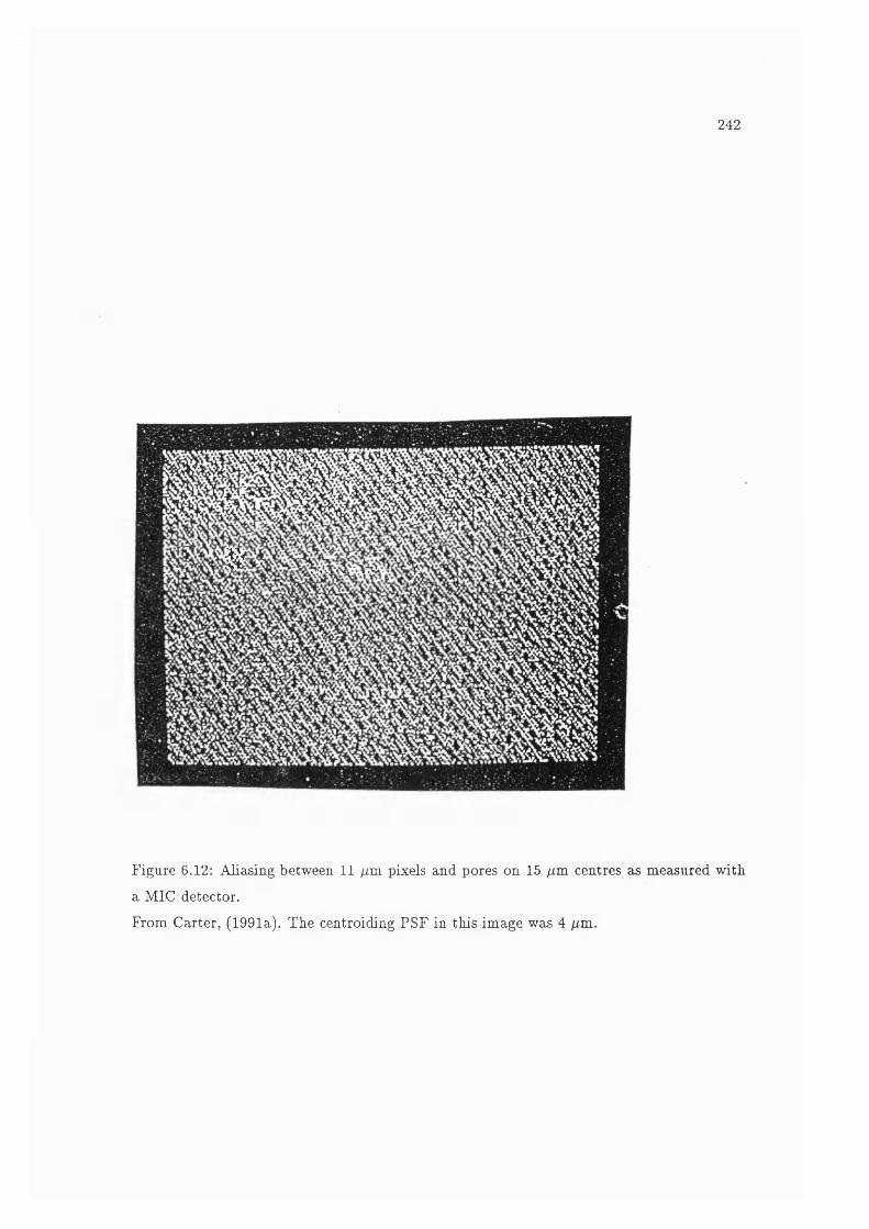
2 4 2

m

Figure 6.12: Aliasing between 11 fj,m pixels and pores on 15 /xm centres cis measured with,

a MIC detector.

From Carter, (1991a). The centroiding PSF in this image was 4 /xm.

243

and a 9 /xm pixel array (Smith, 1991). The fringing has been evaluated for the MCP we use

at present, 15 /xm pore spacing, and an MCP with approximately half the spacing, 8 /xm,

at a variety of centroiding PSFs. The figures show a 32 by 32 pore region of the MCP with

the pixel grid inclined at an angle of 5° to the MCP array, for both pore spacings. These

figures clearly demonstrate that larger PSFs reduce the intensity modulation of the fringes.

The only way to eliminate aliasing between the pores and the pixels is to have

pixels either over twice or less than half the width of the pore spacing. However, it is

possible that a broad enough centroiding PSF could reduce the intensity modulation of the

fringes to acceptable levels. The results of the model suggest that SPAN should not have

serious intensity modulation due to the aliasing for MCPs with either 15 or 8 /xm pore

spacing.

6.6 Chicken W ire Distortion

Several authors have reported a hexagonal modulation of intensity in flat field

images in MCP detectors (e.g. Siegmund et ai , 1989^ Barstow et al , 1990 & Vallerga et

al., 1991 ). As shown in Figure 6.15 this produces an image that looks similar to a chicken

wire fence.

This distortion is not due to digitization, but is thought to be caused by variations

in the behaviour of the MCP at the boundaries of the multi-fibre bundles. However, this

distortion would produce a variation in pixel sensitivity similar to fixed patterning. Val

lerga et al. (1991) report that the distortion is not always present in flat fields and suggest

that it might be due to the preconditioning of the plate.

Chicken wire distortion has not been observed with SPAN, however, we have not

carried out many long flat fields over a large portion of the MCP. As the distortion depends

on the two dimensional structure of the MCP and SPAN encodes the two dimensions inde

pendently, this problem, if present, cannot be overcome during the encoding. It could only

be corrected in the final image.

6.7 Possible Techniques for Reducing Fixed Patterning

Geesman et al. (1991) proposed a method for reducing fixed patterning due to

normalization with respect to pulse height for digitized data by tuning the shape of the PHD.

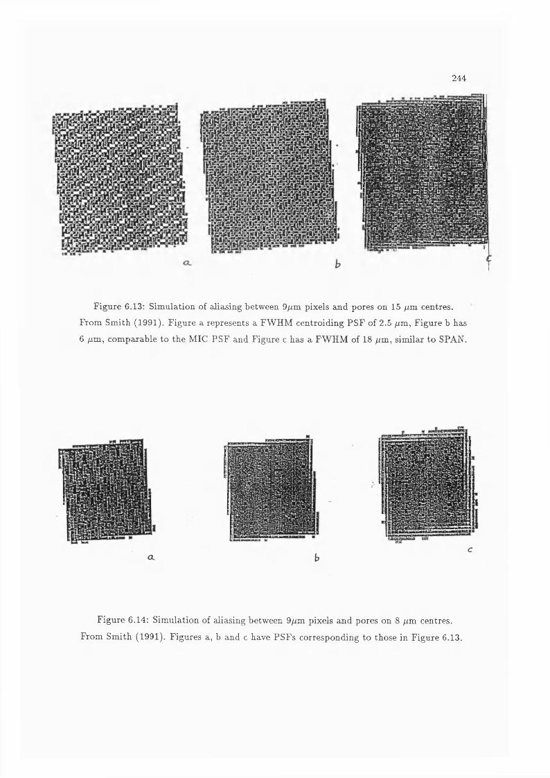
244

Figure 6.13: Simulation of alictsing between dfim pixels and pores on 15 fim centres.

From Smith (1991). Figure a represents a FWHM centroiding PSF of 2.5 /im, Figure b bas

6 /im, comparable to the MIC PSF and Figure c has a FWHM of 18 /im, similar to SPAN.

Figure 6.14: Simulation of aliasing between 9/im pixels and pores on 8 /im centres.

From Smith (1991). Figures a, b and c have PSFs corresponding to those in Figure 6.13.

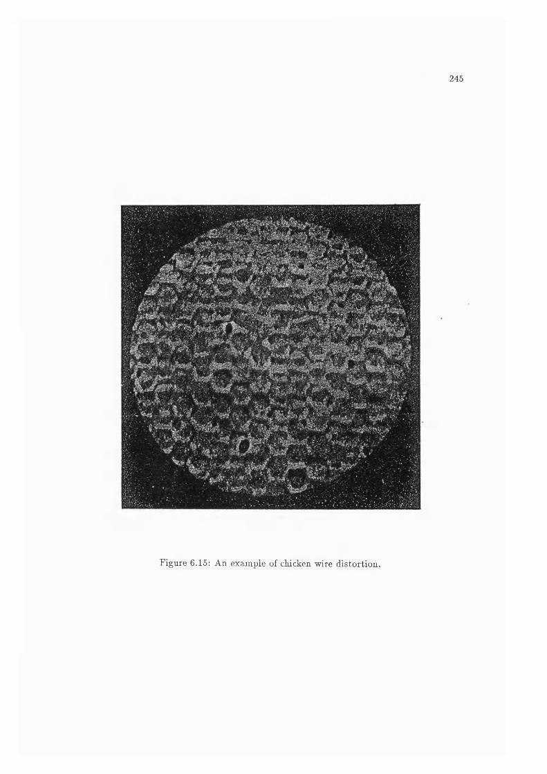
245

Figure 6.15: An example of chicken wire distortion.

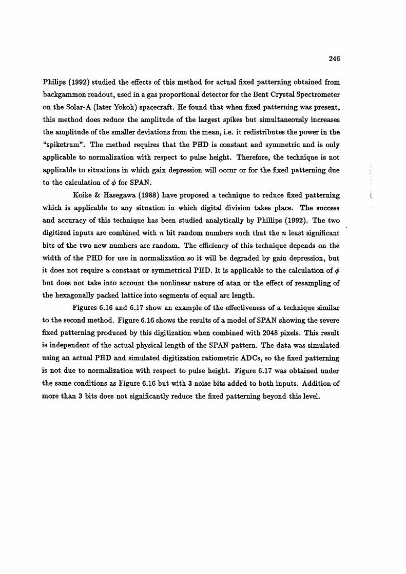
246

Philips (1992) studied the effects of this method for actual fixed patterning obtained from

backgammon readout, used in a gas proportional detector for the Bent Crystal Spectrometer

on the Solar-A (later Yokoh) spacecraft. He found that when fixed patterning was present,

this method does reduce the amplitude of the largest spikes but simultaneously increases

the amplitude of the smaller deviations from the mean, i.e. it redistributes the power in the

“spiketrum”. The method requires that the PHD is constant and symmetric and is only

applicable to normalization with respect to pulse height. Therefore, the technique is not

applicable to situations in which gain depression will occur or for the fixed patterning due

to the calculation of <f> for SPAN.

Koike h Hasegawa (1988) have proposed a technique to reduce fixed patterning

which is applicable to any situation in which digital division takes place. The success

and accuracy of this technique has been studied analytically by Phillips (1992). The two

digitized inputs are combined with n bit random numbers such that the n least significant

bits of the two new numbers are random. The efficiency of this technique depends on the

width of the PHD for use in normalization so it will be degraded by gain depression, but it does not require a constant or symmetrical PHD. It is applicable to the calculation of (f)

but does not take into account the nonlinear nature of atan or the effect of resampling of

the hexagonally packed lattice into segments of equal arc length.Figures 6.16 and 6.17 show an example of the effectiveness of a technique similar

to the second method. Figure 6.16 shows the results of a model of SPAN showing the severe

fixed patterning produced by this digitization when combined with 2048 pixels. This result

is independent of the actual physical length of the SPAN pattern. The data waa simulated

using an actual PHD and simulated digitization ratiometric ADCs, so the fixed patterning

is not due to normalization with respect to pulse height. Figure 6.17 was obtained under

the same conditions as Figure 6.16 but with 3 noise bits added to both inputs. Addition of

more than 3 bits does not significantly reduce the fixed patterning beyond this level.

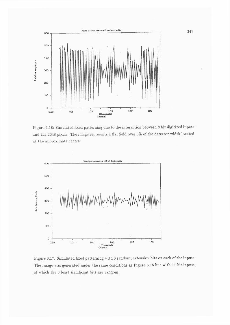
Flxod paUom rvoi»« witfyxjt coaocUon600

500 -

400 -

ICC

300 -

200 -

VDO -

109107103LOI

247

Channol

Figure 6.16; Simulated fixed patterning due to the interaction between 8 bit digitized inputs

and the 2048 pixels. The image represents a hat field over 5% of the detector width located

at the approximate centre.

Rxed pattern not** ♦ 3 bit oofrectîoo600

500 -

I 300 -;

200 -

XX) -

107 109103 IDSLOI(ThousaodslChannel

Figure 6.17: Simulated fixed patterning with 3 random, extension bits on each of the inputs.

The image was generated under the same conditions a.s Figure 6.16 but with 11 bit inputs,

of which the 3 least significant bits are random.

248

Chapter 7

T he Long R ange Interaction

B etw een Pores

7.1 In troduction

7 .1 .1 A djacency

The count rate performance of MCPs has been analysed extensively in terms of

the deadtime due to the recharge of the wall after the channel has fired. MCPs have been

analysed variously as paralysable (Nieschmidt et ai, 1982, Nicoli, 1985, Cho & Morris, 1988,

Cho, 1989, Fraser et ai, 1991b and Sharma & Walker, 1990, 1992) and non-paralysable de

tectors (Sharma & Walker, 1989,1992). The properties of paralysable and non-paralysable

detectors are discussed in Section 1.3.1.

In detectors containing two or more MCPs in the gain stage, the magnitude of the

gain depression at a given count rate is proportional to area of the region illuminated while

the sustainable count rate is inversely proportional to the area (Cho & Morris, 1988, Pear

son et a i, 1988, Cho, 1989, Naxtallo Garcia, 1990 and Fraser et ai, 1991b), see Figure 7.1.

This strongly suggests that there is some interaction between adjacent pores and that the

recharging of the active pores is dependent on their number. This effect has been called

“adjacency” (Sharma & Walker, 1989).

Adjacency effects are not present in single MCPs, for either straight or curved

channels, (Cho, 1989 and Fiaser et ai, 1991b). Statistical deadtime analysis by Cho (1989)

showed that each of the illuminated channels of a single C plate could be treated as an

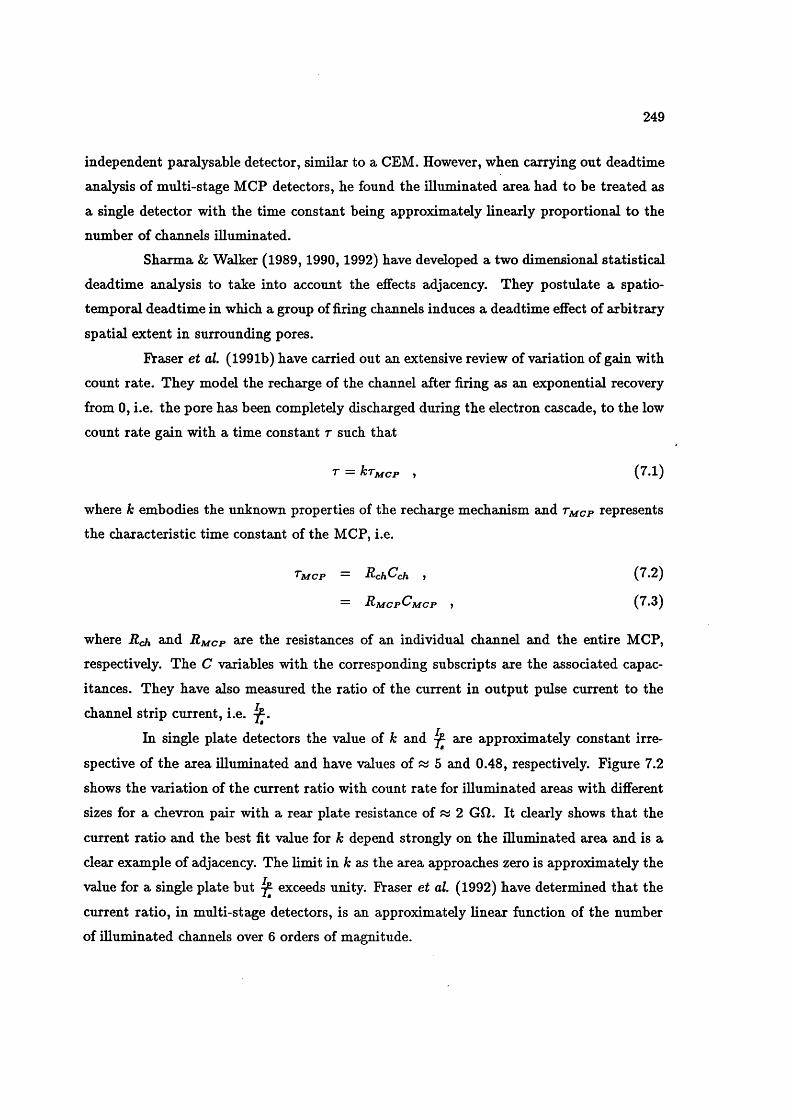
249

independent paralysable detector, similar to a CEM. However, when carrying out deadtime

analysis of mnlti-stage MCP detectors, he found the illuminated area had to be treated as

a single detector with the time constant being approximately linearly proportional to the

number of channels illuminated.

Sharma & Walker (1989,1990,1992) have developed a two dimensional statistical

deadtime analysis to take into account the effects adjacency. They postulate a spatio-

temporal deadtime in which a group of firing channels induces a deadtime effect of arbitrary

spatial extent in surrounding pores.

Fraser et al. (1991b) have carried out an extensive review of variation of gain with

count rate. They model the recharge of the channel after firing as an exponential recovery

from 0, i.e. the pore has been completely discharged during the electron cascade, to the low

count rate gain with a time constant r such that

r = kTj^cp t (7.1)

where k embodies the unknown properties of the recharge mechanism and Tmcp represents

the characteristic time constant of the MCP, i.e.

" MCP — ^ch^ch ) (7.2)

= H'MCP^MCP ? (7.3)

where Rch and R mcp are the resistances of an individual channel and the entire MCP,

respectively. The C variables with the corresponding subscripts are the associated capac

itances. They have also measured the ratio of the current in output pulse current to the

channel strip current, i.e.

In single plate detectors the value of k and ^ are approximately constant irre

spective of the area illuminated and have values of « 5 and 0.48, respectively. Figure 7.2

shows the variation of the current ratio with count rate for illuminated areas with different

sizes for a chevron pair with a rear plate resistance of « 2 Gfi. It clearly shows that the

current ratio and the best fit value for k depend strongly on the illuminated area and is a

clear example of adjacency. The limit in A; as the area approaches zero is approximately the

value for a single plate but ^ exceeds unity. Fraser et al. (1992) have determined that the

current ratio, in multi-stage detectors, is an approximately linear function of the number

of illuminated channels over 6 orders of magnitude.

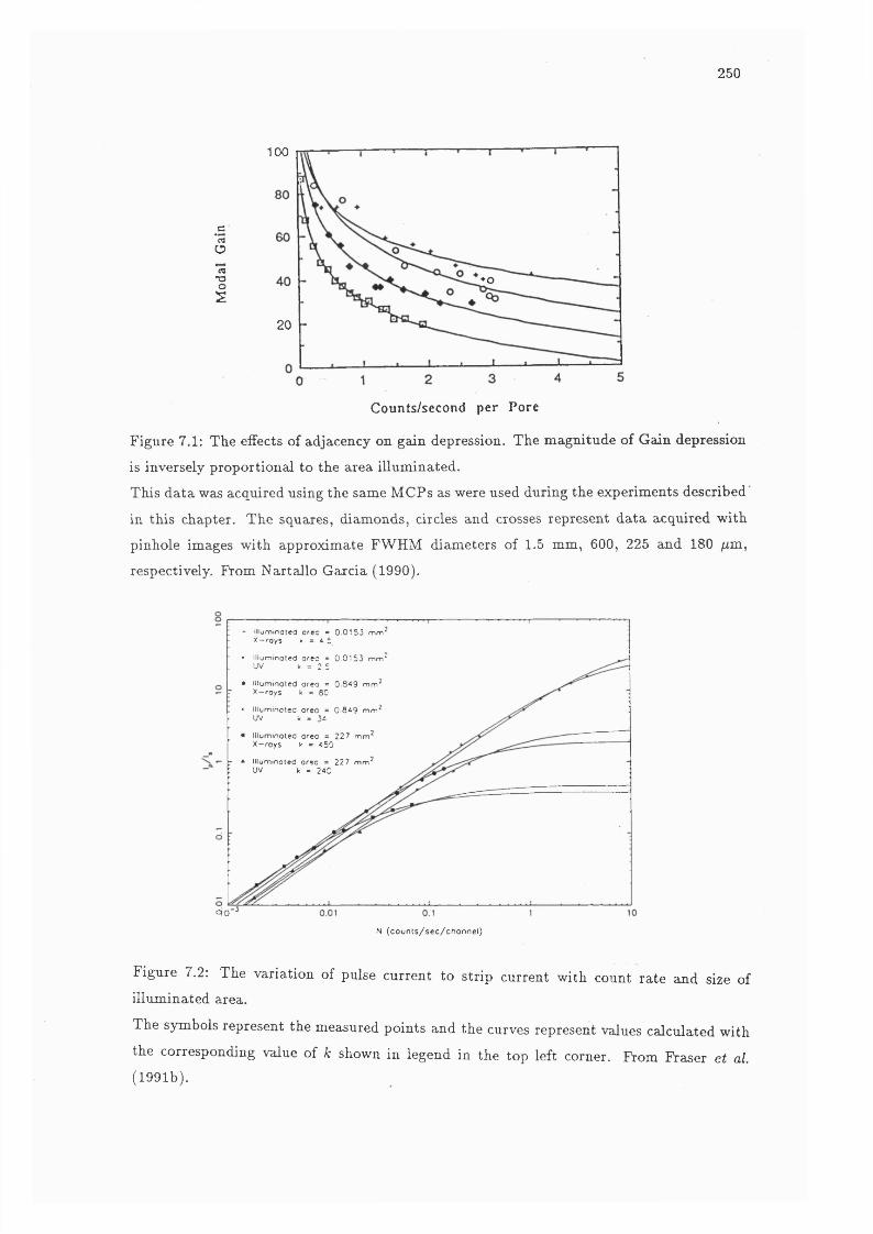
250

c*«Ü*rtT3Os

100

♦o

20

Counts/second per Pore

Figure 7.1: The effects of adjacency on gain depression. The magnitude of Gain depression

is inversely proportional to the area illuminated.

This data was acquired using the same MCPs as were used during the experiments described

in this chapter. The squares, diamonds, circles and crosses represent data acquired with

pinhole images with approximate FWHM diameters of 1.5 mm, 600, 225 and 180 /xm,

respectively. From Nartallo Garcia (1990).

• I llu m in a te d a r e c « 0 .0 1 5 3 m m ' X-royS k = 4.5• lllu m ln o te d o r e c « 0 .0 1 5 3 m m ‘

UV k = 2 .5

• lllu m in o te d o re o = 0 8 4 9 m m ^ X - r o y s k = 8 0

« Illu m in a te d a r e a = 0 .8 4 9 m m ^ UV k « 34

• Illu m in a te d a r e a = 22 7 m m ^ X - r a y s k « 4 5 0

- * Illu m in a te d a r e a = 2 2 7 m m ÛV k = 2 4 0

QO

N (c o u n ts /se c /c h o n n e l)

Figure 7.2: The variation of pulse current to strip current with count rate and size of illuminated area.

The symbols represent the measured points and the curves represent values calculated with

the corresponding value of k shown in legend in the top left corner. From Fraser et ai (1991b).

251

7 .1 .2 E ffects o f G ain D ep ression

The most obvious, and probably the most important effect of gain depression is

that as count rate per pore increases, the pulse heights of more of the events will lie below the

discriminator of the measuring electronics and those events will not be detected. Therefore,

the count rate linearity will be degraded progressively. In extreme cases, the gain may

be depressed so much that almost all of the PHD lies below the discriminator effectively

paralysing the pore.

Reduced gain also lowers the signal to noise ratio for charge measurement elec

tronics, reducing the spatial resolution of charge division readout devices, e.g. Figure 1.20.

As discussed in Chapter 5, SPAN has pulse height related position shifts. The

most serious problem is that gain depression will move a significant proportion of the PHD

into the nonlinear region of the radius/pulse height function and so it will be impossible to

reliably assign events to a spiral arm. Either the presence of ghosts must be tolerated or the

discriminator level must be raised, aggravating the problem of photometric nonlinearity.

Other readouts also suffer from the variation of gain. As discussed in Section 3.1,

variation of charge cloud size affects the positional linearity of the MIC and WSA detectors.

Position shifts of approximately 50 /zm have been observed for delay lines (Freidman et al., 1990) over the range in gain of 1—4 x 10^ e~ . Count rate dependent shifts of approximately

10 to 20 /im have been observed with the HRI (Zombeck & Fraser, 1991). Gain depression

can cause incorrect positional coding in the PAPA detector, producing spurious images

(Sams, 1991).

If active pores have a long range effect on their quiescent neighbours it could

pose a serious problem for the high speed operation of MCP based detectors. An intense

point source might paralyse a pore and reduce the resolution for any images in the area

surrounding it. Statistical analysis of data obtained with a MIC detector by Sharma (1991)

indicates that an event in a single channel causes a spatio-temporal deadtime which extends

into the group of 12 surrounding pores and causes them to remain inactive for 0.1 ms.

In an extreme case, a point source could paralyse a significant proportion of the

MCP. The situation would be much worse for an image containing many bright features or

a spectrum with many close lines. Sharma (1991) has also modelled the effect that a large

“deadradius” would have on speckle, images. He finds that once the deadradius becomes

comparable to the size of the speckle, the speckle peak maybe obscured in the image. Similar

252

effects were seen experimentally with an MCP based image intensifier.

Gain related position shifts could also be produced in the region near a bright

source. Friedman et al. (1990), using a two dimensional, transmission line, delay line

readout, have observed shifts of position of up to 40 ^m at distances of 400 |zm from a

bright source. At larger distances, smaller shifts were noticed. Gain depression with a

long range component is a possible mechanism eis their readout does have gain dependent

positional shifts of this scale.

In this chapter, the results of direct measurements of the effect of active pores on

quiescent, neighbouring channels are presented. These results were measured with a two

dimensional imaging detector and some of these results were the first such measurements

presented in the literature. Possible mechanisms are discussed in Section 7.7.

7.2 E xperim ental P rocedure

In order to investigate the long range effect of active pores on quiescent pores

we superimposed an intense source, concentrated on a small region, over a diffuse source

covering the majority of the active area of the MCP. A schematic of the experimental setup is

shown in Figure 7.3. The diffuse background illumination samples the gain in the quiescent

pores of the MCP. Provided that the interval between the arrival of these sampling events

at each individual pore is many times longer than the recharge time constant, i.e. many

seconds between events, the diffuse illumination will not cause gain depression.

The diffuse source was produced by illuminating a 50 ^m thick A1 mask with

5.9 KeV X-rays from an Fe®® source placed approximately 2 cm away. The A1 mask is not

completely opaque to X-rays at this energy and transmits approximately 4% of the incident

flux. The mask was placed 0.1 mm from the open face of the front MCP of a chevron pair.

The X-rays produced a count rate of approximately 500 Hz spread over most of the 25 mm

active diameter of the MCP. In the central region of the MCP this corresponds to an event

rate of 2.5 Hz.mm"^ or less than 2 counts.pore~^.hour“ .

The intense count rate was produced by illuminating the MCP through a 100 /zm

pinhole, in the centre of the A1 mask, with UV light from a Hg lamp placed about 2 m away.

The UV lamp had a fused silica envelope, therefore the MCP was illuminated mainly by

light from the 253.7 nm Hg line. The intensity of the UV radiation was varied by moving

the lamp with respect to the MCP.

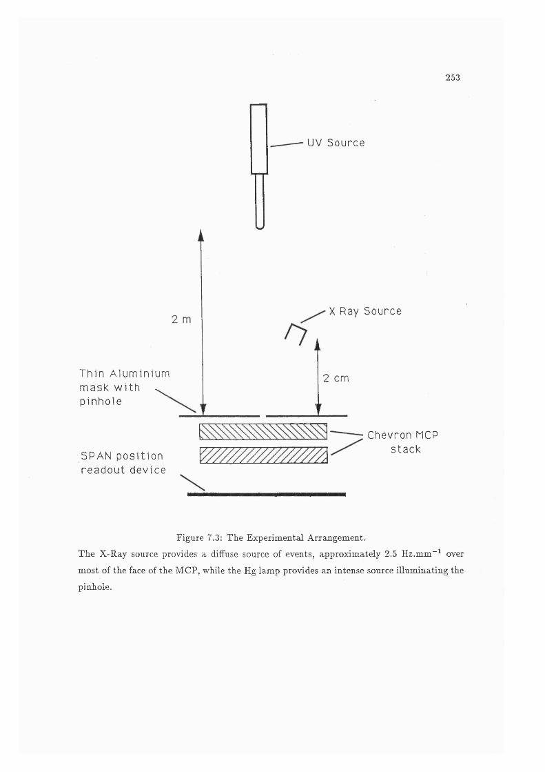
253

UV S o u r c e

X Ray S o u r c e

Thi n A l u m i n i u m m a s k w i t h ^ p i n h o l e

2 cm

SPAN p o s i t i o n r e a d o u t d e v i c e

Chevron MCP s t a c k

Figure 7.3: The Experimental Arrangement.

The X-Ray source provides a diffuse source of events, approximately 2.5 Hz.mm~^ over

most of the face of the MCP, while the Hg lamp provides an intense source illuminating the

pinhole.

254

It is worth emphasising that this arrangement enabled the intensities of the sam

pling events and those causing gain depression to be independently varied. It allowed the

quiescent gain in the region to be measured immediately before or after intense point source

illumination and so provided a control. This was deemed to be a very important aspect in

the design of the experiment as there was no a priori knowledge of the scale length over

which the interaction between pores would act and only vague assumptions about the man

ner in which it would manifest itself. It also allowed the removal of any variation in the

gain across the face of the MCP that was already present.

As adjacency appears as a count rate related phenomenon, one of the criteria

chosen for deciding that any long range effect was actually caused by interaction between

channels, was that the magnitude of effect should be dependent on the intense point source

count rate. If the diffuse and point source intensities are coupled, they will vary together and

any effects caused by increased intensity of sampling events could mistakenly be assumed

to be due to the interaction between channels.

7.2 .1 M C P C onfiguration

The MCP stack consisted of two, 36 mm diameter, 80:1 length to diameter ratio,

Phillips plates with 12.5 pm pores on 15 pm centres and a measured resistance R mcp — 640 Mft. The capacitance of the MCPs has been calculated using the method described by

Fraser et al. (1991b), as Cmcp = 15 pF, therefore t^ cp ^ 10 ms. The MCPs have an open area ratio of 63% with « 5100 pores.mm"^. The plates had a bias angle of 13° and were arranged as a chevron pair with a 190 pm inter-plate gap. The voltage across this gap was

held at 0 V. The MCP-anode gap was defined by three 6 mm diameter spacers separated

by 120°. Therefore, both the front and the back of the MCP are open to vacuum. During

all of the experiments described in this chapter, the anode gap and the applied voltage were

held constant at 4.7 mm and 400 V, respectively.

The MCPs had been baked for 6 days at temperatures ranging from 200° to 240° C

and scrubbed, extracting ~ 3 x 10“® C.s“ ^.cm“ for 5.5 x 10 s. They have been cycled

from vacuum to air on many occasions. Immediately prior to the experiment the MCPs

were held at a pressure of 10“® Torr for a week and were kept at this pressure throughout

the experiment. The vacuum pump was an oil diffusion pump without a cold trap.

255

7 .2 .2 R ead ou t and E lectron ics

The readout device was the two dimensional version of SPAN. The position co

ordinates were used to assign the event to one of 64 annuli of equal area, centred on the

pinhole. All events lying outside of these anmdi were discarded. Pulse height was determined

from the sum of the charge measured on the six SPAN electrodes and was used to construct

256 channel PHDs for each annulus.

The electronics chain for each channel consisted of a charge-integrating preamp,

shaping amp and 14 bit Wilkinson ADC. With Wilkinson ADCs, conversion time depends

on the size of the digital output code for each event. The maximum conversion time of the

ADCs at full 14 bit digitization is rv 37 //s giving a 10% coincidence loss at 2.7 kHz. In

practice, the amplitude of the events is such that they are digitized to only approximately

half of the full ADC range. The time constant on the shaping amp was 2 /xs. Even allowing

for a decay time of 10 time constants, the dominant contribution to the deadtime was the

ADC conversion time.

7 .2 .3 Softw are

The software used was the same as that described in Section 5.6. For each of the

measurements, 1 million events were acquired with x^y co-ordinates and pulse height being

determined for every point. After the acquisition was complete the image was divided into

64 a-uTinli of equal area, centred on the position of peak intensity of the pinhole. Constant

area a-nTinli were chosen to keep the number of events per annulus approximately equal.

Pulse height distributions (PHDs) were obtained for each annulus.

Saving each event’s position and pulse height on the hard disk placed a severe

constraint on the number of events that could be acquired. The hard disk only had a

capacity of 60 MB and each event required 22 bytes of storage. This effectively limited the

total number of events to about 1 million. Also, as no selection was made on which events

were stored during acquisition, these events were distributed over the full active diameter of

the MCP. This limited the number of counts in each PHD to 300, which was insufficient

for good statistics.

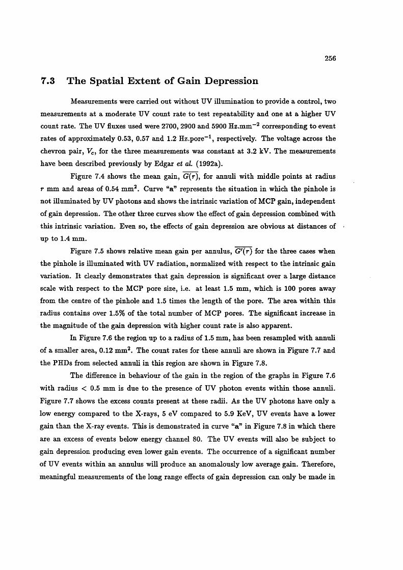
256

7.3 T he Spatial E xten t of Gain Depression

Measurements were carried out without UV illumination to provide a control, two

measurements at a moderate UV count rate to test repeatability and one at a higher UV

count rate. The UV fluxes used were 2700, 2900 and 5900 Hz.mm“ corresponding to event

rates of approximately 0.53, 0.57 and 1.2 Hz.pore"^, respectively. The voltage across the

chevron pair, for the three measurements was constant at 3.2 kV. The measurements

have been described previously by Edgar et al. (1992a).

Figure 7.4 shows the mean gain, G(r), for annuli with middle points at radius

r mm and areas of 0.54 mm^. Curve “a” represents the situation in which the pinhole is

not illuminated by UV photons and shows the intrinsic variation of MCP gain, independent

of gain depression. The other three curves show the effect of gain depression combined with

this intrinsic variation. Even so, the eflects of gain depression are obvious at distances of up to 1.4 mm.

Figure 7 .5 shows relative mean gain per annulus, G'{r) for the three cases when

the pinhole is illuminated with UV radiation, normalized with respect to the intrinsic gain

variation. It clearly demonstrates that gain depression is significant over a large distance

scale with respect to the MCP pore size, i.e. at least 1 .5 mm, which is 100 pores away

from the centre of the pinhole and 1 .5 times the length of the pore. The area within this

radius contains over 1 .5 % of the total number of MCP pores. The significant increase in

the magnitude of the gain depression with higher count rate is also apparent.

In Figure 7 .6 the region up to a radius of 1 .5 mm, has been resampled with annuli

of a smaller area, 0 .1 2 mm^. The count rates for these a n n u l! are shown in Figure 7 .7 and

the PHDs from selected annuli in this region are shown in Figure 7 .8 .

The difference in behaviour of the gain in the region of the graphs in Figure 7 .6

with radius < 0 . 5 mm is due to the presence of UV photon events within those annuli.

Figure 7 .7 shows the excess counts present at these radii. As the UV photons have only a

low energy compared to the X-rays, 5 eV compared to 5 .9 KeV, UV events have a lower

gain than the X-ray events. This is demonstrated in curve “a” in Figure 7 .8 in which there

are an excess of events below energy channel 80 . The UV events will also be subject to

gain depression producing even lower gain events. The occurrence of a significant number

of UV events within an annulus will produce an anomalously low average gain. Therefore,

meaningful measurements of the long range effects of gain depression can only be made in

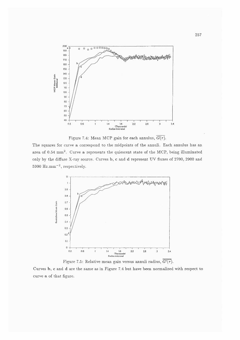
2 5 7

200

190 -

180 -

170 -

150 -

150 -

140 -

130 -

120 -

110 -

100 -

90 -

80 -

70 -

60 -

50 -

40

3.40.2 0.6 14 18 2.2 2.6 3(Thouaands)

Radius ImicronsI

Figure 7.4: Mean MCP gain for each annulus, G{r).

The squares for curve a correspond to the midpoints of the annuli. Each annulus ha an

area of 0.54 mm^. Curve a represents the quiescent state of the MCP, being illuminated

only by the diffuse X-ray source. Curves b, c and d represent UV fluxes of 2700, 2900 and

5900 Hz.mm“ , respectively.

0.9 -

0.8 -

.9<3II

0.7 -

1 0.4 -

0.3 -

0.1 -

0.6 I0.2 14 18 26 3 3.4(Thouaandsl

Radius ImicronsI

Figure 7.5: Relative mean gain versus annuli radius, G'{r).

Curves b, c and d are the same as in Figure 7.4 but have been normalized with respect to

curve a of that figure.

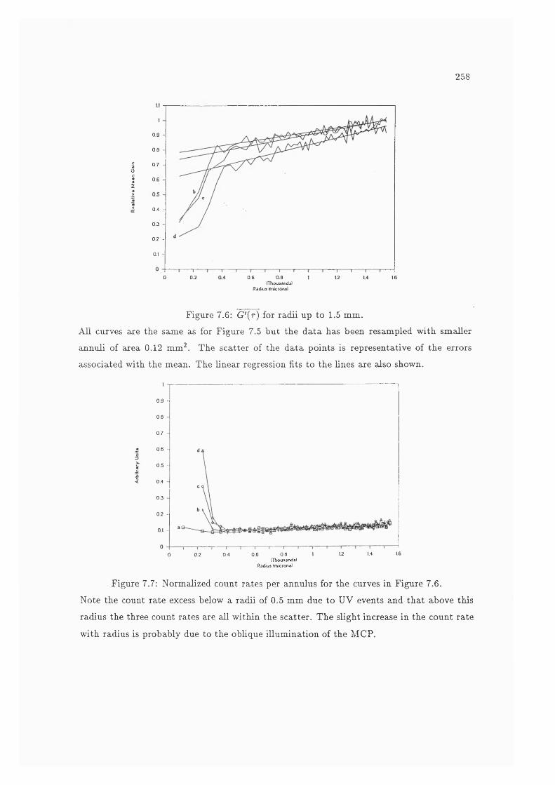
258

0 .9 -

0.8 -

JI.>

0.7 -

0.6 -

s 0.4 -

0.3 -

0.2 -

0.1 -

0 0.2 0,6 0.8 12 14 1.6(Thousandj)

Radius ImicronsI

Figure 7.6: G'{r) for radii up to 1.5 mm.

All curves are the same as for Figure 7.5 but the data has been resampled with smaller

annuli of area 0.12 mm^. The scatter of the data points is representative of the errors

associated with the mean. The linear regression fits to the lines are also shown.

0 .9 -

0 8 -

0 .7 -

0.6 -

0 .5 -«

< 0.4 -

0 .3 -

0.2 -

0.1 -

161.2 1.40.6 0.80.2 0.40(Thousands!

Radius ImicronsI

Figure 7.7: Normalized count rates per annulus for the curves in Figure 7.6.

Note the count rate excess below a radii of 0.5 mm due to UV events and that above this

radius the three count rates are all within the scatter. The slight increase in the count rate

with radius is probably due to the oblique illumination of the MCP.

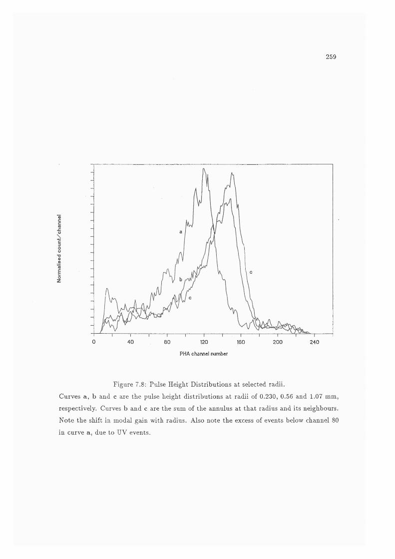
259

0 40 80 120 160 200 240

PHA channel number

Figure 7.8: Pulse Height Distributions at selected radii.

Curves a, b and c are the pulse height distributions at radii of 0.230, 0.56 and 1.07 mm,

respectively. Curves b and c are the sum of the annulus at that radius and its neighbours.

Note the shift in modal gain with radius. Also note the excess of events below channel 80

in curve a, due to UV events.

260

Curve UV Flux Gradient k Offset G'(0)Hz.mm"^ mm~^

b 2700 0.149 0.772c 2900 0.182 0.722d 5900 0.233 0.602

Table 7.1: Fit parameters for relative mean gain versus radius curves in Figure 7.6 param

eters are the same as in Equation 7.4.

the absence of UV events and so we restricted our study to radii greater than 0.5 mm.

We were able to obtain good linear regression fits for G \r ) for radii in the range

0.5 to 1.5 mm. The fits are of the form

Gî'(r) = -h G'(0) . (7.4)

where k is the gradient in mm~^. The fits are shown in Figure 7.6 and the fit parameters are given in Table 7.1.

The linear fits showed that the long range gain depression (LRGD) decreased

linearly with radius, at least over the range 0.5 to 1.5 mm. Also the two measurements

carried out with comparable UV fiuxes, cases “b ” and “c” have similar gradients and

offsets, while the higher count rate caae has, as expected, lower value for G'(0) and a

steeper gradient indicating larger gain depression.

Fraser et al. (1992) have carried out similar measurements with Philips MCPs of

identical resistance and geometry. They also find that gain depression has long range effects

and that the “zone of influence” extends over the range of 1.5-2.0 mm.

7.4 M easurem ents of th e Long Range Effects of Gain Depression

Another series of measurements was made to further study the effects of LRGD.

Measurements were made with illuminated regions with two different geometries; the pin

261

hole, as described in Section 7.2 and a ring.

The X-ray event rate was reduced to 1 Hz.mm"^ in order to reduce the prob

ability of the sampling events interacting with each other. An area of at least 7 mm^ is

affected by the illumination of the pinhole and it was assumed that a similar area would

be affected by the group of pores fired by one photon. At an event rate of 1 Hz.mm“ and

given that Tmcp ~ 10 ms, at least 7 % of sampling events will occur in the affected area of

another, earlier sampling event within one Tmcp of the earlier event’s arrival.

Immediately prior to the experiments the MCPs were held at a pressure of 5 x 10~^ Torr

for at least a week and were kept at this pressure throughout the experiments.

7 .4 .1 F urther M easu rem en ts w ith th e P in H ole

As the characteristic scale of LRGD had been determined, a set of annnli for use

in the further experiments could be pre-selected. Once again, 64 annuli were chosen. The

size of the annuli selected varied slightly for each of the three plate voltages. The radius

of the 64th. annulus was approximately 1.8 mm for plate voltages of 3.0 and 3.1 kV and

2.1 mm for 2.9 kV. These radii correspond to an area of approximately 0.22 and 0.16 mm^

per annulus, respectively.

Approximately 1000 contiguous events were acquired at a time, then all the po

sition decoding calculations for each event were carried out. If an event lay within one of

the pre-selected annuli, the corresponding PHD was incremented and events lying outside

the set of annuli were discarded. Then another 1000 events were acquired and the process

repeated. Only the 64 PHDs were stored. This had the advantage that it required only a

small amount of memory for each measurement, i.e. 64 kB, but meant that the data could

not subsequently be binned into a different set of annuli.

In a typical flat field measurement, i.e. with no UV illumination of the pinhole, a

6 hour integration was carried out, in which data was acquired for a total of approximately

4 hours. During a flat field integration, approximately 10^ events were incident on the MCP

of which about 1% were assigned to one of the annuli, i.e. approximately 1500 counts per

annulus. When the MCP was illuminated, the deadtime associated with the calculations

required longer integration times, typically 7 to 8 hours, to acquire the same number of

events in the non-illuminated annuli.

Count rates were determined by counting the busy signal on one of the shaping

262

amplifiers. Therefore, the absolute UV flux through the pinhole is not known, due to pile- up events in the shaping stage or due to very small pulse height events caused by gain

depression. However, this method is much more sensitive, at higher count rates, than that

used in the measurements described in Section 7.3, i.e. counting the events lying above the

ADC LLD. Therefore, similar, quoted count rates in the two sections do not correspond to

the same flux levels. Both sets of count rates represent lower limits on the UV flux but the

rates quoted in Section 7.3 will underestimate the flux to a larger extent than those in the

rest of this chapter.Ghosting is a problem for these measurements. When gain depression occurs many

events lie in the nonlinear region of the fn /h ' relationship and so are mapped into the wrong

spiral arm, see Section 5.2.2. This reduces the photometric linearity in the gain depressed

regions. However, the vast majority of the ghosted events are low pulse height events, so

ghosting leads to an underestimate of gain depression. There is very little ghosting when

using just X-ray illumination, the data set used as the example throughout Chapter 5 was

obtained during this set of measurements. The ghosts of the measured region are mapped

into a region of the image that lies far outside the set of annuli and so they do not corrupt

the data sets. Any events mapped into the set of a n n u l i are from unaffected regions of

the MCP and so will only lead to a slight underestimate of the magnitude of any gain

depression.

The region illuminated in these measurements was exactly the same as that which

was illuminated in Section 7.3. The new measurements were made approximately 5 months

after the earlier measurements. During that time the MCPs had undergone several cycles

from vacuum to air and had also been exposed to laboratory air for several weeks.

7 .4 .2 M easu rem en ts w ith a R in g

In order to investigate the interaction between more than one illuminated region

we also illuminated the MCP with UV photons through an annulus. I shall henceforth refer

to this annulus as a ring in order to distinguish it from the annuli that sample the PHDs

at various radii. An image of one quadrant of the ring can be seen in the figures showing

the simulated effects of different levels of digitization on fixed patterning, i.e. Figures 6.9

and 6.10.

When choosing the radius of the ring, a compromise had to be struck between

263

making the ring large enough so that not all of the interior would be illuminated by scattered UV light and that a point on the ring would be close enough to interact with most other

points on the ring. The ring had an interior radius of 0.9 mm and a width of 100 //m and

was laser machined into a 50 /im A1 sheet, waa the pinhole. Typical integration times

for the images were 7 hours and 12 hours for flat fields, both yielding %500 counts in the

annuli inside the ring.

The software for the ring measurements was similar to that used for the pinhole

experiments except that 128 a.nmdi were used, 64 inside the ring and 64 outside. The annuli

were aligned with respect to the ring by selecting 16 points, distributed around the internal

circumference of the image of the illuminated ring, from which a statistical estimate of the

ring centre and radius were determined. The outer radius of the 64th. annulus and that

of the 128th. annulus always corresponded to the estimate of the ring internal radius and

3 times that estimate, respectively. The 64 annuli inside the ring all have equal areas and

those outside the ring internal radius also have constant areas, 8 times those inside the ring.

7.5 Dynam ic, Long Range Gain Depression

Figure 7.9 shows the mean gain, G(r), for each annulus with a middle point at a radial distance of r mm from the centre of the pinhole for 3 different plate voltages. This

data represents the intrinsic gain variation of the MCP and was obtained only with the

diffuse X ray, sampling illumination. The saturations for each plate voltage are similar to

those quoted in Section 7.6.2.

I shall use the term “dynamic LRGD” to refer to the LRGD in an area surrounding

a group of pores which are undergoing intense UV illumination but not including the gain

depression in the UV illuminated channels themselves.

Figure 7.10 shows the relative mean gain, G '(r), when the pinhole was illuminated

with UV at various count rates. The gains have been normalized with respect to the

corresponding G{r) curves in Figure 7.9.

Figure 7.10d shows the G \r ) curve obtained at 3.0 kV at a UV count rate of

4.5 kHz. As we observed previously, the G’{r) curve consists of three regions. Beyond a

radius of approximately 1.6 mm, the curve appears to reach a plateau. The curve is linear

with respect to radius between this point and r « 0.6 mm. Below this point the curve

diverges sharply from the gradient in the linear region. The curves show the same overall

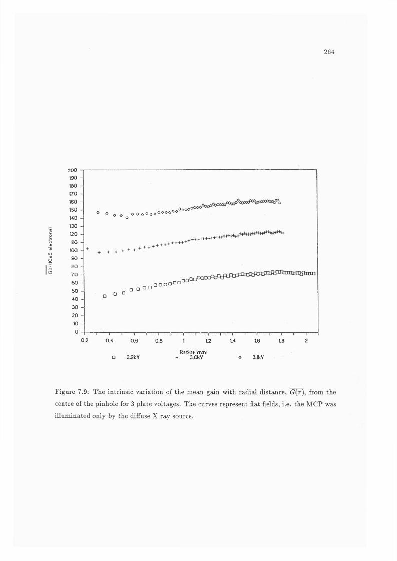
2 6 4

20 0 - |

190 -

180 -

T70 -

160 -

150 -

MO -

130 -co 120 -oo IK) -"* K)0 -(Og 90 -

s 6 0 -o 7 0 -

6 0 -

5 0 -

4 0 -

3 0 -

2 0 -

W -

0 -

^ o o o ^ o o o o o o ^ o o o ^ Ô o o o '

.OCL

+ + - H - H + 4 + + ^

□ O □ □ □ □ □ o o o ° ° □qOO

0J2 OA 0.6

Z9kV

0.8 12RacCu# (nvnJ

+ 3.0kY

14 16

3.1kV

1-----1-----r18 2

Figure 7.9: The intrinsic variation of the mean gain with radial distance, G(r), from the

centre of the pinhole for 3 plate voltages. The curves represent flat fields, i.e. the MCP was

illuminated only by the diifuse X ray source.

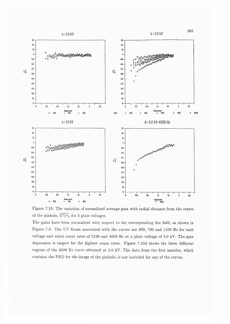
a:2,9kV b:10kV265

|0+(OJ -OJ -

07 -li

Oi -

O J -

OJ ■

040 Of u t 2.412Q 300 * 700

07-li

QJS -

04 -

O J-

0 1 -

12 \t 2 240 04 01IDO 300 700 XOO COO 200 r «00

C:3.1kV d;3.0 kY:4500Hz

02 -OS -

OS -

05-

OJ-

0 OS 2412 U 20 500

ta iu iM♦ 700 no

02 -02 -07-

15

04-

02-01-

0 01 12 IS 2 24tjéaM

T 4500

Figure 7.10: The variation of normalized average gain with radial distance from the centre

of the pinhole, G'(r), for 3 plate voltages.

The gains have been normalized with respect to the corresponding flat field, as shown in

Figure 7.9. The UV fluxes associated with the curves are 300, 700 and 1100 Hz for each

voltage and extra count rates of 2100 and 4500 Hz at a plate voltage of 3.0 kV. The gain

depression is largest for the highest count rates. Figure 7.10d shows the three different

regions of the 4500 Hz curve obtained at 3.0 kV. The data from the first annulus, which

contains the PHD for the image of the pinhole, is not included for any of the curves.

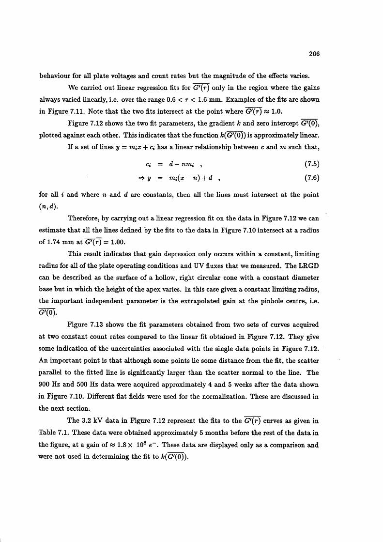
266

behaviour for all plate voltages and count rates but the magnitude of the effects varies.

We carried out linear regression fits for G \r ) only in the region where the gains

always varied linearly, i.e. over the range 0.6 < r < 1.6 mm. Examples of the fits are shown

in Figure 7.11. Note that the two fits intersect at the point where G \r ) « 1.0.

Figure 7.12 shows the two fit parameters, the gradient k and zero intercept C7'(0),

plotted against each other. This indicates that the function A;(G'(0)) is approximately linear.

If a set of lines y = rriiX -)- c,- has a linear relationship between c and m such that,

Ci = d - nrrii , (7.5)

y = m,(x — n) + d , (7.6)

for all i and where n and d are constants, then all the lines must intersect at the point(n,d).

Therefore, by carrying out a linear regression fit on the data in Figure 7.12 we can

estimate that all the lines defined by the fits to the data in Figure 7.10 intersect at a radius

of 1.74 mm at G'{r) = 1.00.

This result indicates that gain depression only occurs within a constant, limiting

radius for all of the plate operating conditions and UV fluxes that we measured. The LRGD

can be described as the surface of a hollow, right circular cone with a constant diameter

base but in which the height of the apex varies. In this case given a constant limiting radius,

the important independent parameter is the extrapolated gain at the pinhole centre, i.e.G'(0).

Figure 7.13 shows the fit parameters obtained from two sets of curves acquired

at two constant count rates compared to the linear fit obtained in Figure 7.12. They give

some indication of the uncertainties associated with the single data points in Figure 7.12.

An important point is that although some points lie some distance from the fit, the scatter

parallel to the fitted line is significantly larger than the scatter normal to the line. The

900 Hz and 500 Hz data were acquired approximately 4 and 5 weeks after the data shown

in Figure 7.10. Different flat fields were used for the normalization. These are discussed in

the next section.

The 3.2 kV data in Figure 7.12 represent the fits to the G'{r) curves as given in

Table 7.1. These data were obtained approximately 5 months before the rest of the data in

the figure, at a gain of « 1.8 x 10® e~. These data are displayed only as a comparison andwere not used in determining the fit to A;(G'(0)).

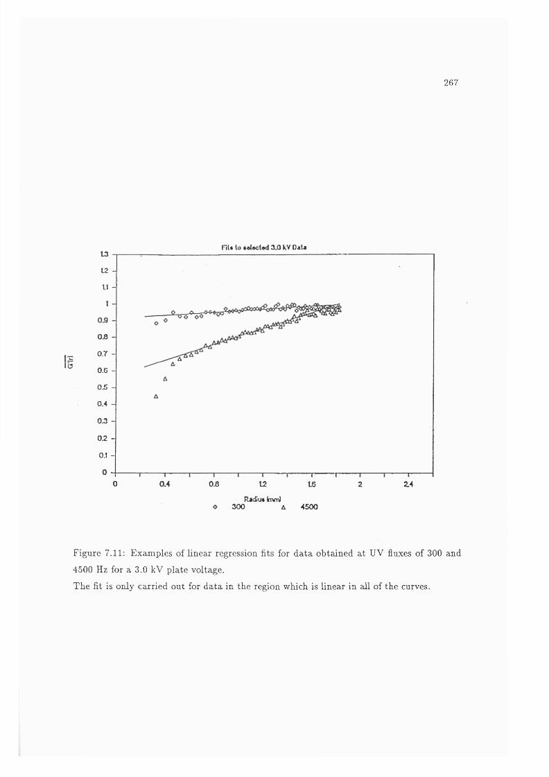
26 7

Fil, lo 3.0 kV OaU

lO

12 -

11 -

0.7 -

0.6 -

0.5 -1

0.4 -

0.2 -

0.1 -

0 120.8 t5 2 2.4

R jk£u« knm l 300 A 4500

Figure 7.11: Examples of linear regression fits for data obtained at UV fluxes of 300 and

4500 Hz for a 3.0 kV plate voltage.

The fit is only carried out for data in the region which is linear in all of the curves.

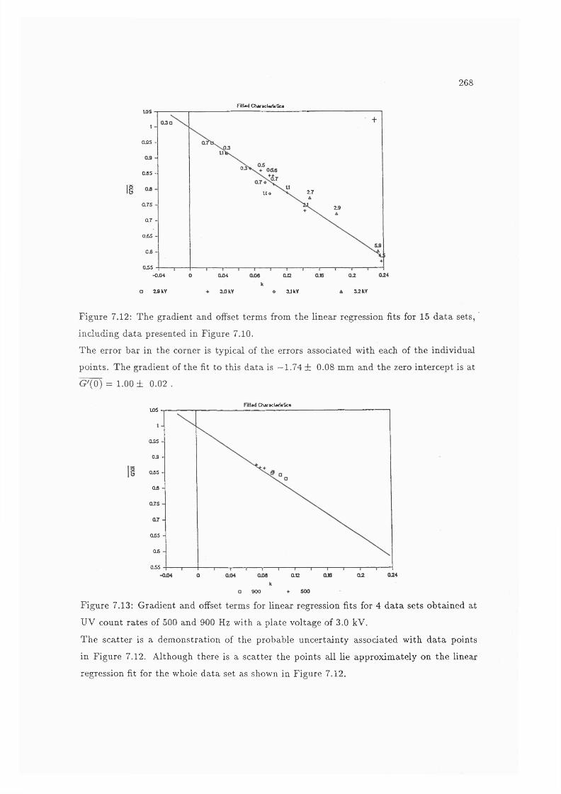
268

F%W CharacUfUOe*tos

OS5 -

O J065 -

11 2.7U «

075 - 2j9

0 7 -

Qj55 -

0 5 -

055-OJM 0 QJZ004 OQ

a Z8kY OOkY 3JkY 0 2 kY

Figure 7.12: The gradient and offset terms from the linear regression fits for 15 data sets,

including data presented in Figure 7.10.

The error bar in the corner is typical of the errors associated with each of the individual

points. The gradient of the fit to this data is —1.74 ± 0.08 mm and the zero intercept is at

G'(0) = 1.00 ± 0.02 .

ChiracUn«Gc«105

035 -

0 3 -

065 -

08 -

065 -

06 -

0550 20 Ot2

900

Figure 7.13: Gradient and offset terms for linear regression fits for 4 data sets obtained at

UV count rates of 500 and 900 Hz with a plate voltage of 3.0 kV.

The scatter is a demonstration of the probable uncertainty associated with data points

in Figure 7.12. Although there is a scatter the points all lie approximately on the linear

regression fit for the whole data set as shown in Figure 7.12.

269

The linear nature of the data in Figure 7.12 shows that the limiting radius of the

gain depression does not vary significantly over a factor of 3 in gain, an order of magnitude

in UV flux, a long period of time or cycling the MCPs between air and vacuum.

Figure 7.12 also shows that the magnitude of the gain depression varies mono-

tonically with UV flux. Although C7'(0) varies monotonically with flux, it is not always

monotonie when flux and plate voltage are considered together. Gain depression appears

to be monotonie with plate voltage at a UV flux of 300 Hz, but at higher fluxes it reaches a

maximum at 3.0 kV and reduces at 3.1 kV. This is also the case for 3.2 kV when compared

to the high flux measurements.

7.5 .1 M easu rem en ts o f th e D yn am ic, L ong R ange G ain D ep ression w ith

th e R in g

The ring was used to observe the behaviour of the LRGD when the MCP was

illuminated by an extended image. Figure 7.14 shows the G'{r) and relative count rates

as measured at various radii. The relative radius refers to the ratio of the annuli radius

to the interior radius of the ring. The relative gains and count rates were determined by

normalization with respect to a flat field, acquired separately, consisting solely of X-ray

events. To allow for small variations in the acquisition times of the various data sets, the

count rates were normalized with respect to the count rate in the 128th. annulus.

A count rate significantly greater than 1 indicates the presence of UV events.

Unfortunately, all the PHDs inside the ring contain a significant proportion of UV events.

which, as discussed in Section 7.3 produces anomalously low values of G(r). So the gain

variations in this diagram are not proof of LRGD.

The total average gain Gt for a PHD containing UV and X-ray events with mean

gains Guv and G^, respectively, is given by

-Q- _ ûvj^t ^g) GxTixfit

— Guv {Gx — Guv) » (7.8)fit

where n® and fit are the number of X-ray events and the sum of X-ray and UV events,

respectively. In the absence of gain depression, Gt is inversely proportional to

Figure 7.15 shows the same data as in Figure 7.14 with G'{r) plotted against the

inverse of the relative rate. Each of the three curves show divergence from a straight line

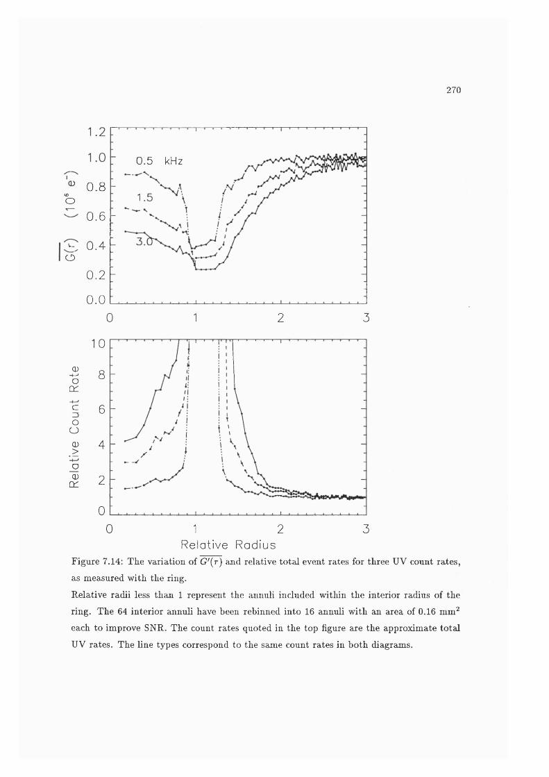
270

0 . 5 kHz

0.8iÛo

0.6

S 0 . 4o

0.2

0.030 1 2

(D-t—'O

CH

coo0>D0

(H

0

8

6

4

2

0

0 31 2

Relative RadiusFigure 7.14: The variation of G'{r) and relative total event rates for three UV count rates,

as measured with the ring.

Relative radii less than 1 represent the annuli included within the interior radius of the

ring. The 64 interior annuli have been rebinned into 16 annuli with an area of 0.16 mm^

each to improve SNR. The count rates quoted in the top figure are the approximate total

UV rates. The line types correspond to the same count rates in both diagrams.

271

relationship which indicates the presence of gain depression.

The gain depression inside and outside the ring cannot be due solely to increasing

interaction between the events in these regions with increasing rate because the magnitude

of the gain depression is dependent on the total UV flux, not the local flux. Also, the gain

depression near the ring is always greater on the inside than the outside, even though the

local UV fluxes are the same. Therefore, LRGD is present and depresses the gain more near

the inside edge of the ring than on the outside. In the centre of the ring the depression is

similar to that on the outside of the ring for the same local flux. This demonstrates the

magnitude of LRGD is dependent on the morphology of the illuminated region.

7.6 Long Term, Long Range Gain Depression

Until now, it has been assumed that LRGD has no long term efiect on the MCP, i.e.

the gain should recover almost immediately after the point source illumination is removed.

Given the long integration times necessary to obtain a reasonable signal to noise ratio in

the PHDs of the annuli illuminated only by X-rays, we cannot measure any rapid variation

of the gain in quiescent pores. While it is expected that prolonged, intense UV exposure

would permanently reduce the gain in the region of the MCP illumination, there should be

no long term effect in the rest of the MCP.

I shall use the expression “long term LRGD” to refer to the LRGD in an area

surrounding a region that has undergone intense UV illumination, many TmcpS after the

UV illumination has flnished. As in dynamic LRGD, it does not refer to gain depression in

the region that weis actually UV illuminated.

Figure 7.16 shows examples of the MCP gains at various stages during the exper

iment, obtained with X-ray iUumination only. Curve “a” was obtained at the start o f this

experiment, 5 months after the last UV illumination. The total UV exposure through the

pinhole and the time between when the curves were obtained is shown in Table 7.2.

It is apparent that the gains in the annuli that were not UV illuminated up to

a radius of at least 1 mm, have not returned to the pre-experiment levels. This clearly

demonstrates that gain depression has a component that is both long term and long range.

The gain in the first annulus, or more accurately the disk, which contains the

region that was UV illuminated, has returned to approximately the same level as at the

start of the experiment, while the gain in many of the non-illuminated annul! has not. This

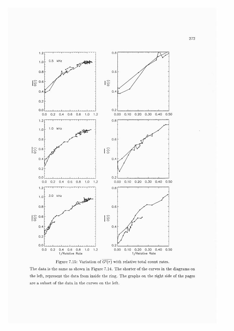
272

0 .5 kHz

0 .0 0 .2 0 .4 0 .6 0 .8 1.0 1.2

1 .0 kHz

0.8

S 0.6

0 .4

0.2

0.00 .0 0 .2 0 .4 0 .6 0 .8 1 .0 1.2

3 .0 kHz1.0

0.8

0 .4

0.2

0.00 .0 0 .2 0 .4 0 .6 0 .8 1.0 1.2

1/R e la tiv e Rote

0.8

0.6

Ô0 .4

0.20 .0 0 0 .1 0 0 .2 0 0 .3 0 0 .4 0 0 .5 0

0.8

0.6

Ô0 .4

0.20 .0 0 0 .1 0 0 .2 0 0 .3 0 0 .4 0 0 .5 0

0.8

0.6

Ü

0 .4

0.20 .0 0 0 .1 0 0 .2 0 0 .3 0 0 .4 0 0 .5 0

1 /R e la tiv e Rate

Figure 7.15: Variation of G'{r) with relative total count rates.

The data is the same as shown in Figure 7.14. The shorter of the curves in the diagrams on

the left, represent the data from inside the ring. The graphs on the right side of the pages

are a subset of the data in the curves on the left.

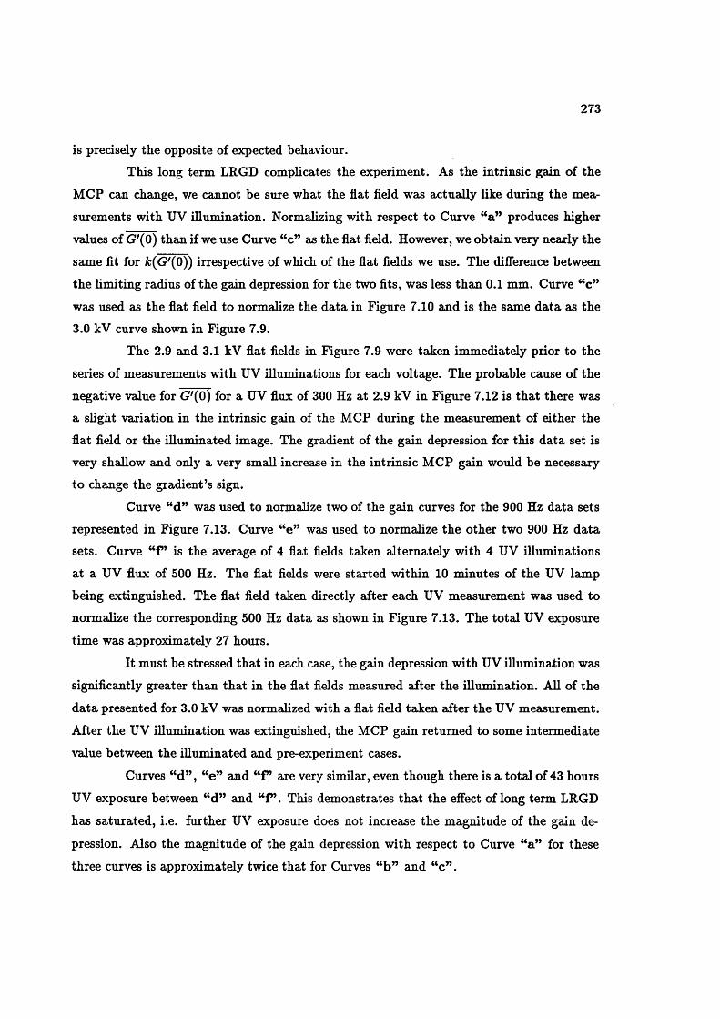
273

is precisely the opposite of expected behaviour.

This long term LRGD complicates the experiment. As the intrinsic gain of the

MCP can change, we cannot be sure what the flat field was actually like during the mea

surements with UV illumination. Normalizing with respect to Curve “a ” produces higher

values of G'(0) than if we use Curve “c” as the flat field. However, we obtain very nearly the

same fit for A;(G'(0)) irrespective of which of the flat fields we use. The difference between

the limiting radius of the gain depression for the two fits, was less than 0.1 mm. Curve “c”

was used as the flat field to normalize the data in Figure 7.10 and is the same data as the

3.0 kV curve shown in Figure 7.9.

The 2.9 and 3.1 kV flat fields in Figure 7.9 were taken immediately prior to the

series of measurements with UV illuminations for each voltage. The probable cause of the

negative value for G'(0) for a UV flux of 300 Hz at 2.9 kV in Figure 7.12 is that there was

a slight variation in the intrinsic gain of the MCP during the measurement of either the

flat field or the illuminated image. The gradient of the gain depression for this data set is

very shallow and only a very small increase in the intrinsic MCP gain would be necessary

to change the gradient’s sign.

Curve “d ” was used to normalize two of the gain curves for the 900 Hz data sets

represented in Figure 7.13. Curve “e ” was used to normalize the other two 900 Hz data

sets. Curve “f ’ is the average of 4 flat fields taken alternately with 4 UV illuminations

at a UV flux of 500 Hz. The flat fields were started within 10 minutes of the UV lamp

being extinguished. The flat field taken directly after each UV measurement was used to

normalize the corresponding 500 Hz data as shown in Figure 7.13. The total UV exposure

time was approximately 27 hours.

It must be stressed that in each case, the gain depression with UV illumination was

significantly greater than that in the flat fields measured after the illumination. All of the

data presented for 3.0 kV was normalized with a flat field taken after the UV measurement.

After the UV illumination was extinguished, the MCP gain returned to some intermediate

value between the illuminated and pre-experiment cases.

Curves “d ” , “e ” and “f ’ are very similar, even though there is a total of 43 hours

UV exposure between “d ” and “f ’ . This demonstrates that the effect of long term LRGD

has saturated, i.e. further UV exposure does not increase the magnitude of the gain de

pression. Also the magnitude of the gain depression with respect to Curve “a ” for these

three curves is approximately twice that for Curves “b ” and “c” .

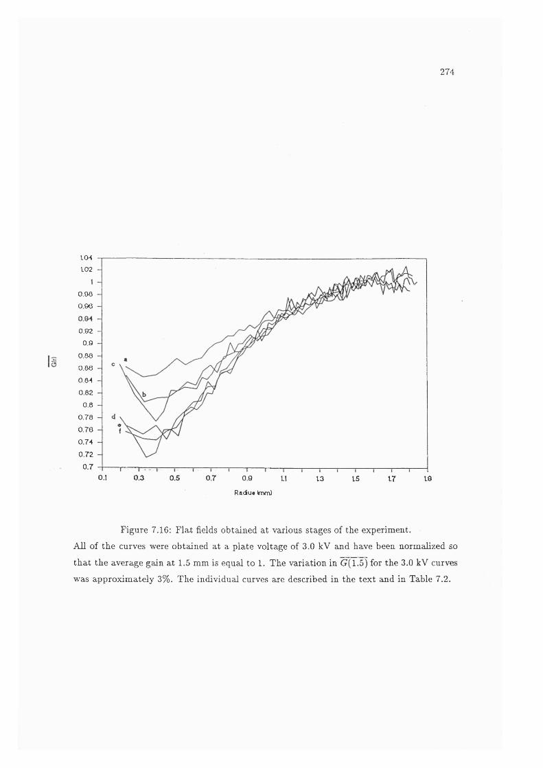
274

ICK

102

0 .9 8

0 .9 6

0.92

0.9

0.88

0.88

0.84

0.82

0.80 .7 8

0 .7 6

0 .74

0 .7 2

0 .70.1 0 .3 0.5 0.7 0.9 11 1713 15 19

Radu* tmm)

Figure 7.16: Flat fields obtained at various stages of the experiment.

All of the curves were obtained at a plate voltage of 3.0 kV and have been normalized so

that the average gain at 1.5 mm is equal to 1. The variation in G(1.5) for the 3.0 kV curves

was approximately 3%. The individual curves are described in the text and in Table 7.2.

275

Curve UV Exposure (hours)

Total Time Since Last Exposure (hours)

96 @ Various and rates.

i e @ V c = 3.0 kV and 900 Hz.

16 @ %; = 3.0 kV and 900 Hz.

27 Û Vc = 3.0 kv and 500 Hz, composite of 4 measurements separated

by « 7 hrs exposure each.

3700Including exposure to air for several weeks.

771

12

146

Table 7.2: Total UV exposure and the intervals between the times at which the curves in

Figure 7.16 were acquired.

Time increases down the page, i.e. an item directly below another occurred immediately

after the upper item.

276

One possible explanation for this behaviour is that the intrinsic gain is progres

sively depressed until the long term eflfect saturates. This is unlikely to cause the variation

between Curves “b ” , “c” and Curves “d ” , “e ” , “f ’ , as the total UV exposure time be

tween “a ” and “c ” was 6 times longer than that between “c” and “d ” . While it is true

that the 96 hour exposure consisted of various fluxes at various gains, it would require that

the magnitude of the gain depression would be strongly nonlinear with respect to integrated

UV exposure. Also, it would be serendipitous, to say the least, if we had randomly chosen

to measure a flat fleld at the critical point just before saturation occurred.

Another possibility is that the long term effect saturates relatively quickly, i.e.

in less than 16 hours, and the intrinsic gain slowly recovers to an intermediate point such

as Curve “c ” . The recovery would have to be quite slow. Curves “d ” , “e ” and “f ’ are

very similar but the time elapsed between extinguishing the UV and starting the flat fleld

acquisition, was of the order of minutes for Curves “d ” and “f” while it was 6 days for

Curve “e ” . Therefore, no significant recovery occurs over approximately a week. Also, if

recovery is the cause of the variation in the magnitude of gain depression, then it has taken

approximately 1 month to recover to approximately halfway between the saturated and

pre-experiment intrinsic gains. Another interesting phenomenon is that the gain appears

to recover faster in the illuminated annulus than in the non-iUuminated annuli.

A flat field obtained at 3.2 kV, see Figure 7.4 before the MCP was illuminated

with UV and before the experiment described in Section 7.3, indicates that the intrinsic

gain was relatively flat up to approximately 1.2 mm. Assuming that the general form of

the gain curve would be the same for 3.0 kV as for 3.2 kV, Figure 7.16 shows that the

intrinsic gain of the MCP has not fully recovered over a period of 5 months which included

prolonged exposure to air.

7.6 .1 T h e V ariation o f Long Term , L ong R ange G ain D ep ression w ith

T im e

Measurements of the evolution of long term LRGD with time were carried out using

the ring. In these measurements a section of the MCP that had not previously undergone

intense UV illumination was used, i.e. a dififerent region than used with the pinhole and

the ring measurements as described in Section 7.5.1.

A series of 14 measurements were made to investigate how LRGD varies during

277

progressive UV illumination. Each measurement consists of data obtained with 2 hour

long, X-ray only flat fields obtained at various stages during a cumulative UV exposure.

The initial flat field was obtained after only 15 minutes exposure, which represents the time

that was necessary to setup the spiral fit parameters and select the annuli positions. This

data is shown in Figure 7.17a. As in most of the diagrams in this section, the 64 annuli

inside the ring have been resampled into 16 equal area annuli to improve the SNR.

After each flat field waa obtained, the MCP was illuminated with UV through the

mask, typically for 35 minutes. After the UV illumination was finished another fiat field

was taken. Flat fields and UV illuminations were both begun within 2 minutes of the end

of the previous measurement. A series of 13 UV illuminations was carried out and the total

UV exposure time after the initial fiat field was 27430 s, « 7.5 hours. Figure 7.17b shows

the combined average X-ray and UV count rates per pore within each of the 80 annuli.

The count rate has been corrected for the acquisition deadtime, i.e. the proportion of the

integration time for which the ADCs were not sampling data, which was over 90%. No

correction has been attempted for losses below the LLD, due to ghosting or coincidence loss

in the electronics. No significant variation in UV intensity with time was noticed.

Figure 7.17c shows the dynamic gain depression, produced during the first and last

UV illumination. It shows that there was no significant variation in the magnitude during

the 13 UV exposures. Figure 7.17d shows the average charge extracted per pore during UV

exposure after the initial fiat field. These values have been corrected in the same manner

as the count rates.

After the sequence of UV exposures, a series of fiat fields was obtained at various

times over a period of 2 weeks. The MCPs were kept in vacuum throughout the entire series

measurements. The MCPs and electronics were run for at least two hours before acquiring

any of the fiat fields.

Figure 7.18 shows the average relative gains as measured in the fiat fields both

during and after the sequence of UV illuminations. Times quoted on the left half of the

diagram refer to the total UV exposure and times on the right side of the figure represent the

time elapsed since the last UV exposure. The two scales share the same origin but represent

two different times. The original 128 annuli were rebinned so that there are 8 interior and

exterior annuli. The various curves axe a selection of these 16 annuli and correspond to the

annular regions indicated in the table in the bottom left comer, for fiat fields acquired at

various stages during the experiment. All data was acquired with Vc = 3.0 kV and have

278

130

120Oo

^ 100

9030 21

10’

3 1

-4,-5

2 30 1120100

0) 80b

60

li 4 0

20

0 2 31

&<u0) 10ouTD0)Ü2"xÜ J

0 2 31Relative R adiu s

Figure 7,17: Details of the UV illumination of the ring.

Figure a shows the flat field for Vc = 3.0 kV at the start of the experiment which W2is mea

sured immediately before the first data point in Figure 7.18. Figure b shows the combined

X-ray and UV event rate during the UV illuminations. Figure c shows the variation in (7(r)

as measured during the first (solid line) and last (dotted) exposure. Curve d shows the total

charge extracted during the series of UV exposures.

279

been normalized such that G{r) = 1 for the 16th. of the new annuli, to allow for drifts

in the amplifier gains with time. These drifts were only noticeable for the flat fields taken

over several days after the last UV exposure. The error bars on the right half of curve 8

correspond to total integration times for those data sets.

Figure 7.18 shows clearly that the magnitude of the gain depression increases with

UV exposure and that the gain recovers slowly. This is the behaviour that was suggested

by the flat fields displayed in Figure 7.16. The maximum magnitude of the gain depression

in the two diagrams is comparable. The rate of recovery is much faster here than was

suggested by Curves “b” and “c” in Figure 7.16, however, there was much more extensive

UV illumination between Curves “a” and “b ” in that figure than in the present case.

The figure also shows the magnitude of the long term, gain depression is greatest

on the inside of the ring and not in ring itself. A similar effect is seen in Figure 7.16 where

the maximum long term, gain depression is located approximately 0.4 mm from the pinhole.

The magnitude of the long term LRGD is also greater on the inside of the ring than on the

outside, as was seen for the dynamic LRGD in Figure 7.15. It is extremely unlikely that

this long term gain depression is due to the increased count rate caused by the local UV

flux inside the ring. As shown in Figure 7.17, the maximum event and charge extraction

rates inside the ring. Curves 1-4 in Figure 7.16, are rv 100 times smaller than those in the

Curve 5, which represents the ring, yet the rate of change of the magnitude gain depression

in all of these curves is comparable.

An interesting feature is that while there is a large variation in the magnitude of the

long term LRGD between the first and last UV exposure, the absolute gain measurements

for the dynamic LRGD do not vary significantly.

Figure 7.19 shows the same data as in Figure 7.18 but plotted linearly with time.

Figure 7.19a clearly shows that the rate of change in the magnitude of long term LRGD

decreases with progressive UV illumination and it also appears to saturate after about

6 hours. This figure and Figure 7.18 show that neither the progressive increase in the

magnitude of gain depression nor the gain recovery follow straight forward power law or

linear relationships.

The PHDs shown in Figure 7.20 correspond to the data points in these curves

obtained 100 hours after the last UV exposure. The modal gain is reduced by ~ 25

channels inside and near the ring compared to PHD 9 located at the edge of the measured

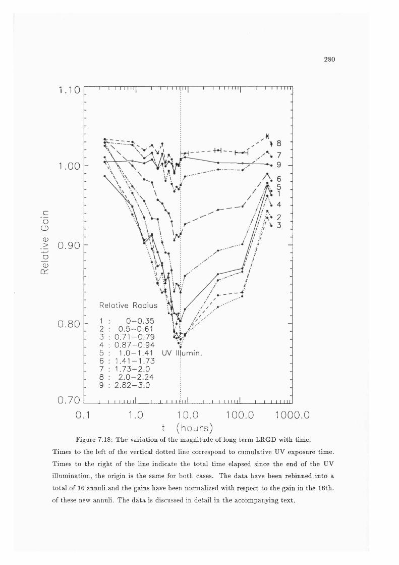
280

1 . 1 0 1 I I I I I I II 1— I r i ~ \ - 1— I I I ITU 1 — I I I I I I I

1.00 -

Do<D.> 0.90-I—'oCD

0.80 -

0.70 0.1

\ \

/ /V* 2

Relative Radius ^

1 0 - 0 . 3 52 0 .5 -0 .6 13 0 .7 1 - 0 . 7 94 0 . 8 7 - 0 . 9 45 1 .0-1 .416 1 .4 1 -1 .7 37 1 .7 3 -2 .08 2 . 0 - 2 . 2 49 2 . 8 2 - 3 . 0

1 1 1 1 II III 1

' w

j I ..I 11 j 1111 I I I I IIII

1000.01.0 10.0 100.0 t ( h o u r s )

Figure 7.18: The variation of the magnitude of long term LRGD with time.

Times to the left of the vertical dotted line correspond to cumulative UV exposure time.

Times to the right of the line indicate the total time elapsed since the end of the UV

illumination, the origin is the same for both cases. The data have been rebinned into a

total of 16 annuli and the gains have been normalized with respect to the gain in the 16th.

of these new annuli. The data is discussed in detail in the accompanying text.

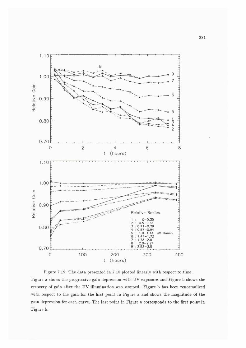
281

1.00

> 0 .9 0

0 .8 0

0 .7 080 2 4 6

1 . 1 0

1.00

ooCD

0 .9 0"oCDcr

0 .8 0

0 .7 0

t (hours)

R elative Radius

1 : 0 - 0 .3 52 : 0 .5 -0 .6 13 : 0 .7 1 - 0 .7 94 : 0 .8 7 - 0 .9 45 : 1 .0 -1 .4 1 UV lllumin.6 : 1 .4 1 -1 .7 37 : 1 .7 3 -2 .08 : 2 .0 - 2 .2 49 : 2 .8 2 - 3 .0

■J i J I I I I I i I I t I I I i ■ i I i 1 i i . - i . i 4 - - i -

0 100 200t (hours)

3 0 0 4 0 0

Figure 7.19: The data presented in 7.18 plotted linearly with respect to time.

Figure a shows the progressive gain depression with UV exposure and Figure b shows the

recovery of gain after the UV illumination was stopped. Figure b has been renormalized

with respect to the gain for the first point in Figure a and shows the magnitude of the

gain depression for each curve. The last point in Figure a corresponds to the first point in

Figure b.

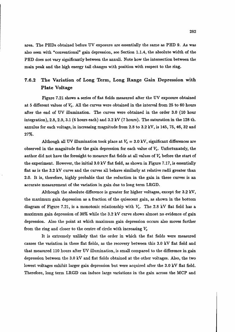
282

area. The PHDs obtained before UV exposure are essentially the same as PHD 9. As was

also seen with “conventional” gain depression, see Section 1.1.4, the absolute width of the

PHD does not vary significantly between the annuli. Note how the intersection between the

main peak and the high energy tail changes with position with respect to the ring.

7 .6 .2 T h e V ariation o f Long Term , Long R an ge G ain D ep ression w ith

P la te V oltage

Figure 7.21 shows a series of flat fields measured after the UV exposure obtained

at 5 different values of Vc. All the curves were obtained in the interval from 25 to 60 hours

after the end of UV illumination. The curves were obtained in the order 3.0 (10 hour

integration), 2.8, 2.9, 3.1 (6 hours each) and 3.2 kV (7 hours). The saturation in the 128 th.

annulus for each voltage, in increasing magnitude from 2.8 to 3.2 kV, is 145, 75, 46, 32 and

27%.

Although all UV illumination took place at %. = 3.0 kV, significant differences are

observed in the magnitude for the gain depression for each value of Vc. Unfortunately, the

author did not have the foresight to measure flat fields at all values of Vc before the start of

the experiment. However, the initial 3.0 kV flat field, as shown in Figure 7.17, is essentially

flat as is the 3.2 kV curve and the curves all behave similarly at relative radii greater than

2.0. It is, therefore, highly probable that the reduction in the gain in these curves is an

accurate measurement of the variation in gain due to long term LRGD.

Although the absolute difference is greater for higher voltages, except for 3.2 kV,

the maximum gain depression as a fraction of the quiescent gain, as shown in the bottom

diagram of Figure 7.21, is a monotonie relationship with Vc. The 2.8 kV flat field haa a

maximum gain depression of 30% while the 3.2 kV curve shows almost no evidence of gain

depression. Also the point at which maximum gain depression occurs also moves further

from the ring and closer to the centre of circle with increasing Vc

It is extremely unlikely that the order in which the flat fields were measured

causes the variation in these flat fields, as the recovery between this 3.0 kV flat field and

that measured 110 hours after UV illumination, is small compared to the difference in gain

depression between the 3.0 kV and flat fields obtained at the other voltages. Also, the two

lowest voltages exhibit larger gain depression but were acquired after the 3.0 kV flat field.

Therefore, long term LRGD can induce large variations in the gain across the MCP and

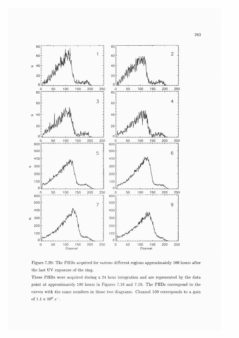
283

80

60

z 40

20

0 5 0 100 150 200 25 0

80

60

40

20

5 0 100 150 200 2 5 0080 80

60 60

z 40 - 40

20

150 2 0 0 5 0 10 0 1 5 0 2 0 0 2 5 00 5 0 100 2 5 0 060 0 600

5 0 0 50 0

4 0 0 40 0

z 3 0 0 30 0

200 200

100 100

0 5 0 100 150 2 0 0 2 5 0 0 50 100 150 200 2 5 060 0 600

5 0 0 50 0

400 40 0

z 3 0 0 30 0

200 200

100 100

150 2 0 0 2 5 00 5 0 100 5 0 10 0 15 0 2 0 0 2 5 00Channel Channel

Figure 7.20: The PHDs acquired for various different regions approximately 100 hours after

the last UV exposure of the ring.

These PHDs were acquired during a 24 hour integration and are represented by the data

point at approximately 100 hours in Figures 7.18 and 7.19. The PHDs correspond to the

curves with the same numbers in those two diagrams. Channel 100 corresponds to a gain

of 1.1 X 10® e“ .

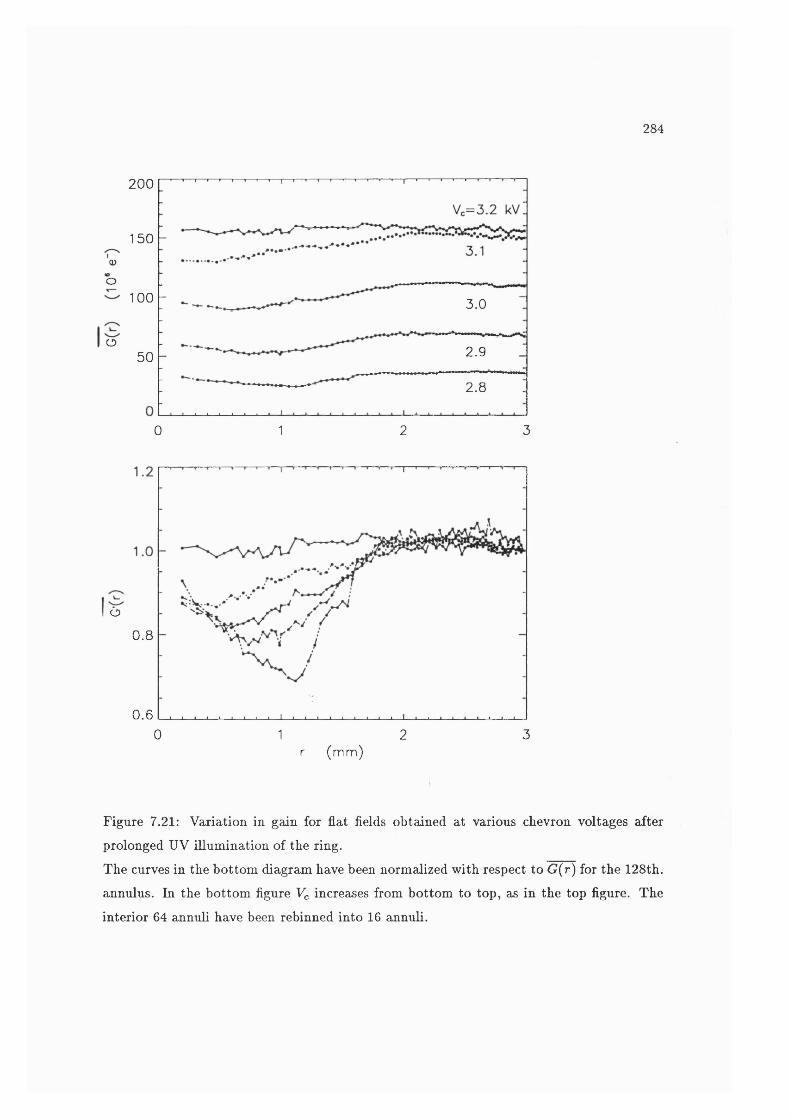
284

2 0 0

150euo

100 3.0

o2.950

2.8

0 2 31

o

0.8

0.60 2 3

r (m m )

Figure 7.21: Variation in gain for flat fields obtained at various chevron voltages after

prolonged UV illumination of the ring.

The curves in the bottom diagram have been normalized with respect to (r(r) for the 128th.

annulus. In the bottom figure Vc increases from bottom to top, as in the top figure. The

interior 64 annuli have been rebinned into 16 annuli.

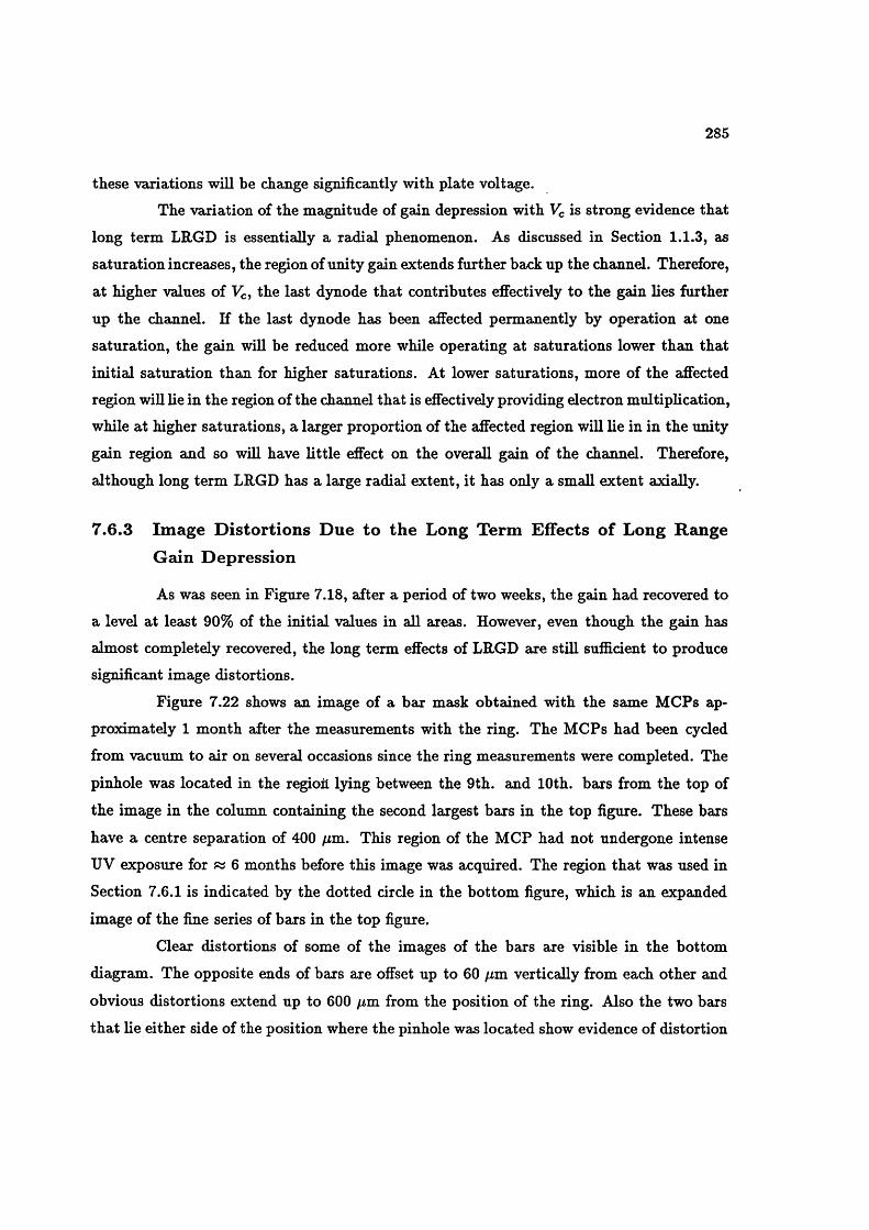
285

these variations will be change significantly with plate voltage.

The variation of the magnitude of gain depression with Vc is strong evidence that

long term LRGD is essentially a radial phenomenon. As discussed in Section 1.1.3, as

saturation increases, the region of unity gain extends further back up the channel. Therefore,

at higher values of 1^, the last dynode that contributes effectively to the gain lies further

up the channel. If the last dynode has been affected permanently by operation at one

saturation, the gain will be reduced more while operating at saturations lower than that

initial saturation than for higher saturations. At lower saturations, more of the affected

region will lie in the region of the channel that is effectively providing electron multiplication,

while at higher saturations, a larger proportion of the affected region will lie in in the unity

gain region and so will have little effect on the overall gain of the channel. Therefore,

although long term LRGD has a large radial extent, it has only a small extent axially.

7 .6 .3 Im age D isto r tio n s D u e to th e Long Term E ffects o f L ong R ange

G ain D ep ression

As was seen in Figure 7.18, after a period of two weeks, the gain had recovered to

a level at least 90% of the initial values in all areas. However, even though the gain has

almost completely recovered, the long term effects of LRGD are still suflScient to produce

significant image distortions.

Figure 7.22 shows an image of a bar mask obtained with the same MCPs ap

proximately 1 month after the measurements with the ring. The MCPs had been cycled

from vacuum to air on several occasions since the ring measurements were completed. The

pinhole was located in the regioil lying between the 9th. and 10th. bars from the top of

the image in the column containing the second largest bars in the top figure. These bars

have a centre separation of 400 /im. This region of the MCP had not undergone intense

UV exposure for « 6 months before this image was acquired. The region that was used in

Section 7.6.1 is indicated by the dotted circle in the bottom figure, which is an expanded

image o f the fine series of bars in the top figure.

Clear distortions of some of the images of the bars are visible in the bottom

diagram. The opposite ends of bars are offset up to 60 /xm vertically from each other and

obvious distortions extend up to 600 /xm from the position of the ring. Also the two bars

that lie either side of the position where the pinhole was located show evidence of distortion

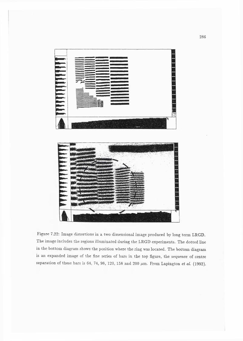
286

m

Figure 7.22: Image distortions in a two dimensional image produced by long term LRGD.

The image includes the regions illuminated during the LRGD experiments. The dotted line

in the bottom diagram shows the position where the ring was located. The bottom diagram

is an expanded image of the fine series of bars in the top figure, the sequence of centre

separation of these bars is 64, 74, 98, 120, 158 and 200 fim. From Lapington et al. (1992).

287

and its possible that the adjacent bars are also slightly distorted. As the distortions are

present at relatively large distance from the regions that underwent prolonged UV exposure,

these distortions are a long term effect of LRGD.

Although SPAN has pulse height related position shifts, see Section 5.7.1, it is

unlikely that the distortions are caused solely by the difference in gain due to long term

LRGD. The position shifts due to gain are most noticeable over a large range of pulse heights.

In this image, the extreme edges of the PHD have been removed. Also, the positional shifts

are always in one direction, wherehas these distortions appear to have a strong dependence

on the azimuthal angle around the circumference of the ring.

The existence of long term effects of LRGD raises the possibility that a localized

region of the readout has been affected, rather than the MCP. Upon examination of theu r

readout after the MCPs were subject to intense localized UV expose, a brown discolouration

was observed. This is probably due to a chemical reaction caused by intense electron

bombardment of residual pump oil molecules. The MCP stack was rotated in one piece,

120° with respect to the readout. The mask was not moved with respsect to the MCP and

so was also rotated with respect to the anode. As shown in Figure 7.23, the distortions have

not moved during rotation, with respect to the deadspots visible in the left edge of the bar

mask but they have moved with respect to the anode, as shown by the inclination of the

bar masks to the x and y axes of the diagram. Therefore, the distortions are phenomenon

of the MCP not the readout and as their most likely cause is LRGD, this is also true for

LRGD itself.

The presence of the deadspots was found to have no effect on the experiment. Care

was taken to make sure that they lay outside the set of annuli. When all the events acquired

across the whole active diameter of the MCP were saved, as in the initial experiment

described in Section 7.2.3, measurements were carried out to the determine the effect of

the deadspots. A set of annuli wcis chosen such that the outer radius of the last annulus

wcis located just outside the closest region obviously affected by the deadspots. Gain and

gain depression measurements were compared for the full annuli and for annuli in which

the octant in the direction of the deadspots was masked out in software. No significant

variation was noticed between the two sets of measurements.

Ifüi

t

288

Figure 7.23: Image distortions similar to those in Figure 7.22 after the MCP stack has been

rotated by 120° with respect to the readout.

The distortions have not moved with respect to deadspots visible on at the left edge of the

bar mask during rotation of the MCPs. The significance of the deadspots on the experiment

is discussed in the accompanying text.

289

7.7 Possible M echanisms for Long Range Gain Depression

7 .7 .1 D yn am ic, Long R ange G ain D ep ression

In the “dynodised” MCP model developed by Eberhardt (1979, 1980, 1981), the

wall collisions inside the pore occur over a preferred distance and the pore behaves as

though it were a discrete electron multiplier with a fixed number of dynodes. Most of the

charge comes from the last dynode, located at ~ 95 % of the pore length. The equivalent

circuit of the dynode, see Figure 7.24, consists of a capacitance and resistance to ground,

Cci, approximately 10“ ® F and R d = R d { n + 1) where Rc is the resistance of the pore,

^ 10 ® n , for the plates used in this work. In a chevron pair, it is the last dynode of the

bottom plate that provides most of the charge and it is at this point where gain depression

would be most severe.

Eberhardt also invokes a lateral capacitance. Cl 50 x Cd and parallel to Cd in

order to explain high gains achieved with Z stacks compared with single plates (Eberhardt,

1980, 1981). The extra charge is provided by a lateral storage capacitance between each

of the active pores in an MCP and the quiescent pores surrounding them, see Figure 7.25.

This process has been used to explain the adjacency phenomenon (Pearson et of., 1988).

Maximum sustainable count rates were obtained when the ratio of quiescent channels to

active channels was at a maximum. It was proposed that the lateral capacitance was

proportional to the circumference of the excited area and the ratio of circumference to

enclosed area increases 8ls the area decreases.

In a simple model, the MCP can be described as a large array of RC circuits in

parallel. All quiescent pores should be at the same potential and so the network of parallel

elements can be replaced by one RC circuit of equivalent magnitude. This equivalent circuit

would be coupled to the active regions of the MCP through lateral capacitance.

This model does not explain the results reported in this work. Charge would be

extracted equally from all the quiescent pores. However, in order to be consistent with

results displayed in Figure 7.6, charge would have to be removed preferentially from nearby

pores, and the amount removed would have to reduce linearly with radius for up to 100

pore diameters. This would require that some series component be present, such as a

resistive path in the conductor on the face of the MCP or a variation with distance for the

capacitance between pores.

The linear variation of the magnitude of gain depression, suggests that it is sym

290

metric around the pinhole. In this work, the pinhole was placed at the centre of the MCP, so

we cannot determine what effects the edge of the MCP would have on the symmetry of gain

depression. Fraser et al. (1991b) have investigated adjacency for a pinhole by illuminating

a spot at the MCP centre and at the edge and measuring the ratio No variation was

found and as this is the most likely method of varying the capacitance between the active

region and the MCP edge, they conclude that adjacency is independent of relative position

of an image on the MCP and that lateral capacitance is unlikely to be the cause. They also

point out if adjacency is caused by lateral capacitance it should be present in single plate

detectors, which it is not.

Anacker & Erskine (1991) have carried out Kirchoff analysis of the equivalent

recharging circuit for the last dynode and found that r >• 9 ms. However, using electron

time of flight measurements they observed the occurrence of gain depression within 500 ns.

The group from Rutherford Appleton Laboratory measured the gain extracted from a MIC

detector subjected to an intense flash of 60 fj,s duration over a 5 x 5 mm square (Carter,

1991b). They find the amount of charge extracted varies across the square, with the maxi

mum extracted at the edges and an approximately constant amount extracted in the centre.

This is a direct measurement of interaction between channels occuring in less than 0.1 ms,

so charge removal by lateral capacitance is too slow to be a viable mechanism.

A second proposed mechanism for gain depression is pore de-activation, in which

the electric field from an active pore interferes with the fleld in several quiescent channels.

In an isolated quiescent pore, the electric field vector E is aligned with the channel axis. If

they become unaligned the gain is reduced as the electrons will be accelerated for shorter

distances and will collide with the channel walls with less energy producing fewer secondary

electrons. Gatti et at., (1983) have measured the effect of the inclination of E and the

pore axis on modal gain by applying an external magnetic field to the MCP. The modal

MCP gain G{6), as a function of the angle, between E and the pore axis, is a nonlinear

relationship and very sensitive to 0, see Figure 7.26. They have also shown that the positive

wall charge in one channel after the electron cascade can introduce potential changes in the

neighbouring pores, which alters the electric field.

When an event occurs in a chevron pair, the positive charge present on the walls

of the cluster of active pores in the rear MCP decays exponentially with a time constant

proportional to the characteristic time constant of the MCP, Tm cp> Approximating the

wall charge as an infinite line of charge with uniform charge density, this charge produces

CH A N N E L

L A S TDYNODE

A R E A EQ U IV A LEN TRECHARGEC IR C U IT

_ _ l

291

O U T

Figure 7.24: The equivalent circuit of the last dynode.

From Eberhardt (1981).

N last dynode a re a s -

V V l

2 ol N ^ q u ie s e n l

ch an n els

Figure 7.25: Schematic diagram and equivalent circuit of coupling by lateral capacitance

between N active pores and Ng quiescent pores.

From Anacker Erskine (1991).

B - 6 k G U m c p " 3 . l k V

6 X 10*

DIRECTION OF THE EX T E R N A L MAG. FIELD

Figure 7.26: The variation of modal gain as a function of the inclination between the electric

field the channel axis.

From Gatti et a i (1983).

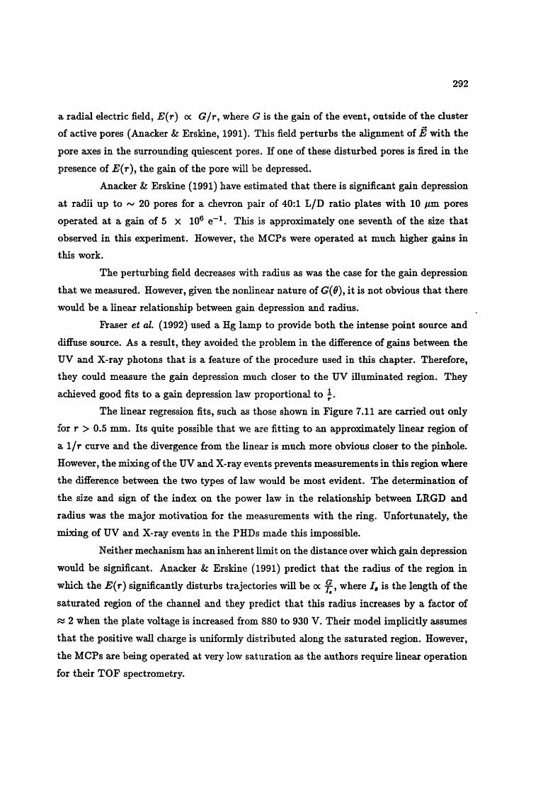
292

a radial electric field, E {r) oc G jr , where G is the gain of the event, outside of the cluster

of active pores (Anacker &: Erskine, 1991). This field perturbs the alignment of E with the

pore axes in the surrounding quiescent pores. If one of these disturbed pores is fired in the

presence of E (r ), the gain of the pore wiU be depressed.

Anacker & Erskine (1991) have estimated that there is significant gain depression

at radii up to 20 pores for a chevron pair of 40:1 L /D ratio plates with 10 /zm pores

operated at a gain of 5 x 10® e“ . This is approximately one seventh of the size that

observed in this experiment. However, the MCPs were operated at much higher gains in

this work.

The perturbing field decreases with radius as was the case for the gain depression

that we measured. However, given the nonlinear nature of G{9), it is not obvious that there

would be a linear relationship between gain depression and radius.

Eraser et al. (1992) used a Hg lamp to provide both the intense point source and

diffuse source. As a result, they avoided the problem in the difference of gains between the

UV and X-ray photons that is a feature of the procedure used in this chapter. Therefore,

they could measure the gain depression much closer to the UV illuminated region. They

achieved good fits to a gain depression law proportional to

The linear regression fits, such as those shown in Figure 7.11 are carried out only

for r > 0.5 mm. Its quite possible that we are fitting to an approximately linear region of

a 1 /r curve and the divergence from the linear is much more obvious closer to the pinhole.

However, the mixing of the UV and X-ray events prevents measurements in this region where

the difference between the two types of law would be most evident. The determination of

the size and sign of the index on the power law in the relationship between LRGD and

radius was the major motivation for the measurements with the ring. Unfortunately, the

mixing of UV and X-ray events in the PHDs made this impossible.

Neither mechanism has an inherent limit on the distance over which gain depression

would be significant. Anacker & Erskine (1991) predict that the radius of the region in

which the E (r ) significantly disturbs trajectories will be oc where is the length o f the

saturated region of the channel and they predict that this radius increases by a factor of

w 2 when the plate voltage is increased from 880 to 930 V. Their model implicitly assumes

that the positive wall charge is uniformly distributed along the saturated region. However,

the MCPs are being operated at very low saturation as the authors require linear operation

for their TOE spectrometry.

293

As discussed in Section 1.1.3, the wall charge can reduce the secondary emission

coefficient, 6, to 1, either by reducing the strength of the electric field or preventing the

low energy electrons escaping from the surface. Once unity gain occurs, the local charge

density on the channel wall can no longer increase with continuing electron bombardment.

Therefore, there wiU be a maximum wall charge density defined by the intrinsic properties of

the glass. As the channel is driven further into saturation or with increasing gain depression,

the length of the pore with this maximum charge density will change but the actual charge

density will not.

As the perturbing electric field can be approximated as a purely radial phenomenon

with magnitude dependent on the charge density, the maximum wall charge defines a max

imum electric field strength and therefore a maximum radius over which trajectories will

be perturbed. So the length over which the trajectories are disturbed in the neighbouring,

quiescent pores will increase but not the distance at which pores are affected. Therefore,

the magnitude o f the gain depression could vary with plate voltage and count rate but the

spatial extent will remain approximately constant.

This is the behaviour indicated in Figure 7.12 where the limiting radius of the gain

depression is a constant over a wide range of operating conditions but the magnitude of the

gain depression, as indicated by G'(0) does vary with operating conditions. At low count

rates, i.e. 300 Hz, G'(0) does reduce monotonically with plate voltage.

Fraser et al. (1992) have measured the gain depression profile for a variety of front

plate voltages keeping the rear plate at 1300 V. They find no significant variation at varying

from 1250 to 1350 V. The combination of their measurements and those presented in this

chapter cover a range in gain of approximately 5 and 300 V in plate voltage for similar

MCPs and produce gain depressions with similar scales.

Fraser et al. (1992) also investigate a recharge model with a reservoir of charge

of fixed depth, G maxi which is the maximum deliverable or stored charge, as proposed by

Nicoli (1985) and Cho (1989). In this model, the channels do not discharge completeley for

each event and the gain for a given pulse depends on the magnitude and temporal spacing

of the previous pulses in that channel. Their model predicts that at high count rates the

PHD will lose its peaked profile. However, as discussed in Section 1.1.4, the saturation

remains essentially constant with increasing count rate. They also observe that the value

of Gmax decreases with increasing count rate. They conclude that the central assumption

of the reservoir model is incorrect and that the reduction of Gmax is due to a perturbing,

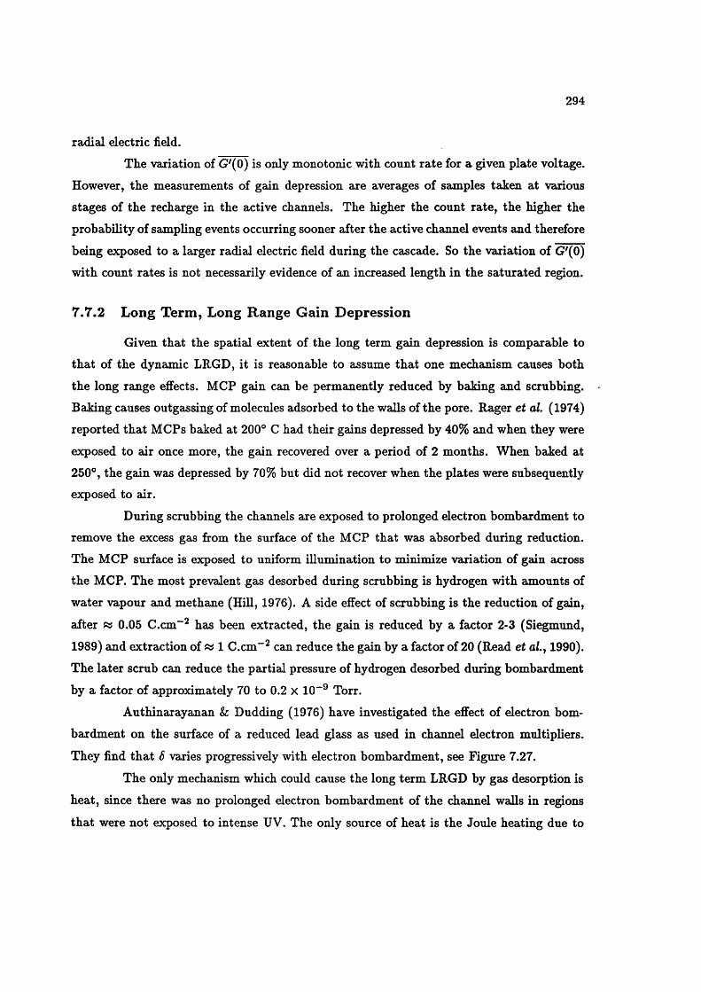
294

radial electric field.

The variation of G^(0) is only monotonie with count rate for a given plate voltage.

However, the measurements of gain depression are averages of samples taken at various

stages of the recharge in the active channels. The higher the count rate, the higher the

probability of sampling events occurring sooner after the active channel events and therefore

being exposed to a larger radial electric field during the cascade. So the variation of G'(0)

with count rates is not necessarily evidence of an increased length in the saturated region.

7 .7 .2 L ong T erm , Long R ange G ain D ep ression

Given that the spatial extent of the long term gain depression is comparable to

that of the dynamic LRGD, it is reasonable to assume that one mechanism causes both

the long range effects. MCP gain can be permanently reduced by baking and scrubbing.

Baking causes outgassing of molecules adsorbed to the walls of the pore. Rager et al. (1974)

reported that MCPs baked at 200° C had their gains depressed by 40% and when they were

exposed to air once more, the gain recovered over a period of 2 months. When baked at

250°, the gain was depressed by 70% but did not recover when the plates were subsequently

exposed to air.

During scrubbing the channels are exposed to prolonged electron bombardment to

remove the excess gas from the surface of the MCP that was absorbed during reduction.

The MCP surface is exposed to uniform illumination to minimize variation of gain across

the MCP. The most prevalent gas desorbed during scrubbing is hydrogen with amounts of

water vapour and methane (Hill, 1976). A side effect of scrubbing is the reduction of gain,

after « 0.05 C.cm~^ has been extracted, the gain is reduced by a factor 2-3 (Siegmund,

1989) and extraction of « 1 C.cm"^ can reduce the gain by a factor of 20 (Read et of., 1990).

The later scrub can reduce the partial pressure of hydrogen desorbed during bombardment

by a factor of approximately 70 to 0.2 x 10“® Torr.

Authinarayanan & Dudding (1976) have investigated the effect of electron bom

bardment on the surface of a reduced lead glass as used in channel electron multipliers.

They find that S varies progressively with electron bombardment, see Figure 7.27.

The only mechanism which could cause the long term LRGD by gas desorption is

heat, since there was no prolonged electron bombardment of the channel walls in regions

that were not exposed to intense UV. The only source of heat is the Joule heating due to

295

the strip current and, possibly, the current due to charge transferral between quiescent and

active pores.

If charge extraction is the cause of dynamic LRGD, we can estimate the total

amount of charge transferred from the quiescent pores by combining the values of G'(0)

from Figure 7.12. It can only be estimated for the pinhole as a much larger proportion

of the area measured for the ring images had considerable UV flux. The total “missing”

charge can be estimated from the volume of the cone with base radius 1.7 mm and height

1 — G'(0) times the quiescent gain as measured in the flat fleld. This value represents an

approximation as it extrapolates the linear range of the gain to zero radius, i.e. into the

region where there is signiflcant UV illumination. The “missing” charge would be transferred

from each of the groups of channels that are fired in the bottom plate by one X ray event.

Carrying out a calculation similar to that in Section 4.4.5, approximately 25 pores are fired

in the bottom plate for each sampling event and it is assumed that the charge is transferred

equally from each of these pores.

The maximum, total current transferred from the quiescent pores would be asso

ciated with the 4.5 kHz data, as shown in Figure 7.12, and is < 10 nA. The estimate of

the total charge transferred from the affected area during the experiment is » 2 x 10“ ' C

which corresponds to % 2 x 10“ C.cm~^. A total extracted charge comparable to this

estimate, can introduce long term gain depression of the order of 10 % during scrubbing

(Barstow & Samson, 1990).

The strip current is estimated by using the measured resistance when no high

voltage was applied to the MCPs, i.e. 640 M il, and estimating the number of channels

which yields Rch % 3.3 x 10 ®S1. The resistance could have reduced appreciably when high

voltage was applied due to heating by the strip current (Pearson et al., 1987).

The current transferring the charge to the active pores should flow through the

same regions of the pore walls as the strip current, i.e. the conducting layer in the channel

wall which is approximately 100 times larger than emissive layer (see Section 1.1). Also,

the average current per pore in the affected area, due to charge transfer, during the most

severe gain depression we measured, would be < 20 % of the strip current (not 10 % as I

reported in Edgar et at., 1992b).

Pearson et al. (1987) have calculated that the strip current raises the temperature

of an MCP approximately 4° C above the ambient temperature. It is unlikely that the

extra currents due to charge transferral could produce enough heat to produce the high

296

temperatures and the rate of gas desorption that occur during baking. And as most of any

extra current would flow through the conduction layer in the channel wall, it is unlikely that

charge transfer could cause gas desorption from the surface layer of the channel except by

heat. Also, if charge transferral was raising the channel temperature a significant amount,

Rch should be reduced more as the number of illuminated channels is increased. Therefore,

^ should increase with illuminated area which is the opposite o f what is actually observed

(Eraser et aZ., 1992).

Although outgassing occurs during scrubbing, it has been argued that the gain

depression is due, at least in part, to continuous, prolonged electron bombardment chang

ing the emissive properties of the surface layer of the pore walls (Rager et aZ., 1974 and

Siegmund, 1989). Authinarayanan & Dudding (1976) found that K was removed from the

surface of the glass during electron bombardment, see Figure 7.28. As shown in Figure 7.29,

6 is sensitive on the K concentration in the surface layer (Hill, 1976). Removal of K from

the surface layer will reduce 6 and hence, the gain.

The Potassium is present in the glass as K2 O. Authinarayanan & Dudding (1976)

point out that direct momentum transfer from the bombarding electrons is insufficient for

disassociation of the K2 O. They and Hill (1976) propose a mechanism where the positive

charge built up on the glass surface produces a large electric field which causes ions to

move away the surface into the bulk material. Therefore, direct electron bombardment is

not necessary to remove K from the surface layer, but only exposure to an electric held.

Therefore, the positive wall charge in an active channel could induce an electric held in

the neighbouring pores and thereby remove K from the emissive layers of these quiescent

channels.

If a electric held is causing K to migrate out of the surface layer of neighbouring

pores, the amount of K removed probably varies with azimuthal angle around those pores.

It is possible this is the cause of the image distortions seen in Figures 7.22 and 7.23.

The radial electric held could explain why gain depression is less in the region

actually illuminated, than in the surrounding quiescent areas. The active pores should have

a similar amount of positive wall charge, and so large potential differences, and therefore

electric helds, should not be present within the active areas.

Fraser et al. (1992) did not observe long term LRGD. The only long term gain

depression that they observed was in the region that was actually exposed to the intense

point source. As the long term LRGD appears to be closely associated with plate pre-

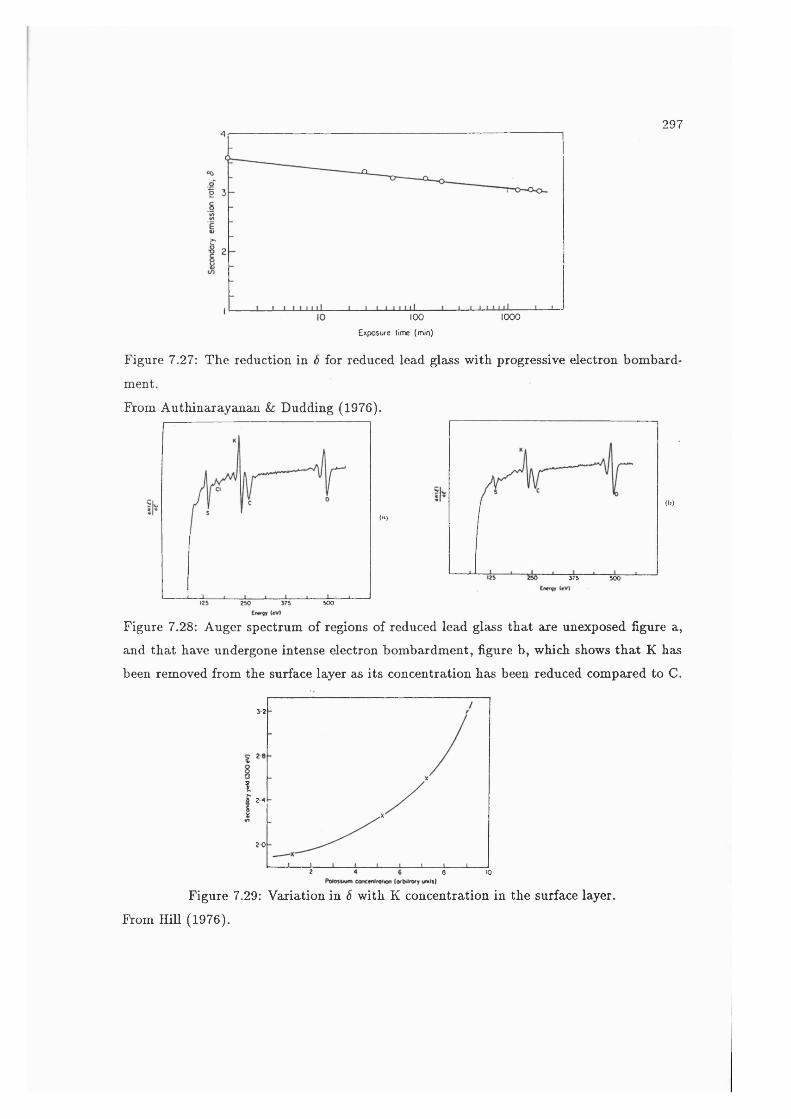
297

1000100Exposure lime (min)

Figure 7.27: The reduction in 6 for reduced lead glass with progressive electron bombard

ment.

From Authinarayanan & Dudding (1976).

500

( « )

S75 500

(l>)

Figure 7.28: Auger spectrum of regions of reduced lead glass that are unexposed figure a,

and that have undergone intense electron bombardment, figure b, which shows that K has

been removed from the surface layer as its concentration has been reduced compared to C.

3 2

I2 4

2 0

2 6 10

Figure 7.29: Variation in 6 with K concentration in the surface layer.

From Hill (1976).

298

conditioning, it is highly probable that variation in the preconditioning will produce large

variations in the magnitude of the observed long term, gain depression. More extensive

scrubbing almost certainly removes the effect completely otherwise it would have definitely

been observed previously. The MCPs used in this chapter only had a light scrub and it ap

peared that the gain depression appeared to saturate after a relatively short UV exposure.

It would certainly be interesting to carry out a series of measurements with sets of MCPs

that have undergone a variety of preconditioning procedures.

Long Term R ecovery of Gain

Authinarayanan & Dudding (1976) and Hill (1976) have found that if after the

bombardment, the surface is exposed to a hydrogen atmosphere, 6, and therefore the gain,

will recover by approximately 10 %. The two experiments used partial pressures of « 10~®

and 10“ Torr, respectively. Exposure of the glass to a partial atmosphere of oxygen did

not lead to a recovery in 8. Hill (1976) also failed to find any recovery when exposing the

glass to air or methane.

The recovery of the gain over a period of weeks, as seen in Figures 7.18, would

require that there was a substantial partial pressure of hydrogen present over this period.

The chamber was pumped continuously during the experiment and the MCPs were open

to the vacuum at both ends of the stack. Although our vacuum (5 x 10"^ Torr) is not

particularly good, it is unlikely that a high partial pressure of hydrogen is present. The

partial pressure of hydrogen released during initial scrubbing is of the order of 10~® Torr.

Even assuming that gas desorption is the cause of long term LRGD, the 2 mm radius area

affected represents only 0.3% of the MCP surface area. Therefore, only an extremely small

amount of hydrogen would be desorbed.

The major component of the gas present in the vacuum chamber is laboratory air.

It is extremely unlikely that this will cause recovery, as Hill (1976) found no effect. Also,

exposure to laboratory air for several weeks did not lead to a more complete recovery of

the gain for the region surrounding the pinhole, see Figure 7.16, than that surrounding the

ring.

One possible mechanism is that after the K has migrated out of the surface layer

under the influence of the electric fleld and when the surface charge is removed, the K

can diffuse back to the surface over a long period of time. The author is unaware of any

299

discussion of this in the literature. At present, the cause of gain recovery remains a mystery.

7 .7 .3 C onclusion

It appears that there are severe problems with explaining either dynamic or long

term LRGD with charge transferred from quiescent to active channels. However, there are

plausible mechanisms for both types of LRGD with the transverse electric field model.

Therefore, in line with the conclusion of Edgar et al. (1992a), rather than my more timid

discussion in Edgar et al. (1992b), the most probable mechanism for interaction between

pores is the perturbation of the axial electric field, established by the plate voltage, by a

transverse electric field due to the positive wall charge developed in active channels during

the electron cascade.

It is particularly interesting that various phenomena in MCPs, saturation, “con

ventional” gain depression, dynamic LRGD, which is the mechanism causing adjacency, and

long term LRGD can all be explained in terms of the wall charge.

300

Chapter 8

C onclusions and Future W ork

8.1 T he Size of th e Charge Cloud

In Chapter 3, techniques and analysis that can successfully determine the size and

form of the radial distribution of the electron cloud leaving the MCP were demonstrated.

The underlying assumptions, necessary conditions and limitations of these methods were

also analysed in detail.

Measurements of the distribution of the charge cloud for a wide variety of MCP operating conditions were presented in Section 4.1. These are the only measurements of

the radial distribution and the most extensive set of measurements of the size of the charge

cloud that have been presented in the literature.

At least two components are always necessary to successfully describe the distri

bution; a narrow central component and a broad wing component. These two terms are

sufficient for a successful fit in almost all cases.

Under most of the MCP operating conditions the radial distribution of both these

components has an exponential form, the scale size of the central component being approx

imately one third that of the wing component. However, this may not necessarily always

be the case. The form of the central component appears to become progressively more

Gaussian with increasing electric field strength across the MCP-anode gap. Eg. In most

instances, the central component is dominant, containing most of the charge.

At high values of Eg^ the form of the wing term also changes and it can be best

described as a constant amplitude offset. The manifestation of this flat wing appears to be

closely associated with the onset of modulation. Measurements suggest that modulation is

301

not just a function of the charge cloud size but arises from the actual form of the radial

distribution. It is possible that the modulation is caused by the introduction of higher

spatial frequency terms into the distribution or that the flat term is itself an artefact of

modulation. As modulation is a problem for all centroiding readouts with a repeat pitch,

the origin of this flat term and its link with modulation are worthy of further intensive

investigation.

The electric fleld in the MCP-anode gap is the operating parameter that has the

largest effect on the size of the charge cloud. The size reduces by a factor fa 3 zs Eg increases

by a factor of « 40.

It was found that a simple ballistic model could not explain the relatively large

charge cloud size. Mutual repulsion between the electrons in the charge cloud as they cross

the anode gap is, most probably, the most important factor in determining the size of the

charge cloud.

However, variation in gain alone does not explain the variations in charge cloud

size when varying plate operating conditions other than Eg, e.g. plate voltage and inter-

plate gap voltage. This strongly suggests that the initial conditions of the charge cloud, i.e.

the distribution of the electrons’ exit velocities and the complex interaction of electric fields

at the end of the pore, significantly affect the charge cloud size. The combination of space

charge and variation of the initial conditions would make any predictive model exceedingly

complex.

The charge cloud is slightly elliptical, the average ratio of the major to minor axis

is w 1.1. Prehaps unexpectedly, the major axis is in the plane of the channels, rather than

normal to this plane.

Variations in the properties of individual MCPs, in particular the endspoiling, and

the stack geometry would be expected to produce large variations in the distribution of the

charge cloud. For example, the results presented are probably only applicable to detectors

using charge division anodes. The large voltages applied across the small MCP-phosphor

gaps in light amplification detectors, will produce very small electron transit times and so the

mutual electron repulsion wiU have less time to accelerate the electrons to high transverse

velocities. Therefore, these detectors will operate in a region closer to the purely ballistic

effects limit. This could explain why the charge clouds measured for the MIC detector are

more elliptical than in the case measured here, due to the variation of electron velocity

distribution with azimuthal angle around the pore. The form of the radial distribution

302

for these detectors may also be much better described by a Gaussian rather than by an

exponential.

A truly quantitative, predictive model would require a large data set containing

measurements obtained for many types of MCPs, configurations and at a wide range of

operating conditions. If it was possible to develop such a model, it would have to be

exceedingly complex to accommodate the large number of degrees of freedom. Therefore,

while the techniques demonstrated can successfully measure the radial distribution of the

charge cloud for a given, or similar, detector, the resulting measurements will be of limited

utility for anything other than qualitative extrapolations to other detectors.

8.2 T he In teraction Between Pores

In Chapter 7 a novel and successful technique for directly measuring the spatial

extent of gain depression was presented. Measurements of the long range effects of gain

depression were also presented. These results included the first direct measurements of the

long range effects of gain depression published in the literature.

Gain depression is a long range phenomenon. When a group of pores fires in

the bottom plate of a chevron stack, the gain is significantly depressed in channels up to 1.7 mm away, i.e. more than 100 pores for the MCPs used. The spatial extent of the gain

depression is constant over a wide range of operating conditions but the magnitude of the

depression varies. The magnitude of the gain depression also depends on the morphology

of the illuminated region.

The most probable cause of the long range gain depression is the positive wall

charge that is developed on the wall of the channel during the electron cascade. This

produces a radial electric field that perturbs the electron trajectories in the quiescent chan

nels, reducing the kinetic energy the electrons acquire between collisions with the wall and

thereby reducing the number of secondary electrons emitted in the collisions.

The perturbing, radial electric field can explain the adjacency phenomena. As the

area illuminated with a constant flux increases, there will be an increased probability of

subsequent events arriving in the affected area surrounding a group pores that have fired,

sooner after those pores have fired. Therefore, these subsequent events will be subject to

a larger perturbing electric field and the magnitude of gain depression wiU be larger. If

the gain depression is large enough, a spatio-temporal deadtime would be produced which

303

would cause the variation of the sustainable count rate with illuminated area.The maximum spatial extent of the gain depression is probably set by the maxi

mum positive wall charge that the channel wall can sustain that does not reduce the sec

ondary electron emission coefficient to 1. The magnitude of the gain depression increases

monotonically with count rate in the active region of the MCP but increases monotonically

with plate voltage only at low count rates.

Gain depression can also be a long term and long range phenomenon. Prolonged,

intense illumination in one region can produce a gain reduction of « 20% in surrounding

pores, at distances of ru 0.5 mm. The gain recovers over a period of weeks but can still

be seen up to several months later, after repeated cycling between air and vacuum and

prolonged exposure to air. This long term gain depression can introduce significant image

distortions, 60 /im, even after a month. The mechanism of this long term, long range gain

depression is unlikely to be gas desorption but is most probably due to the radial electric

field induced by the positive wall charge in active pores, causing potassium ions to diffuse

from the thin emissive layer of the wall into bulk material. This reduces the secondary

emission coefficient of the wall which reduces the gain.

At present the only direct measurements made of the spatial extent long range gain

depression have been carried out with two similar sets of plates. Further measurements

of long range gain depression should include different types of MCPs, particularly those

with lower resistance. In order to determine the index on the power law with radius,

measurements should be made for rings with as many diameters as possible. This would

also confirm whether the mechanism is due to an electric field or not, as the electric field

should cancel at the centre of the ring.

The technique used in this work was satisfactory for determining the spatial extent

of gain depression but it should be modified for further work. At present there is some un

certainty about the index on the power law in the gain depression versus radius relationship.

Using the same energy photons for the intense illumination and the diffuse, sampling events

should help determine this value by removing the problem of the mixing of UV and X-ray

events in the PHD. However, it would still be important to retain two independent light

sources so that there is no coupling in the intensities between the two types of events and

so that flat flelds can be obtained immediately preceeding and after intense illumination.

The values of gain used in the analysis in this work are the average gain of the PHD

in each annulus. However, the events arriving in these annuli are arriving at various intervals

304

after an active channel has fired, so they also contain the effects of temporal variation in

the electric field strength. In order to fu rther investigate adjacency, it will probably be

necessary to time tag individual events. This would require a realtime system and the

ability to acquire many times more contiguous events than the 1000 that can be acquired

at present. It would also be necessary to provide an intense source of illumination with

accurately known flux. Given its property of ghosting low pulse height events, SPAN would

not be the ideal readout for examining deadtime effects. High spatial resolution would not

be necessary but photometric linearity, in a region of severe gain depression, would, so a

WSA would be appropriate.

It would also be worth carrying out a series of measurements with some plates

that have not undergone scrubbing. Ideally, this should carried out in a very clean, high

vacuum system with the ability to measure the partial pressure of the desorbed gas. This

would allow measurements of the long term, long range gain depression during progressive

scrubbing of the plate and should provide further evidence that potassium migration is the

mechanism.

Measurements of dynamic gain depression during a progressive scrub would also

confirm whether the magnitude of the positive wall charge determines the maximum spatial

extent of dynamic gain depression. If this is the case, the spatial extent should vary during

progressive scrubbing of the plate.

8.3 T he Spiral Anode

In Chapter 2 mathematical analysis of cyclic, continuous anodes was presented.

This demonstrated the principles of operation of three examples of these detectors and

established the suitability of treating electrodes a^ orthogonal oscillators and the resultant

Lissajous figures.

In Chapter 5 the method of operating SPAN was described. For the SPAN anode,

mapping into polar coordinates produces a series of parallel lines and the major difficulty

is identifying with which of these lines each event is associated. It was also demonstrated

that this problem occurs in each of the other types of cyclic, continuous readouts considered

and can be solved in a similar manner. Two different methods for determining the position

of the lines were evaluated in detail for real data. The Hough transform offers superior

performance over methods based on various types of edge detectors.

305

The spiral anode (SPAN) has exhibited good spatial resolution. The centroiding

PSF is equivalent to that of the delay lines and only the MIC detectors have significantly

better resolution. It also exhibits excellent positional linearity, % 30 /iin which is comparable

to the best achieved with other charge division detectors.

8 .3 .1 P rob lem s w ith S P A N

The major problem with the SPAN detector has been identified and the probable

mechanism determined. The SPAN readout relies on accurate measurement of the radius

of the spiral Lissajous figure, r, which is needed to determine the coarse position. However,

there can be a strong variation of r with pulse height. The most probable cause of these

differences in r is variations of the charge cloud size with varying gain. If uncorrected, the

r variations produce significant ghost images. Two methods have been demonstrated that

can correct for this variation but there is a lower limit in pulse height for which they are

effective. It is at this level which the LLD should be set to eliminate ghosts. For future

development of SPAN, it will be necessary to understand precisely what determines the

magnitude of these variations and why they vary from detector to detector.

The problems of ghosting cannot be overcome with only a tight PHD, as intense

point illumination of a given region of the MCP will depress the gain and move the modal

gain to lower pulse heights. Therefore, the readout must be able to cope with a wide range

of pulse heights. The position of the LLD necessary to reduce ghosting will determine the

photometric linearity of the detector. However, the LLD is usually set quite low, and the

events lying below it would produce low resolution due to their low gain.

Significant position shifts, « 60 /im, are also produced by variation in gain. They

are caused by a shift in the spiral phase angle, < , with gain. In this work, I have concentrated

on variation of r, as this is the fundamental problem with SPAN. These position shifts are

also probably caused by the interaction of the electrode geometries with the charge cloud but

will require further study. As the gradient between <f> and gain appears to be constant around

the spiral, the position shifts could be corrected in a similar manner to the corrections for

r.

The variation of r with gain is much larger than the variation of Therefore, the

Vernier and the Double Diamond readouts should not suffer from ghosting as the separation

of the parallel lines would be much larger than their widths. As the lines would be much

306

narrower, it should also be possible to fit more cycles on each pattern and so simultaneously

increase the resolution and reduce the fixed patterning.

8 .3 .2 P rop o sed R eal T im e O perating S ystem s

All measurements carried out in this work with the SPAN have been hampered

by the low speed of the data acquisition. A real time data acquisition system is the most

urgent requirement for the continued development of SPAN.

L arg e L ook U p T ab le D ecod ing

The most straight forward data decoding system is to use a single, look up table

(LUT). Assuming that an 11 bit address is output, the minimum practical depth of this LUT

will be 12 bits, i.e. 1.5 bytes. This is the depth of the LUT that will be used throughout

the rest of the discussion in this section.

The three ADC values cannot be used as the inputs to the LUT as this would

require 1.5 X 2^" bytes, where n is the number of bits digitization, i.e. 24 MB for 8 bit

digitization. This is clearly impractical. As discussed in Section 6.4, after normalization

with respect to pulse height, the third ADC value is redundant. Therefore, the LUT only

requires 1.5 x 2^" bytes, i.e. 96 kB for 8 bit digitization. An algorithm for generating this

smaller LUT hzus been developed by the author. It only requires the spiral constants k and

^ and the width of the envelope from which events will be accepted.

The digital electronics of this type of decoding has been simulated using a Motorola

56001 Digital Signal Processor (DSP) mounted on a VME bus. There are First In First Out

(FIFO) memories on the digital inputs, which derandomize the event arrival times. Each

event cycle consists of combining two 8 bit numbers from the ADCs into a 16 bit address,

presenting this address to the LUT and storing the 11 bit output in a register. This part

of the cycle is carried out twice, for the two dimensions, and the two 11 bit values in the

registers are combined into a 22 bit address. This address is passed down the VME bus to

a 8 MB RAM card configured as 2048 X 2048 histogram, 2 bytes deep. The value stored at

this 22 bit is incremented by one. Throughput rates of 250 kHz have been achieved with

this system (Kawakami, 1992).

However, this system makes no allowances for any pulse height variations. Mea

surements made with LUTs generated for the two dimensional SPAN used in this work,

307

indicate that if the PHD is subdivided into at least 4 bins, ghosting can be eliminated.

Thus 4 LUTs would be required, one for each PHD window. As a consequence the pulse

height related position shifts would be reduced to the level of the pore spacing. These 4

LUTs could be combined into one large LUT of size 1.5 X bytes, i.e. 384 kB for 8 bit

digitization.

Increasing the digitization by 1 bit will increase the amount of memory required

by a factor of 4. Its therefore impractical to use the LUT method for larger digitizations.

Similarly adding three noise bits to reduce fixed patterning is also impractical.

Hough Transform Decoding

Figure 8.1 shows a proposal for a real time decoding system not based on large

LUTs. It is based on the decoding method using the Hough transform in realtime, see

Section 5.4. It has not been constructed but the decoding segment has been simulated in

software.

In the example in Figure 8.1, ratiometric ADCs are used and a SPAN with a phase

difference of 90°. The 90° SPAN is used to simplify the coordinate transformation. No float

ing point operations are required and so the transformation can be carried out with simple

digital electronics. This example shows a one dimensional detector, for simplicity. In a two

dimensional detector the two sets of ADC values would probably be multiplexed through

the same sets of digital electronics, so a FIFO would be placed after the ratiometric ADCs.

This has the added advantage of derandomizing the data arrival times. It would require

four ratiometric ADCs and a fifth conventional ADC to provide pulse height information

for both dimensions.

The heart of this system is the Pythagoras Processor which carries out realtime

conversion from Cartesian to polar coordinates. Two manufacturers currently supply such

chips; the PDSP 16330 (GEC Plessey, 1990) and the TMC 2330 (TRW, 1991). Both chips

offer similar performance and carry out the conversion of two 16 bit inputs into a 16 bit

magnitude, r , and a 12 (the PDSP 16330) or 16 bit (TMC 2330) phase angle, < , at 25 MHz.

Both of the outputs on each of these chips have an accuracy greater than that

required. The r„ /h ' plots in Chapter 5 contain only 550 pixels across the entire r„ axis and

not all of the axis is used. So 9 bits gives sufficient accuracy for the radius measurement.

An accuracy of 10 bits on the phase angle is sufficient to ensure that each of the 2048 output

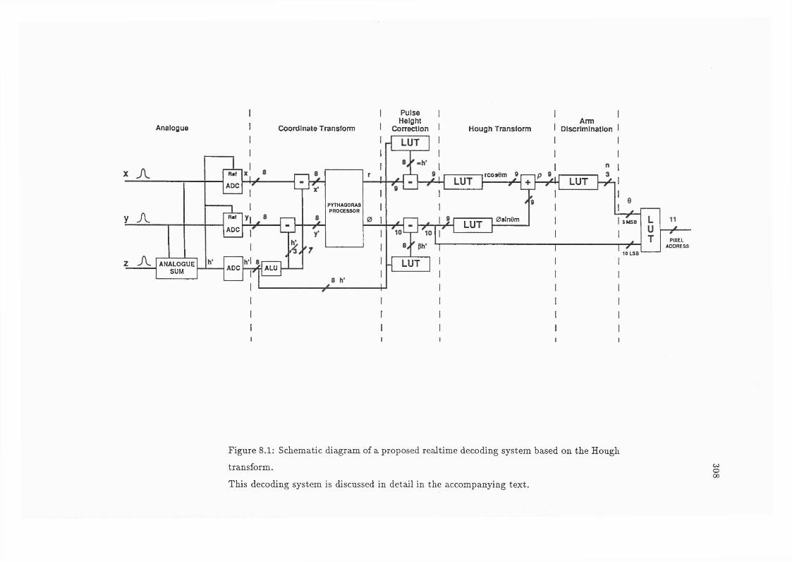
PulseHeight

CorrectionArm

DiscriminationAnalogue Coordinate Transform Hough Transform

rcosem 9

y A 0sln0m 3 MSB

PIXELADDRESS

10LSB

ALUADC

ADC

R af

ADC

R af

LUT

LUT

LUT

LUT

LUT

ANALOGUESUM

PYTHAGORASPROCESSOR

Figure 8.1: Schematic diagram of a proposed realtime decoding system based on the Hough transform.

This decoding system is discussed in detail in the accompanying text.

wo00

309

pixels axe addressable by combining the coarse and fine positions.

The correction for pnlse height related effects would be performed using LUTs

providing a correction value which is then subtracted from r and <j>. The subtraction would

be a straight forward operation on two binary numbers and could be carried out in simple

digital circuitry. As the corrections will be much smaller than the full range of the values

of these two parameters, an 8 bit correction will be more than sufficient. Therefore, the

correction can be carried out with two 256 byte LUTs. The values in the LUT would

be calculated separately by using the pulse height / parameter gradients which would be

measured in a manner similar to that described in Section 5.3.3.

The Hough transform would be carried out with three LUTs and a binary addition.

As the value 9^ that corresponds to the gradient of the spiral arms would have been

determined separately, the Hough transform would be reduced to

p = r cos + < sin dm . (8.1)

The LUTs would be loaded with the appropriate values corresponding to the two parameters multiplied by the trigonometric values. As discussed in Section 5.4, only 9 bits

are necessary for arm discrimination, so the two LUTs need only be 512 X 1.5 bytes each,

giving a total of 1.5 kB. The actual arm discriminator LUT would only require 512x0.5 bytes

as only 2-3 bits would be necessary for the spiral arm number, n.

The values of n and <j> would be combined to form a 13 bit value of 0, the spiral

angle; n forms the 3 most significant bits and <f> the 10 least significant bits. This value

would be used as the address for a leust 12 kB (8 k x l.5 bytes) LUT which contains the final

image pixel address.

Therefore, a system could be built that will run fast enough for the 200 kHz random

event rate required by the Optical Monitor. The total memory requirement, including pulse

height related corrections, is ~ 14 kB, approximately 25 times less than that required for

the laxge LUT decoding. Also, the number of bits on the inputs can be increased without

increasing the total memory requirements. Therefore, up to 16 bit ADCs could be used

for this system, which would require 24 Gigabytes for the large LUT method, or random

extension bits could be added to reduce fixed patterning.

310

8 .3 .3 T h e A nalogu e Front End

The largest problem with respect to the count rate performance of SPAN is the

analogue front end. Fast flight qualifled preamps have been developed for the SOHO CDS

Grazing Incidence Spectrometer (GIS) (Breeveld & Thomas, 1992). The preamps use a

shaping stage with a 148 ns shaping time and have a maximum count rate of 175 kHz. The

equivalent input noise with this shaping constant is 1.5 x 10 e“ , which corresponds to a

SNR of 1000 :1 assuming an average MCP gain of 5 X 10^ e~ distributed evenly between

the three anodes. While the two dimensional SPAN has demonstrated a centroiding PSF of

17 ^m, this was with non-flight electronics and a time constant of 2 //s. The PSF has not

been measured while using high speed electronics and this should be carried out as soon as

possible.

As discussed in Section 6.4, another limitation is the analogue bandwidth on the

reference input of ADCs. However, devices are available that can probably operate at count

rates up to 200 kHz.

8 .3 .4 T h e S u itab ility o f S P A N for U se in Space

In May 1992, due to failure of two image tube manufacturers to deliver working

tubes, of the five tubes delivered five failed, SPAN was withdrawn from consideration for

the Optical Monitor and the MIC detector was chosen.SPAN requires relatively high gain to achieve good resolution. Therefore, the

MCPs cannot undergo extensive scrubbing before the tube is sealed. The best spatial

resolution obtained with a sealed tube containing SPAN was only 60 //m FWHM. This

was due to the low gain, 3 x 10® e“ , approximately 10 times less than that used for the

detector described in this work, as the MCPs had undergone a scrubbing regime similar to

that used for the MIC detector. As MIC requires lower gains than SPAN, it can therefore

undergo more extensive scrubbing and so should have major advantages with respect to

tube lifetime. The spatial extent of long range gain depression may also be reduced.

The point source count rates for SPAN, and most other charge division anodes,

is limited only by the recharge time of the channels. This is the major advantage of these

readouts over scanned readout devices such as the CCD. Low resistance plates would have

to be used to meet the specifications for the Optical Monitor, although the effects of these

plates on tube lifetime have no been determined. Charge division anodes are also inherently

311

radiation tolerant.The amount of power available for the detectors is quite small, 7 W for the blue

detector on Optical Monitor (Bray, 1992) and 13 W between four detectors for the GIS on

SOHO CDS (Breeveld et aL, 1992). The small power allocations are the critical problem

for the SPAN detector. It requires that 8 bit ADCs are used as both these authors conclude

there are no radiation tolerant, high reliability ADCs with more than 8 bit digitization and

low enough power consumption. There is also insufficient power to allow combining two

8 bit ADCs together to attain 9 bit digitization.

Power constraints also place constraints on the amount of memory that can be

used for each detector. The GIS requires a LUT for each detector and so requires a total of

256 X 2 kB of RAM (McCalden, 1992). This is without any pulse height correction and so

requires that SPAN behaves ideally. Unless the MCPs can be operated in a regime where the

pulse height radius gradient is extremely small, which has been achieved on some occasions,

the detectors will either be plagued by severe ghosting or a significant degradation in the

photometric linearity of the detector will have to be accepted.

The size of the LUT also precludes telemetering the LUT contents from Earth.

A flat field will be telemetered to Earth and the spiral constants determined. This will be

sent to the satellite. An algorithm, based on one written by the author, will be used to calculate the LUT on board. This algorithm consists of approximately one quarter of the

total memory space required for on board software for the GIS due to need to use floating

point software libraries.

The Hough transform method of decoding could reduce the amount of memory

required while still providing pulse height related corrections. At a rate of 10 MHz, the

PDSP 16630 dissipates 400 mW. As only a 200 kHz throughput would be required, a

significant reduction in power consumption would be expected. MIL-Spec versions of both

of the chips are available, but they are both fabricated using 1 fim CMOS technology.

Therefore, their radiation tolerance must be suspect. However, Inmos Transputers have

passed radiation tolerance tests for the GIS (McCalden, 1992), so it is feasible that a

radiation tolerant batch of these chips could be selected. The power consumption and

radiation tolerance of these chips should be evaluated in the near future.

As was shown in Chapter 6 and by Breeveld et al. (1992a), the largest single

problem associated with low bit digitization is fixed patterning. Both the SPAN detectors

have a requirement for 2048 pixels but the SOHO detector has 4 spiral arms and the

312

Optical Monitor detector 3 in the active diameter. However, they both exhibit severe fixed

patterning. Constraints on the anode designs will probably prevent any further significant

reduction in the magnitude of fixed patterning through varying anode design parameters.

W ith the constraints on digitization and resolution there is almost no prospect of

reducing fixed patterning by using a different set of user defined parameters than those used

at present. Limitations on memory size also preclude the use of extension bits. The only

remaining the option is to iteratively reassign the vertices in the hexagonally packed lattice

in the spiral plane to different output pixels, in order to produce uniform pixel sensitivity. A

similar method is used in the MIC detector (Carter et of., 1990,1991b) but the correction is

reliable for only a given set of MCP operating conditions and for a localized region. Varying

these conditions, such as gain and charge cloud size can reintroduce fixed patterning. The

stability of such a correction in SPAN is unclear, as it must hold across the entire width of

the detector even when some regions axe driven into severe gain depression.

SPAN has the potential to be a high speed, high resolution detector. It probably

needs only ru 8 bit accuracy on the analogue charge measurement to attain good resolution.

This has yet to be confirmed experimentally but it is suggested by the lack of variability in

the image sizes in the simulations of fixed patterning in Figures 6.9 and 6.10. However, it

requires at least true 9 or, preferably, 10 bit digitization to overcome fixed patterning.

Using the Hough transform decoding scheme, a fast, high performance ground

based detector could be built using 12 bit fixed reference ADCs, e.g. the THC 1201 (TRW,

1991) which is a 10 mega samples per second device that consumes 4.5 W. While power

budgets for detectors are so low or until high reliability, radiation tolerant, low power ADCs

with more than 8 bits are available, SPAN (and any other charge division readout that uses

charge or time measurement) is unsuitable for a high speed, laxge format, high resolution,

satellite based detector.

313

BibliographyAdams, J. & Manley, B. W., 1966, I E E E T r a n s . N u c l . S c i . NS-13, 88.

AUemajid, R, & Thomas, G., 1976, N u c l . I n s t r u m . M e t h . 137, 141.

Allington-Smith, J. R. & Schwarz, H. E., 1984, Q . J l . R . a s t r . S o c . 2 5 ,^ 7 . . .PcurJletU,l.r.,

Allison, J., 1985, N u c l . I n s t r . M e t h . A 236, 284.. Â

Allison, J., Ashton, P., Baines, J. T. M., Barlow, R. J., Chrin, J. T. M., Davies, O. W., Dnerdoth, I. P., Hinde, P. S., Banks, J. N., Hughes-Jones, R. E., Lafferty, G. D., Loebinger, F. K., Macbeth, A. A., Moss, M. W., Murphy. P. G., O’Dowd, A., Pawley, S. J. & Stephens, K., 1991, Proc. 2nd. London Position Sensitive Detectors, London ,U.K. 1990, N u c l . I n s t r .

a n d M e t h . A310, 527.

Anacker, D. C. & Erskine, J. L., R e v . S c i . I n s t r u m . , 62, 1247, 1991.

Analog Devices, 1988, D a t a C o n v e r s i o n P r o d u c t s D a t a b o o k , Norwood, MA, USA, 3-339.

Arfken, G., 1970, M a t h e m a t i c a l M e t h o d s f o r P h y s i c i s t s 2nd. Ed., Academic Press, New York, pg. 725 and pp. 737-741.

Authinarayanan, A. Sz Dudding, R. W., 1976, Photo-Electronic Image Devices, Proc. Third. Symposium, London, 1975, A d v a n c e s i n E l e c t r o n i c s a n d E l e c t r o n P h y s i c s 40A, 167.

Barstow, M. A. k Sansom, A. E.,' 1990, S P I E 1344, 244.

Baum, W. A., 1966, Photo-Electronic Image Devices, Proc. Third. Symposium, London, 1965, A d v a n c e s i n E l e c t r o n i c s a n d E l e c t r o n P h y s i c s 22 A, 617.

Bendat, J. S. k Piersol, A. G., 1966, “ M e a s u r e m e n t a n d A n a l y s i s o f R a n d o m D a t a ” ,

John Wiley k Sons, New York, pg. 15.

Ben-Tzvi, D. k Sandler, M. B., 1990, P a t t e r n R e c o g n i t i o n L e t t e r s , 11, 167.

314

Bevington, P. R., 1969, “ D a t a R e d u c t i o n a n d E r r o r A n a l y s i s f o r t h e P h y s i c a l S c i e n c e s ” ,

McGraw-Hill, New York, pp 187-203.

Bray, N., 1992, “ C o m p a r i s o n o f M I C a n d S P A N E l e c t r o n i c s f o r E n g i n e e r i n g i n t o t h e S p a c e

E n v i r o n m e n t ” , MSSL Optical Monitor Technical Report, XMM-OM/MSSL/RV/004.

Breeveld, A. A., 1992, P h . D . T h e s i s , University of London, i n p r e p a r a t i o n .

Breeveld, A. A., Edgar, M. L., Smith, A., Lapington, J. S. & Thomas, P. D., 1992a, Proc.4th. Int. Conf. Synchrotron Radiation Instrum., Chester, U.K., 1991, R e v . S c i . I n s t r u m .

63 P a rt II, 673.

Breeveld, A. A., Edgar, M. L., Lapington, J. S. k Smith, A., 1992b, S P I E , 1743, 315.

Breeveld, A. A. k Thomas, P. D., 1992, P r o c . I n t . S y m p . P h o t o n D e t e c t o r s f o r S p a c e

I n s t r u m e n t a t i o n , ESA Special Publication SP-356, i n p r e s s .

Bronshteyn, I. M., Yevdokimov, A. V., Stozharov, V. M., k Tyutikov, A. M., 1980, R a d i o

E n g . E l e c t r o . P h y s . 24, 150.

Bryant, D. A. k Johnstone, A. D., 1965, R e v . S c i . I n s t r u m . 36, 1662.

Carter, M. K., Cutler, R., Patchett, B. E., Read, P. D., Waltham, N. k van Breda, I. G.,

1990, S P I E 1235.

Carter, M. K., Patchett, B. E., Read, P. D., Waltham, N. k van Breda,I. G., 1991, Proc.2nd. London Position Sensitive Detectors, London ,U.K. 1990, N u c l . I n s t r . a n d M e t h .

A310, 305.

Carter, M. K., 1991a “ D a t a P r o c e s s i n g R e q u i r e m e n t s i n a C e n t r o i d i n g P h o t o n C o u n t i n g

S y s t e m ” , p r i v a t e c o m m u n i c a t i o n .

Carter, M. K., 1991b, p r i v a t e c o m m u n i c a t i o n .

Chapman, H. N., Nugent, K. A. k Wilkins, S. W., 1991, R e v . S c i . I n s t r u m . 62, 1542.

ChappeU, J. H. k Murray, S. S., 1989, S P I E 1159, 460.

* evu ;cc j^ O / P . M * 4 e A "T. 0 , H . , A 1 a a 2 . 0

P te a to c fe A . R c (. .4- ^

315

Cho, D. J. & Morris, G. M., 1988,5P/Æ? 976, 172.

Cho, D. J., 1989, Ph.D. Thesis^ University of Rochester.

Clampin, M. h Edwin, R. P., 1987, Rev. Sci. Instrum. 58, 167.

Clampin, M., Crocker, J., Paresce, F. & Rafal, M., 1988, Rev. Sci. Instrum. 59, 1269.

Corben, H. C. & Stehle, P., 1974 “Classical Mechanics” 2nd. Ed., Robert E, Krieger, New

York, pg. 140.

Culhane, J. L., 1991, Proc. 2nd. London Position Sensitive Detectors, London, U.K. 1990,

Nucl. Instr. and Meth. A310, 1.

deBoor, C., 1970 , “CADRE: An Algorithm for Numerical Quadrature” , in Mathematical

Software^ edited by John R. Rice, Academic Press, Orlando, Florida, pp. 417—442.

deBoor, C., 1971 , “On Writing an Automatic Integration Algorithm”, in Mathematical

Software., edited by John R. Rice, Academic Press, Orlando, Florida, pp. 201—209.

Eberhardt, E. H., 1977, Appl. Opt. 16, 2127.

Eberhardt, E. H., 1979, Appl. Opt. 18, 1418.

Eberhardt, E. H., 1980, ITT Electro-Optical Products Division, Technical Note, N o 127,

ITT Tube and Sensor Laboratories, Fort Wayne, Indiana.

Eberhardt, E. H., 1981, IEEE Trans. Nucl. Sci. NS-28, 712.

Edgar, M. L., Kessel, R., Lapington, J. S. & Walton, D. M., 1989 Rev. Sci. Instrum. 60, 3673.

Edgar, M. L., Lapington, J. S. & Smith, A., 1992a, Proc. 4th. Int. Conf. Synchrotron

Radiation Instrum., Chester, U.K., 1991, Rev. Sci. Instrum. 63 P a r t II, 816.

Edgar, M. L., Smith, A. & Lapington, J. S., 1992b, SPIE, 1743, 283.

Evans, D. S., 1965, Rev. Sci. Instrum. 36, 375.

316

Feller, W. B., 1991, Proc. 2nd. London Position Sensitive Detectors, London ,U.K. 1990,

Nucl. Instr. and Meth. A310, 249.

Firmani, C., Rniz, E., Bisiachi, G. F., Salas, L., Paresce, F. & Carlson, C. W., 1984, Astron.

Astrophys. 134, 251.

Colson, W. B., Me Pherson, J. & King, F. T., 1973, Rev. Sci. Instrum. 44, 1694.

Fordham, J. L. A., Bone, D. A., Read, P. D., Norton, T. J., Charles, P. A., Carter, D.,

Cannon, R. D. & Pickles, A. J., 1989, Mon. Not. R. astr. Soc. 237, 513.

Fordham, J. L. A., 1990, private communication.

Fraser, G. W. 6 Mathieson, E., 1981, Nucl. Instrum. Meth. 180, 597.

Fraser, G. W., Pearson, J. P., Smith, G. C., Lewis, M. & Barstow M. A., 1983, IEEE Trans.

Nucl. Sci. NS-30, 455.

Fraser, G. W., 1989, “X-ray Detectors in Astronomy”., Cambridge University Press, Cambridge, pp 169-170.

Fraser, G. W., Lees, J. E., Pearson, J. F. & Barstow, M. A., 1991a, Proc. 2nd. London

Position Sensitive Detectors, London ,U.K. 1990, Nucl. Instr. and Meth. A310, 292.

Fraser, G. W., Pain, M. T., Lees, J. E. & Pearson, J. F., 1991b, Nucl. Instr. Meth. A306,

247.

Fraser, G. W., Pain, M. T. & Lees, J. E.,1992, preprint.

Friedman, P. G., Martin, C. & Rasmussen, A. 1990, SPIE 1344, 183.

Fforyan, R. F. & Johnson, C. B., 1989, SPIE 1072, 30.

Gatti, E., Oba, K. & Rehak, P., 1983, IEEE Trans. Nucl. Sci.., NS-30, 461.

Gear, C. W., 1969 Proc. Skytop Conf. US AEG Conf. No.670301,. 552, (as quoted in

Fraser, 1989).

317

GEC Plessey, 1990, “Digital Signal Processing IC Handbook”, Chenney Manor, Swindon,

Wiltshire, UK, 73.

Geesman, H., Hanne, G. F., Stauffer, A. D. & Stauffer, J. A., 1991, Nucl. Instr. and Meth.

A307, 413.

Goodrich, G. W. & Wiley, W. C, 1961, Rev. Sci. Instrum. 32, 846.

Goodrich, G. W. & Wiley, W. C, 1962, Rev. Sci. Instrum. 33, 761.

Guest, A. J., 1971, Acta Electronica 14, 79.

Guest, A. J., 1978, Philips Research Laboratory Annual Review, 15.

Guest, A. J., 1988, Proc. of SID 29, 193.

Guggenheimer, H. W., 1977, “Differential Geometry”, Dover, New York, pp 11-12.

Hamamatsu, 1987, Technical Data Sheet, T-114, Hammamtsu Photonics, Electron Tube

Division, Iwata-gun, Shizuoka-ken, Japan.

Harris, L. A., 1971, Rev. Sci. Instrum. 42, 987.

Hatfield, J. V., Burke, S. A., Comer, J., Currel, P., Goldfinch, J. & York, T. A., 1992, Rev. Sci. Instrum. 63, 235.

Hill, G. E., 1976, Photo-Electronic Image Devices, Proc. Third. Symposium, London, 1975,

Advances in Electronics and Electron Physics 40A, 153.

Hynecek, J., 1988, IEEE Trans. Electron. Device ED-35, 646.

Jelinsky, P., 1979, “The Size and Distribution of Electron Clouds from an MCP Detector”,

private communication.

Kawakami, H., 1992, private communication.

Keller, H., Klingelhofer, G. & Kankeleit, E., 1987, Nucl. Instrum. Meth. A258, 221.

318

Kessel, R., 1988, private communication.

Klinowski, J., 1990, Nature 346, 509.

Knibbeler, C. L. C. M., Hellings, G. J. A., Maaskamp, H. J., Ottevanger, H. & Brongersma,

H. H., 1987, Rev. Sci. Instrum. 58, 125.

Koike, M. & Hasegawa, K., 1988, Nucl. Instr. and Meth. A272, 840.

Koshida, N. & Hosobuchi, M., 1985, Rev. Sci. Instrum. 56, 1329.

Koshida, N., 1986, Rev. Sci. Instrum. 57, 354.

Kowalik, J. & Osborne, M. R., 1968, “Methods for Unconstrained Optimization Problems”

American Elsevier, New York.

Kume, H., Muramatsu, S. & lida, M., 1986, IEEE Trans. Nucl. Sci. NS-33, 359.

Lampton, M., & Paresce, F., 1974, Rev. Sci. Instrum. 45, 1098.

Lampton, M., & Malina, R. F., 1976, Rev. Sci. Instrum. 47, 1360.

Lampton, M. & Bixler, J., 1985, Rev. Sci. Instrum. 56, 164.

Lapington, J. S., Kessel, R. 6: Waltoh D. M., 1988, Nucl. Iristr. Méth. A273, 663.

Lapington, J. S. & Edgar, M. L., 1989, Proc. SPIE 1159, 565.

Lapington, J. S., Breeveld, A. A., Edgar, M. L., Tandy, J. A. & Trow, M. W., 1990, Proc.

SPIE 1344, 324.

Lapington, J. S., Breeveld, A. A., Edgar, M. L. & Trow, M. W., 1991 Proc. 2nd. London

Position Sensitive Detectors, London ,U.K. 1990, Nucl. Instr. and Meth. A310, 299.

Lapington, J. S., Breeveld, A. A., Edgar, M. L. & Smith, A., 1992, SPIE, 1743, 303.

Lombard, F, J., & Martin, F., 1961, Rev. Sci. Instrum. 32, 200.

Loty, C., 1971, Acta Electronica 14, 107.

319

Lyons, A., 1985, J . P h y s . E . : S c i . I n s t r u m . 18, 127.

Me Calden, A. J., 1992, P r o c . I n t . S y m p . P h o t o n D e t e c t o r s f o r S p a c e I n s t r u m e n t a t i o n . ,

ESA Special Publication SP-356, i n p r e s s .

Martin, C., Jelinsky, P., Lampton, M., Malina, R. F. Anger, H. O., 1981, R e v . S c i . I n

s t r u m . 52, 1067.

Martin, C. & Bower, S., 1982, A p p l . O p t 21, 4206.

Massey, H. S. W. & Kestelman, H., 1964, “ A n c i l l a r y M a t h e m a t i c s ” 2 n d e d , Pitman & Sons,

London,261, 523, 847.

Mathieson, E., Smith, G. C. & Gilvin, P. J., 1980, J. P h y s . E : S c i . I n s t r u m . 13, 792.

Me Clintock, W. E., Barth, C. A., Steele, R. E., Lawrence, G. M. & Timothy, J. G., 1982, A p p l . O p t . 21, 3071.

McKee, B. T. A., Duffy, A. G., Feller, W. B. & Stewart, A. T., 1991, Proc. 2nd. London Position Sensitive Detectors, London ,U.K. 1990, N u c l . I n s t r . a n d M e t h . A310, 256.

Me Kinley, M. S., 1986, p r i v a t e c o m m u n i c a t i o n .

Micro Power Systems, 1989, F u l l L i n e C a t a l o g , Santa Clara, CA, USA, 2-50,

Murtagh, F. & Heck, A. , 1987, “ M u l t i v a r i a t e D a t a A n a l y s i s ” D. Riedel, Dodrecht, Chap

ter 4.

Nakamura, T. & Matsumoto, K., 1992, p r e p r i n t .

Nartallo Garcia, R., 1990, M . S c . T h e s i s , University of London.

Neischmidt, E. B., Lawrence, R. S. & Gentillon, C. D., 1982, I E E E T r a n s . N u c l . S c i .

Norton, T. J., 1990, P h . D . T h e s i s , University of London.

320

Norton, T. J., Airey, R. W., Morgan, B. L., Fordham, J. L. A. & Bone, D. A., 1991, Conf.

on Photoelectonic Image DeviceSy London, 1991, lOP Publishing Ltd., 97.

Oba, K. & Rehak, P., 1981, IEEE Trans. Nucl. Sci. NS-28, 683.

OPAL Collaboration, 1991, Nucl. Instr. Meth. A305, 275.

Papaliolos, C., Misenson & Ebstein, 1985, Appl. Opt. 24, 287.

Pearson, J. F., Fraser, G. W. & Whitley M. J., 1987, Nucl. Instr. Meth. A258, 270.

Pearson, J. F., Lees, J. E., &: Fraser, G. W., 1988, IEEE Trans. Nucl. Sci. NS 35, 520.

Phillips, A., 1992, Ph. D. Thesis, University of London, in preparation.

Pratt, W. K., 1978, “Digital Image Processing”,John Wiley & Sons, New York.

Press, W. H., Flannery, B. P., Teukolsky, S. A & Vetterling W. T., 1986,

“Numerical Recipes, The Art of Scientific Computing”, Cambridge University Press, Cam

bridge.

Purshke, M., NuxoU, W., Gaul, G. & Santo, R., 1987, Nucl. Instrum. Meth. A261, 537.

Rager, J. P., Renaud, J. F. & Tezenas du Mont cel, V., 1974, Rev. Sci. Instrum. 45, 927.

Rasmussen, A. & Martin, C., 1989, SPIE 1159, 538.

Randall, R. P., 1966, Photo-Electronic Image Devices, Proc. Third. Symposium, London,

1965, Advances in Electronics and Electron Physics 22A, 87.

Read, P. D., 1990, private communication.

Read, P. D., van Breda, I. G. & Norton, T. J., 1990, Proc. SPIE 1235,305.

Richter, L. J. & Ho, W., 1986, Rev. Sci. Instrum. 57, 1469.

Rodgers, A. W., King, D., Conroy, P. & Harding, P., 1988, preprint.

321

Sams, B. J. Ill, 1991, Rev. Sci. Instrum. 62, 595.

Samson, J. A. R., 1984, Nucl. Instr. and Meth. A222, 215.

Schecker, J. A., Schauer, M. M., Holzschetter, K. & Holzschetter, M. H, 1992, Nucl. In

strum. Meth. A320, 556.

Schmidt, K. C. & Hendee, C. F., 1966, IEEE Trans. Nucl. Set. NS 13, 100.

Sharma A. & Walker, J. G., 1989, Quant. Opt. 1, 11.

Sharma A. & Walker, J. G., 1990, SPIE 1235, 474.

Sharma A., 1991, Ph.D Thesis, University of London.

Sharma A. & Walker, J. G., 1992, Rev. Sci. Instrum., in press.

Siegmimd, O. H. W., Coburn, K. & Malina, R. F., 1985, IEEE Trans. Nucl. Sci. NS 32,443.

Siegmund, O. H. W., Lampton. M. L., Chakrabarti, S., Vallerga, J., Bower, S. & Malina,

R. F., 1986a, SPIE 1159, 476.

Siegmund, O. H. W., Lampton. J., Bower, S. & Malina, R. F., 1986b, IEEE Trans. Nucl. Sci. NS 33, 724.

Siegmund, O. H. W., 1989, Proc. SPIE 1072, 111.

Siegmund, O. H. W., Lampton. M. L. & Raffani, R., 1989a, SPIE 1159, 476.

Siegmund O. H. W., Chakrabarti, S., Cotton^ D. M. & Lampton, M., 1989b, IEEE Trans.

Nucl. Sci. NS 36, 916.

Siegmund, O. H. W., Cully, S., Warren, J., Gaines, G. A., Priedhorsky, W. & Bloch, J.,

1990, Proc. SPIE 1344, 346.

Siegmund, O. H. W. & Stock, J., 1991, SPIE 1549, 81.

322

Slater, D. C. & Timothy, J. G., 1991, SPIE 1549, 68.

Smith, A. D. & AUington-Smith, J. R., 1986, IEEE Trans. Nucl. Sci. NS-33, 295.

Smith A., Kessel, R., Lapington, J. S. & Walton, D. M., 1989, Rev. Sci. Instrum. 60,

3509.

Smith, A. & Bavdaz, M., 1992, Proc. 4th. Int. Conf. Synchrotron Radiation Instrum.,

Chester, U.K., 1991 Rev. Sci. Instrum. 63 P a r t II , 689.

Smith, P. J., 1991, private communication.

Sobottka, S. E. & Williams, M. B., 1988, IEEE Trans. Nucl. Sci. NS 35, 348.

Stiimpel, J. W., Sanford, P. W. & Goddard, H. F., 1973, J. Phys. E: Sci. Instrum. 6, 397.

Tanalca, N., Hashimoto, S., Shinohara, M., Sugawa, S., Morishita, M., Matsumoto, S, Naka

mura, Y. & Ohmi, T., 1990, IEEE Trans. Electron. Device ED-37, 964.

Timothy, J. G., 1974, Rev. Sci. Instrum. 45, 834.

Timothy, J. G. & Bybee, R. L., 1975a, Appl. Opt. 14, 1632.

Timothy, J. G. & Bybee, R. L., 1975b, Rev. Sci. Instrum. 46, 1615.

Timothy, J. G., 1981, Rev. Sci. Instrum. 52, 1131.

Timothy, J. G., Mount, G. H. & Bybee, R. L., 1981 IEEE Trans. Nucl. Sci. 28, 689.

TRW, 1991, “Data Converters - DSP Products Databook” La Jolla, CA, USA, A-163, A-

287 and F-65.

Trap, H. J., L., 1971, Acta Electronica 14, 41.

Turner, M. J. L., Smith, A. & Zimmerman, 1981, Sp. Sci. Rev., 30, 513.

Vallerga, J. V., Kaplan. G. C., Siegmund, O. H. W., Lampton, M., &: Malina, R. F., 1989,

IEEE Trans. Nucl. Sci. NS 36, 881.

323

Vallerga, J. V., Siegmund, O. H. W., Vedder, P. W.& Gibson, J. L., 1991, Froc. 2nd.

London Position Sensitive Detectors, London ,U.K. 1990, Nucl. Instr. and Meth. A310,

317.m \

Veaux, J., Cavailler, C., Gex, JP., Hauduceour, A. & Hyvernage, M., Rev. Sci. Instrum. 62, 1562.

Washington, D., Duchenois, V., Polaert, R. & Beasley, R. M., 1971, Acta Electronica 14,

201.

Weaat, R. C., “Handbook of Chemistry and Physics” 47th. Ed.,

The Chemical Rubber Co., Cleveland, 1966.

Wilkins, S. W., Stevenson, A. W., Nugent, K. A, Chapman, H. & Steenstrup, S., 1989, Rev.

Sci. Instrum. 60, 1026.

Williams, M. B. & Sobottka, S. E., 1989, IEEE Trans. Nucl. Sci. NS 36, 227.

Wiza, J. L., Henkel, P. R. & Roy, R. L., 1977, Rev. Sci. Instrum. , 48, 1217.

Wiza, J. L., 1979, Nucl. Inst. Meth 162, 587.

Yamaguchi, N., Aoki, S. & Miyoshi, S., 1987, Rev. Sci. Instrum. 58, 43.

Yusa, A., Nishizawa, J., Imai, M., Yamada, H.,Nakamura, J., Mizoguchi, T., Ohta, Y. &

Takayama, M., 1986, IEEE Trans. Electron. Device ED-33, 735.

Zombeck, M. V.,& Eraser, G. W., 1991, SPIE 1549, 90.

324

Acknowledgements

I would like to express my sincere appreciation to Prof. Len Culhane for the opportunity

to carry out the research for this thesis, which I know caused him not inconsiderable incon

venience then and since. I would also like to thank him for being my supervisor and for all

his help and encouragement throughout my time at MSSL.

I gratefully acknowledge the award of a Dean’s Studentship by University College

London.

I also wish to thank the members of the Detector Physics Group for their support,

encouragement and friendship: Alice Breeveld, Hajime Kawakami, Jon Lapington, Alan

Smith and especially Matt Trow. And I would like to particularly thank those who suffered

terribly during the proof reading.I would like to thank the members of my panel. Prof. Alan Johnstone and Dr.

Keith Mcison, for their advice and assistance, particularly in two hopeless, though different,

causes. I would also like thank the following people for useful discussions and/or making

unpublished material available: Martin Carter and Pete Read form Rutherford Appleton

Lab, Abhay Sharma from King’s College, Tim Norton from Imperial College and George

Fraser from The University of Leicester.

I would like to thank the ladies in the oflfice, particularly Ros and Libby, the

gentlemen in the workshop and in the electronic engineering group, especially Gary Legge,

Alec McCalden, Kerrih Rees, Jason Tandy and Steve Welch. And I’m happy to express

gratitude to all those who showed me many personal kindnesses during my stay in England,

in particular Eva Alam, Khalid al Janabi, Chris Alsop, Mark Birdseye, Charon Birket, the

Breevelds, Francisco Carrera, the Fosters, the Kessels, Ronghui Lui, Dave Rodgers, the

Rosens, Mike Tidy, the Waltons (especially for the sandwiches), Dave Wonnacott, the staff

and patrons of the “King’s Head” and “The Live and Let Live” and especially At a Etamadi.

Finally, I wish to thank my fellow students during my stay here, for their friend

ship and encouragement : Steve Broadmeadow, Ady James, Ramon Nartallo Garcia, Vito

Graffagnino, John Mittaz, George Papatheodorou, Liz Puchnarewicz, Gavin Ramsey, Phil

Smith, Lee Sproats, Sarah Szita, and my fellow non-persons, Mark Gar lick, Chris Jomaron,

Sri Moorthy and Andy Phillips. Good luck to those still going and I hope that your own

private calvary will not be as protracted as was mine.

ProQuest Dissertations - UCL Discovery

Documents