nm u Ottawa L'Universite canadienne Canada's university

Welcome message from author
This document is posted to help you gain knowledge. Please leave a comment to let me know what you think about it! Share it to your friends and learn new things together.
Transcript

nm u Ottawa L'Universite canadienne
Canada's university
FACULTE DES ETUDES SUPERIEURES l ^ ^ l FACULTY OF GRADUATE AND ET POSTOCTORALES u Ottawa POSDOCTORAL STUDIES
L'Universite canadienne Canada's university
Xianjie Li TufEnRDEl^fHWETXUTHORWTHESTs""
M.A.Sc. (Mechanical Engineering) GRADE/DEGREE
Department of Mechanical Engineering FACULTE, ECOLE, DEPARTEMENT / FACULTY, SCHOOL, DEPARTMENT
Investigation into Spongy Bone Remodeling Through a Semi-mechanistic Bone Remodeling Theory Using Finite Element Analysis
TITRE DE LA THESE / TITLE OF THESIS
Gholamreza Rouhi ~ b 7 R l c f E U R " ( W E C ™ ^ ^
CO-DIRECTEUR (CO-DIRECTRICE) DE LA THESE / THESIS CO-SUPERVISOR
Zin Wang Marianne Fenech
Gary W. Slater Le Doyen de la Faculte des etudes superieures et postdoctorales / Dean ot the Faculty of Graduate and Postdoctoral Studies
Investigation into Spongy Bone Remodeling through a
Semi-mechanistic Bone Remodeling Theory Using
Finite Element Analysis
by
Xianjie Li
A thesis submitted to
the Faculty of Graduate and Postdoctoral Studies
in partial fulfillment of
the requirements for the degree of
MASTER OF APPLIED SCIENCE
in Mechanical Engineering
Ottawa-Carleton Institute for Mechanical and Aerospace Engineering
UNIVERSITY of OTTAWA
© Xianjie Li, Ottawa, Canada, 2010

1*1 Library and Archives Canada
Published Heritage Branch
395 Wellington Street Ottawa ON K1A 0N4 Canada
Bibliotheque et Archives Canada
Direction du Patrimoine de I'edition
395, rue Wellington OttawaONK1A0N4 Canada
Your file Votre reference ISBN: 978-0-494-74187-0 Our file Notre reference ISBN: 978-0-494-74187-0
NOTICE: AVIS:
The author has granted a nonexclusive license allowing Library and Archives Canada to reproduce, publish, archive, preserve, conserve, communicate to the public by telecommunication or on the Internet, loan, distribute and sell theses worldwide, for commercial or noncommercial purposes, in microform, paper, electronic and/or any other formats.
L'auteur a accorde une licence non exclusive permettant a la Bibliotheque et Archives Canada de reproduire, publier, archiver, sauvegarder, conserver, transmettre au public par telecommunication ou par I'lnternet, preter, distribuer et vendre des theses partout dans le monde, a des fins commerciales ou autres, sur support microforme, papier, electronique et/ou autres formats.
The author retains copyright ownership and moral rights in this thesis. Neither the thesis nor substantial extracts from it may be printed or otherwise reproduced without the author's permission.
L'auteur conserve la propriete du droit d'auteur et des droits moraux qui protege cette these. Ni la these ni des extra its substantiels de celle-ci ne doivent etre imprimes ou autrement reproduits sans son autorisation.
In compliance with the Canadian Privacy Act some supporting forms may have been removed from this thesis.
Conformement a la loi canadienne sur la protection de la vie privee, quelques formulaires secondaires ont ete enleves de cette these.
While these forms may be included in the document page count, their removal does not represent any loss of content from the thesis.
Bien que ces formulaires aient inclus dans la pagination, il n'y aura aucun contenu manquant.
1*1
Canada
Investigation into Spongy Bone Remodeling through a Semi-mechanistic
Bone Remodeling Theory Using Finite Element Analysis
Xianjie Li
Department of Mechanical Engineering, University of Ottawa
Submitted in December, 2010
Master thesis abstract
Computer simulation provides a useful approach for the studies on the issues related to
living bone. Here, we performed two simulation studies on the spongy bone remodeling
through Huiskes et al.'s semi-mechanistic bone remodeling theory. In the first study, a
2D finite element (FE) model was developed. The simulation results suggested that
decreasing osteocyte density could cause spongy bone loss in healthy old adults, and
reduction in osteocyte mechanosensitivity might contribute to excessive bone loss in
osteoporotic bones. In the second study, we extended Huiskes et al.'s theory for
overloading condition with respect to clinical findings and proposed a 3D FE model. It
was the first 3D simulation which showed the spongy bone loss caused by overload. It
supported our hypotheses that overload increased osteoclastic activities and reduced
osteocyte influence distance. The simulation results in both two studies are in agreement
with existing experimental evidences, also with Wolffs Law.
1
Abstract
Computer simulation provides a useful approach for the studies on the issues related to living
bone. Here, we performed two simulation studies on the spongy bone remodeling through
Huiskes et al.'s semi-mechanistic bone remodeling theory. In the first study, a 2D finite
element (FE) model was developed. The simulation results suggested that decreasing
osteocyte density could cause spongy bone loss in healthy old adults, and reduction in
osteocyte mechanosensitivity might contribute to excessive bone loss in osteoporotic bones. In
the second study, we extended Huiskes et al.'s theory for overloading condition with respect
to clinical findings and proposed a 3D FE model. It was the first 3D simulation which showed
the spongy bone loss caused by overload. It supported our hypotheses that overload increased
osteoclastic activities and reduced osteocyte influence distance. The simulation results in both
two studies are in agreement with existing experimental evidences, also with Wolffs Law.
11

Acknowledgements
First of all, I would like to express my gratitude immensely to my supervisor Dr. Gholamreza
Rouhi for his guidance, support, hard work and dedication throughout my graduate studies.
His continuous encouragement and his passion for research motivated me all the time when I
experienced any challenge and obstacle in my studies and research.
I would like to thank the University of Ottawa's FGPS for providing the conference
travel grant and thank the University of Ottawa's GSAED for providing additional financial
support.
I am grateful to all of my research group mates. In particular, I would like to thank
Kwan-Ching Geoffrey Ng and Kristina Haase who have always been happy to lend a hand or
share their knowledge. As well, thanks go to Ali Vahdati for his useful feedbacks.
Furthermore, I would like to acknowledge Dr. Michel Labrosse for his advice on my studies.
Last but not least I would like to give a special thank you to my parents, Ziqiu Li and
Ling Lin, and my sisters, Xianxian Li and Xianli Li, who have always encouraged me to purse
my interest. Their endless love, support and patience enabled me to complete my study.
Contents
Abstract ii
Acknowledgements iii
Contents iv
List of Tables vii
List of Figures viii
Nomenclature xi
Chapter 1 Introduction 1
1.1. Motivation 3
1.2. Objectives 6
1.3. Thesis organization 6
Chapter 2 Background and literature reviews 7
2.1. Components of bone matrix 7
2.2. Bone structure 8
2.3. Bone cells 14
2.4. Osteocyte mechanosensing 16
2.5. Spongy bone mechanics 18
2.6. Bone remodeling process 22
2.7. Bone diseases related to bone remodeling 26
2.8. Bone remodeling theories 29
2.8.1. Trajectorial theory and Wolffs Law 31
2.8.2. Frost's mechanostat theory 32
2.8.3. Cowin andHegeda's adaptive elasticity theory 33
2.8.4. Huiskes et al.'s strain energy density model 33
2.9. Open questions related to bone remodeling 33
Chapter 3 General methods 35
3.1. A semi-mechanistic bone remodeling theory 35
3.1.1. A phenomenological model developed by Huiskes and co-workers 35
3.1.2. A semi-mechanistic bone remodeling theory 38
3.2. Finite element analysis 43 iv
Chapter 4 An investigation into the reasons for bone loss in aging and osteoporotic individuals using a two-dimensional computer model 46
4.1. Introduction 46
4.2. Methods 48
4.2.1. A semi-mechanistic bone remodeling theory 48
4.2.2. A two-dimensional computer model 49
4.2.3. Computer simulations of spongy bone remodeling 51
4.3. Results 54
4.4. Discussion and conclusions 62
Chapter 5 A three-dimensional computer model to simulate spongy bone remodeling under overload
65
5.1. Introduction 65
5.2. Methods 68
5.2.1. A semi-mechanistic bone remodeling theory 68
5.2.2. Hypotheses for the effects of overload on bone remodeling 68
5.2.3. A three-dimensional computer model 71
5.2.4. Computer simulations of spongy bone remodeling 74
5.3. Results 76
5.4. Discussion and conclusions 83
Chapter 6 Summary, conclusions and future directions 88
6.1. Summary 88
6.1.1. Investigation into the reasons for spongy bone loss in aging and osteoporotic individuals
89
6.1.2. A three-dimensional computer model to simulate spongy bone remodeling under overload 91
6.2. Conclusions 92
6.3. Future directions 93
References 95
Publications arising from this thesis 108
Appendix I Finite element methods 109
1.1. Equations for two-dimensional (2D) finite elements 109
1.1.1. The matrix of shape function [TV] I l l
1.1.2. The Jacobian matrix [J] 113
V
1.1.3. The elastic material property matrix [D] for plan stress 114
1.1.4. The strain-nodal displacement matrix [B] 114
1.1.5. The element stiffness matrix [fC] 115
1.1.6. The strain energy density Ue 117
1.2. Equations for three-dimensional (3D) finite elements 119
1.2.1. The matrix of shape function [N] 120
1.2.2. The Jacobian matrix [J] 123
1.2.3. The elastic material property matrix [D] 124
1.2.4. The strain-nodal displacement matrix [B] 125
1.2.5. The element stiffness matrix [fC] 126
1.2.6. The strain energy density ue 129
Appendix II Simulation programs for spongy bone remodeling 130
ILL Input files 130
II. 1.1. input_2D.dat 131
II. 1.2. input_3D.dat 132
11.2. Main programs 133
II.2.1. main_2D.f90 133
H.2.2. main_3D.f90 139
11.3. Subroutines 146
11.3.1. main.f90 146
11.3.2. geom.f90 158
11.4. Output files 162
11.4.1. Two-dimension 162
11.4.1.1. twoD_elements.m 162
11.4.2. Three-dimension 163
H.4.2.1. threeDelements.m 163
11.4.2.2. threeD_surface.m 164
11.5. Glossary of main variable names 165
vi
List of Tables
Table 4.1 Parameters settings for the two-dimensional spongy bone remodeling simulations
51
Table 4.2 Osteocyte density of healthy adults and osteoporotic patients 53
Table 5.1 Parameters settings for the three-dimensional spongy bone remodeling simulations
74
Table I.l Sampling points, weighting factors for 4-node square elements with 4 integrating
points 117
Table 1.2 Sampling points, weighting factors for 8-node square elements with 8 integrating
points 128
Vll
List of Figures
Figure 2.1 Human skeleton 9
Figure 2.2 A cutaway view of the human vertebrae and femur 10
Figure 2.3 Cortical and spongy bones 11
Figure 2.4 Diagram of bone cells 14
Figure 2.5 Schematic of the osteocyte mechanosensing 17
Figure 2.6 Bone modeling 23
Figure 2.7 Bone remodeling 24
Figure 2.8 Bone remodeling sequence 25
Figure 2.9 Schematic drawings of cortical and spongy bone remodeling 26
Figure 2.10 Bone mass reductions in spongy bone 28
Figure 2.11 Loosening of a long-stem prosthesis of the left hip with major bone loss 29
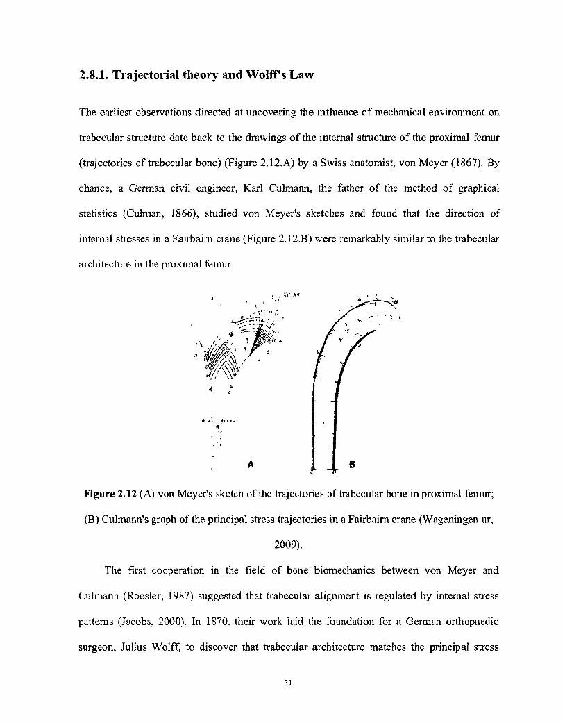
Figure 2.12 (A) von Meyer's sketch of the trajectories of trabecuar bone in proximal femur;
(B) Culmann's graph of the principal stress trajectories in a Fairbairn crane 31
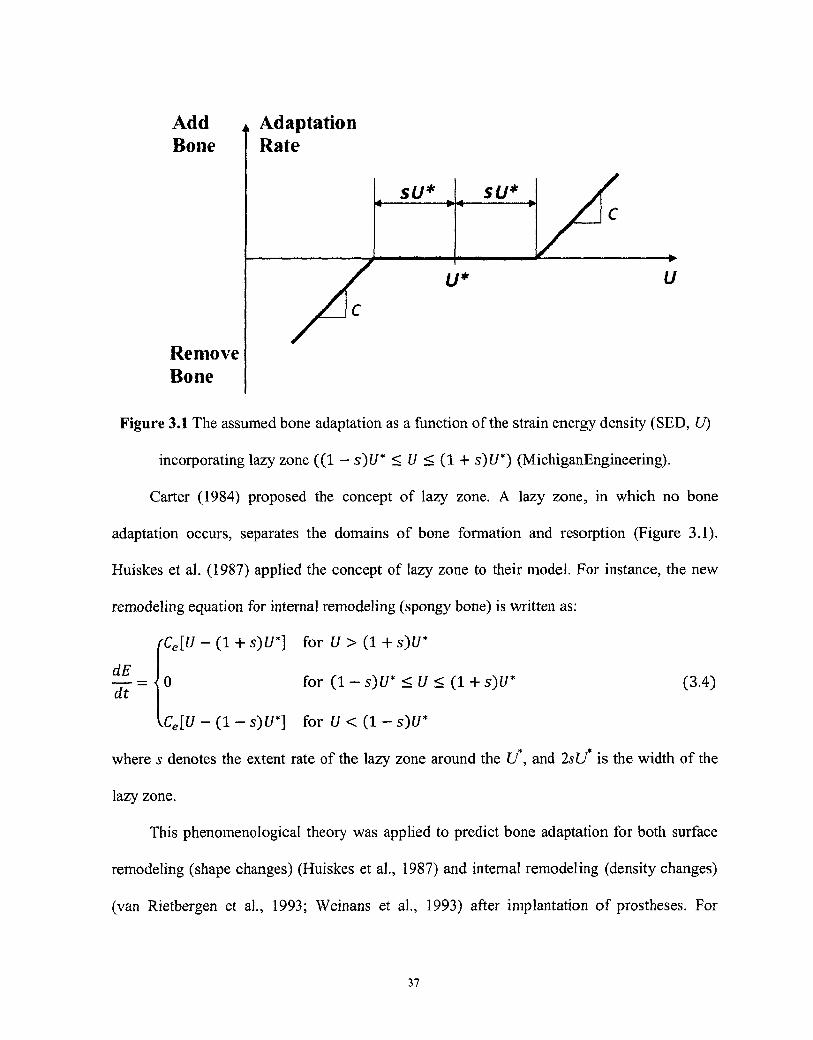
Figure 3.1 The assumed bone adaptation as a function of the strain energy density
incorporating lazy zone 37
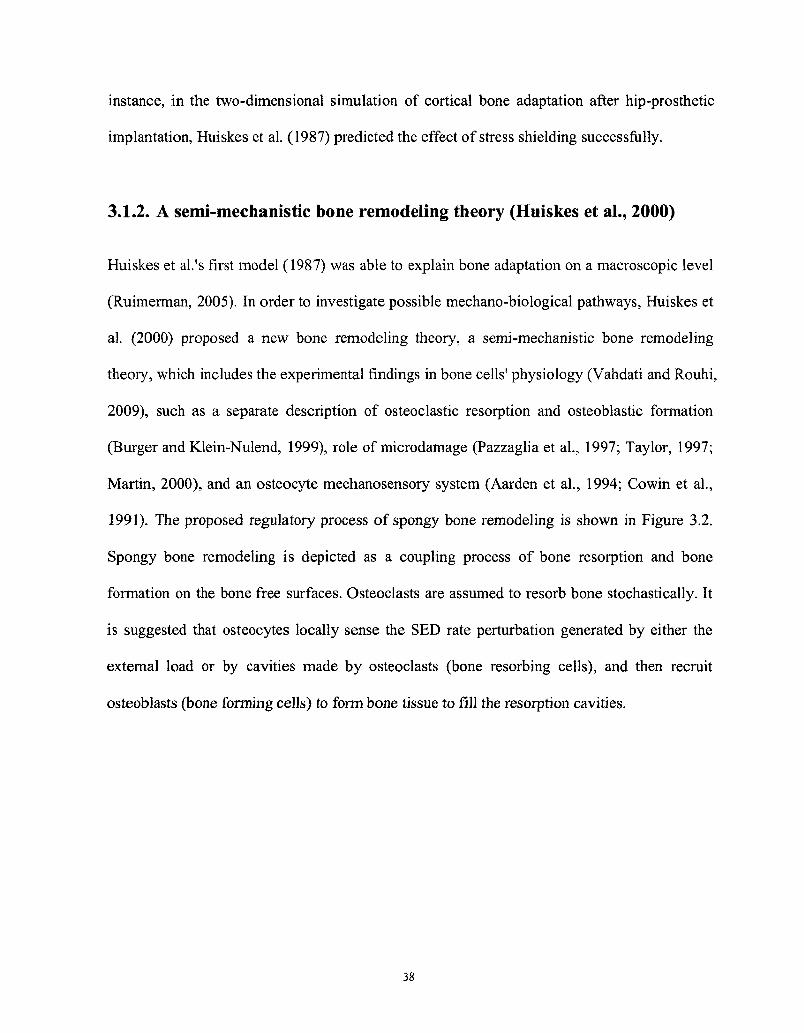
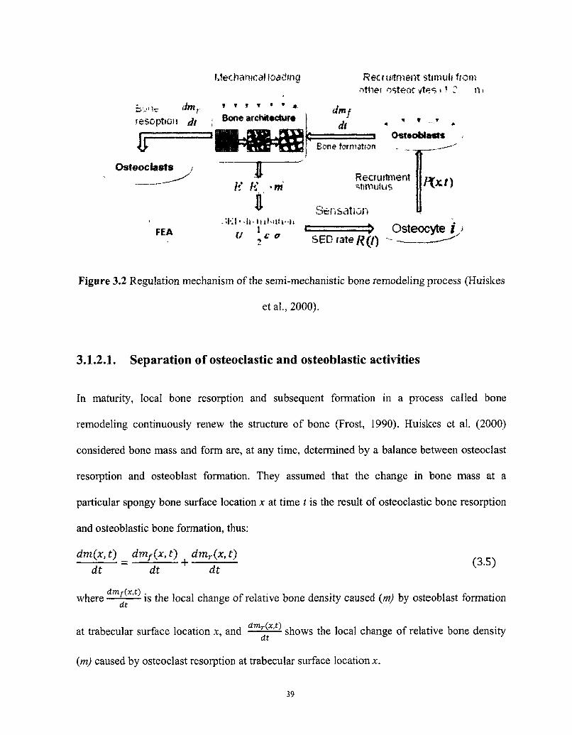
Figure 3.2 Regulation mechanism of the semi-mechanistic bone remodeling process 39
Figure 3.3 The finite element analysis flow chart for calculation of the bone element's SED
45
Figure 4.1 Initial geometry of spongy bone model used in computer simulation 50
Figure 4.2 Trabecular structure was developed and the trabeculae were aligned with the
loading direction 55
Figure 4.3 Increased loading magnitude leads to increased trabeculae thickness 55
Figure 4.4 Decreased loading magnitude leads to a reduction in the thickness of trabeculae ..56
Figure 4.5 Rotating the external loading direction realigned the trabeculae accordingly 56
Figure 4.6 The mean relative density changes caused by different external loading
environmnets 57
Figure 4.7 Left: The initial configuration. Middle: The result of the spongy bone remodeling
simulation (Process E) for the healthy young group (younger than 55 years). The right
Vll!
structure is the result of the simulation (Process F) for the healthy old group (older than 55
years) 58
Figure 4.8 The variation of the relative density of the healthy model with randomly distributed
osteocytes 58
Figure 4.9 Results of the spongy bone remodeling for different values of osteocyte
mechanosensitivity 60
Figure 4.10 Comparison of relative densities of osteoporotic spongy bone models with those
of healthy old adults' bone model 61
Figure 5.1 The initial three-dimensional computer simulation model 72
Figure 5.2 The computer model with plates for applying external loads 72
Figure 5.3.A Starting from the initial structure, trabecular-like structure was obtained after
bone remodeling simulation 77
Figure 5.3.B Starting from the resulting structure of the first series (Figure 5.3.A), trabeculae
got denser when external loads were increased by 20% 78
Figure 5.3.C Starting from the resulting structure of the first series (Figure 5.3.A), trabeculae
became thinner when external loads were decreased by 20% 79
Figure 5.3.D Starting from the resulting structure of the first series (Figure 5.3.A), rotating the
loads by 30 degree in counterclockwise direction around Y axis realigned the trabeculae
accordingly 80
Figure 5.3.E Starting from the resulting structure of the first series (Figure 5.3.A), changing
the loading direction from compressive to tensile or from tensile to compressive did not cause
a significant change in the spongy bone's morphology 81
Figure 5.3.F Simulation result of spongy bone remodeling under overload 82
Figure 5.4 Alteration of average relative bone density during bone remodeling simulation
processes 83
Figure 1.1 Global node, element and global freedom numbering for a mesh of 4-node square
elements 110
Figure 1.2 Local node, freedom numbering for the 4-node square element 110
Figure 1.3 Square element and the coordinate systems 111
Figure 1,4 Global node, element and global freedom numbering for a mesh of 8-node cubic
elements 119
ix

Figure 1.5 8-node cubic element: (a) Global Cartesian coordinates, (b) Natural coordinates
with an origin at the centroid 120
Nomenclature
a Empirical constant
[B] Strain-nodal displacement matrix
b Constant
C Compliance tensor
Ce Proportionality constant
Ctj Generalized matrix of remodeling coefficients
Cx Remodeling rate coefficient
c Constant
D Osteocyte influence distance (or decay constant)
Dot Osteocyte influence distance under overload
[D] Stress-strain matrix
di (x) Distance between osteocyte / and location x
Rate of bone remodeling
Rate of formation by osteoblasts
Rate of resorption by osteoclasts
dm
dt
dmob
dt
dmoc
dt
dX
dt Rate of bone growth perpendicular to the surface
E Elastic modulus of the material
Emax Maximum Young's modulus
F Loading amplitude
F0i Critical load value for overload
F' Static external stress
{F} Global force vector
/ Loading frequency
fi(x) Decay function of bone formative stimulus sent from osteocyte / to location x
[K\ Global stiffness matrix
[K*] Element stiffness matrix
k0i Threshold stimulus for calculating bone resorption probability under overload
kir Bone formation threshold
m Relative density
ntr Mass of total bone
N Number of osteocytes within the influence region
P Porosity
P(x,t) Total bone formative stimulus
p Bone resorption probability
p0i(x,t) Bone resorption probability under overload
Ri(t) Strain energy density rate in the location of osteocyte /
roc Relative amount of mineral resorbed by each osteoclast resorption
foc-oi Amount of mineral resorbed by each osteoclast resorption under overload
5* Stiffness tensor
s Half width of the lazy zone
t Time
U Strain energy density
U* Equilibrium value of strain energy density that determines the boundary between
apposition and resorption
{U} Vector of global displacement
{Ue} Vector of element nodal displacement
xii
VB The volume of bone tissue
VT The volume of total bone
Vy The volume of void (or marrow) parts
JC Surface location
Greek symbols
y Power that relates Young's modulus and relative density
E Strain tensor
e\j Homeostatic strain tensor
Etj Actual strain tensor
ju, Osteocyte mechanosensitivity of osteocyte i
v Poisson ratio
p Apparent density
a Stress tensor
r Proportionality factor that determines the bone formation rate
Acronyms
2D Two-dimensional
3D Three-dimensional
BMD Bone mineral density
BMUs Basic multicellular units
DEXA Dual energy x-ray absorptiometry
DOFs Degrees of freedom
FEA Finite element analysis
xiii
MES Minimum effective strain
PBM Peak bone mass
PGE2 Prostaglandin E2
SED Strain energy density
y«FEA Micro-finite element analysis
XIV
Chapter 1
Introduction
Bone is the main component of the musculoskeletal system. It is characterised physically by
hardness, moderate elasticity, and very limited plasticity. The bone tissue is classified as either
cortical (compact or Haversian) or spongy (trabecular or cancellous) bone. Cortical bone is a
rather dense tissue which forms the outside of the bone as a solid structure. Spongy bone is
porous and primarily found near joint surfaces, at the end of long bones and within vertebrate.
It has a complex three-dimensional structure consisting of struts and plates of trabeculae.
Although bone cells make up a small percentage of bone volume, they play a critical role in
the adaptation of its structure. There are four main types of bone cells. They are: osteoclasts,
which resorb old bone; osteoblasts, which form new bone; osteocytes, which is believed that
act as mechanosensors (Cowin et al., 1991; Burger, 2001; Burger and Klein-Nulend, 1999,
Nijweide, et al., 1996) and bone lining cells, which are inactive cells on the resting surfaces of
bone.
Although bones may seem like hard and lifeless structures, bone is a living,
continuously self-renewing tissue (Elisabeth et al., 1994). This tissue is able to adapt itself to
the variation of mechanical environment. Apart from skeletal growth and fracture healing,
bone maintains and adapts its mass and internal structure by a process called bone remodelling
process. Bone remodeling is a repair mechanism targeted to increase the lifetime of bone
tissue by removing microdamage and substituting it with new bone (Laoise and Patrick, 2007).
It consists of two distinct stages: bone resorption by osteoclasts, and bone formation by
l
osteoblasts. Ostoclasts and osteoblasts which carry out bone remodeling process are called
basic multicellular units or BMUs. Usually, the resorption and formation are in balance and
skeletal strength and integrity are maintained. In cortical bone, BMUs form cylindrical canals
through the bone. In spongy bone, the remodeling process is a surface event. Due to spongy
bone's large surface-to-volume ration, spongy bone is more actively remodeled than cortical
bone (Huiskes and van Rietbergen, 2005).
For restoring normal function and relieving the pain caused by trauma or disease, the
implants are used to replace or augment bone. For example, orthopaedic implants are artificial
devices incorporated into bones and joints, often acting as joint replacements in cases where
the hip, knee, shoulder or elbow have been damaged by injury or by diseases such as
osteoarthritis. In the bone-implant system, bone remodeling plays an important role in the
adaptation of its structure to the changes in the mechanical environment. In order to estimate
the long-term impacts of implants and prostheses on bone tissue, numerical analyses have
been performed for the latest developments of these devices. Furthermore, bone diseases,
especially osteoporosis, are caused by the interruption of bone remodeling process (Thompson,
2007; Rouhi et al., 2007). Osteoporosis is a disease characterized by low bone mass and
deterioration of bone tissue caused by bone loss. This leads to increased bone fragility and risk
of fracture (broken bones), particularly of the hip, spine and wrist. Bone diseases have severe
impacts in terms of human cost and socioeconomic burden (Osteoporosis Canada, 2008). In
Canada, one in four women and at least one in eight men over the age of 50 have osteoporosis
and it is estimated that as many as two million Canadians may be at risk of osteoporotic
fractures. The cost to the Canadian health care system of treating osteoporosis and the
fractures it causes is currently estimated to be $ 1.9 billion annually (Osteoporosis Canada,
2
2008). Because of these severe impacts caused by bone diseases, it is of great importance to
understand the mechanism of bone remodeling process, and so propose a mathematical model
and also simulate this process.
Since Wolff (1892) proposed that bone adapted to mechanical loading in accordance
with mathematical law during its growth and development, numerous researchers have been
encouraged to propose mathematical models for the bone remodeling process. In 2000,
Huiskes and co-workers developed a semi-mechanistic model for bone remodelling theory.
The semi-mechanistic bone remodeling theory (Huiskes et al., 2000) includes the
experimental findings in bone cells' physiology, such as a separate description of osteoclastic
resorption and osteoblastic formation (Burger and Klein-Nulend, 1999); an osteocyte
mechanosensory system (Aarden et al., 1994; Cowin et al., 1991); and role of microdamage
(Pazzaglia et al., 1997; Taylor, 1997; Martin, 2000). In this semi-mechanistic bone remodeling
theory (Huiskes et al., 2000), osteocytes are assumed to be sensitive to the maximal rate of the
strain energy density (SED) in a recent loading history and to recruit the osteoblasts, bone
forming cells which form new bone, to fill the cavities caused by osteoclast resorption.
Osteoclast resorption by microdamage is supposed to occur spatially random.
1.1. Motivation
An imbalance in the regulation of bone remodeling's two sub-processes, i.e. bone resorption
and bone formation, results in many metabolic bone diseases. When the amount of bone
resorption is more than that of bone formation for a long period of time, a net reduction in
bone apparent density, or bone loss, will occur. The serious bone loss leads to osteoporosis.
Bone loss usually starts after maturation and accelerates in osteoporotic bones. It is known
3
that in healthy adults the number of osteocytes decreases significantly with aging (Frost, 1960;
Mullender et al., 1996; Qiu et al., 2002). On the other hand, it is found that osteoporotic
patients have a greater osteocyte density than healthy old adults (Mullender et al., 1996). In
modern time, it was suggested that osteocytes regulated the recruitment of basic multicellular
units (BMUs) in response to mechanical stimuli (Kenzora et al., 1978; Marotti et al., 1990;
Lanyon, 1993). Furthermore, Mullender et al. (1994) and Mullender and Huiskes (1995)
suggested that osteocyte density may affect the trabecular morphology and that reduced
osteocyte mechanosensitivity, sensitivity of osteocyte to mechanical stimulus, may cause bone
loss in a similar way as did disuse. According to the above findings, the changes of osteocyte
density in aging and osteoporotic individuals and the effects of osteocyte density and
osteocyte mechanosensitivity on spongy bone remodeling led us to hypothesize that
decreasing osteocyte density causes spongy bone loss in the case of healthy adults and that a
reduction in osteocyte mechanosensitivity is one of the main contributing factors for the bone
loss in the osteoporotic bones. In order to investigate the validity of our hypothesis, we built a
two-dimensional spongy bone model for simulating spongy bone remodelling. In the case of
the healthy adults, we decreased the model's osteocyte densities with aging according to the
experimental data to test the effects of reduced osteocyte densities on the aging spongy bone
remodeling. In the case of osteoporotic individuals, we increased the model's osteocyte
densities for osteoporotic bone compared to the healthy adults' bone, but decreased the
osteocyte mechanosensitivities to test the effects of reducing osteocyte mechanosensitivities
on the osteoporotic spongy bone remodeling. To the best of our knowledge, this research is
the first computer simulation study investigating the effects of osteocyte mechanosensitivity
on the osteoporotic spongy bone remodeling.
4
Looseness at the bone-implant system caused by bone resorption is a major problem in
prosthetic implantation (Huiskes et al., 1987; McNamara etal., 1997). Besides stress-shielding
which is well accepted as a reason for bone resorption, some researchers (Huiskes and
Nunamaker, 1984; Quirynen et al., 1992) have suggested that bone loss around some implants
was associated with overload. In spongy bone, osteoclast resorption is activated at the bone
surface where inhibitive osteocyte signals no longer reach (Burger and Klein-Nulend, 1999).
This can occur not only when external loads are reduced, but also when the osteocytic network
is blocked because of the presence of microcracks caused by overloading (Martin, 2003; Tanck
et al., 2006). If the loading is so high that the self-repair mechanism cannot keep pace with the
increasing damage, overload resorption will occur (Li et al., 2007). Many mathematical models
have been proposed to describe bone remodeling process, but very few attempts were made to
study bone resorption due to overload. In this study, in order to investigate the spongy bone
remodeling under overload, an extension to Huiskes and co-workers' semi-mechanistic bone
remodeling theory (2000) was made. Based on the previous theoretical and experimental
results, we hypothesized that the osteoclast resorption activity, including the bone resorption
probability and also the amount of resorbed bone, will increase under overload. Furthermore,
we assumed that microdamages caused by overload reduce the osteocyte influence distance.
We also simulated the spongy bone remodelling, when is under overload, with a three-
dimensional finite element model, which promising results have been gained.
5
1.2. Objectives
The general goal of this study is to investigate the spongy bone remodeling using the semi-
mechanistic bone remodeling theory (Huiskes et al., 2000). The specific objectives of this
study are:
1) To develop a two dimensional finite element model of spongy bone and investigate the
effects of osteocyte density and osteocyte mechanosensitivity on the spongy bone
remodeling for aging healthy adults and also osteoporotic patients, respectively.
2) To propose a new mathematical model for overloaded bone resorption. Using our new
formulation and a three-dimensional computer model, investigation will be made on the
spongy bone remodelling under overload.
1.3. Thesis organization
First, chapter 1 briefly states the motivation and objectives of this thesis. Chapter 2 provides
background information on bone physiology and anatomy, bone structure, bone cells, bone
mechanics, bone adaptation, and also literature review on the most popular theories related to
bone remodeling. Chapter 3 introduces the general method used in this thesis, including a
brief introduction on a semi-mechanistic bone remodeling theory and the particular finite
element methods' applications in our researches. Chapters 4 and 5 address the specific
objectives of the thesis in order. The thesis closes with Chapter 6 that provides final
conclusions and recommendations for future work.
Chapter 2
Background and Literature Reviews
Bone is one of the most important components of the musculoskeletal system. It is
characterised physically by hardness, moderate elasticity, and very limited plasticity.
Although apparently immobilized in a petrified state, it is a rather unique tissue with many
functions. Bone forms supportive framework for the body and sites for muscle attachment.
Bone also serves to protect vital organs (brain) and tissue (bone marrow). A number of ions
such as calcium and phosphate are reserved by bone which helps maintain the homeostasis of
these minerals in the blood (Elisabeth et al., 1994).
2.1. Components of bone matrix
Bone is a highly heterogeneous tissue. Its composition and structure both vary in a way that
depends on skeletal site, physiological function, the age and sex of subjects. In contrast with
this heterogeneity, the basic components of the tissue are remarkably consistent (Yuehuei and
Robert, 2000). By volume, bone consists of relatively few cells and much intercellular
substances formed of mineral substances, organic matrix, and water.
By weight, approximately 65% of the bone tissue is made by mineral phase. The feature
that distinguishes bone from other connective tissue is the mineralization of the matrix. This
produces a hard and strong type of tissue capable of providing mechanical integrity for
efficient body motion and also protection for the internal organs. Approximately 95% of the
mineral phase is composed of a specific crystalline hydroxyapatite (Caio(P04)6(OH)3).
7
The organic phase comprises approximately 30% of the total mass of bone. About 90%
of the organic phase is composed of collagen fibres (mainly Type I collagen); Approximately
8% of the organic phase are a variety of non-collagenous proteins such as osteopontin,
osteonectin, bone sialoprotein, and osteocalcin ; cells accounting for the remaining 2% of the
organic phase (Buckwalter et al. 1995; Einhorn, 1996; Gorski, 1998). The arrangement of the
fibrils is important in determining bone's mechanical properties.
Water comprises approximately 5% of the total weight of bone and is located within
collagen fibres, in the pores, and bound in the mineral phase. "Water plays an important role in
determining the mechanical properties of bone. For example, it has been shown that
dehydrated bone samples have increased strength and stiffness, but decreased ductility
(Nyman et al., 2006; Smith and Walmsley, 1959).
2.2. Bone structure
On the basis of shape, bones can be classified into four groups, long bones (e.g. the tibia and
the femur), short bones (e.g. carpal bones of the hand), flat bones (e.g. the sternum), and
irregular bones (e.g. vertebra). Long bones have one dimension much longer than the other
two, short bones have similar extensions in all dimensions, and flat bones have one dimension
much shorter than the other two. Figure 2.1 depicts the human skeleton and thus examples for
each kind of bone.
8
1 • * v - - •> %
•'• A i
Figure 2.1 Human skeleton (Sohit and Parma, 2007).
At macroscopic level, according to the level of porosity and location within the skeleton,
bone is categorized as either cortical (haversian, or compact) bone or spongy (cancellous, or
trabecular) bone (Figure 2.2), easily distinguished by their degree of porosity. Individual
bones in the body can be formed from both of these types of bone tissue. Almost 80% of the
skeletal mass in the adult human skeleton is cortical bone, while the remaining 20% is spongy
bone (Jee, 2001). Cortical bone, which is a low porosity solid material, forms the outer wall of
all bones and is largely responsible for the supportive and protective function of the skeleton.
Spongy bone is a porous structure and is mainly found in the interior of bones, such as
vertebral bodies, and in the end of long bones. The porosity of spongy bone ranges from 40 to
95% depending on the anatomic site (Kuhn et al., 1990; Mosekilde et al., 1989), far greater
than that of cortical bone which is 30% or less (Hayes and Bouxsein, 1997). The main
9
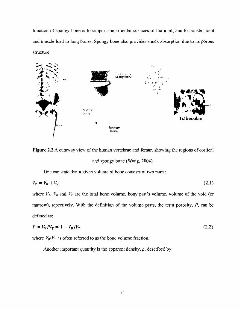
function of spongy bone is to support the articular surfaces of the joint, and to transfer joint
and muscle load to long bones. Spongy bone also provides shock absorption due to its porous
structure.
1
vager-
K
4 Spongy bone
t
£5 Trabecuiae *
Spongy bone
Figure 2.2 A cutaway view of the human vertebrae and femur, showing the regions of cortical
and spongy bone (Wang, 2004).
One can state that a given volume of bone consists of two parts:
VT = VB + Vv (2.1)
where VT, VB and Vy are the total bone volume, bony part's volume, volume of the void (or
marrow), repectively. With the definition of the volume parts, the term porosity, P, can be
defined as:
P = VV/VT = 1 - VB/VT (2.2)
where VRIVT is often referred to as the bone volume fraction.
Another important quantity is the apparent density, p, described by:
10
(2.3)
where m r is the mass of total bone.
Lamella - _ f
Ostcocyle —
Osteon — -(Haversian system)
Circumferential—i, lamellae v\
Lamellae-
"V
/ •
^
*
\ ̂ m
/ - /
>-•
• Central (Haversian! canal
Perforating (Volkmann's^ canal
Blood vessel
Endosteum lining bony carats and covering trabecular
\ v _ Lacuna
x Canaliculus v Central ^Haversian} ranal
Blood vessel continues into medullary cavity containing marrow
Spongy bone
Oht<>obL>;.K
"**•»- O s t f t i n i . i j
-
, , Lrimrtlae (C) Ostpwv '
CrftldiltUUSS
Perforating tSharpey s) fibers Compact b o n e ig
Periosteal — • biood vessel
Periosteum —
(a)
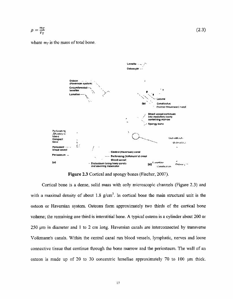
Figure 2.3 Cortical and spongy bones (Fischer, 2007).
Cortical bone is a dense, solid mass with only microscopic channels (Figure 2.3) and
with a maximal density of about 1.8 g/cm3. In cortical bone the main structural unit is the
osteon or Haversian system. Osteons form approximately two thirds of the cortical bone
volume; the remaining one third is interstitial bone. A typical osteon is a cylinder about 200 or
250 urn in diameter and 1 to 2 cm long. Haversian canals are interconnected by transverse
Volkmann's canals. Within the central canal run blood vessels, lymphatic, nerves and loose
connective tissue that continue through the bone marrow and the periosteum. The wall of an
osteon is made up of 20 to 30 concentric lamellae approximately 70 to 100 um thick.
n
Surrounding the outer border of each osteon is a cement line, a 1 to 2 um thick layer of
mineralized matrix deficient in collagen fibres.
Spongy bone has a cellular structure and is made up of a connected network of rods and
plates (70 to 200 um in thickness) of calcified bone tissue called trabeculae (Figure 2.3).
Spongy bone accounts for 20% of total bone mass, but it has nearly ten times the surface area
of compact bone. The high surface area of the trabecular network allows for energy absorption
and dissipation from loads on the joint. The trabeculae are usually oriented in a way that
produces an anisotropic structure (Turner, 1997). The trabeculae are surrounded by marrow
that is vascular and provides nutrients and waste disposal for the bone cells. Individual
trabeculae have a plate or rod shape and are composed primarily of interstitial bone of varying
composition. Analogous to an osteon in cortical bone, the structural unit of spongy bone is the
trabecular packet which consists of sheets of non-concentric lamellae (Figure 2.3.C). The ideal
trabecular packet is shaped like a shallow crescent with a radius of 600 um and is about 50 urn
thick and 1 mm long. As with cortical bone, cement lines hold the trabecular packet together.
Spongy bone tissue is a non-homogeneous and anisotropic porous structure. The
symmetry of the structure in spongy bone depends upon the direction of the applied loads. If
the stress pattern in spongy bone is complex, the structure of the network of trabeculae is also
complex and highly asymmetric. In bones where the loading is largely uniaxial, such as the
vertebrae, the trabeculae often develop a columnar structure with cylindrical symmetry
(Weaver and Chalmers, 1966; Whitehouse et al., 1971).
Tiny cavities in the bone matrix called lacunae are observed throughout both cortical
and spongy bone. A single cell known as an osteocyte is trapped within each lacuna.
Osteocytes form a network with adjacent lacunae allowing for nutrient diffusion and cell to
12
cell communication via a system of cell processes located in canaliculi (Figure 2.3.b, Figure
2.3.c and Figure 2.4).
At the microstructural level, according to the arrangement of the collagen fibrils, both
compact and spongy bone can be of woven or lamellar bone (Yuehuei and Robert, 2000).
Woven bone has a small number of randomly oriented collagen fibres and is mechanically
weak. Lamellar bone has a regular parallel alignment of collagen into sheets (lamellae) and is
mechanically strong. In cortical bone, lamellae are arranged either concentrically in quasi-
cylindrical osteons or circumferentially near the outer and inner surfaces of the compact bone
(Cowin et al., 1991). The trabeculae of spongy bone generally are composed of a collection of
parallel lamellae. In cross-section, the fibres run in opposite directions in alternating layers,
much like in plywood, assisting in the bone's ability to resist torsion forces. During skeletal
embryogenesis, woven bone is the bone formed first. After birth, it is gradually removed by
the process of bone remodeling and is substituted by lamellar bone. In adults, woven bone is
created after fractures or in Paget's disease. Woven bone forms quickly. It is soon replaced by
lamellar bone (Yuehuei and Robert, 2000).
13
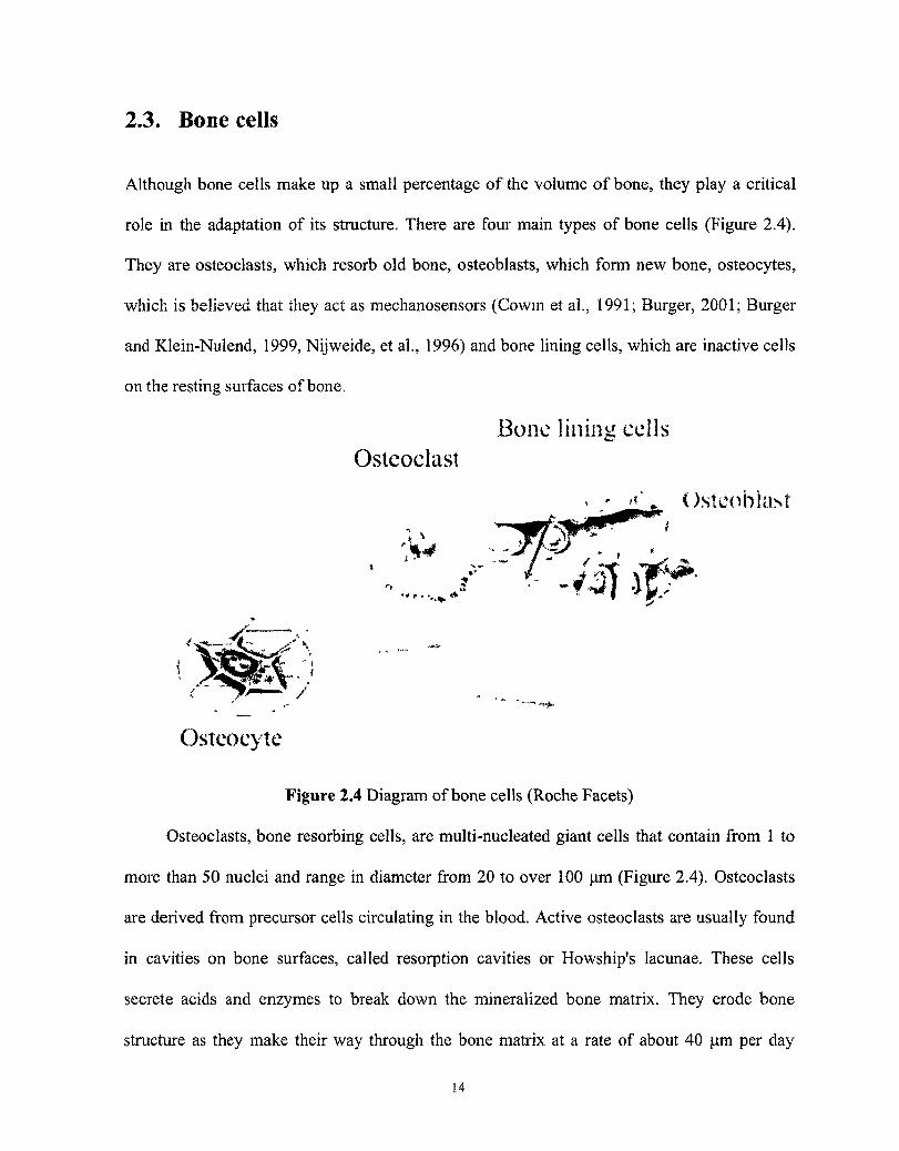
2.3. Bone cells
Although bone cells make up a small percentage of the volume of bone, they play a critical
role in the adaptation of its structure. There are four main types of bone cells (Figure 2.4).
They are osteoclasts, which resorb old bone, osteoblasts, which form new bone, osteocytes,
which is believed that they act as mechanosensors (Cowin et al., 1991; Burger, 2001; Burger
and Klein-Nulend, 1999, Nijweide, et al., 1996) and bone lining cells, which are inactive cells
on the resting surfaces of bone.
Bone lining ceils Osteoclast
. - ** . Osteoblast
" ' • :.*. "* -1$ W*' •S
-"** -Mp f̂e, (" 7'—V
Ostcocyte
Figure 2.4 Diagram of bone cells (Roche Facets)
Osteoclasts, bone resorbing cells, are multi-nucleated giant cells that contain from l to
more than 50 nuclei and range in diameter from 20 to over 100 um (Figure 2.4). Osteoclasts
are derived from precursor cells circulating in the blood. Active osteoclasts are usually found
in cavities on bone surfaces, called resorption cavities or Howship's lacunae. These cells
secrete acids and enzymes to break down the mineralized bone matrix. They erode bone
structure as they make their way through the bone matrix at a rate of about 40 um per day
14
(resorption rate). Debris, both organic and mineral, are packed into little vesicles and pass
through the cell body of the osteoclast and are dumped into the space above. When osteoclasts
have done their job, they disappear and presumably die (Bilezikian et al., 1996).
Osteoblasts are bone forming cells which have a cuboidal form, and are tightly packed
against each other at the tissue surface (Figure 2.4). They are mono-nucleated cells, up to 10
um in diameter. Osteoblasts secrete both the collagen and the ground substance that
constitutes the initial un-mineralized bone or osteoid. During bone remodeling, these cells
refill the gap opened by the osteoclasts at a rate of about 1 um per day (apposition rate).
Initially, the osteoid has a very low elastic modulus, but its value increases when
mineralization takes place. A great number of osteoblasts disappear by a yet unknown process
after their lifespan (Buckwalter et al. 1995). But, some become buried in the tissue and
survive as osteocytes.
Osteocytes are former osteoblasts that have become buried in the mineralize bone matrix
(Bilezikian et al. 1996). They are the most abundant cell type which makes up more than 90-
95% of all bone cells in the adult animal bone (Parfitt, 1977). Osteocytes are regularly
dispersed throughout the mineralized matrix within caves called lacunae, connected to each
other and cells on the bone surface through slender, cytoplasmic processes or dendrites
passing through the bone in thin tunnels (100-300 nm) called canaliculi (Figure 2.3 and 2.4).
The cell processes are on the order of fifty emanating from each cell, and they are surrounded
by a bone fluid space. Comparing to osteoblasts and osteoclasts, no clear functions have been
ascribed to osteocytes (Bonewald, 2006a). For a long time, osteocytes were considered as the
quiescent cells that merely acted as place holders in bone (Bonewald, 2006b; Heino et al.,
2009). Since osteocytes were proposed to be multifunctional cells decades ago (Bonewald,
15
2006b), both theoretical considerations and experimental results have constantly strengthened
the knowledge of the role of osteocytes in mechanosensing and in the consequent regulation
of bone mass and structure, which is accomplished by the process of bone remodeling (Frost,
1960; Cowin et al., 1991; Burger et al., 1995; Burger and Klein-Nulend, 1999; Cheng et al.,
2001; Klein-Nulend and Bakker, 2007) (see section 2.4).
Bone lining cells are flattened, inactive osteoblasts that lay on the bone surface (Figure
2.4). In adult bone, lining cells cover the surface of trabeculae in trabecular bone, the
periosteum and endosteum of cortical bone, and the Haversian and Volkmann's channels of
the osteons. Bone lining cells maintain communication with each other and the osteocytes and
are believed to be hormonal receptors and chemical messengers (Bilezikian et al., 1996). Like
osteocytes, bone lining cells are also thought to initiate bone remodeling in response to
various chemical and mechanical stimuli (Buckwalter et al., 1995).
2.4. Osteocyte mechanosensing
Mechanosensing is the process by which mechanical loads is sensed by mechanosensor cells.
The osteocyte is the most abundant cell type of bone (Klein-Nulend and Bakker, 2007).
Osteocytes are embedded in the mineralized matrix of bone and spaced regularly throughout
the calcified matrix. The number of osteocytes and their particular location in bone make them
seem to be one of the best candidates for the job of detecting mechanical signals in the bone
matrix. In vivo experiments show that loading produces rapid changes in the metabolic
activity of osteocytes and suggest that osteocytes function as mechanosensors in bone (Skerry
et al., 1989; El-Haj et al., 1990; Dallas et al., 1993; Lean et al., 1995; Forwood et al., 1998;
Teraietal., 1999).
16
forces
1 1 •f. i . _ Trabeculae
Bone marrow
. ' <**• -
/ , !
Ostoocyte
Osteoclast X Osteoblasts aligned dlong
trabecule of new bone
„ LfltlltV)
-— LKteotylc
— Process
— Cdrwlitulu*.
Canaliculus
Fluid flow Osteocyte process
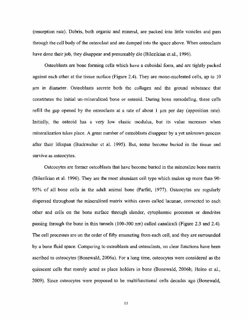
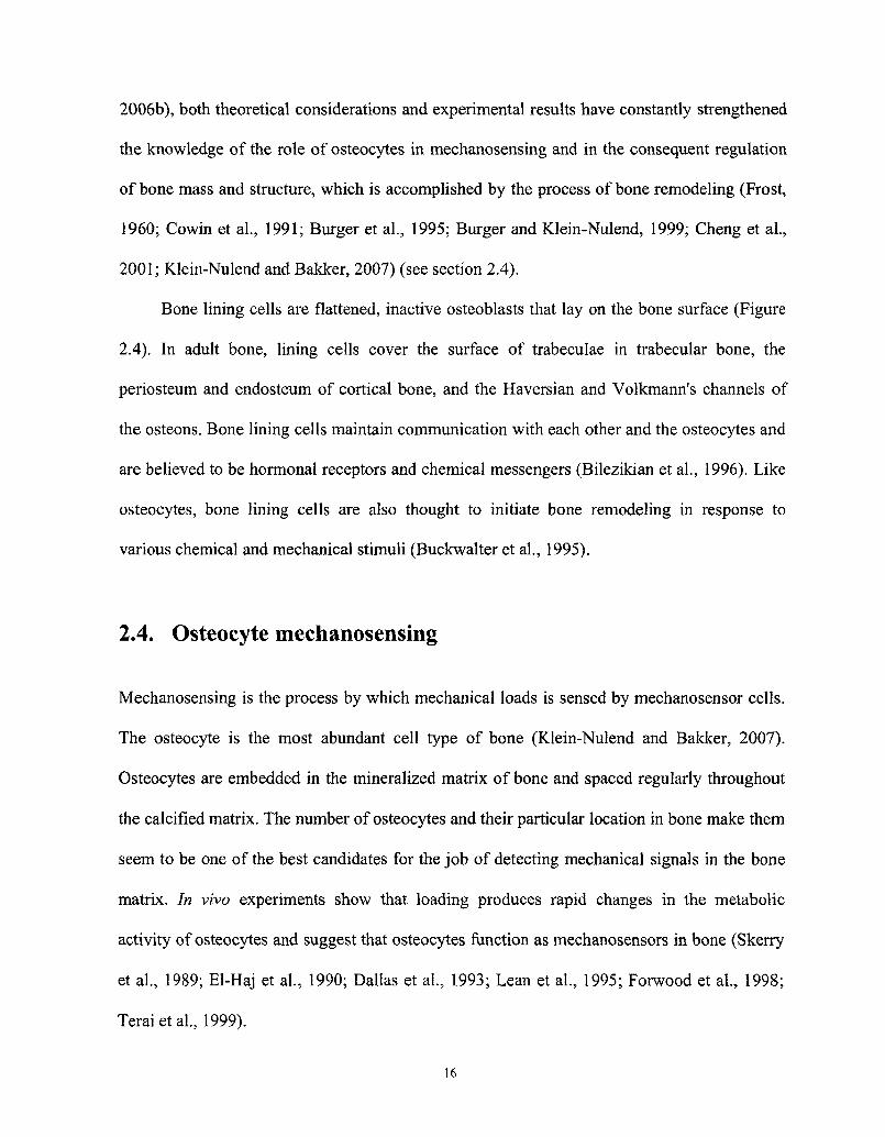
Figure 2.5 Schematic of the osteocyte mechanosensing. Osteocytes are dispersed throughout
the bone matrix. An osteocyte resides in a lacuna, contacting with other osteocytes through its
processes within the channels known as canaliculi. Mechanical loads on bone are assumed to
induce fluid flow in the lacunar-canalicular network. Osteocytes are supposed to detect the
mechanical signal via the fluid flow.
17
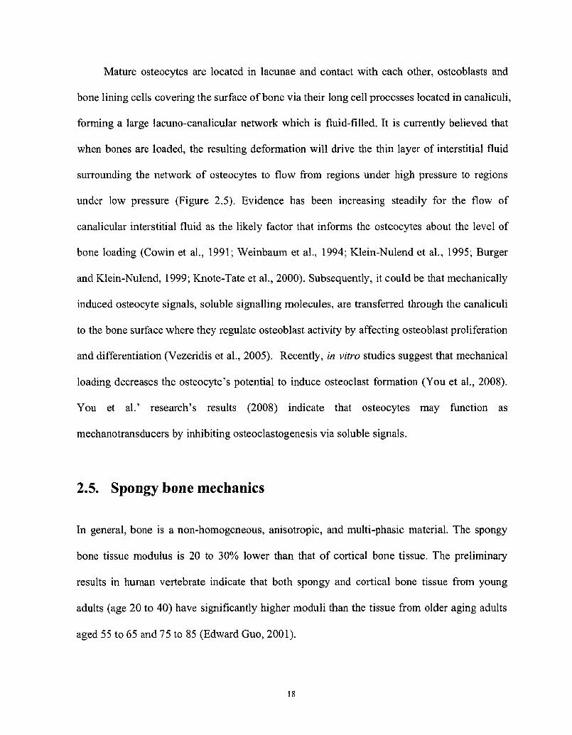
Mature osteocytes are located in lacunae and contact with each other, osteoblasts and
bone lining cells covering the surface of bone via their long cell processes located in canaliculi,
forming a large lacuno-canalicular network which is fluid-filled. It is currently believed that
when bones are loaded, the resulting deformation will drive the thin layer of interstitial fluid
surrounding the network of osteocytes to flow from regions under high pressure to regions
under low pressure (Figure 2.5). Evidence has been increasing steadily for the flow of
canalicular interstitial fluid as the likely factor that informs the osteocytes about the level of
bone loading (Cowin et al., 1991; Weinbaum et al., 1994; Klein-Nulend et al., 1995; Burger
and Klein-Nulend, 1999; Knote-Tate et al., 2000). Subsequently, it could be that mechanically
induced osteocyte signals, soluble signalling molecules, are transferred through the canaliculi
to the bone surface where they regulate osteoblast activity by affecting osteoblast proliferation
and differentiation (Vezeridis et al., 2005). Recently, in vitro studies suggest that mechanical
loading decreases the osteocyte's potential to induce osteoclast formation (You et al, 2008).
You et al.' research's results (2008) indicate that osteocytes may function as
mechanotransducers by inhibiting osteoclastogenesis via soluble signals.
2.5. Spongy bone mechanics
In general, bone is a non-homogeneous, anisotropic, and multi-phasic material. The spongy
bone tissue modulus is 20 to 30% lower than that of cortical bone tissue. The preliminary
results in human vertebrate indicate that both spongy and cortical bone tissue from young
adults (age 20 to 40) have significantly higher moduli than the tissue from older aging adults
aged 55 to 65 and 75 to 85 (Edward Guo, 2001).
18
The mechanical behaviour of spongy bone is best described as viscoelastic due both to
the viscous properties of the tissue material and to the marrow in the pores. The elastic part of
this behaviour is demonstrated by the ability of spongy bone to recover its initial geometry
fully after release of an applied load that did not exceed the elastic limit. The viscous part is
responsible for the dependency of stiffness on strain rate (Carter and Hayes, 1977; Linde et al.,
1991) and for phenomena such as stress relaxation and creep behaviour of spongy bone (Zilch
et al., 1980; Lakes, 2001). It should be noted that for strain rates as they occur during normal
activities (~ 1 Hz), spongy bone could be well described as an elastic material (van Rietbergen
and Huiskes, 2001).
Elastic properties of continua are fully described by the stiffness tensor, S, or by the
compliance tensor, C, in the generalize Hooke's Law:
otj = Sstj, £ij = Caijt S = C _ 1 (2.4)
where <ri;- is the stress tensor, and £i;- is the strain tensor.
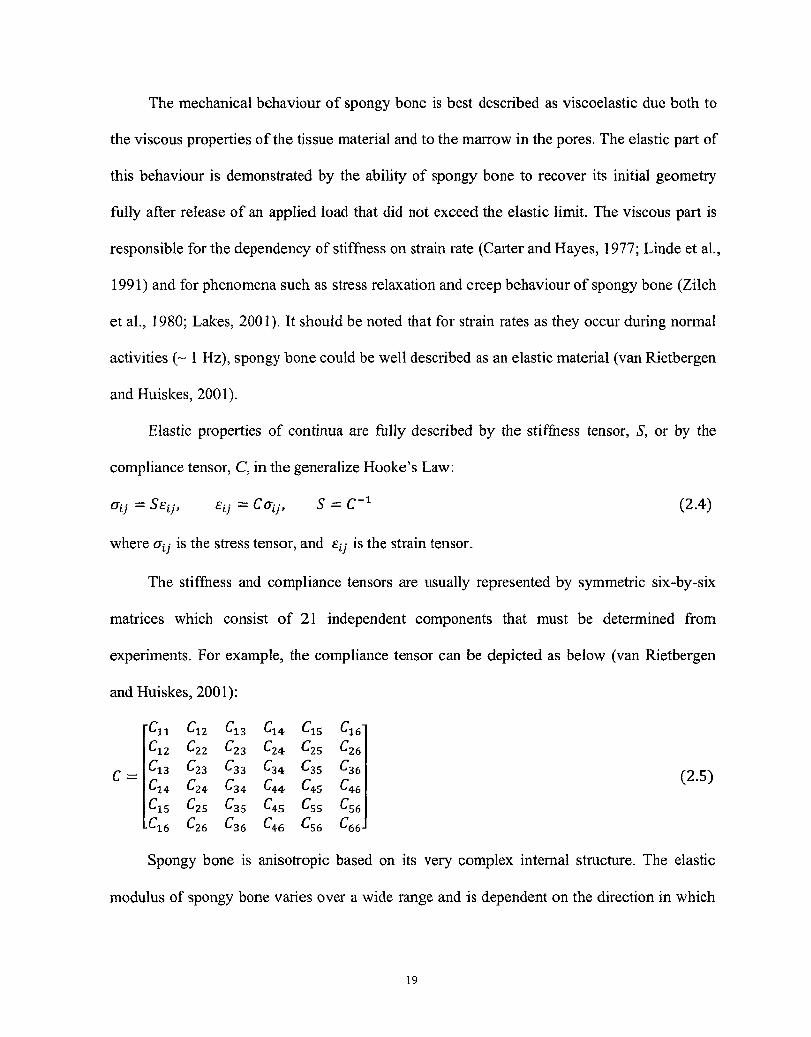
The stiffness and compliance tensors are usually represented by symmetric six-by-six
matrices which consist of 21 independent components that must be determined from
experiments. For example, the compliance tensor can be depicted as below (van Rietbergen
and Huiskes, 2001):
C =
cxl c12 c13 C 1 4 C 1 S C 1 6
C12 C22 C23 C 2 4 C2s C26
^13 ^23 C33 C34 £35 C 3 6
C14 L24 C34 C44 C45 L 4 6
Cl5 ^25 C35 Q-5 Q5 Q6 Cl6 ^26 ^36 Q6 C$6 Q6
(2.5)
Spongy bone is anisotropic based on its very complex internal structure. The elastic
modulus of spongy bone varies over a wide range and is dependent on the direction in which
19

the bone is loaded. It is shown that an orthotropic (three orthogonal planes are plane of
symmetry) assumption can be made for the spongy bone (Gibson, 1985).
Using standard engineering test methods such as tensile tests, three- or four-point
bending tests, and buckling tests, it is far more difficult to measure mechanical properties of
spongy bone tissue than to measure those properties of cortical bone tissue. The technical
difficulties are due to the extremely small dimension (thickness, 100 to 200 um; length, 1 to 2
mm) and irregular shape of individual trabeculae in spongy bone (van Rietbergen and Huiskes,
2001; Edward Guo, 2001). In order to overcome these chanllenges an alternative method so-
called micro-finite-element analysis (uFEA) have been developed to calculate the elastic
constants of spongy bone directly from computer models by simulating experimental tests on
bone specimens (Hollister et al., 1994; van Rietbergen et al., 1995 and 1996). In these
simulations, many uncertainties that play a role in real tests (e.g., bone-platen interface
conditions, protocol errors) can be eliminated or well controlled (van Rietbergen and Huiskes,
2001). Using the /uFEA model, it was found that the anisotropic elastic properties of spongy
bone can be well neglected, and so spongy bone can be represented with isotropic tissue
properties. This effective isotropic tissue modulus can be determined by comparing the results
of fiFEA with those of experimental tests for the same specimen (Kabel et al., 1999). The
values found for the tissue Young's modulus are generally in the range of 4 to 8 GPa (van
Rietbergen et al., 1995; Ladd et al., 1998; Kabel et al., 1999).
Supposing that a given bone specimen is a homogeneous and isotropic material, one can
describe the constitutive behaviour with two material parameters, i.e. the Young's modulus, E,
and the Poisson ratio, v. In the case of isotropy, the compliance tensor, C, can be written as
(van Rietbergen and Huiskes, 2001):
20
c =
• 1 - v - v
E ~E~ T ° —v 1 —v
T E ~E~ ° —v —V
T IT 1
0 0
0
2 + 2v
0
0
0
0
0
0
E
0
0
0
2 + 2v
E
0
0
0
2 + 2v
(2.6)
0
0 0 0
0 0 0
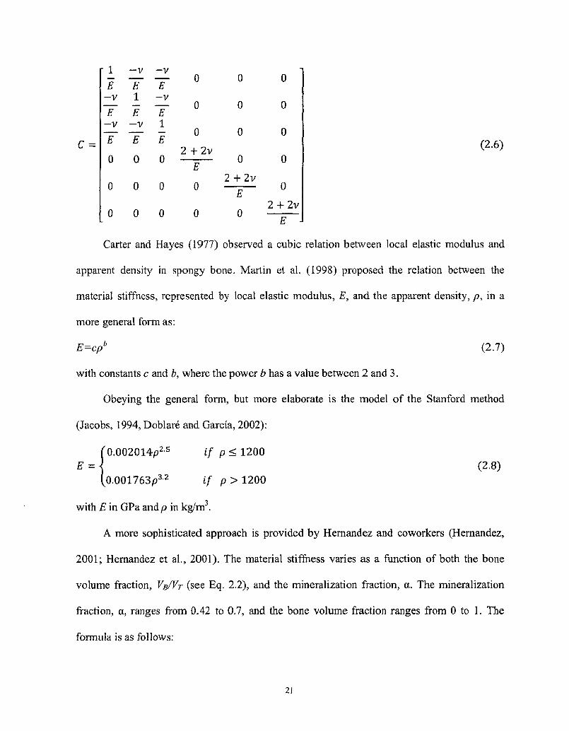
Carter and Hayes (1977) observed a cubic relation between local elastic modulus and
apparent density in spongy bone. Martin et al. (1998) proposed the relation between the
material stiffness, represented by local elastic modulus, E, and the apparent density, p, in a
more general form as:
E=cpb (2.7)
with constants c and b, where the power b has a value between 2 and 3.
Obeying the general form, but more elaborate is the model of the Stanford method
(Jacobs, 1994, Doblare and Garcia, 2002):
'0.002014-p2-5 if p< 1200 E = | (2.8)
a001763p 3 2 if p > 1 2 0 0
with E in GPa andp in kg/m3.
A more sophisticated approach is provided by Hernandez and coworkers (Hernandez,
2001; Hernandez et al., 2001). The material stiffness varies as a function of both the bone
volume fraction, VB/VT (see Eq. 2.2), and the mineralization fraction, a. The mineralization
fraction, a, ranges from 0.42 to 0.7, and the bone volume fraction ranges from 0 to 1. The
formula is as follows:
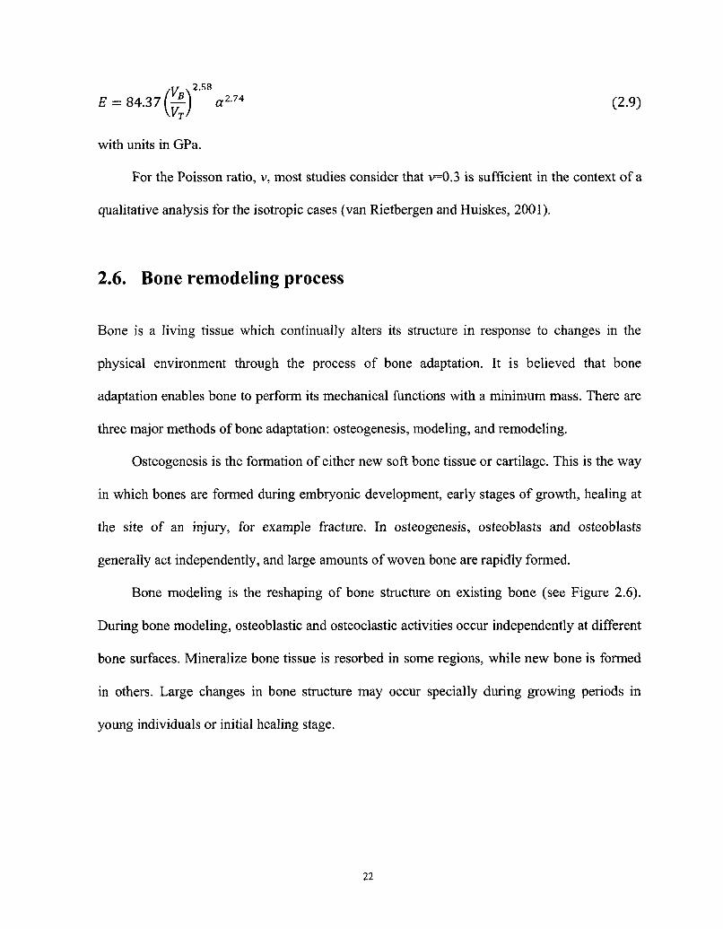
E = 84.37 (-fy a2-74 (2.9)
with units in GPa.
For the Poisson ratio, v, most studies consider that v=0.3 is sufficient in the context of a
qualitative analysis for the isotropic cases (van Rietbergen and Huiskes, 2001).
2.6. Bone remodeling process
Bone is a living tissue which continually alters its structure in response to changes in the
physical environment through the process of bone adaptation. It is believed that bone
adaptation enables bone to perform its mechanical functions with a minimum mass. There are
three major methods of bone adaptation: osteogenesis, modeling, and remodeling.
Osteogenesis is the formation of either new soft bone tissue or cartilage. This is the way
in which bones are formed during embryonic development, early stages of growth, healing at
the site of an injury, for example fracture. In osteogenesis, osteoblasts and osteoblasts
generally act independently, and large amounts of woven bone are rapidly formed.
Bone modeling is the reshaping of bone structure on existing bone (see Figure 2.6).
During bone modeling, osteoblastic and osteoclastic activities occur independently at different
bone surfaces. Mineralize bone tissue is resorbed in some regions, while new bone is formed
in others. Large changes in bone structure may occur specially during growing periods in
young individuals or initial healing stage.
22
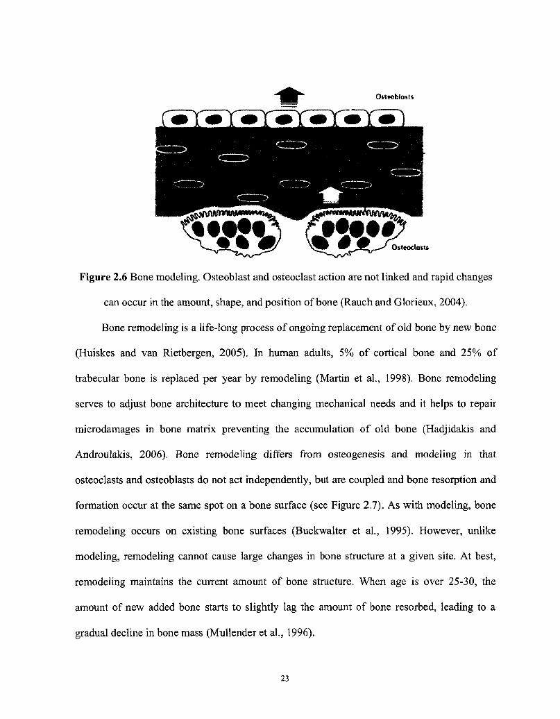
Figure 2.6 Bone modeling. Osteoblast and osteoclast action are not linked and rapid changes
can occur in the amount, shape, and position of bone (Rauch and Glorieux, 2004).
Bone remodeling is a life-long process of ongoing replacement of old bone by new bone
(Huiskes and van Rietbergen, 2005). In human adults, 5% of cortical bone and 25% of
trabecular bone is replaced per year by remodeling (Martin et al., 1998). Bone remodeling
serves to adjust bone architecture to meet changing mechanical needs and it helps to repair
mierodamages in bone matrix preventing the accumulation of old bone (Hadjidakis and
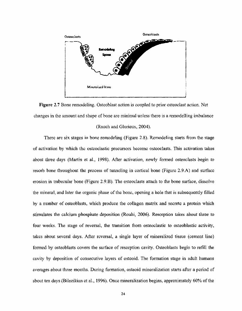
Androulakis, 2006). Bone remodeling differs from osteogenesis and modeling in that
osteoclasts and osteoblasts do not act independently, but are coupled and bone resorption and
formation occur at the same spot on a bone surface (see Figure 2.7). As with modeling, bone
remodeling occurs on existing bone surfaces (Buckwalter et al., 1995). However, unlike
modeling, remodeling cannot cause large changes in bone structure at a given site. At best,
remodeling maintains the current amount of bone structure. When age is over 25-30, the
amount of new added bone starts to slightly lag the amount of bone resorbed, leading to a
gradual decline in bone mass (Mullender et al., 1996).
23
Mineralized b » e
Figure 2.7 Bone remodeling. Osteoblast action is coupled to prior osteoclast action. Net
changes in the amount and shape of bone are minimal unless there is a remodelling imbalance
(Rauch and Glorieux, 2004).
There are six stages in bone remodeling (Figure 2.8). Remodeling starts from the stage
of activation by which the osteoclastic precursors become osteoclasts. This activation takes
about three days (Martin et al., 1998). After activation, newly formed osteoclasts begin to
resorb bone throughout the process of tunneling in cortical bone (Figure 2.9.A) and surface
erosion in trabecular bone (Figure 2.9.B). The osteoclasts attach to the bone surface, dissolve
the mineral, and later the organic phase of the bone, opening a hole that is subsequently filled
by a number of osteoblasts, which produce the collagen matrix and secrete a protein which
stimulates the calcium phosphate deposition (Rouhi, 2006). Resorption takes about three to
four weeks. The stage of reversal, the transition from osteoclastic to osteoblastic activity,
takes about several days. After reversal, a single layer of mineralized tissue (cement line)
formed by osteoblasts covers the surface of resorption cavity. Osteoblasts begin to refill the
cavity by deposition of consecutive layers of osteoid. The formation stage in adult humans
averages about three months. During formation, osteoid mineralization starts after a period of
about ten days (Bilezikian et al, 1996). Once mineralization begins, approximately 60% of the
24
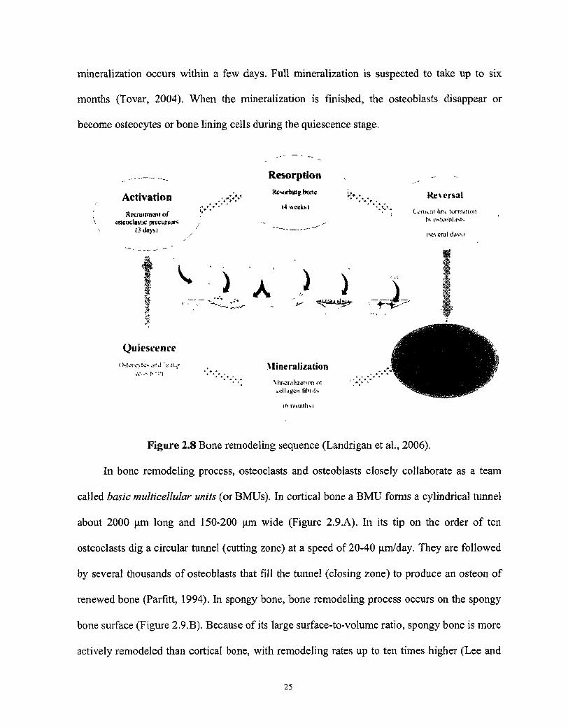
mineralization occurs within a few days. Full mineralization is suspected to take up to six
months (Tovar, 2004). When the mineralization is finished, the osteoblasts disappear or
become osteocytes or bone lining cells during the quiescence stage.
Activation Recruitment of
osteoclastic precursors (3 days)
^
Quiescence lKtcivyic> .mi 'a 114'
4.V..V ! ( • !*]
Resorption Rcsorbmg bone
»4 weeks»
) A ) )
Mineralization Mincr.tliZiition ot toll.igen fibrils
( IMI IDMIIM
Reversal Ce1u4.nl tin*, turnution
h\ tiMcubldtis
lse\eraldi\M
Figure 2.8 Bone remodeling sequence (Landrigan et al., 2006).
In bone remodeling process, osteoclasts and osteoblasts closely collaborate as a team
called basic multicellular units (or BMUs). In cortical bone a BMU forms a cylindrical tunnel
about 2000 um long and 150-200 |un wide (Figure 2.9.A). In its tip on the order of ten
osteoclasts dig a circular tunnel (cutting zone) at a speed of 20-40 um/day. They are followed
by several thousands of osteoblasts that fill the tunnel (closing zone) to produce an osteon of
renewed bone (Parfitt, 1994). In spongy bone, bone remodeling process occurs on the spongy
bone surface (Figure 2.9.B). Because of its large surface-to-volume ratio, spongy bone is more
actively remodeled than cortical bone, with remodeling rates up to ten times higher (Lee and
25
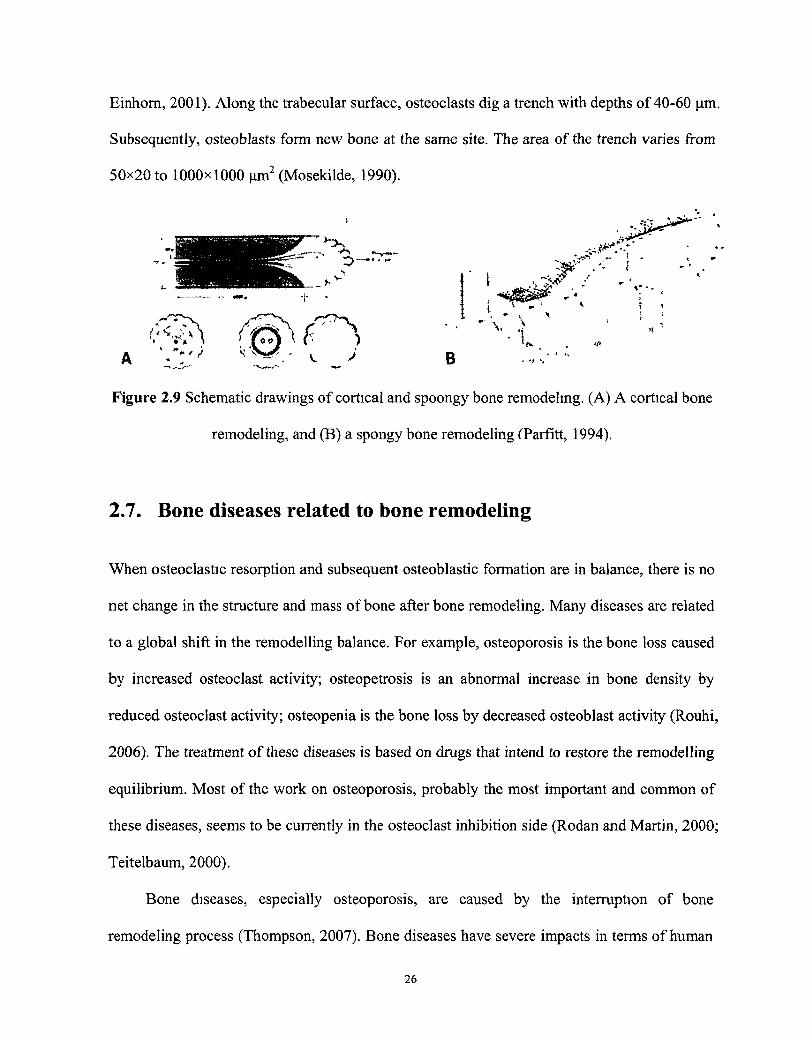
Einhorn, 2001). Along the trabecular surface, osteoclasts dig a trench with depths of 40-60 urn.
Subsequently, osteoblasts form new bone at the same site. The area of the trench varies from
50x20 to 1000x1000 nm2 (Mosekilde, 1990).
Figure 2.9 Schematic drawings of cortical and spoongy bone remodeling. (A) A cortical bone
remodeling, and (B) a spongy bone remodeling (Parfitt, 1994).
2.7. Bone diseases related to bone remodeling
When osteoclastic resorption and subsequent osteoblastic formation are in balance, there is no
net change in the structure and mass of bone after bone remodeling. Many diseases are related
to a global shift in the remodelling balance. For example, osteoporosis is the bone loss caused
by increased osteoclast activity; osteopetrosis is an abnormal increase in bone density by
reduced osteoclast activity; osteopenia is the bone loss by decreased osteoblast activity (Rouhi,
2006). The treatment of these diseases is based on drugs that intend to restore the remodelling
equilibrium. Most of the work on osteoporosis, probably the most important and common of
these diseases, seems to be currently in the osteoclast inhibition side (Rodan and Martin, 2000;
Teitelbaum, 2000).
Bone diseases, especially osteoporosis, are caused by the interruption of bone
remodeling process (Thompson, 2007). Bone diseases have severe impacts in terms of human
26
cost and socioeconomic burden. In Canada one in four women and at least one in eight men
over the age of 50 have osteoporosis and it is estimated that as many as two million Canadians
may be at risk of osteoporotic fractures. The cost to the Canadian health care system of
treating osteoporosis and the fractures it causes is currently estimated to be $1.9 billion
annually (Osteoporosis Canada, 2008). Because of these severe impacts caused by bone
diseases and failure of implants and prostheses, it is of great importance to understand how
bone remodeling works, with the hope of finding practical ways to keep the balance between
the bone resorption and formation.
During childhood and teenage years, the amount of new bone added is more than the
amount of old bone removed. This tendency continues until peak bone mass (PBM) is reached
between 20 and 30 years of age (Compston & Rosen, 2002). Hereditary factors account for
about 80% of the PBM, while about 20% depends on environmental stimuli (Gunnes, 1995).
After age 30, bone resorption exceeds bone formation and it is difficult to build more bone
mass. At that stage, hormonal changes (Ahlborg et al., 2001; Bendavid et al., 1996), nutrition
(Dawson-Hughes et al., 1997) and lifestyle (Hollenbach et al., 1993; Holbrook and Barrett-
Connor, 1993; Greendale et al., 1995) are the main factors that determine bone loss. At every
age, but especially after PBM is reached, eating well and providing the proper mechanical
stimuli to the bone are critical to reduce the risk of problems related to low bone mineral
density (BMD) such as osteopenia and osteoporosis (Chan et al., 2003). Bone mineral density
refers to the amount of mineral per square centimetre of bone and is most frequently measured
by dual energy x-ray absorptiometry (DEXA). Osteoporosis occurs over time when the
amount of bone broken down greatly exceeds the amount of bone replaced by new bone cells.
27
At this point, bone mineral density decreases, and so can cause a reduction in the bone mass.
The ultimate results are that bones become more porous, less stiff and more prone to fracture.
Bone responds to mechanical stimuli with changes in the structure and, consequently,
alteration of the BMD. Immobilization and weightlessness are associated with reduction in
bone mass (Vogel, 1975; Whalen, 1993; Lang et al., 2004; Silva et al., 2004). Conversely,
weight-bearing exercises (work against gravity) help build stronger bones (Calbet et al., 1998,
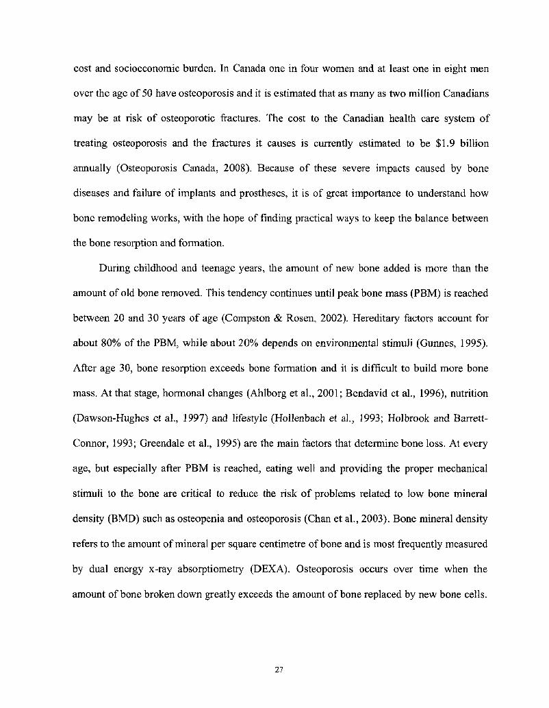
1999; Oleson et al., 2002; Faulkner et al., 2003). Figure 2.10 shows the internal structural
effect of mass reduction in trabecular bone.
Figure 2.10 Bone mass reductions in spongy bone. Micrograph of normal bone (left), thinning
bone (center) and osteoporotic bone (right) (Tovar, 2004).
The insertion of an orthopaedic prosthesis dramatically can alter bone's physical
environment. Whenever an implant is inserted into the body, existing bone has to be removed
for the implant to take its place. This alters the load path and the strain distribution for the
bone tissue in the vicinity of the implant, causing a redistribution of bone mass at the implant-
bone interface. The complex stress transfer between the external device and the host bone
might cause an undesired structural remodeling around the implant. For instance, while the
deposition of higher density bone material near the implant is desirable for good fixation,
gradual resorption of bone tissue around the stem may affect the performance of the prosthesis
28
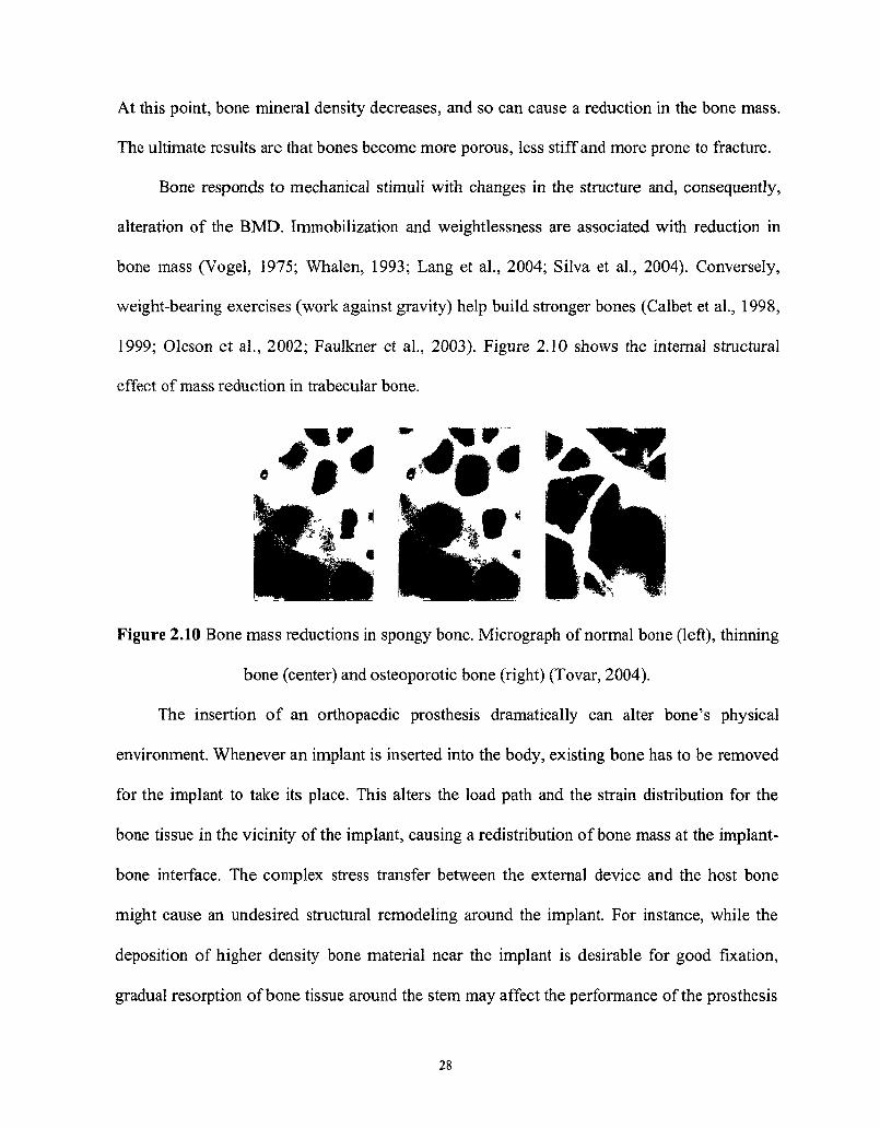
(Tavor, 2004; Haase, 2010). The degenerative adaptation process might result in loosening of
the implant, causing pain for the patient and eventually fracture of the bone (Figure 2.11).
Figure 2.11 Loosening of a long-stem prosthesis of the left hip with major bone loss (Wagner,
H. and Wagner, M.).
2.8. Bone remodeling theories
Based on Wolffs Law (1892) indicating that bone adapts to mechanical loading in accordance
with mathematical law during its growth and development, numerous researchers have been
encouraged to propose mathematical models for the bone remodeling process. In 1987, Frost
developed mechanostat theory which was the starting point for many mathematical theories of
bone remodeling (Frost, 1987). The mechanostat theory states that a minimum effective strain
(MES) should be exceeded in order to trigger an adaptive response in bone. Cowin and
Hegedus developed adaptive elasticity theory (Cowin and Hegedus, 1976; Hegedus and
Cowin, 1976), which considered strain as mechanical stimulus to initiate the bone remodeling
process. However, the attempt to adjust the tensor of remodeling constants ended up in a
variation of data, and yet the exact values of the remodeling constants are not available
29
(Cowin, 2003; Vahdati and Rouhi, 2009). Huiskes et al. (1987) proposed a scalar quantity,
strain energy density (SED), as a mechanical stimulus for bone remodeling and incorporated
the concept of lazy zone, which was introduced by Carter (1984), into their model. Later,
Huiskes and co-workers (2000) developed a semi-mechanistic model for bone remodelling.
The semi-mechanistic bone remodeling theory (Huiskes et al., 2000) includes the
experimental findings in bone cells' physiology (Vahdati and Rouhi, 2009), such as a separate
description of osteoclastic resorption and osteoblastic formation (Burger and Klein-Nulend,
1999), an osteocyte mechanosensory system (Aarden et al., 1994; Cowin et al., 1991), and
role of microdamage (Pazzaglia et al., 1997; Taylor, 1997; Martin, 2000). Recently, a few
remodeling theories considered both mechanical stimuli and microdamage (Rouhi et al., 2006;
McNamara and Prendergast, 2007). Each of the proposed theories of bone remodeling sheds
some lights on this multifactorial and complex process. For example, van der Linder and co
workers' models have been used to predict changes in bone structure due to the effect of anti-
resorptive drugs (van der Linden et al., 2003), and Foldes et al.'s model and Cowin's model
have shown the effects of immobilization or microgravity exposure on the bone structure
(Foldes et al., 1990; Cowin, 1998). However, none of them could predict all different features
of the very complex process of bone remodeling. The following is a review of major
theoretical studies and computational models related to the bone remodelling process.
30
2.8.1. Trajectorial theory and Wolffs Law
The earliest observations directed at uncovering the influence of mechanical environment on
trabecular structure date back to the drawings of the internal structure of the proximal femur
(trajectories of trabecular bone) (Figure 2.12.A) by a Swiss anatomist, von Meyer (1867). By
chance, a German civil engineer, Karl Culmann, the father of the method of graphical
statistics (Culman, 1866), studied von Meyer's sketches and found that the direction of
internal stresses in a Fairbaim crane (Figure 2.12.B) were remarkably similar to the trabecular
architecture in the proximal femur.
,J/'.'''
Ww •i f
M * * 1* •
—Jr
Figure 2.12 (A) von Meyer's sketch of the trajectories of trabecular bone in proximal femur;
(B) Culmann's graph of the principal stress trajectories in a Fairbaim crane (Wageningen ur,
2009).
The first cooperation in the field of bone biomechanics between von Meyer and
Culmann (Roesler, 1987) suggested that trabecular alignment is regulated by internal stress
patterns (Jacobs, 2000). In 1870, their work laid the foundation for a German orthopaedic
surgeon, Julius Wolff, to discover that trabecular architecture matches the principal stress
31
trajectories, known as the Trajectorial Theory of trabecular alignment (Jacobs, 2000). Wolff
(1892) declared the most widely accepted theory on bone remodeling which now bear his
name, Wolffs Law: "the law of bone remodelling is the law according to which alterations of
the internal architecture clearly observed and following mathematical rules, as well as
secondary alterations of the external form of the bones following the same mathematical rules,
occur as a consequence of primary changes in the shape and stressing ... of the bones." He
believed that bone adapted to mechanical loading during its growth and development, and that
the same adaptation process took place during healing after fracture. Even though Wolff
hypothesized that the adaptation is governed by a mathematical law, he never attempted to
formulate a mathematical theory (Martin et al., 1998).
2.8.2. Frost's mechanostat theory
In 1987, Frost developed Mechanostat Theory. Instead of speculating that strains below a
certain threshold are trivial and evoke no adaptive response, Frost suggested that there is an
equilibrium range of strain values which elicits no response. Strains above this range will
evoke deposition of bone, while strains below this range will induce bone resorption. In the
model postulated by Frost (1987), the equilibrium range was defined between 200 and 2500
um/m for compression and between 200 and 1500 um/m for tension. Strains over 4000 um/m
(tension and compression) can cause damage and, consequently, woven bone formation. Frost
is commonly credited with providing the conceptual framework from which many of the
current mechanical theories have been guided (Grosland et al., 2001).
32
2.8.3. Cowin and Hegedas' adaptive elasticity theory
The adaptive elasticity theory developed by Cowin and Hegedus (Cowin and Hegedus, 1976;
Hegedus and Cowin, 1976) was recognized as the mathematically rigorous and potentially
powerful theory which was able to describe the adaptive behaviour of bone (Jacobs, 2000). In
this model, bone is defined as a chemically reacting porous elastic solid whose porosity is
modified through mass deposition or resorption controlled by strain (Cowin and Hegedus,
1976).
2.8.4. Huiskes el al.'s strain energy density model
Please see section 3.1
2.9. Open questions related to bone remodeling
There are many open questions related to bone remodeling process which need urgent
attention. Some of them are listed below:
What is the actual mechanical stimulus to initiate the bone remodelling process? A
variety of mechanical stimuli associated with ambulation (at a frequency of 1 to 2 Hz) have
been considered for bone remodeling (Burger, 2001). The mechanical stimuli suggested
include strain (Cowin and Hegedus, 1976; Frost, 1987), stress (Wolff, 1892; Frost, 1964b),
strain energy density (Huiskes et al., 1987), strain rate (Hert et al, 1969; Fritton et al., 2000),
and fatigue microdamage (Martin and Burr, 1982).
What are the mechanosensors of bone? Although it is believed that osteocytes are the
most suitable candidate for the mechanosensor, there is no consensus on this yet. This is an
33
extremely important question which should be addressed in the future. Moreover, how
osteocytes signal effector cells (osteoclasts and osteoblasts) and initiate bone turnover are not
well understood (You et al., 2008).
In bone remodeling process there is a phase of reversal, which is a 1 to 2 weeks interval
between the completion of resorption and beginning of formation. The cellular and honnonal
mechanisms involved in reversal stage are unclear as well (Rouhi, 2006).
Osteocyte apoptosis as a potential signal source for osteoclastic bone resorption has
been identified. The molecular links between damaged induced apoptosis and targeted
osteoclast activity are unknown and need to be studied further (Noble, 2003; Heino et al.,
2009).
Physical loading and routine activities have been proven to inhibit bone resorption.
However, the cellular mechanism underlying this phenomenon remains largely unknown (You
et al., 2008).
34
Chapter 3
General Methods
This chapter will introduce a semi-mechanistic bone remodeling theory (Huiskes et al., 2000)
and finite element methods employed in this study.
3.1. A semi-mechanistic bone remodeling theory
3.1.1. A phenomenological model developed by Huiskes and co-workers
(1987)
Cowin's adaptive elasticity theory (Cowin and Hegedus, 1976; Hegedus and Cowin, 1976),
which considers strain as mechanical stimulus to initiate the bone remodeling process, has
been extended by Huiskes et al. (1987) with two main differences. They incorporated the
concept of lazy zone (Figure 3.1), proposed by Carter (1984), into their model. Furthermore,
the strain energy density (SED), a scalar quantity, is taken as the mechanical stimulus in their
remodelling equation. However, as other early models, the model relates mechanical signals to
bone adaptation without direct consideration of the underlying cell-biological mechanisms
(Ruimerman, 2005). Strain energy density, the strain energy per unit volume, is defined as:
U = \EO (3.1)
where U is the SED, £ and a are the strain tensor and stress tensor, respectively.
The use of strain tensor, as the remodeling stimulus, makes it difficult to determine the
remodeling rate coefficients (Cowin, 2003; Rouhi, 2006). In order to overcome this problem,
35
Huiskes and coworkers (1987) suggested the SED, a scalar quantity, as a suitable mechanical
stimulus for both surface remodeling (cortical bone) and internal remodeling (spongy bone).
For the surface remodeling (cortical bone), the bone can either add or remove material
according to:
dX — = CX(U - U*) (3.2)
dX where — is the rate of bone growth perpendicular to its surface, Cx is the remodelling rate
coefficient, U is the SED, U* is the equilibrium value of SED that determines the boundary
between apposition and resorption.
For internal remodeling, there will be changes in bone apparent density. By assuming a
modulus-density relationship (Eq. 2.1), one can write:
dE — = Ce(U-U') (3.3)
where E is the local elastic modulus, Ce is a proportionality constant.
36
Add , Bone
Remove Bone
y Adaptation Rate
A c
su* SU* r c
u* u
Figure 3.1 The assumed bone adaptation as a function of the strain energy density (SED, U)
incorporating lazy zone ((1 - s)[/* < U < (1 + s)U*) (MichiganEngineering).
Carter (1984) proposed the concept of lazy zone. A lazy zone, in which no bone
adaptation occurs, separates the domains of bone formation and resorption (Figure 3.1).
Huiskes et al. (1987) applied the concept of lazy zone to their model. For instance, the new
remodeling equation for internal remodeling (spongy bone) is written as:
fCe[U - (1 + s)U*] for £ / > ( ! + s)U*
dE
dt = <0 for ( 1 - 5 ) 1 / * <U < (l + s)U* (3.4)
\Ce[U - (1 - s)U*] forU<(l-s)U*
where s denotes the extent rate of the lazy zone around the U, and 2sU is the width of the
lazy zone.
This phenomenological theory was applied to predict bone adaptation for both surface
remodeling (shape changes) (Huiskes et al., 1987) and internal remodeling (density changes)
(van Rietbergen et al., 1993; Weinans et al., 1993) after implantation of prostheses. For
37
instance, in the two-dimensional simulation of cortical bone adaptation after hip-prosthetic
implantation, Huiskes et al. (1987) predicted the effect of stress shielding successfully.
3.1.2. A semi-mechanistic bone remodeling theory (Huiskes et al., 2000)
Huiskes et al.'s first model (1987) was able to explain bone adaptation on a macroscopic level
(Ruimerman, 2005). In order to investigate possible mechano-biological pathways, Huiskes et
al. (2000) proposed a new bone remodeling theory, a semi-mechanistic bone remodeling
theory, which includes the experimental findings in bone cells' physiology (Vahdati and Rouhi,
2009), such as a separate description of osteoclastic resorption and osteoblastic formation
(Burger and Klein-Nulend, 1999), role of microdamage (Pazzaglia et al., 1997; Taylor, 1997;
Martin, 2000), and an osteocyte mechanosensory system (Aarden et al., 1994; Cowin et al.,
1991). The proposed regulatory process of spongy bone remodeling is shown in Figure 3.2.
Spongy bone remodeling is depicted as a coupling process of bone resorption and bone
formation on the bone free surfaces. Osteoclasts are assumed to resorb bone stochastically. It
is suggested that osteocytes locally sense the SED rate perturbation generated by either the
external load or by cavities made by osteoclasts (bone resorbing cells), and then recruit
osteoblasts (bone forming cells) to form bone tissue to fill the resorption cavities.
38
Mechanical loading
s>y.1er dmr » * * « » * • »esoptton dt ! Bone architecture
Recruitment stimuli fioni othei ost«oc vtes • i ? m
F Osteoclasts
FEA
n
— I I
dmf
dt "> * >_» 3 Osteoblast*
Bone formation
Recruitment stimulus
Sensation
Kzt)
. y i i ' i i t u i - u n - i i l r
11 2 SEDrate#(/)
£ Osteocyte i >
Figure 3.2 Regulation mechanism of the semi-mechanistic bone remodeling process (Huiskes
et al., 2000).
3.1.2.1. Separation of osteoclastic and osteoblastic activities
In maturity, local bone resorption and subsequent formation in a process called bone
remodeling continuously renew the structure of bone (Frost, 1990). Huiskes et al. (2000)
considered bone mass and form are, at any time, determined by a balance between osteoclast
resorption and osteoblast formation. They assumed that the change in bone mass at a
particular spongy bone surface location x at time t is the result of osteoclastic bone resorption
and osteoblastic bone formation, thus:
dm(x, t) dm.f {x, t) dmr {x, t) (3.5)
dt dt dt
where —jp— is the local change of relative bone density caused (jn) by osteoblast formation
dmr(x,t)
dt
at trabecular surface location x, and dt
shows the local change of relative bone density
(m) caused by osteoclast resorption at trabecular surface location x.
39
3.1.2.2. Osteoclastic resorption caused by the presence of microdamage
Huiskes et al. (2000) assumed that the probability, p, of osteoclast activation per surface site at
any time is regulated either by the presence of microdamage within the bone matrix or by
disuse. In this study, for the sake of simplicity, only the incidence of the micro-cracks is
considered. Supported by experimental evidence (Fazzalari et al., 2002), microdamages are
assumed to occur spatially random and microdamage can occur anywhere at any time. Thus,
the probability of resorption by microcracks can be considered stochastic and was expressed
as:
p(x,t) = constant (3.6)
where this constant was selected to be 10%.
In their theory (Huiskes et al., 2000), it is assumed that osteoclasts are attracted towards
the bone surface by microdamage. When activated, each osteoclast is assumed to remove a
fixed amount of mineral. Hence, bone resorption is described by:
dmr(x,t)
—df- = -r°c ( 3 7 )
where roc represents the relative amount of mineral resorbed by osteoclasts, and roc is assumed
to be constant.
3.1.2.3. Osteocyte mechanosensory system and osteoblastic formation
Another basic assumption of Huiskes et al.'s theory (2000) is that osteocytes within the bone
matrix are mechanosensitive cells capable of sensing the mechanical stimulus and transmitting
bone remodeling signals to the bone surface to attract and activate basic multi-cellular units
40
(BMUs, osteoclasts and osteoblasts, which control resorption and formation at the bone
surface, respectively).
The signal sent to the surface by an osteocyte was assumed to decay exponentially with
increasing distance, d„ between osteocyte /' and location x according to:
f.(x) = e-d^'D (3.8)
where parameter D [\xn\~\ represents the osteocyte influence distance (or the decay constant),
which controls average trabecular thickness, for a given external force. It should be noted that
the function, f,(x), was just based on pure speculation. Huiskes and coworkers did not present
any specific reason for this decay function. Their assumption is based on rough experimental
evidence, so a more mechanistic approach is needed to make this model more accurate and
reliable (Rouhi, 2006).
The total bone formation stimulus (osteoblast recruitment stimulus) at the trabecular
surface location, x, are contributed by all the N osteocytes located within the influence region.
So, the osteoblast recruitment stimulus derived from all the osteocytes in the neighbourhood
of the bone surface location x can be written as:
N
P(*,t)=£7i(x)Mi(0 (3.9) £ = 1
where P(x,t) is the total bone formation stimulus value at trabecular surface, x; fij is the
mechanosensitivity of osteocyte i; and Rj(t) is the SED-rate in the location of osteocyte /. In
this theory, the stimulus sensed by osteocytes is assumed to be a typical strain energy density
rate (SED-rate), R,(t), in a recent loading history.
Cyclic loading conditions characterized by frequency and magnitude were imposed, and
it was assumed that osteocytes reacted to the maximum SED-rate during the loading cycle. It
is showed that the maximum SED-rate was related to the SED value for some substitute static
41
load and that it could be calculated by static finite element analysis (Ruimerman et al., 2001).
It seems that considering a scalar quantity such as strain energy density or its rate has a
disadvantage that cannot make any difference between compressive and tensile form of
loadings.
Osteoblast formation at the trabecular surface is assumed to be controlled by the
osteoblast recruitment stimulus, P(x,t). If the stimulus value, sent by neighbouring osteocytes,
is greater than a bone formation threshold, ktr, bone formation at the trabecular surface will
take place. But, if the stimulus value is less than the threshold value, ktr, there will be no bone
formation (Huiskes et al., 2000). So, one can express the bone formation's governing equation
as follows:
\[P{x,t) -ktr\ for P(x,t) > ktr , dmf{x, t)
dt (3.10)
0 for P{x, t) < ktr
where x is a proportionality factor that determines the bone formation rate. The values of the
bone formation threshold, &/,-, and the proportionality factor, r, are chosen empirically.
As stated earlier, the change in the relative density at a particular trabecular surface
location x and at time t is determined by osteoblast bone formation and osteoclast bone
resorption. Substituting Eqs. 3.7- 3.10 into Eq. 3.5, one can write the mathematical expression
of the bone remodeling process as follows:
dm(x, t)
di ~
r N diix)
e" D iiMi) - ktr roc for P(x, t) > ktr , (3.11)
l - r o c for P(x,t)<ktr
According to Currey's relationship (Currey, 1988), the Young's modulus, E(x, t) [GPa],
at each location depends on the relative density of bone, m, and can be obtained using:
42
E(x, t) = Emax x m{x, ty (3.12)
where the maximum Young's modules, Emax, and the exponent, y, are empirical constants.
3.2. Finite element analysis (FEA)
The semi-mechanistic bone remodeling theory used in our study assumed that strain energy
density (SED) was the mechanical stimulus and supposed that the bone remodeling was
coupled with two separate processes: bone resorption and subsequent bone formation.
Osteocytes were assumed to be sensor cells which can sense the SED and recruit osteoblasts at
the bone surface to fill the cavities formed by osteoclasts. The semi-mechanistic bone
remodeling theory was expressed by numerical algorithms. FEA codes were developed in this
research (see Appendix II). The purpose of the FEA codes is to calculate each bone element's
SED. Figure 3.3 shows the finite element analysis flow chart for the calculation of bone
elements' SED.
The computer simulation was conducted as an iterative process, during which each bone
element's relative density, m, was regulated between 0.01 (no bone) and 1.0 (fully mineralized
bone). In the beginning of the iteration, Young's modulus of each bone element E can be
determined from the relative density of bone using E(x, t) = Emax X m(x,ty (Eq. 3.12),
with Emax =5.0 GPa and y=3. As the tissue Poisson's ratio, v, is 0.3 using Eq. 1.16 (Appendix I)
or Eq. 1.44 (Appendix I), the stress-strain matrix, [D], for two- or three-dimensional computer
bone model can be formed.
From Eq. 1.21 (Appendix I) and Eq. 1.50 (Appendix I), we know that the strain-nodal
displacement matrix, [B], can be expressed as a matrix with respect to the local coordinates.
43
[B]r[D][B] is a function of local coordinates, r and s. Referred to Table 1.1 (Appendix I) or
Table 1.2 (Appendix I), we can find the local coordinates of the integrating point and
weighting coefficients. According to Eq. 1.27 (Appendix I) and Eq. 1.56 (Appendix I), the
approximation of the element stiffness matrix, [K*], for two- and three-dimensional mesh can
be evaluated, respectively.
As soon as the element stiffness matrix, [IC], has been formed, it can be assembled into
the global stiffness matrix, [K\. Since external forces are given, we can form the global force
vector, {F}, directly. Following the assembled global equations:
[K]{U] = {F} (3.13)
with {{/} representing the vector of global displacement, the global nodal displacement can be
obtained. Once {[/} is known, the element nodal displacements,{Ue}, are retrieved.
The strain tensor, {s}, at the center of the element is given by the strain-nodal
displacement relations, Eq. 1.20 (Appendix I) or Eq. 1.49 (Appendix I). According to Eq. 1.28
(Appendix) or Eq. 1.57 (Appendix I), the SED, u, at the center of the two- or three-
dimensional element can be obtained.
44
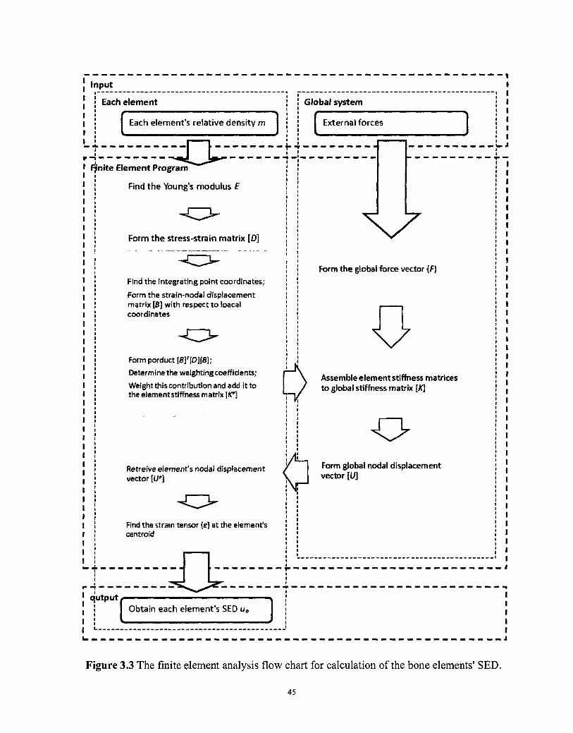
Input
Each element
Each element's relative density m
+-T
Fjnite Element Program
Find the Young's modulus E
Form the stress-strain matrix [0]
Find the integrating point coordinates;
Form the strain-nodal displacement matrix [B] with respect to loacal coordinates
Form porduct lflf[D][8];
Determine the weighting coefficients;
Weight this contribution and add it to the element stiffness matrix \K']
Retreive element's nodal displacement vector [Ue]
Find the strain tensor [e] at the element's centroid
Global system
External forces
Form the global force vector {f}
Assemble element stiffness matrices to global stiffness matrix [K]
o Form global nodal displacement vector [U]
Figure 3.3 The finite element analysis flow chart for calculation of the bone elements' SED.
45
Chapter 4
An Investigation into the Reasons for Bone Loss in Aging
and Osteoporotic Individuals Using a Two-Dimensional
Computer Model
4.1. Introduction
Bone is a dynamic tissue which adapts its mass and architecture to the external loads
constantly. Bone's adaptation is finished through a coupled process of bone resorption by
osteoclasts, and subsequent bone formation by osteoblasts, which is so-called bone
remodeling process (Ruimerman and Huiskes, 2005; Ruimerman et al., 2005). When the
amount of bone resorption is more than the added newly formed bone for a long period of
time, bone loss, a net reduction in bone apparent density which is defined as bone mass per
total volume of bone sample, and so a decrease in bone modulus of elasticity and also its
strength appear. Bone loss usually starts after maturation and accelerates in osteoporotic bones.
For instance, after the age of 25-30 years, a slightly negative balance between bone resorption
and formation may cause progressive bone loss (Mullender et al., 1996). Usually, in the case
of a minor reduction in bone density, mechanical integrity is maintained (Mullender et al.,
1996). However, in the case of osteoporosis or very major bone loss, a substantial reduction
can be seen in both bone modulus of elasticity and strength (Parfitt et al., 1983), in which
46
bone can fail even with lifting a light weight (Dickenson et al., 1981; Bono and Einhom, 2003;
Yuan et al., 2004; Slomka et al., 2008).
In the beginning of 21st century, Huiskes and co-workers (2000) developed a semi-
mechanistic model for bone remodelling. The semi-mechanistic bone remodeling theory
includes the experimental findings in bone cells' physiology (Vahdati and Rouhi, 2009), such
as a separate description of osteoclastic resorption and osteoblastic formation (Burger and
Klein-Nulend, 1999), an osteocyte mechanosensory system (Aarden et al., 1994; Cowin et al.,
1991), and the role of microdamage (Pazzaglia et al., 1997; Taylor, 1997; Martin, 2000). In
this theory, osteocytes are assumed to be sensitive to the maximal rate of the strain energy
density (SED) in a recent loading history and send out signals to recruit the osteoblasts, bone
forming cells, which form new bone to fill the cavities caused by osteoclast resorption.
Osteoclast resorption caused by microdamage is supposed to occur spatially random.
Based on the experiments, it is known that osteocyte density (the number of osteocytes
per unit surface of bone) changes with aging and also in osteoporotic bones (Mullender et al.,
1996). It has been found that osteocyte density declines significantly with aging in healthy
adults from 30 to 91 years of age (Frost, 1960; Mullender et al., 1996; Qiu et al., 2003). On
the other hand, Mullender et al. (1996) interestingly found that the osteocyte density increases
in osteoporotic patients compared to healthy adults, although excessive bone loss and reduced
spongy bone wall thickness have been described as characteristic of osteoporotic bones.
It was suggested that osteocytes regulate the recruitment of basic multicellular units
(BMUs) in response to mechanical stimuli (Kenzora et al., 1978; Marotti et al., 1990; Lanyon,
1993). Based on the fact that the number of osteocytes per unit surface of bone changes in
47
aging healthy adults and also in osteoporotic patients, here we hypothesize that bone loss is
correlated with the reduction of either the number of osteocytes in the aging healthy adults'
bone or the strength of the recruitment signal sent by osteocytes to the bone making cells
(osteoblasts) in the osteoporotic bone. The former part of our hypothesis is raised because of
the evidence indicating that osteocyte density can likely affect the trabecular bone
morphology (Mullender et al., 1994; Mullender and Huiskes, 1995). The later part of our
hypothesis is raised since one may ask: "If the bone loss with aging is provoked and driven by
a decrease in osteocyte density, then what is the explanation for rapid bone loss in
osteoporotic bones wherein there is an increase in osteocyte density?". Since the changes in
bone structure because of osteoporosis are similar to changes resulting from disuse (Frost,
1988; Rodan, 1991; Mullender et al., 1994; Mullender and Huiskes, 1995), we assumed that
one of the causes for bone loss in osteoporotic bones is the reduction in osteocyte
mechanosensitivity. To investigate our hypotheses we employed Huiskes and co-workers'
(2000) semi-mechanistic bone remodeling theory to build computer models for simulating the
spongy bone remodeling.
4.2. Methods
4.2.1. A semi-mechanistic bone remodeling theory
Please see section 3.1.2.
48
4.2.2. A two-dimensional computer model
A two dimensional finite element model of spongy bone, which was a square domain of
1.52x1.52 mm , was created by implementing the mathematical expressions of the semi-
mechanistic bone remodeling theory (Huiskes et al., 2000). This domain was divided into 38
X38 rectangular four-node elements. Relative bone density (m) per element is considered to
alter between 0.01 (no bone, so just bone marrow) and 1.0 (no void, fully solid mineralized
bone) (see Figure 4.1). In order to apply external loads to our 2D computer model, the
perimeter of the square domain was assumed to be surrounded by a band. The thickness of the
band was one element, equal to 40 urn. This band did not participate in the bone remodeling
process, and the load was applied at the edge of the bone model. In order to minimize the
effect of stress shielding caused by continuous band corners, no external load was imposed on
the corner of the band (see Figure 4.1), and the material properties of the band were the same
as those of a fully mineralized trabecular bone tissue, which were given a Young's modulus of
5 GPa and a Poisson ratio of 0.3. The structure was loaded by a sinusoidal stress, cycling
between 0 and 2 MPa, and at frequency of 1 Hz. The semi-mechanistic bone remodelling
theory assumed that the stimulus sensed by osteocytes is the maximal SED-rate during one
loading cycle. It has been shown that the maximum SED-rate can be substituted by the SED
value for some static load (Ruimerman et al., 2001). Hence, the bone remodeling can be
evaluated by static finite element analysis. In this study, the SED value was calculated using a
substitute static stress of 4 MPa.
49
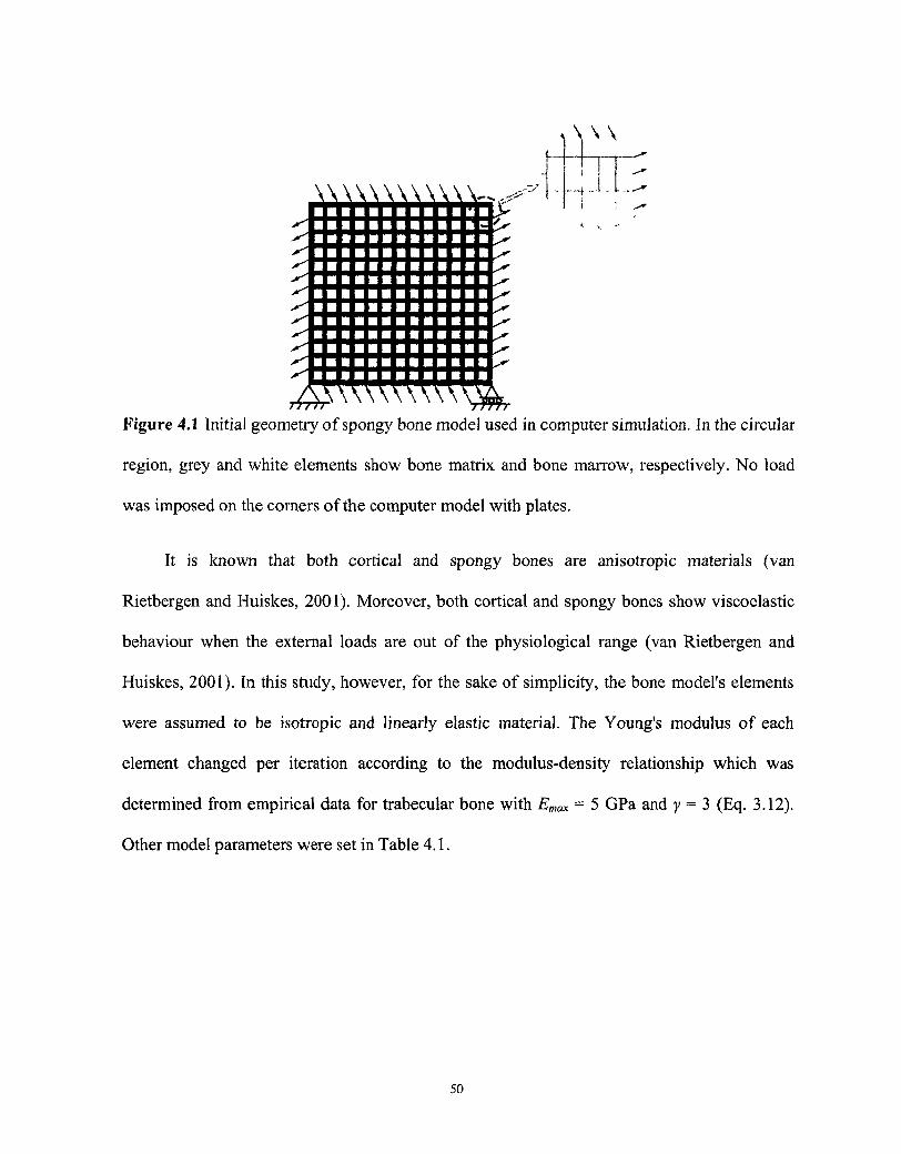
^ w
rrrrr \ \ \ \ \ \ ^ ^ • • • • • • » •
• • • • • • i i i i i i e • • • • •
-~f •
ruri $w«s: Figure 4.1 Initial geometry of spongy bone model used in computer simulation. In the circular
region, grey and white elements show bone matrix and bone marrow, respectively. No load
was imposed on the comers of the computer model with plates.
It is known that both cortical and spongy bones are anisotropic materials (van
Rietbergen and Huiskes, 2001). Moreover, both cortical and spongy bones show viscoelastic
behaviour when the external loads are out of the physiological range (van Rietbergen and
Huiskes, 2001). In this study, however, for the sake of simplicity, the bone model's elements
were assumed to be isotropic and linearly elastic material. The Young's modulus of each
element changed per iteration according to the modulus-density relationship which was
determined from empirical data for trabecular bone with Emax = 5 GPa and y = 3 (Eq. 3.12).
Other model parameters were set in Table 4.1.
50
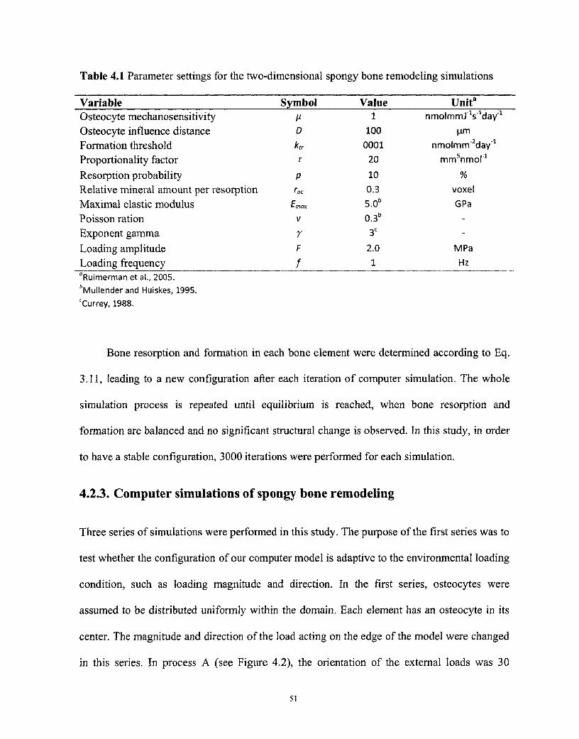
Table 4.1 Parameter settings for the two-dimensional spongy bone remodeling simulations
Variable Osteocyte mechanosensitivity Osteocyte influence distance Formation threshold Proportionality factor Resorption probability Relative mineral amount per resorption Maximal elastic modulus Poisson ration Exponent gamma Loading amplitude Loading frequency
Symbol V-D
*«r
T
P
r0c
tmox
V
r F
f
Value 1
100
0001
20
10
0.3
5.0b
0.3b
3C
2.0
1
Unit3
nmolmm.T1s"1day'1
urn nmolmm^day"1
mmsnmor1
%
voxel
GPa
-
-
MPa
Hz "Ruimerman et al., 2005. bMullender and Huiskes, 1995. rCurrey, 1988.
Bone resorption and formation in each bone element were determined according to Eq.
3.11, leading to a new configuration after each iteration of computer simulation. The whole
simulation process is repeated until equilibrium is reached, when bone resorption and
formation are balanced and no significant structural change is observed. In this study, in order
to have a stable configuration, 3000 iterations were performed for each simulation.
4.2.3. Computer simulations of spongy bone remodeling
Three series of simulations were performed in this study. The purpose of the first series was to
test whether the configuration of our computer model is adaptive to the environmental loading
condition, such as loading magnitude and direction. In the first series, osteocytes were
assumed to be distributed uniformly within the domain. Each element has an osteocyte in its
center. The magnitude and direction of the load acting on the edge of the model were changed
in this series. In process A (see Figure 4.2), the orientation of the external loads was 30
51
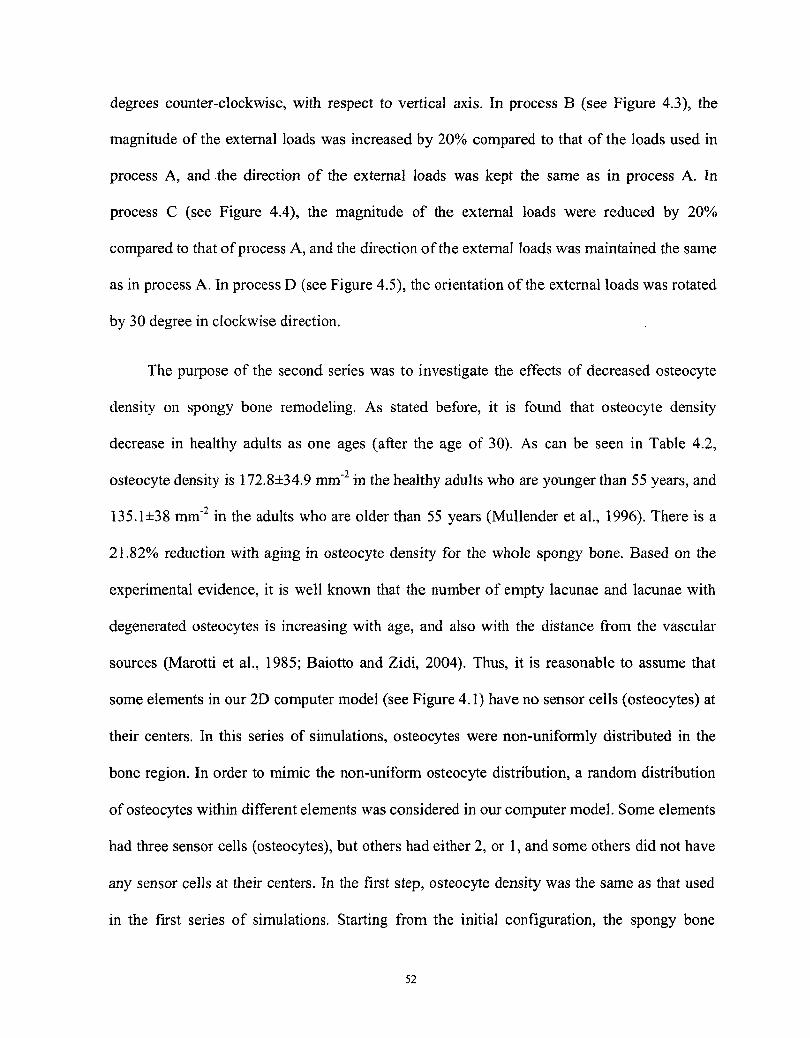
degrees counter-clockwise, with respect to vertical axis. In process B (see Figure 4.3), the
magnitude of the external loads was increased by 20% compared to that of the loads used in
process A, and the direction of the external loads was kept the same as in process A. In
process C (see Figure 4.4), the magnitude of the external loads were reduced by 20%
compared to that of process A, and the direction of the external loads was maintained the same
as in process A. In process D (see Figure 4.5), the orientation of the external loads was rotated
by 30 degree in clockwise direction.
The purpose of the second series was to investigate the effects of decreased osteocyte
density on spongy bone remodeling. As stated before, it is found that osteocyte density
decrease in healthy adults as one ages (after the age of 30). As can be seen in Table 4.2,
osteocyte density is 172.8±34.9 mm" in the healthy adults who are younger than 55 years, and
135.1±38 mm"2 in the adults who are older than 55 years (Mullender et al., 1996). There is a
21.82% reduction with aging in osteocyte density for the whole spongy bone. Based on the
experimental evidence, it is well known that the number of empty lacunae and lacunae with
degenerated osteocytes is increasing with age, and also with the distance from the vascular
sources (Marotti et al., 1985; Baiotto and Zidi, 2004). Thus, it is reasonable to assume that
some elements in our 2D computer model (see Figure 4.1) have no sensor cells (osteocytes) at
their centers. In this series of simulations, osteocytes were non-uniformly distributed in the
bone region. In order to mimic the non-uniform osteocyte distribution, a random distribution
of osteocytes within different elements was considered in our computer model. Some elements
had three sensor cells (osteocytes), but others had either 2, or 1, and some others did not have
any sensor cells at their centers. In the first step, osteocyte density was the same as that used
in the first series of simulations. Starting from the initial configuration, the spongy bone
52
remodeling of the healthy adults under the age of 55 years was simulated (see process E,
Figure 4.7). In the second step, starting from the final configuration of process E, the spongy
bone remodeling of the healthy adults over 55 years was simulated (see process F, Figure 4.7).
In process F, the osteocyte number per bone area was reduced by 21.82%, and the external
loads were kept the same as those used in process E (see Figure 4.7).
Table 4.2
Osteocyte density of healthy adults and osteoporotic patients (Mullender et al., 1996)
Healthy
individuals
Osteoporotic
patients >55years
<55 years
>55 years
Hip fracture
Vertebrae fracture
Number of
osteocytes/bone area
(mm2)
172.8±34.9
135.1±38.0
158.3±23.6
176.0±21.6
Combined number
of osteocytes/bone
area (mm"2)
150.7±40.7
164.5±24.2
The third series were performed to test the probability of bone loss in osteoporotic bones
caused by a reduction in osteocyte mechanosensitivity. Experimental observations show that
in the observed osteoporotic group older than 55 years, osteocyte density has a significant
increase relative to the healthy adults (Mullender et al., 1996). As can be seen in Table 4.2, the
osteocyte density in healthy adults over the age of 55 is 135.1±38.0 mm"2, whereas that of the
osteoporotic patients for the same age group is 164.5±24.2 mm"2. Thus, the osteocyte density
in osteoporotic patients (older than 55 years) increased by 21.76% compared to the osteocyte
density in healthy adults above 55 years. In the third series of simulations, based on the
53
experimental evidence (Marotti et al., 1985; Baiotto and Zidi, 2004), osteocytes were
randomly distributed in the bone region. We considered that an adult was healthy when he (or
she) was under 55 years, but was affected by osteoporosis when he (or she) got older than 55
years. So, in order to model the spongy bone remodeling for the osteoporotic patients, in the
first step, starting from the initial configuration, the spongy bone remodeling for a healthy
adult younger than 55 years was simulated (see process E, Figure 4.7). Then, in the second
step, since osteoporotic patients were assumed to be older than 55 years, we decreased the
osteocyte density in the healthy young adults by 21.82% to get the osteocyte density in the
healthy adults over the age of 55 years, and then increased the osteocyte density by 21.76% to
get the osteocyte density in the osteoporotic patients. The loading conditions, magnitude and
direction, were kept the same for the first and second steps. To investigate the effects of
mechanosensitivity on the spongy bone remodeling in osteoporotic patients, we decreased the
mechanosensitivity of osteocytes from 1 to 0.1 gradually for each simulation in the second
step (see Figure 4.9). The simulations with different osteocyte mechanosensitivities all started
from the structure obtained from the first step, i.e. from process E (see Figure 4.7).
4.3. Results
In the first series of simulations, trabeculae-like structures were obtained from the initial
configuration. Trabeculae were lined up with the loading direction (see Figure 4.2). A 20%
increase in the external loading magnitude increased the trabecular thickness (see Figure 4.3)
which resulted in a 12.5% increase in the bone mass (see process A and B, Figure 4.6).
Reduction in the external loading magnitude by 20% has led to a decrease in trabecular
54
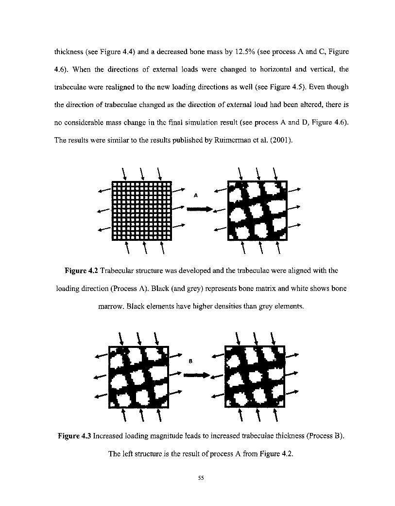
thiclcness (see Figure 4.4) and a decreased bone mass by 12.5% (see process A and C, Figure
4.6). When the directions of external loads were changed to horizontal and vertical, the
trabeculae were realigned to the new loading directions as well (see Figure 4.5). Even though
the direction of trabeculae changed as the direction of external load had been altered, there is
no considerable mass change in the final simulation result (see process A and D, Figure 4.6).
The results were similar to the results published by Ruimerman et al. (2001).
\ \ \
~ •• ~ • •• • • • •
\ \ \ \ \ \
Figure 4.2 Trabecular structure was developed and the trabeculae were aligned with the
loading direction (Process A). Black (and grey) represents bone matrix and white shows bone
marrow. Black elements have higher densities than grey elements.
\ \ V
\ \ \
\ \ \
iiv A * *
\ \ \
Figure 4.3 Increased loading magnitude leads to increased trabeculae thickness (Process B).
The left structure is the result of process A from Figure 4.2.
55
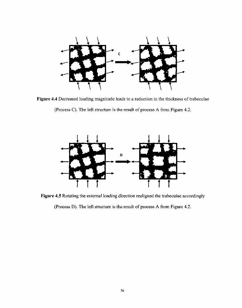
\ \ \ \ \ \
Figure 4.4 Decreased loading magnitude leads to a reduction in the thickness of trabeculae
(Process C). The left structure is the result of process A from Figure 4.2.
i 1 I 1 I 1
Figure 4.5 Rotating the external loading direction realigned the trabeculae accordingly
(Process D). The left structure is the result of process A from Figure 4.2.
56
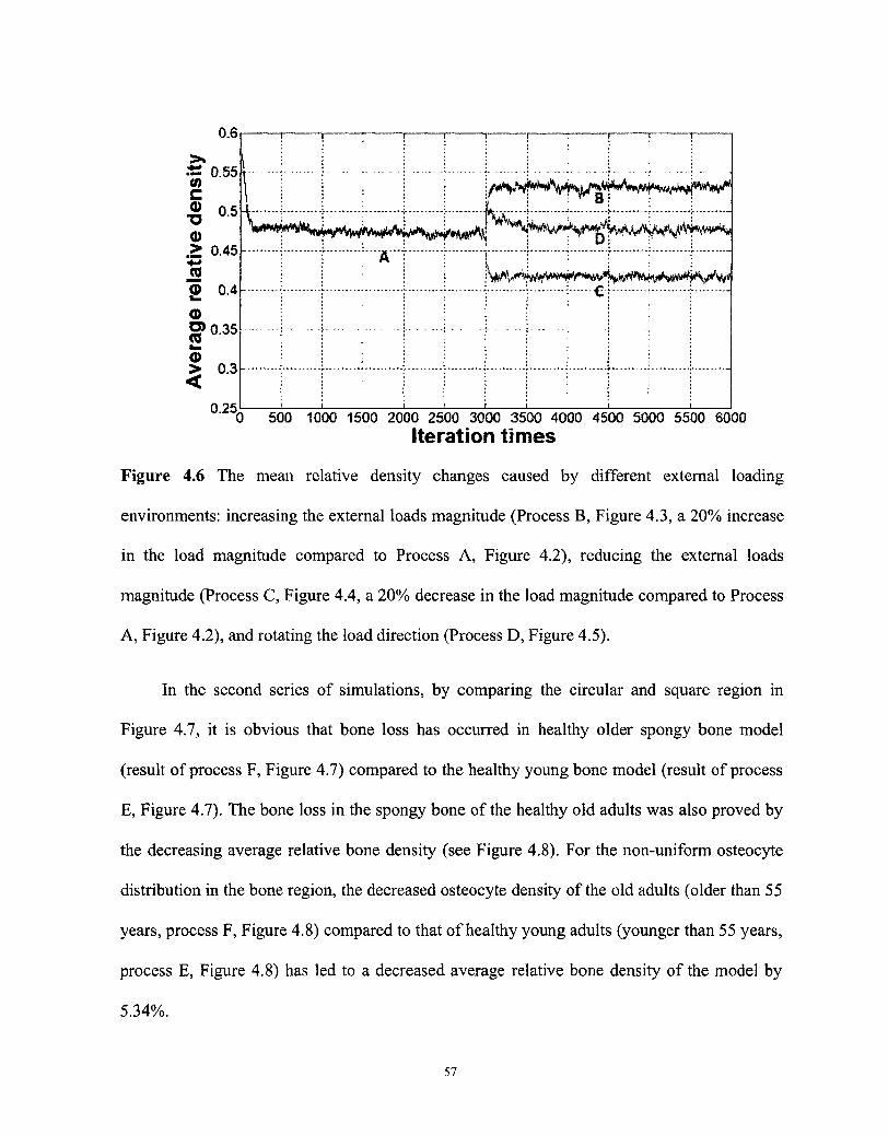
0.6
>» SS 0.55 <0 •§ 0.5
0 > 0.45
fl) 0.4 b
0)
GJ
<u > 0.3 <
0.25
D j
...£•
0 500 1000 1500 2000 2500 3000 3500 4000 4500 5000 5500 6000
Iteration times
Figure 4.6 The mean relative density changes caused by different external loading
environments: increasing the external loads magnitude (Process B, Figure 4.3, a 20% increase
in the load magnitude compared to Process A, Figure 4.2), reducing the external loads
magnitude (Process C, Figure 4.4, a 20% decrease in the load magnitude compared to Process
A, Figure 4.2), and rotating the load direction (Process D, Figure 4.5).
In the second series of simulations, by comparing the circular and square region in
Figure 4.7, it is obvious that bone loss has occurred in healthy older spongy bone model
(result of process F, Figure 4.7) compared to the healthy young bone model (result of process
E, Figure 4.7). The bone loss in the spongy bone of the healthy old adults was also proved by
the decreasing average relative bone density (see Figure 4.8). For the non-uniform osteocyte
distribution in the bone region, the decreased osteocyte density of the old adults (older than 55
years, process F, Figure 4.8) compared to that of healthy young adults (younger than 55 years,
process E, Figure 4.8) has led to a decreased average relative bone density of the model by
5.34%.
57
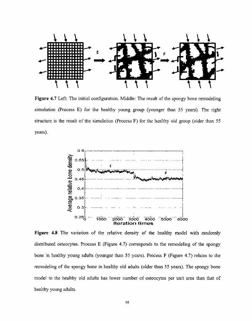
IIIIIIIIUI a a a a a a a a a a a a a • • • • • • • • • • • • I a a a a a a a a a a a a a • • • • • • • • • • • • a • • • • • • • • • • • • • • • • • • • • • • • • • a i n i n n • • • • • • • • • • • • a • • • • • • • • • • • • a
• • • • • • • • • • i • I I I I I I I I I i n
\ \ \
\ \ \
\ \ \ \ \ \
Figure 4.7 Left: The initial configuration. Middle: The result of the spongy bone remodeling
simulation (Process E) for the healthy young group (younger than 55 years). The right
structure is the result of the simulation (Process F) for the healthy old group (older than 55
years).
o 6
g 0.55 <L>
<D 0 . 5
0.45 <D
iS 0.4
g>0.35 to <L> O 3
0 .25
"1
^%*^w\»*e^^
1O0O 2000 30O0 4000 5000 6000
Iteration t i m e s
Figure 4.8 The variation of the relative density of the healthy model with randomly
distributed osteocytes. Process E (Figure 4.7) corresponds to the remodeling of the spongy
bone in healthy young adults (younger than 55 years). Process F (Figure 4.7) relates to the
remodeling of the spongy bone in healthy old adults (older than 55 years). The spongy bone
model in the healthy old adults has lower number of osteocytes per unit area than that of
healthy young adults.
58
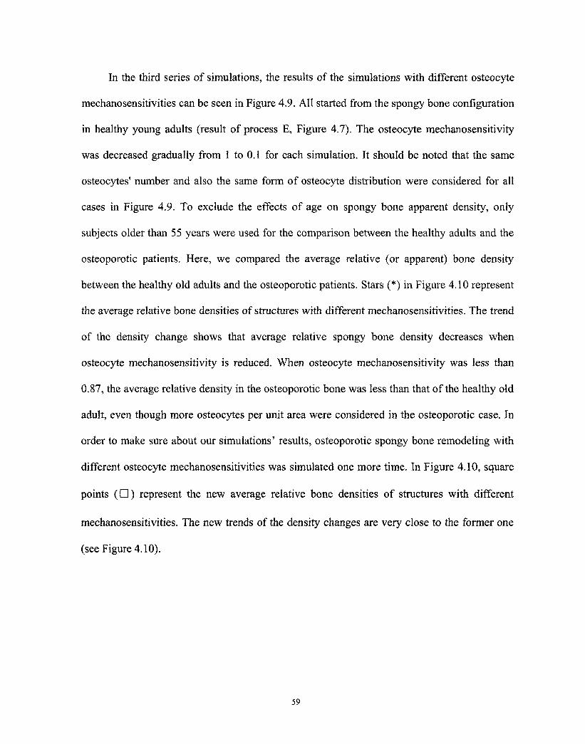
In the third series of simulations, the results of the simulations with different osteocyte
mechanosensitivities can be seen in Figure 4.9. All started from the spongy bone configuration
in healthy young adults (result of process E, Figure 4.7). The osteocyte mechanosensitivity
was decreased gradually from 1 to 0.1 for each simulation. It should be noted that the same
osteocytes' number and also the same form of osteocyte distribution were considered for all
cases in Figure 4.9. To exclude the effects of age on spongy bone apparent density, only
subjects older than 55 years were used for the comparison between the healthy adults and the
osteoporotic patients. Here, we compared the average relative (or apparent) bone density
between the healthy old adults and the osteoporotic patients. Stars (*) in Figure 4.10 represent
the average relative bone densities of structures with different mechanosensitivities. The trend
of the density change shows that average relative spongy bone density decreases when
osteocyte mechanosensitivity is reduced. When osteocyte mechanosensitivity was less than
0.87, the average relative density in the osteoporotic bone was less than that of the healthy old
adult, even though more osteocytes per unit area were considered in the osteoporotic case. In
order to make sure about our simulations' results, osteoporotic spongy bone remodeling with
different osteocyte mechanosensitivities was simulated one more time. In Figure 4.10, square
points ( • ) represent the new average relative bone densities of structures with different
mechanosensitivities. The new trends of the density changes are very close to the former one
(see Figure 4.10).
59
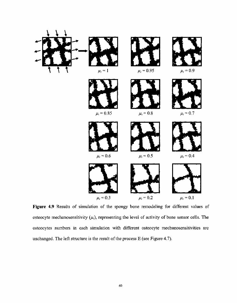
V V \
JU, = \ v, = 0.95 //, = 0.9
,̂ = 0.85 JU, = 0.S ft, = 0.7
ju, = 0.6 ju, = 0.5 fAt = 0 .4
//, = 0.3 ,̂ = 0.2 ^ = 0.1
Figure 4.9 Results of simulation of the spongy bone remodeling for different values of
osteocyte mechanosensitivity (//,), representing the level of activity of bone sensor cells. The
osteocytes numbers in each simulation with different osteocyte mechanosensitivities are
unchanged. The left structure is the result of the process E (see Figure 4.7).
60
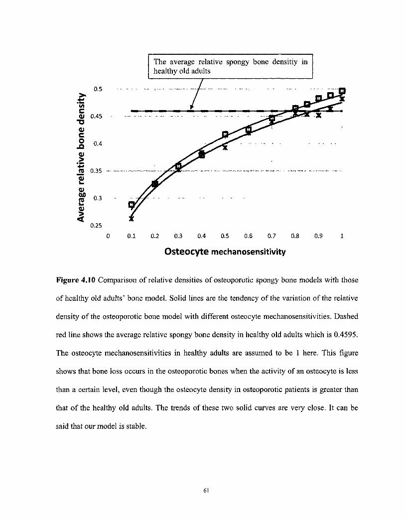
The average relative spongy bone densitiy in healthy old adults
0.25
0 0.1 0.2 0.3 0.4 0.5 0.6 0.7 0.8 0.9 1
Osteocyte mechanosensitivity
Figure 4.10 Comparison of relative densities of osteoporotic spongy bone models with those
of healthy old adults' bone model. Solid lines are the tendency of the variation of the relative
density of the osteoporotic bone model with different osteocyte mechanosensitivities. Dashed
red line shows the average relative spongy bone density in healthy old adults which is 0.4595.
The osteocyte mechanosensitivities in healthy adults are assumed to be 1 here. This figure
shows that bone loss occurs in the osteoporotic bones when the activity of an osteocyte is less
than a certain level, even though the osteocyte density in osteoporotic patients is greater than
that of the healthy old adults. The trends of these two solid curves are very close. It can be
said that our model is stable.
61
4.4. Discussion and conclusions
The spongy bone remodeling simulation results of our computer model in this study are in
agreement with the general statement of Wolff s law (Wolff, 1892). In the first series of
simulations, when osteocytes are uniformly distributed in the bone region, trabeculae-like
architectures are obtained in our computer simulations (see Figures 4.2-4.6). Although the
strain energy density (SED), which is used here as the mechanical stimulus for the initiation of
the bone remodeling process, is a scalar quantity, the simulation results still showed that the
spongy bone structure were adaptive to not only external loading magnitude, but also to the
loading direction. The thickness of the trabeculae in the final configuration decreased when
the magnitude of the external loading was reduced and vice versa (see Figures 4.3 and 4.4).
Moreover, the directions of the trabeculae are aligned with the direction of the external loads
(see Figure 4.5).
Results of this study also show that the osteocyte density has a significant role in the
final shape of spongy bone in the bone remodeling process. In the second series of simulations,
with the same parameter settings as the first series of simulation, including the same
mechanosensitivity for osteocytes, it is shown that by decreasing the osteocyte density
(knowing that the osteocyte density decrease as a healthy adult ages), bone loss will occur and
there will be a decrease in bone apparent density (see Figures 4.7 and 4.8). These results are in
favour of our first hypothesis which says that "by decreasing osteocyte density, there will be a
net bone loss with aging in the healthy adults".
The third series of simulations showed that when osteocyte mechanosensitivity is less
than a certain level, osteoporotic patients lose more spongy bone than healthy old adults, even
62
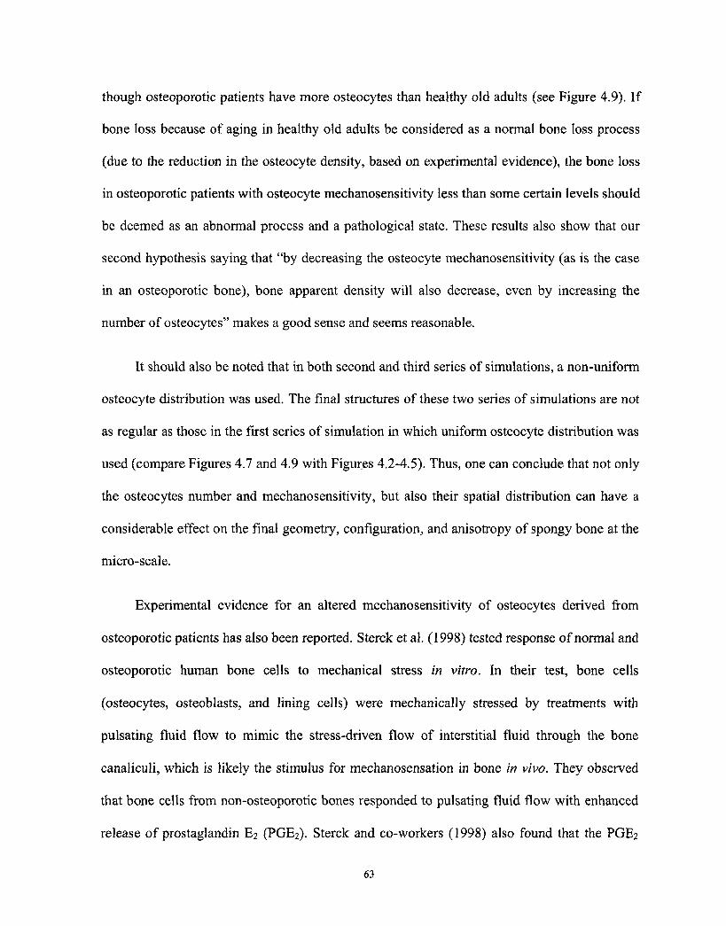
though osteoporotic patients have more osteocytes than healthy old adults (see Figure 4.9). If
bone loss because of aging in healthy old adults be considered as a normal bone loss process
(due to the reduction in the osteocyte density, based on experimental evidence), the bone loss
in osteoporotic patients with osteocyte mechanosensitivity less than some certain levels should
be deemed as an abnormal process and a pathological state. These results also show that our
second hypothesis saying that "by decreasing the osteocyte mechanosensitivity (as is the case
in an osteoporotic bone), bone apparent density will also decrease, even by increasing the
number of osteocytes" makes a good sense and seems reasonable.
It should also be noted that in both second and third series of simulations, a non-uniform
osteocyte distribution was used. The final structures of these two series of simulations are not
as regular as those in the first series of simulation in which uniform osteocyte distribution was
used (compare Figures 4.7 and 4.9 with Figures 4.2-4.5). Thus, one can conclude that not only
the osteocytes number and mechanosensitivity, but also their spatial distribution can have a
considerable effect on the final geometry, configuration, and anisotropy of spongy bone at the
micro-scale.
Experimental evidence for an altered mechanosensitivity of osteocytes derived from
osteoporotic patients has also been reported. Sterck et al. (1998) tested response of normal and
osteoporotic human bone cells to mechanical stress in vitro. In their test, bone cells
(osteocytes, osteoblasts, and lining cells) were mechanically stressed by treatments with
pulsating fluid flow to mimic the stress-driven flow of interstitial fluid through the bone
canaliculi, which is likely the stimulus for mechanosensation in bone in vivo. They observed
that bone cells from non-osteoporotic bones responded to pulsating fluid flow with enhanced
release of prostaglandin E2 (PGE2). Sterck and co-workers (1998) also found that the PGE2
63
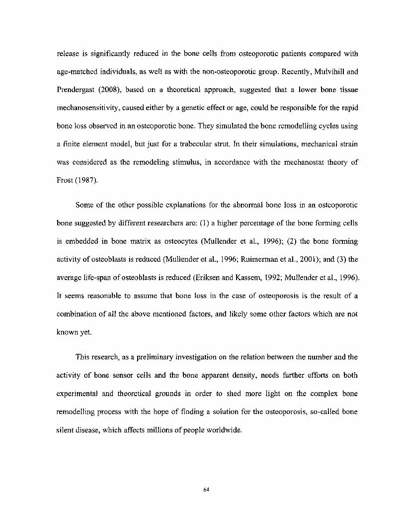
release is significantly reduced in the bone cells from osteoporotic patients compared with
age-matched individuals, as well as with the non-osteoporotic group. Recently, Mulvihill and
Prendergast (2008), based on a theoretical approach, suggested that a lower bone tissue
mechanosensitivity, caused either by a genetic effect or age, could be responsible for the rapid
bone loss observed in an osteoporotic bone. They simulated the bone remodelling cycles using
a finite element model, but just for a trabecular strut. In their simulations, mechanical strain
was considered as the remodeling stimulus, in accordance with the mechanostat theory of
Frost (1987).
Some of the other possible explanations for the abnormal bone loss in an osteoporotic
bone suggested by different researchers are: (1) a higher percentage of the bone forming cells
is embedded in bone matrix as osteocytes (Mullender et al., 1996); (2) the bone forming
activity of osteoblasts is reduced (Mullender et al., 1996; Ruimerman et al., 2001); and (3) the
average life-span of osteoblasts is reduced (Eriksen and Kassem, 1992; Mullender et al., 1996).
It seems reasonable to assume that bone loss in the case of osteoporosis is the result of a
combination of all the above mentioned factors, and likely some other factors which are not
known yet.
This research, as a preliminary investigation on the relation between the number and the
activity of bone sensor cells and the bone apparent density, needs further efforts on both
experimental and theoretical grounds in order to shed more light on the complex bone
remodelling process with the hope of finding a solution for the osteoporosis, so-called bone
silent disease, which affects millions of people worldwide.
64
Chapter 5
A Three-Dimensional Computer Model to Simulate
Spongy Bone Remodeling under Overload
5.1. Introduction
The bone remodeling process is essential for the maintenance of our skeleton. It enables
adaptation of the bone mass and architecture to changes in mechanical loads (Wolff, 1892;
Frost, 1987). Bone remodeling is mainly a two stage process which includes bone resorption
and subsequent bone formation. The coupled bone remodeling process is performed by two
types of bone cells: osteoclasts, which are multinucleated bone resorbing cells, and osteoblasts,
which are bone-forming cells. Osteoclasts resorb packets of bone tissue, and osteoblasts
replace the resorbed tissue with new mineralized bone tissue. Clusters of osteoclasts and
osteoblasts involved in bone remodeling are known as basic multi-cellular units (BMUs).
The ends of the long bones are filled with spongy bone (or cancellous bone), a very
porous bone structure made of mineralized plates and struts, the trabeculae. This spongy bone
gives the bones a relatively low mass, but a relatively high stiffness. Spongy bone is also found
within the interior of vertebrae, in flat bones like the skull and the pelvis and in the hand and
feet. In the spongy bone, remodeling takes place at the surface of the trabeculae (Figure 2.9.B).
In order to perform the bone remodeling process, a connection between external load and
the activities of BMUs must exist (Ruimerman et al., 2001). Firstly, bone requires sensors
which can detect the mechanical load. Secondly, bone needs channels through which necessary
65
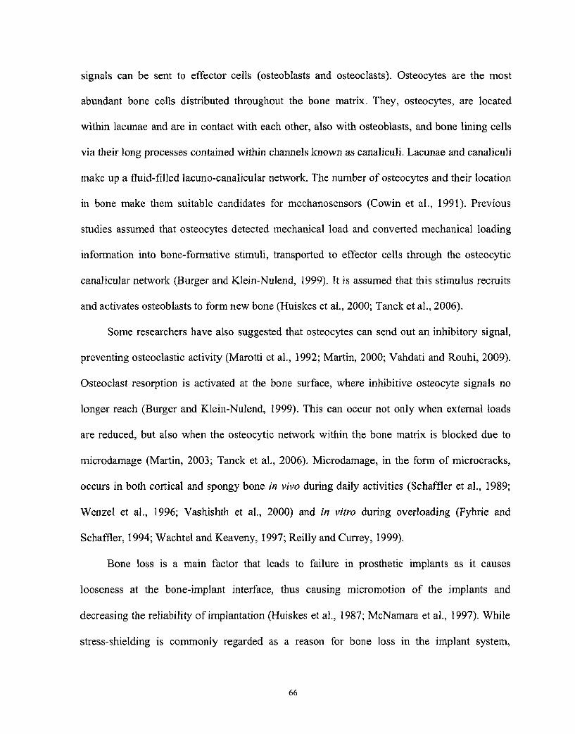
signals can be sent to effector cells (osteoblasts and osteoclasts). Osteocytes are the most
abundant bone cells distributed throughout the bone matrix. They, osteocytes, are located
within lacunae and are in contact with each other, also with osteoblasts, and bone lining cells
via their long processes contained within channels known as canaliculi. Lacunae and canaliculi
make up a fluid-filled lacuno-canalicular network. The number of osteocytes and their location
in bone make them suitable candidates for mechanosensors (Cowin et al., 1991). Previous
studies assumed that osteocytes detected mechanical load and converted mechanical loading
information into bone-formative stimuli, transported to effector cells through the osteocytic
canalicular network (Burger and Klein-Nulend, 1999). It is assumed that this stimulus recruits
and activates osteoblasts to form new bone (Huiskes et al., 2000; Tanck et al., 2006).
Some researchers have also suggested that osteocytes can send out an inhibitory signal,
preventing osteoclastic activity (Marotti et al., 1992; Martin, 2000; Vahdati and Rouhi, 2009).
Osteoclast resorption is activated at the bone surface, where inhibitive osteocyte signals no
longer reach (Burger and Klein-Nulend, 1999). This can occur not only when external loads
are reduced, but also when the osteocytic network within the bone matrix is blocked due to
microdamage (Martin, 2003; Tanck et al., 2006). Microdamage, in the form of microcracks,
occurs in both cortical and spongy bone in vivo during daily activities (Schaffler et al., 1989;
Wenzel et al., 1996; Vashishth et al., 2000) and in vitro during overloading (Fyhrie and
Schaffler, 1994; Wachtel and Keaveny, 1997; Reilly and Currey, 1999).
Bone loss is a main factor that leads to failure in prosthetic implants as it causes
looseness at the bone-implant interface, thus causing micromotion of the implants and
decreasing the reliability of implantation (Huiskes et al., 1987; McNamara et al., 1997). While
stress-shielding is commonly regarded as a reason for bone loss in the implant system,
66
overload at the interface has also been suggested as a contributing factor (Li et al., 2007). For
instance, Huiskes and Nuanmaker (1984) reported that the loosening of and bone resorption
around orthopaedic implants were associated with high peak stresses at the interface. The
coupled remodeling process is capable of increasing the rate of remodeling to cope with
increased damage, but this ability has substantial limits (Hazelwood et al., 2001). While
moderate levels of bone microdamage may play a constructive and important role in
maintaining bone structural integrity, excessive damage caused by overload can result in
accumulation of unrepaired damaged regions (Hazelwood et al., 2001). Bone formation cannot
keep pace with bone resorption experiencing overload, thus bone loss due to overload will
occur (Li et al., 2007). Other possible effects of overload include the degradation of
mechanical properties and development of skeletal fragility, particularly in spongy bone (Frost,
1994; Turner, 2002; Martin, 2003; Schaffler, 2003; Nagaraja et al., 2005).
More than one hundred years ago, Wolffs Law (1892) was proposed. It explained that
bone adapted its structure to mechanical loadings in accordance with mathematical law. In
1964, the first mathematical expression of bone remodeling was developed by Frost (1964b).
In the last 4 decades, several mathematical models of bone remodeling have been proposed to
describe bone remodeling process. However, it is still not clear what the actual mechanical
stimulus of the bone adaptation is. Stress (Wolff, 1892; Frost, 1964b), strain (Cowin and
Hegedus, 1976; Frost, 1987), and strain rate (Hert et al, 1969; Fritton et al., 2000) have been
usually assumed to be the mechanical stimulus. Recently, Huiskes and co-workers (2000)
developed a semi-mechanistic model for bone remodeling theoiy which used strain energy
density (SED) as mechanical stimulus. The semi-mechanistic bone remodeling theory
(Huiskes et al., 2000) includes the experimental findings in bone cells' physiology (Vahdati
67
and Rouhi, 2009), such as a separate description of osteoclastic resorption and osteoblastic
formation (Burger and Klein-Nulend, 1999), an osteocyte mechanosensory system (Aarden et
al., 1994; Cowin et al., 1991), and role of microdamage (Pazzagliaet al., 1997; Taylor, 1997;
Martin, 2000).
Although many mathematical models governing bone's mechanical adaptation have
been proposed, few can consider bone resorption due to overload (Li et al., 2007). In this
study, we investigated the effects of microdamage caused by overload on the bone remodeling
process (section 5.2.2) and implemented these effects in the extension of the pre-existing
semi-mechanistic bone remodeling theory (Huiskes et al., 2000). A three-dimensional (3D)
computational model was developed here to test our mathematical model for spongy bone
remodeling under overload.
5.2. Methods
5.2.1. A Semi-mechanistic bone remodeling theory
Please see section 3.1.2.
5.2.2. Hypotheses for the effects of overload on bone remodeling
We proposed two hypotheses for the effects of overload on the spongy bone remodeling and
extended the semi-mechanistic bone remodeling theory of Huiskes and coworkers (Huiskes et
al., 2000).
68
5.2.2.1. The bone resorption probability and resorption amount increase under overload
Huiskes et al. (2000) stated that the microcracks produced by the dynamic forces of daily
normal physical activities could occur anywhere at any time, and suggested that osteoclast
resorption was activated by microdamage. Hence, osteoclast resorption would be spatially
random. In the semi-mechanistic bone remodeling theory (Huiskes et al, 2000), a probability
function of osteoclastic resorption, p(x,t), was defined and included in their model. The p(x,t)
caused by microcracks was considered to be spatially random and selected to be a constant.
They also assumed that each osteoclast resorption removed a fixed amount of mineral. Bone
resorption is described by:
dmr{x,t)
dt -roc (5.1)
where ——— was the local change of relative bone density (m) caused by osteoclast
resorption at trabecular surface location x; roc represented the relative amount of mineral
resorbed by each osteoclast resorption, and it was supposed to be a constant.
It has been suggested that microdamage trigger resorption in order to remove those
damaged regions (Noble, 2003; Vahdati and Rouhi, 2009) and that signals transported to the
bone surface through osteocytic network inhibit osteoclast activation (Huiskes et al., 2000).
Since overload accumulates microdamages (Hazelwood et al., 2001) which disconnect the
lacuno-canalicular network (Burger and Klein-Nulend, 1999), it is reasonable to assume that
the probability of bone resorption under overload is greater than the resorption probability
under normal daily activities and that the osteoclast activity increases.
In this study, we defined a critical load value and a threshold stimulus which were
required to cause excessive microdamage, i.e. overload. In other words, we proposed that the
69
probability of bone resorption would increase when the external load was greater than the
critical load value and stimulus exceeded the threshold; otherwise bone resorption probability
would remain constant. Since, based on experimental results, there is a positive quadratic
relationship between microdamage and local strain energy density (Nagaraja et al., 2005), we
assumed that resorption probability, p0i(x, t), caused by overload was a quadratic function of
total remodeling stimulus (P(x,t)). Thus, the revised resorption probability, when the external
load exceeds the critical load value, can be written as follows:
(a[P(x, t) - kol]2 + p for P(x, t) > kol ,
Poi(x,t) = \ (5.2) (jp for P(x,t)<kol
where a is an empirical constant (Table 5.1); p is the probability of bone resorption under
normal daily activities (assigned as 20% in our study similar to Ruimerman an coworkers
(Ruimerman et al., 2003)); and k0i is a threshold stimulus (Table 5.1). Li et al. (2007) reported
the overload resorption under a stress of 9 MPa using their mathematical model; hence, we set
the critical load value equals to 9 MPa in this study.
As assumed above, osteoclast activity increased under overload. It means that more
relative amount of mineral is resorbed by each osteoclast under overload than the amount of
mineral resorbed by each osteoclast under normal loading condition. Ruimerman et al. (2003)
set the relative mineral amount per resorption to 30% of a voxel. In our study, the relative
resorption amount, roc-oi, was set to 75% of a voxel.
5.2.2.2. Microdamages caused by overload reduce the osteocyte influence distance
In the semi-mechanistic bone remodeling theory (Huiskes et al.'s, 2000), the stimulus sent to
the trabecular surfaces through canaliculi was assumed to attenuate exponentially with the
increasing distance, d„ between osteocyte i and location x according to:
70
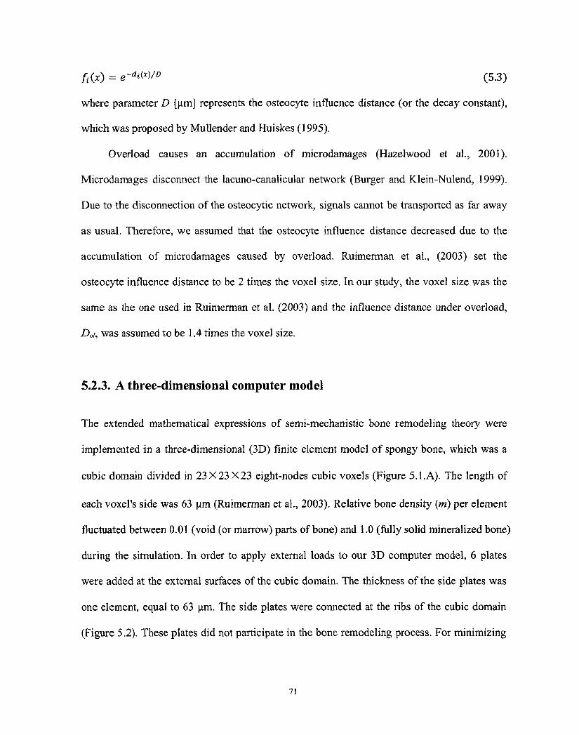
ft(x) = e-d^/D (5.3)
where parameter D [um] represents the osteocyte influence distance (or the decay constant),
which was proposed by Mullender and Huiskes (1995).
Overload causes an accumulation of microdamages (Hazelwood et al., 2001).
Microdamages disconnect the lacuno-canalicular network (Burger and Klein-Nulend, 1999).
Due to the disconnection of the osteocytic network, signals cannot be transported as far away
as usual. Therefore, we assumed that the osteocyte influence distance decreased due to the
accumulation of microdamages caused by overload. Ruimerman et al., (2003) set the
osteocyte influence distance to be 2 times the voxel size. In our study, the voxel size was the
same as the one used in Ruimerman et al. (2003) and the influence distance under overload,
D0i, was assumed to be 1.4 times the voxel size.
5.2.3. A three-dimensional computer model
The extended mathematical expressions of semi-mechanistic bone remodeling theory were
implemented in a three-dimensional (3D) finite element model of spongy bone, which was a
cubic domain divided in 23X23X23 eight-nodes cubic voxels (Figure 5.LA). The length of
each voxel's side was 63 um (Ruimerman et al., 2003). Relative bone density (m) per element
fluctuated between 0.01 (void (or marrow) parts of bone) and 1.0 (fully solid mineralized bone)
during the simulation. In order to apply external loads to our 3D computer model, 6 plates
were added at the external surfaces of the cubic domain. The thickness of the side plates was
one element, equal to 63 um. The side plates were connected at the ribs of the cubic domain
(Figure 5.2). These plates did not participate in the bone remodeling process. For minimizing
71
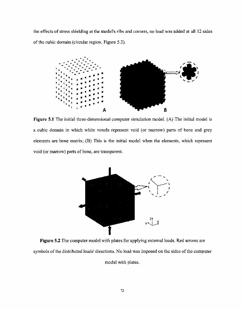
the effects of stress shielding at the model's ribs and corners, no load was added at all 12 sides
of the cubic domain (circular region, Figure 5.2).
' . ' .
' < ; :
« • *
r — p > » * ** _ s
Figure 5.1 The initial three-dimensional computer simulation model. (A) The initial model is
a cubic domain in which white voxels represent void (or marrow) parts of bone and grey
elements are bone matrix; (B) This is the initial model when the elements, which represent
void (or marrow) parts of bone, are transparent.
Figure 5.2 The computer model with plates for applying external loads. Red arrows are
symbols of the distributed loads' directions. No load was imposed on the sides of the computer
model with plates.
72
It is known that both cortical and spongy bones are anisotropic materials (Uten"kin and
Ashkenazi, 1972; van Rietbergen and Huiskes, 2006). Moreover, both cortical and spongy
bones show viscoelastic behavior when the external loads are much greater than those which
are in the physiological range (Pugh et al., 1973; Carter and Hayes, 1977; van Rietbergen and
Huiskes, 2006). With the intention of simplicity, the bone model's elements were assumed to
be isotropic and linearly elastic material in this study. The material properties of fully
mineralized bone elements (m=1.0) were given a Young's modulus of 5 GPa and a Poisson
ratio of 0.3. During computer simulations, the Young's modulus of each element changed per
iteration according to the modulus-density relationship which was determined from empirical
data for trabecular bone with Emax = 5 GPa and y = 3 (Eq. 3.12) (Mullender and Huiskes,
1995). The material properties of the plates for adding external forces were the same as those
of a fully mineralized bone tissue.
Relative bone density per element was determined by the net effects of bone resorption
and formation in each bone element according to Eq. 3.11. A new configuration in term of
elements' relative bone densities was performed after each iteration. The whole simulation
process was repeated until equilibrium state was met, i.e. when no considerable architectural
change was observed. In order to have a stable configuration, 250 iterations were performed
for each spongy bone remodeling simulation in this study.
In this study, osteocytes were assumed to be distributed uniformly within the domain at
a density of 44,000 mm"3 (Mullender et al., 1996). Other parameter settings for the spongy
bone remodeling are as specified in Table 5.1.
73
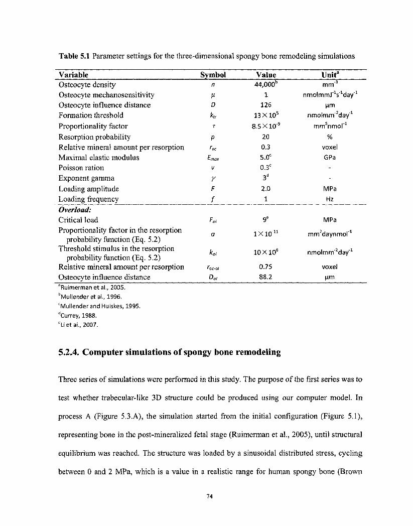
Table 5.1 Parameter settings for the three-dimensional spongy bone remodeling simulations
Variable Osteocyte density Osteocyte mechanosensitivity
Osteocyte influence distance
Formation threshold
Proportionality factor
Resorption probability
Relative mineral amount per resorption
Maximal elastic modulus Poisson ration
Exponent gamma
Loading amplitude
Loading frequency
Overload: Critical load Proportionality factor in the resorption
probability function (Eq. 5.2) Threshold stimulus in the resorption
probability function (Eq. 5.2) Relative mineral amount per resorption
Osteocyte influence distance
Symbol n
M D
ktr
T
P roc
t-max
V
r F
f
Fa
a
koi
foc-ol
D0i
Value 44,000b
1 126
13 X 10s
8.5 X10"9
20 0.3
5.0C
0.3C
3d
2.0
1
9e
1X10 n
10X106
0.75
88.2
Unit3
mm'3
nmolmm.r1s"1day"1
urn nmolmm^day"1
mm5nmor1
%
voxel
GPa -
-
MPa
Hz
MPa
mrr^daynmor1
nmolmm^day"1
voxel
urn
"Ruimermanetal., 2005. bMullenderetal., 1996. cMullenderand Huiskes, 1995. dCurrey, 1988. cLi et al„ 2007.
5.2.4. Computer simulations of spongy bone remodeling
Three series of simulations were performed in this study. The purpose of the first series was to
test whether trabecular-like 3D structure could be produced using our computer model. In
process A (Figure 5.3.A), the simulation started from the initial configuration (Figure 5.1),
representing bone in the post-mineralized fetal stage (Ruimerman et al., 2005), until structural
equilibrium was reached. The structure was loaded by a sinusoidal distributed stress, cycling
between 0 and 2 MPa, which is a value in a realistic range for human spongy bone (Brown
74
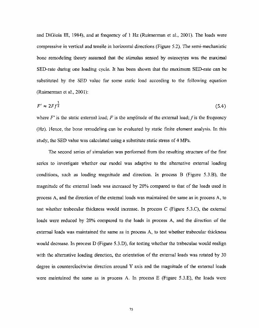
and DiGioia III, 1984), and at frequency of 1 Hz (Ruimerman et al., 2001). The loads were
compressive in vertical and tensile in horizontal directions (Figure 5.2). The semi-mechanistic
bone remodeling theory assumed that the stimulus sensed by osteocytes was the maximal
SED-rate during one loading cycle. It has been shown that the maximum SED-rate can be
substituted by the SED value for some static load according to the following equation
(Ruimerman et al., 2001):
F' « 2Ffi (5.4)
where F' is the static external load; F is the amplitude of the external load;/is the frequency
(Hz). Hence, the bone remodeling can be evaluated by static finite element analysis. In this
study, the SED value was calculated using a substitute static stress of 4 MPa.
The second series of simulation was performed from the resulting structure of the first
series to investigate whether our model was adaptive to the alternative external loading
conditions, such as loading magnitude and direction. In process B (Figure 5.3.B), the
magnitude of the external loads was increased by 20% compared to that of the loads used in
process A, and the direction of the external loads was maintained the same as in process A, to
test whether trabecular thickness would increase. In process C (Figure 5.3.C), the external
loads were reduced by 20% compared to the loads in process A, and the direction of the
external loads was maintained the same as in process A, to test whether trabecular thickness
would decrease. In process D (Figure 5.3.D), for testing whether the trabeculae would realign
with the alternative loading direction, the orientation of the external loads was rotated by 30
degree in counterclockwise direction around Y axis and the magnitude of the external loads
were maintained the same as in process A. In process E (Figure 5.3.E), the loads were
75
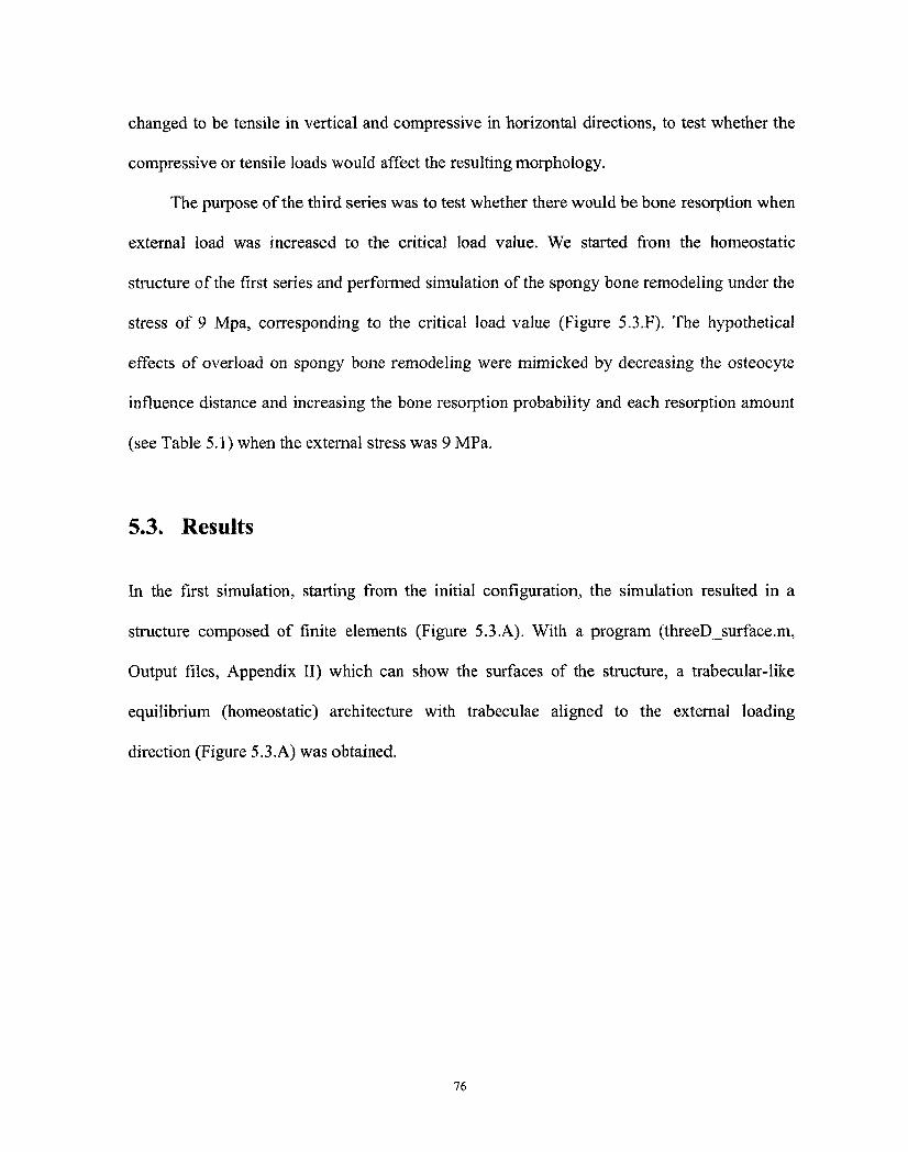
changed to be tensile in vertical and compressive in horizontal directions, to test whether the
compressive or tensile loads would affect the resulting morphology.
The purpose of the third series was to test whether there would be bone resorption when
external load was increased to the critical load value. We started from the homeostatic
structure of the first series and performed simulation of the spongy bone remodeling under the
stress of 9 Mpa, corresponding to the critical load value (Figure 5.3.F). The hypothetical
effects of overload on spongy bone remodeling were mimicked by decreasing the osteocyte
influence distance and increasing the bone resorption probability and each resorption amount
(see Table 5.1) when the external stress was 9 MPa.
5.3. Results
In the first simulation, starting from the initial configuration, the simulation resulted in a
structure composed of finite elements (Figure 5.3.A). With a program (threeD_surface.m,
Output files, Appendix II) which can show the surfaces of the structure, a trabecular-like
equilibrium (homeostatic) architecture with trabeculae aligned to the external loading
direction (Figure 5.3.A) was obtained.
76
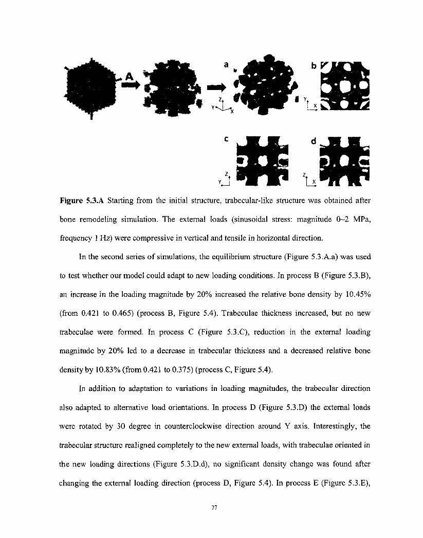
Figure 5.3.A Starting from the initial structure, trabecular-like structure was obtained after
bone remodeling simulation. The external loads (sinusoidal stress: magnitude 0-2 MPa,
frequency 1 Hz) were compressive in vertical and tensile in horizontal direction.
In the second series of simulations, the equilibrium structure (Figure 5.3.A.a) was used
to test whether our model could adapt to new loading conditions. In process B (Figure 5.3.B),
an increase in the loading magnitude by 20% increased the relative bone density by 10.45%
(from 0.421 to 0.465) (process B, Figure 5.4). Trabeculae thickness increased, but no new
trabeculae were formed. In process C (Figure 5.3.C), reduction in the external loading
magnitude by 20% led to a decrease in trabecular thickness and a decreased relative bone
density by 10.83% (from 0.421 to 0.375) (process C, Figure 5.4).
In addition to adaptation to variations in loading magnitudes, the trabecular direction
also adapted to alternative load orientations. In process D (Figure 5.3.D) the external loads
were rotated by 30 degree in counterclockwise direction around Y axis. Interestingly, the
trabecular structure realigned completely to the new external loads, with trabeculae oriented in
the new loading directions (Figure 5.3.D.d), no significant density change was found after
changing the external loading direction (process D, Figure 5.4). In process E (Figure 5.3.E),
77
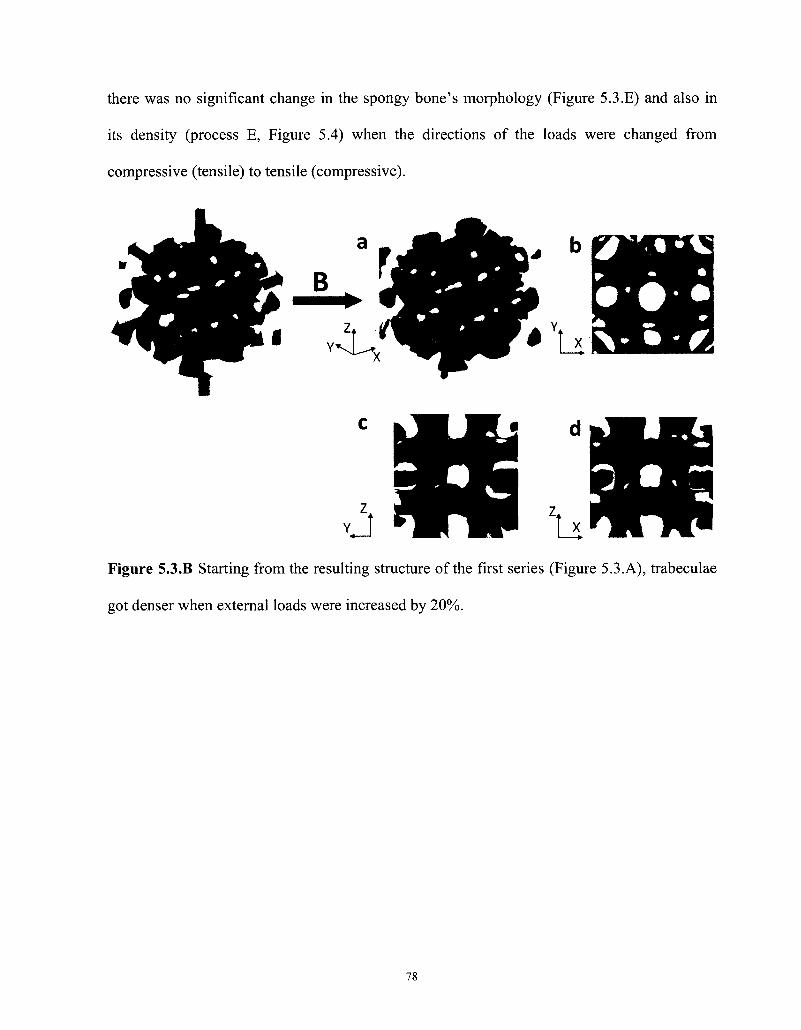
there was no significant change in the spongy bone's morphology (Figure 5.3.E) and also in
its density (process E, Figure 5.4) when the directions of the loads were changed from
compressive (tensile) to tensile (compressive).
Figure 5.3.B Starting from the resulting structure of the first series (Figure 5.3.A), trabeculae
got denser when external loads were increased by 20%.
78
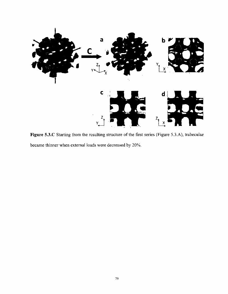
Figure 5.3.C Starting from the resulting structure of the first series
became thinner when external loads were decreased by 20%.
79
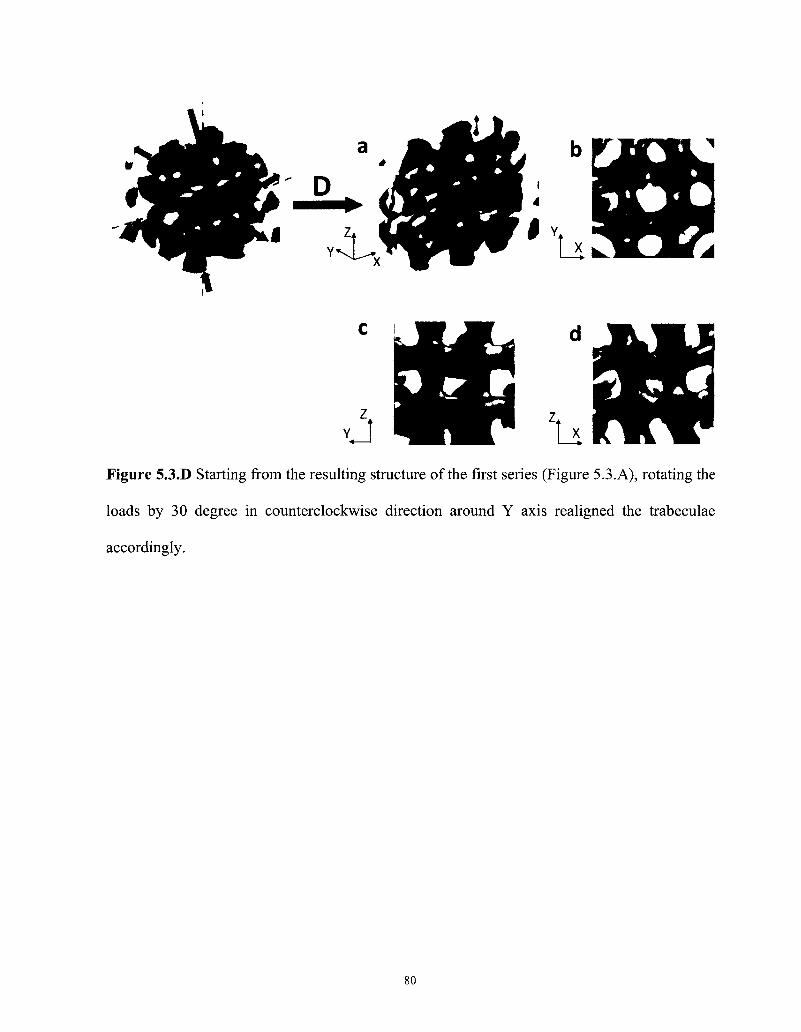
vl Figure 5.3.D Starting from the resulting structure of the first series (Figure 5.3. A), rotating the
loads by 30 degree in counterclockwise direction around Y axis realigned the trabeculae
accordingly.
80
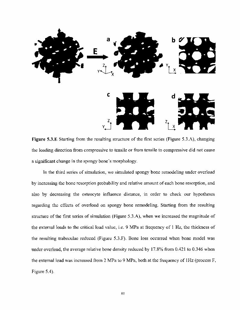
Figure 5.3.E Starting from the resulting structure of the first series (Figure 5.3.A), changing
the loading direction from compressive to tensile or from tensile to compressive did not cause
a significant change in the spongy bone's morphology.
In the third series of simulation, we simulated spongy bone remodeling under overload
by increasing the bone resorption probability and relative amount of each bone resorption, and
also by decreasing the osteocyte influence distance, in order to check our hypotheses
regarding the effects of overload on spongy bone remodeling. Starting from the resulting
structure of the first series of simulation (Figure 5.3.A), when we increased the magnitude of
the external loads to the critical load value, i.e. 9 MPa at frequency of 1 Hz, the thickness of
the resulting trabeculae reduced (Figure 5.3.F). Bone loss occurred when bone model was
under overload, the average relative bone density reduced by 17.8% from 0.421 to 0.346 when
the external load was increased from 2 MPa to 9 MPa, both at the frequency of 1Hz (process F,
Figure 5.4).
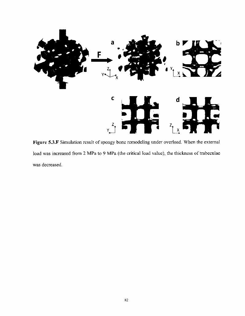
Figure 5.3.F Simulation result of spongy bone remodeling under overload. When the external
load was increased from 2 MPa to 9 MPa (the critical load value), the thickness of trabeculae
was decreased.
82
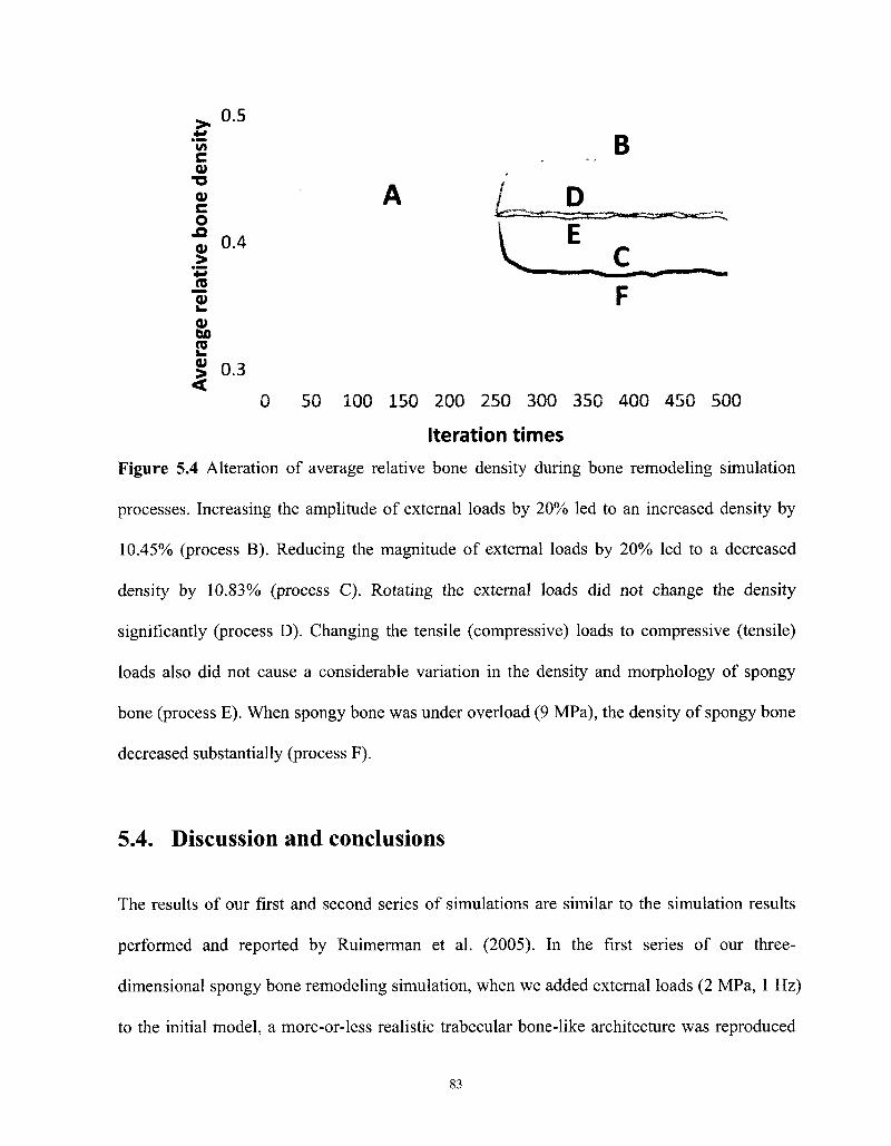
> 0 . 5
c
g A o
"S 0.4 #> jo 2! a> w> 2 SS 0.3
0 50 100 150 200 250 300 350 400 450 500
Iteration times
Figure 5.4 Alteration of average relative bone density during bone remodeling simulation
processes. Increasing the amplitude of external loads by 20% led to an increased density by
10.45% (process B). Reducing the magnitude of external loads by 20% led to a decreased
density by 10.83% (process C). Rotating the external loads did not change the density
significantly (process D). Changing the tensile (compressive) loads to compressive (tensile)
loads also did not cause a considerable variation in the density and morphology of spongy
bone (process E). When spongy bone was under overload (9 MPa), the density of spongy bone
decreased substantially (process F).
5.4. Discussion and conclusions
The results of our first and second series of simulations are similar to the simulation results
performed and reported by Ruimerman et al. (2005). In the first series of our three-
dimensional spongy bone remodeling simulation, when we added external loads (2 MPa, 1 Hz)
to the initial model, a more-or-less realistic trabecular bone-like architecture was reproduced
83
and the trabeculae were aligned with the direction of the external loading (Figure 5.3.A).
Process A on Figure 5.4 showed that average relative bone density first increased sharply,
followed by a decrease and subsequent stabilization. A similar trend was observed in the
development of trabecular bone from porcine vertebrae and tibiae (Tanck et al., 2001). In
addition, this trend was also seen in cortical bone from ulnae of birds, in which the ulnae were
loaded with 36 cycles/day (Rubin and Lanyon, 1984). It seems that an increase in mechanical
forces initially produces excessive bone deposition. Thereafter, trabecular structure is
optimized, i.e. the trabeculae better align to the main loading direction while bone mass
decreases and stabilizes (Tanck et al., 2001).
The results of our second series of simulations are in agreement with Wolffs law (Wolff,
1892), known as the functional adaptation of the trabecular structure. Although the strain
energy density (SED), which was used here as the mechanical stimulus to initiate the bone
remodeling process, is a scalar quantity, the results of the second simulation series showed
that the spongy bone structure were adaptive to not only external loading magnitude, but also
to the external loading direction. Increasing the external loads caused an increase in the
thickness of the trabeculae, and also the average relative bone density (Figure 5.3.B and
process B, Figure 5.4). On the other hand, decreasing loading magnitude caused the opposite
trend, i.e. reduced trabecular thickness and also average relative bone density (Figures 5.3.C
and process C, Figure 5.4). After rotating the external loads by 30 degree, trabeculae
eventually rotated by the same amount (Figure 5.3.D). However, no significant change in
average relative bone density was found as a result of altering the external load's direction
(process D, Figure 5.4). Moreover, Figure 5.3.E and process E in Figure 5.4 showed that no
significant changes in morphology and average relative bone density of spongy bone could be
84
seen when we changed the compressive (tensile) loads to the tensile (compressive) loads. It
implies that whether the loads are compressive or tensile does not influence the resulting
structure because the local SED values in compression and tension are equal.
In the third series of simulation, and investigation was made on the spongy bone
remodeling under overload. In Huiskes and co-workers' semi-mechanistic bone remodeling
theory (2000), the bone resorption probability, the relative amount of mineral resorbed and the
osteocyte influence distance are assumed to be constants. Compared to Huiskes et al.'s (2000),
based on the previous theoretical and experimental results (Burger and Klein-Nulend, 1999;
Nagaraja et al., 2005), we assumed that the local bone resorption probability is SED
dependent, with a higher chance for overloading situation according to Eq. 5.2. Moreover, we
assume that the accumulation of microdamages caused by overload (Hazelwood et al., 2001)
increases the amount of bone resorbed and decreases the average osteocyte influence distance.
Tanck et al. (2006) kept the loading amplitude and frequency constant (2 MPa, 1 Hz)
when they studied trabecular bone remodeling for both disuse and overload. Knowing that in
everyday normal physical activities, both the load magnitude and frequency of loading change
continuously, assuming a constant value for them does not make a good sense. Li et al. (2007)
developed a new mathematical model for studying the dental implant loosening. In their
theoretical study, they varied the stress magnitudes and found that bone density decreased
quickly when they increased the magnitude of stress to 9 MPa. Based on Li et al.'s (2007)
work, we considered the amplitude of the critical load for overload to be 9 MPa and the
frequency of the load to be 1 Hz, in our work.
The results of our third series of three-dimensional simulation showed that spongy bone
remodeling under overload (9 MPa, 1Hz) led to significant and sharp decreases in the
85
trabecular thickness (Figure 5.3.F) and also in spongy bone's relative density (process F,
Figure 5.4). Our results, which considered the overloading effect, prove that the extended
algorithm is sensitive to overload. Whereas, bone loss under overload cannot be shown using
Huiskes et al.'s (2000) semi-mechanistic bone remodeling model, this is quite understandable
due to the lack of the overload effect in their theory. A similar trend for the decrease in bone
density due to overload was also found in some previous theoretical researches (Tanaka et al.,
1999; Tanck et al., 2006; Li et al., 2007) which were simulated on two-dimensional models.
Recently, some investigations have been performed on the overload resorptions that often
occur in dental implant treatments. Li et al. (2007) used their mathematical model to study a
practical case of dental implant treatment. Their FE analysis results showed that bone
resorption at the neck of the implant occurred due to occlusal overload but then resorption
stopped after some time, which may account for progressive implant loosening that is
sometimes observed in clinical situations (Li et al., 2007; Nystrom et al., 2004; Lin et al.,
2009).
Similar to other theoretical studies, our study contains some limitations. In this study,
bone was assumed to be isotropic and a linear elastic material. It is well known that trabecular
bone is an anisotropic and viscoelastic material (van Rietbergen and Huiskes, 2001). The FEA
model of spongy bone analyzed in this study was relatively small, restricted by our computer
capacity. Although the trabeculae in the final architecture of our simulation were aligned with
the external loads' direction, the final density of spongy bone and also its morphology were
insensitive to the polarity of the external load (i.e. compression or tension). In our present
study, just sinusoidal external loads with a constant frequency have been considered, which
are not real loading pattern. Most parameters used in the formulation have physical meanings,
86
nevertheless many parameter values are assumed hypothetically due to lack of experimental
data. Thus, there is a great need for experimental research on the bone remodeling process in
order to find the material constants appeared in the bone remodeling theories.
In conclusion, in agreement with the clinical situations (Li et al., 2007; Nystrom et al.,
2004; Lin et al., 2009), our simulation for spongy bone remodeling under overload results in
bone loss. The integration of our hypotheses with the pre-existing regulatory mechanisms
(Huiskes et al., 2000) does not disrupt the processes. For example, the integration of our
hypotheses can help form and maintain trabecular-like structure. Our hypotheses provide a
direction for experimentation providing a layout for future experimental groundwork. Future
simulations can incorporate physiological values and parameters into the model and simulate
the bone remodeling around implants under realistic loading patterns.
87
Chapter 6
Summary, Conclusions and Future Directions
6.1. Summary
Bone is a very active structure and is continuously remodeled through a coupled process of
bone resorption and bone formation, in a process so-called bone remodeling process. In 2000,
Huiskes and co-workers developed a semi-mechanistic bone remodeling theory. Compared
with other bone remodeling theories, the novelty of their theory is that it explains the effects
of mechanical forces on trabecular bone remodeling by relating local mechanical stimuli in the
bone matrix to assumed cells' activities actually involved in bone matabolism (Ruimerman et
al., 2005). In this theory, the rate of strain energy density (SED) is used as the mechanical
stimulus for bone remodeling process, and osteocytes are assumed to act as mechanosensors
which can sense the rate of SED, and then activate bone making cells, i.e. osteoblasts, to form
new bone, filling the cavities caused by osteoclasts' resorption. This thesis was aimed to
investigate spongy bone remodeling using Huiskes et al.'s semi-mechanistic bone remodeling
theory (Huiskes et al., 2000). Two studies have been done in this research. First, an
investigation was made to study the reasons for spongy bone loss in aging and osteoporotic
individuals, using a two-dimensional computer model. Secondly, a three-dimensional finite
element model was developed to simulate spongy bone remodeling under overload. In our
second study, a modification on the pre-existing semi-mechanistic bone remodeling theory
was made with respect to the effects of accumulated microcracks caused by overload.
88
6.1.1. Investigation into the reasons for spongy bone loss in aging
and osteoporotic individuals
In chapter 4, a two dimensional finite element model of spongy bone was presented with the
aim of investigating the effect of osteocyte density and osteocyte mechanosensitivity on the
spongy bone remodeling for aging healthy adults and osteoporotic patients. Bone loss usually
starts after maturation and accelerates in osteoporotic bones. Experimental evidence shows
that osteocyte density (the number of osteocytes per unit surface of bone) changes with aging
and also in osteoporotic bones (Table 4.2) (Mullender et al., 1996). Osteocyte density declines
significantly with aging in healthy adults who are over the age of 30 years (Frost, 1960;
Mullender et al., 1996; Qiu et al., 2003). On the other hand, osteocyte density increases in
osteoporotic patients compared to healthy adults. Moreover, in vitro experiments show that
the mechanosensitivity of osteocytes derived from osteoporotic patients is significantly
reduced compared to that from the age-matched non-osteoporotic group (Sterck et al., 1998).
Therefore, in this study, it is hypothesized that decreasing osteocyte density (assuming a
normal level of mechanosensitivity for the osteocytes) can cause spongy bone loss in healthy
old adults, and in the case of osteoporotic bones, a reduction in osteocyte mechanosensitivity
is one of the main contributing factors in bone loss. To investigate our hypotheses, a two
dimensional finite element model of spongy bone was developed (Figure 4.1), implementing a
semi-mechanistic bone remodeling theory (Huiskes et al., 2000). Three series of simulations
were performed. In the first series of simulations, osteocytes were assumed to be distributed
uniformly within the bone domain. A trabeculae-like architecture was obtained from our
initial computer model (Figure 4.2). The orientation of trabecular structure and also the
89
thickness of trabeculae changed according to alterations of the external loading direction and
magnitude (Figures 4.3-4.5). The first simulation results are all in agreement with Wolffs
Law (Wolff, 1892). In the second series of simulations, based on the experimental evidence
(Mullender et al., 1996), the osteocyte density was reduced for healthy older adults, and the
osteocytes were assumed to be non-uniformly distributed in the bone region (Marotti et al.,
1985; Baiotto and Zidi, 2004). Our simulation results showed that by decreasing the osteocyte
density, bone loss will occur (Figure 4.7), and so average relative bone density will decrease
(Figure 4.8). These results are in favor of the first part of our hypotheses which states that a
reduction in osteocyte density will cause the bone loss in healthy adults. In the third series of
simulations, based on the experimental evidence (Mullender et al., 1996), we increased the
osteocyte density for osteoporotic bones compared to healthy adults, but decrease osteocyte
mechanosensitivity (Sterck et al., 1998). Again, the osteocytes were randomly distributed in
the bone region (Marotti et al., 1985; Baiotto and Zidi, 2004). The simulation results showed
that the reduction of osteocyte mechanosensitivity can cause bone loss (Figure 4.9), and so
will decrease the average relative bone density (Figure 4.10). When osteocyte
mechanosensitivity is less than a certain level, osteoporotic patients lose more bone than
healthy old adults (Figure 4.10), even though the number of osteocytes in osteoporotic patients
is greater than that in healthy adults. These results support the last part of our hypotheses
stating that reducing osteocyte mechanosensitivity could be one of the crucial factors causing
bone loss in an osteoporotic bone. Comparing results of the first simulation series (Figures
4.2-4.5) with the results of the second and third simulations (Figure 4.7 and Figure 4.9), we
find that the final architectures with the uniform osteocyte distribution are more regular than
those with a non-uniform osteocyte distribution.
90
6.1.2. A three-dimensional computer model to simulate spongy
bone remodeling under overload
In chapter 5, considering the effects of the microcracks on bone remodeling process, we
extended Huiskes et al.'s semi-mechanistic bone remodeling theory (Huiskes et al., 2000) for
the case of overloaded bone, and also developed a three-dimensional finite element model to
simulate spongy bone remodeling under overload. Overload has been suggested to be a
contributing factor for bone loss at the bone-implant interface (Huiskes et al., 1987;
McNamara et al., 1997). Many mathematical models have been proposed to model bone
adaptation, but very few considered bone resorption due to overload (Li et al., 2007). As many
other mathematical models, Huiskes et al.'s semi-mechanistic model (Huiskes et al., 2000)
cannot predict the overload resorption because in their theory it is assumed that the resorption
probability and the amount of bone resorbed by each osteoclast to be constants (Eqs. 3.6 and
3.7). Some researchers have suggested that osteoclastic resorption can be enhanced when
osteocytic network within bone matrix is blocked due to microdamage (e.g. Martin, 2003;
Tanck et al., 2006). Considering the experimental evidence of the accumulating microcracks
caused by overload (Hazelwood et al., 2001), in this study, it is hypothesized that overload can
increase osteoclast activities: the probability of bone resorption, and also the amount of bone
resorbed by each osteoclast (see Table 5). Moreover, we hypothesized that the osteocyte
influence distance will reduce due to the accumulation of microdamage under overloading
conditions (see Table 5). Based on experimental results which shows a positive quadratic
relationship between microdamage and local strain energy density (Nagaraja et al., 2005), it is
91
assumed here that resorption probability caused by overload was a quadratic function of total
remodeling stimulus (Eq. 5.2). In order to investigate the validity of our hypothesis, a three-
dimensional computer model of spongy bone was developed (Figure 5.1) and three series of
simulations were performed. The results of our first (see Figure 5.3.A) and second (see
Figures 5.3.B-5.3.E) series of simulations were in agreement with Wolffs Law (Wolff, 1892).
A trabecular-like structure was obtained, and the orientation of trabecular structure and
thickness of trabeculae changed according to alterations of the external load direction and
magnitude. The third series was related to the spongy bone remodeling under overload. In the
third series, it was observed that spongy bone remodeling under overload will result in
significant and sharp decreases in the trabecular thickness (see Figure 5.3.F), and also a
considerable reduction in the average relative bone density (see Figure 5.4). This trend is
observed in clinical situation as well (Nystrom et al., 2004; Lin et al., 2009), also a similar
behavior can be seen in some other studies which were based on two-dimensional simulations
of the bone remodeling process (Tanaka et al., 1999; Tanck et al., 2006; Li et al., 2007). Our
simulation results imply that the integration of our hypotheses with the pre-existing regulatory
mechanisms does not cause any disruption in the bone remodeling processes. Moreover, the
modified algorithm in this study shows a great sensitivity to overload.
6.2. Conclusions
From chapter 4, it is concluded that, by decreasing osteocyte density, there will be a net bone
loss with aging in the healthy adults. Different from many possible explanations for the
excessive bone loss in osteoporotic bones (Eriksen and Kassem, 1992; Mullender et al., 1996;
Ruimerman et al., 2001), which mostly consider the influence of bone making cells, i.e.
92
osteoblasts, our study shows that the decrease of osteocyte mehanosensitivity might be one of
the crucial causes for abnormal bone loss in osteoporotic patients. Also, based on our study,
one can conclude that not only the osteocytes density and mechanosensitivity, but also their
spatial distribution can have a noticeable effect on the final geometry, and configuration of
spongy bone.
From our simulations for spongy bone remodeling under overload, chapter 5, it is
concluded that overload can cause bone loss in spongy bone. Overload might increase the
osteoclasts' activities, i.e. osteoclast resorption probability and also the amount of bone
resorbed by each osteoclast. Moreover, the osteocyte influence distance might decrease under
overloading conditions. The integration of our hypotheses (the effects of microcracks caused
by overload) and Huiskes et al.'s semi-mechanistic remodeling theory (Huiskes et al., 2000)
will offer reasonable results, which are in agreement with some clinical situations.
6.3. Future directions
Most parameters used in our formulations have physical meanings. However, some
parameters' values are assumed hypothetically due to lack of experimental data. One of the
most important efforts in the future can be measuring these data using experimental
techniques. In this thesis, bone elements were assumed to be isotropic and linearly elastic. It is
well known that trabecular bone is an anisotropic and a viscoelastic material (van Rietbergen
and Huiskes, 2001). It might worth investigating the effects of anisotropy, as well as
viscoelasticity on the spongy bone remodeling in the future. Moreover, the FEA model of
spongy bone analyzed in this study was relatively small, restricted by our computer capacity.
93
Also, for the sake of simplicity, just sinusoidal external loads with a constant frequency have
been applied to our models in this study, which are not the real loading pattern. When there is
no computer restriction, an increase in the size of the three-dimensional model for simulating
the spongy bone remodeling around prosthetic implant under realistic loading patterns can be
a great addition to this work.
94
References
Aarden, E.M., Burger. E.H., and Nijweide, P.J. (1994). Function of osteocytes in bone, J. Cell. Biochem., 55, 287-299.
Ahlborg, H.G., Johnell, O., Nilsson, B.E., Jeppsson, S., Rannevik, G., and Karlsson, M.K. (2001). Bone loss in relation to menopause: a prospective study during 16 years, Bone, 28 (3), 327-331.
Baiotto, S., Zidi, M. (2004). Theoretical and numerical study of a bone remodeling model: The effect of osteocyte cells distribution, Biomechan Model Mechanobiol, 3, 6-16.
Basso, N., Heersche, J.N.M. (2006). Effects of hind limb unloading and reloading on nitric oxide synthase expression and apoptosis of osteocytes and chondrocytes, Bone, 39, 807-814.
Bendavid, E.J., Shan, J., and Barrett-Connor, E. (1996). Factors associated with bone mineral density in middle-aged men, J. Bone Miner. Res., 11 (8), 1185-1190.
Bilezikian, J.P., Raiz, L.G., and Rodan, R.A. (1996). Principles of bone biology, New York: Academic Press, chap. Biomechanics of Bone, 25-37.
Bonewald, L.F. (2006a). Mechanosensation and transduction in osteocytes, Bonekey Osteovision, 3(10): 7-15.
Bonewald, L.F. (2006b). Osteocytes as multifunctional cells, J. Musculoskelet Neuronal Interact, 6(4), 331-333.
Bono, M., Einhorn, A. (2003). Overview of osteoporosis: pathophysiology and determinants of bone strength, Eur Spine J., 12 (Suppl. 2), S90-S96.
Brown, T.D., DiGioia III, A.M. (1984). A contact-coupled finite element analysis of the natural adult hip, Journal of Biomechanics, 17, 437-448.
Buckwalter, J.A., Glimcher, M.J., Cooper, R.R., and Recker, R. (1995). Bone biology. Part I and Part II. Structure, blood supply, cells, matrix, and mineralization. J Bone Joint Surg.,
77A,No. 8, 1255-1290.
Burger, E.H., Klein-Nulend, J., Van Der Plas, A., and Nijweide, P.J. (1995). Function of osteocytes in bone-their role in mechanotransduction. J. Nutr., 125 (Suppl. 7), 2020S-2023S.
Burger, E.H. and Klein-Nulend, J. (1999). Mechanotransduction in bone-role of the lacuno-canalicular network, FASEB J., 13, S101-S112.
Burger, E.H. (2001). Experiments on cells mechanosensitivity: bone cells as mechanical engineers, In: Cowin S.C., ed. Bone mechanics Handbook (2nd edn.), CRC Press, chap. 28.
Calbet, J.A.L., Moysi, J.S., Dorado, C , and Rodriguez, L.P. (1998). Bone mineral content and density in professional tennis players, Calcif. Tissue Int., 62 (6), 491-496.
95
Calbet, J.A.L., Herrera P.D., and Rodriguez, L.P. (1999). High bone mineral density in male elite professional volleyball players, Osteoporosis Int., 10 (6), 468^174.
Carter, D.R. and Hayes, W.C. (1977). The compressive behavior of bone as a two-phase structure, J. Bone Joint Surg. (Am.), 59, 954-962.
Carter, D.R. (1984). Mechanical loading histories and cortical bone remodeling, Calcified Tissue Int., 36. S19-S24.
Chan, K.M., Anderson, M., and Lau, E.M.C. (2003). Exercise interventions: defusing the world's osteoporosis time bomb, B. World Health Organ., 81 (11), 827-830.
Cheng, B., Zhao, S., Luo, J., Sprague, E., Bonewald, L.F. and Jiang, J.X. (2001). Expression of functional gap junctions and regulation by fluid flow in osteocyte-like MLO-Y4 cells, J. Bone Miner Res., 16, 249-259.
Ciarelli, M.J., Goldstein, S.A., Kuhn, J.L., Cody, D.D., Brown, M.B. (1991). Evaluation of orthogonal mechanical properties and density of human trabecular bone from the major metaphyseal regions with materials testing and computed tomography. Journal of Orthopaedic Research, 9, 674-682.
Compston, J.E., Rosen, C.J. (2002). Fast facts-osteoporosis, UK: Health Press, 3rd edn..
Cowin, C.S. and Hegedus, D.H. (1976). Bone remodeling I: a theory of adaptive elasticity, J. Elasticity, 6(3), 313-326.
Cowin, S.C. and Firoozbakhsh, K. (1981). Bone remodeling of diaphysial surfaces under constant load: theoretical predictions, J. Biomechanics, 7, 471-484.
Cowin, S.C, Moss-Salentijn, L., and Moss, M.L. (1991). Candidates for the mechanosensory system in bone, Journal of Biomechanical Engineering, 113, 191-197.
Cowin, S.C. (1998). On mechanosensation in bone under microgravity, Bone, 22 (Suppl. 5), S119-S125.
Cowin, S.C. (2003). Adaptive elasticity: a review and critique of a bone tissue adaptation model, Eng. Transactions, polish academy of science, 51(2-3), 113-193.
Culmann, K. (1866). Die graphische Statik. Zurich: Auflage, Meyer und Zeller.
Currey, J.D. (1984). The mechanical adaptations of bones, Princeton University Press, New Jersey.
Currey, J.D. (1988). The effect of porosity and mineral content on the Young's modulus of elasticity of compact bone, J. Biomech., 21 (2), 131-139.
Dallas, S.L., Zaman, G., Read, M.J., and Lanyon, L.E. (1993). Early strain-related changes in cultured embryonic chick tibiotarsi parallel those associated with adaptive modeling in vivo, J. Bone Miner Res., 8, 251-259;
Dawson-Hughes, B., Harris, S.S., Krall, E.A., and Dallal, G.E. (1997). Effect of calcium and
96
vitamin D supplementation on bone, density in men and women 65 years of age or older, New England J. Med., 337 (10), 670-676.
Dickenson, R.P., Hutton, W.C., Stott, R. (1981). The mechanical properties of bone in osteoporosis, J Bone and Joint Surgery, 63-B (2), 233-238.
Doblare, M., Garcia, J.M. (2002). Anisotropic bone remodelling model based on a continuum damage-repair theory, Journal of Biomechanics, 35, 1-17.
Edward Guo, X. (2001). Mechanical properties of cortical bone and cancellous bone tissue, in Bone mechanics Handbook (Ed. Cowin SC), CRC Press, chap. 10.
Einhorn T.A. (1996). The bone organ system: Form and function. In: Osteoporosis, Eds. R Marcus, D Feldman and J kelsey, Academic Press, New York, 3-22.
Elisabeth, M.A., Elisabeth, H.B., and Peter, J.N. (1994). Function of osteocytes in Bone, Journal of Cellular Biochemistry, 55, 287-299.
El-Haj, A.J., Minter, S.L., Rawlinson, S.C.F., Suswillo, R., and Lanyon, L.E. (1990). Cellular responses to mechanical loading in vitro, J. Bone Miner Res., 5, 923-932.
Eriksen, E.F. and Kassem, M. (1992). The cellular basis of bone remodeling, Triangle, Sandoz Journal of Medical Science, 31 (2/3), 45-57.
Fazzalari, N.L., Kuliwaba, J.S. and Forwood, M.R. (2002). Cancellous bone microdamage in the proximal femur: influence of age and osteoarthritis on damage morphology and regional distribution, Bone, 31, 697-702.
Faulkner, R.A., Forwood, M.R., Beck, T.J., Mafukidze, J.C., Russell, K., and Wallace, W. (2003). Strength indices of the proximal femur and shaft in prepubertal female gymnasts, Med. Sci. Sport. Exer., 35 (3), 513-518.
Firoozbakhsh, K. and Cowin, S.C. (1980). Devolution of inhomogeneities in bone structure predictions of adaptive elasticity theory, J. Biomecha. eng., 102 (4), 287-293.
Fischer, T.G. (2007). Bone structure, http://faculty.irsc.edu/FACULTY/TFischer/APl/.
Foldes, I., Rapcsak, M., Szilagyi, T., and Oganov, V.S. (1990). Effects of space flight on bone formation and resorption, Acta. Physiol. Hung., 75 (4), 271-285.
Forwood, M.R., Kelly, W.L., Worth, N.F. (1998). Localization of prostaglandin endoperoxidase H synthase (PGHS)-l and PGHS-2 in bone following mechanical loading in vivo, Anat. Rec, 252, 580-586.
Fritton, S.P., McLeod, K.J., and Rubin, C.T. (2000). Quantifying the strain history of bone: spatial uniformity and self-similarity of low magnitude strains, J. Biomech., 33, 317-325.
Frost, H.M. (1960). In vivo osteocyte death, Am. J. Orthop., 42, 138-143.
Frost, H.M. (1964a). Dynamics of bone remodeling, In: Frost H.M., ed. Bone biodynamics, Boston: Little, Brown and Company, 315-333.
97
Frost, H.M. (1964b). Mathematical Elements of Lamellar Bone Remodeling, Charles C. Thomas Publisher.
Frost, H.M. (1987). Bone "mass" and the "mechanostat": a proposal, Ant. Rec, 219, 1-9.
Frost, H.M. (1988). Vital biomechanics: proposed general concepts for skeletal adaptations to mechanical usage, Calcif Tissue Int., 42 (3), 145-156.
Frost, H.M. (1990). Skeletal structural adaptations to mechanical usage (SATMU): 2. Redefining Wolffs Law: the bone remodeling problem. Anat. Rec, 226, 414-422.
Frost, H.M. (1994). Wolffs Law and bone's structural adaptation to mechanical usage: an overview for clinicians, Angle Orthod., 64 (3), 175-188.
Fyhrie, D.P., and Schaffler, M.B. (1994). Failure mechanisms in human vertebral cancellous bone, Bone, 15, 105-109.
Gorski, J.P. (1998). Is all bone the same? Distinctive distributions and properties of non-collagenous matrix proteins in lamellar vs. woven bone imply the existence of different underlying osteogenic mechanisms. Crit Rev Oral Biol Med, 9(2): 201-223.
Goulet, R.W., Goldstein, S.A., Giarelli, M.J., Kuhn, J.L., Brown, M.B., and Feldkamp, L.A. (1994). The relationship between the structural and orthogonal compressive properties of trabecular bone, J. Biomech., 27, 375.
Greendale, G.A., Barrett-Connor, E., Edelstein, S., Ingles, S., and Haile, R. (1995). Life-time leisure exercise and osteoporosis- the rancho-bernardo study. Am. J. Epidemiol., 141 (10), 951-959.
Grosland, N.M., Goel, V.K., Lakes, R.S. (2001). Techniques and applications of adaptive bone remodeling concepts, In: Leondes, C , ed. Musculoskeletal models and techniques: Biomechanical systems techniques and applications (Vol. Ill), CRC Press LLC, Chapter 2.
Gunnes, M. (1995). Determinants of peak bone mass and bone mineralization rates in 470 healthy children, adolescents and young adults: A prospective study, Norsk Epidemiology, 5 (2), 178,.
Haase, K. (2010). Finite element analysis of orthopaedic plates and screws to reduce the effects of stress shielding, M.A.Sc. Thesis, University of Ottawa.
Hadjidakis, D.J., Androulakis, I.I. (2006). Bone remodeling, Ann. N. Y. Acad. Sci., 1092, 385-396.
Hayes, W.C. and Bouxsein, M.L. (1997). Biomechanics of cortical and trabecular bone: Implications for assesment of fracture risk. In Mow, V. C. and Hayes, W. C , editors, Basic Orthopaedic Biomechanics, pages 69-111. Lippincott-Raven, Philadelphia, 2 edition.
Hazelwood, S.J., Martin, R.B., Rashid, M.M., and Rodrigo, J.J. (2001). A mechanistic model for internal bone remodeling exhibits different dynamic responses in disuse and overload, Journal of Biomechanics, 34, 299-308.
98
Hegedus, D.H. and Cowin, C.S. (1976). Bone remodeling II: small strain adaptive elasticity, J. Elasticity, 6 (4), 337-352.
Heino, T.J., Kurata, K., Higaki, H., and Vaananen H.K. (2009). Evidence for the role of osteocytes in the initiation of targeted remodeling, Technology and Health Care, 17, 49-56.
Hernandez, C.J. (2001). Simulation of bone remodeling during the development and treatment of osteoporosis, Ph.D. Thesis, Stanford University.
Hernandez, C.J., Beaupre, G.S., Keller, T.S., Carter, D.R. (2001). The influence of bone volume fraction and ash fraction on bone strength and modulus, Bone, 29 (1), 74-78.
Hert, J., Liskova, M., and Landgrot, B. (1969). Influence of the long-term continuous bending on the bone. An experimental study on the bibia of the rabbit, Fol. Morphol., 17, 389-399.
Hodgskinson, R. and Currey, J.D. (1992). Young's modulus, density and material properties in cancellous bone over a large density range, J. Mater. Sci. Mater. Med., 3, 377.
Holbrook, T.L., Barrett-Connor, E. (1993). A prospective study of alcohol consumption and bone mineral density, BMJ., 306 (6891), 1506-1509.
Hollenbach, K.A., Barrett-Connor, E., Edelstein, S.L., and Holbrook, T.L. (1993). Cigarette-smoking and bone-mineral density in older men and women. Am. J. Public Health, 83 (9), 1265-1270.
Hollister, S.J., Brennan, S.J., Kikuchi, N. (1994). A homogenization sampling procedure for calculating trabecular bone effective stiffness and tissue level stress, Journal of Biomechanics, 27, 433-444.
Huiskes, R., Nunamaker, D. (1984). Local stresses and bone adaption around orthopaedic implants, Calcif. Tissue Int., 36, SI 10-S117.
Huiskes, R., Weinans, H., Grootenboer, J., Dalstra, M., Fudala, M., Slooff, T.J. (1987). Adaptive bone remodeling theory applied to prosthetic-design analysis. J. Biomech., 20, 1135-1150.
Huiskes, R., Ruimerman, R., van Lenthe, G.H., Janssen, J.D. (2000). Effects of mechanical forces on maintenance and adaptation of form in trabecular bone, Nature, 405 (6787), 704-706.
Huiskes, R. and van Rietbergen, B. (2005). Biomechanics of bone, In: van Mow C, and Huiskes R., ed. Basic orthopaedic biomechanics and mechano-biology (3rd edn.), Lippincott Williams & Wilkins, Chapter 4.
Hutton, D.V. (2005). Fundamentals of Finite Element Analysis, Tata McGraw-Hill Edition.
Jacobs, C.R. (1994). Numerical simulation of bone adaption to mechanical loading, Ph.D. Thesis, Stanford University.
Jacobs, C.R. (2000). The mechanobiology of cancellous bone structural adaptation, Journal of Rehabilitation Research & Development, 37 (1).
99
Jee, W.S.S. (2001). Integrated bone tissue physiology: Anatomy and physiology. In Cowin, S. C, editor, Bone Mechanics Handbook. CRC Press.
Kabel, J., van Rietbergen, B., Dalstra, M., Odgaard, A. and Huiskes, R. (1999). The role of an effective isotropic tissue modulus in the elastic properties of cancellous bone, Journal of biomechanics, 32, 673-680.
Keller, T.S. (1994). Predicting the compressive mechanical behavior of bone, J. Biomech., 27, 1159.
Kenzora, J.E., Steele, R.E., Yosipovitch, Z.H., and Glimcher, M.J. (1978). Experimental osteonecrosis of the femoral head in adult rabbits, Clin. Orthop., 130, 8.
Klein-Nulend, J., van der Plas, A., Semeins, CM., Ajubi, N.E., Frangos, J.A., Nijweide, P.J., Burger, E.H. (1995). Sensitiviy of osteocytes to biomechanical stress in vitro, FASEB J., 9, 441-445.
Klein-Nulend, J. and Bakker, A.D. (2007). Osteocytes: mechanosensors of bone and orchestrators of mechanical adaptation, Clinic Rev. Bone Miner Metab., 5, 195-209.
Knothe-Tate, M.L., Steck, R., Forwood, M.R., Niederer, P. (2000). In vivo demonstration of load-induced fluid flow in the rat tibia and its potential implications for processes associated with functional adaptation, J. Exp, Biol., 203, 2737-2745.
Kuhn, J.L., Goldstein, S.A., Feldkamp, L.A., Goulet, R.W., and Jesion, G. (1990). Evaluation of a microcomputed tomography system to study trabecular bone structure. Journal of Orthopaedic Research, 8(6), 833-842.
Ladd, A.J., Kinney, J.H., Haupt, D.L., and Goldstein, S.A. (1998). Finite-element modeling of trabecular bone: comparison with mechanical testing and determination of tissue modulus, J. Orthop. Res., 16, 622.
Lakes, R. (2001). Viscoelastic properties of cortical bone, In: Cowin, S.C., ed. Bone mechanics handbook , CRC Press LLC, chapter 11.
Landrigan, M., Penninger, C , Post, M.J. (2006). Experimental and computational investigations in bone structure and adaptation, http://www.nd.edu/~malber/multi_scale_06/bone.pdf.
Lang, T., LeBlanc, A., Evans, H., Lu, Y., Genant, H., and Yu, A. (2004). Cortical and trabecular bone mineral loss from the spine and hip in long-duration spaceflight, J. Bone Miner. Res., 19 (6), 1006-1012.
Lanyon, L.E. (1993). Osteocytes, strain detection, bone modeling and remodeling, Calcif Tissue Int., 53 (suppl. 1), S103-S106.
Laoise, M.M., Patrick, J.P. (2007). Bone remodeling algorithms incorporating both strain and microdamage stimuli, Journal of Biomechanics, 40, 1381-1391.
Lee, D.A., Einhorn, T. (2001). In: Marcus, Feldman, and Kelsey, eds, Osteoporosis, 3-20.
100
Lean, J.M., Jagger, C.J., Chambers, T.J., and Chow, J.W. (1995). Increased insulin-like growth factor I mRNA expression in rat osteocytes in response to mechanical stimulation. Am. J. Physiol., 268, E318-327.
Li, J., Li, H., Shi, Li, Fok, Alex S.L., Ucer, C , Devlin, H., Horner, K., and Silikas, N. (2007). A mathematical model for simulating the bone remodeling process under mechanical stimulus, Dental Materials, 23, 1073-1078.
Lin, D., Li, Q., Li, W., Rungsiyakull, P. and Swain, M. (2009). Bone resorption induced by dental implants with ceramics crowns, Journal of the Australian Ceramic Society, 45 (2), 1-7.
Linde, F., Norgaard, P., Hvid, I., Odgaard, A., and Soballe, K. (1991). Mechanical properties of trabecular bone: dependency on strain rate, J. Biomech., 24, 803.
Liu, G.R. and Quek, S.S. (2003). The Finite Element Method: A Practical Course, Butterworth-Heinemann.
Marotti, G., Remaggi, F., and Zaffe, D. (1985). Quantitative investigation on osteocyte canaliculi in human compact and spongy bone. Bone, 6, 335-337.
Marotti, G., Cane, V., Palazzini, S., and Palumbo, C. (1990). Structure-function relationships in the osteocyte, Ital. J. Miner Electrolyte Metab., 1990, 4, 93-106.
Marotti, G., Ferretti, M., Muglia, M.A., Palumbo, C , Palazzini, S. (1992). A quantitative evaluation of osteoblast-osteocyte relationships on growing endosteal surface of rabbit tibiae, Bone, 13,363-368.
Martin, R.B., and Burr, D.B. (1982). A hypothetical mechanism for the stimulation of osteonal remodeling by fatigue damage, J. Biomech., 15, 1137-1139.
Martin, R.B., Burr, D.B., and Sharkey, N.A. (1998). Skeletal tissue mechanics, Springer, New York.
Martin, R.B. (2000). Toward a unifying theory of bone remodeling, Bone, 26, 1-6.
Martin, R.B. (2003). Fatigue microdamage as an essential element of bone mechanics and biology, Calcified Tissue Int., 73 (2), 101-107.
McNamara, B.P., Taylor, D., and Prendergast, P.J. (1997). Computer prediction of adaptive bone remodeling around noncemented femoral prostheses: the relationship between damage-based and strain-based algorithms, Med. Eng. Phys., 19, 454-463.
Mosekilde, L., Bentzen, S.M., Ortoft, G., and Jorgensen, J. (1989). The predictive value of quantitative computed tomography for vertebral body compressive strength and ash density. Bone, 10(6): 465-^170.
Mosekilde, L. (1990). Consequences of the remodelling process for vertebral trabecular bone structure: a scanning electron microscopy study (uncoupling of unloaded structures), Bone Miner, 10, 13-35.
101
Mullender, M.G., Huiskes, R., and Weinans, H. (1994). A physiological approach to the simulation of bone remodeling as a self-organization control process [technical note], J. Biomech.,27, 1389-1394.
Mullender, M.G. and Huiskes, R. (1995). A proposal for the regulatory mechanism of Wolff s law, J. Orthop. Res., 13, 503-512.
Mullender, M.G., van Der MEER, D.D., Huiskes, R. and Lips, P. (1996). Osteocyte density changes in aging and osteoporosis, Bone, 18 (2), 109-113.
Mulvihill, B.M. and Prendergast, P.J. (2008). An algorithm for bone mechanoresponsiveness: implementation to study the effect of patient-specific cell mechanosensitivity on trabecular bone loss, Computer Methods in Biomechanics and Biomedical Engineering, 11 (5), 443-451.
Nagaraja, S., Couse, T.L., Guldberg, R.E. (2005). Trabecular bone microdamage and microstructural stresses under uniaxial compression, Journal of Biomechanics, 38, 707-716.
Nijweide, P.J., Burger, E.H., Klein-Nulend, J., and Van der Plas, A. (1996). The osteocyte, in Principles of Bone Biology, Bilezikian, J.P., Raisz, L.G., and Rodan, G.A., Eds., Academic Press, San Diego, chap. 9.
Noble, B. (2003). Bone microdamage and cell apoptosis, European Cells and Materials, 6, 46-56.
Nyman, J.S., Roy, A., Shen, X., Acuna, R.L., Tyler, J.H. and Wang, X. (2006), The influence of water removal on the strength and toughness of cortical bone. J Biomech, 39(5): 931-938.
Nystrom, E., Ahlqvist, J., Kahnberg, K.E. (2004). 10-year follow-up of onlay bone grafts and implants in severely resorbed maxillae, Int. J. Oral Maxillofac Surg., 33, 258-262.
Oleson, C.V., Busconi, B.D., and Baran, D.T. (2002). Bone density in competitive figure skaters, Arch. Phys. Med. Rehab., 83 (1), 122-128.
Osteoporosis Canada (2008). Breaking barriers, not bones: 2008 national report on osteoporosis, http://www.osteoporosis.ca/.
Parfitt, A.M. (1977). The cellular basis of bone turnover and bone loss: a rebuttal of the osteocytic resorption-bone flow theory. Clin Orthop Relat Res., 127: 236^17.
Parfitt, A.M., Mathews, C.H.E., Villanueva, A.R., and Kleerekoper, M. (1983). Relationships between surface, volume, and thickness of iliac trabecular bone in aging and osteoporosis, J. Clin. Invest, 72, 1396-1409.
Parfitt, A.M. (1993). Bone age, mineral density, and fatigue damage, Calcified Tissue International, 53 (Supplement 1), S82-S86.
Parfitt, A.M. (1994). Osteonal and hemi-osteonal remodeling: the spatial and temporal framework for signal traffic in adult human bone, J. Cell Biochem., 55, 273-286.
Pazzaglia, U.E., Andrini, L. and Di Nucci, A. (1997). The effects of mechanical forces on bones and joints, J. Bone Jt Surg., 79-B, 1025-1030.
102
Prendergast, P.J., and Maher, S.A. (2001). Issues in pre-clinical testing of implants, J. Mater. Process. Tech., 118 (1-3), 337-342.
Pugh, J.W., Rose, R.M., and Radin, E.L. (1973). Elastic and viscoelastic properties of trabecular bone: dependency or structure, J. Biomecha., 6, 475.
Qiu, S., Rao, D.S., Palnitkar, S. and Parfitt, A.M. (2002). Age and distance from the surface but not menoause reduce osteocyte density in human cancellous bone, Bone, 31 (2), 313-318.
Quirynen, M., Naert, I., van Steenberghe, D. (1992). Fixture design and overload influence marginal bone loss and fixture success in the Branemark system, Clin. Oral Implants Res., 3, 104-111.
Rauch, F., Glorieux, F.H. (2004). Osteogenesis imperfecta, Lancet, 363 (9418), 1377-1385.
Reilly, G.C., and Currey, J.D. (1999). The development of microcracking and failure in bone depends on the loading mode to which it is adapted, J. Exp. Biol., 2002, 543-552.
Roche Facet, Distributed balance in bone remodeling, http://www.roche.com/pages/facets/ll/ostedefe.htm.
Rodan, G.A. (1991). Mechanical loading, estrogen deficiency, and the coupling of bone formation to bone resorption, Journal of Bone and Mineral Research, 6 (6), 527-530.
Roesler, H. (1987). The history of some fundamental concepts in bone biomechanics, J. Biomech., 20, 1025-34.
Rouhi, G., Herzog, W., Sudak, L., Firoozbakhsh, K. and Epstein, M. (2004). Free surface density instead of volume fraction in the bone remodeling equation: theoretical considerations, Forma, 19(3), 165-182.
Rouhi, G. (2006). Theoretical aspects of bone remodeling and resorption processes, PhD Thesis, University of Calgary.
Rouhi, G., Epstein, M., Herzog,W., Sudak, L. (2006). Free surface density and microdamage in the bone remodeling equation: theoretical considerations. Int. J. Eng. Sci., 44 (7), 456-469.
Rouhi, G., Epstein, M., Sudak, L., Herzog, W. (2007). Modeling bone resorption using mixture theory with chemical reactions. J. Mech. Mater. Struct., 2 (6),1141-1156.
Rubin, C.T., Lanyon, L.E. (1984). Regulation of bone formation by applied dynamic loads, Journal of Bone and Joint Surgery, Am 66, 397-402.
Ruimerman, R., Huiskes, R., van Lenthe, G.H. and Janssen, J.D. (2001). A computer-simulation model relating bone-cell metabolism to mechanical adaptation of trabecular architecture, Computer Methods in Biomechanics and Biomedical Engineering, 4, 433-448.
Ruimerman, R., van Rietbergen, B., Hilbers, P., and Huiskes, R. (2003). A 3-dimensional computer model to simulate trabecular bone metabolism, Biorheology, 40, 315-320.
103
Ruimerman, R. (2005). Modeling and remodeling in bone tissue, Technische Universiteit Eindhoven, ISBN 90-386-2856-0.
Ruimerman, R., Hibers, P., van Rietbergen, B. and Huiskes, R. (2005). A theoretical framework for strain-related trabecular bone maintenance and adaptation, Journal of Biomechanics, 38 (4), 931-941.
Ruimerman, R., Huiskes, R. (2005). Development of a unifying theory for mechanical adaptation and maintenance of trabecular bone, Theoretical Issues in Ergonomics, 6 (3/4), 225-238.
Schaffler, M.B., Radin, E.L., and Burr, D.B. (1989). Mechanical and morphological effects of strain rate on fatigue of compact bone, Bone, 10, 207-214.
Schaffler, M.B. (2003). Role of bone turnover in microdamage, Osteoporosis International, 14 (Suppl. 5), 73-80.
Skerry, T.M., Bitensky, L., Chayen, J., and Lanyon L.E. (1989). Early strain-related changes in enzyme activity in osteocytes following bone loading in vivo, J. Bone Miner Res., 4, 783-788.
Silva, J.A.P., Dias, F.C., Fonseca, J.E., Canhao, H., Resende, C , and Queiroz, M.V. (2004). Low bone mineral density in professional scuba divers, Clin. Rheumatol., 23 (1), 19-20.
Slomka, N., Diamant, I., and Gefen, A. (2008). Tissue-level failure accumulate on in vertebral cancellous bone: A theoretical model, Technology and Health Care, 16 (1), 47-60.
Smith, I.M. and Griffiths, D.V. (2004). Programming the Finite Element Method, John Wiley & Sons, Ltd..
Smith, J.W. and Walmsley, R. (1959). Factors affecting the elasticity of bone. J Anat, 93: 503-523.
Sohit, J. and Parma, R. (2007). Evolution, http://www.tqnyc.org/2007/NYC074568/.
Sterck, J.G.H., Klein-Nulend, J., Lips, P., and Burger, E.H. (1998). Response of normal and osteoporotic human bone cells to mechanical stress in vitro, Am J Physiol Endocrinol Metab, 274(6), 1113-1120.
Stolk, J., Maher, S.A., Verdonschot, N., Prendergast, P.J., and Huiskes, R. (2003). Can finite element models detect clinically inferior cemented hip implants? Clin. Orthop. Relat. R., 409, 138-150.
Tan, S.D., de Vries, T.J., Kuijpers-Jagtman, A.M., Semeins, CM., Everts, V., Klein-Nulend, J. (2007). Osteocytes subjected to fluid flow inhibit osteoclast formation and bone resorption, Bone, 41, 745-751.
Tanaka, E., Yamamoto, S., Nishida, T., Aoki, Y. (1999). A mathematical model of bone remodeling under overload and its application to evaluation of bone resorption around dental implants, Acta of Bioengineering and Biomechanics, 1 (1), 117-121.
104
Tanck, E., Homminga, J., Van Lenthe, G.H., Huiskes, R. (2001). Increase in bone volume fraction precedes architectural adaptation in growing bone, Bone, 28, 650-654.
Tanck, E., Ruimerman, R., and Huiskes, R. (2006). Trabecular architecuture can remain intact for both disuse and overload enhanced resorption characteristics, J. Biomech., 39, 2631-2637.
Taylor, D. (1997). Bone maintenance and remodeling: a control system based on fatigue damage, J. Orthop. Res., 15, 601-606.
Terai, K., Takano-Yamamoto, T., Ohba, Y., Hiura, K., Sugimoto, M., Sato, M., Kawahata, H., Inaguma, N., Kitamura, Y., Nomura, S. (1999). Role of osteopontin in bone remodeling caused by mechanical stress, J. Bone Miner Res., 14, 839-849.
Thompson, M. (2007). What is osteoporosis? Understanding what causes bone loss in osteoporosis, http://womenshealth.suitel01.com/article.cfm/what is osteoporosis.
Tovar, A. (2004). Bone remodeling as a hybrid cellular automation optimization process, PhD Thesis, University of Notre Dame.
Turner, C.H. (1997). The relationship between cancellous bone architecture and mechanical properties at a continuum level, Forma, 12 (3, 4) 225-233.
Turner, C.H. (2002). Biomechanics of bone: determinants of skeletal fragility and bone quality, Osteoporosis International, 13 (2), 97-104.
Uten'Kin, A.A. and Ashkenazi, E.K. (1972). The anisotropy of compact bone material, Mechanics of Composite Materials, 8 (4), 614-618.
Vahdati, A. and Rouhi, G. (2009). A model for mechanical adaptation of trabecular bone incorporating cellular accommodation and effects of microdamage and disuse, Mech. Res. Coram., 36 (3), 284-293.
van der Linden, J.C., Verhaar, J.A., and Weinans, H. (2001). A three-dimensional simulation of age-related remodeling in trabecular bone, J. Bone Miner. Res., 16 (4), 688-696.
van der Linden, J.C., Verhaar, J.A., Pols, H.A., and Weinans, H. (2003). A simulation model at trabecular level to predict effects of antiresorptive treatment after menopause. Calcif. Tissue Int., 73 (6), 537-544.
van der Linden, J.C., Day, J.S., Verhaar, J.A., and Weinans, H. (2004). Altered tissue properties induce changes in cancellous bone architecture in aging and diseases, J. Biomech., 37 (3), 367-374.
van Rietbergen, B., Huiskes, R., Weinans, H., Sumner, D.R., Turner, T.M. and Galante, J.O. (1993). The mechanism of bone remodeling and resorption around press-fitted THA stems, J. Biomechanics., 26, 369-382.
van Rietbergen, B., Weinans, H., Huiskes, R., Odgaard, A. (1995). A new method to determine trabecular bone elastic properties and loading using micromechanical finite-element models. Journal of Biomechanics, 28, 69-81.
105
van Rietbergen, B., Weinans, H., Polman, B.J.W., Huiskes, R. (1996). Computational strategies for iterative solutions of large FEM applications employing voxel data. International Journal of Numerical Methods in Engineering, 39, 2743-2767.
van Rietbergen, B. and Huiskes, R. (2001). Elastic constants of cancellous bone, In: Cowin, S.C., ed. Bone mechanics handbook , CRC Press LLC, chapter 15.
Vashishth, D., Koontz, J., Qiu, S.J., Lundin-Cannon, D., Yeni, Y.N., and Schaffler, M.B. (2000). In vivo diffuse damage in human vertebral trabecular bone, Bone, 26, 147-152.
Vezeridis, P.S., Semeins, CM., Chen, Q., Klein-Nulend, J. (2005). Osteocytes subjected to pulsating fluid flow regulate osteoblast proliferation and differentiation, Biochem. Biophys. Res. Comraum, 348, 1082-1088.
Vogel, J.M. (1975). Bone mineral measurement: Skylab experiment M-078, Acta Astronaut., 2(1-2), 129-139.
von Meyer, G. H. (1867). Die Architektur der Spongiosa. Arch Anat. Physiol. Med., 34, 615-628.
Wachtel, E.F., and Keaveny, T.M. (1997). Dependence of trabecular damage on mechanical strain, J. Orthop. Res., 15, 781-787.
Wageningen ur, (2009). Skeletal tissue differentiation in fish, http://www.ezo.wur.nl/UK/MSc+projects/Skeletal+tissue+differentiation+in+fish/.
Wagner, H., Wagner, M., The transfemoral approach in total hip revision arthoplasty, http://www.maitrise-orthop.com/corpusmaitri/orthopaedic/mo71_wagner/wagner_us.shtml.
Wang, X. (2004). Measurement and analysis of microdamage in bone, PhD Thesis, University of Notre Dame.
Weaver, J.K. and Chalmers, J. (1966). Cancellous bone: its strength and changes with aging and an evaluation of some methods for measuring mineral content, age changes in cancellous bone, J. Bone and Joint Surg., 48A: 289-298.
Weinans, H., Huiskes, R., van Rietbergen, B., Summer, D.R., Turner, T.M., Galante, J.O. (1993). Adaptive bone remodeling around bonded noncemented total hip arthroplasty: a comparison between animal experiments and computer simulation, J., Orthop. Res., 11, 500-513.
Weinbaum, S., Cowin, S.C, Zeng, Y. (1994). A model for the excitation of osteocytes by mechanical loading-induced bone fluid shear stresses, J. Biomech., 27, 339-360.
Wenzel, T.E., Schaffler, M.B., and Fyhrie, D.P. (1996). In vivo trabecular microcracks in human vertebral bone, Bone, 19, 89-95.
Whalen, R. (1993). Musculoskeletal adaptation to mechanical forces on earth and in space, Physiologist, 36(1), 127-130.
106
Whitehouse, W.J., Dyson, E.D. and Jackson, C.K. (1971). The scanning electron microscope in studies of trabecular bone from the human vertebral body, J. Anat., 108, 481-496.
Wolff, J. (1892). Das gesetz der transformation der knochen, Berlin A. Hirchwild (1892) translated as "The law of bone remodeling", Maquet P. and Furlong R., Springer-Verlag, Berlin, 1986.
You, L., Temiyasathis, S., Lee, P., Kim, C.H., Tummala, P., Yao, W., Kingery, W., Malone, A.M., Kwon, R.Y., Jacobs, C.R. (2008). Osteocytes as mechanosensors in the inhibition of bone resorption due to mechanical loading, Bone, 2008, 42, 172-179.
Yuehuei. H.A. and Robert A.D. (2000). Mechanical testing of bone and the bone-implant interface, Taylor & Francis, Inc..
Yuan, H.A., Brown, C.W., and Phillpis, F.M. (2004). Osteoporotic spinal deformity: A biomechanical rationale for the linicalconsequences and treatment of vertebral body compression fractures, J. Spinal Disord, 17 (3), 236-242.
Zhao, Y. (2009). Osteocytes as mechanosensory cells: from extracellular structure to intracellular signals, Master Thesis, University of Toronto.
Zilch, H., Rohlmann, A., Bergman, G., and Kolbel, R. (1980). Material properties of femoral cancellous bone in axial loading. Part II: Time dependent properties, Arch. Orthop. Traumat. Surg., 97, 257.
107

Publications Arising from This Thesis
Journal Papers
Xianjie Li, Gholamreza Rouhi, Investigation into the reasons for bone loss in aging and osteoporotic individuals using a semi-mechanistic bone model, Acta Mechanica Sinica, (Submitted in Sep. 2010, currently under review)
Xianjie Li, Gholamreza Rouhi, A three-dimensional computer model to simulate spongy bone remodeling under overload using a semi-mechanistic bone remodeling theory, (Submitted in Dec. 2010, currently under review)
Conference Posters Xianjie Li, Gholamreza Rouhi, An Investigation on the Spongy Bone Remodeling Using a Semi-Mechanistic Bone Remodeling Theory, ASM, Carleton University, Ottawa, February 2009 1st Prize graduate poster
Xianjie Li, Gholamreza Rouhi, Effects of Non-Uniform Osteocyte Distribution and Anisotropic Spongy Bone Properly Bone Remodeling Process, CMBEC32, Calgary, May 2009
Xianjie Li, Gholamreza Rouhi, Theoretical Simulation of Spongy Bone Remodeling under Overload using A Semi-Mechanistic Bone Remodeling Theory, CSB2010, Kingston, June 2010
108
Appendix I
Finite element methods
1.1. Equations for two-dimensional (2D) finite elements
In our finite element study, 4-node square elements were used in 2D computer bone model.
Figure 1.1 shows a mesh of elements, together with the node, element and global freedom
numbering. It is assumed that the sides of the square elements are parallel to the global
Cartesian axes. Figure 1.2 gives the node numbering system adopted for the 4-node square
element. By convention, we number the nodes in each element 1, 2, 3 and 4 in a clockwise
direction. Note that, since each node has two degrees of freedom (DOFs), the total DOFs for a
4-node square element would be eight.
109
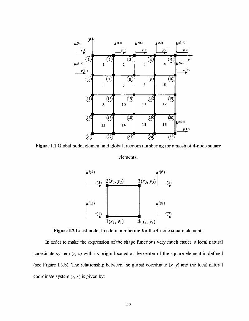
g(2) y
«(D
AS(I2) ©
(H)
®
Q
©
18(4)
g(3)
g(6)
5(5) — ^ >
&»)
SiV
g(IO)
8(9)
©
©
©
© 13
©
®
© 10
® 14
©
©
11
15
@
®
®
12
16
4«(20)
g(J9)
Ag(50)
«(49)
— -̂
Figure I.l Global node, element and global freedom numbering for a mesh of 4-node square
elements.
f(4)
f{3) 2(x2,y2) 3(x3,^3)
f(2)
f(l)
f(6)
f(5)
Af(8)
f(7) —*-
Hx\,y\) Hx4,y4)
Figure 1.2 Local node, freedom numbering for the 4-node square element.
In order to make the expression of the shape functions very much easier, a local natural
coordinate system (r, s) with its origin located at the center of the square element is defined
(see Figure I.3.b). The relationship between the global coordinate (x, y) and the local natural
coordinate system (r, s) is given by:
no
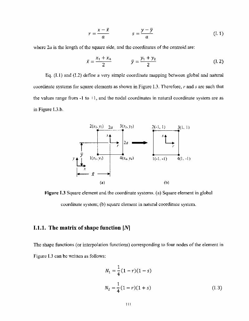
x — X s —
y-y
a a
where 2a is the length of the square side, and the coordinates of the centroid are:
(1.1)
x = X-^ ~r X4,
y = yi + y2 (1.2)
2 J 2
Eq. (1.1) and (1.2) define a very simple coordinate mapping between global and natural
coordinate systems for square elements as shown in Figure 1.3. Therefore, r and s are such that
the values range from -1 to +1, and the nodal coordinates in natural coordinate system are as
in Figure I.3.b.
2(Jfi.V:) 2a 3(.v3,>>:,)
r y
U 1 Cv,. V,)
2( - l , 1) 3 (1 ,1 )
2a
4(*4, y*) l(-l.-l) 4(1.-1)
(a) (b)
Figure 1.3 Square element and the coordinate systems, (a) Square element in global
coordinate system; (b) square element in natural coordinate system.
1.1.1. The matrix of shape function [N]
The shape functions (or interpolation functions) corresponding to four nodes of the element in
Figure 1.3 can be written as follows:
^ = - ( l - r ) ( l - s )
J V 2 = - ( l - r ) ( l + s) (1.3)
111
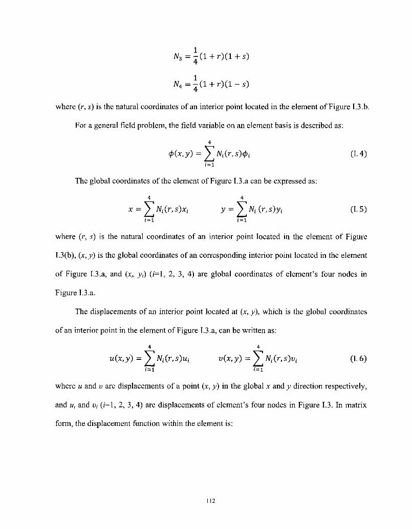
JV 3 =i ( l + r)( l + s)
N 4 = i ( l + r ) ( l - s )
where (r, 5) is the natural coordinates of an interior point located in the element of Figure I.3.b.
For a general field problem, the field variable on an element basis is described as:
4
0O,y) = ^ t y ( r , s ) 0 i (1.4) i = l
The global coordinates of the element of Figure 1.3.a can be expressed as:
4 4
i = l i = l
where (r, s) is the natural coordinates of an interior point located in the element of Figure
1.3(b), (x,y) is the global coordinates of an corresponding interior point located in the element
of Figure 1.3.a, and (x„ y,) (i=l, 2, 3, 4) are global coordinates of element's four nodes in
Figure 1.3.a.
The displacements of an interior point located at (x, y), which is the global coordinates
of an interior point in the element of Figure 1.3.a, can be written as:
4 4
u(x,y) =2^Ni(r,s')ui v(x,y) =2_lNi(r,s)vi (1.6) i = l £=1
where u and v are displacements of a point (x, y) in the global x and y direction respectively,
and u, and y,- (z'=l, 2, 3, 4) are displacements of element's four nodes in Figure 1.3. In matrix
form, the displacement function within the element is:
112
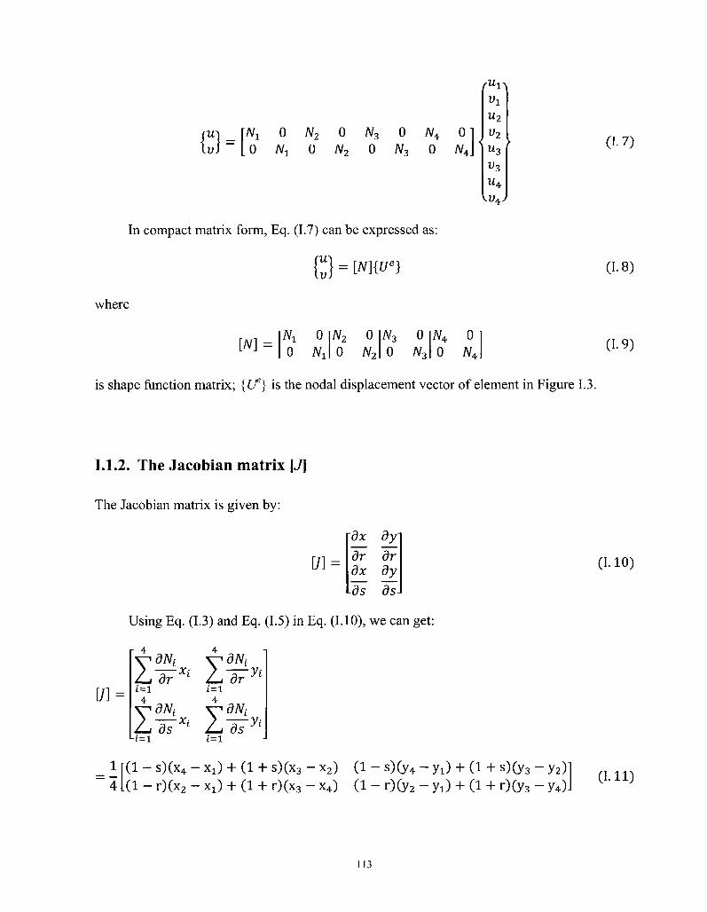
{> Nt 0 N2 0 N3 0 W4 0 0 Wj 0 N2 0 JV3 0 N4
u2
u2
" 3
" 3
l t 4
Vu4y
}
In compact matrix form, Eq. (1.7) can be expressed as:
0 = [N]{Ue}
where
[Ni .0
0 Nl
^ 2 0
0 ^ 2
W3
0 0
N3
iV4
0 0
N*_
(1.7)
(1.8)
M =
is shape function matrix; {£/} is the nodal displacement vector of element in Figure 1.3.
(1.9)
1.1.2. The Jacobian matrix [J]
The Jacobian matrix is given by:
[/]
Using Eq. (1.3) and Eq. (1.5) in Eq. (1.10), we can get:
~dx dr dx
Ite
dy dr dy ds-
[/] =
dN, Ldr%l L t = l i = l
(1.10)
(1 - s)(x4 - X l ) + (1 + s)(x3 - x2) (1 - s)(y4 - 7 l ) + (1 + s)(y3 - y2) 4 L(l - r)(x2 - xx) + (1 + r)(x3 - x4) (1 - r)(y2 - y1) + (1 + r)(y3 - y4)J
(1.11)
113
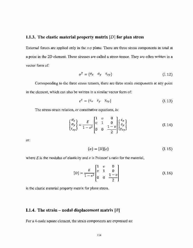
1.1.3. The elastic material property matrix [D] for plan stress
External forces are applied only in the x-y plane. There are three stress components in total at
a point in the 2D element. These stresses are called a stress tensor. They are often written in a
vector form of:
(jT={°x Oy *xy] (1.12)
Corresponding to the three stress tensors, there are three strain components at any point
in the element, which can also be written in a similar vector form of:
£T = {EX £y Yxy] (1.13)
The stress-strain relation, or constitutive equations, is:
lxy) 1-v2
1 V
0
V
1
0
0 1 0
1-v 2 J
[Yxy] (I. 14)
or:
{a} = [D]{e]
where E is the modulus of elasticity and v is Poisson' s ratio for the material,
[D] = 1-v2
1 V
0
V
1
0
0 1 0
1 - 1 7
2 J is the elastic material property matrix for plane stress.
1.1.4. The strain - nodal displacement matrix [B]
For a 4-node square element, the strain components are expressed as:
0.15)
(1.16)
114
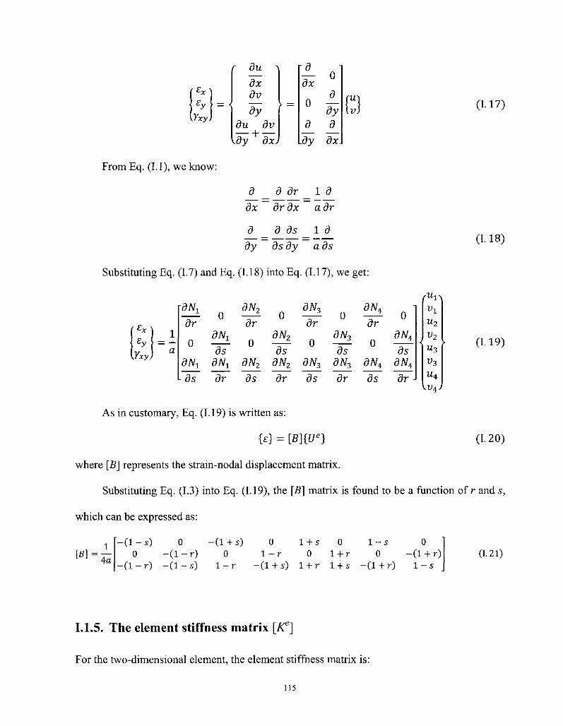
6x\ y H
f du > dx dv
ay du dv
<dy dxj
> =
d
dx d
dy d d
dy dx.
{1}
From Eq. (1.1), we know:
d d dr Id
dx dr dx a dr
d _ d ds _ 1 d
dy ds dy a ds
Substituting Eq. (1.7) and Eq. (1.18) into Eq. (1.17), we get:
£ y = " {.Yxy)
dN±
dr
0
0
dNx
17
dN2
dr
0
0
djh ds
dr
0
0
ds
dNA
dr
0
0
dN4
ds dNx dJVi dN2 dN2 dN3 dN3 dN4 dN4
ds dr ds dr ds dr ds dr
u2
v2
u3
v3
\VAJ
(1.17)
(1.18)
(1.19)
As in customary, Eq. (1.19) is written as:
{e} = [B]{Ue} (1.20)
where [B] represents the strain-nodal displacement matrix.
Substituting Eq. (1.3) into Eq. (1.19), the [5] matrix is found to be a function of r and s,
which can be expressed as:
[B] 1
4a
- ( 1 - s ) 0
- ( 1 - r )
0 - ( 1 - r ) - ( 1 - s )
-(1 + s) 0 l+s 0 1 - s 0 0 1 - r 0 1 + r 0 - (1 + r)
1 - r - ( 1 + s) 1 + r l + s - ( 1 + r ) 1 - s 0.21)
1.1.5. The element stiffness matrix [IC]
For the two-dimensional element, the element stiffness matrix is:
115
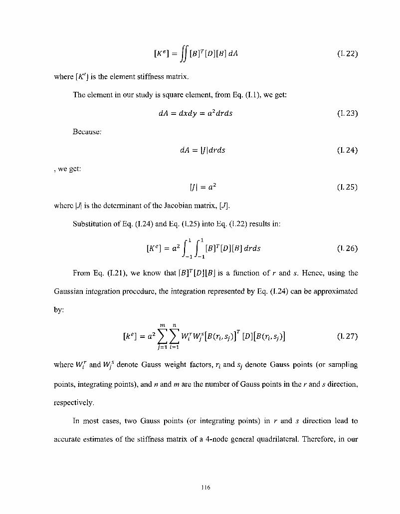
[Ke] = jj[B]T[D][B]dA (1.22)
where [K*] is the element stiffness matrix.
The element in our study is square element, from Eq. (1.1), we get:
dA — dxdy = a2drds (1.23)
Because:
dA = \J\drds (1.24)
, we get:
1/1= a2 (1.25)
where \J\ is the determinant of the Jacobian matrix, [J].
Substitution of Eq. (1.24) and Eq. (1.25) into Eq. (1.22) results in:
-i r i [Ke] = a2( \ [B]T[D][B]drds (1.26)
From Eq. (1.21), we know that [B] r [£>][#] is a function of r and s. Hence, using the
Gaussian integration procedure, the integration represented by Eq. (1.24) can be approximated
by:
m n
[ke] = tf^J^WflBtruSJ)] [D][B(n.Sj)] 0-27) j=l £ = 1
where W{ and Wf denote Gauss weight factors, rt and s;- denote Gauss points (or sampling
points, integrating points), and n and m are the number of Gauss points in the r and s direction,
respectively.
In most cases, two Gauss points (or integrating points) in r and s direction lead to
accurate estimates of the stiffness matrix of a 4-node general quadrilateral. Therefore, in our
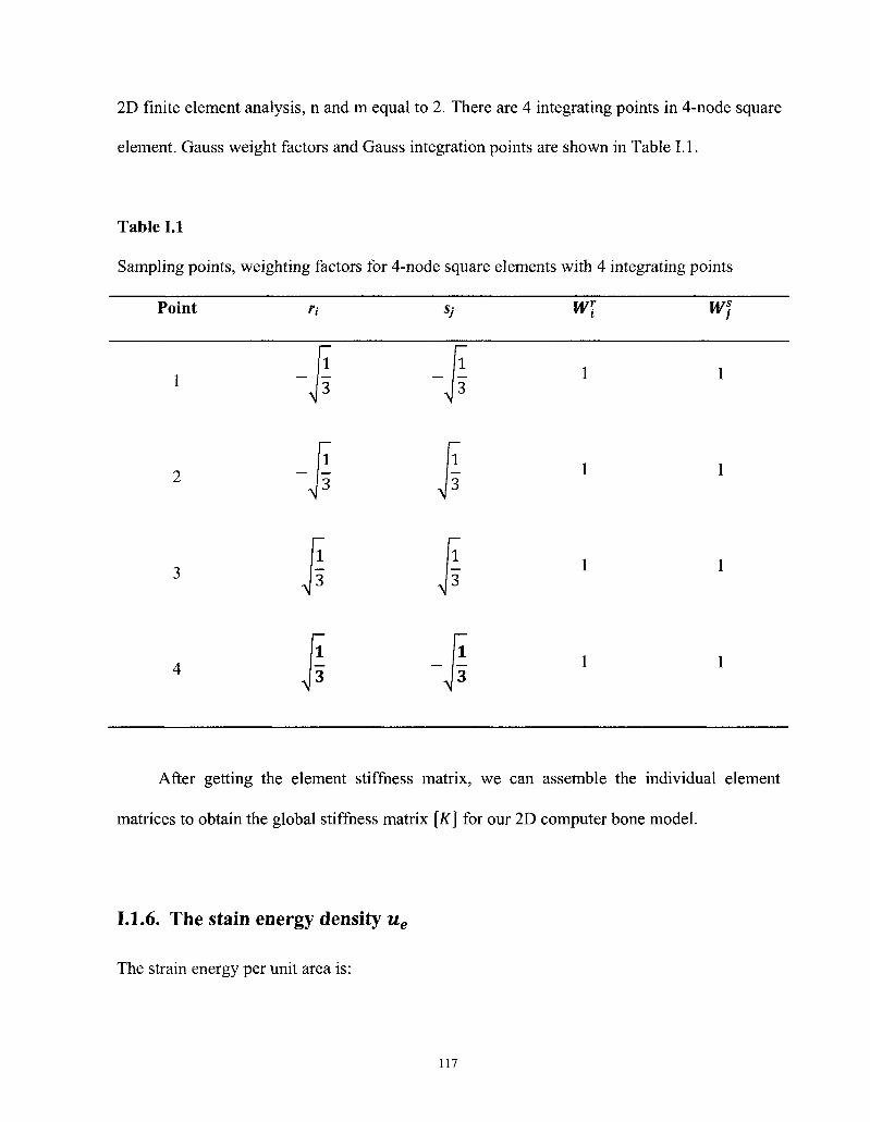
2D finite element analysis, n and m equal to 2. There are 4 integrating points in 4-node square
element. Gauss weight factors and Gauss integration points are shown in Table 1.1.
Table 1.1
Sampling points, weighting factors for 4-node square elements with 4 integrating points
Point 7i 7j W\ wj
-I I
I -I After getting the element stiffness matrix, we can assemble the individual element
matrices to obtain the global stiffness matrix [K] for our 2D computer bone model.
1.1.6. The stain energy density ue
The strain energy per unit area is:
117
ue =\{e}T {e} =\{z}T [D]{e} (1.28)
or, for a 2D element,
1 Ue = 2 (°x£* + °y£y + TxyK*y) 0- 2 9 )
118
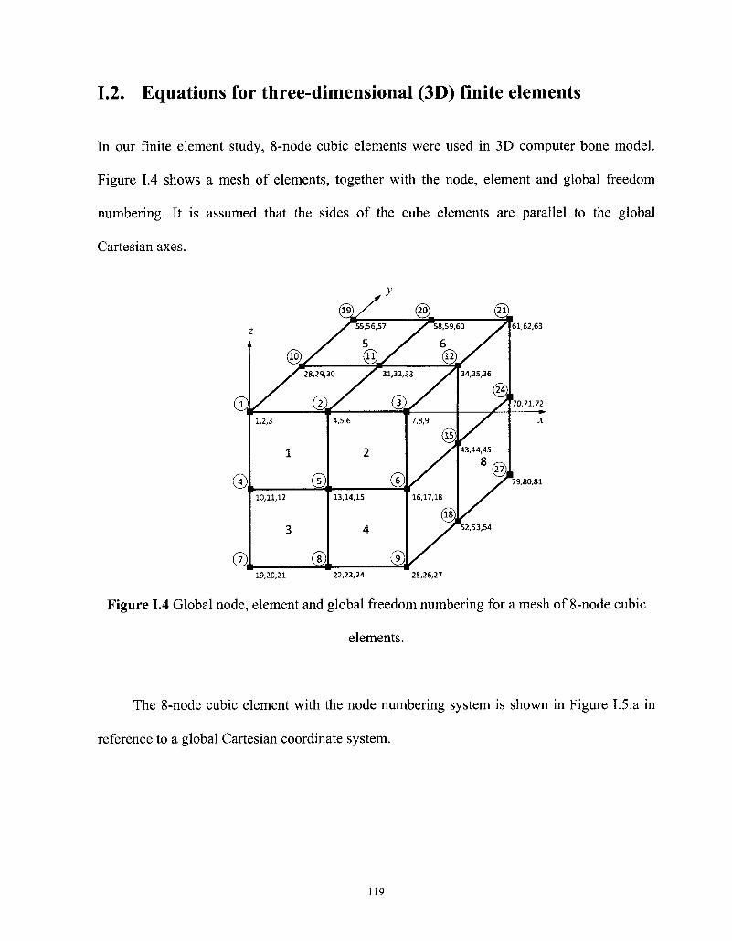
1.2. Equations for three-dimensional (3D) finite elements
In our finite element study, 8-node cubic elements were used in 3D computer bone model.
Figure 1.4 shows a mesh of elements, together with the node, element and global freedom
numbering. It is assumed that the sides of the cube elements are parallel to the global
Cartesian axes.
19,20,21 22,23,24 25,26,27
Figure 1.4 Global node, element and global freedom numbering for a mesh of 8-node cubic
elements.
The 8-node cubic element with the node numbering system is shown in Figure 1.5.a in
reference to a global Cartesian coordinate system.
119
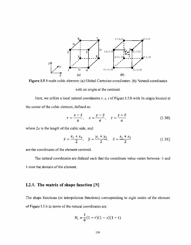
2ay
7i\
fy 1
( - i , - i , i )
la 4
(a)
(- i .- i . - i)
, ( i , i , i )
i,i,-D
(i,-i,-D
x W (b)
Figure 1.5 8-node cubic element: (a) Global Cartesian coordinates, (b) Natural coordinates
with an origin at the centroid.
Here, we utilize a local natural coordinates r, s, t of Figure I.5.b with its origin located at
the center of the cubic element, defined as:
x — x y — y z — z r - , s = , t =
a a
where 2a is the length of the cubic side, and:
a (1.30)
_ x1 + x4 _ y1+ys _ zr + z2 x=—-—, y = — = — , z =
2 ' (1.31)
are the coordinates of the element centroid.
The natural coordinates are defined such that the coordinate value varies between -1 and
1 over the domain of the element.
1.2.1. The matrix of shape function [N]
The shape functions (or interpolation functions) corresponding to eight nodes of the element
of Figure I.5.b in terms of the natural coordinates are:
W 1 = - ( l - r ) ( l - s ) ( l - t )
120
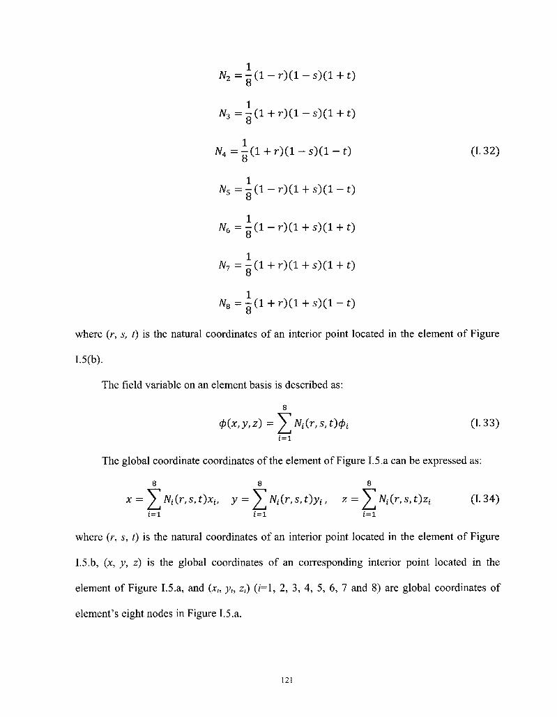
A r 2 = i ( l - r ) ( l - s ) ( l + t)
A r 3 = - ( l + r ) ( l - s ) ( l + t)
W4 = ^ ( l + r ) ( l - s ) ( l - t ) (1.32)
W 5 = i ( l - r ) ( l + s ) ( l - 0
tf6=i(l-r)(l + s)(l + t)
W 7 = - ( l + r ) ( l + s)(l + t)
W 8 = i ( l + r ) ( l + s ) ( l - t )
where (/-, 5, f) is the natural coordinates of an interior point located in the element of Figure
1.5(b).
The field variable on an element basis is described as:
8
0 ( x , y , z ) = ^ t y ( r , s , t ) 0 £ (1.33) i = l
The global coordinate coordinates of the element of Figure 1.5.a can be expressed as:
8 8 8
x = 2_ANi(.r's>t')xi> y = ^Ni(r,s,t)yi, z = 2^Ni(r,s,t)zi (1.34)
i = l i=l i=l
where (r, s, t) is the natural coordinates of an interior point located in the element of Figure
1.5.b, (x, y, z) is the global coordinates of an corresponding interior point located in the
element of Figure I.5.a, and (x„ y„ z,) (z'=l, 2, 3, 4, 5, 6, 7 and 8) are global coordinates of
element's eight nodes in Figure 1.5.a.
121
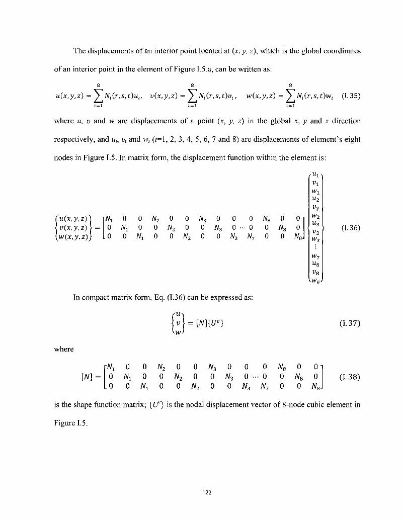
The displacements of an interior point located at (x, y, z), which is the global coordinates
of an interior point in the element of Figure 1.5.a, can be written as:
8 8 8
u(x,y,z)=y N^r,s, t)uu v(x,y,z) = } N^r,s, t)vt, w(x,y,z) = } Nt(r,s, t)wt (1.35) i = i i=i i = i
where u, v and w are displacements of a point (x, y, z) in the global x, y and z direction
respectively, and ul3 v, and w, (/=1, 2, 3, 4, 5, 6, 7 and 8) are displacements of element's eight
nodes in Figure 1.5. In matrix form, the displacement function within the element is:
ru{x,y,z) v{x,y,z) ) = w(x,y,z)
Nt 0 0 N2 0 0 N3 0 0 0 JV8 0 0 0 Nt 0 0 N2 0 0 N3 0 ••• 0 0 N8 0 0 0 Nt 0 0 JV2 0 0 N3 N7 0 0 W8
Vl
v2
W2
u3
w3
w7 u8
vs
vw8y
In compact matrix form, Eq. (1.36) can be expressed as:
\v\ = [N]{Ue]
(1.36)
(1.37)
where
[N] = Nx
0 0
0 Wl 0
0 0
Nl
N2
0 0
0 N2 0
0 0
w2
^3
0 0
0 N3
0
0 0 •
N3
0 •• 0
N7
N8
0 0
0 N8 0
0 0
N8
(1.38)
is the shape function matrix; {If} is the nodal displacement vector of 8-node cubic element in
Figure 1.5.
122
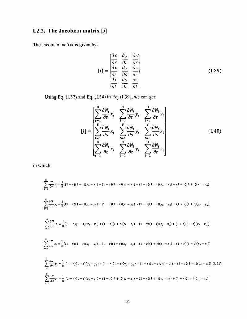
1.2.2. The Jacobian matrix [J]
The Jacobian matrix is given by:
[/] =
dx dy dz
dr dr dr dx dy dz ds ds ds dx dy dz ~di ~dt di
Using Eq. (1.32) and Eq. (1.34) in Eq. (1.39), we can get:
[/]
sr°Ni y ^ i y ^ i L dr Xl L dr Vl L dr i=l i=i 1=1
8 8 8
Z dNj ^dNj y<
ds Xi LdsJi L i=l i=l i=l
Y^Vi Y ^ L Y ^ i LdtXi L dtyi L dt
dNt
IF*
i=l i=l i=l
in which
(1.39)
(1.40)
I -g^x, = - [(1 - s ) ( l - t)(x4 - Xl) + (1 - s ) ( l + t)(x3 - x2) + (1 + s ) ( l - t)(xa - x5) + (1 + s ) ( l + t)(x7 - x6)]
Z dN 1
-gfyi = g [(i - s)(i - 0(y4 - yi) + tt - *)d + 0(y3 - y2) + (i + «)(i - 0(y8 - y5) + (i + s)(i + t)(y7 - y6)]
Xl7z ' = g[(1" s)(:i"t)(:z*" Zl) + (1"s)(1 + t)(z3" Z2) + (1 + s)(1"t)(Zs ~ Zs) + (1 + s)(1 + t)(z7" Z6)]
1=1
Z dN 1
- ^ = - [ ( 1 - r ) ( l - t)(x5 - x,) + (1 - r ) ( l + t)(x6 - *z) + (1 + ^)(1 + t)(x7 - *3) + (1 + r ) ( l - f)(xa - x4)]
Z uN 1
-^j-y, = g [(1 " 0 ( 1 - t)(y s - y i ) + (1 - r ) ( l + t)(y6 - y2) + (I + r ) ( l + t)(y7 - y3) + (1 + r ) ( l - t)(y8 - y4)] (1.41) 1=1
s
Z dN 1
- ^ • z , = - [(1 - r ) ( l - t)(z5 - z,) + (1 - r ) ( l + t)(z6 - z2) + (1 + r ) ( l + t)(z7 - z3) + (1 + r ) ( l - t)(z8 - z4)]
123
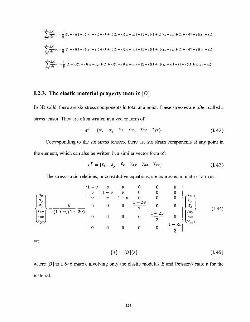
Z dN, 1
-g^*. = g [(1 - 0 ( 1 - s)(x2 - x,) + (1 + r)(l - s)(x3 - x4) + (1 - r)(l + s)(x6 - xs) + (1 + r)(l + s)(*7 - x8)] i= i 8
V 3W 1
ZlT3'1 = 8 [ ( 1 " r ) ( 1 " s)(y2 ~ yi) + (1 + r ) (1 ~~ s)(y3 " y,) + ( 1 " r ) (1 + s ) (y6" ys) + (1 + r ) (1 + s)(y? ~ ys)]
1=1
4->dN, 1 Z , " ^ 2 ' = 8 [ ( 1 _ r ) ( 1 " S ) (Z2 ~~ Z l ) + ( 1 + r ) ( 1 " S ) ( Z 3 " Z4) + ( 1 ~ r ) ( 1 + S ) (Z6 ~ Zs ) + ( 1 + r ) ( 1 + S ) ( Z ? " Z s ) ]
1.2.3. The elastic material property matrix [D]
In 3D solid, there are six stress components in total at a point. These stresses are often called a
stress tensor. They are often written in a vector form of:
aT = {ax oy °z Txy xxz Tyz] (1.42)
Corresponding to the six stress tensors, there are six strain components at any point in
the element, which can also be written in a similar vector form of:
£T = {Ex £y *z Yxy Yxz Yyz] (1.43)
The stress-strain relations, or constitutive equations, are expressed in matrix form as:
rux\
lxy
Txz
VTyz)
> = ( l + v ) ( l - 2 v )
1-v v v 0 0 0 v l - t 7 v 0 0 0 v v 1-v 0 0 0
l - 2 v 0
0
0
0
0
0
0
0
0
2
0
0
0
l - 2 v
2
0
0
0
1 - 2 1 7
fEx\
Sy
*Z
Yxy
Yxz
{-Yyz J
(1.44)
or:
{°} = [D]{e} (1.45)
where [D] is a 6x6 matrix involving only the elastic modulus E and Poisson's ratio v for the
material.
124
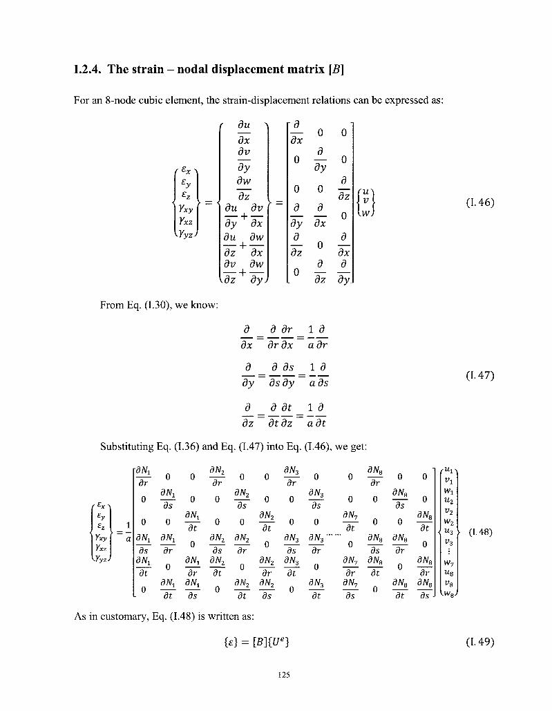
1.2.4. The strain - nodal displacement matrix [B]
For an 8-node cubic element, the strain-displacement relations can be expressed as:
f £x\ £v
y £ z
Yxy
Yxz
y — <
VYyz)
( du ~\
dx dv _ ^ dy dw
dz du dv ^^_ _|_ ____ dy dx du dw
dz dx dv dw
_|_ <dz dy J
y —
\d _^_ dx
0
0
d
dy d
dz
0
0
d
dy
o d
dx
0
d
dz
0
0
d . ^ _ dz
0
d
dx d
dy
(1.46)
From Eq. (1.30), we know:
d dx
d
dy
d dr dr dx
d ds
dsdy
1 d adr
1 d
ads (1.47)
d _ d dt _ 1 d
dz dtdz adt
Substituting Eq. (1.36) and Eq. (1.47) into Eq. (1.46), we get:
f £x\ £y
£z
Yxy
Yxz
1
a
\YyzJ
•dNi
~d~7
0
0
dN-L
~ds~ dNr
~dT
0
0
~ds~
0
dr
0
~~dt
0
0
~dt
0
dNx
~dr~
~ds~
dN2
~dr~
0
0
dN2
~ds~ dN2
~dt
0
0
dN2
Us
0
dN2
dr
0 dN2
0
0
dN2
It
0 dN2
dr dN2
~ds~
dN3
dr
0
0
dN3
ds dN3
dt
0
0
dN3
ds
0
dN3
dr
0 dN3
dt
0
0
dN7
~dT
0 dN7
~dr dN7
~ds~
dN8
dr
0
0
dN8
ds dNe
dt
0
0
dNa
ds
0
dNs dr
0 dNa
dt
0
0
dNa
dt
0
dNs dr
dN8
ds-
u2
v2
w2
• u3
V-> vz
w7
u8
v8
• ( 1 .48 )
As in customary, Eq. (1.48) is written as:
{£} = [B]{Ue] (1.49)
125
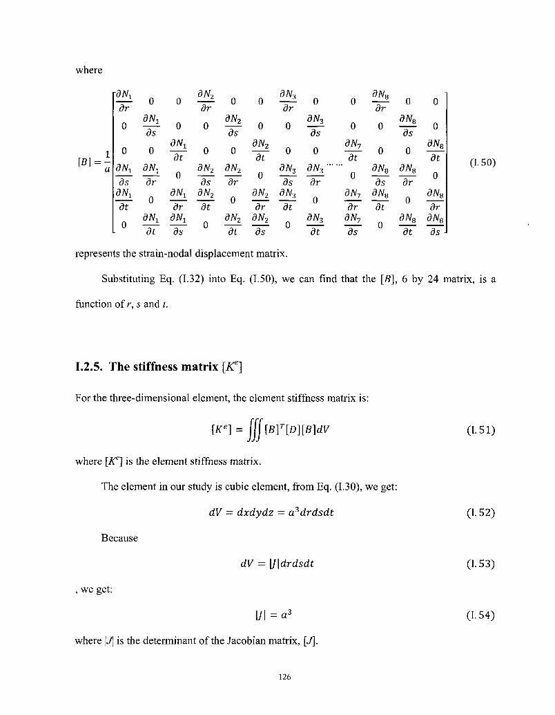
where
a
dr
0
0
dN±
~dT
~df
0
0
dNx
~ds~
0
dNx
dr
0
0
0
dNt
~dt
0
dNx
dr dN1 d^
dN2
dr
0
0
dN2
ds dN2
~df
0
0
dN2
ds
0
djh dr
0
djh dt
0
0
dN2
dt
0
dN2
dr dN2
ds
dr
0
0
djh ds
dt
0
0
dN3
ds
0
dN3
dr
0
dN3
dt
represents the strain-nodal displacement matrix.
0
0
dN7
~~bT 0
dN8
dr
0
0
dN8
ds dN7 dN8
~~dr ~dt dN7
ds 0
0
dNs
ds
0
dl%
dr
0
dNs dt
0
0
dNs dt
0
dN8
dr dNs ds
(1.50)
Substituting Eq. (1.32) into Eq. (1.50), we can find that the [B], 6 by 24 matrix, is a
function of r, s and t.
1.2.5. The stiffness matrix [K*]
For the three-dimensional element, the element stiffness matrix is:
[Ke] = jfj[B]T[D][B]dV
where [K6] is the element stiffness matrix.
The element in our study is cubic element, from Eq. (1.30), we get:
dV — dxdydz = a3drdsdt
Because
dV = \J\drdsdt
, we get:
l/l = a 3
where \J\ is the determinant of the Jacobian matrix, [J].
(1.51)
(1.52)
(1.53)
(I. 54)
126
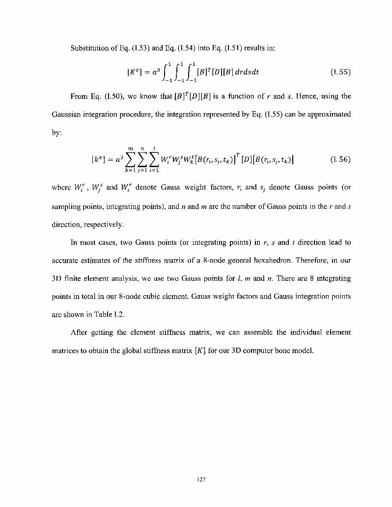
Substitution of Eq. (1.53) and Eq. (1.54) into Eq. (1.51) results in:
[Ke] = a3( ( ( [B]T[D][B]drdsdt (1.55) J-i J-i J-i
From Eq. (1.50), we know that [S]r[D][S] is a function of r and s. Hence, using the
Gaussian integration procedure, the integration represented by Eq. (1.55) can be approximated
by:
m n I
[ke] = a ^ ^ ^ ^ V K / ^ ^ ^ s ^ t ^ J ^ D J l F ^ s ^ t , ) ] (1.56) fc=l ; = 1 i = l
where W[, W}s and Wt
r denote Gauss weight factors, rx and s; denote Gauss points (or
sampling points, integrating points), and n and m are the number of Gauss points in the r and s
direction, respectively.
In most cases, two Gauss points (or integrating points) in r, s and t direction lead to
accurate estimates of the stiffness matrix of a 8-node general hexahedron. Therefore, in our
3D finite element analysis, we use two Gauss points for /, m and n. There are 8 integrating
points in total in our 8-node cubic element. Gauss weight factors and Gauss integration points
are shown in Table 1.2.
After getting the element stiffness matrix, we can assemble the individual element
matrices to obtain the global stiffness matrix [K] for our 3D computer bone model.
127
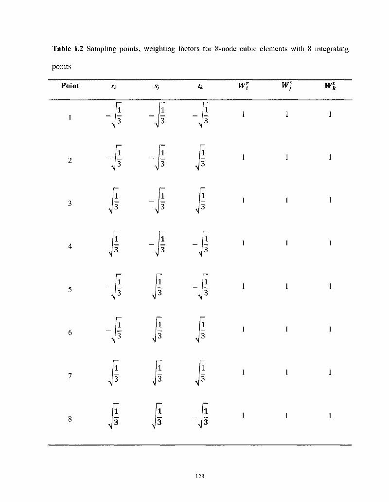
Table 1.2 Sampling points, weighting factors for 8-node cubic elements with 8 integrating
points
Point n Sj tk Wf wj Wi
128
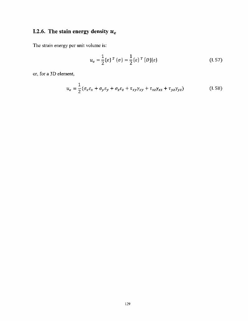
1.2.6. The stain energy density ue
The strain energy per unit volume is:
ue=^{e}T{a}=^{£}T[D]{e} (1.57)
or, for a 3D element,
1 ue = r {pxEx + Oy£y + ^z^z + ^xyYxy + ^xzYxz + lyzYyz) 0- 58)
129
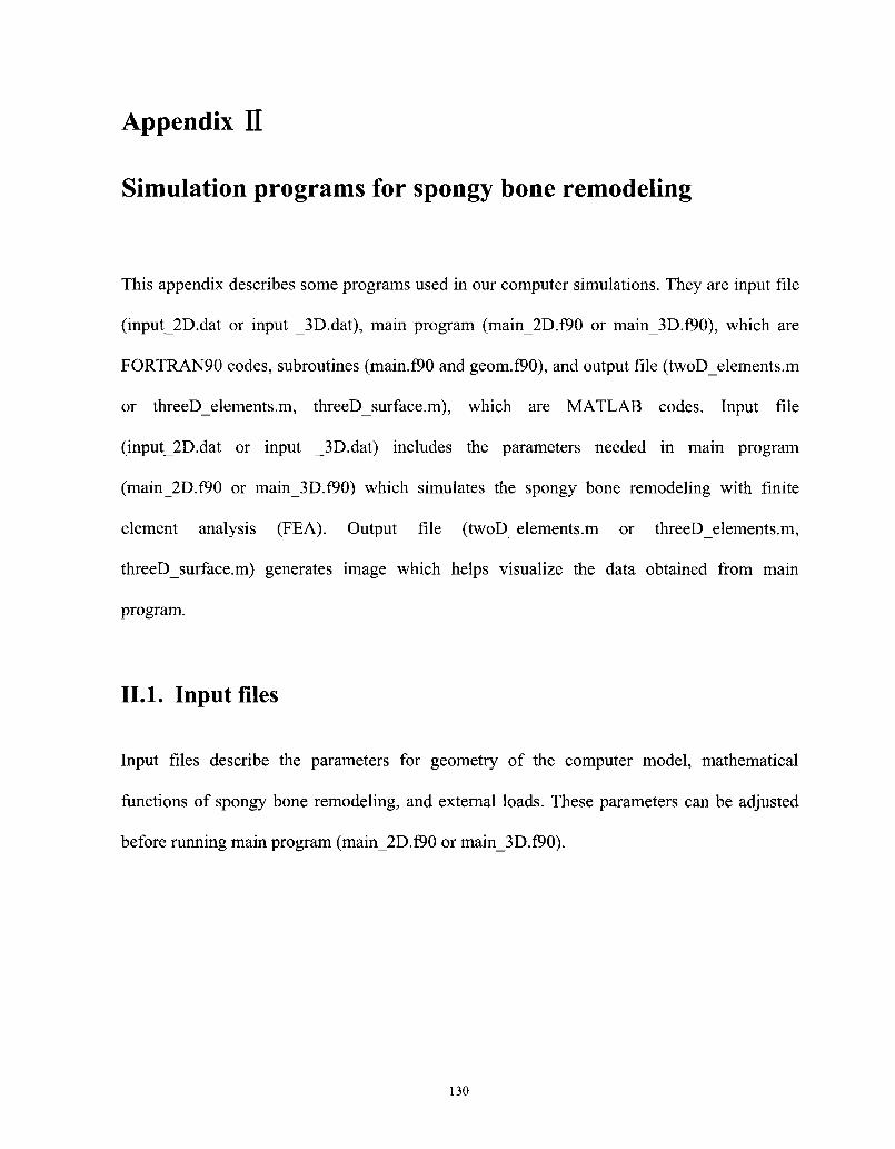
Appendix II
Simulation programs for spongy bone remodeling
This appendix describes some programs used in our computer simulations. They are input file
(input_2D.dat or input _3D.dat), main program (main_2D.f90 or main_3D.f90), which are
FORTRAN90 codes, subroutines (main.f90 and geom.f90), and output file (twoD_elements.m
or threeD_elements.m, threeDsurface.m), which are MATLAB codes. Input file
(input_2D.dat or input _3D.dat) includes the parameters needed in main program
(main_2D.f90 or main_3D.f90) which simulates the spongy bone remodeling with finite
element analysis (FEA). Output file (twoDelements.m or threeDelements.m,
threeDsurface.m) generates image which helps visualize the data obtained from main
program.
II. 1. Input files
Input files describe the parameters for geometry of the computer model, mathematical
functions of spongy bone remodeling, and external loads. These parameters can be adjusted
before running main program (main_2D.f90 or main_3D.f90).
130
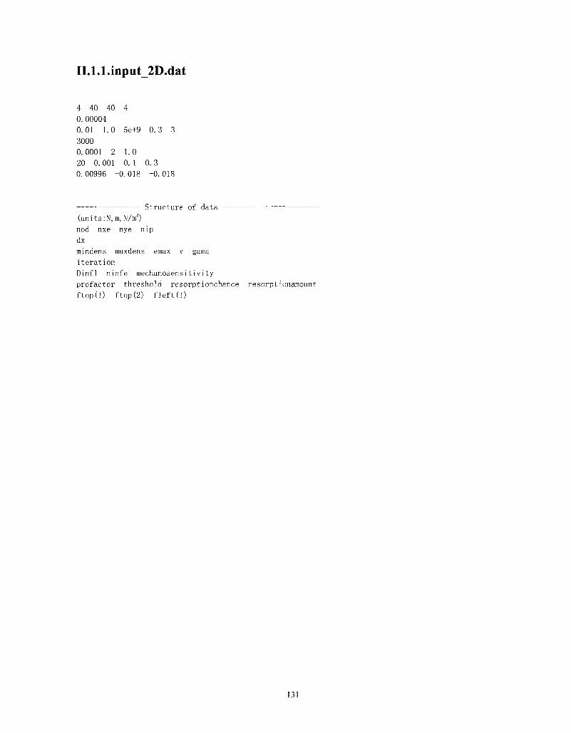
II.l.l.input_2D.dat
4 40 40 4
0. 00004
0.01 1.0 5e+9 0.3 3
3000
0.0001 2 1.0
20 0.001 0. 1 0.3
0.00996 -0.018 -0.018
Structure of data
(units :N, ra, N/m2)
nod nxe nye nip
dx
mindens maxdens emax v gama
iteration
Dinfl ninfe mechanosensitivity
profactor threshold resorptionchance resorptionamount
ftop(l) ftop(2) fleft(l)
131
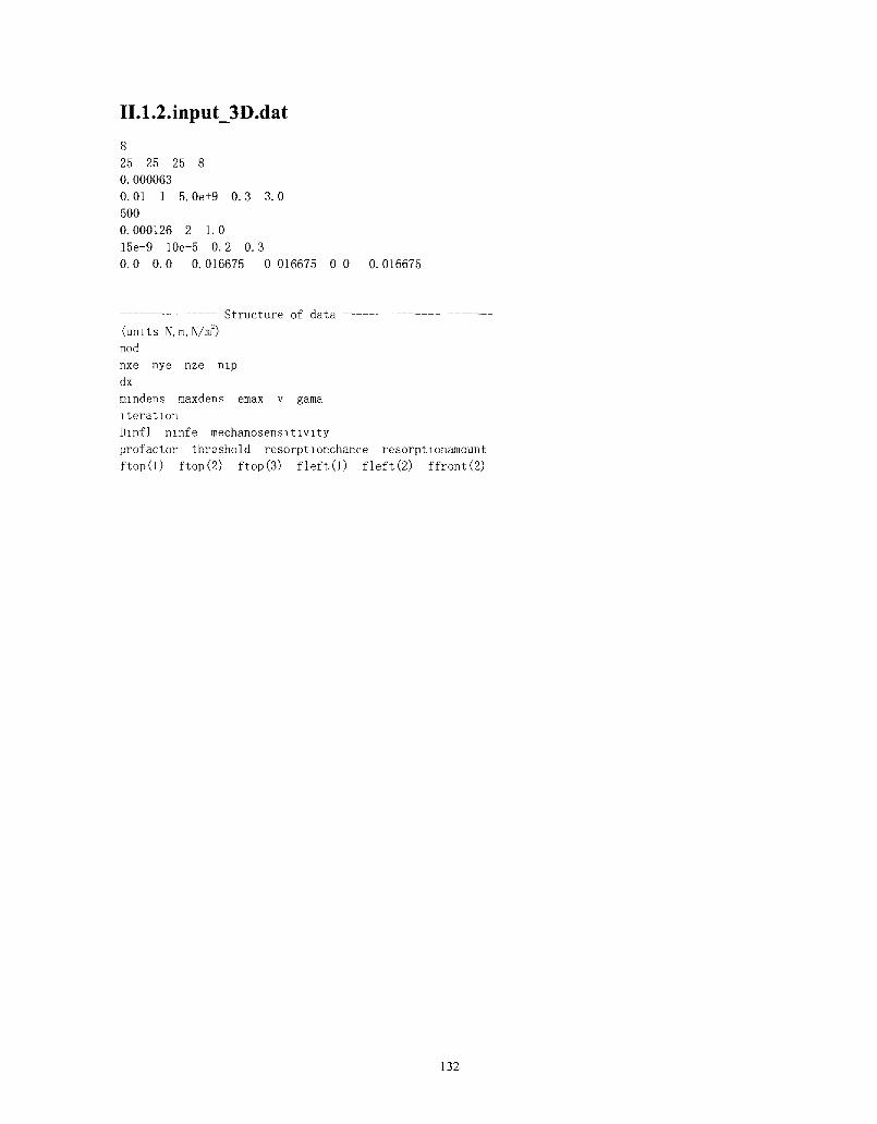
II.1.2.input_3D.dat
8
25 25 25 8
0. 000063
0.01 1 5. Oe+9 0.3 3.0
500
0.000126 2 1.0
15e-9 10e+5 0.2 0.3
0.0 0.0 -0.016675 -0 016675 0 0 -0.016675
Structure of data
(units N, ra, N/m2)
nod
nxe nye nze nip
dx
mindens maxdens emax v gama
iteration
Dinfl ninfe mechanosensitivity
profactor threshold resorptionchance resorptionamount
ftop(l) ftop(2) ftop(3) fleft(l) f left (2) ffront (2)
132
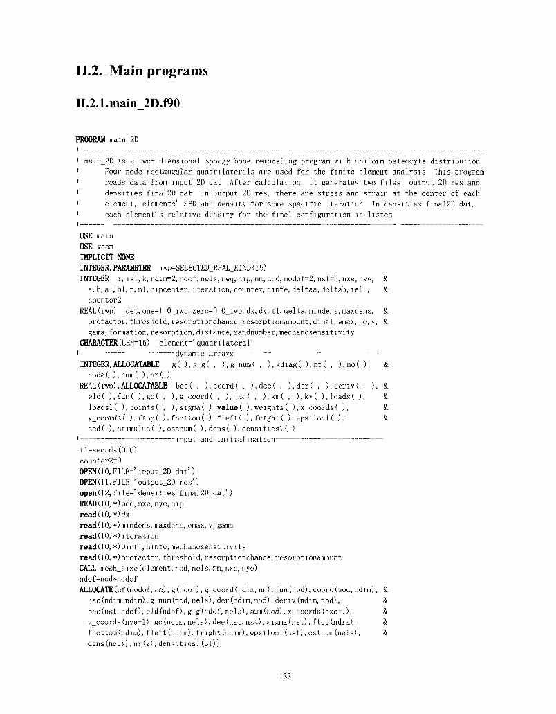
II.2. Main programs
II.2.1.main 2D.f90
PROGRAM main_2D
mam_2D is a two- diemsional spongy bone remodeling program with unitoim osteocyte distribution
Four-node iectangular quadrilaterals are used for the finite element analysis This program
reads data from input_2D ddt After calculation, it generates two files output_2D res and
densities_final2D dat In output_2D res, there are stress and strain at the center of each
element, elements' SED and density for some specific iteration In densities_final2D dat,
each element' s relative density for the final configuration is listed
USE mam
USE geom
IMPLICIT NONE
INTEGER, PARAMETER iwp=SELECTED_REAL_KIND (15)
INTEGER 1, lei, k, ndim=2, ndof, nels, neq, nip, nn, nod, nodof=2, nst=3, nxe, nye, &
a, b, al, bl, n, nl, nipcenter, iteration, counter, ninfe, deltaa, deltab, lell, &
counter2
REAL(iwp) det, one=l 0_iwp, zero-0 0_iwp, dx, dy, tl, delta, mmdens, maxdens, &
profactor, threshold, resorptionchance, resorptionamount, dmf 1, emax, , e, v, &
gama, formation, resorption, distance, randnumber, mechanosensitivity
CHARACTER(LEN=15) element- quadrilateral'
dynamic arrays —
INTEGER, ALLOCATABLE g(),g_g(, ),g_num(, ), kdiag( ), nf ( , ),no(), &
node( ),num( ),nr( )
REAL dwp), ALLOCATABLE bee( , ), coord ( , ),dee( , ),der( , ),denv( , ), &
eld( ),fun( ),gc( , ),g_coord( , ),jac( , ),km( , ),kv( ), loads( ), &
loadsl( ), points( , ),sigma( ),value( ),weights( ),x_coords( ), &
y_coords( ),ftop( ),fbottom( ),fleft( ), fright( ),epsilonl( ), &
sed( ),stimulus( ),ostnum( ),dens( ), densitiesl ( )
input and initialisation
tl=secnds(0 0)
counter2=0
0PEN(10,FILE=' mput_2D dat')
0PEN(ll,FILE='output„2D res')
open(12, f ile=' densities_f inal2D dat')
READ(10, *)nod, nxe, nye, nip
read (10, *)dx
read(10, *)mindens, maxdens, emax, v, gama
read(10, *) iteration
read(10, *)Dinf 1, ninfe, mechanosensitivity
read(10, *)profactor, threshold, resorptionchance, resorptionamount
CALL meshsize (element, nod, nels, nn, nxe, nye)
ndof-nod*nodof
ALLOCATE (nf (nodof, nn), g(ndof), g_coord(ndim, nn), fun (nod), coord (nod, ndim), &
jac(ndim, ndim), g_num(nod, nels), der (ndim, nod), deriv (ndim, nod), &
bee (nst, ndof), eld (ndof), g_g(ndof, nels), num(nod), x_coords(nxe+l), &
y_coords(nye+l), gc(ndim, nels), dee (nst, nst), sigma(nst), f top (ndim), &
f bottom (ndim), fleft (ndim), fright (ndim), epsilonl (nst), ostnum(nels), &
dens(nels), nr(2), densitiesl(31))
133
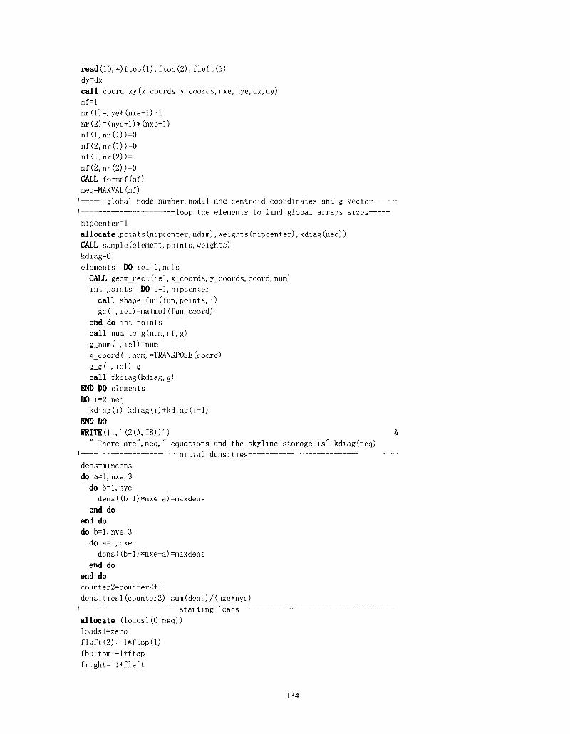
read(10, *) f top (1), f top (2), f lef t (1)
dy=dx
call coord_xy (x_coords, y_coords, nxe, nye, dx, dy)
nf=l
nr (1) =nye* (nxe+1) +1
nr(2) = (nye+l)*(nxe+l)
nf(l,nr(l))=0
nf(2,nr(l))=0
nf(l,nr(2)) = l
nf(2, nr(2))=0
CALL formnf (nf)
neq=MAXVAL(nf)
global node number, nodal and centroid coordinates and g vector
loop the elements to find global arrays sizes
mpcenter=l
allocate(points(nipcenter, ndim), weights(nipcenter), kdiag(neq))
CALL sample (element, points, weights)
kdiag-0
elements DO iel=l,nels
CALL geom_rect del, x_coords, y_coords, coord, num)
int_points DO i=l,nipcenter
call shape_fun (fun, points, l)
gc( , iel)=matmul (fun, coord)
end do mt_points
call num_to_g(num, nf, g)
g_num( , iel)=num
g_coord ( , num) TRANSPOSE (coord)
g_g( , i e l ) = g
call fkdiag(kdiag, g)
END DO elements
DO i=2, neq
kdiag(i)=kdiag(i)+kdiag(i-l)
END DO
WRITE(11,' (2(A, 18))') &
There are", neq, " equations and the skyline storage is", kdiag(neq)
]m 11al dens itles
dens=mindens
do a=l, nxe, 3
do b=l, nye
dens((b~l)*nxe+a)=maxdens
end do
end do
do b=l, nye, 3
do a=l, nxe
dens ((b-1)*nxe+a)=maxdens
end do
end do
counter2=counter2+1
densitiesl (counter2)=sum(dens)/(nxe*nye)
staiting loads
allocate (loadsl(0 neq))
loadsl=zero
fleft(2)=-l*ftop(l)
fbottom=-l*ftop f r ight=- l*f lef t
134
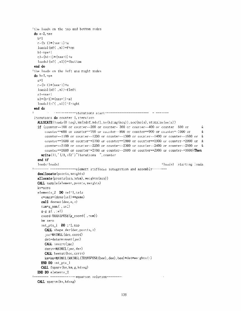
'the loads on the top and bottom sides
do a=2, nxe
b=l
n=(b-l)*(nxe+l)+a
loadsl(nf( ,n))=ftop
bl=nye+l
nl-(bl-l)*(nxe+l)+a
loadsl(nf( ,nl))=fbottom
end do
'the loads on the left and right sides
do b=2, nye
a=l
n-(b-l)*(nxe+l)+a
loadsl(nf( ,n))-fleft
al=nxe+l
nl=(b-l)*(nxe+l)+al
loadsKnf ( ,nl))=fnght
end do
i iterations start
Iterations do counter~l, iteration
ALLOCATE(loads (0 neq), km(ndof, ndof), kv(kdiag(neq)), sed(nels), stimulus (nels))
if (counter-=100 or counter==200 or counter=~300 or counter=-400 or counter 500 or &
counter==600 or counter 700 or counter—800 or counter==900 or counter=-1000 or &
counter==1100 or counter==1200 or counter==1300 or counter=-1400 or counter==1500 or &
counter==1600 or counter~=1700 or counter==1800 or counter==1900 or counter-=2000 or &
counter==2100 or counter==2200 or counter==2300 or counter—2400 or counter==2500 or &
counter==2600 or counter~=2700 or counter—2800 or counter==2900 or counter-=3000)Then
write(11,' (/A, i5)' ̂ 'Iterations ", counter
end if
loads=loadsl 'loadsl starting loads
' element stiffness integration and assembly
deallocate (points, weights)
allocate (points (nip, ndim), weights (nip))
CALL sample(element, points, weights)
kv=zero
elements_2 DO iel=l,nels
e=emax*(dens (iel)**gama)
call deemat (dee, e, v)
num=g_num( , lei)
g=g_g( , lei)
coord-TRANSPOSE(g_coord( ,num))
knrzero
int_pts_l DO i~l,mp
CALL shape_der (der, points, l)
jac=MATMUL (der, coord)
det=determinant(jac)
CALL invert (jac)
denv=MATMUL(jac, der)
CALL beemat (bee, deriv)
km=km+MATMUL (MATMUL (TRANSPOSE (bee), dee), bee) *det*weights(I)
END DO int_pts_l
CALL fsparv(kv, km, g, kdiag)
END DO elements_2
i equation solution —
CALL sparin(kv, kdiag)
135
CALL spabac(kv, loads, kdiag)
loads (0)=zero
if (counter==100 or counter==200 or counter==300 or counter==400 or counter-=500 or &
counter 600 or counter==700 or counter 800 or counter==900 or counter==1000 or &
counter=-1100 or counter==1200 or counter=-1300 or counter==1400 or counter==1500 or &
counter=-1600 or counter==1700 or counter==1800 or counter==1900 or counter==2000 or &
counter==2100 or counter==2200 or counter==2300 or counter==2400 or counter==2500 or &
counter-=2600 or counter==2700 or counter==2800 or counter==2900 or counter==3000)Then
WRITEdl,' (/A)')" Node x-disp y-disp"
DO k=l,nn
WRITE(11, ' (15, 2E12 4)')k, loads (nf ( ,k)) 'here, loads are displacements
END DO
end if
recover stresses at nip integrating points
mpcenter=l
DEALLOCATE(points, weights)
ALLOCATE (points(mpcenter, ndim), weights (nipcenter))
CALL sample (element, points, weights)
if (counter==100 or counter=~200 or counter==300 or counter==400 or counter~=500 or &
counter 600 or counter==700 or counter==800 or counter==900 or counter==1000 or &
counter==1100 or counter~=1200 or counter==1300 or counter~=1400 or counter==1500 or &
counter=~1600 or counter=-1700 or counter 1800 or counter==1900 or counter==2000 or &
counter==2100 or counter==2200 or counter=-2300 or counter==2400 or counter==2500 or &
counter 2600 or counter=-2700 or counter~=2800 or counter=-2900 or counter=_3000)Then
WRITEdl,' (/A, 12, A)') " The integration point (mp=", nipcenter, ") stresses/strain are
WRITEdl,' (A, A, A)')" Element x-coord y-coord", &
sig_x sig_y tau_xy" , &
eps_x eps_y eps_xy"
end if
elements_3 DO iel=l, nels
e=emax* (dens del) **gama)
call deemat (dee, e, v)
num=g_num( , lei)
coord-TRANSPOSE(g_coord( , nura))
g=g_g( , lei)
eld~loads(g)
mt_pts_2 DO 1=1, nipcenter
CALL shape_der (der, points, I)
jac=MATMUL(der, coord)
CALL invert(jac)
denv=MATMUL(jac, der)
CALL beemat(bee, deriv)
epsilonl=matmul (bee, eld)
sigma=MATMUL(dee, epsilonl)
sed(iel)=0 5*(sigma(l)*epsilonl (l)+sigma(2)*epsilonl (2)+sigma(3)*epsilonl (3))
if (counter==100 or counter==200 or counter==300 or counter—400 or counter==500 or &
counter=-600 or counter==700 or counter—800 or counter==900 or counter==1000 or &
counter==1100 or counter~=1200 or counter==1300 or counter==1400 or counter==1500 or &
counter==1600 or counter==1700 or counter==1800 or counter=-1900 or counter==2000 or &
counter==2100 or counter==2200 or counter==2300 or counter==2400 or counter==2500 or &
counter==2600 or counter=~2700 or counter==2800 or counter==2900 or counter==3000)Then
WRITEdl,' (15, 8E12 4)')iel,gc( , lei), sigma, epsilonl
end if
END DO int_pts_2
END DO elements_3
136
if (counter~=100 or counter==200 or counter==300 or counter==400 or counter==500 or &
counter—600 or counter==700 or counter=~800 or counter-=900 or counter==1000 or &
counter==1100 or counter==1200 or counter=-1300 or counter==1400 or counter==1500 or &
counter—1600 or counter==1700 or counter==1800 or counter 1900 or counter==2000 or &
counter==2100 or counter=-2200 or counter-=2300 or counter==2400 or counter==2500 or &
counter==2600 or counter==2700 or counter==2800 or counter==2900 or counter==3000)Then
write(11,' (/A)')"Strain Fnergy Density
WRITE(11,' (8E12 4)')sed
end if
_ calculate stimulus
ostnura-1 0
stimulus=0 0
do a=l, nxe
do b=l, nye
iel=(b-l)*nxe+a
do deltaa -l*ninfe, mnfe
do deltab--l*mnfe, mnfe
if ((a+deltaa)>-l and (a+deltaa)<=nxe)Then
if ((b+deltab)>=l and (b+deltab)<=nye)Then
iell=(b+deltab l)*nxe+(a+deltaa)
distance=sqrt((gc(l, iel)-gc(l, iell))**2 0+(gc(2, iel)-gc(2, iell))**2 0)
if (distance<_Dinfl)Then
stimulus del)-stimulusdel)+mechanosensitivity*ostnum(iell)*sed dell) &
*exp(-l*distance/Dmf 1)
end if
end if
end if
end do
end do
end do
end do
if (counter==100 or counter==200 or counter==300 or counter—400 or counter-=500 or &
counter=-600 or counter==700 or counter==800 or counter==900 or counter==1000 or &
counter==1100 or counter==1200 or counter==1300 or counter==1400 or counter==1500 or &
counter==1600 or counter==1700 or counter=-1800 or counter==1900 or counter==2000 or &
counter—2100 or counter—2200 or counter==2300 or counter=~2400 or counter==2500 or &
counter=~2600 or counter==2700 or counter==2800 or counter==2900 or counter==3000)Then
write(11,' (/A)')"Stimulus "
write(11,' (8el2 4)') stimulus
end if
update densities
call random_seed()
do a-2, (nxe-1)
do b"2, (nye-1)
iel=(b-l)*nxe+a
formation=0 0
resorption-0 0
if ((dens del) <maxdens and dens(iel) >=mindens) or &
(del+K=nels and dens (iel+l)==maxdens) or &
(iel~l>0 and dens(iel~l)==maxdens) or &
(iel+nxe<=nels and dens(iel+nxe)==maxdens) or &
(iel~nxe>0 and dens(iel-nxe)==maxdens)))Then
if (stimulus del) >threshold)Then
formation=profactor*(stimulus(lei)-threshold)
end if
137
end if if ((dens del) <=maxdens and dens(iel) >mindens) or &
((iel+K=nels and dens(iel+l)<0 4) or &
(iel-l>0 and dens(iel-l)<0 4) or &
(iel+nxe<=nels and dens(iel+nxe)<0 4) or &
(iel-nxe>0 and dens(iel-nxe)<0 4)))Then
call random_number (randnuraber)
if (randnumber<=resorptionchance)Then
resorption=resorptionamount
end if
end if
dens(iel)=dens(iel)+formation-resorption
if (dens del) <mindens) dens(iel)=mindens
if (dens del) >maxdens) dens del) =maxdens
end do end do if (counter=~100 or counter=~200 or counter—300 or counter==400 or counter==500 or &
counter==600 or counter==700 or counter==800 or counter—900 or counter—1000 or &
counter=~1100 or counter~=1200 or counter=~1300 or counter==1400 or counter=-1500 or &
counter==1600 or counter=-1700 or counter==1800 or counter==1900 or counter==2000 or &
counter~=2100 or counter==2200 or counter~=2300 or counter=~2400 or counter==2500 or &
counter=-2600 or counter—2700 or counter=-2800 or counter==2900 or counter==3000)Then
write(11,' (/A)') 'Densities
writedl,' (8fl2 3)')dens
counter2~counter2+1
densitiesl (counter2)=sum(dens)/(nxe*nye)
end if i
deallocate (loads, km, kv, sed, stimulus)
end do iterations i
writedl,' (/A)') "Relative Density
writedl,' (8fl2 4)') densitiesl
write (12,' (fl2 3)') dens
delta=secnds(tl)
writedl,' (/A, fl2 3, A)') "The analysis took", delta, "s "
STOP
END PROGRAM main_2D
138
II.2.2.main 3D.f90
PROGRAM main_3D
mam_3D is a three- diemsional spongy bone remodeling program with uniform osteocyte distribution
Eight-node cubic elements are used for the finite element analysis This program reads data
from mput_3D dat After calculation, it generates two files output_3D res and
densities_final3D dat In output_3D res, there are stress and strain at the center of each
element, elements' SED and density for some specific iteration In densities_final3D dat,
each element's relative density for the final configuration is listed
USE main
USE geom
IMPLICIT NONE
INTEGER, PARAMETER iwp=SElECTED_REAL_KIND(15)
INTEGER l, lei, k, ndim=3, ndof, nels, neq, nip, nn, loaded_nodes, nod, nodof=3, &
nod, nodof-3, nst=6, nxe, nye, nze, ninf le, a, b, c, al, bl, cl, kl, nipcenter, &
counter, iteration, ninfe, deltaa, deltab, deltac, lell, counter2
REAL(iwp) det, zero=0 0_iwp, dx, dy, dz, Dinfl, mmdens, maxdens, v, distance, &
resorptionchance, threshold, resorptionamount, profactor, formation, gama, &
formation, resorption, randnumber, tl, delta, mechanosensi tivity, emax, e
CHARACTER(LEN=15) element=' hexahedron'
dynamic arrays
INTEGER, ALLOCATABLE g(),g_g(, ),g_num(, ), kdiag( ), nf ( , ),num(), &
nr( )
REAL (lwp), ALLOCATABLE bee( , ),coord( , ),dee( , ),der( , ),denv( , ), &
eld( ),fun( ),gc( , ),g_coord( , ),jac( , ),km( , ),kv( ), loads( ), &
loadsl( ),points( , ),sigma( ),value( ),weights( ),x_coords( ), &
y_coords( ),z_coords( ),epsilonl( ),dens( ),sed( ),ostnum( ), &
stimulus ( ),ftop( ),fbottom( ),fleft( ), fright ( ),f front ( ),fback( ), &
densitiesl ( )
input and initialisation
tl=secnds(0 0)
counter2=0
0PEN(10, FILE=' input_3D dat')
OPENOl, FILE=' output_3D r e s ' ) 0PEN(12, FILE=' densit ies_f inal3D r e s ' ) READ(10, *)nod, nxe, nye, nze, nip read(10, *)dx read(10, *)mindens, maxdens, emax, v, gama
read(10, *) iteration
read(10, *)Dinf 1, ninfe, mechanosensitivity
read(10, *)profactor, threshold, resorptionchance, resorptionamount
CALL mesh_size(element, nod, nels, nn, nxe, nye, nze) 'generate "nels" and "nn"
ndof_nod*nodof
ALLOCATE (nf (nodof, nn), dee(nst, nst), coord (nod, ndim), jac (ndim, ndim), &
der (ndim, nod), deriv(ndim, nod), g(ndof), bee (nst, ndof), eld (ndof), &
Sigma (nst), g_g(ndof, nels), g_coord(ndim, nn), g_num(nod, nels), num(nod), &
x_coords(nxe+l), y_coords(nye+l), z_coords(nze+l), fun (nod), &
gc(ndim, nels), ostnum(nels), dens (nels), epsilonl (nst), f top (ndim), &
fbottom(ndim), fleft (ndim), fright (ndim), f front (ndim), fback(ndim), nr (4), &
densitiesl (15))
read(10, *) f top (1), f top (2), f top (3), fleft (1), fleft (2), f front (2)
139
dy=dx
dz-dx
call coord_xyz (xcoords, y_coords, z_coords, nxe, nye, nze, dx, dy, dz)
nf-1
nr (1) =nze* (nxe+l) +1
nr(2) = (nze+l)*(nxe+l)
nr (3) = (nze+1) * (nxe+l) * (nye+l)-nxe
nr (4) = (nze+1) * (nxe+l) * (nye+l)
nf(l,nr(l))-0
nf(2, nr(l))=0
nf(3, nr(l))=0
nf(l,nr(2))=l
nf(2,nr(2))=0
nf(3, nr(2))=0
nf(l,nr(3))=0
nf(2, nr(3)) = l
nf(3, nr(3))=0
nf(l,nr(4))-l
nf(2, nr(4))=l
nf(3, nr(4))=0
CALL formnf(nf)
neq-MAXVAL(nf) 1 global node number, nodal and centroid coordinates and g vectoi -1 loop the elements to find global arrays sizes
mpcenter=l
allocate (points (nipcenter, ndim), weights (nipcenter), kdiag(neq))
call sample(element, points, weights)
kdiag=0
elements_l DO i e l= l , ne l s CALL hexahedron_xz(iel, x coords, y_coords, z_coords, coord, num) gauss_pts_l DO i=l, nipcenter
CALL shape_fun (fun, points, I ) gc ( , iel)=matmul (fun, coord)
END DO g a u s s j t s _ l CALL num_to_g (num, nf, g) g_num( ,iel)=num 'num element node number vector
g_coord( , num)=TRANSPOSE(coord) 'coord element nodal coordinates
g_g( , iel)=g
call fkdiag(kdiag, g)
END DO elements_l
DO 1=2, neq
kdiag(i)=kdiag(i)+kdiag(i-l)
END DO
WRITE(11,' (2(A, 112))') &
There are",neq, " equations and the skyline storage is", kdiag(neq)
i initial element relative density
dens=mindens
do a=l, nxe
do b=l, nze, 3
do c=l, nye, 3
dens ((c~l)*nxe*nze+(b~l)*nxe+a)=maxdens
end do
end do
end do
do b=l, nze
140
do a=l, nxe, 3
do c=l, nze, 3
dens ((c-1)*nxe*nze+ (b-1)*nxe+a)"maxdens
end do
end do
end do
do c=l, nye
do a=l, nxe, 3
do b=l, nze, 3
dens ((c-1)*nxe*nze+(b-l)*nxe+a)=maxdens
end do
end do
end do
do a=l, nxe
do b=l, nze
dens ((b~l)*nxe+a)=maxdens
dens ((nye 1)*nxe*nze+ (b-l)*nxe+a)"maxdens
end do
end do
do a_l, nxe
do c=l, nye
dens ((c-1)*nxe*nze+a)"maxdens
dens ((c 1)*nxe*nze+ (nze-l)*nxe+a)=maxdens
end do
end do
do b=l, nze
do c-1, nye
dens ((c-1)*nxe*nze+ (b-l)*nxe+l)=maxdens
dens ((c-1)*nxe*nze+ (b-l)*nxe+nxe)=maxdens
end do
end do
counter2-counter2+1
densitiesl (counter2)=sum(dens)/(nxe*nye*nze)
i iterations start
Iterations do counter-1, iteration
if (counter==50 or counter=-100 or counter==150 or counter 200 or counter—250 or &
counter==300 or counter 350 or counter-=400 or counter==450 or counter_=500 or &
counter==550 or counter==600 or counter==650 or counter-=700)Then
write(ll,' (/A, 15)') "Iteration ".counter
end if
ALLOCATE (loads (0 neq), km (ndof, ndof), kv(kdiag(neq)), sed(nels), stimulus (nels))
i starting loads
loads=zero
fleft(3)=-l*ftop(l)
ffront(l)=fleft(2)
ffront(3)=-l*ftop(2)
fbottom=-l*ftop
fnght=-l*fleft
fback=-l*ffront
'the loads in the top and bottom surfaces
do a=2, nxe
do c=2, nye
b=l
k= (c-1) * (nxe+1) * (nze+1) + (b-l) * (nxe+1) +a
loads (nf( ,k))=ftop
141
bl=nze+l
kl= (c-1) * (nxe+1) * (nze+l) + (bl-1) * (nxe+1) +a
loads(nf( ,kl))=fbottom
end do
end do
'the loads in the left and right surfaces
do b=2, nze
do c=2,nye
a=l
k= (c-1) * (nxe+1) * (nze+1) + (b-1) * (nxe+1) +a
loads (nf( , k))=fleft
al=nxe+l
kl= (c-1)* (nxe+1)* (nze+1) + (b-1)* (nxe+1)+al
loads(nf( ,kl))=fnght
end do
end do
'the loads in the front and back surfaces
do a=2, nxe
do b=2, nze
c=l
k= (c-1) * (nxe+1) * (nze+1) + (b-1) * (nxe+1) +a
loads (nf( , k))=ffront
cl=nye+l
kl= (cl-1) * (nxe+1) * (nze+1) + (b-1) * (nxe+1) +a
loads (nf( ,kl))=fback
end do
end do
' element stiffness integration and assembly
deallocate(points, weights)
allocate (points (nip, ndim), weights (nip))
CALL sample (element, points, weights)
kv=zero
elements_2- DO iel=l,nels
e=emax*(dens (iel)**gama)
call deemat (dee, e, v)
num=g_num( , lei)
g=g_g( . iel)
coord=TRANSPOSE(g_coord( , num))
km=zero
gauss_pts_2 DO i=l,mp
CALL shape^der (der, points, 1)
jac=MATMUL(der, coord)
det=determinant(jac)
CALL invert(jac)
denv=MATMUL(jac, der)
CALL beemat(bee, deriv)
km=km+MATMUL(MATMUL(TRANSPOSE(bee), dee), bee)*det*weights(1)
END DO gauss_pts_2
CALL fsparv(kv, km, g, kdiag)
END DO elements_2
i equatlon so 1 ut ion
CALL sparin(kv, kdiag)
CALL spabac(kv, loads, kdiag)
loads (0)=zero
if (counter==50 or. counter==100. or counter==150. or. counter==200.
142
counter==300. or. counter==350. or. counter==400 or.counter==450 or. counter==500.or. & counter==550. or counter==600. or. counter==650. or. counter==700)Then WRITE(11,' ( /A) ' )" Node x-disp y-disp z-disp" DO k=l,nn
WRITE(11,' (18, 3E12. 4) ' )k , loads (nf( ,k)) END DO
end i f recover stresses at nip integrating points
mpcenter=l DEALLOCATE (points, weights)
ALLOCATE(points(nipcenter, ndira), weights(nipcenter))
CALL sample (element, points, weights)
if (counter==50. or.counter==100. or.counter==150 or counter==200 or counter==250 or. &
counter==300.or. counter==350. or counter==400 or counter==450.or. counter==500 or. &
counter==550. or. counter==600. or counter==650. or. counter==700)Then
WRITE (11, ' (/A, 12, A)') " The integration point (mp=", nipcenter, ") stresses/strains are."
WRITE (11, ' (/A, /, A, /, A)')" Element x-coord y-coord z-coord", &
sig_x sig_y sig_z tau_xy tau_yz tau_zx", &
eps_x eps_y eps_z eps_xy eps_yz eps_zx"
end if
elements_3 DO iel=l,nels
e=emax*(dens(lei)**gama)
call deemat (dee, e, v)
num=g_num( , lei)
coord=TRANSPOSE(g_coord( , num))
g=g_g( , lei)
eld=loads(g)
gauss_pts_3- DO i=l,nipcenter
CALL shape_der (der, points, l)
jac=MATMUL(der, coord)
CALL invert (jac)
denv=MATMUL(jac, der)
CALL beemat(bee, deriv)
epsilonl=matmul (bee, eld)
sigma=MATMUL(dee, epsilonl)
sed(iel)=0. 5*(sigma(l)*epsilonl (l)+sigma(2)*epsilonl (2)+sigma(3)*epsilonl (3) &
+sigma(4)*epsilonl (4)+sigma(5)*epsilonl (5)+sigma(6)*epsilonl (6))
if (counter==50. or. counter==100. or. counter==150. or. counter==200. or. counter==250. or. &
counter==300 or. counter==350. or counter==400. or. counter==450 or.counter==500.or. &
counter==550. or. counter==600. or. counter==650 or counter==700)Then
WRITE(11,' (18, 4X, 3E12. 4)')iel,gc( , lei)
WRITEdl,' (6E12.4)')sigma
writedl,' (6el2. 4)')epsilonl
end if
END DO gauss_pts_3
END DO elements_3
if (counter==50. or. counter==100. or. counter==150. or. counter==200. or counter==250. or. &
counter==300. or. counter==350. or. counter==400. or counter==450. or. counter==500 or. &
counter==550 or. counter==600. or. counter==650. or. counter==700)Then
writedl,' (/A)') "Strain energy densityies."
writedl,' (8el2. 4)')sed
end if
calculate stimulus
ostnum=ll
stimulus=zero
143
do a=l, nxe do b=l, nze do c=l, nye
iel = (c-l)*nxe*nze+(b-l)*nxe+a do deltaa=-l*mnfe, ninfe do deltab=-l*ninfe, ninfe do deltac=-l*mnfe, ninfe
if ((a+deltaa)>=l and. (a+deltaa)<=nxe)Then if ((b+deltab)>=l. and. (b+deltab)<=nze)Then if ((c+deltac)>=l.and. (c+deltac)<=nye)Then
iell=(c+deltac-l)*nxe*nze+(b+deltab-l)*nxe+(a+deltaa) distance=sqrt((gc(l, iel)-gc(l, iell))**2 0+(gc(2, iel)-gc(2, iell))**2 0+
(gc(3, iel)-gc(3, iell))**2. 0) if (distance<=Dinfl)Then stimulus(iel)=stimulus(iel)+mechanosensitivity*ostnum(iell)*sed(iell)*
exp (-l*distance/Dinf1) end if
end if end if
end if end do
end do end do
end do end do
end do
if (counter==50 or. counter==100. or counter==150. or. counter==200. or. counter==250. or counter==300. or. counter==350. or counter==400. or. counter==450. or. counter==500. or counter==550 or.counter==600.or. counter==650. or counter==700)Then writedl,' (/A)')"Stimulus-" writedl,' (8el2. 4)') stimulus
end if update density
do a=2, (nxe-1) do b=2, (nze-1) do c=2, (nye-1)
iel= (c-1)*nxe*nze+(b-l)*nxe+a formation=0. 0 resorption=0. 0 i f ((dens ( lei) <maxdens. and. dens d e l ) >=mindens). or. &
(iel+K=nels. and. densdel+l)==maxdens). or. & ( iel- l>0. and. dens(iel-l)==maxdens). or. & (iel+nxe<=nels. and. dens(iel+nxe)==maxdens). or. & (iel~nxe>0. and. dens(iel-nxe)==maxdens). or. & (iel+nxe*nze<=nels and. dens (iel+nxe*nze)==maxdens). or & del-nxe*nze>0. and. dens (iel-nxe*nze)==maxdens))Then
i f (stimulus(lei)>threshold)Then formation=profactor* (stimulus d e l ) -threshold)
end i f end i f i f ((dens d e l ) <=maxdens. and. dens d e l ) >mindens). or &
( iel + K=nels. and. dens(iel+l)<0 4) or & (iel- l>0. and. dens (iel-1) <0. 4). or & (iel+nxe<=nels and. dens (lel+nxe) <0 4). or & (iel~nxe>0. and. dens(iel-nxe) <0 4). or &
144
(iel+nxe*nze<=nels. and. dens(iel+nxe*nze)<0. 4). or. & (iel~nxe*nze>0. and. dens (iel-nxe*nze) <0. 4) )Then
call random_number(randnumber) if (randnuraber<=resorptlonchance)Then resorption=resorptlonamount
end if end if dens del) =dens(iel)+formation-resorption if (dens(iel)<mindens) dens(iel)=ramdens if (dens(iel)>maxdens) dens(iel)=maxdens
end do end do
end do
if (counter==50. or. counter==100. or. counter==150. or. counter==200. or. counter==250. or. & counter==300. or. counter==350. or. counter==400. or. counter==450. or. counter==500. or. & counter==550.or. counter==600. or. counter==650. or. counter==700)Then write(ll,' (/A)') "Densities:" writedl,' (8fl2. 4)')dens counter2=counter2+l
densitiesl (counter2)=sum(dens)/(nxe*nye*nze) end if
deallocate (loads, km, kv, sed, stimulus) write (*, *) counter
end do Iterations i
writedl,' (/A)') "Relative Density:" writedl,' (8fl2. 3)') densitiesl write (12,' (f 12. 3)') dens delta=secnds(tl)
writedl,' (/A, f 12. 3, A)') "The analysis took", delta, "s. " STOP
END PROGRAM main_3D
145
II.3. Subroutines
II.3.1.main.f90
MODULE main i
contains i
SUBROUTINE beemat(bee, deriv) i
1 This subroutine forms the bee matrix in 2-d (ih=3 or 4) or 3~d (ih=6) i
IMPLICIT NONE INTEGER, PARAMETER iwp=SELECTED_REAL_KIND(15) REAL (iwp), INTENT (IN) denv( , ) REAL (iwp), INTENT(OUT) bee( , ) INTEGER k, 1, m, n, lh, nod REAL x, y, z bee=0 Oiwp ih-UBOUND(bee, 1) nod=UB0UND(denv,2) SELECT CASE dh) CASE (3, 4) DO ra-l,nod
k=2*m 1-k 1 x=deriv(l, m) y=deriv(2, m) bee(l, l)=x bee (3, k)=x bee (2, k)=y
bee(3,l)=y END DO
CASE (6) DO m=l,nod n_3*m
k=n-l l=k-l x=deriv(l, m) y=deriv(2, m) z=deriv(3, m) bee(l, l)=x bee (4, k) =x bee (6, n)=x bee (2, k)=y bee (4, l)=y bee (5, n)=y bee (3, n)=z bee (5, k)=z bee (6, l)=z
END DO CASE DEFAULT
146
WRITE(*,*)'wrong dimension for nst in bee matrix' END SELECT RETURN END SUBROUTINE beemat
SUBROUTINE deemat(dee, e, v) i
1 This subroutine returns the elastic dee matrix for ih=3 (plane strain), ' ih=4 (axisymmetry or plane strain elastoplasticity) or ih=6 1 (three dimensions) i
IMPLICIT NONE INTEGER, PARAMETER iwp=SELECTED_REAL_KIND(15) REAL (iwp), INTENT (IN) e, v REAL (iwp), INTENT (OUT) dee( , ) REAL(iwp) vl, v2, c, vv, zero=0 0_iwp, pt5=0 5_iwp, one=l 0_iwp, two-2 0_iwp
INTEGER i, ih dee=zero ih=UBOUND(dee, 1) vl=one~v c=e/((one+v)*(one~two*v)) SELECT CASE(ih) CASE (3) deed, 1) dee (2, 2)
deed, 2)
dee (2, 1)
dee (3, 3)
CASE (4)
dee(l,l)
dee (2, 2)
dee (4, 4)
dee (3, 3)
deed, 2)
dee (2, 1)
deed, 4)
dee (4, 1)
dee (2, 4)
dee (4, 2)
CASE (6)
=vl*c _vl*c
~v*c
=v*c
=pt5*c* (one~two*v)
=vl*c
=vl*c
=vl*c
=pt5*c* (one-two*v)
=v*c
=v*c
=v*c
=v*c
=v*c
=v*c
v2=v/ (one-v)
vv=(one-
DO i=l,3
deed,
END DO
DO i=4,6
deed,
END DO
dee(l, 2)
dee (2, 1)
deed, 3)
dee (3, 1)
dee (2, 3)
dee (3, 2)
two*v) / (one-v) *pt5
i)=one
i)=vv
=v2 =v2 =v2
=v2 =v2 =v2
147
dee=dee*e/ (two*(one+v)*vv) CASE DEFAULT WRITE(*,*)'wrong size for dee matrix'
END SELECT RETURN END SUBROUTINE deemat
FUNCTION determinant(jac)RESULT (det) i
1 This function returns the determinant of a lxl, 2x2 or 3x3 1 Jacoblan matrix i
IMPLICIT NONE INTEGER, PARAMETER iwp-SELECTED_REAL_KIND(15) REAL dwp), INTENT (IN) jac( , ) REAL(iwp) det
INTEGER it it=UBOUND(jac, 1) SELECT CASE(it)
CASE(l) det=l 0_iwp
CASE (2) det=jac(l, l)*jac(2, 2)-jac(l, 2)*jac(2, 1)
CASE (3) det=jac (1,1)* (jac (2, 2) *jac (3, 3) -jac (3, 2) *jac (2, 3)) det=det-jac (1, 2) * (jac (2, 1) *jac (3, 3) -jac (3, 1) *jac (2, 3)) det=det+jac (1, 3)*(jac (2, 1) *jac (3, 2) -jac (3, 1) *jac (2, 2))
CASE DEFAULT WRITE(*, * ) ' wrong dimension for Jacobian matrix'
END SELECT RETURN END FUNCTION determinant i
i
SUBROUTINE fkdiag(kdiag, g) i
1 This subioutine computes the skyline profile i
IMPLICIT NONE INTEGER, INTENT (IN) g( ) INTEGER, INTENT (OUT) kdiag( ) INTEGER idof, l, lwpl, j, lm, k idof=SIZE(g) DO i=l, idof
iwpl-1
IF(g(i)/=0)THEN DO j=l, idof
IF(g(j)/=0)THEN im=g(i)-g(j)+l
IF(im>iwpl)iwpl=im END IF
END DO k=g(i)
IF (lwpl>kdiag (k))kdiag (k)-lwpl
148
END IF END DO RETURN END SUBROUTINE fkdiag
SUBROUTINE formnf(nf) i
1 This subroutine forms the nf matrix i
IMPLICIT NONE INTEGER, INTENT (IN OUT) nf( , ) INTEGER 1, j, m m=0 DO j=l,UBOUND(nf, 2) DO i=l,UBOUND(nf, 1)
IF(nf(i, j)/=0)THEN nrm+1 nf (i, j)=m
END IF END DO
END DO RETURN END SUBROUTINE formnf
SUBROUTINE fsparv(kv, km, g, kdiag) i
1 This subroutine assembles element matrices into a symmetric skyline 1 global matrix i
IMPLICIT NONE INTEGER, PARAMETER iwp=SELECTED_REAL_KIND(15) INTEGER, INTENT (IN) g(),kdiag() REAL (iwp), INTENT (IN) km( , ) REAL dwp), INTENT (OUT) kv( ) INTEGER l, idof, k, j, IW, lval idof=UBOUND(g, 1) DO i=l, idof k=g(i)
IF(k/=0)THEN DO j=l,idof
IF(g(j)/-0)THEN iw=k-g(j)
IF(iw>=0)THEN ival=kdiag(k)-iw kv(ival)=kv(ival)+km(i, j)
END IF END IF
END DO END IF
END DO RETURN END SUBROUTINE fsparv
149
SUBROUTINE invert(matrix) i
1 This subioutine inverts a small square matrix onto itself i
IMPLICIT NONE INTEGER, PARAMETER iwp=SELECTED_REAL_KIND(15) REAL(iwp), INTENT(IN OUT) matrix(, ) REAL(iwp) det, jll, jl2, jl3, j21, j22, j23, j31, j32, j33, con INTEGER ndim, i,k ndim=UBOUND(matrix, 1) IF(ndim-=2)THEN det~matrix(l, l)*matrix(2, 2)-matrix (1, 2)*matrix(2, 1) jll=matrix(l, 1) matrixO, l)=matrix(2, 2) matrix(2,2)=jll matrix (1, 2)=-raatrix(l, 2) matrix (2, l)=~matrix (2, 1) matrix=matrix/det
ELSE IF(ndim-=3)THEN
det-raatrix(l, l)*(matrix(2, 2)*matnx(3, 3)-matrix(3, 2)*matrix(2, 3)) det=det-matrix(l, 2)*(raatnx(2, l)*matnx(3, 3) matrix(3, l)*matrix(2, 3)) det-det+matrix(l, 3)*(matrix(2, l)*matnx(3, 2)-matrix(3, l)*matnx(2, 2)) jll=matnx(2, 2)*matnx(3, 3)-matrix(3, 2)*matnx(2, 3) j21=-matnx(2, l)*matnx(3, 3)+matrix(3, l)*matnx(2, 3) j31=matnx(2, l)*matnx (3, 2)-matrix (3, l)*matnx(2, 2) jl2=-matnx(l, 2)*matnx(3, 3)+matrix(3, 2)*matrix(l, 3) j22=matnx(l, l)*matnx(3, 3)-matrix (3, l)*matnx(l, 3) j32=-matnx(l, l)*matnx(3, 2)+matrix(3, l)*matrix(l, 2) jl3=matnx(l, 2)*matnx(2, 3)-matnx(2, 2)*matrix(l, 3) j23=-matnx(l, l)*matrix(2, 3)+matrix(2, l)*matnx(l, 3) j33=matnx(l, l)*matnx(2, 2)-matrix(2, l)*matnx(l, 2) matrix (1, 1) =j 11 matrix(l,2)-jl2 matrix(l,3)=jl3 matrix(2, l)-j21 matrix (2, 2)=j22 matrix(2,3)=j23 matrix(3, I)=j31 matrix(3,2)=j32 matrix(3, 3)=j33 matrix_matrlx/det
ELSE
DO k=l,ndim con=matrix(k, k) matrix (k, k) = l 0_iwp matrix(k, )=matrix(k, )/con DO i=l,ndim
IF(i/=k)THEN con=matrix(i, k) matrix (l, k)=0 0_iwp
matnx(i, )=matrix(i, )-matrix(k, )*con END IF
END DO
END DO
150
END IF RETURN END SUBROUTINE invert ! I
SUBROUTINE num_to_g(num, nf, g) i
1 This subroutine finds the g vector from num and nf i
IMPLICIT NONE INTEGER, INTENT (IN) num(),nf(, ) INTEGER, INTENT (OUT) g( ) INTEGER 1, k, nod, nodof nod=UBOUND(num, 1) nodof-UBOUND(nf, 1)
DO i=l, nod k=i*nodof g(k~nodof+l k)~nf( ,num(i))
END DO RETURN END SUBROUTINE num_to^g i
SUBROUTINE sample (element, s,wt) i
1 This subroutine returns the local coordinates and weighting coefficients ' of the integrating points !
IMPLICIT NONE INTEGER, PARAMETER iwp=SELECTED_REAL_KIND(15) REAL(iwp), INTENT(OUT) s( , ) REAL(iwp), INTENT(OUT), OPTIONAL wt( ) CHARACTER(*), INTENT(IN) element INTEGER nip
REAL (iwp) root3, rl5, w(3), v(9), b, c root3-l 0_iwp/SQRT(3 0_iwp) rl5=0 2_iwp*SQRT(15 0_iwp) mp=UBOUND(s, 1)
w=(/5 0_iwp/9 0_iwp, 8 0_iwp/9 0_iwp, 5 0_iwp/9 0_iwp/) v=(/5 0_iwp/9 0_iwp*w, 8 0_iwp/9 0_iwp*w, 5 0_iwp/9 0_iwp*w/) SELECT CASE(element) CASEC quadrilateral') SELECT CASE (nip) CASE(l)
s(l, 1)=0 0_iwp s(l,2)=0 0_iwp wt(l)=4 0_iwp
CASE (4)
s(l, l)=-root3 s(l,2)= root3 s(2, 1)- root3 s(2, 2)= root3 s (3, l)=-root3 s(3, 2)=-root3
s(4, 1)- root3
151
s(4, 2)=-root3 wt=l. 0_iwp
CASE DEFAULT
WRITE(*, *)"wrong number of integrating points for a quadrilateral' END SELECT
CASEC hexahedron') SELECT CASE (nip) CASE(l)
s(l,l:3)=0. 0_iwp wt(l)=8. 0_iwp
CASE (8)
s(i, r s(l,2 s(l,3 s(2, 1 s(2,2] s(2, 3, s(3, 1 s(3, 2 s(3, 3; s(4, i; s(4, 2
s(4,3 s(5, i; s(5,2, s(5, 3 s(6, i; s(6, 2;
s (6, 3: s(7, 1 s(7, 2) s(7,3; s(8, 11 s (8, 2) s (8, 3) wt=l. (
CASE DEI WRITE
END SELI CASE DEFAl
WRITE (* END SELEC1
RETURN
END SUBR0U1
= root3 = root3 = root3 = root3 = root3 =-root3 = root3 =-root3 = root3 = root3 =-root3 =-root3 =-root3 = root3 = root3 =-root3 =~root3 = root3 =-root3 = root3 =-root3 =-root3 =-root3 =-root3 )_iwp ?AULT (*, *) "wrong 2CT JLT
number of i
*)"not a valid
r
'INE sample
element
ntegrating
type"
points for a hexahedron
SUBROUTINE shape_der (der, points, i)
This subroutine produces derivatives of shape functions with respect to local coordinates.
IMPLICIT NONE INTEGER, PARAMETER: :iwp=SELECTED_REAL_KIND(15)
INTEGER, INTENT(IN)::i REAL (iwp), INTENT (IN) : :points(:, :)
152
REAL (iwp), INTENT (OUT) der( , )
REAL(iwp) eta, xi, zeta, xiO, etaO, zetaO, etam, etap, xim, xip, cl, c2, c3
REAL(iwp) tl, t2, t3, t4, t5, t6, t7, t8, t9, x2pl, x2ml, e2pl, e2ml, zetam, zetap
REAL, PARAMETER zero=0 0_iwp, ptl25-0 125_iwp, pt25=0 25_iwp, pt5=0 5_iwp, &
pt75=0 75_iwp, one=l 0 iwp, two~2 0 iwp, d3=3 0_iwp, d4~4 0_iwp, d5=5 0 lftp, &
d6=6 0_iwp, d8=8 0_iwp, d9-9 0_iwp, dlO=10 0„iwp, dll-11 0_iwp, &
dl2"12 0_iwp, dl6-16 0_iwp, dl8=18 0__iwp, d27=27 0_iwp, d32=32 0_iwp, &
d36=36 0_iwp, d54=54 0 iwp, d64=64 0_iwp, dl28=128 0_iwp
INTEGER xn(20), etai(20), zetai(20), 1, ndim, nod
ndim=UBOUND(der, 1)
nod" UBOUND(der, 2)
SELECT CASE(ndim)
CASE(2) ' two dimensional elements
xi=pomts(i, 1)
eta~points (l, 2)
cl xi
c2=eta
c3_one-cl-c2
etam-pt25*(one eta)
etap=pt25*(one+eta)
xim= pt25*(one~xi)
xip- pt25*(one+xi)
x2pl-two*xi+one
x2ml=two*xi-one
e2pl-two*eta+one
e2ml=two*eta-one
SELECT CASE (nod)
CASE (4)
der (1, l)=-etam
der (1, 2)=~etap
der (1, 3)=etap
der (1, 4)=etam
der (2, l)=-xim
der (2, 2)=xim
der (2, 3)-xip
der (2, 4)—xip
CASE DEFAULT
WRITE (*,*) "wrong number of nodes in shape_der"
END SELECT
CASE(3) ' 3 dimensional elements
xi=points(i, 1)
eta=pomts(i, 2)
zeta=pomts(i, 3)
etam=one-eta
xim=one-xi
zetam=one_zeta
etap=eta+one
xip~xi+one
zetap=zeta+one
SELECT CASE (nod)
CASE (8)
der(l,l)= ptl25*etam*zetam
der(l, 2)=-ptl25*etam*zetap
der(1,3)- ptl25*etam*zetap
der (1,4)= ptl25*etam*zetam
153
der (1, 5)
der (1, 6,
der (1,7)
der (1,8)
der (2, 1)
der (2, 2)
der (2, 3)
der (2, 4)
der (2, 5)
der (2, 6)
der (2, 7)
der (2, 8)
der (3, 1)
der (3, 2)
der (3, 3)
der (3, 4)
der (3, 5)
der (3, 6)
der (3, 7)
der (3, 8)
= ptl25*etap*zetam
=-ptl25*etap*zetap
~ ptl25*etap*zetap
- ptl25*etap*zetam
=-ptl25*xim*zetam
=-pt125*xim*zetap
= ptl25*xip*zetap
--ptl25*xip*zetam
= ptl25*xim*zetam
- ptl25*xim*zetap
= ptl25*xip*zetap
= ptl25*xip*zetam
" ptl25*xim*etam
= ptl25*xim*etam
= ptl25*xip*etam
=-ptl25*xip*etam
= ptl25*xim*etap
= ptl25*xim*etap
~ ptl25*xip*etap
=-ptl25*xip*etap
WRITE(*, *) "wrong number of nodes in shape__der" END SELECT
CASE DEFAULT
WRITE(*, *)"wrong number of dimensions in shape_der" END SELECT RETURN END SUBROUTINE shape^der i
i
SUBROUTINE shape_fun (fun, points, l) i
1 This subroutine computes the values of the shape functions 1 to local cooidinates i
IMPLICIT NONE INTEGER, PARAMETER iwp=SELECTED_REAL_KIND(15) INTEGER, INTENT (in) i REAL(iwp), INTENT(IN) points( , ) REAL (iwp), INTENT (OUT) fun( ) REAL(iwp) eta, xi, etam, etap, xim, xip, zetam, zetap, cl, c2, c3
REAL(iwp) tl, t2, t3, t4, t5, t6, t7, t8, t9 REAL(iwp) zeta, xiO, etaO, zetaO INTEGER xn(20),etai(20), zetai(20), l.ndim, nod REAL, PARAMETER ptl25-0 125_iwp, pt25=0 25_iwp, pt5=0 5_iwp, pt75=0 75_iwp, & one-1 0_iwp, two=2 0_iwp, d3=3 0_iwp, d4=4 0_iwp, d8=8 0_iwp, d9=9 0_iwp, & dl6=16 0_iwp, d27=27 0_iwp, d32=32 0_iwp, d64=64 0_iwp, dl28=128 0_iwp
ndim=UBOUND(points, 2) nod=UBOUND(fun, 1) SELECT CASE(ndim) CASE(2) ' two dimensional case
cl=points(i, 1) c2=pomts(i, 2) c3=one-cl-c2 xi=points(i, 1)
154
eta=points(i, 2)
etam=pt25*(one-eta)
etap=pt25*(one+eta)
xim=pt25*(one-xi)
xip=pt25*(one+xi)
SELECT CASE (nod)
CASE (4)
fun=(/d4*xim*etam, d4*xim*etap, d4*xip*etap, d4*xip*etam/)
CASE DEFAULT
WRITE(*,*)"wrong number of nodes in shape_fun"
END SELECT
CASE(3) ' d3 dimensional case
xi=points(i, 1)
eta=pomts(i, 2)
zeta=points(i, 3)
etam=one-eta
xim-one-xi
zetam=one-zeta
etap=eta+one
xip=xi+one
zetap=zeta+one
SELECT CASE(nod)
CASE (8)
fun=(/ptl25*xim*etam*zetam, ptl25*xim*etam*zetap,
ptl25*xip*etam*zetap, ptl25*xip*etam*zetam,
ptl25*xim*etap*zetam, ptl25*xim*etap*zetap,
ptl25*xip*etap*zetap, ptl25*xip*etap*zetam/)
CASE DEFAULT
WRITE(*, *)"wrong number of nodes in shape_fun"
END SELECT
CASE DEFAULT
WRITE(*, *)"wrong number of dimensions in shape_fun"
END SELECT
RETURN
END SUBROUTINE shape_fun
i
I
SUBROUTINE spabac(kv, loads, kdiag) i
1 This subroutine performs Cholesky forward and back-substitut 1 on a symmetric skyline global matrix i
IMPLICIT NONE
INTEGER, PARAMETER iwp=SELECTED_REAL_KIND(15)
REAL dwp), INTENT (IN) kv( )
REAL(iwp), INTENT (IN OUT) loads (0 )
INTEGER, INTENT (IN) kdiag( )
INTEGER n, i,ki, l,m, j, it,k
REAL(iwp) x
n"UB0UND(kdiag, 1)
loads (l)=loads(l)/kv(l)
DO i=2, n
ki=kdiag(i)-i
l=kdiag(i l)-ki + l
x=loads (i)
155

IF(l/=i)THEN
m=i-l
DO j-l,m
x=x-kv(ki+j)*loads(j)
END DO
END IF
loads (l) -x/kv (ki+i)
END DO
DO it=2, n
i-n+2-it
ki=kdiag(i)-i
x-loads(i)/kv(ki + i)
loads(i)=x
l=kdiag(i-l)-ki+l
IF(l/=i)THEN
m=i-l
DO k=l,ra
loads (k) -loads (k) -x*kv (ki+k)
END DO
END IF
END DO
loads(l)-loads(l)/kv(l)
RETURN
END SUBROUTINE spabac
SUBROUTINE sparm(kv, kdiag) i
' This subroutine performs Cholesky factorisation on a symmetric
' skyline global matrix i
IMPLICIT NONE
INTEGER, PARAMETER iwp=SELECTED_REAL_KIND(15)
REAL(iwp), INTENT (IN OUT) kv( )
INTEGER, INTENT (IN) kdiag( )
INTEGER n, i,ki, l,kj, j, ll,m,k
REAL(iwp) x
n=UBOUND(kdiag, 1)
kv(l)=SQRT(kv(l))
DO i=2, n
ki=kdiag(i)-i
l=kdiag(i-l)-ki+l
DO j=l, I
x=kv(ki+j)
kj=kdiag(j)-j
IF(j/=l)THEN
ll=kdiag(j-l)-kj+l
ll=max(l, 11)
IF(ll/=j)THEN
ra=j—1
DO k=ll,m
x=x-kv(ki+k)*kv(kj+k)
END DO
END IF
END IF
156

kv(ki+j)=x/kv(kj+j)
END DO kv(ki+i)=SQRT(x)
END DO RETURN END SUBROUTINE sparm i
END MODULE mam
157
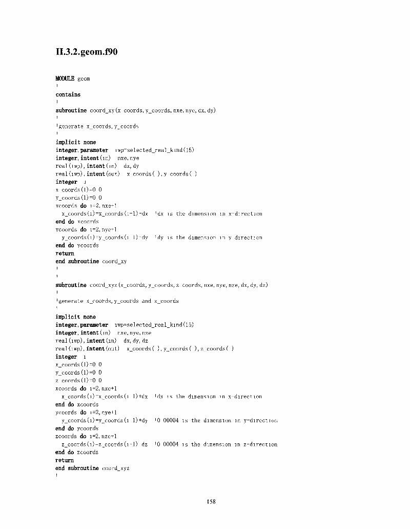
II.3.2.geom.f90
MODULE geom i
contains i
subroutine coord_xy(x coords, y_coords, nxe, nye, dx, dy) i
'generate x_coords, y_coords i
implicit none
integer, parameter iwp=selected_real_kind(l5)
integer, intent (in) nxe, nye
real (lwp), intent (in) dx, dy
real(lwp), intent (out) x_coords( ), y coords( )
integer 1
x_coords(l)=0 0
y_coords(l)=0 0
xcoords do i=2, nxe+1
x_coords(i)=x_coords(]-l)+dx 'dx is the dimension in x-direction
end do xcoords
ycoords do i=2,nye+1
y_coords(i)=y_coords(i l)~dy 'dy is the dimension in y direction
end do ycoords
return
end subroutine coordxy i
i
subroutine coord_xyz (x_coords, y_coords, z coords, nxe, nye, nze, dx, dy, dz) i
'generate x_coords, y_coords and z_coords i
implicit none
integer, parameter iwp=selected_real_kind(15)
integer, intent (in) nxe, nye, nze
real (lwp), intent (in) dx, dy, dz
real(lwp), intent (out) x_coords ( ), y_coords ( ),zcoords ( )
integer I
x_coords(l)=0 0
y_coords(l)=0 0
z coords (l)=0 0
xcoords do i=2,nxe+1
x_coords(i)=x_coords(i l)+dx 'dx is the dimension in x-direction
end do xcoords
ycoords do i=2, nye+1
y_coords(i)=y_coords(l l)+dy '0 00004 is the dimension in y-direction
end do ycoords
zcoords do i=2,nze+1
z_coords(i)=z_coords(i-l)-dz '0 00004 is the dimension in z-direction
end do zcoords
return
end subroutine coordxyz i
158
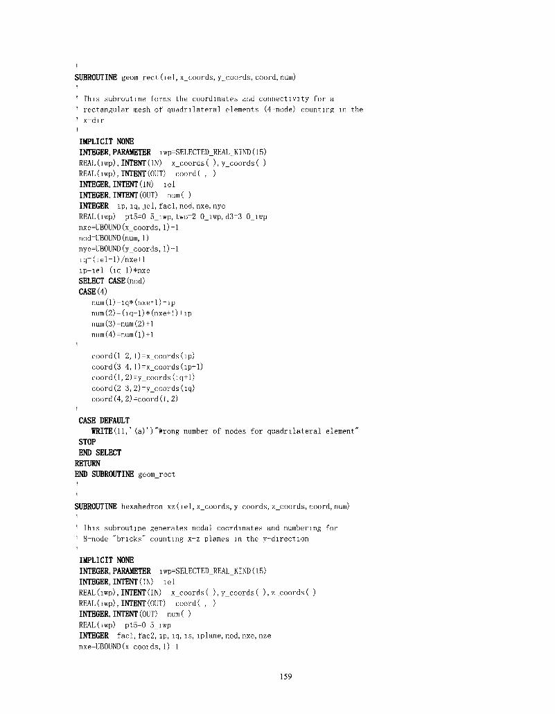
SUBROUTINE geom_rect (lei, x_coords, y^coords, coord, num)
' This subroutine forms the coordinates and connectivity for a 1 rectangular mesh of quadrilateral elements (4-node) counting in the ' x-dir
IMPLICIT NONE INTEGER, PARAMETER iwp=SELECTED_REAL_KIND(15) REAL(iwp), INTENT(IN) x_coords( ),y_coords( ) REAL dwp), INTENT (OUT) coord ( , ) INTEGER, INTENT (IN) lei INTEGER, INTENT (OUT) num( ) INTEGER ip, iq, jel, facl, nod, nxe, nye REAL(iwp) pt5=0 5_iwp, two=2 0_iwp, d3=3 0_iwp nxe=UBOUND(x_coords, 1)-1 nod=UBOUND(num, 1) nye=UBOUND(y_coords, 1)-1
iq=(iel-l)/nxe+l lp-iel (iq-l)*nxe SELECT CASE (nod) CASE (4)
num(l)-iq*(nxe+l)+ip
num(2) = (iq-l)*(nxe+l)+ip num (3)-num (2)+1 num(4)=num(l)+l
i
coord(l 2, l)=x_coords(ip) coord(3 4, l)=x_coords(ip+l) coord (1, 2)=y_coords(iq+l) coord (2 3, 2)=y_coords(iq) coord (4, 2)=coord(l, 2)
i
CASE DEFAULT WRITE(11,' (a)')"Wrong number of nodes for quadrilateral element"
STOP END SELECT RETURN END SUBROUTINE geom_rect i
!
SUBROUTINE hexahedron_xz(iel, x_coords, y_coords, z_coords, coord, num) i
1 lhis subroutine generates nodal coordinates and numbering for 1 8-node "bricks" counting x~z planes in the y-direction i
IMPLICIT NONE INTEGER, PARAMETER iwp=SELECTED_REAL_KIND(15) INTEGER, INTENT(IN) lei REAL (iwp), INTENT (IN) x_coords( ),y_coords( ),z^coords( ) REAL(iwp), INTENT (OUT) coord( , ) INTEGER, INTENT (OUT) num( ) REAL (iwp) pt5=0 5_iwp INTEGER facl, fac2, ip, iq, is, lplane, nod, nxe, nze nxe=UBOUND(x„cooids, 1)-1
159
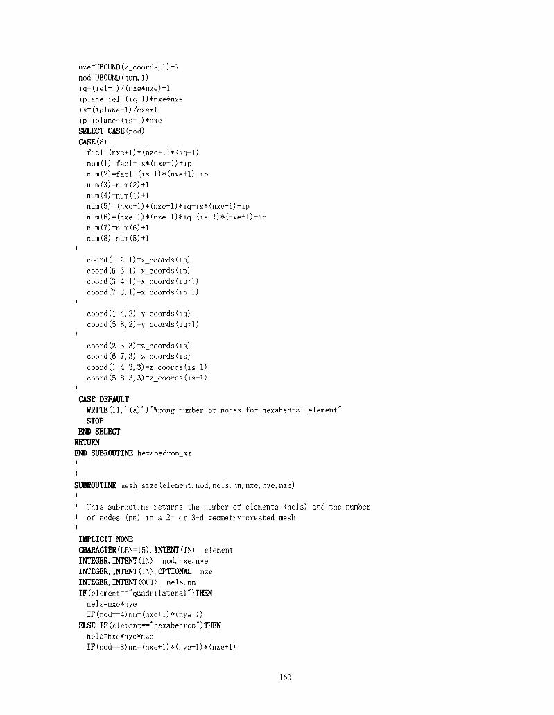
nze=UBOUKD(z_coords, l)-l
nod-UBOUND (num, 1)
iq=(iel-l)/(nxe*nze)+l
iplane~iel-(iq-l)*nxe*nze
is=(iplane~l)/nxe+1
ip=iplane-(is-l)*nxe
SELECT CASE(nod)
CASE (8)
facl-(nxe+1)*(nze+1)* (iq-1)
num (l)-facl + is* (nxe+1)+ip
num(2)=facl+(is-l)*(nxe+l)+ip
num (3)-num (2)+1
num(4)=num(l)+l
num (5) = (nxe+1) * (nze+1) *iq+i s* (nxe+1) +ip
num (6) = (nxe+1) * (nze+1) *iq+(is-l)* (nxe+1 )+ip
num(7)=num(6)+l
num (8)-num (5)+1 i
coord (l 2, l)=x_coords(ip)
coord(5 6, l)-x_coords(ip)
coord (3 4, l)=x_coords(ip+l)
coord(7 8, l)=x_coords(ip+l)
i
coord (l 4, 2)-y_coords(iq)
coord(5 8, 2)=y_coords(iq+l)
i
coord (2 3, 3)=z_coords(is)
coord (6 7, 3)~z_coords(is)
coord(l 4 3, 3)=z_coords(is+l)
coord (5 8 3, 3)~z_coords(is+l) i
CASE DEFAULT
WRITE(ll,' (a)')"Wrong number of nodes for hexahedral element"
STOP
END SELECT
RETURN
END SUBROUTINE hexahedron_xz
i
i
SUBROUTINE mesh_size (element, nod, nels, nn, nxe, nye, nze) i
1 This subroutine returns the number of elements (nels) and the number 1 of nodes (nn) in a 2- or 3~d geometiy-created mesh i
IMPLICIT NONE
CHARACTER(LEN=15), INTENT(IN) element
INTEGER, INTENT (IN) nod, nxe, nye
INTEGER, INTENT(IN), OPTIONAL nze
INTEGER, INTENT (OUT) nel s, nn
IF(element=="quadrilateral")THEN
nels=nxe*nye
IF (nod==4) nn=(nxe+1)*(nye+1)
ELSE IF(element=="hexahedron")THEN
nels=nxe*nye*nze
IF (nod==8)nn-(nxe+1) * (nye+1)* (nze+1)
160

END IF RETURN END SUBROUTINE mesh_size i
END MODULE geom
161
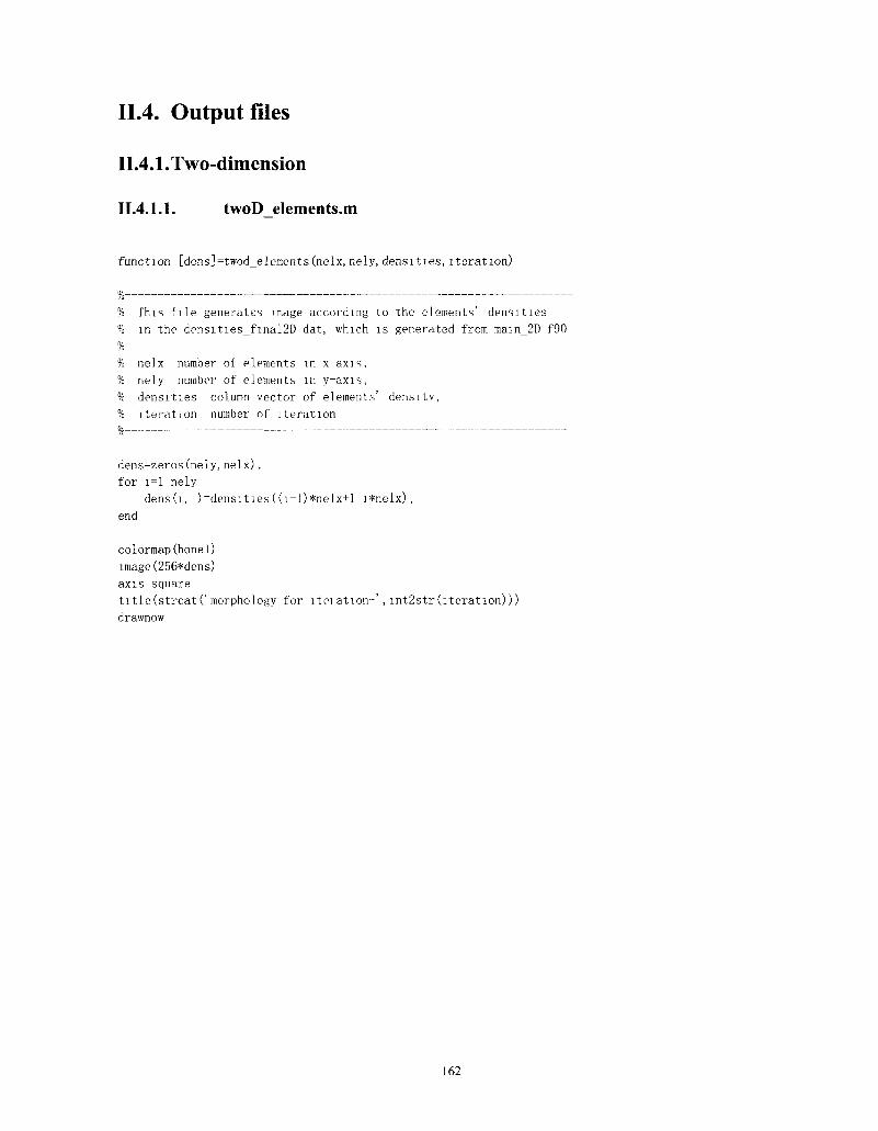
II.4. Output files
II.4.1. Two-dimension
II.4.1.1. twoDelements.m
function [dens]=twod_elements (nelx, nely, densities, iteration)
%
% This file generates image according to the elements' densities
% in the densities_fmal2D dat, which is generated from main_2D f90
%
% nelx number of elements in x~axis,
% nely number of elements in y-axis,
% densities column vector of elements' density,
% iteration number of iteration
%
dens=zeros(nely, nelx) ,
for i=l nely
dens(i, )=densities((i-l)*nelx+l i*nelx) ,
end
colormap(bonel)
image(256*dens)
axis square
title(strcat ('morphology for ltei at ion-' , int2str (iteration)))
drawnow
162
II.4.2.Three-dimension
IL4.2.1. threeDelements.m
function threeDelements (nxe, nye, nze, dx, dy, dz, densities, density)
%
% This tile geneiates image composed of elements according to the
% elements' densities in the densities_f mal3D dat, which is generated
% from main_3D f90
%
% nelx number of elements in x-axis,
% nelv number of elements in y-axis,
% nelz numbei of elements in z~axis,
% dx dimension of element in x-axis,
% dy dimension of element in y~axis
% dz dimension of element in z-axis,
% densities column vector of elements' density,
% density minimal density of element which can be shown in the image %
for a=2 (nxe-1)
for b=2 (nze-1)
for c=2 (nye-1)
iel= (c-1)*nxe*nze+(b~l)*nxe+a,
dens i t ies x=dx*[a-l
a a a-1
y=dy*[c-l c-1 c-1 c-1
( 1 6
a a a a c-c c c-
1)>density
1
1
a a-1 a-1 a c c c c
a-1 a-1 a-1 a-1 c c-1 c-1 c
a-1 a -1 , a a,. . a a,. . a-1 a-1] c-1 c -1 , c-1 c -1 , c c,. . c c ] ,
z=-l*dz*[b-l b-1 b-1 b-1 b-1 b,...
b-1 b-1 b-1 b-1 b-1 b,...
b b b b b-1 b,...
b b b b b-1 b],
clr=[0.4861 0.5486 0.6111],
patch(x, y, z, clr) ,
view (3)
axis equal
hold on
end
end
end
end
163
II.4.2.2. threeD surface.m
function threeD_surface (nxe, nye, nze, dens)
%
% This file generates the surfaces of structure according to the
% elements' densities in the densities_final3D.dat, which is generated
% from main_3D. f90.
%
% nelx: number of elements in x-axis;
% nely: number of elements in y-axis;
% nelz: number of elements in z~axis;
% dens: column vector of elements' density.
%
densl=zeros (nze~2, nxe~2,nye~2);
for b=l:(nze-2)
for a=l: (nxe~2)
for c=l: (nye-2)
densl (c, b, a)=dens ((c+l)*(nze*nxe)-(a+l)*nxe+(b+l)) ;
end
end
end
clr=[0.4861 0.5486 0.6111];
densl=smooth3 (densl, ' gaussian' , 5) ;
pl=patch(isosurface (densl, . 4),' facecolor' , clr,' edgecolor' , ' none') ;
patch (i socaps (densl, . 4), ' facecolor' , clr, ' edgecolor' , ' none' ) ;
isonormals(densl, pi)
view(3) ;
axis vis3d tight
camlight;
lighting phong
164
II.5. Glossary of main variable names
Scalar integers:
iteration
ndim
ndof
nels
neq
nip
ninfe
nn
nod
nodof
nr
nst
nxe
nye
nze
number of total iteration times
number of dimensions
number of degrees of freedom per element
number of elements
number of degrees of freedom in the mesh
number of integrating points per elements
number of elements which are influenced in x-
number of nodes in the mesh
number of nodes per element
number of degree of freedom per node
number of restrained nodes
number of stress (strain) terms (3, 4, or 6)
number of elements in x-direction
number of elements in y-direction
number of elements in z-direction
,or y-,or z-direction
Scalar reals:
det determinant of Jacobian matrix
Dinfl distance of influence
emax maximal Young's modulus of the trabecular tissue
gama exponent of the Young's modulus calculating function
one set to 1.0
maxdens maximal relative density of bone elements
mechanosensitivity mechanosensitivity of osteocytes
mindens minimal relative density of bone elements
165
profactor
resorptionamount
resorptionchance
threshold
v
zero
proportionality factor that regulates the formation rate
amount of bone resorbed by osteoclasts
probability (%) of bone resorption
threshold of bone formation
poisson's ratio of trabecular tissue
set to 0.0
Scalar characters:
element element type
Dynamic integer arrays:
g
g_g
g_num
kdiag
nf
no
node
num
element steering vector
global element steering matrix
global element node numbers matrix
diagonal term location vector
nodal freedom matrix
fixed freedom numbers vector
fixed nodes vector
element node number vector
Dynamic real arrays:
bee
coord
d
dee
der
deriv
dx
eld
strain-displacement matrix
element nodal coordinates
preconditioned rhs vector
stress-strain matrix
shape function derivatives with respect to local coordinates
shape function derivatives with respect to global coordinates
dimension of element in x direction
element nodal displacements
166
fback
fbottom
ffront
fleft
fright
ftop
fun
gc
gcoord
jac
km
kv
loads
points
sigma
weights
xcoords
ycoords
zcoords
external loads on the back surface
external loads on the bottom surface
external loads on the front surface
external loads on the left surface
external loads on the right surface
external loads on the top surface
shape functions
integrating point coordinates
global nodal coordinates
Jacobian matrix
element stiffness matrix
global stiffness matrix
nodal loads and displacements
integrating point local coordinates
stress terms
weighting coefficients
x-coordinates of mesh layout
y-coordinates of mesh layout
z-coordinates of mesh layout
167
Related Documents