Chi Square Goodness of Fit - University of Utahweb.utah.edu/stat/introstats/web-text/chi-square-Fit/chi_good.pdf · There are two different chi square formulas which we will study.

index Page 1 of 24

http://www.utah.edu/stat/introstats/web-text/chi-square-Fit/index.htm 07/12/2000

Chi Square Goodness of FitThis is the text of the in-class lecture which accompanied the Authorware visual graphics

on this topic. You may print this text out and use it as a textbook. Or you may read it

online. In either case it is coordinated with the online Authorware graphics.

Evaluate this StatCenter Function

Copyright Tom Malloy, 2000. All rights reserved

index Page 2 of 24


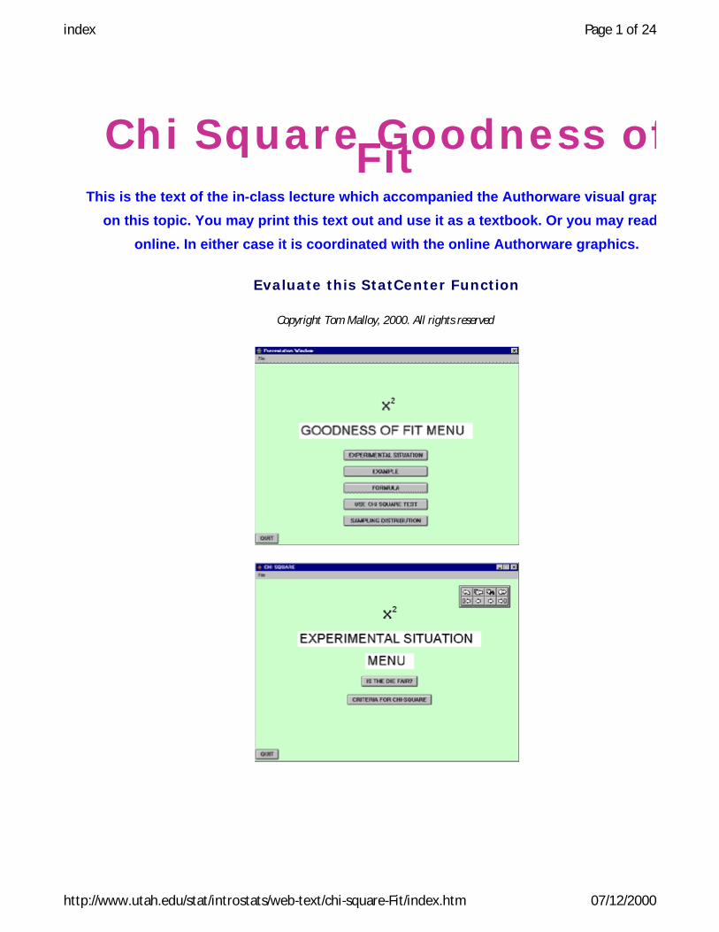
This map allows you to--

1. Jump directly to a topic which interests you. 2. Coordinate the dynamic visual Authorware presentations with the corresponding

text available on this web page.

1. To find a topic which interests you: Look at the map of menus above. Choose a menu that interests you. Notice that the menu buttons have topics printed on them. Click on any button (topic) on the menu; you will jump directly to the text that corresponds to the topic printed on the button.

2. To coordinate this web page with Authorware presentations: The corresponding Authorware program should already be open. Go to the menu of your choice in the Authorware program and click any button which interests you. Then on the topic locator map above click on the same button on the same menu; you will jump to the text that corresponds to the Authorware presentation.

End of Topic Locator Map

Goodness of Fit

There are two different chi square formulas which we will

study. The first one is the chi-square goodness of fit test.

index Page 3 of 24


Go to Top

Ü Ü Þ

index Page 4 of 24


Go to Top

Go to Top

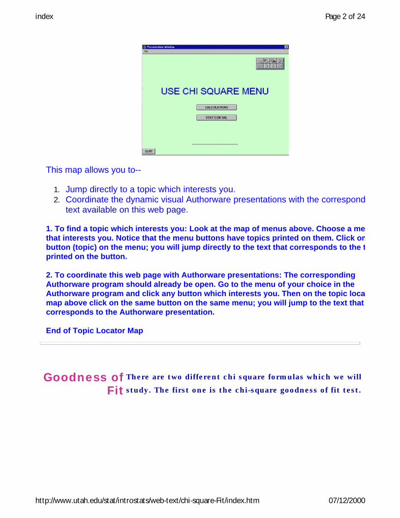
IS THE DIE FAIR?

Experimental Situation and Hypotheses

First, we will examine when to use the

Goodness of Fit Chi-Square. What kind of

research would we be doing that would

prompt us to use this particular test

statistic?

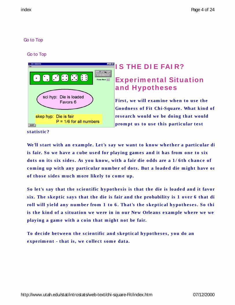
We'll start with an example. Let's say we want to know whether a particular die

is fair. So we have a cube used for playing games and it has from one to six

dots on its six sides. As you know, with a fair die odds are a 1/6th chance of

coming up with any particular number of dots. But a loaded die might have one

of those sides much more likely to come up.

So let's say that the scientific hypothesis is that the die is loaded and it favors

six. The skeptic says that the die is fair and the probability is 1 over 6 that die

roll will yield any number from 1 to 6. That's the skeptical hypotheses. So this

is the kind of a situation we were in in our New Orleans example where we were

playing a game with a coin that might not be fair.

To decide between the scientific and skeptical hypotheses, you do an

experiment - that is, we collect some data.

index Page 5 of 24


Do an Experiment

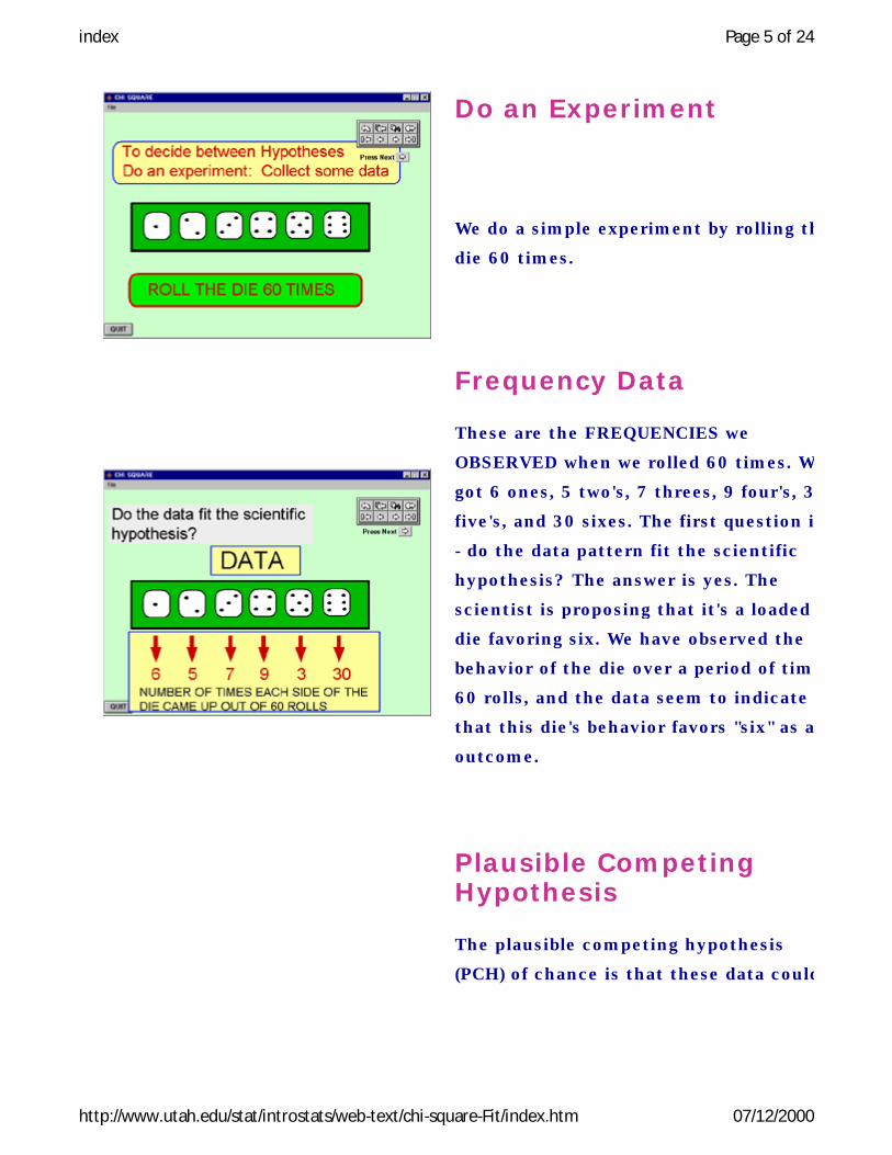
We do a simple experiment by rolling the

die 60 times.

Frequency Data

These are the FREQUENCIES we

OBSERVED when we rolled 60 times. We

got 6 ones, 5 two's, 7 threes, 9 four's, 3

five's, and 30 sixes. The first question is

- do the data pattern fit the scientific

hypothesis? The answer is yes. The

scientist is proposing that it's a loaded

die favoring six. We have observed the

behavior of the die over a period of time,

60 rolls, and the data seem to indicate

that this die's behavior favors "six" as an

outcome.

Plausible Competing Hypothesis

The plausible competing hypothesis

(PCH) of chance is that these data could

index Page 6 of 24


CRITERIA FOR PROPER USE OF CHI SQUARE

Go to Top

Let's discuss the criteria for using Chi Square Goodness of Fit. This is a check

list of things which must be true for the appropriate use of Chi Square

Goodness of Fit test. There are 4 criteria which need to be met.

have come about by chance, simply by

rolling a fair die 60 times. As unlikely as

that seems to the scientist looking at

the data, it certainly is true that by

chance alone the die can give you any

pattern. So it's our usual question: Is

there something systematic going on

here, like a loaded die, or is this

happening by chance?

The goodness of fit chi square can

evaluate the statistical conclusion

validity in cases like this.

Go to Top

index Page 7 of 24


1) PARTITION

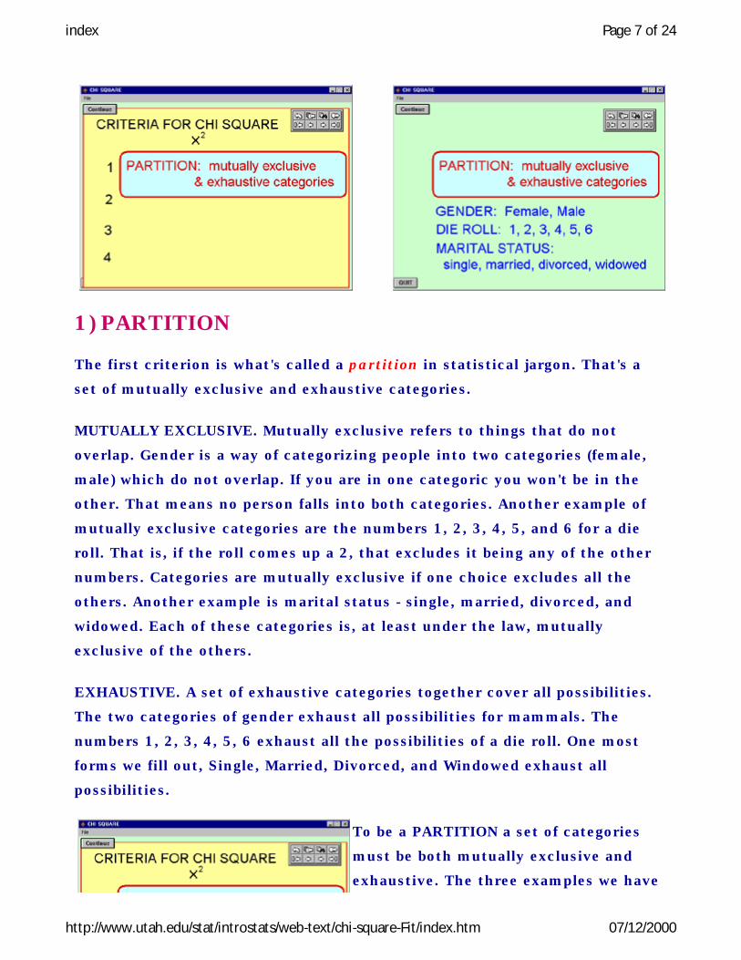
The first criterion is what's called a partition in statistical jargon. That's a

set of mutually exclusive and exhaustive categories.

MUTUALLY EXCLUSIVE. Mutually exclusive refers to things that do not

overlap. Gender is a way of categorizing people into two categories (female,

male) which do not overlap. If you are in one categoric you won't be in the

other. That means no person falls into both categories. Another example of

mutually exclusive categories are the numbers 1, 2, 3, 4, 5, and 6 for a die

roll. That is, if the roll comes up a 2, that excludes it being any of the other

numbers. Categories are mutually exclusive if one choice excludes all the

others. Another example is marital status - single, married, divorced, and

widowed. Each of these categories is, at least under the law, mutually

exclusive of the others.

EXHAUSTIVE. A set of exhaustive categories together cover all possibilities.

The two categories of gender exhaust all possibilities for mammals. The

numbers 1, 2, 3, 4, 5, 6 exhaust all the possibilities of a die roll. One most

forms we fill out, Single, Married, Divorced, and Windowed exhaust all

possibilities.

To be a PARTITION a set of categories

must be both mutually exclusive and

exhaustive. The three examples we have

index Page 8 of 24


been using all are both mutually

exclusive and exhaustive and so they are

partitions.

CATEGORICAL VARIABLES. Sometimes

partitions when used in research are

called "categorical variables."

2) PRIOR PROBABILITIES

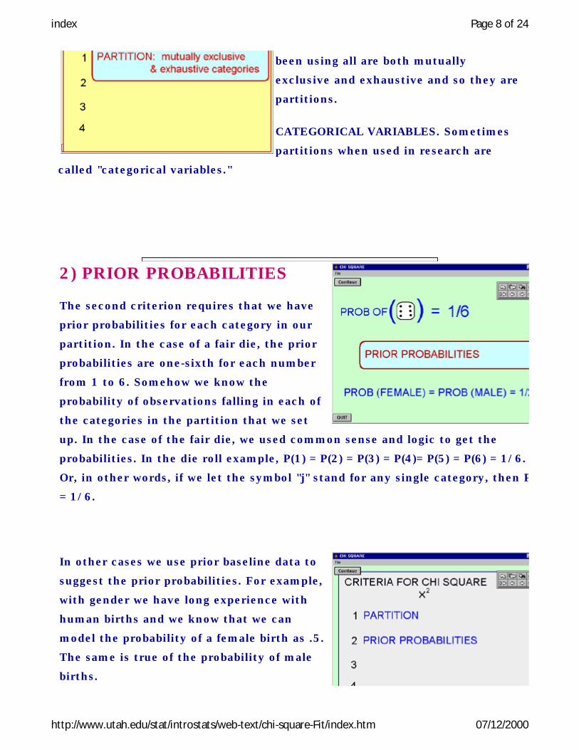
The second criterion requires that we have

prior probabilities for each category in our

partition. In the case of a fair die, the prior

probabilities are one-sixth for each number

from 1 to 6. Somehow we know the

probability of observations falling in each of

the categories in the partition that we set

up. In the case of the fair die, we used common sense and logic to get the

probabilities. In the die roll example, P(1) = P(2) = P(3) = P(4)= P(5) = P(6) = 1/6.

Or, in other words, if we let the symbol "j" stand for any single category, then P(j)

= 1/6.

In other cases we use prior baseline data to

suggest the prior probabilities. For example,

with gender we have long experience with

human births and we know that we can

model the probability of a female birth as .5.

The same is true of the probability of male

births.

index Page 9 of 24


In the die roll example the prior probabilities

are equal in every category. That is peculiar to this example and is not always

true.

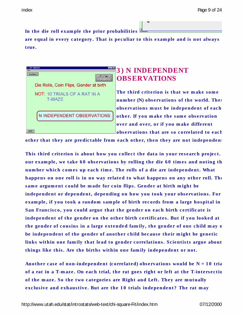
3) N INDEPENDENT OBSERVATIONS

The third criterion is that we make some

number (N) observations of the world. These

observations must be independent of each

other. If you make the same observation

over and over, or if you make different

observations that are so correlated to each

other that they are predictable from each other, then they are not independent.

This third criterion is about how you collect the data in your research project. In

our example, we take 60 observations by rolling the die 60 times and noting the

number which comes up each time. The rolls of a die are independent. What

happens on one roll is in no way related to what happens on any other roll. The

same argument could be made for coin flips. Gender at birth might be

independent or dependent, depending on how you took your observations. For

example, if you took a random sample of birth records from a large hospital in

San Francisco, you could argue that the gender on each birth certificate is

independent of the gender on the other birth certificates. But if you looked at

the gender of cousins in a large extended family, the gender of one child may not

be independent of the gender of another child because their might be genetic

links within one family that lead to gender correlations. Scientists argue about

things like this. Are the births within one family independent or not.

Another case of non-independent (correlated) observations would be N = 10 trials

of a rat in a T-maze. On each trial, the rat goes right or left at the T-intersection

of the maze. So the two categories are Right and Left. They are mutually

exclusive and exhaustive. But are the 10 trials independent? The rat may

index Page 10 of 24


(typically does) have a response bias such that it prefers to turn right or left.

What the rat does on one trial is highly related to what it does on other trials. So

we would argue that these are not 10 independent observations. One the other

hand, take a random sample of 10 rats from a colony who each run the T-maze

once. Categorize the result of each rat as "Right" versus "Left." In this second

case most scientists would construe these to be N = 10 independent

observations.

In the statistical model the Chi Square test

statistic assumes that the N observations are

INDEPENDENT. In the realm of science it's

up to the discretion of the scientific team to

decide with the Chi Square is being properly

applied to a situation in the observations

actually are independent. If they are not, the

statistical procedure may yield misleading

results.

Go to Top

4) FREQUENCY DATA.

Frequency data results when we count the

number of observations that fall in each

category. It's the kind of data we get when

we find ourselves making little "hatch

marks" like on the graphic.

Let's say we have a study in which we're

observing birds spotted up on Red Butte hiking right behind the University of

Utah Hospital. Suppose categorize our observations into Corvids, Raptors, and

Other birds. Corvids are the magpies, ravens, crows, blue jays, and such.

Raptors of course are your various kinds of birds of prey like the hawk falcon.

The category "Other" makes sure that our category system is exhaustive.

index Page 11 of 24


Our data is very simple. We have a sheet of paper and with the names of our

categories on it. Every time we see a bird we put a hatch mark above one of the

category names.

In the data shown on the graphic the frequency of Corvids is 7, the frequency

of Raptors is 4 and of Other birds it is 8.

Of course, for these observations to be independent we have to be sure that we

are not observing the same bird over and over. A well-trained spotter can

distinguish between individual birds of the same species and so not count any

bird twice.

FREQUENCY VERSUS MEASUREMENT DATA. Frequency data is different than

measurement data. Up to now with t-tests and statistics of that type, we were

measuring people and other parts of the world. For instance we would measure a

person's blood pressure. Or we gave people an SAT or ACT. I'm sure you've all

been burdened with at least one of those and you end up with a score, so you've

been measured. Okay so measurement data is usually a fairly complicated

operation that assigns a number to each case.

With frequency data, no measurement is taken. All that is done is to count the

frequency of cases that fall into each category. No measurement is taken. We do

not capture each bird take measurements (weight, wing span). All we do is count

each bird falling into one of our mutually exclusive and exhaustive categories.

That is why these are often called categorical variables

Four criteria

In summary, the four criteria for using the

Chi Square Goodness of Fit Test are 1) a

partition (a set of mutually exclusive and

exhaustive categories), 2) some way to

figure out prior probabilities, 3) some

number of independent observations, and

4) frequency data.

index Page 12 of 24


Let's go back and look at the Example

Go to Top

PRIOR PROBABILITIES

Go to Top

Let's go ahead and continue along with the

die roll example. We have a die and it is

six sided because it's a cube and cubes

have six sides. We put a different number

of dots on each side (1, 2, 3, 4, 5, and 6).

Here the numbers 1 through 6 are merely

the names of categories not actual measurements. We just as well not use

numbers and call the 6 sides of the cube North, South, East, West, Up, and

Down.

Our scientific hypothesis is that the die is loaded and it favors six. The

skeptical hypothesis is that the die is fair. By fair we mean a specific thing. We

mean that the probability is one sixth (1/6th) for every one of the categories

occurring. Let's evaluate whether we are meeting the four criteria. First, we

have six mutually exclusive and exhaustive categories. You can't roll a "one" on

the very same trial that you roll a "two". The categories are mutually exclusive

of each other and they exhaust all possibilities. Second, each category has a

prior probability, at least according to the Skeptical Hypothesis and the PCH of

index Page 13 of 24


Chance. If the skeptic is right and die is fair, chance is the only thing

operating during the research project. So our prior probabilities are one sixth

for each category.

We do an experiment rolling the die 60 times, so we have 60 independent

observations. That meets our third criteria. Finally, we collect frequency data in

our research. We DO NOT measure each die roll (e.g., by count the number of

seconds the die keeps rolling) All we do is count the frequency of times the result

of the roll falls into each category (1 through ).

Expected Frequencies

Now I will introduce an idea which is new

in this course: expected frequencies. We

roll the die 60 times. How many times do

we expect the die to fall into the category

called "One"? How many times into "Two"?

into "Three"? And so forth. We calculate

an expected frequency for each of the six

categories.

We'll denote any particular but unspecified category as category j. By "category

j"we mean one particular category but we're not saying which particular one.

Category j might be 1 or it might be 6, or it might be 4. "j" is what is known as

index Page 14 of 24


a dummy variable.

Each of the categories has a probability denoted by P(j), the prior probability

for that category. For any single category j, the expected frequency for

category j, is the total number of observations (N) times the prior probability

that an observation should fall in that particular category.

The expected frequency in category j is fe(j). fe(j) = P(j)N.

So the expected frequency of getting a one is denoted by fe(1). fe(1) = P(1)N =

(1/6)60 = 10. If the skeptic is correct and the die is fair we expect there to be

about 10 "ones" in 60 rolls.

fe(2) = (1/6)60 = 10, Fe(3) = (1/6)60, and so on.

Observed Frequencies

Observed frequencies result from our

observations of the behavior of the die.

We roll the die 60 times and we're count

the number of 1's, the number of 2's, the

number of 3's, and so on. When we do

that counting by making all those hatch

marks for 60 trials, we will get an actual

observed frequency for each category.

fo(j) is the frequency of observations

that fell into category j. We'll report the

data on a later slide, but when we do,

you will find an observed frequency in

each category.

index Page 15 of 24


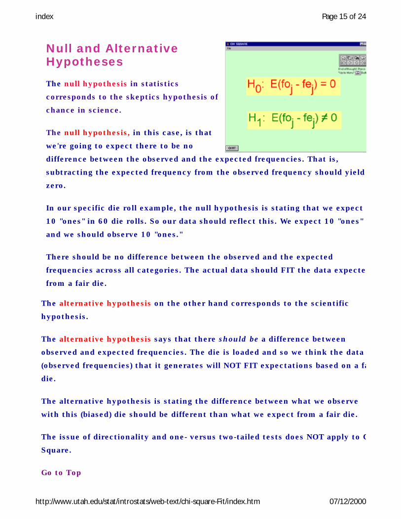
Null and Alternative Hypotheses

The null hypothesis in statistics

corresponds to the skeptics hypothesis of

chance in science.

The null hypothesis, in this case, is that

we're going to expect there to be no

difference between the observed and the expected frequencies. That is,

subtracting the expected frequency from the observed frequency should yield

zero.

In our specific die roll example, the null hypothesis is stating that we expect

10 "ones" in 60 die rolls. So our data should reflect this. We expect 10 "ones"

and we should observe 10 "ones."

There should be no difference between the observed and the expected

frequencies across all categories. The actual data should FIT the data expected

from a fair die.

The alternative hypothesis on the other hand corresponds to the scientific

hypothesis.

The alternative hypothesis says that there should be a difference between

observed and expected frequencies. The die is loaded and so we think the data

(observed frequencies) that it generates will NOT FIT expectations based on a fair

die.

The alternative hypothesis is stating the difference between what we observe

with this (biased) die should be different than what we expect from a fair die.

The issue of directionality and one- versus two-tailed tests does NOT apply to Chi

Square.

Go to Top

index Page 16 of 24


Formula

Examine the formula and write it down in

your notes. It has some similarity to the

formulas that we've already learned for

variance. For each category, we get a

result by calculating the squared distance

between the observed and expected

frequencies and then divide by the

expected frequency. We then add all such results across all categories.

The heart of the formula is the difference between the data we observe in the

world and what we expected to find based on the fair die theory. That is, the

heart of the formula is the difference between foj and Fe(j). The theory said

there was 1/6 chance that a particular roll would fall in each of the categories.

From this P(j) = 1/6, we have deduced our expected frequencies. We collect

data and see whether or not observed frequencies differ from those expected

frequencies. We need to square this deviation of data from expectation because

deviations will always sum to zero. Just as deviations around the mean sum to

zero, so too do the deviations of expected from observed frequencies.

The degrees of freedom are J minus one (J - 1). J is the number of categories,

so you take however many categories you have minus 1. In the die roll

example we have 6 categories so J is equal to six (J = 6) , and J minus one

index Page 17 of 24


Next let's use the formula, do the calculations, and talk about the statistical

conclusion validity.

Go to Top

equals 5 (J - 1 = 5). In the example that I gave with Corvids, raptors, and other,

there were three categories, so there J is three and J minus one is two. The

degrees of freedom is just the number of categories that you have minus one.

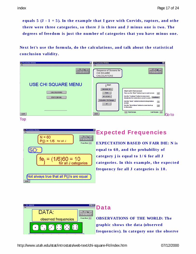
Expected Frequencies

EXPECTATION BASED ON FAIR DIE: N is

equal to 60, and the probability of

category j is equal to 1/6 for all J

categories. In this example, the expected

frequency for all J categories is 10.

Data

OBSERVATIONS OF THE WORLD: The

graphic shows the data (observed

frequencies). In category one the observed

index Page 18 of 24


frequency is 6. That is, we got 6 ones out

of the 60 rolls of the die. The observed

frequency for category 2 was 5. The

observed frequency for category 3 was 7,

for four it was 9, for five it was 3, and the observed frequency for six was 30.

We can see that this data pattern fits the scientific hypothesis. The die

appears to be loaded and it does appear to favor six. If the scientific theory is

true it probably has a lead weight somewhere in the little cube opposite six

because the lead weight would tend to fall to the bottom and therefore force

the six to be facing up.

Of course, the critic will say that the data pattern is due to chance. So we have

to evaluate the PCH of Chance.

The Observed and Expected

Lets summarize the Observed and

expected frequencies all on one graphic.

The observed frequencies are 6, 5, 7, 9, 3,

30 for the six categories. And the expected

frequencies are 10 for each category based

on the hypothesis of a fair die. If you just

picture the formula in your head, you'll

notice that the key part of it is the

deviation between observed and expected

frequency in each category. We're going to

take that deviation and we're going to

square it.

index Page 19 of 24


Substitute Values into the Formula

Substitute in the values on your own and

then the next screen will show you my

substitution.

Here are the values substituted into the formula. The chi square here is six

minus 10 squared over 10, 5 minus 10 squared over 10, 7 minus 10 squared

over 10, 9 minus 10 squared over 10, 3 minus 10 squared over 10, and 30

minus 10 squared over 10. The expected frequency is the same in every case,

remember that's not always true, but here each is the same. You just take the

difference between what science observes and the theory expected, and

squaring that, and then normalize it to what we expected. This comes out to a

chi square of 500 over 10, or a chi square of 50. That's a large chi square value,

obviously I loaded the example to really make it look like a loaded die.

index Page 20 of 24


Go to Top

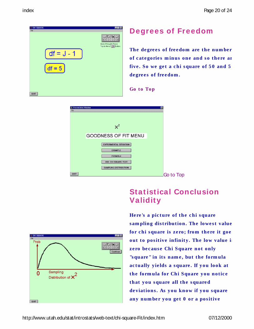
Degrees of Freedom

The degrees of freedom are the number

of categories minus one and so there are

five. So we get a chi square of 50 and 5

degrees of freedom.

Go to Top

Statistical Conclusion Validity

Here's a picture of the chi square

sampling distribution. The lowest value

for chi square is zero; from there it goes

out to positive infinity. The low value is

zero because Chi Square not only

"square" in its name, but the formula

actually yields a square. If you look at

the formula for Chi Square you notice

that you square all the squared

deviations. As you know if you square

any number you get 0 or a positive

index Page 21 of 24


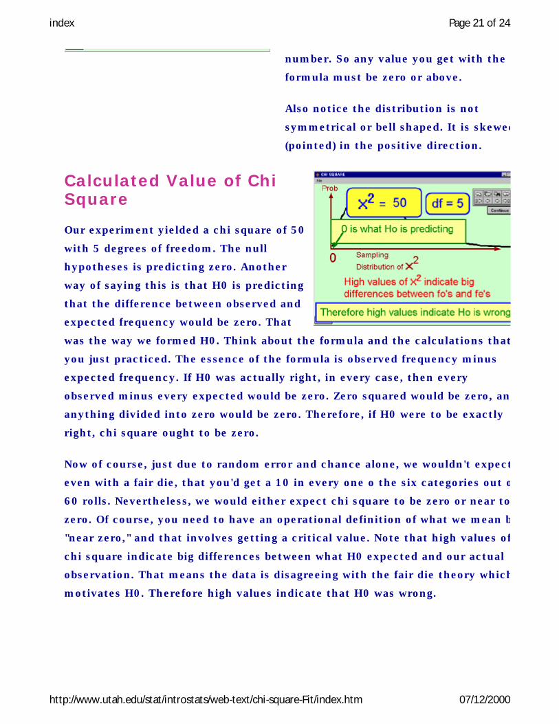
number. So any value you get with the

formula must be zero or above.

Also notice the distribution is not

symmetrical or bell shaped. It is skewed

(pointed) in the positive direction.

Calculated Value of Chi Square

Our experiment yielded a chi square of 50

with 5 degrees of freedom. The null

hypotheses is predicting zero. Another

way of saying this is that H0 is predicting

that the difference between observed and

expected frequency would be zero. That

was the way we formed H0. Think about the formula and the calculations that

you just practiced. The essence of the formula is observed frequency minus

expected frequency. If H0 was actually right, in every case, then every

observed minus every expected would be zero. Zero squared would be zero, and

anything divided into zero would be zero. Therefore, if H0 were to be exactly

right, chi square ought to be zero.

Now of course, just due to random error and chance alone, we wouldn't expect

even with a fair die, that you'd get a 10 in every one o the six categories out of

60 rolls. Nevertheless, we would either expect chi square to be zero or near to

zero. Of course, you need to have an operational definition of what we mean by

"near zero," and that involves getting a critical value. Note that high values of

chi square indicate big differences between what H0 expected and our actual

observation. That means the data is disagreeing with the fair die theory which

motivates H0. Therefore high values indicate that H0 was wrong.

index Page 22 of 24


Critical Value of Chi-Square

In this case, the critical value of chi

square happens to be 11.07, if I use an

alpha value of .05. There is no distinction

of directionality, one-tailed or two-tailed

with this test.

You can get the critical values for Chi Square from a table on StatCenter. You

can download it or print it out. The chi square table is similar to the t-table. It

has degrees of freedom running down the rows and the alpha levels across the

top. There won't be any distinction between one and two tailed tests, so it's a

simpler table to use.

In this particular case, the critical value for Chi Square is 11.07, whereas the

calculated value is 50. That means that the calculated value is in the rejection

region, and we will reject H0 by our usual logic.

A little more theoretically stated, H0 is expecting zero or near zero. You can

see by the shape of the distribution that if H0 is correct then there will be a

probability bulge in the neighborhood of zero. If H0 is correct then there will

be a very small probability of getting beyond critical value of 11.07. In this

case, since we chose alpha =.05, if H0 is correct the probability of falling

beyond 11.07 is about 1 in 20. We have decided we will reject H0 for any score

above 11.07. In other words we will consider calculated Chi Square above 11.07

as so improbable that we're not going to believe H0.

Of course, there is always a little possibility that we're wrong because maybe

H0 is correct and we just sampled low probability data. The probability that

we're wrong when we reject H0 is .05. That's always been our definition of

alpha. Alpha is the probability that you're wrong when you reject H0. This is

the very heart of the whole logic of statistical tests.

index Page 23 of 24


Go to Top

Nevertheless, we always keep in mind that the way we made this decision in

statistics was probabilistic. There is always a small chance that we made an

error in rejecting H0. We can't be perfectly certain when using probabilistic

model like statistics. We always leave this little error and we always tell the

world specifically what the probability is that we're wrong. That way other

people can evaluate what we have done.

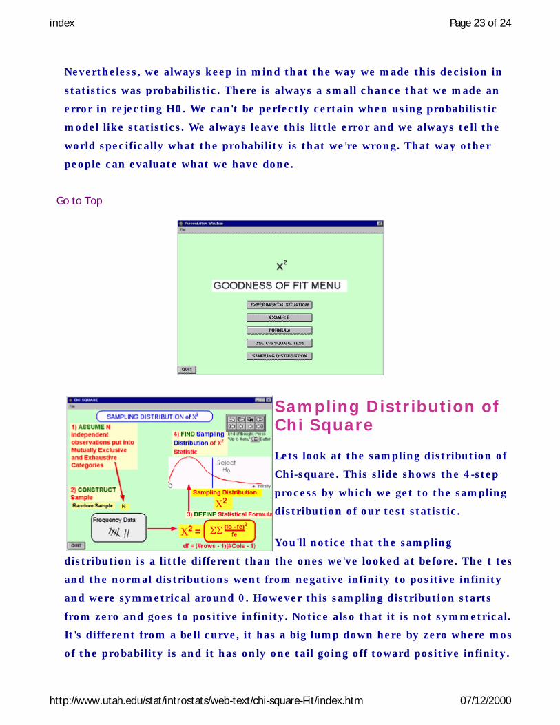
Sampling Distribution of Chi Square

Lets look at the sampling distribution of

Chi-square. This slide shows the 4-step

process by which we get to the sampling

distribution of our test statistic.

You'll notice that the sampling

distribution is a little different than the ones we've looked at before. The t test

and the normal distributions went from negative infinity to positive infinity

and were symmetrical around 0. However this sampling distribution starts

from zero and goes to positive infinity. Notice also that it is not symmetrical.

It's different from a bell curve, it has a big lump down here by zero where most

of the probability is and it has only one tail going off toward positive infinity.

index Page 24 of 24


©Copyright 1997, 2000 Tom Malloy

So you can see that this is going to be different kind of test.

Go to Top

Chi Square Goodness of Fit - University of Utahweb.utah.edu/stat/introstats/web-text/chi-square-Fit/chi_good.pdf · There are two different chi square formulas which we will study.

Documents