Appendix A - Springer LINK

Appendix AProbability Distributions

A.1 Discrete Distributions

A.1.1 Binomial Distribution

The binomial distribution (Bernoulli model) describes the number of failures, X, inn independent Bernoulli trials. The random variable X has a binomial distributionif:

• The number of random trials is one or more and is known in advance.• Each trial results in one of two outcomes, usually called success and failure

(or could be pass-fail, hit-miss, defective-nondefective, etc.).• The outcomes for each trial are statistically independent of the outcomes of

other trials.• The probability of failure, p, is constant across trials.

Equal to the number of failures (or successes depending upon the context) in then trials, a binomial random variable X can take on any integer value from 0 to n,inclusive of the endpoints. The probability associated with each of these possibleoutcomes, x, is given by the binomial(n, p) probability density (mass) function(pdf) as

PrðX ¼ xÞ ¼ nx

� �pxð1� pÞn�x; x ¼ 0; . . .; n

Here

nx

� �¼ n!

x!ðn� xÞ!

is the binomial coefficient and n! = n(n - 1)(n - 2) … (2)(1), the factorialfunction, with 0! defined to be equal to 1. The binomial coefficient provides thenumber of ways in which exactly x failures can occur in n trials (number of

D. Kelly and C. Smith, Bayesian Inference for Probabilistic Risk Assessment,Springer Series in Reliability Engineering, DOI: 10.1007/978-1-84996-187-5,� Springer-Verlag London Limited 2011

201

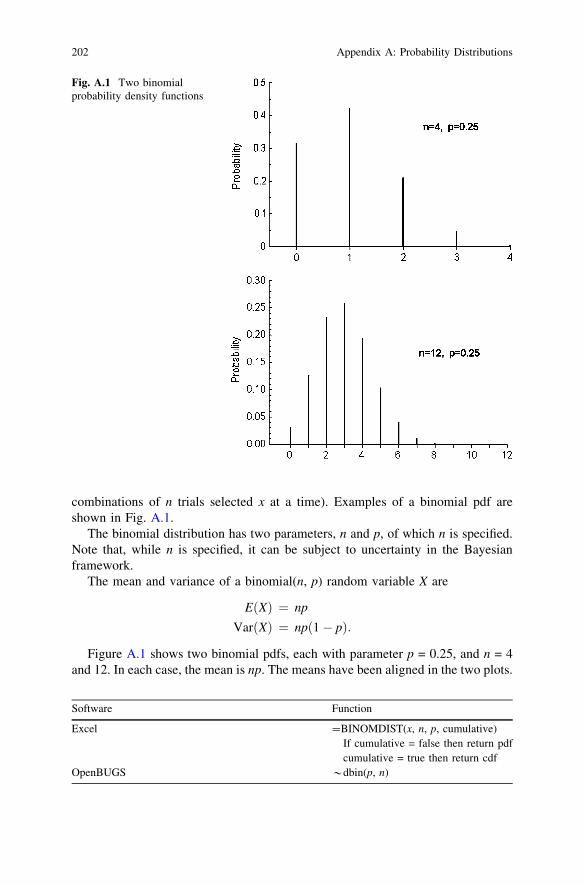
combinations of n trials selected x at a time). Examples of a binomial pdf areshown in Fig. A.1.

The binomial distribution has two parameters, n and p, of which n is specified.Note that, while n is specified, it can be subject to uncertainty in the Bayesianframework.

The mean and variance of a binomial(n, p) random variable X are

E Xð Þ ¼ np

Var Xð Þ ¼ np 1� pð Þ:

Figure A.1 shows two binomial pdfs, each with parameter p = 0.25, and n = 4and 12. In each case, the mean is np. The means have been aligned in the two plots.

Software Function

Excel =BINOMDIST(x, n, p, cumulative)If cumulative = false then return pdfcumulative = true then return cdf

OpenBUGS *dbin(p, n)

Fig. A.1 Two binomialprobability density functions

202 Appendix A: Probability Distributions

A.1.2 Poisson Distribution

The Poisson distribution describes the total number of events occurring in someinterval of time(t) or space. The pdf of a Poisson random variable X, withparameter l = kt, is

PrðX ¼ xÞ ¼ e�llx

x!¼ e�kt ktð Þx

x!

for x = 0, 1, 2, …, and x! = x (x - 1) (x - 2) … (2)(1), as defined previously.Several conditions are assumed to hold for a Poisson process that produces a

Poisson random variable:

• For small intervals, the probability of exactly one occurrence is approximatelyproportional to the length of the interval (where k, the event rate or intensity, isthe constant of proportionality).

• For small intervals, the probability of more than one occurrence is essentiallyequal to zero (see below).

• The numbers of occurrences in two non-overlapping intervals are statisticallyindependent.

The Poisson distribution has a single parameter l, denoted Poisson(l).If X denotes the number of events that occur during some time period of length t,then X is often assumed to have a Poisson distribution with parameter l = kt.In this case, X is generated by a Poisson process with intensity k [ 0.The parameter k is also referred to as the event rate (or failure rate when the eventsare failures). Note that k has units 1/time; thus, kt = l is dimensionless.

The expected number of events occurring in the interval 0 to t is l = kt. Thus,the mean of the Poisson distribution is equal to the parameter of the distribution,which is why l is often used to represent the parameter. The variance of thePoisson distribution is also equal to the parameter of the distribution. Therefore,for a Poisson(l) random variable X,

E Xð Þ ¼ Var Xð Þ ¼ l ¼ kt:

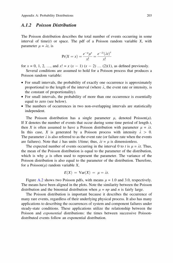
Figure A.2 shows two Poisson pdfs, with means l = 1.0 and 3.0, respectively.The means have been aligned in the plots. Note the similarity between the Poissondistribution and the binomial distribution when l = np and n is fairly large.

The Poisson distribution is important because it describes the occurrence ofmany rare events, regardless of their underlying physical process. It also has manyapplications to describing the occurrences of system and component failures understeady-state conditions. These applications utilize the relationship between thePoisson and exponential distributions: the times between successive Poisson-distributed events follow an exponential distribution.

Appendix A: Probability Distributions 203

A.1.3 Multinomial Distribution

This is an extension to the binomial distribution, where there are more than twopossible outcomes. It is the aleatory model most commonly used for common-cause failure. The observed data typically are in the form of a vector of eventcounts, n = (n1, n2,…, nk), with Rni = N. The pdf is given by

f ðn1; . . .; nmÞ ¼N

n1n2 � � � nm

� �an1

1 an22 � � � anm

m

Fig. A.2 Two Poissonprobability density functions

Software Function

Excel =POISSON(x, mu, cumulative)mu is the meanIf cumulative = false then return pdfCumulative = true then return cdf

OpenBUGS *dpois(lambda)Lambda is the mean


where

Nn1 � � � nm

� �¼ N!

n1! � � � nm!

The marginal means and variances are E(ni) = Nai and Var(ni) = Nai(1 – ai),respectively. The multinomial distribution is specified as a model in OpenBUGSas n[1:m] * dmulti(alpha[1:m], N).

A.2 Continuous Random Variables

A.2.1 Uniform Distribution

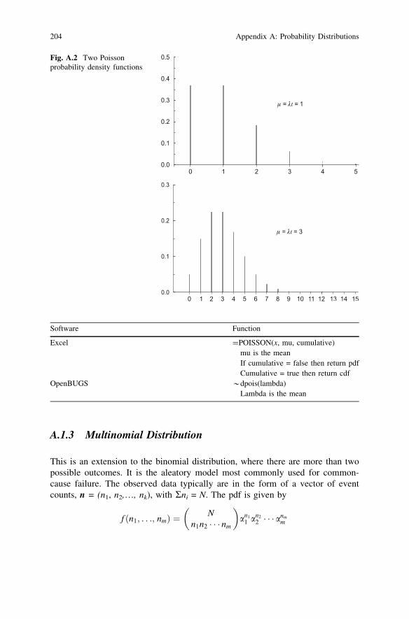
A uniform distribution represents the case where any value in a specified interval[a, b] is equally likely. For a uniform random variable, X, because the outcomesare equally likely, the pdf f(x) is equal to a constant. The pdf of a uniformdistribution with parameters a and b, denoted uniform(a, b) is

f ðxÞ ¼ 1b� a

for a� x� b:

Figure A.3 shows the density of the uniform(a, b) distribution.The mean and variance of a uniform(a, b) distribution are

EðXÞ ¼ bþ a

2

and

Var(X) ¼ b� að Þ2

12

GC00 0432 6a

Area = 1

0

1/(b-a)

b

Fig. A.3 Uniform(a, b) distribution


Software Function

Excel =(b – a) * percentile + aReturns the value for the percentile specified

OpenBUGS *dunif(a, b)

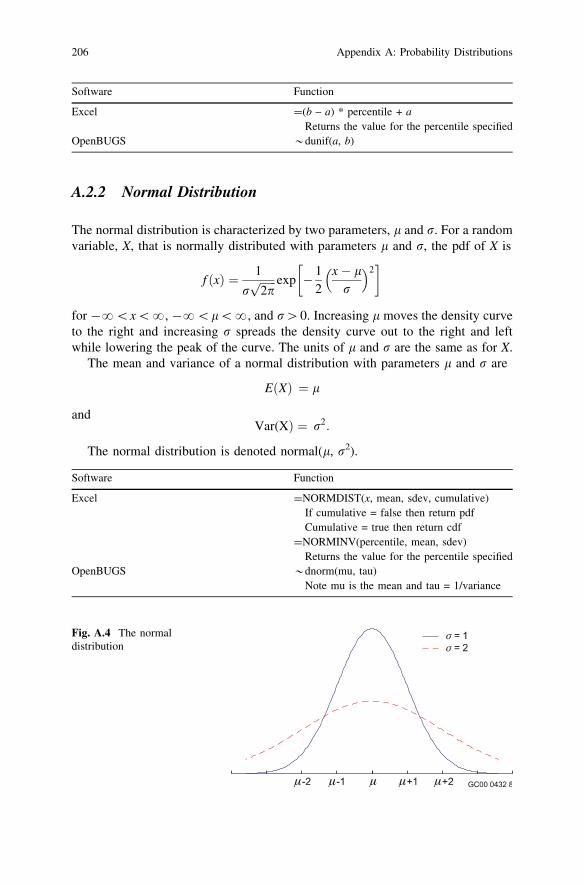
A.2.2 Normal Distribution

The normal distribution is characterized by two parameters, l and r. For a randomvariable, X, that is normally distributed with parameters l and r, the pdf of X is

f ðxÞ ¼ 1

rffiffiffiffiffiffi2pp exp � 1

2x� l

r

� �2� �

for -?\x\?, -?\l\?, and r[0. Increasing l moves the density curveto the right and increasing r spreads the density curve out to the right and leftwhile lowering the peak of the curve. The units of l and r are the same as for X.

The mean and variance of a normal distribution with parameters l and r are

E Xð Þ ¼ l

andVar(XÞ ¼ r2:

The normal distribution is denoted normal(l, r2).

Software Function

Excel =NORMDIST(x, mean, sdev, cumulative)If cumulative = false then return pdfCumulative = true then return cdf

=NORMINV(percentile, mean, sdev)Returns the value for the percentile specified

OpenBUGS *dnorm(mu, tau)Note mu is the mean and tau = 1/variance

Fig. A.4 The normaldistribution


0 1E-3 2E-3 3E-3

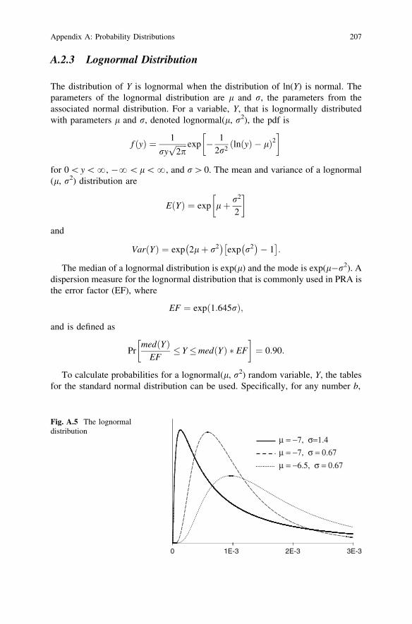
μ = −7, σ=1.4μ = −7, σ = 0.67μ = −6.5, σ = 0.67

Fig. A.5 The lognormaldistribution


A.2.3 Lognormal Distribution

The distribution of Y is lognormal when the distribution of ln(Y) is normal. Theparameters of the lognormal distribution are l and r, the parameters from theassociated normal distribution. For a variable, Y, that is lognormally distributedwith parameters l and r, denoted lognormal(l, r2), the pdf is

f ðyÞ ¼ 1

ryffiffiffiffiffiffi2pp exp � 1

2r2lnðyÞ � lð Þ2

� �

for 0\y\?, -?\l\?, and r[0. The mean and variance of a lognormal(l, r2) distribution are

EðYÞ ¼ exp lþ r2

2

� �

and

VarðYÞ ¼ exp 2lþ r2

exp r2

� 1� �

:

The median of a lognormal distribution is exp(l) and the mode is exp(l-r2). Adispersion measure for the lognormal distribution that is commonly used in PRA isthe error factor (EF), where

EF ¼ expð1:645rÞ;

and is defined as

PrmedðYÞ

EF� Y �medðYÞ � EF

� �¼ 0:90:

To calculate probabilities for a lognormal(l, r2) random variable, Y, the tablesfor the standard normal distribution can be used. Specifically, for any number b,

Pr Y � b½ � ¼ Pr lnðYÞ� lnðbÞ½ � ¼ Pr X� lnðbÞ½ �

¼ UðlnðbÞ � lÞ

r

� �

where X = ln(Y) is normal(l, r2).

Software Function

Excel =LOGNORMDIST(x, mean, sdev)Returns the cdf only

=LOGINV(percentile, mean, sdev)Returns the value for the percentile specified

OpenBUGS *dlnorm(mu, tau)Note mu is the logarithmic mean and tau = 1/(logarithmic variance)

A.2.4 Logistic-normal Distribution

The logistic-normal distribution is not used widely in PRA, but it can be useful as aprior distribution for p in the binomial distribution, especially in settings where thevalues of p are expected to be large. Past PRAs have often used the lognormaldistribution to represent uncertainty in p, and problems can be encountered in suchcases, because values of the lognormal distribution are not constrained to be in theinterval [0, 1]. The logistic-normal distribution can be an alternative to the lognormaldistribution in cases where the heavy tail of the lognormal distribution (relative to aconjugate beta prior) is attractive, but which avoids the problem of having values ofp[1, because the values of the logistic-normal distribution lie in the interval [0, 1].

The pdf is given by

f ðpÞ ¼ 1ffiffiffiffiffiffi2pp

rp 1� pð Þexp �

ln p1�p

� �� l

h i2

2r2

8><>:

9>=>;

Like the lognormal distribution, l and r2 are the parameters of an underlyingnormal distribution. In this case ln[p/(1 – p)] is normal(l, r2). Just as percentiles ofa lognormal distribution were related to percentiles of the underlying normaldistribution, a similar relationship holds here. Percentiles of the logistic-normaldistribution are given by

pq ¼exp yq

1þ exp yq

where yq is the (q 9 100)th percentile of the underlying normal distribution. Forexample, the 95th percentile of p is given by


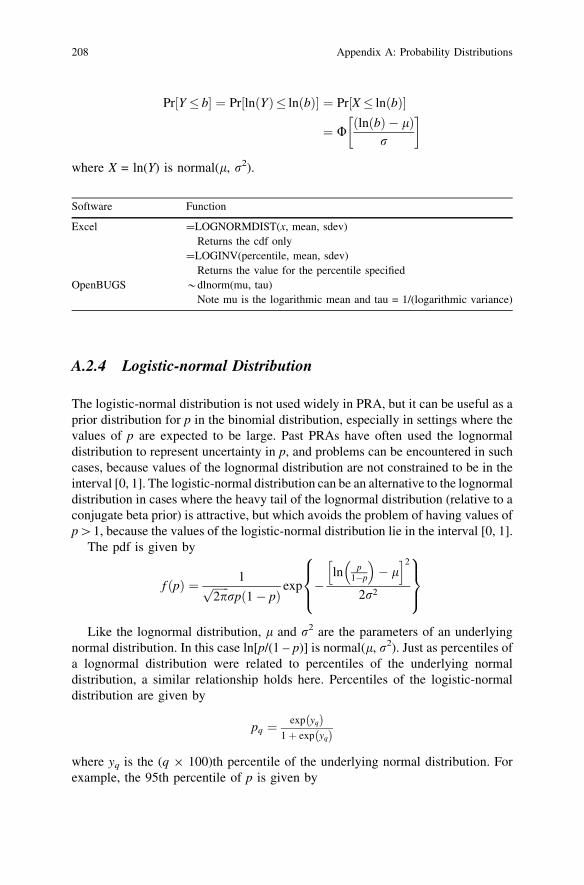
p0:95 ¼exp lþ 1:645rð Þ

1þ exp lþ 1:645rð Þ

The moments of the logistic-normal distribution must be found numerically, asthere is no closed-form analytic expression for the integrals involved. However, itis not difficult to find the moments with modern software.

The logistic-normal pdf can take on a variety of shapes, as shown in Fig. A.6.The logistic-normal distribution is not available directly in OpenBUGS, but can beentered by specifying a normal distribution for the underlying variable, and thendefining the logistic-normal distribution in terms of the inverse logittransformation. For example, to enter a logistic-normal distribution with l = -5and r = 1.2, one would need the following lines of script in OpenBUGS:

A.2.5 Exponential Distribution

For a Poisson random variable X representing the number of events in a timeinterval t and for a random variable T defining the time between events, it can beshown that T has the exponential pdf

Fig. A.6 Logistic-normal densities, each with median equal to 0.5


p.norm * dnorm(mu, tau)tau \- pow(sigma, -2)p \- exp(p.norm)/(1 + exp(p.norm))datalist(mu=-5, sigma=1.2)

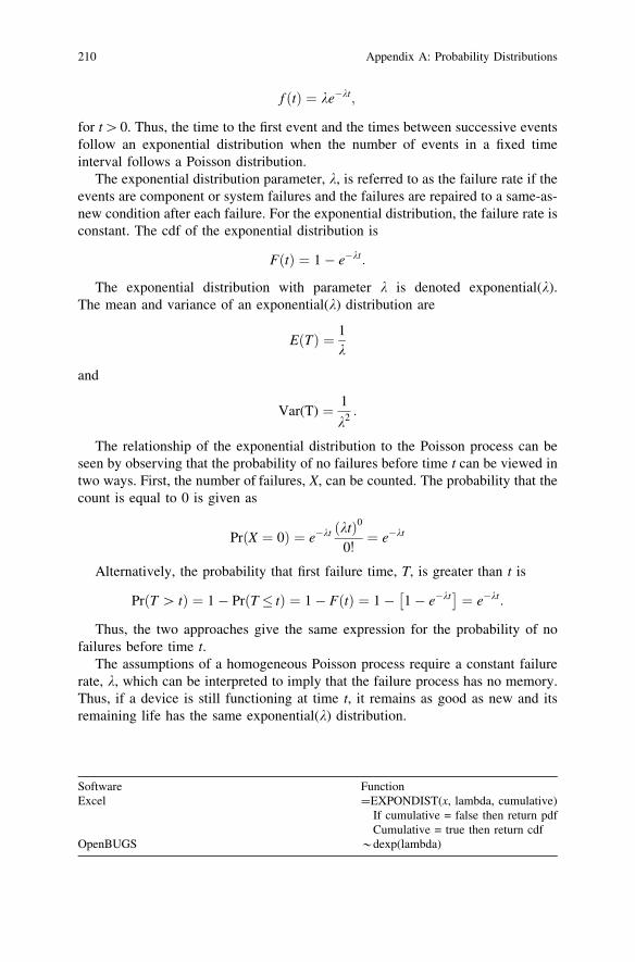
f ðtÞ ¼ ke�kt;

for t[0. Thus, the time to the first event and the times between successive eventsfollow an exponential distribution when the number of events in a fixed timeinterval follows a Poisson distribution.

The exponential distribution parameter, k, is referred to as the failure rate if theevents are component or system failures and the failures are repaired to a same-as-new condition after each failure. For the exponential distribution, the failure rate isconstant. The cdf of the exponential distribution is

FðtÞ ¼ 1� e�kt:

The exponential distribution with parameter k is denoted exponential(k).The mean and variance of an exponential(k) distribution are

EðTÞ ¼ 1k

and

Var(T) ¼ 1

k2 :

The relationship of the exponential distribution to the Poisson process can beseen by observing that the probability of no failures before time t can be viewed intwo ways. First, the number of failures, X, can be counted. The probability that thecount is equal to 0 is given as

PrðX ¼ 0Þ ¼ e�kt ktð Þ0

0!¼ e�kt

Alternatively, the probability that first failure time, T, is greater than t is

PrðT [ tÞ ¼ 1� PrðT � tÞ ¼ 1� FðtÞ ¼ 1� 1� e�kt� �

¼ e�kt:

Thus, the two approaches give the same expression for the probability of nofailures before time t.

The assumptions of a homogeneous Poisson process require a constant failurerate, k, which can be interpreted to imply that the failure process has no memory.Thus, if a device is still functioning at time t, it remains as good as new and itsremaining life has the same exponential(k) distribution.


Software FunctionExcel =EXPONDIST(x, lambda, cumulative)

If cumulative = false then return pdfCumulative = true then return cdf

OpenBUGS *dexp(lambda)

A.2.6 Weibull Distribution

For a random variable, T, that has a Weibull distribution, the pdf is

f ðtÞ ¼ ba

t

a

� �b�1exp � t

a

� �b� �

;

for t C 0 and parameters a[ 0 and b[ 0. The cdf for T is

FðtÞ ¼ 1� expt

a

� �b� �

;

for t C 0.OpenBUGS uses a different parameterization, obtained by defining k = a-b. In

this parameterization the pdf is given by

f ðtÞ ¼ bktb�1exp �ktb

and cdf given by

FðtÞ ¼ 1� exp �ktb

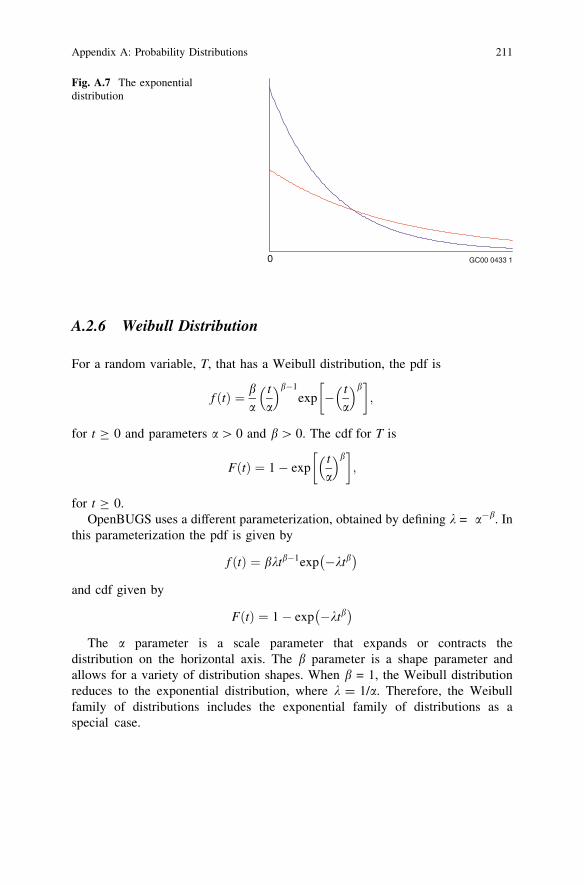
The a parameter is a scale parameter that expands or contracts thedistribution on the horizontal axis. The b parameter is a shape parameter andallows for a variety of distribution shapes. When b = 1, the Weibull distributionreduces to the exponential distribution, where k = 1/a. Therefore, the Weibullfamily of distributions includes the exponential family of distributions as aspecial case.

0 GC00 0433 1

Fig. A.7 The exponentialdistribution


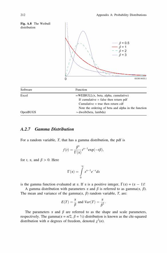
Fig. A.8 The Weibulldistribution

Software Function

Excel =WEIBULL(x, beta, alpha, cumulative)If cumulative = false then return pdfCumulative = true then return cdfNote the ordering of beta and alpha in the function

OpenBUGS *dweib(beta, lambda)

A.2.7 Gamma Distribution

For a random variable, T, that has a gamma distribution, the pdf is

f ðtÞ ¼ ba

CðaÞ ta�1expð�tbÞ;

for t, a, and b [ 0. Here

CðaÞ ¼Z1

0

xa�1e�xdx

is the gamma function evaluated at a. If a is a positive integer, C(a) = (a - 1)!A gamma distribution with parameters a and b is referred to as gamma(a, b).

The mean and variance of the gamma(a, b) random variable, T, are:

EðTÞ ¼ ab

and VarðTÞ ¼ a

b2 :

The parameters a and b are referred to as the shape and scale parameters,respectively. The gamma(a = n/2, b = �) distribution is known as the chi-squareddistribution with n degrees of freedom, denoted v2(n).


For the gamma distribution, when a\1, the density has a vertical asymptote att = 0. When a = 1, the gamma distribution reduces to an exponential distribution.When a is large, the distribution is approximately a normal distribution.

Software Function

Excel =GAMMADIST(x, alpha, 1/beta, cumulative)If cumulative = false then return pdfCumulative = true then return cdf

=GAMMAINV(percentile, alpha, 1/beta)Returns the value for the percentile specified

OpenBUGS *dgamma(alpha, beta)

A.2.8 Beta Distribution

The pdf of a beta random variable, Y, is

f ðyÞ ¼ C aþ bð ÞCðaÞCðbÞ y

a�1 1� yð Þb�1;

for 0 B y B 1, with the parameters a, b[0, and is denoted beta(a, b). The gammafunctions at the front of the pdf form a normalizing constant so that the densityintegrates to 1. The pdf can also be written as

f ðyÞ ¼ ya�1ð1� yÞb�1

Bða;bÞ

Fig. A.9 The gammadistribution


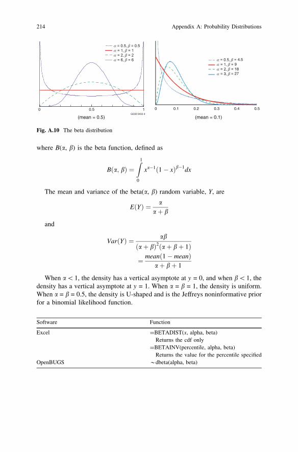
where B(a, b) is the beta function, defined as

Bða; bÞ ¼Z1

0

xa�1 1� xð Þb�1dx

The mean and variance of the beta(a, b) random variable, Y, are

EðYÞ ¼ aaþ b

and

VarðYÞ ¼ ab

aþ bð Þ2 aþ bþ 1ð Þ

¼ mean 1� meanð Þaþ bþ 1

When a\1, the density has a vertical asymptote at y = 0, and when b\1, thedensity has a vertical asymptote at y = 1. When a = b = 1, the density is uniform.When a = b = 0.5, the density is U-shaped and is the Jeffreys noninformative priorfor a binomial likelihood function.

Software Function

Excel =BETADIST(x, alpha, beta)Returns the cdf only

=BETAINV(percentile, alpha, beta)Returns the value for the percentile specified

OpenBUGS *dbeta(alpha, beta)

4.5918

0

(mean = 0.5) (mean = 0.1)

0.1 0.2 0.3 0.4 0.5

273

Fig. A.10 The beta distribution


A.2.9 Dirichlet Distribution

The Dirichlet distribution is the conjugate prior to the multinomial distribution,and is most commonly used in PRA as a prior distribution for the alpha factors inthe alpha-factor model of common-cause failure. It is a multivariate extension ofthe beta distribution. Its pdf is given by

f ða1; . . .; amÞ ¼C a1 þ � � � þ amð ÞC a1ð Þ � � �C amð Þ

ha1�11 � � � ham�1

m ;Xm

i¼1

ai ¼ 1

The marginal means are given by

EðaiÞ ¼hi

ht; ht ¼

Xm

j¼1

hj

The marginal variances are given by

Var aið Þ ¼hi ht � hið Þh2

t ht þ 1ð Þ

The marginal distribution of each ai is beta(hi, ht – hi). The Dirichletdistribution is specified in OpenBUGS as alpha[1: m] * ddirich(theta[1: m]).


Appendix BGuidance for Using OpenBUGS

B.1 WinBUGS and OpenBUGS

BUGS is the acronym for Bayesian inference Using Gibbs Sampling. WinBUGS isfreely available software for implementing Markov chain Monte Carlo (MCMC)sampling. The open source version can be found at the URL: www.openbugs.info

Both versions are commonly referred to as WinBUGS or just BUGS.OpenBUGS is commonly used independently but can be called from other

programs through shell commands or from the open-source statistical program Rthrough the R2WinBUGS or BRUGS packages for R. For more information on R,see the R Project homepage, www.r-project.org.

The OpenBUGS user manual (Spiegelhalter et al. 2007) comes with theprogram and is the basis for much of this appendix.

B.1.1 Distributions Supported in OpenBUGS

Over 20 distributions are supported in OpenBUGS. Discrete and continuousunivariate and multivariate distributions are supported. Common distributions usedin PRA that are supported include:

• Binomial: dbin(p, n)• Poisson: dpois(mu)

– Users will often have mu = kt

• Exponential: dexp(lambda)• Weibull: dweib(v, lambda)• Gamma: dgamma(r, mu)• Uniform: dunif(a, b)


217

http://www.openbugs.info

http://www.r-project.org

• Beta: dbeta(a, b)• Lognormal: dlnorm(mu, tau)

– Tau = 1/r2

– r = ln(EF)/1.645

It is also possible to analyze user-defined distributions in OpenBUGS. See theOpenBUGS User Manual (Spiegelhalter et al. 2007) or Chap. 13 for informationon how to do this.

B.1.2 OpenBUGS Script

OpenBUGS is a scripting language with a menu-driven interface (Thomas 2006).There are three parts to an OpenBUGS script: the model description, data section,and initial values. A sample script is shown below:

Script to update ratemodel { #Model defined between {} symbols

events * dpois(mu) #Poisson distribution for number of eventsmu \- lambda*time #Parameter of Poisson distributionlambda * dgamma(2.6,34) #Prior distribution for lambda

}Data #Observed datalist(events = 2,time = 14)

The model description includes the likelihood function, prior distribution, andany derived quantities (e.g., system reliability). The data can be written within theOpenBUGS script or input from a separate text file. The initial values can bewritten within the OpenBUGS script or input from a separate text file.

The # character is used for comments. Commenting scripts is highlyencouraged.

B.1.3 Demonstration of OpenBUGS via an Example Analysis

Assume the frequency of an event (lambda) has a gamma(2.6, 34 yr) priordistribution. The likelihood function is a Poisson distribution with observed dataconsisting of 2 events in a 14 year period. The posterior distribution is gamma(2.6 ? 2, 34 ? 14 year) and the posterior mean of lambda is 4.6/48 year = 0.096per year.

218 Appendix B: Guidance for Using OpenBUGS

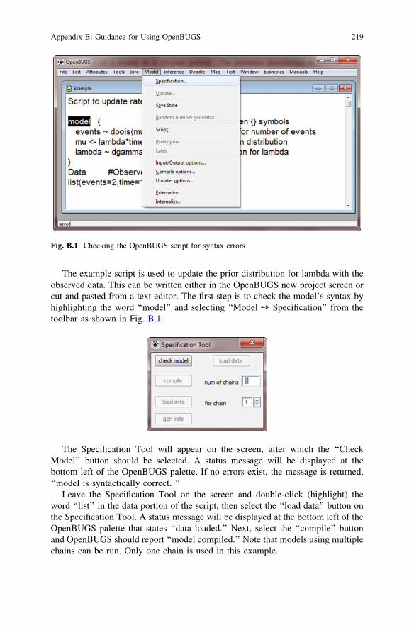
http://dx.doi.org/10.1007/978-1-84996-187-5_13

The example script is used to update the prior distribution for lambda with theobserved data. This can be written either in the OpenBUGS new project screen orcut and pasted from a text editor. The first step is to check the model’s syntax byhighlighting the word ‘‘model’’ and selecting ‘‘Model � Specification’’ from thetoolbar as shown in Fig. B.1.

The Specification Tool will appear on the screen, after which the ‘‘CheckModel’’ button should be selected. A status message will be displayed at thebottom left of the OpenBUGS palette. If no errors exist, the message is returned,‘‘model is syntactically correct. ’’

Leave the Specification Tool on the screen and double-click (highlight) theword ‘‘list’’ in the data portion of the script, then select the ‘‘load data’’ button onthe Specification Tool. A status message will be displayed at the bottom left of theOpenBUGS palette that states ‘‘data loaded.’’ Next, select the ‘‘compile’’ buttonand OpenBUGS should report ‘‘model compiled.’’ Note that models using multiplechains can be run. Only one chain is used in this example.

Fig. B.1 Checking the OpenBUGS script for syntax errors

Appendix B: Guidance for Using OpenBUGS 219

The last step with the Specification Tool is to load the initial values. For theconjugate prior example, the model is such a simple one that we can letOpenBUGS generate initial values. Select the ‘‘gen inits’’ button on theSpecification Tool to have OpenBUGS generate the initial values and a messageof ‘‘initial values generated, model initialized’’ should appear in the status bar.

The next step in setting up the analysis is to select the variables to monitor. Forthe conjugate prior example, we are interested in the frequency, or rate ofoccurrence (lambda). Close the Specification Tool and select ‘‘Inference �

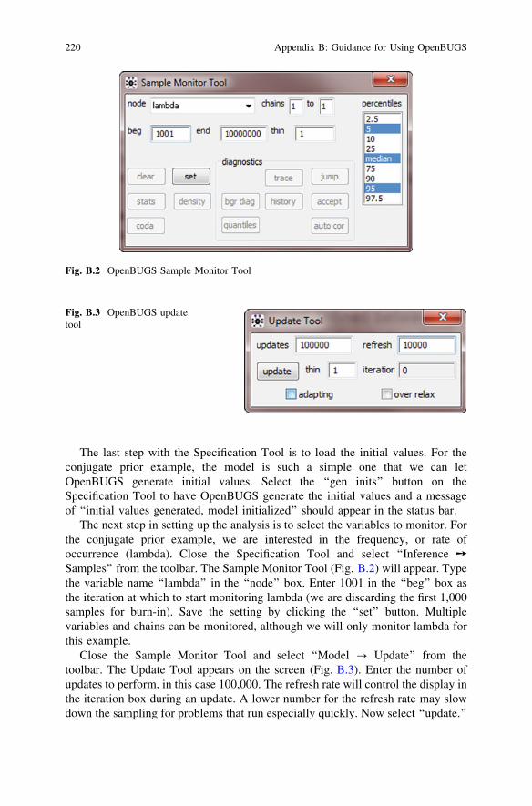
Samples’’ from the toolbar. The Sample Monitor Tool (Fig. B.2) will appear. Typethe variable name ‘‘lambda’’ in the ‘‘node’’ box. Enter 1001 in the ‘‘beg’’ box asthe iteration at which to start monitoring lambda (we are discarding the first 1,000samples for burn-in). Save the setting by clicking the ‘‘set’’ button. Multiplevariables and chains can be monitored, although we will only monitor lambda forthis example.

Close the Sample Monitor Tool and select ‘‘Model ? Update’’ from thetoolbar. The Update Tool appears on the screen (Fig. B.3). Enter the number ofupdates to perform, in this case 100,000. The refresh rate will control the display inthe iteration box during an update. A lower number for the refresh rate may slowdown the sampling for problems that run especially quickly. Now select ‘‘update.’’

Fig. B.2 OpenBUGS Sample Monitor Tool

Fig. B.3 OpenBUGS updatetool


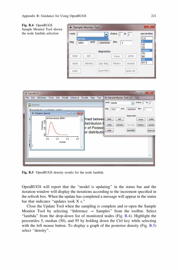
OpenBUGS will report that the ‘‘model is updating’’ in the status bar and theiteration window will display the iterations according to the increment specified inthe refresh box. When the update has completed a message will appear in the statusbar that indicates ‘‘updates took X s.’’

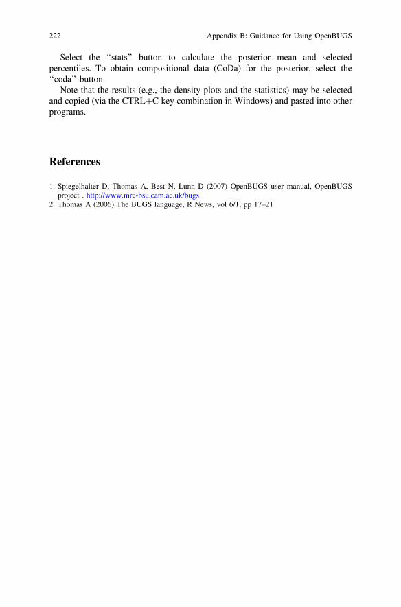
Close the Update Tool when the sampling is complete and re-open the SampleMonitor Tool by selecting ‘‘Inference ? Samples’’ from the toolbar. Select‘‘lambda’’ from the drop-down list of monitored nodes (Fig. B.4). Highlight thepercentiles 5, median (50), and 95 by holding down the Ctrl key while selectingwith the left mouse button. To display a graph of the posterior density (Fig. B.5)select ‘‘density’’.

Fig. B.4 OpenBUGSSample Monitor Tool shownthe node lambda selection

Fig. B.5 OpenBUGS density results for the node lambda

Appendix B: Guidance for Using OpenBUGS 221

Select the ‘‘stats’’ button to calculate the posterior mean and selectedpercentiles. To obtain compositional data (CoDa) for the posterior, select the‘‘coda’’ button.

Note that the results (e.g., the density plots and the statistics) may be selectedand copied (via the CTRL?C key combination in Windows) and pasted into otherprograms.

References

1. Spiegelhalter D, Thomas A, Best N, Lunn D (2007) OpenBUGS user manual, OpenBUGSproject . http://www.mrc-bsu.cam.ac.uk/bugs

2. Thomas A (2006) The BUGS language, R News, vol 6/1, pp 17–21


http://www.mrc-bsu.cam.ac.uk/bugs

Index

AAccelerated life testing, 151

Arrhenius model, 151, 153Aging, 3, 24, 112Aleatory

model, 3, 46, 121, 150, 191uncertainty, 5, 16, 24, 39

BBayes’ Theorem, 8Bayesian anomaly, 169Bayesian inference process, 3, 155, 167Bayesian information criterion (BIC), 103,

106–107Bayesian network, 19, 176Bayesian p-value, 46, 102, 145, 191Bayes’ Theorem, 8Bernoulli, 3, 11, 130

process, 3, 5BETAINV, 17–18Binomial, 3, 40, 61, 126, 135, 183, 193Brooks-Gelman-Rubin (BGR)

diagnostic, 63

CCCF, 135, 137Censoring, 123, 130, 138

interval, 134, 136Type I, 123–124Type II, 125

Chi-square statistic, 45, 47Conditional probability, 148Conjugate, 12, 27, 48, 71, 128, 187

Convergence, 18, 53, 93, 126, 144, 153quantitative checks, 51, 154BGR diagnostic, 63, 80–81

Convolution, 98, 101Correlation, 64, 77, 93, 122, 169, 170Cramer-von Mises statistic, 45, 103, 119Credible interval, 17, 25, 91, 102, 138Cumulative distribution function, 37, 92,

102, 121

DData, 3

censored, 29, 124, 125uncertain, 123

Deterministic, 3, 5Deviance information criterion (DIC), 39, 103,

145, 159Directed acyclic graph (DAG), 19Distribution

beta, 12, 20, 33, 42, 49, 72, 130, 187, 193binomial, 11, 20, 27, 36, 52, 61, 141,

183, 191conditional, 181Dirichlet, 135exponential, 8, 28, 34, 48, 89–90, 108, 119,

154, 191extreme value, 178gamma, 25, 32, 41, 78, 91, 154, 157, 162generalized Pareto, 181Gumbel, 178logistic-normal, 23, 84, 188, 191lognormal, 21, 27, 37, 84, 93, 157, 171,

184, 190multinomial, 135, 136


223

D (cont.)normal, 2, 23, 53, 69, 84, 96, 191Poisson, 24, 29, 30, 41, 51, 61, 123, 141, 184predictive, 8, 40, 48, 59, 69, 72, 81, 100,

146, 162, 189prior, 2, 9, 16, 20, 26, 37, 48, 72, 86, 91,

100, 129, 154, 171, 177, 186, 191uniform, 2, 12, 69, 82, 99, 126, 136, 152Weibull, 92, 95, 109, 118, 121, 126

EEncode information, 7Epistemic, 3, 5, 16, 24, 34, 98, 121,

154, 171, 184Error factor, 21, 31, 48, 82, 99, 107,

134, 162, 188Exchangeability, 86Expert opinion, 177, 184Exponential, 29Extreme value paradigm, 177Extreme value processes, 177

FFailure, 1, 3, 20, 48, 105, 121, 135, 152, 165,

175, 185, 193Fault tree, 3, 8, 165, 169, 172, 176

GGAMMAINV, 25, 30, 32Generic data, 21, 23

HHazard function, 122Hazard rate, 195, 199Hierarchical Bayes, 70, 78, 86, 186, 189, 191Homogeneous, 15

IIndependence, 147Inference, 1–2, 10, 19, 27–28, 30–31, 33, 39,

43, 47, 51, 77, 89, 126, 141, 168,177, 192

Informationcriterion, 108

JJeffreys, 20, 27, 30Joint probability, 146

KKnowledge, 3, 7, 16, 24, 35, 136,

142, 150, 172

LLag autocorrelation coefficient, 64Likelihood, 8

function, 3, 8, 17, 34, 89, 124,155, 184, 191

likelihood-averaging, 130, 135, 138weighted likelihood, 130, 133

Lognormal, 22

MMarkov chain Monte Carlo (MCMC), 61Maximum likelihood estimate (MLE), 2, 30,

142, 179, 182Mean, 17, 31, 74, 88, 91, 122, 156,

180, 198Mean time to failure (MTTF), 50, 154, 185Median, 23, 28, 30–33, 35, 82–83, 87,

93–94, 133–134, 138, 162,172, 185

Mode, 1, 61, 79, 193Model of the world, 4–5, 39Moment, 188, 190–191Monte Carlo error, 69, 195Monte Carlo sampling, 1, 65, 92, 189

NNoninformative, 9, 12, 20, 26–27, 30, 34, 37,

50–51, 136, 157, 162

OOdds, 9, 53OpenBUGS, 17–23, 26–28

PPercentile, 13, 18, 25, 43, 69, 91, 138,

157, 188Poisson process, 3, 8, 24, 192

nonhomogeneous, 191Posterior, 2–3, 12, 24, 50, 69, 84, 100, 119,

133, 157, 196Posterior averaging, 131Power-law process, 119, 122Precision, 32, 53, 69, 94, 184Probability, 1–5Predictive distribution, 8

224 Index

Priorconjugate, 12, 17, 25, 48, 71, 128, 135, 166diffuse, 17, 25, 93, 106, 157, 179, 186first-stage, 71, 80, 87, 188, 190formal, 20informative, 20, 34, 35, 131Jeffreys, 20, 26, 38, 51, 85, 103, 124, 148,

169, 183, 190maximum entropy, 191–192nonconjugate, 16, 21, 27, 30, 33, 42noninformative, 12, 20, 27, 34, 50, 136,

157, 162reference, 20second-stage, 71, 77, 84zero-zero, 21

Priors, 9

RRandom sample, 48, 90, 107, 122, 138, 154,

161, 179Rate of occurrence of failure

(ROCOF), 113Regression

logistic, 143–149loglinear, 141

Reliability growth, 24, 113–117Renewal process, 112–121, 152Repair

same as new, 111–115same as old, 111–114, 121

Replicate, 39, 46, 59, 75, 100, 147, 156, 162,191

Return level, 179–184Return period, 179

SStandard deviation, 32–33, 64, 69, 80, 144,

147, 150, 162, 195Statistic

Bayesian chi-square, 45, 52, 145

VVariance, 32, 38, 45, 48, 63, 69, 84, 187–189

WWeibull, 92

Index 225

Appendix A - Springer LINK

Documents