Appendix A: Stereoviews and Crystal Models - Springer LINK

Appendix A: Stereoviewsand Crystal Models

A.1 Stereoviews

Stereoviews of crystal structures began to be used to illustrate three-dimensional structures in 1926.

Nowadays, this technique is quite commonplace, and computer programs exist (see Appendices D4

and D8.7) that prepare the two views needed for producing a three-dimensional image of a crystal or

molecular structure.

Two diagrams of a given object are necessary in order to form a three-dimensional visual image.

They should be approximately 63 mm apart and correspond to the views seen by the eyes in normal

vision. Correct viewing of a stereoscopic diagram requires that each eye sees only the appropriate half

of the complete illustration, and there are two ways in which it may be accomplished.

The simplest procedure is with a stereoviewer. A supplier of a stereoviewer that is relatively

inexpensive is 3Dstereo.com. Inc., 1930 Village Center Circle, #3-333, Las Vegas, NV 89134, USA.

The pair of drawings is viewed directly with the stereoviewer, whereupon the three-dimensional

image appears centrally between the two given diagrams.

Another procedure involves training the unaided eyes to defocus, so that each eye sees only the

appropriate diagram. The eyes must be relaxed and look straight ahead. The viewing process may be

aided by holding a white card edgeways between the two drawings. It may be helpful to close the eyes

for a moment, then to open them wide and allow them to relax without consciously focusing on the

diagram.

Finally, we give instructions whereby a simple stereoviewer can be constructed with ease. A pair

of plano-convex or bi-convex lenses, each of focal length approximately 100 mm and diameter

approximately 30 mm, is mounted between two opaque cards such that the centers of the lenses

are approximately 63 mm apart. The card frame must be so shaped that the lenses may be brought

close to the eyes. Figure A.1 illustrates the construction of the stereoviewer.

A.2 Model of a Tetragonal Crystal

A model similar to that illustrated in Fig. 1.23 can be constructed easily. This particular model has

been chosen because it exhibits a four-fold inversion axis, which is one of the more difficult symmetry

elements to appreciate from drawings.

M. Ladd and R. Palmer, Structure Determination by X-ray Crystallography:Analysis by X-rays and Neutrons, DOI 10.1007/978-1-4614-3954-7,# Springer Science+Business Media New York 2013

659

A good quality paper or thin card should be used for the model. The card should be marked out in

accordance with Fig. A.2 and then cut out along the solid lines, discarding the shaded portions. Folds

are made in the same sense along all dotted lines, the flaps ADNP and CFLM are glued internally, and

the flap EFHJ is glued externally. What is the point group of the resulting model?

Fig. A.1 Construction of a simple stereoviewer. Cut out two pieces of card as shown and discard the shaded portions.Make cuts along the double lines. Glue the two cards together with lenses EL and ER in position, fold the portions A and

B backward, and engage the projection P into the cut atQ. Strengthen the fold with a strip of “Sellotape.” View from the

side marked B. It may be helpful to obscure a segment on each lens of maximum depth ca. 30 % of the lens diameter,

closest to the nose region

660 Appendix A

Fig. A.2 Construction of a tetragonal crystal with a �4 axis: NQ ¼ AD ¼ BD ¼ BC ¼ DE ¼ CE ¼ CF ¼KM ¼ 100 mm; AB ¼ CD ¼ EF ¼ GJ ¼ 50 mm; AP ¼ PQ ¼ FL ¼ KL ¼ 20 mm; AQ ¼ DN ¼ CM ¼ FK ¼FG ¼ FH ¼ EJ ¼ 10 mm

Appendix A 661

Appendix B: Schonflies’Symmetry Notation

Theoretical chemists and spectroscopists generally use the Schonflies notation for describing

point-group symmetry but, although both the crystallographic (Hermann–Mauguin) and Schonflies

notations are adequate for point groups, only the Hermann–Mauguin system is satisfactory also for

space groups.

The Schonflies notation uses the rotation axis and mirror plane symmetry elements that we have

discussed in Sect. 1.4.2, albeit with differing notation, but introduces the alternating axis of symmetry

in place of the roto-inversion axis.

B.1 Alternating Axis of Symmetry

A crystal is said to have an alternating axis of symmetry Sn of degree n, if it can be brought from one state

to another indistinguishable state by the operation of rotation through (360/n)� about the axis and

reflection across a plane normal to that axis, overall a single symmetry operation. It should be stressed

that this plane is not necessarily a mirror plane in the point group.

Operations Sn are non-performable physically with models (see Sects. 1.4.1 and 1.4.2). Figure B.1

shows stereograms for S2 and S4; crystallographically, we recognize them as �1 and �4, respectively.

The reader should consider what point groups are obtained if the plane of the diagram were a mirror

plane in point groups S2 and S4.

B.2 Symmetry Notations

Rotation axes are symbolized by Cn in the Schonflies notation (cyclic group of degree n); n takes the

meaning ofR in theHermann–Mauguin system.Mirror planes are indicated by subscripts v, d, andh; v andd refer to mirror planes containing the principal axis, and h indicates a mirror plane normal to that axis. In

addition, d refers to those vertical planes that are set diagonally, between the crystallographic axes normal

to the principal axis.

663

The mirror plane symmetry element is denoted by s in the Schonflies system. The symbol Dn

(dihedral group of degree n) is introduced for point groups in which there are n two-fold axes in a

plane normal to the principal axis of degree n. The cubic point groups are represented through the

special symbols T (tetrahedral) and O (octahedral). In point group symbols, subscripts h and d are

used to indicate the presence of horizontal and vertical (dihedral) mirror planes, respectively

Table B.1 compares the Schonflies and Hermann–Mauguin symmetry notations.

Fig. B.1 Stereograms of point groups: (a) S2, (b) S4

Table B.1 Schonflies and Hermann–Mauguin pointgroup symbols

Schonflies Hermann–Mauguina Schonflies Hermann–Mauguina

C1 1 D4 422

C2 2 D6 622

C3 3 D2h mmmC4 4 D3h �6m2C6 6

Ci, S2 �1 D4h 4

mmm

Cs, S1 m; 2

S6 �3S4 �4 D6h 6

mmm

C3h, S3 �6a

C2h 2/mb D2d�42m

C4h 4/mb D3d�3m

C6h 6/mb T 23

C2v mm2 Th m�3mC3v 3m O 432

C4v 4mm Td �43mC6v 6mm Oh m3mD2 222 C1v 1D3 32 D1h 1=mð �1ÞaThe usual Schonflies symbol for �6 is C3h (3/m). The reason that 3/mis not used in the Hermann–Mauguin system is that point groups

containing the element �6 describe crystals that belong to the hexago-

nal system rather than to the trigonal system; �6 cannot operate on a

rhombohedral lattice.

bR/m is an acceptable way of writingR

m; but R/mmm is not as

satisfactory asR

mmm; R/mmm is a marginally acceptable alternative.

664 Appendix B

Appendix C: Cartesian Coordinates

In calculations that lead to results in absolute measure, such as bond distance and angle calculations

and location of hydrogen-atom positions, it may be desirable to convert the crystallographic

fractional coordinates x, y, z, which are dimensionless, to Cartesian (orthogonal) coordinates X, Y,and Z, in A or nm.

C.1 Cartesian to Crystallographic Transformation and Its Inverse

Instead of considering immediately the transformation A ¼ Ma, it is simpler to consider first the

inverse transformation a ¼ M�1 a, where M is the transformation matrix for the triplet AðA;B;CÞ tothe triplet aða; b; cÞ, because the components of a along the Cartesian axes are direction cosines (see

Web Appendix WA1).

Figure C.1 illustrates the two sets of axes. Let A be a unit vector along a, B a unit vector normal to

a, and in the a, b plane, and C a unit vector normal to both A and B.

Then, we can write

a=a

b=b

c=c

264

375 ¼

l1 m1 n1

l2 m2 n2

l3 m3 n3

264

375

A

B

C

264

375 (C.1)

From the figure, we can write down some of the elements of M�1:

M�1 ¼1 0 0

cos g sin g 0

cos b m3 n3

264

375 (C.2)

From the properties of direction cosines, we have

cos a ¼ l2l3 þ m2m3 þ n2n3 ¼ cos b cos gþ m3 sin g

so that

m3 ¼ ðcos a� cos b cos gÞ= sin g ¼ � cos a� sin b (C.3)

665

Since the sums of the squares of the direction cosines is unity,

n23 ¼ 1� cos2b� sin2bcos2a� ¼ sin2bsin2a�

so that

n3 ¼ sin b sin a� ¼ v= sin g (C.4)

since1 V ¼ abc sin a* sin b sin g, and v here refers to the volume of the unit parallelepiped a/a, b/b,

c/c, that is, v ¼ (1 � cos2 a � cos2 b � cos2 g + 2 cos a cos b cos g). Hence, we can write the

transformation in terms of the direct unit-cell parameters, multiplying the lines of the matrix by a, b,

or c, as appropriate:

a

b

c

26643775 ¼

a 0 0

b cos g b sin g 0

c cos b cðcos a� cos b cos gÞ= sin g cv= sin g

2664

3775

A

B

C

2664

3775 (C.5)

which, in matrix notation, is a ¼ M�1 A. From the transformations discussed in Sect. 2.5.5, we have

X ¼ ðM�1ÞTx, or

X

Y

Z

264

375 ¼

a b cos g c cosb

0 b sin g cðcos a� cos b cos gÞ= sin g0 0 cv= sin g

264

375

x

y

z

264375 (C.6)

The deduction of M, the inverse of M�1, is straightforward for a 3 � 3 matrix, albeit somewhat

laborious, and can be found in most elementary treatments of vectors. Thus, we have A ¼ M a and

x ¼ MTX, where

Fig. C.1 A, B and C are unit vectors on Cartesian (orthogonal) axes X, Y, Z, and a/a, b/b, and c/c are unit vectors on theconventional crystallographic axes x, y, z

1Buerger MJ (1942) X-ray crystallography. Wiley, New York.

666 Appendix C

M ¼1=a 0 0

� cos g=ða sin gÞ 1=ðb sin gÞ 0

ðcos g cos a� cos bÞ=ðav sin bÞ ðcos g cos b� cos aÞ=ðbv sin gÞ sin g=ðcvÞ

0B@

1CA (C.7)

The transformation (C.6) is employed in the program INTXYZ (see Sect. 13.6.6) for the calcula-

tion of bond lengths, bond angles, and torsion angles from crystallographic parameters. The sign of a

torsion angle is governed by the convention discussed in Section 8.5.2. For the sequence of atoms,

P, Q, R, S in Fig. C.2, the torsion angle wPQRS is positive if a clockwise rotation of PQ about QR,

as seen along QR, brings PQ over RS.

Fig. C.2 Convention for torsion angles: wPQRS is reckoned positive as shown, when the atom succession P � Q � R� S is viewed along QR

Appendix C 667

Appendix D: Crystallographic Software

This Appendix lists software for X-ray and neutron crystallographic applications that are available to the

academic community. The list is not exhaustive, and many of the packages are listed under one or other

section of the Collaborative Computational Projects.2,3 Often, the program systems are mirrored by the

Engineering and Physical Sciences Research Council (EPSRC) funded CCP projects,4 which have

mirror sites in the U. S. A. and in Canada. In addition to the programs referenced here, a complete set

of crystallographic programs has been promulgated elsewhere.5

The program systems are divided into a number of sections, and an appropriate reference has been

provided for each entry, including author, e-mail address, and web site reference as appropriate.

• Single Crystal Suites

• Single Crystal Structure Solving Programs

• Single Crystal Twinning Software

• Freestanding Structure Visualization Software

• Powder Diffraction Data: Powder Indexing Suites

• Structure Solution from Powder Diffraction Data

• Software for Macromolecular Crystallography

Data Processing; Fourier and Structure Factor Calculations; Molecular Replacement; Single

and Double Isomorphous Replacement; Software for Packing and Molecular; Geometry; Software

for Graphics and Model Building; Software for Molecular Graphics and Display; Software for

Refinement; Software for Molecular Dynamics and Energy Minimization; Data Bases

• Bioinformatics

Molecular Modelling Software; External Links; Useful Homepages

D.1 Single Crystal Suites

Most single crystal program suites have a large variety of functionality; WinGX is an example of a

suite linking to several other programs in a seamless manner via graphical user interfaces. In most

cases, programs link to multiple versions of a structure solution program, such as SHELXS-97 or

SIR2008.

2 http://www.ccp4.ac.uk.3 http://www.ccp14.ac.uk.4 http://www.epsrc.ac.uk/Pages/default.aspx.5 http://ww1.iucr.org/sincris-top/logiciel/lmno.html#O.

669

D.2 Single Crystal Structure Solution Programs

CAOS

Automated Patterson method. Spagna R et al. http://www.ic.cnr.it/caos/what.html

CRYSTALS 14.23

Watkin D. http://www.xtl.ox.ac.uk

DIRDIF 2008

Automated Patterson methods and fragment searching: Windows version ported by L. Farrugia and

available via the WinGX website. http://www.chem.gla.ac.uk/~louis/software/dirdif/

OLEX2User-friendly structure solution and refinement suite with inter alia archiving and report generation.

Dolomanov OV et al (2008) J Appl Crystallogr 42:339. http://olex2.org

PATSEE

Fragment searching methods. http://www.ccp14.ac.uk/ccp/web-mirrors/patsee/egert/html/patsee.

html. Windows version by Farrugia, L. and available via the WinGX website.

System SSHELXS, DIRDIF, SIR, and CRUNCH for solution; EXOR, DIRDIF, SIR, and CRUNCH for autobuild-

ing; SHELXL for refinement. Spek AL. http://www.ccp14.ac.uk/tutorial/platon/index.html

SIR 2008

http://www.ba.ic.cnr.it/content/il-milione-and-sir2008

SNB (SHAKE AND BAKE)

Direct methods. Weeks CM et al. http://www.hwi.buffalo.edu/SnB

WinGX

SHELXS, DIRDIF, SIR, and PATSEE for solution; DIRDIF phases for autobuilding; SHELX for

refinement. Farrugia L. http://www.chem.gla.ac.uk/~louis/software/wingx

D.3 Single Crystal Twinning Software

TWIN 3.0Kahlenberg V et al. http://www.ccp14.ac.uk/solution/twinning/index.html

TwinRotMacSpek AL. http://www.ccp14.ac.uk/solution/ twinning/index.html

Windows version by Farrugia L. http://www.chem.gla.ac.uk/~louis/software/platon

D.4 Freestanding Structure Visualization Software

ORTEP-IIIBurnett MN et al. http://www.chem.gla.ac.uk/~louis/software/ortep3/

670 Appendix D

D.5 Powder Diffraction Data: Powder Indexing Suites (Dedicated and Other)

Checkcell

Laugier J. http://www.ccp14.ac.uk/tutorial/lmgp/achekcelld.htm

CRYSFIRE

Shirley R. http://www.ccp14.ac.uk/tutorial/crys/ (includes the programs ITO, DICVOL, TREOR,

TAUP, KOHL, LZON, LOSH, and FJZN, but is no longer under development)

DICVOL91Louer D. http://www.ccp14.ac.uk/tutorial/crys/program/dicvol91.htm

ITO12/13Visser JW. http://www.iucr.org/resources/commissions/crystallographic-computing/software-museum

ITO15 (Included in FULLPROF)

Visser J et al. http://www.ill.eu/sites/fullprof/php/programs.html

LOSH/LZON

Bergmann J et al. http://www.ccp14.ac.uk/tutorial/tutorial.htm

TAUP/Powder

Taupin D. http://www.ccp14.ac.uk/tutorial/crys/taup.htm

TREOR90 (Included in FULLPROF)

http://www.ill.eu/sites/fullprof/php/programsdc cc.html?pagina¼Treor90

D.6 Powder Pattern Decomposition

ALLHKLPawley GS. http://www.ccp14.ac.uk/solution/pawley/index.html

WPPFHatashi S, Toraya H. http://www.icdd.com/resources/axa/vol41/V41_66.pdf

D.7 Structure Solution from Powder Diffraction Data

ESPOIR

Mileur M, Le Bail A. http://www.cristal.org/sdpd/espoir/

EXTRA (Included in EXPO)

http://www.ccp14.ac.uk/tutorial/expo/index.html

FULLPROF

http://www.ill.eu/sites/fullprof/

Appendix D 671

GSAShttp://www.ccp14.ac.uk/solution/gsas

RIETAN

Izumi F. http://homepage.mac.com/fujioizumi/download/download_Eng.html

SIRPOW (Included in EXPO)

http://www.ccp14.ac.uk/tutorial/expo/index.html

POWDER SOLVE

http://accelrys.com/resource-center/case-studies/powder-solve.html

D.8 Software for Macromolecular Crystallography

Much of the software listed in this section is fast moving, and the CCP sites1,2 should be consulted for

the latest developments.

D.8.1 Data Processing

HKL 4 (Includes DENZO, XDISPLAY, and SCALEPACK)

Gerwith D (2003) The HKL manual, 6th edn. http://www.hkl-xray.com/hkl_web1/hkl/manual_

online.pdf

STRATEGY

Ravelli RBG et al. http://www.crystal.chem.uu.nl/distr/strategy.html

PREDICT

Noble M. http://biop.ox.ac.uk/www/distrib/predict.html

D.8.2 Fourier and Structure Factor Calculations

SFALL (Structure Factors). http://www.ccp4.ac.uk/html/sfall.html

FFT (Fast Fourier Transform). http://www.ccp4.ac.uk/html/fft.html

D.8.3 Molecular Replacement

AmoRe

Navaza J (Autostruct 2001). http://www.ccp4.ac.uk/autostruct/amore/

CNS Solve 1.1

Brunger AT et al. http://cns.csb.yale.edu/v1.1/

MOLREP

Vagin AA. [email protected]

672 Appendix D

MOLPACKWang D et al. http://www.ccp4.ac.uk/html/molrep.html

REPLACE

http://como.bio.columbia.edu/tong/Public/Replace/replace.html

D.8.4 Schematic Structure Plots

LIGPLOT

Laskowski RA. http://www.ebi.ac.uk/thornton-srv/software/LIGPLOT/

SHELXS-86

Location of heavy-atom positions. Sheldrick GM (1994) Crystallographic computing, 3rd edn.

Oxford University Press, Oxford

D.8.5 Software for Packing, Molecular Geometry, Validation and Deposition

COOT

Emsley P et al (2010) Acta Cryst D66:486. http://lmb.bioch.ox.ac.uk/coot/

PROCHECK

Laskowski RS et al. http://www.ebi.ac.uk/thornton-srv/software/PROCHECK

WHATCHECK

Hooft RWW et al. http://www.ccp4.ac.uk/dist/ccp4i/help/modules/valdep.html

D.8.6 Software for Graphics and Model Building

FRODOJones TA. http://www.mendeley.com/research/tek-frodo-new-version-frodo-tektronix-graphics-sta-

tions/

O

Jones TA et al. http://xray0.princeton.edu/~phil/Facility/ono.html

TURBO-FRODO

Jones TA et al. Bio-graphics. http://www.afmb.univ-mrs.fr/-TURBO-

D.8.7 Software for Molecular Graphics and Display

MERCURYhttp://www.ccdc.cam.ac.uk/products/csd_system/ mercury_csd/index.php

ORTEPBarnes CL (1997) ORTEP-3 for Windows, J Appl Cryst 30:568 [based on ORTEP-III by Johnson CK

and Burnett MN.]

Appendix D 673

RASMOLSayle R. http://www.umass.edu/microbio/rasmol/

RASTER 3.0

Bacon DJ et al. http://skuld.bmsc.washington.edu/raster3d

SETOR

Evans SV. http://www.ncbi.nlm.nih.gov/pubmed/8347566

MOLSCRIPT 1.4

Kraulis PJ. http://www.avatar.se/molscript

BOBSCRIPT 2.4 (Extension to MOLSCRIPT 1.4)

Esnouf R. http://www.csb.yale.edu/userguides/graphics/bobscript/bobscript.html

D.8.8 Software for Refinement

X-PLOR 3.1

Brunger AT. http://yalepress.yale.edu/book.asp?isbn¼9780300054026

CNS Solve 1.1

Brunger AT et al. http://cns.csb.yale.edu/v1.1/

RESTRAIN

Driessen HPC et al. http://scripts.iucr.org/cgi-bin/paper?gl0109

SHELXS-86

Sheldrick GM (1994) Crystallographic computing, 3rd edn. Oxford University Press, Oxford

SHELX-97 and SHELXL-97

Sheldrick GM. http://shelx.uni-ac.gwdg.de/SHELX/

REFMAC 5

http://www.ccp4.ac.uk/html/refmac5.html

D.8.9 Software for Molecular Dynamics and Energy Minimization

SYBYL-X

http://tripos.com/index.php?family¼modules,SimplePage,,,&page¼SYBYL-X

D.8.10 Data Bases

Protein Data Bank (PDB)

http://www.pdb.org/pdb/static.do?p¼search/index.html

Basic Local Alignment Search Tool (BLAST)

http://blast.ncbi.nlm.nih.gov/Blast.cgi?PAGE¼ Proteins

Cambridge Crystallographic Data Centre (CCDC)

http://www.ccdc.cam.ac.uk

674 Appendix D

ReLiBase (Finds Ligands for Protein Families)http://www.ccdc.cam.ac.uk/free_services/reliba se_free/

ChemSpider (Contains Much Chemical Information on ca. 25 Million Compounds)

http://cs.m.chemspider.com

D.8.11 Synchrotron Web Page

http://www.esrf.eu/computing/scientific/people/srio/publications/SPIE04_XOP.pdf

D.9 Bioinformatics

D.9.1 Molecular Modelling Software

The sources listed below provide software for molecular modelling. Some of them, for example,

COSMOS and Sybyl are listed above. Others are readily obtained from the web sites that are given by

the names, for example, Abaloneclassical: http://www.sciencedirect.com/science/article/pii/

S0928493110002894.

The following names may be interrogated in a similar manner:

• Abaloneclassical• ADFquantum• AMBERclassical

• Ascalaph Designerclassical and quantum [http://en.wikipedia.org/wiki/Main_Page#cite_note-0]

• AutoDock

• AutoDock Vina

• BALLView

• Biskit

• BOSSclassical• Cerius2

• CHARMMclassical

• Chimera

• Coot [http://en.wikipedia.org/wiki/Main_Pa ge#cite_note-1]

• COSMOS (software) [http://en.wikipedia.org/wiki/Main_Page#cite_note-2]

• CP2Kquantum

• CPMDquantum

• Culgi

• Discovery Studioclassical and quantum [http://en.wikipedia.org/wiki/Main_Page#cite_note-3]

• DOCKclassical

• Fireflyquantum• FoldX

• GAMESS (UK)quantum• GAMESS (US)quantum• GAUSSIANquantum

• Ghemical

• Gorgon [http://en.wikipedia.org/wiki/Main_ Page#cite_note-4]

• GROMACSclassical• GROMOSclassical

Appendix D 675

• InsightIIclassical and quantum

• LAMMPSclassical• Lead Finderclassical [http://en.wikipedia.org/wiki/Main_Page#cite_note-5]

• LigandScout

• MacroModelclassical• MADAMM [http://en.wikipedia.org/wiki/Main_Page#cite_note-6; http://en.wikipedia.org/wiki/

Main_Page#cite_note-Cerqueira-7]

• MarvinSpace [http://en.wikipedia.org/wiki/Main_Page#cite_note-8]

• Materials and Processes Simulations [http://en.wikipedia.org/wiki/Main_Page#cite_note-9]

• Materials Studioclassical and quantum [http://en.wikipedia.org/wiki/Main_Page#cite_note-10]

• MDynaMixclassical• MMTK

• Molecular Docking Server

• Molecular Operating Environment

(MOE)classical and quantum

• MolIDEhomology modelling [http://en.wikipedia.org/wiki/Main_Page#cite_note-11]

• Molsoft ICM [http://en.wikipedia.org/wiki/Main_Page#cite_note-12]

• MOPACquantum

• NAMDclassical

• NOCH

• Oscail X

• PyMOLvisualization

• Q-Chemquantum

• ReaxFF

• ROSETTA

• SCWRLside-chain prediction [http://en.wikipedia.org/wiki/Main_Page#cite_note-13]

• Sirius

• Spartan (software)quantum [http://en.wikipedia.org/wiki/Main_Page#cite_note-14]

• StruMM3D (STR3DI32) [http://en.wikipedia.org/wiki/Main_Page#cite_note-15]

• Sybyl (software)classical [http://en.wikipedia.org/wiki/Main_Page#cite_note-16]

• MCCCS Towhee [http://en.wikipedia.org/wiki/Main_Page#cite_note-17]

• TURBOMOLEquantum

• VMDvisualization

• VLifeMDSIntegrated molecular modelling and simulation

• WHAT IF [http://en.wikipedia.org/wiki/Main_Page#cite_note-18]

• xeo [http://en.wikipedia.org/wiki/Main_Page #cite_note-19]

• YASARA [http://en.wikipedia.org/wiki/Main_Page#cite_note-20]

• Zodiac (software) [http://en.wikipedia.org/wiki/Main_Page#cite_note-21]

D.9.2 External Links

These links relate to important sites on molecular modelling and molecular simulation, but are by no

means exhaustive.

Center for Molecular Modelling at the National Institutes of Health (NIH) (U.S. Government

Agency): http://www.bing.com/search?q¼Center+for+Molecular+Modelling+at++the+National

+Institutes+of+Health+%28NIH%29+%28U.S.+Government+Agency%29&src¼ie9tr

676 Appendix D

Molecular Simulation, details for theMolecular Simulation journal, ISSN: 0892-7022 (print), 1029-

0435 (online): http://www.bing.com/sear ch?q¼Center+for+MolecularModelling+at+the+National

+Institutes+of+Health+%28NIH%29+%28U.S.+Government+Agency%29&src¼ie9tr

The Cheminfo Network and Community of Practice in Informatics and Modelling: http://www.

bing.com/search?q¼The+Cheminfo+Network+and+Community+of+Practice+in+Informatics

+and+Modelling.&src¼ie9tr

D.9.3 Useful Homepages

These sites relate to situations wherein extensive work on protein crystallography is being persued.

Again, it is not an exhaustive list.

York Structural Biology Laboratory

http://www.york.ac.uk/chemistry/research/groups/ ysbl/

COSMOS—Computer Simulation of Molecular Structures

http://www.mybiosoftware.com/3d-molecular-model/1968

Accelrys Inc.

http://accelrys.com/

http://www.ccp4.ac.uk

http://www.ccp14.ac.uk

http://epsrc.ac.uk/Pages/default.aspx

http://ww1.iusr.org/sincris-top/logicel/Imno.html#O

Appendix D 677

Appendix E: Structure Invariants, StructureSeminvariants, Origin and EnantiomorphSpecifications

E.1 Structure Invariants

As we have seen in Sect. 2.2.2, there is an infinite number of ways in which a crystal unit cell may be

chosen. Conventionally, however, any crystal lattice is represented by one of the 14 Bravais lattices

described in Sect. 2.2.3. For a given unit cell, the origin of the x, y, and z coordinates can be relocatedfor convenience, as we have seen in Sect. 2.7.7 for space group P212121. The possible effects of such

origin transformations were mentioned in Sect. 6.6.4, when discussing of Fourier transforms. As a

general rule, the origin of a given space group is chosen with respect to its symmetry elements; for

example, in centrosymmetric space groups the origin is specified on a center of symmetry. Conven-

tions associated with the specification of the origin are fully described for all space groups in the

literature. With no symmetry elements apart from the lattice translations, space group P1 is the

exception and can accommodate an origin of coordinates in any arbitrary position. We discuss here

relationships between structure factors that arise from changes in the location of the coordinate origin.

Following (3.63) we write the structure factor in the form

FðhÞ ¼Xj

fj expði2ph � rjÞ (E.1)

where h represents a reciprocal lattice vector corresponding to reflection hkl and rj is the real space

vector corresponding to the point x, y, z, so that h � rj ¼ hxj þ kyj þ lzj. If the origin is changed to thepoint r0, then (E.1) becomes

FðhÞr0 ¼Xj

fj exp½i2ph � ðrj � r0Þ�

¼Xj

fj expði2ph � rjÞ expð�i2ph � r0Þ(E.2)

679

Thus, we can write

FðhÞr0 ¼ FðhÞ expð�i2ph � r0Þ (E.3)

so that

jFðhÞr0 j ¼ jFðhÞj (E.4)

and

fðhÞr0 ¼ fðhÞr � 2ph � r0 (E.5)

Thus, a change of origin leaves the amplitude of the structure factor unaltered, but changes the

phase by � 2ph � r0whatever the value of r0. The relationships (E.3)–(E.5) apply equally to the

normalized structure factors E(hkl) that are used in direct methods of phase determination. We can

illustrate (E.3)–(E.5) by a simple example.

Consider an atom at 0.3, 0.2, 0.7 in space group P1. For a reflection, say 213, and taking f as 1.0,

we find A01 ¼ 0.8090, B0

1 ¼ �0.5878, so that jF1j ¼ 1 and f1 ¼ 324�. We change the origin to the

point 0.1, 0.1, 0.1, whereupon A02 ¼ �0.3090, B0

2 ¼ 0.9511, so that jF2j ¼ 1 and f2 ¼ 108�.Finally, using the third term in (E.5), we find Df ¼ 2ph � r0¼ 360 ½2 � ð0:1Þ þ 1� ð0:1Þ þ 3�ð0:1Þ� ¼ 216, which is equal to f1 � f2. (Remember to set

tan�1(B0/A0) in the correct quadrant according to the signs of A0 and B0, and to evaluate f in the

positive range 0–2p.)The values of jEj are determined by the structure, whatever the origin, whereas the values of f are

determined by both the structure and the choice of origin. Thus, the values of jEj alone cannot determine

unique values for the phases.We need a process to obtain phases from the values of jEj that incorporates aspecification of the origin. Consider the product of three normalized structure factors in the absence of

symmetry, that is, for space group P1. From (3.15), we can write

E1E2E3 ¼ jE1jjE2jjE3j exp½iðfðh1Þþ ðfðh2Þ þ ðfðh3Þ� (E.6)

If the origin is moved from 0,0,0 to a point r0, it follows from the foregoing that (E.6) becomes

E1E2E3 ¼ jE1jjE2jjE3j exp½�i2pðh1 þ h2 þ h3Þ � r0� (E.7)

Thus, the condition that the product of three structure factors be a structure invariant N3, that is, a

change of origin has no effect on its value in the non-centrosymmetric space group P1, is that

h1 þ h2 þ h3 ¼ 0 (E.8)

Equation (E.8) is a triplet structure invariant; it may be extended to a quartet such that the product

of four structure factors is a structure invariant N4 if

h1 þ h2 þ h3 þ h4 ¼ 0 (E.9)

680 Appendix E

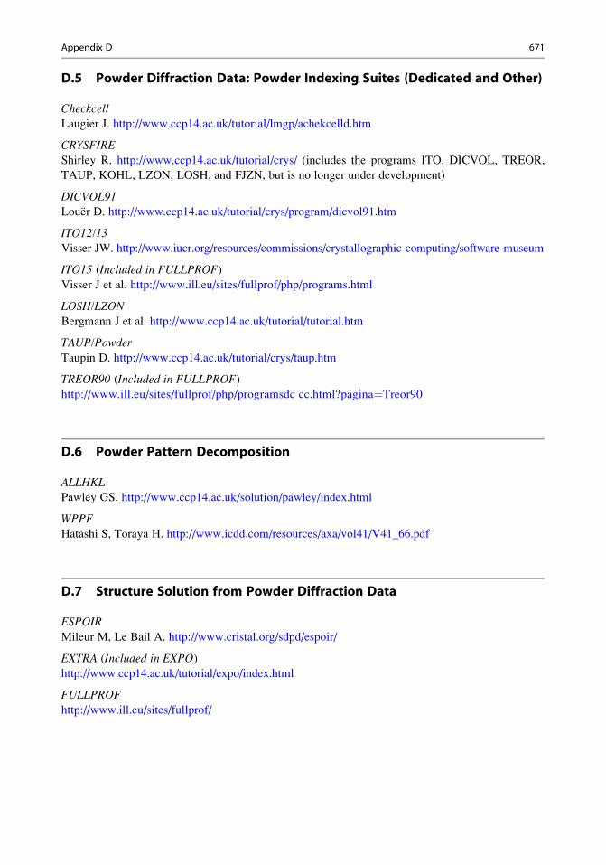
and more:

NÞn ¼Ynj¼1

EðhjÞ (E.10)

provided that the condition

Xnj¼1

hj ¼ 0 (E.11)

For n ¼ 1, the structure factor, which is a structure invariant, is E(0) and has a phase of zero for any

origin. For n ¼ 2, h1 + h2 ¼ 0, or h2 ¼ �h1 so that E1E2 ¼ E(h1)E(�h1) ¼ jE(h1)j2, which is phase

independent. For n > 2, we have (E.10) and (E.11) as already discussed. For n ¼ 3 or more, we have

equations such as (E.8) and (E.9).

E.2 Structure Seminvariants

Equations such as (E.8) apply also to P�1, because the sums of the indices, as in (E.13) below, are each

zero. However, consider next a structure with symmetry P�1, wherein the origin is chosen, normally,

on one of the eight centers of symmetry unique to the unit cell. In the presence of symmetry elements,

it is always desirable to choose the origin on one of these elements, albeit such a choice may not

define the origin point uniquely, such as on the twofold axis parallel to the line [0,y,0] in space group

P2.The normally permitted origins in P�1 are listed in Table 8.2. In general, the sign of E(hkl) depends

on the choice of origin except for reflection in the group eee, for which reflections6

ðhklÞ modulo2 ð222Þ ¼ ð000Þ (E.12)

Such reflections are structure seminvariants (semi-invariants) since their signs (phases) do not

change for variation among the permitted origins. If three structure factors are chosen from different

parity groups, other than eee, such that

h1 þ h2 þ h3; k1 þ k2 þ k3; l1 þ l2 þ l3 modulo ð222Þ (E.13)

then the product of the three structure factors is not a structure seminvariant (semi-invariant), and can

be either positive or negative. An arbitrary sign can be chosen for each such structure factor in the

product, and for one of the eight possible origins the choice will be true, and the origin is fixed

according to that choice. Thus, for example, the reflections 10�6, 40�1, and 71�4 may be chosen to

specify an origin, and if we allocate a + sign arbitrarily to each, the origin is defined as 0, 0, 0. If we

choose instead the reflections 10�6, 40�1, and �507, then the origin is not specified uniquely because the

determinant is less than or equal to zero. The triplet is not linearly independent (see E.14 and text):

6 a � b modulo n if a � b ¼ kn, where k is an integer.

Appendix E 681

1 þ 4 � 5 ¼ 0, 0 þ 0 þ 0 ¼ 0 and �6 � 1 þ 7 ¼ 0, or oee + eeo + oeo ¼ oee, which does notconstitute linear independence. The relation h1 + h2 + h3 ¼ 0 modulo (222) has no special signifi-

cance in space group P1.The structure invariants and structure seminvariants have been well described in the literature for

all space groups.7–11

E.2.1 Difference Between Structure Invariant and Structure Seminvariant

Consider two triplets Eð3�32ÞEð012ÞEð�32�4Þ and Eð3�32ÞEð012ÞEð344Þ. The first product is a structureinvariant because the sums h1 + h2 + h3, k1 + k2 + k3 and l1 + l2 + l3 are each equal to zero. It is a

structure invariant inP1 andP�1wherever the origin point is placed in the unit cell. The second product isa structure seminvariant because the sums h1 + h2 + h3, k1 + k2 + k3 and l1 + l2 + l3 are each equal to

zero modulo (2), and its sign (phase) is not changed by moving to another permitted origin in P�1, but it

would change if the origin were moved to a general point in the unit cell. Note that in both examples,

these reflections would not serve to specify an origin because the parities sum to eee in each case.

E.3 Origin Specification

From the foregoing, we see that for space group P1, which contains no symmetry other than that of

the basic translations, three reflections that form a linearly independent combination will specify the

origin. The three reflections E(h1k1l1), E(h2k2l2), and E(h3k3l3) will specify an origin provided that the

determinant D satisfies the condition

D ¼h1 k1 l1h2 k2 l2h3 k3 l3

������������> 0 (E.14)

or D modulo (222) ¼ 1; the determinant is evaluated in the normal manner.

Normally, the position 0, 0, 0 is chosen for the origin in P1; there is no purpose in choosing any

other site. The three independent phases can be given values between 0 and 2p; generally they are

chosen as zero.

In any space group of symmetry greater than 1, the origin is normally chosen on that symmetry

element. We have discussed the case for P�1 sufficiently for our purposes in Sect. 8.2.2.

E.4 Choice of Enantiomorph

In any of the 65 enantiomorphous space groups listed in Table 10.1, there exists the need to specify a

molecular enantiomorph. From (E.1) we can write

7Hauptman H, Karle J (1953) The solution of the phase problem I, ACA monograph 3.8 idem. (1956) Acta Crystallogr 9:45.9 idem. ibid. (1959) 12:93.10 Karle J, Hauptman H (1961) ibid. 14:217.11 Lessinger L, Wondratschek H (1975) ibid. A31:382.

682 Appendix E

jEðhÞj ¼Xj

Zj exp½i2pðh � rjÞ������

����� (E.15)

If each rj is replaced by its inverse, the right-hand side of (E.15) and, hence, jE(h)j remain unchanged.

The jEj values relate to both a structure and its inverse, or roto-reflection, through a point. If this point isthe origin 0, 0, 0, then the structure factors are E(h) and its conjugate E*(h) and its phases are f(h) and�f(h). Thus, the two values for a structure invariant differ only in sign.

If a structure invariant phase is 0 or p, then it has the same value for both enantiomorphs. If a

structure invariant is enantiomorph-sensitive, then its value differs significantly from 0 or p, and its

value may be specified arbitrarily within this range, generally a value of p/2, p/4, or 3p/4. Of course,the structure determined may not correspond to the true chemical configuration and that problem must

be addressed (see Sect. 7.6.1). The selection of an enantiomorph has been discussed in a practical

manner through the structure analysis in Sect. 8.2.10.

Appendix E 683

Tutorial Solutions

Solutions 1

1.1. Extend CA to cut the x0 axis in H. All angles in the figure are easily calculated (OA = OC = x).

EvaluateOP, or a0 (1.623x), andOH (2.732x). ExpressOH, the required intercept on the x0 axis,as a fraction of a0 (1.683). The intercept along b0 (and b) remains unaltered, so that the fractional

intercepts of the line CA are 1.683 and 1/2 along x0 and y respectively. Hence, CA has the Miller

indices (0.5941, 2), or (1, 3.366), referred to the oblique axes.

1.2. (a) h = a/(a/2) = 2, k ¼ b=ð�b=2Þ ¼ �2, l = c/1 = 0; hence ð2 �2 0Þ. Similarly,

(b) (164) (c) ð0 0 �1Þ (d) ð3 �3 4Þ (e) ð0 �4 3Þ (f) ð�4 2 �3Þ1.3. Use (1.6), (1.7), and (1.8). More simply, set down the planes twice in each of the two rows,

ignore the first and final indices in each row, and then cross-multiply, similarly to the evaluation

of a determinant.

1 2 3 1 2 3

� � �0 1 1 0 1 0

Hence, U = 2 � (�3) = 5, V = 0 � 1 = �1, W = �1 � 0 = �1 so that the zone symbol is

½5 �1 �1�. If we had written the planes down in the reverse order, we would have obtained ½�5 1 1�.(What is the interpretation of this result?) Similarly:

(b) ½3 �5 2� (c) ½�1 �1 �1� (d) [110]1.4. Use (1.9) or, more simply, set down the procedure as in Solution 1.3, but with zone symbols,

which leads to ð5 2 3Þ. This plane and ð5 2 3Þ are parallel; [UVW] and ½UVW� are coincident.1.5. Formally, one could write 422, 4 2 �2, 4 �2 2, 4 �2 �2, �4 2 2, �4 2 �2, �4 �2 2, �4 �2 �2. However, the interac-

tion of two inversion axes leads to an intersecting pure rotation axis, so that all symbols with

one or three inversion axes are invalid. Now �4 2 �2 and �4 �2 2 are equivalent under rotation of the xand y axes in the x, y plane by 45 deg, so that there remain 422, 4 �2 �2, and �4 2 �2 as unique point

groups. Their standard symbols are 422, 4mm, and �4 2m, respectively. Note that if we do

postulate a group with the symbol 4 2 �2, for example, it is straightforward to show, with the aid

of a stereogram, that it is equivalent to, and a non-standard description of4

mmm.

1.6. (a) mmm (b) 2/m (c) 1

1.7. Refer to Fig. S1.1 (a) mmm;mmm � �1 (b) 2=m; 2m � �1

685

1.8.

{010} f1 1 0g f1 1 3g2/m 2 4 4

4 2m 4 4 8

m3 6 12 24

1.9. (a) 1; (b)m; (c) 2; (d)m; (e) 1; (f) 2; (g) 6; (h) 6mm; (i) 3; (j) 2mm. (Did you remember to use the

Laue group for each example?)

1.10. (a) From a thin card, cut out four but identical quadrilaterals; when fitted together, they make a

(plane) figure of symmetry 2. (b) m. (A beer “jug” has the same symmetry.) (c) a, 1=m; b, 3;4

mmm; d, 102m; e,

6

mmm; f, m.

1.11.

(a) �6m 2 D3h

(b) 4

mmm

D4h

(c) m�3m Oh

(d) �4 3m Td

(e) 3m C3v

(f) 1 C1

(g) 6

mmm

D6h

(h) mm2 C2v

(i) mmm D2h

(j) mm2 C2v

(k) 2 C2

(l) 3 C3

(m) 1 Ci

(n) 3 S6

(o) 4 S4

(p) m Cs

(q) 6 C3h

(r) 2/m C2h

(s) 222 D2

(t) 422 D4

(u) 4mm C4v

(v) 4 2m D2d

Fig. S2.1

686 Tutorial Solutions

1.12. Remember first to project the general form of the point group on to a plane of the given form,

and then relate the projected symmetry to one of the two-dimensional point groups. In some

cases, you will have more than one set of representative points in two dimensions.

(a) 2 (b) m (c) 1 (d) m (e) 1 (f) 1 (g) 3 (h)3m (i) 3 (j) 2mm

1.13. (10), (01), ð1 0Þ, ð0 1Þ. They are the same for the parallelogram, provided that the axes are

chosen parallel to the sides of the figure.

1.14. Refer to Fig. S1.2, and from the definition of Miller indices: OA = a/h; OB = b/k. Let the plane(hkil) intercept the u axis at p; drawDE parallel to AO. SinceOD bisects<AOB, AOD = 60 deg,

so that DODE is equilateral; hence OD ¼ DE ¼ OE ¼ p. Triangles EBD and OBA are similar;

hence EB/DE = OB/OA = (b/k)/(a/h). Now EB = b/k � p, and from the above, it follows that

p ¼ ab=ðakþ bhÞ. Since a = b = u, from the symmetry, u/p = h þ k. We write u/p as�i, since

p lies on the negative side of the u axis (OD = �u/p), so that

i ¼ �ðhþ kÞ

1.15. Refer to Chap. 1, Fig. P1.6; the points ACGEmark out one of the diagonalm planes of the cube.

From the symmetry of the cube, the currents through the resistors have the values as shown.

Hence, any path through the cube from A to G has a resistance of 5/6 O.

Fig. S1.2

Tutorial Solutions 687

Solutions 2

2.1. The translations, equal to the lengths of the two sides of any parallelogram unit, repeat the

molecule ad infinitum in the two dimensions shown. A two-fold rotation point placed at any

corner of a parallelogram is, itself, repeated by the same translations (see Fig. P2.1).

(i) The two-fold rotation points lie at each corner, half-way along each edge and at the

geometrical center of each parallelogram unit.

(ii) There are fourunique two-fold points per parallelogramunit: one at a corner, one at the center of

each of two non-collinear edges, and one at the geometrical center.

2.2.

(i) (ii)

(a) 4mm 6mm

(b) Square Hexagonal

(c) (i) If unit cell is centered, then another square can be drawn to form a conventional unit cell

of half the area of the centered unit cell.

(ii) If unit cell is centered it is no longer hexagonal; each point is degraded to the 2mm

symmetry of the rectangular system, and may be described by a conventional p unit cell.The transformation equations in each example are:

a0 ¼ a=2þ b=2; b0 ¼ �a=2þ b=2

Note. A regular hexagon of “lattice” points with another point placed at its center is not a

centered hexagonal unit cell: it represents three adjacent p hexagonal unit cells in different

relative orientations. (Without the point at the center, the hexagon of points is not even a

lattice.)

2.3. A C unit cell may be obtained by the transformations:

aC ¼ aF; bC ¼ bF; cC ¼ �aF=2þ cF=2:

The new c dimension is obtained from evaluating the dot product:

ð�a=2þ c=2Þ � ð�a=2þ c=2Þ

to give c0 5.7627 A; a and b are unchanged. The angle b0 in the transformed unit cell is obtained

by evaluating

cos b 0 ¼ a · ð�a=2þ c=2Þ=a 0c 0 ¼ ð�aþ c cos bÞ=ð2c 0Þ

so that b0 = 139.29�.VCðC cellÞ=VFðF cellÞ ¼ 1

2. (Count the number of unique lattice points in each cell: each lattice

point is associated with a unique portion of the volume.)

2.4. (a) The symmetry is no longer tetragonal, although the lattice is true: it is now orthorhombic.

(b) The tetragonal symmetry is apparently restored, but the lattice is no longer true: the lattice

points are not all in the same environment in the same orientation.

(c) A tetragonal F unit cell is formed and represents a true tetragonal lattice.

688 Tutorial Solutions

However, tetragonal F is equivalent to tetragonal I (of smaller volume) under the transfor-

mation

aI ¼ aF=2þ bF=2; bI ¼ �aF=2þ bF=2; c0I ¼ cF

2.5. F unit cell: r2½312�=A2 ¼ r½312� � r½31�2� ¼ 32a2þ12b2þ22c2þ2 � 3 � ð�2Þ � 6� 8� cos 110, so

that r = 28.64 A. To obtain the value in the C unit cell, we could repeat this calculation with

the dimensions of the C unit cell, leading to 28.64 A. Alternatively, we could use the

transformation matrix to obtain the F equivalent of ½31�2�c, and then use the original F cell

dimensions on it. The matrix for this F cell in terms of the C is:

S ¼1 0 0

0 1 0

1 0 2

24

35 so that ðS�1ÞT ¼

1 0 � 12

0 1 0

0 0 12

24

35

Then, ½UVW�F¼ðS�1ÞT �½UVW�C¼½41�1�F, so that r½41�1�F ¼ 28:64 A .

2.6. It is not an eighth crystal system because the symmetry at each lattice point is �1. It is a specialcase of the triclinic system in which the g angle is 90�.

2.7. (a) Plane group c2mm is shown in Fig. S2.1, with the coordinates listed below it.

(b) Plane group p2mg is shown in Fig. S2.2; this diagram also shows the minimum number of

motifs p, V, and Z.

Note that if the symmetry elements are arranged with 2 at the intersection ofm and g, they

do not form a group. Attempts to draw such an arrangement lead to continued halving of the

repeat distance parallel to the g line.

Fig. S2.1

Tutorial Solutions 689

2.8. (a)

Space group P21/c is shown in Fig. S2.3, on the (010) plane.

(b) Figure S2.4 shows the molecular formula of biphenyl, excluding the hydrogen atoms.

The two molecules in the unit cell lie on any set of special positions, Wyckoff (a)–(d),

with the center of the C(1)–C(1)0 bond on �1. Hence, the molecule is centrosymmetric and

planar. The planarity imposes a conjugation on the molecule, including the C(1)–C(1)0

bond. (This result is supported by the bond lengths C(1)–C(1)0 1.49 A and Carom–-

Carom 1.40 A. In the free-molecule state, the rings rotate about the C(1)–C(1)0 bond tothe energetically favorable conformation with the ring planes at approximately 45� to

each other).

Fig. S2.2

Fig. S2.3

690 Tutorial Solutions

2.9. Each pair of positions forms two vectors, between the origin and the points: {(x2 � x1),(y2 � y1), (z2 � z1)}. Thus, there is a single vector at each of the positions:

2x; 2y; 2z; 2�x; 2�y; 2�z; 2x; 2�y; 2z; 2�x; 2y; 2�z

and two superimposed vectors at each of the positions:

2x; 1=2; 1=2 þ 2z; 0; 1=2 þ 2y; 1=2; 2�x; 1=2; 1=2 � 2z; 0; 1=2 � 2y; 1=2

Note: � ð2x; 1=2; 1=2 þ 2zÞ � 2�x; 1=2; 1=2 �2z2.10.

Since �x; �y; �z and 2p � x, 2q � y, 2r � z are one and the same point, p = q = r = 0, so that the

three symmetry planes intersect in a center of symmetry at the origin.

Otherwise, by applying the half-translation rule, T ¼ a=2þ b=2þ a=2 þb=2 ¼ 0. Hence,

the center of symmetry lies at the intersection of the three symmetry planes.

2.11. Figure S2.5 shows space group Pbam.

Fig. S2.4

Fig. S2.5

Tutorial Solutions 691

Coordinates of general equivalent positions

x; y; z; 1=2 � x; 1=2 � y; z; 1=2 þ x; �y; z; �x; 1=2 þ y; z;

x; y; �z; 1=2 � x; 1=2 � y; �z; 1=2 þ x; �y; �z; �x; 1=2 þ y; �z

Coordinates of centers of symmetry

1=4; 1=4; 0; 1=4; 3=4; 0; 3=4; 1=4; 0; 3=4; 3=4; 0;

1=4; 1=4; 1=2; 1=4; 3=4; 1=2; 3=4; 1=4; 1=2; 3=4; 3=4; 1=2

Change of origin to 14; 14; 0:

(i) Subtract 14; 14; 0 from the above set of coordinates of general equivalent positions.

(ii) Let x0 ¼ x� ¼, y0 = y � ¼, and z0 = z.(iii) After making all substitutions, drop the subscript, and rearrange to give:

fx; y; z; x; y; z; 1=2 þ x; 1=2 � y; z; 1=2 � x; 1=2 þ y; zg

This result may be confirmed by redrawing the space group with the origin on �1.2.12. Figure S2.6 shows two adjacent unit cells of space group Pn on the (010) plane. In the

transformation to Pc, only the c spacing is changed:

cPc¼ �aPn

þ cPn

Hence, Pn � Pc. By interchanging the labels of the x and z axes, which are not constrained by

the two-fold symmetry, we see that Pc � Pa. Note that it is necessary to invert the sign on b, so

as to preserve a right-handed set of axes. The translation a/2 in the C unit cell in Cmmeans that

Ca � Cm. Since there is no half-translation along c in Cm, Cm is not equivalent to Cc, although

Cc is equivalent to Cn. If the x and z axes in Cc are interchanged, with due attention to b, the

symbol becomes Aa. (The standard symbols among these groups are Pc, Cm, and Cc.)

2.13. P2/c

(a) 2/m; monoclinic.

(b) Primitive unit cell; c-glide plane ⊥ b; two-fold axis jj b.(c) h0l: l = 2n.

(d) 12/m1 P . c.

Fig. S2.6

692 Tutorial Solutions

Pca21(a) mm2; orthorhombic.

(b) Primitive unit cell; c-glide plane ⊥ a; a-glide plane ⊥ b; 21 axis jj ic.(c) 0kl: l = 2n; h0l: h = 2n.

(d) mmm P c a .

Cmcm(a) mmm; orthorhombic.

(b) C-face centered unit cell; m plane ⊥ a; c-glide plane ⊥ b; m plane ⊥ c.

(c) hkl: h + k = 2n; h0l :l = 2n.(d) mmm C . c .

P�421c(a) �42m; tetragonal.

(b) Primitive unit cell; �4 axis jj c; 21 axes jj a and b; c-glide planes ⊥ [110] and ½1�10�.(c) hhl: l = 2n; h00: h = 2n.

(d)4

mmm P . 21 c

P6122(a) 622; hexagonal.

(b) Primitive unit cell; 61 axis jj c; two-fold axes jj a, b, and u; two-fold axes 30� to a, b, and u,and in the (0001) plane.

(c) 000 l: l = 6n (Similarly for P6522).

(d)6

mmm P61 . . .

Pa�3(a) m�3; cubic.

(b) Primitive unit cell; a-glide plane ⊥ b (equivalent statements are b-glide plane ⊥ c, c-glide

plane ⊥ a); three-fold axes jj [111], ½1�11�, ½�111�, and ½�111�.(c) 0kl: k = 2n; (equivalent statements are h0l: l = 2n; hk0: h = 2n.)

(d) m�3 Pa.

2.14. Plane group p2; the unit cell repeat along b is halved, and g has the particular value of 90�.Note that, because of the contents of the unit cell, it cannot belong to the rectangular

two-dimensional system.

2.15. (a) Refer to Fig. 2.24, number 10, for a cubic P unit cell (vectors a, b, and c).(b) Tetragonal P

aP = b/2 þ c/2

bP = �b/2 þ c/2cP = a

(c) Monoclinic C

aC = cbC = �b

cC = a

(d) Triclinic PaT = a

bT = b/2 þ c/2

cT = �b/2 þ c/2

Tutorial Solutions 693

2.16.�4 along z m?b

0 1 0

�1 0 0

0 0 �1

264

375

1 0 0

0 �1 0

0 0 1

264

375

R1 R2

R2R1h = h0. Forming first R3 = R2R1, remembering the order of multiplication, we then

evaluate

0 1 0

1 0 0

0 0 �1

264

375

h

k

l

264375 ¼

k

h

�l

264375

R3 h h0

that is, R3h = h0, so that h0 ¼ kh�l; R3 represents a two-fold rotation axis along [110].

2.17. The matrices are multiplied in the usual way, and the components of the translation vectors are

added, resulting in

�1 0 0

0 �1 0

0 0 1

24

35þ

1=21=21=2

24

35

which corresponds to a 21 axis along 1=4;½ 1=4; z�. The space group symbol is Pna21.

2.18. (a) We can see from the hexagonal stereograms (Fig. 1.32) that 2 32 � 6. Hence the matrix for

63 about [0, 0, z] is

1 1 0

1 0 1

0 0 1

24

35þ

0

01=2

24

35

and that for the c- glide is

0 1 0

1 0 0

0 0 1

24

35þ

0

01=2

24

35

(b) Since the sum of the translation vectors of 63 and c is zero, the symbol � represents an m

plane; the point-group symbol is 6mm and the space-group symbol is P63cm.(c) The matrix for the m plane in this space group is given by (remember to multiply the matrices

and add the translation vectors)

694 Tutorial Solutions

0 1 0

�1 0 0

0 0 1

2664

3775þ

0

0

1=2

2664

3775

1 1 0

1 0 0

0 0 1

2664

3775þ

0

0

1=2

2664

3775

63 c

¼

1 0 0

1 1 0

0 0 1

2664

3775þ

0

0

0

26643775

m

(d) Refer to Fig. S2.7; not all symmetry symbols are entirely standard (red = c glide; m =

mirror plane). The general equivalent positions are:

12 d 1 x; y; z; x� y; x; 1=2 þ z; y; x� y; z; x; y; 1=2 þ z; y� x; x; z; y; y� x; 1=2 þ z;

y; x; 1=2 þ z; x; y� x; z; y� x; y; 1=2 þ z; y; x; z; x; x� y; 1=2 þ z; x� y; y; z:

There are three sets of special equivalent positions:

6 c m x; 0; z; x; x; 1=2 þ z; 0; x; z; x; 0; 1=2 þ z; x; x; z; 0; x; 1=2 þ z

4 b 3 1=3; 2=3; z; 2=3; 1=3; z; 1=3; 2=3; 1=2 þ z; 2=3; 1=3; 1=2 þ z

2 a 3m 0; 0; z; 0; 0; 1=2 þ z

Wyckoff site Limiting conditions

d hkil none

hh2hl none

hh0l none

c as above

b as above + hkil: l = 2n

a as for site b

[Courtesy Professor Steven Dutch, University of Wisconsin-Green Bay]

Fig. S2.7

Tutorial Solutions 695

2.19. From Chap. 2, Fig. 2.11, it follows that

aR ¼ 2aH=3þ bH=3þ cH=3

bR ¼ �aH=3þ bH=3þ cH=3

cR ¼ �aH=3� 2bH=3þ cH=3

Following Sect. 2.2.3, we have aR � aR ¼ ð2aH=3þ bH=3þ cH=3Þ� ð2aH=3þ bH=3þ cH=3Þ ¼3a2=9þ c2=9 ¼ 12 A2, so that aR ¼ 3.464 A. Similarly, cos aR ¼ ð2aH=3þ bH=3þ cH=3Þ�ð�aH=3þ bH=3þ cH=3Þ=a2R, so that aR = 51.32�. (Remember that a = b = c and a = b = g ina rhombohedral unit cell.)

2.20. The transformation matrix S for Rhex ! Robv is given, from the solution to Problem 2.19, by

S ¼2=3 1=3 1=3

�1=3 1=3 1=3

�1=3 �2=3 1=3

264

375

and its inverse is

S�1 ¼1 �1 0

0 1 �11 1 1

24

35

so that the transpose becomes

ðS�1ÞT ¼1 0 1�1 1 1

0 �1 1

24

35

Hence (13*4)hex is transformed to ð32�1Þobv, and ½1�2*3�hex to [405]obv.

Fig. S2.8

696 Tutorial Solutions

2.21. Figure S2.8 illustrates the reflection of x, y, z across the plane (qqz), where OC = OW = q, so

that OCW = 45� Q is the point q � x, q � y, z, and the remainder of the diagram is self-

explanatory.

As an alternative procedure, we know that in point group 4mm, 4my = mdiag. Hence, x, y is

transformed to �y, �x by the operation mdiag. If we now move the origin to the point �q, �q, itfollows that �y, �x then becomes q � y, q � x.

2.22.

Diffraction symbol Point group

2 m 2/m

12/m1 P · · · P2 Pm P2/m

12/m1 P · c · Pc P2/c

12/m1 P · 21 · P21 P21/m

12/m1 P · 21/c · P21/c

12/m1 C · · · C2 Cm C2/m

12/m1 C · c · Cc C2/c

2.23. (a) From the matrix

1=2 0 0

0 1 0

0 0 1

24

35; (210) becomes (110) and may be confirmed by drawing

to scale.

(b) From the matrix

1 0 0

0 1=2 0

0 0 1

24

35; (210) becomes (410), after clearing the fraction.

By drawing to scale, we see that the original (210) plane is now the second plane from the

origin in the (410) family of planes; d(410)new = d(210)old/2 under the given transforma-

tion. In each case, the Miller index corresponding to the unit cell halving is also halved.

2.24. In Cmm2, the polar (two-fold) axis is normal to the centered plane, but parallel to it in Amm2.Cmmm and Ammm are equivalent by interchange of axes, so that they are not two distinct

arrangements of points.

2.25. (a) a0 = 4.850, b0 = 6.150, c0 = 7.963 A

(b) (12,12,7)

The following matrix may be helpful

ðM�1ÞT ¼1=2 1=4 1=21=2 0 1

0 1 2

24

35

(c) ½338�(d) 0.09486, 0.008930, 0.3120 A-1

(e) x0 = �0.2192, y0 = 0.6745, z0 = �0.5645

Solutions 3

3.1. dl/A = 0.0243 (1 � cos45) = 0.00712. Energy/J ¼ hc/(1 + 0.00712) ¼ 1.97� 10�15.

3.2. Set an origin at the center of a line joining the two scattering centers; then the coordinates are

l. The amplitude of the separated points Al ¼ 2 cosð2p� l� 2l�1 sin y� cos yÞ ¼

Tutorial Solutions 697

2 cosð2p sin 2yÞ, the angle between r and S being y. For the two centers at one point (r = 0) the

amplitude Ap = 2. Hence:

2y Ratio Al/Ap Intensity

0 1 1

30, 150 �1 1

60, 120 0.666 0.444

90 1 1

180 1 1

3.3. We proved in the text that f1s ¼ c41=ðc41 þ p2S2Þ2 ; where c1=(4�0.3)/0.529 = 6.994 A�1 and

S = 2(sin y)/l. For the 2s contribution, the integralÐ10

x3 expð�axÞ sin bx dx evaluates to

4(a3b � ab3)/(a2 + b2)4, so that f2s, becomes ½2pc52=ð96pSÞ�� 3�16pSc2½c22 � ð2pSÞ2�=½c2 þ4p2S2�4 ¼ c62½c22 � 4p2S2Þ=ðc22 þ 4p2S2Þ4; where c2 = (4 � 2.05)/0.529 = 3.685 A�1. Hence:

Scattering formula Exponential formula

sin y=lZ f1s f2s (2f1s þ 2f2s) f

0.0 1.000 1.000 4.000 4.002

0.2 0.938 0.116 2.108 2.060

0.5 0.692 �0.0082 1.368 1.360

3.4. Photon energy = hv= hc/l = hc/(hc/eV) = 1.6021� 10�19� 30000 = 4.806� 10�15 J.

3.5. Mr(C6H6) = 78.11. Mr(C)/Mr(C6H6) = 0.154; Mr(H)/Mr(C6H6) = 0.0129. Hence, m = 1124

[0.154 � 0.46 � 6) + (0.0129 � 0.04 � 6)] = 481.2 m�1, so that the transmittance (I/I0) isexp(�481.2 � 1 � 10�3) = 0.618, or 61.8 %.

3.6. It is necessary to note carefully the changes in sign of both A(hkl) and B(hkl). Thus, thefollowing diagram is helpful, together with the changes in sign of the argument of the

trigonometric functions. For example, if both A and B change sign, f is not unaltered by

canceling the signs, but becomes p + f

P21: Use (3.80)–(3.83) for k even and k odd

k ¼ 2n : fðhklÞ ¼ �fð�h �k �lÞ ¼ �fðh �k lÞ ¼ fð�h k �lÞ 6¼ fð�hklÞfð�hklÞ ¼ �fðh �k �lÞ ¼ fðhk�lÞ ¼ �fð�h �k lÞ

k ¼ 2nþ 1 : fðhklÞ ¼ �fð�h �k �lÞ ¼ p� fðh�klÞ ¼ pþ fð�h k �lÞ 6¼ fð�h k lÞfð�hklÞ ¼ �fðh �k �lÞ ¼ pþ fðhk �lÞ ¼ p� fð�h �k lÞ

698 Tutorial Solutions

Pma2: Use (3.94) and (3.95) for h even and odd

h even : fðhklÞ ¼ �fð�h �k �lÞ ¼ fð�h k lÞ ¼ fðh �k lÞ ¼ �fðh k �lÞ ¼ �fðh �k �lÞ¼ �fð�h k �lÞ ¼ fð�h �k lÞ

h odd : fðhklÞ ¼ �fð�h �k �lÞ ¼ pþ fð�h k lÞ ¼ pþ fðh �k lÞ ¼ �fðh k �lÞ¼ p� fðh �k �lÞ ¼ p� fð�h k �lÞ ¼ fð�h �k lÞ

3.7. From the equations developed in Sects. 3.4 and 3.4.1, but taking the reciprocal space constant k as

the X-ray wavelength of 1.5418 A, we find:

a* = 0.30314, b* = 0.23115, c* = 0.14096, a* = 60.182, b* = 55.878, g* = 47.591�.V = 618.916 A3; V* = 5.9218 � 10�3. The reciprocal unit-cell lengths are dimensionless here,

and V* may be calculated as l3/V.3.8. If r1 and r2 are the distances of the two atoms from the origin, then we use r1 = x1a + y1b +

z1c and r2 = x2a + y2b + z2c. Then r1 = (r1·r1)1/2 (not forgetting the cross-products), and

similarly for r2. The angle y at the origin is given by cos y = r1·r2/(r1 r2). Thus, the two

distances are 2.986 and 4.310 A, and y = 45.58�.3.9. The resultant R is obtained in terms of the amplitude jRj and phase f from

Rj j¼ ½ðSjA cosfjÞ2 þ ðSjB sinfjÞ2�1=2 ¼ ½ð�21:763Þ2 þð�22:070Þ2�1=2 ¼ 31:00, and f =

tan�1[(�22.070)/(�21.763)] = 45.40�, but because both the numerator and denominator are

negative the phase angle lies in the third quadrant, and 180� must be added to give f = 225.40�.3.10. A-centering implies pairs of positions x, y, z and x; 1

2þ y; 1

2þ z. Hence, we write

FðhklÞ ¼Xn=2j¼1

fjfexp½i2pðhxj þ kyj þ lzjÞ� þ exp½i2pðhxj þ kyj þ lzj þ k 2þ l 2== Þ�g

The terms within the braces {} may be expressed as exp[i2p(hxj + kyj + lzj)]{1 + exp[i2p(k/2 + l/2)]} which is 2 for (k + l) even, and zero for (k + l) odd (einp = 1/0 for n even/odd).

Hence, the limiting condition is hkl: k + l = 2n.

3.11. The coordinates show that the structure is centrosymmetric. Hence, Fðhk0Þ ¼Aðhk0Þ ¼ 2½gP cos 2pðhxP þ kyPÞ þgQ cos 2pðhxQ þ kyQÞ�

hk A(hk) hk A(hk) hk A(hk) hk A(hk)

5 0 2(�gP + gQ) 0 5 2(gP�gQ) 5 5 2(�gP � gQ) 5 10 2(�gP + gQ)

For gP = 2gQ, f (0 5) = 0, f (5 0) = f (5 5) = f (5 10) = p.3.12. F(hk0) = 4gU cos 2p[kyU + (h + k)/4] cos 2p(h + k)/4 which, because (h + k) is even in the

data, reduces to F(hk0) = 4gU cos 2p kyU.

hk0 jF(hk0)y=0.10j jF(hk0)y=0.15j020 86.5 86.5

110 258.9 188.1

Hence, 0.10 is the better value for yU in terms of the two reflections given.

3.13. The shortest U–U distance dU–U is from 0; y; 14to 0; �y; 3

4, so that dU–U = [(0.20b)2 + (0.5

c)2]1/2 = 2.76 A.

3.14. (a) P21, P21/m; (b) Pa, P2/a; (c) Cc, C2/c; (d) P2, Pm, P2/m.

Tutorial Solutions 699

3.15. (a) P21212; (b) Pbm2, Pbmm; (c) Ibm2, Ibmm. Note that Ibm2, for example, might have been

named Icm21: normally, where more than one symmetry element lies in a given orientation, the

rules of precedence in naming is m > a > b > c > n > d and 2 > 21. In a few cases the rules

may be ignored. For example, I4cm could be named I4bm, but with the origin on 4, the c-glides

pass through the origin, and the former symbol is preferred.

Writing example (c) with the redundancies indicated, we have

hkl: h + k + l = 2n0kl: k = 2n, (l = 2n) or l = 2n, (k = 2n)

h0l: (h + l = 2n)

hk0: (h + k = 2n)h00: (h = 2n)

0k0: (k = 2n)

00l: (l = 2n)3.16. (a)

(i) h0l: h = 2n; 0k0: k = 2n.

(ii) h0l: l = 2n(iii) hkl: h + k = 2n

(iv) h00: h = 2n

(v) 0kl: l = 2n; h0l : l = 2n(vi) hkl : h + k + l = 2n; h0l: h = 2n

Other space groups with the same conditions: (i) None; (ii) P2/c; (iii) C2, C2/m; (iv) None;

(v) Pccm; (vi) Ima2 (I2am)(b) hkl: None

h0l: h + l = 2n

0k0: k = 2n(c) C2/c; C222

3.17. (a) In the given setting x0 and a are normal to a c-glide, y0 and �c are normal to an a-glide, and z0

and b are normal to a b-glide. In the standard setting, x is along x0 and the plane normal to

has its glide in the new y direction, so that it is a b-glide; y is along z0 and the plane normal

to it is a glide now in the direction of z, a c glide; z is along �y0 and the plane normal to it is

now an a-glide. Thus, the symbol in the standard setting is Pbca.(b) In Pmna the symmetry leads to translations of (c + a)/2 and a/2, overall c/2, and in Pnma

the translations arising are a/2, b/2, and c/2. Hence, the full symbol for Pmna is P2

m

2

n

21

a,

whereas that for Pnma is P21

n

21

m

21

a.

3.18. mR = 2.00, so that A = 10.0. Hence, jF(hkl)j2 = I � Lp�1 � A = 56.3 � 0.625 � 1.1547

� 10.0 = 406.3.

3.19. ðaÞ C6h ðbÞ 6

m11; P

63

m11 (c) Hexagonal/Trigonal (d) Hexagonal (e) Hexagonal (f) P.

3.20. In this example, we need the A and B terms of the geometrical structure factor. From the

coordinates of the general equivalent position, we have

A ¼ cos 2pðhxþ kyþ lzÞ þ cos 2pð�hx� kyþ lzÞ þ cos 2pð�hyþ kxþ lzÞ þ cos 2pðhy� kxþ lzÞ

þ cos 2p hx� kyþ lzþ hþ k þ l

2

� �þ cos 2p �hxþ kyþ lzþ hþ k þ l

2

� �

þ cos 2p hyþ kxþ lzþ hþ k þ l

2

� �þ cos 2p �hy� kxþ lzþ hþ k þ l

2

� �

700 Tutorial Solutions

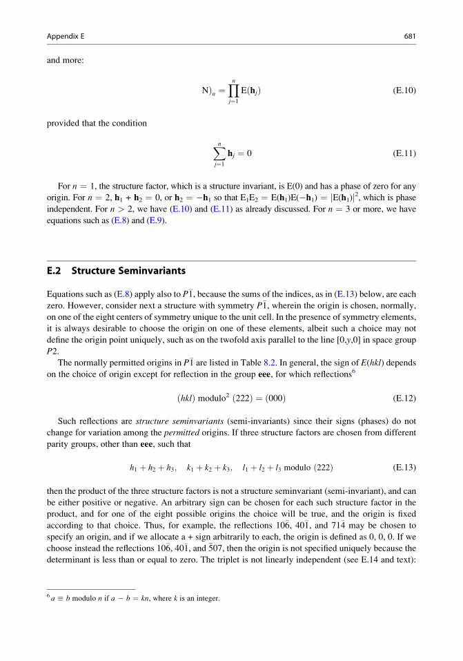
Combining the terms appropriately:

A=2 ¼ cos 2plzfcos 2pðhxþ kyÞ þ cos 2pð�hyþ kxÞg þ cos 2p lzþ hþ k þ l

2

� �cos 2pðhx� kyÞ

þ cos 2p lzþ hþ k þ l

2

� �cos 2pðhyþ kxÞ

The expansion of cos 2p lzþ hþ k þ l

2

� �shows that we need to consider the cases of

h + k + l even and odd, and recalling that cosP cosQ ¼ cosP cosQ� sinP sinQ, we find

the following:

h +k + l = 2n

A ¼ 4 cos 2plzðcos 2phx cos 2pky� sin 2phy sin 2pkxÞ

Similarly

B ¼ 4 sin 2plzðcos 2phx cos 2pky� sin 2phy sin 2pkxÞ

From the equations for jF(hkl)j and f(hkl), we find h + k + l = 2n + 1.

Proceeding in a similar manner, we now find

A ¼ 4 cos 2plzð� sin 2phx sin 2pkyþ sin 2phy sin 2pkxÞ

and

B ¼ � 4 sin 2plzð� sin 2phx sin 2pkyþ sin 2phy sin 2pkxÞ

It is clear now that for h + k + l odd, A = B = 0 if h = 0, or k = 0, or h = k. Hence, the limiting

conditions: 0kl: k + l = 2n12 (h0l: h + l = 2n), and hhl: l = 2n. The first of these conditions

corresponds to an n-glide ⊥a, (b) while the second indicates a c-glide ⊥<110>, consistent with

space group P4nc.

Solutions 4

4.1. For thegiven reflection, (sin y)/l = 0.30, forwhich fC = 2.494.Hence, exp[�B(sin2y)/l2] = 0.5423,

so that fC,27.55� = 1.352, which is 54.2 % of what its value would be at rest. The root mean square

displacement is [6.8/(8p2)]1/2 = 0.29 A. Since vibrational energy is proportional to kT, where k is theBoltzmann constant, a reduced temperature factor with concomitant enhanced scattering would be

achieved by conducting the experiment at a low temperature.

4.2. For NaCl, d111 ¼ a=p3 ¼ 2:2487 A, so that (sin y111)/l = 0.1539 A�1 and (sin y222)/

l = 0.3078 A�1. Similarly, for KCl, (sin y111)/l = 0.1379 A�1 and (sin y222)/l = 0.1379 A�1.

12 [h + k + l ¼ 2n + 1 → k + l ¼ 2n + 1 for h ¼ 0].

Tutorial Solutions 701

Using the structure factor equation for the NaCl structure type, we have

Fð111Þ ¼ 4½fNaþ=Kþ þ fCl� cosð3pÞ� ¼ 4½fNaþ=Kþ� fCl� �, whereas F(222) = 4[fNa+/K+ + fCl

�].Thus, we obtain the following results:

111 222

NaCl KCl NaCl KCl

(sin y)/l 0.1539 0.1379 0.3078 0.2759

f+ 8.979 15.652 6.777 11.576

f� 13.593 14.207 9.387 9.997

F �18.46 1.445 64.66 86.29

Remembering that wemeasure jFj2, it is clear that jF(111)j for KCl is relatively vanishingly small.

4.3. F ¼ ð2=pSÞ1=2 Ð10

F expð�F2=2SÞdF. Let F2=2S ¼ t, so that dF ¼ ðS=2tÞ1=2dt.Then, F ¼ ð2S=pÞ1=2 Ð1

0t0 expð�tÞdt. Since t0 = t(1�1), the integral (see Web Appendix WA7)

is G(1) = 1, Hence, F ¼ ð2S=pÞ1=2.Making the above substitution again, we have F2 ¼ ð2S=pÞ1=2 Ð1

0t1=2 expð�tÞdt ¼ ð2S=p1=2Þ

1=2 Gð1=2Þ ¼ S.Thus, Mc ¼ ð2S=pÞ=S ¼ 2=p ¼ 0:637.

4.4. E3 ¼ ð2=pÞ1=2 Ð10

E3 expð�E2=2ÞdE. Let E2=2 ¼ t, so that dE = (2t)�1/2dt. Then,

E3 ¼ ð8=pÞ1=2 Ð10

t expð�tÞ dt ¼ ð8=pÞ 12Gð2Þ ¼ 1:596.

4.5.

jE2 � 1j ¼ 2

ð10

jE2 � 1jE expð�E2Þ dE

By making the substitution E2 = t, we have

jE2 � 1j ¼ð10

ð1� tÞ expð�tÞ dtþð11

ðt� 1Þ expð�tÞdt

¼ ð�e�tj10 þ ðte�tj10 þ ðe�tj10 � ðte�tj11 � ðe�tj11 þ ðe�tj11¼ 2=e ¼ 0:736

4.6. The statistically distinguishable features of classes 2, m and 2/m are summarized as follows:

P2 Pm P2/m

hkl 1A 1A 1C

h0l 1C 2A 2C

0k0 2A 1C 2C

When finding the average intensities, do not mix the h0l and 0k0 reflections either with

themselves or with the hkl reflections until the space-group ambiguity has been resolved. Instead

get them from some other zone, excluding any terms it contains that lie in [h0l] or [0k0] zones,

and check the distribution of this chosen zone. If it is centric, the space group is P2/m. To

distinguish between the other two space group, examine the distribution in the [h0l] zone.

Generally there will be insufficient 0k0 reflections alone to give reliable results.

4.7. (a) mmmPc - - leaves the following space groups unresolved:

Pcm21 2/2; 2/2; 4(1)

Pc2m 2/2; 4/(1); 2/2

Pcmm (4/2; 4/2; 4/2)

702 Tutorial Solutions

The numbers are the multiples for the principal rows and zones (see Table 4.2). Parentheses

indicate centric zones or the complete weighted reciprocal lattice. One would examine the

distribution in both the [h0l] and [0k0] zones. Alternatively, an examination of the [0k0]

zone, excluding the h0l and 0k0 data, could be considered. A centric distribution would

identify Pccm. The other two could be separated by reference to zones, but distinction may

be difficult at this stage.

(b) mmmC - - - leaves the following space groups unresolved:

Cmm2 2/2; 2/2; 4(1)

Cm2m 2/2; 4/(1); 2/2

C222 2/(1); 2/(1) 2/(1)

Cmmm (4/2; 4/2; 4/2)

Again, parentheses indicate centric zones or the complete weighted reciprocal lattice. All

principal zones must be examined in order to resolve the ambiguities here.

Solutions 5

5.1. (a) The crystal system is tetragonal, and the Laue group is4

mmm; the optic axis lies along the

needle axis (z) of the crystal.(b) The section is in extinction for any rotation in the x,y plane, normal to the needle axis; the

section is optically isotropic.

(c) For a general oscillation photograph with the X-ray beam normal to z, the symmetry is m.For a symmetrical oscillation photograph with the beam along a, b or any direction in the

form h110i at the mid-point of the oscillation, the symmetry is 2mm.

5.2. (a) The crystal system is orthorhombic.

(b) Suitable axes may be taken parallel to three non-coplanar edges of the brick.

(c) Symmetry m.

(d) Symmetry 2mm, with the m lines horizontal and vertical.

5.3. (a) Monoclinic, or possibly orthorhombic.

(b) If monoclinic, p is parallel to the y axis. If orthorhombic, p is parallel to one of x, y, or z.

(c) (i) Mount the crystal perpendicular to p, about either q or r, and take a Laue photograph withthe X-ray beam parallel to p. If the crystal is monoclinic, symmetry 2 would be observed. If

orthorhombic, the symmetry would be 2mm, with the m lines in positions on the film that

define the directions of the crystallographic axes normal to p. If the crystal is rotated such

that the X-rays travel through the crystal perpendicular to p, a vertical m line would appear

on the Laue photograph of either a monoclinic or an orthorhombic crystal. (ii) Use the same

crystal mounting as in (i), but take a symmetrical oscillation photograph with the X-ray

beam parallel or perpendicular to p at the mid-point of the oscillation. The rest of the answer

is as in (i).

5.4. Refer to Fig. S5.1. Let hmax represent the maximum value sought. Since we are concerned with

a large d* value, we take l 0.2 A, the minimum value in the white radiation. Now

d* = ha* = (2/l) sin y and since, from the diagram, y is the angle subtended at the circumfer-

ence by d*, y = 20�, so that hmax is the integral part of 2=ð0:2lÞ sin 20, which is 17.

The X-coordinate on the film is 60 tan 40 = 50.35 mm. The half-width of the film is

62.5 mm, so the 17,00 reflection will be recorded on the film.

Tutorial Solutions 703

5.5. For the first film, we can write IðhklÞ þ Ið2h; 2k; 2lÞ ¼ 300, and for the second film,

after absorption, we have 0:35IðhklÞ þ 0:65Ið2h; 2k; 2lÞ ¼ 130. Solving these equations gives

I(hkl) = 216.7 and I(2h, 2k, 2l) ¼ 83.3.

5.6. (a) For symmetry 2mm in Laue group m�3m, the X-ray beam must be traveling along a <110>

direction (Table 1.6); we will choose [110], so that a and b lie in the horizontal plane; c is then

the vertical direction.

(b) We can use Fig. 5.17, changing the sign of�a*, and with f = 45� because XO is [110] for the

present problem. For an inner spot, it follows readily that 2y = tan�1(43.5/60.0), so that 2y =

35.94�, and e = 27.03� (Chap. 5, Fig. 5.17).(c) Now, tan 27:03 ¼ 0:5102 ¼ h=k, since a = b. In the given orientation, the reflections on the

horizontal line are hk0 and, since the unit cell is F, h and k must be both even, with k = 2h,

from above. Possible reflections are, therefore, 240, 480, 612,0, . . . It is straightforward to

show that l ¼ 2a sin y=ffiffiffiffiN

p, where N = h2 + k2.

For 240, l = 0.746 A, for 480, l = 0.373 A, which is unreasonably small in crystallographic

work.We note from the orientation of the a and b axes (a* and b*) that one of h and kmust be

negative; we can choose k. For an outer spot, we find in a similar manner that tan e = 0.3418,

so that k = 3h. Reasonable indices correspond to h = 2 and k = 6, again with one index

negative; here, l = 0.753 A. To summarize:

The X-ray beam is along [110]. For the inner spots: y = 17.97�; 2 �4 0 and 4 �2 0;

l = 0.746 A. For the outer spots: y = 26.13�; 2�60 and 6�20; l = 0.753 A.

5.7. Since the crystal is uniaxial, it must be hexagonal, tetragonal, or trigonal. The Laue symmetry

along axis 1 indicates that the crystal is trigonal, referred to hexagonal axes, and that axis 1 is

therefore c. Following Chap. 5, Sect. 5.4.3, we find for the repeat distances along the three axes:

Fig. S5.1

704 Tutorial Solutions

Axis 1 2 3

Repeat=A 15:65 8:264 4:772

The smallest repeat distance corresponds to the unit-cell dimension a, direction ½10�10�, Lauesymmetry 2 (Chap. 1, Fig. 1.36 and Table 1.6). Axis 2 must be a direction in the x, y plane, and itis straightforward to show that it is the repeat distance along ½12�30�, Laue symmetrym. Thus, we

have: a = b = 4.772, c = 15.65 A; a = b = 90�, g = 120�; the Laue group is �3m.

5.8. Applying the Bragg equation, l ¼ 2d sin y, where d = 6.696/2 A. Thus, (a) y0002 (Cu) = 13.31�,and (b) y0002 (Mo) = 6.093�.

5.9. (a) The data indicate a pseudo-monoclinic unit cell with g unique. Following Chap. 2, Sect. 2.5,we find a = b = 6.418, c = 3.863 A. It would appear that the c dimension is true, and that

the ab plane is centered. It is straightforward to show that a and b are the half-diagonals of a

rectangle with sides a0 = a � b and b0 = a + b. Thus, the orthorhombic unit cell has the

dimensions a = 3.062, b = 12.465, and c = 3.863 A. The transformation can be written as

atrue = Madiff, where

M ¼1 �1 0

1 1 0

0 0 1

24

35

(b) The reciprocal cell is transformed according to a�true ¼ ðM�1ÞTa�diff . The transpose of the

inverse matrix is

1=2 �1=2 0

1=2 1=2 0

0 0 1

264

375

Hence, a* = 0.2321, b* = 0.05702, c* = 0.1840. These values may be confirmed by dividing

the “true” values, for the orthorhombic cell, into the wavelength.

5.10. (a) Refer to Sect. 5.2.4: tan 2ymax ¼ r=R, where r is the radius of the plate, 172.5 mm.

2dmin sin ymax ¼ 1:05= ð2� 1:0Þ ¼ 0:525; and ymax ¼ 63:336�. Hence, R ¼ 172:5=

tan 63:336; or 86:6mm.

(b) The whole image would shrink but would still contain the same amount of data, and the

spots would become closer together.

(c) Some of the pattern would be lost because the angle subtended at the edge of the plate would

become less: the spots would then be further apart.

5.11. (a) A 5, B 1, C 0.1 mm

(b) A 450, B 250, C 80 mm

(c) A 12, B 60, C 300 s

Solutions 6

6.1.Ð c=2�c=2 sinð2pmx=cÞ cosð2p n x=cÞdx ¼ Ð c=2�c=2 f

1

2sin½2pðmþ nÞx=c� þ 1

2sin½2pðm� nÞx=c�gdx

using identities from Web Appendix WA5. Integration leads to � ½c=2pðmþ nÞ� cos½2pðmþ nÞx=c� jc=2�c=2 � ½c=2pðm� nÞ� cos½2pðm� nÞx=c�jc=2�c=2. Since m and n are integers the

integral is zero for m 6¼ n. For m = n, the original integral becomesÐ c=2�c=2

12sinð4pmx=cÞ dx,

which is also zero.

Tutorial Solutions 705

6.2. A plot of r(x) as a function of x (in 40ths) shows peaks at 0, 20, and 40 for Mg (as expected),

and at ca 8.25, 11.75, 28.25, and 31.75, for the 4F atoms per repeat unit a; thus, xF is (0.206;

0.706). Only the function to a/4 need be calculated, since there is m symmetry across the points14ð10=40Þ; 1

2ð20=40Þ and 3

4ð30=40Þ.

(a) The first three terms alone are insufficient to resolve clearly the pairs of fluorine peaks that

are closest in projection.

(b) Changing the sign of the 600 reflection results in single peaks for fluorine at 10/40 and

30/40. The error in sign (phase) is clearly the more serious fault.

6.3. GðSÞ ¼ Ð p�p a exp ði2pSxÞ dx ¼ aÐ p�p cos ð2pSxÞ þ ia

Ð p�p sinð2pSxÞ dx. The second integral is

zero, because the integrand is an odd function. Hence,

GðSÞ ¼ a ð2p SÞ sinð2pSxÞjp�p ¼ 2ap sinð2pSpÞ=2pSpÞ

and we retain the parameters which would obviously cancel, so as to preserve the characteristic

sin (ax)/(ax) form. To obtain the original function, we evaluate

f ðxÞ ¼ ða=pÞð1�1

ð1=SÞ sinð2pSpÞ expð�i2pxSÞ dS ¼ ða=pÞð1�1

ð1=SÞ sinð2pSpÞ cosð2pxSÞ dS

where the sine term from the expanded integrand is zero as before. Using results from Web

Appendix WA5, the integral becomes

ða=2pÞð1�1

ð1=SÞ sinð2pSðpþ xÞ� dSþð1�1

ð1=SÞ sinð2pSðp� xÞ�� �

dS

aðp� xÞð1�1

sin½2pSðp� xÞ�=½2pðp� xÞ� dS:

From Web Appendix WA9,Ð1�1 ðsin y=yÞ dy ¼ p; hence, we derive

f ðxÞ ¼ ða=2Þðpþ xÞ=jpþ xj þ ða=2Þðp� xÞ=jp� xj:

It is clear from this result that f(x) = a for j x j < p, f(x) = a/2 for x = p, and f(x) = 0 for

j x j = 0, which correspond to the starting conditions.

6.4.

Gðf Þ ¼ A

ð1�1

cosð2pf0tÞ expð�i2pftÞ dt

¼ ðA=2Þð1�1

f½expði2pf0tÞ þ expð�i2pftÞ� expð�i2pf tÞg dt

¼ ðA=2Þð1�1

fexp½�i2pðf � f0Þt� þ exp½�i2pðf þ f0Þt�g dt¼ ðA=2Þdðf þ f0Þ þ ðA=2Þdðf � f0Þ:

In the inversion, the d-function repeats the function at f = f0. Thus,

f ðtÞ ¼ ðA=2Þð1�1

½dðf þ f0Þ þ dðf � f0Þ� expði2pftÞ df¼ ðA=2Þ½expði2pf0tÞ þ expð�i2pf0tÞ�¼ A cosð2pf0tÞ:

706 Tutorial Solutions

6.5. The molecules have the displacements p and �p from the origin. Hence, the total transform

GT(S) is given by

GTðSÞ ¼ G0ðSÞ expði2pp � SÞ þ G�0ðSÞ expð�i2p p � SÞ

Using results from Sect. 3.2.3, we can write G0(S) = jG0j exp(if), and G�0ðSÞ ¼ jG0j exp ð�fÞ,

where f is a phase angle. Hence,

GTðSÞ ¼ jG0j expði2pp � Sþ fÞ þ expð�i2pp � S� fÞf ¼ 2jG0j cosð2pp � Sþ fÞ

As discussed in Sect. 6.6.3, the maximum value of the transform is 2jG0j, at those points wherecos(2pp·S + f) is equal to unity. In this example, however, such points do not lie in planes and,

consequently, the fringe systems are curved rather than planar.

6.6. The atoms related by the screw axis would have the fractional coordinates x, y, z and

�x; 12þ y; 1

2� z. From (6.50), we have

GðSÞ ¼Xn=2j¼1

fj exp½i2pðhxj þ kyj þ lzjÞ� þ exp½i2pð�hxj þ kyj � lzj þ k=2þ l=2Þ��

where the summation is over n/2 atoms in the unit cell not related by the 21 symmetry. Hence,

GðSÞ ¼Xn=2j¼1

fjfexp½i2pkyjfexp½i2pðhxj þ lzjÞþ exp½i2pð�hxj � lzj þ k=2þ l=2Þ�g

In a general transform, h, k, and l could take any values. However, in a crystal they are integers,

but in order to obtain a special condition, we must also consider the case that h = l = 0:

GðSÞh¼l¼0 ¼ 2Xn=2j¼1

fj expði2pkyj½expðipkÞ�Þ

Then, we have G(S)h=l=0 = 0 for k = 2n + 1, that is, the 0k0 reflections are systematically

absent when k is odd.

6.7. Figure S6.1 indicates the nodal lines for the P–S fringe system. Since the transform is chosen to

be positive at the origin, regions can be allocated to the transform, as shown. Hence, the

intense reflections can be allocated signs, as follow:

240� 250� 410 � 520 �650+ 710+ 720 + 820 +

�130þ �140þ �230þ �240þ�370þ �440� �470þ �530��540� �670� �710� �760��910þ �920þ 10; 00þ 10; 10þ10; 20þ

6.8. In Fig. S6.2, the three points are plotted in (a).A transparency ismadeof the structure in (a), inverted

in the origin. The structure (a) is then drawn three times on the transparency, with each of the atoms

of the inversion, in turn, over the origin of (a), and in the same orientation. The completed diagram

(b) is the required convolution: the six triangles outlined in (b) all produce the same set of nine

vectors (three superimposed at the origin).

Tutorial Solutions 707

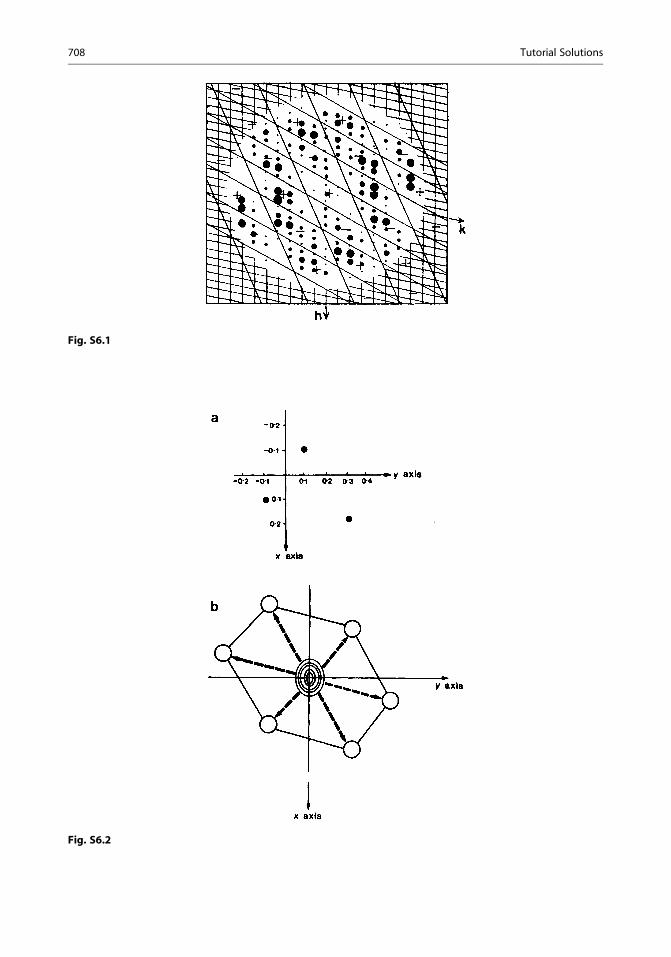
Fig. S6.1

Fig. S6.2

708 Tutorial Solutions

6.9. Figure S6.3 shows the contoured figure field of Fig. S6.2. The same triangles are revealed,

giving six sets of atom coordinates, as follow:

1 0.15, 0.10 �0.15,�0.10 �0.05, 0.30

2 0.05, 0.20 �0.05,�0.20 �0.20,�0.20

3 0.10,�0.10 �0.10, 0.10 �0.20,�0.30

4 0.05,�0.30 0.15, 0.10 �0.15,�0.10

5 0.25, 0.00 0.05, 0.20 �0.05,�0.20

6 0.10,�0.10 �0.10, 0.10 0.20, 0.30

6.10. The transform is positive in sign at the origin. Hence, by noting the succession of contours

along the 00l row, we arrive at the following result:

001 002 003 004 005 006

+ � + + � �

6.11. The transform of f(x) is given by

fTðxÞ ¼ 1ffiffiffiffiffiffi2p

pð1�1

½expð�x2=2Þ expði2pSxÞ�dx ¼ 2ffiffiffiffiffiffi2p

pð10

½expð�x2=2Þ cosð2pSxÞ�dx;

because fT(x) is an even function. Hence, using standard tables of integrals,

Fig. S6.3

Tutorial Solutions 709

fTðxÞ ¼ 2ffiffiffiffiffiffi2p

pffiffiffip

p

2ffiffiffiffiffiffiffiffi1=2

p expð�4p2S2=2Þ ¼ expð�2p2S2Þ:

The transform of g(x), gT(x), is a d-function with the origin at the point x = 2, so that gT(x) =

exp(i4pS), from Sect. 6.6.8. Hence, c(x) = fT(x)*gT(x) = exp(i4pS � 2p2S2).6.12. (a) As h is increased, the form of f(x) approaches a square more and more closely.

(b) m-lines occur at ¼, that is, at 15/60 and 45/60 in x

(c) At x = 0 and 2p the sine term in (6.15) is zero, so that f(x) = p/2. At x = p, the sine term is

sin(2ph)30/60, or sin(ph). Since h is an integer, then again f(x) = p /2.

Solutions 7

7.1. In P21/c, the general positions are ðx; y; z; x; 12� y; 1

2þ zÞ, so that AðhklÞ ¼

2fcos 2pðhxþ kyþ lzÞ þ cos 2pðhx� kyþ lzþ k=2þ l=2Þg¼ 4 cos 2pðhxþ lz þ k=4þl=4Þcos 2pðky� k=4� l=4Þ. Introducing the y-coordinate of ¼, AðhklÞ ¼ 4 cos 2pðhxþlzþ k=4þ l=4Þ cos 2pðl=4Þ, so that the hkl reflections will be systematically absent for

l = 2n + 1. The indication is that the c spacing should be halved, so that the true unit cell

contains two species in space group P21 (see Fig. S7.1). This problem illustrates the conse-

quences of sitting an atom on a glide plane: although we have considered here a hypothetical

structure containing one atom in the asymmetric unit, in a multi-atom structure, an atom may,

by chance, be situated on a translational symmetry element.

7.2. Refer to Chap. 2, Fig. 2.37, and Figs. S7.2 and S7.3.13 There are eight rhodium atoms in the unit

cell. If the atoms are in general positions, the minimum separation of atoms across any m plane

is 1=2 � 2y. For any value of y, the distance would be too small to accommodate two rhodium

atoms. Hence, they must occupy two sets of special positions. Positions on centers of symmetry

may be excluded on the same grounds as above. Thus, the atoms are located on two sets of m

planes as follow:

4 Rh ðx1; 1=4; z1; 1=2 � x1; 3=4; 1=2 þ z1Þ4Rh ðx2; 1=4; z2; 1=2 � x2; 3=4; 1=2 þ z2Þ

Fig. S7.1

13Mooney R, Welch AJE (1954) Acta Crystallogr 7:49.

710 Tutorial Solutions

7.3. The space group is P21/m. The molecular symmetry cannot be �1, but it can be m.

Hence, we can make the following assignments:

(a) Cl on m; (b) N on m; (c) two C on m, with four other C probably in general positions; (d)

sixteen H in four sets of general positions, two H (in N–H groups) on m, and two H from CH3

groups onm—those that have their C atoms onm. This arrangement is shown in Fig. S7.4a. The

species CH3, H1 and H2 lie above and below the m plane. The alternative space group P21 was

considered, but the full structure analysis14 confirmed P21/m. Figure S7.4b illustrates P21/m,

and is reproduced from the International Tables for X-ray Crystallography, Vol. I, by kind

permission of the International Union of Crystallography.

7.4. AðhhhÞ ¼ 4fgPt þ gK½cos 2pð3h=4Þ þ cos 2pð9h=4Þ� þ 6gCl½3 cos 2pðhxÞ�g, where the factor4 relates to an F unit cell (see Sect. 3.7.1). B(hhh) = 0, so that F(hhh) = A(hhh), and A(hhh)

Fig. S7.2

Fig. S7.3

14 Lindgren J, Olovsson I (1968) Acta Crystallogr B24:554.

Tutorial Solutions 711

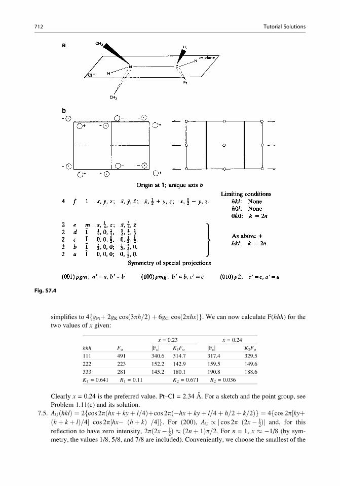
simplifies to 4fgPtþ 2gK cosð3ph=2Þ þ 6gCl cosð2phxÞg. We can now calculate F(hhh) for thetwo values of x given:

x = 0.23 x = 0.24

hhh Fo jFcj K1Fo jFcj K2Fo

111 491 340.6 314.7 317.4 329.5

222 223 152.2 142.9 159.5 149.6

333 281 145.2 180.1 190.8 188.6

K1 = 0.641 R1 = 0.11 K2 = 0.671 R2 = 0.036

Clearly x = 0.24 is the preferred value. Pt–Cl = 2.34 A. For a sketch and the point group, see

Problem 1.11(c) and its solution.

7.5. AUðhklÞ ¼ 2 cos 2pðhxþ kyþ l=4Þþcos 2pð�hxþ kyþ l=4þ h=2þ k=2Þf g ¼ 4fcos 2p½kyþðhþ k þ lÞ=4� cos 2p½hx� ðhþ kÞ =4�g. For (200), AU / j cos 2p ð2x� 1

2Þj and, for this

reflection to have zero intensity, 2pð2x� 12Þ ð2nþ 1Þp 2= . For n = 1, x �1/8 (by sym-

metry, the values 1/8, 5/8, and 7/8 are included). Conveniently, we choose the smallest of the

Fig. S7.4

712 Tutorial Solutions

symmetry-related values, that is, 1/8. For (111), and using this value for

x; AU / cos 2pðyþ 3=4Þ cos 2pð1=8 � 1=2Þ. For high intensity, j cos 2pðyþ 3=4Þj 0; np.For n = 0, y = ¾ (and ¼ by symmetry). For n = 1, y is again 1

4and ¾. Proceeding in this

manner with (231) leads to y = 1/6 (by symmetry, the values 1/3, 2/3, and 5/6 are included),

and with (040) we find y = 3/16 (by symmetry, 5/16, 11/16, and 13/16 are included). The

mean for the three value of y is (1/4 + 1/6 + 3/16)/3, or approximately 0.20.

7.6. Since there are two molecules per unit cell in P21/m in this structure, and the molecules cannot

have �1 symmetry, the special positions sets ðx; 14; zÞ are selected. TheB, C, andN atoms lie onm.

Since the shortest distance between m planes is 3.64 A, the F1, B, N, C, and H1 atoms must lie on

one and the samem plane (see Fig. S7.5a). Hence, the remaining two F and four H atoms must be

placed symmetrically across the samem plane. These conclusions were borne out by the structure

analysis.15 Figure S7.5b is a stereoview of the packing diagram for CH3NH2BF3, showing the H1,

C, N, B and three F atoms. The m plane is normal to the vertical direction in the diagram and the

remaining two pairs of H atoms are disposed across the m plane as described above.

7.7. (a) (i) jFðhklÞj ¼ jFð�h �k �lÞj; (ii) jFð0klÞj ¼ jFð0 �k �lÞj; (iii) jFðh0lÞj ¼ jFð�h 0 �lÞj(b) (i) jFðhklÞj ¼ jFð�h �k �lÞj ¼ jFðh �k lÞ;(ii) jFð0klÞj ¼ Fð0 �k �lÞj ¼ jFð0 �k lÞ(iii) jFðh0lÞj ¼ jFð�h 0 �lÞj

Fig. S7.5

15 Geller S, Hoard JL (1950) Acta Crystallogr 3:121.

Tutorial Solutions 713

(c) (i) jFðh k lÞj ¼ jFð�h �k �lÞj ¼ jFð�h k lÞj ¼ jFðh �k lÞj ¼ jFðh k �lÞj(ii) jFð0 k lÞj ¼ jFð0 �k �lÞj ¼ jFð0 �k lÞj;(iii) jFðh 0 lÞj ¼ jFð�h 0 �lÞj ¼ jFð�h 0 lÞj

Any combination of hkl not listed follows the pattern of (a) (i). In (b), for example,

jFð�h 0 lÞj ¼ jFðh 0 �lÞj7.8. (a) In Pa, the symmetry element relates the sites x, y, z and 1

2þ x; y; z, so that the Harker line is

½1=2 v 0�. In P2/a, the Harker section is (u 0 w) and the line ½12 v 0�.In P2221, there are three Harker sections, (0 v w), (u 0 w), and ðu v 1

2Þ.

(b) The Harker section (u 0 w) must arise through the symmetry-related sites x, y, z and �x; y; �z,

which correspond to a two-fold axis along y. Similarly, the line [0v0] arises from a mirror

plane in the Patterson normal to y. Since the crystal is non-centrosymmetric, the space

group must be P2 or Pm. If it is P2, there must be, by chance, closely similar y coordinates

for many of the atoms in the structure. If it is Pm, chance coincidences occur between the xand z coordinates. [These conditions are somewhat unlikely, especially when many atoms

are present, so that Harker sections and lines can sometimes be used to distinguish between

space groups that are not determined by diffraction symmetry alone.]

7.9. (a) P21/n, a non-standard setting of P21/c (see also Chap. 2, Problem 2.12).

(b) The S–S vectors have the following Patterson coordinates:

(1) ð12; 12þ 2y; 1

2Þ Double weight

(2) ð12þ 2x; 1

2; 12þ 2zÞ Double weight

(3) (2x, 2y, 2z) Single weight

(4) ð2x; 2�y; 2zÞ Single weight

Section v ¼ 12

Type 2 vector x = 0.182, z = 0.235

Section v = 0.092 Type 1 vector y = 0.204

Section v = 0.408 Type 3 or 4 vector x = 0.183, y = 0.204, z = 0.234

Thus we have four S–S vectors at: (0.183, 0.204, 0.235; 0.683, 0.296, 0.735). Any one of the

other seven centers of symmetry, unique to the unit cell, may be chosen as the origin,

whereupon the coordinates would be transformed accordingly. The sulfur atom positions are

plotted in Fig. S7.6 [Small differences in the third decimal places of the coordinates determined

from the maps in Problems 7.9 and 7.10 are not significant.]

Fig. S7.6

714 Tutorial Solutions

7.10. (a) By direct measurement, the sulfur atom coordinates are S (0.266, 0.141) and S0 (�0.266,

�0.141)

(b) Draw an outline of the unit cell on tracing paper, and plot the position of –S on it. Place the

tracing over the idealized Patterson map (Fig. P7.2), in the same orientation, with

the position of –S over the origin of the Patterson map, and copy the Patterson map on

to the tracing (Fig. S7.7a). On another tracing, carry out the same procedure with respect to

the position of �S0 (Fig. S7.7b). Superimpose the two tracings (Fig. S7.7c). Atomic

positions correspond to positive regions of the two superimposed maps.

Fig. S7.7

Tutorial Solutions 715

7.11. (a) The summation to form P(v) can be carried out with program FOUR1D. In using the program,

each data line should contain k,Fo(0k0)2, and 0.0, the zero datum representing theB coefficient

of the Fourier series. P(v) shows three non-origin peaks. If the highest of them is assumed to

arise from theHf–Hf vector, then yHf = 0.105; the smaller peaks are Hf–Si vectors, fromwhich

we could obtain approximate y parameters for the silicon atoms. Their difference in height

arisesmainly from the fact that one of them is, in projection, close to the origin peak. However,

the simplified structure factor equation for Fo(0k0), based on the hafnium atoms alone, is

Foð0k0Þ / cosð2pkyHfÞ

so that the signs of the reflections, ignoring the weak reflections 012,0 and 016,0, are, in order,

+ � � + + �. (b) We can now calculate r(y) with these signs attached to the Fo(0k0) values.

From the result, we obtain yHf = 0.107, ySi1 = 0.033, and ySi2 = 0.25. These values for ySi leadto vectors which appear on P(v). We conclude that the small peak on r(y) at y = 0.17 is

spurious, arising most probably from both the small number of data and experimental errors

in them.

7.12. Since the sites of the replaceable atoms are the same in each derivative, and the space group is

centrosymmetric, we can write FðM1Þ ¼ FðM2Þ þ 4ðfM1 � fM2Þ, where f may be approximated

by the corresponding atomic number, Z. Hence, we can draw up the following table:

(a)

M

h NH4 K Rb T1

1 � � + +

2 a + + +

3 + + + +

4 � a + +

5 + + + +

6 � � a +

7 a + + +

8 a + + +

a = Indeterminate, because F is small or zero.

(b) The peak at 0 represents K and Al, superimposed in projection. The peak at 0.35 would then

be presumed to be due to the S atom.

(c) The effect of the isomorphous replacement of S by Se can be seen at once in the increases in

Fo(555) and Fo(666) and decrease in Fo(333). These changes are not in accord with the

findings in (b). Comparison of the two electron density plots shows that dS/Se must be

0.19 (the x coordinate is d=ffiffiffi3

p). The peak at 0.35 arises from a superposition of oxygen

atoms in projection, and is not appreciably altered by the isomorphous replacement.

7.13. A ¼ 100 cos 60þ ðfo þ Df 0Þ cos 36þ 8 cos126 ¼ 50þ 40:046� 4:702 ¼ 85:344: B ¼ 100

sin 60þðfo þ Df 0Þ sin 36þ 8 sin 126 ¼ 86:603þ 29:095þ 6:472 ¼ 122:17. Hence, jF(010)j =149.0, and f (010) = 55.06�. For the 0�10 reflection, we have A ¼ 100 cos 60þð fo þ Df 0Þ cos 36þ 8 cos 54¼ 50þ40:046þ 4:702 ¼ 94:748: B ¼ 100 sinð�60Þ þ ðfo þ Df 0Þsinð�36Þ þ 8 sin 54 ¼ �86:603� 29:095þ 6:472 ¼ �109:226. Hence, jFð0�10Þj ¼ 144:6,

and fð0�10Þ ¼ � 49.06�.7.14. Draw a circle, at a suitable scale, to represent an amplitude jFPj of 858. From the center of this

circle, set up a “vector” to represent jFH1jexp(if1), where jFH1j = 141 and f1 = (78 + 180) deg.

716 Tutorial Solutions

At the termination of this vector, draw a circle of radius 756 to represent jFPH1j. Repeat thisprocedure for the other two derivatives (Fig. S7.8). The six intersections 1–10, 2–20, and 3–30 arestrongest in the region indicated by •- - -•. The required phase angle fM , calculated from (7.50),

lies in this region. The centroid phase angle fB is biased slightly towards point 1.

7.15. Cos(hx � f) expands to cos hx cosfþ sin hx sinf which, for f = p/2, reduces to sinhx.

Hence, cðxÞ ¼ p=2þ 2P1

h¼1 ð1=hÞ sin hx ¼ p=2þ 2P1

h¼1 ð1=hÞ cosðhx� fÞ: This equation

resembles closely a Fourier series (see Sect. 6.2).

7.16. (a) The total mass of protein per unit cell is 18000Z � 1.6605 � 10�24 g, where Z is the number

of protein molecules per unit cell. Since there is an equal mass of solvent water in the unit cell,

D/2Z = (18000 � 1.6605 � 10�24)/(40 � 50 � 60 � 10�24 sin 100�) = 0.2529 g cm�3, so

thatD = 0.5058Z g cm-3. Sensible values for Z in C2 are 4 and 2. The former leads to a density

that is much too large for a protein; Z = 2 gives D = 1.012 g cm–3, which is an acceptable

answer.

(b) In space group C2 there are four general equivalent positions (see Sect. 2.7.3). Since Z = 2,

the protein molecule must occupy special positions on twofold axes, so that the molecule

has symmetry 2.

7.17. In the notation of the text, we have for F(hkl)

FHðþÞ ¼ F0HðþÞ þ iF00HðþÞand for jFð�h �k �lÞj

FHð�Þ ¼ F0Hð�Þ þ iF00Hð�Þ

where F0HðþÞ and F0Hð�Þ are the structure factor components derived from the real part of (7.64)

and (7.66), and F00HðþÞ and F00Hð�Þ are its anomalous components. It is clear from Fig. S7.9 that

Fig. S7.8

Tutorial Solutions 717

the moduli jFH(+)j and jFH(�)j are equal, but that fH(+) 6¼ fH(�). In terms of the structure

factor equations, we can write a single atom vector for h and �h

FðhÞ ¼ ðf 0 þ iDf 00Þ exp½ið2ph � rþ p=2Þ�Fð�hÞ ¼ ðf þ iDf 00Þ exp½�ið2ph � rþ p=2Þ�

from which we have jFðhÞj ¼ Fð�hÞj, but fðhÞ 6¼ fð�hÞ; p/2 acts in the same sense (positive) in

each case.

7.18. In the notation of the text, and for a centrosymmetric structure, we have FPHðþÞ ¼APðþÞ þ A0

HðþÞ þ iA00HðþÞ where

APðþÞ ¼XNP

j¼1

fj cos 2pðhxj þ kyj þ lzjÞ

A0HðþÞ ¼

XNH

j¼1

f 0j cos 2pðhxj þ kyj þ lzjÞ

A00HðþÞ ¼

XNH

j¼1

Df 00j cos 2pðhxj þ kyj þ lzjÞ

Clearly, jFðh k lÞj ¼ jFð�h �k �lÞj ¼ ðA2þ B2Þ1=2, where A ¼ APðþÞ þ A0HðþÞ and B ¼ A00

H

ðþÞ; fðhklÞ ¼ fð�h �k �lÞ ¼ tan�1 ðB=AÞ, and cannot equal 0 or p because of the finite value of

A00HðþÞ.

7.19. If, for a crystal of a given space group, Friedel’s Law breaks down, then the diffraction

symmetry reverts to that of the corresponding point group. Thus, we have

jF(hkl)j equivalents Bijvoet pairs

(a) C2 (2) hkl=�h k �l hkl=�h k �lwith h �k l=�h �k �l

(continued)

Fig. S7.9

718 Tutorial Solutions

(b) Pm (m) hkl=h �k l hkl=h �k lwith �h k �l=�h �k �l

(c) P212121 (222) hkl=h �k �l=�h k �l=�h �k l hkl=h �k �l=�h k �l=�h �k l with h k l=h �k l=h k �l=�h �k �l

(d) P4(4) hkl=�k h l=�h �k l=k �h l hkl=�k h l=�h �k l=k �h l with k �h �l=h k �l=�k h �l=�h �k �l

Strictly, pairs related as hkl and �h �k �l should be discounted, as they are, of course, Friedel pairs.

7.20. The number N of symmetry-independent reciprocal lattice points with a range 0 < y < ymax is

33.510 Vc sin3 y/(l3Gm), from Chap. 7. The volume Vc of the unit cell is 6 � 104 A3,G = 1 for

a P unit cell, and m, the number of symmetry-equivalent general reflections, is 8 for the Laue

group mmm. Hence, N = 74466.7 sin3 ymax.

(a) 0 < y < 10� : sin3 ymax = 5.236 � 10�3, so that N = 389 (779 if we consider the hkl and�h �k l reflections).

(b) 10 < y < 20� : sin3 ymax = 4.001 � 10�2, so that N = 2979 � 389, or 2590.

(c) 20 < y < 25�: sin3 ymax = 7.548 � 10�3, so that N = 5620 � 2979, or 2641.

The resolution, defined in terms of dmin, is dmin = l/(2 sin ymax)

(a) For ymax = 10�: dmin = 4.32 A

(b) For ymax = 20�: dmin = 2.19 A

(c) For ymax = 25�: dmin = 1.77 A

Solutions 8

8.1. A possible set, with the larger jEj values, is 705, 6 1 7, and 8�1 4. Reflection 4 2 �6 is a structure

seminvariant, and 203 is linearly related to the pair 8�1�4 and 6�1�7. Reflection 43 2 has a low jEjvalue, so that triple relationships involving it would not have a high probability. Alternative sets

are 705, 203, 8�1�4 and 705, 203, 6 �1 �7. A vector triplet exists between 81 4, 42�6, and 4�32.

8.2. The equations for A and B lead to the following relationships:

jFðhklÞj ¼ jFð�h�k �l Þj ¼ jFðh�klÞj ¼ jFð�hk�lÞj 6¼ jFð�hklÞj; jFð�hklÞj ¼ jFðhk�lÞj

Because of the existence of the k/4 term, the phase relationships depend on the parity of k:

k ¼ 2n : fðhklÞ ¼ �fðh k lÞ ¼ �fðh�klÞ ¼ fð�hk�l 6¼ fð�hklÞ;fð�hklÞ ¼ fðhk�lÞ

k ¼ 2nþ 1 : fðhklÞ ¼ �fð�h �k �lÞ ¼ p� fðh�klÞ ¼ pþ fð�hk�lÞ 6¼ fð�hkl;fð�hklÞ ¼ pþ fðhk�lÞ

8.3. Set (b) would be chosen: there is a redundancy in set (a) among 041, �162, and �123, because

jFð041Þj¼ jFð0 �4 1Þj in this space group. In space group C2/c, h + k is even for reflections to

occur, so that reflections 012, �123, 162, and �162 would not occur. The origin could be fixed by

223 and 13�7: there are only four parity groups for a C-centered unit cell.

8.4. Following the procedure given in Chap. 4, Sect. 4.2, it will be found that K = 4.0 0.4,

and B = 6.6 0.3 A2. Since B ¼ 8p2U2, the root mean square atomic displacement is

[6.6/(8p2)]1/2, or 0.29 A. (You were not expected to derive the standard errors in K and

B; they are quoted in order to give an idea of the precision obtainable from a Wilson plot.)

8.5. A plot of the atomic positions in the unit cell and its environs shows that the shortest Cl. . .Cl

contact distance is between atoms at ¼, y, z, and 3=4; �y; z. Hence, d2(Cl. . .Cl) = a2/4 + 4y2b2,

Tutorial Solutions 719

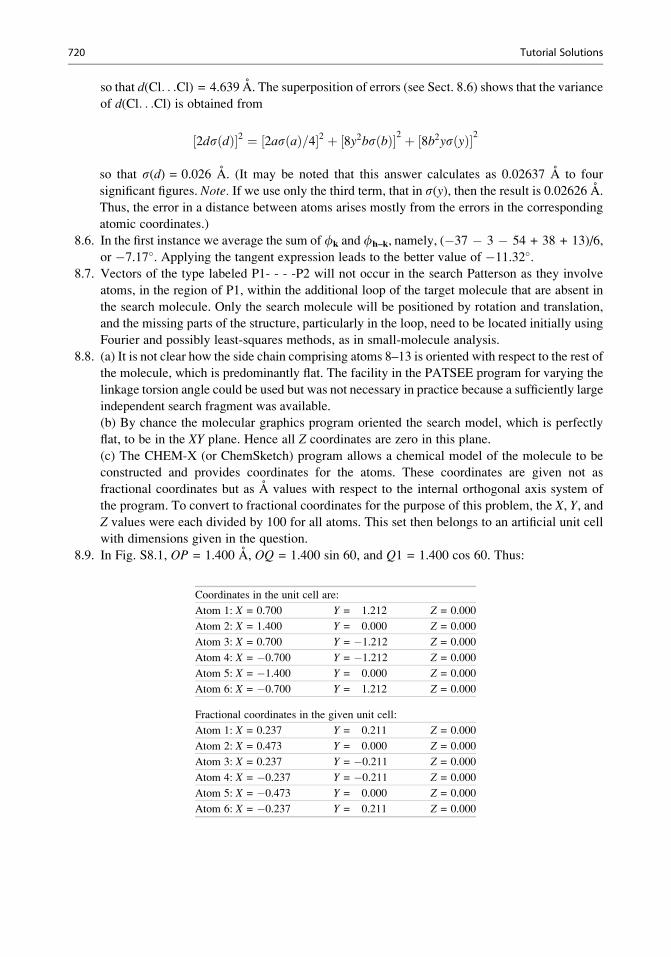
so that d(Cl. . .Cl) = 4.639 A. The superposition of errors (see Sect. 8.6) shows that the variance

of d(Cl. . .Cl) is obtained from

½2dsðdÞ�2 ¼ 2asðaÞ=4½ �2 þ ½8y2bsðbÞ�2 þ ½8b2ysðyÞ�2

so that s(d) = 0.026 A. (It may be noted that this answer calculates as 0.02637 A to four

significant figures. Note. If we use only the third term, that in s(y), then the result is 0.02626 A.Thus, the error in a distance between atoms arises mostly from the errors in the corresponding

atomic coordinates.)

8.6. In the first instance we average the sum of fk and fh–k, namely, (�37 � 3 � 54 + 38 + 13)/6,

or �7.17�. Applying the tangent expression leads to the better value of �11.32�.8.7. Vectors of the type labeled P1- - - -P2 will not occur in the search Patterson as they involve

atoms, in the region of P1, within the additional loop of the target molecule that are absent in

the search molecule. Only the search molecule will be positioned by rotation and translation,

and the missing parts of the structure, particularly in the loop, need to be located initially using

Fourier and possibly least-squares methods, as in small-molecule analysis.

8.8. (a) It is not clear how the side chain comprising atoms 8–13 is oriented with respect to the rest of

the molecule, which is predominantly flat. The facility in the PATSEE program for varying the

linkage torsion angle could be used but was not necessary in practice because a sufficiently large

independent search fragment was available.

(b) By chance the molecular graphics program oriented the search model, which is perfectly

flat, to be in the XY plane. Hence all Z coordinates are zero in this plane.

(c) The CHEM-X (or ChemSketch) program allows a chemical model of the molecule to be

constructed and provides coordinates for the atoms. These coordinates are given not as

fractional coordinates but as A values with respect to the internal orthogonal axis system of

the program. To convert to fractional coordinates for the purpose of this problem, the X, Y, andZ values were each divided by 100 for all atoms. This set then belongs to an artificial unit cell

with dimensions given in the question.

8.9. In Fig. S8.1, OP = 1.400 A, OQ = 1.400 sin 60, and Q1 = 1.400 cos 60. Thus:

Coordinates in the unit cell are:

Atom 1: X = 0.700 Y = 1.212 Z = 0.000

Atom 2: X = 1.400 Y = 0.000 Z = 0.000

Atom 3: X = 0.700 Y = �1.212 Z = 0.000

Atom 4: X = �0.700 Y = �1.212 Z = 0.000

Atom 5: X = �1.400 Y = 0.000 Z = 0.000

Atom 6: X = �0.700 Y = 1.212 Z = 0.000

Fractional coordinates in the given unit cell:

Atom 1: X = 0.237 Y = 0.211 Z = 0.000

Atom 2: X = 0.473 Y = 0.000 Z = 0.000

Atom 3: X = 0.237 Y = �0.211 Z = 0.000

Atom 4: X = �0.237 Y = �0.211 Z = 0.000

Atom 5: X = �0.473 Y = 0.000 Z = 0.000

Atom 6: X = �0.237 Y = 0.211 Z = 0.000

720 Tutorial Solutions

8.10. From Chap. 4, (4.34) and Chap. 8, (8.1), with N atoms per unit cell, assuming scaled Fo values,

dividing throughout byPN

j¼1 g2j;y (the e factor is assumed to be unity), gives

Ej j2 ¼ 1þ1XN

j¼1g2j;y

. �Xj6¼k

gj;ygk;y exp i2ph � rj;k� !

The second term on the right-hand side represents sharpened jFj2 coefficients [see also Chap. 7,(7.19)]. The term in the Patterson function that creates the origin peak,

PNj¼1 g

2j;y, is now unity,

so that a Patterson function with coefficients (jEj2 � 1) produces a sharpened Patterson

function with the origin peak removed.

8.11. (a) When using Molecular Replacement in macromolecular crystallography the search and

target molecules should be compatible in size as well as in their three-dimensional

structures. If this is not the case problems may be encountered in obtaining a dominant

solution to MR. The more possible solutions which have to be inspected, using Fourier

methods, the more laborious the process becomes, maybe to the point where the analysis

becomes untenable.

(b) For small-molecule analysis it is more usual for the search “molecule” to be a fairly small

fragment of the target molecule. In this case the search molecule must be as accurate as

possible in bond lengths and angles because the data are at atomic resolution and the

Patterson peaks similarly resolved. Programs such as PATSEE allow for more complex

search molecules to be used which have one degree of torsional freedom, thus increasing the

size of the whole search fragment.

8.12. The required determinant is

Eð0Þ EðhÞ Eð2hÞEð�hÞ Eð0Þ EðhÞEð�2hÞ Eð�hÞ Eð0Þ

������������� 0, which evaluates as

Eð0Þ3þEðhÞ2Eð�2hÞþEð2hÞ½Eð�hÞ�2� Eð0ÞjEð2hÞj2�Eð0ÞEðhÞj2�Eð0ÞjEðhÞj2� 0 or Eð0ÞfEð0Þ2 � jEð2hÞj2� 2jEðhÞj2g þ 2 jEðhÞj2 Eð2hÞ� 0. Inserting the given values for E(0),

jE(h)j, and jE(2h)j, we obtain 3f9� 4� 8gþ 8ð2Þ� 0, from which it is clear E(2h) is

positive in sign in order to satisfy the determinant expression.

8.13. For the first triplet, h + k + l = 0 0 0 modulo (2 2 2), where h = h1 + h2 + h3, and similarly for

k and l. Hence, the triplet is a structure seminvariant. The second triplet is also a structure

seminvariant, for the same reason. In the third triplet, h + k + l = 0 0 0 and is a structure

invariant. None of these triplets is suitable for specifying an origin because their determinants

are either zero or zero modulo 2 (see Appendix E).

8.14. Apply the structure factor (3.63). (a) In space group P21, the [010] zone is centric, plane group

p2, so that B0 ¼ 0 and A0 ¼ 2 cos 2p½ð1� 0:3Þ þ ð3� 0:1Þ�, so that jFj = 1.62 and f = 180�.

Fig. S8.1

Tutorial Solutions 721

(b) (i) Space group P212121 in projection on to (h0l) becomes plane group p2gg, with

coordinates (x, z; ½ � x, ½ + z). Proceeding as in (a), jFj = 0.38 and f = 180�. (ii) In the

standard orientation, the coordinates are (see Fig. 2.35): x, z; ½ � x, ½ + z; ½ + x, �z; �x,

½ � z. Proceeding as before, A0 = 0 and B0 = �1.18, so that jFj = 1.18 and f = –90�. Alter-natively, we recall from Appendix E that the phase change for an origin shift r is –2ph.r, whichis –2p(¾), so that f = 180 – 270 = �90�.

Solutions 9

9.1. (a) In space groupP21, symmetry-related vectors have the coordinates ð2x; 1=2; 2zÞ; the I–I vectorin the half unit cell is easily discerned. By measurement on the map, x1 = 0.422 and zI = 0.144,

with respect to the origin O.

(b) The contribution of the iodine atoms, FI, to the structure factors is given by 2fI cos 2p(0.422xI + 0.144zI). Hence, the following table:

hkl (sin y)/l 2fI fI Fo

001 0.026 105 65 40

0014 0.364 67 67 37

106 0.175 88 �20 33

300 0.207 84 �8 35

The signs of 001, 0014, and 106 are probably +, +, and �, respectively. The magnitude

jFI (300)j is a small fraction of Fo, and could easily be outweighed by the contribution from

the rest of the structure. Thus, its sign remains uncertain from the data given. Small

variations in the values determined for fI are acceptable; they derive, most probably, from

small differences in the graphical interpolation of the fI values.

(c) The shortest I–I vector is that between the positions listed above. Hence, dI–I = {[2 � 0.422

� 7.26]2 + [0.5 � 11.55]2 + [2 � 0.144 � 19.22]2 + [2 � 0.422 � 0.144 � 7.26 � 19.22

cos (94.07)]}1/2 = 10.05 A.

9.2. A S2 listing is prepared as follows:

h k h � k jE(h)j jE(k)j jE(h – k)j0018 081 0817 9.5

011 024 035 5.0

026 035 0.5

021 038 059 0.4

0310 059 0.4

024 035 059 9.6

038 059 0817 7.2

081 011,7 6.0

081 011,9 10.2

0310 059 081 7.9

081 011,9 9.2

(Note the convention, that a two-figure Miller index takes a comma after it unless it is the

third index.)

In space group P21/a, sðhklÞ ¼ sð�h �k �lÞ ¼ ð�1Þhþksðh �k lÞ, and sðh k �lÞ ¼ ð�1Þhþk sð�h k lÞ.In using only two-dimensional reflections from the data set, we need just two reflections to

722 Tutorial Solutions

specify an origin, say, 0, 0. We take s(081) = s(011,9) = + and proceed to the determination of

signs, as follows:

The two indications for s(021) and the single indication for s(026) will have low probabilities,

because of low jEj values, and must be regarded as unreliable at this stage. Within the data set, no

conclusion can be reached about s(a); both + and� signs are equally likely. Reflection 0312 does

not interact within the data set.

9.3. The space group is P21/c, from Chap. 9, Table 9.4. Thus, sjEðhklÞj ¼ sjEð�h �k �lÞj¼ ð�1Þkþ1sjEðh �k lÞj; for the hk reflections, set l = 0 in these relationships. Figure S9.1 shows

the completed chart. A S2 listing follows; an N indicates that no new relationships were

derivable with the reflection so marked; negative signs are represented by bars over the jEj values.

S2 Listing

Number h k h � k jEhj jEkj jEh�kj1 300 040 3�40 3.5

2 840 5 40 6.0

3 570 2 70 10.0

4 700 570 2�70 13.0

5 800 670 2�70 10.1

6 340 5�40 7.7

7 411,0 4 11; 0 4.9

8 040 8�40 4.2

9 730 0 �4 0 770 3.1

10 5 �4 0 270 6.9

11 040 N

12 340 7�70 �4 1 1; 0 4.1

(continued)

Tutorial Solutions 723

An origin at 0, 0 may be chosen by specifying 270 (eoe, and occurring four times) and 540 (oee,

and occurring three times), both as +. From the S2 listing, we now have:

Number Conclusion Comments

10 s(730) = +

7 s(800) = � s ð411; 0Þ ¼ �sð4 11; 0Þ5 s(670) = +

6 s(340) = � Sign propagation has ended.

Now let s(040) = a

1 s(300) = �a

2 s(840) = �a

3 s(570) = �a

4 s(700) = a

8 s(840) = �a

9 s(770) = a

11 s(411,0) = �a

Fig. S9.1

13 540 N

14 840 N

15 270 N

16 570 N

17 670 N

18 770 N

19 411,0 N

724 Tutorial Solutions

The symbol a would be determined by calculating electron density maps with both + and �values, and assessing the results in terms of sensible chemical entities. In a more extended,

experimental data set, the sign of a may evolve. No S2 relationship is noticeably weak, and the

above solution to the problem may be regarded as acceptable.

9.4. (a) Use Chap. 8, Sect. 8.5.1, (8.105); since a = g = 90 deg, the fourth and sixth terms on the

right-hand side are zero. Thus, the bond length is 2.119 A. From Sect. 8.6, (8.114), the esd

evaluates to 0.0001 A. Thus, we write S(1)–S(2) = 2.119(1) A.

(b) Writing down all Patterson vectors on the x,z projection of space group P21, we obtain:

A

2x1, 2z1; 2x2, 2z2–2x1, –2z1; –2x2, –2z2B

x1 – x2, z1 – z2; –x1 – x2, –z1 – z2; –x1 + x2, –z1 + z2; x1 + x2, z1 + z2;–x1 – x2, –z1 + z2; x1 + x2, z1 + z2; x1 – x2, z1 – z2; –x1 – x2, –z1 – z2Group A vectors are of single weight whereas group B vectors are of double weight. Hence the

vectors around the origin would have the geometry shown in Fig. S9.2, and we expect the

following arrangement, excluding the origin peak:

where S1D1 = D1S2 = S3D3 = D3S4 and S2D2 = D2S3 = S4D4 = D4S1.

Solutions 10

10.1. The number N of unit cells in a crystal is V(crystal)/V(unit cell). Both crystals have the volume

V(crystal) = 2.4 � 10�2 mm3. The protein unit-cell volume V(protein) = 60000 A3, or

60000 � 10�21 mm3. The total number of protein unit cells NP is therefore = 4 � 1014.

For the organic crystal unit cell, V(organic) = 1800 A3, or 1800 � 10�21 mm3, so that the

total number of organic unit cells N0 is 1.333 � 1016.

From Chap. 4, (4.1) and (4.2), we write

EðhklÞ ¼ ðI0=oÞðN2l3Þ½e4=m2ec

4�LpAjFðhklÞj2VðcrystalÞ (S10.1)

where N is the number of unit cells per unit volume of the crystal, L, p, and A are the Lorentz,

polarization, and absorption correction factors, and the other symbols have their usual meanings.

Historically, this equation was derived in 191416 and confirmed by careful measurements on

a crystal of sodium chloride in 192117. In (S10.1), E (hkl) is the experimentally derived quantity

and jF(hkl)j is the term required in X-ray analysis. For our purposes, we write

Fig. S9.2

16 Darwin CG (1914) Philosophical Magazine 27, 315.17 Bragg WL, James RW, Bosanquet CM (1921) Philosophical Magazine 42:1.

Tutorial Solutions 725

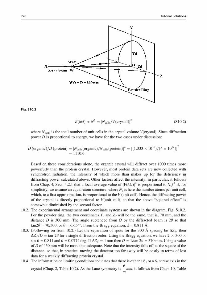
EðhklÞ / N2 ¼ ½Ncells=VðcrystalÞ�2 (S10.2)

where Ncells is the total number of unit cells in the crystal volume V(crystal). Since diffractionpower D is proportional to energy, we have for the two cases under discussion:

D ðorganicÞ=D ðproteinÞ ¼ ½NcellsðorganicÞ NcellsðproteinÞ= �2 ¼ ½ð1:333� 1016Þ=ð4� 1014Þ�2¼ 1110:6

Based on these considerations alone, the organic crystal will diffract over 1000 times more

powerfully than the protein crystal. However, most protein data sets are now collected with

synchrotron radiation, the intensity of which more than makes up for the deficiency in

diffracting power calculated above. Other factors affect the intensity: in particular, it follows

from Chap. 4, Sect. 4.2.1 that a local average value of jF(hkl)j2 is proportional to Ncf2 if, for

simplicity, we assume an equal-atom structure, where Nc is here the number atoms per unit cell,

which, to a first approximation, is proportional to the V (unit cell). Hence, the diffracting power

of the crystal is directly proportional to V(unit cell), so that the above “squared effect” is

somewhat diminished by the second factor.

10.2. The experimental arrangement and coordinate systems are shown in the diagram, Fig. S10.2.

For the powder ring, the two coordinates Yd and Zd will be the same, that is, 70 mm, and the

distance D is 300 mm. The angle subtended from O by the diffracted beam is 2y so that

tan2y = 70/300, or y = 6.654�. From the Bragg equation, l = 0.811 A.

10.3. (Following on from 10.2.) Let the separation of spots for the 300 A spacing be DZd; thenDZd=D ¼ tan 2y for a single diffraction order. Using the Bragg equation, we have 2 � 300 �sin y = 0.811 and y = 0.0774 deg. If DZd ¼ 1mm then D = 1/tan 2y = 370 mm. Using a value

of D of 450 mm will be more than adequate. Note that the intensity falls off as the square of the

distance, so that, in practice, moving the detector too far away will be costly in terms of lost

data for a weakly diffracting protein crystal.

10.4. The information on limiting conditions indicates that there is either a 61 or a 65 screw axis in the

crystal (Chap. 2, Table 10.2). As the Laue symmetry is6

mmm, it follows from Chap. 10, Table

Fig. S10.2

726 Tutorial Solutions

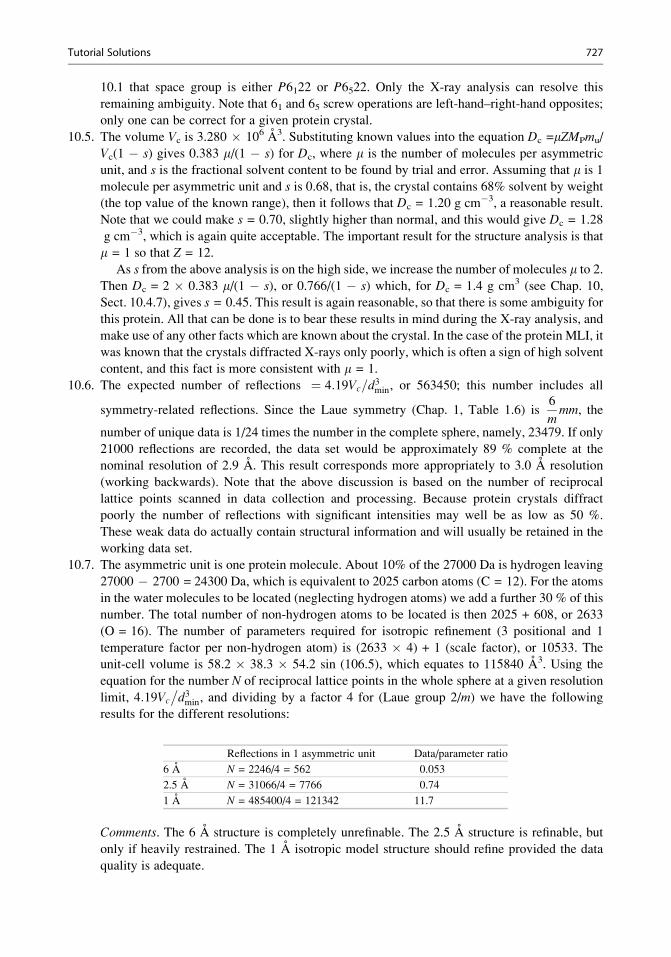
10.1 that space group is either P6122 or P6522. Only the X-ray analysis can resolve this

remaining ambiguity. Note that 61 and 65 screw operations are left-hand–right-hand opposites;

only one can be correct for a given protein crystal.

10.5. The volume Vc is 3.280 � 106 A3. Substituting known values into the equation Dc =mZMPmu/

Vc(1 � s) gives 0.383 m/(1 � s) for Dc, where m is the number of molecules per asymmetric

unit, and s is the fractional solvent content to be found by trial and error. Assuming that m is 1

molecule per asymmetric unit and s is 0.68, that is, the crystal contains 68% solvent by weight

(the top value of the known range), then it follows that Dc = 1.20 g cm�3, a reasonable result.

Note that we could make s = 0.70, slightly higher than normal, and this would give Dc = 1.28

g cm�3, which is again quite acceptable. The important result for the structure analysis is that

m = 1 so that Z = 12.

As s from the above analysis is on the high side, we increase the number of molecules m to 2.

Then Dc = 2 � 0.383 m/(1 � s), or 0.766/(1 � s) which, for Dc = 1.4 g cm3 (see Chap. 10,

Sect. 10.4.7), gives s = 0.45. This result is again reasonable, so that there is some ambiguity for

this protein. All that can be done is to bear these results in mind during the X-ray analysis, and

make use of any other facts which are known about the crystal. In the case of the protein MLI, it

was known that the crystals diffracted X-rays only poorly, which is often a sign of high solvent

content, and this fact is more consistent with m = 1.

10.6. The expected number of reflections ¼ 4:19Vc=d3min, or 563450; this number includes all

symmetry-related reflections. Since the Laue symmetry (Chap. 1, Table 1.6) is6

mmm, the

number of unique data is 1/24 times the number in the complete sphere, namely, 23479. If only

21000 reflections are recorded, the data set would be approximately 89 % complete at the

nominal resolution of 2.9 A. This result corresponds more appropriately to 3.0 A resolution

(working backwards). Note that the above discussion is based on the number of reciprocal

lattice points scanned in data collection and processing. Because protein crystals diffract

poorly the number of reflections with significant intensities may well be as low as 50 %.

These weak data do actually contain structural information and will usually be retained in the

working data set.

10.7. The asymmetric unit is one protein molecule. About 10% of the 27000 Da is hydrogen leaving

27000 � 2700 = 24300 Da, which is equivalent to 2025 carbon atoms (C = 12). For the atoms

in the water molecules to be located (neglecting hydrogen atoms) we add a further 30 % of this

number. The total number of non-hydrogen atoms to be located is then 2025 + 608, or 2633

(O = 16). The number of parameters required for isotropic refinement (3 positional and 1

temperature factor per non-hydrogen atom) is (2633 � 4) + 1 (scale factor), or 10533. The

unit-cell volume is 58.2 � 38.3 � 54.2 sin (106.5), which equates to 115840 A3. Using the

equation for the number N of reciprocal lattice points in the whole sphere at a given resolution

limit, 4:19Vc d3min

�, and dividing by a factor 4 for (Laue group 2/m) we have the following

results for the different resolutions:

Reflections in 1 asymmetric unit Data/parameter ratio

6 A N = 2246/4 = 562 0.053

2.5 A N = 31066/4 = 7766 0.74

1 A N = 485400/4 = 121342 11.7

Comments. The 6 A structure is completely unrefinable. The 2.5 A structure is refinable, but

only if heavily restrained. The 1 A isotropic model structure should refine provided the data

quality is adequate.

Tutorial Solutions 727

10.8. From the general expression Web Appendix A4, (WA4.6), with g = 120� and f = 120�, wederive the matrix

0 �1 0

1 �1 0

0 0 1

264

375 which; together with the translation vector

0

023

264375

for the 32 screw axis, leads to the general equivalent position set: x, y, z; �y, x� y; 23þ z;

y � x; �x; 13þ z. The only condition limiting reflections is 000l: = 3n.

10.9. If the protein belongs to a family, or group, of proteins having similar functions or biological

or other properties in common, and the structure of one member of the family is known, either

from an ab initio or other structure determination, molecular replacement can be attempted.

The method usually requires the two proteins involved in MR to have amino acid sequences

which correspond either identically or are of very similar types, that is, conserved for at least

30% of their total lengths (30% homology). Note that if the two proteins crystallize in the same

space group and have very similar unit cells, they are very likely to be isomorphous, and the

new structure should be determinable initially by Fourier methods alone. If the protein belongs

to a new family for which no known structures exist, an ab inito method, MIR or MAD, has to

be used for structure analysis. In the case of MAD, a tuneable source of synchrotron radiation

is required.

Solutions 11

11.1. (a) From the Bragg equation, 1.25 = 2d(111) sin y(111). Since dð111Þ ¼ a=p3,

y(111) = 12.62�. (b) Differentiating the Bragg equation with respect to y, we obtain

dl ¼ 2dð111Þ cos yð111Þ dy. Remembering that dy here is measured in radian, dl = 0.0243 A.

11.2. For the NaCl structure type, we can write F(hkl) = 4[fNa+ + (�1)lfH

�/D

�]. Hence, the followingresults are obtained:

(111) (220)

NaH NaD NaH NaD

X-rays 30.9 30.9 27.6 27.6

Neutrons 2.88 –1.28 –0.08 4.08

11.3. VIVALDI uses a white-beam Laue technique to record the diffraction data. Consequently each

diffraction record (spot) will have a different wavelength associated with it which will have first

to be determined in order for the spot to be assigned its hkl indices. This would usually require

the unit cell of the crystal to be known, which would be easier to carry out first with

monochromatic X-rays in the user’s laboratory.

11.4. The spallation neutron beam at ORNL has been filtered in order to cover as small a wavelength

range as is required in order to measure the data on a four-circle diffractometer. This would

result in some loss of beam flux (power) which, in turn, would require the use of larger crystals

in order to produce good quality diffraction data. VIVALDI uses a Laue white radiation

technique which does not require the use of flux reducing filters.

11.5. Applying Chap. 11, (11.3) gives l = 1.865 A. [Work out the units of A in (11.3).]

11.6. The final picture should look something like Chap. 11, Fig. 11.12. It can be exported and saved

in a variety of ways from the RASMOL menu.

728 Tutorial Solutions

Solutions 12

12.1. Since R = 57.30 mm, 1 mm on the film is equal to 1� in y. Thus, 0.5 mm = 0.5� = 0.00873 rad.

The mean Cu Ka wavelength is 1.5418 A. Differentiating the Bragg equation with respect to y:

dl ¼ 2d cos y dy ¼ l cot y dy

Since dl = 0.0038, we have cot y = 0.0038/(1.5418 � 0.00873) = 0.2823, so that y 74�,the angle at which the a1a2 doublet would be resolved under the given conditions.

12.2. Perusal of the cubic unit-cell types leads us to expect that (sin2y)/n for the first line (the low yregion) where n = 1, 2, 3, . . . , would result in a factor that would divide into all other experimental

values of sin2y to give integer or near-integer results.By trial,wefind that, for thefirst line, (sin2y)/3leads to a sequence of values that correspond closely to those for a cubicF unit cell. Thus, dividing

all other values of sin2y by 0.0155 we obtain:

Line no. sin2y/0.0155 N a/A hkl y/o1 3.00 3 6.192 111 12.45

2 4.10 4 6.118 200 14.60

3 11.08 11 6.170 311 24.48

4 16.04 16 6.185 400 29.91

5 23.95 24 6.199 422 37.54

6 26.90 27 6.203 333, 511 40.22

7 34.80 35 6.210 531 47.26

8 35.77 36 6.212 600, 442 48.12

9 42.64 43 6.218 533 54.39

10 47.54 48 6.222 444 59.13

Some accidental absences appear in this sequence of lines. Extrapolation of a v. f(y) by the

method of least squares (program LSLI) gives a = 6.217 A. However, lines 1 and 2 produce

significantly greater errors of fit than do the remaining eight lines. Since low-angle measure-

ments tend to be less reliable, we can justifiably exclude lines 1 and 2. Least squares on lines 3

to 10 gives a probably better value, a = 6.223 A.

12.3. The LEPAGE program gives the following results with the C-factor set at 1�:Reduced Cell: P 4.693, 4.929, 5.679 A; 90.12, 90.01, 90.72�

Conventional cell: Orthorhombic P 4.693, 4.929, 5.679 A; 90.12, 90.01, 90.72�,where all three angles are assumed to be 90� within experimental error. If we select the more

stringent LEPAGE parameter C = 0.5�, we obtainReduced Cell: P 4.693, 4.929, 5.679 A; 90.12, 90.01, 90.7�

Conventional cell: Monoclinic P 4.693, 5.679, 4.929 A; 90.72, 89.99�

where a and gmay taken now to be 90� within experimental error. The parameters are reordered

so that b is the unique angle.

12.4. From the program LEPAGE, we find:

Reduced Cell: P 6.021, 6.021, 8.515 A; 110.70, 110.70, 90.01�

Conventional cell: Tetragonal I 6.021, 6.021, 14.75 A; 90.00, 90.00, 90.00�

V(conventional unit cell)/V(given unit cell) = 2.

Tutorial Solutions 729

12.5. Let lines 1, 2, and 3 be 100, 010, and 001, respectively. Then, from multiples of their Q values,

we have a* = 0.09118 (average of 100, 200, 300, and 400; lines 1, 5, 17, and 33, respectively),

b* = 0.09437 (average of 010, 020, 030, and 040; lines 2, 6, 18, and 38, respectively), and

c* = 0.1312 (average of 002 and 003; lines 3 and 15, respectively). Consider next the possible

hk0 lines. Q110 = Q100 + Q010 = 172.2; this line has been allocated to 001, which is probably

erroneous. Continue with the [001] zone:

hk0 Qhk0 Line number

110 172.2 3

120 439.5 9

130 885.0 20

210 421.5 8

220 688.8 15

230 1134.3 29

310 837.0 19

320 1104.3 27

This zone is well represented, and it follows that g* is 90�. If line 4 is now taken as 001, then

line 25 could be 002. We check this assignment by forming expected Q0kl values:Q011 = 338.9,

but there is no line at this Q value, nor a pair of lines equidistant above and below this value,

as there would be if the assignment is correct and a* 6¼ 90�. Q021 = 606.2, but this line fails the

above test. It seems probable that line 4 is not 001. However, it must involve the l index and

one of the indices h or k. If it is 101, then, for b* = 90�, Q001 = 249.8 � 83.1 = 166.7, and if

it is 011, then, for a* = 90�, Q001 = 249.8 � 89.1 = 160.7. For the second of these assign-

ments, although a line at 160.7 is not present, there are the multiples 002 and 003 at lines

12 (642.8) and 39 (1446.3), respectively. With this assumption, line 4 is 011, line 12 is 002,

and line 39 is 003.

Confirmation arises from 012, 021, and 022 at lines 16 (731.9), line 10 (517.1), and line 25

(999.2). Thus, an average c* = 0.1267 and a* = 90�. We now search for h0l lines. For b* = 90�,Q101 = 243.8; this line cannot be fitted into the pattern. Q102 = 725.9: there is no line at this

value, but lines 11 and 21 are very nearly equidistant (166.1 and 166.5) from 725.9. Hence, the

difference, 332.6 is 104 (8c* a* cos b*), so that b* = 68.91�. We have now a set of reciprocal

unit-cell parameters from which, since two angles are 90�, the direct unit cell is calculated as

b = 111.09�, a = 1/(a* sin b) = 11.755, b = 1/b* = 10.597, c = 1/(c* sin b) = 8.459 A. We

make the conventional interchange of a and c, so that b is the unique angle, and c > b > a, and

now apply the further check of calculating the Q values for this unit cell, using the program

QVALS, with the results listed in Table S12.1.

In using this program, we remember that the unit cell appears to be monoclinic, so that we

need to consider hkl and h k �l reflections. From Table S12.1, it is evident that several reflections

overlap, within the given experimental error. The unit cell type is P. The h0l reflections are

present only when h is an even integer. The reflections 30�3 and 300, at the Q values 1444.8 and

1444.9, respectively are probably not present and overlapped by the 23�2 and 230. Hence, the

space group is probably Pa (non-standard form of Pc) or P2/a (non-standard form of P2/c).

To consider if the symmetry is actually higher than monoclinic, the unit cell is reduced, using

730 Tutorial Solutions

the program LEPAGE. We find that the first unit cell is reduced, but the conventional unit cell is

orthorhombic B (� C or A), with a high degree of precision:

a ¼ 8:459; b ¼ 10:597; c ¼ 21:935 A; a ¼ b ¼ g ¼ 90:00o

Since Miller indices transform as unit-cell vectors, we find from the transformation matrix

given by the program LEPAGE that hB = �h, kB = �k, and lB = h + 2l; the transformed

indices are listed in Table S12.2. We note that the indices are listed as directly transformed.

If we were dealing with structure factors, we could negate all the negative indices, because

jFðhklÞj¼jFðh k lÞ ¼ jFðh k lÞj ¼ jFðh �k lÞj ¼ jFðh k �lÞj in the orthorhombic system.

Table S12.1 Observed and calculated Q values

for substance X and the hkl indices of the lines

referred to the first unit cell

Q(obs) hkl Q(calc)

83.1 0 0 1 83.1

89.1 0 1 0 89.1

172.2 0 1 1 172.2

249.8 1 1 0 249.6

1 1 �1 249.6

332.6 0 0 2 332.5

356.1 0 2 0 356.2

416.0 1 1 �2 415.8

1 1 1 415.9

421.5 0 1 2 421.6

439.3 0 2 1 439.3

516.9 1 2 �1 516.7

1 2 0 516.7

559.8 2 0 �1 559.0

642.9 2 0 �2 642.1

2 0 0 642.2

648.6 2 1 �1 648.1

683.3 1 2 �2 683.0

1 2 1 683.0

688.8 0 2 2 688.7

732.1 2 1 �2 731.2

2 1 0 731.2

748.4 0 0 3 748.2

1 1 �3 748.4

1 1 2 748.4

801.5 0 3 0 801.5

837.2 0 1 3 837.3

884.5 0 3 1 884.6

892.4 2 0 �3 891.5

2 0 1 891.6

916.0 2 2 �1 915.2

962.3 1 3 �1 962.0

1 3 0 962.0

(continued)

Tutorial Solutions 731

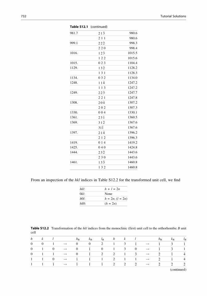
From an inspection of the hkl indices in Table S12.2 for the transformed unit cell, we find

hkl: h + l = 2n

0kl: None

h0l: h = 2n; (l = 2n)

hk0: (h = 2n)

Table S12.1 (continued)

981.7 2 1 �3 980.6

2 1 1 980.6

999.1 2 2 �2 998.3

2 2 0 998.4

1016. 1 2 �3 1015.5

1 2 2 1015.6

1015. 0 2 3 1104.4

1129. 1 3 �2 1128.2

1 3 1 1128.3

1134. 0 3 2 1134.0

1248. 1 1 �4 1247.2

1 1 3 1247.2

1249. 2 2 �3 1247.7

2 2 1 1247.8

1308. 2 0 �4 1307.2

2 0 2 1307.3

1330. 0 0 4 1330.1

1361. 2 3 �1 1360.5

1369. 3 1 �2 1367.6

31�1 1367.6

1397. 2 1 �4 1396.2

2 1 2 1396.3

1419. 0 1 4 1419.2

1425. 0 4 0 1424.8

1444. 2 3 �2 1443.6

2 3 0 1443.6

1461. 1 3 �3 1460.8

1 3 2 1460.8

Table S12.2 Transformation of the hkl indices from the monoclinic (first) unit cell to the orthorhombic B unit

cell

h k l hB kB lB h k l hB kB lB

0 0 1 ! 0 0 2 1 3 �1 ! �1 �3 �1

0 1 0 ! 0 �1 0 1 3 0 ! �1 �3 1

0 1 1 ! 0 �1 2 2 1 �3 ! �2 �1 �4

1 1 0 ! �1 �1 1 2 1 1 ! �2 �1 4

1 1 �1 ! �1 �1 �1 2 2 �2 ! �2 �2 �2

(continued)

732 Tutorial Solutions

giving the diffraction symbol as B . a . which, under the transformation a0 = a, b0 = c, c0 = �c,

becomes C � � a. Hence, the space group is either Cmma or C2ma (� Abm2).

12.6. Crystal XL1: a = 6.425, b = 9.171, c = 5.418 A, a = 90, b = 90, g = 90�. The unit cell is

orthorhombic. The systematic absences indicate the diffraction symbol as mmm P n a � � ,which corresponds to either Pna21 or Pnam. The latter is the ac b setting of Pnma. [Reported:

KNO3; 9.1079, 6.4255, 5.4175 A; Pbnm, which is the cab setting of Pnma.] The LEPAGE

reduction confirms the above cell as reduced and conventional, under reordering, such that

a < b < c. What is the space group now?

12.7. Crystal XL2: a = 10.482, b = 11.332, c = 3.757 A, a = 90, b = 90, g = 90�. The unit cell is

orthorhombic, with space group Pbca. The LEPAGE reduction confirms the above cell as

reduced and conventional, under reordering such that a < b < c.

12.8. Crystal XL3: a = 6.114, b = 10.722, c = 5.960 A, a = 97.59, b = 107.25, g = 77.42�. The unitcell is triclinic, space group P1 or P�1. The LEPAGE reduction gives a = 5.960, b = 6.114,

c = 10.722 A, a = 77.42, b = 82.41, g = 72.75�. [Reported: CuSO4.5H2O: 6.1130, 10.7121,

5.9576 A, 82.30, 107.29, 102.57�; P�1.]

Table S12.2 (continued)

h k l hB kB lB h k l hB kB lB

0 0 2 ! 0 0 4 2 2 0 ! �2 �2 2

0 2 0 ! 0 �2 0 1 2 �3 ! �1 �2 �5

1 1 �2 ! �1 �1 �3 1 2 2 ! �1 �2 5

1 1 1 ! �1 �1 3 0 2 3 ! 0 �2 6

0 1 2 ! 0 �1 4 1 3 �2 ! �1 �3 �3

0 2 1 ! 0 �2 2 1 3 1 ! �1 �3 3

1 2 �1 ! �1 �2 �1 0 3 2 ! 0 �3 4

1 2 0 ! �1 �2 1 1 1 �4 ! �1 �1 �7

2 0 �1 ! �2 0 0 1 1 3 ! �1 �1 7

2 0 �2 ! �2 0 �2 2 2 �3 ! �2 �2 �4

2 0 0 ! �2 0 2 2 2 1 ! �2 �2 4

2 1 �1 ! �2 �1 0 2 0 �4 ! �2 0 �6

1 2 �2 ! �1 �2 �3 2 0 2 ! �2 0 6

1 2 1 ! �1 �2 3 0 0 4 ! 0 0 8

0 2 2 ! 0 �2 4 2 3 �1 ! �2 �3 0

2 1 �2 ! �2 �1 �2 3 1 �2 ! �3 �1 �1

2 1 0 ! �2 �1 2 3 1 �1 ! �3 �1 1

0 0 3 ! 0 0 6 2 1 �4 ! �2 �1 �6

1 1 �3 ! �1 �1 �5 2 1 2 ! �2 �1 6

1 1 2 ! �1 �1 5 0 1 4 ! 0 �1 8

0 3 0 ! 0 �3 0 0 4 0 ! 0 �4 0

0 1 3 ! 0 �1 6 2 3 �2 ! �2 �3 �2

0 3 1 ! 0 �3 2 2 3 0 ! �2 �3 2

2 0 �3 ! �2 0 �4 1 3 �3 ! �1 �3 �5

2 0 1 ! �2 0 4 1 3 2 ! �1 �3 5

2 2 �1 ! �2 �2 0

Tutorial Solutions 733

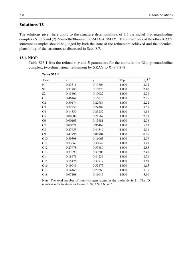
Solutions 13

The solutions given here apply to the structure determinations of (1) the nickel o-phenanthroline

complex (NIOP) and (2) 2-S-methylthiouracil (SMTX& SMTY). The correctness of the other XRAY

structure examples should be judged by both the state of the refinement achieved and the chemical

plausibility of the structure, as discussed in Sect. 8.7.

13.1. NIOP

Table S13.1 lists the refined x, y and B parameters for the atoms in the Ni o-phenanthroline

complex; two-dimensional refinement by XRAY to R 9.8 %.

Table S13.1

Atom x y Pop. B/A2

Ni 0.23511 0.17804 1.000 2.02

S1 0.31780 0.10370 1.000 2.10

S2 0.15409 0.10022 1.000 2.21

C1 0.46164 0.15015 1.000 2.05

C2 0.39174 0.22786 1.000 2.22

C3 0.32252 0.24182 1.000 3.55

C4 0.14559 0.23252 1.000 1.14

C5 0.08009 0.21567 1.000 2.83

C6 0.00165 0.13681 1.000 2.08

C7 0.00321 0.95462 1.000 5.63

C8 0.27653 0.44349 1.000 2.91

C9 0.47796 0.08704 1.000 0.85

C10 0.39398 0.16063 1.000 2.09

C11 0.33069 0.30042 1.000 3.47

C12 0.27678 0.33480 1.000 2.85

C13 0.31090 0.39206 1.000 2.40

C14 0.18671 0.44236 1.000 4.71

C15 0.15426 0.37717 1.000 3.69

C16 0.19049 0.33477 1.000 1.65

C17 0.14168 0.29263 1.000 1.35

C18 0.07108 0.16047 1.000 3.90

Note: The total number of non-hydrogen atoms in the molecule is 21. The ID

numbers refer to atoms as follow: 1 Ni, 2 S, 3 N, 4 C.

734 Tutorial Solutions

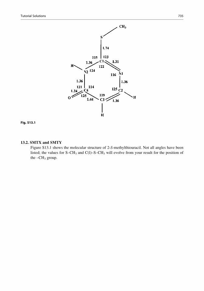
13.2. SMTX and SMTY

Figure S13.1 shows the molecular structure of 2-S-methylthiouracil. Not all angles have been

listed; the values for S–CH3 and C(l)–S–CH3 will evolve from your result for the position of

the –CH3 group.

Fig. S13.1

Tutorial Solutions 735

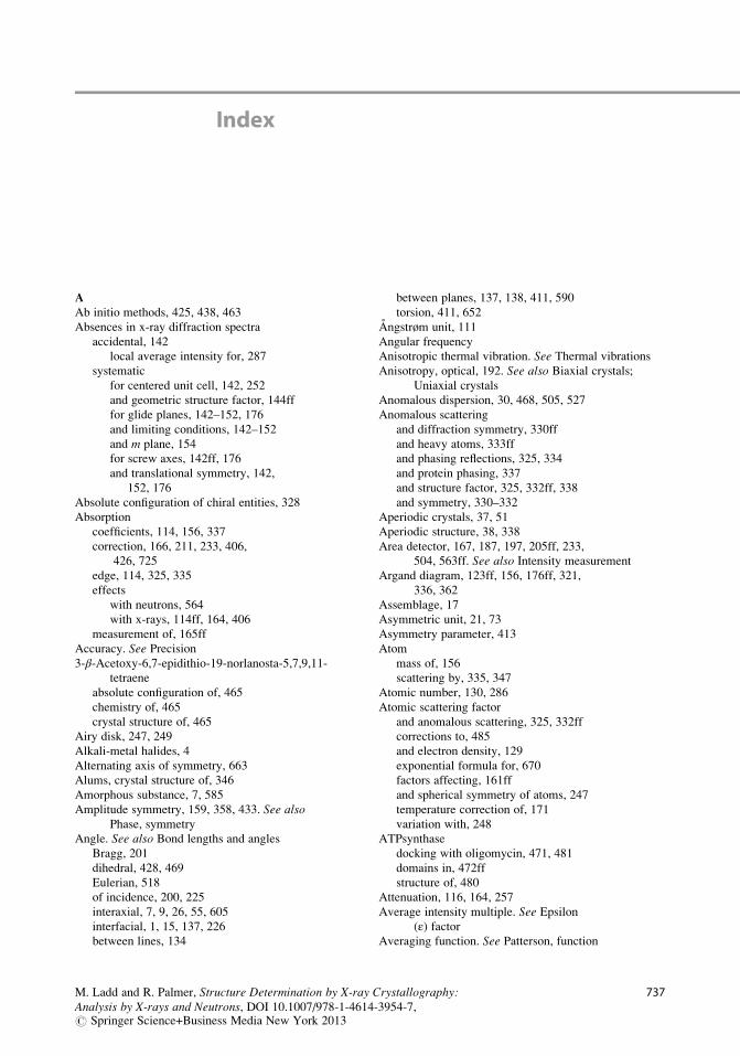
Index

AAb initio methods, 425, 438, 463

Absences in x-ray diffraction spectra

accidental, 142

local average intensity for, 287

systematic

for centered unit cell, 142, 252

and geometric structure factor, 144ff

for glide planes, 142–152, 176

and limiting conditions, 142–152

and m plane, 154

for screw axes, 142ff, 176

and translational symmetry, 142,

152, 176

Absolute configuration of chiral entities, 328

Absorption

coefficients, 114, 156, 337

correction, 166, 211, 233, 406,

426, 725

edge, 114, 325, 335

effects

with neutrons, 564

with x-rays, 114ff, 164, 406

measurement of, 165ff

Accuracy. See Precision3-β-Acetoxy-6,7-epidithio-19-norlanosta-5,7,9,11-

tetraene

absolute configuration of, 465

chemistry of, 465

crystal structure of, 465

Airy disk, 247, 249

Alkali-metal halides, 4

Alternating axis of symmetry, 663

Alums, crystal structure of, 346

Amorphous substance, 7, 585

Amplitude symmetry, 159, 358, 433. See alsoPhase, symmetry

Angle. See also Bond lengths and angles

Bragg, 201

dihedral, 428, 469

Eulerian, 518

of incidence, 200, 225

interaxial, 7, 9, 26, 55, 605

interfacial, 1, 15, 137, 226

between lines, 134

between planes, 137, 138, 411, 590

torsion, 411, 652

Angstrøm unit, 111

Angular frequency

Anisotropic thermal vibration. See Thermal vibrations

Anisotropy, optical, 192. See also Biaxial crystals;

Uniaxial crystals

Anomalous dispersion, 30, 468, 505, 527

Anomalous scattering

and diffraction symmetry, 330ff

and heavy atoms, 333ff

and phasing reflections, 325, 334

and protein phasing, 337

and structure factor, 325, 332ff, 338

and symmetry, 330–332

Aperiodic crystals, 37, 51

Aperiodic structure, 38, 338

Area detector, 167, 187, 197, 205ff, 233,

504, 563ff. See also Intensity measurement

Argand diagram, 123ff, 156, 176ff, 321,

336, 362

Assemblage, 17

Asymmetric unit, 21, 73

Asymmetry parameter, 413

Atom

mass of, 156

scattering by, 335, 347

Atomic number, 130, 286

Atomic scattering factor

and anomalous scattering, 325, 332ff

corrections to, 485

and electron density, 129

exponential formula for, 670

factors affecting, 161ff

and spherical symmetry of atoms, 247

temperature correction of, 171

variation with, 248

ATPsynthase

docking with oligomycin, 471, 481

domains in, 472ff

structure of, 480

Attenuation, 116, 164, 257

Average intensity multiple. See Epsilon(ε) factor

Averaging function. See Patterson, function

M. Ladd and R. Palmer, Structure Determination by X-ray Crystallography:Analysis by X-rays and Neutrons, DOI 10.1007/978-1-4614-3954-7,# Springer Science+Business Media New York 2013

737

Axes

Cartesian right-handed, 167

conventional, 10, 60, 81

crystallographic, 8ff

for hexagonal system, 22, 59

Axial ratios, 12

BBackground scattering

with neutrons, 554

with x-rays, 554, 593

Balanced filter, 223, 225. See also Monochromators

Barlow, W., 3

Bayesian statistics, 175

Beam stop, 442

Beevers–Lipson strips, 345

Bernal, J.D., 138, 491, 541

Bessel function, 246, 266, 365, 399

B factor, 169ff, 173

Biaxial crystals

optical behaviour of, 190

refractive indices of, 190

Bijvoet difference, 305, 331

Bijvoet pairs, 306, 327ff, 347, 527, 718

Biodeuteration. See PerdeuterationBioinformatics, 471, 481. See also ATP synthase;

Oligomycins A, B, C

Biological molecules, 489

Biomolecular modelling, 471

Birefringence, 192ff

Bond lengths and angles

neutron, 417

tables of, 410

x-ray, 410

Bragg equation, 132, 134

Bragg reflection (diffraction)

and Laue diffraction, 200, 223

equivalence of with Bragg reflection, 134

order of, 133

Bragg, W.H., 4

Bragg, W.L., 4

Bravais, A., 3

Bravais lattices

and crystal systems, 54, 60, 64

direct, 63

notation and terminology of, 61

plane, 55, 57, 62

reciprocal, 63ff

representative portion of, 52, 60, 74

rotational symmetry of, 52, 71, 74, 94, 98

and space groups, 72ff

symmetry of, 70, 97–99

tables of, 59

three-dimensional, 54

translations, 51 ff, 72

two-dimensional, 52ff, 73ff

unit cells of, 52ff, 72ff, 86, 93

vector, 65ff

Buckyballs, 32–39

CCamera methods, importance of, 588, 590

Capillary crystal mount, 496, 508, 568

Carangeot, A., 1, 15

Carbon monoxide, molecular symmetry of, 31

CCD. See Charge-coupled device (CCD);

Charge-coupled type area detector (CCD)

CCP4. See Collaborative computational projects

CCP14. See Collaborative computational projects

Central limit theorem, 176

Centred unit cells

in three dimensions, 56

Centre of symmetry (inversion)

alternative origins on, 95

and diffraction pattern, 330

Centric reflection. See Signs of reflections incentrosymmetric crystals

Centric zones, 146, 178, 703

Centrosymmetric crystals

point groups of, 18–31

projection of, 17, 23ff, 36

structure, 32, 36

structure factor for, 141

and x-ray patterns, 103

zones (see Centric zones)Change of hand, 22, 23, 491

Change of origin, 90, 252, 353, 692. See alsoOrigin, change of

Characteristic symmetry, 24, 26

Characteristic x-radiation, 113

Charge-coupled type area detector (CCD), 217ff

Chirality, 327, 534, 539–540

Chi-square (χ2) distribution, 411Closure error, 321, 322

CMOS. See Complementary metal-oxide

semiconductor (CMOS)

Coherent scattering. See Scattering, coherentCollaborative computational projects, 635

Collimation, 117, 504, 594

Collimator

multiple beam, 116

traditional, 116

Complementary metal-oxide semiconductor

(CMOS), 221

Complex numbers

conjugate of, 124, 367

plane, 123, 325

Compton scattering. See Scattering, incoherentComputer graphics, 325, 420, 506

Computer prediction of crystal structure

developments in, 425

lattice energy and, 423

programs for, 422

Conformational parameters, 411, 471

Constant interfacial angles, law of, 1, 15

Convolution

and crystal structure, 264

and diffraction, 261

folding integral, 262ff

738 Index

and structure solution, 266ff

transform of, 261ff

Coordinates

Cartesian, 414, 434, 617, 652

fractional, 54, 65, 135

orthogonal, 151, 720

symmetry related, 74, 290, 308, 722

transformation of axes of, 353

Copper

pyrites crystal, 30

sulphate, 4, 5

Corrections to measured intensities

absorption, 165ff

extinction, 164, 168

Lorentz, 162, 168, 456

polarization, 162, 168, 456

scale, 169, 174, 456

temperature factor, 169ff, 456

Correct phases, importance of, 126

Correlation coefficient, 523

Cross vector, 318, 384, 520

Crown ether derivative, 574

Cryoprotectants for proteins, 491, 543

Crystal. See also Crystalline substance

class, 3, 24, 31, 146, 159, 177, 182, 331

and ε factor, 177, 182, 352classification of

by optics, 90

by symmetry, 24

definition of, 37

density of

calculated, 444

measured, 444

external symmetry of, 17ff

faces of, 9ff, 28, 62, 166, 193

geometry of, 26, 311

growth of, 492ff

habit of, 3, 187, 440, 455

ideally imperfect, 164

ideally perfect, 164

imperfections in, 164, 586

internal symmetry of (see Space groups)lattice (see Lattice)models of, 638

monoclinic, 147, 152ff, 195, 288, 401, 434

mosaic character in, 164, 165

mounting of, 499ff, 508, 545, 703

optical classification of, 190

perfection of, 164, 197

periodicity in, 35

permitted symmetry of, 212

point group (see Point groups)size of, 328, 494, 558, 577

as stack of unit cells, 1, 52, 164

symmetry and physical properties of, 17

unit cell of, 53, 54

Crystal growing

by diffusion, 188

from solution, 155, 188

by sublimation, 188

Crystalline state, 4, 6ff

Crystalline substance, 7

Crystallographic computing. See Software forcrystallography

Crystallographic point groups. See alsoPoint groups

and crystal systems, 3, 24ff, 200

derivation of, 636

and general form, 3, 23ff, 40, 687

and Laue groups, 29ff

notation for, 15, 29

recognition of, scheme for, 24ff, 636

restrictions on, 22

and space groups, 26, 38

and special form, 24, 28, 35

stereograms for, 15, 19ff, 29, 31, 177

tables of, 26, 30

Crystallographic software. See Software forcrystallography

Crystal models, 638

Crystal morphology, 1ff

Crystal systems

and characteristic symmetry, 24, 26

and crystallographic axes, 8, 28

cubic, 12, 15, 28, 190

hexagonal, 22, 59, 61, 94, 155, 599

and lattices, 51ff

and Laue groups, 29ff, 502

monoclinic, 147, 152ff, 195, 288, 401, 434

and optical behaviour, 190

orthorhombic, 24, 60, 100, 154, 157,

194ff, 201, 230, 281, 342,

404, 434, 703

and point group scheme, 25ff

recognition of, 28

and symmetry in Laue photographs, 552

table of, 26

tetragonal, 26, 190, 502

triclinic, 26, 190, 502

trigonal, 26, 190, 502

CSD. See Data basesCube, model of, 638

Cubic crystal system, 28

DData bases

Cambridge crystallographic data base (CSD), 387,

417, 539

International Centre for Diffraction Data

(ICSD), 585

Protein data base, 482, 674

Research Collabotory for Structural Bioinfomatics

(RCSB), 418

searching of, 359

Data collection

strategy

with neutrons, 551ff, 563, 568, 576, 623

with x-rays, 197ff, 219, 225, 564, 623

Index 739

Data processing

neutron, 562

x-ray, 562

Data/variables ratio, 406

Debye–Waller expectation factor, 170

Delta (δ) function, 258–259de Moivre’s theorem, 123, 240, 250, 283

Density

calculated, 115, 273

and contents of unit cell, 273

importance of, 444, 513

measurement of, 466

optical, 204

Detector

neutron, 555, 558

x-ray, 118, 222, 508

Determination of absolute configuration, 326

Deuteration, 554ff, 597

Diad, 23, 54, 81, 97

Diagonal (n) glide plane, 86, 94, 107, 150Diamond (d) glide plane, 86Difference-Fourier series, 615. See also Fourier series

and correctness of structure analysis

and least-squares refinement, 309, 384, 391, 393ff,

419, 524, 532, 610, 649

Difference-Patterson, 316

anomalous, 334

Diffraction. See also X-ray scattering (diffraction)

by atoms, 130, 549, 561, 573

by crystals, 552ff

grating, 118, 253, 261

by holes, 245, 249

pattern, 4, 18, 33, 51, 103, 200ff (see also Atomic

scattering factor)

of assemblage, 17

of atoms, 245

of holes, 245, 249, 250

by regular arrays of scattering centres, 130ff

symbol, 100ff, 152ff, 178, 186, 697, 732, 733

of visible light, 235, 245

Diffractometer

CAD4 (Nonius)

data collection with, 211, 389

structure determination with, 212

kappa CCD (Nonius)

crystal positioning, 210

data collection and strategies, 394

instrument geometry, 209

scans, ω/θ and θ, 212optical, 249ff

powder, 204, 417, 418, 585–632, 654

serial, 208, 504 (see also Intensity measurement

single-counter, Intensity measurement

single-crystal)

transformations with, 211

Dihedral group, 428, 469

Directions

angle between, 14

cosines, 7, 132 (see also Web Appendix WA1)

Direct lattices, 63, 508. See alsoBravais lattices

Direct methods of phase determination

Σ1 equation, 366, 376

Σ2 equation, 355ff, 370

enantiomorph selection, 367

example of the use of, 377, 525

experience with, 366, 372, 391

figures of merit in, 384ff, 395

origin specification, 354, 369

Sayre’s equation, 270

starting set in, 354ff, 372

structure invariant, 352ff, 372

structure seminvariant, 354

success with, 372

symbolic addition, 359ff

use of SHELX in, 372ff

Direct methods of phasing, 352, 516

Direct-space methods, 588, 613ff, 621

Discrepancy index. See R factors

Disorder

dynamic, 404, 420

in single crystals, 419ff

static, 420

Disphenoid, 4, 24

Distribution

acentric, 177ff, 352, 467, 645

centric, 177ff, 352, 456, 645, 703

cumulative, 184, 388

Gaussian, 172, 176

transform of, 258

mean values of, 180

parameter, 172, 176

radial, 246, 419

Duality, 551

EElectromagnetic radiation, interaction of crystal with,

121, 189

Electron

particle properties of, 128

scattering, 121ff, 140

wave nature of, 128

Electron density, 5, 128, 134ff, 169ff, 241ff, 278ff,

355ff, 446ff, 502ff, 564ff, 612ff, 641ff. See alsoDifference-Fourier series

ball-and-stick model for, 279

computation and display of, 279

contour map of, 5, 254, 420

and criteria for correctness of structure

analysis, 416

determined from partial structures, 303

equations for, 243, 278, 285, 651

fitting to, 536

and Fourier series, 241, 273, 416, 513

and Fourier transform of, 528

and hydrogen atom positions, 280, 476

interpretation of, 278ff, 513, 527, 531, 614

in large molecule analysis, 324

740 Index

map, 5, 171, 266, 279, 293, 301ff, 339, 416, 459ff,

513ff, 563, 607, 625, 642

non-negativity of, 362

and Patterson function, 282, 612, 641

peak heights and peak weights in, 279, 612

periodicity of, 241

and phase problem, 243

projections of, 242, 279ff, 446, 641

superposition of peaks in, 281

pseudosymmetry in, 308, 320

real nature of, 128

resolution of, 278, 423, 447, 513, 530

standard deviation of, 416

structure factors and, 244, 513, 641, 648

successive Fourier refinement and, 309

units of, 245

E maps

calculation of, 360

‘sharp’ nature of, 361

Epsilon (ε) factor, 177, 352, 646Equivalent positions, 74, 78, 82, 94. See also General

equivalent positions; Special equivalent positions

Errors, 415

superposition of, 415, 720

Esd. See Estimated standard deviation (esd)

Estimated standard deviation (esd), 415

jEj values, 175, 183, 287, 643. See also Direct methods

of phase determination calculation of

distribution of, 182ff, 352, 365, 456

statistics of, 644

structure factors and, 182, 641

Evans-Sutherland picture system, 420

Even function, 255, 258, 709

Ewald, P.P.

construction, 138

Ewald sphere, 138, 163, 173, 202ff

Extinction

optical

for biaxial crystals, 190, 194ff

for uniaxial crystals, 190

x-ray

parameter, 165, 168

primary, 164

secondary, 164ff

FFAST detector, 215

Fast freezing, 496ff

Fast Fourier transform (FFT), 272, 339, 513, 672

Federov, E.S. See Fyodorov, Y.Figure of merit (FOM), 321ff, 377ff, 528, 604, 627

File

cif, 416

pdb, 532, 535, 569

Filtered x-radiation. See Monochromators

Flack parameter, 305, 326ff, 468. See also Determination

of absolute configuration; Hamilton ratio test

Flash freezing (shock cooling), 501

Focusing mirrors

folding integral (see Convolution; Integrals)Franks, A., 225

Gobel, 235

FOM. See Figure of merit (FOM)

Form

of directions, 51

of planes, 15

Fourier analysis. See Fourier seriesFourier, J.B., 236

Fourier map

difference electron density, 324

electron density, 641

Fo-jFcj map, 266

2Fo-jFcj map, 423, 530, 536, 537, 579

Fourier series, 235ff, 281, 285, 309, 361, 416, 460, 513,

648, 716, 717. See also Difference-Fourier series

coefficients of, 240, 258, 266, 285, 302, 309, 361,

460, 716

exponential form of, 240

frequency variable in, 241, 257

one-dimensional, 241, 257, 346, 651

partial, 301ff

refinement with successive, 309, 468, 531

series termination errors in, 240, 416

in structure analysis, 236, 266, 273, 281

summation of, 239, 344, 651

three-dimensional, 241ff, 463

two-dimensional, 36, 243ff, 651

wavenumber variable in, 237

weighting of coefficients for, 302

Fourier summation tables. See BeeversuLipson strips

Fourier transform

of atom, 245ff

and change of origin, 252

conjugate of, 125, 367 (see also Friedel’s law)

of electron density, 528

of euphenyl iodoacetate, 259

fast, 339, 513

generalized, 246ff

general properties of, 261

and heavy-atom technique, 266

of hole, 245ff

inverse of, 255ff

of molecule, 248

and optical diffractometer, 249

and Patterson function, 273, 282ff, 372

phase free (see Fourier transform; Patterson, function)

of platinum phthalocyanine, 253, 266

practice with, 249ff

reconstruction of image by, 252ff

representation of, 246, 253ff

sampling, 239, 257

and sign relationships, 268

structure factors as, 240, 266, 309

and systematic absences, 252, 270

transform of, 36, 235ff, 338, 528, 627, 651

of two or more holes, 250ff

of unit cell, 248

and weighted reciprocal lattice, 259ff

Index 741

Four-phase structure invariants. See QuartetsFractional coordinates, 54ff, 65, 106, 248

Frankenheim, M.L., 3

Fraunhofer diffraction, 245

Free rotation, 420

Friedel pairs, 211, 305, 325, 331, 719.

See also Bijvoet pairs

Friedel’s law, 140, 147, 175, 181, 200, 228, 237, 243, 330,

342, 358, 374, 718

and absorption edges, 325

Friedrich, W., 5

Fringe function, 250ff, 262

Fullerenes, 38

Fyodorov, Y., 3

GGamma (Γ) function, 181. See alsoWeb Appendix WA7

Gaussian function, 258

General equivalent positions, 74ff, 89ff, 143ff

molecules in, 106

General form of planes, 30. See also Form

for crystallographic point groups, 31

Generator, x-ray. See X-rays, generatorsGeodesic dome, 38

Geometric structure factor, 340ff, 358, 433

Gessner, C., 1

Glass (silica) structure, 7

Glide line, 73, 75, 76, 80

Glide plane, 86, 94, 142ff, 176, 275

Goniometer

contact, 1

optical, 14

x-ray, 441

Graphic symmetry symbols, 25, 73, 87, 695. See alsoStereograms

change of hand, 21, 491

for diad axis, 81

for glide line, 73, 76

for glide plane, 86

for inverse monad (centre of symmetry), 25

for inversion axis, 22, 685 (see alsoRoto-inversion axes)

for mirror line, 76

for mirror plane, 22ff, 200, 637, 695

for pole, 21, 28

for representative point, 21

for rotation axes, 22, 26, 200

for rotation points, 74, 102

for screw axes, 83ff, 142, 176, 276

table of, 25, 85

Great circle, 15, 38

Guglielmini, G., 1

HHalf-translation rule, 93ff, 691

Hamilton ratio test, 468. See also Flack parameter

determination of absolute configuration, 468

Harker (and non-Harker) sections of the Patterson

function, 287, 310ff, 450, 468

Hauptman, H., 355, 362, 435

Hauy, R.J. (Abbe), 1

Heavy-atom method, 301ff, 386, 439, 649. See alsoAnomalous dispersion; Isomorphous replacement;

Patterson, search; Patterson, selection; Structure

analysis

examples of, 303, 308

and Fourier transform, 266

limitations of, 310

and Patterson function, 310, 315

Hermann-Mauguin notation, 27, 29, 41, 86, 159

and Schonflies notation, 29, 41, 159

Hessel, J.F.C., 3

Hexad, 25

Hexagonal crystal system, 1, 22, 26, 34, 155

Hexagonal two-dimensional system, 22

Hexamethylbenzene, 270, 355, 640

Hex(akis)octahedron, 4, 24

Hierarchy for considering limiting conditions, 154

High Flux Isotope Reactor (HFIR) (ORNL,

Tennessee), 556

High-resolution transmission electron microscopy

(HRTEM), 236

Homology modelling, 481

HRTEM. See High-resolution transmission electron

microscopy (HRTEM)

Hydrogen atom positions, 280, 340, 376, 419, 475, 549,

558, 570ff

Hydrogen atoms, 5, 279, 339ff, 406ff, 419, 468, 549.

See also Light atoms

bonds with, 408

location of

by calculation, 340, 406

by difference-Fourier, 279

Hypersymmetry, 175, 184

II(hkl), 140, 161ff, 305ICDD. See International Centre for Diffraction

Data (ICDD)

Icosahedral group, 39

ICSD. See Data bases; Inorganic Crystal StructureDatabase (ICSD)

Ideal intensity, 162

Identity symmetry element, 38, 81

Image formation, 235–236

Image plate, 209, 215ff, 504ff, 592. See also Intensity

measurement

Implication diagram, 318

Incoherent scattering, 127ff, 554ff, 597. See alsoScattering

Independent reflections, 329, 394, 577

Indexing reflections, 441

Indistinguishability in symmetry, 25

In-house data collection, 219

Inorganic Crystal Structure Database

(ICSD), 418

Integral sin x / x. See Web Appendix WA7

Integrated reflection, 161, 576

742 Index

Intensity

averages,

abnormal, 176

enhanced, 176, 310

data, 197

data collection, 197ff, 305

data quality, 304

distributions (see Distribution)expressions for, 161ff

factors affecting, 161

ideal (see Ideal Intensity)measurement of, 167, 189, 221, 282, 303, 325, 444,

456, 474, 504, 599

relative, 230

of scattered x-rays (see X-ray scattering (diffraction)

by crystals)

statistics of, 161ff, 228, 359

variance of, 506

weighted mean, 167

Intensity data, 197

chi-squared test for equivalent reflections in, 168

completeness of, 510

merging of equivalent reflections in, 167

scaling of, 167

by Wilson’s method, 169, 313, 445ff, 641, 646

Intensity measurement

by area detector

charge-coupled type, 217

FAST type, 215

background radiation in, 128, 590

by diffractometer

powder, 593ff, 605ff

serial, 208, 504

single-counter, 208, 504

by image plate, 215ff

Interatomic distances, 385, 409, 463, 614

Interference of x-rays

constructive, 225

destructive, 133

and finite atom size, 171

Intermolecular contact distances, 408, 451

Intermolecular potential, 433

International Centre for Diffraction Data (ICDD), 117,

585, 605

International Union of Crystallography (IUCr), 37,

607, 711

Internuclear distance, 419

Interplanar spacings, 62, 132ff

Inversion axes, 22, 637, 659. See also Roto-inversion axesIonic radii, 416

table of, 416

Ionization spectrometer, x-ray, 5, 103

Isomorphous pairs, 312

Isomorphous replacement, 306, 312ff, 334, 346, 514–515,

531, 716. See also Heavy-atom method

for alums, 346

multiple (MIR), 314, 320ff, 337, 346, 496ff, 503,

513ff, 527, 531, 534, 545, 728

for proteins, 514

single (SIR), 314, 319ff, 335, 503, 527, 611 (see alsoPowder method; Seminvariant representations

(SIR))

single, with anomalous scattering (SIRAS and

MIRAS), 335ff, 503, 527

Isomorphous replacement, single, with anomalous

scattering, 335ff, 503, 527

Isotropic crystals. See Optically isotropic crystals

Isotropic thermal vibrations. See Thermal vibrations

Isotropy, 166ff, 171ff, 190ff, 287

IUCr. See International Union of Crystallography (IUCr)

JJoint Committee on Powder Diffraction Standards

(JCPDS). See International Centre forDiffraction Data

KKarle–Hauptman inequalities, 435

Karle, J., 355, 359

Kepler, J., 1

Knipping, P., 4

K-spectrum, 113ff

LLack of closure error. See Closure errorLADI-III (ILL, Grenoble), 555

Laser wakefield acceleration, 121

Lattice energy, 422ff, 430, 628. See also Computer

prediction of crystal

structure

minimization of, 423, 628

and thermodynamic stability, 433, 483

Lattices. See Bravais latticesLattice, two-dimensional, 52, 60

Laue class. See Laue groupLaue equations, 130

Laue group

and point group, 30, 101, 175, 200, 330, 502

projection symmetry of, 29, 34, 200

Laue method. See also Laue x-ray image/photograph

experimental arrangement for, 199, 202

and synchrotron radiation, 200ff

Laue projection symmetry, 30, 34, 200

Laue symmetry, 175, 180, 225, 288, 509, 545,

562, 704, 726

Laue treatment of x-ray diffraction, 76, 130ff

equivalence with Bragg treatment, 134

Laue x-ray image/photograph. See also Laue method

symmetry of, 200

and uniaxial crystals, 190, 200

Layer lines, 230. See also Oscillation method

Least squares refinement

data errors, 406

data/variables ratio, 406

and estimated standard deviation, 406

and light atoms, 419

and parameter refinement, 401ff

precision in, 405

Index 743

Least squares refinement (cont.)refinement against jFoj and jFoj2, 410refinement strategy, 405ff

rigid-body constraint in, 534

scale factor in, 406, 444

and secondary extinction in, 137

special positions in, 405

strategy in, 405

temperature factors in, 402ff

unit-cell dimensions, 401

and weights, 406

Light atoms, 301, 310, 386, 419, 467, 549. See alsoHydrogen atom positions

Limiting conditions. See also Geometric structure factor;

Space groups unit cell, centred; Translational

symmetry

hierarchal order of considering, 150

non-independent (redundant), 84, 91

redundant (see Non-independent limiting

conditions)

in space group P21, 144in space group Pc, 146in space group P21/c, 146in space group Pma2, 148and systematic absences, 142

for translational symmetry, 142

for unit-cell types, 138

Limiting sphere, 281. See also Ewald sphere;

Sphere of reflection

Line, equation of, 13, 135

intercept form of, 8

Liquid nitrogen shock cooling, 219, 394. See alsoFast freezing

Liquids, x-ray diffraction from, 273, 419

Long-range order, 7

Lonsdale, K., 91ff, 355

Lorentz factor, 163

Low energy neutrons, 573

Low temperature measurements, 208

MMacromolecular structure analysis

flow diagram for, 490

free-R factor (see also Macromolecular structure

analysis; Protein structure analysis; Rfree)

heavy-atoms derivatives for, 306

multiple isomorphous replace (MIR) in structure

factors in, 501

temperature factors in, 501

protein, crystallization of

‘click’ test in, 494

improvement of crystals, 496

precipitants, 493

quality screening, 495

protein, make-up

L-amino acids, 499

amino acid sequence, 497

α-carbon atom, 489, 499

polypeptide chain, 489

primary structure, 489

secondary structure, 490

tertiary structure, 490

protein, properties, 491

protein, purity, 492

protein, structure analysis

cryo-crystallography, 499

crystal mounting for, 498

crystal selection, 501

data collection

with area detector, 197

by camera, 197

by diffractometer, 197, 209

with image plate, 209, 500

problems in and possible cures, 508

radiation sources in, 593

example structure determination, Ricin

Agglutinin (RCA)

AmoRe algorithm, 525

density, 510

difference electron density, 512

electron density in, 512

errors in, 510

2Fo-jFcj map for, 514

geometry of molecule, 387

initial MR model, 527

number of reflections in data set, 281

omit map for, 514

Patterson function for, 282ff

phase information and density modification

in programs for, 527ff

phasing by MAD in, 527

phasing by single isomorphous

techniques in, 527

radius of integration, 525

resolution, of data, 304

R factor, 511

Rfree, 503

self-rotation function for, 509, 520

solvent analysis, 536

space group for, 509

structure validation, 537

unit cell of, 509

heavy-atoms derivatives for, 497,

514, 527

intensity data for, 506

Laue symmetry, 509

multiple isomorphous replace (MIR) in, 496,

514, 527

multiple isomorphous replace (MIR) in:

structure factors in, 527

NCS (see Non-crystallographic symmetry)

non-crystallographic symmetry, 518ff, 523

post-refinement, 506ff

profile fitting, 506

temperature factors in, 501

unit cell determination, 509

MAD. See Multiple wavelength anomalous

dispersion (MAD)

744 Index

Magnetic

field effect, 119, 121

materials, 128

moment, 549

scattering

amplitude, 128

form factor, 128

of neutrons, 553

Matrix

inverse of, 405, 705

multiplication of, 65

notation, 65

representation of symmetry operations, 97ff

transformation, 69, 108, 230, 602, 654, 689, 696, 731

transpose of, 651, 705

Maximum entropy, 609, 624

Maximum likelihood, 516, 535

Mean planes, 414

Miller–Bravais indices, 11, 22

Miller indices

common factor in, 602

in stereograms, 70

transformations of, 69

Miller, W., 3, 9

Minimum function, 293, 641. See also Patterson,

superposition

MIR. See Multiple isomorphous replacement

MIRAS. See Multiple isomorphous replacement with

anomalous scattering

Mirror plane, 18, 22ff, 86, 132, 176, 200, 288, 412, 501,

602, 637, 714

Mirror symmetry. See Reflection symmetry

Model

bias, 516, 527, 538

building, 513, 523ff, 613

structure, 4, 278, 306, 325, 380, 400, 416ff, 513, 531,

533ff, 588, 628, 727

Modulus, 262, 301, 586

Mohs, F., 3

Molecular

geometry, 327, 336, 408ff, 433, 451ff, 471, 513, 529ff,

628, 652

graphics, 385, 388, 434, 516, 527, 531, 541, 554, 720

programs for, 385

Molecular replacement

correct solution, recognition of, 523

phases from, 524

programs for, 518

rigid-body refinement in, 524

rotation function in, 523

search model in, 522

data bases, use of, 522

search Patterson function for, 522

subunits in, 524

target Patterson function for, 522

translation function, 522

Monad, 25

Monochromators

double-type, 224

filter type, 224

single-type, 224

for synchrotron radiation, 225

Monoclinic crystal system, 195

Morphology, 1–49ff, 135, 190, 226, 508

Mosaic spread, 220

Motif, 18, 72ff, 83, 105, 145, 425, 689

MR. See Molecular replacement (MR)

Multiple isomorphous replacement (MIR), 314, 320,

496, 517

Multiple isomorphous replacement with anomalous

scattering (MIRAS), 527

Multiple wavelength anomalous dispersion (MAD), 337,

503, 527. See also Protein (macromolecule),

structure determination of

Multiplicity of reflection data, 511

Multisolution procedure, 372

Multiwire proportional counter (MWPC), 213

NNaphthalene, 265, 275

symmetry analysis of, 275

Net, 52, 73, 106, 121, 132, 164, 202, 236, 251, 551, 614.

See also Lattice

Neutron

crystallography, 550, 560

density map, 570, 576

detectors, 471, 557

diffraction

complementary to x-ray diffraction, 549, 553

data collection by, 552

Laue method in, 552

location of light atoms by, 549

with monochromatic radiation, 560

refinement of light atoms by, 550, 564, 574

structure determination examples by, 560, 574

time-resolved Laue method in, 560

scattering, 103, 419, 550ff, 560, 565

scattering length, 549, 553ff, 568, 597

sources of, 551, 559

spallation source, 551, 558

spectrum, 555

thermal, 553

Nickel tungstate, 276

Niggli cell, 602

Non-crystallographic point groups, 31, 637, 640

Non-crystallographic structure. See Aperiodic structureNon-crystallographic symmetry, 491, 518ff

Non-independent limiting conditions, 84, 91

Normal distribution, 172, 177, 179, 180

Normalized structure factor, 172, 182ff, 351ff

Notation, xxxiii, 15, 21, 23ff, 54ff, 74, 85ff,

134, 362, 663

Nucleic acids, 471, 496, 521

Numerical data, 64, 132, 339, 534, 555

OOblique axes, 40

Oblique extinction, 196, 289, 440

Index 745

Oblique two-dimensional system, 21, 52, 73. See alsoPlane groups

Occupancy, 80, 570, 656

Oligomycins A, B, C

absolute configuration of, 472ff

crystal structure of, 474

docking of, 471, 481

hydrogen bonds in, 473, 477, 484

Omit map, 514, 577, 580

Omitted coordinates, 375, 577

Optical classification of crystals, 190

Optical diffraction pattern, 251

Optical diffractometer, 249

Optically anisotropic crystals, 192

Optically isotropic crystals, 192

Optical methods of crystal examination, 190, 466

Optic axis

and biaxial crystals, 194

and crystallographic axes, 192

and uniaxial crystals, 193

Order of diffraction, 131

Orientation of crystals, 226, 384, 574

Origin

change of, 90, 252, 353, 692

choice of, 76, 87, 93, 106, 253, 354, 372, 657

Origin-fixing reflections, 352ff, 359, 458, 627

Orthogonal axes, 7, 151, 519, 618

Orthogonal function, 9, 137, 151, 215, 382, 525. See alsoWeb Appendix WA8

Orthorhombic crystal system, 342, 426, 577. See alsoCrystal systems

Oscillation method, 205ff

Oscillation record (image/photograph), 197, 206, 221,

229, 441, 506. See also Layer lines

experimental arrangement for, 199, 202

flat-plate technique in, 199, 205

and protein crystal, 207

symmetry indications from, 305, 441

Over-determination, 282, 533, 538

PPacking, 3, 295, 298ff, 385ff, 408, 428ff, 493,

628, 673

Parametral line, 39

Parametral plane, 8, 26

Parity, 138, 144, 353, 354, 367ff, 459, 644, 649, 719

Parity group, 354, 369, 459, 644, 649, 719

Partial-structure phasing. See also Phase, determination

effective power of, 301

for proteins, 400, 539

for small molecules, 538

Path difference

analysis of, 135

in Bragg reflection, 164, 201, 552

PATSEE Patterson search program

crystal packing in, 385

detailed examples of use of, 28, 418

example structure analysis, 388

expansion and refinement in, 386, 391, 397

interatomic vectors in, 267, 381ff

molecular orientation in, 382

Patterson function, storage of in, 387

refinement with, 384

rotation search, 387, 395

strategy for, 388

search model construction for, 384ff

scattering power of, 389ff

translation search, 387

vector verification, comparison with, 381, 388

Pattern motif, 51, 72

and asymmetric unit, 72

Patterson

function (see also Harker sections; Peaks of

Patterson function)

centrosymmetry of, 284

convolution and, 266, 271

electron density product in, 283

Fourier series of, 235ff

Fourier transform of, 235ff

heavy atom in, 310

Laue symmetry of, 288

as map of interatomic vectors, 284

non-origin peaks in, 286

one-dimensional, 241

origin peak in, 269, 285, 291, 296, 299, 352, 435,

521, 716, 725

over-sharpening of, 287

packing analysis in, 298

partial electron density from, 463

peaks in, 285, 463

practical evaluation of, 283

in projection, 279, 446

resolution of, 287, 381, 387

search methods (see Patterson, search)sharpened, 287, 352

solution of phase problem and, 289ff

successive Fourier refinement and, 257

symmetry analysis in, 288

space group Pm, 288and symmetry-related and symmetry-

independent atoms, 286

three-dimensional, 286

and vector interactions, 289

search

crystal packing in, 285

deconvolution by, 286

expansion of structure from, 286

figures of merit in, 385, 395

general procedure with, 381

overlap in, 523

random angle triplets in, 384

refinement of structure from, 531

rotation stage in, 382, 397, 523

search structure, 381

for small molecules, 375, 382ff, 522

target structure for, 382ff

translation stage in, 384, 395, 523

vectors in, 381ff

746 Index

sections

for papaverine hydrochloride, 297

selection, 310ff

space, 285, 286, 288, 292, 447

space group, 286

superposition, 293 (see also Minimum function)

Peaks. See also Patterson, function

arbitrariness in location of, 296

cross-vector, 384

electron density, in, 284

in Harker lines and sections, 289, 448

heights and weights

in electron density, 278, 612

in Patterson function, 285

implication diagram for, 318

non-origin, 286, 317, 380, 386

Patterson, 285, 296, 382, 524

positions of, 285

spurious, 287, 361, 371, 460

and symmetry-related atoms, 288,

290, 302

weights of, 285

Peaks of Patterson function, 285, 296

Penrose tiling, 36

Perdeuteration, 559

Periodicity, 35, 236, 241

Periodic table, 256

Phase. See also Partial-structure phasing; Structure

analysis; Structure factor

angle, 125, 135, 141, 156, 159, 172, 216, 253, 301,

308, 323, 330, 361, 363, 367, 502, 703, 717

annealing, 376ff

by anomalous scattering, 140, 305, 325ff, 527

best, 323, 351, 377

in centrosymmetric crystals, 141, 270, 302, 353, 361

change, 145, 164, 248, 325, 624, 722

combined, 130, 336, 627

determination, 351ff, 516, 611

difference, 122, 164, 251

direct methods of determining, 351ff

error in, 302, 321

extension, 376, 528, 588

heavy-atom method of determining, 301

importance of correct, 126

in non-centrosymmetric crystals, 141, 302, 334, 361ff

from Patterson function, 282ff, 641

power, 123–108, 135, 244, 301, 306

probability methods, 351 (see also Direct methods)

problem, 243, 253, 281ff, 310, 335, 351, 527, 588,

608, 626

in space group P1, 179, 270, 289, 352, 358, 433,622, 650

in space group P21, 86, 106, 146, 184, 259, 296, 330,367, 377, 432, 466, 524, 564, 611, 647, 710, 721

of structure factor, 351 (see also Structure factor)

symmetry, 358, 433, 457

variance of, 179, 363, 535

of wave, 124, 363

of resultant wave, 127, 135

Phase symmetry, 358, 433, 457

Photograph. See X-rays, photographPhoton, 119, 128, 155, 214, 221, 597, 698

PILATUS detector. See Complementary metal-oxide

semiconductor (CMOS)

Plane groups, 60, 73ff, 102ff, 394, 446, 644ff, 689, 693.

See also Projections; Two-dimensional system

the 17 patterns of, 76

by symbol

cm, 75, 78, 81, 83c2mm, 76p2, 73, 446, 651, 693, 721pg, 76, 79p2gg, 76, 78, 87, 90, 644, 649, 721pm, 75, 80, 100, 153, 176, 186, 286, 288

Planes

equation of, 3, 7, 451

intercept form of, 8

family of, 62, 125, 132, 140, 164, 697

form of, 15

indices (Miller) for, 8ff, 37ff, 56, 62ff, 78, 81, 107,

133, 211, 359, 654, 687, 731

mirror, 18, 22, 25, 28, 87, 99, 132, 176, 200, 288, 412,

413, 501, 602, 637, 638, 714

multiplicity of, 173, 511 (see also Epsilon

(a) factor)

spacing of, 12

Platinum derivative of ribonuclease, 317

Point atom, 287, 351, 460, 646

Point groups. See also Crystallographic point groups;

Non-crystallographic point groups; Stereograms

centrosymmetric, 25, 175

and crystal systems, 24

derivation of, 636

examples of (crystals and molecules), 637ff

incompatibility with translation, 97

key to study of, 26

and Laue groups, 29, 229, 444

matrix representation of, 97ff

non-crystallographic, 31, 35, 184, 640

notation for, 29

one-dimensional, 19

point group mm2, 27point group 4mm, 27, 94, 98, 695projection symmetry of, 30, 42

recognition scheme for, 637ff

and space groups, 97, 100

three-dimensional

Hermann-Mauguin symbols for, 27, 29, 159

Schonflies symbols for, 29, 31

two-dimensional, 19, 30, 83

Pointless program, 567

Polarization correction, 158, 212, 475

Polarized light, 189, 228

and structure analysis, 189

Polarizing microscope

analyser, 190

examples of use of, 190

polarizer, 189

Index 747

Polarizing microscope (cont.)Polaroid, 189

Pole. See StereogramPolypeptide, 313, 319, 327, 394, 489ff, 516, 528, 540, 579

Position-sensitive detector. See Area detectorby computer, 618

CRYSFIRE program system in, 603

figures of merit in, 395, 459

general indexing, 599

in high-symmetry systems, 268

ITO12 program system in, 603

by Ito’s method, 599

of magnesium tungstate, 599

Powder method

basis of, 588

Bragg-Brentano geometry in, 593, 614

centroid maps in, 627

conventional unit cells in, 601

crystallite size in, 585

data collection in, 590

overlap of lines in, 590

data indexing (see Powder indexing)difference-Fourier method in, 619

model building with, 613

zeolites as examples of

FOCUS algorithm for, 614

with Fourier recycling, 614

topology studies in, 614

zinc-silicate complex VIP-9, structure of, 614

energy minimization in, 628

expansivity by, 586

genetic algorithms in, 588, 627

geometry of, 590, 606

and Guinier-type cameras, 590

image plate in, 592

identification by, 585

image plate camera, 592

log-likelihood gain in, 626

maximum entropy in, 624

and Monte Carlo technique of structure solving

acceptance criteria in, 606

Markov chain in, 618

Metropolis algorithm in, 618

and Niggli cell, 602

with simulated annealing, 621

starting model for, 622

MYTHEN detector in

neutron source for, 597

diffractometry with, 597

peak modelling in, 596

phase transitions by, 586

and protein structures, 624

reduced unit cells, 602, 629, 654 (see also Niggli cell)refinement, 588, 593ff, 605

R factors in, 493

Rietveld refinement in, 593, 605ff, 614, 618ff

by Patterson method, 609

seminvariant (see Structure seminvariant)

simulated annealing in, 531ff, 609, 621

SIR program system for, 611

specimen preparation for

mounting of, 589

preferred orientation in, 594, 612, 622

strain broadening by, 585

time-of-flight studies in, 597

time-resolved studies in, 597

unit-cell parameters by, 509, 510, 515, 586

unit-cell reduction (LEPAGE), 654

use of synchrotron radiation in, 594

and zinc-insulin T3R3 complex, 623

Powder pattern

integrated intensities, extraction of

by Le Bail method, 605

overlap problem in, 552

by Pawley method, 608ff

Rietveld whole-profile refinement, 609

x-ray structure determination, scheme of

operation, 585

Precession method, 36, 197, 233, 330, 506

unit-cell dimensions from, 401, 516

Precision, 308, 405, 415. See also Errors

Precision of calculations, 415

Primary extinction. See ExtinctionPrimitive, 15, 52, 54

circle, 15, 89

plane, 15

unit cell, 52, 54

Principal symmetry axis, 26, 98

Probability of triple product sign relationship, 355ff

Programs. See Software for crystallography, Web

program suite

Projections. See also Space groups; Stereograms

centrosymmetric, 313ff, 487

electron density, 242, 280

Patterson, 299, 300, 310, 316, 649

spherical, 15

stereographic, 15ff, 50, 135

Proportional counter, 213, 594

Protein alphabet, 489

Protein Data Bank (PDB), 380, 417, 481–483, 514, 531ff,

569ff, 582

Protein structure analysis, 422, 514, 528, 539ff

Protein (macromolecule), structure determination of

by anomalous scattering, 503

by co-crystallization, 496, 515

electron density, properties of, 513

2Fo-jFcj map, 423, 514, 530ff, 579

heavy-atom location in, 523

by heavy-atom method, 386, 649

by molecular replacement (MR), 381ff, 516ff

by multiple isomorphous replacement (MIR), 314,

320, 496, 517

MIR model, 516

by multiple wavelength anomalous dispersion

(MAD), 503, 527, 545, 728

and non-crystallographic symmetry, 518ff, 523

phases, determination of, 514ff

post refinement of, 506

748 Index

and powder methods

example structure determination, zinc-insulin

T3R3 complex, 623

structure analysis of, 586

use of synchrotron radiation in, 594, 726

preparation of derivatives for, 515

sign determination for centric reflections of, 315

structure analysis of (see Macromolecular structure

analysis)

Pseudosymmetry, 186, 226, 308, 320, 412, 468, 566

in trial structure, 309

QQuantum theory, 111, 130, 161, 482, 555, 596

Quartets, 372ff, 399

Quartz, crystal structure of, 2, 7, 225, 441, 491, 568, 590

Quasicrystals, 32ff

RRadial distribution function, 246

Radiation damage, 167, 220, 598

Radi

ionic, 416

van der Waals, 645

Ramachandran plot, 531, 535, 540

Rational intercepts (indices), law of, 3, 8ff

Rayleigh formula, 235

Real space, 63, 68, 135ff, 230, 254ff, 292, 355, 601

Reciprocal lattice. See also Lattice; Unit cell.

analytical treatment of, 135ff. See also Web

Appendix WA6

diffraction pattern as weighted, 148

geometrical treatment of, 63

points of, in limiting sphere, 281

properties of, 137

and reflection conditions, 138

rows in, 64, 178, 443

and sphere of reflection, 138 (see also Ewald sphere)

statistics of, 175

symmetry of, 70, 197, 719

unit cell in, 64, 135, 261, 265

volume of, 281

unit cell-size in, 312

units of, 64, 260, 281

vector treatment of, 135

weighted, 148, 172, 197, 252, 259ff, 270, 330,

590, 703

Recombinant protein expression, 522. See also Selenium-

mutated methionine

Rectangular axes. See AxesRectangular two-dimensional system, 693

two-dimensional (plane) space groups, 73, 90

Reduced structure factor equation. See Geometric

structure factor

Reduced unit cell. See Unit cell, reduction of

Redundant (non-independent) limiting conditions, 150

Reference axes. See AxesRefinement. See Least squares refinement

Reflecting power, 161

Reflection (mirror) line, 22

Reflection (mirror) plane, 22

Reflections. See also Limiting conditions; Signs of

reflections; Structure analysis; X-ray scattering

number of in data set, 281

origin-fixing, 352ff, 359, 433, 458, 627

unobserved, 142

local average intensity for, 287

Reflection, sphere of. See Ewald sphere

Reflection symmetry. See also Symmetry

of square-wave function, 238

in three dimensions, 24

in two dimensions, 21

Reflection, x-ray

integrated, 161, 576

intensity, theory of, 219, 221, 347, 389, 474,

491, 504

phase change on, 145, 164, 248

Refractive index, 190ff, 236, 273, 440, 466

Reliability (R) factors, 303ff. See also R factors

and correctness of structure analysis, 416–418

and parameter refinement, 642

Repeat period of a function, 103, 237, 241, 283

Repeat vector, 72

Repetition, 51, 72, 76, 93

Replaceable site, 334

Resolution, 119, 192, 202, 235ff, 304, 324, 335ff. See alsoReflections, number of in data set

optical, 236

Rayleigh formula for, 235

by x-rays, 522

Resonance level, 114ff

Resultant phase, 376

Resultant wave, 127, 135

Reticular density, 12

R factors, 303ff, 339, 416, 503, 537, 607. See alsoReliability factors

Ranom, 306

Rderiv, 306

Rdiff, 306

Rfree, 307, 503, 523, 538, 576

Rint, 168, 220, 304, 328, 389, 416, 505, 511, 562, 577

Riso, 306

Rλ,Rmeas, 577

Rmerge, 168, 304, 577

Rfree, 307, 503, 523, 538, 576

Rhombic dodecahedron, 3, 15

Rhombohedral symmetry,

Rhombohedral unit cell, 27, 61, 108, 696

Ribonuclease, 315ff, 422, 493, 530, 537

platinum derivative of, 317

Richard, B.F., 38

Rietveld refinement, 593, 605ff. See also Powder method

chi-squared test in, 168

false minima in, 607

profile functions in

Gaussian, 606

pseudo-Voigt, 610

Index 749

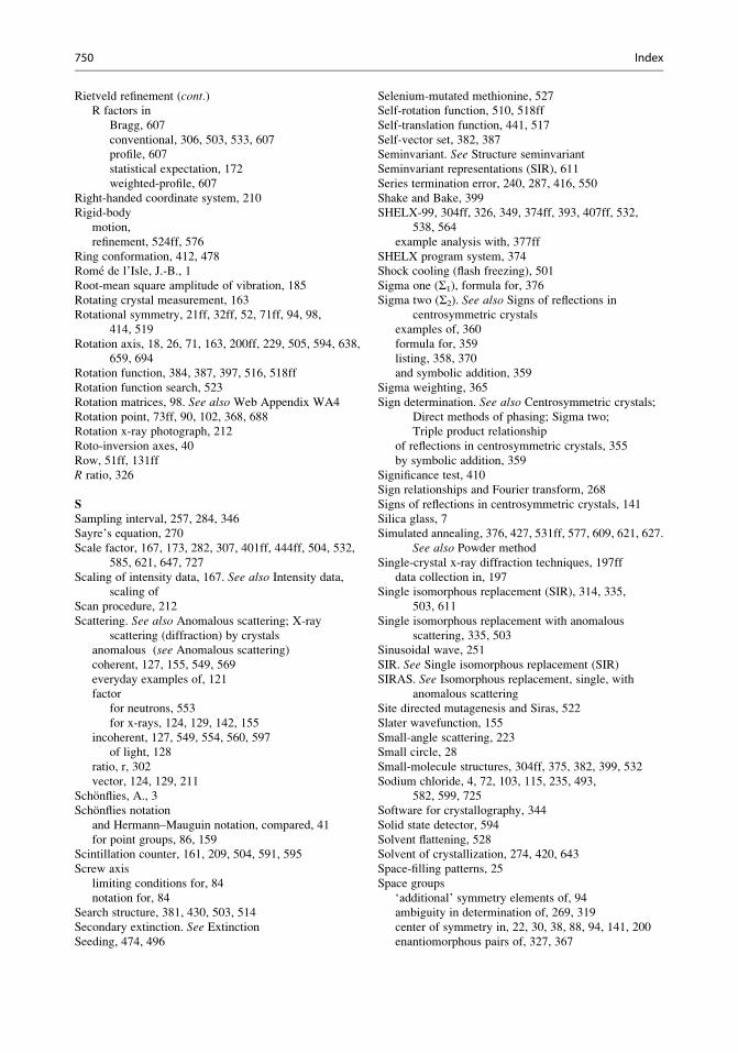
Rietveld refinement (cont.)R factors in

Bragg, 607

conventional, 306, 503, 533, 607

profile, 607

statistical expectation, 172

weighted-profile, 607

Right-handed coordinate system, 210

Rigid-body

motion,

refinement, 524ff, 576

Ring conformation, 412, 478

Rome de l’Isle, J.-B., 1

Root-mean square amplitude of vibration, 185

Rotating crystal measurement, 163

Rotational symmetry, 21ff, 32ff, 52, 71ff, 94, 98,

414, 519

Rotation axis, 18, 26, 71, 163, 200ff, 229, 505, 594, 638,

659, 694

Rotation function, 384, 387, 397, 516, 518ff

Rotation function search, 523

Rotation matrices, 98. See also Web Appendix WA4

Rotation point, 73ff, 90, 102, 368, 688

Rotation x-ray photograph, 212

Roto-inversion axes, 40

Row, 51ff, 131ff

R ratio, 326

SSampling interval, 257, 284, 346

Sayre’s equation, 270

Scale factor, 167, 173, 282, 307, 401ff, 444ff, 504, 532,

585, 621, 647, 727

Scaling of intensity data, 167. See also Intensity data,

scaling of

Scan procedure, 212

Scattering. See also Anomalous scattering; X-ray

scattering (diffraction) by crystals

anomalous (see Anomalous scattering)

coherent, 127, 155, 549, 569

everyday examples of, 121

factor

for neutrons, 553

for x-rays, 124, 129, 142, 155

incoherent, 127, 549, 554, 560, 597

of light, 128

ratio, r, 302

vector, 124, 129, 211

Schonflies, A., 3

Schonflies notation

and Hermann–Mauguin notation, compared, 41

for point groups, 86, 159

Scintillation counter, 161, 209, 504, 591, 595

Screw axis

limiting conditions for, 84

notation for, 84

Search structure, 381, 430, 503, 514

Secondary extinction. See ExtinctionSeeding, 474, 496

Selenium-mutated methionine, 527

Self-rotation function, 510, 518ff

Self-translation function, 441, 517

Self-vector set, 382, 387

Seminvariant. See Structure seminvariant

Seminvariant representations (SIR), 611

Series termination error, 240, 287, 416, 550

Shake and Bake, 399

SHELX-99, 304ff, 326, 349, 374ff, 393, 407ff, 532,

538, 564

example analysis with, 377ff

SHELX program system, 374

Shock cooling (flash freezing), 501

Sigma one (Σ1), formula for, 376

Sigma two (Σ2). See also Signs of reflections in

centrosymmetric crystals

examples of, 360

formula for, 359

listing, 358, 370

and symbolic addition, 359

Sigma weighting, 365

Sign determination. See also Centrosymmetric crystals;

Direct methods of phasing; Sigma two;

Triple product relationship

of reflections in centrosymmetric crystals, 355

by symbolic addition, 359

Significance test, 410

Sign relationships and Fourier transform, 268

Signs of reflections in centrosymmetric crystals, 141

Silica glass, 7

Simulated annealing, 376, 427, 531ff, 577, 609, 621, 627.

See also Powder method

Single-crystal x-ray diffraction techniques, 197ff

data collection in, 197

Single isomorphous replacement (SIR), 314, 335,

503, 611

Single isomorphous replacement with anomalous

scattering, 335, 503

Sinusoidal wave, 251

SIR. See Single isomorphous replacement (SIR)

SIRAS. See Isomorphous replacement, single, with

anomalous scattering

Site directed mutagenesis and Siras, 522

Slater wavefunction, 155

Small-angle scattering, 223

Small circle, 28

Small-molecule structures, 304ff, 375, 382, 399, 532

Sodium chloride, 4, 72, 103, 115, 235, 493,

582, 599, 725

Software for crystallography, 344

Solid state detector, 594

Solvent flattening, 528

Solvent of crystallization, 274, 420, 643

Space-filling patterns, 25

Space groups

‘additional’ symmetry elements of, 94

ambiguity in determination of, 269, 319

center of symmetry in, 22, 30, 38, 88, 94, 141, 200

enantiomorphous pairs of, 327, 367

750 Index

equivalent positions in

general, 74, 83, 93, 274, 288, 296

special, 74

fractional coordinates in, 54, 74, 244, 260, 282, 309

and geometric structure factor, 358

hexagonal, 94, 151, 155

limiting conditions for x-ray reflection in, 598

matrix representation of, 97ff

monoclinic, 81ff, 107, 152, 158, 327ff, 389, 493,

519, 563

origin shift for, 93 (see also Origin, change of)

orthorhombic, 59, 90, 101, 106, 154, 329, 426, 577

pattern for, 33, 72, 509

and point groups, 86ff

practical determination of, 152ff

projections of, 36, 487

as repetition of point group pattern by Bravais

lattice, 72

‘special’ pairs of, 101

standard diagrams for, 94

symbol, analysis of, 89

table of, 92, 101, 352, 431, 456

tetragonal, 94, 154

theory, 51ff

three-dimensional, 7, 23, 80

three-dimensional by symbol

C2, 39, 81, 240

Imma, 247

P1,P1: amplitude and phase symmetry for, 261,

273, 569ff

P1: diagram for, 286, 293

P1: jjEj statistics for, 644P1: general equivalent positions in, 149P1: origin-fixing reflections in, 352ff, 458

P2, 81, 289P21P21: amplitude and phase symmetry for, 282,

314, 320

P21: diagram for, 276, 309

P21: general equivalent positions in, 148, 656P21: geometric structure factor for, 358

P21: limiting conditions in, 85

P21: origin-fixing reflections for, 458

P212121, 90, 101, 154, 347, 352, 367, 423,434, 473, 502, 577, 647, 719

PcPc: equivalence with Pa and Pn, 142Pc: general equivalent positions in, 149Pc: geometric structure factor for, 358

Pc: limiting conditions in, 146

Pc: reciprocal net for, 148P21/cP21/c: amplitude and phase symmetry, 126

P21/c: analysis of symbol for, 152

P21/c: diagram for, 148, 276

P21/c: general equivalent positions in, 149P21/c: geometric structure factor for, 358

P21/c: limiting conditions in, 153

P21/c: origin-fixing reflections in, 352ff, 458

P21/c: special equivalent positions in, 149, 151P63/m, 95, 96, 151Pma2, 101, 148Pman, 150Pmma, 93, 101, 298P4nc, 94, 151Pnma, 90, 99–101, 655

two-dimensional (see Plane groups)Space groups unit cell, centred, 565

Special equivalent positions, 74, 149, 151. See alsoEquivalent positions

molecules in, 74

Special form, 21ff, 35

Special intensity distributions. See DistributionSphere of reflection, 138, 163, 249. See also Ewald sphereSpherical harmonics, 167

Spherical projection, 15

Spherical symmetry, 129, 247

Spherical triangle, 38

Spherical trigonometry, 136. See also Web

Appendix WA3

Square two-dimensional system, 52

Square wave

as Fourier series, 240

Fourier transform of, 255

termination errors for, 240

Standard deviation of electron density, 416

Statistics. See Intensity, statisticsStensen, N., 1

Step-scan moving window measurement, 168

Stereogram. See also Point groups; Projections;

Stereographic projection

fundamental properties of, 556

indexing of, 28

notation for, 23, 34, 81

for point groups, 28

for three-dimensional point groups, 22

for two-dimensional point groups, 20

uses of, 17, 27

Stereograms, 15ff, 70, 81, 177, 520, 636, 659, 694

Stereographic projection, 15ff, 50, 135. See alsoStereograms, Web Appendix WA2

Stereoscopic images. See Stereoviewer; StereoviewsStereoviewer, 5, 659ff

Stereoviews, 4, 22, 34, 57, 89, 274, 277, 319, 454,

470, 713

Straight extinction, 193ff, 229, 289, 440, 455

Structural data. See Bond lengths and angles; Data bases;

Ionic radii; van der Waals contact distances

Structure analysis. See also Direct methods of phase

determination; Heavy-atom method; Reflection,

x-ray; X-ray scattering (diffraction) by crystals

accuracy of (see Precision of calculations)

of atropine, 327, 329, 394

of 5-azauracil, 422

of azidopurine monohydrate, 280

of benzene, 597

of 1-benzyl-1H-tetrazole, 329, 426

Index 751

Structure analysis. (cont.)of bisdiphenylmethyldiselenide, 289, 295

of bromobenzo[b]indeno[1,2-e]pyran, 439of calcium uranate, 609

of cholesteryl iodide, 327

of cimetidine, 610

computer use in, 223, 325, 384, 422

of concanavalin A, 568, 576

of coumarin derivative, 390, 392

criteria for correctness, 406, 416

of crown ether derivative, 574

of cyclosporin H, 560, 574ff

diiodo-(N, N, N’, N’)-tetramethylethylenediamine)

zinc(II), 89

errors in trial structure during, 303

euphenyl iodoacetate, 5, 260, 280

of α-lanthanum tungstate, 622

limitations of, 419

of manganese phosphate monohydrate, 609

and neutron diffraction, 568 (see also Crown ether

derivative)

as over-determined problem, 533

of papaverine hydrochloride, 274

of p-bromophenylethanoic acid, 618

phase problem in, 253, 282ff, 351, 527, 588, 608

of potassium dihydrogen phosphate, 190, 549

of potassium dimercury, 296

of potassium hexachloroplatinate (IV), 285

of potassium 2-hydroxy-3,4-dioxocyclobut-1-en-1-

olate monohydrate, 455

precision of, 596

preliminary stages of, 509, 518, 531

of proteins, 6, 514

pyridoxal phosphate oxime dehydrate, 352ff

symbolic addition in, 359, 368

refinement in, 385, 533, 550, 588

of ricin agglutinin, 509, 512, 520ff

of silver-pyrazole complex, 612

and symmetry analysis, 290

1,8-(3,6,9-trioxaundecane-1,11-diyldioxy)-9,10-

dihydro-10,10-dimethylanthracene-9-ol, 560

tubercidin, 367, 372

of zeolites, 614, 623

of zinc–insulin complex (T3R3), 623

of zinc–silicate complex (VIP-9), 614

Structure factor. See also Phase, determination; Phase,

of structure factor

agreement of, 338, 357, 401

amplitude of

absolute scale of, 215, 351, 563

invariance under change of origin, 253, 353

amplitude symmetry of, 159, 358, 389, 433

with anomalous scattering, 325ff

applications of equation for, 174ff, 249, 276, 351, 532,

582, 702, 714

for body-centred (l) unit cell, 142calculated, 165, 303, 386, 406, 503, 533

for centrosymmetric crystal, 141

change of origin and, 252, 353

conjugate, 367

defined, 179, 240, 306, 363, 400

equation for, 140

as Fourier transform of electron density, 235ff

generalized form of, 242, 244

geometric, 340ff, 358, 433

invariance of under change of origin, 253, 353

local average value of, 287

normalized, 172, 182, 351, 400

observed, 165, 306, 533

and parity group, 354

phase of, 140, 180, 301

phase symmetry of, 358, 457

plotted on Argand diagram, 124ff

reduced equation for, 142

representation as vector, 97, 135, 318

sign-determining formula for, 315, 355ff, 458

and special equivalent positions sets

for space group P21, 85, 144, 156for space group Pc, 146for space group P21/c, 146, 358for space group Pma2, 148, 156for space group Pman, 150

and symmetry elements, 373

and translational symmetry, 176

unitary, 182, 366

Structure invariant, 352, 372, 389, 400, 435, 612, 692

Structure refinement

from neutron data, 569

from x-ray data, 569

Structure seminvariant, 354, 369, 372, 435, 459, 611, 649,

719, 721

Subgroup, 28, 34, 74, 87, 95,

146, 247

Subunit, 471, 473, 479ff, 491, 524

Superposition technique, 300, 650

Symbolic addition procedure, 359

advantages and disadvantages of, 371

Symbolic phases, 360, 369, 372

Symbolic signs for reflections, 360, 459

Symmetric extinction, 195

Symmetry

black-white, 102ff

potassium chloride, 103

characteristic, 24, 26

colour, 102ff

cylindrical, 31

definition of, 36

of diffraction pattern, 330

examples of molecular, 637

external, 17–39

glide plane, 86, 142, 150, 275, 501

and indistinguishability, 25

internal, 194

inversion axis, 22 (see also Roto-inversion axes)

of Laue photograph, 199

mirror (see Reflection symmetry)

notations for, 85, 87

onefold, 21

752 Index

operation, 17, 22, 40, 52, 73ff, 94ff, 146, 152, 228,

378, 384, 390, 405, 452, 491, 636

operator, 99, 106, 637

permitted, 175, 372

and physical properties, 99

rotational, 21, 25, 32, 36, 52, 71, 74, 94, 98, 414, 519

screw axis, 84, 144, 356

and structure analysis, 5

translational, 38, 76ff, 85ff, 120, 142ff, 176, 252,

275, 710

of x-ray diffraction pattern, 4, 30, 142, 200, 290,

330, 509

Symmetry analysis, 275ff, 290, 346

Symmetry axis

alternating, See Schonflies notationprincipal, 26

Symmetry elements. See also Symmetry operations,

combinations of

combinations of, 21

geometrical extension of, 19

matrix representation of, 97ff

notation for, 85ff

sign changes in, 92

in three dimensions, 22ff

in two dimensions, 19ff

Symmetry-equivalent points. See Equivalent positionsSymmetry-independent species, 143

Symmetry operations, combinations of, 24, 636

Symmetry operator, 99, 106, 637

Symmetry plane. See Reflection plane

Symmetry point, 21, 36, 74, 87, 106

Symmetry-related atoms and molecules, 317

Synchrotron radiation (SR)

diamond installation for, 121

filtered, 116 (see also Monochromators)

insertion devices for

undulators, 120

wigglers, 120

oscillation method with, 205ff

worked example of, 207

photon intensity from, 119

polarization of radiation from, 119

radiation flux from, 117

sources, 118, 223, 504

Systematic absences. See Absences; Limiting conditions

Systems

three-dimensional, 21, 27 (see also Crystal systems)

two-dimensional, 21, 52, 73

TTangent formula, 362ff, 372ff

Target structure, 381ff, 434, 503, 522

Temperature factor. See also Thermal vibrations

anisotropic, 444, 449, 579

correction, 402

isotropic, 166ff, 171ff, 190ff, 287, 445

and scale factor, 168, 173, 282, 307, 401ff, 504, 585,

621, 647, 727

Termination errors in Fourier series, 240, 416

Tetrad, 25, 60

Tetragonal crystal system. See also Crystal systems

model of a crystal in,

optical behaviour of crystals in, 190ff

space groups in, 154

symmetry of, 9, 26ff, 192

unit cells in, 60, 90, 409

Tetrahedron, model of, 638

Thermal vibrations. See also Temperature factor

anisotropic, 171

Debye–Waller factor, 170

statistical expectation value of, 172

isotropic, 282, 433

and mean square atom displacement, 170

one-dimensional analysis of, 169

and smearing of electron density, 6

three-dimensional analysis, 403

Thomson scattering. See Coherent; ScatteringThree-phase structure invariants. See TripletsTiled CCD, 219, 222. See also Charge-coupled type

area detector (CCD)

Time-of-flight neutron diffractometer, 558

Time-of-reflection opportunity, 163

Transformations

of coordinate axes, 69, 353

of coordinates in unit cell, 60, 647

of directions, 58, 65

inverse, 65, 211, 255

of Miller indices, 68, 81, 731

mnemonic for, 654

of reciprocal unit cell vectors, 65, 68, 211

of unit cell vectors, 54ff, 78, 731

of zone symbols, 65ff

Translation

function, 517ff, 523ff

search, 387ff

vector, 51, 97, 99, 100, 384, 692, 669

symmetry, 38, 76, 78, 79, 85, 91, 99, 100, 142,

145, 146, 152, 176, 275, 276, 707

Transmission

factor, 159, 165

profile, 166

Triad, 25, 60, 227

Trial-and-error method, 273, 599, 600, 727

Triclinic crystal system, 190

Trigonal crystal system, 190

Trigonal lattice, 61

Trigonometric formulae, 140, 162, 237. See also Web

Appendix WA5

Triple phase relationship (TPR), 374, 376

Triple product relationship, 360, 363

Triple product sign relationship. See also Signs of

reflections in centrosymmetric crystals

physical interpretation of, 356

Σ2 formula for, 355ff

Triplets, 97, 268, 355, 363, 372ff, 400, 433ff, 451ff, 486,

523, 721

Triply primitive hexagonal unit cell, 61, 108

Tungsten Lα-radiation, 116

Index 753

Twin

axis of, 226

contact, 227

hemitropic, 226

interpenetrant, 226

lamellar, 227, 228

mechanical separation of, 226

symmetric, 226

Twinning

in calcite, 227

composition plane in, 226

in fluorite, 227

in gypsum, 226

merohedral, 228

morphology of, 226

non-merohedral, 228

pseudo-merohedral, 228

x-ray diffraction and, 228

Two-dimensional system, 21, 52, 106, 693

UUniaxial crystals. See also Anisotropy, optical; Crystal;

Optically anisotropic crystals

defined, 192

idealized cross-section of, 194

idealized interference figure for, 171

and Laue photograph, 200

optic axis of, 192

Unit cell. See also Bravais lattices; Reciprocal lattice

centred, 550, 565

contents of, 73, 264, 273ff, 290, 298, 342, 518

conventional choice of, 10

dimensions of, 401, 423, 466, 555

limiting conditions for type of, 80ff, 106, 138, 142ff,

249, 510, 598, 604

notation for, 54

number of lattice points in, 55, 57, 61

one-dimensional, 52, 169, 178, 241, 282, 284, 427

parameters

errors in, 390, 599

measurement of, 506

primitive, 52ff, 73ff

reciprocity of F and I, 138reduction of, 569, 654

scattering of x-rays by, 103, 282

symbols for, 52ff, 73, 178

three-dimensional, 54ff, 83, 244

transformations of, 65ff, 565

translations associated with type of, 138

triply primitive hexagonal, 60

volume of, 54, 137

Units, prefixes to, 408

‘Unobserved’ reflections. See Reflections, unobservedUranium heptafluoride, molecular symmetry of, 34

Vvan der Waals contact distances, 224, 645, 649

Vector interactions, 288ff, 342. See also Vectors

Vectors. See also Vector interactions

algebra and reciprocal lattice, 173

complex, 124, 381

cross, 318, 384

interatomic, in Patterson map, 284, 381ff,

518ff, 647

map, 285

overlap, 293

repeat, 72

scalar product of, 58, 64

superposition map, 267

translation, 51, 97ff, 384, 694, 728

triplet, 97, 355ff, 457, 719

vector product of, 136

verification, 381, 388

Velocity, wave, 558

Vibration directions, 189ff

Volume

of real (direct) unit cell, 63

of reciprocal unit cell, 137, 281

von Groth, P., 3

von Laue, M., 4, 130, 133

WWave

amplitude of, 123

and Argand diagram, 124ff

combinations, 124ff, 133, 248

energy associated with, 120, 522

phase of, 123, 241

resultant of combination of, 127, 135

Wavelength

of neutrons, 596

of x-rays, 111ff, 164, 189, 202ff

Wave sums, graphical representation of, 123ff

Web appendix materials.

See also http://extras.springer.com

angle between planes, 137

angle between two lines, 132

direct and reciprocal unit-cell volumes, 136

direction cosines, 7, 353

interplanar spacing, 136

plane trigonometry formulae, 136

reciprocal lattice, 137

reciprocity of I and F unit cells, 138

rotation matrices, 94

spherical trigonometry, 136

Web program packages.

See also http://extras.springer.com

general

coordinate transformation (INTXYZ), 652

linear least squares (LSLI), 653

matrix operations (MATOPS), 653

molecular geometry (MOLGOM),

327, 649

one-dimensional Forier transform (TRANS1),

256, 651

one-dimensional Fourier series (FOUR1D), 256,

257, 270, 650

two-dimensional Fourier series (FOUR2D),

644, 650

source code for, 651

754 Index

point groups

derivation (EULR), 24, 636

recognition (SYMM), 28, 379, 390, 396, 637ff

powder

direct-reciprocal unit-cell parameters (RECIP),

601, 652

indexing, automatic, 568, 604

CRYSFIRE, 604

ITO12, 654

Q values (QVALS), 653

strucure determination (ESPOIR), 621ff

unit-cell reduction (LEPAGE), 602, 654

structure determination, simulated (XRAY)

data preparation (MAKDAT), 640

direct methods, 268, 355

example data sets for, 175, 504, 516, 554, 641

fourier series(electron density), 241

geometry (distance-angle), 415

least-squares refinement, 375, 384, 407, 419

Patterson function, 282ff, 641

Patterson superposition, 341

structure factors, 501ff

Wilson method, 169 Web program suite,

http://extras.springer.com

Weight

function for, 285

measurement of, 606

Weighted reciprocal lattice, 148, 172ff, 197, 259ff,

330, 590,703

Weighted tangent formula, 363ff. See also Tangent

formula

Weiss, C.S., 3

Weissenberg photograph, 441

unit cell dimensions from, 441

Weissenbrg chart, 445

Weiss zone law, 13, 68

Whewell, W., 9

‘White’ radiation, 111ff, 197, 230, 443, 703, 728

Wilson, A.J.C., 173

Wilson plot, 172, 400, 446, 627, 644ff, 690

auxillary plot, 174

Wyckoff space group notation, 74

XX-radiation

copper, 114ff

dependence on wavelength, 123, 140

filtered (see Monochromators)

molybdenum, 220, 328

monochromatic, 205, 230, 552, 593

tungsten, 116

‘white,’ 111ff, 197, 230, 443, 703, 728

X-rays. See also X-radiation

absorption of, 114ff

characteristic, 113

detectors, 118, 213, 222, 508

diffraction and reciprocal lattice, 136, 197, 202, 232,

504, 509 (see also Reciprocal lattice)

diffraction by liquids (see Liquids, x-ray diffraction

from)

diffraction pattern (see also X-ray scattering by

crystals; X-rays, diffraction photograph/image)

centrosymmetric nature of, 29, 140

and Friedel’s law, 140, 147, 332

and geometric structure of crystal, 358

intensity in, 474, 504

position in, 143, 200, 289, 510, 575

symmetry of, 36, 146, 200

as weighted reciprocal lattice, 148, 172ff, 197,

259ff, 330

diffraction photograph/image

important features of, 121, 225

indexing of, 23, 592

by Laue method, 197ff

measurement of intensity of reflection on, 304

by oscillation method, 205

for powder sample, 594

by precession method, 36, 180, 197, 233, 330, 506

for single crystal, 152, 187ff, 375,

441, 501

extinction of, 195

generation of, 217

generators

Bruker AXS, 197, 215, 225

Rigaku MSC, 223

rotating anode, 111ff, 219ff, 337, 504, 569

non-focussing property of, 503

photograph, 30, 152, 180, 200, 212, 259, 330, 332,

440, 441, 466

properties of, 111ff

reflections (see Reflection, x-ray)tube

rotating anode, 111ff, 219ff, 337, 504, 569

sealed tube, 119, 223, 337

wavelengths of, 111ff, 136, 230, 347, 511, 699

wave-like properties of, 4

X-ray scattering (diffraction) by crystals. See alsoDiffraction; Reflection; X-rays,

diffraction pattern; X-rays, diffraction

photograph/image

anomalous, 140, 306, 325, 330ff

by atom, 128, 331

Bragg treatment of, 76, 134

coherent, 127, 549, 569

Compton (see Scattering, incoherent)by crystal structure, 5, 553

as a Fourier analysis, 240

generalized treatment of, 201

incoherent, 127, 155, 549, 554, 560ff, 597

and indices of planes, 8ff, 78

intensity

ideal, 159ff, 172ff

Laue treatment of, 133

equivalence with Bragg treatment, 76, 134

from monoclinic crystals, 152

order of, 576

for orthorhombic crystals, 152

phase difference in, 164

by regular array of atoms, 130ff

for single crystal, 501, 556

Index 755

X-ray scattering (diffraction) by crystals. (cont.)by single electron, 122, 139

and space group determination, 228, 501

and symmetry of Patterson function, 273, 383

theory of, 127

Thomson (see Coherent; Scattering)total energy of, 161

by two or more electrons, 122, 624

from unit cell, 286, 626, 650

vector, 136, 386, 450

X-ray scattering (diffraction) by lattice array of

scattering points

one-dimensional, 19, 52, 131, 169, 264

three-dimensional, 241ff, 285, 328, 446

two-dimensional, 121, 175, 236, 251, 279

YYoung’s fringes, 250

ZZinc sulphide, 4

Zone

axis, 13ff, 197ff

circle, 16

indexing (see Powder indexing)symbol, 13, 40, 51, 65ff, 108, 654

756 Index