A Robust Effect Size Index - Springer LINK

psychometrika—vol. 85, no. 1, 232–246March 2020https://doi.org/10.1007/s11336-020-09698-2

A ROBUST EFFECT SIZE INDEX

Simon Vandekar , Ran Tao and Jeffrey Blume

VANDERBILT UNIVERSITY

Effect size indices are useful tools in study design and reporting because they are unitless measuresof association strength that do not depend on sample size. Existing effect size indices are developed forparticular parametric models or population parameters. Here, we propose a robust effect size index basedon M-estimators. This approach yields an index that is very generalizable because it is unitless across awide range of models. We demonstrate that the new index is a function of Cohen’s d, R2, and standardizedlog odds ratio when each of the parametric models is correctly specified. We show that existing effect sizeestimators are biased when the parametric models are incorrect (e.g., under unknown heteroskedasticity).We provide simple formulas to compute power and sample size and use simulations to assess the biasand standard error of the effect size estimator in finite samples. Because the new index is invariant acrossmodels, it has the potential to make communication and comprehension of effect size uniform across thebehavioral sciences.

Key words: M-estimator, Cohen’s d, R square, standardized log odds, semiparametric.

1. Introduction

Effect sizes are unitless indices quantifying the association strength between dependent andindependent variables. These indices are critical in study design when estimates of power aredesired, but the exact scale of newmeasurement is unknown (Cohen, 1988), and in meta-analysis,where results are compiled across studieswithmeasurements taken on different scales or outcomesmodeled differently (Chinn, 2000; Morris and DeShon, 2002). With increasing skepticism of sig-nificance testing approaches (Trafimow and Earp, 2017; Wasserstein and Lazar, 2016; Harshmanet al., 2016; Wasserstein et al., 2019), effect size indices are valuable in study reporting (Fritz etal., 2012) because they are minimally affected by sample size.

Effect sizes are also important in large open source datasets because inference proceduresare not designed to estimate error rates of a single dataset that is used to address many differentquestions across tens to hundreds of studies. While effect sizes can have similar bias to p-valueswhen choosing among multiple hypotheses, obtaining effect size estimates for parameters speci-fied a priori may be more useful to guide future studies than hypothesis testing because, in largedatasets, p-values can be small for clinically meaningless effect sizes.

There is extensive literature in the behavioral and psychological sciences describing effectsize indices and conversion formulas between different indices (see e.g., Cohen, 1988; Borensteinet al., 2009; Hedges and Olkin, 1985; Ferguson, 2009; Rosenthal, 1994; Long and Freese, 2006).Cohen 1988 defined at least eight effect size indices for different models, different types ofdependent and independent variables, and provided formulas to convert between the indices. Forexample, Cohen’s d is defined for mean differences, R2 is used for simple linear regression, andstandardized log odds ratio is used in logistic regression. Conversion formulas for some of theseparametric indices are given in Table 1 and are widely used in research and software (Cohen,1988; Borenstein et al., 2009; Lenhard and Lenhard, 2017).

Correspondence should be made to Simon Vandekar, Department of Biostatistics, Vanderbilt University, 2525 WestEnd Ave., #1136, Nashville, TN37203, USA. Email: [email protected]

232© 2020 The Author(s)

SIMON VANDEKAR ET AL. 233

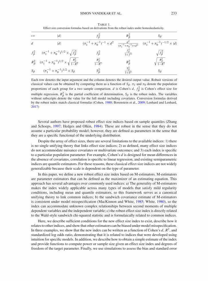
Table 1.Effect size conversion formulas based on derivations from the robust index under homoskedasticity.

�→ |d| f 2β R2β Sβ

d |d| (π−11 + π−1

0 )−1 × d2 d2

(π−11 +π−1

0 )+d2(π−1

1 + π−10 )−1/2 × |d|

f 2β (π−11 + π−1

0 )1/2 ×√

f 2β f 2βf 2β

1+ f 2

√f 2β

R2β (π−1

1 + π−10 )1/2 ×

√R2

β

1−R2

R2β

1−R2 R2β

√R2

β

1−R2

Sβ (π−11 + π−1

0 )1/2 × Sβ S2βS2β

1+S2Sβ

Each row denotes the input argument and the column denotes the desired output value. Robust versions ofclassical values can be obtained by computing them as a function of Sβ . π1 and π0 denote the population

proportions of each group for a two sample comparison. d is Cohen’s d , f 2β is Cohen’s effect size for

multiple regression, R2β is the partial coefficient of determination, Sβ is the robust index. The variables

without subscripts denote the value for the full model including covariates. Conversion formulas derivedby the robust index match classical formulas (Cohen, 1988; Borenstein et al., 2009; Lenhard and Lenhard,2017)

Several authors have proposed robust effect size indices based on sample quantiles (Zhangand Schoeps, 1997; Hedges and Olkin, 1984). These are robust in the sense that they do notassume a particular probability model; however, they are defined as parameters in the sense thatthey are a specific functional of the underlying distribution.

Despite the array of effect sizes, there are several limitations to the available indices: 1) thereis no single unifying theory that links effect size indices; 2) as defined, many effect size indicesdo not accommodate nuisance covariates or multivariate outcomes; and 3) each index is specificto a particular population parameter. For example, Cohen’s d is designed for mean differences inthe absence of covariates, correlation is specific to linear regression, and existing semiparametricindices are quantile estimators. For these reasons, these classical effect size indices are not widelygeneralizable because their scale is dependent on the type of parameter.

In this paper, we define a new robust effect size index based on M-estimators. M-estimatorsare parameter estimators that can be defined as the maximizer of an estimating equation. Thisapproach has several advantages over commonly used indices: a) The generality of M-estimatorsmakes the index widely applicable across many types of models that satisfy mild regularityconditions, including mean and quantile estimators, so this framework serves as a canonicalunifying theory to link common indices; b) the sandwich covariance estimate of M-estimatorsis consistent under model misspecification (MacKinnon and White, 1985; White, 1980), so theindex can accommodate unknown complex relationships between second moments of multipledependent variables and the independent variable; c) the robust effect size index is directly relatedto the Wald-style sandwich chi-squared statistic and is formulaically related to common indices.

Here, we describe sufficient conditions for the new effect size index to exist, describe how itrelates to other indices, and show that other estimators can be biased undermodelmisspecification.In three examples, we show that the new index can be written as a function of Cohen’s d, R2, andstandardized log odds ratio, demonstrating that it is related to indices that were developed usingintuition for specific models. In addition, we describe how to obtain a simple estimate of the indexand provide functions to compute power or sample size given an effect size index and degrees offreedom of the target parameter. Finally, we use simulations to assess the bias and standard error

234 PSYCHOMETRIKA

of the proposed index estimator. An R package to estimate the index is in development; the latestrelease is available at https://github.com/simonvandekar/RESI.

2. Notation

Unless otherwise noted, capital letters denote vectors or scalars and boldface letters denotematrices; lower and upper case greek letters denote vector andmatrix parameters, respectively. LetW1 = {Y1, X1}, . . . ,Wn = {Yn, Xn} be a sample of independent observations fromW ⊂ R

p withassociated probability measure G and let H denote the conditional distribution of Yi given Xi .Here,Wi denotes a combination of a potentiallymultivariate outcome vector Yi with amultivariatecovariate vector Xi .

Let W = {W1, . . . ,Wn} denote the full dataset and θ∗ �→ �(θ∗;W ) ∈ R, θ∗ ∈ Rm be an

estimating equation,

�(θ∗;W ) = n−1n∑

i=1

ψ(θ∗;Wi ), (1)

where ψ is a known function. � is a scalar-valued function that can be maximized to obtain theM-estimator θ . We define the parameter θ as themaximizer of the expected value of the estimatingequation � under the true distribution G,

θ = arg maxθ∗∈�

EG�(θ∗;W ) (2)

and the estimator θ isθ = arg max

θ∗∈��(θ∗;W ).

Assume,θ = (α, β), (3)

where α ∈ Rm0 denotes a nuisance parameter, β ∈ R

m1 is the target parameter, andm0+m1 = m.We define the m × m matrices with j, kth elements

J jk(θ) = −EG∂2�(θ∗;W )

∂θ∗j ∂θ∗

k

∣∣∣θ

K jk(θ) = EG∂�(θ∗;W )

∂θ∗j

∂�(θ∗;W )

∂θ∗k

∣∣∣θ,

which are components of the asymptotic robust covariance matrix of√n(θ − θ).

3. A New Effect Size Index

3.1. Definition

Here, we define a robust effect size that is based on the test statistic for

H0 : β = β0. (4)

SIMON VANDEKAR ET AL. 235

β0 is a reference value used to define the index. Larger distances from β0 represent larger effectsizes. Under the regularity conditions in the Appendix,

√n(θ − θ) ∼ N

{0, J(θ)−1K(θ)J(θ)−1

}. (5)

This implies that the typical robust Wald-style statistic for the test of (4) is approximately chi-squared on m1 degrees of freedom,

Tm1(θ)2 = n(β − β0)Tβ(θ)−1(β − β0) ∼ χ2

m1

{n(β − β0)

Tβ(θ)−1(β − β0)}

, (6)

with noncentrality parameter n(β−β0)Tβ(θ)−1(β−β0), whereβ(θ) is the asymptotic covari-

ance matrix of β, and can be derived from the covariance of (5) (Boos and Stefanski, 2013; Vander Vaart, 2000). We define the square of the effect size index as the component of the chi-squaredstatistic that is due to the deviation of β from the reference value:

Sβ(θ)2 = (β − β0)Tβ(θ)−1(β − β0). (7)

As we demonstrate in the examples below, the covariance β(θ) serves to standardize the param-eter β so that it is unitless. The regularity conditions given in Appendix are sufficient for the index

to exist. The robust index, Sβ(θ) :=√Sβ(θ)2, is defined as the square root of Sβ(θ)2 so that the

scale is proportional to that used for Cohen’s d (see Example 1).This index has several advantages: it is widely applicable because it is constructed from M-

estimators; it relies on a robust covariance estimate; it is directly related to the robust chi-squaredstatistic; it is related to classical indices, and induces several classical transformation formulas(Cohen, 1988; Borenstein et al., 2009; Lenhard and Lenhard, 2017).

3.2. An Estimator

Sβ(θ) is defined in terms of parameter values and so must be estimated from data whenreported in a study. Let Tm1(θ)2 be as defined in (6), then

Sβ(θ) ={max

[0, (Tm1(θ)2 − m)/(n − m)

]}1/2(8)

is consistent for Sβ(θ), which follows by the consistency of the components that make up Tm1(θ)2

(Van der Vaart, 2000; White, 1980). We use the factor (n −m) to account for the estimation of mparameters.

Sβ(θ) is the square root of an estimator for the noncentrality parameters of chisquared statistic.There is a small body of literature on this topic (Saxena and Alam, 1982; Chow, 1987; Neff andStrawderman, 1976; Kubokawa et al., 1993; Shao and Strawderman, 1995; López-Blázquez,2000). While the estimator (8) is inadmissable (Chow, 1987), it has smaller risk than the usualunbiased maximum likelihood estimator (MLE), S2 = (Tm1(θ)2−m)/(n−m), because theMLEis not bounded by zero. We assess estimator bias in Sect. 7.

236 PSYCHOMETRIKA

4. Examples

In this section, we show that the robust index yields several classical effect size indices whenthe models are correctly specified. We demonstrate the interpretability of the effect size indexthrough a series of examples. The following example shows that the robust index for a differencein means is proportional to Cohen’s d, provided that the parametric model is correctly specified;that is, the solution to the M-estimator is equal to the MLE.

Example 1. (Difference in means) In this example, we consider a two mean model, where Wi ={Yi , Xi } and the conditional mean of Yi ∈ R given Xi converges. That is,

n−1x

nx∑i :Xi=x

E(Yi | Xi = x)p−→ μx ∈ R, (9)

for independent observations i = 1, . . . , n, where x, Xi ∈ {0, 1}, nx = ∑ni=1 I (Xi = x), and we

assume the limit (9) exists. In addition, we assume P(Xi = 1) = π1 = 1− π0 is known and that

n−1x

nx∑i :Xi=x

Var(Yi | Xi = x)p−→ σ 2

x < ∞.

Let ∂�(θ;W )/∂θ = n−1 ∑ni=1{(2Xi − 1)π−1

XiYi − θ}, then

θ = n1n

π−11 μ1 − n0

nπ−10 μ0

Eθ = μ1 − μ0

J (θ) = 1

K (θ) = limn→∞ n−1

∑i, j

EH

{(2Xi − 1)π−1

XiYi − θ

} {(2X j − 1)π−1

X jY j − θ

},

where μx = n−1x

∑nxi :Xi=x Yi .When (9) holds, then K (θ) = limn→∞ n−1 ∑n

i=1 π−2Xi

Var(Yi | Xi ).Note that � in this example is not defined as the derivative of a log-likelihood: It defines a singleparameter that is a difference in means and does not require each observation to have the samedistribution. Despite this general approach, we are still able to determine the asymptotic varianceof n1/2θ ,

J (θ)K (θ)−1 J (θ) = limn→∞ n−1

n∑i=1

π−2Xi

Var(Yi | Xi )

= limn→∞ n−1

{n1π

−21 σ 2

1 + n0π−20 σ 2

0

}

= π−11 σ 2

1 + π−10 σ 2

0 .

Then the robust effect size (7) is

Sβ(θ) =√

(μ1 − μ0)2

π−11 σ 2

1 + π−10 σ 2

0

. (10)

SIMON VANDEKAR ET AL. 237

For fixed sample proportions π0 and π1, when σ 20 = σ 2

1 , Sβ(θ) is proportional to the classicalindex of effect size for the comparison of two means, Cohen’s d (Cohen, 1988). However, Sβ(θ)

is more flexible: It can accommodate unequal variance among groups and accounts for the effectthat unequal sample proportions has on the power of the test statistic. Thus, S is an index thataccounts for all features of the study design that will affect the power to detect a difference. Therobust index is proportional to the absolute value of the large sample z-statistic that does not relyon the equal variance assumption. This is what we expect in large samples when the equal varianceassumption is not necessary for “correct” inference. In this example, we did not explicitly assumean identical distribution for all Xi , only that the mean of the variance of Yi given Xi converges inprobability to a constant.

The following example derives the robust effect size for simple linear regression. This is thecontinuous independent variable version of Cohen’s d and is related to R2.

Example 2. (Simple linear regression) Consider the simple linear regression model

Yi = α + Xiβ + εi

where α and β are unknown parameters, Yi ∈ R, Xi ∈ R and εi follows an unknown distributionwith zero mean and conditional variance that can depend on Xi , Var(Yi | Xi ) = σ 2(Xi ). Let�(θ;Wi ) = n−1 ∑n

i=1(Yi − α − Xiβ)2/2. In this model

J(θ)−1 = σ−2x

[σ 2x + μ2

x −μx

−μx 1

]

K(θ) =[

σ 2 μxy

μxy σ 2xy + 2μxμxy − μ2

xσ2

] (11)

whereμx = EG Xi

σ 2x = EG(Xi − μx )

2

σ 2 = EG(Yi − α − Xiβ)2

μxy = EG Xi (Yi − α − Xiβ)2

σ 2xy = EG(Xi − μx )

2(Yi − α − Xiβ)2.

(12)

After some algebra, combining the formulas (11) and (12) gives

β = σ−4x σ 2

xy .

Then (7) is

Sβ(θ)2 = σ 4x

σ 2xy

β2. (13)

The intuition of (13) is best understood by considering the homoskedastic case where EH (Yi −α − Xiβ)2 = σ 2 for all i = 1, . . . , n. Then, σ 4

x /σ 2xyβ

2 = σ 2x /σ 2β2. This is similar to R2, except

that the denominator is the variance of Yi conditional on Xi instead of the marginal variance ofYi . The denominator of (13) accounts for the possible dependence between Xi and Var(Yi | Xi ).

238 PSYCHOMETRIKA

In the following example, we introduce two levels of complexity by considering logisticregression with multidimensional nuisance and target parameters.

Example 3. (Logistic regression with covariates) For logistic regression, we utilize the model

E(Yi | Xi ) = expit(Xi0α + Xi1β) = expit(Xiθ), (14)

where Yi is a Bernoulli random variable, Xi = [Xi0, Xi1] ∈ Rp−1 is a row vector, and α and β

are as defined in (3). Let X = [XT1 . . . XT

n ]T ∈ Rn×(p−1) and similarly define X0 and X1. Let

P ∈ Rn×n be the matrix with Pi i = expit(Xiθ) {1 − expit(Xiθ)} and Pi j = 0 for i = j . Let

Q ∈ Rn×n be the matrix withQi i = {Yi −expit(Xiθ)}2 andQi j = 0 for i = j . If (14) is correctly

specified then EH (Pi i | Xi ) = EH (Qi i | Xi ) = Var(Yi | Xi ). If this equality does not hold, thenthere is under or over dispersion.

To find the robust effect size, we first need to find the covariance matrix of β. To simplifynotation, we define the matrices

Ak�(P) = EGn−1XT

k PX�

for k, � = 0, 1. The block matrix of JG(θ)−1 corresponding to the parameter β is

Iβ(θ)−1 ={A11(P) − A10(P)A00(P)−1A01(P)

}−1. (15)

Equation (15) is the asymptotic covariance of β, controlling for X0, if model (14) is correctlyspecified.

The robust covariance for β can be derived by finding the blockmatrix of J (θ)−1K (θ)J (θ)−1

corresponding to β. In this general case, the asymptotic covariance matrix of β is

β(θ) =Iβ(θ)−1[A10(P)A00(P)−1A00(Q)A00(P)−1A01(P)

−A10(P)A00(P)−1A01(Q)]Iβ(θ)−1

+ Iβ(θ)−1[A11(Q) − A10(Q)A00(P)−1A01(P)

]Iβ(θ)−1.

If the model is correctly specified, P = Q, β(θ) = Iβ(θ)−1, then

Sβ(θ) =√

βT Iβ(θ)β. (16)

The parameter (16) describes the effect of β controlling for the collinearity of variables of interestX1, with the nuisance variables, X0. If the collinearity is high, then the diagonal of Iβ(θ)−1 willbe large and the effect size will be reduced.

Many suggestions have been made to compute standardized coefficients in the context oflogistic regression (for a review see Menard, 2004, 2011). Whenm1 = 1, the square of the robustindex in this context, under correct model specification, is the square of a fully standardizedcoefficient and differs by a factor of

√n from the earliest proposed standardized index (Goodman,

1972). The index proposed byGoodman (1972) is simply aWald statistic andwas rightly criticizedfor its dependence on the sample size (Menard, 2011), despite that it correctly accounts for thefact that the variance of a binomial random variable is functions of its mean, through the useof the diagonal matrix P in the matrix Iβ(θ). The robust index remediates the dependence thatGoodman’s standardized coefficient has on the sample size.

SIMON VANDEKAR ET AL. 239

0.0 0.5 1.0 1.5 2.0

0.0

0.4

0.8

Cohen's dS

a

0.0 0.2 0.4 0.6 0.8 1.0

1.5

0.5

0.5

1.5

R squared

log 1

0(S

)

b

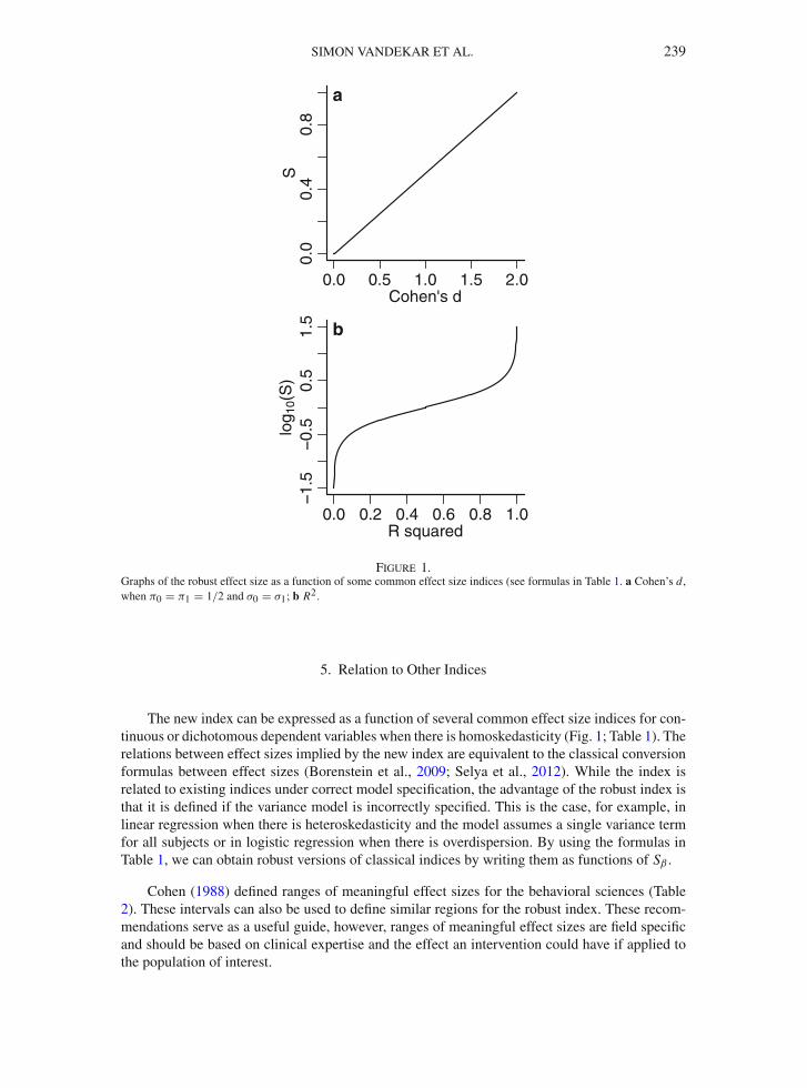
Figure 1.Graphs of the robust effect size as a function of some common effect size indices (see formulas in Table 1. a Cohen’s d,when π0 = π1 = 1/2 and σ0 = σ1; b R2.

5. Relation to Other Indices

The new index can be expressed as a function of several common effect size indices for con-tinuous or dichotomous dependent variables when there is homoskedasticity (Fig. 1; Table 1). Therelations between effect sizes implied by the new index are equivalent to the classical conversionformulas between effect sizes (Borenstein et al., 2009; Selya et al., 2012). While the index isrelated to existing indices under correct model specification, the advantage of the robust index isthat it is defined if the variance model is incorrectly specified. This is the case, for example, inlinear regression when there is heteroskedasticity and the model assumes a single variance termfor all subjects or in logistic regression when there is overdispersion. By using the formulas inTable 1, we can obtain robust versions of classical indices by writing them as functions of Sβ .

Cohen (1988) defined ranges of meaningful effect sizes for the behavioral sciences (Table2). These intervals can also be used to define similar regions for the robust index. These recom-mendations serve as a useful guide, however, ranges of meaningful effect sizes are field specificand should be based on clinical expertise and the effect an intervention could have if applied tothe population of interest.

240 PSYCHOMETRIKA

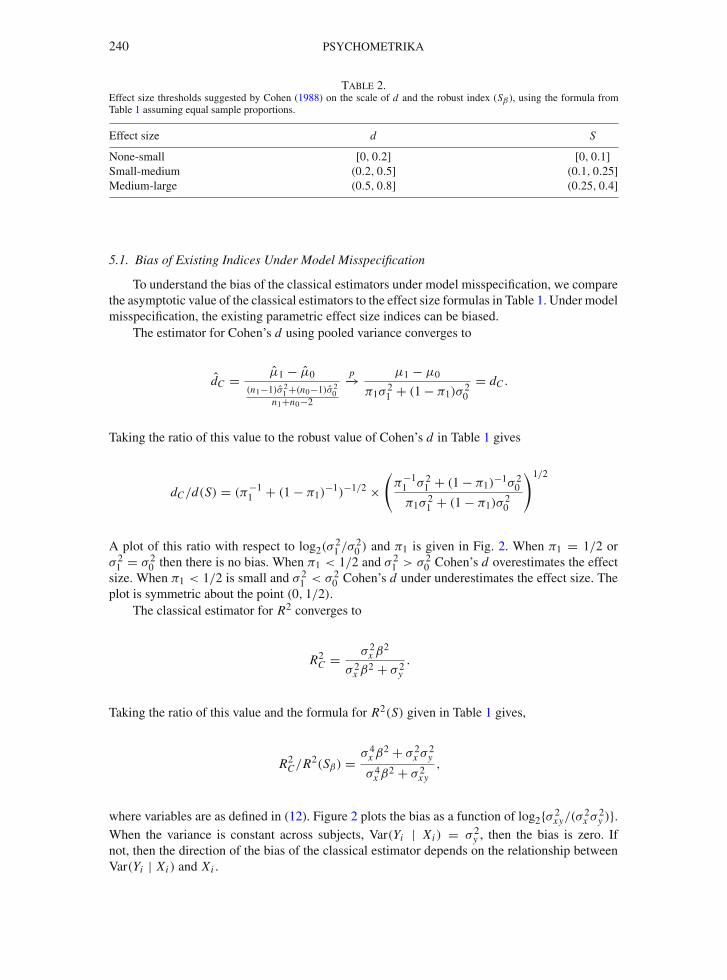
Table 2.Effect size thresholds suggested by Cohen (1988) on the scale of d and the robust index (Sβ ), using the formula fromTable 1 assuming equal sample proportions.

Effect size d S

None-small [0, 0.2] [0, 0.1]Small-medium (0.2, 0.5] (0.1, 0.25]Medium-large (0.5, 0.8] (0.25, 0.4]

5.1. Bias of Existing Indices Under Model Misspecification

To understand the bias of the classical estimators under model misspecification, we comparethe asymptotic value of the classical estimators to the effect size formulas in Table 1. Under modelmisspecification, the existing parametric effect size indices can be biased.

The estimator for Cohen’s d using pooled variance converges to

dC = μ1 − μ0

(n1−1)σ 21 +(n0−1)σ 2

0n1+n0−2

p−→ μ1 − μ0

π1σ21 + (1 − π1)σ

20

= dC .

Taking the ratio of this value to the robust value of Cohen’s d in Table 1 gives

dC/d(S) = (π−11 + (1 − π1)

−1)−1/2 ×(

π−11 σ 2

1 + (1 − π1)−1σ 2

0

π1σ21 + (1 − π1)σ

20

)1/2

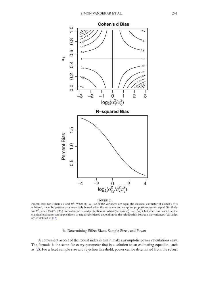
A plot of this ratio with respect to log2(σ21 /σ 2

0 ) and π1 is given in Fig. 2. When π1 = 1/2 orσ 21 = σ 2

0 then there is no bias. When π1 < 1/2 and σ 21 > σ 2

0 Cohen’s d overestimates the effectsize. When π1 < 1/2 is small and σ 2

1 < σ 20 Cohen’s d under underestimates the effect size. The

plot is symmetric about the point (0, 1/2).The classical estimator for R2 converges to

R2C = σ 2

x β2

σ 2x β2 + σ 2

y.

Taking the ratio of this value and the formula for R2(S) given in Table 1 gives,

R2C/R2(Sβ) = σ 4

x β2 + σ 2x σ 2

y

σ 4x β2 + σ 2

xy,

where variables are as defined in (12). Figure 2 plots the bias as a function of log2{σ 2xy/(σ

2x σ 2

y )}.When the variance is constant across subjects, Var(Yi | Xi ) = σ 2

y , then the bias is zero. Ifnot, then the direction of the bias of the classical estimator depends on the relationship betweenVar(Yi | Xi ) and Xi .

SIMON VANDEKAR ET AL. 241

Cohen's d Bias

log2( 12/ 0

2)

1

0.6

0.6

0.8

0.8

1 1

1.2

1.2

1.4

1.4

1.6

1.6

1.8

1.8

2

2

2.2

2.2

3 2 1 0 1 2 3

0.0

0.2

0.4

0.6

0.8

1.0

4 2 0 2 4

0.5

1.0

1.5

R squared Bias

log2( xy2 / x

2y2)

Per

cent

Bia

s

Figure 2.Percent bias for Cohen’s d and R2. When π1 = 1/2 or the variances are equal the classical estimator of Cohen’s d isunbiased, it can be positively or negatively biased when the variances and sampling proportions are not equal. Similarlyfor R2, when Var(Yi | Xi ) is constant across subjects, there is no bias (because σ 2

xy = σ 2x σ 2

y ), but when this is not true, theclassical estimator can be positively or negatively biased depending on the relationship between the variances. Variablesare as defined in (12).

6. Determining Effect Sizes, Sample Sizes, and Power

A convenient aspect of the robust index is that it makes asymptotic power calculations easy.The formula is the same for every parameter that is a solution to an estimating equation, suchas (2). For a fixed sample size and rejection threshold, power can be determined from the robust

242 PSYCHOMETRIKA

50 100 150 200

0.0

0.2

0.4

0.6

0.8

1.0

S = 0.1

n

Pow

er

a

50 100 150 200

0.0

0.2

0.4

0.6

0.8

1.0

S = 0.25

n

Pow

er

b

50 100 150 200

0.0

0.2

0.4

0.6

0.8

1.0

S = 0.4

n

Pow

er

c

50 100 150 200

0.0

0.2

0.4

0.6

0.8

1.0

S = 0.6

n

Pow

er

df = 1df = 2df = 3df = 4df = 5

d

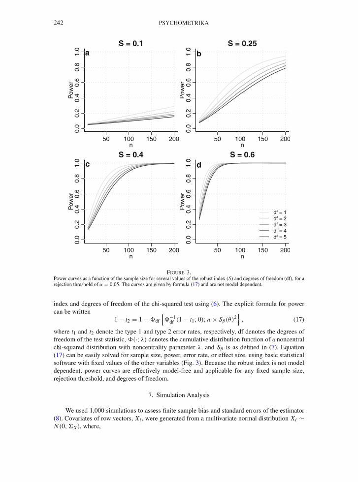
Figure 3.Power curves as a function of the sample size for several values of the robust index (S) and degrees of freedom (df), for arejection threshold of α = 0.05. The curves are given by formula (17) and are not model dependent.

index and degrees of freedom of the chi-squared test using (6). The explicit formula for powercan be written

1 − t2 = 1 − �df

{�−1

df (1 − t1; 0); n × Sβ(θ)2}

, (17)

where t1 and t2 denote the type 1 and type 2 error rates, respectively, df denotes the degrees offreedom of the test statistic, �(·; λ) denotes the cumulative distribution function of a noncentralchi-squared distribution with noncentrality parameter λ, and Sβ is as defined in (7). Equation(17) can be easily solved for sample size, power, error rate, or effect size, using basic statisticalsoftware with fixed values of the other variables (Fig. 3). Because the robust index is not modeldependent, power curves are effectively model-free and applicable for any fixed sample size,rejection threshold, and degrees of freedom.

7. Simulation Analysis

We used 1,000 simulations to assess finite sample bias and standard errors of the estimator(8). Covariates of row vectors, Xi , were generated from a multivariate normal distribution Xi ∼N (0, X ), where,

SIMON VANDEKAR ET AL. 243

Sample size

Bia

s

0.100.050.000.050.10

0 200 600 1000

S = 0rhosq = 0

S = 0.1rhosq = 0

0 200 600 1000

S = 0.25rhosq = 0

S = 0.4rhosq = 0

0 200 600 1000

S = 0.6rhosq = 0

S = 0rhosq = 0.6

0 200 600 1000

S = 0.1rhosq = 0.6

S = 0.25rhosq = 0.6

0 200 600 1000

S = 0.4rhosq = 0.6

0.100.05

0.000.050.10

S = 0.6rhosq = 0.6

Sample size

Sta

ndar

d E

rror

0.00.10.20.30.40.5

0 200 600 1000

S = 0rhosq = 0

S = 0.1rhosq = 0

0 200 600 1000

S = 0.25rhosq = 0

S = 0.4rhosq = 0

0 200 600 1000

S = 0.6rhosq = 0

S = 0rhosq = 0.6

0 200 600 1000

S = 0.1rhosq = 0.6

S = 0.25rhosq = 0.6

0 200 600 1000

S = 0.4rhosq = 0.6

0.00.10.20.30.40.5

S = 0.6rhosq = 0.6

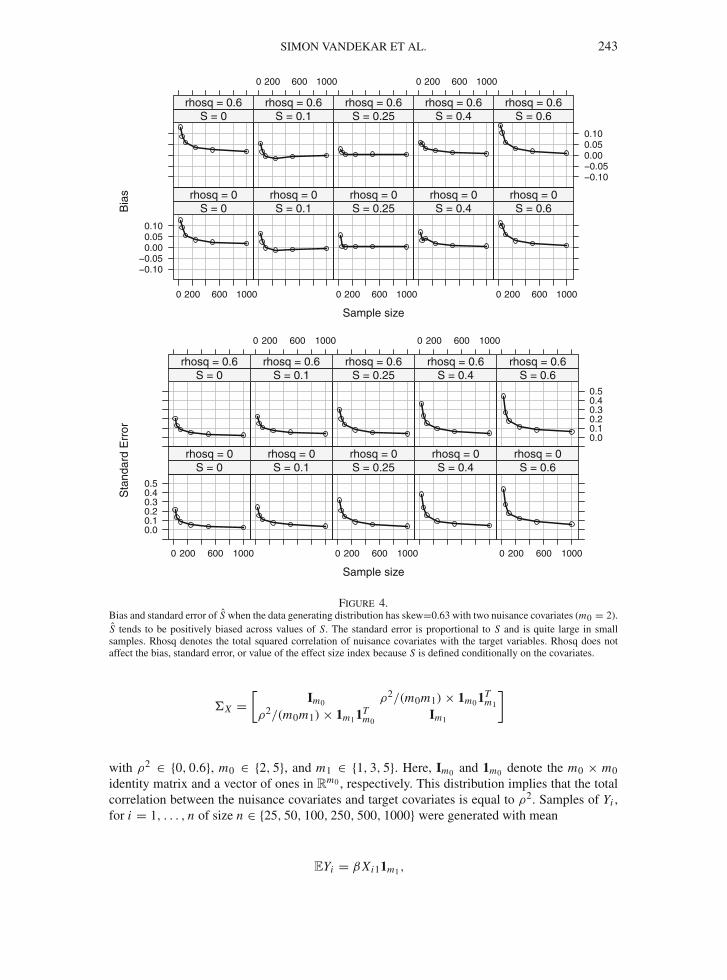
Figure 4.Bias and standard error of S when the data generating distribution has skew=0.63 with two nuisance covariates (m0 = 2).S tends to be positively biased across values of S. The standard error is proportional to S and is quite large in smallsamples. Rhosq denotes the total squared correlation of nuisance covariates with the target variables. Rhosq does notaffect the bias, standard error, or value of the effect size index because S is defined conditionally on the covariates.

X =[

Im0 ρ2/(m0m1) × 1m01Tm1

ρ2/(m0m1) × 1m11Tm0

Im1

]

with ρ2 ∈ {0, 0.6}, m0 ∈ {2, 5}, and m1 ∈ {1, 3, 5}. Here, Im0 and 1m0 denote the m0 × m0identity matrix and a vector of ones in R

m0 , respectively. This distribution implies that the totalcorrelation between the nuisance covariates and target covariates is equal to ρ2. Samples of Yi ,for i = 1, . . . , n of size n ∈ {25, 50, 100, 250, 500, 1000} were generated with mean

EYi = βXi11m1 ,

244 PSYCHOMETRIKA

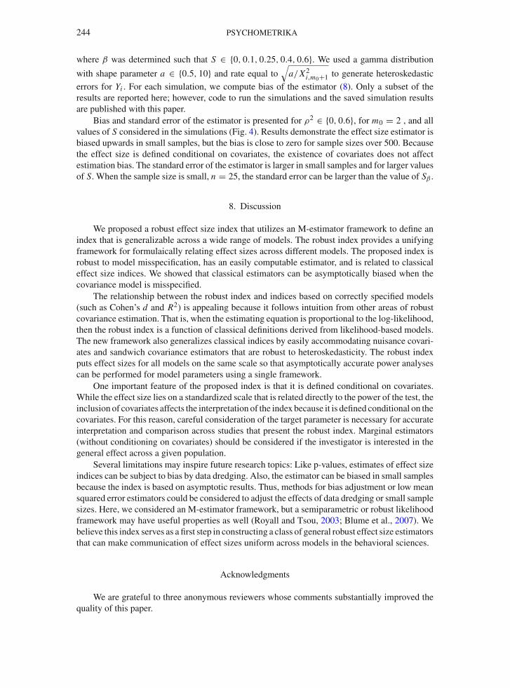
where β was determined such that S ∈ {0, 0.1, 0.25, 0.4, 0.6}. We used a gamma distribution

with shape parameter a ∈ {0.5, 10} and rate equal to√a/X2

i,m0+1 to generate heteroskedastic

errors for Yi . For each simulation, we compute bias of the estimator (8). Only a subset of theresults are reported here; however, code to run the simulations and the saved simulation resultsare published with this paper.

Bias and standard error of the estimator is presented for ρ2 ∈ {0, 0.6}, for m0 = 2 , and allvalues of S considered in the simulations (Fig. 4). Results demonstrate the effect size estimator isbiased upwards in small samples, but the bias is close to zero for sample sizes over 500. Becausethe effect size is defined conditional on covariates, the existence of covariates does not affectestimation bias. The standard error of the estimator is larger in small samples and for larger valuesof S. When the sample size is small, n = 25, the standard error can be larger than the value of Sβ .

8. Discussion

We proposed a robust effect size index that utilizes an M-estimator framework to define anindex that is generalizable across a wide range of models. The robust index provides a unifyingframework for formulaically relating effect sizes across different models. The proposed index isrobust to model misspecification, has an easily computable estimator, and is related to classicaleffect size indices. We showed that classical estimators can be asymptotically biased when thecovariance model is misspecified.

The relationship between the robust index and indices based on correctly specified models(such as Cohen’s d and R2) is appealing because it follows intuition from other areas of robustcovariance estimation. That is, when the estimating equation is proportional to the log-likelihood,then the robust index is a function of classical definitions derived from likelihood-based models.The new framework also generalizes classical indices by easily accommodating nuisance covari-ates and sandwich covariance estimators that are robust to heteroskedasticity. The robust indexputs effect sizes for all models on the same scale so that asymptotically accurate power analysescan be performed for model parameters using a single framework.

One important feature of the proposed index is that it is defined conditional on covariates.While the effect size lies on a standardized scale that is related directly to the power of the test, theinclusion of covariates affects the interpretation of the index because it is defined conditional on thecovariates. For this reason, careful consideration of the target parameter is necessary for accurateinterpretation and comparison across studies that present the robust index. Marginal estimators(without conditioning on covariates) should be considered if the investigator is interested in thegeneral effect across a given population.

Several limitations may inspire future research topics: Like p-values, estimates of effect sizeindices can be subject to bias by data dredging. Also, the estimator can be biased in small samplesbecause the index is based on asymptotic results. Thus, methods for bias adjustment or low meansquared error estimators could be considered to adjust the effects of data dredging or small samplesizes. Here, we considered an M-estimator framework, but a semiparametric or robust likelihoodframework may have useful properties as well (Royall and Tsou, 2003; Blume et al., 2007). Webelieve this index serves as a first step in constructing a class of general robust effect size estimatorsthat can make communication of effect sizes uniform across models in the behavioral sciences.

Acknowledgments

We are grateful to three anonymous reviewers whose comments substantially improved thequality of this paper.

SIMON VANDEKAR ET AL. 245

Funding National Institutes of Health grants: (5P30CA068485-22 to S.N.V.).

OpenAccess This article is licensed under a Creative Commons Attribution 4.0 International License, whichpermits use, sharing, adaptation, distribution and reproduction in any medium or format, as long as you giveappropriate credit to the original author(s) and the source, provide a link to the Creative Commons licence,and indicate if changes were made. The images or other third party material in this article are included in thearticle’s Creative Commons licence, unless indicated otherwise in a credit line to the material. If material isnot included in the article’s Creative Commons licence and your intended use is not permitted by statutoryregulation or exceeds the permitted use, you will need to obtain permission directly from the copyrightholder. To view a copy of this licence, visit http://creativecommons.org/licenses/by/4.0/.

Publisher’s Note Springer Nature remains neutral with regard to jurisdictional claims in pub-lished maps and institutional affiliations.

9. Appendix

The following regularity conditions are required for the asymptotic normality of√n(θ − θ) (Van

der Vaart, 2000)

(a) The function θ∗ �→ �(θ∗;w) is almost surely differentiable at θ with respect to G,where objects are as defined in (1) and (2).

(b) For every θ1 and θ2 in a neighborhood of θ and measurable function m(w) such thatEGm(W )2 < ∞, |�(θ1;w) − �(θ2;w)| ≤ m(w)‖θ1 − θ2‖.

(c) The function θ∗ �→ EG�(θ∗;W ) admits a second-order Taylor expansion at θ with anon-singular second derivative matrix J(θ).

(d) �(θ,W ) ≥ supθ∗ �(θ∗,W ) − op(n−1) and θp−→ θ .

References

Blume, J. D., Su, L., Olveda, R. M., & McGarvey, S. T. (2007). Statistical evidence for GLM regression parameters: Arobust likelihood approach. Statistics in Medicine, 26(15), 2919–2936.

Boos, D. D., & Stefanski, L. A. (2013). Essential statistical inference: Theory and methods. New York: Springer Texts inStatistics. Springer.

Borenstein, M., Hedges, L. V., Higgins, J. P., & Rothstein, H. R. (2009). Converting Among Effect Sizes. In Introductionto Meta-Analysis (pp. 45–49). West Sussex, UK: John Wiley & Sons Ltd.

Chinn, S. (2000). A simple method for converting an odds ratio to effect size for use in meta-analysis. Statistics inMedicine, 19(22), 3127–3131.

Chow, M. S. (1987). A complete class theorem for estimating a noncentrality parameter. The Annals of Statistics, 15(2),800–804.

Cohen, J. (1988). Statistical power analysis for the behavioral sciences. Hillsdale, NJ: Erlbaum Associates.Ferguson, C. J. (2009). An effect size primer: A guide for clinicians and researchers. Professional Psychology: Research

and Practice, 40(5), 532–538.Fritz, C. O., Morris, P. E., & Richler, J. J. (2012). Effect size estimates: Current use, calculations, and interpretation.

Journal of Experimental Psychology: General, 141(1), 2–18.Goodman, L. A. (1972). A modified multiple regression approach to the analysis of dichotomous variables. American

Sociological Review, 37(1), 28–46.Harshman, R. A., Raju, N. S., &Mulaik, S. A. (2016). There is a time and a place for significance testing. InWhat if there

were no significance tests?, (pp. 109–154). Routledge.Hedges, L. V., & Olkin, I. (1984). Nonparametric estimators of effect size in meta-analysis. Psychological Bulletin, 96(3),

573.Hedges, L. V., & Olkin, I. (1985). Statistical methods for meta-analysis. London, UK: Elsevier.Kubokawa, T., Robert, C. P., & Saleh, A. K. M. E. (1993). Estimation of noncentrality parameters. The Canadian Journal

of Statistics / La Revue Canadienne de Statistique, 21(1), 45–57.Lenhard, W., & Lenhard, A. (2017). Calculation of Effect Sizes. https://www.psychometrica.de/effect_size.html.

Accessed: 2019-08-12.Long, J. S., & Freese, J. (2006). Regression models for categorical dependent variables using Stata (2nd ed.). College

Station: Stata press.López-Blázquez, F. (2000). Unbiased estimation in the non-central chi-square distribution. Journal of Multivariate Anal-

ysis, 75(1), 1–12.

246 PSYCHOMETRIKA

MacKinnon, J. G., & White, H. (1985). Some heteroskedasticity–consistent covariance matrix estimators with improvedfinite sample properties. Journal of econometrics, 29(3), 305–325.

Menard, S. (2004). Six approaches to calculating standardized logistic regression coefficients. The American Statistician,58(3), 218–223.

Menard, S. (2011). Standards for standardized logistic regression coefficients. Social Forces, 89(4), 1409–1428.Morris, S. B., & DeShon, R. P. (2002). Combining effect size estimates in meta-analysis with repeated measures and

independent-groups designs. Psychological Methods, 7(1), 105–125.Neff,N.,&Strawderman,W.E. (1976). Further remarks on estimating the parameter of a noncentral chi-square distribution.

Communications in Statistics—Theory and Methods, 5(1), 65–76.Rosenthal, R. (1994). Parametric measures of effect size. The Handbook of Research Synthesis, 621, 231–244.Royall, R., & Tsou, T.-S. (2003). Interpreting statistical evidence by using imperfect models: Robust adjusted likelihood

functions. Journal of the Royal Statistical Society: Series B (Statistical Methodology), 65(2), 391–404.Saxena, K. M. L., & Alam, K. (1982). Estimation of the non-centrality parameter of a chi squared distribution. The Annals

of Statistics, 10(3), 1012–1016.Selya, A. S., Rose, J. S., Dierker, L. C., Hedeker, D., & Mermelstein, R. J. (2012). A Practical Guide to Calculating

Cohen’s f2, a Measure of Local Effect Size, from PROC MIXED. Frontiers in Psychology, 3(111).Shao, P. Y. S., & Strawderman, W. E. (1995). Improving on the positive part of the umvue of a noncentrality parameter

of a noncentral chi-square distribution. Journal of Multivariate Analysis, 53(1), 52–66.Trafimow, D., & Earp, B. D. (2017). Null hypothesis significance testing and Type I error: The domain problem. New

Ideas in Psychology, 45, 19–27.Van der Vaart, A. W. (2000). Asymptotic Statistics (Vol. 3). Cambridge: Cambridge University Press.Wasserstein, R. L., & Lazar, N. A. (2016). The ASA’s statement on p-values: Context, process, and purpose. The American

Statistician, 70(2), 129–133.Wasserstein, R. L., Schirm, A. L., & Lazar, N. A. (2019).Moving to a world beyond “p< 0.05”. The American Statistician,

73(sup1), 1–19.White, H. (1980). A heteroskedasticity–consistent covariance matrix estimator and a direct test for heteroskedasticity.

Econometrica: Journal of the Econometric Society, (pp. 817–838).Zhang, Z., & Schoeps, N. (1997). On robust estimation of effect size under semiparametric models. Psychometrika, 62(2),

201–214.

Manuscript Received: 29 JAN 2019Published Online Date: 30 MAR 2020