Pricing Credit Default Swaps with Option-Implied
Volatility
Charles Cao Fan Yu Zhaodong Zhong1
November 19, 2010
Forthcoming: Financial Analysts Journal
1Cao is from Pennsylvania State University, Yu is from Claremont McKenna College, and Zhong is fromRutgers University. We wish to acknowledge helpful comments from Gurdip Bakshi, Robert Jarrow, PhilippeJorion, Bill Kracaw, Paul Kupiec, C. F. Lee, Haitao Li, Matt Pritsker, Til Schuermann, Louis Scott, Stu-art Turnbull, Hao Zhou, and seminar/conference participants at BGI, HEC Montreal, HKUST, INSEAD,Michigan State University, Penn State University, Rutgers University, Singapore Management University,UC-Irvine, University of Hong Kong, University of Houston, the McGill/IFM2 Risk Management Conference,the 16th Annual Derivative Securities and Risk Management Conference at the FDIC, the American Eco-nomic Association Meetings, and the 15th Mitsui Life Symposium at the University of Michigan. Financialsupport from the FDIC’s Center for Financial Research is greatly appreciated. Special thanks go to RodneySullivan (the Editor) and two anonymous referees for constructive suggestions that greatly improved ourpaper.

Pricing Credit Default Swaps with Option-ImpliedVolatility
Abstract
Using the industry benchmark CreditGrades model to analyze credit default swap (CDS)
spreads across a large number of �rms during the 2007-09 credit crisis, we demonstrate
that the performance of the model can be signi�cantly improved if one calibrates the model
with option-implied volatility in lieu of historical volatility. Moreover, the advantage of
using option-implied volatility is greater among �rms with more volatile CDS spreads, more
actively traded options, and lower credit ratings. These results are robust both in- and out-
of-sample, and are insensitive to historical volatilities estimated at short or long horizons.
1 Introduction
The credit derivatives market, especially that of credit default swaps, has grown exponentially
during the past decade. Along with this new development comes the need to understand
the pricing of credit default swaps. CDS contracts are often used by �nancial institutions
to hedge against the credit risk in their loan portfolios. More recently, however, they have
become popular in relative value trading strategies such as capital structure arbitrage (Currie
and Morris, 2002). Consequently, a suitable pricing model has to reproduce both accurate
CDS spreads and the relation between CDS spreads and the pricing of other corporate
securities, such as common stocks, stock options, and corporate bonds.
In this article, we present an empirical study of CDS pricing using an industry benchmark
model called CreditGrades. As explained in the CreditGrades Technical Document (2002),
this model was jointly developed by Deutsche Bank, Goldman Sachs, JPMorgan, and the
RiskMetrics Group as a standard of transparency in the credit market. Mostly based on
the seminal Black and Cox (1976) model and extended to account for uncertain default
thresholds, CreditGrades provides simple closed-form formulas relating CDS pricing to the
equity price and equity volatility. We examine the performance of the model across a large
number of �rms. More importantly, we estimate the parameters of the model using data
from both equity and options markets by incorporating the option-implied volatility into the
calibration procedure.
The linkage between CDS and options markets can arise in several contexts. From a
theoretical option pricing perspective, the option-implied volatility re�ects the expected
future volatility and the volatility risk premium, both of which have been shown to explain
CDS valuation in a regression-based framework (Cao, Yu, and Zhong, 2010). From a market
microstructure perspective, recent evidence points to the presence of informed trading in
both the options market (Cao, Chen, and Gri¢ n, 2005; Pan and Poteshman, 2006) and
the CDS market (Acharya and Johnson, 2007). Theoretically, whether informed traders
will exploit their information using derivatives is likely to be a function of the leverage
1
and liquidity of the derivatives markets and the overall presence of information asymmetry
(Black, 1975; Back, 1993; Easley, O�Hara, and Srinivas, 1998). Consequently, we expect
the information content of option-implied volatility for CDS valuation to exhibit �rm-level
variations consistent with these predictions.
We begin our analysis by estimating the CreditGrades model for each of the 332 sample
�rms. Speci�cally, we minimize the sum of squared CDS pricing errors over three parameters
of the model: the mean default threshold, the default threshold uncertainty, and the bond
recovery rate. For the equity volatility input, we use either an option-implied volatility or a
backward-looking historical volatility. We then compute the ratio of the implied volatility-
based pricing error to the historical volatility-based pricing error for each �rm, and then link
this ratio to �rm-speci�c characteristics.
Overall, our results indicate that, in comparison to historical volatility, the use of option-
implied volatility yields a better �t of the model to market CDS spreads. To examine how
this improvement of model performance varies at the �rm-level, we regress the pricing error
ratio on a number of �rm-level characteristics. In particular, we include the option trading
volume and open interest as measures of options market liquidity, along with the volatility
of the CDS spread and credit rating as proxies of the amount of informed trading in the
marketplace. We �nd that the ratio of the pricing errors is smaller (the advantage of implied
volatility over historical volatility is greater) among �rms with more volatile CDS spreads
and actively traded options, as well as lower rated �rms. Hence, our results are broadly
consistent with the predictions of market microstructure theories.
We conduct several robustness checks. First, we use a rolling-window estimation ap-
proach to improve the performance of model-�tting; for each day in our sample period, we
use only the previous 22, 126, or 252 daily observations to estimate the parameters of the
CreditGrades model and generate a one-day-ahead forecast of the CDS spread. We �nd that
the advantage of implied volatility over historical volatility remains in these out-of-sample
tests. We also examine the ability of the CreditGrades model to forecast daily CDS spread
2
changes. Consistent with earlier results, we �nd that the implied volatility-based forecasts
better explain actual CDS spread changes. Second, we repeat the pricing analysis with 22-,
63-, 126-, and 1,000-day historical volatilities. We �nd that the historical volatility-based
CDS pricing errors generally declines with the horizon of the historical volatility estimator.
Nevertheless, the cross-sectional behavior of the ratio of pricing errors remains unchanged
in all cases. These results suggest that the information advantage of implied volatility over
historical volatility is robust to the length of data used in the estimation of the CreditGrades
model and the calculation of historical volatility.
There is a large literature on the relation between CDS pricing and equity volatility. For
example, Campbell and Taksler (2003), Ericsson, Jacobs, and Oviedo-Helfenberger (2009),
and Zhang, Zhou, and Zhu (2009) have analyzed the connection between CDS spreads and
equity historical volatilities. Our paper di¤ers from these studies due to its focus on the
option-implied volatility. Cremers, Driessen, Maenhout, and Weinbaum (2008) estimate a
panel regression of corporate bond yield spreads and options market variables. Cao, Yu, and
Zhong (2010) estimate �rm-level time-series regressions of credit spreads and focus on the
role of the volatility risk premium in explaining CDS pricing. In comparison, we address
the inherently nonlinear relation between CDS spreads and equity volatility by �tting a
structural credit risk model. Moreover, we concentrate on the cross-sectional interpretation
of the �rm-level CDS pricing errors. Our paper is also similar in spirit to Stamicar and
Finger (2006), who use case studies to illustrate the calibration of the CreditGrades model
with options data; our analysis is more in-depth and broader in scope with a signi�cantly
larger sample of �rms and sample period inclusive of the recent credit crisis.
Our �nding is important to market participants who need to constantly monitor their
credit risk exposures. First, it suggests that having forward-looking inputs from the market
could be as important as having the �right� model for pricing credit risk. Second, the
better pricing performance from using option-implied volatility is likely to result in fewer
�false�trading signals and therefore enhanced pro�tability for capital structure arbitrageurs.
3
Indeed, the preliminary evidence from Luo (2008) shows that an extension of Yu (2006)�s
analysis of capital structure arbitrage to incorporate options market information signi�cantly
increases the Sharpe ratio of this popular hedge fund strategy.
The rest of this paper is organized as follows: In Section 2, we present the data and
summary statistics. In Section 3, we discuss the CreditGrades model. Section 4 explains
our estimation procedure and overall results. The cross-sectional analysis of pricing errors
is presented in Section 5. Further robustness checks can be found in Section 6. We conclude
with Section 7.
2 Data
The sources of the variables used in our study are documented as follows:
� Credit Default Swaps. We obtain single-name CDS spreads from the Markit Group.
According to Markit, it receives contributed CDS data from market makers based on
their o¢ cial books and records. The data then undergoes a rigorous cleaning process
to test for staleness, outliers, and inconsistency. Any contribution that fails any one
of these tests will be rejected. The full term structures of CDS spreads and recovery
rates are available by entity, tier, currency, and restructuring clause. In this paper, we
use the composite spreads of US dollar-denominated �ve-year CDS contracts written
on senior unsecured debt of North American obligors. Furthermore, we limit ourselves
to CDS contracts that allow for so-called �modi�ed restructuring,�which restricts the
range of maturities of debt instruments that can be delivered in a credit event.
� Equity Options. We collect options data from OptionMetrics, which provides daily
closing prices, open interest, and trading volume on exchange-listed equity options
in the United States. We do not use the standardized implied volatility provided by
OptionMetrics, since this measure can be noisy due to the small number of contracts
used in OptionMetrics�interpolation process. Instead, we use the binomial model for
4

American options with discrete dividend adjustments to estimate the level of implied
volatility that would minimize the sum-of-squared pricing errors across all put options
with non-zero open interests.
� Other Variables. We collect daily stock returns, equity prices, and common shares
outstanding from CRSP, and the book value of total liabilities and total assets from
Computstat. Historical volatility measures with di¤erent estimation horizons, ranging
from 22, 63, 126, 252, to 1,000 trading days are calculated using the stock returns.
Leverage ratio is de�ned as total liabilities divided by the sum of total liabilities and
market capitalization.
We exclude �rms in the �nancial, utility, and government sectors, and we further require
that each �rm have at least 377 observations (about one and a half years of daily observations)
of the CDS spread, the implied volatility, the 252-day historical volatility, and the leverage
ratio, and that each �rm have no more than �ve percent of missing observations between the
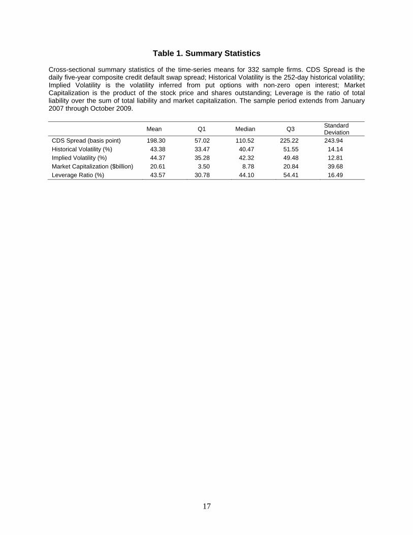
�rst and last dates of its coverage. The �nal sample consists of 332 �rms in the sample period
of January 2007 to October 2009. The cross-sectional summary statistics of the time-series
means of the variables are presented in Table 1. The mean CDS spread is 198bp and the
cross-sectional standard deviation is 244bp. The average �rm also has an implied volatility
of 44.37 percent, a 252-day historical volatility of 43.38 percent, and a leverage ratio of 43.57
percent. Finally, the average �rm has a market capitalization slightly in excess of $20 billion,
which is similar to the size of a typical S&P 500 company.
3 The CreditGrades Model
To e¤ectively address the nonlinear dependence of the CDS spread on its determinants, we
conduct a pricing analysis using a structural credit risk model with equity volatility calcu-
lated using information from either the options market or the stock market. Speci�cally,
we use the CreditGrades model, an industry benchmark model jointly developed by Risk-
5
Metrics, JP Morgan, Goldman Sachs, and Deutsche Bank that is based on the structural
model of Black and Cox (1976). Detailed documentation of this model can be found in the
CreditGrades Technical Document (2002), a summary of which is given below. Although a
full menu of structural models have been developed following the seminal work of Merton
(1974), we choose this industry model for three reasons. First, it appears to be widely used
by practitioners (Currie and Morris, 2002). Second, it contains an element of uncertain re-
covery rates, which helps to generate realistic short-term credit spreads. Third, the model
yields a simple analytic CDS pricing formula. We are aware of the general concern of model
misspeci�cation when choosing to work with any particular model. Our methodology, how-
ever, is applicable to other structural models in a straightforward manner, which we leave
to future research.
The CreditGrades model assumes that under the pricing measure, the �rm�s value per
equity share is given bydVtVt
= �dWt; (1)
where Wt is a standard Brownian motion and � is the asset volatility. The �rm�s debt per
share is a constant D and the (uncertain) default threshold as a percentage of debt per share
is
L = Le�Z��2=2; (2)
where L = E (L) is the expected value of the default threshold, Z is a standard normal
random variable, and �2 = var (lnL) measures the uncertainty in the default threshold
value. Note that the �rm value process is assumed to have zero drift. This assumption is
consistent with the observation that leverage ratios tend to be stationary over time.
Default is de�ned as the �rst passage of Vt to the default threshold LD. The density of
the default time can be obtained by integrating the �rst passage time density of a geometric
Brownian motion to a �xed boundary over the distribution of L. However, CreditGrades pro-
vides an approximate solution to the survival probability q (t) using a time-shifted Brownian
6

motion, yielding the following result:1
q (t) = �
��At2+ln d
At
�� d � �
��At2� ln dAt
�; (3)
where � (�) is the cumulative normal distribution function, and
d =V0
LDe�
2
;
At =p�2t+ �2:
With constant interest rate r, bond recovery rate R, and the survival probability function
q (t), it can be shown that the CDS spread for maturity T is
c = �(1�R)
R T0e�rsdq (s)R T
0e�rsq (s) ds
: (4)
Substituting q (t) into the above equation, the CDS spread for maturity T is given by
c (0; T ) = r (1�R) 1� q (0) +H (T )q (0)� q (T ) e�rT �H (T ) ; (5)
where
H (T ) = er� (G (T + �)�G (�)) ;
G (T ) = dz+1=2�
�� ln d
�pT� z�
pT
�+ d�z+1=2�
�� ln d
�pT+ z�
pT
�;
� = �2=�2;
z =p1=4 + 2r=�2:
Note that equation (5) depends on the asset volatility �, which is unobserved. Stamicar
and Finger (2006) derive an analytic pricing formula for equity options within the above
framework, which can be used to infer the asset volatility from the market prices of equity
options. Moreover, they show that a local approximation to the volatility surface,
� = �SS
S + LD; (6)
1The approximation assumes that Wt starts not at t = 0, but from an earlier time. In essence, theuncertainty in the default threshold is shifted to the starting value of the Brownian motion.
7
in which �S is taken to be the implied volatility from equity options, also produces accurate
CDS spreads.
It is interesting to compare CreditGrades with the I2 model of Giesecke and Goldberg
(2004) with respect to their treatment of the uncertain default barrier. In Giesecke and
Goldberg (2004), the default barrier follows a beta distribution with its mean calibrated to
Compustat�s short-term debt and its variance treated as a constant parameter. Therefore,
as a �rm adjusts its capital structure over time, its mean default threshold varies as well. In
CreditGrades, the default barrier is equal to the debt per share (measured in our empirical
work by total liabilities per share) multiplied by a normal random variable with its mean
and variance treated as constant parameters. Therefore, CreditGrades shares with the I2
model the common feature that the mean default barrier changes over time with the capital
structure of the �rm.
4 Estimation Procedures and Results
To begin the pricing analysis, we note that the CreditGrades model requires the following
eight inputs to generate a CDS spread: the equity price S, the debt per share D, the interest
rate r, the average default threshold L, the default threshold uncertainty �, the bond recovery
rate R, the time to expiration T , and �nally the equity volatility �S, which we take as either a
historical volatility or an option-implied volatility. Hence, the CreditGrades pricing formula
can be abbreviated as
CDSt = f�St; Dt; rt; �t; T � t;L; �;R
�; (7)
recognizing that three of the parameters (L, �, and R) are unobserved. To conduct the
pricing analysis, we take the entire sample period for each �rm (say, of length N) to estimate
these three parameters. Speci�cally, let CDSi and dCDSi denote the observed and modelCDS spreads on day i for a given �rm. We minimize the sum-of-squared relative pricing
8
errors:
SSE = minL;�;R
NXi=1
dCDSi � CDSiCDSi
!2: (8)
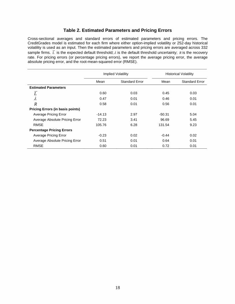
Table 2 present the estimated parameters and the pricing errors. Across the 332 �rms,
the average parameters are similar for both implied volatility-based and historical volatility-
based estimation. In the latter case, the average default threshold is L = 0:45, the default
threshold uncertainty is � = 0:46, and the bond recovery rate is R = 0:56. In comparison,
the CreditGrades Technical Document (2002) assumes L = 0:5, � = 0:3, and takes the bond
recovery rate R from a proprietary database from JPMorgan. These values are reasonably
close to the cross-sectional average parameter estimates presented above.
Table 2 also presents the cross-sectional average of the average pricing error, the average
absolute pricing error, and the root-mean-squared pricing error (RMSE) based on CDS
spread levels as well as percentage deviations from observed levels.2 Generally, the estimation
based on implied volatility yields smaller �tting errors. For instance, the implied volatility-
based RMSE is 105.76bp, while the historical volatility-based counterpart is 131.54bp. When
examining average pricing errors, we �nd that the implied volatility-based and historical
volatility-based pricing errors are -14.13bp and -50.31bp, respectively. Similarly, the implied
volatility-based percentage RMSE is 0.60, while the historical volatility-based percentage
RMSE is 0.72.
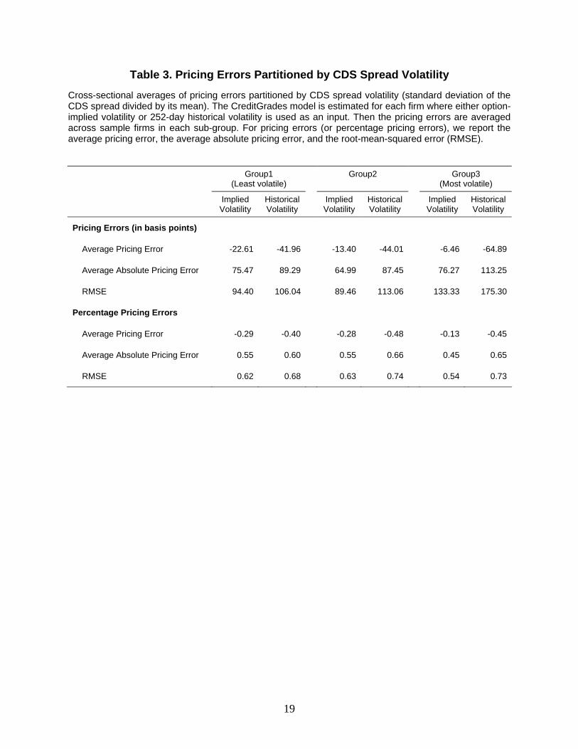
To check if the pricing errors vary among di¤erent groups of �rms, we partition the
sample �rms into three groups according to their sample CDS spread volatility (the standard
deviation of the CDS spread divided by the mean CDS spread). Table 3 present the results.
We observe that the implied volatility yields signi�cantly smaller pricing errors among the
most volatile group of �rms. This �nding motivates us to investigate the cross-sectional
di¤erence of pricing errors in the next section.
2Note that it is the sum of squared relative pricing errors that we minimize to obtain the estimated modelparameters. We have also examined results when we minimize the pricing errors measured in CDS spreadlevels. We �nd that the results are qualitatively similar.
9
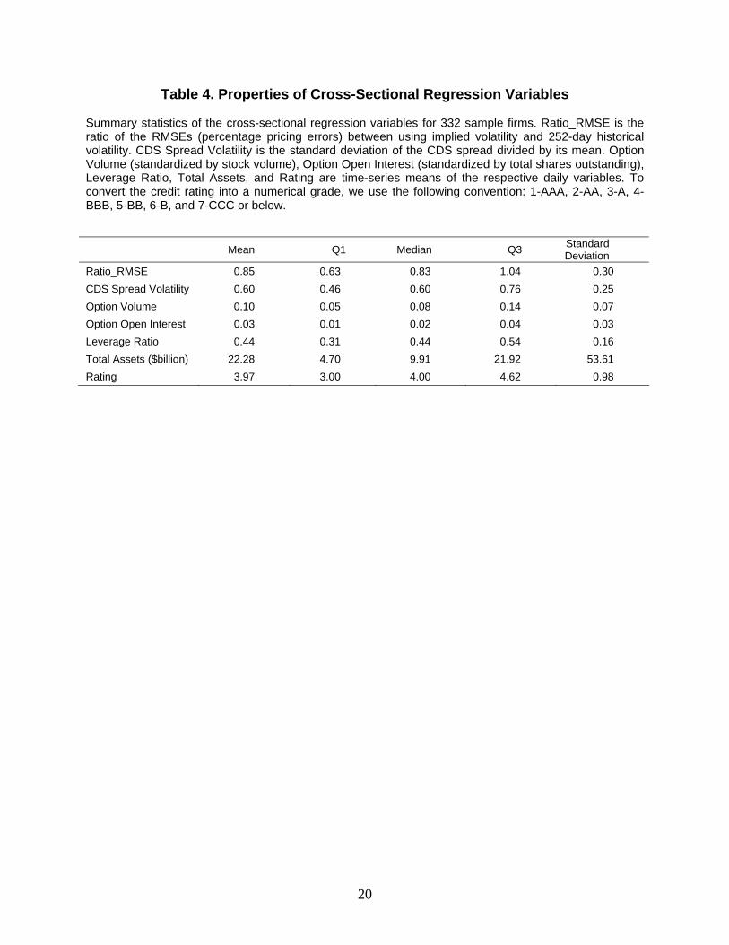
5 Pricing Error Ratio Analysis
To examine the balance between historical and implied volatility-based pricing errors, we
construct a pricing error ratio (Ratio_RMSE), which is equal to the implied volatility-
based percentage RMSE divided by the historical volatility-based percentage RMSE. Table
4 presents the summary statistics of the pricing error ratio. This ratio varies substantially in
the cross-section, with a median value of 0.83. This observation suggests that while implied
volatility yields smaller pricing errors than historical volatility across our entire sample, a
subset of the �rms might enjoy signi�cantly smaller pricing errors when implied volatility
is used in lieu of historical volatility in model calibration. Therefore, in the next step,
we conduct cross-sectional regressions with Ratio_RMSE as the dependent variable and
investigate whether certain �rm-level characteristics are related to this ratio.
When choosing the appropriate �rm-level characteristics, we are motivated by recent
studies that examine the role of option and CDS market information in forecasting future
stock returns. For example, Acharya and Johnson (2007) suggest that the incremental in-
formation revelation in the CDS market relative to the stock market is driven by banks that
trade on their private information. Cao, Chen, and Gri¢ n (2005) show that call option
volume and next-day stock returns are strongly correlated prior to takeover announcements,
but are unrelated during �normal�sample periods. Pan and Poteshman (2006) �nd a pre-
dictive relation between option volume and future stock returns that becomes stronger when
there is a larger presence of informed trading. To the extent that heightened volatility in
the CDS market is an indication of informed trading, option-implied volatility can be espe-
cially useful in explaining the CDS spread for more volatile �rms. We therefore include CDS
spread volatility as one of our explanatory variables.
A related question is whether the information content of implied volatility for CDS
spreads varies across �rms with di¤erent credit ratings. Among the sample �rms, we ob-
serve a broad spectrum of credit quality, ranging from AAA (investment-grade) to CCC
(speculative-grade). We note that information asymmetry is expected to be larger for lower-
10
rated �rms. Banks and other informed traders/insiders are likely to explore their information
advantage in both the CDS and options markets among these �rms, not higher-rated �rms
with fewer credit risk problems. We therefore include credit rating as another explanatory
variable.
Finally, We also include option volume and open interest in the analysis. While it has
been argued that informed investors prefer to trade options because of their inherent leverage,
the success of their strategy depends on su¢ cient market liquidity. To the extent that market
illiquidity or trading cost constitutes a barrier to entry, we expect the signal-to-noise ratio
of implied volatility to be higher for �rms with better options market liquidity. Speci�cally,
we normalize option volume by stock volume and open interest by the total common shares
outstanding for each �rm and each day in the sample period. We normalize option volume
and open interest to facilitate comparison across �rms. We use option open interest in
addition to option volume because it does not su¤er from the double counting of o¤setting
transactions. Table 4 presents the summary statistics of the regression variables. We note
that the majority of sample �rms are large investment-grade �rms with a median rating of
BBB.3
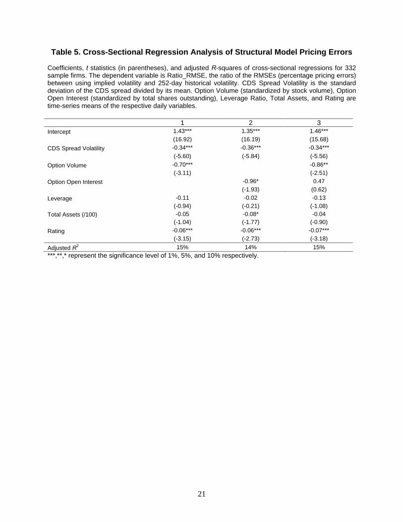
In Table 5, we present the pricing error ratio regression results, and �nd Ratio_RMSE
to be smaller for �rms with higher CDS spread volatility, higher option trading volume, and
lower credit ratings. Additionally, total assets and the option open interest are signi�cant in
the second speci�cation with a negative sign. To put these coe¢ cients (in Regression Three)
into perspective, consider the mean value of Ratio_RMSE at 0.85. A one-standard-deviation
increase in the CDS spread volatility would lower it to 0.77. A one-standard-deviation
increase in the option volume would lower it further to 0.71. Lower the credit rating by
one standard deviation reduces Ratio_RMSE still to 0.64. It appears that for �rms with
higher CDS spread volatility, higher option volume, and lower credit ratings, the implied
volatility is especially informative for explaining CDS spreads, resulting in substantially
3To convert the credit rating into a numerical grade, we use the following convention: 1-AAA, 2-AA, 3-A,4-BBB, 5-BB, 6-B, and 7-CCC.
11
smaller structural model pricing errors relative to when historical volatility is used in the
same calibration.
6 Robustness Checks
6.1 Rolling-Window Out-of-Sample Estimation
Having demonstrated that using option-implied volatility can signi�cantly improve the per-
formance of the CreditGrades model in in-sample tests, we now turn to an out-of-sample
pricing analysis. In this exercise, we attempt to capture what an investor will experience if
he/she uses the implied volatility or historical volatility to forecast the CDS spread. Specif-
ically, for each day t in the sample period, we use a rolling-window (of the past 252 observa-
tions inclusive of day t) to recalibrate the model following the estimation method outlined
in Section 4.4 We then use the recalibrated parameters and the day t+1 inputs to compute
a CDS spread for day t + 1. This allows us to calculate implied volatility- or historical
volatility-based out-of-sample pricing errors.
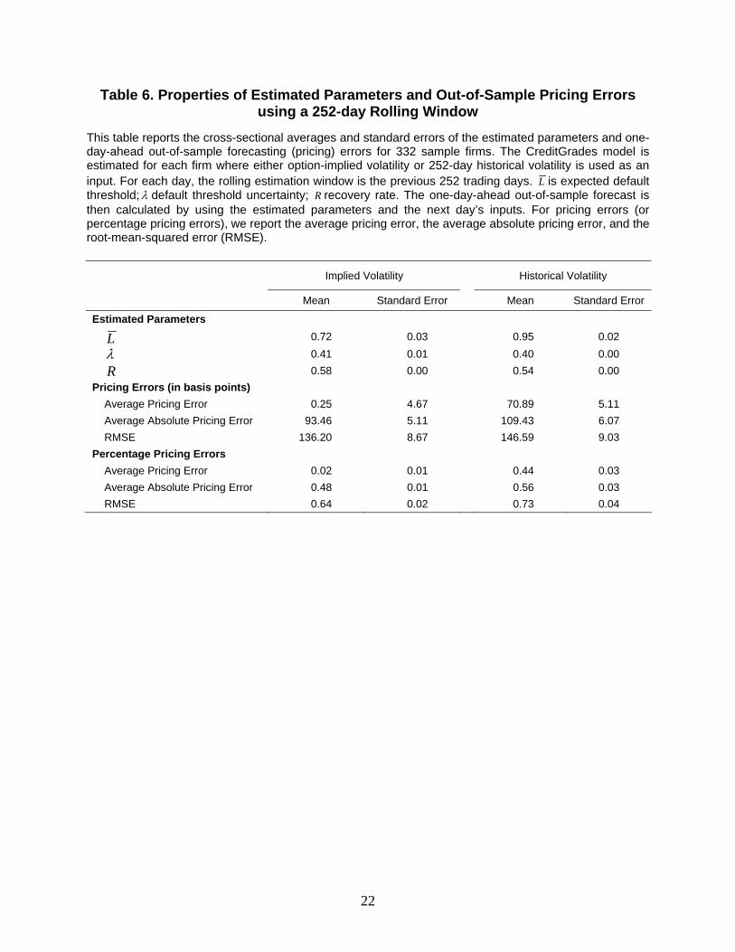
Table 6 presents our �ndings. Compared to the results in Table 2, the rolling-window
estimation generates greater pricing errors. This is likely due to the fact that we need to
set aside the �rst 252 daily observations to estimate the CreditGrades model, hence the
out-of-sample pricing errors are computed only for 2008-09, a much more volatile period
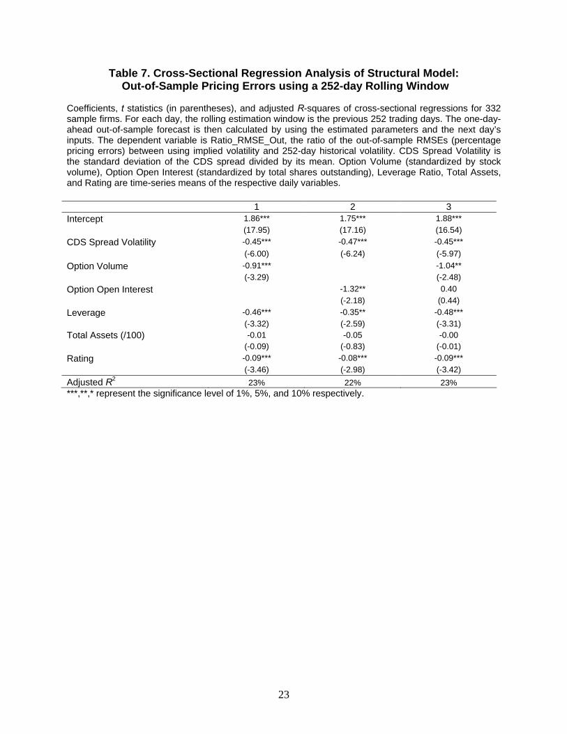
compared to 2007. Nevertheless, a cross-sectional analysis using the ratio of these pricing
errors, presented in Table 7, produces results similar to those of our in-sample pricing error
analysis. Namely, the ratio of out-of-sample percentage RMSE is smaller (i.e., the advantage
of implied volatility over historical volatility is greater) for �rms with more volatile CDS
spreads, larger option volume and open interest, greater leverage, and lower credit ratings.
In light of the well-known di¢ culty of structural models in explaining changes in the credit
spread (Collin-Dufresne, Goldstein, and Martin, 2001), we use CreditGrades to generate
forecasts of credit spread changes, de�ned as the di¤erence between the day t+1 credit spread
4We have also used 22-day and 126-day rolling windows to implement this test and found that our mainresults remain unchanged. To conserve space, these results are not reported, but are available upon request.
12
predicted by CreditGrades (following the above procedure) and the actual day t credit spread.
We then regress actual credit spread changes on the forecasted ones. Table 8 shows that,
when using historical volatility in this forecasting exercise, the resulting forecasts of credit
spread changes do not have signi�cant explanatory power for actual credit spread changes.
In contrast, when using option-implied volatility, the forecasted credit spread changes have
highly signi�cant coe¢ cients in the regression and the average adjusted R2 is about four
percent. The size of the implied volatility-based coe¢ cient and the associatedR2 is consistent
with the results on explaining credit spread changes using the VIX or realized volatility from
Collin-Dufresne, Goldstein, and Martin (2001) and Zhang, Zhou, and Zhu (2009). Overall,
implied volatility-based calibration produces not only smaller in-sample and out-of-sample
�tting errors, but also superior forecasts for daily credit spread changes.
6.2 Historical Volatilities with Alternative Horizons
So far, we have compared the information content of implied volatility to that of the 252-
day historical volatility in predicting CDS spreads. In this section, we present evidence on
historical volatilities with other estimation horizons. Especially, we want to consider both the
ability of long-dated estimators to produce stable asset volatility measures, and the advantage
of short-dated estimators to timely adjust to new market information. Therefore, we repeat
the pricing exercise of the preceding section with di¤erent historical volatility estimators
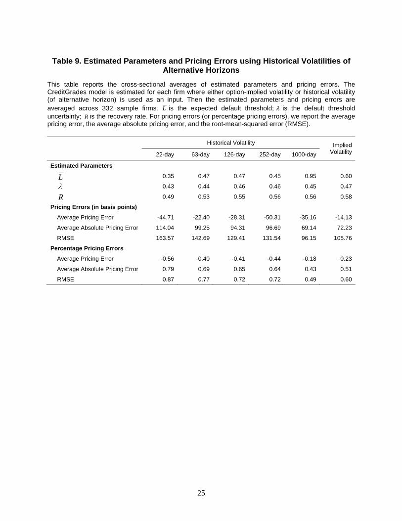
(ranging from 22-day to 1,000-day). The results are presented in Table 9. Regardless of
whether the pricing error is measured in levels or percentages, the pricing error appears to
decline with the estimaton horizon of the historical volatility estimator. The RMSE ranges
from 164bp for the 22-day historical volatility to 96bp for the 1,000-day historical volatility.
In comparison, the implied volatility produces the second lowest pricing errors among all
estimators used. In this case, the slight advantage of the 1,000-day historical volatility over
implied volatility can probably be attributed to its ability to �t smooth and low levels of the
13
CDS spread.5
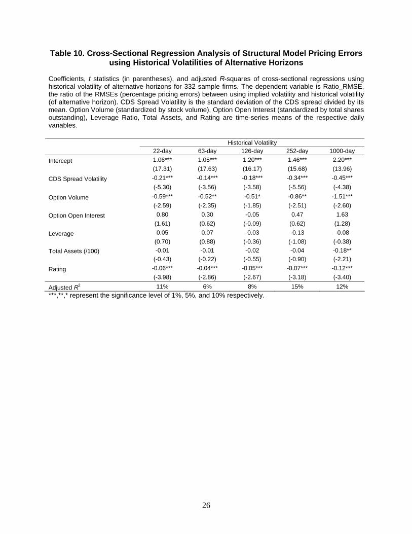
When we conduct the cross-sectional pricing error ratio analysis in Table 10, we �nd that
the results closely resemble those in Table 5. Namely, the Ratio RMSE variable is lower
with higher CDS spread volatility, higher option volume, and lower credit rating. Therefore,
even as the pricing performance varies among the di¤erent historical volatility inputs used in
the calibration, implied volatility continues to be more informative among the same subset
of �rms identi�ed by our earlier analysis. Overall, these additional analyses con�rm that
the information advantage of implied volatility is robust to historical volatility estimators of
di¤erent horizons.
7 Conclusion
Can we use information from the options market to better price credit derivatives? How
does the performance of CDS pricing using option-implied volatility vary with the degree
of information asymmetry and market frictions? Using a large sample of �rms with both
CDS and options data available, we �nd that option-implied volatility dominates historical
volatility in �tting CDS spreads to the CreditGrades model. Moreover, we �nd that the
need to use option-implied volatility is more imperative when there is a larger presence of
informed/insider trading and when the options market is more liquid. Additional robustness
checks con�rm that our �ndings are insensitive to a rolling-window estimation approach and
historical volatilities estimated with di¤erent horizons.
5To see the logic behind this argument, assume that the observed spread is 200bp. A �tted spread of500bp yields a relative pricing error of 150 percent. When the observed spread is 500bp, a �tted spread of200bp yields a relative pricing error of -60 percent. Therefore, the relative pricing error measure tends toreward model speci�cations that provide a better �t to spreads when they are low.
14
References
[1] Acharya, V., and T. Johnson, 2007, Insider trading in credit derivatives, Journal of
Financial Economics 84, 110-141.
[2] Back, K., 1993, Asymmetric information and options, Review of Financial Studies 6,
435-472.
[3] Black, F., 1975, Fact and fantasy in use of options, Financial Analysts Journal 31,
36-41.
[4] Black, F., and J. Cox, 1976, Valuing corporate securities: Some e¤ects of bond indenture
provisions, Journal of Finance 31, 351-367.
[5] Campbell, J., and G.Taksler, 2003, Equity volatility and corporate bond yields, Journal
of Finance 58, 2321-2349.
[6] Cao, C., Z.Chen, and J.Gri¢ n, 2005, Informational content of option volume prior to
takeovers, Journal of Business 78, 1073-1109.
[7] Cao, C., F.Yu, and Z. Zhong, 2010, The informational content of option-implied volatil-
ity for credit default swap valuation, Journal of Financial Markets 13, 321-343.
[8] Collin-Dufresne, P., R. Goldstein, and S.Martin, 2001, The determinants of credit
spread changes, Journal of Finance 56, 2177-2207.
[9] CreditGrades Technical Document, 2002, http://www.creditgrades.com/resources/pdf/
CGtechdoc.pdf.
[10] Cremers, M., J.Driessen, P.Maenhout, and D.Weinbaum, 2008, Individual stock option
prices and credit spreads, Journal of Banking and Finance 32, 2706-2715
[11] Currie, A., and J.Morris, 2002, And now for capital structure arbitrage, Euromoney,
December, 38-43.
15
[12] Easley, D., M.O�Hara, and P. Srinivas, 1998, Option volume and stock prices: Evidence
on where informed traders trade, Journal of Finance 53, 431-465.
[13] Ericsson, J., K. Jacobs, and R.Oviedo-Helfenberger, 2009, The determinants of credit
default swap premia, Journal of Financial and Quantitative Analysis 44, 109-132
[14] Giesecke, K. and L.Goldberg, 2004, Forecasting default in the face of uncertainty, Jour-
nal of Derivatives 12, 11-25.
[15] Luo, Y., 2008, Risk and return of capital structure arbitrage with credit default swaps,
Ph.D. Dissertation, University of California, Irvine.
[16] Merton, R., 1974, On the pricing of corporate debt: The risk structure of interest rates,
Journal of Finance 29, 449-470.
[17] Pan, J., and A.Poteshman, 2006, The information in option volume for future stock
prices, Review of Financial Studies 19, 871-908.
[18] Stamicar, R. and C.Finger, 2006, Incorporating equity derivatives into the CreditGrades
model, Journal of Credit Risk 2, 1-20.
[19] Yu, F., 2006, How pro�table is capital structure arbitrage? Financial Analysts Journal
62(5), 47-62.
[20] Zhang, B.Y., H. Zhou, and H.Zhu, 2009, Explaining credit default swap spreads with
equity volatility and jump risks of individual �rms, Review of Financial Studies 22,
5099-5131.
16
17
Table 1. Summary Statistics Cross-sectional summary statistics of the time-series means for 332 sample firms. CDS Spread is the daily five-year composite credit default swap spread; Historical Volatility is the 252-day historical volatility; Implied Volatility is the volatility inferred from put options with non-zero open interest; Market Capitalization is the product of the stock price and shares outstanding; Leverage is the ratio of total liability over the sum of total liability and market capitalization. The sample period extends from January 2007 through October 2009.
Mean Q1 Median Q3 Standard Deviation
CDS Spread (basis point) 198.30 57.02 110.52 225.22 243.94 Historical Volatility (%) 43.38 33.47 40.47 51.55 14.14 Implied Volatility (%) 44.37 35.28 42.32 49.48 12.81 Market Capitalization ($billion) 20.61 3.50 8.78 20.84 39.68 Leverage Ratio (%) 43.57 30.78 44.10 54.41 16.49
18
Table 2. Estimated Parameters and Pricing Errors Cross-sectional averages and standard errors of estimated parameters and pricing errors. The CreditGrades model is estimated for each firm where either option-implied volatility or 252-day historical volatility is used as an input. Then the estimated parameters and pricing errors are averaged across 332 sample firms. L is the expected default threshold;λ is the default threshold uncertainty; R is the recovery rate. For pricing errors (or percentage pricing errors), we report the average pricing error, the average absolute pricing error, and the root-mean-squared error (RMSE).
Implied Volatility Historical Volatility
Mean Standard Error Mean Standard Error
Estimated Parameters
L 0.60 0.03 0.45 0.03
λ 0.47 0.01 0.46 0.01
R 0.58 0.01 0.56 0.01 Pricing Errors (in basis points) Average Pricing Error -14.13 2.97 -50.31 5.04 Average Absolute Pricing Error 72.23 3.41 96.69 5.45 RMSE 105.76 6.28 131.54 9.23 Percentage Pricing Errors Average Pricing Error -0.23 0.02 -0.44 0.02 Average Absolute Pricing Error 0.51 0.01 0.64 0.01 RMSE 0.60 0.01 0.72 0.01
19
Table 3. Pricing Errors Partitioned by CDS Spread Volatility Cross-sectional averages of pricing errors partitioned by CDS spread volatility (standard deviation of the CDS spread divided by its mean). The CreditGrades model is estimated for each firm where either option-implied volatility or 252-day historical volatility is used as an input. Then the pricing errors are averaged across sample firms in each sub-group. For pricing errors (or percentage pricing errors), we report the average pricing error, the average absolute pricing error, and the root-mean-squared error (RMSE).
Group1 (Least volatile)
Group2
Group3 (Most volatile)
Implied Volatility
Historical Volatility Implied
Volatility Historical Volatility Implied
Volatility Historical Volatility
Pricing Errors (in basis points)
Average Pricing Error -22.61 -41.96 -13.40 -44.01 -6.46 -64.89
Average Absolute Pricing Error 75.47 89.29 64.99 87.45 76.27 113.25
RMSE 94.40 106.04 89.46 113.06 133.33 175.30
Percentage Pricing Errors
Average Pricing Error -0.29 -0.40 -0.28 -0.48 -0.13 -0.45
Average Absolute Pricing Error 0.55 0.60 0.55 0.66 0.45 0.65
RMSE 0.62 0.68 0.63 0.74 0.54 0.73
20
Table 4. Properties of Cross-Sectional Regression Variables Summary statistics of the cross-sectional regression variables for 332 sample firms. Ratio_RMSE is the ratio of the RMSEs (percentage pricing errors) between using implied volatility and 252-day historical volatility. CDS Spread Volatility is the standard deviation of the CDS spread divided by its mean. Option Volume (standardized by stock volume), Option Open Interest (standardized by total shares outstanding), Leverage Ratio, Total Assets, and Rating are time-series means of the respective daily variables. To convert the credit rating into a numerical grade, we use the following convention: 1-AAA, 2-AA, 3-A, 4-BBB, 5-BB, 6-B, and 7-CCC or below.
Mean Q1 Median Q3 Standard Deviation
Ratio_RMSE 0.85 0.63 0.83 1.04 0.30 CDS Spread Volatility 0.60 0.46 0.60 0.76 0.25 Option Volume 0.10 0.05 0.08 0.14 0.07 Option Open Interest 0.03 0.01 0.02 0.04 0.03 Leverage Ratio 0.44 0.31 0.44 0.54 0.16 Total Assets ($billion) 22.28 4.70 9.91 21.92 53.61 Rating 3.97 3.00 4.00 4.62 0.98
21
Table 5. Cross-Sectional Regression Analysis of Structural Model Pricing Errors Coefficients, t statistics (in parentheses), and adjusted R-squares of cross-sectional regressions for 332 sample firms. The dependent variable is Ratio_RMSE, the ratio of the RMSEs (percentage pricing errors) between using implied volatility and 252-day historical volatility. CDS Spread Volatility is the standard deviation of the CDS spread divided by its mean. Option Volume (standardized by stock volume), Option Open Interest (standardized by total shares outstanding), Leverage Ratio, Total Assets, and Rating are time-series means of the respective daily variables. 1 2 3 Intercept 1.43*** 1.35*** 1.46*** (16.92) (16.19) (15.68) CDS Spread Volatility -0.34*** -0.36*** -0.34*** (-5.60) (-5.84) (-5.56) Option Volume -0.70*** -0.86** (-3.11) (-2.51) Option Open Interest -0.96* 0.47 (-1.93) (0.62) Leverage -0.11 -0.02 -0.13 (-0.94) (-0.21) (-1.08) Total Assets (/100) -0.05 -0.08* -0.04 (-1.04) (-1.77) (-0.90) Rating -0.06*** -0.06*** -0.07*** (-3.15) (-2.73) (-3.18) Adjusted R2 15% 14% 15% ***,**,* represent the significance level of 1%, 5%, and 10% respectively.
22
Table 6. Properties of Estimated Parameters and Out-of-Sample Pricing Errors using a 252-day Rolling Window
This table reports the cross-sectional averages and standard errors of the estimated parameters and one-day-ahead out-of-sample forecasting (pricing) errors for 332 sample firms. The CreditGrades model is estimated for each firm where either option-implied volatility or 252-day historical volatility is used as an input. For each day, the rolling estimation window is the previous 252 trading days. L is expected default threshold;λ default threshold uncertainty; R recovery rate. The one-day-ahead out-of-sample forecast is then calculated by using the estimated parameters and the next day’s inputs. For pricing errors (or percentage pricing errors), we report the average pricing error, the average absolute pricing error, and the root-mean-squared error (RMSE).
Implied Volatility Historical Volatility
Mean Standard Error Mean Standard Error
Estimated Parameters
L 0.72 0.03 0.95 0.02
λ 0.41 0.01 0.40 0.00
R 0.58 0.00 0.54 0.00 Pricing Errors (in basis points) Average Pricing Error 0.25 4.67 70.89 5.11 Average Absolute Pricing Error 93.46 5.11 109.43 6.07 RMSE 136.20 8.67 146.59 9.03 Percentage Pricing Errors Average Pricing Error 0.02 0.01 0.44 0.03 Average Absolute Pricing Error 0.48 0.01 0.56 0.03 RMSE 0.64 0.02 0.73 0.04
23
Table 7. Cross-Sectional Regression Analysis of Structural Model: Out-of-Sample Pricing Errors using a 252-day Rolling Window
Coefficients, t statistics (in parentheses), and adjusted R-squares of cross-sectional regressions for 332 sample firms. For each day, the rolling estimation window is the previous 252 trading days. The one-day-ahead out-of-sample forecast is then calculated by using the estimated parameters and the next day’s inputs. The dependent variable is Ratio_RMSE_Out, the ratio of the out-of-sample RMSEs (percentage pricing errors) between using implied volatility and 252-day historical volatility. CDS Spread Volatility is the standard deviation of the CDS spread divided by its mean. Option Volume (standardized by stock volume), Option Open Interest (standardized by total shares outstanding), Leverage Ratio, Total Assets, and Rating are time-series means of the respective daily variables. 1 2 3 Intercept 1.86*** 1.75*** 1.88*** (17.95) (17.16) (16.54) CDS Spread Volatility -0.45*** -0.47*** -0.45*** (-6.00) (-6.24) (-5.97) Option Volume -0.91*** -1.04** (-3.29) (-2.48) Option Open Interest -1.32** 0.40 (-2.18) (0.44) Leverage -0.46*** -0.35** -0.48*** (-3.32) (-2.59) (-3.31) Total Assets (/100) -0.01 -0.05 -0.00 (-0.09) (-0.83) (-0.01) Rating -0.09*** -0.08*** -0.09*** (-3.46) (-2.98) (-3.42) Adjusted R2 23% 22% 23% ***,**,* represent the significance level of 1%, 5%, and 10% respectively.

24
Table 8. Time Series Regression Analysis of Changes in CDS Spreads This table reports the average coefficients and t-statistics (in parentheses) of the 332 sample firms for the following regression:
11 0 1 1( )tt t t tCDS CDS CDS CDSβ β ε++ +− = + − + ,
where tCDS is the actual CDS spreads at t, and 1tCDS + is the one-day-ahead forecast of the CDS spread, calculated using the parameters from the rolling-window estimation of the previous 252 days and the next day’s inputs. The CreditGrades model is estimated with either the option-implied volatility or the 252-day historical volatility.
Implied Volatility Historical Volatility
β0 0.38 0.08 (-0.03) (0.05) β1 0.02 0.00 (3.87) (0.17) Adjusted R2 4.12% 0.22%
25
Table 9. Estimated Parameters and Pricing Errors using Historical Volatilities of
Alternative Horizons This table reports the cross-sectional averages of estimated parameters and pricing errors. The CreditGrades model is estimated for each firm where either option-implied volatility or historical volatility (of alternative horizon) is used as an input. Then the estimated parameters and pricing errors are averaged across 332 sample firms. L is the expected default threshold; λ is the default threshold uncertainty; R is the recovery rate. For pricing errors (or percentage pricing errors), we report the average pricing error, the average absolute pricing error, and the root-mean-squared error (RMSE).
Historical Volatility
22-day 63-day 126-day 252-day 1000-day Implied
Volatility
Estimated Parameters
L 0.35 0.47 0.47 0.45 0.95 0.60
λ 0.43 0.44 0.46 0.46 0.45 0.47
R 0.49 0.53 0.55 0.56 0.56 0.58
Pricing Errors (in basis points)
Average Pricing Error -44.71 -22.40 -28.31 -50.31 -35.16 -14.13
Average Absolute Pricing Error 114.04 99.25 94.31 96.69 69.14 72.23
RMSE 163.57 142.69 129.41 131.54 96.15 105.76
Percentage Pricing Errors
Average Pricing Error -0.56 -0.40 -0.41 -0.44 -0.18 -0.23
Average Absolute Pricing Error 0.79 0.69 0.65 0.64 0.43 0.51
RMSE 0.87 0.77 0.72 0.72 0.49 0.60
26
Table 10. Cross-Sectional Regression Analysis of Structural Model Pricing Errors using Historical Volatilities of Alternative Horizons
Coefficients, t statistics (in parentheses), and adjusted R-squares of cross-sectional regressions using historical volatility of alternative horizons for 332 sample firms. The dependent variable is Ratio_RMSE, the ratio of the RMSEs (percentage pricing errors) between using implied volatility and historical volatility (of alternative horizon). CDS Spread Volatility is the standard deviation of the CDS spread divided by its mean. Option Volume (standardized by stock volume), Option Open Interest (standardized by total shares outstanding), Leverage Ratio, Total Assets, and Rating are time-series means of the respective daily variables.
Historical Volatility 22-day 63-day 126-day 252-day 1000-day
Intercept 1.06*** 1.05*** 1.20*** 1.46*** 2.20*** (17.31) (17.63) (16.17) (15.68) (13.96)
CDS Spread Volatility -0.21*** -0.14*** -0.18*** -0.34*** -0.45***
(-5.30) (-3.56) (-3.58) (-5.56) (-4.38)
Option Volume -0.59*** -0.52** -0.51* -0.86** -1.51*** (-2.59) (-2.35) (-1.85) (-2.51) (-2.60) Option Open Interest 0.80 0.30 -0.05 0.47 1.63
(1.61) (0.62) (-0.09) (0.62) (1.28) Leverage 0.05 0.07 -0.03 -0.13 -0.08 (0.70) (0.88) (-0.36) (-1.08) (-0.38) Total Assets (/100) -0.01 -0.01 -0.02 -0.04 -0.18** (-0.43) (-0.22) (-0.55) (-0.90) (-2.21) Rating -0.06*** -0.04*** -0.05*** -0.07*** -0.12***
(-3.98) (-2.86) (-2.67) (-3.18) (-3.40)
Adjusted R2 11% 6% 8% 15% 12% ***,**,* represent the significance level of 1%, 5%, and 10% respectively.