Liquidity Considerations in Estimating Implied Volatility · Liquidity Considerations in Estimating Implied Volatility 715 “implied volatility” (IV). IV is a direct measure of

Liquidity Considerations

in Estimating Implied

Volatility

ROHINI GROVERSUSAN THOMAS∗

Option markets have significant variation in liquidity across different option series.Illiquidity reduces the informativeness of the price. Price information for illiquidoptions is more noisy, and thus the implied volatilities (IVs) based on these pricesare more noisy. In this study, we propose weighting schemes to estimate IV,which reduce the importance attached to illiquid options. The two indexes usingliquidity weights are SVIX, which is a spread-adjusted volatility index, and TVVIX,which is a traded volume weighted VIX. We find SVIX outperforms TVVIX, theconventional schemes such as the traditional VXO, or vega weights, and volatilityelasticity weights. C© 2012 Wiley Periodicals, Inc. Jrl Fut Mark 32:714–741, 2012

1. INTRODUCTION

When options markets became established and liquid, market prices of op-tions were used to directly calculate the market forecast of volatility called the

We are grateful to Abhisar Srivastava, Tirthankar Patnaik, and the National Stock Exchange of India Ltd.for the data used in this study. We thank Nidhi Aggarwal, Ajay Shah, Rajat Tayal, and the participants of theIGIDR Finance Research Seminars for useful discussions. We also thank our discussant Prof. Moon, SeongJu, and participants of the 7th Annual APAD Conference for useful suggestions. The views expressed in thisstudy belong to the authors and not their employer.

∗Correspondence author, Indira Gandhi Institute of Development Research, Goregaon East, Mumbai400065, India. Tel: (+91) (022)284-165-50, e-mail: [email protected]

Received October 2011; Accepted November 2011

� Rohini Grover is a Ph.D. Scholar at Indira Gandhi Institute of DevelopmentResearch, Mumbai, India.

� Susan Thomas is an Assistant Professor at Indira Gandhi Institute of DevelopmentResearch, Mumbai, India.

The Journal of Futures Markets, Vol. 32, No. 8, 714–741 (2012)C© 2012 Wiley Periodicals, Inc.Published online February 10, 2012 in Wiley Online Library (wileyonlinelibrary.com).DOI: 10.1002/fut.21543

Liquidity Considerations in Estimating Implied Volatility 715

“implied volatility” (IV). IV is a direct measure of the forecast of volatility madeby economic agents. An extensive literature has documented the high quality ofvolatility forecasting that is embedded in IV.

Different options on the same underlying yield different values for the IV.Analytical methods are thus required to reduce multiple values for IV fromdifferent traded options on the same underlying into an efficient point estimateof IV for that underlying.

One endeavor to isolate a volatility forecast from multiple values of IVwas based on developing models of option pricing that incorporated the factorsthat caused IV to change deterministically, such as moneyness of the option,volatility dynamics, or the liquidity of the underlying.

The other strategy adopted was to develop an index of IV. This was discussedextensively in the literature, which led up to the introduction of the ChicagoBoard Options Exchange (CBOE) VIX in 1993. This implied volatility index wascalculated for the S&P 100 index options using the methodology proposed byWhaley (1993) and was disseminated by the CBOE in real time. The index wascalculated using only at-the-money (ATM) options with a defined weightingscheme over the IV values calculated. In 2003, the CBOE shifted the VIXcalculation methodology to one that used option prices over a wide range ofstrike values. In the following years, similar computation of an implied volatilityindex has commenced on numerous options exchanges worldwide. Trading inderivatives on VIX has also commenced.

The CBOE VIX methodology is predicated on all option prices being mea-sured sharply. However, in the real world, there is substantial cross-sectionalvariation in the liquidity of option series. As an example, in tranquil times(September 2007), the bid–offer spread of options on the S&P 500 index at theCBOE ranged from near 0% to 200%. In turbulent times (September 2008),many more options were afflicted with illiquidity.

At present, a variety of heuristics are being utilized by exchanges world-wide in addressing this problem. In this study, we try to frontally address theproblem of illiquid options markets by constructing a weighting scheme for theconstruction of a VIX that directly incorporates the liquidity of the option. Theempirical work of this study is based on one of the most active option marketsin the world: options on the NSE-50 (Nifty) index, traded at the National StockExchange. We use the bid–offer spread in a weighting scheme that adjustsfor illiquidity when calculating the VIX. We call this the spread-adjusted VIX(SVIX). We also use traded volumes of options as another liquidity proxy andcompute volume-adjusted VIX (TVVIX).

We compare the performance of SVIX and TVVIX against three alternativeweighting schemes: the 1993 CBOE index (called VXO), the vega-weightedindex (VVIX), and a volatility elasticity weighted index (EVIX). The performance

Journal of Futures Markets DOI: 10.1002/fut

716 Grover and Thomas

is measured as the forecasting success of each VIX candidate against the realizedvolatility (RV) of the market index. The testing procedure employed is the ModelConfidence Set (MCS) test (Hansen, Lunde, & Nason, 2003). We find that thenew SVIX is a better predictor of future RV. We also run univariate regressionsof RV on each VIX and find that although all VIXs contain information aboutfuture volatility, they are biased forecasts.

Option IV is an important component of the information set of the finan-cial system. The world over, options markets are being used to create impliedvolatility indexes using ideas similar to that of the CBOE VIX. Because all op-tions markets have substantial cross-sectional variation in option liquidity, theideas of this study may potentially yield improved measurement of VIXs.

The study is presented as follows: In Section 2, we present the issues sur-rounding the creation of a VIX and also present the evaluation framework usedto compare the performance of alternative VIXs. In Section 3, we review alter-native schemes to construct VIXs. In Section 4, we describe the data used forthe analysis. In Section 5, we discuss the liquidity-adjusted weighting scheme,after which we present our analysis in Section 6. In Section 7, we conclude.

2. ISSUES IN CONSTRUCTING IV INDEXES

Gastineau (1977) proposed the use of an index to resolve the problem of multiplevalues of IVs from different options on the same underlying. An implied volatilityindex, calculated as a weighted average of the IVs from different option prices,would be the summary measure of underlying future volatility.

The first weighting schemes were suggested by Trippi (1977) andSchmalensee and Trippi (1978), which placed equal weights on all the IVsused in calculating the index. However, because the literature showed thatthe Black–Scholes model priced some options more accurately than others,schemes where the weights varied according to different factors were proposed.In following years, several researchers made significant progress in developingthese concepts further (Galai, 1989; Cox & Rubinstein, 1985; Brenner & Galai,1993; Whaley, 1993).

The maturation of knowledge in this field was signaled with the launch ofan information product in 1993: an implied volatility index based on tradingin options on the S&P 100 index. This was called the CBOE VIX. A researchliterature rapidly demonstrated that VIX was useful in volatility forecasting,over and beyond the state-of-the-art volatility models, because option pricesharnessed the superior information set of traders.1

1Christensen and Prabhala (1998); Christensen, Hansen, and Prabhala (2001) identified and corrected someof the data and methodological problems present in the early studies on this question. They conclude that



Given the importance of VIXs such as VIX in the global financial system,it is useful to explore the methodological issues in the construction of theseindexes. The process of creating an optimal methodology for a VIX involves thefollowing two parts:

1. Identifying alternative weighting schemes based on available data about fac-tors that directly influence the shape of the IV smile.

2. Choosing an optimal weighting scheme.

2.1. Factors Influencing IV Values

If the Black–Scholes model held exactly, all options should have the same IV.However, an extensive literature has demonstrated that IV varies with money-ness, maturity, vega, and liquidity. We discuss each of these in turn.

Moneyness/strike

The first documented variation in IV was as a function of strikes or the mon-eyness. IV was consistently lower for lower values of the moneyness of the op-tion. This variation came to be known as the volatility smile. Rubinstein (1994),Jackwerth and Rubinstein (1996), Dumas, Fleming, and Whaley (1998) showedthat the pattern of the IV of the S&P 500 index options changed from a smileto a sneer after the 1987 crash.

Maturity

Prices of near-month options show lower IV than far months. Heynen, Kemna,and Vorst (1994), Xu and Taylor (1994), and Campa and Chang (1995) showthat IVs are a function of time to expiration and thus exhibit a term structure.

Vega

The derivative of the Black–Scholes price with respect to volatility is calledvega. The vega can be shown to be consistently different for different values of

IV is a more efficient forecast for future volatility than volatility calculated from historical returns. Lataneand Rendleman (1976), Chiras and Manaster (1978), and Beckers (1981) find that IV performs better incapturing future volatility than standard deviations obtained from historical returns. Blair, Poon, and Taylor(2001) find that volatility forecasts provided by the early CBOE VIX are unbiased, and they outperformforecasts augmented with GARCH effects and high-frequency observations. Similar results were reportedearly on by Jorion (1995) for foreign exchange options.Corrado and Miller (2005) examine the forecasting quality of three implied VIXs based on S&P 100, S&P500, and NASDAQ 100 (National Association of Securities Dealers Automated Quotations). They find thatthe forecasting quality of the VIX based on the S&P 100 and S&P 500 has improved since 1995, and thatthose based on the NASDAQ 100 provides better forecasts of future volatility.



the strike, as well as the maturity of the contract.2 Thus, the vega of an optionnaturally lent itself as an input to differentiating the IV of different options whencalculating an implied volatility index (Latane & Rendleman, 1976). Chiras andManaster (1978) suggested weighting by volatility elasticity instead of vega.

Among other influential papers, Beckers (1981) and Whaley (1982) sug-gested minimizing

∑i wi [Ci − BSi (σ̂ )]2, where Ci refers to market price and

BSi refers to Black–Scholes price of option i and wi could either be vega orequal weights.3

Liquidity

A more recent literature has explored the impact of option liquidity on estimatedIV. Brenner, Eldor, and Hauser (2001) show that there is a significant illiquiditypremium between two sets of currency options, when one set is traded and theother is not. Bollen and Whaley (2004) documented an empirical link betweenthe shape of the IV smile and the depth of the market on the buy and the sellside of options with different moneyness. They show that net buying pressureaffects the shape of the IV smile in both the index as well as the single stockoptions markets. Further, they show that the shape of the IV smile is driven bydifferent market forces for index options compared to single stock options.

Models of asymmetric information have been used to provide theoreticalunderpinnings for the link between liquidity and option price. Nandi (2000)sets up a model of asymmetric information linking the level and the shape ofIV function to net order flow of options. The model shows that an increase innet options order flow increases the mispricing by the Black–Scholes model.Garleanu et al. (2009) formalize the findings in Bollen and Whaley (2004) byincorporating end-user demand in a model for options prices. Here they exploitthe feature that end-users tend to hold long index options and short equityoptions to explain the relative expensiveness of index options. Another modelto explicitly incorporate liquidity in the price of stock options was Cetin et al.(2006), who show market liquidity premium4 as a significant part of the optionprice.

The empirical evidence has also linked IV to option liquidity. Etling andMiller (2000) explore the relationship between bid–ask spread as a liquidity

2Vega is higher for options that are further away from the money because they have a lower extrinsic valueand are less likely to change with changes in IV. It is also higher for options with longer expiration in orderto compensate for additional risk taken by the seller.3This method thus allows the call prices to provide an implicit weighting scheme that yields an estimate ofstandard deviation that has least prediction error.4The paper models the liquidity using a generic supply function where option price monotonically increaseswith size of order.



proxy with moneyness of options and find that ATM options have the highestliquidity. Chou et al. (2009) explore how the IV function varies as a functionof liquidity in both the spot and options market. They find that order-basedmeasures of liquidity (such as the bid–ask spread) better explain the variationin IV than trade-based measures (such as traded volume). They also find thatboth spot and options markets liquidity matter for the variation in IV.

This evidence, about the various factors that influence IV, has led to manyalternative approaches to constructing an implied volatility index. The differentweighting schemes are further discussed in Section 3. What is the efficientweighting scheme rests upon the performance of the forecast from each schemeagainst some benchmark volatility measure. The framework to carry out such aperformance evaluation of different weighting schemes is now examined in thenext section.

2.2. Performance Evaluation

One of the reasons that there is no consensus on one best weighting schemefor a VIX is the lack of an observable volatility. The time-series econometricsliterature has extensive work on a framework to evaluate the performance ofa volatility forecast even though volatility is not observed. For example, theseideas have been used in testing the forecasts of volatility models such as Gener-alized Autoregressive Conditional Heteroskedasticity (GARCH), ExponentiallyWeighted Moving Average (EWMA), etc. This framework has two broad ap-proaches: one that delivers a relative measure of performance among a set ofcandidate models, and the other that delivers a measure of performance of eachof the candidate models against a single benchmark.

These questions were revisited when intraday data revealed a superiorvolatility proxy: RV. Once RV was observed, it became possible to measurehow well IV forecasts the RV of the underlying asset over the life of an option.Most studies use a predictive regression of the IV estimate on future volatil-ity where the goodness of prediction is measured through the coefficients ofpredictive regressions. The early studies by Day and Lewis (1988), Lamoureuxand Lastrapes (1993), and Canina and Figlewski (1993) showed that IV is nota good predictor for future return volatilities.

The framework of encompassing regressions was then used to assess thepredictability of IV estimates against other forecast variables. This frameworkaddresses the relative importance of competing volatility forecasts and whetherone volatility forecast subsumes all information contained in other volatilityforecast(s). Within this approach, Poteshman (2000); Jiang and Tian (2005b);Corrado and Miller (2005) have found that IV estimates are biased, but efficientand informative relative to forecasts from other volatility estimates.



A recent study by Becker, Clements, and White (2007) used an approachthat differs from the traditional forecast encompassing approach used in earlierstudies and finds that the S&P 500 implied volatility index does not containany such incremental information relevant for forecasting volatility. Becker,Clements, and White (2008) compare the index against a combination of fore-casts of S&P 500 volatility by using the MCS methodology and finds that acombination of forecasts outperforms individual model-based forecasts and IV.

In this study, we use the following two steps to compare the performanceof our VIXs:

1. Forecasting regressions following Christensen and Prabhala (1998) to testthe information content of the volatility measures. Instrumental variableregressions are also run to correct for potential errors-in-variable problemsin IV estimates as discussed by previous studies.5

2. The MCS methodology of Hansen et al. (2003). This addresses the problemof choosing the best forecasting model. It contains the best model with a givenlevel of confidence. It may contain a number of models, which indicates theyare of equal predictive ability. It has several advantages over other methodssuch as superior predictive ability (SPA) test and the reality check (RC) test.6

The construction of the MCS test is an iterative procedure in that it requiresa sequence of tests for equal predictive ability. The set of candidate models istrimmed by deleting models that are found to be inferior. The final survivingset of models in the MCS contains the optimal model with a given level ofconfidence and these models are not significantly different in terms of theirforecast performance.7

The critical question that remains in this is still the choice of the benchmarkmeasure for volatility, which we discuss in Section 4.2.

3. CHOICES OF IV INDEXES

In this section, we describe different methods we use in order to calculateimplied volatility indexes. We start with a description of the two most widelycomputed VIXs by several exchanges across the world, namely, VXO and VIX.

3.1. VXO

This VIX is calculated using prices of options on the S&P 100 index. The IVsare calculated using the Black–Scholes model, and the VXO is an average of

5Christensen and Prabhala (1998), Jiang and Tian (2005b), Corrado and Miller (2005).6See Hansen et al. (2003).7Hansen et al. (2003).



the IVs on eight near-the-money options, including options at the two nearestmaturities.8

In 2003, VXO was criticized for using an option pricing model and beingbiased due to the trading day conversion. In addition, there were two structuralchanges9 in the U.S. economy that reduced the usefulness of VXO as a measureof future volatility. These were as follows:

1. S&P 500 options became the most actively traded index options.2. Earlier index calls and puts were equally important in investor-trading strate-

gies but in later years the market became dominated by portfolio insurerswho bought out-of-the-money and ATM index puts for insurance purposes.

Such criticisms of VXO along with changes in the structure of the U.S.options market led to a new approach to calculating the VIX based on the pricesof options trading on the S&P 500.

3.2. VIX

In contrast to VXO, VIX has been derived from the concept of fair value ofa volatility swap (Demeterfi et al., 1999). Here, even though the variance isderived from market observable option prices and interest rates, the theoreticalunderpinning is rooted in the broader context of model-free implied varianceof Dupire (1993) and Neuberger (1994). This concept was further developedby Carr and Madan (1998), Demeterfi et al. (1999), and Britten-Jones andNeuberger (2000). Jiang and Tian (2005a) establish that the variance mea-sure under this framework is theoretically equivalent to the model-free impliedvariance formulated by Britten-Jones and Neuberger (2000).

The CBOE calculates and publishes a real-time value of VIX,10 which hasbeen accepted as the market measure of volatility. In this study, we do notdirectly analyze the VIX methodology. However, to the extent that the mainargument of this study is appropriate—that price information for illiquid optionseries is less informative—it should impact upon the VIX methodology also.

3.3. Volatility-Linked Weights

The early literature (Latane & Rendleman, 1976; Chiras & Manaster, 1978)suggests two different weighting schemes based on vega and volatility elasticityweighting scheme to calculate the market implied volatility index.

8See Whaley (1993) for details on construction of VXO.9See Whaley (2009).10See www.cboe.com/micro/vix/vixwhite.pdf for details on construction of VIX.



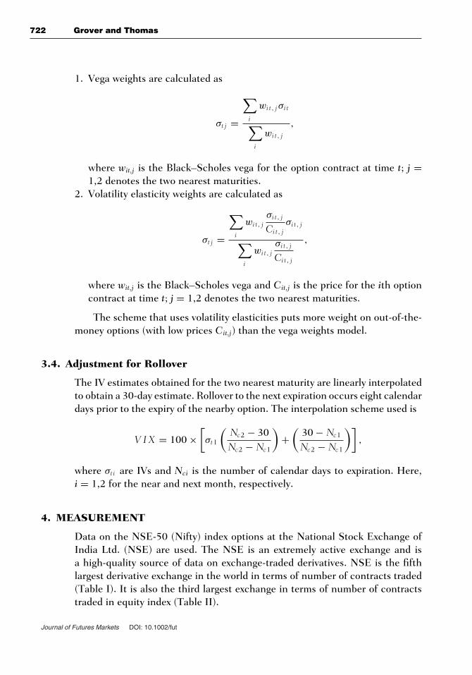
1. Vega weights are calculated as

σt j =

∑i

wi t, jσi t∑i

wi t, j

,

where wit,j is the Black–Scholes vega for the option contract at time t; j =1,2 denotes the two nearest maturities.

2. Volatility elasticity weights are calculated as

σt j =

∑i

wi t, jσi t, j

Cit, jσi t, j

∑i

wi t, jσi t, j

Cit, j

,

where wit,j is the Black–Scholes vega and Cit,j is the price for the ith optioncontract at time t; j = 1,2 denotes the two nearest maturities.

The scheme that uses volatility elasticities puts more weight on out-of-the-money options (with low prices Cit,j) than the vega weights model.

3.4. Adjustment for Rollover

The IV estimates obtained for the two nearest maturity are linearly interpolatedto obtain a 30-day estimate. Rollover to the next expiration occurs eight calendardays prior to the expiry of the nearby option. The interpolation scheme used is

V I X = 100 ×[σt1

(Nc2 − 30Nc2 − Nc1

)+

(30 − Nc1

Nc2 − Nc1

)],

where σti are IVs and Nci is the number of calendar days to expiration. Here,i = 1,2 for the near and next month, respectively.

4. MEASUREMENT

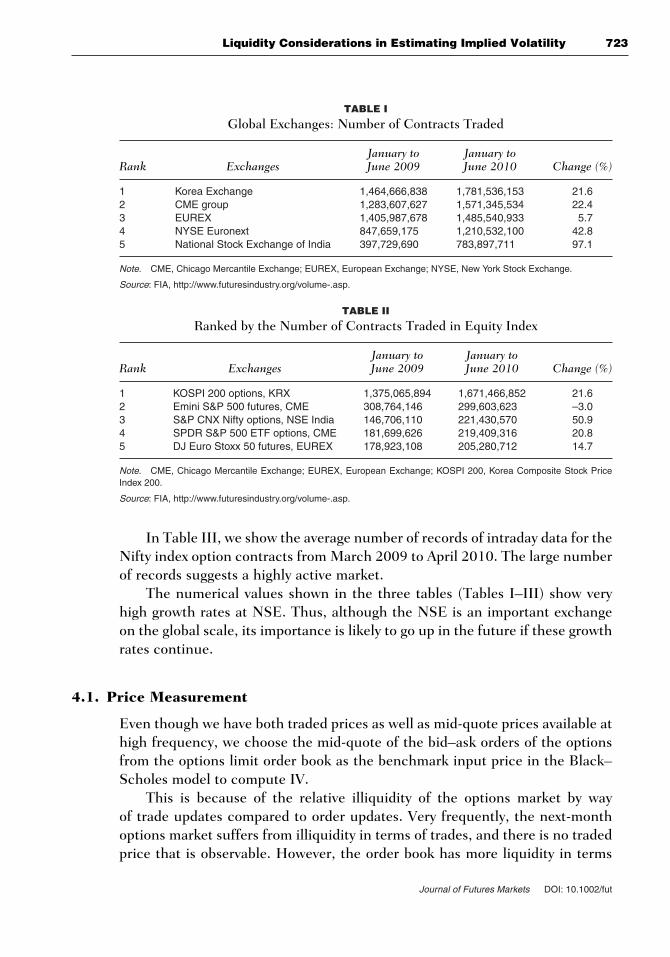
Data on the NSE-50 (Nifty) index options at the National Stock Exchange ofIndia Ltd. (NSE) are used. The NSE is an extremely active exchange and isa high-quality source of data on exchange-traded derivatives. NSE is the fifthlargest derivative exchange in the world in terms of number of contracts traded(Table I). It is also the third largest exchange in terms of number of contractstraded in equity index (Table II).



TABLE I

Global Exchanges: Number of Contracts Traded

January to January toRank Exchanges June 2009 June 2010 Change (%)

1 Korea Exchange 1,464,666,838 1,781,536,153 21.62 CME group 1,283,607,627 1,571,345,534 22.43 EUREX 1,405,987,678 1,485,540,933 5.74 NYSE Euronext 847,659,175 1,210,532,100 42.85 National Stock Exchange of India 397,729,690 783,897,711 97.1

Note. CME, Chicago Mercantile Exchange; EUREX, European Exchange; NYSE, New York Stock Exchange.

Source: FIA, http://www.futuresindustry.org/volume-.asp.

TABLE II

Ranked by the Number of Contracts Traded in Equity Index

January to January toRank Exchanges June 2009 June 2010 Change (%)

1 KOSPI 200 options, KRX 1,375,065,894 1,671,466,852 21.62 Emini S&P 500 futures, CME 308,764,146 299,603,623 –3.03 S&P CNX Nifty options, NSE India 146,706,110 221,430,570 50.94 SPDR S&P 500 ETF options, CME 181,699,626 219,409,316 20.85 DJ Euro Stoxx 50 futures, EUREX 178,923,108 205,280,712 14.7

Note. CME, Chicago Mercantile Exchange; EUREX, European Exchange; KOSPI 200, Korea Composite Stock PriceIndex 200.

Source: FIA, http://www.futuresindustry.org/volume-.asp.

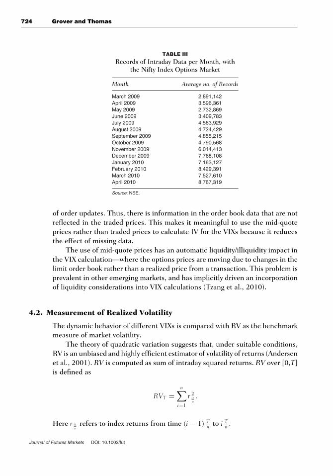
In Table III, we show the average number of records of intraday data for theNifty index option contracts from March 2009 to April 2010. The large numberof records suggests a highly active market.

The numerical values shown in the three tables (Tables I–III) show veryhigh growth rates at NSE. Thus, although the NSE is an important exchangeon the global scale, its importance is likely to go up in the future if these growthrates continue.

4.1. Price Measurement

Even though we have both traded prices as well as mid-quote prices available athigh frequency, we choose the mid-quote of the bid–ask orders of the optionsfrom the options limit order book as the benchmark input price in the Black–Scholes model to compute IV.

This is because of the relative illiquidity of the options market by wayof trade updates compared to order updates. Very frequently, the next-monthoptions market suffers from illiquidity in terms of trades, and there is no tradedprice that is observable. However, the order book has more liquidity in terms



TABLE III

Records of Intraday Data per Month, withthe Nifty Index Options Market

Month Average no. of Records

March 2009 2,891,142April 2009 3,596,361May 2009 2,732,869June 2009 3,409,783July 2009 4,563,929August 2009 4,724,429September 2009 4,855,215October 2009 4,790,568November 2009 6,014,413December 2009 7,768,108January 2010 7,163,127February 2010 8,429,391March 2010 7,527,610April 2010 8,767,319

Source: NSE.

of order updates. Thus, there is information in the order book data that are notreflected in the traded prices. This makes it meaningful to use the mid-quoteprices rather than traded prices to calculate IV for the VIXs because it reducesthe effect of missing data.

The use of mid-quote prices has an automatic liquidity/illiquidity impact inthe VIX calculation—where the options prices are moving due to changes in thelimit order book rather than a realized price from a transaction. This problem isprevalent in other emerging markets, and has implicitly driven an incorporationof liquidity considerations into VIX calculations (Tzang et al., 2010).

4.2. Measurement of Realized Volatility

The dynamic behavior of different VIXs is compared with RV as the benchmarkmeasure of market volatility.

The theory of quadratic variation suggests that, under suitable conditions,RV is an unbiased and highly efficient estimator of volatility of returns (Andersenet al., 2001). RV is computed as sum of intraday squared returns. RV over [0,T]is defined as

RVT =n∑

i=1

r 2i tn.

Here r itn

refers to index returns from time (i − 1) Tn to i T

n .



For the calculation of RV, data on Nifty index price that is available atwithin-one-second intervals from the trades and orders dataset, are used. As afirst step, these data are discretized at 10-minutes. These discretized data arethen used to calculate daily market index volatility.

Earlier studies such as Canina and Figlewski (1993) use overlapping sam-ples to evaluate the performance of IV estimates, although other studies suchas Christensen and Prabhala (1998), Jiang and Tian (2005b), Corrado andMiller (2005) use nonoverlapping samples by using data at a lower frequency(monthly) in evaluating the performance of IV estimates.

For our analysis, all VIXs are reduced to daily values (at the end of thetrading day), by dividing them by the square root of the number of calendardays, 365. Because VIXs are ex-ante measures of the volatility, each day’s VIXis adjusted to the next period.

5. A VOLATILITY INDEX THAT EXPLICITLYUTILIZES LIQUIDITY IN WEIGHTS

The linkages between liquidity and IVs presented in Section 2.1 appear to leadto a calculated VIX value, which may be biased due to illiquidity and noncon-tinuous strike prices. The literature has documented that across different un-derlyings, options on less liquid underlyings have a larger premium compared tothose on more liquid underlyings. An extreme version of the difficulties causedby illiquidity is documented in Jiang and Tian (2005a), who found that the VIXconstructed by the CBOE is flawed due to truncation errors that arise from theunavailability of option data for very low and very high strikes in practice.

5.1. Spread-Adjusted VIX

Two elements of a strategy are proposed for confronting the problem of illiq-uidity. First, the mid-quote prices rather than traded prices are utilized. Thisreduces noise. Second, option IV is explicitly weighted by option liquidity, whichis measured as the bid–ask spread available at that point of time in the limitorder book for that option. These weights are calculated as follows:

σi t =

∑i

wi t, jσi t∑i

wi t, j

,

where wi t, j = 1/sit, j and sit,j refers to the percentage spread defined as (ask–bid)/mid-price of option i at t, and j = 1, 2 stands for the two nearest maturities.



This strategy attaches greater weight to liquid products, where observedprices or quotes have reduced noise. The lack of availability of options pricestraded at a wide range of strikes is known to magnify the truncation error of theCBOE VIX calculation methodology, and increase the bias of the VIX measure.Our method automatically adjusts for the lack of data by incorporating it in thevalue of the spread. If there are data missing on either side of the book, thespread would take a value of infinity, and the weight attributed to that optionwould be zero.

5.2. Volume-Adjusted VIX

Another liquidity-adjusted weighting scheme is considered, where options areweighted using traded volume. Mayhew and Stivers (2003), Dennis, Mayhew,and Stivers (2006), Brous, Ufuk, and Ivilina (2010) have found that stocks withhigher traded volume result in IV estimates that outperform historical volatilityforecasts. These weights are computed as follows:

σi t =

∑i

wi t, jσi t∑i

wi t, j

,

where wi t, j/∑

i wi t, j refers to the fraction of volume traded for option i at theend of day t, and j = 1,2 stands for the two nearest maturities. Options with ahigher traded volume have a greater impact on the IV estimate.

5.3. Stylized Facts on the Cross-SectionalVariation of Option Liquidity

The crucial issue that affects this research is the cross-sectional variation ofoption liquidity. Our empirical work is based on Indian data. This raises theconcern that the results are an artifact of this emerging markets setting—perhaps one where liquidity is spotty, arbitrage is weak, or one where liquidityrisk is large.

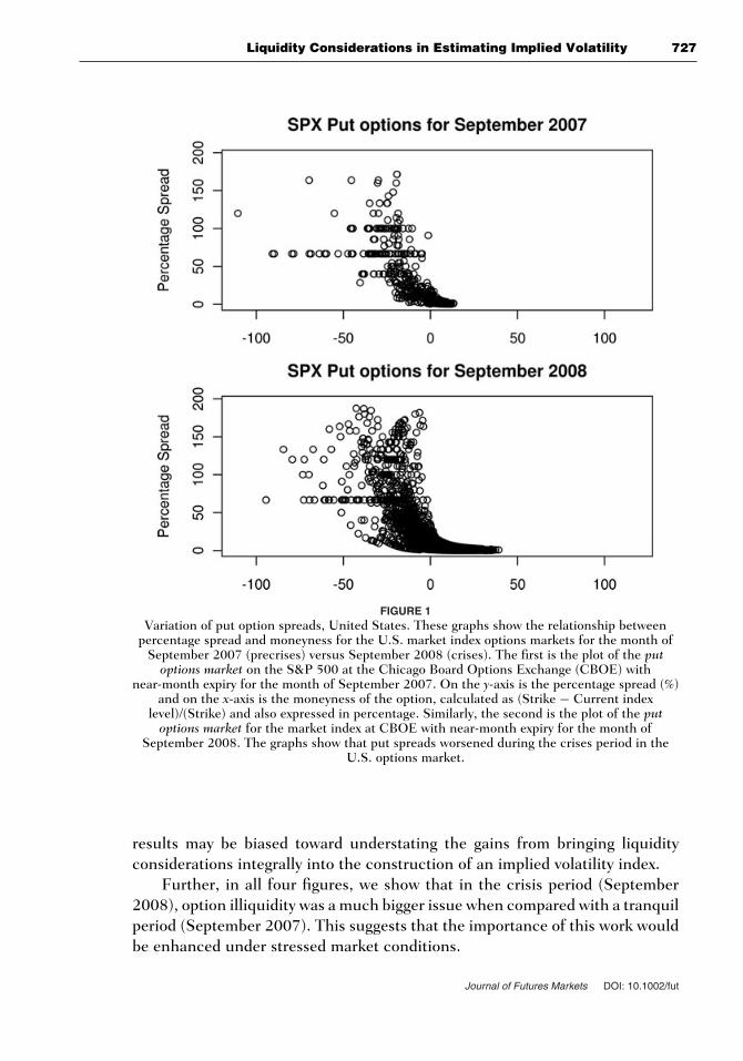
In order to evaluate this question, we plot bid–offer spreads on put op-tions in the United States (Figure 1) and India (Figure 3). We also plotbid–offer spreads on call options in the United States (Figure 2) and India(Figure 4).

In both countries, we see high cross-sectional variation of option liquidity.If anything, option illiquidity is a smaller problem in India. Thus, our empirical



FIGURE 1Variation of put option spreads, United States. These graphs show the relationship between

percentage spread and moneyness for the U.S. market index options markets for the month ofSeptember 2007 (precrises) versus September 2008 (crises). The first is the plot of the put

options market on the S&P 500 at the Chicago Board Options Exchange (CBOE) withnear-month expiry for the month of September 2007. On the y-axis is the percentage spread (%)

and on the x-axis is the moneyness of the option, calculated as (Strike − Current indexlevel)/(Strike) and also expressed in percentage. Similarly, the second is the plot of the put

options market for the market index at CBOE with near-month expiry for the month ofSeptember 2008. The graphs show that put spreads worsened during the crises period in the

U.S. options market.

results may be biased toward understating the gains from bringing liquidityconsiderations integrally into the construction of an implied volatility index.

Further, in all four figures, we show that in the crisis period (September2008), option illiquidity was a much bigger issue when compared with a tranquilperiod (September 2007). This suggests that the importance of this work wouldbe enhanced under stressed market conditions.



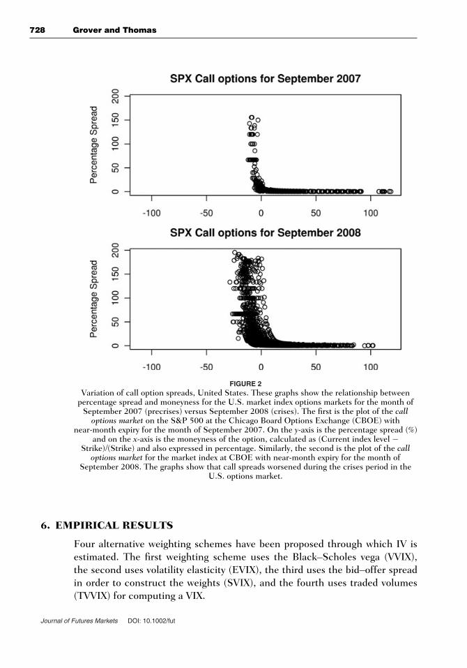
FIGURE 2Variation of call option spreads, United States. These graphs show the relationship between

percentage spread and moneyness for the U.S. market index options markets for the month ofSeptember 2007 (precrises) versus September 2008 (crises). The first is the plot of the call

options market on the S&P 500 at the Chicago Board Options Exchange (CBOE) withnear-month expiry for the month of September 2007. On the y-axis is the percentage spread (%)

and on the x-axis is the moneyness of the option, calculated as (Current index level −Strike)/(Strike) and also expressed in percentage. Similarly, the second is the plot of the call

options market for the market index at CBOE with near-month expiry for the month ofSeptember 2008. The graphs show that call spreads worsened during the crises period in the

U.S. options market.

6. EMPIRICAL RESULTS

Four alternative weighting schemes have been proposed through which IV isestimated. The first weighting scheme uses the Black–Scholes vega (VVIX),the second uses volatility elasticity (EVIX), the third uses the bid–offer spreadin order to construct the weights (SVIX), and the fourth uses traded volumes(TVVIX) for computing a VIX.



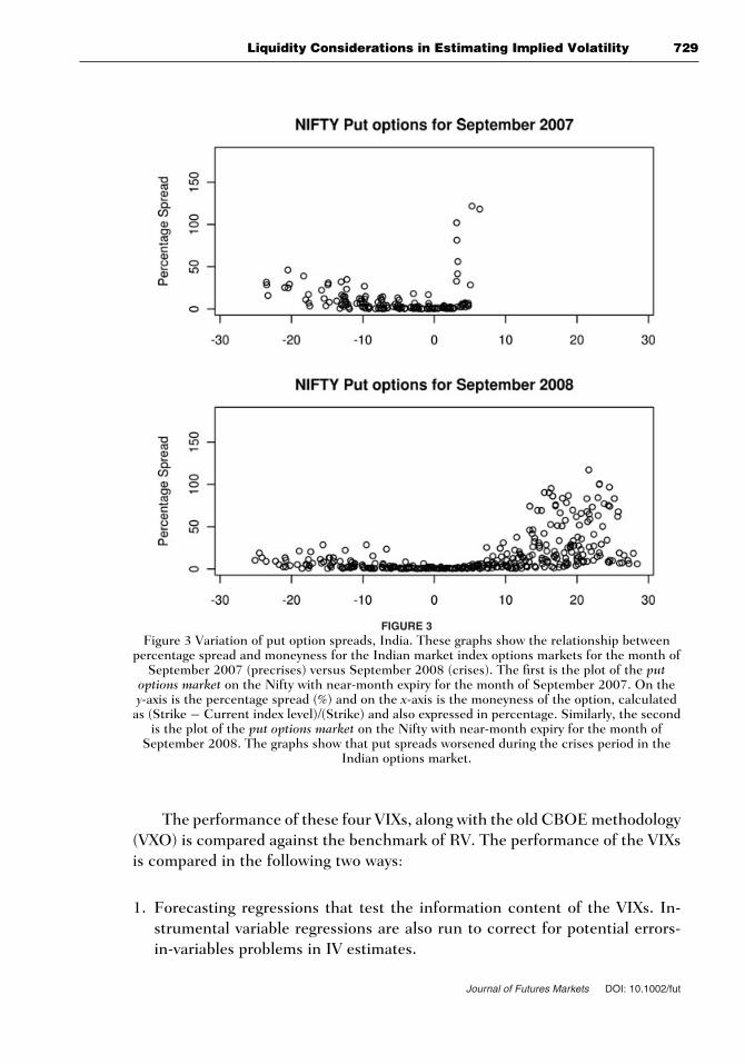
FIGURE 3Figure 3 Variation of put option spreads, India. These graphs show the relationship between

percentage spread and moneyness for the Indian market index options markets for the month ofSeptember 2007 (precrises) versus September 2008 (crises). The first is the plot of the put

options market on the Nifty with near-month expiry for the month of September 2007. On they-axis is the percentage spread (%) and on the x-axis is the moneyness of the option, calculated

as (Strike − Current index level)/(Strike) and also expressed in percentage. Similarly, the secondis the plot of the put options market on the Nifty with near-month expiry for the month of

September 2008. The graphs show that put spreads worsened during the crises period in theIndian options market.

The performance of these four VIXs, along with the old CBOE methodology(VXO) is compared against the benchmark of RV. The performance of the VIXsis compared in the following two ways:

1. Forecasting regressions that test the information content of the VIXs. In-strumental variable regressions are also run to correct for potential errors-in-variables problems in IV estimates.



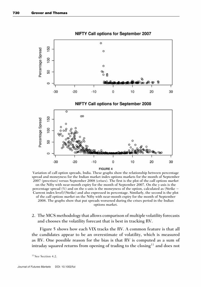
FIGURE 4Variation of call option spreads, India. These graphs show the relationship between percentagespread and moneyness for the Indian market index options markets for the month of September2007 (precrises) versus September 2008 (crises). The first is the plot of the call options market

on the Nifty with near-month expiry for the month of September 2007. On the y-axis is thepercentage spread (%) and on the x-axis is the moneyness of the option, calculated as (Strike −Current index level)/(Strike) and also expressed in percentage. Similarly, the second is the plot

of the call options market on the Nifty with near-month expiry for the month of September2008. The graphs show that put spreads worsened during the crises period in the Indian

options market.

2. The MCS methodology that allows comparison of multiple volatility forecastsand chooses the volatility forecast that is best in tracking RV.

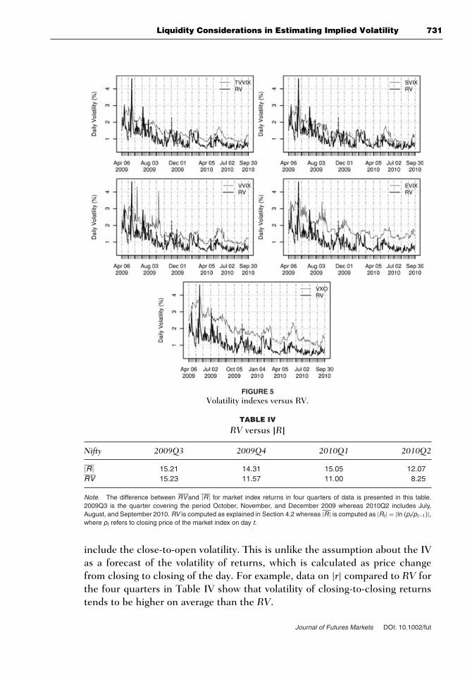
Figure 5 shows how each VIX tracks the RV. A common feature is that allthe candidates appear to be an overestimate of volatility, which is measuredas RV. One possible reason for the bias is that RV is computed as a sum ofintraday squared returns from opening of trading to the closing11 and does not

11See Section 4.2.



FIGURE 5Volatility indexes versus RV.

TABLE IV

RV versus |R|Nifty 2009Q3 2009Q4 2010Q1 2010Q2

|R| 15.21 14.31 15.05 12.07RV 15.23 11.57 11.00 8.25

Note. The difference between RVand |R| for market index returns in four quarters of data is presented in this table.2009Q3 is the quarter covering the period October, November, and December 2009 whereas 2010Q2 includes July,August, and September 2010. RV is computed as explained in Section 4.2 whereas |R| is computed as |Rt| = |ln (pt/pt−1)|,where pt refers to closing price of the market index on day t.

include the close-to-open volatility. This is unlike the assumption about the IVas a forecast of the volatility of returns, which is calculated as price changefrom closing to closing of the day. For example, data on |r| compared to RV forthe four quarters in Table IV show that volatility of closing-to-closing returnstends to be higher on average than the RV.



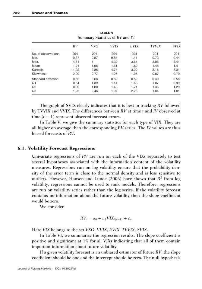
TABLE V

Summary Statistics of RV and IV

RV VXO VVIX EVIX TVVIX SVIX

No. of observations 294 294 294 294 294 294Min. 0.37 0.87 0.84 1.11 0.73 0.44Max. 4.61 4 4.32 3.65 3.08 3.41Mean 1.01 1.95 1.61 1.89 1.48 1.4Kurtosis 11.22 2.86 4.74 3.29 3.16 3.31Skewness 2.09 0.77 1.26 1.05 0.87 0.79

Standard deviation 0.52 0.68 0.62 0.59 0.49 0.56Q1 0.64 1.39 1.14 1.43 1.07 0.99Q2 0.90 1.80 1.43 1.71 1.36 1.29Q3 1.25 2.46 1.97 2.23 1.84 1.81

The graph of SVIX clearly indicates that it is best in tracking RV followedby TVVIX and VVIX. The differences between RV at time t and IV observed attime (t − 1) represent observed forecast errors.

In Table V, we give the summary statistics for each type of VIX. They areall higher on average than the corresponding RV series. The IV values are thusbiased forecasts of RV.

6.1. Volatility Forecast Regressions

Univariate regressions of RV are run on each of the VIXs separately to testseveral hypotheses associated with the information content of the volatilitymeasures. Regressions run on log volatility ensure that the probability den-sity of the error term is close to the normal density and is less sensitive tooutliers. However, Hansen and Lunde (2006) have shown that R2 from logvolatility, regressions cannot be used to rank models. Therefore, regressionsare run on volatility series rather than the log series. If the volatility forecastcontains no information about the future volatility then the slope coefficientwould be zero.

We consider

RVt = a0 + a1VIXi(t−1) + εt .

Here VIX belongs to the set VXO, VVIX, EVIX, TVVIX, SVIX.In Table VI, we summarize the regression results. The slope coefficient is

positive and significant at 1% for all VIXs indicating that all of them containimportant information about future volatility.

If a given volatility forecast is an unbiased estimator of future RV, the slopecoefficient should be one and the intercept should be zero. The null hypothesis



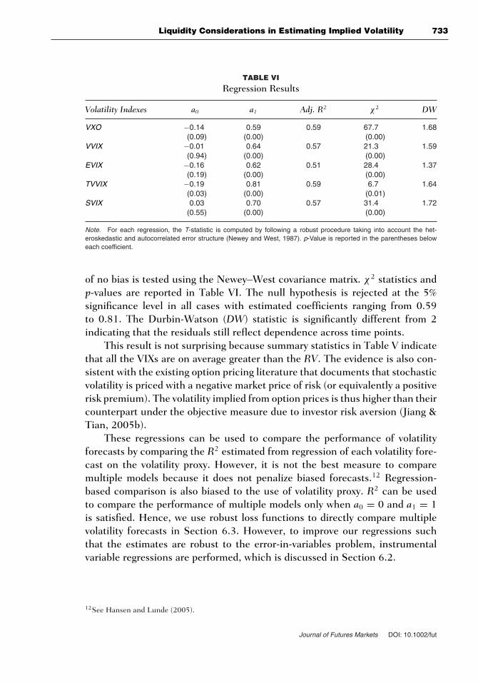
TABLE VI

Regression Results

Volatility Indexes a0 a1 Adj. R2 χ2 DW

VXO −0.14 0.59 0.59 67.7 1.68(0.09) (0.00) (0.00)

VVIX −0.01 0.64 0.57 21.3 1.59(0.94) (0.00) (0.00)

EVIX −0.16 0.62 0.51 28.4 1.37(0.19) (0.00) (0.00)

TVVIX −0.19 0.81 0.59 6.7 1.64(0.03) (0.00) (0.01)

SVIX 0.03 0.70 0.57 31.4 1.72(0.55) (0.00) (0.00)

Note. For each regression, the T-statistic is computed by following a robust procedure taking into account the het-eroskedastic and autocorrelated error structure (Newey and West, 1987). p-Value is reported in the parentheses beloweach coefficient.

of no bias is tested using the Newey–West covariance matrix. χ2 statistics andp-values are reported in Table VI. The null hypothesis is rejected at the 5%significance level in all cases with estimated coefficients ranging from 0.59to 0.81. The Durbin-Watson (DW) statistic is significantly different from 2indicating that the residuals still reflect dependence across time points.

This result is not surprising because summary statistics in Table V indicatethat all the VIXs are on average greater than the RV. The evidence is also con-sistent with the existing option pricing literature that documents that stochasticvolatility is priced with a negative market price of risk (or equivalently a positiverisk premium). The volatility implied from option prices is thus higher than theircounterpart under the objective measure due to investor risk aversion (Jiang &Tian, 2005b).

These regressions can be used to compare the performance of volatilityforecasts by comparing the R2 estimated from regression of each volatility fore-cast on the volatility proxy. However, it is not the best measure to comparemultiple models because it does not penalize biased forecasts.12 Regression-based comparison is also biased to the use of volatility proxy. R2 can be usedto compare the performance of multiple models only when a0 = 0 and a1 = 1is satisfied. Hence, we use robust loss functions to directly compare multiplevolatility forecasts in Section 6.3. However, to improve our regressions suchthat the estimates are robust to the error-in-variables problem, instrumentalvariable regressions are performed, which is discussed in Section 6.2.

12See Hansen and Lunde (2005).



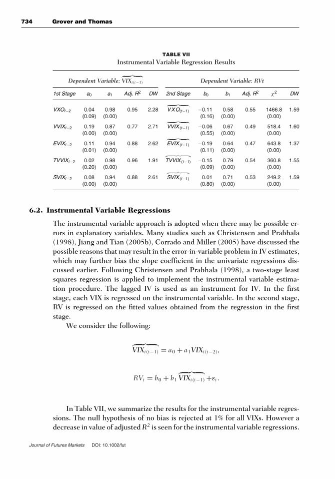
TABLE VII

Instrumental Variable Regression Results

Dependent Variable:︷︸︸︷VIXi(t−1) Dependent Variable: RVt

1st Stage a0 a1 Adj. R2 DW 2nd Stage b0 b1 Adj. R2 χ2 DW

VXOt−2 0.04 0.98 0.95 2.28︷︸︸︷VXO(t−1) −0.11 0.58 0.55 1466.8 1.59

(0.09) (0.00) (0.16) (0.00) (0.00)

VVIXt−2 0.19 0.87 0.77 2.71︷︸︸︷VVIX (t−1) −0.06 0.67 0.49 518.4 1.60

(0.00) (0.00) (0.55) (0.00) (0.00)

EVIXt−2 0.11 0.94 0.88 2.62︷︸︸︷EVIX (t−1) −0.19 0.64 0.47 643.8 1.37

(0.01) (0.00) (0.11) (0.00) (0.00)

TVVIXt−2 0.02 0.98 0.96 1.91︷︸︸︷TVVIX (t−1) −0.15 0.79 0.54 360.8 1.55

(0.20) (0.00) (0.09) (0.00) (0.00)

SVIXt−2 0.08 0.94 0.88 2.61︷︸︸︷SVIX (t−1) 0.01 0.71 0.53 249.2 1.59

(0.00) (0.00) (0.80) (0.00) (0.00)

6.2. Instrumental Variable Regressions

The instrumental variable approach is adopted when there may be possible er-rors in explanatory variables. Many studies such as Christensen and Prabhala(1998), Jiang and Tian (2005b), Corrado and Miller (2005) have discussed thepossible reasons that may result in the error-in-variable problem in IV estimates,which may further bias the slope coefficient in the univariate regressions dis-cussed earlier. Following Christensen and Prabhala (1998), a two-stage leastsquares regression is applied to implement the instrumental variable estima-tion procedure. The lagged IV is used as an instrument for IV. In the firststage, each VIX is regressed on the instrumental variable. In the second stage,RV is regressed on the fitted values obtained from the regression in the firststage.

We consider the following:

︷︸︸︷VIXi(t−1) = a0 + a1VIXi(t−2),

RVt = b0 + b1

︷︸︸︷VIXi(t−1) +εt .

In Table VII, we summarize the results for the instrumental variable regres-sions. The null hypothesis of no bias is rejected at 1% for all VIXs. However adecrease in value of adjusted R2 is seen for the instrumental variable regressions.



TABLE VIII

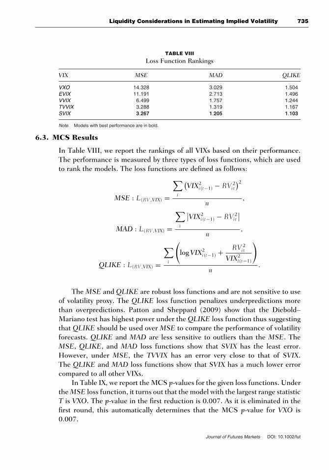
Loss Function Rankings

VIX MSE MAD QLIKE

VXO 14.328 3.029 1.504EVIX 11.191 2.713 1.496VVIX 6.499 1.757 1.244TVVIX 3.288 1.319 1.167SVIX 3.267 1.205 1.103

Note. Models with best performance are in bold.

6.3. MCS Results

In Table VIII, we report the rankings of all VIXs based on their performance.The performance is measured by three types of loss functions, which are usedto rank the models. The loss functions are defined as follows:

MSE : L(RV ,VIX) =

∑i

(VIX2

i(t−1) − RV 2i t

)2

n,

MAD : L(RV,VIX) =

∑i

∣∣VIX2i(t−1) − RV 2

i t

∣∣n

,

QLIKE : L(RV,VIX) =

∑i

(log VIX2

i(t−1) + RV 2i t

VIX2i(t−1)

)

n.

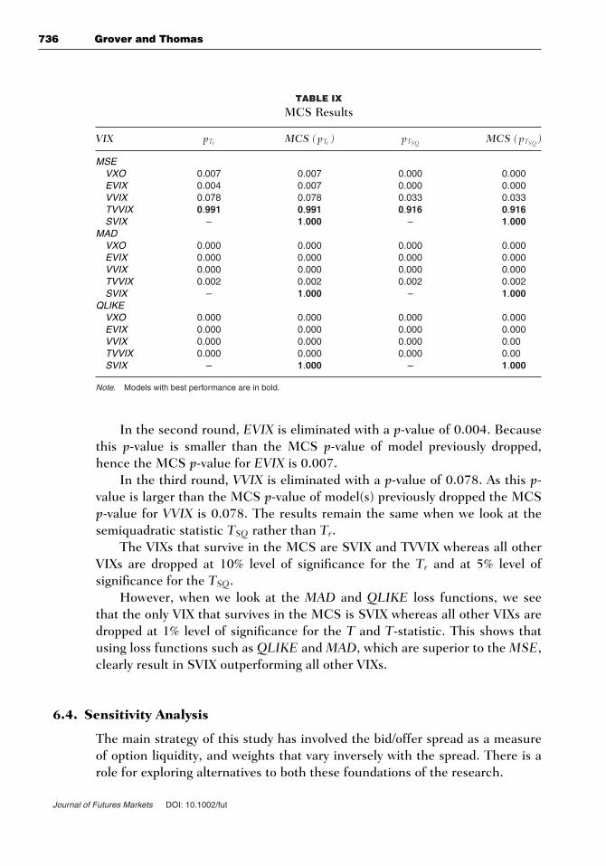
The MSE and QLIKE are robust loss functions and are not sensitive to useof volatility proxy. The QLIKE loss function penalizes underpredictions morethan overpredictions. Patton and Sheppard (2009) show that the Diebold–Mariano test has highest power under the QLIKE loss function thus suggestingthat QLIKE should be used over MSE to compare the performance of volatilityforecasts. QLIKE and MAD are less sensitive to outliers than the MSE. TheMSE, QLIKE, and MAD loss functions show that SVIX has the least error.However, under MSE, the TVVIX has an error very close to that of SVIX.The QLIKE and MAD loss functions show that SVIX has a much lower errorcompared to all other VIXs.

In Table IX, we report the MCS p-values for the given loss functions. Underthe MSE loss function, it turns out that the model with the largest range statisticT is VXO. The p-value in the first reduction is 0.007. As it is eliminated in thefirst round, this automatically determines that the MCS p-value for VXO is0.007.



TABLE IX

MCS Results

VIX pTr MCS (pTr ) pTSQ MCS (pTSQ )

MSEVXO 0.007 0.007 0.000 0.000EVIX 0.004 0.007 0.000 0.000VVIX 0.078 0.078 0.033 0.033TVVIX 0.991 0.991 0.916 0.916SVIX – 1.000 – 1.000

MADVXO 0.000 0.000 0.000 0.000EVIX 0.000 0.000 0.000 0.000VVIX 0.000 0.000 0.000 0.000TVVIX 0.002 0.002 0.002 0.002SVIX – 1.000 – 1.000

QLIKEVXO 0.000 0.000 0.000 0.000EVIX 0.000 0.000 0.000 0.000VVIX 0.000 0.000 0.000 0.00TVVIX 0.000 0.000 0.000 0.00SVIX – 1.000 – 1.000

Note. Models with best performance are in bold.

In the second round, EVIX is eliminated with a p-value of 0.004. Becausethis p-value is smaller than the MCS p-value of model previously dropped,hence the MCS p-value for EVIX is 0.007.

In the third round, VVIX is eliminated with a p-value of 0.078. As this p-value is larger than the MCS p-value of model(s) previously dropped the MCSp-value for VVIX is 0.078. The results remain the same when we look at thesemiquadratic statistic TSQ rather than Tr.

The VIXs that survive in the MCS are SVIX and TVVIX whereas all otherVIXs are dropped at 10% level of significance for the Tr and at 5% level ofsignificance for the TSQ.

However, when we look at the MAD and QLIKE loss functions, we seethat the only VIX that survives in the MCS is SVIX whereas all other VIXs aredropped at 1% level of significance for the T and T-statistic. This shows thatusing loss functions such as QLIKE and MAD, which are superior to the MSE,clearly result in SVIX outperforming all other VIXs.

6.4. Sensitivity Analysis

The main strategy of this study has involved the bid/offer spread as a measureof option liquidity, and weights that vary inversely with the spread. There is arole for exploring alternatives to both these foundations of the research.



In recent work, Chaudhury (2011) proposes the following two alternativemeasures of option liquidity:

s = ask − bidvol

,

vol = Sσ√252

,

where S refers to underlying asset price, σ refers to IV of option.And

s = ask − bid

σδVδσ

,

where V refers to the mid-price of option and σ refers to IV of option.The analysis of this study was repeated using both these measures. The VIX

computed using either of these measures is inferior to our main work.13

Another direction of exploration is the variation of the weight by optionspread. The main work of this study has employed weights w = 1/s. This is anad-hoc specification lacking theoretical rationale. Hence, we also explore twoalternative specifications as follows:

w = 1s 2

and

w = 1√s.

The former has weights that rapidly drop off, when the spread widens, andthe latter has weights that drop off relatively slowly. Neither of these alternativesyield an improvement when compared with the main work.14

7. CONCLUSION

The VXO and VIX are widely accepted VIXs and are computed by manyexchanges across the world. However, options markets show substantial

13Detailed results are available on request from the authors.14Detailed results are available on request from the authors.



cross-sectional variation in liquidity. This cross-sectional variation is accentu-ated in crisis periods. Price information for illiquid options is less informative.The present strategies for construction of VIXs err in treating all price data asequally informative.

The contribution of our study lies in isolating this issue, and proposinga VIX where the option IV, which is computed using the midpoint quote, isweighted by the inverse of the bid–offer spread of the option.

Our work falls under the larger theme of bringing microstructure consider-ations more integrally into the utilization of information from financial markets(Shah & Thomas, 1998). Some markets that are highly liquid in industrial coun-tries may be relatively illiquid in emerging markets. While some traded products(e.g., ATM options) might be highly liquid, other traded products might be illiq-uid. Although some markets may be ordinarily highly liquid in ordinary times(e.g., the U.S. Treasury Inflation Protected Securities [TIPS] market), they maybecome illiquid under stressed conditions. This microstructure perspective canbe useful with many applications of financial market data.

Our results indicate that the liquidity-weighted VIX (SVIX) outperformsother VIXs when compared against future RV. In an ideal world, if all optionseries are identically liquid, then the SVIX would yield an answer that is nodifferent from the conventional scheme: our proposed scheme does no harm attimes when all options are highly liquid, but it improves matters when cross-sectional variation in option liquidity occurs. This improved methodology isthus potentially useful in improving measurement of IV at option exchangesworldwide.

In this study, the simplest strategy—weighting by the inverse spread—proved to yield a VIX that was superior to traditional methods. More generally,a superior VIX might involve utilizing information in both vega and the bid–offerspread, and can be an interesting avenue for future research.

BIBLIOGRAPHY

Andersen, T. G., Bollerslev, T., Diebold, F. X., & Labys, P. (2001). The distribution ofrealized exchange rate volatility. Journal of the American Statistical Association,96, 42–55.

Becker, R., Clements, A. E., & White, S. I. (2007). Does implied volatility provide anyinformation beyond that captured in model-based volatility forecasts? Journal ofBanking and Finance, 31, 2535–2549.

Becker, R., Clements, A. E., & White, S. I. (2008). Are combination forecasts of S&P500 volatility statistically superior? International Journal of Forecasting, 24, 122–133.

Beckers, S. (1981). Standard deviations implied in option prices as predictors of futurestock price variability. Journal of Banking and Finance, 5, 363–381.



Blair, B. J., Poon, S. H., & Taylor, S. J. (2001). Forecasting S&P 100 volatility: Theincremental information content of implied volatilities and high-frequency indexreturns. Journal of Econometrics, 105, 5–26.

Bollen, N. P. B., & Whaley, R. E. (2004). Does net buying pressure affect the shape ofthe implied volatility functions? Journal of Finance, 59, 711–753.

Brenner, M., Eldor, R., & Hauser, S. (2001). The price of options illiquidity. Journal ofFinance, 56, 789–805.

Brenner, M., & Galai, D. (1993). Hedging volatility in foreign currencies. Journal ofDerivatives, 1, 53–59.

Britten-Jones, M., & Neuberger, A. (2000). Option prices, implied price processes, andstochastic volatility. Journal of Finance, 55, 839–866.

Brous, P., Ufuk, I., & Ivilina, P. (2010). Volatility forecasting and liquidity: Evidencefrom individual stocks. Journal of Derivatives & Hedge Funds, 16, 144–159.

Campa, J. M., & Chang, P. H. K. (1995). Testing the expectations hypothesis on theterm structure of volatilities in foreign exchange options. Journal of Finance, 50,529–547.

Canina, L., & Figlewski, S. (1993). The information content of implied volatility. TheReview of Financial Studies, 6, 659–681.

Carr, P., & Madan, D. (1998). Towards a theory of volatility trading. In R. Jarrow(Ed.), Volatility: New estimation techniques for pricing derivatives (pp. 417–427).London: Risk.

Cetin, U., Jarrow, R., Protter, P., & Warachka, M. (2006). Pricing options in an ex-tended Black-Scholes economy with illiquidity: Theory and empirical evidence.The Review of Financial Studies, 19, 493–529.

Chaudhury, M. (2011). Option bid-ask spread and liquidity (working paper). Quebec,Canada: McGill University.

Chiras, D. P., & Manaster, S. (1978). The information content of option prices and atest of market efficiency. Journal of Financial Economics, 6, 213–234.

Chou, R. K., Chung, S. L., Hsiao, Y. J., & Wang, Y. H. (2009). The impact of liquidityrisk on option prices (technical report). Taiwan: National Central University andNational Taiwan University.

Christensen, B. J., Hansen, C. S., & Prabhala, N. R. (2001). The telescoping overlapproblem in options data (working paper). Denmark: University of Aarhus; andCollege Park, MD: University of Maryland.

Christensen, B. J., & Prabhala, N. R. (1998). The relation between realized and impliedvolatility. Journal of Financial Economics, 50, 125–150.

Corrado, C. J., & Miller, T. W., Jr. (2005). The forecast quality of CBOE impliedvolatility indexes. Journal of Futures Markets, 25, 339–373.

Cox, J., & Rubinstein, M. (1985). Options markets. Englewood Cliffs, NJ: Prentice-Hall.Day, T. E., & Lewis, C. M. (1988). The behavior of the volatility implicit in the prices

of stock index options. Journal of Financial Economics, 22, 103–122.Demeterfi, K., Derman, E., Kamal, M., & Zou, J. (1999). A guide to volatility and

variance swaps. Journal of Derivatives, 6, 9–32.Dennis, P., Mayhew, S., & Stivers, C. (2006). Stock returns, implied volatility in-

novations, and the asymmetric volatility phenomenon. Journal of Financial andQuantitative Analysis, 41, 381–406.

Dumas, B., Fleming, J., & Whaley, R. E. (1998). Implied volatility functions: Empiricaltests. Journal of Finance, 53, 2059–2106.



Dupire, B. (1993). Model art. Risk, 6, 118–124.Etling, C., & Miller, T. W., Jr. (2000). The relationship between index option moneyness

and relative liquidity. Journal of Futures Markets, 20, 971–987.Galai, D. (1989). A proposal for indexes for traded call options. Journal of Finance, 34,

1157–1172.Garleanu, N., Pedersen, L. H., & Poteshman, A. M. (2009). Demand-based option

pricing. The Review of Financial Studies, 22, 4259–4299.Gastineau, G. L. (1977). An index of listed option premiums. Financial Analyst Journal,

33, 70–75.Hansen, P. R., & Lunde, A. (2005). A forecast comparison of volatility models: Does

anything beat a GARCH(1, 1)? Journal of Applied Econometrics, 20, 873–889.Hansen, P. R., & Lunde, A. (2006). Consistent ranking of volatility models. Journal of

Econometrics, 131, 97–121.Hansen, P. R., Lunde, A., & Nason, J. M. (2003). Choosing the best volatility models:

The model confidence set approach. Oxford Bulletin of Economics and Statistics,65, 839–861.

Heynen, R., Kemna, A., & Vorst, T. (1994). Analysis of the term structure of impliedvolatilities. Journal of Financial and Quantitative Analysis, 29, 31–56.

Jackwerth, J. C., & Rubinstein, M. (1996). Recovering probability distributions fromoption prices. Journal of Finance, 51, 1611–1631.

Jiang, G. J., & Tian, Y. S. (2005a). Gauging the investor fear gauge: Implementationproblems in the CBOE’s new volatility index and a simple solution (working paper).University of Arizona.

Jiang, G. J., & Tian, Y. S. (2005b). The model-free implied volatility and its informationcontent. The Review of Financial Studies, 18, 1305–1342.

Jorion, P. (1995). Predicting volatility in the foreign exchange market. Journal of Fi-nance, 50, 507–528.

Lamoureux, C. G., & Lastrapes, W. D. (1993). Forecasting stock-return variance: To-ward an understanding of stochastic implied volatilities. The Review of FinancialStudies, 6, 293–326.

Latane, H. A., & Rendleman, R. J., Jr. (1976). Standard deviations of stock price ratiosimplied in option prices. Journal of Finance, 31, 369–381.

Mayhew, S., & Stivers, C. (2003). Stock return dynamics, option volume, and theinformation content of implied volatility. Journal of Futures Markets, 23, 616–646.

Nandi, S. (2000). Asymmetric information about volatility: How does it affect impliedvolatility, options prices and market liquidity? Review of Derivatives Research, 3,215–236.

Neuberger, A. (1994). The log contract: A new instrument to hedge volatility. Journalof Portfolio Management, 2, 74–80.

Newey, W. K., & West, K. D. (1987). Simple positive definite heteroskedasticity andautocorrelation consistent covariance matrix. Econometrica, 55, 703–708.

Patton, A. J., & Sheppard, K. (2009). Evaluating volatility and correlation forecasts. InT. G. Andersen, R. A. Davis, J. P. Kreiss, & T. Mikosch (Eds.), The handbook offinancial time series. Berlin: Springer Verlag.

Poteshman, A. M. (2000). Forecasting future volatility from option prices (workingpaper). University of Illinois at Urbana-Champaign.



Rubinstein, M. (1994). Implied binomial trees. The Journal of Finance, 49, 771–818.Schmalensee, R., & Trippi, R. (1978). Common stock volatility expectations implied by

option premia. Journal of Finance, 33, 129–147.Shah, A., & Thomas, S. (1998). Market microstructure considerations in index con-

struction. In proceedings of CBOT research symposium, Chicago Board of Trade,Chicago, pp. 173–193.

Trippi, R. R. (1977). A test of option market efficiency using a random-walk evaluationmodel. Journal of Economics and Business, 29, 93–98.

Tzang, S. W., Hung, C. H., Wang, C. W., & Shyu, D. S. D. (2010). Do liquidity andsampling methods matter in constructing volatility indices? Empirical evidencefrom Taiwan. International Review of Economics and Finance, 20, 312–324.

Whaley, R. E. (1982). Valuation of American call options on dividend-paying stocks:Empirical tests. Journal of Financial Economics, 10, 29–58.

Whaley, R. E. (1993). Derivatives on market volatility: Hedging tools long overdue.Journal of Derivatives, 1, 71–84.

Whaley, R. E. (2009). Understanding VIX. Journal of Portfolio Management, 35, 98–105.

Xu, X., & Taylor, S. J. (1994). The term structure of volatility implied by foreign exchangeoptions. Journal of Financial and Quantitative Analysis, 29, 57–74.


Liquidity Considerations in Estimating Implied Volatility · Liquidity Considerations in Estimating Implied Volatility 715 “implied volatility” (IV). IV is a direct measure of

Documents