Local Volatility Models Copyright © Changwei Xiong 2016 June 2016 last update: October 28, 2017 TABLE OF CONTENTS Table of Contents .........................................................................................................................................1 1. Kolmogorov Forward and Backward Equations..................................................................................2 1.1. Kolmogorov Forward Equation ....................................................................................................2 1.2. Kolmogorov Backward Equation ..................................................................................................5 2. Local Volatility.....................................................................................................................................6 2.1. Local Volatility by Vanilla Call .....................................................................................................6 2.2. Local Volatility by Forward Call ...................................................................................................8 2.2.1. Local Variance as a Conditional Expectation of Instantaneous Variance ......................... 9 2.2.2. Formula in Log-moneyness ............................................................................................. 10 2.3. Local Volatility by Implied Volatility .......................................................................................... 11 2.3.1. Formula in Log-strike...................................................................................................... 12 2.3.2. Formula in Log-moneyness ............................................................................................. 13 2.3.3. Equivalency in Formulas ................................................................................................. 14 3. Local Volatility: PDE by Finite Difference Method ..........................................................................16 3.1. Date Conventions of Equity and Equity Option..........................................................................16 3.2. Deterministic Dividends..............................................................................................................17 3.3. Forward PDE ...............................................................................................................................18 3.3.1. Treatment of Deterministic Dividends ............................................................................ 19 3.4. Backward PDE ............................................................................................................................21 3.4.1. PDE in Centered Log-spot .............................................................................................. 21 3.4.1.1. Treatment of Deterministic Dividends ............................................................................ 22 3.4.1.2. Vanilla Call ...................................................................................................................... 23 3.4.2. PDE in Log-spot .............................................................................................................. 23 3.4.2.1. Treatment of Deterministic Dividends ............................................................................ 24 3.5. Local Volatility Surface ...............................................................................................................24 3.6. Barrier Option Pricing .................................................................................................................25 References ..................................................................................................................................................27

Welcome message from author
This document is posted to help you gain knowledge. Please leave a comment to let me know what you think about it! Share it to your friends and learn new things together.
Transcript
Local Volatility Models
Copyright © Changwei Xiong 2016
June 2016
last update: October 28, 2017
TABLE OF CONTENTS
Table of Contents .........................................................................................................................................1
1. Kolmogorov Forward and Backward Equations ..................................................................................2
1.1. Kolmogorov Forward Equation ....................................................................................................2
1.2. Kolmogorov Backward Equation ..................................................................................................5
2. Local Volatility .....................................................................................................................................6
2.1. Local Volatility by Vanilla Call .....................................................................................................6
2.2. Local Volatility by Forward Call ...................................................................................................8
2.2.1. Local Variance as a Conditional Expectation of Instantaneous Variance ......................... 9
2.2.2. Formula in Log-moneyness ............................................................................................. 10
2.3. Local Volatility by Implied Volatility .......................................................................................... 11
2.3.1. Formula in Log-strike ...................................................................................................... 12
2.3.2. Formula in Log-moneyness ............................................................................................. 13
2.3.3. Equivalency in Formulas ................................................................................................. 14
3. Local Volatility: PDE by Finite Difference Method ..........................................................................16
3.1. Date Conventions of Equity and Equity Option..........................................................................16
3.2. Deterministic Dividends ..............................................................................................................17
3.3. Forward PDE ...............................................................................................................................18
3.3.1. Treatment of Deterministic Dividends ............................................................................ 19
3.4. Backward PDE ............................................................................................................................21
3.4.1. PDE in Centered Log-spot .............................................................................................. 21
3.4.1.1. Treatment of Deterministic Dividends ............................................................................ 22
3.4.1.2. Vanilla Call ...................................................................................................................... 23
3.4.2. PDE in Log-spot .............................................................................................................. 23
3.4.2.1. Treatment of Deterministic Dividends ............................................................................ 24
3.5. Local Volatility Surface ...............................................................................................................24
3.6. Barrier Option Pricing .................................................................................................................25
References ..................................................................................................................................................27
Changwei Xiong, October 2017 http://www.cs.utah.edu/~cxiong/
2
The note is prepared for the purpose of summarizing local volatility models frequently
encountered in derivative pricing. It at first derives the Kolmogorov forward and backward equations,
which fundamentally govern the transition probability density of the diffusion process in derivative price
dynamics. Subsequently, it introduces the local volatility model in the context of Dupire formula and
then presents a PDE based local volatility model, in which the local volatility function is parametrized to
be piecewise linear in log-moneyness and piecewise constant in time.
1. KOLMOGOROV FORWARD AND BACKWARD EQUATIONS
The time evolution of the transition probability density function is governed by Kolmogorov
forward and backward equations, which will be introduced as follows, without loss of generality, in
multi-dimension.
1.1. Kolmogorov Forward Equation
Let’s consider the following 𝑚-dimensional stochastic spot process 𝑆𝑡 ∈ ℝ𝑚 driven by an 𝑛-
dimensional Brownian motion 𝑊𝑡 whose correlation matrix 𝜌 is given by 𝜌𝑑𝑡 = 𝑑𝑊𝑡𝑑𝑊𝑡′
𝑑𝑆𝑡𝑚×1
= 𝐴(𝑡, 𝑆𝑡)𝑚×1
𝑑𝑡1×1
+ 𝐵(𝑡, 𝑆𝑡)𝑚×𝑛
𝑑𝑊𝑡𝑛×1
(1)
We derive the dynamics of ℎ , where ℎ:ℝ𝑚 ⟶ℝ in this case is a scalar-valued Borel-measurable
function only on variable 𝑆𝑡
𝑑ℎ(𝑆𝑡)1×1
= 𝐽ℎ1×𝑚
𝑑𝑆𝑡𝑚×1
+1
2𝑑𝑆𝑡
′
1×𝑚𝐻ℎ𝑚×𝑚
𝑑𝑆𝑡𝑚×1
= 𝐽ℎ𝐴𝑑𝑡 + 𝐽ℎ𝐵𝑑𝑊𝑡 +1
2𝑑𝑊𝑡
′𝐵′𝐻ℎ𝐵𝑑𝑊𝑡 (2)
where 𝐽ℎ is the 1 × 𝑚 Jacobian (i.e. the same as gradient if ℎ is a scalar-valued function) and 𝐻ℎ the
𝑚 ×𝑚 Hessian (with subscripts of 𝑆 now denoting the indices of vector components)
[𝐽ℎ]𝑖 =𝜕ℎ
𝜕𝑆𝑖 and [𝐻ℎ]𝑖𝑗 =
𝜕2ℎ
𝜕𝑆𝑖𝜕𝑆𝑗 (3)
Expanding the expression in (2), we have
Changwei Xiong, October 2017 http://www.cs.utah.edu/~cxiong/
3
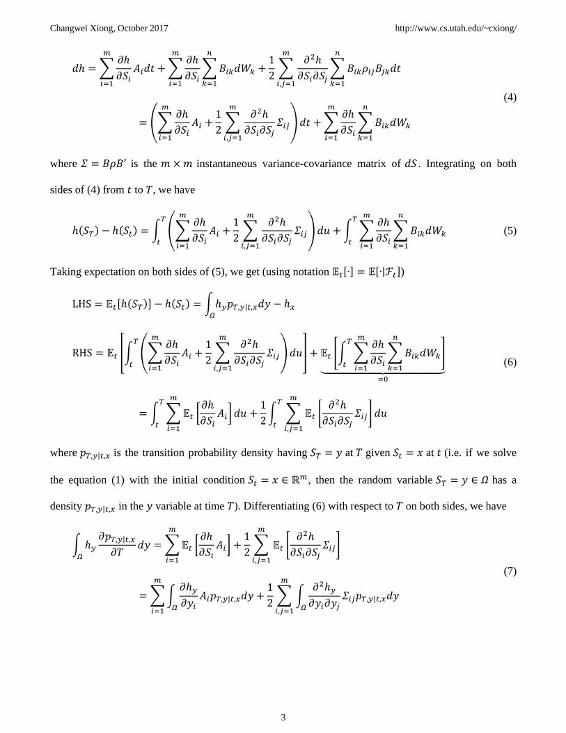
𝑑ℎ =∑𝜕ℎ
𝜕𝑆𝑖𝐴𝑖𝑑𝑡
𝑚
𝑖=1
+∑𝜕ℎ
𝜕𝑆𝑖
𝑚
𝑖=1
∑𝐵𝑖𝑘𝑑𝑊𝑘
𝑛
𝑘=1
+1
2∑
𝜕2ℎ
𝜕𝑆𝑖𝜕𝑆𝑗∑𝐵𝑖𝑘𝜌𝑖𝑗𝐵𝑗𝑘𝑑𝑡
𝑛
𝑘=1
𝑚
𝑖,𝑗=1
= (∑𝜕ℎ
𝜕𝑆𝑖𝐴𝑖
𝑚
𝑖=1
+1
2∑
𝜕2ℎ
𝜕𝑆𝑖𝜕𝑆𝑗𝛴𝑖𝑗
𝑚
𝑖,𝑗=1
)𝑑𝑡 +∑𝜕ℎ
𝜕𝑆𝑖
𝑚
𝑖=1
∑𝐵𝑖𝑘𝑑𝑊𝑘
𝑛
𝑘=1
(4)
where 𝛴 = 𝐵𝜌𝐵′ is the 𝑚 ×𝑚 instantaneous variance-covariance matrix of 𝑑𝑆 . Integrating on both
sides of (4) from 𝑡 to 𝑇, we have
ℎ(𝑆𝑇) − ℎ(𝑆𝑡) = ∫ (∑𝜕ℎ
𝜕𝑆𝑖𝐴𝑖
𝑚
𝑖=1
+1
2∑
𝜕2ℎ
𝜕𝑆𝑖𝜕𝑆𝑗𝛴𝑖𝑗
𝑚
𝑖,𝑗=1
)𝑑𝑢𝑇
𝑡
+∫ ∑𝜕ℎ
𝜕𝑆𝑖
𝑚
𝑖=1
∑𝐵𝑖𝑘𝑑𝑊𝑘
𝑛
𝑘=1
𝑇
𝑡
(5)
Taking expectation on both sides of (5), we get (using notation 𝔼𝑡[∙] = 𝔼[∙|ℱ𝑡])
LHS = 𝔼𝑡[ℎ(𝑆𝑇)] − ℎ(𝑆𝑡) = ∫ℎ𝑦𝑝𝑇,𝑦|𝑡,𝑥𝑑𝑦𝛺
− ℎ𝑥
RHS = 𝔼𝑡 [∫ (∑𝜕ℎ
𝜕𝑆𝑖𝐴𝑖
𝑚
𝑖=1
+1
2∑
𝜕2ℎ
𝜕𝑆𝑖𝜕𝑆𝑗𝛴𝑖𝑗
𝑚
𝑖,𝑗=1
)𝑑𝑢𝑇
𝑡
] + 𝔼𝑡 [∫ ∑𝜕ℎ
𝜕𝑆𝑖
𝑚
𝑖=1
∑𝐵𝑖𝑘𝑑𝑊𝑘
𝑛
𝑘=1
𝑇
𝑡
]⏟
=0
= ∫ ∑𝔼𝑡 [𝜕ℎ
𝜕𝑆𝑖𝐴𝑖]
𝑚
𝑖=1
𝑑𝑢𝑇
𝑡
+1
2∫ ∑ 𝔼𝑡 [
𝜕2ℎ
𝜕𝑆𝑖𝜕𝑆𝑗𝛴𝑖𝑗]
𝑚
𝑖,𝑗=1
𝑑𝑢𝑇
𝑡
(6)
where 𝑝𝑇,𝑦|𝑡,𝑥 is the transition probability density having 𝑆𝑇 = 𝑦 at 𝑇 given 𝑆𝑡 = 𝑥 at 𝑡 (i.e. if we solve
the equation (1) with the initial condition 𝑆𝑡 = 𝑥 ∈ ℝ𝑚 , then the random variable 𝑆𝑇 = 𝑦 ∈ 𝛺 has a
density 𝑝𝑇,𝑦|𝑡,𝑥 in the 𝑦 variable at time 𝑇). Differentiating (6) with respect to 𝑇 on both sides, we have
∫ ℎ𝑦𝜕𝑝𝑇,𝑦|𝑡,𝑥𝜕𝑇
𝑑𝑦𝛺
=∑𝔼𝑡 [𝜕ℎ
𝜕𝑆𝑖𝐴𝑖]
𝑚
𝑖=1
+1
2∑ 𝔼𝑡 [
𝜕2ℎ
𝜕𝑆𝑖𝜕𝑆𝑗𝛴𝑖𝑗]
𝑚
𝑖,𝑗=1
=∑∫𝜕ℎ𝑦𝜕𝑦𝑖
𝐴𝑖𝑝𝑇,𝑦|𝑡,𝑥𝑑𝑦𝛺
𝑚
𝑖=1
+1
2∑ ∫
𝜕2ℎ𝑦𝜕𝑦𝑖𝜕𝑦𝑗
𝛴𝑖𝑗𝑝𝑇,𝑦|𝑡,𝑥𝑑𝑦𝛺
𝑚
𝑖,𝑗=1
(7)
Changwei Xiong, October 2017 http://www.cs.utah.edu/~cxiong/
4
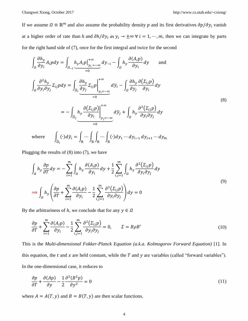
If we assume 𝛺 ≡ ℝ𝑚 and also assume the probability density 𝑝 and its first derivatives 𝜕𝑝/𝜕𝑦𝑖 vanish
at a higher order of rate than ℎ and 𝜕ℎ/𝜕𝑦𝑖 as 𝑦𝑖 → ±∞ ∀ 𝑖 = 1,⋯ ,𝑚, then we can integrate by parts
for the right hand side of (7), once for the first integral and twice for the second
∫𝜕ℎ𝑦𝜕𝑦𝑖
𝐴𝑖𝑝𝑑𝑦𝛺
= ∫ ℎ𝑦𝐴𝑖𝑝|𝑦𝑖 =−∞+∞
⏟ =0
𝑑𝑦−𝑖𝛺−𝑖
−∫ ℎ𝑦𝜕(𝐴𝑖𝑝)
𝜕𝑦𝑖𝑑𝑦
𝛺
and
∫𝜕2ℎ𝑦𝜕𝑦𝑖𝜕𝑦𝑗
𝛴𝑖𝑗𝑝𝑑𝑦𝛺
= ∫𝜕ℎ𝑦𝜕𝑦𝑗
𝛴𝑖𝑗𝑝|𝑦𝑖=−∞
+∞
⏟ =0
𝑑�̅�𝑖�̅�𝑖
−∫𝜕ℎ𝑦𝜕𝑦𝑗
𝜕(𝛴𝑖𝑗𝑝)
𝜕𝑦𝑖𝑑𝑦
𝛺
= −∫ ℎ𝑦𝜕(𝛴𝑖𝑗𝑝)
𝜕𝑦𝑖|𝑦𝑗=−∞
+∞
⏟ =0
𝑑�̅�𝑗�̅�𝑗
+∫ ℎ𝑦𝜕2(𝛴𝑖𝑗𝑝)
𝜕𝑦𝑖𝜕𝑦𝑗𝑑𝑦
𝛺
where ∫ (∙)𝑑�̅�𝑖�̅�𝑖
= ∫ ⋯∫ ∫ ⋯∫(∙)𝑑𝑦1ℝ
⋯𝑑𝑦𝑖−1ℝ
𝑑𝑦𝑖+1ℝ
⋯𝑑𝑦𝑚ℝ
(8)
Plugging the results of (8) into (7), we have
∫ ℎ𝑦𝜕𝑝
𝜕𝑇𝑑𝑦
𝛺
= −∑∫ ℎ𝑦𝜕(𝐴𝑖𝑝)
𝜕𝑦𝑖𝑑𝑦
𝛺
𝑚
𝑖=1
+1
2∑ ∫ ℎ𝑦
𝜕2(𝛴𝑖𝑗𝑝)
𝜕𝑦𝑖𝜕𝑦𝑗𝑑𝑦
𝛺
𝑚
𝑖,𝑗=1
⟹∫ ℎ𝑦 (𝜕𝑝
𝜕𝑇+∑
𝜕(𝐴𝑖𝑝)
𝜕𝑦𝑖
𝑚
𝑖=1
−1
2∑
𝜕2(𝛴𝑖𝑗𝑝)
𝜕𝑦𝑖𝜕𝑦𝑗
𝑚
𝑖,𝑗=1
)𝑑𝑦𝛺
= 0
(9)
By the arbitrariness of ℎ, we conclude that for any 𝑦 ∈ 𝛺
𝜕𝑝
𝜕𝑇+∑
𝜕(𝐴𝑖𝑝)
𝜕𝑦𝑖
𝑚
𝑖=1
−1
2∑
𝜕2(𝛴𝑖𝑗𝑝)
𝜕𝑦𝑖𝜕𝑦𝑗
𝑚
𝑖,𝑗=1
= 0, 𝛴 = 𝐵𝜌𝐵′ (10)
This is the Multi-dimensional Fokker-Planck Equation (a.k.a. Kolmogorov Forward Equation) [1]. In
this equation, the 𝑡 and 𝑥 are held constant, while the 𝑇 and 𝑦 are variables (called “forward variables”).
In the one-dimensional case, it reduces to
𝜕𝑝
𝜕𝑇+𝜕(𝐴𝑝)
𝜕𝑦−1
2
𝜕2(𝐵2𝑝)
𝜕𝑦2= 0 (11)
where 𝐴 = 𝐴(𝑇, 𝑦) and 𝐵 = 𝐵(𝑇, 𝑦) are then scalar functions.
Changwei Xiong, October 2017 http://www.cs.utah.edu/~cxiong/
5
1.2. Kolmogorov Backward Equation
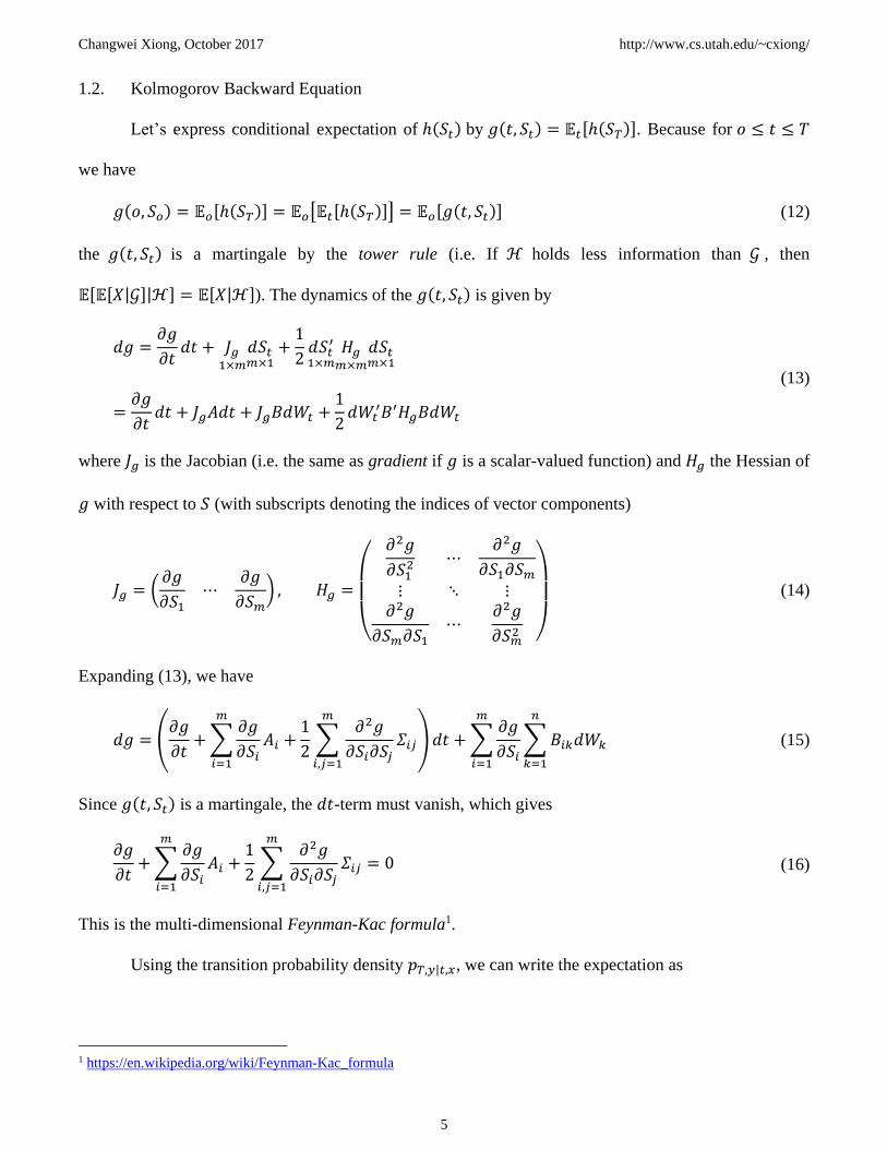
Let’s express conditional expectation of ℎ(𝑆𝑡) by 𝑔(𝑡, 𝑆𝑡) = 𝔼𝑡[ℎ(𝑆𝑇)]. Because for 𝑜 ≤ 𝑡 ≤ 𝑇
we have
𝑔(𝑜, 𝑆𝑜) = 𝔼𝑜[ℎ(𝑆𝑇)] = 𝔼𝑜[𝔼𝑡[ℎ(𝑆𝑇)]] = 𝔼𝑜[𝑔(𝑡, 𝑆𝑡)] (12)
the 𝑔(𝑡, 𝑆𝑡) is a martingale by the tower rule (i.e. If ℋ holds less information than 𝒢 , then
𝔼[𝔼[𝑋|𝒢]|ℋ] = 𝔼[𝑋|ℋ]). The dynamics of the 𝑔(𝑡, 𝑆𝑡) is given by
𝑑𝑔 =𝜕𝑔
𝜕𝑡𝑑𝑡 + 𝐽𝑔
1×𝑚
𝑑𝑆𝑡𝑚×1
+1
2𝑑𝑆𝑡
′
1×𝑚𝐻𝑔𝑚×𝑚
𝑑𝑆𝑡𝑚×1
=𝜕𝑔
𝜕𝑡𝑑𝑡 + 𝐽𝑔𝐴𝑑𝑡 + 𝐽𝑔𝐵𝑑𝑊𝑡 +
1
2𝑑𝑊𝑡
′𝐵′𝐻𝑔𝐵𝑑𝑊𝑡
(13)
where 𝐽𝑔 is the Jacobian (i.e. the same as gradient if 𝑔 is a scalar-valued function) and 𝐻𝑔 the Hessian of
𝑔 with respect to 𝑆 (with subscripts denoting the indices of vector components)
𝐽𝑔 = (𝜕𝑔
𝜕𝑆1⋯
𝜕𝑔
𝜕𝑆𝑚) , 𝐻𝑔 =
(
𝜕2𝑔
𝜕𝑆12 ⋯
𝜕2𝑔
𝜕𝑆1𝜕𝑆𝑚⋮ ⋱ ⋮𝜕2𝑔
𝜕𝑆𝑚𝜕𝑆1⋯
𝜕2𝑔
𝜕𝑆𝑚2 )
(14)
Expanding (13), we have
𝑑𝑔 = (𝜕𝑔
𝜕𝑡+∑
𝜕𝑔
𝜕𝑆𝑖𝐴𝑖
𝑚
𝑖=1
+1
2∑
𝜕2𝑔
𝜕𝑆𝑖𝜕𝑆𝑗𝛴𝑖𝑗
𝑚
𝑖,𝑗=1
)𝑑𝑡 +∑𝜕𝑔
𝜕𝑆𝑖
𝑚
𝑖=1
∑𝐵𝑖𝑘𝑑𝑊𝑘
𝑛
𝑘=1
(15)
Since 𝑔(𝑡, 𝑆𝑡) is a martingale, the 𝑑𝑡-term must vanish, which gives
𝜕𝑔
𝜕𝑡+∑
𝜕𝑔
𝜕𝑆𝑖𝐴𝑖
𝑚
𝑖=1
+1
2∑
𝜕2𝑔
𝜕𝑆𝑖𝜕𝑆𝑗𝛴𝑖𝑗
𝑚
𝑖,𝑗=1
= 0 (16)
This is the multi-dimensional Feynman-Kac formula1.
Using the transition probability density 𝑝𝑇,𝑦|𝑡,𝑥, we can write the expectation as
1 https://en.wikipedia.org/wiki/Feynman-Kac_formula
Changwei Xiong, October 2017 http://www.cs.utah.edu/~cxiong/
6
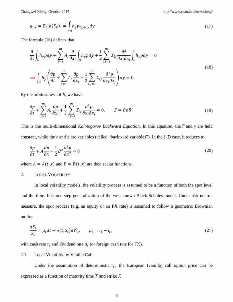
𝑔𝑡,𝑥 = 𝔼𝑡[ℎ(𝑆𝑇)] = ∫ℎ𝑦𝑝𝑇,𝑦|𝑡,𝑥𝑑𝑦𝛺
(17)
The formula (16) defines that
𝜕
𝜕𝑡∫ℎ𝑦𝑝𝑑𝑦𝛺
+∑𝐴𝑖𝜕
𝜕𝑥𝑖∫ℎ𝑦𝑝𝑑𝑦𝛺
𝑚
𝑖=1
+1
2∑ 𝛴𝑖𝑗
𝜕2
𝜕𝑥𝑖𝜕𝑥𝑗∫ℎ𝑦𝑝𝑑𝑦𝛺
𝑚
𝑖,𝑗=1
= 0
⟹∫ ℎ𝑦 (𝜕𝑝
𝜕𝑡+∑𝐴𝑖
𝜕𝑝
𝜕𝑥𝑖
𝑚
𝑖=1
+1
2∑ 𝛴𝑖𝑗
𝜕2𝑝
𝜕𝑥𝑖𝜕𝑥𝑗
𝑚
𝑖,𝑗=1
)𝑑𝑦𝛺
= 0
(18)
By the arbitrariness of ℎ, we have
𝜕𝑝
𝜕𝑡+∑𝐴𝑖
𝜕𝑝
𝜕𝑥𝑖
𝑚
𝑖=1
+1
2∑ 𝛴𝑖𝑗
𝜕2𝑝
𝜕𝑥𝑖𝜕𝑥𝑗
𝑚
𝑖,𝑗=1
= 0, 𝛴 = 𝐵𝜌𝐵′ (19)
This is the multi-dimensional Kolmogorov Backward Equation. In this equation, the 𝑇 and 𝑦 are held
constant, while the 𝑡 and 𝑥 are variables (called “backward variables”). In the 1-D case, it reduces to
𝜕𝑝
𝜕𝑡+ 𝐴
𝜕𝑝
𝜕𝑥+1
2𝐵2𝜕2𝑝
𝜕𝑥2= 0 (20)
where 𝐴 = 𝐴(𝑡, 𝑥) and 𝐵 = 𝐵(𝑡, 𝑥) are then scalar functions.
2. LOCAL VOLATILITY
In local volatility models, the volatility process is assumed to be a function of both the spot level
and the time. It is one step generalization of the well-known Black-Scholes model. Under risk neutral
measure, the spot process (e.g. an equity or an FX rate) is assumed to follow a geometric Brownian
motion
𝑑𝑆𝑡𝑆𝑡= 𝜇𝑡𝑑𝑡 + 𝜎(𝑡, 𝑆𝑡)𝑑�̃�𝑡 , 𝜇𝑡 = 𝑟𝑡 − 𝑞𝑡 (21)
with cash rate 𝑟𝑡 and dividend rate 𝑞𝑡 (or foreign cash rate for FX).
2.1. Local Volatility by Vanilla Call
Under the assumption of deterministic 𝑟𝑡 , the European (vanilla) call option price can be
expressed as a function of maturity time 𝑇 and strike 𝐾
Changwei Xiong, October 2017 http://www.cs.utah.edu/~cxiong/
7
𝒞𝑇,𝐾|𝑡,𝑥 = �̃�𝑡[𝐷𝑡,𝑇(𝑆𝑇 − 𝐾)+] = 𝐷𝑡,𝑇∫ (𝑦 − 𝐾)𝑝𝑇,𝑦|𝑡,𝑥𝑑𝑦
∞
𝐾
(22)
where 𝐷𝑡,𝑇 = exp (−∫ 𝑟𝑢𝑑𝑢𝑇
𝑡) is the deterministic discount factor and 𝑝𝑇,𝑦|𝑡,𝑥 is the transition
probability density having spot 𝑆𝑇 = 𝑦 at 𝑇 given initial condition 𝑆𝑡 = 𝑥 at 𝑡. Differentiating (22) with
respect to 𝐾, we have the first order and second order partial derivative
𝜕𝒞𝑇,𝐾|𝑡,𝑥𝜕𝐾
= −𝐷𝑡,𝑇∫ 𝑝𝑇,𝑦|𝑡,𝑥𝑑𝑦∞
𝐾
,𝜕2𝒞𝑇,𝐾|𝑡,𝑥𝜕𝐾2
= 𝐷𝑡,𝑇𝑝𝑇,𝐾|𝑡,𝑥 (23)
which gives the transition probability density function by
𝑝𝑇,𝐾|𝑡,𝑥 =1
𝐷𝑡,𝑇
𝜕2𝒞𝑇,𝐾|𝑡,𝑥𝜕𝐾2
(24)
The (24) is also known as Breeden-Litzenberger formula.
Taking the first derivative of 𝒞𝑇,𝐾|𝑡,𝑥 in (22) with respect to 𝑇, we find
𝜕𝒞𝑇,𝐾|𝑡,𝑥𝜕𝑇
= −𝑟𝑇𝒞𝑇,𝐾|𝑡,𝑥 + 𝐷𝑡,𝑇∫ (𝑦 − 𝐾)𝜕𝑝𝑇,𝑦|𝑡,𝑥𝜕𝑇
𝑑𝑦∞
𝐾
= −𝑟𝑇𝒞𝑇,𝐾|𝑡,𝑥 + 𝐷𝑡,𝑇∫ (𝑦 − 𝐾)(1
2
𝜕2(𝜎𝑇,𝑦2 𝑦2𝑝𝑇,𝑦|𝑡,𝑥)
𝜕𝑦2−𝜕(𝜇𝑇𝑦𝑝𝑇,𝑦|𝑡,𝑥)
𝜕𝑦)𝑑𝑦
∞
𝐾
(25)
using the Kolmogorov Forward Equation (11)
𝜕𝑝𝑇,𝑦|𝑡,𝑥𝜕𝑇
=1
2
𝜕2(𝜎𝑇,𝑦2 𝑦2𝑝𝑇,𝑦|𝑡,𝑥)
𝜕𝑦2−𝜕(𝜇𝑇𝑦𝑝𝑇,𝑦|𝑡,𝑥)
𝜕𝑦 (26)
Applying integration by parts to the integrals on the right hand side of (25) yields
∫ (𝑦 − 𝐾)𝜕(𝜇𝑇𝑦𝑝𝑇,𝑦|𝑡,𝑥)
𝜕𝑦𝑑𝑦
∞
𝐾
= (𝑦 − 𝐾)𝜇𝑇𝑦𝑝𝑇,𝑦|𝑡,𝑥|𝑦=𝐾∞
⏟ =0
−∫ 𝜇𝑇𝑦𝑝𝑇,𝑦|𝑡,𝑥𝑑𝑦∞
𝐾
= −𝜇𝑇 (∫ (𝑦 − 𝐾)𝑝𝑇,𝑦|𝑡,𝑥𝑑𝑦∞
𝐾
+ 𝐾∫ 𝑝𝑇,𝑦|𝑡,𝑥𝑑𝑦∞
𝐾
) =𝜇𝑇𝐾
𝐷𝑡,𝑇
𝜕𝒞𝑇,𝐾|𝑡,𝑥𝜕𝐾
−𝜇𝑇𝒞𝑇,𝐾|𝑡,𝑥𝐷𝑡,𝑇
and
(27)
Changwei Xiong, October 2017 http://www.cs.utah.edu/~cxiong/
8
∫ (𝑦 − 𝐾)𝜕2(𝜎𝑇,𝑦
2 𝑦2𝑝𝑇,𝑦|𝑡,𝑥)
𝜕𝑦2𝑑𝑦
∞
𝐾
= (𝑦 − 𝐾)𝜕(𝜎𝑇,𝑦
2 𝑦2𝑝𝑇,𝑦|𝑡,𝑥)
𝜕𝑦|𝑦=𝐾
∞
⏟ =0
−∫𝜕(𝜎𝑇,𝑦
2 𝑦2𝑝𝑇,𝑦|𝑡,𝑥)
𝜕𝑦𝑑𝑦
∞
𝐾
= 𝜎𝑇,𝑦2 𝑦2𝑝𝑇,𝑦|𝑡,𝑥|𝑦=𝐾
∞= 𝜎𝑇,𝐾
2 𝐾2𝑝𝑇,𝐾|𝑡,𝑥 =𝜎𝑇,𝐾2 𝐾2
𝐷𝑡,𝑇
𝜕2𝒞𝑇,𝐾|𝑡,𝑥𝜕𝐾2
where we have 𝑝𝑇,∞|𝑡,𝑥 = 0 and 𝜕𝑝𝑇,∞|𝑡,𝑥/𝜕𝑦 = 0 assuming the probability density 𝑝𝑇,𝑦|𝑡,𝑥 and its first
derivative vanish at a higher order of rate as 𝑦 → ∞. Plugging (27) into (25), we find
𝜕𝒞𝑇,𝐾|𝑡,𝑥𝜕𝑇
= −𝑟𝑇𝒞𝑇,𝐾|𝑡,𝑥 +𝜎𝑇,𝐾2 𝐾2
2
𝜕2𝒞𝑇,𝐾|𝑡,𝑥𝜕𝐾2
− 𝜇𝑇𝐾𝜕𝒞𝑇,𝐾|𝑡,𝑥𝜕𝐾
+ 𝜇𝑇𝒞𝑇,𝐾|𝑡,𝑥
=𝜎𝑇,𝐾2 𝐾2
2
𝜕2𝒞𝑇,𝐾|𝑡,𝑥𝜕𝐾2
− 𝜇𝑇𝐾𝜕𝒞𝑇,𝐾|𝑡,𝑥𝜕𝐾
− 𝑞𝑇𝒞𝑇,𝐾|𝑡,𝑥
(28)
and eventually the Dupire formula for the local volatility 𝜎𝑇,𝐾 expressed in terms of vanilla call price
𝜎𝑇,𝐾2
2=
𝜕𝒞𝑇,𝐾|𝑡,𝑥𝜕𝑇
+ 𝜇𝑇𝐾𝜕𝒞𝑇,𝐾|𝑡,𝑥𝜕𝐾
+ 𝑞𝑇𝒞𝑇,𝐾|𝑡,𝑥
𝐾2𝜕2𝒞𝑇,𝐾|𝑡,𝑥𝜕𝐾2
(29)
2.2. Local Volatility by Forward Call
Sometimes, it is more convenient to express the Dupire formula in terms of a forward (i.e.
undiscounted) call, which is defined as
𝐶𝑇,𝐾|𝑡,𝑥 = �̃�𝑡[(𝑆𝑇 − 𝐾)+] = ∫ (𝑦 − 𝐾)𝑝𝑇,𝑦|𝑡,𝑥𝑑𝑦
∞
𝐾
=𝒞𝑇,𝐾|𝑡,𝑥𝐷𝑡,𝑇
(30)
with 𝒞𝑇,𝐾|𝑡,𝑥 given in (22) (note that (30) is true only if the interest rate is deterministic). Following a
similar derivation, we find that
𝜕𝐶𝑇,𝐾|𝑡,𝑥𝜕𝐾
= −∫ 𝑝𝑇,𝑦|𝑡,𝑥𝑑𝑦∞
𝐾
,𝜕2𝐶𝑇,𝐾|𝑡,𝑥𝜕𝐾2
= 𝑝𝑇,𝐾|𝑡,𝑥 and
𝜕𝐶𝑇,𝐾|𝑡,𝑥𝜕𝑇
= ∫ (𝑦 − 𝐾)𝜕𝑝𝑇,𝑦|𝑡,𝑥𝜕𝑇
𝑑𝑦∞
𝐾
=1
2𝜎𝑇,𝐾2 𝐾2
𝜕2𝐶𝑇,𝐾|𝑡,𝑥𝜕𝐾2
+ 𝜇𝑇(𝐶𝑇,𝐾|𝑡,𝑥 − 𝐾𝜕𝐶𝑇,𝐾|𝑡,𝑥𝜕𝐾
)
(31)
Changwei Xiong, October 2017 http://www.cs.utah.edu/~cxiong/
9
Therefore the Dupire formula for 𝜎𝑇,𝐾 expressed in terms of forward call price reads
𝜎𝑇,𝐾2
2=
𝜕𝐶𝑇,𝐾|𝑡,𝑥𝜕𝑇
+ 𝜇𝑇𝐾𝜕𝐶𝑇,𝐾|𝑡,𝑥𝜕𝐾
− 𝜇𝑇𝐶𝑇,𝐾|𝑡,𝑥
𝐾2𝜕2𝐶𝑇,𝐾|𝑡,𝑥𝜕𝐾2
(32)
2.2.1. Local Variance as a Conditional Expectation of Instantaneous Variance
The forward call (30) can be expressed as
𝐶𝑇,𝐾|𝑡,𝑥 = �̃�𝑡[(𝑆𝑇 − 𝐾)+] = �̃�𝑡[𝒽(𝑆𝑇 − 𝐾)(𝑆𝑇 − 𝐾)] = �̃�𝑡[𝒽(𝑆𝑇 − 𝐾)𝑆𝑇] − 𝐾�̃�𝑡[𝒽(𝑆𝑇 − 𝐾)] (33)
where 𝒽 is the Heaviside step function1. Differentiating once with respect to 𝐾, we get
𝜕𝐶𝑇,𝐾|𝑡,𝑥𝜕𝐾
= −∫ 𝑝𝑇,𝑦|𝑡,𝑥𝑑𝑦∞
𝐾
= −�̃�𝑡[𝒽(𝑆𝑇 − 𝐾)] ⟹ �̃�𝑡[𝒽(𝑆𝑇 − 𝐾)𝑆𝑇] = 𝐶𝑇,𝐾|𝑡,𝑥 − 𝐾𝜕𝐶𝑇,𝐾|𝑡,𝑥𝜕𝐾
(34)
Differentiating again with respect to 𝐾, we have
𝜕2𝐶𝑇,𝐾|𝑡,𝑥𝜕𝐾2
= 𝑝𝑇,𝐾|𝑡,𝑥 = �̃�𝑡[𝛿(𝑆𝑇 − 𝐾)] (35)
where 𝛿 is the Dirac delta function2. Applying Ito’s Lemma to the terminal payoff of the option gives
the identity
𝑑(𝑆𝑇 − 𝐾)+ = 𝒽(𝑆𝑇 − 𝐾)𝑑𝑆𝑇 +
1
2𝛿(𝑆𝑇 − 𝐾)𝜎𝑇
2𝑆𝑇2𝑑𝑇
= 𝒽(𝑆𝑇 − 𝐾)𝜇𝑇𝑆𝑇𝑑𝑇 +1
2𝛿(𝑆𝑇 − 𝐾)𝜎𝑇
2𝑆𝑇2𝑑𝑇 + 𝒽(𝑆𝑇 − 𝐾)𝜎𝑇𝑆𝑇𝑑�̃�𝑇
(36)
Taking conditional expectations on both sides gives
𝑑𝐶𝑇,𝐾|𝑡,𝑥 = 𝑑�̃�𝑡[(𝑆𝑇 − 𝐾)+] = 𝜇𝑇�̃�𝑡[𝒽(𝑆𝑇 − 𝐾)𝑆𝑇]𝑑𝑇 +
1
2�̃�𝑡[𝛿(𝑆𝑇 − 𝐾)𝜎𝑇
2𝑆𝑇2]𝑑𝑇
⟹𝜕𝐶𝑇,𝐾|𝑡,𝑥𝜕𝑇
= 𝜇𝑇�̃�𝑡[𝒽(𝑆𝑇 − 𝐾)𝑆𝑇] +1
2�̃�𝑡[𝛿(𝑆𝑇 − 𝐾)𝜎𝑇
2𝑆𝑇2]
(37)
Notice that
1 Heaviside step function: 𝒽(𝑥) = {
0, 𝑥 < 01, 𝑥 ≥ 0
2 Dirac delta function can be viewed as the derivative of the Heaviside step function: 𝛿(𝑥) =𝑑𝒽(𝑥)
𝑑𝑥= {∞, 𝑥 = 00, 𝑥 ≠ 0
,
which is also constrained to satisfy the identity: ∫ 𝛿(𝑥)𝑑𝑥ℝ
= 1.
Changwei Xiong, October 2017 http://www.cs.utah.edu/~cxiong/
10
�̃�𝑡[𝛿(𝑆𝑇 − 𝐾)𝜎𝑇2𝑆𝑇2] = 𝐾2�̃�𝑡[𝛿(𝑆𝑇 − 𝐾)𝜎𝑇
2] (38)
and from Bayes’ rule
�̃�𝑡[𝛿(𝑆𝑇 − 𝐾)𝜎𝑇2] = �̃�𝑡[𝜎𝑇
2|𝑆𝑇 = 𝐾]�̃�𝑡[𝛿(𝑆𝑇 − 𝐾)] (39)
we can derive from (37)
𝜕𝐶𝑇,𝐾|𝑡,𝑥𝜕𝑇
= 𝜇𝑇𝐶𝑇,𝐾|𝑡,𝑥 − 𝜇𝑇𝐾𝜕𝐶𝑇,𝐾|𝑡,𝑥𝜕𝐾
+1
2𝐾2𝜕2𝐶𝑇,𝐾|𝑡,𝑥𝜕𝐾2
�̃�𝑡[𝜎𝑇2|𝑆𝑇 = 𝐾]
⟹�̃�𝑡[𝜎𝑇
2|𝑆𝑇 = 𝐾]
2=
𝜕𝐶𝑇,𝐾|𝑡,𝑥𝜕𝑇
+ 𝜇𝑇𝐾𝜕𝐶𝑇,𝐾|𝑡,𝑥𝜕𝐾
− 𝜇𝑇𝐶𝑇,𝐾|𝑡,𝑥
𝐾2𝜕2𝐶𝑇,𝐾|𝑡,𝑥𝜕𝐾2
(40)
This is identical to (32). It means that the conditional expectation of the stochastic variance must equal
the Dupire local variance [2]. That is, local variance is the risk-neutral expectation of the instantaneous
variance conditional on the final stock price 𝑆𝑇 being equal to the strike price 𝐾 [3].
2.2.2. Formula in Log-moneyness
In real applications, numerical methods are often in favor of log-moneyness to be the spatial
variable, which can be regarded as a centered log-strike
𝑘 = ln𝐾
𝐹𝑡,𝑇 where
𝜕𝑘
𝜕𝐾=1
𝐾,
𝜕𝑘
𝜕𝑇= −𝜇𝑇 (41)
We want to express the Dupire formula in the (𝑇, 𝑘)-plane using call option price 𝐶𝑇,𝑘 (short for 𝐶𝑇,𝑘|𝑡,𝑧
for 𝑧 = ln𝑥
𝐹𝑡,𝑇) equivalent to the forward call 𝐶𝑇,𝐾 (short for 𝐶𝑇,𝐾|𝑡,𝑥). Note that although the 𝐶𝑇,𝑘 and
𝐶𝑇,𝐾 are equivalent, they are two different functions. The conversion from (𝑇, 𝐾)-plane to (𝑇, 𝑘)-plane
is achieved by using the following partial derivatives derived by chain rule
𝜕𝐶𝑇,𝐾𝜕𝑇
=𝜕𝐶𝑇,𝑘𝜕𝑇
+𝜕𝐶𝑇,𝑘𝜕𝑘
𝜕𝑘
𝜕𝑇=𝜕𝐶𝑇,𝑘𝜕𝑇
− 𝜇𝑇𝜕𝐶𝑇,𝑘𝜕𝑘
𝜕𝐶𝑇,𝐾𝜕𝐾
=𝜕𝐶𝑇,𝑘𝜕𝑇
𝜕𝑇
𝜕𝐾+𝜕𝐶𝑇,𝑘𝜕𝑘
𝜕𝑘
𝜕𝐾=1
𝐾
𝜕𝐶𝑇,𝑘𝜕𝑘
𝜕2𝐶𝑇,𝐾𝜕𝐾2
=𝜕
𝜕𝑇(𝜕𝐶𝑇,𝑘𝜕𝑘
)𝜕𝑇
𝜕𝐾+𝜕
𝜕𝑘(𝜕𝐶𝑇,𝑘𝜕𝑘
)𝜕𝑘
𝜕𝐾=1
𝐾
𝜕
𝜕𝑘(1
𝐾
𝜕𝐶𝑇,𝑘𝜕𝑘
) =1
𝐾2(𝜕2𝐶𝑇,𝑘𝜕𝑘2
−𝜕𝐶𝑇,𝑘𝜕𝑘
)
(42)
Changwei Xiong, October 2017 http://www.cs.utah.edu/~cxiong/
11
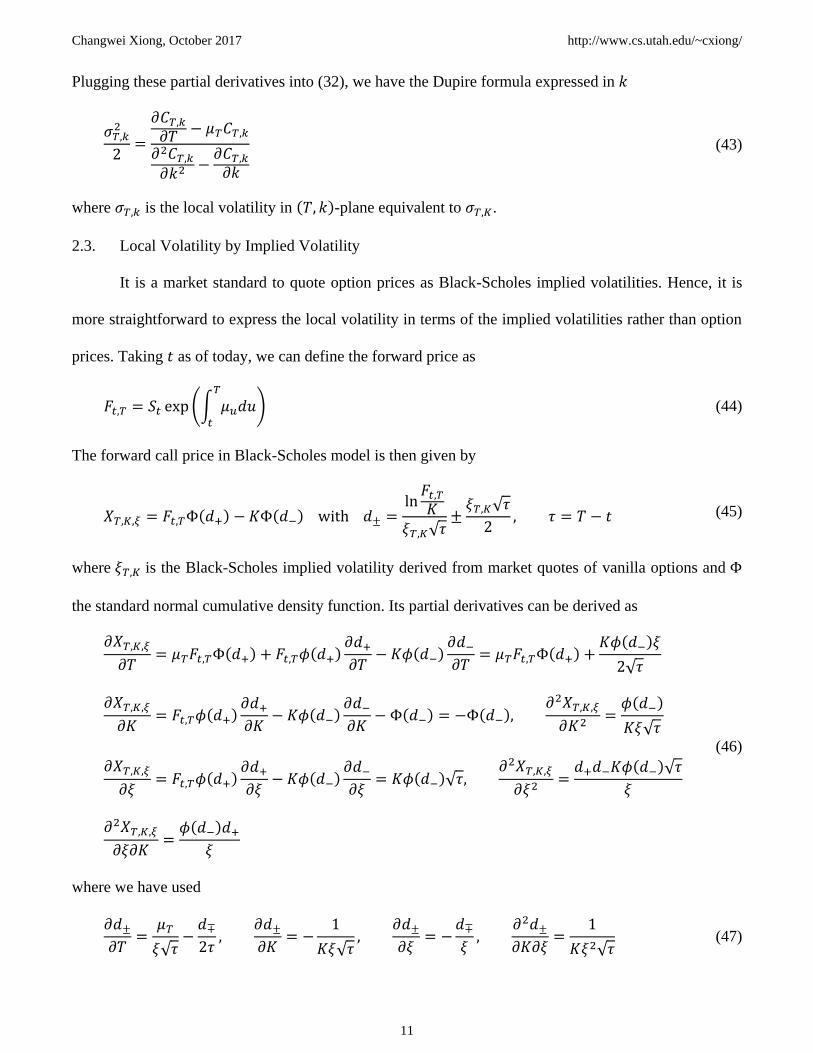
Plugging these partial derivatives into (32), we have the Dupire formula expressed in 𝑘
𝜎𝑇,𝑘2
2=
𝜕𝐶𝑇,𝑘𝜕𝑇
− 𝜇𝑇𝐶𝑇,𝑘
𝜕2𝐶𝑇,𝑘𝜕𝑘2
−𝜕𝐶𝑇,𝑘𝜕𝑘
(43)
where 𝜎𝑇,𝑘 is the local volatility in (𝑇, 𝑘)-plane equivalent to 𝜎𝑇,𝐾.
2.3. Local Volatility by Implied Volatility
It is a market standard to quote option prices as Black-Scholes implied volatilities. Hence, it is
more straightforward to express the local volatility in terms of the implied volatilities rather than option
prices. Taking 𝑡 as of today, we can define the forward price as
𝐹𝑡,𝑇 = 𝑆𝑡 exp(∫ 𝜇𝑢𝑑𝑢𝑇
𝑡
) (44)
The forward call price in Black-Scholes model is then given by
𝑋𝑇,𝐾,𝜉 = 𝐹𝑡,𝑇Φ(𝑑+) − 𝐾Φ(𝑑−) with 𝑑± =ln𝐹𝑡,𝑇𝐾
𝜉𝑇,𝐾√𝜏±𝜉𝑇,𝐾√𝜏
2, 𝜏 = 𝑇 − 𝑡 (45)
where 𝜉𝑇,𝐾 is the Black-Scholes implied volatility derived from market quotes of vanilla options and Φ
the standard normal cumulative density function. Its partial derivatives can be derived as
𝜕𝑋𝑇,𝐾,𝜉
𝜕𝑇= 𝜇𝑇𝐹𝑡,𝑇Φ(𝑑+) + 𝐹𝑡,𝑇𝜙(𝑑+)
𝜕𝑑+𝜕𝑇
− 𝐾𝜙(𝑑−)𝜕𝑑−𝜕𝑇
= 𝜇𝑇𝐹𝑡,𝑇Φ(𝑑+) +𝐾𝜙(𝑑−)𝜉
2√𝜏
𝜕𝑋𝑇,𝐾,𝜉
𝜕𝐾= 𝐹𝑡,𝑇𝜙(𝑑+)
𝜕𝑑+𝜕𝐾
− 𝐾𝜙(𝑑−)𝜕𝑑−𝜕𝐾
− Φ(𝑑−) = −Φ(𝑑−),𝜕2𝑋𝑇,𝐾,𝜉
𝜕𝐾2=𝜙(𝑑−)
𝐾𝜉√𝜏
𝜕𝑋𝑇,𝐾,𝜉
𝜕𝜉= 𝐹𝑡,𝑇𝜙(𝑑+)
𝜕𝑑+𝜕𝜉
− 𝐾𝜙(𝑑−)𝜕𝑑−𝜕𝜉
= 𝐾𝜙(𝑑−)√𝜏,𝜕2𝑋𝑇,𝐾,𝜉
𝜕𝜉2=𝑑+𝑑−𝐾𝜙(𝑑−)√𝜏
𝜉
𝜕2𝑋𝑇,𝐾,𝜉
𝜕𝜉𝜕𝐾=𝜙(𝑑−)𝑑+
𝜉
(46)
where we have used
𝜕𝑑±𝜕𝑇
=𝜇𝑇
𝜉√𝜏−𝑑∓2𝜏,
𝜕𝑑±𝜕𝐾
= −1
𝐾𝜉√𝜏,
𝜕𝑑±𝜕𝜉
= −𝑑∓𝜉,
𝜕2𝑑±𝜕𝐾𝜕𝜉
=1
𝐾𝜉2√𝜏 (47)
Changwei Xiong, October 2017 http://www.cs.utah.edu/~cxiong/
12
and the identity
𝐹𝑡,𝑇𝜙(𝑑+) = 𝐾𝜙(𝑑−) (48)
Further using the partial derivatives
𝜕𝐶𝑇,𝐾𝜕𝑇
=𝜕𝑋𝑇,𝐾,𝜉
𝜕𝑇+𝜕𝑋𝑇,𝐾,𝜉
𝜕𝜉
𝜕𝜉
𝜕𝑇,
𝜕𝐶𝑇,𝐾𝜕𝐾
=𝜕𝑋𝑇,𝐾,𝜉
𝜕𝐾+𝜕𝑋𝑇,𝐾,𝜉
𝜕𝜉
𝜕𝜉
𝜕𝐾
𝜕2𝐶𝑇,𝐾𝜕𝐾2
=𝜕2𝑋𝑇,𝐾,𝜉
𝜕𝐾2+ 2
𝜕2𝑋𝑇,𝐾,𝜉
𝜕𝐾𝜕𝜉
𝜕𝜉
𝜕𝐾+𝜕𝑋𝑇,𝐾,𝜉
𝜕𝜉
𝜕2𝜉
𝜕𝐾2+𝜕2𝑋𝑇,𝐾,𝜉
𝜕𝜉2(𝜕𝜉
𝜕𝐾)2
(49)
the local volatility given by implied volatility can be derived from (32) as
𝜎𝑇,𝐾2 =
𝜕𝐶𝑇,𝐾𝜕𝑇
+ 𝜇𝑇𝐾𝜕𝐶𝑇,𝐾𝜕𝐾
− 𝜇𝑇𝐶𝑇,𝐾
𝐾2
2𝜕2𝐶𝑇,𝐾𝜕𝐾2
=
𝜕𝑋𝜕𝑇+𝜕𝑋𝜕𝜉(𝜕𝜉𝑇,𝐾𝜕𝑇
+ 𝜇𝑇𝐾𝜕𝜉𝑇,𝐾𝜕𝐾
) + 𝜇𝑇𝐾𝜕𝑋𝜕𝐾
− 𝜇𝑇𝑋
𝐾2
2(𝜕2𝑋𝜕𝐾2
+ 2𝜕2𝑋𝜕𝐾𝜕𝜉
𝜕𝜉𝑇,𝐾𝜕𝐾
+𝜕𝑋𝜕𝜉𝜕2𝜉𝑇,𝐾𝜕𝐾2
+𝜕2𝑋𝜕𝜉2
(𝜕𝜉𝜕𝐾)2
)
=
𝜇𝑇𝐹𝑡,𝑇Φ(𝑑+) +𝐾𝜙(𝑑−)𝜉
2√𝜏+𝜕𝑋𝜕𝜉(𝜕𝜉𝜕𝑇+ 𝜇𝑇𝐾
𝜕𝜉𝜕𝐾) − 𝜇𝑇𝐾Φ(𝑑−) − 𝜇𝑇𝑋
𝐾2
2𝜙(𝑑−)
𝐾𝜉√𝜏+ 𝐾2
𝜙(𝑑−)𝑑+𝜉
𝜕𝜉𝜕𝐾
+𝐾2
2𝜕𝑋𝜕𝜉𝜕2𝜉𝜕𝐾2
+𝐾2
2𝑑+𝑑−𝐾𝜙(𝑑−)√𝜏
𝜉(𝜕𝜉𝜕𝐾)2
=
𝜕𝑋𝜕𝜉(𝜉2𝜏+𝜕𝜉𝜕𝑇+ 𝜇𝑇𝐾
𝜕𝜉𝜕𝐾)
12𝜉𝜏
𝜕𝑋𝜕𝜉+𝐾𝑑+𝜉√𝜏
𝜕𝑋𝜕𝜉𝜕𝜉𝜕𝐾
+𝐾2
2𝜕𝑋𝜕𝜉𝜕2𝜉𝜕𝐾2
+𝐾2𝑑+𝑑−2𝜉
𝜕𝑋𝜕𝜉(𝜕𝜉𝜕𝐾)2
=𝜉2 + 2𝜉𝜏 (
𝜕𝜉𝜕𝑇+ 𝜇𝑇𝐾
𝜕𝜉𝜕𝐾)
1 + 2√𝜏𝐾𝑑+𝜕𝜉𝜕𝐾
+ 𝑑+𝑑−𝜏𝐾2 (𝜕𝜉𝜕𝐾)2
+ 𝜉𝜏𝐾2𝜕2𝜉𝜕𝐾2
(50)
Numerical methods, e.g. PDE or Monte Carlo simulation, often demand a local volatility
function constructed on a 2D grid to perform pricing. In these methods, it is often more numerically
stable and convenient to work with a spatial dimension in log-strike or in log-moneyness.
2.3.1. Formula in Log-strike
The local volatility formula in log strike 𝑥 = ln𝐾 can be derived from (50)
Changwei Xiong, October 2017 http://www.cs.utah.edu/~cxiong/
13
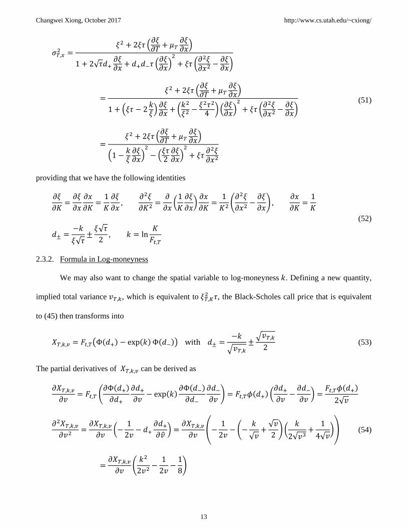
𝜎𝑇,𝑥2 =
𝜉2 + 2𝜉𝜏 (𝜕𝜉𝜕𝑇+ 𝜇𝑇
𝜕𝜉𝜕𝑥)
1 + 2√𝜏𝑑+𝜕𝜉𝜕𝑥+ 𝑑+𝑑−𝜏 (
𝜕𝜉𝜕𝑥)2
+ 𝜉𝜏 (𝜕2𝜉𝜕𝑥2
−𝜕𝜉𝜕𝑥)
=𝜉2 + 2𝜉𝜏 (
𝜕𝜉𝜕𝑇+ 𝜇𝑇
𝜕𝜉𝜕𝑥)
1 + (𝜉𝜏 − 2𝑘𝜉)𝜕𝜉𝜕𝑥+ (𝑘2
𝜉2−𝜉2𝜏2
4 ) (𝜕𝜉𝜕𝑥)2
+ 𝜉𝜏 (𝜕2𝜉𝜕𝑥2
−𝜕𝜉𝜕𝑥)
=𝜉2 + 2𝜉𝜏 (
𝜕𝜉𝜕𝑇+ 𝜇𝑇
𝜕𝜉𝜕𝑥)
(1 −𝑘𝜉𝜕𝜉𝜕𝑥)2
− (𝜉𝜏2𝜕𝜉𝜕𝑥)2
+ 𝜉𝜏𝜕2𝜉𝜕𝑥2
(51)
providing that we have the following identities
𝜕𝜉
𝜕𝐾=𝜕𝜉
𝜕𝑥
𝜕𝑥
𝜕𝐾=1
𝐾
𝜕𝜉
𝜕𝑥,
𝜕2𝜉
𝜕𝐾2=𝜕
𝜕𝑥(1
𝐾
𝜕𝜉
𝜕𝑥)𝜕𝑥
𝜕𝐾=1
𝐾2(𝜕2𝜉
𝜕𝑥2−𝜕𝜉
𝜕𝑥) ,
𝜕𝑥
𝜕𝐾=1
𝐾
𝑑± =−𝑘
𝜉√𝜏±𝜉√𝜏
2, 𝑘 = ln
𝐾
𝐹𝑡,𝑇
(52)
2.3.2. Formula in Log-moneyness
We may also want to change the spatial variable to log-moneyness 𝑘. Defining a new quantity,
implied total variance 𝑣𝑇,𝑘, which is equivalent to 𝜉𝑇,𝐾2 𝜏, the Black-Scholes call price that is equivalent
to (45) then transforms into
𝑋𝑇,𝑘,𝑣 = 𝐹𝑡,𝑇(Φ(𝑑+) − exp(𝑘)Φ(𝑑−)) with 𝑑± =−𝑘
√𝑣𝑇,𝑘±√𝑣𝑇,𝑘
2 (53)
The partial derivatives of 𝑋𝑇,𝑘,𝑣 can be derived as
𝜕𝑋𝑇,𝑘,𝑣𝜕𝑣
= 𝐹𝑡,𝑇 (𝜕Φ(𝑑+)
𝜕𝑑+
𝜕𝑑+𝜕𝑣
− exp(𝑘)𝜕Φ(𝑑−)
𝜕𝑑−
𝜕𝑑−𝜕𝑣) = 𝐹𝑡,𝑇𝜙(𝑑+) (
𝜕𝑑+𝜕𝑣
−𝜕𝑑−𝜕𝑣) =
𝐹𝑡,𝑇𝜙(𝑑+)
2√𝑣
𝜕2𝑋𝑇,𝑘,𝑣𝜕𝑣2
=𝜕𝑋𝑇,𝑘,𝑣𝜕𝑣
(−1
2𝑣− 𝑑+
𝜕𝑑+𝜕�̂�) =
𝜕𝑋𝑇,𝑘,𝑣𝜕𝑣
(−1
2𝑣− (−
𝑘
√𝑣+√𝑣
2) (
𝑘
2√𝑣3+
1
4√𝑣))
=𝜕𝑋𝑇,𝑘,𝑣𝜕𝑣
(𝑘2
2𝑣2−1
2𝑣−1
8)
(54)
Changwei Xiong, October 2017 http://www.cs.utah.edu/~cxiong/
14
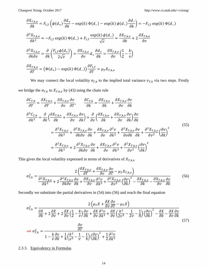
𝜕𝑋𝑇,𝑘,𝑣𝜕𝑘
= 𝐹𝑡,𝑇 (𝜙(𝑑+)𝜕𝑑+𝜕𝑘
− exp(𝑘)Φ(𝑑−) − exp(𝑘)𝜙(𝑑−)𝜕𝑑−𝜕𝑘) = −𝐹𝑡,𝑇 exp(𝑘)Φ(𝑑−)
𝜕2𝑋𝑇,𝑘,𝑣𝜕𝑘2
= −𝐹𝑡,𝑇 exp(𝑘)Φ(𝑑−) + 𝐹𝑡,𝑇exp(𝑘)𝜙(𝑑−)
√𝑣=𝜕𝑋𝑇,𝑘,𝑣𝜕𝑘
+ 2𝜕𝑋𝑇,𝑘,𝑣𝜕𝑣
𝜕2𝑋𝑇,𝑘,𝑣𝜕𝑘𝜕𝑣
=𝜕
𝜕𝑘(𝐹𝑡,𝑇𝜙(𝑑+)
2√𝑣) =
𝜕𝑋𝑇,𝑘,𝑣𝜕𝑣
𝑑+𝜕𝑑+𝜕𝑘
=𝜕𝑋𝑇,𝑘,𝑣𝜕𝑣
(1
2−𝑘
𝑣)
𝜕𝑋𝑇,𝑘,𝑣𝜕𝑇
= (Φ(𝑑+) − exp(𝑘)Φ(𝑑−))𝜕𝐹𝑡,𝑇𝜕𝑇
= 𝜇𝑇𝑋𝑇,𝑘,𝑣
We may connect the local volatility 𝜎𝑇,𝑘 to the implied total variance 𝑣𝑇,𝑘 via two steps. Firstly
we bridge the 𝜎𝑇,𝑘 to 𝑋𝑇,𝑘,𝑣 by (43) using the chain rule
𝜕𝐶𝑇,𝑘𝜕𝑇
=𝜕𝑋𝑇,𝑘,𝑣𝜕𝑇
+𝜕𝑋𝑇,𝑘,𝑣𝜕𝑣
𝜕𝑣
𝜕𝑇,
𝜕𝐶𝑇,𝑘𝜕𝑘
=𝜕𝑋𝑇,𝑘,𝑣𝜕𝑘
+𝜕𝑋𝑇,𝑘,𝑣𝜕𝑣
𝜕𝑣
𝜕𝑘
𝜕2𝐶𝑇,𝑘𝜕𝑘2
=𝜕
𝜕𝑘(𝜕𝑋𝑇,𝑘,𝑣𝜕𝑘
+𝜕𝑋𝑇,𝑘,𝑣𝜕𝑣
𝜕𝑣
𝜕𝑘) +
𝜕
𝜕𝑣(𝜕𝑋𝑇,𝑘,𝑣𝜕𝑘
+𝜕𝑋𝑇,𝑘,𝑣𝜕𝑣
𝜕𝑣
𝜕𝑘)𝜕𝑣
𝜕𝑘
=𝜕2𝑋𝑇,𝑘,𝑣𝜕𝑘2
+𝜕2𝑋𝑇,𝑘,𝑣𝜕𝑘𝜕𝑣
𝜕𝑣
𝜕𝑘+𝜕𝑋𝑇,𝑘,𝑣𝜕𝑣
𝜕2𝑣
𝜕𝑘2+𝜕2𝑋𝑇,𝑘,𝑣𝜕𝑣𝜕𝑘
𝜕𝑣
𝜕𝑘+𝜕2𝑋𝑇,𝑘,𝑣𝜕𝑣2
(𝜕𝑣
𝜕𝑘)2
=𝜕2𝑋𝑇,𝑘,𝑣𝜕𝑘2
+ 2𝜕2𝑋𝑇,𝑘,𝑣𝜕𝑘𝜕𝑣
𝜕𝑣
𝜕𝑘+𝜕𝑋𝑇,𝑘,𝑣𝜕𝑣
𝜕2𝑣
𝜕𝑘2+𝜕2𝑋𝑇,𝑘,𝑣𝜕𝑣2
(𝜕𝑣
𝜕𝑘)2
(55)
This gives the local volatility expressed in terms of derivatives of 𝑋𝑇,𝑘,𝑣
𝜎𝑇,𝑘2 =
2(𝜕𝑋𝑇,𝑘,𝑣𝜕𝑇
+𝜕𝑋𝑇,𝑘,𝑣𝜕𝑣
𝜕𝑣𝜕𝑇− 𝜇𝑇𝑋𝑇,𝑘,𝑣)
𝜕2𝑋𝑇,𝑘,𝑣𝜕𝑘2
+ 2𝜕2𝑋𝑇,𝑘,𝑣𝜕𝑘𝜕𝑣
𝜕𝑣𝜕𝑘+𝜕𝑋𝑇,𝑘,𝑣𝜕𝑣
𝜕2𝑣𝜕𝑘2
+𝜕2𝑋𝑇,𝑘,𝑣𝜕𝑣2
(𝜕𝑣𝜕𝑘)2
−𝜕𝑋𝑇,𝑘,𝑣𝜕𝑘
−𝜕𝑋𝑇,𝑘,𝑣𝜕𝑣
𝜕𝑣𝜕𝑘
(56)
Secondly we substitute the partial derivatives in (54) into (56) and reach the final equation
𝜎𝑇,𝑘2 =
2(𝜇𝑇𝑋 +𝜕𝑋𝜕𝑣𝜕𝑣𝜕𝑇− 𝜇𝑇𝑋)
𝜕𝑋𝜕𝑘+ 2
𝜕𝑋𝜕𝑣+ 2
𝜕𝑋𝜕𝑣(12−𝑘𝑣)𝜕𝑣𝜕𝑘+𝜕𝑋𝜕𝑣𝜕2𝑣𝜕𝑘2
+𝜕𝑋𝜕𝑣(𝑘2
2𝑣2−12𝑣−18)(𝜕𝑣𝜕𝑘)2
−𝜕𝑋𝜕𝑘−𝜕𝑋𝜕𝑣𝜕𝑣𝜕𝑘
⟹ 𝜎𝑇,𝑘2 =
𝜕𝑣𝜕𝑇
1 −𝑘𝑣𝜕𝑣𝜕𝑘+14 (𝑘2
𝑣2−1𝑣−14)(𝜕𝑣𝜕𝑘)2
+12𝜕2𝑣𝜕𝑘2
(57)
2.3.3. Equivalency in Formulas
Changwei Xiong, October 2017 http://www.cs.utah.edu/~cxiong/
15
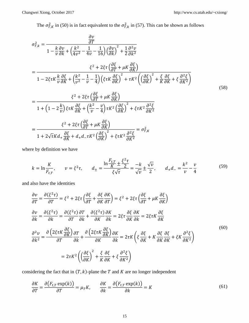
The 𝜎𝑇,𝐾2 in (50) is in fact equivalent to the 𝜎𝑇,𝑘
2 in (57). This can be shown as follows
𝜎𝑇,𝑘2 =
𝜕𝑣𝜕𝑇
1 −𝑘𝑣𝜕𝑣𝜕𝑘+ (
𝑘2
4𝑣2−14𝑣−116) (𝜕𝑣𝜕𝑘)2
+12𝜕2𝑣𝜕𝑘2
=𝜉2 + 2𝜉𝜏 (
𝜕𝜉𝜕𝑇+ 𝜇𝐾
𝜕𝜉𝜕𝐾)
1 − 2𝜉𝜏𝐾𝑘𝑣𝜕𝜉𝜕𝐾
+ (𝑘2
𝑣2−1𝑣−14)(𝜉𝜏𝐾
𝜕𝜉𝜕𝐾)2
+ 𝜏𝐾2 ((𝜕𝜉𝜕𝐾)2
+𝜉𝐾𝜕𝜉𝜕𝐾
+ 𝜉𝜕2𝜉𝜕𝐾2
)
=𝜉2 + 2𝜉𝜏 (
𝜕𝜉𝜕𝑇+ 𝜇𝐾
𝜕𝜉𝜕𝐾)
1 + (1 − 2𝑘𝑣) 𝜉𝜏𝐾
𝜕𝜉𝜕𝐾
+ (𝑘2
𝑣−𝑣4)𝜏𝐾2 (
𝜕𝜉𝜕𝐾)2
+ 𝜉𝜏𝐾2𝜕2𝜉𝜕𝐾2
=𝜉2 + 2𝜉𝜏 (
𝜕𝜉𝜕𝑇+ 𝜇𝐾
𝜕𝜉𝜕𝐾)
1 + 2√𝜏𝐾𝑑+𝜕𝜉𝜕𝐾
+ 𝑑+𝑑−𝜏𝐾2 (𝜕𝜉𝜕𝐾)2
+ 𝜉𝜏𝐾2𝜕2𝜉𝜕𝐾2
= 𝜎𝑇,𝐾2
(58)
where by definition we have
𝑘 = ln𝐾
𝐹𝑡,𝑇, 𝑣 = 𝜉2𝜏, 𝑑± =
ln𝐹𝑡,𝑇𝐾±𝜉2𝜏2
𝜉√𝜏=−𝑘
√𝑣±√𝑣
2, 𝑑+𝑑− =
𝑘2
𝑣−𝑣
4 (59)
and also have the identities
𝜕𝑣
𝜕𝑇=𝜕(𝜉2𝜏)
𝜕𝑇= 𝜉2 + 2𝜉𝜏 (
𝜕𝜉
𝜕𝑇+𝜕𝜉
𝜕𝐾
𝜕𝐾
𝜕𝑇) = 𝜉2 + 2𝜉𝜏 (
𝜕𝜉
𝜕𝑇+ 𝜇𝐾
𝜕𝜉
𝜕𝐾)
𝜕𝑣
𝜕𝑘=𝜕(𝜉2𝜏)
𝜕𝑘=𝜕(𝜉2𝜏)
𝜕𝑇
𝜕𝑇
𝜕𝑘+𝜕(𝜉2𝜏)
𝜕𝐾
𝜕𝐾
𝜕𝑘= 2𝜉𝜏
𝜕𝜉
𝜕𝐾
𝜕𝐾
𝜕𝑘= 2𝜉𝜏𝐾
𝜕𝜉
𝜕𝐾
𝜕2𝑣
𝜕𝑘2=𝜕 (2𝜉𝜏𝐾
𝜕𝜉𝜕𝐾)
𝜕𝑇
𝜕𝑇
𝜕𝑘+𝜕 (2𝜉𝜏𝐾
𝜕𝜉𝜕𝐾)
𝜕𝐾
𝜕𝐾
𝜕𝑘= 2𝜏𝐾 (𝜉
𝜕𝜉
𝜕𝐾+ 𝐾
𝜕𝜉
𝜕𝐾
𝜕𝜉
𝜕𝐾+ 𝜉𝐾
𝜕2𝜉
𝜕𝐾2)
= 2𝜏𝐾2 ((𝜕𝜉
𝜕𝐾)2
+𝜉
𝐾
𝜕𝜉
𝜕𝐾+ 𝜉
𝜕2𝜉
𝜕𝐾2)
(60)
considering the fact that in (𝑇, 𝑘)-plane the 𝑇 and 𝐾 are no longer independent
𝜕𝐾
𝜕𝑇=𝜕(𝐹𝑡,𝑇 exp(𝑘))
𝜕𝑇= 𝜇𝑇𝐾,
𝜕𝐾
𝜕𝑘=𝜕(𝐹𝑡,𝑇 exp(𝑘))
𝜕𝑘= 𝐾 (61)
Changwei Xiong, October 2017 http://www.cs.utah.edu/~cxiong/
16
3. LOCAL VOLATILITY: PDE BY FINITE DIFFERENCE METHOD
In this chapter, we will present a PDE based local volatility model, in which the local volatility
surface is constructed as a 2-D function that is piecewise constant in maturity and piecewise linear in
log-moneyness (for equity) or delta (for FX). Due to great similarity between FX and equity processes,
our interest lies primarily in the context of equity derivatives, the conclusions and formulas drawn from
our discussion here are in general applicable to FX products with minor changes. In contrast to the
traditional way to construct the local volatility by estimating highly sensitive and numerically unstable
partial derivatives in Dupire formulas, this method relies heavily on solving forward PDE’s to calibrate a
parametrized local volatility surface to vanilla option prices in a bootstrapping manner. Once the local
volatility surface is calibrated, the backward PDE can then be used to price exotic options (e.g. barrier
options) that are in consistent with the market observed implied volatility surface.
Before proceeding to the PDE’s, it is important to have an overview of the date conventions for
equity and equity options. The date conventions for FX products are defined in a similar manner.
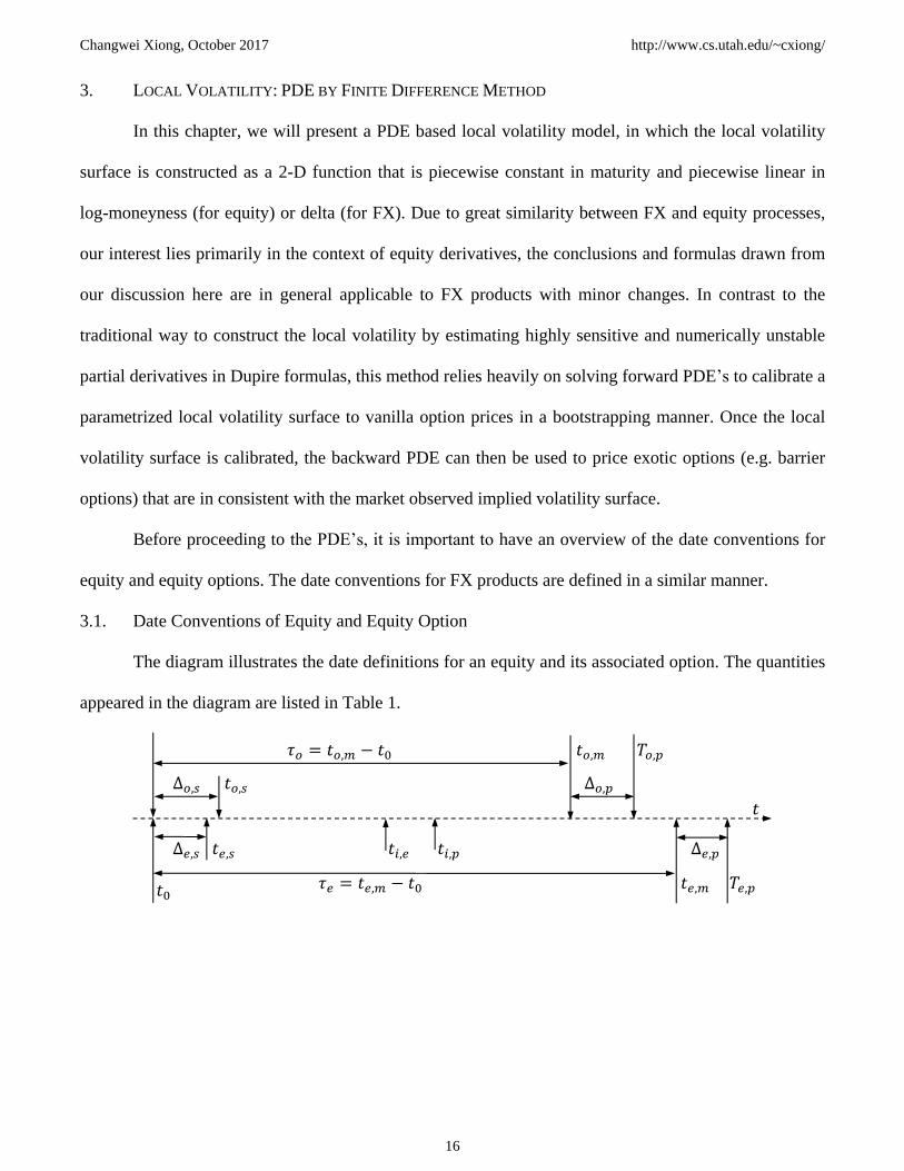
3.1. Date Conventions of Equity and Equity Option
The diagram illustrates the date definitions for an equity and its associated option. The quantities
appeared in the diagram are listed in Table 1.
Δ𝑒,𝑠 𝑡𝑒,𝑠 𝑡𝑖,𝑒 𝑡𝑖,𝑝 Δ𝑒,𝑝
𝑡
Δ𝑜,𝑠 𝑡𝑜,𝑠 Δ𝑜,𝑝
𝜏𝑜 = 𝑡𝑜,𝑚 − 𝑡0 𝑡𝑜,𝑚 𝑇𝑜,𝑝
𝜏𝑒 = 𝑡𝑒,𝑚 − 𝑡0 𝑡𝑒,𝑚 𝑇𝑒,𝑝 𝑡0
Changwei Xiong, October 2017 http://www.cs.utah.edu/~cxiong/
17
Table 1. Dates of Equities and Options
attribute symbol description remark/example
trade date 𝑡0 on which the equity/option is traded today
equity spot lag Δ𝑒,𝑠 equity premium settlement lag 3D
equity spot date 𝑡𝑒,𝑠 on which the equity premium is settled 𝑡𝑒,𝑠 = 𝑡0⊕Δ𝑒,𝑠
equity maturity date 𝑡𝑒,𝑚 equity maturity date 𝑡𝑒,𝑚 = 𝑡0⊕1𝑌
equity pay lag1 Δ𝑒,𝑝 lag between 𝑡𝑒,𝑚 and 𝑡𝑒,𝑝 e.g. same as Δ𝑒,𝑠
equity pay date 𝑡𝑒,𝑝 on which the equity payoff is settled 𝑡𝑒,𝑝 = 𝑡𝑒,𝑚⊕Δ𝑒,𝑝
𝑖-th dividend 𝜃𝑖 dividend payment amount
𝑖-th ex- div. date 𝑡𝑖,𝑒 ex-dividend date
𝑖-th div. pay date 𝑡𝑖,𝑝 dividend pay date
option spot lag Δ𝑜,𝑠 option premium settlement lag 2D
option spot date 𝑡𝑜,𝑠 on which the option is settled 𝑡𝑜,𝑠 = 𝑡0⊕Δ𝑜,𝑠
option maturity date 𝑡𝑜,𝑚 option maturity date 𝑡𝑜,𝑚 = 𝑡0⊕1𝑌
option pay lag Δ𝑜,𝑝 lag between 𝑡𝑜,𝑚 and 𝑡𝑜,𝑝 e.g. same as Δ𝑜,𝑠
option pay date 𝑡𝑜,𝑝 on which the equity payoff is settled 𝑡𝑜,𝑝 = 𝑡𝑜,𝑚⊕Δ𝑜,𝑝
day rolling ⊕ rolling with convention “following” Following
calendar defining business days and holidays US / UK / HK
As most of the quantities are self-explanatory, our discussion focuses more on the treatment of
equity dividends.
3.2. Deterministic Dividends
In our example, we can assume both the short rate and the dividend rate are deterministic and
continuous, e.g. time-dependent 𝑟𝑢 and 𝑞𝑢 as in (21). the equity forward in this case can be calculated by
𝐹(𝑡0, 𝑡𝑒,𝑚) = 𝑆(𝑡0)𝑃𝑞(𝑡𝑒,𝑠, 𝑡𝑒,𝑝)
𝑃𝑟(𝑡𝑒,𝑠, 𝑡𝑒,𝑝) where
𝑃𝑞(𝑡, 𝑇) = exp(−∫ 𝑞𝑢𝑑𝑢𝑇
𝑡
) , 𝑃𝑟(𝑡, 𝑇) = exp(−∫ 𝑟𝑢𝑑𝑢𝑇
𝑡
)
(62)
In a more realistic implementation, we may assume the underlying equity issues a series of
discrete dividends with fixed amounts in a foreseeable future. It is obvious that the equity spot still
follows the SDE (21) with 𝑞𝑢 = 0 in between two adjacent ex-dividend dates (There is discontinuity in
1 Equity settlement delay
Changwei Xiong, October 2017 http://www.cs.utah.edu/~cxiong/
18
spot process on ex-dividend dates that demands special treatment. This will be discussed in detail in due
course). With fixed dividends, the equity forward becomes
𝐹(𝑡0, 𝑡𝑒,𝑚) =𝑆(𝑡0) − ∑ 𝜃𝑖𝑃𝑟(𝑡𝑒,𝑠, 𝑡𝑖,𝑝)𝑖
𝑃𝑟(𝑡𝑒,𝑠, 𝑡𝑒,𝑝) for 𝑡0 < 𝑡𝑖,𝑒 ≤ 𝑡𝑒,𝑚 (63)
where 𝜃𝑖 is the fixed amount of the 𝑖-th dividend issued on ex-dividend date 𝑡𝑖,𝑒.
Discrete dividend can also be modeled as proportional dividend. It assumes that at each ex-
dividend date, the dividend payment will result in a price drop in equity spot proportional to the spot
level. For example, the equity spot before and after the dividend fall has the relationship
𝑆(𝑡𝑖,𝑒 + Δ) = 𝑆(𝑡𝑖,𝑒 − Δ)(1 − 𝜂𝑖) (64)
where Δ denotes an infinitesimal amount of time and 𝜂𝑖 the proportional dividend rate at ex-dividend
date 𝑡𝑖,𝑒. By this relationship, we can write the equity forward as
𝐹(𝑡0, 𝑡𝑒,𝑚) = 𝑆(𝑡0)∏ (1 − 𝜂𝑖)𝑖
𝑃𝑟(𝑡𝑒,𝑠, 𝑡𝑒,𝑝) for 𝑡0 < 𝑡𝑖,𝑒 ≤ 𝑡𝑒,𝑚 (65)
Sometimes it is often more convenient to approximate the fixed dividends by proportional
dividends. The conversion can be achieved by equating the equity forward in (63) and in (65), such that
∏(1− 𝜂𝑖)
𝑖
= 1 −1
𝑆(𝑡0)∑𝜃𝑖𝑃𝑟(𝑡𝑒,𝑠, 𝑡𝑖,𝑝)
𝑖
for 𝑡0 < 𝑡𝑖,𝑒 ≤ 𝑡𝑒,𝑚 (66)
The proportional dividend 𝜂𝑖 can then be bootstrapped from a series of fixed dividends 𝜃𝑖 starting from
the first ex-dividend date.
3.3. Forward PDE
In the following, our derivation is based on the spot process 𝑆𝑡 defined in (21) and its variants.
For example, depending on the application we may write the SDE (21) in terms of log-spot 𝓏𝑢 = ln 𝑆𝑢
or in terms of centered log-spot 𝑧𝑢 = ln𝑆𝑢
𝐹𝑡,𝑢
𝑑𝓏𝑢 = (𝜇𝑢 −1
2𝜎(𝑢, 𝓏)2) 𝑑𝑢 + 𝜎(𝑢, 𝓏)𝑑�̃�𝑢 and 𝑑𝑧𝑢 = −
1
2𝜎(𝑢, 𝑧)2𝑑𝑢 + 𝜎(𝑢, 𝑧)𝑑�̃�𝑢 (67)
Changwei Xiong, October 2017 http://www.cs.utah.edu/~cxiong/
19
where 𝜎(𝑢, 𝓏) and 𝜎(𝑢, 𝑧) are the local volatility function of 𝓏 and 𝑧, respectively.
Let’s denote the forward temporal variable by 𝑢 for 𝑡 < 𝑢 < 𝑇 , the spatial variable by log-
moneyness 𝑘 = ln𝐾
𝐹𝑡,𝑢 (as in (41)) and the spot by 𝑧 = ln
𝑆𝑢
𝐹𝑡,𝑢. Given that 𝑧𝑡 = 0 , the value of a
normalized forward call can be defined as
𝑉𝑢,𝑘|𝑡,𝑧 =𝐶𝑢,𝑘|𝑡,𝑧𝐹𝑡,𝑢
=�̃�[(𝑆𝑢 − 𝐾)
+|𝑡, 𝑆𝑡]
𝐹𝑡,𝑢 (68)
Let 𝜎𝑢,𝑘 be the local volatility function of variable 𝑘 equivalent to 𝜎𝑇,𝐾. We can derive the forward PDE
for 𝑉𝑢,𝑘|𝑡,𝑧 from (43)
𝜎𝑢,𝑘2
2=𝐹𝑡,𝑢
𝜕𝑉𝑢,𝑘|𝑡,𝑧𝜕𝑢
+ 𝜇𝑢𝐹𝑡,𝑢𝑉𝑢,𝑘|𝑡,𝑧 − 𝜇𝑢𝐶𝑢,𝑘|𝑡,𝑧
𝐹𝑡,𝑢𝜕2𝑉𝑢,𝑘|𝑡,𝑧𝜕𝑘2
− 𝐹𝑡,𝑢𝜕𝑉𝑢,𝑘|𝑡,𝑧𝜕𝑘
=
𝜕𝑉𝑢,𝑘|𝑡,𝑧𝜕𝑢
𝜕2𝑉𝑢,𝑘|𝑡,𝑧𝜕𝑘2
−𝜕𝑉𝑢,𝑘|𝑡,𝑧𝜕𝑘
⟹𝜕𝑉𝑢,𝑘|𝑡,𝑧𝜕𝑢
=𝜎𝑢,𝑘2
2(𝜕2𝑉𝑢,𝑘|𝑡,𝑧𝜕𝑘2
−𝜕𝑉𝑢,𝑘|𝑡,𝑧𝜕𝑘
)
(69)
with initial condition
𝑉𝑡,𝑘|𝑡,𝑧 =𝐶𝑡,𝑘|𝑡,𝑧𝐹𝑡,𝑡
=�̃� [(𝑆𝑡 − 𝐹𝑡,𝑡𝑒
𝑘)+| 𝑡, 𝑆𝑡]
𝐹𝑡,𝑡= (1 − 𝑒𝑘)+ (70)
using the partial derivatives
𝜕𝑉𝑢,𝑘|𝑡,𝑧𝜕𝑢
=1
𝐹𝑡,𝑢
𝜕𝐶𝑢,𝑘|𝑡,𝑧𝜕𝑢
− 𝜇𝑢𝑉𝑢,𝑘|𝑡,𝑧 , 𝜕𝑉𝑢,𝑘|𝑡,𝑧𝜕𝑘
=1
𝐹𝑡,𝑢
𝜕𝐶𝑢,𝑘|𝑡,𝑧𝜕𝑘
, 𝜕2𝑉𝑢,𝑘|𝑡,𝑧𝜕𝑘2
=1
𝐹𝑡,𝑢
𝜕2𝐶𝑢,𝑘|𝑡,𝑧𝜕𝑘2
(71)
The PDE (69) appears drift-less and provides more robust calibration stability at low volatility and/or
high drift due to the “transparency” of drift in the PDE.
3.3.1. Treatment of Deterministic Dividends
A (discrete) dividend pay-out will typically result in a drop in equity price on the ex-dividend
date. Suppose that time 𝑢 is the ex-dividend date, the no-arbitrage condition states that at 𝑢+ the time
right after the ex-dividend date (e.g. the difference between 𝑢 and 𝑢+ can be infinitesimal), we must
have
Changwei Xiong, October 2017 http://www.cs.utah.edu/~cxiong/
20
𝑆𝑢+ = 𝑆𝑢 − 𝜃𝑢 (72)
where 𝜃𝑢 is the value of dividend issued at 𝑢 (note that in a rigorous setup the value must take into
account the discounting effect due to dividend payment delay). Since a forward is expectation of spot
under risk neutral measure1, we may write
𝐹𝑡,𝑢+ = �̃�𝑡[𝑆𝑢+] = �̃�𝑡[𝑆𝑢 − 𝜃𝑢] = 𝐹𝑡,𝑢 − �̃�𝑡[𝜃𝑢] (73)
Under the assumption that 𝜃𝑢 is a fixed amount, it reads
𝐹𝑡,𝑢+ = 𝐹𝑡,𝑢 − 𝜃𝑢 (74)
In our finite difference method, the spatial grid for log-moneyness 𝑘 is assumed uniform such that 𝑘𝑖 −
𝑘𝑖−1 is constant for all 𝑖. Dividend payment causes discontinuity in the underlying spot. Evolving the
forward PDE (69) from initial time 𝑡 produces a state vector 𝑉𝑢,𝑘|𝑡,𝑧 at time 𝑢. Immediately after the
issuance of dividend at time 𝑢+, the spot and forward drop the same 𝜃𝑢 amount and hence the state
vector 𝑉𝑢+,𝑘|𝑡,𝑧 must be realigned to reflect the dividend fall. This can be done using the option no-
arbitrage condition, such that
𝐶𝑢+,𝑘|𝑡,𝑧 = �̃�𝑡 [(𝑆𝑢+ − 𝐾)+] = �̃�𝑡 [(𝑆𝑢 − 𝜃𝑢 − 𝐹𝑡,𝑢+𝑒
𝑘)+] = �̃�𝑡 [(𝑆𝑢 − 𝐹𝑡,𝑢𝑒
�̂�)+] = 𝐶𝑢,�̂�|𝑡,𝑧
where �̂� = ln𝐹𝑡,𝑢+𝑒
𝑘 + 𝜃𝑢
𝐹𝑡,𝑢
(75)
Subsequently we can use �̂� to interpolate from the 𝑉𝑢,𝑘|𝑡,𝑧 state vector and transform the interpolated
value to form 𝑉𝑢+,𝑘|𝑡,𝑧 vector by
𝑉𝑢+,𝑘|𝑡,𝑧 =𝐶𝑢+,𝑘|𝑡,𝑧
𝐹𝑡,𝑢+=𝐶𝑢,�̂�|𝑡,𝑧
𝐹𝑡,𝑢
𝐹𝑡,𝑢𝐹𝑡,𝑢+
=𝐹𝑡,𝑢𝐹𝑡,𝑢+
𝑉𝑢,�̂�|𝑡,𝑧 (76)
If the dividend is proportional, we must have spot price 𝑆𝑢+ = 𝑆𝑢(1 − 𝜂𝑢) for a rate 𝜂𝑢 and
hence forward price 𝐹𝑡,𝑢+ = 𝐹𝑡,𝑢(1 − 𝜂𝑢) before and after the dividend fall. Because we can show that
1 Strictly speaking, a forward on time 𝑇 spot is an expectation of the spot under 𝑇-forward measure, i.e. 𝐹𝑡,𝑇 =
�̂�𝑡𝑇[𝑆𝑇]. However since the interest rate is assumed deterministic, the 𝑇-forward measure coincides with the risk
neutral measure.
Changwei Xiong, October 2017 http://www.cs.utah.edu/~cxiong/
21
𝑉𝑢+,𝑘|𝑡,𝑧 =�̃�𝑡 [(𝑆𝑢+ − 𝐾)
+]
𝐹𝑡,𝑢+=(1 − 𝜂𝑢)�̃�𝑡 [(𝑆𝑢 − 𝐹𝑡,𝑢𝑒
𝑘)+]
𝐹𝑡,𝑢(1 − 𝜂𝑢)=�̃�𝑡 [(𝑆𝑢 − 𝐹𝑡,𝑢𝑒
𝑘)+]
𝐹𝑡,𝑢= 𝑉𝑢,𝑘|𝑡,𝑧 (77)
the state vector remains unchanged before and after the issuance of dividend.
With continuous dividend 𝑞𝑢, the realignment of state vector is unnecessary because there is no
discontinuity in equity spot.
3.4. Backward PDE
Again we assume the spot follows the SDE (21). Without loss of generality, let’s denote
𝐺(𝑆𝑇|𝐾) an arbitrary payoff function with parameter 𝐾, whose value is contingent on 𝑆𝑇 at time 𝑇. One
example of such function would be the payoff function of a call option: 𝐺(𝑆𝑇|𝐾) = (𝑆𝑇 − 𝐾)+. Let
𝑈𝑢,𝑥|𝑇,𝐾 be the expectation of the function 𝐺(𝑆𝑇|𝐾) at time 𝑢 with spatial variable 𝑥 = 𝑆𝑢, which can be
written as
𝑈𝑢,𝑥|𝑇,𝐾 = �̃�[𝐺(𝑆𝑇|𝐾)|𝑢, 𝑥] = ∫𝐺(𝑦|𝐾)𝑝𝑇,𝑦|𝑢,𝑥𝑑𝑦ℝ
(78)
where the transition probability 𝑝𝑇,𝑦|𝑢,𝑥 follows the Kolmogorov backward equation (20)
𝜕𝑝𝑇,𝑦|𝑢,𝑥𝜕𝑢
= 𝜇𝑢𝑥𝜕𝑝𝑇,𝑦|𝑢,𝑥𝜕𝑥
+𝜎𝑢,𝑥2 𝑥2
2
𝜕2𝑝𝑇,𝑦|𝑢,𝑥𝜕𝑥2
(79)
In turn, we can derive the backward PDE for the 𝑈𝑢,𝑥|𝑇,𝐾 such that
𝜕𝑈𝑢,𝑥|𝑇,𝐾𝜕𝑢
= ∫ 𝐺(𝑦|𝐾)𝜕𝑝𝑇,𝑦|𝑢,𝑥𝜕𝑢
𝑑𝑦ℝ
= −∫ 𝐺(𝑦|𝐾) (𝜇𝑢𝑥𝜕𝑝𝑇,𝑦|𝑢,𝑥𝜕𝑥
+𝜎𝑢,𝑥2 𝑥2
2
𝜕2𝑝𝑇,𝑦|𝑢,𝑥𝜕𝑥2
)𝑑𝑦ℝ
= −𝜇𝑢𝑥𝜕𝑈𝑢,𝑥|𝑇,𝐾𝜕𝑥
−𝜎𝑢,𝑥2 𝑥2
2
𝜕2𝑈𝑢,𝑥|𝑇,𝐾𝜕𝑥2
(80)
with terminal condition
𝑈𝑇,𝑥|𝑇,𝐾 = 𝐺(𝑥|𝐾) (81)
3.4.1. PDE in Centered Log-spot
Assuming the spatial variable is 𝑧𝑢 = ln𝑥
𝐹𝑡,𝑢 at time 𝑢, we may write 𝑈𝑢,𝑧|𝑇,𝑘 in the (𝑢, 𝑧)-plane
equivalent to 𝑈𝑢,𝑥|𝑇,𝐾. The backward PDE (80) can then be transformed into
Changwei Xiong, October 2017 http://www.cs.utah.edu/~cxiong/
22
𝜕𝑈𝑢,𝑧|𝑇,𝑘𝜕𝑢
= −𝜎𝑢,𝑧2
2(𝜕2𝑈𝑢,𝑧|𝑇,𝑘𝜕𝑧2
−𝜕𝑈𝑢,𝑧|𝑇,𝑘𝜕𝑧
) (82)
with terminal condition
𝑈𝑇,𝑧|𝑇,𝑘 = 𝐺(𝐹𝑡,𝑇𝑒𝑧|𝐹𝑡,𝑇𝑒
𝑘) (83)
by using the following partial derivatives derived from the chain rule
𝜕𝑧
𝜕𝑥=1
𝑥,
𝜕𝑧
𝜕𝑢= −𝜇𝑢,
𝜕𝑈𝑢,𝑥|𝑇,𝐾𝜕𝑢
=𝜕𝑈𝑢,𝑧|𝑇,𝑘𝜕𝑢
+𝜕𝑈𝑢,𝑧|𝑇,𝑘𝜕𝑧
𝜕𝑧
𝜕𝑢=𝜕𝑈𝑢,𝑧|𝑇,𝑘𝜕𝑢
− 𝜇𝑢𝜕𝑈𝑢,𝑧|𝑇,𝑘𝜕𝑧
𝜕𝑈𝑢,𝑥|𝑇,𝐾𝜕𝑥
=𝜕𝑈𝑢,𝑧|𝑇,𝑘𝜕𝑧
𝜕𝑧
𝜕𝑥=1
𝑥
𝜕𝑈𝑢,𝑧|𝑇,𝑘𝜕𝑧
,𝜕2𝑈𝑢,𝑥|𝑇,𝐾𝜕𝑥2
=1
𝑥2(𝜕2𝑈𝑢,𝑧|𝑇,𝑘𝜕𝑧2
−𝜕𝑈𝑢,𝑧|𝑇,𝑘𝜕𝑧
)
(84)
3.4.1.1. Treatment of Deterministic Dividends
With fixed dividend 𝜃𝑢, we have
𝑆𝑢+ = 𝑆𝑢 − 𝜃𝑢 and 𝐹𝑡,𝑢+ = 𝐹𝑡,𝑢 − 𝜃𝑢 (85)
The no arbitrage condition shows that for the spatial grid 𝑧
𝑈𝑢,𝑧|𝑇,𝑘 = �̃�[𝐺(𝑆𝑇|𝐹𝑡,𝑇𝑒𝑘)|𝑢, 𝐹𝑡,𝑢𝑒
𝑧] = �̃�[𝐺(𝑆𝑇|𝐹𝑡,𝑇𝑒𝑘)|𝑢+, 𝐹𝑡,𝑢𝑒
𝑧 − 𝜃𝑢]
= �̃�[𝐺(𝑆𝑇|𝐹𝑡,𝑇𝑒𝑘)|𝑢+, 𝐹𝑡,𝑢+𝑒
�̂�] = 𝑈𝑢+,�̂�|𝑇,𝑘 where �̂� = ln𝐹𝑡,𝑢𝑒
𝑧 − 𝜃𝑢𝐹𝑡,𝑢+
(86)
It is likely that if 𝑧 is sufficiently small (e.g. at lower boundary of spatial grid) we may end up with
𝐹𝑡,𝑢𝑒𝑧 − 𝜃𝑢 < 0, which makes the �̂� not well defined. A solution is to floor it to a small positive number,
e.g. taking max(10−10, 𝐹𝑡,𝑢𝑒𝑧 − 𝜃𝑢) . This is valid because equity spot must be positive and the
𝑈𝑢+,�̂�|𝑇,𝑘 flattens as �̂� goes to negative infinity. After the special treatment, we can use the �̂� to
interpolate from the 𝑈𝑢,𝑧|𝑇,𝑘 state vector and convert the interpolated value into vector 𝑈𝑢+,𝑧|𝑇,𝑘.
With proportional dividend, the conclusion drawn for forward PDE still applies here and the
state vector remains unchanged before and after the dividend fall. With continuous dividend, the
realignment of state vector is unnecessary because there is no discontinuity in equity spot.
Changwei Xiong, October 2017 http://www.cs.utah.edu/~cxiong/
23
3.4.1.2. Vanilla Call
Due to the duality between the forward and backward PDE, it is evident that vanilla calls (or
puts) must admit the identity: 𝑈𝑡,𝑧|𝑇,𝑘 = 𝑉𝑇,𝑘|𝑡,𝑧𝐹𝑡,𝑇 , where 𝑈𝑡,𝑧|𝑇,𝑘 is the forward call solved from
backward PDE (82) and 𝑉𝑇,𝑘|𝑡,𝑧 the normalized forward call solved from forward PDE (69). This
relationship can be used to check the correctness of implementation of the numerical engines of forward
and backward PDE.
3.4.2. PDE in Log-spot
For pricing some exotic options, e.g. barrier options, it is more convenient to use log-spot 𝓏 =
ln 𝑥 as the spatial variable. Similarly we can define 𝓀 = ln𝐾. Let’s denote the (discounted) price of a
derivative product by
𝑋𝑢,𝓏|𝑇,𝓀 = 𝐷𝑢,𝑇𝑈𝑢,𝓏|𝑇,𝓀 = �̃�[𝐷𝑢,𝑇𝐺(𝑆𝑇|𝑒𝑘)|𝑢, 𝑒𝓏] (87)
By taking into account the discount factor, it must follow the following backward PDE
𝜕𝑋𝑢,𝓏|𝑇,𝓀𝜕𝑢
= 𝑟𝑢𝑋𝑢,𝓏|𝑇,𝓀 + 𝐷𝑢,𝑇𝜕𝑈𝑢,𝓏|𝑇,𝓀𝜕𝑢
= 𝑟𝑢𝑋𝑢,𝓏|𝑇,𝓀 + 𝐷𝑢,𝑇 (−𝜇𝑢𝑥1
𝑥
𝜕𝑈𝑢,𝓏|𝑇,𝓀𝜕𝓏
−𝜎𝑢,𝓏2
2
1
𝑥2(𝜕2𝑈𝑢,𝓏|𝑇,𝓀𝜕𝓏2
−𝜕𝑈𝑢,𝓏|𝑇,𝓀𝜕𝓏
))
= −𝜎𝑢,𝓏2
2
𝜕2𝑋𝑢,𝓏|𝑇,𝓀𝜕𝓏2
+ (𝜎𝑢,𝓏2
2− 𝜇𝑢)
𝜕𝑋𝑢,𝓏|𝑇,𝓀𝜕𝓏
+ 𝑟𝑢𝑋𝑢,𝓏|𝑇,𝓀
(88)
where the partial derivatives below have been used
𝜕𝓏
𝜕𝑥=1
𝑥,
𝜕𝓏
𝜕𝑢= 0,
𝜕𝑈𝑢,𝑥|𝑇,𝐾𝜕𝑢
=𝜕𝑈𝑢,𝓏|𝑇,𝓀𝜕𝑢
+𝜕𝑈𝑢,𝓏|𝑇,𝓀𝜕𝓏
𝜕𝓏
𝜕𝑢=𝜕𝑈𝑢,𝓏|𝑇,𝓀𝜕𝑢
𝜕𝑈𝑢,𝑥|𝑇,𝐾𝜕𝑥
=𝜕𝑈𝑢,𝓏|𝑇,𝓀𝜕𝑢
𝜕𝑢
𝜕𝑥+𝜕𝑈𝑢,𝓏|𝑇,𝓀𝜕𝓏
𝜕𝓏
𝜕𝑥=1
𝑥
𝜕𝑈𝑢,𝓏|𝑇,𝓀𝜕𝓏
𝜕2𝑈𝑢,𝑥|𝑇,𝐾𝜕𝑥2
=𝜕
𝜕𝑥(1
𝑥
𝜕𝑈𝑢,𝓏|𝑇,𝓀𝜕𝓏
) = −1
𝑥2𝜕𝑈𝑢,𝓏|𝑇,𝓀𝜕𝓏
+1
𝑥
𝜕2𝑈𝑢,𝓏|𝑇,𝓀𝜕𝓏𝜕𝑢
𝜕𝑢
𝜕𝑥+1
𝑥
𝜕2𝑈𝑢,𝓏|𝑇,𝓀𝜕𝓏2
𝜕𝓏
𝜕𝑥
=1
𝑥2(𝜕2𝑈𝑢,𝓏|𝑇,𝓀𝜕𝓏2
−𝜕𝑈𝑢,𝓏|𝑇,𝓀𝜕𝓏
)
(89)
Changwei Xiong, October 2017 http://www.cs.utah.edu/~cxiong/
24
3.4.2.1. Treatment of Deterministic Dividends
With fixed dividend 𝜃𝑢, the no arbitrage condition states that
𝑋𝑢,𝓏|𝑇,𝓀 = �̃�[𝐷𝑢,𝑇𝐺(𝑆𝑇|𝑒𝓀)|𝑢, 𝑒𝓏] = �̃�[𝐷𝑢+,𝑇𝐺(𝑆𝑇|𝑒
𝓀)|𝑢+, 𝑒𝓏 − 𝜃𝑢]
= �̃�[𝐷𝑢+,𝑇𝐺(𝑆𝑇|𝑒𝓀)|𝑢+, 𝑒
�̂�] = 𝑋𝑢+,�̂�|𝑇,𝓀 where �̂� = ln(𝑒𝓏 − 𝜃𝑢)
(90)
Again, extremely small 𝓏 may result in �̂� that is not well defined, we may floor the difference 𝑒𝓏 − 𝜃𝑢
to a small positive number, e.g. taking max(10−10, 𝑒𝓏 − 𝜃𝑢) . The vector 𝑋𝑢,𝓏|𝑇,𝓀 can then be
interpolated from the known 𝑋𝑢+,𝓏|𝑇,𝓀 using the �̂�.
With proportional dividend 𝜂𝑢, again the no arbitrage condition shows
𝑋𝑢,𝓏|𝑇,𝓀 = �̃�[𝐷𝑢,𝑇𝐺(𝑆𝑇|𝑒𝓀)|𝑢, 𝑒𝓏] = �̃�[𝐷𝑢+,𝑇𝐺(𝑆𝑇|𝑒
𝓀)|𝑢+, 𝑒𝓏(1 − 𝜂𝑢)]
= �̃�[𝐷𝑢+,𝑇𝐺(𝑆𝑇|𝑒𝓀)|𝑢+, 𝑒
�̂�] = 𝑋𝑢+,�̂�|𝑇,𝓀 where �̂� = 𝓏 + ln(1 − 𝜂𝑢)
(91)
The vector 𝑋𝑢,𝓏|𝑇,𝓀 can be interpolated from the 𝑋𝑢+,𝓏|𝑇,𝓀 using the �̂�.
With continuous dividend, the realignment of state vector is unnecessary because there is no
discontinuity in equity spot.
3.5. Local Volatility Surface
This section is devoted to discussing the construction of local volatility surface 𝜎(𝑢, 𝑘). There
are various ways to define the local volatility surface. The one that we would like to discuss is a 2-D
function that is piecewise constant in maturity 𝑢 and piecewise linear in log-moneyness 𝑘 = ln𝐾
𝐹𝑡,𝑢 (or in
delta for FX). The volatility surface comprises a series of volatility smiles 𝜎𝑗(𝑘) for maturity 𝑡 < 𝑢1 <
⋯ < 𝑢𝑗 < ⋯ < 𝑢𝑚 = 𝑇 . At each maturity 𝑢𝑗 , volatility smile 𝜎𝑗(𝑘) is constructed by linear
interpolation between log-moneyness pillars 𝑘𝑖 = ln𝐾𝑖
𝐹𝑡,𝑢 for strikes 𝐾1 < ⋯ < 𝐾𝑖 < ⋯ < 𝐾𝑛 and flat
extrapolation where the volatility values at 𝑘1 and 𝑘𝑛 are used for all 𝑘 < 𝑘1 and 𝑘 > 𝑘𝑛, respectively.
The smile 𝜎𝑗(𝑘) constructed at 𝑢𝑗 is assumed to remain constant over time for any 𝑢 between the two
adjacent maturities 𝑢𝑗−1 < 𝑢 ≤ 𝑢𝑗.
Changwei Xiong, October 2017 http://www.cs.utah.edu/~cxiong/
25
Calibration of the local volatility surface is conducted in a bootstrapping manner starting from
the shortest maturity 𝑢1. It is done by solving the forward PDE such that the local volatility surface is
able to reproduce the vanilla call prices at the prescribed log-moneyness pillars 𝑘𝑖 for each of the
maturities 𝑢𝑗. The PDE can be solved using finite difference method1 on a uniform grid defined on log-
moneyness 𝑘 that extends to ±5 standard deviations of the underlying spot. The choice of boundary
condition has little impact to the solutions of vanilla option prices because at ±5 standard deviations the
transition probability becomes negligibly small. Our application uses linearity boundary condition for its
simplicity. To allow a higher tolerance to market data input and smoother calibration process, the
objective function may include a penalty term to suppress unfavorable concavity of a local volatility
smile. Again, there can be many ways to define the objective function as well as the penalty function. In
this essay, we will only focus on the simplest objective (e.g. at maturity 𝑢𝑗 ): the least square
minimization of vanilla call prices
argmin𝜎𝑗(𝑘𝑖)
∑(𝑈𝑡,𝑧|𝑢𝑗,𝑘𝑖𝐵𝑆 − 𝑈𝑡,𝑧|𝑢𝑗,𝑘𝑖
𝑃𝐷𝐸 )2
𝑛
𝑖=1
(92)
where 𝑈𝑡,𝑧|𝑇,𝑘 is the normalized forward call price defined in (68), the superscript “BS” denotes the
theoretical price by Black-Scholes model and the “PDE” denotes the numerical value by forward PDE.
Note that without a penalty term, the minimization can lead to an exact solution given a proper2 implied
volatility surface.
3.6. Barrier Option Pricing
In contrast to the calibration, the pricing of a barrier option relies on the backward PDE (88) in
line with proper terminal condition (i.e. payoff function) and boundary conditions defined by the
characteristics of the barrier option. Barrier options often demand a spatial grid defined on log-spot 𝓏 =
ln 𝑆𝑢 , which allows an easier fit of time-invariant barrier (e.g. with European or American type of
1 A brief introduction to finite difference method can be found in my notes “Introduction to Interest Rate Models”,
which can be downloaded from http://www.cs.utah.edu/~cxiong/. 2 A proper implied volatility surface should well behave and admit no arbitrage.

Changwei Xiong, October 2017 http://www.cs.utah.edu/~cxiong/
26
observation window) into the domain. For example, an up-and-out barrier option would be priced on a
domain with upper bound at the barrier level 𝑏 where Dirichlet boundary condition is applied (the lower
bound and its boundary condition remain the same as for vanilla options).

Changwei Xiong, October 2017 http://www.cs.utah.edu/~cxiong/
27
REFERENCES
1. Clark, I., Foreign Exchange Option Pricing - A Practitioner’s Guide, Wiley-Finance, 2011, pp.82
2. Online resource: http://itf.fys.kuleuven.be/~nikos/papers/lect4_localvol.pdf
3. Gatheral, J., The Volatility Surface: A Practitioner’s Guide, Wiley-Finance, 2006, pp. 13-14
Related Documents