CHEM 411L
Instrumental Analysis Laboratory
Revision 2.1
Fluorescence Quenching of Human Serum Albumin by Caffeine
In this laboratory exercise we will examine the fluorescence of Human Serum Albumin (HSA)
and its quenching by Caffeine. In molecular fluorescence spectroscopy an analyte is stimulated
by excitation photons and then responds by fluorescing; emitting longer wavelength photons.
The emitted photons are detected by a spectrometer, generating a signal that can be analyzed. It
would be expected that the response signal should be linearly proportional to the analyte
concentration. And this is generally true over a wide range of analyte concentrations. However,
due to limitations in the technique, non-linearities do set in at higher analyte concentrations.
Additionally, other species present in the analyte's solution matrix can quench the analyte's
fluorescence signal. In the present case, HSA's fluorescence signal is quenched by the presence
of Caffeine. Both static and dynamic quenching processes are observed for this system.
Although quenching diminishes an analyte's fluorescence signal, for the present case, we can use
quenching data to determine binding parameters for the interaction of Caffeine with HSA.
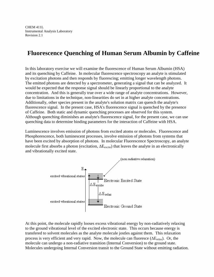
Luminescence involves emission of photons from excited atoms or molecules. Fluorescence and
Phosphorescence, both luminescent processes, involve emission of photons from systems that
have been excited by absorption of photons. In molecular Fluorescence Spectroscopy, an analyte
molecule first absorbs a photon (excitation, Eexcite) that leaves the analyte in an electronically
and vibrationally excited state.
At this point, the molecule rapidly looses excess vibrational energy by non-radiatively relaxing
to the ground vibrational level of the excited electronic state. This occurs because energy is
transfered to solvent molecules as the analyte molecule jostles against them. This relaxation
process is very efficient and very rapid. Now, the molecule can fluoresce (Erelax). Or, the
molecule can undergo a non-radiative transition (Internal Conversion) to the ground state.
Molecules undergoing Internal Conversion transit to the Ground State without emitting radiation.
P a g e | 2
This is an efficient relaxation process when higher vibrational states of the Ground Electronic
State overlap with lower vibrational states of the Excited Electronic State.
Because of non-radiative relaxation in the electronically excited state, excitation energy is
always greater than relaxation energy.
Eexcite > Erelax (Eq. 1)
Since the energy of photons involved in these transitions is inversely related to the photons'
wavelength:
Ephoton = h c / (Eq. 2)
(c is the speed of light and h is Planck’s constant), the wavelength of an exciting photon is
always shorter than that of a photon emitted during relaxation:
excite < relax (Eq. 3)
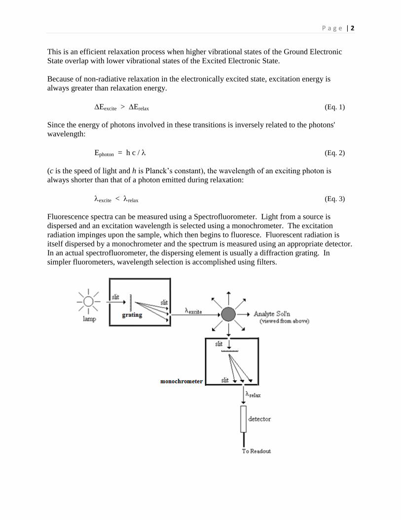
Fluorescence spectra can be measured using a Spectrofluorometer. Light from a source is
dispersed and an excitation wavelength is selected using a monochrometer. The excitation
radiation impinges upon the sample, which then begins to fluoresce. Fluorescent radiation is
itself dispersed by a monochrometer and the spectrum is measured using an appropriate detector.
In an actual spectrofluorometer, the dispersing element is usually a diffraction grating. In
simpler fluorometers, wavelength selection is accomplished using filters.
P a g e | 3
The Flourescent Intensity (F) of an analyte solution will be proportional to the radiant Power
absorbed by the sample (Po-P):
F = K’ (Po – P) (Eq. 4)
Inserting Beer’s Law:
P/Po = 10-bc
(Eq. 5)
and expanding the exponential term, gives us:
F = K’ Po {2.3bc – (2.3bc)2/2 - ...} (Eq. 6)
Provided the sample Absorbance is relatively low, we can truncate the expansion after the first
order terms:
F = 2.3 K’ Po bc (Eq. 7)
When Po is constant, we see the Fluorescent Intensity is proportional to the Concentration of the
analyte:
F = K c (Eq. 8)
This, then, provides a method for quantifying the amount of analyte in a system based on
fluorescence measurements.
A few words of caution. If the concentration of the analyte is high enough, higher order
expansion terms become important and the relationship between F and c is no longer linear.
And, if the concentration becomes very high, the system begins to absorb its own emitted
radiation, causing a decrease in fluorescence intensity and as a result severe non-linearities set in.
Fluorescence spectroscopy is much more sensitive than corresponding Absorbance spectroscopic
techniques. This is because light emitted against a dark background (fluorescence) is much
easier to detect than a slight dimming of intensity against a light background (absorbance).
However, fluorescence techniques are severely limited by the number of analytes that actually
fluoresce. Most systems shed their excitation energy via radiationless pathways. Structurally,
molecules that possess unsubstituted aromatic rings or other structurally rigid elements have a
propensity for fluorescing. Fused-ring heterocycles also fluoresce nicely.
In our case, we will be examining the fluorescence of Human Serum Albumin (HSA). Albumins
constitute a family of globular proteins commonly found in blood serum. They are involved in
the transport of fatty acids, bind cations and buffer the pH of their solution. HSA is a monomeric
67 kDalton protein consisting of 585 amino acid residues and comprises ~50% of all plasma protein.

P a g e | 4
Crystal Structure of Human Serum Albumin
http://en.wikipedia.org/wiki/File:ALB_structure.png
Protein fluorescence is typically due to the presence of three amino acid residues: Tryptophan,
Tyrosine and Phenylalanine. (Note the planarity of these amino acids' side chain rings.)
Tryptophan Tyrosine Phenylalanine
Typically, fluorescence due to the presence of Tryptophan will dominate any protein's spectrum.
Fluorescence Spectra of Tryptophan (Dashed) and 18:1
Tyrosine-Tryptophan Mix (Solid Color)
Biophysical Chemistry
Cantor and Schimmelt
The fluorescence parameters for typical biomolecule constituents are given by Cantor and
Schimmel:

P a g e | 5
As mentioned above, other species in solution can act as quenching agents (Q) and diminish the
fluorescence of the fluorescing analyte. In Dynamic Quenching, the Quencher absorbs radiation
non-radiatively from the excited analyte (S*) causing a decrease in the fluorescence intensity
detected by the instrument's detector.
S + hexcite S* (excitation)
S* + Q S + Q (quenching)
It can be shown the ratio of unquneched-to-quenched fluorescent intensities (Fo/F) is related to
the quenching agent total concentration [Q]Tot via the Stern-Volmer Relation:
Fo/F = 1 + K [Q]Tot (Eq. 9)
where K is the Stern-Volmer constant. K is related to both the fluorescence lifetime of the
fluorescer and the rate constant for the quenching process. Note, Fo/F is linear in the
concentration of the quencher.
If a Stern-Volmer plot, a plot of Fo/F vs.
[Q], is non-linear, a second quenching
process is occurring. An upward
curvature to the plot is indicative of static
quenching. Static quenching occurs when
the quencher complexes with the
fluorescer before excitation can occur.
The complex has unique properties which
may include being non-fluorescent.
When static quenching occurs, the Stern-
Volmer relation must be modified to
P a g e | 6
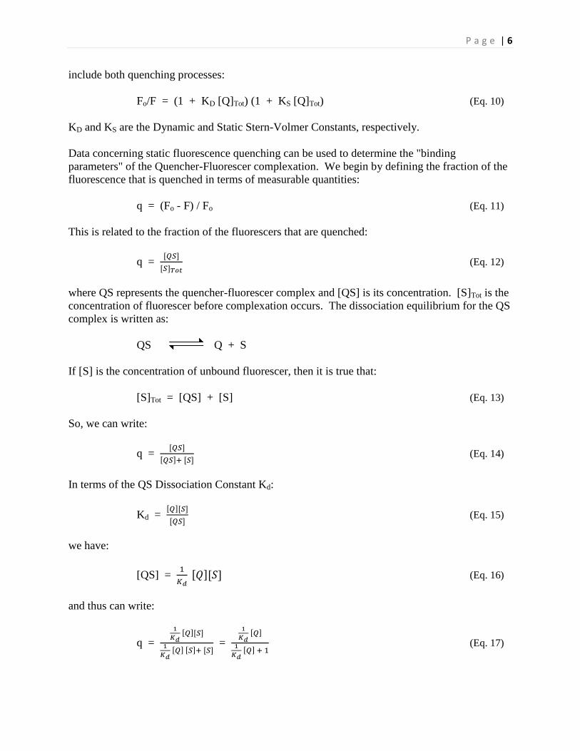
include both quenching processes:
Fo/F = (1 + KD [Q]Tot) (1 + KS [Q]Tot) (Eq. 10)
KD and KS are the Dynamic and Static Stern-Volmer Constants, respectively.
Data concerning static fluorescence quenching can be used to determine the "binding
parameters" of the Quencher-Fluorescer complexation. We begin by defining the fraction of the
fluorescence that is quenched in terms of measurable quantities:
q = (Fo - F) / Fo (Eq. 11)
This is related to the fraction of the fluorescers that are quenched:
q =
(Eq. 12)
where QS represents the quencher-fluorescer complex and [QS] is its concentration. [S]Tot is the
concentration of fluorescer before complexation occurs. The dissociation equilibrium for the QS
complex is written as:
QS Q + S
If [S] is the concentration of unbound fluorescer, then it is true that:
[S]Tot = [QS] + [S] (Eq. 13)
So, we can write:
q =
(Eq. 14)
In terms of the QS Dissociation Constant Kd:
Kd =
(Eq. 15)
we have:
[QS] =
(Eq. 16)
and thus can write:
q =
=
(Eq. 17)
P a g e | 7
Rearranging this equation gives us a relationship between q/[Q] and q that is known as the
Scatchard Equation:
(Eq. 18)
If the fluorescer can independently bind n quenchers, then the Scatchard Equation is modified to
give:
(Eq. 19)
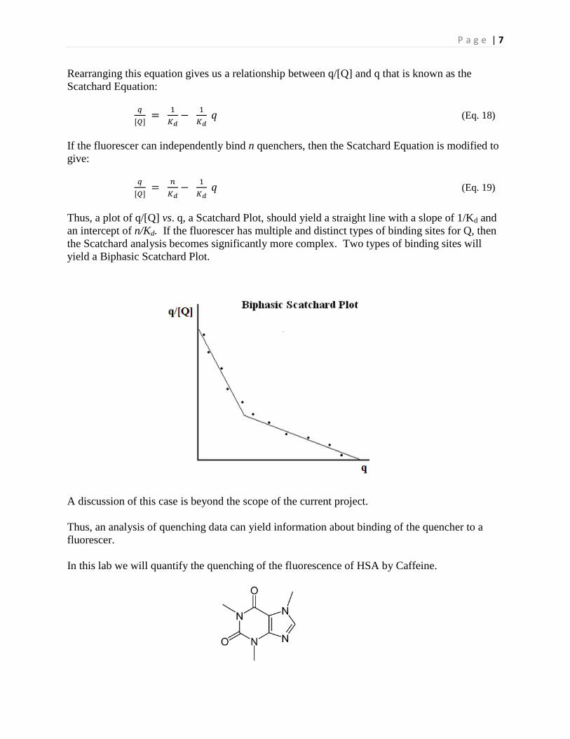
Thus, a plot of q/[Q] vs. q, a Scatchard Plot, should yield a straight line with a slope of 1/Kd and
an intercept of n/Kd. If the fluorescer has multiple and distinct types of binding sites for Q, then
the Scatchard analysis becomes significantly more complex. Two types of binding sites will
yield a Biphasic Scatchard Plot.
A discussion of this case is beyond the scope of the current project.
Thus, an analysis of quenching data can yield information about binding of the quencher to a
fluorescer.
In this lab we will quantify the quenching of the fluorescence of HSA by Caffeine.
P a g e | 8
We will then show both dynamic and static quenching processes are occurring. Finally we will
perform a Scatchard analysis of the quenching data. This analysis will yield the number of
binding sites on the HSA macromolecule for the Caffeine ligand as well as the Caffeine-HSA
dissociation constant.
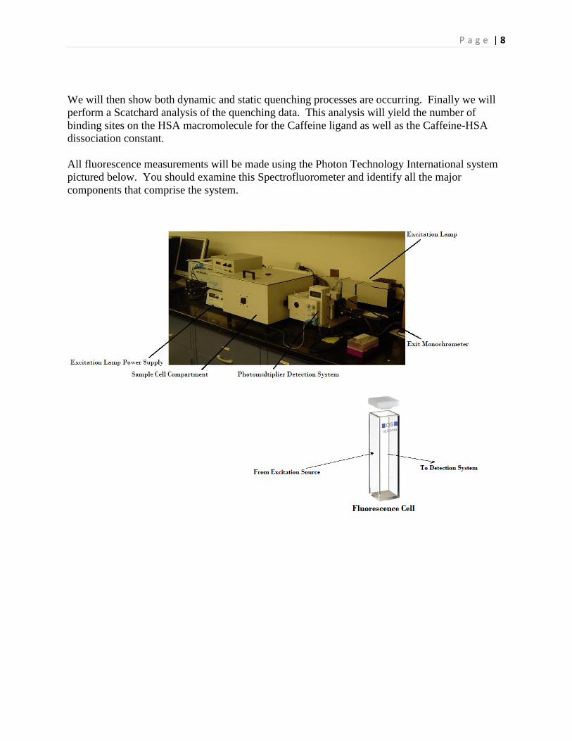
All fluorescence measurements will be made using the Photon Technology International system
pictured below. You should examine this Spectrofluorometer and identify all the major
components that comprise the system.
P a g e | 9
Procedure
Data for HSA
Molecular Weight = 65600 g/mol
Extinction Coefficient = 33700 M-1
cm-1
at 278 nm
Week 1
1. Your laboratory instructor will provide you with a Phosphate buffer (pH = 7.20) with
which to solubilize the powdered HSA. Prepare ~10 mL of HSA solution at about a
concentration of 1mg/mL using this buffer. (This solution may need to be diluted 1:2 in
order to obtain a measurable absorbance and emission signal. You will need to make a few
measurements before deciding whether or not this dilution needs to be performed.)
2. Now obtain an absorbance spectrum for your HSA solution using the Department's UV-
VIS spectrometer Your spectrum should cover the range of 200 - 500 nm. Be sure to use
matched Quartz cuvettes as Glass cuvettes absorb in the UV. (Be very careful with these
cuvettes as Quartz shatters easily when the cuvette is jarred against something.) Determine
the excitation max for HSA from the absorbance spectrum. Use the measured asorbance at
278 nm to determine the concentration of the HSA solution using Beer's Law; A278 =
278bc.
3. Obtain a fluorescence spectrum for your HAS solution using the Department's Photon
Technology International spectrometer. You must use a Quartz fluorescence cuvette for
this spectrum. (Same caution as above.) Use your excitation max as a guide in
determining the wavelength range for the fluorescence spectrum. Determine the emission
max for HSA from the emission spectrum.
4. Store your remaining HSA solution in a refrigerator for use during week 2 of the lab
exercise.
4. Develop a plan for completing the experiment's of week 2 exercises.
Week 2
Week 2 of this experiment will be run as an "Open" lab. The experiment will take about 1 hour
to complete, if you are prepared when coming to the laboratory. Your laboratory instructor will
have a sign-up sheet for available time slots.
1. Determine the range over which the fluorescence of the HSA solution is linear. To do this,
perform serial dilutions of the stock HSA solution and measure the fluorescence F at each
P a g e | 10
dilution. Dilutions should be performed using the Phosphate buffer. Keep in mind you
only need 3mL of solution to fill the spectrometer cell.
2. Measure the quenching of the HSA fluorescence by Caffeine. Do this by first preparing
stock solutions of Caffeine (~5.8 x 10⁻³
M) and HSA (~1.5 x 10⁻⁵ M). The HSA stock
solution should be prepared using the remaining HSA solution from week 1. Then use
variable volumes of the Caffeine solution with a constant volume of the HSA solution to
prepare the series of Caffeine-HAS solutions needed for the Scatchard analysis. Bring all
the solutions to the same volume by adding additional phosphate buffer. Keep in mind you
only need 3mL of solution to fill a spectrometer cell. Also, you need to make a
measurement of the HSA absent any Caffeine to determine Fo.
P a g e | 11
Data Analysis
You will prepare a full laboratory report for this exercise. Your report should include the
following:
Both absorbance and fluorescence spectra for HSA.
A plot of F vs. [HAS] and a discussion of the range of the linearity and causes for
observed non-linearities.
A Stern-Volmer plot: Fo/F vs. [Caff]Tot. It should also include a discussion of the
quenching processes which occur when Caffeine quenches HSA fluorescence.
A plot of Kapp vs. [Caff]Tot, where Kapp is the Apparent Stern-Volmer Constant. This
is given by Kapp = (KD + KS) + KD KS [Caff]Tot = (Fo/F - 1)/[Caff]Tot. Comment
on your results and why Kapp is defined in this manner.
A plot of q vs. [Caff]Tot / [HSA]Tot. Comment on your results.
A Scatchard Plot; q/[Caff] vs. q. Comment on your results.
Note: [Caff] represents the free concentration of the quencher [Q]. This can
be determined from measureable quantities in general via,
[Q]Tot = [Q] + [QS]
or [Q] = [Q]Tot - [QS]
which by (eq. 12) yields,
[Q] = [Q]Tot - q [S]Tot
So,
[Caff] = [Caff]Tot - q [HAS]Tot
Your determination of Kd and n for HAS-Caffeine complexation. Error estimates
should be included. Comment on your results. Further, comment on the legitimacy
of using a Linear Least Squares Analysis to determine these parameters.

P a g e | 12
References
Cantor, Charles R. and Schimmel, Paul R. "Biophysical Chemistry, Part II: Techniques for the
Study of Biological Structure and Function" W.H. Freeman and Company, San Francisco.
Montero, Maria Teresa; Hernandez, Jordi and Estelrich, Joan "Fluorescence Quenching of
Albumin. A spectrofluorimetric experiment" Biochemical Education 18 (1990) 99.
Skoog, Douglas A., Holler, F. James and Crouch, Stanley R. (2007) " Principles of Instrumental
Analysis, 6th
Ed." Thomson, Belmont, California.