
ETHIOPIAN INSTITUTE OF TECHNOLOGY MEKELLE
EiT-M
CIVIL ENGINEERING DEPARTMENT
Hydraulic Engineering Post Graduate Program
Course: Hydraulic Structures II Subject: Diversion Works and Canal Design
Submitted to: Dr. Mohammad. A/Kadir (Asst. Proff.)
Submitted by: Biruk Shewayirga Mohammed Demise Omer Abdi
CONTENTS:
1. CROP WATER REQUIREMENT 2. HEAD WORK DESIGN 3. CANAL LAY OUT AND DESIGN 4. DESIGN OF CROSS DRAINAGE STRUCTURES 5. DESIGN OF DROP STRUCTURES 6. DESIGN OF FLOW MEASUREMENT STRUCTURE
SEPARATE APPENDIXES:
1. Rainfall frequency analysis and peak flood hydrograph (spread sheet) 2. Weir axis and canal profiles (spread sheet)
Stage discharge curves Main canal profile Secondary canals’ profile Parshall flume dimensions
3. Canal profiles (Auto CAD file) 4. Cross drainage structures (Auto CAD file) 5. Weir and under sluice cross-sections (Auto CAD file) 6. Network of irrigation canals (AutoCAD file)
1. PROJECT DEMAND
(CROP WATER REQUIREMENT)
1.1. Crop water requirement:
The analysis of crop water requirement is needed to determine the amount of water that has to be applied
to the crop through irrigation without causing the plant exposed under excessive stress. On the other hand
this value is called the duty of the intended project (the amount of water discharge needed to irrigate one
hectare _lit/sec./ha).
Therefore, the size of any irrigation structure is merely depend on the value of the design discharge or the
duty. Once the discharge has been known the demand of the project for the command area to irrigated can
also be determined.
Generally crop water requirement is vital to determine the size and capacity of irrigation structures to be
constructed; i.e. it helps to:
Determine the height of diversion structure(taking the command area elevation under
consideration)
Fix the size of the off take canal
Fix the size of the main canal, secondary and tertiary canals
Decide if it is necessary to construct a night storage
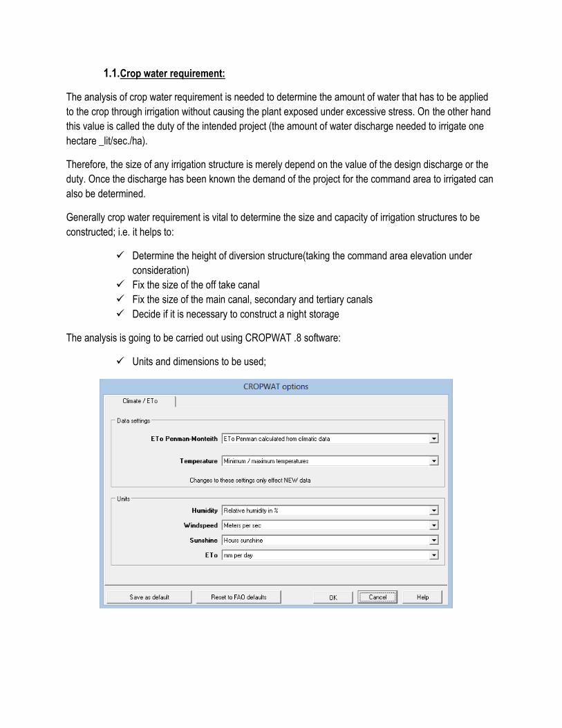
The analysis is going to be carried out using CROPWAT .8 software:
Units and dimensions to be used;
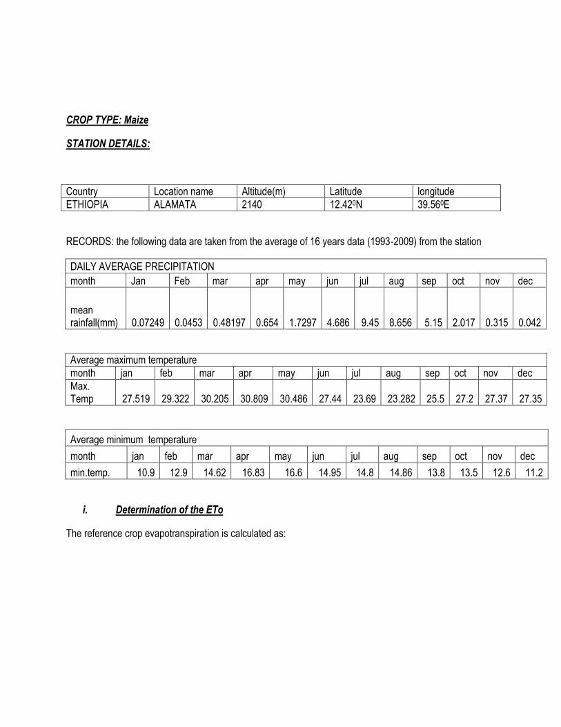
CROP TYPE: Maize
STATION DETAILS:
Country Location name Altitude(m) Latitude longitude
ETHIOPIA ALAMATA 2140 12.420N 39.560E
RECORDS: the following data are taken from the average of 16 years data (1993-2009) from the station
DAILY AVERAGE PRECIPITATION
month Jan Feb mar apr may jun jul aug sep oct nov dec
mean rainfall(mm) 0.07249 0.0453 0.48197 0.654 1.7297 4.686 9.45 8.656 5.15 2.017 0.315 0.042
Average maximum temperature
month jan feb mar apr may jun jul aug sep oct nov dec
Max. Temp 27.519 29.322 30.205 30.809 30.486 27.44 23.69 23.282 25.5 27.2 27.37 27.35
Average minimum temperature
month jan feb mar apr may jun jul aug sep oct nov dec
min.temp. 10.9 12.9 14.62 16.83 16.6 14.95 14.8 14.86 13.8 13.5 12.6 11.2
i. Determination of the ETo
The reference crop evapotranspiration is calculated as:
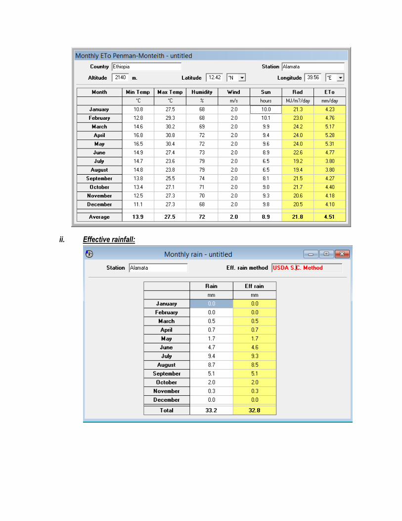
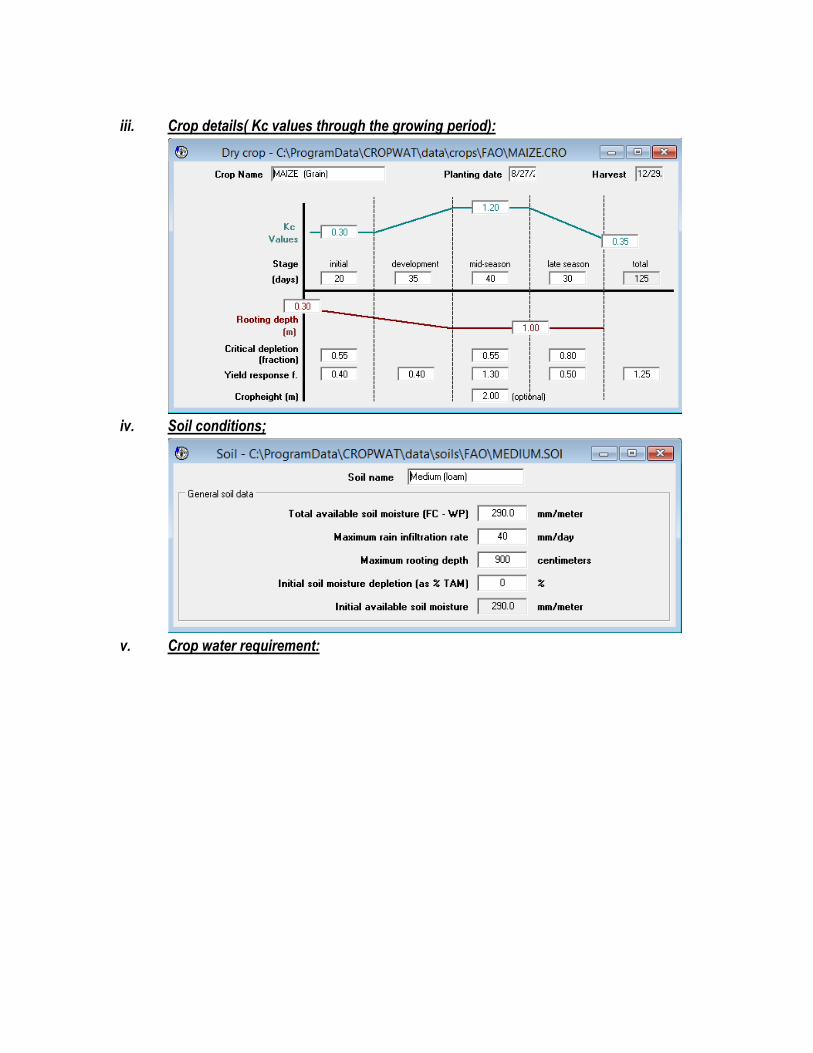
ii. Effective rainfall:
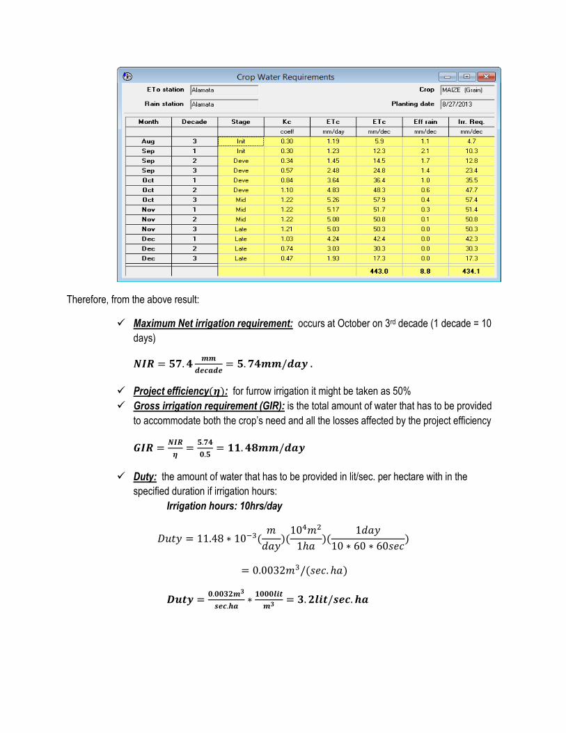
iii. Crop details( Kc values through the growing period):
iv. Soil conditions;
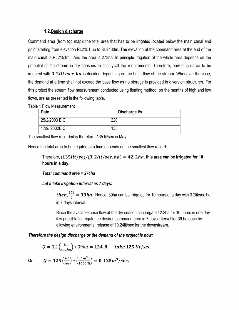
v. Crop water requirement:
Therefore, from the above result:
Maximum Net irrigation requirement: occurs at October on 3rd decade (1 decade = 10
days)
.
Project efficiency : for furrow irrigation it might be taken as 50%
Gross irrigation requirement (GIR): is the total amount of water that has to be provided
to accommodate both the crop’s need and all the losses affected by the project efficiency
Duty: the amount of water that has to be provided in lit/sec. per hectare with in the
specified duration if irrigation hours:
Irrigation hours: 10hrs/day
1.2. Design discharge
Command area (from top map): the total area that has to be irrigated located below the main canal end
point starting from elevation RL2151 up to RL2130m. The elevation of the command area at the end of the
main canal is RL2151m. And the area is 273ha. In principle irrigation of the whole area depends on the
potential of the stream in dry seasons to satisfy all the requirements. Therefore, how much area to be
irrigated with is decided depending on the base flow of the stream. Whenever the case,
the demand at a time shall not exceed the base flow as no storage is provided in diversion structures. For
this project the stream flow measurement conducted using floating method, on the months of high and low
flows, are as presented in the following table.
Table 1 Flow Measurement
Date Discharge l/s
25/2/2003 E.C 220
17/9/ 2002E.C 135
The smallest flow recorded is therefore, 135 lit/sec in May.
Hence the total area to be irrigated at a time depends on the smallest flow record:
Therefore, ( . this area can be irrigated for 10
hours in a day.
Total command area = 274ha
Let’s take irrigation interval as 7 days:
Hence, 39ha can be irrigated for 10 hours of a day with 3.2lit/sec.ha
in 7 days interval.
Since the available base flow at the dry season can irrigate 42.2ha for 10 hours in one day
it is possible to irrigate the desired command area in 7 days interval for 39 ha each by
allowing environmental release of 10.24lit/sec for the downstream.
Therefore the design discharge or the demand of the project is now:
(
)
Or (
) (
) .

2. HEAD WORK
(DESIGN OF WEIR)
2.1 HYDRAULIC DESIGN
2.1.1 Design Levels.
i. Under Sluice Sill Level = 2159.0 m(lowest river bed level at the
weir axis)
ii. Head Regulator Sill Level = 2160.5m (1.55m above the sill of
the under sluice)
iii. Canal Bed Level = 2160.0m (as per longitudinal profile of the
main canal)
iv. Full Supply Level Weir = 2161.55m
v. High flood level = 2162.2(0.65m m above the full supply level of
the Weir)
vi. Permissible afflux =0.65m.
vii. Lacey’s silt factor =1m
viii. Concentration =20%
ix. Bed retrogression =0.5m
x. Assume exit gradient =1/6
2.1. Flood Magnitudes
The following flood magnitudes are taken from the hydrological study for
the project:-
i. Flood of 1 in 5 years recurrence is equal to 79.359 cubic meters
per second
ii. Flood of 1 in 10 years recurrence is equal to 85.397 cubic
meters per second
iii. Flood of 1 in 50 years recurrence is equal to 91.819 cubic
meters per second
iv. Flood of 1 in 100 years recurrence is equal to 93.034 cubic
meters per second
Since the weir can be design only for 50 years practice the 1 in 50 years
flood magnitude is used for determining the discharge capacities of the
under sluice and weir portions, while the flood magnitude of 1 in 100 years
is used for determining the abutment heights and providing an additional
0.75m for freeboard.
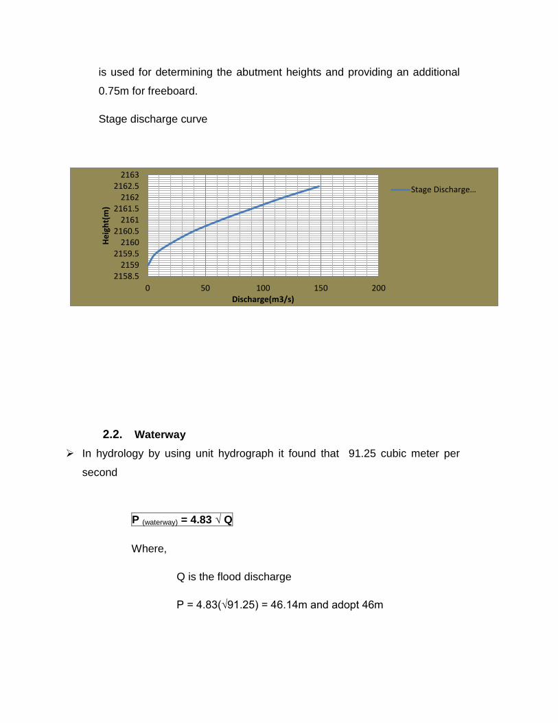
Stage discharge curve
2.2. Waterway
In hydrology by using unit hydrograph it found that 91.25 cubic meter per
second
P (waterway) = 4.83 √ Q
Where,
Q is the flood discharge
P = 4.83(√91.25) = 46.14m and adopt 46m
2158.52159
2159.52160
2160.52161
2161.52162
2162.52163
0 50 100 150 200
He
igh
t(m
)
Discharge(m3/s)
Stage Discharge…
2.3. Flood Discharge capacity of Under Sluice & Weir
2.3.1. Design Data a) For Under Sluice
Two bays of with 2m width each =2*2=6m
One piers width of 2m =2*1 =2m
Total = 6m
b) For Weir
Eight bays of each 2.5m width =8*2.5 =20m
Seven piers width each of 2m =7*2 = 14m
Total =34m
Width of middle wall = 3.0m
Total waterways = 6m+34m+3m =43m
2.3.2. Analysis
Discharge Capacity of Under Sluice and Weir for which rough estimation
Qu = 20%Qmax, Qu = 0.2*91.25=18.27m3/s and
Qweir = Qpeak –Qu= 91.25-18.25 =73m3/s.
Now let us cheek weather the assumed dimension is available to pass the
estimated discharge or not
I) For Under Sluice
Q =1.7(L - KnH)*H3/2
under sluice
Q =1.7(L - 0.1nH)*H3/2 under sluice
Where: L= length of clear water
K= constant coefficient of pier, K =0.1
H =head above crest
n= contact of water piers surface.
discharge intensity, q =Q/B, q=91.25/43 =2.12m3/s/m
Scour depth, R =1.35(q/f)1/3, R =1.35(2.12/1)1/3 =1.73m
Approach velocity, V =q/R =12.12/1.73=1.22m/s
Velocity head, hv = V2/2g =(1.22)2/2*9.81=0.076
U/s TEL =U/s HFL+hv =2162.2+.076 = 2162.276m
Head over the under sluice crest = U/s TEL –under sluice crest
=2162.269-2159=3.276m
Head over weir crest = U/s TEL –crest of weir
= 2162.276-2160.5=1.776m
Now substituting the values in the formula we get
Q1 = 1.7(4 -0.1*2*3.276)*3.2761.5
Q 1=33.66m3/s
II) For weir
Q =1.84(L - KnH)*H3/2
for weir
Q2 =1.84(20 – 0.1*14*1.776)*1.7761.5
Q2 = 76.27m3/s
Now the total Q = Q1 +Q2 = 33.66+76.27 =109.93m3/s > 91.25m
3/s, OK.
2.3.3 HYDRAULIC DESIGN OF THE UNDER SLUICE
2.3.3.1 High Flood Condition with No Concentration of Flow
U/s TEL = d/s HFL +afflux +approach velocity
= 2161.55 + 0.65 +0.076 = 2162.276m
d/s TEL = d/s HFL +hv = 2161.55 +.076
= 2161.626
head loss = U/s TEL - d/s TEL =2162.276 – 2161.626
=0.65m
Discharge intensity between piers, q
q = CH3/2 , q =1.7*(3.276)1.5 =10.08m3/s/m
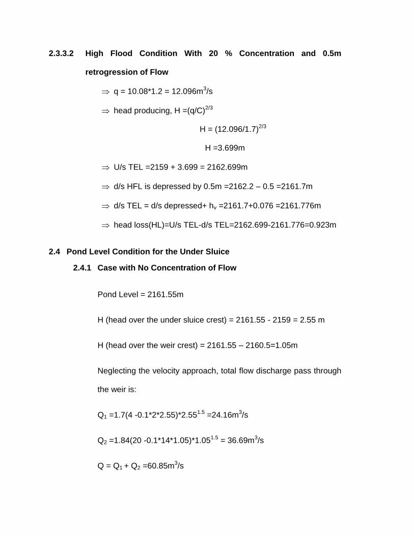
2.3.3.2 High Flood Condition With 20 % Concentration and 0.5m
retrogression of Flow
q = 10.08*1.2 = 12.096m3/s
head producing, H =(q/C)2/3
H = (12.096/1.7)2/3
H =3.699m
U/s TEL =2159 + 3.699 = 2162.699m
d/s HFL is depressed by 0.5m =2162.2 – 0.5 =2161.7m
d/s TEL = d/s depressed+ hv =2161.7+0.076 =2161.776m
head loss(HL)=U/s TEL-d/s TEL=2162.699-2161.776=0.923m
2.4 Pond Level Condition for the Under Sluice
2.4.1 Case with No Concentration of Flow
Pond Level = 2161.55m
H (head over the under sluice crest) = 2161.55 - 2159 = 2.55 m
H (head over the weir crest) = 2161.55 – 2160.5=1.05m
Neglecting the velocity approach, total flow discharge pass through
the weir is:
Q1 =1.7(4 -0.1*2*2.55)*2.551.5 =24.16m3/s
Q2 =1.84(20 -0.1*14*1.05)*1.051.5 = 36.69m3/s
Q = Q1 + Q2 =60.85m3/s
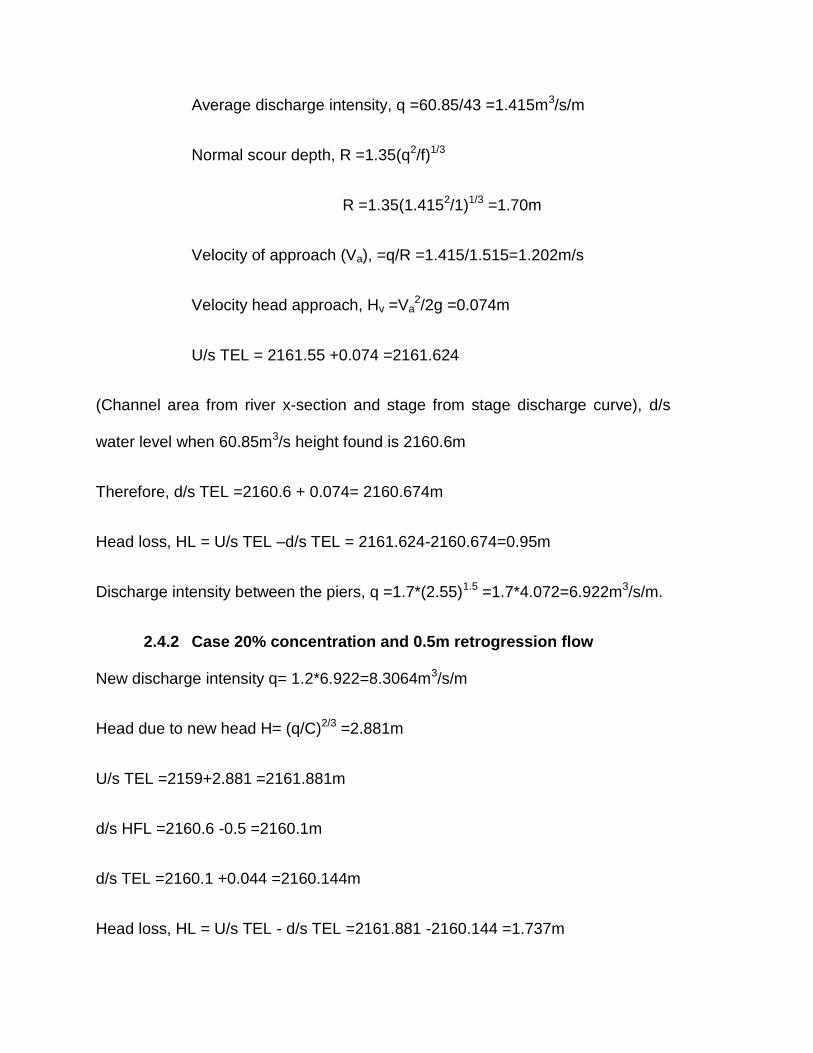
Average discharge intensity, q =60.85/43 =1.415m3/s/m
Normal scour depth, R =1.35(q2/f)1/3
R =1.35(1.4152/1)1/3 =1.70m
Velocity of approach (Va), =q/R =1.415/1.515=1.202m/s
Velocity head approach, Hv =Va2/2g =0.074m
U/s TEL = 2161.55 +0.074 =2161.624
(Channel area from river x-section and stage from stage discharge curve), d/s
water level when 60.85m3/s height found is 2160.6m
Therefore, d/s TEL =2160.6 + 0.074= 2160.674m
Head loss, HL = U/s TEL –d/s TEL = 2161.624-2160.674=0.95m
Discharge intensity between the piers, q =1.7*(2.55)1.5 =1.7*4.072=6.922m3/s/m.
2.4.2 Case 20% concentration and 0.5m retrogression flow
New discharge intensity q= 1.2*6.922=8.3064m3/s/m
Head due to new head H= (q/C)2/3 =2.881m
U/s TEL =2159+2.881 =2161.881m
d/s HFL =2160.6 -0.5 =2160.1m
d/s TEL =2160.1 +0.044 =2160.144m
Head loss, HL = U/s TEL - d/s TEL =2161.881 -2160.144 =1.737m
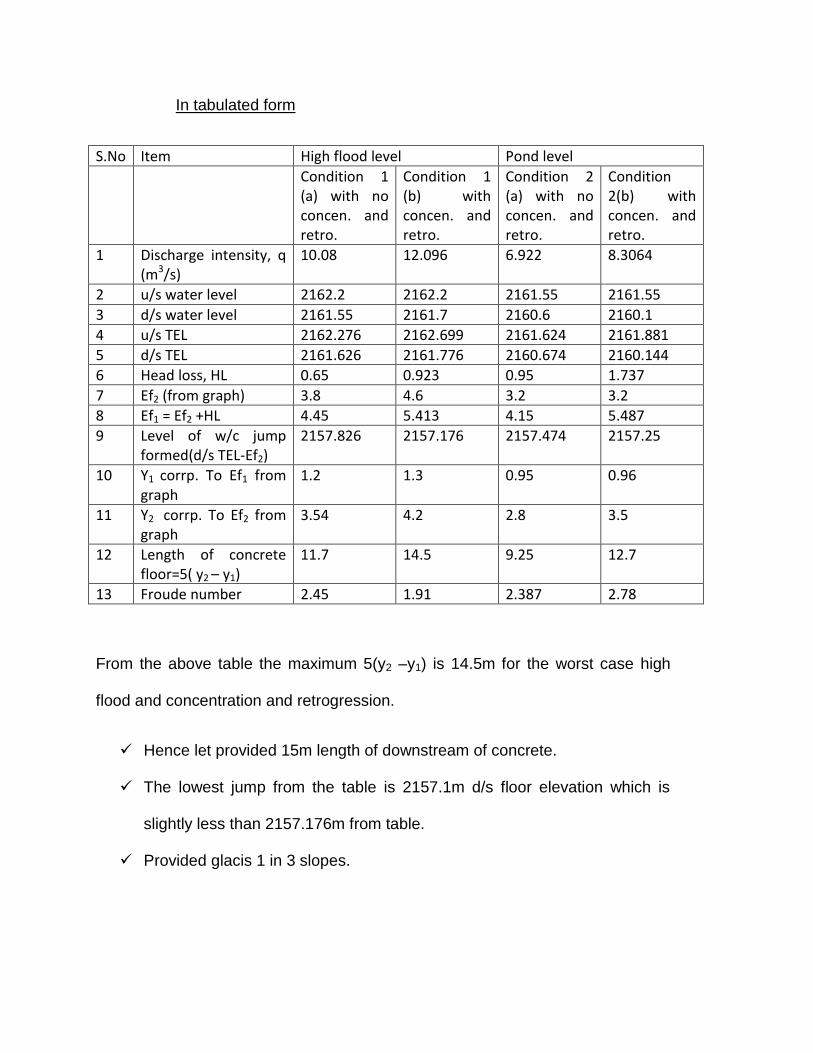
In tabulated form
S.No Item High flood level Pond level
Condition 1 (a) with no concen. and retro.
Condition 1 (b) with concen. and retro.
Condition 2 (a) with no concen. and retro.
Condition 2(b) with concen. and retro.
1 Discharge intensity, q (m3/s)
10.08 12.096 6.922 8.3064
2 u/s water level 2162.2 2162.2 2161.55 2161.55
3 d/s water level 2161.55 2161.7 2160.6 2160.1
4 u/s TEL 2162.276 2162.699 2161.624 2161.881
5 d/s TEL 2161.626 2161.776 2160.674 2160.144
6 Head loss, HL 0.65 0.923 0.95 1.737
7 Ef2 (from graph) 3.8 4.6 3.2 3.2
8 Ef1 = Ef2 +HL 4.45 5.413 4.15 5.487
9 Level of w/c jump formed(d/s TEL-Ef2)
2157.826 2157.176 2157.474 2157.25
10 Y1 corrp. To Ef1 from graph
1.2 1.3 0.95 0.96
11 Y2 corrp. To Ef2 from graph
3.54 4.2 2.8 3.5
12 Length of concrete floor=5( y2 – y1)
11.7 14.5 9.25 12.7
13 Froude number 2.45 1.91 2.387 2.78
From the above table the maximum 5(y2 –y1) is 14.5m for the worst case high
flood and concentration and retrogression.
Hence let provided 15m length of downstream of concrete.
The lowest jump from the table is 2157.1m d/s floor elevation which is
slightly less than 2157.176m from table.
Provided glacis 1 in 3 slopes.
2.5 Let now calculate total required length of floor.
Depth of sheet pile from the scour consideration
o Discharge passing through the under sluice =33.66m3/s
o Average discharge intensity, q =33.66/6 =5.61m3/s/m
o Depth of scour, R =1.35(q2/f)1/3 =4.26m,
o Let provided d/s cut off at 1.25R =1.25*4.26 =5.325m
o RL of bottom of scour cut off = 2162.2 –5.325 =2156.875m
o Depth of u/s =2159.0 -2156.785 =2.125m, assume 2.5m
o Hence RL of bottom of scour cut off =2156.5m
o Let provided d/s cut off at bottom level as 1.5*4.26 =6.39m
o Hence RL of bottom scour = 2161.7 – 6.39 = 2155.31m
o Provided d/s pile at elevation = 2154.1m
o d/s sheet pile depth = 2157.1 – 2154.1= 3m
o total floor length at exit gradient
o maximum static head = pond level – under sluice level
=2162.2-2159 =3.2m
o Considering the upstream cutoff,
o GE = H/d*1/ ()
o Where,
o GE is the exit gradient.
o = (1+1+2)/2 = b/d
o Where, B = total length
d = depth of downstream cutoff
H = pond level- downstream seepage exit level
H = 3.2
GE = H/d*1/ ()
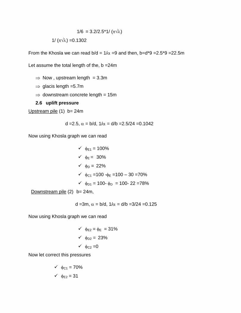
1/6 = 3.2/2.5*1/ ()
1/ () =0.1302
From the Khosla we can read b/d = 1/ =9 and then, b=d*9 =2.5*9 =22.5m
Let assume the total length of the, b =24m
Now , upstream length = 3.3m
glacis length =5.7m
downstream concrete length = 15m
2.6 uplift pressure
Upstream pile (1) b= 24m
d =2.5, = b/d, 1/ = d/b =2.5/24 =0.1042
Now using Khosla graph we can read
E1 = 100%
E = 30%
D = 22%
C1 =100 -E =100 – 30 =70%
D1 = 100- D = 100- 22 =78%
Downstream pile (2) b= 24m,
d =3m, = b/d, 1/ = d/b =3/24 =0.125
Now using Khosla graph we can read
E2 = E = 31%
D2 = 23%
C2 =0
Now let correct this pressures
C1 = 70%
E2 = 31
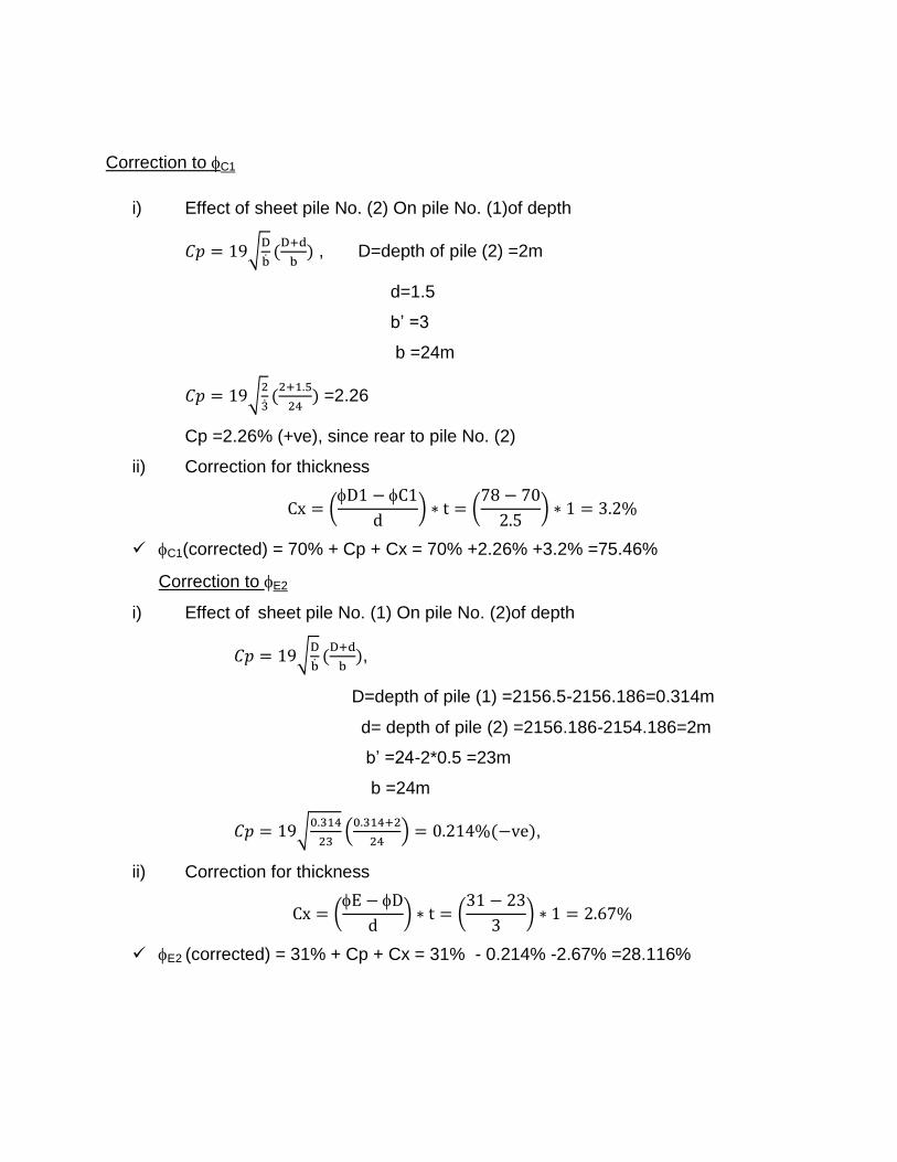
Correction to C1
i) Effect of sheet pile No. (2) On pile No. (1)of depth
√
, D=depth of pile (2) =2m
d=1.5
b’ =3
b =24m
√
=2.26
Cp =2.26% (+ve), since rear to pile No. (2)
ii) Correction for thickness
(
) (
)
C1(corrected) = 70% + Cp + Cx = 70% +2.26% +3.2% =75.46%
Correction to E2
i) Effect of sheet pile No. (1) On pile No. (2)of depth
√
,
D=depth of pile (1) =2156.5-2156.186=0.314m
d= depth of pile (2) =2156.186-2154.186=2m
b’ =24-2*0.5 =23m
b =24m
√
(
) ,
ii) Correction for thickness
(
) (
)
E2 (corrected) = 31% + Cp + Cx = 31% - 0.214% -2.67% =28.116%
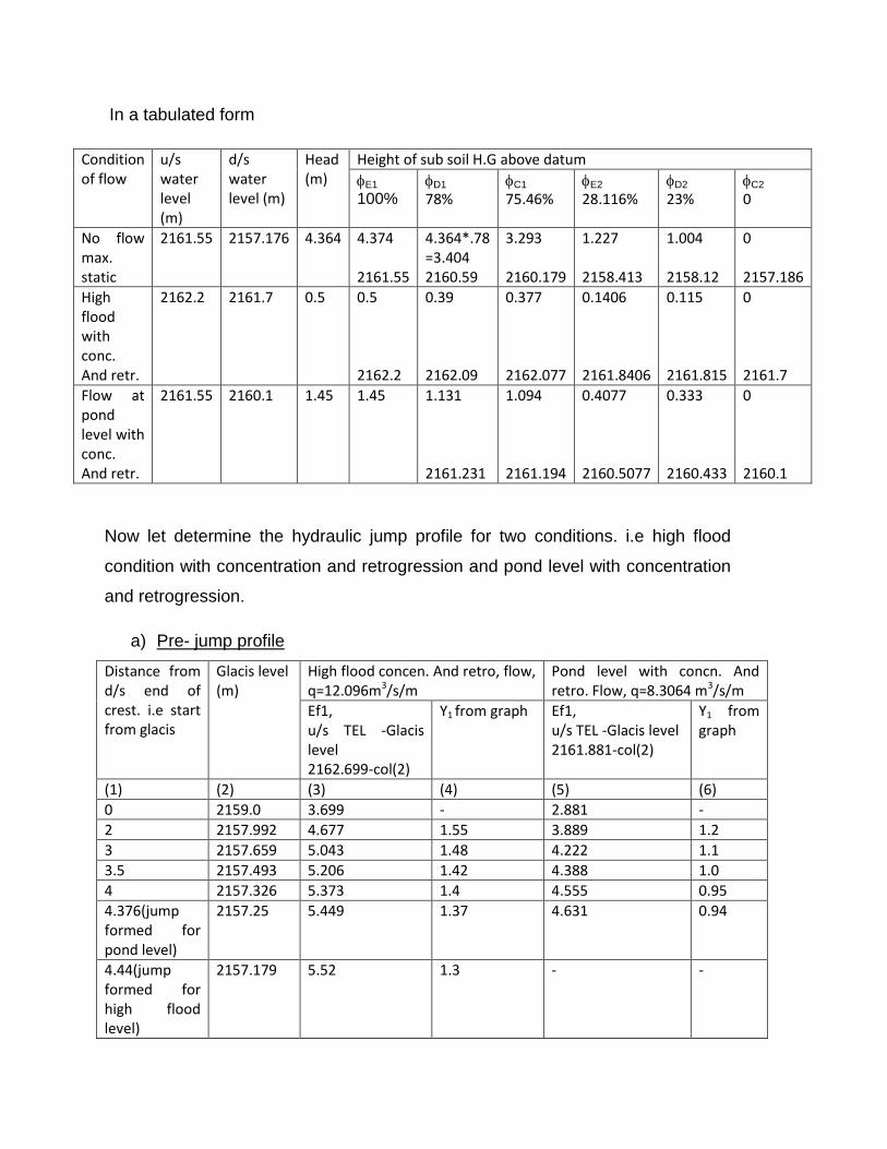
In a tabulated form
Condition of flow
u/s water level (m)
d/s water level (m)
Head (m)
Height of sub soil H.G above datum
E1
100% D1
78% C1
75.46% E2
28.116% D2
23% C2
0
No flow max. static
2161.55 2157.176 4.364 4.374 2161.55
4.364*.78 =3.404 2160.59
3.293 2160.179
1.227 2158.413
1.004 2158.12
0 2157.186
High flood with conc. And retr.
2162.2 2161.7 0.5 0.5 2162.2
0.39 2162.09
0.377 2162.077
0.1406 2161.8406
0.115 2161.815
0 2161.7
Flow at pond level with conc. And retr.
2161.55 2160.1 1.45 1.45 1.131 2161.231
1.094 2161.194
0.4077 2160.5077
0.333 2160.433
0 2160.1
Now let determine the hydraulic jump profile for two conditions. i.e high flood
condition with concentration and retrogression and pond level with concentration
and retrogression.
a) Pre- jump profile
Distance from d/s end of crest. i.e start from glacis
Glacis level (m)
High flood concen. And retro, flow, q=12.096m3/s/m
Pond level with concn. And retro. Flow, q=8.3064 m3/s/m
Ef1, u/s TEL -Glacis level 2162.699-col(2)
Y1 from graph Ef1, u/s TEL -Glacis level 2161.881-col(2)
Y1 from graph
(1) (2) (3) (4) (5) (6)
0 2159.0 3.699 - 2.881 -
2 2157.992 4.677 1.55 3.889 1.2
3 2157.659 5.043 1.48 4.222 1.1
3.5 2157.493 5.206 1.42 4.388 1.0
4 2157.326 5.373 1.4 4.555 0.95
4.376(jump formed for pond level)
2157.25 5.449 1.37 4.631 0.94
4.44(jump formed for high flood level)
2157.179 5.52 1.3 - -
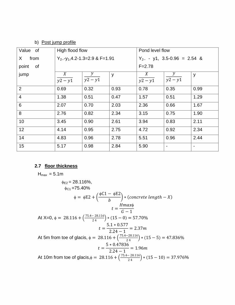
b) Post jump profile
Value of
X from
point of
jump
High flood flow
Y2---y1,4.2-1.3=2.9 & F=1.91
Pond level flow
Y2-- - y1, 3.5-0.96 = 2.54 &
F=2.78
y
y
2 0.69 0.32 0.93 0.78 0.35 0.99
4 1.38 0.51 0.47 1.57 0.51 1.29
6 2.07 0.70 2.03 2.36 0.66 1.67
8 2.76 0.82 2.34 3.15 0.75 1.90
10 3.45 0.90 2.61 3.94 0.83 2.11
12 4.14 0.95 2.75 4.72 0.92 2.34
14 4.83 0.96 2.78 5.51 0.96 2.44
15 5.17 0.98 2.84 5.90 - -
2.7 floor thickness
Hmax = 5.1m
E2 = 28.116%,
C1 =75.40%
(
)
At X=0, (
)
At 5m from toe of glacis, (
)
At 10m from toe of glacis, (
) %
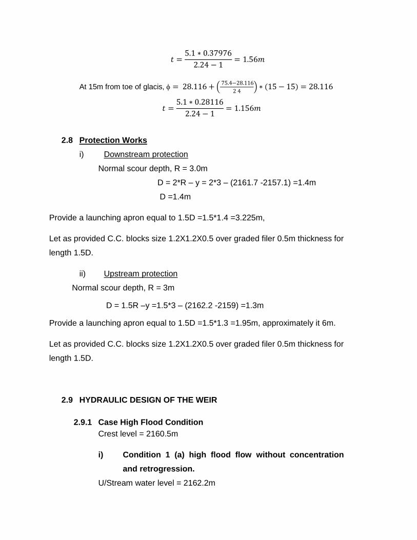
At 15m from toe of glacis, (
)
2.8 Protection Works
i) Downstream protection
Normal scour depth, R = 3.0m
D = 2*R – y = 2*3 – (2161.7 -2157.1) =1.4m
D =1.4m
Provide a launching apron equal to 1.5D =1.5*1.4 =3.225m,
Let as provided C.C. blocks size 1.2X1.2X0.5 over graded filer 0.5m thickness for
length 1.5D.
ii) Upstream protection
Normal scour depth, R = 3m
D = 1.5R –y =1.5*3 – (2162.2 -2159) =1.3m
Provide a launching apron equal to 1.5D =1.5*1.3 =1.95m, approximately it 6m.
Let as provided C.C. blocks size 1.2X1.2X0.5 over graded filer 0.5m thickness for
length 1.5D.
2.9 HYDRAULIC DESIGN OF THE WEIR
2.9.1 Case High Flood Condition
Crest level = 2160.5m
i) Condition 1 (a) high flood flow without concentration
and retrogression.
U/Stream water level = 2162.2m
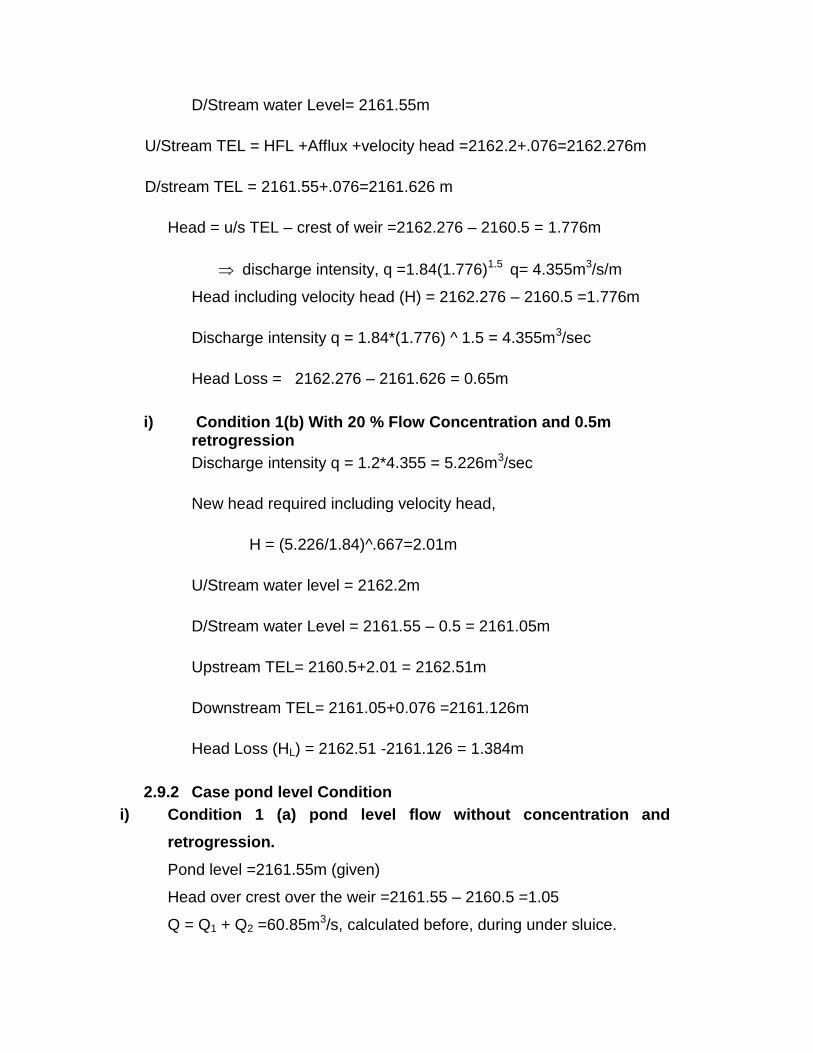
D/Stream water Level= 2161.55m
U/Stream TEL = HFL +Afflux +velocity head =2162.2+.076=2162.276m
D/stream TEL = 2161.55+.076=2161.626 m
Head = u/s TEL – crest of weir =2162.276 – 2160.5 = 1.776m
discharge intensity, q =1.84(1.776)1.5 q= 4.355m3/s/m
Head including velocity head (H) = 2162.276 – 2160.5 =1.776m
Discharge intensity q = 1.84*(1.776) ^ 1.5 = 4.355m3/sec
Head Loss = 2162.276 – 2161.626 = 0.65m
i) Condition 1(b) With 20 % Flow Concentration and 0.5m retrogression
Discharge intensity q = 1.2*4.355 = 5.226m3/sec
New head required including velocity head,
H = (5.226/1.84)^.667=2.01m
U/Stream water level = 2162.2m
D/Stream water Level = 2161.55 – 0.5 = 2161.05m
Upstream TEL= 2160.5+2.01 = 2162.51m
Downstream TEL= 2161.05+0.076 =2161.126m
Head Loss (HL) = 2162.51 -2161.126 = 1.384m
2.9.2 Case pond level Condition
i) Condition 1 (a) pond level flow without concentration and
retrogression.
Pond level =2161.55m (given)
Head over crest over the weir =2161.55 – 2160.5 =1.05
Q = Q1 + Q2 =60.85m3/s, calculated before, during under sluice.
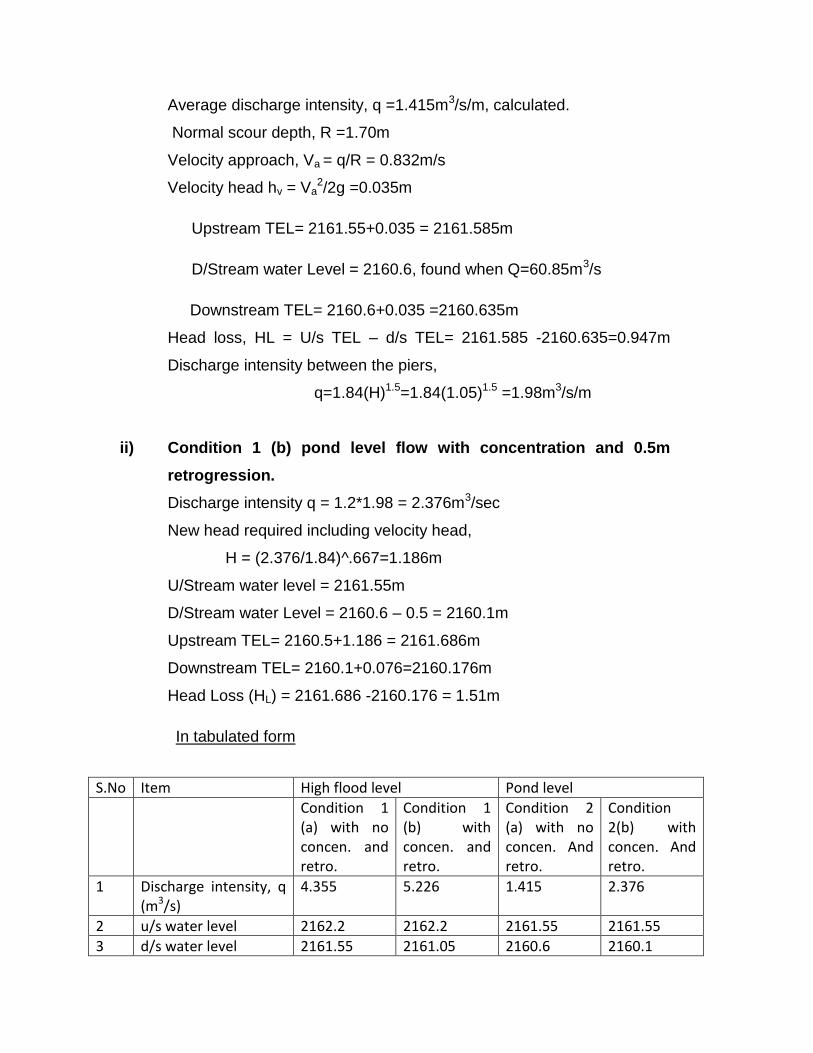
Average discharge intensity, q =1.415m3/s/m, calculated.
Normal scour depth, R =1.70m
Velocity approach, Va = q/R = 0.832m/s
Velocity head hv = Va2/2g =0.035m
Upstream TEL= 2161.55+0.035 = 2161.585m
D/Stream water Level = 2160.6, found when Q=60.85m3/s
Downstream TEL= 2160.6+0.035 =2160.635m
Head loss, HL = U/s TEL – d/s TEL= 2161.585 -2160.635=0.947m
Discharge intensity between the piers,
q=1.84(H)1.5=1.84(1.05)1.5 =1.98m3/s/m
ii) Condition 1 (b) pond level flow with concentration and 0.5m
retrogression.
Discharge intensity q = 1.2*1.98 = 2.376m3/sec
New head required including velocity head,
H = (2.376/1.84)^.667=1.186m
U/Stream water level = 2161.55m
D/Stream water Level = 2160.6 – 0.5 = 2160.1m
Upstream TEL= 2160.5+1.186 = 2161.686m
Downstream TEL= 2160.1+0.076=2160.176m
Head Loss (HL) = 2161.686 -2160.176 = 1.51m
In tabulated form
S.No Item High flood level Pond level
Condition 1 (a) with no concen. and retro.
Condition 1 (b) with concen. and retro.
Condition 2 (a) with no concen. And retro.
Condition 2(b) with concen. And retro.
1 Discharge intensity, q (m3/s)
4.355 5.226 1.415 2.376
2 u/s water level 2162.2 2162.2 2161.55 2161.55
3 d/s water level 2161.55 2161.05 2160.6 2160.1
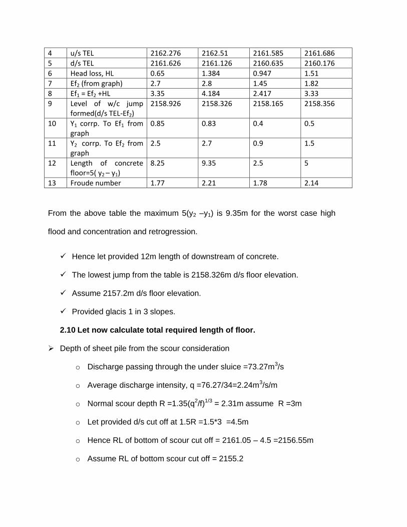
4 u/s TEL 2162.276 2162.51 2161.585 2161.686
5 d/s TEL 2161.626 2161.126 2160.635 2160.176
6 Head loss, HL 0.65 1.384 0.947 1.51
7 Ef2 (from graph) 2.7 2.8 1.45 1.82
8 Ef1 = Ef2 +HL 3.35 4.184 2.417 3.33
9 Level of w/c jump formed(d/s TEL-Ef2)
2158.926 2158.326 2158.165 2158.356
10 Y1 corrp. To Ef1 from graph
0.85 0.83 0.4 0.5
11 Y2 corrp. To Ef2 from graph
2.5 2.7 0.9 1.5
12 Length of concrete floor=5( y2 – y1)
8.25 9.35 2.5 5
13 Froude number 1.77 2.21 1.78 2.14
From the above table the maximum 5(y2 –y1) is 9.35m for the worst case high
flood and concentration and retrogression.
Hence let provided 12m length of downstream of concrete.
The lowest jump from the table is 2158.326m d/s floor elevation.
Assume 2157.2m d/s floor elevation.
Provided glacis 1 in 3 slopes.
2.10 Let now calculate total required length of floor.
Depth of sheet pile from the scour consideration
o Discharge passing through the under sluice =73.27m3/s
o Average discharge intensity, q =76.27/34=2.24m3/s/m
o Normal scour depth R =1.35(q2/f)1/3 = 2.31m assume R =3m
o Let provided d/s cut off at 1.5R =1.5*3 =4.5m
o Hence RL of bottom of scour cut off = 2161.05 – 4.5 =2156.55m
o Assume RL of bottom scour cut off = 2155.2
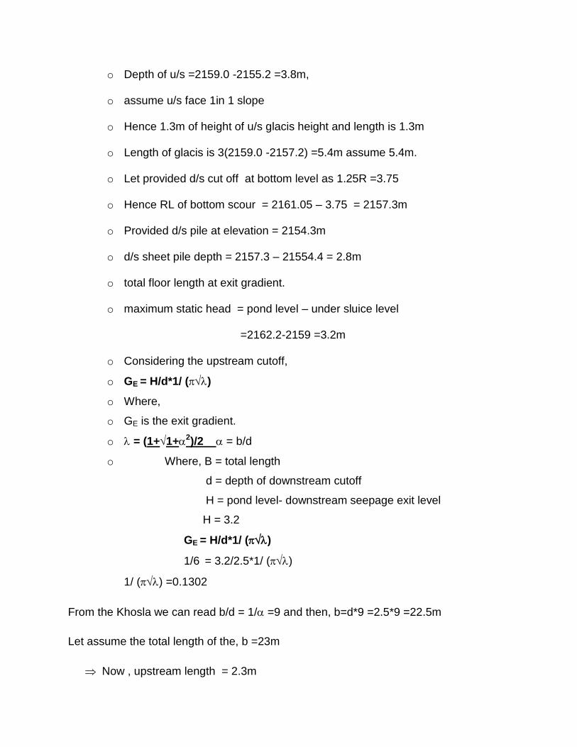
o Depth of u/s =2159.0 -2155.2 =3.8m,
o assume u/s face 1in 1 slope
o Hence 1.3m of height of u/s glacis height and length is 1.3m
o Length of glacis is 3(2159.0 -2157.2) =5.4m assume 5.4m.
o Let provided d/s cut off at bottom level as 1.25R =3.75
o Hence RL of bottom scour = 2161.05 – 3.75 = 2157.3m
o Provided d/s pile at elevation = 2154.3m
o d/s sheet pile depth = 2157.3 – 21554.4 = 2.8m
o total floor length at exit gradient.
o maximum static head = pond level – under sluice level
=2162.2-2159 =3.2m
o Considering the upstream cutoff,
o GE = H/d*1/ ()
o Where,
o GE is the exit gradient.
o = (1+1+2)/2 = b/d
o Where, B = total length
d = depth of downstream cutoff
H = pond level- downstream seepage exit level
H = 3.2
GE = H/d*1/ ()
1/6 = 3.2/2.5*1/ ()
1/ () =0.1302
From the Khosla we can read b/d = 1/ =9 and then, b=d*9 =2.5*9 =22.5m
Let assume the total length of the, b =23m
Now , upstream length = 2.3m
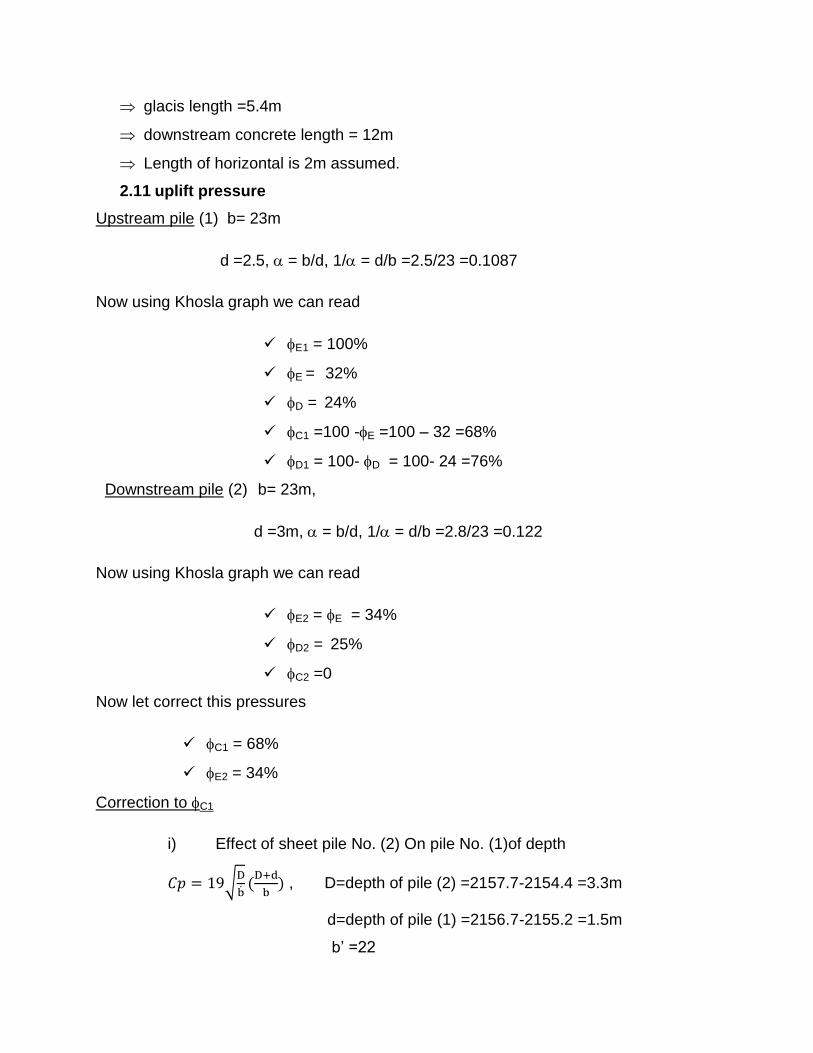
glacis length =5.4m
downstream concrete length = 12m
Length of horizontal is 2m assumed.
2.11 uplift pressure
Upstream pile (1) b= 23m
d =2.5, = b/d, 1/ = d/b =2.5/23 =0.1087
Now using Khosla graph we can read
E1 = 100%
E = 32%
D = 24%
C1 =100 -E =100 – 32 =68%
D1 = 100- D = 100- 24 =76%
Downstream pile (2) b= 23m,
d =3m, = b/d, 1/ = d/b =2.8/23 =0.122
Now using Khosla graph we can read
E2 = E = 34%
D2 = 25%
C2 =0
Now let correct this pressures
C1 = 68%
E2 = 34%
Correction to C1
i) Effect of sheet pile No. (2) On pile No. (1)of depth
√
, D=depth of pile (2) =2157.7-2154.4 =3.3m
d=depth of pile (1) =2156.7-2155.2 =1.5m
b’ =22
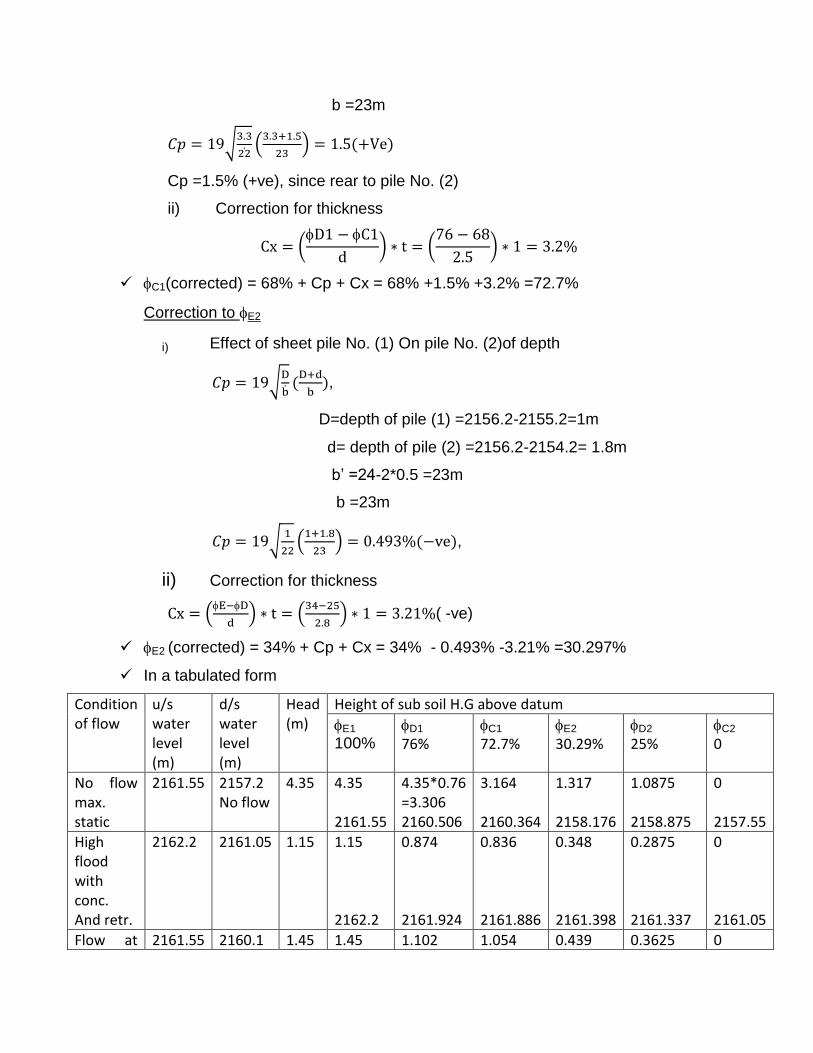
b =23m
√
(
)
Cp =1.5% (+ve), since rear to pile No. (2)
ii) Correction for thickness
(
) (
)
C1(corrected) = 68% + Cp + Cx = 68% +1.5% +3.2% =72.7%
Correction to E2
i) Effect of sheet pile No. (1) On pile No. (2)of depth
√
,
D=depth of pile (1) =2156.2-2155.2=1m
d= depth of pile (2) =2156.2-2154.2= 1.8m
b’ =24-2*0.5 =23m
b =23m
√
(
) ,
ii) Correction for thickness
(
) (
) ( -ve)
E2 (corrected) = 34% + Cp + Cx = 34% - 0.493% -3.21% =30.297%
In a tabulated form
Condition of flow
u/s water level (m)
d/s water level (m)
Head (m)
Height of sub soil H.G above datum
E1
100% D1
76% C1
72.7% E2
30.29% D2
25% C2
0
No flow max. static
2161.55 2157.2 No flow
4.35 4.35 2161.55
4.35*0.76 =3.306 2160.506
3.164 2160.364
1.317 2158.176
1.0875 2158.875
0 2157.55
High flood with conc. And retr.
2162.2 2161.05 1.15 1.15 2162.2
0.874 2161.924
0.836 2161.886
0.348 2161.398
0.2875 2161.337
0 2161.05
Flow at 2161.55 2160.1 1.45 1.45 1.102 1.054 0.439 0.3625 0
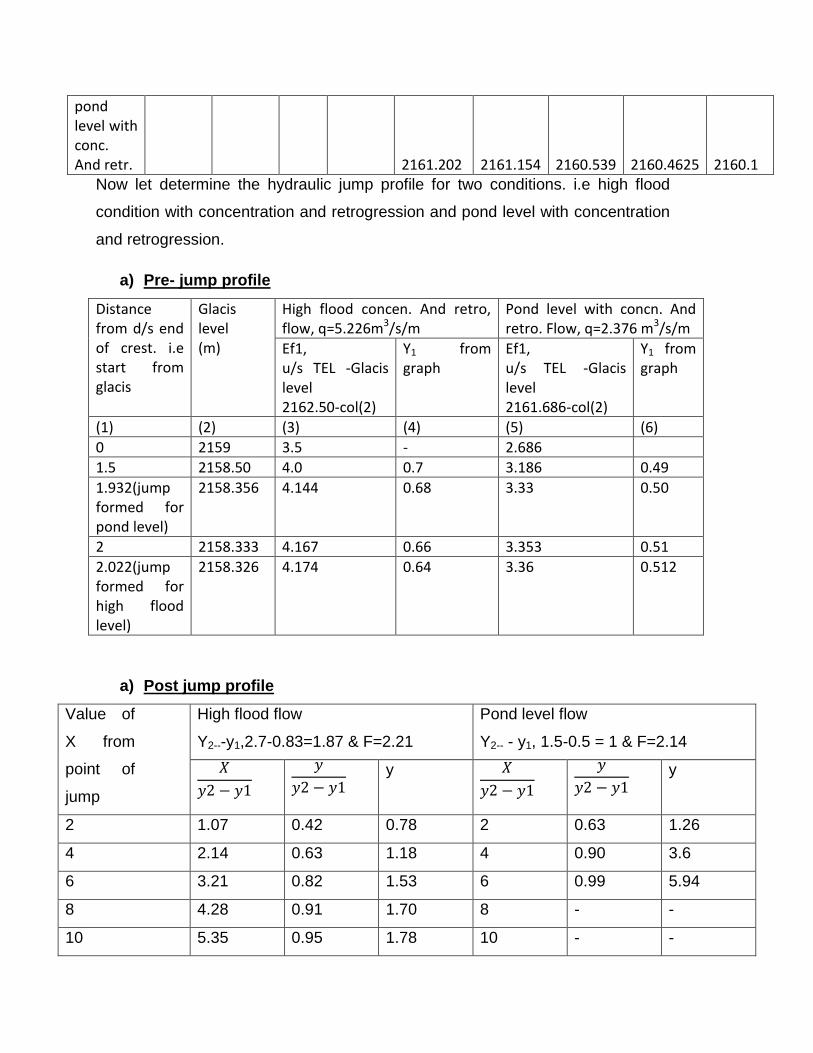
pond level with conc. And retr.
2161.202
2161.154
2160.539
2160.4625
2160.1
Now let determine the hydraulic jump profile for two conditions. i.e high flood
condition with concentration and retrogression and pond level with concentration
and retrogression.
a) Pre- jump profile
Distance from d/s end of crest. i.e start from glacis
Glacis level (m)
High flood concen. And retro, flow, q=5.226m3/s/m
Pond level with concn. And retro. Flow, q=2.376 m3/s/m
Ef1, u/s TEL -Glacis level 2162.50-col(2)
Y1 from graph
Ef1, u/s TEL -Glacis level 2161.686-col(2)
Y1 from graph
(1) (2) (3) (4) (5) (6)
0 2159 3.5 - 2.686
1.5 2158.50 4.0 0.7 3.186 0.49
1.932(jump formed for pond level)
2158.356 4.144 0.68 3.33 0.50
2 2158.333 4.167 0.66 3.353 0.51
2.022(jump formed for high flood level)
2158.326 4.174 0.64 3.36 0.512
a) Post jump profile
Value of
X from
point of
jump
High flood flow
Y2---y1,2.7-0.83=1.87 & F=2.21
Pond level flow
Y2-- - y1, 1.5-0.5 = 1 & F=2.14
y
y
2 1.07 0.42 0.78 2 0.63 1.26
4 2.14 0.63 1.18 4 0.90 3.6
6 3.21 0.82 1.53 6 0.99 5.94
8 4.28 0.91 1.70 8 - -
10 5.35 0.95 1.78 10 - -
12 6.42 0.99 1.85 12 - -
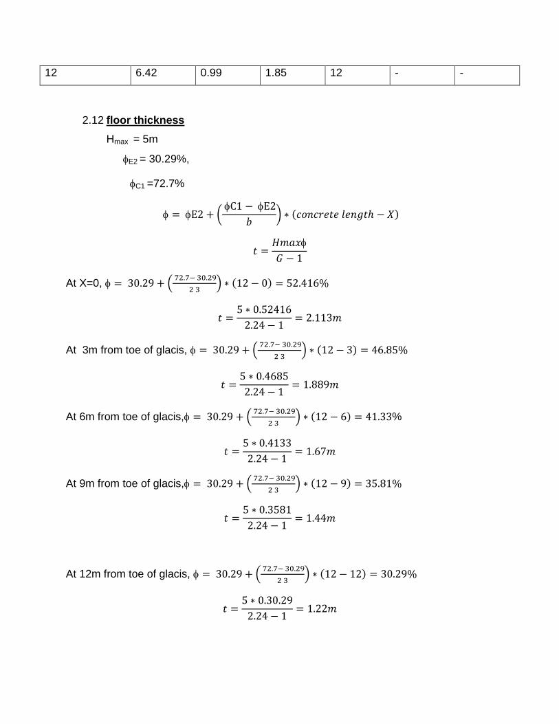
2.12 floor thickness
Hmax = 5m
E2 = 30.29%,
C1 =72.7%
(
)
At X=0, (
)
At 3m from toe of glacis, (
)
At 6m from toe of glacis, (
) %
At 9m from toe of glacis, (
)
At 12m from toe of glacis, (
)
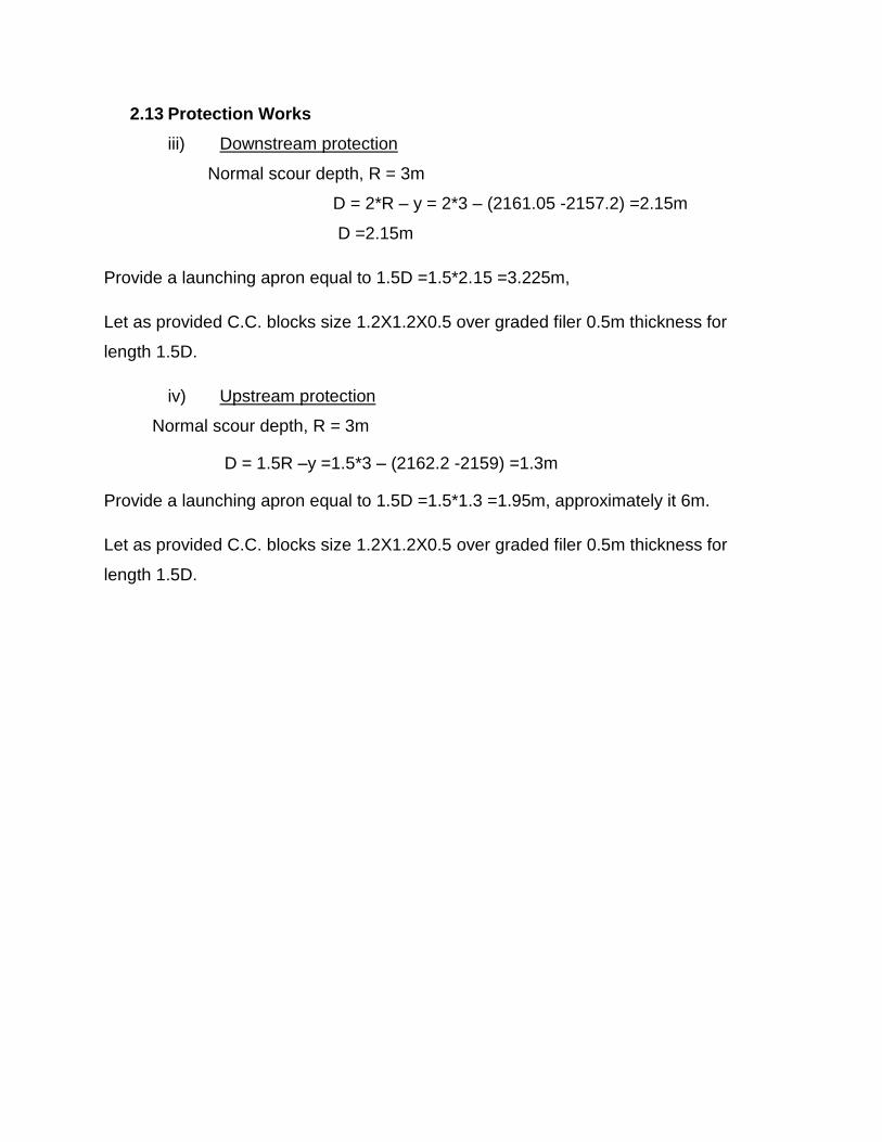
2.13 Protection Works
iii) Downstream protection
Normal scour depth, R = 3m
D = 2*R – y = 2*3 – (2161.05 -2157.2) =2.15m
D =2.15m
Provide a launching apron equal to 1.5D =1.5*2.15 =3.225m,
Let as provided C.C. blocks size 1.2X1.2X0.5 over graded filer 0.5m thickness for
length 1.5D.
iv) Upstream protection
Normal scour depth, R = 3m
D = 1.5R –y =1.5*3 – (2162.2 -2159) =1.3m
Provide a launching apron equal to 1.5D =1.5*1.3 =1.95m, approximately it 6m.
Let as provided C.C. blocks size 1.2X1.2X0.5 over graded filer 0.5m thickness for
length 1.5D.
3. CANAL LAY OUT AND DESIGN
(LONGITUDINAL PROFILE AND CROSS SECTION)
3.1. Geology:
The main canal route is the one from the immediate outlet of the weir axis passing through the
long idle canal right side of the main river to the end of the command area. Most of the canal
route is aligned on steep slope topography. This is mainly composed of differentially weathered
slate-phyllite rock. The slightly weathered and moderately fractured rock unit is covered most of
the canal route length. Its upper part is composed of clayey sand with considerable amount of
gravel and has steep slope topography, which can be considered as a semi-pervious part of the
canal. Hard rock outcrops are also part of the canal route, which are stable, moderately
workable and non-deformable.
3.2. Design of the main canal
The selection of the type of a particular canal depends on the geological condition and the available
economy for the project. Lined main canal trapezoidal in section is going to be adopted.
3.2.1. Main canal Cross-sectional design:
Canals capacity and type are fixed in consideration the area to be irrigated and as per design
criteria set for the project.
In order to fix the dimensions of canal sections the hydraulic design calculated Manning general formula is
adopted.
2/13/2*1
SARn
Q
Where, Q = discharge of the channel
R = Hydraulic radius = A/p
A = Wetted cross-sectional area
m = side slope
p = wetted perimeter
s = bed slope
n = Manning’s roughness coefficient
The main canal is 1778m extending with a uniform cross section throughout the length as there is no
secondary canal is branching out with in the range.
The canal cross section is designed based on the principle that the flow velocity shall not allow silt
deposition which will highly reduce the efficiency because the capacity of the canal is small. Therefore,
the design is based on Kennedy’s theory and Manning’s formula. Even though Kennedy’s theory is
applicable to earth channels, it might be important to consider the flowing velocity has to be fast enough
not to cause siltation in this case. And because the canal is of so small in capacity a little sediment
deposition will make highly sensitive to be smaller further, hence efficiency will be low.
Design procedure:
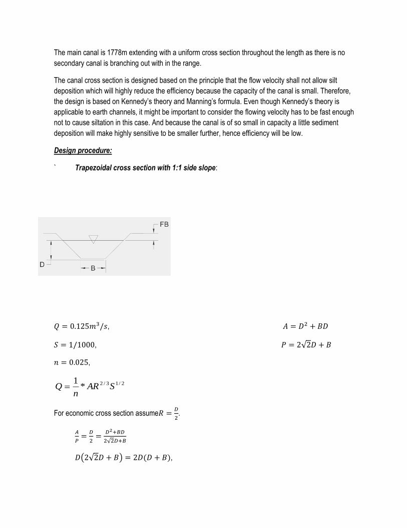
` Trapezoidal cross section with 1:1 side slope:
,
, √
,
2/13/2*1
SARn
Q
For economic cross section assume
.
√
( √ ) ,
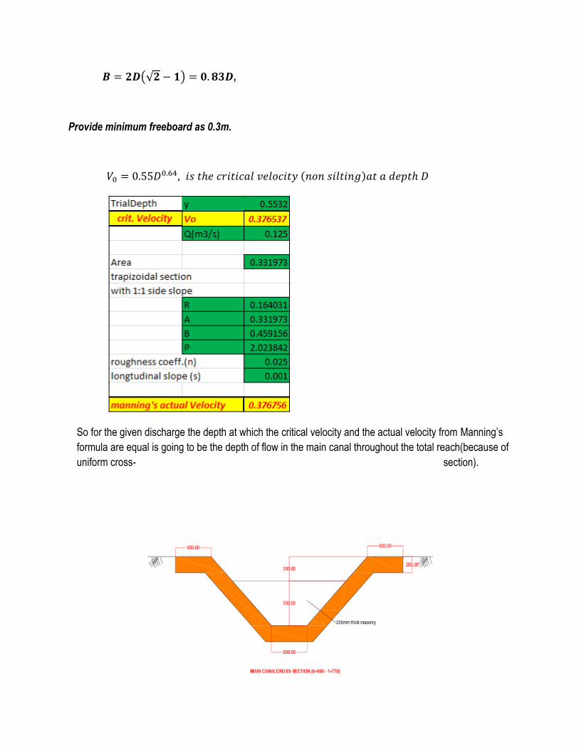
(√ ) ,
Provide minimum freeboard as 0.3m.
So for the given discharge the depth at which the critical velocity and the actual velocity from Manning’s
formula are equal is going to be the depth of flow in the main canal throughout the total reach(because of
uniform cross- section).
Dimensions are in millimeters.
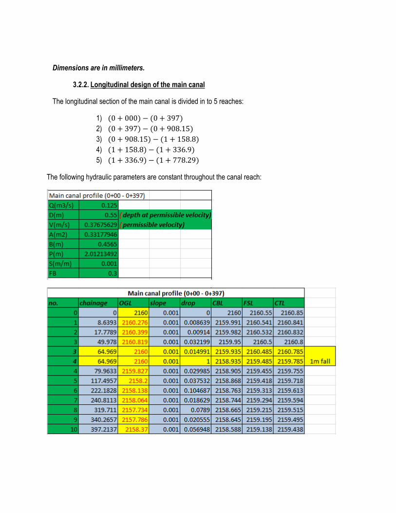
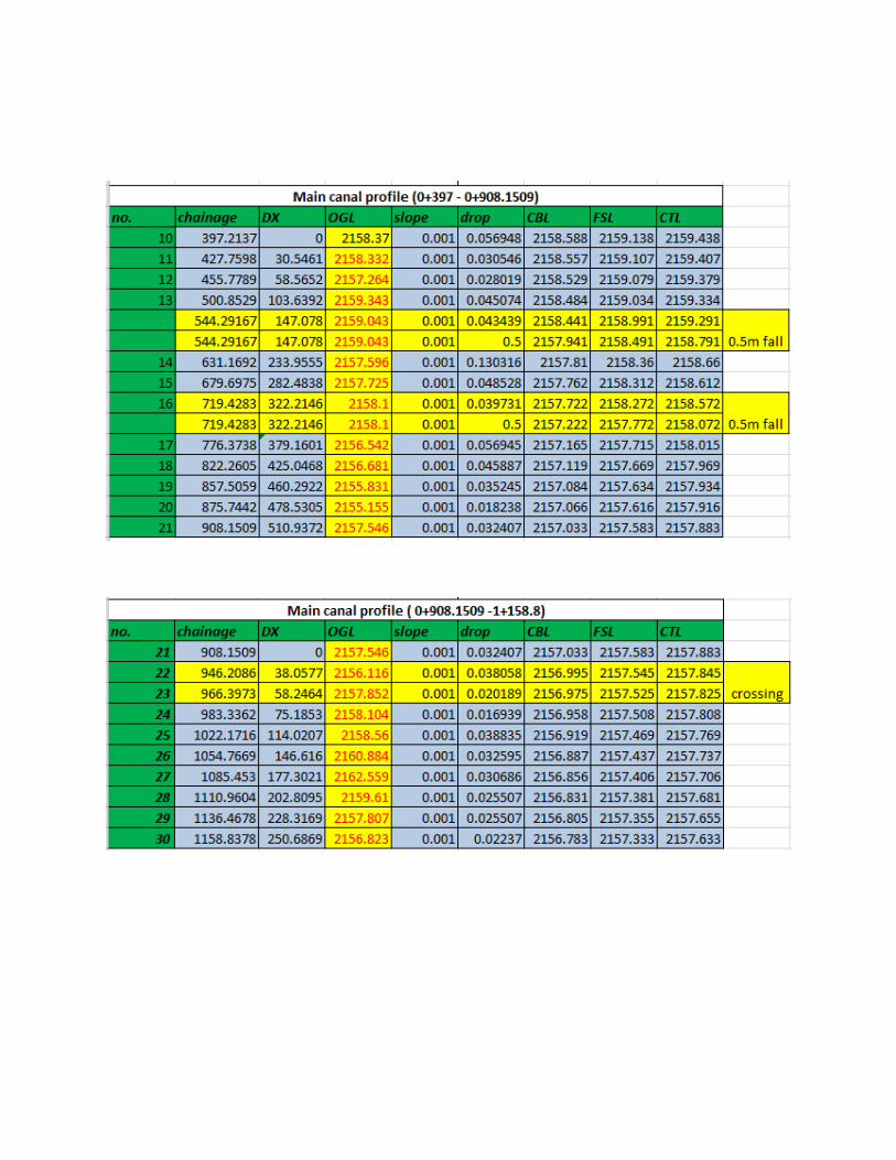
3.2.2. Longitudinal design of the main canal
The longitudinal section of the main canal is divided in to 5 reaches:
1)
2)
3)
4)
5)
The following hydraulic parameters are constant throughout the canal reach:
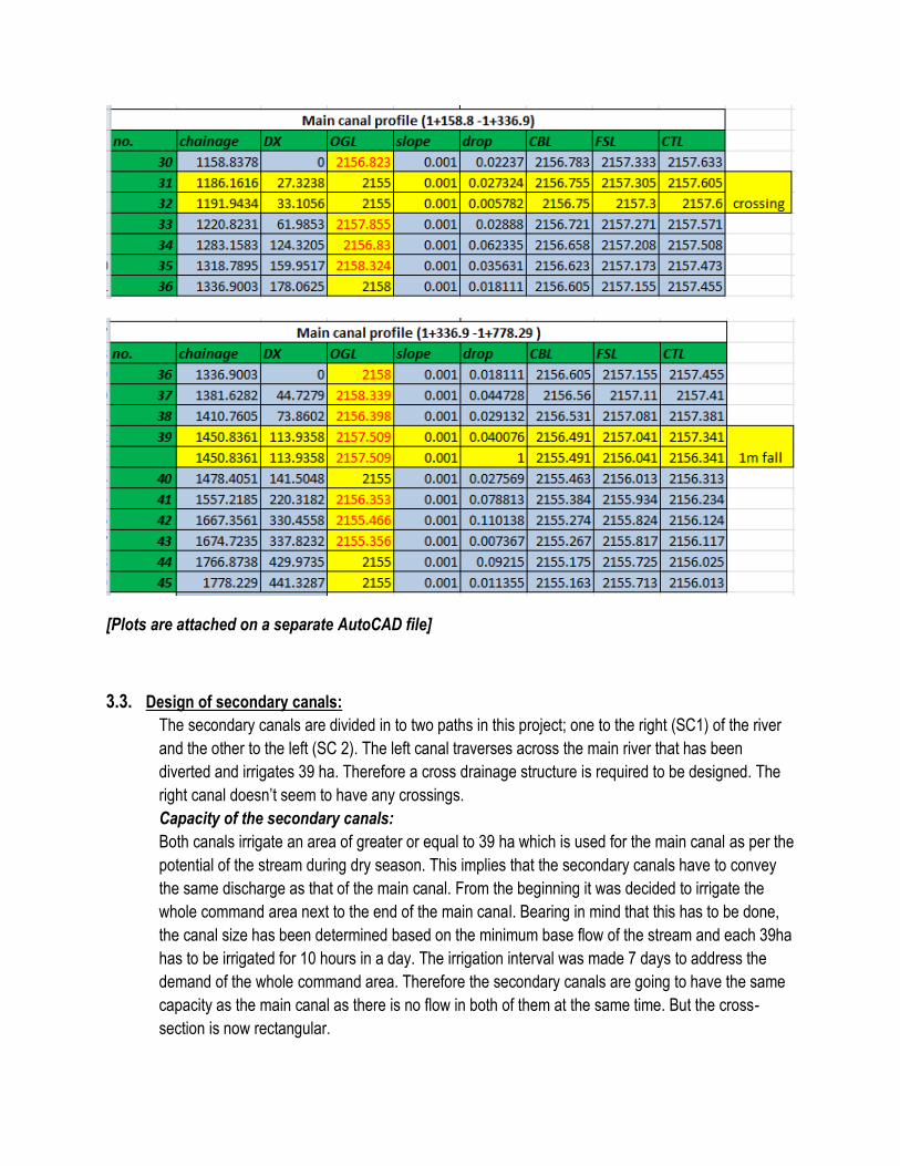
[Plots are attached on a separate AutoCAD file]
3.3. Design of secondary canals:
The secondary canals are divided in to two paths in this project; one to the right (SC1) of the river
and the other to the left (SC 2). The left canal traverses across the main river that has been
diverted and irrigates 39 ha. Therefore a cross drainage structure is required to be designed. The
right canal doesn’t seem to have any crossings.
Capacity of the secondary canals:
Both canals irrigate an area of greater or equal to 39 ha which is used for the main canal as per the
potential of the stream during dry season. This implies that the secondary canals have to convey
the same discharge as that of the main canal. From the beginning it was decided to irrigate the
whole command area next to the end of the main canal. Bearing in mind that this has to be done,
the canal size has been determined based on the minimum base flow of the stream and each 39ha
has to be irrigated for 10 hours in a day. The irrigation interval was made 7 days to address the
demand of the whole command area. Therefore the secondary canals are going to have the same
capacity as the main canal as there is no flow in both of them at the same time. But the cross-
section is now rectangular.
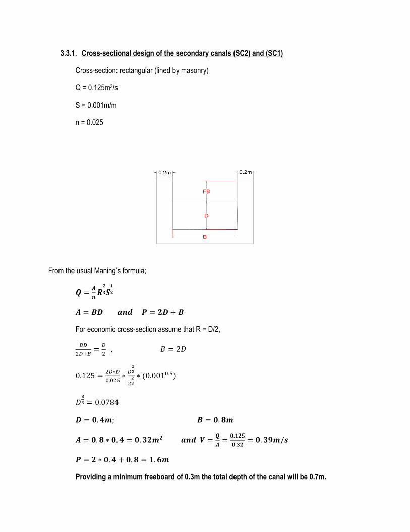
3.3.1. Cross-sectional design of the secondary canals (SC2) and (SC1)
Cross-section: rectangular (lined by masonry)
Q = 0.125m3/s
S = 0.001m/m
n = 0.025
From the usual Maning’s formula;
For economic cross-section assume that R = D/2,
Providing a minimum freeboard of 0.3m the total depth of the canal will be 0.7m.
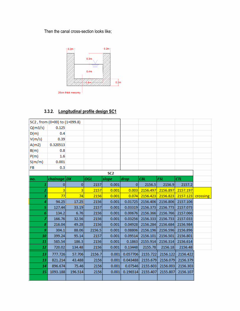
Then the canal cross-section looks like;
3.3.2. Longitudinal profile design SC1
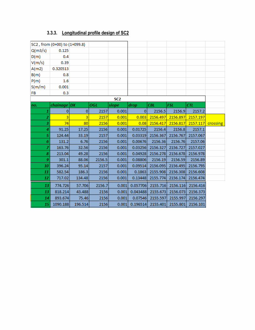
3.3.3. Longitudinal profile design of SC2

4. DESIGN OF CROSS-DRAINAGE STRUCTURES
4.1 General
A cross drainage is a structure constructed to allow canals pass natural depressions, gullies, rivers
or any discontinuities. The rout of the main canal intercepts two gullies comparatively shallow depth up to
2meters, lengths of 22.5m and 25.5m. The type of crossing that has to be designed is an aqueduct. There
is also a long crossing that has to be traversed by the secondary canal (SC2) across the main river that has
been diverted before.
4.1.1 design of aqueduct at on the main canal (0+946 – 0+966):
ID: CRM1
Hydraulic parameters of the main canal at this point:
Cross-section : trapezoidal type
d/s canal bed level: 2156.975m
Q = 0.125m3/s
Depth = 0.55m
Longitudinal slope = 1/1000
Side slope = 1:1
Velocity = 0.3767m/s
FSL = 2157.545
Drainage gully:
Drainage bed level = 2155m
Water way = 22.5m
Depth = 2m
i) Fixing drainage water way;
.
Total water way = 21+2.4 = 23.4m
ii) Canal water way:
Bed width = 0.5m
Bed width of flume shall be provided as 0.3m (minimum) and rectangular in cross section
iii) Head loss calculations:
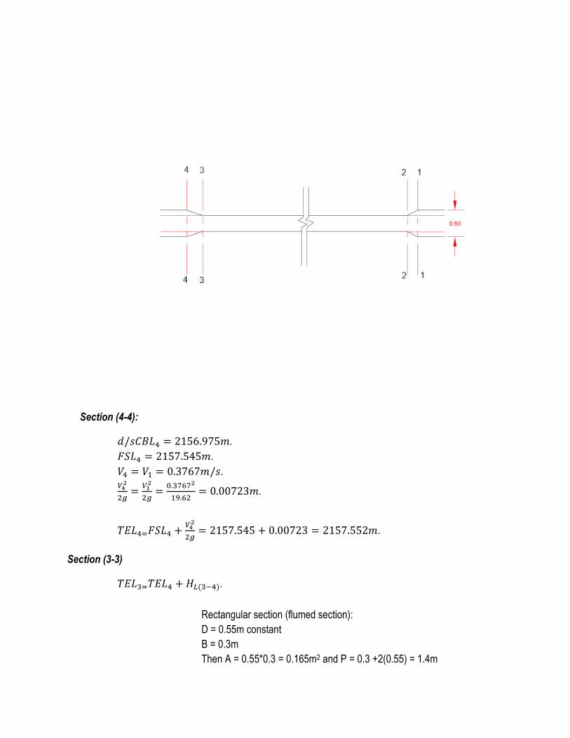
Section (4-4):
.
.
.
.
.
Section (3-3)
.
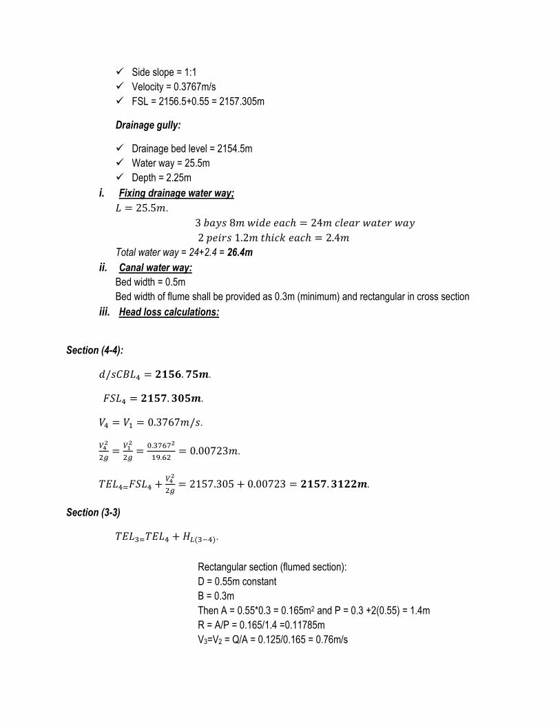
Rectangular section (flumed section):
D = 0.55m constant
B = 0.3m
Then A = 0.55*0.3 = 0.165m2 and P = 0.3 +2(0.55) = 1.4m
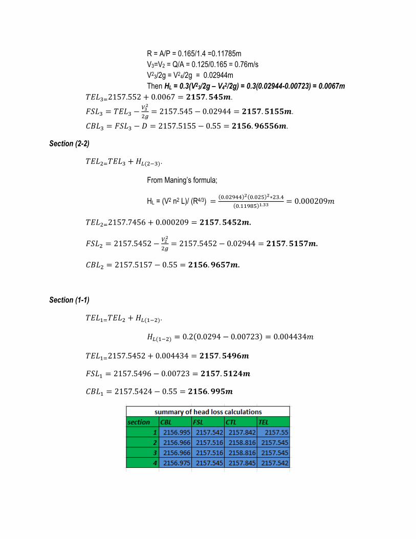
R = A/P = 0.165/1.4 =0.11785m
V3=V2 = Q/A = 0.125/0.165 = 0.76m/s
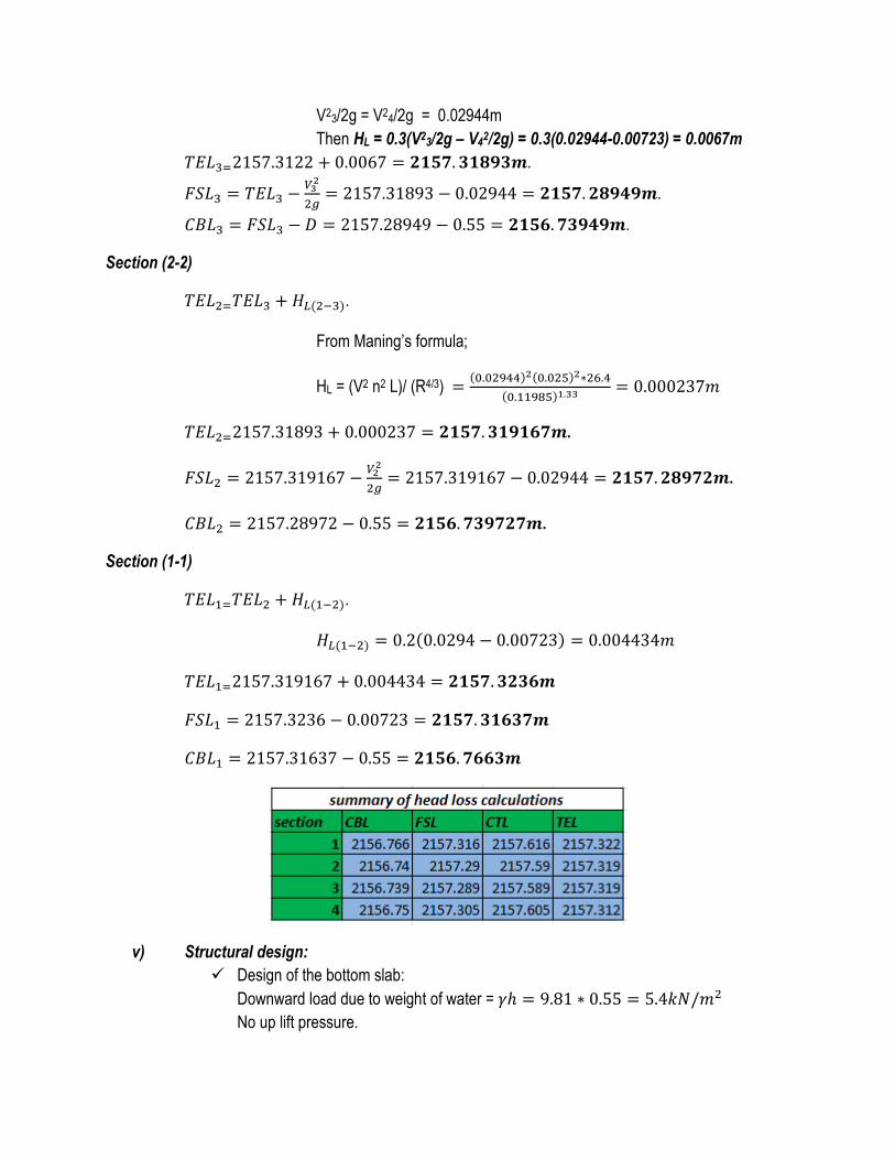
V23/2g = V2
4/2g = 0.02944m
Then HL = 0.3(V23/2g – V4
2/2g) = 0.3(0.02944-0.00723) = 0.0067m
.
.
.
Section (2-2)
.
From Maning’s formula;
HL = (V2 n2 L)/ (R4/3)
.
.
.
Section (1-1)
.
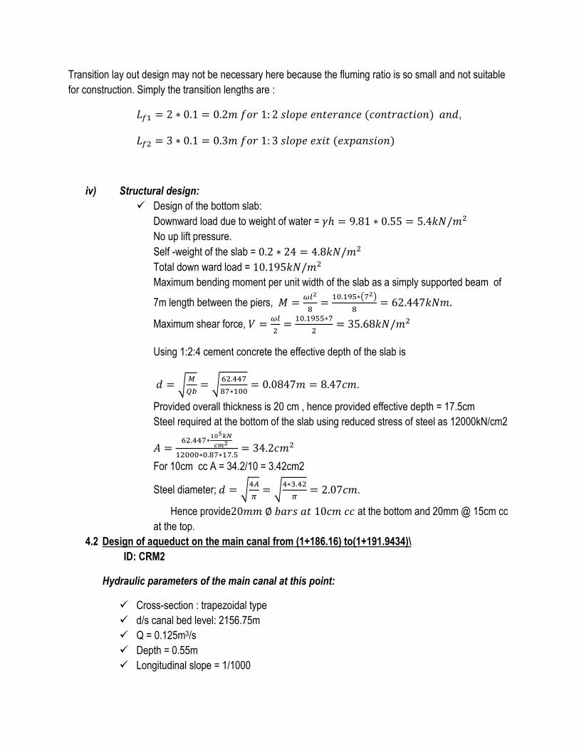
Transition lay out design may not be necessary here because the fluming ratio is so small and not suitable
for construction. Simply the transition lengths are :
,
iv) Structural design:
Design of the bottom slab:
Downward load due to weight of water =
No up lift pressure.
Self -weight of the slab =
Total down ward load =
Maximum bending moment per unit width of the slab as a simply supported beam of
7m length between the piers,
( )
Maximum shear force,
Using 1:2:4 cement concrete the effective depth of the slab is
√
√
.
Provided overall thickness is 20 cm , hence provided effective depth = 17.5cm
Steel required at the bottom of the slab using reduced stress of steel as 12000kN/cm2
For 10cm cc A = 34.2/10 = 3.42cm2
Steel diameter; √
√
.
Hence provide at the bottom and 20mm @ 15cm cc
at the top.
4.2 Design of aqueduct on the main canal from (1+186.16) to(1+191.9434)\
ID: CRM2
Hydraulic parameters of the main canal at this point:
Cross-section : trapezoidal type
d/s canal bed level: 2156.75m
Q = 0.125m3/s
Depth = 0.55m
Longitudinal slope = 1/1000
Side slope = 1:1
Velocity = 0.3767m/s
FSL = 2156.5+0.55 = 2157.305m
Drainage gully:
Drainage bed level = 2154.5m
Water way = 25.5m
Depth = 2.25m
i. Fixing drainage water way;
.
Total water way = 24+2.4 = 26.4m
ii. Canal water way:
Bed width = 0.5m
Bed width of flume shall be provided as 0.3m (minimum) and rectangular in cross section
iii. Head loss calculations:
Section (4-4):
.
.
.
.
.
Section (3-3)
.
Rectangular section (flumed section):
D = 0.55m constant
B = 0.3m
Then A = 0.55*0.3 = 0.165m2 and P = 0.3 +2(0.55) = 1.4m
R = A/P = 0.165/1.4 =0.11785m
V3=V2 = Q/A = 0.125/0.165 = 0.76m/s
V23/2g = V2
4/2g = 0.02944m
Then HL = 0.3(V23/2g – V4
2/2g) = 0.3(0.02944-0.00723) = 0.0067m
.
.
.
Section (2-2)
.
From Maning’s formula;
HL = (V2 n2 L)/ (R4/3)
.
.
.
Section (1-1)
.
v) Structural design:
Design of the bottom slab:
Downward load due to weight of water =
No up lift pressure.
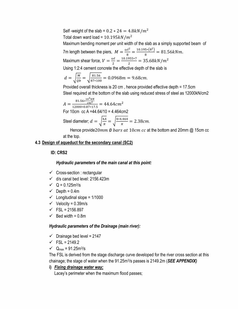
Self -weight of the slab =
Total down ward load =
Maximum bending moment per unit width of the slab as a simply supported beam of
7m length between the piers,
( )
Maximum shear force,
Using 1:2:4 cement concrete the effective depth of the slab is
√
√
.
Provided overall thickness is 20 cm , hence provided effective depth = 17.5cm
Steel required at the bottom of the slab using reduced stress of steel as 12000kN/cm2
For 10cm cc A =44.64/10 = 4.464cm2
Steel diameter; √
√
.
Hence provide at the bottom and 20mm @ 15cm cc
at the top.
4.3 Design of aqueduct for the secondary canal (SC2)
ID: CRS2
Hydraulic parameters of the main canal at this point:
Cross-section : rectangular
d/s canal bed level: 2156.423m
Q = 0.125m3/s
Depth = 0.4m
Longitudinal slope = 1/1000
Velocity = 0.39m/s
FSL = 2156.897
Bed width = 0.8m
Hydraulic parameters of the Drainage (main river):
Drainage bed level = 2147
FSL = 2149.2
Qmax = 91.25m3/s
The FSL is derived from the stage discharge curve developed for the river cross section at this
chainage; the stage of water when the 91.25m3/s passes is 2149.2m (SEE APPENDIX)
i) Fixing drainage water way;
Lacey’s perimeter when the maximum flood passes;
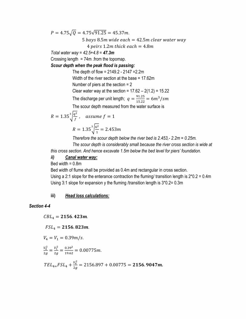
√ √ .
Total water way = 42.5+4.8 = 47.3m
Crossing length = 74m .from the topomap.
Scour depth when the peak flood is passing:
The depth of flow = 2149.2 - 2147 =2.2m
Width of the river section at the base = 17.62m
Number of piers at the section = 2
Clear water way at the section = 17.62 – 2(1.2) = 15.22
The discharge per unit length;
The scour depth measured from the water surface is
√
√
Therefore the scour depth below the river bed is 2.453,- 2.2m = 0.25m.
The scour depth is considerably small because the river cross section is wide at
this cross section. And hence excavate 1.5m below the bed level for piers’ foundation.
ii) Canal water way:
Bed width = 0.8m
Bed width of flume shall be provided as 0.4m and rectangular in cross section.
Using a 2:1 slope for the enterance contraction the fluming/ transition length is 2*0.2 = 0.4m
Using 3:1 slope for expansion y the fluming /transition length is 3*0.2= 0.3m
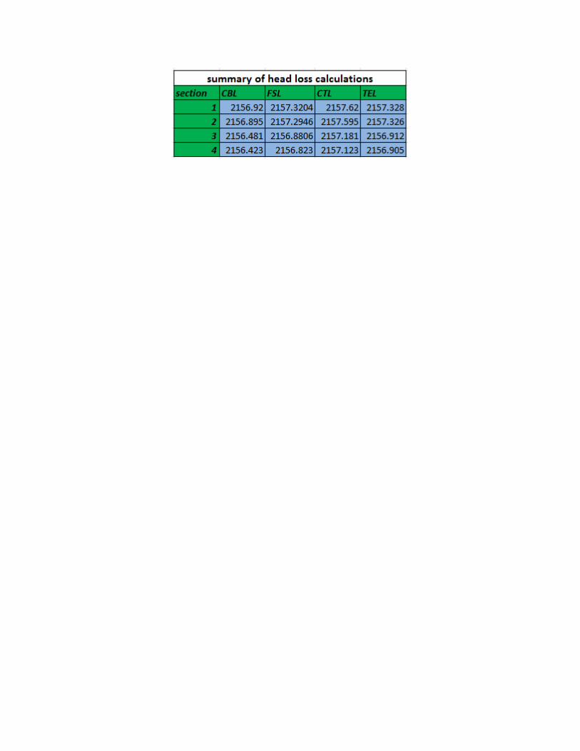
iii) Head loss calculations:
Section 4-4
.
.
.
.
.
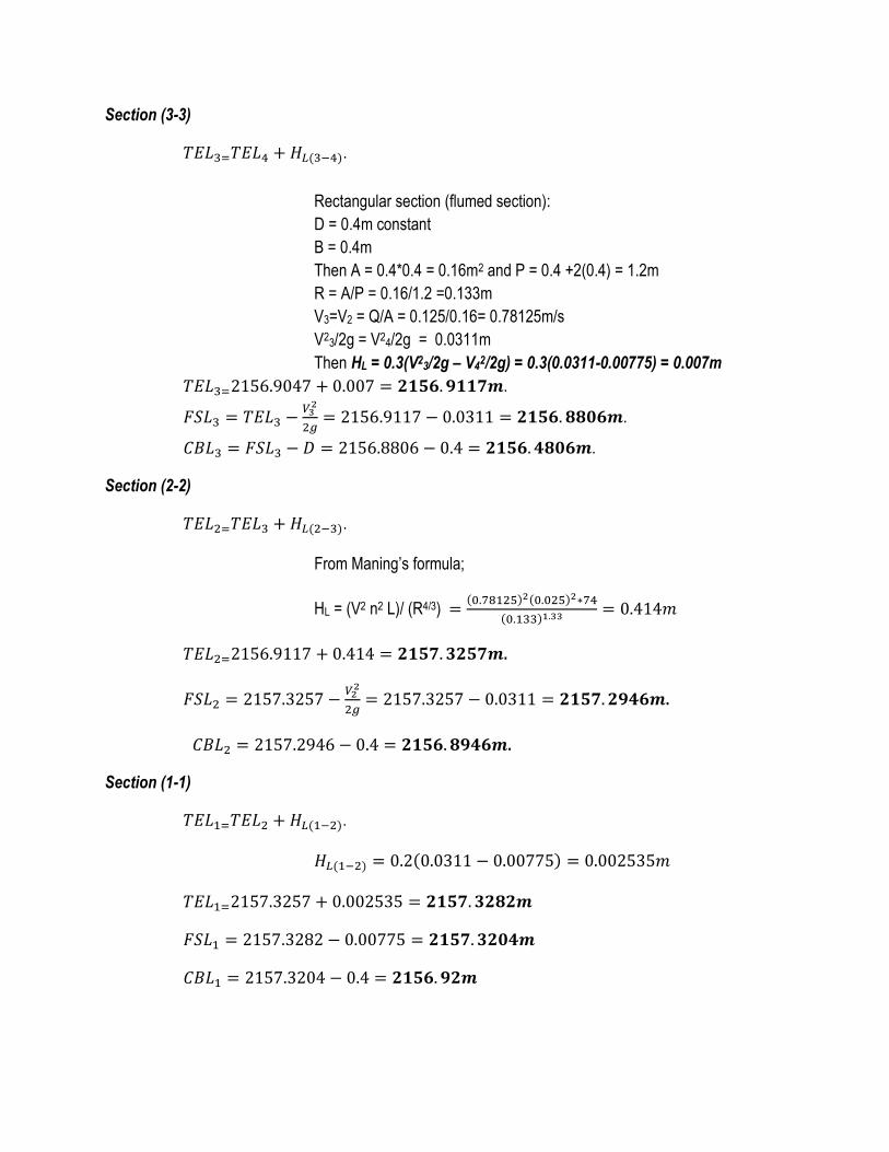
Section (3-3)
.
Rectangular section (flumed section):
D = 0.4m constant
B = 0.4m
Then A = 0.4*0.4 = 0.16m2 and P = 0.4 +2(0.4) = 1.2m
R = A/P = 0.16/1.2 =0.133m
V3=V2 = Q/A = 0.125/0.16= 0.78125m/s
V23/2g = V2
4/2g = 0.0311m
Then HL = 0.3(V23/2g – V4
2/2g) = 0.3(0.0311-0.00775) = 0.007m
.
.
.
Section (2-2)
.
From Maning’s formula;
HL = (V2 n2 L)/ (R4/3)
.
.
.
Section (1-1)
.
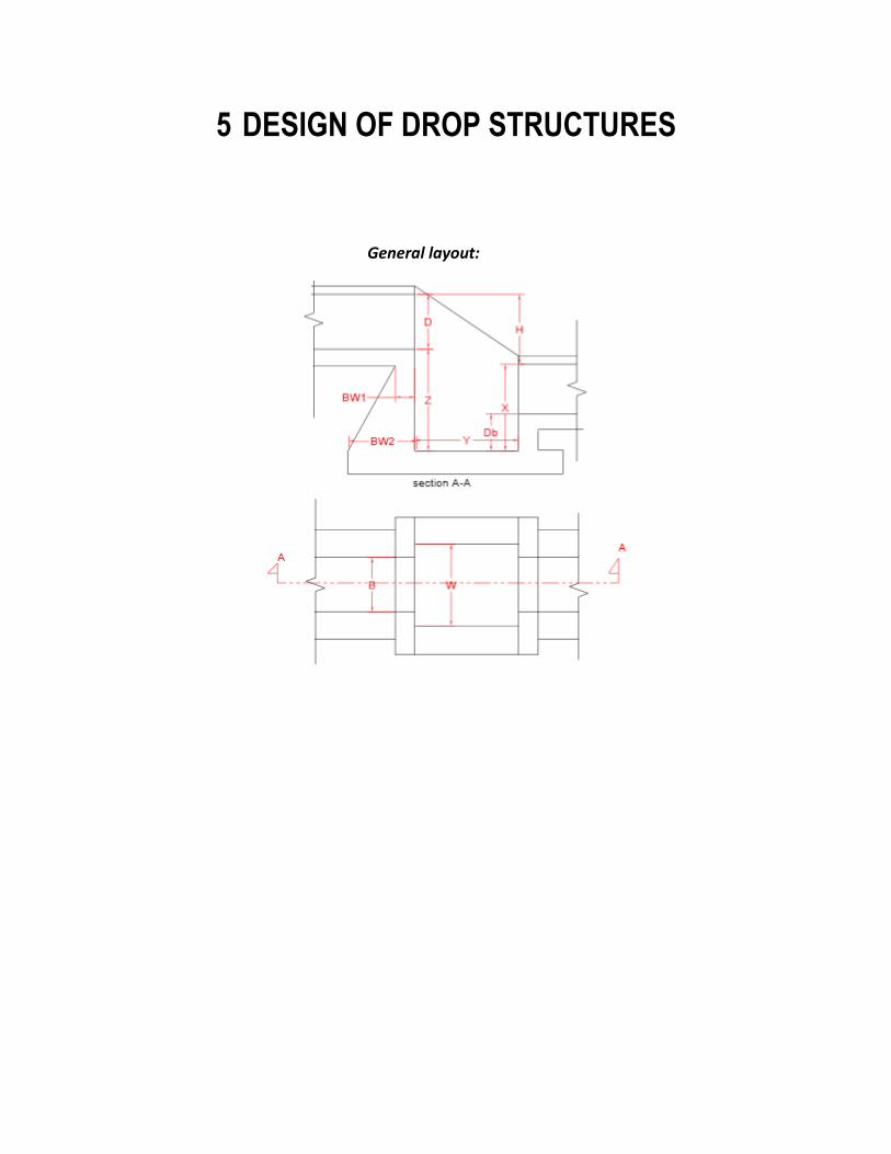
5 DESIGN OF DROP STRUCTURES
General layout:
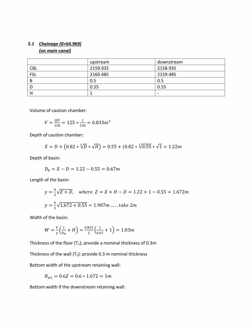
5.1 Chainage (0+64.969)
(on main canal)
upstream downstream
CBL 2159.935 2158.935
FSL 2160.485 2159.485
B 0.5 0.5
D 0.55 0.55
H 1 -
Volume of caution chamber:
Depth of caution chamber:
( √
√ ) √
√
Depth of basin:
Length of the basin:
√
√
Width of the basin:
(
)
(
)
Thickness of the floor (T1); provide a nominal thickness of 0.3m
Thickness of the wall (T2): provide 0.3 m nominal thickness
Bottom width of the upstream retaining wall:
Bottom width if the downstream retaining wall:
Length of the downstream apron:
Provide M = 2m
Length of the upstream apron:
Provide L = 3m
Summary of values:
V(m3) 0.833
X(m) 1.22
Db(m) 0.67
Y(m) 2
W(m) 1.03
Bw1(m) 1
Bw2(m) 0.4
T1(m) 0.3
T2(m) 0.3
M(m) 2
L(m) 3
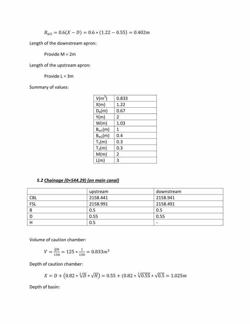
5.2 Chainage (0+544.29) (on main canal)
upstream downstream
CBL 2158.441 2158.941
FSL 2158.991 2158.491
B 0.5 0.5
D 0.55 0.55
H 0.5 -
Volume of caution chamber:
Depth of caution chamber:
( √
√ ) √
√
Depth of basin:
Length of the basin:
√
√
Width of the basin:
(
)
(
)
Thickness of the floor (T1); provide a nominal thickness of 0.3m
Thickness of the wall (T2): provide 0.3 m nominal thickness
Bottom width of the upstream retaining wall:
Bottom width if the downstream retaining wall:
Length of the downstream apron:
Provide M = 2m
Length of the upstream apron:
Provide L = 3m
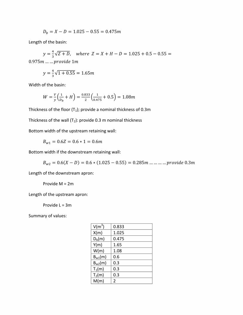
Summary of values:
V(m3) 0.833
X(m) 1.025
Db(m) 0.475
Y(m) 1.65
W(m) 1.08
Bw1(m) 0.6
Bw2(m) 0.3
T1(m) 0.3
T2(m) 0.3
M(m) 2
L(m) 3
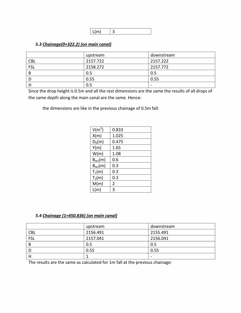
5.3 Chainage(0+322.2) (on main canal)
upstream downstream
CBL 2157.722 2157.222
FSL 2158.272 2157.772
B 0.5 0.5
D 0.55 0.55
H 0.5 -
Since the drop height is 0.5m and all the rest dimensions are the same the results of all drops of
the same depth along the main canal are the same. Hence:
the dimensions are like in the previous chainage of 0.5m fall:
V(m3) 0.833
X(m) 1.025
Db(m) 0.475
Y(m) 1.65
W(m) 1.08
Bw1(m) 0.6
Bw2(m) 0.3
T1(m) 0.3
T2(m) 0.3
M(m) 2
L(m) 3
5.4 Chainage (1+450.836) (on main canal)
upstream downstream
CBL 2156.491 2155.491
FSL 2157.041 2156.041
B 0.5 0.5
D 0.55 0.55
H 1 -
The results are the same as calculated for 1m fall at the previous chainage:
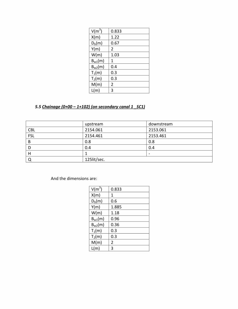
V(m3) 0.833
X(m) 1.22
Db(m) 0.67
Y(m) 2
W(m) 1.03
Bw1(m) 1
Bw2(m) 0.4
T1(m) 0.3
T2(m) 0.3
M(m) 2
L(m) 3
5.5 Chainage (0+00 – 1+102) (on secondary canal 1 _SC1)
upstream downstream
CBL 2154.061 2153.061
FSL 2154.461 2153.461
B 0.8 0.8
D 0.4 0.4
H 1 -
Q 125lit/sec.
And the dimensions are:
V(m3) 0.833
X(m) 1
Db(m) 0.6
Y(m) 1.885
W(m) 1.18
Bw1(m) 0.96
Bw2(m) 0.36
T1(m) 0.3
T2(m) 0.3
M(m) 2
L(m) 3
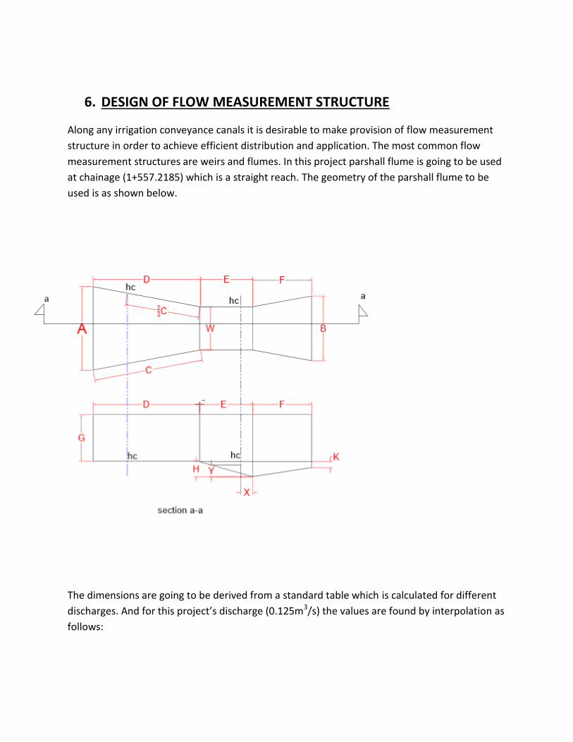
6. DESIGN OF FLOW MEASUREMENT STRUCTURE
Along any irrigation conveyance canals it is desirable to make provision of flow measurement
structure in order to achieve efficient distribution and application. The most common flow
measurement structures are weirs and flumes. In this project parshall flume is going to be used
at chainage (1+557.2185) which is a straight reach. The geometry of the parshall flume to be
used is as shown below.
The dimensions are going to be derived from a standard table which is calculated for different
discharges. And for this project’s discharge (0.125m3/s) the values are found by interpolation as
follows:

Therefore the parshall flume has to be constructed as per the interpolated dimensions shaded
in yellow.