CULTURE� ECONOMIC STRUCTURE� AND THE DYNAMICS OF
ECOLOGICAL ECONOMIC SYSTEMS
By
John M� Anderies
B�Sc�� Colorado School of Mines� Golden� Colorado� U�S�A� ����
M�Sc�� University of British Columbia� ����
a thesis submitted in partial fulfillment of
the requirements for the degree of
Doctor of Philosophy
in
the faculty of graduate studies
department of mathematics
institute of applied mathematics
We accept this thesis as conforming
to the required standard
� � � � � � � � � � � � � � � � � � � � � � � � � � � � � � � � � � � � � � � � � � � � � � � � � � � � � �
� � � � � � � � � � � � � � � � � � � � � � � � � � � � � � � � � � � � � � � � � � � � � � � � � � � � � �
� � � � � � � � � � � � � � � � � � � � � � � � � � � � � � � � � � � � � � � � � � � � � � � � � � � � � �
� � � � � � � � � � � � � � � � � � � � � � � � � � � � � � � � � � � � � � � � � � � � � � � � � � � � � �
� � � � � � � � � � � � � � � � � � � � � � � � � � � � � � � � � � � � � � � � � � � � � � � � � � � � � �
the university of british columbia
July� ����
c� John M� Anderies� ����

Abstract
In this thesis several models are developed and analyzed in an attempt to better un
derstand the interaction of culture� economic structure� and the dynamics of human
ecological economic systems� Specically� how does the ability of humans to change their
individual behavior quickly and easily in response to changing environmental conditions
�behavioral plasticity� alter the dynamics of human ecological economic systems What
role can cultural and social institutions play in a�ecting individual behavior and thus
the dynamics of such systems Finally� how do assumptions about the production and
consumption of goods and services within human ecological economic systems a�ect their
dynamics�
Much work concerning interacting economic and natural processes has focused on
technical issues and problems with standard economic thought� Less attention has been
paid to the role of human behavior� The work presented herein addresses both but em
phasizes the latter� Three models are developed� a model of the Tsembaga of New Guinea
which focuses on the roles of behavior� cultural practices and ritual on the dynamics of
the Tsembaga ecosystem� a model of Easter Island where the linkage between economic
models of utility and the resulting behavioral model is studied� and nally a model of
a modern two sector economy with capital accumulation where the emphasis is evenly
split between behavior and economic issues�
The main results of the thesis are� behavioral plasticity exhibited by humans can
destabilize ecological economic systems and culture and social organization can play a
critical role in o�setting this destabilizing force� Finally� the analysis of the two sector
model indicates that there is a window of feasible investment levels that will lead to a
ii

sustainable economy� The size of this window depends on culture and social organiza
tion� namely the way economic growth is managed and how the associated benets are
distributed� The two sector model claries the idea of a sustainable economy� and allows
the possibility of reaching one to be clearly characterized�
iii

Table of Contents
Abstract ii
List of Tables vii
List of Figures viii
Acknowledgement xi
� Introduction �
� The Modeling Framework �
��� Dynamical Systems Models of Ecological Systems � � � � � � � � � � � � � �
��� Human economic ecological systems � � � � � � � � � � � � � � � � � � � � � ��
����� Background � � � � � � � � � � � � � � � � � � � � � � � � � � � � � � ��
����� The general model � � � � � � � � � � � � � � � � � � � � � � � � � � ��
��� Analytical methods � � � � � � � � � � � � � � � � � � � � � � � � � � � � � � ��
� Culture and human agro�ecosystem dynamics� the Tsembaga of New
Guinea �
��� The ecological and cultural system of the Tsembaga � � � � � � � � � � � � ��
��� The model � � � � � � � � � � � � � � � � � � � � � � � � � � � � � � � � � � � ��
����� Denitions � � � � � � � � � � � � � � � � � � � � � � � � � � � � � � � ��
����� Tsembaga subsistence and the population growth rate� f� � � � � � ��
����� The ecology of slashandburn agriculture � � � � � � � � � � � � � ��
iv

����� The food production function � � � � � � � � � � � � � � � � � � � � ��
��� Dynamic behavior of the model � � � � � � � � � � � � � � � � � � � � � � � ��
��� Behavioral plasticity � � � � � � � � � � � � � � � � � � � � � � � � � � � � � ��
��� Modelling the ritual cycle � � � � � � � � � � � � � � � � � � � � � � � � � � ��
����� The parasitism of pigs � � � � � � � � � � � � � � � � � � � � � � � � ��
����� The ritual cycle � � � � � � � � � � � � � � � � � � � � � � � � � � � � ��
����� The behavior of the full system � � � � � � � � � � � � � � � � � � � ��
��� Conclusions � � � � � � � � � � � � � � � � � � � � � � � � � � � � � � � � � � ��
Non�substitutibility in consumption and ecosystem stability �
��� The Easter Island model � � � � � � � � � � � � � � � � � � � � � � � � � � � ��
��� Model Critique � � � � � � � � � � � � � � � � � � � � � � � � � � � � � � � � ��
����� Behavioral plasticity and collapse � � � � � � � � � � � � � � � � � � ��
��� Adding behavioral plasticity to the Easter Island model � � � � � � � � � � ��
����� Model analysis � � � � � � � � � � � � � � � � � � � � � � � � � � � � ��
��� Conclusions � � � � � � � � � � � � � � � � � � � � � � � � � � � � � � � � � � ��
The dynamics of a two sector ecological economic system ��
��� Simple economic growth models � � � � � � � � � � � � � � � � � � � � � � � ��
����� Basic laws of production and the theory of the rm � � � � � � � � ��
����� Consumer behavior � � � � � � � � � � � � � � � � � � � � � � � � � � ��
��� The ecological economic model � � � � � � � � � � � � � � � � � � � � � � � � ��
����� The economic system � � � � � � � � � � � � � � � � � � � � � � � � � ��
����� Computing the general equilibrium � � � � � � � � � � � � � � � � � ��
��� The ecological system model � � � � � � � � � � � � � � � � � � � � � � � � � ���
��� Analysis of the Model � � � � � � � � � � � � � � � � � � � � � � � � � � � � � ���
����� Investment� distribution of wealth� and ecosystem stability � � � � ���
v

����� Nonrenewable natural capital� e�ciency� and �ows between industries���
��� Conclusions � � � � � � � � � � � � � � � � � � � � � � � � � � � � � � � � � � ���
� Re�ections and future Research ���
Bibliography ��
vi

List of Tables
��� Table of important symbols � � � � � � � � � � � � � � � � � � � � � � � � � ���
��� Table of important symbols� continued � � � � � � � � � � � � � � � � � � � ���
��� Equilibrium consumption versus bc � � � � � � � � � � � � � � � � � � � � � ���
vii

List of Figures
��� Isolated predatorprey model� � � � � � � � � � � � � � � � � � � � � � � � � �
��� Predatorprey model embedded in an ecosystem � � � � � � � � � � � � � � ��
��� The circular �ow of exchange in standard economics� � � � � � � � � � � � ��
��� Economic system in the proper ecological context � � � � � � � � � � � � � ��
��� Two main model structures� �a� attainable steady state� �b� unattainable
steady state� � � � � � � � � � � � � � � � � � � � � � � � � � � � � � � � � � � ��
��� Graphical representation of nutrient cycling process in a forest� � � � � � ��
��� Soil recovery curves � � � � � � � � � � � � � � � � � � � � � � � � � � � � � � ��
��� The production surface for cotton lint � � � � � � � � � � � � � � � � � � � � ��
��� Comparing the Cobb Douglas and von Liebig functions� � � � � � � � � � � ��
��� Bifurcation diagram for swidden agriculture � � � � � � � � � � � � � � � � ��
��� Bifurcation diagram for swidden agriculture � � � � � � � � � � � � � � � � ��
��� Two parameter bifurcation diagram for the swidden agriculture model � � ��
��� Change in dynamics accross bifurcation boundary � � � � � � � � � � � � � ��
��� Bifurcation diagram with cmax� as the bifurcation parameter in the swidden
agriculture model� � � � � � � � � � � � � � � � � � � � � � � � � � � � � � � � ��
���� Tsembaga ecosystem limit cycles � � � � � � � � � � � � � � � � � � � � � � ��
���� Work level �curve �a�� and food production �curve �b��� over time� � � � ��
���� The in�uence of pigs on system dynamics � � � � � � � � � � � � � � � � � � ��
���� The ritual cycle of the Tsembaga � � � � � � � � � � � � � � � � � � � � � � ��
���� Form of g�x� � � � � � � � � � � � � � � � � � � � � � � � � � � � � � � � � � � ��
viii

���� The dynamics of the ritual cycle � � � � � � � � � � � � � � � � � � � � � � � ��
���� An example of of the human �a�� and pig �b�� population trajectories under
cultural outbreak dynamics� � � � � � � � � � � � � � � � � � � � � � � � � � ��
���� Sample trajectories for the full model � � � � � � � � � � � � � � � � � � � � ��
���� Limit cycle for the full model � � � � � � � � � � � � � � � � � � � � � � � � ��
��� Population and resource stock trajectories for Easter Island model from ����� ��
��� Percapita growth rate from the time of initial colonization to the time of
rst European contact� � � � � � � � � � � � � � � � � � � � � � � � � � � � � ��
��� Bifurcation diagram for modied Easter Island model� � � � � � � � � � � ��
��� Population and sectoral labor proportion trajectories � � � � � � � � � � � ��
��� Trajectories for population and total labor in each sector over time � � � ��
��� Schematic of two sector ecological economic model� � � � � � � � � � � � � ��
��� Trajectories of wages� capital� and labor as the economy adjusts� � � � � � ��
��� Surface plot of utility function showing optimal combination of labor and
capital to agriculture� � � � � � � � � � � � � � � � � � � � � � � � � � � � � � ���
��� Example of economic system dynamics � � � � � � � � � � � � � � � � � � � ���
��� Simple economic growth model � � � � � � � � � � � � � � � � � � � � � � � ���
��� State varible trajecories � � � � � � � � � � � � � � � � � � � � � � � � � � � ���
��� Equilibrium Labor� capital� and consumption trajectories � � � � � � � � � ���
��� Bifurcation diagram for simplied model� � � � � � � � � � � � � � � � � � � ���
��� Change in dynamics as the bifurcation boundary is crossed� � � � � � � � � ���
���� State varible trajectories � � � � � � � � � � � � � � � � � � � � � � � � � � � ���
���� Cyclical Labor� capital� and consumption trajectories � � � � � � � � � � � ���
���� Resource good preference versus Kn for di�erent values of �kn � � � � � � ���
���� E�ciency curves � � � � � � � � � � � � � � � � � � � � � � � � � � � � � � � ���
ix

���� State variable trajectories � � � � � � � � � � � � � � � � � � � � � � � � � � ���
���� Equilibrium states versus �kn � � � � � � � � � � � � � � � � � � � � � � � � ���
���� Capital and investment good preferences over time � � � � � � � � � � � � ���
���� Bifurcation structure for full model � � � � � � � � � � � � � � � � � � � � � ���
���� Two parameter bifurcation digram for investmentgood preference and �kr� ���
���� Two parameter bifurcation digram for investmentgood preference and �N � ���
���� Two parameter bifurcation digram for investment good preference and Ram����
x

Acknowledgement
I would like to thank Dr� Colin Clark for his nancial and moral support over the past
� years� his many readings of my work and helpful ideas and comments� I would also
like to thank my committee members for helpful comments and ideas as I developed the
thesis� especially Leah Keshet and James Brander� Finally I am greatly indebted to my
wife and friend Margaret� thanks� your turn�
xi

Chapter �
Introduction
Since the �����s� the impact of human activities on ecosystems has been receiving more
and more attention� Through this increased awareness� �sustainability� � the basic ques
tion of whether and how human populations can continue to live on earth indenitely
without threatening the survival of all biological populations � has become an important
international issue� and the focus of much research� Unfortunately there are deep divi
sions between di�erent groups of people regarding the fundamentals of the sustainability
issue�
Examples of such divisions are everywhere � in the popular media and in academic de
bates� For example� several authors have argued that the economic process is fundamen
tally in�uenced by entropic decay ���� ��� while others ���� argue that the entropy law is
irrelevant because the earth is a thermodynamically open system� Some experts are very
concerned about the degradation of agricultural ecosystems �soil erosion� etc�� ���� ��� ���
while others praise the power of technology to �liberate the environment� and give us
�e�ectively landless agriculture� ����p� ���� via ��a� cluster of innovations including
tractors� seeds� chemicals� and irrigation� joined through timely information �ows and
better organized markets �that will� raise yields to feed billions more without clearing
new elds� ����p� �����
The aim of this thesis is to address several aspects of this division� For this purpose�
di�erent views on sustainability can be divided in to two broad classes�
A� �expansionist view� Sustainability is mainly a technical issue� The present paradigm
�

Chapter �� Introduction �
of economic growth can continue indenitely as long as increases in e�ciency o�set
increasing pressure on natural resources and ecological systems�
B� �steady state view� Sustainability involves a comprehensive understanding of the
place of human populations within ecosystems� Achieving a sustainable world will
require a fundamental paradigm shift concerning the way humans lead their lives�
There are two key points to note about these di�erent positions� First� the existence
of this di�erence hinders the development of e�ective policy to govern the relationship
between human economic and ecological systems� Second� position A is the paradigm
of choice in present policy formation without su�cient evidence that it is the �correct�
view�
Clearly� the only way society can move toward a sustainable state is to extract impor
tant truths from both views and with them forge some strategy to guide future human
environmental interactions� This is not an easy task for two reasons� First� human agro
ecosystems may be too complex to understand in enough detail to be useful in policy
formation� Second the views of people on either side of the issue may be� as Rees ����
notes� based more � �on� di�ering fundamental beliefs and assumptions about the nature
of humankindenvironment relationships� rather than fact� At the heart of the issue are
assumptions that underly the models and arguments made in support of either view �see
the forum in ��� for a collection of recent papers on the continuing debate��
I believe there are three fundamental questions the must be addressed before real
progress can be made in resolving di�erences concerning the concept of sustainability�
First� the expansionist view assumes that our ability to solve problems with technology
is necessarily a good thing� Is this so Second� how important are our cultural and
social institutions in determining whether a human economic system is sustainable Fi
nally� how do assumptions that underly economic growth models used to support the

Chapter �� Introduction �
expansionist position a�ect the dynamics of human ecological economic systems The
main thrust of this thesis is to develop a modeling framework to help answer these three
questions�
My approach is to develop dynamical systems models to study humans as ecological
populations� These models focus on how human behavioral and cultural systems interact
with the environment� and they are deliberately stylized to avoid the trap of generating
models that are too complicated with too many assumptions to be of practical use�
e�g� ���� ���� Only the most basic features of general human economic ecological systems
are included� In attempting to answer the questions posed above I develop three di�erent
models of this type� two involving simple societies of anthropological interest and one
modern economic system with capital accumulation� with the following objectives�
� The rst model addresses the rst two questions in the context of a simple human
agroecosystem� The human ability to modify behavior quickly and over a wide
range of di�erent activities� �dened as behavioral plasticity�� is emphasized� The
role that behavioral plasticity plays in the dynamics of a human agroecosystem
is studied in detail� Of special interest is the destabilizing e�ect of behavioral
plasticity� and the stabilizing role culture and social organization may play�
� The second model is directed towards the third question� Here� a linkage between
economic concepts and an evolving ecological economic system is developed� Eco
nomic models of behavior based on the optimization of some measure of utility are
introduced� Utility measures that result in realistic behavior in the context of an
evolving ecological economic system are identied� Again� the destabilizing e�ect
of behavioral plasticity is highlighted�
� In the third model� the ideas developed in the rst two models are combined to
develop the model of the modern economic system� This model model addresses

Chapter �� Introduction �
all three questions in the context of economic growth in a bounded environment�
In addition to shedding light on the three fundamental questions posed above� the
models developed in this thesis provide tools to study operational aspects of sustain
ability� This is very useful since much of the problem with the sustainability concept is
that it is easy to imagine what a sustainable state might be like� but few ask whether
it is possible to get from our present state to a sustainable state� As Rees ���� notes�
�����sustainability will require a �paradigm shift� or a �fundamental change� in the way
we do business� but few go on to describe just what needs to be shifted����� Thinking
about a sustainable world is pointless unless we can nd a way to get there� In a recent
article� Proops et al� ���� emphasize the need to formulate a goal of sustainability� set an
intermediate target� and develop feasible paths toward this goal� The analytical frame
work developed in this thesis provides a �exible� simple� and precise means of studying
�for a given set of assumptions� exactly what cultural attributes are sustainable or not�
and more importantly� what key aspects a�ect the feasibility of potential paths to a
sustainable human ecological economic system�
The structure of the thesis is as follows� Chapter � outlines the background� assump
tions and basic structure of the modelling framework� Next� in Chapter � the modelling
framework is applied to the society of the Tsembaga� a tribe that occupies the highlands
of New Guinea� Next� the ideas developed in Chapter � are extended in Chapter � where
a model proposed by Brander et� al ��� to explain the rise and fall of the Easter Island
civilization is used to develop and study more advanced economic concepts typically used
to model human consumptive and productive activities� These authors argue that the
Polynesian culture that occupied Easter Island was mismatched to the ecosystem they
found and thus perished� The authors also discuss the implications of their model for
other societies that collapsed� and for our own society� The main point is that more

Chapter �� Introduction �
complex economic models in which agents exhibit maximizing behaviors based on a cer
tain utility function do not necessarily give rise to richer models behavior indeed they
can result in very simple� not very realistic behavioral patterns� Here we emphasize how
nonsubstitutability in consumption fundamentally alters the behavior of the model and
the nature of the approach to the sustainable state� and that realistic behavior depends
on the inclusion of this aspect in utility functions�
Finally� pulling together the ideas of chapters � and �� I develop a model of a two
sector �a sector in economics is a grouping of associated productive activities� economy
and embed it in a model ecosystem� The economy has an agricultural �bioresource� sector
and a manufacturing sector� Economic agents �individuals who take part in productive
and consumptive activities within the economy� can devote the productive capacity of
the economy to four di�erent activities� the consumption of agricultural� manufactured�
investment� and resource goods� This model includes all the components that form the
basis of the current debate about human environmental interaction� we rely on �ows from
the environment but we can use our productive capacity to substitute for these �ows�
increase e�ciency� reduce waste� and help regenerate the environment� Those holding the
steady state view emphasize the importance of the former while expansionists emphasize
the power and importance of the latter� With the modelling framework developed herein�
their interaction can be studied�

Chapter �
The Modeling Framework
In this chapter� the background and assumptions underlying the modeling framework are
addressed� The modeling approach is outlined� and the general model that is employed
throughout the thesis is developed� Next� the important features of the models that are
important to the questions posed in the introduction are discussed� Finally� the analytical
techniques used to uncover these features are presented�
When trying to model the interaction between elements in a system� e�g� predators
with prey� one competitor with another� an organism with its environment� one neces
sarily has to model the way each element a�ects how other elements change over time�
The most common approaches are to write down di�erential equations� di�erence equa
tions� functional di�erential equations �when age structure is important�� or a stochastic
process� Often several approaches are appropriate for a given problem so the choice of
approach often depends on the intentions of the modeler�
The models I develop in this thesis are all deterministic dynamical systems� The ad
vantage of this approach is that the models are clear and simple� allowing the underlying
assumptions and concepts to be easily seen by inspecting the di�erential equations that
constitute the model� Drawbacks are that implicit in deterministic models is the assump
tion that everything is �well mixed� and there are no spatial or random e�ects allowed�
That is to say that each variable in the model necessarily represents an average value of a
particular quantity� Clearly no real system is well mixed and deviations from the average
can substantially alter the dynamics of the system in question� Fortunately� it is often
�
Chapter �� The Modeling Framework �
the case that many aspects of a real system can be inferred from the structure of the
�mean eld� or average model given by the deterministic ordinary di�erential equation
system�
Studying the dynamics of such models is a di�cult task� If the model is simple enough
it can be studied by analytical methods� The models in this thesis are too complex
to study analytically� Fortunately� there are numerical techniques available that allow
dynamical systems theory to be used on more complex systems� In the next section I will
brie�y discuss the application of dynamical systems type models to ecological systems
and explain how I extend them for the special case of human economic ecological systems�
� � Dynamical Systems Models of Ecological Systems
Ecologists have long used simple systems of di�erential equations to model ecosystems
so as to understand how di�erent behavioral patterns may e�ect the dynamics between
individuals that interact in the ecosystem� Because my interest is specically with be
havior and environmental constraints� the way behavior is modeled� and the way a model
is placed in an ecological context are very important� I will illustrate this by way of a
simple example�
Di�erential equation models of ecosystems often take form
dx
dt f�x� p� �����
where x � �n describes the state of the ecosystem and p � �k is a parameter vector� This
type of model has been extensively studied �e�g� ���� ��� ��� ��� ����� In such models�
the behavior of organisms is often modeled by a functional response that is completely
determined by the state of the system� For example the simplest LotkaVolterra predator
prey model given by

Chapter �� The Modeling Framework �
dh
dt rh � �ph ����a�
dp
dt ��h! �ph� ����b�
where h�t� and p�t� are the prey and predator population densities� respectively� This
model exhibits unrealistic neutral oscillations where predator and prey numbers can take
on arbitrarily large values� This is due to the fact that behavior is modeled too simply and
there is no ecological context� Prey behavior is limited to eating and growing� They do
nothing to avoid predators or carry out any other complex behavior� Predators die and eat
prey� never changing their behavior whether they are hungry or full� The organisms are
behaviorally rigid� or for our purposes� not behaviorally plastic� Almost all animals have
some measure of behavioral plasticity� and this is especially true of humans� Ecologists
often include more complex behavior by introducing a functional response term to model
the way a predator consumes prey� At the very least� these models include some means
of satiating the appetite of the predator� For example equations ��� could be modied by
replacing the term �ph in equation ���a with the functional response g�h� p�� Holling ����
proposed the functional response�
g�h� p� �ph
p ! k�����
where k is the prey concentration at which the predator consumes at onehalf its max
imum rate� As p increases� the rate at which prey are removed approaches �h� each
predator is consuming at a constant� maximum rate� Note that although some increased
behavioral plasticity is added and the model is more realistic� the behavior or the predator
is completely determined by the state of the system and not by any internal feedback� For
example� if there are fewer prey and the predator becomes hungry� there is no mechanism
in the model to allow the predator to change its strategy or work harder� If we attempt

Chapter �� The Modeling Framework �
to model a human ecosystem� this is a key feature to include� Indeed� in chapter � we will
see just how important this is� To properly model a system where individual organisms
are behaviorally plastic� we have to add equations that model the internal state of the
organisms and how they in�uence behavior� I will address this issue in a moment� but
rst let me turn to the second point mentioned above� the ecological context�
The predator prey model given by ��� is completely isolated from the environment�
The equations model the system shown in gure ���� In reality� ecological systems are
not isolated but are embedded in a physical environment and are dissipative� they con
tinuously dissipate derivatives of solar energy�
PreyPredator
Figure ���� Isolated predatorprey model�
For a realistic model� we must include the fact that there is some abiotic component� xa�
the medium through which this dissipative process occurs� A recent paper addressing
this point ����� suggests that the equations of motion be written this way�
"x f�xa� x� p� z�t�� d� �����
where xa are abiotic components� d describes the dissipative process� and z�t� represents
some external forcing� This is just a general mathematical statement that instead of
modeling the system shown in gure ��� we must model the system shown in gure ����
In such a model� the fundamental processes that make the interaction between preda
tor and prey possible are included� In terms of equation ���� the abiotic components
would include the soil structure of the ecosystem� The forcing might be the weather
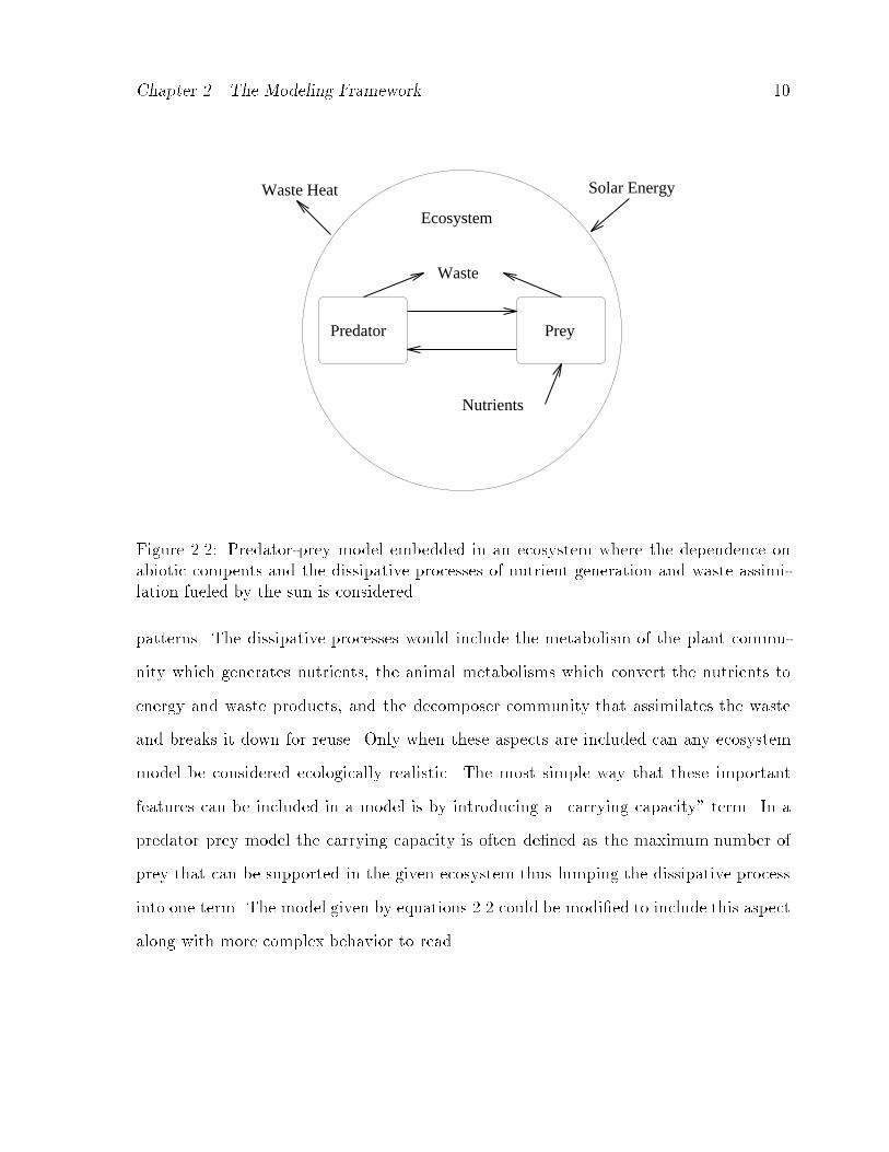
Chapter �� The Modeling Framework ��
Predator Prey
Solar Energy
Ecosystem
Waste
Nutrients
Waste Heat
Figure ���� Predatorprey model embedded in an ecosystem where the dependence onabiotic compents and the dissipative processes of nutrient generation and waste assimilation fueled by the sun is considered�
patterns� The dissipative processes would include the metabolism of the plant commu
nity which generates nutrients� the animal metabolisms which convert the nutrients to
energy and waste products� and the decomposer community that assimilates the waste
and breaks it down for reuse� Only when these aspects are included can any ecosystem
model be considered ecologically realistic� The most simple way that these important
features can be included in a model is by introducing a �carrying capacity� term� In a
predator prey model the carrying capacity is often dened as the maximum number of
prey that can be supported in the given ecosystem thus lumping the dissipative process
into one term� The model given by equations ��� could be modied to include this aspect
along with more complex behavior to read

Chapter �� The Modeling Framework ��
dh
dt r���
h
K�h�
�ph
p ! k����a�
dp
dt ��h!
�ph
p! k� ����b�
where K is the carrying capacity� This model yields a stable xed point or a stable limit
cycle� This is much more reasonable than the arbitrarily large �uctuations possible in the
model specied by equation ���� The key point I wish to draw out is the importance of
behavior and ecological context in ecological models� If we wish to extend this modeling
framework to human ecological economic systems� these are key issues we need to address�
Indeed� the issue of ecological context is fundamental in the debate about sustainable
development�
� � Human economic ecological systems
� � � Background
Most of the work on human economic ecological systems has been either in the context
of �optimal� economic growth� or the optimal exploitation of resources� Unfortunately�
economic models often lack ecological context� The example above shows that modeling
without proper ecological context may lead to quite absurd results� and economic models
are no exception�
For example� the model of Solow ���� in the context of optimal economic growth with
exhaustible resources states that along an optimal growth path� constant net output can
be maintained in the face of dwindling resource inputs� Later� when further analyzing
Solow�s work� Hartwick ���� presented the savings rule� invest all rents from exhaustible
resources �in replenishable manmade capital� to maintain constant net output inde
nitely� This result is based on a model like that shown in gure ���� The economic

Chapter �� The Modeling Framework ��
system is viewed as a circular �ow of exchange between rms and households as shown
on the left in gure ��� interacting with the physical world on the right� The physical
world is often just viewed as a source of raw materials �to be optimally extracted as in
the case of the Solow#Hartwick model� and a sink for wastes�
Source of rawmaterial
Sink forwastes
Income
HOUSE �
HOLDSFIRMS
Physical
World
Goods and Services
Expenditures
Factors of Production
Figure ���� Schematic of the circular �ow of exchange as perceived by standard economics�The connection to the real world� even as merely a source of raw materials and a wastebin� is seldom shown�
Clearly� the underlying assumptions in such models are critical to obtaining results
such as those above� In the case above� it is assumed that the production of commodities�
Y � is given by
Y K�L�N� �����
where K and L are manmade capital stocks and population respectively� N is a �ow of

Chapter �� The Modeling Framework ��
natural resources� and �� �� and � are parameters assumed to satisfy �! �! � �� For
the case where the population is held constant and there is no technological progress� the
dynamical system for this optimal economic growth model is
dK
dt AK�N� � C ����a�
dN
dt ��
�
�� ��CN
K� ����b�
where A is a constant representing the contribution to production of the xed labor force�
and C is total consumption of the population� The rst equation states that capital� K�
increases at a rate given by the total commodity production rate less what is consumed�
The second equation states that the resource �ow diminishes �optimally� as resources
are used up� Now� C is always less than or equal to AK�N� �you can�t consume more
than you make� thusdK
dt� �� This implies that K�t� � � for all t � � which results
in the right hand side of ���b being negative for all t � � forcing N�t� to approach zero
asymptotically as time tends toward innity�
A glance at this model will reveal its similarity to ��� where K is analogous to the
predator and N is analogous to �in this case a nite stock of� the prey� The parallel
I wish to draw is the similarity in the growth function assumed for the predator and
capital� The predator can still grow at very low prey levels if there are su�ciently many
predators$ Similarly� the capital can continue to grow with a very low resource �ow�
as long as there are su�cient capital stocks� The absurdity in the case of the predator
model is obvious� and ecologists quickly modied this model as already discussed� The
di�culty in the economic growth model is more di�cult to see� and economists have been
slower than ecologists to modify such models�
The Solow result depends on the assumption that the factors of production� manmade
capital �a stock�� and resources �a �ow�� are near perfect substitutes� Much of ecological

Chapter �� The Modeling Framework ��
economics is concerned with exposing the underlying physical problems associated with
such models and developing more realistic models �for recent examples see ���� ����� The
emphasis of this work is the nonsubstitutability among di�erent stocks and between
stocks and �ows� Even if these modications were made to the Solow model� there is still
no clear ecological context� the only connection to the physical world is through a nite
stock of resources to optimally use up�
Herman Daly ���� and Nicholas Georgescu Roegen ���� were among the rst �ecolog
ically minded� economists to recognize the need to study the system shown in gure ���
and to emphasize that in addition to the issue of nite resource stocks� there is the is
sue of ecological context� we are embedded in a natural world that is important to our
survival regardless of its connection to the economic process� This is the type of model
which is developed and analyzed in the rest of this thesis�
The other key component that governs the evolution of an ecological economic system�
namely human behavior� has received much less attention in the literature than technical
issues related to economic models and ideas� For example maximization of utility over
the next twenty years is most often assumed as the primary goal driving behavior� This
has two important consequences� this assumption has become ingrained in standard
economics� encouraging this behavior within society whether natural or not� in policy
formation the model implies that only the next few years are important� In defense of
his model� Solow ���� makes this very point� He indicates that the main purpose of these
models is for planning over the next �� years� How feasible is this planning strategy
Before turning our attention to the mathematical model� note two main points�
� Any realistic model of the interaction of organisms with their environment must
address the role of individual behavior�
� Maintaining realism in the way that di�erent inputs interact in the productive

Chapter �� The Modeling Framework ��
Energy and Raw Materials
Waste Heat Solar Energy
Factors of Production
Goods and Services
Income
Expenditures
FirmsHouse - Holds
WasteWaste
Figure ���� Schematic of the circular �ow of exchange as perceived by standard economicsembedded in the proper ecological context�
process is important� but ecological context may be more so� Explicit modelling
of the in�uence of organisms on the abiotic components and dissipative processes
upon which they rely is crucial to capturing the dynamics of the system�
The topic of the next section is the mathematical expression of these ideas�
� � � The general model
It is di�cult to dene a model that would be suitable to study a wide variety of ecological
economic systems because of the variability of human cultural and social systems� Thus�
Chapter �� The Modeling Framework ��
the following is a general description of the model intended to emphasize basic structures
common to human ecological economic systems� The general model will then be made
specic in later chapters� State variables will be dened� a behavioral model is developed
and the dynamics of the physical system are specied� Consistency with these denitions
is maintained where possible� but there are slight notational di�erences between di�erent
models�
State variable de�nitions
The minimum ecological contextual variables are the productivity of the biophysical
processes and the stock of low entropy material in the ecosystem� The only organisms
explicitly modeled are humans� Unique to economic systems is the ability of humans
to create capital which greatly enhances their ability to carry out productive activities�
Thus� the following �stock� variables are necessary to track the state of the system�
h Human population density�
kr Stock of renewable natural capital�
kn Stock of nonrenewable natural capital�
kh Stock of manmade capital�
The precise denitions of the state variables and their units are as follows�
� Human population density� Units are people per cultivable hectare� These units were
chosen because organisms are inextricably linked to some energy conversion process�
A population of ��� people occupying ��������� hectares would seem a low population
density but not if only ��� hectares of the total land were productive� Thus we are
explicit about population per cultivable hectare� For comparison� this number might
typically be ������ for huntergatherers ����� ��� for swidden agriculturalists in New
Guinea ����� and about � for the industrialized world ����

Chapter �� The Modeling Framework ��
� Renewable natural capital� It is di�cult to assign units to capital� natural or man
made� Consider an example of manmade capital� the common passenger car� Should
we measure the capital by a physical quantity Should it be measured in tons of rubber�
steel� or glass The entire heap of physical objects that comprise the car is totally useless
without one quart of transmission �uid or some fuel� Clearly� we must dene capital in
terms of the service it provides per unit of input� Car engine capital could be dened as
horsepower output per fuel input� Now an engine that has been used for ������ miles
can be compared to a new one� The objects are almost physically indistinguishable� but
the service they provide per unit of input is discernibly di�erent� The case is similar for
renewable natural capital� Renewable natural capital can be measured as the potential of
natural systems to generate streams of biophysical processes that stabilize the biosphere�s
structure and function �natural income streams�� The capital value of agricultural land�
for example� is measured as its productivity per unit of input�
� Nonrenewable natural capital� Again there are di�culties with units but I simply dene
nonrenewable natural capital as any low entropy material such as iron ore� petroleum�
etc� for which human society can nd a use�
� Human made capital� As with natural capital� the units of human made capital are
related to productivity� or ability to do work� In our model� capital is related to how
muchwork can be accomplished per capita� In a communitywith no humanmade capital�
the percapita work potential is somewhere between ��� kcal#hour for light activity to
���� kcal#hour for extremely hard work� For a highly capitalized society� the percapita
work potential would be ������� times these values� I would like to stress the idea of
work potential for without fuel� the work potential provided by the capital stock is not
realizable�

Chapter �� The Modeling Framework ��
The behavioral model
The behavioral model consists of two components� a description of the population�s
allocation of available time and energy to di�erent tasks� and a description of how a
particular allocation would change in response to a change in the state of the system�
The model is based on neoclassical theories of production and consumer behavior ����
��� ���� As already mentioned� these models often have no ecological context� To remedy
this� these models are modied to re�ect thermodynamic considerations and limits to
substitutability that many economists and scientists stress ���� ��� ��� ��� ��� ��� ��� ����
The basic model of behavior assumes that people act to maximize their utility� i�e�
they solve the optimization problem�
max U�y�� y�� ����� yn��c� �����
s�t�Pn
i�� yipi w �����
where U�y�� y�� ����� yn� is the utility associated with the consumption of commodity yi
whose prices are pi� �c is a vector of parameters that describe the preferences �or culture� of
the society being modeled� and w is the wage rate� The solution of this problem generates
an expenditure system which species how much of each good will be purchased� and
thus how many resources should be devoted to the production of each of these goods for
any given set of prices� Prices are determined by rms trying to maximize prots in the
face of a given demand with a certain technology specied by a production function of
the form
yi fi�x�� ��� xm� ������
where yi is the output of the ith commodity and the xj are inputs� or in the language
of economics� factors of production� In economics� the �classic� factors of production
were labor� land� and manmade capital� In my models� factors of production include

Chapter �� The Modeling Framework ��
labor� manmade capital� renewable natural capital� and nonrenewable natural capital�
The inclusion of these latter two inputs links the productivity of the economy to the
physical state of the system� Thus human preferences in�uence the nature of economic
activity which in turn in�uences the ecosystem� This two step linkage connects human
culture to the physical environment� The other component of the cultural model is
to specify a decision process to cope with the situation when the optimal solution to
the consumer problem is not feasible for the state of the physical system and current
technology� Mathematically� this amounts to parameters that dene the utility and
production functions changing over time�
The nature of the utility function plays a very important role in the dynamics of the
system as does the way the population changes its preferences over time� These issues
are explored in detail in chapters �� �� and �� The nal element we must address in
developing the model is the set of rules that govern the dynamics of the system�
Before describing the dynamics of the system� I would like to make clear the usage
of the term �behavioral plasticity�� As used in this thesis� behavioral plasticity refers
individual behavior� Each individual can change their behavior in response to changing
environmental conditions� The group behavior is then the result of the aggregation of
individual behaviors� This is to be contrasted with behavioral plasticity at the group� or
cultural level� i�e� cultural or social institutions changing with changing environmental
conditions� This assumes that cultural process form with some purpose� an assumption
with which I disagree� I view cultural processes as outgrowths of individual interactions�
or �emergent variables�� Whether or not a particular set of cultural processes �e�g�
the ritual cycle of the Tsembaga� are adaptive is� to a large extent� accidental� Social
institutions� on the other hand� can and do form in response to particular problems�
They can be viewed as behaviorally plastic at the group level� I do not address this issue
directly in the thesis� but propose some directions for further research in chapter ��

Chapter �� The Modeling Framework ��
System dynamics
The dynamics of the system are based on the following basic assumptions�
� All human activities require materials and energy and create waste �ows there
are no �free lunches�� Statements about feeding billions with clusters of innovations
while sparing land are really about shifting our reliance from one resource to another
and this must be recognized�
� Ecosystems provide �ows of critical services climate stabilization� waste assimila
tion� food production� etc�
� Man can� through capital creation� innovation and technical advances increase the
e�ciency with which both renewable and nonrenewable resources are used�
� There are limits to substitution in both production and consumption�
� Human economic activity can degrade natural capital �e�g� pollution� soil erosion�
etc��� Humans can o�set this degradation to some extent by directing a portion of
the economy�s productive capacity toward this end�
� The dissipative nature of the system requires the constant input �ow of energy to
maintain a certain level of organization at a given level of technology �i�e� things
wear out��
� As materials become more scarce� more work will be required to collect and trans
form them into useful objects�
In order to simplify notation� I represent the state of the system with a vector� i�e� let
�s �h� kr� kn� kh� �the human population density� the stock of renewable natural capital�

Chapter �� The Modeling Framework ��
nonrenewable natural capital� and manmade capital� respectively� at an instant in time�
Then� a general model that embodies the assumptions listed above has the form�
dh
dt gh��s��c�h �����a�
dkrdt
gkr ��s��c� � dkr ��s��c� �����b�
dkndt
gkn��s��c�� dkn��s��c� �����c�
dkhdt
gkh��s��c�� dkh��s��c�� �����d�
All of the functions above depend on the state of the system� �s� and the preferences
�culture� of the population as represented by �c�
In equation ����a� gh��s��c� represents the percapita growth rate of the population� It
will depend on� among other things� percapita consumption of commodities� and per
capita birth rates� Similarly in equation ����b� gkr ��s��c� denes the natural regeneration
of bioresources� A common form for gkr ��s��c� might be the logistic function� or Gompertz
function commonly used in sheries ����� The growth of nonrenewable natural capital
modeled by gkn is associated with the continued discovery of new reserves� new materials�
and new and better ways to use materials� Finally� the growth in manmade capital
stocks� gkh is the result of new investment�
The term dkr ��s��c� models decreasing quality of renewable natural capital as nutrients
are removed and soil structure is damaged through agricultural activities� The func
tion dkn��s��c� represents the simple fact that �ows of resources are required to produce
economic output� while dkh��s��c� captures the simple fact that machines wear out�
Associated with each dynamical system for the physical state space outlined by equa
tions ����a through ����d is one for the cultural state space� The cultural dynamics are
very specic to a particular model realization and are impossible to state in general� In a

Chapter �� The Modeling Framework ��
pure labor economy for example� the cultural dynamics might simply consist of how the
population changes its work e�ort over time� In an economy with capital accumulation�
work e�ort� desired capital to output ratio� and savings rate might constitute the cultural
state space� In each of the models discussed in chapters �� �� and � the cultural models
are slightly di�erent�
� � Analytical methods
A given family of models specied by equations ���� can be cataloged by a parameter
space in which each point represents a realization of the model� The main objective of
studying this family of models is to divide this parameter space into regions where the
model has the same qualitative behavior� When a boundary between these regions is
crossed� the behavior of the model fundamentally changes�i�e� a bifurcation occurs� An
example is a parameter space divided into two regions� one where the model exhibits a
stable equilibrium �sustainable economy�� and one where the model exhibits only large
amplitude cyclical behavior �unsustainable economy�� The nature of these regions gen
erally depends on key parameters or ratios of parameters� For example� in the specic
application of the model in chapter �� the nature of the model behavior depends on three
parameters� the work level of the population and the marginal rates of technical substi
tution of land and labor� Parameter combinations where the model exhibits a sudden
change of behavior generate the boundaries between regions in parameter space�
The two basic model features of stable equilibrium and cyclical behavior relate to
whether an economy can attain a sustainable state� In both cases� one can describe a
stationary point where each of the state variables remains constant� Such a description
would correspond to one for a sustainable economy where human population� natural�
and manmade capital stocks are constant� This says nothing of whether the system

Chapter �� The Modeling Framework ��
can sustain the �ows of materials necessary to maintain this state� This is directly
related to the di�cult question of the meaningfulness of assessing sustainability using
the idea of natural capital versus �ows of materials ����� The analysis applied herein
illustrates the importance of both measures� If the steady state is stable� then the
�ows of materials necessary to maintain it are feasible� If it is not� the steady state is
unattainable� The bifurcation from a steady state to limit cycle marks the boundary
between these possibilities� Figure ��� illustrates this point�
Limit Cycle
Stable FixedPoint
Initial Point
Natural Capital
Hum
an P
opul
atio
n
Hum
an P
opul
atio
n
Natural Capital
PointUnstable Fixed
Initial Point
�a� �b�
Figure ���� Two main model structures� �a� attainable steady state� �b� unattainablesteady state�
In graph �a�� any reasonable initial condition with high renewable natural capital and
low population will evolve to a sustainable state� In graph �b�� on the other hand� no
reasonable initial condition with high renewable natural capital and low population will
evolve to a sustainable state� In this case� the di�erence between equilibrium natural
capital stocks might not provide enough information to discriminate between the two
cases as ���� points out� The modelling framework developed herein does�
Unfortunately� computing the boundary between the behavior exhibited in graph
�a� from that shown in graph �b� is a di�cult task in general� If the system is of
low dimension� standard analytic methods of dynamical systems theory can be applied

Chapter �� The Modeling Framework ��
reasonably easily ����� For large dimensional systems� such analysis becomes impractical�
The main tool I employ is a numerical technique known as pseudo arclength continuation
available in the software package Auto ����� The analysis amounts to starting at a known
xed point of the system and tracking its behavior in very small steps� By locating points
where the stability of the xed point changes� we can detect local bifurcations and use
these to divide the parameter space as mentioned above�
The main transition we encounter in the models presented in this thesis is called a Hopf
bifurcation� Hopf bifurcations occur when a stable xed point changes to an unstable
xed point surrounded by a stable limit cycle� In mathematical terms� two eigenvalues
of the Jacobian of the system in question occur as complex conjugates� and all other
eigenvalues have negative real parts� When a parameter is varied� if the real parts of the
eigenvalues that occur as complex conjugates change from negative to positive� then the
steady state changes from being locally stable to locally unstable� and a periodic orbit
develops around the steady state� It is the detection of these Hopf bifurcation and the
tracking of their dependence on parameter values using the software package Auto that
helps us to study the underlying structure of the models presented herein�

Chapter �
Culture and human agro�ecosystem dynamics� the Tsembaga of New Guinea
In his classic ethnography of the Tsembaga of New Guinea� Pigs for the Ancestors�
Roy Rappaport ���� proposed that the cultural practices and elaborate ritual cycle of
these tribal people was a mechanism to regulate human population growth and prevent
the degradation of the Tsembaga ecosystem� This is probably the best known work in
applying ecological ideas� especially systems ecology ����� in anthropology� Rappaport
treated the Tsembaga ecosystem as an integrated whole in which the the ritual cycle was
a nely tuned mechanism to maintain ecosystem integrity�
Although Rappaport provided detailed ethnographic and ecological information to
support his claim� many aspects of his model were subsequently criticized� The main
points of criticism were that his work ignored historical factors and the role of the in
dividual� relied on the controversial concept of group selection� and focused too much
on the idea of equilibrium� Several simulation models of the Tsembaga ecosystem were
constructed to test Rappaport�s hypothesis ���� ��� and evaluate possible alternatives�
e�g� ����� The basic conclusions were that it was possible to develop models support
ing Rappaport�s hypothesis but they were extremely sensitive to parameter choices� and
other simpler population control mechanisms might be more likely ���� ����
Rappaport�s original work and associated modeling work by others provide an ex
cellent context in which to apply the modeling framework outlined in chapter �� The
Tsembaga system is a perfect example by which to address the rst two questions pro
posed in the introduction� What role does behavioral plasticity play in this ecosystem
��

Chapter �� Culture and the dynamics of the Tsembaga ecosystem ��
Does it cause problems or solve them Do cultural processes play as important a role as
Rappaport suggested� and if so how
To answer these questions� the model is developed in three stages� After summarizing
the relevant information for the model in the next section� a physical model for a simple
human agroecosystem is developed and calibrated based on quantitative information
provided by Rappaport ����� Behavior �in terms of the e�ort devoted to agriculture� is
xed� and the focus is on the importance of the food production function and associated
feedbacks on the dynamics of the physical system� Next� the model is extend to allow
for changing levels of work e�ort in agriculture based on the needs of the human and pig
populations �i�e the behavioral plasticity of the population is increased�� Finally� more
complex behavioral dynamics representing the ritual cycle of the Tsembaga are added�
� � The ecological and cultural system of the Tsembaga
The Tsembaga occupy a rugged mountainous region in the Simbai and Jimi River Valleys
of New Guinea along with several other Maring speaking groups with whom they engage
in some material and personnel exchanges through marriages and ritual activity� These
groups each occupy semixed territories that intersperse in times of plenty and become
more rigidly separated in times of hardship� Outside these interactions� the Tsembaga act
as a unit in ritual performance� material relations with the environment� and in warfare�
The Tsembaga rely on a simple swidden �slashandburn� agricultural system as a
means of subsistence� At the time of Rappaport�s ���� eld work they occupied about
��� ha� ��� of which were cultivable� The Tsembaga also practice animal husbandry �the
most prominent domesticated animal being pigs� but derive little energetic value from
this activity� Pork probably serves as a concentrated source of protein for particular
segments of the population as it is rarely eaten other than on ceremonial occasions� and

Chapter �� Culture and the dynamics of the Tsembaga ecosystem ��
several taboos surround its consumption that seem to direct it to women and children
who need it most�
Much of the activity of the Tsembaga is related to the observance of rituals tied up
with spirits of the low ground and the red spirits� The spirits of the low ground are
associated with fertility and growth while the red spirits which occupy the high forest
forbid the felling of trees� The ritual activity that is the focus here is the Kaiko� The
Kaiko is a year long pig festival where a host group entertains other groups which are
allies to the host group in times of war� The Kaiko serves to end a � to �� year long
ritual cycle that is coupled with pig husbandry and warfare� It is this ritual cycle that
Rappaport hypothesized acted as selfregulatory mechanism for the Tsembaga population
preventing the degradation of their ecosystem�
The three main ingredients of the ritual cycle� pig husbandry� the Kaiko itself� and
the subsequent warfare� are intricately interwovenwith the political relationships between
the Tsembaga and the neighboring groups� The Tsembaga maintain perpetual hostilities
with some groups and are allied with other groups without whose support they will not
go to war� There are two important aspects of pig husbandry� raising pigs requires
more energy than is derived from their consumption� pigs are the main source of con�ict
between neighboring groups because they invade gardens� From this perspective the
keeping of pigs is completely nonsensical� However� the e�ort required to raise pigs
is a strong information source about pressure on the ecosystem� The greater the pig
population� the greater the chance an accidental invasion of neighboring gardens will
occur� Each time a garden is invaded� there is a chance that the person whose garden
was invaded will kill the owner of the invading pig� Records are kept of such deaths
which must be avenged during the next ritually sanctioned bout of warfare� From this
perspective� pigs provide a meter of ecological and human population pressure and help
�measure� the right amount of human population reduction required to prevent the

Chapter �� Culture and the dynamics of the Tsembaga ecosystem ��
degradation of their ecosystem� The Kaiko� when all but a few of the pigs in the herd
of the host group are slaughtered� helps facilitate material transfers with other groups�
allows the host group to assess the support of its allies� and resets the pig population�
The ritual cycle as the homeostatic mechanism proposed by Rappaport operates as
follows� human and pig populations grow until the work required to raise pigs is too
great� A Kaiko is called and most of the pig herd is slaughtered for gifts to allies and
to meet ritual requirements� The Tsembaga then uproot the rumbim plant in an elabo
rate ritual and thus release themselves from taboos prohibiting con�ict with neighbors�
Warfare� motivated by the requirement of each tribe to exact blood revenge for all past
deaths caused by the enemy tribe� begins with a series of minor �nothing ghts� where
casualties are unlikely then escalates to the �true ght� where axes are the weapons of
choice and casualties are much more likely� Periods of active hostilities seldom end in
decisive victories but rather when both sides have agreed on �enough killing� related to
blood revenge from past injustices� The ritual cycle then begins anew with both the
pig and human populations reduced to �hopefully� levels that will not cause ecological
degradation� As the model is developed I will ll in the relevant details of each of the
components summarized here�
An obvious question is if the ritual cycle does play such and important role in the
Tsembaga ecosystem� how did it come about It is this point that has received much
attention in subsequent literature regarding Rappaport�s hypothesis� In this thesis� the
focus is not how the Tsembaga cultural system evolved� but rather on the more general
question of how behavioral plasticity �i�e� the very presence of humans� and associated
cultural practices a�ect the structure and dynamics of agroecosystems� For more on the
issue of the evolution of group behavior �culture� versus individual behavior� and how a
cultural system such as the Tsembaga might come about� see Anderies ��� �� and Alden
Smith ����

Chapter �� Culture and the dynamics of the Tsembaga ecosystem ��
� � The model
� � � De�nitions
Following the framework set out in chapter �� the following physical state variables apply
to the Tsembaga�
h�t�� Tsembaga population density in persons per cultivable hectares� At the time of
Rappaport�s ���� study the Tsembaga numbered ��� and occupied ��� cultivable
hectares� thus h ���
��� �����
kr�t�� Renewable natural capital in the Tsembaga ecosystem� Here� renewable natural
capital is related to the productive potential of the ��� hectares upon which the
Tsembaga rely for their survival� The variable kr should be thought of as an index
of productivity� i�e� productivity per unit of land per unit of e�ort directed to
agriculture�
Similarly� the appropriate cultural state variables are�
c��t�� Tsembaga per capita birthrate�
c��t�� Fraction of population devoting � man year of energy ����� hours at ��� kcal#hr�
to horticulture each year� Thus the total energy devoted to horticulture at time
t is given by c��t� � h�t� � Ac man years of energy per year� where Ac is the total
number of cultivable hectares available to the population�
We then specify the dynamics for each of the variables based on the interaction of
human activities and the energy �ows through the system� We dene the function that
governs human population growth as f��h� kr� c�� c�� the formal statement that popula
tion growth depends on the human population� land productivity� per capita birthrate�
and work e�ort directed to cultivating the land� Similarly� the biophysical regenerative

Chapter �� Culture and the dynamics of the Tsembaga ecosystem ��
process of forest recovery is dened as f��h� kr� c�� c��� The functions f� and f� represent
the change in the human population and renewable natural capital over time which leads
to the two dimensional dynamical system�
dh
dt f��h� kr� c�� c�� ����a�
dkrdt
f��h� kr� c�� c��� ����b�
In the next two sections� we explicitly dene the forms of f� and f� based on the ecology
of the Tsembaga system� Major considerations are� the nutritional requirements of the
Tsembaga population� soil properties and the food production process of the Tsembaga
that couples them to the land�
� � � Tsembaga subsistence and the population growth rate� f�
The canonical way to represent f� is
f� �b� d�h �����
where b and d are the per capita birth and death rates respectively� We are specically
interested in how these rates depend on food production and nutrition� so we separate
in�uences on birth and mortality into a constant component not associated with food
intake and a component that does depend on food intake� First we dene the food
production of the population as e�h� kr�� then f� can be written as�
f� �bn�c��� dn�e�h� kr� c����h� �����
The term bn is the �net birth rate� which is the natural �culturally dependent� birth rate
less the natural death rate and does not depend on food intake� The term dn�e�h� kr� c� is

Chapter �� Culture and the dynamics of the Tsembaga ecosystem ��
the �net death rate� which is the di�erence between the portions of fertility and mortality
that do depend on food intake�
The form of dn is inferred from the subsistence pattern of the Tsembaga who rely
almost completely on fruits and vegetables ���% by weight� for their usual daily intake�
the greatest portion of which come from their gardens� Of this nonanimal intake� taro�
sweet potato� and fruits and stems constitute the largest part �over ��%� of the diet�
These starchy staples combined with a wide variety of leafy vegetables and grains� in
cluding protein rich hibiscus leaves� combine to provide adequate calories for the entire
population and adequate protein for all but the young children� At low levels of produc
tion� below a minimum requirement of around ���� kcal#day� the net per capita death
rate increases quickly due to malnutrition� Buchbinder ���� proposed that the mechanism
linking malnutrition and mortality could be increased malaria infection due to reduced
immunity� Above this minimum� the net death rate of the population can be decreased
through the improved nutrition associated with better quality animal protein that im
proves characteristics such as sexual development� immunity� etc� This decrease in net
death rate is� however� small compared with the increase in net death rate associated
with malnutrition�
The simplest way to represent dn��� mathematically is to assume that once the per
capita food requirements are met� dn��� approaches � asymptotically� Below this mini
mum requirement� dn��� rises quickly� If we choose the units of e�h� kr� c�� to be energy
requirements per person per year then the quantity e�h� kr� c���h represents the relative
level of nutrition of the population� If this ratio is one� the nutritional needs of the pop
ulation are just being met� If this ratio is larger than one� the population is producing
more than it needs� It devotes the excess to pig husbandry and receives the benets in
terms of increased intake of concentrated protein and fat� The ratio being less than one
has the obvious implications� A convenient function with the desired properties is the

Chapter �� Culture and the dynamics of the Tsembaga ecosystem ��
exponential� and we can represent the mortality�dn��� as
dn�e���� a exp
���
e���
h
������
where the parameter a characterizes the speed at which people die due to malnutrition
and � indicates the response to nutrients� For example if a � and there is no nutrient
intake� ��% percent of the population would be dead within two months� and ��% would
perish by � months� In the model� I have chosen � and a in the interval ��� ���� There are
many reasonable choices but the behavior of the model is qualitatively unchanged by any
reasonable combination of these parameters� We can now dene f��h� kr� c�� completely
as
f��h� kr� c�� c�� �bn�c��� a exp
���
e�h� kr� c�� c��
h
��h� �����
� � � The ecology of slash�and�burn agriculture
The Tsembaga agricultural system amounts to a piece of land being cleared� cultivated
for one year and then left fallow for �� to �� years� The gardens are cut in the wetter
season in May and early June� allowed to dry� then burned in the dryer season between
June and September� and planted immediately thereafter� Because the Tsembaga live on
a xed amount of land� the fallow period and amount of land in production at any one
time are directly related� For the Tsembaga� the �� to �� year fallow period correlates
to about �� hectares or a little over ve percent of the available land being cultivated at
any one time�
The dynamics of slash and burn agriculture can be viewed as a cycle with two phases�
the cultivation phase and the fallow recovery phase� During the cultivation phase� nu
trients contained in the biomass of the forest are released into the soil through burning�
a portion of which are subsequently removed through cultivation� In addition to direct
nutrient removal� gardening has other negative e�ects on soil quality� especially on soil
Chapter �� Culture and the dynamics of the Tsembaga ecosystem ��
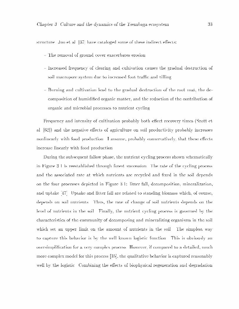
structure� Juo et al� ���� have cataloged some of these indirect e�ects�
The removal of ground cover exacerbates erosion�
Increased frequency of clearing and cultivation causes the gradual destruction of
soil macropore system due to increased foot tra�c and tilling�
Burning and cultivation lead to the gradual destruction of the root mat� the de
composition of humidied organic matter� and the reduction of the contribution of
organic and microbial processes to nutrient cycling�
Frequency and intensity of cultivation probably both e�ect recovery times �Szott et
al� ����� and the negative e�ects of agriculture on soil productivity probably increases
nonlinearly with food production� I assume� probably conservatively� that these e�ects
increase linearly with food production�
During the subsequent fallow phase� the nutrient cycling process shown schematically
in Figure ��� is reestablished through forest succession� The rate of the cycling process
and the associated rate at which nutrients are recycled and xed in the soil depends
on the four processes depicted in Figure ���� litter fall� decomposition� mineralization�
and uptake ����� Uptake and litter fall are related to standing biomass which� of course�
depends on soil nutrients� Thus� the rate of change of soil nutrients depends on the
level of nutrients in the soil� Finally� the nutrient cycling process is governed by the
characteristics of the community of decomposing and mineralizing organisms in the soil
which set an upper limit on the amount of nutrients in the soil� The simplest way
to capture this behavior is by the well known logistic function� This is obviously an
oversimplication for a very complex process� However� if compared to a detailed� much
more complex model for this process ����� the qualitative behavior is captured reasonably
well by the logistic� Combining the e�ects of biophysical regeneration and degradation

Chapter �� Culture and the dynamics of the Tsembaga ecosystem ��
due to agriculture� the rate of change of renewable natural capital is
f��h� kr� c�� nrkr�� � kr�kmaxr �� �e�h� kr� c�� �����
where nr is the maximum regeneration rate� kmaxr is the maximum soil nutrient level for
the ecosystem� and � is the appropriate conversion factor relating food production to
productivity�
Decomposition
Litter Fall
Organic PoolsMineralization
UptakeGaseous
Losses
Leaching
Figure ���� Graphical representation of nutrient cycling process in a forest� Adaptedfrom ������
There is some di�culty associated with the determination of the intrinsic regeneration
rate� nr� for the forests the Tsembaga occupy� It is possible� however� to get an idea of the
order of magnitude nr from other studies� The time of successional recovery from slash
and burn to stable litter falls ranges from seven years in the plains of the United States
���� to ���� years in the tropics ����� The numbers for Guatemala closely match the

Chapter �� Culture and the dynamics of the Tsembaga ecosystem ��
fallow periods for the Tsembaga in New Guinea� so we can scale nr for a characteristic
recovery time of �� to �� years if the forest is left undisturbed� Figure ��� shows recovery
curves for di�erent values of nr and di�erent initial conditions for kr���� Since we do not
know kr��� we can only bracket reasonable values of nr in the following way� If enough
nutrients are removed to reduce kr to ��% of its maximum value� we examine recovery
curves from this value �graph �a� in Figure ���� to see that if nr ��� or ���� the system
recovers too fast� The recovery time for this initial condition and nr ��� is reasonable
so we take ��� to be the upper bound for nr� If cropping does not reduce soil nutrients
so drastically� say to a level of ��%� lower values of nr are reasonable� Graph �b� in
Figure ��� shows the results for nr ����� ���� and ���� respectively� suggesting that
���� might be taken as a lower bound for nr� Thus we assume that nr � ������ ����� This
range could be signicantly narrowed from a quantitative measurement of soil parameters
before and after cropping� Unfortunately� it seems that when these measurements have
been attempted� the range of error of measurement exceeds the magnitude of the variables
themselves�
0
0.2
0.4
0.6
0.8
1
0 5 10 15 20 25 30
postcrop interval �years�
�a� post crop nutrient levels���% of original
%precropnutrientlevels
0
0.2
0.4
0.6
0.8
1
0 5 10 15 20 25 30%precropnutrientlevels
postcrop interval �years�
�b� post crop nutrient levels���% of original
Figure ���� Recovery curves for di�erent values of the condition of the soil after croppingand recovery rate nr� In gure �a�� the values of nr coresponding to curves of increasingsteepness are ���� ���� and ���� Likewise� in gure �b�� these values are ����� ���� and�����

Chapter �� Culture and the dynamics of the Tsembaga ecosystem ��
With f� and f� now completely dened� we can rewrite the dynamical system repre
sentation of the Tsembaga ecosystem dened by Equations ���a and ���b as
dh
dt �bn�c��� a exp
���
e�h� kr� c�� c��
h
��h ����a�
dkrdt
krnr�� � kr�kmaxr �� �e�h� kr� c��� ����b�
Given the problems with associating units to renewable natural capital� it is convenient
to rescale the model by kmaxr by letting kr fkr �kmax
r � with fkr � ��� ��� Now� ekr representsthe mean productivity index per hectare of the land the population is occupying� one
being maximum productivity� zero being barren� We also drop the explicit dependence
of bn on c� by assuming bn is a linear function of c� and treating bn as a parameter� The
rescaled equations are �dropping the tilde notation��
dh
dt �bn � a exp
���
e�h� kr� c�� c��
h
��h ����a�
dkrdt
krnr�� � kr�� �e�h� kr� c��� ����b�
Our nal task is the specication of e����
� � The food production function
For Equation ���b of the model� we need an explicit form of the food production function�
e�h� kr� c��� Unfortunately� although several simple causal relationships are understood�
there is no fundamental scientic understanding of how nutrients� soil processes� and crop
output are related� Examples of work on this problem include France and Thornley�s ����
development of plant growth models and Keulen and Heemst�s ���� empirical work on

Chapter �� Culture and the dynamics of the Tsembaga ecosystem ��
crop response to the supply of macronutrients� Economic approaches that focus on
energy inputs and resource degradation can be found in work by Cleveland ���� ��� and
Giampietro et al� ����� Econometric work on determining the form of production functions
has been carried out by many authors� see for example ��� ����
Several functional forms have been suggested for modeling crop output in the work
just mentioned� but two are of interest for the model� the von Liebig and the Cobb
Douglas� The von Liebig function is based on von Liebig�s law which states that crop
output is a function of the most limiting resource� The functional form is
y Asw mini�I
�fi�xi�� �����
where y is output� Asw is the yield plateau set by the soil and weather� xi is the total
availability of the ith nutrient� and each fi is a concave function from R to ��� ��� Lanzer
and Paris ���� proposed to use this functional form in place of the commonly used poly
nomial forms and in a later paper� AckelloOgutu� Paris� et al� ��� tested the von Liebig
crop response against polynomial specications and were able to reject the hypothesis
that crop response is polynomial� Further� they could not reject that crop response was
of the minimum or von Liebig type�
Paris et al� ���� estimated the von Liebig function for cotton lint response to the input
of water and nitrogen� They assumed that fN and fW were linear and lumped all other
scarcities into one variable m� to get
y minN�W
��N ! �NN��W ! �WW�m�� ������
Note that �N and �W represent nutrients already present� while the other terms repre
sent applied nutrients� The production surface for this production function is shown in
Figure ����
The key point to note is that the variable m places a constraint on production due
to all the other variables not accounted for�

Chapter �� Culture and the dynamics of the Tsembaga ecosystem ��
Nitrogen Input
Water input
A
B
COutput
Figure ���� The production surface for cotton lint as modeled by the von Liebig production function� A� B� and C are the Nitrogen� Water� and �m� limiting planes respectively�
Although the von Liebig function may be the best representation of reality� the fact
that it is not smooth will cause di�culties when analyzing the dynamical system� Instead�
a commonly used production function from economics� the CobbDouglas given by
y knYi��
xaii ������
where xi is the ith input and ai are constants is used as an approximation� The problem
with this function is that it allows innite substitutability� That is� if the inputs were
land and water� this function says that productivity can be maintained in the face of a
drought by bringing more land under cultivation� This is clearly absurd� If on the other
hand� the inputs of interest are not physical quantities� for example energy input� the
situation is di�erent�
If the general form of the von Liebig function given by Equation ��� is used to model

Chapter �� Culture and the dynamics of the Tsembaga ecosystem ��
output where the input variable is human work energy� the physical inputs fi�energy in�
may be nonlinear� This is denitely the case for the Tsembaga with regard to the amount
of land brought into cultivation for a given amount of labor� Here� the CobbDouglas is
not such a bad approximation to the von Liebig as shown in Figure ����
�a� �b�Land
Soil Quality
Output
Work
Soil Quality
Output
Figure ���� The Cobb Douglas production function overlayed on the von Liebig function�Case �a� inputs are physical quanities� Case �b�one input is a nonphysical quantity�work� upon which the physical input� land depends in a nonlinear way�
The two inputs to agriculture accounted for in my model are human energy and re
newable natural capital� Other inputs such as rainfall and solar energy input are assumed
to be fairly constant� which based on the indications of the Tsembaga� is accurate� They
indicate that the weather never �uctuates signicantly enough to in�uence crop output�
at least not in their lifetimes� Under these assumptions� the food energy production
function is of the form�
e�h� kr� c�� k�w�h� c���a�ka�r ������
where w�h� c�� is the amount of energy the population directs towards agriculture� a� and
a� are the output elasticity of energy and renewable natural capital respectively� and k
is a proportionality constant� Fortunately Rappaport ���� made detailed measurements
of the energy input per unit area of land cultivated along with the associated output�

Chapter �� Culture and the dynamics of the Tsembaga ecosystem ��
Using this information we can calibrate the food energy production function� i�e�� for a
given choice of a� and a�� Rappaport�s data can be used to compute an estimate of k as
follows�
Rappaport indicates that when the human population was ��� and the pig population
was ��� animals weighing between ��� and ��� pounds� the amount of land cultivated
was about �� hectares or �% of the total cultivable land� leaving ��% fallow� The trophic
requirements of pigs are similar to those of humans� and their population can thus be
converted into equivalent Tsembaga numbers� The average Tsembaga weighs �� pounds
so their ��� pigs would have the same trophic demands as ��� Tsembaga� Thus� the ��
hectares supported approximately ��� Tsembaga equivalents�
Based on his energetic analysis� one person year � ���� hours at ��� kcal#hr� of energy
input is su�cient to clear� burn� cultivate� and harvest one hectare of land� Using energy
units in human annual energy requirements� �� man years of energy input produced ���
units of total energy output or ���� energy units per hectare� Now� making a guess at
the stage of recovery the secondary forest when brought into cultivation� we can estimate
k� Supposing the nutrient level is ��% that of a mature forest� we have
���� k����a����a� � k ����
����a����a�� ������
Then� given the denition of c�� the work devoted to agriculture is w�h� c�� hc�Ac� For
the situation described above� c� ����� and Ac ����
Assuming that the villagers do not waste labor� a certain work e�ort is roughly cor
related to the amount of land being cultivated� If the relationship were linear� increased
e�ort would increase land under cultivation proportionately� If an additional proportional
amount of land of equal quality is is brought under cultivation� one would expect that
output would increase proportionately� This situation would be modeled by choosing

Chapter �� Culture and the dynamics of the Tsembaga ecosystem ��
a� �� Given the terrain of the Tsembaga� however� increased work input will not in
crease the amount of land cultivated proportionately� Each marginal unit of land brought
into cultivation requires further travel distances which may require substantial elevation
gains� and the passage of natural barriers such as ridges and rivers� This suggests that
a� � but not substantially� Estimating a reasonable value for a� is more di�cult and
will be discussed later� The model is now fully specied�
dh
dt �bn � a exp
���
k�c�hAc�a�ka�rh
��h �����a�
dkrdt
krnr��� kr�� �k�c�hAc�a�ka�r � �����b�
and we can now study its behavior�
� � Dynamic behavior of the model
Equations ���a and ���b represent a family of models parameterized by c�� a�� and a��
Applying the techniques described in chapter � to our model system allows us to assess
its sensitivity to the structure of the food production function and the work level of the
population� Over a wide range of physically meaningful values for bn� a� �� nr� and ��
the model exhibits a �locally� asymptotically stable equilibrium population density of
around ��� when c� ���� which agrees with the demographic data previously discussed�
The corresponding equilibrium renewable natural capital value is around ����� quite
reasonable given that cultivated land is rotated so at any one time at least ��% of the
land has just been cultivated and other land is in various stages of recovery�
The model�s qualitative behavior is sensitive to c�� a��and a�� If we x a� ���
and a� ��� representing the case where bringing more land under cultivation is more
marginally productive than increasing renewable natural capital �soil quality�� the model

Chapter �� Culture and the dynamics of the Tsembaga ecosystem ��
exhibits a Hopf bifurcation when c� is varied as shown in the bifurcation diagram in
Figure ���� Points on the solid line represent stable equilibria while those on the dotted
line represent unstable equilibria� The large solid circles represent stable limit cycles�
For c� less than approximately ������ the system will exhibit a stable equilibrium� For
c� greater than ������� the equilibrium becomes unstable� and a stable limit cycle with a
period of about ��� years appears in which population builds and reaches its maximum
after about ��� years then declines over the next �� to �� years� When the population
density is extremely low� the land recovers over the next �� to �� years and the process
begins again�
0
0.2
0.4
0.6
0.8
1
0.06 0.08 0.1 0.12 0.14 0.16 0.18
Work level� c�
Equilibriumpopulationdensity
Figure ���� Bifurcation diagram for swidden agriculture with a� ��� and a� ���� Theheavy solid line represents stable equilibria points while the thin line represents unstableequilibrium points� The dark circles represent the maximum and minimum values takenon by x� on the stable limit cycle� i�e� as the system goes through one cycle� x� variesfrom ��� to ��� people#cultivable hectare�
The key point is that if the population works at a level c� ���� as it was during

Chapter �� Culture and the dynamics of the Tsembaga ecosystem ��
Rappaport�s eld work� the ecosystem is very stable�
More interesting is the model�s dependence on the relative marginal productivities
of soil and labor� If we make the common assumption that a� ! a� � �the economic
implications of which will be discussed later�� then the e�ect of the output elasticity of
soil and labor on the dynamics of the model can be studied by varying one parameter�
either a� or a�� It turns out that there is a relationship between the output elasticity of
energy input versus renewable natural capital as is made clear by comparing Figure ���
with Figure ����
0
0.2
0.4
0.6
0.8
1
0 0.25 0.5 0.75 1
Work level� c�
Equilibriumpopulationdensity
Figure ���� Bifurcation diagram for swidden agriculture with a� ��� and a� ���� Asin gure ����� the solid line represents stable xed points�
When a� ��� a bifurcation occurs near c� ������ as previously noted but when
a� ���� no bifurcation occurs for any value of c� as indicated by Figure ����
In order to understand this behavior� we create a two parameter bifurcation diagram�
Figure ���� that shows all the combinations of c� and a� for which a Hopf bifurcation

Chapter �� Culture and the dynamics of the Tsembaga ecosystem ��
occurs� The curve generated by these points separates c� a� parameter space into
regions with qualitatively di�erent behaviors shown in Figure ���� Curves for two di�erent
cases are shown� one where the population is more and less susceptible to death due to
malnutrition as indicated on the diagram� In each case there is a threshold value of a�
below which no bifurcation occurs� i�e� the system remains stable for any level of work�
This phenomenon has an interesting ecological interpretation�
0
0.2
0.4
0.6
0.8
1
0 0.1 0.2 0.3 0.4 0.5 0.6 0.7
Work level� c�
Outputelasticityoflabor�a�
more sensitive to malnutrition
less sensitive to malnutrition
Figure ���� Two parameter bifurcation diagram for the swidden agriculture model� Thecurves represent parameter combinations at which a Hopf bifurcation occurs�
In any ecological model� the relative strengths and timing of feedbacks between state
variables governs model stability� In our case� the agriculturalists receive feedback from
the land in terms of productivity per unit e�ort and the land receives feedback from the
agriculturalists in the form of population density�
Given that e�h� kr� c�� k�c�hAc�a�ka�r � the marginal productivity of each input is

Chapter �� Culture and the dynamics of the Tsembaga ecosystem ��
0.6
0.8
1
0 0.1 0.2
Work level� c�
Outputelasticityoflabor�a�
Figure ���� Change in dynamics as the bifurcation boundary is crossed� The system goesto a stable equilibrium for parameter values to the left and below the curve while forthose above and to the right� the system exhibits stable� cyclic behavior�
dened as
e�h� kr� c��
h
a�e�h� kr� c��
c�hAc
� ������
ande�h� kr� c��
kr
a�e�h� kr� c��
kr� ������
respectively� The parameters a� and a�� called output elasticities in economics� are
measures of proportional increase in productivity associated with increasing work e�ort
and renewable natural capital respectively� If the output elasticity of labor is higher than
the output elasticity of natural capital� it will pay to bring more lower quality land into
production �shorter fallow periods� as opposed to preserving soil quality� The declining

Chapter �� Culture and the dynamics of the Tsembaga ecosystem ��
natural capital feedback is weakened by the stronger feedback of increased yields due to
increased cultivation e�ort� Under these circumstances� the ecological system exhibits a
bifurcation from a stable to an unstable system if the work level becomes too high�
If on the other hand� the output elasticity of labor is lower and that of renewable
natural capital correspondingly higher� the possibility of bifurcating from a stable to an
unstable system is reduced� The feedback from decreased renewable natural capital is now
stronger and exerts more pressure on the population� This pressure keeps the population
in check before natural capital is degraded to the point below which the population can
not be supported� From the agriculturalists� point of view� the gains from cultivating
more land are more than o�set by the productivity losses associated with reduced soil
quality and nutrient levels resulting from the shorter fallowing periods� a strong feedback
to avoid working the land too hard�
Notice that the curve for the case where the population is less sensitive to malnutrition
and disease extends to lower values of a� for which a bifurcation occurs� Malnutrition
and disease is the mechanism through which reduced agricultural productivity a�ects the
population� If this mechanism is weakened� the stabilizing in�uence of reduced natural
capital is also weakened� This has the e�ect of making the model unstable for wider range
of values of a�� The critical point to take away from this analysis is that as output elastic
ity of labor is increased and the relationship of malnutrition and disease to mortality in
the population is weakened� the potential for ecosystem instability increases� Whether
or not that potential is realized depends on how behaviorally plastic the population is�
the issue to which we now turn our attention�

Chapter �� Culture and the dynamics of the Tsembaga ecosystem ��
� Behavioral plasticity
In general� in models of animal population dynamics� behavior� although state dependent�
is relatively in�exible� Dynamics and stability characteristics are determined by physical
aspects of the ecosystem coupled with the xed behaviors of organisms that occupy it�
Mechanisms that might cause a change in the qualitative behavior of such a systemmight
be changes in the external environment �e�g� ���� � or evolutionary dynamics �e�g� ������
In an ecological model involving humans� the situation is quite di�erent� The system
can move in and out of regimes of stability and instability very quickly with changing
behavior� For example� the amount of land that the Tsembaga put into cultivation �the
value of c�� is not constant�it depends on the human and pig population� To investigate
the e�ect this has on the model� we now treat c� not as an exogenously set parameter�
but rather� as an endogenously determined quantity by allowing the population to adjust
c� to attempt to meet nutritional requirements� The work level is governed by the di�er
ence between actual food production and desired food production and the availability of
additional labor� A simple expression for the dynamics of c� is�
dc�dt �c�
�df �
e�h� kr� c��
h
��cmax
� � c�� ������
where df is the food demand� cmax� is the upper limit on the fraction of the population
working full time cultivating the land� and �c� is the speed of response of the population
to changes in demand�
The food demand is culturally set� and I dene it as follows� if the minimum food
requirements of the population are being met on average �about ���� calories per day��
then df �� Signicant deviations away from one are possible� as human populations
exist on a daily caloric intake ranging from around ���� up to ���� calories� The pa
rameter cmax� could be culturally set or set by physical limitations� The parameter �c� is
a measure of the behavioral plasticity of the population� setting the time scale on which

Chapter �� Culture and the dynamics of the Tsembaga ecosystem ��
behavioral change can occur� As �c� increases� the population can change its behavior
on shorter time scales� If we append Equations ���a and ���b with Equation ���� we
have a three dimensional dynamical system that describes the human agroecosystem�
This system exhibits a steady state if either food demand is met � e�h�kr �c��h
��� or the
population is working at the maximum permissible level �c� cmax� ��
By treating cmax� as a bifurcation parameter� we can explore the behavior of the
system dened by Equations ���a� ���b� and ����� The results are shown in Figure ���� If
cmax� ������ the model exhibits a stable equilibrium� The stable equilibrium vanishes
when cmax� � ������ and a stable limit cycle develops�
If the population is somehow limited in the maximum e�ort it devotes to agriculture�
the nutrition and disease population control mechanism proposed by Buchbinder ����
would e�ectively stabilize the system� From the description of their computer simulation
model� it seems that Foin and Davis ���� set an upper limit on �cultivation intensity�
which would explain their conclusion supporting Buchbinder�s hypothesis�
If� on the other hand� the maximum e�ort the Tsembaga could devote to agriculture
if necessary is above the critical level� �which is reasonable to believe since� for example�
this would only require that ��% of the population be willing to work in agriculture if
necessary� the stabilizing mechanism proposed by Buchbinder would not be su�cient to
stabilize the system� Thus� if there is any hope of the ecological system being stable�
some other mechanism� perhaps cultural� must come into play�
If we let cmax� ����� meaning one fourth of the population could devote a person
year of energy to agriculture if necessary� the population could work hard enough to meet
food demand and then c� is dynamically set by the relation
� e�h� kr� c��
h� ������
Then from Equation ���a and ���b� for equilibrium we must have

Chapter �� Culture and the dynamics of the Tsembaga ecosystem ��
0
0.2
0.4
0.6
0.8
1
0.05 0.1 0.15 0.2 0.25 0.3 0.35 0.4 0.45 0.5
0
0.05
0.1
0.15
0.2
0.25
0.3
0.35
0.4
0.45
0.5
0.135 0.136 0.137 0.138 0.139 0.14 0.141
Maximum work level� cmax�
Equilibriumpopulationdensity
Figure ���� Bifurcation diagram with cmax� as the bifurcation parameter in the swidden
agriculture model� The upper inset is an exploded view of the boxed region in the mainbifurcation diagram showing the increase in complexity of the dynamics when culture isadded to the system� These dynamics occur over an extremely narrow parameter range�thus having a low probability of being observed in the physical system�
bn � a exp ��� � �� � �����a�
krnr�� � kr�� �h �� �����b�
If the parameters bn� a� and � are such that Equation ����a is satised� the nonlinear
system dened by Equation ���� and ����b denes a one dimensional manifold of xed
points in ��� The equilibrium population� natural capital level� and work level depend on
initial conditions� Of interest to us is how the net birthrate must be exactly balanced by

Chapter �� Culture and the dynamics of the Tsembaga ecosystem ��
the net death rate associated with the nutritional level achieved when food demand is met�
If the population could� through some cultural mechanism such as infanticide or some
other type of birth control� match these rates� the system would be �neutrally� stable�
Here� we see how extreme behavioral plasticity can destabilize a system by nullifying the
feedback control of resource limitation and transferring the responsibility of ecosystem
regulation from environmental to cultural mechanisms�
It is probable that the net growth rate of the population is positive when food demand
is met which violates the stability condition given by ����a� In this case the ecosystem
exhibits cyclic behavior� It is very interesting to compare the limit cycle behavior of
the cases with and without behavioral plasticity� Figure ���� shows the limit cycles that
develop in the system where the work level is treated as a parameter �inner cycle� set
constant at c� ���� and those that develop when the work level is dynamically set with
cmax� ���� �outer cycle�� Figure ���� shows the work level and food production over
time� Several interesting points are worth making about these gures�
First� the period of the outer cycle where the work level is dynamically set is about
twice that of the case were the work level is constant� The reason for this can be seen
in Figure ����� The initial work level is very low� around ����� because if the population
is low and renewable natural capital is high at t � little e�ort is required to meet
food demands� The population does not over exploit its environment just because it can�
and just meets food demand� With the case where the work level is constant at �����
the population exploits the environment at a constant rate� When renewable natural
capital is high� the population can produce an abundance of food which increases the
growth rate of the population� Thus� when the level of renewable natural capital is high�
a population that just meets food demand grows more slowly than a population with a
constant work level� The di�erence is indicated in Figure ���� by the di�erence in time
required for the population to reach a maximum� ��� versus ��� years for the constant

Chapter �� Culture and the dynamics of the Tsembaga ecosystem ��
0
0.2
0.4
0.6
0.8
1
0 0.2 0.4 0.6 0.8 10
0.2
0.4
0.6
0.8
1
0 0.2 0.4 0.6 0.8 1
Natural Capital� kr
HumanPopulaiton�h
t �
t ���
t ���
t ���t ���
t ���
Figure ����� Limit cycles that develop as the the system becomes unstable� The innercycle is for the case where the work level is constant at ����� The outer cycle representsthe case where the work level is set by demand�
and dynamic work level cases� respectively�
Next� notice that in the constant work level case� after the population reaches a max
imum� it begins to decline immediately� This decline to the lowest population level takes
about �� years� In the dynamic work level case� by increasing work level dramatically as
shown in Figure ���� around t ���� the population is able to delay the precipitous de
cline in population for about another �� years� In doing so� however� the population puts
itself into a more precarious position of very high population density in a very degraded
environment� The precipitous decline now takes � years instead of ��$
Since the Tsembaga do adjust their work level� the model suggests that unless some
mechanism intervenes� their ecosystem is doomed to crash� This could be avoided by
maintaining the knife edge set of parameters required for stability in ����a by controlling

Chapter �� Culture and the dynamics of the Tsembaga ecosystem ��
0
0.05
0.1
0.15
0.2
0.25
0 200 400 600 800 1000
Time
Worklevel�c �
Foodproduction�e���
����
���
����
���
����
���
�b�
�a�
Figure ����� Work level �curve �a�� and food production �curve �b��� over time�
birth and death rates within the population� or possibly by the ritual cycle� It seems that
the former is not the case� the Tsembaga actively seek to be as �fertile� as possible as
evidenced by their rituals to improve fertility� In the next section� we add the dynamics
of the ritual cycle and determine the conditions under which it could maintain a balance
in and prevent the degradation of the Tsembaga ecosystem�
� Modelling the ritual cycle
The ritual cycle dynamics are added in two parts� First we address pig husbandry to nd
that even without the ritual cycle� pig husbandry alone can help stabilize the system�
Next we add the ritual cycle to show that under certain assumptions the ritual cycle
can stabilize the system� and that stability is not as sensitive to parameter choices as it
is to how the number of people who ought to be killed during warfare is related to pig

Chapter �� Culture and the dynamics of the Tsembaga ecosystem ��
invasions�
� � The parasitism of pigs
The bulk of the responsibility of keeping pigs falls on Tsembaga women� They do most
of the work in planting� harvesting and carrying the crops used to feed the pigs� In this
sense� the pigs can be viewed as parasitizing Tsembaga women� They benet from energy
derived from the ecosystem but do not contribute to obtaining that energy� It turns out
that this relationship� in and of itself� is enough to help stabilize the ecosystem� The
mechanism is related to the fact that working too hard is a major factor in destabilizing
the ecosystem� If the human population is the sole benefactor of its agricultural e�ort�
it grows in number� produces a larger labor pool� and the percapita work level remains
constant� If� on the other hand� the population keeps pigs� as the pig population grows
relative to the human population� the percapita work level increases� In this way� the
pigs act as an ecosystem monitoring device�
This is clearly illustrated by the model� In all the previous investigations� it was as
sumed that the Tsembaga devoted a constant ��% of their harvest �based on demographic
information at a point in time� to pigs maintained a constant pig to person ratio �no rit
ual cycle�� By treating this ratio as a parameter� rp� we can generate a gure similar to
Figure ��� where the parameters of interest are the percentage of food being consumed
by humans and cmax� � Figure ���� is the result� The curve in graph �a� separates regions
in parameter space of stability and instability� Notice that the more food the humans
eat themselves� i�e� rp �� the lower the level of cmax� at which the system becomes
unstable� Recall that with rp ����� the system goes unstable when cmax� �������
This represents only a ��% increase in work e�ort which is plausible� Now consider the
case where rp ���� the system remains stable until cmax� reaches approximately �����
This represents a more than doubling of work e�ort which may be intolerable to the

Chapter �� Culture and the dynamics of the Tsembaga ecosystem ��
0
0.2
0.4
0.6
0.8
1
0 0.2 0.4 0.6 0.8 10
0.2
0.4
0.6
0.8
1
0 0.05 0.1 0.15 0.2 0.25 0.3
NaturalCapital�kr
Humanfoodproportion�r p
Maximum work level� cmax�
�a�Human food proportion� rp
�b�
Figure ����� The in�uence of pigs on system dynamics� Figure �a� shows the bifurcationboundary in cmax
� rp parameter space� Figure �b� shows the equilibrium natural capitallevel as a function of rp�
population� Thus� just by being there� the pigs help stabilize the system� Note that this
stability comes at the expense of human nutrition� In this model� food is rst fed to the
pigs and the remainder is fed to the population� This is not what happens� the Tsembaga
eat the best food rst and give the rest to their pigs� This di�erence requires the more
elaborate ritual cycle mechanism to stabilize the system�
� � The ritual cycle
The ritual cycle consists of periods of ritually sanctioned truces separated by warfare�
The rituals that mark the transitions between the phases are the Kaiko that marks the
end of the truce period and the planting of a plant called rumbim �cordyline fruticosa�
that marks the beginning of the next truce� Figure ���� is a representation of the cycle�
The length of the arcs on the circle is loosely representative of the times between
events� The Kaiko itself lasts one year� Warfare lasts for a matter of months� The
time between planting the rumbim that signies truce and the Kaiko �typically about

Chapter �� Culture and the dynamics of the Tsembaga ecosystem ��
Uproot rumbin
Warfare
Plant rumbim
grow pigs
Kaiko
Figure ����� The ritual cycle of the Tsembaga
�� years� depends on the demographics of the pigs� In this period enough pigs must be
grown to satisfy ritual requirements� but the staging of the Kaiko also depends on when
women get tired of being parasitized by pigs� The question mark between the uprooting
of the rumbim and the beginning of warfare indicates uncertainty about the timing of
the onset of warfare� although Rappaport indicated that ghting had usually resumed
within � months of the uprooting of the rumbim�
After a truce� the populations return to tending gardens and pigs� As the pig popula
tion increases� work load on the women also increases� Rappaport computed that there
were an average of ��� pigs of the ��� to ���pound size to each mature female at the
outset of the ���� Kaiko� This translates into a pig to person ratio �in terms of biomass�
of about ���� The range of the number of pigs kept was � to �� Rappaport observed
only one woman keeping �� and four keeping � and postulates that these gures may
represent the maximum physically possible� When females are burdened with this many
pigs� their complaints to their husbands become more frequent� The husbands then call
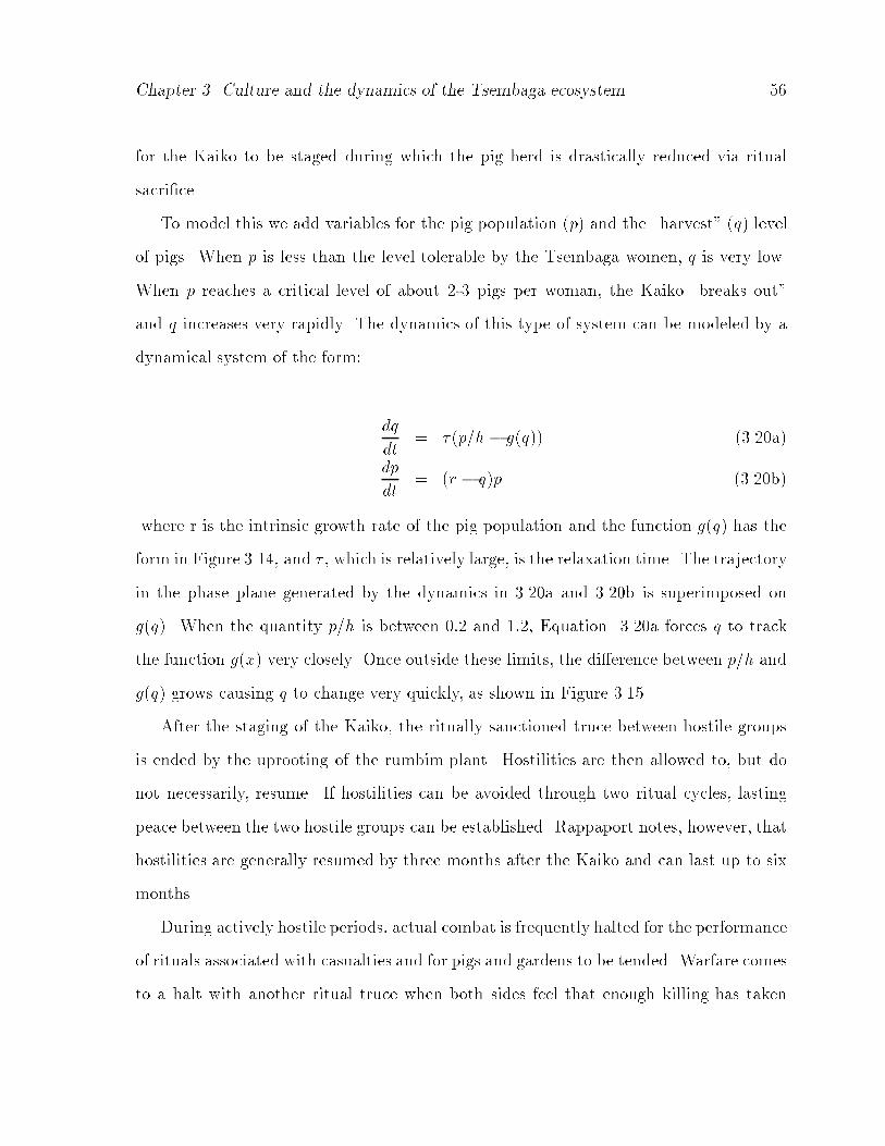
Chapter �� Culture and the dynamics of the Tsembaga ecosystem ��
for the Kaiko to be staged during which the pig herd is drastically reduced via ritual
sacrice�
To model this we add variables for the pig population �p� and the �harvest� �q� level
of pigs� When p is less than the level tolerable by the Tsembaga women� q is very low�
When p reaches a critical level of about �� pigs per woman� the Kaiko �breaks out�
and q increases very rapidly� The dynamics of this type of system can be modeled by a
dynamical system of the form�
dq
dt � �p�h � g�q�� �����a�
dp
dt �r � q�p �����b�
where r is the intrinsic growth rate of the pig population and the function g�q� has the
form in Figure ����� and � � which is relatively large� is the relaxation time� The trajectory
in the phase plane generated by the dynamics in ����a and ����b is superimposed on
g�q�� When the quantity p�h is between ��� and ���� Equation ����a forces q to track
the function g�x� very closely� Once outside these limits� the di�erence between p�h and
g�q� grows causing q to change very quickly� as shown in Figure �����
After the staging of the Kaiko� the ritually sanctioned truce between hostile groups
is ended by the uprooting of the rumbim plant� Hostilities are then allowed to� but do
not necessarily� resume� If hostilities can be avoided through two ritual cycles� lasting
peace between the two hostile groups can be established� Rappaport notes� however� that
hostilities are generally resumed by three months after the Kaiko and can last up to six
months�
During actively hostile periods� actual combat is frequently halted for the performance
of rituals associated with casualties and for pigs and gardens to be tended� Warfare comes
to a halt with another ritual truce when both sides feel that enough killing has taken

Chapter �� Culture and the dynamics of the Tsembaga ecosystem ��
0
0.2
0.4
0.6
0.8
1
1.2
1.4
-0.2 0 0.2 0.4 0.6 0.8 1 1.2
pig#peopleratio�
p h
Harvest rate� q
g�q�
Figure ����� Form of g�x� in equation �����a� and the associated limit cycle�
place or combatants simply tire of ghting� Since the ghting forces are composed of
principal combatants and their allies� as time goes on� the support of allies becomes
more di�cult to maintain which increases pressure to bring hostilities to an end� To
model this we use the fact that after several casualties have occurred� the people to pig
ratio begins to decrease� As this happens� the perperson work level begins to increase
and daily living activities become more pressing� The pig to person ratio acts as a proxy
for this increased work e�ort and the warfare outbreak dynamics can be expressed by�
dw
dt � �h�p � �g�w� ! � ������
where w is the percapita death rate due to war and � and merely scale and shift the
ratio of people to pigs where the outbreak of war and ritual truce occur� The human and
pig population dynamics under this scenario are shown in Figure �����
The most critical aspect of the model for the ritual cycle and its e�ect on the human
population is the set assumptions made about the e�ect of warfare on the population�

Chapter �� Culture and the dynamics of the Tsembaga ecosystem ��
0
0.2
0.4
0.6
0.8
1
1.2
1.4
0 5 10 15 20 25
0
0.2
0.4
0.6
0.8
1
1.2
0 5 10 15 20 25
pigpersonratio�
p h
harvestrate�q
time time
Kaiko
Figure ����� The dynamics of the ritual cycle� These represent the time plots of the limitcycle shown in gure ������� Between Kaikos� the harvest rate is very low� When thepig to person ratio exceeds the tolerable level� the harvest rate increases dramaticallyrepresenting the pig slaughter associated with the Kaiko as shown in the graph on theright�
Unfortunately� data on warfarerelated mortality are not rich estimates range from two
to eight percent of the population ����� This is not an important issue with regard to
stability� however� The key point is the assumption that the number of deaths due to
warfare is a constant fraction of the population� If we make this assumption then the
human population dynamics would be given by
dh
dt �bn � a exp
���
e�h� kr� c�� c��
h
�� w�h ������
If the system is to evolve to a stable limit cycle� the parameters that govern the dynamics
of w must be chosen such that the average value over one cycle of the quantity
�bn � a exp
���
e�h� kr� c�� c��
h
�� w� ������
vanishes� Since the cultural dynamics act to drive e�h� kr� c�� c�� toward �� the growth
rate of the human population is nearly constant and only very weakly dependent on the
physical state of the system over most of a cycle� The average war mortality over a cycle
must be balanced against essentially a constant growth rate� and there is no mechanism
by which the model can �seek� an equilibrium population level� In this case the ability

Chapter �� Culture and the dynamics of the Tsembaga ecosystem ��
0.6
0.8
1
1.2
1.4
1.6
1.8
2
2.2
0 5 10 15 20 25
time
PopulationDensity�h
�a�
Kaiko begins
Warfare begins
�b�
Figure ����� An example of of the human �a�� and pig �b�� population trajectories undercultural outbreak dynamics� After the Kaiko when the pig population drops drastically�curve �b�� warfare resumes and the the human population drops �curve �a��� As peopleare killed� the human pig ratio drops until a cuto� is reached and a truce is called�
of the Kaiko to stabilize the system is very sensitive to parameter choices� This may help
explain why the model due to Shantzis and Behrens ���� was neutrally stable and� of
course� why when Foin and Davis ���� used di�erent parameters �making the counterpart
of expression ���� in their model positive in mean over one cycle� found that the Kaiko
would not stabilize the system� Here� there is no mechanism by which the model can
�seek� an equilibrium population level�
If� on the other hand� we assume that mortality due to warfare increases nonlinearly
with the population size� the Kaiko can stabilize the system� Rappaport actually indi
cated that this was the case� As there are more pigs� people� and gardens there are more
ways for pigs to invade gardens and cause con�ict� increasing the number of required
blood revenge deaths during an active period of warfare� The number of ways a pig
might invade an enemy�s garden rises much faster than linearly with increases in pig and

Chapter �� Culture and the dynamics of the Tsembaga ecosystem ��
garden numbers� If we assume that number of war moralities behaves roughly as the
square of the population size� the human population dynamics are given by
dh
dt �bn � a exp
���
e�h� kr� c�� c��
h
�� wh�h� ������
We then dene the full ecological system by the physical component dened by Equa
tions ����� ����b� and ����b and the cultural component dened by Equations ����a� �����
and ���� to arrive at the following dynamical system�
dh
dt �bn � a exp
���
k�c�hAc�a�ka�rh
��wh�h �����a�
dkrdt
krnr�� � kr�� �k�c�hAc�a�ka�r �����b�
dp
dt �r � q�p �����c�
dc�dt
�c�
�df �
k�c�hAc�a�ka�rh
��cmax
� � c�� �����d�
dq
dt � �p�h � g�q�� �����e�
dw
dt � �h�p � �g�w� ! �� �����f�
� � The behavior of the full system
The dynamics of the ritual variables are conned to stable limit cycles and the work level
follows food demand forcing the overall system behavior to be cyclic� With the human
population dynamics dened by ����� the ritual warfare acts to drive the system to
equilibrium keeping the human population in check� Figure ���� illustrates the behavior
of several trajectories beginning from di�erent reasonable initial conditions� They all
collapse onto a very small amplitude stable limit cycle� Projections of this cycle onto the
h� p and kr � h planes are shown in Figure �����

Chapter �� Culture and the dynamics of the Tsembaga ecosystem ��
0
0.2
0.4
0.6
0.8
1
1.2
1.4
1.6
1.8
2
0 0.2 0.4 0.6 0.8 1
Biophysical Capital� kr
PopulationDensity�h
Figure ����� Sample trajectories for the full model� Any time that the human populationis large compared to biophysical capital� the pig to people ratio will be high and warfarewill break out� This drives the population to a more stable �or sustainable� region in thestate space whence the system collapses onto the very low amplitude limit cycle shownin gure� ������
The ritual cycle e�ectively keeps the human population density in the interval ������ �����
and the natural capital in the interval ������ ������ Compare these �uctuations to the
case without the ritual cycle �see Figure ������ The model predicts that if the Tsembaga
attempt to meet food demand� it is possible that the ritual cycle could play a critical
role in stabilizing the ecosystem�
� � Conclusions
The dynamical system model for the Tsembaga ecosystem based on the ethnographic
work of Rappaport ���� developed in this paper suggests that behavioral plasticity� feed
back from the land� and the relationship between people and pigs are the main factors
a�ecting ecosystem stability� Behavioral plasticity� in the form of the ability of the
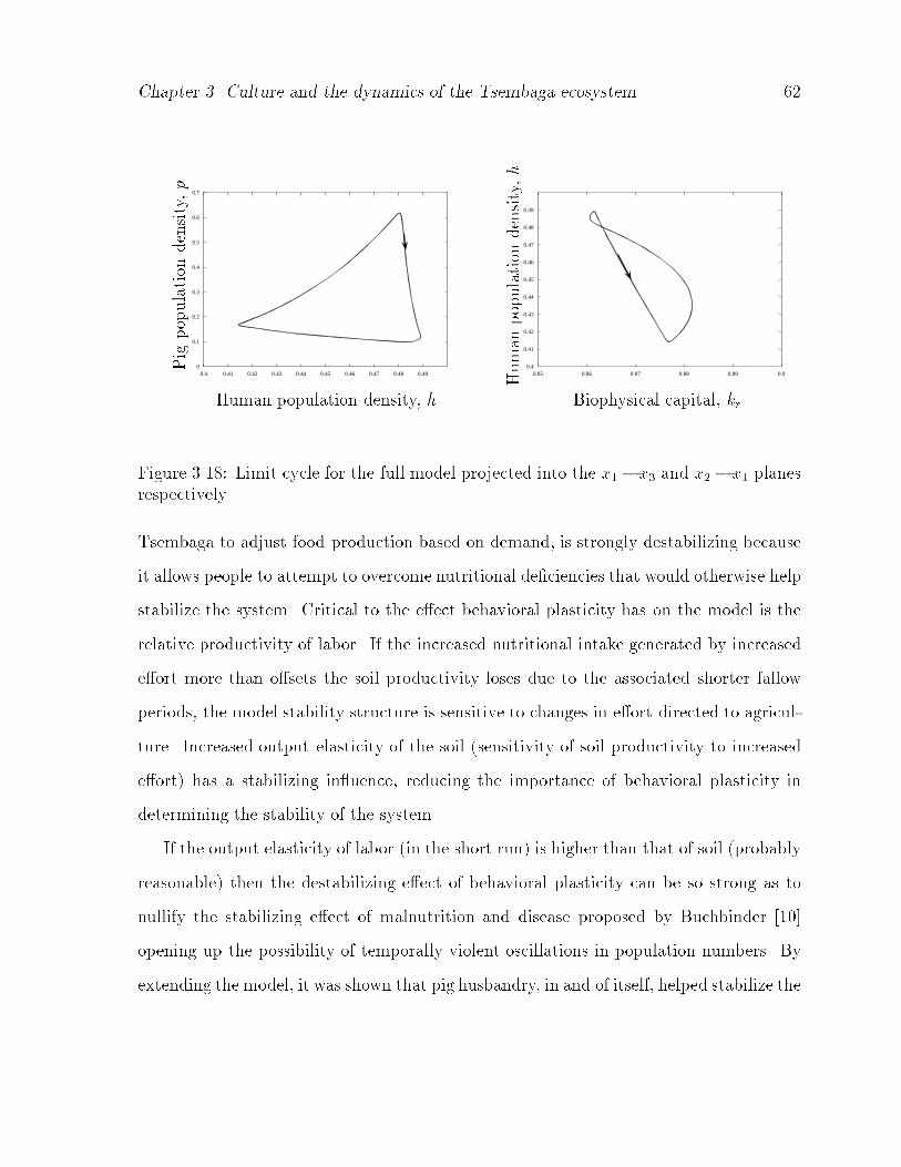
Chapter �� Culture and the dynamics of the Tsembaga ecosystem ��
0
0.1
0.2
0.3
0.4
0.5
0.6
0.7
0.4 0.41 0.42 0.43 0.44 0.45 0.46 0.47 0.48 0.490.4
0.41
0.42
0.43
0.44
0.45
0.46
0.47
0.48
0.49
0.85 0.86 0.87 0.88 0.89 0.9
Biophysical capital� kr
Pigpopulationdensity�p
Humanpopulationdensity�h
Human population density� h
Figure ����� Limit cycle for the full model projected into the x�� x� and x�� x� planesrespectively�
Tsembaga to adjust food production based on demand� is strongly destabilizing because
it allows people to attempt to overcome nutritional deciencies that would otherwise help
stabilize the system� Critical to the e�ect behavioral plasticity has on the model is the
relative productivity of labor� If the increased nutritional intake generated by increased
e�ort more than o�sets the soil productivity loses due to the associated shorter fallow
periods� the model stability structure is sensitive to changes in e�ort directed to agricul
ture� Increased output elasticity of the soil �sensitivity of soil productivity to increased
e�ort� has a stabilizing in�uence� reducing the importance of behavioral plasticity in
determining the stability of the system�
If the output elasticity of labor �in the short run� is higher than that of soil �probably
reasonable� then the destabilizing e�ect of behavioral plasticity can be so strong as to
nullify the stabilizing e�ect of malnutrition and disease proposed by Buchbinder ����
opening up the possibility of temporally violent oscillations in population numbers� By
extending the model� it was shown that pig husbandry� in and of itself� helped stabilize the
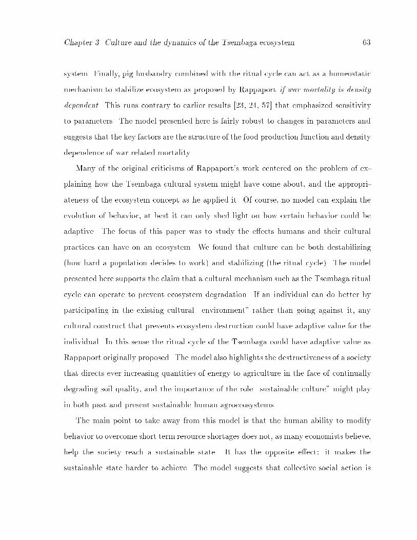
Chapter �� Culture and the dynamics of the Tsembaga ecosystem ��
system� Finally� pig husbandry combined with the ritual cycle can act as a homeostatic
mechanism to stabilize ecosystem as proposed by Rappaport if war mortality is density
dependent� This runs contrary to earlier results ���� ��� ��� that emphasized sensitivity
to parameters� The model presented here is fairly robust to changes in parameters and
suggests that the key factors are the structure of the food production function and density
dependence of war related mortality�
Many of the original criticisms of Rappaport�s work centered on the problem of ex
plaining how the Tsembaga cultural system might have come about� and the appropri
ateness of the ecosystem concept as he applied it� Of course� no model can explain the
evolution of behavior� at best it can only shed light on how certain behavior could be
adaptive� The focus of this paper was to study the e�ects humans and their cultural
practices can have on an ecosystem� We found that culture can be both destabilizing
�how hard a population decides to work� and stabilizing �the ritual cycle�� The model
presented here supports the claim that a cultural mechanism such as the Tsembaga ritual
cycle can operate to prevent ecosystem degradation� If an individual can do better by
participating in the existing cultural �environment� rather than going against it� any
cultural construct that prevents ecosystem destruction could have adaptive value for the
individual� In this sense the ritual cycle of the Tsembaga could have adaptive value as
Rappaport originally proposed� The model also highlights the destructiveness of a society
that directs ever increasing quantities of energy to agriculture in the face of continually
degrading soil quality� and the importance of the role �sustainable culture� might play
in both past and present sustainable human agroecosystems�
The main point to take away from this model is that the human ability to modify
behavior to overcome short term resource shortages does not� as many economists believe�
help the society reach a sustainable state� It has the opposite e�ect� it makes the
sustainable state harder to achieve� The model suggests that collective social action is

Chapter �� Culture and the dynamics of the Tsembaga ecosystem ��
more critical making a sustainable world a reality� Also� it must be emphasized that
this social action can not be �soft� by which I mean actions that focus on trying to
continue what we are doing with less� The social action has to be an emergent property
of individual beliefs� Think� for example� if excessive individual wealth accumulation
and greed were viewed with as much indignation and disgust as say incest or rape� we
might be faced with a quite di�erent present and future world� Simple economic and
technological xes that are not accompanied by cultural change might do nothing more
than help paint us into a corner� This will be illustrated in chapter � with regard to
investment and wealth distribution practices�

Chapter
Non�substitutibility in consumption and ecosystem stability
If we wish to extend the modelling framework to more complex economic systems with
a wider range of possible activities and more state variables� dening how the linkage
between them operates becomes the main challenge� The main question is how do peo
ple decide to allocate energy to the di�erent activities and how do feedbacks from the
environment in�uence this allocation� Economists have dealt with this problem in great
detail through the use of the market� where the main feedbacks from the environment are
prices� and utility functions determine how income is allocated among available activities�
The aim of this section is to examine in detail the implications of assuming a standard
economic model for the interaction between behavior and environment� i�e� how certain
assumptions about utility generate very specic cultural structures� We accomplish this
by studying and extending a model of the economic system of Easter Island developed
by Brander et al� ���� In this model the authors develop the hypothesis that the culture
and economic system of the invading Polynesians were incompatible with the physical
properties of Easter Island� This mismatch between cultural and ecological systems lead
to the eventual collapse of the system� This is an excellent example of the importance of
studying culture and economic systems within an ecological context�
� The Easter Island model
Brander et al� ��� developed a simple general equilibrium model to characterize the col
lapse of the society on Easter Island that created the stone monuments for which the
��

Chapter �� Non�substitutibility in consumption and ecosystem stability ��
Island is so well known� The model has two state variables�
S�t�� Renewable resource stock � kr in my notation�
L�t�� Available labour in the population � h in my notation�
The renewable resource stock would include agricultural output and sh catch potential�
As is traditional with economic models� the population is modeled as a labor pool that
is proportional to the physical population� The dynamics of the Easter Island ecosystem
according to Brander et al� ��� are then given by
dS
dt G�S��H�S�L� ����a�
dL
dt �b� d ! F �H�L��L ����b�
where G�s� is the intrinsic growth rate of the renewable resource �food and wood��
H�S�L� is the harvest rate of the resource� b and d are the constant birth and death
rates for the labor force �population� and F �H�L� is the variable growth rate of the
population that depends on resource use� The cultural subsystem is associated with
the determination of H�S�L� and F �H�L�� The cultural system is modeled by treat
ing the inhabitants of Easter Island rational economic agents attempting to maximize
utility through the consumption of material goods� This cultural structure� of course�
determines a large part of the model�s behavior� just as it did in the Tsembaga case�
This provides an example of how cultures can be compared� Tsembaga ritual culture
�non economic behavior� stabilized the system while if the culture commonly ascribed to
modern industrial man prevailed on Easter Island� they would be doomed to �overshoot
and collapse��
Within this cultural model� the population consumes two goods bioresource goods
�agricultural output and sh�� H� and manufactured goods �tools� housing� and artistic
output�� M � The cultural dynamics� i�e� the way the population decides to partition

Chapter �� Non�substitutibility in consumption and ecosystem stability ��
available energy among possible activities of producing and consuming goods are then
determined by solving a constrained maximization problem� Brander et al� use a Cobb
Douglas utility function�
u�h�m� h�m��� �����
where h and m are per capita consumption rates of the bioresource and manufactured
goods respectively� and � denes the preferences for these goods� If w is the wage rate�
the budget constraint is
phh! pmm w� �����
ph and pm being the respective prices of the two goods� By the choice of units Brander
et al� set pm � �M is dened as the numeraire good whose price is the benchmark
by which all prices are measured�� Solving this maximization problem results in the
following percapita demand functions�
h �w
phand m w�� � ��� �����
Equation ��� thus denes the demand side of the economy� To model the supply side�
we must employ production functions to link demands with physical possibilities� The
production functions chosen by Brander et al� are
H �SLH ����a�
M LM � ����b�
Equation ���a asserts that the quantity of H produced is proportional to the product of
the size of the resource stock and the quantity of labor devoted to obtaining it� LH � Such
production functions are commonly used in sheries ����� Equation ���b states that M
depends on labor alone� LM and by choice of units� one unit of labor produces one unit
of M �

Chapter �� Non�substitutibility in consumption and ecosystem stability ��
The link between the supply and demand side is� of course� the market� The market
will equilibrate when the supply prices equal the demand prices� Assuming that the
economic processes are much faster than natural processes� Brander et al� assume that
the market is always in equilibrium so that linking the supply and demand sides of the
economy reduces to solving a set of algebraic equations� Assuming that the only costs of
production are due to labor� the perunit supply prices are given by
ph wLH
H����a�
pm wLM
M� ����b�
From equation ���b we see that LMM � and since pm � we must have that the wage
rate is also �� Combining this fact with equations ���a and ���a we see that
ph �
�S�����
which merely says as the resource stock decreases� its supply price increases� Substituting
the supply prices and wage rate into equation ��� yields the actual percapita amounts
of H and M produced�
h ��S ����a�
m �� � ����b�
In order to extend this model and illustrate how the choice of utility functions relates
to the level of behavioral plasticity exhibited by the populations we express culture as the
amount of energy devoted to each available activity� This requires relating the percapita
consumption to the energy required to produce it� We will accomplish this in the same
manner as with the Tsembaga model� Let us assume that the available labor is a fraction
of the total population� i�e�
L �N �����

Chapter �� Non�substitutibility in consumption and ecosystem stability ��
where N is the total population at time t� Brander et al� assume that � is equal to �
�again by choice of units� thus N L� By denition� the total demand for H and M is
the percapita demand multiplied by the total population�
H Nh Lh L��S and M Nm Lm L��� �� ������
Now� using the production functions once again� we can determine the energy �or labor�
required to meet these demands� i�e� we set the total production equations equal to the
total demand equations�
L��S LH�S � LH �L �����a�
L��� �� LM �����b�
Thus� the Easter Island Culture as characterized by this economic model is one in which
a constant proportion� �� of the labor force is directed towards producing bioresource
goods� while the remaining portion of the labor force� � � �� directs its energy towards
the production of manufactured goods�
The nal aspect of the model to be specied is how the fertility function F depends
on the percapita intake of bioresource goods �nourishment�� Here Brander et al� make
the assumption that net fertility increases linearly with percapita consumption of biore
sources� i�e� the better life is the higher the propensity to reproduce� Thus they let
F �H
L������
where � is a positive constant and the ratio of H to L represents the actual percapita
intake of bioresource goods� Thus the culture of Easter Island can be completely spec
ied by two parameters� �� its taste for bioresource goods and �� its fertility response
coe�cient�
With the cultural submodel specication complete� we are left to quantify the phys
ical aspect of the model� the growth rate of the bioresource� G�S�� Here Brander et

Chapter �� Non�substitutibility in consumption and ecosystem stability ��
al� assume the common logistic function� G�S� rS�� � S�K� where r is the intrinsic
growth rate and K is the carrying capacity� The planar dynamical system we wish to
study is then given by�
dS
dt rS�� � S�K� � ��SL �����a�
dL
dt �b� d! ���S�L� �����b�
� Model Critique
A glance at equations ����a reveals that they are equivalent to a LotkaVolterra predator
prey system with densitydependent prey growth rate� The behavior of such systems
is well known and I will not discuss it here �see ������ Rather� I will focus on how
assumptions about culture a�ect the model especially focusing on the role of behavioral
plasticity�
The model specied by equations ����a has one nontrivial equilibrium point �S�� L��
that satises S� � �� L� � � and
dS�S�� L��
dt � �����a�
dL�S�� L��
dt �� �����b�
This equilibrium point is globally asymptotically stable� the proof of which relies on a
simple application of a theorem due to Kolmogorov relating to planar systems of this
type �see ���� or ������ Beginning from any interior initial condition� the system will
converge to the steady state� Depending on parameter values� the steady state will
either be a node or a spiral which will force the system to converge to the equilibrium
either monotonically or through a series of damped oscillations� Of interest to Brander et
al� is that for certain parameter values representative of the situation on Easter Island�
the system will exhibit transitory oscillatory behavior which manifests itself in overshoot

Chapter �� Non�substitutibility in consumption and ecosystem stability ��
and collapse� Figure ��� shows the human population and resource stock trajectories for
an initial condition of �� humans landing on Easter Island with the resource stock at
carrying capacity �The units for the resource are a matter of scaling� Brander et al� ���
choose a carrying capacity of ������ units for convenience��
2000
4000
6000
8000
10000
12000
400 600 800 1000 1200 1400 1600 1800
Resourcestockandpopulation
Time
Figure ���� Population and resource stock trajectories for Easter Island model from �����
The archaeological record indicates the rst presence of humans at around ��� AD�
The population increases which is accompanied by a decrease in resource stock� The
population �and available labor� peaks at around ���� AD corresponding to the period
of intense carving in the archaeological record� The population subsequently declines
due to resource depletion� The model predicts a population of about ���� in ����� close
to the estimated value of ����� The model thus gives a reasonable qualitative picture
of what may have happened to the culture on Easter Island� The culture became very
productive and able to undertake the construction of major monuments� i�e� the labor
force increased thus making LM large enough to complete such a large scale project�
The population subsequently declined due to resource degradation which left the small

Chapter �� Non�substitutibility in consumption and ecosystem stability ��
population who knew nothing of the origin of the great monuments to meet the Dutch
ships in the eighteenth century� The discussion in Brander et al� ��� is very interesting
and I refer the reader there for more detail�
� � Behavioral plasticity and collapse
In this section we examine how the nature of the population collapse depends on the
level of behavioral plasticity exhibited by the population� The nature of the collapse can
be more clearly understood by examining the percapita growth rate over a time scale
meaningful to a member of the population� Figure ��� shows the annual percapita net
growth rate of the population from the time of initial colonization to the time of the
Dutch ships arrived in the eighteenth century�
-0.002
0
0.002
0.004
0.006
0.008
400 600 800 1000 1200 1400 1600 1800
Percapitagrowthrate
Time
Figure ���� Percapita growth rate from the time of initial colonization to the time ofrst European contact�
The population exhibits positive growth up to approximately ���� AD when it peaks
at around ������ individuals� The maximum percapita annual growth rate is around

Chapter �� Non�substitutibility in consumption and ecosystem stability ��
����%�very low by today�s standards� Similarly� the minimumnet growth rate is �����%
which implies that even under the most extreme resource shortage conditions the popu
lation is decreasing very slowly� It takes ��� years for population to drop from ������ to
����� Compare this to populations doubling every �� years at present� Next consider the
perceived change in an individual�s standard of living over a life span of say �� years from
the year ���� AD to ���� AD when it is decreasing most rapidly � In this period one
would experience a ��% decrease in bioresource intake over an entire lifetime� Although
the quality of life is going down� it is not changing catastrophically� From our present day
point of view the manner in which the population adjusts to the environment depicted
by the model might not be that bad�
We can now investigate the role behavioral plasticity has to play in the nature of the
collapse� Recall from equations ���� we deduced that the population directs a constant
proportion � of the labor force towards the bioresource sector while what is left is directed
to the manufacturing sector� Further� equations ��� indicate that the percapita rate of
consumption of the manufactured goods is constant� no matter what quantity of biore
sources are being consumed� This implies that as the bioresource stock is depleted and
becomes more expensive to produce� individuals continue to consume the same amount
of manufactured goods and consume less and less bioresources� The population could be
starving� yet the utility maximizing strategy is to keep the proportion of labor directed
to each activity constant�
The problem here is substitutability� CobbDouglass utility functions allow for one
input to be substituted for another without a�ecting utility� Based on this model� the
optimal strategy in the face of a resource good shortage is to increase consumption of
cheaper manufactured goods� This is reasonable in some cases� but not where bioresource
goods that sustain one�s very life are concerned� In short� the standard CobbDouglass
utility function cannot capture the possibility that labor could be shifted from one sector
Chapter �� Non�substitutibility in consumption and ecosystem stability ��
to the other�the structure of the economic system is xed over time�
The only aspect of the model that allows for behavioral �exibility is the fertility
function� and this depends on how it is interpreted� If the change in percapita growth is
due to active choices on the part of individuals depending on �quality of life� as measured
as percapita intake of bioresource goods then these changes would be considered the
result of behavioral plasticity� If on the other hand� these changes are due to indirect
e�ects and not active choice� then there is no behavioral plasticity built into the model�
� Adding behavioral plasticity to the Easter Island model
There are two aspects of the Easter Island model where behavioral plasticity might
manifest itself� either in the structure of the economy� or in the overall e�ort expended
by each individual in the population� One way to introduce the possibility for structural
change in the economy is to modify the utility function� I do so by utilizing a StoneGeary
type utility function which assumes that there is a minimum amount of bioresource goods
�subsistence level� at which utility is zero� i�e��
U�h�m� �h � hmin��m��� ������
where h � hmin� Modifying the model so that overall work e�ort can change is accom
plished by changing � from equation ��� from a constant to a state variable� As before� we
can determine the optimal consumption of resources by maximizing U�h�m� as dened
by ���� subject to the income constraint
phh! pmm � �w ������
where w is the wage paid per unit of labor� The resulting optimal consumption levels
are�
h �� � ��hmin !�w�
ph�����a�
Chapter �� Non�substitutibility in consumption and ecosystem stability ��
m �� � ����w � phhmin
pm� �����b�
Now we have that the optimal consumption level of h consists of a price dependent and
a price independent portion� This is more realistic as it says to spend excess income on
certain proportions of h and m only after meeting minimum nutritional requirements�
Equations ���� only make physical sense when
ph ��w
hmin
� ������
but this condition will always be satised if h � hmin� Substituting equation ��� for
ph into equation ���� and assuming as before that w � and pm �� we see that the
condition for the system to make physical sense reduces to
hmin � ��S ������
which simply says that if the demand hmin can be met at the present work level� use the
optimality conditions given by ���� to divide excess capacity to the tasks of producing
m and h�
If ���� is not met� the optimality conditions do not say what to do� Common sense
suggests that if people are tying to meet minimum nutritional requirements� they would
produce all the bioresource goods possible� i�e�
h ��S� ������
Finally� we can� by combining the above equations with the production functions given
by ���a and ���b� compute the amount of labor �available work� the population should
devote to producing bioresource goods and manufactured goods�
Lh
�����N�����hmin
�S!N�� if hmin � ��S
N� otherwise�����a�

Chapter �� Non�substitutibility in consumption and ecosystem stability ��
Lm
������� � ��N�� � hmin
�S� if hmin � ��S
� otherwise�����b�
The �culture� dened by ���� combined with the physical system dened by ���a
and ���b generates the decision process dened by ����� Notice that in contrast to the
original model� the division of labor is no longer xed� As the price of bioresource
goods increases� labor is shifted out of the production of manufactured goods into the
bioresource sector i�e� there is structural change in the economy� Finally� the population
has the option to increase the work level � in an e�ort to meet its needs� just as in the
Tsembaga model� I assume that the population will increase its work level only after all
labor is shifted into producing bioresource goods� This leads to the new system we wish
to analyze�
dS
dt rS�� � S�K� � �SLh �����a�
dN
dt �b� d! ��SLh�N �����b�
d�
dt ��hopt � hprod���max � ��� �����c�
where hprod ��S is the quantity of bioresource goods actually produced� When con
dition ���� is met� hopt � hprod and the amount of bioresource goods the population is
capable of making will exceed the amount it wishes to make so work levels will decrease
to the optimal level� If� on the other hand� condition ���� is not met� the population
will try to increase its work level to meet optimal demand� We can now analyze how the
dynamics of the model change under these conditions�
� � Model analysis
We begin the analysis by rst letting � � and focusing our attention on the e�ect
that hmin has on the model� If we take w��� � and and hmin �� we retrieve the

Chapter �� Non�substitutibility in consumption and ecosystem stability ��
original model� For the parameters chosen by Brander et al�� we know there is globally
stable equilibrium point at N ������ and S ����� We can again use pseudo
arclength continuation to investigate the nature of this equilibriumpoint as hmin is varied�
Figure ��� is the result of this exercise�
0
2000
4000
6000
8000
10000
0 0.005 0.01 0.015 0.02 0.025 0.03 0.035 0.04
hmin
PopulationDensity
Figure ���� Bifurcation diagram for modied Easter Island model�
As with the Tsembaga model� the way in which the population partitions its energy
profoundly a�ects the dynamics of the model ecosystem� We see from gure ��� that a
stable equilibriumpoint persists up to a value of hmin near ����� where a Hopfbifurcation
occurs� For values of hmin beyond the bifurcation point� not only does the system lose
stability� but the nature of the dynamics far from the singular point change as well�
Figure ��� shows the change in the dynamics as well as the role behavioral plasticity has
to play�
The gure to the left shows the population trajectories for the original model and for
the modied model with hmin ��� The gure to the right shows how the structure of
the economy evolves over time� initially� the two trajectories are roughly the same� For

Chapter �� Non�substitutibility in consumption and ecosystem stability ��
2000
4000
6000
8000
10000
12000
14000
400 600 800 1000 1200 1400 1600 1800
0
0.2
0.4
0.6
0.8
1
400 600 800 1000 1200 100 1400 1800
Time
Population
LaborProportions
Time
���
���
bioresources
manufacturing
Figure ���� Trajectories for population and proportions of labor in each sector over time�In the leftmost graph� curve ��� is for the original model as proposed by Brander while��� is from the modifed model�
the rst ��� years the structure of the economy remains fairly stable with approximately
��% of the labor force working in the bioresource sector and the remainder in the man
ufacturing sector� As bioresources become more scarce� the economic structure begins
to change and labor is shifted into the bioresource sector until all of the population is
working in this sector by between ���� and ���� AD� This shifting of available work into
the bioresource sector enables the population to grow about ��� years longer than in the
original model up to a peak of around ������ as compared to ������� Also evident is the
much more rapid decline that the more behaviorally plastic population must endure after
it has pushed its ecosystem too far� Here� behavioral plasticity enabled the population
to maintain its positive growth trajectory longer resulting in a more dramatic decline�
The nal aspect of this model to be discussed is the e�ect of allowing the population
to decide to work harder� i�e� set � � �� Figure ��� shows the results for wmax �� i�e�
the population is willing to triple its work e�ort if necessary�
The graph on the right in gure ��� shows the structure of the economy changing over

Chapter �� Non�substitutibility in consumption and ecosystem stability ��
2000
4000
6000
8000
10000
12000
14000
16000
1100 1150 1200 1250 1300 1350 1400 1450 1500 1550 1600-0.5
0
0.5
1
1.5
2
2.5
3
3.5
400 600 800 1000 1200 1400 1600 1800
Time
Population
TotalLabor
Time
���
���
���
bioresources
manufacturing
Figure ���� Trajectories for population and total labor in each sector over time for thecase � � �� In the leftmost graph� curve ��� is for the original model as proposed byBrander� ��� is from the modifed model with � �� and ��� is the case for the modiedmodel with � � ��
time as bioresources becomemore scarce� In this case� when all the labor force has shifted
into the bioresource sector the population begins to increase its work e�ort� Trajectory
��� in the gure to the left shows the case where the population increases its work e�ort�
By doing so� the population averts a further decrease in the intake of bioresources �and
thus quality of life� for about �� years� Unfortunately� this decision ultimately increases
the price the population has to pay in the rate of decrease of the population when it
nally does collapse� The rate of decrease is four times that of the original model and
two times that of the modied model with a xed work level� This type of scenario is
very reminiscent of our situation today� We are increasing the amount of work we do
as we attempt to maintain our standard of living� Obviously� we may be simply buying
ourselves a little time and increasing the ultimate price we will have to pay�
Chapter �� Non�substitutibility in consumption and ecosystem stability ��
Conclusions
In this section we have studied the interaction between culture and ecosystems in the
context of a model where the economy is more complex� The model I proposed where
both the structure and the overall work level of the economy were allowed to change
experienced a bifurcation from a stable steady state to a limit cycle which produced
more dramatic changes in population dynamics� The key point to observe is that� as
with the Tsembaga model� increased behavioral plasticity decreased the stability of the
system� In this light� the ability of modern economies to change their structure quickly in
response to changing environmental conditions so frequently lauded by the expansionist
view� might not be such a positive asset in achieving sustainability�
Obviously one can argue that this model is not rich enough to capture our ability
to become more e�cient� to utilize di�erent goods to perform certain tasks� to generate
capital� and to try to improve natural capital before it degrades� thus averting the collapse
experienced by the simple model and enabling a transition to sustainability� Examining
such a model is the focus of the next chapter of this thesis�
Chapter
The dynamics of a two sector ecological economic system
In this chapter� I will extend the concepts I have developed so far to study the dynamics
of a model of a two sector economy with capital accumulation� This is a much harder
problem than we have addressed so far� The Tsembaga and Easter Island models were
both pure labor economies� The only decisions taking place in these economies were
how hard to work and what portion of available labor to devote to each activity� In
an economy with labor and capital� the decisions are more complex� Here we have
rms that are trying to utilize resources e�ciently while consumers are simultaneously
trying to maximize utility� In order to tackle this problem� we will have to develop more
sophisticated economic concepts for modeling economic growth�
To this end� this chapter is organized as follows� In the rst section� I summarize
important concepts from the theory of economic growth that are important for this model�
Next� I outline the relevant concepts from production and utility theory and related issues
such as nonsubstitutability of consumer goods that we investigated in chapter � and the
importance of the nature of the production function that we encountered in chapter �
that are used to construct the model economic growth system� Finally� I develop the
ecological system in which the economic growth system is embedded� The nal step is
then to analyze the dynamics of the resulting system�
��

Chapter �� The dynamics of a two sector ecological economic system ��
� Simple economic growth models
Jensen ���� gives an exhaustive treatment of simple economic growth models with two
state variables� labor and capital� Such simple models have received much attention
in the economic literature� often focusing on the steady state growth trajectory of an
economy� This steady state trajectory corresponds to a constant capitallabor ratio with
economic output growing with capital and labor growth� An economic growth model
necessarily consists of three components� relationships that describe the dynamics of
labor and capital over time� a relationship between economic output and a given level
of capital and labor �factors of production�� and information specifying what society
does with economic output� Mathematically� the model consists of a dynamical system
coupled with algebraic equations governing production and consumption�
A common example of a simple economic growth model with a single production
sector would be�
dL�dt nL �����
dK�dt sY �����
where L is labor �generally viewed as the number of workers in a population�� K is the
quantity of capital� n is the percapita growth rate of the population� Y is the physical
output of the economy and s is the proportion of output that is saved� The output of
the economy is typically given by a function of the form Y f�L�K� where f�L�K� is
assumed to satisfy the following conditions� f�L� �� f���K� �� K and L� �f
�L� ��
�f
�K� �� ��f
�L� �� ��f
�K� �� The behavioral dynamics of the population modeled here
are obviously quite simple a constant proportion s of output is devoted to savings and
��� s�Y units of output are consumed� Clearly� the behavior of such a system hinges on
the assumptions about the production function and the behavior of the population�

Chapter �� The dynamics of a two sector ecological economic system ��
It is easy to see that for the conditions normally placed on f � the behavior of the
above system is very simple� Using simple di�erential inequalities one can see that
any trajectory beginning in the rst quadrant �both capital and labor are positive� will
remain there for all time and both state variables will grow without bound� Thus� the
population� capital stocks� and productivity all grow exponentially� To address economic
growth in a bounded ecosystem the dynamical system has to be extended to include
dynamic resource constraints and economic model must be extended to accommodate
more complex behavior� In order to develop such a model� some additional concepts
from production and utility theory must be employed� which I will brie�y review in the
next section�
� � Basic laws of production and the theory of the �rm
Very basic to an economic growth model is the specication of the laws of production
or the production technology of the economy� Some specic examples of production
functions were discussed in the model for agricultural output in the Tsembaga ecosystem
�Chapter ��� The production technology is represented by a production function� Y
f�x�� x�� ���� xn�� that characterizes technological alternatives for the inputs xi and the
maximal output Y obtainable for a given choice of these inputs� The characteristic of
the production function most important for this model is the possibility of technical
substitution between inputs�
The technical substitution possibilities specied by a particular production function
refers to what extent one input may be substituted for another to maintain a xed level
of output� As we already saw� the CobbDouglas allows innite substitutability between
inputs� an assumption that may be completely unrealistic� Problems associated with
such assumptions have received much attention in the ecological economics literature �e�g�
see ���� for a review�� At the opposite end of the spectrum is the Leontief production

Chapter �� The dynamics of a two sector ecological economic system ��
function usually written as
Y mini������n
fxi�ig �����
where �i is the requirement of input i per unit of output�
This is the analogue of the vonLiebig function used to describe agricultural produc
tion that we have already met� Here� there is absolutely no possibility for substitution
between inputs� Clearly� neither extreme is entirely realistic� and di�erent levels of sub
stitutability are to be found for di�erent types of inputs and outputs� For example� land
can�t be substituted for water to maintain productivity during a drought� A sewing ma
chine and electrical energy can be substituted for a person with needle and thread in the
construction of a garment� In my model� I assume that the overall production technology
is of the Leontief form for physical inputs but capital and labor are substitutable to carry
out productive activity in the production process� That is� let xi be the ith physical input
and let ��L�K� represent productive activity where L is labor in hours and K represents
services provided by capital� then
Y min
�����L�K��a� min
i������n
�xi�i
�� � �����
I represent ��L�K� with a CobbDouglas production function i�e� ��L�K� L�K�� The
resulting production function given by equation ��� allows innite substitution between
capital and labor� but no substitution between labor and capital �stocks�� and raw ma
terials ��ows�� This production function would not allow labor to be substituted for
aluminum in the production of a bicycle� but it does allow a frame jig to be substituted
for a human hand to hold the frame in place as it is welded�
Recall from Chapter � that � and � measure the marginal productivities of labor
and capital respectively� It is commonly assumed that �! � � or that the production
function has constant returns to scale �or the elasticity of scale is ��� Elasticity of scale ��s�
is a measure of the proportionate change in output associated with a proportionate change

Chapter �� The dynamics of a two sector ecological economic system ��
of all inputs� If �s �� doubling all inputs exactly doubles output� If �s � �� doubling of
all inputs more than doubles output� etc� In my model I assume that productive activity
exhibits constant returns to scale�
Next� I assume perfect competition �individual rms cannot a�ect prices by their
choices of output levels� and that rms are making decisions in the �short run�� In the
economics literature� time scales are resolved to the �short run� and the �long run�� This
distinction is related to what managers are able to change as they make decisions� It is
assumed that in the short run� managers can�t change capital stocks� Thus for short run
decisions� managers are faced with a xed capital stock and will select the optimal labor
input� In the long run� managers can adjust both capital and labor stocks in response
to the conditions in the labor and capital markets� In my model� there is no explicit
modeling of investment supply and demand� managers make only short run decisions
and capital growth is determined completely by savings rates�
Finally I assume that rms will make full and e�cient utilization of available factors
of production� They will attempt to fully utilize capital stocks and select the optimal
labor and output levels to minimize cost �or maximize prot�� For an economy with
multiple rms� full and e�cient utilization means the total capital is divided optimally
among the rms and then optimal labor is selected within each industry� The nal aspect
of rm behavior important to this model is the labor market� The optimal labor input
for a given industry depends on the relationship of the cost of labor �wage� to the cost
of capital� Thus given the cost of capital as xed� the availability and cost of labor will
determine the optimal combination of labor and capital�
� � Consumer behavior
The behavior of consumers is modeled using the standard approach from neoclassical
economics� consumers maximize utility subject to an income constraint� We have already

Chapter �� The dynamics of a two sector ecological economic system ��
seen the importance the form of the utility function plays in ecosystem dynamics in
Chapter �� We saw with the Easter Island model that restricted substitutability between
bioresources and manufactured goods was destabilizing� The StoneGeary utility function
is given by
log u nXi��
log �qi � qmini � �����
where u is utility� qi are commodities� and qmini are the minimumamounts of a commodity
required� This function is intuitively appealing� If the economy is capable of production
levels above minimum requirements� people will substitute among favorite goods� trading
o� nightly llet mignon for a better quality compact disc player� However� starving people
won�t try to ease their su�ering by making bead necklaces� simply because there is no
food and there are beads� The StoneGeary utility function nicely captures this behavior
as demonstrated in chapter ��
� The ecological economic model
The model that is the focus of the rest of this thesis is a two sector economicmodel coupled
with an ecological model� The economy has an agricultural and non farm business sector
�manufacturing�� This choice of division for economic activities is motivated by the fact
that we wish to model the e�ects of economic activity on two basic stocks� renewable
natural capital and nonrenewable natural capital� A more common division of economic
activity is between the agricultural� manufacturing� and service sectors� In my model I
have vertically integrated the manufacturing and service sectors with the idea that the
provision of services relies heavily on manufactured goods �insurance agents use cars�
cell phones� computers� fuel� paper� etc� to do their jobs� and that the impact of these
activities tend to be more focused on nonrenewable natural capital�
The economic ecological system model is shown schematically in gure ���� There

Chapter �� The dynamics of a two sector ecological economic system ��
are two basic �ows in the model� the �ow of raw materials and services from the state
variables into the economic system and the �ow of goods and services out of the economic
system� The economic system represented by the nonfarm business and agricultural
sectors draw �ows of low entropy materials from the stock of nonrenewable natural capital
and services from labor� manmade capital� and renewable natural capital converts them
to a �ow of goods and services� The arrows between the two sectors represent the inter
industry transfer of goods and services� The human population� based on its preferences�
can decide to consume goods and services� direct them towards investment� or increasing
nonrenewable natural capital stocks through research and development for new materials�
recycling� more e�cient use of materials� or more e�cient extraction techniques�
The model attempts to capture as simply as possible the fundamental aspects of both
sides of the argument about sustainable development� All of the processes by which many
believe we will continue to avert environmental degradation are included� everincreasing
e�ciency� better material use� etc�� but the achievement of these ends all require �ows of
economic goods and services and generate their own impact on the ecosystem� A perfect
example is recycling� Recycling reduces the environmental impact of some production
processes but requires capital� labor� energy input� and generates a waste stream� i�e� it
merely transfers ecological stress from one form to another�
� � The economic system
In this section I will solve the simultaneous consumer and rm optimization problems
in order to specify how labor and capital are allocated to each sector� We begin by
specifying the technology in each of the sectors� Should the need arise� please refer to
the table provided at the end of the chapter for an easy reference for the denitions of
symbols�
As we have seen before� agriculture is best modeled with the vonLiebig or Leontief

Chapter �� The dynamics of a two sector ecological economic system ��
BusinessNonFarm
Sector
Agricul-tural
Sector
(Social Organization
EconomicSystem
Preferences, etc)
hNonrenewable
Natural Man-made
Natural Human
(Labor)
Renewable
Flow of economic outputs (goods and services)
Flow of economic inputs (raw materials and services from capital stocks)
kkCapital, Capital, Capital, n k rPopulation,
Figure ���� Schematic of two sector ecological economic model�
function� I assume that
Ya Ea�kr�minf�a��a
�l
�l�N
�Ng �����
where Ya is annual agricultural output� Ea�kr� is a measure of e�ciency related to soil and
weather and is a function of the stock of natural capital� kr� The inputs are productive
activity �a� land l� and nutrients N �phosphorus� nitrogen� potassium� etc��� The ��s are
the per unit input requirements per unit of output� E�cient utilization implies that
�a��a
l
�l
N
�N�����
thus for a given amount of land� there is a set nutrient requirement and a physically

Chapter �� The dynamics of a two sector ecological economic system ��
determined amount of work required to carry out the production process� The population
will decide how much productive activity ��a� to direct to agricultural production via the
optimal combination of capital �Ka� and labor �La� based on the production function
�a Laaa K
baa � �����
In the model� natural capital provides several free services and could be called an eco
nomic sector in a sense� Among other things� it generates soil and soil nutrients� as
similates waste� and irrigates via the solar water pump� In equation ��� this is re�ected
by the fact that e�ciency is a function of the stock of natural capital� but also through
the nutrient input required for a given level of output� The required nutrients can be
supplied by the �natural sector� as is the case in the Tsembaga ecosystem� or by the
manufacturing sector �fertilizer� etc���
Thus at low levels of agricultural output� natural nutrient production is su�cient to
meet demand� As output increases� nutrients in the form of fertilizer� pesticides� and
genetically engineered seed must be provided from the manufacturing sector� Let Rma be
the manufactured goods required per unit of agricultural output� As agricultural produc
tion increases Rma increases from zero up to some maximum where most of the nutrients
for agriculture are supplied by the manufacturing sector� It is a messy bookkeeping and
computational problem to try to relate Rma directly to agricultural output� Instead�
the ratio of population density to renewable natural capital�h
kris used as an indirect
measure of agricultural output� The higher this ratio� the more pressure is being put on
kr and more nutrients must be injected into the system from the manufacturing sector�
The functional relationship is
Rma�x� �Nx
�
x� ! �half� �����
where �N is the nutrient requirement per unit of agricultural output� and �half is the

Chapter �� The dynamics of a two sector ecological economic system ��
level ofh
krat which Rma is onehalf the maximum� This function has the property that
below a certain threshold value of x� Rma�x� is very small �nutrients are being provided
by natural capital�� As x increases above the threshold� Rma�x� begins to increase rapidly
up to a maximum where all nutrient inputs come from the manufacturing industry�
Choosing the units so that ��a �� and assuming e�cient factor utilization we have
Ya Ea�kr�Laaa Kba
a � ������
with nutrient demand from the manufacturing sector� Yma given by
Yma Rma�h
kr�Ya� ������
The story is similar for manufacturing � non farm business sector� except that here�
the manufacturing industry includes the production of inputs and the nished product�
This is necessary to avoid including a third sector in the model for the production of
raw materials� Thus we can write manufacturing production in terms of the productive
activity directed towards the process of extracting raw materials and using them to deliver
goods and services�
Ym Em�kn��m ������
where Ym is manufacturing output� The e�ciency of the manufacturing process� Em�
depends on the stock of nonrenewable natural capital� kn� because as stocks of low entropy
materials go down �e�g� metal per ton of ore� reservoir petroleum saturation� etc���
more and more work is required to extract raw materials� As in the agricultural sector
�m Lamm Kbm
m thus we have
Ym Em�kn�Lamm Kbm
m � ������
If we dene the capitallabor ratio �i Ki
Li
� and assume constant returns to scale�
equations ���� and ���� can be rewritten in the form
Ya Ea�kr�La�baa Ea�kr��
�aaa Ka �����a�

Chapter �� The dynamics of a two sector ecological economic system ��
Ym Em�kn�Lm�bmm Em�kn��
�amm Km �����b�
which we will employ later� Equations ���� and ���� determine how agricultural and
manufacturing outputs are related to labor and capital devoted to them� The question
remains� how does society decide how much to consume of each product and how much
labor and capital should be devoted to each activity
To answer the rst question� we assume that society directs energy to producing
agricultural� manufactured� investment� and resource goods� The rst three require no
explanation� Resource goods would consist of any e�ort to nd more raw materials�
improve material e�ciency or develop new materials� Consumers then solve the following
constrained maximization problem�
max U�qa� qm� qi� qr� �qa � q�a�ca�qm � q�m�
cmqcii qcrr ������
subject to� Paqa ! Pmqm ! Piqi ! Prqr � I ������
where qa� qm� qi� and qr are the percapita consumption rates of agricultural� manufac
turing� investment� and resource goods� Pa� Pm� Pi� and Pr are their respective prices�
I is percapita income� and ca through cr are the cultural parameters that characterize
the preference for each good� As in the Easter Island model� there are minimum intake
levels of certain commodities below which the population will alter its behavior� Here we
assume that there is a minimum level of agricultural goods q�a set by human nutritional
requirements and a minimum quantity of manufactured goods� q�m necessary to meet
housing� clothing� and minimal capital requirements such as very simple tools� There is
no minimum investment or resourcegood levels when faced with merely surviving� the
population concentrates on the bare essentials�
By applying the technique of Lagrange multipliers� we can solve the problem specied
by ����� Dene supernumery income� Is by
Is I � Paq�
a ! Pmq�
m ������

Chapter �� The dynamics of a two sector ecological economic system ��
then we obtain the following rst order conditions for the optimal percapita consumption
levels �
qa q�a !caIsPa
�����a�
qm q�m !cmIsPm
�����b�
qi ciIsPi
�����c�
qr crIsPr
�����d�
Equations ���� are interpreted as follows� After meeting minimum demands of agricul
tural and manufactured goods� a proportion of the income left over� the supernumery
income Is is devoted to each of the four activities� This denes the demand side of the
economy�
The supply side of the economy is characterized by rms maximizing prots� The
prot functions for the agricultural and manufacturing sectors � nonfarm business� are
&a�La�Ka� PaYa � wLa � rKa � YaRmaPm �����a�
&m�Lm�Km� PmYm � wLm � rKm � YmRamPa �����b�
where w and r are the perunit costs of labor and capital respectively� Rma is the rate
at which manufacturing goods are utilized by the agricultural industry� and Ram is the
rate at which agricultural goods are utilized by the manufacturing industry� I assume
that labor and capital decisions made in one industry will not a�ect prices in the other
so rms will maximize prots by nding the optimal laborcapital inputs via rst order
conditions given by �for example in agriculture�
&a�La�Ka�
La
aaYaLa
�Pa �RmaPm�� w � �����a�
&a�La�Ka�
Ka
baYaKa
�Pa �RmaPm�� r � �����b�
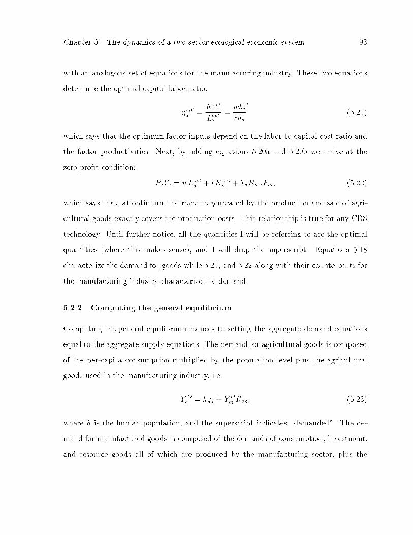
Chapter �� The dynamics of a two sector ecological economic system ��
with an analogous set of equations for the manufacturing industry� These two equations
determine the optimal capital labor ratio�
�opta Kopt
a
Lopta
wbaraa
�
������
which says that the optimum factor inputs depend on the labor to capital cost ratio and
the factor productivities� Next� by adding equations ����a and ����b we arrive at the
zero prot condition�
PaYa wLopta ! rKopt
a ! YaRmaPm� ������
which says that� at optimum� the revenue generated by the production and sale of agri
cultural goods exactly covers the production costs� This relationship is true for any CRS
technology� Until further notice� all the quantities I will be referring to are the optimal
quantities �where this makes sense�� and I will drop the superscript� Equations ����
characterize the demand for goods while ����� and ���� along with their counterparts for
the manufacturing industry characterize the demand�
� � Computing the general equilibrium
Computing the general equilibrium reduces to setting the aggregate demand equations
equal to the aggregate supply equations� The demand for agricultural goods is composed
of the percapita consumption multiplied by the population level plus the agricultural
goods used in the manufacturing industry� i�e�
Y Da hqa ! Y D
m Ram ������
where h is the human population� and the superscript indicates �demanded�� The de
mand for manufactured goods is composed of the demands of consumption� investment�
and resource goods all of which are produced by the manufacturing sector� plus the

Chapter �� The dynamics of a two sector ecological economic system ��
manufactured goods consumed by the agricultural sector� Thus
Y Dm hqm ! hqi ! hqr ! Y D
a Rma� ������
The demands for agricultural and manufactured goods are easily computed by dividing
equation ���� and the counterpart for manufacturing through by the appropriate prices�
Setting the results equal to the right hand sides of equation ���� and ���� yields the
general equilibrium equations�
Pahqa ! PaYmRam wLa ! rKa ! YaRmaPm �����a�
Pmhqm ! Pmhqi ! Pmhqr ! PmYaRma wLm ! rKm ! YmRamPa �����b�
Equations ���� specify the equilibrium with e�cient factor utilization� Recall that in
the model full factor utilization is enforced� This requires that
La ! Lm L �����a�
Ka !Km K �����b�
where L andK are the total labor and capital available� respectively� Equations ����� ����
and ���� constitute a system of ve equations �of which three are nonlinear because prices
and output are nonlinear functions of capital and labor� and six unknowns� La� Lm� Ka�
Km� r� and w� Thus given any one variable� all other equations could be solved for the
other variables� Since in this model money acts only as a numeraire� the system is closed
by xing r �the factor cost of a unit of capital� as the numeraire good and measuring
prices in terms of r�
There are several problems with this approach� First and most obvious is the prob
lem of existence and uniqueness of solutions to systems of nonlinear equations� Then�
supposing there is a unique solution� there is the di�culty of locating it� The algebraic
system of equations that characterize the economic system is coupled with a dynamical

Chapter �� The dynamics of a two sector ecological economic system ��
system that characterizes the ecosystem � i�e� the human population� capital stocks�
natural capital stocks� and so on� Thus� the economic system equations must be solved
continuously as the physical system evolves� If there is no explicit solution to the eco
nomic model as was the case for the models in Chapter �� the ecological economic system
model is a set of di�erential algebraic equations �DAE� Although there are techniques to
solve DAE�s �i�e� collocation� ����� dynamical system and bifurcation analysis tools such
as XPPaut and Auto are not set up to handle this situation� Thus� in order to study the
structure of the model� we must reformulate the general equilibrium problem�
I reformulate the problem by adding a labor market and writing the ve equation
system as one explicit algebraic equation and one di�erential equation� First� we substi
tute the values of Ya� Ym� and qa given by ����a� ����b� and ����a respectively into ����a
to get
Pahq�
a ! cahI � cahPaq�
a � cahPmq�
m ! PaRamEm�kn���amm Km
wLa ! rKa ! PmRmaEa�kr���aaa Ka� ������
Then� from equation ���� and its counterpart for the manufacturing industry� we get a
set of coupled equations for the optimal prices�
Pa Law !Kar
Ea�kr���aaa Ka
!RmaPm �����a�
Pm Lmw !Kmr
Em�kn���amm Km
!RamPa� �����b�
We can again use equation ���� to eliminate capital and labor from equations ����� i�e��
at optimum we have�
Law Karaaba
������
thus
Law !Kar
Ea�kr���aaa Ka
Karaaba
!Kar
Ea�kr���aaa Ka
r�� ! aa
ba�
Ea�kr���aaa
r�aaa
Ea�kr�ba� ������
Chapter �� The dynamics of a two sector ecological economic system ��
A similar relation holds for the manufacturing sector� enabling us to write equations ����
as
Pa r�aaa
Ea�kr�ba!RmaPm �����a�
Pm r�amm
Em�kn�bm!RamPa� �����b�
Solving these coupled equations for the prices yields�
Pa r
� �RmaRam
��aaa
Ea�kr�ba!
Rma�amm
Em�kn�bm
������a�
Pm r
� �RmaRam
��amm
Em�kn�bm!
Ram�aaa
Ea�kr�ba
�� �����b�
Notice the upward e�ect decreasing e�ciencies and increasing interindustry transfers
have on prices� It is important to include this aspect in the model to capture the impor
tant fact of the heavy reliance of modern agriculture on manufacturing inputs� Notice
that the prices in ���� depend only on physical constants� the per unit capital cost� and
the capitallabor ratios �a� and �m� At optimum� the capital labor ratio can be replaced
by the factor cost ratio via ����� Thus� given the factor cost ratio� optimal prices are
determined up to the constant r� Thus equations ���� can be rewritten as
Pa rfa��� andPm rfm��� ������
where � w
rand
fa��� �
��RmaRam
��aa�ba�aa�aa
Ea�kr�ba!Rma�
am�bm�am�am
Em�kn�bm
������a�
fm��� �
��RmaRam
��am�bm�am�
am
Em�kn�bm!Ram�
aa�ba�aa�aa
Ea�kr�ba
�� �����b�
By writing the prices this way� we will see that r cancels and the equilibrium labor and
capital devoted to agriculture and manufacturing depend only on the factor cost ratio
�� Finally� if I� the percapita income of the economy could be written in terms of ��
Chapter �� The dynamics of a two sector ecological economic system ��
equations ���� and ���� can be combined to write Ka as an explicit function of �� Since
hI� the total income of the economy� is equal to the sum of the total income generated
by labor and capital� respectively� �factor rewards� we have�
hI Lw !Kr �La ! Lw�w ! �Ka !Km�r ������
and using ���� we can eliminate the labor terms arriving at
hI rKa
ba!rKm
bm� ������
Here we see that income and prices both depend on r� Fixing r is equivalent to choosing
units for the money in the system i�e� r is a numeraire� Since we are only including
the dynamics of the labor market� we x r �� then � w� Finally� combining
equations ����� ����� ����b� and ���� we arrive at at explicit formula for Ka in terms of
K� h� and w�
Ka�K�h�w�
�� � ca�hfa�w�q�a !caK
bm!RamEm�kn�
�amwbm
�amfa�w�K � hcafmq
�
m
� � caba
!cabm!RamEm�kn�
�amwbm
�amfa�w� !RmaEa�kr�
�aawba
�aafm�w�
� ������
Thus given the total capital endowment of the economy� the human population� and the
wage rate � factor cost ratio�� the optimal amount of capital to devote to agriculture
is easily computed by ����� Then using ����b� and ����� the optimal levels of capital
and labor to manufacturing and labor to agriculture can be computed� The problem
is that the optimal labor quantities computed this way may not be equal to the labor
endowment of the economy� that is� La ! Lm � L in general and the economy is out of
equilibrium� This is where the role of the labor market comes into play� The labor market
will link wages to available labor and force the economy to tend towards equilibrium�
Before discussing the labor market� however� I would like to make a critical point about

Chapter �� The dynamics of a two sector ecological economic system ��
equation ����� This equation says that a certain portion of the revenue generated by the
productive process is paid to workers in the form of wages while the remainder is paid
to �capital� in the form of interest� dividends� etc� It says nothing however about the
distribution of income� I will address this point in more detail later�
Several �nonlinear� algebraic relationships have been proposed to relate labor supply�
demand� and wages� e�g� ����� but I will employ a simple linear �in labor supply and
demand� di�erential equation to model wage dynamics� The assumptions are basic� an
oversupply of labor will put downward pressure on wages while and undersupply will
have the opposite e�ect� This simpleminded model does nothing to address important
labor market issues such as union activity and so on� but is su�cient for a start� Thus
we have
dw
dt �w�L� La�w�� Lm�w�� ������
where �w is the speed of response of wages to disparities between labor supply and de
mand� Equation ���� coupled with ���� comprise a fast e�cient method forcing the
economy to seek equilibrium in a dynamically evolving system� The alternative of solv
ing a set of coupled nonlinear equations for the equilibrium is not only slower and more
di�cult� but also articial� Economies are never in equilibrium� and equation ���� cap
tures this fact� Further� we can actually adjust �out of equilibriumness� via the factor
�w and study its e�ect on the dynamics of the system�
In order to illustrate the operation of the economic system� I have computed the
equilibrium with arbitrary initial capital and labor endowments of ��� units each� Pa
rameters are� aa ���� am ���� q�a ���� q�
m ���� ca ���� cm ���� ci cr �� and
Ea Em are constant and set equal to �� Figure ��� shows the results of this exercise�
The initial guess at the wage rate is ��� so each unit of labor is half as costly as a
corresponding unit of capital� With such cheap labor� it is optimal to use well over ���

Chapter �� The dynamics of a two sector ecological economic system ��
0
0.2
0.4
0.6
0.8
1
1.2
1.4
1.6
1.8
2
0 0.2 0.4 0.6 0.8 1 1.2 1.4 1.6 1.8 20
20
40
60
80
100
120
140
160
180
200
0 0.2 0.4 0.6 0.8 1 1.2 1.4 1.6 1.8 20
20
40
60
80
100
0 0.2 0.4 0.6 0.8 1 1.2 1.4 1.6 1.8 2
Wagerate
Labor
Capital
Time Time Time
Lm
La
Ka
Km
Figure ���� Trajectories of wages� capital� and labor as the economy adjusts�
units which far exceeds labor availability� Upward pressure on wages drives the system
very quickly to the equilibrium state with w ������ Ka ������� Km ������� La
������� Lm ������� The question is� is this solution unique and optimal Figure ���
helps put this question in perspective� it shows the utility function and the optimum
solution above�
Note that the utility function is strictly convex inside the region where the economy
can exceed its minimum demands of q�a ��� and q�m ���� The inset gure on the
upper right is a contour plot of the surface on the lower left showing the optimum with
a white dot� the region where minimum demands can�t be met with available labor and
capital endowments �white area�� and where they can �grey scale area�� For values of
labor and capital in the grey scale region� it is tedious but not di�cult to show that the
necessary condition for optimality given by ���� is su�cient and the solution is unique�
In the region in the La � Ka plane where minimum needs cannot be met� the util
ity function is dened to be identically �� In this case there is no optimum solution so
some other mechanism must be dened to allocate available resources to di�erent activ
ities� I accomplish this by assuming that if minimum needs cannot be met� the economy

Chapter �� The dynamics of a two sector ecological economic system ���
020
4060
80100
0
20
40
60
80
100
0
0.05
0.1
0.15
0.2
0.25
0.3
0.35
0.4
0 10 20 30 40 50 60 70 80 90 1000
10
20
30
40
50
60
70
80
90
100
Utility
LaborCap
ital
Labor
Capital
Figure ���� Surface plot of utility function showing optimal combination of labor andcapital to agriculture�
will rst attempt to meet food needs and devote what is left over to other activities�
Mathematically� this translates to�
qa
�������������q�a !
caIsPa
Is � �
q�a Is � and I � Paq�
a � �
Ea�kr�LaaKba otherwise
�����a�
qm
�������������q�m !
cmIsPm
Is � �
I�Paq�
a
PmIs � and I � Paq
�
a � �
� otherwise
�����b�
qi
�����ciIsPm
Is � �
� otherwise�����c�

Chapter �� The dynamics of a two sector ecological economic system ���
qr
�����crIsPm
Is � �
� otherwise�����d�
Before turning our attention to the physical system� I would like to emphasize two
important aspects of the economic system� the e�ect of interindustry transfers� and the
�sensible� way the economy evolves when it becomes more di�cult to meet minimum
demands �i�e� how equations ���� work� � I do this by examining the evolution of
the economy as the amount of manufactured goods purchased by the agricultural sector
increases� Figure ��� shows how the consumption and expenditure patterns change under
these conditions�
0
0.1
0.2
0.3
0.4
0.5
0.6
0.7
0.4 0.45 0.5 0.55 0.6 0.65
0.1
0.2
0.3
0.4
0.5
0.6
0 10 20 30 40 50 600
0.2
0.4
0.6
0.8
1
0 10 20 30 40 50 60
q m
Consumption
Incomefraction
qa�a�
Time�b�
Time�c�
qa
qm
Ia
Im���������
Figure ���� Graph �a� shows qm versus qa� Notice that consumption evolves toward�q�a� q
�
m�� Graph �b� shows qm �dotted� and qa �solid� over time� Graph �c� shows theproportion of income devoted to purchasing manufacturing and agricultural goods� Imand Ia respectively�
Figure ����a� plots qm versus qa and illustrates how the economy moves to the point
�q�m� q�
a�� Beyond this point� the economy rst meets agricultural needs and uses what
is left for manufactured goods as illustrated by the vertical line� Figure ����b� shows
consumption over time large sacrices in the consumption of manufactured goods are
necessary to maintain agricultural production� Finally� gure ����c� shows how increased
reliance on manufactured inputs in agriculture will cause relative price increases for

Chapter �� The dynamics of a two sector ecological economic system ���
agricultural goods� With the economic system model complete� we now turn to the
nal task of specifying the physical system�
� The ecological system model
The cultural �distributional� component of the model is contained in the economic system
in the four parameters� ca� cm� ci� and cr that govern how the productive capacity of
the economy is portioned to the di�erent activities of consuming food� manufactured
goods� investment goods� and resource goods respectively� We are left to specify how
these activities interact with the state variables h� kh� kn� and kr as dened in chapter ��
The dynamical system that we will analyze for the remainder of this chapter is�
dh
dt �b�qm�� d�qa��h �����a�
dkhdt
ekr �ihqi � kh �����b�
dkndt
�ekn�mYm ! ekn�rhqr �����c�
dkrdt
krnr��� kr�� ekr �aYa �����d�
where b�qm� is the per capita birth rate as a function of per capita consumption of
manufactured goods which incorporates the idea of �demographic transition�� d�qa�� is
the nutrition dependent death rate function just as in the Tsembaga model� the ei�j are
�conversion� factors measuring the e�ect of the jth process on the ith state variable�
i�e� ekr�a measures the e�ect of agriculture on renewable natural capital� is the rate of
depreciation of manmade capital� and nr is the �possibly dependent on economic output
or the state of the system� regeneration rate of renewable natural capital�
The model specied by ���� is perhaps the simplest possible that incorporates all
the key features that are debated in the literature� For example� equation ����a taken
with equation ����b with � and b � d held constant is a typical example of an

Chapter �� The dynamics of a two sector ecological economic system ���
economic growth model with no connection to the physical world� This would correspond
to the model in gure ���� Figure ��� shows the evolution of a model economy under
these circumstances� Graph �a� shows the trajectory of the economy in phase space
from di�erent initial capital and labor endowments� In this case� capital and labor
grow without bound� converging to a xed capital labor ratio determined by the level
of investment of the economy� ci as shown in graph �b�� While the capital labor ratio is
below the long run equilibrium level� standard of living increases up to a maximum as
indicated in graph �c�� After the long run equilibrium is reached� economic output grows
exponentially� with per capita consumption constant�
0
200
400
600
800
1000
0 200 400 600 800 10000
0.5
1
1.5
2
2.5
3
0 20 40 60 80 100 1200
0.5
1
1.5
2
2.5
3
0 20 40 60 80 100 120
Capital
Capital
Labor
Percapitacons�
Labor�a�
Time�b�
Time
qa
qm
�c�
Figure ���� Graph �a� shows capital versus labor for the simple economic growth modelcorresponding to gure ����� and equations ������ Notice each trajectory has the sameslope� Graph �b� shows the capitallabor ratio� Graph �c� shows the per capita consumption of manufactured �dotted� and agricultural goods �solid� over time�
Exponential economic growth is unrealistic in the long run� and the model incor
porates important implications of entropic considerations called for by authors such
as ���� ��� by allowing things to wear out i�e� � � in equation ����b� and including
the physical reality that producing goods can degrade both renewable and nonrenewable
natural capital in equations ����c and ����d�
Now� if one sets the right hand sides of equations ���� to zero to nd the steady

Chapter �� The dynamics of a two sector ecological economic system ���
state�s�� this would correspond to locating a steady state economy in phase space� Indeed�
setting the equations above to zero and reading o� the conditions for this to be true
matches our intuitive idea about what a sustainable human agro ecosystem is� i�e� at
a steady state� birth rates will be depressed by changing economic structure �improved
living standards and the increased marginal cost of children�� investment rates will just
o�set depreciation �entropic decay� keeping capital stocks constant� and recycling� more
e�cient resource use� and reduced waste streams will o�set degradation of natural capital�
So what can be gained studying a complicated dynamical system The verbal description
does not say anything about the magnitudes of the state variables at equilibrium� nor does
it say anything about whether the equilibrium is attainable� i�e� under what conditions
can a system arrive at a sustainable state� It is one thing to characterize a sustainable
state� but another to study its structure� the task to which we now turn our attention�
Analysis of the Model
Because the model structure is very rich� it will be explored a piece at a time� The
rst issue we will explore with the model is the interaction of investment� evenness of
economic growth� and the distribution of wealth in an economy that relies on renewable
natural capital i�e� one step up from the most basic economic growth model involving
only labor and capital� Complexity will then be added step by step� nishing with the
analysis of the full model�
� Investment� distribution of wealth� and ecosystem stability
Intuitively� the process of investment by which productive capacity is increased should
make everyone�s life better o�� It is possible however to invest too much whereby� for
example� the capital stock may grow to such a point that its maintenance puts such

Chapter �� The dynamics of a two sector ecological economic system ���
a drain on the economy that the standard of living is reduced� Another problem with
too much investment is associated with overexploitation of resources due to being too
e�cient� In our model� investment helps productivity not only in the manufactured
goods sector� but also in agriculture� This increased productivity in agriculture may
destabilize the system by allowing the population to grow far beyond the level that an
ecosystem could bear without degradation� One mechanism that might halt this process
is behavioral changes associated with changing economic structure sometimes referred
to as the �demographic transition�� As the structure of the economy changes� the roles
children play in the economy change which in turn suppresses birth rates� We investigate
the interplay between these two process by analyzing the dynamics of the model while
two parameters are varied� ci the investment level� and bc a parameter that relates how
sensitive the birth rate is to per capita consumption of manufactured goods which I will
explain in a moment� In this analysis� we assume that the e�ciency in the manufacturing
sector is constant and does not depend on the availability of low entropy materials� This
leaves only three physical state variables� h� kh� and kr�
The function b�x� relates the birth rate to per capita consumption of manufactured
goods� As economic structure changes� there are several factors that might in�uence birth
rates� First� the marginal cost of children increases as economic complexity increases� In
simple rural economies� children can produce more than they consume at a young age
�below �� years�� In a complex industrial economy� children are a nancial burden to their
parents for a much longer time� Values might also shift the enjoyment of having children
and of family life might be replaced with other leisure activities aided by having fewer
children � What ever the mechanism� changing economic structure and the associated
increased economic productivity seem to depress birth rates� It is this rationale that
leads to the idea that continued economic development is the best policy if we wish to
guide the global economy to a sustainable state� Again� although this argument is very

Chapter �� The dynamics of a two sector ecological economic system ���
attractive� there is the question of under what circumstances this goal is attainable� To
capture this� I assume that b�x� has the form
b�x� b� exp ��bcx� ������
where b� is the percapita birth rate when no manufactured goods are consumed and bc
measures the sensitivity of birth rates to the level of consumption� For large values of
bc� births decrease very rapidly with increased per capita consumption of manufactured
goods and vice versa� The physical interpretation of bc could be either that each indi
vidual in the population has a certain response to consumption or it could measure the
distribution of income� or more precisely� the evenness of economic development� The
latter is of most interest to us� Notice that the argument of b�x� is qm which is the
average per capita consumption of manufactured goods� If economic development is not
even� some individuals might enjoy certain benets that reduce mortality with out expe
riencing other aspects of the development process that might suppress birth rates� In this
case the response of the birth rate to consumption levels would be weak� This situation
is modeled by a low value of bc� If� on the other hand� economic growth is more even
and income is distributed evenly� birth rates would fall o� more quickly as consumption
increased because more individuals in the population would reduce births for the same
level of per capita intake� It turns out that for an economy that decides to invest� how
evenly the the economy develops and distributes income is an important factor for its
survival�
To illustrate� we examine the structure of the model as the parameters ci and bc are
varied� To set the stage� suppose that economic growth is even and income is distributed
very well within the economy� The system is then integrated with the following parameter
values�
� Economic parameters� for the marginal productivities of labor in each industry

Chapter �� The dynamics of a two sector ecological economic system ���
we take aa ��� and am ���� The value for manufacturing is based on some
empirical work that suggests that values in the range of ��� to ��� are reasonable �����
The value for agriculture is more speculative and is based on the heavy reliance
on capital in modern agriculture� We take q�a ��� and q�m ��� which are
arbitrary and depend on scaling and choice of units in the rest of the model� The
only important thing is that agricultural goods become relatively more important in
times of scarcity� The cultural parameters are ca ����� cm ���� ci ����� cr ��
I selected these values based on consumer data from the ���� Statistical Abstract
of the United States ����� I simply adjusted the parameters until the proportion
of income spent in each category generated by the model roughly matched those
for the U�S�� roughly �� percent to food� �� percent to investment� and the rest to
personal consumption �manufactured goods�� Next I set Ea ��kr and Em ��
The e�ciency in agriculture is based on energy data for agricultural production �����
In this case� I assume that the e�ciency of manufacturing is constant and unity
and that there are no interindustry transfers assumptions that will be relaxed
later�
� Ecological parameters� ����� ekr �i ����� ekn�m �� The parameter ekn�r is
irrelevant because no income is directed toward resource goods� Finally� ekr�a
������ and nr ���� These parameters merely scale time in the model �i�e� just
specify the units of measurement�� The key physical parameters are b� and bc� For
example if b� ����� at low levels of consumption� a couple �on average� would
have around � births over a lifetime� Now we can study how the parameter bc
a�ects the model�

Chapter �� The dynamics of a two sector ecological economic system ���
With these assumptions� we are left to analyze the following dynamical system�
dh
dt ����� exp��bcqm�� � exp����qa��h �����a�
dkhdt
����hqi � ����kh �����b�
dkrdt
���kr��� kr�� �����Ya �����c�
dw
dt ����h� La�w�� Lm�w�� �����d�
where the following set of algebraic constraints apply� The optimal capital levels to devote
to agriculture and manufacturing are
Ka
���������� h
krw��� ! �����kh � �����hw��� Ka ka
kh otherwise�����a�
Km kh �Ka� �����b�
Then equations ����� ����a� ����b� and ���� allow the optimal labor� output� and price
levels to be computed�
La �����Ka
wLm �
Km
w������
Ya ����krw���� Ym ����w
���� ������
Pa �����w���k��
r Pm �����w���� ������
Recall that L La!Lm so per capita income and supernumery income can be computed�
I kh ! wL
hIs I � ���Pa � ���Pm� ������

Chapter �� The dynamics of a two sector ecological economic system ���
Finally� the per capita consumption levels are given by
qa
���������������� ! ���Is
PaIs � �
��� Is � and I � ���Pa � �
��krhaakbah otherwise
�����a�
qm
���������������� ! ��Is
PmIs � �
I���PaPm
Is � and I � ���Pa � �
� otherwise
�����b�
qi
��������IsPm
Is � �
� otherwise�����c�
and the model is fully specied�
Figure ��� shows the trajectories of the model in phase space for bc � �relatively
even economic development and wealth distribution�� Graph �a� shows the population
versus natural capital� As population grows� natural capital is reduced� but the system
comes to stable equilibrium� i�e� a sustainable state� Graph �b� shows the population
versus manmade capital� Notice that when the population is low� capital and labor grow
maintaining a constant ratio �i�e� the labor versus capital curve is a straight line� as is
common for simple economic growth models� However� as the system grows� it encounters
limitations in natural capital which restricts human population and� in turn� capital
growth� The capitallabor trajectory tends away from the linear growth trajectory �that
would continue on indenitely in a simple economic growth model including just labor
and capital� and comes to equilibrium� Here we see the distinct di�erence embedding
the economic growth model in a physical environment makes population and capital
cannot grow indenitely�
Nonetheless� the outcome of the model under these conditions is very positive� If
economic growth is even and wealth is reasonably distributed� the economy settles down

Chapter �� The dynamics of a two sector ecological economic system ���
0
1
2
3
4
5
6
7
8
0.4 0.5 0.6 0.7 0.8 0.9 10
1
2
3
4
5
6
7
8
0 0.5 1 1.5 2 2.5 3 3.5 4
Population�h
Population�h
Natural Capital� kr�a�
Manmade Capital� kh�b�
Figure ���� Graph �a� shows h versus kr� Graph �b� shows h versus kh�
to a steady state with each individual enjoying a high standard of living� The population
equilibrates at a little over � people per �cultivated� hectare� with natural capital at about
�� % of the maximum� Figure ��� shows the evolution of capital� labor� and consumption
over time�
0
1
2
3
4
5
6
0 200 400 600 800 1000 12000
0.2
0.4
0.6
0.8
1
1.2
1.4
1.6
0 200 400 600 800 1000 1200
0.62
0.64
0.66
0.68
0.7
0.72
0.74
0.76
0 200 400 600 800 1000 1200
Labor
Capital
Percapitacons�
Time�a�
Time�b�
Time
La
Lm
Ka
Km
qaqm
�c�
Figure ���� Graphs �a� and �b� show the distribution of labor and capital to agriculture and manufactuing respectively� Graph �c� shows the per capita consumption ofmanufactured and agricultural goods over time�
The bulk of the labor and capital are directed towards non farm business� consistent
with what would be observed in a modern economy� The population consumes around
��� units of agricultural goods and manufactured goods respectively� both above their

Chapter �� The dynamics of a two sector ecological economic system ���
minimum values i�e� life is quite good�
Now suppose we reduce bc� Figure ��� is a bifurcation diagram showing the e�ect this
has on the model� As bc is reduced� a subcritical Hopf bifurcation occurs at bc � ���
Below this point the steady state is unstable� and the system undergoes large amplitude
oscillations� This is to say that if the system begins from an initial condition with a
value of bc below ���� there is a barrier that precludes the system from arriving at a
�sustainable state��
0
2
4
6
8
10
12
0 1 2 3 4 5 6
Population
bc
Figure ���� Bifurcation diagram for simplied model�
It turns out that there is an explicit relationship between investment� evenness of
economic growth and distribution of wealth� and system stability that we can elucidate
by performing a twoparameter continuation with bc and ci� Figure ��� is the result�
For combinations of ci and bc in the region below the bifurcation boundary �more even

Chapter �� The dynamics of a two sector ecological economic system ���
development and wealth distribution for a given level of investment� there is always
an attainable sustainable state� For combinations of ci and bc in the region above
the bifurcation boundary �less even development wealth distribution for a given level of
investment� the steady state is unattainable� The steady state is surrounded by a stable
limit cycle which forms a boundary between any initial state outside the limit cycle and
a sustainable economy�
0
2
4
6
8
10
12
0 0.2 0.4 0.6 0.8 10
2
4
6
8
10
12
0 0.2 0.4 0.6 0.8 1
0
0.05
0.1
0.15
0.2
0.25
0.3
0.35
0.4
0.45
0.5
0 2 4 6 8 10
0
1
2
3
4
5
6
7
8
0.4 0.5 0.6 0.7 0.8 0.9 1
Income Distribution� bc
InvestmentgoodPreference�c i
Figure ���� Change in dynamics as the bifurcation boundary is crossed� The system goesto a stable equilibrium �sustainable economy for parameter values to the right and belowthe curve �lower investment and better income distribution�� For parameter combinationsabove and to the left � �higher investment and less even economic development and wealthdistribution� the system undergoes stable� large amplitude �uctuations�
Figure ���� shows the trajectories for the model in phase space for bc �� and
ci ��� Graph �a� shows the population versus natural capital� As population grows�
natural capital is reduced but in this case the population does not come to a steady state�

Chapter �� The dynamics of a two sector ecological economic system ���
Instead� after the human population density reaches a maximum� continued increase
in capital stocks and e�ciency in agricultural production allows the population to be
maintained for a short time while natural capital continues to decline� Figure ���� shows
the evolution of labor� capital and consumption over time� Then we see both labor and
capital being shifted out of manufacturing into agriculture in an attempt to maintain
agricultural output� This corresponds to the �at portion of the curve in kr � h phase
space on the left in gure ����� Increased productivity that accompanies capital growth
masks the degradation of natural capital allowing the population to grow far beyond
the capacity of the environment to support it� Finally� the population cannot maintain
either agricultural or manufacturing output and capital stocks fall as shown in gure �����
Notice that in graph �c� in gure ����� per capita output of agricultural and manufactured
goods are maintained up to the point when the system collapses suggesting that the
signals to consumers about environmental degradation through the market system would
not be strong enough to cause them to change their habits� Thus the rst prediction of
the model is that investment must be accompanied by e�orts to insure that economic
growth is even and and its associated benets are evenly distributed to have any hope of
reaching a �sustainable economy��
There are several other points that could be addressed here� For example how does
changing the productivities of labor in agriculture and manufacturing change the struc
ture of the model One might also argue that the model does not really correctly charac
terize the nature of the the agricultural sector because it does not take into consideration
measures that might preserve natural capital� On the other hand� both sectors are per
fectly nonpolluting� Also the manufacturing sector has a constant e�ciency which does
not capture the negative e�ects of dwindling resource supplies or the positive e�ects of
innovation� Are the model predictions of any value then
I believe so� The model predictions relate to a general phenomenon that transcends

Chapter �� The dynamics of a two sector ecological economic system ���
0
2
4
6
8
10
12
14
0 0.2 0.4 0.6 0.8 10
2
4
6
8
10
12
14
0 1 2 3 4 5 6 7 8
Population�h
Population�h
Natural Capital� kr�a�
Manmade Capital� kh�b�
Figure ����� Graph �a� shows h versus Kr� Graph �b� shows h versus Km�
the actual assumptions about the organization of a particular social system� That phe
nomenon is when the society can no longer bear increased complexity and must necessarily
collapse� As Joseph Tainter ���� puts it� the marginal benets of increased complexity
approach zero� In our simplied model� as the society increases in complexity �manu
factured capital increases� it receives positive benets in terms of improved standard of
living� If� however� the society moves into a position where it can no longer maintain
the complex structure it has created� it becomes a burden and may cause the society
to collapse� In our simple model� this occurs when all capital and labor is shifted into
agriculture in an attempt to feed the population� When this occurs� capital stocks are
neglected and decay i�e� the society can no longer maintain its complex structure�
The point is� in one case increasing complexity leads to a sustainable economic ecologi
cal system and in the other case� increasing complexity leads to collapse� This emphasizes
the important role that evenness of economic development and the management of the
benets of increased complexity play in the evolution of an economy� In Collapse of
Complex Societies ����� Joseph Tainter describes several societies that he believes went
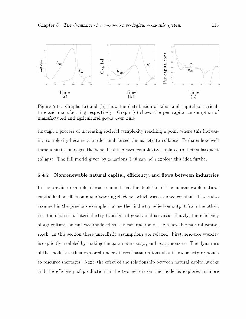
Chapter �� The dynamics of a two sector ecological economic system ���
2
4
6
8
10
0 50 100 150 200 2500
0.5
1
1.5
2
2.5
0 50 100 150 200 2500
0.2
0.4
0.6
0.8
1
1.2
1.4
0 50 100 150 200 250
Labor
Capital
Percapitacons�
Time�a�
Time�b�
Time
La
Lm Ka
Km
qaqm
�c�
Figure ����� Graphs �a� and �b� show the distribution of labor and capital to agriculture and manufactuing respectively� Graph �c� shows the per capita consumption ofmanufactured and agricultural goods over time�
through a process of increasing societal complexity reaching a point where this increas
ing complexity became a burden and forced the society to collapse� Perhaps how well
these societies managed the benets of increased complexity is related to their subsequent
collapse� The full model given by equations ���� can help explore this idea further�
� Nonrenewable natural capital� e�ciency� and �ows between industries
In the previous example� it was assumed that the depletion of the nonrenewable natural
capital had no e�ect on manufacturing e�ciency which was assumed constant� It was also
assumed in the previous example that neither industry relied on output from the other�
i�e� there were no interindustry transfers of goods and services� Finally� the e�ciency
of agricultural output was modeled as a linear function of the renewable natural capital
stock� In this section these unrealistic assumptions are relaxed� First� resource scarcity
is explicitly modeled by making the parameters ekn�m� and ekn�mr nonzero� The dynamics
of the model are then explored under di�erent assumptions about how society responds
to resource shortages� Next� the e�ect of the relationship between natural capital stocks
and the e�ciency of production in the two sectors on the model is explored in more

Chapter �� The dynamics of a two sector ecological economic system ���
detail� Finally� the role of interindustry transfers �i�e� the dependence of agriculture on
a �ow of manufactured goods and services� on the model is investigated�
First� consider the role of nonrenewable natural capital depletion as modeled by equa
tion ����d� At equilibrium� we must have
hqr ekn�mekn�r
Ym� ������
Since the amount of manufacturing output devoted to maintaining nonrenewable natural
capital stocks �through such activities as exploration and technological development� is
a fraction of the total output Ym� the ratioekn�mekn�r
must be less than �� This simply means
that the output used to nd new nonrenewable resources has to more than replace those
used in producing that output�
The next question is how society allocates output to the activity of generating new
nonrenewable natural capital stocks� A simple way to model this process is to let the
preference for resource goods increase as these stocks become more scarce� A reasonable
function representing this relationship is
cr �� ca � ci�knkn ! �
� ������
As resources become more scarce� society shifts its preference for consumption of goods
and services to replacing sources of raw materials� Since the preferences must add up
to one� the maximum value of cr is � � ca � ci� the preference �remainder� after food
and investment needs are met� �kn is a measure of how responsive society is to resource
shortages� Figure ���� depicts the relationship between kn and cr for di�erent values of
�kn� The lower �kn� the more responsive the society is to raw material shortages� If �kn
is large� society will not devote output to replacing raw material stocks until the actual
stock is quite low�
Finally� before exploring the implications of resource scarcity on the model� the depen
dence of the e�ciency of the manufacturing and agricultural sectors on resource stocks

Chapter �� The dynamics of a two sector ecological economic system ���
0
0.1
0.2
0.3
0.4
0.5
0.6
0.7
0.8
0 0.2 0.4 0.6 0.8 1 1.2 1.4 1.6 1.8 2Resourcegoodpreference�c r
Kn
Figure ����� Resource good preference versus Kn for di�erent values of �kn� From top tobottom� the values for �kn are ��� ��� and ���
must be modeled� Above a certain level� the relative abundance of raw materials has
little e�ect on manufacturing e�ciency because only a small portion of total economic
output must be directed towards their procurement� As they become more scarce� more
economic output must be directed towards obtaining raw materials which reduces the
overall e�ciency of the production process� A simple function that captures this e�ect is
Em�kn� kn
kn ! kn������
where kn is the resource level at which e�ciency is half the maximum� A similar functional
form is used for productivity in agriculture� but is scaled so that when kr �� Er�kr�
��� The result is
Ea�kr� ��kr�� ! kr�
kr ! kr� ������
Figure ���� illustrates the form of these relationships� Graph �a� shows the manufacturing
e�ciency for kn ���� E�ciency is mildly reduced until kn ��� �onehalf of the
original endowment� after which it falls o� rapidly� Graph �b� shows the analogous
relationship between Er and kr for di�erent values of kr� In the following example�

Chapter �� The dynamics of a two sector ecological economic system ���
kr �� kn ���� This choice is arbitrary� with the only motivation being to capture the
e�ects of nonlinearities in e�ciency that are consistent with common sense� The e�ects
of these parameters on the structure of the model are addressed in the next section where
the full model is analyzed�
0
0.1
0.2
0.3
0.4
0.5
0.6
0.7
0.8
0.9
1
0 0.2 0.4 0.6 0.8 10
2
4
6
8
10
0 0.2 0.4 0.6 0.8 1
ManufacturingProductivity�Em
AgriculturalProductivity�Ea
Nonrenewable Natural Capital� kn�a�
Renewable Natural Capital� kr�b�
Figure ����� Graph �a� shows Em versus kn with �kn ���� Graph �b� shows Er versuskr for three di�erent values of �kr� ��� �� ��� with decreasing values corresponding toincreased curvature�
Nonrenewable Natural Capital
Here it is assumed that ekn�m ����� ekn�r ���� and bc �� In this analysis� the
assumption of no interindustry transfers is maintained� The dynamical system analyzed
in this section is given by equations ���� appended with the expression for nonrenewable
natural capital�
dkndt
�����Ym ! ���hqr� ������

Chapter �� The dynamics of a two sector ecological economic system ���
Also� now that cr � �� the per capita consumption equations given by ���� must be
appended with an expression for qr�
qr
�����crIsPm
Is � �
� otherwise�������
where
cr ���
�knkn ! �� ������
Finally� using the denitions of Em�kn�� and Ea�kr� given by equations ���� and �����
equations ����� ���� and ���� are replaced by
Ka
����������hPa ! �����kh � ������hPm Ka ka
kh otherwise�����a�
Km kh �Ka� �����b�
and
Ya �����krw����
� ! krYm
����knw����
��� ! kn������
Pa ������� ! kr�w���
krPm
��������� ! kn�w���
kn� ������
Figure ���� shows the state variable trajectories for the case for �kn ��� This cor
responds to the society being relatively responsive to resource shortages and the raw
material replacement process being able to generate ten times the raw materials it con
sumes� As long as society devotes economic output to replacing raw material stocks� the
economic system can reach a sustainable steady state �h� kr� kh� kn� � ��� ���� ���� ������
The economic system is still subject to the problem of overexploiting renewable natural
capital and collapsing� The problem introduced by nonrenewable natural capital occurs
when investment is too low� or stocks are allowed to dwindle to a low level before e�orts
are made to replace them �high value for �kn��

Chapter �� The dynamics of a two sector ecological economic system ���
0
2
4
6
8
10
12
0.4 0.5 0.6 0.7 0.8 0.9 1 1.10
0.2
0.4
0.6
0.8
1
1.2
1.4
1.6
1.8
2
0.4 0.5 0.6 0.7 0.8 0.9 1 1.1Humanpopulationdensity
ManmadeCapital
Renewable Natural Capital�a�
Nonrenewable Natural Capital�b�
Figure ����� Graph �a� shows human population versus renewable natural capital� Graph�b� shows manmade capital versus nonrenewable natural capital�
Notice in gure �b� how nonrenewable natural capital is transformed into manmade
capital as the economy develops� Once the economy is su�ciently developed� new sources
of raw materials are being found �via improvements in e�ciency� using new materials�
using materials in new ways� etc� as fast as they are used in the production of goods and
services� After this point� nonrenewable natural capital remains constant as the economy
continues to develop towards its nal state� If �kn is large� the situation is di�erent�
Figure ���� shows the equilibrium human population and manmade capital levels for
di�erent values of �kn�
As long as �kn is below about ��� the economy will reach a sustainable stable equilib
rium state� As �kn is increased� equilibriumvalues of manmade capital decreases because
society waits too long before addressing resource scarcity� When it nally does� manu
facturing e�ciency is low� more economic output must be directed towards maintaining
raw material �ows� and less can be directed to increasing manmade capital stocks� In
this case the economy begins to develop just as with low levels of �kn but reaches a level

Chapter �� The dynamics of a two sector ecological economic system ���
0
2
4
6
8
10
0 5 10 15 20 25 30 35 40 45 500
0.5
1
1.5
2
2.5
3
0 5 10 15 20 25 30 35 40 45 50
Equilibrium
humanpopulationdensity
Equilibrium
manmadecapital
�kn
�a�
�kn
�b�
Figure ����� Graph �a� shows the stable equilibriumhuman population versus �kn� Graph�b� shows the stable equilibrium manmade capital versus �kn�
of complexity where it can no longer maintain agricultural and manufacturing output as
well as look for new sources of raw materials� Figure ���� shows the transient dynamics
for �kn ��� and ci �����
Graph �a� shows the evolution of manmade and nonrenewable natural capital over
time� As with the previous example� nonrenewable natural capital is depleted as it is
transformed into manmade capital� Here however� nonrenewable natural capital stocks
are quite low �around ��� versus ��� in the example with �kn ��� before society responds
and begins to replace these stocks �around t ����� Between t ��� and t ���
nonrenewable natural capital stocks are maintained by directing more economic output
towards their replacement at the expense of new investment �as well as consumption
but to a lesser degree� as shown in graph �b�� The problem is that the e�ort to nd
replacements for nonrenewable natural capital stocks comes too late� At around t ����
the cost of maintaining economic infrastructure� feeding the population� and replacing
nonrenewable natural capital becomes to high for society to bear� All remaining factors
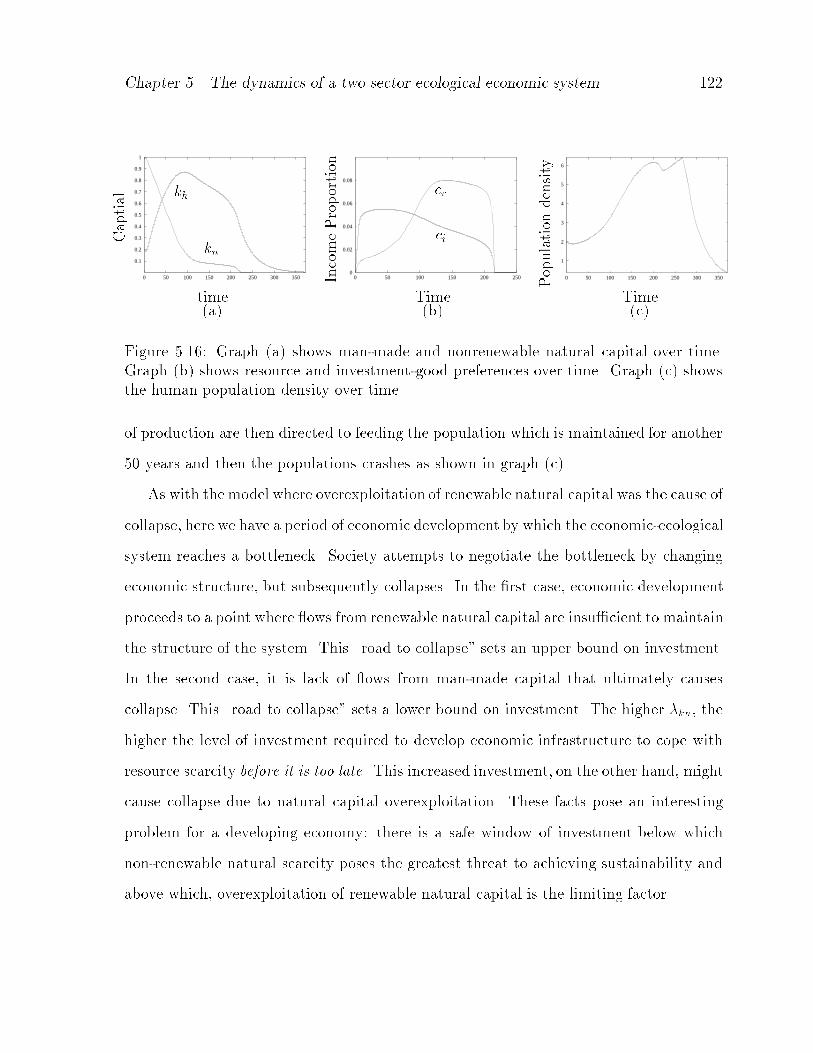
Chapter �� The dynamics of a two sector ecological economic system ���
0.1
0.2
0.3
0.4
0.5
0.6
0.7
0.8
0.9
1
0 50 100 150 200 250 300 3500
0.02
0.04
0.06
0.08
0 50 100 150 200 250
1
2
3
4
5
6
0 50 100 150 200 250 300 350
Captial
IncomeProportion
Populationdensity
time�a�
Time�b�
Time�c�
cr
ci
kh
kn
Figure ����� Graph �a� shows manmade and nonrenewable natural capital over time�Graph �b� shows resource and investmentgood preferences over time� Graph �c� showsthe human population density over time�
of production are then directed to feeding the population which is maintained for another
�� years and then the populations crashes as shown in graph �c��
As with the model where overexploitation of renewable natural capital was the cause of
collapse� here we have a period of economic development by which the economicecological
system reaches a bottleneck� Society attempts to negotiate the bottleneck by changing
economic structure� but subsequently collapses� In the rst case� economic development
proceeds to a point where �ows from renewable natural capital are insu�cient to maintain
the structure of the system� This �road to collapse� sets an upper bound on investment�
In the second case� it is lack of �ows from manmade capital that ultimately causes
collapse� This �road to collapse� sets a lower bound on investment� The higher �kn� the
higher the level of investment required to develop economic infrastructure to cope with
resource scarcity before it is too late� This increased investment� on the other hand� might
cause collapse due to natural capital overexploitation� These facts pose an interesting
problem for a developing economy� there is a safe window of investment below which
nonrenewable natural scarcity poses the greatest threat to achieving sustainability and
above which� overexploitation of renewable natural capital is the limiting factor�

Chapter �� The dynamics of a two sector ecological economic system ���
The problem of nding the appropriate window to grow fast enough to overcome
limitations in man made capital yet slow enough to avoid destroying natural capital is
illustrated in gure �����
0
2
4
6
8
10
0.025 0.03 0.035 0.04 0.045 0.05 0.055 0.060
10
20
30
40
50
60
70
0 0.02 0.04 0.06 0.08Humanpopulationdensity�h
�kn
Investmentgood preference� ci�a�
Investmentgood preference� ci�b�
non feasible�overexploitation ofrenewable naturalcapital
non feasible�nonrenewable natu�ral capital scarcity
feasible
Figure ����� Graph �a� shows the bifurcation structure for �kn ��� Graph �b� is thetwo parameter bifurcation diagram for �kn versus investment good preference�
Graph �a� shows the bifurcation structure for �kn �� i�e� society is relatively
responsive to resource shortages� The window of feasible investmentgood preference is
quite narrow� The economy will evolve to a sustainable steady state if investment good
preference is between ����� and ������ Investment good preferences outside this range will
give rise to an economic development path that leads to collapse due to resource shortages
or overexploitation of natural capital respectively� Graph �b� shows the dependence of
this result on the responsiveness of society to resource shortages� The curve on the
right depicts all the combinations of �kn and investmentgood preference for which a
Hopf bifurcation occurs� For a given �kn the corresponding value for investmentgood
preference is an upper bound for the feasible level of investmentgood preference that
will lead to a sustainable steady state economic ecological system� The curve on the

Chapter �� The dynamics of a two sector ecological economic system ���
left is the corresponding lower bound for investmentgood preference to prevent resource
shortages�
The region between these two curves denes the feasible region of investmentgood
preferences that will lead to a sustainable economy� Given that the range of possible
values for investmentgood preferences is from � to �� ca � ���� in the example above��
the width of the feasible region �about ����� in the example above� is quite narrow� Of
course� these numbers should not be taken as representative of those a modern economy
might face� but in the context of the model� they do indicate that the possibility of
attaining a sustainable economic ecological system may be very sensitive to investment
patterns�
E�ciency and feasible investment patterns
The nature of the relationship between investment patterns and feasible paths can depend
on many things� Two key aspects of the model that a�ect this relationship are the
relationships between e�ciency and capital stocks and the transfer of goods between
industries� In the above example� recall that kn ���� and kr �� A low value like this
for kn corresponds to the fact that if an economy has a stock of raw materials available
for productive activities� the size of that stock does not a�ect these activities until it
is reduced to a level where some portion of productive capacity must be diverted to
maintaining the stock� The lower kn� the more dramatic this transition� The signicance
of the relative nonlinearity in the relationship between kr and Ea is more di�cult to
imagine� It could correspond roughly to the idea of ecosystem resilience� If an ecosystem
is not resilient� productivity would decline rapidly due to agricultural disturbances �high
value for kr�� If an ecosystem is resilient� it might remain fairly productive even with
a high level of disturbance� but break down more rapidly after some threshold level of
disturbance is surpassed� The question is� how do di�erent values for kn and kr a�ect

Chapter �� The dynamics of a two sector ecological economic system ���
the results shown in gure ����
To investigate this� the model is analyzed by xing �kn �� and varying kn� and kr�
leaving the rest of the model assumptions unchanged from the previous section� Thus�
we now have
cr ���
��kn ! �� ������
and
Ya ����kr�� ! kr�w����
kr ! krYm
����knw����
kn ! kn������
Pa ������kr ! kr�w���
kr�� ! kr�Pm
������kn ! kn�w���
kn� ������
It turns out that increasing kn shifts the feasible region to the right but does not sig
nicantly a�ect the width of the region� This is consistent with intuition� increasing
kn makes manufacturing e�ciency more sensitive to resource shortages requiring more
investment to avoid them� Also� reduced e�ciency associated with increased kn puts
a drag on the economy slowing the growth process� This allows for a higher level of
investment without overexploiting renewable natural capital� Thus both the minimum
and maximum feasible values for investmentgood preference are increased� shifting the
feasible region to the right�
The model is much more sensitive to kr� This sensitivity is illustrated in gure ����
which shows a two parameter bifurcation diagram for investmentgood preference versus
kr� As ecosystems become less resilient �higher kr� � the system can tolerate more invest
ment� This seems a bit counter intuitive� but is similar in nature to the Tsembaga model
where increased productivity of renewable natural capital had a stabilizing tendency�
The key is that the feedback from ecosystems is stronger if they are less resilient�
Unlike kn� increasing kr widens the feasible range� For kr �� and kn ��� the feasible
values for investmentgood preference lie between ����� and ������ about double the range
for the case with kr �� As kr is reduced� ecosystems remain productive at higher levels

Chapter �� The dynamics of a two sector ecological economic system ���
0.03
0.04
0.05
0.06
0.07
0.08
0.09
0.1
0 2 4 6 8 10 12 14 16
Investmentgoodpreference�c i
kr
non feasible�overexploitation ofrenewable naturalcapital
feasible�no overexploitationof renewablenatural capital
Figure ����� Two parameter bifurcation digram for investmentgood preference and �kr�
of agricultural disturbance� This weakens the feedback from natural systems and allows
the human economic system to develop beyond the capacity of ecosystem to support it�
Thus the more resilient ecosystems are� the more likely it is for human economic systems
develop into situations from which they cannot extricate themselves� Thus the human
propensity to try to x things through attempting to increase productivity may be the
worst development strategy possible�
The e�ect of interindustry transfers
The nal aspect of the model that we address in this section is the role of interindustry
transfers� In the previous examples� each industry was assumed to operate independently
of the other� Neither sector relied on the other for raw material inputs� This is unrealistic
for modern agriculture which relies heavily on manufactured products� most notably
chemicals� Similarly� the manufacturing sector relies on bers from the agricultural sector�
In order to study the e�ects of interindustry transfers� we examine the e�ect that the

Chapter �� The dynamics of a two sector ecological economic system ���
parameters �N � �half � and Ram have on the model� All other parameters are xed and the
model assumptions remain unchanged from previous sections� i�e� the dynamical system
is given by equations ���� and equation ����� optimal consumption by equations ����
and ����� output by ����� labor by ����� income by ����� and resourcegood preference
by ����� Because Ram and Rma are not zero� no simplications occur for the optimal
capital and price levels� The full equations for the optimal capital and price levels given
by ���� and ����� respectively� must be used�
Recall that �N measures the quantity of nutrient inputs required per unit of agricul
tural output �a unit conversion factor� while �half measures the productivity of natural
capital� As �half is increased� the higher the ratio ofh
krcan be before nutrients produced
by biological processes are no longer su�cient to meet demand� It turns out that the
e�ect of material transfers from manufacturing to agriculture has a stabilizing e�ect�
This is illustrated by the two parameter bifurcation diagram in gure ���� with �half �
�meaning as population density per hectare approaches a typical value for a modern in
dustrial economy� depending on the level of degradation of natural capital� a substantial
amount of manufactured inputs would be required to meet food demand�� As �N in
creases� there is more pressure on the manufacturing sector which allows for increased
investment without overexploiting renewable natural capital� Again� the harder natural
capital is to exploit� the more stable the model�
Interestingly� changing �N does not a�ect the minimum investment level necessary
to avoid raw material shortages in the manufacturing sector� For example for ci ����
and �N ���� the feasible window for investmentgood preference is ������� to �������
For �N ���� the feasible window for investment good preference is ������� to �������
This result is slightly counterintuitive� One would think that increased demand for
manufactured goods in the agricultural sector would divert productive capacity away from
investment and nonrenewable natural capital replacement� Avoiding resource shortages
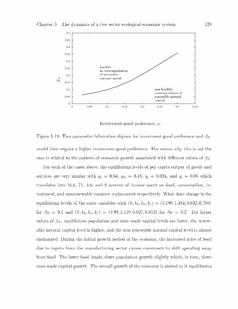
Chapter �� The dynamics of a two sector ecological economic system ���
0
0.05
0.1
0.15
0.2
0.25
0.3
0.35
0.4
0.45
0.5
0 0.05 0.1 0.15 0.2 0.25 0.3 0.35
�N
Investmentgood preference� ci
feasible�no overexploitationof renewablenatural capital
non feasible�overexploitation ofrenewable naturalcapital
Figure ����� Two parameter bifurcation digram for investmentgood preference and �N �
would then require a higher investmentgood preference� The reason why this is not the
case is related to the pattern of economic growth associated with di�erent values of �N �
For each of the cases above� the equilibrium levels of per capita output of goods and
services are very similar with qa ����� qm ����� qi ������ and qi ���� which
translates into ����� ��� ���� and � percent of income spent on food� consumption� in
vestment� and nonrenewable resource replacement respectively� What does change is the
equilibrium levels of the state variables with �h� kh� kn� kr� ������� ������ ������ ������
for �N ��� and �h� kh� kn� kr� ������ ������ ������ ������ for �N ���� For larger
values of �N � equilibrium population and man made capital levels are lower� the renew
able natural capital level is higher� and the non renewable natural capital level is almost
unchanged� During the initial growth period of the economy� the increased price of food
due to inputs from the manufacturing sector causes consumers to shift spending away
from food� The lower food intake slows population growth slightly which� in turn� slows
manmade capital growth� The overall growth of the economy is slowed so it equilibrates

Chapter �� The dynamics of a two sector ecological economic system ���
with a smaller human population and manmade capital stock� The result is that the
scale of the nal economy is smaller� putting less pressure on both nonrenewable and
renewable natural capital stocks� Thus the lower bound for feasible investment remains
unchanged while the upper bound increases�
It is interesting how the two cases above which di�er only very slightly in terms of their
development over time and equilibrium economic output di�er muchmore signicantly in
the equilibrium scale of the economy and levels of state variables� A drag on the economy
that slows economic growth� which is often considered bad� may in the long run produce
the same economic outcome as faster growth� The only di�erence is that the nal scale
of the slower growing economy is smaller� and the quality of renewable natural capital
higher� If the state of the natural environment is related to quality of life� then the slower
growing economy produces the better end result� This should be a major concern when
considering how policy a�ects economic growth�
Next� we turn our attention to the role that transfers from the agricultural to the
manufacturing sector have on the model� These transfers simply put more pressure on
renewable natural capital for a given level of economic output� Figure ���� illustrates the
relationship between the minimum and maximum feasible investmentgood preference
and Ram�
The maximum feasible investmentgood preference is more sensitive to increases in
Ram than is the minimum� This causes the feasible region to narrow as Ram is increased�
Thus the more taxing the manufacturing sector is on the agricultural sector� the smaller
the feasible investment region and the more di�cult achieving sustainability is� For
example� the model predicts that our reliance on paper products and wood ber for use
in the manufacturing sector may signicantly reduce the range of feasible investment for
our economy�
Another important aspect of the manufacturing industry is the pollution it generates�

Chapter �� The dynamics of a two sector ecological economic system ���
0
0.02
0.04
0.06
0.08
0.1
0 0.05 0.1 0.15 0.2 0.25 0.3
Investmentgoodpreference
Ram
non feasible�non renewableresource scarcity
feasible
non feasible�overexploitation ofrenewable naturalcapital
Figure ����� Two parameter bifurcation digram for investment good preference and Ram�
Although I have not addressed pollution directly �eg� as a state variable� its e�ect on
the dynamics of the system can be studied indirectly� One key aspect of pollution in
an ecological system is its negative e�ect on the operation of ecosystems� This can be
modeled as a reduction in renewable natural capital associated with economic activity�
This is similar to the e�ect Ram has on the economy when manufacturing puts in
creased pressure on renewable natural capital� whether by compromising its operation
through contamination or direct removal of nutrients� attaining sustainability is made
more di�cult�
Conclusions
In this chapter we have developed and studied the dynamics of a model for a two sector
ecological economic system� The main results of this modelling exercise are that increases
in e�ciency �or more generally� productivity� do not necessarily increase the likelihood

Chapter �� The dynamics of a two sector ecological economic system ���
that a human ecological economic system can attain a sustainable state� Increasing
productivity through capital growth �increased investment�� and increasing the e�ciency
of the utilization of nonrenewable resources both make achieving a sustainable state less
likely� This and the similar result in the Tsembaga model are mounting evidence that
the answer to the rst question posed in the introduction is �No�� Our ability to solve
problems is not necessarily a good thing�
Next� cultural parameters� like in the case of the Tsembaga� do play a key role in
achieving sustainability� Here� key cultural parameters are investment good preference
and how society manages economic growth and distributes its benets� These results
suggest that the answer to the second question posed in the introduction is �Very�� Cul
ture is very important in determining whether a human economic system is sustainable�
These two points taken together suggest that the requirement for a sustainable ecological
system are the right kind of values and cultural institutions� not the right technological
xes�
Finally� recall that nonsubstitutability in consumption is very destabilizing as demon
strated in chapter �� The two sector model suggests that nonsubstitutability in produc
tion� on the other hand� can have both positive and negative impacts on the possibility of
achieving a sustainable ecological economic system� Di�culty in nding substitutes for
agricultural goods used in manufacturing dramatically reduces the possibility of achieving
a sustainable ecological economic system� The possibility of substituting manufactured
products for nutrients generated by renewable natural capital can have a stabilizing ef
fect� The mechanism is the fact that diverting output from the manufacturing sector to
agriculture can slow overall economic growth�
Several specic points that came to light through the analysis of the two sector model
are�

Chapter �� The dynamics of a two sector ecological economic system ���
� There is a critical relationship between the level of investment �speed of economic
growth� an ecological economic system can tolerate and the evenness of economic
growth� If an ecological economic system is to attain a sustainable state� for a
certain level of investment� there is a minimum evenness of growth and distribution
of wealth that must be maintained� If not� the system will grow beyond a point
where the renewable natural capital can renew itself while providing su�cient �ows
of goods and services to maintain economic complexity� and the system will crash�
Thus for a given value of bc �which measures evenness of economic growth�� the pos
sibility of overexploiting renewable natural capital sets an upper bound on feasible
levels of investment�
� If an economic system relies on �ows of raw materials from non renewable natural
capital stocks� there is a minimum level of investment and willingness to address
resource shortages in a timely manner to attain a sustainable state� If not� the
system will collapse because economic output is insu�cient to maintain manmade
capital and simultaneously maintain raw material �ows� This possibility sets a
lower bound on feasible levels of investment�
� The window of feasible levels of investment set by natural capital constraints is
a�ected by the nature or the dependence of e�ciency of production on natural
capital stocks� If this relationship is highly nonlinear� and e�ciency remains rel
atively high as stocks decline but then declines rapidly when stocks are below a
certain threshold level� the window for feasible investment signicantly narrows�
� The window of feasible levels of investment set by natural capital constraints is
a�ected by the structure of the economic system� If the agricultural sector relies
heavily on inputs from the manufacturing sector� the upper bound for feasible
investment increases while the lower bound remains unchanged and the feasible

Chapter �� The dynamics of a two sector ecological economic system ���
window is widened� If the manufacturing sector relies on the agricultural sector for
inputs� pressure on renewable natural capital increases and the feasible investment
window is narrowed�
These aspects of the model structure have several interesting policy implications�
� Any policy that a�ects the rate of economic growth should be assessed as to its a�ect
on the evenness of growth and the distribution of the benets of that growth� How
will the benets of economic growth a�ect di�erent segments of the population
Any economic activity that provides benets from economic growth without the
associated societal context associated with that economic growth should be viewed
as highly suspect and fundamentally destabilizing� An example might be the green
revolution which provides products to enhance agricultural production to groups
who live outside the technologically based social structure that produces those
goods� The result� potentially improved nutrition and increased birth rates without
the increased marginal cost of children or other factors that might reduce birth
rates�
� How much can we rely on market signals for resource scarcity The market may
signal shortages� but depending on the relationship between e�ciency and resource
stocks� the market signal may come too late� This is not due to a failure of the
market� but rather to fundamental �unknowability� in the behavior of complex
systems�
� Feedback generated by economic activity regarding the health of renewable natural
capital stocks may be very weak and this fact must be built in to management
policies� Such a scenario corresponds to graph �b� in gure ���� for kr ���
�highest curvature�� which recall was highly destabilizing and narrowed the range

Chapter �� The dynamics of a two sector ecological economic system ���
of feasible investmentgood preference� This type of situation has been receiving
more attention with respect to the specic renewable natural capital stock of marine
sheries ����� Although terrestrial ecosystems are more easily observed than marine
ecosystems� they are no less complex� Their articially maintained productivity
masks the continued degradation of agricultural resources due to erosion� loss of soil
structure� and contamination� which may eventually cause a crash in productivity
similar to what has been witnessed in marine sheries�
� Any process that puts a drag on economic growth should not be viewed as neces
sarily bad in terms of the big picture of reaching a sustainable ecological economic
system� Indeed� the model predicts that the propensity of humans to view these
drags negatively and attempt to remove them through improvements in e�ciency is
fundamentally destabilizing and may severely reduce our chances of ever achieving
a sustainable ecological economic system� This runs directly counter to the argu
ment that increased e�ciency will rescue us from ecological disaster� Further� any
manufacturing process that puts pressure on renewable natural capital severely re
stricts the amount of economic growth an ecological system can endure� Thus any
argument that proposes increased economic productivity as improving chances for
achieving a sustainable ecological economic system without specically addressing
the pressure this economic activity places on ecosystems is �awed�
In this chapter we have studied not sustainable economic growth� but rather� feasible
economic growth paths that will lead to a sustainable ecological economic system� The
rst implies that there is some way to grow sustainably �such as through environmen
tally friendly consumption�� Admittedly� it seems economic growth is a necessary part
of the particular evolutionary trajectory the human race is presently on� but we need
economic growth of a very special kind� We need economic growth where the benets

Chapter �� The dynamics of a two sector ecological economic system ���
and responsibilities of growth are evenly distributed among the participants in the eco
nomic system� Thus the concept of sustainable growth is not very useful� The concept of
feasible economic growth paths generated by the two sector model we have studied in this
chapter is� Such models help clarify critical relationships that may help in the design of
policy to direct future development down such paths� Granted� the work presented here
is speculative� but I believe that it is an important step in the right direction� I have only
begun to explore the basic structure of the model� There are many directions to go from
here to gain more understanding about economic growth in a bounded environment� I
outline some directions for future research in the nal chapter�

Chapter �� The dynamics of a two sector ecological economic system ���
Symbol Interpretation
aa Marginal productivity of labor in agricultuream Marginal productivity of labor in manufacturingba Marginal productivity of capital in agriculturebm Marginal productivity of capital in manufacturingb��� Percapita birth rate� Depends on percapita consumption of
manufactured goods�b� Maximum percapita birth ratebc Response of birth rate to percapita consumption of manufac
tured goods�ca Agricultural good consumption preferenceci Investment good consumption preferencecm Manufactured good consumption preferencecr Resource good consumption preferenced��� Percapita death rate� Depends on percapita consumption of
agricultural goods�Ea��� Agricultural sector production e�ciency� Depends on renewable
natural capital stock� kr�Em��� Manufacturing sector production e�ciency� Depends on non
renewable natural capital stock� kr�ei�j E�ect �conversion factor� of jth process on ith state variableh Human population densityI Percapita incomeIs Supernumery percapita income� �Income left over after basic
needs have been met��kh Manmade capital stockKa Manmade capital devoted to agricultureKm Manmade capital devoted to manufacturingkn Nonrenewable natural capitalkr Renewable natural capitalkn Nonrenewable natural capital level at which e�ciency is half of
the maximumkr Measure of the nonlinearity in the relationship between renew
able natural capital and e�ciency in the agricultural sector�nr Intrinsic regeneration rate of renewable natural capital
Table ���� Table of important symbols

Chapter �� The dynamics of a two sector ecological economic system ���
Symbol Interpretation
Pa Perunit price of agricultural goodsPi Perunit price of investment goodsPm Perunit price of manufactured goodsPr Perunit price of resource goodsqa Percapita consumption of agricultural goodsqi Percapita consumption of investment goodsqm Percapita consumption of manufactured goodsqr Percapita consumption of resource goodsq�a Minimum tolerable percapita consumption of agricultural goodsq�m Minimum tolerable percapita consumption of manufactured
goodsRma��� Manufactured goods required per unit of agricultural goods pro
ducedRam��� Agricultural goods required per unit of manufactured goods pro
ducedr Perunit cost of manmade capital
U��� Utilityw Perunit cost of labor �wage rate�Ya Output of agricultural goodsYm Output of manufactured goods�a Manmade capital to labor ratio in agriculture�m Manmade capital to labor ratio in manufacturing� Factor cost ratio Depreciation rate of Manmade capital�w Speed of response of wages to di�erences between labor supply
and demand�kn Speed of response of resourcegood preference to resource scarcity
Table ���� Table of important symbols� continued

Chapter �
Re�ections and future Research
In this thesis I have tried to develop the fundamental idea that the extreme behavioral
plasticity of humans can be a fundamentally destabilizing force in the ecosystems they
inhabit� It seems that the most stabilizing force is also related to this plasticity� our
ability to generate culture and social organizations� For the Tsembaga� this was the
ritual cycle� What stabilizing forces are available for modern industrial economies is
unclear� What does modern industrial society and its associated culture have to o�er to
counter its own destabilizing tendencies
I also tried to put the idea of behavioral plasticity and social structure in the context
of neoclassical economic theory by addressing the a�ects that di�erent assumptions about
utility and production have on the evolution of ecological economic systems� I addressed
non substitutability in consumption in the Easter Island model and non substitutability
in both consumption and production in the two sector model� Finally I attempted to
address the relative importance that cultural versus physical parameters play in the
evolution of ecological economic systems�
The analysis of these models seem to point in the direction that social organization
and cultural practices may be more in�uential than technical prowess in attaining a
sustainable ecological economic system� Recall that if society directs enough economic
output to replacing non renewable resources� the system will reach a sustainable equi
librium� This result is in a similar vein as that of Solow ���� and Hartwick ���� in the
context of the theory of economic growth� My result is conservative� it assumes that
���

Chapter � Reections and future Research ���
e�orts directed towards nding new resources or substitutes and improving e�ciency are
always successful� The problem in my model of a two sector economy it not too little
investment� but rather too much investment and too much e�ciency� In this case� social
organization and cultural practices must play a role in reaching a sustainable state� They
must o�set destabilizing forces of investment and increasing e�ciency�
Critics would argue that the model did not include the possibility of substituting
manmade capital for renewable natural capital� the possibility of investing in natural
capital� or intergenerational equity� Future research should focus on three main areas�
Simplifying the model
Based on the results of the analysis of the two sector model� we have a good idea of
what the most important aspects of the model are� namely the over exploitation of nat
ural capital� If we assume that society invests enough to avoid non renewable natural
capital scarcity we can simplify the model considerably� We can drop equation ����c� If
interindustry transfers could be neglected� this would simplify the model considerably�
but we saw the signicant e�ect that transfers from the agricultural sector to the manu
facturing sector had on the model� We could retain this aspect of the model by including
the negative e�ects of manufacturing processes on the environment directly rather than
through the economic system� The simplication of the economic system would allow the
temporary equilibrium wage rate to be computed directly� eliminating the need for equa
tion ����� The model would then consist of only three di�erential equations for which it
might be possible to obtain closed form analytical results for feasible investment paths�
Investing in natural capital
What if society set aside a reserve of renewable natural capital By adding the possibil
ity of society directing some portion of economic output to maintaining such a reserve

Chapter � Reections and future Research ���
or enhancing the quality of renewable natural capital being exploited we can explore
this question� The idea of maintaining such reserves in sheries has recently been ad
dressed �����
Culture versus Social Institutions
Recall that throughout the thesis� behavioral plasticity referred to individuals� At this
level� I concluded that behavioral plasticity could be a very destabilizing force� Whether
or not the culture of a particular group o�sets this destabilizing force is accidental�
On the other hand� behavioral plasticity can operate at the group level when a group
decides to set up an institution in response to changing environmental conditions with a
particular purpose in mind� A very important question is whether social institutions be
set up to mediate human environmental interactions even though the underlying culture is
destabilizing� For example� can social institutions stop the degradation of an ecosystem
inhabited by a group where cultural practices attach social status to hoarding This
question could be addressed by extending the model to include both individual behavior
and the behavior modications induced by institutions�
Optimal economic growth
Given the possibility of investing in renewable natural capital �resource good preference��
society would now have the following problem� What is the best set of preferences for con
sumption� investment� and resource goods and evenness of economic development This
depends on the denition of best� One denition might be a path that would provide
the highest percapita consumption levels over time with the least degraded environment
possible� Table ��� shows some equilibrium levels of consumption of agricultural and
manufactured goods and renewable natural capital for the model with no interindustry
transfers� The rst line of the table shows that lower levels of bc� low levels of invest
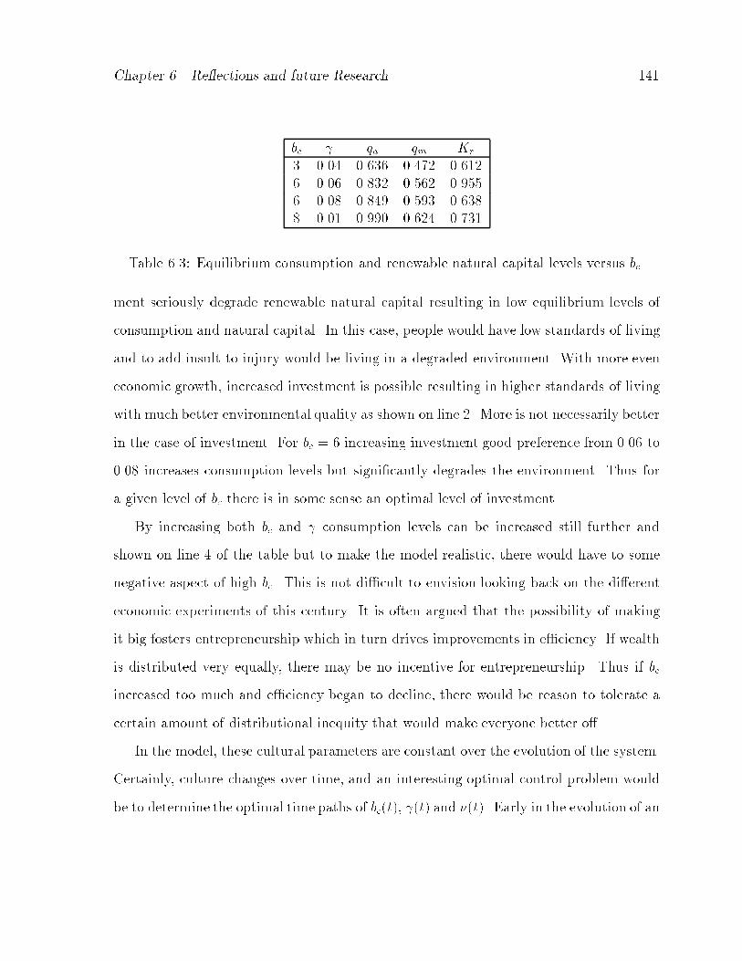
Chapter � Reections and future Research ���
bc � qa qm Kr
� ���� ����� ����� ������ ���� ����� ����� ������ ���� ����� ����� ������ ���� ����� ����� �����
Table ���� Equilibrium consumption and renewable natural capital levels versus bc�
ment seriously degrade renewable natural capital resulting in low equilibrium levels of
consumption and natural capital� In this case� people would have low standards of living
and to add insult to injury would be living in a degraded environment� With more even
economic growth� increased investment is possible resulting in higher standards of living
with much better environmental quality as shown on line �� More is not necessarily better
in the case of investment� For bc � increasing investment good preference from ���� to
���� increases consumption levels but signicantly degrades the environment� Thus for
a given level of bc there is in some sense an optimal level of investment�
By increasing both bc and � consumption levels can be increased still further and
shown on line � of the table but to make the model realistic� there would have to some
negative aspect of high bc� This is not di�cult to envision looking back on the di�erent
economic experiments of this century� It is often argued that the possibility of making
it big fosters entrepreneurship which in turn drives improvements in e�ciency� If wealth
is distributed very equally� there may be no incentive for entrepreneurship� Thus if bc
increased too much and e�ciency began to decline� there would be reason to tolerate a
certain amount of distributional inequity that would make everyone better o��
In the model� these cultural parameters are constant over the evolution of the system�
Certainly� culture changes over time� and an interesting optimal control problem would
be to determine the optimal time paths of bc�t�� ��t� and ��t�� Early in the evolution of an

Chapter � Reections and future Research ���
ecological economic system investment in manmade capital may be the most important
activity while later� evenness of growth and wealth distribution along with investment in
natural capital might be more important to utility maximization� If it were possible to
obtain a feedback control for this system� then it could be used to develop optimal future
policies given the present state of our system� Given the incredible challenges that lie
ahead for the world ecological economic system� I am hopeful that future work in this
area might provide some insight into possible means of dealing with them�

Bibliography
��� C� Ackello�Ogutu� Q� Paris� and W� Williams� Testing a von liebig crop re�sponse function against polynomial speci�cations� American Journal of AgriculturalEconomics� �� ������� pp� �������
��� E� Alden Smith� Anthropology� evolutionary ecology� and the explanatory limita�tions of the ecosystem concept� in The Ecosystem Concept in Anthropology� Westview Press� Boulder� CO� �����
��� J� Anderies� Culture and human agro�ecosystem dynamics� the tsembaga of newguinea�� Journal of Theoretical Biology� ��� �������
��� J� M� Anderies� An adaptive model for predicting kung reproductive performance�A stochastic dynamic programming approach� Ethology and Sociobiology� �� �������pp� ��������
��� U� M� Ashcer and R� J� Speteri� Collocation software for boundary valuedi�erential�algebraic equations� SIAM J� Sci� Comput�� �� ������� pp� ��������
��� J� H� Ausubel� The liberation of the environment� American Scientist� �� �������
��� S� Authors� Forum section on resources and economic growth� Ecological Economics� �� �������
��� W� Baltensweiler�The relevance of changes in the composition of larch bud mothpopulations for the dynamics of its numbers� in The Dynamics of Populatons� P� V�den Boer and G� R� Gradwell� eds�� Wageningen� Center for agricultural publishingand documentation� �����
��� J� A� Brander and M� S� Taylor� The simple economics of easter island�a ricardo�malthus model of renewable resource use� American Economic Review��forthcoming� ������
���� G� Buchbincer� Nutritional stress and post�contact population decline among themaring of new guinea� in Malnutrition� Behavior and Social organization� C� S�Greene� ed�� Academic Press� �����
���� M� Bulmer� Theoretical Evolutionary Ecology� Sinauer Associates� Sunderland�Mass�� �����
���
Bibliography ���
���� M� Cabeza Gut�es� The concept of weak sustainability� Ecological Economics� ���������
���� P� F� Chapman and F� Roberts� Metal Resources and Energy� Butterworths�London� �����
���� J� W� Chung� Utility and production functions � theory and applications� Blackwell������
���� C� W� Clark� Mathematical Bioeconomics� The Optimal Management of Renew�able Resources� J� Wiley� New York� �����
���� C� Cleveland� The direct and indirect use of fossil fuels and electricity in usaagriculture� ������� Agriculture� Ecosystems ' Environment� �� ������� pp� ��������
���� � Resource degradation� technical change� and productivity of energy in u�s� agri�culture� Ecological Economics� �� ������� pp� ��������
���� H� E� Daly� Steady�State Economics � the Economics of Biophysical Equilibriumand Moral Growth� San Francisco� W� H� Freeman� �����
���� H� E� Daly and K� N� Townsend� Is the entropy law relevant to the economics ofnatural resource scarcity � yes� of course it is� comment� Journal of EnvironmentalEconomics and Management� �� ������� pp� �������
���� E� Doedel� A program for the automatic bifurcation analysis of autonomous sys�tems� Cong� Num�� �� ������� pp� ��������
���� L� Edelstein�Keshet�Mathematical models in biology� RandomHouse� NewYork������
���� J� Ewel� Litter fall and leaf decompostion in a tropical forest succession in easternguatmala� Guatamalan Journal of Ecology� �� ������� pp� ��������
���� T� C� Foin and W� G� Davis� Ritual and self�regulation of the tsembaga maringecosystem in the new guinea highlands� Human Ecology� �� ������� pp� ��������
���� � Equilibrium and nonequilibrium models in ecological anthropology� an evalua�tion of �stability� in maring ecosystems in new guinea� American Anthropology� ��������� pp� �����
���� J� France and J� H� M� Thornley� Mathematical Models in Agriculture� Butterworths� London� �����

Bibliography ���
���� H� I� Freedman� Deterministic Mathematical Models in Population Ecology� M�Dekker� New York� �����
���� N� Georgescu Roegen� Entropy Law and Economic Process�� Harvard Univ�Press� Cambridge� Mass�� �����
���� M� Giampietro� G� Cerratelli� and D� Pimentel� Energy analysis of agricul�tural ecosystem management� Agriculture� Ecosystems ' Environment� �� �������pp� ��������
���� M� E� Gilpin� Group Selection in Predator�Prey Communities� Princeton University Press� Princeton� N�J�� �����
���� H� Groscurth� R� Kummel� and V� G� W�� Thermodynamic limits to energyoptimization� Energy� �� ������� pp� ��������
���� J� M� Hartwick� Intergenerational equity and the investing of rents from ex�haustible resources� American Economic Review� �� ������� pp� ��������
���� D� F� Heathfield and S� Wibe� An Introduction to Cost and Production Func�tions� Macmillan Education� �����
���� F� Hinterberger� F� Luks� and F� Schmidt�Bleek� Material �ows vs� �natu�ral capital��what makes an economy sustainable � Ecological Economics� �� �������pp� �����
���� C� S� Holling� The functional response of predators to prey density and its role inmimicry and populations regulation�� Mem� Entomol� Soc� Can�� �� ������� pp� �����
���� R� J� Huggett� Modelling the Human Impact on Nature � Systems Analysis ofEnvironmental Problems� Oxford University Press� Oxford � New York� �����
���� B� S� Jensen� The Dynamic Systems of Basic Economic Growth Models� KluwerAcademic� �����
���� A� Juo and A� Manu� Chemical dynamics in slash�and�burn agriculture� Agriculture� Ecosystems ' Environment� �� ������� pp� ������
���� H� v� Keulen and H� D� J� v� Heemst� Crop response to the supply of macronu�trients� tech� report� Pudoc� Wageningen� �����
���� I� A� Kuznetsov� Elements of applied bifurcation theory� SpringerVerlag� �����
���� E� Lanzer and Q� Paris� A new analytical framework for the fertilization problem�American Journal of Agricultural Economics� �� ������� pp� �������
Bibliography ���
���� T� Lauck� C� Clark� M� Mangel� and G� Munro� Implementing the pre�cautionary pronciple in �sheries management through marine reserves� EcologicalApplications� � ������� pp� S���S��� Supplement�
���� R� M� May� Stability and Complexity in Model Ecosystems� Princeton UniversityPress� Princeton� N�J� �����
���� D� H� Meadows et al�� The Limits to growth� a report for the Club of Rome�sproject on the predicament of mankind� Universe Books� New York� �����
���� D� H� Meadows� D� Meadows� and J� Randers� Beyond the limits� Con�fronting Global Collapse� Envisioning a Sustainable Future� Chelsea Green Pub� Co�������
���� E� Odum� Fundamentals of Ecology� Saunders� Philidelphia� �����
���� U� D� of Commerce� Economics� S� Administration� and B� of the Cen�sus� Statistical Abstract of the United States� U�S� Department of Commerce� �����
���� C� Palm� M� Swift� and P� Woomer� Soil biological dynamics in slash�and�burnagriculture� Agriculture� Ecosystems ' Environment� �� ������� pp� ������
���� Q� Paris and K� Knapp� Estimation of von liebig response functions� AmericanJournal of Agricultural Economics� �� ������� pp� �������
���� D� Pimentel� Ecological systems� natural resources� and food supplies� in Food andNatrual Resources� D� Pimentel and C� Hall� eds�� Academic Press� �����
���� D� Pimentel� World Soil Erosion and Conservation� Cambridge University Press������
���� D� Pimentel and M� Pimentel� Food� Energy and Society� Colorado UniversityPress� Niwot Colorado� �����
���� J� Proops� M� Faber� R� Manstetten� and F� Jost� Acheiving a sustainableworld� Ecological Economics� �� �������
���� R� A� Rappaport� Pigs for the ancestors � ritual in the ecology of a New Guineapeople� Yale University Press� �����
���� W� E� Rees� Achieving sustainability� Journal of Planning Literature� � �������
���� M� Ruth� Integrating Economics� Ecology� and Thermodynamics� Kluwer Academic� Dordrecht � Boston� �����

Bibliography ���
���� M� Scott� The importance of old �eld succession on biomass increments to shiftingagriculture� Rocky Mountain Geological Journal� � ������� pp� ��������
���� S� B� Shantzis and W� W� Behrens� Population control mechanisms in a prim�itive agricultural society� in Towards global equilibrium� D� L� Meadows and D� H�Meadows� eds�� WrightAllen Press� �����
���� R� Solow� Intergenerational equity and exhaustible resources� in Symposium on theEconomics of Exhaustible Resources� ����� pp� ������
���� � Georgescu�roegen versus solow�stiglitz� Reply� Ecological Economics� �������
���� D� � Stern� Limits to substitution and irreversibility in production and consump�tion� A neoclassical interpretation of ecological economics� Ecological Economics� ���������
���� M� Stra�skraba� Cybernetic theory of complex ecosystems� in Complex Ecology �The PartWhole Relation in Ecosystems� B� C� Patten and S� E� Jorgensen� eds��Prentice Hall� Englewood Cli�s� N�J�� �����
���� L� Szott� C� Palm� and C� Davey� Biomass and litter accumulation undermanaged and natural tropical fallows� Forest Ecology and Management� �� �������pp� ��������
���� J� A� Tainter� The collapse of complex societies� Cambridge University Press������
���� H� R� Varian� Microeconomic analysis� Norton� �����
���� R� Waltman� Competition Models in Population Biology� SIAM� �����
���� A� L� Wright� An introduction to the theory of dynamic economics � a theoreticalstudy in long run disequilibrium� Oxford University Press� �����
���� J� T� Young� Is the entropy law relevant to the economics of natural re�source scarcity � Journal of Environmental Economics and Management� �� �������pp� ��������