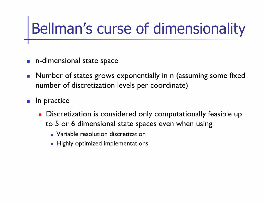
Bellman’s curse of dimensionality
n n-dimensional state space
n Number of states grows exponentially in n (assuming some fixed number of discretization levels per coordinate)
n In practice
n Discretization is considered only computationally feasible up to 5 or 6 dimensional state spaces even when using
n Variable resolution discretization n Highly optimized implementations
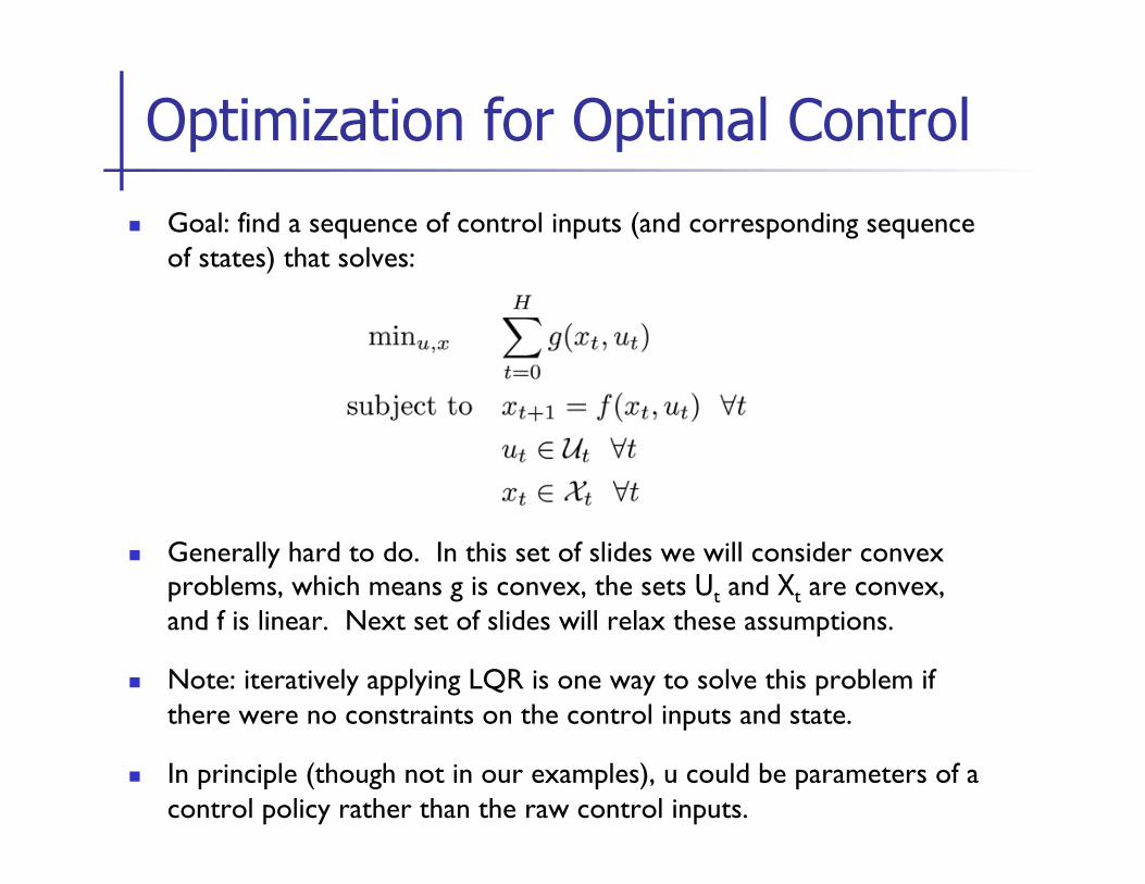
n Goal: find a sequence of control inputs (and corresponding sequence of states) that solves:
n Generally hard to do. In this set of slides we will consider convex problems, which means g is convex, the sets Ut and Xt are convex, and f is linear. Next set of slides will relax these assumptions.
n Note: iteratively applying LQR is one way to solve this problem if there were no constraints on the control inputs and state.
n In principle (though not in our examples), u could be parameters of a control policy rather than the raw control inputs.
Optimization for Optimal Control
Convex Optimization
Pieter Abbeel UC Berkeley EECS
Many slides and figures adapted from Stephen Boyd [optional] Boyd and Vandenberghe, Convex Optimization, Chapters 9 – 11 [optional] Betts, Practical Methods for Optimal Control Using Nonlinear Programming
TexPoint fonts used in EMF. Read the TexPoint manual before you delete this box.: AAAAAAAAAAAA
n Convex optimization problems
n Unconstrained minimization
n Gradient Descent
n Newton’s Method
n Equality constrained minimization
n Inequality and equality constrained minimization
Outline
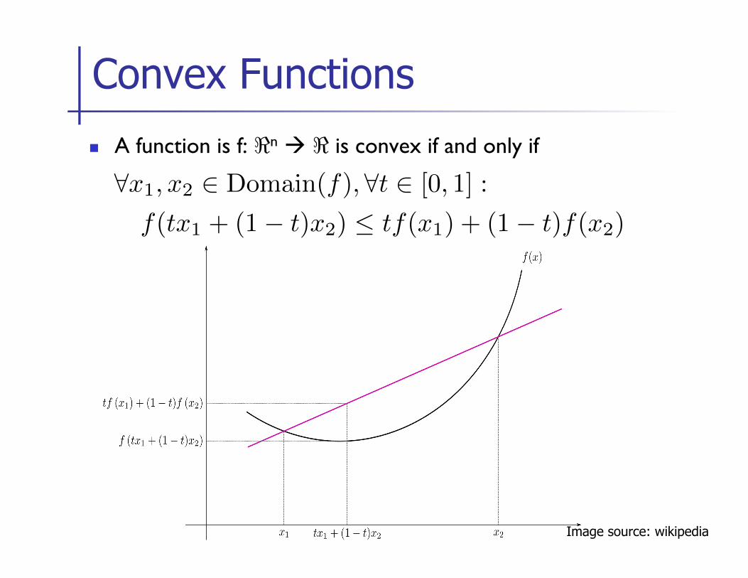
n A function is f: <n à < is convex if and only if
Convex Functions
∀x1, x2 ∈ Domain(f), ∀t ∈ [0, 1] :
f(tx1 + (1− t)x2) ≤ tf(x1) + (1− t)f(x2)
Image source: wikipedia
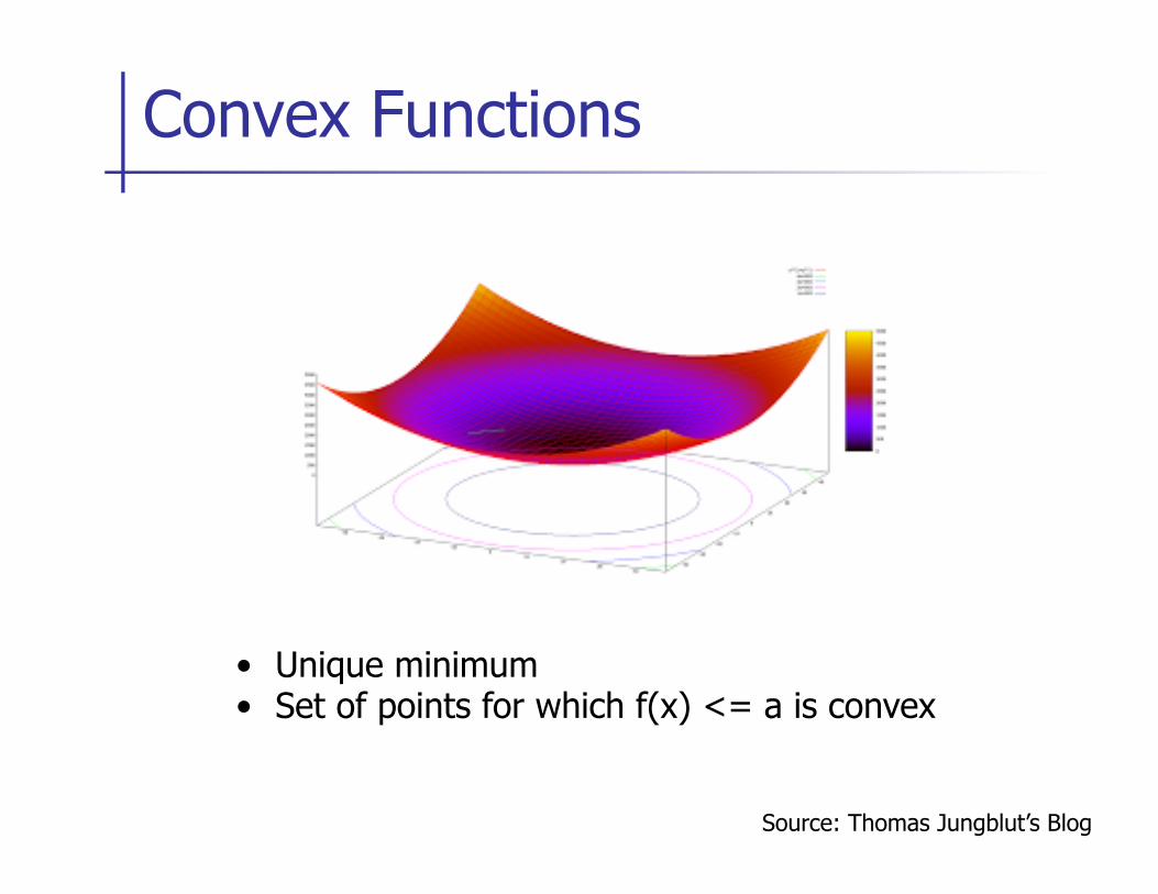
Convex Functions
Source: Thomas Jungblut’s Blog
• Unique minimum • Set of points for which f(x) <= a is convex
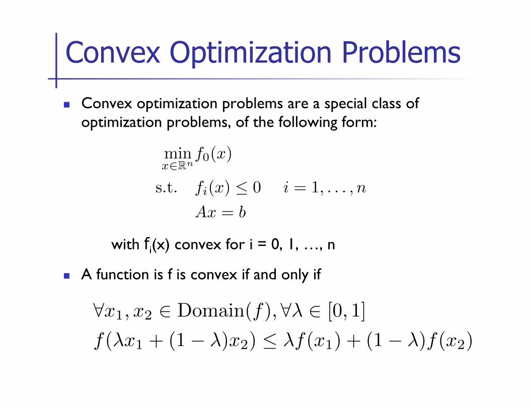
n Convex optimization problems are a special class of optimization problems, of the following form:
with fi(x) convex for i = 0, 1, …, n
n A function is f is convex if and only if
Convex Optimization Problems
minx∈Rn
f0(x)
s.t. fi(x) ≤ 0 i = 1, . . . , n
Ax = b
∀x1, x2 ∈ Domain(f), ∀λ ∈ [0, 1]
f(λx1 + (1− λ)x2) ≤ λf(x1) + (1− λ)f(x2)
n Convex optimization problems
n Unconstrained minimization
n Gradient Descent
n Newton’s Method
n Equality constrained minimization
n Inequality and equality constrained minimization
Outline
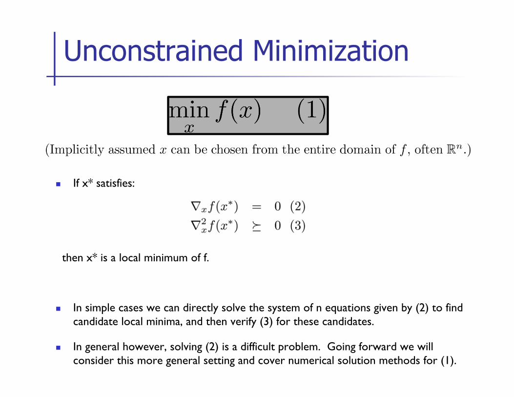
n If x* satisfies:
then x* is a local minimum of f.
n In simple cases we can directly solve the system of n equations given by (2) to find candidate local minima, and then verify (3) for these candidates.
n In general however, solving (2) is a difficult problem. Going forward we will consider this more general setting and cover numerical solution methods for (1).
Unconstrained Minimization
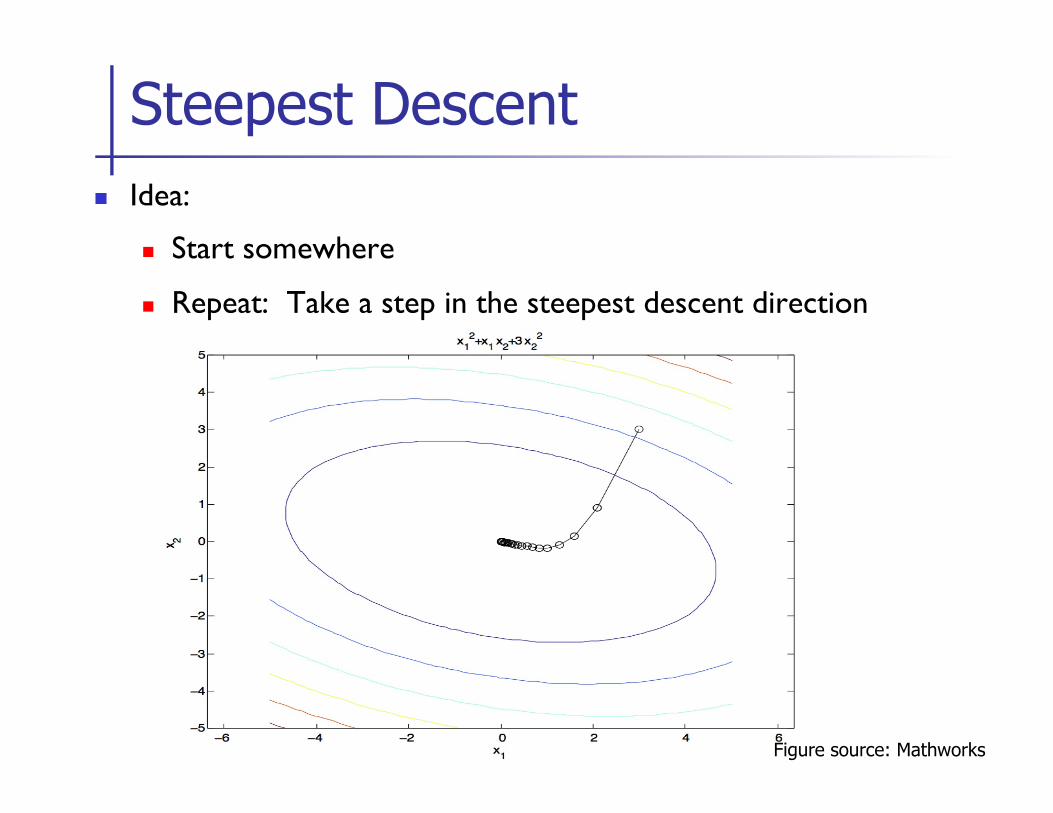
n Idea:
n Start somewhere
n Repeat: Take a step in the steepest descent direction
Steepest Descent
Figure source: Mathworks
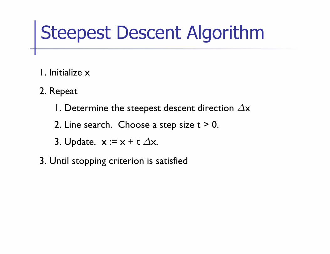
1. Initialize x
2. Repeat
1. Determine the steepest descent direction ¢x
2. Line search. Choose a step size t > 0.
3. Update. x := x + t ¢x.
3. Until stopping criterion is satisfied
Steepest Descent Algorithm
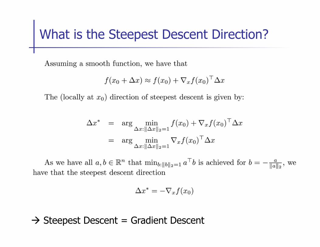
What is the Steepest Descent Direction?
à Steepest Descent = Gradient Descent
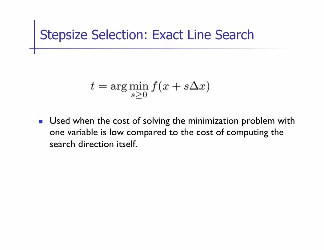
n Used when the cost of solving the minimization problem with one variable is low compared to the cost of computing the search direction itself.
Stepsize Selection: Exact Line Search
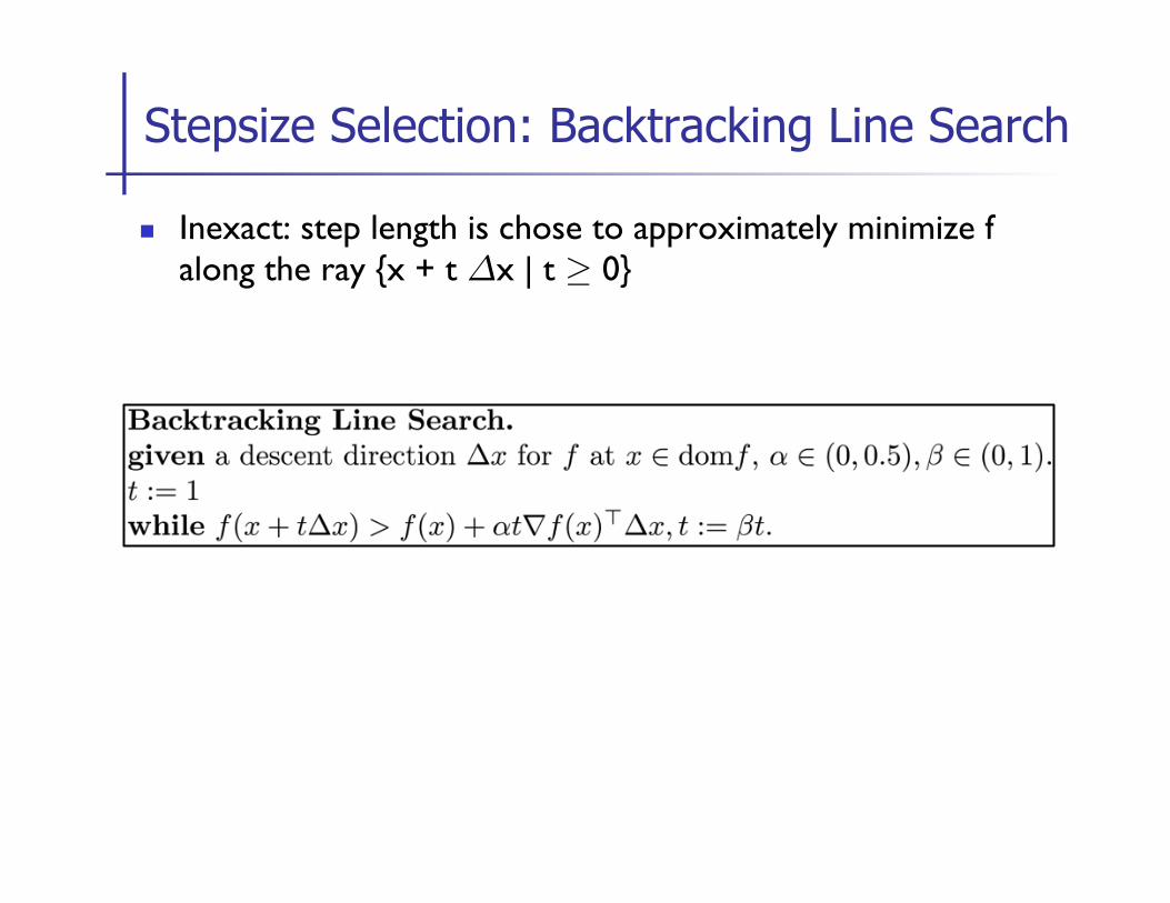
n Inexact: step length is chose to approximately minimize f along the ray {x + t ¢x | t ¸ 0}
Stepsize Selection: Backtracking Line Search
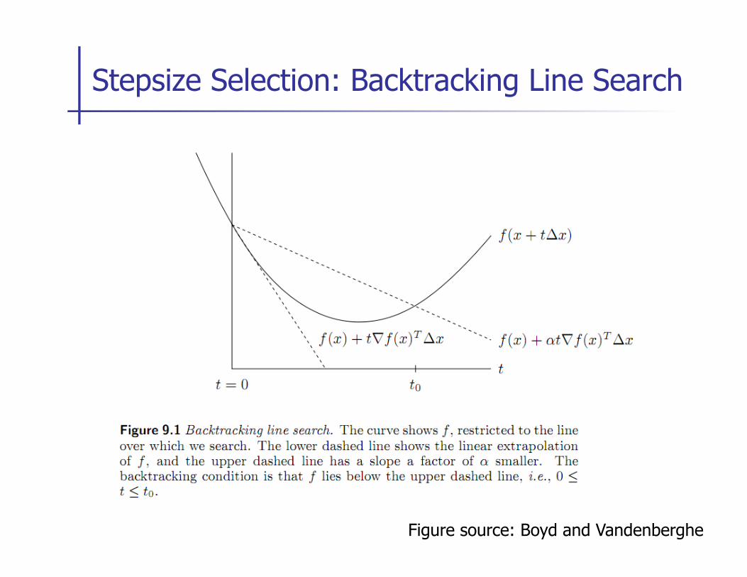
Stepsize Selection: Backtracking Line Search
Figure source: Boyd and Vandenberghe
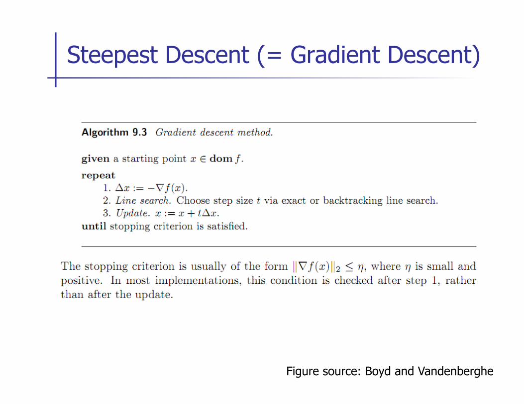
Steepest Descent (= Gradient Descent)
Figure source: Boyd and Vandenberghe

Gradient Descent: Example 1
Figure source: Boyd and Vandenberghe
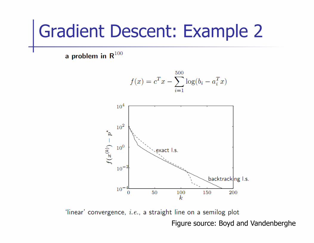
Gradient Descent: Example 2
Figure source: Boyd and Vandenberghe

Gradient Descent: Example 3
Figure source: Boyd and Vandenberghe
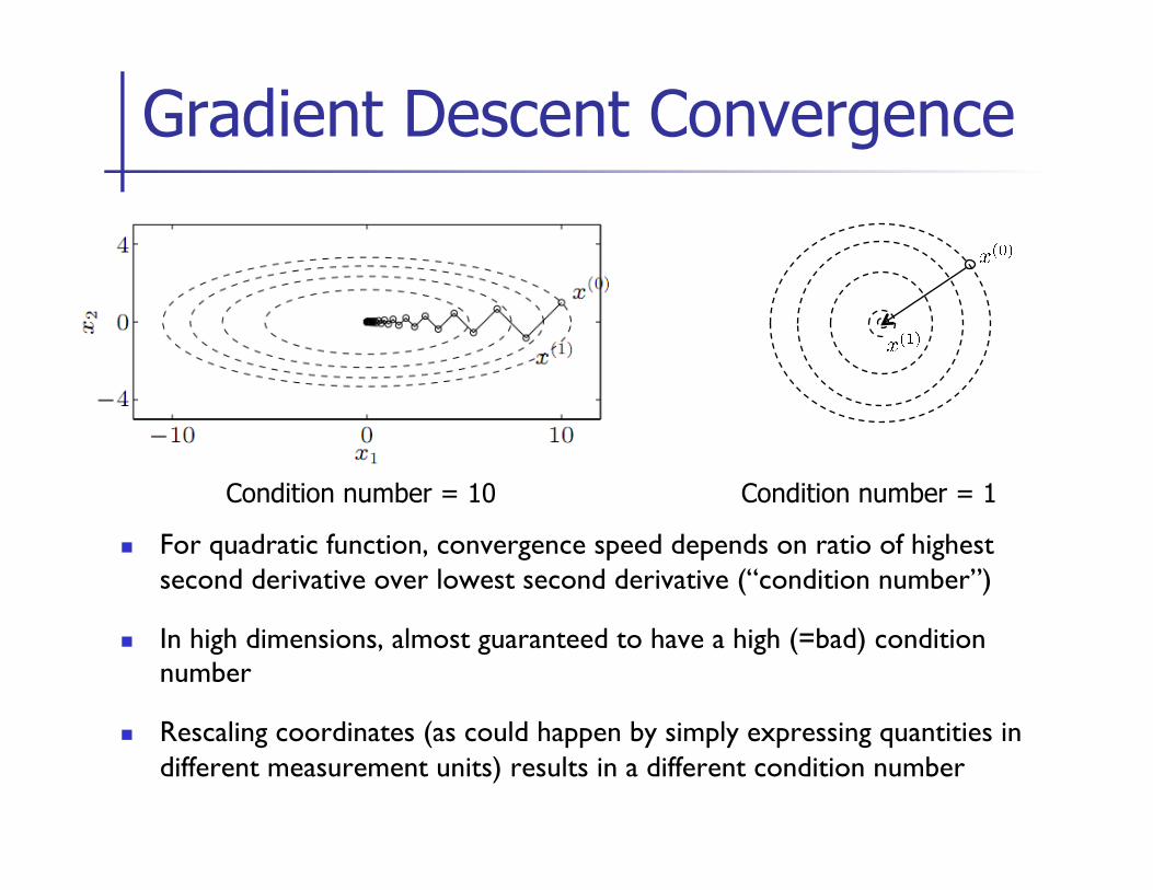
n For quadratic function, convergence speed depends on ratio of highest second derivative over lowest second derivative (“condition number”)
n In high dimensions, almost guaranteed to have a high (=bad) condition number
n Rescaling coordinates (as could happen by simply expressing quantities in different measurement units) results in a different condition number
Gradient Descent Convergence
Condition number = 10 Condition number = 1
n Unconstrained minimization
n Gradient Descent
n Newton’s Method
n Equality constrained minimization
n Inequality and equality constrained minimization
Outline
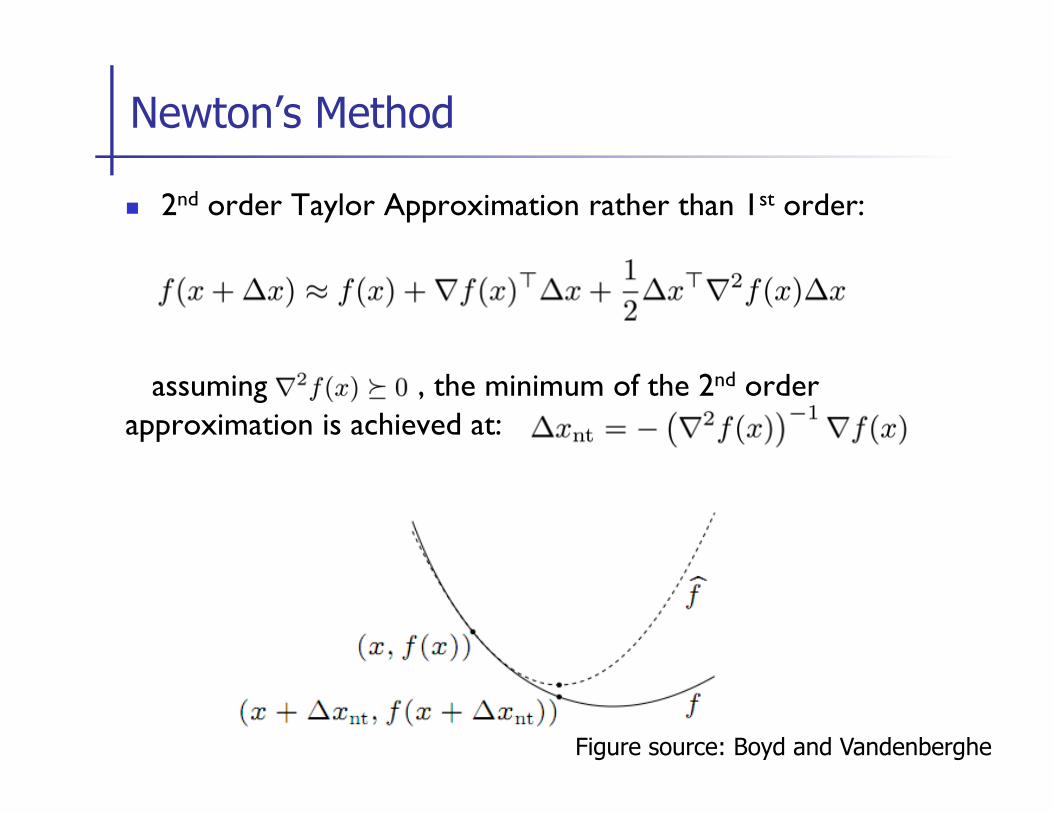
n 2nd order Taylor Approximation rather than 1st order:
assuming , the minimum of the 2nd order approximation is achieved at:
Newton’s Method
Figure source: Boyd and Vandenberghe
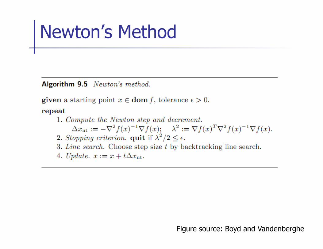
Newton’s Method
Figure source: Boyd and Vandenberghe
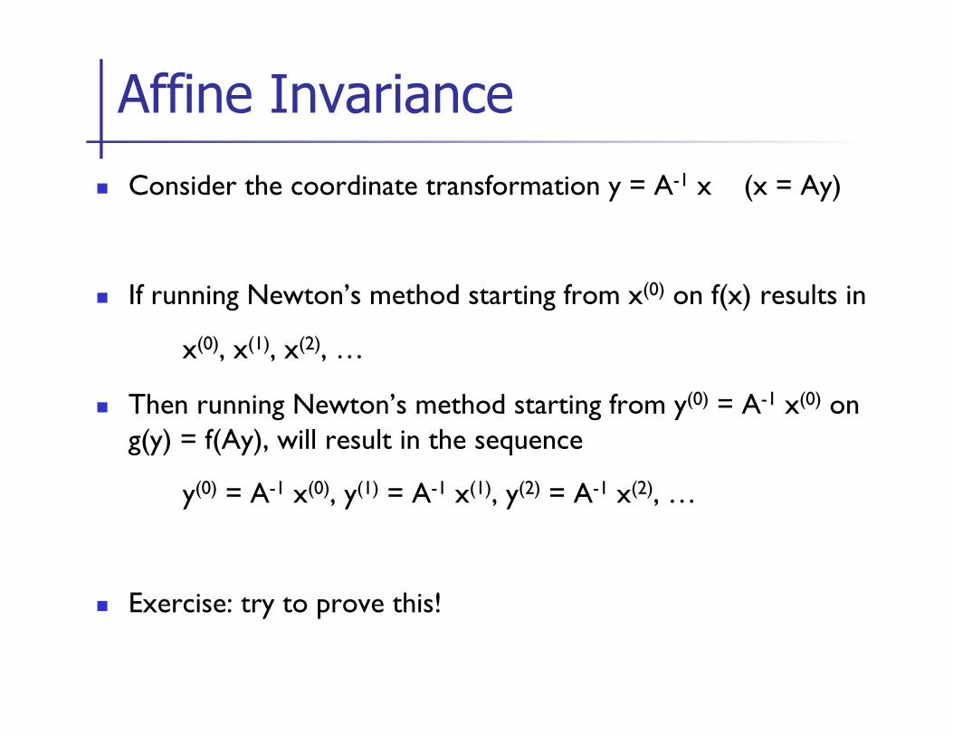
n Consider the coordinate transformation y = A-1 x (x = Ay)
n If running Newton’s method starting from x(0) on f(x) results in
x(0), x(1), x(2), …
n Then running Newton’s method starting from y(0) = A-1 x(0) on g(y) = f(Ay), will result in the sequence
y(0) = A-1 x(0), y(1) = A-1 x(1), y(2) = A-1 x(2), …
n Exercise: try to prove this!
Affine Invariance
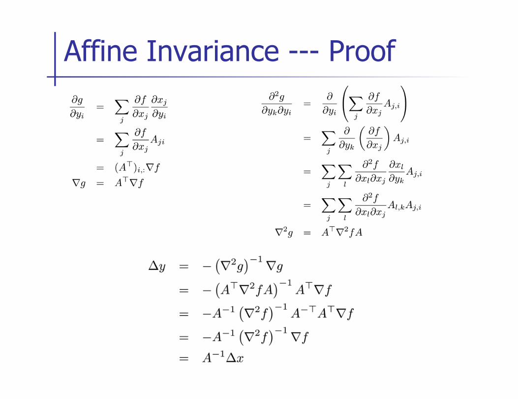
Affine Invariance --- Proof
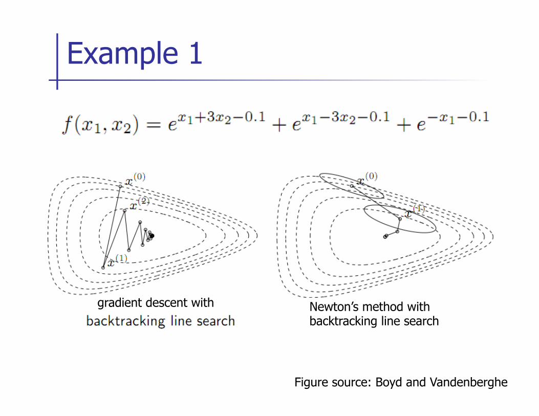
Example 1
Figure source: Boyd and Vandenberghe
gradient descent with Newton’s method with backtracking line search
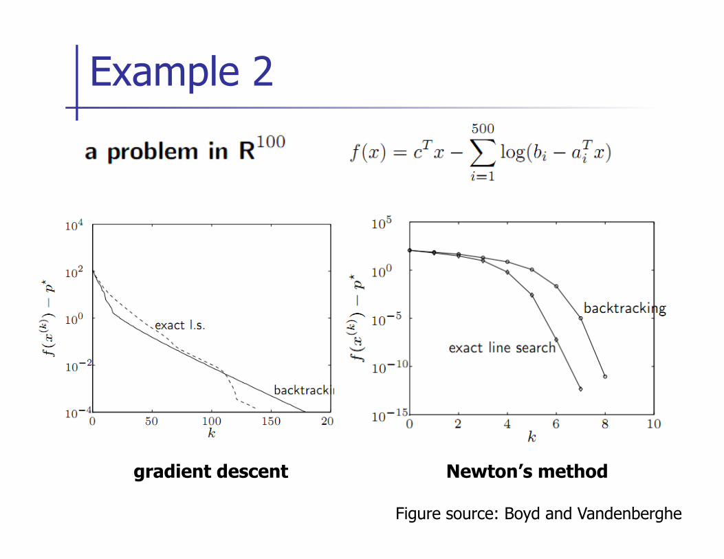
Example 2
Figure source: Boyd and Vandenberghe
gradient descent Newton’s method
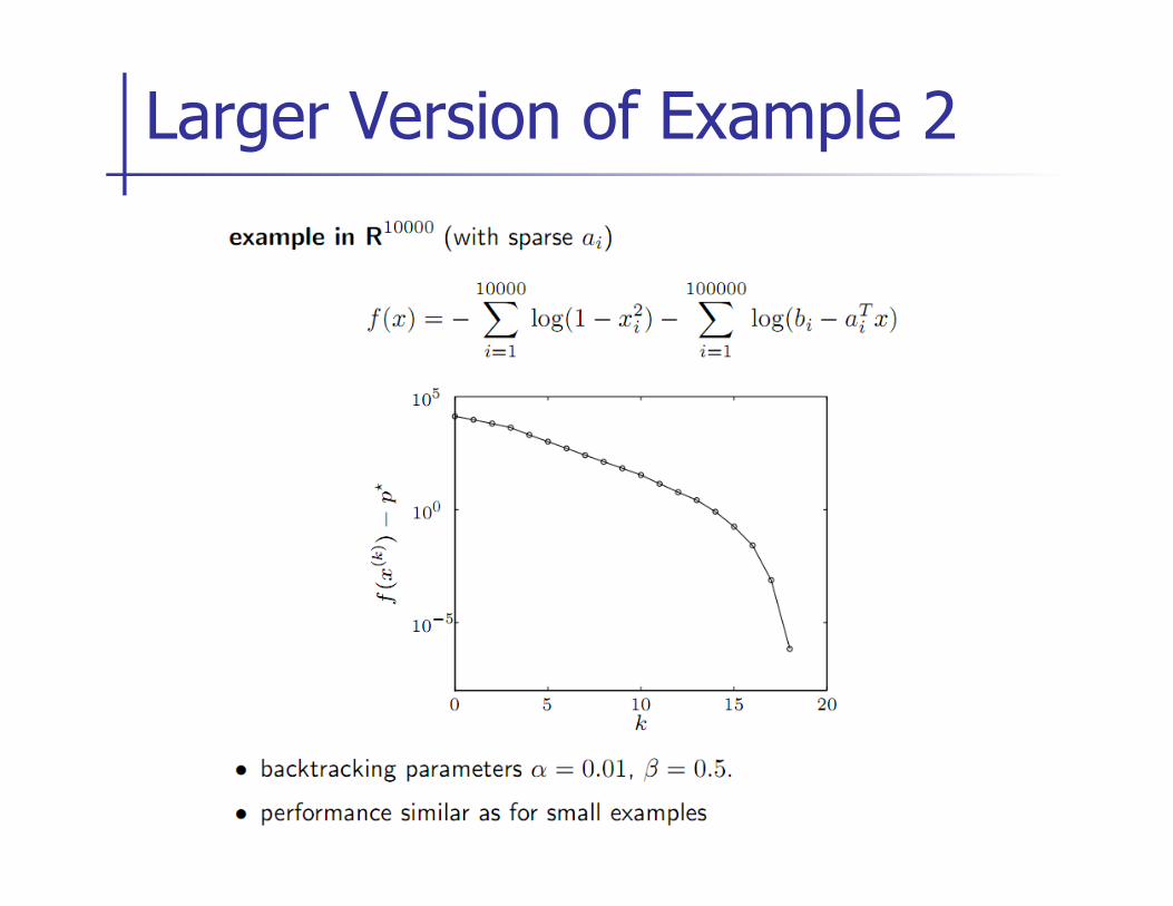
Larger Version of Example 2
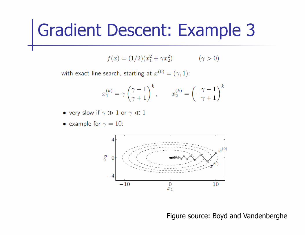
Gradient Descent: Example 3
Figure source: Boyd and Vandenberghe
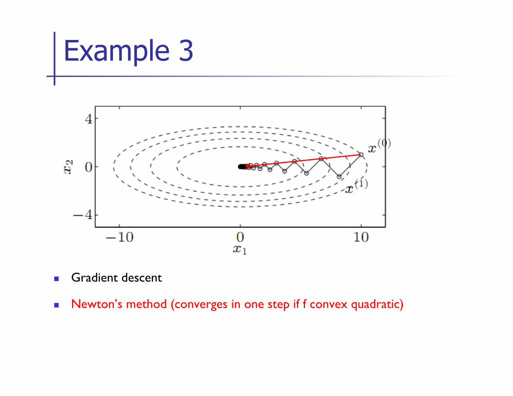
n Gradient descent
n Newton’s method (converges in one step if f convex quadratic)
Example 3
n Quasi-Newton methods use an approximation of the Hessian
n Example 1: Only compute diagonal entries of Hessian, set others equal to zero. Note this also simplifies computations done with the Hessian.
n Example 2: natural gradient --- see next slide
Quasi-Newton Methods
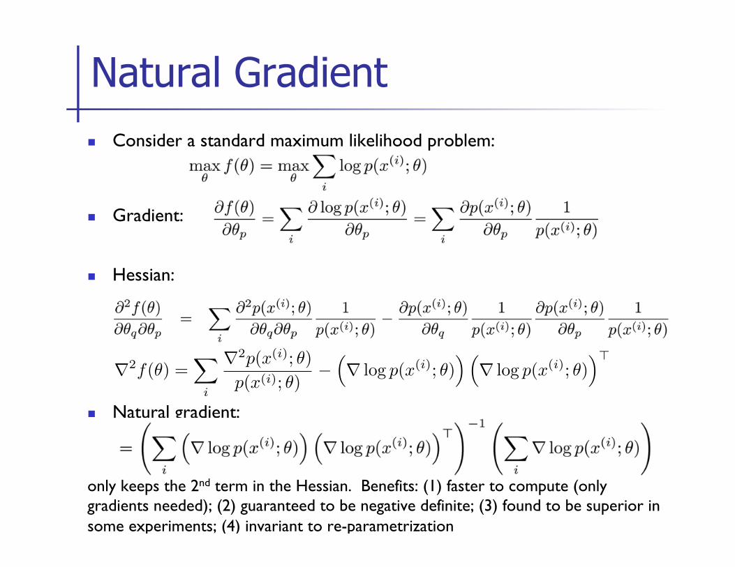
n Consider a standard maximum likelihood problem:
n Gradient:
n Hessian:
n Natural gradient:
only keeps the 2nd term in the Hessian. Benefits: (1) faster to compute (only gradients needed); (2) guaranteed to be negative definite; (3) found to be superior in some experiments; (4) invariant to re-parametrization
Natural Gradient
∇2f(θ) =�
i
∇2p(x(i); θ)
p(x(i); θ)−
�∇ log p(x(i); θ)
��∇ log p(x(i); θ)
��
n Property: Natural gradient is invariant to parameterization of the family of probability distributions p( x ; µ)
n Hence the name.
n Note this property is stronger than the property of Newton’s method, which is invariant to affine re-parameterizations only.
n Exercise: Try to prove this property!
Natural Gradient
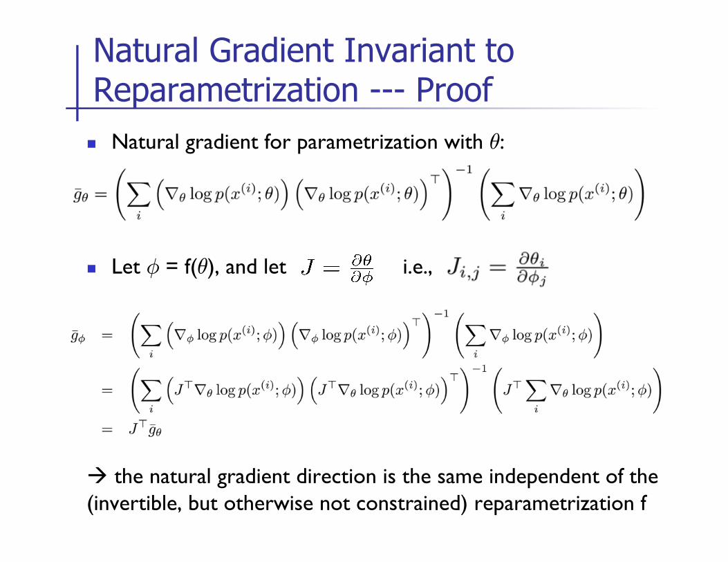
n Natural gradient for parametrization with µ:
n Let Á = f(µ), and let i.e.,
à the natural gradient direction is the same independent of the (invertible, but otherwise not constrained) reparametrization f
Natural Gradient Invariant to Reparametrization --- Proof
n Unconstrained minimization
n Gradient Descent
n Newton’s Method
n Equality constrained minimization
n Inequality and equality constrained minimization
Outline
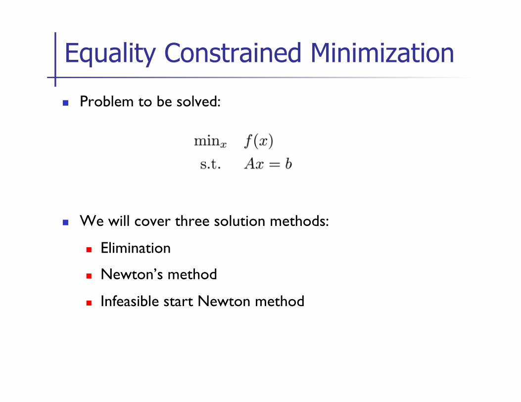
n Problem to be solved:
n We will cover three solution methods:
n Elimination
n Newton’s method
n Infeasible start Newton method
Equality Constrained Minimization
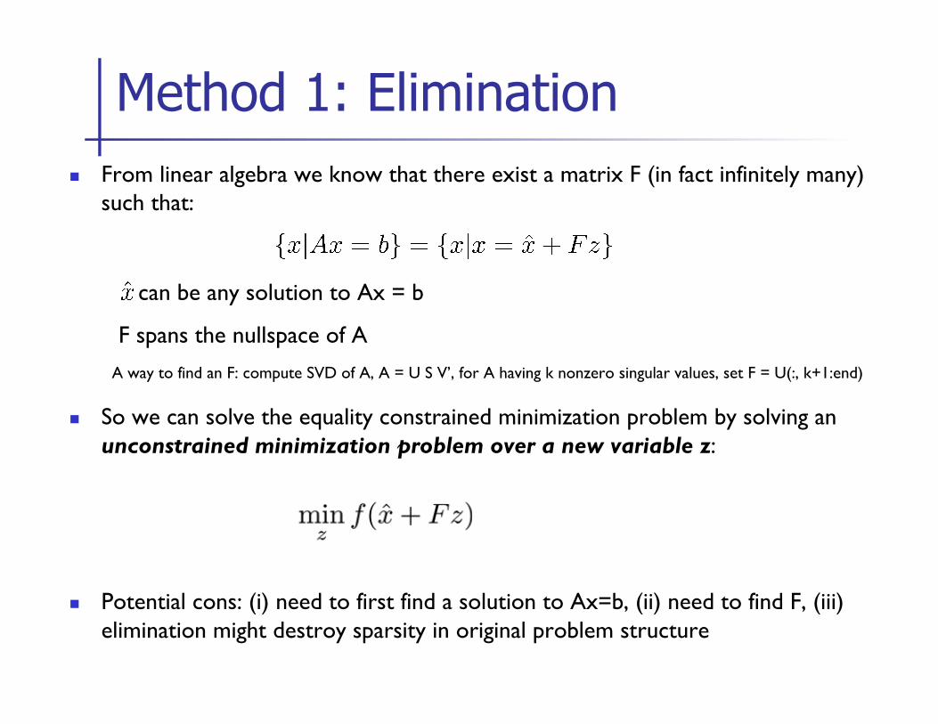
n From linear algebra we know that there exist a matrix F (in fact infinitely many) such that:
can be any solution to Ax = b
F spans the nullspace of A A way to find an F: compute SVD of A, A = U S V’, for A having k nonzero singular values, set F = U(:, k+1:end)
n So we can solve the equality constrained minimization problem by solving an unconstrained minimization problem over a new variable z:
n Potential cons: (i) need to first find a solution to Ax=b, (ii) need to find F, (iii) elimination might destroy sparsity in original problem structure
Method 1: Elimination
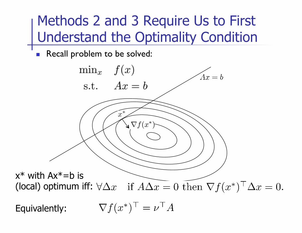
n Recall problem to be solved:
Methods 2 and 3 Require Us to First Understand the Optimality Condition
x* with Ax*=b is (local) optimum iff: Equivalently:

n Recall the problem to be solved:
Methods 2 and 3 Require Us to First Understand the Optimality Condition
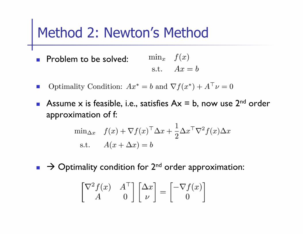
n Problem to be solved:
n
n Assume x is feasible, i.e., satisfies Ax = b, now use 2nd order approximation of f:
n à Optimality condition for 2nd order approximation:
Method 2: Newton’s Method
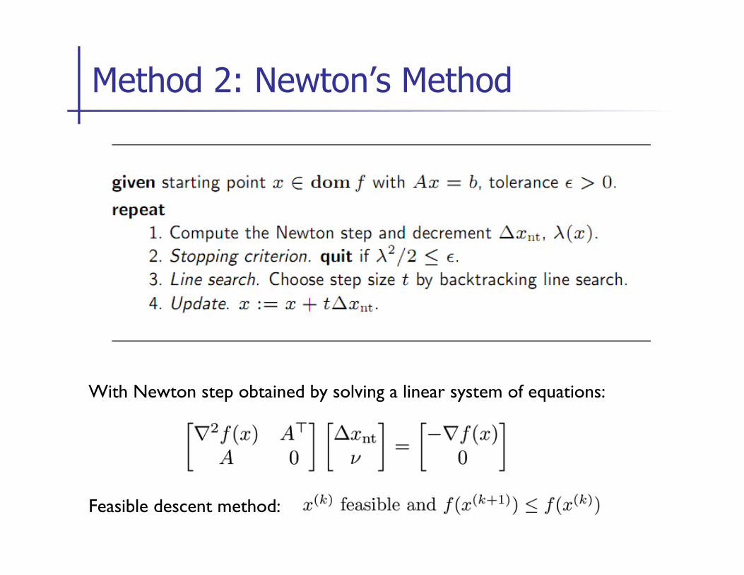
With Newton step obtained by solving a linear system of equations:
Feasible descent method:
Method 2: Newton’s Method
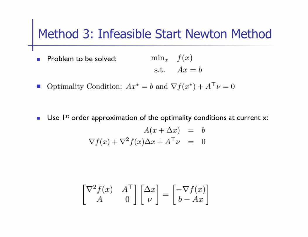
n Problem to be solved:
n
n Use 1st order approximation of the optimality conditions at current x:
Method 3: Infeasible Start Newton Method
n Unconstrained minimization
n Equality constrained minimization
n Inequality and equality constrained minimization
Outline
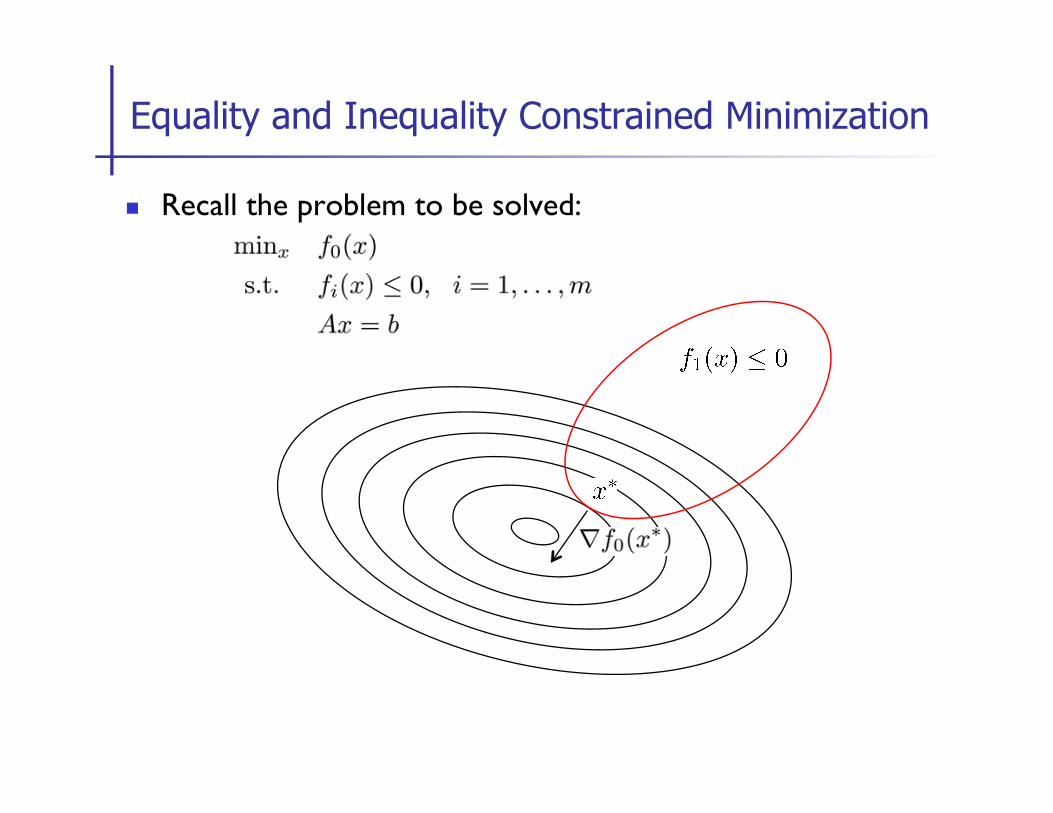
n Recall the problem to be solved:
Equality and Inequality Constrained Minimization
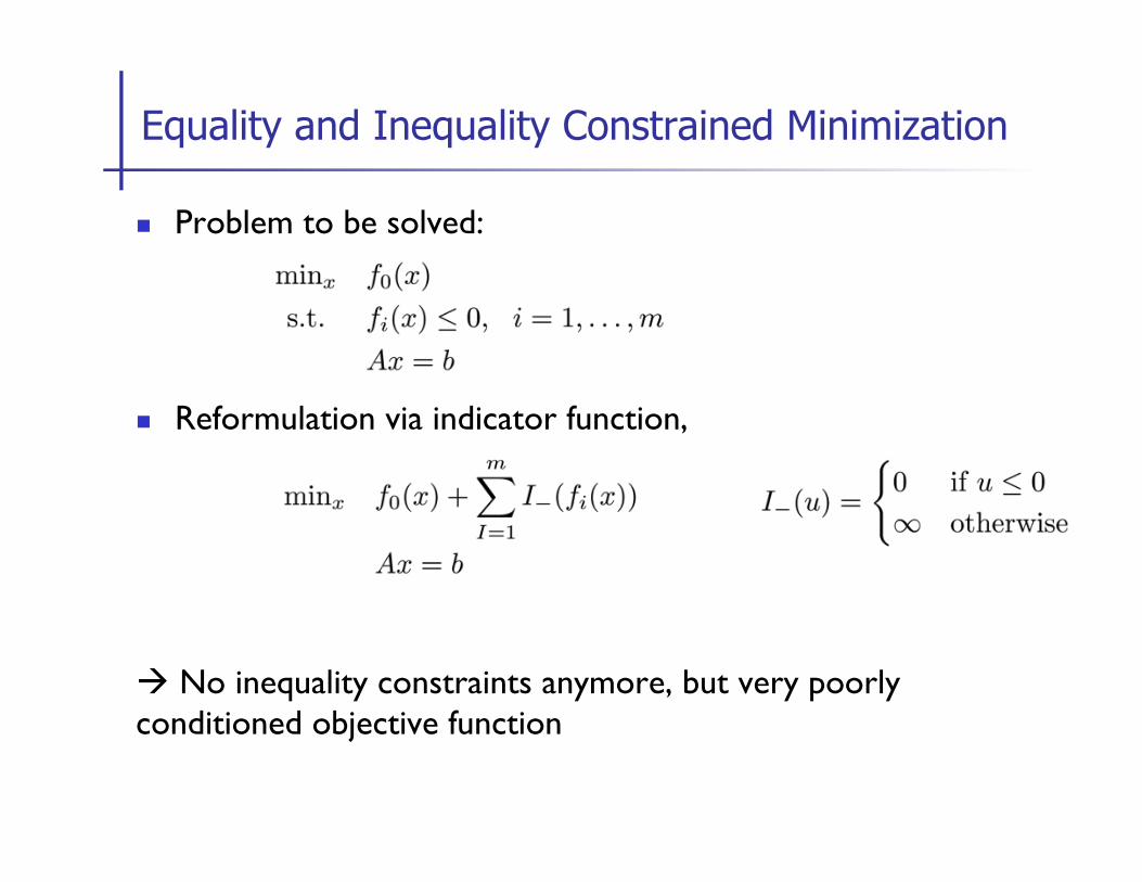
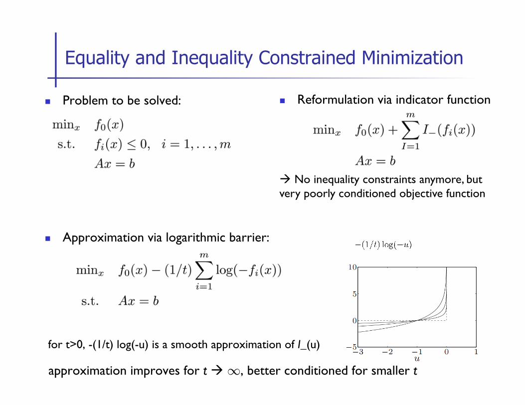
n Problem to be solved:
n Reformulation via indicator function,
à No inequality constraints anymore, but very poorly conditioned objective function
Equality and Inequality Constrained Minimization
n Problem to be solved:
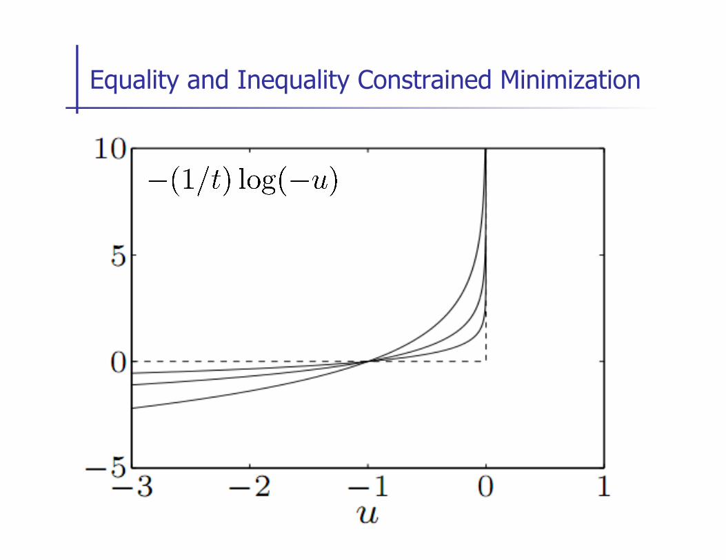
n Approximation via logarithmic barrier:
for t>0, -(1/t) log(-u) is a smooth approximation of I_(u)
approximation improves for t à 1, better conditioned for smaller t
Equality and Inequality Constrained Minimization
n Reformulation via indicator function
à No inequality constraints anymore, but very poorly conditioned objective function
Equality and Inequality Constrained Minimization
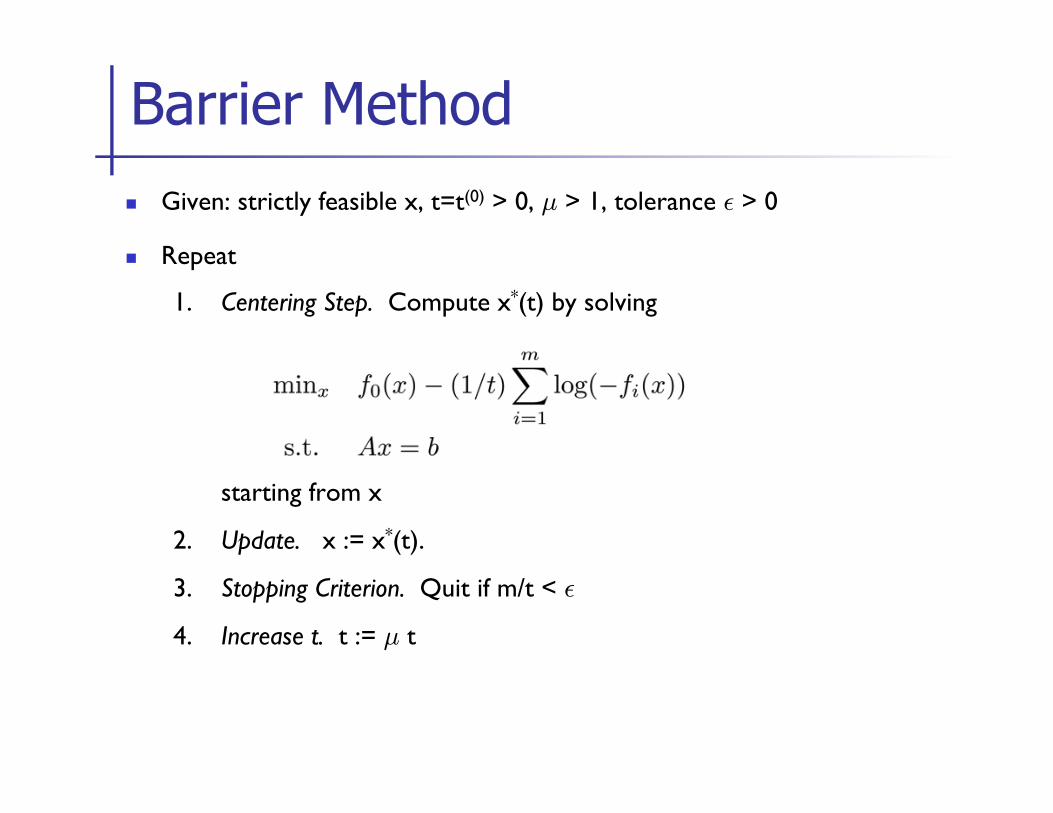
n Given: strictly feasible x, t=t(0) > 0, µ > 1, tolerance ² > 0
n Repeat
1. Centering Step. Compute x*(t) by solving
starting from x
2. Update. x := x*(t).
3. Stopping Criterion. Quit if m/t < ²
4. Increase t. t := µ t
Barrier Method
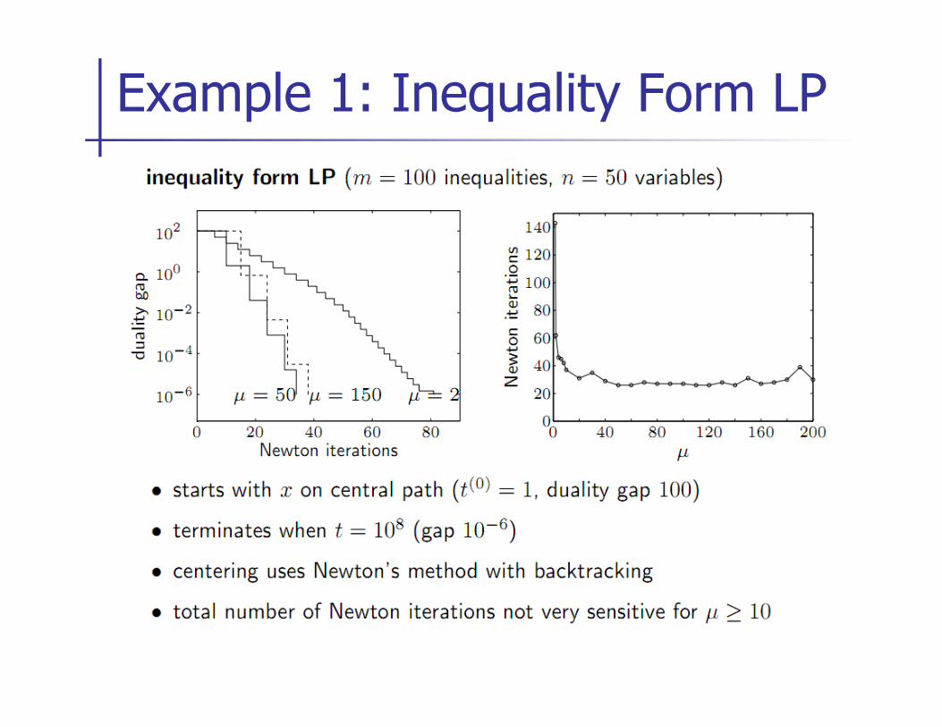
Example 1: Inequality Form LP
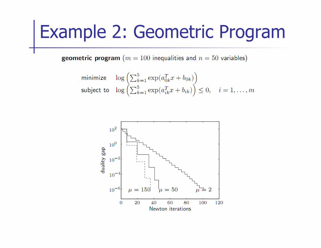
Example 2: Geometric Program
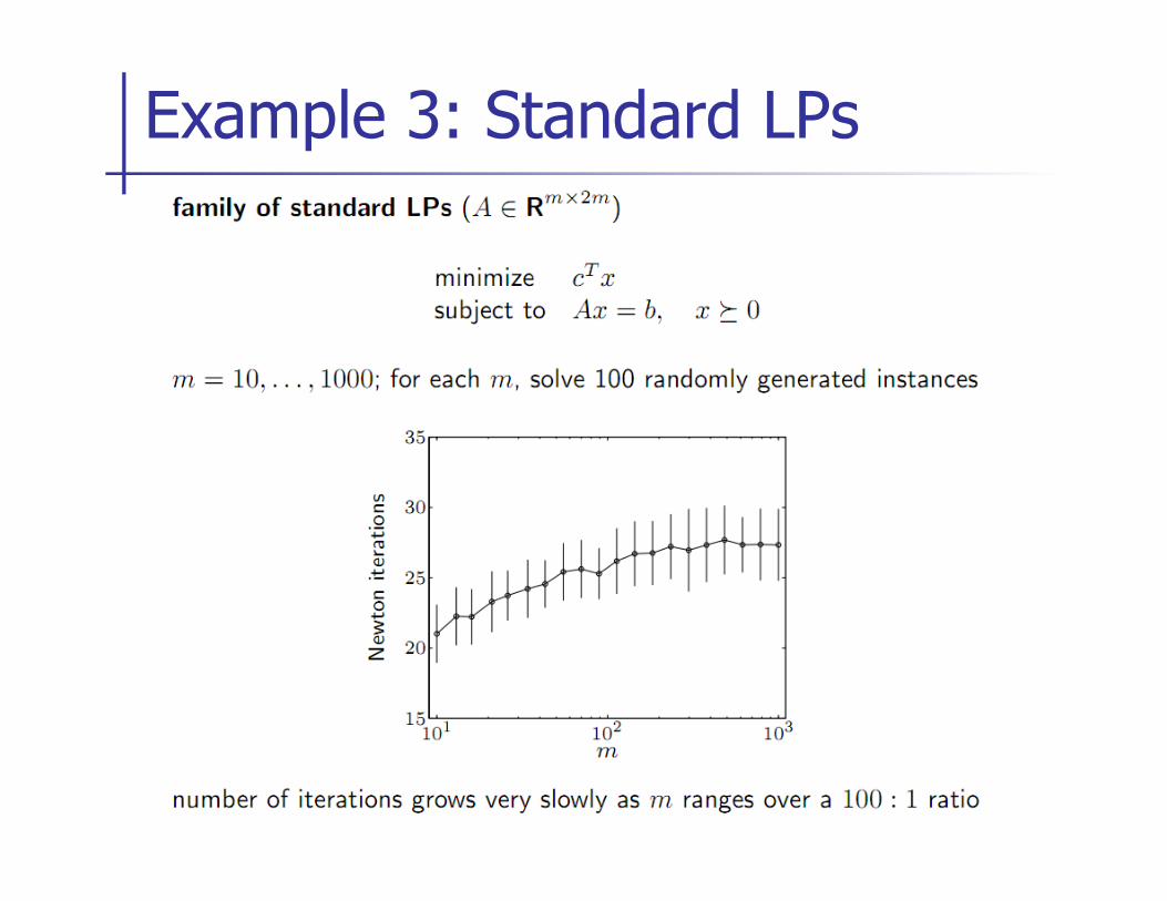
Example 3: Standard LPs
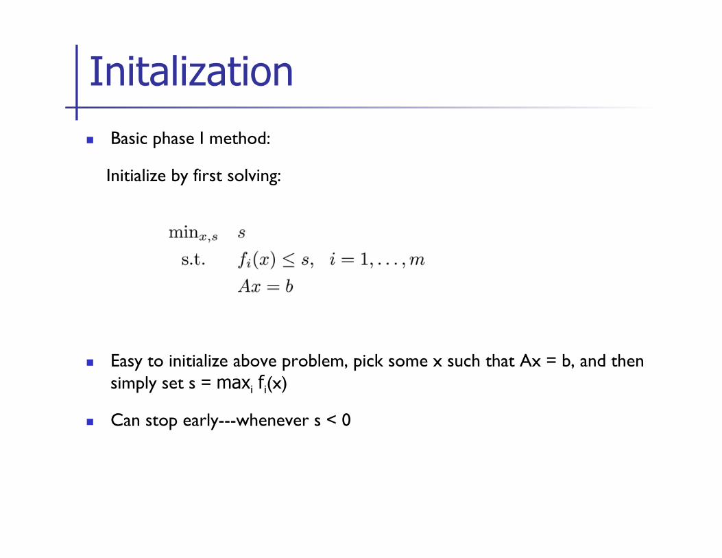
n Basic phase I method:
Initialize by first solving:
n Easy to initialize above problem, pick some x such that Ax = b, and then simply set s = maxi fi(x)
n Can stop early---whenever s < 0
Initalization
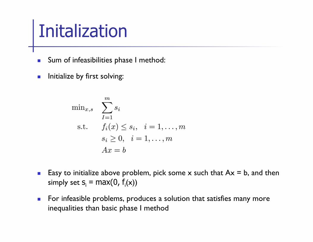
n Sum of infeasibilities phase I method:
n Initialize by first solving:
n Easy to initialize above problem, pick some x such that Ax = b, and then simply set si = max(0, fi(x))
n For infeasible problems, produces a solution that satisfies many more inequalities than basic phase I method
Initalization
n We have covered a primal interior point method
n one of several optimization approaches
n Examples of others:
n Primal-dual interior point methods
n Primal-dual infeasible interior point methods
Other methods
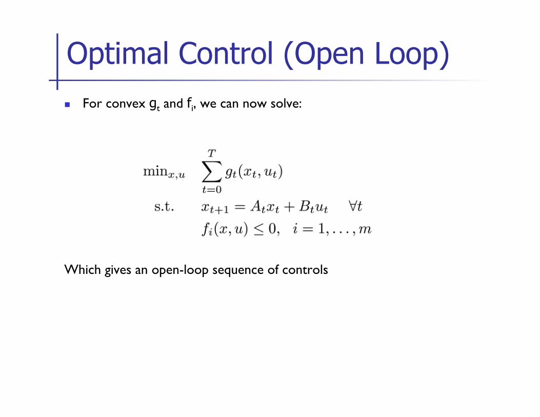
n For convex gt and fi, we can now solve:
Which gives an open-loop sequence of controls
Optimal Control (Open Loop)
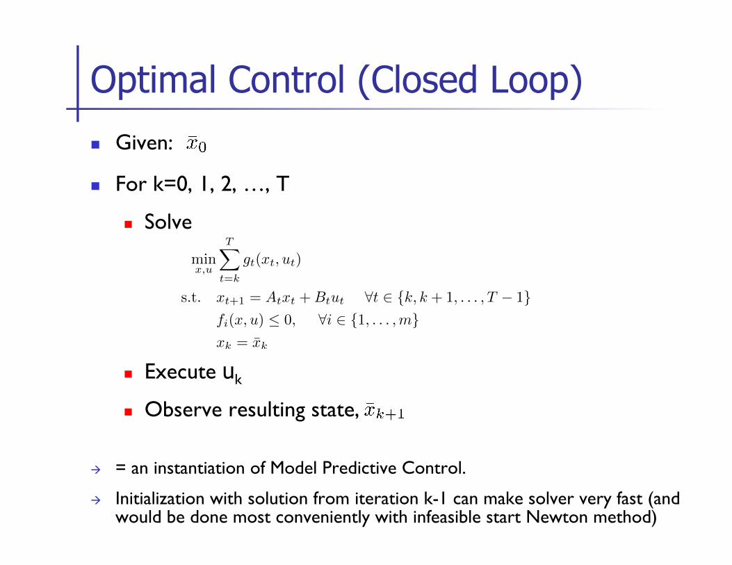
n Given:
n For k=0, 1, 2, …, T
n Solve
n Execute uk
n Observe resulting state,
à = an instantiation of Model Predictive Control.
à Initialization with solution from iteration k-1 can make solver very fast (and would be done most conveniently with infeasible start Newton method)
Optimal Control (Closed Loop)
minx,u
T�
t=k
gt(xt, ut)
s.t. xt+1 = Atxt +Btut ∀t ∈ {k, k + 1, . . . , T − 1}fi(x, u) ≤ 0, ∀i ∈ {1, . . . ,m}xk = x̄k

n Disciplined convex programming
n = convex optimization problems of forms that it can easily verify to be convex
n Convenient high-level expressions
n Excellent for fast implementation
n Designed by Michael Grant and Stephen Boyd, with input from Yinyu Ye.
n Current webpage: http://cvxr.com/cvx/
CVX
n Matlab Example for Optimal Control, see course webpage
CVX