From Matrix to Tensor: The Transition to Numerical Multilinear Algebra Lecture 9. The Curse of Dimensionality Charles F. Van Loan Cornell University The Gene Golub SIAM Summer School 2010 Selva di Fasano, Brindisi, Italy ⊗ Transition to Computational Multilinear Algebra ⊗ Lecture 9. The Curse of Dimensionality 1 / 27

Welcome message from author
This document is posted to help you gain knowledge. Please leave a comment to let me know what you think about it! Share it to your friends and learn new things together.
Transcript

From Matrix to Tensor:The Transition to Numerical Multilinear Algebra
Lecture 9. The Curse of Dimensionality
Charles F. Van Loan
Cornell University
The Gene Golub SIAM Summer School 2010Selva di Fasano, Brindisi, Italy
⊗ Transition to Computational Multilinear Algebra ⊗ Lecture 9. The Curse of Dimensionality 1 / 27

Where We Are
Lecture 1. Introduction to Tensor Computations
Lecture 2. Tensor Unfoldings
Lecture 3. Transpositions, Kronecker Products, Contractions
Lecture 4. Tensor-Related Singular Value Decompositions
Lecture 5. The CP Representation and Tensor Rank
Lecture 6. The Tucker Representation
Lecture 7. Other Decompositions and Nearness Problems
Lecture 8. Multilinear Rayleigh Quotients
Lecture 9. The Curse of Dimensionality
Lecture 10. Special Topics
⊗ Transition to Computational Multilinear Algebra ⊗ Lecture 9. The Curse of Dimensionality 2 / 27

What is this Lecture About?
Big Problems
1. A single N-by-N matrix problem is big if N is big.
2. A problem that involves N small p-by-p problems is big if N is big.
3. A problem that involves a tensor A ∈ IRn1×···×nd is big if
N = n1 · · · nd
is big and that can happen rather easily if d is big.
⊗ Transition to Computational Multilinear Algebra ⊗ Lecture 9. The Curse of Dimensionality 3 / 27

What is this Lecture About?
Data Sparse Representation
We are used to solving big matrix problems when the matrix isdata-sparse, i.e., when A ∈ IRN×N can be represented with manyfewer than N2 numbers.
What if N is so big that we cannot even store length-N vectors?
How could we apply (for example) the Rayleigh Quotient procedure insuch a situation?
⊗ Transition to Computational Multilinear Algebra ⊗ Lecture 9. The Curse of Dimensionality 4 / 27
What is this Lecture About?
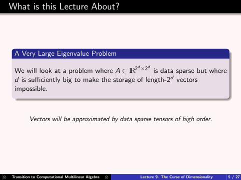
A Very Large Eigenvalue Problem
We will look at a problem where A ∈ IR2d×2dis data sparse but where
d is sufficiently big to make the storage of length-2d vectorsimpossible.
Vectors will be approximated by data sparse tensors of high order.
⊗ Transition to Computational Multilinear Algebra ⊗ Lecture 9. The Curse of Dimensionality 5 / 27
A Very Large Eigenvalue Problem
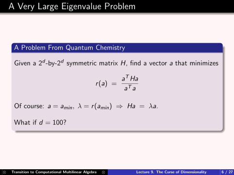
A Problem From Quantum Chemistry
Given a 2d -by-2d symmetric matrix H, find a vector a that minimizes
r(a) =aTHa
aTa
Of course: a = amin, λ = r(amin) ⇒ Ha = λa.
What if d = 100?
⊗ Transition to Computational Multilinear Algebra ⊗ Lecture 9. The Curse of Dimensionality 6 / 27
The Google Slide
⊗ Transition to Computational Multilinear Algebra ⊗ Lecture 9. The Curse of Dimensionality 7 / 27

A Very Large Eigenvalue Problem
The H-Matrix
H =d∑ij
tijHTi Hj +
d∑ijkl
vijklHTi HT
j HkHl
Hi = I2i−1 ⊗[
0 10 0
]⊗ I2d−i
T ∈ IRd×d is symmetric and V ∈ IRd×d×d×d has symmetries.
Sparsity
nzeros =
(1
64d4 − 3
32d3 +
27
64d2 − 11
32d + 1
)2d − 1
⊗ Transition to Computational Multilinear Algebra ⊗ Lecture 9. The Curse of Dimensionality 8 / 27
A Very Large Eigenvalue Problem
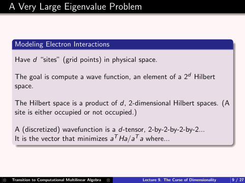
Modeling Electron Interactions
Have d “sites” (grid points) in physical space.
The goal is compute a wave function, an element of a 2d Hilbertspace.
The Hilbert space is a product of d , 2-dimensional Hilbert spaces. (Asite is either occupied or not occupied.)
A (discretized) wavefunction is a d-tensor, 2-by-2-by-2-by-2...It is the vector that minimizes aTHa/aTa where...
⊗ Transition to Computational Multilinear Algebra ⊗ Lecture 9. The Curse of Dimensionality 9 / 27

A Very Large Eigenvalue Problem
The H-Matrix
H =d∑ij
tijHTi Hj +
d∑ijkl
vijklHTi HT
j HkHl
⇑KineticEnergy
Weights
⇑PotentialEnergyWeights
Hi = I2i−1 ⊗[
0 10 0
]⊗ I2d−i
⊗ Transition to Computational Multilinear Algebra ⊗ Lecture 9. The Curse of Dimensionality 10 / 27
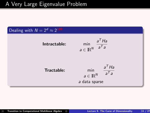
A Very Large Eigenvalue Problem
Dealing with N = 2d ≈ 2100
Intractable: min
a ∈ IRN
aTHa
aTa
Tractable: min
a ∈ IRN
a data sparse
aTHa
aTa
⊗ Transition to Computational Multilinear Algebra ⊗ Lecture 9. The Curse of Dimensionality 11 / 27

Tensor Networks
Definition
A tensor network is a tensor of high dimension that is built up frommany sparsely connected tensors of low-dimension.
⊗ Transition to Computational Multilinear Algebra ⊗ Lecture 9. The Curse of Dimensionality 12 / 27

TN slides
⊗ Transition to Computational Multilinear Algebra ⊗ Lecture 9. The Curse of Dimensionality 13 / 27

Linear Tensor Network
Recall the Block Vec Operation
[F1
F2
]⊗
G1
G2
G3
⊗ [ H1
H2
] =
[F1
F2
]⊗
G1H1
G1H2
G2H1
G2H2
G3H1
G3H2
=
F1G1H1
F1G1H2
F1G2H1
F1G2H2
F1G3H1
F1G3H2
F2G1H1
F2G1H2
F2G2H1
F2G2H2
F2G3H1
F2G3H2
⊗ Transition to Computational Multilinear Algebra ⊗ Lecture 9. The Curse of Dimensionality 14 / 27

Linear Tensor Network
In the ”Language” of Block Vec Products...
a =
[A11
A21
]⊗[
A12
A22
]⊗ · · · ⊗
[A1,d−1
A2,d−1
]⊗[
A1d
A2d
]where [
A11
A21
]=
[wT
1
wT2
]2 row vectors
[A1k
A2k
]=
[m-by-mm-by-m
]k = 2:d − 1
[A1d
A2d
]=
[z1
z2
]2 column vectors
a is a length-2d vector that depends on O(dm2) numbers
⊗ Transition to Computational Multilinear Algebra ⊗ Lecture 9. The Curse of Dimensionality 15 / 27
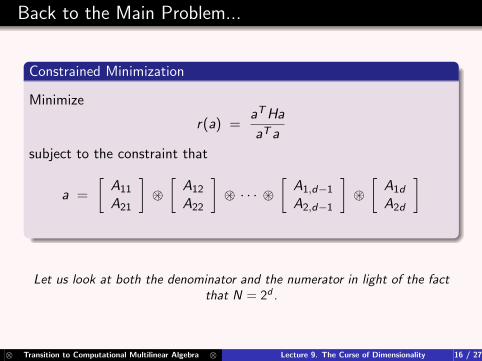
Back to the Main Problem...
Constrained Minimization
Minimize
r(a) =aTHa
aTa
subject to the constraint that
a =
[A11
A21
]⊗[
A12
A22
]⊗ · · · ⊗
[A1,d−1
A2,d−1
]⊗[
A1d
A2d
]
Let us look at both the denominator and the numerator in light of the factthat N = 2d .
⊗ Transition to Computational Multilinear Algebra ⊗ Lecture 9. The Curse of Dimensionality 16 / 27
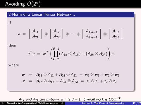
Avoiding O(2d)
2-Norm of a Linear Tensor Network...
If
a =
[A11
A21
]⊗[
A12
A22
]⊗ · · · ⊗
[A1,d−1
A2,d−1
]⊗[
A1d
A2d
]then
aTa = wT
(d−1∏k=2
(A1k ⊗ A1k) + (A2k ⊗ A2k)
)z
where
w = A11 ⊗ A11 + A21 ⊗ A21 = w1 ⊗ w1 + w2 ⊗ w2
z = A1d ⊗ A1d + A2d ⊗ A2d = z1 ⊗ z1 + z2 ⊗ z2
A1k and A2k are m-by-m, k = 2:d − 1. Overall work is O(dm3).⊗ Transition to Computational Multilinear Algebra ⊗ Lecture 9. The Curse of Dimensionality 17 / 27

Avoiding O(d4)
Recall...
H =d∑ij
tijHTi Hj +
d∑ijkl
vijklHTi HT
j HkHl
Hi = I2i−1 ⊗[
0 10 0
]⊗ I2d−i
The V-Tensor Has Familiar Symmetries
V(i , j , k, `) =
V(j , i , k, `)V(i , j , `, k)V(k, `, i , j)
and so we can find symmetric matrices B1, . . . ,Br so
V = B1 ◦ B1 + · · ·+ Br ◦ Br
⊗ Transition to Computational Multilinear Algebra ⊗ Lecture 9. The Curse of Dimensionality 18 / 27
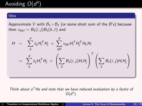
Avoiding O(d4)
Idea
Approximate V with B1 ◦ B1 (or some short sum of the B’s) becausethen vijk` = B1(i , j)B1(k, `) and
H =d∑ij
tijHTi Hj +
d∑ijkl
vijklHTi HT
j HkHl
=d∑ij
tijHTi Hj +
∑ij
B1(i , j)HiHj
T ∑ij
B1(i , j)HiHj
Think about aTHa and note that we have reduced evaluation by a factor ofO(d2).
⊗ Transition to Computational Multilinear Algebra ⊗ Lecture 9. The Curse of Dimensionality 19 / 27
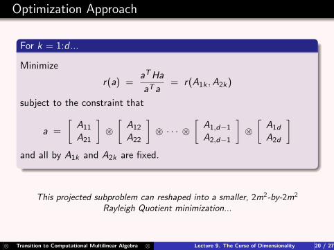
Optimization Approach
For k = 1:d ...
Minimize
r(a) =aTHa
aTa= r(A1k ,A2k)
subject to the constraint that
a =
[A11
A21
]⊗[
A12
A22
]⊗ · · · ⊗
[A1,d−1
A2,d−1
]⊗[
A1d
A2d
]and all by A1k and A2k are fixed.
This projected subproblem can reshaped into a smaller, 2m2-by-2m2
Rayleigh Quotient minimization...
⊗ Transition to Computational Multilinear Algebra ⊗ Lecture 9. The Curse of Dimensionality 20 / 27
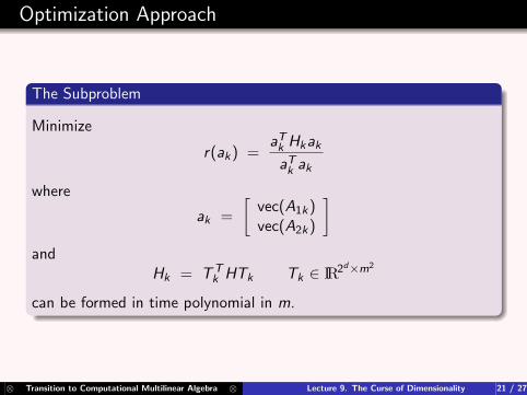
Optimization Approach
The Subproblem
Minimize
r(ak) =aTk Hkak
aTk ak
where
ak =
[vec(A1k)vec(A2k)
]and
Hk = TTk HTk Tk ∈ IR2d×m2
can be formed in time polynomial in m.
⊗ Transition to Computational Multilinear Algebra ⊗ Lecture 9. The Curse of Dimensionality 21 / 27

Tensor-Based Thinking
Key Attributes
1 An ability to reason at the index-level about the constituentcontractions and the order of their evaluation.
2 An ability to reason at the block matrix level in order to exposefast, underlying Kronecker product operations.
⊗ Transition to Computational Multilinear Algebra ⊗ Lecture 9. The Curse of Dimensionality 22 / 27

Data-Sparse Representations and Facorizations
How Could We Compute the QR Factorization of This?
[F1
F2
]⊗
G1
G2
G3
⊗ [ H1
H2
] =
[F1
F2
]⊗
G1H1
G1H2
G2H1
G2H2
G3H1
G3H2
=
F1G1H1
F1G1H2
F1G2H1
F1G2H2
F1G3H1
F1G3H2
F2G1H1
F2G1H2
F2G2H1
F2G2H2
F2G3H1
F2G3H2
Without “Leaving” the Data Sparse Representation?
⊗ Transition to Computational Multilinear Algebra ⊗ Lecture 9. The Curse of Dimensionality 23 / 27
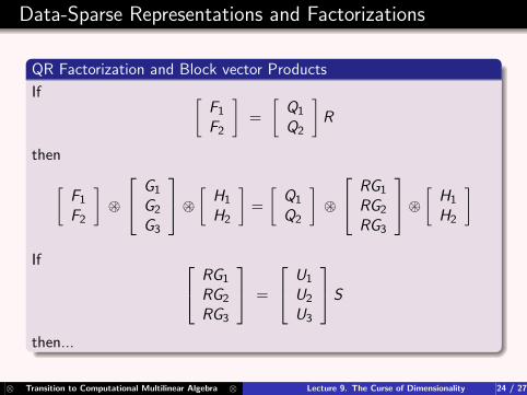
Data-Sparse Representations and Factorizations
QR Factorization and Block vector Products
If [F1
F2
]=
[Q1
Q2
]R
then[F1
F2
]⊗
G1
G2
G3
⊗ [ H1
H2
]=
[Q1
Q2
]⊗
RG1
RG2
RG3
⊗ [ H1
H2
]
If RG1
RG2
RG3
=
U1
U2
U3
S
then...
⊗ Transition to Computational Multilinear Algebra ⊗ Lecture 9. The Curse of Dimensionality 24 / 27

Data-Sparse Representations and Factorizations
QR Factorization and Block vector Products
[F1
F2
]⊗
G1
G2
G3
⊗ [ H1
H2
]=
[Q1
Q2
]⊗
U1
U2
U3
⊗ [ SH1
SH2
]
If [SH1
SH2
]=
[V1
V2
]T
then[F1
F2
]⊗
G1
G2
G3
⊗ [ H1
H2
]=
[ Q1
Q2
]⊗
U1
U2
U3
⊗ [ V1
V2
]T
The Matrix in Parentheses is Orthogonal
⊗ Transition to Computational Multilinear Algebra ⊗ Lecture 9. The Curse of Dimensionality 25 / 27

Summary of Lecture 9.
Key Words
The Curse of Dimensionality refers to the challenges that arisewhen dimension increases.
Clever data-sparse representations are one way to address theissues.
A tensor network is a way of combining low-order tensors toobtain a high-order tensor.
Reliable methods that scale with dimension are the goal.
⊗ Transition to Computational Multilinear Algebra ⊗ Lecture 9. The Curse of Dimensionality 26 / 27
References
G. Beylkin and M.J. Mohlenkamp (2002). “Numerical Operator Calculus in HigherDimensions,” Proceedings of the National Academy of Sciences, 99(16),10246–10251.
G. Beylkin and M. Mohlenkamp (2005). “Algorithms for Numerical Analysis inHigh Dimensions,” SIAM J. Scientific Computing, 26, 2133–2159.
A. Hartono, A. Sibiryakov, M. Nooijen, G. Baumgartner, D.E. Bernholdt, S.Hirata, C. Lam, R. Pitzer, J. Ramanujam, and P. Sadayappan (2005).“Automated Operation Minimization of Tensor Contraction Expressions inElectronic Structure Calculations,” in Proc. International Conference onComputational Science 2005, Atlanta.
S. Hirata (2003). “Tensor Contraction Engine: Abstraction and Automatic ParallelImplementation of Configuration Interaction, Coupled-Cluster, andMany-Body Perturbation Theories,” J. Phys. Chem. A., 107, 9887–9897.
A. Auer, G. Baumgartner, D. Bernholdt, A. Bibireata, V. Choppella, D. Cociorva,X. Gao, R. Harrison, S. Krishnamoorthy, S. Krishnan, C. Lam, Q. Lu, M.Nooijen, R. Pitzer, J. Ramanujam, P. Sadayappan, and A. Sibiryakov (2006).“Automatic Code Generation for Many-Body Electronic Structure Methods:The Tensor Contraction Engine,” Molecular Physics, 104, no. 2, 211–228.
G. Baumgartner, A. Auer, D. Bernholdt, A. Bibireata, V. Choppella, D. Cociorva,X. Gao, R. Harrison, S. Hirata, S. Krishnamoorthy, S. Krishnan, C. Lam, Q.Lu, M. Nooijen, R. Pitzer, J. Ramanujam, P. Sadayappan, and A. Sibiryakov(2005). “Synthesis of High-Performance Parallel Programs for a Class of abinitio Quantum Chemistry Models,” Proceedings of the IEEE, 93, no. 2,276–292.
A. Bibireata, S. Krishnan, G. Baumgartner, D. Cociorva, C. Lam, P. Sadayappan,J. Ramanujam, D. Bernholdt, and V. Choppella (2004).“Memory-Constrained Data Locality Optimization for Tensor Contractions,”in Languages and Compilers for Parallel Computing,(L. Rauchwergeret et alEds.), Lecture Notes in Computer Science, Vol. 2958, 93–108,Springer-Verlag.
U. Bondhugula, A. Hartono, J. Ramanujam, and P. Sadayappan (2008). “APractical and Automatic Polyhedral Program Optimization System,” Proc.ACM SIGPLAN 2008 Conference on Programming Language Design andImplementation (PLDI 08), Tucson.
U. Bondhugula, M. Baskaran, S. Krishnamoorthy, J. Ramanujam, A. Rountev, andP. Sadayappan (2008). “Automatic Transformations forCommunication-Minimized Parallelization and Locality Optimization in thePolyhedral Model,” in Proc. CC 2008 -International Conference on CompilerConstruction, Budapest.
C-H Huang, J.R. Johnson, and R.W. Johnson (1991). “Multilinear Algebra andParallel Programming,” J. Supercomputing, 5, 189–217.
E. Elmroth, F. Gustavson, I. Jonsson, B. Kagstrom (2004). “Recursive BlockedAlgorithms and Hybrid Data Structures for Dense Matrix Library Software,”SIAM Review 46, 3–45.
J. Demmel, J. Dongarra, V. Eijkhout, E. Fuentes, A. Petitet, R. Vuduc, R.C.Whaley, and K. Yelick (2005). “Self-Adapting Linear Algebra Algorithmsand Software,” Proc. IEEE, 93, 293–312.
P. Drineas and M. Mahoney (2007). “A Randomized Algorithm for a Tensor-BasedGeneralization of the Singular Value Decomposition,” Linear Algebra and ItsApplications, 420, 553-571.
M.W. Mahoney, M. Maggioni, and P. Drineas (2008). “Tensor-CURDecompositions For Tensor-Based Data”, SIAM J. Matrix Analysis andApplications, 30, 957–987.
S.R. White and R.L. Martin (1999). “Ab Initio Quantum Chemistry Using theDensity Matrix Renormalization Group,” J. Chem. Phys., 110, no. 9, p.4127.
G. K-L Chan (2004). “An Algorithm for Large Scale Density MatrixRenormalization Group Calculations,” J. Chem. Phys., 120 (7), 3172.
G.K.-L. Chan, J. Dorando, D. Ghosh, J. Hachmann, E. Neuscamman, H. Wang,and T. Yanai (2007). “An Introduction to the Density MatrixRenormalization Group Ansatz in Quantum Chemistry,” arXiv:cond-mat, vol.0711.1398v1.
⊗ Transition to Computational Multilinear Algebra ⊗ Lecture 9. The Curse of Dimensionality 27 / 27
Related Documents