Challenging the curse of dimensionality in multivariate local linear regression

Noname manuscript No.(will be inserted by the editor)

Challenging the curse of dimensionality inmultivariate local linear regression

James Taylor · Jochen Einbeck

Received: date / Accepted: date

Abstract Local polynomial fitting for univariate data has been widely stud-ied and discussed, but up until now the multivariate equivalent has often beendeemed impractical, due to the so-called curse of dimensionality. Here, ratherthan discounting it completely, we use density as a threshold to determinewhere over a data range reliable multivariate smoothing is possible, whilstaccepting that in large areas it is not. The merits of a density threshold de-rived from the asymptotic influence function are shown using both real andsimulated data sets. Further, the challenging issue of multivariate bandwidthselection, which is known to be affected detrimentally by sparse data which in-evitably arise in higher dimensions, is considered. In an effort to alleviate thisproblem, two adaptations to generalized cross-validation are implemented, anda simulation study is presented to support the proposed method. It is also dis-cussed how the density threshold and the adapted generalized cross-validationtechnique introduced herein work neatly together.

Keywords Multivariate smoothing · density estimation · bandwidthselection · influence function

J. TaylorDurham UniversityDepartment of Mathematical SciencesDurham, UKE-mail: [email protected]

J. EinbeckDurham UniversityDepartment of Mathematical SciencesDurham, UKE-mail: [email protected]

2 James Taylor, Jochen Einbeck

1 Introduction

Univariate nonparametric regression is widely used to fit a curve to a datasetfor which a parametric method is not suitable. Multivariate nonparametric re-gression methods are not so prevalent, although several methods do exist suchas the additive models of Hastie and Tibshirani (1990) and thin plate splines,introduced by Duchon (1977). Here we study the multivariate case of local lin-ear regression, the origins of the univariate equivalent of which can be tracedback to the late nineteenth century. The multivariate technique has often beendeemed impractical due to the problems encountered in regions of sparse data,which become practically an unavoidable part of data in higher dimensions.This issue is often referred to as the curse of dimensionality. However, mul-tivariate local regression has been implemented successfully in Cleveland andDevlin (1988) for 2 and 3–dimensional data and in Fowlkes (1986) for data ofeven higher dimensions. In this paper we introduce techniques which make thecurse of dimensionality avoidable and so regression feasible for any reasonabledimension.

Given d-dimensional covariates Xi = (Xi1, ..., Xid)T with density f(·) andscalar response values Yi where i = 1, ..., n, the task is to estimate the meanfunction m(.) = E(Y |X = .) at a vector x. Assumed is that

Yi = m(Xi) + εi (1)

where εi are random variables with zero mean and variance σ2. We concentrateon local linear regression which uses a kernel–weighted version of least squares,in order to fit hyperplanes of the form β0 + βT

1 x locally, i.e., at each targetpoint x ∈ Rd. Both the scalar β0 and the vector β1 depend on x, but wesuppress this dependence for notational ease. To find the regression estimate,m(x), one minimizes with respect to β = (β0,β

T1 )T = (β0, β11, ..., β1d)T ;

n∑i=1

Yi − β0 −d∑

j=1

β1j(Xij − xj)

2

KH(Xi − x). (2)

The estimator of the mean function m(x) is β0. Here K is a multivariate kernel

function with∫K(u)du = 1 and KH(x) = |H|−1/2K(H−1/2x). The d × d

bandwidth matrix H is crucial in determining the amount and direction ofsmoothing since it is this that defines the size and shape of the neighbourhoodaround x, enclosing data points which are considered in the estimation atthis point. For each x, the contours of the weights KH(· − x) form ellipsoidscentered at x, with more weight usually given to those points closer to x.

We choose to use a diagonal matrix, H = diag(h21, ..., h2d), since compu-

tationally this is significantly easier than a full matrix. For K, we primarilyuse a product of Gaussian kernels since in practice we found this the leasttemperamental kernel function in regions where data is sparse.

Minimization (2) is a weighted least squares problem. The solution to thisis

β0 = m(x) = e1T (XT

xWxXx)−1XTxWxY (3)

Challenging the curse of dimensionality in multivariate local linear regression 3

where

Xx =

1 X11 − x1 ... X1d − xd1 X21 − x1 ... X2d − xd...

.... . .

...1 Xn1 − x1 ... Xnd − xd

(4)

Y =

Y1...Yn

(5)

Wx = diag {KH(X1 − x), ...,KH(Xn − x)} (6)

and e1 is a vector with 1 as its first entry and 0 in the other d entries.Local polynomial regression in general, and local linear regression in par-

ticular, has many advantages which makes it of interest to find a solution tothe problem of the curse of dimensionality. Firstly, the idea has great intuitiveappeal, as it is easily visualized and understood which data points are con-tributing to the estimation at a point. Work by Cleveland and Devlin (1988)and Hastie and Loader (1993a) suggests that multivariate local polynomialregression compares favourably with other smoothers in terms of computa-tional speed. Furthermore, kernels are attractive from a theoretical point ofview, since they allow straightforward asymptotic analysis. It has been foundthat the technique exhibits excellent theoretical properties. Local polynomialswere shown to achieve optimal rates of convergence in Stone (1980). In theunivariate case, Fan (1993) showed that local linear regression achieves 100%minimax efficiency. The asymptotic bias and variance are known to have thesame order of magnitude at the boundary as in the interior of the data, whichis a particularly encouraging property for higher–dimensional data sets (Rup-pert and Wand, 1994). For finite samples in high dimensions, in our experience,the quality of the regression is in fact likely to be poorer at the boundary thanin the interior, with the variance in the boundary region being higher for locallinear than for local constant estimation. This behaviour is also noted in Rup-pert and Wand (1994). However, the quality of estimation of the local linearestimator, in terms of mean squared error, is usually still superior to localconstant in these regions, due to the significantly reduced bias. Other advan-tages, as detailed in Hastie and Loader (1993b), include that it adapts easilyto different data design and also has the interesting side-effect of implicitlyproviding the gradient of m at x through the same least squares calculation.Indeed, this is given by β1.

Scott (1992) describes the curse of dimensionality as ‘the apparent paradoxof neighbourhoods in higher dimensions — if the neighbourhoods are ‘local’,then they are almost surely ‘empty’, whereas if a neighbourhood is not ‘empty’,then it is not ‘local’.’ If there is not sufficient data in a neighbourhood, thenthe variance of the fit is too high, or with some kernel functions, such as theEpanechnikov kernel, the calculations may break down completely.

In order to simplify the problem, one may consider using dimension re-duction or variable selection techniques in a pre–processing step. Examples


of such techniques include principal component analysis, with the selection of‘principal variables’ (Cumming and Wooff, 2007) as an interesting variant, theLASSO, originally of Tibshirani (1996) and since implemented in a variety offorms, and the Dantzig method (Candes and Tao, 2007), which is specificallydesigned for situations with very large d > n.

Although such procedures may alleviate the curse of dimensionality greatly,there are certain limits to what they can achieve. Firstly, even after successfulapplication of such a technique, one will remain with a subset of ‘relevant’ vari-ables. The remaining local linear regression problem may still suffer from thecurse of dimensionality, which begins to have an impact in dimensions as littleas d = 3 or 4. Furthermore, most such variable selection or dimension reductiontechniques will make some implicit linear modelling assumption, which maynot be adequate from a nonparametric perspective. In order to deal with thisproblem properly, one would need to interweave the bandwidth selection andthe variable selection processes, as suggested by Cleveland and Devlin (1988).Recently, an interesting approach in this direction was provided by Laffertyand Wasserman (2008), who introduced the rodeo (regularization of derivativeexpectation operator). This technique initially assigns a large bandwidth inevery covariate direction. The bandwidths are then gradually decreased, andvariables are deemed irrelevant if this does not lead to a substantial change inthe estimated regression function. This concept of ‘relevance’ is not withoutcontroversy; for instance, Vidaurre, Bielza and Larranaga (2011) argue thatthis definition is somewhat strange, since all variables which have a linearimpact onto the response would be deemed irrelevant by construction. In analternative approach, Vidaurre, Bielza and Larranaga (2011) implemented alasso locally to reduce the number of variables in local regression.

These hybrid bandwidth/variable selection methods were demonstrated towork reliably in certain situations, but they clearly carry some non–canonicalfeatures. In this work, we return to a more basic setup in which all estimation iscarried out by ‘standard’ multivariate local linear regression in d−dimensionalspace. In the developments that follow, it is irrelevant whether the d−variatedata set corresponds to the original data, or is the result of a dimension–reducing pre–processing step. In terms of the magnitude of d, we have quitelarge (say, up to two dozen), but not huge, numbers of variables in mind. Wecomment on the case of very large dimensions d in the Discussion.

Hastie, Tibshirani and Friedman (2001) and Cleveland and Devlin (1988)agree that the way to overcome the curse of dimensionality would be to in-crease the sample size n in order to capture complexities in the regressionsurface that might otherwise be lost through the necessary introduction oflarger bandwidths. Of course, increasing n is often not a realistic option fora given data set, but, putting their statement in other words, there must besufficient data around x for a reliable estimate to be made at that point. Thisis the attitude adopted in this paper, and in Section 2 we describe a solutionwhich essentially identifies such “reliable” regions by dismissing all neighbour-hoods which do not contain enough data. The actual smoothing step is thenonly performed over such regions in which estimation is considered reliable,


where the bias and variance of m can be kept reasonably low. This is achievedthrough a threshold imposed on a suitable estimate of the density f . In Section3 a bandwidth matrix selection procedure is suggested which specifically tai-lors generalized cross-validation, first developed by Craven and Wahba (1979),for use with multivariate data. A simulation study is included to demonstratethe value of this technique, before finishing the paper with a Discussion inSection 4.

2 A density threshold

The basic idea is to identify regions which are suitable for local regressionestimation by looking at the density, f . Since this is unknown, it needs to beestimated. At a multivariate point x ∈ Rd, the kernel density estimate, f(x),is

f(x) = n−1n∑

i=1

KH(Xi − x) (7)

where KH is a multivariate kernel function, as defined earlier, and again abandwidth matrix H is needed. For reasons that will become clear later, weuse the same H in calculating f as in the regression step. A threshold T issought such that, if at point x we have f(x) ≥ T , then an estimate usinglocal linear regression can be considered somewhat reliable, and otherwise,care should be taken and an alternative method sought. Intuitively, T shoulddepend on n and H, as decreasing either of them will reduce the number ofdata points which are locally available at x, requiring in turn a larger thresholdto allow reliable estimation.

There seems to exist a tempting shortcut solution to the problem. Onecould argue that, for sufficient local estimation of a hyperplane with p = d+ 1parameters, one needs effectively p pieces of information in the neighbourhoodof x. In other words, the observations in the vicinity of x need to contributep times the information which would be provided by a data point situatedexactly at x. Using (7), this means that an initial candidate threshold, say T0,would take the form

T0 =(d+ 1)K(0)

n|H|1/2, (8)

which contains the quantities n and |H| in the denominator, as expected. Laterin this section we will arrive, through a more rigorous justification than theabove, at a threshold of the same shape as (8), but with the constant d + 1replaced by a more adequate one, which is of the same magnitude as d + 1only for small values of d.

We present a data set to illustrate the motives. This data set contains9 variables on 14000 chamois, a species of goat-antelope, shot between themonths of October and December between the years 1973-2009, in the Trentinoarea of the Italian Alps. The response is body mass and the 8 covariates areclimate variables, age and elevation. A subset of size 12000 is used as training


data while a further 2000 observations act as test data. For each point in thetest set the body mass is estimated using (3) and compared with the observedresponse values. Since d is relatively large, automatic bandwidth selection iscomputationally too intensive and so here the hj , j = 1, . . . , 8 are chosen asone fifteenth of the data range in each direction. The difficulties of bandwidthselection will be discussed at length in Section 3. In the first graph in Fig. 1the difference between Yi and m(Xi) is plotted against f(Xi), calculated using(7), for each of the 2000 test points. The effects of the curse of dimensionalityare clearly visible in the way that large errors in estimating the regressionsurface exist on the left hand side of the graph which examines the lowerf(Xi) and so sparser regions of the data set. This is the area which wouldideally be cut off. For this data set, with p = 9 parameters, one would obtainT0 = 9K(0)/n|H|1/2 = 1.13× 10−7. If this was employed as threshold T , then

599 of the test points would be considered to have a large enough f(Xi) forregression to be reliable. The second plot in Fig. 1 again plots m(Xi) − Yiagainst f(Xi), but only for these denser 599 points. However, this threshold isconsidered inadequate since errors of magnitude as large as 200 are observedat points where regression would be considered feasible, when the responserange is approximately 40. For this reason we develop T differently, using theconcept of influence.

●●●●●●●●●●

●●

●

●●●●●●●●●●●●●●●●●●●●●●●●●●●●●●●●●●●●●●●●●●●●●●●●●●●●●●●●●●

●●●●

●●●●●●●●●●●●●●●●●●●●●●●●●●●●●●●●●●●●●●●●●●●●●●●●

●

●●●●●●●

●

●●●●●●●

●

●●●●●●●●●●●●●●●●

●●●●

●

●

●●●●●●●●●●●●●●●●●●●●●●●●●●●●●●●●●

●●●●●●●●●●●●●●●●●●●●●●●●●●●●●●●●●●●●●●●●●●●●●●●●●●●●●●●●●●●●●●●●●●●●●●●●●●●●●●●●●●●●●●●●●●●●●●●●●●●●●●●●●●●●●●●●●●●●●●●

●●●●●●●●●●●●●●●●●●●●●●●●●●●●●●●●●●●●●●●●●●●●●●●●●●●●●●●●●●●●●●●●●●●●●●●●●●●●●●●●●●●●●●●●●●●●●●●●●●●●●●●●●●●●●●●●●●●●●●●●●●●●●●●●●●●●●●●●●●●●●●●●●●●●●●●●●●●●●●●●●●●●●●●●●●●●●●●●●●●●●●●●●●●●●●●●●●●●●●●●●●●●●●●●●●●●●●●●●●●●●●●●●●●●●●●●●●●●●●●●●●●●●●●●●●●●●●●●●●●●●●●●●●●●●●●●●●●●●●●●●●●●●●●●●●●●

●●●●●●●●●●●●●●●●●●●●●●●●●●●●●●●●●●●●●●●●●●●●●●●●●●●●●●●●●●●●●●●●●●●●●●●●●●●●●●●●●●●●●●●●●●●●●●●●●●●●●●●●●●●●●●●●●●●●●●●●●●●●●●●●●●●●●●●●●●●●●●●●●●●●●●●●●●●●●●●●●●●●●●●●●●●●●●●●●●●●●●●●●●●●●●●●●●●●●●●●

●

●●●●●●●●●●●●●●●●●●●●●●●●●●●●●●●●●●●●●●●●●●●●●●●●●●●●●●●

●

●●●●●●●●●●●●●●●●●●●●●●●●●●●●●●●●●●●●●●●●●●●●●●●●●●●●●●●●●●●●●●●●●●●●●●●●●●●●●●●●●●●●●●●●●●●●●●●●●●●●●●●●●●●●●●●●●●●●●●●●●●●●●●

●

●●●●●●●●●●●●●●●●●●●●●●●●●●●●●●●●

●

●●●●●●●●●●●●●●●●●●●●●●●●●●

●

●●●●●●●●●●●●●●●●●●●●●●●●●●●●●●●●●●●●●●●●●●●●●●●●●●●●●●●●●●●●●●●●●●●●●●●●●●●●●●●●●●●●●●●●●●●●●●●●●●●●●●●●●●●●●●●●●●●●●●●●●●●●●●●●●●●●●●●●●●●●●●●●●●●●●●●●●●●●●●●●●●●●●●●●●●●●●●●●●●●●●●●●●●●●●●●●●●●●●●●●●●●●●●●●●●●●●●●●●●●●●●●●●●●●●●●●●●●●●●●●●●●●●●●●●●●●●●●●●●●●●●●●●●●●●●●●●●●●●●●●●●

●

●

●●●●●●●●●●●●●●●●●●●●●●●●●●●●●●●●●●●●●●●●●●●●●●●●●●●●●●●●●●●●●●●●●●●●●●●

●

●●●●●●●●●●●●●●●●●●●●●●●●●●●●●●●●●●●●●●●●●●●●

●●●●●●●●●●●●●●●●●●●●●●●●●●●●●●●●●●●●●●●●●●●●●●●●●●●●●●●●●●●●●●●●●●●●●●●●●●●●●●●●●

●

●●●●●

●

●●●●●●●●●

●

●●●●●●●●●●●●●●●●●●●●●●●●●●●●

●

●●●●●●●●●●●●●●●●●●●●●●●●●●●●●●●●●●●●●

●●●

●●●●●●●●●●●●●●●●●●●●●●●●●●●●●●●●●●●●●●●●●●●●●●●●●●●●

●

●●●●●●●●●●●●●●●●●●●●●●●●●●

●

●●●●●

●

●●●●●●

●

●●●●●●●●●●●●●●●●●●●●●●●●●

●●●●●●●●●●●●●●●●●●●●●●●●●●●●●●●●●●●●●●●●●●●●

●●●●●●●●●●●●●●●●●●●●●●●●●●●●●●●●●●●●●●●●●●●●●●●●●

●●●●●●●●●●●●●

●●●●●●●●●●●●●●●●●●●●●●●●●●●●●●●●

●●●●●●●●●●●●●●●●●●●●●●●●●●●●●●●●●●●●●●●

●●●●●●●●●●●●●●●●●●●●●●●●●●●●●●●●●

●●●●●●●●●●●●●●●●● ●●●●●●●●●●●●●●●●●●●●●●●●

●●●●●●

●●●●●● ●●

0e+00 1e−07 2e−07 3e−07 4e−07 5e−07

−20

0−

100

010

020

030

040

0

density

erro

r

●●●●●

●

●●●●●●●●●●●●●●●●●●●●●●●●●●●●●●●●●●●●●●●●●●●●

●

●●●●●●●●●●●●●●●●●●●●●●●●●●●●●●●●●●●●●●●●●●●●●●●●●●●●●●●●●●●●●●●●●●●●●●●●●●●●●●●●

●

●●●●●

●

●●●●●●●●●

●

●●●●●●●●●●●●●●●●●●●●●●●●●●●●

●

●●●●●●●●●●●●●●●●●●●●●●●●●●●●●●●●●●●●●●●●

●

●●●●●●●●●●●●●●●●●●●●●●●●●●●●●●●●●●●●●●●●●●●●●●●●●●●

●

●●●●●

●●●●●●●●●●●●●●●●●●●●●

●

●●●●●

●

●●●●●●

●

●●●●●●●●●●●●●●●●●●●●●●●●●

●●●●●●●●●●●●●●●●●●●●●●●●●●●●●●●●●●●●●●●●●

●●●●●●●●●●●●●●●●●●●●●●●●●●

●●●●●●●●●●●●●●●●●●●●●●●●

●●●●●●●●●●●●●●●

●●●●●●●●●●●●●●●●●●●●●●●●●●●●●●●●

●●●●●●●●●●

●●●●●●●●●●●●●●●●●●●●●●●●●●●●●

●●●●●●●●●●●●●●●

●●●●●●●●●●●●

●●●●●●●●●●

●●●●●●●●●●

●● ● ●●●●●●●●●●●●●●●●●●●●●●●●

●●●

●●●●●●●●● ●●

1e−07 2e−07 3e−07 4e−07 5e−07

−20

0−

100

010

020

0

density

erro

r

Fig. 1 The graph on the left shows m(Xi) − Yi v. f(Xi) for all 2000 test points of the

chamois data, and the graph on the right shows this for the 599 test points at which f(Xi)is greatest

The influence, infl(Xi), describes the contribution of observation Xi to theestimation at x = Xi. It is given by the diagonal element of the ith row of the


smoother matrix S, where (m(X1), . . . , m(Xn))T = SY, i.e.

infl(Xi) = eT1 (XTWX)−1XTWei = eT1 (XTWX)−1

KH(0)

0...0

= |H|−1/2eT1 (XTWX)−1e1K(0), (9)

where X = X{x=Xi}, W = W{x=Xi}, ei is a vector of length n with 1 in the

ith position, and (KH(0), 0, ..., 0)T

is a vector of length d+ 1.It seems a sensible approach to dismiss local regression at observations for

which infl(Xi) is very large. In the search for a criterion which identifies whata “very large influence” means in this context, we use Theorem 2.3 in Loader(1999), which states that the inequality

infl(Xi) ≤ 1 (10)

holds at all observation points Xi.In order to relate the influence function to the density, we develop an

asymptotic version of (9). At x ∈ Rd, let f be continuously differentiable andf(x) > 0. Assuming n−1|H|−1/2 −→ 0 as n −→∞, one can show that

infl(x) ≈ ρK(0)

nf(x)|H|1/2+ op(n−1|H|−1/2), (11)

where

ρ =

[∫K(u)du−

∫uTK(u)du

(∫uuTK(u)du

)−1 ∫uK(u)du

]−1.

(12)See Appendix A for the derivation of this result. Although the original defini-tion of influence, (9), only applies at the observed values Xi, the asymptoticinfluence function given by (11) can be computed at every x. It can be seen asthe influence which would be expected under idealized (asymptotic) conditionsfor a (hypothetical) data point situated at x. Similarly, the inequality (10) ap-plies only to the observed valued Xi. However, due to the implicit averagingprocess happening in the computation of the asymptotic influence function,any x which is situated in between or close to data points Xi is still likelyto possess the property infl(x) ≤ 1. In other words, in populated regions ofthe predictor space, the asymptotic influence will be less than 1, while it willexceed 1 in very sparse or remote regions. Using this rationale, it makes senseto define T by bounding the asymptotic influence by 1;

ρK(0)

nf(x)|H|1/2≤ 1

so

f(x) ≥ ρK(0)

n|H|1/2


and, hence,

T =ρK(0)

n|H|1/2, (13)

which is of the same form as (8) but with d+ 1 replaced by ρ.Let us firstly note that the bandwidth matrix, H, featuring in this density

threshold stems from an expression involving the influence of the regression,which explains our earlier statement that the bandwidth matrix used for thedensity estimation should be the same as that used in the actual regressionstep.

Of great importance are the limits used in the integrals in ρ. If one esti-mates at an interior point, then these integral limits would range from −∞to ∞. For a boundary point, the lower integral limit would need to be alteredaccording to the distance to the boundary (for instance, assuming a diagonalbandwidth matrix and f(x) > 0, then if x is half a bandwidth hj away fromthe boundary of the support of f in each coordinate direction, then the lowerlimit of each integral would be −0.5; for a rigorous definition of boundarypoints see Ruppert and Wand (1994)). This is of crucial importance for ussince the boundary region, where data become sparse, is just the region inwhich we are interested. Hence, in order to represent the true influence asaccurately as possible in the area of interest, we replace the lower integrallimit by a small negative value, say a, which reflects the distance between theboundary of f and the area for which the criterion is optimized (notice thatthe integrals in (12) are d−variate, but we always use the same a for eachcoordinate direction). A choice of a = 0 would optimize the threshold for useat the edge of the data range, while a value of a = −∞ would be best foruse in the interior. For us, a value in between is optimal, to assess reliablythe region where there is doubt over the validity of local linear regression as asuitable regression technique.

In fact, ρ varies quite strongly with a, as is shown in the top left plot inFig. 2 in the case d = 3. This plot suggests that a value of a between -0.5 and-1 is approximately the point where ρ stabilises as a moves away from 0, whichmakes this a logical range to choose a from.

Our primary method of determining a suitable value of a has been to workbackwards and look directly at the data by examining the error of estimatedpoints. To illustrate this strategy, we generate two training data sets by sub-jecting the functions

m3(x1, x2, x3) = −12 cos(x1) + 5 sin(5x2) + 10 log(x3) + 17

andm5(x1, x2, x3, x4, x5) = m3(x1, x2, x3) + cos(3x4) + 7 tan(x5)

to independent Gaussian noise, whereby x1, . . . , x5 were generated from ap-propriately centered t−distributions with 2 df. These training data sets, eachof size n = 300, were used to fit the respective local linear models. Test datasets, also of size n = 300, were generated in the same manner from m3 andm5. Fig. 2 (right) examines the MSEs for these test data (top: d = 3; bottom:


●●

●

●

●

●

−2.0 −1.5 −1.0 −0.5 0.0

010

2030

4050

a

ρρ

1 2 3 4 5 6

0.8

1.0

1.2

1.4

1.6

1.8

2.0

ρρ

rem

aini

ng M

SE

100

150

200

250

no. o

f poi

nts

excl

uded

remaining MSEno. of points excluded

●

●

●

●

●

●

●

●

●

●

●

●

●

●

●●

●

●

●

●

●

●

●

●

●

●●

●

●

●●

●

●●●

●

●

●●

●

●

●

●

●

●

●

●

●

●

●●

●●

●

●

●●●●

●

●●●●●

●

●

●●●

●

●

●

●●●

●●

●

●

●●●●

●

●●

●

●●●●●●●●●●●●●

●●●●

●●●●●●●●●

●●●

●●●●●●●●●●

●●

●●●●●●●●●●●

●●●●●●●●●●●●●●

●●●

●

●●●●●●●●

●●●

●●●

●●

●

●●●●●●●●●

●

●●● ●●● ●

●● ●● ●● ●

0.000 0.005 0.010 0.015

010

2030

40

density

abso

lute

err

or

2 4 6 8 10

020

0040

0060

0080

00

ρρ

rem

aini

ng M

SE

150

200

250

no. o

f poi

nts

excl

uded

remaining MSEno. of points excluded

Fig. 2 Top left: ρ v. a; Bottom left: |m(Xi)−m(Xi)| v. f(Xi) for the trivariate simulation;Right: MSE for points accepted by T , and number of points excluded, as a function of ρ,for the trivariate simulation (top) and the five-dimensional simulation (bottom)

d = 5), but only including those points accepted by threshold (13). The twoplots show initially quite a steep decline in the MSE, but then flatten at acertain value of ρ. One also observes from these figures that the number ofexcluded points increases quite linearly with ρ. Once all badly fitting pointsare excluded, the exclusion of further points does not continue to improve thefit. As one wishes to exclude as few data as possible, it is important to finda value of ρ situated shortly after the steep descent in the MSE(ρ) function.Hence, an adequate integral limit a should correspond approximately to thesevalues of ρ (which depend on d). In both plots, at these values of ρ, approxi-mately one third of the test points are considered adequate, which seems likea reasonable proportion.


The bottom left plot shows the absolute error, |m(Xi) − m(Xi)|, against

f(Xi) for the trivariate simulation. The vertical line in this plot is T witha = −0.85, and this is approximately where the threshold should cut in orderto exclude the large errors associated with low density. Similar analyses werecarried out for a variety of real and simulated data sets of varying dimension,and the value of a = −0.85 performed consistently well in these analyses,regardless of d. A value of a = −0.85 gives ρ = 3.12 for trivariate, and ρ = 6.1for five-dimensional, data. Indeed, in the plots on the right hand side the curvesseem to flatten at approximately these values of ρ, suggesting that any furtherincrease in T would be pointless.

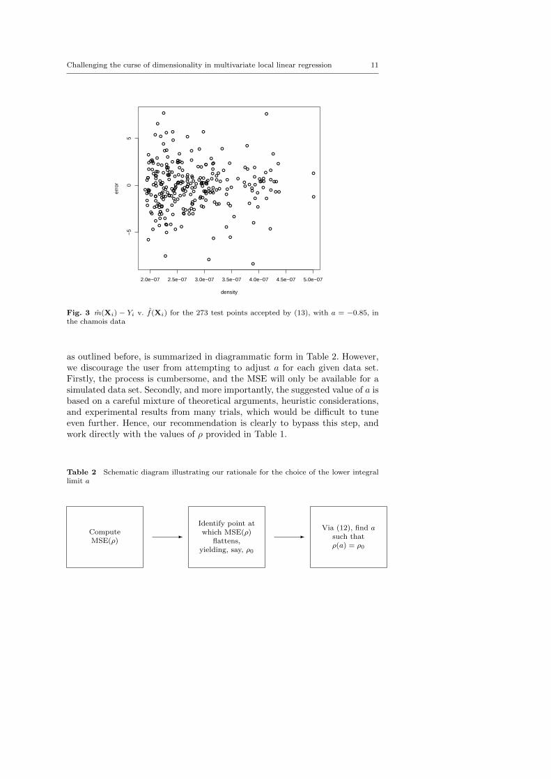
There is no theoretical argument that would tell us exactly where thethreshold should cut. The most important aim is that extreme estimates, orpoints at which estimation breaks down computationally, are ruled out by thethreshold. These analyses suggest that by making a = −0.85, (13) is capableof achieving this. This value corresponds to a point situated 0.85hj inside theboundary, which is quite intuitive since this is approximately the region whereone would assume data sparsity to become a problem. An attractive feature ofthreshold (13) is its interpretability, since (13) is neat in the sense that it takesthe form of a multiple of the density of one point. The threshold is effectivelyimposing a required equivalent number of data points at x. Applying thisthreshold to the chamois data gives T = 1.93 × 10−7, which means only 273of the test points are considered to have large enough f(Xi) for regression,via (3), to be reliable. As Fig. 3 illustrates, this is a considerable improvementcompared to the residual pattern obtained in Fig. 1, with all unreasonablylarge errors now being eliminated.

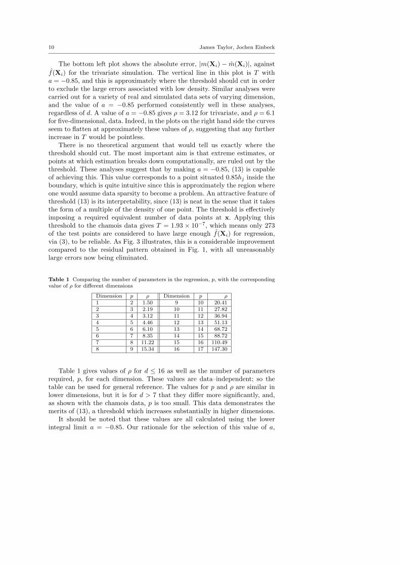
Table 1 Comparing the number of parameters in the regression, p, with the correspondingvalue of ρ for different dimensions

Dimension p ρ Dimension p ρ1 2 1.50 9 10 20.412 3 2.19 10 11 27.823 4 3.12 11 12 36.944 5 4.46 12 13 51.135 6 6.10 13 14 68.726 7 8.35 14 15 88.727 8 11.22 15 16 110.498 9 15.34 16 17 147.30

Table 1 gives values of ρ for d ≤ 16 as well as the number of parametersrequired, p, for each dimension. These values are data–independent; so thetable can be used for general reference. The values for p and ρ are similar inlower dimensions, but it is for d > 7 that they differ more significantly, and,as shown with the chamois data, p is too small. This data demonstrates themerits of (13), a threshold which increases substantially in higher dimensions.

It should be noted that these values are all calculated using the lowerintegral limit a = −0.85. Our rationale for the selection of this value of a,


●●

●

●

●

●●

●

●

●

●●

●

●

●

●

●

●

●

●

●

●

●

●

●

●

●

●

●

●

●

●

●

●

●

●

●

●

●

●

●

●

●

●●

●

●

●

●

●

●

●●

●

●●

●

●

●

●

●

●

●

●

●●

●

●

●

●

●

●

●

●

●

●

●

●

●

●

●

●

●●

●

●

●

●

●

●

●

●

●

●

●

●

●

●

●

●

●

●

●

●

●

●

●

●●

●

●

●

●

●●

●

●

●

●●

●●

●

●

●

●

●

●

●

●

●

●

●

●

●

●

●

●

●●

●

●●

●

●

●

●

●

●

●

●

●

●●

●

●

●

●

●

●

●

●

●

●●

●

●

●

●

●

●●

●

●

●

●

●

●

●

●

●

●●●

●

●

●

●

●

●●●

●

●●

●

●

●●●

●

●

●

●

●

●

●

●

●

●

●

●

●

●

●

●

●

●

●

●

●

●

●

●

●

●

●

●

●

●

●

●

●

●

●

●●

●

●

●

●

●

●●●

●

●

●

●

●

●

●

●

●●●

●

●●

●

●

●

●

●

●

●

●

●

●

●

●

●

●

●

2.0e−07 2.5e−07 3.0e−07 3.5e−07 4.0e−07 4.5e−07 5.0e−07

−5

05

density

erro

r

Fig. 3 m(Xi) − Yi v. f(Xi) for the 273 test points accepted by (13), with a = −0.85, inthe chamois data

as outlined before, is summarized in diagrammatic form in Table 2. However,we discourage the user from attempting to adjust a for each given data set.Firstly, the process is cumbersome, and the MSE will only be available for asimulated data set. Secondly, and more importantly, the suggested value of a isbased on a careful mixture of theoretical arguments, heuristic considerations,and experimental results from many trials, which would be difficult to tuneeven further. Hence, our recommendation is clearly to bypass this step, andwork directly with the values of ρ provided in Table 1.

Table 2 Schematic diagram illustrating our rationale for the choice of the lower integrallimit a

ComputeMSE(ρ)

Identify point atwhich MSE(ρ)

flattens,yielding, say, ρ0

Via (12), find asuch thatρ(a) = ρ0

- -


3 AGCV

3.1 Adaptations to GCV

Bandwidth selection is also influenced detrimentally by the curse of dimension-ality, so that appropriate measures need to be taken also at this stage. Thefirst question arising is which family of bandwidth selection techniques shouldbe used at all. While asymptotic bandwidth selection criteria have been foundto work well in the univariate case, the assumption of bandwidths tending to 0seems inappropriate in the multivariate context, where the bandwidths neededare relatively large. This was less of an issue in the previous section, whereasymptotics were solely used to find an approximation of the influence func-tion, but it is obviously an issue here as the goal is now bandwidth selectionitself. Therefore, we focus on generalized cross-validation (GCV), developedby Craven and Wahba (1979), due to its relative computational ease and thefact that, unlike some competing methods, it does not rely on asymptotics.The criterion takes the form

GCV (H) =1

n

n∑i=1

{Yi − mH(Xi)

1− trace(S)n

}2

. (14)

GCV struggles greatly to cope with high dimensional data, even when adiagonal bandwidth matrix is used, which we will assume throughout thissection. GCV suggests the bandwidth matrix H = diag(h21, . . . , h

2d) which

minimizes (14), and it is the actual minimization process which causes com-putational problems.

When using R to carry out the minimization (R Development Core Team,2010), computation of this minimum frequently breaks down entirely and anerror message is returned. When this is not the case, often this process is verysensitive to the starting point of the minimization algorithm, and differentoptimal parameters are suggested depending on the starting point. Even ifthese problems are overcome and a reasonable looking selection is made, oftenthe chosen bandwidth matrix performs poorly, and extreme values will besuggested frequently for the hj , much larger than even the data range.

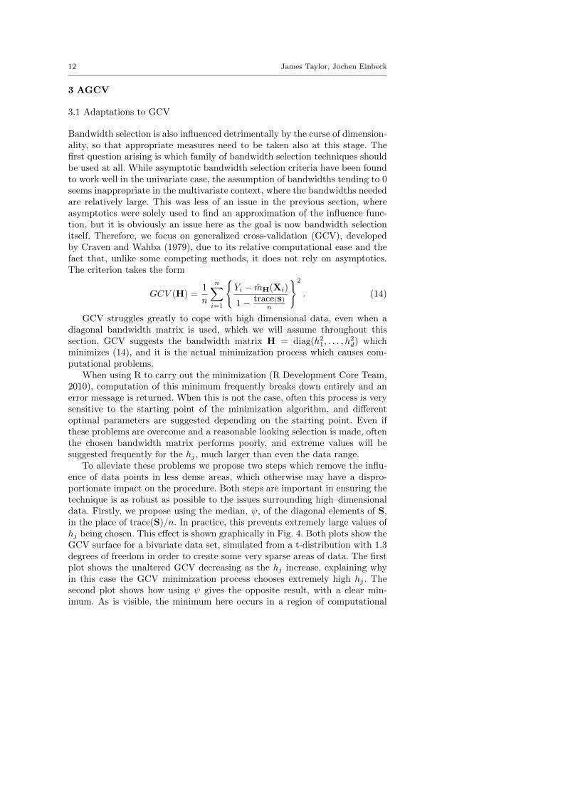
To alleviate these problems we propose two steps which remove the influ-ence of data points in less dense areas, which otherwise may have a dispro-portionate impact on the procedure. Both steps are important in ensuring thetechnique is as robust as possible to the issues surrounding high–dimensionaldata. Firstly, we propose using the median, ψ, of the diagonal elements of S,in the place of trace(S)/n. In practice, this prevents extremely large values ofhj being chosen. This effect is shown graphically in Fig. 4. Both plots show theGCV surface for a bivariate data set, simulated from a t-distribution with 1.3degrees of freedom in order to create some very sparse areas of data. The firstplot shows the unaltered GCV decreasing as the hj increase, explaining whyin this case the GCV minimization process chooses extremely high hj . Thesecond plot shows how using ψ gives the opposite result, with a clear min-imum. As is visible, the minimum here occurs in a region of computational


h1

h2

GC

V

h1

h2

GC

V

Fig. 4 The effect of replacing trace(S)/n by ψ on the GCV surface of a simulated bivariatedata set. The first plot shows the GCV calculated using trace(S)/n and the second plotusing ψ

instability, but, importantly, it is still captured by the proposed median–basedversion of GCV.

The second adaptation we propose is removing isolated points completelyfrom the process. An isolated point, in this context, is one at which no pointother than itself contributes to its local regression estimate. Often an isolatedpoint will impose a computational constraint on the minimization process. Inthe numerator of GCV, and within the diagonal elements of S, is mH(Xi),which is very sensitive to the bandwidths hj . It is computationally impossibleto compute mH(Xi) at an isolated Xi if the hj are not sufficiently large tomake the point not isolated. This means that the solution space of the mini-mization problem is restricted to those bandwidths which are large enough toavoid computational error. In effect, the isolated points are enforcing minimumbandwidths (spanning the distance to their nearest neighbours), which are infact far higher than the optimal hj for the majority of the data. Therefore,

we eliminate those r points at which f(Xi) is smallest, by allocating thema weight w(Xi) = 0, and w(Xi) = 1 otherwise. The value r should be largeenough to eliminate at least all isolated points, which will be explained in moredetail below.

Applying these two adaptations to GCV, we formulate adapted generalizedcross-validation (AGCV) which is defined as follows;

AGCV (H) = n−1n∑

i=1

{Yi − mH(Xi)

1− ψw

}2

w(Xi) (15)

where ψw is the median of the diagonal elements of the smoother matrix, S,after excluding the elements contributed by the Xi for which w(Xi) = 0.

To demonstrate the effect of these measures, we present a simple exam-ple. Consider a simulated five-dimensional dataset, of size n = 300, simulated


through a t-distribution with 1 degree of freedom. The response values are gen-erated according to the model m(Xi) = m5(Xi1, Xi2, Xi3, Xi4, Xi5) and noiseεi ∼ N(0, 1). An altered GCV containing the median, but without the isolatedpoints removed, is minimized with hj values of (21.1, 3.45, 11.1, 0.8, 50.9), andhere the selection of h1, h3 and h5 in particular, is adversely affected by therestrictions caused by the points in less dense areas. If the 100 data pointsat which the density is smallest are removed from the procedure, equivalentto taking r = 100 in AGCV, then the AGCV criterion can be minimized at(h1, . . . h5) = (2.5, 4.5, 2.4, 0.4, 1.6), which are parameters of a more reasonablemagnitude, given the range of the majority of the data.

Removing points is both a matter of removing any computational con-straint imposed by points in sparser regions, and also fine-tuning by focusingon the denser region in which we are interested. Any points excluded fromAGCV should be outside the region of acceptability defined by (13). In thisway AGCV is tailored towards finding optimal hj for the areas accepted byT . Choosing r is effectively choosing a pilot region in which local polynomialregression is considered feasible. As a rule of thumb, we recommend settingr as the number of points at which the density is equal to the density esti-mate for just one data point, n−1|H|−1/2K(0). This density estimate shouldbe calculated using the Epanechnikov kernel K(u) = 3

4 (1 − u2) · 1{−1≤u≤1}in (7), since this kernel, due to its truncated nature, identifies isolated pointsmore clearly, compared with a Gaussian kernel. The bandwidth parameters tobe used in (7) can be obtained through standard routines such as Scott’s rule(Scott, 1992). We used the npudensbw function in the np package by Hayfieldand Racine (2008) in R, which employs least-squares cross validation usingthe method of Li and Racine (2003).

It is possible to choose r higher than this rule–of–thumb suggests, whichwould lead to hj values optimal for a denser part of the data range. A choiceof r which includes exactly the points accepted by T would be ideal since thiswould then provide the best regression estimates at those points. However,since T is dependent on the hj an optimal r cannot be chosen, and the simplerule of thumb, specified above, acts as an effective method of selecting r.

3.2 AGCV as a measure of error

GCV, as introduced by Craven and Wahba (1979), is the average squared errorcorrected by a factor.

GCV (H) =1

n

n∑i=1

{Yi − mH(Xi)

1− trace(S)n

}2

= ASR(H)

(1− trace(S)

n

)−2, (16)

where

ASR(H) =1

n

n∑i=1

{Yi − mH(Xi)}2 . (17)


This is shown in Craven and Wahba (1979) as being effective in finding anestimate of the smoothing parameter that minimizes the mean squared error.Now

AGCV (H) =1

n

n∑i=1

{Yi − mH(Xi)

1− ψw

}2

w(Xi) = AWSR(H)(1− ψw)−2 (18)

with the average of weighted squared residuals,

AWSR(H) =1

n

n∑i=1

{Yi − mH(Xi)}2 w(Xi). (19)

So AGCV is the average of weighted squared residuals, corrected by a factor.The factors used in (16) and (18) both calculate an average over the diagonalof S and subtract it from 1. The factor used in the AGCV is simply morerobust. The other difference between the GCV and the AGCV is that theAGCV approximates the average weighted squared residual rather than theunweighted. Again, this is used to make the procedure more robust. In thisway, AGCV can be justified as a legitimate proxy for the mean squared error,since it works in the same way as GCV, but in a more robust manner.

We finally note that, in principle, weight functions other than the strictzero/one–valued weights could be used, in which case ψw would be the weightedmedian of the diagonal elements of S; although for our purposes there seemsto be little benefit in doing so.

3.3 Simulation study

A rigorous simulation was carried out to measure the performance of AGCVagainst other bandwidth selection tools for multivariate data. Two trivariatedata sets were generated.

– P— 3-dimensional covariates simulated through a t-distribution with 5degrees of freedom. The response values were generated according to themodel m(Xi) = m3(Xi1, Xi2, Xi3) and εi ∼ N(0, 1), i = 1, ..., 250.

– Q— 3-dimensional covariates simulated through a t-distribution with 1.5degrees of freedom. The response values were generated according to themodel m(Xi) = m3(Xi1, Xi2, Xi3) and εi ∼ N(0, 3), i = 1, ..., 250.

The difference between the two data sets is that Q contains much sparser areasof data.

Each of these data sets was simulated 100 times and then the optimalsmoothing parameters were calculated using four different methods; AGCV,GCV, least squares cross-validation (the default method in the np package)and GCV for thin plate splines. For the methods dependent on a startingpoint, this was chosen carefully to give each method the best chance of findingthe optimal hj . The MSE was then calculated using each set of smoothingparameters. The MSE was calculated both including all 250 points and for


●

●

●

●

●

●

●

●

●

●

●

●

●

●

●

●●

●

●

●

●

●

●

●

●●●●●

AGCV all np all tps all GCV all AGCV half np half tps half GCV half

24

68

●●

●

●

●

●●

●

●

●

●●●●●●●●

●

●

●

●●

●

●

●

AGCV all np all tps all GCV all AGCV half np half tps half GCV half

020

4060

8010

0

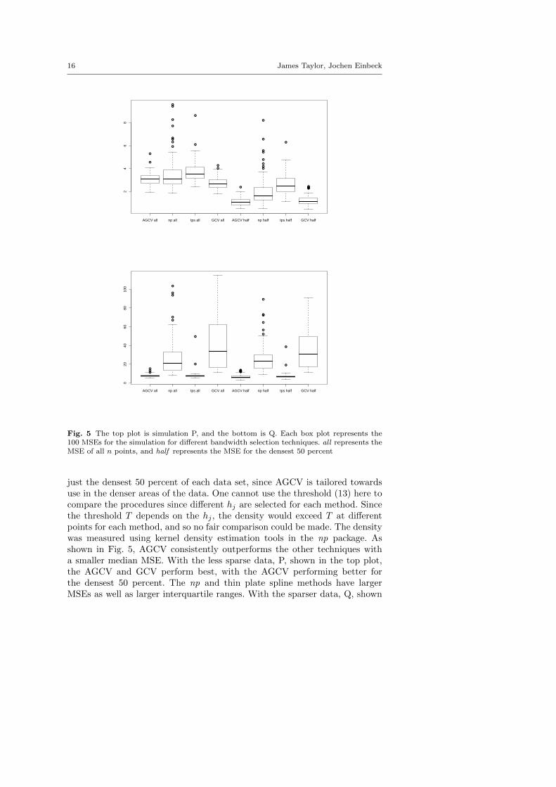
Fig. 5 The top plot is simulation P, and the bottom is Q. Each box plot represents the100 MSEs for the simulation for different bandwidth selection techniques. all represents theMSE of all n points, and half represents the MSE for the densest 50 percent

just the densest 50 percent of each data set, since AGCV is tailored towardsuse in the denser areas of the data. One cannot use the threshold (13) here tocompare the procedures since different hj are selected for each method. Sincethe threshold T depends on the hj , the density would exceed T at differentpoints for each method, and so no fair comparison could be made. The densitywas measured using kernel density estimation tools in the np package. Asshown in Fig. 5, AGCV consistently outperforms the other techniques witha smaller median MSE. With the less sparse data, P, shown in the top plot,the AGCV and GCV perform best, with the AGCV performing better forthe densest 50 percent. The np and thin plate spline methods have largerMSEs as well as larger interquartile ranges. With the sparser data, Q, shown


in the bottom plot, the AGCV and thin plate splines are the only techniqueswhose MSEs could be considered of a reasonable size given the magnitude ofthe response values. Out of these, AGCV is marginally better with a smallermedian, which again improves when only including the densest 50 percent ofthe data. The GCV and the np least squares cross-validation both performextremely poorly on this sparser data.

3.4 Notes on computational issues

– Throughout this study we have used the optim function on R, which usesthe Nelder-Mead algorithm, detailed in Nelder and Mead (1965), to carryout the minimization of the (A)GCV functions.

– AGCV is still sensitive to the starting point specified for optim, and amore successful minimization is more likely if this point is chosen withcare. From experience it is observed that a starting point smaller than theactual minimum is often more successful, and it is sometimes helpful toperform the minimization more than once, using the result of the previousminimization as the new starting point. However, due to the nature ofoptim the selection of the overall minimum cannot be guaranteed. Thisis not a problem with AGCV itself, rather a problem of the minimizingtechnique selecting one of many minima, but not necessarily the smallest,as desired.

– Although AGCV is fast in comparison to GCV (using R), it is still time-consuming for d > 6, and a potential solution to this is to search for aconstant h = h1 = ... = hd, after standardizing the covariates.

4 Discussion

We have proposed two relatively simple measures which enable local linearsmoothing with high–dimensional data. The problem of “local neighbourhoodsbeing not local”, as usually reported in this setting, is circumvented by focus-ing on dense regions of the predictor space where reliable estimation, withrelatively small bandwidths, is achievable. It was demonstrated how such afeasible region is identified through a simple criterion based on the asymptoticinfluence function. A multivariate version of GCV, which uses a pilot regionto select a suitable diagonal bandwidth matrix, was also introduced.

The adjustments made to GCV here are made specifically in response toproblems encountered on R. In spite of this, it fits perfectly with the generalsolution to the curse of dimensionality expressed in this work, of excludingthe areas of low density from consideration. The points that are ignored inAGCV are sufficiently isolated that they would never be accepted by T . Inthis way, the hj selected by AGCV are more suited to the points accepted bythe threshold, by not having to take into account other points excluded byit. This conclusion is supported by the strong performance of AGCV in the


densest 50 percent of the data in the simulation study. Our overall attitude ofignoring data in sparse regions seems successful in creating a reliable smoothingstrategy elsewhere.

A variable bandwidth matrix H(x), similar to that described for kerneldensity estimation by Sain (2002), could be beneficial for multivariate kernelregression too, but this would be computationally costly. AGCV can be seenas the first step towards a variable bandwidth matrix, in the sense that itselects bandwidths hj suitable for a proportion of the data, determined by r.

It is important to reflect on the relevance of the techniques presented hereto data sets of very high dimension. We have tested our methods successfullywith data of dimension up to d = 16, and we did not identify an immediateobstacle which would prevent us from going further than that. However, ascan be seen from Table 1, the parameter ρ increases very strongly for higherdimensions. While this increase has been demonstrated to be appropriate,often n will not be large enough to satisfy this threshold. In other words,for very large d, we are likely to encounter situations where practically thewhole data set will be eliminated by the threshold, unless n is large enoughto counterbalance the effect of ρ. Data sets which have such properties stilldo exist, and are most likely to be generated by numerical simulation fromcomplex computer models.

One timely question would be whether the proposed techniques could dealwith situations where d > n, as encountered for genomic data in computationalbiology, or even with functional data (Ramsay and Silverman, 1997), whichcan be considered to be of quasi-infinitely dimensional character. Though onemay feel encouraged by results such as in Ferraty and Vieu (2006), who demon-strate how to adapt multivariate local constant regression to functional data,we hit an obstacle when taking the step to local linear regression: by construc-tion, at least n = d + 1 data points are locally (and, hence, globally) neededto fit a hyperplane involving d + 1 parameters. Hence, for data sets of suchlarge dimension d, some form of variable selection or dimension reduction, asmentioned in the introduction, is necessary, before the methods proposed inthis paper can be applied. In the case of functional data, an attractive pre–processing tool which identifies the design points with the “greatest predictiveinfluence”, was suggested by Ferraty, Hall and Vieu (2010).

An issue that we did not discuss in this paper is the shape of the spaceST = {x|f(x) ≥ T}. Generally, this space does not need to be either convex orconnected, but we found it usually to be of a reasonably well–behaved shape(i.e., not consisting of lots of scattered pieces, etc.) in practice, provided thata sensible bandwidth is chosen for the initial density estimator. The space STwill be compact by construction. This is an important property as it enablesaccess to boundary measures for ST (for instance, for d = 3, the surface area).The reader is referred to a recent paper by Armendariz, Cuevas, and Fraiman(2009) for recent advances in this respect.

Acknowledgements Many thanks to Marco Apollonio, of the Dept. of Zoology and Evo-lutionary Genetics, University of Sassari, and Tom Mason, of the School of Biological and


Biomedical Sciences, University of Durham, for permitting us to use the chamois data. Theauthors are also grateful to two anonymous referees for their helpful comments, particularlyfor pointing us to interesting literature which enabled us to motivate our methods from awider perspective than in the original version.

A Derivation of (11)

Take expression (9)

infl(Xi) = |H|−1/2eT1 (XTWX)−1e1K(0)

where X = X{x=Xi} and W = W{x=Xi}. Now

XTWX = ∑ni=1KH(Xi − x)

∑ni=1KH(Xi − x)(Xi − x)T∑n

i=1KH(Xi − x)(Xi − x)∑n

i=1KH(Xi − x)(Xi − x)(Xi − x)T

Approximating each of these entries;

n∑i=1

KH(Xi − x) = E

(n∑

i=1

KH(Xi − x)

)+Op

√√√√Var

(n∑

i=1

KH(Xi − x)

) . (20)

Since the Xi are i.i.d.

E

(n∑

i=1

KH(Xi − x)

)= n

∫KH(t− x)f(t)dt = n

∫|H|−1/2K(H−1/2(t− x))f(t)dt

Then using the substitution u = (u1, ..., ud)T = H−1/2(t − x) and Taylor’s theorem, onegets

n

∫|H|−1/2K(u)f(x + H1/2u)|H|1/2du = n

∫K(u)f(x + H1/2u)du

= n

(f(x)

∫K(u)du + o(1)

).

For the variance term,

Var

(n∑

i=1

KH(Xi − x)

)= n

[E((KH(X1 − x))2

)− (E (KH(X1 − x)))2

]

= n

[∫|H|−1K2(H−1/2(t− x))f(t)dt−

(∫|H|−1/2K(H−1/2(t− x))f(t)dt

)2]

Then using the same substitution as above

Var

(n∑

i=1

KH(Xi − x)

)= n

[|H|−1/2f(x)

(∫K2(u)du + o(1)

)−(f(x)

∫K(u)du + o(1)

)2]

= n|H|−1/2

[f(x)

∫K2(u)du + o(1)

]= o(n2)


Using (20)

n∑i=1

KH(Xi − x) = n

(f(x)

∫K(u)du + o(1)

)+Op

(√o(n2)

)

= n

(f(x)

∫K(u)du + op(1)

). (21)

Similarly

E

(n∑

i=1

KH(Xi − x)(Xi − x)

)

= nH1/2

∫uK(u)f(x + H1/2u)du

= nH1/2

[f(x)

∫uK(u)du +

∫uuTK(u)H1/2(∇f(x) + o(1))du

]= nH1/2f(x)

∫uK(u)du + nH1/2

(∫uuTK(u)du

)H1/2∇f(x) (1 + o(1))

and

n∑i=1

KH(Xi − x)(Xi − x)

= nH1/2f(x)

∫uK(u)du + nH1/2

(∫uuTK(u)du

)H1/2∇f(x) (1 + op(1)) . (22)

Similarly

n∑i=1

KH(Xi − x)(Xi − x)T

= nf(x)

∫uTK(u)duH1/2 + n∇f(x)TH1/2

(∫uuTK(u)du

)H1/2 (1 + op(1)) . (23)

Finally,

E

(n∑

i=1

KH(Xi − x)(Xi − x)(Xi − x)T

)

= n

∫|H|−1/2K(H−1/2(t− x))(t− x)(t− x)T f(t)dt

= n

∫|H|−1/2K(u)H1/2u(H1/2u)T f(x + H1/2u)|H|1/2du

= nH1/2

[(∫uuTK(u)du

)f(x) + o(1)

]H1/2

and

n∑i=1

KH(Xi − x)(Xi − x)(Xi − x)T

= nH1/2

[(∫uuTK(u)du

)f(x) + op(1)

]H1/2. (24)

So XTWX can be written as (21) (23)

(22) (24)

(25)


For (9) one needs the top left entry of the inverse of (25). For a general block matrix B, suchas this one, The Matrix Cookbook (Petersen & Pedersen, 2008) states that this is equivalentto, (B11 −B12B

−122 B21)−1. For (25),

(B11 −B12B−122 B21)

= n

(f(x)

∫K(u)du + op(1))

)−(

nf(x)

∫uTK(u)duH1/2 + n

(∇f(x)TH1/2

∫uuTK(u)duH1/2

)(1 + op(1))

)×(

nH1/2

((∫uuTK(u)du

)f(x) + op(1)

)H1/2

)−1

×(nH1/2f(x)

∫uK(u)du + nH1/2

(∫uuTK(u)du

)H1/2∇f(x) (1 + op(1))

)= n

(f(x)

∫K(u)du + op(1)

)− n

(f(x)

∫uTK(u)duH1/2 + op(1TH1/2)

)×(

n

(H1/2

(∫uuTK(u)du

)f(x)H1/2 + op(H)

))−1

× n(H1/2f(x)

∫uK(u)du + op(H1/21)

)(26)

Within (26), defining an as a sequence an = op(H), bn as a sequence bn = op(1) and cnas a sequence cn = O(H−1) one uses the Kailath Variant from the Matrix Cookbook tore-express the inverse. The Kailath Variant states that (A + BC)−1 = A−1 −A−1B(I +

CA−1B)−1CA−1. Here, say A = H1/2(∫

uuTK(u)du)f(x)H1/2, B = an and C = I.

Hence (H1/2

(∫uuTK(u)du

)f(x)H1/2 + op(H)

)−1

=

(H1/2

(∫uuTK(u)du

)f(x)H1/2

)−1

− cnan(I + cnan)−1cn

=

(H1/2

(∫uuTK(u)du

)f(x)H1/2

)−1

− bncn

=

(H1/2

(∫uuTK(u)du

)f(x)H1/2

)−1

+ op(H−1)

= H−1/2

(∫uuTK(u)du

)−1

(f(x))−1H−1/2 + op(H−1)

Replacing this in (26) one gets

(B11 −B12B−122 B21)

= n

(f(x)

∫K(u)du + op(1)

)− n

(f(x)

∫uTK(u)duH1/2 + op(1TH1/2)

)×

1

n

(H−1/2

(∫uuTK(u)du

)−1

(f(x))−1H−1/2 + op(H−1)

)× n

(H1/2f(x)


)

= n

(f(x)

∫K(u)du + op(1)

)−(∫

uTK(u)du

(∫uuTK(u)du

)−1

H−1/2 + op(1TH−1/2)

)× n

(H1/2f(x)


)

= n

[f(x)

[∫K(u)du−

∫uTK(u)du

(∫uuTK(u)du

)−1 ∫uK(u)du

]+ op(1)

]


Applying the inverse, one obtains an approximation for the top left entry of the inverse of(25)

(B11 −B12B−122 B21)−1

= n−1(f(x))−1

[∫K(u)du−

∫uTK(u)du

(∫uuTK(u)du

)−1 ∫uK(u)du

]−1

+ op(n−1)

Substituting this in (9) gives the result

infl(x) =K(0)

nf(x)|H|1/2

[∫K(u)du−

∫uTK(u)du

(∫uuTK(u)du

)−1 ∫uK(u)du

]−1

+ op(n−1|H|−1/2)

The above calculations for the asymptotic approximation to (XTWX)−1 are moregeneral compared to those in other sources, such as Ruppert and Wand (1994), since herethe kernel moments are not assumed to vanish. This allows for non-symmetric kernels, aswell as handling of boundary points.

References

1. ARMENDARIZ, I., CUEVAS, A., and FRAIMAN, R. (2009). Nonparametric estimationof boundary measures and related functionals: Asymptotic properties. Adv. Appl. Prob.41, 311–322.

2. CANDES, E. and TAO, T. (2007). The Dantzig selector: Statistical estimation when pis much larger than n. Ann. Statist. 35, 2313–2351.

3. CLEVELAND, W.S. and DEVLIN, S.J. (1988). Locally weighted regression: an approachto regression analysis by local fitting. J. Amer. Statist. Assoc. 83, 596–610.

4. CRAVEN, P. and WAHBA, G. (1979). Smoothing noisy data with spline functions:estimating the correct degree of smoothing by the method of generalized cross-validation.Numer. Math. 3, 377–403.

5. CUMMING, J.A. and WOOFF, D.A. (2007). Dimension reduction via principal variables.Computational Statistics and Data Analysis 52, 550-565.

6. DUCHON, J. (1977). Splines minimizing rotation-invariant semi-norms in Sobolevspaces. Constructive Theory of Functions of Several Variables, W. Schempp and K. Zeller,eds., 85–100. Springer-Verlag, Berlin.

7. FAN, J. (1993). Local linear regression smoothers and their minimax efficiencies. Ann.Statist. 21, 196–216.

8. FERRATY, F., HALL, P. and VIEU, P. (2010). Most-predictive design points for func-tional data predictors. Biometrika 97, 807–824.

9. FERRATY, F., and VIEU, P. (2006). Nonparametric Functional Data Analysis. Springer,New York.

10. FOWLKES, E.B. (1986). Some diagnostics for binary logistic regression via smoothing(with discussion). Proceedings of the Statistical Computing Section, American StatisticalAssociation 1, 54–56.

11. HASTIE, T. and LOADER, C.R. (1993a). Rejoinder to: “Local regression: Automatickernel carpentry.” Statistical Science 8, 139–143.

12. HASTIE, T. and LOADER, C.R. (1993b). Local regression: Automatic kernel carpentry.Statistical Science 8, 120–129.

13. HASTIE, T. and TIBSHIRANI, R. (1990). Generalized Additive Models. Chapman andHall, London.

14. HASTIE, T., TIBSHIRANI, R. and FRIEDMAN, J. (2001). The Elements of StatisticalLearning. Springer, New York.

15. HAYFIELD, T. and RACINE, J.S. (2008). Nonparametric Econometrics: The np pack-age. Journal of Statistical Software 27, 1–32.

16. LI, Q. and RACINE, J.S. (2003). Nonparametric estimation of distributions with cate-gorical and continuous data. Journal of Multivariate Analysis 86, 266–292.


17. LAFFERTY, J. and WASSERMAN, L. (2008). Rodeo: sparse, greedy nonparametricregression. Ann. Statist. 36, 28–63.

18. LOADER, C.R. (1999). Local Regression and Likelihood. Springer, New York.19. NELDER, J.A. and MEAD, R. (1965). A simplex method for function minimization.Computer Journal 7, 308–313.

20. PETERSEN, K.B. and PEDERSEN, M.S. (2008). The Matrix Cookbook.http://matrixcookbook.com/.

21. R DEVELOPMENT CORE TEAM (2010). R: A Language and Environment for Sta-tistical Computing. R Foundation for Statistical Computing, Vienna, Austria.

22. RUPPERT, D. and WAND, M.P. (1994). Multivariate locally weighted least squaresregression. Ann. Statist. 22, 1346–1370.

23. SAIN, S.R. (2002). Multivariate locally adaptive density estimation. ComputationalStatistics and Data Analysis 39, 165–186.

24. SCOTT, D.W. (1992). Multivariate Density Estimation. Wiley, New York.25. STONE, C.J. (1980). Optimal rates of convergence for nonparametric estimators. Ann.Statist. 8, 1348–1360.

26. TIBSHIRANI, R. (1996). Regression shrinkage and selection via the lasso. J. Roy.Statist. Soc. Ser. B 58, 267–288.

27. VIDAURRE, D., BIELZA, C. and LARRANAGA, P. (2011). Lazy lasso for local re-gression. Computational Statistics, DOI 10.1007/s00180-011-0274-0.

Challenging the curse of dimensionality in multivariate local linear regression

Documents