Perspectivesoncharacteristicsbased curse-of … curse-of-dimensionality-freenumericalapproachesfor solvingHamilton–Jacobiequations Ivan Yegorov1 y, Peter Dower1 November 10, 2017

Perspectives on characteristics basedcurse-of-dimensionality-free numerical approaches for

solving Hamilton–Jacobi equations

Ivan Yegorov1 ∗ †, Peter Dower1

November 10, 2017

Abstract

This paper extends the considerations of the works [1, 2] regarding curse-of-dimensio-nality-free numerical approaches to solve certain types of Hamilton–Jacobi equations aris-ing in optimal control problems, differential games and elsewhere. A rigorous formula-tion and justification for the extended Hopf–Lax formula of [2] is provided together withnovel theoretical and practical discussions including useful recommendations. By using themethod of characteristics, the solutions of some problem classes under convexity/concavityconditions on Hamiltonians (in particular, the solutions of Hamilton–Jacobi–Bellman equa-tions in optimal control problems) are evaluated separately at different initial positions.This allows for the avoidance of the curse of dimensionality, as well as for choosing arbi-trary computational regions. The corresponding feedback control strategies are obtainedat selected positions without approximating the partial derivatives of the solutions. Theresults of numerical simulations demonstrate the high potential of the proposed techniques.It is also pointed out that, despite the indicated advantages, the related approaches stillhave a limited range of applicability, and their extensions to Hamilton–Jacobi–Isaacs equa-tions in zero-sum two-player differential games are currently developed only for sufficientlynarrow classes of control systems. That is why further extensions are worth investigating.

Keywords: optimal control, differential games, feedback strategies, Hamilton–Jacobi equa-tions, minimax/viscosity solutions, Pontryagin’s principle, method of characteristics, grid-basedmethods, curse of dimensionality

1 IntroductionIt is well known that first-order Hamilton–Jacobi equations constitute a central theoreticalframework to describe feedback (closed-loop) solutions of deterministic continuous-time optimal

1 The University of Melbourne, Department of Electrical and Electronic Engineering, Parkville Campus,Melbourne, Victoria 3010, Australia† Corresponding author. E-mail: [email protected]∗ Also known as Ivan Egorov

1

arX

iv:1

711.

0331

4v1

[m

ath.

OC

] 9

Nov

201

7

control problems and differential games [3–8]. A complete analytical investigation of theseequations is provided only for rather specific problems. Most of the widely used numericalapproaches, such as finite-difference schemes [6,9–15], semi-Lagrangian schemes [7,15–18], levelset methods [19–25], etc., require dense state space discretizations, and their computational costgrows exponentially with the increase of the state space dimension n, so that they in generalbecome almost inapplicable for n > 4. The related circumstances were referred to as the curseof dimensionality by R. Bellman [26, 27]. Thus, it is relevant to develop techniques that canhelp to avoid the curse of dimensionality for nontrivial problems.

In [28–35], several approaches for overcoming the curse of dimensionality through the ad-vanced framework of max-plus algebra and analysis were proposed. They work for specificclasses of nonlinear optimal control problems. For example, the methods of [28–32] can beapplied if the Hamiltonian is represented as the maximum or minimum of a finite numberof elementary Hamiltonians corresponding to linear-quadratic optimal control problems. De-spite the evident potential of mitigating the curse of dimensionality, some practical issues oftenappear when implementing such methods, i. e., the curse of complexity may be a formidablebarrier (see [28, §7.5], [29, Section 6], [30, Sections IV,VI], [31, Section 9], [32]).

Another promising direction is representing the solutions of Hamilton–Jacobi equations ina way that reduces their computation at isolated positions to finite-dimensional optimization(throughout the current paper, a position means a vector of the form (t, x), where t is atime and x is a state at this time). As opposed to grid-based numerical approaches, thisallows the solutions to be evaluated separately at different initial positions. Then the curse ofdimensionality can be avoided, and it becomes easy to arrange parallel computations. However,there may still appear the curse of complexity when constructing global (or semi-global) solutionapproximations, and sparse grid techniques [36] can be useful for this purpose if the state spacedimension is not too high (n 6 6).

For state-independent Hamiltonians under certain conditions, the sought-after representa-tions are given by Hopf–Lax and Hopf formulae [3,37–40]. The related practical considerationscan be found in [1]. In [2], some extensions of these representations to problems with state-dependent Hamiltonians were conjectured. The method of characteristics (or, more precisely, ageneralization of its classical form) for first-order Hamilton–Jacobi equations played a key rolethere.

This paper encompasses the following goals:

• to give a rigorous formulation and justification for the first main conjecture of [2] (i. e., forthe extended Hopf–Lax formula) concerning Hamilton–Jacobi equations whose Hamiltoni-ans are convex or concave with respect to the adjoint variable (Hamilton–Jacobi–Bellmanequations for optimal control problems form a typical subclass here);

• to provide novel theoretical and practical discussions including useful recommendations,as well as a detailed numerical investigation;

• to point out the limited range of applicability of the related approaches, and, in particular,to highlight principal issues in their extension to Hamilton–Jacobi–Isaacs equations (forzero-sum two-player differential games) whose Hamiltonians are in general nonconvex andnonconcave with respect to the adjoint variable.

Note also the works [41–44] that used the method of characteristics in order to derivefundamental representations for the minimax/viscosity solutions of Hamilton–Jacobi equations

2

under specific assumptions including some smoothness and convexity/concavity conditions onHamiltonians. The boundary value problems for characteristic systems of ordinary differentialequations (describing the dynamics of the state and adjoint variables along characteristic curves)were involved there. However, the related computational algorithms as formulated in [45–47]are rather complicated and also suffer from the curse of dimensionality.

For simplifying the numerical implementation of such characteristics approaches and makingthem curse-of-dimensionality-free, it is crucial to parametrize characteristic fields not withrespect to the terminal state but with respect to the initial adjoint vector [2]. This allowsCauchy problems for characteristic systems to be solved instead of boundary value problemsthat might have multiple solutions and thereby cause the practical dilemma of obtaining aneeded solution. The theoretical constructions of the current work employ this idea, with theconsiderations of [2] serving as a primary motivation.

Our paper is organized as follows. In Section 2, a general Hamilton–Jacobi equation undersmoothness and convexity/concavity conditions on the Hamiltonian is considered. Under cer-tain assumptions, we establish a representation of its minimax/viscosity solution through theparametrization of the characteristic field with respect to the initial adjoint vector. Section 3develops that for Hamilton–Jacobi–Bellman equations in optimal control problems without theaforementioned smoothness conditions on Hamiltonians. It also contains important practicalrecommendations and a detailed analysis for Eikonal type partial differential equations. In Sec-tion 4 and Appendix, we provide an overview of existing curse-of-dimensionality-free techniquesfor solving particular classes of Hamilton–Jacobi–Isaacs equations in linear zero-sum two-playerdifferential games (besides, most of the introduced results and examples were not available inEnglish-language scientific literature according to our knowledge). This helps to better under-stand the limited range of applicability of the curse-of-dimensionality-free approaches in ourstudy and others. The results of our numerical investigation are presented in Section 5.

Let us also indicate some basic notations that are used throughout the paper:

• given integer numbers j1 and j2 > j1, we write i = j1, j2 instead of i = j1, j1 + 1, . . . , j2;

• given j ∈ N, the origin in Rj is denoted by Oj or simply 0 (if there is no confusion withzeros in other spaces), ‖ · ‖ = ‖ · ‖j = ‖ · ‖Rj is the Euclidean norm in Rj (some otherkinds of vector norms are specified in Section 4), ‖ · ‖Rj×j is the matrix norm in Rj×j

induced by the Euclidean vector norm, and, for vectors v1, v2 ∈ Rj, we write v1 ↑↑ v2 ifthey have the same direction, i. e., if v2 = αv1 for some α > 0;

• if a vector variable ξ consists of some arguments of a map F = F (. . . , ξ, . . .), thenDξF denotes the standard (Fréchet) derivative of F with respect to ξ, and DF is thestandard derivative with respect to the vector of all arguments (the exact definitions ofthe derivatives depend on the domain and range of F );

• given a function F : Ξ1 → R, the sets of its global minimizers and maximizers on Ξ ⊆ Ξ1

are denoted by Arg minξ∈Ξ F (ξ) and Arg maxξ∈Ξ F (ξ), respectively, while the criteria forthe related optimization problems are written as F (ξ) −→ infξ∈Ξ (or F (ξ) −→ minξ∈Ξ

if the minimum is reached), F (ξ) −→ supξ∈Ξ (or F (ξ) −→ maxξ∈Ξ if the maximum isreached);

• the convex hull of a set M in some linear space is denoted by conv M, and the effectivedomain of a convex function F : M → R ∪ {+∞} is written as

dom Fdef= {ξ ∈M : F (ξ) < +∞};

3

• the Minkowski sum of two sets M1,M2 in some linear space is defined as

M1 +M2def= {ξ1 + ξ2 : ξ1 ∈M1, ξ2 ∈M2},

and, if M1 = {ξ} is singleton, it is convenient to write ξ +M2 instead of {ξ}+M2.

Other notations are introduced as needed.

2 A curse-of-dimensionality-free characteristics approachfor solving Hamilton–Jacobi equations undersmoothness and convexity/concavity conditions onHamiltonians

Given a fixed finite time horizon T ∈ (0,+∞), consider the Cauchy problem for a generalHamilton–Jacobi equation

∂V (t, x)

∂t+ H(t, x, DxV (t, x)) = 0, (t, x) ∈ (0, T )× Rn, (1)

V (T, x) = σ(x), x ∈ Rn. (2)

Let the following basic conditions hold.

Assumption 2.1. The following properties hold:

1) the Hamiltonian

[0, T ]× Rn × Rn 3 (t, x, p) 7−→ H(t, x, p) ∈ R (3)

is continuous;

2) there exist positive constants C1, C2 such that, for all (t, x) ∈ [0, T ]×Rn and p′, p′′ ∈Rn, we have

|H(t, x, p′) − H(t, x, p′′)| 6 C1 (1 + ‖x‖) ‖p′ − p′′‖, (4)

and|H(t, x, 0)| 6 C2 (1 + ‖x‖); (5)

3) for any compact set K ⊂ Rn, there exists a number C3(K) > 0 such that, for all(t, p) ∈ [0, T ]× Rn and x′, x′′ ∈ K, we have

|H(t, x′, p) − H(t, x′′, p)| 6 C3(K) (1 + ‖p‖) ‖x′ − x′′‖; (6)

4) the terminal functionRn 3 x 7−→ σ(x) ∈ R (7)

is continuous.

4

For the considerations of this section, it is convenient to understand a generalized solutionof the problem (1), (2) in the minimax sense [3, Chapter II]. A continuous function

(0, T ]× Rn 3 (t, x) 7−→ V (t, x) ∈ R

is called a minimax solution of (1), (2) if it fulfills the terminal condition (2) and the following:for any (t0, x0) ∈ (0, T ) × Rn and p ∈ Rn, there exist a time t1 ∈ (t0, T ) and a Lipschitzcontinuous function

[t0, t1] 3 t 7−→ (x(t), z(t)) ∈ Rn × Rsuch that

(x(t0), z(t0)) = (x0, V (t0, x0)), z(t) = V (t, x(t))

for all t ∈ [t0, t1] and the equation

z(t) = 〈x(t), p〉 − H(t, x(t), p)

holds for almost every t ∈ [t0, t1].Let us introduce a fundamental result on the existence of a unique minimax solution of

(1), (2).

Theorem 2.2. [3, Theorem II.8.1] Under Assumption 2.1, there exists a unique minimaxsolution of the Cauchy problem (1), (2).

Remark 2.3. In the literature concerning Hamilton–Jacobi equations, the notion of minimaxsolutions is used less frequently than the notion of viscosity solutions [4–8], although they arein principle equivalent. Indeed, due to [3, §I.4] and [6, §II.4], the unique minimax solutionin Theorem 2.2 coincides with the unique viscosity solution of the formally rewritten Cauchyproblem −

∂V (t, x)

∂t− H(t, x, DxV (t, x)) = 0, (t, x) ∈ (0, T )× Rn,

V (T, x) = σ(x), x ∈ Rn.(8)

Note also that, if the problem (1), (2) is considered not in the whole set (0, T ]×Rn but just in thesubregion (0, T ]×G with an open domain G ⊂ Rn, then the corresponding minimax/viscositysolution can be similarly defined.

Let us briefly describe an approach for representing the minimax solution of (1), (2) throughboundary value problems for the related characteristic system under some additional conditions(see, for instance, [3, §II.10.5, §II.10.6] and [44, §7.3]).

First, the convexity of the Hamiltonian with respect to the adjoint variable is required.

Assumption 2.4. For any (t, x) ∈ [0, T ]×Rn, the reduction Rn 3 p 7−→ H(t, x, p) is convex.

Let (t, x) ∈ [0, T ]× Rn. For H(t, x, ·), introduce the conjugate function (convex dual)

Rn 3 f 7−→ H∗(t, x, f)def= sup

p∈Rn

{〈f, p〉 − H(t, x, p)} (9)

and its effective domain

domH∗(t, x, ·) = {f ∈ Rn : H∗(t, x, f) < +∞} . (10)

By virtue of the condition (4) and Assumption 2.4, the set (10) is nonempty, bounded andconvex (recall the affine support properties of convex functions [48, 49]).

For the sake of simplicity, we also use the next technical assumption, even though it is infact not essential [3, §II.10.5].

5

Assumption 2.5. There exists a continuous function

[0, T ]× Rn 3 (t, x) 7−→ β(t, x) ∈ R

such that

H∗(t, x, f) 6 β(t, x) ∀ f ∈ domH∗(t, x, ·) ∀ (t, x) ∈ [0, T ]× Rn.

Consider the differential inclusion

(x(t), z(t)) ∈ {(f, g) ∈ Rn × R : f ∈ domH∗(t, x(t), ·),H∗(t, x(t), f) 6 g 6 β(t, x(t))}.

(11)

For (t0, x0) ∈ [0, T ]× Rn, let S(t0, x0) be the set of its trajectories

[0, T ] 3 t 7−→ (x(t), z(t)) ∈ Rn × R

satisfying the conditionsx(t0) = x0, z(T ) = σ(x(T )), (12)

and introduce the functional

γ(t0, x(·), z(·)) def= σ(x(T )) −

T∫t0

z(t) dt ∀ (x(·), z(·)) ∈ S(t0, x0). (13)

Theorem 2.6. [3, §II.10.5] Under Assumptions 2.1, 2.4, 2.5, the function

V (t0, x0)def= max

(x(·), z(·)) ∈ S(t0,x0)γ(t0, x(·), z(·)) ∀ (t0, x0) ∈ [0, T ]× Rn (14)

is the unique minimax solution of the Cauchy problem (1), (2).

Remark 2.7. If convexity is replaced with concavity in Assumption 2.4, then a similar char-acterization of the minimax solution of (1), (2) can be obtained, and minimization appearsinstead of maximization in (14).

Now impose some smoothness conditions on the Hamiltonian and terminal function.

Assumption 2.8. The Hamiltonian (3) and terminal function (7) are continuously differen-tiable, and the derivatives DtxH, DtpH exist for all (t, x, p) ∈ [0, T ]× Rn × Rn.

The next statement can be derived by using basic results of convex analysis [48, 49].

Proposition 2.9. Under Assumptions 2.1, 2.4, 2.5, 2.8, the effective domain (10) can be rep-resented as

domH∗(t, x, ·) = conv {DpH(t, x, ψ) : ψ ∈ Rn}∀ (t, x) ∈ [0, T ]× Rn,

(15)

and the following formula also holds:

H∗(t, x, DpH(t, x, ψ)) = 〈ψ,DpH(t, x, ψ)〉 − H(t, x, ψ)

∀ (t, x, ψ) ∈ [0, T ]× Rn × Rn.(16)

6

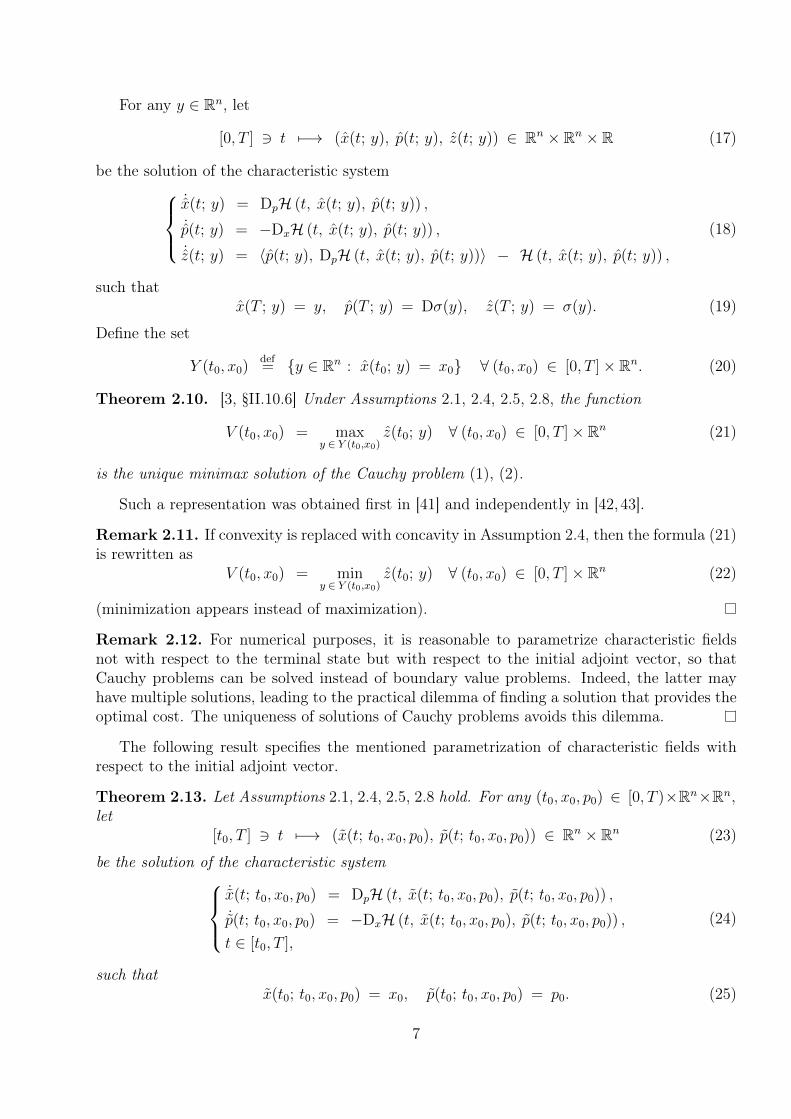
For any y ∈ Rn, let

[0, T ] 3 t 7−→ (x(t; y), p(t; y), z(t; y)) ∈ Rn × Rn × R (17)

be the solution of the characteristic system˙x(t; y) = DpH (t, x(t; y), p(t; y)) ,

˙p(t; y) = −DxH (t, x(t; y), p(t; y)) ,

˙z(t; y) = 〈p(t; y), DpH (t, x(t; y), p(t; y))〉 − H (t, x(t; y), p(t; y)) ,

(18)

such thatx(T ; y) = y, p(T ; y) = Dσ(y), z(T ; y) = σ(y). (19)

Define the set

Y (t0, x0)def= {y ∈ Rn : x(t0; y) = x0} ∀ (t0, x0) ∈ [0, T ]× Rn. (20)

Theorem 2.10. [3, §II.10.6] Under Assumptions 2.1, 2.4, 2.5, 2.8, the function

V (t0, x0) = maxy ∈ Y (t0,x0)

z(t0; y) ∀ (t0, x0) ∈ [0, T ]× Rn (21)

is the unique minimax solution of the Cauchy problem (1), (2).

Such a representation was obtained first in [41] and independently in [42,43].

Remark 2.11. If convexity is replaced with concavity in Assumption 2.4, then the formula (21)is rewritten as

V (t0, x0) = miny ∈ Y (t0,x0)

z(t0; y) ∀ (t0, x0) ∈ [0, T ]× Rn (22)

(minimization appears instead of maximization).

Remark 2.12. For numerical purposes, it is reasonable to parametrize characteristic fieldsnot with respect to the terminal state but with respect to the initial adjoint vector, so thatCauchy problems can be solved instead of boundary value problems. Indeed, the latter mayhave multiple solutions, leading to the practical dilemma of finding a solution that provides theoptimal cost. The uniqueness of solutions of Cauchy problems avoids this dilemma.

The following result specifies the mentioned parametrization of characteristic fields withrespect to the initial adjoint vector.

Theorem 2.13. Let Assumptions 2.1, 2.4, 2.5, 2.8 hold. For any (t0, x0, p0) ∈ [0, T )×Rn×Rn,let

[t0, T ] 3 t 7−→ (x(t; t0, x0, p0), p(t; t0, x0, p0)) ∈ Rn × Rn (23)

be the solution of the characteristic system˙x(t; t0, x0, p0) = DpH (t, x(t; t0, x0, p0), p(t; t0, x0, p0)) ,

˙p(t; t0, x0, p0) = −DxH (t, x(t; t0, x0, p0), p(t; t0, x0, p0)) ,

t ∈ [t0, T ],

(24)

such thatx(t0; t0, x0, p0) = x0, p(t0; t0, x0, p0) = p0. (25)

7

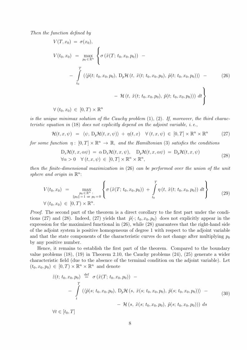
Then the function defined by

V (T, x0) = σ(x0),

V (t0, x0) = maxp0 ∈Rn

σ (x(T ; t0, x0, p0)) −

−T∫

t0

(〈p(t; t0, x0, p0), DpH (t, x(t; t0, x0, p0), p(t; t0, x0, p0))〉 −

− H (t, x(t; t0, x0, p0), p(t; t0, x0, p0))) dt

∀ (t0, x0) ∈ [0, T )× Rn

(26)

is the unique minimax solution of the Cauchy problem (1), (2). If, moreover, the third charac-teristic equation in (18) does not explicitly depend on the adjoint variable, i. e.,

H(t, x, ψ) = 〈ψ, DpH(t, x, ψ)〉 + η(t, x) ∀ (t, x, ψ) ∈ [0, T ]× Rn × Rn (27)

for some function η : [0, T ]× Rn → R, and the Hamiltonian (3) satisfies the conditions

DxH(t, x, αψ) = αDxH(t, x, ψ), DpH(t, x, αψ) = DpH(t, x, ψ)

∀α > 0 ∀ (t, x, ψ) ∈ [0, T ]× Rn × Rn,(28)

then the finite-dimensional maximization in (26) can be performed over the union of the unitsphere and origin in Rn:

V (t0, x0) = maxp0 ∈Rn :

‖p0‖= 1 or p0 = 0

σ (x(T ; t0, x0, p0)) +

T∫t0

η (t, x(t; t0, x0, p0)) dt

∀ (t0, x0) ∈ [0, T )× Rn.

(29)

Proof. The second part of the theorem is a direct corollary to the first part under the condi-tions (27) and (28). Indeed, (27) yields that p(·; t0, x0, p0) does not explicitly appear in theexpression for the maximized functional in (26), while (28) guarantees that the right-hand sideof the adjoint system is positive homogeneous of degree 1 with respect to the adjoint variableand that the state components of the characteristic curves do not change after multiplying p0

by any positive number.Hence, it remains to establish the first part of the theorem. Compared to the boundary

value problems (18), (19) in Theorem 2.10, the Cauchy problems (24), (25) generate a widercharacteristic field (due to the absence of the terminal condition on the adjoint variable). Let(t0, x0, p0) ∈ [0, T )× Rn × Rn and denote

z(t; t0, x0, p0)def= σ (x(T ; t0, x0, p0)) −

−T∫t

(〈p(s; t0, x0, p0), DpH (s, x(s; t0, x0, p0), p(s; t0, x0, p0))〉 −

− H (s, x(s; t0, x0, p0), p(s; t0, x0, p0))) ds

∀t ∈ [t0, T ]

(30)

8

(if t = t0, this is the expression for the maximized functional in (26)). We have

z(T ; t0, x0, p0) = σ (x(T ; t0, x0, p0)) (31)

and˙z(t; t0, x0, p0) = 〈p(t; t0, x0, p0), DpH (t, x(t; t0, x0, p0), p(t; t0, x0, p0))〉 −

− H (t, x(t; t0, x0, p0), p(t; t0, x0, p0))

∀t ∈ [t0, T ].

(32)

Consider also the solution (23) to (24), (25). According to Theorem 2.6, it suffices to show that(x(·; t0, x0, p0), z(·; t0, x0, p0)) is a solution of the differential inclusion (11) almost everywhereon [t0, T ] (the related initial and terminal conditions (12) are trivially satisfied by virtue of (25)and (31)). The formulae (15) and (16) in Proposition 2.9 can be used for this purpose. From(24) and (15), we get

˙x(t; t0, x0, p0) = DpH (t, x(t; t0, x0, p0), p(t; t0, x0, p0))

∈ domH∗ (t, x(t; t0, x0, p0), ·)(33)

for almost every t ∈ [t0, T ]. Due to (32) and (16), we obtain

˙z(t; t0, x0, p0) = H∗ (t, x(t; t0, x0, p0), DpH (t, x(t; t0, x0, p0), p(t; t0, x0, p0))) (34)

for all t ∈ [t0, T ]. Finally, the sought-after property directly follows from (33) and (34).

Remark 2.14. The representation (27) is typical for many optimal control problems withsmooth Hamiltonians (see Section 3).

Remark 2.15. For optimal control problems with smooth Hamiltonians, the second conditionin (28) appears to be rather strict, but it allows an extension to a wide class of optimal controlproblems with Mayer cost functionals and nonsmooth Hamiltonians (see Theorem 3.8).

3 A curse-of-dimensionality-free characteristics approachfor solving Hamilton–Jacobi–Bellman equations inoptimal control problems

Let G and U be sets in the state and control spaces, respectively. Consider the control system

x(t) = f(t, x(t), u(t)), t ∈ [t0, T ],

x(t0) = x0 ∈ G is fixed,T ∈ (0,+∞) and t0 ∈ [0, T ) are fixed,u(·) ∈ Ut0, T ,Ut0, T is the class of measurable functions defined on [t0, T ] with values in U,

(35)

and the optimization criterion

Jt0, T, x0(u(·)) def= σ(x(T ; t0, x0, u(·))) +

+

T∫t0

η(t, x(t; t0, x0, u(·)), u(t)) dt −→ infu(·) ∈ Ut0, T

,(36)

9

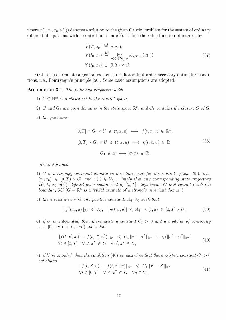
where x(·; t0, x0, u(·)) denotes a solution to the given Cauchy problem for the system of ordinarydifferential equations with a control function u(·). Define the value function of interest by

V (T, x0)def= σ(x0),

V (t0, x0)def= inf

u(·) ∈ Ut0, TJt0, T, x0(u(·))

∀ (t0, x0) ∈ [0, T )×G.

(37)

First, let us formulate a general existence result and first-order necessary optimality condi-tions, i. e., Pontryagin’s principle [50]. Some basic assumptions are adopted.

Assumption 3.1. The following properties hold:

1) U ⊆ Rm is a closed set in the control space;

2) G and G1 are open domains in the state space Rn, and G1 contains the closure G of G;

3) the functions

[0, T ]×G1 × U 3 (t, x, u) 7−→ f(t, x, u) ∈ Rn,

[0, T ]×G1 × U 3 (t, x, u) 7−→ η(t, x, u) ∈ R,

G1 3 x 7−→ σ(x) ∈ R

(38)

are continuous;

4) G is a strongly invariant domain in the state space for the control system (35), i. e.,(t0, x0) ∈ [0, T ) × G and u(·) ∈ Ut0, T imply that any corresponding state trajectoryx(·; t0, x0, u(·)) defined on a subinterval of [t0, T ] stays inside G and cannot reach theboundary ∂G (G = Rn is a trivial example of a strongly invariant domain);

5) there exist an a ∈ G and positive constants A1, A2 such that

‖f(t, a, u)‖Rn 6 A1, |η(t, a, u)| 6 A2 ∀ (t, u) ∈ [0, T ]× U ; (39)

6) if U is unbounded, then there exists a constant C1 > 0 and a modulus of continuityω1 : [0,+∞)→ [0,+∞) such that

‖f(t, x′, u′) − f(t, x′′, u′′)‖Rn 6 C1 ‖x′ − x′′‖Rn + ω1 (‖u′ − u′′‖Rm)

∀t ∈ [0, T ] ∀ x′, x′′ ∈ G ∀ u′, u′′ ∈ U ;(40)

7) if U is bounded, then the condition (40) is relaxed so that there exists a constant C1 > 0satisfying

‖f(t, x′, u) − f(t, x′′, u)‖Rn 6 C1 ‖x′ − x′′‖Rn

∀t ∈ [0, T ] ∀ x′, x′′ ∈ G ∀u ∈ U ;(41)

10

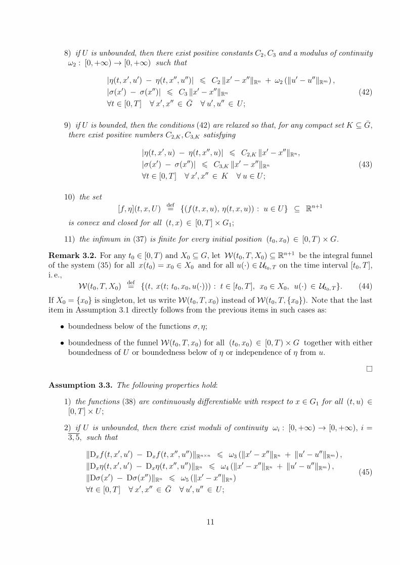
8) if U is unbounded, then there exist positive constants C2, C3 and a modulus of continuityω2 : [0,+∞)→ [0,+∞) such that

|η(t, x′, u′) − η(t, x′′, u′′)| 6 C2 ‖x′ − x′′‖Rn + ω2 (‖u′ − u′′‖Rm) ,

|σ(x′) − σ(x′′)| 6 C3 ‖x′ − x′′‖Rn

∀t ∈ [0, T ] ∀ x′, x′′ ∈ G ∀ u′, u′′ ∈ U ;

(42)

9) if U is bounded, then the conditions (42) are relaxed so that, for any compact set K ⊆ G,there exist positive numbers C2,K , C3,K satisfying

|η(t, x′, u) − η(t, x′′, u)| 6 C2,K ‖x′ − x′′‖Rn ,

|σ(x′) − σ(x′′)| 6 C3,K ‖x′ − x′′‖Rn

∀t ∈ [0, T ] ∀ x′, x′′ ∈ K ∀ u ∈ U ;

(43)

10) the set[f, η](t, x, U)

def= {(f(t, x, u), η(t, x, u)) : u ∈ U} ⊆ Rn+1

is convex and closed for all (t, x) ∈ [0, T ]×G1;

11) the infimum in (37) is finite for every initial position (t0, x0) ∈ [0, T )×G.

Remark 3.2. For any t0 ∈ [0, T ) and X0 ⊆ G, let W(t0, T,X0) ⊆ Rn+1 be the integral funnelof the system (35) for all x(t0) = x0 ∈ X0 and for all u(·) ∈ Ut0, T on the time interval [t0, T ],i. e.,

W(t0, T,X0)def= {(t, x(t; t0, x0, u(·))) : t ∈ [t0, T ], x0 ∈ X0, u(·) ∈ Ut0, T}. (44)

If X0 = {x0} is singleton, let us writeW(t0, T, x0) instead ofW(t0, T, {x0}). Note that the lastitem in Assumption 3.1 directly follows from the previous items in such cases as:

• boundedness below of the functions σ, η;

• boundedness of the funnel W(t0, T, x0) for all (t0, x0) ∈ [0, T )×G together with eitherboundedness of U or boundedness below of η or independence of η from u.

Assumption 3.3. The following properties hold:

1) the functions (38) are continuously differentiable with respect to x ∈ G1 for all (t, u) ∈[0, T ]× U ;

2) if U is unbounded, then there exist moduli of continuity ωi : [0,+∞) → [0,+∞), i =3, 5, such that

‖Dxf(t, x′, u′) − Dxf(t, x′′, u′′)‖Rn×n 6 ω3 (‖x′ − x′′‖Rn + ‖u′ − u′′‖Rm) ,

‖Dxη(t, x′, u′) − Dxη(t, x′′, u′′)‖Rn 6 ω4 (‖x′ − x′′‖Rn + ‖u′ − u′′‖Rm) ,

‖Dσ(x′) − Dσ(x′′)‖Rn 6 ω5 (‖x′ − x′′‖Rn)

∀t ∈ [0, T ] ∀ x′, x′′ ∈ G ∀ u′, u′′ ∈ U ;

(45)

11

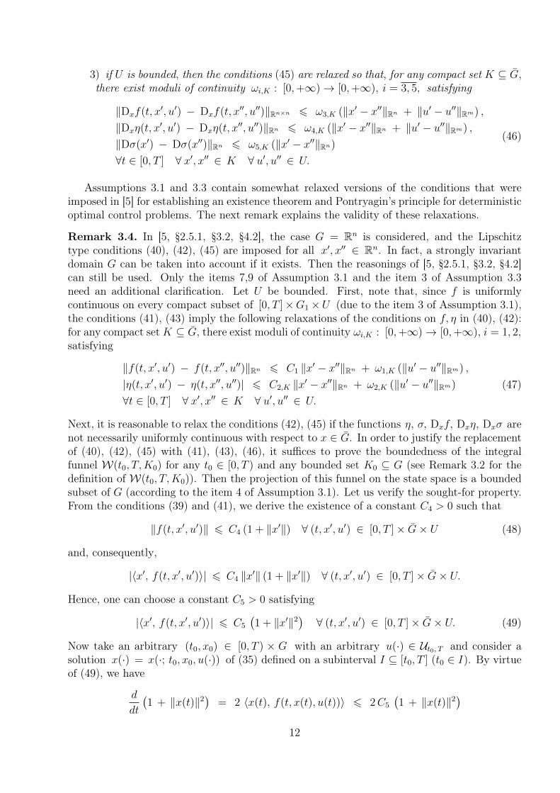
3) if U is bounded, then the conditions (45) are relaxed so that, for any compact set K ⊆ G,there exist moduli of continuity ωi,K : [0,+∞)→ [0,+∞), i = 3, 5, satisfying

‖Dxf(t, x′, u′) − Dxf(t, x′′, u′′)‖Rn×n 6 ω3,K (‖x′ − x′′‖Rn + ‖u′ − u′′‖Rm) ,

‖Dxη(t, x′, u′) − Dxη(t, x′′, u′′)‖Rn 6 ω4,K (‖x′ − x′′‖Rn + ‖u′ − u′′‖Rm) ,

‖Dσ(x′) − Dσ(x′′)‖Rn 6 ω5,K (‖x′ − x′′‖Rn)

∀t ∈ [0, T ] ∀ x′, x′′ ∈ K ∀ u′, u′′ ∈ U.

(46)

Assumptions 3.1 and 3.3 contain somewhat relaxed versions of the conditions that wereimposed in [5] for establishing an existence theorem and Pontryagin’s principle for deterministicoptimal control problems. The next remark explains the validity of these relaxations.

Remark 3.4. In [5, §2.5.1, §3.2, §4.2], the case G = Rn is considered, and the Lipschitztype conditions (40), (42), (45) are imposed for all x′, x′′ ∈ Rn. In fact, a strongly invariantdomain G can be taken into account if it exists. Then the reasonings of [5, §2.5.1, §3.2, §4.2]can still be used. Only the items 7,9 of Assumption 3.1 and the item 3 of Assumption 3.3need an additional clarification. Let U be bounded. First, note that, since f is uniformlycontinuous on every compact subset of [0, T ]×G1×U (due to the item 3 of Assumption 3.1),the conditions (41), (43) imply the following relaxations of the conditions on f, η in (40), (42):for any compact setK ⊆ G, there exist moduli of continuity ωi,K : [0,+∞)→ [0,+∞), i = 1, 2,satisfying

‖f(t, x′, u′) − f(t, x′′, u′′)‖Rn 6 C1 ‖x′ − x′′‖Rn + ω1,K (‖u′ − u′′‖Rm) ,

|η(t, x′, u′) − η(t, x′′, u′′)| 6 C2,K ‖x′ − x′′‖Rn + ω2,K (‖u′ − u′′‖Rm)

∀t ∈ [0, T ] ∀ x′, x′′ ∈ K ∀ u′, u′′ ∈ U.

(47)

Next, it is reasonable to relax the conditions (42), (45) if the functions η, σ, Dxf, Dxη, Dxσ arenot necessarily uniformly continuous with respect to x ∈ G. In order to justify the replacementof (40), (42), (45) with (41), (43), (46), it suffices to prove the boundedness of the integralfunnel W(t0, T,K0) for any t0 ∈ [0, T ) and any bounded set K0 ⊆ G (see Remark 3.2 for thedefinition of W(t0, T,K0)). Then the projection of this funnel on the state space is a boundedsubset of G (according to the item 4 of Assumption 3.1). Let us verify the sought-for property.From the conditions (39) and (41), we derive the existence of a constant C4 > 0 such that

‖f(t, x′, u′)‖ 6 C4 (1 + ‖x′‖) ∀ (t, x′, u′) ∈ [0, T ]× G× U (48)

and, consequently,

|〈x′, f(t, x′, u′)〉| 6 C4 ‖x′‖ (1 + ‖x′‖) ∀ (t, x′, u′) ∈ [0, T ]× G× U.

Hence, one can choose a constant C5 > 0 satisfying

|〈x′, f(t, x′, u′)〉| 6 C5

(1 + ‖x′‖2

)∀ (t, x′, u′) ∈ [0, T ]× G× U. (49)

Now take an arbitrary (t0, x0) ∈ [0, T ) × G with an arbitrary u(·) ∈ Ut0, T and consider asolution x(·) = x(·; t0, x0, u(·)) of (35) defined on a subinterval I ⊆ [t0, T ] (t0 ∈ I). By virtueof (49), we have

d

dt

(1 + ‖x(t)‖2

)= 2 〈x(t), f(t, x(t), u(t))〉 6 2C5

(1 + ‖x(t)‖2

)12

almost everywhere on [t0, T ]. Therefore,

1 + ‖x(t)‖2 6(1 + ‖x0‖2

)e2C5 (t−t0),

‖x(t)‖ 6√

1 + ‖x0‖2 eC5 (t−t0) 6√

1 + ‖x0‖2 eC5 T

∀t ∈ [t0, T ].

(50)

This yields the sought-for statement. One can also see that, in case of an unbounded U , (39)and (40) imply (48) with some constant C4 > 0, and the same subsequent reasonings againlead to (50). Thus, Remark 3.4 can be simplified as follows: the last item in Assumption 3.1is a corollary to the previous items either if U is bounded or if η is bounded below or if η doesnot depend on u.

Theorem 3.5. [5, §2.5.1] Let Assumption 3.1 hold with a fixed time horizon T ∈ (0,+∞).Then, for any fixed initial position (t0, x0) ∈ [0, T )×G, there exists an optimal control in theproblem (35), (36).

The following theorem is Pontryagin’s principle.

Theorem 3.6. [5, §3.2] Let Assumptions 3.1, 3.3 hold with a fixed time horizon T ∈ (0,+∞),and let (x∗(·), u∗(·)) be an optimal pair in the problem (35), (36) for a fixed initial position(t0, x0) ∈ [0, T )×G. Denote

H(t, x, u, p)def= 〈p, f(t, x, u)〉 + η(t, x, u),

H(t, x, p)def= inf

u′ ∈UH(t, x, u′, p)

∀ (t, x, u, p) ∈ [0, T ]×G× U × Rn.

(51)

Then there exists a function p∗ : [t0, T ] → Rn such that (x∗(·), p∗(·)) is a solution of thecharacteristic boundary value problem

x∗(t) = f(t, x∗(t), u∗(t)) = DpH(t, x∗(t), u∗(t), p∗(t)),

p∗(t) = −DxH(t, x∗(t), u∗(t), p∗(t)),

t ∈ [t0, T ],

x∗(t0) = x0, p∗(T ) = Dσ (x∗(T )),

(52)

and the condition

H(t, x∗(t), u∗(t), p∗(t)) = minu∈U

H(t, x∗(t), u, p∗(t))

= H(t, x∗(t), p∗(t))(53)

holds for almost every t ∈ [t0, T ].

Remark 3.7. For any (t, x) ∈ [0, T ]×G, the function

Rn 3 p 7−→ H(t, x, p) (54)

is concave, since this is the infimum of the linear function H(t, x, u, ·) over u ∈ U (see (51)).

13

Introduce the set of minimizers

U∗(t, x, p)def= Arg min

u∈UH(t, x, u, p) ∀ (t, x, p) ∈ [0, T ]×G× Rn (55)

(it is either empty or convex if H is convex with respect to u).In line with Remark 2.12, it is reasonable to modify Theorem 3.6 in order to parametrize

characteristic fields with respect to the initial adjoint vector.

Theorem 3.8. Let Assumptions 3.1, 3.3 hold with a fixed T ∈ (0,+∞). For any (t0, x0) ∈[0, T )×G, the value function (37) can be represented as the minimum of

σ(x∗(T )) +

T∫t0

η(t, x∗(t), u∗(t)) dt

over the solutions of the characteristic Cauchy problems

x∗(t) = f(t, x∗(t), u∗(t)),

p∗(t) = −DxH(t, x∗(t), u∗(t), p∗(t)),

u∗(t) ∈ U∗(t, x∗(t), p∗(t)),

t ∈ [t0, T ],

x∗(t0) = x0, p∗(t0) = p0,

(56)

for all possible values p∗(t0) = p0 ∈ Rn. If, moreover, η ≡ 0 (Mayer form of the cost func-tional (36)) and (55) satisfies

U∗(t, x, p) = U∗(t, x, α p)

∀α > 0 ∀ (t, x, p) ∈ [0, T ]×G× Rn,(57)

then it is enough to consider a bounded set of parameter values, i. e., for any (t0, x0) ∈ [0, T )×G,the value function (37) is the minimum of σ(x∗(T )) over the solutions of the Cauchy prob-lems (56) for all

p0 ∈ {p ∈ Rn : ‖p‖ = 1 or p = 0} . (58)

Proof. The first statement directly follows from Theorems 3.5, 3.6 and the fact that, com-pared to the boundary value problems (52), (53), the Cauchy problems (56) generate a widercharacteristic field (due to the absence of the terminal condition on the adjoint variable).

Under the conditions η ≡ 0 and (57), the right-hand side of the adjoint system is positivehomogeneous of degree 1 with respect to the adjoint variable, and the state components of thecharacteristic curves do not change after multiplying p0 by any positive number. This leads tothe second part of the theorem.

Remark 3.9. Similar properties can be obtained if inf is replaced with sup in (36) (maximiza-tion problem). Then sup appears instead of inf in the Hamiltonian (51), the reduction (54)becomes convex, Arg min is replaced with Arg max in (55), and V is determined through max-imization (rather than minimization) in Theorem 3.8.

14

Remark 3.10. Let Assumption 3.1 hold with a fixed T ∈ (0,+∞). Furthermore, suppose thatthe functions (38) are uniformly continuous on [0, T ] × G × U if U is unbounded, and recallRemark 3.4 in case of a bounded U . Then, similarly to [5, §4.2], one can establish that thevalue function (37) is the unique viscosity solution of the Cauchy problem −

∂V (t, x)

∂t− H(t, x, DxV (t, x)) = 0, (t, x) ∈ (0, T )×G,

V (T, x) = σ(x), x ∈ G,(59)

or, equivalently, the unique minimax solution of∂V (t, x)

∂t+ H(t, x, DxV (t, x)) = 0, (t, x) ∈ (0, T )×G,

V (T, x) = σ(x), x ∈ G.(60)

Remark 3.11. If, by using Pontryagin’s principle (Theorem 3.6), one can reasonably excludesingular regimes from consideration, so that the nonuniqueness in the choice of control valuesoccurs only at isolated time instants, then each of the considered Cauchy problems (56) has aunique solution. Due to the second part of Theorem 3.8, the bounded set (58) of initial adjointvectors is enough for determining the value function if one has a Mayer cost functional and thecondition (57) holds. This is important from the computational point of view.

Remark 3.12. If one cannot guarantee the absence of singular regimes, then the multi-valuedextremal control map may yield more than one solution of a particular Cauchy problem (56).This is rather difficult to handle in a numerical algorithm. Besides, if, for example, the theoret-ical optimal control synthesis contains a universal singular surface [4, §3.5.1] (transversally en-tered by forward-time characteristics from both sides, so that u = u′ on one side and u = u′′ 6= u′

on the other), then computations may lead to excessive bang-bang switchings (from u = u′ tou = u′′ and vice versa) around the singular surface instead of just following the continuoussingular control regime. This can essentially decrease the numerical accuracy of integrating thecharacteristic system. In such situations, it is reasonable to consider a smooth uniform approx-imation of the Hamiltonian H (and then to apply Theorem 2.13) if the latter is not smooth,so that the choice of control values in (56) becomes unique. A general theoretical result on thestability of the value function with respect to problem data is given, for instance, in [5, §4.4.1].Note that the required a priori estimates may directly follow from standard smoothing tech-niques, such as adding a small positive-definite control-dependent quadratic form to H in theminimization problem with a compact U . However, suitable smooth approximations of Hamil-tonians often lead to the appearance of an integral term in the cost functional, and then thesecond part of Theorem 3.8 is not applicable, i. e., the finite-dimensional optimization withrespect to p0 has to be performed over the whole space Rn. Moreover, a standard transforma-tion of a Bolza functional to Mayer form (by introducing a new state variable) may violate theuniqueness in the choice of control values in (56).

Remark 3.13. Using the method of characteristics according to Theorem 3.8 (if possible)has a number of key advantages over solving Cauchy problems for Hamilton–Jacobi–Bellmanequations by well-known grid-based approaches, such as finite-difference schemes [6,9–15], semi-Lagrangian schemes [7,15–18], level set methods [19–25], etc. First, the method of characteris-tics allows the value function to be computed separately at different initial positions (contrary

15

to the generic nature of grid methods). Thereby, the curse of dimensionality can be miti-gated, and parallel computations can significantly increase the numerical efficiency, althoughconstructing global (or semi-global) value function approximations often suffers from the curseof complexity (sparse grid techniques [36] may help to overcome the latter). Furthermore, thepractical dilemma of choosing a suitable bounded computational domain in the state spaceoften arises when implementing grid methods. In fact, if one can analytically verify the ex-istence of a bounded strongly invariant domain in the state space, then it can be used insemi-Lagrangian iteration procedures, but the actual convergence of the latter strongly de-pends on how the assumed initial approximation of the value function is taken, which is aheuristic choice. Finite-difference schemes do not need initial approximations of solutions butcannot take possible strong invariance into account, i. e., a sufficiently large computational do-main has to be chosen in order to reduce boundary cutoff errors in a relevant subdomain, andthere is also lack of general recommendations for that. These difficulties do not appear whendifferent initial positions are treated separately by the method of characteristics. Next, theoptimal feedback control strategy at any isolated position can be obtained directly from inte-grated optimal characteristics, and one does not need to compute partial derivatives of the valuefunction, which may be an unstable procedure. However, despite the indicated strong pointsof the presented characteristic approach, it still has a limited range of practical applicability,as follows from Remarks 2.14, 2.15, 3.11, 3.12 and the aforementioned curse of complexity.Besides, its extensions to zero-sum two-player differential games have been developed only forsufficiently narrow classes of control systems (see Section 4 and Appendix).

Example 3.14. Consider the Cauchy problem for an Eikonal equation∂V (t, x)

∂t+ c(x) ‖DxV (t, x)‖ = 0, (t, x) ∈ (0, T )× Rn,

V (T, x) = σ(x), x ∈ Rn,(61)

in which c : Rn → R and σ : Rn → R are twice continuously differentiable functions, c isLipschitz continuous, and one of the following two conditions holds:

c(x) < 0 ∀x ∈ Rn, (62)

c(x) > 0 ∀x ∈ Rn. (63)

For any fixed (t0, x0) ∈ [0, T )×Rn, the viscosity solution V (t0, x0) of (61) is the value functionin the control problem

x(t) = c(x(t))u(t),

x(t0) = x0,

u(t) ∈ U = {v ∈ Rn : ‖v‖ 6 1} ,t ∈ [t0, T ],

(64)

with the criterionσ(x(T )) −→ min (65)

in the case (62) andσ(x(T )) −→ max (66)

16

in the case (63). Then Theorem 3.8 and Remarks 3.9, 3.10 can be applied. The Cauchyproblems (56) become

x∗(t) = c(x∗(t)) u∗(t),

p∗(t) = −Dc (x∗(t)) 〈p∗(t), u∗(t)〉 = −Dc (x∗(t)) ‖p∗(t)‖,u∗(t) ∈ U∗(p∗(t)),

t ∈ [t0, T ],

x∗(t0) = x0, p∗(t0) = p0,

(67)

where

U∗(p) =

{

1

‖p‖p

}, p 6= 0,

U, p = 0,(68)

for all p ∈ Rn, and the set of possible values of p0 can be taken as (58). Note that p∗ ≡ 0everywhere on [t0, T ] if p∗(t′) = 0 at some instant t′ ∈ [t0, T ]. Therefore, p∗(t) 6= 0 and U∗(p∗(t))is singleton for all t ∈ [t0, T ] if p0 6= 0, but no information concerning u∗(·) is available whenp0 = 0. Recall also the terminal condition in Pontryagin’s principle (Theorem 3.6), whichshould be formulated as p∗(T ) ↑↑ Dσ (x∗(T )), i. e., as

p∗(T ) ∈ {αDσ (x∗(T )) : α > 0}, (69)

if p0 is normalized. Then it is easy to conclude that the value p0 = 0 can be excluded fromconsideration if

Dσ(x) 6= 0 ∀x ∈ Rn (70)

or

{x ∈ Rn : Dσ(x) = 0} ⊆

Arg maxx∈Rn

σ(x) in the case (62),

Arg minx∈Rn

σ(x) in the case (63).(71)

For the problems (64), (65) and (64), (66) under the corresponding basic assumptions, it isin fact possible to modify the statement of Theorem 3.8 in order to exclude the nonuniqueness inthe choice of extremal control values without imposing the particular conditions (70), (71). Letus demonstrate this for the problem (64), (65) in the case (62). One can use similar reasoningsfor the problem (64), (66) in the case (63).

Let x′ ∈ Rn be a zero point of Dσ, i. e., Dσ(x′) = 0. Theorem 3.8 does not allow thecharacterization of the extremal trajectories fulfilling x∗(T ) = x′, p∗(T ) = Dσ(x′) = 0 andp∗ ≡ 0. Let such a trajectory emanating from x∗(t0) = x0 exist. Then the minimum timeproblem

x(t) = c(x(t))u(t),

x(t0) = x0, x(T ′) = x′,

u(t) ∈ U,

t ∈ [t0, T′],

T ′ > t0 is free,T ′ −→ min ,

(72)

admits a solution for which T ′ = T ′min 6 T . If we extend the related control function to thewhole time interval [t0, T ] by taking it as zero on (T ′min, T ], then the resulting process fulfills

17

x∗(t) = x′ for all t ∈ [T ′min, T ] and thereby gives the cost σ(x′). This will be an optimal processfor the original problem (64), (65) if V (t0, x0) = σ(x′). Furthermore, Pontryagin’s principle forthe minimum time problem (72) (see [50]) leads to the same system of characteristic equationsas in (52), but in the absence of the terminal condition on p∗(T ′) and under the requirementthat p∗(t) 6= 0 for all t ∈ [t0, T

′]. Let us also emphasize that these reasonings are applicable toany zero point of Dσ which can be reached at t = T by an extremal state trajectory emanatingfrom x∗(t0) = x0.

Thus, one arrives at the following statement: for any (t0, x0) ∈ [0, T )×Rn, the minimax so-lution V (t0, x0) of the problem (61) or, equivalently, the value function in the problem (64), (65)(under the formulated basic conditions on the functions c, σ, including (62)) is the minimumof the quantity σ(x∗(T ′′)) over the solutions of the Cauchy problems (67), (68) for all possiblevalues T ′′ ∈ [t0, T ] and

p0 ∈ {p ∈ Rn : ‖p‖ = 1} (73)

(the value p0 = 0 is excluded here). If, moreover,

{x ∈ Rn : Dσ(x) = 0} = Arg minx∈Rn

σ(x) = {x′}

for some x′ ∈ Rn, then, in the latter characterization of V (t0, x0), it is enough to specify T ′′ asthe minimum over all T ′ ∈ [t0, T ] at which x∗(T ′) = x′ if such T ′ exist, and as T otherwise.

Example 3.15. Consider the Cauchy problem∂V (t, x)

∂t+ c(x) ‖DxV (t, x)‖ + η(x) = 0, (t, x) ∈ (0, T )× Rn,

V (T, x) = σ(x), x ∈ Rn,(74)

in which c : Rn → R, η : Rn → R and σ : Rn → R are twice continuously differentiablefunctions, c is Lipschitz continuous, and one of the conditions (62), (63) holds.

The special case of (74) with η ≡ 0 was studied in Example 3.14.For any fixed (t0, x0) ∈ [0, T ) × Rn, the viscosity solution V (t0, x0) of (74) is the value

function in the control problem (64) with the criterion

σ(x(T )) +

T∫t0

η(x(t)) dt −→ min (75)

in the case (62) and

σ(x(T )) +

T∫t0

η(x(t)) dt −→ max (76)

in the case (63). As per Example 3.14, Theorem 3.8 and Remarks 3.9, 3.10 can be applied.The Cauchy problems (56) become

x∗(t) = c(x∗(t)) u∗(t),

p∗(t) = −Dc (x∗(t)) ‖p∗(t)‖ − Dη (x∗(t)),

u∗(t) ∈ U∗(p∗(t)),

t ∈ [t0, T ],

x∗(t0) = x0, p∗(t0) = p0,

(77)

18

where U∗(p) is defined by (68) for all p ∈ Rn, and p0 takes values in the whole space Rn.For the Bolza functional in (75) and (76), the set of possible values of p0 cannot be reduced

to the bounded set (58). However, by introducing the new scalar state variable x such that

˙x(t) = η(x(t)), t ∈ [t0, T ], x(t0) = 0, (78)

one arrives at the Mayer functional σ(x(T )) + x(T ). Then the characteristic Cauchy problemstake the form

x∗(t) = c(x∗(t)) u∗(t),

˙x∗(t) = η(x∗(t)),

p∗(t) = −Dc (x∗(t)) ‖p∗(t)‖ − p∗(t) Dη (x∗(t)),

˙p∗ ≡ 0 =⇒ p∗ ≡ const,

u∗(t) ∈ U∗(p∗(t)),

t ∈ [t0, T ],

x∗(t0) = x0, x∗(t0) = 0, p∗(t0) = p0,

(79)

where(p0, p

∗) ∈ {(p, p) ∈ Rn × R : ‖(p, p)‖ ∈ {0, 1}} (80)

according to the second part of Theorem 3.8. Since the coefficient of Dη (x∗(t)) in the adjointsystem of the original Cauchy problems (77) does not vanish (it equals −1), the case p∗ = 0can be excluded when considering the transformed Cauchy problems (79), i. e., (80) is reducedto

(p0, p∗) ∈ {(p, p) ∈ Rn × R : ‖(p, p)‖ = 1, p 6= 0} . (81)

Hence, the value function V (t0, x0) at any fixed position (t0, x0) ∈ [0, T ) × Rn can beobtained by optimizing the functional

σ(x∗(T )) + x∗(T ) = σ(x∗(T )) +

T∫t0

η(x∗(t)) dt (82)

(minimizing in the case (62), (75) and maximizing in the case (63), (76)) over the solutions ofthe Cauchy problems (79), (68) for all parameters (81).

The extremal control set U∗(p) is not singleton only when p = 0. If p∗(t) 6= 0 for all instantst ∈ [t0, T ) at which p∗(t) = 0, then every zero of p∗(·) on [t0, T ) is isolated, and any particularchoice of extremal control values at such isolated instants does not affect the correspondingcharacteristic curve. A sufficient condition for that is

Dη(x) 6= 0 ∀x ∈ Rn. (83)

Indeed, the system (79) and condition p∗ 6= 0 yield that the expression

p∗(t)∣∣p∗(t) = 0 = −p∗ Dη (x∗(t)) (84)

is nonzero for all t ∈ [t0, T ] if (83) holds.Finally, let us relax the condition (83) and modify the value function representations so as

to avoid the nonuniqueness in the choice of extremal control values. Instead of (83), assumethat

{x ∈ Rn : Dη(x) = 0} ⊆ Arg minx∈Rn

η(x) ∩ Arg minx∈Rn

σ(x) (85)

19

in the case (62) and that

{x ∈ Rn : Dη(x) = 0} ⊆ Arg maxx∈Rn

η(x) ∩ Arg maxx∈Rn

σ(x) (86)

in the case (63). Then the following implication holds for the problem (64), (75) in the case (62),as well as for the problem (64), (76) in the case (63): if an optimal characteristic curve satisfiesx∗(t′) = x′ for some t′ ∈ [t0, T ) and Dη(x′) = 0, it will remain optimal after setting u∗(t) = 0for all t ∈ (t′, T ] (which yields x∗(t) = x′ and p∗(t) = 0 for all t ∈ [t′, T ] due to Pontryagin’sprinciple). This leads to the sought-for value function representations. Let us provide theone for the problem (64), (75) in the case (62). A similar statement can be given for theproblem (64), (76) in the case (63).

For any (t0, x0) ∈ [0, T ) × Rn, the minimax solution V (t0, x0) of the problem (74) or,equivalently, the value function in the problem (64), (75) (under the formulated basic conditionson the functions c, η, σ, including (62), (85)) is the minimum of (82) over such solutions of(79), (68), (81) that satisfy the following property: if x∗(t′) = x′ for some t′ ∈ [t0, T ) andDη(x′) = 0, then u∗(t) = 0 for all t ∈ (t′, T ] (and, consequently, x∗(t) = x′ for all t ∈ [t′, T ]).

4 Curse-of-dimensionality-free approaches for solvingHamilton–Jacobi–Isaacs equations in zero-sumtwo-player differential games: principal issues andsome applications

The aim of this section is to discuss principal issues in overcoming the curse of dimensionalityfor zero-sum two-player differential games and to indicate existing curse-of-dimensionality-freeapproaches for specific classes of systems.

Different classes of admissible control strategies lead to different notions of lower and uppervalues, saddle points and Nash equilibrium in zero-sum two-player differential games. Undersome standard technical assumptions and the so-called Isaacs condition, there exists an equi-librium in feedback (closed-loop) strategies, and the corresponding value function is a uniqueminimax/viscosity solution of the appropriate Cauchy problem for the Hamilton–Jacobi–Isaacsequation [3, 51–54]. For the class of nonanticipative (Varaiya–Roxin–Elliot–Kalton) strategies,the value function appears to be the same [8]. However, the existence of an equilibrium inclosed-loop or nonanticipative strategies does not imply the existence of an equilibrium inopen-loop (programmed) strategies, as the classical example of the “lady in the lake” gameindicates [55].

As opposed to optimal control problems, Pontryagin’s principle for zero-sum two-playerdifferential games gives necessary conditions only for saddle open-loop strategies, but not forsaddle closed-loop ones. The main qualitative difference in the behavior of characteristics foroptimal control problems and differential games lies in the corner conditions for switchingsurfaces that are reached on one side and left on the other side [56, 57]. While Pontryagin’stheorem extends to optimal control theory the Weierstrass–Erdmann condition stating thatthe adjoint function is continuous along an extremal trajectory, differential game theory allowsdiscontinuities there. In general, these singularities cannot be found by a local analysis alongisolated characteristics and require the construction of a complete field of extremals, leadingto a global synthesis map. The related notions of equivocal, envelope and focal manifolds

20

are discussed in [4, 40, 56, 58]. Thus, developing curse-of-dimensionality-free characteristicsapproaches for wide classes of Hamilton–Jacobi–Isaacs equations in differential games turnsout to be extremely difficult.

Given a fixed finite time horizon T ∈ (0,+∞), consider the control system of ordinarydifferential equations

x(t) = f(t, x(t), u1(t), u2(t)),

ui(t) ∈ Ui, i = 1, 2,

t ∈ [0, T ],

(87)

where x : [0, T ]→ Rn is a state function and ui : [0, T ] → Ui ⊆ Rmi , i = 1, 2, are measurablecontrol functions corresponding to two players, labelled 1 and 2.

Suppose that the aim of the player 1 is to minimize a terminal payoff σ(x(T )), while theplayer 2 intends to maximize it. Hence, we arrive at the zero-sum differential game for (87)that can formally be written as

σ(x(T )) −→ infu1(·)

supu2(·)

or supu2(·)

infu1(·)

. (88)

Let the game (87), (88) fulfill standard technical assumptions and the Isaacs condition,so that the closed-loop game value function V exists (its rigorous definition relies on specificmathematical constructions [3, §III.11] and is omitted here for the sake of brevity).

For t0 ∈ [0, T ) and i = 1, 2, let U it0, T be the class of measurable functions defined on [t0, T ]with values in Ui. If, moreover, x0 ∈ Rn and ui(·) ∈ U it0, T , i = 1, 2, then x(·; t0, x0, u1(·), u2(·)))denotes the solution of (87) satisfying x(t0) = x0 and corresponding to the open-loop controlstrategies u1(·), u2(·). The lower open-loop game value function (or, in other words, the pro-grammed maximin function) is defined by

V ∗(T, x0)def= σ(x0),

V ∗(t0, x0)def= sup

u2(·)∈U2t0, T

infu1(·)∈U1

t0, T

σ(x(T ; t0, x0, u1(·), u2(·)))

∀ (t0, x0) ∈ [0, T )× Rn.

(89)

If the programmed maximin and closed-loop game value functions are equal to each otherin the whole considered domain of initial positions, the game is called regular.

In [52, §IV.5], a so-called programmed iteration procedure starting from the programmedmaximin function V ∗ was proposed, and a result on its pointwise convergence to the closed-loopgame value function V was established. Since the corresponding constructions are in generalrather complicated, it is important to investigate the problem classes for which the sought-forlimit is exactly reached after a small number of iterations.

The rest of this section is organized as follows. Example 4.1 presents a differential gamefor which the closed-loop game value cannot be reached in a finite number of programmediterations. Theorem 4.3 gives a regularity criterion for a certain class of differential games, andExample 4.4 shows a trivial regular game. Theorem 4.9 describes a problem class for which theclosed-loop game value is reached exactly after one step of the programmed iteration procedure,and Examples 4.10, 4.11 indicate two particular applications (besides, numerical simulationresults for Example 4.11 can be seen in Section 5). Another related class of differential gamesis introduced in Appendix. Note that the mentioned problem classes were earlier describedin [52]. However, their review still seems to be useful, because most of the corresponding general

21

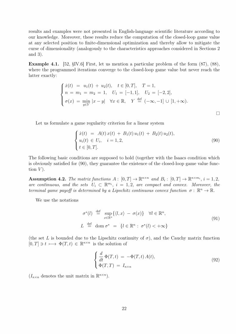
results and examples were not presented in English-language scientific literature according toour knowledge. Moreover, these results reduce the computation of the closed-loop game valueat any selected position to finite-dimensional optimization and thereby allow to mitigate thecurse of dimensionality (analogously to the characteristics approaches considered in Sections 2and 3).

Example 4.1. [52, §IV.6] First, let us mention a particular problem of the form (87), (88),where the programmed iterations converge to the closed-loop game value but never reach thelatter exactly:

x(t) = u1(t) + u2(t), t ∈ [0, T ], T = 1,

n = m1 = m2 = 1, U1 = [−1, 1], U2 = [−2, 2],

σ(x) = miny∈Y|x− y| ∀x ∈ R, Y

def= (−∞,−1] ∪ [1,+∞).

Let us formulate a game regularity criterion for a linear systemx(t) = A(t)x(t) + B1(t)u1(t) + B2(t)u2(t),

ui(t) ∈ Ui, i = 1, 2,

t ∈ [0, T ].

(90)

The following basic conditions are supposed to hold (together with the Isaacs condition whichis obviously satisfied for (90), they guarantee the existence of the closed-loop game value func-tion V ).

Assumption 4.2. The matrix functions A : [0, T ]→ Rn×n and Bi : [0, T ]→ Rn×mi , i = 1, 2,are continuous, and the sets Ui ⊂ Rmi , i = 1, 2, are compact and convex. Moreover, theterminal game payoff is determined by a Lipschitz continuous convex function σ : Rn → R.

We use the notations

σ∗(l)def= sup

x∈Rn

{〈l, x〉 − σ(x)} ∀l ∈ Rn,

Ldef= dom σ∗ = {l ∈ Rn : σ∗(l) < +∞}

(91)

(the set L is bounded due to the Lipschitz continuity of σ), and the Cauchy matrix function[0, T ] 3 t 7−→ Φ(T, t) ∈ Rn×n is the solution of

d

dtΦ(T, t) = −Φ(T, t)A(t),

Φ(T, T ) = In×n

(92)

(In×n denotes the unit matrix in Rn×n).

22

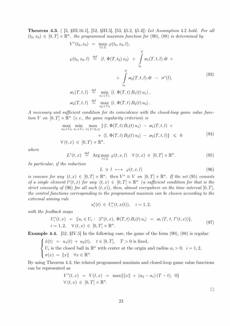
Theorem 4.3. ( [3, §III.16.1], [52, §III.5], [53, §5.2, §5.4]) Let Assumption 4.2 hold. For all(t0, x0) ∈ [0, T ]× Rn, the programmed maximin function for (90), (88) is determined by

V ∗(t0, x0) = maxl∈L

ϕ(t0, x0, l),

ϕ(t0, x0, l)def= 〈l, Φ(T, t0)x0〉 +

T∫t0

κ1(T, t, l) dt +

+

T∫t0

κ2(T, t, l) dt − σ∗(l),

κ1(T, t, l)def= min

u1 ∈U1

〈l, Φ(T, t)B1(t)u1〉 ,

κ2(T, t, l)def= max

u2 ∈U2

〈l, Φ(T, t)B2(t)u2〉 .

(93)

A necessary and sufficient condition for its coincidence with the closed-loop game value func-tion V on [0, T ]× Rn (i. e., the game regularity criterion) is

maxu2 ∈U2

minu1 ∈U1

maxl∈L∗(t,x)

{〈l, Φ(T, t)B1(t)u1〉 − κ1(T, t, l) +

+ 〈l, Φ(T, t)B2(t)u2〉 − κ2(T, t, l)} 6 0

∀ (t, x) ∈ [0, T )× Rn,

(94)

whereL∗(t, x)

def= Arg max

l∈Lϕ(t, x, l) ∀ (t, x) ∈ [0, T ]× Rn. (95)

In particular, if the reductionL 3 l 7−→ ϕ(t, x, l) (96)

is concave for any (t, x) ∈ [0, T ] × Rn, then V ∗ ≡ V on [0, T ] × Rn. If the set (95) consistsof a single element l∗(t, x) for any (t, x) ∈ [0, T ] × Rn (a sufficient condition for that is thestrict concavity of (96) for all such (t, x)), then, almost everywhere on the time interval [0, T ],the control functions corresponding to the programmed maximin can be chosen according to theextremal aiming rule

u∗i (t) ∈ U∗i (t, x(t)), i = 1, 2,

with the feedback maps

U∗i (t, x) = {ui ∈ Ui : 〈l∗(t, x), Φ(T, t)Bi(t)ui〉 = κi (T, t, l∗(t, x))},i = 1, 2, ∀ (t, x) ∈ [0, T ]× Rn.

(97)

Example 4.4. [52, §IV.5] In the following case, the game of the form (90), (88) is regular:x(t) = u1(t) + u2(t), t ∈ [0, T ], T > 0 is fixed,Ui is the closed ball in Rn with center at the origin and radius ai > 0, i = 1, 2,

σ(x) = ‖x‖ ∀x ∈ Rn.

By using Theorem 4.3, the related programmed maximin and closed-loop game value functionscan be represented as

V ∗(t, x) = V (t, x) = max{‖x‖ + (a2 − a1) (T − t), 0}∀ (t, x) ∈ [0, T ]× Rn.

23

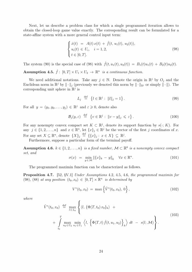
Next, let us describe a problem class for which a single programmed iteration allows toobtain the closed-loop game value exactly. The corresponding result can be formulated for astate-affine system with a more general control input term:

x(t) = A(t)x(t) + f(t, u1(t), u2(t)),

ui(t) ∈ Ui, i = 1, 2,

t ∈ [0, T ].

(98)

The system (90) is the special case of (98) with f(t, u1(t), u2(t)) = B1(t)u1(t) + B2(t)u2(t).

Assumption 4.5. f : [0, T ]× U1 × U2 → Rn is a continuous function.

We need additional notations. Take any j ∈ N. Denote the origin in Rj by Oj and theEuclidean norm in Rj by ‖ · ‖j (previously we denoted this norm by ‖ · ‖Rj or simply ‖ · ‖). Thecorresponding unit sphere in Rj is

Ljdef=

{l ∈ Rj : ‖l‖j = 1

}. (99)

For all y = (y1, y2, . . . , yj) ∈ Rj and ε > 0, denote also

Bj(y, ε)def=

{v ∈ Rj : ‖v − y‖j 6 ε

}. (100)

For any nonempty convex compact set K ⊂ Rj, denote its support function by s(·; K). Forany j ∈ {1, 2, . . . , n} and x ∈ Rn, let {x}j ∈ Rj be the vector of the first j coordinates of x.For any set X ⊆ Rn, denote {X}j

def= {{x}j : x ∈ X} ⊆ Rj.

Furthermore, suppose a particular form of the terminal payoff.

Assumption 4.6. k ∈ {1, 2, . . . , n} is a fixed number,M⊂ Rk is a nonempty convex compactset, and

σ(x) = miny ∈M

‖{x}k − y‖k ∀x ∈ Rn. (101)

The programmed maximin function can be characterized as follows.

Proposition 4.7. [52, §V.1] Under Assumptions 4.2, 4.5, 4.6, the programmed maximin for(98), (88) at any position (t0, x0) ∈ [0, T ]× Rn is determined by

V ∗(t0, x0) = max{V ∗(t0, x0), 0

}, (102)

where

V ∗(t0, x0)def= max

l∈Lk

〈l, {Φ(T, t0)x0}k〉 +

+

T∫t0

maxu2 ∈U2

minu1 ∈U1

⟨l,{

Φ(T, t) f(t, u1, u2)}k

⟩dt − s(l; M)

.

(103)

24

For the system (90) with a linear control input term, the representation (103) transforms into

V ∗(t0, x0) = maxl∈Lk

〈l, {Φ(T, t0)x0}k〉 +

+

T∫t0

minu1 ∈U1

〈l, {Φ(T, t)B1(t)u1(t)}k〉 dt +

+

T∫t0

maxu2 ∈U2

〈l, {Φ(T, t)B2(t)u2(t)}k〉 dt − s(l; M)

.

(104)

One more assumption is required.

Assumption 4.8. There exist continuous functions h : [0, T ] → R, z : [0, T ] → Rk and amapping Π of [0, T ] into the family of all nonempty convex compact sets in Rk, such that

T∫t

maxu2 ∈U2

minu1 ∈U1

⟨l,{

Φ(T, ξ) f(ξ, u1, u2)}k

⟩dξ − s(l; M)

= 〈l, z(t)〉 − s(l; Π(t)) + h(t)

∀ (t, l) ∈ [0, T ]× Lk

(105)

andmaxl∈Lk

{〈l, y〉 − s(l; Π(t))} > 0 ∀ (t, y) ∈ [0, T ]× Rk. (106)

The sought-after result can now be formulated.

Theorem 4.9. [52, §V.1] Under Assumptions 4.2, 4.5, 4.6, 4.8, the lower (sup–inf) closed-loopgame value function for (98), (88) is represented as

Vlow(t0, x0) = max

{V ∗(t0, x0), max

t∈ [t0,T ]h(t)

}∀ (t0, x0) ∈ [0, T ]× Rn,

(107)

where V ∗ is the programmed maximin function specified in Proposition 4.7. If, moreover, theIsaacs condition

minu1 ∈U1

maxu2 ∈U2

⟨p, f(t, u1, u2)

⟩= max

u2 ∈U2

minu1 ∈U1

⟨p, f(t, u1, u2)

⟩∀ (t, p) ∈ [0, T ]× Rn

(108)

holds, then there exists a closed-loop game value function, i. e.,

V (t0, x0) = Vlow(t0, x0) = Vup(t0, x0) ∀ (t0, x0) ∈ [0, T ]× Rn,

and, for all (t, x) ∈ [0, T ]×Rn, the corresponding saddle feedback strategies can be determined by

ui(t, x) ∈ Ui(t, x),

25

where the sets Ui(t, x), i = 1, 2, are described as follows:

Ui(t, x) = Ui, i = 1, 2, if V ∗(t, x) 6 max {0, h(t)},

L(t, x)def= Arg max

l∈Lk

{〈l, {Φ(T, t)x}k + z(t)〉 − s(l; Π(t))} ,

L(t, x) ={l(t, x)

}is singleton if V ∗(t, x) > max {0, h(t)},

U1(t, x) =

{u1 ∈ U1 : max

u2 ∈U2

⟨l(t, x),

{Φ(T, t) f (t, u1, u2)

}k

⟩=

= minu1 ∈U1

maxu2 ∈U2

⟨l(t, x),

{Φ(T, t) f (t, u1, u2)

}k

⟩}if V ∗(t, x) > max {0, h(t)},

U2(t, x) =

{u2 ∈ U2 : min

u1 ∈U1

⟨l(t, x),

{Φ(T, t) f (t, u1, u2)

}k

⟩=

= maxu2 ∈U2

minu1 ∈U1

⟨l(t, x),

{Φ(T, t) f (t, u1, u2)

}k

⟩}if V ∗(t, x) > max {0, h(t)}.

(109)

One can use Theorem 4.9 in the next two examples.

Example 4.10. [52, §V.2] For the game

x1(t) = x3(t) + v1(t),

x2(t) = x4(t) + v2(t),

x3(t) = u1(t),

x4(t) = u2(t),

x(t) = (x1(t), x2(t), x3(t), x4(t))> ∈ R4,

u(t) = (u1(t), u2(t))> ∈ U1 = B2(O2, a1),

v(t) = (v1(t), v2(t))> ∈ U2 = B2(O2, a2),

ai = const > 0, i = 1, 2,

t ∈ [0, T ], T > 0 is fixed,k = 2, M = {O2},

σ(x(T )) = ‖{x(T )}2‖2 =√x2

1(T ) + x22(T ) −→

−→ infu(·)

supv(·)

or supv(·)

infu(·)

,

(110)

Theorem 4.9 leads to the representation

V(t0, x

0)

= max

{V ∗(t0, x

0), maxt∈ [t0,T ]

{(a2 −

a1

2(T − t)

)(T − t)

}}∀(t0, x

0)∈ [0, T ]× R4,

(111)

where V ∗ is determined according to Proposition 4.7.

26

Example 4.11. [52, §V.1] For the game

x1(t) = x3(t) + v1(t),

x2(t) = x4(t) + v2(t),

x3(t) = −αx3(t) + u1(t),

x4(t) = −αx4(t) + u2(t),

x(t) = (x1(t), x2(t), x3(t), x4(t))> ∈ R4,

u(t) = (u1(t), u2(t))> ∈ U1 = U0 + B2(O2, a),

U0 def=

{µu0 : µ ∈ [−1, 1]

},

v(t) = (v1(t), v2(t))> ∈ U2 = B2(O2, b),

α > 0, a > 0, b > 0 are scalar constants,

u0 =(u0

1, u02

)> ∈ R2 is a constant vector,t ∈ [0, T ], T > 0 is fixed,k = 2, M = {O2},

σ(x(T )) = ‖{x(T )}2‖2 =√x2

1(T ) + x22(T ) −→

−→ infu(·)

supv(·)

or supv(·)

infu(·)

,

(112)

Proposition 4.7 and Theorem 4.9 lead to the representations

V(t0, x

0)

= max

{V ∗(t0, x

0), maxt∈ [t0,T ]

h(t)

},

V ∗(t0, x

0)

= max{V ∗(t0, x

0), 0},

V ∗(t0, x

0)

= maxl = (l1,l2) ∈ L2

{(x0

1 + rα(T, t0)x03

)l1 +

+(x0

2 + rα(T, t0)x04

)l2 − Rα(T, t)

∣∣l1 u01 + l2 u

02

∣∣} + h(t0)

∀(t0,(x0)>)

=(t0, x

01, x

02, x

03, x

04

)∈ [0, T ]× R4,

(113)

whereh(t) = (T − t) b − aRα(T, t),

rα(T, t)def=

1 − e−α (T−t)

α> 0,

Rα(T, t)def=

T∫t

rα(T, ξ) dξ =T − tα

− 1 − e−α (T−t)

α2> 0

∀t ∈ [0, T ].

(114)

Furthermore, at any position (t, x) ∈ [0, T ] × Rn, the related saddle feedback strategies canbe chosen according to

u(t, x) ∈ U1(t, x), v(t, x) ∈ U2(t, x),

27

where the sets Ui(t, x), i = 1, 2, are determined by (109) with the following specifications:

Φ(T, t) =

1 0 rα(T, t) 00 1 0 rα(T, t)0 0 e−α (T−t) 00 0 0 e−α (T−t)

,

z(t) ≡ (0, 0)>,

{Φ(T, t)x}2 + z(t) =

(x1 + rα(T, t)x3

x2 + rα(T, t)x4

),

Φ(T, t) f(t, u, v) = Φ(T, t)

v1

v2

u1

u2

=

v1 + rα(T, t)u1

v2 + rα(T, t)u2

e−α (T−t) u1

e−α (T−t) u2

,

⟨l, {Φ(T, t) f(t, u, v)}2

⟩= 〈l, v〉 + rα(T, t) 〈l, u〉 ,

maxv ∈U2

〈l, v〉 is reached at v = b l,

minu∈U1

〈l, u〉 is reached at all u ∈({−a l} + Arg min

w∈U0〈l, w〉

),

Π(t) = Rα(T, t)U0 ={µRα(T, t)u0 : µ ∈ [−1, 1]

},

〈l, {Φ(T, t)x}2 + z(t)〉 − s(l; Π(t)) = (x1 + rα(T, t)x3) l1 +

+ (x2 + rα(T, t)x4) l2 − Rα(T, t) maxw∈U0

〈l, w〉

∀(t, x>, u>, v>, l>

)= (t, x1, x2, x3, x4, u1, u2, v1, v2, l1, l2) ∈

∈ [0, T ]× R4 × U1 × U2 × L2.

(115)

Thus,U1(t, x) =

{−a l(t, x)

}+ Arg min

w∈U0

⟨l(t, x), w

⟩,

Arg minw∈U0

⟨l(t, x), w

⟩=

u0,

⟨l(t, x), u0

⟩< 0,

−u0,⟨l(t, x), u0

⟩> 0,

U0,⟨l(t, x), u0

⟩= 0,

U2(t, x) = {b l(t, x)},L(t, x) = Arg max

l = (l1,l2) ∈ L2

{(x1 + rα(T, t)x3) l1 +

+ (x2 + rα(T, t)x4) l2 − Rα(T, t)∣∣l1 u0

1 + l2 u02

∣∣} ={l(t, x)

}if V ∗(t, x) > max {0, h(t)},

(116)

andUi(t, x) = Ui, i = 1, 2, if V ∗(t, x) 6 max {0, h(t)}. (117)

In Appendix, we describe one more class of differential games for which a single programmediteration leads to the closed-loop game value.

28

5 Numerical simulationsIn this section, we discuss our computational results. The numerical simulations have beenconducted (without algorithm parallelization) on a relatively weak machine with 1.4 GHz Intel2957U CPU, and the corresponding runtimes are mentioned here.

Example 5.1. Consider the problem (61) from Example 3.14 with

c(x) = 1 + 3 exp (−4 ‖x − (1, 1, 0, 0, . . . , 0)‖2Rn) > 0,

σ(x) =1

2(〈Ax, x〉 − 1),

A = diag [0.25, 1, 0.5, 0.5, . . . , 0.5] ∈ Rn×n.

(118)

This particular problem appears from the problem of [2, Section 5, Example 3] just by changingthe first diagonal element of the matrix A from 2.5 to 0.25. Since Dσ vanishes only at the pointx = 0 which gives the global minimum to σ, then Theorem 3.8 can be directly applied here(together with Remark 3.9), and the finite-dimensional optimization can be performed over theunit sphere (73), so that the choice of extremal control values is unique (recall the reasoningsof Example 3.14).

Fig. 1 indicates the two value function approximations VMoC and VFD constructed respec-tively by the method of characteristics (Theorem 3.8, Example 3.14) and via the monotoneLax-Friedrichs finite-difference scheme [9,10,15] (which ensures a theoretical convergence prop-erty and an error estimate) for n = 2 (two-dimensional state space) and T − t0 = 0.5. Somerelated level sets are depicted in Fig. 2. They qualitatively resemble the corresponding resultsreported in [2, Section 5, Example 3]. Fig. 3 shows the optimal feedback control strategyobtained together with VMoC directly from the integrated optimal characteristics.

The Cauchy problems (67), (68) have been solved numerically via the fifth-order Runge–Kutta algorithm from the C++ library of [59]. We have also verified the obtained results byusing the implicit Rosenbrock method [59, §17.5.1] (which is in general more stable but muchmore computationally expensive), and a good agreement has been observed. When launchingthe Runge–Kutta routine, the initial guess for the stepsize was set as 10−3, and the absolute andrelative tolerances were specified as 10−5. The initial states were taken from the uniform grid onthe rectangle [−3, 3]× [−1.5, 1.5] with the spatial step 0.05. The two-dimensional unit sphereof initial adjoint vectors was parametrized by one angle with values in the interval [0, 2π). Theuniform grid for the latter consisted of 1000 points. The maximum of the cost functional waschosen directly around this grid (taking the denser grid of 2000 points has led to very closeresults, as illustrated in Fig. 4). The approximate runtime of computing the value functionby the method of characteristics (as shown in the first subfigure of Fig. 1) has been 400.798 stotally and 0.054301314 s per point. The runtime can be decreased if the optimization overthe two-dimensional unit sphere is performed by means of an advanced one-dimensional max-imization/minimization algorithm (see, for instance, [59, Chapter 10]) after a random choiceof a certain amount of starting points. Note that unconstrained maximization/minimizationroutines can be reasonably used for optimization over sphere parametrizations due to the peri-odicity of the latter.

For computing the finite-difference approximation VFD, we have used the C++ packageROC–HJ [15]. We chose the greater computational region [−5, 5]× [−3, 3] in order to reduce

29

-3-2

-10

12

3

-1.5

-1

-0.5

0

0.5

1

1.5

-0.5

0

0.5

1

1.5

2

2.5

3

VMoC

x1

x2

VMoC

-3

-2

-1

0

1

2

3

-1.5

-1

-0.5

0

0.5

1

1.5

-0.5

0

0.5

1

1.5

2

2.5

3

VFD

x1

x2

VFD

-3-2

-10

12

3

-1.5-1

-0.50

0.51

1.5

-0.06

-0.04

-0.02

0

0.02

0.04

0.06

0.08

0.1

VM

oC

- V

FD

x1

x2

VM

oC

- V

FD

Figure 1: The value function approximations VMoC, VFD and their difference VMoC − VFD inExample 5.1 for n = 2 and T − t0 = 0.5. In order to see the graph of VMoC − VFD clearer, anessentially larger scale on the vertical axis is used there.

-1.5

-1

-0.5

0

0.5

1

1.5

-3 -2 -1 0 1 2 3

x2

x1

Level sets of VMoC

-1.5

-1

-0.5

0

0.5

1

1.5

-3 -2 -1 0 1 2 3

x2

x1

Level sets of VFD

Figure 2: Level sets of the value function approximations VMoC and VFD in Example 5.1 forn = 2 and T − t0 = 0.5.

30

-3

-2

-1

0

1

2

3

-1.5

-1

-0.5

0

0.5

1

1.5

-1

-0.5

0

0.5

1

u1

x1

x2

u1

-3

-2

-1

0

1

2

3

-1.5

-1

-0.5

0

0.5

1

1.5

-1

-0.5

0

0.5

1

u2

x1

x2

u2

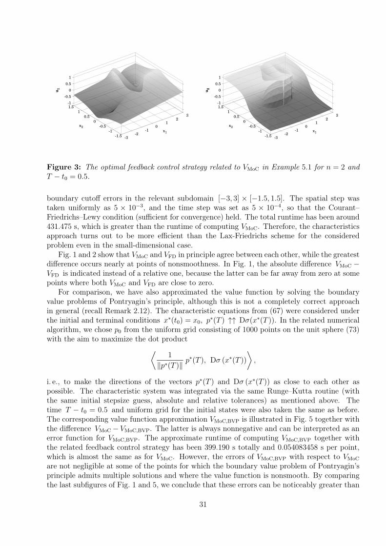
Figure 3: The optimal feedback control strategy related to VMoC in Example 5.1 for n = 2 andT − t0 = 0.5.

boundary cutoff errors in the relevant subdomain [−3, 3] × [−1.5, 1.5]. The spatial step wastaken uniformly as 5 × 10−3, and the time step was set as 5 × 10−4, so that the Courant–Friedrichs–Lewy condition (sufficient for convergence) held. The total runtime has been around431.475 s, which is greater than the runtime of computing VMoC. Therefore, the characteristicsapproach turns out to be more efficient than the Lax-Friedrichs scheme for the consideredproblem even in the small-dimensional case.

Fig. 1 and 2 show that VMoC and VFD in principle agree between each other, while the greatestdifference occurs nearly at points of nonsmoothness. In Fig. 1, the absolute difference VMoC −VFD is indicated instead of a relative one, because the latter can be far away from zero at somepoints where both VMoC and VFD are close to zero.

For comparison, we have also approximated the value function by solving the boundaryvalue problems of Pontryagin’s principle, although this is not a completely correct approachin general (recall Remark 2.12). The characteristic equations from (67) were considered underthe initial and terminal conditions x∗(t0) = x0, p∗(T ) ↑↑ Dσ(x∗(T )). In the related numericalalgorithm, we chose p0 from the uniform grid consisting of 1000 points on the unit sphere (73)with the aim to maximize the dot product⟨

1

‖p∗(T )‖p∗(T ), Dσ (x∗(T ))

⟩,

i. e., to make the directions of the vectors p∗(T ) and Dσ (x∗(T )) as close to each other aspossible. The characteristic system was integrated via the same Runge–Kutta routine (withthe same initial stepsize guess, absolute and relative tolerances) as mentioned above. Thetime T − t0 = 0.5 and uniform grid for the initial states were also taken the same as before.The corresponding value function approximation VMoC,BVP is illustrated in Fig. 5 together withthe difference VMoC− VMoC,BVP. The latter is always nonnegative and can be interpreted as anerror function for VMoC,BVP. The approximate runtime of computing VMoC,BVP together withthe related feedback control strategy has been 399.190 s totally and 0.054083458 s per point,which is almost the same as for VMoC. However, the errors of VMoC,BVP with respect to VMoC

are not negligible at some of the points for which the boundary value problem of Pontryagin’sprinciple admits multiple solutions and where the value function is nonsmooth. By comparingthe last subfigures of Fig. 1 and 5, we conclude that these errors can be noticeably greater than

31

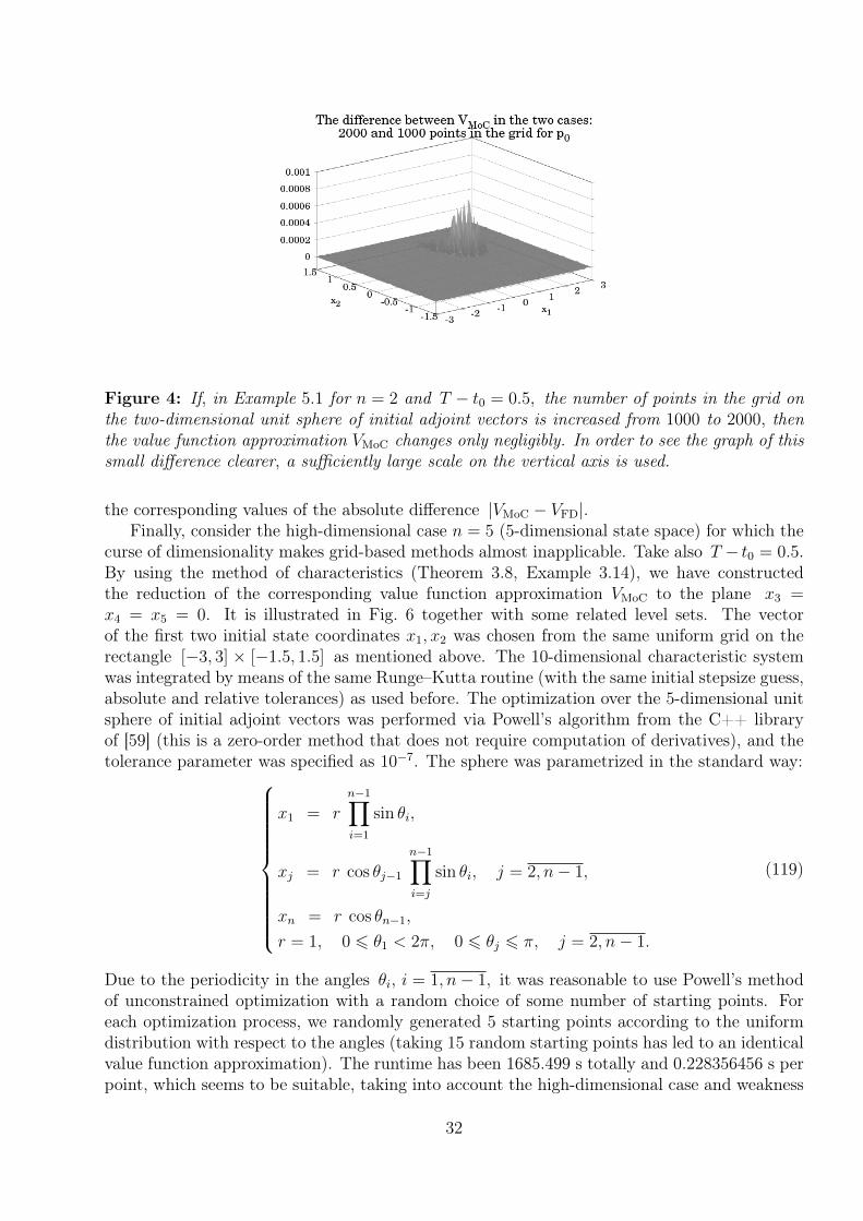
Figure 4: If, in Example 5.1 for n = 2 and T − t0 = 0.5, the number of points in the grid onthe two-dimensional unit sphere of initial adjoint vectors is increased from 1000 to 2000, thenthe value function approximation VMoC changes only negligibly. In order to see the graph of thissmall difference clearer, a sufficiently large scale on the vertical axis is used.

the corresponding values of the absolute difference |VMoC − VFD|.Finally, consider the high-dimensional case n = 5 (5-dimensional state space) for which the

curse of dimensionality makes grid-based methods almost inapplicable. Take also T − t0 = 0.5.By using the method of characteristics (Theorem 3.8, Example 3.14), we have constructedthe reduction of the corresponding value function approximation VMoC to the plane x3 =x4 = x5 = 0. It is illustrated in Fig. 6 together with some related level sets. The vectorof the first two initial state coordinates x1, x2 was chosen from the same uniform grid on therectangle [−3, 3] × [−1.5, 1.5] as mentioned above. The 10-dimensional characteristic systemwas integrated by means of the same Runge–Kutta routine (with the same initial stepsize guess,absolute and relative tolerances) as used before. The optimization over the 5-dimensional unitsphere of initial adjoint vectors was performed via Powell’s algorithm from the C++ libraryof [59] (this is a zero-order method that does not require computation of derivatives), and thetolerance parameter was specified as 10−7. The sphere was parametrized in the standard way:

x1 = r

n−1∏i=1

sin θi,

xj = r cos θj−1

n−1∏i=j

sin θi, j = 2, n− 1,

xn = r cos θn−1,

r = 1, 0 6 θ1 < 2π, 0 6 θj 6 π, j = 2, n− 1.

(119)

Due to the periodicity in the angles θi, i = 1, n− 1, it was reasonable to use Powell’s methodof unconstrained optimization with a random choice of some number of starting points. Foreach optimization process, we randomly generated 5 starting points according to the uniformdistribution with respect to the angles (taking 15 random starting points has led to an identicalvalue function approximation). The runtime has been 1685.499 s totally and 0.228356456 s perpoint, which seems to be suitable, taking into account the high-dimensional case and weakness

32

-3-2

-10

12

3

-1.5

-1

-0.5

0

0.5

1

1.5-0.5

00.51

1.52

2.53

VMoC,B

VP

x1

x2

VMoC,B

VP

-3-2

-10

12

3

-1.5-1

-0.50

0.51

1.5

0

0.02

0.04

0.06

0.08

0.1

VM

oC

- V

MoC

,BV

P

x1

x2

VM

oC

- V

MoC

,BV

P

Figure 5: The value function approximation VMoC,BVP and its error VMoC − VMoC,BVP inExample 5.1 for n = 2 and T − t0 = 0.5. In order to see the graph of VMoC−VMoC,BVP clearer,an essentially larger scale on the vertical axis is used there.

-3-2

-10

12

3

-1.5

-1

-0.5

0

0.5

1

1.5

0

0.5

1

1.5

2

2.5

3

3.5

VMoC

x1

x2

VMoC

-1.5

-1

-0.5

0

0.5

1

1.5

-3 -2 -1 0 1 2 3

x2

x1

Level sets of VMoC

Figure 6: The value function approximation VMoC on the plane x3 = x4 = x5 = 0 inExample 5.1 for n = 5 and T − t0 = 0.5.

of the computational resources we have used. The runtime can be substantially smaller formore powerful machines, especially when parallelization is done.

Example 5.2. Consider the game (112) from Example 4.11 with

α = 1, a = 0.2, b = 0.1, u0 = (0, 0)>,

t0 = 0, T = 2.

(120)

The formulae (113) determine the programmed maximin function V ∗ and closed-loop gamevalue function V , while the saddle feedback control maps are represented by (116), (117). In(117), let us select the unique values as u0 from U1 and (0, 0)> from U2.

Fig. 7 indicates the reductions of the functions V, V ∗ and their difference V − V ∗ to theplane x3 = x4 = 0, t0 = 0 (it is in fact enough to fix T − t0 = 2 instead of specifying theparticular initial and final instants t0 = 0, T = 2). Some related level sets are depicted in

33

Fig. 8. The corresponding reductions of the saddle feedback control strategies are illustratedin Fig. 9.

The vector of the first two initial state coordinates x1, x2 was taken from the uniform gridon the square [−0.2, 0.2]× [−0.2, 0.2] with the spatial step 4×10−3. The two-dimensional unitsphere L2 was parametrized by one angle with values in the interval [0, 2π). The uniform gridfor the latter consisted of 104 points. In our implementation of (116), the maximum over L2

was computed directly around this grid. Furthermore, the number

hmaxdef= max

t∈ [t0,T ]h(t) (121)

was computed directly around the uniform grid on [t0, T ] consisting of 104 + 1 points. Weobtained hmax ≈ 0.0307. The approximate runtime of computing the mentioned reductionsof the programmed maximin function, closed-loop game value function and saddle feedbackcontrol strategies has been 6.994 s totally and 0.000685619 s per point.

The last subfigure of Fig. 7 shows that the programmed maximin and closed-loop gamevalue functions differ from each other in some neighborhood of the origin (V − V ∗ reaches thevalue hmax there).

Example 5.3. Consider the problem (74) from Example 3.15 with

c(x) = −1 − 3 exp (−4 ‖x − (1, 1, 0, 0, . . . , 0)‖2Rn) < 0,

σ ≡ 0, η(x) =1

2〈Ax, x〉 ,

A = diag [0.25, 1, 0.5, 0.5, . . . , 0.5] ∈ Rn×n.

(122)

Then{x ∈ Rn : Dη(x) = 0} = {x′} = {0}

= Arg minx∈Rn

η(x) ⊂ Arg minx∈Rn

σ(x) = Rn,(123)

i. e., the condition (85) holds. By using the final statement of Example 3.15, one can computethe related value function V and optimal feedback (closed-loop) control strategy u∗c-l at anyselected position (t, x) ∈ [0, T )× Rn.

Now let the deterministic system (64) be perturbed by stochastic noise, so that the resultingsystem becomes

dx(t) = c(x(t))u(t) dt + Λ dw(t; t0),

x(t0) = x0,

u(t) ∈ U = {v ∈ Rn : ‖v‖ 6 1} ,t ∈ [t0, T ],

(124)

where (t0, x0) ∈ [0, T ) × Rn is a deterministic initial position, Λ ∈ Rn×n is a constant noiseintensity matrix, w(·; t0) is an n-dimensional standard Brownian motion (Wiener process) onthe time interval [t0, T ], and the stochastic ordinary differential equations are understood inthe Itô sense. An open-loop control strategy can also be a stochastic process if it is obtainedfrom a closed-loop map. It is reasonable to assess the control quality through the mean value

E

σ(x(T )) +

T∫t0

η(x(t)) dt

= E

T∫t0

η(x(t)) dt

=

T∫t0

E[η(x(t))] dt. (125)

34

Figure 7: The reductions of the closed-loop game value function V , programmed maximinfunction V ∗ and their difference V − V ∗ to the plane x3 = x4 = 0, T − t0 = 2 in Example 5.2.In order to see the graph of V − V ∗ clearer, a larger scale on the vertical axis is used there.

35

-0.2

-0.15

-0.1

-0.05

0

0.05

0.1

0.15

0.2

-0.2 -0.15 -0.1 -0.05 0 0.05 0.1 0.15 0.2

x2

x1

Level sets of V

-0.2

-0.15

-0.1

-0.05

0

0.05

0.1

0.15

0.2

-0.2 -0.15 -0.1 -0.05 0 0.05 0.1 0.15 0.2

x2

x1

Level sets of V*

Figure 8: Level sets of the reductions of the functions V and V ∗ to the plane x3 = x4 = 0,T − t0 = 2 in Example 5.2.

-0.2-0.15

-0.1-0.05

00.05

0.10.15

0.2

-0.2

-0.15

-0.1

-0.05

0

0.05

0.1

0.15

0.2

-0.2-0.15-0.1

-0.050

0.050.1

0.150.2

u1

x1

x2

u1

-0.2-0.15

-0.1-0.05

00.05

0.10.15

0.2

-0.2

-0.15

-0.1

-0.05

0

0.05

0.1

0.15

0.2

-0.2-0.15-0.1

-0.050

0.050.1

0.150.2

u2

x1

x2

u2

-0.2-0.15

-0.1-0.05

00.05

0.10.15

0.2

-0.2

-0.15

-0.1

-0.05

0

0.05

0.1

0.15

0.2

-0.1

-0.05

0

0.05

0.1

v1

x1

x2

v1

-0.2-0.15

-0.1-0.05

00.05

0.10.15

0.2

-0.2

-0.15

-0.1

-0.05

0

0.05

0.1

0.15

0.2

-0.1

-0.05

0

0.05

0.1

v2

x1

x2

v2

Figure 9: The reductions of the saddle feedback control strategies u = (u1, u2)> and v =(v1, v2)> to the plane x3 = x4 = 0, T − t0 = 2 in Example 5.2. For the sake of convenience,different viewpoints for the horizontal axes are used in the graphs of u1, u2 and v1, v2.

36

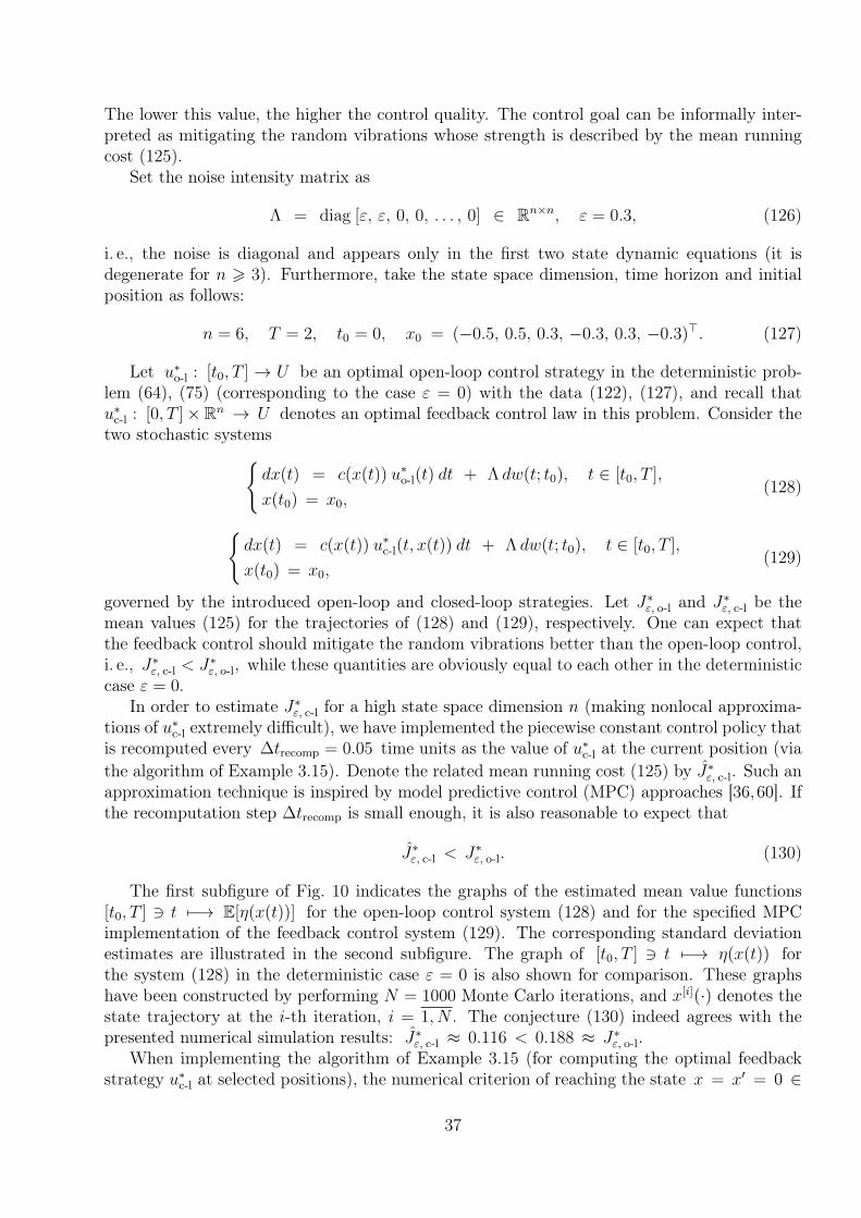
The lower this value, the higher the control quality. The control goal can be informally inter-preted as mitigating the random vibrations whose strength is described by the mean runningcost (125).

Set the noise intensity matrix as

Λ = diag [ε, ε, 0, 0, . . . , 0] ∈ Rn×n, ε = 0.3, (126)

i. e., the noise is diagonal and appears only in the first two state dynamic equations (it isdegenerate for n > 3). Furthermore, take the state space dimension, time horizon and initialposition as follows:

n = 6, T = 2, t0 = 0, x0 = (−0.5, 0.5, 0.3, −0.3, 0.3, −0.3)>. (127)

Let u∗o-l : [t0, T ] → U be an optimal open-loop control strategy in the deterministic prob-lem (64), (75) (corresponding to the case ε = 0) with the data (122), (127), and recall thatu∗c-l : [0, T ]×Rn → U denotes an optimal feedback control law in this problem. Consider thetwo stochastic systems{

dx(t) = c(x(t)) u∗o-l(t) dt + Λ dw(t; t0), t ∈ [t0, T ],

x(t0) = x0,(128)

{dx(t) = c(x(t)) u∗c-l(t, x(t)) dt + Λ dw(t; t0), t ∈ [t0, T ],

x(t0) = x0,(129)

governed by the introduced open-loop and closed-loop strategies. Let J∗ε, o-l and J∗ε, c-l be themean values (125) for the trajectories of (128) and (129), respectively. One can expect thatthe feedback control should mitigate the random vibrations better than the open-loop control,i. e., J∗ε, c-l < J∗ε, o-l, while these quantities are obviously equal to each other in the deterministiccase ε = 0.

In order to estimate J∗ε, c-l for a high state space dimension n (making nonlocal approxima-tions of u∗c-l extremely difficult), we have implemented the piecewise constant control policy thatis recomputed every ∆trecomp = 0.05 time units as the value of u∗c-l at the current position (viathe algorithm of Example 3.15). Denote the related mean running cost (125) by J∗ε, c-l. Such anapproximation technique is inspired by model predictive control (MPC) approaches [36,60]. Ifthe recomputation step ∆trecomp is small enough, it is also reasonable to expect that

J∗ε, c-l < J∗ε, o-l. (130)

The first subfigure of Fig. 10 indicates the graphs of the estimated mean value functions[t0, T ] 3 t 7−→ E[η(x(t))] for the open-loop control system (128) and for the specified MPCimplementation of the feedback control system (129). The corresponding standard deviationestimates are illustrated in the second subfigure. The graph of [t0, T ] 3 t 7−→ η(x(t)) forthe system (128) in the deterministic case ε = 0 is also shown for comparison. These graphshave been constructed by performing N = 1000 Monte Carlo iterations, and x[i](·) denotes thestate trajectory at the i-th iteration, i = 1, N . The conjecture (130) indeed agrees with thepresented numerical simulation results: J∗ε, c-l ≈ 0.116 < 0.188 ≈ J∗ε, o-l.

When implementing the algorithm of Example 3.15 (for computing the optimal feedbackstrategy u∗c-l at selected positions), the numerical criterion of reaching the state x = x′ = 0 ∈

37

Figure 10: Estimates of the mean values E[η(x(t))] and standard deviations√

Var [η(x(t))]for the open-loop control system (128) and for the specified MPC implementation of the feedbackcontrol system (129) in Example 5.3.

38

Arg minx∈Rn

η(x) was chosen as η(x)− η(x′) = η(x) < 5 · 10−6 (the exact deterministic optimal

control has zero action at x = x′). The 12-dimensional deterministic characteristic system wasintegrated via the same Runge–Kutta routine (with the same initial stepsize guess, absoluteand relative tolerances) as mentioned in Example 5.1. The optimization over the 7-dimensionalunit sphere of the vectors (p0, p

∗) was performed by using Powell’s algorithm of [59] with thetolerance parameter 10−5. No special method was needed to exclude the value p∗ = 0, sinceit was not approached enough (at least with the tolerance 10−5) in the executed optimizationiterations. The sphere was parametrized in the standard way. The related representation wasobtained from (119) by replacing n = 6 with n + 1 = 7. For each optimization process, 5starting points were randomly generated in line with the uniform angles distribution.

The Itô stochastic differential equations have been solved by means of the Euler–Maruyamascheme that coincides with the Milstein scheme for the constant and diagonal noise intensitymatrix (126) [61,62]. The corresponding time step was taken as ∆tSDE = 10−5. Under certainsmoothness and Lipschitz continuity conditions on the drift vector function and noise intensitymatrix function, the Milstein scheme has the first strong convergence order (while the order ofthe Euler–Maruyama scheme in general equals 0.5 if the noise intensity matrix is not constant).One can expect that the first order of accuracy should be preserved in our MPC implementationof the system (129), because the related control policy is piecewise constant and the ratio∆trecomp/∆tSDE = 5 · 103 is integer. When integrating the open-loop control system (128),one may face an additional numerical error caused by the discontinuity of u∗o-l at the time ofentering the state x = x′. Since this has been the only discontinuity of u∗o-l on the whole timeinterval [t0, T ], the resulting error has not appeared to be significant.

As follows from Fig. 10, the feedback MPC approach allows for a rather successful randomvibrations mitigation by periodic recomputation of the control according to the current position.The open-loop control cannot be adapted in this way and is therefore unstable. Starting fromsome time, it has zero action as if x = x′, while the noise is likely to move the state awayfrom x′.

6 ConclusionThis paper extends the considerations of the works [1,2] concerning curse-of-dimensionality-freenumerical approaches to solve certain types of Hamilton–Jacobi equations arising in optimalcontrol problems, differential games and elsewhere. A rigorous formulation and justification forthe extended Hopf–Lax formula of [2] is provided together with novel theoretical and practicaldiscussions including useful recommendations. By using the method of characteristics, thesolutions of some problem classes under convexity/concavity conditions on Hamiltonians (inparticular, the solutions of Hamilton–Jacobi–Bellman equations in optimal control problems)are evaluated separately at different initial positions. This allows for the avoidance of the curseof dimensionality, as well as for choosing arbitrary computational regions. The correspondingfeedback control strategies are obtained at selected positions without approximating the partialderivatives of the solutions. The numerical simulation results demonstrate the high potentialof the proposed techniques.

Despite the indicated advantages, the related approaches still have a limited range of appli-cability (recall Remarks 2.14, 2.15, 3.11–3.13), and their extensions to Hamilton–Jacobi–Isaacsequations in zero-sum two-player differential games are currently developed only for rather nar-row classes of linear control systems (as shown in Section 4 and Appendix). That is why further

39

extensions are worth investigating. In particular, it is relevant to find a wider description forthe classes of optimal control problems, where the finite-dimensional optimization in the algo-rithms of computing the value functions can be performed over bounded sets. Regarding thesecond main conjecture of [2] (i. e., the extended Hopf formula) that may be applied to someclasses of nonlinear differential games, its rigorous formulation and justification also remainsan open problem.

Finally, note that the paper [36] proposed to solve boundary value problems for character-istic systems numerically with the aim to approximate the value functions of optimal controlproblems at separate sparse grid nodes. However, this may lead to incorrect results at the initialpositions for which the boundary value problems have multiple solutions and the value functionsare nonsmooth (recall Fig. 5 in Example 5.1). Therefore, it seems promising to combine theapproaches of the current work with the sparse grid techniques of [36] so as to construct globalapproximations of the value functions and corresponding feedback control laws in domains ofrelatively high dimensions.

AcknowledgementsThis work was supported in part by AFOSR/AOARD grant FA2386-16-1-4066.

References1. Darbon, J. and Osher, S. Algorithms for overcoming the curse of dimensionality for certainHamilton–Jacobi equations arising in control theory and elsewhere. Research in the Mathe-matical Sciences 2016; 3: 19.

2. Chow, Y.T., Darbon, J., Osher, S., and Yin, W. Algorithm for overcoming thecurse of dimensionality for state-dependent Hamilton–Jacobi equations. 2017. URL:https://arxiv.org/abs/1704.02524

3. Subbotin, A. I. Generalized Solutions of First-Order PDEs: The Dynamical OptimizationPerspective. Birkhauser: Boston, 1995.

4. Melikyan, A.A. Generalized Characteristics of First Order PDEs: Application in OptimalControl and Differential Games. Birkhauser: Boston, 1998.

5. Yong, J. and Zhou, X.Yu. Stochastic Controls: Hamiltonian Systems and HJB Equations.Springer-Verlag: New York, 1999.

6. Fleming, W.H. and Soner, H.M. Controlled Markov Processes and Viscosity Solutions.Springer-Verlag: New York, 2006.

7. Bardi, M. and Capuzzo-Dolcetta, I. Optimal Control and Viscosity Solutions of Hamilton–Jacobi–Bellman Equations. Birkhauser: Boston, 2008.

8. Yong, J. Differential Games: A Concise Introduction. World Scientific Publishing: Singa-pore, 2015.

9. Crandall, M.G. and Lions, P.-L. Two approximations of solutions of Hamilton–Jacobi equa-tions. Mathematics of Computation 1984; 43: 1–19.

40

10. Osher, S. and Shu, C.-W. High order essentially non-oscillatory schemes for Hamilton–Jacobi equations. SIAM Journal on Numerical Analysis 1991; 28(4): 907–922.

11. Jiang, G. and Peng, D. P. Weighted ENO schemes for Hamilton–Jacobi equations. SIAMJournal on Scientific Computing 2000; 21(6): 2126–2143.

12. Zhang, Y.-T. and Shu, C.-W. High-order WENO schemes for Hamilton–Jacobi equationson triangular meshes. SIAM Journal on Scientific Computing 2003; 24(3): 1005–1030.

13. Bokanowski, O., Forcadel, N., and Zidani, H. Reachability and minimal times for stateconstrained nonlinear problems without any controllability assumption. SIAM Journal onControl and Optimization 2010; 48: 4292–4316.

14. Bokanowski, O., Cristiani, E. and Zidani, H. An efficient data structure and accurate schemeto solve front propagation problems. Journal of Scientific Computing 2010; 42(2): 251–273.

15. Bokanowski, O., Desilles, A., Zidani, H., and Zhao, J. User’s guide for the ROC-HJ solver:Reachability, Optimal Control, and Hamilton–Jacobi equations. May 10, 2017. Version 2.3.URL: http://uma.ensta-paristech.fr/soft/ROC-HJ/

16. Falcone, M. and Ferretti, R. Convergence analysis for a class of high-order semi-Lagrangianadvection schemes. SIAM Journal on Numerical Analysis 1998; 35(3): 909–940.

17. Falcone, M. Numerical methods for differential games based on partial differential equations.International Game Theory Review 2006; 8: 231–272.

18. Cristiani, E. and Falcone, M. Fast semi-Lagrangian schemes for the Eikonal equation andapplications. SIAM Journal on Numerical Analysis 2007; 45: 1979–2011.

19. Osher, S. and Sethian, J. Fronts propagating with curvature-dependent speed: Algorithmsbased on Hamilton–Jacobi formulations. Journal of Computational Physics 1988; 79: 12–49.

20. Osher, S. A level set formulation for the solution of the Dirichlet problem for Hamilton–Jacobi equations. SIAM Journal on Mathematical Analysis 1993; 24(5): 1145–1152.

21. Sethian, J. Level Set Methods and Fast Marching Methods. Cambridge University Press:New York, 1999.

22. Osher, S. and Fedkiw, R. Level Set Methods and Dynamic Implicit Surfaces. Springer-Verlag: New York, 2003.

23. Mitchell, I., Bayen, A., and Tomlin, C. Computing reachable setsfor continuous dynamic games using level set methods. 2002. URL:http://hybrid.stanford.edu/∼bayen/publications.html

24. Mitchell, I., Bayen, A., and Tomlin, C. A time-dependent Hamilton–Jacobi formulation ofreachable sets for continuous dynamic games. IEEE Transactions on Automatic Control 2005;50(7): 947–957.

25. Mitchell, I. A Toolbox of Level Set Methods. Department of Computer Science, Universityof British Columbia. 2012. URL: http://www.cs.ubc.ca/∼mitchell/ToolboxLS

41

26. Bellman, R. Dynamic Programming. Princeton University Press: Princeton, 1957.

27. Bellman, R. Adaptive Control Processes: A Guided Tour. Princeton University Press:Princeton, 1961.

28. McEneaney, W.M. Max-Plus Methods in Nonlinear Control and Estimation. Birkhauser:Boston, 2006.

29. McEneaney, W.M. A curse-of-dimensionality-free numerical method for solution of certainHJB PDEs. SIAM Journal on Control and Optimization 2007; 46(4): 1239–1276.

30. McEneaney, W.M., Deshpande, A., and Gaubert, S. Curse-of-complexity attenuation inthe curse-of-dimensionality-free method for HJB PDEs. Proceedings of The 2008 AmericanControl Conference 2008: 4684–4690.

31. McEneaney, W.M. and Kluberg, J. Convergence rate for a curse-of-dimensionality-freemethod for a class of HJB PDEs. SIAM Journal on Control and Optimization 2009; 48(5):3052–3079.

32. Gaubert, S., McEneaney, W.M., and Qu, Z. Curse of dimensionality reduction in max-plus based approximation methods: theoretical estimates and improved pruning algorithms.Proceedings of The 50th IEEE Conference on Decision and Control 2011: 1054–1061.

33. Akian, M., Gaubert, S., and Lakhoua, A. The max-plus finite element method for solvingdeterministic optimal control problems: basic properties and convergence analysis. SIAMJournal on Control and Optimization 2008; 47(2): 817–848.

34. Kaise, H. and McEneaney, W.M. Idempotent expansions for continuous-time stochasticcontrol: compact control space. Proceedings of the 49th IEEE Conference on Decision andControl 2010: 7015–7020.

35. Akian, M. and Fodjo, E. A probabilistic max-plus numerical method for solving stochasticcontrol problems. Proceedings of the 55th IEEE Conference on Decision and Control 2016.DOI: 10.1109/CDC.2016.7799411

36. Kang, W. and Wilcox, L.C. Mitigating the curse of dimensionality: sparse grid character-istics method for optimal feedback control and HJB equations. Computational Optimizationand Applications 2017; 68(2): 289–315.

37. Hopf, E. Generalized solutions of nonlinear equations of first order. Journal of Mathematicsand Mechanics 1965; 14: 951–973.

38. Evans, L.C. Partial Differential Equations. Graduate Studies in Mathematics, 19, Ameri-can Mathematical Society, 1998.

39. Rublev, I. V. Generalized Hopf formulas for the nonautonomous Hamilton–Jacobi equation.Computational Mathematics and Modeling 2000; 11(4): 391–400.

40. Evans, L.C. Envelopes and nonconvex Hamilton–Jacobi equations. Calculus of Variationsand Partial Differential Equations 2014; 50(1–2): 257–282.

42

41. Mirică, S. Extending Cauchy’s method of characteristics for Hamilton–Jacobi equations.Studii şi Cercetări de Matematică 1985; 37(6): 555–565.

42. Subbotina, N.N. Method of Cauchy characteristics and generalized solutions of Hamilton–Jacobi–Bellman equations. Doklady AN SSSR 1991; 320: 556–561 (in Russian).

43. Subbotina, N.N. Necessary and sufficient optimality conditions in terms of characteristicsof the Hamilton–Jacobi–Bellman equation. Report 393, Institut für Angewandte Mathematikund Statistic, Universität Würzburg, Würzburg, 1992.

44. Subbotina, N.N. The method of characteristics for Hamilton–Jacobi equations and applica-tions to dynamical optimization. Journal of Mathematical Sciences 2006; 135(3): 2955–3091.

45. Subbotina, N.N. and Tokmantsev, T.B. On the efficiency of optimal grid synthesis inoptimal control problems with fixed terminal time. Differential Equations 2009; 45: 1686–1697.

46. Subbotina, N.N. and Tokmantsev, T.B. Estimating error of the optimal grid design inthe problems of nonlinear optimal control of prescribed duration. Automation and RemoteControl 2009; 70(9): 1565–1578.

47. Subbotina, N.N. and Kolpakova, E.A. On the structure of locally Lipschitz minimax solu-tions of the Hamilton-Jacobi-Bellman equation in terms of classical characteristics. Proceed-ings of the Steklov Institute of Mathematics 2010; 268(suppl. 1): 222–239.

48. Rockafellar, R.T. Convex Analysis. Princeton University Press: Princeton, New Jersey,1970.

49. Rockafellar, R.T. Conjugate Duality and Optimization. SIAM Publications: Philadelphia,1974.

50. Pontryagin, L. S., Boltyansky, V.G., Gamkrelidze, R.V., and Mishchenko, E. F. The Math-ematical Theory of Optimal Processes. Macmillan: New York, 1964.

51. Krasovskii, N.N. and Subbotin, A. I. Positional Differential Games. Nauka: Moscow, 1974(in Russian).

52. Subbotin, A. I. and Chentsov, A.G.Optimization of Guaranteed Result in Control Problems.Nauka: Moscow, 1981 (in Russian).

53. Krasovskii, N.N. and Subbotin, A. I. Game-Theoretical Control Problems. Springer-Verlag:New York, 1988.

54. Berkovitz, L.D. The existence of value and saddle point in games of fixed duration. SIAMJournal on Control and Optimization 1985; 23(2): 172–196.

55. Başar, T. and Olsder, G. J. Dynamic Noncooperative Game Theory. Academic Press:New York, 1995.

56. Bernhard, P. Singular surfaces in differential games: An introduction. In: Hagedorn, P.,Knobloch, H.W., and Olsder, G. J. (Eds.) Differential Games and Applications, volume 3of the series Lecture Notes in Control and Information Sciences, pp. 1–33. Springer-Verlag:Berlin, 1977.

43

57. Bernhard, P. Pursuit-evasion games and zero-sum two-person differential games. Ency-clopedia of Systems and Control 2014; 1–7. DOI: 10.1007/978-1-4471-5102-9_270-1. URL:https://hal.inria.fr/hal-01215556/document

58. Melikyan, A. and Bernhard, P. Geometry of optimal trajectories around a focal singularsurface in differential games. Applied Mathematics and Optimization 2005; 52: 23–37.

59. Press, W.H., Teukolsky, S.A., Vetterling, W.T., and Flannery, B. P. Numerical Recipes:The Art of Scientific Computing. Cambridge University Press: New York, 2007.

60. Wang, L. Model Predictive Control System Design and Implementation Using MATLAB.Springer-Verlag: London, 2009.

61. Kloeden, P. E. and Platen, E. Numerical Solution of Stochastic Differential Equations.Springer-Verlag: Berlin, 1995.

62. Carletti, M. Numerical solution of stochastic differential problems in the biosciences. Jour-nal of Computational and Applied Mathematics 2006; 185(2): 422–440.

A AppendixLet us introduce one more class of differential games for which a single programmed iteration isenough to reach the closed-loop game value. The corresponding result was derived in [52, §V.2].

Consider the linear differential game (90), (88) under Assumptions 4.2, 4.6. In addition tothe notations presented in the introduction and Section 4, adopt that

‖y‖0j

def= max

i ∈ {1,2,...,j}|yi|, ‖y‖1

jdef=

j∑i=1

|yi|,

B0j (y, ε)

def=

{v ∈ Rj : ‖v − y‖0

j 6 ε} (131)

for all j ∈ N, y = (y1, y2, . . . , yj) ∈ Rj and ε > 0. Several more conditions are imposed.

Assumption A.1. There exist a vector y0 ∈ Rk, numbers r ∈ [0,+∞), r ∈ [0,+∞) andcontinuous functions

y : [0, T ] → Rk, z : [0, T ] → Rk,

h1 : [0, T ] → [0,+∞), h21 : [0, T ] → [0,+∞),

h22 : [0, T ] → [0,+∞),

such that the setM from Assumption 4.6 is determined by

M = y0 + B0k(Ok, r) + Bk(Ok, r) (132)

and, for all t ∈ [0, T ], l ∈ Lk, one has

{Φ(T, t)B1(t)U1(t)}k = B0k (y(t), h1(t)) ,

T∫t

maxu2 ∈U2

〈l, {Φ(T, ξ)B2(ξ)u2}k〉 dξ = h21(t) + h22(t) ‖l‖1k + 〈l, z(t)〉 ,

h22(t) 6T∫t

h1(ξ) dξ + r.

(133)

44

Denote also

h3(t)def=

T∫t

h1(ξ) dξ + r − h22(t) ∀t ∈ [0, T ]. (134)

The sought-after result can now be formulated.

Theorem A.2. [52, §V.2] Under Assumptions 4.2, 4.6, A.1, the closed-loop game value for(90), (88) at any position (t0, x0) ∈ [0, T ]× Rn is represented as

V (t0, x0) = max

{V ∗(t0, x0), max

t∈ [t0,T ]{h21(t) − h3(t)} − r

}, (135)

where V ∗ is the programmed maximin function specified in Proposition 4.7.

Theorem A.2 can be applied in the two subsequent examples.

Example A.3. [52, §V.2] Consider the problem that appears from the game of Example 4.10just by replacing U1 = B2(O2, a1) with U1 = B0

2(O2, a1). Then the closed-loop game valuefunction is also represented as in (111), but the programmed maximin function V ∗ is nowdifferent.

Example A.4. [52, §V.2] For the game

x1(t) = x3(t) + v1(t),

x2(t) = x4(t) + v2(t),

x3(t) = −αx3(t) + u1(t) + v3(t),

x4(t) = −αx4(t) + u2(t) + v4(t),

x(t) = (x1(t), x2(t), x3(t), x4(t))> ∈ R4,

u(t) = (u1(t), u2(t))> ∈ U1 = B02

(ω0, a

),

v(t) = (v1(t), v2(t), v3(t), v4(t))>

∈ U2 = (−B2(ω∗, b∗)) × B02(ω∗, b∗),

α > 0, b∗ > 0, b∗ > 0, a > b∗ are scalar constants,ω0, ω∗, ω

∗ are constant vectors in R2,

t ∈ [0, T ], T > 0 is fixed,k = 2, M = {O2},

σ(x(T )) = ‖{x(T )}2‖2 =√x2

1(T ) + x22(T ) −→

−→ infu(·)

supv(·)

or supv(·)

infu(·)

,

(136)

Theorem A.2 leads to the representation

V(t0, x

0)

= max

{V ∗(t0, x

0), maxt∈ [t0,T ]

{(T − t) b∗ − Rα(T, t) (a− b∗)}}

∀(t0, x

0)∈ [0, T ]× R4,

(137)

where Rα is defined as in (114) and V ∗ is determined according to Proposition 4.7.

45