UNIVERSITY OF CALIFORNIA
Los Angeles
Automated Performance and Correctness Debugging for Big Data Analytics
A dissertation submitted in partial satisfaction
of the requirements for the degree
Doctor of Philosophy in Computer Science
by
Jia Shen Teoh
2022

© Copyright by
Jia Shen Teoh
2022

ABSTRACT OF THE DISSERTATION
Automated Performance and Correctness Debugging for Big Data Analytics
by
Jia Shen Teoh
Doctor of Philosophy in Computer Science
University of California, Los Angeles, 2022
Professor Miryung Kim, Chair
The constantly increasing volume of data collected in every aspect of our daily lives has neces-
sitated the development of more powerful and efficient analysis tools. In particular, data-intensive
scalable computing (DISC) systems such as Google’s MapReduce [36], Apache Hadoop [4], and
Apache Spark [5] have become valuable tools for consuming and analyzing large volumes of data.
At the same time, these systems provide valuable programming abstractions and libraries which
enable adoption by users from a wide variety of backgrounds such as business analytics and data
science. However, the widespread adoption of DISC systems and their underlying complexity
have also highlighted a gap between developers’ abilities to write applications and their abilities to
understand the behavior of their applications.
By merging distributed systems debugging techniques with software engineering ideas, our hy-
pothesis is that we can design accurate yet scalable approaches for debugging and testing of big
data analytics’ performance and correctness. To design such approaches, we first investigate how
we can combine data provenance with latency propagation techniques in order to debug computa-
tion skew —abnormally high computation costs for a small subset of input data —by identifying
expensive input records. Next, we investigate how we can extend taint analysis techniques with
ii
influence-based provenance for many-to-one dependencies to enhance root cause analysis and im-
prove the precision of identifying fault-inducing input records. Finally, in order to replicate perfor-
mance problems based on described symptoms, we investigate how we can redesign fuzz testing
by targeting individual program components such as user-defined functions for focused, modu-
lar fuzzing, defining new guidance metrics for performance symptoms, and adding skew-inspired
input mutations and mutation operation selector strategies.
For the first hypothesis, we introduce PERFDEBUG, a post-mortem performance debugging
tool for computation skew—abnormally high computation costs for a small subset of input data.
PERFDEBUG automatically finds input records responsible for such abnormalities in big data appli-
cations by reasoning about deviations in performance metrics such as job execution time, garbage
collection time, and serialization time. The key to PERFDEBUG’s success is a data provenance-
based technique that computes and propagates record-level computation latency to track abnor-
mally expensive records throughout the application pipeline. Finally, the input records that have the
largest latency contributions are presented to the user for bug fixing. Our evaluation of PERFDE-
BUG using in-depth case studies demonstrates that remediation such as removing the single most
expensive record or simple code rewrites can achieve up to 16X performance improvement.
Second, we present FLOWDEBUG, a fault isolation technique for identifying a highly precise
subset of fault-inducing input records. FLOWDEBUG is designed based on key insights using pre-
cise control and data flow within user-defined functions as well as a novel notion of influence-based
provenance to rank importance between aggregation function inputs. By design, FLOWDEBUG
does not require any modification to the framework’s runtime and thus can be applied to exist-
ing applications easily. We demonstrate that FLOWDEBUG significantly improves the precision
of debugging results by up to five orders-of-magnitude and avoids repetitive re-runs required for
post-mortem analysis by a factor of 33 compared to existing state-of-the-art systems.
Finally, we discuss PERFGEN, a performance debugging aid which replicates performance
symptoms via automated workload generation. PERFGEN effectively generates symptom-
producing test inputs by using a phased fuzzing approach that extends traditional fuzz testing
iii

to target specific user-defined functions and avoids additional fuzzing complexity from program
executions that are unlikely unrelated to the target symptom. To support PERFGEN, we define
a suite of guidance metrics and performance skew symptom patterns which are then used to de-
rive skew-oriented mutations for phased fuzzing. We evaluate PERFGEN using four case studies
which demonstrate an average speedup of at least 43X speedup compared to traditional fuzzing
approaches, while requiring less than 0.004% of fuzzing iterations.
iv

The dissertation of Jia Shen Teoh is approved.
Harry Guoqing Xu
Ravi Netravali
Todd Millstein
Miryung Kim, Committee Chair
University of California, Los Angeles
2022
v

To my family
vi
TABLE OF CONTENTS
1 Introduction . . . . . . . . . . . . . . . . . . . . . . . . . . . . . . . . . . . . . . . 1
1.1 Research Problem . . . . . . . . . . . . . . . . . . . . . . . . . . . . . . . . . . . 1
1.2 Thesis Statement . . . . . . . . . . . . . . . . . . . . . . . . . . . . . . . . . . . 3
1.3 PerfDebug: Performance Debugging of Computation Skew in Dataflow Systems . . 4
1.4 Enhancing Provenance-based Debugging for Dataflow Applications with Taint
Propagation and Influence Functions . . . . . . . . . . . . . . . . . . . . . . . . . 5
1.5 PerfGen: Automated Performance Workload Generation for Dataflow Applications 7
1.6 Contributions . . . . . . . . . . . . . . . . . . . . . . . . . . . . . . . . . . . . . 8
1.7 Outline . . . . . . . . . . . . . . . . . . . . . . . . . . . . . . . . . . . . . . . . 9
2 Related Work . . . . . . . . . . . . . . . . . . . . . . . . . . . . . . . . . . . . . . 10
2.1 Data Provenance . . . . . . . . . . . . . . . . . . . . . . . . . . . . . . . . . . . 10
2.2 Correctness Debugging . . . . . . . . . . . . . . . . . . . . . . . . . . . . . . . . 12
2.3 Performance Analysis of DISC Applications . . . . . . . . . . . . . . . . . . . . . 17
2.4 Test Input Generation for DISC Performance . . . . . . . . . . . . . . . . . . . . 20
3 PerfDebug: Performance Debugging of Computation Skew in Dataflow Systems . . 23
3.1 Introduction . . . . . . . . . . . . . . . . . . . . . . . . . . . . . . . . . . . . . . 23
3.2 Background . . . . . . . . . . . . . . . . . . . . . . . . . . . . . . . . . . . . . . 25
3.2.1 Computation Skew . . . . . . . . . . . . . . . . . . . . . . . . . . . . . . 25
3.2.2 Apache Spark and Titian . . . . . . . . . . . . . . . . . . . . . . . . . . . 27
3.3 Motivating Scenario . . . . . . . . . . . . . . . . . . . . . . . . . . . . . . . . . . 28
vii

3.4 Approach . . . . . . . . . . . . . . . . . . . . . . . . . . . . . . . . . . . . . . . 31
3.4.1 Performance Problem Identification . . . . . . . . . . . . . . . . . . . . . 32
3.4.2 Capturing Data Lineage and Latency . . . . . . . . . . . . . . . . . . . . 33
3.4.3 Expensive Input Isolation . . . . . . . . . . . . . . . . . . . . . . . . . . . 38
3.5 Experimental Evaluation . . . . . . . . . . . . . . . . . . . . . . . . . . . . . . . 41
3.5.1 Experimental Setup . . . . . . . . . . . . . . . . . . . . . . . . . . . . . . 41
3.5.2 Case Study A: NYC Taxi Trips . . . . . . . . . . . . . . . . . . . . . . . . 42
3.5.3 Case Study B: Weather . . . . . . . . . . . . . . . . . . . . . . . . . . . . 45
3.5.4 Case Study C: Movie Ratings . . . . . . . . . . . . . . . . . . . . . . . . 46
3.5.5 Accuracy and Instrumentation Overhead . . . . . . . . . . . . . . . . . . . 47
3.6 Discussion . . . . . . . . . . . . . . . . . . . . . . . . . . . . . . . . . . . . . . . 49
4 Enhancing Provenance-based Debugging with Taint Propagation and Influence Func-
tions . . . . . . . . . . . . . . . . . . . . . . . . . . . . . . . . . . . . . . . . . . . . . 51
4.1 Introduction . . . . . . . . . . . . . . . . . . . . . . . . . . . . . . . . . . . . . . 51
4.2 Motivating Example . . . . . . . . . . . . . . . . . . . . . . . . . . . . . . . . . 53
4.2.1 Running Example 1 . . . . . . . . . . . . . . . . . . . . . . . . . . . . . 53
4.2.2 Running Example 2 . . . . . . . . . . . . . . . . . . . . . . . . . . . . . 58
4.3 Approach . . . . . . . . . . . . . . . . . . . . . . . . . . . . . . . . . . . . . . . 61
4.3.1 Transformation Level Provenance . . . . . . . . . . . . . . . . . . . . . . 62
4.3.2 UDF-Aware Tainting . . . . . . . . . . . . . . . . . . . . . . . . . . . . . 63
4.3.3 Influence Function Based Provenance . . . . . . . . . . . . . . . . . . . . 66
4.4 Evaluation . . . . . . . . . . . . . . . . . . . . . . . . . . . . . . . . . . . . . . . 69
4.4.1 Weather Analysis . . . . . . . . . . . . . . . . . . . . . . . . . . . . . . . 72
viii

4.4.2 Airport Transit Analysis . . . . . . . . . . . . . . . . . . . . . . . . . . . 73
4.4.3 Course Grade Analysis . . . . . . . . . . . . . . . . . . . . . . . . . . . . 75
4.4.4 Student Info Analysis . . . . . . . . . . . . . . . . . . . . . . . . . . . . . 77
4.4.5 Commute Type Analysis . . . . . . . . . . . . . . . . . . . . . . . . . . . 79
4.5 Discussion . . . . . . . . . . . . . . . . . . . . . . . . . . . . . . . . . . . . . . . 81
5 PerfGen: Automated Performance Workload Generation for Dataflow Applications 82
5.1 Introduction . . . . . . . . . . . . . . . . . . . . . . . . . . . . . . . . . . . . . . 82
5.2 Motivating Example . . . . . . . . . . . . . . . . . . . . . . . . . . . . . . . . . 84
5.3 Approach . . . . . . . . . . . . . . . . . . . . . . . . . . . . . . . . . . . . . . . 88
5.3.1 Targeting UDFs . . . . . . . . . . . . . . . . . . . . . . . . . . . . . . . . 90
5.3.2 Modeling performance symptoms . . . . . . . . . . . . . . . . . . . . . . 92
5.3.3 Skew-Inspired Input Mutation Operations . . . . . . . . . . . . . . . . . . 95
5.3.4 Phased Fuzzing . . . . . . . . . . . . . . . . . . . . . . . . . . . . . . . . 98
5.4 Evaluation . . . . . . . . . . . . . . . . . . . . . . . . . . . . . . . . . . . . . . . 102
5.4.1 Case Study: Collatz Conjecture . . . . . . . . . . . . . . . . . . . . . . . 103
5.4.2 Case Study: WordCount . . . . . . . . . . . . . . . . . . . . . . . . . . . 105
5.4.3 Case Study: DeptGPAsMedian . . . . . . . . . . . . . . . . . . . . . . . . 107
5.4.4 Case Study: StockBuyAndSell . . . . . . . . . . . . . . . . . . . . . . . . 111
5.4.5 Improvement in RQ1 and RQ2 . . . . . . . . . . . . . . . . . . . . . . . . 115
5.4.6 RQ3: Effect of mutation weights . . . . . . . . . . . . . . . . . . . . . . . 117
5.5 Discussion . . . . . . . . . . . . . . . . . . . . . . . . . . . . . . . . . . . . . . . 118
6 Conclusion and Future Work . . . . . . . . . . . . . . . . . . . . . . . . . . . . . 119
ix
6.1 Summary . . . . . . . . . . . . . . . . . . . . . . . . . . . . . . . . . . . . . . . 119
6.2 Future Research Directions . . . . . . . . . . . . . . . . . . . . . . . . . . . . . . 120
6.3 Final Remarks . . . . . . . . . . . . . . . . . . . . . . . . . . . . . . . . . . . . . 123
A Chapter 5 Supplementary Materials . . . . . . . . . . . . . . . . . . . . . . . . . . 124
A.1 Monitor Templates Implementation . . . . . . . . . . . . . . . . . . . . . . . . . 124
A.2 Performance Metrics Implementation . . . . . . . . . . . . . . . . . . . . . . . . 133
A.3 Mutation Operator Implementations. . . . . . . . . . . . . . . . . . . . . . . . . . 134
A.4 Mutation Identification and Weight Assignment Implementation . . . . . . . . . . 143
References . . . . . . . . . . . . . . . . . . . . . . . . . . . . . . . . . . . . . . . . . 149
x
LIST OF FIGURES
2.1 An example of Titian’s data provenance tables which track input-output mappings
across stages. The records highlighted in green represent a trace from the output1
output record backwards through the entire application, ending at the input records . . 11
3.1 Alice’s program for computing the distribution of movie ratings. . . . . . . . . . . . . 25
3.2 An example screenshot of Spark’s Web UI where each row represents task-level per-
formance metrics. From left to right, the columns represent task identifier, the address
of the worker hosting that task, running time of the task, garbage collection time, and
the size (space and quantity) of input ingested by the task, respectively. . . . . . . . . 28
3.3 The physical execution of the motivating example by Apache Spark. . . . . . . . . . . 30
3.4 During program execution, PERFDEBUG also stores latency information in lineage
tables comprising of an additional column of ComputationLatency. . . . . . . . . . . . 33
3.5 The snapshots of lineage tables collected by PERFDEBUG. Ê, Ë, and Ì illustrate the
physical operations and their corresponding lineage tables in sequence for the given
application. In the first step, PERFDEBUG captures the Out, In, and Stage Latency
columns, which represent the input-output mappings as well as the stage-level laten-
cies per record. During output latency computation, PERFDEBUG calculates three
additional columns (Total Latency, Most Impactful Source, and Remediated Latency)
to keep track of cumulative latency, the ID of the original input with the largest impact
on Total Latency, and the estimated latency if the most impactful record did not impact
application performance. . . . . . . . . . . . . . . . . . . . . . . . . . . . . . . . . . 35
3.6 A Spark application computing the average cost of a taxi ride for each borough. . . . . 43
3.7 A weather data analysis application . . . . . . . . . . . . . . . . . . . . . . . . . . . 45
xi
4.1 Example 1 identifies, for each state in the US, the delta between the minimum and the
maximum snowfall reading for each day of any year and for any particular year. Mea-
surements can be either in millimeters or in feet. The conversion function is described
at line 27. The red rectangle highlights code edits required to enable FLOWDEBUG’s
UDF-aware taint propagation of numeric and string data types, discussed in Section
4.3.2. Although Scala does not require explicit types to be declared, some variable
types are mentioned in orange color to highlight type differences. . . . . . . . . . . . . 54
4.2 A filter function that searches for input data records with more than 6000mm of snow-
fall reading. . . . . . . . . . . . . . . . . . . . . . . . . . . . . . . . . . . . . . . . . 55
4.3 Using textFileWithTaint, FLOWDEBUG automatically transforms the applica-
tion DAG. ProvenanceRDD enables transformation-level provenance and influence-
function capability, while tainted primitive types enable UDF-level taint propagation.
Influence functions are enabled directly through ProvenanceRDD’s aggregation
APIs via an additional argument, described in Section 4.3.3 . . . . . . . . . . . . . . . 57
4.4 Running example 2 identifies, for each state in the US, the variance of snowfall reading
for each day of any year and for any particular year. The red rectangle highlights the
required changes to enable influence-based provenance for a tainting-enabled program,
consisting of a single influenceTrackerCtr argument that creates influence function in-
stances to track provenance information within FLOWDEBUG’s RDD-like aggregation
API. Influence-based provenance is discussed further in Section 4.3.3. . . . . . . . . . 58
4.5 Abstract representation of operator-level provenance, UDF-Aware provenance, and
influence-based provenance. TaintedData refers to wrappers introduced in Section
4.3.2 that internally store provenance at the data object level, and Influence Func-
tions support customizable provenance retention policies over aggregations discussed
in Section 4.3.3. . . . . . . . . . . . . . . . . . . . . . . . . . . . . . . . . . . . . . . 61
xii
4.6 FLOWDEBUG supports control-flow aware provenance at the UDF level (left UDF)
and can merge provenance on aggregation (right UDF). . . . . . . . . . . . . . . . . . 63
4.7 TaintedString intercepts String’s method calls to propagate the provenance by
implementing Scala.String methods. . . . . . . . . . . . . . . . . . . . . . . . . 64
4.8 Comparison of operator-based data provenance (blue) vs. influence-function based
data provenance (red). The aggregation logic computes the variance of a collection
of input numbers and the influence function is configured to capture outlier aggrega-
tion inputs (StreamingOutlier in Table 4.1) that might heavily impact the computed
result. . . . . . . . . . . . . . . . . . . . . . . . . . . . . . . . . . . . . . . . . . . . 66
4.9 FLOWDEBUG defines influence functions which mirror Spark’s aggregation semantics
to support customizable provenance retention policies for aggregation functions. . . . . 67
4.10 The implementation of the predefined Custom Filter influence function, which im-
plements the influence function API in 4.9 and uses a provided boolean function to
evaluate which values’ provenance to retain. . . . . . . . . . . . . . . . . . . . . . . . 68
4.11 The instrumented running time of FLOWDEBUG, Titian, and BigSift. . . . . . . . . . 71
4.12 The debugging time to trace each set of faulty output records in FLOWDEBUG,
BigSift, and Titian. . . . . . . . . . . . . . . . . . . . . . . . . . . . . . . . . . . . . 71
4.13 The Airport Transit Analysis program with and without FLOWDEBUG. Line 13 in
Figure 4.13b enables provenance tracking support which is required in order to support
usage of the StreamingOutlier influence function defined at line 24. . . . . . . . . . . 74
4.14 The Course Grade Analysis program with and without FLOWDEBUG. Line 3 in Figure
4.14b enables provenance tracking support and line 41 defines the StreamingOutlier
influence function. . . . . . . . . . . . . . . . . . . . . . . . . . . . . . . . . . . . . 76
4.15 The Student Info Analysis program with and without FLOWDEBUG. Provenance
supporrt is enabled in line 3 of Figure 4.15b while line 13 defines the StreamingOutlier
influence function. . . . . . . . . . . . . . . . . . . . . . . . . . . . . . . . . . . . . 78
xiii
4.16 The Commute Type Analysis program with and without FLOWDEBUG. Line 3 in
Figure 4.16b enables provenance tracking support while line 22 defines the TopN in-
fluence function with a size parameter of 1000. . . . . . . . . . . . . . . . . . . . . . 80
5.1 Three sources of performance skews . . . . . . . . . . . . . . . . . . . . . . . . . . . 83
5.2 The Collatz program which applies the solve collatz function (Figure 5.3) to
each input integer and sums the result by distinct integer input. . . . . . . . . . . . . . 84
5.3 The solve collatz function used in Figure 5.2 to determine each integer’s Collatz
sequence length and compute a polynomial-time result based on the sequence length.
For example, an input of 3 has a Collatz length of 7 and calling solve collatz(3)
takes 1 ms to compute, while an input of 27 has a Collatz length of 111 and takes 4989
ms to compute. . . . . . . . . . . . . . . . . . . . . . . . . . . . . . . . . . . . . . . 85
5.4 The Collatz pseudo-inverse function to convert solved inputs into inputs for the entire
Collatz program (Figure 5.2, lines 1-7). For example, calling this function on a single-
record RDD (10, [1, 1, 1]) produces a Collatz input RDD of three records: ”10”,
”10”, and ”10”. . . . . . . . . . . . . . . . . . . . . . . . . . . . . . . . . . . . . . . 86
5.5 Code demonstrating how a user can use PERFGEN for the Collatz program discussed
in Section 5.2. A user specifies the program definition and target UDF (lines 1-2)
through HybridRDDs variables corresponding to the program output and UDF output
(Figure 5.2), an initial seed input (line 5), the performance symptom as a MonitorTem-
plate (lines 8-9), and a pseudo-inverse function (line 25, defined in Figure 5.4). They
may optionally customize mutation operators produced by PERFGEN (lines 15-16)
which are represented as a map of mutation operators and their corresponding sam-
pling weights (MutationMap). These parameters are combined into a configuration
object (lines 18-25) that PERFGEN uses to generate test inputs. . . . . . . . . . . . . 88
xiv
5.6 An overview of PERFGEN’s phased fuzzing approach. A user specifies (1) a target
UDF within their program and (2) a performance symptom definition which is used to
detect whether or not a symptom is present for a given program execution. PERF-
GEN uses the definition to generate (3) a weighted set of mutations for both UDF and
program input fuzzing. It first (4) fuzzes the target UDF to reproduce the desired per-
formance symptom, then applies a pseudo-inverse function to generate an improved
program input seed that is used to (5) fuzz the entire program and generate a program
input that reproduces the target symptom. . . . . . . . . . . . . . . . . . . . . . . . . 89
5.7 PERFGEN mimics Spark’s RDD API with HybridRDD to support extraction and reuse
of individual UDFs without significant program rewriting. Variable types in 5.7b are
shown to highlight type differences as a result of the HybridRDD conversion, though
in practice these types are optional for users to provide as Scala can automatically infer
types. The data types shown in each HybridRDD correspond to the inputs and outputs
of the transformation function applied to the original Spark RDD. . . . . . . . . . . . 90
5.8 HybridRDDs operate similarly to Spark RDDs while decoupling Spark transforma-
tions (computeFn) from the input RDDs on which they are applied (parent). . . . 91
5.9 Monitor Templates monitor Spark program (or subprogram) execution metrics to (1)
detect performance skew symptoms and (2) produce feedback scores that are used as
fuzzing guidance. . . . . . . . . . . . . . . . . . . . . . . . . . . . . . . . . . . . . . 92
5.10 Simplified implementation of MaximumThreshold from Table 5.1, which implements
the MonitorTemplate API in Figure 5.9 to detect if any job execution metric exceeds a
specified threshold. . . . . . . . . . . . . . . . . . . . . . . . . . . . . . . . . . . . . 93
5.11 Pseudocode example of the AppendSameKey mutation (M13) in Table 5.3 which tar-
gets data skew by appending new records containing a pre-existing key. . . . . . . . . 97
xv
5.12 PERFGEN’s generated mutations and weights for the solved HybridRDD in Figure
5.7b, which has an input type of (Int, Iterable[Int]), and the computation
skew symptom defined in Section 5.2. For example, ”M10 + M7 + M1” specifies a
mutation operator for the RDD[(Int, Iterable[Int])] dataset that selects a
random tuple record (ReplaceRandomRecord, M10) and replaces the integer key of
that tuple (ReplaceTupleElement, M7) with a new integer value (ReplaceInteger, M1).
PERFGEN heuristically adjusts mutation sampling weights; based on the computation
skew symptom, the data skew-oriented M11 and M12 sampling probabilities are de-
creased while the M5 mutation (which targets computation skew) is assigned a higher
sampling probability. . . . . . . . . . . . . . . . . . . . . . . . . . . . . . . . . . . . 98
5.13 PERFGEN’s phased fuzzing approach for generating symptom-reproducing inputs. . . 99
5.14 Outline of PERFGEN’s fuzzing loop which uses feedback scores from monitor tem-
plates to guide fuzzing for both UDFs and entire programs. . . . . . . . . . . . . . . . 100
5.15 The WordCount program implementation in Scala which counts the occurrences of
each space-separated word. . . . . . . . . . . . . . . . . . . . . . . . . . . . . . . . . 105
5.16 The DeptGPAsMedian program implementation in Scala which calculates the median
of average course GPAs within each department. . . . . . . . . . . . . . . . . . . . . 108
5.17 The StockBuyAndSell program implementation in Scala which calculates maximum
achievable profit with at most three transactions (maxProfits, lines 13-32), for each
stock symbol. To support a user-defined metric, a Spark accumulator (line 1) is defined
and updated via a custom iterator (lines 27-28, 34-41). . . . . . . . . . . . . . . . . . 113
5.18 Time series plots of each case study’s monitor template feedback score against time.
PERFGEN results are plotted in black with the final program result indicated by a
circle, while baseline results are plotted in red crosses. The target threshold for each
case study’s symptom definition is represented by a horizontal blue dotted line. . . . . 116
xvi

5.19 Plot of PERFGEN input generation time against varying sampling probabilities for the
M13 and M14 mutations used in the DeptGPAsMedian program. . . . . . . . . . . . . 117
xvii

LIST OF TABLES
3.1 Subject programs with input datasets. . . . . . . . . . . . . . . . . . . . . . . . . . . 42
3.2 Identification Accuracy of PERFDEBUG and instrumentation overheads compared to
Titian, for the subject programs described in Section 3.5.5. . . . . . . . . . . . . . . . 49
4.1 Influence function implementations provided by FLOWDEBUG. . . . . . . . . . . . . 68
4.2 Debugging accuracy results for Titian, BigSift, and FLOWDEBUG. For Course
Grades, Titian and BigSift returned 0 records for backward tracing. . . . . . . . . . . 70
4.3 Instrumentation and tracing times for Titian, BigSift, and FLOWDEBUG on each sub-
ject program, along with the number of iterations required by BigSift. Table 4.2 lists
the specific FLOWDEBUG provenance strategy (e.g., influence function) for each sub-
ject program. BigSift internally leverages Titian for instrumentation and thus shares
the same instrumentation time. For the Course Grades program, BigSift was unable to
generate an input trace as described in Section 4.4.3. Instrumentation and debugging
times for each program are also shown side-by-side in Figures 4.11 and 4.12 respectively. 70
5.1 Monitor Templates define predicates that are used to (1) detect specific symptoms
and (2) calculate feedback scores, given a collection of values X derived using per-
formance metrics definitions such as those from Table 5.2. Full Monitor Template
implementations are listed in Appendix A.1. . . . . . . . . . . . . . . . . . . . . . . 94
5.2 Performance metrics captured by PERFGEN through Spark’s Listener API to monitor
performance symptoms, along with the associated performance skew they are used to
measure. All metrics are reported separately for each partition and stage within an
execution.Code implementations are listed in Appendix A.2. . . . . . . . . . . . . . . 95
xviii

5.3 Skew-inspired mutation operations implemented by PERFGEN for various data types
and their typical skew categories. Some mutations depend on others (e.g., due to nested
data types); in such cases, the most common target skews are listed. Mutation imple-
mentations are listed in Appendix A.3. . . . . . . . . . . . . . . . . . . . . . . . . . 96
5.4 Fuzzing times and iterations for each case study program. For programs marked with
a “*”, the baseline evaluation timed out after 4 hours and was unsuccessful in repro-
ducing the desired symptom. . . . . . . . . . . . . . . . . . . . . . . . . . . . . . . . 115
xix

ACKNOWLEDGMENTS
I have been fortunate to have met many amazing people during my PhD, and it is safe to say
that their guidance and encouragement have been crucial in every step of this journey. First, I
would like to thank my advisor, Miryung Kim. She welcomed me into her research group at a
time when I doubted my place in the PhD program, and her hands-on guidance and constructive
criticism have shaped not only my research but also my approach to problems in all facets of life.
Her encouragement and support has inspired me to hold myself to higher standards and constantly
strive to improve. I am also thankful to my initial advisor, Tyson Condie, who welcomed me to
UCLA despite my lack of research experience and guided me early on in my PhD career.
I would like to thank my committee members, Harry Xu, Ravi Netravali, and Todd Millstein.
Their feedback on my research, one-on-one discussions, and support have been invaluable through-
out my PhD. I am additionally grateful to Harry for the expertise and insights he shared for my
first work on performance debugging.
I am honored to have had great student collaborators throughout my time at UCLA, and am
grateful for those opportunities with Mohammad Ali Gulzar, Jiyuan Wang, and Qian Zhang. It
takes time and effort to bring a research idea to fruition, and none of this would have been possible
without their contributions. I am especially thankful for Gulzar, who became an invaluable mentor
and pseudo-advisor from the moment I inquired about joining his group.
Through my classes and the SEAL, PLSE, SOLAR, and ScAI research groups, I have had the
opportunity to meet many friends and colleagues. In no particular order, thank you to Tianyi
Zhang, Saswat Padhi, Christian Kalhauge, Shaghayegh Mardani, Lana Ramjit, Fabrice Harel-
Canada, Pradeep Dogga, Akshay Utture, Zeina Migeed, Shuyang Liu, Micky Abir, Poorva Garg,
Aishwarya Sivaram, Siva Kesava Reddy Kakarla, Brett Chalabian, Kyle Liang, Matteo Interlandi,
Joseph Noor, Ling Ding, Jonathan Lin, David Rangel, and many others for the advice, research
discussions, casual chats, snack runs, dinners, entertainment, and encouragement. Our interactions
together made my time at UCLA more colorful than I could have ever hoped for. I am especially
xx

thankful to Tianyi Zhang, for offering his time and advice when I struggled in figuring out how
to wrap up my PhD, and to Joseph Noor, who mentored me when I was just getting started with
research and introduced me to life at UCLA.
During my time at UCLA, I was given the opportunity to teach multiple times and learn what
it means to be an educator. I am thankful to my fellow teaching staff for their advice and feedback
as well as thankful to my former students for suffering through my lessons.
I might never have found my research direction if not for my experiences in industry, and I
am thankful for the team members and mentors that I met along the way. I am especially grateful
to Shirshanka Das for guiding me during my PhD applications, Hien Luu and Swetha Karthik for
helping me grow from a programmer to a problem solver, and YongChul Kwon for invaluable
advice in navigating PhD life and the job application process.
Most importantly, I am thankful to my family for their unwavering support. I am lucky to
have two sets of parents that have always cheered me on while also never missing an opportunity
to remind me to take a break and visit them. I am grateful for Chester who always offers, if not
demands, to keep me company when I stay up late for deadlines. Finally, none of this would be
possible if not for Emily Sheng. Words can never express how thankful I am for her encourage-
ment, late night discussions, worldly travels (both physical and virtual), boba, and countless other
contributions.
xxi
VITA
Sept. 2016 - March 2022 Graduate Student Researcher/Teaching Assistant, Computer Sci-
ence Department, University of California, Los Angeles
March 2019 M.S. in Computer Science, University of California, Los Ange-
les
June 2019 - Sept. 2019 Software Engineering Intern, Google, Kirkland, WA
May 2015 - Sept. 2016 Senior Software Engineer, LinkedIn, Mountain View, CA
June 2013 - May 2015 Software Engineer, LinkedIn, Mountain View, CA
May 2013 B.A. in Computer Science, University of California, Berkeley
May 2012 - Aug. 2012 Software Engineer Intern, LinkedIn, Mountain View, CA
PUBLICATIONS
PerfGen: Automated Performance Workload Generation for Dataflow Applications. Jason Teoh,
Muhammad Ali Gulzar, Jiyuan Wang, Qian Zhang, and Miryung Kim. To be submitted.
Influence-Based Provenance for Dataflow Applications with Taint Propagation. Jason Teoh,
Muhammad Ali Gulzar, and Miryung Kim. In Proceedings of the ACM Symposium on Cloud
Computing, SoCC ’20.
xxii

PerfDebug: Performance Debugging of Computation Skew in Dataflow Systems. Jason Teoh,
Muhammad Ali Gulzar, Guoqing Harry Xu, and Miryung Kim. In Proceedings of the ACM Sym-
posium on Cloud Computing, SoCC ’19.
xxiii
CHAPTER 1
Introduction
1.1 Research Problem
As the capacity to store and process data has increased remarkably, large scale data processing
has become an essential part of software development. Data-intensive scalable computing (DISC)
systems, such as Google’s MapReduce [36], Apache Hadoop [4], and Apache Spark [5], have
shown great promise in addressing the scalability challenge of large scale data processing. Fur-
thermore, these systems provide programming abstractions and libraries which enable developers
from a wide variety of non-technical backgrounds to write DISC applications. However, due to
the sheer amount of data and computation used in these complex systems combined with lower
domain knowledge requirements, users are increasingly faced with difficulties in debugging and
testing their big data analytics applications. In this thesis, we discuss three challenges that users
face when trying to understand the behavior of their programs.
Due to the scale of ingested data, DISC systems inherently suffer from long execution times.
Consequently, studying and improving their performance has been a major research area [94, 114,
115, 41, 54, 68, 64]. When an application shows signs of poor performance through an increase in
general CPU time, garbage collection time, or serialization time, the first question a user may ask
is “what caused my program to slow down?” While stragglers—slow executors in a cluster—and
hardware failures can often be automatically identified by existing dataflow system monitors, many
real-world performance issues are not system problems; instead, they stem from a combination
of certain data records from the input and specific computation logic of the application code that
1

incurs much longer latency due to interactions between the data and code —a phenomenon referred
to as computation skew. Although there is a large body of work [39, 68, 67] that attempts to
mitigate data skew, computation skew has been largely overlooked and tools that can identify and
diagnose computation skew, unfortunately, do not exist.
Another challenge in debugging DISC systems is investigating the root cause of incorrect re-
sults. To address this problem of identifying the root cause of a wrong output or an application
failure, data provenance techniques [59, 79, 33] have been developed to provide traceability. These
provenance techniques capture the input-output record mappings at each transformation-level (e.g.,
map, reduce, join) at runtime and enable backward tracing on a suspicious output in order to
find its corresponding inputs. However, these techniques suffer from two fundamental limitations.
First, these techniques capture input-to-output mappings only at the dataflow operator level and
thus overapproximate input traces for user-defined functions (UDFs) whose outputs are not depen-
dent on every input, such as a max aggregation. The second limitation is that existing provenance
techniques operate under a binary notion of whether or not an input maps to an output. How-
ever, it is often the case that inputs will not contribute to an aggregate result in an equal degree of
influence, depending on the semantics of the aggregation UDF. In such cases, inputs with larger
contributions may be more valuable for root cause analysis. For example, outliers in a numer-
ical distribution have a greater impact on the standard deviation and are thus more likely to be
of interest to a developer than values that fit well within the distribution. Provenance techniques
that fail to account for the varying degrees of input contribution to an output ultimately produce
unnecessarily large input traces which include low-contribution inputs of little or no value. As an
alternative to provenance-based approaches, search-based debugging techniques [128, 47] can be
used for post-mortem analysis as they repetitively run the program with different input subsets and
check whether a test failure appears. However, DISC programs can take hours to days for a sin-
gle execution and multiple reruns can become prohibitively time-consuming for debugging efforts.
Furthermore, these approaches still fail to address the second challenge of measuring each input’s
contribution to the resulting output.
2

The third and final challenge with DISC systems that we discuss in this thesis is that of repro-
ducibility: given a program definition and an observed performance problem (e.g., as described
in a StackOverflow post), how can we identify an input set that will trigger the described behavior
or performance symptom? One option is to rely on developers to select a subset of production
data inputs with the hope that the selection will reproduce the targeted performance issues. Not
surprisingly, such sampling is unlikely to yield performance skews and repeated sampling can
quickly become time-consuming. Within the software engineering community, fuzz testing has
been proven to be highly effective in revealing a diverse set of bugs, including performance de-
fects [118, 71, 99, 89], correctness bugs [97, 98, 15], and security vulnerabilities [20, 45, 35, 107].
Generally speaking, these techniques start from a seed input and generate new inputs by applying
data mutations in an effort to improve some guidance metric such as branch coverage. However,
it is nontrivial to apply traditional fuzzing to data-intensive applications due to the long-running
nature of DISC applications. While techniques exist to target code coverage [129], they modify
the underlying execution environment and thus do not preserve the performance characteristics of
DISC systems. Furthermore, the challenge of reproducing performance symptoms requires a new
class of input mutations which target not only individual record values but also distributed dataset
properties (e.g., key distribution) which impact underlying DISC system performance. While these
properties may change depending on application semantics, their performance effects remain rel-
evant throughout all stages of a DISC application. As a result, such mutations must be applicable
not only for DISC application inputs, but also for intermediate results at all stages of a distributed
program.
1.2 Thesis Statement
To address the challenges that users face in investigating DISC application behavior, this disserta-
tion investigates the following hypothesis:
Hypothesis: By designing automated debugging and testing techniques that incorporate
3

properties of DISC computing, we can improve the precision of root cause analysis techniques for
both performance and correctness debugging and reduce the time required to reproduce perfor-
mance symptoms.
To test this hypothesis, we design three approaches for improving developer comprehension
of big data applications. First, we design a fine-grained, performance-tracking data provenance
technique for post-mortem debugging of expensive inputs (i.e., inputs that lead to time-consuming
computation). Second, we leverage dynamic taint analysis to implement influence-based prove-
nance which boosts fault isolation precision by pruning unnecessary inputs. Finally, we enhance
performance symptom reproducibility by defining performance-oriented feedback metrics, new
input mutations, and a new method of targeted fuzzing.
Our key insight is that we can design big data debugging and testing techniques by combin-
ing software engineering ideas with DISC application properties. Using our hypothesis and key
insight, this dissertation evaluates each approach’s ability to address key challenges in DISC de-
bugging and testing. In the next three sections, we give an overview each individual contribution,
propose a sub-hypothesis for each work, and summarize empirical evaluations to test each hypoth-
esis.
1.3 PerfDebug: Performance Debugging of Computation Skew in Dataflow
Systems
Due to the size and distributed nature of big data applications, understanding and improving the
performance of DISC systems is crucial. While prior work [39, 68, 67] can diagnose and correct
performance issues caused by uneven data distribution known as data skew, the problem of compu-
tation skew—abnormally high computation costs for a small subset of input data—has been largely
overlooked. Computation skew commonly occurs in real-world applications and yet no debugging
tool is available for developers to pinpoint underlying causes. To enable developers to debug com-
putation skew within their big data applications, we investigate the following hypothesis:
4
Sub-Hypothesis (SH1): By extending traditional data provenance techniques with perfor-
mance metrics , we can provide developers with a post-mortem debugging approach to pinpoint
computationally expensive inputs which contribute to computation skew.
We design PERFDEBUG [111],which combines data provenance with fine-grained latency
tracking instrumentation to identify root causes of computation skew. It propagates record com-
putation latency across stages of a DISC application to estimate record-level computation latency,
which is then used to identify inputs or outputs with the largest contribution towards an applica-
tion’s execution time.
We demonstrate PERFDEBUG using in-depth case studies and additionally evaluate PERFDE-
BUG on three evaluation criteria: ability to accurately identify skew-inducing inputs, precision
improvement enabled by PERFDEBUG, and instrumentation overhead. Our case studies illustrate
that PERFDEBUG enables developers to improve the performance of their applications by an av-
erage of 16X through simple changes such as removal of a single input record or simple code
rewriting. In a systematic evaluation with injected delay-inducing records, PERFDEBUG is able to
accurately identify 100% of injected faults. Furthermore, PERFDEBUG identifies a set of inputs
that is many orders of magnitude (102 to 108) more precise compared to an existing data provenance
technique, Titian [59]. Finally, PERFDEBUG introduces an average 1.30X overhead compared to
Titian despite the addition of additional metadata as well as storage and analysis requirements to
support performance debugging. Through PERFDEBUG, we demonstrate that computation skew
debugging is feasible and can enable developers to precisely identify root causes of performance
bugs.
1.4 Enhancing Provenance-based Debugging for Dataflow Applications
with Taint Propagation and Influence Functions
Debugging big data analytics often requires root cause analysis to pinpoint the precise input records
responsible for producing incorrect or anomalous output. However, many existing debugging or
5
data provenance approaches do not track fine-grained control and data flows in user-defined appli-
cation code. Thus, the returned culprit data is often too large for manual inspection and additional
post-mortem analysis is required. In order to address this challenge, we pose the following hypoth-
esis:
Sub-Hypothesis (SH2): We can improve the precision of fault isolation techniques by extend-
ing data provenance techniques to incorporate application code semantics as well as individual
record contribution towards producing an output.
We design FLOWDEBUG to identify a highly precise set of input data records based on two key
insights. First, FLOWDEBUG precisely tracks control and data flow within user-defined functions
to propagate taints at a fine-grained level by inserting custom data abstractions through data type
wrappers. Second, it introduces a novel notion of influence function provenance for many-to-one
dependencies to prioritize which input records are more significant than others in producing an
output, by analyzing the semantics of a user-defined aggregation functions.
We evaluate this hypothesis by comparing FLOWDEBUG’s input identification precision and
recall as well as execution time against Titian [59], a data provenance tool, and BigSift [47], a
search-based debugging tool. Our experiments show that FLOWDEBUG improves the precision
of debugging results by up to 99.9 percentage points compared to Titian while achieving up to
99.3 percentage points more recall compared to BigSift. Additionally, FLOWDEBUG’s execution
times are 12X-51X faster than Titian and 500X-1000X faster than BigSift, and FLOWDEBUG
adds an overhead of 0.4X-6.1X compared to vanilla Apache Spark. Through FLOWDEBUG, we
demonstrate that it is not only feasible but highly effective to include application code semantics
as means of prioritizing which inputs are more influential than others in DISC applications.
6
1.5 PerfGen: Automated Performance Workload Generation for Dataflow
Applications
Many symptoms of poor DISC performance —such as computational skews, data skews, and mem-
ory skews —are heavily input dependent. As a result, it is difficult to test the presence of potential
performance problems in applications without established inputs. For example, developers could
spend a tremendous of time attempting to replicate a bug report that is submitted without a cor-
responding input dataset. To address this problem of identifying inputs to trigger performance
symptoms, we pose the following hypothesis:
Sub-Hypothesis 3 (SH3): By targeting fuzz testing to specific components of DISC applica-
tions and defining DISC-oriented performance feedback metrics and mutations, we can efficiently
generate test inputs that trigger specific or reproduce performance symptoms.
To evaluate this hypothesis, we design PERFGEN which overcomes three challenges of adapt-
ing fuzz testing for automated performance workload generation. First, to trigger performance
symptoms which may occur at any stage of the computation pipeline, PERFGEN uses a phased
fuzzing approach which targets fuzzing components of the program, such as individual functions,
to identify symptom-causing intermediate inputs which can then be used to infer corresponding
inputs for the original program. Second, PERFGEN enables users to specify performance symp-
toms by implementing customizable monitor templates, which then serve as a feedback guidance
metric for fuzz testing. Third, PERFGEN improves its chances of constructing meaningful in-
puts by defining sets of skew-inspired input mutations for targeted program components which are
weighted according to the specified monitor templates.
We evaluate PERFGEN using four case studies to measure its speedup and the number of
fuzzing iterations taken to reproduce performance symptoms, as well as the impact of its skew-
inspired mutations and mutation selection method on the input generation time. Our experimental
results show that PERFGEN achieves an average speedup of at least 43.22X compared to tradi-
tional fuzzing, while requiring less than 0.004% fuzzing iterations. Additionally, PERFGEN’s
7
skew-targeted input mutations and mutation selection process achieve a 1.81X speedup in input
generation time compared to a uniform sampling approach over all mutations. By effectively
generating inputs which trigger a variety of DISC performance symptoms, PERFGEN enables de-
velopers to reproduce concrete test inputs that trigger specific performance problems in their big
data applications.
1.6 Contributions
The contributions of this dissertation are as follows:
• We propose a fine-grained performance debugging approach for big data applications. This
work extends traditional data provenance with record-level performance instrumentation in
order to estimate the performance impacts of individual input and output records. We imple-
ment our ideas in PERFDEBUG, which is the first performance debugging tool for Apache
Spark that is targeted towards investigating computation skew [111].
• We design a precise root cause analysis technique for big data applications to identify input
records which produce specific outputs. This approach enhances existing provenance-based
debugging with taint analysis and influence functions to prioritize individual records that
influence output production [110].
• We design an automated performance workload generation tool for triggering or reproducing
performance symptoms in big data applications. This work extends traditional fuzzing ap-
proaches by defining monitor templates to detect performance symptoms, targeting fuzzing
to specific subprograms, and leveraging feedback guidance metrics and mutations which
target properties of distributed applications and datasets.
8

1.7 Outline
The remainder of this dissertation is organized as follows. Chapter 2 discusses related work on data
provenance, correctness debugging, performance debugging, and test input generation. Chapter 3
introduces computation skew and our design for fine-grained performance debugging of DISC
systems. Chapter 4 describes data provenance extensions to incorporate code semantics in order
to precisely identify input records responsible for producing a given set of outputs. Chapter 5
introduces a workload generation technique for reproducing targeted performance symptoms in
DISC applications. Finally, Chapter 6 concludes this dissertation and discusses areas for future
investigation.
9
CHAPTER 2
Related Work
This chapter discusses existing work relevant to this dissertation. Section 2.1 discusses data prove-
nance techniques used in DISC systems and provides background on a key approach that is reused
in Chapter 3. Section 2.2 presents several software engineering techniques for correctness debug-
ging and their applications in the DISC setting. Section 2.3 describes performance analysis liter-
ature and techniques for DISC applications. Finally, Section 2.4 discusses test input generation
for DISC performance, focusing on general test input generation techniques for DISC applications
as well as fuzzing techniques in the software engineering community that are directed towards
performance testing.
2.1 Data Provenance
Data provenance refers to the historical record of data movement through transformations. It is
an active area of research in databases and big data analytics systems that helps explain how a
certain query output is related to input data [33]. Data provenance has been successfully applied
both in scientific workflows and databases [53, 33, 18, 14]. Wu et al. design a new database engine,
Smoke, that incorporates lineage logic within the dataflow operators and constructs a lineage query
as the database query is being developed [101]. Ikeda et al. present provenance properties such as
minimality and precision for individual transformation operators to support data provenance [58,
56]. Data provenance has been implemented for streaming DISC systems such as Spark Streaming
[132, 131] and Flink [123]; to support the high-throughput nature of streaming applications, these
systems rely on optimization techniques such as sampling [132] and a combination of coarse- and
10

fine-grained lineage along with replay functionality [123]. In addition to traditional databases and
DISC computing, data provenance techniques have been applied in a variety of other fields for use
cases such as responsible AI usage [119], blockchain security [103, 75], debugging data science
preprocessing operations [23], and lineage tracing for machine learning pipelines [100].
In this thesis, data provenance is primarily discussed in the context of batch processing systems.
Spline [106] captures lineage information at the attribute level (as opposed to individual records)
and provides a web UI that exposes a lineage graph similar to the logical plan of a Spark program,
as opposed to the physical plan exposed on the Spark Web UI. While lightweight, Spline is not able
to answer provenance queries about individual records. RAMP [57], Newt [79], Lipstick [13], and
Titian [59] add record- or tuple-level data provenance support to batch processing DISC systems
such as Hadoop, Pig, and Spark; all are capable of performing backward tracing of faulty outputs
to failure-inducing inputs.
Figure 2.1: An example of Titian’s data provenance tables which track input-output mappings
across stages. The records highlighted in green represent a trace from the output1 output record
backwards through the entire application, ending at the input records
Titian [59] implements data provenance within Apache Spark and is used as a foundation for
11

our work in Chapter 3. It implements data provenance by assigning each data record a unique ID
and instrumenting shuffle boundaries in Spark’s RDD graph to capture provenance tables consist-
ing of input-output mappings. To compute the provenance for a given output record, a backwards
trace is executed by starting from the output record and recursively joining its input ID to the out-
put IDs in the provenance table for the previous stage as illustrated in Figure 2.1. In addition to
the work described in Chapter 3, Titian has also been extended for interactive debugging [48] and
automated fault isolation [47].
Record-level data provenance approaches for DISC systems capture lineage at a coarse-
grained, transformation, or operator granularity. However, they neglect the semantics and per-
formance characteristics of arbitrary UDFs. To address these shortcomings, Chapter 3 presents our
approach to incorporate fine-grained record level latency into data provenance systems to better
model performance and Chapter 4 discusses our approach to merge dynamic tainting and influence
functions with data provenance to more accurately capture UDF semantics. Pebble [38] takes a dif-
ferent approach by introducing structural provenance to the Spark DataFrame API and capturing
provenance of nested data items which can then be explored by tree matching queries. Compared
to our work in Chapter 4, Pebble focuses on nested provenance rather than UDF operations and
relies on a higher level API (DataFrames) which supports structured data on top of the RDD API
used by our work in this thesis. OptDebug [49] also extends Titian and improves fault isolation
techniques by isolating code rather than data. Its approach shares some similarities with our ap-
proach in Chapter 4 and is discussed more in detail in Section 2.2.
2.2 Correctness Debugging
Taint Analysis. In software engineering, taint analysis is normally leveraged to perform security
analysis [86, 82] and also used for debugging and testing [28, 70]. At a high level, it tracks the flow
of user inputs through a program. One common approach, dynamic taint analysis, marks each input
with a label or tag in order to track its flow during program execution. As the input passes through
12
the program, it copies or propagates its tag to any values derived from the input. Developers can
then inspect the tags of program outputs for a variety of use cases. As a brief example, consider
a web form that issues parameterized SQL queries to a backend relational database. Dynamic
taint analysis can be used to inspect each argument to the SQL query for security purposes. If a
developer finds that any SQL query argument contains a taint tag corresponding to user-provided
input, there is a potential security vulnerability if that input is not properly sanitized before usage
in the parameterized SQL query.
Penumbra [29] automatically identifies the inputs related to a program failure by attaching fine-
grained tags with program variables to track information flows through data and control dependen-
cies. Conflux [55] expands upon this dynamic taint tracking by proposing alternative semantics
for taint propagation along control flows to address the problem of over-tainting —unnecessary
propagation of information, e.g., propagating a label that indicates a false relationship between
two unrelated values. Program slicing is another technique that can be used to isolate statements
or variables involved in generating a certain faulty output [117, 11, 51] using static and dynamic
analysis. Chan et al. identify failure-inducing data by leveraging dynamic slicing and origin track-
ing [22]. DataTracker is another data provenance tool that slides in between the Linux Kernel and
a Unix application binary to capture system-level provenance via dynamic tainting [108]. It inter-
cepts systems calls such as open(), read(), and mmap2() to attach and analyze taint marks.
Similar to DataTracker, Taint Rabbit [44] is a general taint analysis tool that instruments binaries
and reduces tainting overheads through just-in-time generation of fast paths to optimize compu-
tation for frequently encountered taint states. In doing so, it reduces the number of executions of
fully instrumented computation blocks by replacing them with optimized blocks that omit instruc-
tions irrelevant to common taint states. Taint Rabbit’s approach supports flexible user-defined taint
labels and can thus theoretically support data provenance similar to that of DataTracker. However,
applying such instrumentation techniques to DISC systems can be prohibitively expensive as they
would tag every system call, including those irrelevant to the DISC application.
In general, directly applying these techniques to DISC applications can be computationally ex-
13
pensive due to their inability to distinguish DISC framework code from application code such as
UDFs. In contrast, the work we discuss in Chapter 4 combines data provenance with taint analysis
on DISC data records to improve fault isolation precision, while avoiding unnecessary instru-
mentation of the entire DISC framework. TaintStream [122] implements a similar taint tracking
framework for DISC streaming systems. However, its taint tags are generalized to support non-
provenance use cases such data retention and access control. For example, it uses taint tags to
associate each record with an expiration date. The system can then periodically rescan datasets
and automatically delete records for which the expiration date has passed. TaintStream defines
code rewriting rules which include taint propagation semantics depending on the data transforma-
tions (e.g., select, groupBy) and their arguments. While similar in nature to the influence functions
described in Chapter 4, these semantics are determined automatically through program analysis
and conservatively track provenance by associating each output cell with every corresponding in-
put. TaintStream also supports user-defined policies for managing taint tags. While these are not
currently designed to support ranking or prioritization of taint tags, it is theoretically possible to
do so by modifying its taint propagation semantics. Similar to our work in Chapter 4, OptDebug
[49] implements taint analysis in a DISC setting with a similar goal of improving fault isolation
precision. However, it isolates faults with respect to code rather than individual data records. Opt-
Debug’s dynamic tainting implementation tracks the history of applied operations as opposed to
data record identifiers discussed in Chapter 4. Leveraging user-defined test predicates, OptDebug
uses spectra-based fault localization and several suspicious score computation methods to rank
code lines or APIs that are likely to be fault-inducing operations.
Search Based Debugging. Delta debugging [128] has been used for a variety of applications to
isolate the cause-effect chain or fault-inducing thread schedules [30, 127, 26]. It requires multiple
re-executions of the program to identify a minimal set of fault-inducing inputs. Unfortunately,
multiple program re-executions in the DISC setting can become prohibitively expensive depending
on application performance. One way to reduce the number of program re-executions is to generate
only valid configurations of inputs as implemented in HDD [84]. However, HDD assumes the
14

input to be in a well defined hierarchical structure (e.g., XML, JSON), which only allows a very
small number of valid input sub-configurations. This assumption does not hold true for DISC
applications, as the input is usually unstructured or semi-structured. BigSift [47] combines Titian’s
data provenance [59] and delta debugging with several systems optimizations in order to make
delta debugging feasible on DISC applications. However, its approach requires users to define an
appropriate test oracle function and can experience long debugging times due to a large number of
program executions as shown in Section 4.4.
Causality and Explainability Techniques. Prior work on the explainability of database queries
uses the notion of influence to reason about an anomalous results. Similar to delta debugging,
these approaches eliminate groups of tuples from the input set such that the remaining inputs, in
isolation, do not lead to an anomalous result. The goal is to find the most influential groups of
tuples, usually referred to as explanations [83, 102, 120]. Meliou et al. [83] study causality in
the database area and identify tuples responsible for answers (why) and non-answers (why-not)
to queries by introducing the degree of responsibility. To address the scalability and usability
challenges of why and why-not provenance for large datasets, Lee et al. [69] generate approximate
summaries that present concise and informative descriptions of identified tuples. Bertossi et al. [16]
extend [83] to generate explanations for machine learning classifiers. Fariha et al. [40] pinpoint
and generate explanations of root causes of intermittent program failures in big data applications
through a combination of statistics, causal analysis, fault injection, and group testing.
Scorpion [120] uses aggregation-specific partitioning strategies to construct a predicate that
separates the most influential partition (subset of input). Here the notion of influence is that of
a sensitivity analysis, where the generated predicate removes the input records which, if changed
slightly, would lead to the biggest change in the outlier output. In other words, it finds the inputs
records that are most sensitive to the outlier output instead of finding the most contributing inputs.
Scorpion supports relational algebra in which the keys of a group-by operator are explicitly men-
tioned in structured data. However, in DISC applications, keys are extracted from unstructured
data or generated from other values through arbitrarily complex UDFs. Scorpion also uses pre-
15

defined partition strategies to decrease the search scope (similar to HDD [84]) and still requires
repetitive executions of the SQL query, thus limiting its performance in similar ways to the search
based debugging approaches described above.
To preserve output reproducibility while minimizing the size of explanations or identified in-
puts in the context of differential dataflow, Chothia et al. [27] design custom rules for dataflow
operators, i.e., map, reduce, join to record record-level data delta at each operator for each
iteration and for each increment of dataflow execution. This approach in part resembles the
StreamingOutlier influence function discussed in Chapter 4 that captures influence over incre-
mental computation. However, applying this approach to batch processing models such as those
found in DISC computing requires partitioning the input and then capturing delta corresponding to
every partition during incremental computation, making it expensive both in terms of storage and
runtime overheads.
Carbin et al. solve a similar problem of finding the influential (critical) regions in the input
that have a higher impact on the output using fuzzed input, execution traces, and classification
[21]. These approaches typically target structured data with relational or logical queries (e.g.,
datalog) to generate another counter-query to answer Why and Why not questions. In contrast,
our work in Chapter 4 works with unstructured or semi-structured data and must support arbitrary,
complex UDFs common in DISC applications such as parsing and custom aggregation functions.
Furthermore, our work in Chapters 3 and 4 avoids repeated executions of DISC applications due to
their potentially long-running nature, while also avoiding sampling in order to guarantee complete
results when isolating fault-inducing inputs.
Guided Analysis for Online Analytics Processing. Sarawagi et al. [105] propose a discovery-
driven exploration approach that preemptively analyzes data for statistical anomalies and guides
user analysis by identifying exceptions at various levels of data cube aggregations. Later work
[104] also automatically summarizes these exceptions to highlight increases or drops in aggregate
metrics. Such approaches are suitable for aggregation-based analysis of numerical fields across
multiple dimensions. For example, they can be used to check if a student’s grade for a specific
16
course is abnormally high with respect to the student’s classmates or with respect to the student’s
academic history; the former would result in an abnormal increase in the class grade, while the
latter would result in an abnormal increase in the student’s average grade throughout their academic
career.
Both works focus on online analytics processing (OLAP) operations such as rollup and drill-
down, which are only a subset of operations available in DISC applications. As a result, they are
not general enough to handle all complex mappings between input and output records in DISC ap-
plications and are primarily limited to OLAP applications. For example, techniques for analyzing
OLAP aggregations are not suitable for a Spark program that splits strings into multiple tokens
using the flatMap operator, as this introduces a one-to-many mapping between inputs and outputs
rather than the many-to-one aggregations typically found in OLAP.
Debugging Big Data Analytics. Gulzar et al. design a set of interactive debugging primitives
such as simulated breakpoint and watchpoint features to perform breakpoint debugging of a DISC
application running on cloud [48]. TagSniff introduces new debugging probes to monitor program
states at runtime [31] for DISC applications. Upon inspection, a user can skip, resume or perform
a backward trace on a suspicious state. Conceptually, its approach is general enough to support
the record-level latency instrumentation we use in Chapter 3. Other tools such as Arthur [34],
Daphne [61], and Inspector Gadget [92] also support coarse grained analysis (e.g., at the record
level) for DISC systems. Due to their granularity, these tools have difficulty precisely isolating
fault-inducing inputs compared to the DISC-based taint analysis techniques discussed earlier.
2.3 Performance Analysis of DISC Applications
Performance Skew Studies. Kwon et al. present a survey of various sources of performance
skew in [67]. In particular, they identify data-related skews such as expensive record skew and
partitioning skew. Many of the skew sources described in the survey influenced our definition of
computation skew and motivated potential use cases for our work in Chapter 3. Irandoost et al. [60]
17

focus specifically on data skew and present a more recent literature survey classifying data skew
problems and handling techniques.
Job Performance Modeling. Ernest [114], ARIA [115], and Jockey [41] model job performance
by observing system and job characteristics. These systems as well as Starfish [54] construct
performance models and propose system configurations that either meet the budget or deadline
requirements. In a similar vein, DAC [124] is a data-size aware auto-tuning approach to efficiently
identify the high dimensional configuration for a given Apache Spark program to achieve optimal
performance on a given cluster. It builds the performance model based on both the size of input
dataset and Spark configuration parameters. Cheng et al. [25] incorporate up to 180 Spark con-
figuration parameters to predict Spark application performance for a given application and dataset
size. They do so by training Adaboost ensemble learning models to predict performance at each
stage, while minimizing required training data through a data mining technique known as projec-
tive sampling.
Marcus et al. [80] remove the need for human-derived features and models query prediction
by building a plan-structured neural network consisting of database operator-level and plan-level
networks. The resulting hierarchy allows for reusable performance prediction at the operator level,
based on both operator definition and relation-level input features similar to those used in tradi-
tional database query optimizers such as input cardinality estimates. It notably does not support
record-level features such as values or record size, and it is unclear how well this approach would
scale in both accuracy and performance if extended with such functionality.
In general, these systems predict performance based on input features such as input size and
the number of compute nodes which are reasonable performance indicators for a majority of well-
behaved applications. However, they overlook how job performance is directly dependent on the
content of input records, which is especially apparent when dealing with applications exhibiting
performance issues such as computation skew. This shortcoming motivates our work in Chapter 3
to provide visibility into fine-grained computation at the individual record level.
Job Performance Debugging. PerfXplain [64] is a debugging tool that allows users to compare
18
two similar jobs under different configurations through a simple query language. When comparing
similar jobs or tasks, PerfXplain automatically generates an explanation using the differences in
collected metrics. Tian et al. [112] propose an approach to correlate job performance with resource
usage by building a performance-resource model from DAG execution profiles, lexical and syntac-
tical code analysis, and operation resource usage inferred through machine learning classifiers. The
performance-resource model can then be used identify resource bottlenecks such as excessive CPU
usage from CPU-intensive raw data decoding. CrystalPerf [113] further extends this approach to
analyze expected performance changes under different resource configurations and demonstrates
the approach’s generality by diagnosing resource bottlenecks in Spark, Flink, and TensorFlow such
as IO-bound memory-to-GPU copy operations. AutoDiagn [37] detects performance degradation
in DISC systems and automatically enables root cause analysis. It is able to identify root causes
of outlier tasks using Diagnosers which capture common causes of performance issues such as
non-local data access and poor compute node health. These Diagnosers share some similarities
with the monitor templates discussed in Chapter 5 in that both are used to define and detect perfor-
mance issues. Diagnosers detect specific known causes of performance issues that are exposed by
the underlying DISC system, while monitor templates detect performance skew symptoms through
test functions evaluated on partition-level performance metrics.
Similar to the job performance modeling work discussed earlier, these approaches typically
rely on system-level features and resource usage but do not account for the computational latency
of individual records. As a result, they are also unable to analyze how performance delays can be
attributed to a subset of input records.
Skew Mitigation. SkewTune [68] is an automatic skew mitigation approach for MapReduce which
elastically redistributes data based on estimated time to completion for each worker node. Mishra
et al. [85] conduct a brief literature survey of other similar Hadoop-based data skewness mitigation
techniques including Libra [24] and Dreams [78] and categorize them based on each technique’s
support for map-side and reduce-side data skew. Hurricane [17] leverages a similar data redis-
tribution approach to SkewTune, but relaxes data ordering requirements and enables fine-grained
19

data access to enable independent and parallel worker access in Apache Spark. SKRSP [109]
improves upon skew mitigation approaches by estimating key distribution and defining separate
partitioning algorithms for sorting and non-sorting shuffle operations. SP-Partitioner [76] imple-
ments skew mitigation in streaming DISC systems by analyzing key distributions of sampled data
from prior executions. It implements an adaptive partitioner that uses these distributions to relocate
key groups to balance workloads across reduce tasks.
Each of these approaches is primarily focused on data skew mitigation, and most propose some
form of data repartitioning to balance workloads. They are designed to automatically address data
skew rather than support developers in investigating their applications’ performance. As a result,
application developers cannot use these tools to answer performance debugging queries about their
jobs nor analyze performance or latency at the record level.
2.4 Test Input Generation for DISC Performance
Test Generation for DISC Applications. State of the art test generation techniques for DISC
applications fall into two main categories: symbolic-execution based approaches [50, 73, 91] and
fuzzing-based approaches [129]. Gulzar et al. model the semantics of these operators in first-order
logical specifications alongside with the symbolic representation of UDFs [50] and generate a test
suite to reveal faults. Prior DISC testing approaches either do not model the UDF or only model
the specifications of dataflow operators partially [73, 91]. Li et al. propose a combinatorial testing
approach to bound the scope of possible input combinations [74]. All these symbolic execution
approaches generate path constraints up to a given depth and are thus ineffective in generating test
inputs that can lead to deep execution and trigger performance skews. To reduce fuzz testing time
for dataflow-based big data applications, BigFuzz [129] rewrites dataflow APIS with executable
specifications; however, its guidance metric concerns branch coverage only and thus cannot detect
performance skews. Additionally, there is no guarantee that the rewritten program preserves the
original DISC application’s performance behaviors.
20
Fuzz Testing for Performance. Fuzzing has gained popularity in both academia and industry
due to its black/grey box approach with a low barrier to entry [125]. The key idea of fuzz testing
originates from random test generation where inputs are incrementally produced with the hope to
exercise previously undiscovered behavior [95, 32, 43]. For example, AFL mutates a seed input to
discover previously unseen branch coverage [125].
Instead of using fuzzing for code coverage, several techniques have investigated how to adapt
fuzzing for performance testing. PMFuzz [77] generates test cases to test the crash consistency
guarantee of programs designed for persistent memory systems. It monitors the statistics of PM
paths that consist of program statements with PM operations. PerfFuzz [71] uses the execution
counts of exercised instructions as fuzzing guidance to explore pathological performance behavior.
MemLock [118] employs both coverage and memory consumption metrics to guide fuzzing for
uncontrolled memory consumption bugs. Compared to these approaches, our work in Chapter 5
uses performance metrics in conjunction with targeted fuzzing for specific program components in
order to reproduce a variety of performance symptoms.
Program Synthesis for Data Transformation. Inductive program synthesis [46] learns a program
(i.e., a procedure) from incomplete specifications such as input and output examples. FlashPro-
file [96] adapts this approach to the data domain, presents a novel domain-specific language (DSL)
for patterns, defines a specification over a given set of strings, and learns a syntactic pattern auto-
matically. PADS [42] provides a data description language allowing users to describe their ad-hoc
data for various fields in the data and their corresponding type. The data description is then gen-
erated automatically by an inference algorithm. Oncina et al. [93] propose a new algorithm which
learns a DFA compatible with a given sample of positive and negative examples. However, none
of these techniques are combined with test input generation techniques. The work we present in
Chapter 5 can potentially leverage program synthesis techniques to support its targeted fuzzing
technique. While developing that approach, we investigated using Prose [7] (a module used by
FlashProfile [96]) to synthesize inverse functions to convert intermediate datasets into program
inputs. However, we faced difficulties in missing dataflow operator support (which requires sub-
21

stantial DSL extensions in Prose) as well as insufficient input and output examples (due to our
technique’s singular seed input requirement).
22
CHAPTER 3
PerfDebug: Performance Debugging of Computation Skew in
Dataflow Systems
Performance is a key factor for big data applications, and much research has been devoted to
optimizing these applications. While there is an abundance of research addressing well-known
performance problems such as data skew, computation skew—abnormally high computation costs
for a small subset of input data—has been largely overlooked. In order to address this lack of
computation skew debugging capability, we investigate the sub-hypothesis SH1: By extending tra-
ditional data provenance techniques with performance metrics, we can provide developers with a
post-mortem debugging approach to pinpoint computationally expensive inputs which contribute
to computation skew. In this chapter, we present an automated post-mortem debugging tool for
identifying computation skew through a combination of data provenance and record-level compu-
tation latency tracking.
3.1 Introduction
Currently, developers lack the means to accurately investigate causes of computation skew in DISC
applications. While tools such as Apache Spark’s Web UI (Figure 3.2) expose relevant performance
metrics at partition-level granularities, this only aids in detecting potential computation skew. In
order to identify inputs which cause computation skew, developers must invest additional time and
effort examining their data.
We design PERFDEBUG, a novel runtime technique that aims to pinpoint expensive records
23

(“needles”) from potentially billions (“haystack”) of input records order to identify causes of com-
putation skew. PERFDEBUG provides fully automated support for postmortem debugging of com-
putation skew by tracking record-level latency and incorporating it into a data-provenance-based
technique that computes and propagates record latency along a dataflow pipeline.
A typical usage scenario of PERFDEBUG consists of the following three steps. First, PERFDE-
BUG monitors coarse-grained performance metrics (e.g., CPU, GC, or serialization time) and uses
task-level performance anomalies (e.g., certain tasks have much lower throughput than other tasks)
as a signal for computation skew. Second, upon identification of an abnormal task, PERFDEBUG
re-executes the application in the debugging mode to collect data lineage as well as record-level
latency measurements. Finally, using both lineage and latency measurements, PERFDEBUG com-
putes the cumulative latency for each output record and isolates the input records contributing most
to these cumulative latencies.
Our evaluation shows that PERFDEBUG can be used to identify sources of computation skew
within 86% of the original job time on average. Applying appropriate remediations such as record
removal or code rewrites leads to 1.5X to 16X performance improvement across our benchmarks.1
In comparison to a traditional data provenance tool, Titian [59], PERFDEBUG matches its 100%
accuracy in identifying delay-inducing records while also achieving 102 to 106 orders of magni-
tude precision improvement by ignoring irrelevant input records that Titian would typically trace
through data provenance. PERFDEBUG provides these precision improvements and insights into
computation skew at the cost of an average 30% instrumentation overhead compared to Titian.
The rest of this chapter is organized as follows: Section 3.2 provides necessary background.
Section 3.3 motivates the problem and Section 3.4 describes the implementation of PERFDEBUG.
Section 3.5 presents experimental details and results. Finally, we conclude the chapter in section
3.6 and introduce the next research direction.
1While these figures demonstrate potential performance gains from addressing computation skew, PERFDEBUGdelegates repair efforts to the user.
24
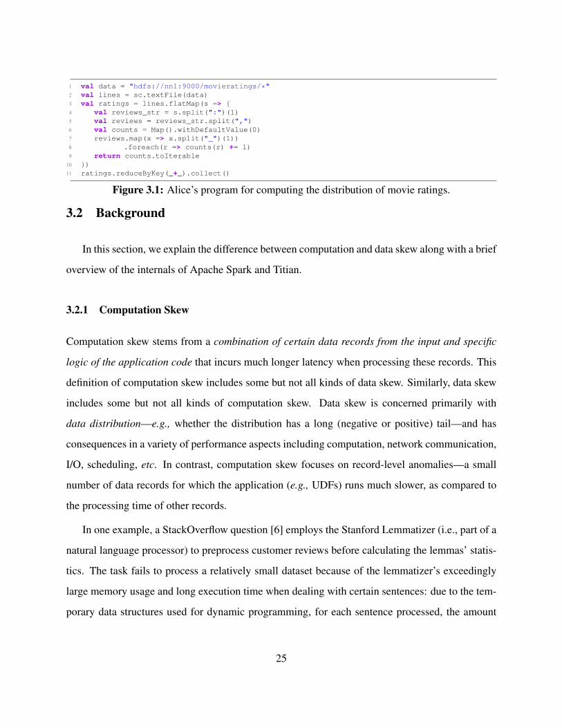
1 val data = "hdfs://nn1:9000/movieratings/*"2 val lines = sc.textFile(data)3 val ratings = lines.flatMap(s => {4 val reviews_str = s.split(":")(1)5 val reviews = reviews_str.split(",")6 val counts = Map().withDefaultValue(0)7 reviews.map(x => x.split("_")(1))8 .foreach(r => counts(r) += 1)9 return counts.toIterable
10 })11 ratings.reduceByKey(_+_).collect()
Figure 3.1: Alice’s program for computing the distribution of movie ratings.
3.2 Background
In this section, we explain the difference between computation and data skew along with a brief
overview of the internals of Apache Spark and Titian.
3.2.1 Computation Skew
Computation skew stems from a combination of certain data records from the input and specific
logic of the application code that incurs much longer latency when processing these records. This
definition of computation skew includes some but not all kinds of data skew. Similarly, data skew
includes some but not all kinds of computation skew. Data skew is concerned primarily with
data distribution—e.g., whether the distribution has a long (negative or positive) tail—and has
consequences in a variety of performance aspects including computation, network communication,
I/O, scheduling, etc. In contrast, computation skew focuses on record-level anomalies—a small
number of data records for which the application (e.g., UDFs) runs much slower, as compared to
the processing time of other records.
In one example, a StackOverflow question [6] employs the Stanford Lemmatizer (i.e., part of a
natural language processor) to preprocess customer reviews before calculating the lemmas’ statis-
tics. The task fails to process a relatively small dataset because of the lemmatizer’s exceedingly
large memory usage and long execution time when dealing with certain sentences: due to the tem-
porary data structures used for dynamic programming, for each sentence processed, the amount
25
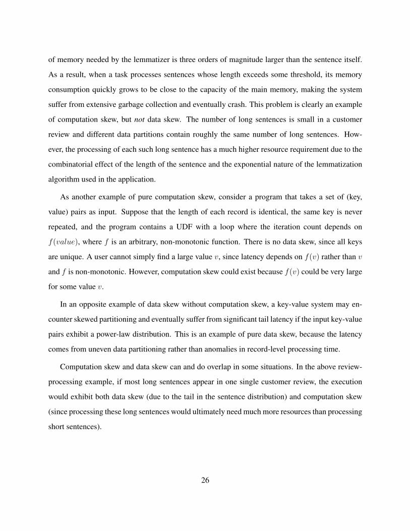
of memory needed by the lemmatizer is three orders of magnitude larger than the sentence itself.
As a result, when a task processes sentences whose length exceeds some threshold, its memory
consumption quickly grows to be close to the capacity of the main memory, making the system
suffer from extensive garbage collection and eventually crash. This problem is clearly an example
of computation skew, but not data skew. The number of long sentences is small in a customer
review and different data partitions contain roughly the same number of long sentences. How-
ever, the processing of each such long sentence has a much higher resource requirement due to the
combinatorial effect of the length of the sentence and the exponential nature of the lemmatization
algorithm used in the application.
As another example of pure computation skew, consider a program that takes a set of (key,
value) pairs as input. Suppose that the length of each record is identical, the same key is never
repeated, and the program contains a UDF with a loop where the iteration count depends on
f(value), where f is an arbitrary, non-monotonic function. There is no data skew, since all keys
are unique. A user cannot simply find a large value v, since latency depends on f(v) rather than v
and f is non-monotonic. However, computation skew could exist because f(v) could be very large
for some value v.
In an opposite example of data skew without computation skew, a key-value system may en-
counter skewed partitioning and eventually suffer from significant tail latency if the input key-value
pairs exhibit a power-law distribution. This is an example of pure data skew, because the latency
comes from uneven data partitioning rather than anomalies in record-level processing time.
Computation skew and data skew can and do overlap in some situations. In the above review-
processing example, if most long sentences appear in one single customer review, the execution
would exhibit both data skew (due to the tail in the sentence distribution) and computation skew
(since processing these long sentences would ultimately need much more resources than processing
short sentences).
26

3.2.2 Apache Spark and Titian
Apache Spark [5] is a dataflow system that provides a programming model using Resilient Dis-
tributed Datasets (RDDs) which distributes the computations on a cluster of multiple worker nodes.
Spark internally transforms a sequence of transformations (logical plan) into a directed acyclic
graph (DAG) (physical plan). The physical plan consists of a sequence of stages, each of which
is made up of pipelined transformations and ends at a shuffle. Using the DAG, Spark’s scheduler
executes each stage by running, on different nodes, parallel tasks each taking a partition of the
stage’s input data.
Titian [59] extends Spark to provide support for data provenance—the historical record of data
movement through transformations. It accomplishes this by inserting tracing agents at the start
and end of each stage. Each tracing agent assigns a unique identifier to each record consumed or
produced by the stage. These identifiers are collected into agent tables that store the mappings
between input and output records. In order to minimize the runtime tracing overhead, Titian asyn-
chronously stores agent tables in Spark’s BlockManager storage system using threads separated
from those executing the application. Titian enables developers to trace the movement of individ-
ual data records forward or backward along the pipeline by joining these agent tables according to
their input and output mappings.
However, Titian has limited usefulness in debugging computation skew. First, it cannot reason
about computation latency for any individual record. In the event that a user is able to isolate a
delayed output, Titian can leverage data lineage to identify the input records that contribute to the
production of this output. However, it falls short of singling out input records that have the largest
impact on application performance. Due to the lack of a fine-grained computation latency model
(e.g., record-level latency used in PERFDEBUG), Titian would potentially find a much greater num-
ber of input records that are correlated to the given delayed output, as measured in Section 3.5.5,
while only a small fraction of them may actually contribute to the observed performance problem.
27
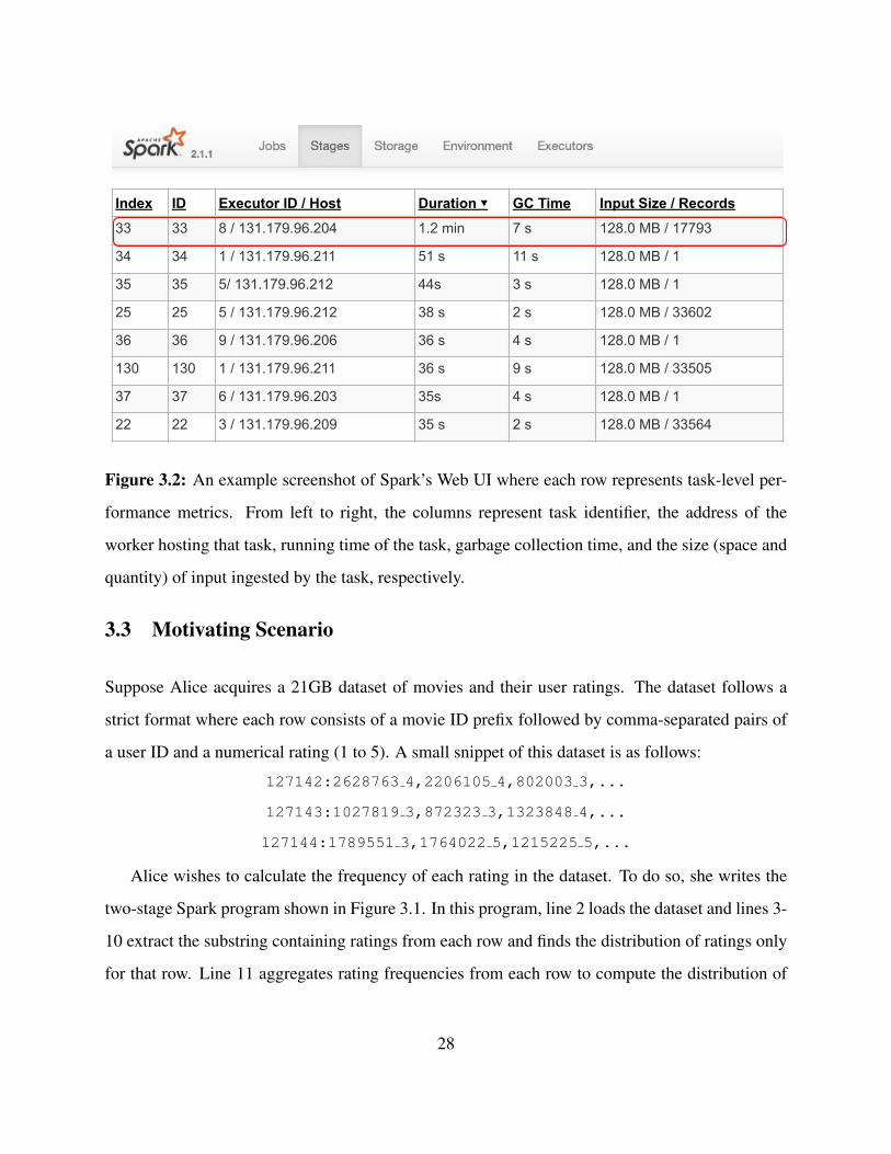
Index ID Executor ID / Host Duration ▾ GC Time Input Size / Records
33 33 8 / 131.179.96.204 1.2 min 7 s 128.0 MB / 17793
34 34 1 / 131.179.96.211 51 s 11 s 128.0 MB / 1
35 35 5/ 131.179.96.212 44s 3 s 128.0 MB / 1
25 25 5 / 131.179.96.212 38 s 2 s 128.0 MB / 33602
36 36 9 / 131.179.96.206 36 s 4 s 128.0 MB / 1
130 130 1 / 131.179.96.211 36 s 9 s 128.0 MB / 33505
37 37 6 / 131.179.96.203 35s 4 s 128.0 MB / 1
22 22 3 / 131.179.96.209 35 s 2 s 128.0 MB / 33564
Figure 3.2: An example screenshot of Spark’s Web UI where each row represents task-level per-
formance metrics. From left to right, the columns represent task identifier, the address of the
worker hosting that task, running time of the task, garbage collection time, and the size (space and
quantity) of input ingested by the task, respectively.
3.3 Motivating Scenario
Suppose Alice acquires a 21GB dataset of movies and their user ratings. The dataset follows a
strict format where each row consists of a movie ID prefix followed by comma-separated pairs of
a user ID and a numerical rating (1 to 5). A small snippet of this dataset is as follows:
127142:2628763 4,2206105 4,802003 3,...
127143:1027819 3,872323 3,1323848 4,...
127144:1789551 3,1764022 5,1215225 5,...
Alice wishes to calculate the frequency of each rating in the dataset. To do so, she writes the
two-stage Spark program shown in Figure 3.1. In this program, line 2 loads the dataset and lines 3-
10 extract the substring containing ratings from each row and finds the distribution of ratings only
for that row. Line 11 aggregates rating frequencies from each row to compute the distribution of
28
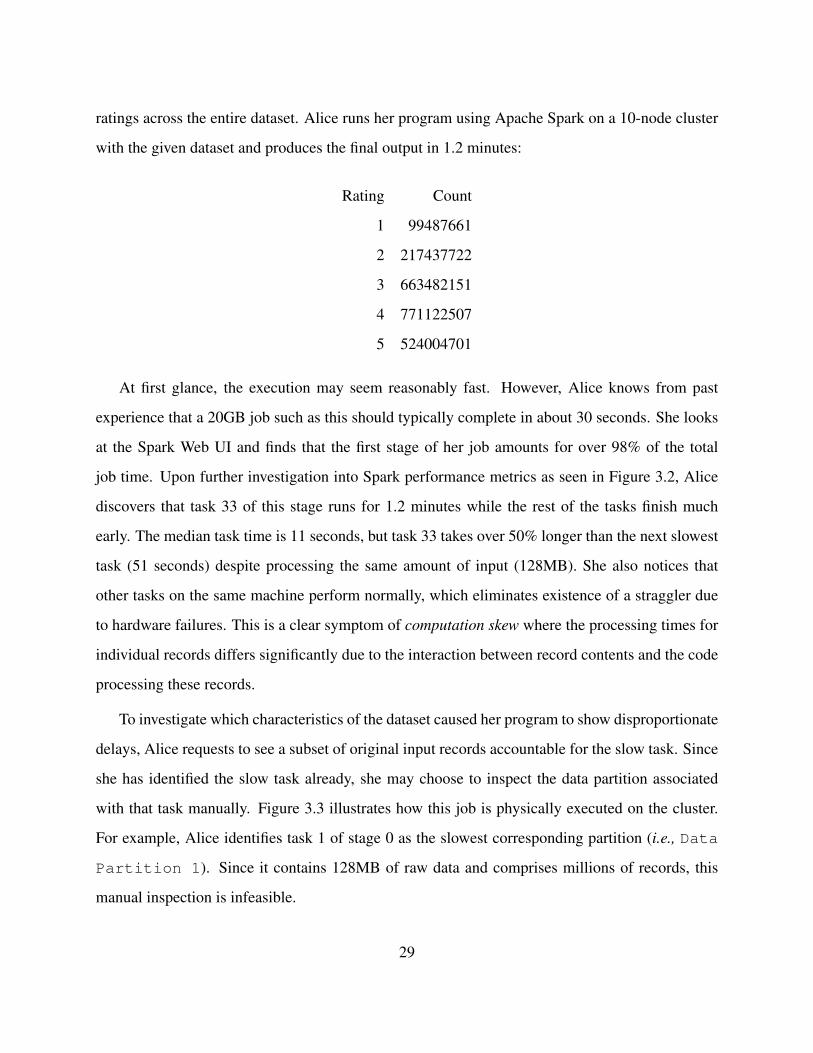
ratings across the entire dataset. Alice runs her program using Apache Spark on a 10-node cluster
with the given dataset and produces the final output in 1.2 minutes:
Rating Count
1 99487661
2 217437722
3 663482151
4 771122507
5 524004701
At first glance, the execution may seem reasonably fast. However, Alice knows from past
experience that a 20GB job such as this should typically complete in about 30 seconds. She looks
at the Spark Web UI and finds that the first stage of her job amounts for over 98% of the total
job time. Upon further investigation into Spark performance metrics as seen in Figure 3.2, Alice
discovers that task 33 of this stage runs for 1.2 minutes while the rest of the tasks finish much
early. The median task time is 11 seconds, but task 33 takes over 50% longer than the next slowest
task (51 seconds) despite processing the same amount of input (128MB). She also notices that
other tasks on the same machine perform normally, which eliminates existence of a straggler due
to hardware failures. This is a clear symptom of computation skew where the processing times for
individual records differs significantly due to the interaction between record contents and the code
processing these records.
To investigate which characteristics of the dataset caused her program to show disproportionate
delays, Alice requests to see a subset of original input records accountable for the slow task. Since
she has identified the slow task already, she may choose to inspect the data partition associated
with that task manually. Figure 3.3 illustrates how this job is physically executed on the cluster.
For example, Alice identifies task 1 of stage 0 as the slowest corresponding partition (i.e., Data
Partition 1). Since it contains 128MB of raw data and comprises millions of records, this
manual inspection is infeasible.
29
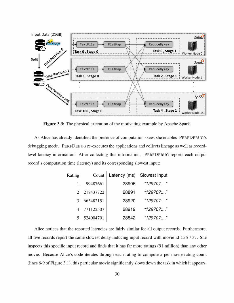
.
.
.
Task0,Stage0 WorkerNode0
WorkerNode1
WorkerNode15
TextFile
TextFile
TextFile
FlatMap
FlatMap
FlatMap
ReduceByKey
ReduceByKey
ReduceByKey
Task1,Stage0
Task166,Stage0
Task0,Stage1
Task2,Stage1
Task4,Stage1
Split
.
.
....
InputData(21GB)
Figure 3.3: The physical execution of the motivating example by Apache Spark.
As Alice has already identified the presence of computation skew, she enables PERFDEBUG’s
debugging mode. PERFDEBUG re-executes the applications and collects lineage as well as record-
level latency information. After collecting this information, PERFDEBUG reports each output
record’s computation time (latency) and its corresponding slowest input:
Rating Count Latency (ms) Slowest Input
1 99487661 28906 “129707:...”
2 217437722 28891 “129707:...”
3 663482151 28920 “129707:...”
4 771122507 28919 “129707:...”
5 524004701 28842 “129707:...”
Alice notices that the reported latencies are fairly similar for all output records. Furthermore,
all five records report the same slowest delay-inducing input record with movie id 129707. She
inspects this specific input record and finds that it has far more ratings (91 million) than any other
movie. Because Alice’s code iterates through each rating to compute a per-movie rating count
(lines 6-9 of Figure 3.1), this particular movie significantly slows down the task in which it appears.
30
Alice suspects this unusually high rating count to be a data quality issue of some sort. As a result,
she chooses to handle movie 129707 by removing it from the input dataset. In doing so, she finds
that the removal of just one record decreases her program’s execution time from 1.2 minutes to 31
seconds, which is much closer to her initial expectations.
Note that Alice’s decision to remove movie 129707 is only one example of how she may
choose to address this computation skew. PERFDEBUG is designed to detect and investigate
computation skew, but appropriate remediations will vary depending on use cases and must be
determined by the user.
3.4 Approach
When a sign of poor performance is seen, PERFDEBUG performs post-mortem debugging by tak-
ing in a Spark application and a dataset as inputs, and pinpoints the precise input record with the
most impact on the execution time. Once PERFDEBUG is enabled, it is fully automatic and does
not require any human judgment. Its approach is broken down into three steps. First, PERFDE-
BUG monitors coarse-grained performance metrics as a signal for computation skew. Second,
PERFDEBUG re-executes the application on the entire input to collect lineage information and la-
tency measurements. Finally, the lineage and latency information is combined to compute the time
cost of producing individual output records. During this process, PERFDEBUG also assesses the
impact of individual input records on the overall performance and keeps track of those with the
highest impact on each output.
Sections 3.4.2 and 3.4.3 describe how to accumulate and attribute latencies to individual records
throughout the multi-stage pipeline. This record level latency attribution differentiates PERFDE-
BUG from merely identifying the top-N expensive records within each stage because the mappings
between input records and intermediate output records are not 1:1 in modern big data analytics.
Operators such as join, reduce, and groupByKey generate n:1 mappings, while flatmap
creates 1:n mappings. Thus, finding the top-N slow records from each stage may work on a single
31

stage program but does not work for multi-stage programs with aggregation and data-split opera-
tors.
3.4.1 Performance Problem Identification
When PERFDEBUG is enabled on a Spark application, it identifies irregular performance by mon-
itoring built-in performance metrics reported by Apache Spark. In addition to the running time
of individual tasks, we utilize other constituent performance metrics, such as GC and serialization
time, to identify irregular performance behavior. Several prior works, such as Yak [88], have high-
lighted the significant impact of GC on Big Data application performance. They also report that
GC can even account for up to 50% of the total running time of such applications.
A high GC time can be observed due to two reasons: (1) millions of objects are being created
within a task’s runtime and (2) by the sheer size of individual objects created by UDFs while
processing the input data. Similarly, a high serialization/deserialization time is usually induced for
the same reasons. In both cases, high GC or serialization times are usually triggered by a specific
characteristic of the input dataset. Referring back to our motivating scenario, a single row in the
input dataset may comprise a large amount of information and lead to the creation of many objects.
As a dataflow framework handles many such objects within a given task, both GC and serialization
for that particular task soar. Since stage boundaries represent blocking operations (meaning that
each task has to complete before moving to the next stage), the high volume of objects holds back
the whole stage and leads to slower application performance. This effect can be propagated over
multiple stages as objects are passed around and repeatedly serialized and deserialized.
PERFDEBUG applies lightweight instrumentation to the Spark application by attaching a cus-
tom listener that observes performance metrics reported by Spark such as (1) task time, (2) GC
time, and (3) serialization time. Note that PERFDEBUG is not limited to only these metrics and
can be extended to support other performance measurements. For example, we can implement a
custom listener to measure additional statistics described in [87] such as shuffle object serialization
32

In Out Computation Latencyr1 o1 latency1r2 o2 latency2
Titian PerfDebug
In Outr1 o1r2 o2
Figure 3.4: During program execution, PERFDEBUG also stores latency information in lineage
tables comprising of an additional column of ComputationLatency.
and deserialization times. This lightweight monitoring enables PERFDEBUG to avoid unnecessary
instrumentation overheads for applications that do not exhibit computation skew. When an abnor-
mality is identified, PERFDEBUG starts post-mortem debugging to enable deeper instrumentation
at the record level and to find the root cause of performance delays. Alternatively, a user may
manually identify performance issues and explicitly invoke PERFDEBUG’s debugging mode.
3.4.2 Capturing Data Lineage and Latency
As the first step in post-mortem debugging, PERFDEBUG re-executes the application to collect
latency (computation time of applying a UDF) of each record per stage in addition to data lineage
information. For this purpose, PERFDEBUG extends Titian [59] and stores the per-record latency
alongside record identifiers.
3.4.2.1 Extending Data Provenance
PERFDEBUG adopts Titian [59] to capture record level input-output mapping. However, using
off-the-shelf Titian is insufficient as it does not profile the compute time of each intermediate
record which is crucial for locating the expensive input records. To enable performance profiling in
33

addition to data provenance, PERFDEBUG extends Titian by measuring the time taken to compute
each intermediate record and storing these latencies alongside the data provenance information.
Titian captures data lineages by generating lineage tables that map the output record at one stage
to the input of the next stage. Later, it constructs a complete lineage graph by joining the lineage
tables, one at a time, across multiple stages. While Titian generates lineage tables, PERFDEBUG
measures the computational latency of executing a chain of UDFs in a given stage on each record
and appends it to the lineage tables in an additional column as seen in Figure 3.4. This extension
produces a data provenance graph that exposes individual record computation times, which is used
in Section 3.4.3 to precisely identify expensive input records.
Titian stores each lineage table in Spark’s internal memory layer (abstracted as a file system
through BlockManager) to lower runtime overhead of accessing memory. However, this approach
is not feasible for post-mortem performance debugging as it hogs the memory available for the ap-
plication and restricts the lifespan of lineage tables to the liveliness of a Spark session. PERFDE-
BUG supports post-mortem debugging in which a user can interactively debug anytime without
compromising other applications by holding too many resources. To realize this, PERFDEBUG
stores lineage tables externally using Apache Ignite [2] in an asynchronous fashion. As a per-
sistent in-memory storage, Ignite decouples PERFDEBUG from the session associated to a Spark
application and enables PERFDEBUG to support post-mortem debugging anytime in the future. We
choose Ignite for its compatibility with Spark RDDs and efficient data access time, but PERFDE-
BUG can also be generalized to other storage systems.
Figure 3.5 demonstrates the lineage information collected by PERFDEBUG, shown as In and
Out. Using this information, PERFDEBUG can execute backward tracing to identify the in-
put records for a given output. For example, the output record o3 under the Out column of
Ì post-shuffle can be traced backwards to [i3,i8] (In column of Ì) through the Out
column of Ë pre-shuffle. We further trace those intermediate records from In column of
pre-shuffle back to the program inputs [h1, h2, h3, h4, h5] in the Out column of Ê
HDFS.
34

StageLatency
TotalLatency
MostImpactfulSource
RemediatedLatency Out
- 0 h1 0 h1- 0 h2 0 h2
- 0 h3 0 h3
Partition0
Partition1
StageLatency
TotalLatency
MostImpactfulSource
RemediatedLatency Out
- 0 h4 0 h4- 0 h5 0 h5
In StageLatency TotalLatency
MostImpactfulSource
RemediatedLatency Out
[h1,h2] max(486,28848)+2/10*60 28860 h2 498 i1[h1,h2] max(486,28848)+2/10*60 28860 h2 498 i2
[h1,h2,h3] max(486,28848,611)+3/10*60 28866 h2 629 i3
[h1,h2] max(486,28848)+2/10*60 28860 h2 498 i4[h1] max(239)+1/10*60 245 h1 0 i5PartitionLatency:60ms
In StageLatency TotalLatency MostImpactful Source RemediatedLatency Out[i1,i6] 2/4*60=30 max(28860,274)+30=28890 h2 304 o1[i2,i7] 2/4*60=30 max(28860,274)+30=28890 h2 304 o2
PartitionLatency:60ms
HDFS Pre-Shuffle
Post-Shuffle
In StageLatency TotalLatency MostImpactful Source RemediatedLatency Out[i3,i8] 2/6*120=40 max(28866,284)+40=28906 h2 324 o3
[i4,i9] 2/6*120=40 max(28860,284)+40=28900 h2 324 o4[i5,i10] 2/6*120=40 max(245,170)+40=285 h1 210 o5
PartitionLatency:120ms
In StageLatency TotalLatency
MostImpactfulSource
RemediatedLatency Out
[h5] max(264)+1/7*70 274 h5 0 i6[h5] max(264)+1/7*70 274 h5 0 i7
[h4,h5] max(160,264)+2/7*70 284 h5 180 i8[h4,h5] max(160,264)+2/7*70 284 h5 180 i9[h4] max(160)+1/7*70 170 h4 0 i10PartitionLatency:70ms
1 2
3
Figure 3.5: The snapshots of lineage tables collected by PERFDEBUG. Ê, Ë, and Ì illustrate the
physical operations and their corresponding lineage tables in sequence for the given application.
In the first step, PERFDEBUG captures the Out, In, and Stage Latency columns, which represent
the input-output mappings as well as the stage-level latencies per record. During output latency
computation, PERFDEBUG calculates three additional columns (Total Latency, Most Impactful
Source, and Remediated Latency) to keep track of cumulative latency, the ID of the original input
with the largest impact on Total Latency, and the estimated latency if the most impactful record
did not impact application performance.
3.4.2.2 Latency Measurement
Data provenance alone is insufficient for calculating the impact of individual records on overall ap-
plication performance. As performance issues can be found both within stages (e.g., an expensive
filter) and between stages (e.g., due to data skew in shuffling), PERFDEBUG tracks two types
35

of latency. Computation Latency is measured from a chain of UDFs in dataflow operators such as
map and filter, while Shuffle Latency is measured by timing shuffle-based operations such as
reduce and distributing this measurement based on input-output ratios.
For a given record r, the total time to execute all UDFs of a specific stage, StageLatency(r)
is computed as:
StageLatency(r) = ComputationLatency(r) + ShuffleLatency(r)
Computation Latency As described in Section 3.2, a stage consists of multiple pipelined trans-
formations that are applied to input records to produce the stage output. Each transformation is in
turn defined by an operator that takes in a UDF. To measure computation latency, PERFDEBUG
wraps every non-shuffle UDF in a timing function that measures the time span of that UDF invoca-
tion for each record. We define non-shuffle UDFs as those passed as inputs to operators that do not
trigger a shuffle such as flatmap. Since the pipelined transformations in a stage are applied sequen-
tially on each record, PERFDEBUG calculates the computation latency ComputationLatency(r)
of record r by adding the execution times of each UDF applied to r within the current stage:
ComputationLatency(r) =∑f∈UDF
Time(f, r)
For example, consider the following program:
1 val f1 = (x: Int) => List(x, x*2) // 50ms2 val f2 = (x: Int) => x < 100 // 10ms, 20ms3 integerRdd.flatMap(f1).filter(f2).collect()
When executing this program for a single input 42, we obtain outputs of 42 and 84. Suppose
PERFDEBUG observes that f1(42) takes 50 milliseconds, while f2(42) and f2(84) take 10 and 20
milliseconds respectively. PERFDEBUG computes the computation latency for the first output,
42, as 50 + 10 = 60 milliseconds. Similarly, the second output, 84, has a computation latency of
50 + 20 = 70 milliseconds.
In stages preceding a shuffle, multiple input records may be pre-aggregated to produce a single
output record. In the Ë-Pre-Shuffle lineage table shown in Figure 3.5, the In column and the
36
left term in the StageLatency column reflect these multiple input identifiers and computation la-
tencies. As the Spark application’s execution proceeds through each stage, PERFDEBUG captures
StageLatency for each output record per stage and includes it into the lineage tables under the
Stage Latency column as seen in Figure 3.5. These lineage tables are stored in PERFDEBUG’s Ig-
nite storage where each table encodes the computation latency of each record and the relationship
of that record to the output records of the previous stage.
Shuffle Latency In Spark, a shuffle at a stage boundary comprises of two steps: a pre-shuffle
step and a post-shuffle step. In the pre-shuffle step, each task’s output data is sorted or aggregated
and then stored in the local memory of the current node. We measure the time it takes to perform
the pre-shuffle step on the whole partition as pre-shuffle latency. In the post-shuffle step, a node
in the next stage fetches this remotely stored data from individual nodes and sorts (or aggregates)
it again. Because of this distinction, PERFDEBUG’s shuffle latency is categorized into pre-shuffle
and post-shuffle estimations.
As both pre- and post- shuffle operations are atomic and performed in batches over each parti-
tion, we estimate the latency of an individual output record in a pre-shuffle step by (1) measuring
the proportion of the input records consumed by the output record and then (2) multiplying it with
the total shuffle time of that partition.
ShuffleLatency(r) =|Inputsr||Inputs|
∗ PartitionLatency(stager)
stager represents the stage of the record r, |Inputs| is the size of a partition, and |Inputr| is
the size of input consumed by output r. For example, the top most lineage table under Ë-
pre-shuffle in Figure 3.5 has a pre-shuffle latency of 60ms. Because output i1 is computed
from two of the partition’s ten inputs, ShuffleLatency(i1) is equal to two tenths of partition
latency i.e., 210∗ 60. Similarly, output i3 is computed from three inputs so its shuffle latency is
310∗ 60.
37
3.4.3 Expensive Input Isolation
To identify the most expensive input for a given application and dataset, PERFDEBUG analyzes
data provenance and latency information from Section 3.4.2 and calculates three values for each
output record: (1) the total latency of the output record, (2) the input record that contributes most
to this latency (most impactful source), and (3) the expected output latency if that input record
had zero latency or otherwise did not affect application performance (remediated latency). Once
calculated, PERFDEBUG groups these values by their most impactful source and compares each
input’s maximum latency with its maximum remediated latency to identify the input with the most
impact on application performance.
Output Latency Calculation. PERFDEBUG estimates the total latency for each output record
as a sum of associated stage latencies established by data provenance based mappings. By lever-
aging the data lineage and latency tables collected earlier, it computes the latency using two key
insights:
• In dataflow systems, records for a given stage are often computed in parallel across several
tasks. Assuming all inputs for a given record are computed in this parallel manner, the time
required for all the inputs to be made available is at least the time required for the final input
to arrive. This corresponds to the maximum of the dependent input latencies.
• A record can only be produced when all its inputs are made available. Thus, the total latency
of any given record must be at least the sum of its stage-specific individual record latency,
described in Section 3.4.2, and the slowest latency of its inputs, described above.
The process of computing output latencies is inspired by the forward tracing algorithm from
Titian, starting from the entire input dataset.2 PERFDEBUG recursively joins lineage tables to con-
struct input-output mappings across stages. For each recursive join in the forward trace, PERFDE-
2 PERFDEBUG leverages lineage-based backward trace to remove inputs that do not contribute to program outputswhile computing output latencies.
38
BUG computes the accumulated latency TotalLatency(r) of an output r by first finding the latency
of the slowest input (SlowestInputLatency(r)) among the inputs from the preceding stage on
which the output depends upon, and then adding the stage-specific latency StageLatency(r) as
described in Section 3.4.2:
SlowestInputLatency(r) = max(∀i ∈ Inputsprev stage : TotalLatency(i))
TotalLatency(r) = SlowestInputLatency(r) + StageLatency(r)
Once TotalLatency is calculated for each record at each step of recursive join, it is added in
the corresponding lineage tables under the new column, Total Latency. For example, the out-
put record i1 in Ë-Pre-Shuffle lineage table of Figure 3.5 has two inputs from the pre-
vious stage, h1 and h2 with their total latencies of 486ms and 28848ms respectively. There-
fore, its SlowestInputLatency(i1) is the maximum of 70 and 28848 which is then added to its
ShuffleLatency(i1) = 210∗ 60ms, making the total latency of i1 28860ms.
Tracing Input Records. Based on the output latency, a user can select an output and use
PERFDEBUG to perform a backward trace as described in Section 3.4.2. However, the input iso-
lated through this technique may not be precise as it relies solely on data lineage. For example,
Alice uses PERFDEBUG to compute the latency of individual output records, shown in Figure
3.5. Next, Alice isolates the slowest output record, o3. Finally, she uses PERFDEBUG to trace
backward and identify the inputs for o3. Unfortunately, all five inputs contribute to o3. Because
there is only one significant delay-inducing input record (h2) which contributes to o3’s latency,
the lineage-based backward trace returns a super-set of delay-inducing inputs and achieves a low
precision of 20%.
Tracking Most Impactful Input. To improve upon the low precision of lineage-based backward
traces, PERFDEBUG propagates record identifiers during output latency computation and retains
the input records with the most impact on an output’s latency. We define the impact of an input
record as the difference between the maximum latency of all associated output records in program
39
executions with and without the given input record. Intuitively, this represents the degree to which
a delay-inducing input is a bottleneck for output record computation.
To support this functionality, PERFDEBUG takes an approach inspired by the Titian-P variant
described in [59]. In Titian-P (referred to as Titian Piggy Back), lineage tables are joined together
as soon as the lineage table of the next stage is available during a program execution. This obviates
the need for a backward trace as each lineage table contains a mapping between the intermediate
or final output and the original input, but also requires additional memory to retain a list of input
identifiers for each intermediate or final output record. PERFDEBUG’s approach differs in that
it retains only a single input identifier for each intermediate or final output record. As such, its
additional memory requirements are constant per output record and do not increase with larger
input datasets. Using this approach, PERFDEBUG is able to compute a predefined backward
trace with minimal memory overhead while avoiding the expensive computation and data shuffles
required for a backward trace.
As described earlier, the latency of a given record is dependent on the maximum latency of its
corresponding input records. In addition to this latency, PERFDEBUG computes two additional
fields during its output latency computation algorithm to easily support debugging queries about
the impact of a particular input record on the overall performance of an application.
• Most Impactful Source: the identifier of the input record deemed to be the top contributor to
the latency of an intermediate or final output record. We pre-compute this so that debugging
queries do not need a backward trace and can easily identify the single most impactful record
for a given output record.
• Remediated Latency: the expected latency of an intermediate or final output record if Most
Impactful Source had zero latency or otherwise did not affect application performance. This
is used to quantify the impact of the Most Impactful Source on the latency of the output
record.
As with TotalLatency, these fields are inductively updated (as seen in Figure 3.5) with each
40

recursive join when computing output latency. During recursive joins, Most Impactful Source field
becomes the Most Impactful Source of the input record possessing the highest TotalLatency, similar
to an argmax function. Remediated Latency becomes the current record’s StageLatency plus the
maximum latency over all input records except the Most Impactful Source. For example, the output
o3 has the highest TotalLatency with the most impactful source of h2. This is reported based on
the reasoning that, if we remove h2, the latencies of input i3 and i8 drop the most compared to
removing either h1 or h3.
In addition to identifying the most impactful record for an individual program output,
PERFDEBUG can also use these extended fields to identify input records with the largest impact
on overall application performance. This is accomplished by grouping the output latency table
by Most Impactful Source and finding the group with the largest difference between its maximum
TotalLatency and maximum Remediated Latency. In the case of Figure 3.5, input record h2 is
chosen because its difference (28906ms - 324ms) is greater than that of h1 (285ms - 210ms).
3.5 Experimental Evaluation
Our applications and datasets are described in Table 3.1. Our inputs come from industry-standard
PUMA benchmarks [12], public institution datasets [90], and prior work on automated debugging
of big data analytics [47]. Case studies described in Sections 3.5.3, 3.5.2, and 3.5.4 demonstrate
when and how a user may use PERFDEBUG. PERFDEBUG provides diagnostic capability by iden-
tifying records attributed to significant delays and leaves it to the user to resolve the performance
problem, e.g., by re-engineering the analytical program or refactoring UDFs.
3.5.1 Experimental Setup
All case studies are executed on a cluster consisting of 10 worker nodes and a single master, all
running CentOS 7 with a network speed of 1000 Mb/s. The master node has 46GB available RAM,
a 4-core 2.40GHz CPU, and 5.5TB available disk space. Each worker node has 125GB available
41
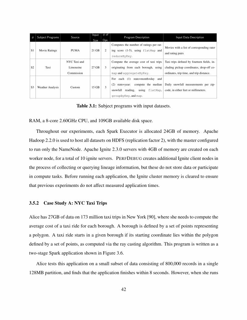
# Subject Programs SourceInput
Size
# of
OpsProgram Description Input Data Description
S1 Movie Ratings PUMA 21 GB 2
Computes the number of ratings per rat-
ing score (1-5), using flatMap and
reduceByKey.
Movies with a list of corresponding rater
and rating pairs
S2 Taxi
NYC Taxi and
Limousine
Commission
27 GB 3
Compute the average cost of taxi trips
originating from each borough, using
map and aggregateByKey.
Taxi trips defined by fourteen fields, in-
cluding pickup coordinates, drop-off co-
ordinates, trip time, and trip distance.
S3 Weather Analysis Custom 15 GB 3
For each (1) state+month+day and
(2) state+year: compute the median
snowfall reading, using flatMap,
groupByKey, and map.
Daily snowfall measurements per zip-
code, in either feet or millimeters.
Table 3.1: Subject programs with input datasets.
RAM, a 8-core 2.60GHz CPU, and 109GB available disk space.
Throughout our experiments, each Spark Executor is allocated 24GB of memory. Apache
Hadoop 2.2.0 is used to host all datasets on HDFS (replication factor 2), with the master configured
to run only the NameNode. Apache Ignite 2.3.0 servers with 4GB of memory are created on each
worker node, for a total of 10 ignite servers. PERFDEBUG creates additional Ignite client nodes in
the process of collecting or querying lineage information, but these do not store data or participate
in compute tasks. Before running each application, the Ignite cluster memory is cleared to ensure
that previous experiments do not affect measured application times.
3.5.2 Case Study A: NYC Taxi Trips
Alice has 27GB of data on 173 million taxi trips in New York [90], where she needs to compute the
average cost of a taxi ride for each borough. A borough is defined by a set of points representing
a polygon. A taxi ride starts in a given borough if its starting coordinate lies within the polygon
defined by a set of points, as computed via the ray casting algorithm. This program is written as a
two-stage Spark application shown in Figure 3.6.
Alice tests this application on a small subset of data consisting of 800,000 records in a single
128MB partition, and finds that the application finishes within 8 seconds. However, when she runs
42
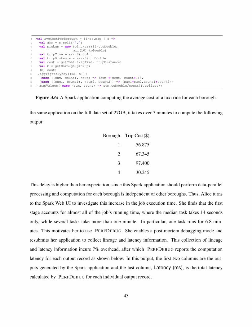
1 val avgCostPerBorough = lines.map { s =>2 val arr = s.split(’,’)3 val pickup = new Point(arr(11).toDouble,4 arr(10).toDouble)5 val tripTime = arr(8).toInt6 val tripDistance = arr(9).toDouble7 val cost = getCost(tripTime, tripDistance)8 val b = getBorough(pickup)9 (b, cost)}
10 .aggregateByKey((0d, 0))(11 {case ((sum, count), next) => (sum + next, count+1)},12 {case ((sum1, count1), (sum2, count2)) => (sum1+sum2,count1+count2)}13 ).mapValues({case (sum, count) => sum.toDouble/count}).collect()
Figure 3.6: A Spark application computing the average cost of a taxi ride for each borough.
the same application on the full data set of 27GB, it takes over 7 minutes to compute the following
output:
Borough Trip Cost($)
1 56.875
2 67.345
3 97.400
4 30.245
This delay is higher than her expectation, since this Spark application should perform data-parallel
processing and computation for each borough is independent of other boroughs. Thus, Alice turns
to the Spark Web UI to investigate this increase in the job execution time. She finds that the first
stage accounts for almost all of the job’s running time, where the median task takes 14 seconds
only, while several tasks take more than one minute. In particular, one task runs for 6.8 min-
utes. This motivates her to use PERFDEBUG. She enables a post-mortem debugging mode and
resubmits her application to collect lineage and latency information. This collection of lineage
and latency information incurs 7% overhead, after which PERFDEBUG reports the computation
latency for each output record as shown below. In this output, the first two columns are the out-
puts generated by the Spark application and the last column, Latency (ms), is the total latency
calculated by PERFDEBUG for each individual output record.
43
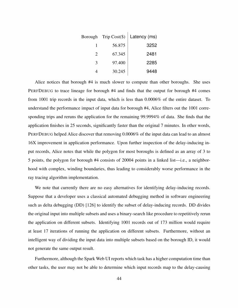
Borough Trip Cost($) Latency (ms)
1 56.875 3252
2 67.345 2481
3 97.400 2285
4 30.245 9448
Alice notices that borough #4 is much slower to compute than other boroughs. She uses
PERFDEBUG to trace lineage for borough #4 and finds that the output for borough #4 comes
from 1001 trip records in the input data, which is less than 0.0006% of the entire dataset. To
understand the performance impact of input data for borough #4, Alice filters out the 1001 corre-
sponding trips and reruns the application for the remaining 99.9994% of data. She finds that the
application finishes in 25 seconds, significantly faster than the original 7 minutes. In other words,
PERFDEBUG helped Alice discover that removing 0.0006% of the input data can lead to an almost
16X improvement in application performance. Upon further inspection of the delay-inducing in-
put records, Alice notes that while the polygon for most boroughs is defined as an array of 3 to
5 points, the polygon for borough #4 consists of 20004 points in a linked list—i.e., a neighbor-
hood with complex, winding boundaries, thus leading to considerably worse performance in the
ray tracing algorithm implementation.
We note that currently there are no easy alternatives for identifying delay-inducing records.
Suppose that a developer uses a classical automated debugging method in software engineering
such as delta debugging (DD) [126] to identify the subset of delay-inducing records. DD divides
the original input into multiple subsets and uses a binary-search like procedure to repetitively rerun
the application on different subsets. Identifying 1001 records out of 173 million would require
at least 17 iterations of running the application on different subsets. Furthermore, without an
intelligent way of dividing the input data into multiple subsets based on the borough ID, it would
not generate the same output result.
Furthermore, although the Spark Web UI reports which task has a higher computation time than
other tasks, the user may not be able to determine which input records map to the delay-causing
44
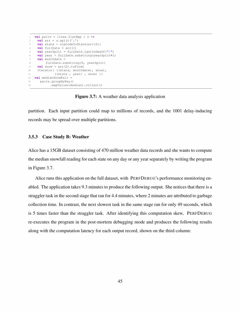
1 val pairs = lines.flatMap { s =>2 val arr = s.split(’,’)3 val state = zipCodeToState(arr(0))4 val fullDate = arr(1)5 val yearSplit = fullDate.lastIndexOf("/")6 val year = fullDate.substring(yearSplit+1)7 val monthdate =8 fullDate.substring(0, yearSplit)9 val snow = arr(2).toFloat
10 Iterator( ((state, monthdate), snow),11 ((state , year) , snow) )}12 val medianSnowFall =13 pairs.groupByKey()14 .mapValues(median).collect()
Figure 3.7: A weather data analysis application
partition. Each input partition could map to millions of records, and the 1001 delay-inducing
records may be spread over multiple partitions.
3.5.3 Case Study B: Weather
Alice has a 15GB dataset consisting of 470 million weather data records and she wants to compute
the median snowfall reading for each state on any day or any year separately by writing the program
in Figure 3.7.
Alice runs this application on the full dataset, with PERFDEBUG’s performance monitoring en-
abled. The application takes 9.3 minutes to produce the following output. She notices that there is a
straggler task in the second stage that ran for 4.4 minutes, where 2 minutes are attributed to garbage
collection time. In contrast, the next slowest task in the same stage ran for only 49 seconds, which
is 5 times faster than the straggler task. After identifying this computation skew, PERFDEBUG
re-executes the program in the post-mortem debugging mode and produces the following results
along with the computation latency for each output record, shown on the third column:
45
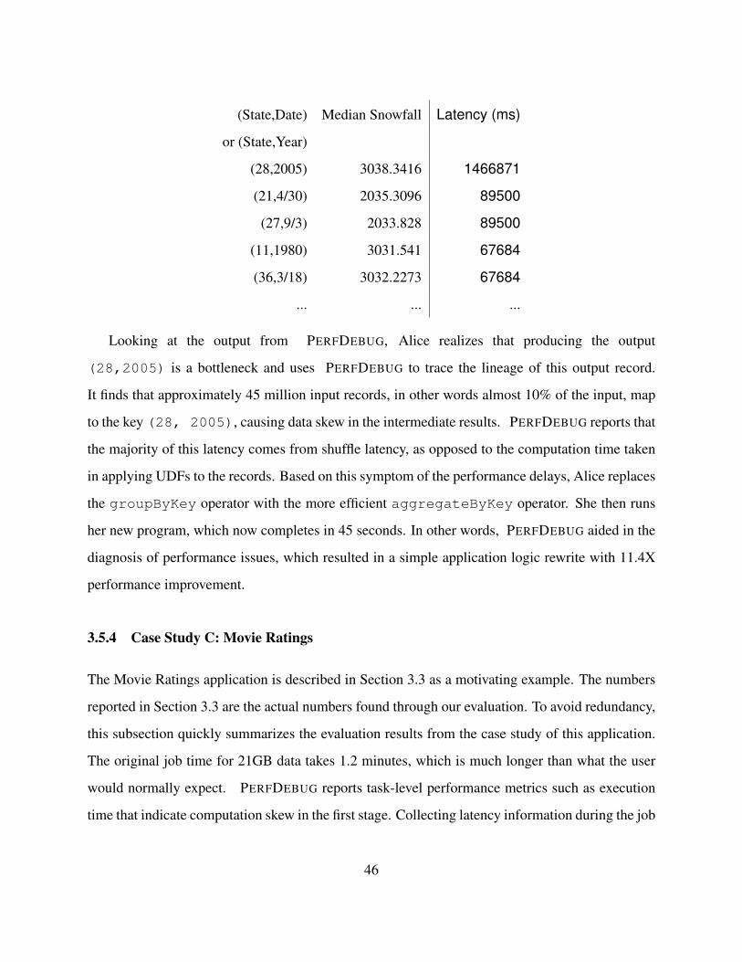
(State,Date) Median Snowfall Latency (ms)
or (State,Year)
(28,2005) 3038.3416 1466871
(21,4/30) 2035.3096 89500
(27,9/3) 2033.828 89500
(11,1980) 3031.541 67684
(36,3/18) 3032.2273 67684
... ... ...
Looking at the output from PERFDEBUG, Alice realizes that producing the output
(28,2005) is a bottleneck and uses PERFDEBUG to trace the lineage of this output record.
It finds that approximately 45 million input records, in other words almost 10% of the input, map
to the key (28, 2005), causing data skew in the intermediate results. PERFDEBUG reports that
the majority of this latency comes from shuffle latency, as opposed to the computation time taken
in applying UDFs to the records. Based on this symptom of the performance delays, Alice replaces
the groupByKey operator with the more efficient aggregateByKey operator. She then runs
her new program, which now completes in 45 seconds. In other words, PERFDEBUG aided in the
diagnosis of performance issues, which resulted in a simple application logic rewrite with 11.4X
performance improvement.
3.5.4 Case Study C: Movie Ratings
The Movie Ratings application is described in Section 3.3 as a motivating example. The numbers
reported in Section 3.3 are the actual numbers found through our evaluation. To avoid redundancy,
this subsection quickly summarizes the evaluation results from the case study of this application.
The original job time for 21GB data takes 1.2 minutes, which is much longer than what the user
would normally expect. PERFDEBUG reports task-level performance metrics such as execution
time that indicate computation skew in the first stage. Collecting latency information during the job
46
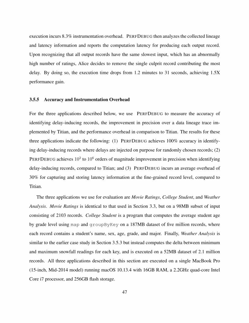
execution incurs 8.3% instrumentation overhead. PERFDEBUG then analyzes the collected lineage
and latency information and reports the computation latency for producing each output record.
Upon recognizing that all output records have the same slowest input, which has an abnormally
high number of ratings, Alice decides to remove the single culprit record contributing the most
delay. By doing so, the execution time drops from 1.2 minutes to 31 seconds, achieving 1.5X
performance gain.
3.5.5 Accuracy and Instrumentation Overhead
For the three applications described below, we use PERFDEBUG to measure the accuracy of
identifying delay-inducing records, the improvement in precision over a data lineage trace im-
plemented by Titian, and the performance overhead in comparison to Titian. The results for these
three applications indicate the following: (1) PERFDEBUG achieves 100% accuracy in identify-
ing delay-inducing records where delays are injected on purpose for randomly chosen records; (2)
PERFDEBUG achieves 102 to 106 orders of magnitude improvement in precision when identifying
delay-inducing records, compared to Titian; and (3) PERFDEBUG incurs an average overhead of
30% for capturing and storing latency information at the fine-grained record level, compared to
Titian.
The three applications we use for evaluation are Movie Ratings, College Student, and Weather
Analysis. Movie Ratings is identical to that used in Section 3.3, but on a 98MB subset of input
consisting of 2103 records. College Student is a program that computes the average student age
by grade level using map and groupByKey on a 187MB dataset of five million records, where
each record contains a student’s name, sex, age, grade, and major. Finally, Weather Analysis is
similar to the earlier case study in Section 3.5.3 but instead computes the delta between minimum
and maximum snowfall readings for each key, and is executed on a 52MB dataset of 2.1 million
records. All three applications described in this section are executed on a single MacBook Pro
(15-inch, Mid-2014 model) running macOS 10.13.4 with 16GB RAM, a 2.2GHz quad-core Intel
Core i7 processor, and 256GB flash storage.
47
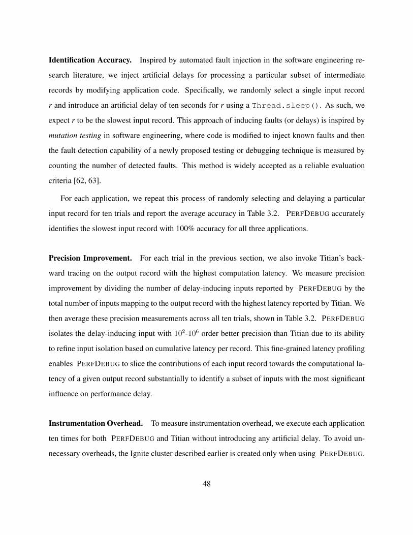
Identification Accuracy. Inspired by automated fault injection in the software engineering re-
search literature, we inject artificial delays for processing a particular subset of intermediate
records by modifying application code. Specifically, we randomly select a single input record
r and introduce an artificial delay of ten seconds for r using a Thread.sleep(). As such, we
expect r to be the slowest input record. This approach of inducing faults (or delays) is inspired by
mutation testing in software engineering, where code is modified to inject known faults and then
the fault detection capability of a newly proposed testing or debugging technique is measured by
counting the number of detected faults. This method is widely accepted as a reliable evaluation
criteria [62, 63].
For each application, we repeat this process of randomly selecting and delaying a particular
input record for ten trials and report the average accuracy in Table 3.2. PERFDEBUG accurately
identifies the slowest input record with 100% accuracy for all three applications.
Precision Improvement. For each trial in the previous section, we also invoke Titian’s back-
ward tracing on the output record with the highest computation latency. We measure precision
improvement by dividing the number of delay-inducing inputs reported by PERFDEBUG by the
total number of inputs mapping to the output record with the highest latency reported by Titian. We
then average these precision measurements across all ten trials, shown in Table 3.2. PERFDEBUG
isolates the delay-inducing input with 102-106 order better precision than Titian due to its ability
to refine input isolation based on cumulative latency per record. This fine-grained latency profiling
enables PERFDEBUG to slice the contributions of each input record towards the computational la-
tency of a given output record substantially to identify a subset of inputs with the most significant
influence on performance delay.
Instrumentation Overhead. To measure instrumentation overhead, we execute each application
ten times for both PERFDEBUG and Titian without introducing any artificial delay. To avoid un-
necessary overheads, the Ignite cluster described earlier is created only when using PERFDEBUG.
48
Benchmark AccuracyPrecision
ImprovementOverhead
Movie Ratings 100% 2102X 1.04X
College Student 100% 1250000X 1.39X
Weather Analysis 100% 294X 1.48X
Average 100% 417465X 1.30X
Table 3.2: Identification Accuracy of PERFDEBUG and instrumentation overheads compared to
Titian, for the subject programs described in Section 3.5.5.
The resulting performance multipliers are shown in Table 3.2. We observe that the performance
overhead of PERFDEBUG compared to Titian ranges from 1.04X to 1.48X. Across all applica-
tions, PERFDEBUG’s execution times average 1.30X times as long as Titian’s. Titian reports an
overhead of about 30% compared to Apache Spark [59]. PERFDEBUG introduces additional over-
head because it instruments every invocation of a UDF to capture and store the record level latency.
However, such fine-grained profiling differentiates PERFDEBUG from Titian in terms of its ability
to isolate expensive inputs. PERFDEBUG’s overhead to identify a delay inducing record is small
compared to the alternate method of trial and error debugging, which requires multiple execution
of the original program.
3.6 Discussion
This chapter discusses PERFDEBUG, the first automated performance debugging tool to diagnose
the root cause of performance delays induced by interaction between data and application code.
PERFDEBUG automatically reports the symptoms of computation skew—abnormally high compu-
tation costs for a small subset of data records—by combining a novel latency estimation technique
with an existing data provenance tool to automatically isolate delay-inducing inputs. In our evalua-
tion, PERFDEBUG validates the sub-hypothesis (SH1) by identifying 100% of injected faults with
49

the resulting input sets yielding many orders of magnitude (102 to 108) improvement in precision
compared to Titian.
PERFDEBUG goes beyond traditional data provenance and models input contribution towards
an output as a quantifiable metric, rather than a binary condition. However, this notion of input
record influence towards output production is not restricted solely to performance debugging. In
the next chapter, we investigate the next sub-hypothesis (SH2) and explore how we can improve the
precision of correctness debugging techniques by leveraging application code semantics combined
with individual record contribution towards producing aggregation results.
50
CHAPTER 4
Enhancing Provenance-based Debugging with Taint
Propagation and Influence Functions
Root cause analysis in DISC systems often involves pinpointing the precise culprit records in an
input dataset responsible for incorrect or anomalous output. However, existing provenance-based
approaches do not accurately capture control and data flows in user-defined application code and
fail to measure the relative impact each input record has towards producing an output. As a result,
the identified input data may be too large for manual inspection and insufficient for debugging with-
out additional expensive post-mortem analysis. To address the need for more precise root cause
analysis, we investigate sub-hypothesis (SH2): We can improve the precision of fault isolation
techniques by extending data provenance techniques to incorporate application code semantics as
well as individual record contribution towards producing an output. In this chapter, we present an
influence-based debugging tool for precisely identifying relevant input records through a combi-
nation of white-box taint analysis and influence functions which rank or prioritize individual input
records based on their contribution towards aggregated outputs.1
4.1 Introduction
The correctness of DISC applications depends on their ability to handle real-world data; however,
data is constantly changing and erroneous or invalid data can lead to data processing failures or
1This notion of influence functions is inspired by work in machine learning explainability [65] which itself borrowsfrom statistics [52].
51

incorrect outputs. Developers then need to identify the exact cause of these failures by distinguish-
ing a critical set of input records from billions of other records. While existing data provenance
techniques [59, 79, 33] enable developers to trace outputs to identify their corresponding inputs,
they fail to accommodate the internal semantics of user-defined functions (UDFs) as well as the
differing contributions between records in an aggregation, leading to imprecise of overapproxi-
mated input traces. On the other hand, search-based debugging techniques [128, 47] are targeted
towards identifying minimal reproducing input subsets but require mutiple re-runs which can be-
come prohibitively expensive for DISC applications operating with large-scale data.
We design FLOWDEBUG, the first influence-based debugging tool for DISC applications.
Given a suspicious output in a DISC application, FLOWDEBUG identifies the precise record(s)
that contributed the most towards generating the suspicious output for which a user wants to in-
vestigate its origin. The key idea of FLOWDEBUG is two-fold. First, FLOWDEBUG incorporates
white-box tainting analysis to account for the effect of control and data flows in UDFs, all the
way to individual variable-level in tandem with traditional data provenance. This fine-grained taint
analysis is implemented through automated transformation of a DISC application by injecting new
data types to capture logical provenance mappings within UDFs. Second, to drastically improve
both performance and utility of identified input records, FLOWDEBUG incorporates the notion of
influence functions [66] at aggregation operators to selectively monitor the most influential input
subset. For example, it can use an outlier-detecting influence function to identify unusually large
values increase an average above expected ranges. FLOWDEBUG pre-defines influence functions
for commonly used UDFs, and a user may also provide custom influence functions as needed to
encode their notion of selectivity and priority suitable for the specific UDF passed as an argument
to the aggregation operator.
Our evaluation demonstrates that FLOWDEBUG achieves up to five orders-of-magnitude im-
provement in precision compared to Titian, a state-of-the-art data provenance tool. Compared
to BigSift, a search-based debugging technique, FLOWDEBUG improves recall by up to 150X.
Finally, FLOWDEBUG performs its analysis up to 51X faster than Titian and 1000X faster than
52
BigSift.
The rest of this chapter is organized as follows. Section 4.2 provides two motivating examples
which inspire our approach described in Section 4.3. Section 4.4 presents our evaluations. Finally,
Section 4.5 concludes the chapter and introduces the next research direction.
4.2 Motivating Example
This section discusses two examples of Apache Spark applications, inspired by the motivating ex-
ample presented elsewhere [47], to show the benefit of FLOWDEBUG. FLOWDEBUG targets
commonly used big data analytics running on top of Apache Spark, but its key idea generalizes
to any big data analytics applications running on data intensive scalable computing (DISC) frame-
works.
Suppose we want to analyze a large dataset that contains weather telemetry data in the US over
several years. Each data record is in a CSV format, where the first value is the zip code of a location
where the snowfall measurement was taken, the second value marks the date of the measurement
in the mm/dd/yyyy format, and the third value represents the measurement of the snowfall taken
in either feet (ft) or millimeters (mm). For example, the following sample record indicates that
on January 1st of Year 1992, in the 99504 zip code (Anchorage, AK) area, there was 1 foot of
snowfall: 99504, 01/01/1992, 1ft .
4.2.1 Running Example 1
Consider an Apache Spark program, shown in Figure 4.1a, that performs statistical analysis on
the snowfall measurements. For each state, the program computes the largest difference between
two snowfall readings for each day in a calendar year and for each year. Lines 5-19 show how
each input record is split into two records: the first representing the state, the date (mm/dd),
and its snowfall measurement and the second representing the state, the year (yyyy), and its
53
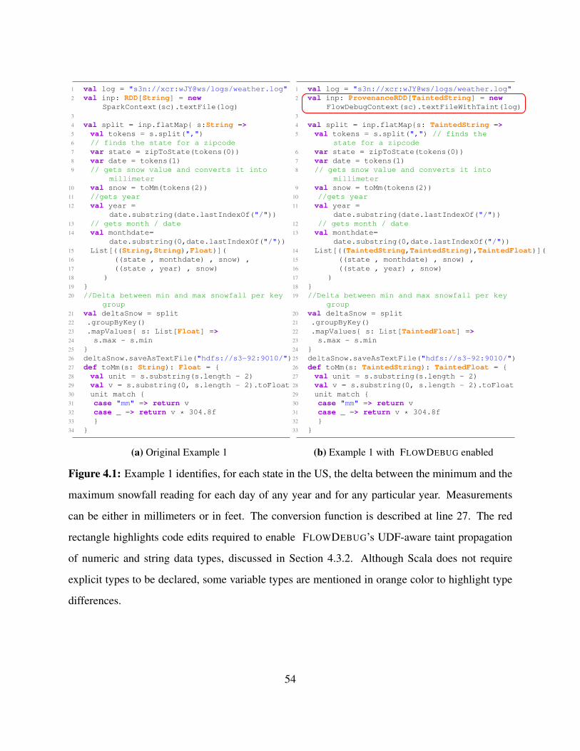
1 val log = "s3n://xcr:wJY@ws/logs/weather.log"2 val inp: RDD[String] = new
SparkContext(sc).textFile(log)3
4 val split = inp.flatMap{ s:String =>5 val tokens = s.split(",")6 // finds the state for a zipcode7 var state = zipToState(tokens(0))8 var date = tokens(1)9 // gets snow value and converts it into
millimeter10 val snow = toMm(tokens(2))11 //gets year12 val year =
date.substring(date.lastIndexOf("/"))13 // gets month / date14 val monthdate=
date.substring(0,date.lastIndexOf("/"))15 List[((String,String),Float)](16 ((state , monthdate) , snow) ,17 ((state , year) , snow)18 )19 }20 //Delta between min and max snowfall per key
group21 val deltaSnow = split22 .groupByKey()23 .mapValues{ s: List[Float] =>24 s.max - s.min25 }26 deltaSnow.saveAsTextFile("hdfs://s3-92:9010/")27 def toMm(s: String): Float = {28 val unit = s.substring(s.length - 2)29 val v = s.substring(0, s.length - 2).toFloat30 unit match {31 case "mm" => return v32 case _ => return v * 304.8f33 }34 }
(a) Original Example 1
1 val log = "s3n://xcr:wJY@ws/logs/weather.log"2 val inp: ProvenanceRDD[TaintedString] = new
FlowDebugContext(sc).textFileWithTaint(log)3
4 val split = inp.flatMap{s: TaintedString =>5 val tokens = s.split(",") // finds the
state for a zipcode6 var state = zipToState(tokens(0))7 var date = tokens(1)8 // gets snow value and converts it into
millimeter9 val snow = toMm(tokens(2))
10 //gets year11 val year =
date.substring(date.lastIndexOf("/"))12 // gets month / date13 val monthdate=
date.substring(0,date.lastIndexOf("/"))14 List[((TaintedString,TaintedString),TaintedFloat)](15 ((state , monthdate) , snow) ,16 ((state , year) , snow)17 )18 }19 //Delta between min and max snowfall per key
group20 val deltaSnow = split21 .groupByKey()22 .mapValues{ s: List[TaintedFloat] =>23 s.max - s.min24 }25 deltaSnow.saveAsTextFile("hdfs://s3-92:9010/")26 def toMm(s: TaintedString): TaintedFloat = {27 val unit = s.substring(s.length - 2)28 val v = s.substring(0, s.length - 2).toFloat29 unit match {30 case "mm" => return v31 case _ => return v * 304.8f32 }33 }
(b) Example 1 with FLOWDEBUG enabled
Figure 4.1: Example 1 identifies, for each state in the US, the delta between the minimum and the
maximum snowfall reading for each day of any year and for any particular year. Measurements
can be either in millimeters or in feet. The conversion function is described at line 27. The red
rectangle highlights code edits required to enable FLOWDEBUG’s UDF-aware taint propagation
of numeric and string data types, discussed in Section 4.3.2. Although Scala does not require
explicit types to be declared, some variable types are mentioned in orange color to highlight type
differences.
54

snowfall measurement. We use function toMm at line 10 of Figure 4.1a to normalize all snowfall
measurements to millimeters. Similarly, we uses zipToState at line 7 to map zipcode to its
corresponding state. To measure the biggest difference in snowfall readings (Figure 4.1a), we
group the key value pairs using groupByKey in line 22, yielding records that are grouped in two
ways (1) by state and day and (2) by state and year. Then, we use mapValues to find the delta
between the maximum and the minimum snowfall measurements for each group and save the final
results.1 //finds input data with more 6000mm of snow reading2 def scan(snowfall:Float, unit:String):Boolean = {3 if(unit =="ft") snowfall > 6000/3044 else snowfall > 60005 }
Figure 4.2: A filter function that searches for input data records with more than 6000mm of
snowfall reading.
After running the program in Figure 4.1a and inspecting the result, the programmer finds that a
few output records have suspiciously high delta snowfall values (e.g., AK, 1993, 21251). To trace
the origin of these high output values, suppose that the programmer performs a simple scan on the
entire input to search for extreme snowfall values using the code shown in Figure 4.2. However,
such scan is unsuccessful, as it does not find any obvious outlier.
An alternative approach would be to isolate a subset of input records contributing to each
suspicious output value. To perform this debugging task, the programmer may use search-based
debugging [47] or data provenance [59], both of which have limitations related to inefficiency and
imprecision, which are discussed below.
Imprecision of Data Provenance. Data provenance is a popular technique in databases. It cap-
tures the input-output mappings of a data processing pipeline to explain the output of a query. In
DISC applications, these mappings are usually captured at each transformation-level (e.g., map,
reduce, join) [59] and then backward recursive join queries are run to trace the lineage of each
output record. Most data provenance approaches [59, 79, 53, 33, 18, 14, 57] are coarse-grained
55
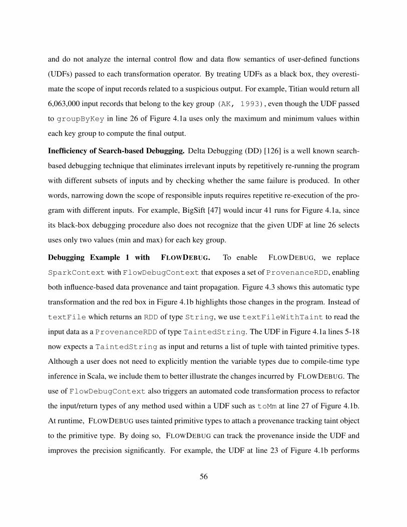
and do not analyze the internal control flow and data flow semantics of user-defined functions
(UDFs) passed to each transformation operator. By treating UDFs as a black box, they overesti-
mate the scope of input records related to a suspicious output. For example, Titian would return all
6,063,000 input records that belong to the key group (AK, 1993), even though the UDF passed
to groupByKey in line 26 of Figure 4.1a uses only the maximum and minimum values within
each key group to compute the final output.
Inefficiency of Search-based Debugging. Delta Debugging (DD) [126] is a well known search-
based debugging technique that eliminates irrelevant inputs by repetitively re-running the program
with different subsets of inputs and by checking whether the same failure is produced. In other
words, narrowing down the scope of responsible inputs requires repetitive re-execution of the pro-
gram with different inputs. For example, BigSift [47] would incur 41 runs for Figure 4.1a, since
its black-box debugging procedure also does not recognize that the given UDF at line 26 selects
uses only two values (min and max) for each key group.
Debugging Example 1 with FLOWDEBUG. To enable FLOWDEBUG, we replace
SparkContext with FlowDebugContext that exposes a set of ProvenanceRDD, enabling
both influence-based data provenance and taint propagation. Figure 4.3 shows this automatic type
transformation and the red box in Figure 4.1b highlights those changes in the program. Instead of
textFile which returns an RDD of type String, we use textFileWithTaint to read the
input data as a ProvenanceRDD of type TaintedString. The UDF in Figure 4.1a lines 5-18
now expects a TaintedString as input and returns a list of tuple with tainted primitive types.
Although a user does not need to explicitly mention the variable types due to compile-time type
inference in Scala, we include them to better illustrate the changes incurred by FLOWDEBUG. The
use of FlowDebugContext also triggers an automated code transformation process to refactor
the input/return types of any method used within a UDF such as toMm at line 27 of Figure 4.1b.
At runtime, FLOWDEBUG uses tainted primitive types to attach a provenance tracking taint object
to the primitive type. By doing so, FLOWDEBUG can track the provenance inside the UDF and
improves the precision significantly. For example, the UDF at line 23 of Figure 4.1b performs
56
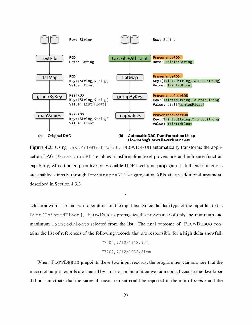
textFile
flatMap
groupByKey
mapValues
RDDKey:(String,String)Value: Float
RDDData: String
PairRDDKey:(String,String)Value: List[Float]
PairRDDKey:(String,String)Value: Float
Row: String
textFileWithTaint
flatMap
groupByKey
mapValues
ProvenanceRDDKey:(TaintedString,TaintedString)Value: TaintedFloat
ProvenanceRDDData: TaintedString
Row: String
ProvenancePairRDDKey:(TaintedString,TaintedString)Value: List[TaintedFloat]
ProvenancePairRDDKey:(TaintedString,TaintedString)Value: TaintedFloat
(a) Original DAG (b) Automatic DAG Transformation Using FlowDebug’s textFileWithTaint API
Figure 4.3: Using textFileWithTaint, FLOWDEBUG automatically transforms the appli-
cation DAG. ProvenanceRDD enables transformation-level provenance and influence-function
capability, while tainted primitive types enable UDF-level taint propagation. Influence functions
are enabled directly through ProvenanceRDD’s aggregation APIs via an additional argument,
described in Section 4.3.3
.
selection with min and max operations on the input list. Since the data type of the input list (s) is
List[TaintedFloat], FLOWDEBUG propagates the provenance of only the minimum and
maximum TaintedFloats selected from the list. The final outcome of FLOWDEBUG con-
tains the list of references of the following records that are responsible for a high delta snowfall.
77202,7/12/1933,90in
77202,7/12/1932,21mm
When FLOWDEBUG pinpoints these two input records, the programmer can now see that the
incorrect output records are caused by an error in the unit conversion code, because the developer
did not anticipate that the snowfall measurement could be reported in the unit of inches and the
57
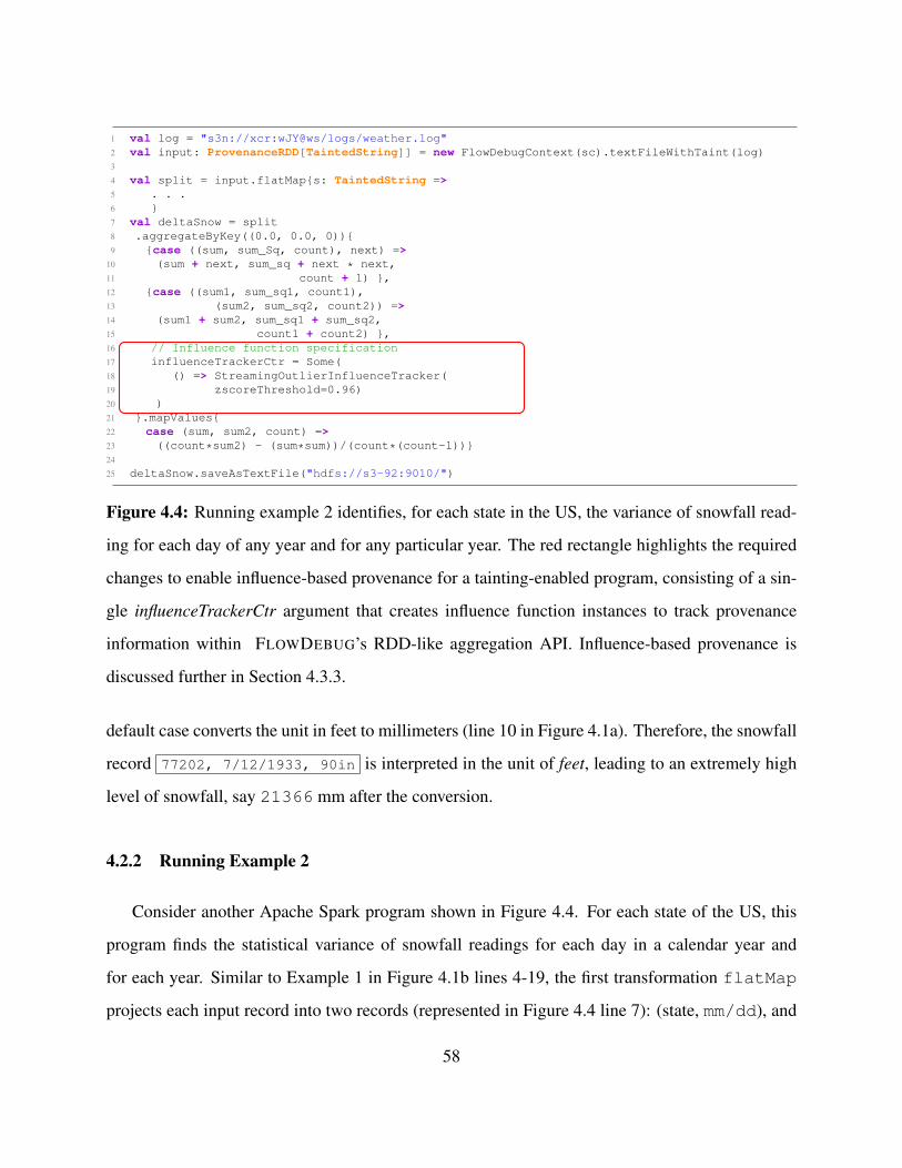
1 val log = "s3n://xcr:wJY@ws/logs/weather.log"2 val input: ProvenanceRDD[TaintedString]] = new FlowDebugContext(sc).textFileWithTaint(log)3
4 val split = input.flatMap{s: TaintedString =>5 . . .6 }7 val deltaSnow = split8 .aggregateByKey((0.0, 0.0, 0)){9 {case ((sum, sum_Sq, count), next) =>
10 (sum + next, sum_sq + next * next,11 count + 1) },12 {case ((sum1, sum_sq1, count1),13 (sum2, sum_sq2, count2)) =>14 (sum1 + sum2, sum_sq1 + sum_sq2,15 count1 + count2) },16 // Influence function specification17 influenceTrackerCtr = Some(18 () => StreamingOutlierInfluenceTracker(19 zscoreThreshold=0.96)20 )21 }.mapValues{22 case (sum, sum2, count) =>23 ((count*sum2) - (sum*sum))/(count*(count-1))}24
25 deltaSnow.saveAsTextFile("hdfs://s3-92:9010/")
Figure 4.4: Running example 2 identifies, for each state in the US, the variance of snowfall read-
ing for each day of any year and for any particular year. The red rectangle highlights the required
changes to enable influence-based provenance for a tainting-enabled program, consisting of a sin-
gle influenceTrackerCtr argument that creates influence function instances to track provenance
information within FLOWDEBUG’s RDD-like aggregation API. Influence-based provenance is
discussed further in Section 4.3.3.
default case converts the unit in feet to millimeters (line 10 in Figure 4.1a). Therefore, the snowfall
record 77202, 7/12/1933, 90in is interpreted in the unit of feet, leading to an extremely high
level of snowfall, say 21366 mm after the conversion.
4.2.2 Running Example 2
Consider another Apache Spark program shown in Figure 4.4. For each state of the US, this
program finds the statistical variance of snowfall readings for each day in a calendar year and
for each year. Similar to Example 1 in Figure 4.1b lines 4-19, the first transformation flatMap
projects each input record into two records (represented in Figure 4.4 line 7): (state, mm/dd), and
58
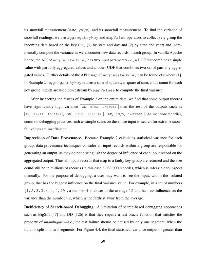
its snowfall measurement (state, yyyy), and its snowfall measurement. To find the variance of
snowfall readings, we use aggregateyKey and mapValue operators to collectively group the
incoming data based on the key (i.e., (1) by state and day and (2) by state and year) and incre-
mentally compute the variance as we encounter new data records in each group. In vanilla Apache
Spark, the API of aggregateByKey has two input parameters i.e., a UDF that combines a single
value with partially aggregated values and another UDF that combines two set of partially aggre-
gated values. Further details of the API usage of aggregateByKey can be found elsewhere [1].
In Example 2, aggregateByKey returns a sum of squares, a square of sum, and a count for each
key group, which are used downstream by mapValues to compute the final variance.
After inspecting the results of Example 2 on the entire data, we find that some output records
have significantly high variance AK, 9/02, 1766085 than the rest of the outputs such as
AK, 17/11, 1676129 , AK, 1918, 1696512 , AK, 13/5, 1697703 . As mentioned earlier,
common debugging practices such as simple scans on the entire input to search for extreme snow-
fall values are insufficient.
Imprecision of Data Provenance. Because Example 2 calculates statistical variance for each
group, data provenance techniques consider all input records within a group are responsible for
generating an output, as they do not distinguish the degree of influence of each input record on the
aggregated output. Thus all inputs records that map to a faulty key-group are returned and the size
could still be in millions of records (in this case 6,063,000 records), which is infeasible to inspect
manually. For the purpose of debugging, a user may want to see the input, within the isolated
group, that has the biggest influence on the final variance value. For example, in a set of numbers
{1,2,3,3,4,4,4,99}, a number 4 is closer to the average 15 and has less influence on the
variance than the number 99, which is the farthest away from the average.
Inefficiency of Search-based Debugging. A limitation of search-based debugging approaches
such as BigSift [47] and DD [126] is that they require a test oracle function that satisfies the
property of unambiguity—i.e., the test failure should be caused by only one segment, when the
input is split into two segments. For Figure 4.4, the final statistical variance output of greater than
59

1,750,000 is marked as incorrect, as it is slightly higher than the other half. BigSift applies DD
on the backward trace of the faulty output and isolates the following two input records as faulty:
29749,9/2/1976,3352mm
29749,9/2/1933, 394mm
Although the two input records fail the test function, they are completely valid inputs and should
not considered as faulty. This false positive is due to the violation of the unambiguity assumption.
During the automated fault isolation process, DD restricts its search on the first half of the input,
assuming that none of the second half set leads to a test failure. However, in our case, there are
multiple input subsets that could cause a test failure, and only one of those subsets contain the real
faulty input. Therefore, DD either returns correct records as faulty or does not return anything at
all.
Debugging Example 2 with FLOWDEBUG. Similar to Example 1, a user can replace the
SparkContext with FlowDebugContext to enable FLOWDEBUG. This change automati-
cally replaces all the succeeding RDDs with ProvenanceRDDs. As a result, split at line 7
of Figure 4.4 becomes a ProvenanceRDD which uses the refactored version of all aggregation
operators APIs provided by FLOWDEBUG (e.g., reduce or aggregateByKey). These APIs
provided by FLOWDEBUG include optional parameters: (1) enableTaintPropagation, a
toggle to enable or disable taint propagation and (2) influenceTrackerCtr, an influence
function to rank input records based on their impact on the final aggregated value. The user
only need to make the edits shown in the red rectangle to enable influence-based data prove-
nance (Figure 4.4), and the rest of taint tracking is done fully automatically by FLOWDEBUG.
A user may select one of many pre-defined influence functions described in Section 4.3.3 or
can provide their own custom influence function to define selectivity and priority for debug-
ging aggregation logic. Lines 8-20 of Figure 4.4 show the invocation of aggregateByKey
that takes in an influence function StreamingOutlierInfluenceTracker to prioritize
records with extreme snowfall readings during provenance tracking. The guidelines of writing
an influence function is presented in Section 4.3.3. Based on this influence function, FLOWDE-
60
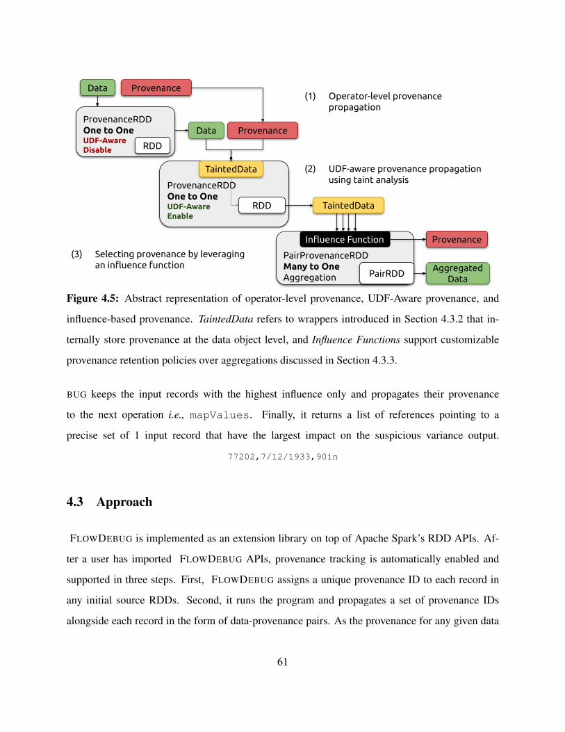
ProvenanceRDDOne to OneUDF-AwareEnable
RDD
PairProvenanceRDDMany to OneAggregation PairRDD
Data Provenance
Data Provenance
TaintedData
Influence Function Provenance
AggregatedData
TaintedData
ProvenanceRDDOne to OneUDF-AwareDisable RDD
(1) Operator-level provenance propagation
(2) UDF-aware provenance propagation using taint analysis
(3) Selecting provenance by leveraging an influence function
Figure 4.5: Abstract representation of operator-level provenance, UDF-Aware provenance, and
influence-based provenance. TaintedData refers to wrappers introduced in Section 4.3.2 that in-
ternally store provenance at the data object level, and Influence Functions support customizable
provenance retention policies over aggregations discussed in Section 4.3.3.
BUG keeps the input records with the highest influence only and propagates their provenance
to the next operation i.e., mapValues. Finally, it returns a list of references pointing to a
precise set of 1 input record that have the largest impact on the suspicious variance output.
77202,7/12/1933,90in
4.3 Approach
FLOWDEBUG is implemented as an extension library on top of Apache Spark’s RDD APIs. Af-
ter a user has imported FLOWDEBUG APIs, provenance tracking is automatically enabled and
supported in three steps. First, FLOWDEBUG assigns a unique provenance ID to each record in
any initial source RDDs. Second, it runs the program and propagates a set of provenance IDs
alongside each record in the form of data-provenance pairs. As the provenance for any given data
61

record may vary greatly depending on application semantics, FLOWDEBUG utilizes an efficient
RoaringBitmap [72] for storing the provenance ID sets. Finally, when a user queries which input
records are responsible for a given output, FLOWDEBUG retrieves the provenance IDs for each of
the inputs and joins them against the source RDDs from the first step to produce the final subset of
input records. Figure 4.5 shows the propagation of provenance at both the operator level and UDF
level, as well as how influence functions are used to refine provenance tracking for aggregation op-
erators (many to one). In practice, UDF-aware tainting and influence functions can be used either
in tandem or independently.
4.3.1 Transformation Level Provenance
ProvenanceRDD API mirrors Spark’s RDD API and enables developers to easily apply FLOWDE-
BUG to their existing Spark applications with minimal changes. An example of edits that the de-
veloper need to make to enable FLOWDEBUG’s taint tracking is shown in Figure 4.1b.
As provenance is paired with each intermediate or output data record, the provenance propaga-
tion technique can be broken down into the following:2.
• For one-to-one dependencies, provenance propagation requires copying the provenance of
the input record to the resulting output record. Such dependencies stem from RDD opera-
tions such as map and filter.
• For many-to-one mappings, the provenance of all input records is unioned into a single
instance. Examples of many-to-one mappings include combineByKey and reduceByKey.
• For one-to-many mappings created by flatMap, FLOWDEBUG considers them as multiple
dependencies sharing the same source(s).
As we discuss in the next two subsections, FLOWDEBUG enables higher precision provenance
tracking than this transformation operator level provenance by propagating taints within UDFs
2Implementations available at https://github.com/UCLA-SEAL/FlowDebug/blob/main/src/main/scala/provenance/rdd/ProvenanceRDD.scala.
62
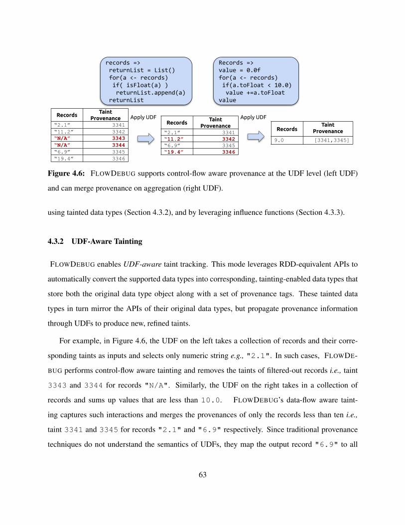
RecordsTaint
Provenance“2.1” 3341“11.2” 3342“N/A” 3343“N/A” 3344“6.9” 3345“19.4” 3346
RecordsTaint
Provenance“2.1” 3341“11.2” 3342“6.9” 3345“19.4” 3346
records => returnList = List() for(a <- records) if( isFloat(a) ) returnList.append(a) returnList
Records =>value = 0.0ffor(a <- records) if(a.toFloat < 10.0) value +=a.toFloatvalue
RecordsTaint
Provenance
9.0 [3341,3345]
Apply UDF Apply UDF
Figure 4.6: FLOWDEBUG supports control-flow aware provenance at the UDF level (left UDF)
and can merge provenance on aggregation (right UDF).
using tainted data types (Section 4.3.2), and by leveraging influence functions (Section 4.3.3).
4.3.2 UDF-Aware Tainting
FLOWDEBUG enables UDF-aware taint tracking. This mode leverages RDD-equivalent APIs to
automatically convert the supported data types into corresponding, tainting-enabled data types that
store both the original data type object along with a set of provenance tags. These tainted data
types in turn mirror the APIs of their original data types, but propagate provenance information
through UDFs to produce new, refined taints.
For example, in Figure 4.6, the UDF on the left takes a collection of records and their corre-
sponding taints as inputs and selects only numeric string e.g., "2.1". In such cases, FLOWDE-
BUG performs control-flow aware tainting and removes the taints of filtered-out records i.e., taint
3343 and 3344 for records "N/A". Similarly, the UDF on the right takes in a collection of
records and sums up values that are less than 10.0. FLOWDEBUG’s data-flow aware taint-
ing captures such interactions and merges the provenances of only the records less than ten i.e.,
taint 3341 and 3345 for records "2.1" and "6.9" respectively. Since traditional provenance
techniques do not understand the semantics of UDFs, they map the output record "6.9" to all
63
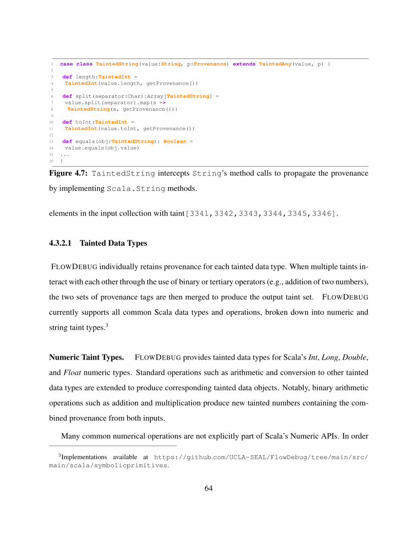
1 case class TaintedString(value:String, p:Provenance) extends TaintedAny(value, p) {2
3 def length:TaintedInt =4 TaintedInt(value.length, getProvenance())5
6 def split(separator:Char):Array[TaintedString] =7 value.split(separator).map(s =>8 TaintedString(s, getProvenance()))9
10 def toInt:TaintedInt =11 TaintedInt(value.toInt, getProvenance())12
13 def equals(obj:TaintedString): Boolean =14 value.equals(obj.value)15 ...16 }
Figure 4.7: TaintedString intercepts String’s method calls to propagate the provenance
by implementing Scala.String methods.
elements in the input collection with taint[3341,3342,3343,3344,3345,3346].
4.3.2.1 Tainted Data Types
FLOWDEBUG individually retains provenance for each tainted data type. When multiple taints in-
teract with each other through the use of binary or tertiary operators (e.g., addition of two numbers),
the two sets of provenance tags are then merged to produce the output taint set. FLOWDEBUG
currently supports all common Scala data types and operations, broken down into numeric and
string taint types.3
Numeric Taint Types. FLOWDEBUG provides tainted data types for Scala’s Int, Long, Double,
and Float numeric types. Standard operations such as arithmetic and conversion to other tainted
data types are extended to produce corresponding tainted data objects. Notably, binary arithmetic
operations such as addition and multiplication produce new tainted numbers containing the com-
bined provenance from both inputs.
Many common numerical operations are not explicitly part of Scala’s Numeric APIs. In order
3Implementations available at https://github.com/UCLA-SEAL/FlowDebug/tree/main/src/main/scala/symbolicprimitives.
64
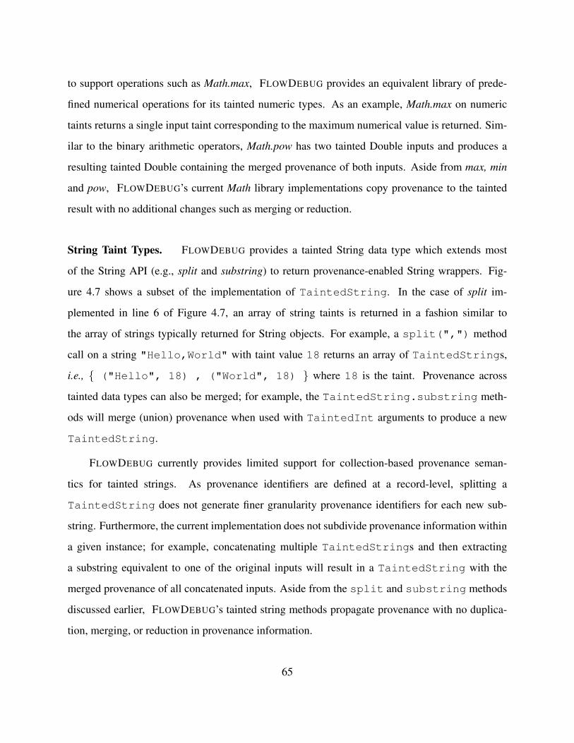
to support operations such as Math.max, FLOWDEBUG provides an equivalent library of prede-
fined numerical operations for its tainted numeric types. As an example, Math.max on numeric
taints returns a single input taint corresponding to the maximum numerical value is returned. Sim-
ilar to the binary arithmetic operators, Math.pow has two tainted Double inputs and produces a
resulting tainted Double containing the merged provenance of both inputs. Aside from max, min
and pow, FLOWDEBUG’s current Math library implementations copy provenance to the tainted
result with no additional changes such as merging or reduction.
String Taint Types. FLOWDEBUG provides a tainted String data type which extends most
of the String API (e.g., split and substring) to return provenance-enabled String wrappers. Fig-
ure 4.7 shows a subset of the implementation of TaintedString. In the case of split im-
plemented in line 6 of Figure 4.7, an array of string taints is returned in a fashion similar to
the array of strings typically returned for String objects. For example, a split(",") method
call on a string "Hello,World" with taint value 18 returns an array of TaintedStrings,
i.e., { ("Hello", 18) , ("World", 18) } where 18 is the taint. Provenance across
tainted data types can also be merged; for example, the TaintedString.substring meth-
ods will merge (union) provenance when used with TaintedInt arguments to produce a new
TaintedString.
FLOWDEBUG currently provides limited support for collection-based provenance seman-
tics for tainted strings. As provenance identifiers are defined at a record-level, splitting a
TaintedString does not generate finer granularity provenance identifiers for each new sub-
string. Furthermore, the current implementation does not subdivide provenance information within
a given instance; for example, concatenating multiple TaintedStrings and then extracting
a substring equivalent to one of the original inputs will result in a TaintedString with the
merged provenance of all concatenated inputs. Aside from the split and substring methods
discussed earlier, FLOWDEBUG’s tainted string methods propagate provenance with no duplica-
tion, merging, or reduction in provenance information.
65

4.3.3 Influence Function Based Provenance
21303
661
902
18922
872
122
337
8851
aggregateByKey:
Sum_of_square, next => sum_of_square + next*nextsum, next => sum + nextcount => count + 1
mapValues:
sum_of_square, sum, count =>((count*sum_of_square) - (sum*sum) /
(count*(count-1)))
Influence Function21303
18922
FlowDebug’s Influence Based Provenance
Traditional Operator Based Data Provenance
Figure 4.8: Comparison of operator-based data provenance (blue) vs. influence-function based
data provenance (red). The aggregation logic computes the variance of a collection of input num-
bers and the influence function is configured to capture outlier aggregation inputs (StreamingOut-
lier in Table 4.1) that might heavily impact the computed result.
The transformation operator-level provenance described in Section 4.3.1 suffers from the same
issue of over-approximation that other data provenance techniques have [33, 57, 79]. This short-
coming inherently stems from the black box treatment of UDFs passed an an argument to aggre-
gation operators such as reduceByKey. For example, in Figure 4.8, aggregateByKey’s UDF
computes statistical variance. Although all input records contribute towards computing variance,
input numbers with anomalous values have greater influence than other. Traditional data prove-
nance techniques are incapable of detecting such interaction and map all input records to the final
aggregated value.
FLOWDEBUG provides additional options in the ProvenanceRDD aggregation API to selec-
66

1 trait InfluenceFunction[T] extends Serializable {2 // Initialize with first value + provenance (initCombiner in Spark)3 def init(value: T, prov: Provenance): InfluenceFunction[T]4
5 // add another value to result and update provenance (mergeValue in Spark)6 def mergeValue(value: T, prov: Provenance): InfluenceFunction[T]7
8 // add another influence function result and its provenance (mergeCombiner in Spark)9 def mergeFunction(other: InfluenceFunction[T]): InfluenceFunction[T]
10
11 // postprocessing to produce final result provenance12 def finalize(): Provenance13 }
Figure 4.9: FLOWDEBUG defines influence functions which mirror Spark’s aggregation semantics
to support customizable provenance retention policies for aggregation functions.
tively choose which input records have greater influence on the outcome of aggregation. This
extension, shown in Figure 4.9, mirrors Spark’s combineByKey API by providing init, mergeValue,
and mergeFunction methods which allow customization for how provenance is filtered and priori-
tized for aggregation functions:
• init(value, provenance): Initialize an influence function object with the provided data value
and provenance object.
• mergeValue(value, provenance): Add another value and its provenance to an already initial-
ized influence function, updating the provenance if necessary.
• mergeFunction(influenceFunction): Merge an existing influence function (which may al-
ready be initialized and updated with values) into the current instance.
• finalize(): Compute any final postprocessing steps and return a single provenance object for
all values observed by the influence function.
Developers can define their own custom influence functions or use pre-defined, parametrized
influence-function implementations provided by FLOWDEBUG as a library, described in Table
4.1.4 Figure 4.10 presents an example implementation of the influence function API and the pre-
4Implementations available at https://github.com/UCLA-SEAL/FlowDebug/blob/main/src/main/scala/provenance/rdd/InfluenceTracker.scala.
67
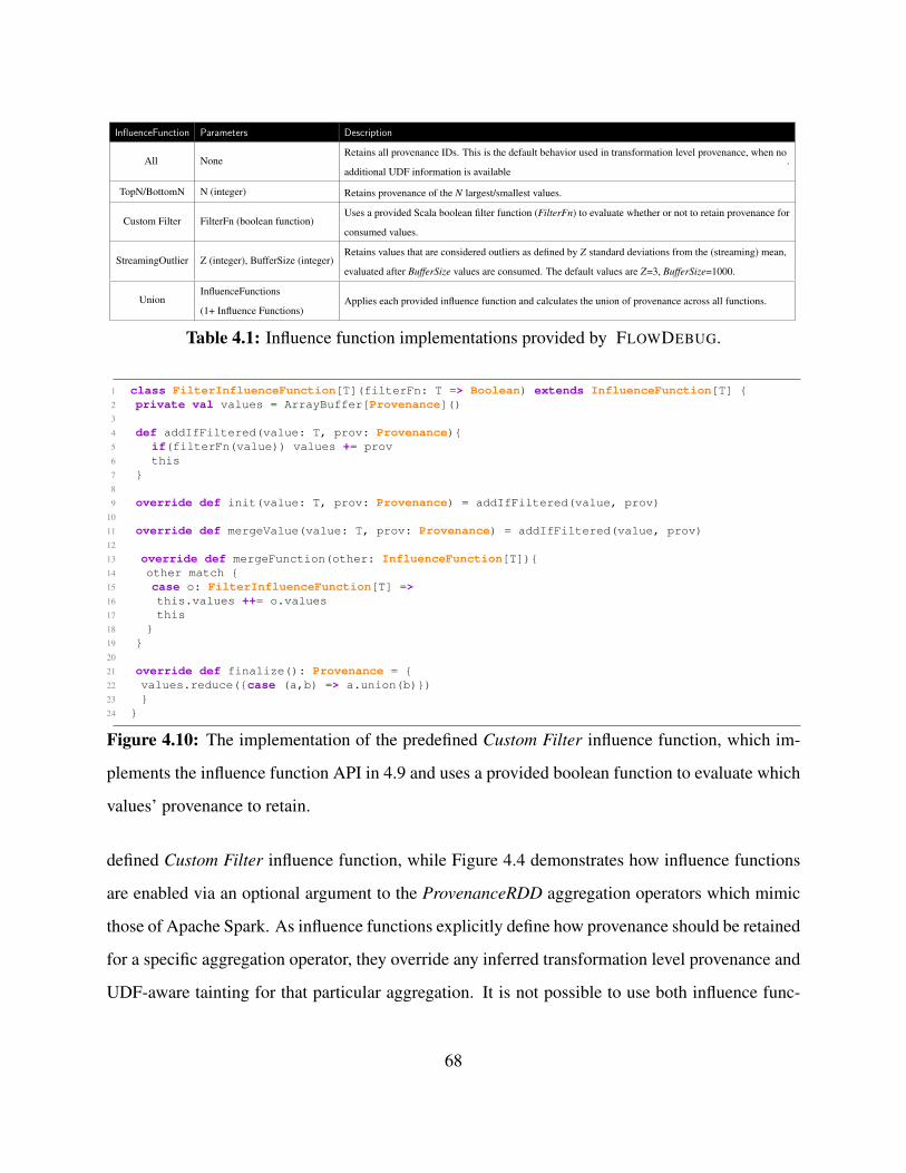
InfluenceFunction Parameters Description
All NoneRetains all provenance IDs. This is the default behavior used in transformation level provenance, when no
additional UDF information is available.
TopN/BottomN N (integer) Retains provenance of the N largest/smallest values.
Custom Filter FilterFn (boolean function)Uses a provided Scala boolean filter function (FilterFn) to evaluate whether or not to retain provenance for
consumed values.
StreamingOutlier Z (integer), BufferSize (integer)Retains values that are considered outliers as defined by Z standard deviations from the (streaming) mean,
evaluated after BufferSize values are consumed. The default values are Z=3, BufferSize=1000.
UnionInfluenceFunctions
(1+ Influence Functions)Applies each provided influence function and calculates the union of provenance across all functions.
Table 4.1: Influence function implementations provided by FLOWDEBUG.
1 class FilterInfluenceFunction[T](filterFn: T => Boolean) extends InfluenceFunction[T] {2 private val values = ArrayBuffer[Provenance]()3
4 def addIfFiltered(value: T, prov: Provenance){5 if(filterFn(value)) values += prov6 this7 }8
9 override def init(value: T, prov: Provenance) = addIfFiltered(value, prov)10
11 override def mergeValue(value: T, prov: Provenance) = addIfFiltered(value, prov)12
13 override def mergeFunction(other: InfluenceFunction[T]){14 other match {15 case o: FilterInfluenceFunction[T] =>16 this.values ++= o.values17 this18 }19 }20
21 override def finalize(): Provenance = {22 values.reduce({case (a,b) => a.union(b)})23 }24 }
Figure 4.10: The implementation of the predefined Custom Filter influence function, which im-
plements the influence function API in 4.9 and uses a provided boolean function to evaluate which
values’ provenance to retain.
defined Custom Filter influence function, while Figure 4.4 demonstrates how influence functions
are enabled via an optional argument to the ProvenanceRDD aggregation operators which mimic
those of Apache Spark. As influence functions explicitly define how provenance should be retained
for a specific aggregation operator, they override any inferred transformation level provenance and
UDF-aware tainting for that particular aggregation. It is not possible to use both influence func-
68
tions and UDF-aware tainting for the same aggregation operator, though both techniques can be
used within the same program for different transformations.
As an example, suppose a developer is trying to debug a program which computes a per-
key average that yields an abnormally high value. The developer may thus be interested in the
largest input records within each key group. As a result, she may choose to use a TopN influence
function and retain only the top ten values’ provenance within each key. Using this influence
function, FLOWDEBUG can then reduce the number of inputs traced to a more manageable subset
for developer inspection.
Figure 4.8 highlights the benefits of influence-based data provenance on an aggregation opera-
tion. Every incoming record into the aggregation operator passes through a user-defined influence
function that determines which input records provenance to retain. Using a StreamingOutlier in-
fluence function, FLOWDEBUG identifies the 21303 and 18922 records, marked in red, which
are found to be statistical outliers that contribute heavily to the aggregation output. In comparison,
operator-based data provenance returns the entire set of inputs marked in blue.
4.4 Evaluation
We investigate five programs and compare FLOWDEBUG to Titian and BigSift in precision, recall,
and the number of inputs that each tool traces from the same set of faulty output records. Each
program is evaluated on a single MacBook Pro (15-inch, Mid-2018 model) running macOS 10.15.3
with 16GB RAM, a 2.6GHz 6-core Intel Core i7 processor, and 512GB flash storage. All subject
program variants used with each tool are available at https://github.com/UCLA-SEAL/
FlowDebug/tree/main/src/main/scala/examples/benchmarks.
The results are summarized in Table 4.2, Table 4.3, Figure 4.11, and Figure 4.12. Table 4.2
presents the debugging accuracy results, in precision and recall, for each tool and subject pro-
gram. The running time for each tool can be broken into two parts: (1) the instrumented running
time shown in Figure 4.11, as all three tools capture and store provenance tags by executing an
69
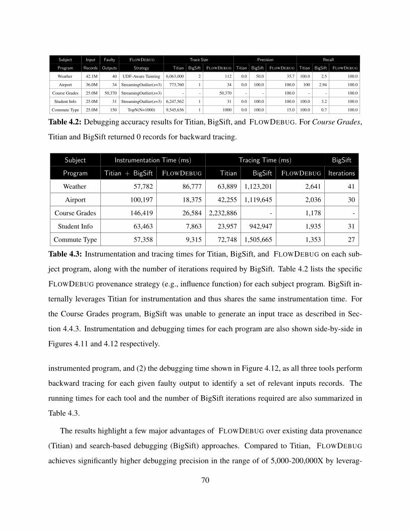
Subject Input Faulty FLOWDEBUG Trace Size Precision Recall
Program Records Outputs Strategy Titian BigSift FLOWDEBUG Titian BigSift FLOWDEBUG Titian BigSift FLOWDEBUG
Weather 42.1M 40 UDF-Aware Tainting 6,063,000 2 112 0.0 50.0 35.7 100.0 2.5 100.0
Airport 36.0M 34 StreamingOutlier(z=3) 773,760 1 34 0.0 100.0 100.0 100 2.94 100.0
Course Grades 25.0M 50,370 StreamingOutlier(z=3) - - 50,370 - - 100.0 - - 100.0
Student Info 25.0M 31 StreamingOutlier(z=3) 6,247,562 1 31 0.0 100.0 100.0 100.0 3.2 100.0
Commute Type 25.0M 150 TopN(N=1000) 9,545,636 1 1000 0.0 100.0 15.0 100.0 0.7 100.0
Table 4.2: Debugging accuracy results for Titian, BigSift, and FLOWDEBUG. For Course Grades,
Titian and BigSift returned 0 records for backward tracing.
Subject Instrumentation Time (ms) Tracing Time (ms) BigSift
Program Titian + BigSift FLOWDEBUG Titian BigSift FLOWDEBUG Iterations
Weather 57,782 86,777 63,889 1,123,201 2,641 41
Airport 100,197 18,375 42,255 1,119,645 2,036 30
Course Grades 146,419 26,584 2,232,886 - 1,178 -
Student Info 63,463 7,863 23,957 942,947 1,935 31
Commute Type 57,358 9,315 72,748 1,505,665 1,353 27
Table 4.3: Instrumentation and tracing times for Titian, BigSift, and FLOWDEBUG on each sub-
ject program, along with the number of iterations required by BigSift. Table 4.2 lists the specific
FLOWDEBUG provenance strategy (e.g., influence function) for each subject program. BigSift in-
ternally leverages Titian for instrumentation and thus shares the same instrumentation time. For
the Course Grades program, BigSift was unable to generate an input trace as described in Sec-
tion 4.4.3. Instrumentation and debugging times for each program are also shown side-by-side in
Figures 4.11 and 4.12 respectively.
instrumented program, and (2) the debugging time shown in Figure 4.12, as all three tools perform
backward tracing for each given faulty output to identify a set of relevant inputs records. The
running times for each tool and the number of BigSift iterations required are also summarized in
Table 4.3.
The results highlight a few major advantages of FLOWDEBUG over existing data provenance
(Titian) and search-based debugging (BigSift) approaches. Compared to Titian, FLOWDEBUG
achieves significantly higher debugging precision in the range of of 5,000-200,000X by leverag-
70
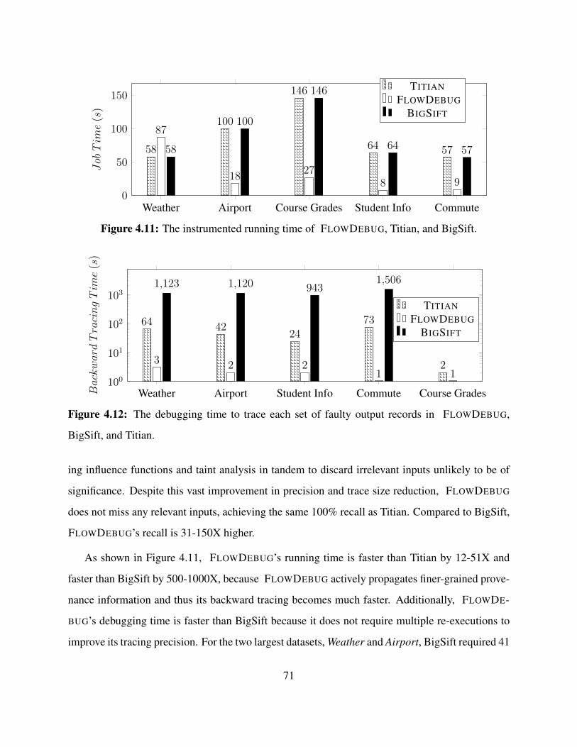
AirportWeather Student Info CommuteCourse Grades0
50
100
150
100
58 64 57
146
18
87
8 927
100
58 64 57
146JobTime(s)
TITIANFLOWDEBUG
BIGSIFT
Figure 4.11: The instrumented running time of FLOWDEBUG, Titian, and BigSift.
AirportWeather Student Info Commute Course Grades100
101
102
103
426424
73
223 21 1
1,1201,123 9431,506
BackwardTracingTime(s)
TITIANFLOWDEBUG
BIGSIFT
Figure 4.12: The debugging time to trace each set of faulty output records in FLOWDEBUG,
BigSift, and Titian.
ing influence functions and taint analysis in tandem to discard irrelevant inputs unlikely to be of
significance. Despite this vast improvement in precision and trace size reduction, FLOWDEBUG
does not miss any relevant inputs, achieving the same 100% recall as Titian. Compared to BigSift,
FLOWDEBUG’s recall is 31-150X higher.
As shown in Figure 4.11, FLOWDEBUG’s running time is faster than Titian by 12-51X and
faster than BigSift by 500-1000X, because FLOWDEBUG actively propagates finer-grained prove-
nance information and thus its backward tracing becomes much faster. Additionally, FLOWDE-
BUG’s debugging time is faster than BigSift because it does not require multiple re-executions to
improve its tracing precision. For the two largest datasets, Weather and Airport, BigSift required 41
71
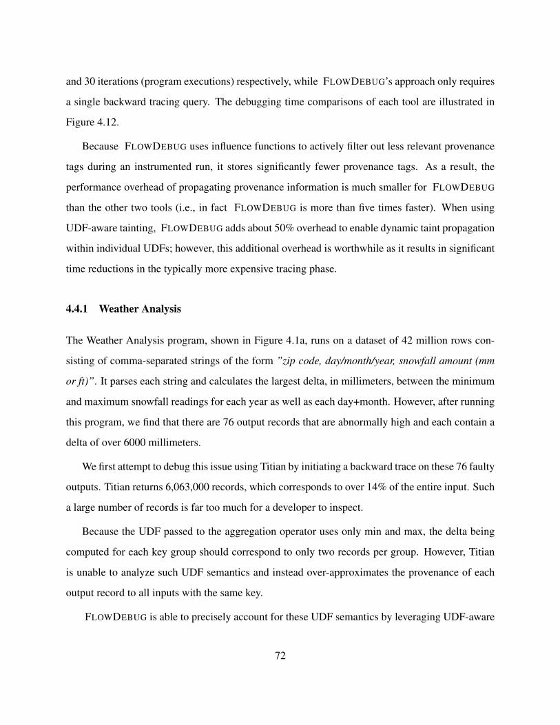
and 30 iterations (program executions) respectively, while FLOWDEBUG’s approach only requires
a single backward tracing query. The debugging time comparisons of each tool are illustrated in
Figure 4.12.
Because FLOWDEBUG uses influence functions to actively filter out less relevant provenance
tags during an instrumented run, it stores significantly fewer provenance tags. As a result, the
performance overhead of propagating provenance information is much smaller for FLOWDEBUG
than the other two tools (i.e., in fact FLOWDEBUG is more than five times faster). When using
UDF-aware tainting, FLOWDEBUG adds about 50% overhead to enable dynamic taint propagation
within individual UDFs; however, this additional overhead is worthwhile as it results in significant
time reductions in the typically more expensive tracing phase.
4.4.1 Weather Analysis
The Weather Analysis program, shown in Figure 4.1a, runs on a dataset of 42 million rows con-
sisting of comma-separated strings of the form ”zip code, day/month/year, snowfall amount (mm
or ft)”. It parses each string and calculates the largest delta, in millimeters, between the minimum
and maximum snowfall readings for each year as well as each day+month. However, after running
this program, we find that there are 76 output records that are abnormally high and each contain a
delta of over 6000 millimeters.
We first attempt to debug this issue using Titian by initiating a backward trace on these 76 faulty
outputs. Titian returns 6,063,000 records, which corresponds to over 14% of the entire input. Such
a large number of records is far too much for a developer to inspect.
Because the UDF passed to the aggregation operator uses only min and max, the delta being
computed for each key group should correspond to only two records per group. However, Titian
is unable to analyze such UDF semantics and instead over-approximates the provenance of each
output record to all inputs with the same key.
FLOWDEBUG is able to precisely account for these UDF semantics by leveraging UDF-aware
72
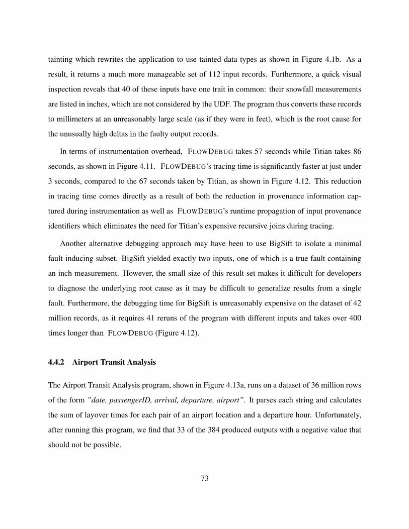
tainting which rewrites the application to use tainted data types as shown in Figure 4.1b. As a
result, it returns a much more manageable set of 112 input records. Furthermore, a quick visual
inspection reveals that 40 of these inputs have one trait in common: their snowfall measurements
are listed in inches, which are not considered by the UDF. The program thus converts these records
to millimeters at an unreasonably large scale (as if they were in feet), which is the root cause for
the unusually high deltas in the faulty output records.
In terms of instrumentation overhead, FLOWDEBUG takes 57 seconds while Titian takes 86
seconds, as shown in Figure 4.11. FLOWDEBUG’s tracing time is significantly faster at just under
3 seconds, compared to the 67 seconds taken by Titian, as shown in Figure 4.12. This reduction
in tracing time comes directly as a result of both the reduction in provenance information cap-
tured during instrumentation as well as FLOWDEBUG’s runtime propagation of input provenance
identifiers which eliminates the need for Titian’s expensive recursive joins during tracing.
Another alternative debugging approach may have been to use BigSift to isolate a minimal
fault-inducing subset. BigSift yielded exactly two inputs, one of which is a true fault containing
an inch measurement. However, the small size of this result set makes it difficult for developers
to diagnose the underlying root cause as it may be difficult to generalize results from a single
fault. Furthermore, the debugging time for BigSift is unreasonably expensive on the dataset of 42
million records, as it requires 41 reruns of the program with different inputs and takes over 400
times longer than FLOWDEBUG (Figure 4.12).
4.4.2 Airport Transit Analysis
The Airport Transit Analysis program, shown in Figure 4.13a, runs on a dataset of 36 million rows
of the form ”date, passengerID, arrival, departure, airport”. It parses each string and calculates
the sum of layover times for each pair of an airport location and a departure hour. Unfortunately,
after running this program, we find that 33 of the 384 produced outputs with a negative value that
should not be possible.
73
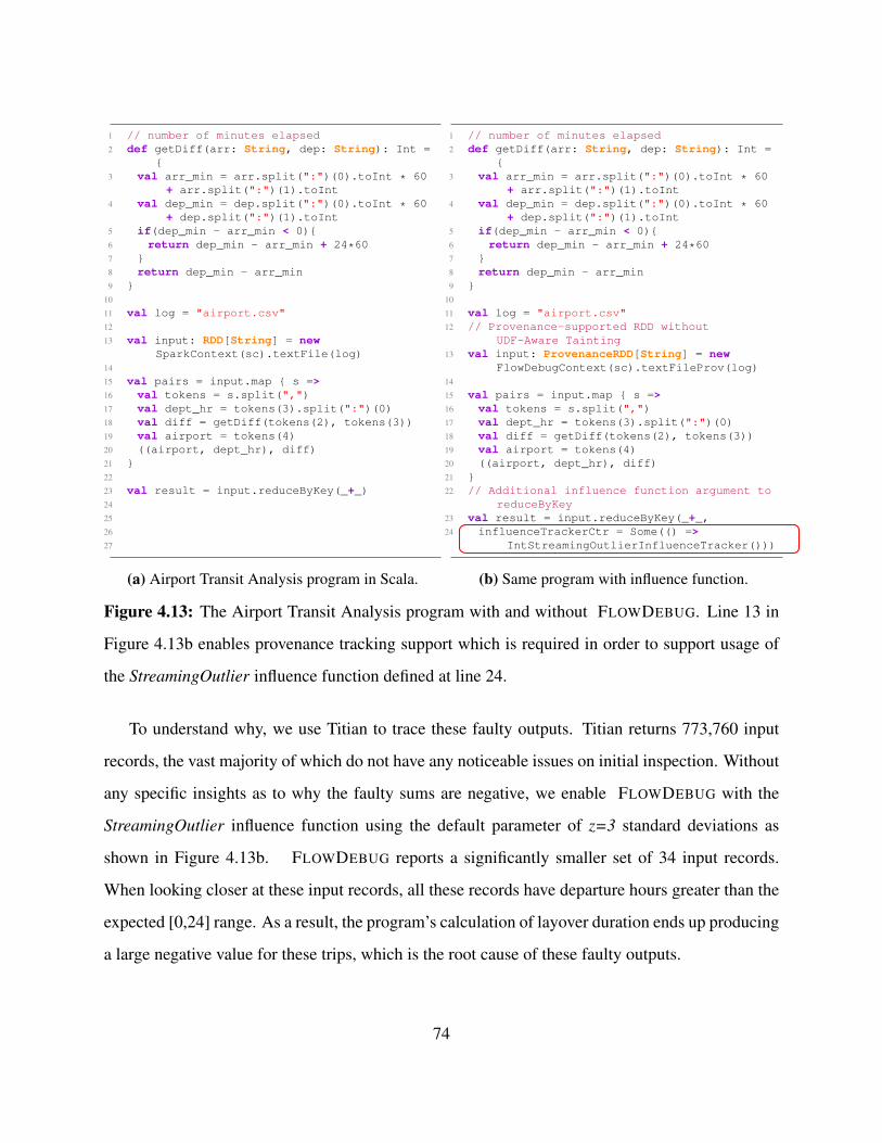
1 // number of minutes elapsed2 def getDiff(arr: String, dep: String): Int =
{3 val arr_min = arr.split(":")(0).toInt * 60
+ arr.split(":")(1).toInt4 val dep_min = dep.split(":")(0).toInt * 60
+ dep.split(":")(1).toInt5 if(dep_min - arr_min < 0){6 return dep_min - arr_min + 24*607 }8 return dep_min - arr_min9 }
10
11 val log = "airport.csv"12
13 val input: RDD[String] = newSparkContext(sc).textFile(log)
14
15 val pairs = input.map { s =>16 val tokens = s.split(",")17 val dept_hr = tokens(3).split(":")(0)18 val diff = getDiff(tokens(2), tokens(3))19 val airport = tokens(4)20 ((airport, dept_hr), diff)21 }22
23 val result = input.reduceByKey(_+_)24
25
26
27
(a) Airport Transit Analysis program in Scala.
1 // number of minutes elapsed2 def getDiff(arr: String, dep: String): Int =
{3 val arr_min = arr.split(":")(0).toInt * 60
+ arr.split(":")(1).toInt4 val dep_min = dep.split(":")(0).toInt * 60
+ dep.split(":")(1).toInt5 if(dep_min - arr_min < 0){6 return dep_min - arr_min + 24*607 }8 return dep_min - arr_min9 }
10
11 val log = "airport.csv"12 // Provenance-supported RDD without
UDF-Aware Tainting13 val input: ProvenanceRDD[String] = new
FlowDebugContext(sc).textFileProv(log)14
15 val pairs = input.map { s =>16 val tokens = s.split(",")17 val dept_hr = tokens(3).split(":")(0)18 val diff = getDiff(tokens(2), tokens(3))19 val airport = tokens(4)20 ((airport, dept_hr), diff)21 }22 // Additional influence function argument to
reduceByKey23 val result = input.reduceByKey(_+_,24 influenceTrackerCtr = Some(() =>
IntStreamingOutlierInfluenceTracker()))
(b) Same program with influence function.
Figure 4.13: The Airport Transit Analysis program with and without FLOWDEBUG. Line 13 in
Figure 4.13b enables provenance tracking support which is required in order to support usage of
the StreamingOutlier influence function defined at line 24.
To understand why, we use Titian to trace these faulty outputs. Titian returns 773,760 input
records, the vast majority of which do not have any noticeable issues on initial inspection. Without
any specific insights as to why the faulty sums are negative, we enable FLOWDEBUG with the
StreamingOutlier influence function using the default parameter of z=3 standard deviations as
shown in Figure 4.13b. FLOWDEBUG reports a significantly smaller set of 34 input records.
When looking closer at these input records, all these records have departure hours greater than the
expected [0,24] range. As a result, the program’s calculation of layover duration ends up producing
a large negative value for these trips, which is the root cause of these faulty outputs.
74
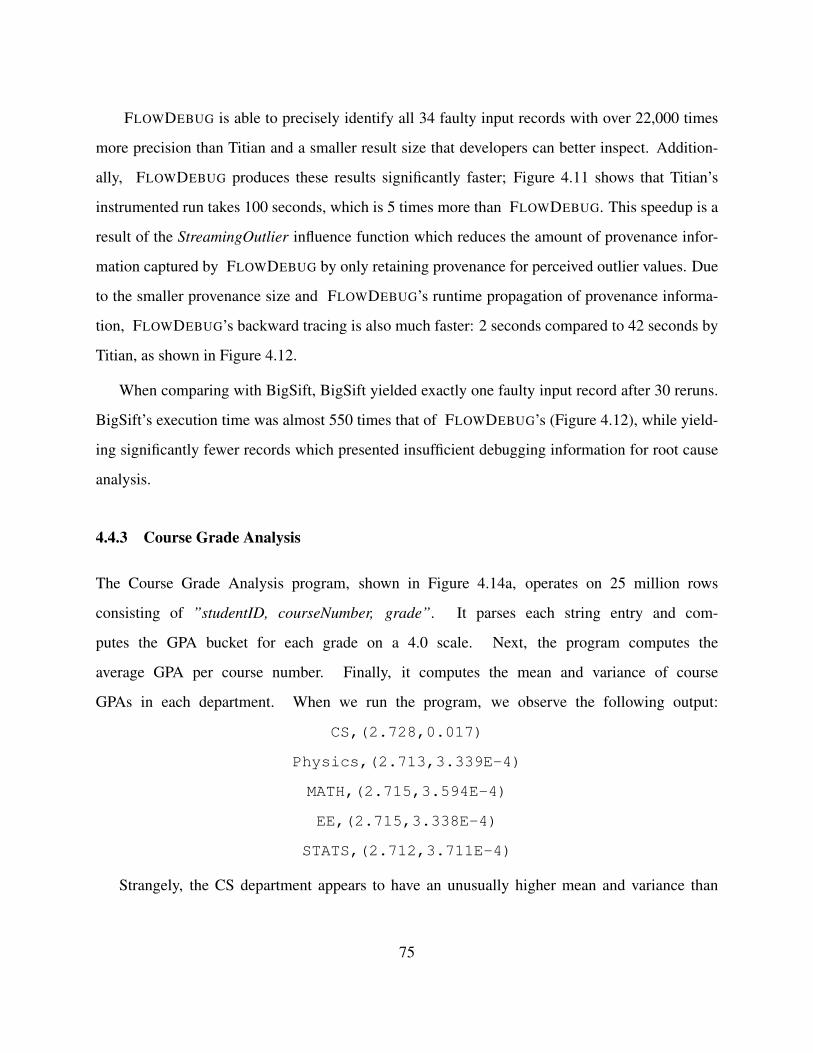
FLOWDEBUG is able to precisely identify all 34 faulty input records with over 22,000 times
more precision than Titian and a smaller result size that developers can better inspect. Addition-
ally, FLOWDEBUG produces these results significantly faster; Figure 4.11 shows that Titian’s
instrumented run takes 100 seconds, which is 5 times more than FLOWDEBUG. This speedup is a
result of the StreamingOutlier influence function which reduces the amount of provenance infor-
mation captured by FLOWDEBUG by only retaining provenance for perceived outlier values. Due
to the smaller provenance size and FLOWDEBUG’s runtime propagation of provenance informa-
tion, FLOWDEBUG’s backward tracing is also much faster: 2 seconds compared to 42 seconds by
Titian, as shown in Figure 4.12.
When comparing with BigSift, BigSift yielded exactly one faulty input record after 30 reruns.
BigSift’s execution time was almost 550 times that of FLOWDEBUG’s (Figure 4.12), while yield-
ing significantly fewer records which presented insufficient debugging information for root cause
analysis.
4.4.3 Course Grade Analysis
The Course Grade Analysis program, shown in Figure 4.14a, operates on 25 million rows
consisting of ”studentID, courseNumber, grade”. It parses each string entry and com-
putes the GPA bucket for each grade on a 4.0 scale. Next, the program computes the
average GPA per course number. Finally, it computes the mean and variance of course
GPAs in each department. When we run the program, we observe the following output:
CS,(2.728,0.017)
Physics,(2.713,3.339E-4)
MATH,(2.715,3.594E-4)
EE,(2.715,3.338E-4)
STATS,(2.712,3.711E-4)
Strangely, the CS department appears to have an unusually higher mean and variance than
75

1 val log = "courseGrades.csv"2
3 val lines: RDD[String] = newSparkContext(sc).textFile(log)
4 val courseGrades = lines.map(line => {5 val arr = line.split(",")6 (arr(1), arr(2).toInt) })7 val courseGpas = // GPA conversion mapping8 courseGrades.mapValues(grade => {9 if (grade >= 93) 4.0
10 ...11 else 0.0 })12 val courseGpaAvgs = // average by course13 courseGpas.aggregateByKey((0.0, 0))(14 {case ((s, c), v) => (s + v, c+1)},15 {case ((sum1, count1), (sum2, count2))
=> (sum1+sum2,count1+count2)}16 ).mapValues({case (sum, count) =>
sum.toDouble/count})17 val deptGpas = courseGpaAvgs.map({18 case (cId, gpa) => // parse dept19 val dept = cId.split("\\d", 2)(0).trim()20 (dept, gpa) })21
22 val partialMeanVar = // Welford’s algorithm23 deptGpas.aggregateByKey((0.0, 0.0, 0.0))({24 case (agg, newValue) =>25 var (count, mean, m2) = agg26 count += 127 val delta = newValue - mean28 mean += delta / count29 val delta2 = newValue - mean30 m2 += delta * delta231 (count, mean, m2) }, {32 case (aggA, aggB) =>33 val (countA, meanA, m2A) = aggA34 val (countB, meanB, m2B) = aggB35 val count = countA + countB36 val delta = meanB - meanA37 val mean = meanA + delta * countB / count38 val m2 = m2A + m2B + (delta * delta) *
(countA * countB / count)39 (count, mean, m2) })40
41
42 val deptGpaMeanVar = // population variance43 partialMeanVar.mapValues({ case (count,
mean, m2) =>44 (mean, m2 / count) })45
(a) Course Grade Analysis program in Scala.
1 val log = "courseGrades.csv"2 // Provenance-supported RDD without Tainting3 val lines: ProvenanceRDD[String] = new
FlowDebugContext(sc).textFileProv(log)4 val courseGrades = lines.map(line => {5 val arr = line.split(",")6 (arr(1), arr(2).toInt) })7 val courseGpas = // GPA conversion mapping8 courseGrades.mapValues(grade => {9 if (grade >= 93) 4.0
10 ...11 else 0.0 })12 val courseGpaAvgs = // average by course13 courseGpas.aggregateByKey((0.0, 0))(14 {case ((s, c), v) => (s + v, c+1)},15 {case ((sum1, count1), (sum2, count2))
=> (sum1+sum2,count1+count2)}16 ).mapValues({case (sum, count) =>
sum.toDouble/count})17 val deptGpas = courseGpaAvgs.map({18 case (cId, gpa) => // parse dept19 val dept = cId.split("\\d", 2)(0).trim()20 (dept, gpa) })21
22 val partialMeanVar = // Welford’s algorithm23 deptGpas.aggregateByKey((0.0, 0.0, 0.0))({24 case (agg, newValue) =>25 var (count, mean, m2) = agg26 count += 127 val delta = newValue - mean28 mean += delta / count29 val delta2 = newValue - mean30 m2 += delta * delta231 (count, mean, m2) }, {32 case (aggA, aggB) =>33 val (countA, meanA, m2A) = aggA34 val (countB, meanB, m2B) = aggB35 val count = countA + countB36 val delta = meanB - meanA37 val mean = meanA + delta * countB / count38 val m2 = m2A + m2B + (delta * delta) *
(countA * countB / count)39 (count, mean, m2)},40 // Additional influence function argument41 influenceTrackerCtr = Some(() =>
StreamingOutlierInfluenceTracker())42 val deptGpaMeanVar = // population variance43 partialMeanVar.mapValues({ case (count,
mean, m2) =>44 (mean, m2 / count) })
(b) Same program with influence function.
Figure 4.14: The Course Grade Analysis program with and without FLOWDEBUG. Line 3 in Fig-
ure 4.14b enables provenance tracking support and line 41 defines the StreamingOutlier influence
function.
76
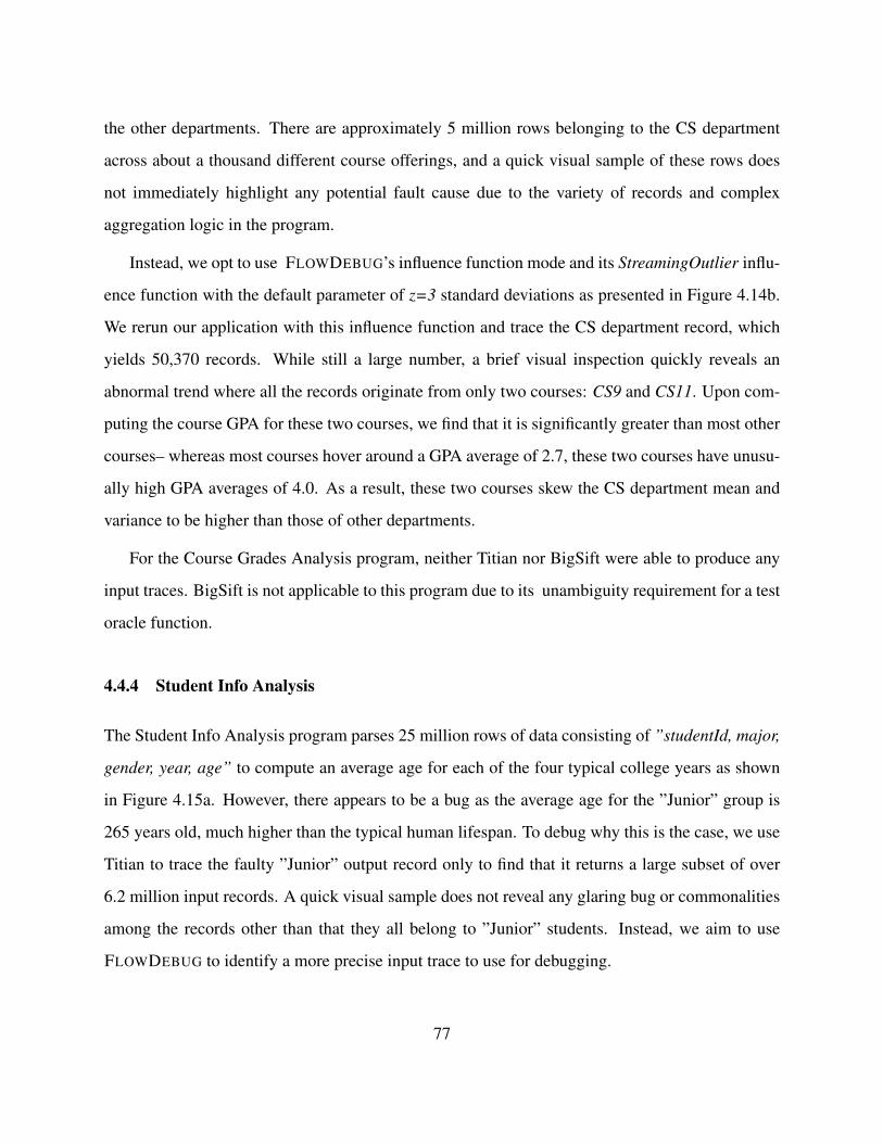
the other departments. There are approximately 5 million rows belonging to the CS department
across about a thousand different course offerings, and a quick visual sample of these rows does
not immediately highlight any potential fault cause due to the variety of records and complex
aggregation logic in the program.
Instead, we opt to use FLOWDEBUG’s influence function mode and its StreamingOutlier influ-
ence function with the default parameter of z=3 standard deviations as presented in Figure 4.14b.
We rerun our application with this influence function and trace the CS department record, which
yields 50,370 records. While still a large number, a brief visual inspection quickly reveals an
abnormal trend where all the records originate from only two courses: CS9 and CS11. Upon com-
puting the course GPA for these two courses, we find that it is significantly greater than most other
courses– whereas most courses hover around a GPA average of 2.7, these two courses have unusu-
ally high GPA averages of 4.0. As a result, these two courses skew the CS department mean and
variance to be higher than those of other departments.
For the Course Grades Analysis program, neither Titian nor BigSift were able to produce any
input traces. BigSift is not applicable to this program due to its unambiguity requirement for a test
oracle function.
4.4.4 Student Info Analysis
The Student Info Analysis program parses 25 million rows of data consisting of ”studentId, major,
gender, year, age” to compute an average age for each of the four typical college years as shown
in Figure 4.15a. However, there appears to be a bug as the average age for the ”Junior” group is
265 years old, much higher than the typical human lifespan. To debug why this is the case, we use
Titian to trace the faulty ”Junior” output record only to find that it returns a large subset of over
6.2 million input records. A quick visual sample does not reveal any glaring bug or commonalities
among the records other than that they all belong to ”Junior” students. Instead, we aim to use
FLOWDEBUG to identify a more precise input trace to use for debugging.
77

1 val log = "studentInfo.csv"2
3 val records: RDD[String] = newSparkContext(sc).textFile(log)
4
5 val grade_age_pair = records.map(line => {6 val list = line.split(",")7 (list(3), list(4).toInt)8 })9 val average_age_by_grade =
grade_age_pair.aggregateByKey((0.0, 0))(10 {case ((sum, count), next) => (sum + next,
count+1)},11 {case ((sum1, count1), (sum2, count2)) =>
(sum1+sum2,count1+count2)})12 .mapValues({case (sum, count) =>
sum.toDouble/count})13
14
15
(a) Student Info Analysis program in Scala.
1 val log = "studentInfo.csv"2 // Provenance-supported RDD without Tainting3 val records: ProvenanceRDD[String] = new
FlowDebugContext(sc).textFileProv(log)4
5 val grade_age_pair = records.map(line => {6 val list = line.split(",")7 (list(3), list(4).toInt)8 })9 val average_age_by_grade =
grade_age_pair.aggregateByKey((0.0, 0))(10 {case ((sum, count), next) => (sum + next,
count+1)},11 {case ((sum1, count1), (sum2, count2)) =>
(sum1+sum2,count1+count2)},12 // Additional influence function argument13 influenceTrackerCtr = Some(() =>
IntStreamingOutlierInfluenceTracker()))14 .mapValues({case (sum, count) =>
sum.toDouble/count})
(b) Same program with influence function.
Figure 4.15: The Student Info Analysis program with and without FLOWDEBUG. Provenance
supporrt is enabled in line 3 of Figure 4.15b while line 13 defines the StreamingOutlier influence
function.
When using FLOWDEBUG’s StreamingOutlier influence function with the default parameter
of z=3 standard deviations as shown in Figure 4.15b, FLOWDEBUG identifies a much smaller
set of 31 input records. Inspection of these records reveals that the student ID and age values are
swapped, resulting in impossible ages such as ”92611257” which drastically increase the overall
average for the ”Junior” key group.
FLOWDEBUG produces an input set that is both smaller and over 200,000X more precise
than Titian. Additionally, FLOWDEBUG’s execution times are much faster than those of Titian.
FLOWDEBUG’s instrumented run takes 8 seconds, 8 times less than Titian’s, while its input trace
takes 2 seconds compared to Titian’s 23 seconds. The speedup in instrumentation time is due
to the reduction in provenance information captured by FLOWDEBUG due to the usage of the
StreamingOutlier influence function, while the speedup in backwards tracing time is a result of
both the reduced provenance size and the propagation of provenance information at runtime for
each output record. Overall, FLOWDEBUG finds fault-inducing inputs in approximately 8% of the
78

original job processing time.
Compared to BigSift, which reports a single faulty record after 31 program re-executions,
FLOWDEBUG is over 500 times faster while providing higher recall and equivalent precision.
4.4.5 Commute Type Analysis
The Commute Type Analysis program begins with parsing 25 million rows of comma-separated
values with the schema ”zipCodeStart, zipCodeEnd, distanceTraveled, timeElapsed”. Each record
is grouped into one of three commute types–car, public transportation, bicycle–according to its
speed as calculated by distance over time in miles per hour. After computing the commute
type and speed of each record, the average speed within each commute type is calculated by
computing the sum and count within each group. The program definition is shown in Figure
4.16a. When we run the Commute Type Analysis program, we observe the following output:
car,50.88
public transportation,27.99
bicycle,11.88
The large gap between public transportation speeds and car speeds is immediately concerning,
as 50+ miles per hour is typically in the domain of highway speeds rather than daily work com-
mutes which typically include surface streets and traffic lights. To investigate why the average car
speed is so high, we use Titian to conduct a backwards trace, Titian identifies approximately 9.5
million input records, which amounts to over one third of the entire input dataset. Due to the sheer
size of the trace, it is difficult to comprehensively analyze the input records for any patterns that
may cause the abnormally high average speed.
Instead, we choose to use FLOWDEBUG to reduce the size of the input trace. Since we know
that the average speed is unexpectedly high, we configure FLOWDEBUG to use the TopN influ-
ence function with an initial parameter of n=1000 to trace the ”car” output record. The modified
program using this influence function is shown in Figure 4.16b. FLOWDEBUG returns 1000 input
79

1 val log = "commute.csv"2
3 val inputs: RDD[String] = newSparkContext(sc).textFile(log)
4
5 val trips = inputs.map { s: String =>6 val cols = s.split(",")7 val distance = cols(3).toInt8 val time = cols(4).toInt9 val speed = distance / time
10 if (speed > 40) {11 ("car", speed)12 } else if (speed > 15) {13 ("public transportation", speed)14 } else {15 ("bicycle", speed)16 }17 }18 val result = trips.aggregateByKey((0L, 0))(19 {case ((sum, count), next) => (sum + next,
count+1)},20 {case ((sum1, count1), (sum2, count2)) =>
(sum1+sum2,count1+count2)}21 ).mapValues({case (sum, count) =>22 sum.toDouble/count}23 )24
25
26
(a) Commute Type Analysis program in Scala.
1 val log = "commute.csv"2 // Provenance-supported RDD without Tainting3 val inputs: ProvenanceRDD[String] = new
FlowDebugContext(sc).textFileProv(log)4
5 val trips = inputs.map { s: String =>6 val cols = s.split(",")7 val distance = cols(3).toInt8 val time = cols(4).toInt9 val speed = distance / time
10 if (speed > 40) {11 ("car", speed)12 } else if (speed > 15) {13 ("public transportation", speed)14 } else {15 ("bicycle", speed)16 }17 }18 val result = trips.aggregateByKey((0L, 0))(19 {case ((sum, count), next) => (sum + next,
count+1)},20 {case ((sum1, count1), (sum2, count2)) =>
(sum1+sum2,count1+count2)},21 // Additional influence function argument22 influenceTrackerCtr = Some(() =>
TopNInfluenceTracker(1000))23 ).mapValues({case (sum, count) =>24 sum.toDouble/count}25 )
(b) Same program with influence function.
Figure 4.16: The Commute Type Analysis program with and without FLOWDEBUG. Line 3
in Figure 4.16b enables provenance tracking support while line 22 defines the TopN influence
function with a size parameter of 1000.
records, of which 150 records have impossibly high speeds of 500+ miles per hour.
FLOWDEBUG’s identified input set is over 9,500 times more precise than that of Titian. Ad-
ditionally, FLOWDEBUG’s instrumentation time (9 seconds) is much faster than Titian’s (57 sec-
onds) due to the reduction in provenance information captured by the TopN influence function. A
similar trend is shown for tracing fault-inducing inputs, where FLOWDEBUG takes under 2 sec-
onds to isolate the faulty inputs while Titian takes 73 seconds. FLOWDEBUG is able to achieve
this speedup in backwards tracing time because of its runtime propagation of input provenance IDs
(eliminating the need for a recursive backwards join as in Titian) as well as the reduced amount of
provenance information associated with the target records. We also note that our initial parameter
80
choice of 1000 for our TopN influence function is an overestimate—larger values would increase
the size of the input trace and processing time, while smaller values would have the opposite effect
and might not capture all the faults present in the input.
For comparison, we also use BigSift to identify a minimal subset of input faults. On the dataset
of 25 million trips, BigSift pinpoints a single faulty record after 27 re-runs. However, this pro-
cess takes over 1100 times as long as FLOWDEBUG’s backward query analysis, as reported in
Figure 4.12, while yielding only a single, incomplete result for developer inspection.
4.5 Discussion
This chapter describes FLOWDEBUG, which leverages code semantics and influence functions
to support precise root cause analysis in big data applications. Our evaluations validate our sub-
hypothesis (SH2) by demonstrating that FLOWDEBUG’s two key insights help achieve up to five
orders-of-magnitude better precision than existing data provenance approaches [59, 47], potentially
eliminating the need for manual followups from developers.
Both FLOWDEBUG and PERFDEBUG (discussed in Chapter 3) enable developers to investi-
gate the root causes of suspicious outputs in big data applications. However, these techniques are
restricted to post-mortem debugging where existing inputs must already produce an undesirable
behavior to be investigated. This limitation motivates us to explore ideas that enable developers to
generate appropriate inputs that produce or trigger performance symptoms in programs. In the next
chapter, we investigate the sub-hypothesis (SH3) and present an automated performance workload
generation tool that targets fuzzing to subprograms of DISC applications to generate test inputs
that trigger specific performance symptoms such as data and computation skew.
81

CHAPTER 5
PerfGen: Automated Performance Workload Generation for
Dataflow Applications
In big data applications, input datasets can cause poor performance symptoms such as computation
skew, data skew, and memory skew. As a result, debugging these symptoms typically requires pos-
session of an appropriate input that triggers the symptom to be investigated. However, such inputs
may not always be available, and identifying or producing inputs which trigger the target symptom
is both difficult and time-consuming, especially when the target symptom may appear later in a
program after many stages of computation. To address the challenge of finding inputs that trigger
specific performance symptoms, we investigate sub-hypothesis (SH3): By targeting fuzz testing
to specific components of DISC applications and defining DISC-oriented performance feedback
metrics and mutations, we can efficiently generate test inputs that trigger specific or reproduce
performance symptoms. In this chapter, we present an automated performance workload gener-
ation tool for triggering or reproducing performance symptoms by extending traditional fuzzing
approaches with targeted fuzzing for specific subprograms, symptom-detecting monitoring with
templates, and input mutation strategies that are inspired by performance skew symptoms.
5.1 Introduction
Due to the scale and widespread usage of DISC systems, performance issues are inevitable. Figure
5.1 visualizes three kinds of performance problems —data skew [68], computation skew [111], and
memory skew [19] —which stem from uneven distributions of data, computation, and memory
82

</> .jar7 min
30 sec
21 sec
2.1 minInput Dataset
</> .jar1 min
30 sec
4 min
2.1 minInput Dataset
</> .jar1 min
30 sec
6.1 min
2.1 minInput Dataset
n =>fib(3^n)
Compute intensiveCode
n =>for 1 to nnew Obj()
Memory intensiveCode
Uneven Data Partition Data Skew
Computation Skew
Memory Skew
Figure 5.1: Three sources of performance skews
across compute nodes and records. Because such performance problems are input dependent,
existing test data fails to expose performance symptoms.
We design PERFGEN to automatically generate test inputs to trigger a given symptom of
performance skew. PERFGEN enables a user to specify a performance skew symptom using
pre-defined performance predicates. It then automatically inserts the corresponding performance
monitor and uses performance feedback as an objective for automated test input generation. PER-
FGEN combines three technical innovations to adapt fuzz testing for DISC performance workload
generation. First, PERFGEN uses a phased fuzzing approach to first target specific program com-
ponents and thus reach deeper program paths. It then uses a user-provided pseudo-inverse function
to convert these intermediate inputs to the targeted location into corresponding inputs in the begin-
ning of the program, which are used as improved seeds for fuzzing the entire program. Second,
83

PERFGEN enables users to specify performance symptoms through a customizable monitor tem-
plate. This specified custom monitor is then used to guide the fuzzing process. Finally PERFGEN
improves its chances of constructing meaningful inputs by defining skew-inspired mutations for
targeted program components and adjusting its mutation operator selection strategies according to
the target symptom.
We evaluate PERFGEN using four case studies and show that PERFGEN achieves more than
43X speedup in time compared to a baseline fuzzing approach. Additionally, PERFGEN requires
less than 0.004% iterations compared to the same baseline approach. Finally, we conduct an in-
depth analysis of PERFGEN’s skew-inspired mutation selection strategy which shows that PER-
FGEN achieves 1.81X speedup in input generation time compared to a uniform mutation operator
selection approach.
Section 5.2 presents an example to motivate the problem of test input generation for repro-
ducing DISC performance symptoms. Section 5.3 describes PERFGEN’s approach and its key
components. Section 5.4 presents our experimental setup, case studies, and evaluation results.
Finally, we conclude the chapter in Section 5.5.
5.2 Motivating Example
1 val inputs = sc.textFile("collatz.txt") // read inputs2
3 val trips = inputs4 .flatMap(line => line.split(" ")) // split space-separated integers5 .map(s=>(Integer.parseInt(s),1)) // parse integers and convert to pair6
7 val grouped = trips.groupByKey(4) // group data by integer key with 4 partitions8
9 val solved = grouped.map { s =>10 (s._1, solve_collatz(s._1)) } // apply UDF to generate new pair value11
12 val sum = solved.reduceByKey((a, b) => a + b) // sum by key
Figure 5.2: The Collatz program which applies the solve collatz function (Figure 5.3) to
each input integer and sums the result by distinct integer input.
To demonstrate the challenges of performance debugging and how PERFGEN addresses such
84
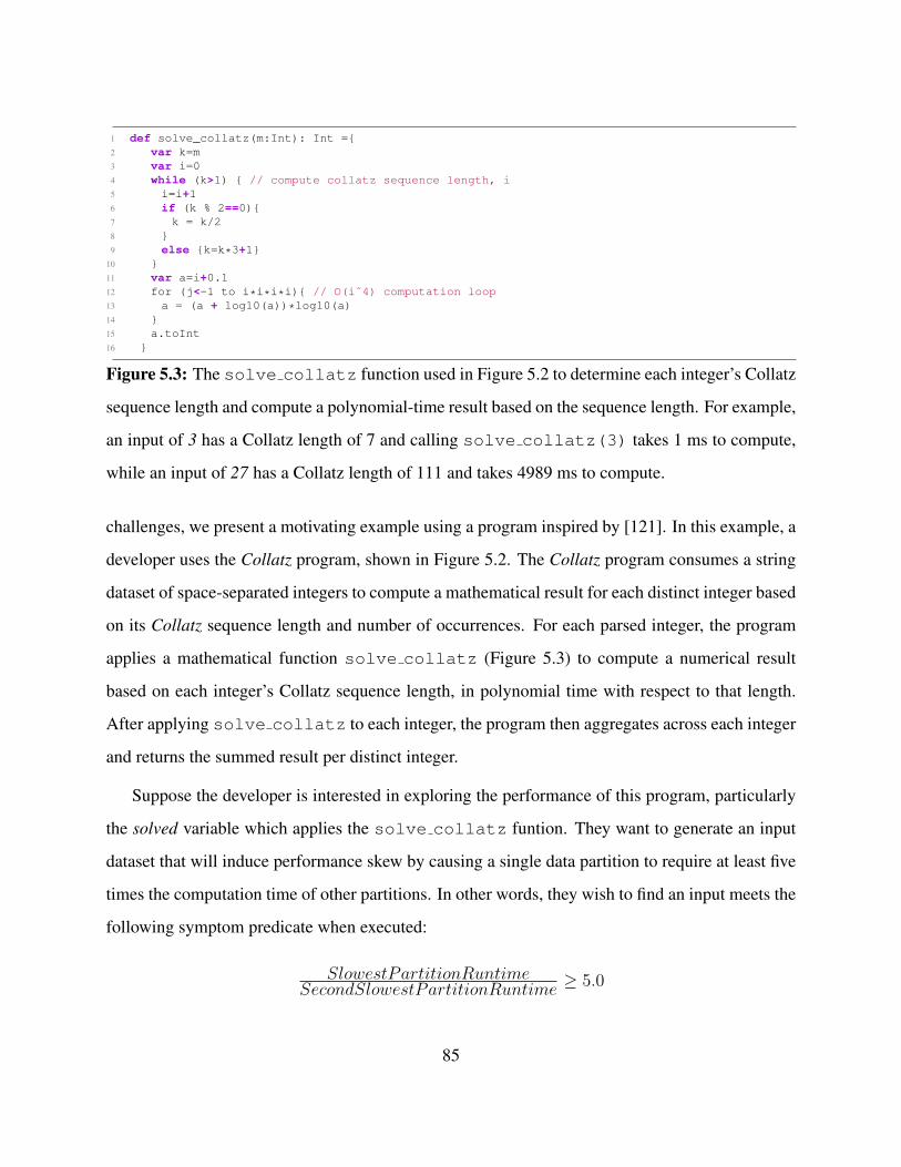
1 def solve_collatz(m:Int): Int ={2 var k=m3 var i=04 while (k>1) { // compute collatz sequence length, i5 i=i+16 if (k % 2==0){7 k = k/28 }9 else {k=k*3+1}
10 }11 var a=i+0.112 for (j<-1 to i*i*i*i){ // O(iˆ4) computation loop13 a = (a + log10(a))*log10(a)14 }15 a.toInt16 }
Figure 5.3: The solve collatz function used in Figure 5.2 to determine each integer’s Collatz
sequence length and compute a polynomial-time result based on the sequence length. For example,
an input of 3 has a Collatz length of 7 and calling solve collatz(3) takes 1 ms to compute,
while an input of 27 has a Collatz length of 111 and takes 4989 ms to compute.
challenges, we present a motivating example using a program inspired by [121]. In this example, a
developer uses the Collatz program, shown in Figure 5.2. The Collatz program consumes a string
dataset of space-separated integers to compute a mathematical result for each distinct integer based
on its Collatz sequence length and number of occurrences. For each parsed integer, the program
applies a mathematical function solve collatz (Figure 5.3) to compute a numerical result
based on each integer’s Collatz sequence length, in polynomial time with respect to that length.
After applying solve collatz to each integer, the program then aggregates across each integer
and returns the summed result per distinct integer.
Suppose the developer is interested in exploring the performance of this program, particularly
the solved variable which applies the solve collatz funtion. They want to generate an input
dataset that will induce performance skew by causing a single data partition to require at least five
times the computation time of other partitions. In other words, they wish to find an input meets the
following symptom predicate when executed:
SlowestPartitionRuntimeSecondSlowestPartitionRuntime
≥ 5.0
85
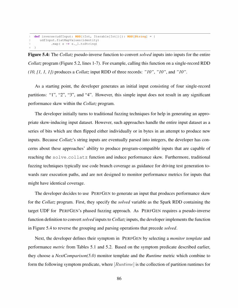
1 def inverse(udfInput: RDD[(Int, Iterable[Int])]): RDD[String] = {2 udfInput.flatMapValues(identity)3 .map( s => s._1.toString)4 }
Figure 5.4: The Collatz pseudo-inverse function to convert solved inputs into inputs for the entire
Collatz program (Figure 5.2, lines 1-7). For example, calling this function on a single-record RDD
(10, [1, 1, 1]) produces a Collatz input RDD of three records: ”10”, ”10”, and ”10”.
As a starting point, the developer generates an initial input consisting of four single-record
partitions: “1”, “2”, “3”, and “4”. However, this simple input does not result in any significant
performance skew within the Collatz program.
The developer initially turns to traditional fuzzing techniques for help in generating an appro-
priate skew-inducing input dataset. However, such approaches handle the entire input dataset as a
series of bits which are then flipped either individually or in bytes in an attempt to produce new
inputs. Because Collatz’s string inputs are eventually parsed into integers, the developer has con-
cerns about these approaches’ ability to produce program-compatible inputs that are capable of
reaching the solve collatz function and induce performance skew. Furthermore, traditional
fuzzing techniques typically use code branch coverage as guidance for driving test generation to-
wards rare execution paths, and are not designed to monitor performance metrics for inputs that
might have identical coverage.
The developer decides to use PERFGEN to generate an input that produces performance skew
for the Collatz program. First, they specify the solved variable as the Spark RDD containing the
target UDF for PERFGEN’s phased fuzzing approach. As PERFGEN requires a pseudo-inverse
function definition to convert solved inputs to Collatz inputs, the developer implements the function
in Figure 5.4 to reverse the grouping and parsing operations that precede solved.
Next, the developer defines their symptom in PERFGEN by selecting a monitor template and
performance metric from Tables 5.1 and 5.2. Based on the symptom predicate described earlier,
they choose a NextComparison(5.0) monitor template and the Runtime metric which combine to
form the following symptom predicate, where [Runtime] is the collection of partition runtimes for
86

a given job execution:
max([Runtime])max([Runtime]− {max([Runtime])}) ≥ 5.0
This predicate inspects the partition runtimes for a given job execution and checks if the longest
partition runtime is at least five times as long as all other partition runtimes.
Using this symptom definition, PERFGEN produces mutations from Table 5.3 for both inter-
mediate solved inputs as well as Collatz program inputs. For example, the mutations for solved’s
(Int, Iterable[Int]) inputs include mutations which randomly replace the integer values in record
keys or values, or alter the distribution of data by appending newly generated records. In addition
to producing mutations, PERFGEN also defines mutation sampling probabilities by assigning sam-
pling weights to each mutation based on their alignment with the symptom definition; for example,
mutations associated with computation skew have higher sampling probabilities when PERFGEN
is given a computation skew symptom.
The user-specified target UDF, monitor template, and metric are shown in Figure 5.5. Using
this configuration, PERFGEN begins its phased fuzzing approach. It first executes Collatz with the
input data until reaching inputs to solved, producing the partitioned UDF input shown in Figure
5.6. Next, it uses the derived mutations to fuzz solved and, after a few iterations, produces the
symptom-triggering UDF input starred in Figure 5.6 by adding the bolded record. As a result of
the key’s long Collatz length and the solve collatz function, this input executes slowly for
only one of the data partitions and satisfies the performance skew definition.1
Next, PERFGEN applies the pseudo-inverse function to this UDF input to produce the Collatz
program input shown in Figure 5.6. Upon testing, PERFGEN finds that the converted input also
exhibits performance skew for the full Collatz and returns the dataset to the user for further anal-
ysis. At this point, the user now possesses a Collatz program input which produces their desired
performance skew symptom.
1“474680340” has a Collatz sequence length of 192, while the remaining records’ lengths are no more than 7.
87
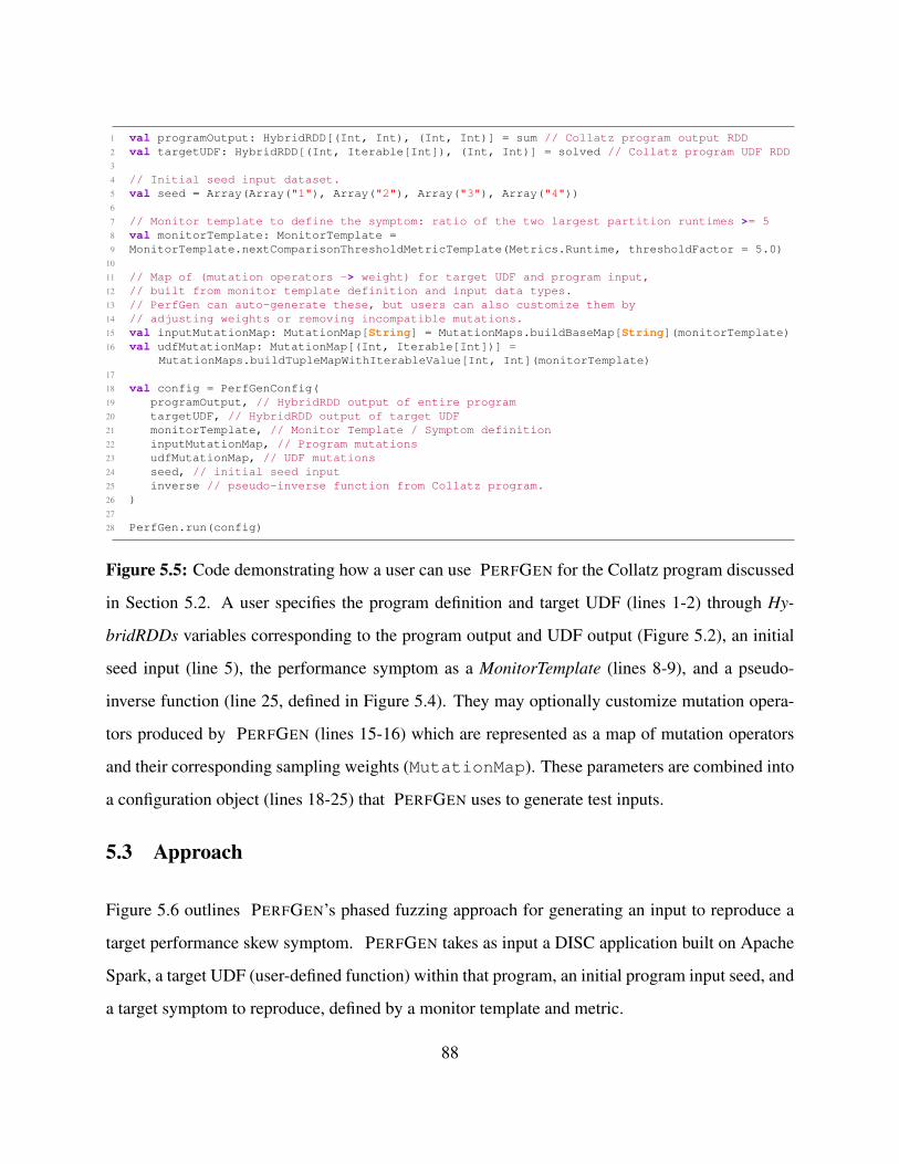
1 val programOutput: HybridRDD[(Int, Int), (Int, Int)] = sum // Collatz program output RDD2 val targetUDF: HybridRDD[(Int, Iterable[Int]), (Int, Int)] = solved // Collatz program UDF RDD3
4 // Initial seed input dataset.5 val seed = Array(Array("1"), Array("2"), Array("3"), Array("4"))6
7 // Monitor template to define the symptom: ratio of the two largest partition runtimes >= 58 val monitorTemplate: MonitorTemplate =9 MonitorTemplate.nextComparisonThresholdMetricTemplate(Metrics.Runtime, thresholdFactor = 5.0)
10
11 // Map of (mutation operators -> weight) for target UDF and program input,12 // built from monitor template definition and input data types.13 // PerfGen can auto-generate these, but users can also customize them by14 // adjusting weights or removing incompatible mutations.15 val inputMutationMap: MutationMap[String] = MutationMaps.buildBaseMap[String](monitorTemplate)16 val udfMutationMap: MutationMap[(Int, Iterable[Int])] =
MutationMaps.buildTupleMapWithIterableValue[Int, Int](monitorTemplate)17
18 val config = PerfGenConfig(19 programOutput, // HybridRDD output of entire program20 targetUDF, // HybridRDD output of target UDF21 monitorTemplate, // Monitor Template / Symptom definition22 inputMutationMap, // Program mutations23 udfMutationMap, // UDF mutations24 seed, // initial seed input25 inverse // pseudo-inverse function from Collatz program.26 )27
28 PerfGen.run(config)
Figure 5.5: Code demonstrating how a user can use PERFGEN for the Collatz program discussed
in Section 5.2. A user specifies the program definition and target UDF (lines 1-2) through Hy-
bridRDDs variables corresponding to the program output and UDF output (Figure 5.2), an initial
seed input (line 5), the performance symptom as a MonitorTemplate (lines 8-9), and a pseudo-
inverse function (line 25, defined in Figure 5.4). They may optionally customize mutation opera-
tors produced by PERFGEN (lines 15-16) which are represented as a map of mutation operators
and their corresponding sampling weights (MutationMap). These parameters are combined into
a configuration object (lines 18-25) that PERFGEN uses to generate test inputs.
5.3 Approach
Figure 5.6 outlines PERFGEN’s phased fuzzing approach for generating an input to reproduce a
target performance skew symptom. PERFGEN takes as input a DISC application built on Apache
Spark, a target UDF (user-defined function) within that program, an initial program input seed, and
a target symptom to reproduce, defined by a monitor template and metric.
88

User Program Target UDF… …
“1”“2”“3”“4”
Seed Input
(1, [1])(2, [1])(3, [1])(4, [1])
Partial Program
Execution
Performance Symptom
UDF Input Mutations
2
3
(1, [1])(2, [1])(7, [1])(4, [1])
x
UDF Fuzzing
Generated UDF Inputs
4
UDF Execution
✓
UDF Input
NextComparison(5.0)“One partition runtime is 5x greater than others”
Partition Runtime
Program Input Mutations
3
Program Fuzzing
Generated Program Inputs
5
Program Execution
Symptom Detection
✓
(1, [1])(2, [1])(3, [1])
(474680340, [1])
Program Input
“1”“2”“3”
“474680340”
Pseudo-Inverse Function
“1”“2”“3”
“474680340”
1Input Output
Symptom Definition Monitor Template Metric
Symptom Detection
Figure 5.6: An overview of PERFGEN’s phased fuzzing approach. A user specifies (1) a target
UDF within their program and (2) a performance symptom definition which is used to detect
whether or not a symptom is present for a given program execution. PERFGEN uses the definition
to generate (3) a weighted set of mutations for both UDF and program input fuzzing. It first (4)
fuzzes the target UDF to reproduce the desired performance symptom, then applies a pseudo-
inverse function to generate an improved program input seed that is used to (5) fuzz the entire
program and generate a program input that reproduces the target symptom.
PERFGEN extends a traditional fuzzing workflow with four novel contributions. Section 5.3.1
describes PERFGEN’s HybridRDD extension to the Spark RDD API in order to support execution
of individual UDFs for more precise fuzzing. Section 5.3.2 enables a user to specify a desired
symptom via execution metrics and predefined monitor templates which define patterns to detect
symptoms. Section 5.3.3 leverages type knowledge from the isolated UDF as well as the symptom
definition to define a weighted set of skew-inspired mutations designed to generate syntactically
valid inputs geared towards producing the target skew symptom. Finally, Section 5.3.4 combines
these techniques to fuzz the specified UDF for symptom-reproducing UDF inputs, then leverages
a pseudo-inverse function to derive program inputs which are then used as an enhanced starting
89

1 val inputs = sc.textFile ("collatz.txt")
2
3 val trips = inputs
4 .flatMap(line => line.split(" "))
5 .map(s=>(Integer.parseInt(s),1))
6
7 val grouped = trips.groupByKey(4)
8
9 val solved = grouped.map { s =>
10 (s._1, solve_collatz(s._1)) }
11
12 val sum = solved.reduceByKey((a, b) => a + b)
(a) A DISC Application Collatz.scala
1 val inputs = HybridRDD(sc.textFile ("collatz.txt"))
2 val trips: HybridRDD[String, (Int, Int)] = inputs
3 .flatMap(line => line.split(" "))
4 .map(s=>(Integer.parseInt(s),1))
5 val grouped: HybridRDD[(Int, Int), (Int, Iterable[Int])] =
6 trips.groupByKey(4)
7 // RDD corresponding to the target UDF
8 val solved: HybridRDD[(Int, Iterable[Int]), (Int, Int)] =
9 grouped.map { s =>
10 (s. 1, solve collatz(s. 1)) }
11 val sum: HybridRDD[(Int, Int), (Int, Int)] =
solved.reduceByKey((a, b) => a + b)
(b) Transformed Collatz with HybridRDD
User-defined function
Figure 5.7: PERFGEN mimics Spark’s RDD API with HybridRDD to support extraction and
reuse of individual UDFs without significant program rewriting. Variable types in 5.7b are shown
to highlight type differences as a result of the HybridRDD conversion, though in practice these
types are optional for users to provide as Scala can automatically infer types. The data types
shown in each HybridRDD correspond to the inputs and outputs of the transformation function
applied to the original Spark RDD.
point for fuzzing the original program from end to end.
5.3.1 Targeting UDFs
DISC applications inherently have longer latency than other applications, making them unsuitable
for iterative fuzz testing [129] which expects millions of invocations per second. Reproducing a
specified performance skew is also an extremely rare event to trigger by chance via input mutation,
particularly when the symptom occurs deep in the program where mutations are unlikely to result
in significant changes.
To overcome this challenge of test input exploration time while reproducing performance
skews, PERFGEN designs a novel phased fuzzing process based on the observation that fuzzing is
easier for a single UDF in isolation than fuzzing an entire application to reach a specific, deep exe-
90

cution path. To enable this, PERFGEN requires users to specify a target UDF for analysis (Figure
5.6 label 1). However, existing DISC systems such as Spark define datasets in terms of transfor-
mations (including UDFs) directly applied to previous datasets. As a result, such programs do not
support decoupling UDFs from input datasets without manual refactoring or system modifications
and it is nontrivial to execute a program (or subprogram) with new inputs.2
1 class HybridRDD[I, T](val parent: HybridRDD[_, I],2 val computeFn: RDD[I] => RDD[T]) {3 val _rdd: RDD[T] = computeFn(parent._rdd)4
5 // RDD-equivalent APIs that wrap Spark RDD and decouple6 // transformations (functions) from parent datasets.7 def map[U](f: T=>U): HybridRDD[T, U] = {8 new HybridRDD(this, rdd => rdd.map(f))9 }
10
11 def filter(f: T > Boolean): HybridRDD[T, U] = {12 new HybridRDD(this, rdd => rdd.filter(f))13 }14
15 ...16
17 def collect(): Array[T] = {18 _rdd.collect()19 }20 }
Figure 5.8: HybridRDDs operate similarly to Spark RDDs while decoupling Spark transforma-
tions (computeFn) from the input RDDs on which they are applied (parent).
In order to automatically extract UDFs from a Spark program, PERFGEN wraps Spark RDDs
with its own HybridRDDs. While HybridRDDs are functionally equivalent to RDDs, they inter-
nally separate transformations from the datasets on which they are applied and store information
about the corresponding input and output data types. The simplified HybridRDD implementation
in Figure 5.8 illustrates how PERFGEN captures transformations as Scala functions while sup-
porting RDD-like operations. Using HybridRDDs, developers can specify individual HybridRDD
instances (variables), which PERFGEN can then use to directly infer the corresponding UDFs
2For example, Spark’s various RDD implementations including MapPartitionsRDD and ShuffledRDD capture in-formation about transformations via private, operator-specific objects such as iterator-to-iterator functions or SparkAggregator instances. Reusing these transformation definitions with new inputs requires direct access to Spark’sinternal classes.
91

through the computeFn function. Similarly, PERFGEN can derive a reusable function for the
entire program (decoupled from the program input seed) from the final output HybridRDD by com-
bining consecutive transformation functions between the program input and output. As a result,
users can specify both a target UDF and a function for the entire program by providing correspond-
ing HybridRDD instances to PERFGEN.
Figures 5.7a and 5.7b illustrate the API changes required to leverage PERFGEN’s HybridRDD
for the Collatz program discussed in Section 5.2. Using this extension, PERFGEN automatically
decouples the map transformation of solved from its predecessor (grouped) to produce a func-
tion of type RDD[(Int, Iterable[Int])] => RDD[(Int, Int)] which captures the
solve collatz function used in the map transformation.
5.3.2 Modeling performance symptoms
1 trait MonitorTemplate {2 val metric: Metric3
4 // Detect performance symptoms and generate feedback based on the provided metric definition.5 def checkSymptoms(partitionMetrics: Array[Long]): SymptomResult6
7 case class SymptomResult(meetsCriteria: Boolean, feedbackScore: Double)8 }
Figure 5.9: Monitor Templates monitor Spark program (or subprogram) execution metrics to (1)
detect performance skew symptoms and (2) produce feedback scores that are used as fuzzing guid-
ance.
In practice, performance skews can often be detected by patterns within metrics such as task
execution time, the number of records read or written during a shuffle, and memory usage. In order
to guide test generation towards exposing specific performance symptoms, PERFGEN provides a
set of 8 customizable monitor templates which model performance symptoms through 10 perfor-
mance metrics derived through Spark’s Listener API, shown in Tables 5.1 and 5.2 respectively. The
full implementations of both can also be found in Appendix A.1 and Appendix A.2. Our insight
behind these templates is that DISC performance skews often follow patterns and thus a user can
92
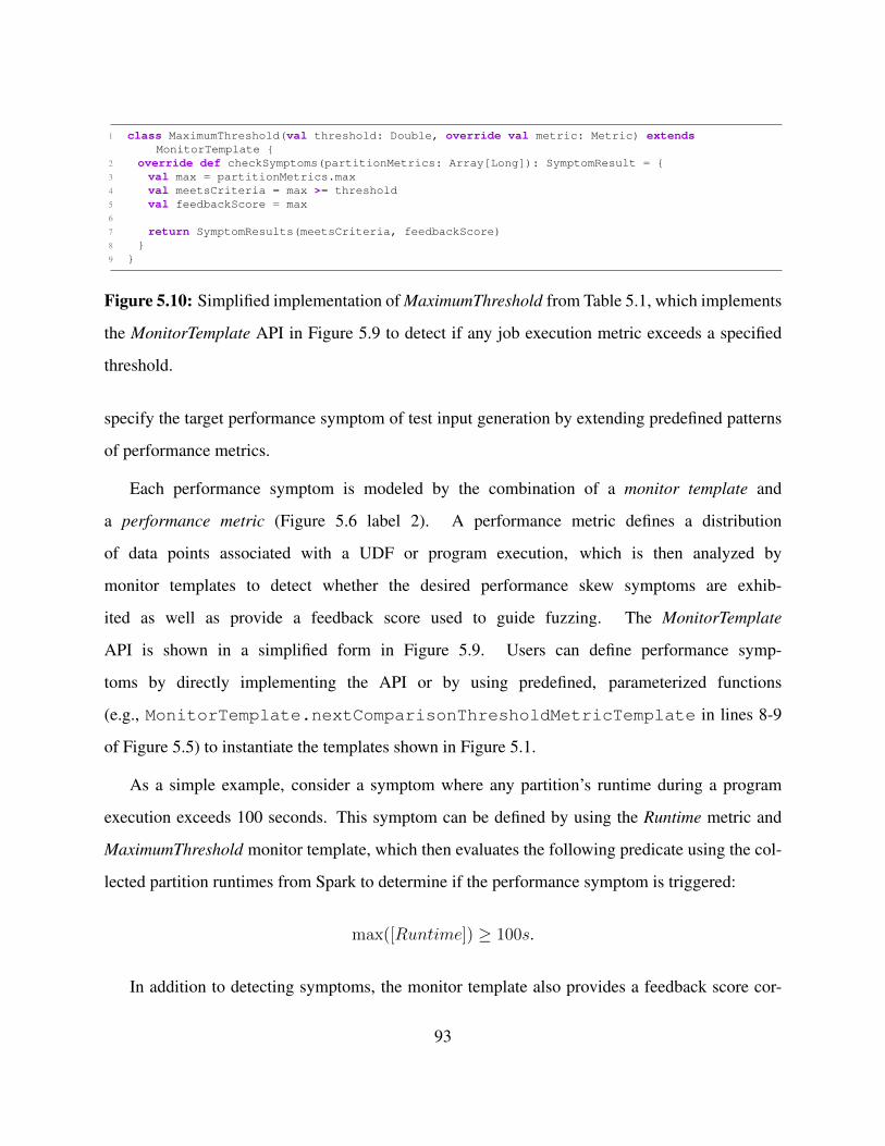
1 class MaximumThreshold(val threshold: Double, override val metric: Metric) extendsMonitorTemplate {
2 override def checkSymptoms(partitionMetrics: Array[Long]): SymptomResult = {3 val max = partitionMetrics.max4 val meetsCriteria = max >= threshold5 val feedbackScore = max6
7 return SymptomResults(meetsCriteria, feedbackScore)8 }9 }
Figure 5.10: Simplified implementation of MaximumThreshold from Table 5.1, which implements
the MonitorTemplate API in Figure 5.9 to detect if any job execution metric exceeds a specified
threshold.
specify the target performance symptom of test input generation by extending predefined patterns
of performance metrics.
Each performance symptom is modeled by the combination of a monitor template and
a performance metric (Figure 5.6 label 2). A performance metric defines a distribution
of data points associated with a UDF or program execution, which is then analyzed by
monitor templates to detect whether the desired performance skew symptoms are exhib-
ited as well as provide a feedback score used to guide fuzzing. The MonitorTemplate
API is shown in a simplified form in Figure 5.9. Users can define performance symp-
toms by directly implementing the API or by using predefined, parameterized functions
(e.g., MonitorTemplate.nextComparisonThresholdMetricTemplate in lines 8-9
of Figure 5.5) to instantiate the templates shown in Figure 5.1.
As a simple example, consider a symptom where any partition’s runtime during a program
execution exceeds 100 seconds. This symptom can be defined by using the Runtime metric and
MaximumThreshold monitor template, which then evaluates the following predicate using the col-
lected partition runtimes from Spark to determine if the performance symptom is triggered:
max([Runtime]) ≥ 100s.
In addition to detecting symptoms, the monitor template also provides a feedback score cor-
93
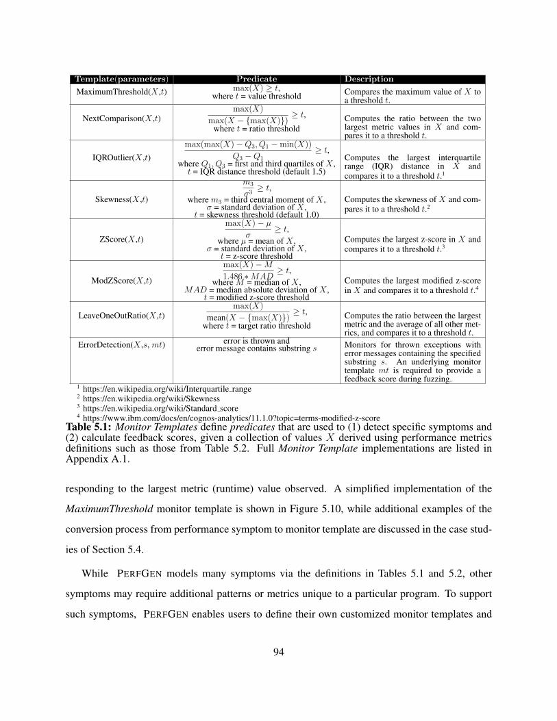
Template(parameters) Predicate Description
MaximumThreshold(X ,t) max(X) ≥ t,where t = value threshold Compares the maximum value of X to
a threshold t.
NextComparison(X ,t)max(X)
max(X − {max(X)})≥ t,
where t = ratio thresholdComputes the ratio between the twolargest metric values in X and com-pares it to a threshold t.
IQROutlier(X ,t)
max(max(X)−Q3, Q1 −min(X))
Q3 −Q1
≥ t,
where Q1, Q3 = first and third quartiles of X ,t = IQR distance threshold (default 1.5)
Computes the largest interquartilerange (IQR) distance in X andcompares it to a threshold t.1
Skewness(X ,t)
m3
σ3≥ t,
where m3 = third central moment of X ,σ = standard deviation of X ,
t = skewness threshold (default 1.0)
Computes the skewness of X and com-pares it to a threshold t.2
ZScore(X ,t)
max(X)− µσ
≥ t,where µ = mean of X ,
σ = standard deviation of X ,t = z-score threshold
Computes the largest z-score in X andcompares it to a threshold t.3
ModZScore(X ,t)
max(X)−M1.486 ∗MAD
≥ t,where M = median of X ,
MAD = median absolute deviation of X ,t = modified z-score threshold
Computes the largest modified z-scorein X and compares it to a threshold t.4
LeaveOneOutRatio(X ,t)max(X)
mean(X − {max(X)})≥ t,
where t = target ratio thresholdComputes the ratio between the largestmetric and the average of all other met-rics, and compares it to a threshold t.
ErrorDetection(X ,s, mt) error is thrown anderror message contains substring s Monitors for thrown exceptions with
error messages containing the specifiedsubstring s. An underlying monitortemplate mt is required to provide afeedback score during fuzzing.
1 https://en.wikipedia.org/wiki/Interquartile range2 https://en.wikipedia.org/wiki/Skewness3 https://en.wikipedia.org/wiki/Standard score4 https://www.ibm.com/docs/en/cognos-analytics/11.1.0?topic=terms-modified-z-score
Table 5.1: Monitor Templates define predicates that are used to (1) detect specific symptoms and(2) calculate feedback scores, given a collection of values X derived using performance metricsdefinitions such as those from Table 5.2. Full Monitor Template implementations are listed inAppendix A.1.
responding to the largest metric (runtime) value observed. A simplified implementation of the
MaximumThreshold monitor template is shown in Figure 5.10, while additional examples of the
conversion process from performance symptom to monitor template are discussed in the case stud-
ies of Section 5.4.
While PERFGEN models many symptoms via the definitions in Tables 5.1 and 5.2, other
symptoms may require additional patterns or metrics unique to a particular program. To support
such symptoms, PERFGEN enables users to define their own customized monitor templates and
94

Name Skew Category Description
RuntimeComputation
DataTime spent (ms) computing a single partition’s result.
Garbage Collection Memory Time spent (ms) by the JVM running garbage collection to free up
memory.
Peak Memory Memory Maximum memory usage (bytes) from all Spark-internal data struc-
tures used to handle data shuffling and aggregation.
Memory Bytes Spilled Memory Number of bytes spilled to disk from all Spark-internal data struc-
tures used to handle data shuffling and aggregation.
Input Read Records Data Number of records read from an input source (non-shuffle).
Output Write Records Data Number of records written to an output destination (non-shuffle).
Shuffle Read Records Data Number of records read from shuffle inputs.
Shuffle Read Bytes Data Number of bytes read from shuffle inputs.
Shuffle Write Records Data Number of records written to shuffle outputs.
Shuffle Write Bytes Data Number of bytes written to shuffle outputs.
Table 5.2: Performance metrics captured by PERFGEN through Spark’s Listener API to monitor
performance symptoms, along with the associated performance skew they are used to measure. All
metrics are reported separately for each partition and stage within an execution.Code implementa-
tions are listed in Appendix A.2.
performance metrics by implementing interfaces such as MonitorTemplate in Figure 5.9.
5.3.3 Skew-Inspired Input Mutation Operations
Consider the Collatz program from Section 5.2, which parses strings as space-separated integers.
When bit-level or byte-level mutations are applied to such inputs, they can hardly generate mean-
ingful data that drives the program to a deep execution path since bit-flipping is likely to destroy
the data format or data type. For example, modifying an input “10” to “1a” would produce a pars-
ing error since an integer number is expected. Additionally, DISC applications include distributed
performance bottlenecks such as data shuffling that are dependent on characteristics of the entire
dataset and may be difficult or impossible to trigger with only record-level mutations. Designing
95

ID Name Data Type Target Skew(s) DescriptionM1 ReplaceInteger Integer Computation Replace the input integer with a randomly gen-
erated integer value within a configurable range(default: [0, Int.MaxValue)).
M2 ReplaceDouble Double Computation Replace the input double with a randomly gen-erated double value within a configurable range(default: [0, Double.MaxValue))
M3 ReplaceBoolean Boolean Computation Replace the input boolean with a random booleanvalue.
M4 ReplaceSubtring String Computation Mutate a string by replacing a random substring(including either empty or the full string) with anewly generated random string of random lengthwithin a configurable range (default: [0, 25)).
M5 ReplaceCollectionElement Collection Computation Randomly select and mutate a random elementwithin a collection according to its type.
M6 AppendCollectionCopy Collection Computation,Data, Memory Extend a collection by appending a copy of itself.
M7 ReplaceTupleElement 2-Element Tuple Computation Randomly select and mutate an element within atwo-element tuple according to its type.
M8 ReplaceTripleElement 3-Element Tuple Computation Randomly select and mutate an element within athree-element tuple according to its type.
M9 ReplaceQuadrupleElement 4-Element Tuple Computation Randomly select and mutate an element within afour-element tuple according to its type.
M10 ReplaceRandomRecord Dataset Computation Randomly select a record and mutate it accordingto one of the mutations applicable to the datasettype. For example, this mutation could choose arandom integer out of an integer dataset and ap-ply the ReplaceInteger mutation.
M11 PairKeyToAllValues 2-Element Tuple Dataset Data, Memory Randomly select a random record. For each dis-tinct value within that record’s partition, appenda new record to the partition consisting of the theselected record’s key and the distinct value, suchthat the key is paired with every value in the par-tition.
M12 PairValueToAllKeys 2-Element Tuple Dataset Data Similar to PairKeyToAllValues but instead pairinga random record’s value with all distinct keys ina partition.
M13 AppendSameKey 2-Element Tuple Dataset Data, Memory Randomly select a random record. Append ad-ditional records consisting of that record’s keypaired with mutations of its value some numberof times (default: up to 10% of partition size).
M14 AppendSameValue 2-Element Tuple Dataset Data Similar to AppendSameKey but instead with afixed value and mutated keys.
Table 5.3: Skew-inspired mutation operations implemented by PERFGEN for various data typesand their typical skew categories. Some mutations depend on others (e.g., due to nested data types);in such cases, the most common target skews are listed. Mutation implementations are listed inAppendix A.3.
mutations to detect performance skews in DISC applications requires that (1) mutations must en-
sure type-correctness, and (2) mutations should be able to manipulate input datasets in ways that
comprehensively exercise the performance-sensitive aspects of distributed applications including
but not limited to record-level operators and shuffling to redistribute data.
PERFGEN defines skew-inspired mutations to reduce the unfruitful fuzzing trials caused by
ill-formatted data or ineffective mutations. For example, PERFGEN targets data skew symptoms
by defining mutations which alter the distribution of keys and values in tuple inputs, as well as
mutations that extend the length of collection-based fields (which might be flattened into multiple
records and contribute to data skew later in the application). PERFGEN also defines mutation
96
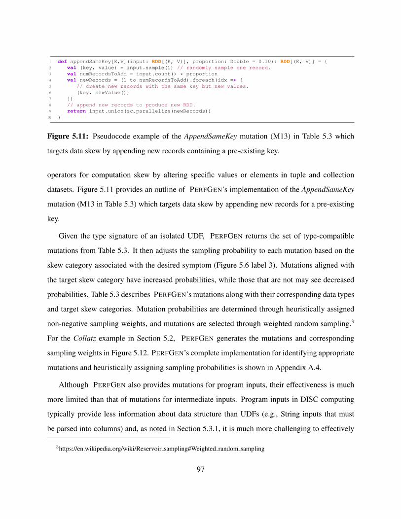
1 def appendSameKey[K,V](input: RDD[(K, V)], proportion: Double = 0.10): RDD[(K, V)] = {2 val (key, value) = input.sample(1) // randomly sample one record.3 val numRecordsToAdd = input.count() * proportion4 val newRecords = (1 to numRecordsToAdd).foreach(idx => {5 // create new records with the same key but new values.6 (key, newValue())7 })8 // append new records to produce new RDD.9 return input.union(sc.parallelize(newRecords))
10 }
Figure 5.11: Pseudocode example of the AppendSameKey mutation (M13) in Table 5.3 which
targets data skew by appending new records containing a pre-existing key.
operators for computation skew by altering specific values or elements in tuple and collection
datasets. Figure 5.11 provides an outline of PERFGEN’s implementation of the AppendSameKey
mutation (M13 in Table 5.3) which targets data skew by appending new records for a pre-existing
key.
Given the type signature of an isolated UDF, PERFGEN returns the set of type-compatible
mutations from Table 5.3. It then adjusts the sampling probability to each mutation based on the
skew category associated with the desired symptom (Figure 5.6 label 3). Mutations aligned with
the target skew category have increased probabilities, while those that are not may see decreased
probabilities. Table 5.3 describes PERFGEN’s mutations along with their corresponding data types
and target skew categories. Mutation probabilities are determined through heuristically assigned
non-negative sampling weights, and mutations are selected through weighted random sampling.3
For the Collatz example in Section 5.2, PERFGEN generates the mutations and corresponding
sampling weights in Figure 5.12. PERFGEN’s complete implementation for identifying appropriate
mutations and heuristically assigning sampling probabilities is shown in Appendix A.4.
Although PERFGEN also provides mutations for program inputs, their effectiveness is much
more limited than that of mutations for intermediate inputs. Program inputs in DISC computing
typically provide less information about data structure than UDFs (e.g., String inputs that must
be parsed into columns) and, as noted in Section 5.3.1, it is much more challenging to effectively
3https://en.wikipedia.org/wiki/Reservoir sampling#Weighted random sampling
97
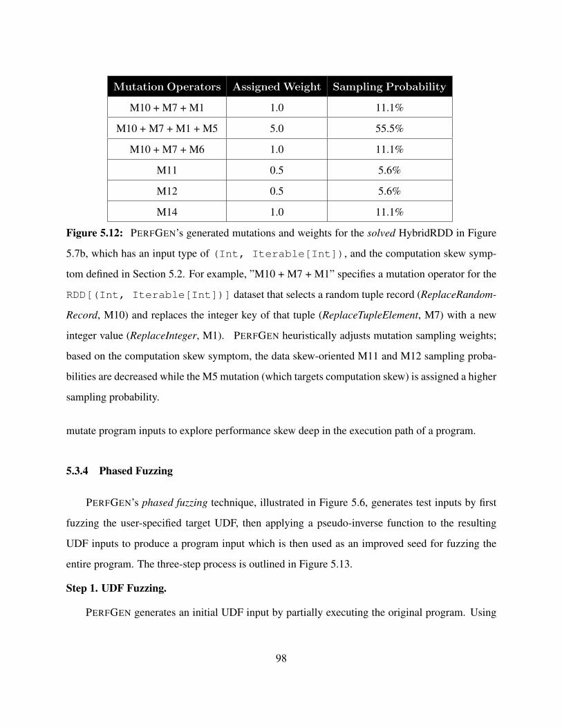
Mutation Operators AssignedWeight Sampling Probability
M10 + M7 + M1 1.0 11.1%
M10 + M7 + M1 + M5 5.0 55.5%
M10 + M7 + M6 1.0 11.1%
M11 0.5 5.6%
M12 0.5 5.6%
M14 1.0 11.1%
Figure 5.12: PERFGEN’s generated mutations and weights for the solved HybridRDD in Figure
5.7b, which has an input type of (Int, Iterable[Int]), and the computation skew symp-
tom defined in Section 5.2. For example, ”M10 + M7 + M1” specifies a mutation operator for the
RDD[(Int, Iterable[Int])] dataset that selects a random tuple record (ReplaceRandom-
Record, M10) and replaces the integer key of that tuple (ReplaceTupleElement, M7) with a new
integer value (ReplaceInteger, M1). PERFGEN heuristically adjusts mutation sampling weights;
based on the computation skew symptom, the data skew-oriented M11 and M12 sampling proba-
bilities are decreased while the M5 mutation (which targets computation skew) is assigned a higher
sampling probability.
mutate program inputs to explore performance skew deep in the execution path of a program.
5.3.4 Phased Fuzzing
PERFGEN’s phased fuzzing technique, illustrated in Figure 5.6, generates test inputs by first
fuzzing the user-specified target UDF, then applying a pseudo-inverse function to the resulting
UDF inputs to produce a program input which is then used as an improved seed for fuzzing the
entire program. The three-step process is outlined in Figure 5.13.
Step 1. UDF Fuzzing.
PERFGEN generates an initial UDF input by partially executing the original program. Using
98

1 def phasedFuzzing[I, U, O](config: PerfGenConfig[I, U, O]): RDD[I] = {2 // Step 1: Fuzz the target UDF to produce symptom-triggering intermediate inputs3 val udfSeed: RDD[U] = computeUDFInput(config.seed) // partially run program up until UDF4 val udfSymptomInput: RDD[U] =5 fuzz(config.udfProgram, udfSeed, config.monitorTemplate, config.udfInputMutations)6
7 // Step 2: Apply pseudo-inverse function to generate program seed8 val programSeed: RDD[I] = config.inverseFn.apply(udfSymptomInput)9
10 // Step 3: Fuzz the full program to produce symptom-triggering program inputs11 val programSymptomInput: RDD[I] =12 fuzz(config.fullProgram, programSeed, config.monitorTemplate,
config.programInputMutations)13
14 return programSymptomInput15 }
Figure 5.13: PERFGEN’s phased fuzzing approach for generating symptom-reproducing inputs.
this intermediate result as a seed, it then fuzzes the target UDF using the procedure outlined in
Figure 5.14. The process is illustrated in Figure 5.6 label 4 with concrete inputs from the motivating
example. Two nontrivial outcomes exist for each fuzzing loop iteration: (1) the monitor template
detects that the desired symptom is triggered and terminates the fuzzing loop or (2) the monitor
template does not detect skew but returns a feedback score that is better than previously observed,
so PERFGEN adds saves the mutated input, updates the best observed feedback score, and resumes
fuzzing with the updated input queue.
Step 2. Pseudo-Inverse Function
While targeted UDF fuzzing enables PERFGEN to generate symptom-triggering intermediate
inputs, the final objective is to identify inputs to the entire program that reproduce the desired
symptom. To address this gap, PERFGEN requires users to define a pseudo-inverse function which
directly converts intermediate UDF inputs to program inputs. For example, Figure 5.6 illustrates
the input and output of the Collatz pseudo-inverse function in Figure 5.4.
The key requirement for a pseudo-inverse function definition is that it generates valid program
inputs when given an intermediate UDF input. In particular, these valid program inputs should be
executable by the full program without any unexpected errors. It is not always necessary that the
resulting program input can be used to exactly reproduce the intermediate UDF input that was first
99
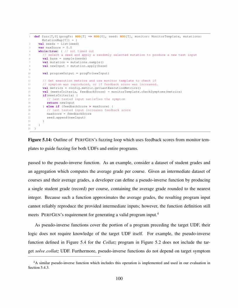
1 def fuzz[T,U](progFn: RDD[T] => RDD[U], seed: RDD[T], monitor: MonitorTemplate, mutations:MutationMap[T]) = {
2 val seeds = List(seed)3 var maxScore = 0.04 while(true) { // not timed out5 // select a seed and apply a randomly selected mutation to produce a new test input6 val base = sample(seeds)7 val mutation = mutations.sample()8 val newInput = mutation.apply(base)9
10 val programOutput = progFn(newInput)11
12 // Get execution metrics and use monitor template to check if13 // symptom was reproduced, or if feedback score was increased.14 val metrics = config.metric.getLastExecutionMetrics()15 val (meetsCriteria, feedbackScore) = monitorTemplate.checkSymptoms(metrics)16 if(meetsCriteria) {17 // last tested input satisfies the symptom18 return newInput19 } else if (feedbackScore > maxScore) {20 // last tested input increases feedback score21 maxScore = feedbackScore22 seed.append(newInput)23 }24 }25 }
Figure 5.14: Outline of PERFGEN’s fuzzing loop which uses feedback scores from monitor tem-
plates to guide fuzzing for both UDFs and entire programs.
passed to the pseudo-inverse function. As an example, consider a dataset of student grades and
an aggregation which computes the average grade per course. Given an intermediate dataset of
courses and their average grades, a developer can define a pseudo-inverse function by producing
a single student grade (record) per course, containing the average grade rounded to the nearest
integer. Because such a function approximates the average grades, the resulting program input
cannot reliably reproduce the provided intermediate inputs; however, the function definition still
meets PERFGEN’s requirement for generating a valid program input.4
As pseudo-inverse functions cover the portion of a program preceding the target UDF, their
logic does not require knowledge of the target UDF itself. For example, the pseudo-inverse
function defined in Figure 5.4 for the Collatz program in Figure 5.2 does not include the tar-
get solve collatz UDF. Furthermore, pseudo-inverse functions do not depend on target symptom
4A similar pseudo-inverse function which includes this operation is implemented and used in our evaluation inSection 5.4.3.
100
definitions. As a result, pseudo-inverse functions can be defined outside of PERFGEN’s phased
fuzzing process and can in practice be simple enough for a developer to manually define in a matter
of minutes.
Automatically inferring pseudo-inverse functions remains an open problem. While some
dataflow operators may have clear inverse mappings, the logic of UDFs within those operators
can vary greatly. Consider the Spark flatMap transformation, which can return an arbitrary number
of output records for a single input record depending on the user-provided function. A flatMap
function that mimics a filter operation by returning either an empty or singleton list has a clear
one-to-one inverse mapping, but it is unclear how to define an exact inverse mapping for a flatMap
function that splits a comma-separated string into individual substrings unless additional informa-
tion about the size of flatMap outputs is also available. Program synthesis offers some promise
for automatically defining pseudo-inverse functions. For example, Prose [8] supports automatic
program generation based on input-output examples. However, such techniques are not currently
designed to support DISC systems and require nontrivial extension in order to support key DISC
properties such as data shuffling and distributed datasets with arbitrary record data types. For in-
stance, a given aggregation output such as a sum can be computed not only from different input
records (e.g., ”1” and ”3”, or ”0” and ”4”), but also from the same input records partitioned in
different ways (e.g., one record per partition or all records in a single partition); consequently,
psuedo-inverse function generation tools for DISC computing should consider both input-output
record relationships and equivalent data partitioning patterns. In the context of PERFGEN’s re-
quirements, there is an additional challenge due to a lack of examples; the existence of a single
input seed means that there is only one input-output example available, but techniques such as
Prose typically require more examples for optimal performance.
Step 3. End-to-End Fuzzing with Improved Seeds. As a final step, PERFGEN tests the pseudo-
inverse function result to see if it is a symptom-triggering input. If not, it uses the derived program
input as an improved seed for fuzzing the entire application as shown in Figure 5.6 label 5. This
step resembles UDF fuzzing (Figure 5.14) and reuses the same monitor template, but initializes
101

with the pseudo-inverse function output as a seed and utilizes a different set of mutations suitable
for the entire program’s input data type.
5.4 Evaluation
We evaluate PERFGEN by posing the following research questions:
RQ1 How much speedup in total execution time can PERFGEN achieve by phased fuzzing, as
opposed to naive fuzzing of the entire program?
RQ2 How much reduction in the number of fuzzing iterations does PERFGEN provide through
improved seeds derived from phased fuzzing, as opposed to using the initial seed with naive
fuzzing?
RQ3 How much improvement in speedup is gained by PERFGEN’s adjustment of mutation sam-
pling probabilities based on the target symptom, as opposed to uniform selection of mutation
operators?
RQ1 assesses overall time savings in using PERFGEN, while RQ2 measures the change in
number of required fuzzing iterations. RQ3 explores the effects of mutation sampling probabilities
on test input generation time.
Evaluation Setup. Existing techniques such as [129] either lack support for performance symptom
detection or do not preserve underlying performance characteristics of Spark programs. As a
baseline, we instead compare against a simplified version of PERFGEN that does not apply phased
fuzzing to produce intermediate inputs. This baseline configuration instead fuzzes the original
program with the same monitor template, but invoking the entire program the initial seed input.
Similar to the PERFGEN setup, the baseline fuzzes the program until a skew-inducing input is
identified. All case study programs start with a String RDD input, so only the M4 + M10 mutation
is used for fuzzing the full program in both PERFGEN as well as the baseline evaluations. As
102
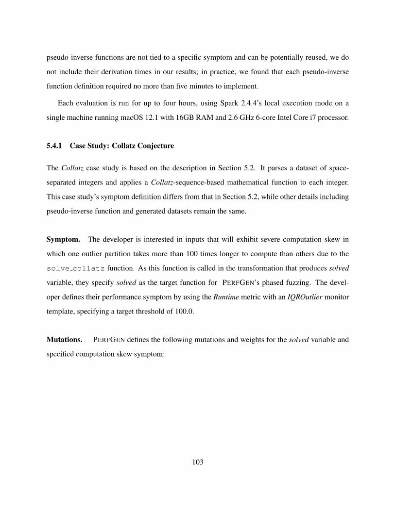
pseudo-inverse functions are not tied to a specific symptom and can be potentially reused, we do
not include their derivation times in our results; in practice, we found that each pseudo-inverse
function definition required no more than five minutes to implement.
Each evaluation is run for up to four hours, using Spark 2.4.4’s local execution mode on a
single machine running macOS 12.1 with 16GB RAM and 2.6 GHz 6-core Intel Core i7 processor.
5.4.1 Case Study: Collatz Conjecture
The Collatz case study is based on the description in Section 5.2. It parses a dataset of space-
separated integers and applies a Collatz-sequence-based mathematical function to each integer.
This case study’s symptom definition differs from that in Section 5.2, while other details including
pseudo-inverse function and generated datasets remain the same.
Symptom. The developer is interested in inputs that will exhibit severe computation skew in
which one outlier partition takes more than 100 times longer to compute than others due to the
solve collatz function. As this function is called in the transformation that produces solved
variable, they specify solved as the target function for PERFGEN’s phased fuzzing. The devel-
oper defines their performance symptom by using the Runtime metric with an IQROutlier monitor
template, specifying a target threshold of 100.0.
Mutations. PERFGEN defines the following mutations and weights for the solved variable and
specified computation skew symptom:
103
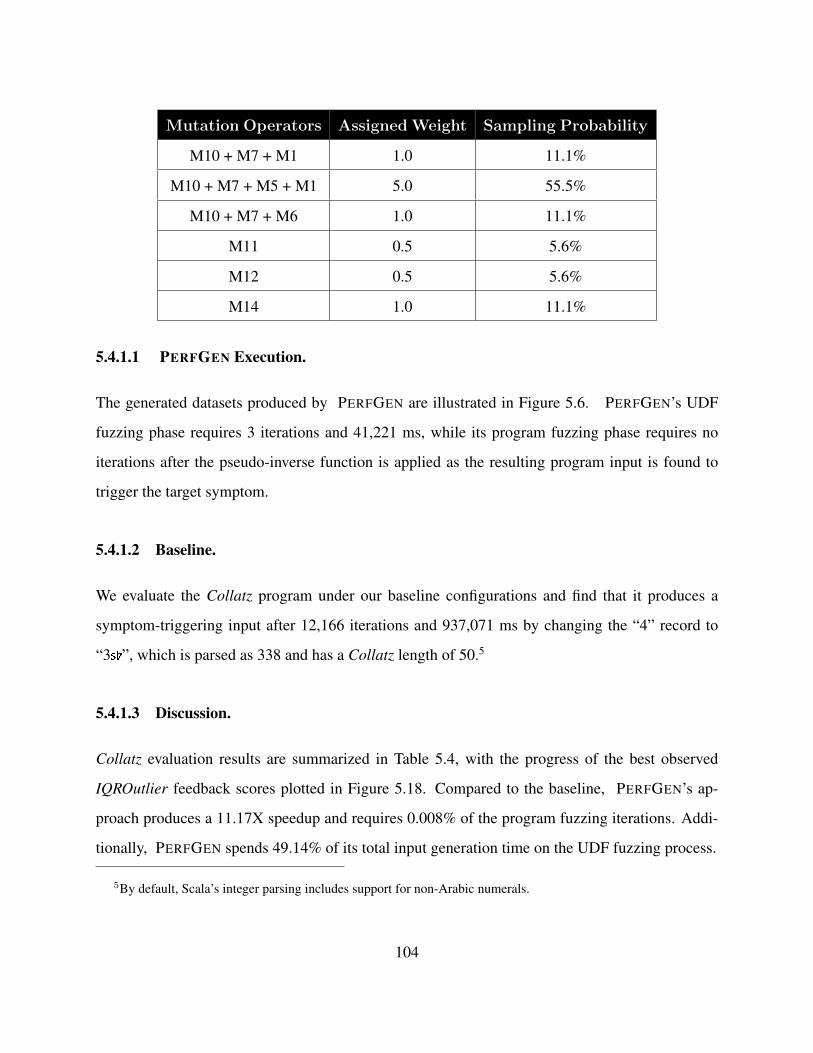
Mutation Operators AssignedWeight Sampling Probability
M10 + M7 + M1 1.0 11.1%
M10 + M7 + M5 + M1 5.0 55.5%
M10 + M7 + M6 1.0 11.1%
M11 0.5 5.6%
M12 0.5 5.6%
M14 1.0 11.1%
5.4.1.1 PERFGEN Execution.
The generated datasets produced by PERFGEN are illustrated in Figure 5.6. PERFGEN’s UDF
fuzzing phase requires 3 iterations and 41,221 ms, while its program fuzzing phase requires no
iterations after the pseudo-inverse function is applied as the resulting program input is found to
trigger the target symptom.
5.4.1.2 Baseline.
We evaluate the Collatz program under our baseline configurations and find that it produces a
symptom-triggering input after 12,166 iterations and 937,071 ms by changing the “4” record to
“3 ”, which is parsed as 338 and has a Collatz length of 50.5
5.4.1.3 Discussion.
Collatz evaluation results are summarized in Table 5.4, with the progress of the best observed
IQROutlier feedback scores plotted in Figure 5.18. Compared to the baseline, PERFGEN’s ap-
proach produces a 11.17X speedup and requires 0.008% of the program fuzzing iterations. Addi-
tionally, PERFGEN spends 49.14% of its total input generation time on the UDF fuzzing process.
5By default, Scala’s integer parsing includes support for non-Arabic numerals.
104

While both configurations are able to successfully generate inputs which trigger the desired
symptom, PERFGEN is able to do so much more efficiently because its type knowledge allows
it to focus on generating integer inputs while the baseline is restricted to string-based mutations
which often fail the integer parsing process.
5.4.2 Case Study: WordCount
5.4.2.1 Setup.
Suppose a developer is interested in the WordCount program from [116], shown in Figure 5.15.
WordCount reads a dataset of Strings and counts how often each space-separated word appears in
the dataset. As a starting input dataset, the developer uses a 5MB sample of Wikipedia entries
consisting of 49,930 records across 20 partitions.
1 val inputs = HybridRDD(sc.textFile("wiki_data")))2 val words = inputs.flatMap(line => line.split(" "))3 val wordPairs = words.map(word => (word, 1))4 val counts = wordPairs.reduceByKey(_ + _)
Figure 5.15: The WordCount program implementation in Scala which counts the occurrences of
each space-separated word.
Symptom. The developer wants to generate an input for which the number of shuffle records
written per partition exhibits a statistical skew value of more than 2. They identify the counts
variable on line 4 in Figure 5.15 as the UDF of interest because it induces a data shuffle, and define
the desired symptom by using the Shuffle Write Records metric in combination with a Skewness
monitor template with a threshold of 2.0.
Mutations. The target UDF takes as input tuples of the type (String, Integer). Expecting a large
number of intermediate records, the developer configures PERFGEN to use a decreased duplication
factor of 0.01. As the integer values are fixed to 1, the developer also disables mutations which
modify values in the UDF inputs. In addition to these configurations, PERFGEN uses the data skew
105
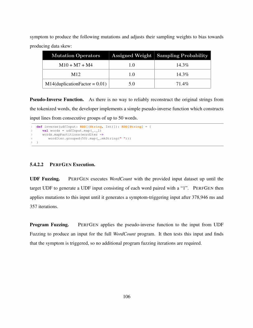
symptom to produce the following mutations and adjusts their sampling weights to bias towards
producing data skew:
Mutation Operators AssignedWeight Sampling Probability
M10 + M7 + M4 1.0 14.3%
M12 1.0 14.3%
M14(duplicationFactor = 0.01) 5.0 71.4%
Pseudo-Inverse Function. As there is no way to reliably reconstruct the original strings from
the tokenized words, the developer implements a simple pseudo-inverse function which constructs
input lines from consecutive groups of up to 50 words.
1 def inverse(udfInput: RDD[(String, Int)]): RDD[String] = {2 val words = udfInput.map(_._1)3 words.mapPartitions(wordIter =>4 wordIter.grouped(50).map(_.mkString(" ")))5 }
5.4.2.2 PERFGEN Execution.
UDF Fuzzing. PERFGEN executes WordCount with the provided input dataset up until the
target UDF to generate a UDF input consisting of each word paired with a “1”. PERFGEN then
applies mutations to this input until it generates a symptom-triggering input after 378,946 ms and
357 iterations.
Program Fuzzing. PERFGEN applies the pseudo-inverse function to the input from UDF
Fuzzing to produce an input for the full WordCount program. It then tests this input and finds
that the symptom is triggered, so no additional program fuzzing iterations are required.
106

5.4.2.3 Baseline.
We evaluate WordCount under the baseline configurations specified earlier in Section 5.4, using the
same sample of Wikipedia data. The baseline times out after approximately 4 hours and 46,884
iterations without producing any inputs that trigger the target symptom.
5.4.2.4 Discussion.
Table 5.4 summarizes the WordCount evaluation results, and Figure 5.18 visualizes the progress
of the maximum attained skewness statistics determined by the Skewness monitor template. Com-
pared to the baseline which is unable to produce results after 4 hours, PERFGEN produces a
speedup of at least 37.43X while requiring at most 0.0002% of the program fuzzing iterations.
98.48% of PERFGEN’s total execution time is spent on UDF fuzzing.
While PERFGEN is able to meet the target skewness threshold of 2.0, the baseline times out
while never exceeding a skewnesss of 0.7. This gap in skewness comes from the baseline’s inability
to produce large quantities of new words which directly contribute to the number of shuffle records
written by Spark.6 Meanwhile, PERFGEN’s M14 mutation produces many distinct words in each
iteration, and thus enables PERFGEN to quickly trigger the target symptom.
5.4.3 Case Study: DeptGPAsMedian
5.4.3.1 Setup.
Suppose a developer is investigating the DeptGPAsMedian program, modified from [110] and
shown in Figure 5.16 . Given a string dataset with lines in the format “studentID,courseID,grade”,
the program first computes each course’s average GPA. Next, it groups each average GPA accord-
ing to the course’s department and computes each department’s median average course GPA.
6Due to Spark’s map-side aggregation support, duplicate words do not increase the number of shuffle recordswritten.
107

1 val lines = HybridRDD(sc.textFile("grades"))2
3 val courseGrades = lines.map(line => {4 val arr = line.split(",")5 val (courseId, grade) = (arr(1), arr(2).toInt)6 (courseId, grade)7 })8
9 // assign GPA buckets10 val courseGpas = courseGrades.mapValues(grade => {11 if (grade >= 93) 4.012 else if (grade >= 90) 3.713 else if (grade >= 87) 3.314 else if (grade >= 83) 3.015 else if (grade >= 80) 2.716 else if (grade >= 77) 2.317 else if (grade >= 73) 2.018 else if (grade >= 70) 1.719 else if (grade >= 67) 1.320 else if (grade >= 65) 1.021 else 0.022 })23
24
25 // Compute average per key26 val courseGpaAvgs =27 courseGpas.aggregateByKey((0.0, 0))(28 { case ((sum, count), next) =>29 (sum + next, count + 1) },30 { case ((sum1, count1), (sum2, count2)) =>31 (sum1 + sum2, count1 + count2) }32 ).mapValues({ case (sum, count) =>33 sum.toDouble / count })34
35 val deptGpas = courseGpaAvgs.map({ case (courseId, gpa) =>36 val dept = courseId.split("\\d", 2)(0).trim()37 (dept, gpa)38 })39
40 // Use 3 partitions due to few keys41 val grouped = deptGpas.groupByKey(3)42
43 val median = grouped.mapValues(values => {44 val sorted = values.toArray.sorted45 val len = sorted.length46 (sorted(len / 2) + sorted((len - 1) / 2)) / 2.047 })
Figure 5.16: The DeptGPAsMedian program implementation in Scala which calculates the median
of average course GPAs within each department.
To investigate the program, the developer generates a 40-partition dataset with 5,000 records
per partition, totaling 2.8MB. The dataset includes five departments, 20 courses per department,
and 200 unique students.
108
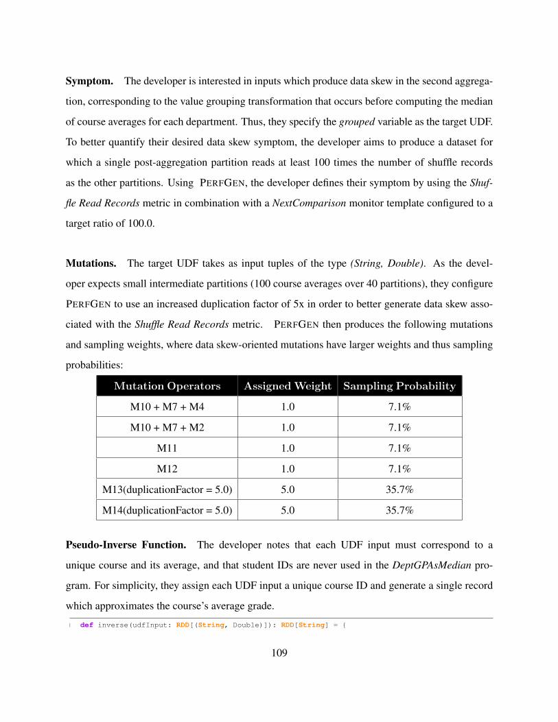
Symptom. The developer is interested in inputs which produce data skew in the second aggrega-
tion, corresponding to the value grouping transformation that occurs before computing the median
of course averages for each department. Thus, they specify the grouped variable as the target UDF.
To better quantify their desired data skew symptom, the developer aims to produce a dataset for
which a single post-aggregation partition reads at least 100 times the number of shuffle records
as the other partitions. Using PERFGEN, the developer defines their symptom by using the Shuf-
fle Read Records metric in combination with a NextComparison monitor template configured to a
target ratio of 100.0.
Mutations. The target UDF takes as input tuples of the type (String, Double). As the devel-
oper expects small intermediate partitions (100 course averages over 40 partitions), they configure
PERFGEN to use an increased duplication factor of 5x in order to better generate data skew asso-
ciated with the Shuffle Read Records metric. PERFGEN then produces the following mutations
and sampling weights, where data skew-oriented mutations have larger weights and thus sampling
probabilities:
Mutation Operators AssignedWeight Sampling Probability
M10 + M7 + M4 1.0 7.1%
M10 + M7 + M2 1.0 7.1%
M11 1.0 7.1%
M12 1.0 7.1%
M13(duplicationFactor = 5.0) 5.0 35.7%
M14(duplicationFactor = 5.0) 5.0 35.7%
Pseudo-Inverse Function. The developer notes that each UDF input must correspond to a
unique course and its average, and that student IDs are never used in the DeptGPAsMedian pro-
gram. For simplicity, they assign each UDF input a unique course ID and generate a single record
which approximates the course’s average grade.
1 def inverse(udfInput: RDD[(String, Double)]): RDD[String] = {
109

2 val unusedSID = 423 rdd.zipWithUniqueId().map({4 case ((dept, avg), uniqueID) =>5 val courseStr = dept + uniqueID6 val grade = avg.toInt7 s"$unusedSID,$courseStr,$grade"8 })9 }
While relatively easy to implement, it is worth noting that this function does not reliably pro-
duce program inputs that can be used to reproduce the intermediate course average values. For
example, applying this pseudo-inverse function on a RDD containing a single single intermedi-
ate (UDF) record of (”EE”, 80.7) produces a RDD containing a single DeptGPAsMedian input
record of ”42,EE,80”. Running the DeptGPAsMedian program with this input to compute the
intermediate UDF results then produces an intermediate RDD of a single record, (”EE”, 80.0),
which differs from the original input to the pseudo-inverse function. Nonetheless, the output of
the pseudo-inverse function (i.e., the generated DeptGPAsMedian input RDD) is still a valid in-
put to the DeptGPAsMedian program and the function thus satisfies PERFGEN’s requirements as
discussed in Section 5.3.4.
5.4.3.2 PERFGEN Execution.
UDF Fuzzing. PERFGEN uses the generated dataset and partially executes DeptGPAsMedian to
derive UDF inputs consisting of each course’s department name paired with the course’s average
grade.
Next, PERFGEN applies mutations to generate new inputs and tests them to see if they trigger
the target data skew symptom. After 259,205 ms and 1,519 iterations, it produces such an input by
using a M13 mutation which significantly increases the frequency of UDF inputs associated with
the “EE” department.
Program Fuzzing. PERFGEN applies the pseudo-inverse function to the UDF Fuzzing result to
produce an input which contains thousands of unique courses in the “EE” department. It then tests
110

this input with the full DeptGPAsMedian program and finds that the target symptom is triggered
with no additional modifications.
5.4.3.3 Baseline.
We utilize the generated DeptGPAsMedian input and the baseline configuration specified earlier
at the start of Section 5.4. Under these settings, the baseline is unable to generate any symptom-
triggering inputs after approximately 4 hours and 21,575 iterations.
5.4.3.4 Discussion.
The DeptGPAsMedian case study results are summarized in Table 5.4, and the progress of the best
observed NextComparison ratios are displayed in Figure 5.18. Using PERFGEN over the baseline
configuration produces at least 54.80X speedup while requiring at most 0.005% of the program
fuzzing iterations. PERFGEN’s UDF fuzzing process comprises 98.61% of its total execution time.
While PERFGEN is able trigger the target symptom of a Next Comparison ratio greater than
100.0, the baseline is unable to reach even 7% of this threshold. This gap in performance can
be attributed to baseline’s inability to target record mutations that significantly affect intermediate
input records associated with the target data skew symptoms. On the other hand, PERFGEN is
able to precisely target the appropriate stage in the Spark program through its use of UDF fuzzing,
and is able to leverage skew-oriented mutations to modify the data distribution and produce data
skew.
5.4.4 Case Study: StockBuyAndSell
5.4.4.1 Setup.
Suppose a developer is interested in the StockBuyAndSell program, which is based on the LeetCode
Best Time to Buy And Sell Stock III coding problem [9]. Using a dataset of comma-separated
111
strings in the form “Symbol,Date,Open,High,Low,Close,Volume,OpenInt”, the StockBuyAndSell
calculates each stock’s maximum achievable profit with at most three transactions (using a dynamic
programming implementation adapted from [10]) by grouping closing prices by stock symbol and
chronologically sorting within each symbol. The program implementation (adapted from [10]) is
shown in Figure 5.17, where the maxProfits variable is the result of applying the profit calculation
for each group.
As an initial dataset, the developer samples 1% of the 20 largest stock symbols from a Kaggle
dataset [81].7 The dataset consists of 2,389 records across 20 partitions, totaling 244KB of data in
total.
Symptom. The developer wants to generate an input for which one partition increases the max-
imum observed profit of the dynamic programming loop in maxProfits (Figure 5.17, line 29) at
least five times more frequently than other partitions. They specify maxProfits as their target UDF.
As PERFGEN does not support such a metric by default, the developer implements this metric by
extending their maximum profit calculation with Spark’s Accumulator API8 to count the number
of branch executions that result in an increase of the maximum observed profit for each partition.
This metric is then passed to a NextComparison monitor template with a target ratio of 5.0.
Mutations. The target UDF takes (String, Iterable[Double]) tuples as input. The developer uses
their knowledge of the StockBuyAndSell program to disable key-based mutations for these inputs,
as well as impose a restriction that UDF input keys must be unique due to an earlier aggregation.
As a result, only the following two mutations and their weights are generated:
Mutation Operators AssignedWeight Sampling Probability
M10 + M7 + M5 + M2 5.0 83.3%
M10 + M7 + M6 1.0 16.7%
7Preprocessing is also applied to include stock symbols in each line.
8https://spark.apache.org/docs/2.4.4/rdd-programming-guide.html#accumulators
112
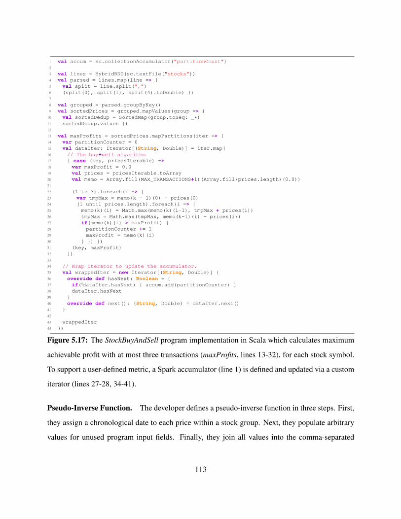
1 val accum = sc.collectionAccumulator("partitionCount")2
3 val lines = HybridRDD(sc.textFile("stocks"))4 val parsed = lines.map(line => {5 val split = line.split(",")6 (split(0), split(1), split(4).toDouble) })7
8 val grouped = parsed.groupByKey()9 val sortedPrices = grouped.mapValues(group => {
10 val sortedDedup = SortedMap(group.toSeq: _*)11 sortedDedup.values })12
13 val maxProfits = sortedPrices.mapPartitions(iter => {14 var partitionCounter = 015 val dataIter: Iterator[(String, Double)] = iter.map(16 // The buy+sell algorithm17 { case (key, pricesIterable) =>18 var maxProfit = 0.019 val prices = pricesIterable.toArray20 val memo = Array.fill(MAX_TRANSACTIONS+1)(Array.fill(prices.length)(0.0))21
22 (1 to 3).foreach(k => {23 var tmpMax = memo(k - 1)(0) - prices(0)24 (1 until prices.length).foreach(i => {25 memo(k)(i) = Math.max(memo(k)(i-1), tmpMax + prices(i))26 tmpMax = Math.max(tmpMax, memo(k-1)(i) - prices(i))27 if(memo(k)(i) > maxProfit) {28 partitionCounter += 129 maxProfit = memo(k)(i)30 } }) })31 (key, maxProfit)32 })33
34 // Wrap iterator to update the accumulator.35 val wrappedIter = new Iterator[(String, Double)] {36 override def hasNext: Boolean = {37 if(!dataIter.hasNext) { accum.add(partitionCounter) }38 dataIter.hasNext39 }40 override def next(): (String, Double) = dataIter.next()41 }42
43 wrappedIter44 })
Figure 5.17: The StockBuyAndSell program implementation in Scala which calculates maximum
achievable profit with at most three transactions (maxProfits, lines 13-32), for each stock symbol.
To support a user-defined metric, a Spark accumulator (line 1) is defined and updated via a custom
iterator (lines 27-28, 34-41).
Pseudo-Inverse Function. The developer defines a pseudo-inverse function in three steps. First,
they assign a chronological date to each price within a stock group. Next, they populate arbitrary
values for unused program input fields. Finally, they join all values into the comma-separated
113

string format required by StockBuyAndSell.
1 def inverse(udfInput: RDD[(String, Iterable[Double])]): RDD[String] = {2 val datePrice = udfInput.flatMapValues(prices => {3 val DEFAULT_START_DATE = new java.util.Date(0)4 val dateFormat = new SimpleDateFormat("yyyy-MM-dd")5 val cal = Calendar.getInstance()6 cal.setTime(DEFAULT_START_DATE)7
8 val datePriceTuples: Iterable[(String, Double)] =9 prices.map(price => {
10 val date = cal.getTime11 val dateStr = dateFormat.format(date)12 cal.add(Calendar.DATE, 1) // increment 1 day13 (dateStr, price)14 })15 datePriceTuples16 })17
18 val stringJoin = datePrice.map({19 case (key, valueTuple) =>20 val (date, price) = valueTuple21 val DEFAULT_VOLUME = 10000022 val DEFAULT_OPEN_INT = 023 // "Date,Open,High,Low,Close,Volume,OpenInt"24 Seq(key, date, price, price, price, DEFAULT_VOLUME, DEFAULT_OPEN_INT).mkString(",")25 })26
27 return stringJoin28 }
5.4.4.2 PERFGEN Execution.
UDF Fuzzing. PERFGEN partially executes StockBuyAndSell on the provided input dataset to
generate a UDF input consisting of stock symbols and their chronologically ordered prices.
PERFGEN then applies mutations to this input and, after 205,084 ms and 4,775 iterations,
produces an input which satisfies the monitor template. The resulting input is produced from a M5
which directly affects the developer’s custom metric by modifying individual values in the grouped
stock prices.
Program Fuzzing. PERFGEN applies the pseudo-inverse function to this UDF input, tests the
resulting StockBuyAndSell input, and finds that it also triggers the target symptom. As a result, no
additional fuzzing iterations are necessary.
114
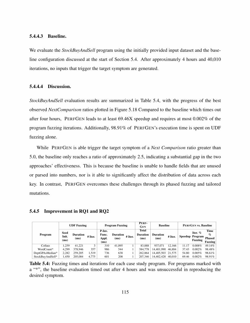
5.4.4.3 Baseline.
We evaluate the StockBuyAndSell program using the initially provided input dataset and the base-
line configuration discussed at the start of Section 5.4. After approximately 4 hours and 40,010
iterations, no inputs that trigger the target symptom are generated.
5.4.4.4 Discussion.
StockBuyAndSell evaluation results are summarized in Table 5.4, with the progress of the best
observed NextComparison ratios plotted in Figure 5.18 Compared to the baseline which times out
after four hours, PERFGEN leads to at least 69.46X speedup and requires at most 0.002% of the
program fuzzing iterations. Additionally, 98.91% of PERFGEN’s execution time is spent on UDF
fuzzing alone.
While PERFGEN is able trigger the target symptom of a Next Comparison ratio greater than
5.0, the baseline only reaches a ratio of approximately 2.5, indicating a substantial gap in the two
approaches’ effectiveness. This is because the baseline is unable to handle fields that are unused
or parsed into numbers, nor is it able to significantly affect the distribution of data across each
key. In contrast, PERFGEN overcomes these challenges through its phased fuzzing and tailored
mutations.
5.4.5 Improvement in RQ1 and RQ2
Program
UDF Fuzzing Program FuzzingPERF-GENTotal
Baseline PERFGEN vs. Baseline
SeedInit.(ms)
Duration(ms) # Iter.
P-Inv.Func.Appl.(ms)
Duration(ms) # Iter.
Duration(ms)
Duration(ms) # Iter. Speedup
Iter. %ProgramFuzzing
Time%
PhasedFuzzing
Collatz 1,259 41,221 3 310 41,095 1 83,888 937,071 12,166 11.17 0.008% 49.14%WordCount* 4,299 378,946 357 986 544 1 384,778 14,401,990 46,884 37.43 0.002% 98.48%
DeptGPAsMedian* 2,282 259,205 1,519 736 638 1 262,864 14,405,503 21,575 54.80 0.005% 98.61%StockBuyAndSell* 1,450 205,084 4,775 601 208 1 207,346 14,402,428 40,010 69.46 0.002% 98.91%
Table 5.4: Fuzzing times and iterations for each case study program. For programs marked witha “*”, the baseline evaluation timed out after 4 hours and was unsuccessful in reproducing thedesired symptom.
115

0 5 10 15 20
1
2
3
4
5·104
Time (min)
IQR
Out
liers
core
Collatz
0 60 120 180 240
1
2
3
Time (min)
Skew
ness
scor
e
WordCount
0 60 120 180 240
100
200
300
400
Time (min)
Nex
tCom
pari
son
scor
e
DeptGPAsMedian
0 50 100 150 200
1
2
3
4
5
Time (min)
Nex
tCom
pari
son
scor
e
StockBuyAndSell
Figure 5.18: Time series plots of each case study’s monitor template feedback score against time.
PERFGEN results are plotted in black with the final program result indicated by a circle, while
baseline results are plotted in red crosses. The target threshold for each case study’s symptom
definition is represented by a horizontal blue dotted line.
Table 5.4 presents each case study’s evaluation results, and Figure 5.18 shows each case study’s
progress over time. Averaged across all four case studies,9 PERFGEN leads to a speedup of at
least 43.22X while requiring no more than 0.004% of the program fuzzing iterations required by
the baseline. Additionally, PERFGEN’s UDF fuzzing process accounts for an average 86.28% of
its total execution time.
9As three of the four case study baselines timed out after four hours, numbers are reported as bounds.
116
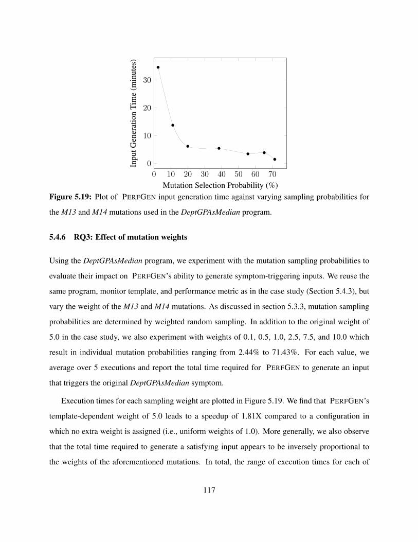
0 10 20 30 40 50 60 70
0
10
20
30
Mutation Selection Probability (%)
Inpu
tGen
erat
ion
Tim
e(m
inut
es)
Figure 5.19: Plot of PERFGEN input generation time against varying sampling probabilities for
the M13 and M14 mutations used in the DeptGPAsMedian program.
5.4.6 RQ3: Effect of mutation weights
Using the DeptGPAsMedian program, we experiment with the mutation sampling probabilities to
evaluate their impact on PERFGEN’s ability to generate symptom-triggering inputs. We reuse the
same program, monitor template, and performance metric as in the case study (Section 5.4.3), but
vary the weight of the M13 and M14 mutations. As discussed in section 5.3.3, mutation sampling
probabilities are determined by weighted random sampling. In addition to the original weight of
5.0 in the case study, we also experiment with weights of 0.1, 0.5, 1.0, 2.5, 7.5, and 10.0 which
result in individual mutation probabilities ranging from 2.44% to 71.43%. For each value, we
average over 5 executions and report the total time required for PERFGEN to generate an input
that triggers the original DeptGPAsMedian symptom.
Execution times for each sampling weight are plotted in Figure 5.19. We find that PERFGEN’s
template-dependent weight of 5.0 leads to a speedup of 1.81X compared to a configuration in
which no extra weight is assigned (i.e., uniform weights of 1.0). More generally, we also observe
that the total time required to generate a satisfying input appears to be inversely proportional to
the weights of the aforementioned mutations. In total, the range of execution times for each of
117
the evaluated sampling weights ranged between 23.32% and 564.74% of the time taken for an
unweighted evaluation.
5.5 Discussion
This chapter presents PERFGEN, an automated performance workload generation tool for repro-
ducing performance symptoms. PERFGEN generates inputs that trigger specific performance
system by targeting fuzzing to specific program components, defining monitor templates to detect
performance symptoms, guiding fuzzing with feedback from performance metrics, and leveraging
skew-inspired mutations and mutation selectors. Through our evaluation, we validate our sub-
hypothesis (SH3) by demonstrating that PERFGEN is able to achieve an average speedup of at
least 43.22X compared to traditional fuzzing approaches, while requiring at most 0.004% of the
program fuzzing iterations. Using PERFGEN, developers can generate concrete inputs to trigger
specific performance symptoms in their DISC applications.
118

CHAPTER 6
Conclusion and Future Work
6.1 Summary
The rapid and persisting growth of data has cemented the need for data-intensive scalable com-
puting systems. As such systems become more widely adopted, a growing population of users
lacking domain expertise is faced with the challenges of developing and maintaining their big data
applications. Consequently, the underlying complexity of DISC systems has highlighted a gap in
between existing support for writing applications and tools for investigating and understanding the
behavior of those applications.
This dissertation explores methods to combine distributed systems debugging techniques with
software engineering insights to produce accurate yet scalable approaches for debugging and test-
ing the performance and correctness of DISC applications. In PERFDEBUG, we demonstrate how
extending data provenance with record-level latency propagation can enable developers to investi-
gate computation skew. To improve fault isolation precision in correctness debugging, we discuss
FLOWDEBUG which extends data provenance with taint analysis and influence functions to rank
input records based on their contributions towards output production. Finally, we demonstrate
with PERFGEN that we can reproduce described performance symptoms by targeting fuzzing to
specific subprograms, introducing performance feedback guidance metrics, and defining skew-
inspired mutations and mutation selection strategies. In summary, this dissertation validates our
hypothesis that, by designing automated debugging and testing techniques with DISC computing
properties in mind, we can improve the precision of root cause analysis for both performance and
119
correctness debugging and reduce the time required to reproduce performance symptoms.
While this dissertation presents our work towards advancing testing and debugging in DISC,
there remain several unexplored opportunities for further research. In the following sections, we
outline and discuss potential future directions.
6.2 Future Research Directions
Defining Additional Record Contribution Patterns. In Chapter 4, we propose several influence
functions which are used to estimate each input record’s contribution towards producing an aggre-
gation output. However, these functions are defined with an assumption that record contribution
towards an output can be computed by individually analyzing input records or comparing them to
a small set of other inputs. While this assumption holds for common mathematical aggregations
such as sum and max, it does not hold for all possible aggregations in DISC applications. As a
counterexample, consider an aggregation that applies the bitwise XOR operator to all inputs. Such
an aggregation depends not on the values of input records, but rather the bit representation of each
record as well as the other records within the same aggregation group. In order to investigate what
inputs contribute most to the production of a specific output bit, a developer would also require
knowledge about the corresponding bits from all other inputs.
To support debugging record contributions over a broader set of aggregation functions, we ask
the research question “What other record contribution patterns exist and how can we represent
them?” We propose beginning with an analysis of aggregation functions and their record contri-
bution patterns in real world applications to determine what patterns are not captured by our work
in Chapter 4.3. In addition to bitwise aggregations, we expect this to also include, at minimum,
distinct aggregations and aggregations relying on probabilistic data structures (e.g., bloom filters
that may be used for approximating set membership). After identifying additional record contribu-
tion patterns, we can then explore whether it is feasible to implement them as influence functions
for our work in Chapter 4 or if new approaches must be developed to support record contribution
120
debugging for these patterns.
Improving Access to Debugging Input Contributions. Another limitation of the influence func-
tions introduced in Chapter 4’s record contribution debugging technique is the requirement that
they must be manually defined by users. This in turn requires that users possess some degree of
understanding about how input records might contribute towards outputs. For developers with lim-
ited knowledge about the implementation of aggregation functions within their application (e.g.,
developers working with legacy code), this requirement prevents them from leveraging record con-
tribution debugging without first investing time and manual effort into understanding application
semantics. Motivated by this limitation, we pose the following research question: “How can we
make record contribution debugging more accessible for non-expert users?”
One approach is to automatically infer record contribution patterns (influence functions)
through unsupervised learning. Unsupervised learning operates on unlabeled data, making them
suitable for our scenario in which users do not possess sufficient knowledge to suggest record con-
tribution patterns. There are a variety of unsupervised learning approaches that may be applicable
for inferring record contribution patterns. For example, clustering approaches such as K-Means
clustering allow for grouping of data according to similarity, and thus may be useful for auto-
matically identifying outliers or anomalous records that significantly affect an aggregation output.
However, one potential challenge is identifying optimal configurations such as the ideal number
of clusters to generate; suboptimal configurations can result in grouping high-contribution records
with low-contribution records, which then decreases the precision of identified input records.
OptDebug [49] offers inspiration for an alternate approach that reduces user requirements. It
addresses a similar question of automatically enabling users to identify suspicious code statements
that are likely to contribute to faulty outputs. OptDebug uses a user-defined test predicate, taint
analysis, and spectra-based fault localization to automatically identify code statements belonging
to passing and failing test cases. The key insight for ranking suspicious code statements is suspi-
cious scores calculated from the number of passing or failing test cases for that operation as well as
across the entire test suite. These suspicious scores are adopted from existing spectra-based fault
121
localization literature. Compared to the work in Chapter 4, OptDebug replaces the need for influ-
ence functions with simpler test predicates that determine whether a given program output is faulty
and do not require developer knowledge of internal program semantics. OptDebug’s approach may
also be applicable for record contribution debugging as follows: users can specify a test function
for aggregation outputs to indicate whether or not the outputs are faulty. By selectively testing with
subsets of aggregation inputs (e.g., by removing some records from the original aggregation input
group), we can generate a test suite and apply similar suspicious score calculations to rank each
input record. More investigation is required to evaluate the challenges and feasibility of adapting
this approach for record contribution debugging; for example, the outlined approach only supports
debugging record contributions within a single aggregation group, but DISC applications typically
contain multiple such groups for a given dataset.
Influence-Guided Performance Remediation Suggestions. The work discussed in Chapter 3
introduces fine-grained performance debugging and demonstrates that it is possible to identify in-
fluential records contributing to performance bugs. Furthermore, it shows that small changes such
as removing a single record or making small code modifications can boost application perfor-
mance. However, these fixes are determined by the developer on a case-to-case basis and, to our
knowledge, no system currently suggests or automatically applies fixes based on expensive inputs
identified through fine-grained performance debugging.
As a first step in this research direction, we propose a survey of bug reports and resolutions
that specifically benefit from fine-grained performance debugging. In doing so, we can analyze the
root cause, corresponding resolution action, and application requirements that restrict the flexibil-
ity of solutions such as whether or not the developer can modify the input data or application code.
Given the low usage of fine-grained performance debugging in real world applications, we antici-
pate a challenge in identifying sufficient data for this survey. It may also be necessary to augment
the survey findings by manually reproducing bug reports that do not leverage fine-grained perfor-
mance debugging and investigating those reports with the technique discussed in Chapter 3. Once
this survey has been completed, we can then integrate the results into debugging and monitoring
122
systems by surfacing common fixes after inputs are identified. Dr. Elephant [3] implements a sim-
ilar monitoring system that applies heuristics based on job monitoring metrics to detect potential
performance problems and suggests fixes through a web interface. We envision our survey results
can be incorporated in a similar manner; based on characteristics of the expensive inputs identified
through fine-grained performance debugging, we can reference similar cases in our survey and
suggest corresponding fixes.
The suggested fixes we present can be enhanced by incorporating solutions from other research.
For example, code rewriting suggestions may benefit from API usage analysis techniques from the
software engineering community [130]. Similarly, data skew-related suggestions may benefit from
the skew mitigation techniques discussed in Chapter 2, most of which are unobtrusive in that they
do not require changes to data or application code.
6.3 Final Remarks
Big data computing systems continue to grow in both scalability and functionality with no signs
of slowing down. As a result, a growing population of both technical and non-technical users
are faced with the difficulties of developing and maintaining big data analytics applications. In
this dissertation, we seek to help these users by leveraging ideas from software engineering as
well as properties of DISC computing to design automated tools which improve the precision of
root cause analysis techniques and reduce the time required to reproduce performance symptoms.
These proposed techniques automatically enable users to better comprehend big data application
performance and correctness. As big data systems and their user populations continue to grow,
it is essential that we continue to develop new tools and techniques that further boost developer
productivity for all users regardless of their background and expertise.
123
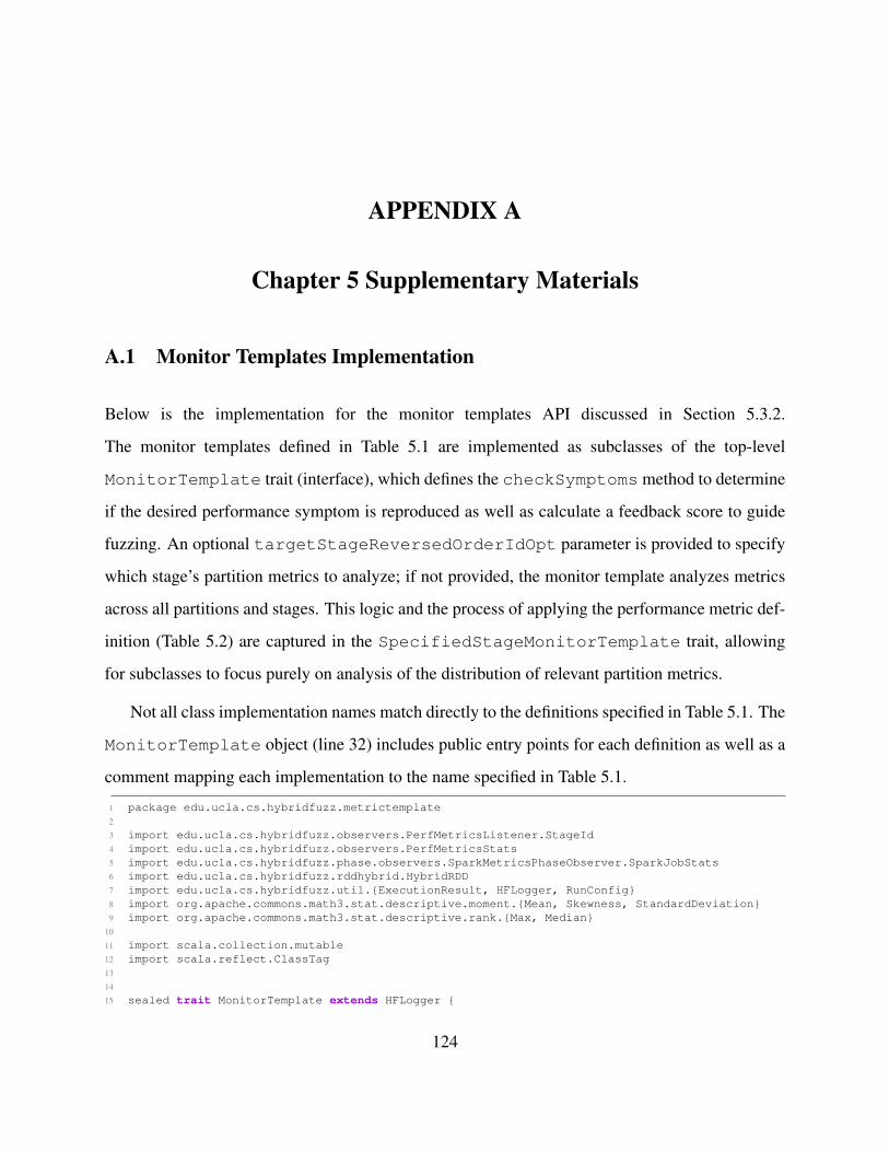
APPENDIX A
Chapter 5 Supplementary Materials
A.1 Monitor Templates Implementation
Below is the implementation for the monitor templates API discussed in Section 5.3.2.
The monitor templates defined in Table 5.1 are implemented as subclasses of the top-level
MonitorTemplate trait (interface), which defines the checkSymptoms method to determine
if the desired performance symptom is reproduced as well as calculate a feedback score to guide
fuzzing. An optional targetStageReversedOrderIdOpt parameter is provided to specify
which stage’s partition metrics to analyze; if not provided, the monitor template analyzes metrics
across all partitions and stages. This logic and the process of applying the performance metric def-
inition (Table 5.2) are captured in the SpecifiedStageMonitorTemplate trait, allowing
for subclasses to focus purely on analysis of the distribution of relevant partition metrics.
Not all class implementation names match directly to the definitions specified in Table 5.1. The
MonitorTemplate object (line 32) includes public entry points for each definition as well as a
comment mapping each implementation to the name specified in Table 5.1.
1 package edu.ucla.cs.hybridfuzz.metrictemplate2
3 import edu.ucla.cs.hybridfuzz.observers.PerfMetricsListener.StageId4 import edu.ucla.cs.hybridfuzz.observers.PerfMetricsStats5 import edu.ucla.cs.hybridfuzz.phase.observers.SparkMetricsPhaseObserver.SparkJobStats6 import edu.ucla.cs.hybridfuzz.rddhybrid.HybridRDD7 import edu.ucla.cs.hybridfuzz.util.{ExecutionResult, HFLogger, RunConfig}8 import org.apache.commons.math3.stat.descriptive.moment.{Mean, Skewness, StandardDeviation}9 import org.apache.commons.math3.stat.descriptive.rank.{Max, Median}
10
11 import scala.collection.mutable12 import scala.reflect.ClassTag13
14
15 sealed trait MonitorTemplate extends HFLogger {
124
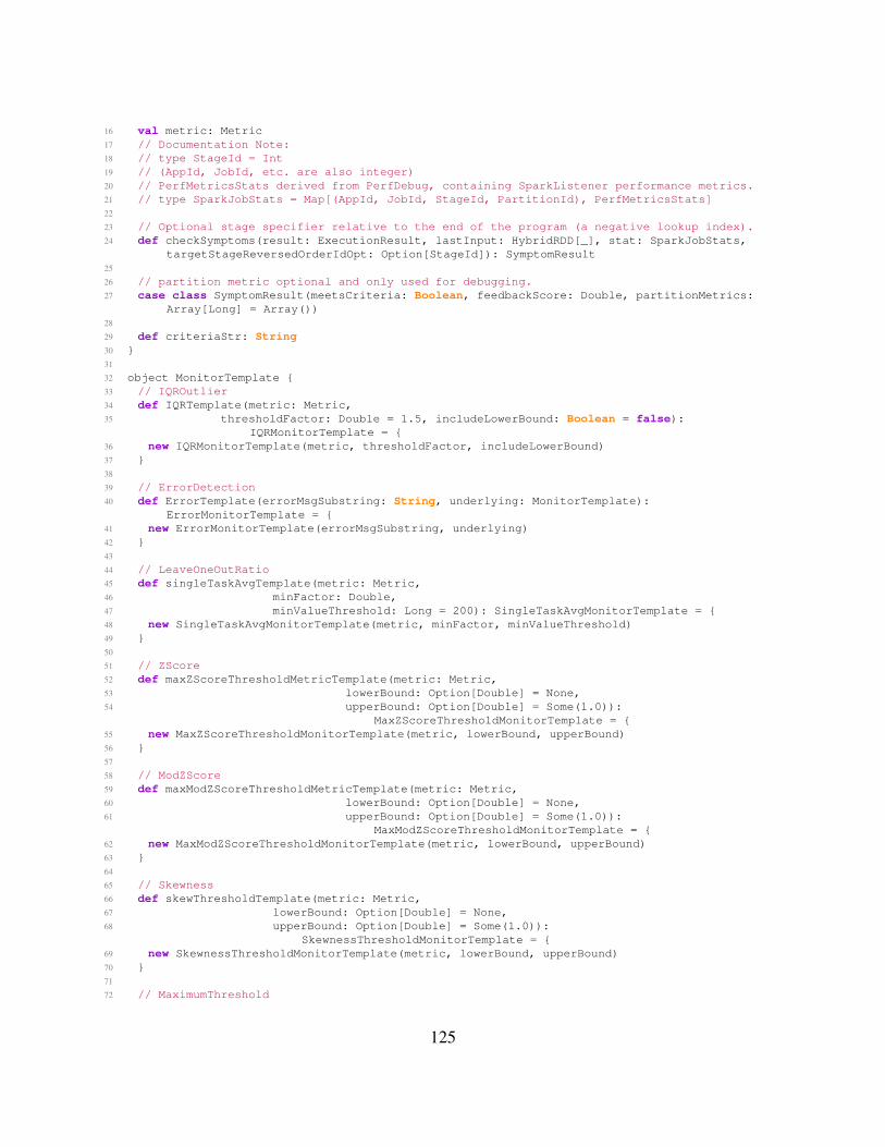
16 val metric: Metric17 // Documentation Note:18 // type StageId = Int19 // (AppId, JobId, etc. are also integer)20 // PerfMetricsStats derived from PerfDebug, containing SparkListener performance metrics.21 // type SparkJobStats = Map[(AppId, JobId, StageId, PartitionId), PerfMetricsStats]22
23 // Optional stage specifier relative to the end of the program (a negative lookup index).24 def checkSymptoms(result: ExecutionResult, lastInput: HybridRDD[_], stat: SparkJobStats,
targetStageReversedOrderIdOpt: Option[StageId]): SymptomResult25
26 // partition metric optional and only used for debugging.27 case class SymptomResult(meetsCriteria: Boolean, feedbackScore: Double, partitionMetrics:
Array[Long] = Array())28
29 def criteriaStr: String30 }31
32 object MonitorTemplate {33 // IQROutlier34 def IQRTemplate(metric: Metric,35 thresholdFactor: Double = 1.5, includeLowerBound: Boolean = false):
IQRMonitorTemplate = {36 new IQRMonitorTemplate(metric, thresholdFactor, includeLowerBound)37 }38
39 // ErrorDetection40 def ErrorTemplate(errorMsgSubstring: String, underlying: MonitorTemplate):
ErrorMonitorTemplate = {41 new ErrorMonitorTemplate(errorMsgSubstring, underlying)42 }43
44 // LeaveOneOutRatio45 def singleTaskAvgTemplate(metric: Metric,46 minFactor: Double,47 minValueThreshold: Long = 200): SingleTaskAvgMonitorTemplate = {48 new SingleTaskAvgMonitorTemplate(metric, minFactor, minValueThreshold)49 }50
51 // ZScore52 def maxZScoreThresholdMetricTemplate(metric: Metric,53 lowerBound: Option[Double] = None,54 upperBound: Option[Double] = Some(1.0)):
MaxZScoreThresholdMonitorTemplate = {55 new MaxZScoreThresholdMonitorTemplate(metric, lowerBound, upperBound)56 }57
58 // ModZScore59 def maxModZScoreThresholdMetricTemplate(metric: Metric,60 lowerBound: Option[Double] = None,61 upperBound: Option[Double] = Some(1.0)):
MaxModZScoreThresholdMonitorTemplate = {62 new MaxModZScoreThresholdMonitorTemplate(metric, lowerBound, upperBound)63 }64
65 // Skewness66 def skewThresholdTemplate(metric: Metric,67 lowerBound: Option[Double] = None,68 upperBound: Option[Double] = Some(1.0)):
SkewnessThresholdMonitorTemplate = {69 new SkewnessThresholdMonitorTemplate(metric, lowerBound, upperBound)70 }71
72 // MaximumThreshold
125
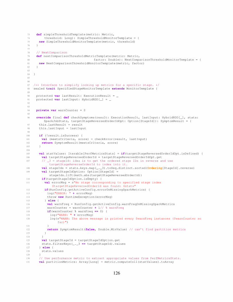
73 def simpleThresholdTemplate(metric: Metric,74 threshold: Long): SimpleThresholdMonitorTemplate = {75 new SimpleThresholdMonitorTemplate(metric, threshold)76 }77
78 // NextComparison79 def nextComparisonThresholdMetricTemplate(metric: Metric,80 factor: Double): NextComparisonThresholdMonitorTemplate = {81 new NextComparisonThresholdMonitorTemplate(metric, factor)82 }83
84 }85
86
87 /** Interface to simplify looking up metrics for a specific stage. */88 sealed trait SpecifiedStageMonitorTemplate extends MonitorTemplate {89
90 protected var lastResult: ExecutionResult = _91 protected var lastInput: HybridRDD[_] = _92
93
94 private var warnCounter = 095
96 override final def checkSymptoms(result: ExecutionResult, lastInput: HybridRDD[_], stats:SparkJobStats, targetStageReversedOrderIdOpt: Option[StageId]): SymptomResult = {
97 this.lastResult = result98 this.lastInput = lastInput99
100 if (!result.isSuccess) {101 val (meetsCriteria, score) = checkError(result, lastInput)102 return SymptomResult(meetsCriteria, score)103 }104
105 val statValues: Iterable[PerfMetricsStats] = if(targetStageReversedOrderIdOpt.isDefined) {106 val targetStageReversedOrderId = targetStageReversedOrderIdOpt.get107 // _3 = stageId: idea is to get the ordered stage IDs in reverse and use
targetStageReverseOrderId to index into it.108 val stageIds = stats.keys.map(_._3).toSeq.distinct.sorted(Ordering[StageId].reverse)109 val targetStageIdOption: Option[StageId] =
stageIds.lift(math.abs(targetStageReversedOrderId))110 if(targetStageIdOption.isEmpty) {111 val errorMsg = s"No stage corresponding to specified stage index
$targetStageReversedOrderId was found: $stats"112 if(RunConfig.getActiveConfig.errorOnMissingSparkMetrics) {113 log("ERROR: " + errorMsg)114 throw new RuntimeException(errorMsg)115 } else {116 val warnFreq = RunConfig.getActiveConfig.warnFreqOnMissingSparkMetrics117 warnCounter = warnCounter + 1// % warnFreq118 if(warnCounter % warnFreq == 0) {119 log("WARN: " + errorMsg)120 log(s"WARN: The above message is printed every $warnFreq instances ($warnCounter so
far)")121 }122 return SymptomResult(false, Double.MinValue) // can’t find partition metrics123 }124 }125 val targetStageId = targetStageIdOption.get126 stats.filterKeys(_._3 == targetStageId).values127 } else {128 stats.values129 }130 // Use performance metric to extract appropriate values from PerfMetricsStats.131 val partitionMetrics: Array[Long] = metric.computeColl(statValues).toArray
126
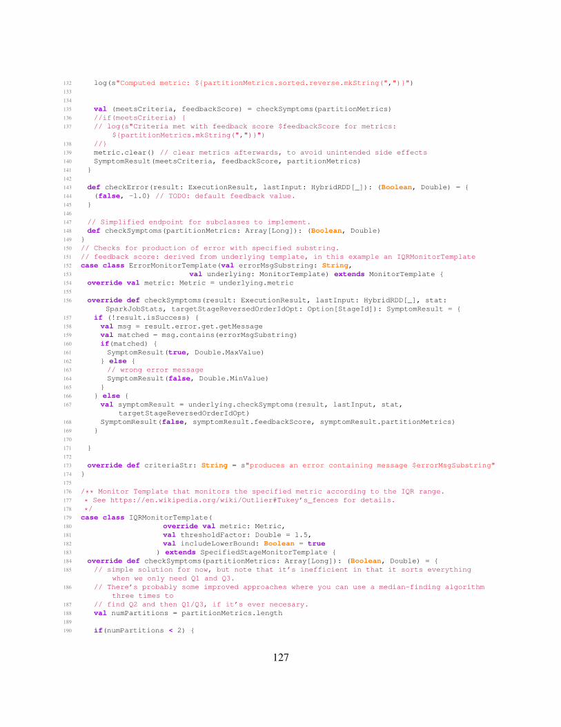
132 log(s"Computed metric: ${partitionMetrics.sorted.reverse.mkString(",")}")133
134
135 val (meetsCriteria, feedbackScore) = checkSymptoms(partitionMetrics)136 //if(meetsCriteria) {137 // log(s"Criteria met with feedback score $feedbackScore for metrics:
${partitionMetrics.mkString(",")}")138 //}139 metric.clear() // clear metrics afterwards, to avoid unintended side effects140 SymptomResult(meetsCriteria, feedbackScore, partitionMetrics)141 }142
143 def checkError(result: ExecutionResult, lastInput: HybridRDD[_]): (Boolean, Double) = {144 (false, -1.0) // TODO: default feedback value.145 }146
147 // Simplified endpoint for subclasses to implement.148 def checkSymptoms(partitionMetrics: Array[Long]): (Boolean, Double)149 }150 // Checks for production of error with specified substring.151 // feedback score: derived from underlying template, in this example an IQRMonitorTemplate152 case class ErrorMonitorTemplate(val errorMsgSubstring: String,153 val underlying: MonitorTemplate) extends MonitorTemplate {154 override val metric: Metric = underlying.metric155
156 override def checkSymptoms(result: ExecutionResult, lastInput: HybridRDD[_], stat:SparkJobStats, targetStageReversedOrderIdOpt: Option[StageId]): SymptomResult = {
157 if (!result.isSuccess) {158 val msg = result.error.get.getMessage159 val matched = msg.contains(errorMsgSubstring)160 if(matched) {161 SymptomResult(true, Double.MaxValue)162 } else {163 // wrong error message164 SymptomResult(false, Double.MinValue)165 }166 } else {167 val symptomResult = underlying.checkSymptoms(result, lastInput, stat,
targetStageReversedOrderIdOpt)168 SymptomResult(false, symptomResult.feedbackScore, symptomResult.partitionMetrics)169 }170
171 }172
173 override def criteriaStr: String = s"produces an error containing message $errorMsgSubstring"174 }175
176 /** Monitor Template that monitors the specified metric according to the IQR range.177 * See https://en.wikipedia.org/wiki/Outlier#Tukey’s_fences for details.178 */179 case class IQRMonitorTemplate(180 override val metric: Metric,181 val thresholdFactor: Double = 1.5,182 val includeLowerBound: Boolean = true183 ) extends SpecifiedStageMonitorTemplate {184 override def checkSymptoms(partitionMetrics: Array[Long]): (Boolean, Double) = {185 // simple solution for now, but note that it’s inefficient in that it sorts everything
when we only need Q1 and Q3.186 // There’s probably some improved approaches where you can use a median-finding algorithm
three times to187 // find Q2 and then Q1/Q3, if it’s ever necesary.188 val numPartitions = partitionMetrics.length189
190 if(numPartitions < 2) {
127
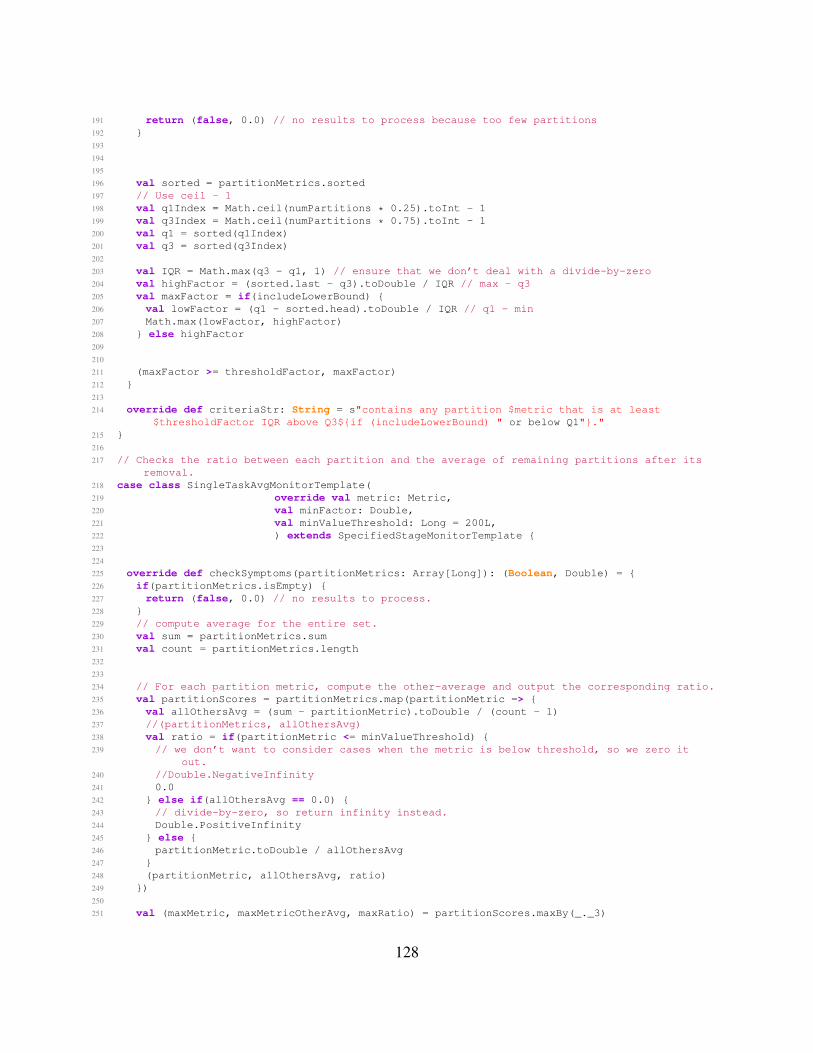
191 return (false, 0.0) // no results to process because too few partitions192 }193
194
195
196 val sorted = partitionMetrics.sorted197 // Use ceil - 1198 val q1Index = Math.ceil(numPartitions * 0.25).toInt - 1199 val q3Index = Math.ceil(numPartitions * 0.75).toInt - 1200 val q1 = sorted(q1Index)201 val q3 = sorted(q3Index)202
203 val IQR = Math.max(q3 - q1, 1) // ensure that we don’t deal with a divide-by-zero204 val highFactor = (sorted.last - q3).toDouble / IQR // max - q3205 val maxFactor = if(includeLowerBound) {206 val lowFactor = (q1 - sorted.head).toDouble / IQR // q1 - min207 Math.max(lowFactor, highFactor)208 } else highFactor209
210
211 (maxFactor >= thresholdFactor, maxFactor)212 }213
214 override def criteriaStr: String = s"contains any partition $metric that is at least$thresholdFactor IQR above Q3${if (includeLowerBound) " or below Q1"}."
215 }216
217 // Checks the ratio between each partition and the average of remaining partitions after itsremoval.
218 case class SingleTaskAvgMonitorTemplate(219 override val metric: Metric,220 val minFactor: Double,221 val minValueThreshold: Long = 200L,222 ) extends SpecifiedStageMonitorTemplate {223
224
225 override def checkSymptoms(partitionMetrics: Array[Long]): (Boolean, Double) = {226 if(partitionMetrics.isEmpty) {227 return (false, 0.0) // no results to process.228 }229 // compute average for the entire set.230 val sum = partitionMetrics.sum231 val count = partitionMetrics.length232
233
234 // For each partition metric, compute the other-average and output the corresponding ratio.235 val partitionScores = partitionMetrics.map(partitionMetric => {236 val allOthersAvg = (sum - partitionMetric).toDouble / (count - 1)237 //(partitionMetrics, allOthersAvg)238 val ratio = if(partitionMetric <= minValueThreshold) {239 // we don’t want to consider cases when the metric is below threshold, so we zero it
out.240 //Double.NegativeInfinity241 0.0242 } else if(allOthersAvg == 0.0) {243 // divide-by-zero, so return infinity instead.244 Double.PositiveInfinity245 } else {246 partitionMetric.toDouble / allOthersAvg247 }248 (partitionMetric, allOthersAvg, ratio)249 })250
251 val (maxMetric, maxMetricOtherAvg, maxRatio) = partitionScores.maxBy(_._3)
128

252
253 val meetsCriteria = maxRatio >= minFactor254
255 if(meetsCriteria) {256 log(f"Found partition metric with ratio $maxRatio%.2f, value $maxMetric >
max($minValueThreshold, $minFactor * $maxMetricOtherAvg%.2f (($sum - $maxMetric) /$count - 1))")
257 } else {258 // did not pass threshold check.259 }260
261 (meetsCriteria, maxRatio)262 }263
264 override def criteriaStr: String = s"has a single executor with metric $metric that is atleast ${minFactor}x that of remaining average"
265 }266
267 // Partial implementation to specify upper and lower bounds for some numerically computedfeedback score.
268 abstract class BoundedThresholdMonitorTemplate(val lowerBound: Option[Double],269 val upperBound: Option[Double]270 ) extends SpecifiedStageMonitorTemplate {271 assert(lowerBound.isDefined || upperBound.isDefined, "At least one of upper/lower bound must
be defined.")272
273 /** Compute the desired aggregation feedback score (e.g., max z-score). */274 def computeFeedback(partitionMetrics: Array[Long]): Double275 val feedbackDescription: String276
277
278 override final def checkSymptoms(partitionMetrics: Array[Long]): (Boolean, Double) = {279 val metricValue = computeFeedback(partitionMetrics)280 val belowRange = lowerBound.exists(metricValue <= _)281 val aboveRange = upperBound.exists(metricValue >= _)282 val outOfRange = belowRange || aboveRange283 (outOfRange, metricValue)284 }285
286
287 private val lbStringOpt = upperBound.map(b => s"greater than or equal to $b")288 private val ubStringOpt = lowerBound.map(b => s"less than or equal to $b")289
290
291 override final lazy val criteriaStr: String = {292 val sb = new StringBuilder(s"has a $feedbackDescription ")293 ubStringOpt.foreach(sb.append)294 if (ubStringOpt.isDefined && lbStringOpt.isDefined) {295 sb.append(" or ")296 }297 lbStringOpt.foreach(sb.append)298 sb.append(".")299 sb.toString()300 }301 }302
303 // Internal optimized array wrapper to only allocate more memory when necessary.304 private class ResizableArrayConverter[T, U: ClassTag]() extends HFLogger {305 private var reusable: Array[U] = _306 private var maxLength = -1307 private var lastLength = -1308
309 def data: Array[U] = reusable310 def currentLength: Int = lastLength
129
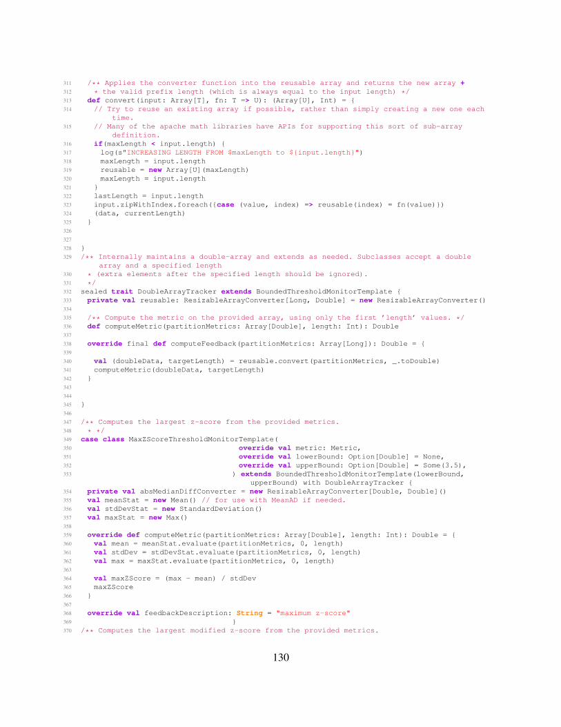
311 /** Applies the converter function into the reusable array and returns the new array +312 * the valid prefix length (which is always equal to the input length) */313 def convert(input: Array[T], fn: T => U): (Array[U], Int) = {314 // Try to reuse an existing array if possible, rather than simply creating a new one each
time.315 // Many of the apache math libraries have APIs for supporting this sort of sub-array
definition.316 if(maxLength < input.length) {317 log(s"INCREASING LENGTH FROM $maxLength to ${input.length}")318 maxLength = input.length319 reusable = new Array[U](maxLength)320 maxLength = input.length321 }322 lastLength = input.length323 input.zipWithIndex.foreach({case (value, index) => reusable(index) = fn(value)})324 (data, currentLength)325 }326
327
328 }329 /** Internally maintains a double-array and extends as needed. Subclasses accept a double
array and a specified length330 * (extra elements after the specified length should be ignored).331 */332 sealed trait DoubleArrayTracker extends BoundedThresholdMonitorTemplate {333 private val reusable: ResizableArrayConverter[Long, Double] = new ResizableArrayConverter()334
335 /** Compute the metric on the provided array, using only the first ’length’ values. */336 def computeMetric(partitionMetrics: Array[Double], length: Int): Double337
338 override final def computeFeedback(partitionMetrics: Array[Long]): Double = {339
340 val (doubleData, targetLength) = reusable.convert(partitionMetrics, _.toDouble)341 computeMetric(doubleData, targetLength)342 }343
344
345 }346
347 /** Computes the largest z-score from the provided metrics.348 * */349 case class MaxZScoreThresholdMonitorTemplate(350 override val metric: Metric,351 override val lowerBound: Option[Double] = None,352 override val upperBound: Option[Double] = Some(3.5),353 ) extends BoundedThresholdMonitorTemplate(lowerBound,
upperBound) with DoubleArrayTracker {354 private val absMedianDiffConverter = new ResizableArrayConverter[Double, Double]()355 val meanStat = new Mean() // for use with MeanAD if needed.356 val stdDevStat = new StandardDeviation()357 val maxStat = new Max()358
359 override def computeMetric(partitionMetrics: Array[Double], length: Int): Double = {360 val mean = meanStat.evaluate(partitionMetrics, 0, length)361 val stdDev = stdDevStat.evaluate(partitionMetrics, 0, length)362 val max = maxStat.evaluate(partitionMetrics, 0, length)363
364 val maxZScore = (max - mean) / stdDev365 maxZScore366 }367
368 override val feedbackDescription: String = "maximum z-score"369 }370 /** Computes the largest modified z-score from the provided metrics.
130
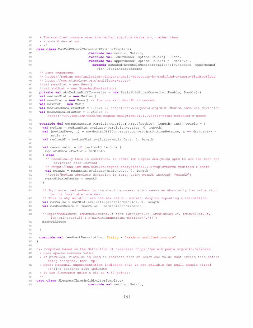
371 * The modified z-score uses the median absolute deviation, rather than372 * standard deviation.373 * */374 case class MaxModZScoreThresholdMonitorTemplate(375 override val metric: Metric,376 override val lowerBound: Option[Double] = None,377 override val upperBound: Option[Double] = Some(3.5),378 ) extends BoundedThresholdMonitorTemplate(lowerBound, upperBound)
with DoubleArrayTracker {379 // Some resources:380 // https://medium.com/analytics-vidhya/anomaly-detection-by-modified-z-score-f8ad6be62bac381 // https://www.statology.org/modified-z-score/382 //val meanStat = new Mean()383 //val stdStat = new StandardDeviation()384 private val absMedianDiffConverter = new ResizableArrayConverter[Double, Double]()385 val medianStat = new Median()386 val meanStat = new Mean() // for use with MeanAD if needed.387 val maxStat = new Max()388 val medianADScaleFactor = 1.4826 // https://en.wikipedia.org/wiki/Median_absolute_deviation389 val meanADScaleFactor = 1.253314 //
https://www.ibm.com/docs/en/cognos-analytics/11.1.0?topic=terms-modified-z-score390
391 override def computeMetric(partitionMetrics: Array[Double], length: Int): Double = {392 val median = medianStat.evaluate(partitionMetrics, 0, length)393 val (medianDevs, _) = absMedianDiffConverter.convert(partitionMetrics, x => Math.abs(x -
median))394 val medianAD = medianStat.evaluate(medianDevs, 0, length)395
396 val denominator = if (medianAD != 0.0) {397 medianADScaleFactor * medianAD398 } else {399 // technically this is undefined. It seems IBM Cognos Analytics opts to use the mean abs
deviation here instead.400 // https://www.ibm.com/docs/en/cognos-analytics/11.1.0?topic=terms-modified-z-score401 val meanAD = meanStat.evaluate(medianDevs, 0, length)402 //log(s"Median absolute deviation is zero, using meanAD instead: $meanAD")403 meanADScaleFactor * meanAD404 }405
406 // Impl note: medianDevs is the absolute maxes, which means an abnormally low value mightbe the ’max’ absolute dev.
407 // This is why we still use the max value - median, despite repeating a calculation.408 val maxValue = maxStat.evaluate(partitionMetrics, 0, length)409 val maxModZScore = (maxValue - median)/denominator410
411 //log(f"ModZScore: $maxModZScore%.2f from ($median%.2f, $medianAD%.2f, $maxValue%.2f,$denominator%.2f): ${partitionMetrics.mkString(",")}")
412 maxModZScore413
414 }415
416 override val feedbackDescription: String = "maximum modified z-score"417 }418
419 /** Computed based on the definition of Skewness: https://en.wikipedia.org/wiki/Skewness420 * Uses apache commons math3.421 * If provided, minValue is used to indicate that at least one value must exceed this before
being accepted. (not impl)422 * Note: Personal experimentation indicates this is not reliable for small sample sizes!
(online searches also indicate423 * it can fluctuate quite a bit at < 50 points)424 */425 case class SkewnessThresholdMonitorTemplate(426 override val metric: Metric,
131

427 override val lowerBound: Option[Double] = None,428 override val upperBound: Option[Double] = Some(1.0),429 //val minValue: Option[Long] = None430 ) extends BoundedThresholdMonitorTemplate(lowerBound, upperBound)
with DoubleArrayTracker {431 val skewnessStat = new Skewness()432
433 override def computeMetric(partitionMetrics: Array[Double], length: Int): Double = {434 // skewnessStat.clear()435 val skewness: Double = skewnessStat.evaluate(partitionMetrics, 0, length)436 if(skewness.isNaN) {437 // edge case to consider, e.g., if all values are equal438 if (partitionMetrics.length < 3) {439 log("Skewness metric requires at least three data points. Skipping (defaulting to 0)")440 } else if (partitionMetrics.forall(_ == partitionMetrics.head)) {441 //log("Skewness NaN due to uniform values")442 // This is expected in some cases, e.g. GC443 } else {444 log("Unknown reason for NaN skewness. Defaulting to 0...")445 log(partitionMetrics.mkString(","))446 }447 }448 skewness449 }450
451 override val feedbackDescription: String = "skewness metric"452 }453
454 /** Checks if the largest metric meets or exceeds the specified threshold. */455 case class SimpleThresholdMonitorTemplate(override val metric: Metric,456 val threshold: Long457 ) extends BoundedThresholdMonitorTemplate(None, Some(threshold)) {458
459 override def computeFeedback(partitionMetrics: Array[Long]): Double = partitionMetrics.max460
461 override val feedbackDescription: String = "maximum value"462 }463
464 /** Checks if the ratio between the max and second-largest values is greater than thespecified factor. */
465 case class NextComparisonThresholdMonitorTemplate(override val metric: Metric,466 val factor: Double) extends
BoundedThresholdMonitorTemplate(None, Some(factor)){
467 assert(factor > 1.0, "Factor must be at least one (i.e., at least 1x the next greatestvalue)")
468
469 val minHeap = new mutable.PriorityQueue[Long]()(Ordering[Long].reverse)470 val maxSize = 2471 /** Compute the desired aggregation metric (e.g., max z-score). */472 override def computeFeedback(partitionMetrics: Array[Long]): Double = {473 if(partitionMetrics.length < maxSize) throw new IllegalArgumentException(s"Partition
metrics too small: ${partitionMetrics.length}")474 partitionMetrics.foreach(value => {475 if(minHeap.size < maxSize) {476 minHeap.enqueue(value)477 } else if (minHeap.head < value) {478 minHeap.enqueue(value)479 minHeap.dequeue()480 }481 })482
483 val values = minHeap.dequeueAll484 val secondMax = values(0)
132

485 val max = values(1)486 val factor = max.toDouble / secondMax487 factor488 }489
490 override val feedbackDescription: String = "ratio between largest and second largest value"491 }
A.2 Performance Metrics Implementation
Below is the implementation for the performance metrics API discussed in Section 5.3.2. The
metrics discussed in Table 5.2 are implemented in lines 37-45. The PerfMetricsStats data
class comes from Chapter 3’s implementation which collects performance metrics through the
SparkListener API. 1
1 package edu.ucla.cs.hybridfuzz.metrictemplate2
3 import edu.ucla.cs.hybridfuzz.observers.PerfMetricsStats4 import edu.ucla.cs.hybridfuzz.util.HFLogger5
6 sealed trait Metric extends HFLogger {7
8 def computeColl(stats: Traversable[PerfMetricsStats]): Traversable[Long]9
10 // Optional reset function in case anything needs to be cleaned up - does nothing by default.11 def clear(): Unit = {}12
13 def isDataSkew: Boolean14 def isRuntimeSkew: Boolean15
16 }17
18 case class CustomMetric(computeFn: Traversable[PerfMetricsStats] => Traversable[Long],clearFn: Option[() => Unit] = None,
19 override val isDataSkew: Boolean = false, override val isRuntimeSkew:Boolean = false,
20 description: Option[String] = None) extends Metric {21 override def computeColl(stats: Traversable[PerfMetricsStats]): Traversable[Long] =
computeFn(stats)22
23 override def clear(): Unit = clearFn.foreach(_()) // call the function if it’s defined,otherwise does nothing.
24
25 override def toString: String = description.map(s =>s"${getClass.getSimpleName}($s)}").getOrElse(super.toString)
26
27 }28
29 object Metrics {
1https://github.com/UCLA-SEAL/PerfDebug/blob/main/core/src/main/scala/org/apache/spark/lineage/perfdebug/perfmetrics/PerfMetricsStats.scala
133
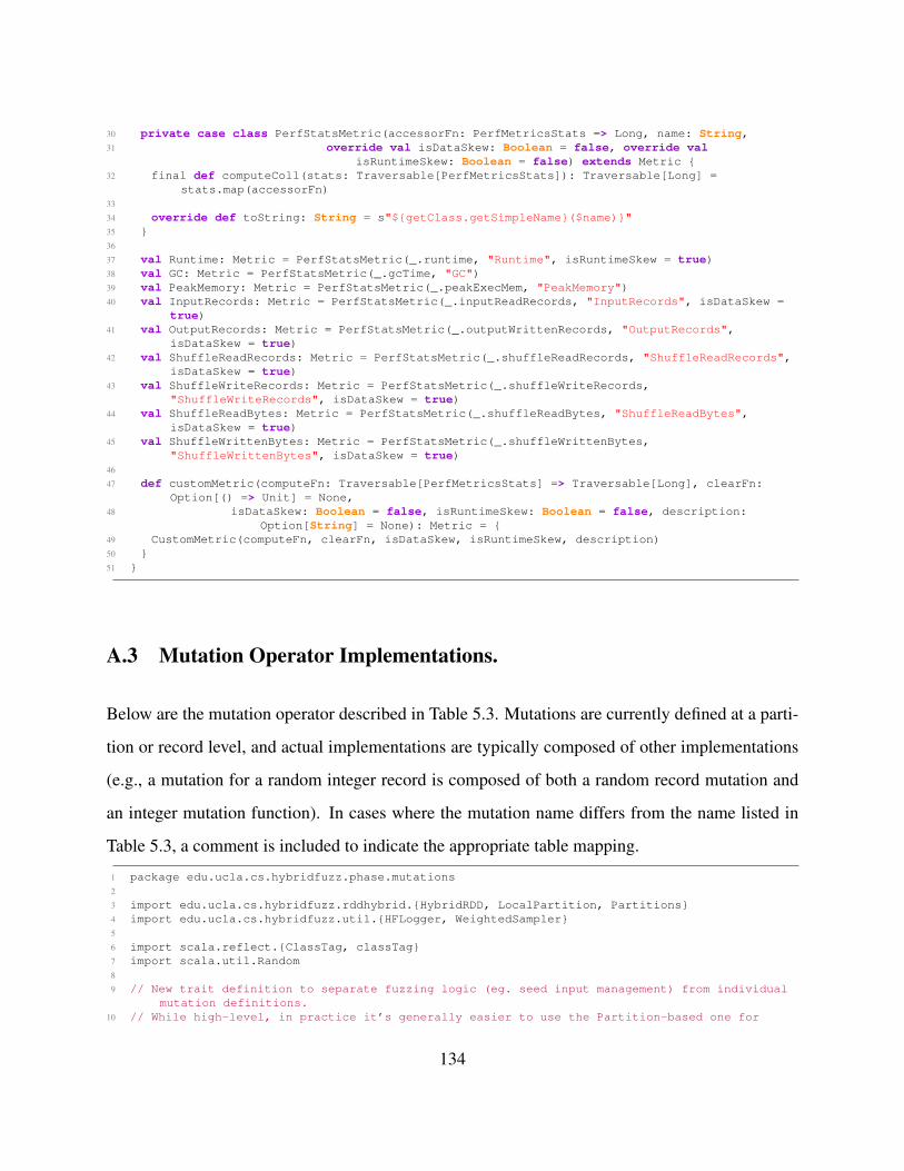
30 private case class PerfStatsMetric(accessorFn: PerfMetricsStats => Long, name: String,31 override val isDataSkew: Boolean = false, override val
isRuntimeSkew: Boolean = false) extends Metric {32 final def computeColl(stats: Traversable[PerfMetricsStats]): Traversable[Long] =
stats.map(accessorFn)33
34 override def toString: String = s"${getClass.getSimpleName}($name)}"35 }36
37 val Runtime: Metric = PerfStatsMetric(_.runtime, "Runtime", isRuntimeSkew = true)38 val GC: Metric = PerfStatsMetric(_.gcTime, "GC")39 val PeakMemory: Metric = PerfStatsMetric(_.peakExecMem, "PeakMemory")40 val InputRecords: Metric = PerfStatsMetric(_.inputReadRecords, "InputRecords", isDataSkew =
true)41 val OutputRecords: Metric = PerfStatsMetric(_.outputWrittenRecords, "OutputRecords",
isDataSkew = true)42 val ShuffleReadRecords: Metric = PerfStatsMetric(_.shuffleReadRecords, "ShuffleReadRecords",
isDataSkew = true)43 val ShuffleWriteRecords: Metric = PerfStatsMetric(_.shuffleWriteRecords,
"ShuffleWriteRecords", isDataSkew = true)44 val ShuffleReadBytes: Metric = PerfStatsMetric(_.shuffleReadBytes, "ShuffleReadBytes",
isDataSkew = true)45 val ShuffleWrittenBytes: Metric = PerfStatsMetric(_.shuffleWrittenBytes,
"ShuffleWrittenBytes", isDataSkew = true)46
47 def customMetric(computeFn: Traversable[PerfMetricsStats] => Traversable[Long], clearFn:Option[() => Unit] = None,
48 isDataSkew: Boolean = false, isRuntimeSkew: Boolean = false, description:Option[String] = None): Metric = {
49 CustomMetric(computeFn, clearFn, isDataSkew, isRuntimeSkew, description)50 }51 }
A.3 Mutation Operator Implementations.
Below are the mutation operator described in Table 5.3. Mutations are currently defined at a parti-
tion or record level, and actual implementations are typically composed of other implementations
(e.g., a mutation for a random integer record is composed of both a random record mutation and
an integer mutation function). In cases where the mutation name differs from the name listed in
Table 5.3, a comment is included to indicate the appropriate table mapping.
1 package edu.ucla.cs.hybridfuzz.phase.mutations2
3 import edu.ucla.cs.hybridfuzz.rddhybrid.{HybridRDD, LocalPartition, Partitions}4 import edu.ucla.cs.hybridfuzz.util.{HFLogger, WeightedSampler}5
6 import scala.reflect.{ClassTag, classTag}7 import scala.util.Random8
9 // New trait definition to separate fuzzing logic (eg. seed input management) from individualmutation definitions.
10 // While high-level, in practice it’s generally easier to use the Partition-based one for
134

direct data type access11 trait MutationFn[T] {12 def mutate(input: HybridRDD[T]): HybridRDD[T]13 }14
15 object MutationFn {16 // Logging utility, but it would be better to standardize somewhere else...17 var mostRecent: Option[MutationFn[_]] = None18 }19
20 // Primary trait for definitions, as it allows direct access to underlying data types.21 trait PartitionsBasedMutationFn[T] extends MutationFn[T] with HFLogger {22 logEnabled = false23
24 override final def mutate(input: HybridRDD[T]): HybridRDD[T] = {25 val mutatedPartitions = mutatePartitions(input.collectAsPartitions())26 HybridRDD(mutatedPartitions)(input.ctOutput)27 }28
29 // Partitions is an alias for Array[List[T]], for various serialization/management purposes30 def mutatePartitions(partitions: Partitions[T]): Partitions[T]31
32 }33
34 // TABLE MAPPING: ReplaceRandomRecord35 abstract class RandomRecordMutationFn[T: ClassTag] extends PartitionsBasedMutationFn[T] {36 override final def mutatePartitions(partitions: Partitions[T]): Partitions[T] = {37 // Utility function to randomly select a random record from a collection of partitions38 import DataFuzzer.PartitionsRecordReplacer39 /* Code reproduced here, where Partitions = Array[LocalPartitions[T]] and LocalPartitions
= List.40
41 def mutateRandomRecord(mutate: T => T): Partitions[T] = {42 val (partitionIndex, indexWithinPartition) = randomRecordIndex()43 val newElement: T = mutate(partitions(partitionIndex)(indexWithinPartition))44
45 val newPartition: LocalPartition[T] = partitions(partitionIndex).updated(46 indexWithinPartition, newElement47 ).toLocalPartition48
49 partitions.updated(partitionIndex, newPartition).toArray[LocalPartition[T]].toPartitions50 */51
52
53 partitions.mutateRandomRecord(this.mutateValue)54
55 }56
57 def mutateValue(input: T): T58 }59
60 abstract class StringSubstringReplacementMutationFn extends RandomRecordMutationFn[String] {61 private val _mutateRecord =
TypeFuzzingUtil.mutateStrBySubstring(generateSubstringReplacement)62 override final def mutateValue(input: String): String = {63 _mutateRecord(input)64 }65
66 def generateSubstringReplacement(orig: String): String67 }68
69 /** Base mutation function for String-types: replaces a random substring with a newlygenerated random substring. */
70 case class GenericStringMutationFn(minLength: Int = TypeFuzzingUtil.MIN_STRING_SUB_LENGTH,
135

71 maxLength: Int = TypeFuzzingUtil.MAX_STRING_SUB_LENGTH) extendsStringSubstringReplacementMutationFn {
72 override def generateSubstringReplacement(orig: String): String = {73 TypeFuzzingUtil.randomString(minLength, maxLength)74 }75 }76
77 case class GenericIntMutationFn(min: Int = TypeFuzzingUtil.DEFAULT_INT_MIN, max: Int =TypeFuzzingUtil.DEFAULT_INT_MAX) extends RandomRecordMutationFn[Int] {
78 override def mutateValue(input: Int): Int = {79 TypeFuzzingUtil.randomIntInRange(min, max)80 }81 }82
83 case class GenericBooleanMutationFn() extends RandomRecordMutationFn[Boolean] {84 override def mutateValue(input: Boolean): Boolean = {85 TypeFuzzingUtil.randBoolean()86 }87 }88
89 /** Base class for key-specific mutations.90 * TABLE MAPPING: ReplaceTupleElement */91 class RandomKeyMutationFn[K: ClassTag, V: ClassTag](keyMutation: K => K) extends
RandomRecordMutationFn[(K, V)] {92 override def mutateValue(input: (K, V)): (K, V) = {93 input.copy(_1 = keyMutation(input._1))94 }95 }96
97 /** Generic key mutation class relying on [[TypeFuzzingUtil.genericValueMutator()]] */98 case class GenericRandomKeyMutationFn[K: ClassTag, V: ClassTag]()99 extends RandomKeyMutationFn[K, V](TypeFuzzingUtil.genericValueMutator[K]()) {
100 }101
102 /** Base class for value-specific mutations.103 * TABLE MAPPING: ReplaceTupleElement*/104 class RandomValueMutationFn[K: ClassTag, V: ClassTag](valueMutation: V => V) extends
RandomRecordMutationFn[(K, V)] {105 override def mutateValue(input: (K, V)): (K, V) = {106 input.copy(_2 = valueMutation(input._2))107 }108 }109
110 /** Generic value mutation class relying on [[TypeFuzzingUtil.genericValueMutator()]] */111 case class GenericRandomValueMutationFn[K: ClassTag, V: ClassTag]()112 extends RandomValueMutationFn[K, V](TypeFuzzingUtil.genericValueMutator[V]()) {113 }114
115 // TABLE MAPPING: AppendCollectionCopy116 case class GenericValueArrayDuplMutationFn[K: ClassTag, V: ClassTag](duplFactor: Int = 2)117 extends RandomValueMutationFn[K, Array[V]](118 // duplicate array by concatenating with itself119 if(duplFactor == 2) {120 // hardcode for 2-case for efficiency121 arr => arr ++ arr122 } else {123 arr => {124 // Previously tried: Seq.fill(...)(...).flatten.toArray - flatten operation is expensive125 // next tried replacing with Array.concat, but the initial Seq.fill can be expensive
anyways.126 // Now just doing it manually.127 val arrLen = arr.length128 val newArrLen = arrLen * duplFactor129 //log(s"MEMDEBUG: Allocating array[$newArrLen]...")
136
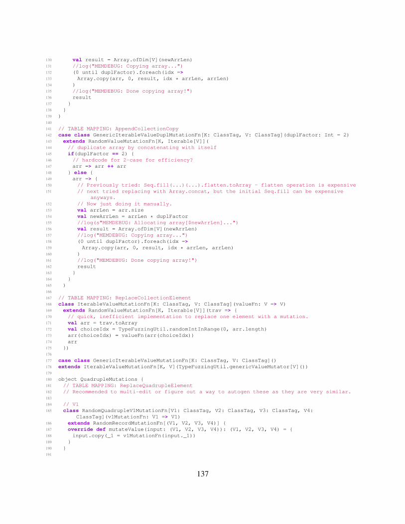
130 val result = Array.ofDim[V](newArrLen)131 //log("MEMDEBUG: Copying array...")132 (0 until duplFactor).foreach(idx =>133 Array.copy(arr, 0, result, idx * arrLen, arrLen)134 )135 //log("MEMDEBUG: Done copying array!")136 result137 }138 }139 )140
141 // TABLE MAPPING: AppendCollectionCopy142 case class GenericIterableValueDuplMutationFn[K: ClassTag, V: ClassTag](duplFactor: Int = 2)143 extends RandomValueMutationFn[K, Iterable[V]](144 // duplicate array by concatenating with itself145 if(duplFactor == 2) {146 // hardcode for 2-case for efficiency?147 arr => arr ++ arr148 } else {149 arr => {150 // Previously tried: Seq.fill(...)(...).flatten.toArray - flatten operation is expensive151 // next tried replacing with Array.concat, but the initial Seq.fill can be expensive
anyways.152 // Now just doing it manually.153 val arrLen = arr.size154 val newArrLen = arrLen * duplFactor155 //log(s"MEMDEBUG: Allocating array[$newArrLen]...")156 val result = Array.ofDim[V](newArrLen)157 //log("MEMDEBUG: Copying array...")158 (0 until duplFactor).foreach(idx =>159 Array.copy(arr, 0, result, idx * arrLen, arrLen)160 )161 //log("MEMDEBUG: Done copying array!")162 result163 }164 }165 )166
167 // TABLE MAPPING: ReplaceCollectionElement168 class IterableValueMutationFn[K: ClassTag, V: ClassTag](valueFn: V => V)169 extends RandomValueMutationFn[K, Iterable[V]](trav => {170 // quick, inefficient implementation to replace one element with a mutation.171 val arr = trav.toArray172 val choiceIdx = TypeFuzzingUtil.randomIntInRange(0, arr.length)173 arr(choiceIdx) = valueFn(arr(choiceIdx))174 arr175 })176
177 case class GenericIterableValueMutationFn[K: ClassTag, V: ClassTag]()178 extends IterableValueMutationFn[K, V](TypeFuzzingUtil.genericValueMutator[V]())179
180 object QuadrupleMutations {181 // TABLE MAPPING: ReplaceQuadrupleElement182 // Recommended to multi-edit or figure out a way to autogen these as they are very similar.183
184 // V1185 class RandomQuadrupleV1MutationFn[V1: ClassTag, V2: ClassTag, V3: ClassTag, V4:
ClassTag](v1MutationFn: V1 => V1)186 extends RandomRecordMutationFn[(V1, V2, V3, V4)] {187 override def mutateValue(input: (V1, V2, V3, V4)): (V1, V2, V3, V4) = {188 input.copy(_1 = v1MutationFn(input._1))189 }190 }191
137

192 case class GenericRandomQuadrupleV1MutationFn[V1: ClassTag, V2: ClassTag, V3: ClassTag, V4:ClassTag]()
193 extends RandomQuadrupleV1MutationFn[V1, V2, V3,V4](TypeFuzzingUtil.genericValueMutator[V1]())
194
195 // V2196 class RandomQuadrupleV2MutationFn[V1: ClassTag, V2: ClassTag, V3: ClassTag, V4:
ClassTag](v2MutationFn: V2 => V2)197 extends RandomRecordMutationFn[(V1, V2, V3, V4)] {198 override def mutateValue(input: (V1, V2, V3, V4)): (V1, V2, V3, V4) = {199 input.copy(_2 = v2MutationFn(input._2))200 }201 }202
203 case class GenericRandomQuadrupleV2MutationFn[V1: ClassTag, V2: ClassTag, V3: ClassTag, V4:ClassTag]()
204 extends RandomQuadrupleV2MutationFn[V1, V2, V3,V4](TypeFuzzingUtil.genericValueMutator[V2]())
205
206 // V3207 class RandomQuadrupleV3MutationFn[V1: ClassTag, V2: ClassTag, V3: ClassTag, V4:
ClassTag](v3MutationFn: V3 => V3)208 extends RandomRecordMutationFn[(V1, V2, V3, V4)] {209 override def mutateValue(input: (V1, V2, V3, V4)): (V1, V2, V3, V4) = {210 input.copy(_3 = v3MutationFn(input._3))211 }212 }213
214 case class GenericRandomQuadrupleV3MutationFn[V1: ClassTag, V2: ClassTag, V3: ClassTag, V4:ClassTag]()
215 extends RandomQuadrupleV3MutationFn[V1, V2, V3,V4](TypeFuzzingUtil.genericValueMutator[V3]())
216
217 // V4218 class RandomQuadrupleV4MutationFn[V1: ClassTag, V2: ClassTag, V3: ClassTag, V4:
ClassTag](v4MutationFn: V4 => V4)219 extends RandomRecordMutationFn[(V1, V2, V3, V4)] {220 override def mutateValue(input: (V1, V2, V3, V4)): (V1, V2, V3, V4) = {221 input.copy(_4 = v4MutationFn(input._4))222 }223 }224
225 case class GenericRandomQuadrupleV4MutationFn[V1: ClassTag, V2: ClassTag, V3: ClassTag, V4:ClassTag]()
226 extends RandomQuadrupleV4MutationFn[V1, V2, V3,V4](TypeFuzzingUtil.genericValueMutator[V4]())
227
228
229 }230
231
232 /** Base class that exposes an endpoint to mutate a single random partition. By default, thisclass
233 * will attempt to find a non-empty partition to mutate. If all partition are empty, thismutation
234 * returns the original input.*/235 abstract class RandomPartitionMutationFn[T: ClassTag] extends PartitionsBasedMutationFn[T] {236 override final def mutatePartitions(partitions: Partitions[T]): Partitions[T] = {237 val nonEmptyPartitions = partitions.zipWithIndex.filter({238 case (partition: LocalPartition[T], idx) =>239 partition.nonEmpty})240 if(nonEmptyPartitions.isEmpty) return partitions //241
242 val choice = TypeFuzzingUtil.randomChoice(nonEmptyPartitions)._2
138

243 log(s"Selected partition #$choice")244 val origPartition = partitions(choice)245 /*246 val choice = TypeFuzzingUtil.randomIntInRange(0, partitions.length)247 val origPartition: LocalPartition[T] = partitions(choice)248 */249 val newPartition: LocalPartition[T] = this.mutatePartition(origPartition)250 // cast due to build errors.251 val result: Partitions[T] = partitions.updated(choice,
newPartition).asInstanceOf[Partitions[T]]252 result253 }254
255 def mutatePartition(partition: LocalPartition[T]): LocalPartition[T]256
257 // helper function for subclasses258 protected def randomRecord(partition: LocalPartition[T]): T = {259 TypeFuzzingUtil.randomChoice(partition)260 }261 }262
263
264 /** Pick a random key and reuse it to append (generate) additional records with differentvalues.
265 * Up to ‘duplProportion‘ * partitionSize records will be added, with the actual numberselected randomly.)
266 * TABLEMAPPING: AppendSameKey267 */268 class KeyDuplGenMutationFn[K: ClassTag, V: ClassTag](valueGenerator: V => V,269 duplProportion: Double)270 extends RandomPartitionMutationFn[(K, V)] {271 override def mutatePartition(partition: LocalPartition[(K, V)]): LocalPartition[(K, V)] = {272 val (key, origValue) = randomRecord(partition)273 //println("DEBUG:" + partition.size)274 val maxDupes = Math.ceil(duplProportion * partition.size).toInt275 val numDupes = TypeFuzzingUtil.randomIntInRange(1, maxDupes + 1) // +1 because end range
is exclusive.276 val newRecords = (1 to numDupes).map(_ => (key, valueGenerator(origValue)))277 partition ++ newRecords278 }279 }280
281 // Concrete class with existing/available classtag to facilitate inference.282 case class GenericKeyDuplGenMutationFn[K: ClassTag, V: ClassTag](duplProportion: Double =
0.10) extends KeyDuplGenMutationFn[K, V](TypeFuzzingUtil.genericValueMutator[V](),duplProportion)
283
284 /** Identical to [[KeyDuplGenMutationFn]] except with key/value swapped.285 * TABLEMAPPING: AppendSameValue286 */287 class ValueDuplGenMutationFn[K: ClassTag, V: ClassTag](keyGenerator: K => K,288 duplProportion: Double)289 extends RandomPartitionMutationFn[(K, V)] {290 //logEnabled = true // temp override.291 override def mutatePartition(partition: LocalPartition[(K, V)]): LocalPartition[(K, V)] = {292 val (origKey, value) = randomRecord(partition)293
294 val maxDupes = Math.ceil(duplProportion * partition.size).toInt295 val numDupes = TypeFuzzingUtil.randomIntInRange(1, maxDupes + 1) // +1 because end range
is exclusive.296 log(s"Adding $numDupes records out of potential max $maxDupes in partition of size
${partition.size} (* $duplProportion)")297 val newRecords = (1 to numDupes).map(_ => (keyGenerator(origKey), value))298 partition ++ newRecords
139
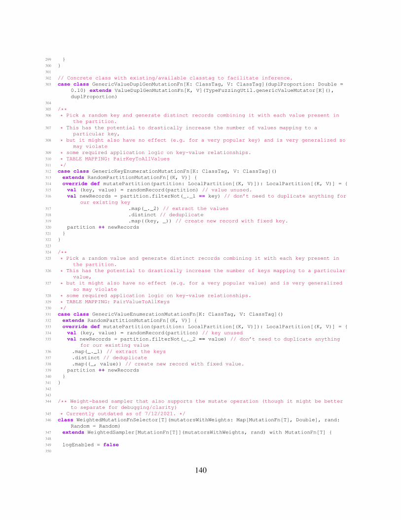
299 }300 }301
302 // Concrete class with existing/available classtag to facilitate inference.303 case class GenericValueDuplGenMutationFn[K: ClassTag, V: ClassTag](duplProportion: Double =
0.10) extends ValueDuplGenMutationFn[K, V](TypeFuzzingUtil.genericValueMutator[K](),duplProportion)
304
305 /**306 * Pick a random key and generate distinct records combining it with each value present in
the partition.307 * This has the potential to drastically increase the number of values mapping to a
particular key,308 * but it might also have no effect (e.g. for a very popular key) and is very generalized so
may violate309 * some required application logic on key-value relationships.310 * TABLE MAPPING: PairKeyToAllValues311 */312 case class GenericKeyEnumerationMutationFn[K: ClassTag, V: ClassTag]()313 extends RandomPartitionMutationFn[(K, V)] {314 override def mutatePartition(partition: LocalPartition[(K, V)]): LocalPartition[(K, V)] = {315 val (key, value) = randomRecord(partition) // value unused.316 val newRecords = partition.filterNot(_._1 == key) // don’t need to duplicate anything for
our existing key317 .map(_._2) // extract the values318 .distinct // deduplicate319 .map((key, _)) // create new record with fixed key.320 partition ++ newRecords321 }322 }323
324 /**325 * Pick a random value and generate distinct records combining it with each key present in
the partition.326 * This has the potential to drastically increase the number of keys mapping to a particular
value,327 * but it might also have no effect (e.g. for a very popular value) and is very generalized
so may violate328 * some required application logic on key-value relationships.329 * TABLE MAPPING: PairValueToAllKeys330 */331 case class GenericValueEnumerationMutationFn[K: ClassTag, V: ClassTag]()332 extends RandomPartitionMutationFn[(K, V)] {333 override def mutatePartition(partition: LocalPartition[(K, V)]): LocalPartition[(K, V)] = {334 val (key, value) = randomRecord(partition) // key unused335 val newRecords = partition.filterNot(_._2 == value) // don’t need to duplicate anything
for our existing value336 .map(_._1) // extract the keys337 .distinct // deduplicate338 .map((_, value)) // create new record with fixed value.339 partition ++ newRecords340 }341 }342
343
344 /** Weight-based sampler that also supports the mutate operation (though it might be betterto separate for debugging/clarity)
345 * Currently outdated as of 7/12/2021. */346 class WeightedMutationFnSelector[T](mutatorsWithWeights: Map[MutationFn[T], Double], rand:
Random = Random)347 extends WeightedSampler[MutationFn[T]](mutatorsWithWeights, rand) with MutationFn[T] {348
349 logEnabled = false350
140

351 def selectMutator(): MutationFn[T] = sample() // alias352
353 override def mutate(input: HybridRDD[T]): HybridRDD[T] = {354 val (fn, mutation) = selectAndMutate(input)355 mutation356 }357
358 def selectAndMutate(input: HybridRDD[T]): (MutationFn[T], HybridRDD[T]) = {359 val mutator = selectMutator()360 log(s"Selected mutation function: $mutator")361 MutationFn.mostRecent = Some(mutator)362 (mutator, mutator.mutate(input))363 }364 }365
366 /** Weight-based sampler that also supports the mutate operation (though it might be betterto separate for debugging/clarity) */
367 class WeightedPartitionMutationFnSelector[T](mutatorsWithWeights:Map[PartitionsBasedMutationFn[T], Double], rand: Random = Random)
368 extends WeightedSampler[PartitionsBasedMutationFn[T]](mutatorsWithWeights, rand) withPartitionsBasedMutationFn[T] {
369
370 logEnabled = false371
372 // Use weighted random sampling.373 def selectMutator(): PartitionsBasedMutationFn[T] = sample() // alias374
375 override def mutatePartitions(input: Partitions[T]): Partitions[T] = {376 val (fn, mutation) = selectAndMutate(input)377 mutation378 }379
380
381 def selectAndMutate(input: Partitions[T]): (PartitionsBasedMutationFn[T], Partitions[T]) = {382 val mutator = selectMutator()383 log(s"Selected partition mutation function: $mutator")384 MutationFn.mostRecent = Some(mutator)385 (mutator, mutator.mutatePartitions(input))386 }387 }388
389 object TypeFuzzingUtil extends HFLogger {390 val rand = Random391 val MAX_STRING_SUB_LENGTH = 25392 val MIN_STRING_SUB_LENGTH = 0393
394 // Note: MinValue means that Max-Min = -1, which results in an error395 // when selecting within range (might also be why default nextInt is in range [0, max)? )396 val DEFAULT_INT_MIN = 0397 val DEFAULT_INT_MAX = Int.MaxValue398
399 // TABLE MAPPING: ReplaceBoolean400 def randBoolean(): Boolean = {401 rand.nextBoolean()402 }403
404 /** Random integer in specified range [min, max). */405 def randomIntInRange(min: Int, max: Int): Int = {406 min + rand.nextInt(max - min)407 }408
409 /** Random double in specified range [min, max). */410 def randomDoubleInRange(min: Double, max: Double): Double = {411 min + (rand.nextDouble() * max - min)
141
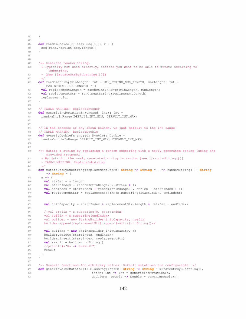
412 }413
414 def randomChoice[T](seq: Seq[T]): T = {415 seq(rand.nextInt(seq.length))416 }417
418
419 /** Generate random string.420 * Typically not used directly, instead you want to be able to mutate according to
substring.421 * (See [[mutateStrBySubstring()]])422 */423 def randomString(minLength: Int = MIN_STRING_SUB_LENGTH, maxLength: Int =
MAX_STRING_SUB_LENGTH) = {424 val replacementLength = randomIntInRange(minLength, maxLength)425 val replacementStr = rand.nextString(replacementLength)426 replacementStr427 }428
429 // TABLE MAPPING: ReplaceInteger430 def genericIntMutationFn(unused: Int): Int =431 randomIntInRange(DEFAULT_INT_MIN, DEFAULT_INT_MAX)432
433
434 // In the absence of any known bounds, we just default to the int range435 // TABLE MAPPING: ReplaceDouble436 def genericDoubleFn(unused: Double): Double =437 randomDoubleInRange(DEFAULT_INT_MIN, DEFAULT_INT_MAX)438
439
440 /** Mutate a string by replacing a random substring with a newly generated string (using theprovided argument).
441 * By default, the newly generated string is random (see [[randomString()]]442 * TABLE MAPPING: ReplaceSubstring443 */444 def mutateStrBySubstring(replacementStrFn: String => String = _ => randomString()): String
=> String = {445 s => {446 val strLen = s.length447 val startIndex = randomIntInRange(0, strLen + 1)448 val endIndex = startIndex + randomIntInRange(0, strLen - startIndex + 1)449 val replacementStr = replacementStrFn(s.substring(startIndex, endIndex))450
451
452 val initCapacity = startIndex + replacementStr.length + (strLen - endIndex)453
454 /*val prefix = s.substring(0, startIndex)455 val suffix = s.substring(endIndex)456 val builder = new StringBuilder(initCapacity, prefix)457 builder.append(replacementStr).append(suffix).toString()*/458
459 val builder = new StringBuilder(initCapacity, s)460 builder.delete(startIndex, endIndex)461 builder.insert(startIndex, replacementStr)462 val result = builder.toString()463 //println(s"$s => $result")464 result465 }466 }467
468 /** Generic functions for arbitrary values. Default mutations are configurable. */469 def genericValueMutator[T: ClassTag](strFn: String => String = mutateStrBySubstring(),470 intFn: Int => Int = genericIntMutationFn,471 doubleFn: Double => Double = genericDoubleFn,
142
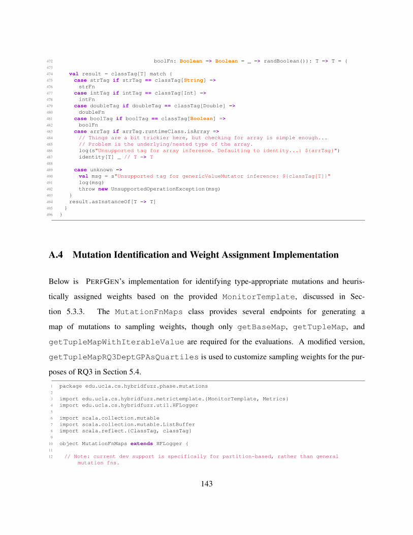
472 boolFn: Boolean => Boolean = _ => randBoolean()): T => T = {473
474 val result = classTag[T] match {475 case strTag if strTag == classTag[String] =>476 strFn477 case intTag if intTag == classTag[Int] =>478 intFn479 case doubleTag if doubleTag == classTag[Double] =>480 doubleFn481 case boolTag if boolTag == classTag[Boolean] =>482 boolFn483 case arrTag if arrTag.runtimeClass.isArray =>484 // Things are a bit trickier here, but checking for array is simple enough...485 // Problem is the underlying/nested type of the array.486 log(s"Unsupported tag for array inference. Defaulting to identity...: ${arrTag}")487 identity[T] _ // T => T488
489 case unknown =>490 val msg = s"Unsupported tag for genericValueMutator inference: ${classTag[T]}"491 log(msg)492 throw new UnsupportedOperationException(msg)493 }494 result.asInstanceOf[T => T]495 }496 }
A.4 Mutation Identification and Weight Assignment Implementation
Below is PERFGEN’s implementation for identifying type-appropriate mutations and heuris-
tically assigned weights based on the provided MonitorTemplate, discussed in Sec-
tion 5.3.3. The MutationFnMaps class provides several endpoints for generating a
map of mutations to sampling weights, though only getBaseMap, getTupleMap, and
getTupleMapWithIterableValue are required for the evaluations. A modified version,
getTupleMapRQ3DeptGPAsQuartiles is used to customize sampling weights for the pur-
poses of RQ3 in Section 5.4.
1 package edu.ucla.cs.hybridfuzz.phase.mutations2
3 import edu.ucla.cs.hybridfuzz.metrictemplate.{MonitorTemplate, Metrics}4 import edu.ucla.cs.hybridfuzz.util.HFLogger5
6 import scala.collection.mutable7 import scala.collection.mutable.ListBuffer8 import scala.reflect.{ClassTag, classTag}9
10 object MutationFnMaps extends HFLogger {11
12 // Note: current dev support is specifically for partition-based, rather than generalmutation fns.
143
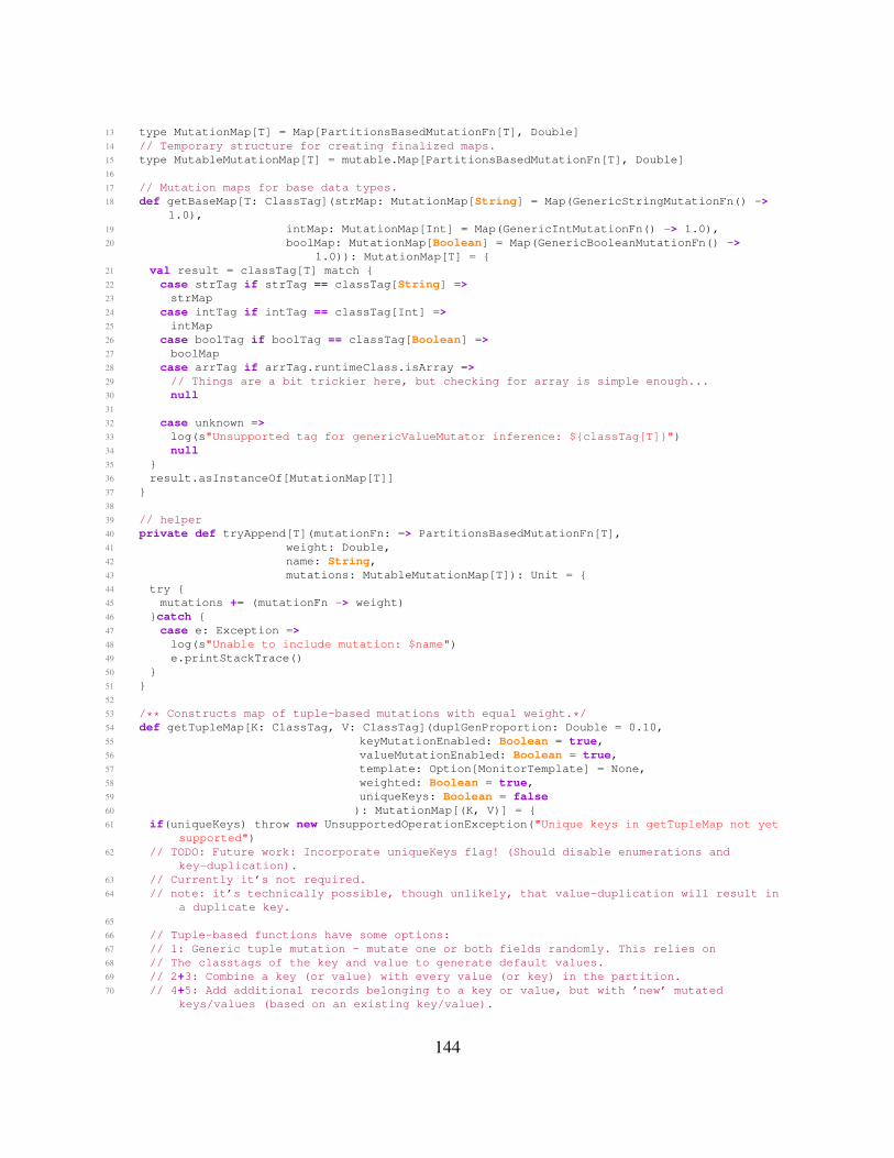
13 type MutationMap[T] = Map[PartitionsBasedMutationFn[T], Double]14 // Temporary structure for creating finalized maps.15 type MutableMutationMap[T] = mutable.Map[PartitionsBasedMutationFn[T], Double]16
17 // Mutation maps for base data types.18 def getBaseMap[T: ClassTag](strMap: MutationMap[String] = Map(GenericStringMutationFn() ->
1.0),19 intMap: MutationMap[Int] = Map(GenericIntMutationFn() -> 1.0),20 boolMap: MutationMap[Boolean] = Map(GenericBooleanMutationFn() ->
1.0)): MutationMap[T] = {21 val result = classTag[T] match {22 case strTag if strTag == classTag[String] =>23 strMap24 case intTag if intTag == classTag[Int] =>25 intMap26 case boolTag if boolTag == classTag[Boolean] =>27 boolMap28 case arrTag if arrTag.runtimeClass.isArray =>29 // Things are a bit trickier here, but checking for array is simple enough...30 null31
32 case unknown =>33 log(s"Unsupported tag for genericValueMutator inference: ${classTag[T]}")34 null35 }36 result.asInstanceOf[MutationMap[T]]37 }38
39 // helper40 private def tryAppend[T](mutationFn: => PartitionsBasedMutationFn[T],41 weight: Double,42 name: String,43 mutations: MutableMutationMap[T]): Unit = {44 try {45 mutations += (mutationFn -> weight)46 }catch {47 case e: Exception =>48 log(s"Unable to include mutation: $name")49 e.printStackTrace()50 }51 }52
53 /** Constructs map of tuple-based mutations with equal weight.*/54 def getTupleMap[K: ClassTag, V: ClassTag](duplGenProportion: Double = 0.10,55 keyMutationEnabled: Boolean = true,56 valueMutationEnabled: Boolean = true,57 template: Option[MonitorTemplate] = None,58 weighted: Boolean = true,59 uniqueKeys: Boolean = false60 ): MutationMap[(K, V)] = {61 if(uniqueKeys) throw new UnsupportedOperationException("Unique keys in getTupleMap not yet
supported")62 // TODO: Future work: Incorporate uniqueKeys flag! (Should disable enumerations and
key-duplication).63 // Currently it’s not required.64 // note: it’s technically possible, though unlikely, that value-duplication will result in
a duplicate key.65
66 // Tuple-based functions have some options:67 // 1: Generic tuple mutation - mutate one or both fields randomly. This relies on68 // The classtags of the key and value to generate default values.69 // 2+3: Combine a key (or value) with every value (or key) in the partition.70 // 4+5: Add additional records belonging to a key or value, but with ’new’ mutated
keys/values (based on an existing key/value).
144

71 val mutationMap: MutableMutationMap[(K, V)] = mutable.Map()72
73 if(template.isEmpty) throw new IllegalArgumentException("Jason: Templates required forevaluations now.")
74 val isDataSkew = template.exists(_.metric.isDataSkew)75 val isRuntimeSkew = template.exists(_.metric.isRuntimeSkew)76 // Rule-based weight assignment:77 // if data skew, then it helps to increase the number of keys/values. Random typically
only affects by one while78 // enumeration is capped and ’balanced’ (i.e., not useful running multiple times), so
upweight the duplications79 // even more than usual.80 val fixedDuplicationWeight =81 if(isDataSkew && weighted) 5.082 else if (isRuntimeSkew && weighted) 3.083 else 1.084
85 // configure according to symptoms/templates,86 // e.g comp skew is more value-focused vs data skew more key-focused87 // deprecated in favor of smaller/more precise field mutations:
tryAppend(GenericTupleMutationFn(), 1.0, "generic tuple mutation fn", mutationMap)88 if(keyMutationEnabled) {89 log("Key mutations enabled!")90 tryAppend(GenericRandomKeyMutationFn[K,V](), 1.0, "generic key mutation", mutationMap)91
92 // Note: This means fixed value and altered keys (duplicated value)93 tryAppend(GenericValueEnumerationMutationFn[K, V](), 1.0, "generic value enum fn",
mutationMap)94 tryAppend(GenericValueDuplGenMutationFn[K, V](duplGenProportion), fixedDuplicationWeight,
"generic value duplication", mutationMap)95
96 }97
98 if(valueMutationEnabled) {99 log("Value mutations enabled!")
100 tryAppend(GenericRandomValueMutationFn[K, V](), 1.0, "generic value mutation",mutationMap)
101
102 // Note: This means fixed key and altered values103 tryAppend(GenericKeyEnumerationMutationFn[K, V](), 1.0, "generic key enum fn",
mutationMap)104 tryAppend(GenericKeyDuplGenMutationFn[K, V](duplGenProportion), fixedDuplicationWeight,
"generic key duplication", mutationMap)105 }106
107
108 mutationMap.toMap109 }110
111 /** A specialized version of TupleMap used only for RQ3 and DeptGPAsQuartiles.112 * The objective here is to experiment with different weights of mutations, so113 * they have been parameterized.114 * */115 def getTupleMapRQ3DeptGPAsQuartiles[K: ClassTag, V: ClassTag](116 fixedDuplicationWeight: Double,117 duplGenProportion: Double = 0.10,118 keyMutationEnabled: Boolean = true,119 valueMutationEnabled: Boolean = true,120 template: Option[MonitorTemplate] = None,121 weighted: Boolean = true,122 uniqueKeys: Boolean = false,123 ): MutationMap[(K, V)] = {124 if(uniqueKeys) throw new UnsupportedOperationException("Unique keys in getTupleMap not yet
supported")
145

125 // TODO: Future work: Incorporate uniqueKeys flag! (Should disable enumerations andkey-duplication).
126 // Currently it’s not required.127 // note: it’s technically possible, though unlikely, that value-duplication will result in
a duplicate key.128
129 // Tuple-based functions have some options:130 // 1: Generic tuple mutation - mutate one or both fields randomly. This relies on131 // The classtags of the key and value to generate default values.132 // 2+3: Combine a key (or value) with every value (or key) in the partition.133 // 4+5: Add additional records belonging to a key or value, but with ’new’ mutated
keys/values (based on an existing key/value).134 val mutationMap: MutableMutationMap[(K, V)] = mutable.Map()135
136 if(template.isEmpty) throw new IllegalArgumentException("Jason: Templates required forevaluations now.")
137 val isDataSkew = template.exists(_.metric.isDataSkew)138 val isRuntimeSkew = template.exists(_.metric.isRuntimeSkew)139
140 //Removed: fixedDuplicationWeight is now determined by parameter.141
142 // configure according to symptoms/templates,143 // e.g comp skew is more value-focused vs data skew more key-focused144 // deprecated in favor of smaller/more precise field mutations:
tryAppend(GenericTupleMutationFn(), 1.0, "generic tuple mutation fn", mutationMap)145 if(keyMutationEnabled) {146 log("Key mutations enabled!")147 tryAppend(GenericRandomKeyMutationFn[K,V](), 1.0, "generic key mutation", mutationMap)148
149 // Note: This means fixed value and altered keys (duplicated value)150 tryAppend(GenericValueEnumerationMutationFn[K, V](), 1.0, "generic value enum fn",
mutationMap)151 tryAppend(GenericValueDuplGenMutationFn[K, V](duplGenProportion), fixedDuplicationWeight,
"generic value duplication", mutationMap)152
153 }154
155 if(valueMutationEnabled) {156 log("Value mutations enabled!")157 tryAppend(GenericRandomValueMutationFn[K, V](), 1.0, "generic value mutation",
mutationMap)158
159 // Note: This means fixed key and altered values160 tryAppend(GenericKeyEnumerationMutationFn[K, V](), 1.0, "generic key enum fn",
mutationMap)161 tryAppend(GenericKeyDuplGenMutationFn[K, V](duplGenProportion), fixedDuplicationWeight,
"generic key duplication", mutationMap)162 }163
164
165 mutationMap.toMap166 }167
168 // Not used in any benchmarks.169 def getQuadrupleMap[V1: ClassTag, V2: ClassTag, V3: ClassTag, V4: ClassTag]:
MutationMap[(V1, V2, V3, V4)] ={170 type Quadruple = (V1, V2, V3, V4)171 val mutationMap: MutableMutationMap[(V1, V2, V3, V4)] = mutable.Map()172
173 import QuadrupleMutations._174 tryAppend(GenericRandomQuadrupleV1MutationFn[V1, V2, V3, V4](), 1.0, "generic V1 mutation
fn", mutationMap)175 tryAppend(GenericRandomQuadrupleV2MutationFn[V1, V2, V3, V4](), 1.0, "generic V2 mutation
fn", mutationMap)
146

176 tryAppend(GenericRandomQuadrupleV3MutationFn[V1, V2, V3, V4](), 1.0, "generic V3 mutationfn", mutationMap)
177 tryAppend(GenericRandomQuadrupleV4MutationFn[V1, V2, V3, V4](), 1.0, "generic V4 mutationfn", mutationMap)
178
179
180 mutationMap.toMap181 }182
183 // Not used in any benchmarks.184 def getTupleMapWithArrayValue[K: ClassTag, V: ClassTag]: MutationMap[(K, Array[V])] = {185 type ArrV = Array[V]186 val mutationMap: MutableMutationMap[(K, ArrV)] = mutable.Map()187
188 // configure according to symptoms/templates,189 // e.g comp skew is more value-focused vs data skew more key-focused190 // tryAppend(GenericTupleMutationFn(), 1.0, "generic tuple mutation fn", mutationMap)191 tryAppend(GenericRandomKeyMutationFn[K, ArrV](), 1.0, "generic key mutation", mutationMap)192 // Due to classtag limitations, arrays need to be handled separately193 // Heuristic assignment: array values need to be explored more frequently, so increase
weight.194 tryAppend(GenericValueArrayDuplMutationFn[K, V](10), 5.0, "generic value array dupl",
mutationMap)195 tryAppend(GenericKeyEnumerationMutationFn[K, ArrV](), 1.0, "generic key enum", mutationMap)196 tryAppend(GenericValueEnumerationMutationFn[K, ArrV](), 1.0, "generic value enum",
mutationMap)197
198
199 mutationMap.toMap200 }201
202 // Collatz uses this with (Int, Iterable[Int])203 def getTupleMapWithIterableValue[K: ClassTag, V: ClassTag](template: Option[MonitorTemplate]
= None,204 duplGenProportion: Double = 0.10,205 keyMutationEnabled: Boolean = true,206 valueMutationEnabled: Boolean = true,207 weighted: Boolean = true,208 uniqueKeys: Boolean = false209 ): MutationMap[(K, Iterable[V])] = {210 type IterV = Iterable[V]211 val mutationMap: MutableMutationMap[(K, IterV)] = mutable.Map()212 // uniqueKeys disables enumerations and key-duplication (key dupe not yet supported for
iterable values though)213 // note: it’s technically possible, though unlikely, that value-duplication will result in
a duplicate key.214
215 // configure according to symptoms/templates,216 // e.g comp skew is more value-focused vs data skew more key-focused217 // if we’re dealing with data or memory skew enumerations are more valuable in increasing
record mapings/consumption at a time218 val isDataSkew = template.exists(_.metric.isDataSkew)219 val isRuntimeSkew = template.exists(_.metric.isRuntimeSkew)220
221 // Heuristically assigned weights.222 val enumerationWeight = if (isDataSkew) 3.0 else 0.5223 val fixedDuplicationWeight = 1.0224
225 if(keyMutationEnabled) {226 tryAppend(GenericRandomKeyMutationFn[K, IterV](), 1.0, "generic key mutation",
mutationMap)227 if(!uniqueKeys) {228 tryAppend(GenericValueEnumerationMutationFn[K, IterV](), enumerationWeight, "generic
value enum", mutationMap)
147
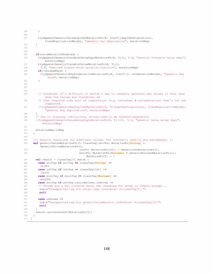
229 }230
231 tryAppend(GenericValueDuplGenMutationFn[K, IterV](duplGenProportion),fixedDuplicationWeight, "generic key duplication", mutationMap)
232 }233
234
235 if(valueMutationEnabled) {236 tryAppend(GenericIterableValueDuplMutationFn[K, V](), 1.0, "generic iterable value dupl",
mutationMap)237 tryAppend(GenericIterableValueMutationFn[K, V](),238 5.0, "derived single-value mutation function", mutationMap)239 if(!uniqueKeys) {240 tryAppend(GenericKeyEnumerationMutationFn[K, IterV](), enumerationWeight, "generic key
enum", mutationMap)241 }242
243
244
245 // Disabled: It’s difficult to define a way to randomly generate new values in this casewhen the values are iterables, as
246 // that requires some sort of composition (e.g. valuedupl + valuemutation) that’s not yetsupported.
247 //tryAppend(GenericKeyDuplGenMutationFn[K, V](duplGenProportion), fixedDuplicationWeight,"generic key duplication", mutationMap)
248 }249 // Due to classtag limitations, arrays need to be handled separately250 //tryAppend(GenericValueArrayDuplMutationFn[K, V](10), 5.0, "generic value array dupl",
mutationMap)251
252 mutationMap.toMap253 }254
255 /** Generic functions for arbitrary values. Not currently used in any benchmarks. */256 def genericValueMutationFn[T: ClassTag](strFn: MutationFn[String] =
GenericStringMutationFn(),257 intFn: MutationFn[Int] = GenericIntMutationFn(),258 boolFn: MutationFn[Boolean] = GenericBooleanMutationFn()):
MutationFn[T] = {259 val result = classTag[T] match {260 case strTag if strTag == classTag[String] =>261 strFn262 case intTag if intTag == classTag[Int] =>263 intFn264 case boolTag if boolTag == classTag[Boolean] =>265 boolFn266 case arrTag if arrTag.runtimeClass.isArray =>267 // Things are a bit trickier here, but checking for array is simple enough...268 log(s"Unsupported tag for array type inference: ${classTag[T]}")269 null270
271 case unknown =>272 log(s"Unsupported tag for genericValueMutator inference: ${classTag[T]}")273 null274 }275 result.asInstanceOf[MutationFn[T]]276 }277 }
148

REFERENCES
[1] Aggregatebykey. https://spark.apache.org/docs/2.1.1/api/java/org/apache/spark/rdd/PairRDDFunctions.html.
[2] Apache ignite. https://ignite.apache.org/.
[3] Dr. elephant. https://github.com/linkedin/dr-elephant.
[4] Hadoop. http://hadoop.apache.org/.
[5] Spark documentation. http://spark.apache.org/docs/1.2.1/.
[6] Out of memory error in customer review processing.https://stackoverflow.com/questions/20247185, 2015.
[7] https://www.microsoft.com/en-us/research/project/prose-framework/#!tutorial, 2020.
[8] https://www.microsoft.com/en-us/research/group/prose/, 2022.
[9] https://leetcode.com/problems/best-time-to-buy-and-sell-stock-iii/, 2022.
[10] https://leetcode.com/problems/best-time-to-buy-and-sell-stock-iii/discuss/39608/A-clean-DP-solution-which-generalizes-to-k-transactions, 2022.
[11] H. Agrawal and J. R. Horgan. Dynamic program slicing. In Proceedings of the ACMSIGPLAN 1990 Conference on Programming Language Design and Implementation, PLDI’90, pages 246–256, New York, NY, USA, 1990. ACM.
[12] F. Ahmad, S. Lee, M. Thottethodi, and T. Vijaykumar. Puma: Purdue mapreduce bench-marks suite. Technical report, 2012 . TRECE-12-11.
[13] Y. Amsterdamer, S. B. Davidson, D. Deutch, T. Milo, J. Stoyanovich, and V. Tannen.Putting lipstick on pig: Enabling database-style workflow provenance. Proc. VLDB En-dow., 5(4):346–357, dec 2011.
[14] M. K. Anand, S. Bowers, and B. Ludascher. Techniques for efficiently querying scien-tific workflow provenance graphs. In Proceedings of the 13th International Conference onExtending Database Technology, EDBT ’10, pages 287–298, New York, NY, USA, 2010.ACM.
149
[15] D. Babic, S. Bucur, Y. Chen, F. Ivancic, T. King, M. Kusano, C. Lemieux, L. Szekeres,and W. Wang. Fudge: Fuzz driver generation at scale. In Proceedings of the 2019 27thACM Joint Meeting on European Software Engineering Conference and Symposium on theFoundations of Software Engineering, ESEC/FSE 2019, page 975–985, New York, NY,USA, 2019. Association for Computing Machinery.
[16] L. Bertossi, J. Li, M. Schleich, D. Suciu, and Z. Vagena. Causality-based explanation ofclassification outcomes. In Proceedings of the Fourth International Workshop on DataManagement for End-to-End Machine Learning, DEEM’20, New York, NY, USA, 2020.Association for Computing Machinery.
[17] L. Bindschaedler, J. Malicevic, N. Schiper, A. Goel, and W. Zwaenepoel. Rock you likea hurricane: Taming skew in large scale analytics. In Proceedings of the Thirteenth Eu-roSys Conference, EuroSys ’18, New York, NY, USA, 2018. Association for ComputingMachinery.
[18] O. Biton, S. Cohen-Boulakia, S. B. Davidson, and C. S. Hara. Querying and managingprovenance through user views in scientific workflows. In Proceedings of the 2008 IEEE24th International Conference on Data Engineering, ICDE ’08, pages 1072–1081, Wash-ington, DC, USA, 2008. IEEE Computer Society.
[19] S. M. Blackburn, P. Cheng, and K. S. McKinley. Myths and realities: The performanceimpact of garbage collection. SIGMETRICS Perform. Eval. Rev., 32(1):25–36, June 2004.
[20] T. Brennan, S. Saha, and T. Bultan. Jvm fuzzing for jit-induced side-channel detection.In Proceedings of the ACM/IEEE 42nd International Conference on Software Engineering,ICSE ’20, page 1011–1023, New York, NY, USA, 2020. Association for Computing Ma-chinery.
[21] M. Carbin and M. C. Rinard. Automatically identifying critical input regions and code inapplications. In Proceedings of the 19th International Symposium on Software Testing andAnalysis, ISSTA ’10, pages 37–48, New York, NY, USA, 2010. ACM.
[22] T. W. Chan and A. Lakhotia. Debugging program failure exhibited by voluminous data.Journal of Software Maintenance, 1998.
[23] A. Chapman, P. Missier, G. Simonelli, and R. Torlone. Capturing and querying fine-grainedprovenance of preprocessing pipelines in data science. Proc. VLDB Endow., 14(4):507–520,dec 2020.
[24] Q. Chen, J. Yao, and Z. Xiao. Libra: Lightweight data skew mitigation in mapreduce. IEEETransactions on parallel and distributed systems, 26(9):2520–2533, 2014.
[25] G. Cheng, S. Ying, B. Wang, and Y. Li. Efficient performance prediction for apache spark.Journal of Parallel and Distributed Computing, 149:40–51, 2021.
150
[26] J.-D. Choi and A. Zeller. Isolating failure-inducing thread schedules. In Proceedings of the2002 ACM SIGSOFT International Symposium on Software Testing and Analysis, ISSTA’02, pages 210–220, New York, NY, USA, 2002. ACM.
[27] Z. Chothia, J. Liagouris, F. McSherry, and T. Roscoe. Explaining outputs in modern dataanalytics. Proc. VLDB Endow., 9(12):1137–1148, Aug. 2016.
[28] J. Clause, W. Li, and A. Orso. Dytan: A generic dynamic taint analysis framework. InProceedings of the 2007 International Symposium on Software Testing and Analysis, ISSTA’07, pages 196–206, New York, NY, USA, 2007. ACM.
[29] J. Clause and A. Orso. Penumbra: Automatically identifying failure-relevant inputs usingdynamic tainting. In Proceedings of the Eighteenth International Symposium on SoftwareTesting and Analysis, ISSTA ’09, pages 249–260, New York, NY, USA, 2009. ACM.
[30] H. Cleve and A. Zeller. Locating causes of program failures. In Proceedings of the 27thInternational Conference on Software Engineering, ICSE ’05, pages 342–351, New York,NY, USA, 2005. ACM.
[31] B. Contreras-Rojas, J.-A. Quiane-Ruiz, Z. Kaoudi, and S. Thirumuruganathan. Tagsniff:Simplified big data debugging for dataflow jobs. In Proceedings of the ACM Symposium onCloud Computing, SoCC ’19, page 453–464, New York, NY, USA, 2019. Association forComputing Machinery.
[32] C. Csallner and Y. Smaragdakis. Jcrasher: an automatic robustness tester for java. Software:Practice and Experience, 34(11):1025–1050, 2004.
[33] Y. Cui and J. Widom. Lineage tracing for general data warehouse transformations. TheVLDB Journal, 12(1):41–58, May 2003.
[34] A. Dave, M. Zaharia, and I. Stoica. Arthur: Rich post-facto debugging for productionanalytics applications. Technical report, 2013.
[35] J. De Ruiter and E. Poll. Protocol state fuzzing of tls implementations. In Proceedings ofthe 24th USENIX Conference on Security Symposium, SEC’15, page 193–206, USA, 2015.USENIX Association.
[36] J. Dean and S. Ghemawat. Mapreduce: Simplified data processing on large clusters. Com-mun. ACM, 51(1):107–113, Jan. 2008.
[37] U. Demirbaga, Z. Wen, A. Noor, K. Mitra, K. Alwasel, S. Garg, A. Y. Zomaya, and R. Ran-jan. Autodiagn: An automated real-time diagnosis framework for big data systems. IEEETransactions on Computers, 71(5):1035–1048, May 2022.
151
[38] R. Diestelkamper and M. Herschel. Capturing and querying structural provenance in sparkwith pebble. In Proceedings of the 2019 International Conference on Management of Data,SIGMOD ’19, page 1893–1896, New York, NY, USA, 2019. Association for ComputingMachinery.
[39] L. Fang, K. Nguyen, G. Xu, B. Demsky, and S. Lu. Interruptible tasks: Treating memorypressure as interrupts for highly scalable data-parallel programs. In Proceedings of the 25thSymposium on Operating Systems Principles, pages 394–409, 2015.
[40] A. Fariha, S. Nath, and A. Meliou. Causality-guided adaptive interventional debugging.In Proceedings of the 2020 ACM SIGMOD International Conference on Management ofData, SIGMOD ’20, page 431–446, New York, NY, USA, 2020. Association for ComputingMachinery.
[41] A. D. Ferguson, P. Bodik, S. Kandula, E. Boutin, and R. Fonseca. Jockey: Guaranteed joblatency in data parallel clusters. In Proceedings of the 7th ACM European Conference onComputer Systems, EuroSys ’12, pages 99–112, New York, NY, USA, 2012. ACM.
[42] K. Fisher and D. Walker. The pads project: An overview. In Proceedings of the 14thInternational Conference on Database Theory, ICDT ’11, pages 11–17, New York, NY,USA, 2011. ACM.
[43] G. Fraser and A. Arcuri. Evosuite: Automatic test suite generation for object-orientedsoftware. In Proceedings of the 19th ACM SIGSOFT Symposium and the 13th EuropeanConference on Foundations of Software Engineering, ESEC/FSE ’11, page 416–419, NewYork, NY, USA, 2011. Association for Computing Machinery.
[44] J. Galea and D. Kroening. The taint rabbit: Optimizing generic taint analysis with dynamicfast path generation. In Proceedings of the 15th ACM Asia Conference on Computer andCommunications Security, ASIA CCS ’20, page 622–636, New York, NY, USA, 2020. As-sociation for Computing Machinery.
[45] S. Gan, C. Zhang, X. Qin, X. Tu, K. Li, Z. Pei, and Z. Chen. Collafl: Path sensitive fuzzing.In 2018 IEEE Symposium on Security and Privacy (SP), pages 679–696, 2018.
[46] S. Gulwani. Dimensions in program synthesis. In Proceedings of the 12th InternationalACM SIGPLAN Symposium on Principles and Practice of Declarative Programming, PPDP’10, page 13–24, New York, NY, USA, 2010. Association for Computing Machinery.
[47] M. A. Gulzar, M. Interlandi, X. Han, M. Li, T. Condie, and M. Kim. Automated debuggingin data-intensive scalable computing. In Proceedings of the 2017 Symposium on CloudComputing, SoCC ’17, page 520–534, New York, NY, USA, 2017. ACM, Association forComputing Machinery.
152
[48] M. A. Gulzar, M. Interlandi, S. Yoo, S. D. Tetali, T. Condie, T. D. Millstein, and M. Kim.Bigdebug: Debugging primitives for interactive big data processing in spark. In Proceed-ings of the 38th International Conference on Software Engineering, ICSE 2016, Austin, TX,USA, May 14-22, 2016, ICSE ’16, pages 784–795, New York, NY, USA, 2016. Associationfor Computing Machinery.
[49] M. A. Gulzar and M. Kim. Optdebug: Fault-inducing operation isolation for dataflow ap-plications. In Proceedings of the ACM Symposium on Cloud Computing, SoCC ’21, page359–372, New York, NY, USA, 2021. Association for Computing Machinery.
[50] M. A. Gulzar, M. Musuvathi, and M. Kim. Bigtest: A symbolic execution based systematictest generation tool for apache spark. In Proceedings of the ACM/IEEE 42nd InternationalConference on Software Engineering: Companion Proceedings, ICSE ’20, page 61–64,New York, NY, USA, 2020. Association for Computing Machinery.
[51] N. Gupta, H. He, X. Zhang, and R. Gupta. Locating faulty code using failure-inducingchops. In Proceedings of the 20th IEEE/ACM International Conference on Automated Soft-ware Engineering, ASE ’05, pages 263–272, New York, NY, USA, 2005. ACM.
[52] F. R. Hampel. The influence curve and its role in robust estimation. Journal of the AmericanStatistical Association, 69(346):383–393, 1974.
[53] T. Heinis and G. Alonso. Efficient lineage tracking for scientific workflows. In Proceedingsof the 2008 ACM SIGMOD International Conference on Management of Data, SIGMOD’08, pages 1007–1018, New York, NY, USA, 2008. ACM.
[54] H. Herodotou, H. Lim, G. Luo, N. Borisov, L. Dong, F. B. Cetin, and S. Babu. Starfish: Aself-tuning system for big data analytics. In In CIDR, pages 261–272, 2011.
[55] K. Hough and J. Bell. A practical approach for dynamic taint tracking with control-flowrelationships. ACM Trans. Softw. Eng. Methodol., 31(2), dec 2021.
[56] R. Ikeda, J. Cho, C. Fang, S. Salihoglu, S. Torikai, and J. Widom. Provenance-based de-bugging and drill-down in data-oriented workflows. In 2012 IEEE 28th International Con-ference on Data Engineering, pages 1249–1252, April 2012.
[57] R. Ikeda, H. Park, and J. Widom. Provenance for generalized map and reduce workflows.In In Proc. Conference on Innovative Data Systems Research (CIDR), 2011.
[58] R. Ikeda, A. D. Sarma, and J. Widom. Logical provenance in data-oriented workflows? In2013 IEEE 29th International Conference on Data Engineering (ICDE), pages 877–888,April 2013.
[59] M. Interlandi, A. Ekmekji, K. Shah, M. A. Gulzar, S. D. Tetali, M. Kim, T. Millstein,and T. Condie. Adding data provenance support to apache spark. The VLDB Journal,27(5):595–615, Oct. 2018.
153
[60] M. A. Irandoost, A. M. Rahmani, and S. Setayeshi. Mapreduce data skewness handling:a systematic literature review. International Journal of Parallel Programming, 47(5):907–950, 2019.
[61] V. Jagannath, Z. Yin, and M. Budiu. Monitoring and debugging dryadlinq applications withdaphne. In 2011 IEEE International Symposium on Parallel and Distributed ProcessingWorkshops and Phd Forum, pages 1266–1273, 2011.
[62] Y. Jia and M. Harman. An analysis and survey of the development of mutation testing.IEEE Transactions on Software Engineering, 37(5):649–678, Sep. 2011.
[63] R. Just, D. Jalali, L. Inozemtseva, M. D. Ernst, R. Holmes, and G. Fraser. Are mutantsa valid substitute for real faults in software testing? In Proceedings of the 22Nd ACMSIGSOFT International Symposium on Foundations of Software Engineering, FSE 2014,pages 654–665, New York, NY, USA, 2014. ACM.
[64] N. Khoussainova, M. Balazinska, and D. Suciu. Perfxplain: Debugging mapreduce jobperformance. Proc. VLDB Endow., 5(7):598–609, Mar. 2012.
[65] P. W. Koh and P. Liang. Understanding black-box predictions via influence functions, 2017.
[66] P. W. Koh and P. Liang. Understanding black-box predictions via influence functions.In Proceedings of the 34th International Conference on Machine Learning - Volume 70,ICML’17, page 1885–1894, Sydney, NSW, Australia, 2017. JMLR.org.
[67] Y. Kwon, M. Balazinska, B. Howe, and J. Rolia. A study of skew in mapreduce applications.Open Cirrus Summit 11, 2011.
[68] Y. Kwon, M. Balazinska, B. Howe, and J. Rolia. Skewtune: Mitigating skew in mapre-duce applications. In Proceedings of the 2012 ACM SIGMOD International Conference onManagement of Data, SIGMOD ’12, pages 25–36, New York, NY, USA, 2012. ACM.
[69] S. Lee, B. Ludascher, and B. Glavic. Approximate summaries for why and why-not prove-nance (extended version). arXiv preprint arXiv:2002.00084, 2020.
[70] T. R. Leek, G. Z. Baker, R. E. Brown, M. A. Zhivich, and R. Lippmann. Coverage maxi-mization using dynamic taint tracing. Technical report, 2007.
[71] C. Lemieux, R. Padhye, K. Sen, and D. Song. Perffuzz: Automatically generating patho-logical inputs. In Proceedings of the 27th ACM SIGSOFT International Symposium onSoftware Testing and Analysis, pages 254–265. ACM, 2018.
[72] D. Lemire, G. Ssi-Yan-Kai, and O. Kaser. Consistently faster and smaller compressedbitmaps with roaring. Softw. Pract. Exper., 46(11):1547–1569, Nov. 2016.
154
[73] K. Li, C. Reichenbach, Y. Smaragdakis, Y. Diao, and C. Csallner. Sedge: Symbolic exampledata generation for dataflow programs. In Automated Software Engineering (ASE), 2013IEEE/ACM 28th International Conference on, pages 235–245. IEEE, 2013.
[74] N. Li, Y. Lei, H. R. Khan, J. Liu, and Y. Guo. Applying combinatorial test data generationto big data applications. In Proceedings of the 31st IEEE/ACM International Conference onAutomated Software Engineering, ASE 2016, page 637–647, New York, NY, USA, 2016.Association for Computing Machinery.
[75] X. Liang, S. Shetty, D. Tosh, C. Kamhoua, K. Kwiat, and L. Njilla. Provchain: Ablockchain-based data provenance architecture in cloud environment with enhanced privacyand availability. In 2017 17th IEEE/ACM International Symposium on Cluster, Cloud andGrid Computing (CCGRID), pages 468–477, 2017.
[76] G. Liu, X. Zhu, J. Wang, D. Guo, W. Bao, and H. Guo. Sp-partitioner: A novel partitionmethod to handle intermediate data skew in spark streaming. Future Generation ComputerSystems, 86:1054–1063, 2018.
[77] S. Liu, S. Mahar, B. Ray, and S. Khan. Pmfuzz: test case generation for persistent mem-ory programs. In Proceedings of the 26th ACM International Conference on ArchitecturalSupport for Programming Languages and Operating Systems, pages 487–502, 2021.
[78] Z. Liu, Q. Zhang, M. F. Zhani, R. Boutaba, Y. Liu, and Z. Gong. Dreams: Dynamic resourceallocation for mapreduce with data skew. In 2015 IFIP/IEEE International Symposium onIntegrated Network Management (IM), pages 18–26. IEEE, 2015.
[79] D. Logothetis, S. De, and K. Yocum. Scalable lineage capture for debugging disc analytics.In Proceedings of the 4th annual Symposium on Cloud Computing, page 17. ACM, 2013.
[80] R. Marcus and O. Papaemmanouil. Plan-structured deep neural network models for queryperformance prediction. arXiv preprint arXiv:1902.00132, 2019.
[81] B. Marjanovic. Huge stock market dataset — kaggle, 11 2017.
[82] W. Masri, A. Podgurski, and D. Leon. Detecting and debugging insecure information flows.In 15th International Symposium on Software Reliability Engineering, pages 198–209, Nov2004.
[83] A. Meliou, W. Gatterbauer, K. F. Moore, and D. Suciu. The complexity of causality andresponsibility for query answers and non-answers. PVLDB, 4(1):34–45, 2010.
[84] G. Misherghi and Z. Su. Hdd: Hierarchical delta debugging. In Proceedings of the 28thInternational Conference on Software Engineering, ICSE ’06, pages 142–151, New York,NY, USA, 2006. ACM.
155

[85] S. Mishra, N. Sethi, and A. Chinmay. Various data skewness methods in the hadoop environ-ment. In 2019 International Conference on Recent Advances in Energy-efficient Computingand Communication (ICRAECC), pages 1–4, 2019.
[86] J. Newsome and D. Song. Dynamic taint analysis: Automatic detection, analysis, and sig-nature generation of exploit attacks on commodity software. In In In Proceedings of the12th Network and Distributed Systems Security Symposium. Citeseer, 2005.
[87] K. Nguyen, L. Fang, C. Navasca, G. Xu, B. Demsky, and S. Lu. Skyway: Connectingmanaged heaps in distributed big data systems. In Proceedings of the Twenty-Third Inter-national Conference on Architectural Support for Programming Languages and OperatingSystems, ASPLOS ’18, pages 56–69, New York, NY, USA, 2018. ACM.
[88] K. Nguyen, L. Fang, G. Xu, B. Demsky, S. Lu, S. Alamian, and O. Mutlu. Yak: A high-performance big-data-friendly garbage collector. In 12th USENIX Symposium on Operat-ing Systems Design and Implementation (OSDI 16), pages 349–365, Savannah, GA, 2016.USENIX Association.
[89] Y. Noller, R. Kersten, and C. S. Pasareanu. Badger: Complexity analysis with fuzzing andsymbolic execution. In Proceedings of the 27th ACM SIGSOFT International Symposiumon Software Testing and Analysis, ISSTA 2018, page 322–332, New York, NY, USA, 2018.Association for Computing Machinery.
[90] NYC Taxi and Limousine Commission. Nyc taxi trip data 2013 (foia/foil). https://archive.org/details/nycTaxiTripData2013. Accessed: 2019-05-31.
[91] C. Olston, S. Chopra, and U. Srivastava. Generating example data for dataflow programs.In Proceedings of the 2009 ACM SIGMOD International Conference on Management ofData, SIGMOD ’09, pages 245–256, New York, NY, USA, 2009. ACM.
[92] C. Olston and B. Reed. Inspector gadget: A framework for custom monitoring and de-bugging of distributed dataflows. In Proceedings of the 2011 ACM SIGMOD InternationalConference on Management of Data, SIGMOD ’11, page 1221–1224, New York, NY, USA,2011. Association for Computing Machinery.
[93] J. Oncina and P. Garcia. Identifying regular languages in polynomial time. In ADVANCESIN STRUCTURAL AND SYNTACTIC PATTERN RECOGNITION, VOLUME 5 OF SERIESIN MACHINE PERCEPTION AND ARTIFICIAL INTELLIGENCE, pages 99–108. WorldScientific, 1992.
[94] K. Ousterhout, R. Rasti, S. Ratnasamy, S. Shenker, and B.-G. Chun. Making sense of per-formance in data analytics frameworks. In 12th USENIX Symposium on Networked SystemsDesign and Implementation (NSDI 15), pages 293–307, Oakland, CA, 2015. USENIX As-sociation.
156
[95] C. Pacheco, S. K. Lahiri, M. D. Ernst, and T. Ball. Feedback-directed random test gener-ation. In 29th International Conference on Software Engineering (ICSE’07), pages 75–84,2007.
[96] S. Padhi, P. Jain, D. Perelman, O. Polozov, S. Gulwani, and T. D. Millstein. Flashprofile:Interactive synthesis of syntactic profiles. CoRR, 2017.
[97] R. Padhye, C. Lemieux, and K. Sen. Jqf: Coverage-guided property-based testing in java.In Proceedings of the 28th ACM SIGSOFT International Symposium on Software Testingand Analysis, ISSTA 2019, page 398–401, New York, NY, USA, 2019. Association forComputing Machinery.
[98] R. Padhye, C. Lemieux, K. Sen, M. Papadakis, and Y. Le Traon. Semantic fuzzing withZest. In Proceedings of the 28th ACM SIGSOFT International Symposium on SoftwareTesting and Analysis, ISSTA 2019, page 329–340, New York, NY, USA, 2019. Associationfor Computing Machinery.
[99] T. Petsios, J. Zhao, A. D. Keromytis, and S. Jana. Slowfuzz: Automated domain-independent detection of algorithmic complexity vulnerabilities. In Proceedings of the2017 ACM SIGSAC Conference on Computer and Communications Security, CCS ’17, page2155–2168, New York, NY, USA, 2017. Association for Computing Machinery.
[100] A. Phani, B. Rath, and M. Boehm. LIMA: Fine-Grained Lineage Tracing and Reuse inMachine Learning Systems, page 1426–1439. Association for Computing Machinery, NewYork, NY, USA, 2021.
[101] F. Psallidas and E. Wu. Smoke: Fine-grained lineage at interactive speed. Proc. VLDBEndow., 11(6):719–732, Feb. 2018.
[102] S. Roy and D. Suciu. A formal approach to finding explanations for database queries. InSIGMOD, pages 1579–1590, 2014.
[103] P. Ruan, G. Chen, T. T. A. Dinh, Q. Lin, B. C. Ooi, and M. Zhang. Fine-grained, secure andefficient data provenance on blockchain systems. Proc. VLDB Endow., 12(9):975–988, may2019.
[104] S. Sarawagi. Explaining differences in multidimensional aggregates. In Proceedings of the25th International Conference on Very Large Data Bases, VLDB ’99, pages 42–53, SanFrancisco, CA, USA, 1999. Morgan Kaufmann Publishers Inc.
[105] S. Sarawagi, R. Agrawal, and N. Megiddo. Discovery-driven exploration of olap datacubes. In In Proc. Int. Conf. of Extending Database Technology (EDBT’98, pages 168–182. Springer-Verlag, 1998.
157
[106] J. Scherbaum, M. Novotny, and O. Vayda. Spline: Spark lineage, not only for the bank-ing industry. In 2018 IEEE International Conference on Big Data and Smart Computing(BigComp), pages 495–498. IEEE, 2018.
[107] J. Somorovsky. Systematic fuzzing and testing of tls libraries. In Proceedings of the2016 ACM SIGSAC Conference on Computer and Communications Security, CCS ’16, page1492–1504, New York, NY, USA, 2016. Association for Computing Machinery.
[108] M. Stamatogiannakis, P. Groth, and H. Bos. Looking inside the black-box: Capturing dataprovenance using dynamic instrumentation. In B. Ludascher and B. Plale, editors, Prove-nance and Annotation of Data and Processes, pages 155–167, Cham, 2015. Springer Inter-national Publishing.
[109] Z. Tang, W. Lv, K. Li, and K. Li. An intermediate data partition algorithm for skew mitiga-tion in spark computing environment. IEEE Transactions on Cloud Computing, 9(2):461–474, 2021.
[110] J. Teoh, M. A. Gulzar, and M. Kim. Influence-based provenance for dataflow applicationswith taint propagation. In Proceedings of the 11th ACM Symposium on Cloud Computing,SoCC ’20, page 372–386, New York, NY, USA, 2020. Association for Computing Machin-ery.
[111] J. Teoh, M. A. Gulzar, G. H. Xu, and M. Kim. Perfdebug: Performance debugging ofcomputation skew in dataflow systems. In Proceedings of the ACM Symposium on CloudComputing, SoCC ’19, page 465–476, New York, NY, USA, 2019. Association for Com-puting Machinery.
[112] H. Tian, Q. Weng, and W. Wang. Towards framework-independent, non-intrusive perfor-mance characterization for dataflow computation. In Proceedings of the 10th ACM SIGOPSAsia-Pacific Workshop on Systems, APSys ’19, page 54–60, New York, NY, USA, 2019.Association for Computing Machinery.
[113] H. Tian, M. Yu, and W. Wang. CrystalPerf: Learning to characterize the performance ofdataflow computation through code analysis. In 2021 USENIX Annual Technical Confer-ence (USENIX ATC 21), pages 253–267. USENIX Association, July 2021.
[114] S. Venkataraman, Z. Yang, M. Franklin, B. Recht, and I. Stoica. Ernest: Efficient perfor-mance prediction for large-scale advanced analytics. In Proceedings of the 13th UsenixConference on Networked Systems Design and Implementation, NSDI’16, pages 363–378,Berkeley, CA, USA, 2016. USENIX Association.
[115] A. Verma, L. Cherkasova, and R. H. Campbell. Aria: Automatic resource inference andallocation for mapreduce environments. In Proceedings of the 8th ACM International Con-ference on Autonomic Computing, ICAC ’11, pages 235–244, New York, NY, USA, 2011.ACM.
158

[116] L. Wang, J. Zhan, C. Luo, Y. Zhu, Q. Yang, Y. He, W. Gao, Z. Jia, Y. Shi, S. Zhang,C. Zheng, G. Lu, K. Zhan, X. Li, and B. Qiu. Bigdatabench: A big data benchmark suitefrom internet services. In 2014 IEEE 20th International Symposium on High PerformanceComputer Architecture (HPCA), pages 488–499, 2014.
[117] M. Weiser. Program slicing. In Proceedings of the 5th International Conference on Soft-ware Engineering, ICSE ’81, pages 439–449, Piscataway, NJ, USA, 1981. IEEE Press.
[118] C. Wen, H. Wang, Y. Li, S. Qin, Y. Liu, Z. Xu, H. Chen, X. Xie, G. Pu, and T. Liu. Memlock:Memory usage guided fuzzing. In ICSE 2020, ICSE ’20, page 765–777, New York, NY,USA, 2020. Association for Computing Machinery.
[119] K. Werder, B. Ramesh, and R. S. Zhang. Establishing data provenance for responsibleartificial intelligence systems. ACM Trans. Manage. Inf. Syst., 13(2), mar 2022.
[120] E. Wu and S. Madden. Scorpion: Explaining away outliers in aggregate queries. Proc.VLDB Endow., 6(8):553–564, June 2013.
[121] H. Xu, Z. Zhao, Y. Zhou, and M. R. Lyu. Benchmarking the capability of symbolic exe-cution tools with logic bombs. IEEE Transactions on Dependable and Secure Computing,17(6):1243–1256, 2020.
[122] C. Yang, Y. Li, M. Xu, Z. Chen, Y. Liu, G. Huang, and X. Liu. TaintStream: Fine-GrainedTaint Tracking for Big Data Platforms through Dynamic Code Translation, page 806–817.Association for Computing Machinery, New York, NY, USA, 2021.
[123] Q. Ye and M. Lu. s2p: Provenance research for stream processing system. Applied Sciences,11(12), 2021.
[124] Z. Yu, Z. Bei, and X. Qian. Datasize-aware high dimensional configurations auto-tuningof in-memory cluster computing. In Proceedings of the Twenty-Third International Confer-ence on Architectural Support for Programming Languages and Operating Systems, pages564–577, 2018.
[125] M. Zalewski. American fuzz loop. http://lcamtuf.coredump.cx/afl/, 2021.
[126] A. Zeller. Yesterday, my program worked. today, it does not. why? In Proceedings of the7th European Software Engineering Conference, ESEC, pages 253–267, London, UK, UK,1999. Springer-Verlag.
[127] A. Zeller. Isolating cause-effect chains from computer programs. In Proceedings of the 10thACM SIGSOFT Symposium on Foundations of Software Engineering, SIGSOFT ’02/FSE-10, pages 1–10, New York, NY, USA, 2002. ACM.
[128] A. Zeller and R. Hildebrandt. Simplifying and isolating failure-inducing input. SoftwareEngineering, IEEE Transactions on, 28(2):183–200, 2002.
159
[129] Q. Zhang, J. Wang, M. A. Gulzar, R. Padhye, and M. Kim. Bigfuzz: Efficient fuzz test-ing for data analytics using framework abstraction. In The 35th IEEE/ACM InternationalConference on Automated Software Engineering, 2020.
[130] T. Zhang, G. Upadhyaya, A. Reinhardt, H. Rajan, and M. Kim. Are code examples onan online q amp;a forum reliable?: A study of api misuse on stack overflow. In 2018IEEE/ACM 40th International Conference on Software Engineering (ICSE), pages 886–896,2018.
[131] Z. Zvara, P. G. Szabo, B. Balazs, and A. Benczur. Optimizing distributed data stream pro-cessing by tracing. Future Generation Computer Systems, 90:578–591, 2019.
[132] Z. Zvara, P. G. Szabo, G. Hermann, and A. Benczur. Tracing distributed data stream pro-cessing systems. In 2017 IEEE 2nd International Workshops on Foundations and Applica-tions of Self* Systems (FAS*W), pages 235–242, 2017.
160