VIRTUAL MICROSCOPY FOR THE ASSESSMENT OF COMPETENCY AND TRAINING FOR MALARIA DIAGNOSIS L J AHMED PhD 2012

Welcome message from author
This document is posted to help you gain knowledge. Please leave a comment to let me know what you think about it! Share it to your friends and learn new things together.
Transcript
VIRTUAL MICROSCOPY FOR THE
ASSESSMENT OF COMPETENCY
AND TRAINING FOR MALARIA
DIAGNOSIS
L J AHMED
PhD 2012
i
VIRTUAL MICROSCOPY FOR THE
ASSESSMENT OF COMPETENCY AND
TRAINING FOR MALARIA DIAGNOSIS
LAURA JANE AHMED
A thesis submitted in partial fulfilment of the
requirements of the Manchester
Metropolitan University for the degree of
Doctor of Philosophy
School of Healthcare Science, Faculty of
Science and Engineering
SEPTEMBER 2012
ii
DECLARATION
This thesis is the result of my own work. The
material contained in the thesis has not been
presented, nor is currently being presented,
either wholly or in part for any other degree or
other qualification.
iii
ACKNOWLEDGMENTS
The project has been funded by the World Health Organization
Department of Diagnostic and Laboratory Technology. I would like to
thank Dr Gaby Vercauteren for her continued support for the project.
Secondly, I would like to thank the staff at UK NEQAS (H), in particular Dr
Mary West, Barbara De la Salle and Zuotimi Eke, for both reviewing
material and providing slides and paperwork as required.
Also thanks to the digital morphology team at Manchester Royal
Infirmary, Dr John Burthem, Dr John Ardern and Michelle Brereton.
I thank staff at the University for their help, in particular Dr Len Seal,
Professor Keith Hyde and Professor Bill Gilmore.
I also thank Monika Manser of the London Hospital for Tropical Diseases,
Dr Imelda Bates at the Liverpool School of Tropical Medicine.
I would like to thank all participants both in the UK and Internationally for
their engagement with the project and being patient when difficulties were
faced. Also staff in Tanzania in particular Professor Zul Premji of
Muhimbili University of Health and Allied Science for their help in
identifying the training need and what equipment was available.

iv
DEDICATION
I would like to dedicate by thesis to
my family, for all their support
throughout my studies.
v
GLOSSARY OF TERMS
ACT: Artemisinin based combination therapies
CPD: Continued professional development
DOP: Digital Outback Photo
EDTA: Ethylenediaminetetraacetic acid
FTP: File transfer protocol
GP: General practitioner
HTML: Hypertext Mark-up language
HRP-2: Histidine rich protein 2
IFA- Immunofluorescence antibody testing
Ig- Immunoglobulin
JPEG: Joint Photographic Experts Group- image format
LSTM: Liverpool School of Tropical Medicine
Mb: Megabyte
MPx: Megapixel
MRI: Manchester Royal Infirmary
NHS: National Health Service
NPV: Negative predictive value
PCR: Polymerase chain reaction
P.: Plasmodium
pLDH: Parasite lactate dehydrogenase
PPV: Positive predictive value
PS3: Photoshop CS3
QBC: Quantitative Buffy Coat
RAFT: Réseau Afrique Francophone de Télémédecine
RBC: Red blood cell
RDT: Rapid diagnostic test
ssrRNA: Small subunit ribosomal ribonucleic acid
SVS: ScanScope Virtual Slide- image format
SWF: Shockwave Flash format
TIFF: Tagged Image File Format – image format
vi
UK NEQAS: United Kingdom National External Quality Assessment
Scheme
UK NEQAS (H): United Kingdom National External Quality Assessment
Scheme for General Haematology
USB: Universal Serial Bus
WBC: White blood cell
WHO: World Health Organization
vii
TABLE OF CONTENTS
Chapter 1: Project introduction
1.1 Project aims p1
1.2 Preparation and evaluation of material for digital
Microscopy p2
1.3 Participant recruitment p4
1.3.1 Participant internet requirements p5
Chapter 2: Malaria diagnosis: Relevance to practice in endemic regions
2.1 Background p6
2.1.1 Malaria species p7
2.2 Diagnosis p9
2.2.1 Clinical diagnosis p9
2.2.2 Microscopic diagnosis p10
2.3 Variables affecting the accuracy of malaria diagnosis by
microscopy p13
2.4 Other methods of diagnosis malaria p17
2.4.1 Rapid diagnostic tests p17
2.4.2 Molecular diagnosis p19
2.4.3 Quantitative Buffy Coat p20
2.4.4 Malaria Antibody Detection p21
2.4.5 Automated detection of malaria pigment p22
2.4.6 Laser desorption mass spectrometry p23
2.4.7 Dark field microscopy p23
2.5 The cost of misdiagnosis p23
2.6 Conclusions p24
Chapter 3: Generation of microscopic images to be used for competency of
diagnosis assessment
3.1 Application of virtual microscopy p25
3.1.1 Advantages and disadvantages of virtual microscopy p29
viii
3.2 Sourcing malaria samples for imaging p29
3.2.1 Introduction p29
3.2.2 Method p30
3.2.3 Results and discussion p31
3.3 Generating images of blood films for virtual microscopy p31
3.3.1 Introduction p31
3.3.2 Methods p31
3.3.3 Results and discussion p40
3.3.4 Conclusion p46
3.4 Image processing for online presentation p47
3.4.1 Introduction p47
3.4.2 Methods p47
3.4.3 Results and discussion p48
3.4.4 Conclusion p50
3.5 Choosing images to be used for competency quality
assessment and training p51
3.5.1 Introduction p51
3.5.2 Methods p52
3.5.3 Results and discussion p54
3.6 The use of the online virtual microscope- SlideBox p58
3.6.1 Introduction p58
3.6.2 Methods p60
3.6.3 Discussion p67
3.7 Overall conclusion p67
Chapter 4: Generation of e-learning intervention for the enhancement of
morphological diagnosis of malaria
4.1 Introduction p68
4.2 Pedagogy of e-learning p69
4.3 Intervention package content p75
4.3.1 Target audience p75
4.3.2 Assessment of material already available on-line p76
ix
4.4 Intervention package structure p78
4.4.1 Participant experience and knowledge p78
4.4.2 Participant guidance p79
4.4.3 Structure p79
4.5 Format of delivery p80
4.5.1 Introduction p80
4.5.2 Methods p82
4.5.3 Results p84
4.5.4 Discussion p86
4.6 Developing interactive feedback p86
4.6.1 Introduction p86
4.6.2 Methods p87
4.6.3 Results p92
4.6.4 Discussion p94
4.7 Generating images for atlas galleries p94
4.7.1 Introduction p94
4.7.2 Methods p95
4.7.3 Results p97
4.7.4 Discussion p98
4.8 Processing images for atlas galleries p98
4.8.1 Introduction p98
4.8.2 Methods p98
4.8.3 Results p100
4.8.4 Discussion p101
4.9 Review of the training programme p102
4.9.1 Introduction p102
4.9.2 Methods p102
4.9.3 Results p103
4.9.4 Discussion p104
Chapter 5: Results for the International and UK groups
5.1 Participants recruited onto the intervention study p105
5.1.1 International group participants recruited p105
x
5.1.2 UK group participants recruited onto intervention
study p107
5.2 Delivery of the intervention training programme p107
5.3 Results from the initial recruitment questionnaire p108
5.3.1 International group results from the recruitment
questionnaire p108
5.3.2 UK group results from the recruitment questionnaire p113
5.4 Initial assessment p119
5.4.1 International group p119
5.4.2 Initial assessment: UK group p135
5.4.3 Comparison of UK and International groups in the
initial assessment p150
5.5 Intervention training stage p153
5.5.1 International group p153
5.5.2 UK group p153
5.6 Final assessment p154
5.6.1 International group p154
5.6.2 UK group final assessment results p169
5.6.3 Comparison of UK and International groups p183
5.7 Comparison of initial and final assessment p186
5.7.1 International group p186
5.7.2 UK group p213
Chapter 6: Discussion
6.1 Production of images for using in training, education
and EQA p240
6.1.1 Images used for virtual microscopy p240
6.1.2 Images used to generate image galleries as
part of the training package p241
6.2 Use of the internet to deliver a virtual microscope p241
6.3 Production and delivery of the training package p242
6.4 The International group p243
6.4.1 Participant recruitment p243
6.4.2 Participant engagement p246
xi
6.4.3 Results from the International group in the initial
and final assessment p247
6.4.4 Problems provided by case images p248
6.4.5 Assessment of performance in relation to the
laboratory staff training, experience and laboratory location p253
6.4.6 Equipment issues that may have affected
performance p255
6.4.7: Summary of performance of the International group p257
6.5 The UK group p258
6.5.1 Participant recruitment p258
6.5.2 Participant engagement p259
6.5.3 Results from the UK group in the initial and final
assessment p259
6.5.4 Problems provided by case images p260
6.5.5 Assessment of the performance in relation to the
laboratory staff experience and laboratory location p265
6.5.6 Equipment issues that may have affected
performance p266
6.5.7: Summary of the performance of the UK group p267
6.6 Comparison of UK and International results p268
6.7 Comparing participant performance against published
performance criteria p270
6.7.1 Relation to other international studies p270
6.8 Conclusions and future work p273
6.8.1 Project conclusions p273
6.8.2 Future work p274
References p276
Appendices p297
1.1 USB training programme trial questionnaire p297
1.2 Details for case images in the initial and final assessment p299
1.3 International group questionnaire p310
1.4 UK group questionnaire p323
xii
1.5 Results analysis methods p325
1.6 Conference posters p327
1.7 Conference presentations abstracts p331
1.8 DVD of training programme and images See attached DVD
TABLE OF TABLES
Table 3.1 Rank of the slides in the initial and final assessment p54
Table 3.2: Artefact rank of the slides in the initial and final assessment p54
Table 3.3: Number of cases from each species in the initial and final
assessment p55
Table 3.4: Number of P. falciparum cases at different ranks p55
Table 3.5 : Number of P. falciparum cases present at different
parasite density ranks p56
Table 3.6: Number of cases at each artefact rank in the initial and final
assessment p56
Table 3.7: Rank of P. vivax slides in the initial and final assessment p56
Table 3.8: Artefact rank of P. vivax cases in the initial and final
assessment p57
Table 3.9: The rank of P. ovale cases in the initial and final assessment p57
Table 3.10: Artefacts present in P. ovale cases in the initial and final
assessment p57
Table 4.1: Results from the training programme review questionnaire p103
Table 5.1: International participant recruitment questionnaire results p110
Table 5.2: The UK participants response to the recruitment questionnaire
and their locations and experience p114
Table 5.3: The detection of parasites in the initial assessment stage
slides (n=40) for the international participants group p119
Table 5.4:Performance on the individual cases (n=40) in the initial
assessment by the international group p121
Table 5.5: Results from participants in initial assessment stage (n=40)
for the International group p132
Table 5.6: The detection of parasites in the initial assessment stage cases
(n=40) for the UK participants group p135
xiii
Table 5.7: The performance on the individual cases (n=40) in the initial
assessment by participants in the UK group p136
Table 5.8: Results from individual participants for the initial assessment
stage cases in the UK group p147
Table 5.9: Results of the 18 international participants for the 40 cases
in the initial assessment p150
Table 5.10: Results of the 13 UK participants for the 40 cases in the initial
assessment p151
Table 5.11: Initial assessment, percentage detection accuracy and
species identification accuracy for both the UK and International group p152
Table 5.12: The detection of parasites in the final assessment stage cases
(n=40) for the International participants group p154
Table 5.13: Performance on the individual cases in the final assessment
by the International group p155
Table 5.14: Results from the international group participants for the final
assessment stage cases p166
Table 5.15: The detection of parasites in the final assessment stage
cases (n=40) for the UK participants group p169
Table 5.16: The performance on the 40 individual cases in the final
assessment by the UK group p170
Table 5.17: Results from individual participants for the final assessment
stage (n=40) for the UK group p180
Table 5.18: Results for the 18 participants in the international group
for the final assessment p183
Table 5.19: Results for the 13 participants in the UK group for the 40
cases in the final assessment p184
Table 5.20: Detection accuracy and species identification accuracy in
the final assessment for both the UK and International group p185
Table 5.21: Cases from the initial and final assessment and the
participant’s results for these cases for the international group p187
Table 5.22: The detection accuracy and the species identification
accuracy of the different artefact rank categories in the initial and final
assessment for the International group p199
Table 5.23: Comparison of individual participant results in the
xiv
International group in the initial and final assessment p202
Table 5.24: Comparison of results from initial assessment cases that were
repeated in the final assessment for the international group p211
Table 5.25: Agreement of results between the five repeated cases for the
international group p212
Table 5.26: Comparison of case results in the initial and final
assessments (n=80) for the UK group p213
Table 5.27: The detection accuracy and the species identification
accuracy of the different artefact rank categories in the initial
and final assessment p225
Table 5.28: Comparison of individual results in the initial and final
assessment p229
Table 5.29: Comparison of results from the initial assessment case that were
repeated in the final assessment for the UK group p237
Table 5.30: Comparison of the consistency of results between the
five repeated cases for the UK group p238
Table 6.1.: Interim WHO grades for accreditation of malaria microscopists p271
Table 6.2: Minimum competency levels for peripheral level microscopists
as recommended by WHO p272
TABLE OF FIGURES
Figure 3.1: The Zeiss Axio Imager M1 microscope p33
Figure 3.2: Generating a stitched image in Axiovision p35
Figure 3.3: Adjusting the resolution and frame size on
the AxioImager microscope p36
Figure 3.4: Automated stitching, planning out the area to
be stitched and choosing the overlap in Axiovision p38
Figure 3.5: Producing a stitched image with overlap p39
Figure 3.6: Image taken P. falciparum gametocyte with 1.2 MPx camera p41
Figure 3.7: Image taken P. falciparum gametocyte with 5 MPx camera p42
Figure 3.8: Image taken P. falciparum gametocyte with 12 MPx camera p43
Figure 3.9: One parasite in and one out of focus due to a
different focus plane p44
Figure 3.10: Problems encountered with image generation
xv
using automated stitching p45
Figure 3.11: The stitching icon in AxioVision p46
Figure 3.12: Comparison of detail enhancement methods p49
Figure 3.13: Comparison of the detail enhanced image before (left)
and after detail enhancement (right) p50
Figure 3.14: The SlidePath digital SlideBox environment p59
Figure 3.15: Administration pages of virtual microscope p61
Figure 3.16: Adding a questionnaire to SlideBox p62
Figure 3.17: Adding an annotation to the stitched image p65
Figure 3.18: Editing the narrative to provide feedback p66
Figure 4.1: Creating a web page as a Google site p81
Figure 4.2: Adding pages to the Google site p81
Figure 4.3: Adding content to a Google page p82
Figure 4.4: Uploading a document as a Google document p82
Figure 4.5: Inserting a Google document, setting the size of the screen p83
Figure 4.6: Inserting an image into a table for gallery format p84
Figure 4.7: Adding links to the full size image p84
Figure 4.8: Saving Google pages to allow editing away from the internet p85
Figure 4.9: Adobe Dreamweaver to edit links in the web page p85
Figure 4.10: Adding a multimedia page onto the Slidepath site p86
Figure 4.11: Inserting a flash quiz template p87
Figure 4.12: Examples of the different quiz frameworks available to
be used in flash p88
Figure 4.13: The component inspector window, allows the question
to be added and the correct answer to be chosen p91
Figure 4.14: The participant score shown in the final screen p91
Figure 4.15: The question page provided on the left with the feedback
page on the right p92
Figure 4.16: Publishing of the SWF file in Flash Professional p93
Figure 4.17: The final quiz file inserted into the HTML page as an SWF
file p93
Figure 4.18: The live view window showing the properties window
and settings that can be adjusted p96
Figure 4.19: Comparison of images at different resolutions p97
xvi
Figure 4.20: Comparison of images generated using the different methods p101
Figure 5.1: Locations of participants around the world p105
Figure 5.2: Map of Nigeria, participants were in Lagos, Ibadan and Kano p106
Figure 5.3: International Group: Comparison of the detection accuracy and
species identification accuracy for the individual species in the initial
assessment p128
Figure 5.4: International group: Comparison of detection accuracy
and species identification accuracy for the rank of the parasite density
in the initial assessment p129
Figure 5.5: International group: Comparison of detection accuracy
and species identification accuracy for rank of the microscopic image
in the initial assessment p130
Figure 5.6: International group: Comparison of detection accuracy
and species identification accuracy for the artefact rank in the initial
assessment p131
Figure 5.7: International group: The relationship between location
and the results for detection and species identification accuracy p134
Figure 5.8: UK group: Comparison of detection accuracy and species
identification accuracy on cases of different species in the initial
assessment p144
Figure 5.9: UK group: Comparison of detection and species identification
accuracy and the rank of the parasite density in the initial assessment p144
Figure 5.10: UK group: Comparison of detection and species
identification accuracy and the rank of the microscopic image in the
initial assessment p145
Figure 5.11: UK group: Comparison of the detection and species
identification accuracy and the artefact rank in the initial assessment p146
Figure 5.12: UK group: The relationship between the location and the
results for detection and species identification accuracy in the initial
assessment p149
Figure 5.13: International Group: Comparison of the detection and
species identification accuracy for the different species present in
the final assessment p162
Figure 5.14: International group: Comparison of the detection and species
xvii
identification accuracy for the parasite density rank in the final
assessment p163
Figure 5.15: International group: Comparison of detection and species
identification accuracy with the rank of the microscopic image in the final
assessment p164
Figure 5.16: International group: The effect of the artefact rank on the
detection and species identification accuracy in the final assessment p165
Figure 5.17: International group: The relationship between the location
and the results for detection and species identification accuracy in the final
assessment p168
Figure 5.18: UK group: Comparison of detection and species
identification accuracy for the different species present in the final
assessment p176
Figure 5.19: UK group: Comparison of detection and species
identification accuracy for the rank of parasite density in the final
assessment p177
Figure 5.20: UK group: Comparison of detection and species
identification accuracy for the rank of the microscopic image in the final
assessment p178
Figure 5.21: UK group: Comparison of detection and species identification
accuracy when artefacts are present in the final assessment p179
Figure 5.22: UK group: The relationship between location and the results of
detection and species identification accuracy in the final assessment p182
Figure 5.23: International group: Comparison of the detection accuracy
on thick and thin films in the initial and final assessments p191
Figure 5.24: International group: Comparison of the species identification
accuracy on thick and thin films in the initial and final assessment p192
Figure 5.25: International group: Comparison of the detection accuracy
for each case for the different species in the initial and final assessment p193
Figure 5.26: International group: Comparison of the species identification
accuracy for each case for the different species in the initial and final
assessment p194
Figure 5.27: International group: Comparison of detection accuracy and
the parasite density in the initial and final assessment p195
xviii
Figure 5.28: International group: Comparison of species identification
accuracy and the parasite density in the initial and final assessment p196
Figure 5.29: International group: Comparison of the detection accuracy
and the ranking of the microscopic image in the initial and final
assessment p197
Figure 5.30: International group: Comparison of the species identification
accuracy and the ranking of the microscopic image in the initial and final
assessment p198
Figure 5.31: International group: Comparison of the detection accuracy
in the presence of artefacts in the initial and final assessment p200
Figure 5.32: International group: Comparison of the species identification
accuracy in the presence of artefacts in the initial and final assessment p200
Figure 5.33: International group: Comparison of the detection
accuracy in the initial and final assessment p203
Figure 5.34: Individual participant correct results in the initial and final
assessment in the International group p203
Figure 5.35: International group: Comparison of the species identification
accuracy in the initial and final assessment p204
Figure 5.36: International group: Individual correct species results in
the initial and final assessment p205
Figure 5.37: International group: Comparison of the detection
accuracy results and the experience of the individual in the initial
and final assessment p206
Figure 5.38: International group: Comparison of the species
identification accuracy and the experience of the individual in the
initial and final assessment p207
Figure 5.39: International group: Comparison of the detection accuracy
with the training of the individual in the initial and final assessment p208
Figure 5.40: International group: Comparison of the species
identification accuracy with the training of the individual in the
initial and final assessment p208
Figure 5.41: International group: Comparison of the detection
accuracy at different participant locations p209
Figure 5.42: Comparison of the species identification accuracy
xix
at different participant locations in the International group p210
Figure 5.43: UK group: Comparison of the detection accuracy on
thick and thin films in the initial and final assessment p217
Figure 5.44: UK group: Comparison of the species identification
accuracy on the thick and thin films in the initial and final assessment p218
Figure 5.45: UK group: Comparison of the detection accuracy for
the different species in the initial and final assessment p219
Figure 5.46: UK group: Comparison of the species identification
accuracy for the different species in the initial and final assessment p220
Figure 5.47: UK group: Comparison of detection accuracy and
the parasite density in the initial and final assessment p221
Figure 5.48: Comparison of species identification accuracy and
the parasite density in the initial and final assessment p222
Figure 5.49: UK group: Comparison of the detection accuracy and the
rank of the microscopic image in the initial and final assessment p223
Figure 5.50: UK group: Comparison of the species identification
accuracy and the ranking of the microscopic image in the initial
and final assessment p224
Figure 5.51: UK group: Comparison of the detection accuracy in the
presence of artefacts in the initial and final assessment p226
Figure 5.52: UK group: Comparison of the species identification
accuracy in the presence of artefacts in the initial and final assessment p227
Figure 5.53: UK group: Comparison of the detection accuracy in the
initial and final assessment p230
Figure 5.54: UK group: Individual participant correct results in the initial
and final assessment p231
Figure 5.55: UK group: Comparison of the species identification
accuracy in the initial and final assessment p232
Figure 5.56: UK group: Individual participant correct species results
in the initial and final assessment p233
Figure 5.57: UK group: Comparison of the detection accuracy results
and the experience of the individual in the initial and final assessment p234
Figure 5.58: UK group: Comparison of the species identification accuracy
and the experience of the individual in the initial and final assessment p235
xx
Figure 5.59: UK group: Comparison of the detection accuracy at different
participant locations p236
Figure 5.60: UK group: Comparison of the species identification
accuracy at different participant locations p236
xxi
ABSTRACT
Microscopy is regarded by many healthcare professionals as the international
gold standard for diagnosing malaria; however, the ability to reach a correct
diagnosis is affected by training, experience and availability of laboratory
resources including adequate quality assurance procedures.
In the work reported in this thesis we have generated virtual microscope slides
from patients, with malaria for use as external quality assurance specimens.
These virtual microscope slides were also incorporated into a training
programme to improve the diagnosis of malaria in UK and International
laboratories. In addition a novel gallery of photomicrographs taken from blood
smears from various patients was used in the training programme.
Internationally, 40 participants were recruited from 14 laboratories
recommended by the WHO, UKNEQAS (H) and the Liverpool School of
Tropical Medicine. In the UK, a group of laboratory individuals was contacted
through UK NEQAS (H) and 34 interested individuals were recruited.
Participants were initially asked to make a diagnosis on 40 electronically
generated blood smear images to determine the presence, or absence, of
malaria and to identify the species present. These participants were then given
access to an Internet based training and quality assessment programme over a
six-month period, aiming to improve malaria diagnosis by microscopy, before
completing another assessment of 40 images.
In the initial assessment, 24 participants completed all 40 cases in the
international and UK groups. In the final assessment 21 participants in the
international group completed all 40 cases and 18 participants in the UK group.
For the comparison of the initial and final assessments the results of 18 and 13
participants from the international and UK groups respectively were analysed.
In the initial assessment, the international group achieved the correct diagnosis
in 76.4% of cases, and the correct species in 48.9%. The UK group achieved
the correct diagnosis in 90.1% of cases and the correct species in 58.4%. In the
final assessment the international group achieved the correct diagnosis in
xxii
72.7% and the correct species in 46.9% of cases. The UK group achieved the
correct diagnosis in 95.6% of cases and the correct species in 73.8%.
The training programme resulted in a significant improvement (p≤0.05) in
malarial diagnosis in the UK group, but the difference was not significant for the
International group. The reasons for not being effective in Developing Nations
could be due to difficulties in understanding English, speed of Internet
connection, computers being used or the compliance of the participants.
Chapter 1: Project introduction 1
Chapter 1: Project introduction
1.1 Project aims
The diagnosis of haematological diseases such as malaria can be monitored
using virtual microscopy. The work reported in this thesis describes a pilot study
used to determine if the Internet and virtual microscopy can be used as a
method of delivering training and quality assurance for malaria diagnosis. The
project was funded by the World Health Organization (WHO) Department of
Diagnostic and Laboratory Technology, and supported by the United Kingdom
National External Quality Assessment Scheme for General Haematology
(UKNEQAS (H)), Manchester Royal Infirmary (MRI) and Liverpool School of
Tropical Medicine (LSTM).
The overall aim of the project was:
To improve the diagnosis of malaria in the UK and Internationally using the
Internet as a training tool, and as a provider of EQA to assess and improve
competence
There were a number of objectives:
• To provide high quality digital images for use in quality assessment to
take the place of EQA material
• To assess malaria microscopy in the UK and Internationally using the
internet as a provider of a virtual microscope
• To determine to what extent sample variables such as artefacts and film
preparation affect the diagnosis
• To analyse malaria diagnosis at different hospitals within the UK and
Internationally to determine if there are any differences
• To assess internet access at the different participating sites, and
determine if virtual microscopy is suitable for use in maintaining and
improving standards of accuracy in malarial diagnosis.
Chapter 1: Project introduction 2
To achieve these objectives the intervention study was designed to have three
stages.
1. The initial assessment, this assessed the baseline competency in malaria
diagnosis, and acted as the initial starting point on which further analysis
was made.
2. The training stage, or the intervention, was provided between the two
assessment stages. This was a combination of the virtual microscope and a
web-based training programme.
3. The final assessment scheme was run in the same way as the initial, with
these being compared to determine if the training had improved competency
and the diagnosis of malaria.
1.2 Preparation and evaluation of material for digital microscopy
The initial assessment stage was designed to include images of blood smears
that may be encountered in the day-to-day diagnosis of malaria. Sample
variables were present, such as high numbers of platelets, staining artefact and
other features that may lead to misdiagnosis. Both thick and thin films were
used as these would be used in routine diagnosis. The exact method used was
variable by location and laboratory, to account for this, each laboratory had the
means to say that they normally did not use these slides. The images also
represented all four malaria species that infect humans, along with negative
samples and those with mixed infections. Forty high quality digital images were
chosen for the initial assessment, to reflect the usual frequency of cases in the
laboratory the majority of these were Plasmodium falciparum. These large
stitched images, which are produced from 40 individual microscope fields, were
used to assess the baseline competency. They were delivered over the Internet
using the virtual microscope system designed by SlidePath Ltd. The high quality
images provided a representative sample of EQA material.
Each case image was associated with a series of questions, these recorded the
diagnosis made, comments on image quality and whether the slide would
normally be used for diagnosis.
Chapter 1: Project introduction 3
The answers provided by each participant were anonymous, each participant
having an identification code, which was only known by a member of
UKNEQAS (H) staff who was not directly involved in the project.
Following the initial assessment stage, the training programme was provided.
This consisted of an interactive training package containing a gallery of images
of individual parasite species and stages. These linked to larger images to
simulate smear examination, in turn linking to stitched images, to represent the
glass slide used in routine microscopic diagnosis. Along with these images,
information about malaria in general and how each stage of the lifecycle is
formed was provided, along with information detailing patient symptoms.
Additional information pages covered good practice in sample preparation, in
order to reduce pre-analytical variables. The training programme was provided
in combination with annotated stitched images. The images previously viewed
in the initial assessment were annotated showing where the parasites were
present or in negative slides, artefacts that could have been confused with
parasites. These annotated images were provided along with the answers the
individuals provided when they answered the case.
Following the training programme, the final assessment stage was made
available in the same way as the initial assessment. This provided a direct
comparison of each participant’s competency in diagnosis before and after the
training programme to monitor if there had been any improvement. The
participants were compared to their peer groups, in the same laboratory, as well
as those in the same country and against all the participants involved. The
images chosen for each assessment stage were comparable to prevent bias in
the results from image selection.
Chapter 1: Project introduction 4
1.3 Participant recruitment
Participants were recruited through UK NEQAS/ WHO, LSTM and via personal
contacts.
The recruitment criteria used were
Four different countries, aiming for one centre per country
At least ten malaria diagnostic specimens examined per week
Within laboratories all staff to participate, with one focal person acting as a
trainer.
This focal person must be willing to use the project material to teach other
staff and/ or students.
Participants would be required to dedicate less than three hours per month
to analyses and must also dedicate time to training other staff.
On meeting the above criteria, the participants were then sent two types of
questionnaire to complete. These questionnaires were, one for the laboratory
manager to complete giving information about the procedures and methods
followed in their laboratory. There was also a personal questionnaire which
each participant completed asking about their training and experience. The
minimum size for a significant result at p≤0.05 is 37.
Participants were recruited from four different African countries Ghana, Kenya,
Malawi and Nigeria, in addition to laboratories, which were requested to
participate by the WHO, in Chile, Colombia, Hong Kong, India, and Lebanon.
In total, forty participants from 14 laboratories were recruited onto the project.
These laboratories were mainly at tertiary level hospitals, with some based
within university research departments and others in private laboratories.
Further details of the participants recruited are given in table 5.1.
UK participants were also recruited via UK NEQAS (H). Ten laboratories were
chosen at random from a list of the participants receiving slides for the parasite
quality assurance scheme. If the contact agreed, they were then emailed further
Chapter 1: Project introduction 5
details and nominated members of staff who were interested. Thirty-four
individuals were recruited onto the project. Further details of the participants
recruited can be seen in table 5.2.
1.3.1 Participant Internet requirements
Internet access in the different locations was variable. Some laboratories had
direct access to the Internet, while others had no computers. Internet access in
Nigeria was particularly difficult and resource inputs were required to enable
them to access the Internet. All other individuals had access to the Internet. The
participants were also asked to ascertain that they could connect to the project
site before committing to the project.
Chapter 2: Malaria diagnosis: Relevance to Practice in Endemic Regions 6
Chapter 2: Malaria diagnosis: Relevance to Practice in Endemic Regions
The accuracy of malaria diagnosis throughout the world is variable and
somewhat unreliable (Amexo et al., 2004). There are an ever-increasing
number of methods available for diagnosis; this review highlights the methods
available and their applicability for use in diagnosis, in countries where malaria
is endemic.
2.1 Background
Malaria is one of the most common infectious diseases worldwide and the most
important parasitic infection in humans (Greenwood et al., 2005), causing an
average of 189 – 327 million cases a year and 610,000 – 1,212,000 deaths
annually (World Health Organization, 2008). The majority of deaths are in
children and pregnant women (Williams, 2009). Malaria has a wide region of
distribution, being found in most tropical areas, and is particularly prevalent in
sub-Saharan Africa (Ashley et al., 2006). Ninety per cent of malaria cases and
deaths occur in sub-Saharan Africa, with young children and pregnant women
being the most severely affected (Sherman, 1998).
Malaria is caused by a protozoan parasite of the genus Plasmodium (Ashley et
al., 2006). There are five different Plasmodium species that can infect humans,
P. falciparum, P. vivax, P. ovale, P. malariae and P. knowlesi. The vector for the
transmission of malaria is the female Anopheles mosquito (Ashley et al., 2006)
when the mosquito takes a blood meal. In recent years cases of P. knowlesi a
malaria species seen in monkeys, has been reported in humans (World Health
Organization, 2010a). These cases have been mainly reported in South East
Asia, with a number of deaths also reported (Cox-Singh et al., 2008).
About 40% of the world’s population is at risk from malaria infection, in some of
the poorest countries (Amexo et al., 2004), making treatment and diagnosis
difficult due to a lack of adequate resources. Malaria in these regions is
becoming increasingly difficult to treat due to the development of drug
resistance, with innovative treatments being costly and with increased side-
effects (Amexo et al., 2004). As drug resistance has developed, treatments are
Chapter 2: Malaria diagnosis: Relevance to Practice in Endemic Regions 7
being altered; the new artemisinin drugs are becoming increasingly used.
Artemisinin based combination therapies (ACTs) are now considered the best
treatment by the WHO (World Health Organization, 2006).
2.1.1 Malaria species
Plasmodium falciparum
P. falciparum, also known as malignant tertian malaria, is associated with the
most severe disease (Trampuz et al., 2003). P. falciparum is the most highly
pathogenic species, having an acute course of infection (Warrell and Gilles,
2002). Severe malaria classification is based on the clinical symptoms and
causes the most deaths due to complications and organ involvement. Severe
malaria is uncommonly seen with the other Plasmodium species, mainly due to
the ability of P. falciparum to replicate in any age of cell at a rapid rate.
P. falciparum’s lifecycle is the shortest of all the malaria species, rapidly leading
to high parasite numbers and severe infection. Some species of malaria infect
erythrocytes at a specific stage of development; P. falciparum however can
infect all stages, leading to more erythrocytes being infected and more severe
disease. Red blood cells that are infected with the parasite are also associated
with clumping which can cause blockage of capillaries leading to organ damage
(Warrell and Gilles, 2002). The major cause of death from malaria related
conditions is cerebral malaria (Abdalla and Pasvol, 2004), caused by the
aggregation of erythrocytes in the brain and blockage of capillaries.
P. falciparum is the predominate species in most endemic countries, with
P. vivax only dominating in India and South America (Ashley et al., 2006).
Plasmodium vivax
Plasmodium vivax is the second most common type of malaria, and is also
associated with malaria related death, but not to the same extent as
P. falciparum. P. vivax infects only reticulocytes (Weatherall and Abdalla, 1982),
and therefore has a longer incubation time of 10-17 days, there is a dormant
liver form (hypnozoite), which can cause subsequent infections upon
reactivation (Warhurst and Williams, 1996). Correct treatment can prevent the
reactivation of the hypnozoite form. Chloroquine is the recommended treatment
Chapter 2: Malaria diagnosis: Relevance to Practice in Endemic Regions 8
for P. vivax as resistance is low, in resistant forms alternative treatment of
amodiaquine is used instead in combination with primaquine (Griffith et al.,
2007).
P. vivax is largely absent from West Africa as it requires the Duffy antigen to be
present on erythrocytes as a receptor to facilitate entry into the cell (Luzzatto,
1979). This antigen is usually not present in natives of West Africa, therefore
P. vivax cannot infect these people.
Plasmodium ovale
Infection with P. ovale is much less common than P. falciparum and P. vivax.
P. ovale is mainly seen in Sub-Saharan Africa and in regions of islands in the
Western Pacific. P. ovale has an incubation period of 10-17 days, and also
forms hypnozoites causing incubation and reactivation (Warhurst and Williams,
1996). Resistance to drugs in P. ovale infections is not common and therefore
treatment is usually comprised of chloroquine and primaquine (Griffith et al.,
2007).
P. ovale is morphologically similar to P. vivax but was distinguished as a
separate species in 1922 (Collins and Jeffery, 2005). The main distinction
between P. ovale and P. vivax is that P. ovale can infect cells without the
presence of the Duffy antigen. The morphological distinction is that 20% of cells
show a characteristic oval shape, from which the species obtained its name. All
stages of the P. ovale erythrocytic cycle can be seen in the peripheral blood.
Since P. ovale was first described in 1922 (Collins and Jeffery, 2005), it has
been considered that there are four different malaria species that infect
humans. Genetic sub-divisions of P. ovale have also been proposed (Williams,
2009), leading to further complications in diagnosis.
Plasmodium malariae
P. malariae is the least common form of malaria in humans. The infection is
usually benign and is commonly diagnosed as an incidental finding. Chronic
infection can lead to severe complications such as nephrotic syndrome.
Chapter 2: Malaria diagnosis: Relevance to Practice in Endemic Regions 9
The slow development of P. malariae is different from all the other species, with
slow development in both mosquitoes and humans, due to inefficient
schizogony. There are less merozoites in each pre-erythrocytic schizont and
also less in the erythrocytic schizonts, leading to less cells being infected during
each cycle. The asexual cycle is also longer, with it taking 72 hours rather than
around 48 hours for all other species. Fever occurs every fourth day because of
this, and is therefore known as quartan malaria. Incubation times for P. malariae
are also longer with a period of 18-40 days, causing a less efficient infection
and a smaller likelihood of patient morbidity and mortality.
P. knowlesi
P. knowlesi, a monkey parasite, has recently been discovered to be infecting
humans. The majority of cases have been reported in South-East Asia (Cox-
Singh et al., 2008). No training was provided for this species, which has a
similar appearance to P. malariae, due to a lack of diagnostic material available.
2.2 Diagnosis
Diagnosis can be carried out using a number of different methods, each with
their own benefits and problems. Here, each method is reviewed and relevance
to routine diagnosis in laboratories in endemic countries is evaluated.
2.2.1 Clinical diagnosis
Clinical or presumptive diagnosis of malaria is carried out from the clinical
symptoms alone with no diagnostic tests being carried out. This method is
commonly used due to tradition and as it is the least expensive (Petti et al.,
2006). However, symptoms especially in the early stages of the disease are
non-specific (World Health Organization and Usaid, 1999) and are seen in a
number of common conditions. Symptoms seen in early infection include fever
and chills, often accompanied by headaches, myalgias, arthralgias, weakness,
vomiting, and diarrhoea (Centers for Disease Control and Prevention, 2008).
Presumptive clinical diagnosis not only leads to misdiagnosis, but as more
people are exposed to unnecessary treatment it can also promote drug
resistance in the parasites (Reyburn et al., 2006).
Chapter 2: Malaria diagnosis: Relevance to Practice in Endemic Regions 10
Clinical diagnosis was initially seen as the most cost effective method when
treatment was inexpensive, but as drug resistance has developed more
problems have emerged. With the introduction of artemisinin combination
therapies the cost of treatment has increased significantly (Rafael et al., 2006),
meaning that presumptive treatment is no longer cost effective (Jonkman et al.,
1995). Partly due to the number of false positive diagnoses made in patients
showing symptoms of other conditions that are misdiagnosed as malaria that
would receive unnecessary treatment. The cost of chloroquine is US $0.20 –
0.40 per course, compared to $5-8 for artemisinin combination therapies
(Economist, 2007). The specificity of clinical diagnosis is only 20-60%
compared to microscopy as the reference standard (Guerin et al., 2002). It can
also mean the true cause of the illness remains unidentified and lead to an
inability to determine the correct prevalence of disease, both of malaria and of
conditions it is misdiagnosed as (Petti et al., 2006). Patients that are treated
with antimalarials but whose condition does not improve could either have drug
resistant malaria or another condition, clinical diagnosis cannot make this
distinction (Barat et al., 1999). The reverse of this problem can be even more
devastating when patients with malaria do not receive treatment and leading to
possible increased mortality rates (Amexo et al., 2004).
Different diagnostic algorithms have been shown to improve the sensitivity of
diagnosis. In a study by Muhe et al (1999), it was shown that the most specific
diagnostic findings in malaria were pallor and splenomegaly. A combination of
fever with a history of malaria or pallor or splenomegaly had a sensitivity of 80%
in the high season and 65% low season. The specificity was 69% in the high
season and 81% in low season (Muhe et al., 1999). The WHO now
recommends that laboratory diagnosis is carried out on all suspected cases
(World Health Organization, 2010b)
2.2.2 Microscopic diagnosis
Using microscopy for the diagnosis of malaria is regarded as the gold standard
method for the detection and identification of parasites for routine diagnosis in
endemic countries (Endeshaw et al., 2008). Microscopy can enable the
presence of parasites, the species and parasitaemia to be determined
Chapter 2: Malaria diagnosis: Relevance to Practice in Endemic Regions 11
(Kakkilaya, 2009), at relatively low cost (Boonma et al., 2007). However,
microscopy is viewed as an imperfect standard (Schindler et al, 2001) as the
quality of the diagnosis is dependent on the skills of the microscopist.
Alternatives to microscopy, as the gold standard, are sought, however, these
techniques have not, as yet, completed sufficient numbers of tests to overturn
microscopy as the gold standard (Ohrt, 2008). There are different opinions on
the effectiveness of microscopy. The use of microscopy as the gold standard is
supported by Drakeley and Reyburn, 2009; Thomson et al, 2000; Moody, 2002;
Wongsrichanalai et al, 2007; Chotivanich et al, 2007; Coleman et al, 2002;
Talisuna et al, 2007; Kakkilaya et al, 2003; Johnston et al, 2006; Noedl et al,
2006; Rogerson et al, 2003 and Maguire et al, 2006. Other papers, however,
see microscopy as the imperfect gold standard (Briggs et al, 2006;
Wongchotigul et al, 2004; Andrews et al, 2005; Rakotonirina et al, 2008 and
Reyburn et al, 2007).
Microscopic diagnosis is carried out using the blood smear, the smear can be
made from a finger prick sample or a venepuncture sample. There are two
different preparations that are commonly used in diagnosis, the thick and thin
film.
The thin film is made by spreading the blood along the slide with another slide
to create a single cell layer, allowing individual blood cells to be seen, and
parasites to be detected aiding specific species diagnosis. The morphology is
examined between the middle to tail of the film (Houwen, 2000) where the
erythrocytes are just overlapping (Chiodini P and Moody, 1989).
The thick film is made by spreading a blood drop into an oval shape (Bruce-
Chwatt L, 1993). Multiple blood cells lie on top of one another, staining causes
the unfixed erythrocytes to lyse (Houwen, 2000), but not the parasites, making it
easier to see parasites, in the larger volume of blood increasing the sensitivity
of diagnosis. The detail in the parasites can be lost however and they can be
difficult to identify without experience (Draper, 1971).
Microscopy of Giemsa stained thick and thin blood films has been carried out
since the early 20th century, methods used today have changed very little from
the original (Giemsa, 1904, Tangpukdee et al., 2009). For the thin film, the
Chapter 2: Malaria diagnosis: Relevance to Practice in Endemic Regions 12
staining method is based on the Romanowsky stain, which uses a combination
of eosin Y and methylene blue, with the use of methanol as a fixative (Houwen,
2000). A number of different variations are used including, Wrights stain,
Giemsa stain, May-Grunwald Giemsa stain, Fields stain and Leishman stain.
Giemsa and Field’s stain (rapid or normal) are the two most common methods
used. Both Wright’s and Field’s stain can be used in rapid diagnosis (Haditsch,
2004), however the staining is often not of the same quality as the Giemsa
stain. All these stains are also used for routine blood smear staining at pH 6.8,
however the pH needs to be changed to 7.2 for malaria diagnosis to allow full
parasite detail to be seen (Lewis et al., 2006).
The thick film should be used for identification of parasites at lower parasite
densities, but not for speciation, as this is considerably more difficult than on the
thin film (Moody and Chiodini, 2002). The thick film is designed to allow an
increased sensitivity, however this can be affected by the preparation of the
film. If the film is incorrectly prepared i.e. the blood is spread too thinly, the
sensitivity can be less than the thin film (Dowling and Shute, 1966). The
sensitivity can also be reduced when the blood is spread too thickly, artefacts
are introduced and parasites can be difficult to see. The film can also appear to
be spread too thickly when inadequate lysis of the erythrocytes occurs, usually
when the film has been partially fixed or has dried too much (Chiodini P and
Moody, 1989). In tropical regions, flies can also be a problem removing blood
from the slides if left in the open (Shoklo Malaria Research Unit, 2002).
Examination of the blood film is carried out using the 60x or 100x oil immersion
objective (Warrell and Gilles, 2002). Each different species of malaria has a
different appearance on the blood film. Different species also show different
stages of infection on the blood film. Schizonts are rare in P. falciparum
infection and are only present in severe infection, whereas P. malariae
infections normally show all stages (Choudhury and Ghosh, 1985). The quality
of diagnosis can be affected, both by the individual’s experience and the quality
of microscope that they have access to (Opoku-Okrah et al., 2000).
The quality of diagnosis by microscopy depends on the facilities available but
also on the training of the staff. Electricity supplies in rural areas can be
Chapter 2: Malaria diagnosis: Relevance to Practice in Endemic Regions 13
unreliable, restricting the equipment that is available to be used in the
laboratories. Microscopes in these laboratories may be old and not be of an
adequate quality for diagnosis. Two microscopes were being used which had
no focusing ability (Mundy et al., 2000). Variations between different
microscopes have been shown to influence results of tuberculosis testing (Lumb
et al., 2006). The microscope has also been shown to be of an influence in
malaria diagnosis (Kilian et al., 2000). Training can be problematic; there may
be no one with adequate experience to do the teaching and monitor
performance. Often rural laboratories will have one or two members of staff,
some with little training. There is a lack of recognition of quality assurance in
these sites and little regulation, resulting in a lack of promotion of improvements
in results (Petti et al., 2006).
2.3 Variables affecting the accuracy of malaria diagnosis by microscopy
The accuracy of diagnosis of malaria is variable between different locations and
different individuals. The accuracy of diagnosis has been shown by various
investigators to be influenced by
Staining method (Mendiratta et al., 2006)
Thick or thin film (Mendiratta et al., 2006, Ohrt et al., 2008)
Method for calculation of parasitaemia (O'meara et al., 2006b)
Variation between slides (O'meara et al., 2005)
Artefacts and stain debris (Milne et al., 1994)
Species of malaria present (Milne et al., 1994)
Equipment available (Mundy et al., 2000)
Reader technique (O'meara et al., 2006a)
Training improving diagnosis (Ngasala et al., 2008)
Mendiratta et al (2006) compared blood film microscopy using the Leishman
stain on thick and thin blood films to Field’s stain, a modified acridine orange
Chapter 2: Malaria diagnosis: Relevance to Practice in Endemic Regions 14
stain and the Paracheck Pf antigen kit (HRP 2). Mendiratta compared 443
smears evaluated by two microscopists to determine the presence or absence
of malaria. Field’s stain detected only 28 out of the 81 cases detected by the
Leishman stain. Problems have been reported with the Field’s stain film
occasionally washing off of the slide (Lema et al., 1999). Leishman stain is not
commonly used in the UK as Giemsa is used in other staining techniques and is
quicker and easier to use for batched samples (Dowling and Shute, 1966).
Ohrt et al (2008) has shown differences between thin and thick films stained
with the same stain. Specified criteria were used to avoid variation in slide
preparation, however, the thick and thin blood film were made on the same
slide. This risks the thick film being fixed preventing cell lysis (Cheesbrough,
2005). Thick and thin blood films on separate slides help to aid correct and
accurate diagnosis (Draper, 1971), however one slide reduces costs and is
easier for staff (Cheesbrough, 2005). Ohrt’s study involved the independent
reading of thirty-six thick and thin films, eight microscopists read the thick films
and five read the thin films, as part of an investigation into training of
microscopists. Only one person was used to read both the thick and thin films.
The study showed considerable disagreement between microscopists; on the
thin film there was 53% disagreement, with 42% at variance over for positivity or
negativity, and 58% due to species determination. This paper does not compare
the sensitivity of the thick and the thin film, but the individual’s interpretation.
O’Meara et al, (2006b) showed differences in the parasitaemia evaluation using
different counting methods. The grid method (counting cells within a grid) was
compared to the RBC method on thin films and the WBC method on thick films.
The study was well designed with eight microscopists taking part, receiving
training for a week in the techniques prior to sample analysis. Densities
recorded by the grid method were significantly lower than using the WBC
method. Overestimation of parasitaemia was seen at higher densities and an
underestimation at the lower concentrations using all the methods. One
microscopist’s results were discrepant and their results were excluded. This
weakened the experimental design, but also raised concerns over the
consistency of microscopists preceding training. The WBC method used
Chapter 2: Malaria diagnosis: Relevance to Practice in Endemic Regions 15
accurate white cell counts to determine the density, aiming to ensure that the
only discrepancy was between readers. For thick films, the grid method gave
discrepancies, there were no discrepancies seen on the thin film, parasite loss
during staining of the thick film may have accounted for this (Dowling and
Shute, 1966).
An earlier paper by O’Meara et al (2005) compared different individuals looking
at the same slide, and also one individual looking at different slides from the
same patient, and then asked them to make a diagnosis and calculate the
parasitaemia. To minimise equipment variation between readings,
microscopists were supplied with identical microscopes. The findings suggested
that the discrepancies between the readers decreased as the parasite level
increased, mainly due to different techniques in parasitaemia counting and the
parasite level. This could suggest that with further training there would be more
reliability in the results given. 242 slides produced from a single patient sample
were examined by slide readers and an expert microscopist. The expert
microscopist however, was not the same for every slide. Discrepancies between
the slides were significantly lower than between readers, with lower densities
showing the greatest differences.
Milne et al (1994) carried out a comparative study of samples submitted to two
reference laboratories. There were 17 P. ovale infections of which only five
(29.4%) were diagnosed correctly, 162 (77.1%) single infection cases
(excluding P. ovale cases) were correctly diagnosed. Only one of six mixed
infections was correctly diagnosed. Sequestrene effects were seen in 85% of
samples due to prolonged storage in EDTA. There were 104 technical faults
from 82 specimens, acidic pH was the most common problem, occurring in 46
specimens. The correct diagnosis was given in 12 out of 15 cases with high
platelet counts, with one laboratory reporting a false positive P. falciparum
infection. There was no significant correlation between technical faults, the
number of platelets or an incorrect diagnosis. As only samples referred to the
reference laboratory were analysed, there is a bias in the samples present, and
false negative samples would be missed.
Chapter 2: Malaria diagnosis: Relevance to Practice in Endemic Regions 16
Mundy et al (2000), carried out an observational study of microscope condition
in Malawi. One questionnaire was distributed in each district, there were a total
of 90 microscopes examined, averaging 10 per district (range 3-24) of which
only 50% were in a good condition; 13% of the microscopes were unusable,
22% required attention. This indicates that the microscope quality is poor and
with poor microscopes accurate diagnosis is made even more difficult (Opoku-
Okrah et al., 2000). The questionnaire was only distributed centrally; there may
have been more microscopes on site that staff were unaware off. Assessment
as to whether the microscope was in a usable condition has been made by the
laboratory involved and this judgement may change throughout the region.
O’ Meara et al (2006a), assessed the sources of variation in reader technique.
The interpretation by 27 microscopists of 895 slides collected from 35 donors
was monitored. Samples were stained in batches to avoid any cross
contamination. The parasitaemia was reported as the absolute number of
parasites counted on the examined area. Variability between readers included
interpretation and handling technique. Technique variations were mainly
sampling errors in the calculation of parasitaemia, with different individuals
counting different numbers of cells. This varied from 8600 WBC to three WBCs
and 150,000 RBC to 400 RBC. The parasitaemia calculations were more
accurate on the thick film. There were however fewer parasites counted on the
thick film, which could be due to parasites washing off the slide as reported in
1966 (Dowling and Shute). It is difficult to see from these results the
performance of individual’s, to determine whether variability was due to a few
individuals or generalised across the group and relates to the analytical
performance of the laboratory.
Ngasala et al (2008) investigated the accuracy of diagnosis in 16 laboratories in
Tanzania, three were in health centres and the rest in dispensaries. These were
split into three groups, Arm I received training on microscopy and clinical
diagnosis, Arm II to receive training on clinical diagnosis and Arm III received no
training. Significantly less antimalarial drugs were prescribed in Arm I compared
to any other, less than 50% of the other groups, 76.7% of antimalarial drugs
were correctly prescribed. 936 blood slides were re-examined at the reference
Chapter 2: Malaria diagnosis: Relevance to Practice in Endemic Regions 17
centre, 607 (65%) agreed, 269 true positives and 338 true negatives. Overall
sensitivity was 74.5%, specificity 59%, positive predictive value (PPV) 53.4%
and negative predictive value (NPV) 78.6%, higher sensitivity was shown at
higher parasite densities. 11.3% of patients with a negative blood smear had
been prescribed antimalarials. As there was poor accuracy in diagnosis, to
prove that the training had a true effect on diagnosis, pre and post analysis
results should have been analysed at each location.
2.4 Other methods of malarial diagnosis
Due to problems in accuracy identified by previous studies discussed above,
alternative less subjective methods are always being sought. The current
methods that are being used alongside microscopic diagnosis are
Rapid diagnostic tests (RDTs)
Molecular diagnosis
Quantitative Buffy Coat method
Antimalarial antigen detection
Detection of malarial pigment
Dark field microscopy
2.4.1 Rapid diagnostic tests
Rapid diagnostic tests give a rapid result in as little as 15 minutes, from a finger
prick sample, and require little training to give a positive or negative result.
RDTs mainly detect three antigens, the histidine rich protein 2 (HRP-2), parasite
lactate dehydrogenase (pLDH) and Plasmodium aldolase antigens (Moody and
Chiodini, 2002, Kakkilaya, 2003).
HRP-2 is expressed only by P. falciparum, found in all stages of infection as it is
expressed on the membrane surface of the red cell (Kakkilaya, 2003). The
protein is water-soluble and has been detected for up to 28 days after the start
of antimalarial therapy. Humar et al (1997) showed that 27% of patients still had
a positive test result after 28 days. Swarthout et al (2007) also showed
Chapter 2: Malaria diagnosis: Relevance to Practice in Endemic Regions 18
prolonged presence of the antigen up to 35 days after initial treatment.
pLDH is expressed by all four of the Plasmodium species by all stages of live
parasites. The soluble glycolytic protein is released by the infected cell as well
as being present within the cell (Kakkilaya, 2003).
Plasmodium aldolase is also expressed by all Plasmodium species. This an
enzyme of the glycolytic pathway (Kakkilaya, 2003), used to help detect non-
falciparum infections. Aldolase is usually used in combination with HRP-2 to
allow for the detection of non-falciparum infections (Wongsrichanalai et al.,
2007). However, using these kits, mixed infections cannot be ruled out when P.
falciparum is present.
The sensitivity and specificity of these tests is said to be approaching that of
microscopy (i.e.100-200 parasites/µl). The sensitivity of the kits is dependent on
the parasitaemia of the case. When parasites were present at <100 parasites/µl
the sensitivity fell to 53.9% (Murray and Bennett, 2009). Below 1000
parasites/µl the sensitivity of P. vivax the sensitivity falls to 47.4% from 81% for
those with more than 1000 parasites/µl. Below 100 parasites/µl the sensitivity
for P. vivax was 6.2% in Murray's experiments (Murray and Bennett, 2009).
Other considerations when using RDTs should be taken into account when
making a diagnosis. RDTs do not allow quantification of parasitaemia, meaning
that a low parasite density will receive the same treatment as a high
parasitaemia case. In very high parasite density cases the kit may appear to be
negative, as there is too much antigen present for the enzyme to react with
(Van Den Ende et al., 1998). High storage temperatures can also cause
inactivation of the strips, (Jorgensen et al., 2006).
RDTs are also more expensive in comparison to blood films (Wongsrichanalai
et al., 2007), and in many regions had not been used in preference. The cost of
each test varies by location, Mosha et al (2010) reported malaria microscopy as
costing US $0.27, RDT $0.75 and ACT treatment as $0.95. Batwala et al
(2010).
Rapid diagnostic kits are now being introduced into endemic areas, where
some problems have been encountered. Due to storage conditions the strips
Chapter 2: Malaria diagnosis: Relevance to Practice in Endemic Regions 19
can become inactivated by high heat, but there is no way of knowing if the strip
has been affected, leading to false negatives. Other antigens within the body
have also been shown to react with the HRP-2; rheumatoid factor can cross
react with the system, also leading to false positive results. Whilst the pLDH test
gives a positive or negative result, due to the lack of species identification,
microscopy will still be required to determine the species present. The WHO
recommends the use of RDTs if microscopic diagnosis is not available (World
Health Organization, 2006)
2.4.2 Molecular diagnosis
Molecular diagnosis is carried out in malaria diagnosis to determine the species
present but can also be used quantitatively. Molecular techniques for malaria
diagnosis, is based upon the identification of the small subunit of ribosomal
RNA (ssrRNA) of Plasmodium (Singh et al., 1996). This can be used for the
detection of all species, as different sequences are present for each species.
Polymerase chain reaction (PCR) can be carried out in two ways, nested PCR
can be used with four independent reactions for species determination, or direct
PCR can be used for the detection of P. falciparum (Rubio et al., 1999). The
nested PCR can be carried out by different mechanisms, the standard is to use
a semi-nested multiple PCR to amplify the ssrRNA using a single reaction, four
species specific primers and a universal Plasmodium primer are used for the
second amplification (Rubio et al., 1999).
Some of the conditions which are used for the initial amplification of the DNA
differ for the different species. Johnston (Johnston et al., 2006) reported using
the same denaturing temperature of 94°C for each species, with variations in
the annealing temperature and time for each species. This further complicates
the procedure, making it more difficult to integrate into routine practice. Results
showed an increased sensitivity compared to microscopy, with a sensitivity of
up to 99.5%. Sensitivity for P. falciparum has been reported down to 0.004
parasites / µl (Elsayed et al., 2006), a comparison of the different sensitivities
achieved is given by Bourgeois (Bourgeois et al., 2009). The sensitivity of
microscopy is around 20 parasites / µl (Jonkman et al., 1995).
Molecular diagnosis is currently used only to confirm microscopy findings, as
Chapter 2: Malaria diagnosis: Relevance to Practice in Endemic Regions 20
results can take a day to be obtained (Johnston et al., 2006), causing significant
delays in patient treatment. PCR has the capacity to detect very low levels of
parasitaemia, and is seen as being the most sensitive and specific method, but
currently is too expensive for routine use in endemic regions, and requires not
only a lot of complex techniques but also the use of large numbers of highly
specialised reagents (Hanscheid and Grobusch, 2002). The current
development of automated methods using real time PCR (Farcas et al., 2004)
aim to decrease the complexity of diagnosis to make it suitable for routine
diagnosis, and also increase the speed at which diagnosis can be made.
In endemic regions molecular diagnosis is not currently suitable for routine
diagnosis. However, trials have been carried out in endemic countries. Mens
(2007) investigated the use of PCR in rural Kenya and urban Tanzania. This
investigation showed that in rural areas microscopy in combination with RDTs
are the most accurate, due to a lack of facilities to provide PCR based tests. In
the more developed hospital laboratories molecular diagnosis can be used,
providing that the adequate skills are available.
2.4.3 Quantitative Buffy Coat
The Quantitative Buffy Coat (QBC) method involves the staining of nuclear
material with acridine orange stain. The technique is a variation of fluorescence
microscopy, in which the cells are centrifuged in a capillary tube prior to staining
enabling separation of cells by mass (Chotivanich et al., 2007). Acridine orange
stains the nucleic acid-containing cells (Makler et al., 1998), highlighting white
blood cells and parasites, which can then be identified using UV light. The
nucleus of the parasite stains bright green, with the cytoplasm appearing
yellow-orange (Chotivanich et al., 2007).
The main cost with this technique is the fluorescent microscope, however it may
be used for other laboratory techniques, to justify the cost of fluorescence
microscopy. The capillary tubes (haematocrit tubes) needed for the test are
expensive, and there have been difficulties in species identification (Adeoye
and Nga, 2007). The capillary tubes are also difficult to store and therefore can
be read only once, which may lead to difficulties in cases that need to be
referred back to, or in performance monitoring.
Chapter 2: Malaria diagnosis: Relevance to Practice in Endemic Regions 21
The sensitivity of the method is disputed between different studies that have
been carried out, but is generally said to be similar to the thick film (Moody and
Chiodini, 2002). The sensitivity with <100 parasites / µl has been reported to be
between 41.1% and 93% (Delacollett and Vanderstuyft, 1994), the specificity
however is affected by the species. Hakim et al (1993) reported the specificity
for P. vivax to be around 52%; in contrast the specificity for P. falciparum was
reported at around 93%.
Clendennen et al (1995) compared the sensitivity and specificity of QBC
method versus Giemsa thick blood films in a group of inexperienced laboratory
technicians. The sensitivity achieved with QBC was 75% compared with 84%
for Giemsa stained thick films. However, the specificity was improved with the
QBC method with a specificity of 84% versus 76%. The authors believed that
improved sensitivity would be achieved with experience.
There are problems with the disposal of acridine orange as it is considered
hazardous (Moody and Chiodini, 2002). However, the method is deemed to be
suitable for malaria diagnosis (Moody and Chiodini, 2002), either alongside
Giemsa thick and thin blood smears or alone.
2.4.4 Malarial antibody detection
The serological detection of antibodies against the asexual stages of malaria, is
usually carried out using Immunofluorescence antibody testing (IFA)
(Tangpukdee et al., 2009). A wide range of antibodies are produced, specifically
against the malaria antigens. The plasmodium antibodies can be specific to the
stage of infection as well as species present (Castelli and Carosi, 1997).
Antibodies can persist for months or years in the case of individuals who are
constantly exposed for example, making the method inadequate for diagnosis in
endemic regions.
The IFA testing can be used to specifically detect either IgG or IgM antibodies.
If the antibody titre is below 1:20 the diagnosis is unconfirmed and probably
negative, above 1:20 is positive and above 1:200 probably represents a recent
infection (Chotivanich et al., 2007).
The test is simple and highly sensitive and specific, but cannot be used for
Chapter 2: Malaria diagnosis: Relevance to Practice in Endemic Regions 22
routine diagnosis due to the time taken for antibodies to be produced and
therefore the result cannot be detected for some days after initial infection
(Warrell and Gilles, 2002). This limits the use of the method to retrospective
diagnosis in those who have already been treated (Hanscheid, 1999). This
method is also therefore of limited use in endemic regions where most
individuals have malaria antibodies present.
2.4.5 Automated Detection of malarial pigment
This is a relatively new method using automated analysers and software
programmes to detect the malarial pigment in white blood cells using flow
cytometry (Hanscheid et al., 2001). Detection of the malaria pigment in
leukocytes is by the use of depolarised laser light, Volume Conductivity and
Scatter techniques (Tangpukdee et al., 2009). The method is still in the
developmental stages (Briggs et al., 2006).
There have been a number of studies carried out in this area by the instrument
manufacturers, Abbott Cell-Dyn 3500 and 4000 have been the most widely
published. Initial studies were carried out using the Cell-Dyn 3500 to detect the
presence of malaria pigment (haemozoin) within leukocytes (Hanscheid et al.,
2001). Compared to microscopy a sensitivity of 95% was achieved and a
specificity of 88%. Five false positive cases were reported, in those who had
previously had malaria.
The Cell-Dyn 3500 was also used to detect the presence of malaria using
polarised laser light, this had a sensitivity of 72% and a specificity of 96%
(Mendelow et al., 1999). The Cell-Dyn 4000 has since been shown to have
increased specificity at 98% (Padial et al., 2005).
Beckman Coulter has also trialled this system on the LH 750 (Briggs et al.,
2006) and the Gen.S (Fourcade et al., 2004). The LH 750 demonstrated a
sensitivity of 98% and specificity of 94% (Briggs et al., 2006). The Gen.S
system using combined parameters gave a sensitivity of 97% and specificity of
83% (Fourcade et al., 2004).
For this method to be applicable in the endemic regions, automated analysis is
required, and this is generally not available in most endemic regions, however
Chapter 2: Malaria diagnosis: Relevance to Practice in Endemic Regions 23
another confirmatory test would be required.
2.4.6 Laser desorption mass spectrometry
Laser desorption time-of-flight mass spectrometry has been used in trials. It
detects heme that is concentrated by the parasites. The process begins with
RBC lysis to free the parasite; the parasite is then lysed to detect the heme
within it. There is potential to use the method in the field but is considerably
more expensive and complex than other methods (Demirev et al., 2002).
Parasites can be detected at parasitaemias as low as ten parasites/ l.
2.4.7 Dark field microscopy
By using wet preparations of blood films both thick and thin unstained, using the
dark field setup on the microscope, parasites can be viewed. There are similar
levels of training required as for standard Giemsa microscopy, and detail is
difficult to see. The parasites are bright patches in the dark field (Jamjoom,
1983), however there are no reports of comparisons to the other features seen.
2.5 The cost of misdiagnosis
Misdiagnosis of malaria affects patient outcomes and increases the economic
burden of the disease (Amexo et al 2004). False positive diagnoses lead to
unnecessary treatment that, in turn, may lead to drug resistance and
unnecessary expenditure. In attempting to determine the economic cost of
misdiagnosis in North-Eastern Tanzania, Mosha et al (2010) found that
misdiagnosis occurs at a rate of 45% in some geographical areas and that costs
could be reduced by up to 15% by lowering the number of false positive
diagnoses. In another study in Sudan, A-Elgayoum et al, (2009) reported a false
positive diagnosis rate of 75.6%. These authors estimated the cost of diagnosis
and treatment of malaria to be $100 million, whereas they calculated the true
cost should be $14 million. It was also determined that 43% of the general
practitioners (GPs) lacked the clinical experience in recognition of malaria
symptoms.
Chapter 2: Malaria diagnosis: Relevance to Practice in Endemic Regions 24
2.6 Conclusions
Microscopy is still regarded as the most reliable method available for diagnosis
of malaria in endemic countries. As new methods are developed sensitivity and
specificity should improve, but problems with false negative results, lack of
ability to monitor treatment and complexity of techniques, limit the current
practical applications of these novel techniques. Molecular methods, alongside
microscopy, are becoming increasingly regarded as the gold standard method
in the UK (Bailey et al, 2005).
Chapter 3: Generation of microscopic images to be used for competency of
diagnosis assessment 25
Chapter 3: Generation of the microscopic images to be used for the
assessment of competency of diagnosis of malaria
Virtual microscopy has been developed over the last ten years, with many
possible uses including education, training and quality assessment (Lundin et
al., 2004). The virtual microscope can be used in all pathology disciplines, with
most research being carried out in histopathology. During the development of
virtual microscopy a number of obstacles have been discovered, the biggest of
which is storage capacity of images (Albe and Fierz, 2005).
A virtual microscope is an interactive tool that can be used to visualise a
digitised microscope slide (Albe and Fierz, 2005). The area of the slide digitised
depends on the amount required to achieve an accurate diagnosis, the
magnification required and the size of the final file. The technology is usually
used for a static image, however it can also be used for the transmission of live
real time images across the Internet (Lundin et al., 2004).
Virtual microscopy, can be delivered in many forms, single images can be used
to highlight features and guide on approaches to examination. Large scale
stitched images, virtual slides (Burthem et al., 2005) are used to give a
representation of diagnosis in the laboratory, giving a healthcare scientist an
opportunity to test their skills, perhaps passing a competency test before they
are permitted to undertake diagnosis on a patient sample.
3.1 Application of virtual microscopy
Gu and Ogilvie (2005) report that microscopy was first introduced into medical
training in Edinburgh, Scotland in the 1830’s. By 1990 computerised assisted
learning was used alongside microscopy for training. Heidger et al (2002) have
proposed that due to the recent changes in the training of medical staff, there is
less time on the curriculum for teaching practical pathology and therefore not
enough time to provide adequate microscopic training. There have been many
studies carried out on the examination of histological slides using virtual
microscopy and the implementation of this technique in medical and healthcare
Chapter 3: Generation of microscopic images to be used for competency of
diagnosis assessment 26
science education (Fontelo et al, 2009; Rossier, 2009; Koch et al 2009, Lundin
et al, 2004; Burton, 2005; Treanor, 2009; Dee, 2009; Heidger et al, 2002;
Kumar et al, 2004). .
Heidger et al (2002) report on the use of virtual microscopy in the teaching of
histology at University of Iowa College of Medicine, where the virtual
microscope was provided alongside conventional microscopy, initially as the
laboratory session introduction. The light microscope was used to confirm
findings, reviewing material after the session and for revision. Virtual
microscopy was also used for examination, with students achieving similar
results to previous years when traditional microscopy was employed. The new
procedures were rated highly by students. An alternative method was employed
by Deniz and Cakir (2006) who generated prototype software on CD for use in
histology education, which was trialled with ten students. They explored the
design of a formative environment for computer-assisted learning. Student
comments were reported and future design modifications were discussed. An
alternative method was developed by Goubran and Vinjamury (2007) who
developed an interactive atlas for histology. This method was used in a
controlled trial, with one group not receiving access to the atlas. The final
assessment results of the group exposed to the atlas were significantly higher
than the not exposed group.
In addition to these studies Dewhurst et al (1994) experimented with computer
assisted learning techniques. Some of the computer-assisted learning was
designed to simulate laboratory experiments in histology, however not
necessarily microscopy. The knowledge gained compared to standard teaching
methods was shown to be equivalent, but the costs were considerably lower for
the computer-assisted learning.
There are very few haematological studies carried out for the use of the virtual
microscope. However, a few studies have been carried out in teaching and
learning for parasitology. Gunn and Pitt (2003) used computer-assisted learning
for the teaching of one part of the parasitology curriculum. In the first year, the
computer-assisted learning was delivered alongside the curriculum. In the
second year, the online training was provided alone. In the year subsequent to
Chapter 3: Generation of microscopic images to be used for competency of
diagnosis assessment 27
this, the exam results for this section were considerably lower, although they
reported spending more time on the training than other years.
Virtual microscopy can be used to compare an individual microscopists results
on the virtual image to the glass slide and can also be used to monitor an
individual’s performance over time. Furness (2007), using renal sections,
compared the accuracy of diagnosis of the virtual microscope versus the
conventional light microscope. There was no significant difference between the
two groups, however the virtual slides took slightly longer to examine. Only a
small proportion of participants completed the virtual microscope images,
diagnosis was submitted for six out of the 12 cases by 27% of participants. The
conclusions that can be drawn are therefore limited.
In haematology, there are a number of websites offering limited area images in
a simple atlas format. The larger format images have so far been used in
competence assessment and external quality assurance. UK NEQAS (H) has
developed a continuing professional development scheme that uses a virtual
microscope (Hutchinson et al., 2005, Burthem et al., 2005). Initial trials involved
the use of single visual field images showing key features in a blood film.
Participants were asked to identify abnormal features and choose those that are
diagnostic, making a diagnosis where possible. Following this a quick time
image was used to allow the user to move around the image. Recently the team
has collaborated with a software company to provide a CPD scheme with a
virtual microscope that allows use of multiple magnifications as well as
movement around the specimen. The basic virtual microscopy system was
developed as described by Costello et al (2003).
A similar scheme has also been trialled by the Royal College of Pathologists
Australia Quality Assurance Programmes Pty Limited (Intan et al., 2009). Three
images taken using the Aperio ScanScope slide scanner were provided online
for individuals to make a diagnosis, these results were compared with the
results of the specimens on glass slides from which the images were taken. The
diagnosis was similar on the first two of the cases, however large differences
were seen on the last case. The slide appears to be identical in size to the
original. The resolution of the scanned image has been shown to be poor for
Chapter 3: Generation of microscopic images to be used for competency of
diagnosis assessment 28
small features present in white cells (Sibanda et al., 2009), which could explain
these difficulties.
The use of virtual microscopy in telemedicine has been described in a number
of situations. Telemedicine in these circumstances is the use of a virtual
microscope image to be used for diagnosis at another location or for
consultation on diagnosis. There is potential for this technology to be used in
remote diagnosis in developing countries where the expertise is not available
on site. Fontelo et al (2005) investigated the use of virtual microscopy in
medical education and telemedicine in these regions. They concluded that the
area of the image chosen by the microscopist affected the results, however all
the results came to the same diagnosis as those resulting from slide
examination.
Murray et al (2006) used email and live transmission over the Internet at
different speeds, to send different images to readers. 221 images were
analysed for the presence or absence of malaria and also for speciation. When
images were deemed to be of sufficient quality the presence of parasites were
determined in 98% of cases. Of those speciated 86% was carried out correctly,
with a higher proportion of correct results for emailed compared to the live
transmitted images. Participants were confident to treat malaria when truly
present in 62% of cases, and withdraw treatment in 36% of negative cases.
A similar trial was carried out in Africa by the Réseau Afrique Francophone de
Télémédecine (RAFT) project (Bagayoko et al., 2006). The physician in this
case was based in a reference centre. Images were sent remotely and via the
Internet, to the physician to confirm diagnosis. The Internet was also used for
training, using digital libraries to improve diagnosis. The system has now been
expanded to other regions of the country.
Linder et al (2008) have produced a virtual microscope for use in quality
assurance for parasitology. The system was produced to be viewed over the
Internet, with the whole slide being visible and also a zoom tool to which allows
higher magnification to be seen. The system does not provide any feedback,
but does provide a virtual microscope for a range of examples.
Chapter 3: Generation of microscopic images to be used for competency of
diagnosis assessment 29
3.1.1 Advantages and disadvantages of virtual microscopy
Advantages
Allows image to be accessed at any time or place
Identical images can be viewed by a number of individuals at the same
time
Image can be annotated to provide feedback
Useful for rare cases where there would not be enough glass slides to be
used for educational or quality assessment purposes.
Images are cheap and easy to distribute (Hutchinson et al., 2005)
Disadvantages
Does not allow experience of using a microscope
Viewing techniques are not the same as using a microscope (Hutchinson
et al., 2005)
Optimal viewing requires high quality equipment
Image quality will be affected by equipment used
Require fast internet access
Representative part of blood film must be used
Access to a fast reliable computer is required
The following sections explain how the images for competency assessment
were developed and delivered throughout the project.
3.2 Sourcing malaria samples for imaging
3.2.1 Introduction
Before digitisation of specimens could occur, the specimens on glass slides for
the initial and final assessment had to be collected. At least 80 slides would be
required to allow the assessment to be successful. Some specimens would also
Chapter 3: Generation of microscopic images to be used for competency of
diagnosis assessment 30
only be used for gallery images as these were present at very high parasite
density and were not suitable for detecting whether parasites were present.
Cases were sought to fit the following criteria
All malaria species
Species distribution similar to that found in practice
Different parasite densities
Presence of artefacts
Different staining methods
Thick or thin blood films
The specimens were chosen to reflect those cases seen in routine diagnosis.
There were more P. falciparum cases chosen than the others as this reflects the
routine laboratory workload.
3.2.2 Method
To obtain specimens participants involved in the project were asked if they were
able to provide specimens to enable the images used to be as close to those
used for routine diagnosis as possible.
Despite ethical approval being sought from three locations and a patient
consent form being drawn up, no specimens were received from overseas
laboratories, as there was not significant incentive for the extra workload
involved.
Glass slide specimens were obtained from The Hospital of Tropical Diseases,
London and UK NEQAS for General Haematology. These samples were
obtained for external quality assessment purposes and therefore under the
Human Tissue Act regulations do not require ethical approval for this purpose.
The UK NEQAS samples were distributed as part of the blood film parasites
scheme over the last ten years. For each of these specimens there is molecular
Chapter 3: Generation of microscopic images to be used for competency of
diagnosis assessment 31
confirmation of the microscopic diagnosis made. The UK NEQAS slides also
have consensus diagnosis and results from over 400 individuals.
3.2.3 Results and discussion
Of the 80 cases used in the project, 20 were obtained from The Hospital of
Tropical Diseases, with the remainder being from UK NEQAS for Parasitology.
All cases used had the diagnosis confirmed by PCR.
3.3 Generating images of blood films for virtual microscopy
3.3.1 Introduction
To provide a virtual microscopy system to be used for competency assessment,
the images provided were required to be of a high quality. The images provided
should be the best possible, which then enables individuals to find the same
type of cells on their own microscope, in the samples they see on a daily basis.
The resolution of the microscope and the camera combined has to be good
enough to allow small differences between cells to be detected. For
haematology for example, a resolution of 0.2 – 0.5 μm is required for the
identification of neutrophil granules (Burthem, et al., 2005). Without this
resolution identification could be difficult and stippling in parasites would be
missed, making species determination very difficult.
3.3.2 Methods
Microscope used for generating virtual images
Microscopes for generating virtual images are available from a number of
manufacturers, these are either fully automated (Aperio ScanScope), semi-
automated (Zeiss AxioImager M1) or manual (Nikon DS Fi L2 digital camera and
Eclipse microscope). For this project mosaic images were generated from
consecutive overlapping fields. The criteria for choosing the virtual microscope
system were based on automation and the image quality.
Chapter 3: Generation of microscopic images to be used for competency of
diagnosis assessment 32
For research purposes as high a resolution as possible was required to give an
experience as close as possible to the real microscope. Manchester Royal
Infirmary conducted extensive trials in 2006 with different systems to find the
best system for use with a blood smear sample. For these reasons the Zeiss
AxioImager M1 microscope was chosen for imaging (figure 3.1). The digital
camera option chosen was the HRc (412-312) with 1.2, 5 and 12 MP resolution
available. The x63 lens (Plan APO CHROMAT 1.4 oil, ∞/0.17) was used to give
a high quality image.
The microscope was connected to the attached PC via a universal serial bus
(USB) two connection to enable the fast transmission of the image from the
microscope onto the computer screen.
The semi-automated system has a mechanical stage, which was motorised and
controlled to automatically scan slides. The stage also had an autofocus
system. The whole system was controlled by Zeiss proprietary software
(Axiovision 4.7).
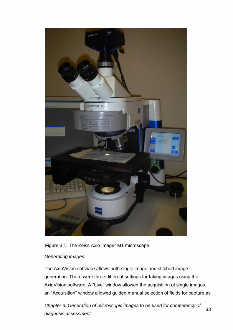
Chapter 3: Generation of microscopic images to be used for competency of
diagnosis assessment 33
Generating images
The AxioVision software allows both single image and stitched image
generation. There were three different settings for taking images using the
AxioVision software. A “Live” window allowed the acquisition of single images,
an “Acquisition” window allowed guided manual selection of fields for capture as
Figure 3.1: The Zeiss Axio Imager M1 microscope
Chapter 3: Generation of microscopic images to be used for competency of
diagnosis assessment 34
part of a stitched image, and the “Mosaic acquisition” carried out an automatic
stitch using auto focusing if required. The second of these, the “Acquisition”
window is illustrated in figure 3.2.
A number of variables in image capture were examined. Initial settings are
described here and these were further developed throughout the project.
Prior to taking an image, settings have to be made in the microscope, control
software and the camera.
Microscope settings
Optimise condenser
Mount slide and initially focus
Locate image area to be acquired
Note stage-starting position.
The microscope screen displays x, y and z values.
Focus using the 63X oil immersion lens
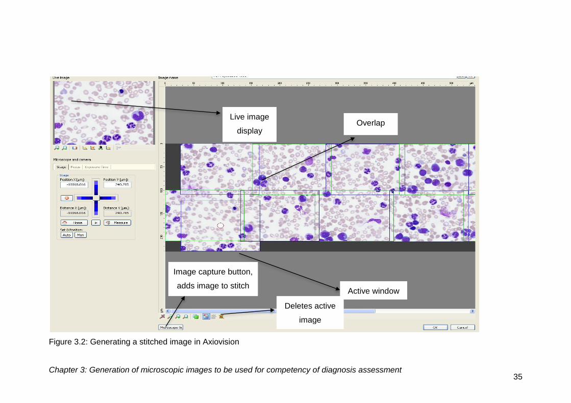
Chapter 3: Generation of microscopic images to be used for competency of diagnosis assessment 35
Figure 3.2: Generating a stitched image in Axiovision
Live image
display Overlap
Active window
Image capture button,
adds image to stitch
Deletes active
image
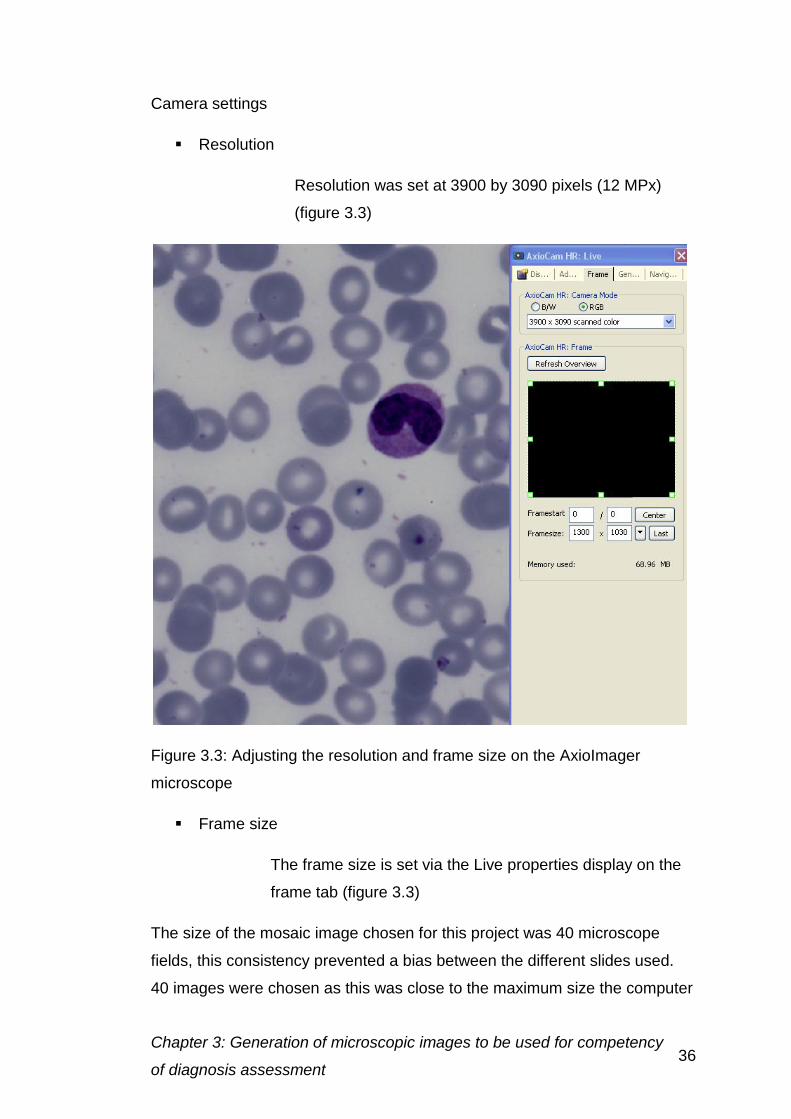
Chapter 3: Generation of microscopic images to be used for competency
of diagnosis assessment 36
Camera settings
Resolution
Resolution was set at 3900 by 3090 pixels (12 MPx)
(figure 3.3)
Figure 3.3: Adjusting the resolution and frame size on the AxioImager
microscope
Frame size
The frame size is set via the Live properties display on the
frame tab (figure 3.3)
The size of the mosaic image chosen for this project was 40 microscope
fields, this consistency prevented a bias between the different slides used.
40 images were chosen as this was close to the maximum size the computer
Chapter 3: Generation of microscopic images to be used for competency
of diagnosis assessment 37
could process at 12 MPx setting, with each field being over 30 Mb, making
the stitch over one Gb.
Automated stitching
Automated stitching used the “Mosaic acquisition” window within AxioVision.
Initially the area to be photographed was chosen and mapped on the screen
(figure 3.4). To allow the images to be joined together accurately, there
needed to be an overlap of more than 10%, to allow the stitching software to
correctly align images. Once these settings had been inputted, the focussing
options were chosen. The focus can either be turned off, so the slide will be
taken in the same focus as was present at starting the acquisition or focus
correction chosen, with focus points chosen manually around the mapped
area or autofocus could be carried out on every tile or every other tile.
Advantages
Quick to set up and create stitched image
Once area is chosen minimal input is required
Ideal for images with little variation in focus plane
Disadvantages
Autofocus may focus on the wrong plane within the image
Vibration during imaging can cause focus to be lost during acquisition
Autofocusing can take a long while and requires a fast stable
computer system to work effectively
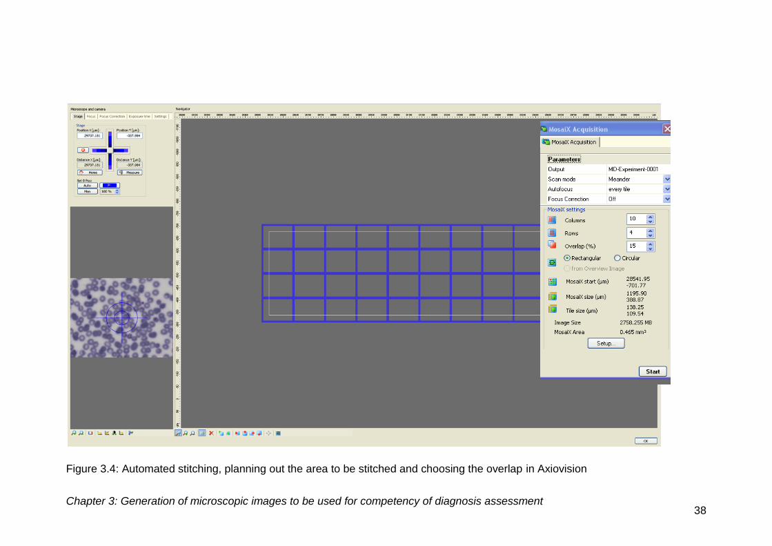
Chapter 3: Generation of microscopic images to be used for competency of diagnosis assessment 38
Figure 3.4: Automated stitching, planning out the area to be stitched and choosing the overlap in Axiovision
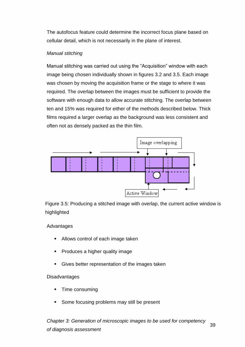
Chapter 3: Generation of microscopic images to be used for competency
of diagnosis assessment 39
The autofocus feature could determine the incorrect focus plane based on
cellular detail, which is not necessarily in the plane of interest.
Manual stitching
Manual stitching was carried out using the “Acquisition” window with each
image being chosen individually shown in figures 3.2 and 3.5. Each image
was chosen by moving the acquisition frame or the stage to where it was
required. The overlap between the images must be sufficient to provide the
software with enough data to allow accurate stitching. The overlap between
ten and 15% was required for either of the methods described below. Thick
films required a larger overlap as the background was less consistent and
often not as densely packed as the thin film.
Advantages
Allows control of each image taken
Produces a higher quality image
Gives better representation of the images taken
Disadvantages
Time consuming
Some focusing problems may still be present
Figure 3.5: Producing a stitched image with overlap, the current active window is
highlighted
Chapter 3: Generation of microscopic images to be used for competency
of diagnosis assessment 40
Single images e.g. of key features can be captured from the “Live” window,
but cannot be used to generate stitches. The Live image allowed increased
magnification and focusing of the image, and could also be used in
combination with the live properties window to set up the microscope.
Image files were either saved individually to be stitched later or just the final
stitch produced in the AxioVision software. To save the entire stitch “Save
as” was used. To save all the individual images “Save all” was used. File
formats were chosen from ZVI (Zeiss Raw format), JPEG and TIFF formats.
3.3.3 Results and discussion
Camera settings
Resolution
To assess the range of zooming possible, trials were run testing low and
high magnification of the acquired image at each camera resolution setting.
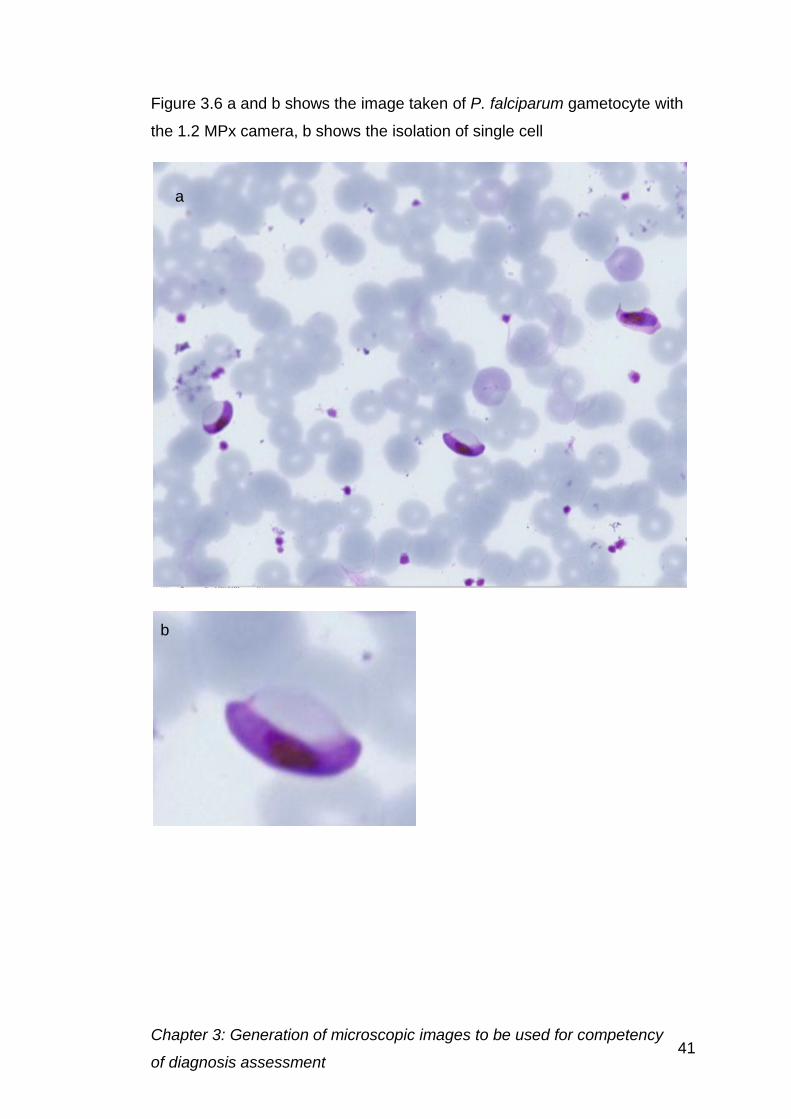
Chapter 3: Generation of microscopic images to be used for competency
of diagnosis assessment 41
Figure 3.6 a and b shows the image taken of P. falciparum gametocyte with
the 1.2 MPx camera, b shows the isolation of single cell
a
b
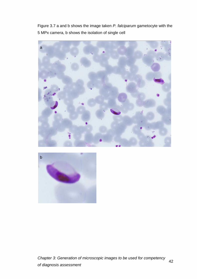
Chapter 3: Generation of microscopic images to be used for competency
of diagnosis assessment 42
Figure 3.7 a and b shows the image taken P. falciparum gametocyte with the
5 MPx camera, b shows the isolation of single cell
a
b
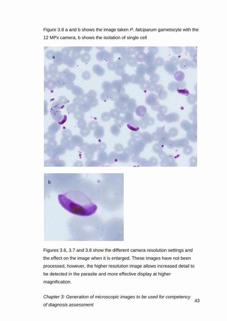
Chapter 3: Generation of microscopic images to be used for competency
of diagnosis assessment 43
Figure 3.8 a and b shows the image taken P. falciparum gametocyte with the
12 MPx camera, b shows the isolation of single cell
Figures 3.6, 3.7 and 3.8 show the different camera resolution settings and
the effect on the image when it is enlarged. These images have not been
processed, however, the higher resolution image allows increased detail to
be detected in the parasite and more effective display at higher
magnification.
a
b
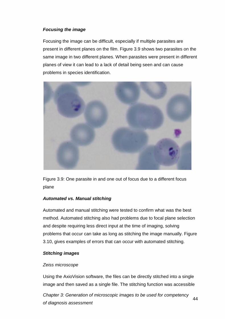
Chapter 3: Generation of microscopic images to be used for competency
of diagnosis assessment 44
Focusing the image
Focusing the image can be difficult, especially if multiple parasites are
present in different planes on the film. Figure 3.9 shows two parasites on the
same image in two different planes. When parasites were present in different
planes of view it can lead to a lack of detail being seen and can cause
problems in species identification.
Figure 3.9: One parasite in and one out of focus due to a different focus
plane
Automated vs. Manual stitching
Automated and manual stitching were tested to confirm what was the best
method. Automated stitching also had problems due to focal plane selection
and despite requiring less direct input at the time of imaging, solving
problems that occur can take as long as stitching the image manually. Figure
3.10, gives examples of errors that can occur with automated stitching.
Stitching images
Zeiss microscope
Using the AxioVision software, the files can be directly stitched into a single
image and then saved as a single file. The stitching function was accessible
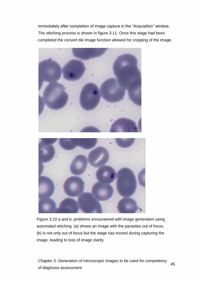
Chapter 3: Generation of microscopic images to be used for competency
of diagnosis assessment 45
immediately after completion of image capture in the “Acquisition” window.
The stitching process is shown in figure 3.11. Once this stage had been
completed the convert tile image function allowed for cropping of the image.
b
Figure 3.10 a and b, problems encountered with image generation using
automated stitching. (a) shows an image with the parasites out of focus,
(b) is not only out of focus but the stage has moved during capturing the
image, leading to loss of image clarity.
a
Chapter 3: Generation of microscopic images to be used for competency
of diagnosis assessment 46
Adobe Photoshop
The photomerge function (File> Photomerge>Automate) can be used to
create mosaic images panoramic software in Photoshop CS3 (PS3). To
allow images generated in the AxioVision software to be used in PS3, the
files were saved as the TIFF format. One of the objectives for using PS3 was
that individual captures images could be processed to enhance detail.
The auto arrangement function in PS3 was used, with the files either being
selected from the folder in which they are saved or the window if they are
already open. If there was enough overlap a perfect stitched image was
produced, which was then cropped and layer flattened into a single image.
Poor images requiring replacement
Even after following a precise protocol some images like those shown in
figure 3.10 would require replacement to ensure that the final large image
was of the optimal quality required.
3.3.4 Conclusion
The 12 MPx camera was chosen to allow more detail to be seen at a higher
magnification to simulate microscopy objective choice up to x100. Even
though the size of the image was three times that of the 1.2 MPx Image, this
was considered necessary to achieve the required image quality.
Due to difficulties in focusing the manual stitching method was chosen, with
extra care being taken to ensure that the slide was flat on the stage, to try to
prevent large differences in the focal plane.
The files were saved as TIFF format, to preserve image quality and to ensure
compatibility with a number of systems. Alternative formats include .zvi a raw
image format used by AxioVision, which was only accessible through
Figure 3.11: The stitching icon in AxioVision
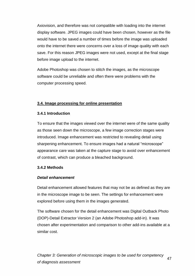
Chapter 3: Generation of microscopic images to be used for competency
of diagnosis assessment 47
Axiovision, and therefore was not compatible with loading into the internet
display software. JPEG images could have been chosen, however as the file
would have to be saved a number of times before the image was uploaded
onto the internet there were concerns over a loss of image quality with each
save. For this reason JPEG images were not used, except at the final stage
before image upload to the internet.
Adobe Photoshop was chosen to stitch the images, as the microscope
software could be unreliable and often there were problems with the
computer processing speed.
3.4. Image processing for online presentation
3.4.1 Introduction
To ensure that the images viewed over the internet were of the same quality
as those seen down the microscope, a few image correction stages were
introduced. Image enhancement was restricted to revealing detail using
sharpening enhancement. To ensure images had a natural “microscope”
appearance care was taken at the capture stage to avoid over enhancement
of contrast, which can produce a bleached background.
3.4.2 Methods
Detail enhancement
Detail enhancement allowed features that may not be as defined as they are
in the microscope image to be seen. The settings for enhancement were
explored before using them in the images generated.
The software chosen for the detail enhancement was Digital Outback Photo
(DOP)-Detail Extractor Version 2 (an Adobe Photoshop add-in). It was
chosen after experimentation and comparison to other add-ins available at a
similar cost.
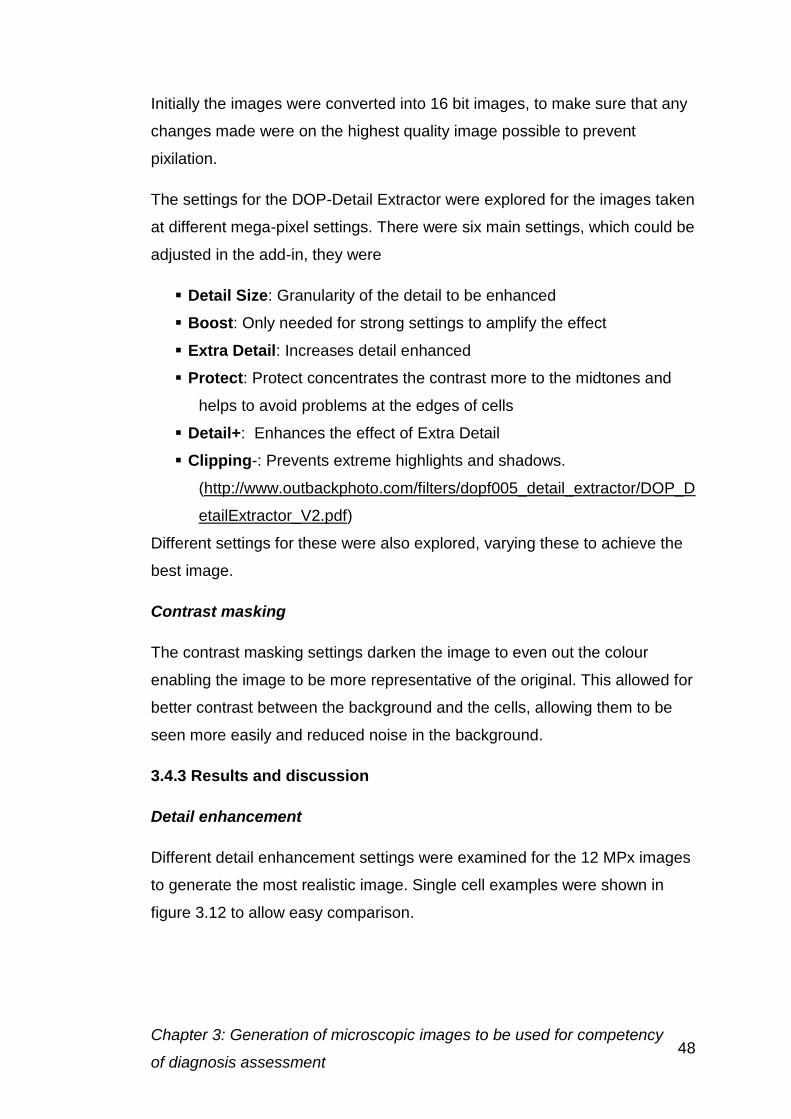
Chapter 3: Generation of microscopic images to be used for competency
of diagnosis assessment 48
Initially the images were converted into 16 bit images, to make sure that any
changes made were on the highest quality image possible to prevent
pixilation.
The settings for the DOP-Detail Extractor were explored for the images taken
at different mega-pixel settings. There were six main settings, which could be
adjusted in the add-in, they were
Detail Size: Granularity of the detail to be enhanced
Boost: Only needed for strong settings to amplify the effect
Extra Detail: Increases detail enhanced
Protect: Protect concentrates the contrast more to the midtones and
helps to avoid problems at the edges of cells
Detail+: Enhances the effect of Extra Detail
Clipping-: Prevents extreme highlights and shadows.
(http://www.outbackphoto.com/filters/dopf005_detail_extractor/DOP_D
etailExtractor_V2.pdf)
Different settings for these were also explored, varying these to achieve the
best image.
Contrast masking
The contrast masking settings darken the image to even out the colour
enabling the image to be more representative of the original. This allowed for
better contrast between the background and the cells, allowing them to be
seen more easily and reduced noise in the background.
3.4.3 Results and discussion
Detail enhancement
Different detail enhancement settings were examined for the 12 MPx images
to generate the most realistic image. Single cell examples were shown in
figure 3.12 to allow easy comparison.
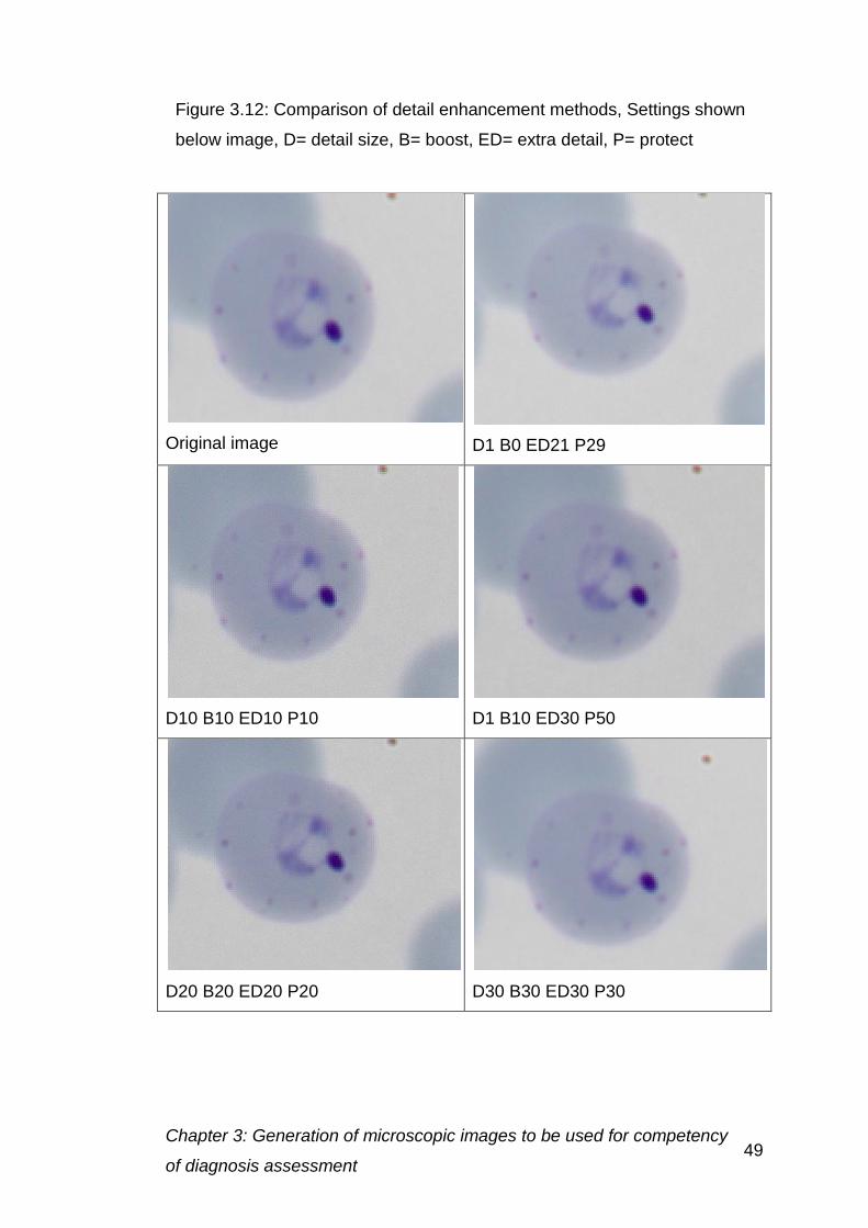
Chapter 3: Generation of microscopic images to be used for competency
of diagnosis assessment 49
Original image
D1 B0 ED21 P29
D10 B10 ED10 P10
D1 B10 ED30 P50
D20 B20 ED20 P20
D30 B30 ED30 P30
Figure 3.12: Comparison of detail enhancement methods, Settings shown
below image, D= detail size, B= boost, ED= extra detail, P= protect
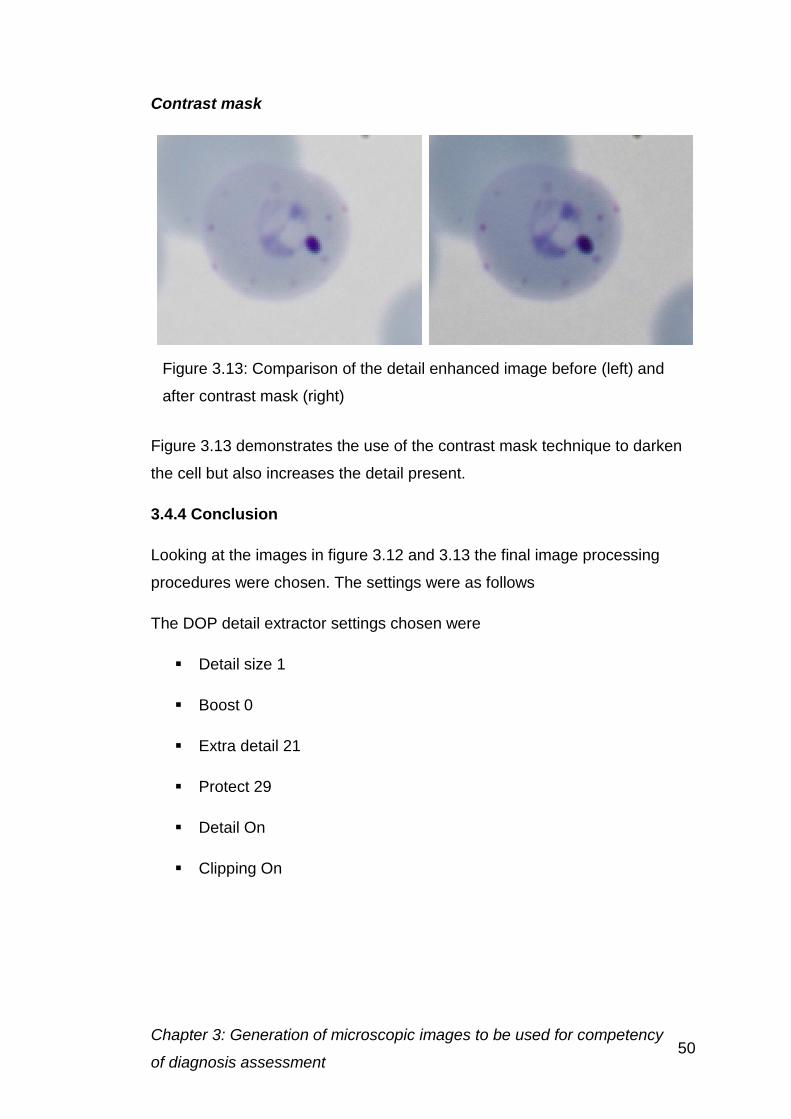
Chapter 3: Generation of microscopic images to be used for competency
of diagnosis assessment 50
Contrast mask
Figure 3.13 demonstrates the use of the contrast mask technique to darken
the cell but also increases the detail present.
3.4.4 Conclusion
Looking at the images in figure 3.12 and 3.13 the final image processing
procedures were chosen. The settings were as follows
The DOP detail extractor settings chosen were
Detail size 1
Boost 0
Extra detail 21
Protect 29
Detail On
Clipping On
Figure 3.13: Comparison of the detail enhanced image before (left) and
after contrast mask (right)
Chapter 3: Generation of microscopic images to be used for competency
of diagnosis assessment 51
Contrast mask settings
Convert image to 16 bit
Duplicate current layer
Desaturate duplicated layer
Invert
Set duplicated layer to 70% opacity
Set duplicated layer to overlay
Apply gaussian blur – 98.7 pixels
Flatten image
Convert image to 8 bit
These were deemed to give the best quality image in the processing time
available. Thick and thin films were treated in the same way, to ensure
consistency in processing.
3.5 Choosing images to be used for competency quality assessment
and training
3.5.1 Introduction
Images were chosen to reflect the challenges that might be faced in a routine
laboratory. These incorporated images of simple and challenging diagnoses.
These include images from the four species that infect humans,
P. falciparum, P. vivax, P. ovale and P. malariae as well as negative
samples.
To ensure that the images were of a comparable quality between the initial
and final assessment preventing bias, the images were each assigned a
classification for:
Chapter 3: Generation of microscopic images to be used for competency
of diagnosis assessment 52
Rank of the microscopic image difficulty
Artefact rank
Species
Parasite density
Thick or thin film
Stage of life cycle present
3.5.2 Methods
Rank of the microscopic image difficulty
The rank of the image was determined by the difficulty of the diagnosis, the
species present, the parasite density and the preparation of the specimen.
There are three values assigned to the rank of the image
1.
Easy to reach diagnosis
Few artefacts present on the specimen
Parasites are obvious and defined
Little stain deposit present
Well prepared blood film
Usually a high parasite density
2.
Moderate difficultly
Some artefacts are present
Parasites are less obvious
Stain deposit is present, but is usually generalised across
the specimen
Some discrepancies in blood film preparation may be
present
Parasite density will be lower than in rank 1
3.
Diagnosis difficult
Artefacts are present
Parasites are difficult to find
Chapter 3: Generation of microscopic images to be used for competency
of diagnosis assessment 53
Stain deposit may be present and may influence diagnosis
Blood film may be poorly prepared
Parasite density is usually very low (one to five cells
present)
Artefact rank
The artefacts on the blood film ranged from stain deposit to the presence of
high numbers of platelets, especially those that were present on top of the
erythrocytes and could be deemed to influence the diagnosis made.
Artefacts were classified from 0 to 4.
0. No artefacts present
1. Few artefacts present, unlikely to influence diagnosis
2. Artefact present, some may be covering cells
3. Artefact present, numerous may prevent parasites being seen
4. Large numbers of artefacts present, may prevent parasites being
seen, but also may be confused as parasites themselves.
Species
The number of cases of each species were chosen to reflect the routine
laboratory workload. However, there were fewer negative cases, as the main
aim of the exercise was to determine if they first identified that parasites were
present and secondly determined the correct species. Negative cases were
however used to determine whether false positive diagnosis was made and
incorrect treatment for the patient, which could contribute to drug resistance.
P falciparum cases were chosen to be the main species, as for the majority
of the laboratories involved, this would be the only species seen. A limited
number of P. malariae cases were available and therefore this was chosen
as the species with the least cases presented.
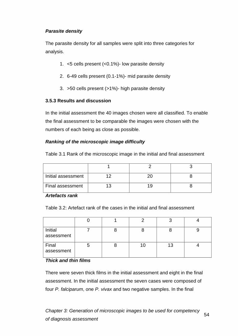
Chapter 3: Generation of microscopic images to be used for competency
of diagnosis assessment 54
Parasite density
The parasite density for all samples were split into three categories for
analysis.
1. <5 cells present (<0.1%)- low parasite density
2. 6-49 cells present (0.1-1%)- mid parasite density
3. >50 cells present (>1%)- high parasite density
3.5.3 Results and discussion
In the initial assessment the 40 images chosen were all classified. To enable
the final assessment to be comparable the images were chosen with the
numbers of each being as close as possible.
Ranking of the microscopic image difficulty
Table 3.1 Rank of the microscopic image in the initial and final assessment
1 2 3
Initial assessment 12 20 8
Final assessment 13 19 8
Artefacts rank
Table 3.2: Artefact rank of the cases in the initial and final assessment
0 1 2 3 4
Initial assessment
7 8 8 8 9
Final assessment
5 8 10 13 4
Thick and thin films
There were seven thick films in the initial assessment and eight in the final
assessment. In the initial assessment the seven cases were composed of
four P. falciparum, one P. vivax and two negative samples. In the final
Chapter 3: Generation of microscopic images to be used for competency
of diagnosis assessment 55
assessment there were eight thick film cases, three P. falciparum, two P.
vivax, one negative, one mixed infection and one P. malariae.
Species
The number of images present for each species was controlled between the
initial and final assessment (table 3.3).
Table 3.3: Number of cases from each species in the initial and final
assessment
P. falciparum
P. vivax
P. ovale
P. malariae
Mixed infection
Negative
Initial assessment
24 3 4 1 1 7
Final assessment
24 3 3 2 1 7
Each of these were then categorised to match those in the initial assessment
P. falciparum
The rank has been compared for the initial and final assessment in table 3.4.
Table 3.4: Number of P. falciparum cases at different ranks
1 2 3
Initial assessment 11 9 4
Final assessment 11 9 4
The parasite density of the P. falciparum cases in the initial and final
assessment is shown in table 3.5.
Chapter 3: Generation of microscopic images to be used for competency
of diagnosis assessment 56
Table 3.5: Number of P. falciparum cases present at different parasite
density ranks
1 2 3
Initial assessment 12 6 6
Final assessment 12 6 6
The presence of artefacts in the initial and final assessment were taken into
account. Table 3.6 shows the artefacts present in the initial and final
assessment.
Table 3.6: Number of cases at each artefact rank in the initial and final
assessment
0 1 2 3 4
Initial assessment
5 6 4 4 5
Final assessment
4 6 5 6 3
P. vivax
The same process was carried out for the other Plasmodium species. As
there were only a small number of cases of these the parasite density was
not taken into account. All cases were present at mid to low parasite density.
The rank of the microscopic image was initially taken into account as in the
initial assessment. Table 3.7 gives the comparison of cases in the initial and
final assessment and the rank given to these cases.
Table 3.7: Rank of P. vivax cases in the initial and final assessment.
1 2 3
Initial assessment 0 2 1
Final assessment 0 2 1
Chapter 3: Generation of microscopic images to be used for competency
of diagnosis assessment 57
As there was only a small number of cases available controlling the artefacts
present in the initial and final assessment was difficult. Table 3.8 shows the
artefact ranking of the images present in the initial and final assessment.
Table 3.8: Artefact rank of P. vivax cases in the initial and final assessment.
0 1 2 3 4
Initial assessment 1 0 1 1 0
Final assessment 0 0 1 2 0
The same procedure was used for the other species.
P. ovale
The rank for the initial and final assessment is compared in table 3.9.
Table 3.9: The rank of P. ovale cases in the initial and final assessment.
1 2 3
Initial assessment 3 1
Final assessment 1 2
The artefacts present in the initial and final assessment for P. ovale cases is
shown in table 3.10.
Table 3.10: Artefacts present in P. ovale cases in the initial and final
assessment
0 1 2 3 4
Initial
assessment
1 1 2 0 0
Final
assessment
1 2 0 0 0
Chapter 3: Generation of microscopic images to be used for competency
of diagnosis assessment 58
P. malariae
In the initial assessment only one P. malariae case was chosen with a rank
of two and three for artefacts. As two images were chosen for the final
assessment on thick film was included. The images had a rank of two and
three for artefacts.
Mixed infection
The mixed infection case was the same for the initial and final assessment,
with an image from the thin film being used in the initial assessment, and
from the thick film in the final assessment.
Overall, the images were chosen to be as close as possible to those used in
the initial assessment to prevent bias occurring in the results.
3.6 The use of the online virtual microscope- SlideBox
3.6.1 Introduction
The virtual microscope system used for this project was used as it was
already in use for haematology digital morphology by UK NEQAS(H) for their
CPD scheme. The system was available without any additional costs to allow
the provision of the images for training and educational purposes.
The Digital SlideBox system (figure 3.14) permits participants’ interaction,
allowing them to complete cases with individual questionnaires being
attached. The system also allows annotations to be added to images, so that
the individual could be given feedback on their performance.
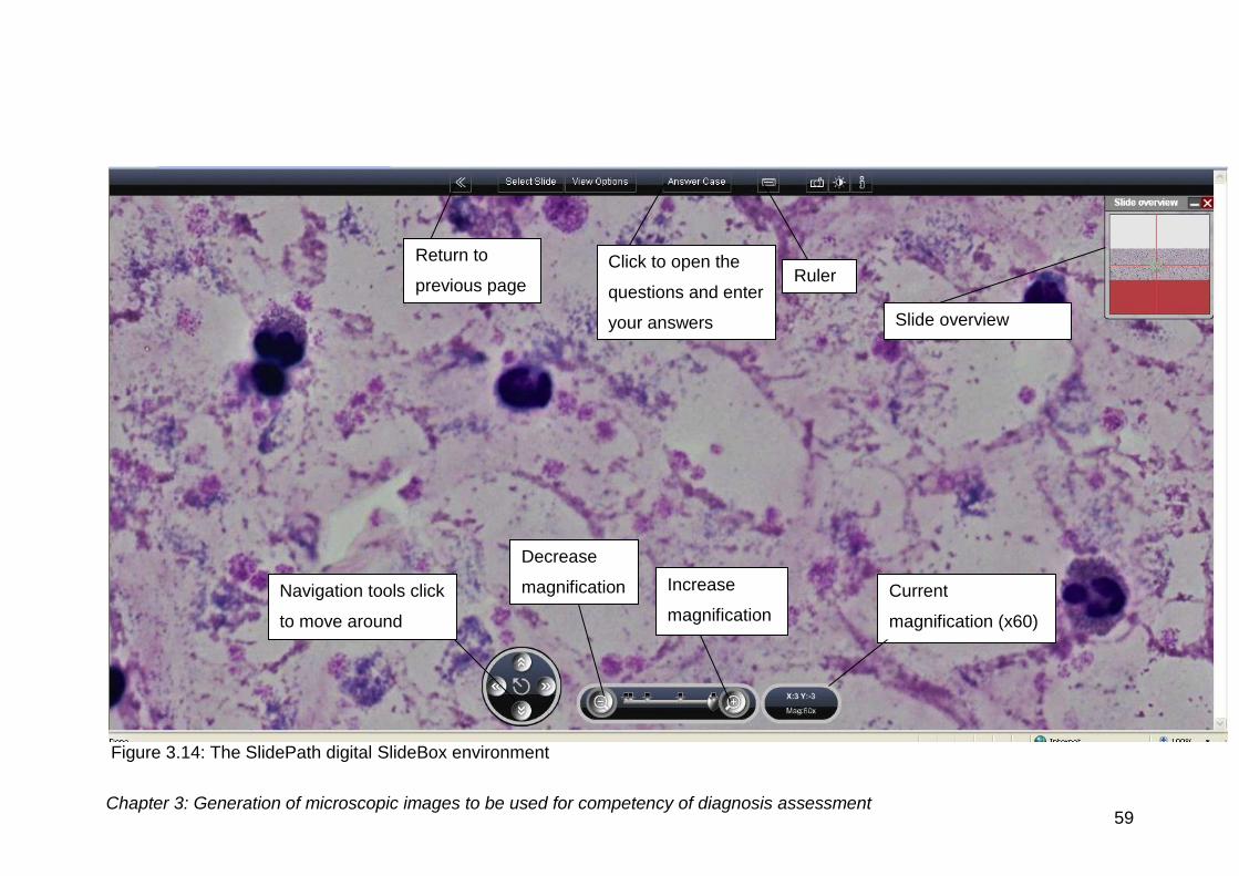
Chapter 3: Generation of microscopic images to be used for competency of diagnosis assessment 59
Figure 3.14: The SlidePath digital SlideBox environment
Ruler
Slide overview
Current
magnification (x60)
Decrease
magnification Increase
magnification
Return to
previous page
Click to open the
questions and enter
your answers
Navigation tools click
to move around
image
Chapter 3: Generation of microscopic images to be used for competency
of diagnosis assessment 60
A number of stages are required throughout the online process to allow
interaction with the images.
3.6.2 Methods
Converting file for upload to SlideBox
Initially the image has to be added to the system. SlidePath could not directly
upload the TIFF images into their software environment as it was only set up
to work with the SVS file format. The images were sent to the software
company via file transfer protocol (FTP) over the Internet. Using Digital Slide
Studio software the TIFF image was converted into an SVS file. This uses
compression to make the image a tenth of its original size to allow quick
access over the Internet and to apply the magnification to the image. There
is a loss of image quality at this stage, which is why the sharpening
procedures are used, to allow the image provided to be of the highest quality
possible.
Testing the image uploaded into SlideBox
Once the image had been uploaded the software can then be set up to allow
the case to be accessed directly on the virtual microscope administration
pages (figure 3.15). The image can be selected from its location on the
server using the add slide command.
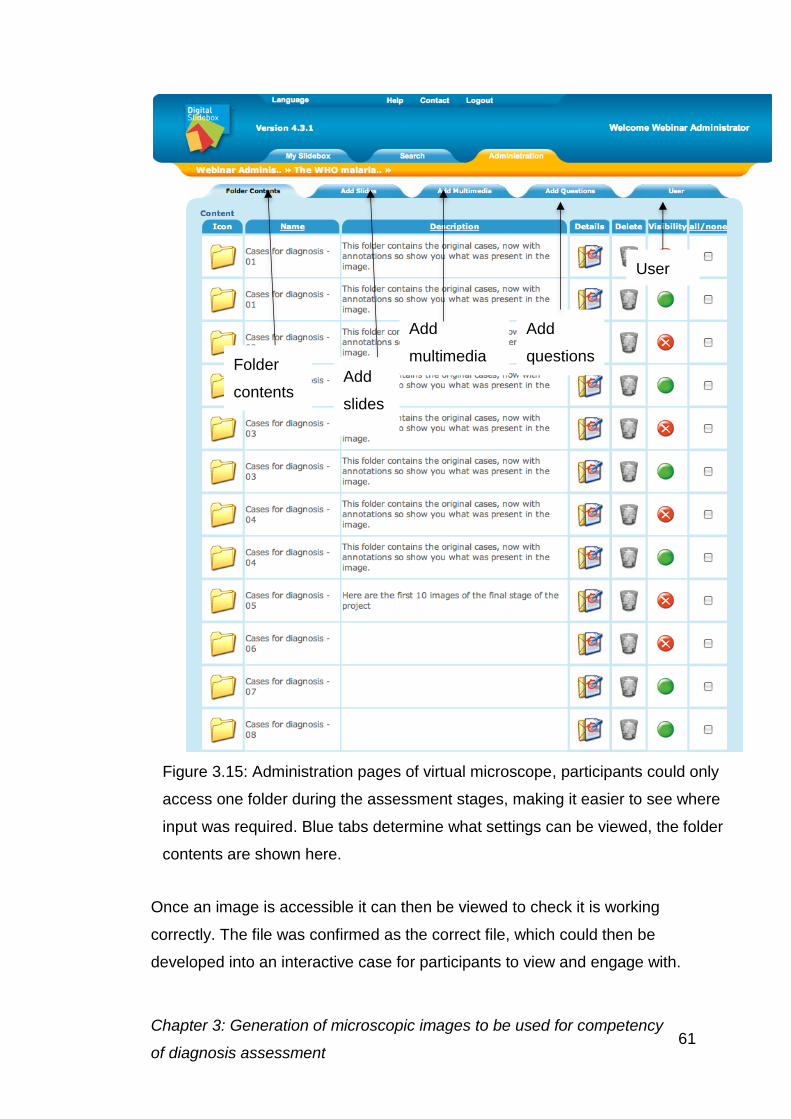
Chapter 3: Generation of microscopic images to be used for competency
of diagnosis assessment 61
Once an image is accessible it can then be viewed to check it is working
correctly. The file was confirmed as the correct file, which could then be
developed into an interactive case for participants to view and engage with.
Figure 3.15: Administration pages of virtual microscope, participants could only
access one folder during the assessment stages, making it easier to see where
input was required. Blue tabs determine what settings can be viewed, the folder
contents are shown here.
Folder
contents Add
slides
Add
multimedia
Add
questions
User
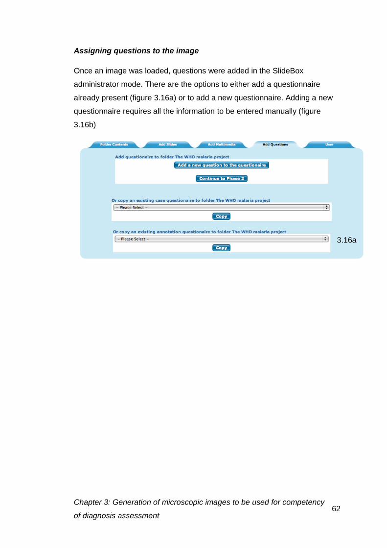
Chapter 3: Generation of microscopic images to be used for competency
of diagnosis assessment 62
Assigning questions to the image
Once an image was loaded, questions were added in the SlideBox
administrator mode. There are the options to either add a questionnaire
already present (figure 3.16a) or to add a new questionnaire. Adding a new
questionnaire requires all the information to be entered manually (figure
3.16b)
3.16a
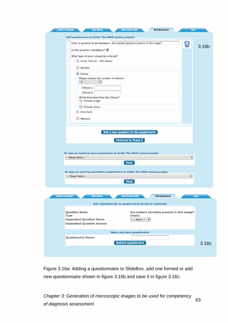
Chapter 3: Generation of microscopic images to be used for competency
of diagnosis assessment 63
Figure 3.16a: Adding a questionnaire to SlideBox, add one formed or add
new questionnaire shown in figure 3.16b and save it in figure 3.16c.
3.16b
3.16c
Chapter 3: Generation of microscopic images to be used for competency
of diagnosis assessment 64
Adding annotations
When an image is open, annotations can also be added. Annotations can
either be in the form of a box, a circle or as an arrow. The area for the
annotation to be added will first be chosen; once the annotation has been
drawn information can then be added (figure 3.17). The feature can first be
named, a description added and then placed into a group so that similar cells
can be viewed together.
Preparing feedback
Feedback on the image is useful for the individual to indicate how they have
performed. The narrative was written in the edit narrative box (figure 3.18),
links can also be added either to annotations on the case, layers of similar
features or to a separate website, in this case to the photo gallery website.
This provides all the stages involved in the generation of the stitched image.
The processes involved in generated images for the gallery images will be
described in the next section.
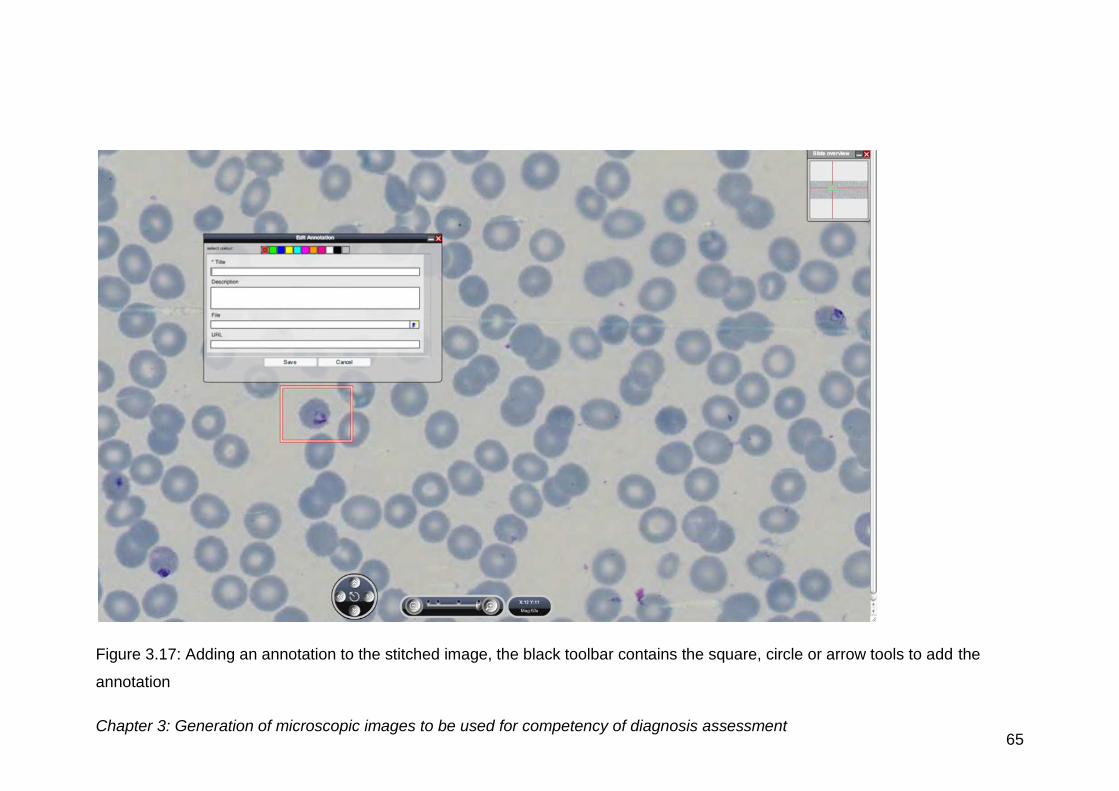
Chapter 3: Generation of microscopic images to be used for competency of diagnosis assessment 65
Figure 3.17: Adding an annotation to the stitched image, the black toolbar contains the square, circle or arrow tools to add the
annotation
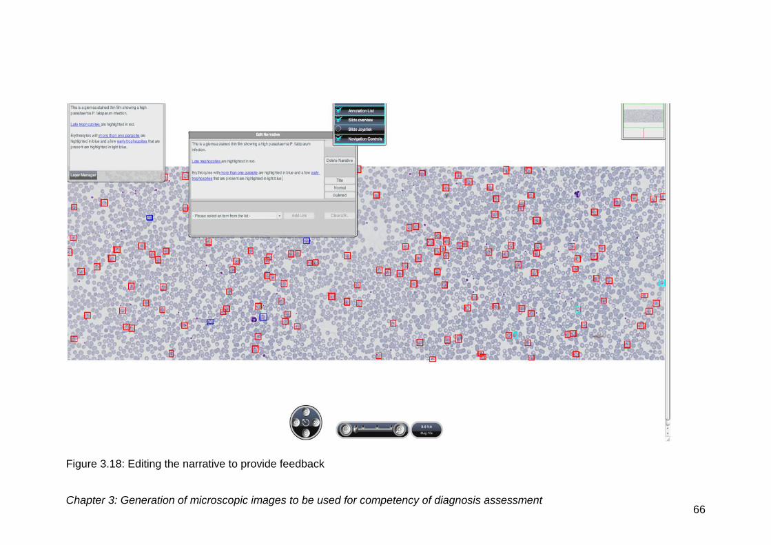
Chapter 3: Generation of microscopic images to be used for competency of diagnosis assessment 66
Figure 3.18: Editing the narrative to provide feedback
Chapter 3: Generation of microscopic images to be used for competency
of diagnosis assessment 67
3.6.3 Discussion
There were difficulties with the upload of the 12 MPx stitched image as the
image displayed incorrectly with the wrong magnification, making the image
three times the normal size. The reason this occurred, was that the system
based scale on a 1.2 MPx image and used the number of pixels to determine
the size of the image and therefore the magnification. As at 12 MPx there
were three times the number of pixels than at 1.2 MPx, the image appeared
three times as large. The file therefore had to be converted to the size of a
1.2 MPx image in Adobe Photoshop before upload, as the sharpening and
detail enhancement was done with the file at 12 MPx, this did not affect the
image quality at the image magnification required. The upload converts the
file into an SVS format, allowing the image to be viewed on the system.
When assigning questions to an image, difficulties were encountered with the
wording of the questions. Any question that contained an apostrophe caused
difficulties, the system was unable to identify these and therefore the
questionnaire could not be completed. On removing the apostrophes from
the questionnaire all of these features worked as would be expected.
Annotated images could only be of a certain size. The addition of too many
annotations to an image caused the image to be slow to load and also
caused annotations to be lost. For images with more than 200 annotations
(i.e. more than 200 parasites present), some of these had to be removed,
with only parasites with characteristic diagnostic features or EDTA changes
being highlighted.
3.7 Overall conclusion
We have clearly demonstrated that it is possible to generate images of blood
smears that can be used for quality assurance in order to improve the
diagnosis and, thereby improve treatment, of haematological disease.
Chapter 4: Generation of e-learning for the morphological diagnosis of 68
malaria
Generation of e-learning for the morphological diagnosis of malaria
4.1 Introduction
E-learning enables individual training without the trainer having to be present
and is referred to by Nichols (2008) as “pedagogy empowered by digital
technology”. However, Guri-Rosenblit (2005) explains that distance
education and e-learning are not necessarily the same thing.
E-learning has been developed in many different areas of higher education,
to provide initial learning materials (Laurillard, 2005) and to act as a vehicle
of continuous professional development (Klein and Ware, 2003) and has
been used in biomedical science education and training for some time (Ryan
et al, 2000). Moreover, the use of a virtual microscope to enhance these
activities, has been demonstrated to be of benefit to the learner when used in
teaching and training in pathology (Sinn et al., 2008).
E-learning offers many benefits over conventional teaching, but also has
disadvantages associated with a lack of direct student supervision.
Benefits of e-learning (About E-Learning, 2007-2010; Littlejohn and Higgison,
2003)
Allows working at students pace
Access at anytime, anywhere
Interactive environment
Individual progress can be monitored
Reduces transport costs
Enables people living in remote areas and developing nations to
receive education and material to which they would not normally have
access
Provides access to a range of resources which may not otherwise be
available

Chapter 4: Generation of e-learning for the morphological diagnosis of 69
malaria
Encourages collaborative learning
Problems of e-learning
Engagement of the learner into the training
Lack of structure to simulate student effort
Problems with internet connectivity
Instructor not always available when required
Isolation of students
Collaboration when all inexperienced individual learners report false
results
Language used and understanding of training information
4.2 Pedagogy of e-learning
The arrival of the Internet has facilitated the enhancement of training in many
different areas. This process is often called e-learning. The effectiveness of
e-learning provision can depend greatly on the preferred learning styles of
the individuals; therefore, learning styles should be taken into account during
the design stage (Wang et al, 2006) of the programme. There are a number
of learning style models that have been proposed, a brief description of each
follows.
Kolb’s model is based on experiential learning theory (Kolb, 1984). The
Kolb theory is based on learning through experience, followed by observation
and reflection on the experience. Abstract concepts can then be created,
based upon the reflection, followed by testing the new concepts, which
reinforces learning. Kolb determined that the ideal educational material
provides all of these processes (Kolb, 1984). Individuals however, show
strengths in specific areas, allowing specific learners to be identified
Chapter 4: Generation of e-learning for the morphological diagnosis of 70
malaria
1. Converger- use active experience and abstract concepts to learn,
making them good at practically applying ideas and solving problems
using reasoning
2. Diverger- use concrete experience and reflective observation, making
them imaginative, producing ideas and having the ability to see things
from other perspectives
3. Assimilators- abstract conceptualisation and reflective observation,
create theoretical models using inductive reasoning
4. Accommodators- concrete experience and active experimentation,
engage by actions rather than reading and studying
Manochehr (2006) compared e-learning with traditional teaching for students
of different learning styles. He showed that the learning style of the individual
was significantly important for individuals undertaking e-learning but not for a
laboratory based class. Assimilators and convergers performed better with
the online training than with an instructor led course. Other studies have had
difficulty proving the effectiveness of learning styles and have not reached
consensus in their conclusions (Coffield et al, 2004).
Kolb’s method has been adapted by Honey and Mumford, who initially
renamed the phases in the cycle, to align them with problem solving and
decision making processes (Mumford, 1995).
1. Having an experience
2. Reviewing the experience
3. Concluding from the experience
4. Planning the next steps
The styles were also renamed to Activist, Reflector, Theorist and Pragmatist.
Two questionnaires were developed to help categorise learners, containing
either 40 or 80 questions (Honey and Mumford, 2000). The self-assessment
allowed the learning style to be used within industrial and commercial
settings studied.
Chapter 4: Generation of e-learning for the morphological diagnosis of 71
malaria
Gregorc also developed a learning style based around two perceptual
qualities concrete and abstract and two ordering abilities sequential and
random (Anon, 2008). A questionnaire was developed to categorise learners,
based upon their responses to questions. There are four groups Concrete
Sequential (CS), Abstract Random (AR), Abstract Sequential (AS) and
Concrete Random (CR). This takes into account each individual’s strengths
and weaknesses, using the combination of learning methods.
The Flemings Vark model is one of the most common and widely used
models (Leite, 2010). The model is an expansion on Neuro-linguistic
programming models. Learners are classified as visual learners, auditory
learners and kinaesthetic or tactile learners (Hawk, 2007).
Other models include the Dunn and Dunn model in which sociological and
environmental factors are taken into account in addition to those in the other
models combined (Hawk, 2007).
Alongside these basic learning models, specific models for e-learning
programmes have also been developed to cover specific learning needs and
also to include interactivity. Three models have been specifically developed
for e-learning pedagogy (The University of Manchester, n.d.).
Mayes: The conceptualisation cycle. The cycle describes learning as a
cyclical dynamic feedback process, having three components
conceptualisation, construction and application, (Mayes and Fowler, 1999).
Conceptualisation is focused on the transfer of knowledge from the teacher
to the learner (Buzzetto-More, 2007). This involves the exposure to other
people’s ideas or concepts (The University of Manchester, n.d.). The later
stages expand on the conceptualisation step, construction builds upon
concepts. The construction is using the ideas they have been given and
practically applying these to meaningful tasks (JISC, 2012). The application
component, tests the conceptualisation component, using applied concepts.
The goal is to test the understanding of abstract concepts, often developed
during conversations and reflection with tutors and fellow learners, mainly
through feedback on quizzes or tasks (Mayes and Fowler, 1999). The
Chapter 4: Generation of e-learning for the morphological diagnosis of 72
malaria
learning is increased by constant feedback between the different stages in
the process. To provide these components, three levels of learning are
proposed, primary, secondary and tertiary courseware. The primary
courseware presents the subject matter. The secondary courseware is the
environment in which the matter is presented and the tools the learner uses.
The tertiary courseware is material produced by previous learners, peer
discussions and outputs from assessments (Mayes and Fowler, 1999).
Laurillard’s conversational model (Laurillard, 1993) is based on the
discussions between tutors and students. The model emphasises the use of
communication within e-learning environments e.g. narratives (JISC, 2012).
Interactions are designed to provide feedback, e.g. interactive feedback on
outcomes of tasks and is used adaptively to revise the content for future
groups. Discussion forums are also recommended, to allow the tutor to
provide feedback and students can reflect on their achievements (University
of Manchester, n.d.).
Salmon: 5 stage model and e-moderating, is designed for computer-
mediated communication, the model is proposed as a five stage highly
practical approach.
Stage 1: Access and motivation, providing quick and easy access to
the virtual learning environment
Stage 2: Online socialisation, becoming comfortable with the online
environment
Stage 3: Information Exchange, Interactivity with virtual learning
environment and e.g. web links, databases case studies and fellow
learners.
Stage 4: Knowledge Construction, building online communities
focusing on learning.
Stage 5: Development, taking responsibility for their own learning and
becoming more confident and critical thinkers. (Salmon, 2003)
Mastery for learning was initially proposed by Bloom (1968), in 1971 this
was modified to mastery learning (Bloom, 1971). Mastery learning proposes
Chapter 4: Generation of e-learning for the morphological diagnosis of 73
malaria
that all students can learn to any level given enough time. The approach is to
allow each student to complete a section and making sure they achieve a
predetermined level of achievement before moving onto the next stage
(Block and Burns, 1976). The level of achievement needs to be
predetermined to ensure the level achieved at this stage is high enough to
allow individual’s to progress.
Mastery has been used in a number of studies, Barsuk (2010) reported on
the use on mastery learning in the training of venous catheter insertion.
Simulation-based mastery learning requires students to meet a required
standard before progression to carrying out testing on patients. The results
from the mastery training showed that skills acquired were substantially
retained.
Leonard and Gerace (2010) report the use of mastery learning in the
teaching of Physics at the University of North Carolina. Due to poor
performance in one of the modules a prerequisite course was developed to
improve understanding. In order to progress onto the module students were
required to reach the desired level of mastery.
A number of studies in medical education have assessed the learning styles
of the students, using a number of different methods. Zeraati et al, (2008)
used the VARK questionnaire to assess the learning styles of their students.
The majority of these students were auditory learners.
Lujah and DiCarlo (2006) also carried out the VARK assessment on a group
of first year students. They discovered the majority of the students used
multiple learning styles (63.8%), with the highest individual category being
kinaesthetic at 18.1%. Similar results were seen by Johnson (2009) with
52.4% of their first year students using multiple modes of learning. However,
a group of students were investigated who had been admitted to the
university from targeted groups, these individuals were split between
multimodal (28.1%) and kinaesthetic (28.1%). There were no auditory
learners amongst the standard admission students, however in the targeted
group there were 12.5%.
Chapter 4: Generation of e-learning for the morphological diagnosis of 74
malaria
Engels and de Gara (2010) used Kolb’s method to assess medical students
in comparison with surgeons. The medical students were mainly
assimilators, however qualified surgeons were mainly convergers. This
indicated a different teaching mechanism was required for students and
surgeons. In another study with medical students, Danish and Awan (2008)
found that the majority of their students (54.6%) were accommodators.
However, Rohrer and Pashler (2012) argue that learning styles have no
effect on medical education, as a review of the data shows no significant
difference in results achieved. Due to the cost of assessing the student and
re-writing some courses, they argue that the change is not cost effective for
limited, if any, benefit for the students. They say “educators should instead
focus on developing the most effective and coherent ways to present
particular bodies of content, which often involve combining different forms of
instruction”. A principle that can be applied to online delivery of cell
morphology using the virtual microscope.
Most studies on the use of virtual microscopy have been in histology
teaching. Harris et al, 2001) compared a virtual microscopy laboratory and
the regular microscope laboratory for teaching histology. Harris concluded
that the virtual microscope is a viable addition to, if not a replacement for
microscopes and glass slides. The students also preferred the use of the
virtual microscope to the standard microscope. Jonas-Dwyer et al (2011)
investigated the use of learning styles with virtual microscopy teaching. They
used the ASSIST inventory to assess the learning styles of the individuals,
both at the beginning and end of the teaching period. The ASSIST inventory
categorises individuals as deep, strategic or surface apathetic learners. The
study showed an increase in the number of deep learners as the course
progressed, indicating increased involvement with the microscope over time.
This change in approach was not observed in students solely using the
laboratory based microscope and traditional teaching.
There are a number of training schemes for education in the diagnosis of
malaria, histology and haematology, but the authors have not indicated
Chapter 4: Generation of e-learning for the morphological diagnosis of 75
malaria
whether learning styles were taken into account during the development of
these training programmes. The WHO malaria microscopy teachers guides
(2010b), describe how to provide a training programme for malaria diagnosis,
but no consideration of learning styles seems to have been taken into
account.
Goubran and Vinjamury (2007) designed a tool for selective directed learning
in histology, using an atlas-based approach. The atlas was shown to
significantly improve the results of students who used the system, compared
to those with no access and was highly popular with students.
Other training guides developed for malaria diagnosis include World Health
Organization (2010b), World Health Organization (1999), and Shoklo malaria
research institute (2002), none of these used learning styles in the design of
the training.
The ideal training programme for malaria diagnosis should be designed
around the mastery learning approach. With an unlimited time frame
students would be able to work at their own pace to achieve high levels of
competency on the recognition of each parasite stage and species before
moving onto the next.
4.3 Intervention package content
To enable the delivery of training materials a number of potential issues were
considered.
4.3.1 Target audience
In generating an e-learning programme the target audience should always be
the initial consideration (Ismail, 2001). The audience was laboratory
scientists, from around the world, possibly with English not being the first
language.
Chapter 4: Generation of e-learning for the morphological diagnosis of 76
malaria
Participants had different experience levels, which were determined using
the questionnaire. The data provided was then used to categorise the
participants’ results in the initial and final assessment.
Learning styles of the individuals were also considered, the training was
designed to cover all possible learning styles deliverable via e-learning.
Visual and kinaesthetic approaches were covered, however auditory was
not, as the computers in use may not have had audio capability.
4.3.2 Assessment of material that was already available on-line
A variety of websites are available for the diagnosis of malaria, some giving
information about the malaria parasite in general, others giving diagnostic
information. The WHO offers a recently updated training guide to be used in
the diagnosis of malaria (World Health Organization, 2010b). The guide
gives basic information about malaria and laboratory techniques involved in
its diagnosis. A few examples of the parasite’s appearance at different
stages of development are given, with one image of each stage of
development of the protists. The WHO generates bench aids (World Health
Organization, 1999) to go alongside this information. These aids provide
limited examples of parasite species and stages, but do use photographic
examples of parasite appearance. Most provide single examples of cells and
provide no interactive challenge.
The Shoklo Malaria Research Unit (2002) in Thailand have also generated
an in house training guide, based on a modification of the original WHO
guide (World Health Organization, 1991). There is more extensive
information about blood morphology in general and further malaria examples.
Methodology is also considered in this guide, with criteria for assessing the
quality of staining given. Images provided are of poor quality, with the colour
of the images, in some cases, giving misleading representations.
There are also a number of different websites that provide similar information
to these training guides. The Center for Disease and Control website
(Centers for Disease Control and Prevention, 2008) lists information about all
Chapter 4: Generation of e-learning for the morphological diagnosis of 77
malaria
tests carried out in diagnosis, and also provides links to galleries of images
of individual parasite infected blood cells, the equivalent to the bench aids
produced by the WHO.
The Royal Perth Hospital, Australia (Royal Perth Hospital, 2003) website
gives information on the laboratory diagnosis of malaria and offers an
engaging teach and test section. This website asks users to view a patient
case and determine, from the images given, whether malaria is present and
to identify the species.
The UK NEQAS parasitology scheme has a website dedicated to the
diagnosis of malaria (United Kingdom Quality Assessment Scheme for
Parasitology, 2006). This website gives details of the methods required for
the accurate diagnosis of malaria and the effects of storage of whole blood in
EDTA on the morphology of the parasites.
Material available to laboratory workers to aid the diagnosis of malaria was
discussed with recognised experts who identified some problem areas in the
diagnosis of malaria. Species identification was highlighted as a major issue,
along with the quantification of the parasite density and microscopic slide
preparation (Williams, 2009). These issues were all addressed within the
project, by including images and examples to compliment the written text.
Upon assessment of the currently available learning/ training material the
following topics were identified as being essential to the proposed training
schedule:
Laboratory methods
o Problems associated with incorrect preparation of the blood
smear
o How to avoid problems in preparation of microscopic materials
Background information about malaria
Assessing the presence of parasites
Chapter 4: Generation of e-learning for the morphological diagnosis of 78
malaria
Appearance of parasite stages
o Information of life cycle stages
o Multiple images of each stage
Species comparison
o Details of differences between species
o Images showing variation in morphology with the same species
Quantitation of parasite density
Thick films versus thin films
4.4 Intervention package structure
An integrated training package capable of being offered to laboratory
workers currently undertaking microscopical analysis of malaria parasites.
This package would allow participants to study at their own pace, to their
own knowledge level and learning style.
4.4.1 Participant experience and knowledge
The content of the training was designed to build on the current knowledge
the participants already had and allow them to further develop their skills.
The format of the training would, therefore, take this into consideration,
facilitating individuals with more experience to benefit from the training given.
To this end, training material was initially generated for three different
experience levels
Basic - newly qualified staff or those with less than 1 years experience
Intermediate laboratory staff with considerable experience working in
the laboratory for 2 – 5 years
Advanced- senior staff with more than 6 years experience
Chapter 4: Generation of e-learning for the morphological diagnosis of 79
malaria
However, the file structure this created was complicated, and made
navigation difficult, especially at this stage when Microsoft Word documents
were being used. To solve this, one document was developed for each topic
with increasing complexity being delivered as the participant progressed
through the single document. To encourage engagement, a quiz would be
placed at the bottom of each page. The feedback associated with this
process would allow the participants to revisit any areas of the learning
material in which they had difficulty in understanding. Therefore, the
participants did not have to categorise their experience and therefore their
training was optimised.
4.4.2 Participant guidance
To enable the participants to study the programme, guidance was given to
ensure that they understood the objectives of the study and what they were
expected to achieve (learning objectives). The guidance provided help and
information at every stage of the learning material.
Although the training programme contains background information about
malaria, the main purpose was to improve the detection and identification of
parasites. Participants were, therefore, guided to study this area first, which
in addition contained substantial information about diagnosis.
The participants were provided with a “how to study” document along with
the information provided on the initial access page.
Participants also had email contact with the author at all times to allow any
other questions to be answered. The quizzes were provided with a
submission button, to allow them to submit the results of any quizzes if they
wanted any further feedback.
4.4.3 Structure
The structure of the training aimed to be sequential, to help the participants
progress from one stage to the next. There was also the facility to link
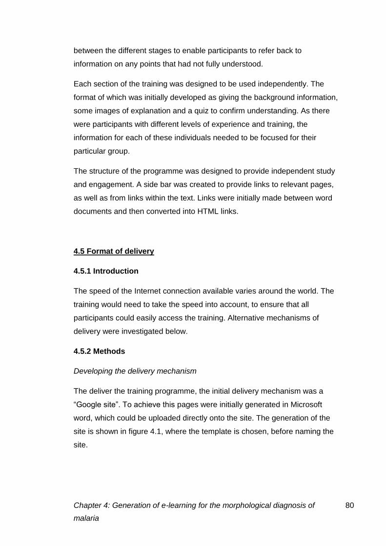
Chapter 4: Generation of e-learning for the morphological diagnosis of 80
malaria
between the different stages to enable participants to refer back to
information on any points that had not fully understood.
Each section of the training was designed to be used independently. The
format of which was initially developed as giving the background information,
some images of explanation and a quiz to confirm understanding. As there
were participants with different levels of experience and training, the
information for each of these individuals needed to be focused for their
particular group.
The structure of the programme was designed to provide independent study
and engagement. A side bar was created to provide links to relevant pages,
as well as from links within the text. Links were initially made between word
documents and then converted into HTML links.
4.5 Format of delivery
4.5.1 Introduction
The speed of the Internet connection available varies around the world. The
training would need to take the speed into account, to ensure that all
participants could easily access the training. Alternative mechanisms of
delivery were investigated below.
4.5.2 Methods
Developing the delivery mechanism
The deliver the training programme, the initial delivery mechanism was a
“Google site”. To achieve this pages were initially generated in Microsoft
word, which could be uploaded directly onto the site. The generation of the
site is shown in figure 4.1, where the template is chosen, before naming the
site.
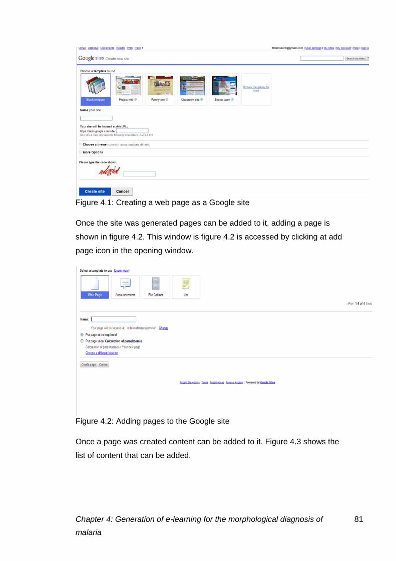
Chapter 4: Generation of e-learning for the morphological diagnosis of 81
malaria
Figure 4.1: Creating a web page as a Google site
Once the site was generated pages can be added to it, adding a page is
shown in figure 4.2. This window is figure 4.2 is accessed by clicking at add
page icon in the opening window.
Figure 4.2: Adding pages to the Google site
Once a page was created content can be added to it. Figure 4.3 shows the
list of content that can be added.
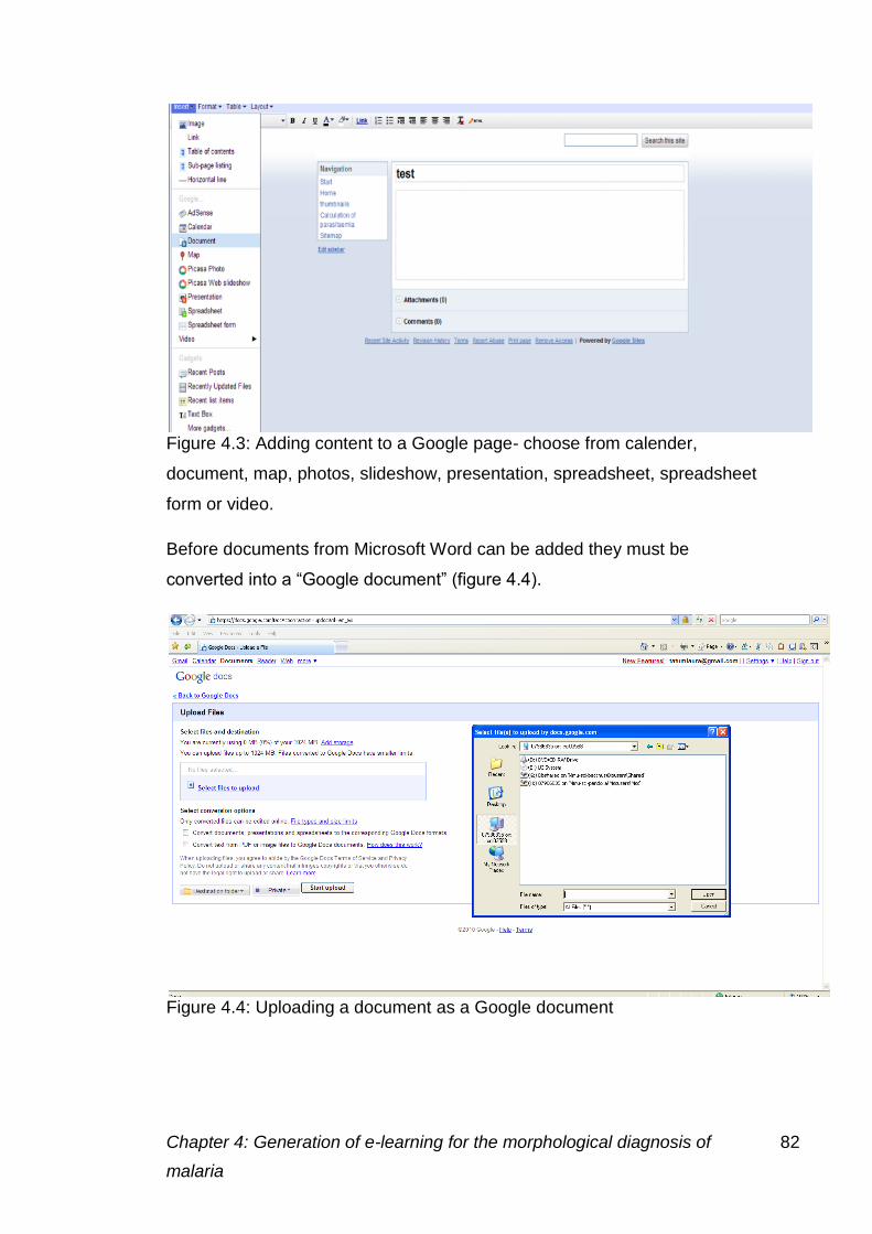
Chapter 4: Generation of e-learning for the morphological diagnosis of 82
malaria
Figure 4.3: Adding content to a Google page- choose from calender,
document, map, photos, slideshow, presentation, spreadsheet, spreadsheet
form or video.
Before documents from Microsoft Word can be added they must be
converted into a “Google document” (figure 4.4).
Figure 4.4: Uploading a document as a Google document
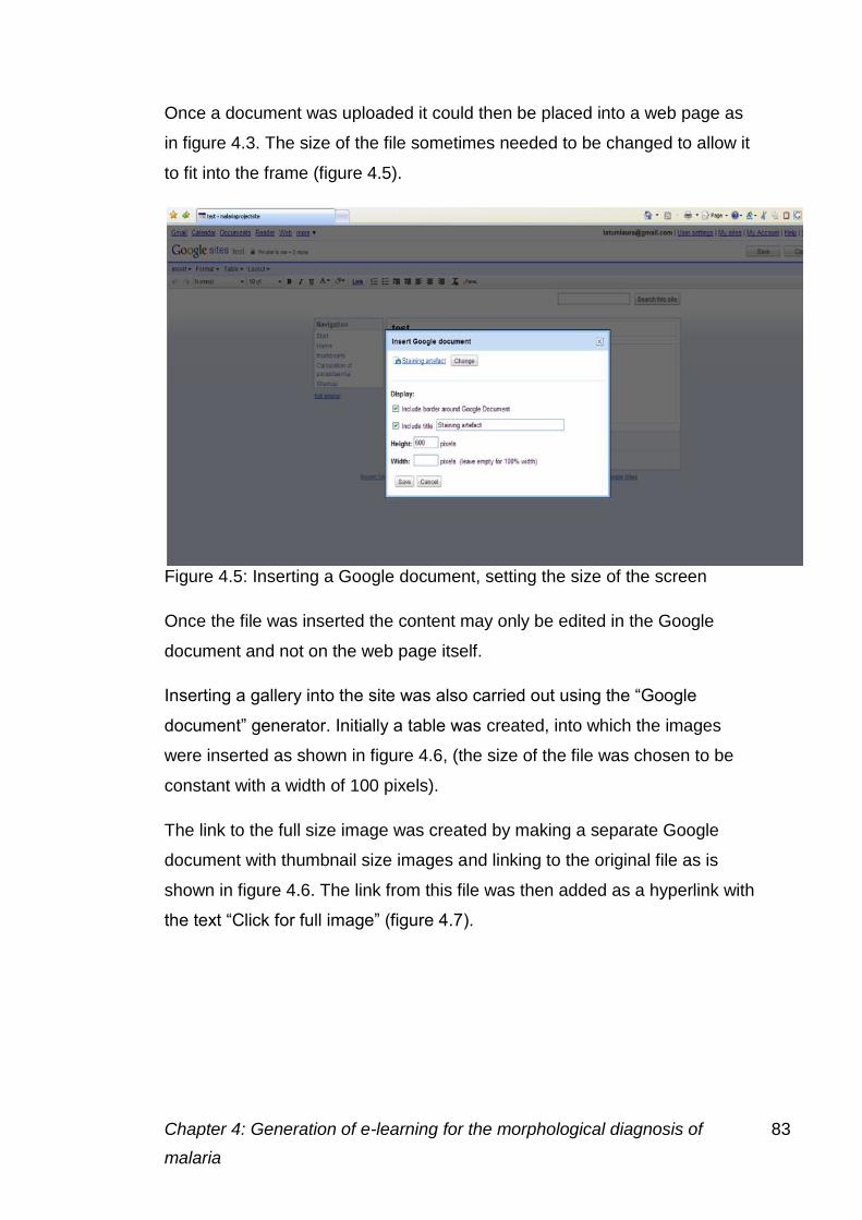
Chapter 4: Generation of e-learning for the morphological diagnosis of 83
malaria
Once a document was uploaded it could then be placed into a web page as
in figure 4.3. The size of the file sometimes needed to be changed to allow it
to fit into the frame (figure 4.5).
Figure 4.5: Inserting a Google document, setting the size of the screen
Once the file was inserted the content may only be edited in the Google
document and not on the web page itself.
Inserting a gallery into the site was also carried out using the “Google
document” generator. Initially a table was created, into which the images
were inserted as shown in figure 4.6, (the size of the file was chosen to be
constant with a width of 100 pixels).
The link to the full size image was created by making a separate Google
document with thumbnail size images and linking to the original file as is
shown in figure 4.6. The link from this file was then added as a hyperlink with
the text “Click for full image” (figure 4.7).
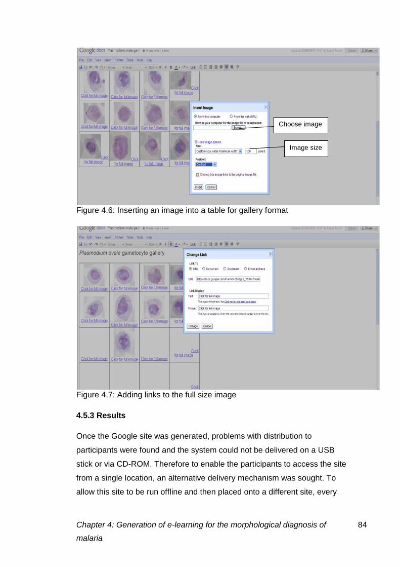
Chapter 4: Generation of e-learning for the morphological diagnosis of 84
malaria
Figure 4.6: Inserting an image into a table for gallery format
Figure 4.7: Adding links to the full size image
4.5.3 Results
Once the Google site was generated, problems with distribution to
participants were found and the system could not be delivered on a USB
stick or via CD-ROM. Therefore to enable the participants to access the site
from a single location, an alternative delivery mechanism was sought. To
allow this site to be run offline and then placed onto a different site, every
Image size
Choose image
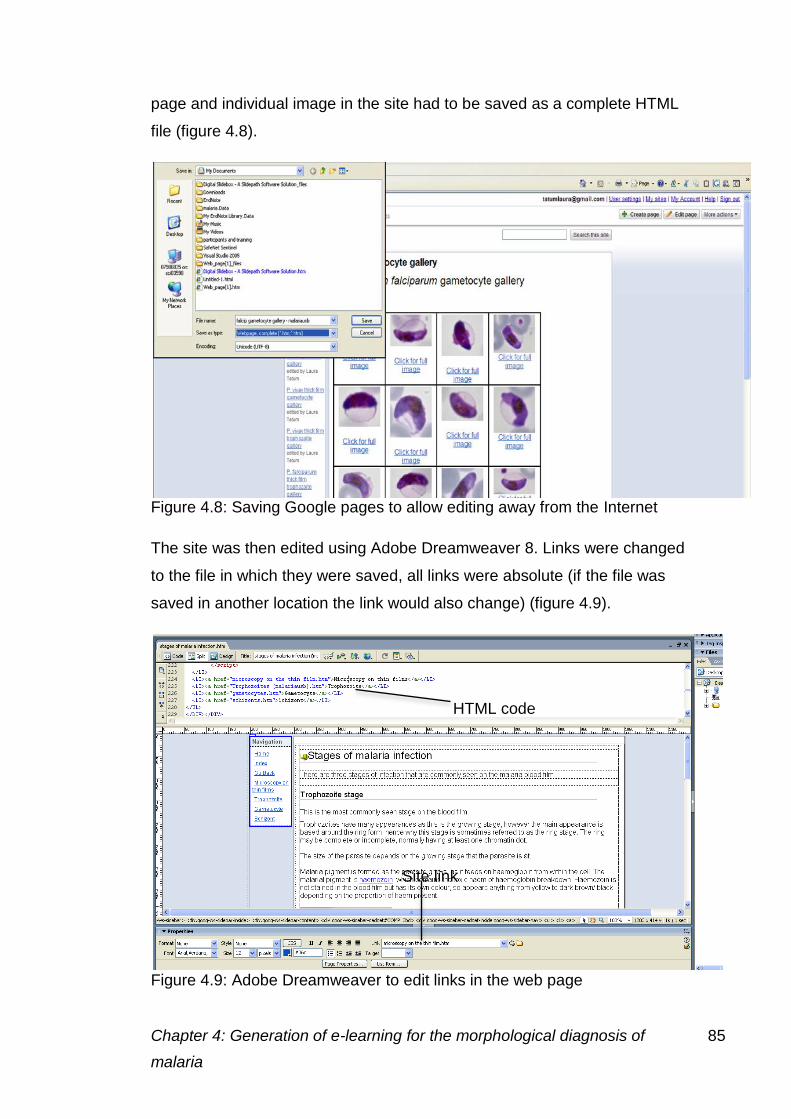
Chapter 4: Generation of e-learning for the morphological diagnosis of 85
malaria
page and individual image in the site had to be saved as a complete HTML
file (figure 4.8).
Figure 4.8: Saving Google pages to allow editing away from the Internet
The site was then edited using Adobe Dreamweaver 8. Links were changed
to the file in which they were saved, all links were absolute (if the file was
saved in another location the link would also change) (figure 4.9).
Figure 4.9: Adobe Dreamweaver to edit links in the web page
Site link
HTML code
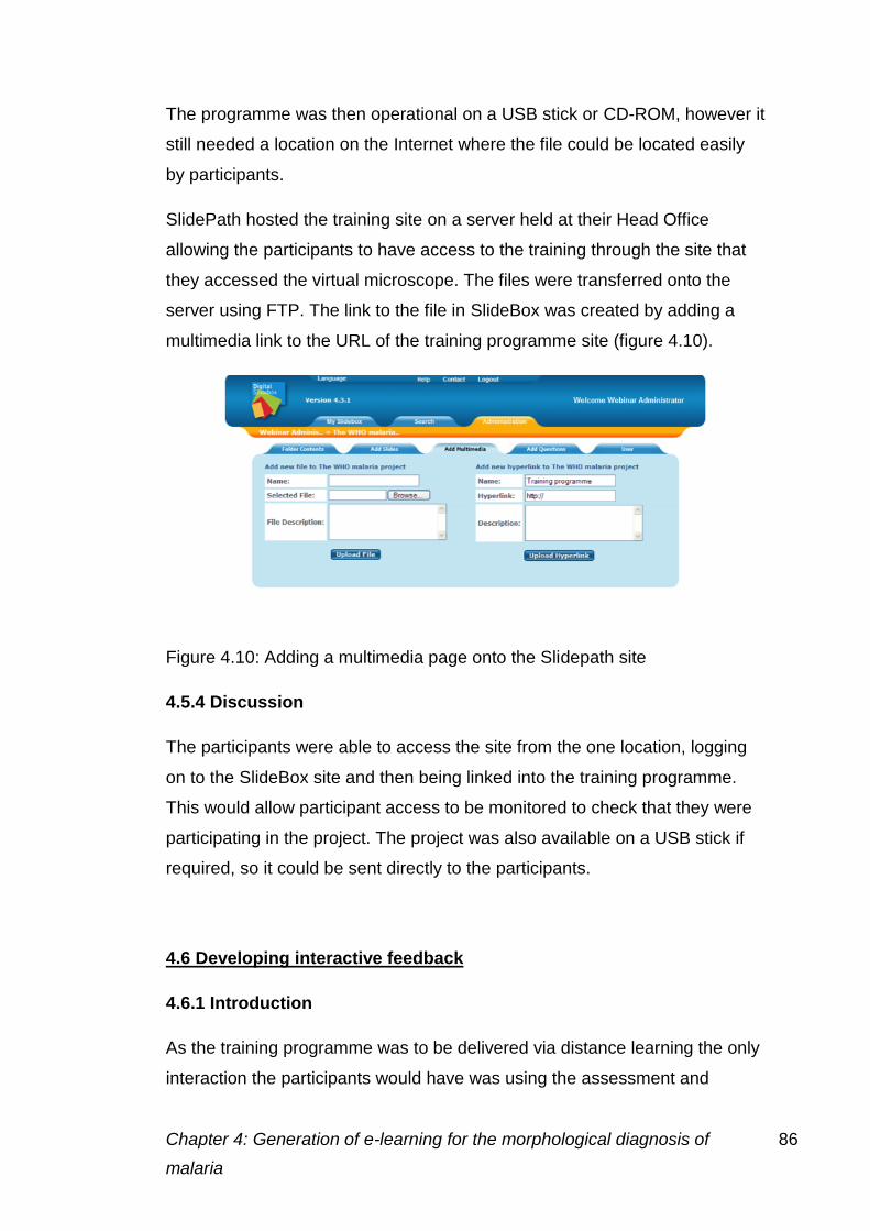
Chapter 4: Generation of e-learning for the morphological diagnosis of 86
malaria
The programme was then operational on a USB stick or CD-ROM, however it
still needed a location on the Internet where the file could be located easily
by participants.
SlidePath hosted the training site on a server held at their Head Office
allowing the participants to have access to the training through the site that
they accessed the virtual microscope. The files were transferred onto the
server using FTP. The link to the file in SlideBox was created by adding a
multimedia link to the URL of the training programme site (figure 4.10).
Figure 4.10: Adding a multimedia page onto the Slidepath site
4.5.4 Discussion
The participants were able to access the site from the one location, logging
on to the SlideBox site and then being linked into the training programme.
This would allow participant access to be monitored to check that they were
participating in the project. The project was also available on a USB stick if
required, so it could be sent directly to the participants.
4.6 Developing interactive feedback
4.6.1 Introduction
As the training programme was to be delivered via distance learning the only
interaction the participants would have was using the assessment and
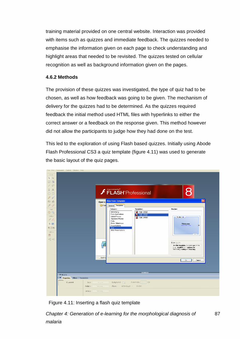
Chapter 4: Generation of e-learning for the morphological diagnosis of 87
malaria
training material provided on one central website. Interaction was provided
with items such as quizzes and immediate feedback. The quizzes needed to
emphasise the information given on each page to check understanding and
highlight areas that needed to be revisited. The quizzes tested on cellular
recognition as well as background information given on the pages.
4.6.2 Methods
The provision of these quizzes was investigated, the type of quiz had to be
chosen, as well as how feedback was going to be given. The mechanism of
delivery for the quizzes had to be determined. As the quizzes required
feedback the initial method used HTML files with hyperlinks to either the
correct answer or a feedback on the response given. This method however
did not allow the participants to judge how they had done on the test.
This led to the exploration of using Flash based quizzes. Initially using Abode
Flash Professional CS3 a quiz template (figure 4.11) was used to generate
the basic layout of the quiz pages.
Figure 4.11: Inserting a flash quiz template
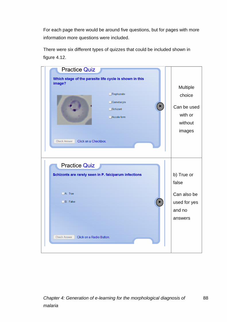
Chapter 4: Generation of e-learning for the morphological diagnosis of 88
malaria
For each page there would be around five questions, but for pages with more
information more questions were included.
There were six different types of quizzes that could be included shown in
figure 4.12.
Multiple
choice
Can be used
with or
without
images
b) True or
false
Can also be
used for yes
and no
answers
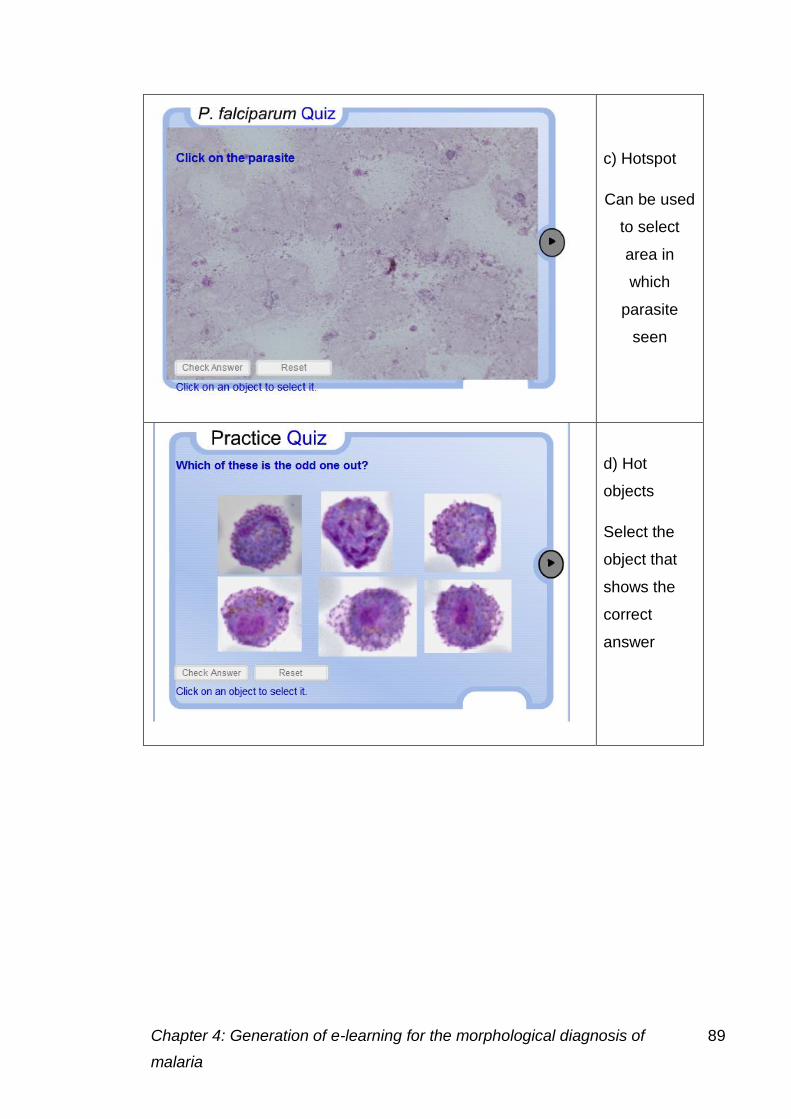
Chapter 4: Generation of e-learning for the morphological diagnosis of 89
malaria
c) Hotspot
Can be used
to select
area in
which
parasite
seen
d) Hot
objects
Select the
object that
shows the
correct
answer
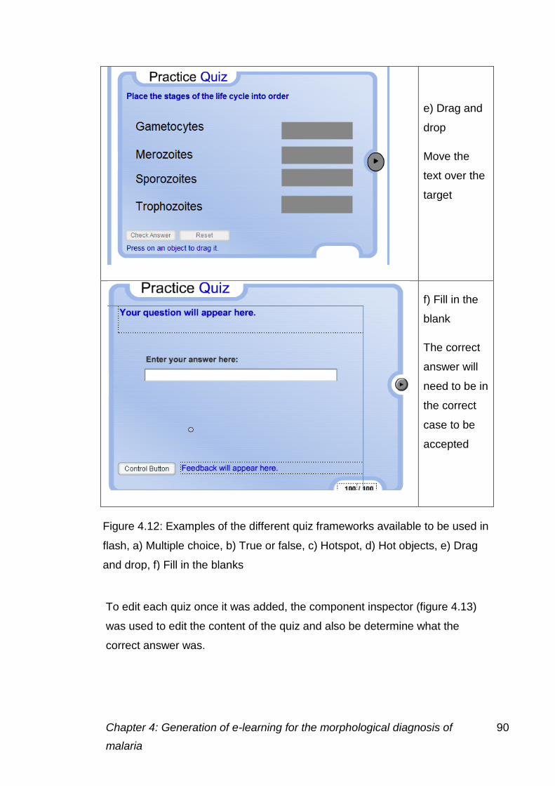
Chapter 4: Generation of e-learning for the morphological diagnosis of 90
malaria
e) Drag and
drop
Move the
text over the
target
f) Fill in the
blank
The correct
answer will
need to be in
the correct
case to be
accepted
To edit each quiz once it was added, the component inspector (figure 4.13)
was used to edit the content of the quiz and also be determine what the
correct answer was.
Figure 4.12: Examples of the different quiz frameworks available to be used in
flash, a) Multiple choice, b) True or false, c) Hotspot, d) Hot objects, e) Drag
and drop, f) Fill in the blanks

Chapter 4: Generation of e-learning for the morphological diagnosis of 91
malaria
The participants were given a score at the end of the quiz to allow them to
monitor progress (figure 4.14).
4.6.3 Results
Figure 4.13: The component inspector window, allows the question to be added and the
correct answer to be chosen
Figure 4.14: The participant score shown in the final screen
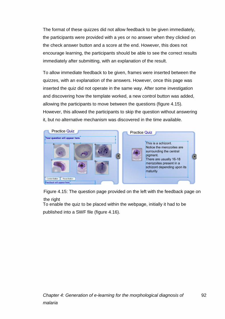
Chapter 4: Generation of e-learning for the morphological diagnosis of 92
malaria
The format of these quizzes did not allow feedback to be given immediately,
the participants were provided with a yes or no answer when they clicked on
the check answer button and a score at the end. However, this does not
encourage learning, the participants should be able to see the correct results
immediately after submitting, with an explanation of the result.
To allow immediate feedback to be given, frames were inserted between the
quizzes, with an explanation of the answers. However, once this page was
inserted the quiz did not operate in the same way. After some investigation
and discovering how the template worked, a new control button was added,
allowing the participants to move between the questions (figure 4.15).
However, this allowed the participants to skip the question without answering
it, but no alternative mechanism was discovered in the time available.
To enable the quiz to be placed within the webpage, initially it had to be
published into a SWF file (figure 4.16).
Figure 4.15: The question page provided on the left with the feedback page on
the right
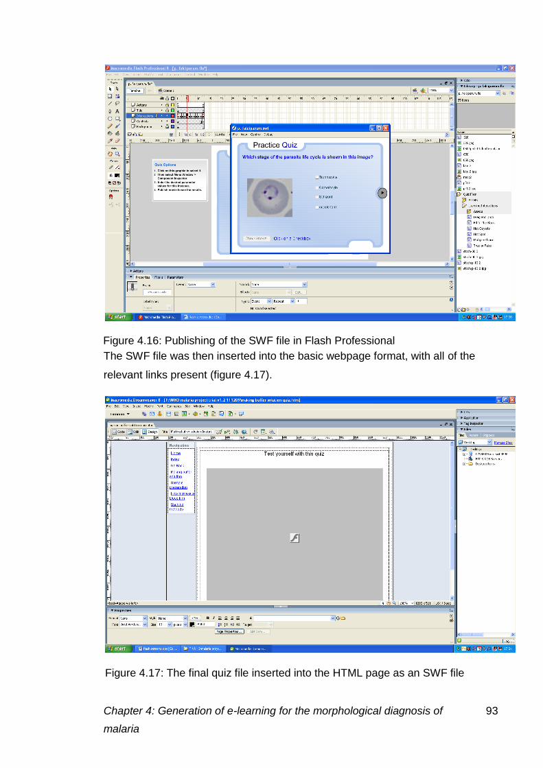
Chapter 4: Generation of e-learning for the morphological diagnosis of 93
malaria
The SWF file was then inserted into the basic webpage format, with all of the
relevant links present (figure 4.17).
Figure 4.16: Publishing of the SWF file in Flash Professional
Figure 4.17: The final quiz file inserted into the HTML page as an SWF file
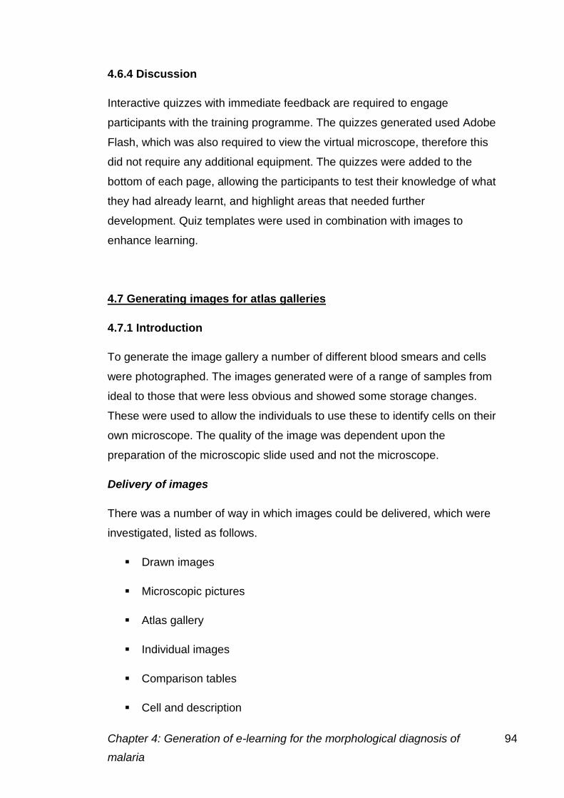
Chapter 4: Generation of e-learning for the morphological diagnosis of 94
malaria
4.6.4 Discussion
Interactive quizzes with immediate feedback are required to engage
participants with the training programme. The quizzes generated used Adobe
Flash, which was also required to view the virtual microscope, therefore this
did not require any additional equipment. The quizzes were added to the
bottom of each page, allowing the participants to test their knowledge of what
they had already learnt, and highlight areas that needed further
development. Quiz templates were used in combination with images to
enhance learning.
4.7 Generating images for atlas galleries
4.7.1 Introduction
To generate the image gallery a number of different blood smears and cells
were photographed. The images generated were of a range of samples from
ideal to those that were less obvious and showed some storage changes.
These were used to allow the individuals to use these to identify cells on their
own microscope. The quality of the image was dependent upon the
preparation of the microscopic slide used and not the microscope.
Delivery of images
There was a number of way in which images could be delivered, which were
investigated, listed as follows.
Drawn images
Microscopic pictures
Atlas gallery
Individual images
Comparison tables
Cell and description
Chapter 4: Generation of e-learning for the morphological diagnosis of 95
malaria
All of these methods were used to different degrees throughout the project.
4.7.2 Methods
Individual images were taken with the Zeiss AxioImager M1 microscope as
described in section 3.3.2. The microscope was initially set up using the live
properties (figure 4.18) window in the live view.
To achieve a high quality image a number of steps had to be carried out
using the live properties tab. Once the image had been focused the following
adjustments were made
Light settings- the measure button on the adjust tab, was used to
detect the correct light exposure required.
Colour settings- to achieve the correct colour initially the white
balance button was used (figure 4.18) followed by the interactive tool,
on the adjust tab which was placed in a white area between cells. The
dropper was placed where the red, green and blue readings were as
close as possible and then pressed.
Even background- to achieve an even background the slide was
moved off the smear to a clear area with no stain deposit, the shading
correction button on the general tab was used.
Camera settings- the camera was set to 12MPx and the high quality
setting found in the frame tab of the live properties window.
Histogram- The curve of the histogram was adjusted to achieve the
correct brightness and contrast settings, to achieve an image as close
to that seen down the microscope eye pieces as possible.
Images were taken using the snap button shown in figure 4.18. The image is
then left on the desktop and is required to be saved before closing the file.
The files were saved as TIFF files to allow processing to generate the gallery
images.
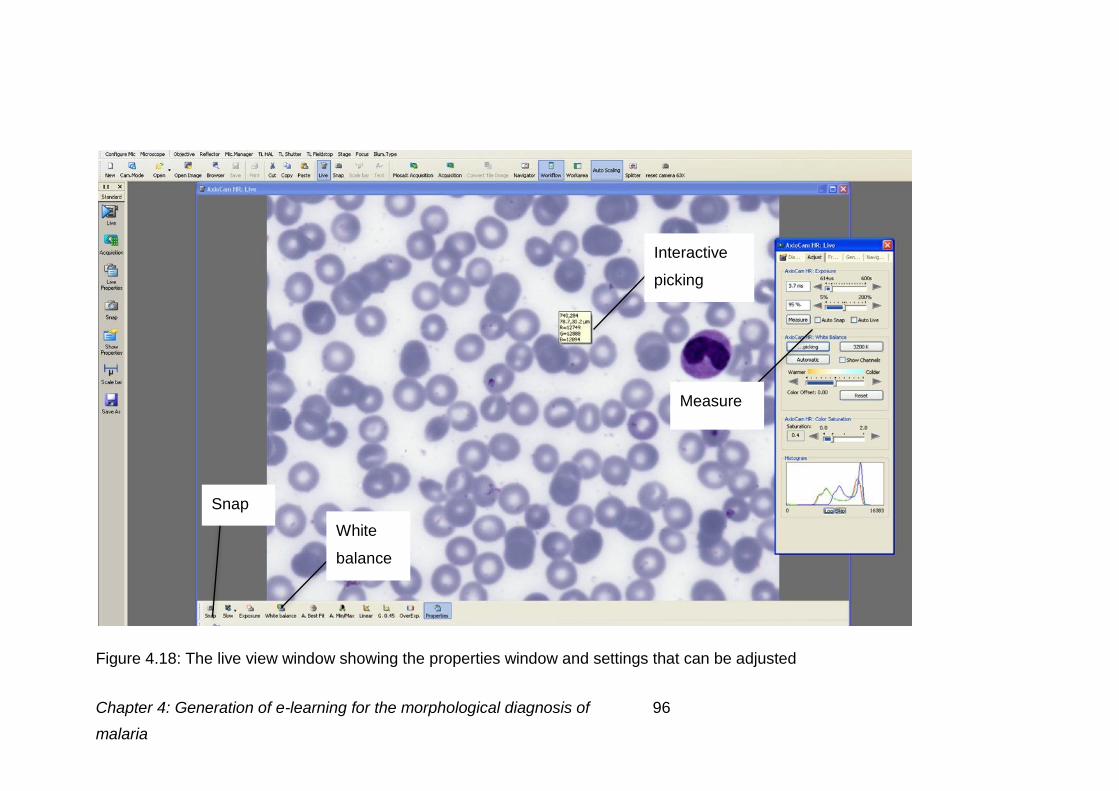
Chapter 4: Generation of e-learning for the morphological diagnosis of 96
malaria
Figure 4.18: The live view window showing the properties window and settings that can be adjusted
White
balance
Interactive
picking
Measure
Snap
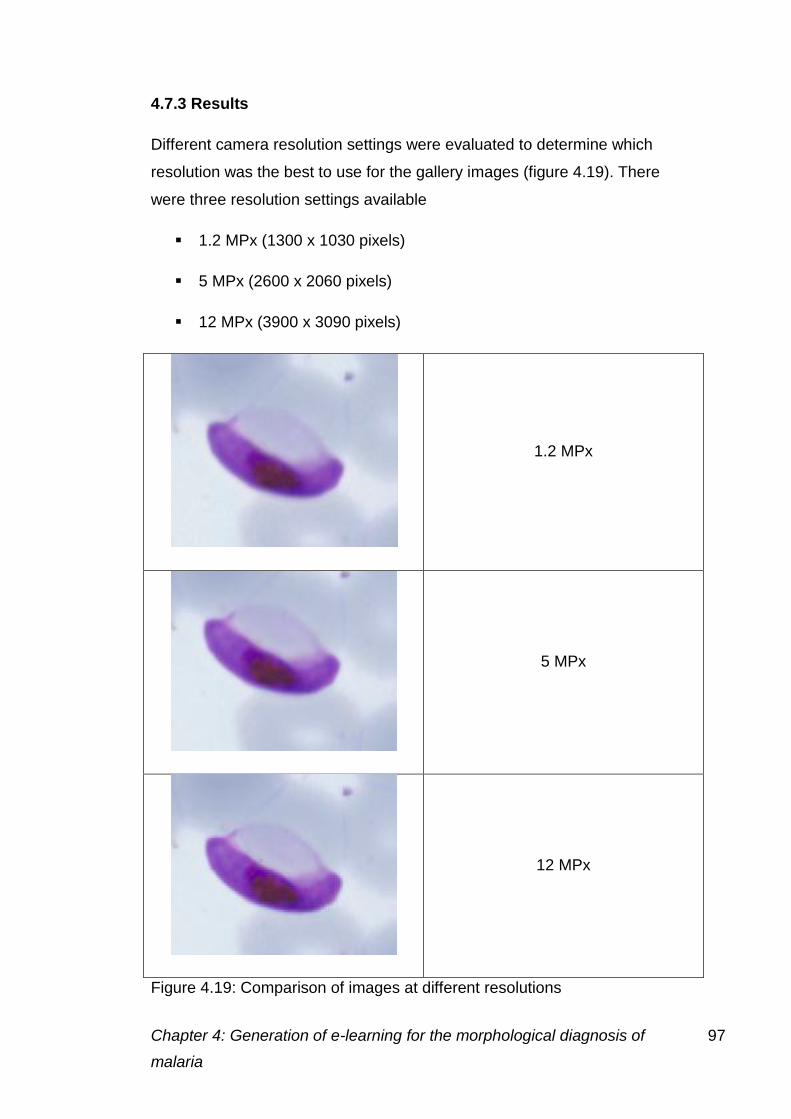
Chapter 4: Generation of e-learning for the morphological diagnosis of 97
malaria
4.7.3 Results
Different camera resolution settings were evaluated to determine which
resolution was the best to use for the gallery images (figure 4.19). There
were three resolution settings available
1.2 MPx (1300 x 1030 pixels)
5 MPx (2600 x 2060 pixels)
12 MPx (3900 x 3090 pixels)
1.2 MPx
5 MPx
12 MPx
Figure 4.19: Comparison of images at different resolutions
Chapter 4: Generation of e-learning for the morphological diagnosis of 98
malaria
The image from the 12 MPx camera can provide the same resolution as a
100X lens.
4.7.4 Discussion
Images were generated with the 12 MPx camera on the Zeiss microscope to
create the largest possible image to be used in the image gallery. The 12
MPx image was three times the size of the 1.2 MPx image due to the greater
number of pixels present. When placing the image into the gallery the size of
the image was then adjusted to ensure that there was no pixilation. The
image all saved as TIFF files, but were converted to JPEG images after they
had been processed.
4.8 Processing images for atlas galleries
4.8.1 Introduction
To ensure that the images viewed over the Internet were of the same quality
as those seen down the microscope, a few image correction stages were
carried out. Image enhancement was restricted to revealing detail and
enhancing focus. To ensure images had a natural “microscope” appearance
care was taken at the capture stage to avoid over enhancement of contrast,
producing a bleached background.
4.8.2 Methods
Cropping the image
Only a small area of the image captured was required for the photo gallery.
To obtain the size of image required Adobe Photoshop was used to reduce
the size of the original image. Before modifying the original file a duplicate
was saved under a different name. This file was then reduced to the required
size using the crop tool.
Chapter 4: Generation of e-learning for the morphological diagnosis of 99
malaria
Detail enhancement
Detail enhancement allows features that may not be as defined as they are
in the microscope image to be improved. The settings for this were explored
before using them in the images generated.
Initially the software to be used for the detail enhancement was chosen, an
Adobe Photoshop add-in Digital Outback Photo -Detail Extractor Version 2
was chosen through experimentation and comparison to other add-ins
available at a similar cost. The same settings were used as described in
section 3.4.4.
Different settings for these were also explored, varying these to achieve the
best image.
Contrast mask
The contrast mask settings darken the image to even out the colour enabling
the image to be more representative of the original. This process allows
better contrast between the background and the cells, allowing them to be
seen more easily and reduced noise in the background.
Smart sharpen
Smart sharpen allows particular colour settings to be processed to allow the
image to be of the optimal quality. The following smart sharpen settings were
used
Convert to 16 bit (image menu)
Choose smart sharpen (in filter menu)
o Amount 125%
o Radius 11 pixels
o Angle 0
o With more accurate
Chapter 4: Generation of e-learning for the morphological diagnosis of 100
malaria
o Remove: Lens blur
o Shadow: Parameters
o Amount 5%
o Tone width 80%
o Radius 10
o Highlight: Parameters
o Amount 20%
o Tone width 70%
o Radius 70
Convert to 8 bit
The files were saved as TIFF files after the process was completed.
4.8.3 Results
Detail enhancement and contrast mask
These settings were explored in section 3.4.4.
Smart sharpen
Figure 4.20 compares the original image, detail-enhanced image and smart
sharpen image.
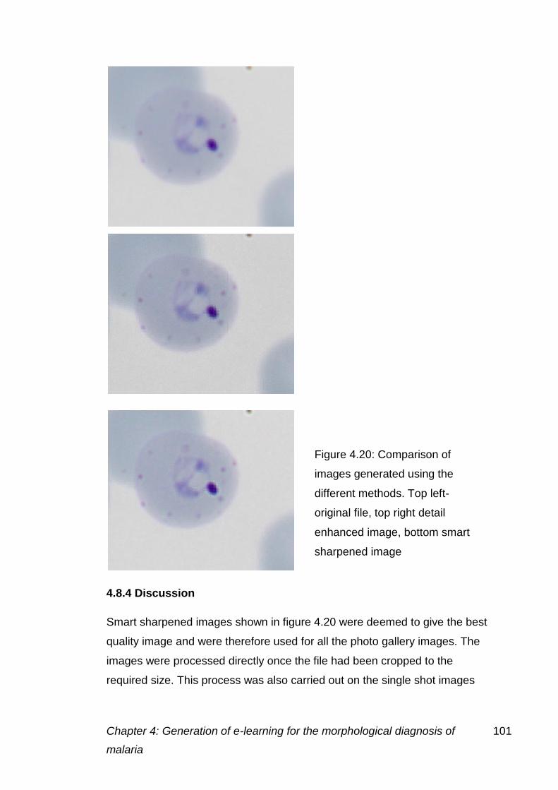
Chapter 4: Generation of e-learning for the morphological diagnosis of 101
malaria
4.8.4 Discussion
Smart sharpened images shown in figure 4.20 were deemed to give the best
quality image and were therefore used for all the photo gallery images. The
images were processed directly once the file had been cropped to the
required size. This process was also carried out on the single shot images
Figure 4.20: Comparison of
images generated using the
different methods. Top left-
original file, top right detail
enhanced image, bottom smart
sharpened image
Chapter 4: Generation of e-learning for the morphological diagnosis of 102
malaria
linked to from the gallery to make sure the participants viewed the same
image.
4.9 Review of the training programme
4.9.1 Introduction
The author solely developed the training programme, with input from the
supervisory team, however it was felt expert review was needed to ensure
the information given was “fit for purpose”.
4.9.2 Method
The content of the training programme was initially reviewed within the digital
morphology team at Manchester Royal Infirmary and edits were made.
Following these edits members of the UK NEQAS Morphology Specialist
Advisory group made comments. The training and a questionnaire was
distributed on a USB stick to
Educationalists (1)
Consultants (5)
Biomedical Scientists (10)
Trainees/ students (1)
Seventeen USB sticks where distributed in total, eleven of which were
returned. The questionnaire distributed can be seen in appendix 1.1.
The comments made by these individuals were then incorporated into the
final version of the programme. Some errors in the text were corrected as
well as additional information added. Some of the page formats were also
altered to improve understanding.
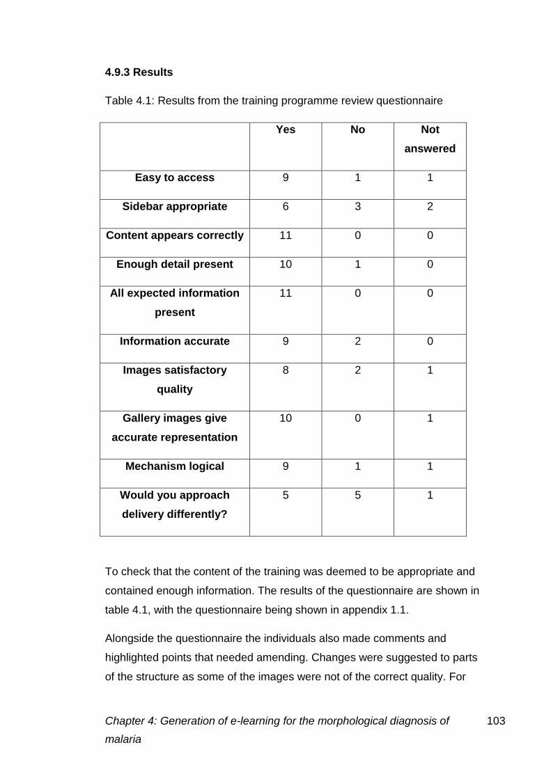
Chapter 4: Generation of e-learning for the morphological diagnosis of 103
malaria
4.9.3 Results
Table 4.1: Results from the training programme review questionnaire
Yes No Not
answered
Easy to access 9 1 1
Sidebar appropriate 6 3 2
Content appears correctly 11 0 0
Enough detail present 10 1 0
All expected information
present
11 0 0
Information accurate 9 2 0
Images satisfactory
quality
8 2 1
Gallery images give
accurate representation
10 0 1
Mechanism logical 9 1 1
Would you approach
delivery differently?
5 5 1
To check that the content of the training was deemed to be appropriate and
contained enough information. The results of the questionnaire are shown in
table 4.1, with the questionnaire being shown in appendix 1.1.
Alongside the questionnaire the individuals also made comments and
highlighted points that needed amending. Changes were suggested to parts
of the structure as some of the images were not of the correct quality. For
Chapter 4: Generation of e-learning for the morphological diagnosis of 104
malaria
example, one individual noted that links should be made to more detailed
pages at the end of each section to make links clearer. On the stages of
malaria infection page the link to the trophozoite page was placed after the
description, in a separate sentence. Comments upon changing the approach
included further description of the features of each species, rather than by
stage; giving a more practical approach; adding diagrams to reduce text and
adding more colour. These were addressed where possible within the basic
html format used,
4.9.4 Discussion
Following the results of the questionnaire, the suggested amendments were
made. The order of delivery was changed in some places to make the links
more relevant. For example, links to the galleries were moved to the bottom
of the text section on the trophozoites page, to prevent confusion with other
links within the text.
At the time of the review the planned quizzes were not included, however a
number of individuals suggested that quizzes should be added. The thick film
information had also not been added at this stage, with many individuals
saying that it was necessary.
Some individuals had problems accessing the sidebar, which was amended.
Many found they lost where they were in the project, an index page was
therefore added to enable participants to determine which pages they had or
had not visited. The links on the sidebar were also changed, to allow
individuals to link easily between relevant pages.
All comments received were positive and many showed the training to other
colleagues or requested a copy of the final version.
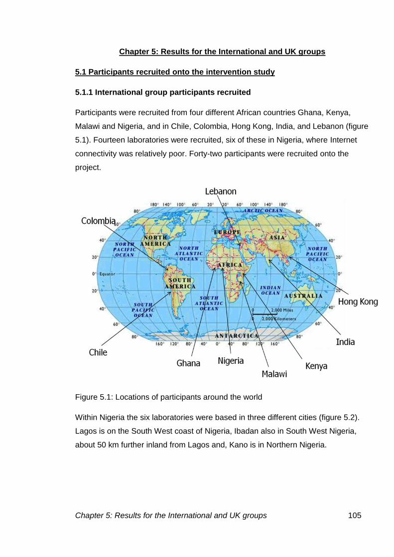
Chapter 5: Results for the International and UK groups 105
Chapter 5: Results for the International and UK groups
5.1 Participants recruited onto the intervention study
5.1.1 International group participants recruited
Participants were recruited from four different African countries Ghana, Kenya,
Malawi and Nigeria, and in Chile, Colombia, Hong Kong, India, and Lebanon (figure
5.1). Fourteen laboratories were recruited, six of these in Nigeria, where Internet
connectivity was relatively poor. Forty-two participants were recruited onto the
project.
Figure 5.1: Locations of participants around the world
Within Nigeria the six laboratories were based in three different cities (figure 5.2).
Lagos is on the South West coast of Nigeria, Ibadan also in South West Nigeria,
about 50 km further inland from Lagos and, Kano is in Northern Nigeria.
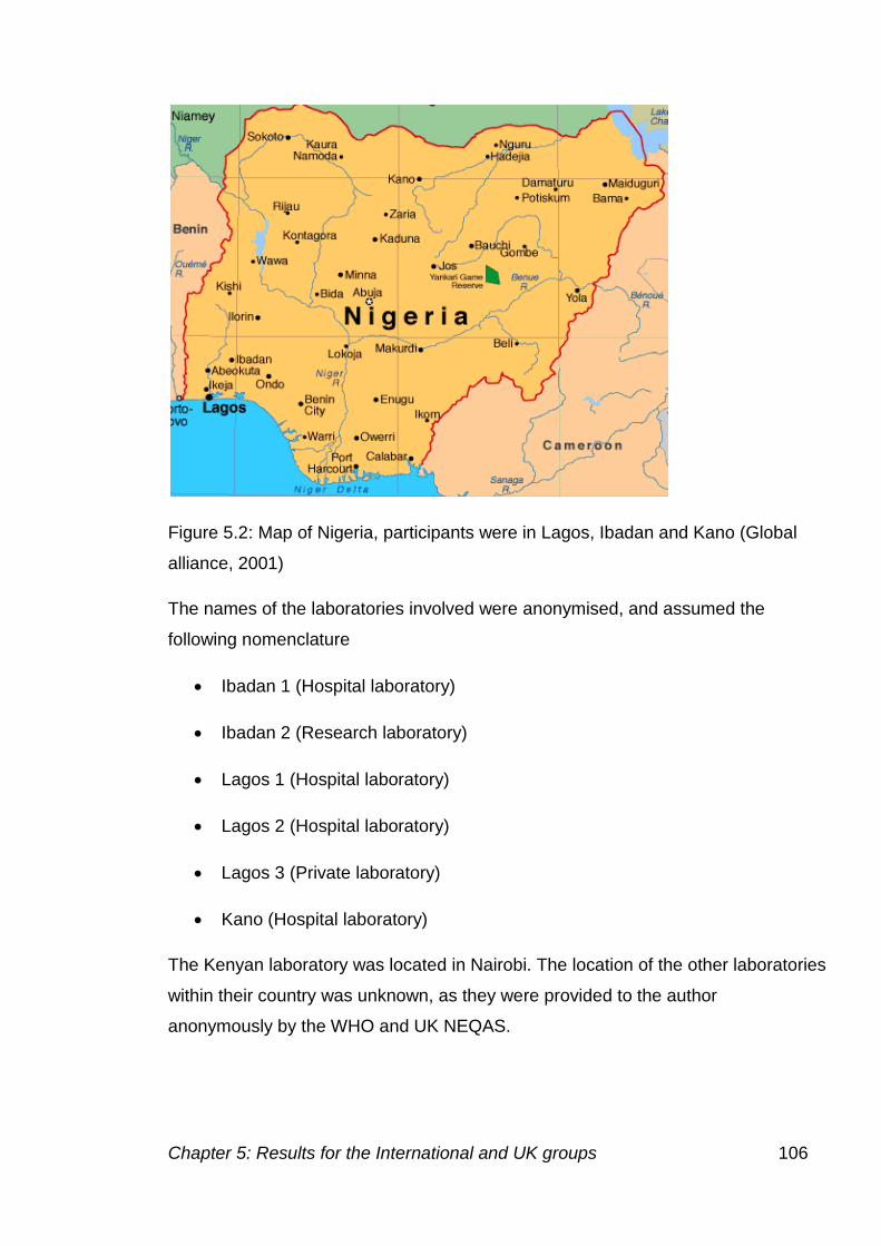
Chapter 5: Results for the International and UK groups 106
Figure 5.2: Map of Nigeria, participants were in Lagos, Ibadan and Kano (Global
alliance, 2001)
The names of the laboratories involved were anonymised, and assumed the
following nomenclature
Ibadan 1 (Hospital laboratory)
Ibadan 2 (Research laboratory)
Lagos 1 (Hospital laboratory)
Lagos 2 (Hospital laboratory)
Lagos 3 (Private laboratory)
Kano (Hospital laboratory)
The Kenyan laboratory was located in Nairobi. The location of the other laboratories
within their country was unknown, as they were provided to the author
anonymously by the WHO and UK NEQAS.
Chapter 5: Results for the International and UK groups 107
5.1.2 UK group participants recruited onto intervention study
Participants were recruited initially by contacting laboratory managers at random
from a list of laboratories that participate in the UK NEQAS scheme for parasite
identification. Initially ten individuals were contacted by telephone, and then
subsequently by email giving further details. All the members of staff contacted
were then asked to provide the names of individuals within their laboratory who
would be included in two specific staff categories.
<2 years experience, and pre-specialist portfolio
>5 years experience, and post-specialist portfolio
These categories were used to see if the information in the training programme
required any precursor knowledge, or whether there was not enough information for
the more experienced individuals. The groupings were used to analyse results
achieved in the initial and final assessment.
Interested participants were asked to complete an online questionnaire to record
their professional background and training experience. An outline of the questions
asked can be seen in Appendix 1.4. These participants were then given access to
the training website to access the images. 39 participants were asked to complete
the questionnaire, 33 did so, 34 participants commenced the study by accessing
the images.
5.2 Delivery of the intervention training programme
Due to the increased availability of Internet access for this group in the UK, the time
scales of the project were shortened from those in the international group. The
participants were given access to the initial assessment images over a six-week
period. The images were released in sets of ten, with a set released each week for
the first four weeks, and all available for the last two weeks. The training was then
delivered over a six-week period, with a final six weeks for the final assessment.
Chapter 5: Results for the International and UK groups 108
5.3 Results from the initial recruitment questionnaire
5.3.1 International group results from the recruitment questionnaire
Upon recruitment, participants were asked to complete a questionnaire about their
personal experience and training (appendix 1.3). The laboratory coordinator also
completed a questionnaire about the laboratory and the techniques used in malaria
diagnosis.
Laboratory questionnaire
Number of staff
The number of staff present within the laboratory was dependent on the number of
tests requested, the location of the laboratory and its size. The majority of
laboratories had 5-6 members of scientific staff (n=7) although there were also
laboratories with 1-2 (n=1) and more than 15 (n=1) also recruited. In most
laboratories there were five or more members of staff carrying out malaria
microscopy (n=10). There were however, two laboratories with only one member of
staff diagnosing malaria.
Number of malaria cases
Twelve laboratories reported seasonal variation in the number of malaria cases
seen. In the high season the majority of laboratories saw 30-49 cases (n=6) per
week, there were four laboratories that saw more than 50 cases per week. In the
low season 10-29 cases were most frequently reported (n=7), there was one
laboratory reporting more than 50 cases, this was not the laboratory with the
highest number of staff however. The parasite density was reported to be between
one and 8% by ten of the laboratories. There was one laboratory reporting parasite
densities of more than 8% in the majority of cases.
Microscopes
The majority of laboratories had two microscopes for malaria diagnosis (n=7), three
laboratories had more than five. In the 14 laboratories questioned there were a total
of seven non-functioning microscopes and more than 40 functioning microscopes,
Chapter 5: Results for the International and UK groups 109
in broad agreement with the findings of (Mundy et al., 2000). The number of
microscopes therefore influences the number of cases that can be examined,
especially in the high season.
Staining techniques
The microscope slides for malaria were commonly stained with Giemsa stain with
the thin film being fixed with methanol. However, the methanol was not changed
more often during the wet season, potentially leading to an increase in poorly
prepared microscope slides. Methanol allows fixation of the cells to the slide, the
presence of water can prevent fixation of the cells, and also lead to artefactual
changes. The artefactual changes include rings within the erythrocytes, which can
look like parasites causing false positives, or false negatives if this overlaid a
parasite, making it impossible to see.
Power supply and computer access
Of the respondents ten reported that electricity was usually reliable. Ten of the
laboratories questioned had their electricity supplied by generator for 24 hours of
the day, one for 12, and one for six hours or whenever enough fuel was available.
Half of the laboratories questioned had access to computers in the laboratory, six of
these laboratories had Internet access. Those laboratories that did not have a
computer in the laboratory or did not have Internet access were required, for the
study, to visit Internet cafes. Financial support was provided to allow access for
these individuals.
Questionnaire completed by laboratory based individuals
Figure 5.1 shows some of the international participant responses to the
questionnaire.
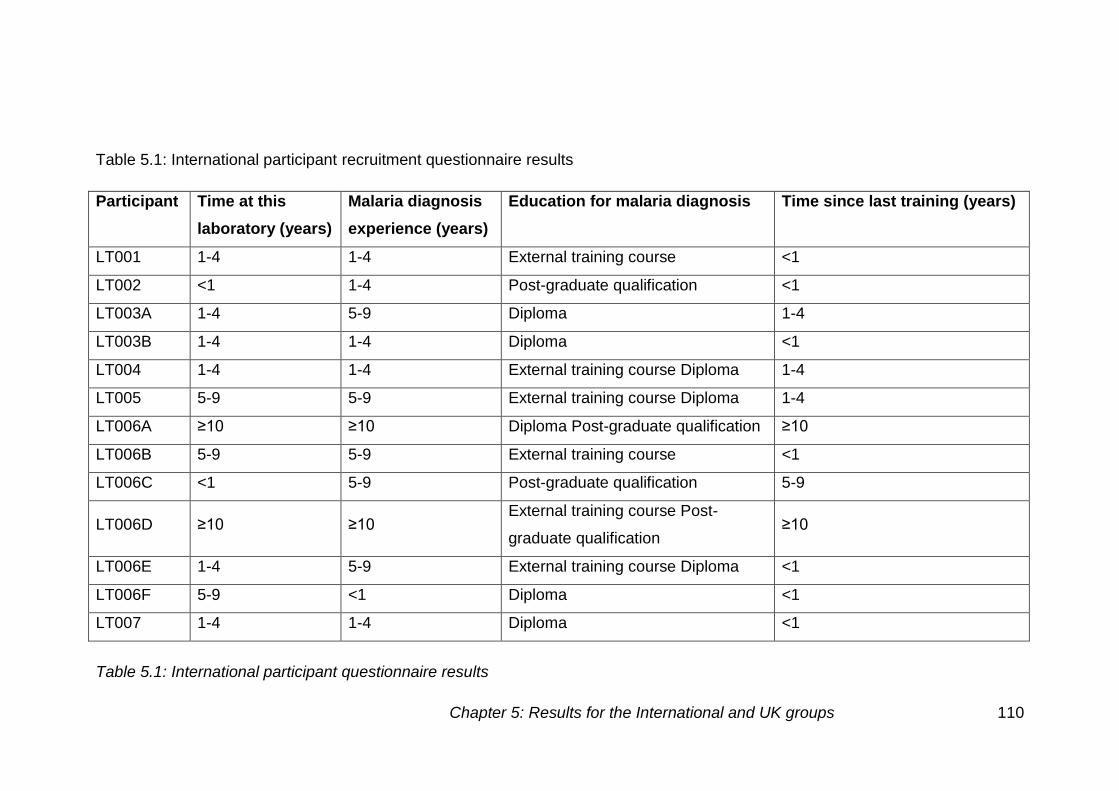
Table 5.1: International participant questionnaire results
Chapter 5: Results for the International and UK groups 110
Table 5.1: International participant recruitment questionnaire results
Participant Time at this
laboratory (years)
Malaria diagnosis
experience (years)
Education for malaria diagnosis Time since last training (years)
LT001 1-4 1-4 External training course <1
LT002 <1 1-4 Post-graduate qualification <1
LT003A 1-4 5-9 Diploma 1-4
LT003B 1-4 1-4 Diploma <1
LT004 1-4 1-4 External training course Diploma 1-4
LT005 5-9 5-9 External training course Diploma 1-4
LT006A ≥10 ≥10 Diploma Post-graduate qualification ≥10
LT006B 5-9 5-9 External training course <1
LT006C <1 5-9 Post-graduate qualification 5-9
LT006D ≥10 ≥10 External training course Post-
graduate qualification ≥10
LT006E 1-4 5-9 External training course Diploma <1
LT006F 5-9 <1 Diploma <1
LT007 1-4 1-4 Diploma <1
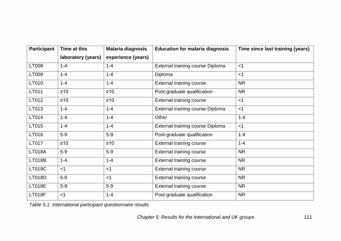
Table 5.1: International participant questionnaire results
Chapter 5: Results for the International and UK groups 111
Participant Time at this
laboratory (years)
Malaria diagnosis
experience (years)
Education for malaria diagnosis Time since last training (years)
LT008 1-4 1-4 External training course Diploma <1
LT009 1-4 1-4 Diploma <1
LT010 1-4 1-4 External training course NR
LT011 ≥10 ≥10 Post-graduate qualification NR
LT012 ≥10 ≥10 External training course <1
LT013 1-4 1-4 External training course Diploma <1
LT014 1-4 1-4 Other 1-4
LT015 1-4 1-4 External training course Diploma <1
LT016 5-9 5-9 Post-graduate qualification 1-4
LT017 ≥10 ≥10 External training course 1-4
LT018A 5-9 5-9 External training course NR
LT018B 1-4 1-4 External training course NR
LT018C <1 <1 External training course NR
LT018D 5-9 <1 External training course NR
LT018E 5-9 5-9 External training course NR
LT018F <1 1-4 Post-graduate qualification NR
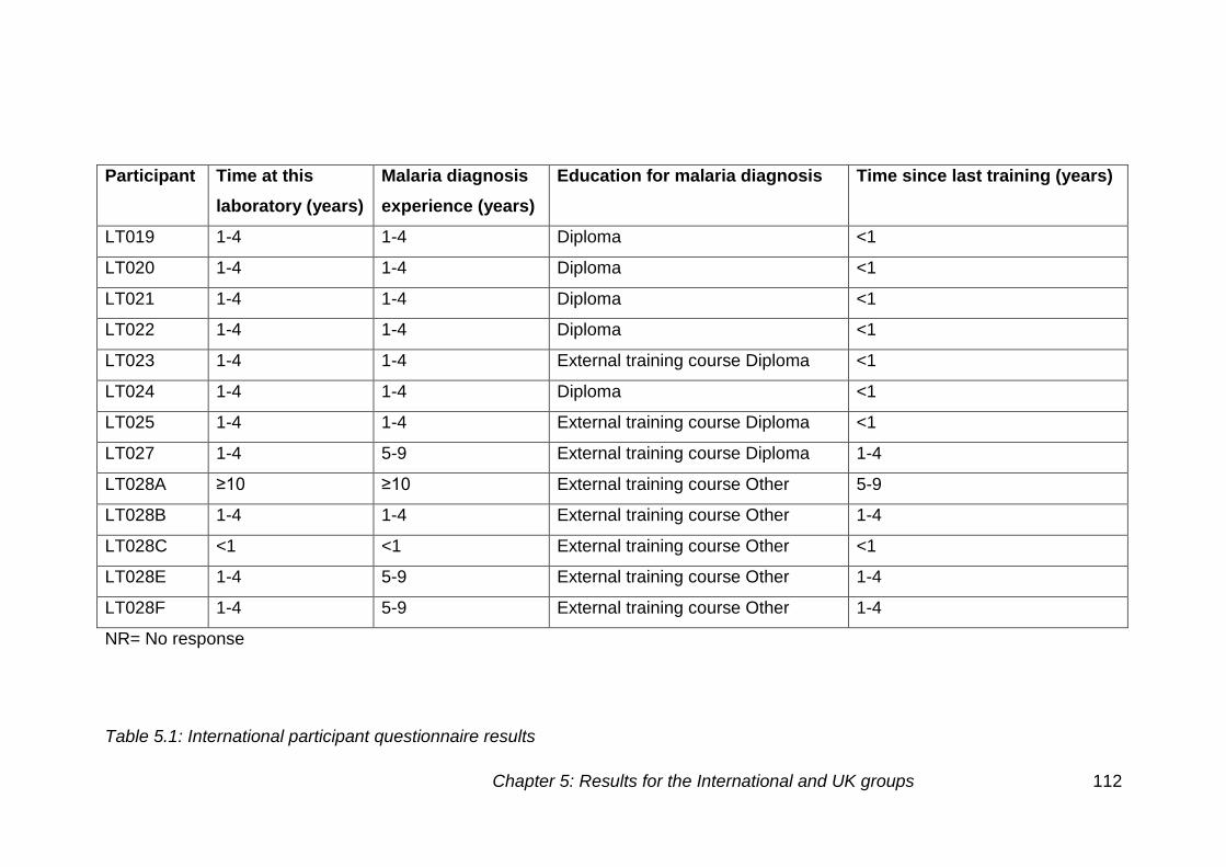
Table 5.1: International participant questionnaire results
Chapter 5: Results for the International and UK groups 112
Participant Time at this
laboratory (years)
Malaria diagnosis
experience (years)
Education for malaria diagnosis Time since last training (years)
LT019 1-4 1-4 Diploma <1
LT020 1-4 1-4 Diploma <1
LT021 1-4 1-4 Diploma <1
LT022 1-4 1-4 Diploma <1
LT023 1-4 1-4 External training course Diploma <1
LT024 1-4 1-4 Diploma <1
LT025 1-4 1-4 External training course Diploma <1
LT027 1-4 5-9 External training course Diploma 1-4
LT028A ≥10 ≥10 External training course Other 5-9
LT028B 1-4 1-4 External training course Other 1-4
LT028C <1 <1 External training course Other <1
LT028E 1-4 5-9 External training course Other 1-4
LT028F 1-4 5-9 External training course Other 1-4
NR= No response
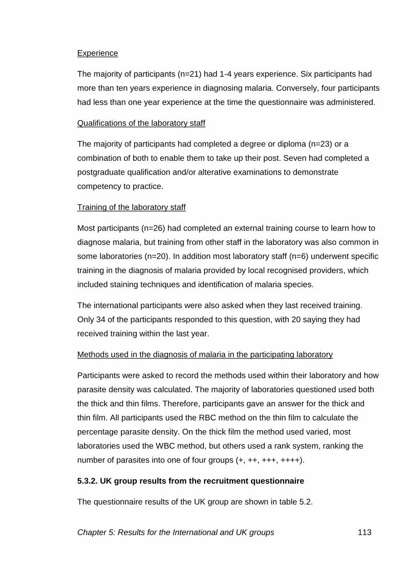
Chapter 5: Results for the International and UK groups 113
Experience
The majority of participants (n=21) had 1-4 years experience. Six participants had
more than ten years experience in diagnosing malaria. Conversely, four participants
had less than one year experience at the time the questionnaire was administered.
Qualifications of the laboratory staff
The majority of participants had completed a degree or diploma (n=23) or a
combination of both to enable them to take up their post. Seven had completed a
postgraduate qualification and/or alterative examinations to demonstrate
competency to practice.
Training of the laboratory staff
Most participants (n=26) had completed an external training course to learn how to
diagnose malaria, but training from other staff in the laboratory was also common in
some laboratories (n=20). In addition most laboratory staff (n=6) underwent specific
training in the diagnosis of malaria provided by local recognised providers, which
included staining techniques and identification of malaria species.
The international participants were also asked when they last received training.
Only 34 of the participants responded to this question, with 20 saying they had
received training within the last year.
Methods used in the diagnosis of malaria in the participating laboratory
Participants were asked to record the methods used within their laboratory and how
parasite density was calculated. The majority of laboratories questioned used both
the thick and thin films. Therefore, participants gave an answer for the thick and
thin film. All participants used the RBC method on the thin film to calculate the
percentage parasite density. On the thick film the method used varied, most
laboratories used the WBC method, but others used a rank system, ranking the
number of parasites into one of four groups (+, ++, +++, ++++).
5.3.2. UK group results from the recruitment questionnaire
The questionnaire results of the UK group are shown in table 5.2.
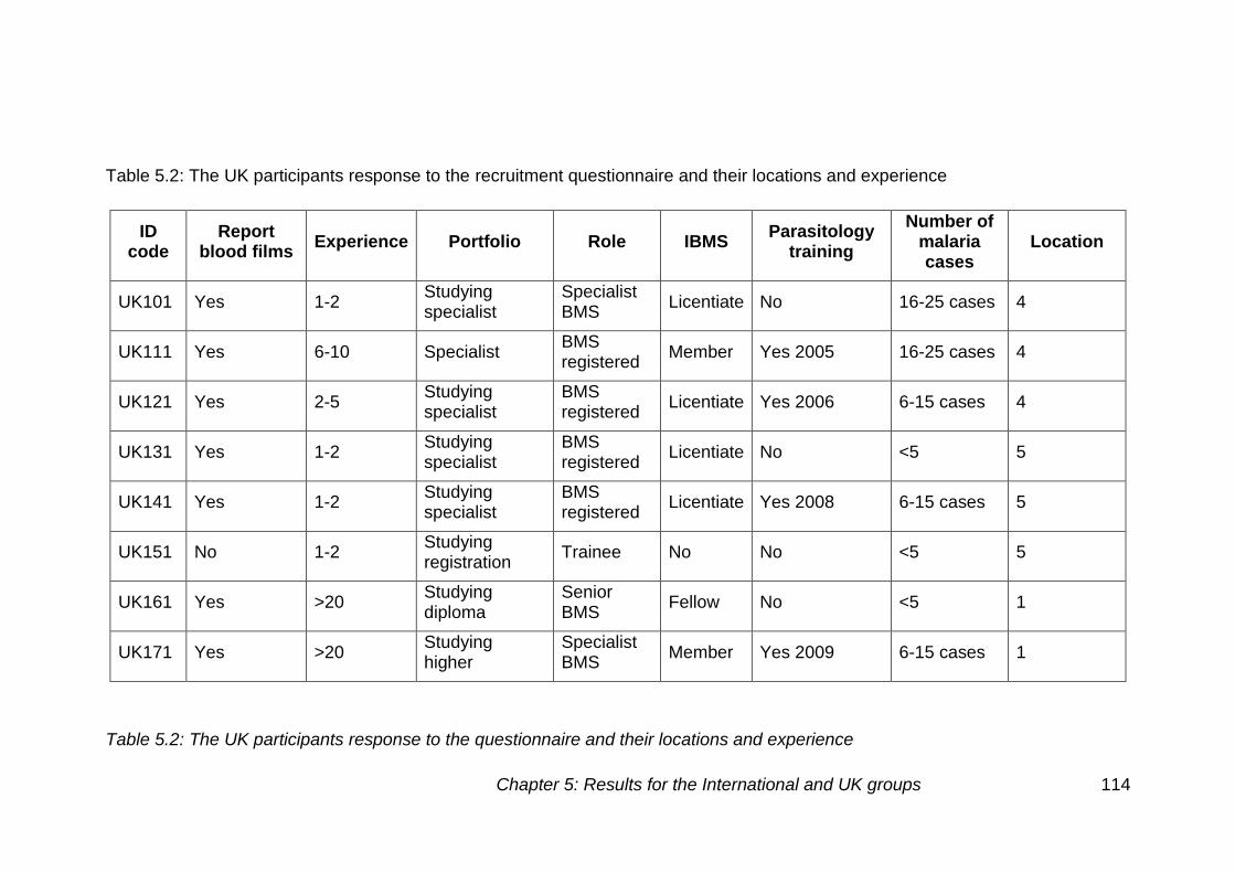
Table 5.2: The UK participants response to the questionnaire and their locations and experience
Chapter 5: Results for the International and UK groups 114
Table 5.2: The UK participants response to the recruitment questionnaire and their locations and experience
ID code
Report blood films
Experience Portfolio Role IBMS Parasitology
training
Number of malaria cases
Location
UK101 Yes 1-2 Studying specialist
Specialist BMS
Licentiate No 16-25 cases 4
UK111 Yes 6-10 Specialist BMS registered
Member Yes 2005 16-25 cases 4
UK121 Yes 2-5 Studying specialist
BMS registered
Licentiate Yes 2006 6-15 cases 4
UK131 Yes 1-2 Studying specialist
BMS registered
Licentiate No <5 5
UK141 Yes 1-2 Studying specialist
BMS registered
Licentiate Yes 2008 6-15 cases 5
UK151 No 1-2 Studying registration
Trainee No No <5 5
UK161 Yes >20 Studying diploma
Senior BMS
Fellow No <5 1
UK171 Yes >20 Studying higher
Specialist BMS
Member Yes 2009 6-15 cases 1
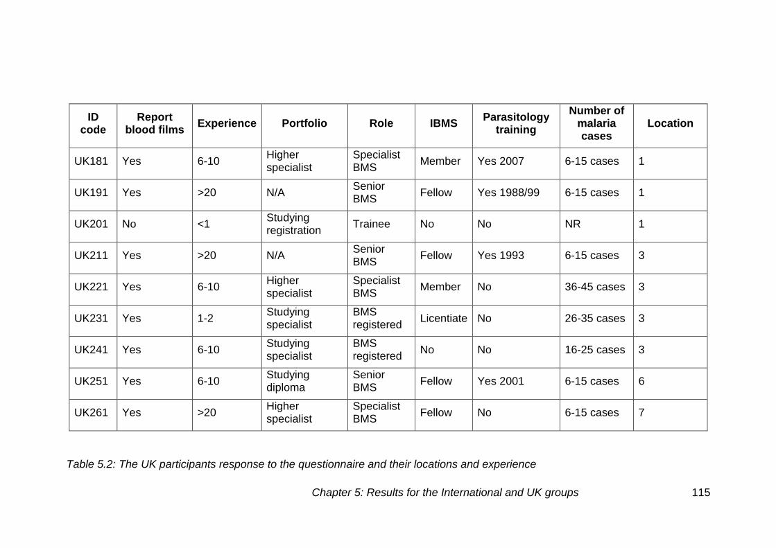
Table 5.2: The UK participants response to the questionnaire and their locations and experience
Chapter 5: Results for the International and UK groups 115
ID code
Report blood films
Experience Portfolio Role IBMS Parasitology
training
Number of malaria cases
Location
UK181 Yes 6-10 Higher specialist
Specialist BMS
Member Yes 2007 6-15 cases 1
UK191 Yes >20 N/A Senior BMS
Fellow Yes 1988/99 6-15 cases 1
UK201 No <1 Studying registration
Trainee No No NR 1
UK211 Yes >20 N/A Senior BMS
Fellow Yes 1993 6-15 cases 3
UK221 Yes 6-10 Higher specialist
Specialist BMS
Member No 36-45 cases 3
UK231 Yes 1-2 Studying specialist
BMS registered
Licentiate No 26-35 cases 3
UK241 Yes 6-10 Studying specialist
BMS registered
No No 16-25 cases 3
UK251 Yes 6-10 Studying diploma
Senior BMS
Fellow Yes 2001 6-15 cases 6
UK261 Yes >20 Higher specialist
Specialist BMS
Fellow No 6-15 cases 7
Table 5.2: The UK participants response to the questionnaire and their locations and experience
Chapter 5: Results for the International and UK groups 116
ID code
Report blood films
Experience Portfolio Role IBMS Parasitology
training
Number of malaria cases
Location
UK271 Yes >20 N/A Senior BMS
Fellow Yes 1998 6-15 cases 8
UK281 Yes 6-10 Higher specialist
BMS registered
Licentiate Yes 2008 6-15 cases 8
UK301 Yes 2-5 Studying specialist
BMS registered
Licentiate No 6-15 cases 8
UK311 Yes 2-5 Studying specialist
BMS registered
Licentiate No 6-15 cases 8
UK331 No 1-2 Studying specialist
BMS registered
Member No 6-15 cases 6
UK341 No 1-2 Studying specialist
BMS registered
Licentiate No NR 6
UK361 Yes 6-10 Studying specialist
BMS registered
Licentiate No 6-15 cases 2
UK371 Yes 16-20 Higher specialist
Senior BMS
No Yes 1997 6-15 cases 2
UK381 Yes 16-20 N/A BMS registered
No Yes 2004 16-25 cases 2
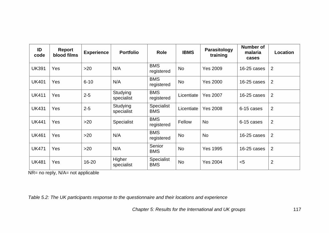
Table 5.2: The UK participants response to the questionnaire and their locations and experience
Chapter 5: Results for the International and UK groups 117
ID code
Report blood films
Experience Portfolio Role IBMS Parasitology
training
Number of malaria cases
Location
UK391 Yes >20 N/A BMS registered
No Yes 2009 16-25 cases 2
UK401 Yes 6-10 N/A BMS registered
No Yes 2000 16-25 cases 2
UK411 Yes 2-5 Studying specialist
BMS registered
Licentiate Yes 2007 16-25 cases 2
UK431 Yes 2-5 Studying specialist
Specialist BMS
Licentiate Yes 2008 6-15 cases 2
UK441 Yes >20 Specialist BMS registered
Fellow No 6-15 cases 2
UK461 Yes >20 N/A BMS registered
No No 16-25 cases 2
UK471 Yes >20 N/A Senior BMS
No Yes 1995 16-25 cases 2
UK481 Yes 16-20 Higher specialist
Specialist BMS
No Yes 2004 <5 2
NR= no reply, N/A= not applicable
Chapter 5: Results for the International and UK groups 118
The questionnaire for the UK group was used to obtain detailed professional
information about the individuals involved in the project. The responses
initially split the individuals into two categories as described above. Of the
responders there were 15 individuals in category one (<2 years experience)
and 18 in category two (>5 years experience).
51.5% of participants had taken part in the UK NEQAS parasitology training
scheme.
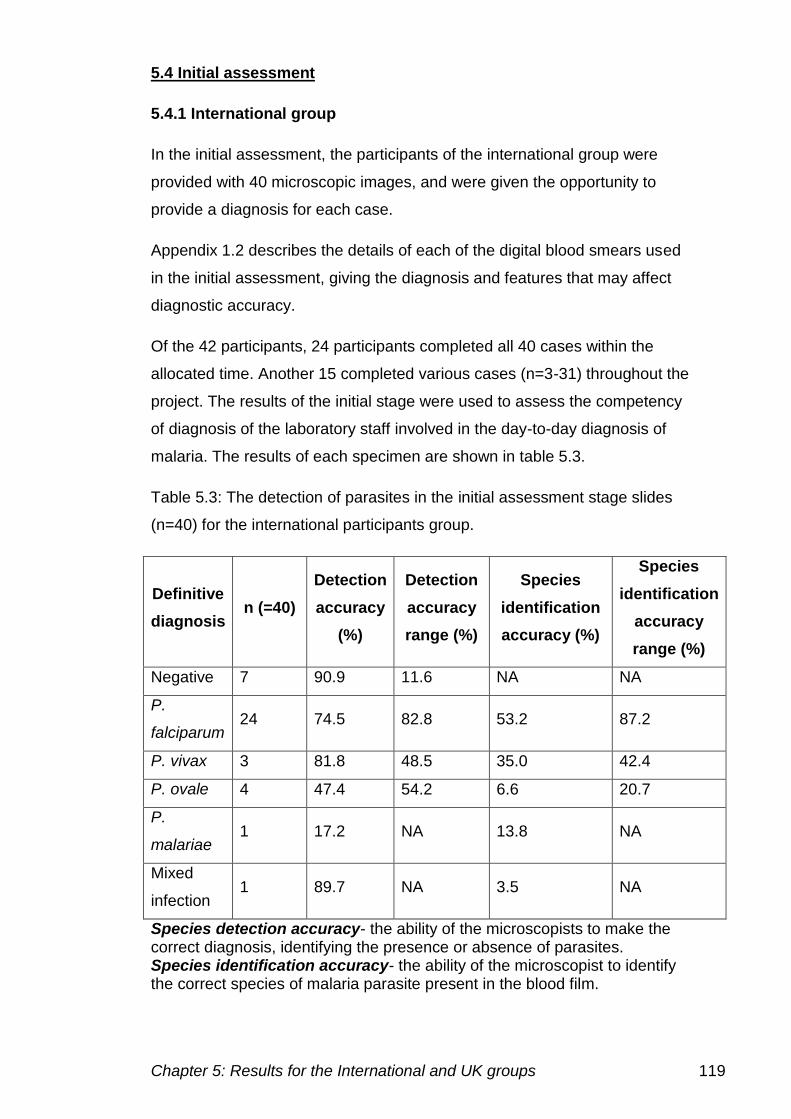
Chapter 5: Results for the International and UK groups 119
5.4 Initial assessment
5.4.1 International group
In the initial assessment, the participants of the international group were
provided with 40 microscopic images, and were given the opportunity to
provide a diagnosis for each case.
Appendix 1.2 describes the details of each of the digital blood smears used
in the initial assessment, giving the diagnosis and features that may affect
diagnostic accuracy.
Of the 42 participants, 24 participants completed all 40 cases within the
allocated time. Another 15 completed various cases (n=3-31) throughout the
project. The results of the initial stage were used to assess the competency
of diagnosis of the laboratory staff involved in the day-to-day diagnosis of
malaria. The results of each specimen are shown in table 5.3.
Table 5.3: The detection of parasites in the initial assessment stage slides
(n=40) for the international participants group.
Definitive
diagnosis n (=40)
Detection
accuracy
(%)
Detection
accuracy
range (%)
Species
identification
accuracy (%)
Species
identification
accuracy
range (%)
Negative 7 90.9 11.6 NA NA
P.
falciparum 24 74.5 82.8 53.2 87.2
P. vivax 3 81.8 48.5 35.0 42.4
P. ovale 4 47.4 54.2 6.6 20.7
P.
malariae 1 17.2 NA 13.8 NA
Mixed
infection 1 89.7 NA 3.5 NA
Species detection accuracy- the ability of the microscopists to make the correct diagnosis, identifying the presence or absence of parasites. Species identification accuracy- the ability of the microscopist to identify the correct species of malaria parasite present in the blood film.
Chapter 5: Results for the International and UK groups 120
Overall, the diagnosis of malaria for all international participants across all 40
cases gave a detection accuracy of 74.6% (±29.3). However, in no single
case was the outcome correctly diagnosed by all participants in terms of
determining the presence of parasites and in identifying correct species.
There were eight cases in which all participants correctly identified the
presence or absence of parasites.
The species detection accuracy was low at 43.7% (±28.1). One case had the
correct species identified by all participants, who had identified the presence
of parasite density. The species identification accuracy was highest for
P. falciparum cases, which all participants from this international group see
on a daily basis.
Table 5.4 demonstrates performance on the individual cases in the initial
assessment by the international group.
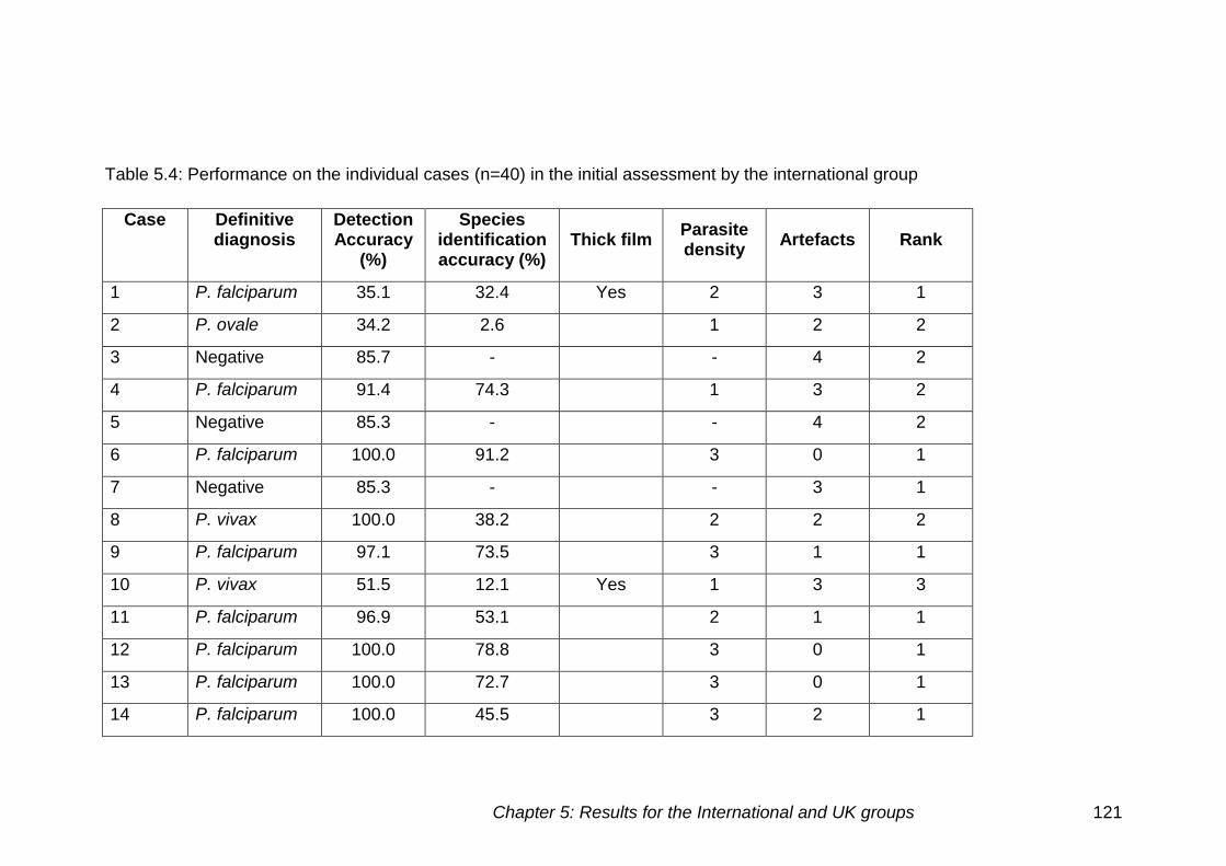
Chapter 5: Results for the International and UK groups 121
Table 5.4: Performance on the individual cases (n=40) in the initial assessment by the international group
Case Definitive diagnosis
Detection Accuracy
(%)
Species identification accuracy (%)
Thick film Parasite density
Artefacts Rank
1 P. falciparum 35.1 32.4 Yes 2 3 1
2 P. ovale 34.2 2.6 1 2 2
3 Negative 85.7 - - 4 2
4 P. falciparum 91.4 74.3 1 3 2
5 Negative 85.3 - - 4 2
6 P. falciparum 100.0 91.2 3 0 1
7 Negative 85.3 - - 3 1
8 P. vivax 100.0 38.2 2 2 2
9 P. falciparum 97.1 73.5 3 1 1
10 P. vivax 51.5 12.1 Yes 1 3 3
11 P. falciparum 96.9 53.1 2 1 1
12 P. falciparum 100.0 78.8 3 0 1
13 P. falciparum 100.0 72.7 3 0 1
14 P. falciparum 100.0 45.5 3 2 1
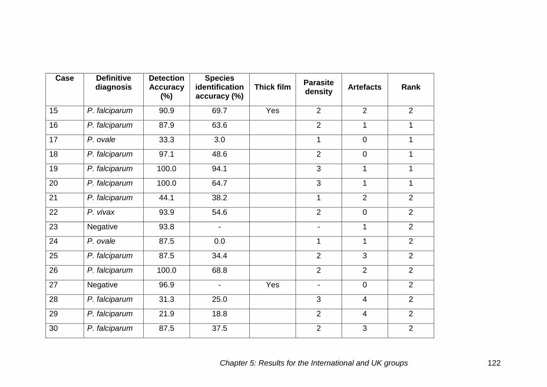
Chapter 5: Results for the International and UK groups 122
Case Definitive diagnosis
Detection Accuracy
(%)
Species identification accuracy (%)
Thick film Parasite density
Artefacts Rank
15 P. falciparum 90.9 69.7 Yes 2 2 2
16 P. falciparum 87.9 63.6 2 1 1
17 P. ovale 33.3 3.0 1 0 1
18 P. falciparum 97.1 48.6 2 0 1
19 P. falciparum 100.0 94.1 3 1 1
20 P. falciparum 100.0 64.7 3 1 1
21 P. falciparum 44.1 38.2 1 2 2
22 P. vivax 93.9 54.6 2 0 2
23 Negative 93.8 - - 1 2
24 P. ovale 87.5 0.0 1 1 2
25 P. falciparum 87.5 34.4 2 3 2
26 P. falciparum 100.0 68.8 2 2 2
27 Negative 96.9 - Yes - 0 2
28 P. falciparum 31.3 25.0 3 4 2
29 P. falciparum 21.9 18.8 2 4 2
30 P. falciparum 87.5 37.5 2 3 2
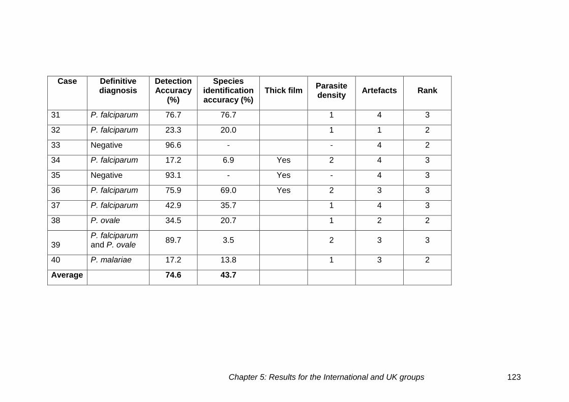
Chapter 5: Results for the International and UK groups 123
Case Definitive diagnosis
Detection Accuracy
(%)
Species identification accuracy (%)
Thick film Parasite density
Artefacts Rank
31 P. falciparum 76.7 76.7 1 4 3
32 P. falciparum 23.3 20.0 1 1 2
33 Negative 96.6 - - 4 2
34 P. falciparum 17.2 6.9 Yes 2 4 3
35 Negative 93.1 - Yes - 4 3
36 P. falciparum 75.9 69.0 Yes 2 3 3
37 P. falciparum 42.9 35.7 1 4 3
38 P. ovale 34.5 20.7 1 2 2
39 P. falciparum and P. ovale
89.7 3.5 2 3 3
40 P. malariae 17.2 13.8 1 3 2
Average 74.6 43.7
Chapter 5: Results for the International and UK groups 124
The main errors made allocated into three categories
False negatives
False positives
Incorrect species
False negatives
False negative results were mainly due to one or more of the following:
Low parasite density
False negative results were reported on a number of low parasite density
cases. For example, case 32, a thin film positive for P. falciparum with only
one gametocyte present, was identified as negative by 23 out of 30
participants. Of the seven that identified the presence of parasite density, six
made the correct diagnosis.
All 12 cases with a low parasite density had false negative results. The low
parasite density P. falciparum cases 2 (25), 4 (3), 21 (19), 31 (7) and 37 (16),
appear to have caused false negative results (number of negative cases
reported in brackets). There were two low parasite density P. vivax cases;
case 10, a thick film, was reported as negative by 16 participants, and case
22 was reported as negative by two participants. All three P. ovale cases
were low parasite density cases; case 17 had 22 false negative results, case
24 had four and case 38 had 19. There was one P. malariae case, case 40,
which had 24 of the international participants giving negative results.
Thick films obscuring parasites
There were seven thick blood films used in the initial assessment, and there
were two negative films used. The use of thick blood films appeared to
obscure parasites from the microscope user, even at higher parasite
densities (number of negative cases reported in brackets), cases 1 (24), 10
(16), 15(3) 34 (24) and 36 (7) had high false negative rates.
Chapter 5: Results for the International and UK groups 125
Artefacts
There were five positive cases with an abundance of artefacts (rank 4).
Cases 28 and 29 not only had high parasite densities but also had false
negative results (22 and 25 respectively). In case 28, the parasites were faint
and slightly out of focus, this combined with the stain deposit could have lead
to the parasites being missed even at such high densities. Case 29 showed
very small P. falciparum trophozoites in a patient that also had chronic
granulocytic leukaemia, six correctly identified the P. falciparum infection.
False negative results were also seen for cases 31 (7), 34 (24) and 37 (16)
(number of negative cases reported in brackets).
False positives
False positives were seen mainly on cases with artefacts present, which
could be confused with parasites present.
There were four negative cases with numerous artefacts present (rank 4).
Case 3 showed five false positive results amongst the participants, possibly
due to the artefacts present. These artefacts include platelets overlying
erythrocytes and stain deposits overlying the erythrocytes.
Cases 5 and 7 showed five false positive results. Case 7 showed intense
basophilic stippling found in other haematological disorders, such as heavy
metal poisoning. The basophilic stippling has a similar appearance to the
stippling seen in P. vivax and P. ovale infection but without the parasite
within the cell.
Incorrect species
The identification of the species present caused more difficulty than
identifying the presence of parasite density, especially in cases other than P.
falciparum, which is most commonly seen in the study regions involved. The
species identification accuracy in cases 2, 17 and 24 was poor, these were
all cases with P. ovale infection. There were also problems with P. vivax
identification, case 8 had the incorrect species identified by 25 participants,
case 10 by 13 and case 22 by 13. A large number of participants did not
correctly identify the late trophozoites and recorded these infections as P.
Chapter 5: Results for the International and UK groups 126
falciparum infection. This is clinically significant as the treatment differs
between these two species.
Low parasite density
There were six low parasite density P. falciparum cases used in the initial
assessment, in five of which difficulties in species determination were
observed. Case 2 was identified as a different species by four participants,
case 4 by six, case 21 by two, case 32 by one and case 7 by two. These
difficulties were probably caused by a lack of parasites present in the
specimens.
Thick films
All of the four P. falciparum thick films used caused difficulties in species
identification. Case 1 had one participant who identified this specimen as P.
vivax, case 15 was identified as P. vivax by four participants and three
identified it as P. malariae. Case 34 had three incorrect species
determinations, and finally, case 36 had two, one P. ovale and one P.
malariae.
Artefact
Little influence on species determination was seen in the five cases, where
numerous artefacts were present (rank 4). Cases 28 (2), 29 (1), 34 (3) and
37 (2), caused more difficulties in detection than in species determination
(figures in brackets indicate number of incorrect species).
Cell inclusions
Cases 6 (3), 9 (8), 11 (14), 12 (7), 13 (9), 14 (18), 16 (8), 18 (17), 19 (2), 20
(12), 25 (17), 26 (10) and 30 (16) were all P. falciparum infections in which
there was a difficulty diagnosing the correct species (figures in brackets
indicate number of incorrect species). All of these cases however had higher
parasite densities being in the 6-49 or >50 cell categories. Confusing factors
included stippling, Maurer’s dots and EDTA changes.
Chapter 5: Results for the International and UK groups 127
Mixed infections
Case 39 showed a mixed infection of P. falciparum and P. vivax and was
identified correctly by five participants. However, one participant identified P.
falciparum and P. ovale infection showing the similarities in their morphology,
and 18 participants identified P. falciparum infection alone. Two other
participants identified P. ovale and P. vivax in isolation.
Comparison of images used in the initial assessment of the
International group
Thick and thin films used
There were seven thick films and 33 thin films used in the International
group. The detection accuracy for thick films was 68.5%(±31.5) and for thin
films 76.4%(±28.9). The species identification accuracy for thick films was
38%(±30.1) and 44.7%(±28.2) for thin films. The differences between the
thick and thin film were not significant (detection accuracy p=0.276) (species
identification accuracy p=0.581).
Species
There was only one mixed species case, which was excluded from the
analysis. The results for P. malariae were also obtained from a single case.
Figure 5.3 shows the comparison of detection accuracy and species
identification accuracy for the different species and different slide
preparations. The species identification accuracy for P. falciparum is higher
than other species, with P. ovale specimens showing the lowest species
identification accuracy at 6% (±6.5).
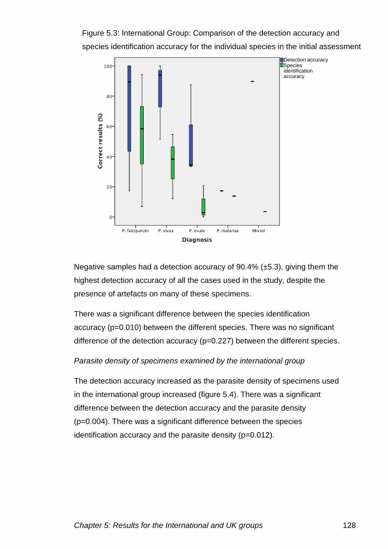
Chapter 5: Results for the International and UK groups 128
Negative samples had a detection accuracy of 90.4% (±5.3), giving them the
highest detection accuracy of all the cases used in the study, despite the
presence of artefacts on many of these specimens.
There was a significant difference between the species identification
accuracy (p=0.010) between the different species. There was no significant
difference of the detection accuracy (p=0.227) between the different species.
Parasite density of specimens examined by the international group
The detection accuracy increased as the parasite density of specimens used
in the international group increased (figure 5.4). There was a significant
difference between the detection accuracy and the parasite density
(p=0.004). There was a significant difference between the species
identification accuracy and the parasite density (p=0.012).
Detection accuracy
Species identification accuracy
Figure 5.3: International Group: Comparison of the detection accuracy and
species identification accuracy for the individual species in the initial assessment
Detection accuracy Species identification accuracy
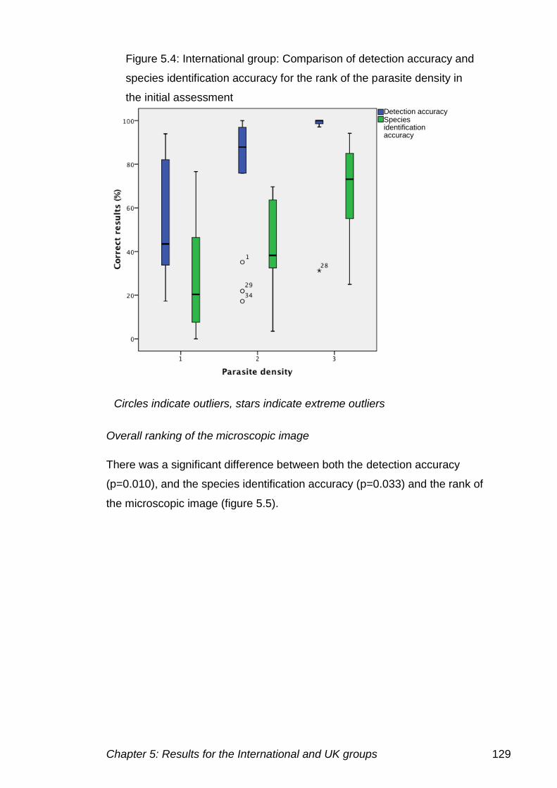
Chapter 5: Results for the International and UK groups 129
Overall ranking of the microscopic image
There was a significant difference between both the detection accuracy
(p=0.010), and the species identification accuracy (p=0.033) and the rank of
the microscopic image (figure 5.5).
Figure 5.4: International group: Comparison of detection accuracy and
species identification accuracy for the rank of the parasite density in
the initial assessment Detection accuracy Species identification accuracy
Circles indicate outliers, stars indicate extreme outliers
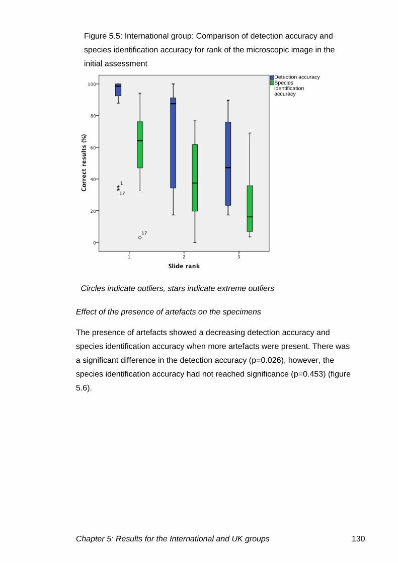
Chapter 5: Results for the International and UK groups 130
Effect of the presence of artefacts on the specimens
The presence of artefacts showed a decreasing detection accuracy and
species identification accuracy when more artefacts were present. There was
a significant difference in the detection accuracy (p=0.026), however, the
species identification accuracy had not reached significance (p=0.453) (figure
5.6).
Figure 5.5: International group: Comparison of detection accuracy and
species identification accuracy for rank of the microscopic image in the
initial assessment
Detection accuracy Species identification accuracy
Circles indicate outliers, stars indicate extreme outliers
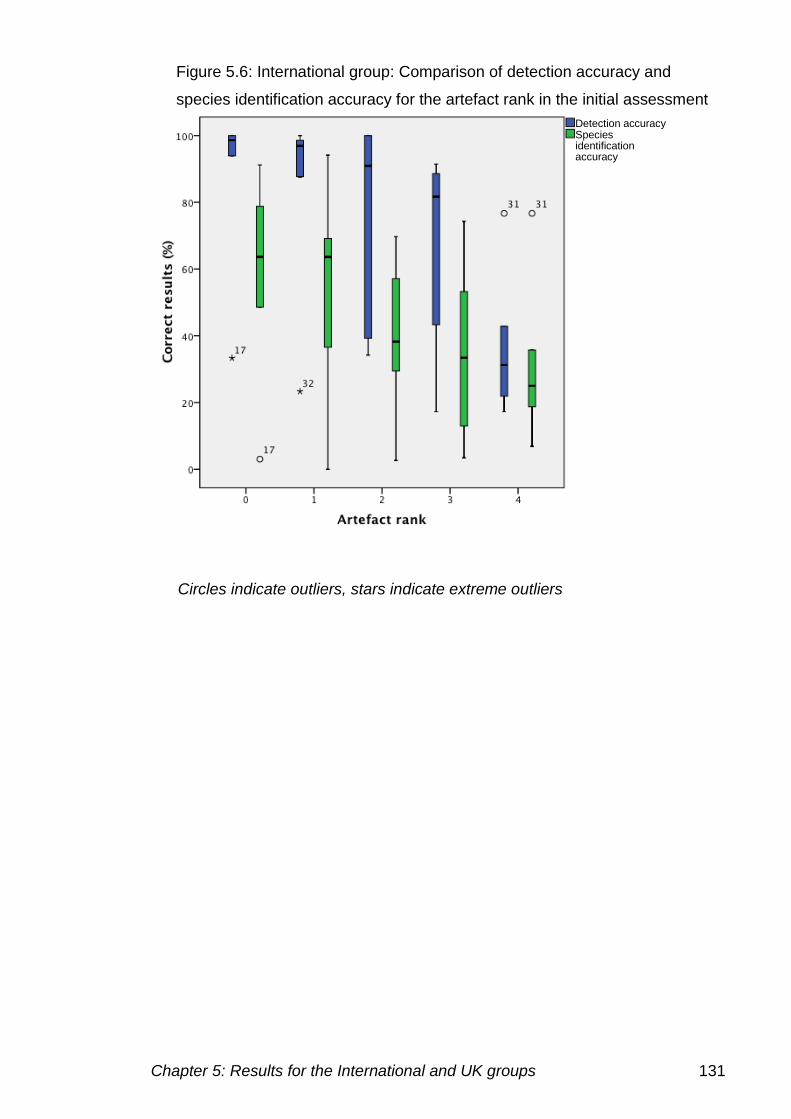
Chapter 5: Results for the International and UK groups 131
Figure 5.6: International group: Comparison of detection accuracy and
species identification accuracy for the artefact rank in the initial assessment
Detection accuracy Species identification accuracy
Circles indicate outliers, stars indicate extreme outliers
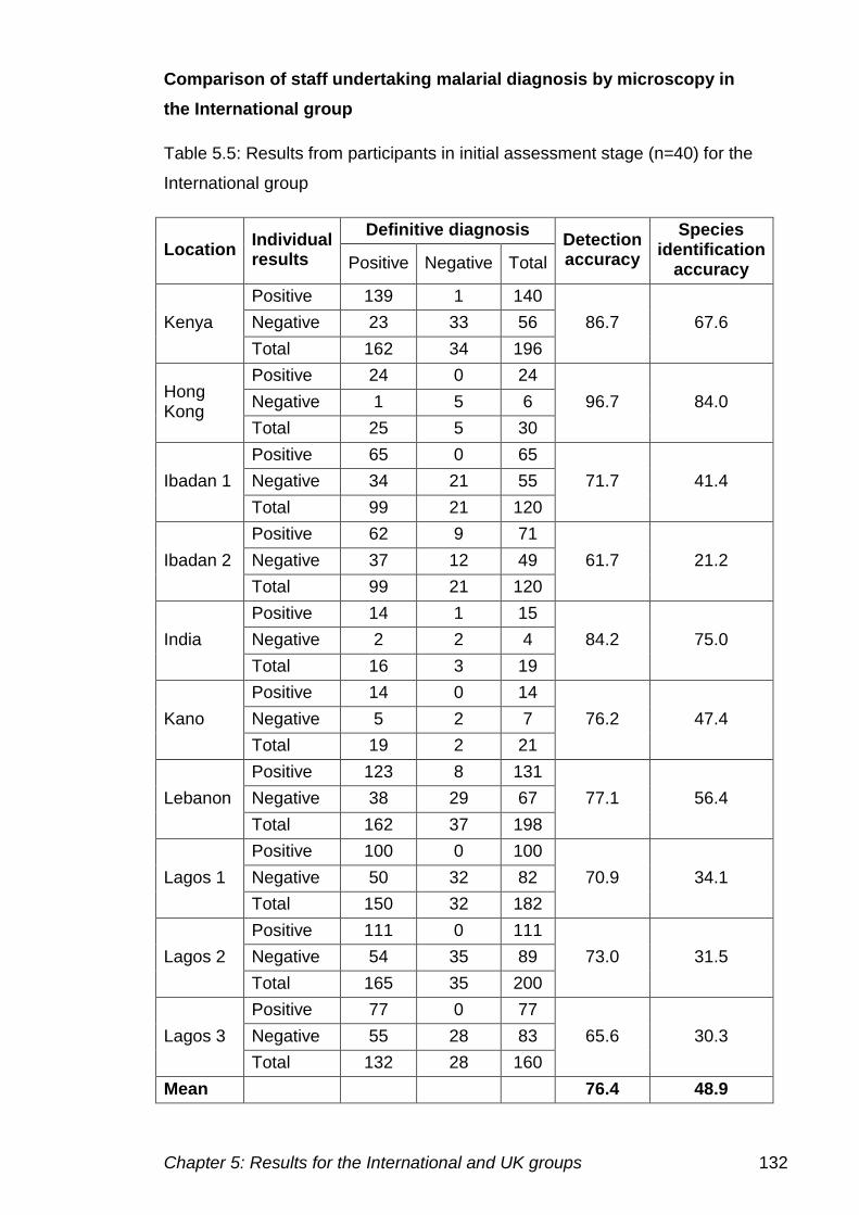
Chapter 5: Results for the International and UK groups 132
Comparison of staff undertaking malarial diagnosis by microscopy in
the International group
Table 5.5: Results from participants in initial assessment stage (n=40) for the
International group
Location Individual results
Definitive diagnosis Detection accuracy
Species identification
accuracy Positive Negative Total
Kenya
Positive 139 1 140
86.7 67.6 Negative 23 33 56
Total 162 34 196
Hong Kong
Positive 24 0 24
96.7 84.0 Negative 1 5 6
Total 25 5 30
Ibadan 1
Positive 65 0 65
71.7 41.4 Negative 34 21 55
Total 99 21 120
Ibadan 2
Positive 62 9 71
61.7 21.2 Negative 37 12 49
Total 99 21 120
India
Positive 14 1 15
84.2 75.0 Negative 2 2 4
Total 16 3 19
Kano
Positive 14 0 14
76.2 47.4 Negative 5 2 7
Total 19 2 21
Lebanon
Positive 123 8 131
77.1 56.4 Negative 38 29 67
Total 162 37 198
Lagos 1
Positive 100 0 100
70.9 34.1 Negative 50 32 82
Total 150 32 182
Lagos 2
Positive 111 0 111
73.0 31.5 Negative 54 35 89
Total 165 35 200
Lagos 3
Positive 77 0 77
65.6 30.3 Negative 55 28 83
Total 132 28 160
Mean 76.4 48.9
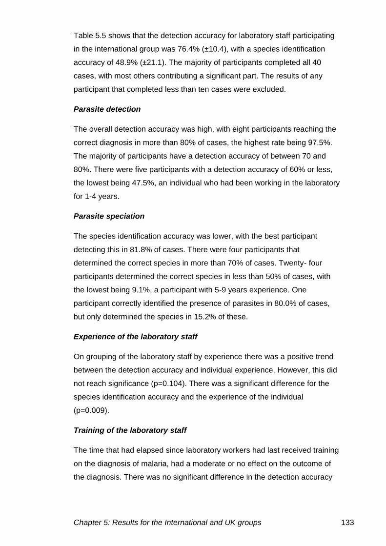
Chapter 5: Results for the International and UK groups 133
Table 5.5 shows that the detection accuracy for laboratory staff participating
in the international group was 76.4% (±10.4), with a species identification
accuracy of 48.9% (±21.1). The majority of participants completed all 40
cases, with most others contributing a significant part. The results of any
participant that completed less than ten cases were excluded.
Parasite detection
The overall detection accuracy was high, with eight participants reaching the
correct diagnosis in more than 80% of cases, the highest rate being 97.5%.
The majority of participants have a detection accuracy of between 70 and
80%. There were five participants with a detection accuracy of 60% or less,
the lowest being 47.5%, an individual who had been working in the laboratory
for 1-4 years.
Parasite speciation
The species identification accuracy was lower, with the best participant
detecting this in 81.8% of cases. There were four participants that
determined the correct species in more than 70% of cases. Twenty- four
participants determined the correct species in less than 50% of cases, with
the lowest being 9.1%, a participant with 5-9 years experience. One
participant correctly identified the presence of parasites in 80.0% of cases,
but only determined the species in 15.2% of these.
Experience of the laboratory staff
On grouping of the laboratory staff by experience there was a positive trend
between the detection accuracy and individual experience. However, this did
not reach significance (p=0.104). There was a significant difference for the
species identification accuracy and the experience of the individual
(p=0.009).
Training of the laboratory staff
The time that had elapsed since laboratory workers had last received training
on the diagnosis of malaria, had a moderate or no effect on the outcome of
the diagnosis. There was no significant difference in the detection accuracy
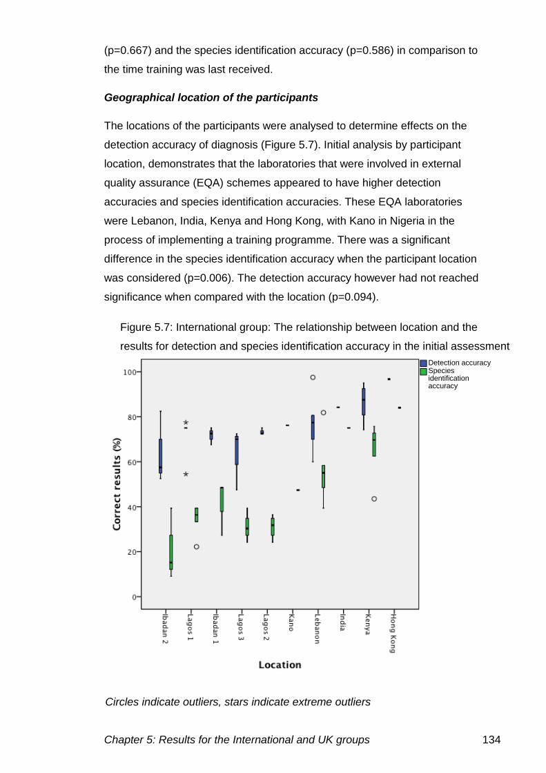
Chapter 5: Results for the International and UK groups 134
(p=0.667) and the species identification accuracy (p=0.586) in comparison to
the time training was last received.
Geographical location of the participants
The locations of the participants were analysed to determine effects on the
detection accuracy of diagnosis (Figure 5.7). Initial analysis by participant
location, demonstrates that the laboratories that were involved in external
quality assurance (EQA) schemes appeared to have higher detection
accuracies and species identification accuracies. These EQA laboratories
were Lebanon, India, Kenya and Hong Kong, with Kano in Nigeria in the
process of implementing a training programme. There was a significant
difference in the species identification accuracy when the participant location
was considered (p=0.006). The detection accuracy however had not reached
significance when compared with the location (p=0.094).
Figure 5.7: International group: The relationship between location and the
results for detection and species identification accuracy in the initial assessment
Detection accuracy Species identification accuracy
Circles indicate outliers, stars indicate extreme outliers
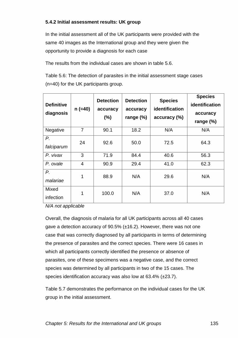
Chapter 5: Results for the International and UK groups 135
5.4.2 Initial assessment results: UK group
In the initial assessment all of the UK participants were provided with the
same 40 images as the International group and they were given the
opportunity to provide a diagnosis for each case
The results from the individual cases are shown in table 5.6.
Table 5.6: The detection of parasites in the initial assessment stage cases
(n=40) for the UK participants group.
Definitive
diagnosis n (=40)
Detection
accuracy
(%)
Detection
accuracy
range (%)
Species
identification
accuracy (%)
Species
identification
accuracy
range (%)
Negative 7 90.1 18.2 N/A N/A
P.
falciparum 24 92.6 50.0 72.5 64.3
P. vivax 3 71.9 84.4 40.6 56.3
P. ovale 4 90.9 29.4 41.0 62.3
P.
malariae 1 88.9 N/A 29.6 N/A
Mixed
infection 1 100.0 N/A 37.0 N/A
N/A not applicable
Overall, the diagnosis of malaria for all UK participants across all 40 cases
gave a detection accuracy of 90.5% (±16.2). However, there was not one
case that was correctly diagnosed by all participants in terms of determining
the presence of parasites and the correct species. There were 16 cases in
which all participants correctly identified the presence or absence of
parasites, one of these specimens was a negative case, and the correct
species was determined by all participants in two of the 15 cases. The
species identification accuracy was also low at 63.4% (±23.7).
Table 5.7 demonstrates the performance on the individual cases for the UK
group in the initial assessment.
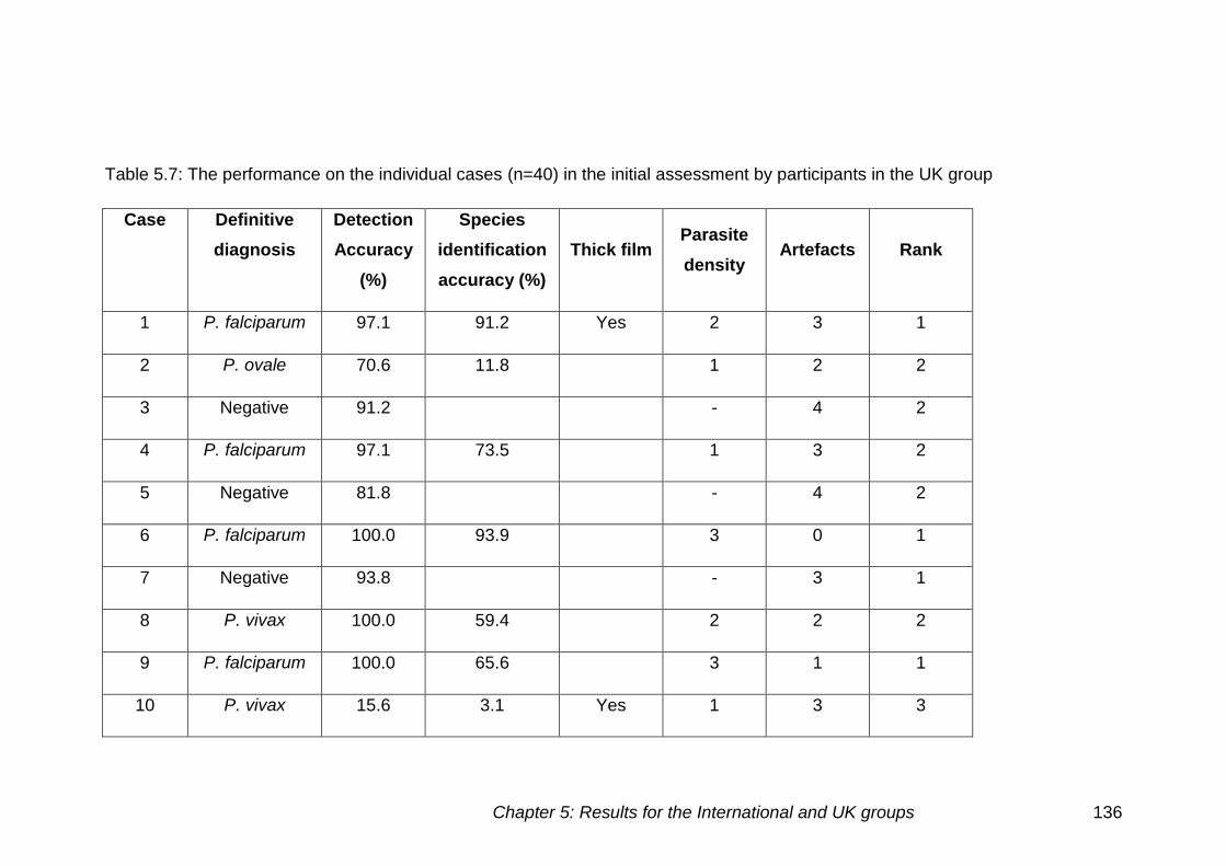
Chapter 5: Results for the International and UK groups 136
Table 5.7: The performance on the individual cases (n=40) in the initial assessment by participants in the UK group
Case Definitive
diagnosis
Detection
Accuracy
(%)
Species
identification
accuracy (%)
Thick film Parasite
density Artefacts Rank
1 P. falciparum 97.1 91.2 Yes 2 3 1
2 P. ovale 70.6 11.8 1 2 2
3 Negative 91.2 - 4 2
4 P. falciparum 97.1 73.5 1 3 2
5 Negative 81.8 - 4 2
6 P. falciparum 100.0 93.9 3 0 1
7 Negative 93.8 - 3 1
8 P. vivax 100.0 59.4 2 2 2
9 P. falciparum 100.0 65.6 3 1 1
10 P. vivax 15.6 3.1 Yes 1 3 3
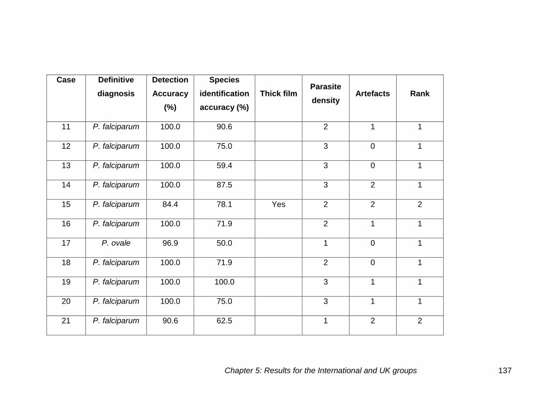
Chapter 5: Results for the International and UK groups 137
Case Definitive
diagnosis
Detection
Accuracy
(%)
Species
identification
accuracy (%)
Thick film Parasite
density Artefacts Rank
11 P. falciparum 100.0 90.6 2 1 1
12 P. falciparum 100.0 75.0 3 0 1
13 P. falciparum 100.0 59.4 3 0 1
14 P. falciparum 100.0 87.5 3 2 1
15 P. falciparum 84.4 78.1 Yes 2 2 2
16 P. falciparum 100.0 71.9 2 1 1
17 P. ovale 96.9 50.0 1 0 1
18 P. falciparum 100.0 71.9 2 0 1
19 P. falciparum 100.0 100.0 3 1 1
20 P. falciparum 100.0 75.0 3 1 1
21 P. falciparum 90.6 62.5 1 2 2
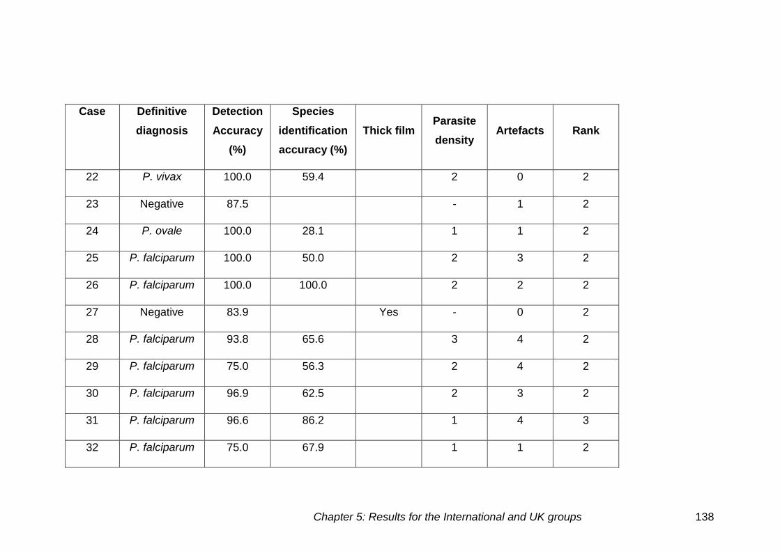
Chapter 5: Results for the International and UK groups 138
Case Definitive
diagnosis
Detection
Accuracy
(%)
Species
identification
accuracy (%)
Thick film Parasite
density Artefacts Rank
22 P. vivax 100.0 59.4 2 0 2
23 Negative 87.5 - 1 2
24 P. ovale 100.0 28.1 1 1 2
25 P. falciparum 100.0 50.0 2 3 2
26 P. falciparum 100.0 100.0 2 2 2
27 Negative 83.9 Yes - 0 2
28 P. falciparum 93.8 65.6 3 4 2
29 P. falciparum 75.0 56.3 2 4 2
30 P. falciparum 96.9 62.5 2 3 2
31 P. falciparum 96.6 86.2 1 4 3
32 P. falciparum 75.0 67.9 1 1 2
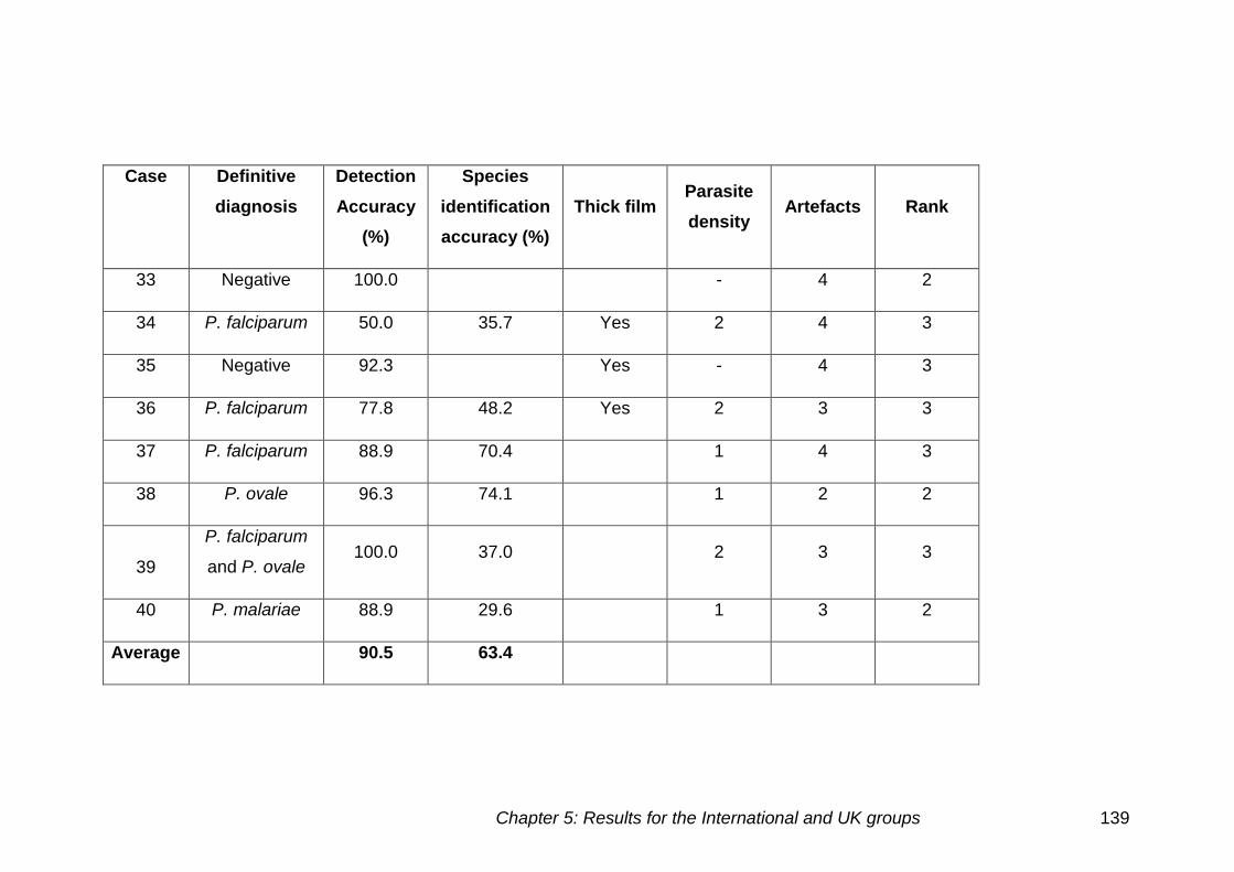
Chapter 5: Results for the International and UK groups 139
Case Definitive
diagnosis
Detection
Accuracy
(%)
Species
identification
accuracy (%)
Thick film Parasite
density Artefacts Rank
33 Negative 100.0 - 4 2
34 P. falciparum 50.0 35.7 Yes 2 4 3
35 Negative 92.3 Yes - 4 3
36 P. falciparum 77.8 48.2 Yes 2 3 3
37 P. falciparum 88.9 70.4 1 4 3
38 P. ovale 96.3 74.1 1 2 2
39
P. falciparum
and P. ovale 100.0 37.0 2 3 3
40 P. malariae 88.9 29.6 1 3 2
Average 90.5 63.4
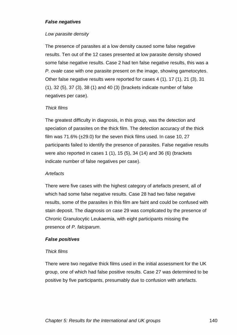
Chapter 5: Results for the International and UK groups 140
False negatives
Low parasite density
The presence of parasites at a low density caused some false negative
results. Ten out of the 12 cases presented at low parasite density showed
some false negative results. Case 2 had ten false negative results, this was a
P. ovale case with one parasite present on the image, showing gametocytes.
Other false negative results were reported for cases 4 (1), 17 (1), 21 (3), 31
(1), 32 (5), 37 (3), 38 (1) and 40 (3) (brackets indicate number of false
negatives per case).
Thick films
The greatest difficulty in diagnosis, in this group, was the detection and
speciation of parasites on the thick film. The detection accuracy of the thick
film was 71.6% (±29.0) for the seven thick films used. In case 10, 27
participants failed to identify the presence of parasites. False negative results
were also reported in cases 1 (1), 15 (5), 34 (14) and 36 (6) (brackets
indicate number of false negatives per case).
Artefacts
There were five cases with the highest category of artefacts present, all of
which had some false negative results. Case 28 had two false negative
results, some of the parasites in this film are faint and could be confused with
stain deposit. The diagnosis on case 29 was complicated by the presence of
Chronic Granulocytic Leukaemia, with eight participants missing the
presence of P. falciparum.
False positives
Thick films
There were two negative thick films used in the initial assessment for the UK
group, one of which had false positive results. Case 27 was determined to be
positive by five participants, presumably due to confusion with artefacts.
Chapter 5: Results for the International and UK groups 141
Artefacts
False positive results were seen for six out of the seven negative cases used.
Case 3 had three false positive results possibly because of stain deposit,
case 7 had two false positive results probably due to basophilic stippling,
case 35 a thick film had two false positive results.
Incorrect species
Low parasite density
Twelve low parasite density cases were used in the initial assessment, all of
which caused problems with parasite identification, possibly due to the lack of
cells present to allow identification. There were six P. falciparum cases that
caused difficulties, cases 4 (8), 6 (2), 21 (9), 31 (3), 32 (4) and 37 (5). There
were two P. vivax low parasite density infections (cases 10 (4) and 22 (6))
which had incorrect species identified (brackets indicate the number of
incorrect species identified).
All four P. ovale cases used in the initial assessment (cases 2 (20), 17 (16),
24 (20) and 38 (6)) were at low parasite density and caused difficulties in
diagnosis made. As the P. ovale infected cells have a similar appearance to
P. vivax and receive the same treatment any confusion between these
species was regarded as a minor error.
Case 40, a P. malariae infection had only two parasites present, 16
individuals incorrectly diagnosed the species.
Thick films
The species is not normally determined on the thick film and is not
recommended practice in the UK. There were five positive thick films cases 1
(2), 10 (4), 15 (2), 34 (4) and 37 (5) (brackets indicate the number of incorrect
species identified).
Artefact
Artefacts cannot only cause confusion in identifying whether parasites are
present, but also can look like different species, in cases 25 (16), 28 (9) and
29 (6) (brackets indicate the number of incorrect species identified).
Chapter 5: Results for the International and UK groups 142
Cell inclusions
The majority of cases that caused problems in speciation were affected by
EDTA, increasing the number of Accole forms and Maurer's clefts present.
Cases 4 (8), 6 (2), 9 (11), 12 (8), 13 (13), 18 (9), and 20 (8), all had
diagnoses of P. vivax and P. ovale made due to the presence of Maurer's
clefts being confused with stippling. Cases 11 (3), 14 (4), 16 (9), 20 (8) and
30 (11) also had a diagnosis of P. malariae as well as P. vivax and P. ovale
(brackets indicate the number of incorrect species identified).
P. ovale and P. vivax cases
The main difficulty in the UK group was determining the species in P. ovale
and P. vivax infections as they have a very similar appearance. However,
both species have the same treatment, therefore a sub category of treatment
species identification accuracy, was analysed. The overall treatment species
identification accuracy was increased to 70.8% (±21.2) in comparison to the
species identification accuracy. The treatment species identification accuracy
for P. ovale was 80% (±17.9), with a species identification accuracy of 41.0%
(±27.1). The same was seen for P. vivax with the species identification
accuracy increasing from 40.6% (±32.5) to 61.5% (±48.4). The increase in
the treatment species accuracy indicates that most species misidentification
were for the alternative species. Case 2 for example, a P. ovale case, was
only correctly diagnosed by four participants, 16 participants diagnosed this
case as P. vivax this would increase the species identification accuracy from
11.8% to 58.8%.
Mixed infections
Case 39 showed a mixed infection of P. ovale and P. falciparum. Ten
individuals identified that both species were present, nine identifying P.
falciparum alone. Seven individuals mistook P. ovale for P. vivax and one
identified only P. vivax.
Chapter 5: Results for the International and UK groups 143
Comparison of cases used in the initial assessment for the UK group
Thick and thin films
There were seven thick films and 33 thin films. The detection accuracy for
thick films was 71.6% (±29.0) and 94.6% (±8.2) for thin films. The species
identification accuracy of thick films was 51.3% (±34.9) and for thin films
65.5% (±21.3). There was a significance difference in detection accuracy
(p=0.003) between the thick and thin films. However, the species
identification accuracy for the thick and thin films did not reach significance
(p=0.421).
Species identification
There was only one mixed species case, due to the small number of results,
this case was excluded from the analysis. The results for P. malariae were
obtained from a single case.
Figure 5.8 shows the comparison of detection accuracy and species
identification accuracy for the different species and different slide
preparations. The species identification accuracy for P. falciparum was
higher than the other species (72.5 ± 16.6%).
There was a significant difference in the species identification accuracy
(p=0.025) between the different malaria species. However, the detection
accuracy did not reach significance (p=0.494) when compared to the different
malaria species.
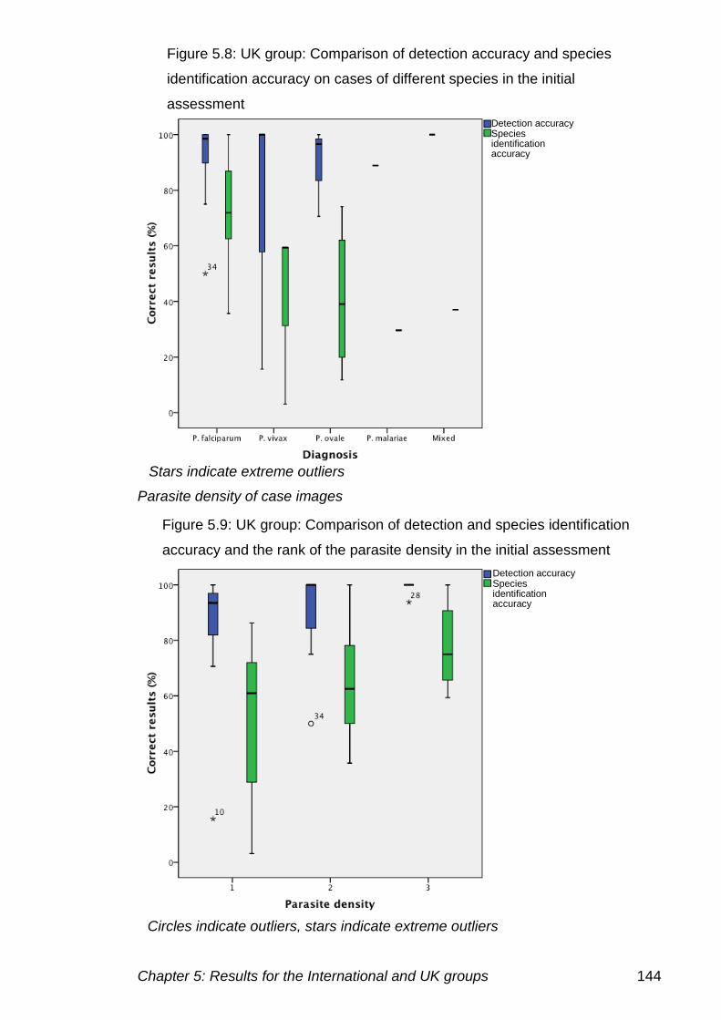
Chapter 5: Results for the International and UK groups 144
Parasite density of case images
Figure 5.8: UK group: Comparison of detection accuracy and species
identification accuracy on cases of different species in the initial
assessment
Figure 5.9: UK group: Comparison of detection and species identification
accuracy and the rank of the parasite density in the initial assessment
Detection accuracy Species identification accuracy
Detection accuracy Species identification accuracy
Stars indicate extreme outliers
Circles indicate outliers, stars indicate extreme outliers
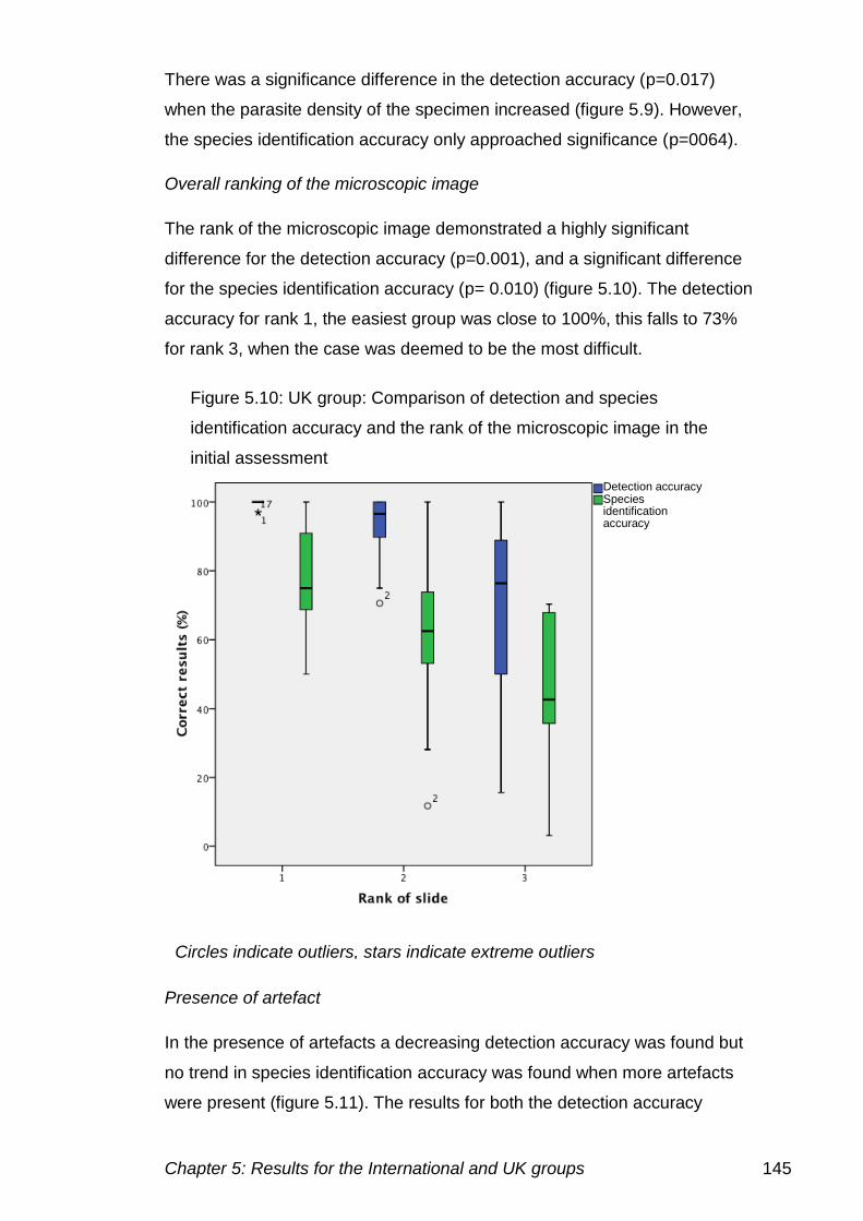
Chapter 5: Results for the International and UK groups 145
There was a significance difference in the detection accuracy (p=0.017)
when the parasite density of the specimen increased (figure 5.9). However,
the species identification accuracy only approached significance (p=0064).
Overall ranking of the microscopic image
The rank of the microscopic image demonstrated a highly significant
difference for the detection accuracy (p=0.001), and a significant difference
for the species identification accuracy (p= 0.010) (figure 5.10). The detection
accuracy for rank 1, the easiest group was close to 100%, this falls to 73%
for rank 3, when the case was deemed to be the most difficult.
Presence of artefact
In the presence of artefacts a decreasing detection accuracy was found but
no trend in species identification accuracy was found when more artefacts
were present (figure 5.11). The results for both the detection accuracy
Figure 5.10: UK group: Comparison of detection and species
identification accuracy and the rank of the microscopic image in the
initial assessment
Detection accuracy Species identification accuracy
Circles indicate outliers, stars indicate extreme outliers
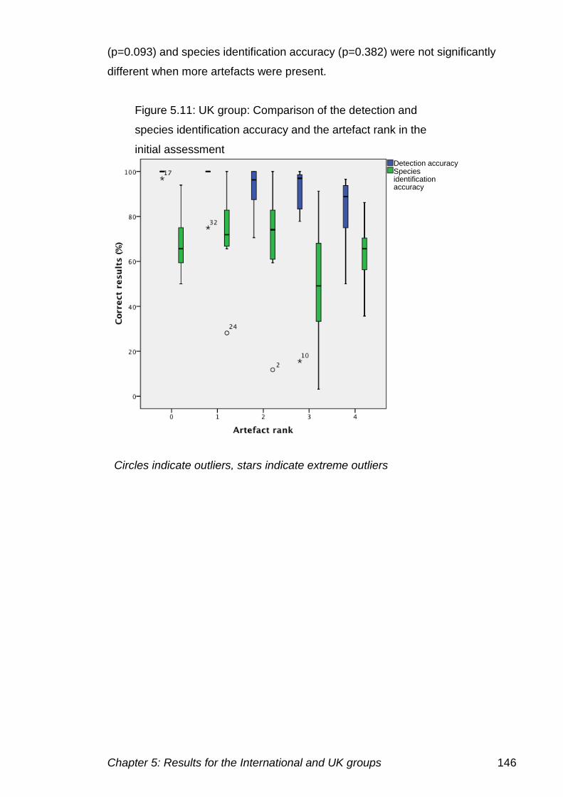
Chapter 5: Results for the International and UK groups 146
(p=0.093) and species identification accuracy (p=0.382) were not significantly
different when more artefacts were present.
Figure 5.11: UK group: Comparison of the detection and
species identification accuracy and the artefact rank in the
initial assessment Detection accuracy Species identification accuracy
Circles indicate outliers, stars indicate extreme outliers
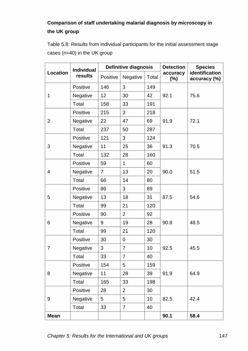
Chapter 5: Results for the International and UK groups 147
Comparison of staff undertaking malarial diagnosis by microscopy in
the UK group
Table 5.8: Results from individual participants for the initial assessment stage
cases (n=40) in the UK group
Location Individual
results
Definitive diagnosis Detection accuracy
(%)
Species identification accuracy (%) Positive Negative Total
1
Positive 146 3 149
92.1 75.6 Negative 12 30 42
Total 158 33 191
2
Positive 215 3 218
91.9 72.1 Negative 22 47 69
Total 237 50 287
3
Positive 121 3 124
91.3 70.5 Negative 11 25 36
Total 132 28 160
4
Positive 59 1 60
90.0 51.5 Negative 7 13 20
Total 66 14 80
5
Positive 86 3 89
87.5 54.6 Negative 13 18 31
Total 99 21 120
6
Positive 90 2 92
90.8 48.5 Negative 9 19 28
Total 99 21 120
7
Positive 30 0 30
92.5 45.5 Negative 3 7 10
Total 33 7 40
8
Positive 154 5 159
91.9 64.9 Negative 11 28 39
Total 165 33 198
9
Positive 28 2 30
82.5 42.4 Negative 5 5 10
Total 33 7 40
Mean 90.1 58.4
Chapter 5: Results for the International and UK groups 148
There were 24 participants that completed all 40 cases in the initial
assessment. Another seven completed more than 30 of the cases. One
participant was excluded from the analysis due to the small number of cases
completed.
Table 5.8 describes the results for the UK participants over the 40 cases or
those that they attempted. The detection accuracy for laboratory staff
participating was 90.1% (±3.2), with a species identification accuracy of
58.4% (±12.5).
Parasite detection
One participant detected the presence or absence of parasites correctly in
the 13 cases they completed. Twenty-two participants detected the parasites
present in more than 90% of cases. Two participants achieved a detection
accuracy of 97.5%. The lowest detection accuracy was 77.5%, an individual
with less than two years experience.
Parasite speciation
A clear difference can be seen between detecting the presence of parasites
and determining the correct species. The highest species identification
accuracy was 87.9%, with the lowest at 39.4%.
Experience of the laboratory staff
The participants were divided into two groups depending upon their
experience. Group one refers to those with less than two years experience or
newly registered Biomedical Scientists. Group two is the individuals with
more than five years experience, varied from five years up to more than 20
years. The detection accuracy for group one, those with less than two years
experience was 90.0% (±5.8) and for group two was 92.1% (±5.2), this
difference was not significant (p=0.171). The species detection accuracy for
group one was 55.8% and group two was 68.8%, this difference was
significant (p=0.009).
Location of the laboratory staff
There was no significant difference in detection accuracy results (p=0.918)
between the different hospitals in which the participants were based. There
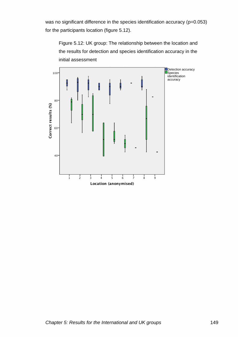
Chapter 5: Results for the International and UK groups 149
was no significant difference in the species identification accuracy (p=0.053)
for the participants location (figure 5.12).
Figure 5.12: UK group: The relationship between the location and
the results for detection and species identification accuracy in the
initial assessment
Detection accuracy Species identification accuracy
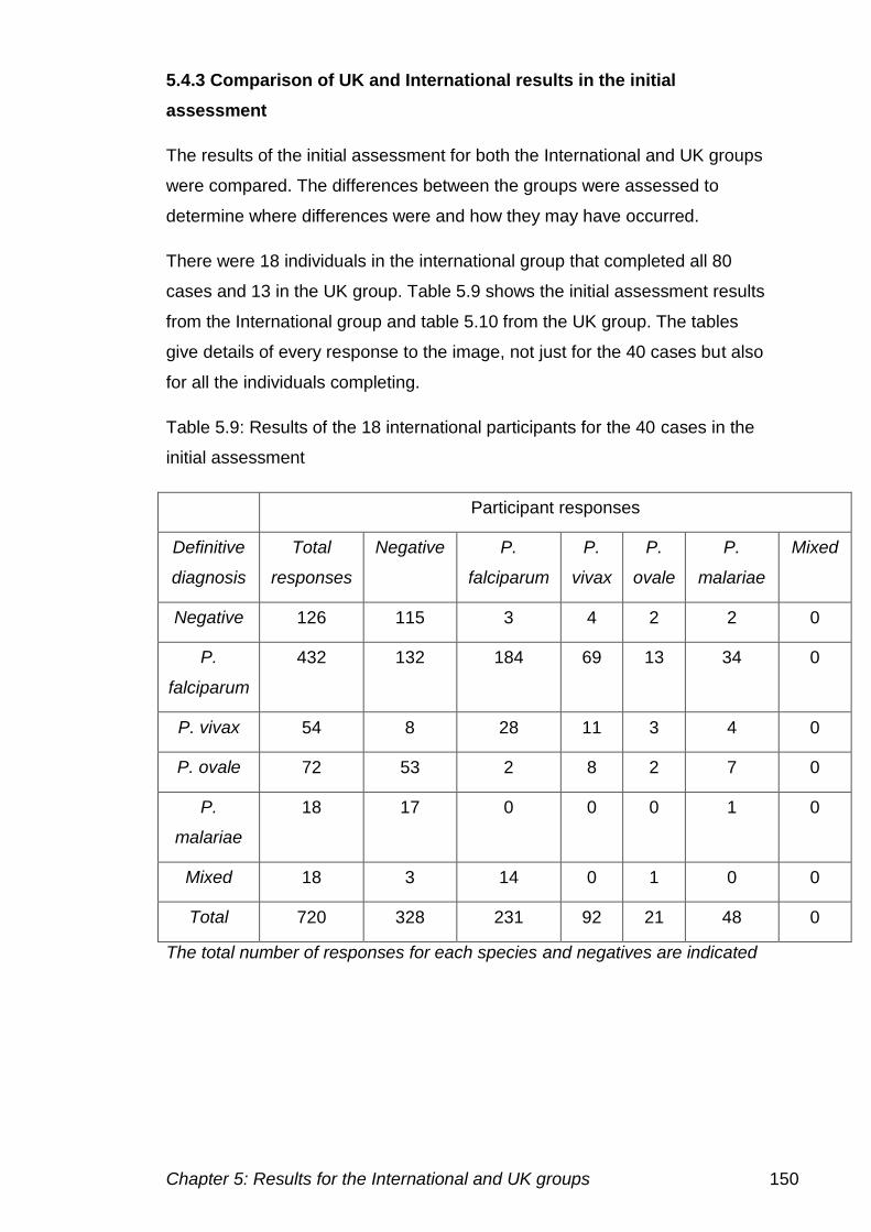
Chapter 5: Results for the International and UK groups 150
5.4.3 Comparison of UK and International results in the initial
assessment
The results of the initial assessment for both the International and UK groups
were compared. The differences between the groups were assessed to
determine where differences were and how they may have occurred.
There were 18 individuals in the international group that completed all 80
cases and 13 in the UK group. Table 5.9 shows the initial assessment results
from the International group and table 5.10 from the UK group. The tables
give details of every response to the image, not just for the 40 cases but also
for all the individuals completing.
Table 5.9: Results of the 18 international participants for the 40 cases in the
initial assessment
Participant responses
Definitive
diagnosis
Total
responses
Negative P.
falciparum
P.
vivax
P.
ovale
P.
malariae
Mixed
Negative 126 115 3 4 2 2 0
P.
falciparum
432 132 184 69 13 34 0
P. vivax 54 8 28 11 3 4 0
P. ovale 72 53 2 8 2 7 0
P.
malariae
18 17 0 0 0 1 0
Mixed 18 3 14 0 1 0 0
Total 720 328 231 92 21 48 0
The total number of responses for each species and negatives are indicated
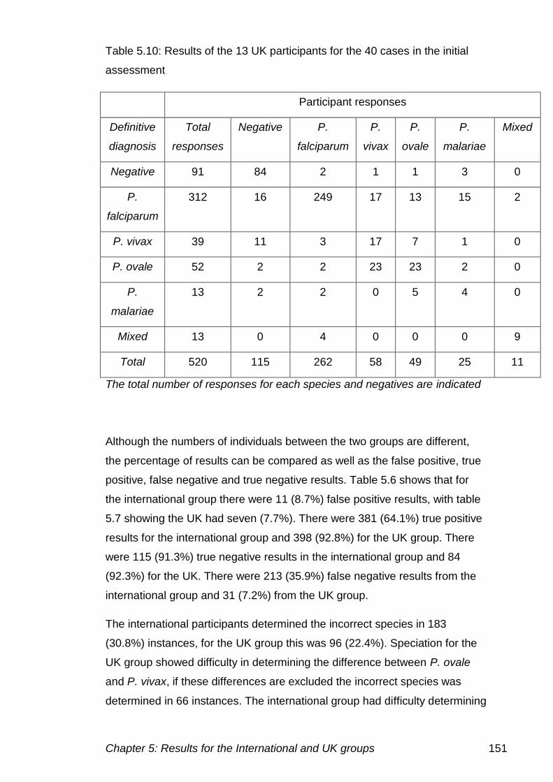
Chapter 5: Results for the International and UK groups 151
Table 5.10: Results of the 13 UK participants for the 40 cases in the initial
assessment
Participant responses
Definitive
diagnosis
Total
responses
Negative P.
falciparum
P.
vivax
P.
ovale
P.
malariae
Mixed
Negative 91 84 2 1 1 3 0
P.
falciparum
312 16 249 17 13 15 2
P. vivax 39 11 3 17 7 1 0
P. ovale 52 2 2 23 23 2 0
P.
malariae
13 2 2 0 5 4 0
Mixed 13 0 4 0 0 0 9
Total 520 115 262 58 49 25 11
The total number of responses for each species and negatives are indicated
Although the numbers of individuals between the two groups are different,
the percentage of results can be compared as well as the false positive, true
positive, false negative and true negative results. Table 5.6 shows that for
the international group there were 11 (8.7%) false positive results, with table
5.7 showing the UK had seven (7.7%). There were 381 (64.1%) true positive
results for the international group and 398 (92.8%) for the UK group. There
were 115 (91.3%) true negative results in the international group and 84
(92.3%) for the UK. There were 213 (35.9%) false negative results from the
international group and 31 (7.2%) from the UK group.
The international participants determined the incorrect species in 183
(30.8%) instances, for the UK group this was 96 (22.4%). Speciation for the
UK group showed difficulty in determining the difference between P. ovale
and P. vivax, if these differences are excluded the incorrect species was
determined in 66 instances. The international group had difficulty determining
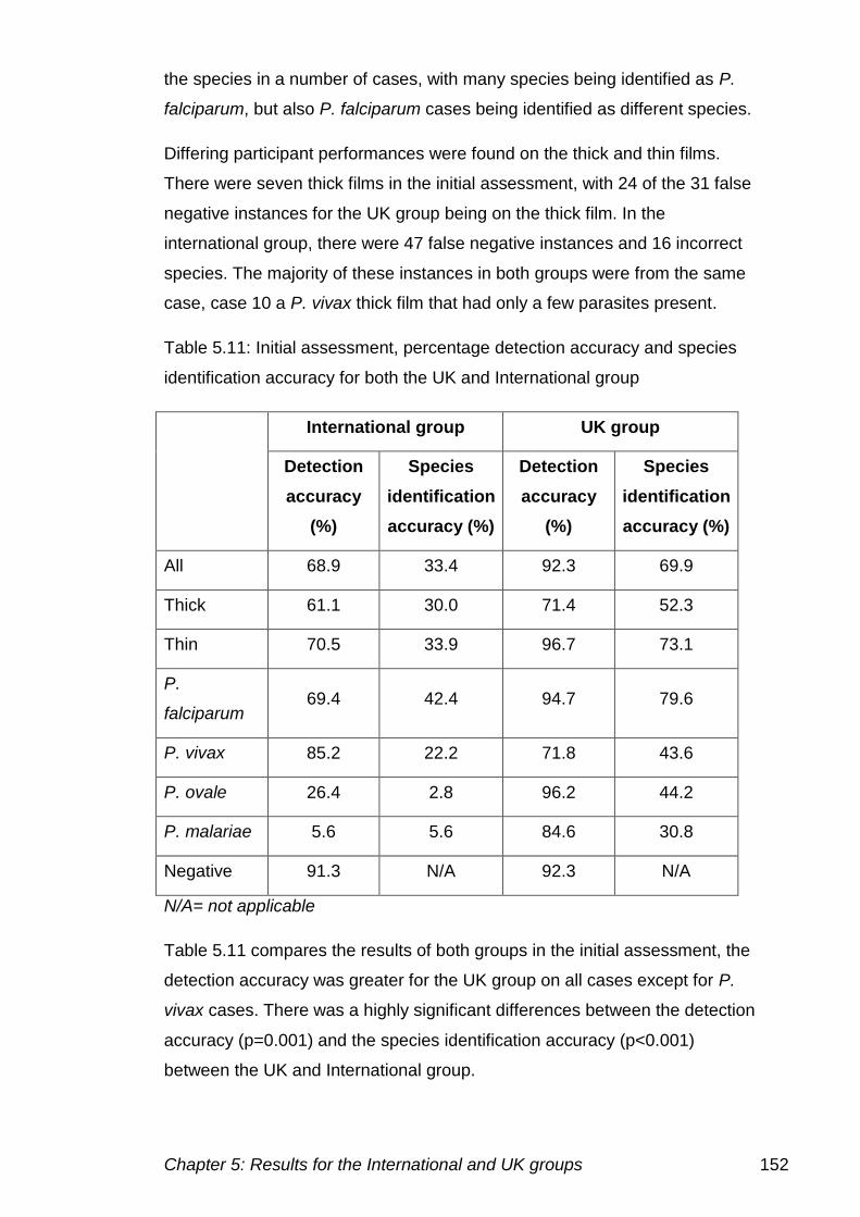
Chapter 5: Results for the International and UK groups 152
the species in a number of cases, with many species being identified as P.
falciparum, but also P. falciparum cases being identified as different species.
Differing participant performances were found on the thick and thin films.
There were seven thick films in the initial assessment, with 24 of the 31 false
negative instances for the UK group being on the thick film. In the
international group, there were 47 false negative instances and 16 incorrect
species. The majority of these instances in both groups were from the same
case, case 10 a P. vivax thick film that had only a few parasites present.
Table 5.11: Initial assessment, percentage detection accuracy and species
identification accuracy for both the UK and International group
International group UK group
Detection
accuracy
(%)
Species
identification
accuracy (%)
Detection
accuracy
(%)
Species
identification
accuracy (%)
All 68.9 33.4 92.3 69.9
Thick 61.1 30.0 71.4 52.3
Thin 70.5 33.9 96.7 73.1
P.
falciparum 69.4 42.4 94.7 79.6
P. vivax 85.2 22.2 71.8 43.6
P. ovale 26.4 2.8 96.2 44.2
P. malariae 5.6 5.6 84.6 30.8
Negative 91.3 N/A 92.3 N/A
N/A= not applicable
Table 5.11 compares the results of both groups in the initial assessment, the
detection accuracy was greater for the UK group on all cases except for P.
vivax cases. There was a highly significant differences between the detection
accuracy (p=0.001) and the species identification accuracy (p<0.001)
between the UK and International group.
Chapter 5: Results for the International and UK groups 153
5.5 Intervention training stage
5.5.1 International group
The International group were given access to the training stage over a four-
month period. The training was released in two stages, with the thin film
training be provided initially and then followed by the thick film training. The
training programme can be viewed on the appendix 1.8.
5.5.2 UK group
The training was provided to the UK group over a six-week period. The
training was delivered all at the same time.
Chapter 5: Results for the International and UK groups 154
5.6 Final assessment
5.6.1 International group
Of the 42 participants, initially recruited 26 participants took part in the final
assessment stage. Twenty-one of these participants completed all 40 cases
in the final assessment. One participant only completed three cases and was
therefore excluded from the analysis based on individual participant results.
The results from the individual cases are shown in table 5.12.
Table 5.12: The detection of parasites in the final assessment stage cases
(n=40) for the International participants group.
Definitive
diagnosis n (=40)
Detection
accuracy
(%)
Detection
accuracy
range (%)
Species
identification
accuracy (%)
Species
identification
accuracy
range (%)
Negative 7 95.2 20.8 NA NA
P.
falciparum 24 74.6 78.0 51.8 78.0
P. vivax 3 36.4 90.9 7.3 21.7
P. ovale 3 23.3 25.7 13.0 26.1
P.
malariae 2 21.6 6.8 8.7 9.1
Mixed
infection 1 90.9 NA 4.6 NA
Diagnosis of malaria for all participants across all 40 cases gave a detection
accuracy of 69.1% (±35.5). There were five cases, in which all participants
correctly identified the presence or absence of parasites. There were not any
cases in which the correct species was determined by all participants. The
species identification accuracy was low at 40.2% (±28.8). Of the cases that
were positive, only one case had the correct species identified by all
participants that determined that parasites were present, this was case 62.

Chapter 5: Results for the International and UK groups 155
Table 5.13:Performance on the individual cases in the final assessment by the International group
Case Definitive
diagnosis
Detection
Accuracy
(%)
Species
identification
accuracy (%)
Thick
film
Parasite
density Artefacts Rank
41 Negative 79.2 - 3 2
42 P. falciparum 100.0 83.3 3 1 1
43 P. falciparum 100.0 58.3 1 4 2
44 P. falciparum 82.6 78.3 Yes 2 4 2
45 P. falciparum 100.0 79.2 3 0 1
46 P. ovale 26.1 13.0 1 1 3
47 Negative 100.0 Yes - 2 2
48 P. falciparum 100.0 65.2 3 1 1
49 P. falciparum 17.4 17.4 Yes 2 4 3
50 P. falciparum 34.8 30.4 2 2 2
51 P. falciparum 100.0 65.2 3 2 1
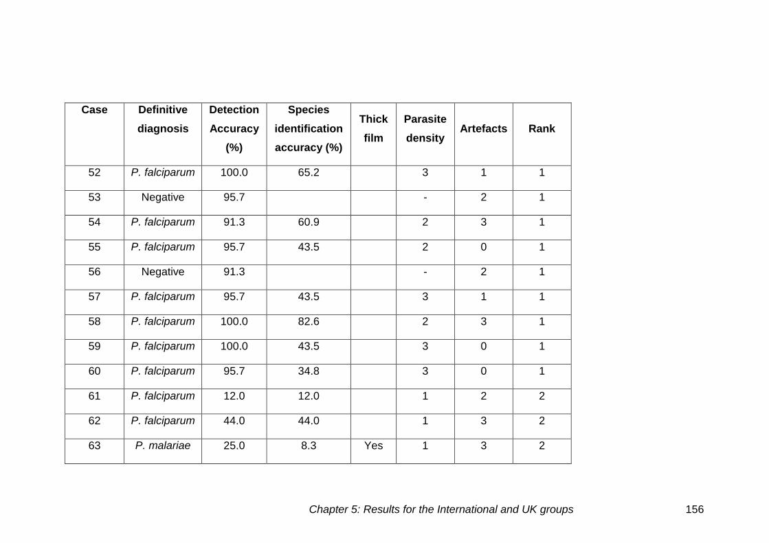
Chapter 5: Results for the International and UK groups 156
Case Definitive
diagnosis
Detection
Accuracy
(%)
Species
identification
accuracy (%)
Thick
film
Parasite
density Artefacts Rank
52 P. falciparum 100.0 65.2 3 1 1
53 Negative 95.7 - 2 1
54 P. falciparum 91.3 60.9 2 3 1
55 P. falciparum 95.7 43.5 2 0 1
56 Negative 91.3 - 2 1
57 P. falciparum 95.7 43.5 3 1 1
58 P. falciparum 100.0 82.6 2 3 1
59 P. falciparum 100.0 43.5 3 0 1
60 P. falciparum 95.7 34.8 3 0 1
61 P. falciparum 12.0 12.0 1 2 2
62 P. falciparum 44.0 44.0 1 3 2
63 P. malariae 25.0 8.3 Yes 1 3 2
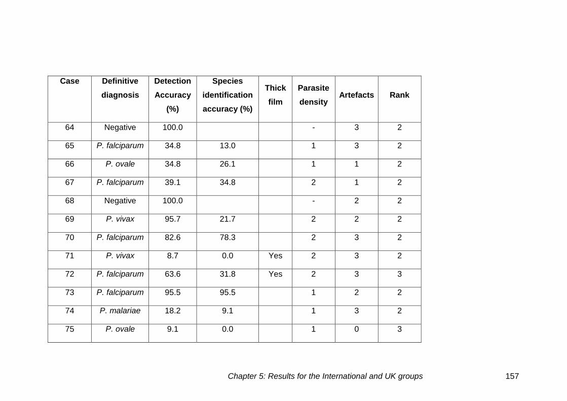
Chapter 5: Results for the International and UK groups 157
Case Definitive
diagnosis
Detection
Accuracy
(%)
Species
identification
accuracy (%)
Thick
film
Parasite
density Artefacts Rank
64 Negative 100.0 - 3 2
65 P. falciparum 34.8 13.0 1 3 2
66 P. ovale 34.8 26.1 1 1 2
67 P. falciparum 39.1 34.8 2 1 2
68 Negative 100.0 - 2 2
69 P. vivax 95.7 21.7 2 2 2
70 P. falciparum 82.6 78.3 2 3 2
71 P. vivax 8.7 0.0 Yes 2 3 2
72 P. falciparum 63.6 31.8 Yes 2 3 3
73 P. falciparum 95.5 95.5 1 2 2
74 P. malariae 18.2 9.1 1 3 2
75 P. ovale 9.1 0.0 1 0 3
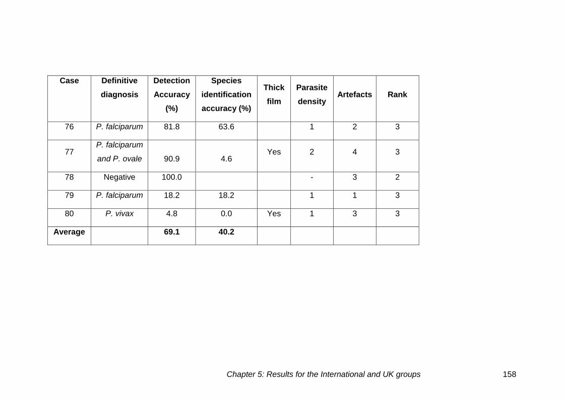
Chapter 5: Results for the International and UK groups 158
Case Definitive
diagnosis
Detection
Accuracy
(%)
Species
identification
accuracy (%)
Thick
film
Parasite
density Artefacts Rank
76 P. falciparum 81.8 63.6 1 2 3
77 P. falciparum
and P. ovale 90.9 4.6 Yes 2 4 3
78 Negative 100.0 - 3 2
79 P. falciparum 18.2 18.2 1 1 3
80 P. vivax 4.8 0.0 Yes 1 3 3
Average 69.1 40.2
Chapter 5: Results for the International and UK groups 159
Table 5.13 demonstrates performance on the individual cases in the final
assessment for the international group.
False negative results
There were 14 cases in which more than 14 participants failed to identify the
presence of parasites. The false negative results were split into categories as
follows:
Low parasite density
There were ten out of 13 low parasite density cases, which had false
negative results. P. ovale thin films had a number of false negative results on
cases 46 (17), 66 (15) and 75 (20) (number of false negatives in brackets).
The same difficulty was presented on case 80 a thick film P. vivax case with
20 false negative results.
Case 63 a P. malariae thick film also had a high false negative rate, with 18
participants not identifying parasites were present. A P. malariae thin film
case 74 also had 18 participants determining parasites were not present.
The remaining cases were all P. falciparum thin films all of which had a low
parasite density. Cases 61 (22), 62 (14), 65 (15), 67 (14), 76 (4) and 79 (18)
showed these false negative results.
Thick films
Seven positive thick films were used, however all of these were falsely
determined to be negative by some participants. False negative results were
seen on cases 44 (4), 49 (19), 71 (21), 72 (8) and 80 (20) (brackets indicate
number of instances).
Artefacts
Cases 43, 44, 49 and 77 had the highest quantity of artefacts present. There
was one participant in case 43, two on case 44, 19 on case 49 and two on
case 77 who called the case negative. Case 44 was a thick film, so staining
artefact was present and parasites were difficult to see in the background
staining.
Chapter 5: Results for the International and UK groups 160
False positive results
There were three out of seven negative cases in which false positive results
were identified by a small number of individuals. Case 41 was identified as
positive by five individuals. Two individuals falsely classified case 56 as
positive, with one individual determining case 53 to be positive.
Incorrect species
Determining the correct species seemed to be the most difficult task for the
individuals, even when the presence of parasites had been correctly
detected. There were seven cases in which more than ten individuals
incorrectly determined the species present.
There were 24 P. falciparum cases in total, 19 of which were identified as
a different species by one or more individuals. There were only two P.
malariae cases used in the final assessment but difficulties in diagnosis
were seen in both of these. Case 63 was a thick film, with four incorrect
diagnoses and case 74, a thin film, with two participants determining the
incorrect species. There were three P. vivax cases used in the final
assessment all of which had incorrect species determined, cases 69 (17),
71 (2) and 80 (1) (brackets indicate the number of incorrect species
identified).
Low parasite density
Case 76 had a low parasite density, there were four individuals that reported
the wrong species was present.
Artefacts
Case 43 had very high levels of artefact present, the incorrect species was
recorded by ten participants. Cases 54, 58, 67, 72 and 77 also had high
numbers of artefacts present, difficulty in species determination was seen.
Thick films
Three out of the seven positive cases, cases 63, 72 and 77 caused
difficulties in diagnosis. Case 77 showed a mixed infection of P. falciparum
and P. ovale, nine participants only identified P. falciparum was present.
Chapter 5: Results for the International and UK groups 161
Cell inclusions
Cases 42 (4), 45 (5), 48 (8), 51 (8), 52 (7), 55 (12), 57 (12), 59 (13) and
60 (14) show high parasite density P. falciparum cases where the species
was incorrectly identified (brackets indicate the number of incorrect
species identified).
Comparison of cases used in the final assessment for the International
group
Thick and thin films
There were eight thick films and 32 thin films in the final assessment. The
detection accuracy for thick films was 49.1% (±39.4) and 74.1% (±33.3) for
thin films. The species identification accuracy for thick films was 20.1%
(±28.0) and thin films 45.6% (±27.0). There were significant differences in the
detection accuracy (p=0.039) and the species identification accuracy
(p=0.021) between the thick and thin films.
Species
Figure 5.13 demonstrates the comparison of the detection accuracy and
species identification accuracy for the different species present. The lowest
species identification accuracy shown is for that of P. vivax at 7.3% (±12.6),
influenced by one thick film case. Negative films show that the participants
are able to correctly determine that parasites are not present in 95.2% (±7.8)
cases.
There was a significant difference between both the detection accuracy
(p=0.022) and species identification accuracy (p=0.003) for the different
species.
Parasite density of case images
Figure 5.14 demonstrates how the detection accuracy and species
identification accuracy increases as the parasite density increases.
There was a highly significant difference between the detection accuracy and
the parasite density (p<0.001). There was a significant difference between
the species identification accuracy and the parasite density (p=0.025).
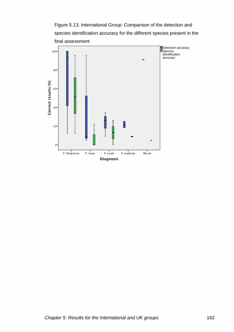
Chapter 5: Results for the International and UK groups 162
Figure 5.13: International Group: Comparison of the detection and
species identification accuracy for the different species present in the
final assessment
Detection accuracy Species identification accuracy
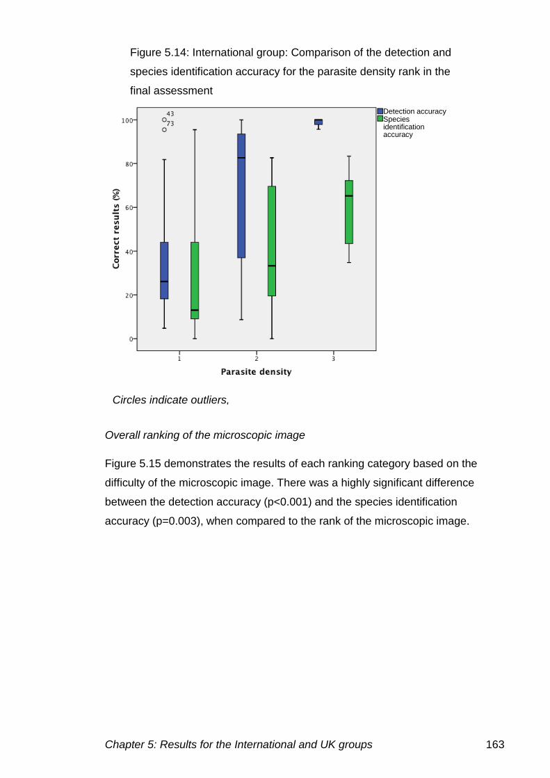
Chapter 5: Results for the International and UK groups 163
Overall ranking of the microscopic image
Figure 5.15 demonstrates the results of each ranking category based on the
difficulty of the microscopic image. There was a highly significant difference
between the detection accuracy (p<0.001) and the species identification
accuracy (p=0.003), when compared to the rank of the microscopic image.
Figure 5.14: International group: Comparison of the detection and
species identification accuracy for the parasite density rank in the
final assessment
Detection accuracy Species identification accuracy
Circles indicate outliers,
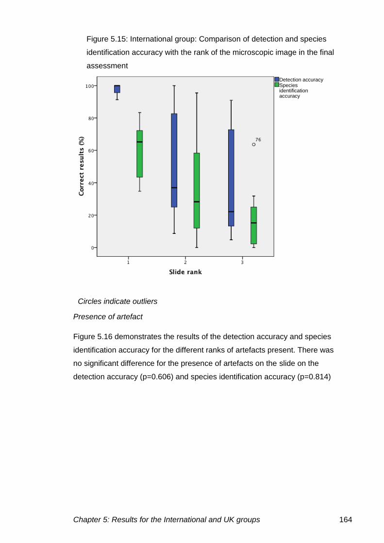
Chapter 5: Results for the International and UK groups 164
Presence of artefact
Figure 5.16 demonstrates the results of the detection accuracy and species
identification accuracy for the different ranks of artefacts present. There was
no significant difference for the presence of artefacts on the slide on the
detection accuracy (p=0.606) and species identification accuracy (p=0.814)
Figure 5.15: International group: Comparison of detection and species
identification accuracy with the rank of the microscopic image in the final
assessment
Detection accuracy Species identification accuracy
Circles indicate outliers
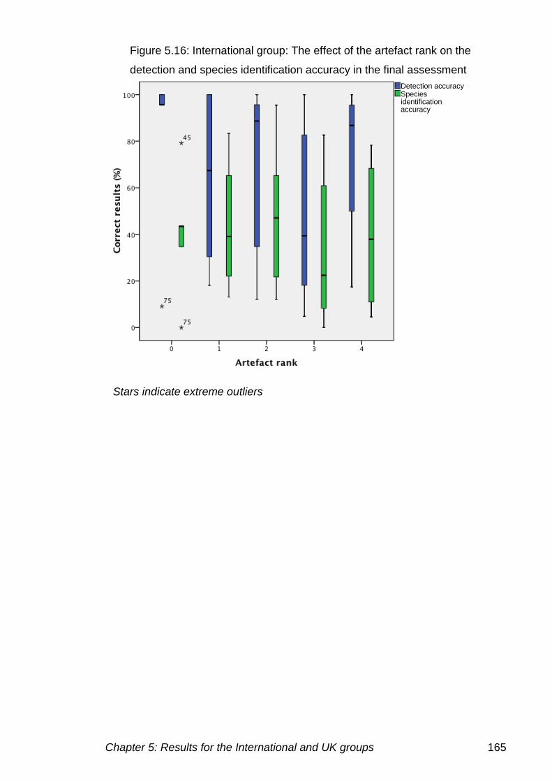
Chapter 5: Results for the International and UK groups 165
Figure 5.16: International group: The effect of the artefact rank on the
detection and species identification accuracy in the final assessment
Detection accuracy Species identification accuracy
Stars indicate extreme outliers
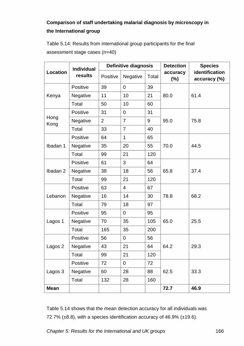
Chapter 5: Results for the International and UK groups 166
Comparison of staff undertaking malarial diagnosis by microscopy in
the International group
Table 5.14: Results from international group participants for the final
assessment stage cases (n=40)
Location Individual
results
Definitive diagnosis Detection
accuracy
(%)
Species
identification
accuracy (%) Positive Negative Total
Kenya
Positive 39 0 39
80.0 61.4 Negative 11 10 21
Total 50 10 60
Hong
Kong
Positive 31 0 31
95.0 75.8 Negative 2 7 9
Total 33 7 40
Ibadan 1
Positive 64 1 65
70.0 44.5 Negative 35 20 55
Total 99 21 120
Ibadan 2
Positive 61 3 64
65.8 37.4 Negative 38 18 56
Total 99 21 120
Lebanon
Positive 63 4 67
78.8 68.2 Negative 16 14 30
Total 79 18 97
Lagos 1
Positive 95 0 95
65.0 25.5 Negative 70 35 105
Total 165 35 200
Lagos 2
Positive 56 0 56
64.2 29.3 Negative 43 21 64
Total 99 21 120
Lagos 3
Positive 72 0 72
62.5 33.3 Negative 60 28 88
Total 132 28 160
Mean 72.7 46.9
Table 5.14 shows that the mean detection accuracy for all individuals was
72.7% (±8.8), with a species identification accuracy of 46.9% (±19.6).
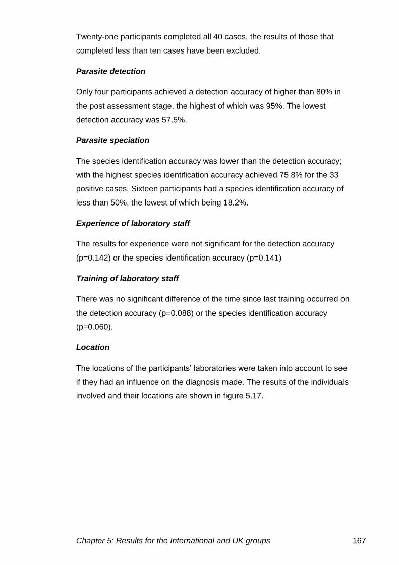
Chapter 5: Results for the International and UK groups 167
Twenty-one participants completed all 40 cases, the results of those that
completed less than ten cases have been excluded.
Parasite detection
Only four participants achieved a detection accuracy of higher than 80% in
the post assessment stage, the highest of which was 95%. The lowest
detection accuracy was 57.5%.
Parasite speciation
The species identification accuracy was lower than the detection accuracy;
with the highest species identification accuracy achieved 75.8% for the 33
positive cases. Sixteen participants had a species identification accuracy of
less than 50%, the lowest of which being 18.2%.
Experience of laboratory staff
The results for experience were not significant for the detection accuracy
(p=0.142) or the species identification accuracy (p=0.141)
Training of laboratory staff
There was no significant difference of the time since last training occurred on
the detection accuracy (p=0.088) or the species identification accuracy
(p=0.060).
Location
The locations of the participants’ laboratories were taken into account to see
if they had an influence on the diagnosis made. The results of the individuals
involved and their locations are shown in figure 5.17.
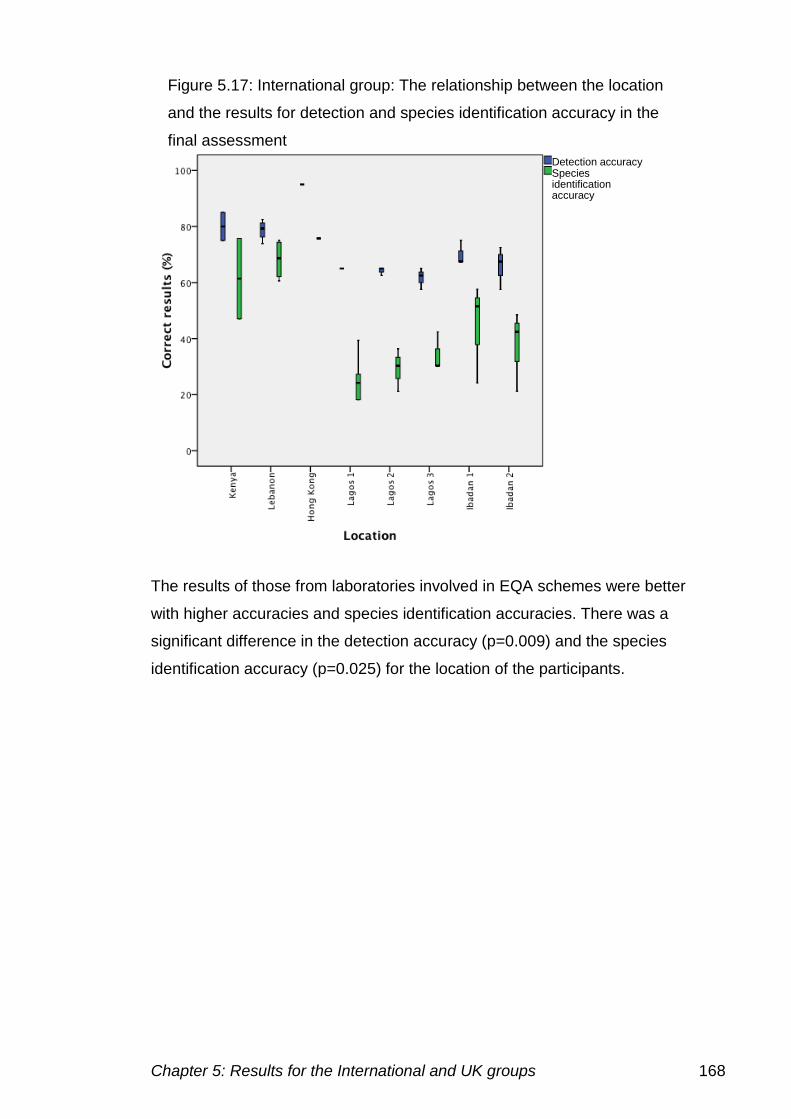
Chapter 5: Results for the International and UK groups 168
The results of those from laboratories involved in EQA schemes were better
with higher accuracies and species identification accuracies. There was a
significant difference in the detection accuracy (p=0.009) and the species
identification accuracy (p=0.025) for the location of the participants.
Figure 5.17: International group: The relationship between the location
and the results for detection and species identification accuracy in the
final assessment
Detection accuracy Species identification accuracy
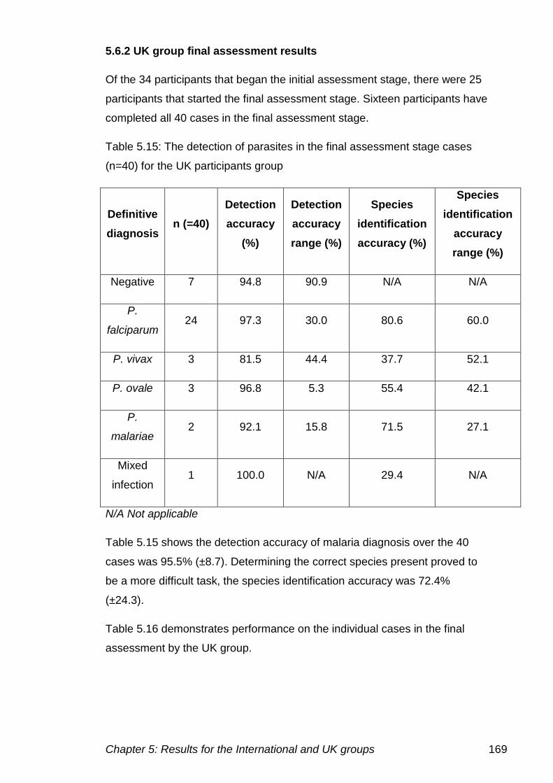
Chapter 5: Results for the International and UK groups 169
5.6.2 UK group final assessment results
Of the 34 participants that began the initial assessment stage, there were 25
participants that started the final assessment stage. Sixteen participants have
completed all 40 cases in the final assessment stage.
Table 5.15: The detection of parasites in the final assessment stage cases
(n=40) for the UK participants group
Definitive
diagnosis n (=40)
Detection
accuracy
(%)
Detection
accuracy
range (%)
Species
identification
accuracy (%)
Species
identification
accuracy
range (%)
Negative 7 94.8 90.9 N/A N/A
P.
falciparum 24 97.3 30.0 80.6 60.0
P. vivax 3 81.5 44.4 37.7 52.1
P. ovale 3 96.8 5.3 55.4 42.1
P.
malariae 2 92.1 15.8 71.5 27.1
Mixed
infection 1 100.0 N/A 29.4 N/A
N/A Not applicable
Table 5.15 shows the detection accuracy of malaria diagnosis over the 40
cases was 95.5% (±8.7). Determining the correct species present proved to
be a more difficult task, the species identification accuracy was 72.4%
(±24.3).
Table 5.16 demonstrates performance on the individual cases in the final
assessment by the UK group.
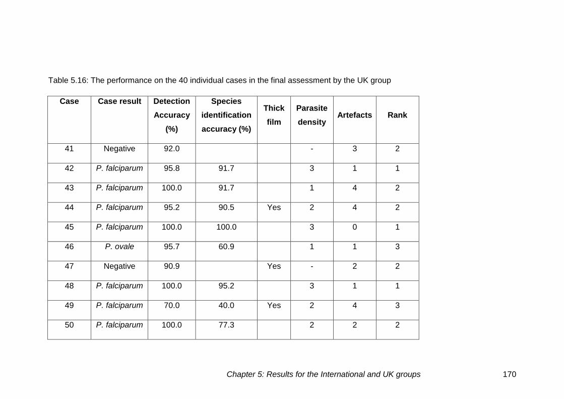
Chapter 5: Results for the International and UK groups 170
Table 5.16: The performance on the 40 individual cases in the final assessment by the UK group
Case Case result Detection
Accuracy
(%)
Species
identification
accuracy (%)
Thick
film
Parasite
density Artefacts Rank
41 Negative 92.0 - 3 2
42 P. falciparum 95.8 91.7 3 1 1
43 P. falciparum 100.0 91.7 1 4 2
44 P. falciparum 95.2 90.5 Yes 2 4 2
45 P. falciparum 100.0 100.0 3 0 1
46 P. ovale 95.7 60.9 1 1 3
47 Negative 90.9 Yes - 2 2
48 P. falciparum 100.0 95.2 3 1 1
49 P. falciparum 70.0 40.0 Yes 2 4 3
50 P. falciparum 100.0 77.3 2 2 2
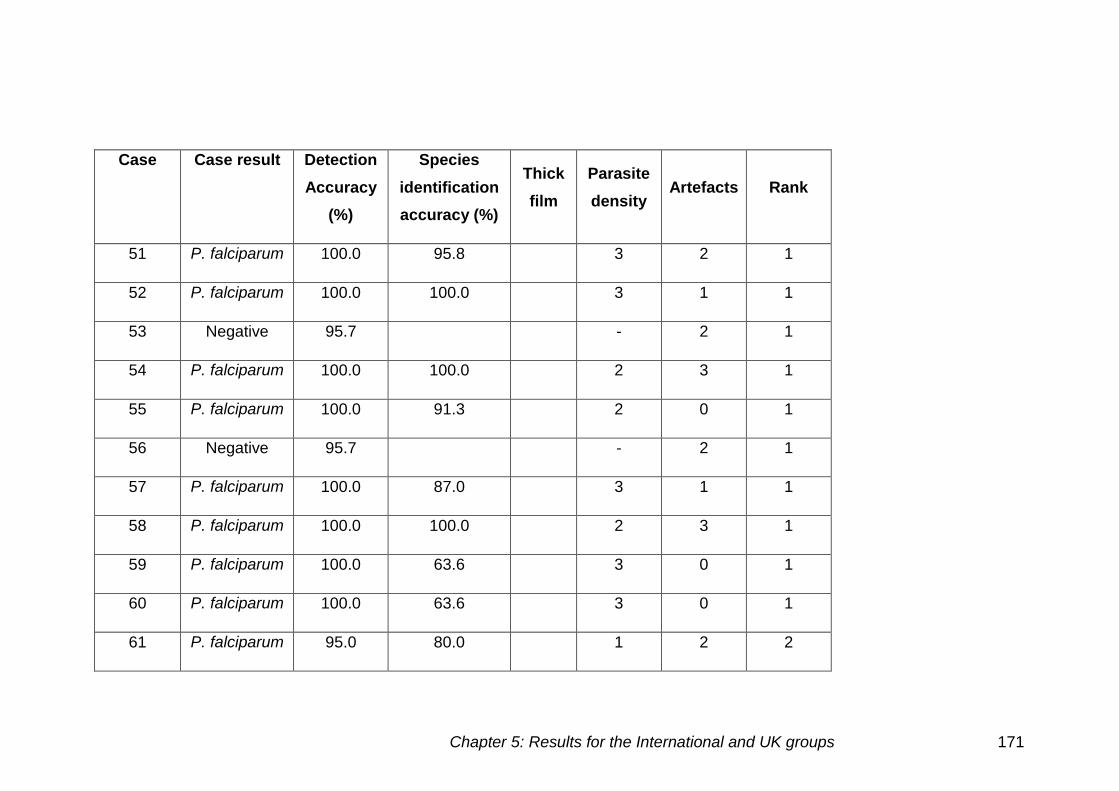
Chapter 5: Results for the International and UK groups 171
Case Case result Detection
Accuracy
(%)
Species
identification
accuracy (%)
Thick
film
Parasite
density Artefacts Rank
51 P. falciparum 100.0 95.8 3 2 1
52 P. falciparum 100.0 100.0 3 1 1
53 Negative 95.7 - 2 1
54 P. falciparum 100.0 100.0 2 3 1
55 P. falciparum 100.0 91.3 2 0 1
56 Negative 95.7 - 2 1
57 P. falciparum 100.0 87.0 3 1 1
58 P. falciparum 100.0 100.0 2 3 1
59 P. falciparum 100.0 63.6 3 0 1
60 P. falciparum 100.0 63.6 3 0 1
61 P. falciparum 95.0 80.0 1 2 2
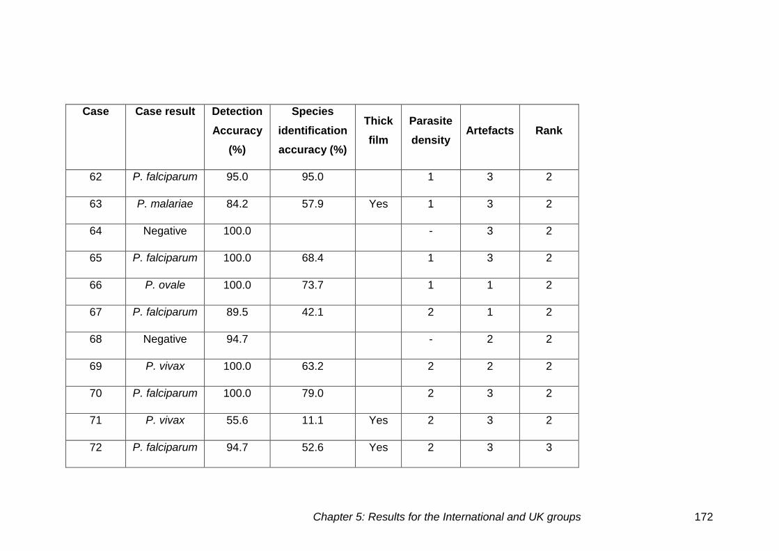
Chapter 5: Results for the International and UK groups 172
Case Case result Detection
Accuracy
(%)
Species
identification
accuracy (%)
Thick
film
Parasite
density Artefacts Rank
62 P. falciparum 95.0 95.0 1 3 2
63 P. malariae 84.2 57.9 Yes 1 3 2
64 Negative 100.0 - 3 2
65 P. falciparum 100.0 68.4 1 3 2
66 P. ovale 100.0 73.7 1 1 2
67 P. falciparum 89.5 42.1 2 1 2
68 Negative 94.7 - 2 2
69 P. vivax 100.0 63.2 2 2 2
70 P. falciparum 100.0 79.0 2 3 2
71 P. vivax 55.6 11.1 Yes 2 3 2
72 P. falciparum 94.7 52.6 Yes 2 3 3
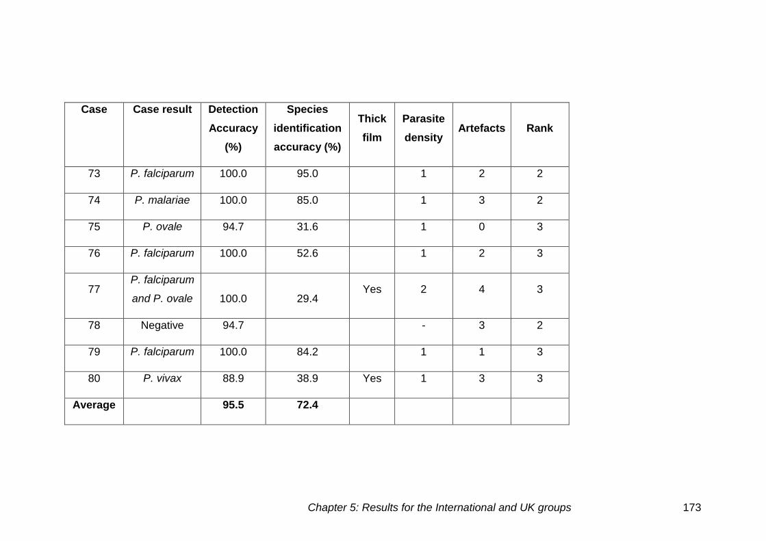
Chapter 5: Results for the International and UK groups 173
Case Case result Detection
Accuracy
(%)
Species
identification
accuracy (%)
Thick
film
Parasite
density Artefacts Rank
73 P. falciparum 100.0 95.0 1 2 2
74 P. malariae 100.0 85.0 1 3 2
75 P. ovale 94.7 31.6 1 0 3
76 P. falciparum 100.0 52.6 1 2 3
77 P. falciparum
and P. ovale 100.0 29.4 Yes 2 4 3
78 Negative 94.7 - 3 2
79 P. falciparum 100.0 84.2 1 1 3
80 P. vivax 88.9 38.9 Yes 1 3 3
Average 95.5 72.4
Chapter 5: Results for the International and UK groups 174
False negatives
There were a number of false negative results, the reasons for these were
split into the following categories.
Low parasite density
There were 13 cases at low parasite density, six of which had some false
negatives. For cases 46, 61, 62, and 75 one individual missed the presence
of parasites.
Thick films
The majority of false negatives were seen on the thick film. There were
five out of six cases in total in which parasites were missed on the thick
film. False negative results were seen in the following cases 44 (1), 49
(6), 63 (3), 67 (2), 71 (8), 72 (1) and 80 (2) (brackets indicate the number
of false negative cases identified).
Case 67 was also found to be negative by two participants. The case was a
thin film, with medium parasite density and few artefacts present.
False positives
Of the seven negative cases there were six in which parasites were falsely
identified. Cases 53, 56, 68 and 78 were identified as having parasites
present by one individual and case 41 by two. Case 47 a thick film was also
identified as positive by two individuals.
Incorrect species
The lowest species identification accuracy was seen in case 71 a P. vivax
thick film, incorrectly identified by eight participants. The other P. vivax case,
case 69 was also identified as a different species by seven participants, five
as P. ovale and two others as a mixed infection that included P. vivax.
Artefacts appeared to have had little influence on the diagnosis made, but did
have some influence on the species determination.
Chapter 5: Results for the International and UK groups 175
Low parasite density
Of the 12 low parasite density cases used, 11 cases had problems with
speciation. Case 80 a P. vivax thick film had eight individuals that incorrectly
determined the species. Case 63 was a P. malariae thick film that was
diagnosed by two individuals as P. ovale, two as P. falciparum and one
mixed infection. Case 74 the P. malariae thin film was incorrectly identified by
three participants.
All three P. ovale cases were present at low parasite densities. Case 46 was
identified as P. vivax by eight participants, case 66 as P. vivax by five
participants and case 75 as P. vivax by six participants and P. falciparum by
one participant.
There were six P. falciparum cases at low parasite density which had the
incorrect species determined, cases 43 (1), 61 (2), 65 (6), 73 (1), 76 (8)
and 79 (2) (brackets indicate the number of incorrect species identified).
Thick films
Two P. vivax cases 71 and 80 had the incorrect species determined by eight
and nine individuals respectively. Case 63 a P. malariae case was
misdiagnosed by five participants.
Of the three P. falciparum cases, case 44, 49 and 72 had the incorrect
species determined by one, six and eight participants respectively.
Comparison of cases used in the final assessment for the UK group
Thick and thin films
There were eight thick films and 32 thin films in the final assessment. The
detection accuracy for thick films was 84.9% (±15.0) in comparison to thin
films 98.1% (±2.9). The species identification accuracy for the thick films was
45.8% (±25.0), compared to thin films at 79.7% (±18.9). There was a highly
significant difference for the detection accuracy (p<0.001) and the species
identification accuracy (p=0.003) for thick and thin films.
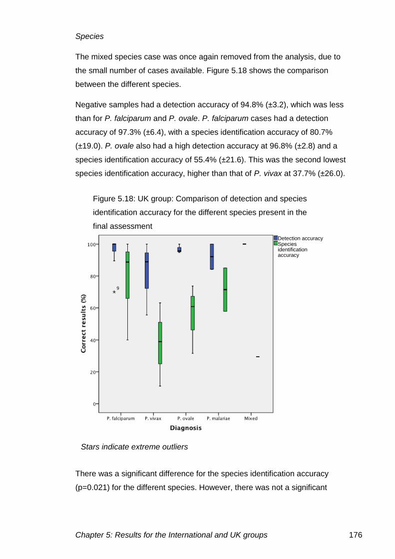
Chapter 5: Results for the International and UK groups 176
Species
The mixed species case was once again removed from the analysis, due to
the small number of cases available. Figure 5.18 shows the comparison
between the different species.
Negative samples had a detection accuracy of 94.8% (±3.2), which was less
than for P. falciparum and P. ovale. P. falciparum cases had a detection
accuracy of 97.3% (±6.4), with a species identification accuracy of 80.7%
(±19.0). P. ovale also had a high detection accuracy at 96.8% (±2.8) and a
species identification accuracy of 55.4% (±21.6). This was the second lowest
species identification accuracy, higher than that of P. vivax at 37.7% (±26.0).
There was a significant difference for the species identification accuracy
(p=0.021) for the different species. However, there was not a significant
Figure 5.18: UK group: Comparison of detection and species
identification accuracy for the different species present in the
final assessment
Detection accuracy Species identification accuracy
Stars indicate extreme outliers
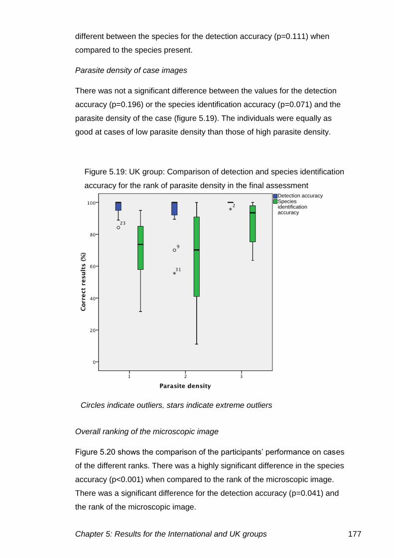
Chapter 5: Results for the International and UK groups 177
different between the species for the detection accuracy (p=0.111) when
compared to the species present.
Parasite density of case images
There was not a significant difference between the values for the detection
accuracy (p=0.196) or the species identification accuracy (p=0.071) and the
parasite density of the case (figure 5.19). The individuals were equally as
good at cases of low parasite density than those of high parasite density.
Overall ranking of the microscopic image
Figure 5.20 shows the comparison of the participants’ performance on cases
of the different ranks. There was a highly significant difference in the species
accuracy (p<0.001) when compared to the rank of the microscopic image.
There was a significant difference for the detection accuracy (p=0.041) and
the rank of the microscopic image.
Figure 5.19: UK group: Comparison of detection and species identification
accuracy for the rank of parasite density in the final assessment Detection accuracy Species identification accuracy
Circles indicate outliers, stars indicate extreme outliers
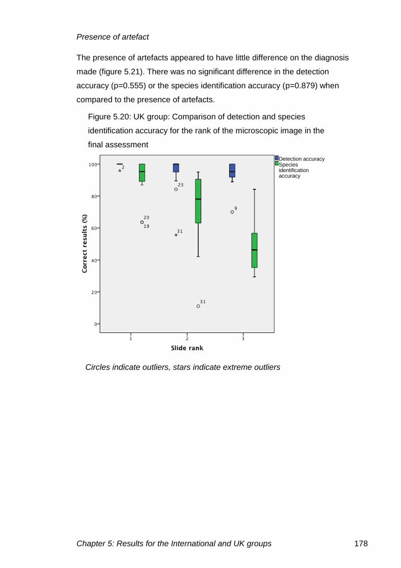
Chapter 5: Results for the International and UK groups 178
Presence of artefact
The presence of artefacts appeared to have little difference on the diagnosis
made (figure 5.21). There was no significant difference in the detection
accuracy (p=0.555) or the species identification accuracy (p=0.879) when
compared to the presence of artefacts.
Figure 5.20: UK group: Comparison of detection and species
identification accuracy for the rank of the microscopic image in the
final assessment
Detection accuracy Species identification accuracy
Circles indicate outliers, stars indicate extreme outliers
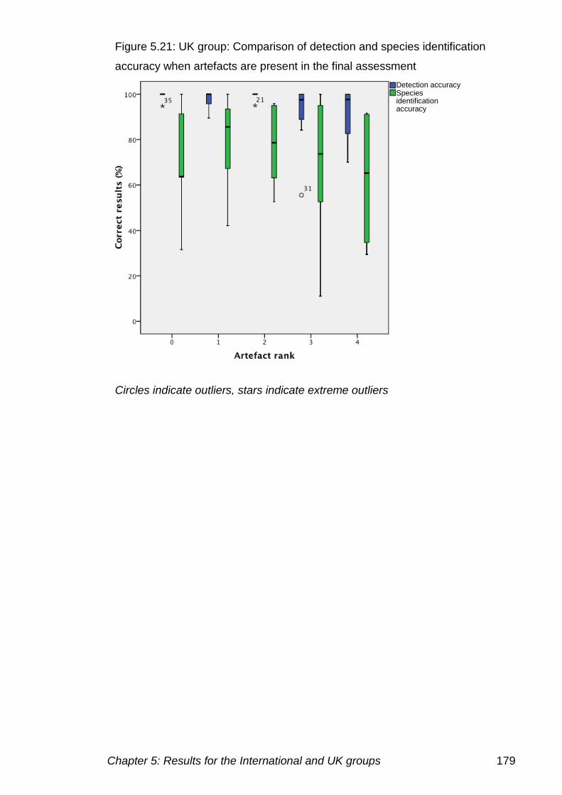
Chapter 5: Results for the International and UK groups 179
Figure 5.21: UK group: Comparison of detection and species identification
accuracy when artefacts are present in the final assessment
Detection accuracy Species identification accuracy
Circles indicate outliers, stars indicate extreme outliers
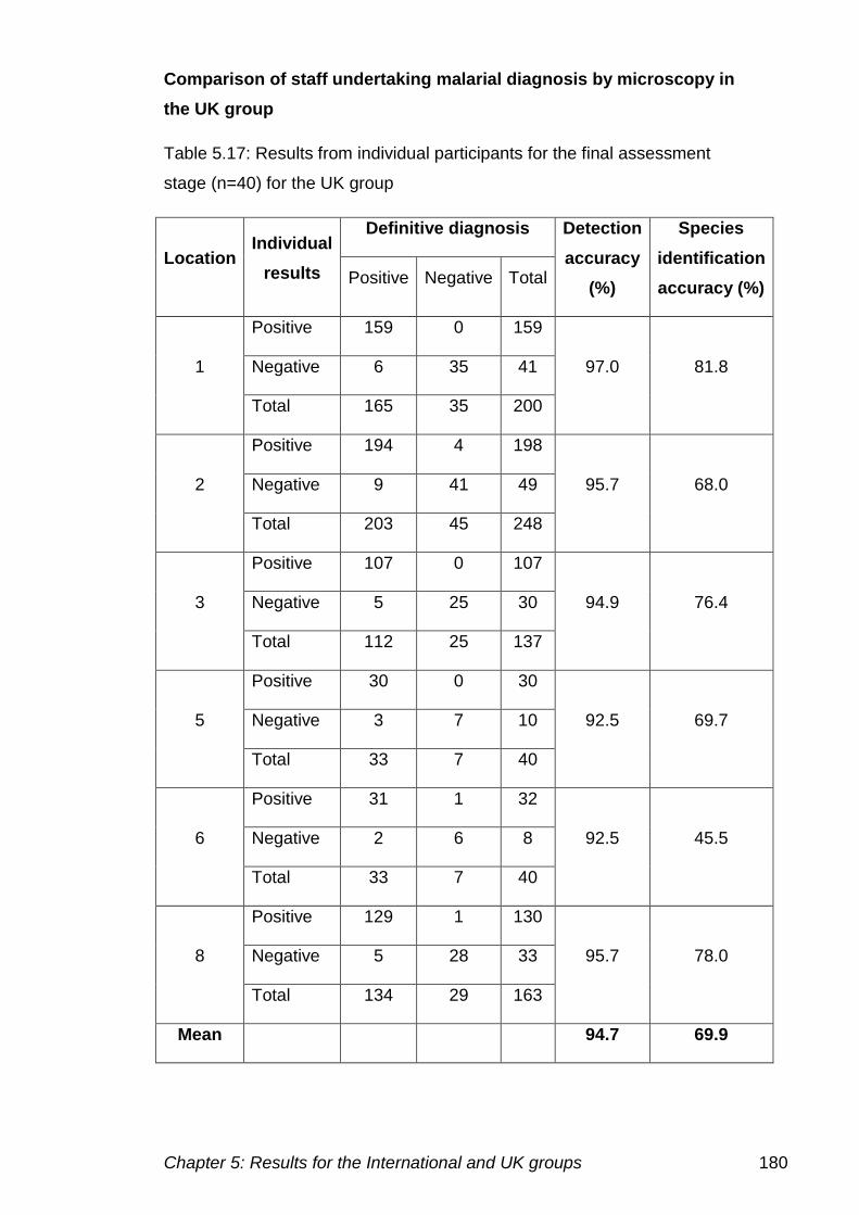
Chapter 5: Results for the International and UK groups 180
Comparison of staff undertaking malarial diagnosis by microscopy in
the UK group
Table 5.17: Results from individual participants for the final assessment
stage (n=40) for the UK group
Location Individual
results
Definitive diagnosis Detection
accuracy
(%)
Species
identification
accuracy (%) Positive Negative Total
1
Positive 159 0 159
97.0 81.8 Negative 6 35 41
Total 165 35 200
2
Positive 194 4 198
95.7 68.0 Negative 9 41 49
Total 203 45 248
3
Positive 107 0 107
94.9 76.4 Negative 5 25 30
Total 112 25 137
5
Positive 30 0 30
92.5 69.7 Negative 3 7 10
Total 33 7 40
6
Positive 31 1 32
92.5 45.5 Negative 2 6 8
Total 33 7 40
8
Positive 129 1 130
95.7 78.0 Negative 5 28 33
Total 134 29 163
Mean 94.7 69.9
Chapter 5: Results for the International and UK groups 181
Table 5.17 shows the results for the individual participants, the detection
accuracy for all individuals was 95.6% (±3.8) and a species identification
accuracy of 73.8% (±12.8).
Eighteen participants completed all 40 cases, two other participants
completed more than 30 cases. The results of those that completed less than
ten cases have been excluded.
Parasite detection
The detection accuracy was high, with seven participants achieving 100%
detection accuracy. The lowest detection accuracy achieved was 85%, which
was obtained after answering 20 cases, incorrectly determining that parasites
were absent in three cases. This was the only individual that achieved less
than 90% detection accuracy, this individual was in the group with the least
experience.
Parasite speciation
The species identification accuracy was as before lower than the detection
accuracy, with a detection accuracy of 73.8% (±12.8). The highest species
identification accuracy was by individual UK311 of 96.2%, who completed 32
cases. The lowest species identification accuracy was by UK391 with 48.5%.
This participant however correctly determined the presence of parasites in
92.5% of cases.
Location
The location results are shown in figure 5.22. There was no significant
difference in detection accuracy results (p=0.618) between the different
hospitals in which the participants were based. The species identification
accuracy results were also not significantly different (p=0.247) when
compared to location.
Experience of laboratory staff
The detection accuracy for less than two years experience (group 1) was
96.6% (±2.8) and for group two (>5 years experience) was 93.7% (±4.8).
This difference was not significant (p=0.074). For species identification
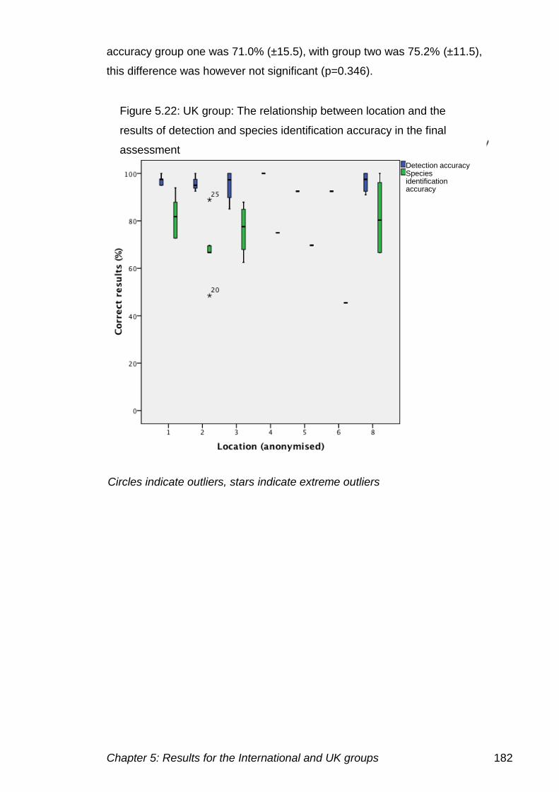
Chapter 5: Results for the International and UK groups 182
accuracy group one was 71.0% (±15.5), with group two was 75.2% (±11.5),
this difference was however not significant (p=0.346).
Figure 5.22: UK group: The relationship between location and the
results of detection and species identification accuracy in the final
assessment
Detection accuracy Species identification accuracy
Circles indicate outliers, stars indicate extreme outliers
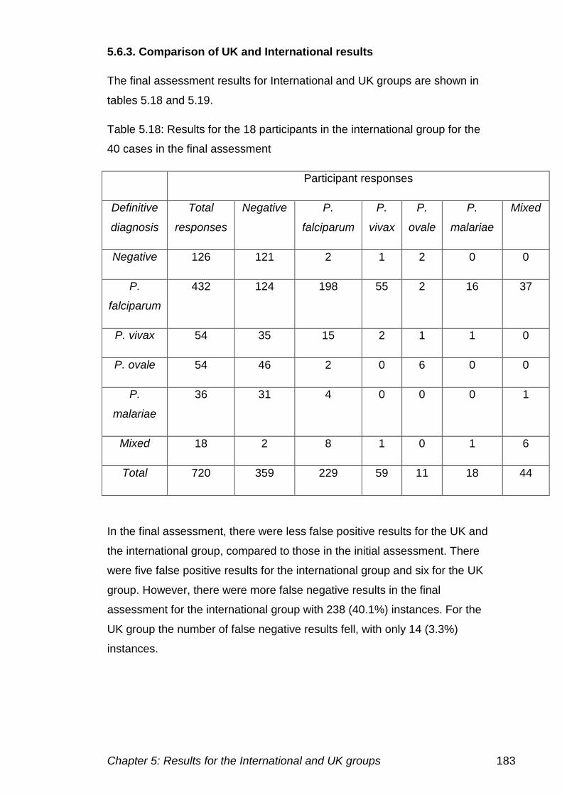
Chapter 5: Results for the International and UK groups 183
5.6.3. Comparison of UK and International results
The final assessment results for International and UK groups are shown in
tables 5.18 and 5.19.
Table 5.18: Results for the 18 participants in the international group for the
40 cases in the final assessment
Participant responses
Definitive
diagnosis
Total
responses
Negative P.
falciparum
P.
vivax
P.
ovale
P.
malariae
Mixed
Negative 126 121 2 1 2 0 0
P.
falciparum
432 124 198 55 2 16 37
P. vivax 54 35 15 2 1 1 0
P. ovale 54 46 2 0 6 0 0
P.
malariae
36 31 4 0 0 0 1
Mixed 18 2 8 1 0 1 6
Total 720 359 229 59 11 18 44
In the final assessment, there were less false positive results for the UK and
the international group, compared to those in the initial assessment. There
were five false positive results for the international group and six for the UK
group. However, there were more false negative results in the final
assessment for the international group with 238 (40.1%) instances. For the
UK group the number of false negative results fell, with only 14 (3.3%)
instances.
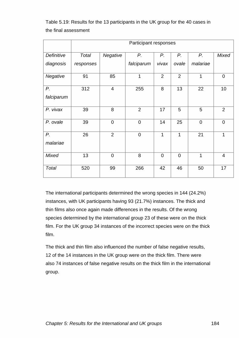
Chapter 5: Results for the International and UK groups 184
Table 5.19: Results for the 13 participants in the UK group for the 40 cases in
the final assessment
Participant responses
Definitive
diagnosis
Total
responses
Negative P.
falciparum
P.
vivax
P.
ovale
P.
malariae
Mixed
Negative 91 85 1 2 2 1 0
P.
falciparum
312 4 255 8 13 22 10
P. vivax 39 8 2 17 5 5 2
P. ovale 39 0 0 14 25 0 0
P.
malariae
26 2 0 1 1 21 1
Mixed 13 0 8 0 0 1 4
Total 520 99 266 42 46 50 17
The international participants determined the wrong species in 144 (24.2%)
instances, with UK participants having 93 (21.7%) instances. The thick and
thin films also once again made differences in the results. Of the wrong
species determined by the international group 23 of these were on the thick
film. For the UK group 34 instances of the incorrect species were on the thick
film.
The thick and thin film also influenced the number of false negative results,
12 of the 14 instances in the UK group were on the thick film. There were
also 74 instances of false negative results on the thick film in the international
group.
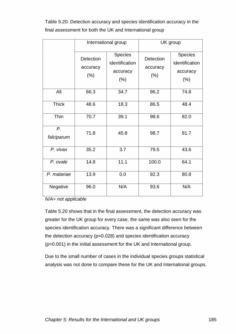
Chapter 5: Results for the International and UK groups 185
Table 5.20: Detection accuracy and species identification accuracy in the
final assessment for both the UK and International group
International group UK group
Detection
accuracy
(%)
Species
identification
accuracy
(%)
Detection
accuracy
(%)
Species
identification
accuracy
(%)
All 66.3 34.7 96.2 74.8
Thick 48.6 18.3 86.5 48.4
Thin 70.7 39.1 98.6 82.0
P.
falciparum 71.8 45.8 98.7 81.7
P. vivax 35.2 3.7 79.5 43.6
P. ovale 14.8 11.1 100.0 64.1
P. malariae 13.9 0.0 92.3 80.8
Negative 96.0 N/A 93.6 N/A
N/A= not applicable
Table 5.20 shows that in the final assessment, the detection accuracy was
greater for the UK group for every case, the same was also seen for the
species identification accuracy. There was a significant difference between
the detection accuracy (p=0.028) and species identification accuracy
(p=0.001) in the initial assessment for the UK and International group.
Due to the small number of cases in the individual species groups statistical
analysis was not done to compare these for the UK and International groups.
Chapter 5: Results for the International and UK groups 186
5.7 Comparison of initial and final assessment
5.7.1 International group
There were 18 participants that completed all of the initial and final
assessment, allowing their results to be compared and the effectiveness of
the training to be assessed.
Table 5.21 shows the results of these individuals for the 80 cases in the
entire project. There were differences between the cases and individuals’
performance during the initial and final assessment were reviewed.
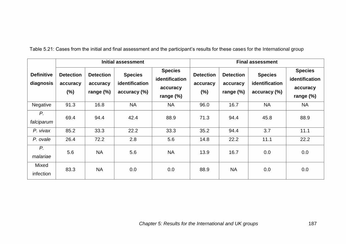
Chapter 5: Results for the International and UK groups 187
Table 5.21: Cases from the initial and final assessment and the participant’s results for these cases for the International group
Definitive
diagnosis
Initial assessment Final assessment
Detection
accuracy
(%)
Detection
accuracy
range (%)
Species
identification
accuracy (%)
Species
identification
accuracy
range (%)
Detection
accuracy
(%)
Detection
accuracy
range (%)
Species
identification
accuracy (%)
Species
identification
accuracy
range (%)
Negative 91.3 16.8 NA NA 96.0 16.7 NA NA
P.
falciparum 69.4 94.4 42.4 88.9 71.3 94.4 45.8 88.9
P. vivax 85.2 33.3 22.2 33.3 35.2 94.4 3.7 11.1
P. ovale 26.4 72.2 2.8 5.6 14.8 22.2 11.1 22.2
P.
malariae 5.6 NA 5.6 NA 13.9 16.7 0.0 0.0
Mixed
infection 83.3 NA 0.0 0.0 88.9 NA 0.0 0.0
Chapter 5: Results for the International and UK groups 188
The eighteen individuals that completed the initial and final assessment
achieved a detection accuracy of 68.8% (±38.7) in the initial assessment and
66.3% (±36.2) in the final assessment. There was no significant difference in
the detection accuracy in the initial and final assessment (p=0.692). The
species identification accuracy in the initial assessment was 33.3% (±31.5)
and 34.7% (±29.6) in the final assessment. There was no significant
difference in the species identification accuracy (p=0.879) in the initial and
final assessment.
During the initial and final assessment participants struggled with some
particular cases. Described below are the cases in which less than 50%
detection accuracy was achieved.
False negative results
Low parasite density
There were 15 out of 25 low parasite density cases in which less than half of
the participants made the correct diagnosis.
The main difficulty was seen with P. ovale cases, cases 2 (17), 17 (15),
38 (17), 46 (14), 66 (14) and 75 (18) showed these false negative results
(brackets indicate the number of false negative cases identified).
Problems were also seen in P. malariae cases, in all three cases used. Case
40 was identified as positive by one participant, 63 by four participants and
case 74 by one participant.
Six out of a possible 12 P. falciparum cases at low parasite density had a
high number of false negative results, case 21 (14), 32 (16), 61 (16), 62
(12), 65 (14) and 67 (13), (brackets indicate the number of false negative
cases identified)
Thick and thin films
There were three P. falciparum thick films out of a possible five that had
high numbers of false negative results. There were the following number
of false negative results on each case, case 1 (16), 34 (16), 49 (15), 63
Chapter 5: Results for the International and UK groups 189
(14), 71 (16), (brackets indicate the number of false negative cases
identified)
Presence of artefacts
Two cases with artefacts present caused difficulties in determining whether
parasites were present. Both of the cases involved were P. falciparum cases.
Case 28 was a high parasite density infection had 16 false negative results
and case 29 showing early trophozoites and chronic granulocytic leukaemia
had 17 false negative results. .
Incorrect species
There were 16 cases in which the species was correctly determined by less
than half of the participants, the cases with high numbers of false negative
results were not included.
There were four P. vivax cases in which there was difficulty determining the
species present. Cases 8, 10 and 69 only had the correct species determined
by two individuals, Case 22 was correctly identified by eight participants.
Similar difficulties were seen with P. ovale cases, only one case was
identified as positive. Case 24 was identified as positive by 14 participants,
however none of these determined the correct species present.
Species identification was also difficult on the two mixed infection cases
used. Cases 39 and 77 were both mixed infections of P. falciparum and P.
ovale, however case 77 was a thick film. No participants determined the
correct combination of species in either case.
There were nine P. falciparum cases in which difficulties in species
determination were seen, all of these were cases with cell inclusions. The
correct species was determined by six participants for case 11, five
participants for case 13 and a similar trend was seen for the remaining
cases, cases 18, 25, 30, 55, 57, 59 and 60,
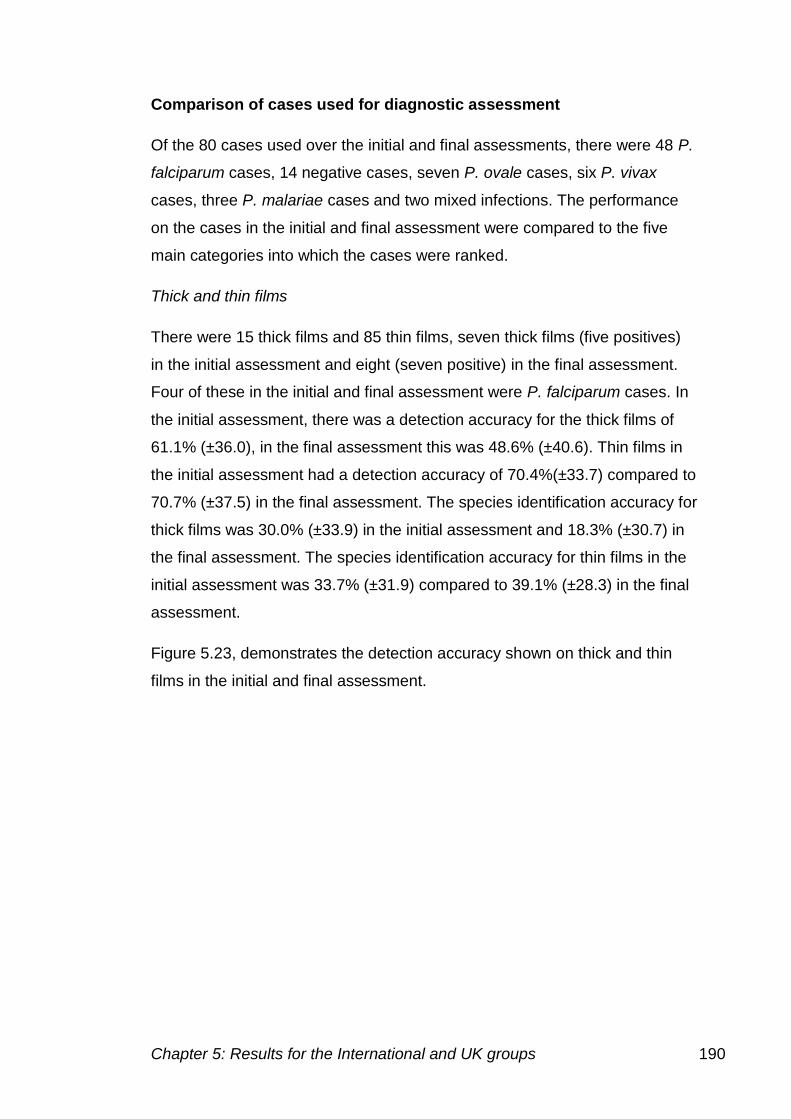
Chapter 5: Results for the International and UK groups 190
Comparison of cases used for diagnostic assessment
Of the 80 cases used over the initial and final assessments, there were 48 P.
falciparum cases, 14 negative cases, seven P. ovale cases, six P. vivax
cases, three P. malariae cases and two mixed infections. The performance
on the cases in the initial and final assessment were compared to the five
main categories into which the cases were ranked.
Thick and thin films
There were 15 thick films and 85 thin films, seven thick films (five positives)
in the initial assessment and eight (seven positive) in the final assessment.
Four of these in the initial and final assessment were P. falciparum cases. In
the initial assessment, there was a detection accuracy for the thick films of
61.1% (±36.0), in the final assessment this was 48.6% (±40.6). Thin films in
the initial assessment had a detection accuracy of 70.4%(±33.7) compared to
70.7% (±37.5) in the final assessment. The species identification accuracy for
thick films was 30.0% (±33.9) in the initial assessment and 18.3% (±30.7) in
the final assessment. The species identification accuracy for thin films in the
initial assessment was 33.7% (±31.9) compared to 39.1% (±28.3) in the final
assessment.
Figure 5.23, demonstrates the detection accuracy shown on thick and thin
films in the initial and final assessment.
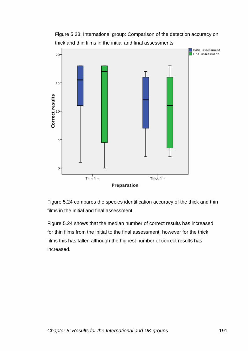
Chapter 5: Results for the International and UK groups 191
Figure 5.24 compares the species identification accuracy of the thick and thin
films in the initial and final assessment.
Figure 5.24 shows that the median number of correct results has increased
for thin films from the initial to the final assessment, however for the thick
films this has fallen although the highest number of correct results has
increased.
Figure 5.23: International group: Comparison of the detection accuracy on
thick and thin films in the initial and final assessments
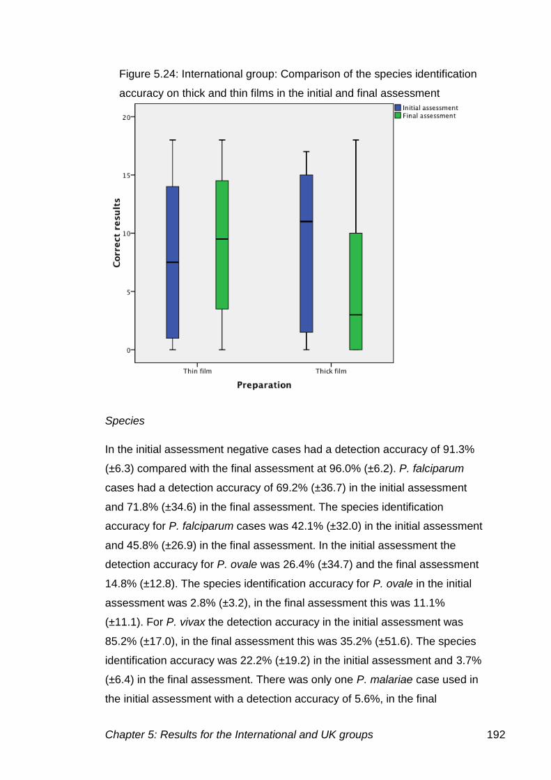
Chapter 5: Results for the International and UK groups 192
Species
In the initial assessment negative cases had a detection accuracy of 91.3%
(±6.3) compared with the final assessment at 96.0% (±6.2). P. falciparum
cases had a detection accuracy of 69.2% (±36.7) in the initial assessment
and 71.8% (±34.6) in the final assessment. The species identification
accuracy for P. falciparum cases was 42.1% (±32.0) in the initial assessment
and 45.8% (±26.9) in the final assessment. In the initial assessment the
detection accuracy for P. ovale was 26.4% (±34.7) and the final assessment
14.8% (±12.8). The species identification accuracy for P. ovale in the initial
assessment was 2.8% (±3.2), in the final assessment this was 11.1%
(±11.1). For P. vivax the detection accuracy in the initial assessment was
85.2% (±17.0), in the final assessment this was 35.2% (±51.6). The species
identification accuracy was 22.2% (±19.2) in the initial assessment and 3.7%
(±6.4) in the final assessment. There was only one P. malariae case used in
the initial assessment with a detection accuracy of 5.6%, in the final
Figure 5.24: International group: Comparison of the species identification
accuracy on thick and thin films in the initial and final assessment
Chapter 5: Results for the International and UK groups 193
assessment two cases were used, giving a detection accuracy of 13.9%
(±11.8). The species identification accuracy was 5.6% in the initial
assessment and zero in the final assessment.
The comparison of detection accuracy between the different species in the
initial and final assessment are shown in figure 5.25. The comparison of the
species identification accuracy was shown in figure 5.26.
Figure
5.25 shows the median number of correct results has increased between the
initial and final assessment for negative cases, P. falciparum cases, P. ovale
cases and P. malariae. There was a large drop between the detection
accuracy in the initial and final assessment for P. vivax.
Figure 5.25: International group: Comparison of the detection accuracy
for each case for the different species in the initial and final assessment
Circles indicate outliers
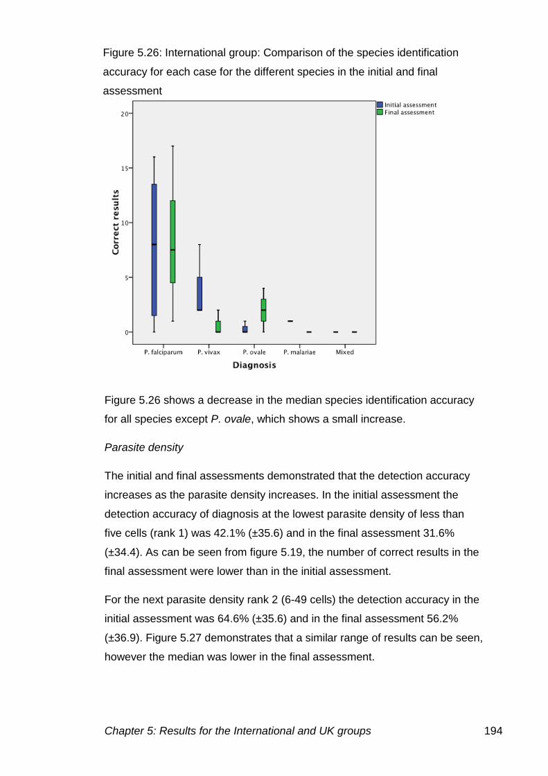
Chapter 5: Results for the International and UK groups 194
Figure 5.26 shows a decrease in the median species identification accuracy
for all species except P. ovale, which shows a small increase.
Parasite density
The initial and final assessments demonstrated that the detection accuracy
increases as the parasite density increases. In the initial assessment the
detection accuracy of diagnosis at the lowest parasite density of less than
five cells (rank 1) was 42.1% (±35.6) and in the final assessment 31.6%
(±34.4). As can be seen from figure 5.19, the number of correct results in the
final assessment were lower than in the initial assessment.
For the next parasite density rank 2 (6-49 cells) the detection accuracy in the
initial assessment was 64.6% (±35.6) and in the final assessment 56.2%
(±36.9). Figure 5.27 demonstrates that a similar range of results can be seen,
however the median was lower in the final assessment.
Figure 5.26: International group: Comparison of the species identification
accuracy for each case for the different species in the initial and final
assessment
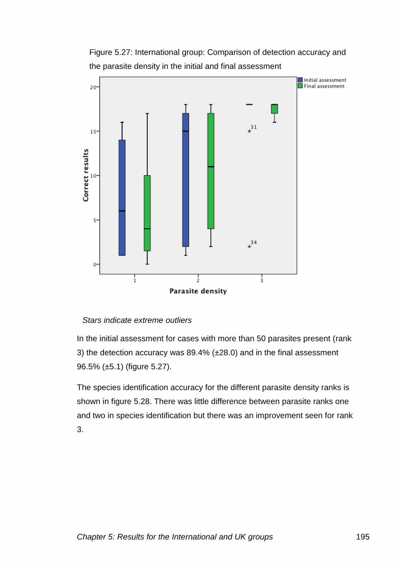
Chapter 5: Results for the International and UK groups 195
In the initial assessment for cases with more than 50 parasites present (rank
3) the detection accuracy was 89.4% (±28.0) and in the final assessment
96.5% (±5.1) (figure 5.27).
The species identification accuracy for the different parasite density ranks is
shown in figure 5.28. There was little difference between parasite ranks one
and two in species identification but there was an improvement seen for rank
3.
Figure 5.27: International group: Comparison of detection accuracy and
the parasite density in the initial and final assessment
Stars indicate extreme outliers
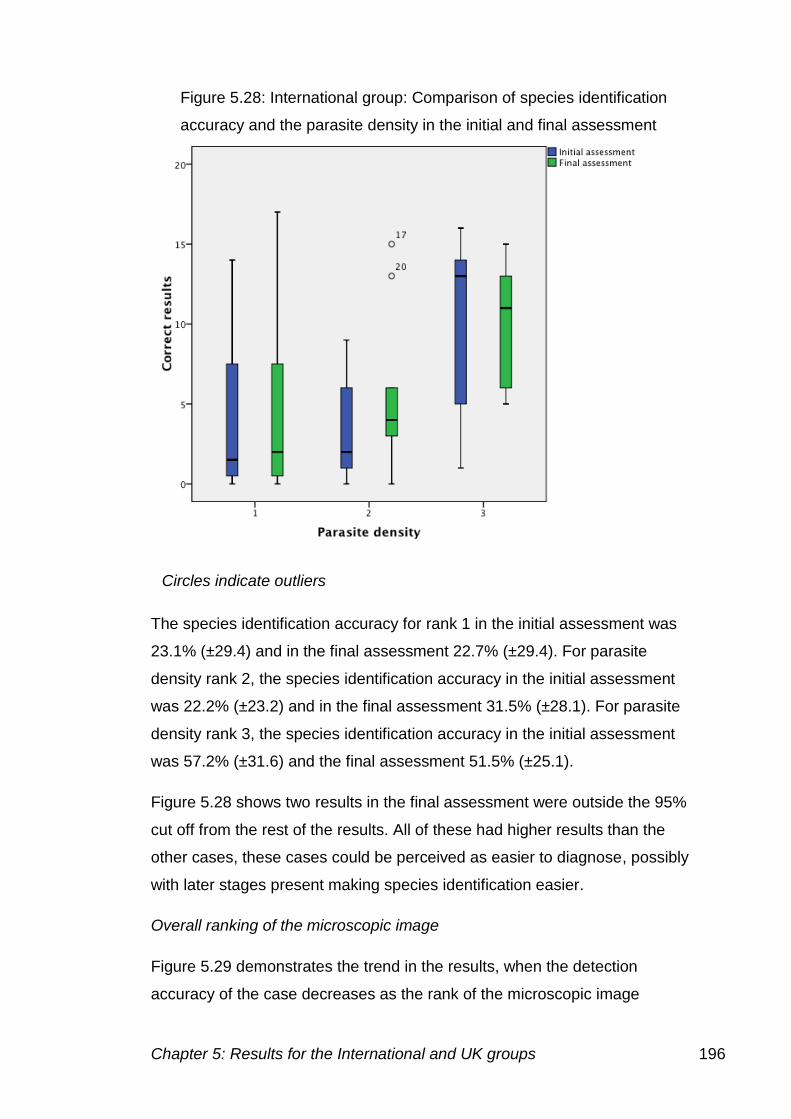
Chapter 5: Results for the International and UK groups 196
The species identification accuracy for rank 1 in the initial assessment was
23.1% (±29.4) and in the final assessment 22.7% (±29.4). For parasite
density rank 2, the species identification accuracy in the initial assessment
was 22.2% (±23.2) and in the final assessment 31.5% (±28.1). For parasite
density rank 3, the species identification accuracy in the initial assessment
was 57.2% (±31.6) and the final assessment 51.5% (±25.1).
Figure 5.28 shows two results in the final assessment were outside the 95%
cut off from the rest of the results. All of these had higher results than the
other cases, these cases could be perceived as easier to diagnose, possibly
with later stages present making species identification easier.
Overall ranking of the microscopic image
Figure 5.29 demonstrates the trend in the results, when the detection
accuracy of the case decreases as the rank of the microscopic image
Figure 5.28: International group: Comparison of species identification
accuracy and the parasite density in the initial and final assessment
Circles indicate outliers
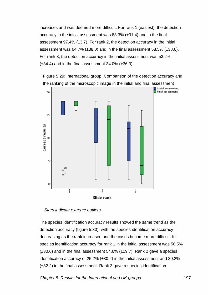
Chapter 5: Results for the International and UK groups 197
increases and was deemed more difficult. For rank 1 (easiest), the detection
accuracy in the initial assessment was 83.3% (±31.4) and in the final
assessment 97.4% (±3.7). For rank 2, the detection accuracy in the initial
assessment was 64.7% (±38.0) and in the final assessment 58.5% (±38.6).
For rank 3, the detection accuracy in the initial assessment was 53.2%
(±34.4) and in the final assessment 34.0% (±36.3).
The species identification accuracy results showed the same trend as the
detection accuracy (figure 5.30), with the species identification accuracy
decreasing as the rank increased and the cases became more difficult. In
species identification accuracy for rank 1 in the initial assessment was 50.5%
(±30.6) and in the final assessment 54.6% (±19.7). Rank 2 gave a species
identification accuracy of 25.2% (±30.2) in the initial assessment and 30.2%
(±32.2) in the final assessment. Rank 3 gave a species identification
Figure 5.29: International group: Comparison of the detection accuracy and
the ranking of the microscopic image in the initial and final assessment
Stars indicate extreme outliers
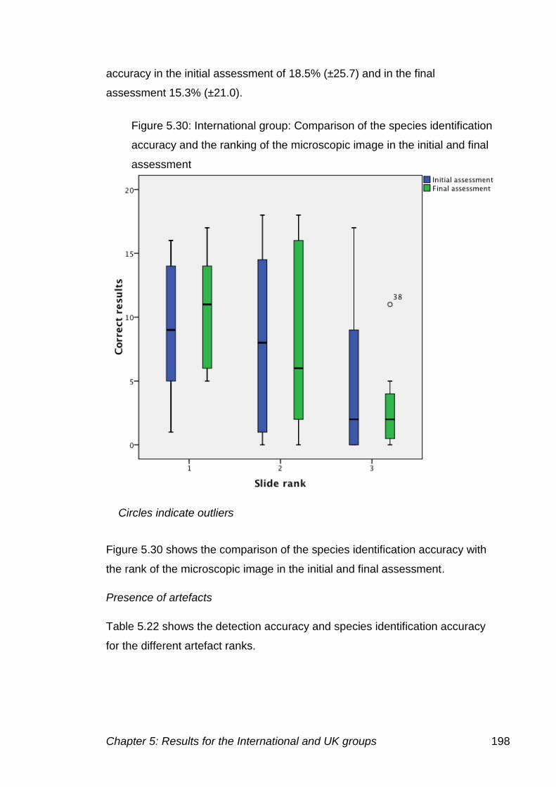
Chapter 5: Results for the International and UK groups 198
accuracy in the initial assessment of 18.5% (±25.7) and in the final
assessment 15.3% (±21.0).
Figure 5.30 shows the comparison of the species identification accuracy with
the rank of the microscopic image in the initial and final assessment.
Presence of artefacts
Table 5.22 shows the detection accuracy and species identification accuracy
for the different artefact ranks.
Figure 5.30: International group: Comparison of the species identification
accuracy and the ranking of the microscopic image in the initial and final
assessment
Circles indicate outliers
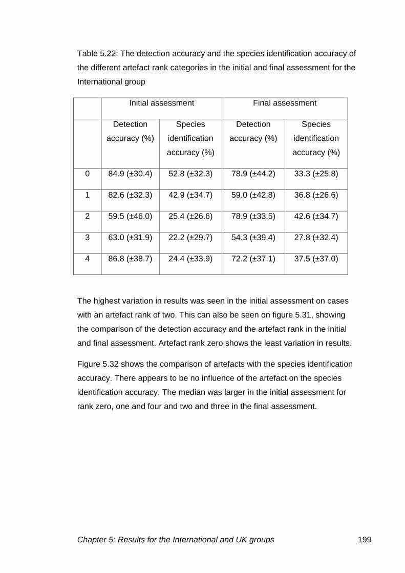
Chapter 5: Results for the International and UK groups 199
Table 5.22: The detection accuracy and the species identification accuracy of
the different artefact rank categories in the initial and final assessment for the
International group
Initial assessment Final assessment
Detection
accuracy (%)
Species
identification
accuracy (%)
Detection
accuracy (%)
Species
identification
accuracy (%)
0 84.9 (±30.4) 52.8 (±32.3) 78.9 (±44.2) 33.3 (±25.8)
1 82.6 (±32.3) 42.9 (±34.7) 59.0 (±42.8) 36.8 (±26.6)
2 59.5 (±46.0) 25.4 (±26.6) 78.9 (±33.5) 42.6 (±34.7)
3 63.0 (±31.9) 22.2 (±29.7) 54.3 (±39.4) 27.8 (±32.4)
4 86.8 (±38.7) 24.4 (±33.9) 72.2 (±37.1) 37.5 (±37.0)
The highest variation in results was seen in the initial assessment on cases
with an artefact rank of two. This can also be seen on figure 5.31, showing
the comparison of the detection accuracy and the artefact rank in the initial
and final assessment. Artefact rank zero shows the least variation in results.
Figure 5.32 shows the comparison of artefacts with the species identification
accuracy. There appears to be no influence of the artefact on the species
identification accuracy. The median was larger in the initial assessment for
rank zero, one and four and two and three in the final assessment.
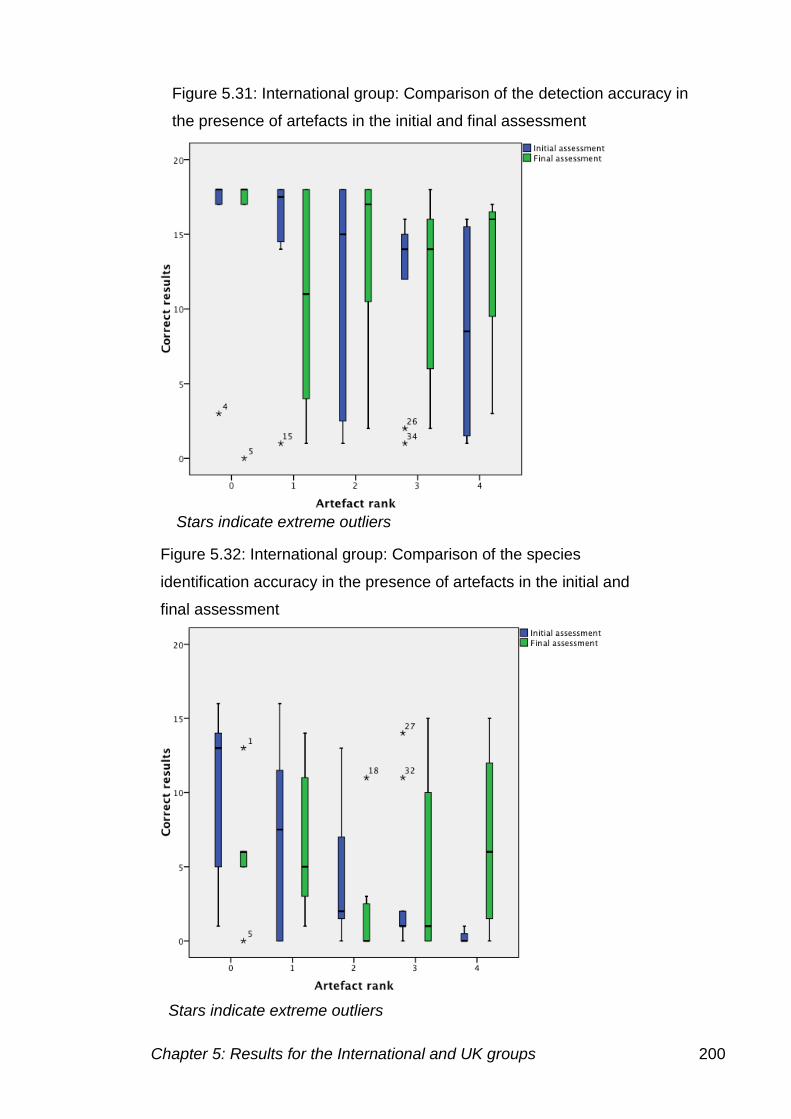
Chapter 5: Results for the International and UK groups 200
Figure 5.31: International group: Comparison of the detection accuracy in
the presence of artefacts in the initial and final assessment
Figure 5.32: International group: Comparison of the species
identification accuracy in the presence of artefacts in the initial and
final assessment
Stars indicate extreme outliers
Stars indicate extreme outliers
Chapter 5: Results for the International and UK groups 201
Comparison of staff undertaking malarial diagnosis by microscopy in
the International group
Table 5.23 shows the comparison of the results of members of laboratory
staff in the initial and final assessment. Nine participants determined the
correct species in more cases in the final assessment, two that had the same
number correct and seven that diagnosed fewer cases correctly. Only five
participants detected more parasites in the final assessment than the initial.
Individual LT018(D) showed the greatest improvement in results correctly
diagnosing 25 cases in the final assessment, compared to 18 in the initial,
and the number of incorrect results fell from 16 to seven. LT014 diagnosed
18 cases correctly in the initial assessment, this increased to 23 in the final
assessment, and the number of incorrect results fell from 19 to 13. LT005
had eight correct diagnoses in the initial assessment and 14 in the final
assessment, incorrect results fell from 19 to 17, showing that for this
individual the species identification accuracy increased.
LT001 did not increase the number of correct diagnoses, but had less
incorrect results leading to an increased detection accuracy from 19 to 23
cases. LT027 increased the number of correct cases from 23 in the initial
assessment to 25 in the final and also decreased the number of incorrect
results from 13 to ten.
All other individuals did not improve their diagnoses from the initial to the final
assessment.
Overall there was no significant difference in the detection accuracy
(p=0.195) or species identification accuracy (p=0.451) between laboratory
staff in the initial and final assessment. Figure 5.33 shows the box plot
comparing the detection accuracy in the initial and final assessment.
The overall median had fallen between the initial and final assessment. As
figure 5.34 demonstrates the correct results achieved by the individuals in the
initial and final assessment.
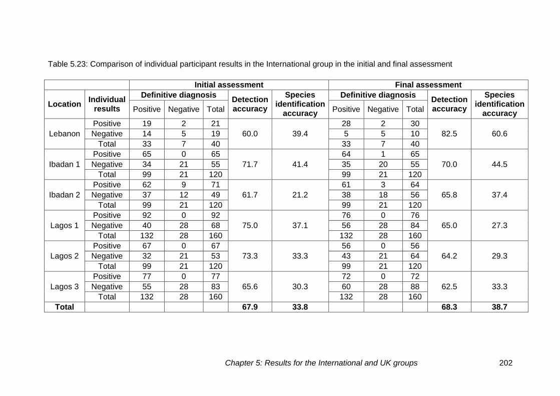
Chapter 5: Results for the International and UK groups 202
Table 5.23: Comparison of individual participant results in the International group in the initial and final assessment
Initial assessment Final assessment
Location Individual
results
Definitive diagnosis Detection accuracy
Species identification
accuracy
Definitive diagnosis Detection accuracy
Species identification
accuracy Positive Negative Total Positive Negative Total
Lebanon
Positive 19 2 21
60.0 39.4
28 2 30
82.5 60.6 Negative 14 5 19 5 5 10
Total 33 7 40 33 7 40
Ibadan 1
Positive 65 0 65
71.7 41.4
64 1 65
70.0 44.5 Negative 34 21 55 35 20 55
Total 99 21 120 99 21 120
Ibadan 2
Positive 62 9 71
61.7 21.2
61 3 64
65.8 37.4 Negative 37 12 49 38 18 56
Total 99 21 120 99 21 120
Lagos 1
Positive 92 0 92
75.0 37.1
76 0 76
65.0 27.3 Negative 40 28 68 56 28 84
Total 132 28 160 132 28 160
Lagos 2
Positive 67 0 67
73.3 33.3
56 0 56
64.2 29.3 Negative 32 21 53 43 21 64
Total 99 21 120 99 21 120
Lagos 3
Positive 77 0 77
65.6 30.3
72 0 72
62.5 33.3 Negative 55 28 83 60 28 88
Total 132 28 160 132 28 160
Total 67.9 33.8 68.3 38.7
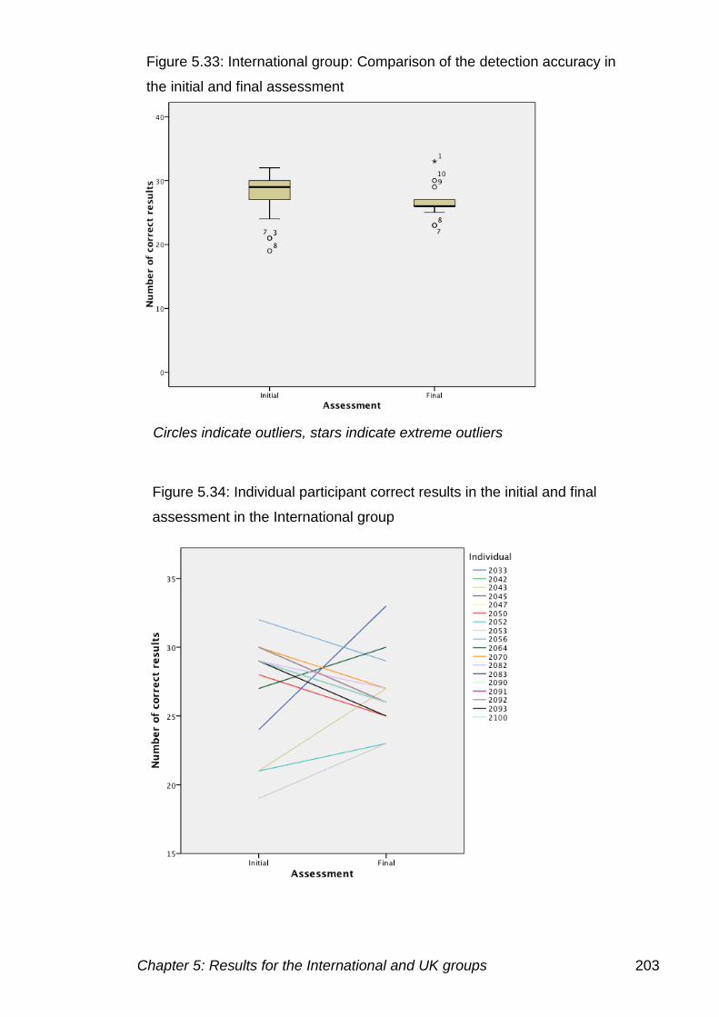
Chapter 5: Results for the International and UK groups 203
Figure 5.34: Individual participant correct results in the initial and final
assessment in the International group
Figure 5.33: International group: Comparison of the detection accuracy in
the initial and final assessment
Circles indicate outliers, stars indicate extreme outliers
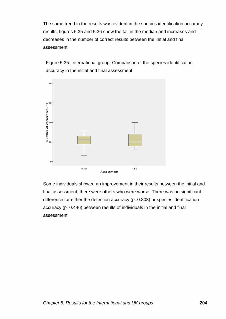
Chapter 5: Results for the International and UK groups 204
The same trend in the results was evident in the species identification accuracy
results, figures 5.35 and 5.36 show the fall in the median and increases and
decreases in the number of correct results between the initial and final
assessment.
Some individuals showed an improvement in their results between the initial and
final assessment, there were others who were worse. There was no significant
difference for either the detection accuracy (p=0.803) or species identification
accuracy (p=0.446) between results of individuals in the initial and final
assessment.
Figure 5.35: International group: Comparison of the species identification
accuracy in the initial and final assessment
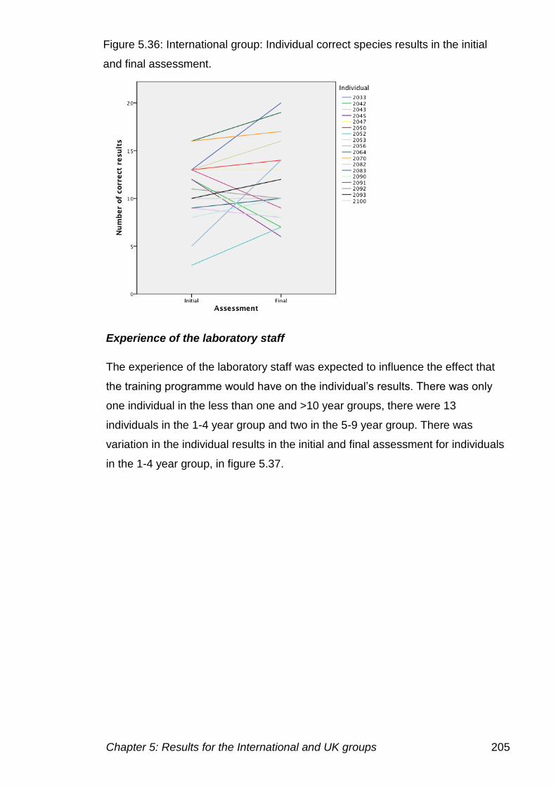
Chapter 5: Results for the International and UK groups 205
Experience of the laboratory staff
The experience of the laboratory staff was expected to influence the effect that
the training programme would have on the individual’s results. There was only
one individual in the less than one and >10 year groups, there were 13
individuals in the 1-4 year group and two in the 5-9 year group. There was
variation in the individual results in the initial and final assessment for individuals
in the 1-4 year group, in figure 5.37.
Figure 5.36: International group: Individual correct species results in the initial
and final assessment.
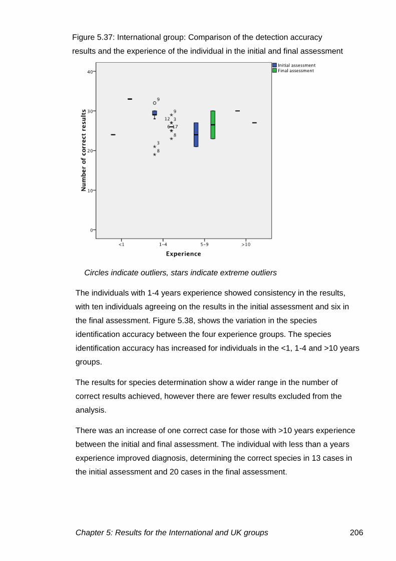
Chapter 5: Results for the International and UK groups 206
The individuals with 1-4 years experience showed consistency in the results,
with ten individuals agreeing on the results in the initial assessment and six in
the final assessment. Figure 5.38, shows the variation in the species
identification accuracy between the four experience groups. The species
identification accuracy has increased for individuals in the <1, 1-4 and >10 years
groups.
The results for species determination show a wider range in the number of
correct results achieved, however there are fewer results excluded from the
analysis.
There was an increase of one correct case for those with >10 years experience
between the initial and final assessment. The individual with less than a years
experience improved diagnosis, determining the correct species in 13 cases in
the initial assessment and 20 cases in the final assessment.
Figure 5.37: International group: Comparison of the detection accuracy
results and the experience of the individual in the initial and final assessment
Circles indicate outliers, stars indicate extreme outliers
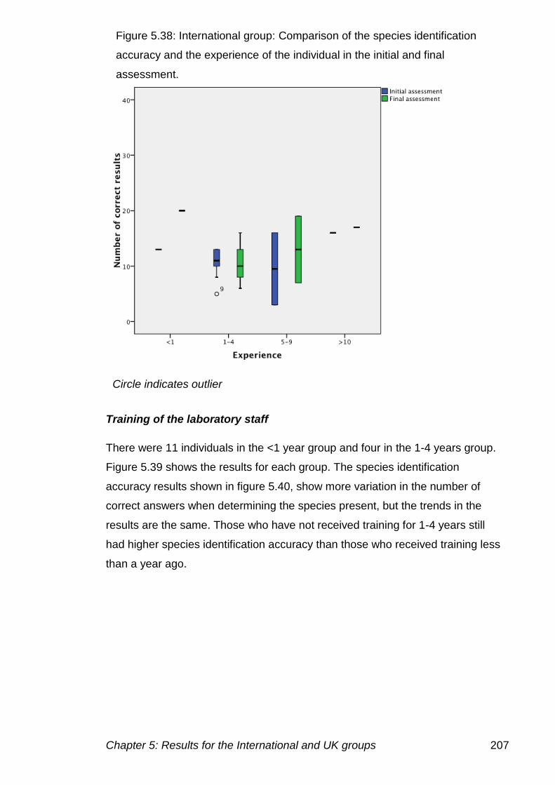
Chapter 5: Results for the International and UK groups 207
Training of the laboratory staff
There were 11 individuals in the <1 year group and four in the 1-4 years group.
Figure 5.39 shows the results for each group. The species identification
accuracy results shown in figure 5.40, show more variation in the number of
correct answers when determining the species present, but the trends in the
results are the same. Those who have not received training for 1-4 years still
had higher species identification accuracy than those who received training less
than a year ago.
Figure 5.38: International group: Comparison of the species identification
accuracy and the experience of the individual in the initial and final
assessment.
Circle indicates outlier
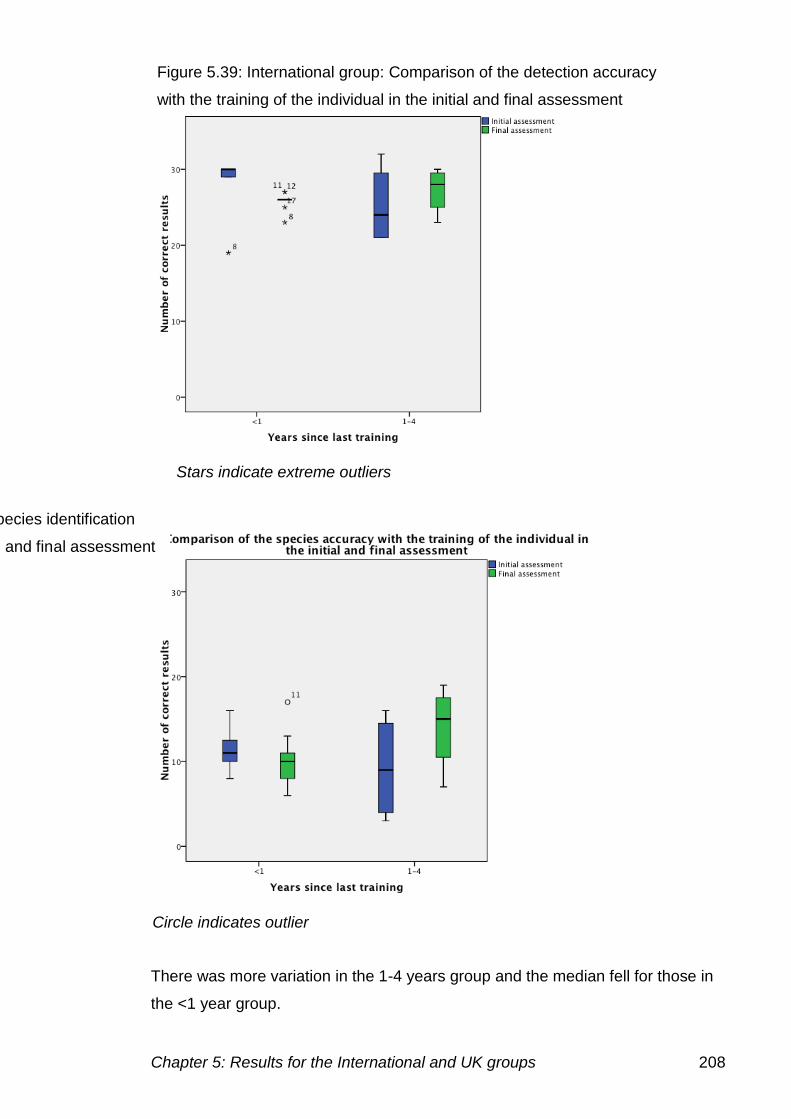
Chapter 5: Results for the International and UK groups 208
There was more variation in the 1-4 years group and the median fell for those in
the <1 year group.
Figure 5.39: International group: Comparison of the detection accuracy
with the training of the individual in the initial and final assessment
Figure 5.40: International group: Comparison of the species identification
accuracy with the training of the individual in the initial and final assessment
Stars indicate extreme outliers
Circle indicates outlier
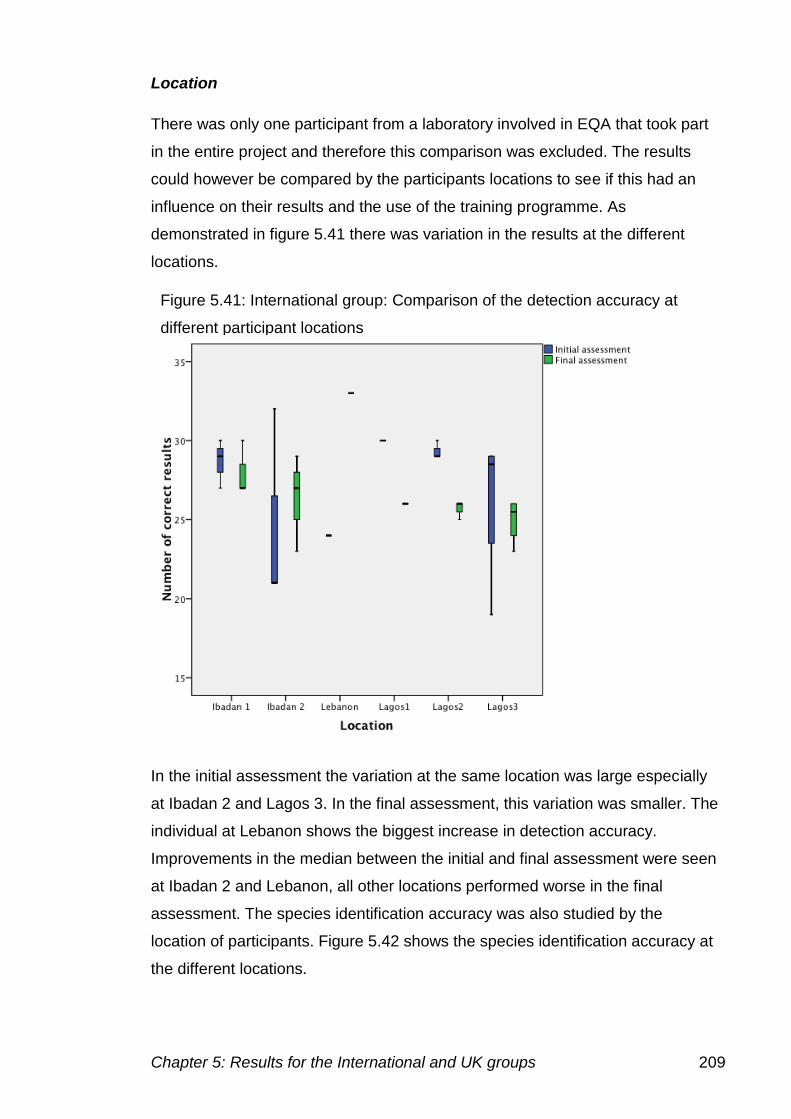
Chapter 5: Results for the International and UK groups 209
Location
There was only one participant from a laboratory involved in EQA that took part
in the entire project and therefore this comparison was excluded. The results
could however be compared by the participants locations to see if this had an
influence on their results and the use of the training programme. As
demonstrated in figure 5.41 there was variation in the results at the different
locations.
In the initial assessment the variation at the same location was large especially
at Ibadan 2 and Lagos 3. In the final assessment, this variation was smaller. The
individual at Lebanon shows the biggest increase in detection accuracy.
Improvements in the median between the initial and final assessment were seen
at Ibadan 2 and Lebanon, all other locations performed worse in the final
assessment. The species identification accuracy was also studied by the
location of participants. Figure 5.42 shows the species identification accuracy at
the different locations.
Figure 5.41: International group: Comparison of the detection accuracy at
different participant locations
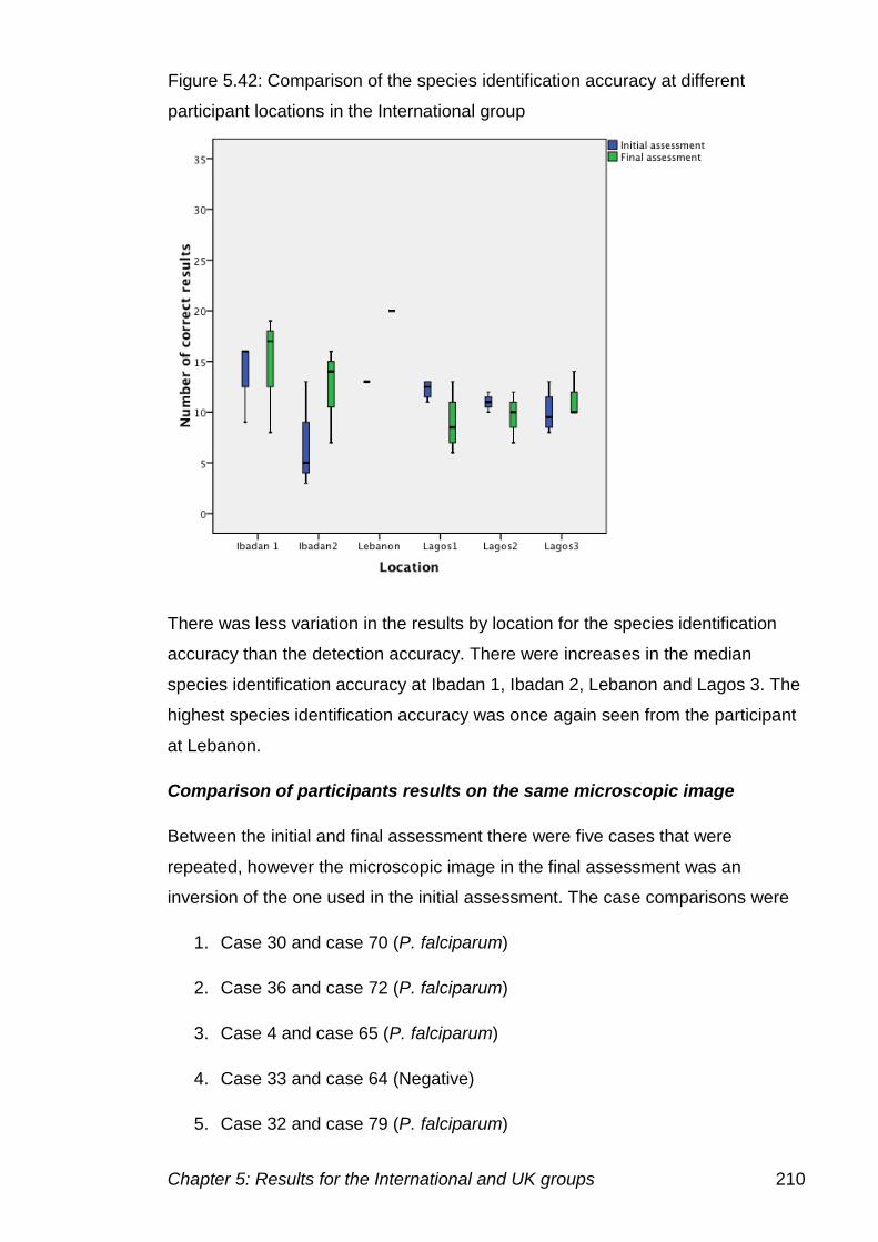
Chapter 5: Results for the International and UK groups 210
There was less variation in the results by location for the species identification
accuracy than the detection accuracy. There were increases in the median
species identification accuracy at Ibadan 1, Ibadan 2, Lebanon and Lagos 3. The
highest species identification accuracy was once again seen from the participant
at Lebanon.
Comparison of participants results on the same microscopic image
Between the initial and final assessment there were five cases that were
repeated, however the microscopic image in the final assessment was an
inversion of the one used in the initial assessment. The case comparisons were
1. Case 30 and case 70 (P. falciparum)
2. Case 36 and case 72 (P. falciparum)
3. Case 4 and case 65 (P. falciparum)
4. Case 33 and case 64 (Negative)
5. Case 32 and case 79 (P. falciparum)
Figure 5.42: Comparison of the species identification accuracy at different
participant locations in the International group
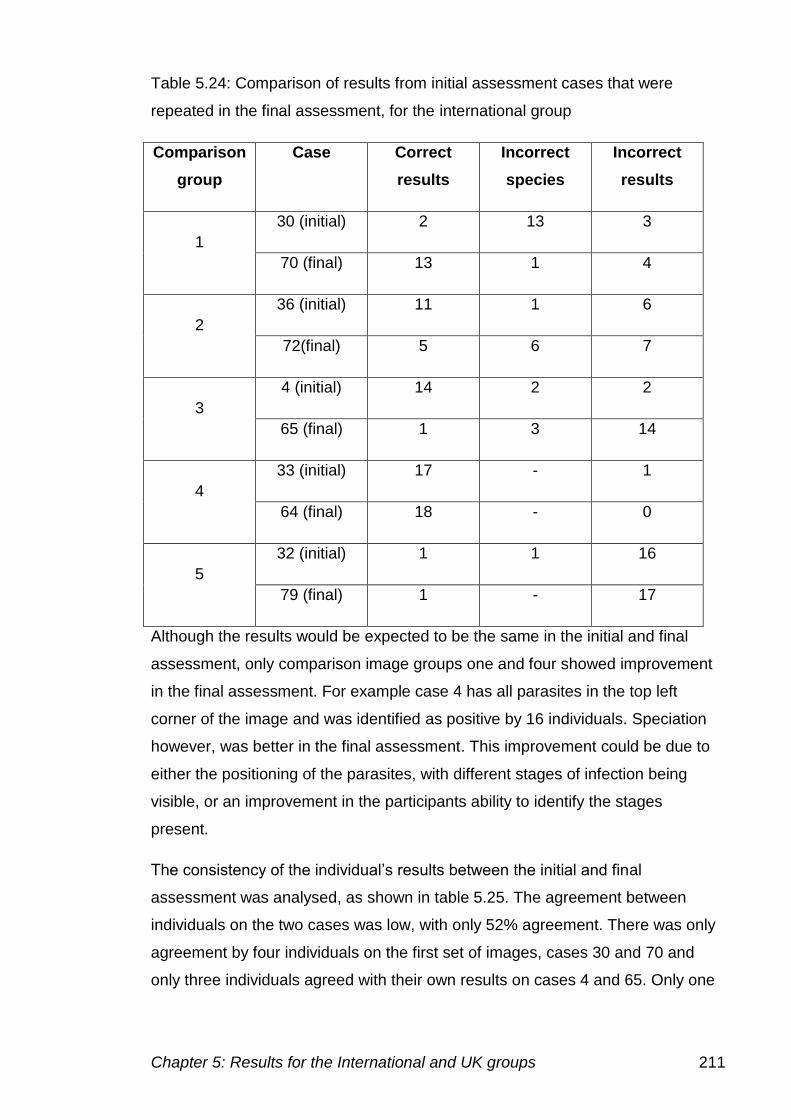
Chapter 5: Results for the International and UK groups 211
Table 5.24: Comparison of results from initial assessment cases that were
repeated in the final assessment, for the international group
Comparison
group
Case Correct
results
Incorrect
species
Incorrect
results
1
30 (initial) 2 13 3
70 (final) 13 1 4
2
36 (initial) 11 1 6
72(final) 5 6 7
3
4 (initial) 14 2 2
65 (final) 1 3 14
4
33 (initial) 17 - 1
64 (final) 18 - 0
5
32 (initial) 1 1 16
79 (final) 1 - 17
Although the results would be expected to be the same in the initial and final
assessment, only comparison image groups one and four showed improvement
in the final assessment. For example case 4 has all parasites in the top left
corner of the image and was identified as positive by 16 individuals. Speciation
however, was better in the final assessment. This improvement could be due to
either the positioning of the parasites, with different stages of infection being
visible, or an improvement in the participants ability to identify the stages
present.
The consistency of the individual’s results between the initial and final
assessment was analysed, as shown in table 5.25. The agreement between
individuals on the two cases was low, with only 52% agreement. There was only
agreement by four individuals on the first set of images, cases 30 and 70 and
only three individuals agreed with their own results on cases 4 and 65. Only one
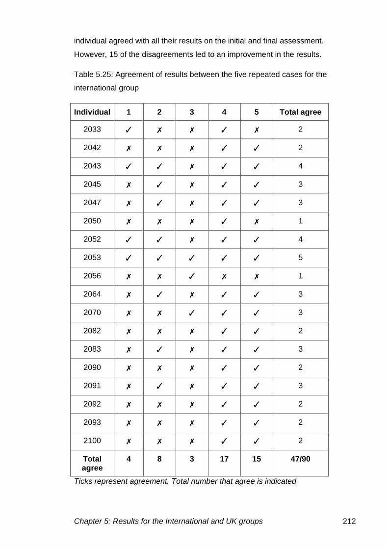
Chapter 5: Results for the International and UK groups 212
individual agreed with all their results on the initial and final assessment.
However, 15 of the disagreements led to an improvement in the results.
Table 5.25: Agreement of results between the five repeated cases for the
international group
Individual 1 2 3 4 5 Total agree
2033 ✓ ✗ ✗ ✓ ✗ 2
2042 ✗ ✗ ✗ ✓ ✓ 2
2043 ✓ ✓ ✗ ✓ ✓ 4
2045 ✗ ✓ ✗ ✓ ✓ 3
2047 ✗ ✓ ✗ ✓ ✓ 3
2050 ✗ ✗ ✗ ✓ ✗ 1
2052 ✓ ✓ ✗ ✓ ✓ 4
2053 ✓ ✓ ✓ ✓ ✓ 5
2056 ✗ ✗ ✓ ✗ ✗ 1
2064 ✗ ✓ ✗ ✓ ✓ 3
2070 ✗ ✗ ✓ ✓ ✓ 3
2082 ✗ ✗ ✗ ✓ ✓ 2
2083 ✗ ✓ ✗ ✓ ✓ 3
2090 ✗ ✗ ✗ ✓ ✓ 2
2091 ✗ ✓ ✗ ✓ ✓ 3
2092 ✗ ✗ ✗ ✓ ✓ 2
2093 ✗ ✗ ✗ ✓ ✓ 2
2100 ✗ ✗ ✗ ✓ ✓ 2
Total agree
4 8 3 17 15 47/90
Ticks represent agreement. Total number that agree is indicated
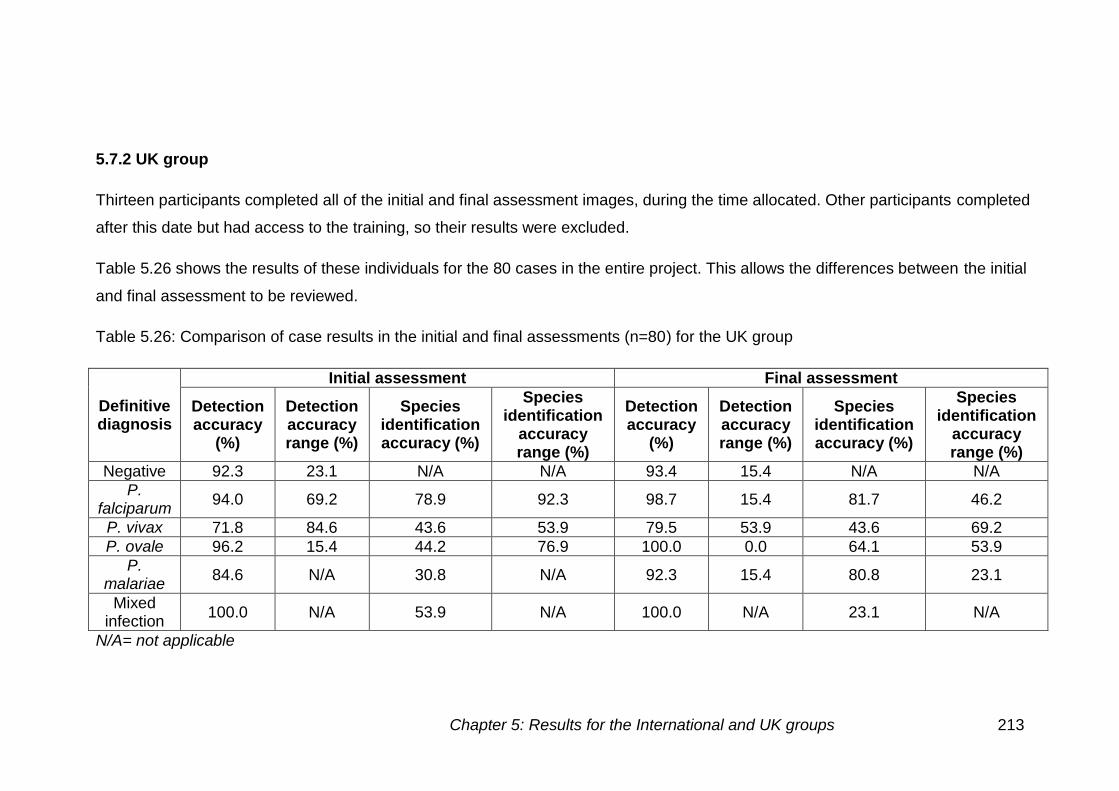
Chapter 5: Results for the International and UK groups 213
5.7.2 UK group
Thirteen participants completed all of the initial and final assessment images, during the time allocated. Other participants completed
after this date but had access to the training, so their results were excluded.
Table 5.26 shows the results of these individuals for the 80 cases in the entire project. This allows the differences between the initial
and final assessment to be reviewed.
Table 5.26: Comparison of case results in the initial and final assessments (n=80) for the UK group
Definitive diagnosis
Initial assessment Final assessment
Detection accuracy
(%)
Detection accuracy range (%)
Species identification accuracy (%)
Species identification
accuracy range (%)
Detection accuracy
(%)
Detection accuracy range (%)
Species identification accuracy (%)
Species identification
accuracy range (%)
Negative 92.3 23.1 N/A N/A 93.4 15.4 N/A N/A
P. falciparum
94.0 69.2 78.9 92.3 98.7 15.4 81.7 46.2
P. vivax 71.8 84.6 43.6 53.9 79.5 53.9 43.6 69.2
P. ovale 96.2 15.4 44.2 76.9 100.0 0.0 64.1 53.9
P. malariae
84.6 N/A 30.8 N/A 92.3 15.4 80.8 23.1
Mixed infection
100.0 N/A 53.9 N/A 100.0 N/A 23.1 N/A
N/A= not applicable
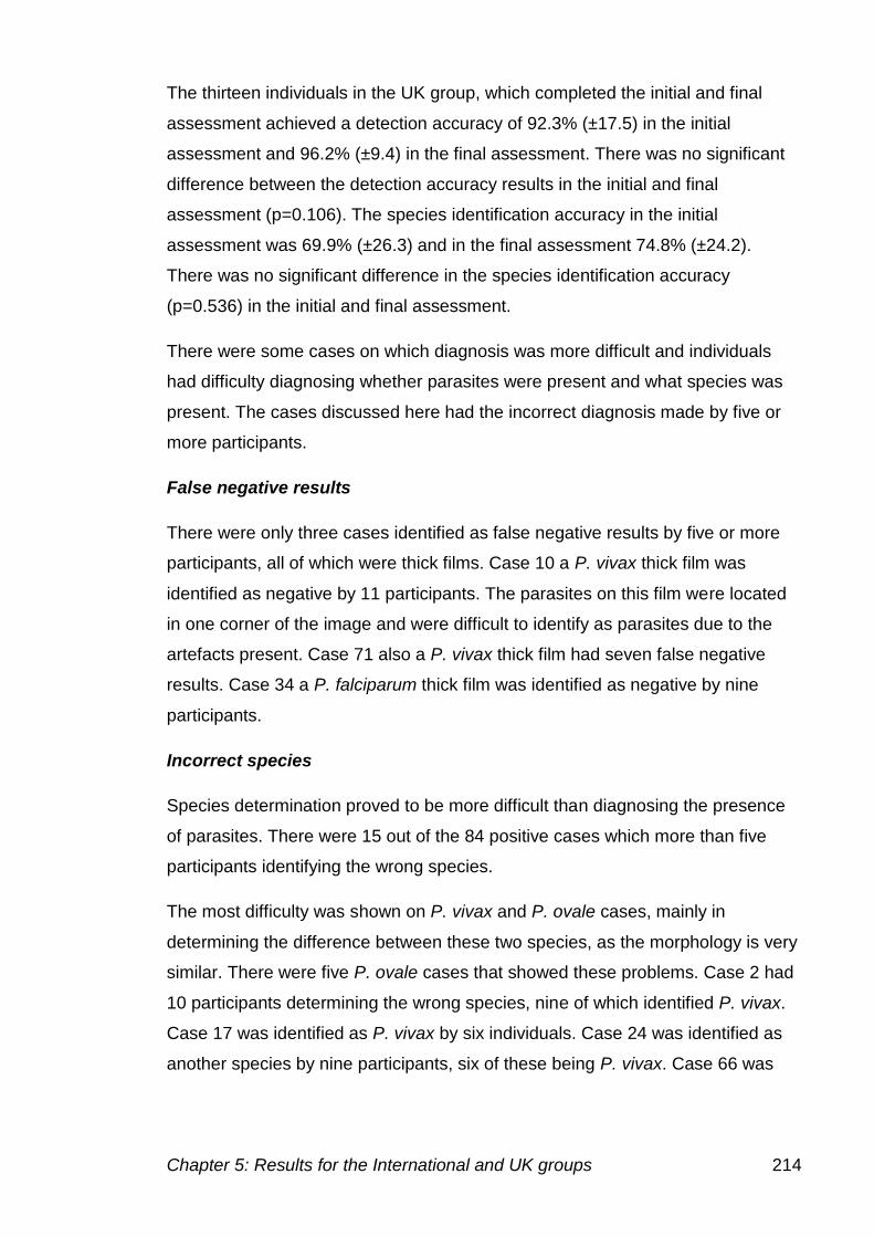
Chapter 5: Results for the International and UK groups 214
The thirteen individuals in the UK group, which completed the initial and final
assessment achieved a detection accuracy of 92.3% (±17.5) in the initial
assessment and 96.2% (±9.4) in the final assessment. There was no significant
difference between the detection accuracy results in the initial and final
assessment (p=0.106). The species identification accuracy in the initial
assessment was 69.9% (±26.3) and in the final assessment 74.8% (±24.2).
There was no significant difference in the species identification accuracy
(p=0.536) in the initial and final assessment.
There were some cases on which diagnosis was more difficult and individuals
had difficulty diagnosing whether parasites were present and what species was
present. The cases discussed here had the incorrect diagnosis made by five or
more participants.
False negative results
There were only three cases identified as false negative results by five or more
participants, all of which were thick films. Case 10 a P. vivax thick film was
identified as negative by 11 participants. The parasites on this film were located
in one corner of the image and were difficult to identify as parasites due to the
artefacts present. Case 71 also a P. vivax thick film had seven false negative
results. Case 34 a P. falciparum thick film was identified as negative by nine
participants.
Incorrect species
Species determination proved to be more difficult than diagnosing the presence
of parasites. There were 15 out of the 84 positive cases which more than five
participants identifying the wrong species.
The most difficulty was shown on P. vivax and P. ovale cases, mainly in
determining the difference between these two species, as the morphology is very
similar. There were five P. ovale cases that showed these problems. Case 2 had
10 participants determining the wrong species, nine of which identified P. vivax.
Case 17 was identified as P. vivax by six individuals. Case 24 was identified as
another species by nine participants, six of these being P. vivax. Case 66 was
Chapter 5: Results for the International and UK groups 215
identified by five participants as P. vivax. Finally case 75 was identified as P.
vivax by eight participants.
The same problem was seen for P. vivax cases. Case 8 was identified as P.
ovale by four participants and P. falciparum by one. Case 22 was identified as P.
ovale by three participants and P. falciparum by two. Case 71 a thick film was
identified as P. falciparum by two participants, P. ovale by two and P. malariae
by one. Case 80 also a thick film was identified by P. malariae by four
participants, P. ovale by one and one participants could not identify the species.
P. malariae also caused problems with species identification in the initial
assessment on case 40. Six individuals identified this case as P. vivax, one as P.
ovale and one participant did not identify the species present.
Mixed species infections caused a few problems with species identification.
However, the species identified was usually correct, although the mixed infection
was often missed. Case 39 a P. falciparum and P. ovale was identified as P.
falciparum by four participants and P. falciparum and P. vivax by two
participants. Case 77 the thick film showing P. falciparum and P. ovale mixed
infection had a similar pattern. Eight participants identified P. falciparum alone,
one P. malariae, and one as a P. falciparum and P. malariae mixed infection.
However, as speciation is not usually carried out on the thick film, these
differences may not be relevant.
Speciation difficulties
All problems with speciation on P. falciparum cases were seen in the final
assessment. Thick films caused the most problems, with case 49 being identified
as another species by five individuals and six identified case 72 also a thick film
as another species.
Cell inclusions caused problems in species identification on cases 59 (5), 60
(5), 67 (6) and 76 (6) (brackets indicate the number of incorrect species
identified).
Chapter 5: Results for the International and UK groups 216
Comparison of cases used in the initial and final assessment
Of the 80 cases used over the initial and final assessments, there were 48 P.
falciparum cases, 14 negative cases, seven P. ovale cases, six P. vivax cases,
three P. malariae cases and two mixed infections. The performance on the
cases in the initial and final assessment, were compared to the five main
categories into which the cases were ranked.
Thick and thin films
There were 15 thick films and 65 thin films, seven thick films in the initial
assessment and eight in the final assessment. In the initial assessment, there
were five thick film positive cases, compared to seven in the final assessment.
Four of the thick film cases in the initial assessment and four in the final
assessment were P. falciparum cases. In the initial assessment, there was
detection accuracy for the thick films of 71.4% (±33.7), in the final assessment
this was 86.5% (±17.8). Thin films in the initial assessment had a detection
accuracy of 96.7% (±6.7) compared to 98.6% (±3.1) in the final assessment. The
species identification accuracy for thick films was 52.3% (±43.0) in the initial
assessment and 48.4% (±28.0) in the final assessment. The species
identification accuracy for thin films in the initial assessment was 73.1% (±21.9)
compared to 82.0% (±17.7) in the final assessment.
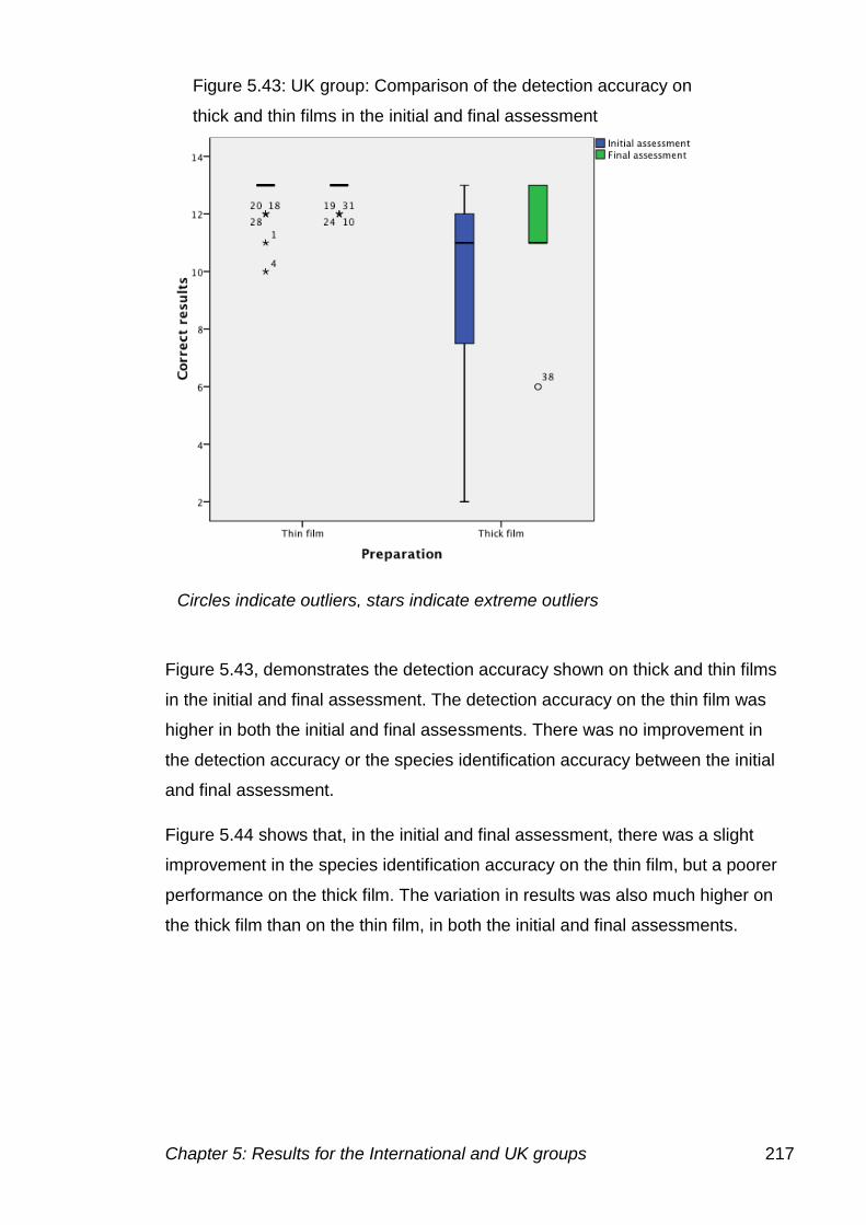
Chapter 5: Results for the International and UK groups 217
Figure 5.43, demonstrates the detection accuracy shown on thick and thin films
in the initial and final assessment. The detection accuracy on the thin film was
higher in both the initial and final assessments. There was no improvement in
the detection accuracy or the species identification accuracy between the initial
and final assessment.
Figure 5.44 shows that, in the initial and final assessment, there was a slight
improvement in the species identification accuracy on the thin film, but a poorer
performance on the thick film. The variation in results was also much higher on
the thick film than on the thin film, in both the initial and final assessments.
Figure 5.43: UK group: Comparison of the detection accuracy on
thick and thin films in the initial and final assessment
Circles indicate outliers, stars indicate extreme outliers
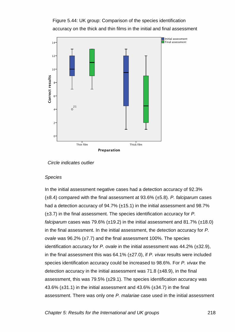
Chapter 5: Results for the International and UK groups 218
Species
In the initial assessment negative cases had a detection accuracy of 92.3%
(±8.4) compared with the final assessment at 93.6% (±5.8). P. falciparum cases
had a detection accuracy of 94.7% (±15.1) in the initial assessment and 98.7%
(±3.7) in the final assessment. The species identification accuracy for P.
falciparum cases was 79.6% (±19.2) in the initial assessment and 81.7% (±18.0)
in the final assessment. In the initial assessment, the detection accuracy for P.
ovale was 96.2% (±7.7) and the final assessment 100%. The species
identification accuracy for P. ovale in the initial assessment was 44.2% (±32.9),
in the final assessment this was 64.1% (±27.0), if P. vivax results were included
species identification accuracy could be increased to 98.6%. For P. vivax the
detection accuracy in the initial assessment was 71.8 (±48.9), in the final
assessment, this was 79.5% (±29.1). The species identification accuracy was
43.6% (±31.1) in the initial assessment and 43.6% (±34.7) in the final
assessment. There was only one P. malariae case used in the initial assessment
Figure 5.44: UK group: Comparison of the species identification
accuracy on the thick and thin films in the initial and final assessment
Circle indicates outlier
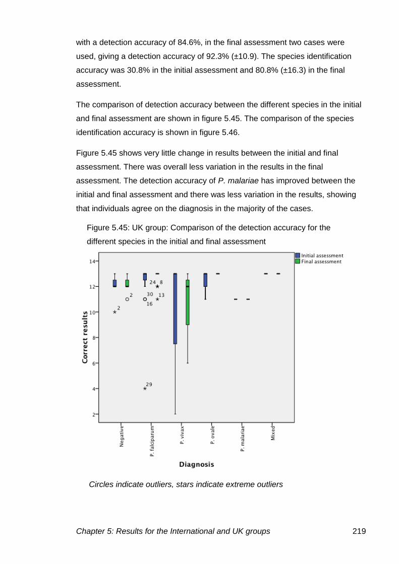
Chapter 5: Results for the International and UK groups 219
with a detection accuracy of 84.6%, in the final assessment two cases were
used, giving a detection accuracy of 92.3% (±10.9). The species identification
accuracy was 30.8% in the initial assessment and 80.8% (±16.3) in the final
assessment.
The comparison of detection accuracy between the different species in the initial
and final assessment are shown in figure 5.45. The comparison of the species
identification accuracy is shown in figure 5.46.
Figure 5.45 shows very little change in results between the initial and final
assessment. There was overall less variation in the results in the final
assessment. The detection accuracy of P. malariae has improved between the
initial and final assessment and there was less variation in the results, showing
that individuals agree on the diagnosis in the majority of the cases.
Figure 5.45: UK group: Comparison of the detection accuracy for the
different species in the initial and final assessment
Circles indicate outliers, stars indicate extreme outliers
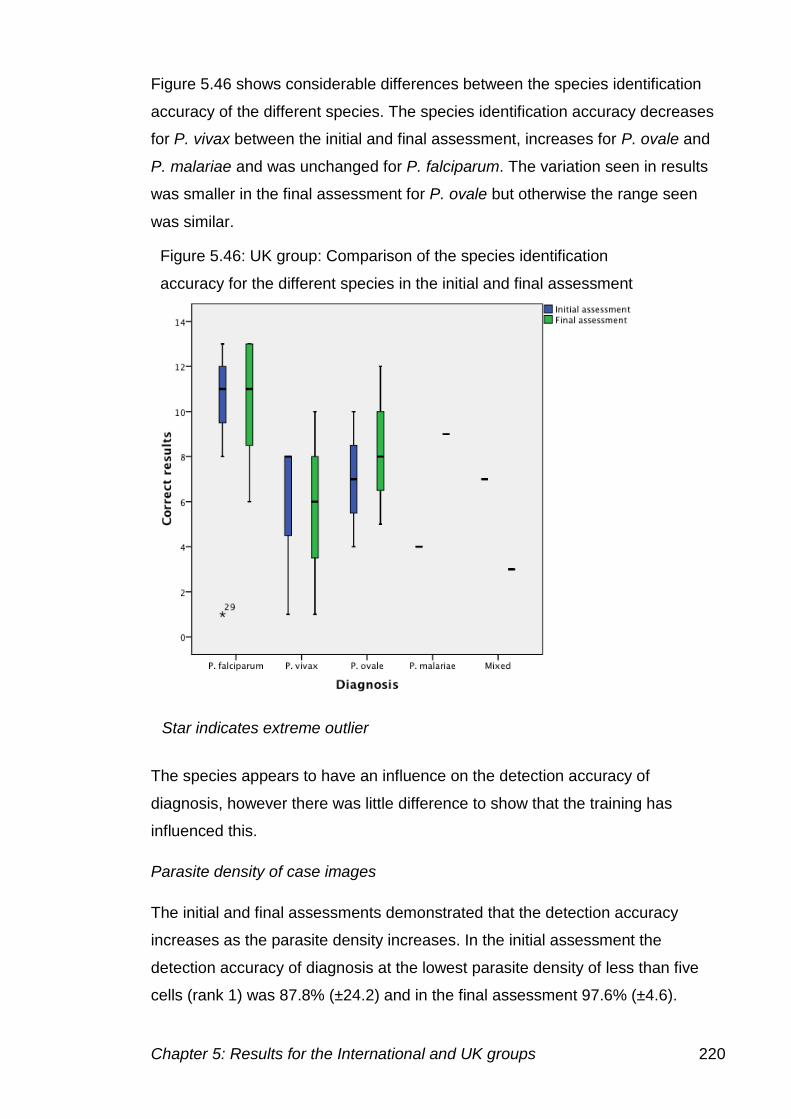
Chapter 5: Results for the International and UK groups 220
Figure 5.46 shows considerable differences between the species identification
accuracy of the different species. The species identification accuracy decreases
for P. vivax between the initial and final assessment, increases for P. ovale and
P. malariae and was unchanged for P. falciparum. The variation seen in results
was smaller in the final assessment for P. ovale but otherwise the range seen
was similar.
The species appears to have an influence on the detection accuracy of
diagnosis, however there was little difference to show that the training has
influenced this.
Parasite density of case images
The initial and final assessments demonstrated that the detection accuracy
increases as the parasite density increases. In the initial assessment the
detection accuracy of diagnosis at the lowest parasite density of less than five
cells (rank 1) was 87.8% (±24.2) and in the final assessment 97.6% (±4.6).
Figure 5.46: UK group: Comparison of the species identification
accuracy for the different species in the initial and final assessment
Star indicates extreme outlier
Chapter 5: Results for the International and UK groups 221
For the next parasite density rank 2 (6-49 cells) the detection accuracy in the
initial assessment was 91.6% (±20.8) and in the final assessment 92.3% (±18.0).
In the initial assessment for cases with more than 50 parasites present (rank 3)
the detection accuracy was 98.5% (±4.9) and in the final assessment 99.3%
(±2.3).
Figure 5.47 indicates that the parasite density has no effect on the detection
accuracy in the initial and final assessment. There was also no difference in the
median between the initial and final assessment, however there was a reduction
in the variation seen. Any results that are outside of the median are deemed to
be outside the distribution due to the small variation in results.
The species identification accuracy for rank 1 in the initial assessment was
57.1% (±30.7) and in the final assessment 75.2% (±20.2). For parasite density
rank 2, the species identification accuracy in the initial assessment was 72.0%
(±26.0) and in the final assessment 65.8% (±29.1). For parasite density rank 3,
Figure 5.47: UK group: Comparison of detection accuracy and the parasite
density in the initial and final assessment
Circles indicate outliers, stars indicate extreme outliers
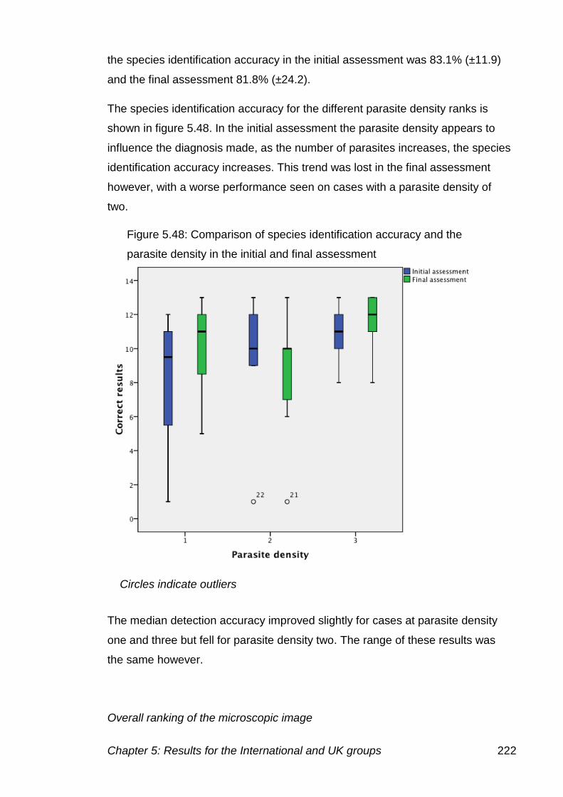
Chapter 5: Results for the International and UK groups 222
the species identification accuracy in the initial assessment was 83.1% (±11.9)
and the final assessment 81.8% (±24.2).
The species identification accuracy for the different parasite density ranks is
shown in figure 5.48. In the initial assessment the parasite density appears to
influence the diagnosis made, as the number of parasites increases, the species
identification accuracy increases. This trend was lost in the final assessment
however, with a worse performance seen on cases with a parasite density of
two.
The median detection accuracy improved slightly for cases at parasite density
one and three but fell for parasite density two. The range of these results was
the same however.
Overall ranking of the microscopic image
Figure 5.48: Comparison of species identification accuracy and the
parasite density in the initial and final assessment
Circles indicate outliers
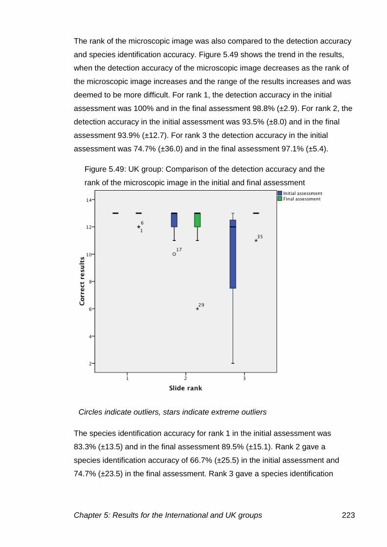
Chapter 5: Results for the International and UK groups 223
The rank of the microscopic image was also compared to the detection accuracy
and species identification accuracy. Figure 5.49 shows the trend in the results,
when the detection accuracy of the microscopic image decreases as the rank of
the microscopic image increases and the range of the results increases and was
deemed to be more difficult. For rank 1, the detection accuracy in the initial
assessment was 100% and in the final assessment 98.8% (±2.9). For rank 2, the
detection accuracy in the initial assessment was 93.5% (±8.0) and in the final
assessment 93.9% (±12.7). For rank 3 the detection accuracy in the initial
assessment was 74.7% (±36.0) and in the final assessment 97.1% (±5.4).
The species identification accuracy for rank 1 in the initial assessment was
83.3% (±13.5) and in the final assessment 89.5% (±15.1). Rank 2 gave a
species identification accuracy of 66.7% (±25.5) in the initial assessment and
74.7% (±23.5) in the final assessment. Rank 3 gave a species identification
Figure 5.49: UK group: Comparison of the detection accuracy and the
rank of the microscopic image in the initial and final assessment
Circles indicate outliers, stars indicate extreme outliers
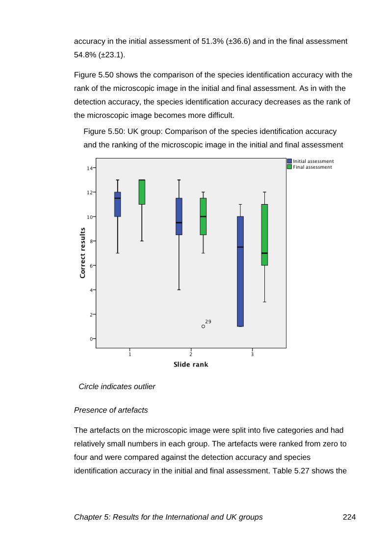
Chapter 5: Results for the International and UK groups 224
accuracy in the initial assessment of 51.3% (±36.6) and in the final assessment
54.8% (±23.1).
Figure 5.50 shows the comparison of the species identification accuracy with the
rank of the microscopic image in the initial and final assessment. As in with the
detection accuracy, the species identification accuracy decreases as the rank of
the microscopic image becomes more difficult.
Presence of artefacts
The artefacts on the microscopic image were split into five categories and had
relatively small numbers in each group. The artefacts were ranked from zero to
four and were compared against the detection accuracy and species
identification accuracy in the initial and final assessment. Table 5.27 shows the
Figure 5.50: UK group: Comparison of the species identification accuracy
and the ranking of the microscopic image in the initial and final assessment
Circle indicates outlier
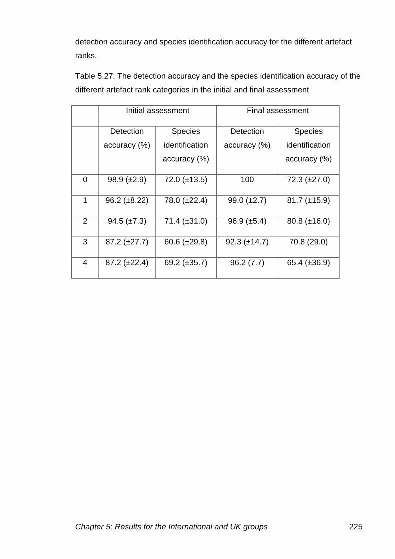
Chapter 5: Results for the International and UK groups 225
detection accuracy and species identification accuracy for the different artefact
ranks.
Table 5.27: The detection accuracy and the species identification accuracy of the
different artefact rank categories in the initial and final assessment
Initial assessment Final assessment
Detection
accuracy (%)
Species
identification
accuracy (%)
Detection
accuracy (%)
Species
identification
accuracy (%)
0 98.9 (±2.9) 72.0 (±13.5) 100 72.3 (±27.0)
1 96.2 (±8.22) 78.0 (±22.4) 99.0 (±2.7) 81.7 (±15.9)
2 94.5 (±7.3) 71.4 (±31.0) 96.9 (±5.4) 80.8 (±16.0)
3 87.2 (±27.7) 60.6 (±29.8) 92.3 (±14.7) 70.8 (29.0)
4 87.2 (±22.4) 69.2 (±35.7) 96.2 (7.7) 65.4 (±36.9)
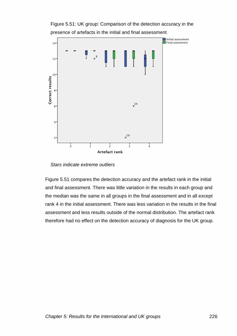
Chapter 5: Results for the International and UK groups 226
Figure 5.51 compares the detection accuracy and the artefact rank in the initial
and final assessment. There was little variation in the results in each group and
the median was the same in all groups in the final assessment and in all except
rank 4 in the initial assessment. There was less variation in the results in the final
assessment and less results outside of the normal distribution. The artefact rank
therefore had no effect on the detection accuracy of diagnosis for the UK group.
Figure 5.51: UK group: Comparison of the detection accuracy in the
presence of artefacts in the initial and final assessment
Stars indicate extreme outliers
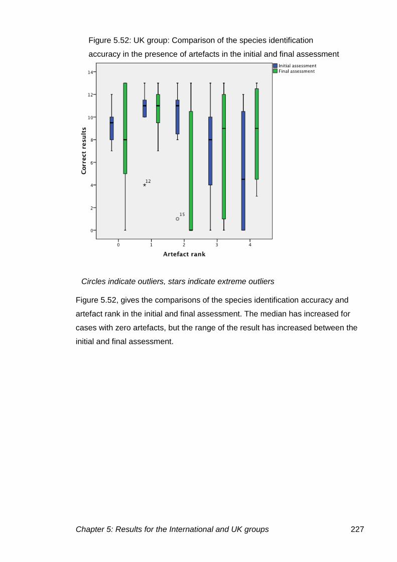
Chapter 5: Results for the International and UK groups 227
Figure 5.52, gives the comparisons of the species identification accuracy and
artefact rank in the initial and final assessment. The median has increased for
cases with zero artefacts, but the range of the result has increased between the
initial and final assessment.
Figure 5.52: UK group: Comparison of the species identification
accuracy in the presence of artefacts in the initial and final assessment
Circles indicate outliers, stars indicate extreme outliers
Chapter 5: Results for the International and UK groups 228
Comparison of staff undertaking malarial diagnosis by microscopy in the
UK group
Table 5.28 shows the comparison of individual results in the initial and final
assessment. Out of the 13 participants, there were seven that correctly identified
the species in more cases in the final assessment, four with the same number
and two with a lower number of correct cases in the final assessment.
The number of incorrect results fell for 11 participants, with one participant
staying the same and one increasing from two to three incorrect cases. Four
participants had no incorrect results in the final assessment, which was seen as
the most important diagnosis, determining whether parasites are present forms
the basis of the patient treatment. There were six individuals that increased the
number of incorrect species results and six that decreased the number, one
participant had the same number throughout.
The most improvement in diagnosing the correct species was seen from
participant UK171. The number of correct diagnoses increased from 33 to 38,
with no incorrect species in the final assessment, however there were still two
incorrect results. The species in the initial assessment were mainly due to the
confusion of P. ovale and P. vivax cases in the initial assessment. UK201 also
showed considerable improvement in diagnosis, increasing from achieving the
correct diagnosis in 28 cases in the initial assessment to 36 in the final
assessment, and reduced the number of incorrect species from nine to four, with
no incorrect results in the final assessment.
UK141 increased the number of correctly diagnosed cases from 21 in the initial
assessment to 27 in the final assessment. The number of incorrect species fell
from 15 cases to ten. The incorrect species determined was different to those in
the initial assessment with four of the P. falciparum cases being confused with P.
malariae, only one case was confused in the initial assessment.
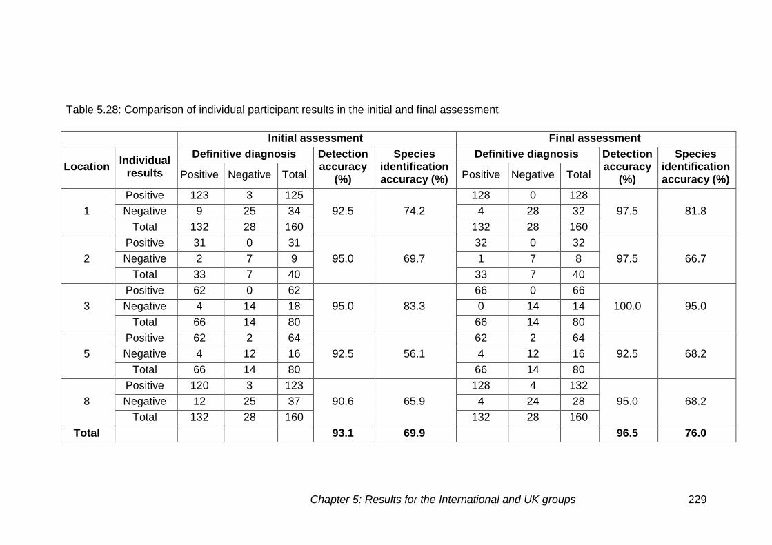
Chapter 5: Results for the International and UK groups 229
Table 5.28: Comparison of individual participant results in the initial and final assessment
Initial assessment Final assessment
Location Individual
results
Definitive diagnosis Detection accuracy
(%)
Species identification accuracy (%)
Definitive diagnosis Detection accuracy
(%)
Species identification accuracy (%) Positive Negative Total Positive Negative Total
1
Positive 123 3 125
92.5 74.2
128 0 128
97.5 81.8 Negative 9 25 34 4 28 32
Total 132 28 160 132 28 160
2
Positive 31 0 31
95.0 69.7
32 0 32
97.5 66.7 Negative 2 7 9 1 7 8
Total 33 7 40 33 7 40
3
Positive 62 0 62
95.0 83.3
66 0 66
100.0 95.0 Negative 4 14 18 0 14 14
Total 66 14 80 66 14 80
5
Positive 62 2 64
92.5 56.1
62 2 64
92.5 68.2 Negative 4 12 16 4 12 16
Total 66 14 80 66 14 80
8
Positive 120 3 123
90.6 65.9
128 4 132
95.0 68.2 Negative 12 25 37 4 24 28
Total 132 28 160 132 28 160
Total 93.1 69.9 96.5 76.0
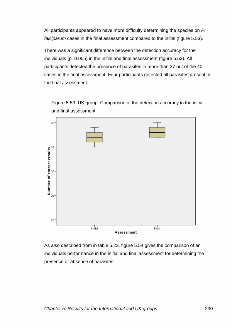
Chapter 5: Results for the International and UK groups 230
All participants appeared to have more difficulty determining the species on P.
falciparum cases in the final assessment compared to the initial (figure 5.53).
There was a significant difference between the detection accuracy for the
individuals (p=0.005) in the initial and final assessment (figure 5.53). All
participants detected the presence of parasites in more than 37 out of the 40
cases in the final assessment. Four participants detected all parasites present in
the final assessment.
As also described from in table 5.23, figure 5.54 gives the comparison of an
individuals performance in the initial and final assessment for determining the
presence or absence of parasites.
Figure 5.53: UK group: Comparison of the detection accuracy in the initial
and final assessment
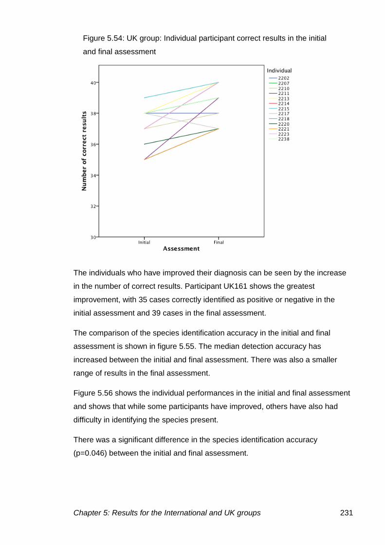
Chapter 5: Results for the International and UK groups 231
The individuals who have improved their diagnosis can be seen by the increase
in the number of correct results. Participant UK161 shows the greatest
improvement, with 35 cases correctly identified as positive or negative in the
initial assessment and 39 cases in the final assessment.
The comparison of the species identification accuracy in the initial and final
assessment is shown in figure 5.55. The median detection accuracy has
increased between the initial and final assessment. There was also a smaller
range of results in the final assessment.
Figure 5.56 shows the individual performances in the initial and final assessment
and shows that while some participants have improved, others have also had
difficulty in identifying the species present.
There was a significant difference in the species identification accuracy
(p=0.046) between the initial and final assessment.
Figure 5.54: UK group: Individual participant correct results in the initial
and final assessment
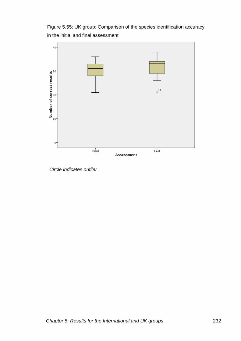
Chapter 5: Results for the International and UK groups 232
Figure 5.55: UK group: Comparison of the species identification accuracy
in the initial and final assessment
Circle indicates outlier
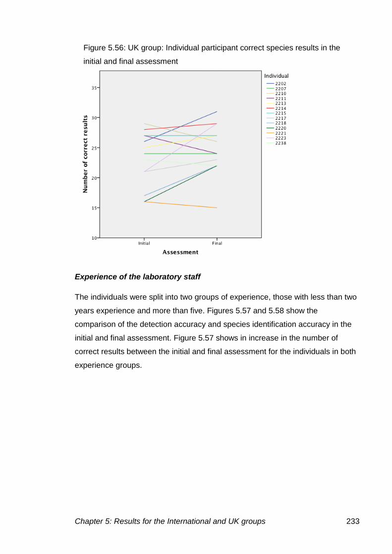
Chapter 5: Results for the International and UK groups 233
Experience of the laboratory staff
The individuals were split into two groups of experience, those with less than two
years experience and more than five. Figures 5.57 and 5.58 show the
comparison of the detection accuracy and species identification accuracy in the
initial and final assessment. Figure 5.57 shows in increase in the number of
correct results between the initial and final assessment for the individuals in both
experience groups.
Figure 5.56: UK group: Individual participant correct species results in the
initial and final assessment
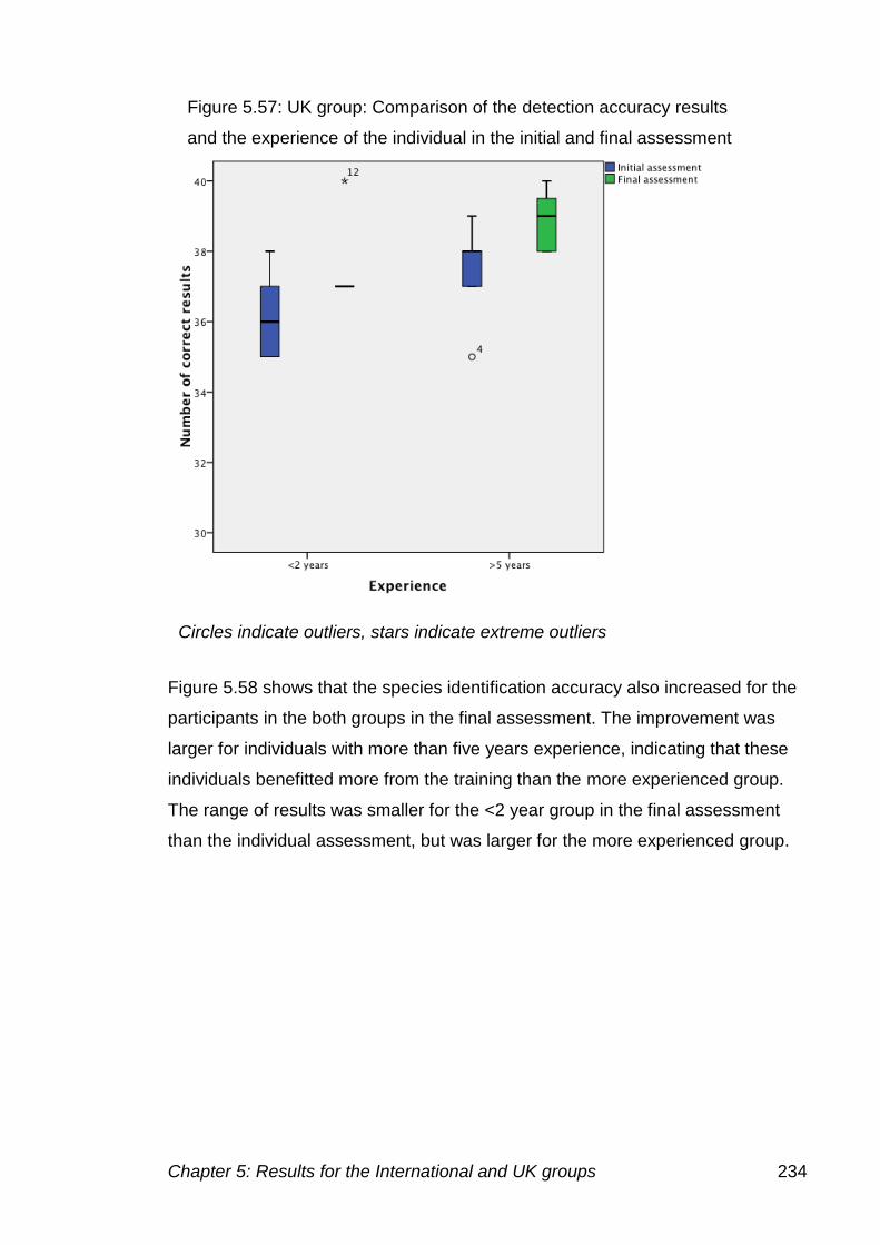
Chapter 5: Results for the International and UK groups 234
Figure 5.58 shows that the species identification accuracy also increased for the
participants in the both groups in the final assessment. The improvement was
larger for individuals with more than five years experience, indicating that these
individuals benefitted more from the training than the more experienced group.
The range of results was smaller for the <2 year group in the final assessment
than the individual assessment, but was larger for the more experienced group.
Figure 5.57: UK group: Comparison of the detection accuracy results
and the experience of the individual in the initial and final assessment
Circles indicate outliers, stars indicate extreme outliers
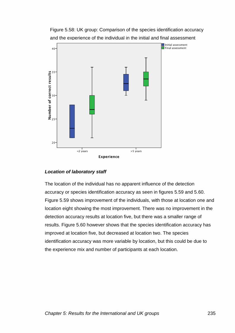
Chapter 5: Results for the International and UK groups 235
Location of laboratory staff
The location of the individual has no apparent influence of the detection
accuracy or species identification accuracy as seen in figures 5.59 and 5.60.
Figure 5.59 shows improvement of the individuals, with those at location one and
location eight showing the most improvement. There was no improvement in the
detection accuracy results at location five, but there was a smaller range of
results. Figure 5.60 however shows that the species identification accuracy has
improved at location five, but decreased at location two. The species
identification accuracy was more variable by location, but this could be due to
the experience mix and number of participants at each location.
Figure 5.58: UK group: Comparison of the species identification accuracy
and the experience of the individual in the initial and final assessment
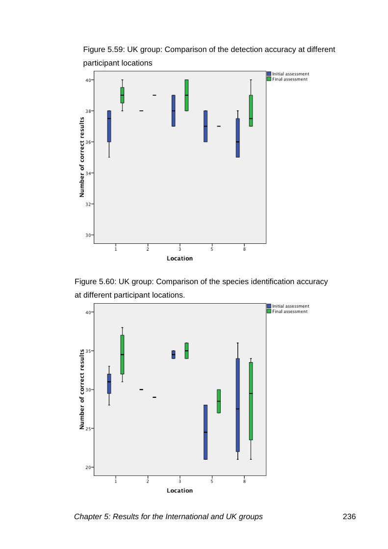
Chapter 5: Results for the International and UK groups 236
Figure 5.59: UK group: Comparison of the detection accuracy at different
participant locations
Figure 5.60: UK group: Comparison of the species identification accuracy
at different participant locations.
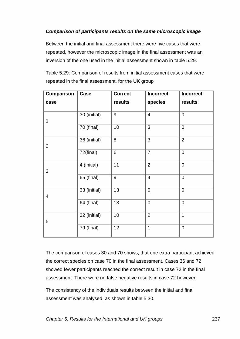
Chapter 5: Results for the International and UK groups 237
Comparison of participants results on the same microscopic image
Between the initial and final assessment there were five cases that were
repeated, however the microscopic image in the final assessment was an
inversion of the one used in the initial assessment shown in table 5.29.
Table 5.29: Comparison of results from initial assessment cases that were
repeated in the final assessment, for the UK group
Comparison
case
Case Correct
results
Incorrect
species
Incorrect
results
1
30 (initial) 9 4 0
70 (final) 10 3 0
2
36 (initial) 8 3 2
72(final) 6 7 0
3
4 (initial) 11 2 0
65 (final) 9 4 0
4
33 (initial) 13 0 0
64 (final) 13 0 0
5
32 (initial) 10 2 1
79 (final) 12 1 0
The comparison of cases 30 and 70 shows, that one extra participant achieved
the correct species on case 70 in the final assessment. Cases 36 and 72
showed fewer participants reached the correct result in case 72 in the final
assessment. There were no false negative results in case 72 however.
The consistency of the individuals results between the initial and final
assessment was analysed, as shown in table 5.30.
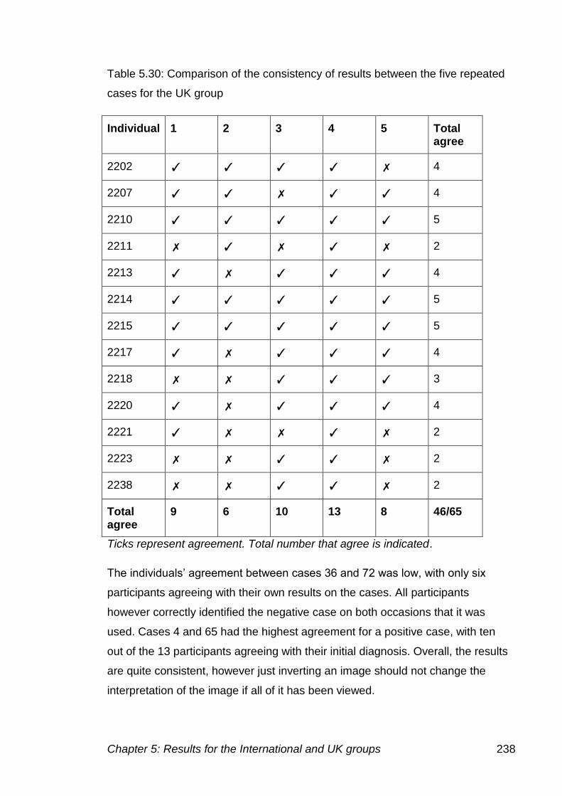
Chapter 5: Results for the International and UK groups 238
Table 5.30: Comparison of the consistency of results between the five repeated
cases for the UK group
Individual 1 2 3 4 5 Total agree
2202 ✓ ✓ ✓ ✓ ✗ 4
2207 ✓ ✓ ✗ ✓ ✓ 4
2210 ✓ ✓ ✓ ✓ ✓ 5
2211 ✗ ✓ ✗ ✓ ✗ 2
2213 ✓ ✗ ✓ ✓ ✓ 4
2214 ✓ ✓ ✓ ✓ ✓ 5
2215 ✓ ✓ ✓ ✓ ✓ 5
2217 ✓ ✗ ✓ ✓ ✓ 4
2218 ✗ ✗ ✓ ✓ ✓ 3
2220 ✓ ✗ ✓ ✓ ✓ 4
2221 ✓ ✗ ✗ ✓ ✗ 2
2223 ✗ ✗ ✓ ✓ ✗ 2
2238 ✗ ✗ ✓ ✓ ✗ 2
Total agree
9 6 10 13 8 46/65
Ticks represent agreement. Total number that agree is indicated.
The individuals’ agreement between cases 36 and 72 was low, with only six
participants agreeing with their own results on the cases. All participants
however correctly identified the negative case on both occasions that it was
used. Cases 4 and 65 had the highest agreement for a positive case, with ten
out of the 13 participants agreeing with their initial diagnosis. Overall, the results
are quite consistent, however just inverting an image should not change the
interpretation of the image if all of it has been viewed.
Chapter 6: Discussion 239
Chapter 6: Discussion
To investigate the use of the Internet as a mechanism for the provision of
external quality assurance (EQA) and the delivery of training, an intervention
study was designed. Virtual microscopy was used to assess diagnostic
capabilities pre and post the intervention with an Internet training based training
programme.
The overall aim of the project was:
To improve the diagnosis of malaria in the UK and Internationally using the
Internet as a training tool and as a provider of EQA, to assess and improve
competence
There were a number of objectives:
To provide high quality digital images for use in quality assessment to
take the place of EQA material
To assess malaria microscopy in the UK and Internationally using the
internet as a provider of external quality assurance material via the use of
a virtual microscope
To determine to what extent sample variables such as artefacts and film
preparation affect the diagnosis
To analyse malaria diagnosis at different hospitals within the UK and
Internationally to determine if there are any differences
To assess internet access at the different participating sites, and
determine if virtual microscopy is suitable for use in maintaining and
improving standards of accuracy in malarial diagnosis.
The results of the overall project demonstrate that for the UK group there were
significant differences between the initial and final external quality assessment
results and therefore provide proof of the effectiveness of the Internet based
external quality assurance and training programme intervention. However, the
results of the initial and final external quality assessment for the International
group did not prove to be significantly different, indicating that, in this group, the
intervention did not improve diagnosis. The reasons for these differences are
examined below.
Chapter 6: Discussion 240
6.1: Production of images for using in training, education and EQA
The methods used for producing the images that were developed throughout
the project allowed virtual microscope slides of the highest possible quality to
be achieved and provided high quality materials to be used in place of EQA
specimens.
High quality photomicrographs of blood cells and parasites were required for
both the virtual microscope images and for the image galleries within the
training programme. As photomicrographs within the image galleries would
be magnified to optimise training, a higher resolution image was necessary.
The 12 MPx camera allowed one photomicrograph to be taken for both uses.
Once the image was taken, digital sharpening processes were used to
achieve the best possible image.
6.1.1: Images used for virtual microscopy
The images used in the initial and final external quality assessments were
processed using a detail enhancement protocol and then using contrast
masking. These techniques were used to counteract the effect of uploading
the image into SlideBox, which slightly degrades the quality.
A number of issues were encountered during image generation, which
affected the final quality of the stitched image and the time taken to generate
the stitches. Problems encountered included focusing, especially on thick
films, as only a single plane image was provided to participants, not all
features were focused on every field. This may have influenced the ability to
determine whether parasites were present, a future development of the
virtual microscope software could be to include z plane focusing, to allow
individuals to focus through the plane. Issues with stitching the images were
also encountered, Photoshop was used instead of the Axiovision software on
the microscope for increased reliability.
Subsequently, modification in the software and an upgrade of the computer
has made images easier to capture. The software has been modified to allow
each image to be taken at a number of different focus (z) planes, which can
then be combined to provide the best focus across the entire image. The
stitching method is automated, providing the best overlap to prevent the
problems encountered with stitching.
Chapter 6: Discussion 241
6.1.2: Images used to generate image galleries as part of the training
package
To generate the training package a number of small images were required,
which would also link to a single microscopic field view. The images would
demonstrate features that would usually be examined at x100 magnification
(as recommended in World Health Organization, 2009). To achieve this the
image collected needed to be at high resolution, preventing pixilation of small
features present.
Difficulties were initially faced achieving a good enough image quality for
online presentation, because compression of the file was required. The
highest possible quality JPEG file was chosen, the images were placed
within the pages as links, preventing a loss of image quality when saved
within the HTML page.
The 12 MPx images used provided the correct resolution, to enable these
high quality images to show small features present, and provided features
that are not available in other atlases.
6.2: Use of the Internet to deliver a virtual microscope
There are currently only a few virtual microscope systems capable of
delivering large stitched images at high magnification. The only other system
in use for parasitology is that of Linder et al (2008). As far as the author is
aware it was the first time this type of system has been used for image
delivery in developing countries, in Africa in particular.
The aim of the project was to create high quality digital images that could be
used alongside and replace traditional EQA materials when samples are
difficult to obtain and distribute. The images provided in the assessments
were deemed to be of a high enough quality to perform this role.
There were problems with the upload of some images, as they would not
convert into the SVS format needed to upload them into SlideBox. There
appeared to be no reason for this, as some files would work on one occasion
and not another.
The size of the image file also became an issue. Using the 12 MPx camera,
resulted in the final image being three times as large as it was meant to be
Chapter 6: Discussion 242
for upload into SlideBox. The software used to convert images into the SVS
format used the number of pixels to determine the size of the image.
Therefore, these images had to be reduced to the size of a 1.2 MPx image
before upload to be compatible with this system.
The SlideBox system is not available on USB or CD-ROM due to company
patents, however an alternative image viewer such as QuickTime could be
used to display the images, but it would not have any of the interactive
features.
6.3: Production and delivery of the training package
In order to provide a training package, initial research was carried out to
determine what was required as part of the training, along with the
pedagogical approaches that are required for e-learning. The training was
developed to initially provide information, followed by quizzes to provide
feedback to the learners. Photomicrographic images were used alongside
textual information, for the visual learners. Narratives were used to provide
feedback on large stitched virtual microscope slides. The learning was
developed throughout the project to improve the interactivity of the training
and quizzes. The aim was to design a training programme that was designed
on the mastery learning style, however this was not achieved mainly due to a
lack of technical knowledge to prevent participants accessing other slides
before reaching the desired level of competency. Due to this limitation, the
training was modelled on the alternative Miller model of clinical competence
(Miller, 1990), using the training to build upon current knowledge and build
competence. The training was designed to assess and then build upon
knowledge they already had, as they were already diagnosing malaria. Case
and image based quizzes were used as part of the training, to cement the
knowledge given and feedback was provided to allow the individual to reflect
upon their results.
The training package was designed to be delivered both via the Internet and
via a local computer on either a USB stick or CD-ROM. To achieve this
HTML files were created, which contained all of the text and images for the
training. The quizzes were created in Abode Flash, the development of which
Chapter 6: Discussion 243
was not fully completed before the project had to be delivered to participants
and was therefore not as interactive as would have been liked.
The content of the training package is shown in the appendix 1.8.
The review of the training package by 17 external experts, highlighted a
number of developments to the training programme, but also emphasised
positive and negative points, which could be modified. Sections of the
training were rearranged to allow them to provide more in depth information
and make it clearer for participants, as well as adding some additional
sections. Other suggestions were incorporated into the training, including
adding more diagrams and reducing descriptive text. However, there were
still further modifications that could have been made to the training if time
permitted. As software and the Internet develop, a more interactive approach
could have been used, with quizzes presented in a better format, and with
the structure of these also being improved. Icons could have been used to
navigate the training, rather than textual descriptions, along with a greater
variety of photomicrographic images from different blood films to provide a
even more realistic range of galleries. The training should also have included
discussion forums, to allow those receiving the training to be in conversation
with one another.
To allow participants to use the mastery learning approach, a system would
have been put in place where the participant could not move onto the next
section until the desired level of mastery achieved, i.e. 90-100% on the quiz.
The participants could then be allowed to work through the training at their
own pace, however due to the limitations of time in the assessment, this may
not have been appropriate for the training in the current format.
6.4: The International group
6.4.1: Participant recruitment
Of a total of 42 participants contacted, 37 logged onto the virtual microscope
system. Participants in Ghana were lost at this initial stage due to staffing
issues and involvement with other projects. Participants in Malawi had an
intermittent Internet connection and decided not to take part. In Africa, the
Internet is available to only about 5% of the population in Ghana and Malawi
Chapter 6: Discussion 244
and connection speeds are extremely slow (Miniwatt Marketing Group,
2010). Despite receiving a questionnaire from Chile and Colombia, these
participants did not log onto the SlideBox system. The Internet connections
in South America are accessible by about 50% of the population (Miniwatt
Marketing Group, 2010). Therefore, access may not have been available at
all times, the individuals gave email addresses but responded only to contact
via the postal system.
Communication with participants in Chile and Colombia was via the postal
system, as this was controlled at UK NEQAS to preserve confidentiality,
however it caused communication issues. As participants were not contacted
directly, they lost some of the interactivity and therefore involvement in the
study.
Of the 37 participants that logged onto SlideBox, twenty-five completed all
cases in the initial assessment another 12 completed some of the images,
including two participants that completed one and three cases respectively.
By the beginning of the final assessment 26 participants remained, with 21 of
these completing all 40 images. Five participants only completed some of the
images, one of these only completing three cases. Eighteen participants
completed all the images in the initial and final assessment to allow
comparison of the initial and final assessment. Of the participants that were
lost, five of these were during the initial assessment and the remaining six
participants were lost during the training stage. Four of these participants
contacted the author explaining that the Internet access was too slow to
continue engagement with the project. Three other participants were in direct
contact with UK NEQAS at Watford and were not therefore receiving as
much contact as other participants. Participants from India and Kano were
lost during the initial assessment. There was no direct contact with
participants at Kano, which probably lead to the loss of these participants.
Participants at Kano were contacted via a lead individual on the site, but
there was confusion over direct communication with the participants as the
author did not have the contact details of the individuals and the person on
site thought they were being contacted directly. Email addresses at this
location were provided to UK NEQAS but were not supplied to the author. As
Chapter 6: Discussion 245
emails were sent via blind copy, none of the participants knew who was
being contacted, which may have prevented information from being passed
on.
The number of participants recruited to the project and the number lost
throughout weakened the experimental design in that whilst overall numbers
remained satisfactory the geographical spread was reduced with the loss of
nine countries. The majority of participants recruited were from within
Nigeria, with up to six participants at each location. These participants mainly
contacted the project team, indicating they were both interested in the
project, but also felt that they themselves needed training. The original aim
was to involve as many staff as possible from each laboratory, in reality there
were only one or two participants from laboratories outside of Nigeria. As
participants at other locations were also lost throughout the project, the
number of individuals to compare decreased, not allowing the true
effectiveness of the training in representative malaria endemic regions to be
fully assessed.
A lack of local contacts within Africa and within the five other WHO regions,
the Americas, South-East Asia, Europe, Western Pacific and Eastern
Mediterranean Region, led to reduced numbers of participants. Some
laboratories initially contacted by the investigators demanded monetary
payment for their participation and this was deemed unethical by the project
team.
Funding Internet access
The provision of funding for Internet access introduced significant delays at
the start of the project, taking six months to fully resolve. During the time
payments were waiting to be delivered, participants were not able to access
the Internet and therefore could not take part in the project, delaying the
project for every participant.
Initially banker’s drafts were used, generated by the university and sent via
the post. There were a large number of delays getting these out of the
university, once the forms were submitted it took a further two months until
the payments were sent. Once the payments were sent, there were further
problems. Many bankers’ drafts did not arrive; one participant who received
Chapter 6: Discussion 246
theirs could not cash it in. Only one participant received and was able to
access the money.
Only a few participants had bank accounts, preventing a direct transfer being
used. Participants were asked what would be the best mechanism for them;
the two most popular routes were Western Union and MoneyGram. Both
allowed the transfer of funds, either online, in person at a local shop or via
the phone. However, MoneyGram would only transfer to Nigeria via the retail
store, which was not applicable in this situation, and therefore Western Union
was the only option.
After some consultation within the university, a member of staff authorised to
arrange Western Union transfers to take place was found. Another month
went by before the participants received any funding. As two payments were
to be sent together, another problem was encountered, as Western Union
has a limit on the amount that can be transferred within a month. Therefore,
the funding provision had to be staged, further delaying the start. The delays
and uncertainty that this caused which possibly contributed to the loss of
participants during this stage.
6.4.2: Participant engagement
The engagement of these participants depended upon the effectiveness of
communication; participants that were in regular contact were more engaged
in the project than those who were only in contact infrequently. Some
participants also did not evaluate all the images made available to them,
meaning that they were not able to be used in the comparison of results, as
they had not completed all the cases. There were also two participants that
partially completed the images in the initial and final assessment and
therefore their results could not be used, as they were incomplete. Some
participants reported that they thought they had completed the final
assessment, when they had only completed the first 20 images, but did not
complete the remaining images as monitored by SlideBox. Communication
with participants through UK NEQAS was out of the author’s control. Contact
could only be made with UK NEQAS who would then pass on the information
to the participants. Contact was usually via post, making contact slower and
less engaging. Instructions were given via email, but these participants did
Chapter 6: Discussion 247
not receive all communications and therefore may not have received this
information.
To create a timed gateway to the training, access to the files was routed
through SlideBox. However participants’ individual access history to the
training programme could not be monitored in this environment due to
anonymity requirements and to avoid bias. SlideBox only allows files to be
placed in name order, preventing a structure being developed within the
system.
Although the university has a student e-learning environment this is only
available to registered students to study modules in standard study
programmes, therefore this was not available to be used for this project. At
the time of writing, a new system based on Moodle is being implemented in
the next 12 months, with a dedicated system for short course learning. These
students could have used this system, but the best option available at the
time was used. The ideal environment for the training would be a virtual
learning environment, where all timelines would be controlled and automatic
trigger of emails for deadlines for submission of completed tasks.
Some participants also may have colluded, as individuals from the same site
achieved the same results on a majority of cases.
Images were duplicated in the initial and final assessment to check for
consistency. The same case was repeated, but was flipped around, moving
the parasites to the other end of the image. In some cases moving a small
number of parasites when the image was flipped caused difficulties in
detection. The difficultly in parasite detection could be due to not examining
the entire image. Heat mapping technology could help determine how much
of the image being examined.
6.4.3: Results from the International group in the initial and final
assessment
In the initial assessment a detection accuracy of 68.9% was achieved and a
species identification accuracy of 33.3%. The sensitivity was 64.1% and the
specificity 91.3%. In the final assessment, the International group achieved a
detection accuracy of 66.3% and a species identification accuracy of 34.7%.
The difference in the detection accuracy and species identification accuracy
Chapter 6: Discussion 248
between the initial and final assessment were not significantly different
(p=0.692 and p=0.879).
The results found in this experiment are in agreement with to others carried
out in the same geographical area. In a similar study Ngasala, et al (2008)
found microscopy to have a sensitivity of 74.5% and a specificity of 59.0%. A
positive predictive value of 97.2% and a negative predictive value of 35.1%
were achieved by the International participants, with Ngasala reporting
values of 53.4% and 78.6% respectively. Ngasala’s study was carried out in
Tanzania, comparing individuals at the peripheral health centre to those in
the reference laboratory. The international group achieved an agreement
between individuals of 68.9%. Mitiku et al, (2003) achieved an agreement of
75%, similar to that obtained by Ngasala. Reyburn et al, (2007) found
microscopy to have a sensitivity of 71.3% and a specificity of 92.8%.
The results of this study raise concerns about the quality of malaria diagnosis
available, especially with such high numbers of false negative results. The
results of this study show that 32% of patients would wrongly be diagnosed
and possibly die because of this. Of the P. falciparum cases 30% were not
detected, this being the most severe malaria could have had serious
consequences for the patient. Incorrect species determination could also
lead to incorrect treatment, possibly allow resistance to develop but also to
the development of hypnozoite forms in P. ovale and P. vivax causing
subsequent reinfection. Results in the final assessment showed little
improvement on those in the initial assessment.
6.4.4: Problems provided by case images
The examination of the microscopic images in the initial and final
assessment produced a number of problems in parasite detection and
identification.
Parasite species
There were differences in the detection accuracy and species identification
accuracy on images with different species present. In the initial assessment
P. falciparum cases had a detection accuracy of 69.4% and a species
identification accuracy of 42.4%. These would be the type of cases these
participants had most day-to-day experience with and should show their best
Chapter 6: Discussion 249
performance. However, as the samples had been stored in EDTA, the
appearance of the parasites may have been different to what they were used
to (Milne et al., 1994). In the final assessment the detection accuracy of P.
falciparum cases was 71.8% and the species identification accuracy 45.8%.
For P. vivax cases, a detection accuracy of 85.2% was achieved in the initial
assessment, with a species identification accuracy of 22.2%. In the final
assessment P. vivax cases had a detection accuracy of 35.2% cases and a
species identification accuracy of 3.7%. The parasite density of P. ovale
cases was lower, with participants achieving a detection accuracy of 26.4%
and a species identification accuracy of 2.8% in the initial assessment. In the
final assessment P. ovale cases achieved a detection accuracy of 14.8% and
a species identification accuracy of 11.1%. There was only one P. malariae
case in the initial assessment with few parasites present, the detection
accuracy and species identification accuracy achieved were the same at
5.6%. There were two P. malariae cases in the final assessment, with a
detection accuracy of 13.9% and a species identification accuracy of zero.
The detection accuracy on the negative slides was 91.3% in the initial
assessment. The detection accuracy on the negative slides in the final
assessment was 96.0%.
The species of parasite was only significant for the species identification
accuracy (detection accuracy p=0.227, species identification accuracy
p=0.010) in the initial assessment, but was significant for both the detection
accuracy (p=0.022) and species identification accuracy (p=0.003) in the final
assessment.
The majority of participants would normally see P. falciparum in their routine
laboratory work. The performance on these cases was therefore expected to
be the best. However, some participants struggled to identify the species
present when EDTA storage changes were present. Most participants are
used to a freshly prepared sample and may not see EDTA changes in
routine practice. Some participants, not recognising these features, called
every P. falciparum case one of the other species. Some participants may
also not have usually carried out speciation, but just determine whether
parasites were present, speciation for these individuals therefore caused
Chapter 6: Discussion 250
some difficulty. An attempt was made to receive samples from the individuals
own laboratory, but due to ethical and transport issues, this was not
achieved. A previous MSc project (Adewunmi, 2007) showed participants in
Nigeria performed better on local slides compared to UK slides.
Difficulty in species identification was notable on the rarer species, which the
participants were not familiar with. The most difficulty in speciation was seen
on cases with low parasite densities. For example P. malariae cases were
present at very low parasite density, with only a few parasites present on
each image provided. The less parasites present, the less identifying
features that are present that allow the species to be easily determined.
Parasite density
In the international group initial assessment, the detection accuracy
increased as the parasite density increased. There was a significant
difference between the detection accuracy and the ranks of parasite density
(p=0.004). There was a significant difference between the species
identification accuracy and the parasite density (p=0.012).
In the final assessment there was a highly significant difference between the
detection accuracy and the ranks of parasite density (p<0.001). There was a
significant difference between the species identification accuracy and the
ranks of parasite density (p=0.025).
The initial and final assessments demonstrated that the detection accuracy
increases as the parasite density increases. In the initial assessment the
detection accuracy of diagnosis at the lowest parasite density of <5 cells
(rank 1) was 42.1% and in the final assessment 31.6%. For the next parasite
density rank 2 (6-49 cells) the detection accuracy in the initial assessment
was 64.6% and in the final assessment 56.2%, In the initial assessment for
cases with more than 50 parasites present (rank 3) the detection accuracy
was 89.4% and in the final assessment 96.5%.
The species identification accuracy for rank 1 in the initial assessment was
23.1% and in the final assessment 22.7%. For parasite density rank 2, the
species identification accuracy in the initial assessment was 22.2% and in
the final assessment 31.5%. For parasite density rank 3, the species
Chapter 6: Discussion 251
identification accuracy in the initial assessment was 57.2% and the final
assessment 51.5%.
Participants indicated in the recruitment questionnaire that they were used to
cases at high parasite density, with the majority of cases having a parasite
density of 1-8%. Participants may not have experience of low parasite
densities and therefore are more easily missed, which is reflected by the low
detection accuracy for rank 1 images. As images were often slow to load on
some Internet connections, some participants may not have examined the
entire image, with the areas with parasites in possibly not being examined in
some cases. The heat mapping technology present in newer versions of the
software would have helped in analysing the reasons for this finding allowing
determination of what areas of the slide were examined and at what
magnification.
Determining the species present on low parasite density cases is more
difficult as fewer parasites are present to allow characteristic features to be
identified. The most difficulty on low parasite density cases was with species
other than P. falciparum. Some cases only had a few late trophozoites with
characteristic features present, alongside early trophozoites, making
diagnosis more challenging.
Thick and thin film preparation
The performances on the thick and thin films were compared. In the initial
assessment, the international group showed only a small difference in
performance with a better performance on the thin film. On the thin film a
detection accuracy of 70.5% was achieved and a species identification
accuracy of 33.9%. For the thick film a detection accuracy of 61.1% and a
species identification accuracy of 30.0%. The differences between the thick
and thin film in the initial assessment were not significant (detection accuracy
p=0.276) (species identification accuracy p=0.581).
The performance on the thick film was worse in the final assessment, but this
could have been due to the case distribution as there was a mixed infection
case and species present other than P. falciparum. The detection accuracy
on the thick film was 48.6%, with the species identification accuracy being
18.3%. For the thin film, the detection accuracy was 70.7% and a species
Chapter 6: Discussion 252
identification accuracy of 39.1%. Speciation is not usually carried out on the
thick film however. There were significant differences in the final assessment
in the detection accuracy (0.039) and the species identification accuracy
(p=0.021) between the thick and thin films.
The performance on the thick film may also have been affected by the
delivery of the image. The virtual microscope does not give `z’ plane focusing
abilities, which is often necessary on the thick film due to the depth of the
field. Although parasites were focused upon taking the images, other
confusing features could not be focused through to allow the plane of the
object to be determined. This could also have been true for some images on
from the thin film, but not to as great an extent.
New advances in the microscope technology may improve the quality of the
image and prevent parasites being out of focus. The new software upgrade
allows the image to be photographed at multiple focus planes, to achieve the
best focus over the entire image, as the different planes are merged
together.
Artefacts
There were five categories for the presence of artefacts varying by the
number of artefacts present. Artefacts included the presence of stain deposit
and platelets overlying the erythrocytes. In the initial assessment the ranks of
the presence of artefacts caused a significant difference in the detection
accuracy (p=0.026), however, the species identification accuracy had not
reached significance (p=0.453),
However, in the final assessment there was no significant difference for the
ranks of the presence of artefacts on the detection accuracy (p=0.606) and
species identification accuracy (p=0.814).
The effect of the presence of artefacts appears to have been masked by the
parasite density of the cases. There were two particular cases that caused
problems in diagnosis, case 28 where parasites were faint and out of focus,
and case 29 when P. falciparum was present alongside chronic granulocytic
leukaemia. In case 29 in particular, participants could have been distracted
from the presence of very small parasites at mid parasite density.
Chapter 6: Discussion 253
Rank of the microscopic image
The cases were ranked for overall difficulty based upon the species,
preparation and presence of artefacts, rank 1 being the least challenging and
rank 3 the most challenging.
For rank 1, the detection accuracy in the initial assessment was 83.3% and
in the final assessment 97.4%. For rank 2, the detection accuracy in the
initial assessment was 64.7% and in the final assessment 58.5%. For rank 3,
the detection accuracy in the initial assessment was 53.2% and in the final
assessment 34.0%.
The species identification accuracy results showed the same trend as the
detection accuracy, with the species identification accuracy decreasing as
the rank increased and the cases became more challenging In species
identification accuracy for rank 1 in the initial assessment was 50.5% and in
the final assessment 54.6%. Rank 2 gave a species identification accuracy of
25.2% in the initial assessment and 30.2% in the final assessment. Rank 3
gave a species identification accuracy in the initial assessment of 18.5% and
in the final assessment 15.3%.
In the initial assessment there was a significant difference between both the
detection accuracy (p=0.010), and the species identification accuracy
(p=0.033) and the rank of the microscopic image for all categories. In the
final assessment there was a highly significant difference between the
detection accuracy (p<0.001) and the species identification accuracy
(p=0.003), when compared to the rank of the microscopic image.
The rank of the microscopic image therefore reflects the results seen, with
the lower detection and species identification accuracies on the images that
are deemed to be the most challenging. The combination of all of the
features discussed above make the diagnosis more difficult.
6.4.5: Assessment of performance in relation to the laboratory staff
training, experience and laboratory location
The performance in the initial and final assessment and consequently the
effectiveness of the training programme was compared to the experience of
the individual, time since last received training and the location of the
laboratory in which the participants are employed.
Chapter 6: Discussion 254
Examining the results from some individuals showed improvement, others
however showed a decrease in performance. Of the 12 participants that said
they completed the training, ten completed all of the initial and final
assessment. Two participants showed improvements in the detection
accuracy and species identification accuracy results. A further four
participants improved their species identification accuracy, but showed a
decrease in the detection accuracy.
Training
There were four categories for the time since a participant had last had
training, these were all compared using non-parametric statistical analysis.
There were 11 individuals in the <1 year group and four in the 1-4 years
group. The time that had elapsed since laboratory workers had last received
training on the diagnosis of malaria, had a moderate or no effect on the
outcome of the diagnosis. In the initial assessment, there was no significant
difference in the detection accuracy (p=0.667) and the species identification
accuracy (p=0.586) in comparison to the time training was last received. In
final assessment there was no significant difference of the time since last
training occurred on the detection accuracy (p=0.088) or the species
identification accuracy (p=0.060).
It can be debated whether the figures for training are accurate, as these were
provided by individual questionnaire answers. As this was information
provided by the individual and not recorded on a central system, this
information is not verifiable.
Experience of the laboratory staff
In the initial assessment, grouping of the laboratory staff by experience
demonstrated a positive trend between the detection accuracy and individual
experience. However, this did not reach significance (p=0.104). There was a
significant difference for the species identification accuracy and the
experience of the individual (p=0.009).
In the final assessment, the results for experience were not significant for the
detection accuracy (p=0.142) or the species identification accuracy
(p=0.141).
Chapter 6: Discussion 255
Geographical location of participants
The locations of the participants were analysed to determine effects on the
detection accuracy of diagnosis. Initial analysis by participant location,
demonstrates that the laboratories that were involved in external quality
assurance (EQA) schemes appeared to have higher detection accuracies
and species identification accuracies in the initial assessment. These EQA
laboratories were Lebanon, India, Kenya and Hong Kong, with Kano in
Nigeria in the process of implementing a training programme.
There was a significant difference in the species identification accuracy in the
initial assessment when the participant location was considered (p=0.006).
The detection accuracy however had not reached significance when
compared with the location (p=0.094).
In the final assessment, the results of those from laboratories involved in
EQA schemes were better with higher accuracies and species identification
accuracies. There was a significant difference in the detection accuracy
(p=0.009) and the species identification accuracy (p=0.025) for the location
of the participants. The median results increased but it was difficult to
determine whether there was an improvement as different numbers of
individuals were involved in the final assessment.
6.4.6: Equipment issues that may have affected performance
Computer screen
The quality of computer screen used can affect the image seen and could
affect diagnosis. Participants had difficulty accessing computers and those
that they did access were probably of a poor quality. The screens may not
have been of a high enough resolution to provide sufficient information to
both determine whether parasites are present and then identify the species
present. SlidePath advise that the screen resolution is at least 1024x768
pixels (SlidePath Ltd, 2010). This was not recorded, due to participants
accessing computers at Internet cafes and therefore may have been different
on every occasion.
The screen quality the participants were viewing the images on also could
have varied between different sessions. The quality of the image depends on
Chapter 6: Discussion 256
the viewing equipment as well as the speed of the Internet connection, which
makes the diagnosis in this group even more difficult.
Internet connection speed
The speed of the Internet connection could affect the quality of image seen if
the image was not fully loaded, the willingness of the participant to examine
the image for parasites and identification of the parasite when present.
SlidePath recommend a connection speed of 1 Mbps (SlidePath Ltd, 2010),
which many participants would have difficulty reaching as the maximum
speeds are only slightly higher, e.g. Nigeria 1.01 Mbps (Ookla, 2010). Many
participants reported problems with Internet access, mainly having problems
accessing the site, but there were also problems with the loading of the
image. Many participants had problems with Flash player, on which the
digital microscope is solely based. Throughout the project there were 300
flash problems flagged up by the SlideBox system.
Participants reported that the images for the final assessment took longer to
load, however as the images were on the same site, any problems must
have been with the local Internet connection used. The participants were
also using different computers, as they were reliant on Internet cafes,
therefore the connection speed could not be guaranteed.
The speed at which the image loaded could also have affected how much of
the image was examined. If an image loaded slowly, it was likely that the
participant would only have time to look at a few fields in the stitched image,
possibly leading to the high numbers of false negative results on low parasite
density samples. The image may also have been examined before it was
fully loaded and therefore not in proper focus.
Area of the image examined
The version of the SlidePath software used in this project did not allow
tracking of where the individual had examined. It is therefore not possible to
determine how much of each image was examined by the participants and
therefore why they missed the presence of parasites. Later versions of this
software have a heat map facility, which enables monitoring of the participant
activity on each slide, at each magnification and how long they spent
examining each region. The heat map would give a clearer idea of the
Chapter 6: Discussion 257
participants’ habits when examining an image and give a clearer idea of how
false negative results were achieved. The drawback with this system is that it
may take longer to load the slide, making the problems faced by participants
in this project more profound.
Language difficulties
Another factor that may have influenced the participants’ results was their
understanding of the task required and of English in general. English was not
the first language for any participant, which may have caused difficulties in
understanding not only in the information provided, but also in understanding
what was required. Without a full understanding of the training structure, if
may have been difficult to find the important images and information provided
by the galleries. Due to the design of the website, it may also have been
difficult to find the training programme, especially if they did not read the
associated materials and look at the screenshots provided.
6.4.7: Summary of performance of the International group
The international group showed no improvement in results between the initial
and final assessment. The results produced by the participants were similar,
although there were a number of categories that were significantly different in
the initial assessment and not the final assessment and vice versa. There
were significant differences in the parasite density and the rank of the slide
for both the detection accuracy and species identification accuracy in the
initial and final assessment. The species of parasite was only significant for
the species identification accuracy in the initial assessment, but was
significant for both the detection accuracy and species identification accuracy
in the final assessment. The location was significant for the detection
accuracy in the initial assessment, but both the detection accuracy and
species identification accuracy were significant in the final assessment. The
artefact rank showed a significant difference in the initial assessment for
detection accuracy, but was not significant for either in the final assessment.
Experience was significant for the species identification accuracy for
individuals in the initial assessment, was not significant in the final
assessment. The difference between the thick and thin films was not
Chapter 6: Discussion 258
significant in the initial assessment, but was significant for both the detection
accuracy and species identification accuracy in the final assessment.
For this study, the training therefore, does not seem to influence the
diagnosis made. Although, the images in the initial and final assessment
were chosen to be of the same quality and have the same properties, the
international group had more difficulty with these slides.
The result of incorrect diagnosis in clinical practice can result in the death of
the patient. Missing P. falciparum cases can result in death within a few
hours. Incorrectly determining the species can lead to unnecessary treatment
(for another condition that malaria was misdiagnosed as or vice versa), along
with drug resistance when treatment is provided unnecessarily. A patient with
P. vivax that is treated for P. falciparum will develop hypnozoite liver forms,
which can then cause reactivation of parasites and reinfection. The results
from these participants are worrying, as many patients would be receiving
the wrong treatment.
6.5 The UK group
6.5.1: Participant recruitment
Participants were contacted through UK NEQAS (H) as members that
participated in the glass slide scheme for parasite identification. There were
39 participants that were initially recruited, of which 33 completed the
recruitment questionnaire. The participants were recruited from ten
laboratories around the UK and were split into two groups based on
experience. There were 15 participants in the less than 2 years group and 18
in the more than five years group. Twenty-five participants completed all 40
images in the initial assessment. A further seven participants completed
more than 30 cases. Eleven participants completed the post-training
questionnaire, with thirteen completing all the images in the initial and final
assessment. Seventeen individuals completed all the final assessment, but
the results of four had to be excluded as they had not completed all of
images within the cut off period and therefore had further access to the
training.
Chapter 6: Discussion 259
Due to the reduced timeframe of the project for the UK group, some
participants did not have time to complete the assessment stages. The
number of participants engaged throughout the project showed similar
reductions to the international group, despite the differences in timescale
scheduled.
6.5.2: Participant engagement
Participants in the UK group appeared to be more engaged with the project,
due to the shortened timeframe compared to the International group.
Participants were in regular contact with the author, asking questions about
the different stages of the project.
Some participants asked for further instructions on how to access the training
and what was expected of them. Eleven participants completed the
questionnaire at the end of the training to say that they had accessed all of
the pages in the training.
Some participants were lost throughout the project, mainly due to time
constraints. One participant was on holiday throughout the training stage,
therefore not being able to complete the final assessment, for this individual
the training was made available later, for use as an atlas during diagnosis.
This approach was also taken with individuals who had not completed the
final assessment. No participant completed this however, possibly as the
participants this solution was given to, were already poor responders.
Some participants worked with the help of textbooks, especially in the initial
assessment, mainly due to an inadequate knowledge of the parasite species,
as they only encountered these in EQA materials.
6.5.3: Results from the UK group in the initial and final assessment
In the initial assessment detection accuracy of 92.3% and a species
identification accuracy of 69.9% was achieved. The detection accuracy was
generally high, however there were some differences between the different
species. In the final assessment detection accuracy of 96.2% and a species
identification accuracy of 74.8% was achieved.
There were only a few cases that demonstrated false positive and negative
results, however this would still have an effect on the patient. Five per cent of
P. falciparum cases were still incorrectly diagnosed, more worryingly the
Chapter 6: Discussion 260
correct species was not achieved in 27% of cases. The incorrect species
identification could have therefore led to the incorrect treatment for the
patient and possibly the development of drug resistance. This had improved
in the final assessment, possibly indicating a need for training amongst
laboratory staff. In the UK the effect on the patient may be smaller, as all
positive cases are referred for confirmation of diagnosis by PCR, which
would see the patient receiving the correct treatment quickly, often a
duplicate test is carried out and more than one microscopist examines each
case.
There was a significant difference between the detection accuracy (p=0.005)
and species identification accuracy (p=0.046) in the initial and final
assessment. The training has therefore been shown to have a significant
effect on the diagnosis made, with the number of correctly diagnosed cases
improving as well as he number of correctly determined species.
6.5.4: Problems provided by case images
The examination of the microscopic images in the initial and final
assessment provided a number of problems in parasite detection and
identification for the UK group.
Parasite species
In the initial assessment, the highest detection accuracy was achieved for P.
ovale cases, with a detection accuracy of 96.2% and a species identification
accuracy of 44.2%. In the final assessment, the detection accuracy of the low
parasite density P. ovale cases was 100%, with a species identification
accuracy of 64.1%.
P. falciparum cases had the next highest detection accuracy in the initial
assessment, at 94.7% and a species identification accuracy of 73.1%. Milne
et al, (1994) reported that 78.6% of P. falciparum cases referred to the
reference laboratory were correctly diagnosed. In the final assessment, the
detection accuracy on P. falciparum cases was 98.7%, with a species
identification accuracy of 81.7%.
The three P. vivax cases in the initial assessment, had a detection accuracy
of 71.8% and a species identification accuracy of 43.6%. Milne et al (1994)
also reported that 76.6% of P. vivax cases were diagnosed correctly. P. vivax
Chapter 6: Discussion 261
cases in the final assessment, had a detection accuracy of 79.5% and a
species identification accuracy of 43.6%.
The one P. malariae case in the initial assessment, had a detection accuracy
of 84.6% and a species identification accuracy of 30.8%. There were two P.
malariae cases in the final assessment, with a detection accuracy of 92.3%
and a species identification accuracy of 80.8%.
The most difficulty in species identification in the UK group was seen
between P. ovale and P. vivax cases. When combining the species
identification accuracy for both species in the initial assessment, the species
identification accuracy for P. ovale increased to 88.5% and for P. vivax to
61.5%. Bailey et al (2005) reported that in 2004 on UK NEQAS P. ovale case
was identified as P. vivax by 43% of participants. These species receive the
same treatment and therefore the diagnosis made does not influence the
patient directly. The same procedure in the final assessment increased P
ovale species identification accuracy 98.6% and that of P. vivax to 51.3%.
Indicating that there was a higher chance that a P. ovale case was
diagnosed as P. vivax rather than vice versa, possibly due to the increased
prevalence of P. vivax.
Non-parametric statistical analysis was used to determine whether there was
a difference in diagnosis seen on cases of the different malarial species,
comparing all species. There was a significant difference in the species
identification accuracy (p=0.025) between the different malaria species in the
initial assessment. However, the detection accuracy did not reach
significance (p=0.494) when compared to the different malaria species. In the
final assessment there was a significant difference between both the
detection accuracy (p=0.022) and species identification accuracy (p=0.003)
for the different species.
The UK participants see a predominance of P. falciparum cases, however as
cases are due to international travel, any species can be seen. This could be
why the UK group are better at identifying all species and can determine the
species on cases that show characteristic features, possibly with the help of
textbooks and atlases. Due to the similarity in appearance, confusion
Chapter 6: Discussion 262
between P vivax and P. ovale is commonly seen in EQA schemes (Milne et
al 1994).
Parasite density
In the initial assessment the detection accuracy increased as the parasite
density of the specimens used in the UK group increased. There was a
significant difference in the detection accuracy (p=0.017) in the initial
assessment between the ranks of parasite density. However, the species
identification accuracy only approached significance (p=0064).
In the final assessment there was not a significant difference between the
values for the detection accuracy (p=0.196) or the species identification
accuracy (p=0.071) and the rank of the parasite density of the case (figure
5.19). The individuals were equally as good at cases of low parasite density
than those of high parasite density. Participants are more used to looking for
low parasite density cases, as they are often only looking for a single
parasite to determine that the patient has malaria.
The initial and final assessments demonstrated that the detection accuracy
increases as the parasite density increases. In the initial assessment the
detection accuracy of diagnosis at the lowest parasite density of less than
five cells (rank 1) was 87.8% and in the final assessment 97.6%. For the next
parasite density rank 2 (6-49 cells) the detection accuracy in the initial
assessment was 91.6% and in the final assessment 92.3%. In the initial
assessment for cases with more than 50 parasites present (rank 3) the
detection accuracy was 98.5% and in the final assessment 99.3%.
The species identification accuracy for rank 1 in the initial assessment was
57.1% and in the final assessment 75.2%. For parasite density rank 2, the
species identification accuracy in the initial assessment was 72.0% and in
the final assessment 65.8%. For parasite density rank 3, the species
identification accuracy in the initial assessment was 83.1% and the final
assessment 81.8%.
The parasite density of most malaria infections seen in the UK is low, which
may explain the small difference between the detection accuracy. The
species accuracy is possibly lower on low parasite density cases due to a
Chapter 6: Discussion 263
lack of parasites present, especially those with characteristic features, which
allow the species to be determined easily.
Thick and thin film preparation
The performance on the thick and thin films were compared. The UK group
also showed better results on the thin film compared to the thick film. The
detection accuracy achieved on the thin film was 96.7%, compared to 71.4%
on the thick film. The species identification accuracy on the thin film was
73.1%, with the thick film being 52.3%. There were a few participants who
refused to answer the thick film questions and many would not provide a
species on the thick film, speciation on the thick film is not common practice
in the UK.
In the initial assessment, the detection accuracy was significantly different
between the thick and thin films. The species identification accuracy was not
significantly different between the thick and thin films.
In the final assessment the differences between the thick and the thin film
were also still present. The detection accuracy in the initial assessment on
the thin film was 98.6% and on the thick film 86.5%. The species
identification accuracy achieved on the thin film was 82.0% and the thick film
48.4%. Bailey et al (2005) reported that the 2004 UK NEQAS results gave
the incorrect species in 22.2% of instances, the results here on the thin film
exceed this. The results of this study represent a diagnosis made by an
individual, however the UK NEQAS results were as a result of a group effort.
In the final assessment, both the detection accuracy (p<0.001) and the
species identification accuracy (p=0.003) were significantly different.
Thick films are only usually examined in the UK to try to identify parasites
present at very low parasite densities. However, some laboratories do not
make a thick film, but use a rapid diagnostic kit for this purpose. Participants
would not have know how to speciate on the thick film, except for the
presence of some characteristic features they would be used to seeing, i.e.
crescent shapes gametocytes of P. falciparum.
Chapter 6: Discussion 264
Artefacts
There were five categories for the presence of artefacts varying by the
number of artefacts present and the perceived effect these could have on
diagnosis.
In the initial assessment, the detection accuracy decreased as more
artefacts were present, however there was no trend seen in the species
identification accuracy. The results for both the detection accuracy (p=0.093)
and species identification accuracy (p=0.382) were not significantly different
when more artefacts were present.
In the final assessment the presence of artefacts appeared to have little
effect on the diagnosis made. There was no significant difference in the
detection accuracy (p=0.555) or the species identification accuracy (p=0.879)
when compared to the ranks of the presence of artefacts.
There were probably too many categories for the presence of artefacts,
giving only small numbers within each group, making it difficult to achieve
significance. The UK group, commonly see EDTA changes and artefacts
present due to workload management, especially in cases provided by UK
NEQAS for EQA purposes, due to the time it takes for these slides to be
made and transported to the laboratory.
Rank of the microscopic image
The rank of the microscopic image was also compared to the detection
accuracy and species identification accuracy. The detection accuracy
decreases and the rank of the microscopic image increases and the case
was deemed to be more challenging. The range of the results seen also
increases as the rank of the microscopic image increases. For rank 1, the
detection accuracy in the initial assessment was 100% and in the final
assessment 98.8%. For rank 2, the detection accuracy in the initial
assessment was 93.5% and in the final assessment 93.9%. For rank 3 the
detection accuracy in the initial assessment was 74.7% and in the final
assessment 97.1%.
The species identification accuracy for rank 1 in the initial assessment was
83.3% and in the final assessment 89.5%. Rank 2 gave a species
identification accuracy of 66.7% in the initial assessment and 74.7% in the
Chapter 6: Discussion 265
final assessment. Rank 3 gave a species identification accuracy in the initial
assessment of 51.3% and in the final assessment 54.8%.
In the initial assessment the comparison between the three ranks of the
microscopic image demonstrated a highly significant difference for the
detection accuracy (p=0.001), and a significant difference for the species
identification accuracy (p= 0.010). In the final assessment there was a highly
significant difference in the species accuracy (p<0.001) when compared to
the difference between the ranks of the microscopic image. There was a
significant difference for the detection accuracy (p=0.041) and the rank of the
microscopic image.
The UK participants showed the lowest detection and species identification
accuracies, on the cases that were deemed to be the most challenging
having a rank of three.
6.5.5: Assessment of the performance in relation to the laboratory staff
experience and laboratory location
The performance of participants in the UK group in the initial and final
assessment, and the effectiveness of the training programme were
compared to the experience of the individual and the location of the
laboratory in which they work.
Experience
The participants were divided into two groups depending upon their
experience. Group one refers to those with less than two years experience or
newly registered Biomedical Scientists. Group two is the individuals with
more than five years experience, varied from five years up to more than 20
years.
In the initial assessment, the detection accuracy for group one, those with
less than two years experience was 90.0% and for group two was 92.1%.
The species identification accuracy for group one was 60.5% and group two
was 81.9%. This shows that there is a significant difference in the species
identification accuracy when compared to the experience of the individual
(p=0.009). However, the detection accuracy was not significantly different
(p=0.171) when compared to the individuals’ experience.
Chapter 6: Discussion 266
In the final assessment, the detection accuracy for less than two years
experience was 96.6% and for group two was 93.7%. This difference was not
significant (p=0.074). For species identification accuracy group one was
71.0%, with group two was 75.2%, this difference was however not
significant (p=0.346).
The training has therefore been shown to have a significant effect on the
results of participants in the less experienced group. In the initial assessment
there was a significant difference between the results of group one and
group two, however in the final assessment there is no longer a significant
difference and the results of the two groups are similar. This also indicates
that the more experienced group benefitted less from the training.
Laboratory location
In the initial assessment there was no significant difference in detection
accuracy results (p=0.918) between the different hospitals in which the
participants were based. There was no significant difference in the species
identification accuracy (p=0.053) for the participants location.
In the final assessment there was no significant difference in detection
accuracy results (p=0.618) between the different hospitals in which the
participants were based. The species identification accuracy results were
also not significantly different (p=0.247) when compared to location.
6.5.6 Equipment issues that may have affected performance
Throughout the project a few issues were encountered with access to the
virtual microscope for the UK group. Internet access was sometimes slow
and sometimes participants could not access the site.
Internet firewalls
Within the NHS the firewalls sometimes slowed access to the site, and in
some cases prevented access to the training. To allow the participants to
access the training the software company contacted the IT department at
each hospital to ensure access. The firewalls also slowed access, preventing
the image being viewed at optimum quality, with some pixilation to the image
until it had fully loaded. Problems were also reported with ActiveX control
permission, which also for a time prevented access.
Chapter 6: Discussion 267
Area of the image examined
As for the international participants, UK participants also use the version of
the software that did not allow participant activity to be tracked, therefore it
was not possible to track how much of the image was examined. The
benefits of this inclusion could help this to be determined in the future.
6.5.7: Summary of the performance of the UK group
There was a significant difference between the detection accuracy and
species identification accuracy in the initial and final assessment for the UK
group. The training therefore appears to have made an improvement in the
diagnosis. The improvement seen for the individuals was higher in those with
less experience, in the less than two year group than the more than five year
group. By the end of the training both groups showed an improvement in
diagnosis made, and were achieving similar detection accuracies in the two
groups. This could indicate that the participants had all reached the
maximum level possible by microscopy or the maximum achievable on these
slides. This may also indicate that the more inexperienced staff benefit more
from the training than those with more experience.
There were significant differences in the rank of the slide for the detection
accuracy and species identification accuracy in the initial and final
assessment. The species of parasite had a significant effect on the initial and
final assessment for the species identification accuracy, but not the detection
accuracy. In the initial assessment, the detection accuracy was significantly
different between the thick and thin films. The species identification accuracy
was not significantly different between the thick and thin films.
In the final assessment, both the detection accuracy and the species
identification accuracy were significantly different for the difference between
the thick and thin films. The detection accuracy in the initial assessment
showed a significant difference when compared to the ranks of the parasite
density, however it was not significantly different for the species identification
accuracy. Neither the detection accuracy or the species identification
accuracy was significantly different when compared to the parasite density in
the final assessment. In both the initial and final assessment for detection
accuracy and species identification accuracy the presence of artefact,
Chapter 6: Discussion 268
experience, location and participation in the training scheme, did not have a
significant effect on the results.
The UK group accessed the training over a one month period, and then had
access to the images again immediately afterwards. This reduced timescale
may allow the benefit of the training to be seen more clearly, but may also
indicate that there is a washout period. Participants by the end of the final
assessment may have already started to lose some of the information
gained. This would require further experimentation to see if it is the case, and
indicates that the training could be followed by provision of the material on an
atlas basis, using it as a guide whilst making diagnosis. A further group of
individuals were recruited for this purpose, but these were already non-
returners and they did not engage with the task.
6.6 Comparison of UK and International results
The UK participants achieved a higher detection accuracy and species
identification accuracy in the initial and final assessment than the
International group. There was a significant difference between the detection
accuracy (Initial p= 0.001 and Final p=0.028) and species identification
accuracy (Initial p<0.001 and Final p=0.001) for the UK and International
groups in the initial and final assessments. The UK group showed better
performance on the thin film, achieving a detection accuracy of 71.4% in the
initial assessment and 86.5% in the final assessment, however their results
on the thick film were also better than the International group, with 61.1% in
the initial assessment and 48.6% in the final assessment. The numbers of
false positive results for these groups were small with 8.3% for the
international group and 7.3% for the UK group. However there were less true
positive results for the international group with only 64.1% of instances
compared to 92.8% for the UK group.
There were also more false negative results in the international group with
35.9% of occurrences, compared to 7.2% for the UK group. There were also
difficulties in species determination, the incorrect species was determined in
30.8% instances for the international group and 22.4% for the UK group.
Chapter 6: Discussion 269
The high number of false negative results in the international group were
mainly on low parasite density cases, this could be due to not examining the
entire image, possibly linked to a slow Internet connection as discussed
earlier.
Although the International and UK groups viewed the same slides and
accessed the same training, the timescales of the project were different. The
international group accessed the programme over a 14-month period,
whereas the UK group accessed over a 4-month period. Due to this time
scale, the UK participants may have been more continuously engaged with
the project, as there was always something that needed to be done.
Participants communicated, via e-mail, that they were having difficulty finding
time to access the training, due to staff holidays, staff absences and
workloads. This may indicate that the time periods to access the project were
too short. A longer period to access each stage of the training, could have
meant that a greater number would have completed the programme. The
time of the year of delivery also affects the number of staff in the laboratory,
as this training was delivered over the summer vacation period, the number
of staff available to participate was reduced. The eventual future training
programme would be used as a stand-alone system, and these time limits
would not cause difficulties, as limits would be by self-determined
participation, not imposed time. It is possible that the international group had
too long to access the training, as there were numerous unforeseen delays
along the way and deadlines were extended to maintain a viable number of
participants. When participants had not completed a stage, the deadline was
extended to allow some to complete, but this left others unengaged.
Furthermore, waiting for funding for Internet access caused the longest
delays, but the availability of the Internet in some regions also caused
problems. The initial timeline proposed was extended a number of times,
with participants reporting that they could not access the site. The completion
deadlines were also changed, thereby disrupting other participants who had
completed on time. Some participants did not complete as they thought they
had already completed this stage, possibly due to the changing of deadlines
or a lack of understanding in what was required. Most of the activity was in
Chapter 6: Discussion 270
the last month of the intervention; once participants had been reminded of
the limited time they had available to access the training.
The ideal viewing time would depend on the location of the participants and
the speed of their Internet connection. A future experiment could be carried
out to determine the best timescales for the project, or to be left open for
participants to work on in their own time. As the current timescales were
deemed to be too long for the International group and too short for the UK
group the proposed times scale gives a maximum of ten months. Ten
months was the initial timescale planned for the International group, with
three months to complete the initial and final assessment and four months for
the training. A more robustly structured timetable, with specific deadlines
would allow this to be achieved. The participants needed a clearer timescale
of what needed to be done in each section, to allow better time management.
Possibly because of the timescale given, the UK participants showed a
significant improvement in their detection accuracy (p=0.005) and species
identification accuracy (p=0.046) results between the initial and final
assessment. There was no improvement seen for the international group,
this could have been due to the timescale involved and a possible washout
of information. Alternatively, participants may not have fully understood the
training because of language difficulties.
It should be taken into account that the UK group may have used textbooks
to help them throughout the study, as they are readily available. This may
have influenced some of the results seen in the initial assessment and may
be why the results from the UK group are better than the International group.
6.7 Comparing participant performance against published performance
criteria
6.7.1 Relation to other International studies
The only significant study on the quality of microscopy was carried out by the
WHO, in their Malaria Microscopy Quality Assurance Manual (World Health
performance of microscopists carrying out routine diagnosis. For the
international participants the parasite density calculations were not analysed,
due to the large variability in the results received. The WHO recommended
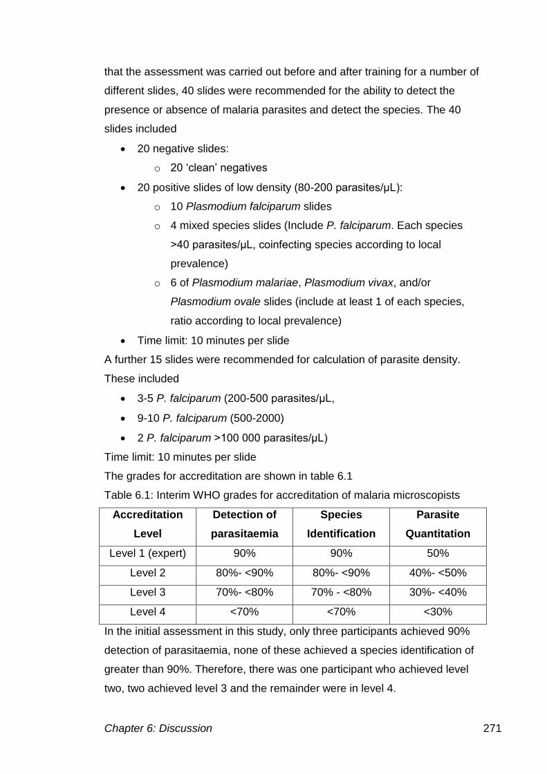
Chapter 6: Discussion 271
that the assessment was carried out before and after training for a number of
different slides, 40 slides were recommended for the ability to detect the
presence or absence of malaria parasites and detect the species. The 40
slides included
20 negative slides:
o 20 ‘clean’ negatives
20 positive slides of low density (80-200 parasites/μL):
o 10 Plasmodium falciparum slides
o 4 mixed species slides (Include P. falciparum. Each species
>40 parasites/μL, coinfecting species according to local
prevalence)
o 6 of Plasmodium malariae, Plasmodium vivax, and/or
Plasmodium ovale slides (include at least 1 of each species,
ratio according to local prevalence)
Time limit: 10 minutes per slide
A further 15 slides were recommended for calculation of parasite density.
These included
3-5 P. falciparum (200-500 parasites/μL,
9-10 P. falciparum (500-2000)
2 P. falciparum >100 000 parasites/μL)
Time limit: 10 minutes per slide
The grades for accreditation are shown in table 6.1
Table 6.1: Interim WHO grades for accreditation of malaria microscopists
Accreditation
Level
Detection of
parasitaemia
Species
Identification
Parasite
Quantitation
Level 1 (expert) 90% 90% 50%
Level 2 80%- <90% 80%- <90% 40%- <50%
Level 3 70%- <80% 70% - <80% 30%- <40%
Level 4 <70% <70% <30%
In the initial assessment in this study, only three participants achieved 90%
detection of parasitaemia, none of these achieved a species identification of
greater than 90%. Therefore, there was one participant who achieved level
two, two achieved level 3 and the remainder were in level 4.
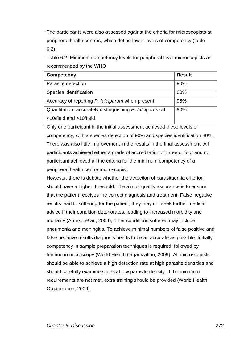
Chapter 6: Discussion 272
The participants were also assessed against the criteria for microscopists at
peripheral health centres, which define lower levels of competency (table
6.2).
Table 6.2: Minimum competency levels for peripheral level microscopists as
recommended by the WHO
Competency Result
Parasite detection 90%
Species identification 80%
Accuracy of reporting P. falciparum when present 95%
Quantitation- accurately distinguishing P. falciparum at
<10/field and >10/field
80%
Only one participant in the initial assessment achieved these levels of
competency, with a species detection of 90% and species identification 80%.
There was also little improvement in the results in the final assessment. All
participants achieved either a grade of accreditation of three or four and no
participant achieved all the criteria for the minimum competency of a
peripheral health centre microscopist.
However, there is debate whether the detection of parasitaemia criterion
should have a higher threshold. The aim of quality assurance is to ensure
that the patient receives the correct diagnosis and treatment. False negative
results lead to suffering for the patient; they may not seek further medical
advice if their condition deteriorates, leading to increased morbidity and
mortality (Amexo et al., 2004), other conditions suffered may include
pneumonia and meningitis. To achieve minimal numbers of false positive and
false negative results diagnosis needs to be as accurate as possible. Initially
competency in sample preparation techniques is required, followed by
training in microscopy (World Health Organization, 2009). All microscopists
should be able to achieve a high detection rate at high parasite densities and
should carefully examine slides at low parasite density. If the minimum
requirements are not met, extra training should be provided (World Health
Organization, 2009).
Chapter 6: Discussion 273
6.8: Conclusions and future work
6.8.1: Project conclusions
The Internet has been shown to be suitable as a delivery mechanism for
virtual microscopy and for the delivery of EQA specimens. The image
produced was of an adequate quality to allow malaria diagnosis to take
place. The training programme has also been delivered over the Internet,
providing high-resolution images, to allow smaller features to be identified
that would be pixelated in lower resolution images.
The training programme has been shown to be effective in improving
competence in the UK group, but not in the international group. Due to a lack
of detailed participation access data, it is impossible to tell whether this was
due to the international group participants having difficulty understanding the
content of the training programme or due to a lack of engagement with the
programme.
Monitoring participant engagement was a particular problem throughout the
project. Access to the SlideBox site was monitored by the investigator,
allowing the date and time the participant accessed to be recorded. However
how long, or what was accessed, was not. The lack monitoring means it was
difficult to determine whether participants had looked at the entire slide or
even accessed the training site.
There was no improvement in the results for the international group in the
final assessment. The results of participants that did not complete the final
assessment were not included in the comparison carried out. In the final
assessment the detection accuracy of the international group for the thick
film was poorer than in the initial assessment, however the final assessment
cases were present at lower parasite density, and there were more cases
from species other than P. falciparum than in the initial assessment. The
main difficulty seen in the international group was on cases of low parasite
density, possibly due to the cases they see on a daily basis being mainly of
high parasite density. Difficulty was also noted on species other than P.
falciparum especially in determining the species present.
The UK group showed a significant improvement in results between the initial
and final assessment. Those who had less experience in the diagnosis of
Chapter 6: Discussion 274
malaria showed the most improvement. Improvements were seen in parasite
detection on the thick and thin film in the final assessment, however
improvements in parasite speciation were only seen on the thin film. The
most difficulty in species determination was seen between P. ovale and P.
vivax cases.
6.8.2: Future work
The use of the Internet as a delivery of the virtual microscope has been
proven, along with the training package, however as participants still had
difficulties in accessing the materials in some locations, an alternative
delivery mechanism could be sought. Due to the variability in Internet access
between different locations, a CD-ROM or DVD could be used to allow
delivery in any location. The mechanism could be trialled with the individuals
who did not have an adequate Internet connection to take part.
Delivery of the training programme could also be carried out via mobile
phone technology. On a visit to Tanzania, the prevalence of mobile phones
that have Internet connections was noted, with connections even in the most
rural areas. Most mobile phones now have coloured screens, with smart
phones also becoming available. This could be a mechanism of providing the
training programme.
The WHO has developed their training manuals (World Health Organization,
2010b) to give both background information and atlas-based material. The
training can be provided in groups with the trainer guided by the part 2
manual, or just by following the part 1 manual. The training programme
developed during this PhD study was designed to extend on this, providing a
gallery of multiple examples, rather than the individual examples of each
species and stage provided by the WHO. Using this atlas alongside the
microscope can help in the identification of the parasite present. The future
use of the training programme could see it used solely as an atlas, with the
multiple image examples being compared to the feature of interest seen
down the microscope.
As the training programme was not proven to be effective in the international
locations used in this study, the training programme could be distributed in
the same way to other countries, with an altered format. The format would
Chapter 6: Discussion 275
aim to achieve mastery, having defined competency targets before allowing
participants to progress to the next stage. To provide more extensive
competency assessment the virtual microscope would be used to assess
whether they can accurately identify the presence of parasites on a larger
scale image. A number of examples could be given, if competency was not
met on the initial image, a number of others would be provided until this was
reached. Feedback would be provided on each image to enhance the
training provided, links to specific stages in the training would also be
provided to provide the further information required to reach the desired level
of competency. Basic competency would initially be assessed in the same
was as the initial assessment and the final assessment, to determine
whether the training had any influence on the competency. There would not
need to be timescales with this setup, as participants would only be able to
access the next stage when they completed the previous one.
As there were possible issues with the understanding of the training provided
to the international group, the training programme would be translated into
the local language of the region in which it is delivered.
Using the new version of the SlideBox software the participant activity could
be tracked, allowing more specific information about smear examination and
giving more insight about why parasites were missed, or why the wrong
diagnosis was made. The feedback could be personalised and could be used
as a formative activity to help participants learn where they can improve in
the future. Alongside this, a virtual learning environment could be used to
engage distant tutors with participants on a one to one basis and to provide
them with guidance throughout the project.
The virtual microscope has many other uses, besides the diagnosis of
malaria. The virtual microscope could be used for other haematological
disorders, parasitology, microbiology and histology learning and competence
development. The training programme format could also be expanded to
allow other topics or disciplines to be covered.
References 276
References
A-Elgayoum, S., El-Feki, A., Mahgoub, B., El-Rayah, E. and Giha, H. (2009)
'Malaria overdiagnosis and burden of malaria misdiagnosis in the suburbs of
central Sudan: special emphasis on artemisinin-based combination therapy era.'
Diagnostic Microbiology and Infectious Disease, 64(1), MAY 2009, pp. 20-26.
Abdalla, S. H. and Pasvol, G. (2004) Malaria: A Hematological Perspective.
London: Imperial College Press.
About E-learning. (2007-2010) e-learning Advantages and disadvantages.
[Online] [Accessed on 15/11/10] http://www.about-elearning.com/e-learning-
advantages-and-disadvantages.html
Adeoye, G. O. and Nga, I. C. (2007) 'Comparison of Quantitative Buffy Coat
technique (QBC) with Giemsa-stained thick film (GTF) for diagnosis of malaria.'
Parasitology International, 56(4) pp. 308-312.
Adewunmi, A. (2007) Evaluation of malaria diagnosis in blood smear images in
Nigeria and the UK. MSc Biomedical Science. Manchester Metropolitan
University.
Albe, X. and Fierz, W. (2005) 'Virtual Microscopy a new and effective tool in the
laboratory'. In Swiss Cytometry Society 17-18 November 2005. Bern:
Altman, D. and Bland, J. (1994a) 'Diagnostic-Tests-2 - Predictive Values .4.'
British Medical Journal, 9 Jul 1994, pp. 102
Altman, D. And Bland, J. (1994b) 'Statistics Notes - Diagnostic-Tests-1 -
Sensitivity and Specificity .3.' British Medical Journal, 11 Jun 1994, pp. 1552.
Amexo, M., Tolhurst, R., Barnish, G. and Bates, I. (2004) 'Malaria misdiagnosis:
References 277
effects on the poor and vulnerable.' Lancet, 364(9448), 20 Nov 2004, pp. 1896-
1898.
Andrews, L., Andersen, R. F., Webster, D., Dunachie, S., Walther, R. M., Bejon,
P., Hunt-Cooke, A., Bergson, G., Sanderson, F., Hill, A. V. S. and Gilbert, S. C.
(2005) 'Quantitative real-time polymerase chain reaction for malaria diagnosis
and its use in malaria vaccine clinical trials.' American Journal of Tropical
Medicine and Hygiene, 73(1), Jul, pp. 191-198.
Anonymous. (2008) The Gregorc model. University of Idaho. [Online] [Accessed
on 7 May 2012]
http://www.agls.uidaho.edu/fcs461/Class%20Notes/Unit_01_SoEachMayLearn/
The%20Gregorc%20Model.ppt
Ashley, E., McGready, R., Prouxa, S. and Nosten, F. (2006) 'Malaria.' Travel
Medicine and Infectious Disease, 4 pp. 159-173.
Bagayoko, C. O., Muller, H. and Geissbuhler, A. (2006) 'Assessment of Internet-
based tele-medicine in Africa (the RAFT project).' Computerized Medical
Imaging and Graphics, 30(6-7) pp. 407-416.
Bailey, J. W., Williams, J., Bain, B. J., Parker-Williams, J. and Chiodini, P.,
(2005) 'Guideline: The Laboratory diagnosis of malaria.'
Barat, L., Chipipa, J., Kolczak, M. and Sukwa, T. (1999) 'Does the availability of
blood slide microscopy for malaria at health centers improve the management of
persons with fever in Zambia?' American Journal of Tropical Medicine and
Hygiene, 60(6), Jun, pp. 1024-1030.
Barsuk JH, Cohen ER, McGaghie WC, Wayne DB. Long-term retention of
central venous catheter insertion skills after simulation-based mastery learning.
Acad Med. 2010 Oct;85(10 Suppl):S9-12.
References 278
Bates, I., Bekoe, V. and Asamoa-Adu, A. (2004) 'Improving the accuracy of
malaria-related laboratory tests in Ghana.' Malaria Journal, 3, Nov,
Batwala, V., Magnussen, P. and Nuwaha, F. (2010) 'Are rapid diagnostic tests
more accurate in diagnosis of plasmodium falciparum malaria compared to
microscopy at rural health centres?' Malaria Journal, 9, DEC 2 2010
Block, J. H., & Burns, R. B. (1976). Mastery learning. In L. Shulman (Ed.),
Review of research in education (Vol. 4, pp. 3–49). Itasca, IL: Peacock.
Bloom, B. (1968). Learning for mastery. Evaluation Comment,1(2), 1-5.
Bloom, B. (1971). Mastery learning. In Block J.H. (Ed.) Mastery learning: Theory
and Practice, (pp 47-63). New York: Holt, Rinehart, & Winston.
Boonma, P., Christensen, P. R., Suwanarusk, R., Price, R. N., Russell, B. and
Lek-Uthai, U. (2007) 'Comparison of three molecular methods for the detection
and speciation of Plasmodium vivax and Plasmodium falciparum.' Malaria
Journal, 6, Sep, p. 7.
Bourgeois, N., Boutet, A., Bousquet, P.J., Basset, D., Douard-Enault, C.,
Charachon, S. and Lachaud, L. (2009) 'Comparison of three real-time PCR
methods with blood smears and rapid diagnostic test in Plasmodium sp.
infection.' Clinical Microbiology and Infection, 16(8), pp. 1305-1311
Briggs, C., Da Costa, A., Freeman, L., Aucamp, I., Ngubeni, B. and Machin, S.
J. (2006) 'Development of an automated malaria discriminant factor using VCS
technology.' American Journal of Clinical Pathology, 126(5), Nov, pp. 691-698.
Bruce-Chwatt L, J. (1993) Bruce-Chwatt's Essential Malariology. 3rd ed.:
Hodder Arnold.
Burthem, J., Brereton, M., Ardern, J., Hickman, L., Seal, L., Serrant, A.,
Hutchinson, C., Wells, E., McTaggart, P., De la Salle, B., Parker-Williams, J.
References 279
and Hyde, K. (2005) 'The use of digital 'virtual slides' in the quality assessment
of haematological morphology: results of a pilot exercise involving UKNEQAS
(H) participants.' British Journal of Haematology, 130(2), pp. 293-296.
Burton, J. L. (2005) 'Teaching pathology to medical undergraduates.' Current
diagnostic pathology, 11 pp. 308-316.
Castelli, F. and Carosi, G. (1997) 'Diagnosis of Malaria Infection.' In Carosi, G.
and Castelli, F. (eds.) Handbook of Malaria Infection in the Tropics. pp. 27.
Centers for Disease Control and Prevention. (2008) DPDx Laboratory
identification of Parasites of Public Health Concern. Atlanta, U.S.A: [Online]
[Accessed on 11 January 2009] http://www.dpd.cdc.gov/dpdx/Default.htm
Cheesbrough, M. (2005) District Laboratory Practice in Tropical Countries Part
1, 2nd edition ed., Cambridge UK: Cambridge University Press.
Chiodini, P. and Moody, A. (1989) 'Techniques for the detection of malaria
parasites.' Journal of the Royal Society of Medicine, 82 (Supplement 17) pp. 41-
43.
Chotivanich, K., Silamut, K. and Day, N. P. J. (2007) 'Laboratory diagnosis of
malaria infection- A short review of methods.' New Zealand Journal of Medical
Laboratory Science, 61 pp. 4-7.
Choudhury, D. S. and Ghosh, S. K. (1985) 'Laboratory Diagnosis of Malaria.'
Indian Journal of Pediatrics, 52(416) pp. 261-267.
Clendennen, T. E., Long, G. W. and Baird, J. K. (1995) 'QBC(R) and Giemsa-
stained thick blood films - Diagnostic performance of laboratory technologists.'
Transactions of the Royal Society of Tropical Medicine and Hygiene, 89(2), Mar-
Apr, pp. 183-184.
Coffield, F., Moseley, D., Hall, E. and Ecclestone, K. (2004) Learning styles and
References 280
pedagogy in post-16 learning A systematic and critical review (application/pdf
Object). Learning and Skills Research Centre.
Coleman, R., Maneechai, N., Rachaphaew, N., Kumpitak, C., Miller, R.,
Soyseng, V., Thimasarn, K. and Sattabongkot, J. (2002) 'Comparison of field
and expert laboratory microscopy for active surveillance for asymptomatic
Plasmodium falciparum and Plasmodium vivax in Western Thailand.' American
Journal Of Tropical Medicine And Hygiene, 67(2), Aug 2002, pp. 141-144.
Collins, W. and Jeffery, G. (2005) 'Plasmodium ovale: Parasite and disease.'
Clinical Microbiology Reviews, 18(3), Jul 2005, pp. 570-581.
Costello, S. S. P., Johnston, D. J., Dervan, P. A. and O'Shea, D. G. (2003)
'Development and Evaluation of the Virtual Pathology Slide: A New Tool in
Telepathology.' Journal of Medical Internet Research, 5(2) pp. e11.
Cox-Singh, J., Davis, T. M. E., Lee, K. S., Shamsul, S. S. G., Matusop, A.,
Ratnam, S., Rahman, H. A., Conway, D. J. and Singh, B. (2008) 'Plasmodium
knowlesi malaria in humans is widely distributed and potentially life threatening.'
Clinical Infectious Diseases, 46(2), Jan, pp. 165-171.
Danish, K. F. and Awan, A. S. (2008) 'A Study of Students’ Learning
Styles in a Medical Institution in Pakistan.' RMJ, 33(2) pp. 239-241.
Dee, F. (2009) 'Virtual microscopy in pathology education.' Human Pathology,
40(8), AUG 2009, pp. 1112-1121.
Delacollett, D. and VanderStuyft, P. (1994) 'Direct Acridine orange staining is
not a `miracle' solution to the problems of malaria diagnosis in the field.'
Transactions of the Royal Society of Tropical Medicine and Hygiene, 88 pp.
187-188.
Demirev, P. A., Feldman, A. B., Kongkasuriyachai, D., Scholl, P., Sullivan, D.
and Kumar, N. (2002) 'Detection of Malaria Parasites in Blood by Laser
References 281
Desorption Mass Spectrometry.' Analytical Chemistry, 74(14) pp. 3262-3266.
Deniz, H. and Cakir, H. (2006) 'Design Principles for Computer-assisted
Instruction in Histology Education: An Exploratory Study.' Journal of Science
Education and Technology, 15(5) pp. 399-408.
Dewhurst, D. G., Hardcastle, J., Hardcastle, P. T. and Stuart, E. (1994)
'Comparison of a computer simulation program and a traditional laboratory
practical class for teaching the principles of intestinal absorption.' American
Journal of Physiology, 267(6(3)), 1994, pp. S95-S104.
Digital Outback Photo, (2008) DOP Detail Extractor V2. [Online] [Accessed
http://www.outbackphoto.com/filters/dopf005_detail_extractor/DOP_DetailExtrac
tor_V2.pdf
Dowling, M. A. C. And Shute, G. T. (1966) 'A Comparative Study of Thick And
Thin Blood Films In Diagnosis of Scanty Malaria Parasitaemia.' Bulletin of The
World Health Organization, 34, pp. 249-267.
Drakeley, C. and Reyburn, H. (2009) 'Out with the old, in with the new: the utility
of rapid diagnostic tests for malaria diagnosis in Africa.' Transactions of the
Royal Society of Tropical Medicine and Hygiene, 103(4), APR 2009, pp. 333-
337.
Draper, C. C. (1971) 'Malaria - Laboratory Diagnosis.' British Medical Journal,
2(5753) pp. 93-95
Economist. (2007). Money v malaria. The Economist.
Elsayed, S., Plewes, K., Church, D., Chow, B. and Zhang, K. (2006) 'Use of
Molecular Beacon Probes for Real-Time PCR Detection of Plasmodium
falciparum and Other Plasmodium Species in Peripheral Blood Specimens.' J.
Clin. Microbiol., 44(2), February 1, 2006, pp. 622-624.
References 282
Endeshaw, T., Gebre, T., Ngondi, J., Graves, P. M., Shargie, E. B., Ejigsemahu,
Y., Ayele, B., Yohannes, G., Teferi, T., Messele, A., Zerihun, M., Genet, A.,
Mosher, A. W., Emerson, P. M. and Richards, F. O. (2008) 'Evaluation of light
microscopy and rapid diagnostic test for the detection of malaria under
operational field conditions: a household survey in Ethiopia.' Malaria Journal, 7,
Jul, pp. 7.
Engels, P. and de Gara, C. (2010) 'Learning styles of medical students, general
surgery residents, and general surgeons: implications for surgical education.'
Bmc Medical Education, 10, JUN 30 2010,
Farcas, G. A., Zhong, K. J. Y., Mazzulli, T. and Kain, K. C. (2004) 'Evaluation of
the RealArt Malaria LC Real-Time PCR Assay for Malaria Diagnosis.' J. Clin.
Microbiol., 42(2), February 1, 2004, pp. 636-638.
Fontelo, P., DiNino, E., Johansen, K., Khan, A. and Ackerman, M. (2005) 'Virtual
microscopy: Potential applications in medical education and telemedicine in
countries with developing economies.'. In Proceedings of the 38th Hawaii
international conference on system sciences:
Fourcade, C., Casbas, M. J. C., Belaouni, H., Gonzalez, J. J. D., Garcia, P. J. J.
and Pepio, M. A. E. (2004) 'Automated detection of malaria by means of the
haematology analyser Coulter GEN.S.' Clinical laboratory haematology, 26(6)
pp. 367-372.
Furness, P. (2007) 'A randomized controlled trial of the diagnostic accuracy of
internet-based telepathology compared with conventional microscopy.'
Histopathology, 50(2), JAN 2007, pp. 266-273.
Giemsa, G. (1904) 'Eine Vereinfachung und Vervollkommnung meiner
Methylenblau-Eosin-Farbemethode zur Erzielung der Romanowsky-Nocht'schen
Chromatinfarbung.' Centralblatt fur Bakteriologie I Abteilung, 32 pp. 307-313.
References 283
Global alliance. (2001) About Nigeria. [Online] [Accessed on 20 Aug 2010]
http://www.globalalliancesmet.org/nigeria_about.htm
Goubran, E. Z. and Vinjamury, S. P. (2007) 'Interactive Atlas of Histology A Tool
for Self-Directed Learning, Practice, and Self-Assessment.' The Journal of
chiropractic education, 21(1) pp. 12-18.
Greenwood, B., Bojang, K., Whitty, C. and Targett, G. (2005) 'Malaria.' Lancet,
365(9469), APR 23 2005, pp. 1487-1498.
Griffith, K., Lewis, L., Mali, S. and Parise, M. (2007) 'Treatment of malaria in the
United States - A systematic review.' JAMA-Journal Of The American Medical
Association, 297(20), May 23 2007, pp. 2264-2277.
Gu, J. and Ogilvie, R. W. (2005) Virtual Microscopy and Virtual Slides in
Teaching, Diagnosis and Research. Boca Raton, USA: Taylor Francis group.
Guerin, P., Olliaro, P., Nosten, F., Druilhe, P., Laxminarayan, R., Binka, F.,
Kilama, W., Ford, N. and White, N. (2002) 'Malaria: current status of control,
diagnosis, treatment, and a proposed agenda for research and development.'
Lancet Infectious Diseases, 2(9), Sep 2002, pp. 564-573.
Gunn, A. and Pitt, S. J. (2003) 'The effectiveness of computer-based teaching
packages in supporting student learning of parasitology.' Bioscience Education
E-journal, 1(1) pp. 1-7.
Guri-Rosenblit, S. (2005) '‘Distance education’ and ‘e-learning’: Not the same
thing.' Higher Education, 49(4) pp. 467-493.
Haditsch, M. (2004) 'Quality and reliability of current malaria diagnostic
methods.' Travel Medicine and Infectious Disease, 2(3-4) pp. 149-160.
Hakim, S. L., Furuta, T., Rain, A. N., Normaznah, Y., Zamri, M. R., Kojima, S.
and Mak, J. W. (1993) 'Diagnosis of malaria using a light microscope fitted with
References 284
an interference filter for the diagnosis of malaria.' Transactions of the Royal
Society of Tropical Medicine and Hygiene, 56 pp. 44-48.
Hanscheid, T. (1999) 'Diagnosis of malaria: a review of alternatives to
conventional microscopy.' Clinical and Laboratory Haematology, 21(4) pp. 235-
245.
Hanscheid, T. and Grobusch, M. P. (2002) 'How useful is PCR in the diagnosis
of malaria?' Trends in Parasitology, 18(9), Sep, pp. 395-398.
Hanscheid, T., Melo-Cristino, J. and Pinto, B. G. (2001) 'Automated detection of
malaria pigment in white blood cells for the diagnosis of malaria in Portugal.'
American Journal of Tropical Medicine and Hygiene, 64(5-6), May-Jun, pp. 290-
292.
Harris, T., Leaven, T., Heidger, P., Kreiter, C., Duncan, J. and Dick, F. (2001)
'Comparison of a virtual microscope laboratory to a regular microscope
laboratory for teaching histology.' ANATOMICAL RECORD, 265(1), FEB 15
2001, pp. 10-14.
Hawk, T. F. and Shah, A. J. (2007) 'Using Learning Style Instruments to
Enhance Student Learning.' Decision Sciences Journal of Innovative Education,
5(1) pp. 1-19.
Heidger, P. M., Dee, F., Consoer, D., Leaven, T., Duncan, J. and Kreiter, C.
(2002) 'Integrated approach to teaching and testing in histology with real and
virtual imaging.' The Anatomical Record, 269(2) pp. 107-112.
Honey, P. and Mumford, A. (2000) the Learning Styles Helper's Guide. Peter
Honey Publications.
Houwen, D. (2000) 'Blood film preparation and staining procedures.' Laboratory
Haematology, 6 pp. 1-7.
References 285
Humar, A., Ohrt, C., Harrington, M., Pillai, D. and Kain, K. (1997) 'ParaSight(R)
F test compared with the polymerase chain reaction and microscopy for the
diagnosis of Plasmodium falciparum malaria in travellers.' Am J Trop Med Hyg,
56 pp. 44-48.
Hutchinson, C. V., Brereton, M. L. and Burthem, J. (2005) 'Digital imaging of
haematological morphology.' CLINICAL AND LABORATORY HAEMATOLOGY,
27(6), DEC 2005, pp. 357-362.
Intan, F., Earl, G. and Marsden, K. (2009) Virtual Microscopy Online Pilot
Survey 2009. Sydney, Australia: RCPA Quality Assurance Programs Pty
Limited.
Ismail, J. (2001) 'The design of an e-learning system: Beyond the hype.' The
Internet and Higher Education, 4(3-4) pp. 329-336.
Jamjoom, G. A. (1983) 'Dark-field microscopy for detection of malaria in
unstained blood films.' J. Clin. Microbiol., 17(5), May 1, 1983, pp. 717-721.
JISC. (2012). Models of learning and teaching, Northumbria University
Johnston, S. P., Pieniazek, N. J., Xayavong, M. V., Slemenda, S. B., Wilkins, P.
P. and da Silva, A. J. (2006) 'PCR as a confirmatory technique for laboratory
diagnosis of malaria.' Journal of Clinical Microbiology, 44(3), Mar, pp. 1087-
1089.
Jonas-Dwyer D, Sudweeks F, McGill T and Nicholls P. (2011) Learning to learn
with Virtual microscopes.
Jonkman, A., Chibwe, R. A., Khoromana, C. O., Liabunya, U. L., Chaponda, M.
E., Kandiero, G. E., Molyneux, M. E. and Taylor, T. E. (1995) 'Cost-Saving
Through Microscopy-Based Versus Presumptive Diagnosis of Malaria in Adult
Outpatients in Malawi.' Bulletin of the World Health Organization, 73(2) pp. 223-
227.
References 286
Jorgensen, P., Chanthap, L., Rebueno, A., Tsuyuoka, R. And Bell, D. (2006)
'Malaria Rapid Diagnostic Tests In Tropical Climates: The Need For A Cool
Chain.' American Journal of Tropical Medicine and Hygiene, 74(5), May 1, 2006,
pp. 750-754.
Kakkilaya, B. S. (2003) 'Rapid Diagnosis of Malaria.' Lab Medicine, 34(8),
August 2003, pp. 602-608.
Kakkilaya, B. S. (2009) Malaria site: Diagnosis of malaria. [Online] [Accessed
http://www.malariasite.com/malaria/DiagnosisOfMalaria.htm
Kilian, A. H. D., Metzger, W. G., Mutschelknauss, E. J., Kabagambe, G., Langi,
P., Korte, R. and von Sonnenburg, F. (2000) 'Reliability of malaria microscopy in
epidemiological studies: results of quality control.' Tropical Medicine and
International Health, 5(1), Jan, pp. 3-8.
Klein, D. and Ware, M. (2003) 'E-learning: new opportunities in continuing
professional development.' Learned Publishing, 16 pp. 34-46.
Koch, L., Lampros, J., Delong, L., Chen, S., Woosley, J. and Hood, A. (2009)
'Randomized comparison of virtual microscopy and traditional glass microscopy
in diagnostic accuracy among dermatology and pathology residents.' Human
Pathology, 40(5), MAY 2009, pp. 662-667.
Kolb, D. A. (1984) Experiential learning : experience as the source of learning
and development / David A. Kolb. Englewood Cliffs, N.J. :: Prentice-Hall.
Kumar, R. K., Velan, G. M., Korell, S. O., Kandara, M., Dee, F. R. and
Wakefield, D. (2004) 'Virtual microscopy for learning and assessment in
pathology.' JOURNAL OF PATHOLOGY, 204(5), DEC 2004, pp. 613-618.
Laurillard, D. M. (1993). Rethinking University Teaching: A Framework for the
Effective Use of Educational Technology. Routledge, London.
References 287
Laurillard, D. (2005) 'E-learning in higher education.' In Ashwin, P. (ed.)
Changing Higher Education: The Development of Learning and Teaching.
Routledge, pp. 71 - 84.
Leite, W. L., Svinicki, M. and Shi, Y. (2010) 'Attempted Validation of the Scores
of the VARK: Learning Styles Inventory With Multitrait‚ Multimethod
Confirmatory Factor Analysis Models.' Educational and Psychological
Measurement, 70(2), April 1, 2010, pp. 323-339.
Lema, O. E., Carter, J. Y., Nagelkerke, N., Wangai, M. W., Kitenge, P., Gikunda,
S. M., Arube, P. A., Munafu, C. G., Materu, S. F., Adhiambo, C. A. and
Mukunza, H. K. (1999) 'Comparison of five methods of malaria detection in the
outpatient setting.' American Journal of Tropical Medicine and Hygiene, 60(2),
Feb, pp. 177-182.
Leonard W.J. &. Gerace W.J. "Work in Progress: Application of Mastery
Learning in an Introductory Mathematical Physics Course." Proceedings of the
40th Annual ASEE/IEEE Frontiers in Education Conference, 2010
Lewis, S. M., Bain, B. J. and Bates, I. (2006) Practical Haematology, 10 Ed.,
Philadelphia: Churchill Livingstone Elsevier.
Linder, E., Lundin, M., Thors, C., Lebbad, M., Winiecka-Krusnell, J., Helin, H.,
Leiva, B., Isola, J. and Lundin, J. (2008) 'Web-Based Virtual Microscopy for
Parasitology: A Novel Tool for Education and Quality Assurance.' PLoS
Neglected Tropical Diseases, 2(10) p. e315.
Littlejohn, A. and Higgison, C. (2003) 'A guide for teachers.' In LTSN Generic
Centre, e-learning Series. Vol. 3. Learning and Teaching Support Network,
Lujan, H. L. and DiCarlo, S. E. (2006) 'First-year medical students prefer
multiple learning styles.' In Adv Physiol Educ. Vol. 30. United States pp. 13-16.
Lumb, R., Van Deun, A., Kelly, R. and Bastian, I. (2006) 'Not all microscopes
References 288
are equal.' International Journal Of Tuberculosis And Lung Disease, 10(2), Feb
2006, pp. 227-229.
Lundin, M., Lundin, J. and Isola, J. (2004) 'Virtual microscopy.' Journal Of
Clinical Pathology, 57(12), Dec 2004, pp. 1250-1251.
Luzzatto, L. (1979) 'Genetics Of Red-Cells And Susceptibility To Malaria.' Blood,
54(5), 1979, pp. 961-976.
Maguire, D. J., Lederman, E. R., Barcus, M. J., O'Meara, W. A. P., Jordon, R.
G., Duong, S., Muth, S., Sismadi, P., Bangs, M. J., Prescott, W. R., Baird, J. K.
and Wongsrichanalai, C. (2006) 'Production and validation of durable, high
quality standardized malaria microscopy slides for teaching, testing and quality
assurance during an era of declining diagnostic proficiency.' Malaria Journal, 5,
Oct,
Makler, M. T., Palmer, C. J. and Ager, A. L. (1998) 'A review of practical
techniques for the diagnosis of malaria.' Annals of Tropical Medicine and
Parasitology, 92(4), Jun, pp. 419-433.
Manochehr, N.N. (2006) 'The Influence of Learning Styles on Learners in E-
Learning Environments: An Empirical Study.' Computers in Higher Education
Economics Review, 18(1) pp. 10-14.
Mayes, J. and Fowler, C. (1999) 'Learning technology and usability: a
framework for understanding courseware.' Interacting With Computers, 11(5),
MAY 1999, pp. 485-497.
Mendelow, B. and Coetzer, T. (1999) 'Automated malaria detection.' British
Journal of Haematology, Jul 1999, pp. 257-258.
Mendiratta, D. K., Bhutada, K., Narang, R. and Narang, P. (2006) 'Evaluation of
different methods for diagnosis of P. falciparum malaria.' Indian Journal of
Medical Microbiology, 24(1) pp. 49-51.
References 289
Mens, P., Spieker, N., Omar, S., Heijnen, M., Schallig, H. and Kager, P. A.
(2007) 'Is molecular biology the best alternative for diagnosis of malaria to
microscopy? A comparison between microscopy, antigen detection and
molecular tests in rural Kenya and urban Tanzania.' Tropical Medicine and
International Health, 12(2), Feb, pp. 238-244.
Miller, G. E. (1990) 'The assessment of clinical skills/competence/performance.'
Acad Med, 65(9 Suppl), Sep, pp. S63-67.
Milne, L. M., Kyi, M. S., Chiodini, P. L. and Warhurst, D. C. (1994) 'Accuracy Of
Routine Laboratory Diagnosis Of Malaria In The United-Kingdom.' Journal of
Clinical Pathology, 47(8), Aug, pp. 740-742.
Miniwatt Marketing Group. (2010) Internet World statistics: Usage and
population. [Online] [Accessed on 10/12/2010]
http://www.internetworldstats.com/stats.htm
Mitiku, K., Mengistu, G. and Gelaw, B. (2003) 'The reliability of blood film
examination for malaria at the peripheral health unit.' Ethiopian Journal of Health
Development, 17(3) pp. 197-204.
Moody, A. and Chiodini, P. (2002) 'Methods for the detection of blood parasites.'
Clinical Laboratory Haematology, 22 pp. 189-201.
Mosha, J., Conteh, L., Tediosi, F., Gesase, S., Bruce, J., Chandramohan, D.
and Gosling, R. (2010) 'Cost Implications of Improving Malaria Diagnosis:
Findings from North-Eastern Tanzania.' Plos One, 5(1), JAN 14 2010,
Muhe, L., Oljira, B., Degefu, H., Enquesellassic, F. and Weber, M. (1999)
'Clinical algorithm for malaria during low and high transmission seasons.'
Archives of Disease In Childhood, 81(3), Sep 1999, pp. 216-220.
Mumford, A. (1995) 'Learning styles and mentoring.' Industrial and commercial
training, 27(8) pp. 4-7.
References 290
Mundy, C., Ngwira, M., Kadewele, G., Bates, I., Squire, S. and Gilks, C. (2000)
'Evaluation of microscope condition in Malawi.' Transactions of the Royal
Society of Tropical Medicine And Hygiene, 94(5), Sep-Oct 2000, pp. 583-584.
Murray, C. K. and Bennett, J. W. (2009) 'Rapid Diagnosis of Malaria.'
Interdisciplinary Perspectives on Infectious Diseases, (Article ID 415953) pp. 7.
Murray, C. K., Moody, R. M., Dooley, D. P., Hospenthal, D. R., Horvath, L. L.,
Moran, K. A. and Muntz, R. W. (2006) 'The remote diagnosis of malaria using
telemedicine or e-mailed images.' Military Medicine, 171(12), Dec, pp. 1167-
1171.
Ngasala, B., Mubi, M., Warsame, M., Petzold, M., Massele, A., Gustafsson, L.,
Tomson, G., Premji, Z. and Bjorkman, A. (2008) 'Impact of training in clinical
and microscopy diagnosis of childhood malaria on antimalarial drug prescription
and health outcome at primary health care level in Tanzania: A randomized
controlled trial.' Malaria Journal, 7(1) p. 199.
Nichols, M. (2008) 'E-learning in Context.' In E-primer series.
Nicole A. Buzzetto-More, e. (2007) Advanced Principles of Effective E-Learning.
Informing Science Press.
Noedl, H., Yingyuen, K., Laoboonchai, A., Fukuda, M., Sirichaisinthop, J. and
Miller, R. (2006) 'Sensitivity and specificity of an antigen detection ELISA for
malaria diagnosis.' American Journal of Tropical Medicine and Hygiene, 75(6),
DEC 2006, pp. 1205-1208.
O'Meara, W. P., Barcus, M., Wongsrichanalai, C., Muth, S., Maguire, J. D.,
Jordan, R. G., Prescott, W. R. and McKenzie, F. E. (2006) 'Reader technique as
a source of variability in determining malaria parasite density by microscopy.'
Malaria Journal, 5, Dec, pp. 118-125.
O'Meara, W. P., McKenzie, F. E., Magill, A. J., Forney, J. R., Permpanich, B.,
References 291
Lucas, C., Gasser, R. A. and Wongsrichanalai, C. (2005) 'Sources of variability
in determining malaria parasite density by microscopy.' American Journal of
Tropical Medicine and Hygiene, 73(3), Sep, pp. 593-598.
O'Meara, W. P., Remich, S., Ogutu, B., Lucas, M., Mtalib, R., Obare, P., Oloo,
F., Onoka, C., Osoga, J., Ohrt, C. and McKenzie, F. E. (2006) 'Systematic
comparison of two methods to measure parasite density from malaria blood
smears.' Parasitology Research, 99(4), Sep, pp. 500-504.
Ohrt, C., O'Meara, W. P., Remich, S., McEvoy, P., Ogutu, B., Mtalib, R. and
Odera, J. S. (2008) 'Pilot assessment of the sensitivity of the malaria thin film.'
Malaria Journal, 7 p. 22.
Ookla. (2010) Internet Speed Tests. [Online] [Accessed
http://www.speedtest.net/global.php#0
Opoku-Okrah, C., Rumble, R., Bedu-Addo, G. and Bates, I. (2000) 'Improving
microscope quality is a good investment for under-resourced laboratories.'
Transactions of the Royal Society of Tropical Medicine and Hygiene, 94(5),
Sep-Oct, pp. 582-582.
Padial, M. M., Subirats, M., Puente, S., Lago, M., Crespo, S., Palacios, G. and
Baquero, M. (2005) 'Sensitivity of laser light depolarization analysis for detection
of malaria in blood samples.' J Med Microbiol, 54(5), May 1, 2005, pp. 449-452.
Petti, C. A., Polage, C. R., Quinn, T. C., Ronald, A. R. and Sande, M. A. (2006)
'Laboratory medicine in Africa: A barrier to effective health care.' Clinical
Infectious Diseases, 42(3), Feb 1 2006, pp. 377-382.
Rafael, M. E., Taylor, T. M., A, Lim, Y.-W., Girosi, F. and Allan, R. (2006)
'Reducing the burden of childhood malaria.' Nature, Nov, pp. 39-48.
Rakotonirina, H., Barnadas, C., Raherijafy, R., Andrianantenaina, H.,
Ratsimbasoa, A., Randrianasolo, L., Jahevitra, M., Andriantsoanirina, V. and
References 292
Menard, D. (2008) 'Accuracy and reliability of malaria diagnostic techniques for
guiding febrile outpatient treatment in malaria-endemic countries.' American
Journal of Tropical Medicine and Hygiene, 78(2), FEB 2008, pp. 217-221.
Reyburn, H., Mbakilwa, H., Mwangi, R., Mwerinde, M., Olomi, R., Drakeley, C.
and Whitty, C. J. M. (2007) 'Rapid diagnostic tests compared with malaria
microscopy for guiding outpatient treatment of febrile illness in Tanzania:
randomised trial.' British Medical Journal, 334(7590), Feb 24 2007, pp. 403-
406A.
Reyburn, H., Ruanda, J., Mwerinde, O. and Drakeley, C. (2006) 'The
contribution of microscopy to targeting antimalarial treatment in a low
transmission area of Tanzania.' Malaria Journal, 5, Jan,
Rogerson, S. J., Mkundika, P. and Kanjala, M. K. (2003) 'Diagnosis of
Plasmodium falciparum malaria at delivery: Comparison of blood film
preparation methods and of blood films with histology.' Journal of Clinical
Microbiology, 41(4) pp. 1370-1374.
Rohrer, D. and Pashler, H. (2012) 'Learning styles: where is the evidence?'
Medical Education, 46(7) pp. 634-635.
Rossier, M. (2009). A concept for eLearning postgraduate and continuous
medical education in laboratory medicine. Pipette, 3, 16-19.
Royal Perth Hospital. (2003) Laboratory diagnosis. [Online] [Accessed on
12/11/09] http://www.rph.wa.gov.au/malaria/teachtest.html
Rubio, J. M., Benito, A., Roche, J., Berzosa, P. J., Garcia, M. L., Mico, M., Edu,
M. and Alvar, J. (1999) 'Semi-nested, multiplex polymerase chain reaction for
detection of human malaria parasites and evidence of Plasmodium vivax
infection in equatorial guinea.' American Journal of Tropical Medicine And
Hygiene, 60(2), Feb 1999, pp. 183-187.
References 293
Ryan, M., Mulholland, C. W., Gilmore, W. S. (2000) Applications of computer-
aided learning in biomedical sciences: considerations in design and evaluation,
British Journal of Biomedical Science, 57(1), pp. 28-34
Salmon, G., (2003), e-Moderating: The key to teaching and learning online,
Taylor and Francis books, London, pp. 24-50
Schindler, H. C., Montenegro, L., Montenegro, R., Carvalho, A. B., Abath, F. G.
and Jaureguiberry, G. (2001) 'Development and optimization of polymerase
chain reaction-based malaria diagnostic methods and their comparison with
quantitative buffy coat assay.' The American Journal of Tropical Medicine and
Hygiene, 65(4), October 1, 2001, pp. 355-361.
Sherman, I. W. (1998) Malaria: parasite biology, pathogenesis, and protection.
Washington, DC: ASM Press.
Shoklo Malaria Research Unit (2002) Laboratory Manual for Laboratory
Technician Training. Mae Hong Son- Mae-Sod, Thailand.
Sibanda, V., Brereton, M. L., Hickman, L., Tatum, L., Burthem, J., Ardern, J., De
la Salle, B. and Hyde, K. (2009) 'The virtual slide; evaluation of three different
methods for quality digital imaging for the UK NEQAS (H) digital morphology
scheme.' British Journal of Haematology, 145(s1) p. 61.
Singh, B., CoxSingh, J., Miller, A., Abdullah, M., Snounou, G. and Rahman, H.
(1996) 'Detection of malaria in Malaysia by nested polymerase chain reaction
amplification of dried blood spots on filter papers.' Transactions of The Royal
Society Of Tropical Medicine And Hygiene, 90(5), Sep-Oct 1996, pp. 519-521.
Sinn, H. P., Andrulis, M., Mogler, C. and Schirmacher, P. (2008) '[Virtual
microscopy in pathology teaching and postgraduate training (continuing
education)].' Pathologe, 29 Suppl 2, Nov, pp. 255-258.
SlidePath Ltd. (2010). System User Requirements. In communication, personal
References 294
communication
Swarthout, T., Counihan, H., Senga, R. and van den Broek, I. (2007)
'Paracheck-Pf(R) accuracy and recently treated Plasmodium falciparum
infections: is there a risk of over-diagnosis?' Malaria Journal, 6(1) pp. 58.
Talisuna, A. O. and Meya, D. N. (2007) 'Diagnosis and treatment of malaria -
Despite accurate diagnostic tests over-diagnosis and presumptive treatment are
common practice.' British Medical Journal, 334(7590), Feb, pp. 375-376.
Tangpukdee, N., Duangdee, C., Wilairatana, P. and Krudsood, S. (2009)
'Malaria Diagnosis: A Brief Review.' Korean Journal of Parasitology, Jun 2009,
pp. 93-102.
Thomson, S., Lohmann, R. C., Crawford, L., Dubash, R. and Richardson, H.
(2000) 'External quality assessment in the examination of flood films for malarial
parasites within Ontario, Canada.' Archives of Pathology & Laboratory Medicine,
124(1), Jan, pp. 57-60.
Trampuz, A., Jereb, M., Muzlovic, I. and Prabhu, R. M. (2003) 'Clinical review:
Severe malaria.' Critical Care, 7(4), Aug, pp. 315-323.
Treanor, D. (2009) 'Virtual slides: an introduction.' Diagnostic histopathology,
15(2) pp. 99-103.
United Kingdom Quality Assessment Scheme for Parasitology. (2006) UK
NEQAS Parasitology Teaching Programme. [Online] [Accessed on 18/01/08]
http://home.btconnect.com/neqas-teach/index.htm
University of Manchester. (n.d.) Introduction to e-learning pedagogy.
Van den Ende, J., Vervoort, T., Van Gompel, A. and Lynen, L. (1998)
'Evaluation of two tests based on the detection of Histidine Rich Protein 2 for the
diagnosis of imported Plasmodium falciparum malaria.' Transactions of the
References 295
Royal Society of Tropical Medicine and Hygiene, 92(3) pp. 285-288.
Wang, K. H., Wang, T. H., Wang, W. L. and Huang, S. C. (2006) 'Learning
styles and formative assessment strategy: enhancing student achievement in
Web-based learning.' Journal of computer assisted learning, 22 pp. 207-217.
Warhurst, D. C. and Williams, J. E. (1996) 'Laboratory diagnosis of malaria.'
Journal Of Clinical Pathology, 49(7), Jul 1996, pp. 533-538.
Warrell, D. A. and Gilles, H. M. J. (2002) Essential malariology. 4th ed., London:
Arnold.
Weatherall, D. J. and Abdalla, S. (1982) 'The Anemia Of Plasmodium-
Falciparum Malaria.' British Medical Bulletin, 38(2), 1982, pp. 147-151.
Williams, J. (2009) 'Update on malaria- epidemiology, morphology and
diagnosis'. In Institute of Biomedical Science Congress. ICC, Birmingham:
Wongchotigul, V., Suwanna, N., Krudsood, S., Chindanond, D., Kano, S.,
Hanaoka, N., Akai, Y., Maekawa, Y., Nakayama, S., Kojima, S. and
Looareesuwan, S. (2004) 'The use of flow cytometry as a diagnostic test for
malaria parasites.' Southeast Asian J Trop Med Public Health, 35(3), Sep, pp.
552-559.
Wongsrichanalai, C., Barcus, M. J., Muth, S., Sutamihardja, A. and
Wernsdorfer, W. H. (2007) 'A Review of Malaria Diagnostic Tools: Microscopy
and Rapid Diagnostic Test (RDT).' American Journal of Tropical Medicine and
Hygiene, 77(6_Suppl), December 1, 2007, pp. 119-127.
World Health Organization (1991) Basic malaria microscopy. Part 1.Learner’s
guide. Geneva: World Health Organization.
World Health Organization (1999) Bench aids for the diagnosis of malaria.
Geneva: World Health Organization.
References 296
World Health Organization (2006) Guidelines for the treatment of malaria. World
Health Organization, (World Health Organization Report).
World Health Organization (2009) Malaria Microscopy Quality Assurance
Manual Version 1. Geneva, Switzerland: World Health Organization, (World
Health Organization Report).
World Health Organization (2010a) World Malaria Report 2010. Geneva,
Switzerland: (World Health Organization Report).
World Health Organization (2010b) Basic malaria microscopy. 2nd ed., Geneva:
World Health Organization.
World Health Organization and USAID (1999) New perspectives in malaria
diagnosis report.
World Health Organization. (2008) World Malaria Report 2008.
World Health Organization. (2010c) Malaria Fact Sheet Number 94.
Zeraati, A., Hajian, H. and Shojaian, R. (2008) 'Learning styles of medical and
midwifery students in Mashhad University of medical sciences.' Journal of
medical education, 12(1+2) pp. 17-22.
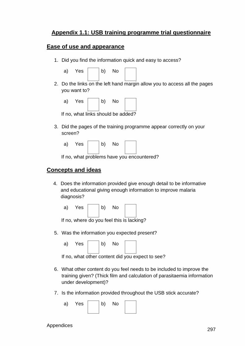
Appendices 297
Appendix 1.1: USB training programme trial questionnaire
Ease of use and appearance
1. Did you find the information quick and easy to access?
a) Yes b) No
2. Do the links on the left hand margin allow you to access all the pages
you want to?
a) Yes b) No
If no, what links should be added?
3. Did the pages of the training programme appear correctly on your
screen?
a) Yes b) No
If no, what problems have you encountered?
Concepts and ideas
4. Does the information provided give enough detail to be informative
and educational giving enough information to improve malaria
diagnosis?
a) Yes b) No
If no, where do you feel this is lacking?
5. Was the information you expected present?
a) Yes b) No
If no, what other content did you expect to see?
6. What other content do you feel needs to be included to improve the
training given? (Thick film and calculation of parasitaemia information
under development)?
7. Is the information provided throughout the USB stick accurate?
a) Yes b) No
Appendices 298
If no, Can you please point out any discrepancies that you feel need
to be amended? Please be critical, to allow improvements to be made.
8. Are the images of satisfactory quality to give an accurate
representation of parasites on the blood film?
a) Yes b) No
9. Do the gallery examples of different appearances of the same cell
type on the blood film provide an accurate representation of the range
of features likely to be seen?
a) Yes b) No
10. Do you feel the mechanism of delivery is logical?
a) Yes b) No
11. Would you approach the delivery differently?
a) Yes b) No
If yes, how would you do this?
12. Any further comments are very welcome
Thank you for your comments and feedback.
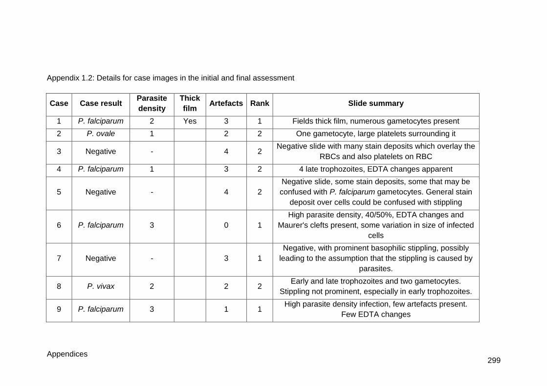
Appendices 299
Appendix 1.2: Details for case images in the initial and final assessment
Case Case result Parasite
density
Thick
film Artefacts Rank Slide summary
1 P. falciparum 2 Yes 3 1 Fields thick film, numerous gametocytes present
2 P. ovale 1 2 2 One gametocyte, large platelets surrounding it
3 Negative - 4 2 Negative slide with many stain deposits which overlay the
RBCs and also platelets on RBC
4 P. falciparum 1 3 2 4 late trophozoites, EDTA changes apparent
5 Negative - 4 2
Negative slide, some stain deposits, some that may be
confused with P. falciparum gametocytes. General stain
deposit over cells could be confused with stippling
6 P. falciparum 3 0 1
High parasite density, 40/50%, EDTA changes and
Maurer's clefts present, some variation in size of infected
cells
7 Negative - 3 1
Negative, with prominent basophilic stippling, possibly
leading to the assumption that the stippling is caused by
parasites.
8 P. vivax 2 2 2 Early and late trophozoites and two gametocytes.
Stippling not prominent, especially in early trophozoites.
9 P. falciparum 3 1 1 High parasite density infection, few artefacts present.
Few EDTA changes
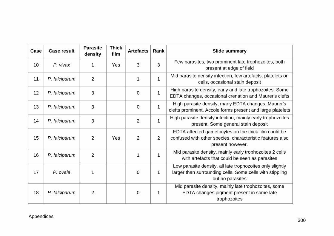
Appendices 300
Case Case result Parasite
density
Thick
film Artefacts Rank Slide summary
10 P. vivax 1 Yes 3 3 Few parasites, two prominent late trophozoites, both
present at edge of field
11 P. falciparum 2 1 1 Mid parasite density infection, few artefacts, platelets on
cells, occasional stain deposit
12 P. falciparum 3 0 1 High parasite density, early and late trophozoites. Some
EDTA changes, occasional crenation and Maurer's clefts
13 P. falciparum 3 0 1 High parasite density, many EDTA changes, Maurer's
clefts prominent. Accole forms present and large platelets
14 P. falciparum 3 2 1 High parasite density infection, mainly early trophozoites
present. Some general stain deposit
15 P. falciparum 2 Yes 2 2
EDTA affected gametocytes on the thick film could be
confused with other species, characteristic features also
present however.
16 P. falciparum 2 1 1 Mid parasite density, mainly early trophozoites 2 cells
with artefacts that could be seen as parasites
17 P. ovale 1 0 1
Low parasite density, all late trophozoites only slightly
larger than surrounding cells. Some cells with stippling
but no parasites
18 P. falciparum 2 0 1
Mid parasite density, mainly late trophozoites, some
EDTA changes pigment present in some late
trophozoites
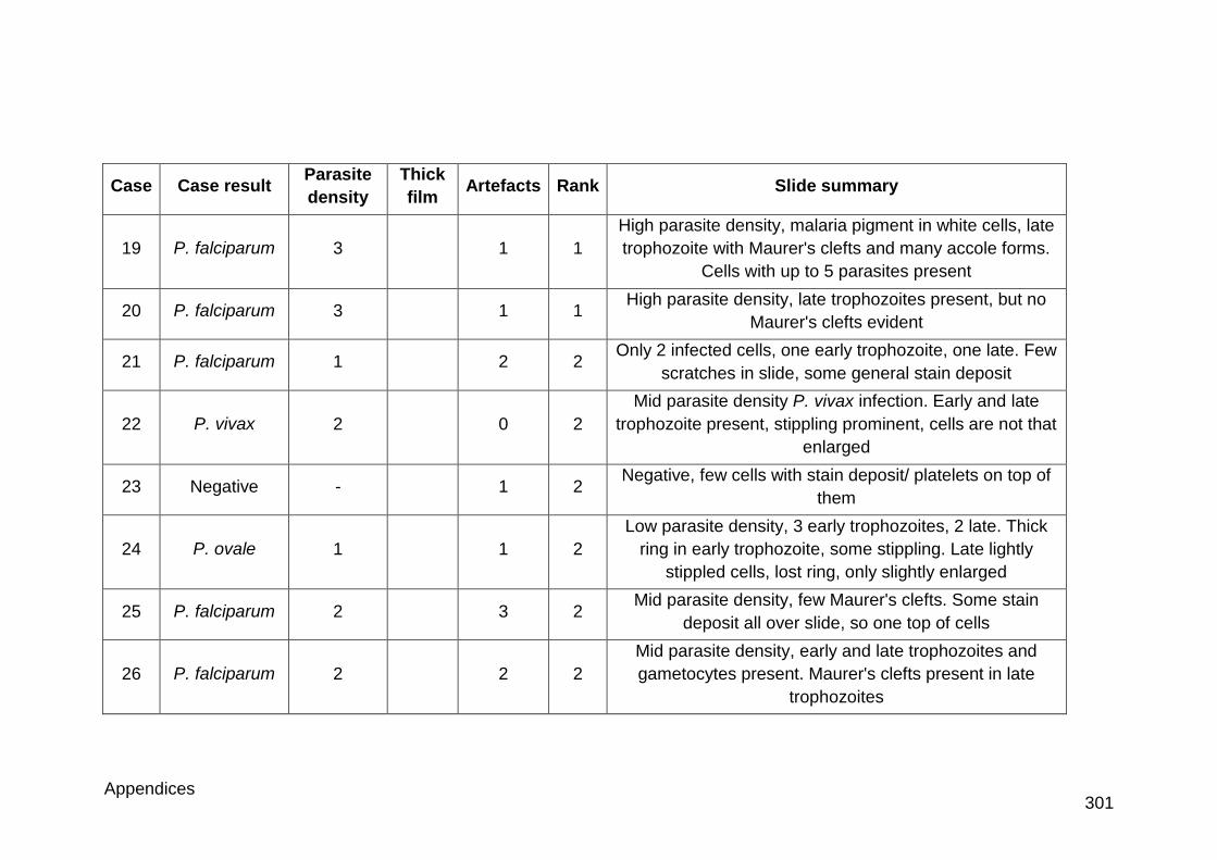
Appendices 301
Case Case result Parasite
density
Thick
film Artefacts Rank Slide summary
19 P. falciparum 3 1 1
High parasite density, malaria pigment in white cells, late
trophozoite with Maurer's clefts and many accole forms.
Cells with up to 5 parasites present
20 P. falciparum 3 1 1 High parasite density, late trophozoites present, but no
Maurer's clefts evident
21 P. falciparum 1 2 2 Only 2 infected cells, one early trophozoite, one late. Few
scratches in slide, some general stain deposit
22 P. vivax 2 0 2
Mid parasite density P. vivax infection. Early and late
trophozoite present, stippling prominent, cells are not that
enlarged
23 Negative - 1 2 Negative, few cells with stain deposit/ platelets on top of
them
24 P. ovale 1 1 2
Low parasite density, 3 early trophozoites, 2 late. Thick
ring in early trophozoite, some stippling. Late lightly
stippled cells, lost ring, only slightly enlarged
25 P. falciparum 2 3 2 Mid parasite density, few Maurer's clefts. Some stain
deposit all over slide, so one top of cells
26 P. falciparum 2 2 2
Mid parasite density, early and late trophozoites and
gametocytes present. Maurer's clefts present in late
trophozoites
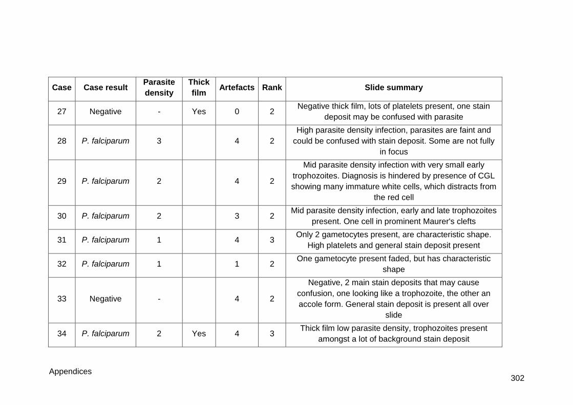
Appendices 302
Case Case result Parasite
density
Thick
film Artefacts Rank Slide summary
27 Negative - Yes 0 2 Negative thick film, lots of platelets present, one stain
deposit may be confused with parasite
28 P. falciparum 3 4 2
High parasite density infection, parasites are faint and
could be confused with stain deposit. Some are not fully
in focus
29 P. falciparum 2 4 2
Mid parasite density infection with very small early
trophozoites. Diagnosis is hindered by presence of CGL
showing many immature white cells, which distracts from
the red cell
30 P. falciparum 2 3 2 Mid parasite density infection, early and late trophozoites
present. One cell in prominent Maurer's clefts
31 P. falciparum 1 4 3 Only 2 gametocytes present, are characteristic shape.
High platelets and general stain deposit present
32 P. falciparum 1 1 2 One gametocyte present faded, but has characteristic
shape
33 Negative - 4 2
Negative, 2 main stain deposits that may cause
confusion, one looking like a trophozoite, the other an
accole form. General stain deposit is present all over
slide
34 P. falciparum 2 Yes 4 3 Thick film low parasite density, trophozoites present
amongst a lot of background stain deposit
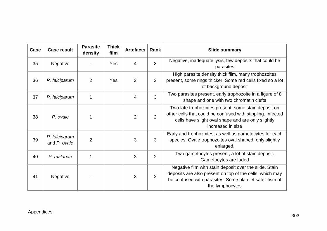
Appendices 303
Case Case result Parasite
density
Thick
film Artefacts Rank Slide summary
35 Negative - Yes 4 3 Negative, inadequate lysis, few deposits that could be
parasites
36 P. falciparum 2 Yes 3 3
High parasite density thick film, many trophozoites
present, some rings thicker. Some red cells fixed so a lot
of background deposit
37 P. falciparum 1 4 3 Two parasites present, early trophozoite in a figure of 8
shape and one with two chromatin clefts
38 P. ovale 1 2 2
Two late trophozoites present, some stain deposit on
other cells that could be confused with stippling. Infected
cells have slight oval shape and are only slightly
increased in size
39 P. falciparum
and P. ovale 2 3 3
Early and trophozoites, as well as gametocytes for each
species. Ovale trophozoites oval shaped, only slightly
enlarged.
40 P. malariae 1 3 2 Two gametocytes present, a lot of stain deposit.
Gametocytes are faded
41 Negative - 3 2
Negative film with stain deposit over the slide. Stain
deposits are also present on top of the cells, which may
be confused with parasites. Some platelet satellitism of
the lymphocytes
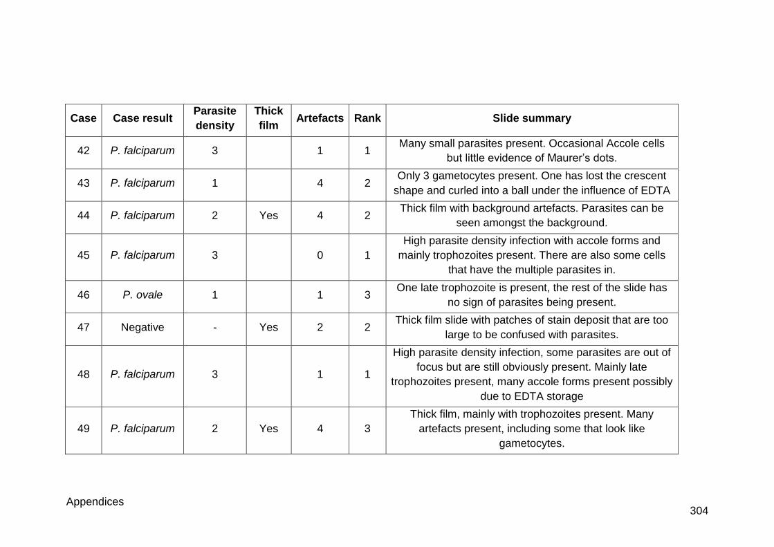
Appendices 304
Case Case result Parasite
density
Thick
film Artefacts Rank Slide summary
42 P. falciparum 3 1 1 Many small parasites present. Occasional Accole cells
but little evidence of Maurer’s dots.
43 P. falciparum 1 4 2 Only 3 gametocytes present. One has lost the crescent
shape and curled into a ball under the influence of EDTA
44 P. falciparum 2 Yes 4 2 Thick film with background artefacts. Parasites can be
seen amongst the background.
45 P. falciparum 3 0 1
High parasite density infection with accole forms and
mainly trophozoites present. There are also some cells
that have the multiple parasites in.
46 P. ovale 1 1 3 One late trophozoite is present, the rest of the slide has
no sign of parasites being present.
47 Negative - Yes 2 2 Thick film slide with patches of stain deposit that are too
large to be confused with parasites.
48 P. falciparum 3 1 1
High parasite density infection, some parasites are out of
focus but are still obviously present. Mainly late
trophozoites present, many accole forms present possibly
due to EDTA storage
49 P. falciparum 2 Yes 4 3
Thick film, mainly with trophozoites present. Many
artefacts present, including some that look like
gametocytes.
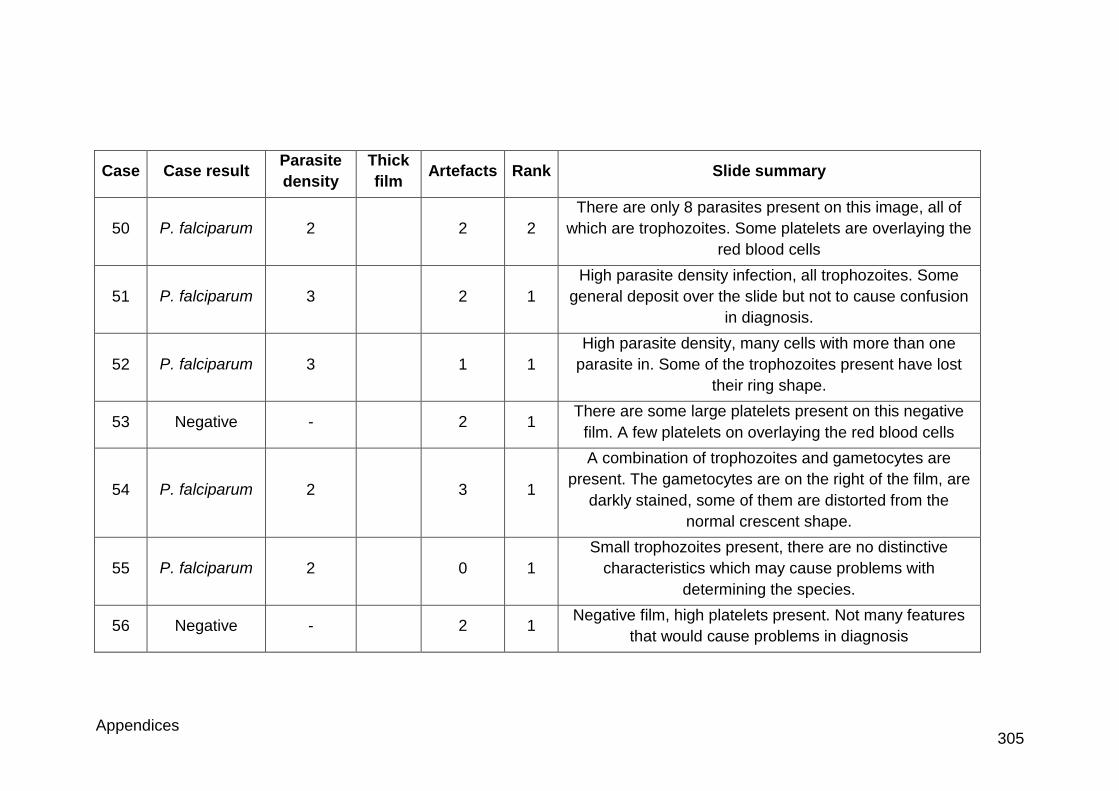
Appendices 305
Case Case result Parasite
density
Thick
film Artefacts Rank Slide summary
50 P. falciparum 2 2 2
There are only 8 parasites present on this image, all of
which are trophozoites. Some platelets are overlaying the
red blood cells
51 P. falciparum 3 2 1
High parasite density infection, all trophozoites. Some
general deposit over the slide but not to cause confusion
in diagnosis.
52 P. falciparum 3 1 1
High parasite density, many cells with more than one
parasite in. Some of the trophozoites present have lost
their ring shape.
53 Negative - 2 1 There are some large platelets present on this negative
film. A few platelets on overlaying the red blood cells
54 P. falciparum 2 3 1
A combination of trophozoites and gametocytes are
present. The gametocytes are on the right of the film, are
darkly stained, some of them are distorted from the
normal crescent shape.
55 P. falciparum 2 0 1
Small trophozoites present, there are no distinctive
characteristics which may cause problems with
determining the species.
56 Negative - 2 1 Negative film, high platelets present. Not many features
that would cause problems in diagnosis
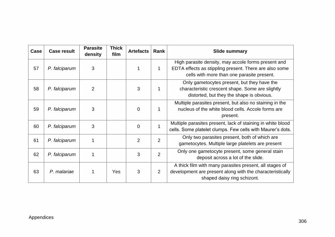
Appendices 306
Case Case result Parasite
density
Thick
film Artefacts Rank Slide summary
57 P. falciparum 3 1 1
High parasite density, may accole forms present and
EDTA effects as stippling present. There are also some
cells with more than one parasite present.
58 P. falciparum 2 3 1
Only gametocytes present, but they have the
characteristic crescent shape. Some are slightly
distorted, but they the shape is obvious.
59 P. falciparum 3 0 1
Multiple parasites present, but also no staining in the
nucleus of the white blood cells. Accole forms are
present.
60 P. falciparum 3 0 1 Multiple parasites present, lack of staining in white blood
cells. Some platelet clumps. Few cells with Maurer’s dots.
61 P. falciparum 1 2 2 Only two parasites present, both of which are
gametocytes. Multiple large platelets are present
62 P. falciparum 1 3 2 Only one gametocyte present, some general stain
deposit across a lot of the slide.
63 P. malariae 1 Yes 3 2
A thick film with many parasites present, all stages of
development are present along with the characteristically
shaped daisy ring schizont.
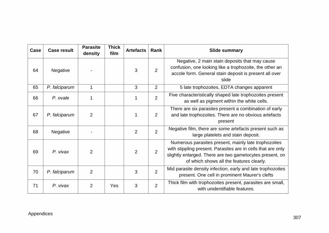
Appendices 307
Case Case result Parasite
density
Thick
film Artefacts Rank Slide summary
64 Negative - 3 2
Negative, 2 main stain deposits that may cause
confusion, one looking like a trophozoite, the other an
accole form. General stain deposit is present all over
slide
65 P. falciparum 1 3 2 5 late trophozoites, EDTA changes apparent
66 P. ovale 1 1 2 Five characteristically shaped late trophozoites present
as well as pigment within the white cells.
67 P. falciparum 2 1 2
There are six parasites present a combination of early
and late trophozoites. There are no obvious artefacts
present
68 Negative - 2 2 Negative film, there are some artefacts present such as
large platelets and stain deposit.
69 P. vivax 2 2 2
Numerous parasites present, mainly late trophozoites
with stippling present. Parasites are in cells that are only
slightly enlarged. There are two gametocytes present, on
of which shows all the features clearly.
70 P. falciparum 2 3 2 Mid parasite density infection, early and late trophozoites
present. One cell in prominent Maurer's clefts
71 P. vivax 2 Yes 3 2 Thick film with trophozoites present, parasites are small,
with unidentifiable features.
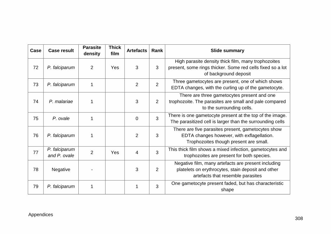
Appendices 308
Case Case result Parasite
density
Thick
film Artefacts Rank Slide summary
72 P. falciparum 2 Yes 3 3
High parasite density thick film, many trophozoites
present, some rings thicker. Some red cells fixed so a lot
of background deposit
73 P. falciparum 1 2 2 Three gametocytes are present, one of which shows
EDTA changes, with the curling up of the gametocyte.
74 P. malariae 1 3 2
There are three gametocytes present and one
trophozoite. The parasites are small and pale compared
to the surrounding cells.
75 P. ovale 1 0 3 There is one gametocyte present at the top of the image.
The parasitized cell is larger than the surrounding cells
76 P. falciparum 1 2 3
There are five parasites present, gametocytes show
EDTA changes however, with exflagellation.
Trophozoites though present are small.
77 P. falciparum
and P. ovale 2 Yes 4 3
This thick film shows a mixed infection, gametocytes and
trophozoites are present for both species.
78 Negative - 3 2
Negative film, many artefacts are present including
platelets on erythrocytes, stain deposit and other
artefacts that resemble parasites
79 P. falciparum 1 1 3 One gametocyte present faded, but has characteristic
shape
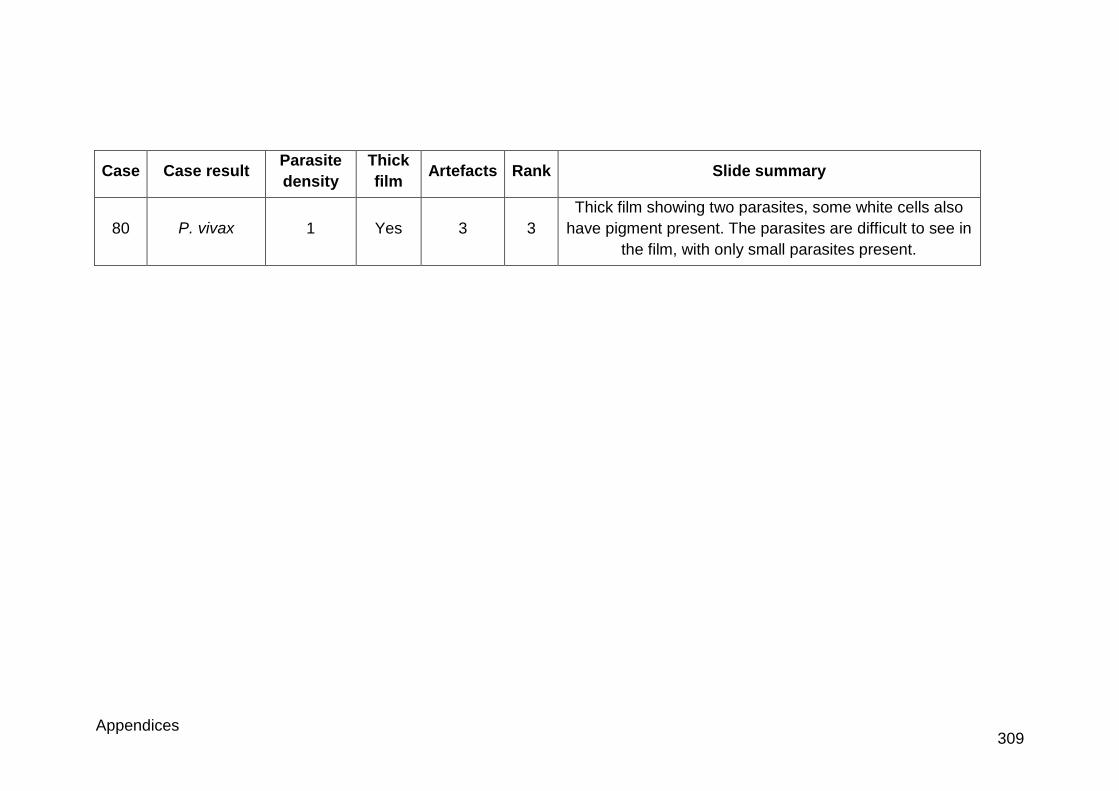
Appendices 309
Case Case result Parasite
density
Thick
film Artefacts Rank Slide summary
80 P. vivax 1 Yes 3 3
Thick film showing two parasites, some white cells also
have pigment present. The parasites are difficult to see in
the film, with only small parasites present.
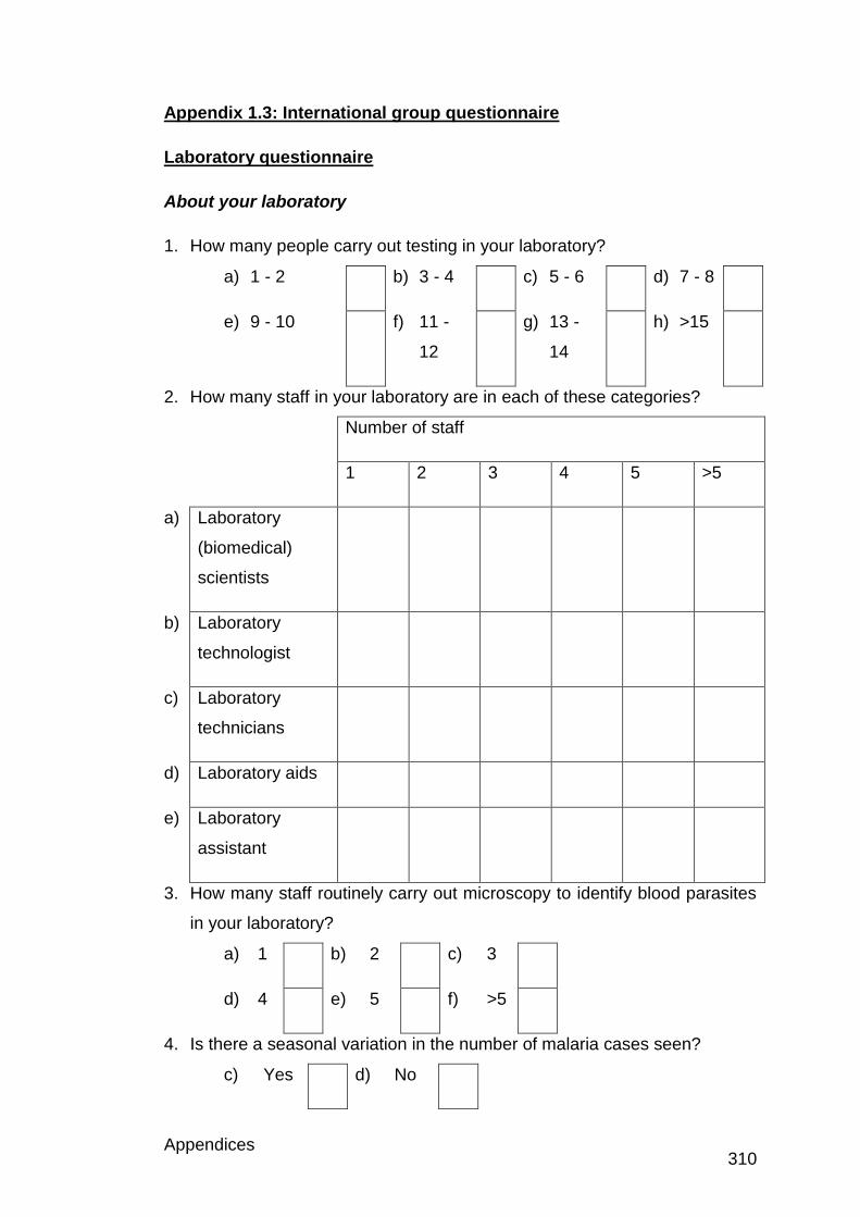
Appendices 310
Appendix 1.3: International group questionnaire
Laboratory questionnaire
About your laboratory
1. How many people carry out testing in your laboratory?
a) 1 - 2 b) 3 - 4 c) 5 - 6 d) 7 - 8
e) 9 - 10 f) 11 -
12
g) 13 -
14
h) >15
2. How many staff in your laboratory are in each of these categories?
Number of staff
1 2 3 4 5 >5
a) Laboratory
(biomedical)
scientists
b) Laboratory
technologist
c) Laboratory
technicians
d) Laboratory aids
e) Laboratory
assistant
3. How many staff routinely carry out microscopy to identify blood parasites
in your laboratory?
a) 1 b) 2 c) 3
d) 4 e) 5 f) >5
4. Is there a seasonal variation in the number of malaria cases seen?
c) Yes d) No
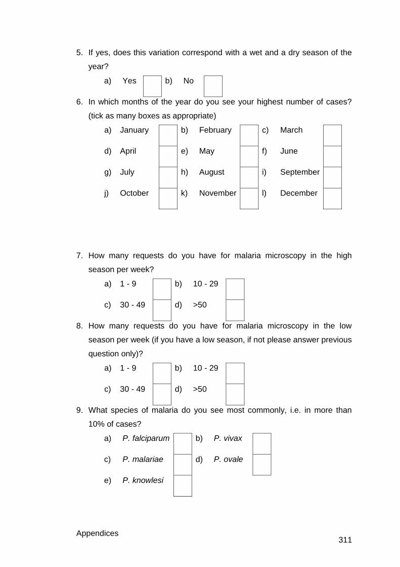
Appendices 311
5. If yes, does this variation correspond with a wet and a dry season of the
year?
a) Yes b) No
6. In which months of the year do you see your highest number of cases?
(tick as many boxes as appropriate)
a) January b) February c) March
d) April e) May f) June
g) July h) August i) September
j) October k) November l) December
7. How many requests do you have for malaria microscopy in the high
season per week?
a) 1 - 9 b) 10 - 29
c) 30 - 49 d) >50
8. How many requests do you have for malaria microscopy in the low
season per week (if you have a low season, if not please answer previous
question only)?
a) 1 - 9 b) 10 - 29
c) 30 - 49 d) >50
9. What species of malaria do you see most commonly, i.e. in more than
10% of cases?
a) P. falciparum b) P. vivax
c) P. malariae d) P. ovale
e) P. knowlesi
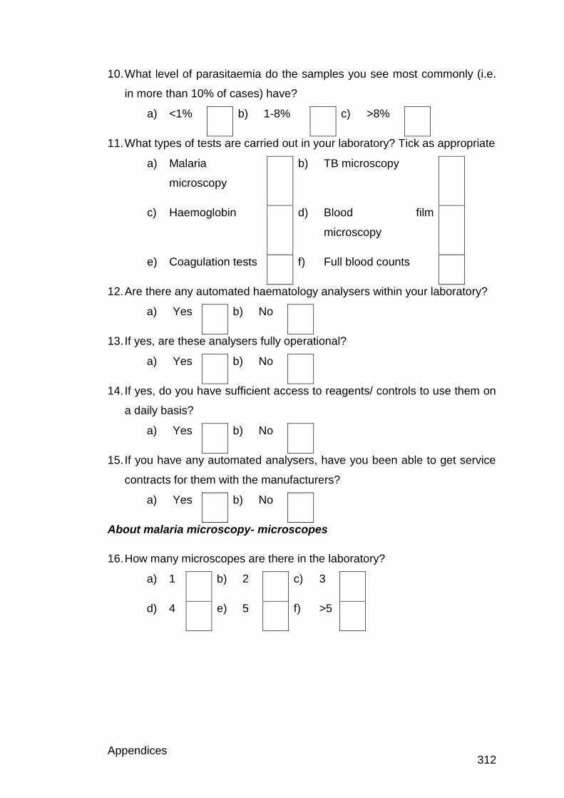
Appendices 312
10. What level of parasitaemia do the samples you see most commonly (i.e.
in more than 10% of cases) have?
a) <1% b) 1-8% c) >8%
11. What types of tests are carried out in your laboratory? Tick as appropriate
a) Malaria
microscopy
b) TB microscopy
c) Haemoglobin d) Blood film
microscopy
e) Coagulation tests f) Full blood counts
12. Are there any automated haematology analysers within your laboratory?
a) Yes b) No
13. If yes, are these analysers fully operational?
a) Yes b) No
14. If yes, do you have sufficient access to reagents/ controls to use them on
a daily basis?
a) Yes b) No
15. If you have any automated analysers, have you been able to get service
contracts for them with the manufacturers?
a) Yes b) No
About malaria microscopy- microscopes
16. How many microscopes are there in the laboratory?
a) 1 b) 2 c) 3
d) 4 e) 5 f) >5
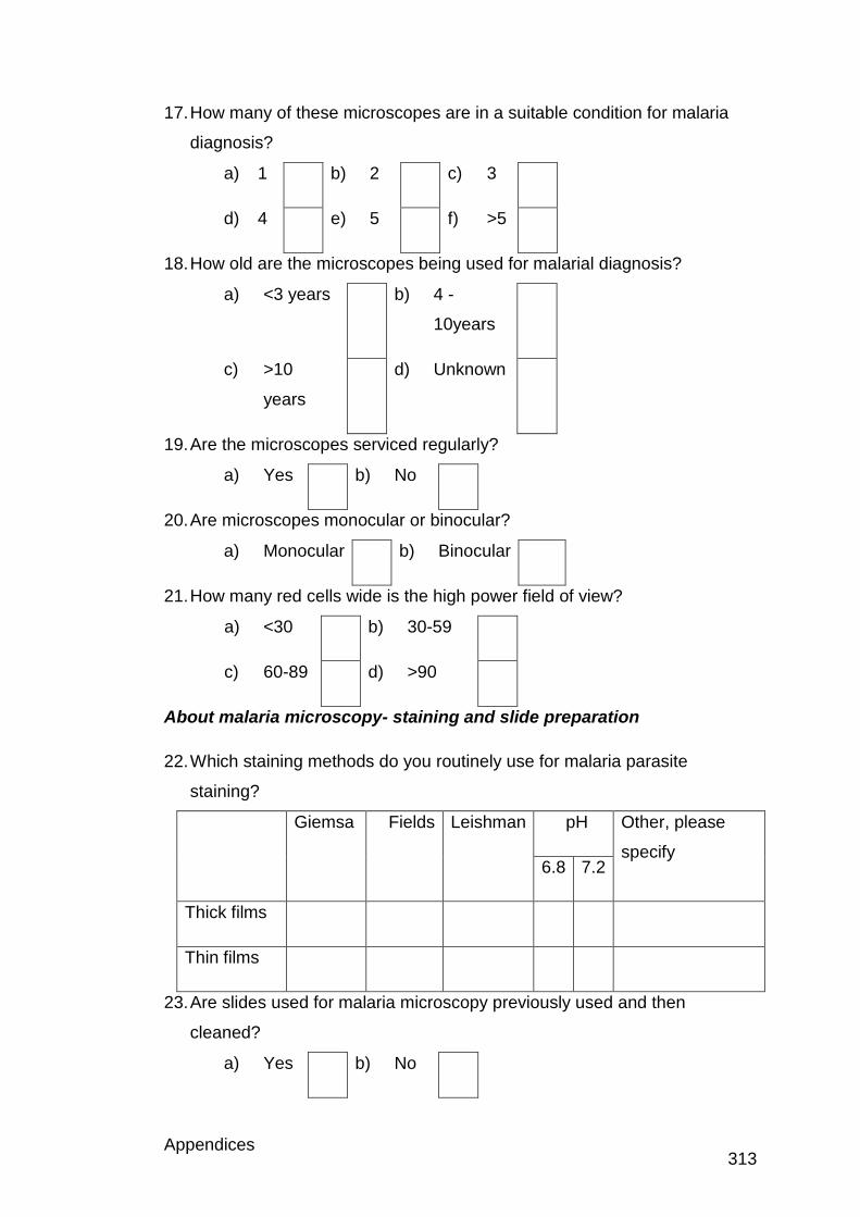
Appendices 313
17. How many of these microscopes are in a suitable condition for malaria
diagnosis?
a) 1 b) 2 c) 3
d) 4 e) 5 f) >5
18. How old are the microscopes being used for malarial diagnosis?
a) <3 years b) 4 -
10years
c) >10
years
d) Unknown
19. Are the microscopes serviced regularly?
a) Yes b) No
20. Are microscopes monocular or binocular?
a) Monocular b) Binocular
21. How many red cells wide is the high power field of view?
a) <30 b) 30-59
c) 60-89 d) >90
About malaria microscopy- staining and slide preparation
22. Which staining methods do you routinely use for malaria parasite
staining?
Giemsa Fields Leishman pH Other, please
specify 6.8 7.2
Thick films
Thin films
23. Are slides used for malaria microscopy previously used and then
cleaned?
a) Yes b) No
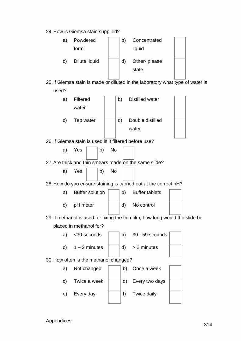
Appendices 314
24. How is Giemsa stain supplied?
a) Powdered
form
b) Concentrated
liquid
c) Dilute liquid d) Other- please
state
25. If Giemsa stain is made or diluted in the laboratory what type of water is
used?
a) Filtered
water
b) Distilled water
c) Tap water d) Double distilled
water
26. If Giemsa stain is used is it filtered before use?
a) Yes b) No
27. Are thick and thin smears made on the same slide?
a) Yes b) No
28. How do you ensure staining is carried out at the correct pH?
a) Buffer solution b) Buffer tablets
c) pH meter d) No control
29. If methanol is used for fixing the thin film, how long would the slide be
placed in methanol for?
a) <30 seconds b) 30 - 59 seconds
c) 1 – 2 minutes d) > 2 minutes
30. How often is the methanol changed?
a) Not changed b) Once a week
c) Twice a week d) Every two days
e) Every day f) Twice daily
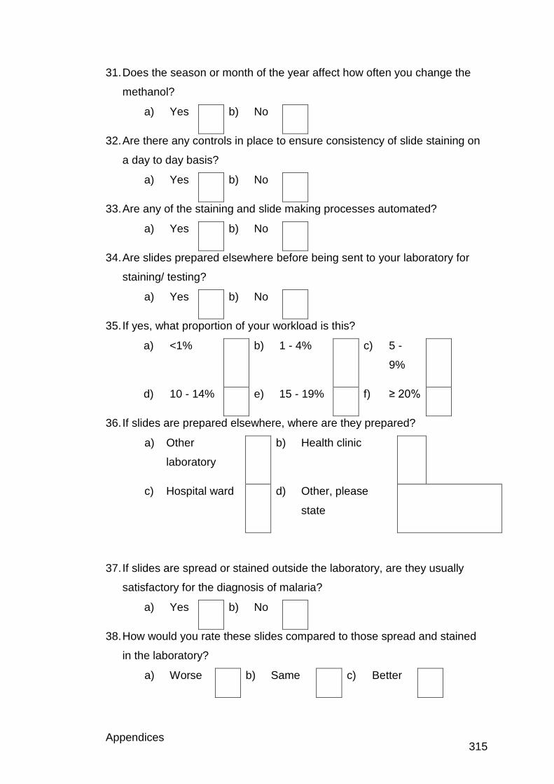
Appendices 315
31. Does the season or month of the year affect how often you change the
methanol?
a) Yes b) No
32. Are there any controls in place to ensure consistency of slide staining on
a day to day basis?
a) Yes b) No
33. Are any of the staining and slide making processes automated?
a) Yes b) No
34. Are slides prepared elsewhere before being sent to your laboratory for
staining/ testing?
a) Yes b) No
35. If yes, what proportion of your workload is this?
a) <1% b) 1 - 4% c) 5 -
9%
d) 10 - 14% e) 15 - 19% f) ≥ 20%
36. If slides are prepared elsewhere, where are they prepared?
a) Other
laboratory
b) Health clinic
c) Hospital ward d) Other, please
state
37. If slides are spread or stained outside the laboratory, are they usually
satisfactory for the diagnosis of malaria?
a) Yes b) No
38. How would you rate these slides compared to those spread and stained
in the laboratory?
a) Worse b) Same c) Better
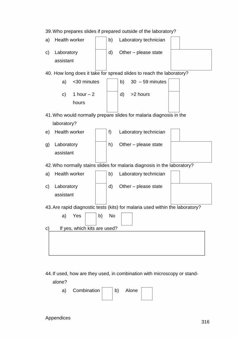
Appendices 316
39. Who prepares slides if prepared outside of the laboratory?
a) Health worker b) Laboratory technician
c) Laboratory
assistant
d) Other – please state
40. How long does it take for spread slides to reach the laboratory?
a) <30 minutes b) 30 – 59 minutes
c) 1 hour – 2
hours
d) >2 hours
41. Who would normally prepare slides for malaria diagnosis in the
laboratory?
e) Health worker f) Laboratory technician
g) Laboratory
assistant
h) Other – please state
42. Who normally stains slides for malaria diagnosis in the laboratory?
a) Health worker b) Laboratory technician
c) Laboratory
assistant
d) Other – please state
43. Are rapid diagnostic tests (kits) for malaria used within the laboratory?
a) Yes b) No
c) If yes, which kits are used?
44. If used, how are they used, in combination with microscopy or stand-
alone?
a) Combination b) Alone
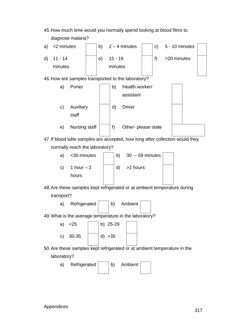
Appendices 317
45. How much time would you normally spend looking at blood films to
diagnose malaria?
a) <2 minutes b) 2 – 4 minutes c) 5 - 10 minutes
d) 11 - 14
minutes
e) 15 - 19
minutes
f) >20 minutes
46. How are samples transported to the laboratory?
a) Porter b) Health worker/
assistant
c) Auxiliary
staff
d) Driver
e) Nursing staff f) Other- please state
47. If blood tube samples are accepted, how long after collection would they
normally reach the laboratory?
a) <30 minutes b) 30 – 59 minutes
c) 1 hour – 2
hours
d) >2 hours
48. Are these samples kept refrigerated or at ambient temperature during
transport?
a) Refrigerated b) Ambient
49. What is the average temperature in the laboratory?
a) <25 b) 25-29
c) 30-35 d) >35
50. Are these samples kept refrigerated or at ambient temperature in the
laboratory?
a) Refrigerated b) Ambient
Appendices 318
51. Do you use any internal quality controls in the examination of malaria
films?
a) Yes b) No
c) If yes what procedures do you use?
52. Do you use any external quality control procedures in malaria
microscopy?
a) Yes b) No
c) If yes what procedures do you use?
Appendices 319
About computer and laboratory supplies
53. Is the electricity supply to the laboratory reliable or intermittent?
a) Reliable b) Intermittent
54. If intermittent how many hours per day do you have a power supply?
Hours
55. Does the hospital have a backup generator?
a) Yes b) No
56. If yes, how many hours per day does this supply the electricity for?
Hours
57. Do you have times of the day when you have no power supply at all?
a) Yes b) No
58. Do you have difficulties with obtaining laboratory supplies?
a) Yes b) No
59. If yes, are these difficulties due to distribution problems?
a) Yes b) No
60. How many computers are available within your laboratory?
a) 0 b) 1 c) 2
d) 3 e) 4 f) ≥
5
61. Is internet access available within the laboratory?
a) Yes b) No
62. How many of the computers within the laboratory have internet access?
a) 0 b) 1 c) 2
d) 3 e) 4 f) ≥
5
Appendices 320
63. Does the hospital have an internet subscription?
a) Yes b) No
64. Is the internet available for you to use?
a) Yes b) No
65. Is the internet connection lost/ disrupted regularly?
a) Yes b) No
66. If the internet is lost/ disrupted how long are you able to access the
internet per day?
Hours
67. Do you have to use internet cafes to use the internet?
a) Yes b) No
c) If yes, how much do you have to pay (please state which currency this
is in)
Appendices 321
Individual questionnaire
About your experience
1. How long have you worked at this laboratory?
a) <1 year b) 1 - 4 years
c) 5 - 10 years d) >10 years
2. How long have you been carrying out microscopy for the diagnosis of
malaria?
a) <1 year b) 1 - 4
years
c) 5 - 10
years
d) >10
years
3. Do you have any of the following qualifications relevant to your work?
a) Degree b) Diploma
c) Post-graduate
qualification
d) Other relevant
qualification- please
state
4. What specific training have you been given for malaria microscopy?
a) External training
course
b) Demonstration by
another member of
staff
c) None d) Other, please state
e) If you had specific training, what information and methods were
covered?
5. How long ago did you have your last training for malaria microscopy?
a) < 1 year b) 1 – 4 years
c) 5 - 9
years
d) ≥ 10 years
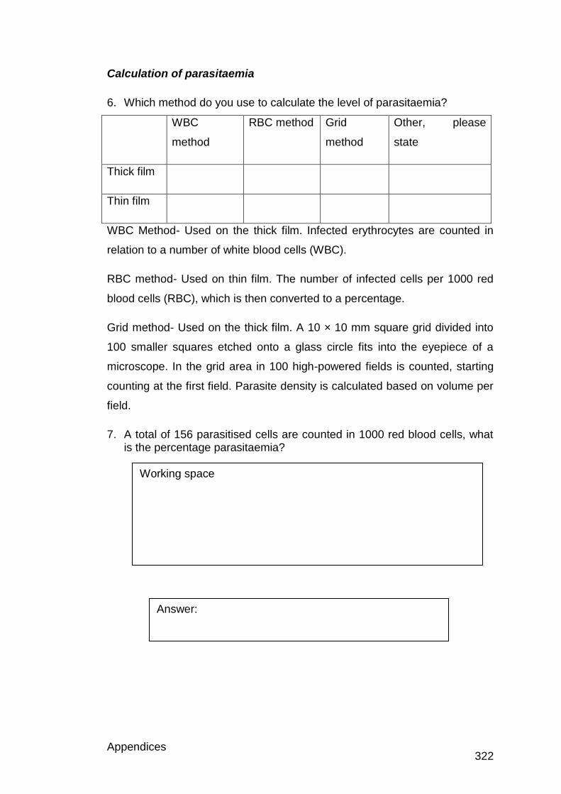
Appendices 322
Calculation of parasitaemia
6. Which method do you use to calculate the level of parasitaemia?
WBC
method
RBC method Grid
method
Other, please
state
Thick film
Thin film
WBC Method- Used on the thick film. Infected erythrocytes are counted in
relation to a number of white blood cells (WBC).
RBC method- Used on thin film. The number of infected cells per 1000 red
blood cells (RBC), which is then converted to a percentage.
Grid method- Used on the thick film. A 10 × 10 mm square grid divided into
100 smaller squares etched onto a glass circle fits into the eyepiece of a
microscope. In the grid area in 100 high-powered fields is counted, starting
counting at the first field. Parasite density is calculated based on volume per
field.
7. A total of 156 parasitised cells are counted in 1000 red blood cells, what is the percentage parasitaemia?
Working space
Answer:
Appendices 323
Appendix 1.4: UK group questionnaire
1. Please enter your ID code here
2. Do you report blood films?
Yes
No
3. How long have you worked in a haematology laboratory for?
< 1 year
1 - 2 years
2 - 5 years
6 - 10 years
11 - 15 years
16 - 20 years
>20 years
4. Have you completed or are you studying for any of the following?
Completed Studying for N/A
Registration portfolio
Specialist portfolio
Higher specialist portfolio (MSc)
Advanced higher specialist portfolio
Diploma of expert practice
5. What is your staff grade?
Trainee BMS
BMS Registered
Specialist BMS
Senior BMS
Chief BMS
Head BMS
Other (please specify) 6. What grade of membership do you have with the IBMS?
Not a member
Student or associate
Licentiate
Member
Appendices 324
Fellow 7. Have you ever attended the UK NEQAS parasitology teaching scheme?
Yes
No
If so please enter date/ year attended 8. On average how many cases of malaria does your laboratory see on a yearly basis?
<5 cases
6 - 15 cases
16 - 25 cases
26 - 35 cases
36 - 45 cases
>46 cases
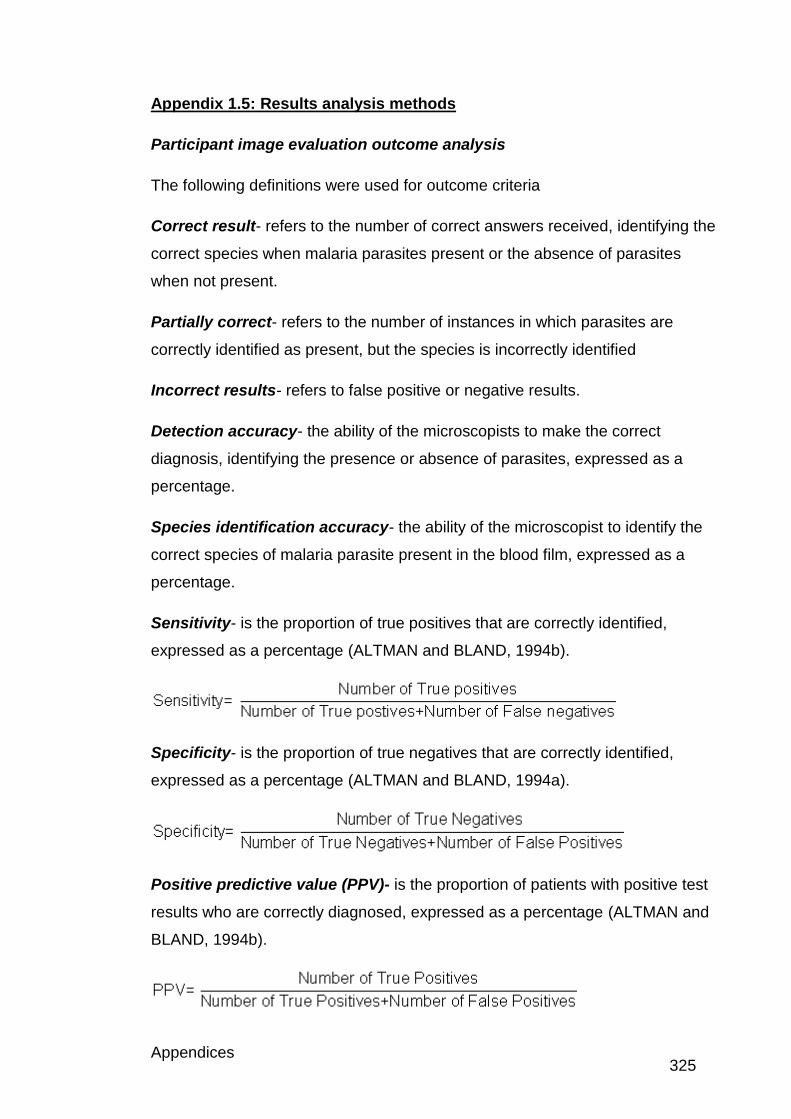
Appendices 325
Appendix 1.5: Results analysis methods
Participant image evaluation outcome analysis
The following definitions were used for outcome criteria
Correct result- refers to the number of correct answers received, identifying the
correct species when malaria parasites present or the absence of parasites
when not present.
Partially correct- refers to the number of instances in which parasites are
correctly identified as present, but the species is incorrectly identified
Incorrect results- refers to false positive or negative results.
Detection accuracy- the ability of the microscopists to make the correct
diagnosis, identifying the presence or absence of parasites, expressed as a
percentage.
Species identification accuracy- the ability of the microscopist to identify the
correct species of malaria parasite present in the blood film, expressed as a
percentage.
Sensitivity- is the proportion of true positives that are correctly identified,
expressed as a percentage (ALTMAN and BLAND, 1994b).
Specificity- is the proportion of true negatives that are correctly identified,
expressed as a percentage (ALTMAN and BLAND, 1994a).
Positive predictive value (PPV)- is the proportion of patients with positive test
results who are correctly diagnosed, expressed as a percentage (ALTMAN and
BLAND, 1994b).
Appendices 326
Negative predictive value (NPV)- is the proportion of patients with negative test
results who are correctly diagnosed, expressed as a percentage (ALTMAN and
BLAND, 1994a).
Statistical analysis
Kruskal-Wallis test for independent samples was used for all comparisons in the
initial and final assessment using SPSS 18.0.
Comparison results between the initial and final assessment were carried out
using Wilcoxon Signed Ranks, again using SPSS 18.0.
Box-plots were also used for comparisons.
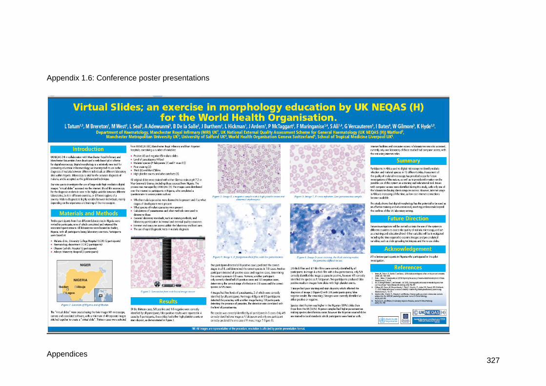
Appendices 327
Appendix 1.6: Conference poster presentations
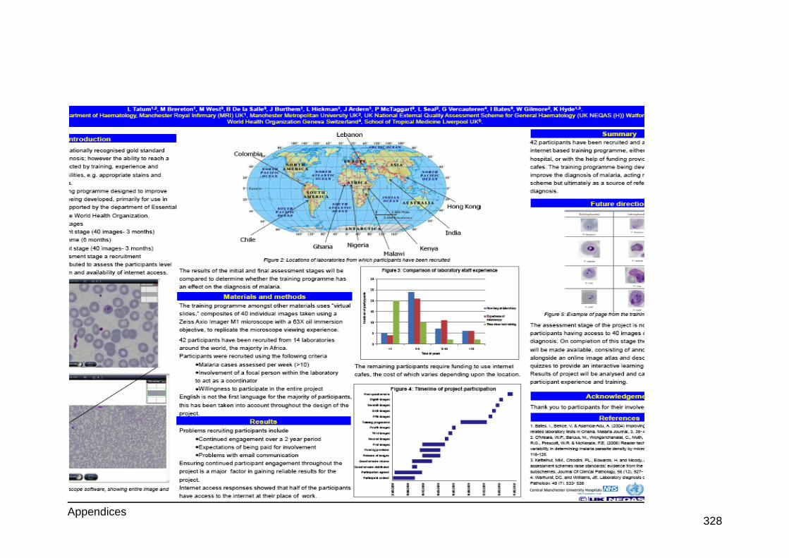
Appendices 328
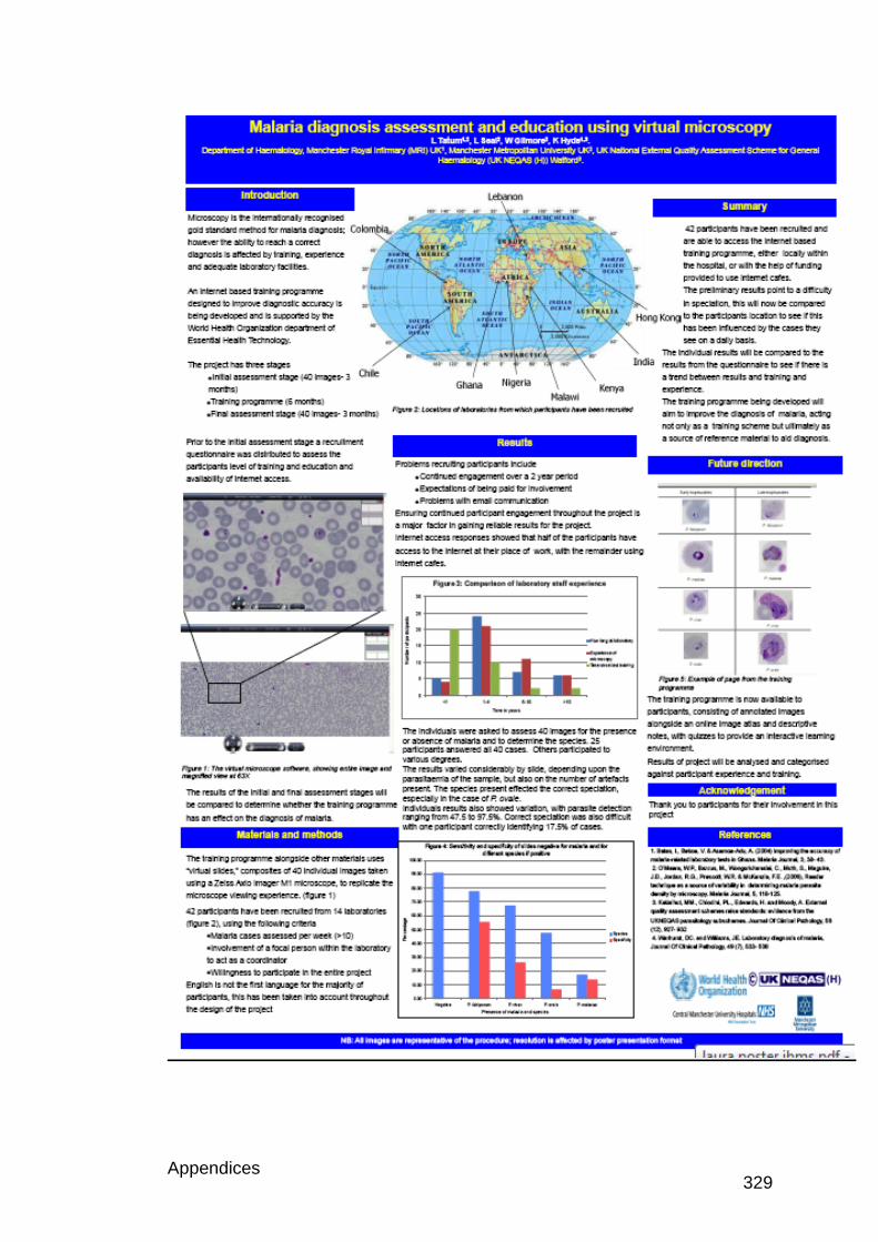
Appendices 329
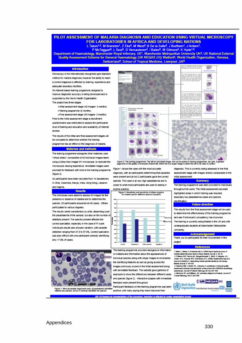
Appendices 330
Appendices 331
Appendix 1.7: Conference presentation: Sysmex users symposium
2010
Digital Morphology: A training tool for the UK and Developing Nations
Digital morphology has been used in a similar format for training of laboratory
staff based in Africa and laboratories involved in the International External
Quality Assessment scheme run by UK NEQAS. Participants were based in
Kenya, Nigeria, Chile, Colombia, Hong Kong, India and Lebanon.
Participants were initially asked to make a diagnosis on 40 blood smear
images to determine the presence or absence of malaria and to identify the
species present. These participants were then given access to a training
programme over a six-month period, before completing another assessment
of 40 images. The images in the initial and final assessment were chosen to
match a set of criteria, to allow the effectiveness of the training to be
determined.
The training programme, an internet based training package was delivered
over six months, providing annotated feedback along with detailed
information and images of cells containing parasites from the different
species and stages of infection. Quizzes were also used to allow immediate
feedback throughout the training.
Forty-two participants were recruited from 14 laboratories recommended by
the WHO, UK National External Quality Assessment Scheme for general
haematology (UKNEQAS (H)) and the Liverpool School of Tropical Medicine.
Of the 42 participants, 24 completed all 40 cases in the initial assessment,
another 15 completing various parts. Twenty-one participants completed all
40 cases in the final assessment. The comparison of results in the initial and
final assessment were carried out for 18 participants, who completed all the
images in the initial and final assessment.
Results from the initial assessment indicate that the correct diagnosis was
made in 68.8% of cases, with the correct species being identified in 33.2%.
Appendices 332
The final assessment indicated that the number of correct diagnoses made
was unchanged at 66.3% and there was also no change in the species
determination at 34.7%. Although individual features within the analysis did
improve, there was no evidence that the training programme improved
diagnosis.
The training programme has been shown to be effective in individuals in the
UK, therefore the reasons for not being effective in Developing Nations have
to be determined. These could due to difficulties in understanding English,
speed of internet connection, computers being used or the compliance of the
participants.
Appendices 333
Appendix 1.8 DVD of training programme and images
Related Documents