Small-signal Stability Analysis and Power System ... · PDF filei Small-signal Stability Analysis and Power System Stabilizer Design for Grid-Connected Photovoltaic Generation System

i

Small-signal Stability Analysis and Power System

Stabilizer Design for Grid-Connected Photovoltaic

Generation System

by

Akshay Kashyap

A thesis submitted to the Faculty of Graduate and Postdoctoral

Affairs in partial fulfillment of the requirements for the degree of

Master of Applied Science

in

Electrical and Computer Engineering

Carleton University

Ottawa, Ontario

© 2014, Akshay Kashyap

ii

Abstract:

Solar energy is one of the emerging forms of renewable energy, and has been proved to be a

potential source for generation of electricity. However, the rise in number of photovoltaic (PV)

generators presents issues for electric power utilities. Thus, integration of a PV system to the

grid, is an important area of research. Out of the various issues faced by the utilities, one of

the main issues is related to power system stability.

The objective of this thesis is to achieve stability for a grid-connected PV system with the

proposed new power system stabilizer (PSS). Stability is attained by conducting small signal

analysis and time domain analysis on the investigated PV system. First, time domain analysis

on detailed and average PV system models without PSS is performed. Second, small signal

stability analysis on average PV system model with and without PSS is performed. It is

observed that the damping effect and the dynamic stability of the investigated PV system are

achieved, with the help of the proposed new PSS

iii

Acknowledgements:

“I am deeply grateful to my thesis supervisor for his untiring support, encouragement and

guidance throughout the entire research. Thank you Sir, for sharing your passion for good

research in the area of Power System Stability with me.”

- to Professor Xiaoyu Wang

“A very significant thanks to you for the support and for being patient with me in our numerous

discussions.”

- to Shichao (Systems and Computer Eng. Dept)

“Thanks to my research collaborators for the thoughtful insights and helping me think with an

open mind for approaching my research.”

- to Rahul Kosuru & Jian Xiong

“Sir you provided great technical support and made sure we used the latest software for our

research in Hydro Lab.”

- to Mikhail Nagui

“Thank you for making all the administrative procedures, especially regarding registration,

so easy.”

- to M/s. Anna Lee & Staff of DOE

“Thanks for the great moral support you guys provided throughout my degree, and for being

there for me always.”

- to Ashwini Sadekar & Satwik Shetty

“I appreciate your love and patience for me and without your support, I couldn’t have

achieved this important step of my life.”

- to Mom, Dad & Shirin

iv

Contents

List of tables…..…………………………………………………………………………vi

List of figures……………………………………………………………….…………..vii

1 Introduction…………………………………………………………………………1

1.1 Background…………………....……………………………….…………...…1

1.2 Review of Power System Stabilizers ……...……………………….………….3

1.3 Photovoltaic Systems………………………………..…..……...……...……...6

1.3.1 Stand-alone PV system…………………………………...……………8

1.3.2 Grid connected PV system……………………………………..………9

1.4 Concept of PV DG…………...………………………………………..………9

1.4.1 Utility scale PV DG…………………………………………………..10

1.4.2 Medium scale PV DG………………………………………………..11

1.4.3 Small scale PV DG…………………………………………………...11

1.5 Motivation and Thesis Objectives……..……………………………………..12

1.6 Thesis Organization…...……………………………………………………..13

2 Structure of Grid-connected Photo-Voltaic System……………………………..15

2.1 Introduction…………………………………………………………………. 15

2.2 Overall System Architecture………………………..………………………..15

2.3 Photovoltaic PV Module.…………………………………………………….16

2.4 Maximum Power Point Tracking (MPPT)…………………………...………22

2.5 DC-DC (Boost) Converter…………………………...…………………...….23

2.6 Grid Connected Inverter…………...…………………………………………25

2.7 Phase Lock Loop (PLL)……………………………………………………...29

2.7.1 Parks transformation………………………………...………………....29

2.8 PV System Control Strategies ……………………………………...………..31

3 Average Modeling of Grid-connected Photovoltaic System…....…..…….…...…32

3.1 Introduction…………………………………………………………………. 32

3.2 PV Single Diode Model ………………………….………………..…………32

3.2.1 Effect of temperature and irradiance on the PV cell …………………...37

3.3 Modeling DC-DC Converter …………………………...……………………38

3.4 Modeling of PV System Dynamics…………………...……………………...45

v

3.5 Modeling of Grid Connected Inverter……...………………………………...46

3.6 PLL Design…………………………………………………………………..52

3.7 Design of Current Control ……………………………………………….…..54

4 Small Signal Modeling of Grid-connected Photovoltaic System…………...……57

4.1 Introduction…………………………………………………………………. 57

4.2 Small Signal Stability Analysis…….………………………………………...57

4.2.1 Linearization methodology…………………………………………58

4.3 Small Signal of the PV System Connected to a Parallel RLC Load…..…….61

4.4 Model Validation…………………………………………………………….64

4.4.1 Small signal stability analysis of PV system without PSS…………65

4.4.2 Large signal model analysis of PV system…………………………69

4.5 Summary……………………………………………………………………..72

5 Power System Stabilizer Design for the Grid-connected Photovoltaic System....73

5.1 Introduction…………………………………………………………………. 73

5.2 Overview …………………………….…………..……………………......…73

5.3 Oscillations in Power Systems………………………...……………………..76

5.4 Design of Power System Stabilizer…………………………………………..77

5.5 Small Signal Stability Analysis of PV System with PSS……………….…….80

5.6 Large Signal Model Analysis of PV System with and without PSS……….….84

5.7 Summary…………………………………………………………………......87

6 Conclusions and Future Work……………………………………….…………....88

6.1 Summary and Conclusion …………………………………………………...88

6.2 Future Work ……………………………………………………………...….89

7 Appendices………………………………………....………………………..…….. 91

8 Bibliography…………………………………..…………………….…………….103

vi

List of tables:

Table 4.1: Eigenvalues for PV system without PSS ……………………………………….…66

Table 4.2: Participation factor matrix for PV system without PSS…………………………...67

Table 4.3: Eigenvalues and the corresponding state variables ……………………………….68

Table 5.1: Eigenvalues for PV system with PSS ……………………………………………..81

Table 5.2: Participation factor matrix for PV system with PSS……………………………..82

Table 5.3: Eigenvalues and corresponding state variables for PSS connected PV system……83

Table A.1: System Parameters ………………………………………………………...…….91

Table A.2: Steady state variables and their values……………………………………………92

Table A.3: Load Parameters …………………………………………………………………92

Table A.4: PV panel parameters ……………………………………………………………..93

Table A.5: Controller parameters ……………………………………………………………94

vii

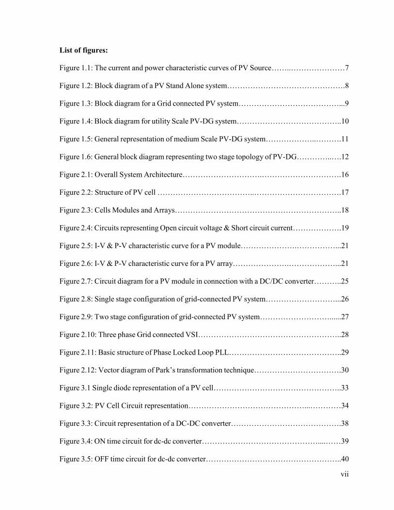
List of figures:

Figure 1.1: The current and power characteristic curves of PV Source……..…………………7

Figure 1.2: Block diagram of a PV Stand Alone system……………………………………….8

Figure 1.3: Block diagram for a Grid connected PV system…………………………………...9

Figure 1.4: Block diagram for utility Scale PV-DG system…………………………………..10

Figure 1.5: General representation of medium Scale PV-DG system………………..……….11

Figure 1.6: General block diagram representing two stage topology of PV-DG…………..….12

Figure 2.1: Overall System Architecture………………………….………………………….16

Figure 2.2: Structure of PV cell ………………………………..…………………………….17

Figure 2.3: Cells Modules and Arrays………………………………………………………..18

Figure 2.4: Circuits representing Open circuit voltage & Short circuit current……………….19

Figure 2.5: I-V & P-V characteristic curve for a PV module………………….……………...21

Figure 2.6: I-V & P-V characteristic curve for a PV array………………….………………...21

Figure 2.7: Circuit diagram for a PV module in connection with a DC/DC converter………..25

Figure 2.8: Single stage configuration of grid-connected PV system………………………...26

Figure 2.9: Two stage configuration of grid-connected PV system………………………......27

Figure 2.10: Three phase Grid connected VSI………………………………………………..28

Figure 2.11: Basic structure of Phase Locked Loop PLL……………………………………..29

Figure 2.12: Vector diagram of Park’s transformation technique…………………………….30

Figure 3.1 Single diode representation of a PV cell…………………………………………..33

Figure 3.2: PV Cell Circuit representation………………………………………...…………34

Figure 3.3: Circuit representation of a DC-DC converter…………………………………….38

Figure 3.4: ON time circuit for dc-dc converter………………………………………....……39

Figure 3.5: OFF time circuit for dc-dc converter……………………………………………..40

viii

Figure 3.6: Waveforms for Inductor voltage and current………………………..……………42

Figure 3.7: Equivalent circuit for ON state of DC-DC converter……………………………..43

Figure 3.8: Equivalent circuit for OFF state of DC-DC converter……………………………43

Figure 3.9: Equivalent circuit for DC-DC converter…………………………….…………...45

Figure 3.10: Averaged Inverter control and PLL……………………………………………..46

Figure 3.11: Equivalent circuit for grid connected DC/AC converter………………………..47

Figure 3.12: PLL control……………………………………………………………………..52

Figure 3.13: current and voltage controller…………………………………………………..54

Figure 4.1: PV system connected to a parallel RLC load……………………………………..62

Figure 4.2: Eigenvalue plot for PV system without PSS……………………………………...65

Figure 4.3: DC-voltage for the Average and Detailed large signal model without PSS………69

Figure 4.4: DC link voltage for PV system…………………………………………………...70

Figure 4.5: Active Power for Average and Detailed model of the system……………………71

Figure 4.6: Reactive Power for Average and Detailed model of the system………………….71

Figure 5.1: General representation of PSS…………………………………………….……...77

Figure 5.2: PSS controller diagram in the PV system………………………………………...78

Figure 5.3: Eigenvalue plot for system with PSS……………………………………………..80

Figure 5.4: DC-Link voltage model with and without PSS…………………………………...84

Figure 5.5: Active power curve for model with and without PSS…………………………….85

Figure 5.6: Reactive power curve for model with and without PSS…………………………..85

Figure 5.7: Active power curve for model with and without PSS to observe settling time……86

Figure B.1: Average model circuit of PV system connected to grid………………………….98

ix

List of Abbreviations

PV Photovoltaic

PV-DG PhotoVoltaic-Distributed Generation

PSS Power System Stabilizer

ISC Short-circuit Current

MPPT Maximum Power Point Tracking

PLL Phase Lock Loop

PCC Point of Common Connection

VSI Voltage Source Inverter

P Active Power

Q Reactive Power

1

Chapter 1

Introduction

1.1 Background

Renewable energy sources have enormous potential and are capable of generating energy

levels much greater than the current world demand. The use of such sources can help to reduce

pollution, increase environmental sustainability, and lower the consumption of fossil fuels.

Increasing climate changes, coupled with the depletion of fossil fuels, are the main driving

forces for renewable energy legislation, incentives, and commercialization. The principal types

of renewable energy sources include solar, wind, and hydro. Solar power is one of the most

promising renewable sources, as it is more predictable than wind energy, and less vulnerable

to seasonal changes as hydro power. Power generation by hydro or wind is restricted to the

sites where resources are available. Solar energy can be harnessed at the point of demand both

in rural and urban areas, thus decreasing the cost of transmitting the electricity (costs of

transmission). Grid connected Photovoltaic (PV) systems that are connected to the distribution

level, particularly with MW capacity, are increasing at an aggressive rate, in order to meet the

energy demand. However, there is less experience in the interconnection of utility-scale PV

systems with the distribution network, where loads are present. The Grid or also known as the

utility is an interconnected network, which supplies electricity to the consumers. This

interconnected network consists of resources for transmission and distribution of power or

electricity from the generation station to a distribution station, via high-voltage transmission

lines. This voltage is then delivered to the customers, from the distribution stations.

Utility-scale PV systems need special attention, unlike small scale PV systems, which are

limited to a few hundreds kW and are unlikely to show an impression on the distribution

2

system. Thus, there is a need to analyze the large scale, three-phase PV systems employed as

Photovoltaic Distributed Generation (PV-DGs), in terms of performance, dynamic

characteristics, and control. D.M Chapin, C.S Fuller, and G.S. Person of Bell laboratory

patented the solar cell, in 1954. The next year, Hoffman Electronics’ semiconductor division

announced the first commercial photo- voltaic product that was 2% efficient, priced at 25$ per

cell, and generating power of 14 mW each. By 1980, photovoltaics began finding many off-

grid applications such as pocket calculators, highway lights, and small home applications. By

2002, worldwide photovoltaic power production reached 600 MW per year, and was increasing

at a rate of over 40% per year. The continued discovery and development of silicon and other

photovoltaic materials have helped increase cell efficiency and decrease cost. At present, solar

PV power costs less than 2$ per watt [1]. The total global solar photovoltaic capacity is fast

approaching the 100 GW milestone, as per the International Energy Agency. [4] About 37 GW

was connected to the grid in 2013, and almost the same amount in 2012. Europe currently

represents 59% of the world PV market, but is facing competition from the Asia-Pacific

Region. In 2012, China was the second-largest PV market for new installations [3], thus

placing solar power generation in second position in terms of the new sources of power

generation.

Solar Photovoltaic Distributed Generation (PV-DG) systems represent one of the fastest-

growing types of renewable energy sources worldwide, currently being integrated into

distribution systems [2]. The most crucial aspect of the system is that the technical

requirements of the utility power system need to be satisfied to ensure the safety of the PV

installer and the reliability of the utility grid [5]. It is very important to understand the technical

requirements when performing an interconnection between two systems. For example, critical

interconnection problems such as harmonic distortion, islanding detection, and

3

electromagnetic interference need to be identified and solved. The interconnection of PV

systems with the grid is accomplished with the help of a supply electric power to electrical

equipment. The inverter plays an important role in this interconnection. There is a need for the

PV arrays and inverter to be characterized based on the geographical location of the PV system

and the installation configuration, but also based on the defects that occur during the operation

of the system [6-10]. In a grid-interconnected PV system, the inverter plays a key role, and its

reliability and safety are of the utmost importance to the system. As part of the PV-DG plant

interconnection impact studies, which include the typical power flow analysis, an in-depth

research is required into the potentially dynamic impacts of PV-DG units on the feeder

voltages under various load conditions. The investigation into the dynamic impacts of the

system lead to the development of various control strategies/techniques needed for the stability

and smooth operation of the PV-DG systems.

1.2 Review of Power System Stabilizers

As the power systems evolved over time, the stability problems associated to them have

increased. Power system stability, as defined in [11], is the ability of an electric power system

for an initial operating condition to regain the state of operating equilibrium after being

subjected to a physical disturbance. The power network system or grid is a highly changing

environment, whose various parameters are subject to change continually. A stabilizer tries to

keep these continually changing parameters at their original or steady states, to ensure the

smooth operation of the power system. Thus, [11] & [12] show the importance of stability for

a power system. This portion of the thesis will review the different types of power system

stabilizers that have previously been proposed. The detailed design and description of the

proposed power system stabilizer in this research is presented in Chapter 4. The PV system

4

designed in this thesis makes use of controllers to control the DC voltage collected at the output

of the boost (DC-DC) converter, as well as the reactive power. They also control the grid’s

voltage and power. The power system stabilizer can be applied to either the input side of the

controllers or the output terminals of the inverter, where the grid voltages and power can be

stabilized. In this thesis, the power system stabilizer is connected to the output of the DC

voltage controller at the input of the inner loop current controller. Reference [13] explains the

modeling of various power system components, such as power system networks, loads,

synchronous generators, excitation systems, and power system stabilizers (PSS). A PSS [14]

is an additional block of a generator excitation control, added to improve the dynamic

performance of the overall power system, particularly to damp the power/frequency

oscillations.

The PSS structure employed in [13], uses the rotor angle deviation as an auxiliary stabilizing

signal, which is applied at the input of the controller, based on the literature from [15-18]. The

difference between this and the proposed thesis is the stabilizing signal and its point of

application in the PV system. Reference [19] discusses the use of a robust controller for

damping low frequency power oscillations in a PV power plant, as the PV plant is subject to

various positive and negative influences caused by the oscillations in power, depending on

various factors such as location and size of the PV plant. Generally, for oscillation damping or

stabilizing, the real power modulation technique is considered. When damping or stabilizing,

control is based on real power modulation, and renewable energy sources normally have to

curtail their real power output [20-22], thus making use of reactive power modulation

techniques for power oscillation damping. Reference [19] utilizes a PSS design with a rotor

speed deviation as the input auxiliary stabilizing signal, and also has an additional block for

the lead-lag phase compensation in the PSS. Reference [23] talks about a damping technique

5

that can be achieved through independent control of the flow of real power from the stabilizer

and the voltage at the point of common coupling, which is positioned between the stabilizer

and the grid system. Instability problems resulting from inter-area oscillations are caused by

insufficient system damping and relatively weak tie-line connectors. If no appropriate action

takes place, then this oscillation may endanger the power network [25-29].

The design of the intermediate bus voltage feedback controller using the frequency technique

helps achieve damping. This controller uses the frequency as a stabilizing signal for the system,

compared with the PSS proposed in this thesis, where no voltage feedback controller is used.

Reference [30] discusses a power system stabilizer with positive voltage feedback to facilitate

anti-islanding schemes in inverter-based distributed generator DG’s. This research tries to

detect the variations that may occur in the DG-terminal voltage to generate a positive feedback

signal. The DG is a PV system to take into consideration, as the technique used to find the

feedback signal is similar to that of a PSS design. The PSS design in this thesis is used for

stability purposes only.

Reference [12] provides a detailed analysis of various power system stability parameters and

their designs for large generating stations. The detailed analysis of the power system is

essential to the identification of the various parameters that affect the system, so that a

technique can be established for adequately stabilizing the system. The PSS in [30] connects

to the overall system as part of an excitation system. This is a result of a machine being

connected to the system, as mentioned in the reference. Reference [31] talks about a control

strategy for the dynamic stability of a grid-connected PV system.

The main reason for having control techniques to support dynamic stability is the complexity

of PV penetration issues. Issues such as active power variation, bus voltage fluctuation,

reactive power flow, system stability etc., are all related to PV penetration. The control strategy

6

proposed in [31] to achieve dynamic stability includes the design components of a PSS, thus

not requiring an additional PSS block; it was able to successfully dampen the signal caused by

any faults occurring in the system. A reasonable amount of literature is available on the effects

of PV penetration [44] on the dynamic stability of a power system. Therefore, it is important

to realize the parameters that are affecting the system stability and to try and control these

parameters, in order to ensure the smooth functioning of any complex power system. The

functionalities of a damping controller and of a power system stabilizer are basically the same.

The two try to achieve system stability by damping the signal that is identified as the critical

parameter or the signal affecting system stability.

The techniques mentioned above to achieve stability in a grid-connected PV system, differ

from the technique proposed in this thesis. Firstly, the thesis proposes a model with no

machine. Thus, no need of an excitation system design as, mentioned in [24] and [12], [15],

[29], [31]. Secondly, the network frequency is used as the auxiliary stabilizing signal, which

is fed to the proposed power system stabilizer. This, PSS is applied at the input of the inner

loop current controller.

Lastly, the proposed power system stabilizer helps achieve higher stability and better damping

of oscillations. This is achieved, due to a better understanding of the critical parameters

affecting system stability. Thus, helping in selecting an appropriate stabilizing signal. The

detailed design of the PSS and its parameters are explained in Chapter 5.

1.3 Photovoltaic Systems

Solar energy can be exploited through solar thermal and solar photovoltaic systems, for a

variety of applications. While solar thermal utilizes the heat energy of the sun, photovoltaic

technology is enabled by the direct conversion of sunlight energy to electricity through a

7

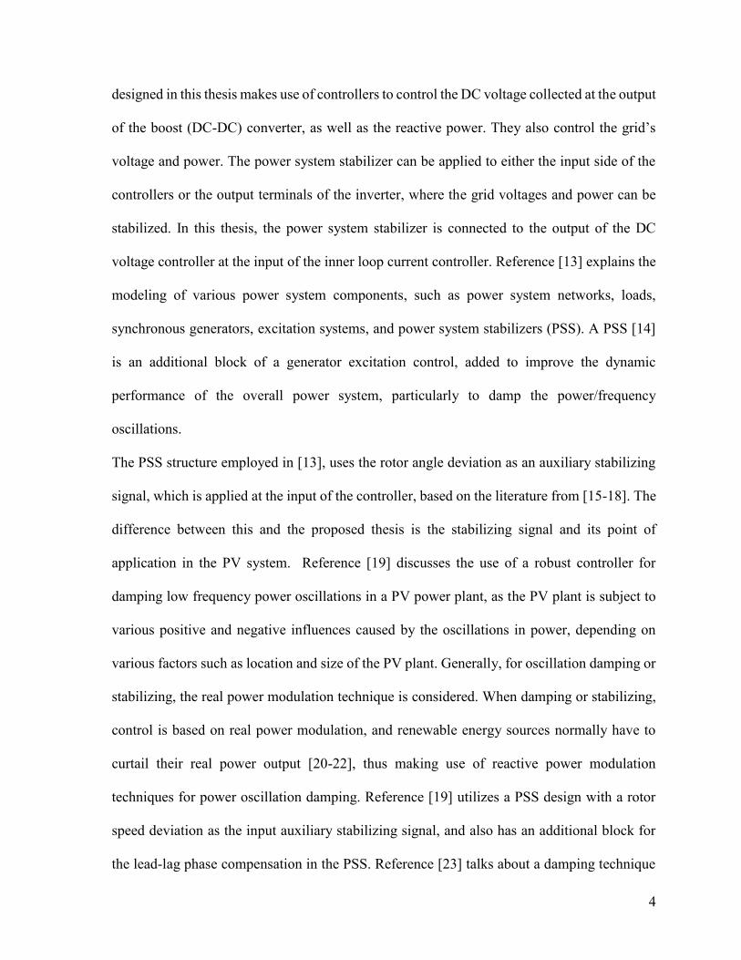
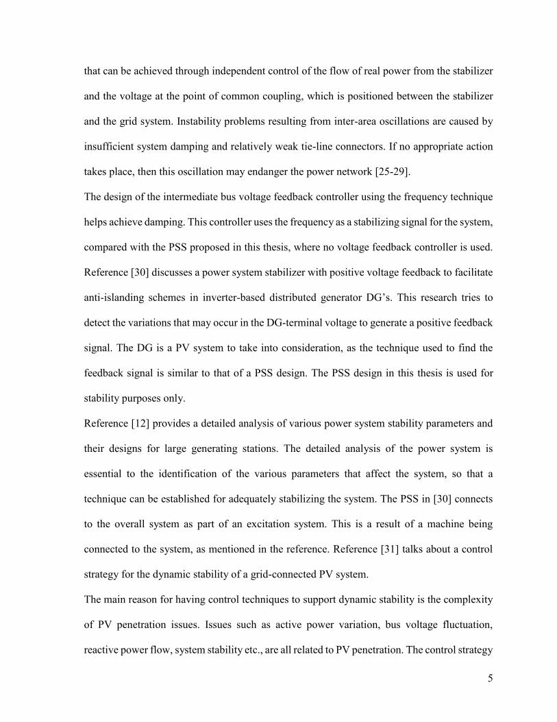
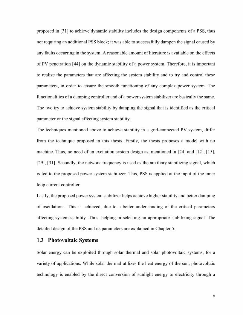
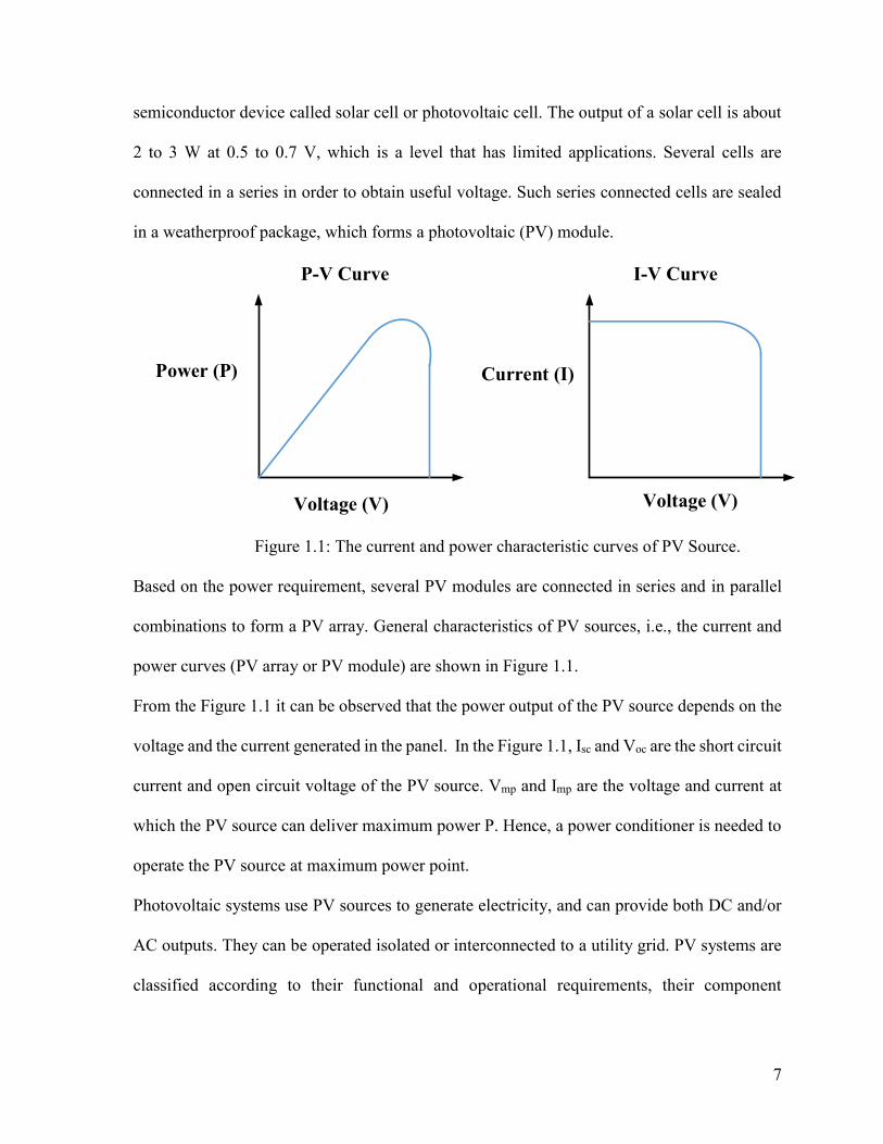
semiconductor device called solar cell or photovoltaic cell. The output of a solar cell is about

2 to 3 W at 0.5 to 0.7 V, which is a level that has limited applications. Several cells are

connected in a series in order to obtain useful voltage. Such series connected cells are sealed

in a weatherproof package, which forms a photovoltaic (PV) module.

P-V Curve I-V Curve

Voltage (V)

Power (P) Current (I)

Voltage (V)

Figure 1.1: The current and power characteristic curves of PV Source.

Based on the power requirement, several PV modules are connected in series and in parallel

combinations to form a PV array. General characteristics of PV sources, i.e., the current and

power curves (PV array or PV module) are shown in Figure 1.1.

From the Figure 1.1 it can be observed that the power output of the PV source depends on the

voltage and the current generated in the panel. In the Figure 1.1, Isc and Voc are the short circuit

current and open circuit voltage of the PV source. Vmp and Imp are the voltage and current at

which the PV source can deliver maximum power P. Hence, a power conditioner is needed to

operate the PV source at maximum power point.

Photovoltaic systems use PV sources to generate electricity, and can provide both DC and/or

AC outputs. They can be operated isolated or interconnected to a utility grid. PV systems are

classified according to their functional and operational requirements, their component

8

configuration, and how they are connected to other power sources and loads. The two basic

classifications are stand-alone (off-grid) and grid connected systems.

1.3.1 Stand-alone PV system

BATTERY

DC LOAD

AC LOADPV PANEL DC-DC CONVERTER DC-AC CONVERTER

Figure 1.2: Block diagram of a PV Stand Alone system

Stand-alone systems produce power independent to the utility grid. They are appropriately

suitable for remote and environmentally sensitive areas such as national parks and residences

which are located remotely. Figure 1.2 shows the block diagram for a Stand Alone PV system.

These PV systems are immune to system blackouts and do not rely on penetration of long

distance transmission lines. Main disadvantage of this system is they only work in day light

hours and battery storage is required, so that excess energy produced during day can be stored

and used in night. However, with batteries it require additional cost, maintenance and increases

the complexity of control.

9

1.3.2 Grid connected PV system

To feed the continuously increasing electric consumers, the distribution lines are generally

extended beyond the acceptable lengths. Figure 1.3 shown below is the block diagram for a

grid connected PV system. This results in a poor voltage profile for the customers at far end.

Moreover, feeding power to various load centers through transmission lines causes a

significant amount of power losses. By installing a power generating source at the distribution

level overcomes these problems. Installation of a generating source at the distribution level

also eliminates the need of upgrading the transmission lines and their associated switch gear.

PV PANEL INTERFACEDISTRIBUTION

SYSTEM

Figure 1.3: Block diagram for a Grid connected PV system

Due to these economic and regulatory factors, the vast majority of the PV systems are

connected to the existing distribution network in the form of Photovoltaic Distributed

Generation (PV-DG) instead of connecting to the transmission network. Unlike stand-alone

systems, these do not require batteries. The interface requirement between the PV sources and

utility grid depends upon size and application.

1.4 Concept of PV-DG

PV systems connected to the distribution network can be basically classified into three types,

they are described in the following subsections [2].

10

1.4.1 Utility-scale PV-DG

PV PANEL DC-AC CONVERTER

TRANSFORMER

DISTRIBUTION LINE

Figure 1.4: Block diagram Utility Scale PV-DG system

PV systems ranging from 1 to 10 MW are utility scale PV-DG. These are directly connected

to conventional feeders or distribution substation via express feeders. Utility scale PV-DG has

nominal capacities compatible with substation ratings or manageable by medium-voltage

distribution feeders. These are typically three-phase and requires one or more transformers.

A MW-size PV-DG plant generally includes several power electronic DC-AC converters

(inverter) modules connected in parallel that vary in size depending on the model and

manufacturer as shown in the Figure 1.4.

Each inverter is equipped with both internal and external protection schemes such as fast

overcurrent protection, under and over voltage and frequency safeguards, as well as active

anti-island protection schemes to prevent the PV system from feeding power to the grid in

11

the event that the utility grid connection is lost.

1.4.2 Medium scale PV-DG

PV systems whose capacity are in the range of 10 to 1000 kW are categorized under medium-

scale PV-DG. These are mainly installed on small or large buildings such as residential

complexes, retail stores, government sites and other buildings. Their typical interconnection

configuration depends on the capacity of the PV system. Larger plants (those with the capacity

in hundreds of kW) may typically have installation similar to utility-size PV-DG, including

separate interconnecting transformer, with the main difference in the nominal rating of the

associated equipment (transformers, inverters and switchgears). Smaller plants in which the

PV system capacity is comparable to the load may have typical installations similar to small

scale PV systems, using existing customer transformers, with minor changes in the

interconnection.

PV PANEL DC-AC CONVERTER

SECONDARY

DISTRIBUTION

LINE

Figure 1.5: General representation of Medium scale PV-DG

1.4.3 Small scale PV-DG

PV systems having capacity less than 10 kW are small-scale PV-DG. These are installed at

customer roof tops and connected to secondary distribution lines (230 V). These systems are

usually a single-phase or three-phase and produce less power required to consumer and do not

need transformer for interconnection as shown in Figure 1.5.

The PV-DG topology shown previously are called as single-stage grid-connected inverter

12

POWER GRIDPV PANEL DC-DC CONVERTER DC-AC CONVERTER

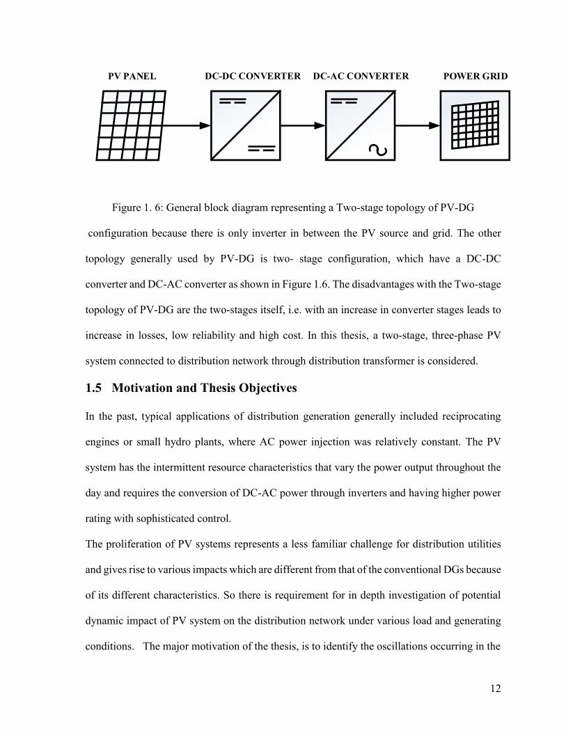
Figure 1. 6: General block diagram representing a Two-stage topology of PV-DG

configuration because there is only inverter in between the PV source and grid. The other

topology generally used by PV-DG is two- stage configuration, which have a DC-DC

converter and DC-AC converter as shown in Figure 1.6. The disadvantages with the Two-stage

topology of PV-DG are the two-stages itself, i.e. with an increase in converter stages leads to

increase in losses, low reliability and high cost. In this thesis, a two-stage, three-phase PV

system connected to distribution network through distribution transformer is considered.

1.5 Motivation and Thesis Objectives

In the past, typical applications of distribution generation generally included reciprocating

engines or small hydro plants, where AC power injection was relatively constant. The PV

system has the intermittent resource characteristics that vary the power output throughout the

day and requires the conversion of DC-AC power through inverters and having higher power

rating with sophisticated control.

The proliferation of PV systems represents a less familiar challenge for distribution utilities

and gives rise to various impacts which are different from that of the conventional DGs because

of its different characteristics. So there is requirement for in depth investigation of potential

dynamic impact of PV system on the distribution network under various load and generating

conditions. The major motivation of the thesis, is to identify the oscillations occurring in the

13

grid-connected PV system. To develop a technique, to achieve damping of these oscillations

to provide a stable power system.

Despite the need, there is no standard bench mark model of large scale PV systems for power

system simulation studies. Thus, there is a need for developing an accurate model for studying

the impact of PV system on distribution network [4]. Moreover, the components (inverter, PV

sources etc.) present in PV system are supplied by different manufactures, who may not

disclose their product dynamic properties (control structure or methodology, parameters).

Therefore, the only option is to build an adequate model, which may not exactly represent the

real world PV system but provides a satisfactory tool to analyze the PV system by expert point

of view. The main objectives of this thesis are:

To develop the mathematical model for the grid-connected PV system.

To build an adequate simulation model in MATLAB/SIMULINK for analysis purpose

along with the control architecture..

To design a power system stabilizer, to achieve better stability and damping of

oscillations to the grid-connected PV system.

To perform stability analysis on the grid-connected PV system with the proposed

control technique.

1.6 Thesis Organization

This thesis is organized in six chapters. The current chapter discusses briefly the history of PV

generation and various types of PV generations. It describes the basic architectures of different

types of PV system and its components. It emphasizes the necessity of studying the impact of

PV system on distribution network. It presents the literature survey/state of the art on the

controller design and sets the motivation for the present work carried out in this thesis.

14

In Chapter 2, first a circuit based PV array is modeled. Then mathematical model of the PV

system interfaced with stiff grid in dq reference frame is described. Based on the mathematical

model, controller for the AC side grid current and PLL are developed. A controller is proposed

in order to design the DC-link voltage controller instead of the Active Power Controller. The

simulations of the detailed switched model with the proposed control strategy are evaluated at

different operating conditions of PV system.

Chapter 3 describes the development of the small signal model, its stability and the eigenvalue

analyses of the overall PV system model. In this chapter, the nonlinear equations of the entire

PV system are linearized around an equilibrium point. The responses of the linearized model

are compared with the responses of the detailed switched model, for verifying the small signal

linearized model. An eigenvalue analysis of the linearized model is carried out, so as to observe

the various types of interactions in the PV system, help to understand the dynamics of the

system, to determine the robustness of the entire PV system, and to identify the control of the

system against parameter variations.

Chapter 4 deals with the design and development of the damping controller. The new proposed

controller’s mathematical model is developed into a Simulink model. A linearized model of

the entire PV system with the controller is carried out so as to compare the responses of the

two systems thus verifying the linearized model design. The chapter is concluded with the

comparison of the PV system with and without damping controller.

Chapter 5 develops a linearized mathematical model for PV system and distribution network.

The responses of the new PV system are recorded and analyzed for impacts of PV system on

the network and check for parameters which affect the stability of the system.

Chapter 6 concludes the entire thesis and provides scope for future research.

15

Chapter 2

Structure of the Grid-connected Photovoltaic System

2.1 Introduction

This chapter focuses on the overall design of a PV system interfaced with a grid/stiff grid or

utility. In the design, we give a description of each of the components of the PV system, namely

the PV module, the boost converter, the inverter, and the grid. This description helps to

understand the functionality of each component of the system, leading to its detailed

mathematical design, the results of which are shown in the following chapters.

In this part of the thesis, a detailed description of the parts of the two-stage grid connected PV

system is provided. The research conducted for each of these major parts of the PV system has

helped us understand why each particular component is required in the system. We also

mention the type of photovoltaic cell, DC-DC converter, and DC-AC converter model that has

been selected as part of this research.

The chapter has been organized as follows: section 2.2 speaks of the overall system

architecture, providing a glimpse of the architecture of the two-stage PV system connected to

a grid. It is followed with sections describing the PV cell, the MPPT controller, the DC-DC

converter, the DC-AC converter, and finally the phase lock loop PLL.

2.2 Overall System Architecture

Figure 2.1 shows the single line diagram of a two-stage PV system that is interfaced with the

stiff grid, represented by voltage source Vg. The main components of PV system are the PV

array, the DC-DC converter, the VSI or inverter, and the three-phase LC interfacing filter. The

PV array is connected to the DC side terminals of the VSI. The DC-link capacitance of the

VSI is represented by C. The AC side terminals of the VSI are interfaced with the LC filter.

16

Each phase of the filter has a series reactor and shunt capacitor. The inductance and resistance

of the reactor are represented by L and R respectively.

A parallel RLC load is connected to the system. P and Q represent the active and the reactive

power, respectively, that is delivered from the PV system to the grid, at Point of Common

Connection (PCC). Figure 2.1 also illustrates different control aspects involved in a PV system.

Phase Locked Loop (PLL) is used to extract the phase angle (θ) and frequency (ω) at PCC.

The current controller is used to control the AC side inverter currents. A DC-link voltage

controller is used to maintain the PV array voltage (Vdc or Vpv) at the reference value Vdcref

which is given by the MPPT controller. Thus, the Figure 2.1 represents the complete PV

generation, conversion and connection to the grid with a load. This model can be assumed for

Figure 2. 1: Overall System Architecture

performing stability analysis. It covers the basic architecture of a PV-DG, the mathematical

model of this system shall help us identify oscillations occurring in the system. The main

motivation, is to deliver maximum and stable supply of power from the PV.

17

2.3 Photovoltaic (PV) Module

A material or gadget that is equipped to change the energy contained in photons of light into

an electrical voltage and current is said to be photovoltaic. The history of photovoltaics can be

traced as far back as 1839, to Edmund Becquerel, who caused a voltage to appear by

illuminating a metal electrode in a weak electrolyte solution. Since then, the development of

photovoltaics has continued rising, from the development of Selenium photovoltaic cells with

an efficiency of 1% to 2% [4], to the latest silicon based cells (efficiency of 24%). A

photovoltaic (PV) system directly converts solar radiation (sunlight) into electricity. The PV

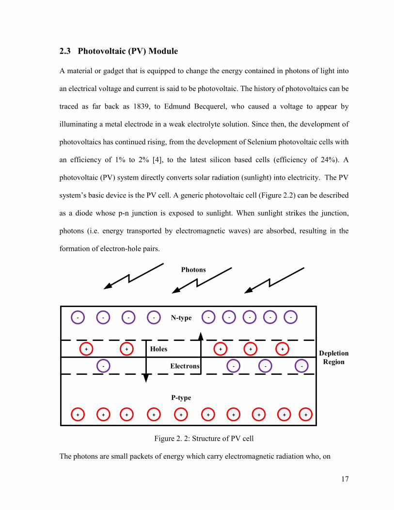
system’s basic device is the PV cell. A generic photovoltaic cell (Figure 2.2) can be described

as a diode whose p-n junction is exposed to sunlight. When sunlight strikes the junction,

photons (i.e. energy transported by electromagnetic waves) are absorbed, resulting in the

formation of electron-hole pairs.

- - - - - - - - -

+ + +

N-type

-

+

-

+

+

- -

+

+ + + + + + + +

P-type

Holes

Electrons

Depletion

Region

Photons

Figure 2. 2: Structure of PV cell

The photons are small packets of energy which carry electromagnetic radiation who, on

18

reaching the depletion region, cause the holes to move to the p-side of the junction and the

electrons to move to the n-side, thus resulting in the generation of an electric voltage which

can be tapped by placing electrical contacts, and delivering the voltage to the load. The

workings of the whole PV cell can be described as the absorption of sunlight causing the

generation of free carriers at the p-n junction, resulting in an electric current being generated

and collected at the terminals of the PV cell. The photovoltaic cell described above can

produce a voltage of approximately of 0.5 V, but very few applications make use of a single

cell. Usually, the basic building block of a PV application is a module. A module is a number

of PV cells connected in series and properly packaged. Typically, a module contains 36 cells

in series and is often designated as a “12-V module” [1]; it is capable of delivering voltages

higher than the specified value. At times, there are 12 V modules that only have 33 cells

connected in series. In turn, a number of such modules can be connected in either series

combinations to increase voltage, or in parallel combinations to increase current, the end result

always being power.

Cell ArrayModule

Figure 2. 3: Cells, Modules and Arrays

These different combinations of modules can be referred to as arrays. Figure 2.3 shows us the

19

distinction between cells, modules, and arrays. When a module is in series, the total voltage of

the array is calculated as the sum of the individual module voltages. The current flowing

through all the modules remains the same. In a parallel connection of the modules, the total

current of the array is calculated as the sum of the individual module currents. The voltage

through all modules remains the same. Thus, to achieve a large power from the PV system,

various combinations of series and parallel modules are constructed. Before connecting a load

to a PV module, we need to identify certain important electrical characteristics such as short-

circuit current ISC and open-circuit voltage VOC. The current and the voltage, i.e., the power of

the PV system, depend on the temperature and the amount of solar irradiation. These two

parameters keep varying throughout the day, which is why standard test conditions are

established to help compare different modules. These conditions are an irradiance of 1 kW/m2,

a cell temperature of 25 oC, and an air mass ratio of AM 1.5.

The PV cell described in this section can be represented as an equivalent circuit containing a

single diode used to calculate the current and the voltage at the key operating points (i.e.

maximum power point MPP).

+-

+-

+

-

V = 0

I = IscV=Voc

I = 0

Short Circuit currentOpen Circuit Voltage

Figure 2.4: Circuits representing Open circuit voltage & Short circuit current

The equations are a function of the cell temperature, irradiation and other data given by the

20

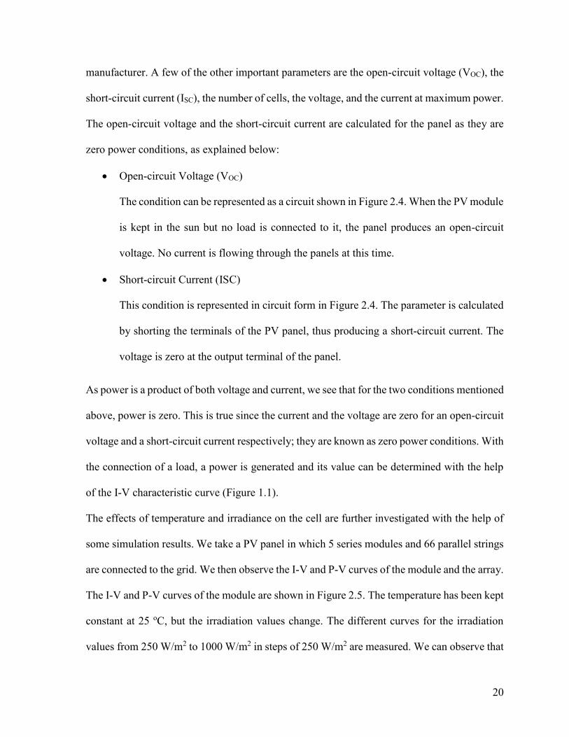
manufacturer. A few of the other important parameters are the open-circuit voltage (VOC), the

short-circuit current (ISC), the number of cells, the voltage, and the current at maximum power.

The open-circuit voltage and the short-circuit current are calculated for the panel as they are

zero power conditions, as explained below:

Open-circuit Voltage (VOC)

The condition can be represented as a circuit shown in Figure 2.4. When the PV module

is kept in the sun but no load is connected to it, the panel produces an open-circuit

voltage. No current is flowing through the panels at this time.

Short-circuit Current (ISC)

This condition is represented in circuit form in Figure 2.4. The parameter is calculated

by shorting the terminals of the PV panel, thus producing a short-circuit current. The

voltage is zero at the output terminal of the panel.

As power is a product of both voltage and current, we see that for the two conditions mentioned

above, power is zero. This is true since the current and the voltage are zero for an open-circuit

voltage and a short-circuit current respectively; they are known as zero power conditions. With

the connection of a load, a power is generated and its value can be determined with the help

of the I-V characteristic curve (Figure 1.1).

The effects of temperature and irradiance on the cell are further investigated with the help of

some simulation results. We take a PV panel in which 5 series modules and 66 parallel strings

are connected to the grid. We then observe the I-V and P-V curves of the module and the array.

The I-V and P-V curves of the module are shown in Figure 2.5. The temperature has been kept

constant at 25 oC, but the irradiation values change. The different curves for the irradiation

values from 250 W/m2 to 1000 W/m2 in steps of 250 W/m2 are measured. We can observe that

21

the power vs voltage curve in the Figure 2.5 shows the points of maximum power (pink

circles). The I-V and P-V curves of the array is shown in Figure 2.6. The major differences

that can be observed are that the

Figure 2. 5: The I-V & P-V characteristic curves for a PV module

Figure 2. 6: The I-V & P-V characteristic curves for a PV array

values of the current, power, and voltage have all increased, which was expected since the

22

array contains multiple modules in series and parallel combinations. The conditions for

temperature and the irradiation values are the same. Through this we have investigated the

effects of irradiance on PV cells. The PV panel used in this thesis is of mono-crystalline Silicon

with multi-contact output terminals. The PV characteristics are mentioned in Chapter 3.

2.4 Maximum Power Point Tracking (MPPT)

Maximum power point tracking is the relationship between the behavior of the current-voltage

of solar panels and the solar irradiance and temperature. As seen in Figure 2.6, an increase in

solar irradiance leads to a higher current and voltage output. The variations in environmental

conditions affect the maximum output power of PV panels.

As mentioned in the overall system architecture, the power produced by PV panels is given to

the DC-DC converter for boosting before being supplied to the DC-AC converter. To ensure

that the maximum power is being delivered to the DC-DC converter, an interface is being used

between the panels and the boost converter; this interface is known as maximum power point

tracking (MPPT).

Various MPPT algorithms have been developed based on different implementation topologies.

In respect to analog implementations, the options for MPPT techniques are short-circuit

current, open-circuit voltage, and temperature. Similarly, for the digital circuit

implementation, the various algorithms are perturb and observe (P&O) and incremental

conductance (IC) [45]. Currently, the most popular MPPT algorithm is the perturb and observe

algorithm (P&O). It has very few mathematical calculations, making its implementation fairly

easy. Its principal disadvantage occurs during steady state operation, where there is an

oscillation of power at the maximum power point [19].

For the purpose of this research, we use an MPPT control already available in the Simulink

23

environment. The design and mathematical modeling of the MPPT is out of the scope of this

thesis.

2.5 DC/DC (Boost) Converter

The need for converters can be explained with the help of a practical example. The voltage

ratings and frequency are different for various countries. To use an electronic device with

electrical specifications that are from a different location (country), we need to match the

electrical specifications of the electronic device to that of the local utility in that location.

Therefore, we use a converter to help achieve the voltage match, making it easy to use our

electronic device (e.g. a phone bought in North America needs a converter in order to be

charged in Europe). Similarly, we make use of these various converters depending on its

functionality in the power system. A converter provides various functionalities on the signals

being fed to it; this also depends on the type of converter being used in the process.

The various types of converters are:

Switching converter

DC-DC converter

AC-DC rectifier

DC-AC inversion

AC-AC cyclo-conversion

These converters provide a number of functions such as step-up of voltage, step-down, polarity

inversion, and conversion of AC to DC, and vice-versa. This thesis makes use of the DC-AC

converter and the DC-DC converter. In this section we elaborate on the design and

mathematical modeling of the DC-DC converter. The major functions of the DC-DC converter

are:

24

As a basic function, as the name suggests, it converts an input DC voltage of some

magnitude to an output DC voltage of a different magnitude (step-up or step-down).

Regulates the output DC voltage against load and line variations;

Reduces the AC ripple voltage on the DC output voltage below required levels;

Provides the isolation between the input source and the load;

Provides protection from electromagnetic interferences to the supply and input

systems;

Also satisfies various international and national safety standards.

DC-DC converters can be classified into two types: hard-switching pulse width modulated

(PWM) converters and resonant or soft-switching converters. In this thesis, we use a hard

switching pulse width modulated converter. The advantages of using a PWM converter are

high efficiency, constant frequency operation, and simple control. The PWM converter helps

to control the switch used in the boost converter, and this control of the switch of a DC-DC

converter also helps to achieve the step-up application of the converter. The two operation

modes for the DC-DC converter are:

Continuous conduction mode (CCM) &

Discontinuous conduction mode (DCM).

These operating modes are with respect to the value of the current flowing through the inductor

(refer Figure 2.9). In CCM mode, the value of the inductor current is always greater than zero.

When the value of input current is low, or the switching frequency is low, the converter enters

DCM mode. The inductor current is zero for a certain time when it is in DCM mode. In this

research we considered the DC-DC converter to be operating in CCM mode, as it has better

efficiency and utilizes the semiconductor switches in a good manner. As the power generated

25

from the module is very low, we make use of a boost converter that takes the low input DC-

voltage and provides a high output DC-voltage. Figure 2.7 shows a general connection

between the PV array and the boost converter. The output voltage and current of the PV module

is fed to the DC-DC converter. The input and output voltage relationship is controlled by the

duty cycle (D).

DiodeInductor

DC-link Capacitor

Switch

PV Boost Converter

Figure 2. 7: Circuit diagram for a PV module in connection with a DC-DC converter

2.6 Grid Connected Inverter

This section describes the inverter and its design and modeling. The inverter, also known as

the DC-AC converter, is a crucial part of a grid connected PV system. As we have seen, the

output of the PV panel is DC voltage, but the local utility or grid supplies AC voltage and

current. The conversion of the PV system DC voltage and current to the AC voltage and current

is necessary for the PV system to be connected to the grid. If the AC power generated by the

PV system is greater than the need of the owner, the inverter shall supply this surplus power

to the utility grid. At night, the utility provides AC power to satisfy the requirements of the

owners that have exceeded the capability of the PV system [32].

26

The design of the grid-connection inverter must take into consideration the peak power of the

system and deal with issues such as power quality, islanding detection, grounding, and

maximum power point tracking [33]. The inverter peak power is the net power of the PV

generator that is installed. The two types of inverters considered for such DG applications are

the voltage source inverter (VSI) and the current source inverter (CSI). The difference is in

their design, as the CSI makes use of silicon controlled rectifiers (SCR’s) or gate commutated

thyristors (GCT’s) for the switching devices, whereas the VSI uses the insulated gate bipolar

transistors (IGBT’s). Generally, the VSI is used in DG applications as it is easy to control and

also better satisfies the requirements for DG interconnection to the grid. Another drawback of

CSI is that it requires filters at the input and output, due to high harmonic content [34]. This

thesis also considers the design of the voltage source inverter to convert the DC voltage to AC

voltage. Once the type of inverter is selected, the topology of the inverter is chosen based on

the system configuration. The system can be configured depending on the number of stages:

Single stage configuration: In this configuration, the PV array is directly connected to

the DC-AC inverter, and then a transformer is used to change the voltage levels to suit

that of the utility grid. The configuration is shown in Figure 2.8.

PV ArrayDC/AC

InverterGridTransformerFilter

Figure 2. 8: Single-stage configuration of a grid-connected PV system

Two-stage configuration: Here, the system initially uses a DC-DC converter to step-up

the PV generated voltage, then connecting it to the DC-AC inverter for grid

interconnection no transformers are used in the design. In this research, the two-stage

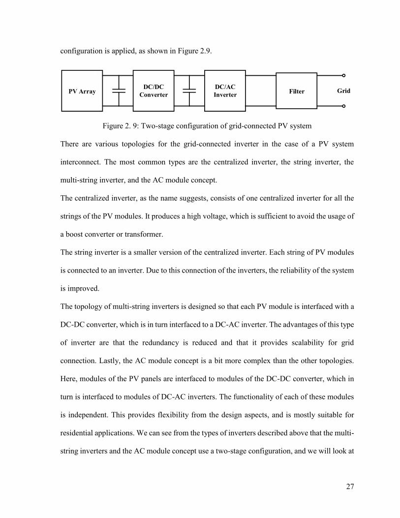
27

configuration is applied, as shown in Figure 2.9.

GridFilterDC/AC

Inverter

DC/DC

ConverterPV Array

Figure 2. 9: Two-stage configuration of grid-connected PV system

There are various topologies for the grid-connected inverter in the case of a PV system

interconnect. The most common types are the centralized inverter, the string inverter, the

multi-string inverter, and the AC module concept.

The centralized inverter, as the name suggests, consists of one centralized inverter for all the

strings of the PV modules. It produces a high voltage, which is sufficient to avoid the usage of

a boost converter or transformer.

The string inverter is a smaller version of the centralized inverter. Each string of PV modules

is connected to an inverter. Due to this connection of the inverters, the reliability of the system

is improved.

The topology of multi-string inverters is designed so that each PV module is interfaced with a

DC-DC converter, which is in turn interfaced to a DC-AC inverter. The advantages of this type

of inverter are that the redundancy is reduced and that it provides scalability for grid

connection. Lastly, the AC module concept is a bit more complex than the other topologies.

Here, modules of the PV panels are interfaced to modules of the DC-DC converter, which in

turn is interfaced to modules of DC-AC inverters. The functionality of each of these modules

is independent. This provides flexibility from the design aspects, and is mostly suitable for

residential applications. We can see from the types of inverters described above that the multi-

string inverters and the AC module concept use a two-stage configuration, and we will look at

28

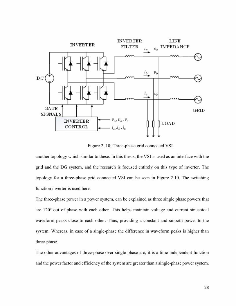
Figure 2. 10: Three-phase grid connected VSI

another topology which similar to these. In this thesis, the VSI is used as an interface with the

grid and the DG system, and the research is focused entirely on this type of inverter. The

topology for a three-phase grid connected VSI can be seen in Figure 2.10. The switching

function inverter is used here.

The three-phase power in a power system, can be explained as three single phase powers that

are 120o out of phase with each other. This helps maintain voltage and current sinusoidal

waveform peaks close to each other. Thus, providing a constant and smooth power to the

system. Whereas, in case of a single-phase the difference in waveform peaks is higher than

three-phase.

The other advantages of three-phase over single phase are, it is a time independent function

and the power factor and efficiency of the system are greater than a single-phase power system.

29

2.7 Phase Locked Loop

DC/AC

InverterVCOFilter

Frequency Divider

Input

Output

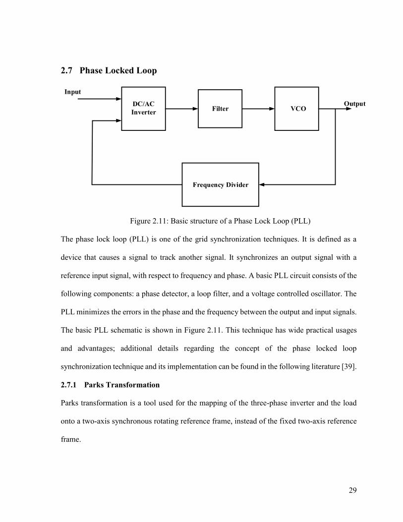
Figure 2.11: Basic structure of a Phase Lock Loop (PLL)

The phase lock loop (PLL) is one of the grid synchronization techniques. It is defined as a

device that causes a signal to track another signal. It synchronizes an output signal with a

reference input signal, with respect to frequency and phase. A basic PLL circuit consists of the

following components: a phase detector, a loop filter, and a voltage controlled oscillator. The

PLL minimizes the errors in the phase and the frequency between the output and input signals.

The basic PLL schematic is shown in Figure 2.11. This technique has wide practical usages

and advantages; additional details regarding the concept of the phase locked loop

synchronization technique and its implementation can be found in the following literature [39].

2.7.1 Parks Transformation

Parks transformation is a tool used for the mapping of the three-phase inverter and the load

onto a two-axis synchronous rotating reference frame, instead of the fixed two-axis reference

frame.

30

a

b

c

d

q

d

q

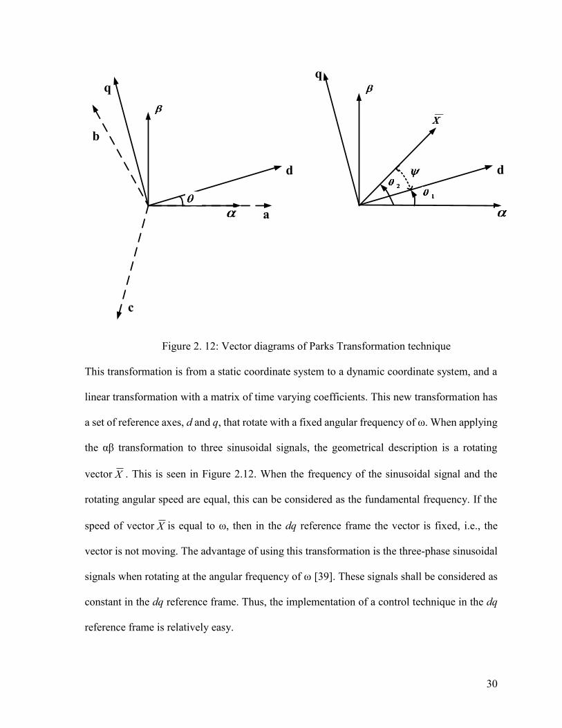
Figure 2. 12: Vector diagrams of Parks Transformation technique

This transformation is from a static coordinate system to a dynamic coordinate system, and a

linear transformation with a matrix of time varying coefficients. This new transformation has

a set of reference axes, d and q, that rotate with a fixed angular frequency of ω. When applying

the αβ transformation to three sinusoidal signals, the geometrical description is a rotating

vector X . This is seen in Figure 2.12. When the frequency of the sinusoidal signal and the

rotating angular speed are equal, this can be considered as the fundamental frequency. If the

speed of vector X is equal to ω, then in the dq reference frame the vector is fixed, i.e., the

vector is not moving. The advantage of using this transformation is the three-phase sinusoidal

signals when rotating at the angular frequency of ω [39]. These signals shall be considered as

constant in the dq reference frame. Thus, the implementation of a control technique in the dq

reference frame is relatively easy.

31

2.8 PV System Control Strategies

The major tasks related to control in the structure shown in Figure 2.1 are:

The synchronization of the PWM and control techniques to the voltage at the point of

common connection, with the help of a phase locked loop (PLL). This ensures the

change of the frame of reference to a dq- frame for the three-phase AC signals. Also,

the processing of the DC equivalents of the sinusoidal varying signals, by the

controllers.

The connection of a negative feedback damping controller at the input of the inner

control loop. It enables the control of the grid frequency.

The signal drefi is given to the dq reference frame, as shown in Figure 2.1. The inner

current loop scheme ensures that the signal di tracks the signal drefi . The control over

the di signal helps to achieve control over the voltage dcV . The inner current loop also

ensures that the signal qi tracks the signal qrefi . The signal qi is nothing but the reactive

power of the system represented by Q; this is discussed in greater detail in Chapter 3.

To ensure that the PV system has a unity power factor, the reference signal qrefi is zero,

resulting in the reference signal for the reactive power to be zero as well.

32

Chapter 3

Average Modeling of the Grid-connected Photovoltaic System

3.1 Introduction

This chapter focuses on the detailed design of the PV system interfaced with a grid/stiff grid

or utility. The design is a mathematical modeling of the components of the PV system, namely

the PV module, the boost converter, the inverter, and the grid. The average large signal

equation for each of the components mentioned above are derived, helping in the creation of

the average large signal model, which was created in the MATLAB/SIMULINK 2014b

environment, and the results of which are shown in the following chapters. In this part of the

thesis, an equivalent circuit based PV array is modelled. The system makes use of the

Maximum Power Point Tracking (MPPT) controller to obtain the maximum power from the

PV module. A DC-link voltage controller is proposed so as to regulate the DC voltage linking

to the Voltage Source Inverter (VSI). Controllers for the d and q components of the AC side

currents and the Phase Locked Loop (PLL) are derived.

The chapter is organized as follows, sections 3.1.1 to 3.6 provides the details and mathematical

designs of the PV modules, the DC-DC converter, and the DC-AC converter. The

mathematical model will include the derivation of equations in abc forms to their

transformation into the dq frame of reference. The simulation results of the entire PV system

described in the chapter are also shown. Finally, the chapter concludes with a comparison of

the average and detailed large signal models and their results.

3.2 PV Single Diode Model

Figure 3.1 shows the equivalent schematic of an ideal PV single diode model. It’s an ideal

current source connected in parallel with a diode. The modeling of the PV cell requires data

33

about four parameters, which can be obtained from the commercially available photovoltaic

modules. These parameters are the short-circuit current (ISC), the open-circuit voltage (VOC),

the current (Imp), and voltage (Vmp) at the maximum power point. The values of the temperature

coefficients for the current and voltage are equally important. The equations describing the I-

V characteristics of the ideal equivalent model are:

Iph D

Figure 3. 1: Single diode representation of a PV cell

The current flowing through the ideal PV cell shown above is mathematically represented as:

DphIII ………………………………………… (3.1).

The total current of the ideal equivalent circuit shown in Figure 2.5 is obtained by the

difference of the photocurrent and current through diode (ID). The expression for the diode

current is obtained from Shockley’s expression.

1exp

kTnN

qVII

s

oD …………………………….. (3.2),

where,

Iph = photocurrent (A);

Io = saturation current (A);

q= electrons charge (-1.602*10-19C);

n= quality factor of diode;

Ns= number of cells in series;

k= Boltzmann’s constant;

34

T= temperature of the p-n junction (K); [Almost same as the cell temperature]

Thus, substituting (3.2) in (3.1) we get

1exp

kTnN

qVIII

s

oph …………………………….. (3.3).

The equations for the ideal equivalent circuit are utilized to derive the equations for the more

appropriate circuit (Figure 3.2) being considered in this thesis. The circuit has series and

parallel resistance.

Iph D

Id Ish

Vcell

Icell

Rsh

Rs

Figure 3. 2: PV cell circuit representation

The circuit shown in Fig 3.2 is the practical PV cell. Series resistance RS represents the contact

resistance associated with the bond between the cell and its wire leads and a resistance of

semiconductor, which results in voltage loss of PV cell. Parallel resistance Rsh represents a cell

leakage current. The effect of the resistances modifies the equation (3.3),

sh

s

s

scellcell

ophR

IRV

kTnN

RIVqIII

1exp ………………. (3.4).

After comparing equations (3.4) and (3.3), we see that the series resistance affects the output

voltage and the shunt resistance affects the current. The saturation current (IO) is a result of the

charge diffusion and recombination in the space-charge layer. The I-V equation is expressed

as shown in (3.5). Where Io1= charge diffusion mechanism saturation current and Io2= re-combi

35

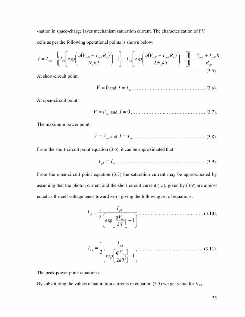
-nation in space-charge layer mechanism saturation current. The characterization of PV

cells as per the following operational points is shown below:

sh

scellcell

s

scellcell

o

s

scellcell

ophR

RIV

kTN

RIVqI

kTN

RIVqIII

1

2exp1exp

21

…….. (3.5).

At short-circuit point:

0V and scII ………………………………………. (3.6).

At open-circuit point:

ocVV and 0I …………………..…………………… (3.7).

The maximum power point:

mpVV and mp

II ………………..…….…..………….. (3.8).

From the short-circuit point equation (3.6), it can be approximated that

scphII ……………………………………….………. (3.9).

From the open-circuit point equation (3.7) the saturation current may be approximated by

assuming that the photon current and the short circuit current (Isc), given by (3.9) are almost

equal as the cell voltage tends toward zero, giving the following set of equations:

1exp2

11

kT

qV

II

oc

ph

o ………………………………….. (3.10),

12

exp2

12

kT

qV

II

oc

ph

o …………………..……………… (3.11).

The peak power point equations:

By substituting the values of saturation currents in equation (3.5) we get value for Voc

36

o

scs

ocI

I

q

kTnNV 1ln ……………………………. (3.12).

Solving the exponent part of (3.3) with Voc

kTnN

qV

kTnN

qV

kTnN

qV

s

mp

s

mp

s

oc exp1exp … ……….…… (3.13),

Then substituting the solved exponent in (3.3) we get,

1exp

kTnN

qVIII

s

mp

ophmp ……………………………. (3.14).

The PV cell has a hybrid behavior, i.e., of current source at short-circuit point and of voltage

source at open-circuit voltage, and we observe that the maximum power point corresponds to

trade-off condition between current and voltage, and is found at the point where the current is

still high, just before it starts decreasing with the increasing output voltage. We therefore

consider a tangent to the I-V curve to evaluate a region of the graph that is similar to the above

mentioned behavior, this gives

kTnN

qV

kTnN

qI

dV

dI

ss

o exp ………………………………. (3.15).

The expression (3.15) is used to calculate the output voltage corresponding to that of Vmp.

mpVo

ss

mpdV

dI

qI

kTnN

q

kTnNV ln …................................ (3.16).

We know that the derivative in (3.16) is,

oc

sc

oc

sc

mpV

I

V

IV

dV

dI

0

0~ ……………………………….. (3.17),

Using (3.17) in (3.16) we get

37

oc

sc

o

ss

mpV

I

qI

kTnN

q

kTNln

nV ……….................................. (3.18).

Similarly we get

oc

scrs

ophmpV

I

q

kTnNIII ………………………….... (3.19).

3.2.1 Effect of Temperature and Irradiance on the PV cell

The two major parameters that affect the characteristics of the PV cell or array are the solar

irradiance (G) and the cell temperature (T). The relation between the irradiance and short-

circuit current ISC are directly proportional to each other. If the irradiance drops, short-circuit

current also drops, and vice-versa. The relation between the irradiance and the open-circuit

voltage VOC is logarithmic, thus resulting in a small change of the open-circuit voltage for a

change in solar irradiance. As the cell temperature increases, the open-circuit voltage descends

by a substantial amount, while short-circuit current rises by a small amount. These changes

can be placed into a single mathematical equation, as shown in (3.20), for modeling purposes.

The equation for the photocurrent Iph is as follows:

refsc

ref

phTTI

G

GI ………………………………… (3.20),

where the Isc is the value of the short-circuit current calculated at standard temperature

conditions (STC), meaning that the operating reference cell temperature (Tref) is 25 oC and the

solar irradiance reference value (Gref) is 1000 W/m2. α is the temperature co-efficient for the

short-circuit current (0.0005/oC). Equations (3.18), (3.19) and (3.20) get values for Vmp, Imp

and Iph. These values are for the PV module only, with no connection to the DC-DC converter.

Since this connection is made, we shall consider the equation (3.14) from PV module which

38

is

1exp

kTnN

qVIII

s

mp

ophmp

This equation is solved for the exponent term, linearizing using Taylor series we get,

kTnN

vq

kTnN

qVIii

s

mp

s

mp

ophmp

ˆexpexpˆˆ …………….……. (3.21),

solving the series

1

2

1ˆˆˆ

2

kTnN

qV

kTnN

qVvqIii

s

mp

s

mp

mpophmp…………… (3.22),

from (3.22) we can derive the equation for the current at maximum power. This is dependent

on the voltage at the maximum power, the relation of which can be obtained from the design

of the DC-DC converter.

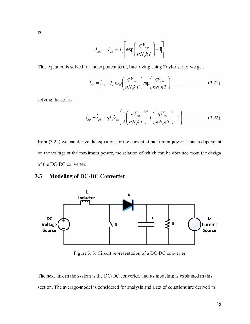
3.3 Modeling of DC-DC Converter

DC Voltage Source

D

Iz Current Source

L Inductor

C

RS

Figure 3. 3: Circuit representation of a DC-DC converter

The next link in the system is the DC-DC converter, and its modeling is explained in this

section. The average-model is considered for analysis and a set of equations are derived in

39

the process. In this thesis, the voltage from the PV panels at maximum power are stepped up

to a voltage Vdc, which can be later fed into an inverter for grid-interconnection. The DC-DC

converter model used to boost the voltage for mathematical modeling in this research is shown

in Figure 3.3. The model consists of an input DC voltage source (Vmp), which is the voltage at

the maximum peak power of the array and is calculated with the help of a maximum power

point tracking controller. The boost converter contains the following basic power components,

which are also present in the various other converters mentioned previously. It consists of a

switch (S), which is usually an IGBT or a thyristor. Iz is a current generator in parallel to a

resistance, so that the responses of the converter to the load changes can be examined. The

boost converter operation is simple, as the switch controls the inductor; it alternates between

charging the inductor by connecting it to the input voltage source, and discharging the stored

inductor current into the load.

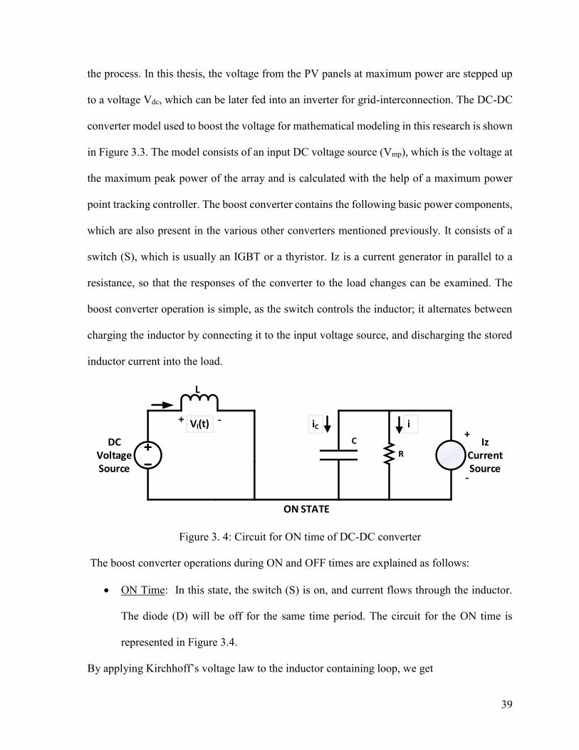
DC Voltage Source

Iz Current Source

L

C

R

ON STATE

+ -

+

-

Vl(t) iC i

Figure 3. 4: Circuit for ON time of DC-DC converter

The boost converter operations during ON and OFF times are explained as follows:

ON Time: In this state, the switch (S) is on, and current flows through the inductor.

The diode (D) will be off for the same time period. The circuit for the ON time is

represented in Figure 3.4.

By applying Kirchhoff’s voltage law to the inductor containing loop, we get

40

mp

l vdt

diL …………………………....………….. (3.23).

And by applying Kirchhoff’s current law on the node of the capacitor branch, we get

iidt

dvC

z

c ……………………………………… (3.24),

R

vi

dt

dvC c

z

c …………..…………………………. (3.25).

The two equations (3.23) and (3.25) mathematically represent the boost converter in ON

time.

OFF State: In this state, the switch is off and the current is flowing through the diode

(D) into the capacitor. The circuit is shown in Figure 3.5.

Iz Current Source

L

C

RDC

Voltage Source

OFF STATE

+

-

iCi

iZ

Figure 3. 5: Circuit for OFF time of DC-DC converter

When applying Kirchhoff’s voltage law to the loop containing the inductor and the capacitor,

we obtain the following equation:

cmp

l vvdt

diL …………………………………..… (3.26).

Similar, to the procedure followed in ON, when applying Kirchhoff’s current law to the node

with the capacitor, the following equation is derived:

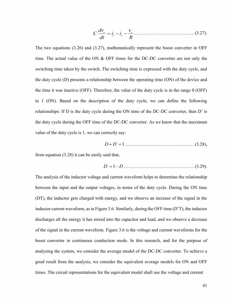
41

R

vii

dt

dvC c

zl

c ……………………………..….. (3.27).

The two equations (3.26) and (3.27), mathematically represent the boost converter in OFF

time. The actual value of the ON & OFF times for the DC-DC converter are not only the

switching time taken by the switch. The switching time is expressed with the duty cycle, and

the duty cycle (D) presents a relationship between the operating time (ON) of the device and

the time it was inactive (OFF). Therefore, the value of the duty cycle is in the range 0 (OFF)

to 1 (ON). Based on the description of the duty cycle, we can define the following

relationships: If D is the duty cycle during the ON time of the DC-DC converter, then D’ is

the duty cycle during the OFF time of the DC-DC converter. As we know that the maximum

value of the duty cycle is 1, we can correctly say:

1' DD ……………………………………… (3.28),

from equation (3.28) it can be easily said that,

DD 1'………………………………………. (3.29).

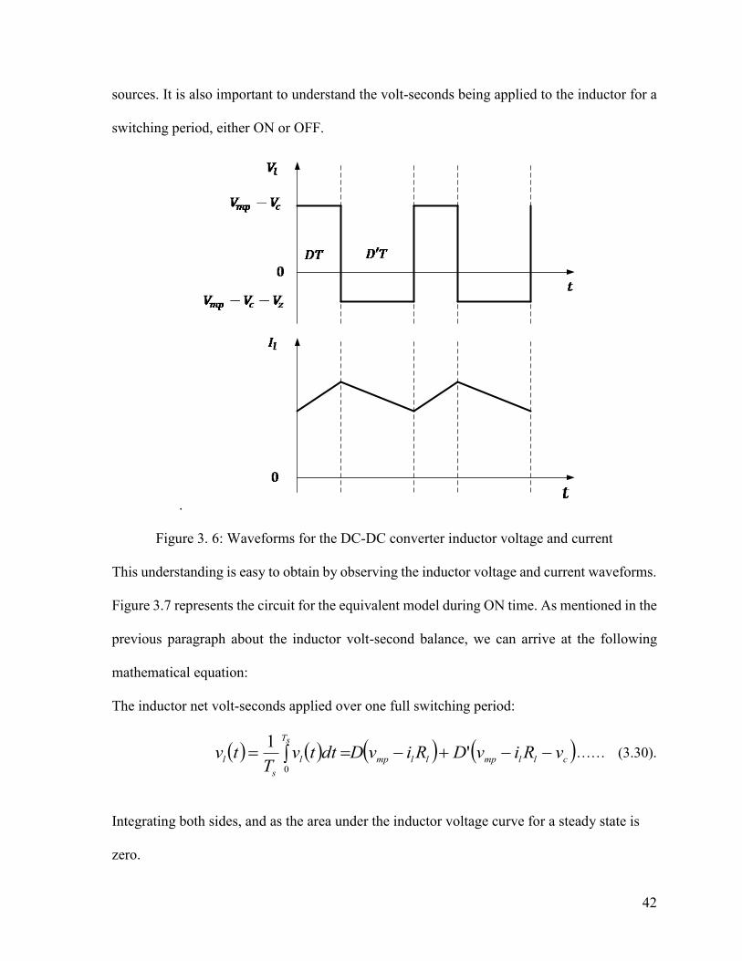
The analysis of the inductor voltage and current waveform helps to determine the relationship

between the input and the output voltages, in terms of the duty cycle. During the ON time

(DT), the inductor gets charged with energy, and we observe an increase of the signal in the

inductor current waveform, as in Figure 3.6. Similarly, during the OFF time (D’T), the inductor

discharges all the energy it has stored into the capacitor and load, and we observe a decrease

of the signal in the current waveform. Figure 3.6 is the voltage and current waveforms for the

boost converter in continuous conduction mode. In this research, and for the purpose of

analyzing the system, we consider the average model of the DC-DC converter. To achieve a

good result from the analysis, we consider the equivalent average models for ON and OFF

times. The circuit representations for the equivalent model shall use the voltage and current

42

sources. It is also important to understand the volt-seconds being applied to the inductor for a

switching period, either ON or OFF.

.

Figure 3. 6: Waveforms for the DC-DC converter inductor voltage and current

This understanding is easy to obtain by observing the inductor voltage and current waveforms.

Figure 3.7 represents the circuit for the equivalent model during ON time. As mentioned in the

previous paragraph about the inductor volt-second balance, we can arrive at the following

mathematical equation:

The inductor net volt-seconds applied over one full switching period:

cllmpllmp

sT

l

s

lvRivDRivDdttv

Ttv '

1

0

…… (3.30).

Integrating both sides, and as the area under the inductor voltage curve for a steady state is

zero.

43

DC

Voltage

Source

ON STATE

+ -

+-

D’Vc

L

Figure 3. 7: Equivalent circuit for ON state of DC-DC converter

Equating (3.30) to zero,

cllmp

vDDDRiDDv 0

cllmpvDRiv 0

cllmpl

vDRivv ……….…..….…………… (3.31).

The principles of inductor volt-second balance state that the average values of the periodic

inductor voltage are zero when the converter operates in a steady state.

Iz

Current

Source

R

OFF STATE

+

-

i

D’Ic

Figure 3. 8: Equivalent circuit for OFF state of DC-DC converter

To determine these steady-state conditions for the DC-DC converter, we equate their average

values to zero. We obtain equation (3.31) after equating to zero. Similarly, the OFF time

44

represented in Figure 3.8 follows the principles of the capacitor charge balance technique,

which is the same procedure as for the ON time.

Similarly, the capacitor charge balance over a full switching period:

R

viD

R

vDdtti

Tti c

z

csT

c

s

c'

1

0

………………… (3.32).

Integrating both sides, as the area under the capacitor current waveform is zero.

Equate (3.32) to zero,

z

c iDDDR

v''0

z

c iDR

v'0

ci

z

c iDR

v' ……………………..………….. (3.33).

Equation ((3.33) helps to determine the DC component of the inductor current. A complete

equivalent circuit, a combination of the ON and OFF states, is shown in Figure 3.9. The

mathematical equations (3.31) and (3.33) represent the DC-DC converter as a boost converter.

The power generated at the DC-DC converter is DC power, which when generated in excess

cannot be supplied to the utility/grid, as the grid supplies only AC power. We therefore need

an inverter to convert the generated DC power to AC power. Before connecting the inverter,

we connect a capacitor to achieve the power balance on the DC-DC converter side as well as

on the DC-AC inverter side.

45

Vmp

+ -

+

-D’ImpD’Vdc Vdc

C

L

imp

Figure 3. 9: Equivalent circuit for DC-DC converter

3.4 Modeling of PV System Dynamics

The most crucial link in the modeling of the whole system is the DC-link capacitor, which

follows the principle of power balance. The equation (34) shows the power balance equation

dcpv

dc PPdt

dvC

2

2………………………………….. (3.34),

here, Ppv is the power being drawn by the capacitor from the PV array, and Pdc is the power

drawn by the DC-side of the inverter. By assuming that the power losses in the inverter and

the filter are negligible, we can conclude that the power being delivered to the input will be

equal to the power at the output terminals of the inverter at the point of common connection.

This gives the following equation (3.35).

acdc PP ……………..…………………….……… (3.35),

where Pac is the power being delivered to the grid at point of common connection.

*IVrealPPsacdc

……………………………. (3.36),

46

when substituting the values of (3.36) in (3.34) we get,

*

2

2IVrealP

dt

dvCspv

dc ………..……………… (3.37).

The equation (3.37) represents the dynamics of the DC-link capacitor. This equation depends

on the dynamics of the inverter current as well.

3.5 Modeling of Grid Connected Inverter

Figure 3.10: Averaged inverter control and PLL

In the previous chapter, we read about the different configurations and topologies of the

inverters available to use for grid interconnection. The inverter may also decide on the voltage

level at which the PV panel operates, or use the maximum power point tracking function to

identify the operating voltage point. The inverter is designed to operate in sync with the utility

or grid (i.e. unity power factor), and it generally delivers the maximum power to the electric

utility/grid, depending on the environmental conditions for PV power generation.

47

For analyzing purposes, we will use the average inverter model. Figure 3.10 shows the average

model of the three phase VSI inverter. The inverter’s current dynamics can be represented by

equations (3.38) and onwards. The inverter is the start of the connection with the grid. The

inverter uses the DC voltage provided by the DC-DC converter (boost) and converts it to AC

voltage. It has an in series inductor that acts as a filter. The average model is used in this thesis,

as it is suitable for analytical purposes. In the average model, we replace the PWM generator,

DC sources, and switches (i.e. insulated gate bipolar transistors IGBT’s) by ideal voltage

sources. These are controlled by the inverter control block. The generator terminal voltage is

the sum of the voltage drop across the inductive filter and the inverter terminal voltages. va, vb

and vc are inverter terminal voltages, and vsa, vsb and vsc are the generator terminal voltages.

Figure 3.11: Equivalent circuit for grid connected DC-AC converter

The equations for the analysis are given in the synchronous reference frame dq, as seen in

Figure 3.10. We will be using the grid synchronization technique of Park’s Transformation, as

mentioned in Chapter 2. The mathematical equations describing the change of reference

frames from abc to dq, and dq to abc, are expressed by equations (3.38) and (3.39) respectively.

The equivalent circuit for the PV system connected to the inverter is shown in Figure 3.11.

The left half of the Figure 3.11 is the equivalent circuit of the PV panel and the DC-DC

converter with the DC-link capacitor. The right half of Figure 2.11 depicts the equivalent

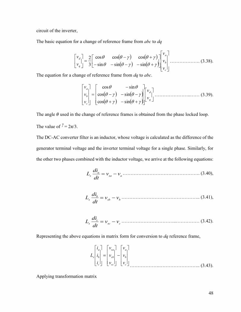
48

circuit of the inverter,

The basic equation for a change of reference frame from abc to dq

c

b

a

q

d

v

v

v

v

v

sinsinsin

coscoscos

3

2………………. (3.38).

The equation for a change of reference frame from dq to abc.

q

d

c

b

a

v

v

v

v

v

sincos

sincos

sincos

…………………..…… (3.39).

The angle 𝜃 used in the change of reference frames is obtained from the phase locked loop.

The value of = 2π/3.

The DC-AC converter filter is an inductor, whose voltage is calculated as the difference of the

generator terminal voltage and the inverter terminal voltage for a single phase. Similarly, for

the other two phases combined with the inductor voltage, we arrive at the following equations:

asa

a

svv

dt

diL …………………………………………. (3.40),

bsb

b

svv

dt

diL ………………………………………….. (3.41),

csc

c

svv

dt

diL ……………………………..…………… (3.42).

Representing the above equations in matrix form for conversion to dq reference frame,

c

b

a

sc

sb

sa

c

b

a

s

v

v

v

v

v

v

i

i

i

L

……………….…………………….. (3.43).

Applying transformation matrix

49

c

b

a

sc

sb

sa

c

b

a

s

v

v

v

T

v

v

v

T

i

i

i

TL

.

…………………………....……. (3.44).

Here, T is the transformation matrix shown in (3.45)

sinsinsin

coscoscosT …………...……. (3.45).

The terms in (3.44) will become

q

d

c

b

a

v

v

v

v

v

T

……………………………………………. (3.46a),

sq

sd

sc

sb

sa

v

v

v

v

v

T

…………………………………………… (3.46b),

q

d

q

d

c

b

a

i

iAT

i

i

i

i

i

T 1

ˆ

ˆ

…………………….………….. (3.46c).

ω is the measured voltage frequency ωPLL, which can be calculated at the PLL. After

applying the transformations we get,

dsqsdsdiLiLvv ………………………….……….. (3.47),

qsdsqsqiLiLvv …………………………..……….. (3.48).

Equations (3.47) and (3.48) are the main equations for the inverter and filter.

The capacitor in Figure 3.11 is nothing but the DC link which shows us the conversion of

DC power to AC power, and its connection. We already know that one of equations used to

ensure the equality of the power, for transmission is:

50

acdc PP …………………………………….. (3.49a),

this is,

qqdddcdciviviv . …………………….………….. (3.49b).

The power relation shown above in (3.49a) is the instantaneous power. Thus, the values of

the current and voltage in equation (3.49b) are all instantaneous values. From Figure 3.11 we

can deduce that the instantaneous value for DC current is.

dcmp

dc iidt

dvC ………………………………….. (3.50),

re-arranging the equation, taking into account overall equivalent model, we get the duty cycle

factor in it as well:

dcmp

dc iiDdt

dvC ' ………………..………………. (3.51).

A grid connected inverter is used to generate electrical quantities at a fixed frequency. The

grid is modeled as a simple AC source with line impedance. The equations for the voltage at

the grid connection point are expressed in abc form, as follows:

a

a

gagae

dt

diLiRv ………………………………. (3.52a),

b

b

gbgbe

dt

diLiRv ………………………………. (3.52b),

c

c

gcgce

dt

diLiRv ……………………………….. (3.52c).

The Rg and Lg are the line impedance in the grid side. We can express the equations (3.52) in

matrix form as follows:

c

b

a

c

b

a

g

c

b

a

g

c

b

a

e

e

e

i

i

i

L

i

i

i

R

v

v

v

……………………….. (3.53),

51

converting to the dq transform:

c

b

a

c

b

a

g

c

b

a

g

c

b

a

e

e

e

T

i

i

i

TL

i

i

i

TR

v

v

v

T

………………….. (3.54).

The values for the transforms of equation (3.54) are shown below:

q

d

c

b

a

v

v

v

v

v

T

…………………………………………. (3.55a),

q

d

c

b

a

i

i

i

i

i

T

………….………………………………. (3.55b),

q

d

q

d

c

b

a

i

iAT

i

i

i

i

i

T 1

…………………………… (3.55c),

q

d

c

b

a

e

e

e

e

e

T

………………………………………… (3.55d).

When the equations of (3.55) are substituted in (3.54) we get the following:

q

d

q

d

q

d

g

q

d

g

q

d

e

e

i

iAT

i

iL

i

iR

v

v1

……………….. (3.56).

When we open the term in equation (3.56), we get

sin

cos

E

E

i

iL

i

i

RL

LR

v

v

q

d

g

q

d

q

d

……………. (3.57).

From (3.57) we deduce the values for ed and eq as

PLLd Ee cos…………………………..………… (3.58),

52

PLLq Ee sin

……………………….…………… (3.59).

The equations (3.58) and (3.59) are the final grid equations in the dq form.

3.6 Phase Locked Loop (PLL) Design

A three-phase PLL helps to find the angle and frequency information of the grid voltage

coming to the inverter. The angle obtained will be used for the conversion of the reference

frames from abc to dq. We consider the inverter terminal voltages in three-phases, as follows:

0

cos tVva

………………………………… (3.60a),

03

2cos

tVv

b…………..….…..……... (3.60b),

03

2cos

tVv

c………….…….……….. (3.60c).

Where V is the voltage magnitude and ω is the voltage frequency. At a steady state of

operation, the system will have an initial phase angle δo.

abc

dq

sin, cos

Figure 3.12: PLL control

Figure 3.12 represents the PLL control structure used in the research.

We assume that a change in the phase reflects a change in the voltage frequency, so we have

53

t ………………………………………….. (3.61),

where δ is the unknown angle, the change shall be shown by considering the derivative of the

angle, thus representing a change in the voltage frequency. This is mathematically represented

in equation (3.62).

o ………………………………………….. (3.62).

The angle in which we are interested is θ; it is being tracked by the phase locked loop measured

angle θPLL. From the grid equations mentioned previously, we know that:

sin

cos

V

V

v

v

q

d

sinVvq ……………………….………….. (3.63).

The measured inverter terminal voltage angle from PLL is θPLL. This value tracks the actual

voltage angle θ. The difference between them is seen when a transition occurs. The value of

the measured voltage phase angle is defined as:

toPLLPLL

……………….………………….. (3.64).

We make use of a simple PI controller to the find the correct difference in the frequency.

This difference is then added to the system as ωo, as seen in Figure 3.12. To obtain the exact

frequency, we add the initial voltage frequency to the difference, as follows:

oq

iPLL

pPLLPLLv

s

kk

……………………… (3.65).

So equation (62) can be re-written as

54

oPLLPLL …………………………………. (3.66).

The actual voltage angle θPLL can be calculated by considering the integral of equation (3.66).

3.7 Design of Current Control

As mentioned in Chapter 2 when discussing the various controls used in this thesis, we shall

explain the inverter’s role in the current and voltage control. To control the quality of the

output power being delivered to the grid, we use a current control and a voltage control as the

DC-AC converter control. The inverter control block consists of a voltage regulator (voltage

controller) and a current regulator (current controller). Fig 3.13 shows the voltage and current

controllers.

Figure 3.13: The voltage and current controllers

From Figure 3.13 we can observe that the proportional-integral (PI) controllers are used with

qsPLL iL and dsPLL iL as the decoupling components. This thesis uses a technique to control

the DC voltage, which in turn controls the power, as power is the product of voltage and

current. The constant current control acts as an inner current loop. The active current reference

55

drefi comes from the voltage controller. The following equations can be derived from the

controller structures:

s

kkvvi

ip

ppdcdcrefdref………………………….. (3.67a),

s

kkQQi

ip

pprefqref…………………….……… (3.67b),

qsPLLd

ii

piddrefsdiLv

s

kkiiv

……………….. (3.68),

dsPLLq

ii

piqqrefsqiLv

s

kkiiv

………….…… (3.69).

The output voltage of the filter in connection with the grid controller is given by:

dsqsPLLdsdiLiLvv ……………………..……….. (3.70a),

qsdsPLLqsqiLiLvv ………...……………………… (3.70b).

The output of current control is the compensation for the drop in voltage across the filter.

The equation is given by

ddref

ii

pidii

s

kku

1……………………...……….. (3.71a),

qqref

ii

piqii

s

kku

1……………………...……….. (3.71b).

The active and the reactive powers at the inverter terminal can be measured as follows

qqddivivP ………………………………..………. (3.72a),

dqqdivivQ ………………………..………………. (3.72b).

The inverter controller equations above are all expressed in the per unit system. The three-

phase per unit system adopted in the thesis is as follows:

56

base

base

baseI

VZ ………………………………………….. (3.73),

base

base

baseV

SI

3

2 ……….………………………………... (3.74).

The Vbase is the system rated voltage at a peak value, and the Sbase is the three-phase system

base power. The angle and frequency information is obtained from the PLL, as seen in the

previous section.

Thus, with the inverter control design, we complete the entire PV system connected to the grid.

This chapter provided a detailed description of the mathematical modeling of all the

components of the PV system, from the PV cell to the grid side. Thus, able to successfully

derive the mathematical equations for the PV cell, the DC-DC converter, the link capacitor,

the DC-AC converter, and the grid. These equations help to design the system in an

environment where various parameters can be tested for its stability.

57

Chapter 4

Small Signal Modeling of the Grid-connected Photovoltaic System

4.1 Introduction

This chapter shall present large signal analysis and small signal analysis conducted within

this thesis.

We saw in Chapter 3 that the mathematical equations for the PV system connected to a grid

were designed. These equations will be used to create a model on which the above mentioned

two analyses will be performed.

The large signal analysis shall be done by creating an average model of the PV system in the

MATLAB/Simulink environment, with the help of the equations. This model will help us to

understand how the system works, and thus also validate our model.

The small signal analysis is conducted on the same model but by following a different

procedure. This procedure is explained in this chapter and the results of this analysis will help

to understand the various parameters that affect the PV system. Finally, the chapter concludes

with a comparison of the average and detailed large signal models and their results.

4.2 Small Signal Analysis

Small signal stability, as defined in [12], is a system’s ability to be stable or maintain

synchronism when subjected to small disturbances. The disturbances mentioned in the

definition depend on the equation description of the system response, which, for the purpose

of analysis, can be linearized. In the power systems available today, the problem of small-

signal stability arises due to insufficient damping. This need for damping is the result of either

the increasing amplitude of the rotor oscillations or the steady increase in the rotor angle of

the generator, the latter being caused by a lack of synchronizing torque [41]. The small signal

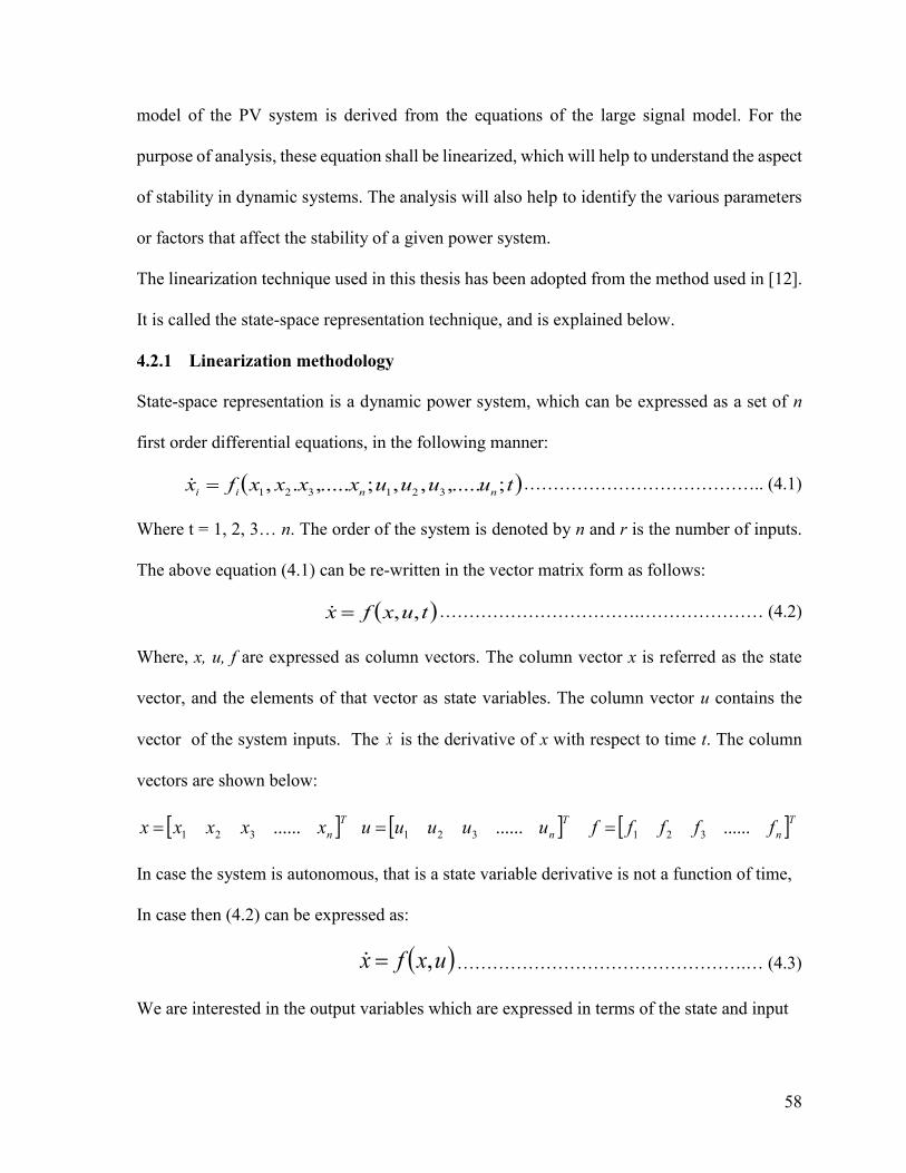
58

model of the PV system is derived from the equations of the large signal model. For the

purpose of analysis, these equation shall be linearized, which will help to understand the aspect

of stability in dynamic systems. The analysis will also help to identify the various parameters

or factors that affect the stability of a given power system.

The linearization technique used in this thesis has been adopted from the method used in [12].

It is called the state-space representation technique, and is explained below.

4.2.1 Linearization methodology

State-space representation is a dynamic power system, which can be expressed as a set of n

first order differential equations, in the following manner:

tuuuuxxxxfxnnii;,.....,,;,......,

321321 ………………………………….. (4.1)

Where t = 1, 2, 3… n. The order of the system is denoted by n and r is the number of inputs.

The above equation (4.1) can be re-written in the vector matrix form as follows:

tuxfx ,, …………………………….………………… (4.2)

Where, x, u, f are expressed as column vectors. The column vector x is referred as the state

vector, and the elements of that vector as state variables. The column vector u contains the

vector of the system inputs. The x is the derivative of x with respect to time t. The column

vectors are shown below:

Tnxxxxx ......321 Tnuuuuu ......321 Tnfffff ......321

In case the system is autonomous, that is a state variable derivative is not a function of time,

In case then (4.2) can be expressed as:

uxfx , ………………………………………….… (4.3)

We are interested in the output variables which are expressed in terms of the state and input

59

Variables are:

uxgy , ……………………………………………. (4.4)

Where y and g are column vectors representing the output variables and the nonlinear function

of input variables and state variables. These column vectors are shown below:

Tm

yyyyy ......321

Tm

ggggg ......321

A set of n linearly dependent variables in a system can be used to describe the state of the

system. These variables are referred to as state variables. These variables, along with the

system inputs, can provide a complete description of the behavior of the system. A

mathematical variable, or a physical quantity such as voltage, speed, etc., can qualify as a state

variable, which in turn can describe the system dynamics. Any set of chosen state variables

will provide the same information about the system dynamics. Defining too many state

variables may lead to a redundancy in the variables, and they will become dependent on some

of the other variables. The state of the system can be represented in an n dimension Euclidean

space called the state space [12]. The next step is the identification of the equilibrium points

or the steady state points. This is achieved by equating the derivatives in the system to zero.

00xf ………………………………………….. (4.5)

Here, xo is the state vector, and x is the equilibrium point. While testing local stability, or

stability in the small or the small signal analysis, we consider the system to be stable around

an equilibrium point or a steady state point, and then subject the system to small perturbations.

Consider the equation (4.3), in which xo is the initial state vector and uo is the input variable at

a steady state point. We introduce a small perturbation into the system, which leads to the

following new variables:

60

xxx 0 uuu

0

Where Δ denotes the small deviation, all perturbations are assumed to be small, and the terms

are expressed with the help of Taylor’s series expansion. The higher order terms are neglected

for the purpose of analysis.

The linearized set of equations are finally expressed in the following way:

xAxE ˆˆ ……………………………………. (4.6)

Where term E represents a matrix with the coefficients of the derivative part of size n*n.

The term A represents a state matrix of size n*n. After the calculation of the state-space matrix

for a steady state point of the entire power system, we can check for the Eigen properties of

the matrix. The eigenvalues can be real or complex values, and always occur in conjugate pairs

[12]. The significance of eigenvalues is explained as follows: The real component of the

eigenvalues gives the damping, and the imaginary component gives the oscillation. A negative

real part represents a damped oscillation whereas a positive real part represents an oscillation

of increasing amplitude [12].

We can calculate the frequency of oscillation and the damping ratio from a pair of eigenvalues.

A complex pair of eigenvalue is represented generally as:

j ………………………………………. (4.7).

The frequency of the oscillations is calculated in Hz as:

2

OSCf …………………………………………. (4.8).

The damping ratio is calculated as:

22

……………………………………. (4.9).

61

As mentioned previously, in this thesis the methodology was developed and the small signal

stability test were conducted on the PV system. Some of the small signal linearized equations

are shown in the next section. A complete list of the small signal linearized equations is

available in Appendix B.

4.3 Small Signal of the PV System Connected to a Parallel RLC Load

Figure 4.1 shows a three-phase PV system with a parallel RLC load connected to the grid. The

PV system shown above is considered for the small signal stability analysis. R and L are the

distribution line impedance. A circuit breaker is placed between the grid and the distributed

generation system. The power being delivered by the PV-DG system is𝑃𝐷𝐺 ,𝑄𝐷𝐺. The power

flowing to the parallel RLC load is𝑃𝐿,𝑄𝐿. The difference of the power consumed by the load

and the PV-DG supplied power is then fed to the distribution system or grid, i.e. 𝑃𝐺 ,𝑄𝐺. The

direction of the power flow is defined from the DG side to the grid side. The current of the DG

are cba iii ,, . The parallel RLC branch currents are as follows for the RL branch is RcRbRa iii ,,

for the LL branch is LcLbLa iii ,, and for the CL branch is CcCbCa iii ,, . The current flowing through

the distribution line is GcGbGa iii ,, and the and the terminal voltages of the PV-DG system are

cba vvv ,, .

The equations for the system shown in Figure 4.1 are expressed as follows:

a

Ga

Gaae

dt

diLRiv ………………………………. (4.10a)

b

Gb

Gbbe

dt

diLRiv ………………………………. (4.10b)

c

Gc

Gcce

dt

diLRiv ………………………...…….. (4.10c)

62

Figure 4.1: PV system connected to a parallel RLC load

The equation for the PV-DG current is the sum of the currents through the load and the current

flowing to the grid. This is expressed as follows:

GaCaLaRaa iiiii ………………………………. (4.11a)

GbCbLbRbb iiiii ………………..……….…….. (4.11b)

GcCcLcRcc iiiii ……………..…………………. (4.11c)

The value for the current flowing through the load resistance can be calculated by using the

Ohms law; it is found by dividing the DG terminal voltage with the load resistance.

L

a

RaR

vi ………………………………………….. (4.12a)

L

b

RbR

vi ………………………………………….. (4.12b)

63

L

c

RcR

vi ………………………………………….. (4.12c)

The relation between the load inductance, the capacitance to the terminal voltages, and the

current are shown below

LaLa

idt

dLv ………………………………………….. (4.13a)

LbLbi

dt

dLv ………………………………………….. (4.13b)

LcLci

dt

dLv ………………………………………….. (4.13c)

The load capacitance equations:

aLCav

dt

dCi ………………………………………….. (4.14a)

bLCbv

dt

dCi ………………………………………….. (4.14b)

cLCcv

dt

dCi ………………………………………….. (4.14c)

These equations are also represented in the dq frame

dGqPLL

Gd

GddeLi

dt

diLRiv …………………. (4.15a)

qGdPLL

Gq

GqqeLi

dt

diLRiv …………………. (4.15b)

Similarly, the dq reference frame equations for the DG current, the load resistance, and the

inductance and capacitance are shown below:

GdCdLdRdd iiiii ………………………………. (4.16a)

GqCqLqRqq iiiii ………………………………. (4.16b)

64

L

dRd

R

vi ………………………………………….. (4.17a)

L

q

RqR

vi ………………………………………….. (4.17b)

LqLPLLLd

Ld iLdt

diLv ……………………………. (4.18a)

LdLPLL

Lq

Lq iLdt

diLv ……………………………. (4.18b)

qLPLLdLCd vCvdt

dCi …………………………... (4.19a)

dLPLLqLCq vCvdt

dCi …………………………... (4.19b)

As mentioned in Chapter 3, the angle of the transformation is obtained from the PLL, as it is

in the case of the transformations conducted above for the PV system with a parallel RLC load.

The remaining set of equations are the same as modelled before. The detailed set of linearized

equations as well as the state-space matrix for the entire system is shown in Appendix B and

Appendix C.

4.4 Model Validation

The PV distributed generation system designed in Chapter 3 and Chapter 4 was constructed

with the help of MATLAB 2014b and the Simulink Toolbox. The exact parameters are

mentioned in Appendix A. In the following sections, we consider two cases for model

verification; the case of a small signal stability analysis without PSS, and the case of a large

signal model analysis of the average and detailed models.

65

4.4.1 Small signal stability analysis of PV system without PSS

Figure 4.2: Eigenvalue plot for the PV system without PSS controller

The system in Figure 2.1 is linearized and a small signal model is generated from the large

signal model by following the procedure explained previously in this chapter. The model

considered for the small signal stability analysis is one without the power system stabilizer.

The steady state points are calculated and used for the eigenvalue analysis, and the reference

command qŗef is set to zero. The eigenvalue analysis helps to understand the PV system’s

control against the variations in the parameters of the system. The operating conditions are G

= 1000 W/m2 and Vdc = 550 V. The eigenvalues plotted in Figure 4.2 are all in the left half of

the s-plane, therefore the system is said to be stable, as per Lyapunov’s first method. Table 4.1

reports the eigenvalues of the overall system with calculations for the damping ratio and their

oscillating frequencies. The base values are set and calculated for the per unit system. The

steady state values of the PV system, which were obtained in the analysis, can be seen in

66

Appendix A.

Table 4.1: Eigenvalues for PV system without PSS

λ = σ ± jω σ 𝜔 ξ 𝑓𝑜𝑠𝑐

𝜆1, 𝜆2 -165.02±j922.2 -165.0201 922.27509 0.17613 146.78

𝜆3, 𝜆4 -7.10±j375.35 -7.104521 375.35074 0.01892 59.97

𝜆5, 𝜆6 -18.64±j267.54 -18.64304 267.54748 0.06951 42.58

𝜆7, 𝜆8 -206.3±j191.76 -206.3377 191.76182 0.73250 30.52

𝜆9, 𝜆10 -7.88±j19.55 -7.881436 19.5548 0.37382 3.11

𝜆11 -6.419 -6.419737 0 1 0

𝜆12 -132.644 -132.6444 0 1 0

𝜆13 -240.412 -240.4123 0 1 0

𝜆14 -260.351 -260.3511 0 1 0

𝜆15 -0.02496 E+8 -2496250.3 0 1 0

𝜆16 -2.26590 E+8 -226590471.5 0 1 0

We use a participation matrix in order to obtain the association of the state variables and the

eigenvalues. The element in the matrix in (4.21) is called as the participation factor. The

participation factor is the measure of participation of a state variable in a particular mode and

vice versa. The participation factors for the system are shown in Table 4.2. The values

highlighted in the Table 4.2 show the maximum participation of the state variables. Thus,

helping to identify the relation between the eigenvalue and the state variable.

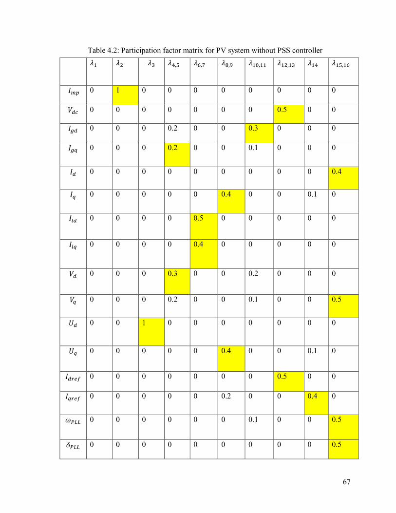
67

Table 4.2: Participation factor matrix for PV system without PSS controller

𝜆1 𝜆2 𝜆3 𝜆4,5 𝜆6,7 𝜆8,9 𝜆10,11 𝜆12,13 𝜆14 𝜆15,16

𝐼𝑚𝑝 0 1 0 0 0 0 0 0 0 0

𝑉𝑑𝑐 0 0 0 0 0 0 0 0.5 0 0

𝐼𝑔𝑑 0 0 0 0.2 0 0 0.3 0 0 0

𝐼𝑔𝑞 0 0 0 0.2 0 0 0.1 0 0 0

𝐼𝑑 0 0 0 0 0 0 0 0 0 0.4

𝐼𝑞 0 0 0 0 0 0.4 0 0 0.1 0

𝐼𝑙𝑑 0 0 0 0 0.5 0 0 0 0 0

𝐼𝑙𝑞 0 0 0 0 0.4 0 0 0 0 0

𝑉𝑑 0 0 0 0.3 0 0 0.2 0 0 0

𝑉𝑞 0 0 0 0.2 0 0 0.1 0 0 0.5

𝑈𝑑 0 0 1 0 0 0 0 0 0 0

𝑈𝑞 0 0 0 0 0 0.4 0 0 0.1 0

𝐼𝑑𝑟𝑒𝑓 0 0 0 0 0 0 0 0.5 0 0

𝐼𝑞𝑟𝑒𝑓 0 0 0 0 0 0.2 0 0 0.4 0

𝜔𝑃𝐿𝐿 0 0 0 0 0 0 0.1 0 0 0.5

𝛿𝑃𝐿𝐿 0 0 0 0 0 0 0 0 0 0.5

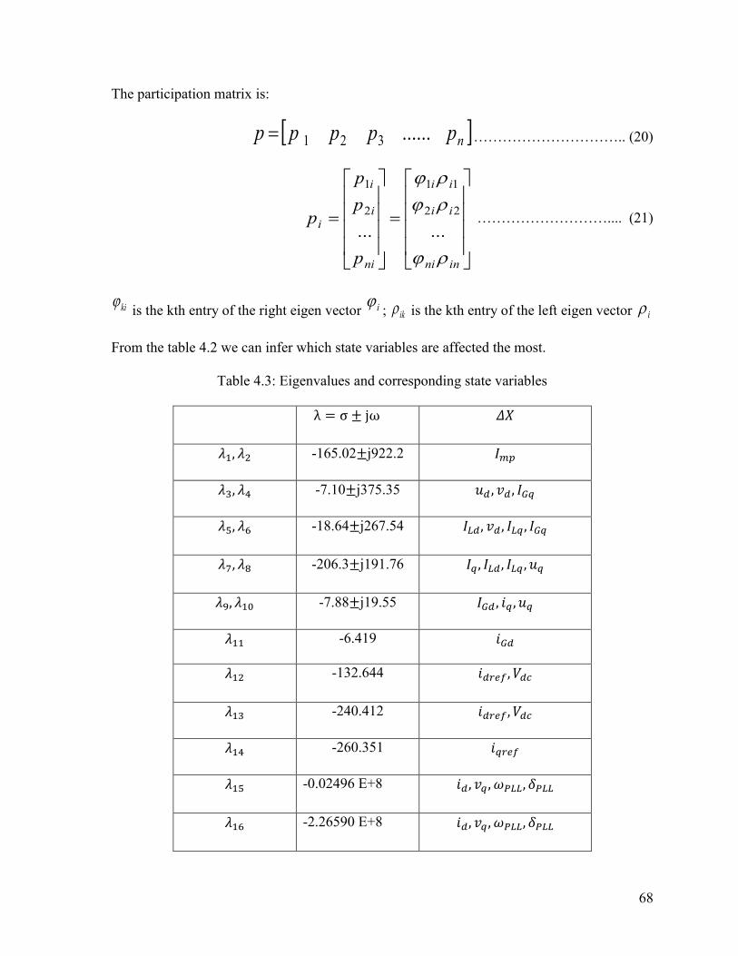
68

The participation matrix is:

nppppp ......321 ………………………….. (20)

inni

ii

ii

ni

i

i

i

p

p

p

p

......

22

11

2

1

……………………….... (21)

ki is the kth entry of the right eigen vector i ; ik is the kth entry of the left eigen vector i

From the table 4.2 we can infer which state variables are affected the most.

Table 4.3: Eigenvalues and corresponding state variables

λ = σ ± jω 𝛥𝑋

𝜆1, 𝜆2 -165.02±j922.2 𝐼𝑚𝑝

𝜆3, 𝜆4 -7.10±j375.35 𝑢𝑑 , 𝑣𝑑 , 𝐼𝐺𝑞

𝜆5, 𝜆6 -18.64±j267.54 𝐼𝐿𝑑, 𝑣𝑑 , 𝐼𝐿𝑞 , 𝐼𝐺𝑞

𝜆7, 𝜆8 -206.3±j191.76 𝐼𝑞 , 𝐼𝐿𝑑, 𝐼𝐿𝑞 , 𝑢𝑞

𝜆9, 𝜆10 -7.88±j19.55 𝐼𝐺𝑑 , 𝑖𝑞 , 𝑢𝑞

𝜆11 -6.419 𝑖𝐺𝑑

𝜆12 -132.644 𝑖𝑑𝑟𝑒𝑓, 𝑉𝑑𝑐

𝜆13 -240.412 𝑖𝑑𝑟𝑒𝑓, 𝑉𝑑𝑐

𝜆14 -260.351 𝑖𝑞𝑟𝑒𝑓

𝜆15 -0.02496 E+8 𝑖𝑑, 𝑣𝑞 , 𝜔𝑃𝐿𝐿, 𝛿𝑃𝐿𝐿

𝜆16 -2.26590 E+8 𝑖𝑑, 𝑣𝑞 , 𝜔𝑃𝐿𝐿, 𝛿𝑃𝐿𝐿

69

The participation factor table values have been rounded and the thousand place and

participation factor values below 0.001 have been considered as zero in the table. From the

table 4.2 we can infer which state variables are affected the most. We observe from the matrix,

that the eigenvalue λ2 = -165.02 – j922.2 which belongs to the PV panel in the system, as the

state variable which shows dominant participation of the eigenvalue λ2 is that of the current at

maximum power of the panel. In the Table 4.2, the relationship between the eigenvalues and

the corresponding state variables is evident. The participation factor matrix helps to derive

these results, clearly showing which parameters in the system are affected by the dominant

eigenvalues. This analysis helps us to understand the system better and improve its

performance by focusing only on the variables with a high value of participation for that mode

of operating points.

4.4.2 Large signal model analysis of PV system

Figure 4.3: DC-voltage for the Average and Detailed large signal model without PSS

70

The model being validated in this section is the large signal model that was described in

Chapters 2 and 3. The system equations designed in the previous chapters are used to build a

model in the MATLAB2014b environment by making use of the Simulink toolbox.

Figure 4.4: DC link voltage for PV system

The system equations developed were the large signal equations, and with the help of these

equations a large signal model is developed for analysis. In this thesis we have developed the

average model and the switching or detailed model to validate the equations. The two models

differ from each other due to their components.

The basic components are the same, i.e., the PV panel, the MPPT controller, DC-DC converter,

and the grid connected DC-AC inverter. In the detailed model, the DC-DC converter or boost

used consists of IGBT switches, and the pulses for switching are produced by the pulse width

modulation. Figure 4.3 is of the dc link voltage, as it is one of the most important parameters

being controlled. The system parameters for the average and detailed models are kept same.

The other parameters are listed in Appendix A.

71

Figure 4.5: Active Power for Average and Detailed model of the system.

We observe that the DC link voltages produced in both the models are very similar, thus

proving that both models, as designed, are operating correctly for the mentioned parameters.

Figure 4.6: Reactive Power for Average and Detailed model of the system.

72

The detailed model curve (red curve) is not clear, as this model uses the forced commutated

devices as switches. The switching action occurs at high rate, resulting in a waveform with lot

of switching in it. Whereas, in the average model, we use a set of power electronic converters

for the switching. These power electronic converters help attain smoother curves. Since the

DC-link voltage is not clearly seen in the Figure 4.3, the proper values can be observed in

Figure 4.4. The other important parameters are the active and reactive powers of the system.

These two parameters can be observed in Figure 4.5 and Figure 4.6.

4.5 Summary

We understand from the figures that the required active power is being delivered and both the

models are in sync with each other as they are producing the same amount of power, thus

validating the design of the system. The small signal stability has also shown that the designed

system is stable. We shall be observing a similar set of results in the following chapter, where

a power system stabilizer is connected. We will try to validate the PSS model designed in the

following chapter.

73

Chapter 5

Power System Stabilizer Design for the Grid-connected Photovoltaic System

5.1 Introduction

This chapter talks about the stability of the power system. It begins with the dynamics of the

power system, which helps to understand the stability aspect of a power system. A general

overview of the power system dynamics is provided.

The chapter also covers the oscillations in a power system, thus describing the need for

damping controllers or power system stabilizers. A general description of the basic structure

of a PSS is then described, followed by the design of the PSS adopted in this thesis.

The model of the PSS investigated as part of this research, based on its design, shall be tested

for its small signal stability, and the results will validate the PSS design described in the thesis.

The results shall also include the calculation of the participation factors for the system with

the PSS. Finally, the chapter concludes with the results of a PV system connected to the grid

with the PSS controller.

5.2 Overview

In the previous chapter we have read about the stability of the power systems. To gain a better

understanding of power system stability, we need to understand the dynamics of it. The term

dynamics means the behavior of the system when it encounters a disturbance. The disturbance

can be a deliberate one, such as the scheduled switching of generators, or an accidental one,

such as the strike of lightning. Power system dynamics are classified on the basis of the time

the system takes to respond to these disturbances [42].

The power system dynamics can be categorized into four types:

Wave dynamics: are more commonly known as surges. They are the fastest

74

dynamics, mostly occurring in high voltage transmission lines. They can be caused by

the switching of operations in the system.

Electromagnetic dynamics: are slower in comparison to wave dynamics. They usually

occur in the windings of the machine, when the system is subjected to a certain

disturbance.

Electromechanical dynamics: When a system is subjected to a disturbance, it not only

affects the power system but also affects the components such as the rotating parts of

the generator or the motor, which get subjected to oscillations due to the disturbance

of the system.

Thermodynamics: This is the slowest type of response to variations or disturbances.

An example is boiler control action in steam power plants.

The growth of new and more complex power systems has led to the birth of various forms of

system instability, leading to the proposal of various stability methods, such as voltage stability

or frequency stability. However, power system stability is, in itself, a problem with different

classes in it.

As mentioned, voltage stability is one of the proposed techniques for system stability. It

basically means the ability of a power system to maintain steady voltages when operating

under normal conditions or when subjected to disturbances. When instability occurs, it is either

caused by a rise or a fall in voltage. One of the main reasons for voltage instability is the loads.

The loads on subject to a disturbance usually restores itself, leading to the consumption of

reactive power and the voltage keeps falling till it collapses. At this no sufficient power transfer

capacity is available nor any generation capability. The problems related to the voltage stability

also arise when weak AC systems are connected to HVDC links. It is useful to sub-categorize

75

the voltage stability as the following:

Large disturbance voltage stability: As the name suggests, it is the system’s ability to

overcome the disturbance and control the voltage of the power system. The large

disturbance can be due to a generation loss or system faults. To determine the large

disturbance stability, we need to analyze the system over a certain period of time to

understand its non-linear dynamic performance. Running dynamic simulations for a

long time can help in the analysis [24].

Small disturbance voltage stability: it is the system’s ability to maintain the voltage

levels when it is subjected to small changes or perturbations. The small changes can be

in the form of small load increments. This method is useful as it helps to understand

the behavior of a system in response to a change at any given time. The essential part

of this analysis is that the entire analysis is conducted for an operating condition or a

steady state. The voltage level in the system increases as the reactive power injection

is increased for the given operating conditions.

The sub-categorization of the different stability techniques is possible as a linear system is

independent of its input. In the case of a non-linear system, it depends on the input and the

initial state of the system. The stability of a non-linear system is generally classified into the

following:

A. Local stability or small signal stability;

B. Finite stability;

C. Global stability or large signal stability.

Local stability or small signal stability is experienced when a system is subjected to a small

perturbation near a steady state point. As time increases, the system will return to its initial or

original state. The system remains stable over a small area around the steady state point. To

76

obtain this stability, we convert the system from non-linear to linear. The technique for

linearization has been explained in Chapter 4 and is adopted in this thesis.

5.3 Oscillations in Power Systems

The need for a power system stabilizer (PSS) or a damping controller in power systems has

been present since the very beginning, when the damping of oscillations was recognized as an

important aspect in the operation of a power system. Over the years, various forms of

oscillations in power systems were identified, and although at one point researchers believed

they had devised a technique to remove the oscillations, they always re-appeared. There are

multiple reasons for these oscillations. To better understand, we shall consider oscillations that

are classified based on their interaction characteristics. They are classified as follows:

Local plant mode oscillations: These oscillations are common at generating stations.

They arise when the units at the power generating station oscillate with respect to the

rest of the units of the generating station. They are usually caused by the generating

units’ AVRs working at high output and feeding weak transmission networks. The

natural frequency of these oscillations lies in the range of 1-2Hz. Damping can be

achieved with the help of PSS, which also helps to understand the characteristics of

the oscillation.

Inter-area mode oscillations: These oscillations occur when machines in one portion

of the system oscillate against machines in other parts of the system. They occur when

a group of machines are kept in close proximity to one another. The natural frequency

of these oscillations lie in the range of 0.1-1 Hz. The characteristics of these

oscillations are more tedious and complex.

Torsional mode oscillations: These are associated with the mechanical aspect of the

77

turbine-generator’s rotational parts. Other instances of these oscillations have been

caused by generating unit excitation [42].

Control mode oscillations: These oscillations are linked to the controls of the

generating units. The usual cause of these oscillations is the poorly tuned control of an

excitation system, HVDC converters, and other similar equipment.

Based on the above classifications of the nature of the power system oscillations, it is observed

that these oscillations in a system are due to its natural mode, and can therefore be damped or

eliminated by modification. It is important to note the following: firstly, power systems are

evolving with time, leading to the formation of new modes. Secondly, the main reason for

negative damping is power system controls, most importantly, excitation systems. Lastly, the

inter-area oscillations involve multiple utilities or DG systems, making Power System

Stabilizers (PSS) the most commonly used method for damping.

5.4 Design of Power System Stabilizer

As we saw in the previous section, the PSS is commonly used for the damping of the

oscillations in a power system.

GAINWASHOUT

FILTERPHASE

COMPENSATION

INPUT

SIGNAL

Figure 5.1: General representation of PSS

There are various representations of the PSS, about which literature was reviewed in Chapter

1, with the same motive of providing damping in the power system. The basic design of the

PSS on which the controller designed in this thesis is based, is explained below, with the help

of Figure 5.1.

78

The three major components of a PSS are shown above: the phase compensator, the washout

filter, and the gain. The phase compensation block is used to compensate for the phase lag

between the output of the PSS and the control action being performed. For different conditions

of the system, the phase compensation also changes. Usually, an agreed-upon phase

compensation is fixed for the different conditions of the power system. The washout filter acts

as a high-pass filter by setting a high time constant, enabling the system to allow only the

signals associated to the system to pass through. It also allows the PSS to respond in situations

when there are changes that are only related to the input signal. The gain decides the amount

of damping being achieved by the PSS. It is often fixed at a value where the maximum amount

of damping can be achieved, but the value might change depending on the other assumptions

made during the design process of the PSS. The addition of the PSS should not decrease the

stability of the system but should instead enhance it.

Figure 5.2: PSS controller diagram in the PV system

79

The power system stabilizer designed and implemented in this thesis is similar to the general

representation seen above. The PSS controller design tested in this thesis is shown in Figure

5.2. From Figure 5.2, we observe that the PSS controller is connected to the inner current

controller loop. The negative frequency feedback signal detects any change in the Vdcref signal,

sending a feedback in the form of If. The error signal is first obtained at the output of the

washout filter block, with a time constant of Tω.

This error signal is then amplified with the help of the negative feedback gain Ksp + Ksi/s.

When the system is connected to a grid, the frequency of the system is determined by that of

the grid. The PSS will destabilize the system when unwanted oscillations affect the system of

operation.

s

kk

sT

sTI si

sp

w

wf

1 ……………..……………… (5.1)

dfdrefii

pid iIis

kku

1 ……………...…………… (5.2)

The mathematical design of the power system stabilizer adopted as part of this thesis is given

by equations (5.1) and (5.2). Now, with the addition of these two new equations we shall design

the large signal model and implement it in a Simulink environment. The small signal model

was developed from this large signal model, to be used in the small signal stability analysis.

The procedure followed for the analysis is the same as the one used for the system without

PSS, as explained in Chapter 4. In the following sections, the validation of the large signal

models with and without PSS is provided, as well as the small signal stability analysis for the

PV system with PSS.

80

5.5 Small Signal Stability Analysis of PV System with PSS

The system is Fig 5.2 is linearized and a small signal model is generated from the large signal

model by following the procedure mentioned in Chapter 4. The model considered for the small

signal stability analysis is one with a power system stabilizer. The steady state points are

calculated and used for the eigenvalue analysis, and the reference command qŗef is set to zero.

The eigenvalue plot for the grid-connected PV system with PSS, introduces a new state

variable and an eigenvalue associated with it (see -1 of Real axis).

Figure 5.3: Eigenvalue plot for system with PSS.

The other eigenvalues plotted in Figure 5.3 have moved more to the left as compared to the

eigenplot for system without PSS. This proves, that the grid-connected PV system is more

stable. The operating conditions are G = 1000 W/m2 and Vdc = 550 V. The eigenvalues plotted

in Figure 5.3 are all in the left half of the s-plane, and the system is said to be stable as per

Lyapunov’s first method. Table 5.1 reports the eigenvalues of the overall system, with

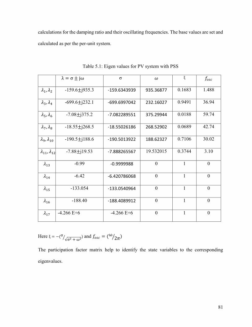
81

calculations for the damping ratio and their oscillating frequencies. The base values are set and

calculated as per the per-unit system.

Table 5.1: Eigen values for PV system with PSS

λ = σ ± jω σ 𝜔 ξ 𝑓𝑜𝑠𝑐

𝜆1, 𝜆2 -159.6±j935.3 -159.6343939 935.36877 0.1683 1.488

𝜆3, 𝜆4 -699.6±j232.1 -699.6997042 232.16027 0.9491 36.94

𝜆5, 𝜆6 -7.08±j375.2 -7.082289551 375.29944 0.0188 59.74

𝜆7, 𝜆8 -18.55±j268.5 -18.55026186 268.52902 0.0689 42.74

𝜆9, 𝜆10 -190.5±j188.6 -190.5013922 188.62327 0.7106 30.02

𝜆11, 𝜆12 -7.88±j19.53 -7.888265567 19.532015 0.3744 3.10

𝜆13 -0.99 -0.9999988 0 1 0

𝜆14 -6.42 -6.420786068 0 1 0

𝜆15 -133.054 -133.0540964 0 1 0

𝜆16 -188.40 -188.4089912 0 1 0

𝜆17 -4.266 E+6 -4.266 E+6 0 1 0

Here ξ = −(σ√σ2 + ω2⁄ ) and 𝑓𝑜𝑠𝑐 = (ω

2𝜋⁄ )

The participation factor matrix help to identify the state variables to the corresponding

eigenvalues.

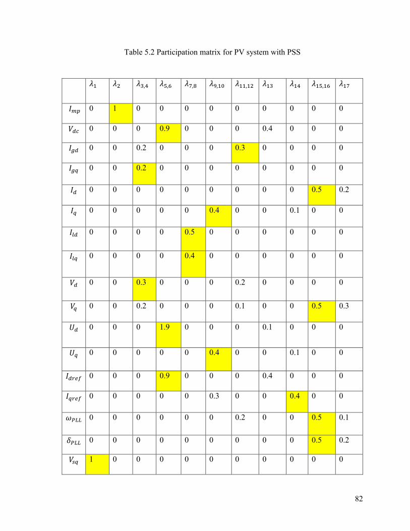
82

Table 5.2 Participation matrix for PV system with PSS

𝜆1 𝜆2 𝜆3,4 𝜆5,6 𝜆7,8 𝜆9,10 𝜆11,12 𝜆13 𝜆14 𝜆15,16 𝜆17

𝐼𝑚𝑝 0 1 0 0 0 0 0 0 0 0 0

𝑉𝑑𝑐 0 0 0 0.9 0 0 0 0.4 0 0 0

𝐼𝑔𝑑 0 0 0.2 0 0 0 0.3 0 0 0 0

𝐼𝑔𝑞 0 0 0.2 0 0 0 0 0 0 0 0

𝐼𝑑 0 0 0 0 0 0 0 0 0 0.5 0.2

𝐼𝑞 0 0 0 0 0 0.4 0 0 0.1 0 0

𝐼𝑙𝑑 0 0 0 0 0.5 0 0 0 0 0 0

𝐼𝑙𝑞 0 0 0 0 0.4 0 0 0 0 0 0

𝑉𝑑 0 0 0.3 0 0 0 0.2 0 0 0 0

𝑉𝑞 0 0 0.2 0 0 0 0.1 0 0 0.5 0.3

𝑈𝑑 0 0 0 1.9 0 0 0 0.1 0 0 0

𝑈𝑞 0 0 0 0 0 0.4 0 0 0.1 0 0

𝐼𝑑𝑟𝑒𝑓 0 0 0 0.9 0 0 0 0.4 0 0 0

𝐼𝑞𝑟𝑒𝑓 0 0 0 0 0 0.3 0 0 0.4 0 0

𝜔𝑃𝐿𝐿 0 0 0 0 0 0 0.2 0 0 0.5 0.1

𝛿𝑃𝐿𝐿 0 0 0 0 0 0 0 0 0 0.5 0.2

𝑉𝑠𝑞 1 0 0 0 0 0 0 0 0 0 0

83

This analysis helps in providing information about the parameter which affects the systems

stability. The values highlighted in Table 5.2 help identify the relation of the state variable and

eigenvalue. The values with highest participation are considered (highlighted). The Table 5.2

provides the relation between the eigenvalues and the variables. This data is collectively

presented in Table 5.3.

Table 5.3 Eigenvalue relation with state variables for PSS connected PV system

λ = σ ± jω State Variables

𝛥𝑋

𝜆1, 𝜆2 -159.6±j935.3 𝐼𝑚𝑝, 𝑣𝑠𝑞

𝜆3, 𝜆4 -699.6±j232.1 𝑣𝑑 , 𝐼𝐺𝑞

𝜆5, 𝜆6 -7.08±j375.2 𝑉𝑑𝑐 , 𝑢𝑑 , 𝑖𝑑𝑟𝑒𝑓

𝜆7, 𝜆8 -18.55±j268.5 𝐼𝐿𝑑 , 𝐼𝐿𝑞

𝜆9, 𝜆10 -190.5±j188.6 𝑖𝑞 , 𝑢𝑞

𝜆11, 𝜆12 -7.88±j19.53 𝐼𝐺𝑑

𝜆14 -6.42 𝑖𝑞𝑟𝑒𝑓

𝜆15 -133.054 𝑖𝑑, 𝑣𝑞 , 𝜔𝑃𝐿𝐿, 𝛿𝑃𝐿𝐿

𝜆16 -188.40 𝑖𝑑, 𝑣𝑞 , 𝜔𝑃𝐿𝐿, 𝛿𝑃𝐿𝐿

The eigenvalue 𝜆2 from the participation factor matrix Table 5.2 we can observe that, the

highest participation is associated with variable Imp. This state variable affects the parameter

of the current at maximum point being generated by the panel. The major results obtained as

part of this analysis is by comparing the Figure 4.2 and Figure 5.3, we observe that on applying

84

PSS to the system the eigenvalues have shifted more towards the left half of the s-plane in

Figure 5.3. Thus making the system with PSS highly stable as compared to that without PSS

in which the eigenvalues are close to the axis (inclining towards instability). This system

stability can be achieved by damping the oscillations. The damping effect can be observed in

the results of the large signal model.

5.6 Large Signal Model Analysis of PV System with and without PSS

The model being validated here is the large signal model described in Chapters 2 and 3, with

the addition of the PSS. The system equations developed were the large signal equations, and

with the help of these equations a large signal model is developed for the purpose of analysis.

In this thesis, the average model of a system without PSS and the average model of a system

with PSS have been developed for validation. The models are exactly the same with respect to

Figure 5.4: DC-Link voltage model with and without PSS

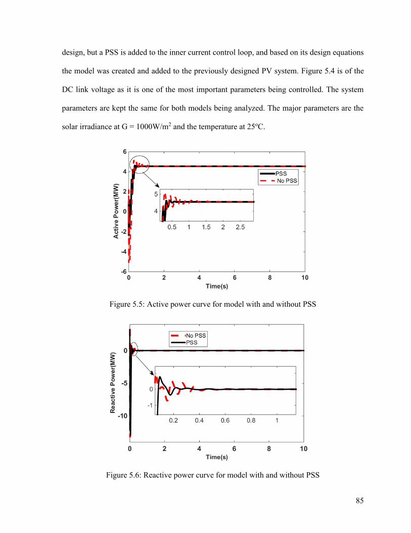
85

design, but a PSS is added to the inner current control loop, and based on its design equations

the model was created and added to the previously designed PV system. Figure 5.4 is of the

DC link voltage as it is one of the most important parameters being controlled. The system

parameters are kept the same for both models being analyzed. The major parameters are the

solar irradiance at G = 1000W/m2 and the temperature at 25oC.

Figure 5.5: Active power curve for model with and without PSS

Figure 5.6: Reactive power curve for model with and without PSS

86

Figure 5.4 clearly shows that by applying a power system stabilizer to the system we can

achieve the damping of the oscillations. This damping is also observed in the curves for active

and reactive power, as shown in Figure 5.5 and Figure 5.6 respectively.

The damping effect of the power system stabilizer can be seen clearly from the figures,

showing the active power and reactive power curves. The curve with PSS shows that the

amplitude of the power curve for the oscillations is dampened, thus validating the use of the

power system stabilizer in the system. Another aspect to observe is the settling time of the

curve, be it voltage or power.

Figure 5.7: Active power curve for model with and without PSS to observe settling time

Fig. 5.7 clearly shows that the settling time for the system without PSS is more than 2 seconds.

This means the time taken by the system to achieve a steady state is higher than the time taken

by the system with PSS. The black curve indicates that the system has entered a steady state

87

in less than 1 second. This helps to validate the functionality of the designed power system

stabilizer. The damping effect is required more on the Active power curve, as it is the power

being delivered by the PV system to the grid. The better damping of oscillations proves a

smoother and more stable supply of power from the PV system to the grid. Thus, the active

power is the most important parameter to be damped. By control of dc-voltage the smoother

power curve is achieved.

5.7 Summary

In this chapter we saw the design of the power system stabilizer using a washout filter and the

PI controller, which is being fed to the current controller of the designed PV system. We

performed the small signal stability analysis, which led us to the conclusion that the system is

not only stable but also more stable than the small signal model of the PV system without a

power system stabilizer. The stability was decided based on the comparison of the eigenvalue

plot of the system. The damping effect of the PSS was also observed in the large signal model

comparisons. The observation of the settling time from the plots were as expected for the PSS.

Thus, we can successfully validate the design of the power system stabilizer designed in this

thesis.

88

Chapter 6

Conclusions and Future work

6.1 Summary & Conclusion

The demand for renewable energy is increasing, and solar power generation is one of the fastest

growing generation techniques today, with a rise in the number of households using solar

power and connecting to the grid/utility. This causes the conversion of the DC voltages

produced to AC voltages, with the help of inverters that have different responses, therefore

creating an impact when connected to the grid. The study of these dynamic impacts and of

system stability for a PV system connected to the grid was the objective of the thesis; the

research has proved it to be successful as well.

The major results of the thesis are as follows:

Chapter 2 mostly discussed the various components or blocks of the PV system used

in the thesis. It explained the need for each block in the system and the role that it

played.

Chapter 3 focused on the mathematical modeling of the system described in the

previous chapter. This lead to the derivation of the major mathematical equations

that will be useful in creating a model in an environment like MATLAB 2014b using

the Simulink Toolbox. The models created by these equations help to understand the

working of the PV system, and the results can be observed by connecting various

scopes at different points in the system.

In chapter 4, we saw the small-signal technique used in the thesis by linearizing the

large signal equations. The model with a parallel RLC load connected to it was

designed. The small signal stability analysis of the PV system without a power

89

system stabilizer is done, and this is validated by the results obtained through the

eigenvalue plot, showing that the system is stable with all points in the left-half of

the s-plane.

The participation matrix was successfully calculated, resulting in the identification

of the relationship between the eigenvalues and the state variables. A comparison of

the average and detailed large signal models is also shown, and the results obtained

helped us conclude and validate the system design.

Chapter 5 discussed the power system stabilizer design implemented in the thesis.

The mathematical equations representing the PSS were designed, and the results of

the average large signal model with and without PSS were compared. Through this

analysis we could clearly validate the observations regarding the damping effect and

the settling time comparisons with and without PSS. The small signal stability model

for the system with PSS proves to be highly stable as compared to the system without

PSS. This conclusion was made when comparing the eigenvalue plots of the two

small signal models. The eigenvalues were more to the left of the s-plane in the case

of a system with PSS.

When we summarize all the conclusions above, we can see that the objectives of this thesis,

which were to create a mathematical model of the PV system connected to a grid, with and

without the power system stabilizer, were achieved successfully. The design was validated

with the help of the results obtained from the small-signal stability analysis and the large signal

analysis of the systems.

6.2 Future Work

A few suggestions on which further investigation could be carried out in the future are:

90

Firstly, the dynamic effects of the use of an MPPT controller on the system needs to be looked

into. The MPPT technique used in the thesis is one that is already available. The major

consideration here should be the algorithm chosen for tracking the maximum power point.

One, each algorithm has a different implementation method, introducing a new variable in the

analysis of the system. Secondly, the research and development of an inverter with good

efficiency to provide a better AC output, and an analysis on the chosen inverter so as to

maintain the stability of the system. As the inverter plays a crucial role in the connection of

the PV system to the grid.

Thirdly, the load considered in the thesis is a constant load or a parallel RLC load. It would be

interesting, to find out the performance of the system when catering to a varying load. The

stability analysis might help us identify, if the load is the source of instability to the system

and the method to curb this instability. Also a fault analysis of the system; would be useful to

the utility companies to understand the system’s responses when a fault occurs. Lastly,

analyzing the islanding behavior of the DG system. This would help to create various anti-

islanding schemes.

91

Appendices

Appendix A

The system parameters are mentioned in the table A.1.

Table A.1: System Parameters

Parameters Values

Reference DC link voltage(Vdcref) 554 V

Reference Reactive Power (Qref) 0

Washout Filter constant (Tw) 0

Interface inductance (Ls) 1e-5 H

Line Resistance (R) 0.2

Line Inductance (L) 1 mH

Inverter Filter Inductance 1 mH

Vbase 120*√2

Sbase 10000

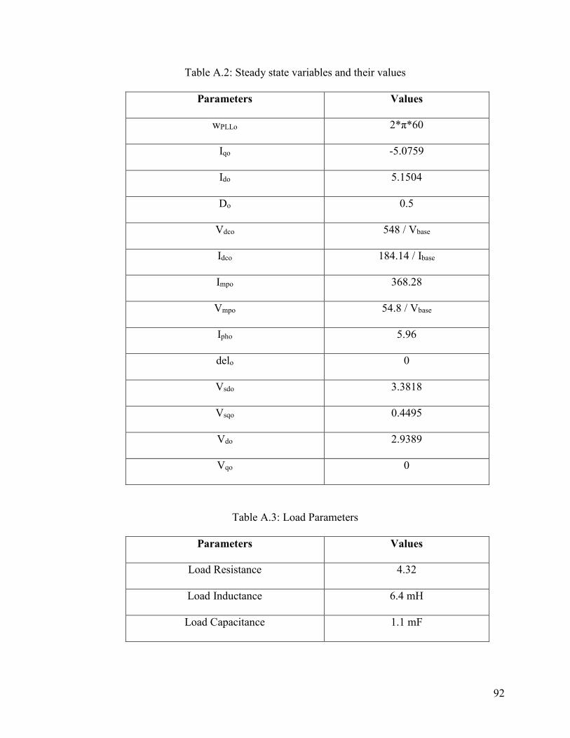
92

Table A.2: Steady state variables and their values

Parameters Values

wPLLo 2*π*60

Iqo -5.0759

Ido 5.1504

Do 0.5

Vdco 548 / Vbase

Idco 184.14 / Ibase

Impo 368.28

Vmpo 54.8 / Vbase

Ipho 5.96

delo 0

Vsdo 3.3818

Vsqo 0.4495

Vdo 2.9389

Vqo 0

Table A.3: Load Parameters

Parameters Values

Load Resistance 4.32

Load Inductance 6.4 mH

Load Capacitance 1.1 mF

93

Table A.4: PV Parameters

Parameters Values

Short-circuit current (ISC) 5.96 A

Open-circuit voltage (VOC) 64.2 V

Irradiance reference value (Gref) 1000 W/m2

Temperature reference value (Tref) 298 K

Charge (q) 1.6e-19 C

Diode Quality Factor (n) 1.3

Number of series cells per module (Ns) 96

No. of series connected modules/ string (Nm) 5

Saturation current (Io) 1.175e-8 A

Boltzmann constant (k) 1.3806503e-23 m2 kg s-2

K-1

Short-circuit current temperature coefficient (mu) -0.00057 A/K

Open-circuit voltage temperature coefficient

(muV)

-0.0027 V/K

Photocurrent reference value (Iphref) 5.96 A

Actual operating temperature (T) 298 K

Actual operating Irradiance (G) 1000 W/m2

94

The controller parameters are mentioned below:

Table A.5: Controller parameter values

Voltage Controller Kpp = 2 Kip = 500

Current Controller Kpi = 3

Kii = 500

PLL Controller KpPLL = 50

KiPLL = 500

PSS Controller Ksp = 1 Ksi = 1

The per unit conversions are obtained by the help of the following formulae’s:

2*120baseV

10000baseS

base

base

baseV

SI

3

2

base

base

baseI

VZ

95

60**2 base

base

base

base

ZL

basebase

baseZ

C*

1

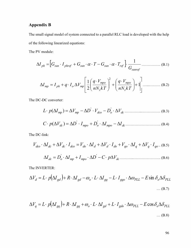
96

Appendix B

The small signal model of system connected to a parallel RLC load is developed with the help

of the following linearized equations:

The PV module:

sunref

refsunsunphrefsunphG

TGTGIGI1

…………… (B.1)

1

2

12

kTnN

Vq

kTnN

VqVIqII

s

mpo

s

mpo

mpophmp …...……… (B.2)

The DC-DC converter:

dcodcompmp VDVDVIpL '')( …………..…………… (B.3)

dcmpoompodc IIDIDVpC '')( ………………………. (B.4)

The DC-link:

qoqqqododddodcodcdcdco IVIVIVIVIVIV .. (B.5)

dcmpompodc VpCDIIDI ''………..…………………. (B.6)

The INVERTER:

PLLoPLLgqogqogdgdd EILILIRIpLV sin

… (B.7)

PLLoPLLgdogdogqgqq EILILIRIpLV cos

… (B.8)

97

dsd IpLu ……………………………………. (B.9)

qsq IpLu …………………..………………. (B.10)

cdldrddgd IIIII ……………………………... (B.11)

cqlqrqqgq IIIII ……………………………… (B.12)

l

drd

R

VI

…………………………………… (B.13)

l

q

rqR

VI

………………….……………….. (B.14)

PLLlqollqloldld ILILIpLV ……………. (B.15)

PLLldolldlolqlq ILILIpLV ……………. (B.16)

PLLqolqlodlcd VCVCVpCI …………….. (B.17)

PLLdoldloqlcq VCVCVpCI ……..……. (B.18)

ddrefiiddrefpid IIpkIIpkup …………..…. (B.19)

98

qqrefiiqqrefpiq IIpkIIpkup ………...…….. (B.20)

dcrefipdcipdcppdref VkVkVpkip ………………….. (B.21)

refipipppqref QkQkQpkip ……………….…….. (B.22)

PLLPLLp ………………………………… (B.23)

qiPLLqpPLLPLL VkVpkp ………………………….. (B.24)

qqoqqoddoddo VIIVVIIVP ..………….. (B.25)

qdodqodqoqdo VIIVVIIVQ …………… (B.26)

The average model of the grid connected PV system is shown in Fig B.1.

PV

L

S

D

Co

Vsa

Vsb

Vsc

Ls

Ls

Ls

R+jX

R+jX

R+jX

Ea

Eb

Ec

GridDC Link FilterInverterDC-DC ConverterPV Module

Figure B.1: Average model circuit of PV system connected to grid.

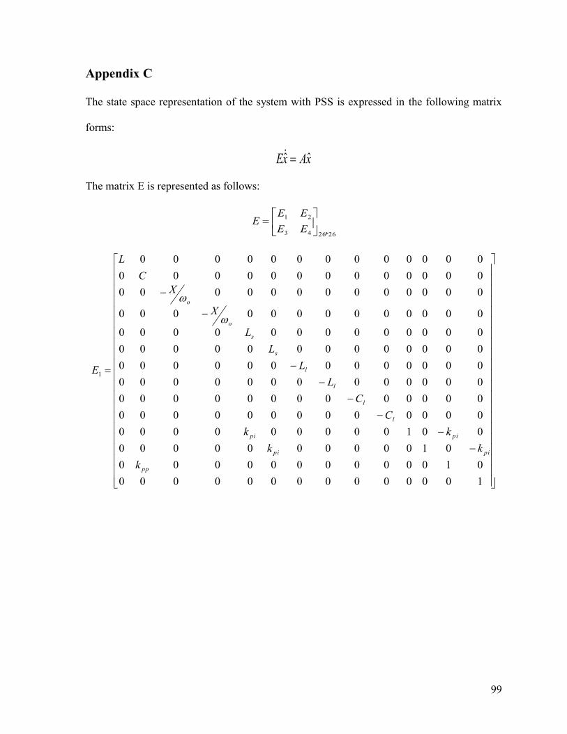
99

Appendix C

The state space representation of the system with PSS is expressed in the following matrix

forms:

xAxE ˆˆ

The matrix E is represented as follows:

26*2643

21

EE

EEE

10000000000000

0100000000000

010000000000

001000000000

0000000000000

0000000000000

0000000000000

0000000000000

0000000000000

0000000000000

0000000000000

0000000000000

0000000000000

0000000000000

1

pp

pipi

pipi

l

l

l

l

s

s

o

o

k

kk

kk

C

C

L

L

L

L

X

X

C

L

E

100

00000000000

000000000000

000000000000

00000000000

000000000000

000000000000

000000000000

000000000000

000000000000

000000000000

000000000000

000000000000

000000000000

000000000000

2

pp

pi

k

k

E

00000000000000

00000000000000

00000000000000

00000000000000

00000000000000

00000000000000

00000000000000

00000000000000

00000000000000

00000000000000

00000000000000

0000000000000

3

pPLLk

E

101

10000000000

000000000000

000000000000

000000000000

000000000000

000000000000

000000000000

000000000000

000000000000

000000000000

000000000100

000000000010

4

spk

E

The Matrix A values are as follows:

26*2643

21

AA

AAA

00000000000000

0000000000000

000000000000

000000000000

0000000000000

0000000000000

0000100000000

0000010000000

00100000000000

00010000000000

000010000000

000001000000

0000000000000

0000000000000

1

ip

iiii

iiii

lo

lo

lo

lo

o

o

o

o

k

kk

kk

C

C

L

L

RL

LR

D

D

A

102

00000000000

000000000000

000000000000

00000000000

0100000000*0

0001000000*0

0000000000*0

0000000000*0

000000000000

000000000000

000000000sin0

000000000cos0

000000010000

000000001000

2

ip

ii

dol

qol

ldol

lqol

ogdo

ogqo

k

k

VC

VC

IL

IL

IL

IL

A

00000000000000

0000000000

001010000*0000

00001000000000

00000100000000

00000010101000

00000001010100

00000000000

00000000000001

00010100*00000

00000000000000

00000000000000

3

doqodoqo

so

l

l

sqosdodco

so

IIVV

L

R

R

VVI

L

A

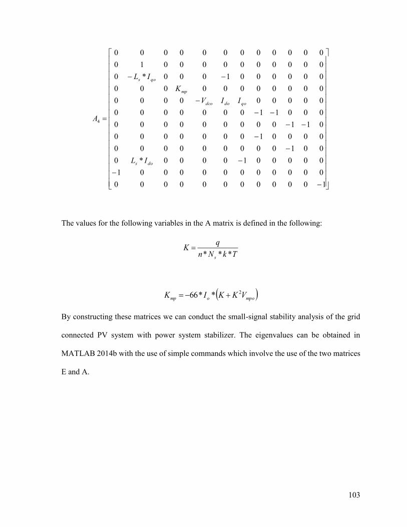
103

100000000000

000000000001

0000010000*0

001000000000

000010000000

011000000000

000110000000

000000000

00000000000

0000001000*0

000000000010

000000000000

4

dos

qododco

mp

qos

IL

IIV

K

IL

A

The values for the following variables in the A matrix is defined in the following:

TkNn

qK

s ***

mpoomp VKKIK 2**66

By constructing these matrices we can conduct the small-signal stability analysis of the grid

connected PV system with power system stabilizer. The eigenvalues can be obtained in

MATLAB 2014b with the use of simple commands which involve the use of the two matrices

E and A.

104

Bibliography

[1] G. M. Masters, Renewable and Efficient Electric Power Systems, 2nd ed., New

York: John Wiley & Sons Inc., 2013, p.277.

[2] J. R. Katiraei, F. Agueero, “Solar PV integration challenges,” IEEE power and energy

magazine, vol. 9, pp. 62-71, JUN 2011.

[3] Z. Shahan. “World Solar Power Capacity Increased 35% in 2013 (Charts)”. Internet:

http://cleantechnica.com/2014/04/13/world-solar-power-capacity-increased-35-2013-

charts/ , April 13, 2014.

[4] A. James “Total Global Solar PV Capacity Now Approaching or Over 100 GW”.

Internet: http://cleantechnica.com/2013/04/11/total-global-solar-pv-capacity-

approaching-100-gw/, April 11, 2013.

[5] M. A. Eltawil, Z. Zhao, “Grid-connected photovoltaic power systems: technical and

potential problems—A review”, Elsevier, vol. 14, pp. 112-129, 2010.

[6] M.G. Villalva, E.R. Filho, J.R. Gazoli, “Comprehensive approach to modeling and

simulation of photovoltaic arrays”, IEEE Transactions on Power Electronics, vol. 24,

no. 5, pp. 1198-1208, March 2009.

[7] H. Asano, K. Yajima, Y Kaya, “Influence of photovoltaic power generation on

required capacity for load frequency control”, IEEE Transactions on Energy

conversion, vol. 11, no. 1, pp. 188-193, March 1996.

[8] V. Quezada, J. Abbad, T. S. Roman, “Assessment of energy distribution losses for

increasing penetration of distributed generation”, IEEE Transactions on Power

Systems, vol. 21, no. 2, pp. 533-540, May 2006.

105

[9] T. Hoff, D.S. Shugar, “The value of grid-support photovoltaics in reducing distribution

system losses,” IEEE Transactions on Energy Conversion, vol. 10, no. 3, pp. 569-579,

Sep. 1995.

[10] B.S. Rigby, R.G. Harley, N.S. Chonco, “Analysis of a power oscillation damping

scheme using a voltage source inverter.” IEEE Transactions on Industry Applications,

vol. 38, no. 4, pp. 0093-9994, Jul/Aug 2002.

[11] Li Wang, Yuan-Yih, “Damping of a parallel ac-dc power system using PID power

system stabilizers and rectifier current regulators,” IEEE Transactions on Energy

Conversion, vol. 3 no. 3, pp. 0885-8969, Sep. 1988.

[12] P Kundur, M. Klein, G. J. Rogers, M. S. Zywno, “Application of power system

stabilizers for enhancement of overall system stability.” IEEE Transactions on Power

Systems, vol. 4, no. 2, pp. 614-621, May 1989.

[13] S. Ravichandran, S.G. Bharathi Dasan, Dr. R.P. Kumudini Devi, “Small signal

stability analysis of grid connected photovoltaic distributed generator system,” in

Proc. 2011 IEEE International Conf. on Power and Energy Sys., pp. 1-6.

[14] M.A Pai, D.P Sen Gupta, K.R Padiyar, “Small signal analysis of power systems”,

Narosa Publishing House, New Delhi, 2004.

[15] Li Wang, Ying-Hao Lin, “Dynamic stability analyses of a photovoltaic array connected

to a large utility grid”, in: Proc. 2000 IEEE Power Eng. Soc. Winter Meeting, vol. 1,

pp. 476-480.

[16] Y. T. Tan, D. S. Kirschen and N. Jenkins, “A model of PV generation

suitable for stability analysis”, IEEE Trans. Energy Convers., vol. 19, no, 4, pp. 748-

755, Dec 2004.

[17] Rodriguez, G. A. J. Amaratunga, “Dynamic stability of a grid connected photovoltaic

106

systems”, in: Proc. 2004 IEEE Power Eng. Soc. Gen. Meeting, Denver CO, USA,

vol. 2, pp. 2193-2199.

[18] P. M. Anderson and A. A. Fouad, “Power System Control and Stability,” Iowa State

University Press, Ames, Iowa, 1978.

[19] R. Shah, N Mithulananthan and K. Y. Lee, “Design of robust power oscillation

damping controller for large-scale PV plant,” in: Proc. 2012 IEEE Power

and Energy Society Gen. Meeting San Diego CA, USA, pp. 1-8.

[20] S. Y. Ruan, G. J. Li, B. T. Ooi and Y. Z. Sun, “Power system damping from real and

reactive power modulations of voltage source converter station,” Generation,

Transmission & Distribution, IET, vol. 2, no. 3, 2008, pp. 311-320.

[21] A. Dysko, W. E. Leithead and J. O’Reily, “Enhanced power system stability

coordinated by the PSS design,” IEEE Trans. on Power Systems, vol. 25, no. 1, pp.

413-422, Feb. 2010.

[22] A. C. Zolostas, B. Chaudhuri, I. M. Jaimoukha and P. Korba, “A study on LQG/LTR

control for damping inter-area oscillations in power systems,” IEEE Trans. Control

Syst. Technol., vol. 15, no. 1, pp. 151-160, Jan. 2007.

[23] M. H. Khan and M. A. Abido, “Controller design of PV system to enhance

the dynamic stability of smart grid network.”, in Proc. 2011 IEEE PES Conf. Innovative

Smart Grid Technologies-Middle East (ISGT Middle East), pp. 1-5.

[24] P. Kundur, Power system stability and control, California: McGraw-Hill Inc., 1994.

[25] N. E. El-Kharbawe and S. O. Faried, “Damping inter-area oscillations using a static

phase shifter,” 2009 Canadian Conference on Electrical and Computer Engineering ,

St. John’s NL, pp. 575-578.

[26] G. Li, “Implementation of coordinated multiple facts controllers for damping

107

oscillations,” International Journal of Electrical Power & Energy Systems, vol. 22, no.

2, pp. 79-92, Feb. 2000.

[27] M. Joorabian, M. Razzaz, M. Ebadi, M. Moghaddasian,”Employing fuzzy logic in

damping power system oscillations using SVC,” 2008 Second International

Conf. on Electrical Engineering, Lahore, pp. 1-5.

[28] M. Sedighizadeh, M. S. Toulabi, A. Rezazadeh, M. Khatibi, and B. Allahverdi-

Charandabi, “Damping improvement by SSSC and STATCOM in a part of Iran

electrical network,” 2008 43rd International Universities Power Engineering

Conference, Padova, pp. 1-5.

[29] S. Ju Lee, H. Yong Park, G. Hun Kim, H. Ryong Seo, and M. H. Ali, “The experimental

analysis of the grid-connected PV system applied by POS MPPT,” ICEMS, 2007

International Conference on Electrical Machines and Systems, Seoul, pp. 1786-1791.

[30] X. Wang, W. Freitas, “Influence of voltage positive feedback anti-islanding

scheme on inverter –based distributed generator stability,” IEEE Trans. on Power

Deliv. vol. 24, no. 2, pp. 972-973, Apr. 2009.

[31] R. G. Wandhare and V. Agarwal, “A modified control strategy for centralized

PV- grid systems for assisting dynamic stability to overcome penetration issues,” In:

Proc. 38th 2012 IEEE Photovoltaics Specialists Conf., Austin, TX, USA, pp.540-1544.

[32] P Kundur, M. Klein, G. J. Rogers, S. Moorty, “Analytical investigation of factors

influencing power system stabilizers performance.” IEEE Transactions on Energy

Conversion, vol. 7, no. 3, pp. 382-390, Sep. 1992.

[33] J. Hernandez, N. L. Diaz and G. Gordillo, “Design-dimensioning

models for grid-connected photovoltaic systems,” In: Proc. of the 9th IEEE Electrical

Power & Energy Conf. (EPEC 2009), Bogota, pp. 1-5.

108

[34] A. VanderMeulen and J. Maurin, “Current source inverter vs. Voltage source

inverter topology,” Whitepaper, WP020001EN, June 2014.

[35] R. Faranda and S. Leva, “Energy comparison of MPPT techniques for PV systems,”

WSEAS Trans. on Power Systems, Issue no. 6, vol. 3, pp. 1-6, June 2008.

[36] S. L. Brunton, C. W. Rowley, S. R. Kulkarni and C. Clarkson, “Maximum power point

tracking for photovoltaic optimization using ripple-based extremum seeking control,”

IEEE Trans. on Power Electronics, vol. 25, no. 10, pp. 2531-2540, Oct. 2010.

[37] Timbus A., Liserre M., Teodorescu R., Blaabjerg F, “Synchronization methods for

three-phase distributed power generation systems- An overview and evaluation,” in

Proc. 2005 IEEE PESC, pp. 2474-2481.

[38] G. Hsieh and J. Hung, “Phase-locked loop techniques- A survey,” IEEE Trans. Ind.

Electron. vol. 43, no. 6, pp. 609-615, Dec. 1996.

[39] S. Buso and P. Mattavelli, “Extension to Three-Phase Inverters” Digital

Control in Power Electronics, ed. 1, Jerry Hudgins, USA: Morgan & Claypool, 2006,

pp. 81-100.

[40] B. Huang, “Stability of Distribution Systems with a Large Penetration of Distributed

Generation.” Phd. Thesis, University of Dortmund, Dortmund, Germany, 2006.

[41] J. Machowski, J. W. Bialek and J. R. Bumby, “Power System Dynamics and Stability”,

New York: John Wiley & Sons Ltd. 1997.

[42] Leonard L. Grigsby,” Power System Stability”, in Power System Stability and

Control, FL: CRC Press, 2007, pp. 7-1 – 7-7.

[43] W. Du, H. Wang and R. Dunn, “Power system small-signal oscillation stability as

affected by large-scale PV penetration,” in 2009 Proc. of International Conference on

Sustainable Power Generation and Supply, Nanjing, pp. 1-6.

109

[44] V. John, Z. Ye, A. Kolwalkar, “Investigation of anti-islanding protection of power

converter based distributed-generators using frequency domain analysis.” IEEE

Transactions of Power Electronics, vol. 19, no. 5, pp. 1177-1183, Sep. 2004.

[45] H. Malek, “Control of Grid-connected Photovoltaic Systems using fractional order

operators,” Ph.D. dissertation, Utah State University, Logan, Utah, 2014.

[46] A. Yazdani and et al, “Modeling guidelines and a benchmark for power system

simulation studies of three-phase single-stage photovoltaic systems,” IEEE Trans. on

Power Del., vol. 26, no. 2, pp. 1247-1264, April 2011.