DEVELOPMENT OF DIFFERENTIAL EVOLUTION BASED POWER SYSTEM ... · development of differential evolution based power system stabilizer (pss) with hvdc in small signal stability analysis

DEVELOPMENT OF DIFFERENTIAL EVOLUTION BASED POWER

SYSTEM STABILIZER (PSS) WITH HVDC IN SMALL SIGNAL

STABILITY ANALYSIS USING MATLAB

MOHD SYUKUR BIN AZIZAN

This thesis is submitted as partial fulfilment of the requirements for the award

of the Degree of Master of Electrical Engineering

Faculty of Electrical & Electronic Engineering

Universiti Tun Hussein Onn Malaysia

JULY 2015

vi

ABSTRACT

Power system (PS) oscillation damping remains as one of the major concerns for

secure and reliable operation of large PS network, and is of great presently interest to

both industry and academia. This research presents the designing of Differential

Evolution (DE) power system stabilizer (PSS) controller with High Voltage Direct

Current (HVDC) to improve the small signal stability (SSS). The Power System

Toolbox version 3 MATLAB based software is used as a tool to simulate the results.

The results shown that the location of HVDC supplementary in the network contribute

to the effectiveness in improving power system SSS if applied together with the PSS.

The results show a significant improvement to the damping of the inter-area mode as

well the local mode oscillation when the DEPSS incorporated into system together

with HVDC which is approximated 5% improvement. Thus the time domain response

also shown improve beyond 10%.

vii

TABLES OF CONTENTS

DECLARATION ii

ACKNOWLEDGEMENTS v

ABSTRACT vi

TABLE OF CONTENTS vii

LIST OF TABLES x

LIST OF FIGURES xi

LIST OF ABBREVATIONS/NOTATIONS/GLOSSORY OF TERMS xiv

CHAPTER 1- INTRODUCTION

1.1 Problem background 1

1.2 Problem statement 5

1.3 Research Objectives 5

1.4 Scope of Project 6

1.5 Thesis Organization 6

CHAPTER 2- LITERATURE REVIEW

2.1 Introduction to power system damping 7

2.2 Power System Stabilizer (PSS) 8

2.2.1 Conventional Power System Stabilizer (CPSS) 9

viii

2.2.2 Differential Evolution Based Power System Stabilizers

(DEPSS)

10

2.3 High Voltage Direct Current (HVDC) 10

2.3.1 HVDC Operation – Two Terminal DC Link 11

2.3.2 HVDC Control Characteristic (V-I Characteristic) 12

CHAPTER 3- METHODOLOGY

3.1 Introduction to methodology 16

3.2 Software Tool 16

3.3 Introduction to state space representation 17

3.3.1 State Space Representation 17

3.3.2 Linearization 19

3.4 Modal Analysis 20

3.4.1 Eigenvalue and stability analysis 20

3.4.2 Eigenvector Analysis 21

3.4.3 Participation Factor 22

3.5 Differential Evolution (DE) Algorithm 23

3.5.1 Population Structure 23

3.5.2 Initialization 24

3.5.3 Mutation 25

3.5.4 Recombination or crossover 25

3.5.5 Selection 26

3.6 DEPSS Parameter Setting 26

3.6.1 Objective function 26

3.7 DEPSS tuning approach 27

ix

3.7.1 Application of DE to PSS design 28

3.8 Methodology Summary 30

CHAPTER 4- SIMULATION RESULT

4.1 Introduction 32

4.2 System Setting 32

4.3 PSS Parameter Optimization 35

4.3.1 CPSS parameter selection 35

4.3.2 DEPSS parameter selection 35

4.4 Load flow 36

4.4.1 Case 1: HVAC system 36

4.4.2 Case 2: HVAC-HVDC system 38

4.5 Small Signal Stability Analysis 39

4.5.1 Case 1: HVAC system 40

4.5.2 Case 2: HVAC-HVDC system 43

4.5.3 Case 3: Comparison HVAC and HVDC 46

4.6 Time domain Response 50

4.7 Summary 57

CHAPTER 5- CONCLUSIONS AND RECOMMENDATIONS

5.1 Conclusion 58

5.2 Recommendation 60

REFFERENCES 61

APPENDIX A 63

APPENDIX B 69

x

LIST OF TABLES

Table no

Page

3.1 DeMat package parameter setting 28

4.1 HVAC and HVAC-HVDC respective buses with

component and rating setting

35

4.2 CPSS parameters 35

4.3 Parameters boundaries 36

4.4 DEPSS parameters 36

4.5 Voltage magnitude and angle for HVAC system 37

4.6 Active and reactive power for HVAC system 37

4.7 Voltage magnitude and angle for HVDC system 38

4.8 Active and reactive power for HVAC-HVDC system 39

4.9 Mode types and frequency range for electromechanical

oscillation

40

4.10 HVAC System 41

4.11 HVAC-HVDC System 44

4.12 Comparison HVAC and HVAC-HVDC System 47

xi

LIST OF FIGURES

Figure No

Page

1.1 Power system stability classification 2

1.2 Power System Control 4

2.1 PSS block diagram 8

2.2 Two terminal HVDC scheme 12

2.3 Voltage-Current (VI) Characteristic 13

3.1 General DE cycle 23

3.2 Chart for the PSS design using DE 29

3.3 Methodology summarize chart 31

4.1 HVAC System 34

4.2 HVAC-HVDC System 34

4.3 Frequency against damping ration of HVAC two-area

system modes for small signal stability without PSS

41


system modes for small signal stability with AVR with

CPSS

42

xii


system modes for small signal stability with AVR with

DEPSS

43

4.6 Frequency against damping ration of HVAC-HVDC two-

area system modes for small signal stability with AVR

without PSS

44



with CPSS

45



with DEPSS

46

4.9 Comparison frequency against damping ration of HVAC

and HVAC-HVDC two-area system modes for small

signal stability without PSS

48



signal stability with AVR with CPSS

49



signal stability with AVR with DEPSS

49

4.12 HVAC system response of generator 1 speed 50




4.16 HVAC-HVDC system response of generator 1 speed 53




xiii

4.20 Comparison HVAC with HVAC-HVDC system response

of generator 1 speed

55



56



56



57

xiv

LIST OF ABBREVIATIONS/NOTATIONS/GLOSSARY OF TERMS

FACTS Flexible AC Transmission System

HVDC High Voltage Direct Current

SVC Static Var Compensator

PSS Power System Stabilizer

PSD Power Swing Damping

p.u. Per-unit

PS Power System

SSS Small Signal Stability

TSCS Thyristor Controlled Series Compensator

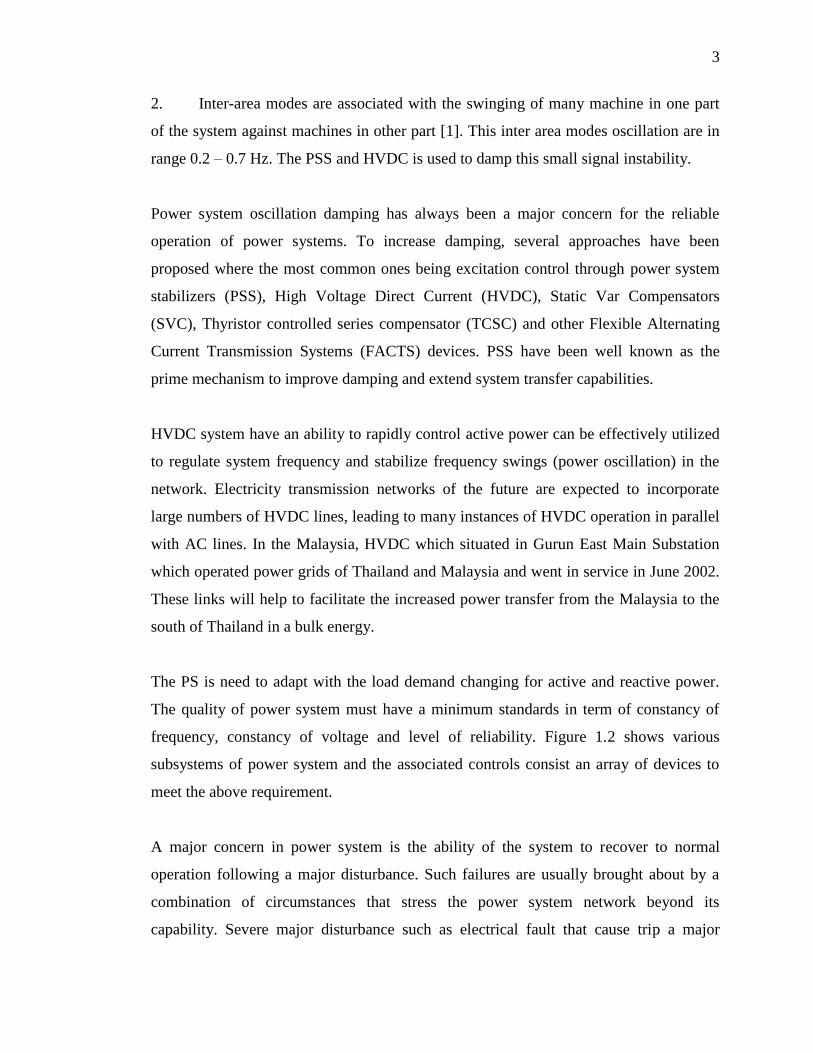
CHAPTER 1

INTRODUCTION

1.1 Problem background

The Stability of power system (PS) problem is concern with the behavior of the

synchronous machines after they have been perturbed. If the perturbation does not

involve any net change in power, the machines should return to their original state.

Power system stability may be broadly defined as that property of a PS that enables it to

remain in a state of operating equilibrium under normal operating conditions and to

regain an acceptable state of equilibrium after being subjected to a disturbance [1].

SSS (SSS) is the ability of the system to maintain synchronism under small disturbances

which occur continually on the system due to the small variations in loads and

generation or other small disturbances on the system. A disturbance is considered to be

small if the equations that give the response of the system may be linearized for the

purpose of analysis. Investigations involving this stability concept usually involve the

analysis of the linearized state space equations that define the power system dynamics.

Power system stability can be simplified as shown in figure 1.1.

2

Power System Stability

Frequency

StabilityAngle Stability

Voltage

Stability

Transient

Stability

Small Signal

Stability

Non-oscillation

instability

Oscillation

instability

Inter area modes Local modes Control modesTorsional

modes

Small

disturbance

stability

Large

disturbance

stability

Figure 1.1 Power system stability classification [1]

Instability that may result can be of two form. (i) Steady increase in rotor angle due to

lack of sufficient synchronizing torque or (ii) Rotor oscillations of increasing amplitude

due to lack of sufficient damping torque. The nature of system response to small

disturbances depend on a number of factors including the initial operating conditions,

the transmission system strength, and the type of generator excitation controls used.

Nowadays in modern power systems, SSS is largely a problem of insufficient damping

of oscillations. The stability of the following types of oscillations [1]:

1. Local Modes or machine system modes are associated with swinging of units at a

generating station with respect to the rest of the power system [1]. This local modes

oscillation are in the range 0.8 – 2.0 Hz.

3

2. Inter-area modes are associated with the swinging of many machine in one part

of the system against machines in other part [1]. This inter area modes oscillation are in

range 0.2 – 0.7 Hz. The PSS and HVDC is used to damp this small signal instability.

Power system oscillation damping has always been a major concern for the reliable

operation of power systems. To increase damping, several approaches have been

proposed where the most common ones being excitation control through power system

stabilizers (PSS), High Voltage Direct Current (HVDC), Static Var Compensators

(SVC), Thyristor controlled series compensator (TCSC) and other Flexible Alternating

Current Transmission Systems (FACTS) devices. PSS have been well known as the

prime mechanism to improve damping and extend system transfer capabilities.

HVDC system have an ability to rapidly control active power can be effectively utilized

to regulate system frequency and stabilize frequency swings (power oscillation) in the

network. Electricity transmission networks of the future are expected to incorporate

large numbers of HVDC lines, leading to many instances of HVDC operation in parallel

with AC lines. In the Malaysia, HVDC which situated in Gurun East Main Substation

which operated power grids of Thailand and Malaysia and went in service in June 2002.

These links will help to facilitate the increased power transfer from the Malaysia to the

south of Thailand in a bulk energy.

The PS is need to adapt with the load demand changing for active and reactive power.

The quality of power system must have a minimum standards in term of constancy of

frequency, constancy of voltage and level of reliability. Figure 1.2 shows various

subsystems of power system and the associated controls consist an array of devices to

meet the above requirement.

A major concern in power system is the ability of the system to recover to normal

operation following a major disturbance. Such failures are usually brought about by a

combination of circumstances that stress the power system network beyond its

capability. Severe major disturbance such as electrical fault that cause trip a major

4

circuit or failure of major plant (generator or transformer) may result in cascading

outage that must be contained within a small part of the system if a small part system if a

major blackout is to be prevented.

SYSTEM GENERATION CONTROL

Load Frequency Control with Economic

Allocation

Primer

Mover and

Control

Generator

Excitation

System and

Control

GENERATING UNIT CONTOLS

Shaft

Power

Field

Current

Voltage

Speed/Power

Speed

TRANSMISSION CONTROLS

Reactive Power and Voltage Control,

HVDC transmission nad Associated Controls

Electrical

Power

Frequency Generator PowerTie Flows

Oth

er

Genera

ting U

nits

and

Ass

ocia

ted C

ontr

ol

Frequency Tie Flows Generator Power

Schedule Power

Supplementary

Control

Figure 1.2: Power System Control [1]

5

1.2 Problem Statement

In the modern PS a number of large turbo generators are installed. With growing

generation capacity, different areas in a power system are added with ever larger inertia,

making the system sensitive to inter-area and local area oscillation [1]. PS oscillation

damping has always been a major concern for the reliable operation of PS. To increase

damping, several approaches have been proposed and the most common one being

excitation control using conventional power system stabilizers (CPSS) with HVDC [2].

CPSS are not always able to guarantee the stability in PS because nowadays the PS

network are more highly nonlinear, large scale, and multivariable. Hence, recently

Differential Evolution Power System Stabilizer (DEPSS) introduce in order to optimize

the PS oscillation damping [3] [4]. But there are still some modifications needs to be

done in order to improve the SSS damping like introducing an optimizing control which

can be achieved by developing DEPSS controller with HVDC. Therefore in this project,

more focus is made on how to improve the SSS by using the DEPSS controller with

HVDC and the analysis is made by using eigenvalue method respectively.

1.3 Research Objective

The objectives of this research are:

1. To develop Differential Evolution (DE) approach based PSS controllers for the two-

area multi machine (TAMM) system.

2. To analyse and evaluate the performance of DEPSS and HVDC in order to damp

inter-area and local area oscillation using eigenvalue technique.

3. To analyse the performance of DEPSS and HVDC in order to damp inter-area and

local area oscillation using time response analysis.

6

1.4 Scope of Project

The focuses on this project are as follow:

1. The designing of DEPSS is accomplished using DeMat package [5].

1. MATLAB PST v3 is used in this research to analyse the SSS for the TAMM

system.

2. The dissertation is using the HVAC and HVAC-HVDC systems for a two-area four

generators system [1].

1.5 Thesis Organization

This thesis will discuss the study of Power Oscillation damping using Power System

Stabilizer and HVDC Control.

Chapter 1 is introductory chapter which discuss on problem identification, research

objective, research scope of work and thesis organization.

Chapter 2 is discusses specifically on literature review of Power System Stability

Phenomena and problem. Power system stabilizer function and design using Differential

Evolution (DEPSS) as well as HVDC control. Power system oscillation also discuss in

this chapter.

Chapter 3 is discusses on methodology of test system, the concept of linearization and

modal analysis as well as DEPSS design.

Chapter 4 presents the result and analysis. The result encompass the load flow, the

modal analysis and the step response.

Chapter 5 is discuss on conclusion and recommendation.

CHAPTER 2

LITERATURE REVIEW

2.1 Introduction to power system damping

Power system oscillation damping has always been a major concern for the reliable

operation of PS. To increase damping, several approaches have been proposed. The

most common ones being excitation control through PSS and supplementary damping

control of HVDC, SVC, TCSC and other FACTS devices. In this thesis, I’m focusing

to design PSS using Differential Evolution (DE) to damp the oscillation with HVDC.

There are variety method to design PSS and the previous PSS design using Pole

Placement [1], H∞ robust control technique [6], Linear Matrix Inequalities (LMI)

robust control technique [7], μ-Synthesis (or singular value decomposition) a robust

control technique [8].

PSS are supplementary control devices which are installed in generator excitation

systems. Their main function is to improve stability by adding an additional stabilizing

signal to compensate for undamped oscillations [9]. In addition, it has become more

common to use the supplementary damping control available in FACTS.

Conceptually, this supplementary damping control is similar to PSSs.

The main purpose of application HVDC system is to transfer bulk power transmission

efficiently between two different AC networks or to resolve power stability problem

for longest power transfer. However the ability of HVDC system to rapidly control

active power can be effectively utilized to regulate system frequency and stabilize

frequency swings (power oscillation) in the network. The basic principle of mitigation

strategies using HVDC to damp oscillation by injecting extra active power into the

8

system or/and consumed the extra active power in the system, which can

instantaneously decelerated the oscillation.

This research presents analysis performance by comparing the effectiveness of using

the HVDC and generator PSS in damping small signal power system oscillations under

different system operating conditions.

2.2 Power System Stabilizer (PSS)

PSS function is a control device to improve stability by adding an additional stabilizing

signal to compensate for undamped oscillations which are installed in generator

excitation systems. The basic objective of power system stabilizer is to modulate the

generator’s excitation in order to produce an electrical torque at the generator

proportional to the rotor speed [1]. In some research, the concept of oscillation

damping which available in FACTS is similar to PSSs. The TCSC and SVC along with

PSSs have been used to enhance the power system oscillation damping and

performance.

The PSS can use various inputs which deviate in the rotor speed will be the change in

electrical power and accelerating power. Figure 2.1 below illustrates the block diagram

of a typical PSS. The PSS structure generally consists of a washout, lead-lag networks,

a gain and a limiter stages. Each stage performs a specific function.

sTw

1 + sTw

1+ sT1

1 + sT2

1 + sT3

1 + sT4

D Input

VPSSmax

VPSSmin

VPSS

Figure 2.1: PSS block diagram

9

2.2.1 Conventional Power System Stabilizer (CPSS)

The main function of CPSS is to damp electromechanical oscillations. The CPSS

controls the AVR excitation using auxiliary stabilizing signal in order to achieve the

damping. The CPSS’s block diagram is shown in Figure 2.1. The Phase compensation

and root locus are the two basic tuning techniques have been successfully utilized with

power system stabilizer application.

Phase compensation consists of adjusting the stabilizer to compensate for the phase

lags through the generator, excitation system and power system such that the stabilizer

path provides torque changes which are in phase with speed changes. The root locus

involves shifting the eigenvalues associated with the power system modes of

oscillation by adjusting the stabilizer pole and zero locations in the S-plane. This is

more complicated to apply particularly in the field [10]. PSSs generally must be tuned

one at a time through off-line analysis during commissioning. To determine the

stabilizer’s parameters in systems with both local and inter area modes has a more

complex approach.

The stabilizer provide damping by produces a component of electrical torque in phase

with the rotor speed deviations. The basic components in PSS are the PSS input, Gain,

washout and phase compensation. The signal washout block serves as a high pass filter

with the time constant Tw. It is important to choose an appropriate value for the

washout Tw. The appropriate time constant is between 1 and 2 seconds if the damping

of the local mode is the only concern. However a Tw of 10 seconds or higher when

inter area is considered [11].

Phase lead network provide compensation for the phase lag between the exciter input

and the generator electrical torque output over the frequency range of 0.2 to 2.5 Hz.

Ks is the stabilizer gain that determines the amount of damping introduced by the

power system stabilizer [1]. The gain on the other hand is obtained by applying the

root locus method. The gain must be carefully selected to stabilize the

electromechanical mode without adversely affecting the other modes.

10

2.2.2 Differential Evolution Based Power System Stabilizers (DEPSS)

Recently DE is one of the famous approach in designing the PSS is applying

optimization techniques. The technique is to convert the problem of selecting PSS

parameters into a simple optimization problem. One of the optimization is the

Evolution Algorithms (EAs). EA is a population-based optimizer inspired by the

mechanism of evolution and natural selection [12]. Like all Genetic Algorithm (GA),

DE used the similar operators which are crossover, mutation and selection.

The main difference between the DE and GA is that DE more relies on the mutation

parameters as a search mechanism and selection operation to direct the search toward

the prospective regions in the search space compare to GA which is more applying the

crossover operator. The DE also encodes parameters in floating point regardless of

their type, whereas GA encoding is mainly binary although floating, gray, etc.

With increasing number of researches have proposed EAs to optimally tune the

parameters of the PSS to guarantee a robust performance. For instance, in [3] DE was

successfully applied to design PSSs for multi-machines system and in [4] the DE was

successfully designed PSSs for Single Machine Infinite Bus (SMIB).

2.3 High Voltage Direct Current (HVDC)

Few decades ago the development of the HVDC technology has contributed to make

HVDC more competitive in comparison to AC. With the consumption, and the

increased exchange of energy between different powers pools the HVDC is introduce

as mechanism for bulk energy transfer between region which have different frequency

or voltage level. This power exchange results from it being more economical to utilize

the installed generating capacity in different regions than to build new power stations

in each region.

Currently, in the field of HVDC, research into the influences of HVDC on AC systems,

or AC on HVDC systems has created a great deal of interest. It is essential to develop

11

HVDC and AC simulation systems, particularly HVDC control and protection

simulation systems, which can be used for such research purposes. It is known that AC

systems can operate without strict control, but for a HYDC system to operate, a control

system is a must [13].

The HVDC technique using thyristors as switching element can be characterized as a

technique for conversion and control of active power. A well-known technical

advantage of HVDC is its inherent ability for controlling the transmitted power. The

controllability can be utilized for different objectives such as stabilization of the

connected AC network, control of the frequency of a receiving island network and to

assist in frequency control of generator radially connected to the rectifier of the HVDC

transmission.

2.3.1 HVDC Operation – Two Terminal DC Link

Figure 2.2 shows a two-terminal dc link structure. It consists of a controlled rectifier

and a controlled inverter both fed from tap changing transformers. The rectifier

converts the ac current at the rectifier transformer to dc and the inverter converts the

dc current to ac. In normal operation, the voltage of a two terminal dc link is set by

the inverter controls, and the current is set by the rectifier controls. The inverter firing

angle (i) may be used to control the inverter dc voltage, or to maintain constant

extinction angle (γi). In the dc voltage control mode, the controlled voltage may be

compounded so as to move the set point to a selected point on the dc line. The rectifier

firing angle (r) is used to control rectifier dc voltage and hence the dc line current or

power.

12

Figure 2.2: Two terminal HVDC scheme

The converter transformer taps are adjusted so that the rectifier firing angles and

inverter extinction angles are kept within their operating range. However, this may be

impossible under all ac system conditions. If the rectifier transformer tap is at a limit,

and the rectifier firing angle is less than its minimum limit, the firing angle is controlled

the limit. The inverter takes over the control of line current at a specified proportion

of the required value, and the dc voltage drops below its rated value. If the inverter

extinction angle falls below its minimum value, it is controlled to that minimum.

In a load flow, the real and reactive power injected into the dc system are considered

as ac system loads. The loads may be represented as being at either the converter

transformer HT buses, or at the converter transformer LT buses. When using the HT

bus interface, the equivalent ac reactance of the dc line commutating reactance (xaceq)

must be equal to the reactance of the converter transformer (xt). With a LT bus

interface, xaceq may differ from xt, for example to represent the Thevenin equivalent

impedance.

2.3.2 HVDC Control Characteristic (V-I Characteristic)

Voltage-Current (VI) Characteristic shown in figure 2.3 explained the basis for HVDC

control philosophy. Under normal operation conditions the rectifier maintains constant

current (CC) while the inverter operates with constant extinction angle (CEA)

maintaining the voltage. The rectifier control constant current by changing delay angle

α so long as the delay angle is not at its minimum limit (usually). The steady state

constant current characteristic of the rectifier is shown as the vertical section Q-C-H-

R. Where the rectifier and inverter characteristic intersect, either at points C or H, is

VHTr

VLTr

Vdcr

VHTi

VLTi

Vdci

idc

13

the operating point of the HVDC system. The operating point is reached by action of

tap-changer of converter transformer at both stations.

Ud

Rectifier

Rectifier Voltage Control

(Minimun delay angle charecteristic 5 degree)

Operating point

P

H

Q

D

E

CB

A

F

G

S

T

IdId order0.9 Id

order

I margin

Inverter Gamma Control

(minimum extinction angle 18 degree)

Inverter Current Control

(current margin error) Inverter Voltage Control

Rectifier Current Iref ControlVDCOL Characteristic

Figure 2.3: Voltage-Current (VI) Characteristic

The Inverter is set as DC voltage control (characteristic B-H-E) under steady state

condition with necessary to maintain a certain minimum CEA (characteristic A-B-C-

D) to avoid commutation failure. The CEA characteristic intersects the rectifier

characteristic to define the operation point. Nonetheless, when the rectifier

characteristic is set at reduced voltage, which means a reduction in the rectifier voltage,

then a suitable operation point is not reached. Under these circumstances the system

would run down. Because of this reason, the inverter characteristic is complemented

with a region of CC adjusted at a lower value than the current setting of the rectifier.

The difference between both settings is called current margin and its value is normally

fixed in the range of 10%‐15% of the rated current of the system. Subsequently, under

reduced voltage condition at the rectifier the role of each converter is switched (mode

shift) and thus the rectifier regulates the voltage while the inverter regulates the

current.

14

Similarly the tap-changer at Rectifier is controlled to adjust their voltage so that the

delay angle α has a working range at level between approximately 5𝑂 to 17𝑂 for

maintaining the constant current Iorder. If the inverter is operating in constant DC

voltage control at the operating point H, and if the DC current order Iorder is increased

so that the operating point H shift towards and beyond point B, the Inverter mode of

control will revert to constant extinction angle control and operate on characteristic A-

B. DC Voltage Ud will be less than the desired value and the tap changer at Inverter

will boost its DC voltage until DC Voltage control is resumed.

The DC Current order Iorder is sent to both the rectifier and inverter station. It is usual

to subtract a small value of current order sent to the Inverter. This is known as the

current margin Imargin. The inverter also has a current controller and it attempts to

control the DC current Id to the value Iorder - Imargin but the current controller at rectifier

normally overrides it to maintain the DC current at Iorder. The current control at Inverter

becomes active only when the current control at rectifier ceases when its delay angle

α is pegged against its minimum delay angle limit. This is readily observed in the

operating characteristic where the minimum delay angle limit at rectifier is

characteristic P-Q.

If for some reason a low AC Commutating voltage at the rectifier end, the P-Q

characteristic falls below points D or E, the operating point will shift from point H to

somewhere on the vertical characteristic D-E-F where it is intersected by the lowered

P-Q characteristic. The inverter reverts to current control, controlling the DC current

Id to the value Iorder - Imargin and the rectifier is effectively controlling DC voltage so

long as it is operating at its minimum delay angle characteristic P-Q. The controls can

be designed such that the transition from the rectifier controlling current to the inverter

controlling current is automatic and smooth.

During disturbances where the AC voltage at rectifier or inverter is depressed, it will

not be helpful to a weak AC system if the HVDC transmission system attempts to

maintain full load current. A sag in AC voltage at either end will result in a lowered

DC voltage too. The DC control characteristic shown in figure 2.3 indicates the DC

current order is reduced if the DC voltage lowered.

15

This can be observed in the rectifier characteristic R-S-T and in the inverter

characteristic F-G. The controller which reduces the maximum current order is known

as a Voltage Dependent Current Order Limit or VDCOL. The VDCOL control, if

invoked by an AC system disturbance will keep the DC current Id to the lowered limit

during recovery Ud has recovered sufficiently will the DC current return to its original

Iorder level.

CHAPTER 3

METHODOLOGY

3.1 Introduction to methodology

This chapter discuss the method that being used to solve the SSS of the TAMM. As

discuss in chapter 2 there are various method that used to solve SSS as well as the

simulation tools [2]. PSS is an effective devise to damp the inter area and local

oscillation. This research is focusing designing the PSS using DE and apply together

with the HVDC to damp the inter area and local oscillation. The development of a

system model is quite complex, even for the small TAMM. But by using the MATLAB

based toolbox Power System Toolbox ver3 (PSAT v3) the complex modelling is

become simpler.

3.2 Software Tool

PST v3 is a MATLAB based software that takes a solved Load Flow network object,

and dynamic data associated with all of the systems dynamic devices and their controls

[14]. PST v3 facilitates the users to obtain SSS results such as the system eigenvalues,

eigenvector, participation factors, the frequency of oscillations and damping ratio of

the eigenvalues.

Data for the power system's transmission system, loads, generation and controls are

used to construct a data system. Once this has been constructed, functions which

17

operate on objects may be used to perform power flow analysis, and examine the

system's steady state performance.

1.3 Introduction To State Space Representation

The SSS behaviour is that it is an ability of a power system to maintain stability when

subject to small disturbances as discuss in chapter 1. Hence, the linear techniques is

used to analyse small signal oscillations by using the modal analysis, eigenvectors,

eigenvalues sensitivity and participation factors technique.

3.3.1 State-Space Representation

The State-Space representation is often used to describe the behaviour of a dynamic

system. Let us consider from the mathematical model a dynamic system expressed in

term of a system of n first order non-linear differential equation:

ix = fi (x 1, x

2,……,x

n; u

1, u

2,……..,u

n; t) where i = 1,2,….n (3.1)

Where n is the order of the system and if the derivatives of the state variables are not

explicit functions of time, equation 3.1 may be reduced to

x = f (x,u) (3.2)

where

x is state vector contains the state variables of the power system

u is vector contains the system input

x is encompasses the derivatives of the state variables with respect to time.

The equation relating the outputs to the inputs and state variables can be written as

18

Y = g(x,u) (3.3)

The state concept may be illustrated by expressing the swing equation of the generator

in per-unit torque as follows:

0

2

H2

2

dt

d = Tm – Te – KDr (3.4)

where

H is the inertia constant at the synchronous speed 0 (0 in electrical

radians/sec),

t is time in seconds,

is the rotor angle in electrical radians,

Tm and Te are the per-unit mechanical and electrical torque,

KD is the damping coefficient on the rotor

r is the per-unit speed deviation

Now expression equation 3.2 as two first-order differential equations yields

dt

d r=

H2

1(Tm – Te - KDr ) (3.5)

dt

d= 0r (3.6)

If the classical generator model is used and assumed to be connected to an infinite bus

through a reactance XT, the dependence of Te on can be written as:

Te = T

BGT

X

EE sin (3.7)

Where

EGT is generator terminal voltage

EB is infinite bus voltage

19

XT is line reactance

is the rotor angle in electrical radians

3.3.2 Linearization

For the general state space system, the linearization of eq (3.1) and (3.2) about the

operating point x0 and u0 yields the linearized state space system given by

x = Ax + Bu (3.8)

y = Cx + Du (3.9)

Where

x is the n state vector increment

y is the m output vector increment

u is the r input vector increment

A is n x n state matrix

B is n x r input matrix

C is n x m output matrix

D is m x r feed-forward matrix

As an example, eq (3.5) and (3.6) are linearized about the operating point (0, 0),

yielding

dt

dr =

H2

1(Tm - Ks - KDr ) (3.10)

dt

d = 0r (3.11)

20

3.4 Modal Analysis

3.4.1 Eigenvalue and stability analysis

Once the state space system for the power system is written in the general form by eq

(3.8) and (3.9), the stability of the system can be calculated and analyzed. The

eigenvalue I are calculated for the A-matrix, which are non-trivial solutions of the

equation

A = (3.12)

where

is an n x l vector. Rearranging eq. (3.12) to solve yields

det (A - I)= 0 (3.13)

The n solutions of eq (3.13) are the eigenvalues (1, 2,….., n)of the n x n matrix A.

These eigenvalues may be real or complex, and are of the form . If A is real, the

complex eigenvalues always occur in conjugate pairs.

The stability of the operating point (0 , 0) may be analyzed by studying the

eigenvalues. The operating point is stable if all of the eigenvalue are on the left-hand

side of the imaginary axis of the complex plane; otherwise it is unstable. If any of the

eigenvalues appear on or to the right of this axis, the corresponding modes are said to

be unstable, as is the system. This stability is confirmed by looking at the time

dependent characteristic of the oscillatory modes corresponding to each eigenvalue I,

given by eti. The latter shows that a real eigenvalue corresponds to a non-oscillatory

mode. If the real eigenvalue is negative, the mode decays over time. The magnitude is

related to the time of decay: the larger the magnitude, the quicker the decay. If the real

eigenvalue is positive, the mode is said to have aperiodic instability.

21

On the other hand, the conjugate-pair complex eigenvalue ( ) each correspond to

an oscillatory mode. A pair with a positive represents an unstable oscillatory mode

since these eigenvalue yield an unstable time response of the system. In contrast, a pair

with a negative represents a desired stable oscillatory mode. Eigenvalues associated

with an unstable or poorly damped oscillatory mode are also called dominant modes

since their contribution dominates the time response of the system. It is quite obvious

that the desired state of the system is for all of the eigenvalues to be in the left-hand

side of the complex plane.

Other information that can be determined from the eigenvalues are the oscillatory

frequency and the damping factor. The damped frequency of the oscillatory in Hertz

is given by and the damping factor (or damping ratio):

f =

2 (3.14)

= 22

(3.15)

3.4.2 Eigenvector Analysis

Given any eigenvalue I, the n-column vector I, which satisfies

Ai = ii (3.16)

is called the right eigenvector of A associated with the eigenvalue i. Quite similarly,

the n-row vector i which satisfies

i A = i i (3.17)

The left eigenvector associated with the eigenvalue i. For convenience, it is

assumed here that the eigenvectors are normalized so that

22

i i = 1 (3.18)

To continue the eigen analysis of the matrix A, the following modal matrices are

introduced:

= [1 2 …. n] (3.19)

= [ T

1 T

2 …… T

n ]T (3.20)

= diagonal matrix with eigenvalues as diagonal element

The relationships eq (3.18) and (3.19) can be written in a compact form as

A = (3.21)

= 1, yielding = -1 (3.22)

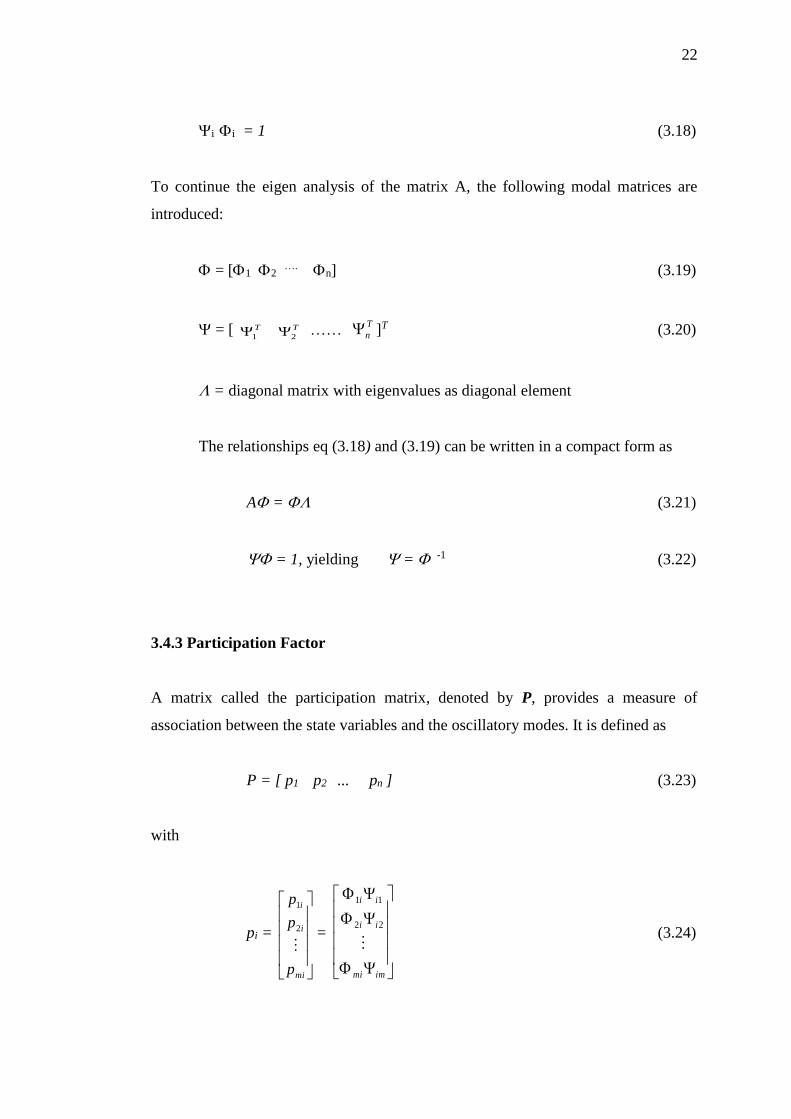
3.4.3 Participation Factor

A matrix called the participation matrix, denoted by P, provides a measure of

association between the state variables and the oscillatory modes. It is defined as

P = [ p1 p2 ... pn ] (3.23)

with

pi =

mi

i

i

p

p

p

2

1

=

immi

ii

ii

22

11

(3.24)

23

The element pki = kiik is called the participation factor, and gives a measure of the

participation of the kth state variable in the ith mode, and vice versa. The participation

factor is used in that analysis of the oscillation profile of the power system.

3.5 Differential Evolution (DE) Algorithm

The DE sequence is presented in figure 3.1, until optimization is reached or

termination occurs.

Initial population Mutation Recombination Selection Best individualMaximum iteration

NO

YES

Figure 3.1: General DE cycle

3.5.1 Population Structure

DE starts with a population of Np vectors of D – dimensional real – valued parameters

as represented in equation 3.25.

Px,g = (xi,g), i = 0,1,…., Np-1, g = 0,1,…,gmax (3.25)

Xi,g = (xj,i,g), j = 0,1, …., D-1. (3.26)

The current population, symbolized by P is composed of those vectors xi,g, that have

already been found to be acceptable either as initial points, or by comparison with

other vectors. The index, g = 0, 1,…, gmax, indicates the generation to which a vector

belongs. In addition, each vector is assigned a population index, i, which runs from 0

to Np - 1. Parameters within vectors are indexed with j, which runs from 0 to D - 1.

In the mutation stage, DE creates an intermediate population vg of the same size as the

initial population composed of vi,g vectors:

24

Pv,g = (vi,g), i = 0,1,….., Np-1, g = 0,1,….,gmax (3.27)

vi,g = (vj,i,g), j = 0,1, ….., D-1. (3.28)

The intermediate population proceeds to the next stage. DE also creates a second

intermediate population ui,g, which is also of the size Np with uj,i,g vectors. The

population is created after the recombination stage.

Pu,g = (ui,g), i = 0,1,….., Np-1, g = 0,1,….,gmax (3.29)

ui,g = (uj,i,g), j = 0,1, ….., D-1. (3.30)

During recombination, trial vectors overwrite the mutant population, so a single array

can hold both populations.

3.5.2 Initialization

The Upper and Lower bound for each parameter of a vector is initialize the DE

population. DE generates Np vectors candidates xi,g,. The ith trial solution can be

written as xi,g = [zj,i,g] where j=1,2, ... ,D. The vector's parameters are initialized within

the specified upper and lower bounds of each parameter.

x𝑗𝐿≤ xj,i,1 ≤ x𝑗

𝑈 (3.31)

Randomly select the initial parameter values uniformly on the intervals

[x𝑗𝐿, x𝑗

𝑈] (3.32)

Where “i" represents the vector and "g" the generation.

61

REFERENCES

[1] P.Kundur, “Power System Stability and Control”’ McGraw-Hill, Inc, New

York, USA, 1994

[2] A.V Folly, K.A Awodele, K.O Oyedokun, D.T. “Comparison of Matlab PST,

PSAT and DigSILENT for transient stability studies on parallel HVACHVDC

transmission lines “ Ubisse, Universities Power Engineering Conference

(UPEC), 2010 45th International, Pages: 1 – 6, 2010

[3] T. Mulumba, K.A. Folly, “Application of Self-Adaptive Differential Evolution

to tuning PSS parameters”, IEEE Conference Publications, Pages: 1-5, 2012

[4] Selvabala, B. Devaraj, D. “Co-Ordinated Tuning Of AVR-PSS Using

Differential Evolution Algorithm”, IPEC, 2010 Conference Proceedings, pp

439 -444, 2010

[5] K.V. Price, R.M. Storn, J.A. Lampinen, “Differential Evolution: A practical

approach to global optimization” Springer – Verlag Berlin Heidelberg, 2005

[6] J. Chow, J. Sanchez-Gasca, H. Ren, and S. Wang, “Power system damping

controller design using multiple input signals,” IEEE Control Syst. Mag., pp.

82–90, August 2000.

[7] G. Rogers, Power System Oscillations. Kluwer Academic Publishers Group,

2000.

[8] T. Senjyu, R. Kuninaka, N. Urasaki, H. Fujita, and T. Funabashi, “Power

system stabilization based on robust centralized and decentralized controllers,”

IEEE 7th International Power Eng. Conf. IPEC, 2005.

62

[9] E. Larsen and D. Swann, “Applying power system stabilizers: Parts I, II and

III,” IEEE Trans. Power App. Syst., vol. PAS-100, pp. 3017–3046, 1981.

[10] Graham Rogers, Power System Oscillations. Boston: Kluwer Academic, 1999.

[11] E.V. Larsen and D.A. Swann, "Applying Power System Stabilizers, Part I;

General concepts, Part II; Performance objectives and Tuning concepts, Part

III; Practical considerations," IEEE Trans. on Power Apparatus and Systems,

vol. PAS-100, pp. 3017-3046, 1981.

[12] K. Price, R. Storn, and J. Lampinem, Differential Evolution: A practical

approach to global optimization. Berlin Heldelberg: Springer-Verlag, 2005.

[13] Y.P. Li, D.G. Wang, A. P. Hu, Real-time Simulation Study on HVDC Control

and Protection, IEEE International Conference, Page(s): 1 - 6, 2010

[14] Power System Toolbox version 3.0 Tutorial and Functions, Cherry Tree

Scientific Software, 1994 – 2004.

[15] S.P.N Sheetekela, "Design of Power System Stabilizers using Evolutionary

Algorithms,", Electrical, University of Cape Town, Cape Town, MSc. Thesis

2010

DEVELOPMENT OF DIFFERENTIAL EVOLUTION BASED POWER SYSTEM ... · development of differential evolution based power system stabilizer (pss) with hvdc in small signal stability analysis

Documents