Title Impact analysis of variable generation on small ... · Impact Analysis of Variable Generation on Small Signal Stability ... Index Terms—power system oscillations, small signal

Title Impact analysis of variable generation on small signal stability

Author(s) Shim, JW; Verbic, G; Hur, K; Hill, DJ

Citation

The 24th Australasian Universities Power EngineeringConference (AUPEC 2014), Curtin University, Perth, WA.,Australia, 28 September-1 October 2014. In ConferenceProceedings, 2014, p. 1-6

Issued Date 2014

URL http://hdl.handle.net/10722/216562

Rights Australasian Universities Power Engineering Conference(AUPEC). Copyright © IEEE.

Impact Analysis of Variable Generation on SmallSignal Stability

Jae Woong Shim ∗†, Student Member IEEE, Gregor Verbic ∗, Senior Member IEEE,Kyeon Hur†, Senior Memebr IEEE, David J. Hill∗‡, Fellow IEEE

∗The University of Sydney, Sydney, Australia, {jae-woong.shim, gregor.verbic, david.hill}@sydney.edu.au†Yonsei University, Seoul, S. Korea, {jeuhnshim, khur}@yonsei.ac.kr

‡The University of Hong Kong, Hong Kong, [email protected]

Abstract—This paper aims to analyse the influence of fluctu-ating renewables on small-signal stability. Most of the researchon renewable energy integration assumes that power is providedfrom a static generation unit and studies how much dampingratio and frequency changes as a result of changing power andinertia. This research is motivated by mode coupling where oneoscillatory mode may have an effect on other modes if themode frequencies are similar. The paper discusses the impactof fluctuating power sources, Type IV wind turbines in our case,on possible coupling between the fluctuating wind power and theexisting modes in the system. Since the fluctuating power maycombine a large band of frequency components, the power systemcan react to any specific frequency of a variable generator. Inthis paper, several influential frequencies were injected throughthe renewable generator. System identification is used first toobtain the linearized state-space model of the system and therelevant transfer functions, which are then used to identifypossible resonant frequencies. DIgSILENT/Power Factory is usednext to analyse the system’s response to specific frequencies inthe time domain.

Index Terms—power system oscillations, small signal stability,mode coupling, renewable energy sources, wind power, resonance.

I. INTRODUCTION

PENETRATION of intermittent renewable energy sources

(RES) is steadily increasing following the renewable

portfolio targets that have been put in place in many countries

around the world to speed up the transition to more RES based

power systems. The University of Melbourne Energy Research

Institute’s study [1] suggests that a 100% renewable scenario

can be achieved as early as 2020, although the Australian

Energy Market Operator (AEMO) considers the 2030 to 2050

time frame to be more realistic for Australia [2]. To tackle

the integration of RES, the analysis of grid characteristics

with RES is essential, and used for operation and planning

in the long-term future. Without the fundamental work for

implications of variable generation, future power system may

have difficulty operating stably with high penetration of RES.

Much research effort has been put into studying the impact

of RES, mostly solar and wind, on power system stability,

focusing predominantly on small-signal [3]–[7] and transient

[7], [8] angle stability. Such initiatives internationally notwith-

standing, the influence of RES on power system stability and

performance still requires a lot of attention. The common

denominator of the existing research is the use of quasi-

static analysis, implicitly assuming that variations in the RES’

output are slow enough not to impact the system modes.

This approach seems to be widely accepted. For example, a

comprehensive CIGRE Technical Brochure [9] and a more

recent AEMO study [10] don’t even mention this assumption.

We make an attempt to cover this gap by considering the

output of a RES not to be static at the studied operating point

but rather consisting of a fixed component and a superimposed

fluctuating component of a frequency similar to the existing

system’s modes.

The problem of mode coupling hasn’t attracted much atten-

tion in the power engineering community so far. The earliest

references date back to 1980s [11]. The phenomenon has been

observed in practice, e.g. in the WECC with implications for

PSS tuning [12]. To the best of our knowledge, this is the

first attempt to study the impact of RES on mode coupling.

The goal of this paper is thus to establish hypotheses about

the influence on system stability from variable generators.

Unlike the conventional thermal and hydro power plants whose

output variation is very slow with no or negligible higher-

frequency components, the output of intermittent RES consists

of fluctuating components with frequencies that can potentially

interact with the existing system modes. This can change

the behaviour of the system or even cause instability in a

large scale network. The focal point of our discussion is

on the influence of the fluctuating frequency component on

the small disturbance stability. We first use sub-space system

identification to obtain a reduced-order linearized model of

the system and the relevant transfer functions. Then we use

time-domain simulation to analyse the behaviour of the system

subject to penetration of fluctuating RES in the selected

frequency bands.

The rest of paper is organized as follows: an introduction

discussing the concept of mode coupling and power system

oscillations is given in Section II. In Section III, system

identification used in the paper is briefly discussed. In Section

IV, the results of the case study on test system are given, and

Section V concludes the paper.

II. BACKGROUND

The main focus of this study is small-signal stability,

which is defined as the ability of the power network to keep

synchronism under small disturbances, typically changes in

Australasian Universities Power Engineering Conference, AUPEC 2014, Curtin University, Perth, Australia, 28 September – 1 October 2014 1

either load or generation [13]. The changes are considered to

be small enough so the system can be linearized around the

operating point. The remainder of this section discusses small-

signal stability and mode coupling, which lays the groundwork

for the case studies considered later in the paper.

A. Small-signal Stability and Mode Coupling

The behaviour of a power system can be described by a set

of differential and algebraic equations of the form:

x = f1(x1,x2,u) (1)

0 = f2(x1,x2,u) (2)

y = g0(x1,x2,u) (3)

where f1, f2 and g0 give the vectors of non-linear differential,

algebraic and output equations, respectively; and x1 ∈ Rn,

x2 ∈ Rl, u ∈ R

m and y ∈ Rp denote the vectors of state

variables, algebraic variables, inputs and outputs, respectively.

Typically, the system in (1) is assumed time-invariant so the

time-derivatives of the state variables are not explicit functions

of the time. Assuming ∂f2∂x2

is nonsingular we can eliminate

x2. Let x = x1 and we get

x = f(x,u) (4)

y = g(x,u) (5)

In small-signal stability analysis, the disturbances are con-

sidered small so the system can be linearized around the

operating point (x0,u0) resulting in

Δx =∂f

∂x

∣∣∣∣0

Δx+∂f

∂u

∣∣∣∣0

Δu = AΔx+BΔu (6)

Δy =∂f

∂x

∣∣∣∣0

Δx+∂f

∂u

∣∣∣∣0

Δu = CΔx+DΔu (7)

where Δx, Δy and Δu represent deviations from operating

point values.

The linearized system (6,7) can be used to investigate

the system’s response to small variations in the input or

state variables. A possible instability can be due to lack

of synchronizing torque, resulting in an increase in rotor

angle through a non-oscillatory or aperiodic mode; or due to

lack of sufficient damping torque, resulting in oscillations of

increasing amplitude. The oscillations can be either local or

global, depending on the machines involved. Global or inter-area mode oscillations, involve one group of generators in one

part of the system swinging against a group of generators in

another part of the system. Local mode oscillations, on the

other hand, are restricted to a small part of the system and

often refer to one generator’s motion with respect to the rest

of the system.

Mode coupling is a situation where an oscillation mode in

one part of the system interacts with a mode of oscillation

in a remote part [11]. Mode coupling had been observed in

the WECC when studying the placement of PSSs [12]. It was

found that a generator in one part of the system had a relatively

high participating factor in an oscillatory mode associated with

a group of generators located in a remote part of the system. In

this particular example, the coupling was triggered due to the

mode frequencies being very close. Another possible trigger

can be disturbances entering the system at frequencies close

to the system modes, i.e. fluctuating RES, which, to the best

of authors’ knowledge, hasn’t been studied yet.

B. Mode Coupling Triggered by Fluctuating RES

Unlike the conventional energy sources, some RES can

exhibit fluctuating behaviour due to the variability of the

primary energy source. While geothermal, tidal and solar

thermal cannot change the output quickly due to the large

inherent inertia, solar PV, wave and wind can. Solar PV doesn’t

possess any energy buffer so the output can fluctuate due to

varying cloud coverage. The resulting fluctuations however

will likely be aperiodic. Wave and wind generation, on the

other hand, can generate periodic power fluctuations. Unlike

wind, wave generation is still in its infancy, so little operational

data is available in the literature. In this paper, we therefore

consider wind power as a trigger of possible mode coupling.

The fluctuation in the wind can be thought of as resulting

from a composite of sinusoidally varying winds superimposed

on the mean steady wind [14]. If the frequency of a sufficient

strong wind component matches the frequency of one the

system’s poorly damped oscillatory modes, the mode gets

excited by the fluctuating RES, which results in resonance.

This phenomenon is called mode coupling and is not restricted

by the electrical distance between the source and the machine

participating in the affected mode. In other words, mode

coupling can affect both local and inter-area modes.

C. Wind Power Spectrum

The variability of wind spans multiple time scales. Medium-

and long-term fluctuations can be modelled with Van der

Hoven’s spectral model, while for short-term fluctuations, cap-

turing the turbulent behaviour, either von Karman’s or Kaimal

spectral models are typically used [15]. Van der Hoven’s

spectrum is modelled as a stationary random process, whereas

the turbulence spectrums, either von Karman’s or Kaimal’s,

are non-stationary. Van der Hoven’s spectrum spans the range

between 0.001 cycles/h (inter-seasonal variations) and 1000

cycles/h (intra-minute variations). The turbulent short-term

power spectrum spans the frequencies between 0.01 and 4 Hz,

which covers the typical frequency range of the local and

inter-area oscillatory modes (between 0.25 and 2 Hz). The

turbulent wind fluctuations should therefore be considered in

the analysis of mode coupling due to fluctuation RES. For

illustration, a sample Van Der Hoven’s and Kaimal wind power

spectra are shown in Figs. 1 and 2, respectively.

Observe in Fig. 2 the effect of the rotational sampling of the

wind turbine blades caused by the tower shadow. For the most

common 3-blade turbine, the sharp spike occurs at the triple

of the turbine’s rotational speed. The exact frequency thus

depends on the rotational speed of the turbine, determined

by the design and the control method used. This deserves

further attention, as the frequency of the spike could be close


10−3 10−2 10−1 100 101 102 1030

2

4

6

f [Cycle/h]

fgs(f)

[m2 /s

2 ]

Fig. 1. Van Der Hoven’s wind power spectrum.

10−2 10−1 100 10110−4

10−2

100

f [Hz]

fgs(f)

[m2 /s

2 ]

Fig. 2. Kaimal’s wind power spectrum.

to the frequency of an oscillatory mode. This particular issue

is however beyond the scope of the paper.

III. IDENTIFYING THE STATE SPACE MODEL OF THE

SYSTEM

Power systems are time varying and highly non-linear so

it is almost impossible to identify the non-linear models.

Instead, linearization could be used to analyse the impact of a

small deviation in system’s inputs. DIgSILENT/PowerFactory

doesn’t allow the user to obtain the linearized state-space

model of the system. Instead, we used the N4SID sub-space

system identification technique available in Matlab’s System

Identification Toolbox [16]. The state-space model has been

used to obtain the transfer functions of interest for a particular

operating condition, as described later.

One of the most important aspects of system identification is

the selection of the probing signal [17]. Firstly, the frequency

spectrum needs to cover the frequency band of interest, and,

secondly, the amplitude of the signal must be sufficiently high

to excite the critical oscillatory modes without pushing the

system into a nonlinear zone [18]. We tested the following

probing signals: Random Gaussian Signal, Random Binary

Signal, Pseudo Random Binary Signal (PRBS), and Sum

of Sinusoid Signal. PRBS was chosen due to its superior

performance over the widest frequency range.

Intuitively, perturbation of the system with a fluctuating

RES is similar to system identification. In response to the

perturbation signal with a wide frequency spectrum, most of

the frequency band is filtered out except for the oscillatory

frequency, where the system resonates with the perturbation

signal.

A. Numerical Subspace State Space System Identification

In our study, system identification was used to identify the

transfer functions between the wind turbine, modeled as a

controlled current using the in-built converter model, as the

input and the angular speeds of the four generators as the

outputs to study the resonant behaviour, i.e. the mode cou-

pling between the fluctuating RES and the existing oscillatory

modes. The resulting system identification problem is thus

Single Input Multiple Output (SIMO). The model with minputs, p outputs and n states was estimated in discrete domain

and the converted into continuous domain resulting in

x(t) = Ax(t) +Bu(t) +Ke(t) (8)

y(t) = Cx(t) +Du(t) + e(t) (9)

where x ∈ Rn is the state vector; u ∈ R

m is the input vector;

y ∈ Rp denotes the output vector; and A ∈ R

n×n, B ∈R

n×m, C ∈ Rp×n and D ∈ R

p×m are the system matrices.

Ke(t) ∈ Rn and e(t) ∈ R

p are, respectively, the disturbances

and the noise acting on the system. In our case m = 1, p = 4and n = 13. The dynamic order of the original system is 49.

IV. TEST SYSTEM

A. Test Bed: Two-area System

We used the four-machine, two-area test system proposed

in [19] as the test bed. The system consists of four generators

located in two areas; G1 and G2 in the east, and G3 and G4 in

the west. A wind power plant, modelled as a single 120MW

Type IV (synchronous machine with a fully rated converter)

wind turbine has been connected to the high voltage bus near

G2. The system is shown in Fig. 3. As a result, the power of

the slack bus (G1) has been reduced to keep the system in

balance.

Three oscillatory modes exist in this system: one interarea

mode with the generators in the east oscillating against the

generators in the west; and two local modes, one between G1

and G2 and the other between G3 and G4. We considered the

case of a thyristor exciter with high transient gain and PSS.

To get mode coupling in the system, the renewable generator

(sender) needs to have a component with a frequency similar to

one of the existing oscillatory modes. To this end, we modified

some PSS parameters to create two cases with a different

oscillatory behaviour—see Table I.

Other parameters were left unchanged, resulting in three

study cases: (1) the original case, (2) a case where a local

mode (G3, G4) with reduced damping resonates with the wind

turbine; and (3) a case with an unstable local mode (G3, G4).

In all three cases, we first identified the sub-space linearized

Fig. 3. Two Area Test System.


TABLE IMODIFIED EXCITER AND PSS PARAMETERS.

G1 G1

Case 1 2 3 1 2 3

Kstab 20 200 200 20 20 20

T2 0.02 0.02 0.02 0.02 0.02 0.02

T3 3 30 30 3 30 30

G3 G4

Case 1 2 3 1 2 3

Kstab 20 185 200 20 20 5

T2 0.02 0.17 0.17 0.02 0.02 0.02

T3 3 3 3 3 3 5

models of the system that were used to obtain the transfer

functions between the wind turbine as the input and the angular

speeds of all four generators as the outputs. This enabled

us to identify possible resonance in the system subject to

fluctuations in the wind power. Next, we injected a sinusoidal

signal at three different frequencies, representing fluctuating

wind power spectral components, and simulated the response

of the system in time domain.

B. Case 1: Standard System

The standard system corresponds to the case with the

thyristor exciter with high transient gain and PSS in [19]. Fig.

4 shows the oscillatory modes in the complex plane. Observe

that the local modes (G1,G2) and (G3,G4) have very similar

frequencies.

Fig. 5 shows the Bode plots of the transfer functions

between the wind power and the machine angular speeds of

the four generators.

Three signals with different frequency are injected: (A)

interarea mode frequency; (B) local mode frequency; and (C)

a signal with a frequency significantly different from mode

frequencies. The spike in the bode plot around frequency

−1.4 −1.2 −1 −0.8 −0.6 −0.4 −0.2 0 0.22

4

6

8

10

12

14

A=0.5517Hz

B=1.0446Hz

C=2.2122Hz

Local mode (G1,G2)λ: −0.5865±j6.5638ζ: 8.899 % fd :1.0446 Hz


Interarea modeλ: −0.0747±j3.4670ζ: 2.1541 % fd :0.5517 Hz

Imag

[rad

/s]

Real [1/s]

Fig. 4. Case 1: Oscillatory modes and the frequencies of the injected signals.

100

101

−100

−80

−60

−40

−20

Mag

nitu

de (d

B)

A B C

Frequency (rad/s)

Wind ref. − Spd of Gen1Wind ref. − Spd of Gen2Wind ref. − Spd of Gen3Wind ref. − Spd of Gen4


−15

−10

−5

0

5

10

15

Pow

er [M

W]

Signal A

0.9992

0.9996

1

1.0004

1.0008

Rot

or s

peed

[pu]

0 10 20 300.998

0.999

1

1.001

1.002

Rot

or s

peed

[pu]

Time [s]

Signal B

0 10 20 30Time [s]

Signal C

Wind

Gen1Gen2

0 10 20 30Time [s]

Gen3Gen4

Fig. 6. Case 1: Time-domain simulation results.

A indicates that the injected sinusoidal signal might interact

with the interarea mode while we don’t expect any interaction

for frequencies B and C. This is confirmed by time-domain

simulations, Fig. 6. Observe in Fig. 6 the amplified response

of the four generators subject to a sinusoidal wind power

injection with frequency A. As expected, frequencies B and C

have negligible impact.

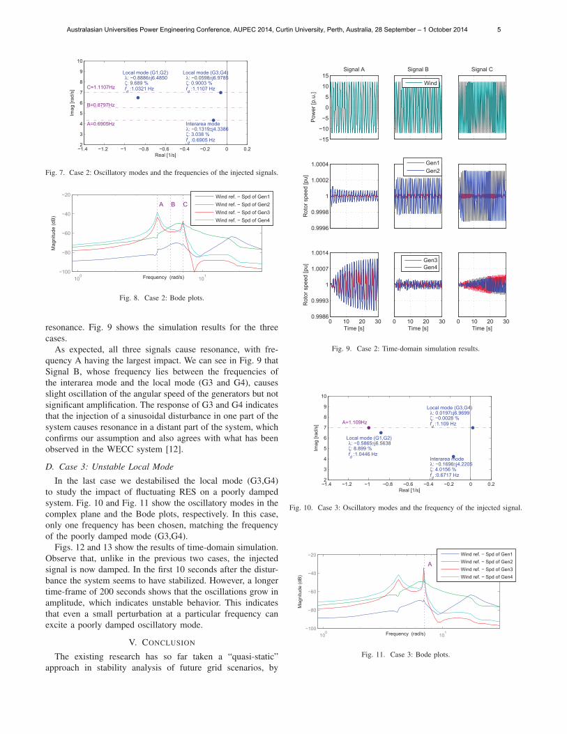
C. Case 2: Resonant Local Mode

In this case, we modified the parameters of the excitation

system to reduce damping of the local mode (G3,G4). Fig. 7

and Fig. 8 show the oscillatory modes in the complex plane

and the Bode plots, respectively.

Unlike in Case 1, we now expect the wind turbine input

to resonate with the three modes for frequencies A and C. In

addition, because the frequencies A and C are similar, we also

expect frequency B, which lies between A and C, to cause


−1.4 −1.2 −1 −0.8 −0.6 −0.4 −0.2 0 0.22

3

4

5

6

7

8

9

10

A=0.6905Hz

B=0.8797Hz

C=1.1107Hz




Imag

[rad

/s]

Real [1/s]


100

101

−100

−80

−60

−40

−20

Mag

nitu

de (d

B)

A B C

Frequency (rad/s)


Fig. 8. Case 2: Bode plots.

resonance. Fig. 9 shows the simulation results for the three

cases.

As expected, all three signals cause resonance, with fre-

quency A having the largest impact. We can see in Fig. 9 that

Signal B, whose frequency lies between the frequencies of

the interarea mode and the local mode (G3 and G4), causes

slight oscillation of the angular speed of the generators but not

significant amplification. The response of G3 and G4 indicates

that the injection of a sinusoidal disturbance in one part of the

system causes resonance in a distant part of the system, which

confirms our assumption and also agrees with what has been

observed in the WECC system [12].

D. Case 3: Unstable Local Mode

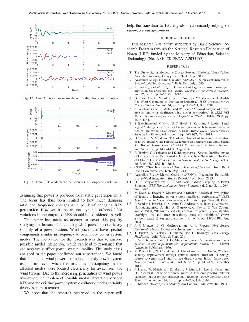
In the last case we destabilised the local mode (G3,G4)

to study the impact of fluctuating RES on a poorly damped

system. Fig. 10 and Fig. 11 show the oscillatory modes in the

complex plane and the Bode plots, respectively. In this case,

only one frequency has been chosen, matching the frequency

of the poorly damped mode (G3,G4).

Figs. 12 and 13 show the results of time-domain simulation.

Observe that, unlike in the previous two cases, the injected

signal is now damped. In the first 10 seconds after the distur-

bance the system seems to have stabilized. However, a longer

time-frame of 200 seconds shows that the oscillations grow in

amplitude, which indicates unstable behavior. This indicates

that even a small perturbation at a particular frequency can

excite a poorly damped oscillatory mode.

V. CONCLUSION

The existing research has so far taken a “quasi-static”

approach in stability analysis of future grid scenarios, by

−15

−10

−5

0

5

10

15

Pow

er [p

.u.]

Signal A

0.9996

0.9998

1

1.0002

1.0004

Rot

or s

peed

[pu]

0 10 20 300.9986

0.9993

1

1.0007

1.0014

Rot

or s

peed

[pu]

Time [s]

Signal B

Wind

Gen1Gen2

0 10 20 30Time [s]

Gen3Gen4

Signal C

0 10 20 30Time [s]

Fig. 9. Case 2: Time-domain simulation results.

−1.4 −1.2 −1 −0.8 −0.6 −0.4 −0.2 0 0.22

3

4

5

6

7

8

9

10

A=1.109Hz


Local mode (G3,G4)λ: 0.0197±j6.9699ζ: −0.0028 % fd :1.109 Hz


Imag

[rad

/s]

Real [1/s]

Fig. 10. Case 3: Oscillatory modes and the frequency of the injected signal.

100

101

−100

−80

−60

−40

−20

Mag

nitu

de (d

B)

A

Frequency (rad/s)


Fig. 11. Case 3: Bode plots.


0 2 4 6 8 10−15−10−5

05

1015

Pow

er [M

W]

Wind

0 2 4 6 8 100.99980.9999

11.00011.00021.0003

Rot

or s

peed

[pu]

Gen1Gen2

0 2 4 6 8 100.99980.9999

11.00011.00021.0003

Rot

or s

peed

[pu]

Time [s]

Gen3Gen4

Fig. 12. Case 3: Time-domain simulation results; short-term evolution.

0 50 100 150 200−15−10−5

05

1015

Pow

er [M

W]

Wind

0 50 100 150 2000.9992

0.9996

1

1.0004

1.0008

Rot

or s

peed

[pu]

Gen1Gen2

0 50 100 150 2000.998

0.999

1

1.001

1.002

Rot

or s

peed

[pu]

Time [s]

Gen3Gen4

Fig. 13. Case 3: Time-domain simulation results; long-term evolution.

assuming that power is provided from static generation units.

The focus has thus been limited to how much damping

ratio and frequency changes as a result of changing RES

penetration. However, it appears that dynamic effects of fast

variations in the output of RES should be considered as well.

This paper has made an attempt to cover this gap by

studying the impact of fluctuating wind power on oscillatory

stability of a power system. Wind power can have spectral

components similar in frequency to oscillatory power system

modes. The motivation for the research was thus to analyse

possible modal interaction, which can lead to resonance that

can negatively affect power system stability. The study cases

analysed in the paper confirmed our expectations. We found

that fluctuating wind power can indeed amplify power system

oscillations, even when the machines participating in the

affected modes were located electrically far away from the

wind turbine. Due to the increasing penetration of wind power

worldwide, the problem of possible modal interaction between

RES and the existing power system oscillatory modes certainly

deserves more attention.

We hope that the research presented in the paper will

help the transition to future grids predominantly relying on

renewable energy sources.

ACKNOWLEDGMENT

This research was partly supported by Basic Science Re-

search Program through the National Research Foundation of

Korea (NRF) funded by the Ministry of Education, Science,

Technology (No. NRF- 2012K2A1A2033153).

REFERENCES

[1] The University of Melbourne Energy Research Institute, “Zero CarbonAustralia Stationary Energy Plan,” Tech. Rep., 2010.

[2] Australian Energy Market Operator (AEMO), “100 Per Cent RenewablesStudy–Modelling Outcomes,” Tech. Rep. July, 2013.

[3] J. Slootweg and W. Kling, “The impact of large scale wind power gen-eration on power system oscillations,” Electric Power Systems Research,vol. 67, no. 1, pp. 9–20, Oct. 2003.

[4] G. Tsourakis, B. Nomikos, and C. Vournas, “Contribution of DoublyFed Wind Generators to Oscillation Damping,” IEEE Transactions onEnergy Conversion, vol. 24, no. 3, pp. 783–791, Sep. 2009.

[5] J. Sanchez-Gasca, N. Miller, and W. Price, “A modal analysis of a two-area system with significant wind power penetration,” in IEEE PESPower Systems Conference and Exposition, 2004. IEEE, 2004, pp.1537–1541.

[6] S. Eftekharnejad, V. Vittal, G. T. Heydt, B. Keel, and J. Loehr, “SmallSignal Stability Assessment of Power Systems With Increased Penetra-tion of Photovoltaic Generation: A Case Study,” IEEE Transactions onSustainable Energy, vol. 4, no. 4, pp. 960–967, Oct. 2013.

[7] D. Gautam, V. Vittal, and T. Harbour, “Impact of Increased Penetrationof DFIG-Based Wind Turbine Generators on Transient and Small SignalStability of Power Systems,” IEEE Transactions on Power Systems,vol. 24, no. 3, pp. 1426–1434, Aug. 2009.

[8] B. Tamimi, C. Canizares, and K. Bhattacharya, “System Stability Impactof Large-Scale and Distributed Solar Photovoltaic Generation: The Caseof Ontario, Canada,” IEEE Transactions on Sustainable Energy, vol. 4,no. 3, pp. 680–688, Jul. 2013.

[9] CIGRE, “Grid Integration of Wind Generation,” Working Group 08 ofStudy Committee C6, Tech. Rep., 2009.

[10] Australian Energy Market Operator (AEMO), “Integrating RenewableEnerg–Wind Integration Studies Report,” Tech. Rep., 2013.

[11] D. K. Mugwanya and J. E. Van Ness, “Mode Coupling in PowerSystems,” IEEE Transactions on Power Systems, vol. 2, no. 2, pp. 264–269, 1987.

[12] M. Klein, G. Rogers, S. Moorty, and P. Kundur, “Analytical investigationof factors influencing power system stabilizers performance,” IEEETransactions on Energy Conversion, vol. 7, no. 3, pp. 382–390, 1992.

[13] P. Kundur, J. Paserba, V. Ajjarapu, G. Andersson, A. Bose, C. Canizares,N. Hatziargyriou, D. Hill, A. Stankovic, C. Taylor, T. Van Cutsem,and V. Vittal, “Definition and classification of power system stabilityieee/cigre joint task force on stability terms and definitions,” PowerSystems, IEEE Transactions on, vol. 19, no. 3, pp. 1387–1401, Aug2004.

[14] J. F. Manwell, J. G. McGowan, and A. L. Rogers, Wind EnergyExplained: Theory, Design and Application. Wiley, 2010.

[15] T. Burton, N. Jenkins, D. Sharpe, and E. Bossanyi, Wind EnergyHandbook. John Wiley & Sons, 2011.

[16] P. Van Overschee and B. De Moor, Subspace identification for linearsystems: theory, implementation, applications, Volume 1. KluwerAcademic Publishers, 1996.

[17] Y. Pipelzadeh, N. Chaudhuri, B. Chaudhuri, and T. Green, “Systemstability improvement through optimal control allocation in voltagesource converter-based high-voltage direct current links,” Generation,Transmission Distribution, IET, vol. 6, no. 9, pp. 811–821, September2012.

[18] J. Hauer, W. Mittelstadt, K. Martin, J. Burns, H. Lee, J. Pierre, andD. Trudnowski, “Use of the wecc wams in wide-area probing tests forvalidation of system performance and modeling,” Power Systems, IEEETransactions on, vol. 24, no. 1, pp. 250–257, Feb 2009.

[19] P. Kundur, Power System Stability and Control. McGraw-Hill, 1994.


Title Impact analysis of variable generation on small ... · Impact Analysis of Variable Generation on Small Signal Stability ... Index Terms—power system oscillations, small signal

Documents