2018 INRO User Guide – SANDAG Travel Model in Emme

Welcome message from author
This document is posted to help you gain knowledge. Please leave a comment to let me know what you think about it! Share it to your friends and learn new things together.
Transcript

2018 INRO
U s e r G u i d e – S A N D A G T r a v e l M o d e l i n E m m e
2018 INRO 1
06/07/2018
T a b l e o f C o n t e n t s
1. Overview 3
2. Model conversion summary 3
3. System design 4
Model description ........................................................................................ 5
4. Setup 7
5. Model operation and Master run tool 10
Master run tool ........................................................................................... 10
Scripted operation ...................................................................................... 13
Model runtime ........................................................................................... 14
6. SANDAG Toolbox and Tools 14
7. Import network 17
Mode definitions ........................................................................................ 20
8. Traffic assignment 21
Volume-delay functions ............................................................................. 22
Traffic skims .............................................................................................. 23
Traffic assignment tool .............................................................................. 23
Traffic select link analysis ......................................................................... 25
9. Transit assignment 26
Travel time components ............................................................................ 26
Representing fares ..................................................................................... 27
Additional custom transit network adjustments ......................................... 28
Build transit network tool .......................................................................... 30
Transit assignment tool .............................................................................. 31
Transit select analysis ................................................................................ 31
10. Aggregate demand models and other tools 33
Truck model ............................................................................................... 33
Commercial vehicle model ........................................................................ 33
External models ......................................................................................... 34
Data management tools .............................................................................. 34
11. Appendix 39
Matrix naming convention ......................................................................... 39
Attribute name mappings ........................................................................... 42
SANDAG Travel Model User Guide
2018 INRO 2
2018-07-06
L i s t o f F i g u r e s
Figure 1 - Emme project setup with base (SANDAG base 2012) and transit (SANDAG base
2012-transit) databases and result scenarios after model run. ............................................ 5
Figure 2 - System diagram of main model steps and data transfer between Emme and non-
Emme procedures............................................................................................................... 6
Figure 3 – ABM scenario directory structure............................................................................. 8
Figure 4 - The Modeller window and Master run tool............................................................. 10
Figure 5 - Master run ABM tool user interface ....................................................................... 11
Figure 6 – Logbook output following a model. ....................................................................... 12
Figure 7 - Logbook and traffic impedance summaries and assignment convergence chart ..... 13
Figure 8 - the user interface and inputs for the Import network tool ....................................... 17
Figure 9 – The green tool page status message indicating minor errors, and the red halting
error status message following runs of Import network tool. ........................................... 18
Figure 10 - SANDAG Traffic assignment tool user interface .................................................. 24
Figure 11 - user interface for select link analysis in Traffic assignment tool ........................... 25
Figure 12 - Illustration of network modifications to represent timed transfers. ....................... 29
Figure 13 - Illustration of network modification to prohibit walking to a different stop on a
transfer link for the initial boarding from a TAP. ............................................................ 29
Figure 14 - user interface for Build transit network tool .......................................................... 30
Figure 15 - user interface for SANDAG Transit assignment tool ............................................ 31
Figure 16 - user interface for Transit select analysis tool ........................................................ 32
L i s t o f T a b l e s
Table 1 - Summary of model runtime by model step. .............................................................. 14
Table 2 - Summary of model runtime by major model component. ........................................ 14
Table 3 - List of tools in SANDAG toolbox ............................................................................ 14
Table 4 - Mode definitions for traffic and transit network ....................................................... 20
Table 5 - Key mode fields from hwycov.e00 and trcov.e00 .................................................... 21
Table 6 - List of traffic demand classes and key class parameter values ................................. 22
Table 7 - costs and perception factors which vary by mode .................................................... 26
Table 8 - Journey level table for bus mode only assignments. ................................................. 27
Table 9 - Journey level table for all modes assignments. ......................................................... 28
Table 10 - Traffic link attribute name mapping from hwycov.e00 .......................................... 42
Table 11 - Transit link attribute name mapping from trcov.e00 .............................................. 44
Table 12 - Transit route attribute name mapping from trrt.csv and mode5tod.dbf .................. 45
Table 13 - Transit segment (and stop) attribute name mapping from trstop.csv ...................... 45

SANDAG Travel Model User Guide
2018 INRO 3
2018-07-06
1 . O v e r v i e w
This user guide documents the SANDAG travel demand model as implemented using the
Emme modelling framework and components (traffic and transit assignments and aggregate
demand modelling tools), integrated with disaggregate demand model components (CT-
RAMP family of activity-based models). It also provides “how-to” instructions for master run
model operation (see page 10) and the operation of the components implemented within the
Emme framework.
This user guide has a companion report "Comparison and Validation - SANDAG Travel
Model in Emme" which documents the comparison of the SANDAG travel model conversion
to Emme against the previous implementation and the validation of the updated model.
Emme is a complete travel demand modelling system for urban, regional and national
transportation forecasting. Emme offers a transport modelling application framework for
leading computational performance and promotes true model transparency and offers an easy
transition between interactive use and modern scripting using Python.
The Emme components of the SANDAG model are implemented as a set of discrete
components in the Python scripting language, using Emme APIs, and Emme assignment,
analysis, calculators and other modelling procedures. Each component is provided as a
separate Emme Modeller tool which can be run independently with its own user interface and
logging and reporting services. The entire model can be configured and executed using the
Master run tool.
The tools are packaged and delivered as a Modeller toolbox within the Emme project. The
main model components implemented in this framework are:
• Traffic assignment and skims
• Transit assignment and skims
• Truck demand model for heavy trucks within, into, out of and through San Diego
• Commercial vehicle model for other goods and services movements within San
Diego
• An external-internal travel model covering non-resident travel into and out of San
Diego made by non-Mexican residents (USA-SD)
• An external-external travel model covering travel through the San Diego region
In addition to the main components, there are also tools for select element type network
analysis for traffic and transit, tools for reporting and data management.
Further information on disaggregate demand model components (for San Diego residents’
travel and other special market travel) can be found in other reports such as the Activity-Based
Travel Model User’s Guide.
2 . M o d e l c o n v e r s i o n s u m m a r y
This section highlights the key changes in model implementation during the conversion to
Emme. The main goal of the conversion project was to replace the previous traffic and transit
assignments, aggregate demand model components, and other ancillary tools with equivalent
Emme procedures. Most components were mapped to direct "drop-in" replacements with few
model procedure changes.
Previous GISDK scripts files have been replaced by Emme Modeller tools implemented as
Python scripts. There is a general mapping of previous files to new tools, however there are a
couple of exceptions:
• Both createhwynet.rsc and createtrnroutes.rsc are replaced by the Import
network tool
SANDAG Travel Model User Guide
2018 INRO 4
2018-07-06
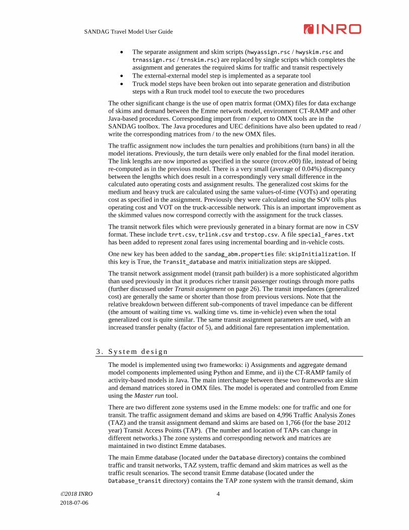
• The separate assignment and skim scripts (hwyassign.rsc / hwyskim.rsc and
trnassign.rsc / trnskim.rsc) are replaced by single scripts which completes the
assignment and generates the required skims for traffic and transit respectively
• The external-external model step is implemented as a separate tool
• Truck model steps have been broken out into separate generation and distribution
steps with a Run truck model tool to execute the two procedures
The other significant change is the use of open matrix format (OMX) files for data exchange
of skims and demand between the Emme network model, environment CT-RAMP and other
Java-based procedures. Corresponding import from / export to OMX tools are in the
SANDAG toolbox. The Java procedures and UEC definitions have also been updated to read /
write the corresponding matrices from / to the new OMX files.
The traffic assignment now includes the turn penalties and prohibitions (turn bans) in all the
model iterations. Previously, the turn details were only enabled for the final model iteration.
The link lengths are now imported as specified in the source (trcov.e00) file, instead of being
re-computed as in the previous model. There is a very small (average of 0.04%) discrepancy
between the lengths which does result in a correspondingly very small difference in the
calculated auto operating costs and assignment results. The generalized cost skims for the
medium and heavy truck are calculated using the same values-of-time (VOTs) and operating
cost as specified in the assignment. Previously they were calculated using the SOV tolls plus
operating cost and VOT on the truck-accessible network. This is an important improvement as
the skimmed values now correspond correctly with the assignment for the truck classes.
The transit network files which were previously generated in a binary format are now in CSV
format. These include trrt.csv, trlink.csv and trstop.csv. A file special_fares.txt
has been added to represent zonal fares using incremental boarding and in-vehicle costs.
One new key has been added to the sandag_abm.properties file: skipInitialization. If
this key is True, the Transit_database and matrix initialization steps are skipped.
The transit network assignment model (transit path builder) is a more sophisticated algorithm
than used previously in that it produces richer transit passenger routings through more paths
(further discussed under Transit assignment on page 26). The transit impedances (generalized
cost) are generally the same or shorter than those from previous versions. Note that the
relative breakdown between different sub-components of travel impedance can be different
(the amount of waiting time vs. walking time vs. time in-vehicle) even when the total
generalized cost is quite similar. The same transit assignment parameters are used, with an
increased transfer penalty (factor of 5), and additional fare representation implementation.
3 . S y s t e m d e s i g n
The model is implemented using two frameworks: i) Assignments and aggregate demand
model components implemented using Python and Emme, and ii) the CT-RAMP family of
activity-based models in Java. The main interchange between these two frameworks are skim
and demand matrices stored in OMX files. The model is operated and controlled from Emme
using the Master run tool.
There are two different zone systems used in the Emme models: one for traffic and one for
transit. The traffic assignment demand and skims are based on 4,996 Traffic Analysis Zones
(TAZ) and the transit assignment demand and skims are based on 1,766 (for the base 2012
year) Transit Access Points (TAP). (The number and location of TAPs can change in
different networks.) The zone systems and corresponding network and matrices are
maintained in two distinct Emme databases.
The main Emme database (located under the Database directory) contains the combined
traffic and transit networks, TAZ system, traffic demand and skim matrices as well as the
traffic result scenarios. The second transit Emme database (located under the
Database_transit directory) contains the TAP zone system with the transit demand, skim
SANDAG Travel Model User Guide
2018 INRO 5
2018-07-06
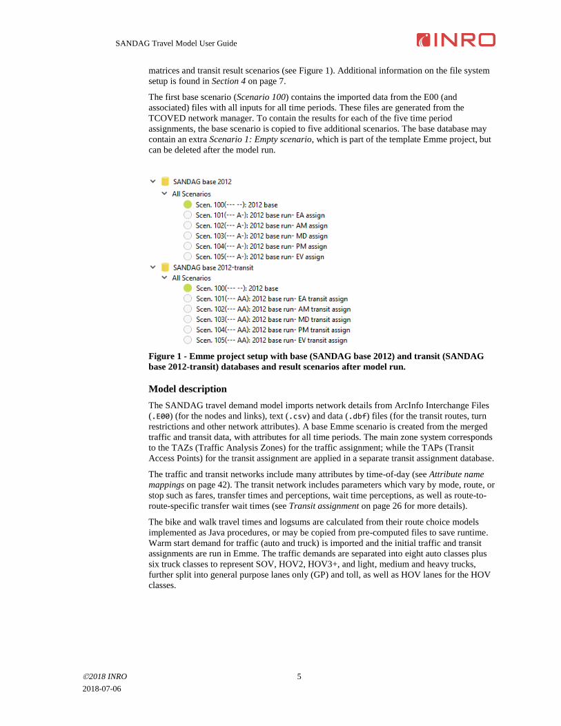
matrices and transit result scenarios (see Figure 1). Additional information on the file system
setup is found in Section 4 on page 7.
The first base scenario (Scenario 100) contains the imported data from the E00 (and
associated) files with all inputs for all time periods. These files are generated from the
TCOVED network manager. To contain the results for each of the five time period
assignments, the base scenario is copied to five additional scenarios. The base database may
contain an extra Scenario 1: Empty scenario, which is part of the template Emme project, but
can be deleted after the model run.
Figure 1 - Emme project setup with base (SANDAG base 2012) and transit (SANDAG
base 2012-transit) databases and result scenarios after model run.
Model description
The SANDAG travel demand model imports network details from ArcInfo Interchange Files
(.E00) (for the nodes and links), text (.csv) and data (.dbf) files (for the transit routes, turn
restrictions and other network attributes). A base Emme scenario is created from the merged
traffic and transit data, with attributes for all time periods. The main zone system corresponds
to the TAZs (Traffic Analysis Zones) for the traffic assignment; while the TAPs (Transit
Access Points) for the transit assignment are applied in a separate transit assignment database.
The traffic and transit networks include many attributes by time-of-day (see Attribute name
mappings on page 42). The transit network includes parameters which vary by mode, route, or
stop such as fares, transfer times and perceptions, wait time perceptions, as well as route-to-
route-specific transfer wait times (see Transit assignment on page 26 for more details).
The bike and walk travel times and logsums are calculated from their route choice models
implemented as Java procedures, or may be copied from pre-computed files to save runtime.
Warm start demand for traffic (auto and truck) is imported and the initial traffic and transit
assignments are run in Emme. The traffic demands are separated into eight auto classes plus
six truck classes to represent SOV, HOV2, HOV3+, and light, medium and heavy trucks,
further split into general purpose lanes only (GP) and toll, as well as HOV lanes for the HOV
classes.
SANDAG Travel Model User Guide
2018 INRO 6
2018-07-06
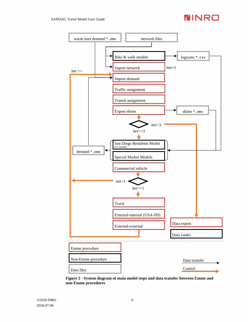
Figure 2 - System diagram of main model steps and data transfer between Emme and
non-Emme procedures
Import network
Control
Data transfer
Bike & walk models
Traffic assignment
Transit assignment
Commercial vehicle
San Diego Residents Model (CT-RAMP)
Special Market Models
Truck
External-internal (USA-SD)
External-external
Import demand
Data loader
Data export
Export skims
warm start demand *.omx
demand *.omx
skims *.omx
logsums *.csv
network files
iter>3
iter<=3
Non-Emme procedure
Emme procedure
Data files
iter ++ iter=1
iter>1
iter==1
SANDAG Travel Model User Guide
2018 INRO 7
2018-07-06
The transit vehicles are input as background traffic flow in the traffic assignment, and the
congested link travel times from the traffic assignment are used in the transit assignment for
bus routes in mixed traffic. The transit assignments use two configurations of parameters: one
for local bus-only demand and one for all modes (that is, including premium modes). The final
assigned flows for transit includes 15 slices of demand by access mode (walk, PNR, KNR)
and primary mode (local bus, express bus, BRT, LRT, commuter rail). Once the assignments
finish, the traffic and transit skims are exported to OMX files.
Once the skims are complete, the CT-RAMP simulation models are initiated which import
skims from these OMX files. For operational purposes, the models are separated into general
travel by San Diego residents and a set of special market models which includes: trips to and
from the San Diego airport; cross-border trips by Mexican residents; trips by visitors staying
within San Diego; and special event trips. Upon completion, the zone-to-zone demands (TAZ
for traffic, TAP for transit) are exported to OMX for each of the disaggregate demand models.
The aggregate commercial vehicle, truck, external-internal and external-external models are
then run. Note only the first of these is run every iteration, while the final three are only run
for the initial iteration (this is an adopted methodology to optimize runtime which was carried
over from the previous implementation). These models operate directly on the Emme
database, using the saved skims from the assignments and saving the demand matrices within
the database. After the demand models are all completed, the demands from the disaggregate
models are imported from OMX and summed up by mode and time-of-day, along with the
commercial vehicle, external-internal and external-external auto demands for the next iteration
of assignments and skims.
The demand model components are run for three iterations, with the traffic and transit
assignments run four times. After the model run is completed, the assignment (network)
results, skims and demands are exported to OMX and CSV files for later import into a
database for reporting services.
4 . S e t u p
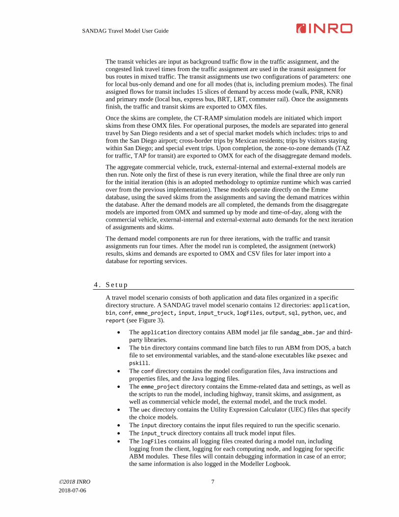
A travel model scenario consists of both application and data files organized in a specific
directory structure. A SANDAG travel model scenario contains 12 directories: application,
bin, conf, emme_project, input, input_truck, logFiles, output, sql, python, uec, and
report (see Figure 3).
• The application directory contains ABM model jar file sandag_abm.jar and third-
party libraries.
• The bin directory contains command line batch files to run ABM from DOS, a batch
file to set environmental variables, and the stand-alone executables like psexec and
pskill.
• The conf directory contains the model configuration files, Java instructions and
properties files, and the Java logging files.
• The emme_project directory contains the Emme-related data and settings, as well as
the scripts to run the model, including highway, transit skims, and assignment, as
well as commercial vehicle model, the external model, and the truck model.
• The uec directory contains the Utility Expression Calculator (UEC) files that specify
the choice models.
• The input directory contains the input files required to run the specific scenario.
• The input_truck directory contains all truck model input files.
• The logFiles contains all logging files created during a model run, including
logging from the client, logging for each computing node, and logging for specific
ABM modules. These files will contain debugging information in case of an error;
the same information is also logged in the Modeller Logbook.
SANDAG Travel Model User Guide
2018 INRO 8
2018-07-06
• The output directory contains all ABM outputs, including both intermediate and
final outputs, such as trip lists, trip tables by mode, highway, transit and bike
assignment results, highway and transit skimming results, and EMFAC summaries.
• The sql directory contains all SQL scripts for creating ABM database structure and
data loading. At the end of each model run, results in the output directory are loaded
into a SQL database, which serves as the foundation for system performance
summary and statistical analysis.
• The python directory contains all Python scripts for creating EMFAC2011 and
EMFAC2014 input files.
• The report directory contains the network and matrix results at the end of the model
run for processing by the data loader.
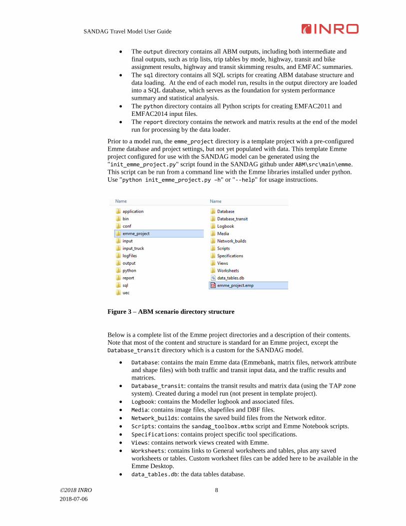
Prior to a model run, the emme_project directory is a template project with a pre-configured
Emme database and project settings, but not yet populated with data. This template Emme
project configured for use with the SANDAG model can be generated using the
"init_emme_project.py" script found in the SANDAG github under ABM\src\main\emme.
This script can be run from a command line with the Emme libraries installed under python.
Use "python init_emme_project.py –h" or "--help" for usage instructions.
Figure 3 – ABM scenario directory structure
Below is a complete list of the Emme project directories and a description of their contents.
Note that most of the content and structure is standard for an Emme project, except the
Database_transit directory which is a custom for the SANDAG model.
• Database: contains the main Emme data (Emmebank, matrix files, network attribute
and shape files) with both traffic and transit input data, and the traffic results and
matrices.
• Database_transit: contains the transit results and matrix data (using the TAP zone
system). Created during a model run (not present in template project).
• Logbook: contains the Modeller logbook and associated files.
• Media: contains image files, shapefiles and DBF files.
• Network_builds: contains the saved build files from the Network editor.
• Scripts: contains the sandag_toolbox.mtbx script and Emme Notebook scripts.
• Specifications: contains project specific tool specifications.
• Views: contains network views created with Emme.
• Worksheets: contains links to General worksheets and tables, plus any saved
worksheets or tables. Custom worksheet files can be added here to be available in the
Emme Desktop.
• data_tables.db: the data tables database.
SANDAG Travel Model User Guide
2018 INRO 9
2018-07-06
• emme_project.emp: the main Emme project settings file. Open (double-click) to the
launch the Emme Desktop with this project.
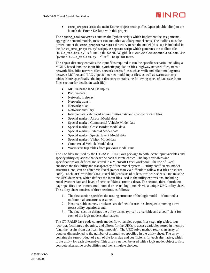
The sandag_toolbox.mtbx contains the Python scripts which implement the assignments,
aggregate demand models, master run and other auxiliary model steps. The toolbox must be
present under the emme_project/Scripts directory to run the model (this step is included in
the "init_emme_project.py" script). A separate script which generates the toolbox file
"build_toolbox.py" is found in the SANDAG github at ABM\src\main\emme\toolbox. Use
"python build_toolbox.py –h" or "--help" for more.
The input directory contains the input files required to run the specific scenario, including a
MGRA-based land use input file, synthetic population files, highway network files, transit
network files, bike network files, network access files such as walk and bike time/logsums
between MGRAs and TAZs, special market model input files, as well as warm start trip
tables. More specifically, the input directory contains the following types of data (see Input
Files section for details on each file):
• MGRA-based land use inputs
• PopSyn data
• Network: highway
• Network: transit
• Network: bike
• Network: auxiliary
• Intermediate: calculated accessibilities data and shadow pricing files
• Special market: Airport Model data
• Special market: Commercial Vehicle Model data
• Special market: Cross Border Model data
• Special market: External Model data
• Special market: Special Event Model data
• Special market: Visitor Model data
• Commercial Vehicle Model data
• Warm start trip tables from previous model runs
The uec files are used by the CT-RAMP UEC Java package to both locate input variables and
specify utility equations that describe each discrete choice. The input variables and
specifications are defined and stored in a Microsoft Excel workbook. The use of Excel
enhances the flexibility and transparency of the model system -- utility coefficients, model
structures, etc., can be edited via Excel (rather than via difficult to follow text files or source
code). Each UEC workbook (i.e. Excel file) consists of at least two worksheets. One must be
the UEC datasheet, which defines the input files used in the utility expressions, including
zonal (vector) data and level-of-service "skims" (matrix data). The second, third, fourth, etc.
page specifies one or more multinomial or nested logit models via a unique UEC utility sheet.
The utility sheet consists of three sections, as follows:
1. The first section specifies the nesting structure of the logit model -- if omitted, a
multinomial structure is assumed;
2. Next, variable names, or tokens, are defined for use in subsequent (moving down
rows) utility equations; and,
3. The final section defines the utility terms, typically a variable and a coefficient for
each of the logit model's alternatives.
The CT-RAMP Java code controls model flow, handles output files (e.g., trip tables, tour
records), facilitates debugging, and allows for the UECs to access variables stored in memory
(e.g., the results from upstream logit models). The UEC solve method returns an array of
doubles dimensioned to the number of alternatives specified in the utility sheet. The array
contains the sum-product of each of the formulas and coefficients for each alternative, which
is the utility for each alternative. This array can then be used with a logit model object to first
compute alternative probabilities and then simulate choices.
SANDAG Travel Model User Guide
2018 INRO 10
2018-07-06
Emme comes with a distribution of Python 2.7 that is configured to work with the Emme
APIs. If third-party Python libraries are required, the Python path (under Application Options)
may be changed to use a different Python installation. The Emme libraries must also be
installed in this Python installation using the Install Modeller Package button. For further
details on configuring a custom installation see "Python path" in the Emme help.
5 . M o d e l o p e r a t i o n a n d M a s t e r r u n t o o l
The following section serves as an overview of the Master run tool and quick start guide. For
additional details on the model steps and other tools, see Section 6: SANDAG Toolbox and
Tools.
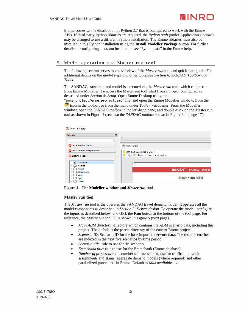
The SANDAG travel demand model is executed via the Master run tool, which can be run
from Emme Modeller. To access the Master run tool, start from a project configured as
described under Section 4: Setup. Open Emme Desktop using the
"emme_project/emme_project.emp" file, and open the Emme Modeller window, from the
icon in the toolbar, or from the menu under Tools -> Modeller. From the Modeller
window, open the SANDAG toolbox in the left-hand pane, and double-click on the Master run
tool as shown in Figure 4 (see also the SANDAG toolbox shown in Figure 8 on page 17).
Figure 4 - The Modeller window and Master run tool
Master run tool
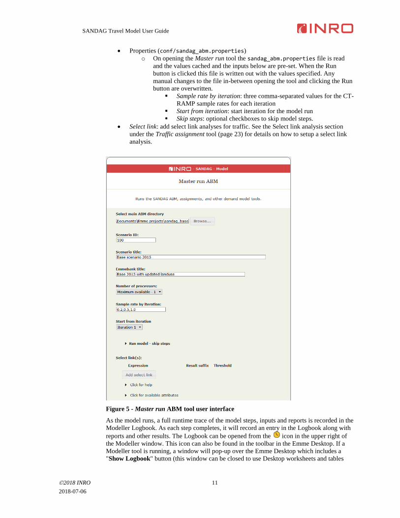
The Master run tool is the operates the SANDAG travel demand model. It operates all the
model components as described in Section 3: System design. To operate the model, configure
the inputs as described below, and click the Run button at the bottom of the tool page. For
reference, the Master run tool UI is shown in Figure 5 (next page).
• Main ABM directory: directory which contains the ABM scenario data, including this
project. The default is the parent directory of the current Emme project.
• Scenario ID: Scenario ID for the base imported network data. The result scenarios
are indexed in the next five scenarios by time period.
• Scenario title: title to use for the scenario.
• Emmebank title: title to use for the Emmebank (Emme database)
• Number of processors: the number of processors to use for traffic and transit
assignments and skims, aggregate demand models (where required) and other
parallelized procedures in Emme. Default is Max available – 1.
SANDAG Travel Model User Guide
2018 INRO 11
2018-07-06
• Properties (conf/sandag_abm.properties)
o On opening the Master run tool the sandag_abm.properties file is read
and the values cached and the inputs below are pre-set. When the Run
button is clicked this file is written out with the values specified. Any
manual changes to the file in-between opening the tool and clicking the Run
button are overwritten.
▪ Sample rate by iteration: three comma-separated values for the CT-
RAMP sample rates for each iteration
▪ Start from iteration: start iteration for the model run
▪ Skip steps: optional checkboxes to skip model steps.
• Select link: add select link analyses for traffic. See the Select link analysis section
under the Traffic assignment tool (page 23) for details on how to setup a select link
analysis.
Figure 5 - Master run ABM tool user interface
As the model runs, a full runtime trace of the model steps, inputs and reports is recorded in the
Modeller Logbook. As each step completes, it will record an entry in the Logbook along with
reports and other results. The Logbook can be opened from the icon in the upper right of
the Modeller window. This icon can also be found in the toolbar in the Emme Desktop. If a
Modeller tool is running, a window will pop-up over the Emme Desktop which includes a
"Show Logbook" button (this window can be closed to use Desktop worksheets and tables
SANDAG Travel Model User Guide
2018 INRO 12
2018-07-06
while any tool is running). Click on the Refresh button to update the logbook view with the
latest status.
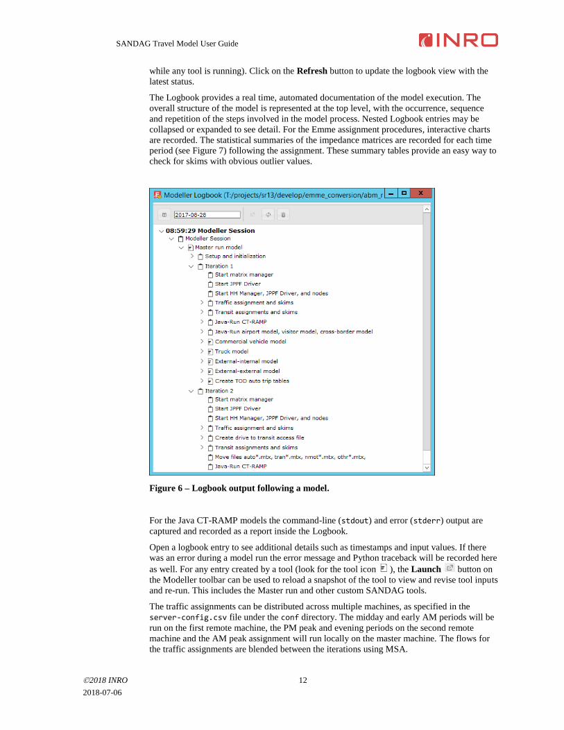
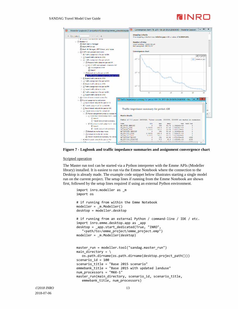
The Logbook provides a real time, automated documentation of the model execution. The
overall structure of the model is represented at the top level, with the occurrence, sequence
and repetition of the steps involved in the model process. Nested Logbook entries may be
collapsed or expanded to see detail. For the Emme assignment procedures, interactive charts
are recorded. The statistical summaries of the impedance matrices are recorded for each time
period (see Figure 7) following the assignment. These summary tables provide an easy way to
check for skims with obvious outlier values.
Figure 6 – Logbook output following a model.
For the Java CT-RAMP models the command-line (stdout) and error (stderr) output are
captured and recorded as a report inside the Logbook.
Open a logbook entry to see additional details such as timestamps and input values. If there
was an error during a model run the error message and Python traceback will be recorded here
as well. For any entry created by a tool (look for the tool icon ), the Launch button on
the Modeller toolbar can be used to reload a snapshot of the tool to view and revise tool inputs
and re-run. This includes the Master run and other custom SANDAG tools.
The traffic assignments can be distributed across multiple machines, as specified in the
server-config.csv file under the conf directory. The midday and early AM periods will be
run on the first remote machine, the PM peak and evening periods on the second remote
machine and the AM peak assignment will run locally on the master machine. The flows for
the traffic assignments are blended between the iterations using MSA.
SANDAG Travel Model User Guide
2018 INRO 13
2018-07-06
Figure 7 - Logbook and traffic impedance summaries and assignment convergence chart
Scripted operation
The Master run tool can be started via a Python interpreter with the Emme APIs (Modeller
library) installed. It is easiest to run via the Emme Notebook where the connection to the
Desktop is already made. The example code snippet below illustrates starting a single model
run on the current project. The setup lines if running from the Emme Notebook are shown
first, followed by the setup lines required if using an external Python environment.
import inro.modeller as _m import os # if running from within the Emme Notebook modeller = _m.Modeller() desktop = modeller.desktop # if running from an external Python / command-line / IDE / etc. import inro.emme.desktop.app as _app desktop = _app.start_dedicated(True, "INRO",
"<path/to>/emme_project/emme_project.emp") modeller = _m.Modeller(desktop) master_run = modeller.tool("sandag.master_run") main_directory = \
os.path.dirname(os.path.dirname(desktop.project_path())) scenario_id = 100 scenario_title = "Base 2015 scenario" emmebank_title = "Base 2015 with updated landuse" num_processors = "MAX-1" master_run(main_directory, scenario_id, scenario_title,
emmebank_title, num_processors)
SANDAG Travel Model User Guide
2018 INRO 14
2018-07-06
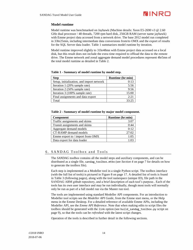
Model runtime
Model runtime was benchmarked on Jayhawk (Machine details: Xeon E5-2690 v3 @ 2.60
GHz dual processor / 48 threads, 7200 rpm hard disk, 256GB RAM (server name jayhawk)
with Emme project data accessed from a network drive. The base 2012 model run completed
in 33hr25min, including intermediate data conversions from/to OMX and the export of results
for the SQL Server data loader. Table 1 summarizes model runtime by iteration.
Model runtime improved slightly to 31hr48mn with Emme project data accessed on a local
disk, but this result does not include the extra time required to offload the data to the remote
drive. The Emme network and zonal aggregate demand model procedures represent 4hr5mn of
the total model runtime as detailed in Table 2.
Table 1 - Summary of model runtime by model step.
Step Runtime (hr:min)
Setup, initialization, and import network 0:13
Iteration 1 (20% sample rate) 5:56
Iteration 2 (50% sample rate) 9:56
Iteration 3 (100% sample rate) 15:00
Final assignments and data export 2:21
Total 33:25
Table 2 - Summary of model runtime by major model component.
Component Runtime (hr:min)
Traffic assignments and skims 3:07
Transit assignments and skims 0:44
Aggregate demand models 0:12
CT-RAMP demand models 27:02
Emme export to / import from OMX 1:05
Data export for data loader 1:03
6 . S A N D A G T o o l b o x a n d T o o l s
The SANDAG toolbox contains all the model steps and auxiliary components, and can be
distributed as a single file, sandag_toolbox.mtbx (see Section 4 on page 7 for details on how
to generate the toolbox file).
Each step is implemented as a Modeller tool in a single Python script. The toolbox interface
(with the full list of tools) is pictured in Figure 8 on page 17. A detailed list of tools is found
in Table 3 (following pages), along with the tool namespace (unique ID), file path in the
SANDAG ABM github repository, and a brief description of each tool’s purpose.. Each of the
tools has its own user interface and may be run individually, though most tools will normally
only be run as part of a full model run via the Master run tool.
The tools are implemented using standard Modeller API components. For an introduction to
Modeller tool scripts see the Modeller API Guide, from the Emme start menu, or the Help
menu in the Emme Desktop. For a detailed reference of available Emme APIs, including the
Modeller API, see the Emme API Reference. Note that when making edits to script files the
toolbox should be generated with the link option (see build_sandag_toolbox.py script on
page 9), so that the tools can be refreshed with the latest script changes.
Operation of the tools is described in further detail in the following sections.
SANDAG Travel Model User Guide
2018 INRO 15
2018-07-06
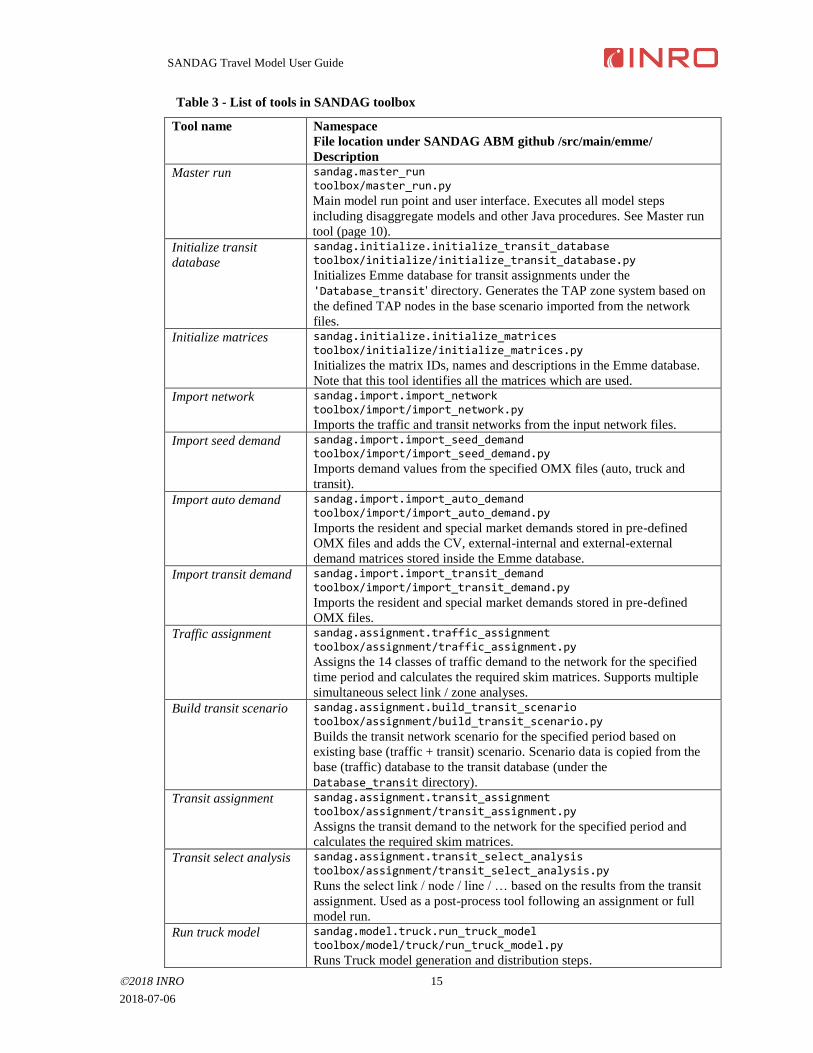
Table 3 - List of tools in SANDAG toolbox
Tool name Namespace
File location under SANDAG ABM github /src/main/emme/
Description
Master run sandag.master_run toolbox/master_run.py
Main model run point and user interface. Executes all model steps
including disaggregate models and other Java procedures. See Master run
tool (page 10).
Initialize transit
database
sandag.initialize.initialize_transit_database toolbox/initialize/initialize_transit_database.py
Initializes Emme database for transit assignments under the
'Database_transit' directory. Generates the TAP zone system based on
the defined TAP nodes in the base scenario imported from the network
files.
Initialize matrices
sandag.initialize.initialize_matrices toolbox/initialize/initialize_matrices.py
Initializes the matrix IDs, names and descriptions in the Emme database.
Note that this tool identifies all the matrices which are used.
Import network
sandag.import.import_network toolbox/import/import_network.py
Imports the traffic and transit networks from the input network files.
Import seed demand
sandag.import.import_seed_demand toolbox/import/import_seed_demand.py
Imports demand values from the specified OMX files (auto, truck and
transit).
Import auto demand
sandag.import.import_auto_demand toolbox/import/import_auto_demand.py
Imports the resident and special market demands stored in pre-defined
OMX files and adds the CV, external-internal and external-external
demand matrices stored inside the Emme database.
Import transit demand
sandag.import.import_transit_demand toolbox/import/import_transit_demand.py
Imports the resident and special market demands stored in pre-defined
OMX files.
Traffic assignment
sandag.assignment.traffic_assignment toolbox/assignment/traffic_assignment.py
Assigns the 14 classes of traffic demand to the network for the specified
time period and calculates the required skim matrices. Supports multiple
simultaneous select link / zone analyses.
Build transit scenario
sandag.assignment.build_transit_scenario toolbox/assignment/build_transit_scenario.py
Builds the transit network scenario for the specified period based on
existing base (traffic + transit) scenario. Scenario data is copied from the
base (traffic) database to the transit database (under the
Database_transit directory).
Transit assignment
sandag.assignment.transit_assignment toolbox/assignment/transit_assignment.py
Assigns the transit demand to the network for the specified period and
calculates the required skim matrices.
Transit select analysis
sandag.assignment.transit_select_analysis toolbox/assignment/transit_select_analysis.py
Runs the select link / node / line / … based on the results from the transit
assignment. Used as a post-process tool following an assignment or full
model run.
Run truck model
sandag.model.truck.run_truck_model toolbox/model/truck/run_truck_model.py
Runs Truck model generation and distribution steps.
SANDAG Travel Model User Guide
2018 INRO 16
2018-07-06
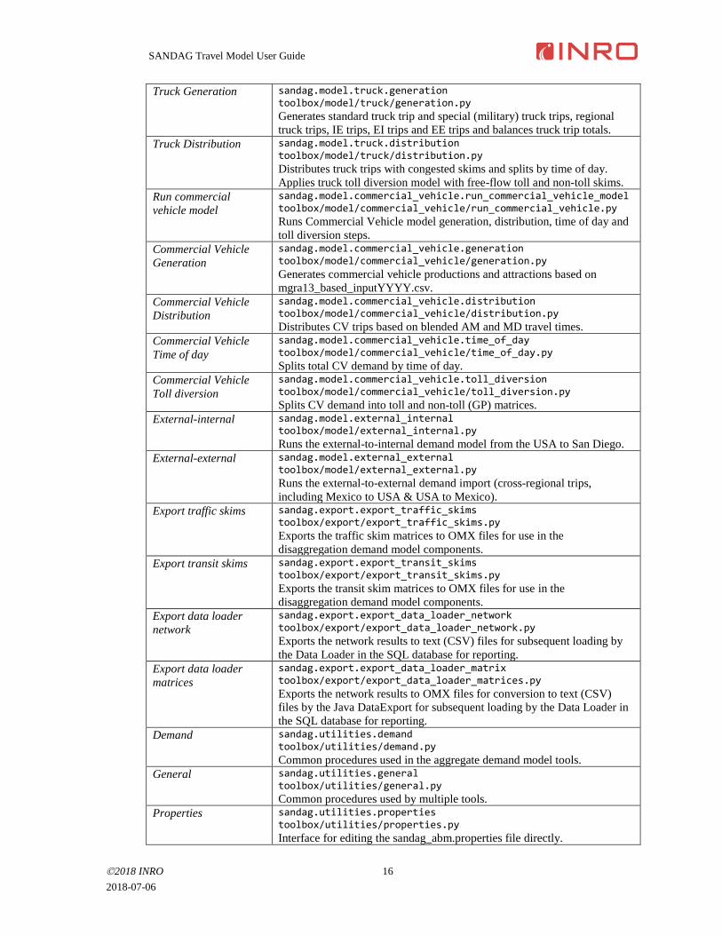
Truck Generation
sandag.model.truck.generation toolbox/model/truck/generation.py
Generates standard truck trip and special (military) truck trips, regional
truck trips, IE trips, EI trips and EE trips and balances truck trip totals.
Truck Distribution
sandag.model.truck.distribution toolbox/model/truck/distribution.py
Distributes truck trips with congested skims and splits by time of day.
Applies truck toll diversion model with free-flow toll and non-toll skims.
Run commercial
vehicle model
sandag.model.commercial_vehicle.run_commercial_vehicle_model toolbox/model/commercial_vehicle/run_commercial_vehicle.py
Runs Commercial Vehicle model generation, distribution, time of day and
toll diversion steps.
Commercial Vehicle
Generation
sandag.model.commercial_vehicle.generation toolbox/model/commercial_vehicle/generation.py
Generates commercial vehicle productions and attractions based on
mgra13_based_inputYYYY.csv.
Commercial Vehicle
Distribution
sandag.model.commercial_vehicle.distribution toolbox/model/commercial_vehicle/distribution.py
Distributes CV trips based on blended AM and MD travel times.
Commercial Vehicle
Time of day
sandag.model.commercial_vehicle.time_of_day toolbox/model/commercial_vehicle/time_of_day.py
Splits total CV demand by time of day.
Commercial Vehicle
Toll diversion
sandag.model.commercial_vehicle.toll_diversion toolbox/model/commercial_vehicle/toll_diversion.py
Splits CV demand into toll and non-toll (GP) matrices.
External-internal sandag.model.external_internal toolbox/model/external_internal.py
Runs the external-to-internal demand model from the USA to San Diego.
External-external sandag.model.external_external toolbox/model/external_external.py
Runs the external-to-external demand import (cross-regional trips,
including Mexico to USA & USA to Mexico).
Export traffic skims sandag.export.export_traffic_skims toolbox/export/export_traffic_skims.py
Exports the traffic skim matrices to OMX files for use in the
disaggregation demand model components.
Export transit skims sandag.export.export_transit_skims toolbox/export/export_transit_skims.py
Exports the transit skim matrices to OMX files for use in the
disaggregation demand model components.
Export data loader
network
sandag.export.export_data_loader_network toolbox/export/export_data_loader_network.py
Exports the network results to text (CSV) files for subsequent loading by
the Data Loader in the SQL database for reporting.
Export data loader
matrices
sandag.export.export_data_loader_matrix toolbox/export/export_data_loader_matrices.py
Exports the network results to OMX files for conversion to text (CSV)
files by the Java DataExport for subsequent loading by the Data Loader in
the SQL database for reporting.
Demand sandag.utilities.demand toolbox/utilities/demand.py
Common procedures used in the aggregate demand model tools.
General sandag.utilities.general toolbox/utilities/general.py
Common procedures used by multiple tools.
Properties sandag.utilities.properties toolbox/utilities/properties.py
Interface for editing the sandag_abm.properties file directly.
SANDAG Travel Model User Guide
2018 INRO 17
2018-07-06
7 . I m p o r t n e t w o r k
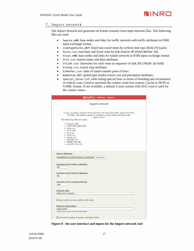
The Import network tool generates an Emme scenario from input network files. The following
files are used:
• hwycov.e00: base nodes and links for traffic network with traffic attributes in ESRI
input exchange format
• linktypeturns.dbf: fixed turn travel times by to/from link type (field IFC) pairs
• turns.csv: turn bans and fixed costs by link from/to ID (field HWYCOV-ID)
• trcov.e00: base nodes and links for transit network in ESRI input exchange format
• trrt.csv: transit routes and their attributes
• trlink.csv: itineraries for each route as sequence of link IDs (TRCOV-ID field)
• trstop.csv: transit stop attributes
• timexfer.csv: table of timed transfer pairs of lines
• mode5tod.dbf: global (per-mode) transit cost and perception attributes
• special_fares.txt: table listing special fares in terms of boarding and incremental
in-vehicle costs. Used to represent the coaster zonal fare system. Can be in JSON or
YAML format. If not available, a default 3-zone system with 2012 costs is used for
the coaster routes.
Figure 8 - the user interface and inputs for the Import network tool
SANDAG Travel Model User Guide
2018 INRO 18
2018-07-06
The user interface for the Import network tool provides the following inputs, as shown in
Figure 8:
• Source directory: path to the location of the input network files
• Scenario ID for traffic: optional scenario to store the imported network from the
traffic files only. Use to review traffic data in Emme Desktop separately from transit
data.
• Scenario ID for transit: optional scenario to store the imported network from the
transit files only. Use to review transit data in Emme Desktop separately from traffic
data.
• Scenario ID for merged network: scenario to store the combined traffic and transit
data from all network files (usual operation)
• Save reference data tables of file data: if checked, create a data table for each
reference file for viewing in the Emme Desktop. Use to review input data alongside
imported Emme Scenario. Note that the table containing the timed transfer
information from timexter.csv is always created.
• Name for data tables: prefix to use to identify all data tables. Should be unique if
importing multiple scenarios
• Overwrite: if checked, any existing data tables or scenarios with the same ID or name
will be overwritten. If not checked and a corresponding scenario or data table already
exists, an error will be raised.
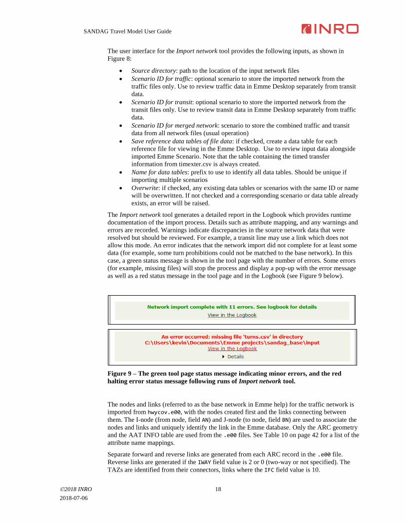
The Import network tool generates a detailed report in the Logbook which provides runtime
documentation of the import process. Details such as attribute mapping, and any warnings and
errors are recorded. Warnings indicate discrepancies in the source network data that were
resolved but should be reviewed. For example, a transit line may use a link which does not
allow this mode. An error indicates that the network import did not complete for at least some
data (for example, some turn prohibitions could not be matched to the base network). In this
case, a green status message is shown in the tool page with the number of errors. Some errors
(for example, missing files) will stop the process and display a pop-up with the error message
as well as a red status message in the tool page and in the Logbook (see Figure 9 below).
Figure 9 – The green tool page status message indicating minor errors, and the red
halting error status message following runs of Import network tool.
The nodes and links (referred to as the base network in Emme help) for the traffic network is
imported from hwycov.e00, with the nodes created first and the links connecting between
them. The I-node (from node, field AN) and J-node (to node, field BN) are used to associate the
nodes and links and uniquely identify the link in the Emme database. Only the ARC geometry
and the AAT INFO table are used from the .e00 files. See Table 10 on page 42 for a list of the
attribute name mappings.
Separate forward and reverse links are generated from each ARC record in the .e00 file.
Reverse links are generated if the IWAY field value is 2 or 0 (two-way or not specified). The
TAZs are identified from their connectors, links where the IFC field value is 10.
SANDAG Travel Model User Guide
2018 INRO 19
2018-07-06
The prohibited turns by to- and from- link ID are read from turns.csv. The import process
also supports fixed turn costs for individual turns (Emme additionally supports general
algebraic turn penalty functions relating travel time / cost to turn flow). If the indicated link
IDs do not make a valid turn (links not adjacent) an error is reported. General turn costs by
link type (IFC field) pairs are set from linktypeturns.dbf. The nodes and links for transit
are imported from trcov.e00 in the same way as the traffic nodes and links. Note that the
correspondence between the HWYCOV-ID to TRCOV-ID values for the same physical links is
important in order for the network merge to be correct. See Table 11, page 44 for a list of the
attribute name mappings. The transit routes are imported from the trrt.csv, trlink.csv and
trstop.csv files and matched to the transit base network. The transit line and stop / segment
attributes (including per-line fares) are imported to Emme attributes (see Table 12 and Table
13 on page 45).
The mode-level attributes from mode5tod.dbf which vary by mode are copied to transit line
attributes and used in the transit assignment specification. These are:
• WT_IVTPK: @vehicle_per_pk
• WT_IVTOP: @vehicle_per_op
• WT_FAREPK: @fare_per_pk
• WT_FAREOP: @fare_per_op
• XFERPENTM * WTXFERTM: @transfer_penalty
• DWELLTIME: set as the dwell time for transit segments with stops
The values for the perception factor on the auxiliary transit modes (WT_IVTPK and WT_IVTOP),
and the waiting time perception factors (WT_FWTPK, WT_XWTPK, WT_FWTOP, and WT_XWTOP) are
specified directly in the Transit assignment tool script (page 26).
The timed transfer information (route-to-route specific transfer times) from timexfer.csv is
stored in a data table with the suffix "_timed_xfers". This table is used in the Build transit
assignment tool to generate the time-period specific transit assignment scenario (see
Additional custom transit network adjustments on page 28).
The special_fares.txt lists network-level incremental fares by boarding (line and/or stop)
and in-vehicle segment. They specify additive fares based on the network elements
encountered on a transit journey and are used to represent the Coaster (or other) zonal fare
system. The input values are set on the network in the segment attributes
"@coaster_fare_board" and "@coaster_fare_inveh". The lines are identified by their ID
(route name) and the segments by the stop name. Both JSON and YAML format are
supported. The following example special_fares.txt represents the Coaster zonal fare
system for 2012 and shows the keywords and nesting (in YAML format):
boarding_cost: base: - {line: "398104", cost: 4.0} - {line: "398204", cost: 4.0} stop_increment: - {line: "398104", stop: "SORRENTO VALLEY", cost: 0.5} - {line: "398204", stop: "SORRENTO VALLEY", cost: 0.5} in_vehicle_cost: - {line: "398104", from: "SOLANA BEACH", cost: 1.0} - {line: "398104", from: "SORRENTO VALLEY", cost: 0.5} - {line: "398204", from: "OLD TOWN", cost: 1.0} - {line: "398204", from: "SORRENTO VALLEY", cost: 0.5}
The transit network is merged onto the traffic base network using the @tcov_id link attributes
(HWCOV-ID and TRCOV-ID). If the transit links do not match to a traffic link by ID, the process
attempts to match by node ID (AN/BN fields), followed by the exact spatial location. If there is
no existing traffic link (transit only links for rail lines, busways, TAP connectors or special
walk links) new links and nodes are added. Links which do not have an ID (primarily the
downtown walk links) are matched using the spatial location of the end nodes. Walk-only
links are allowed to match to two traffic links to reduce incidents of overlapping links.
SANDAG Travel Model User Guide
2018 INRO 20
2018-07-06
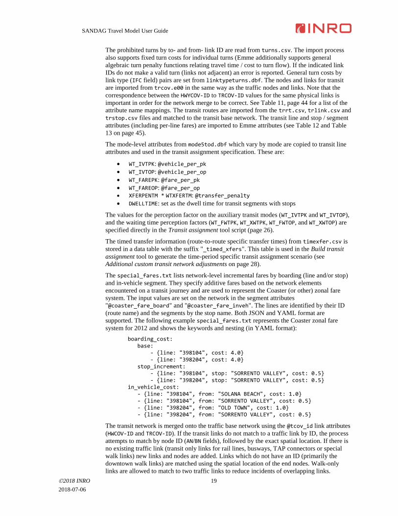
Mode definitions
A mode defines a group of vehicles or users which have access to the same parts of the
network. Modes are used in both the traffic and transit assignments to define the available
network for each class of demand. Each mode is uniquely identified by a single case-sensitive
character. The modes which have access to a given link are listed on that link, and each link
must allow at least one mode.
Table 4 - Mode definitions for traffic and transit network
Mode type Mode Description Calculation
aux. auto s SOV IHOV == 1 && ITRUCK <= 4
aux. auto h HOV2 IHOV <= 2 && ITRUCK <= 4
aux. auto i HOV3+ IHOV <= 3 && ITRUCK <= 4
aux. auto t TRKL
(Light truck)
IHOV == 1 && (ITRUCK <=3 || ITRUCK ==7)
aux. auto m TRKM
(Medium truck)
IHOV == 1 && (ITRUCK <=2 || ITRUCK >= 6)
aux. auto v TRKH
(Heavy truck)
IHOV == 1 && (ITRUCK ==1 || ITRUCK >= 5)
aux. auto S SOV TOLL [ (IHOV == 1 || IHOV == 4) || (2 <= IHOV <=3 && ITOLL >0) ] && ITRUCK <= 4
aux. auto H HOV2 TOLL [ (IHOV <= 2 || IHOV == 4) || (IHOV ==3 && ITOLL >0) ] && ITRUCK <= 4
aux. auto I HOV3+ TOLL ITRUCK <= 4
aux. auto T TRKL TOLL
(Light truck toll)
[ (IHOV == 1 || IHOV == 4) || (2 <= IHOV <=3 && ITOLL >0) ] && (ITRUCK <=3 || ITRUCK ==7)
aux. auto M TRKM TOLL
(Medium truck
toll)
[ (IHOV == 1 || IHOV == 4) || (2 <= IHOV <=3 && ITOLL >0) ] && (ITRUCK <=2 || ITRUCK >= 6)
aux. auto V TRKV TOLL
(Heavy truck toll)
[ (IHOV == 1 || IHOV == 4) || (2 <= IHOV <=3 && ITOLL >0) ] && (ITRUCK ==1 || ITRUCK >= 5)
transit b BUS MINMODE >= 6
transit c CMR
(Commuter rail)
MINMODE == 4
transit e EXP BUS
(Express bus)
MINMODE >= 6
transit l LRT
(Trolley, sprinter)
MINMODE == 5
transit p LTDEXP BUS
(Limited express
or premium bus)
MINMODE >= 6
transit r BRT RED MINMODE == 6
transit y BRY YEL
(yellow)
MINMODE == 7
aux. transit a ACCESS MINMODE == 3
aux. transit w WALK MINMODE == 2
aux. transit x TRANSFER MINMODE == 1

SANDAG Travel Model User Guide
2018 INRO 21
2018-07-06
Table 5 - Key mode fields from hwycov.e00 and trcov.e00
ARC field name in E00 files Description
IHOV Link operation type where:
1 = General purpose
2 = 2+ HOV (Managed lanes if lanes > 1)
3 = 3+ HOV (Managed lanes if lanes > 1)
4 = Toll lanes
ITRUCK Truck restriction code (ITRUCK) where:
1 = All Vehicle Classes
2 = HHDT Excluded
3 = MHDT & HHDT Excluded
4 = LHDT & MHDT & HHDT Excluded (All
Trucks Excluded)
5 = HHDT Only
6 = MHDT & HHDT Only
7 = LHDT & MHDT & HHDT Only (Truck
Only)
MINMODE Transit type where:
1 = special transfer walk links between certain
nearby stops
2 = walk links in the downtown area
3 = the special TAP connectors
4 = Coaster Rail Line
5 = Light Rail Transit (LRT) Line
6 = Yellow Car Bus Rapid Transit (BRT)
7 = Red Car Bus Rapid Transit (BRT)
8 = Limited Express Bus
9 = Express Bus
10 = Local Bus
Modes are categorized by type in Emme:
• Auto: defines the complete traffic network
o A dummy auto mode “d” is created to represent the entire accessible
automobile network, even though no single other mode has comprehensive
access.
• Auxiliary Auto: defines a subset of the auto network for use by a given class of
traffic demand
• Transit: route-type modes (bus, train, etc.) with fixed itineraries and frequencies
• Auxiliary Transit: active modes used to access the transit routes (walk)
The traffic link mode definitions are calculated from two fields IHOV and ITRUCK while the
transit link mode definitions are specified by the MINMODE field. The mode definitions and their
calculations are listed in Table 4. For reference the definitions for the relevant input fields are
listed in Table 5.
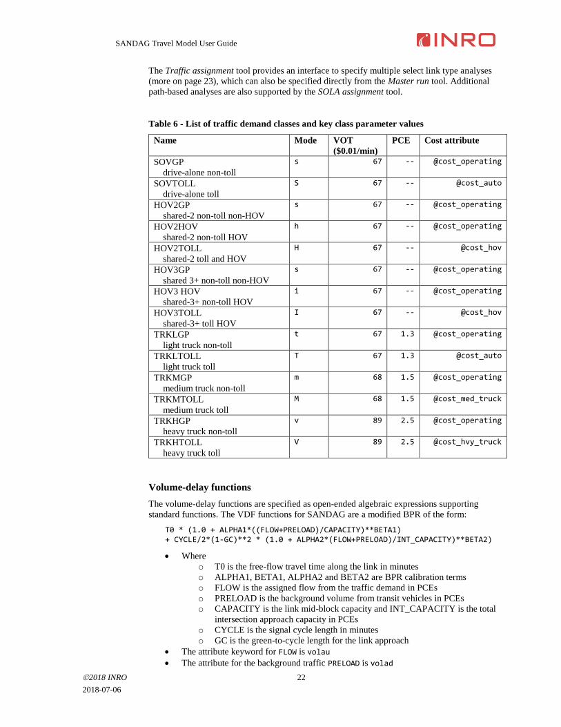
8 . T r a f f i c a s s i g n m e n t
The traffic assignment for the SANDAG model is a 14-class assignment with generalized cost
on links and BPR-type volume-delay functions which include capacities on links and at
intersection approaches. The assignment is run using the fast-converging Second-Order Linear
Approximation (SOLA) method in Emme to a relative gap of 5x10⁻⁴. The per-link fixed costs
include toll values and operating costs which vary by class of demand (see Table 6 for the
complete list of classes). Assignment matrices and resulting network flows are always in PCE.
SANDAG Travel Model User Guide
2018 INRO 22
2018-07-06
The Traffic assignment tool provides an interface to specify multiple select link type analyses
(more on page 23), which can also be specified directly from the Master run tool. Additional
path-based analyses are also supported by the SOLA assignment tool.
Table 6 - List of traffic demand classes and key class parameter values
Name Mode VOT
($0.01/min)
PCE Cost attribute
SOVGP
drive-alone non-toll
s 67 -- @cost_operating
SOVTOLL
drive-alone toll
S 67 -- @cost_auto
HOV2GP
shared-2 non-toll non-HOV s 67 -- @cost_operating
HOV2HOV
shared-2 non-toll HOV h 67 -- @cost_operating
HOV2TOLL
shared-2 toll and HOV H 67 -- @cost_hov
HOV3GP
shared 3+ non-toll non-HOV s 67 -- @cost_operating
HOV3 HOV
shared-3+ non-toll HOV i 67 -- @cost_operating
HOV3TOLL
shared-3+ toll HOV I 67 -- @cost_hov
TRKLGP
light truck non-toll
t 67 1.3 @cost_operating
TRKLTOLL
light truck toll
T 67 1.3 @cost_auto
TRKMGP
medium truck non-toll
m 68 1.5 @cost_operating
TRKMTOLL
medium truck toll
M 68 1.5 @cost_med_truck
TRKHGP
heavy truck non-toll
v 89 2.5 @cost_operating
TRKHTOLL
heavy truck toll
V 89 2.5 @cost_hvy_truck
Volume-delay functions
The volume-delay functions are specified as open-ended algebraic expressions supporting
standard functions. The VDF functions for SANDAG are a modified BPR of the form:
T0 * (1.0 + ALPHA1*((FLOW+PRELOAD)/CAPACITY)**BETA1) + CYCLE/2*(1-GC)**2 * (1.0 + ALPHA2*(FLOW+PRELOAD)/INT_CAPACITY)**BETA2)
• Where
o T0 is the free-flow travel time along the link in minutes
o ALPHA1, BETA1, ALPHA2 and BETA2 are BPR calibration terms
o FLOW is the assigned flow from the traffic demand in PCEs
o PRELOAD is the background volume from transit vehicles in PCEs
o CAPACITY is the link mid-block capacity and INT_CAPACITY is the total
intersection approach capacity in PCEs
o CYCLE is the signal cycle length in minutes
o GC is the green-to-cycle length for the link approach
• The attribute keyword for FLOW is volau
• The attribute for the background traffic PRELOAD is volad
SANDAG Travel Model User Guide
2018 INRO 23
2018-07-06
o This is calculated from the transit itineraries, their frequency, and the length
of the period and is also stored in link data 2 (ul2)
• Per-link attributes:
o T0: link data 1 (ul1)
o CAPACITY: link data 2 (ul3)
o GC: @green_to_cycle, which is cross-referenced by el1
o INT_CAPACITY: @capacity_inter, which is cross-referenced by el3
• Global parameters (small subset of values for all links):
o CYCLE, either 1.25, 1.5, 2.0 or 2.5
o ALPHA1, always 0.8
o BETA1, always 4
o ALPHA2, either 6.0 or 4.5
o BETA2, always 2
With the global parameters there are 6 total volume delay functions:
• fd10 for freeways and links which do not end at an intersection ul1 * (1.0 + 0.8 * ((volau + volad) / ul3) **4)
• fd20 for local collector and lower intersection and stop controlled approaches ul1 * (1.0 + 0.8 * ((volau + volad) / ul3) **4) + 1.25 / 2 * (1-el1) ** 2 * (1 + 4.5 * ((volau + volad) / el3) **2)
• fd21 for collector intersection approaches ul1 * (1.0 + 0.8 * ((volau + volad) / ul3) **4) + 1.5 / 2 * (1-el1) ** 2 * (1.0 + 4.5 * ((volau + volad) / el3) **2)
• fd22 for major arterial and major or prime arterial intersection approaches ul1 * (1.0 + 0.8 * ((volau + volad) / ul3) **4) + 2.0 / 2 * (1-el1) ** 2 * (1.0 + 4.5 * ((volau + volad) / el3) **2)
• fd23 for primary arterial intersection approaches ul1 * (1.0 + 0.8 * ((volau + volad) / ul3) **4) + 2.5/ 2 * (1-el1) ** 2 * (1.0 + 4.5 * ((volau + volad) / el3) **2)
• fd24 for metered ramps ul1 * (1.0 + 0.8 * ((volau + volad) / ul3) **4) + 2.5/ 2 * (1-el1) ** 2 * (1.0 + 6.0 * ((volau + volad) / el3) **2)
Traffic skims and results
The traffic skims are calculated by fixing the flows and running a second zero-iteration
assignment, which computes the O-D skim values using path analyses. The total generalized
cost, travel time, and distance are computed for all classes, as well as the toll cost, HOV
facility distance, and managed lane distance for the applicable classes (see also matrix
definitions on page 39). The fixed flows are the MSA averaged flows for iterations after the
first global iteration.
Note that the assigned flows for trucks are in PCE values unless otherwise specified. This
includes any select type results.
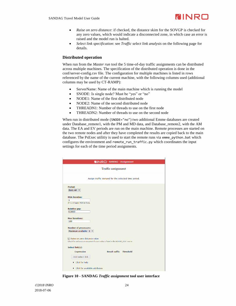
Traffic assignment tool
The Traffic assignment tool runs the traffic assignment and skims per period on the current
primary scenario. The tool has the following inputs (see also Figure 10):
• Period: the time-of-day period, one of EA, AM, MD, PM, EV.
• MSA iteration: global iteration number. If greater than 1, existing flow values must
be present and the resulting flows on links and turns will be the weighted average of
this assignment and the existing values.
• Relative gap: minimum relative stopping criteria.
• Max iterations: maximum iterations stopping criteria.
• Number of processors: number of processors to use for the traffic assignments.
SANDAG Travel Model User Guide
2018 INRO 24
2018-07-06
• Raise on zero distance: if checked, the distance skim for the SOVGP is checked for
any zero values, which would indicate a disconnected zone, in which case an error is
raised and the model run is halted.
• Select link specification: see Traffic select link analysis on the following page for
details.
Distributed operation
When run from the Master run tool the 5 time-of-day traffic assignments can be distributed
across multiple machines. The specification of the distributed operation is done in the
conf/server-config.csv file. The configuration for multiple machines is listed in rows
referenced by the name of the current machine, with the following columns used (additional
columns may be used by CT-RAMP):
• ServerName: Name of the main machine which is running the model
• SNODE: Is single node? Must be “yes” or “no”
• NODE1: Name of the first distributed node
• NODE2: Name of the second distributed node
• THREADN1: Number of threads to use on the first node
• THREADN2: Number of threads to use on the second node
When run in distributed mode (SNODE="no") two additional Emme databases are created
under Database_remote1, with the PM and MD data, and Database_remote2, with the AM
data. The EA and EV periods are run on the main machine. Remote processes are started on
the two remote nodes and after they have completed the results are copied back to the main
database. The PsExec utilitiy is used to start the remote runs via emme_python.bat which
configures the environment and remote_run_traffic.py which coordinates the input
settings for each of the time period assignments.
Figure 10 - SANDAG Traffic assignment tool user interface
SANDAG Travel Model User Guide
2018 INRO 25
2018-07-06
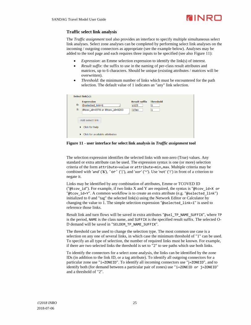
Traffic select link analysis
The Traffic assignment tool also provides an interface to specify multiple simultaneous select
link analyses. Select zone analyses can be completed by performing select link analyses on the
incoming / outgoing connectors as appropriate (see the example below). Analyses may be
added to the tool page and each requires three inputs to be specified (see also Figure 11):
• Expression: an Emme selection expression to identify the link(s) of interest.
• Result suffix: the suffix to use in the naming of per-class result attributes and
matrices, up to 6 characters. Should be unique (existing attributes / matrices will be
overwritten).
• Threshold: the minimum number of links which must be encountered for the path
selection. The default value of 1 indicates an "any" link selection.
Figure 11 - user interface for select link analysis in Traffic assignment tool
The selection expression identifies the selected links with non-zero (True) values. Any
standard or extra attribute can be used. The expression syntax is one (or more) selection
criteria of the form attribute=value or attribute=min,max. Multiple criteria may be
combined with 'and' ('&'), 'or' ('|'), and 'xor' ('^'). Use 'not' ('!') in front of a criterion to
negate it.
Links may be identified by any combination of attributes, Emme or TCOVED ID
("@tcov_id"). For example, if two links X and Y are required, the syntax is "@tcov_id=X or
"@tcov_id=Y". A common workflow is to create an extra attribute (e.g. "@selected_link")
initialized to 0 and "tag" the selected link(s) using the Network Editor or Calculator by
changing the value to 1. The simple selection expression "@selected_link=1" is used to
reference those links.
Result link and turn flows will be saved in extra attributes "@sel_TP_NAME_SUFFIX", where TP
is the period, NAME is the class name, and SUFFIX is the specified result suffix. The selected O-
D demand will be saved in "SELDEM_TP_NAME_SUFFIX".
The threshold can be used to change the selection type. The most common use case is a
selection on any one of several links, in which case the minimum threshold of "1" can be used.
To specify an all type of selection, the number of required links must be known. For example,
if there are two selected links the threshold is set to "2" to see paths which use both links.
To identify the connectors for a select zone analysis, the links can be identified by the zone
IDs (in addition to the link ID, or a tag attribute). To identify all outgoing connectors for a
particular zone use "i=ZONEID". To identify all incoming connectors use "j=ZONEID", and to
identify both (for demand between a particular pair of zones) use "i=ZONEID or j=ZONEID"
and a threshold of "2".
SANDAG Travel Model User Guide
2018 INRO 26
2018-07-06
9 . T r a n s i t a s s i g n m e n t
The transit assignment uses a headway-based approach, where the average headway between
vehicle arrivals for each transit line is known, but not exact schedules. Passengers and
vehicles arrive at stops randomly and passengers choose their travel itineraries considering the
expected average waiting time (usually half the combined headways of the attractive lines).
The Emme Extended transit assignment is based on the concept of optimal strategy but
extended to support a number of behavioral variants. The optimal strategy is a set of rules
which define sequence(s) of walking links, boarding and alighting stops which produces the
minimum expected travel time (generalized cost) to a destination. At each boarding point the
strategy may include multiple possible attractive transit lines with different itineraries. A
transit strategy will often be a tree of options, not just a single path. A line is considered
attractive if it reduces the total expected travel time by its inclusion. The demand is assigned
to the attractive lines in proportion to their relative frequencies.
The shortest "travel time" is a generalized cost formulation, including perception factors (or
weights) on the different travel time components, along with fares, and other costs /
perception biases such as transfer penalties which can vary over the network and transit
journey. For more details on the transit assignment see the Algorithm section for the Extended
transit assignment in the Emme Help.
The model has three access modes to transit (walk, park-and-ride (PNR), and kiss-and-ride
(KNR)) and five main modes (local bus, express / premium bus, bus rapid transit (BRT), light
rail transit (LRT), and commuter rail), for 15 total demand classes. These classes are assigned
by slices, one at a time, to produce the total transit passenger flows on the network.
While there are 15 slices of demand, there are only two classes of skims: Local bus only, and
all modes (access to the premium services). The assignment specification and skims do not
vary by access mode and are the same for the four main modes which are considered premium
modes: express bus, BRT, LRT and commuter rail. The access mode does not change the
assignment parameters or skims.
Travel time components
The in-vehicle travel times for vehicles in mixed traffic is based on the results of the traffic
assignment, which is referenced by the attribute "timau". For vehicles with dedicated lanes /
facilities, the travel times are imported by period from trcov.e00 as "@time_link_ea",
"@time_link_am", "@time_link_md", "@time_link_pm", or "@time_link_ev". The
perception of in-vehicle travel time is imported from mode5tod.dbf and can vary by mode
and time-of-day. The perception factors are stored in transit line attributes
"@vehicle_per_pk" and "@vehicle_per_op". The time / cost perception factors (PF) and
penalties are as follows:
• Walk: PF of 1.8 for peak and 1.6 for off-peak
• Initial wait: PF of 1.5 for peak and 1.6 for off-peak
• Transfer wait: PF of 3.0 for peak and 2.5 for off-peak
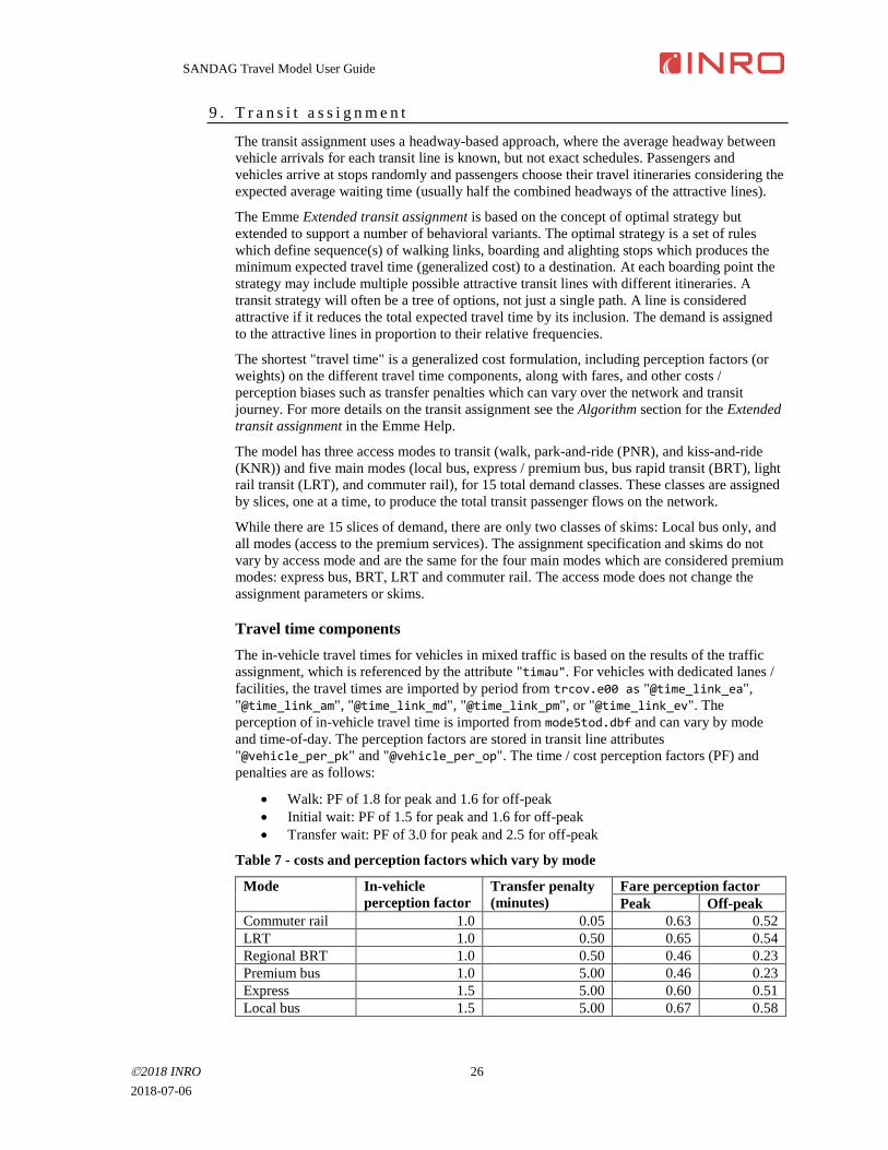
Table 7 - costs and perception factors which vary by mode
Mode In-vehicle
perception factor
Transfer penalty
(minutes)
Fare perception factor
Peak Off-peak
Commuter rail 1.0 0.05 0.63 0.52
LRT 1.0 0.50 0.65 0.54
Regional BRT 1.0 0.50 0.46 0.23
Premium bus 1.0 5.00 0.46 0.23
Express 1.5 5.00 0.60 0.51
Local bus 1.5 5.00 0.67 0.58
SANDAG Travel Model User Guide
2018 INRO 27
2018-07-06
Representing fares
The fares for most routes are paid per-boarding, except for free transfers between trolley lines,
and the Coaster commuter rail which has a zonal fare system. However, the day passes ($5)
and regional day passes ($12) provide effective maximum fares which in most cases works
out to a small increment over the single boarding fare. To set the maximum trip fare we
assume there is a second transit trip and therefore this maximum fare is half the price of a day
pass, or $2.50 for regular services (local buses, trolley, express bus and BRT), and $6 for
premium services. Monthly passes are not represented.
To represent the fares Journey levels are used to keep track of the sequence of boardings by
mode. Journey levels allow the generalized costs experienced by passengers to vary depending
upon the particular sequence of transit modes that they board. The boarding cost is specified
as a line extra attribute, and each boarding of a mode can change the boarding costs for
subsequent boardings (which use a different extra attribute). For full details on Journey levels
see the Extended transit assignment in the Emme Help.
A fare extra attribute is calculated for each state (relevant sequence of boardings), to represent
the subsequent incremental boarding fares for each line. The local bus assignment case is
relatively simple and there are three levels (states):
• Not boarded yet: pay the full boarding fare for this line, usually $1.75 or $2.25
• Boarded bus once: pay the incremental fare up to half a day pass, $0.75 or $0.25
• Boarded bus twice, have a day pass: all subsequent boardings are free
The base fares are stored in the line extra attribute "@fare", copied from the trrt.csv file in
the Import Network tool. The incremental fares are calculated as "2.50 - @fare" for each
line (for those with fares > $1.00) and stored in "@xfer_from_bus". This represents the
incremental fare for the separate NCTD ($1.75 boarding fare) and MTS ($2.25 boarding fare)
geographic areas well. There is a very small area of overlap between the two service areas at
the University of California San Diego where the represented fare will be off by $0.25 for
passengers connecting between the two areas. There are also a small number of community
services which are free (five lines) or have fares of $1.00 (two lines). The incremental fares
when transferring from other bus lines to these lines is correctly represented
(@xfer_from_bus=0 for free lines and 0.25 for $1.00 lines); however, the calculated fare
when boarding other lines after these community lines will be low (@fare on community lines
+ @xfer_from_bus on the regular line). A straightforward improvement to this representation
would be to code each group of lines with the same fare as a separate mode so that the transfer
fare could be calculated.
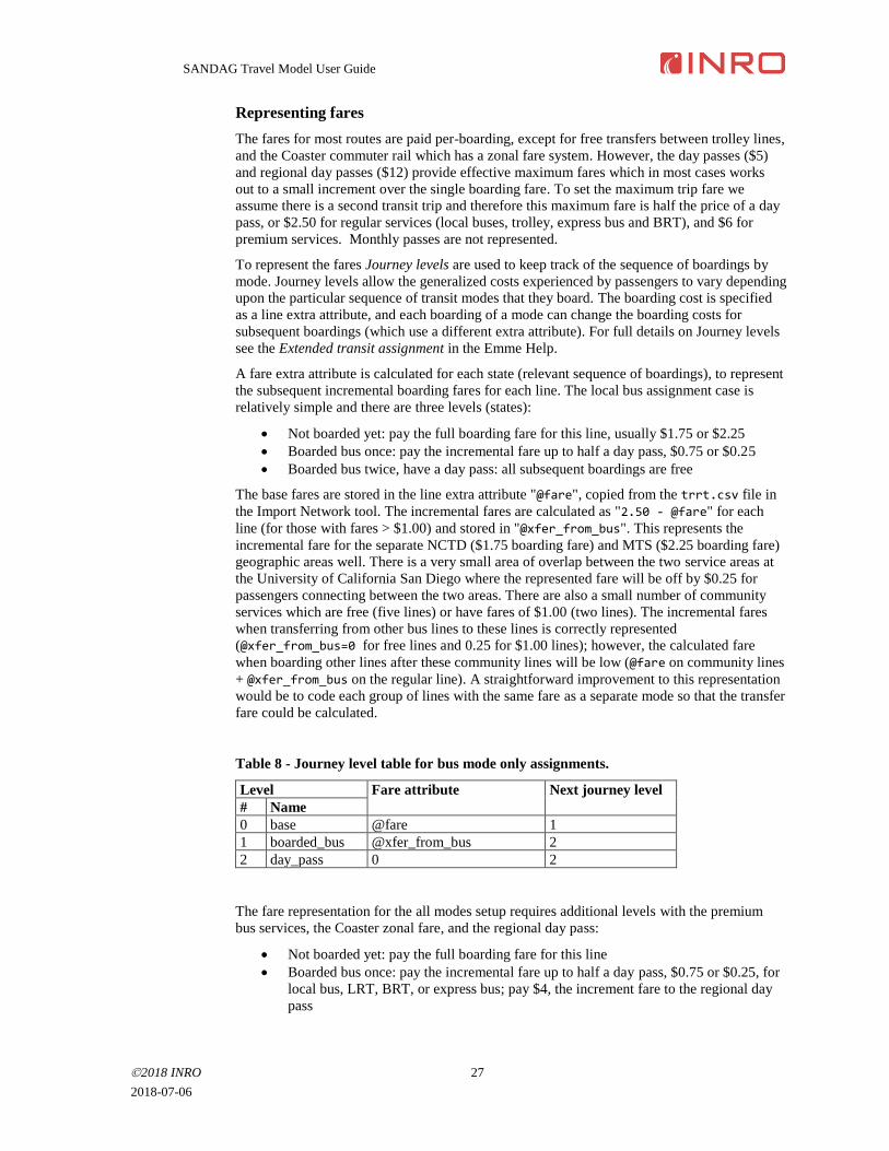
Table 8 - Journey level table for bus mode only assignments.
Level Fare attribute Next journey level
# Name
0 base @fare 1
1 boarded_bus @xfer_from_bus 2
2 day_pass 0 2
The fare representation for the all modes setup requires additional levels with the premium
bus services, the Coaster zonal fare, and the regional day pass:
• Not boarded yet: pay the full boarding fare for this line
• Boarded bus once: pay the incremental fare up to half a day pass, $0.75 or $0.25, for
local bus, LRT, BRT, or express bus; pay $4, the increment fare to the regional day
pass
SANDAG Travel Model User Guide
2018 INRO 28
2018-07-06
• Have a day pass (boarded bus twice, or LRT / BRT / express bus once): all
subsequent boardings of these four modes are free; if boarding a premium bus service
or Coaster pay $3.50, the increment up to a regional day pass
• Boarded premium bus once: pay the incremental fare of $1, from the premium fare
($5) to the regional day pass ($6)
• Boarded coaster: pay the incremental fare of $1.25 from the average Coaster fare
($4.75, range $4 to $5.50) to the regional day pass ($6)
There are additional cost attributes to represent the Coaster zonal fare when it is the first
boarding. If other modes have already been used before boarding the Coaster line, the fare
becomes the regional day pass level so there is no further incremental cost. The zonal fare is
represented as an initial boarding cost at stations and the incremental in-vehicle cost at zone
boundary crossings. These costs are stored in the segment attributes "@coaster_fare_board"
and "@coaster_fare_inveh" (see special_fares under Import network on page 19 for how
this is specified).
There are four bus lines in the base year coded as having the premium mode but take an
express bus fare ($2.50) and should be covered by the day pass instead of the regional day
pass (route 870 variants). Strategies which include this route and other premium services may
underestimate the fare, while strategies which include this route and other non-premium
services (local bus, LRT…) may overestimate the fare. When skimming the fare cost, the
maximum allowed fare is half the regional day pass.
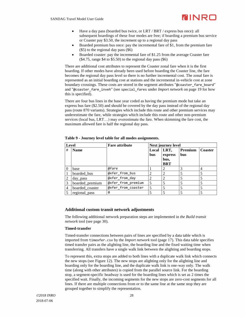
Table 9 - Journey level table for all modes assignments.
Level Fare attribute Next journey level
# Name Local
bus
LRT,
express
bus,
BRT
Premium
bus
Coaster
0 base @fare 1 2 3 4
1 boarded_bus @xfer_from_bus 2 2 5 5
2 day_pass @xfer_from_day 2 2 5 5
3 boarded_premium @xfer_from_premium 5 5 5 5
4 boarded_coaster @xfer_from_coaster 5 5 5 5
5 regional_pass 0 5 5 5 5
Additional custom transit network adjustments
The following additional network preparation steps are implemented in the Build transit
network tool (see page 30).
Timed-transfer
Timed-transfer connections between pairs of lines are specified by a data table which is
imported from timexfer.csv by the Import network tool (page 17). This data table specifies
timed transfer pairs as the alighting line, the boarding line and the fixed waiting time when
transferring. All transfers have a single walk link between the alighting and boarding stops.
To represent this, extra stops are added to both lines with a duplicate walk link which connects
the new stops (see Figure 12). The new stops are alighting only for the alighting line and
boarding only for the boarding line, and the duplicate walk link is one-way only. The walk
time (along with other attributes) is copied from the parallel source link. For the boarding
stop, a segment-specific headway is used for the boarding lines which is set as 2 times the
specified wait. Finally, the incoming segments for the new stops are zero-cost segments for all
lines. If there are multiple connections from or to the same line at the same stop they are
grouped together to simplify the representation.
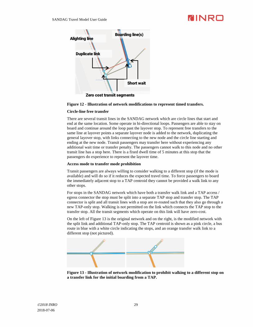
SANDAG Travel Model User Guide
2018 INRO 29
2018-07-06
Figure 12 - Illustration of network modifications to represent timed transfers.
Circle-line free transfer
There are several transit lines in the SANDAG network which are circle lines that start and
end at the same location. Some operate in bi-directional loops. Passengers are able to stay on
board and continue around the loop past the layover stop. To represent free transfers to the
same line at layover points a separate layover node is added to the network, duplicating the
general layover stop, with links connecting to the new node and the circle line starting and
ending at the new node. Transit passengers may transfer here without experiencing any
additional wait time or transfer penalty. The passengers cannot walk to this node and no other
transit line has a stop here. There is a fixed dwell time of 5 minutes at this stop that the
passengers do experience to represent the layover time.
Access mode to transfer mode prohibition
Transit passengers are always willing to consider walking to a different stop (if the mode is
available) and will do so if it reduces the expected travel time. To force passengers to board
the immediately adjacent stop to a TAP centroid they cannot be provided a walk link to any
other stops.
For stops in the SANDAG network which have both a transfer walk link and a TAP access /
egress connector the stop must be split into a separate TAP stop and transfer stop. The TAP
connector is split and all transit lines with a stop are re-routed such that they also go through a
new TAP-only stop. Walking is not permitted on the link which connects the TAP stop to the
transfer stop. All the transit segments which operate on this link will have zero-cost.
On the left of Figure 13 is the original network and on the right, is the modified network with
the split link and additional TAP-only stop. The TAP centroid is shown as a pink circle, a bus
route in blue with a white circle indicating the stops, and an orange transfer walk link to a
different stop (not pictured).
Figure 13 - Illustration of network modification to prohibit walking to a different stop on
a transfer link for the initial boarding from a TAP.
Duplicate link
Zero cost transit segments
Alighting line Boarding line(s)
Short wait
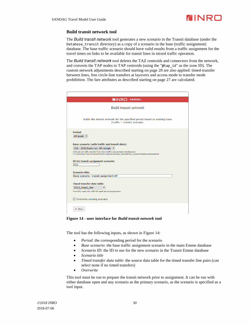
SANDAG Travel Model User Guide
2018 INRO 30
2018-07-06
Build transit network tool
The tool generates a new scenario in the Transit database (under the
Database_transit directory) as a copy of a scenario in the base (traffic assignment)
database. The base traffic scenario should have valid results from a traffic assignment for the
travel times on links to be available for transit lines in mixed traffic operation.
The tool deletes the TAZ centroids and connectors from the network,
and converts the TAP nodes to TAP centroids (using the "@tap_id" as the zone ID). The
custom network adjustments described starting on page 28 are also applied: timed-transfer
between lines, free circle-line transfers at layovers and access mode to transfer mode
prohibition. The fare attributes as described starting on page 27 are calculated.
Figure 14 - user interface for Build transit network tool
The tool has the following inputs, as shown in Figure 14:
• Period: the corresponding period for the scenario
• Base scenario: the base traffic assignment scenario in the main Emme database
• Scenario ID: the ID to use for the new scenario in the Transit Emme database
• Scenario title
• Timed transfer data table: the source data table for the timed transfer line pairs (can
select none if no timed transfers)
• Overwrite
This tool must be run to prepare the transit network prior to assignment. It can be run with
either database open and any scenario as the primary scenario, as the scenario is specified as a
tool input.
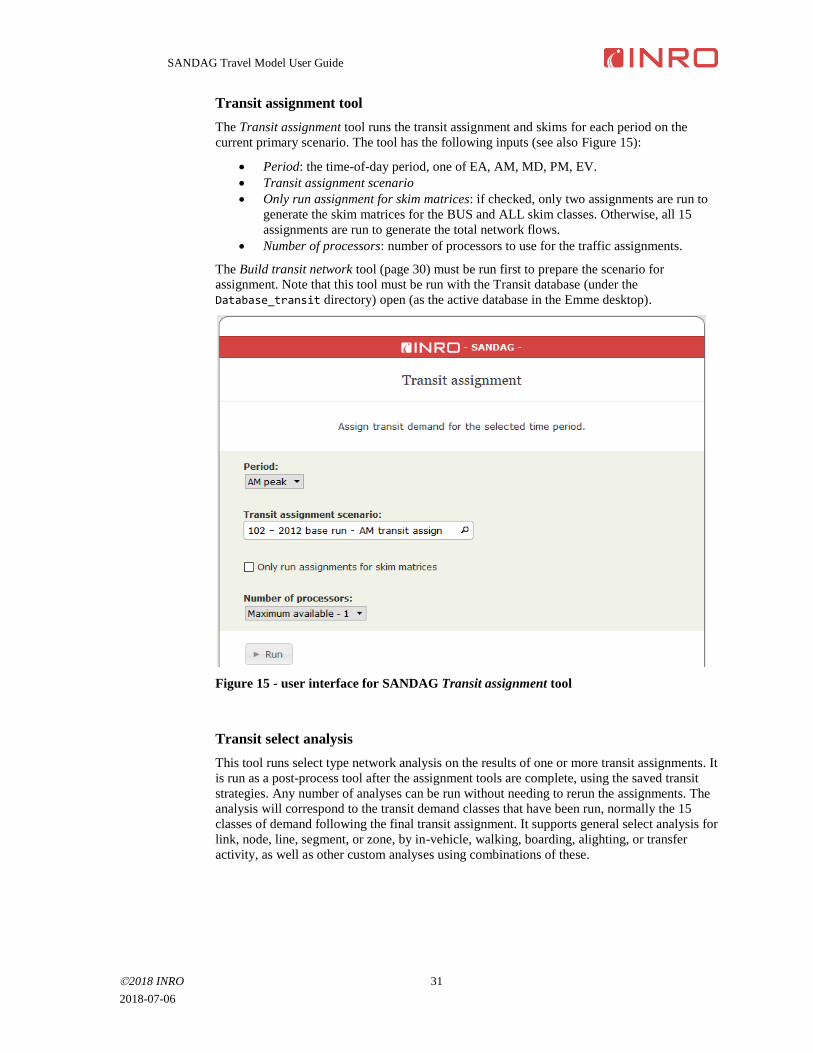
SANDAG Travel Model User Guide
2018 INRO 31
2018-07-06
Transit assignment tool
The Transit assignment tool runs the transit assignment and skims for each period on the
current primary scenario. The tool has the following inputs (see also Figure 15):
• Period: the time-of-day period, one of EA, AM, MD, PM, EV.
• Transit assignment scenario
• Only run assignment for skim matrices: if checked, only two assignments are run to
generate the skim matrices for the BUS and ALL skim classes. Otherwise, all 15
assignments are run to generate the total network flows.
• Number of processors: number of processors to use for the traffic assignments.
The Build transit network tool (page 30) must be run first to prepare the scenario for
assignment. Note that this tool must be run with the Transit database (under the
Database_transit directory) open (as the active database in the Emme desktop).
Figure 15 - user interface for SANDAG Transit assignment tool
Transit select analysis
This tool runs select type network analysis on the results of one or more transit assignments. It
is run as a post-process tool after the assignment tools are complete, using the saved transit
strategies. Any number of analyses can be run without needing to rerun the assignments. The
analysis will correspond to the transit demand classes that have been run, normally the 15
classes of demand following the final transit assignment. It supports general select analysis for
link, node, line, segment, or zone, by in-vehicle, walking, boarding, alighting, or transfer
activity, as well as other custom analyses using combinations of these.
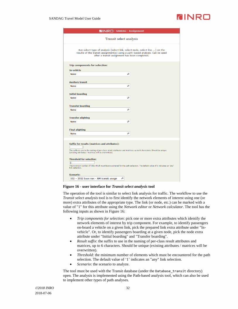
SANDAG Travel Model User Guide
2018 INRO 32
2018-07-06
Figure 16 - user interface for Transit select analysis tool
The operation of the tool is similar to select link analysis for traffic. The workflow to use the
Transit select analysis tool is to first identify the network elements of interest using one (or
more) extra attributes of the appropriate type. The link (or node, etc.) can be marked with a
value of "1" for this attribute using the Network editor or Network calculator. The tool has the
following inputs as shown in Figure 16:
• Trip components for selection: pick one or more extra attributes which identify the
network elements of interest by trip component. For example, to identify passengers
on-board a vehicle on a given link, pick the prepared link extra attribute under "In-
vehicle". Or, to identify passengers boarding at a given node, pick the node extra
attribute under "Initial boarding" and "Transfer boarding".
• Result suffix: the suffix to use in the naming of per-class result attributes and
matrices, up to 6 characters. Should be unique (existing attributes / matrices will be
overwritten).
• Threshold: the minimum number of elements which must be encountered for the path
selection. The default value of ‘1’ indicates an "any" link selection.
• Scenario: the scenario to analyze.
The tool must be used with the Transit database (under the Database_transit directory)
open. The analysis is implemented using the Path-based analysis tool, which can also be used
to implement other types of path analyses.
SANDAG Travel Model User Guide
2018 INRO 33
2018-07-06
1 0 . A g g r e g a t e d e m a n d m o d e l s a n d o t h e r t o o l s
Truck model
The truck model is implemented in two separate tools, found under the Model → Truck
directory in the SANDAG toolbox: Generation and Distribution. A Run truck model tool
executes both these tools in sequence. These tools take as input the directory for their input
files, which defaults to the standard input directory and does not normally need to be
changed.
Generation
Truck trip productions and attractions are calculated for three categories of truck types: light,
medium and heavy in two steps. The standard truck trips use trip rates stored in
TruckTripRates.csv and employment by type and households from
mgra13_based_inputYEAR.csv (where YEAR is the year of interest identified in
conf/sandag_abm.properties by the truck.FFyear token). Both files are found under the
input directory. The special truck trips (e.g. military, cruise ship terminal) are calculated
based on specialGenerators.csv. The truck trips by type are balanced to the average of the
productions and attractions. Regional truck trip ends, internal-external, external-internal and
external-external (IE, EI, and EE), are read from separate files in the input_truck directory.
Distribution
The distribution step distributes the truck trips using friction factors which are negative
exponentials of the mid-day travel time for the "generic" truck skim, MD_TRK_TIME. The
external trips (IE, EI, EE) are distributed separately and added to the truck types (light,
medium and heavy) using fixed proportions. The total truck trips by type are split by time-of-
day using fixed factors for all OD pairs, except those crossing the border which have a
separate set of time-of-day factors.
The truck toll diversion (split between toll access and GP lanes only) is calculated using toll
and GP skims (TIME and TOLLCOST) by truck type and time-of-day. The final stored truck
demand matrices are adjusted to PCEs for assignment, and a controlled rounding process
(reduce matrix precision) applied which removes demand if below a specified threshold
(RunModel.MatrixPrecision in sandag_abm.properties) and adjusts remaining cells by
the ratio of the difference to maintain the same total demand.
Commercial vehicle model
The commercial vehicle model is implemented in four tools found under the Model →
Commercial vehicle directory in the SANDAG toolbox: Generation, Distribution, Time of
day, and Toll diversion. A Run commercial vehicle model tool executes these tools in
sequence. These tools take as input the directory for their input files, which defaults to the
standard input directory and does not normally need to be changed. The very small truck
generation model is based on the Phoenix four-tire truck model documented in the TMIP
Quick Response Freight Manual.
Generation
The generation step calculates total productions and attractions from employment by category
and total households per TAZ, read from input/mgra13_based_inputYEAR.csv (YEAR is
replaced by truck.FFyear in the conf/sandag_abm.properties file). The attractions are
balanced so the total matches the total productions.
Distribution
The distribution step is based on a blended impedance skim of 1/3 AM_SOVGP_TIME and 2/3
MD_SOVGP_TIME. The blended skim is used to lookup friction factors from a table stored in
input/commVehFF.csv, which is then used in the matrix balancing to calculate the total daily
production-attraction matrix.
SANDAG Travel Model User Guide
2018 INRO 34
2018-07-06
Time of day
The five time-of-day matrices are calculated using fixed proportions of the average of the total
daily production-attraction matrix and its transpose (𝑃𝐴 + 𝐴𝑃) 2⁄ .
Toll diversion
The toll diversion (split between toll access and GP lanes only) is calculated using the SOV
toll and GP skims (TIME and TOLLCOST) by time-of-day. The final commercial vehicle demand
is added to the SOV demand by the Import auto demand tool (discussed below).
External models
Two tools calculate the external demand which is not covered by the disaggregate models.
The External external tool calculates the cross-regional demand, and the External internal tool
calculates the demand from the external USA gateways to within the San Diego region.
External internal
The External internal tool runs the external USA to internal San Diego region demand model.
The demands are calculated for work and non-work purposes by time-of-day and toll / GP-
only and later added to the auto demand for assignment. Work and non-work trip gateway
total trips (control totals) are read from
input/externalInternalControlTotalsByYear.csv for the scenarioYear token in
sandag_abm.properties. If this file does not exist at runtime
input/externalInternalControlTotals.csv is used instead.
The trip end probability is generated from the employment totals by type and households
(from input/mgra13_based_inputYEAR.csv) and multiplied by the vector of gateway
control totals to obtain a production-attraction matrix (PA). The time-of-day matrices and
traffic occupancy class matrices (SOV, HOV2, and HOV3) are calculated using fixed
proportions of the average of the total daily demand and its transpose (𝑃𝐴 + 𝐴𝑃) 2⁄ for both
work and non-work.
The toll diversion model splits the demand between toll access and GP lanes only for the SOV
classes, and between toll access and HOV access for the HOV classes. This is calculated using
the toll and GP skims (TIME and TOLLCOST) by time-of-day for each of work and non-work
separately. The final external-internal demand is added to the auto demand matrices by the
Import auto demand tool (discussed below).
External external
The total daily external demand is imported from
input/externalExternalTripsByYear.csv, using the demand for the scenarioYear token
in sandag_abm.properties. If this file does not exist, the values
externalExternalTrips.csv will be used instead. The total daily demand is split by time-
of-day and traffic class SOVGP, HOV2HOV, and HOV3HOV using fixed factors.
Data management tools
Initialize transit database
The Initialize transit database creates the transit database and copies a base scenario from the
base database using the Build transit scenario tool (page 30). The Emme database is created
under 'Database_transit' directory, and will overwrite any existing database. The TAZs from
the base scenario are removed and the TAP nodes are converted to centroids.
The transit database must be created prior to running the transit assignment and skims.
Initialize matrices
The Initialize matrices tool coordinates the initialization of all matrices. The matrix names are
listed for each of the model components / steps, and the matrix IDs are assigned consistently
SANDAG Travel Model User Guide
2018 INRO 35
2018-07-06
from the complete list of matrices names. In each of the other model tools the matrices are
only referenced by name, never by ID. The matrix name convention is explained in section 11
Appendix (page 39). The inputs for this tool are:
• Components: A list of the model components / steps for which to initialize matrices.
One or more of "traffic_demand", "transit_demand", "traffic_skims",
"transit_skims", "external_internal_model", "external_external_model",
"truck_model", or "commercial_vehicle_model".
• Periods: A list of periods for which to initialize matrices, "EA", "AM", "MD", "PM", "EV"
The initialize matrices tool must be run prior to any other tool which references matrix data,
which is all tools except Import network, and Initialize transit database.
Import seed demand
The Import seed demand tool imports the warm start demand matrices from specified OMX
files for auto, truck and transit. The imported truck demand can be converted to PCE values in
preparation for the assignment (default behavior). The mapping from the names in the OMX
files to the matrix names in the Emme database is:
• Auto demand matrices by period: o SOV_GP: SOVGP o SOV_PAY: SOVTOLL o SR2_GP: HOV2GP o SR2_HOV: HOV2HOV o SR2_PAY: HOV2TOLL o SR3_GP: HOV3GP o SR3_HOV: HOV3HOV o SR3_PAY: HOV3TOLL
• Truck seed demand by period: o hhdn: TRKHGP o hhdt: TRKHTOLL o lhdn: TRKLGP o lhdt: TRKLTOLL o mhdn: TRKMGP o mhdt: TRKMTOLL
• Transit seed demand by period: o WLK_LOC: WLKBUS o WLK_LRT: WLKLRT o WLK_CMR: WLKCMR o WLK_EXP: WLKEXP o WLK_BRT: WLKBRT o PNR_LOC: PNRBUS o PNR_LRT: PNRLRT o PNR_CMR: PNRCMR o PNR_EXP: PNREXP o PNR_BRT: PNRBRT o KNR_LOC: KNRBUS o KNR_LRT: KNRLRT o KNR_CMR: KNRCMR o KNR_EXP: KNREXP o KNR_BRT: KNRBRT
The auto and truck matrices are stored in the same OMX file by time period, with the name
trip_pp.omx where pp is one of the five time-of-day periods. Note that the transit seed
demand is not imported during the Master run as it is not needed for the initial skim
assignments. This demand can, however, be used to prepare demand for an independent run of
the transit assignment.
Import auto demand
The Import auto demand tool imports the auto demand generated from an iteration of the
disaggregate demand models (CT-RAMP) and adds the saved disaggregated demand matrices

SANDAG Travel Model User Guide
2018 INRO 36
2018-07-06
to generate the total auto demand in preparation for the auto assignment. The disaggregate
demand models save O-D trip matrices by TAZ in the following files under the output
directory, where pp is one of the five time-of-day periods:
• autoTrips_pp.mtx
• autoInternalExternalTrips_pp.mtx
• autoVisitorTrips_pp.mtx
• autoCrossBorderTrips_pp.mtx
• autoAirportTrips_pp.mtx
The OMX name to Emme database name mapping is the same as listed for Import seed
demand. A summary of the imported demand is recorded in the logbook.
Import transit demand
The Import transit demand tool imports the transit demand generated from an iteration of the
disaggregate demand models (CT-RAMP) in preparation for the transit assignment. The
disaggregate demand models save O-D trip matrices by TAP in the following files under the
output directory, where pp is one of the five time-of-day periods:
• tranVisitorTrips_pp.mtx
• tranCrossBorderTrips_pp.mtx
• tranAirportTrips_pp.mtx
• tranTrips_pp.mtx
• tranInternalExternalTrips_pp.mtx
The OMX name to Emme database name mapping is the same as listed for Import seed
demand. A summary of the imported demand is recorded in the logbook.
Export traffic skims
The Export traffic skims tool exports the traffic skim matrices to OMX format for the selected
period for use in the next disaggregate demand model iteration or the data loader process. See
Section 11 Appendix (page 39) for the list of the matrix names. The OMX files are defined in
the Master run tool, and are traffic_skims_pp.omx in the output directory, where pp is one
of the set of five time-periods.
Export transit skims
The Export transit skims tool exports the transit skim matrices to OMX format for use in the
next disaggregate demand model iteration or the data loader process. See Section 11 Appendix
(page 39) for the list of the matrix names.
This tool includes an option to filter large values from the skim matrices and replace with
zeros values ("Replace big values (>10E6) with zero"). This is used in the final iteration skim
(after the demand models are complete) to filter large values from the OMX files which are
not compatible with the data loader process. The transit assignment will assign a large value
of 10e20 for TAP pairs which are disconnected (there is no feasible route).
The OMX file is defined in the Master run tool, and it is transit_skims.omx in the output
directory.
Export data loader network
The Export data loader network tool generates CSV files with the network results used by the
Java Data export process and the Data loader for the reporting database. The files are created
under the report directory. These are:
• hwyload_pp.csv: (pp is one of "EA", "AM", "MD", "PM", "EV"), traffic class flows by
time period
o The class flows are reported in vehicles; note that the per-class results in the
Emme database are stored in PCEs
• hwy_tcad.csv: total traffic flows, travel times, and other link attributes for all time
periods
SANDAG Travel Model User Guide
2018 INRO 37
2018-07-06
• transit_aggflow.csv: transit link level results by class and time period
• transit_flow.csv: transit segment results by class and time period
• transit_onoff.csv: transit stop results by class and time period
Export data loader matrices
The Export data loader matrices tool generates OMX and CSV files with the network results
used by the Java Data export process and the Data loader for the reporting database. The
OMX files are created under the output directory and the CSV file is created under the
report directory. The files and their contents (the OMX key to Emme matrix mapping) are as
follows:
• OMX format files, pp is replaced by "EA", "AM", "MD", "PM", and "EV". Note that there
is no extension used for these files.
o commVehTODTrips: total, toll, and GP commercial vehicles trips by time
period. ▪ OD Trips: COMVEH_TOTAL_DEMAND ▪ pp Trips: pp_COMVEH ▪ pp NonToll: pp_COMVEHGP ▪ pp Toll: pp_COMVEHTOLL
o Trip_pp: truck trips by class and time period ▪ lhdn: pp_TRKLGP ▪ mhdn: pp_TRKMGP ▪ hhdn: pp_TRKHGP ▪ lhdt: pp_TRKLTOLL ▪ mhdt: pp_TRKMTOLL ▪ hhdt: pp_TRKHTOLL
o usSdwrk_pp, usSdNon_pp: external-internal demand for work (EIWORK), and
non-work (EINONWORK) respectively ▪ DAN: pp_SOVGP ▪ DAT: pp_SOVTOLL ▪ S2N: pp_HOV2HOV ▪ S2T: pp_HOV2TOLL ▪ S3N: pp_HOV3HOV ▪ S3T: pp_HOV3TOLL
o externalExternalTrips: external-external demand ▪ Trips: ALL_TOTAL_EETRIPS
o implocl_ppo: transit skim results for local bus mode ▪ Walk Time: pp_BUS_TOTALWALK ▪ Initial Wait Time: pp_BUS_FIRSTWAIT ▪ Transfer Wait Time: pp_BUS_XFERWAIT ▪ Fare: pp_BUS_FARE ▪ Number of Transfers: pp_BUS_XFERS
o impprem_ppo: transit skim results for all modes (premium) ▪ Walk Time: pp_ALL_TOTALWALK ▪ Initial Wait Time: pp_ALL_FIRSTWAIT ▪ Transfer Wait Time: pp_ALL_XFERWAIT ▪ Fare: pp_ALL_FARE ▪ Number of Transfers: pp_ALL_XFERS ▪ Length:LB: pp_ALL_BUSDIST ▪ Length:LR: pp_ALL_LRTDIST ▪ Length:CR: pp_ALL_CMRDIST ▪ Length:EXP: pp_ALL_EXPDIST ▪ Length:BRT: pp_ALL_BRTDIST
o impdan_pp: auto skim results for SOVGP ▪ *SCST_{0}: GENCOST ▪ *STM_{0} (Skim): TIME ▪ Length (Skim): DIST
o impdat_pp: auto skim results for pp_SOVTOLL

SANDAG Travel Model User Guide
2018 INRO 38
2018-07-06
▪ *SCST_{0}: GENCOST ▪ *STM_{0} (Skim): TIME ▪ Length (Skim): DIST ▪ dat_{0} - itoll_{0}: TOLLCOST
o imps2nh_pp: auto skim results for pp_HOV2HOV ▪ *H2CST_{0}: GENCOST ▪ *HTM_{0} (Skim): TIME ▪ Length (Skim): DIST
o imps2th_pp: auto skim results for pp_HOV2TOLL ▪ *H2CST_{0}: GENCOST ▪ *HTM_{0} (Skim): TIME ▪ Length (Skim): DIST ▪ s2t_{0} - itoll_{0}: TOLLCOST
o imps3nh_pp: auto skim results for pp_HOV3HOV ▪ *H3CST_{0}: GENCOST ▪ *HTM_{0} (Skim): TIME ▪ Length (Skim): DIST
o imps3th_pp: auto skim results for pp_HOV3TOLL ▪ *H3CST_{0}: GENCOST ▪ *HTM_{0} (Skim): TIME ▪ Length (Skim): DIST ▪ s3t_{0} - itoll_{0}: TOLLCOST
o imphhdn_pp: truck skim results for pp_ TRKHGP ▪ *SCST_{0}: GENCOST ▪ *STM_{0} (Skim): TIME ▪ Length (Skim): DIST
o imphhdt_pp: truck skim results for pp_ TRKHTOLL ▪ *SCST_{0}: GENCOST ▪ *STM_{0} (Skim): TIME ▪ Length (Skim): DIST ▪ hhdt - ITOLL2_{0}: TOLLCOST
• CSV file
o ../report/trucktrip.csv: truck trips by class and time period
SANDAG Travel Model User Guide
2018 INRO 39
2018-07-06
1 1 . A p p e n d i x
Matrix naming convention
The Emme database stores matrices by internal number ID, with one matrix table of values
per ID slot. The matrices are given names of up to 40 characters which can be used to
reference them in expressions, inputs, worksheets, scripts and so on. The full matrices are
identified using the two-character prefix "mf", e.g. mfAM_SOVGP_GENCOST for the AM peak
period SOV General Purpose lanes (drive-alone, no toll) class generalized cost skim. To
maintain consistent correspondence of matrices the generation of matrices is coordinated by
the Initialize matrices tool. For the full list of matrices, see the Full matrix directory (under
General -> Matrices) in Emme Desktop following a model run.
All assigned demand and skim matrices are preceded by the time period, EA, AM, MD, PM,
EV, or ALL (for total matrices for all day). This is followed by the class name, and, in the
case of skim matrices only, the name of the skim component. These three identifiers are
separated by underscores, TP_CLASSNAME_SKIMNAME. For transit, while there are 15 classes of
demand per time period, there are only two classes of skims: BUS for local bus only, and ALL
for access to all modes (premium mode).
The traffic class names are as follows:
• SOVGP
• SOVTOLL
• HOV2GP
• HOV2HOV
• HOV2TOLL
• HOV3GP
• HOV3HOV
• HOV3TOLL
• TRKHGP
• TRKHTOLL
• TRKLGP
• TRKLTOLL
• TRKMGP
• TRKMTOLL
The traffic skim components are as follows:
• GENCOST: total generalized cost
• TIME: travel time from evaluation of volume-delay functions
• DIST: travel distance
• Toll classes only (class names ending with TOLL)
o TOLLCOST: total toll cost
o TOLLDIST: total distance on toll facilities
o MLCOST: toll cost for managed lane facilities
• HOV classes only (class names starting with HOV)
o HOVDIST: distance on HOV facilities
The transit class names (demand only) are as follows:
• WLKBUS: walk access local bus
• WLKLRT: walk access light-rail (trolley/sprinter)
• WLKCMR: walk access commuter rail (coaster)
• WLKBRT: walk access bus rapid transit
• WLKEXP: walk access express and premium bus
• PNRBUS: park-and-ride access local bus
• PNRLRT: park-and-ride access light-rail (trolley/sprinter)
SANDAG Travel Model User Guide
2018 INRO 40
2018-07-06
• PNRCMR: park-and-ride access commuter rail (coaster)
• PNRBRT: park-and-ride access bus rapid transit
• PNREXP: park-and-ride access express and premium bus
• KNRBUS: kiss-and-ride access local bus demand
• KNRLRT: kiss-and-ride access light-rail (trolley/sprinter)
• KNRCMR: kiss-and-ride access commuter rail (coaster)
• KNRBRT: kiss-and-ride access bus rapid transit
• KNREXP: kiss-and-ride access express and premium bus
The transit skim components (skim type group is either BUS or ALL) are as follows:
• GENCOST: total generalized cost which includes perception factors from assignment
• FIRSTWAIT: actual wait time at initial boarding point
• XFERWAIT: actual wait time at all transfer boarding points
• TOTALWAIT: total actual wait time
• FARE: fare paid
• XFERS: number of transfers
• ACCWALK: access actual walk time prior to initial boarding
• EGRWALK: egress actual walk time after final alighting
• TOTALWALK: total actual walk time
• TOTALIVTT: total actual in-vehicle travel time
• DWELLTIME: total dwell time at stops
• For BUS skim class only
o DIST: distance travel in-vehicle
• For ALL skim class only
o BUSIVTT: actual in-vehicle travel time on local bus mode
o LRTIVTT: actual in-vehicle travel time on LRT mode
o CMRIVTT: actual in-vehicle travel time on commuter rail mode
o EXPIVTT: actual in-vehicle travel time on express bus mode
o LTDEXPIVTT: actual in-vehicle travel time on premium bus mode
o BRTREDIVTT: actual in-vehicle travel time on red BRT mode
o BRTYELIVTT: actual in-vehicle travel time on yellow BRT mode
o BUSDIST: distance travel in-vehicle on local bus mode
o LRTDIST: distance travel in-vehicle on LRT mode
o CMRDIST: distance travel in-vehicle on commuter rail mode
o EXPDIST: distance travel in-vehicle on express/premium bus modes
o BRTDIST: distance travel in-vehicle BRT mode
The list of additional matrices from the aggregate truck model is below. Note that the final
demand matrices for trucks are listed under the traffic assignment matrices. The first three
names are per time period matrices, while the remainder are single matrices.
• TRKL: light truck demand (per period)
• TRKM: medium truck demand (per period)
• TRKH: heavy truck demand (per period)
• TRKL_FRICTION: light truck friction factors
• TRKM_FRICTION: medium truck friction factors
• TRKH_FRICTION: heavy truck friction factors
• TRKIE_FRICTION: internal-external truck friction factors
• TRKEI_FRICTION: external-internal truck friction factors
• TRKL_DEMAND: total all day light truck demand
• TRKM_DEMAND: total all day medium truck demand
• TRKH_DEMAND: total all day heavy truck demand
• TRKIE_DEMAND: total all day internal-external truck demand
• TRKEI_DEMAND: total all day external-internal truck demand
• TRKEE_DEMAND: total all day external-external truck demand
SANDAG Travel Model User Guide
2018 INRO 41
2018-07-06
The list of matrices for the commercial vehicle model is below. The first three names are per
time period matrices, while the remainder are single matrices.
• COMVEH: total commercial vehicle demand (per time period)
• COMVEHGP: commercial vehicle general purpose lanes (non-toll) demand (per time
period)
• COMVEHTOLL: commercial vehicle toll demand (per time period)
• COMVEH_BLENDED_SKIM: blended AM and MD skim for CV model
• COMVEH_FRICTION: friction factors for CV model
• COMVEH_TOTAL_DEMAND: total all day commercial vehicle demand
The other matrices used for the aggregate external models are as follows:
• EIWORK: external-internal (USA-San Diego) demand for work trips by time period
and 6 auto modes
o SOVGP
o SOVTOLL
o HOV2HOV
o HOV2TOLL
o HOV3HOV
o HOV3TOLL
• EINONWORK: external-internal (USA-San Diego) demand for non-work trips by
time period and 6 auto modes
o SOVGP
o SOVTOLL
o HOV2HOV
o HOV2TOLL
o HOV3HOV
o HOV3TOLL
• ALL_TOTAL_EETRIPS: total all day external-external vehicle trips
• SOVGP_EETRIPS: external-external trips for SOV, general purpose lanes (per time
period)
• HOV2HOV_EETRIPS: external-external trips for HOV2, HOV lanes (per time
period)
• HOV3HOV_EETRIPS: external-external trips for HOV3+, HOV lanes (per time
period)
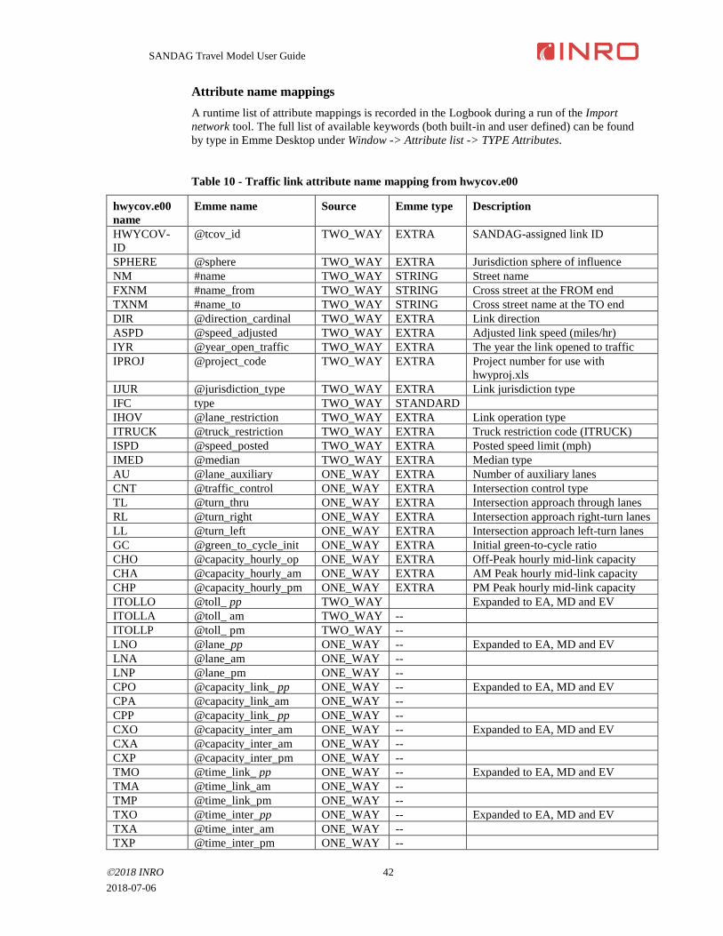
SANDAG Travel Model User Guide
2018 INRO 42
2018-07-06
Attribute name mappings
A runtime list of attribute mappings is recorded in the Logbook during a run of the Import
network tool. The full list of available keywords (both built-in and user defined) can be found
by type in Emme Desktop under Window -> Attribute list -> TYPE Attributes.
Table 10 - Traffic link attribute name mapping from hwycov.e00
hwycov.e00
name
Emme name Source Emme type Description
HWYCOV-
ID
@tcov_id TWO_WAY EXTRA SANDAG-assigned link ID
SPHERE @sphere TWO_WAY EXTRA Jurisdiction sphere of influence
NM #name TWO_WAY STRING Street name
FXNM #name_from TWO_WAY STRING Cross street at the FROM end
TXNM #name_to TWO_WAY STRING Cross street name at the TO end
DIR @direction_cardinal TWO_WAY EXTRA Link direction
ASPD @speed_adjusted TWO_WAY EXTRA Adjusted link speed (miles/hr)
IYR @year_open_traffic TWO_WAY EXTRA The year the link opened to traffic
IPROJ @project_code TWO_WAY EXTRA Project number for use with
hwyproj.xls
IJUR @jurisdiction_type TWO_WAY EXTRA Link jurisdiction type
IFC type TWO_WAY STANDARD
IHOV @lane_restriction TWO_WAY EXTRA Link operation type
ITRUCK @truck_restriction TWO_WAY EXTRA Truck restriction code (ITRUCK)
ISPD @speed_posted TWO_WAY EXTRA Posted speed limit (mph)
IMED @median TWO_WAY EXTRA Median type
AU @lane_auxiliary ONE_WAY EXTRA Number of auxiliary lanes
CNT @traffic_control ONE_WAY EXTRA Intersection control type
TL @turn_thru ONE_WAY EXTRA Intersection approach through lanes
RL @turn_right ONE_WAY EXTRA Intersection approach right-turn lanes
LL @turn_left ONE_WAY EXTRA Intersection approach left-turn lanes
GC @green_to_cycle_init ONE_WAY EXTRA Initial green-to-cycle ratio
CHO @capacity_hourly_op ONE_WAY EXTRA Off-Peak hourly mid-link capacity
CHA @capacity_hourly_am ONE_WAY EXTRA AM Peak hourly mid-link capacity
CHP @capacity_hourly_pm ONE_WAY EXTRA PM Peak hourly mid-link capacity
ITOLLO @toll_ pp TWO_WAY
Expanded to EA, MD and EV
ITOLLA @toll_ am TWO_WAY --
ITOLLP @toll_ pm TWO_WAY --
LNO @lane_pp ONE_WAY -- Expanded to EA, MD and EV
LNA @lane_am ONE_WAY --
LNP @lane_pm ONE_WAY --
CPO @capacity_link_ pp ONE_WAY -- Expanded to EA, MD and EV
CPA @capacity_link_am ONE_WAY --
CPP @capacity_link_ pp ONE_WAY --
CXO @capacity_inter_am ONE_WAY -- Expanded to EA, MD and EV
CXA @capacity_inter_am ONE_WAY --
CXP @capacity_inter_pm ONE_WAY --
TMO @time_link_ pp ONE_WAY -- Expanded to EA, MD and EV
TMA @time_link_am ONE_WAY --
TMP @time_link_pm ONE_WAY --
TXO @time_inter_pp ONE_WAY -- Expanded to EA, MD and EV
TXA @time_inter_am ONE_WAY --
TXP @time_inter_pm ONE_WAY --
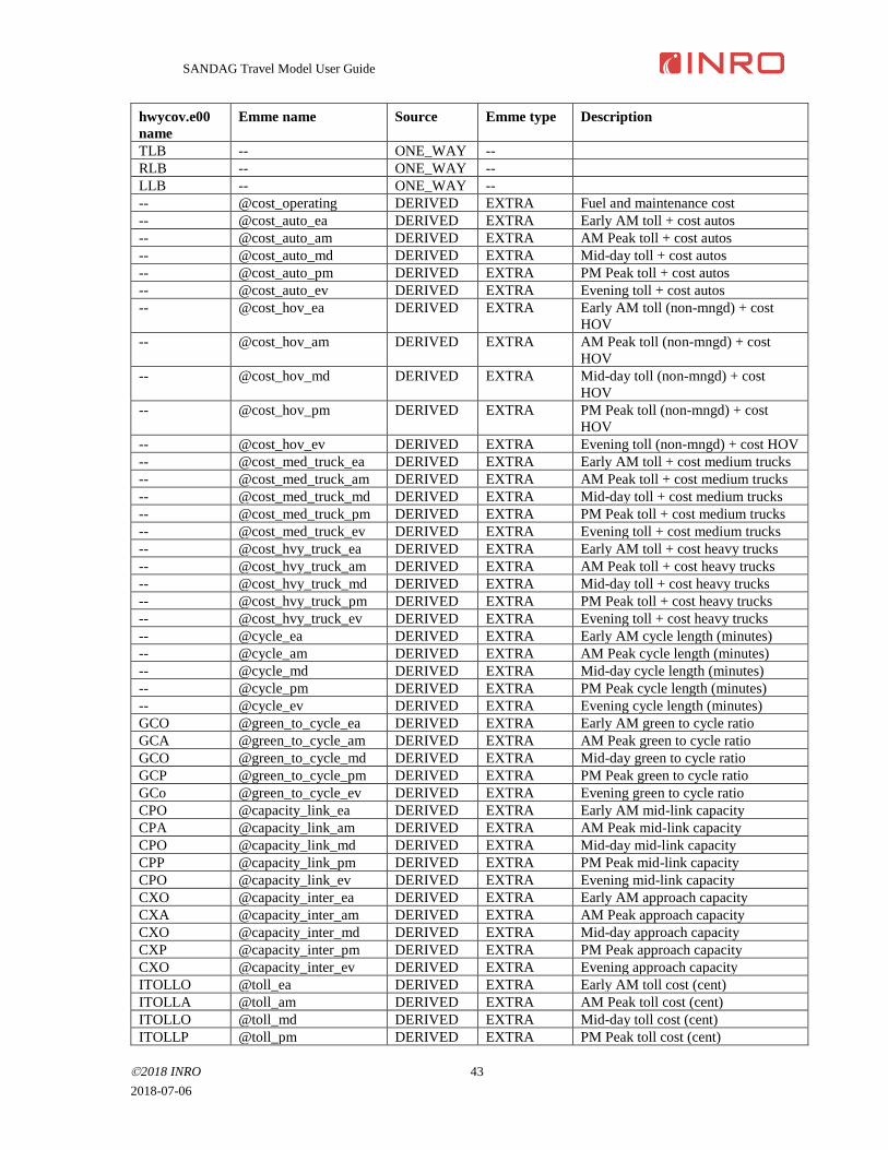
SANDAG Travel Model User Guide
2018 INRO 43
2018-07-06
hwycov.e00
name
Emme name Source Emme type Description
TLB -- ONE_WAY --
RLB -- ONE_WAY --
LLB -- ONE_WAY --
-- @cost_operating DERIVED EXTRA Fuel and maintenance cost
-- @cost_auto_ea DERIVED EXTRA Early AM toll + cost autos
-- @cost_auto_am DERIVED EXTRA AM Peak toll + cost autos
-- @cost_auto_md DERIVED EXTRA Mid-day toll + cost autos
-- @cost_auto_pm DERIVED EXTRA PM Peak toll + cost autos
-- @cost_auto_ev DERIVED EXTRA Evening toll + cost autos
-- @cost_hov_ea DERIVED EXTRA Early AM toll (non-mngd) + cost
HOV
-- @cost_hov_am DERIVED EXTRA AM Peak toll (non-mngd) + cost
HOV
-- @cost_hov_md DERIVED EXTRA Mid-day toll (non-mngd) + cost
HOV
-- @cost_hov_pm DERIVED EXTRA PM Peak toll (non-mngd) + cost
HOV
-- @cost_hov_ev DERIVED EXTRA Evening toll (non-mngd) + cost HOV
-- @cost_med_truck_ea DERIVED EXTRA Early AM toll + cost medium trucks
-- @cost_med_truck_am DERIVED EXTRA AM Peak toll + cost medium trucks
-- @cost_med_truck_md DERIVED EXTRA Mid-day toll + cost medium trucks
-- @cost_med_truck_pm DERIVED EXTRA PM Peak toll + cost medium trucks
-- @cost_med_truck_ev DERIVED EXTRA Evening toll + cost medium trucks
-- @cost_hvy_truck_ea DERIVED EXTRA Early AM toll + cost heavy trucks
-- @cost_hvy_truck_am DERIVED EXTRA AM Peak toll + cost heavy trucks
-- @cost_hvy_truck_md DERIVED EXTRA Mid-day toll + cost heavy trucks
-- @cost_hvy_truck_pm DERIVED EXTRA PM Peak toll + cost heavy trucks
-- @cost_hvy_truck_ev DERIVED EXTRA Evening toll + cost heavy trucks
-- @cycle_ea DERIVED EXTRA Early AM cycle length (minutes)
-- @cycle_am DERIVED EXTRA AM Peak cycle length (minutes)
-- @cycle_md DERIVED EXTRA Mid-day cycle length (minutes)
-- @cycle_pm DERIVED EXTRA PM Peak cycle length (minutes)
-- @cycle_ev DERIVED EXTRA Evening cycle length (minutes)
GCO @green_to_cycle_ea DERIVED EXTRA Early AM green to cycle ratio
GCA @green_to_cycle_am DERIVED EXTRA AM Peak green to cycle ratio
GCO @green_to_cycle_md DERIVED EXTRA Mid-day green to cycle ratio
GCP @green_to_cycle_pm DERIVED EXTRA PM Peak green to cycle ratio
GCo @green_to_cycle_ev DERIVED EXTRA Evening green to cycle ratio
CPO @capacity_link_ea DERIVED EXTRA Early AM mid-link capacity
CPA @capacity_link_am DERIVED EXTRA AM Peak mid-link capacity
CPO @capacity_link_md DERIVED EXTRA Mid-day mid-link capacity
CPP @capacity_link_pm DERIVED EXTRA PM Peak mid-link capacity
CPO @capacity_link_ev DERIVED EXTRA Evening mid-link capacity
CXO @capacity_inter_ea DERIVED EXTRA Early AM approach capacity
CXA @capacity_inter_am DERIVED EXTRA AM Peak approach capacity
CXO @capacity_inter_md DERIVED EXTRA Mid-day approach capacity
CXP @capacity_inter_pm DERIVED EXTRA PM Peak approach capacity
CXO @capacity_inter_ev DERIVED EXTRA Evening approach capacity
ITOLLO @toll_ea DERIVED EXTRA Early AM toll cost (cent)
ITOLLA @toll_am DERIVED EXTRA AM Peak toll cost (cent)
ITOLLO @toll_md DERIVED EXTRA Mid-day toll cost (cent)
ITOLLP @toll_pm DERIVED EXTRA PM Peak toll cost (cent)
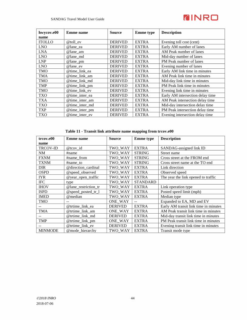
SANDAG Travel Model User Guide
2018 INRO 44
2018-07-06
hwycov.e00
name
Emme name Source Emme type Description
ITOLLO @toll_ev DERIVED EXTRA Evening toll cost (cent)
LNO @lane_ea DERIVED EXTRA Early AM number of lanes
LNA @lane_am DERIVED EXTRA AM Peak number of lanes
LNO @lane_md DERIVED EXTRA Mid-day number of lanes
LNP @lane_pm DERIVED EXTRA PM Peak number of lanes
LNO @lane_ev DERIVED EXTRA Evening number of lanes
TMO @time_link_ea DERIVED EXTRA Early AM link time in minutes
TMA @time_link_am DERIVED EXTRA AM Peak link time in minutes
TMO @time_link_md DERIVED EXTRA Mid-day link time in minutes
TMP @time_link_pm DERIVED EXTRA PM Peak link time in minutes
TMO @time_link_ev DERIVED EXTRA Evening link time in minutes
TXO @time_inter_ea DERIVED EXTRA Early AM intersection delay time
TXA @time_inter_am DERIVED EXTRA AM Peak intersection delay time
TXO @time_inter_md DERIVED EXTRA Mid-day intersection delay time
TXP @time_inter_pm DERIVED EXTRA PM Peak intersection delay time
TXO @time_inter_ev DERIVED EXTRA Evening intersection delay time
Table 11 - Transit link attribute name mapping from trcov.e00
trcov.e00
name
Emme name Source Emme type Description
TRCOV-ID @tcov_id TWO_WAY EXTRA SANDAG-assigned link ID
NM #name TWO_WAY STRING Street name
FXNM #name_from TWO_WAY STRING Cross street at the FROM end
TXNM #name_to TWO_WAY STRING Cross street name at the TO end
DIR @direction_cardinal TWO_WAY EXTRA Link direction
OSPD @speed_observed TWO_WAY EXTRA Observed speed
IYR @year_open_traffic TWO_WAY EXTRA The year the link opened to traffic
IFC type TWO_WAY STANDARD
IHOV @lane_restriction_tr TWO_WAY EXTRA Link operation type
ISPD @speed_posted_tr_l TWO_WAY EXTRA Posted speed limit (mph)
IMED @median TWO_WAY EXTRA Median type
TMO -- ONE_WAY -- Expanded to EA, MD and EV
-- @trtime_link_ea DERIVED EXTRA Early AM transit link time in minutes
TMA @trtime_link_am ONE_WAY EXTRA AM Peak transit link time in minutes
-- @trtime_link_md DERIVED EXTRA Mid-day transit link time in minutes
TMP @trtime_link_pm ONE_WAY EXTRA PM Peak transit link time in minutes
-- @trtime_link_ev DERIVED EXTRA Evening transit link time in minutes
MINMODE @mode_hierarchy TWO_WAY EXTRA Transit mode type
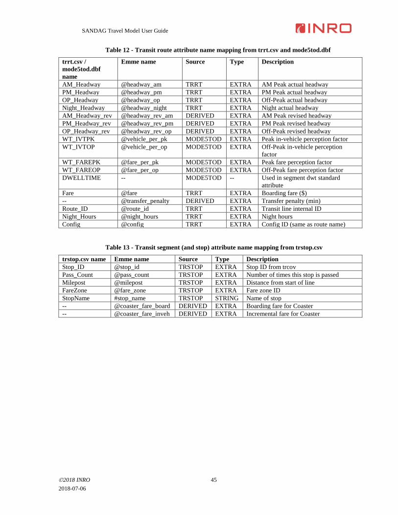
SANDAG Travel Model User Guide
2018 INRO 45
2018-07-06
Table 12 - Transit route attribute name mapping from trrt.csv and mode5tod.dbf
trrt.csv /
mode5tod.dbf
name
Emme name Source Type Description
AM_Headway @headway_am TRRT EXTRA AM Peak actual headway
PM_Headway @headway_pm TRRT EXTRA PM Peak actual headway
OP_Headway @headway_op TRRT EXTRA Off-Peak actual headway
Night_Headway @headway_night TRRT EXTRA Night actual headway
AM_Headway_rev @headway_rev_am DERIVED EXTRA AM Peak revised headway
PM_Headway_rev @headway_rev_pm DERIVED EXTRA PM Peak revised headway
OP_Headway_rev @headway_rev_op DERIVED EXTRA Off-Peak revised headway
WT_IVTPK @vehicle_per_pk MODE5TOD EXTRA Peak in-vehicle perception factor
WT_IVTOP @vehicle_per_op MODE5TOD EXTRA Off-Peak in-vehicle perception
factor
WT_FAREPK @fare_per_pk MODE5TOD EXTRA Peak fare perception factor
WT_FAREOP @fare_per_op MODE5TOD EXTRA Off-Peak fare perception factor
DWELLTIME -- MODE5TOD -- Used in segment dwt standard
attribute
Fare @fare TRRT EXTRA Boarding fare ($)
-- @transfer_penalty DERIVED EXTRA Transfer penalty (min)
Route_ID @route_id TRRT EXTRA Transit line internal ID
Night_Hours @night_hours TRRT EXTRA Night hours
Config @config TRRT EXTRA Config ID (same as route name)
Table 13 - Transit segment (and stop) attribute name mapping from trstop.csv
trstop.csv name Emme name Source Type Description
Stop_ID @stop_id TRSTOP EXTRA Stop ID from trcov
Pass_Count @pass_count TRSTOP EXTRA Number of times this stop is passed
Milepost @milepost TRSTOP EXTRA Distance from start of line
FareZone @fare_zone TRSTOP EXTRA Fare zone ID
StopName #stop_name TRSTOP STRING Name of stop
-- @coaster_fare_board DERIVED EXTRA Boarding fare for Coaster
-- @coaster_fare_inveh DERIVED EXTRA Incremental fare for Coaster
Related Documents