Radio Signal Propagation and Models

2.1 INTRODUCTION

This chapter focuses on those aspects of wireless transmissionwhich are necessary to understand the problems faced by higherlayers in atmosphere as well as the obstacles in the transmissionpath.

In vacuum, transmission path is in simply line of sight butit varies greatly in atmosphere due to the obstacles that arepresent in the path of transmission. These may be large mountains,high rise buildings, trees, etc. These obstacles may create somelosses in the strength of signal because the path is no longerline-of-sight now but waves actualy reach the receiver by followingmultipaths. Several other effects also occur during transmissionwhich are reflection, diffraction, scattering, shadowing, refractionetc. Therefore, radio channels are externally random and do notoffer easy analysis. To predict the signal strength from transmitterto receiver, some propagation models are used. The detail ofpath loss, propagation effects and models are given insight.

C H A P T E R

Radio SignalPropagation and

Models2ACRONYMS

• LOS : Line of Sight• DG : Diffraction Gain• V : Fresnel–Kirchoff Diffraction Parameter• SNR : Signal to Noise Ratio• N : Path Loss Exponent• XV : Zero-mean Gaussion Distributed Random Variable• U(V) : Percentage of Useful Service Area• JRC : Joint Radio Committee• RTSD : Roof-to-street Diffraction• ML : Multiscreen Loss

RADIO SIGNAL PROPAGATION AND MODELS 25

2.2 SIGNAL PROPAGATION

Signal propagation in wireless communication needs two points(like wired communication), one to generate the signal and otherto detect the signal. But in wireless networks, the signal has nowire to determine the direction of propagation.

In case of wired (or PSTN) connection, one can preciselydetermine the behavior of a signal travelling along this wirewhile in wireless connection, this predictable behavior is onlyvalid in a vacuum. Practically radio transmission has to contendwith our atmosphere, mountains, buildings, moving sendersand receivers etc. Refer Fig. 2.1 in reality, the three circlesrefere to ranges for transmission, detection and interferenceof signals.

Fig. 2.1 Ranges for transmission, detection andInterference of Signals

••••• Transmission Range: It is possible within a certainradius of the sender transmission. In this range, a receiverreceives the signals with an error rate low enough toable to be communicate and can also act as sender toestablish a new connection.

••••• Detection Range: It lies within second radius of thesender transmission side. In this range, the transmittedpower is large enough to be differentiated from backgroundnoise. However, the error rate is too high to establishconnection in this range.

26 WIRELESS COMMUNICATION

••••• Interference Range : This range lies within a thirdeven larger radius. The sender may interfere with othertransmission by adding a background noise. A receiverwill not be able to detect the signals under this range.

2.3 ADDITIONAL SIGNAL PROPAGATION EFFECTS

In free space, signals propagate quite similar to how light doesi.e. they follow a straight line-of-sight path. But in real life, werarely have a line-of-sight between the sender and receiver ofradio signals. Before reaching upto receiver, signals have to facea lot of disturbances like, mountains, valleys, big buildings etc.Here several effects occur in addition to the attenuation causedby the distance between sender and receiver. These effects are

1. Shadowing or Blocking2. Reflection3. Refraction4. Scattering5. Diffraction

All these effects are shown in Fig. 2.2.

.

Fig. 2.2

For more clarity, all these effects are described in brief :1. Shadowing : An extreme form of attenuation is blocking or

shadowing of radio signals due to large obstacles. Largeobjects create their shadow which may penetrate or blockthe signal. The higher the frequency of a signal, the more


it behaves like light. Even small obstacles like a simple wall,a bus on the stop or trees etc. may block the signal.

2. Reflection : This effect occurs if the object is large comparedto the wavelength of the transmitted signal, e.g. huge buildings,mountains or surface of the earth etc. After striking withsuch object, the signal gets reflected in different directions.In this effect, some power of the signal gets absorbed by theobject therefore the reflected signal is not as strong as original.The more often the signal is reflected, the weaker it becomes.

3. Refraction : This effect occurs because the velocity of EMwaves depends on the density of the medium through whichit travels. Those waves which travel into a denser mediumare bent towards the medium. This is the reason for line ofsight radio waves being bent towards the earth because thedensity of the atmosphere is higher closer to the ground.

4. Scattering : While Shadowing and Reflection are causedby the objects much larger than the wavelength of the signal,the scattering occurs due to obstacles i.e. in order of thewavelength or less. We can say that if the obstacle size ismuch less than the wavelength of transmitted signal thenwaves can be scattered. An incoming signal is scattered intoseveral weaker outgoing signals.

5. Diffraction : This effect shows the wave character of radiosignals. This effect means that the radio waves will be deflectedat an edge and propagated in different directions. The resultsof diffraction are patterns with varying signal strengthsdepending on the location of the receiver.

Note: Reflection, scattering and diffraction are more prominantpropagation mechanisms which impact propagation in mobilecommunication systems. These mechanisms are explained indetail in next section.

2.4 REFLECTION

The basic concept of reflection, has already been studied in previoussection. In this section we will study the effect of medium onreflection.

When a propagating wave in one medium impinges uponanother medium then the wave may be partially reflected andpartially transmitted and there is no loss of energy by absorption.If the second medium is a perfect conductor then all the incident


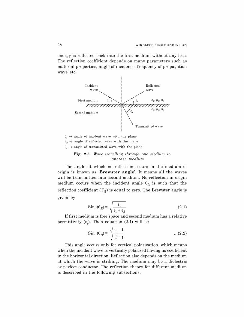
energy is reflected back into the first medium without any loss.The reflection coefficient depends on many parameters such asmaterial properties, angle of incidence, frequency of propagationwave etc.

θi → angle of incident wave with the planeθr → angle of reflected wave with the planeθt → angle of transmitted wave with the plane

Fig. 2.3 Wave travelling through one medium toanother medium

The angle at which no reflection occurs in the medium oforigin is known as ‘Brewster angle’. It means all the waveswill be transmitted into second medium. No reflection in originmedium occurs when the incident angle θB is such that thereflection coefficient ( Γ||) is equal to zero. The Brewster angle isgiven by

Sin (θB) = 1

1 2

εε + ε

...(2.1)

If first medium is free space and second medium has a relativepermittivity (εr). Then equation (2.1) will be

Sin (θB) = ε −

ε −2

1

1r

r

...(2.2)

This angle occurs only for vertical polarization, which meanswhen the incident wave is vertically polarized having no coefficientin the horizontal direction. Reflection also depends on the mediumat which the wave is striking. The medium may be a dielectricor perfect conductor. The reflection theory for different mediumis described in the following subsections.


2.4.1 Reflection from Dielectrics

In general, electromagnetic or radio waves are polarized, meaningthey have instantaneous electric field components in the orthogonaldirections in space. A polarized wave may be represented as thesum of vertical and horizontal orthogonal components or lefthand and right hand circularly polarized components. For anarbitrary polarization, superposition may be used to compute thereflected fields from a reflecting surface. Fig. 2.4 shows two casesof E-field polarization in the plane of incidence. Plane of incidenceis defined as the plane containing incident, reflected and transmittedwave. In Fig. 2.4 (a), the E-field has a vertical polarization withrespect to the reflecting surface or we can say the E-field polarizationis parallel with the plane of incidence while in Fig. 2.4(b), the E-field polarization is perpendicular to the plane of incidence orthe E-field is parallel to the reflecting surface.

Fig. 2.4 Reflection coefficients between two dielectric

Here, the subscript i, r, t refer to the incident, reflected andtransmitted fields, respectively. And ε, µ, σ represents thepermittivity, permeability and conductance of different media.

The dielectric constant of a perfect dielectric isε = ε0 εr ...(2.3)

where ε0 = 8.85 × 10–12 F/m (Constant)and εr = Relative permittivity

Whereas, the dielectric constant of a lossy dielectric materialis

ε = ε0 εr – jε′ ...(2.4)

where ε′ = 2 fσπ

σ is the conductivity of material.


The reflection co-efficients for the two cases of parallel andperpendicular E-field polarization at the boundary of two dielectricsare given by,

Parallel reflection coefficient

Γ|| = r

i

EE

= 2 1

2 1

sin sinsin sin

t i

t i

η θ − η θη θ + η θ

...(2.5)

Perpendicular reflection coefficient

G^ = r

i

EE

= 2 1

2 1

sin sinsin sin

i t

i t

η θ − η θη θ + η θ

...(2.6)

where ηi is the intrinsic impedance of the ith medium (i = 1,2, ...) and given by /i iµ ε .

The velocity of an electromagnetic wave is given by ( )1µε

.

The boundary conditions at the surface of incidence obeys Shell’slaw which is given by,

µ ε − θ1 1, sin (90º )i = µ ε − θ2 2 sin (90º )t ...(2.7)

The boundary conditions from Maxwell’s equations are usedto derive equations (2.5) and (2.6) as well as Equations 2.8, 2.9and 2.10.

θi = θr ...(2.8)and Εr = Γ Ei ...(2.9)

Et = (i + τ) Ei ...(2.10)where Γ is either Γ|| or Γ⊥, depending on whether the E-field isin parallel or perpendicular to the plane of incidence.

For the case when the first medium is free space and µ1 = µ2.The reflection coefficients can be simplified as,

Γ|| = 2

2

sin cos

sin cosr i r i

r i r i

− ε θ + ε − θ

ε θ + ε − θ...(2.11)

an d

Γ⊥ = 2

2

sin cos

sin cosi r i

i r i

θ − ε − θ

θ + ε − θ...(2.12)

For elliptical polarized waves, the wave may be broken down(depolarized) into its vertical and horizontal E components and


then superposition principle may be applied to determinetransmitted and reflected wave.

Fig. 2.5 Axis of orthogonally polarized components. Wave ispropagating out of the page (toward the reader)

The parallel and perpendicular components are related to thehorizontal and vertical spatial coordinates. The vertical andhorizontal field components at a dielectric boundary may be relatedby,

dHdV

E

E

= i

T Hc i

V

ER D R

E

...(2.13)

where,EH

d = Depolarized field component in the horizontal directionEV

d = Depolarized field component in the vertical directionEH

i = Horizontally polarized component of the incident waveEV

i = Vertically polarized component of the incident wave.A transformation matrix (R) maps vertical and horizontal

polarized components to components which are perpendicularand parallel to the plane of incidence. The transformation matrix(R) is given by

R = cos sinsin cos

θ θ − θ θ

where θ = angle between the two sets of axes (see Fig. 2.5)The depolarization matrix (DC) is given by

DC = ⊥⊥ ||

00

D

D ...(2.14)

where Dxx = Γx for the case of reflection andDxx = Tx = 1 + Γx for the case of transmission


Fig. 2.6 shows reflection coefficient as angle of incidence forthe case when a wave propagates in free space (εr = 1) and thereflection surface has (a) εr = 4 and (b) εr = 12.

Through this figure, we are able to study parallel polarizationand perpendicular polarization at various relative permittivity.

Fig. 2.6 Reflection coefficients vs angle of incidence

2.4.2 Reflection from Perfect Conductors

The wave impinges on a perfect conductor is completely reflectedbecause electro megnatic energy cannot pass through a perfectconductor. The reflected wave must be equal in magnitude to theincident wave.

For the case when E-field polarization is vertically polarizedthe boundary condition requires that

θi = θr ...(2.15)and Ei = Er (E-field parallel to the plane of incidence) ...(2.16)


Similarly, when E-field is horizontally polarized, the boundarycondition requires that

θi = θr ...(2.17)

and Ei = – Er

(E-field perpendicular to the plane of incidence) ...(2.18)

Therefore, by referring above equations, we may concludethat for a perfect conductor, the reflection coefficient paralleland perpendicular to the plane of incidence is :

τ|| = 1and

τ⊥ = –1,

2.5 SCATTERING

In addition to reflection, another property of EM wave is thatwhen a radio wave impinges on a rough surface, then the reflectedenergy get spread in all directions. This is due to the scatteringproperty. Objects which have dimension less than the wavelengthof EM wave, tend to scatter energy in all directions, thereforeproviding additional radio energy at receiver.

Generally, the dimensions of flat surfaces is much largerthan the wavelength of the wave. Different propagation effectsdepend on surface flatness and roughness. Surface roughness isoften tested using the Rayleigh criterion. According to Rayleighcriterion the critical height (hc) of surface protuberances (Swellingor bulge) for a given angle of incidence θi, given by

λθ

=8 sinc

ih ...(2.19)

A surface is considered smooth if its minimum to maximumswelling (height) h is less than hc (h < hc) and it is consideredrough if h is greater than hc (h > hc). To find out the diminishedreflected field for rough surfaces, the flat surface reflection coefficientis multiplied with scattering loss factor (ρs), where ρs is given by,

ρs = π σ θ − λ

2sinexp 8 h i ...(2.20)


here, σh = Standard deviation of the surface height about themean surface height

λ = wavelength of waveand θi = angle of incidence of wave at surface.

The reflected E-fields for h > hc can be solved for roughsurfaces using a modified reflection coefficient given as

Trough = ρs . τ ...(2.21)

2.5.1 Radar Cross Section Model

This model is used to accurately predict the scattered signalstrengths. As we know that the received signal varies in strengthdue to scattering by distant objects. A knowledge of the physicallocation of such objects is used to find out the approximatedsignal strength at that point.

The received power for urban mobile radio systems is computedusing bistatic radar equation. This equation describes thepropagation of a wave traveling in free space which impinges(Strikes) on a distant scattering object, and is then reradiated inthe direction of the receiver, given by

PR(dBm) = PT(dBm) + GT(dBi) + 20 log(λ) + RCS(dBm2) – 30 log (4π) – 20 log dT

– 20 log dR ...(2.22)where,

dT = Distance from transmitter to scattering objectdR = Distant from receiver to scattering object

RCS = Radar Cross SectionEquation (2.22) is useful for predicting receiver power which

scatters off large objects such as buildings, mountains etc. whichare for both the transmitter and receiver.

2.6 DIFFRACTION

It is a significant effect for terrestrial propagation. In physics,diffraction refers to the phenomenon whereby, when e.m. wavesare forced to travel through a small slit, they tend to spread outon the far end of the slit as shown in Fig. 2.7.


Fig. 2.7 Plane passing through a slit left to right

The diffraction mechanism is often explained by Hugen’sprinciple, which may be stated as follows–

“Each point on a wave form acts as a point source for furtherpropagation. However, the point source does not radiate equallyin all directions, but favours the forward direction of the front”.

This principle is generally used to explain the reason, whye.m. waves bend over hills and around buildings.

The diffraction property of radio signal enables it to propagateeven after the line-of-sight (LOS) or around the curved surfaceof the earth. Although the received field strength decreases rapidlywhen the receiver moves deeper into the shadowed region.Differection is basically caused by the propagation of secondarywavelets from a wave front into the shadowed region.

The field strength of a diffracted wave in the shadowed regionis the vector sum of the electric field components of all the secondarywavelets in the space around the obstacle.


2.6.1 Fresnel Zone Geometry

According to this geometry, the phase difference between a directline-of-sight path and diffracted path is a function of heightand position of the obstacle (may be building, mountain etc.) aswell as the location of transmitter and receiver.

Let, a sharpedge (or knife edge) obstacle of height h is placedbetween transmitter and receiver. The distance of this obstructionfrom transmitter and receiver is d1 and d2 respectively. (SeeFig. 2.8) Then the difference between the direct path (LOSPath) and diffracted path is the excess path length denoted by∆, and given as

∆ ≈ +21 2

1 2

( )2

d dhd d

The corresponding phase difference is

φ = 2π∆λ

= 2

1 2

1 2

( )2 .2

d dhd d

+πλ

...(2.23)

when tan x ≈ x then α = β + γ (from Fig. 2.7(c)) and

α ≈ h +

1 2

1 2

d dd d

Equation (2.23) can be more minimized using the dimensionlessFresnel-Kirchoff diffraction parameter v which is given by

v = +

λ1 2

1 2

2( )d dd d

= α λ +1 2

1 2

2( )

d dd d ...(2.24)

where a is shown in Fig. 2.7.Put the value of v in equation (2.23)

φ = +π

λ

21 2

1 2

( )22

d dhd d

φ = π 22

v ...(2.25)

Hence, it is proved that the phase difference between a directLOS path and diffracted path is a function of height and theposition of the obstacle from the transmitter and receiver. In


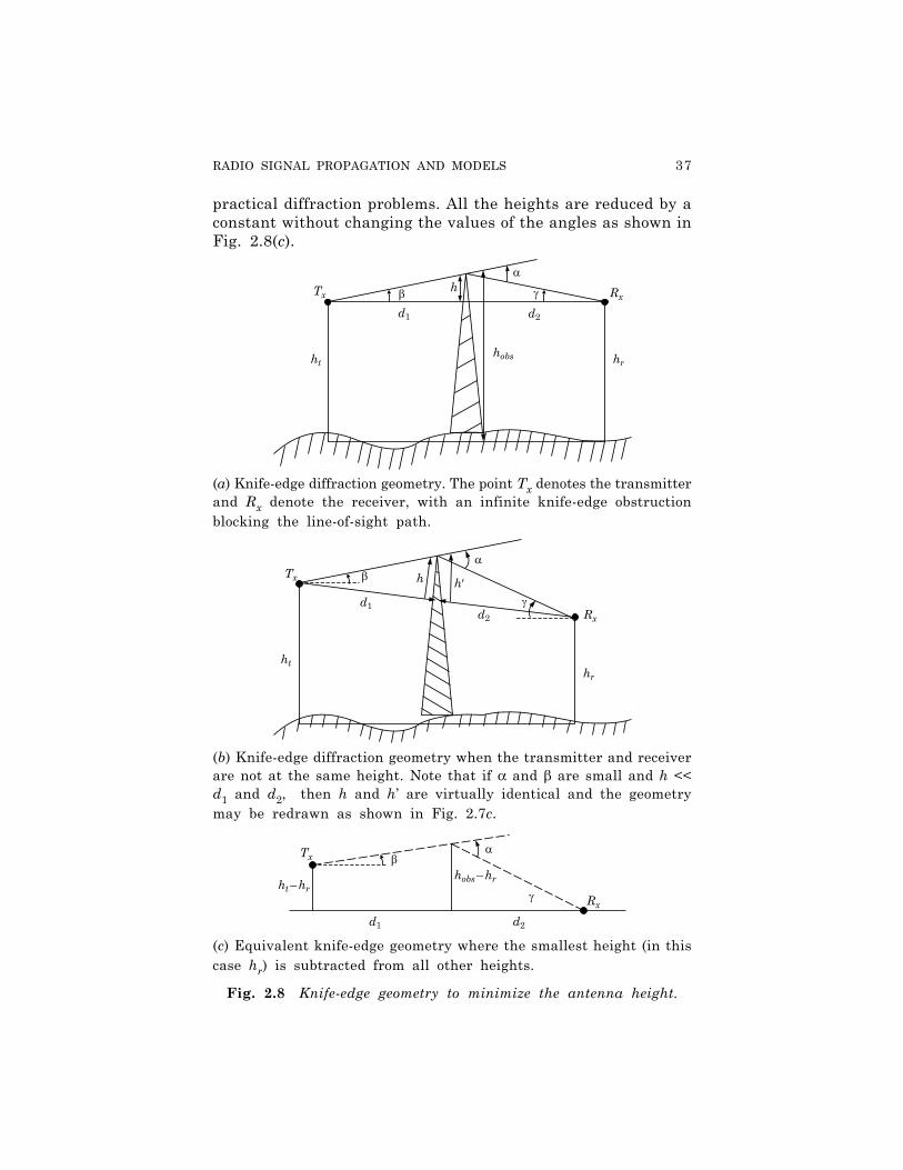
practical diffraction problems. All the heights are reduced by aconstant without changing the values of the angles as shown inFig. 2.8(c).

(a) Knife-edge diffraction geometry. The point Tx denotes the transmitterand Rx denote the receiver, with an infinite knife-edge obstructionblocking the line-of-sight path.

(b) Knife-edge diffraction geometry when the transmitter and receiverare not at the same height. Note that if α and β are small and h <<d1 and d2, then h and h’ are virtually identical and the geometrymay be redrawn as shown in Fig. 2.7c.

(c) Equivalent knife-edge geometry where the smallest height (in thiscase hr) is subtracted from all other heights.

Fig. 2.8 Knife-edge geometry to minimize the antenna height.


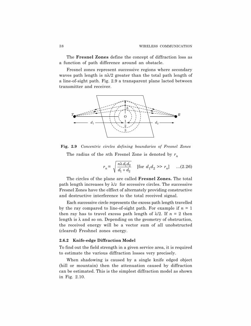
The Fresnel Zones define the concept of diffraction loss asa function of path difference around an obstacle.

Fresnel zones represent successive regions where secondarywaves path length is nλ/2 greater than the total path length ofa line-of-sight path. Fig. 2.9 a transparent plane lacted betweentransmitter and receiver.

Fig. 2.9 Concentric circles defining boundaries of Fresnel Zones

The radius of the nth Fresnel Zone is denoted by rn

rn = 1 2

1 2

n d dd d

λ+

[for d1d2 >> rn] ...(2.26)

The circles of the plane are called Fresnel Zones. The totalpath length increases by λ/z for sccessive circles. The successiveFresnel Zones have the elffect of alternately providing constructiveand destructive interference to the total received signal.

Each successive circle represents the excess path length travelledby the ray compared to line-of-sight path. For example if n = 1then ray has to travel excess path length of λ/2. If n = 2 thenlength is λ and so on. Depending on the geometry of obstruction,the received energy will be a vector sum of all unobstructed(cleared) Freshnel zones energy.

2.6.2 Knife-edge Diffraction Model

To find out the field strength in a given service area, it is requiredto estimate the various diffraction losses very precisely.

When shadowing is caused by a single knife edged object(hill or mountain) then the attenuation caused by diffractioncan be estimated. This is the simplest diffraction model as shownin Fig. 2.10.


Fig. 2.10 Knife-edge diffraction model geometry. The receiver Rxis located in the shadow region

The field strength (Ed) of a diffracted wave at receiver (Rx)which is located in the shadowed region (diffraction zone), isthe vector sum of the fields due to secondary sources in theplane above the knife edge.

Ed = Eo . F(ν)

or, d

o

EE

= F(V) = ∞

ν

+ − π∫ 2(1 ) (( ) / 2)2

jexp j t dt ...(2.27)

where, Eo = Free space field strength in absence of knife edge

and F(ν) = Complex Fresnel integralThe diffraction gain due to knife edge is

Gd(dB) = 20 log |F(ν)| ...(2.28)An approximate solution of equation (2.28) for different values

of ν is given–Gd(dB) = 0 for ν ≤ –1Gd(dB) = 20 log(0.5 – 0.62 ν) for –1 ≤ ν ≤ 0Gd(dB) = 20 log[0.5 exp (– 0.95ν)] for 0 ≤ ν ≤ 1

Gd(dB) = − − − ν 220 log[0.4 0.1184 (0.38 0.1 ) ]for 1 ≤ ν ≤ 2.4

Gd(dB) = ν

0.22520 log for ν > 2.4


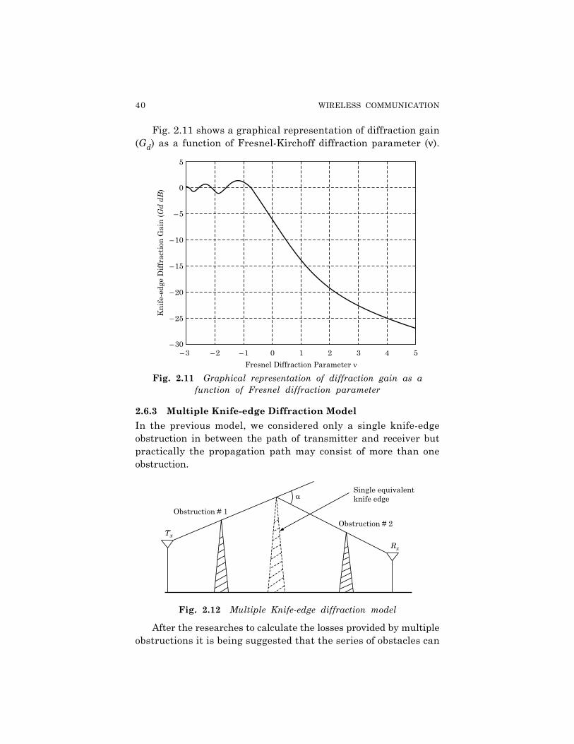
Fig. 2.11 shows a graphical representation of diffraction gain(Gd) as a function of Fresnel-Kirchoff diffraction parameter (ν).

Fig. 2.11 Graphical representation of diffraction gain as afunction of Fresnel diffraction parameter

2.6.3 Multiple Knife-edge Diffraction Model

In the previous model, we considered only a single knife-edgeobstruction in between the path of transmitter and receiver butpractically the propagation path may consist of more than oneobstruction.

Fig. 2.12 Multiple Knife-edge diffraction model

After the researches to calculate the losses provided by multipleobstructions it is being suggested that the series of obstacles can


be replaced by a single equivalent obstacle to compute the path-losses easily. This method is shown in Fig. 2.12. The main advantageof this method is that it provides very optimistic estimates of thereceived signal strength.

2.7 PATH LOSS OF RADIO SIGNALS

In free space, radio signals follow a straight line. The propagationof radio signals is same as light in free space. If such a straightline exists (or establishes) between a transmitter and a receiverthen it is said as line-of-sight communication. Even if the signalsare propagating in vaccum in LOS path, still the signals experiencethe Free Space Loss.

The signal power (Pr) received at receiver is inverselyproportional to the square of the distance (d) between thetransmitter and the receiver.

Pr α 21

dIn addition to the distance between transmitter and receiver,

the signal power (Pr) also depends on the wavelength and gainof receiver and transmitter antennas.

The received power calculation gets more complex when signaltransmission takes place through the atmosphere (not throughvaccum). Now, the radio signal has to face a lot of factors(conditions) like rain, snow, air, fog, dust, smog etc.

Now, the attenuation of power in the signal path is knownas path loss which influences transmission over long distances.Due to this loss or absorption of energy in atmosphere maycause a established link to get break down.

2.8 PROPAGATION BEHAVIOUR

Depending on the frequency, radio waves can also penetrateobjects. The lower the frequency, the better the penetration.Generally, radio waves can exhibit three fundamental propagationbehaviours depending on their frequency.

1. Ground wave (for < 2 MHz)2. Sky wave (for 2 – 30 MHz)3. Line of sight propagation (> 30 MHz)


A brief description of these propagation behaviours is givenbelow:

1. Ground wave: This propagation is suitable for the broadcastat low frequencies. Waves with low frequencies follows the earth’ssurface and can propagate over long distances. It is useful forcommunication at very low frequency (VLF), low frequency (LF)and mid frequency (MF) range. These waves are used in submarinecommunication, AM radio communication etc.

Note: The prime drawback of ground wave propagation isthat ground wave signals are suitable for propagation onlyupto few kilometers range.

Fig. 2.13 Ground Wave Propagation (< 2MHz)

2. Sky wave: In this propagation, the signal reception is byreflection of the waves from the ‘Ionosphere’. These waves travelaround the globe by bouncing back and forth between theionosphere and the earth’s surface as shown in Fig. 2.14.

Fig. 2.14 Sky wave propagation through Ionosphere

Note: Ionosphere is an ionised region, ranging between 60 kmto 450 km in the earth’s atmosphere. The sky waves are reflectedfrom some of the ionized layers of ionosphere and return back toearth in single hop or multiple hops. [See Fig. 2.14]

In sky wave propagation, for a single hop, the electromagneticwaves cover a distance upto 400 km. Therefore it is best suitedfor long distance and international broadcasts.


3. Line-of-Sight (LOS): LOS propagation is also known as spacewave propagation space waves generally travel in straight line. Thesewaves use LOS propagation because the wavelength of space wavesare too short for reflection from the ionosphere. This propagationuses higher frequency range (> 30 MHz). These higher frequencywaves follows line of sight path. This enables direct communicationwith satellite. These are generally used by mobile phone systems,satellite systems, cordless telephones etc.

Fig. 2.15 LOS Propagation

2.9 FREQUENCY BANDS AND THEIR PROPAGATION MODES

Table 2.1 show frequency bands along with their mode ofpropagation.

Table 2.1

Band Abbreviation Frequency Mode ofrange Propagation

ELF Extra Low Frequency 30 – 300 Hz Ground waveVF Voice Frequency 300 – 3000 Hz Ground WaveVLF Very Low Frequency 3 – 30 KHz Ground WaveLF Low Frequency 30 – 300 KHz Ground waveMF Mid Frequency 300 – 3000 KHz Ground waveHF High Frequency 3 – 30 MHz Sky waveVHF Very High Frequency 30 – 300 MHz LOSUHF Ultra High Frequency 300 – 3000 MHz LOSSHF Super High Frequency 3 – 30 GHz LOSEHF Extra High Frequency 30 – 300 GHz LOSInfrared 300 GHz LOS

– 400 THzVisible 400 THz LOSlight – 900 THz


2.10 PRACTICAL LINK BUDGET DESIGN USINGPATH LOSS MODELS

The level of received signal gets changed as distance changes.This decides the coverage of mobile systems and is used in designingof mobile communication systems. Over time, some classicalpropagation models have emerged which are now used to predictlarge scale coverage for mobile communication system design.All these models use path loss estimation techniques to accuratelypredict the signal strength and signal to noise ratio (SNR). Somepractical path loss estimation techniques are given below.

2.10.1 Log-Distance Path Loss Model

As we know that the signal strength gets diminished as signaltravels from transmitter to receiver. The signal strength decreaseslogarithmically as distance increases.

The average large-scale path loss for an arbitrary transmitter-receiver separation is expressed as a function of distance byusing a path loss exponent n

×

( )n

o

dPL d

d...(2.29)

or ( )PL dB = +

( ) 10 logo

o

dPL d n

d...(2.30)

where n = Path loss exponent indicates the rate at which thepath loss increases with distance.

do = Close in reference distance which is determined frommeasurements close to the transmitter.

d = Transmitter receiver separation distance.

When the graph is plotted on a log-log scale, then the modulatedpath loss shows a straight line with a slope equal to 10 n dB perdecade. The value of path loss exponent (n) varies in differentenvironments as given in Table 2.2.

The selection of reference distance should always be in thefar field of the antenna so that near field effects do not alter thepath loss. In large coverage mobile systems, 1 km referencedistances are commonly used whereas in microcellular systems,100 m or 1m distances are used.


Table 2.2 Estimation of path loss (n) for different environments

Environment Path Loss Exponent, n

In building line of sight 1.6 to 1.8Free space 2.0Obstructed in factories 2.0 to 3.0Urban area Cellular radio 2.7 to 3.5Shadowed urban Cellular radio 3.0 to 5.0Obstructed in buildings 4.0 to 6.0

2.10.2 Log-normal Shadowing Model

In the previous equation (2.30), the effect of clutter at sametransmitter-receiver separation is not being considered. Note thatthe clutter may be vastly different at two different locationshaving same transmitter receiver separation as shown in Fig.2.16.

Fig. 2.16 Clutter variation at different locations.

For first mobile, the clutter will be high due to mountains,with respect to the second mobile while both are at same distanceto the transmitter. Therefore, the measured signal at receiver(mobile 1 and 2) will be different than the average value predictedby equation (2.30).

Measurements have shown that at any value of d, the pathloss PL(d) at a particular location is random and distributed log-normally (normal in dB) about the mean distance dependentvalue – that is,


PL(d) [dB] = σ+( )PL d X

= σ

+ + 00

( ) 10 log dPL d n X

d...(2.31)

and Pr(d) [dBm] = Pt[dBm] – PL(d) [dB] ...(2.32)where, Xσ = Zero-mean Gaussian distributed random variable

(in dB) with standard deviation σ (also in dB)This logarithmic distribution describes the random shadowing

effects which occur at different locations having same transmitter-receiver separation distnace but varying clutter levels. Thisphenomenon is known as log-normal shadowing.

This model may be used in computer simulation to providereceived power levels for random locations in communicationsystem design and analysis.

2.10.3 Determination of Percentage of Coverage Area

In the previous section, we have studied the random effect ofshadowing. Due to this effect, the signal strength at some locationswithin a coverage area will become below a particular desiredthreshold level.

Let, there be a circular coverage area having radius R fromthe base station and the desired received signal threshold isassumed as γ. Then the percentage of useful service area U(γ)provides a known likelihood of coverage at the cell boundary.Here, useful service area U(γ) is the area at which the receivedsignal strength is equal to or greater than γ. Letting d = rrepresents the radial distance from the transmitter at which thereceived signal exceeds the threshold γ within an incrementalarea dA, then U(γ) can be found by

U(γ) = > γπ ∫2

1 [ ( ) ]r rP P r dAR

...(2.33)

= π

> γ θπ ∫ ∫

2 R

20 0

1 [ ( ) ]r r rP P r r d dR

...(2.34)

But at the cell boundary r = R, the path loss exponent will be

( )PL r = + + 0

010 log 10 log ( )R r

n n PL dd R

...(2.35)


After solving these equations, the useful service area will be

U(γ) = + − 21 1 11 exp 12

erfbb

...(2.36)

where, erf error functionand b = σ(10 log ) / 2n e .

2.11 PROPAGATION MODELS

Propagation models are used to determine how many cell sitesare required to provide the coverage requirements for thenetwork. The propagation model helps to determine wherethe cell sites should be located to achieve an optimal positionin the network.

The coverage requirement is coupled with the traffic loadingrequirement which rely on the propagation model chosen todetermine the traffic distribution and the off-loading from theexisting cell site to new cell sites as part of a capacity relief program.Propagation models are also useful for interference predictions.

Although no propagation model can account for all variationsexperienced in the real world. Therefore, it is essential that one shoulduse one or several models for determining the path losses in thenetwork. Generally, propagation models are divided into two parts:1. Outdoor propagation models2. Indoor propagation models

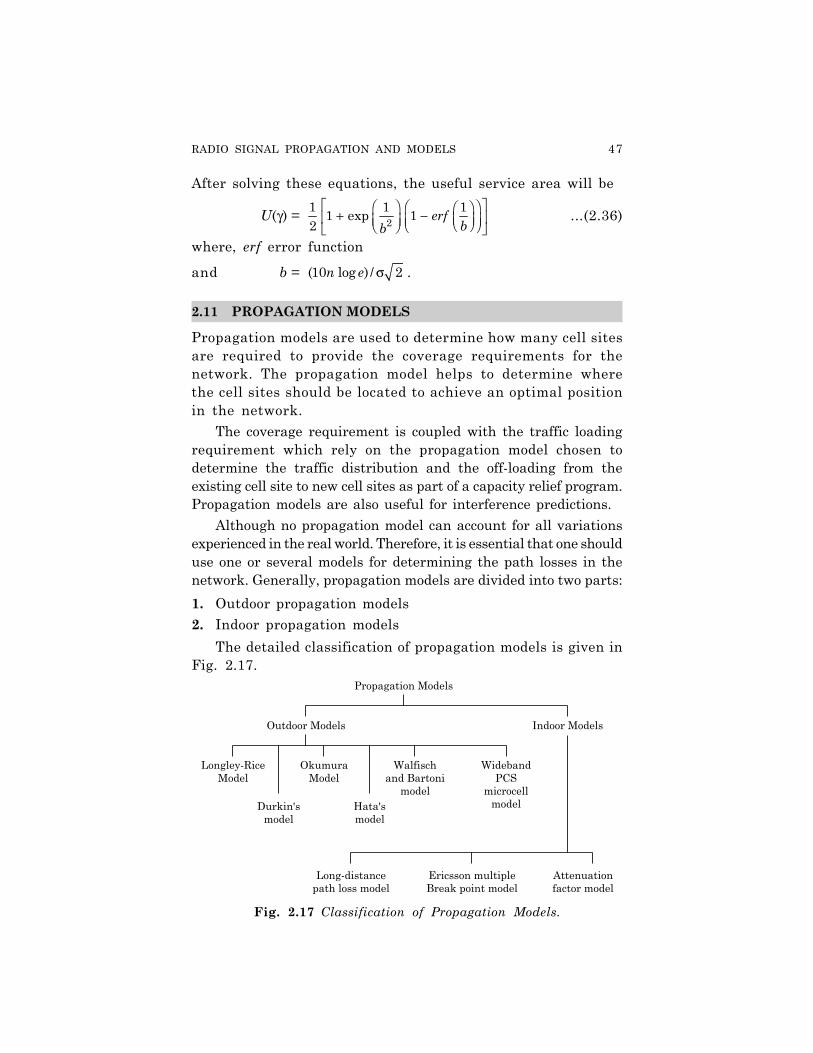
The detailed classification of propagation models is given inFig. 2.17.

Fig. 2.17 Classification of Propagation Models.


2.12 OUTDOOR PROPAGATION MODELS

These models are related with the outside environment. Thesemodels aim to predict signal strength at a particular receivingpoint or in a specific local area (called a Sector). The irregularterrain like presence of trees, buildings and other obstacles generatepath loss thereby the signal strength fluctuates at different points.Most of these models are based on a systematic interpretation ofmeasurement data obtained in the service area. Some commonlyused models are given below :

2.12.1 Longley-Rice Model

• This model is also referred to as ITS irregular terrainmodel.

• It is applicable in the frequency range from 40 MHz to100 GHz over different kinds of terrain (means series ofobstacles like buildings mountains etc.)

• In this model, two-ray ground reflection model is used topredict the signal strength within the radio horizon.

• Fresnel-Kirchoff knife-edge model is used to estimatediffraction losses.

• This model operates in two models :1. When the terrain path profile detail is available then

the path specific parameters can be easily determinedand such a prediction is called as ‘Point-to-Point’Prediction.

2. When the terrain path profile detail is not availablethen some techniques are used to determine the pathspecific parameters and such a prediction is called on‘area made’ prediction.

• For a given transmission path, a lot of parameters areused to calculate the path losses (transmission losses),for e.g. polarization, ground conductivity, ground dielectricconstant, surface refractivity, effective radius of earth,antenna heights, transmission frequency, path lengthand climate etc.

2.12.2 Durkin’s Model

• This model was developed by Durkin and Edward.


• This model consists of a computer simulator, for predictingfield strength over irregular terrain.

• This was adopted by joint radio committee (JRC) in theU.K. for the estimation of mobile coverage area.

• The simulator predicts large-scale phenomena (i.e. pathloss) and the losses caused by obstacles in a radio path.

• The execution of path loss simulator consists two parts:1. The first part access the tropographic data base of a

proposed service area and reconstructs the groundprofile information.

2. The second part calculates the expected path loss alongthe radial.

• This model is very attractive because it can read in adigital elevation map and perform a site specific propagationcomputation on the elevation data.

• The main drawback of this model is that it can notaccurately predict propagation effects due to foliage,buildings etc. and it does not account for multipathpropagation (other than ground reflection).

2.12.3 Okumura’s Model

• This model is widely used for signal prediction in urbanareas.

• It is applicable in the frequency range from 150 MHz to1920 MHz.

• It can be used for distances from 1 km to 100 km fromtransmitter to receiver.

• It can be applied for base station antenna heights rangingfrom 30 meter to 1000 meter.

• To determine the path loss using Okumura’s model, theequation can be expressed as :

L50(dB) = LF + Amu( f, d) – G(hte) – G(hre) – GAREA

...(2.37)where, L50 = 50th percentile (i.e. median) value of

propagation path lossLF = Free space propagation loss

Amu = Median attenuation relative to free spaceG(hte) = Base station antenna height gain factorG(hre) = Mobile antenna height gain factor


• This model is completely based on measured data anddoes not provide any analytical explanation.

• This model is considered as best in terms of accuracy inpath loss prediction in cluttered environments.

• The main drawback of Okumura’s model is that it doesnot response sufficiently quick to rapid changes in radiopath profile or in terrain. Therefore, this model is goodin urban and suburban areas but not as good in ruralareas.

2.12.4 Hata’s Model

• Hata’s Model does not account for any of the path-specificcorrections used in Okumura’s model.

• Hata’s model is an experimental formulation of thegeographical path loss data provided by Okumura.

• This model is valid from 150 MHz to 1500 MHz.• Hata’s model is applicable in urban, suburban and open

areas.• This model is well suited for large cell mobile systems,

but not personal communication systems (PCS) whichhave cells of the order of 1 km radius.

• This model predicts the median path loss in three typesof environment: urban, suburban and rural areas. Themedian path loss in dB for these three environments aregiven by the equations

L50 = A + B log10d (dB) Urban ...(2.38)L50 = A + B log10d – C (dB) Suburban ...(2.39)L50 = A + B log10d – D (dB) Open ...(2.40)

where d is the range in kilometers from BS to MS. The parametersin these equations depend on the frequency of operation fc, theheight of transmitting station, hte and the height of the receivingstation, hre. These parameters are given by the empirical formulas

A = 69.55 + 26.16 log10fc – 13.82 log10hte – a(hre)B = 44.9 – 6.55 log10hte

C = 5.4 + 2[log10(fc/28)]2

D = 40.94 + 4.78(log10 fc)2 – 18.33 log10 fc


where fc is measured in MHz, hte and hre are in meters anda(hre) is a correction factor for mobile antenna height. This modelis valid for the following ranges–

fc ⇒ 150 MHz – 1000 MHzhte ⇒ 30 m – 200 mhre ⇒ 1 m – 10 m

d ⇒ 1 km – 20 km

Fig. 2.18 shows path loss predictions with Hata Model for30 m Base antenna and 1 m mobile antenna for a midsized city.

Fig. 2.18 Path loss predictions with Hata propagationmodel for a midsized city [Base antenna – 30 m,

Mobile antenna – 1 m]

2.12.5 Walfisch and Bertoni’s Model

• This model is a combination of experimental (empirical)and deteministic models for estimating the path loss inan urban environment over the frequency range of 800–2000 MHz.

• This model was used primarily for GSM systems and insome propagation models in the united states.

• This model contains three elements; free-space loss, roof-to-street diffraction and scatter loss, and multiscreen loss(i.e. diffraction and scatter loss from other structures).


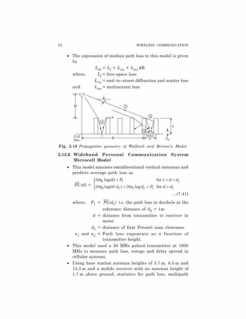
• The expression of median path loss in this model is givenby

L50 = Lf + Lrts + Lms dBwhere, Lf = free-space loss

Lrts = roof–to–street diffraction and scatter lossand Lms = multiscreen loss

Fig. 2.19 Propagation geometry of Walfisch and Bertoni’s Model.

2.12.6 Wideband Personal Communication SystemMicrocell Model

• This model assumes omnidirectional vertical antennas andpredicts average path loss as

( )PL d = η + < <

η + + >

1 1

2 1 1

10 log( ) for 110 log( / ) 10 log for

f

f f f

d P d d

d d n d P d d

...(7.41)

where, P1 = ( )oPL d i.e. the path loss in decibels at thereference distance of d0 = 1m

d = distance from transmitter to receiver inmeter

df = distance of first Fresnel zone clearancen1 and n2 = Path loss exponents as a function of

transmitter height.• This model used a 20 MHz pulsed transmitter at 1900

MHz to measure path loss, outage and delay spread incellular systems.

• Using base station antenna heights of 3.7 m, 8.5 m and13.3 m and a mobile receiver with an antenna height of1.7 m above ground, statistics for path loss, multipath


and coverage area were developed from extensivemeasurements in line-of-sight (LOS) and obstructedenvironment.

2.13 INDOOR PROPAGATION MODELS

These models characterize the radio propagation inside buildings.These are much different from the outdoor models because inindoor radio channels the distances covered are much smallerand the variations in environment is much greater.

Indoor propagation (Inside the building) is highly influencedby the building layout, the construction material used, etc. Againthe study of reflection, diffraction and scattering is quite importantfor indoor propagation models as was used for outdoor propagationmodels. Inside the building the signal strength may vary fromdoor to door as we so towards inner side of building. It alsodepends on whether the door is open or close.

Experimental studies have shown that the signal strengthreceived inside a building increases with height of a building.At the lower floors of a building, the urban cluster inducesgreater attenuation and thereby reduces the level of penetration.While on higher floors, the LOS path may exist, thus causinga stronger signal at the exterior wall of the building.

One major loss known as Partition loss that is due toinside partitions of a building. Partition may be of two types :1. Hard Partition : Which are formed as part of building

structure and not movable.2. Soft Partition : Which do not connected with the ceiling

and may be moved.Partition losses also occur between floors. These are based

on the external dimensions and materials of a building, numberof windows in a building etc.

In general, the indoor channels may be classified either asline–of–sight (LOS) or obstructed (OBS) with varying degree ofclutter. Given below are some key models used for indoor propagation.

2.13.1 Log-distance Path Loss Model

Indoor path loss obey the distance power law as given

PL(dB) = σ

+ +

00

( ) 10 log dPL d n X

d...(2.42)


where, n = depends on surroundings and building typeXσ = Normal random variable (dB) having a

standard deviation of σ dB.Table 2.3. Shows typical values of n and σ for various buildings.

Table 2.3 Path Loss Exponent and Standard Deviationmeasured in Different Buildings

Building Frequency (MHz) n σ(dB)

Retail Stores 914 2.2 8.7Grocery Store 914 1.8 5.2Office, hard partition 1500 3.0 7.0Office, soft partition 900 2.4 9.6Office, soft partition 1900 2.6 14.1Factory LOS

Textile/Chemical 1300 2.0 3.0Textile/Chemical 4000 2.1 7.0Paper/Cereals 1300 1.8 6.0Metalworking 1300 1.6 5.8Suburban Home

Indoor Street 900 3.0 7.0Factory OBS

Textile/Chemical 4000 2.1 9.7Metalworking 1300 3.3 6.8

2.13.2 Ericsson Multiple Breakpoint Model

• This model was obtained by measurements in a multi-floor office building.

• This model is divided into four breakpoints.• This model also assumes that there is 30dB attenuation

at reference distance d0 = 1m.• This model provides a deterministic limit on the range of

path loss at a particular distance.

2.13.3 Attenuation Factor Model

• It is an in building site specific propagation model thatincludes the effect of building type as well as the variationscaused by obstacles.


• This model is used to reduce the standard deviation betweenmeasured and predicted path loss nearly around 4dB.This was 13dB in case of log-distance model.

• The attenuation factor model is given by,

( )PL d =

+ + + ∑00

( ) 10 logSFd

PL d n FAF PAF dBd

...(2.43)

where nSF = Exponent value for the same floor.FAF = Floor attenuation factorPAF = Partition attenuation factor

• The FAF may be replaced by an exponent which alreadyconsiders the effects of multiple floor separation :

( )PL d = +

∑0

0( ) 10 logMF

dPL d n PAF dB

d...(2.44)

where, nMF represents the path loss exponent based onmeasurements through multiple floors.


SUMMARY

• The propagation of radio signals is categorized into threeranges, transmission, detection and interference range.

• In free space, the radio signals exhibit the samecharacteristics as light does.

• Signal faces some losses when propagate throughatmosphere.

• Shadowing is a form of attenuation of radio signals dueto large obstacles.

• Reflection occurs when the signal strike with an obstaclewhich dimension is large compared to the wavelength ofthe signal.

• Refraction occurs when signal travels through one mediumto other medium whose density is change than first medium.

• Scattering occurs when the dimension of the obstacle isin order of the wavelength of signal or less.

• Diffraction occurs when the radio wave strikes at anedge of the obstacle and propagated in different directions.

• The Fresnel zone defines the concept of diffraction lossas a function of path difference around an obstacle.

• The attenuation of power in the signal path is known aspath loss.

• Propagation models are used to determine the exact cellsite location, coverage, interference prediction, path lossexponent etc.

• Outdoor propagation model deals with external environmentwhile indoor propagation models are used inside buildings.

• The angle at which no reflection occurs in the medium oforigin is known as ‘Brewster Angle’, which is definedby

sin ( DB) = 1εε + ε1 2

• For a perfect conductor, the reflection coefficient paralleland perpendicular to the plane of incidence is:

and ⊥

ττ11 =1

= –1


REVIEW QUESTIONS

1. What are the different ranges of signals in propagationtheory?

2. Explain the following in brief :(a) Reflection(b) Diffraction(c) Scattering(d) Shadowing(e) Refraction

3. How reflection depends on the medium? Explain reflectionfrom perfect conductors.

4. Explain Radar cross section model of scattering.5. What do you understand by Fresnel Zone geometry?6. Explain knife-edge diffraction model in detail.7. What do you mean by the term ‘Path loss’?8. Explain the log distance path loss model in practical link

budget design.9. What are the purposes for which propagation models are

used in wireless communication? Explain the basic differencebetween outdoor and indoor propagation models.

10. Explain Hata’s outdoor propagation models and find themedian path loss for urban, suburban and rural areas.

11. What do you understand by partition losses in indoorpropagation models? Explain attenuation factor model indetail.

Radio Signal Propagation and Models

Documents