Free Space Radio Wave Propagation - iitg.ac.in · Chapter 4 Free Space Radio Wave Propagation 4.1 Introduction There are two basic ways of transmitting an electro-magnetic (EM) signal,

Chapter 4

Free Space Radio Wave

Propagation

4.1 Introduction

There are two basic ways of transmitting an electro-magnetic (EM) signal, through a

guided medium or through an unguided medium. Guided mediums such as coaxial

cables and fiber optic cables, are far less hostile toward the information carrying

EM signal than the wireless or the unguided medium. It presents challenges and

conditions which are unique for this kind of transmissions. A signal, as it travels

through the wireless channel, undergoes many kinds of propagation effects such as

reflection, diffraction and scattering, due to the presence of buildings, mountains and

other such obstructions. Reflection occurs when the EM waves impinge on objects

which are much greater than the wavelength of the traveling wave. Diffraction

is a phenomena occurring when the wave interacts with a surface having sharp

irregularities. Scattering occurs when the medium through the wave is traveling

contains objects which are much smaller than the wavelength of the EM wave.

These varied phenomena’s lead to large scale and small scale propagation losses. Due

to the inherent randomness associated with such channels they are best described

with the help of statistical models. Models which predict the mean signal strength

for arbitrary transmitter receiver distances are termed as large scale propagation

models. These are termed so because they predict the average signal strength for

large Tx-Rx separations, typically for hundreds of kilometers.

54

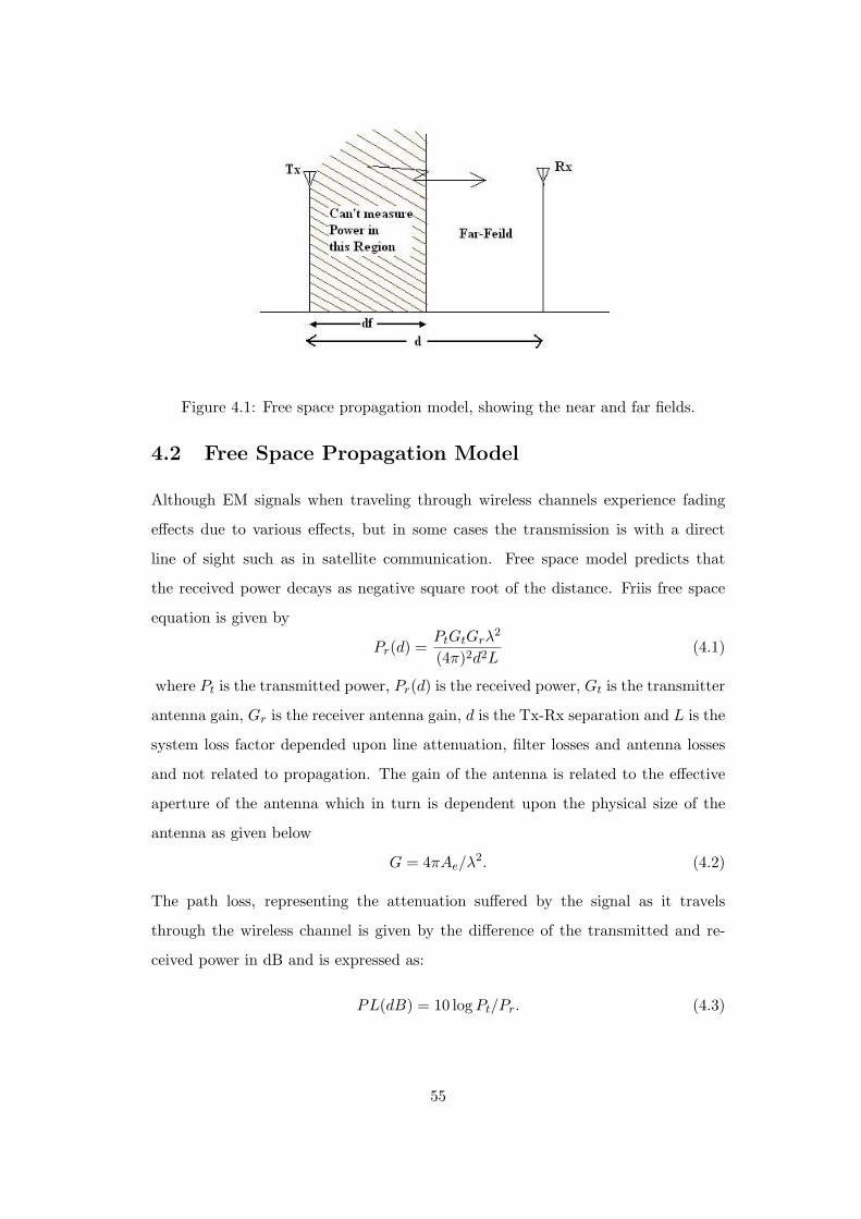
Figure 4.1: Free space propagation model, showing the near and far fields.

4.2 Free Space Propagation Model

Although EM signals when traveling through wireless channels experience fading

effects due to various effects, but in some cases the transmission is with a direct

line of sight such as in satellite communication. Free space model predicts that

the received power decays as negative square root of the distance. Friis free space

equation is given by

Pr(d) =PtGtGrλ

2

(4π)2d2L(4.1)

where Pt is the transmitted power, Pr(d) is the received power, Gt is the transmitter

antenna gain, Gr is the receiver antenna gain, d is the Tx-Rx separation and L is the

system loss factor depended upon line attenuation, filter losses and antenna losses

and not related to propagation. The gain of the antenna is related to the effective

aperture of the antenna which in turn is dependent upon the physical size of the

antenna as given below

G = 4πAe/λ2. (4.2)

The path loss, representing the attenuation suffered by the signal as it travels

through the wireless channel is given by the difference of the transmitted and re-

ceived power in dB and is expressed as:

PL(dB) = 10 log Pt/Pr. (4.3)

55

The fields of an antenna can broadly be classified in two regions, the far field and

the near field. It is in the far field that the propagating waves act as plane waves

and the power decays inversely with distance. The far field region is also termed

as Fraunhofer region and the Friis equation holds in this region. Hence, the Friis

equation is used only beyond the far field distance, df , which is dependent upon the

largest dimension of the antenna as

df = 2D2/λ. (4.4)

Also we can see that the Friis equation is not defined for d=0. For this reason, we

use a close in distance, do, as a reference point. The power received, Pr(d), is then

given by:

Pr(d) = Pr(do)(do/d)2. (4.5)

Ex. 1: Find the far field distance for a circular antenna with maximum dimension

of 1 m and operating frequency of 900 MHz.

Solution: Since the operating frequency f = 900 Mhz, the wavelength

λ =3 × 108m/s

900 × 106Hzm

. Thus, with the largest dimension of the antenna, D=1m, the far field distance is

df =2D2

λ=

2(1)2

0.33= 6m

.

Ex. 2: A unit gain antenna with a maximum dimension of 1 m produces 50 W

power at 900 MHz. Find (i) the transmit power in dBm and dB, (ii) the received

power at a free space distance of 5 m and 100 m.

Solution:

(i) Tx power = 10log(50) = 17 dB = (17+30) dBm = 47 dBm

(ii) df = 2×D2

λ = 2×12

1/3 = 6m

Thus the received power at 5 m can not be calculated using free space distance

formula.

At 100 m ,

PR =PT GT GRλ2

4πd2

=50 × 1 × (1/3)2

4π1002

56

= 3.5 × 10−3mW

PR(dBm) = 10logPr(mW ) = −24.5dBm

4.3 Basic Methods of Propagation

Reflection, diffraction and scattering are the three fundamental phenomena that

cause signal propagation in a mobile communication system, apart from LoS com-

munication. The most important parameter, predicted by propagation models based

on above three phenomena, is the received power. The physics of the above phe-

nomena may also be used to describe small scale fading and multipath propagation.

The following subsections give an outline of these phenomena.

4.3.1 Reflection

Reflection occurs when an electromagnetic wave falls on an object, which has very

large dimensions as compared to the wavelength of the propagating wave. For ex-

ample, such objects can be the earth, buildings and walls. When a radio wave falls

on another medium having different electrical properties, a part of it is transmitted

into it, while some energy is reflected back. Let us see some special cases. If the

medium on which the e.m. wave is incident is a dielectric, some energy is reflected

back and some energy is transmitted. If the medium is a perfect conductor, all

energy is reflected back to the first medium. The amount of energy that is reflected

back depends on the polarization of the e.m. wave.

Another particular case of interest arises in parallel polarization, when no re-

flection occurs in the medium of origin. This would occur, when the incident angle

would be such that the reflection coefficient is equal to zero. This angle is the

Brewster’s angle. By applying laws of electro-magnetics, it is found to be

sin(θB) =√

ε1

ε1 + ε2. (4.6)

Further, considering perfect conductors, the electric field inside the conductor is

always zero. Hence all energy is reflected back. Boundary conditions require that

θi = θr (4.7)

and

Ei = Er (4.8)

57

for vertical polarization, and

Ei = −Er (4.9)

for horizontal polarization.

4.3.2 Diffraction

Diffraction is the phenomenon due to which an EM wave can propagate beyond the

horizon, around the curved earth’s surface and obstructions like tall buildings. As

the user moves deeper into the shadowed region, the received field strength decreases.

But the diffraction field still exists an it has enough strength to yield a good signal.

This phenomenon can be explained by the Huygen’s principle, according to

which, every point on a wavefront acts as point sources for the production of sec-

ondary wavelets, and they combine to produce a new wavefront in the direction of

propagation. The propagation of secondary wavelets in the shadowed region results

in diffraction. The field in the shadowed region is the vector sum of the electric field

components of all the secondary wavelets that are received by the receiver.

4.3.3 Scattering

The actual received power at the receiver is somewhat stronger than claimed by the

models of reflection and diffraction. The cause is that the trees, buildings and lamp-

posts scatter energy in all directions. This provides extra energy at the receiver.

Roughness is tested by a Rayleigh criterion, which defines a critical height hc of

surface protuberances for a given angle of incidence θi, given by,

hc =λ

8sinθi. (4.10)

A surface is smooth if its minimum to maximum protuberance h is less than hc,

and rough if protuberance is greater than hc. In case of rough surfaces, the surface

reflection coefficient needs to be multiplied by a scattering loss factor ρS , given by

ρS = exp(−8(πσhsinθi

λ)2) (4.11)

where σh is the standard deviation of the Gaussian random variable h. The following

result is a better approximation to the observed value

ρS = exp(−8(πσhsinθi

λ)2)I0[−8(

πσhsinθi

λ)2] (4.12)

58

Figure 4.2: Two-ray reflection model.

which agrees very well for large walls made of limestone. The equivalent reflection

coefficient is given by,

Γrough = ρSΓ. (4.13)

4.4 Two Ray Reflection Model

Interaction of EM waves with materials having different electrical properties than

the material through which the wave is traveling leads to transmitting of energy

through the medium and reflection of energy back in the medium of propagation.

The amount of energy reflected to the amount of energy incidented is represented

by Fresnel reflection coefficient Γ, which depends upon the wave polarization, angle

of incidence and frequency of the wave. For example, as the EM waves can not pass

through conductors, all the energy is reflected back with angle of incidence equal to

the angle of reflection and reflection coefficient Γ = −1. In general, for parallel and

perpendicular polarizations, Γ is given by:

Γ|| = Er/Ei = η2 sin θt − η1 sin θi/η2 sin θt + η1 sin θi (4.14)

59

Γ⊥ = Er/Ei = η2 sin θi − η1 sin θt/η2 sin θi + η1 sin θt. (4.15)

Seldom in communication systems we encounter channels with only LOS paths and

hence the Friis formula is not a very accurate description of the communication link.

A two-ray model, which consists of two overlapping waves at the receiver, one direct

path and one reflected wave from the ground gives a more accurate description as

shown in Figure 4.2. A simple addition of a single reflected wave shows that power

varies inversely with the forth power of the distance between the Tx and the Rx.

This is deduced via the following treatment. From Figure 4.2, the total transmitted

and received electric fields are

ETOTT = Ei + ELOS , (4.16)

ETOTR = Eg + ELOS . (4.17)

Let E0 is the free space electric field (in V/m) at a reference distance d0. Then

E(d, t) =E0d0

dcos(ωct − φ) (4.18)

where

φ = ωcd

c(4.19)

and d > d0. The envelop of the electric field at d meters from the transmitter at

any time t is therefore

|E(d, t)| =E0d0

d. (4.20)

This means the envelop is constant with respect to time.

Two propagating waves arrive at the receiver, one LOS wave which travels a

distance of d′and another ground reflected wave, that travels d

′′. Mathematically,

it can be expressed as:

E(d′, t) =

E0d0

d′ cos(ωct − φ′) (4.21)

where

φ′= ωc

d′

c(4.22)

and

E(d′′, t) =

E0d0

d′′ cos(ωct − φ′′) (4.23)

where

φ′′

= ωcd′′

c. (4.24)

60

Figure 4.3: Phasor diagram of electric

fields.

Figure 4.4: Equivalent phasor diagram of

Figure 4.3.

According to the law of reflection in a dielectric, θi = θ0 and Eg = ΓEi which means

the total electric field,

Et = Ei + Eg = Ei(1 + Γ). (4.25)

For small values of θi, reflected wave is equal in magnitude and 180o out of phase

with respect to incident wave. Assuming perfect horizontal electric field polarization,

i.e.,

Γ⊥ = −1 =⇒ Et = (1 − 1)Ei = 0, (4.26)

the resultant electric field is the vector sum of ELOS and Eg. This implies that,

ETOTR = |ELOS + Eg|. (4.27)

It can be therefore written that

ETOTR (d, t) =

E0d0

d′ cos(ωct − φ′) + (−1)

E0d0

d′′ cos(ωct − φ′′) (4.28)

In such cases, the path difference is

∆ = d′′ − d

′=

√(ht + hr)2 + d2 −

√(ht − hr)2 + d2. (4.29)

However, when T-R separation distance is very large compared to (ht + hr), then

∆ ≈ 2hthr

d(4.30)

Ex 3: Prove the above two equations, i.e., equation (4.29) and (4.30).Once the path difference is known, the phase difference is

θ∆ =2π∆

λ=

∆ωc

λ(4.31)

61

and the time difference,

τd =∆c

=θ∆

2πfc. (4.32)

When d is very large, then ∆ becomes very small and therefore ELOS and Eg are

virtually identical with only phase difference,i.e.,

|E0d0

d| ≈ |E0d0

d′ | ≈ |E0d0

d′′ |. (4.33)

Say, we want to evaluate the received E-field at any t = d′′

c . Then,

ETOTR (d, t =

d′′

c) =

E0d0

d′ cos(ωcd′′

c− ωc

d′

c) − E0d0

d′′ cos(ωcd′′

c− ωc

d′′

c) (4.34)

=E0d0

d′ cos(∆ωc

c) − E0d0

d′′ cos(0o) (4.35)

=E0d0

d′ � θ∆ − E0d0

d′′ (4.36)

≈ E0d0

d(� θ∆ − 1). (4.37)

Using phasor diagram concept for vector addition as shown in Figures 4.3 and 4.4,

we get

|ETOTR (d)| =

√(E0d0

d+

E0d0

dcos(θ∆))2 + (

E0d0

dsin(θ∆))2 (4.38)

=E0d0

d

√(cos(θ∆) − 1)2 + sin2(θ∆) (4.39)

=E0d0

d

√2 − 2cosθ∆ (4.40)

= 2E0d0

dsin(

θ∆

2). (4.41)

For θ∆2 < 0.5rad, sin( θ∆

2 ) ≈ θ∆2 . Using equation (4.31) and further equation (4.30),

we can then approximate that

sin(θ∆

2) ≈ π

λ∆ =

2πhthr

λd< 0.5rad. (4.42)

This raises the wonderful concept of ‘cross-over distance’ dc, defined as

d > dc =20πhthr

5λ=

4πhthr

λ. (4.43)

The corresponding approximate received electric field is

ETOTR (d) ≈ 2

E0d0

d

2πhthr

λd= k

hthr

d2. (4.44)

62

Therefore, using equation (4.43) in (4.1), we get the received power as

Pr =PtGtGrh

2t h

2r

Ld4. (4.45)

The cross-over distance shows an approximation of the distance after which the

received power decays with its fourth order. The basic difference between equation

(4.1) and (4.45) is that when d < dc, equation (4.1) is sufficient to calculate the

path loss since the two-ray model does not give a good result for a short distance

due to the oscillation caused by the constructive and destructive combination of the

two rays, but whenever we distance crosses the ‘cross-over distance’, the power falls

off rapidly as well as two-ray model approximation gives better result than Friis

equation.

Observations on Equation (4.45): The important observations from this

equation are:

1. This equation gives fair results when the T-R separation distance crosses the

cross-over distance.

1. In that case, the power decays as the fourth power of distance

Pr(d) =K

d4, (4.46)

with K being a constant.

2. Path loss is independent of frequency (wavelength).

3. Received power is also proportional to h2t and h2

r , meaning, if height of any of the

antennas is increased, received power increases.

4.5 Diffraction

Diffraction is the phenomena that explains the digression of a wave from a straight

line path, under the influence of an obstacle, so as to propagate behind the obstacle.

It is an inherent feature of a wave be it longitudinal or transverse. For e.g the

sound can be heard in a room, where the source of the sound is another room

without having any line of sight. The similar phenomena occurs for light also but

the diffracted light intensity is not noticeable. This is because the obstacle or slit

need to be of the order of the wavelength of the wave to have a significant effect.

Thus radiation from a point source radiating in all directions can be received at any

63

Figure 4.5: Huygen’s secondary wavelets.

point, even behind an obstacle (unless it is not completely enveloped by it), as shown

in Figure 4.5. Though the intensity received gets smaller as receiver is moved into the

shadowed region. Diffraction is explained by Huygens-Fresnel principle which states

that all points on a wavefront can be considered as the point source for secondary

wavelets which form the secondary wavefront in the direction of the prorogation.

Normally, in absence of an obstacle, the sum of all wave sources is zero at a point

not in the direct path of the wave and thus the wave travels in the straight line. But

in the case of an obstacle, the effect of wave source behind the obstacle cannot be

felt and the sources around the obstacle contribute to the secondary wavelets in the

shadowed region, leading to bending of wave. In mobile communication, this has a

great advantage since, by diffraction (and scattering, reflection), the receiver is able

to receive the signal even when not in line of sight of the transmitter. This we show

in the subsection given below.

4.5.1 Knife-Edge Diffraction Geometry

As shown in Figure 4.6, consider that there’s an impenetrable obstruction of hight

h at a distance of d1 from the transmitter and d2 from the receiver. The path

difference between direct path and the diffracted path is

δ =√

d21 + h2 +

√d2

2 + h2 − (d1 + d2) (4.47)

64

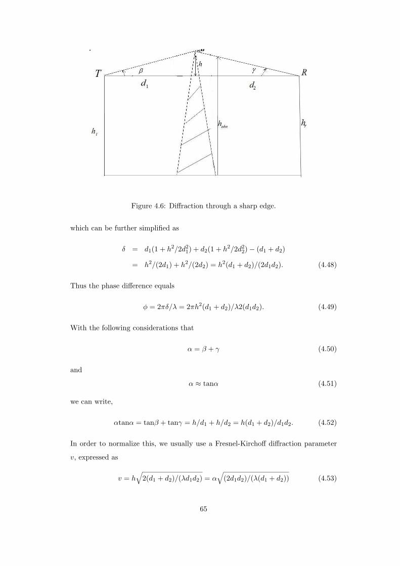
Figure 4.6: Diffraction through a sharp edge.

which can be further simplified as

δ = d1(1 + h2/2d21) + d2(1 + h2/2d2

2) − (d1 + d2)

= h2/(2d1) + h2/(2d2) = h2(d1 + d2)/(2d1d2). (4.48)

Thus the phase difference equals

φ = 2πδ/λ = 2πh2(d1 + d2)/λ2(d1d2). (4.49)

With the following considerations that

α = β + γ (4.50)

and

α ≈ tanα (4.51)

we can write,

αtanα = tanβ + tanγ = h/d1 + h/d2 = h(d1 + d2)/d1d2. (4.52)

In order to normalize this, we usually use a Fresnel-Kirchoff diffraction parameter

v, expressed as

v = h√

2(d1 + d2)/(λd1d2) = α√

(2d1d2)/(λ(d1 + d2)) (4.53)

65

Figure 4.7: Fresnel zones.

and therefore the phase difference becomes

φ = πv2/2. (4.54)

From this, we can observe that: (i) phase difference is a function of the height of

the obstruction, and also, (ii) phase difference is a function of the position of the

obstruction from transmitter and receiver.

4.5.2 Fresnel Zones: the Concept of Diffraction Loss

As mentioned before, the more is the object in the shadowed region greater is the

diffraction loss of the signal. The effect of diffraction loss is explained by Fresnel

zones as a function of the path difference. The successive Fresnel zones are limited

by the circular periphery through which the path difference of the secondary waves

is nλ/2 greater than total length of the LOS path, as shown in Figure 4.7. Thus

successive Fresnel zones have phase difference of π which means they alternatively

66

provide constructive and destructive interference to the received the signal. The

radius of the each Fresnel zone is maximum at middle of transmitter and receiver

(i.e. when d1 = d2 ) and decreases as moved to either side. It is seen that the loci

of a Fresnel zone varied over d1 and d2 forms an ellipsoid with the transmitter and

receiver at its focii. Now, if there’s no obstruction, then all Fresnel zones result in

only the direct LOS prorogation and no diffraction effects are observed. But if an

obstruction is present, depending on its geometry, it obstructs contribution from

some of the secondary wavelets, resulting in diffraction and also the loss of energy,

which is the vector sum of energy from unobstructed sources. please note that height

of the obstruction can be positive zero and negative also. The diffraction losses are

minimum as long as obstruction doesn’t block volume of the 1st Fresnel zone. As a

rule of thumb, diffraction effects are negligible beyond 55% of 1st Fresnel zone.

Ex 4: Calculate the first Fresnel zone obstruction height maximum for f = 800

MHz.

Solution:

λ =c

f=

3 × 108

8 × 102 × 106=

38m

H =√

λ(d1+d2)d1+d2

H1 =

√38250×250

500 = 6.89m

Thus H1 = 10 + 6.89 = 16.89m

(b)

H2 =

√38 × 100 × 400

500= 10

√(0.3) = 5.48m

Thus

H2 = 10 + 5.6 = 15.48m

. To have good power strength, obstacle should be within the 60% of the first fresnel

zone.

Ex 5: Given f=900 MHz, d1 = d2 = 1 km, h = 25m, where symbols have usual

meaning. Compute the diffraction loss. Also find out in which Fresnel zone the tip

of the obstruction lies.

67

Figure 4.8: Knife-edge Diffraction Model

Given,

Gd(dB) = 20 log(0.5 − 0.62v) − 1 < v <= 0

Gd(dB) = 20 log(0.225/v) v > 2.24

Solution:

v = h

√2(d1 + d2)

λd1d2= 25

√2 × 2000

1310

= 2.74

Gd(dB) = 20 log(225v ) = −21.7dB

Since loss = -Gd (dB) = 21.7 dB

n =(2.74)2

2= 3.5

Thus n=4.

4.5.3 Knife-edge diffraction model

Knife-edge diffraction model is one of the simplest diffraction model to estimate the

diffraction loss. It considers the object like hill or mountain as a knife edge sharp

68

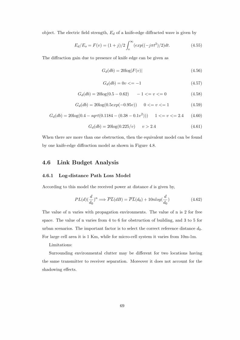
object. The electric field strength, Ed of a knife-edge diffracted wave is given by

Ed/Eo = F (v) = (1 + j)/2∫ ∞

v(exp((−jπt2)/2)dt. (4.55)

The diffraction gain due to presence of knife edge can be given as

Gd(db) = 20log|F (v)| (4.56)

Gd(db) = 0v <= −1 (4.57)

Gd(db) = 20log(0.5 − 0.62) − 1 <= v <= 0 (4.58)

Gd(db) = 20log(0.5exp(−0.95v)) 0 <= v <= 1 (4.59)

Gd(db) = 20log(0.4 − sqrt(0.1184 − (0.38 − 0.1v2))) 1 <= v <= 2.4 (4.60)

Gd(db) = 20log(0.225/v) v > 2.4 (4.61)

When there are more than one obstruction, then the equivalent model can be found

by one knife-edge diffraction model as shown in Figure 4.8.

4.6 Link Budget Analysis

4.6.1 Log-distance Path Loss Model

According to this model the received power at distance d is given by,

PL(d)(d

d0)n =⇒ PL(dB) = PL(d0) + 10nlog(

d

d0) (4.62)

The value of n varies with propagation environments. The value of n is 2 for free

space. The value of n varies from 4 to 6 for obstruction of building, and 3 to 5 for

urban scenarios. The important factor is to select the correct reference distance d0.

For large cell area it is 1 Km, while for micro-cell system it varies from 10m-1m.

Limitations:

Surrounding environmental clutter may be different for two locations having

the same transmitter to receiver separation. Moreover it does not account for the

shadowing effects.

69

4.6.2 Log Normal Shadowing

The equation for the log normal shadowing is given by,

PL(dB) = PL(dB) + Xσ = PL(d0) + 10nlog(d

d0) + Xσ (4.63)

where Xσ is a zero mean Gaussian distributed random variable in dB with standard

deviation σ also in dB. In practice n and σ values are computed from measured

data.

Average received power

The ‘Q’ function is given by,

Q(z) = 0.5(1 − erf(z√2)) (4.64)

and

Q(z) = 1 − Q(−z) (4.65)

So the probability that the received signal level (in dB) will exceed a certain value

γ is

P (Pd > γ) = Q(γ − Pr

σ). (4.66)

4.7 Outdoor Propagation Models

There are many empirical outdoor propagation models such as Longley-Rice model,

Durkin’s model, Okumura model, Hata model etc. Longley-Rice model is the most

commonly used model within a frequency band of 40 MHz to 100 GHz over different

terrains. Certain modifications over the rudimentary model like an extra urban

factor (UF) due to urban clutter near the reciever is also included in this model.

Below, we discuss some of the outdoor models, followed by a few indoor models too.

4.7.1 Okumura Model

The Okumura model is used for Urban Areas is a Radio propagation model that is

used for signal prediction.The frequency coverage of this model is in the range of

200 MHz to 1900 MHz and distances of 1 Km to 100 Km.It can be applicable for

base station effective antenna heights (ht) ranging from 30 m to 1000 m.

70

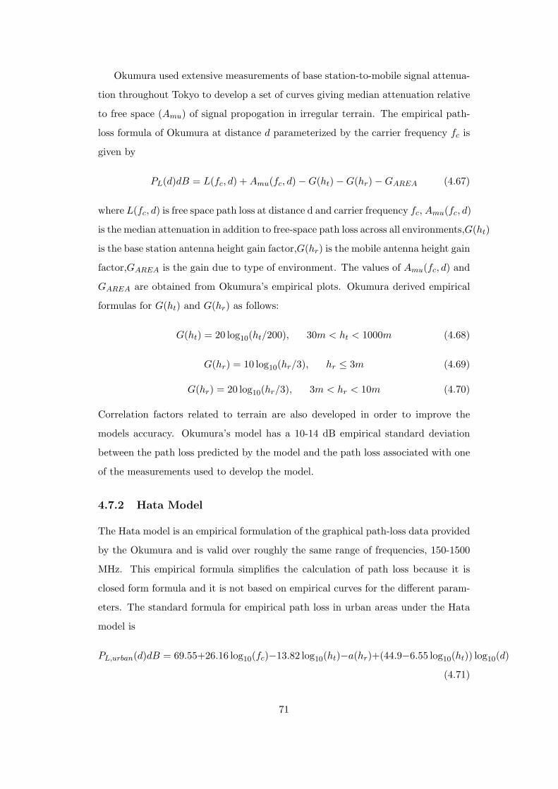
Okumura used extensive measurements of base station-to-mobile signal attenua-

tion throughout Tokyo to develop a set of curves giving median attenuation relative

to free space (Amu) of signal propogation in irregular terrain. The empirical path-

loss formula of Okumura at distance d parameterized by the carrier frequency fc is

given by

PL(d)dB = L(fc, d) + Amu(fc, d) − G(ht) − G(hr) − GAREA (4.67)

where L(fc, d) is free space path loss at distance d and carrier frequency fc, Amu(fc, d)

is the median attenuation in addition to free-space path loss across all environments,G(ht)

is the base station antenna height gain factor,G(hr) is the mobile antenna height gain

factor,GAREA is the gain due to type of environment. The values of Amu(fc, d) and

GAREA are obtained from Okumura’s empirical plots. Okumura derived empirical

formulas for G(ht) and G(hr) as follows:

G(ht) = 20 log10(ht/200), 30m < ht < 1000m (4.68)

G(hr) = 10 log10(hr/3), hr ≤ 3m (4.69)

G(hr) = 20 log10(hr/3), 3m < hr < 10m (4.70)

Correlation factors related to terrain are also developed in order to improve the

models accuracy. Okumura’s model has a 10-14 dB empirical standard deviation

between the path loss predicted by the model and the path loss associated with one

of the measurements used to develop the model.

4.7.2 Hata Model

The Hata model is an empirical formulation of the graphical path-loss data provided

by the Okumura and is valid over roughly the same range of frequencies, 150-1500

MHz. This empirical formula simplifies the calculation of path loss because it is

closed form formula and it is not based on empirical curves for the different param-

eters. The standard formula for empirical path loss in urban areas under the Hata

model is

PL,urban(d)dB = 69.55+26.16 log10(fc)−13.82 log10(ht)−a(hr)+(44.9−6.55 log10(ht)) log10(d)

(4.71)

71

The parameters in this model are same as in the Okumura model,and a(hr) is a

correction factor for the mobile antenna height based on the size of coverage area.For

small to medium sized cities this factor is given by

a(hr) = (1.11 log10(fc) − 0.7)hr − (1.56 log10(fc) − 0.8)dB

and for larger cities at a frequencies fc > 300 MHz by

a(hr) = 3.2(log10(11.75hr))2 − 4.97dB

else it is

a(hr) = 8.29(log10(1.54hr))2 − 1.1dB

Corrections to the urban model are made for the suburban, and is given by

PL,suburban(d)dB = PL,urban(d)dB − 2(log10(fc/28))2 − 5.4 (4.72)

Unlike the Okumura model,the Hata model does not provide for any specific path-

correlation factors. The Hata model well approximates the Okumura model for

distances d > 1 Km. Hence it is a good model for first generation cellular systems,

but it does not model propogation well in current cellular systems with smaller cell

sizes and higher frequencies. Indoor environments are also not captured by the Hata

model.

4.8 Indoor Propagation Models

The indoor radio channel differs from the traditional mobile radio channel in ways

- the distances covered are much smaller ,and the variability of the environment

is much greater for smaller range of Tx-Rx separation distances.Features such as

lay-out of the building,the construction materials,and the building type strongly in-

fluence the propagation within the building.Indoor radio propagation is dominated

by the same mechanisms as outdoor: reflection, diffraction and scattering with vari-

able conditions. In general,indoor channels may be classified as either line-of-sight

or obstructed.

4.8.1 Partition Losses Inside a Floor (Intra-floor)

The internal and external structure of a building formed by partitions and obstacles

vary widely.Partitions that are formed as a part of building structure are called

72

hard partitions , and partitions that may be moved and which do not span to

the ceiling are called soft partitions. Partitions vary widely in their physical and

electrical characteristics,making it difficult to apply general models to specific indoor

installations.

4.8.2 Partition Losses Between Floors (Inter-floor)

The losses between floors of a building are determined by the external dimensions

and materials of the building,as well as the type of construction used to create the

floors and the external surroundings. Even the number of windows in a building

and the presence of tinting can impact the loss between floors.

4.8.3 Log-distance Path Loss Model

It has been observed that indoor path loss obeys the distance power law given by

PL(dB) = PL(d0) + 10n log10(d/d0) + Xσ (4.73)

where n depends on the building and surrounding type, and Xσ represents a normal

random variable in dB having standard deviation of σ dB.

4.9 Summary

In this chapter, three principal propagation models have been identified: free-space

propagation, reflection and diffraction, which are common terrestrial models and

these mainly explains the large scale path loss. Regarding path-loss, one important

factor introduced in this chapter is log-distance path loss model. These, however,

may be insignificant when we consider the small-scale rapid path losses. This is

discussed in the next chapter.

4.10 References

1. T. S. Rappaport, Wireless Communications: Principles and Practice, 2nd ed.

Singapore: Pearson Education, Inc., 2002.

2. S. Haykin and M. Moher, Modern Wireless Communications. Singapore: Pear-

son Education, Inc., 2002.

73

3. J. W. Mark and W. Zhuang, Wireless Communications and Networking. New

Delhi: PHI, 2005.

74