OPSM 501: Operations Management Week 6: The Goal Koç University Graduate School of Business MBA Program Zeynep Aksin [email protected].

OPSM 501: Operations Management

Week 6:

The Goal

Koç University Graduate School of BusinessMBA Program

Zeynep [email protected]

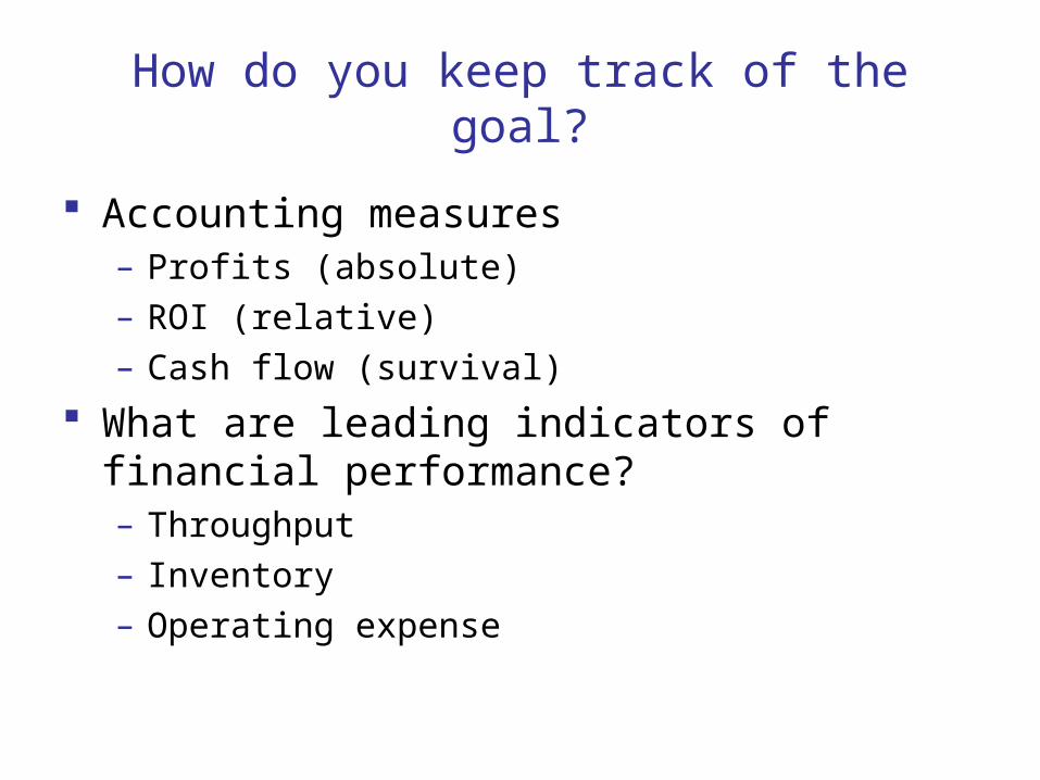
How do you keep track of the goal?

Accounting measures– Profits (absolute)– ROI (relative)– Cash flow (survival)

What are leading indicators of financial performance?– Throughput– Inventory– Operating expense

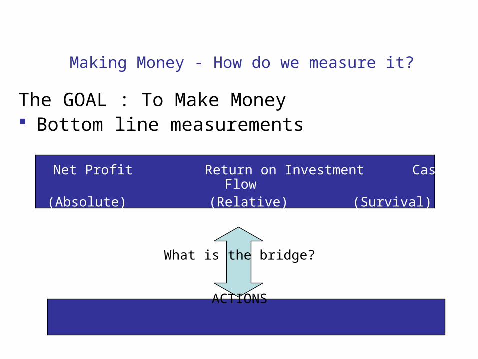
Making Money - How do we measure it?

The GOAL : To Make Money Bottom line measurements

Net Profit Return on Investment Cash Flow(Absolute) (Relative) (Survival)

What is the bridge?

ACTIONS

Use Global Operational Measures

Throughput (T)The rate at which the system generates money through sales

Inventory (I)All the money the system invests in purchasing things the system intends to sell

Operating expense (OE)All the money the system spends in turning inventory into throughput

The Direct Impact

Operational Measurements and the Bottom Line

Net Profit Return on Investment Cash Flow

Throughput Inventory Operating Expense

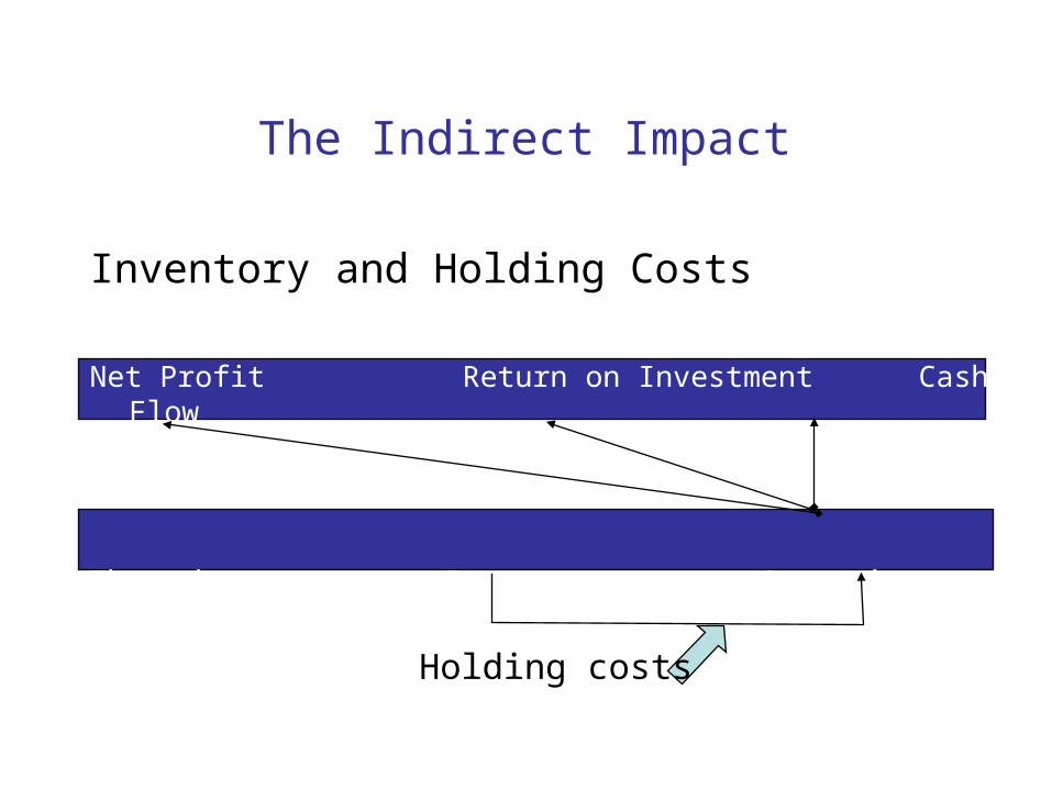
The Indirect Impact

Inventory and Holding Costs

Net Profit Return on Investment Cash Flow

Throughput Inventory Operating Expense

Holding costs

The Competitive Edge Impact

Net Profit Return on Investment Cash Flow

Throughput Inventory Operating Expense

Competitive edge

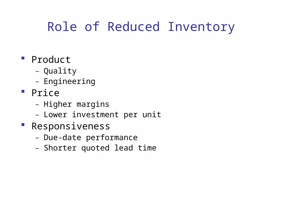
Role of Reduced Inventory

Product– Quality– Engineering

Price– Higher margins– Lower investment per unit

Responsiveness– Due-date performance– Shorter quoted lead time

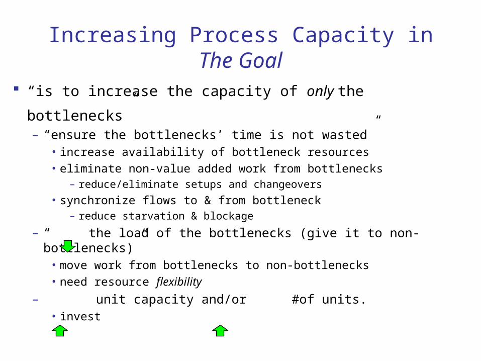
Increasing Process Capacity in The Goal “is to increase the capacity of only the bottlenecks”

– “ensure the bottlenecks’ time is not wasted”• increase availability of bottleneck resources• eliminate non-value added work from bottlenecks

– reduce/eliminate setups and changeovers

• synchronize flows to & from bottleneck– reduce starvation & blockage

– “ the load of the bottlenecks (give it to non-bottlenecks)”• move work from bottlenecks to non-bottlenecks• need resource flexibility

– unit capacity and/or #of units.• invest

Drum-Buffer-Rope

The drum is the constraint-sets the speed The buffer is a time buffer used to protect the

drum from disruptions in the preceding production steps

The rope is a schedule that dictates the timing of the release of raw materials, or jobs, into the system

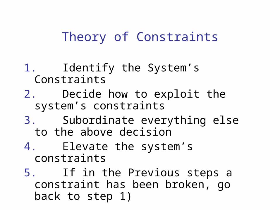
Theory of Constraints

1. Identify the System’s Constraints2.Decide how to exploit the system’s

constraints3.Subordinate everything else to the above

decision4.Elevate the system’s constraints5. If in the Previous steps a constraint has been

broken, go back to step 1)

Lessons from the Goal

Identify the goal: making money Making money requires clear operational measures Management systems (accounting, incentives, measurement) often

get in the way of good plant management There are typically only a few bottleneck resources: every other

resource should be subordinated to them Balance flow, not capacity Once you identify the bottleneck, you can elevate its capacity:

continuous improvement How do you protect the bottleneck?

– Effective scheduling (drum-buffer-rope)– Effective lot sizing (transfer versus order lotsize)

Work smarter, not harder

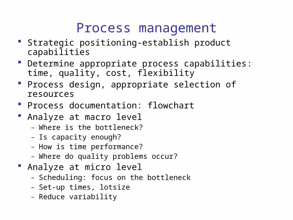
Process management Strategic positioning-establish product capabilities Determine appropriate process capabilities: time, quality,

cost, flexibility Process design, appropriate selection of resources Process documentation: flowchart Analyze at macro level

– Where is the bottleneck?– Is capacity enough?– How is time performance?– Where do quality problems occur?

Analyze at micro level– Scheduling: focus on the bottleneck– Set-up times, lotsize– Reduce variability

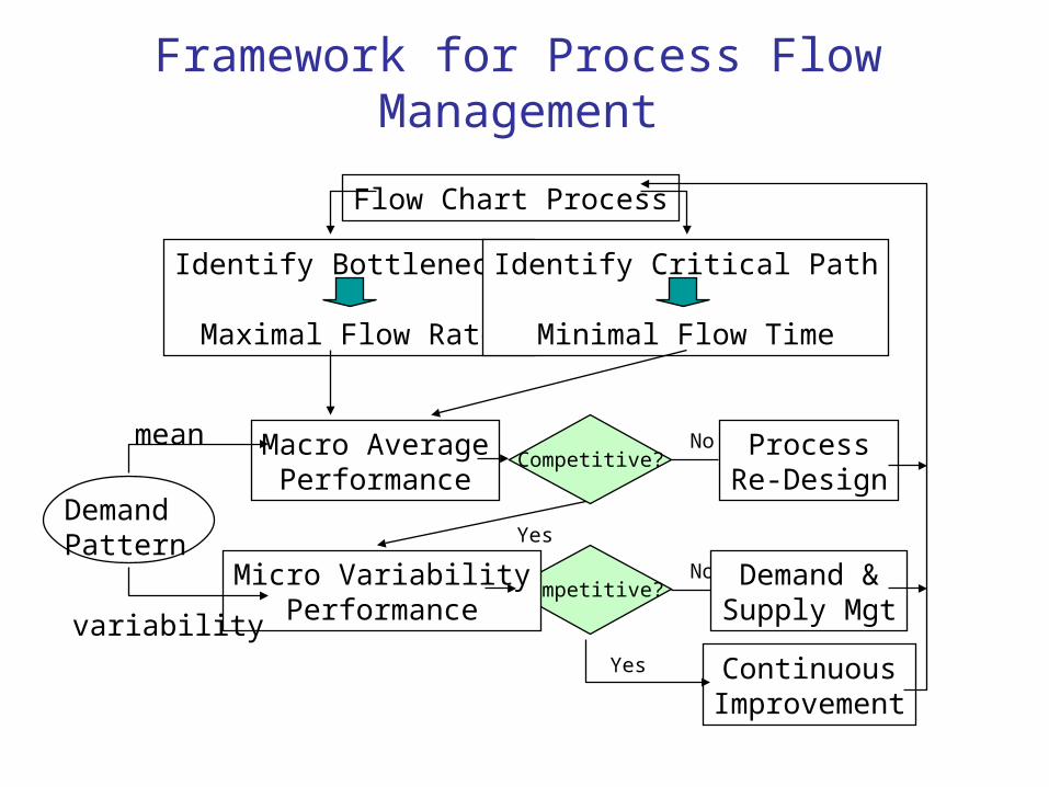
Framework for Process Flow Management

Competitive?No

Flow Chart Process

Identify Bottlenecks

Maximal Flow Rate

Identify Critical Path

Minimal Flow Time

DemandPattern

Macro AveragePerformance

ProcessRe-Design

Competitive?NoMicro Variability

PerformanceDemand &Supply Mgt

ContinuousImprovement

mean

variability

Yes

Yes

15

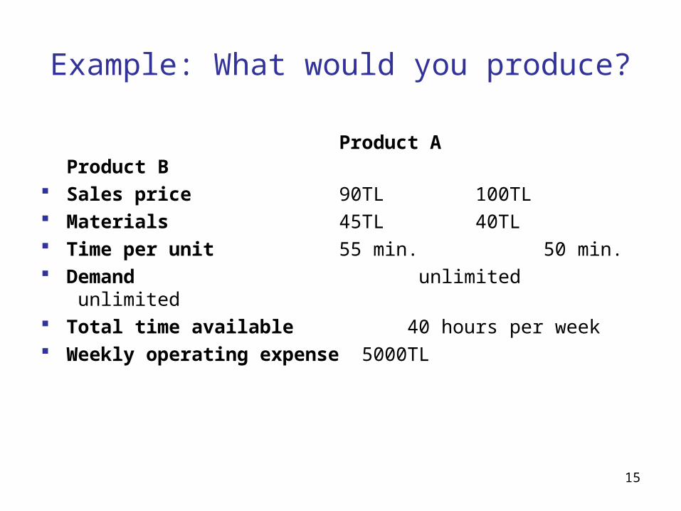
Example: What would you produce?

Product A Product B Sales price 90TL 100TL Materials 45TL 40TL Time per unit 55 min. 50 min. Demand unlimited unlimited Total time available 40 hours per week Weekly operating expense 5000TL

16

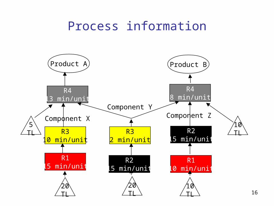
Process information

Product A Product B

R413 min/unit

R48 min/unit

R310 min/unit

R115 min/unit

R32 min/unit

R215 min/unit

R110 min/unit

R215 min/unit

5TL

10TL

20TL

20TL

10TL

Component X

Component YComponent Z

17

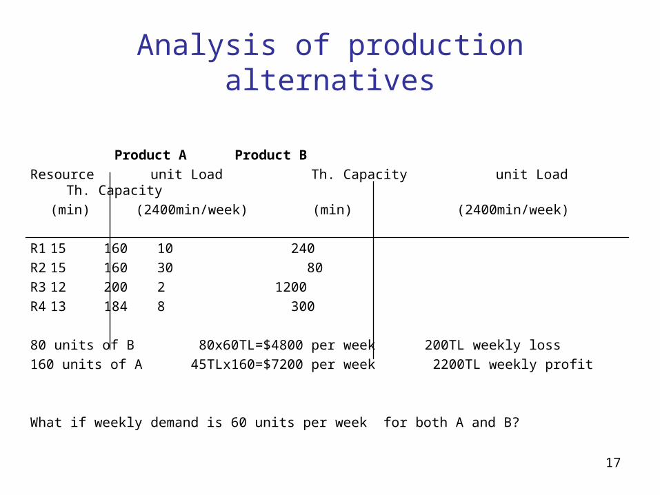
Analysis of production alternatives

Product A Product B

Resource unit Load Th. Capacity unit Load Th. Capacity

(min) (2400min/week) (min) (2400min/week)

R1 15 160 10 240

R2 15 160 30 80

R3 12 200 2 1200

R4 13 184 8 300

80 units of B 80x60TL=$4800 per week 200TL weekly loss

160 units of A 45TLx160=$7200 per week 2200TL weekly profit

What if weekly demand is 60 units per week for both A and B?

Recall the house game: an unbalanced line

if average task times are different, will have an unbalanced line• will have idleness

in unbalanced case, slowest task determines output rate• bottleneck is busy• idleness in other stages

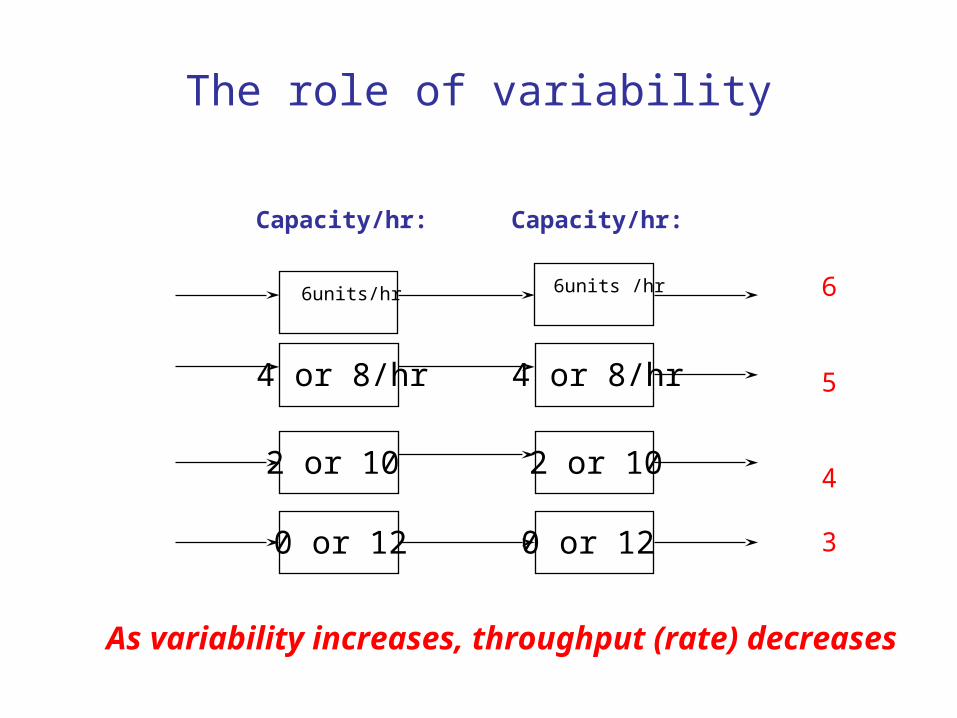
The role of variability

6units/hr 6units /hr

4 or 8/hr 4 or 8/hr

2 or 10 2 or 10

0 or 120 or 12

As variability increases, throughput (rate) decreases

Capacity/hr: Capacity/hr:

6

5

4

3

The role of task times: a balanced line

if task times are similar will have a balanced line

• in the absence of variability (deterministic) complete synchronization is possible

• in a balanced line idleness is minimized, though in the presence of variability full synchronization cannot be achieved

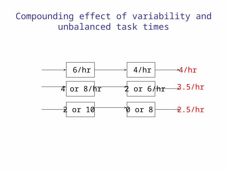
Compounding effect of variability and unbalanced task times

6/hr 4/hr

4 or 8/hr 2 or 6/hr

2 or 10 0 or 8

4/hr

3.5/hr

2.5/hr

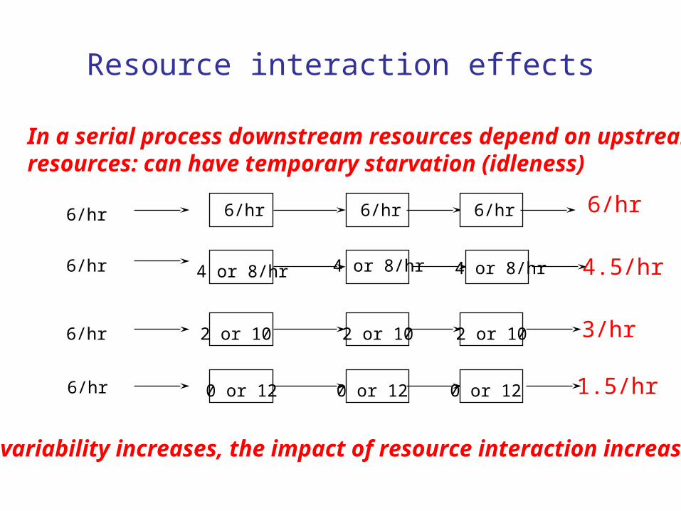
Resource interaction effects

6/hr 6/hr

4 or 8/hr 4 or 8/hr

2 or 10 2 or 10

0 or 120 or 12

6/hr

6/hr

6/hr

6/hr

6/hr

4 or 8/hr

2 or 10

0 or 12

6/hr

4.5/hr

3/hr

1.5/hr

In a serial process downstream resources depend on upstreamresources: can have temporary starvation (idleness)

As variability increases, the impact of resource interaction increases

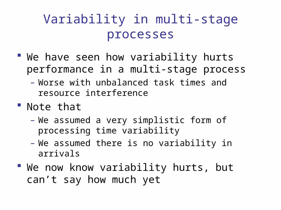
Variability in multi-stage processes

We have seen how variability hurts performance in a multi-stage process– Worse with unbalanced task times and resource

interference

Note that– We assumed a very simplistic form of processing time

variability– We assumed there is no variability in arrivals

We now know variability hurts, but can’t say how much yet

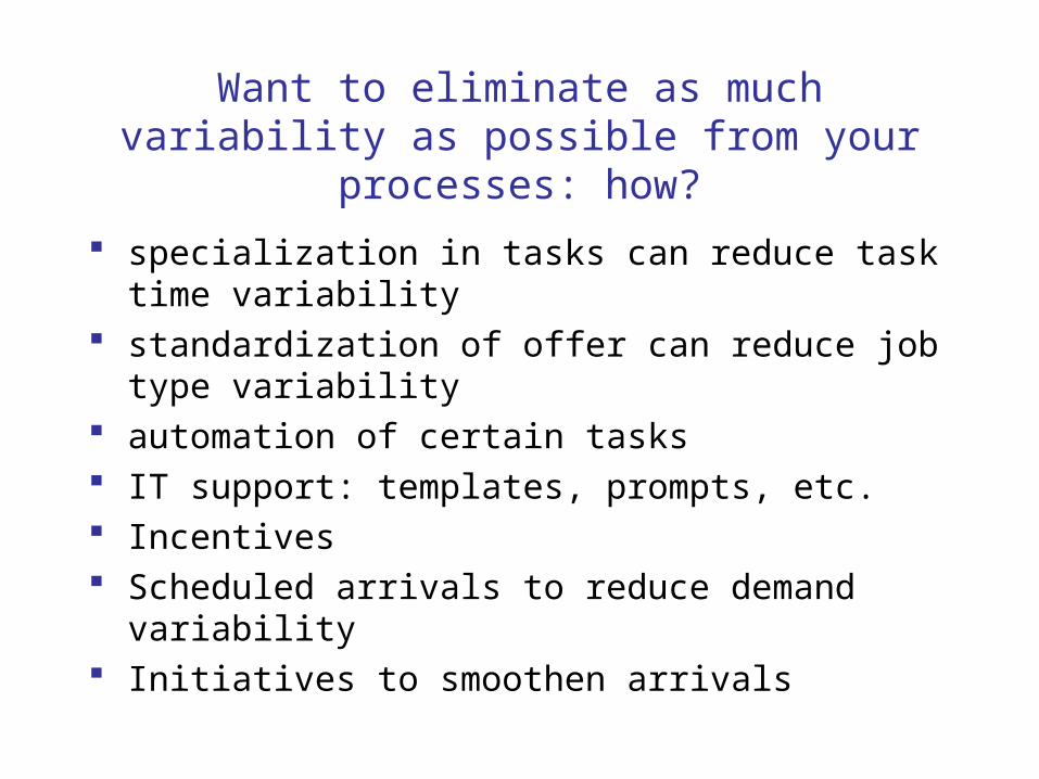
Want to eliminate as much variability as possible from your processes: how?

specialization in tasks can reduce task time variability standardization of offer can reduce job type variability automation of certain tasks IT support: templates, prompts, etc. Incentives Scheduled arrivals to reduce demand variability Initiatives to smoothen arrivals

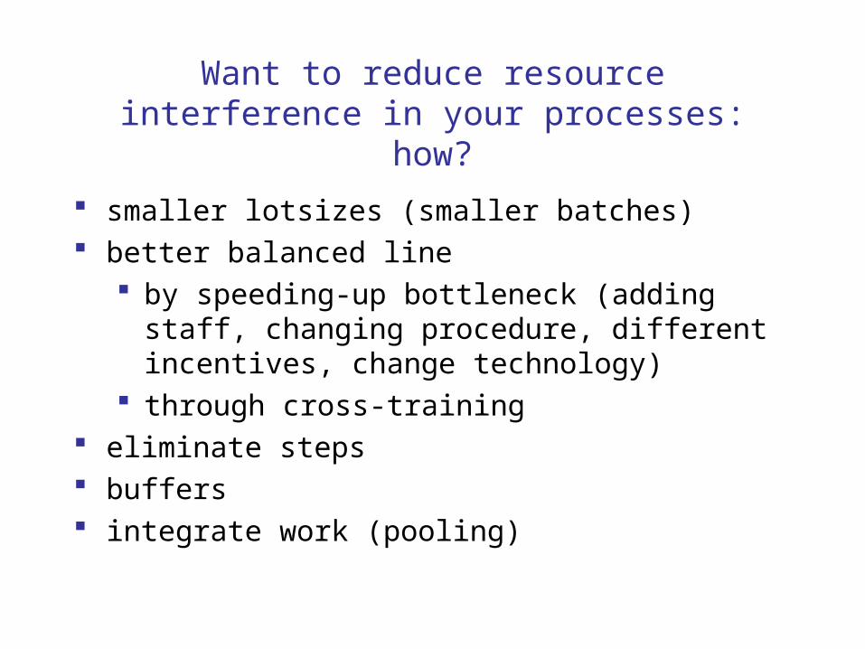
Want to reduce resource interference in your processes: how?

smaller lotsizes (smaller batches) better balanced line

by speeding-up bottleneck (adding staff, changing procedure, different incentives, change technology)

through cross-training eliminate steps buffers integrate work (pooling)

Flow Times with Arrival Every 4 Secs(Service time=5 seconds)

Customer Number

Arrival Time

Departure Time

Time in Process

1 0 5 5

2 4 10 6

3 8 15 7

4 12 20 8

5 16 25 9

6 20 30 10

7 24 35 11

8 28 40 12

9 32 45 13

10 36 50 14

0 10 20 30 40 50

Time

1

2

3

4

5

6

7

8

9

10

Cust

omer

Num

ber

What is the queue size? Can we apply Little’s Law?What is the capacity utilization?

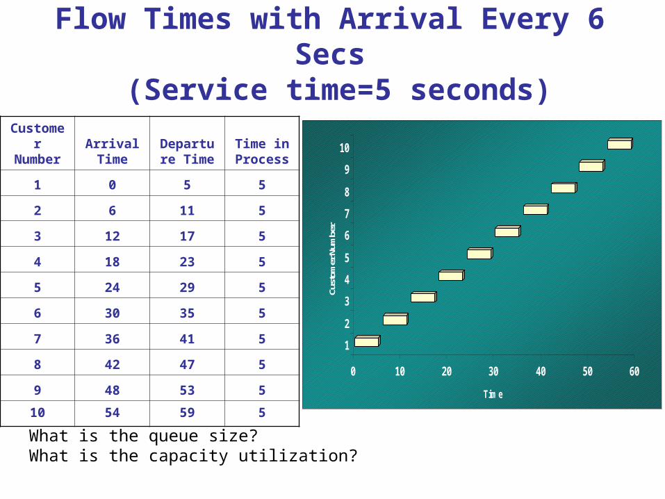
Customer Number

Arrival Time

Departure Time

Time in Process

1 0 5 5

2 6 11 5

3 12 17 5

4 18 23 5

5 24 29 5

6 30 35 5

7 36 41 5

8 42 47 5

9 48 53 5

10 54 59 5

0 10 20 30 40 50 60

Time

1

2

3

4

5

6

7

8

9

10

Cust

omer

Num

ber

Flow Times with Arrival Every 6 Secs (Service time=5 seconds)

What is the queue size?What is the capacity utilization?

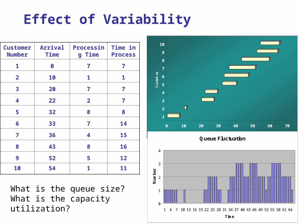
Customer Number

Arrival Time

Processing Time

Time in Process

1 0 7 7

2 10 1 1

3 20 7 7

4 22 2 7

5 32 8 8

6 33 7 14

7 36 4 15

8 43 8 16

9 52 5 12

10 54 1 11

0 10 20 30 40 50 60 70

Time

1

2

3

4

5

6

7

8

9

10

Cu

sto

mer

Queue Fluctuation

0

1

2

3

4

1 4 7 10 13 16 19 22 25 28 31 34 37 40 43 46 49 52 55 58 61 64

Time

Nu

mb

er

Effect of Variability

What is the queue size?What is the capacity utilization?

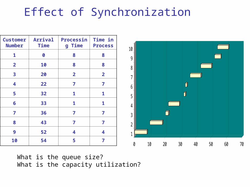
Customer Number

Arrival Time

Processing Time

Time in Process

1 0 8 8

2 10 8 8

3 20 2 2

4 22 7 7

5 32 1 1

6 33 1 1

7 36 7 7

8 43 7 7

9 52 4 4

10 54 5 7 0 10 20 30 40 50 60 70

1

2

3

4

5

6

7

8

9

10

Effect of Synchronization

What is the queue size?What is the capacity utilization?

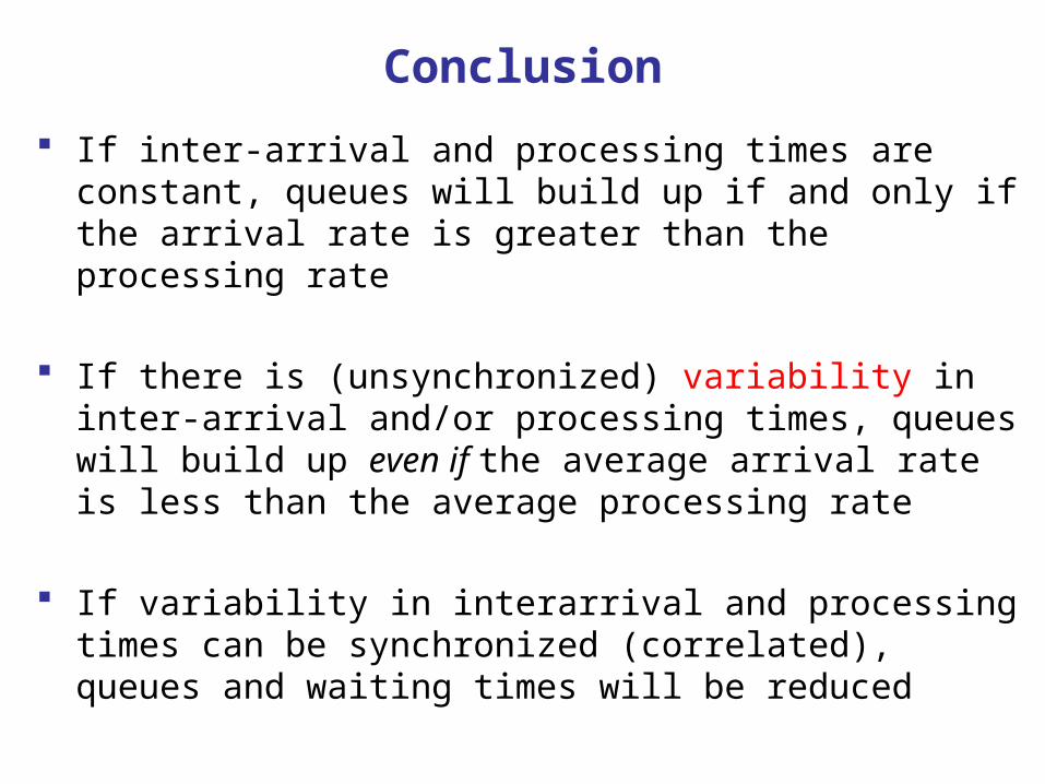
Conclusion

If inter-arrival and processing times are constant, queues will build up if and only if the arrival rate is greater than the processing rate

If there is (unsynchronized) variability in inter-arrival and/or processing times, queues will build up even if the average arrival rate is less than the average processing rate

If variability in interarrival and processing times can be synchronized (correlated), queues and waiting times will be reduced

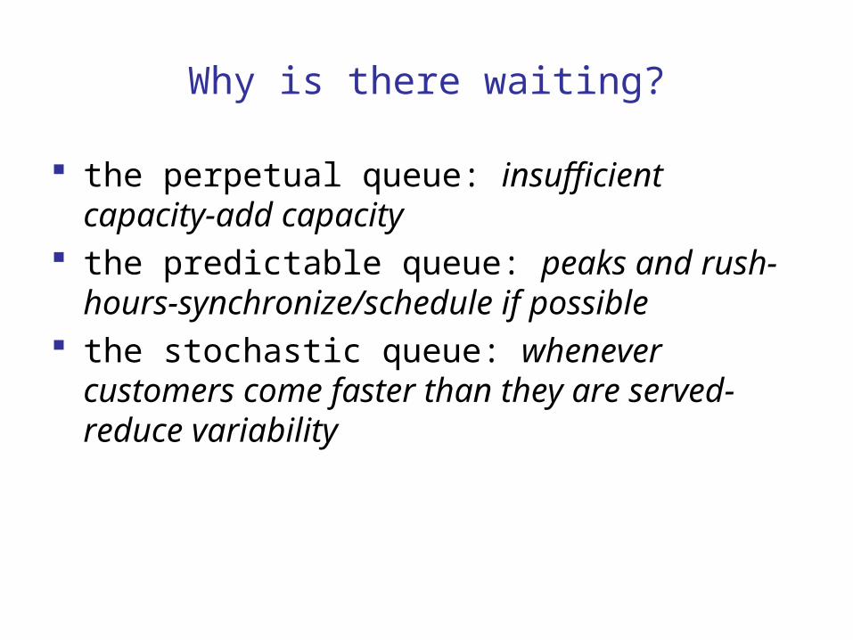
Why is there waiting?

the perpetual queue: insufficient capacity-add capacity

the predictable queue: peaks and rush-hours-synchronize/schedule if possible

the stochastic queue: whenever customers come faster than they are served-reduce variability

Components of the Queuing System Visually

Customers Customers come income in

Customers are Customers are servedserved

Customers Customers leaveleave

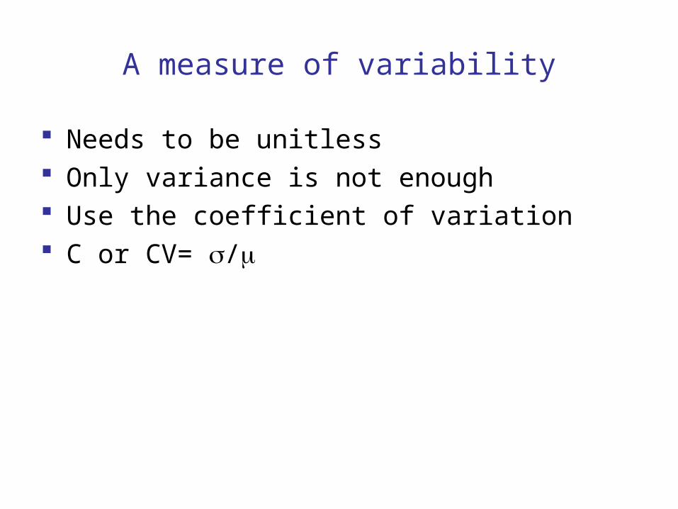
A measure of variability

Needs to be unitless Only variance is not enough Use the coefficient of variation C or CV= /

Interpreting the variability measures

Ci = coefficient of variation of interarrival times

i) constant or deterministic arrivals Ci = 0

ii) completely random or independent arrivals Ci =1

iii) scheduled or negatively correlated arrivals Ci < 1

iv) bursty or positively correlated arrivals Ci > 1

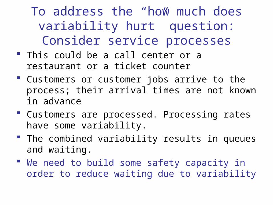
To address the “how much does variability hurt” question: Consider service processes

This could be a call center or a restaurant or a ticket counter

Customers or customer jobs arrive to the process; their arrival times are not known in advance

Customers are processed. Processing rates have some variability.

The combined variability results in queues and waiting. We need to build some safety capacity in order to reduce

waiting due to variability

Specifications of a Service Provider

ServiceProvider

Leaving Customers

Waiting Customers

Demand Pattern

Resources

• Human resources

• Information system

• other...

Arriving Customers

Satisfaction Measures

Reneges or abandonments

Waiting Pattern

Served Customers

Service Time

Upcoming events

Next week we will have an in-class activity, don’t miss class!

Midterm exam will be Week 10-proposed date November 26 Monday