Oligopsony With Fixed Market Supply - CiteSeerX

Utah State UniversityDigitalCommons@USU

Economic Research Institute Study Papers Economics

1999

Oligopsony With Fixed Market SupplyLeslie J. ReinhornUtah State University

Quinn WeningerUtah State University

Follow this and additional works at: http://digitalcommons.usu.edu/eri

This Article is brought to you for free and open access by the Economics atDigitalCommons@USU. It has been accepted for inclusion in EconomicResearch Institute Study Papers by an authorized administrator ofDigitalCommons@USU. For more information, please [email protected].

Recommended CitationReinhorn, Leslie J. and Weninger, Quinn, "Oligopsony With Fixed Market Supply" (1999). Economic Research Institute Study Papers.Paper 152.http://digitalcommons.usu.edu/eri/152

Economic Research Institute Study Paper

ERI#99-02

OLIGOPSONY WITH FIXED MARKET SUPPLY

by

LESLIE J. REINHORN

QUINN WENINGER

Department of Economics Utah State University 3530 Old Main Hill

Logan, UT 84322-3530

June 1999

OLIGOPSONY WITH FIXED MARKET SUPPLY

Leslie J. Reinhorn, Assistant Professor Quinn Weninger, Assistant Professor

Department of Economics Utah State University 3530 Old Main Hill

Logan, UT 84322-3530

11

The analyses and views reported in this paper are those of the author(s). They are not necessarily endorsed by the Department of Economics or by Utah State University.

Utah State University is committed to the policy that all persons shall have equal access to its programs and employment without regard to race, color, creed, religion, national origin, sex, age, marital status, disability, public assistance status, veteran status, or sexual orientation.

Information on other titles in this series may be obtained from: Department of Economics, Utah State University, 3530 Old Main Hill, Logan, Utah 84322-3530.

Copyright © 1999 by Leslie J. Reinhorn and Quinn Weninger. All rights reserved. Readers may make verbatim copies of this document for noncommercial purposes by any means, provided that this copyright notice appears on all such copies.

111

OLIGOPSONY WITH FIXED MARKET SUPPLY

Leslie J. Reinhorn and Quinn Weninger

ABSTRACT

This paper analyzes oligopsonistic price competition under a fixed input supply constraint.

Firms simultaneously and noncooperatively choose input prices. A "highest offer first" allocation

rule determines each firm's share of the fixed supply. Under this rule, if a firm offers a particularly

low price, then it may be shut out of the market. Moreover, low offer prices cannot be sustained in

the market as a whole since firms have an incentive to outbid their rival(s) and increase individual

market share. A pure strategy Nash equilibrium exists if the number of competing firms is

sufficiently large. When this condition is satisfied, all equilibrium prices are near the firms'

marginal valuation of input: The market outcome is approximately Walrasian.

OLIGOPSONY WITH FIXED MARKET SUPPLY

1 Introduction

This paper develops a model in which firms compete to purchase a fixed supply of an essential

input. For example, seasonal production in agriculture, regulated exploitation of natural

resources, and other government quotas can cause the short run supply curve to be effectively

vertical.! If buyers could collude they would offer no more than the sellers' reservation price.

We consider a case in which there is no collusion.

A simultaneous-move, non-cooperative game is presented. The choice variable for each .

firm is the price that it offers for the input.2 A "highest offer first" (HOF) allocation rule

then determines how the fixed supply is allocated to buyers. Under the HOF rule, suppliers

actively seek the highest offer price for their product. Thus, high offer buyers satisfy their

demand first, leaving any residual for lower offer firms. We find that if the number of compet­

ing buyers is sufficiently large, then the game has a pure strategy Nash equilibrium in which

the offer price is close to the marginal valuation of input: The equilibrium approximates a

Walrasian outcome.

The set of Nash equilibrium prices for the game is determined by balancing the tradeoff

between higher input costs and the possibility of an increase in market share. Over a range

of low offers, buyers have an incentive to outbid their rivals in order to increase their share

of the total supply (under the HOF rule). This incentive remains until the benefits from

outbidding rivals is offset by the costs of paying a higher price for marginal and infra-marginal

units. The flip side of this argument is that a firm can lower its input costs by offering a

lower price, but then market share shrinks. At the equilibrium price, there are no further

profit opportunities available from trading off price against market share.

Models of oligopsony have received much less attention in the economics literature than

ISee Adams and Haynes [1989]; Matulich, Mittelhammer, and Reberte {1996]; Rucker, Thurman, and Sumner [1995]; Sexton and Zhang {1996].

2rr buyers compete in quantity (A la Cournot) rather than price, then the equil1brium price will equal the sellers' reservation price.

J

2

oligopoly.3 In part, this is because competition by buyers is naturally viewed as the mirror

image of competition by sellers. However, the market structure that we analyze - price

competition by buyers who face a vertical supply curve - does not have a natural analogue

in the oligopoly literature (price competition by sellers facing perfectly inelastic demand).

Rents will exist if demand exceeds the fixed supply at the sellers' reservation price. Sellers

are willing to accept any price above reservation, and buyers are willing to pay any price

below their marginal valuation of input. Within this range, high prices cause rents to flow to

sellers, and vice versa. Our results indicate that if the number of buyers is large then price

will be high and rents will flow to sellers. This is likely to affect the investment incentives

of both buyers and sellers, and it may also influence the decision to vertically integrate

(Grossman and Hart [1986]). This suggests an interesting relationship between horizontal

and vertical market structure. The extent of horizontal concentration will influence the

division of rents, which then affects the incentives for vertical integration.

The model provides a benchmark for assessing anti-competitive behavior in markets

wi th fixed supply. The recent dispute in the Bristol Bay (Alaska) salmon fishery is one

example. This fishery, and most others, fit the model since the supply of fish is completely

inelastic in the short run - it is determined by biological factors as well as government

regulations. A $1 billion class-action lawsuit has been filed on behalf of approximately 5000

Bristol Bay fishers who claim that processing firms conspired to keep the price of raw fish

below competitive levels (Anchorage Daily News [1998]). This example identifies a need for

oligopsony models that can distinguish collusive from non-collusive behavior. Our model

takes a first step in this direction.

Section 2 presents the model and the HOF allocation rule. Section 3 defines and charac­

terizes a Nash equilibrium for the model. Section 4 presents theoretical results regarding the

existence and qualitative features of equilibria. The results and model intuition are further

3 A quick search of EconLit confirms this.

/

3

explored with an example in section 5. We identify the effect on equilibrium prices of changes

in various model parameters. Section 6 informally considers equilibria in which otherwise

identical firms differ in their offer prices. This section also briefly addresses the problem of

multiple equilibria and suggests possible equilibrium refinements. Section 7 concludes the

paper. Proofs are contained in an appendix.

2 Model

The input is a homogeneous product. The suppliers of this input have a common reservation

price W r . They will not sell their product for any price less than W r , but at any higher

price the market supply curve is vertical at quantity Q > O. To simplify the notation

we will normalize Wr = O. This is equivalent to expressing all prices and all values as

differences from the reservation price. There are n 2:: 2 buyers that purchase the input in

an oligopsonistic setting. These firms compete by choosing offer prices W for the input, with

quantities determined by an allocation mechanism to be described below. The smallest unit

of account is denoted 8 > o. Thus, offer prices must be of the form m8 for some integer m.

The parameter 8 plays a significant role in the analysis of the model. A justification for

the existence of this smallest unit of account is in order. As a practical matter, most markets

seem to have an established 8. A familiar example is gasoline stations where 8 is one cent per

gallon (since prices almost always end with nine-tenths of a cent). An oligopsonistic market

which appears to have a well established 8 is the Alaska salmon fishery where the smallest

price increment for raw fish is a penny per pound.

To help understand this practice, consider an oligopsonist that wishes to attract new

suppliers. Clearly, this firm must increase its offer price enough to differentiate itself from

rival buyers. Infinitesimal increases would, in effect, be imperceptible to suppliers and hence

would not attract additional supply, but would increase costs. Thus, it seems reasonable to

4

have a lower bound for price increases. What about price reductions? If the above argument

is applied to the case of price reductions, then a firm could lower its offer by a small amount

without losing any of its supply. This would result in an increase in profits. However, such

behavior is rarely observed. Perhaps suppliers would regard such tiny price reductions as

being in bad taste, much like cheating. If so, the firm would suffer a damaged reputation

and an eventual loss of suppliers.

An alternative line of reasoning is that firms are able to foresee the instability caused by

endless price adjustments. If so, market participants may choose to forego temporary profit

opportunities in favor of longer term stability. We shall not explicitly model such effects.

Rather, we simply assume that there is a lower bound 8 > 0 for all price changes, and that

suppliers are influenced by price differences as small as 8.4

Let R(q) denote the maximized net revenue for a firm that has q units of input in its

possession (same R for all n firms). That is, if the firm uses this input optimally and

maximizes profits in its downstream operations, then its net revenue is R( q) and its overall

profits are R(q) - wq, where w is the input price. 5 Assume that R is strictly concave and

continuously differentiable. Strict concavity of R implies declining marginal valuation for q.

For example, if R(q) denotes the maximized net revenue for a processing firm that faces

a constant downstream price for its value-added product, strict concavity of R obtains if

marginal costs are strictly increasing.

Let W(q) := R'(q). W(q) is the marginal increment to net revenue from the q'th unit of

optimally utilized input. From the above assumptions, it follows that W is continuous and

strictly decreasing. We shall also assume that 0 < W(O) < 00 and limqjoo W(q) < O. Let Q

4The exact value of the lower bound for price reductions plays no role in the analysis that follows. The lower bound for reductions could differ from that for increases, but this would only complicate the notation.

5Recall that w is expressed as a difference from the reservation price W r , and R(q) is expressed as a difference from wrq.

/

be the inverse function of W: Q(W(q)) - q and W(Q(w)) - w. Then

R(q) f W(~)~ - F

rW(O) io min{q, Q(v)}dv - F

5

where F is fixed costs. The equivalence between integration along the quantity axis and

integration along the price axis will be convenient for the analysis below. If w is the input

price then profits, R( q) - wq, are given by

r q rW(O) io [W(~) - w]d~ - F = io min{q, Q(v)}dv - wq - F.

If w ::; W(q) then this last expression can be written as J:(O) min{q, Q(v)}dv - F.

2.1 "Highest offer first" (HOF) allocation rule

Given that the total quantity of input is limited in supply, there must be some allocation

rule to determine the actual quantities purchased by each firm. If input suppliers actively

seek the highest price for their product, then it seems reasonable to assume that the firm

with the highest offer price gets to purchase its desired quantity first. Any remaining supply

will then be sold to the firm with the second l:lighest offer price, and so on until the fixed

supply is exhausted. Each firm pays its own offer price for the quantity that it actually

purchases. Hence, each firm faces conflicting objectives. If it offers a particularly low price,

then according to the HOF rule it may be shut out of the market. On the other hand, if

it offers a particularly high price, then it will secure ample market share but will face high

input costs and low profits. The HOF rule makes this a strategic decision. Each firm's offer

price is influenced by its perception of the offer prices of all other firms.

The HOF rule is defined formally as follows . Consider the price vector w = (WI, W2, ... ,wn )

where Wi is the offer price of firm i. The first step is to order these prices from lowest to

6

highest. To simplify the notation, assume that

i=l, ... ,n-1.

The description of the rule begins with the special case in which all prices are distinct:

i=l, ... ,n-1.

Then the HOF rule dictates that the actual quantities purchased by each firm are

n n

qi = max{q E [O,Q(Wi)] : q+ ~ qj::; Q} =min{Q- ~ qj,Q(Wi)} i 2: 1. j=i+1 j=i+1

Now consider the case of ties. Suppose firms i, i + 1, ... , j all offer the same price:

If i = 1 (j = n), one can ignore Wi-1 (wj+d in the above expression. Then the HOF rule

dictates that the actual quantities purchased are

n

qi = qi+1 = ... = qj = max { q E [0, Q( Wi)] (j - i + l)q + ~ qk::; Q} k=j+1

n

= min { (j - i + 1) -1 . (Q - ~ qk), Q (Wi) }. k=j+1

Firms involved in a tie will purchase their full desired quantity Q( Wi) if it is available;

otherwise they will share equally and exhaust the residual supply. 6

6The uniform rationing rule (Kreps and Scheinkman [1983]) and the random rationing rule (Allen and Hellwig [1986]) have been developed to model competition for consumer market sales under capacity con­straints. Stahl [1988] develops a "winner-take-all" rationing rule to model competition between merchants for upward sloping input supplies. Under the winner-take-all rule, the high offer buyer is obliged to purchase the entire quantity supplied at that offer price. Quantity supplied is split equally in the case of an offer price tie. By contrast, under the HOF rule a buyer may outbid its rivals without fear of being forced to purchase the entire quantity supplied. This seems more reasonable for markets in which buyers' demand curves are downward sloping.

7

The HOF rule defines a mapping Q* from price vectors w into quantity vectors q = Q*(w).

This induces a mapping from prices to firms' profits. When the price vector is w, firm i's

profits are given by

lW (O)

Wi min{qi,Q(v)}dv-F

where qi is the i'th entry of Q* ( w ).

3 Equilibrium

3.1 Definitions

We proceed by characterizing the short-run offer price equilibrium of the game. That is, we

suppose that fixed costs have been sunk and each firm chooses its offer price to maximize

J3i [W(() - wi]d(. A brief discussion of entry and exit in a long run market equilibrium is

presented at the end of section 4 below.

For each buyer, the set of pure strategies is finite - offer prices must be of the form m8

for some integer m and 0 ~ m8 ~ W (0). Offers that lie on this price grid will be referred

to as feasible. It immediately follows that a Nash equilibrium in mixed strategies must exist

(Nash [1950]). However, our focus will be on pure strategies.

A pure strategy Nash equilibrium is a vector w of feasible offer prices that satisfies the

following condition. For any i = 1, ... ,n and for any feasible 11\,

A symmetric pure strategy Nash equilibrium is an equilibrium in which all firms offer

the same price: Wi = w for all i.7 For a symmetric equilibrium, the HOF rule yields

7In this case, the same symbol w will be used for both the n-tuple and each of its entries. It should be clear from the context whether the reference is to the vector or the scalar.

/

8

qi = q = min{Q/n, Q(w)} for all i and

rW(O) -IIi(W) = Jw min{Q/n, Q(v)}dv - F.

It is clear that all n buyers unambiguously prefer those symmetric equilibria with the lowest

values for w. Conversely, the input suppliers prefer just the opposite (provided the price is

not so high that there is excess supply).

Symmetric equilibria are appealing since they avoid the inequity that would result if

some suppliers were able to sell their product for a higher price than others. For this reason,

the analysis that follows will be devoted primarily to symmetric equilibria, though section 6

will briefly consider the asymmetric case. In order to characterize symmetric equilibria, it

is necessary and sufficient to consider deviations from w by anyone firm since all firms are

identical. This analysis will be divided into two separate cases: deviations above wand

deviations below w.

3.2 Characterization and discussion

Consider deviations above a candidate equilibrium, w. If firm 1 were to offer WI > w, then

the HOF rule yields iiI = min{Q, Q(wd}, and III(W) = J:(O) min{Q, Q(v)}dv - F. Since

this is a decreasing function of WI, it follows that max{III (w) : WI > w & Wi = W Vi i= 1}

occurs at WI = w + 8. Thus, in order for w to be a symmetric equilibrium it is necessary

that8

lW (O) - l W(O)-

min{Q, Q(v)}dv ~ min{Q/n, Q(v)}dv. w+b w

(1)

Lemma 1 in section 4 below will demonstrate that (1) defines the lower bound to the

set of symmetric equilibria. This lower bound is determined by the price at which the

increase in market share from a higher offer ceases to offset the additional costs that must

be paid on marginal and infra-marginal units of input. The situation is shown graphically in

81£ w + b > W(D) then there are no feasible offers Wl > w, so (1) holds vacuously.

/

figure 1. Consider the case where each firm is currently offering the price wand purchasing

the quantity Q / n. If a firm deviates up from w to w + 8, it distinguishes itself as the high

offer buyer and is able to expand its market share. This leads to a net revenue gain of

R(Q(w + 8)) - R(Q/n), which is represented by B + C + D in the figure. The additional

costs include the price increment that must be paid on all infra-marginal units (A) plus the

total cost of new purchases (C -+ D). The net change in profit is B - A. In order for w to

be a symmetric equilibrium, B must not exceed A. The figure indicates that larger values

of w lead to reductions in B without affecting A. This suggests that (1) will be satisfied if

w is sufficiently large. Lemma 1 will formalize this argument by identifying a threshold w;;

such that w satisfies (1) if and only if w ~ w;;.

Consider deviations below a candidate equilibrium. If firm 1 offers WI < w, the HOF

rule yields iii = min{Q/(n - 1), Q(w)} for i ~ 2 and iiI = min{Q - (n - 1)ii2, Q(wd}. Then

III(W) = J:;(O) min{iiI, Q(lI)}dll - F. Therange of integration is decreasing in WI' Also,

since Q ( WI) is a decreasing function of WI, it follows that iiI is a non-increasing function of

WI' This implies that the maximum of {III (w) : WI < w & Wi = W Vi i= I} occurs at

WI = O. Thus, in order for w to be a symmetric equilibrium it is necessary that

(W(O) lW(O)-Jo min{ ii, Q(lI) }dll ~ w min { Q/n, Q(lI) }dll (2)

where ii = min{Q - (n -1)ii2,Q(0)} and ii2 = min{Q/(n -l),Q(w)}. These conditions on

ii can be combined:

Q-(n-1)Q(w) ~O

o ~ Q - (n - l)Q(w) ~ Q(O) => ii = Q - (n - l)Q(w) (3)

Q(O) ~ Q - (n - l)Q(w) => ii = Q(O).

A downward deviation has two counteracting effects on the net profits of the firm. Clearly,

dropping the offer price leads to a reduction in input costs. However, the HOF rule dictates

10

that low offers are filled last which suggests the possibility that downward deviations can

lead to a significant decline in market share. Referring to figure 2, we compare the profits

at an offer price of wand at an offer price of O. When all firms are offering w, the supply

constraint is binding and each obtains quantity Qjn and profits A + C. When a single firm

drops its offer, its rivals satisfy their demand first and increase their supply to the minimum

of Q(w) and Qj(n - 1). This increase multiplied by n - 1 gives the total increase in rivals'

supply which must equal the decrease in supply to the low offer buyer. Residual supply is

q which will tend to be small when n is large. The deviator's profits are A + B. Deviating

down will not pay when the decline in market share is sufficiently large to offset the benefit

from purchasing at the sellers' reservation price - when C exceeds B. The figure seems to

indicate that this condition will be satisfied if w is small. However, since q is itself a function

of w the argument is incomplete. Lemma 2 below fills in the details.

The set of all symmetric equilibria is characterized by feasibility, condition (1), and

condition (2) with q defined in (3).

4 Results

Our main result is proposition 6 which states that a symmetric Nash equilibrium must exist

if the number of firms, n, is sufficiently large. FUrthermore, when n is large the equilibrium

price w approaches the firms' marginal valuation of input. Thus, rents will tend to flow to

the suppliers, not the purchasers, of the input. We reach this result through a sequence of

lemmas. First, lemma 1 describes the set of all w values that satisfy (1).

Lemma 1 There exists w;; ~ 0 such that (1) is satisfied if and only if W E [w;;, W(O)].

If 8 ~ W(O) or if nQ(8) ~ Q then w;; = O. If w;; > 0 then w;; < W(Qjn) - 8 and

w;; < W~+l' That is, either w;; is equal to zero for all n, or else it becomes positive for

some n, and thereafter it is a strictly increasing function of n. Finally, if 8 < W(O) then

.I

11

limn -+oo w;; = W(O) - 8.

This lemma places a lower bound w;; on the set of possible symmetric equilibrium prices.

(Note that w;; need not lie on the grid of feasible offer prices.) FUrthermore, this lower

bound is a strictly increasing function of n, at least when 8 < W (0) and n is sufficiently

large. This immediately implies that if the number of firms is large, and 8 is small relative to

W(O), then it will be impossible for these firms to keep their offer prices low in equilibrium.

Section 5 uses an example to address the issue of how large n must be.

The next three lemmas describe the values of w that satisfy condition (2).

Lemma 2 There exists w: < W(O) such that (2) is satisfied if and only if w E [0, w:]. If

Q ~ nQ(O) then w: = o. Otherwise, w: > o.

There is an upper bound w: < W(O) to the set of possible symmetric equilibria. The

next lemma provides some information regarding the value of w; .

Lemma 3 SupposeQ<nQ(O). Definew:asinlemma2. ThenQ/n<Q(w:) <Q/(n-1).

If n is relatively large and if the demand curve Q(w) is relatively elastic, th~n lemma 3

provides rather stringent bounds on w;. Let E denote the (absolute value of the) elasticity

at w = w:. Then

o < W(Q/n) - w; ~ Q(w;) - Q/n < ! (1 _ Q/n .) = ~ . w~ EQ(W:) E Q/(n - 1) En

The extent to which w: can differ from W(Q/n), in percentage terms, is limited by the

number of firms and by the elasticity of demand for input.9

9This bears some resemblance to familiar results from Cournot competition. Specifically, in a Cournot oligopoly with n identical firms, any symmetric equilibrium satisfies (P - Me)/ P = l/{in) where P is the equilibrium price of output, Me is marginal cost, and i is the elasticity of market demand. For a Cournot oligopsony with n identical firms, the analogous result is (MRP-w)/w = l/{ln) where w is the equilibrium price of input, M RP is marginal revenue product, and l is the elasticity of market supply.

/

12

The following corollary uses the previous two lemmas to prove an interesting result. If

Q < nQ(O) then for any symmetric equilibrium the offer price w will fall short of the marginal

valuation of input W (q), where q is the quantity purchased by each firm. Pricing will not

be Walrasian, though the gap W (q) - w could be very small.

Corollary 4 If Q < nQ(O) then in any symmetric equilibrium with offer price w, each firm

purchases q = Qjn units of input and w < W(Qjn).

The next lemma addresses the effect of n on the upper bound w;;-.

Lemma 5 Define w;; as in lemma 2. If w;; > 0 then w;; < w;;+ l' Also, limn~oo w;;- = W (0) .

In order for a price w to be a symmetric equilibrium it must satisfy 3 conditions. First,

it must lie on the grid of feasible offer prices. Second, it must satisfy (1). By lemma 1,

this is equivalent to w E [w;;, W(O)]. Third, it must satisfy (2). By lemma 2, this is

equivalent to w E [0, w;;]. Clearly, in order to satisfy these last two conditions it is necessary

that w; ::; w;;. In general, this inequality cannot be verified unless parameter values and

functional forms are fully specified. However, if n is sufficiently large and if 8 < W (0) then

the results regarding the limiting values of w;; (lemma 1) and w;; (lemma 5) can be used to

establish the existence of a unique symmetric equilibrium.

Proposition 6

(a) If Q > nQ(O) or if 8 ~ W(O) then w = 0 is the unique symmetric equilibrium price.

(b) If 8 < W(O) then there exists N and there exists w* E [W(O) - 8, W(O)) such that for

each n ~ N, w* is the unique symmetric equilibrium price.

Part (a) of the proposition deals with two cases that are of little practical interest. If

Q ~ nQ (0) then the supply of input is so plentiful that it is a free good. If 8 ~ W (0)

./

13

then the only feasible offer priceB are 0 and perhaps W(O). Part (b) not only eBtablishes

the existence of an equilibrium price, it also reBolves an issue that corollary 4 left open.

The corollary demonstrated that (if Q < nQ(O)) equilibrium priceB cannot be Walrasian.

But it did not determine the size of this gap. The proposition, however, does provide this

information, at least for 71, 2: N. The equilibrium price w* must satisfy W(O) - 8 ~ w* ~

w; < W(Q/n) < W(O) where the third inequality follows from lemma 3. Thus, for n 2: N,

o < W(Q/n) - w* < 8: The equilibrium price differs from the competitive price by leBS than

the minimum price increment.

One topic that has not been addressed is profitability. The model allows for the possibility

that firms face fixed costs. If 71, is large then not only dOeB the input price almost equal the

buyers' marginal valuation of input, but also quantity Q/n is small. In this case, fixed costs

would have to be quite small in order for the equilibrium to be sustainable. Otherwise, some

firms would exit the industry and it would be necessary to analyze the characteristics of

equilibria for small n.

5 Example

This section preBents an example to further illustrate the role played by model parameters.

We explore the impact of the number of firms, the fixed market supply, and the slope and

intercept of the firms' marginal valuation function on the existence of equilibrium priceB. We

are also intereBted in the deviation of equilibrium priceB from firms' marginal valuation of

input since this indicateB the extent to which priceB are non-Walr as ian. For this example, let

R(q) = Pkq - C(q) - F, where P is the exogenous consumer price, k :::; 1 is a constant waste

coefficient, C(q) = aq2/2 is variable costs, and F is fixed costs. Then the buyers' marginal

valuation of input is W(q) = R'(q) = Pk - aq.

With theBe functional forms, it is possible to compute the outcome of the oligopsonistic

14

game as n vanes. Specifically, we calculate the lower and upper bounds of the equilibrium

set as defined in lemmas 1 and 2: w;; and w; respectively. We also calculate the firms'

marginal valuation of input which allows us to compare equilibrium and Walrasian prices.

It is straightforward, though tedious, to verify that when Pk > 0 the following holds. If

Pk - 0 2:: o:Q and 211,0 2:: (11, - 1)20:Q then w;; = max{O, Pk - no/(n -1) - (11, + 1)o:Q/(2n)}.

Otherwise, w;; = max{O, Pk - 0 - o:Q/n - V20:Qo/n}. Also, if Pk - o:Q/n S; 0 then

w; = O. Otherwise, w; = ¢/(n - 1) where ¢ := nPk - o:Q + o:Q/[n(n - 1)] - v'e and

():= (Pk+o:Q/[n(n-1)])2 - (11,+ 1)(o:Q/n)2/(n-1). These formulas are somewhat difficult

to interpret, so we shall proceed by choosing particular parameter values and computing the

outcome. Before we do so, one final analytical result is of interest. One can show that if

2no/(n-1)2 S; o:Q S; 2no(n-1)2 then a pure strategy symmetric Nash equilibrium exists. 10

This condition will be satisfied if n is large relative to the other parameter values.

The numerical results are shown graphically in figure 3, cases 1-4. In each case, we set

k = 0.9, F = 0, and 0 = 0.01. We vary 11" the number of firms in the market, from 2 to 8.

The values assigned to P, Q, and W'(q) = -0: are listed for each case in the figure.

For all cases, there is a threshold value of 11, beyond which symmetric equilibrium prices

exist, and these prices rise with n. Larger n implies a smaller market share for each firm. A

smaller quantity per firm reduces marginal cost and permits higher offers. This creates an

inverse relationship between market concentration and equilibrium prices - an interesting

result since collusive agreements may also have this property.

Case 1 is our benchmark. The parameters are set at Q = 500, P = 1, and 0: = 0.002.

Each of the remaining cases will change one of these values, leaving the others fixed. It is

easy to determine from the figure which market structures support an equilibrium. In case 1,

w~ lies below w;; for n = 2,3 but rises above w;; for 11, 2:: 4, and since. the gap is larger than

IOIf Pk - 6 - aQ/n - -/2aQ6/n ~ 0 then w;i - w;; > 6, while if this condition is not satisfied then w = 0 is an equilibrium.

15

8 = 0.01 equilibria exist.

In case 2, P is reduced from 1 to 0.6. This causes a vertical shift of the firms' marginal

valuation function. ll Note that fewer firms are needed to support an equilibrium when P is

decreased; an equilibrium exists for all n ~ 2. The decline in Pk causes a one-for-one decline

in both W(Q/n) and w;; (as long as w;; ~ 0). However, w: does not decline by this full

amount since the incentive for a deviator to offer a price of zero is inversely related to the

initial price.

In case 3, the market supply is increased to Q = 1000. When n = 2, w = 0 is the unique

equilibrium price since the increased supply exceeds market demand at every price. For all

larger values of 11" equilibria with positive prices exist. Note that these equilibrium prices are

lower than in case 1. If market supply is larger then for each n buyers will face less rationing

under the HOF rule. This reduces their incentive to outbid one another.

Case 4 explores the effects of a steeper marginal valuation function (n = 0.005). Equi­

libria exist for all n although the unique equilibrium price is zero for n = 2. At n = 3 the

equilibrium prices are zero and 8. For n ~ 4 all equilibrium prices are strictly positive. This

result is intuitive. If the marginal valuation curve is steep, firms' demand for input is not

particularly sensitive to price reductions. When price is zero, the combined demand of a

small number of firms will not be sufficient to absorb the fixed supply. But if 11, > 3 the

cumulative demand at w = 0 exceeds supply and zero can no longer be an equilibrium price.

The existence of strictly positive equilibrium prices for all n > 2 is also quite intuitive since a

steep marginal valuation curve implies rapidly rising marginal costs. Were a firm to deviate

and raise its offer price, it could claim the entire market. However, with sharply rising costs

this move is less likely to be profitable. This reduces the incentive to raise price and it keeps

the w;; curve low.

11 Since all prices are measured as deviations from the sellers' reservation price Wr, this parallel vertical shift is equivalent to an increase in W r . See footnote 5.

/

16

In all four cases equilibria exist even when the number of buyers is very small. Although

this depends on the specific parameter values that were chosen, recall that an equilibrium

must exist if 2n8/ ( n -1) 2 ::; nQ ::; 2n8 (n -1) 2 . FUrthermore, with a linear marginal valuation

function the rate at which the w;; curve approaches W(Q/n) - 8 is of order 0(n- 1/

2), and

the rate at which the w: curve approaches W(Q/n) is of order 0(71,-2.). This provides further

evidence that as the number of buyers increases there is rapid convergence to conditions that

support symmetric equilibria. That is, since w: rises toward its limit at a much faster rate

than does w;;, as n increases the market will move rapidly toward satisfying the sufficient

condition w: - w;; > 8.

Finally, we discuss the effect of a change in 8, the minimum unit of account. This

parameter has no effect on either W(Q/n) or w:. However, w;; is a decreasing function of

8. (See the formula above.) A smaller 8 means that the benefit from being the high offer

firm and choosing quantity before rivals can be achieved at lower incremental cost. The

point at which it no longer pays to become the high offer firm, w;;, lies closer to the firm's

marginal valuation of input. The extent to which a decrease in 8 shifts w;; up is more than

one-for-one, though the magnitude of the shift is a decreasing function of n.

6 Asymmetric equilibria and equilibrium refinements

6.1 Asymmetric equilibria

In general, we cannot rule out the possibility of asymmetric equilibria. The nature of such

equilibria may be partially characterized as follows. Let w denote an equilibrium price vector,

and q = Q* (w) the corresponding quantity vector. First, note that all firms, including the

lowest offer firms, must have qi > o. A firm with zero market share would have to fully

absorb its fixed costs, whereas it could always offer a high enough Wi < W(O) to ensure

positive market share and an increase in profits.

17

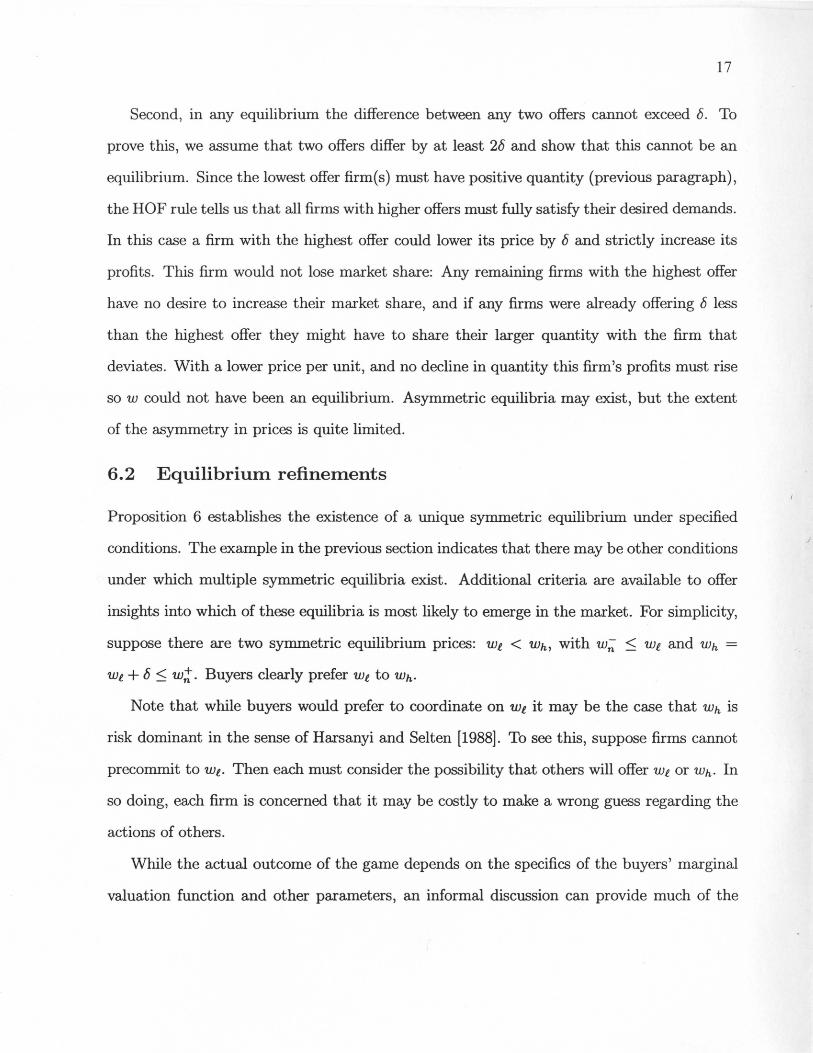
Second, in any equilibrium the difference between any two offers cannot exceed 8. To

prove this, we assume that two offers differ by at least 28 and show that this cannot be an

equilibrium. Since the lowest offer firm(s) must have positive quantity (previous paragraph),

the HOF rule tells us that all firms with higher offers must fully satisfy their desired demands.

In this case a firm with the highest offer could lower its price by 8 and strictly increase its

profits. This firm would not lose market share: Any remaining firms with the highest offer

have no desire to increase their market share, and if any firms were already offering 8 less

than the highest offer they might have to share their larger quantity with the firm that

deviates. With a lower price per unit, and no decline in quantity this firm's profits must rise

so W could not have been an equilibrium. Asymmetric equilibria may exist, but the extent

of the asymmetry in prices is quite limited.

6.2 Equilibrium refinements

Proposition 6 establishes the existence of a unique symmetric equilibrium under specified

conditions. The example in the previous section indicates that there may be other conditions

under which multiple symmetric equilibria exist. Additional criteria are available to offer

insights into which of these equilibria is most likely to emerge in the market. For simplicity,

suppose there are two symmetric equilibrium prices: Wi < Wh, with W;;' ~ Wi and Wh =

Wi + 8 ~ wt. Buyers clearly prefer Wi to Who

Note that while buyers would prefer to coordinate on Wi it may be the case that Wh is

risk dominant in the sense of Harsanyi and Selten [1988]. To see this, suppose firms cannot

precommit to Wi. Then each must consider the possibility that others will offer Wi or Who In

so doing, each firm is concerned that it may be costly to make a wrong guess regarding the

actions of others.

While the actual outcome of the game depends on the specifics of the buyers' marginal

valuation function and other parameters, an informal discussion can provide much of the

/

18

intuition. Consider the decision that firm i must make. If this firm believes that WI'. will be

the outcome, then it will offer this price. But if this belief were wrong and several other

firms were actually offering Wh, then under the HOF rule firm i would likely receive a small

market share and small profits. Such a mistake could be extremely costly. Firm i could

protect itself against this scenario by offering Who The argument is not complete, however,

since it could also be costly if firm i offers Wh when some other firms are offering WI'.. In this

case the HOF rule would provide firm i with substantial market share, but at the cost of

paying the high offer price. Though if 8 is relatively small this cost will also be quite small.

This leads us to suggest that if firm i is concerned about the risks of guessing wrong, then it

may be led to offer Who Since each firm faces the identical problem, there is reason to believe

that Wh will be the actual equilibrium outcome even though all firms would be better off if

they could coordinate on Wi. More generally, if the model admits more than two symmetric

equilibria, the risk dominance criterion may direct firms to the highest of these prices, which

suggests that price will be close to buyers' marginal valuation of input.

7 Extensions and conclusion

This paper analyzes oligopsonistic price competition in a market with a vertical supply

curve. In the model, buyers simultaneously and independently choose offer prices. A highest

offer first (HOF) allocation rule determines the supply of input for each buyer. Conditions

under which a Nash equilibrium exists are identified and characterized. When the number of

competing buyers is large, a symmetric equilibrium exists in which the common offer price

is very close to the marginal valuation of input. As indicated by the example in section 5,

this is likely to remain true with a smaller number of buyers.

A vertical supply curve generates quasi-rents that must be divided between buyers and

sellers. If buyers could collude they would lower their offers to the sellers' reservation price

/

19

and extract all the rents. In our model with price competition there is a tendency for this

result to be reversed. Buyers bid the price up as they compete for market share and this

causes rents to flow to sellers.

The model offers suggestions for applied research into collusive behavior in oligopsonistic

markets. If the data for a given industry are consistent with the model studied here, this

would provide some evidence against the presence of collusion. In order to conduct such a

study, it would be necessary to gather data on all of the model's key variables. For instance,

changes in market supply, number of firms, and buyers' marginal valuation of input all have

an impact on both market price and the distribution of rents between buyers and sellers.

A change in price or a shift in the distribution of rents may result from changes in market

conditions and is not necessarily evidence of collusion.

The static game may provide insights into the outcome of a dynamic extension in which

the same group of buyers repeatedly face each other in price competition. The set of static

N ash equilibria defines the bounds of punishment that may be imposed in a game of tacit

collusion. Buyers are able to maintain a low price only to the extent that a deviation would

be punished by higher prices in the future. Since the punishment price could cause most

rents to be transferred to sellers, it may be possible to support substantially lower prices in

a repeated setting. This suggests a direction for future research. However, if the parameters

of the stage game are not constant through time (e.g., number of buyers, market supply)

then this problem could be quite complex. Nonetheless, the static game considered here,

and the HOF allocation rule, could provide guidance.

Throughout the paper we have assumed that market supply is fixed. This was motivated

by examples from agriculture and regulated natural resources. Various complications arise

if we relax this assumption and allow supply to be sensitive to price. In particular, carefully

defined rationing rules become essential. The simplest extension of the HOF rule would

state that the firm with the highest offer buys its full desired quantity at that price. But

20

with upward sloping supply, consider what happens when a buyer raises its price to become

the high offer firm. Not only does this firm attract supply to itself, it also causes supply to

increase for the entire market. If this firm's demand is not sufficient to absorb the increase

in market supply, then some of the suppliers will have to settle for a lower price. It becomes

necessary to have a rationing rule for suppliers to complement the HOF rule. The interactions

between rationing/allocation rules on the two sides of the market could yield quite interesting

results in the analysis of oligopsony with price competition.

21

Appendix

Proof of lelllllla 1

First we identify the set of all non-negative w values that satisfy (1) for a given n. Then

we analyze the behavior of this solution set as n varies.

Any w for which w + 8 ~ W(O) satisfies (1) by default.

Next consider any w for which W(Q/n) ::; w+8 < W(O), and hence Q/n ~ Q(w+8) > O.

Then

l.W(O)

RHS (1) > w min{Q(w + 8), Q(v)}dv

l.W +8 l.W(O)

min{· .. }dv + rnin{· .. }dv w w+8

l.W(O)

8Q(w + 8) + Q(v)dv w+8

> 8Q(w + 8) + LHS (1).

Hence, any such w satisfies (1) with strict inequality.

Now consider any w for which w + 8 < W(Q/n), and hence Q(w + 8) > Q/n. In this

case, the following is true:

LHS (1) fnmill{Q,Q(W+cS)}

[W(~) - w - 8]d~ o

fnmill{Q/n,Q(w+cS)} lmill{Q,Q(w+cS)}

[ .. . ]£L; + _ [ .. ·]d~ o Q/n

RHS (1) l.w +cS - l.W(O)-

min{Q/n, Q(v)}dv + rnin{Q/n, Q(v)}dv w w~

_ rmill{Q/n,Q(w+cS)}

8Q/n + 10 [W(~) - w - 8]£L;

LHS (1) - RHS (1) = lmill{Q,Q(w+cS)} -_ [W(~) - w - 8]£L; - 8Q/n.

Q/n

The last expression above is a continuous and strictly decreasing function of w, and it

approaches -8Q/n as w approaches W(Q/n) - 8.

22

If we put the pieces together, it follows that (1) is satisfied for all w in some interval

[w;, W(O)]. If 8 ~ W(O) or if 8 ~ W(Q/n) (i.e., Q(8) ::; Q/n) then w; = O. Otherwise,

o ::; w; < W(Q/n) - 8.

The remainder of the proof analyzes the effect. of n on w;. If w; > 0 then the previous

results yield

!cmin{Q,Q(W;;- +8)} -_ [W(~) - w;: - 8]d~ - 8Q/n = O. Q/n

From this equality it follows that

!cmin{Q,Q(W;;- +8)} -_ [W(~) - w;: - 8]d~ - 8Q/(n + 1) > O.

Q/(n+l)

In words, if w remains equal to w; but the number of firms increases to n + 1, then (1) fails

to be satisfied. Hence w; ¢ [W;+l' W(O)], or equivalently, w; < w~+l'

Finally, if 8 < W(O) then for n sufficiently large w; > 0 (i.e., w = 0 fails to satisfy (1))

since LHS (l)lw=o > 0 = limn--too RHS (l)lw=o. Thus, for n sufficiently large w; IS an

increasing function of n and it satisfies (1) with equality:

lW~ - lW~-_ min{Q, Q(v)}dv = _ min{Q/n, Q(v)}dv. w n +8 Wn

As n --t 00 the LHS of this equation converges monotonically to

rW(O) -

JIimn-<>oo w;;- +6 min { Q , Q (v) }dv

while the RHS converges monotonically to O. Therefore, limn--too w; = W(O) - 8 . •

Proof of lemma 2

For the sake of clarity it will be convenient to emphasize that q in (3) is a function of w

and n: q(w, n).

Since Q - (n - l)Q(w) is a continuous and strictly increasing function of w, it follows

that q(w, n) is a continuous and non-decreasing function of w. Therefore, the LHS of (2) is a

continuous and non-decreasing function of w. The RHS of (2) is a continuously differentiable

./

23

and strictly decreasing function of w. Thus, if (2) fails to hold when w = 0 then it will fail

to hold for any w ~ O. If it holds with equality when w = 0 then it is satisfied only when

w = O. If it holds with strict inequality when w = 0 then it is satisfied on a non-degenerate

closed interval with left endpoint at O.

When w = 0 the RRS of (2) equals Jomin{Q/n,Q(O)} W(~)d~, while the LHS of (2) equals

Joii(O,n) W(~)~ since min{ q(O, n), Q(O)} = q(O, n) by (3). Hence, at w = 0, (2) is just satisfied

(satisfied strictly) if and only if q(O,n) = min{Q/n,Q(O)} (q(O,n) < min{Q/n,Q(O)}). If

Q ~ nQ(O) then min{ Q/n, Q(O)} = Q(O) and also q(O, n) = Q(O) by (3). So if Q ~ nQ(O)

then (2) is satisfied if and only if w = O. Alternatively, if Q < nQ(O) then Q - (n -l)Q(O) <

Q/n so q(O, n) = max{O, Q - (n - l)Q(O)} < Q/n = min{Q/n, Q(O)}. In this case (2) is

satisfied if and only if w E [0, w~] for some w~ > O.

The proof will be complete if w~ < W(O). Observe that q(W(O), n) = min{Q, Q(O)} so

at w = W(O) the LHS of (2) is strictly positive while the RRS is O. Therefore W(O) (j. [0, w~],

which yields w~ < W(O). •

Proof of lemma 3

Consider any w ~ 0 that satisfies Q ( w) ~ Q / n. By hypothesis, any such w must actually

be strictly positive. Since Q(w) ~ Q/n implies Q - (n - l)Q(w) ~ Q(w), (3) yields the

following: q(w, n) = min{Q - (n - l)Q(w), Q(O)} ~ Q(w). Thus,

rW(O) LHS (2) > io min{Q(w), Q(v)}dv

rW(O) > iw min{Q(w), Q(v)}dv

rW(O) iw Q(v)dv

RHS (2)

where the last line follows from the fact that if v E [w, W(O)] and Q(w) < Q/n then

/

24

Q(v) = min{ Q/n, Q(v)}. Therefore, any such w fails to satisfy (2). Since w~ does satisfy (2),

it must be the case that Q(w~) > Q/n.

Now consider any w that satisfies Q(w) 2:: Q/(n -1). Then q(w, n) = 0, so LHS (2) = O.

Since Q(w) > 0 (and hence w < W(O)), RES (2) > O. Therefore, any such w satisfies (2)

with strict inequality. From the proof of lemma 2, w~ satisfies (2) with equality. It follows

that Q(w~) < Q/(n - 1). _

Proof of corollary 4

Since any symmetric equilibrium price w must satisfy (2), it follows from lemma 2 that

w ~ w~. Then lemma 3 yields w < W(Q/n). Finally, according to the HOF rule, q =

min{Q/n,Q(w)} = Q/n. _

Proof of lemma 5

From the proof of lemma 2, W:+l satisfies (2) with equality. Also, since W~+l < W(O),

RES (2)lw=w~+1 is strictly positive. Hence q(w:+1 , n+ 1) > O. (More generally, q(w;!;" m) > 0

for any integer m ~ 2.) From lemma 3, Q - (n + 1 - l)Q(w~) < O. Therefore, (3) yields

q(w~, n + 1) = O. In addition, from the proof of lemma 2, q(w, n + 1) is a non-decreasing

function of w. Since this function equals zero when w = w~ and it is strictly positive when

Now {w:}~=2 is a monotone sequence that is bounded from above by W(O). In order to

prove that limn-+ex> w: = W (0), it is sufficient to show that for all w < W (0) there exists n

such that w: > w. So consider any w < W(O). By (3), there exists n sufficiently large such

that q(w, n) = O. From the previous paragraph q(w~, n) > O. Also, recall that q(., n) is a

non-decreasing function of its first argument. This yields w~ > w .•

Proof of proposition 6

(a) If Q ~ nQ(O) or if 8 2:: W(O) then from lemma 1, w;; = 0, in which case the set

of symmetric equilibrium prices is the intersection of [0, w~] and the price grid. If

25

8 ~ W(O) then this intersection consists of only w = 0 since w: < W(O) (lemma 2).

If Q ~ nQ(O) then from lemma 2, w: = 0, so once again the intersection consists of

only w = O.

(b) Any half-open interval in IR+ of length 8 must contain exactly one point that lies on

the price grid. Therefore, since W(O) - b > 0, [W(O) - 8, W(O)) must contain exactly

one such point. Let w* denote this point. From lemma 1, there exists Nl such that if

n ~ Nl then w* - 8 < w;;' < W(O) - 8 :::; w*. From lemma 5, there exists N2 such that

ifn ~ N2 thenw* < w: < W(O). Let N = max{N1 ,N2}. Ifn ~ Nthenw* E [w;;.,w:J

and hence w* is a symmetric equilibrium price. Uniqueness follows since the adjacent

points on the price grid, namely w* - 8 and w* + 8, are respectively less than w;;' and

greater than w: .•

/

26

References

[1] Adams, Darius M. and Richard W. Haynes [1989]. "A model 6f national forest timber

supply and stumpage markets in the Western United States." Forest Science 35 (June),

401-424.

[2] Allen, Beth and Martin Hellwig [1986]. "Price-setting firms and the oligopolistic foun­

dations of perfect competition." American Economic Review 76 (May), 387-392.

[3] Anchorage Daily News [1998]. "Bristol Bay suit stands; Class-action status ruled OK."

Thursday 19 March, page IF.

[4] Grossman, Sanford J. and Oliver D. Hart [1986]. "The costs and benefits of ownership:

A theory of vertical and lateral integration." Journal of Political Economy 94 (August),

691-719.

[5] Harsanyi, John C. and Reinhard Selten [1988]. A general theory of equilibrium selection

in games. Cambridge, MA: MIT Press.

[6] Kreps, David M. and Jose A. Scheinkman [1983]. "Quantity precommitment and

Bertrand competition yield Cournot outcomes." Bell Journal of Economics 14 (au­

tumn), 326-337.

[7] Matulich, Scott C., Ron C. Mittelhammer, and Carlos Reberte [1996]. "Toward a more

complete model of individual transferable fishing quotas: Implications of incorporating

the processing sector. " Journal of Environmental Economics and Management 31 (July),

112-128.

[8] Nash, John F., Jr. [1950]. "Equilibrium points in n-person games." Proceedings of the

National Academy of Sciences 36,48-49.

27

[9] Rucker, Randal R., Walter N. Thurman, Daniel A. Sumner [1995]. "Restricting the

market for quota: An analysis of tobacco production rights with corroboration from

congressional testimony." Journal of Political Economy 103 (February), 142-175.

[10] Sexton, Richard J. and Mingxia Zhang [1996]. "A model of price determination for fresh

produce with application to California iceberg lettuce." American Journal of Agricul­

tural Economics 78 (November), 924-934.

[11] Stahl, Dale 0., II [1988]. "Bertrand competition for inputs and Walrasian outcomes." ·

American Economic Review 78 (March), 189-201.

.J

28

Figure 1. Offer Price Increase

v

W(O) W(~), Q(v)

w+8

w

D

o ~---------~--~--~------------~~~ Qln Q(w+8) Q(w) Q(O)

J

29

Figure 2. Offer Price Decrease

v

W(O)

w

"-q -Qln Q(w) Q(O) ~ o

30

Cll

CD CD

C\I \ \

\\ 0

\ ~ If)

\ ~

~

0

\ \ t-

o \\

r-I

\\ \\

0'

\\ CD

0'

\\ CD

~

\ : '-

"

.\ .•.. \\

~

"\ •.. eD 0

\\ It)

.~ .. It)

Ul

(f)

\\ E

.~ ..

E

I-. 0...

I-. 0...

\\ ~

.~ .. ~

a ., ...

<ot a

.~ ..

<ot 0

0 If)

If) . ~ ..

.~: . c

·X·. c

" (')

0'

" X

(')

0'

~+C:IC: .~.

~+C:IC: ~ ~ ~

~

~ ~ ~

C\I

I ~

I i

~

i ~

rn rn

<

<

u u

a a

0·[

6·0

g·o

l:O

9·0

g·O

t·O

C·O

Z

·O

[·0 0

·0 0

·[ 6

·0 g·O

l:O

9

·0 g

·O

t·O

C·O

Z·O

[·0

0·0

aO!.ld

aO!.ld

Cll

CD CD

C\I ,~

C

C\I \ \

i i "

0 \ \

0 ~+C:IC:

~

~

\\ ~ ~ ~

I \\

r-I

I \\

i \\

\\ ~

\\ CD

0'

'-'

~

\\ ~

\\ ....

\\ ....

.\"..:, \\

It)

.,: .. It)

III (f)

\ .... E

0...

.~. E

0...

I-. I-.

a ~.

~

a \.

~

v.l <ot

0 <ot

.. 0

\ 0

-, :;

If)

v.l \.

c -,

~

0'

.:~

" -'\

(')

~

a a

.. :, ....... +

c: I c:

Q

~ ~ ~

... , (')

I .~

~

..... '. ~

i ..

rn·

CII

rn C':

<

<

:; u

u

e .-0

0

~

~

a a

.... =

0·[

6·0

g·o

L·O

9

·0

g·O

t·O

C·O

G

·O

[·0

0·0

0·1

6·0

g·O

L·O

9

·0 g

·O

t·O

C·O

Z

·O

1·0 0

·0 b

l) aO

!.ld aO

!Jd .-~