Bayesian k-Space-Time Reconstruction of MR Spectroscopic Imaging for Enhanced Resolution John Kornak 1,2 , Karl Young 3,4 , Brian J. Soher 5 , and Andrew A. Maudsley 6 1 University of California, San Francisco, Department of Radiology and Biomedical Imaging, Center for Molecular and Functional Imaging, China Basin Landing, 185 Berry Street, Lobby 6, Suite 350, San Francisco, CA 94107 2 University of California, San Francisco, Department of Epidemiology and Biostatistics, Division of Biostatistics, China Basin Landing, 185 Berry St, Lobby 5, Ste. 5700, San Francisco, CA 94107 3 University of California, San Francisco, Department of Radiology and Biomedical Imaging, Center for Imaging of Neurodegenerative Diseases, 4150 Clement Street (114M), San Francisco, CA 94121 4 Center for Imaging of Neurodegenerative Diseases, Veterans Affairs Medical Center, San Francisco, 4150 Clement Street (114M), San Francisco, CA 94121 5 Duke Center for Advanced MR Development, Duke University Medical Center, Box 3808, Durham, NC 27710 6 University of Miami School of Medicine, Department of Radiology, 1150 N.W. 14th St, Miami, FL 33136 Abstract A k-space-time Bayesian statistical reconstruction method (K-Bayes) is proposed for the reconstruction of metabolite images of the brain from proton ( 1 H) Magnetic Resonance Spectroscopic Imaging (MRSI) data. K-Bayes performs full spectral fitting of the data while incorporating structural (anatomical) spatial information through the prior distribution. K-Bayes provides increased spatial resolution over conventional discrete Fourier transform (DFT) based methods by incorporating structural information from higher-resolution co-registered and segmented structural Magnetic Resonance Images. The structural information is incorporated via a Markov random field (MRF) model that allows for differential levels of expected smoothness in metabolite levels within homogeneous tissue regions and across tissue boundaries. By further combining the structural prior model with a k-space-time MRSI signal and noise model (for a specific set of metabolites and based on knowledge from prior spectral simulations of metabolite signals) the impact of artifacts generated by low-resolution sampling is also reduced. The posterior mode estimates are used to define the metabolite map reconstructions, obtained via a generalized Expectation-Maximization algorithm. K-Bayes was tested using simulated and real MRSI datasets consisting of sets of k-space-time-series (the recorded free induction decays). The results demonstrated that K-Bayes provided qualitative and quantitative improvement over DFT methods. Address Correspondence to: John Kornak University of California, San Francisco, Department of Radiology and Biomedical Imaging, Center for Molecular and Functional Imaging, China Basin Landing, 185 Berry Street, Suite 350, San Francisco, CA 94107 Tel: 415-353-4740 Fax: 415-353-9423 [email protected]. NIH Public Access Author Manuscript IEEE Trans Med Imaging. Author manuscript; available in PMC 2010 July 29. Published in final edited form as: IEEE Trans Med Imaging. 2010 July ; 29(7): 1333–1350. doi:10.1109/TMI.2009.2037956. NIH-PA Author Manuscript NIH-PA Author Manuscript NIH-PA Author Manuscript

Welcome message from author
This document is posted to help you gain knowledge. Please leave a comment to let me know what you think about it! Share it to your friends and learn new things together.
Transcript

Bayesian k-Space-Time Reconstruction of MR SpectroscopicImaging for Enhanced Resolution
John Kornak1,2, Karl Young3,4, Brian J. Soher5, and Andrew A. Maudsley6
1 University of California, San Francisco, Department of Radiology and Biomedical Imaging,Center for Molecular and Functional Imaging, China Basin Landing, 185 Berry Street, Lobby 6,Suite 350, San Francisco, CA 941072 University of California, San Francisco, Department of Epidemiology and Biostatistics, Divisionof Biostatistics, China Basin Landing, 185 Berry St, Lobby 5, Ste. 5700, San Francisco, CA 941073 University of California, San Francisco, Department of Radiology and Biomedical Imaging,Center for Imaging of Neurodegenerative Diseases, 4150 Clement Street (114M), San Francisco,CA 941214 Center for Imaging of Neurodegenerative Diseases, Veterans Affairs Medical Center, SanFrancisco, 4150 Clement Street (114M), San Francisco, CA 941215 Duke Center for Advanced MR Development, Duke University Medical Center, Box 3808,Durham, NC 277106 University of Miami School of Medicine, Department of Radiology, 1150 N.W. 14th St, Miami, FL33136
AbstractA k-space-time Bayesian statistical reconstruction method (K-Bayes) is proposed for thereconstruction of metabolite images of the brain from proton (1H) Magnetic ResonanceSpectroscopic Imaging (MRSI) data. K-Bayes performs full spectral fitting of the data whileincorporating structural (anatomical) spatial information through the prior distribution. K-Bayesprovides increased spatial resolution over conventional discrete Fourier transform (DFT) basedmethods by incorporating structural information from higher-resolution co-registered andsegmented structural Magnetic Resonance Images. The structural information is incorporated via aMarkov random field (MRF) model that allows for differential levels of expected smoothness inmetabolite levels within homogeneous tissue regions and across tissue boundaries. By furthercombining the structural prior model with a k-space-time MRSI signal and noise model (for aspecific set of metabolites and based on knowledge from prior spectral simulations of metabolitesignals) the impact of artifacts generated by low-resolution sampling is also reduced. The posteriormode estimates are used to define the metabolite map reconstructions, obtained via a generalizedExpectation-Maximization algorithm. K-Bayes was tested using simulated and real MRSI datasetsconsisting of sets of k-space-time-series (the recorded free induction decays). The resultsdemonstrated that K-Bayes provided qualitative and quantitative improvement over DFT methods.
Address Correspondence to: John Kornak University of California, San Francisco, Department of Radiology and Biomedical Imaging,Center for Molecular and Functional Imaging, China Basin Landing, 185 Berry Street, Suite 350, San Francisco, CA 94107 Tel:415-353-4740 Fax: 415-353-9423 [email protected].
NIH Public AccessAuthor ManuscriptIEEE Trans Med Imaging. Author manuscript; available in PMC 2010 July 29.
Published in final edited form as:IEEE Trans Med Imaging. 2010 July ; 29(7): 1333–1350. doi:10.1109/TMI.2009.2037956.
NIH
-PA Author Manuscript
NIH
-PA Author Manuscript
NIH
-PA Author Manuscript
KeywordsBayesian Image Analysis; Expectation-Maximization; K-Bayes; Magnetic ResonanceSpectroscopy Imaging (MRSI); Metabolite maps; MRSI reconstruction
I. IntroductionMagnetic resonance (MR) techniques provide a means for mapping a number of physicaland chemical parameters in the human body. In particular, magnetic resonance spectroscopicimaging (MRSI) [1, 2] combines the spatial sampling methods of structural magneticresonance imaging (structural MRI) with sampling of a spectroscopic data dimension,thereby enabling discrimination of multiple resonance frequencies and mapping of multipletissue metabolites. MRSI information is of diagnostic interest because alterations ofmetabolite concentrations can provide a more sensitive indication of disease than observingtissue structure via structural MRI alone.
The spatial resolution of MR techniques differs greatly, from approximately 1 mm3 forstructural MRI (which images anatomy through measurement of variation in waterconcentration) to 1000-2000 mm3 for MRSI. This is because concentrations of metabolitesare approximately a factor of 10,000 times smaller than that of water, leading to lowersignal-to-noise ratio (SNR) for MRSI than structural MRI. The lower SNR must be partiallyoffset by obtaining data at much lower spatial resolution, i.e. by sampling at fewer spatialfrequencies, usually the center region of k-space (or spatial frequency-space).
Proton (1H) MRSI datasets consist of a set of (discrete) time series with typical lengths onthe order of 512 timepoints. Each series is recorded at an individual point in k-space, (kx,ky), where the various kx and ky values correspond to different settings of the x and ydirection magnetic field gradients, respectively. Typically, a set of slices to cover the brain isrecorded and the z - (or slice) direction can be encoded in standard image space throughgradient slice selection or as a 3rd k-space dimension. The k-space data are usually recordedin the form of a square lattice over k-space, and this is the form of the data considered here.However, an advantage of the proposed modeling scheme over standard discrete Fouriertransformation (DFT) methodology is that it can naturally incorporate any k-space samplingschemes, for example where the center of k-space, which has the greatest SNR, is sampledthe most densely.
The most widely used methods for reconstructing MRSI datasets focus on 4D DFT andspectral fitting or 3D spatial DFT followed by time domain fitting [3-6]. Conventional use ofDFT for reconstruction of low-resolution MRSI data produces low-resolution images andartifacts associated with the limited sampling of spatial frequencies, such as Gibbs ringing,aliasing and blurring. Moreover, DFT has no mechanism for regularization via theincorporation of prior information, e.g. noise is transformed directly from k-space to imagespace. While a number of techniques have been suggested to address these issuesindividually (see e.g., Chapter 8 of Liang and Lauterbur [7]), a unified solution would be ofgreat utility.
A number of general methods for improving spatial resolution within MR modalities havebeen proposed; however none of these has the dual advantage of combining a low-resolutionk-space-time data generation model with prior information obtained from high-resolutionstructural (anatomical) scanning methods. Reconstruction to higher resolution usingBayesian image analysis methods for multi-contrast structural MRI is presented in [8];however, they do not incorporate a full signal model and hence are subject to all of the
Kornak et al. Page 2
IEEE Trans Med Imaging. Author manuscript; available in PMC 2010 July 29.
NIH
-PA Author Manuscript
NIH
-PA Author Manuscript
NIH
-PA Author Manuscript
problems with artifacts that are incurred from use of the DFT for reconstruction of low-resolution modalities. A model that incorporates a raw signal model for structural MRI waspresented for maximum likelihood estimation in [9] and Bayesian maximum a posteriorireconstruction in [10]; however, the first model's focus was on high-resolution structuralMRI, and the only prior information considered in [10] was a notion of overall a priorismoothness. Denney and Reeves [11] have developed a Bayesian approach for MRSIreconstruction that models the data in k-space-time and utilizes an edge preserving prior.They do not directly model the raw k-space-time series data of MRSI but instead usespectrally integrated estimates of the metabolites at each k-space point; for the paper theyonly considered the relatively strong water and lipid signals. Important uncertaintyinformation is discarded when ignoring the original data and working with spectrallyintegrated estimates directly. Furthermore, the edge-preserving prior does not utilize tissueclass information that could be valuable when determining effects specific to certain tissuetypes.
A related body of literature exists for the Bayesian reconstruction of emission tomographydata using a co-registered and segmented structural MRI as prior information [12-14]. Theidea is to model the distribution of counts at the receptors from individual voxels andcombine this with structural prior spatial models of varying types, including models thatincorporate line site detection for determining the tissue boundaries [12]; models thatclassify into a number of tissue regions within the emission tomography map [13]; andtissue composition models similar to the prior spatial model developed herein for MRSI[14].
A number of papers [15-20] aim to use tissue classification information to improve thereconstruction (and associated resolution) of MRSI data outside the Bayesian framework.The idea is to utilize basis function in order to smoothly represent signals withinhomogeneous tissue areas. Because it needs to be kept sparse (either by limiting the size ofthe basis set or by penalizing selection from a larger basis set), the basis functionrepresentation restricts the space of potential reconstructions. The earliest basis sets usedwere piece-wise constant functions such as those used in Spectral Localization by Imaging(SLIM) [15] and in Spectral Localization with Optimal Pointspread function (SLOOP)techniques, [16]. The SLOOP method extends on SLIM by optimizing the set of phaseencoding gradients to match the pointspread function of the volumes of interest. The SLIMpiece-wise constant basis function approach was also generalized to a wide range of basisfunction sets through the generalized series formulation [17]. A related Bayesian method isproposed by Haldar et al [21] that combines the basis set approach with prior structuralinformation. The idea is to obtain k-space data at high-resolution, accepting significant lossof SNR in the data, and then use a structural prior distribution with “soft” edgeclassifications to recover the lost SNR.
In this report, an alternative image reconstruction method based on a combination of MRSIprocess modeling and Bayesian image analysis is presented for the enhancement ofmetabolite maps (K-Bayes). First developed for (non-dynamic) perfusion MRI [22, 23], theK-Bayes approach is here expanded considerably to accommodate the additional spectralfitting problem inherent to MRSI. K-Bayes combines information from high-resolutiontissue segmented structural MRIs with low-resolution k-space-time MRSI data. Theacquired MRSI data are supplemented by additional sources of prior information thatcharacterize known relationships between local tissue structural patterns and the spatialdistribution of metabolites in the brain. Therefore, K-Bayes effectively performs a fullspectral fitting of the data along with incorporation of spatial information. To the authors’knowledge, there are no other existing reconstruction methods that use a true Bayesian k-space-time signal acquisition model to directly reconstruct metabolite maps from low-
Kornak et al. Page 3
IEEE Trans Med Imaging. Author manuscript; available in PMC 2010 July 29.
NIH
-PA Author Manuscript
NIH
-PA Author Manuscript
NIH
-PA Author Manuscript
resolution MRSI data. K-Bayes thereby provides a unified solution for reducing artifacts andincreasing image resolution and accuracy.
II. The K-Bayes ModelThe main modeling objectives of K-Bayes for MRSI data are: 1) to incorporate a full signal(and noise) model to relate the raw k-space-time data to the metabolite maps to bereconstructed and 2) to incorporate anatomical information from high-resolution structuralMRIs. This is achieved within the framework of Bayesian image analysis modeling [24-26].The definition of a full k-space-time signal acquisition model alongside a noise model formsthe likelihood part of K-Bayes. The prior distribution for K-Bayes relates the spatialdistribution of metabolites to a high-resolution and coregistered structural MRI that issegmented into gray matter (GM), white matter (WM), and cerebro-spinal fluid (CSF). Theprior model incorporates knowledge of the expected ‘smoother’ behavior of metaboliteswithin homogeneous tissue regions as opposed to less smooth behavior across theboundaries of different tissues; differences between gray and white matter metaboliteconcentrations have been determined to reach as much as 30% for creatine (Cr) in thetemporal lobe and choline (Cho) in the parietal lobe [27]. That is, neighboring locationswithin homogeneous tissue type are expected to have more similar values than either 1)neighboring voxels of different tissue type, or 2) voxels of homogeneous tissue type that arefurther apart. These expectations are incorporated into a prior distribution via the use ofMarkov random field (MRF) models [25, 26, 28] that describe (probabilistically) the spatialdistribution of metabolites: characterizing the different spatial correlation structure ofmetabolites within homogeneous tissue regions compared with that across tissue boundaries.Also incorporated into the prior distribution is the knowledge that metabolite levels shouldbe zero outside the head and can be assumed negligible within CSF. The information in thedata (incorporated via the likelihood) and the structural information used in the priordistribution are combined via Bayes’ Theorem. The combination leads to a posteriordistribution of metabolite maps that is defined at the higher resolution of the structural MRI.K-Bayes reconstructed metabolite maps are obtained by maximizing the posteriordistribution. Maximization is achieved by applying an iterative (generalized) Expectation-Maximization (EM) algorithm [29] to an expanded set of model variables.
A. The K-Bayes MRSI Signal Model and LikelihoodThe 4D multi-slice MRSI signal model for K-Bayes both corrects and expands upon themodel given in Young et al. [4] and Soher et al. [5]. Each signal time series, s(kx, ky, w,t),for a fixed kx, ky and w, is modeled as a discretely sampled, exponentially decaying, sum ofsinusoids that correspond to the resonance frequencies of the metabolite spectra present.Here, kx, ky represent the strength of the magnetic field gradients in the x and y directionsrespectively (the k-space position); w represents the MRSI slice index; and t = 0,δ,2δ,...,δ(T– 1) represents time after the onset of the free-induction-decay (FID), or from the maximumof a signal echo. The model relates the complete set of k-space complex time-series to 3Dimage volumes of metabolite signals located at different spectral frequencies (the metabolitemaps):
[1]
The multiple integral of Eq. [1] is evaluated over each voxel at the higher resolution of thestructural MRI. The signal s(kx, ky, w,t) at each k-space-time-point (kx,ky, w,t), sums the
Kornak et al. Page 4
IEEE Trans Med Imaging. Author manuscript; available in PMC 2010 July 29.
NIH
-PA Author Manuscript
NIH
-PA Author Manuscript
NIH
-PA Author Manuscript
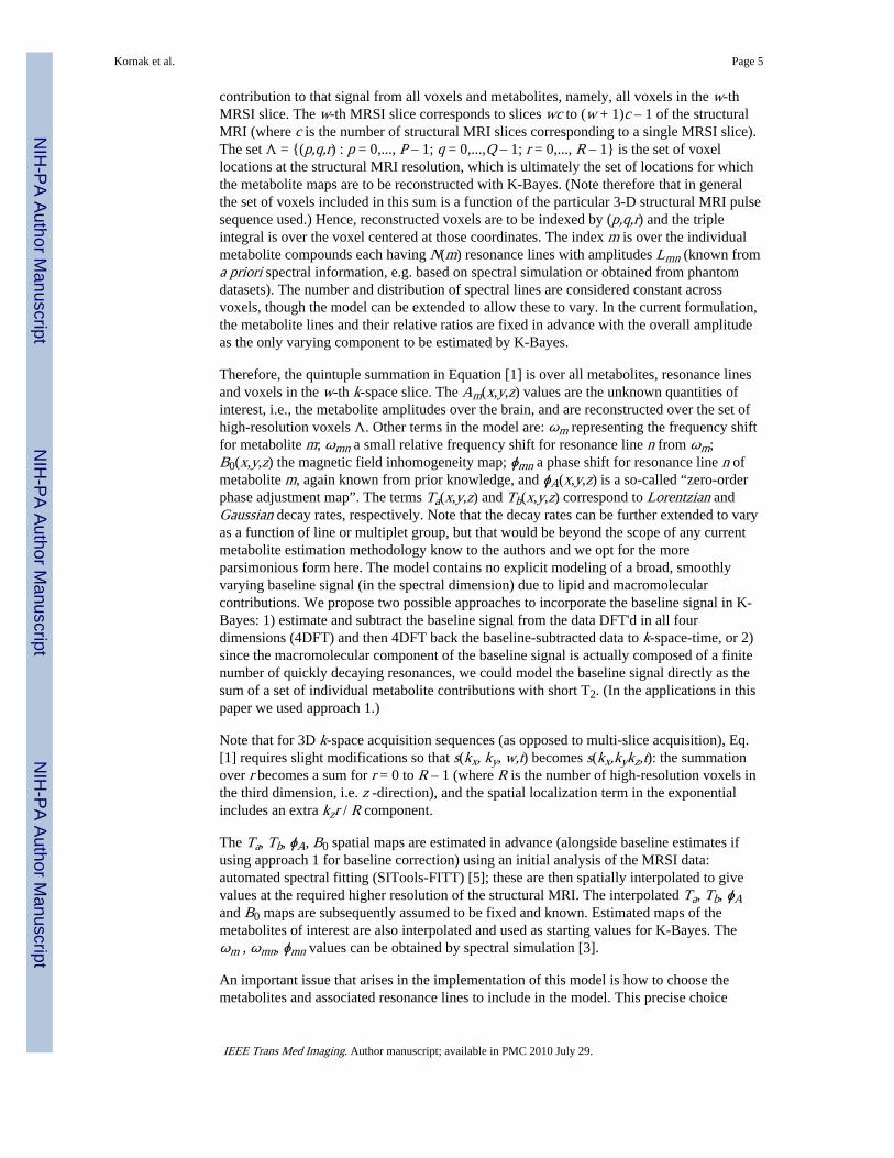
contribution to that signal from all voxels and metabolites, namely, all voxels in the w-thMRSI slice. The w-th MRSI slice corresponds to slices wc to (w + 1)c – 1 of the structuralMRI (where c is the number of structural MRI slices corresponding to a single MRSI slice).The set Λ = {(p,q,r) : p = 0,..., P – 1; q = 0,...,Q – 1; r = 0,..., R – 1} is the set of voxellocations at the structural MRI resolution, which is ultimately the set of locations for whichthe metabolite maps are to be reconstructed with K-Bayes. (Note therefore that in generalthe set of voxels included in this sum is a function of the particular 3-D structural MRI pulsesequence used.) Hence, reconstructed voxels are to be indexed by (p,q,r) and the tripleintegral is over the voxel centered at those coordinates. The index m is over the individualmetabolite compounds each having N(m) resonance lines with amplitudes Lmn (known froma priori spectral information, e.g. based on spectral simulation or obtained from phantomdatasets). The number and distribution of spectral lines are considered constant acrossvoxels, though the model can be extended to allow these to vary. In the current formulation,the metabolite lines and their relative ratios are fixed in advance with the overall amplitudeas the only varying component to be estimated by K-Bayes.
Therefore, the quintuple summation in Equation [1] is over all metabolites, resonance linesand voxels in the w-th k-space slice. The Am(x,y,z) values are the unknown quantities ofinterest, i.e., the metabolite amplitudes over the brain, and are reconstructed over the set ofhigh-resolution voxels Λ. Other terms in the model are: ωm representing the frequency shiftfor metabolite m; ωmn a small relative frequency shift for resonance line n from ωm;B0(x,y,z) the magnetic field inhomogeneity map; ϕmn a phase shift for resonance line n ofmetabolite m, again known from prior knowledge, and ϕA(x,y,z) is a so-called “zero-orderphase adjustment map”. The terms Ta(x,y,z) and Tb(x,y,z) correspond to Lorentzian andGaussian decay rates, respectively. Note that the decay rates can be further extended to varyas a function of line or multiplet group, but that would be beyond the scope of any currentmetabolite estimation methodology know to the authors and we opt for the moreparsimonious form here. The model contains no explicit modeling of a broad, smoothlyvarying baseline signal (in the spectral dimension) due to lipid and macromolecularcontributions. We propose two possible approaches to incorporate the baseline signal in K-Bayes: 1) estimate and subtract the baseline signal from the data DFT'd in all fourdimensions (4DFT) and then 4DFT back the baseline-subtracted data to k-space-time, or 2)since the macromolecular component of the baseline signal is actually composed of a finitenumber of quickly decaying resonances, we could model the baseline signal directly as thesum of a set of individual metabolite contributions with short T2. (In the applications in thispaper we used approach 1.)
Note that for 3D k-space acquisition sequences (as opposed to multi-slice acquisition), Eq.[1] requires slight modifications so that s(kx, ky, w,t) becomes s(kx,kykz,t): the summationover r becomes a sum for r = 0 to R – 1 (where R is the number of high-resolution voxels inthe third dimension, i.e. z -direction), and the spatial localization term in the exponentialincludes an extra kzr / R component.
The Ta, Tb, ϕA, B0 spatial maps are estimated in advance (alongside baseline estimates ifusing approach 1 for baseline correction) using an initial analysis of the MRSI data:automated spectral fitting (SITools-FITT) [5]; these are then spatially interpolated to givevalues at the required higher resolution of the structural MRI. The interpolated Ta, Tb, ϕAand B0 maps are subsequently assumed to be fixed and known. Estimated maps of themetabolites of interest are also interpolated and used as starting values for K-Bayes. Theωm , ωmn, ϕmn values can be obtained by spectral simulation [3].
An important issue that arises in the implementation of this model is how to choose themetabolites and associated resonance lines to include in the model. This precise choice
Kornak et al. Page 5
IEEE Trans Med Imaging. Author manuscript; available in PMC 2010 July 29.
NIH
-PA Author Manuscript
NIH
-PA Author Manuscript
NIH
-PA Author Manuscript
would be experiment and TE-specific. Obviously all metabolites of interest in the studyshould be included, as well as any other metabolites that are thought to contribute asignificant signal (thereby reducing residual noise levels). The papers by Young et al. [3, 4]and Soher et al. [5] address the choice of metabolites and spectral lines for inclusion inMRSI signal models in detail.
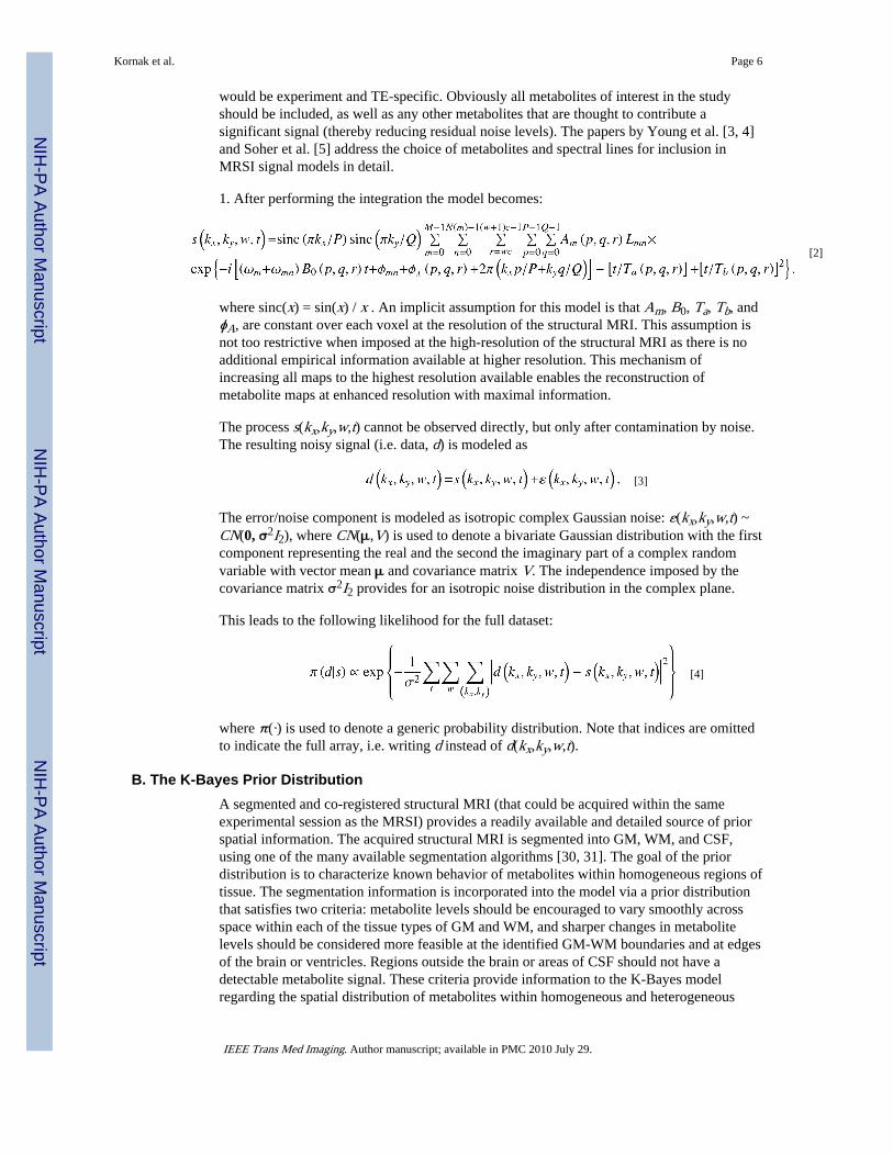
1. After performing the integration the model becomes:
[2]
where sinc(x) = sin(x) / x . An implicit assumption for this model is that Am, B0, Ta, Tb, andϕA, are constant over each voxel at the resolution of the structural MRI. This assumption isnot too restrictive when imposed at the high-resolution of the structural MRI as there is noadditional empirical information available at higher resolution. This mechanism ofincreasing all maps to the highest resolution available enables the reconstruction ofmetabolite maps at enhanced resolution with maximal information.
The process s(kx,ky,w,t) cannot be observed directly, but only after contamination by noise.The resulting noisy signal (i.e. data, d) is modeled as
[3]
The error/noise component is modeled as isotropic complex Gaussian noise: ε(kx,ky,w,t) ~CN(0, σ2I2), where CN(μ,V) is used to denote a bivariate Gaussian distribution with the firstcomponent representing the real and the second the imaginary part of a complex randomvariable with vector mean μ and covariance matrix V. The independence imposed by thecovariance matrix σ2I2 provides for an isotropic noise distribution in the complex plane.
This leads to the following likelihood for the full dataset:
[4]
where π(·) is used to denote a generic probability distribution. Note that indices are omittedto indicate the full array, i.e. writing d instead of d(kx,ky,w,t).
B. The K-Bayes Prior DistributionA segmented and co-registered structural MRI (that could be acquired within the sameexperimental session as the MRSI) provides a readily available and detailed source of priorspatial information. The acquired structural MRI is segmented into GM, WM, and CSF,using one of the many available segmentation algorithms [30, 31]. The goal of the priordistribution is to characterize known behavior of metabolites within homogeneous regions oftissue. The segmentation information is incorporated into the model via a prior distributionthat satisfies two criteria: metabolite levels should be encouraged to vary smoothly acrossspace within each of the tissue types of GM and WM, and sharper changes in metabolitelevels should be considered more feasible at the identified GM-WM boundaries and at edgesof the brain or ventricles. Regions outside the brain or areas of CSF should not have adetectable metabolite signal. These criteria provide information to the K-Bayes modelregarding the spatial distribution of metabolites within homogeneous and heterogeneous
Kornak et al. Page 6
IEEE Trans Med Imaging. Author manuscript; available in PMC 2010 July 29.
NIH
-PA Author Manuscript
NIH
-PA Author Manuscript
NIH
-PA Author Manuscript

tissue regions and can be mathematically represented within a prior distribution based onMRF models [26, 28, 32]. The prior model used here is defined at the spatial resolution ofthe structural MRI as follows:
[5]
with the added constraint that Am is assumed zero everywhere both outside the brain andwithin regions consisting of CSF. (This condition can be relaxed if required.) The sum inEq. [5] over < (p,q,r),(p',q',r') > is over all pairs of ‘neighboring’ voxels (p,q,r), (p',q',r') andis only over first-order neighbors, i.e. where only horizontally and vertically adjacent pairsare considered to be neighbors; though this can be generalized to higher-orders (and in thelanguage of the MRF literature, arbitrary cliques) in a straightforward manner. The functionsIG[(p,q,r),(p',q',r')], IW[(p,q,r),(p',q',r')] and IB[(p,q,r),(p',q',r')] are indicator functions formatching pairs of GM, WM and brain tissue (GM or WM) voxels, respectively, e.g.IG[(p,q,r)(p',q',r')] = 1 if both (p,q,r) and (p',q',r') are GM voxels and = 0 otherwise. The
parameters , , and control the level of stochastic smoothing between neighbors(stochastic because it is determined by a random field model that describes the similarity of
neighboring values); describes the a priori expected smoothness of non-matching
tissue type neighbors, and , describe the extra components of smoothness for GMand WM neighboring pairs, respectively. (The m index allows these parameters to bedifferent for each of the metabolites.) This prior distribution model can be considered as anextension of the intrinsic pairwise Gaussian difference prior [33, 34]; extended such that thesmoothness parameter depends on the tissue type(s) of the voxel pairs. The prior thereforeacts as an adaptive stochastic smoothing mechanism that is able to reduce the level ofsmoothing constraint when crossing tissue type boundaries. The variance/smoothing
parameters , , and could be estimated directly via an additional E-step in the EMalgorithm (described below) for a set of training subjects chosen from existing datasetsacquired under the imaging protocol. Averages of these estimates could then be used asfixed parameter values in all future datasets acquired under the same imaging protocol.Fixing parameters within any multi-subject imaging study is important to avoid inducingpotential biases for group comparisons. As an alternative approach to estimating the
parameters, we could choose , , and by calibrating past experimental results tomatch the biological expectations for the spatial structure of metabolite maps. This wouldrequire a complex process whereby, for example, a biologist would sit and reviewreconstructed maps based on different sets of prior parameters (again from a training set)and score them based on their biological plausibility. Finally, note that if the dimensions of
voxels are not isotropic, then , and should not take the same values in all principledirections.
C. Posterior EstimationIn order to obtain an estimate (reconstruction) of the metabolite maps, the posteriordistribution is maximized with respect to the sets of metabolite amplitudes at all voxels. Thisis equivalent to maximizing the product of the likelihood and the prior distribution and isonly one of many possible estimates that can be obtained from the posterior distribution.However, it is a common choice for Bayesian image analysis because a) it is easy tounderstand, and b) there is known (and relatively computationally efficient) methodologythat can be used to obtain it [26]. A generalized form of the Expectation-Maximization (EM)procedure [29] was used for optimization. The algorithm is generated in a similar fashion to
Kornak et al. Page 7
IEEE Trans Med Imaging. Author manuscript; available in PMC 2010 July 29.
NIH
-PA Author Manuscript
NIH
-PA Author Manuscript
NIH
-PA Author Manuscript

the algorithms in Green [35] and Miller et al. [9], where a set of unobservable latentvariables is created to simplify the computational algorithm. These variables are treated asmissing data within the EM algorithm. The latent variables for the EM reconstructionapproach described here are defined as:
[6]
The term z(kx,ky,p,q,r,w,t,m) is the contribution of data (signal plus noise) at k-spacelocation (kx,ky) within slice w and at time t to the total amount of metabolite m within voxel
(p,q,r), namely, Am(p,q,r). The noise term εz(kx,ky,p,q,r,w,t,m) ~ is basedon the assumption that the signal noise for a particular k-space-time data point is distributedwith even magnitude across all voxels and metabolite signals in the associated MRSI slice.This is not the same as saying that the noise structure is homogeneously distributed acrossthe reconstructed metabolite maps. The K-Bayes model does not directly relate to the overallnoise structure in image space, but only to a single k-space-time point. A key advantage ofK-Bayes is that noise generated by non-uniform k-space sampling schemes such as spiral orradial acquisitions is appropriately modeled without the need to reference the noise structurein image space.
Note that the individual z -variables are not actually defined in a rigorous sense because ofthe uncertainty principle, i.e. it is impossible to simultaneously specify a point precisely inboth k -space and image-space [36]. However, because we only consider different linearcombinations of the z -variables (which are well defined) within the M-step of the EMoptimization procedure, our methodology remains valid at all times.
For a certain set of starting values an iterative procedure is taken where firstly theexpectation is calculated for each z -variable given the current values of the metaboliteamplitudes Am and all other z -variables (the E-step). When all the z -variables have beencalculated, the metabolite maps are then re-calculated by maximizing the conditionalposterior distribution given the current estimates of the z -variables for each Am(p,q,r) inturn (the M-step). The algorithm then iterates between E- and M-steps and is considered tohave converged when there are no further changes (to some specified tolerance) of the Amterms within subsequent iterations. For the M-step the image is stepped-through in achecker-board manner; all the ‘black squares’ are updated followed by all the ‘whitesquares’. This creates maximally independent coding sets [32] of voxels for a first-orderMRF as used here. The E- and M-steps have analytic solutions for each variable, and thus noapproximation or iterative procedures are required. However, if K-Bayes were extended toincorporate further terms as unknowns (such as Ta and Tb currently estimated outside K-Bayes using SITools-FITT), numerical optimization procedures would be required. Thespecific E- and M-steps are derived in the Appendix. The j -th iteration of the K-Bayes EMalgorithm has E-step:
[7]
Kornak et al. Page 8
IEEE Trans Med Imaging. Author manuscript; available in PMC 2010 July 29.
NIH
-PA Author Manuscript
NIH
-PA Author Manuscript
NIH
-PA Author Manuscript
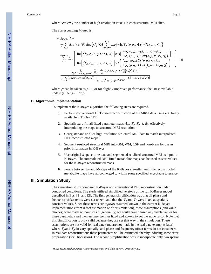
where ν = cPQ the number of high-resolution voxels in each structural MRI slice.
The corresponding M-step is:
[8]
where j* can be taken as j – 1, or for slightly improved performance, the latest availableupdate (either j – 1 or j).
D. Algorithmic ImplementationTo implement the K-Bayes algorithm the following steps are required.
1. Perform conventional DFT-based reconstruction of the MRSI data using e.g. freelyavailable SITools-FITT
2. Spatially zero-fill all fitted parameter maps Am, Ta, Tb, ϕ, B0, effectivelyinterpolating the maps to structural MRI resolution.
3. Coregister and re-slice high-resolution structural MRI data to match interpolatedDFT reconstructed maps.
4. Segment re-sliced structural MRI into GM, WM, CSF and non-brain for use asprior information in K-Bayes.
5. Use original k-space-time data and segmented re-sliced structural MRI as input toK-Bayes. The interpolated DFT fitted metabolite maps can be used as start valuesfor the K-Bayes reconstructed maps.
6. Iterate between E- and M-steps of the K-Bayes algorithm until the reconstructedmetabolite maps have all converged to within some specified acceptable tolerance.
III. Simulation StudyThe simulation study compared K-Bayes and conventional DFT reconstruction undercontrolled conditions. The study utilized simplified versions of the full K-Bayes modeldescribed in Eqs. [1] and [2]. The first general simplification was that all phase andfrequency offset terms were set to zero and that the Ta and Tb were fixed at spatiallyconstant values. Since these terms are a priori assumed known in the current K-Bayesimplementation (from direct estimation or prior simulation), these assumptions (and valuechoices) were made without loss of generality; we could have chosen any viable values forthese parameters and then assume them as fixed and known to get the same result. Note thatthis simplification is only valid because they are set that way in the simulation. Theseassumptions are not valid for real data (and are not made in the real data examples later)where Ta and Tb do vary spatially, and phase and frequency offset terms do not equal zero.In real data reconstructions these parameters will be estimated, thereby inducing some errorpropagation (see Discussion). The second simplification was to incorporate only two spatial
Kornak et al. Page 9
IEEE Trans Med Imaging. Author manuscript; available in PMC 2010 July 29.
NIH
-PA Author Manuscript
NIH
-PA Author Manuscript
NIH
-PA Author Manuscript
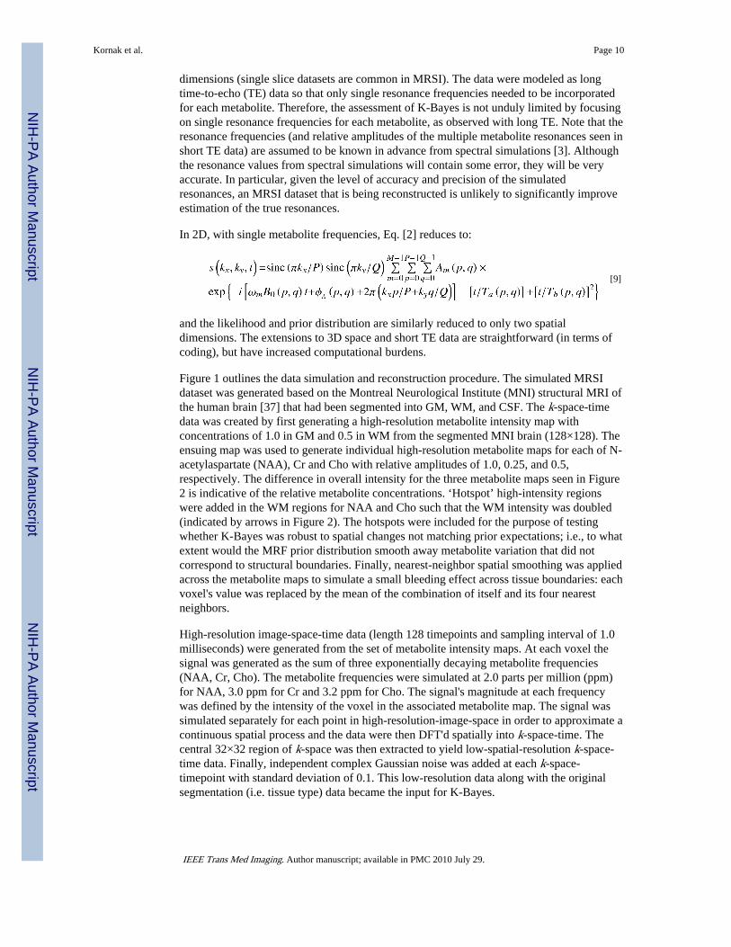
dimensions (single slice datasets are common in MRSI). The data were modeled as longtime-to-echo (TE) data so that only single resonance frequencies needed to be incorporatedfor each metabolite. Therefore, the assessment of K-Bayes is not unduly limited by focusingon single resonance frequencies for each metabolite, as observed with long TE. Note that theresonance frequencies (and relative amplitudes of the multiple metabolite resonances seen inshort TE data) are assumed to be known in advance from spectral simulations [3]. Althoughthe resonance values from spectral simulations will contain some error, they will be veryaccurate. In particular, given the level of accuracy and precision of the simulatedresonances, an MRSI dataset that is being reconstructed is unlikely to significantly improveestimation of the true resonances.
In 2D, with single metabolite frequencies, Eq. [2] reduces to:
[9]
and the likelihood and prior distribution are similarly reduced to only two spatialdimensions. The extensions to 3D space and short TE data are straightforward (in terms ofcoding), but have increased computational burdens.
Figure 1 outlines the data simulation and reconstruction procedure. The simulated MRSIdataset was generated based on the Montreal Neurological Institute (MNI) structural MRI ofthe human brain [37] that had been segmented into GM, WM, and CSF. The k-space-timedata was created by first generating a high-resolution metabolite intensity map withconcentrations of 1.0 in GM and 0.5 in WM from the segmented MNI brain (128×128). Theensuing map was used to generate individual high-resolution metabolite maps for each of N-acetylaspartate (NAA), Cr and Cho with relative amplitudes of 1.0, 0.25, and 0.5,respectively. The difference in overall intensity for the three metabolite maps seen in Figure2 is indicative of the relative metabolite concentrations. ‘Hotspot’ high-intensity regionswere added in the WM regions for NAA and Cho such that the WM intensity was doubled(indicated by arrows in Figure 2). The hotspots were included for the purpose of testingwhether K-Bayes was robust to spatial changes not matching prior expectations; i.e., to whatextent would the MRF prior distribution smooth away metabolite variation that did notcorrespond to structural boundaries. Finally, nearest-neighbor spatial smoothing was appliedacross the metabolite maps to simulate a small bleeding effect across tissue boundaries: eachvoxel's value was replaced by the mean of the combination of itself and its four nearestneighbors.
High-resolution image-space-time data (length 128 timepoints and sampling interval of 1.0milliseconds) were generated from the set of metabolite intensity maps. At each voxel thesignal was generated as the sum of three exponentially decaying metabolite frequencies(NAA, Cr, Cho). The metabolite frequencies were simulated at 2.0 parts per million (ppm)for NAA, 3.0 ppm for Cr and 3.2 ppm for Cho. The signal's magnitude at each frequencywas defined by the intensity of the voxel in the associated metabolite map. The signal wassimulated separately for each point in high-resolution-image-space in order to approximate acontinuous spatial process and the data were then DFT'd spatially into k-space-time. Thecentral 32×32 region of k-space was then extracted to yield low-spatial-resolution k-space-time data. Finally, independent complex Gaussian noise was added at each k-space-timepoint with standard deviation of 0.1. This low-resolution data along with the originalsegmentation (i.e. tissue type) data became the input for K-Bayes.
Kornak et al. Page 10
IEEE Trans Med Imaging. Author manuscript; available in PMC 2010 July 29.
NIH
-PA Author Manuscript
NIH
-PA Author Manuscript
NIH
-PA Author Manuscript
We tested different combinations of values for σ2, , , and within the model, andfound that the resulting reconstructions were reasonably robust to specification of thesmoothing parameters in the MRF model. The actual values used for the simulation results
shown in Figure 2 were σ2 = 0.1, , , and , with the values keptthe same for all metabolites, m. The increased strength of a priori smoothness in GM over
WM (i.e. compared with ) is required to balance the reducedconnectedness amongst GM neighbors as compared with WM (i.e., because GM consists ofthe relatively thin surface of the cortex). The absolute value of σ2 does not directly influencethe posterior estimation of the metabolite maps; only the relative magnitude of σ2 comparedwith the prior smoothing parameters is important. This lack of identifiability for the
combined set of σ2, , , and can be seen by examination of the M-step of the EMalgorithm in Eq. [8].
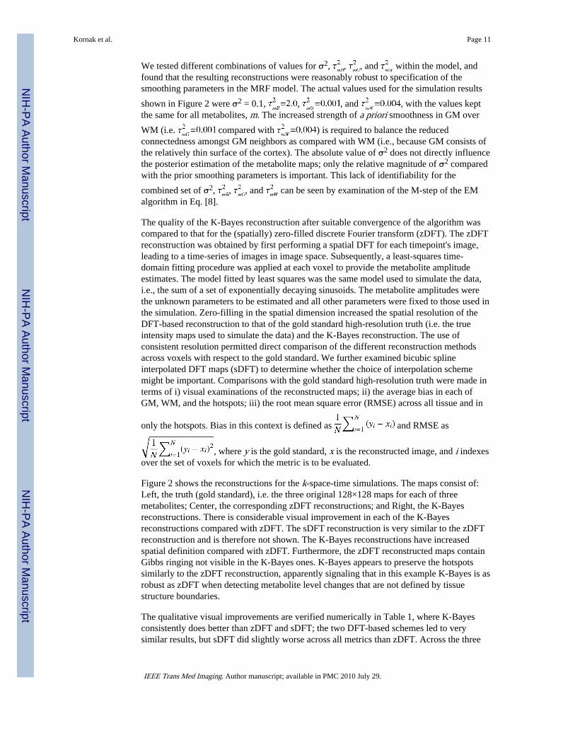
The quality of the K-Bayes reconstruction after suitable convergence of the algorithm wascompared to that for the (spatially) zero-filled discrete Fourier transform (zDFT). The zDFTreconstruction was obtained by first performing a spatial DFT for each timepoint's image,leading to a time-series of images in image space. Subsequently, a least-squares time-domain fitting procedure was applied at each voxel to provide the metabolite amplitudeestimates. The model fitted by least squares was the same model used to simulate the data,i.e., the sum of a set of exponentially decaying sinusoids. The metabolite amplitudes werethe unknown parameters to be estimated and all other parameters were fixed to those used inthe simulation. Zero-filling in the spatial dimension increased the spatial resolution of theDFT-based reconstruction to that of the gold standard high-resolution truth (i.e. the trueintensity maps used to simulate the data) and the K-Bayes reconstruction. The use ofconsistent resolution permitted direct comparison of the different reconstruction methodsacross voxels with respect to the gold standard. We further examined bicubic splineinterpolated DFT maps (sDFT) to determine whether the choice of interpolation schememight be important. Comparisons with the gold standard high-resolution truth were made interms of i) visual examinations of the reconstructed maps; ii) the average bias in each ofGM, WM, and the hotspots; iii) the root mean square error (RMSE) across all tissue and in
only the hotspots. Bias in this context is defined as and RMSE as
, where y is the gold standard, x is the reconstructed image, and i indexesover the set of voxels for which the metric is to be evaluated.
Figure 2 shows the reconstructions for the k-space-time simulations. The maps consist of:Left, the truth (gold standard), i.e. the three original 128×128 maps for each of threemetabolites; Center, the corresponding zDFT reconstructions; and Right, the K-Bayesreconstructions. There is considerable visual improvement in each of the K-Bayesreconstructions compared with zDFT. The sDFT reconstruction is very similar to the zDFTreconstruction and is therefore not shown. The K-Bayes reconstructions have increasedspatial definition compared with zDFT. Furthermore, the zDFT reconstructed maps containGibbs ringing not visible in the K-Bayes ones. K-Bayes appears to preserve the hotspotssimilarly to the zDFT reconstruction, apparently signaling that in this example K-Bayes is asrobust as zDFT when detecting metabolite level changes that are not defined by tissuestructure boundaries.
The qualitative visual improvements are verified numerically in Table 1, where K-Bayesconsistently does better than zDFT and sDFT; the two DFT-based schemes led to verysimilar results, but sDFT did slightly worse across all metrics than zDFT. Across the three
Kornak et al. Page 11
IEEE Trans Med Imaging. Author manuscript; available in PMC 2010 July 29.
NIH
-PA Author Manuscript
NIH
-PA Author Manuscript
NIH
-PA Author Manuscript
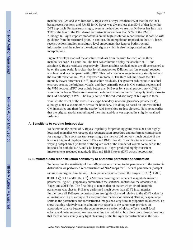
metabolites, GM and WM bias for K-Bayes was always less than 6% of that for the DFT-based reconstructions, and RMSE for K-Bayes was always less than 50% of that for eitherDFT approach. Perhaps surprisingly, even in the hotspot we see that K-Bayes has less than35% of the bias of the DFT-based reconstructions and less than 50% of the RMSE.Although K-Bayes imposes smoothness on the high-resolution reconstruction it does so withguidance from the structural prior. In contrast, the interpolation imposed on the DFT-basedreconstructions implies an arbitrary level smoothness that ignores both structuralinformation and the noise in the original signal (which is also incorporated into theinterpolation).
Figure 3 displays maps of the absolute residuals from the truth for each of the threemetabolites NAA, Cr and Cho. The first two columns display the absolute zDFT andabsolute K-Bayes residuals, respectively. These absolute residual maps are all constrained tobe on the same scale. It is clear that for all metabolites K-Bayes has (on average) reducedabsolute residuals compared with zDFT. This reduction in average intensity simply reflectsthe overall reduction in RMSE expressed in Table 1. The third column shows the zDFTminus K-Bayes difference (Diff.) in absolute residuals. The greatest reductions in residualerror are seen as the brightest voxels, and they primarily occur in GM cortical regions andthe WM hotspot. zDFT does a little better than K-Bayes for a small proportion (~10%) ofvoxels in the brain. These are shown as the darkest voxels in the Diff. map, typically close tothe GM boundary in WM. The likely cause of the reduced accuracy of K-Bayes in these
voxels is the effect of the cross-tissue-type boundary smoothing/variance parameter ;although zDFT also smoothes across the boundary, it is doing so based on underestimatedGM intensities and therefore the nearby WM intensities are less elevated. (It is noted earlierthat the original spatial smoothing of the simulated data was applied in a highly localizedfashion.)
A. Sensitivity to varying hotspot sizeTo determine the extent of K-Bayes’ capability for providing gains over zDFT for highlylocalized anomalies we repeated the reconstruction procedure and performed comparisonsfor a range of hotspot sizes (not surprisingly the metrics did not vary much outside of thehotspot). Figure 4 displays plots of Bias and RMSE for zDFT and K-Bayes across thevarying hotspot sizes (in terms of the square root of the number of voxels contained in thehotspot) for both the NAA and Cho hotspots. K-Bayes produced highly consistentimprovements (reduced magnitude Bias and RMSE) over zDFT across hotpot sizes.
B. Simulated data reconstruction sensitivity to anatomic parameter specificationTo determine the sensitivity of the K-Bayes reconstruction to the parameters of the anatomicdistribution we performed reconstructions of NAA maps for 16 sets of parameters (hotspot
radius as in original simulation). These parameter sets covered the ranges ,
and : thus covering two orders of magnitude in eachparameter. Figure 5 graphically summarizes the statistical metrics for the associated K-Bayes and zDFT fits. The first thing to note is that no matter which set of anatomicparameters was chosen, K-Bayes performed much better than zDFT in all metrics.Furthermore all K-Bayes reconstructions are tightly clustered relative to the zDFT value forall metrics (with just a couple of exceptions for the hotspot metrics). That is, despite largeshifts in the parameters, the reconstructed images had very similar properties in all cases. Toshow that this relatively stable solution with respect to the parameters provides anappropriate balance between the accurate reconstruction of global effects, small focaleffects, and noise removal, we must examine the individual box plots more closely. We notethat there is consistently very tight clustering of the K-Bayes reconstructions in the non-
Kornak et al. Page 12
IEEE Trans Med Imaging. Author manuscript; available in PMC 2010 July 29.
NIH
-PA Author Manuscript
NIH
-PA Author Manuscript
NIH
-PA Author Manuscript
hotspot metrics. For the hotspot metrics we see two exceptions. One set of parameters thatleads to an outlier (lowest a priori smoothness level) only increases the RMSE. In thesecases the hotspot is flattened by too strong smoothing parameters causing increased bias andRMSE simultaneously (all the error is to one side of the truth). Nonetheless, even these mostlimited of K-Bayes reconstructions still have greatly improved hotspot bias and RMSEcompared with zDFT.
This sensitivity analysis indicates that K-Bayes is robust to a wide range of anatomicparameter sets and hence that the optimal balance between the anatomic information and thek-space-time data is well defined by the two data sources and not substantially influenced byany particular choice of parameter set.
Overall, these simulation results generate a very encouraging assessment of the potentialgains afforded by K-Bayes in the reconstruction of MRSI datasets. However, they doprovide close to an upper bound on the gains because the datasets are generated based on theK-Bayes model. That is, the signal model used is from the likelihood, and the metabolitemaps are generated from the structural information (albeit with added blurring and hotspots).Inaccuracies in the signal model will equally propagate into errors for DFT-basedreconstructions as well as K-Bayes. The potential realization of the relative gains of K-Bayes for real data reconstruction is therefore bounded by the extent to which differentialsin metabolite levels respect tissue boundaries. Despite this limitation, some gains are madeby K-Bayes in the simulation study even when metabolite differentials do not match thetissue boundaries, i.e. in the hotspot.
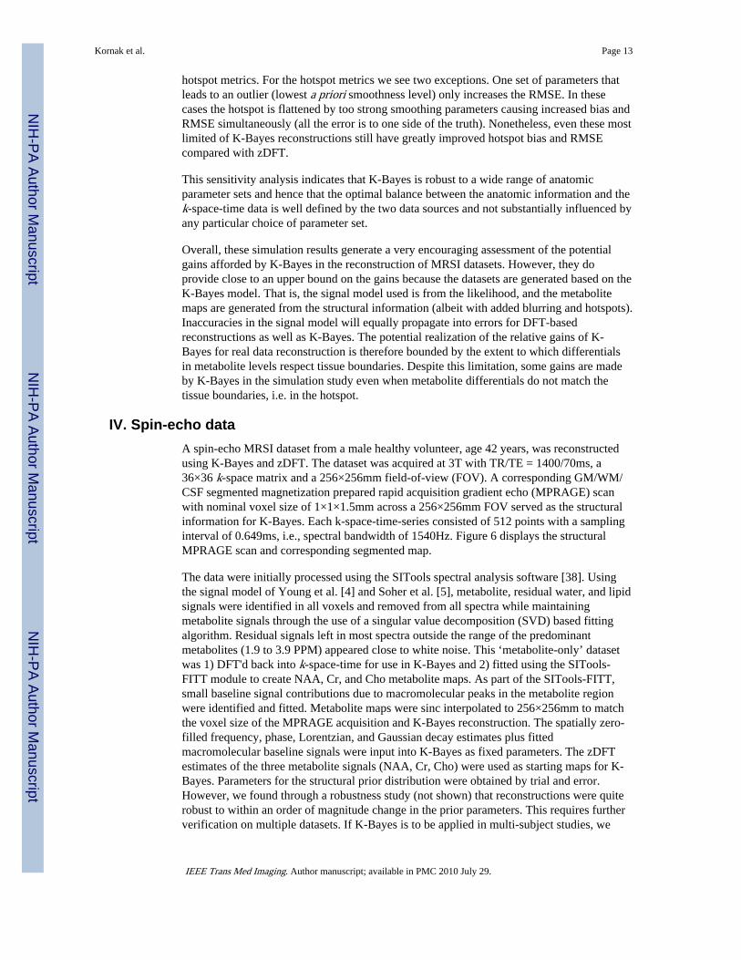
IV. Spin-echo dataA spin-echo MRSI dataset from a male healthy volunteer, age 42 years, was reconstructedusing K-Bayes and zDFT. The dataset was acquired at 3T with TR/TE = 1400/70ms, a36×36 k-space matrix and a 256×256mm field-of-view (FOV). A corresponding GM/WM/CSF segmented magnetization prepared rapid acquisition gradient echo (MPRAGE) scanwith nominal voxel size of 1×1×1.5mm across a 256×256mm FOV served as the structuralinformation for K-Bayes. Each k-space-time-series consisted of 512 points with a samplinginterval of 0.649ms, i.e., spectral bandwidth of 1540Hz. Figure 6 displays the structuralMPRAGE scan and corresponding segmented map.
The data were initially processed using the SITools spectral analysis software [38]. Usingthe signal model of Young et al. [4] and Soher et al. [5], metabolite, residual water, and lipidsignals were identified in all voxels and removed from all spectra while maintainingmetabolite signals through the use of a singular value decomposition (SVD) based fittingalgorithm. Residual signals left in most spectra outside the range of the predominantmetabolites (1.9 to 3.9 PPM) appeared close to white noise. This ‘metabolite-only’ datasetwas 1) DFT'd back into k-space-time for use in K-Bayes and 2) fitted using the SITools-FITT module to create NAA, Cr, and Cho metabolite maps. As part of the SITools-FITT,small baseline signal contributions due to macromolecular peaks in the metabolite regionwere identified and fitted. Metabolite maps were sinc interpolated to 256×256mm to matchthe voxel size of the MPRAGE acquisition and K-Bayes reconstruction. The spatially zero-filled frequency, phase, Lorentzian, and Gaussian decay estimates plus fittedmacromolecular baseline signals were input into K-Bayes as fixed parameters. The zDFTestimates of the three metabolite signals (NAA, Cr, Cho) were used as starting maps for K-Bayes. Parameters for the structural prior distribution were obtained by trial and error.However, we found through a robustness study (not shown) that reconstructions were quiterobust to within an order of magnitude change in the prior parameters. This requires furtherverification on multiple datasets. If K-Bayes is to be applied in multi-subject studies, we
Kornak et al. Page 13
IEEE Trans Med Imaging. Author manuscript; available in PMC 2010 July 29.
NIH
-PA Author Manuscript
NIH
-PA Author Manuscript
NIH
-PA Author Manuscript
advocate that a structured approach to parameter setting be taken, such as that described inSection III.
The reconstructed maps in Figure 7 show that K-Bayes produces additional detail (relativeto zDFT reconstruction) unrelated to the underlying anatomy as well as showing variationclearly related to anatomy. These encouraging results suggest that K-Bayes is capable offinding a reasonable balance between the accurate reconstruction of global effects, smallfocal effects, and noise.
A. Sensitivity analysis of spin-echo data reconstructions to anatomic parameter settingsTo determine the sensitivity of K-Bayes to the parameters of the anatomic distribution, weperformed reconstructions for 8 sets of anatomic parameters. For the three parameters, these
8 sets covered the range , , . Theseranges are all greater than an order of magnitude. Although the ranges appear different fromthose in the simulation, they are in fact quite similar in the relative magnitude of theparameters to the (square of the) range of the data.
The eight K-Bayes reconstructed NAA maps are shown in Figure 8, contrasted with thesingle zDFT reconstruction. (We show only figures since we lack a gold standard withwhich to assess statistical metrics.) Clearly, variation in K-Bayes reconstructions is smallcompared to the difference between them and the zDFT reconstruction, indicating that K-Bayes is robust to a wide range of anatomical distribution parameter sets. Thus the optimalway to balance anatomic and k-space-time data is well defined in the data sourcesthemselves. More precisely, the location of the posterior maximum (the optimalreconstruction) does not vary greatly for a wide range of prior smoothing parameter values;despite large shifts in parameters, the image at the posterior maximum is quite similar in allcases.
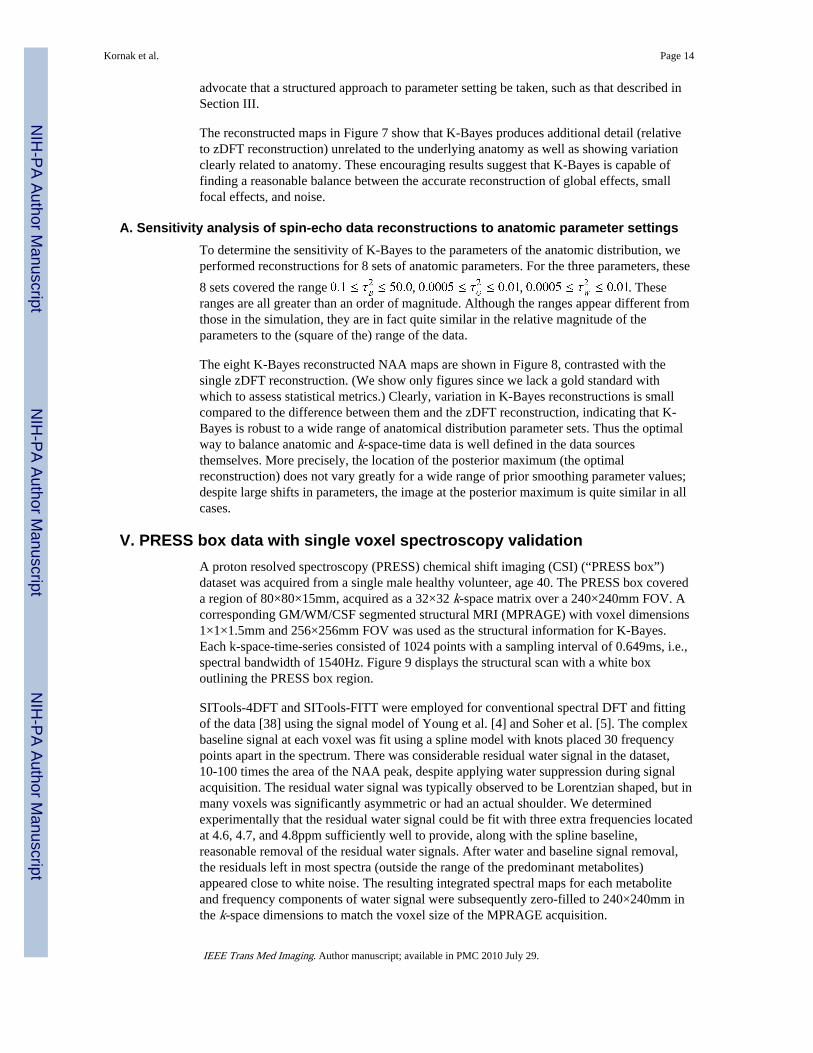
V. PRESS box data with single voxel spectroscopy validationA proton resolved spectroscopy (PRESS) chemical shift imaging (CSI) (“PRESS box”)dataset was acquired from a single male healthy volunteer, age 40. The PRESS box covereda region of 80×80×15mm, acquired as a 32×32 k-space matrix over a 240×240mm FOV. Acorresponding GM/WM/CSF segmented structural MRI (MPRAGE) with voxel dimensions1×1×1.5mm and 256×256mm FOV was used as the structural information for K-Bayes.Each k-space-time-series consisted of 1024 points with a sampling interval of 0.649ms, i.e.,spectral bandwidth of 1540Hz. Figure 9 displays the structural scan with a white boxoutlining the PRESS box region.
SITools-4DFT and SITools-FITT were employed for conventional spectral DFT and fittingof the data [38] using the signal model of Young et al. [4] and Soher et al. [5]. The complexbaseline signal at each voxel was fit using a spline model with knots placed 30 frequencypoints apart in the spectrum. There was considerable residual water signal in the dataset,10-100 times the area of the NAA peak, despite applying water suppression during signalacquisition. The residual water signal was typically observed to be Lorentzian shaped, but inmany voxels was significantly asymmetric or had an actual shoulder. We determinedexperimentally that the residual water signal could be fit with three extra frequencies locatedat 4.6, 4.7, and 4.8ppm sufficiently well to provide, along with the spline baseline,reasonable removal of the residual water signals. After water and baseline signal removal,the residuals left in most spectra (outside the range of the predominant metabolites)appeared close to white noise. The resulting integrated spectral maps for each metaboliteand frequency components of water signal were subsequently zero-filled to 240×240mm inthe k-space dimensions to match the voxel size of the MPRAGE acquisition.
Kornak et al. Page 14
IEEE Trans Med Imaging. Author manuscript; available in PMC 2010 July 29.
NIH
-PA Author Manuscript
NIH
-PA Author Manuscript
NIH
-PA Author Manuscript
ZDFT reconstructed maps of the B0, phase, Lorentzian and Gaussian decay map estimates(plus the fitted macromolecular baseline signals) from SITools-FITT were used as fixedquantities in K-Bayes. The corresponding zDFT map estimates from SITools-FITT of thethree metabolite signals (NAA, Cr, Cho), as well as the three frequency components ofwater signal, were used as starting maps for K-Bayes. Parameters for the structural priordistribution were obtained by trial and error. There appeared to be more sensitivity in thereconstruction to the specific choice of parameter values for the PRESS box reconstruction.This is possibly due to the limitations of using K-Bayes with this particular PRESS boxdataset, as discussed below).
Figure 10 displays zDFT and K-Bayes reconstructed maps of NAA, Cr, and Cho.Qualitatively, K-Bayes produces improved definition and reduced noise in the reconstructedmetabolite maps. Although these PRESS results demonstrate feasibility, there arelimitations. The PRESS box dataset is far from the ideal form for utilizing K-Bayes; therewas a sharp drop-off at the top of the PRESS box that led to bias in the neighboringhomogeneous tissue regions that do contain signal affected by the MRF prior (i.e., biasedtowards zero in regions of high signal). Note that the conservative approach was taken byassuming that the prior PRESS box segmented tissue map corresponded to the a prioridefined PRESS box. This approach is in contrast to trying to determine the PRESS box afterlooking at the data. Further evidence of the inaccuracy in spatial localization of the PRESSbox can be seen in the edge-effects of the upper right corner of the K-Bayes reconstructedCho map: any signal outside the demarked PRESS box is likely being “squeezed into theedge of the box”.
A further limitation of both real MRSI data studies was that we only considered a single-slice 2D segmented structural MRI as prior information (the middle slice). Since bothdatasets consisted of 15mm thick slices, there would be variation in tissue compositionalong the slice in the z -direction. Taking z -direction variability into account via 3D spatialmodeling would likely further improve K-Bayes reconstruction quality. This is discussedfurther in the next section.
VI. Summary and DiscussionA. Summary
Although MRSI provides useful regional information on metabolite levels in the brain, theresults of conventional reconstruction methods are limited by the low spatial resolutioninherent in the data acquisition imposed by typical signal to noise ratio considerations. K-Bayes can help quantify regional metabolite levels with much greater precision than thatattainable through DFT/spectral-integration-based reconstruction. The increased precision isdue to the enhanced spatial specification obtained by incorporating segmented structuralMRI prior information, and the use of a full signal model for the k-space-time data. Theincreased precision of estimated metabolite levels could considerably benefit clinical studiesthat quantify regional differences in metabolite concentrations between different subjectpopulations (e.g. patients with Alzheimer's disease versus healthy controls). The extraaccuracy obtained by K-Bayes could be crucial in detecting real differences between diseasestates. Furthermore, the use of K-Bayes could expand to non-brain applications of MRSI.All that is required to implement K-Bayes is a high-resolution structural segmentation of theanatomy along with a physiologically reasonable model of the distribution of metabolitesconcentrations within and between structurally homogeneous regions.
B. On advance estimation of maps using FITTIn the current implementation of K-Bayes the maps Ta(x,y,z), Tb(x,y,z), ϕa(x,y,z) andB0(x,y,z) are estimated in advance using SITools-FITT, raising a question as to how use of
Kornak et al. Page 15
IEEE Trans Med Imaging. Author manuscript; available in PMC 2010 July 29.
NIH
-PA Author Manuscript
NIH
-PA Author Manuscript
NIH
-PA Author Manuscript
these zDFT results might be affecting the K-Bayes results through error propagation. Thedegree of this potential error propagation would depend on the true relative smoothness ofeach map (i.e. the smoothness of the actual underlying process). Our assumption is that thesemaps vary more slowly in practice than the metabolite maps do, especially at tissueboundaries and in particular at brain edges. This seems reasonable. K-Bayes does providevisual improvements in the metabolite maps. Since the errors in Ta(x,y,z), Tb(x,y,z),ϕa(x,y,z) and B0(x,y,z) are common to both K-Bayes and zDFT reconstruction, one assumesthat the improvements derive from K-Bayes despite the limitations of the propagated error.In the future, if estimation of these parameter maps becomes feasible as extra estimationsteps within the K-Bayes process (via planned algorithmic enhancements) we expect furtherimprovements in metabolite quantification from K-Bayes.
C. On the variation of T2 with respect to metabolite peaksWe know that the terms Ta(x,y,z) and Tb(x,y,z) can vary as a function of metabolite, and thismay have important consequences, particularly in short-TE applications where spectralpeaks with a wide range of T2 values are present. However, our choice to ignore it in themodel presented deserves justification.
Currently, Ta(x,y,z) and Tb(x,y,z) are estimated in advance via SITools-FITT. There is infact an undocumented provision in the SITools-FITT software package to fit differentTa(x,y,z) and Tb(x,y,z) for distinct metabolite peaks. If these maps are obtained, then verylittle additional effort or computation is required to extend the K-Bayes model to incorporatethe additional maps (other than a little extra memory requirement). However, we opted notto utilize this option because current SNR values for spectroscopic imaging data for coupledmetabolites (those for which this provision would matter) make it extremely difficult toquantify such subtle differences. In fact, other effects, such as the chemical shift effect andother spatial effects due to the presence of gradients, currently dominate variations in T2 forin vivo data [39, 40]. In the case of strongly coupled metabolites, properly labelingmetabolite peaks in terms of multiplet group is a difficult theoretical problem, in particularfor strongly coupled metabolites, while separately fitting Ta(x,y,z) and Tb(x,y,z) for everypeak in every voxel would lead to an infeasible spectral fitting problem. Therefore, somework remains in terms of devising an optimal strategy for including Ta(x,y,z) and Tb(x,y,z)variation over peaks for spectral fitting. One advantage to generation of prior spectralinformation via phantom measurement is that it might principle provide information on suchvariations [41] in which case this information could be incorporated into a K-Bayes analysis.But in practice any such differences are currently too subtle to detect and the mostsignificant differences would be expected to arise in the case in-vivo data for whichphantom generated prior information provides no advantage.
In the long run we aim to incorporate estimation of Ta(x,y,z) and Tb(x,y,z) within the K-Bayes framework as maps to be estimated via additional M-steps (at the cost of considerableextra computational complexity). As part of this process we will consider the extension toinclude separate maps for each line or/and multiplet. To ensure a tractable solution to thisextension, additional prior assumptions may be required to relate maps of differentmetabolite peaks to each other.
D. On the issue of MRI versus MRSI slice thicknessIn our real data examples (spin-echo and PRESS) the slice thickness of the MRSI was muchthicker than that of the corresponding structural MRI slice used as prior information. The15mm slice will contain partial voluming effects since the tissue structure will not beperfectly homogeneous across the MRSI slice. This is a notable limitation of the real dataexamples. The complete solution is to extend application of K-Bayes to full 3D-space
Kornak et al. Page 16
IEEE Trans Med Imaging. Author manuscript; available in PMC 2010 July 29.
NIH
-PA Author Manuscript
NIH
-PA Author Manuscript
NIH
-PA Author Manuscript
datasets. Considerable computational enhancement will be required in order to make thispractical.
In our spin-echo and PRESS data examples, we selected the central segmented structuralMRI slice to define the anatomical prior information in the simplified 2D space case ratherthan the many other reasonable choices: e.g. defining a prior over blurred boundaries ortaking the voxel-wise tissue class mode across all structural MRI slices. We chose thecentral slice partly for simplicity, partly because it represents the tissue class at the point ofhighest excitation in the slice, and finally because the central anatomic image represents atrue slice through the brain, which is helpful for visualization purposes.
E. Future applicabilityTwo methodological issues should be addressed before K-Bayes can achieve more generalapplicability. The first is that the method requires good co-registration of segmentedstructural MRI with MRSI data. Similarly, poor quality segmentation can reduce the benefitsof K-Bayes. Poor segmentation again corresponds to poor prior information, though unlessthe segmentation has high mis-classification rates, the problems associated with low-resolution MRSI data will be worse than any error introduced by inaccurate segmentation.The second (and primary) issue encountered with using K-Bayes is computational time. The2D reconstruction examples were performed on a Dell Precision 370 desktop computerrunning RedHat Enterprise Linux 4.0 on a single thread of an Intel Xeon 2.33GHzprocessor. These were programmed in C and compiled with a gcc compiler. Reconstructionsreached reasonable convergence in a day. Although it is impractical to achieve fullconvergence to the level of machine tolerance, the statistical metrics of the reconstructionsdid not change significantly after this time. Parallelization similar to that used in [10] willhelp to significantly reduce computational time. Because the algorithm is highlyparallelizable, a large reduction in computational time can be achieved by distributing theprocessing and spreading the memory load amongst multiple processors. The benefit ofparallelization will potentially be greater than linear speed up with the number of processors,because the significant memory burden will be distributed as well. Computationalimprovement of this level would potentially allow for K-Bayes to be used as a routineapproach for obtaining high-resolution and accurate metabolite maps. Given the decreasingprices for multiprocessor supercomputers and random access memory (RAM), there is greatpotential for K-Bayes to become widely applicable in clinical settings.
AcknowledgmentsThis work was supported by a Society for Imaging Informatics in Medicine (SIIM) research grant; NIH grants R01NS41946, P41 RR023953, R01 EB008387. We acknowledge the San Francisco Veterans Affairs Medical Centerwhere part of this work was performed.
Appendix
Derivation of K-Bayes E- and M-stepsE-step
The E-step update applied to each missing data point z(kx,ky,p,q,r,w,t,m) is determined byits expectation given the data and the set of metabolite maps A: E[z(kx,ky,p,q,r,w,t,m)|d,A] =E[z(kx,ky,p,q,r,w,t,m)|d(kx,ky,w,t),A], where z(kx,ky,p,q,r,w,t,m) is only defined when the r -th slice of the structural MRI is contained within the w -th slice of the MRSI. Note that thevalue of r effectively defines that for w though we keep w as a parameter of z for notationalclarity.
Kornak et al. Page 17
IEEE Trans Med Imaging. Author manuscript; available in PMC 2010 July 29.
NIH
-PA Author Manuscript
NIH
-PA Author Manuscript
NIH
-PA Author Manuscript

Bayes’ Theorem gives
Now,
where ν = cPQ
Therefore,
Completing the square, this leads to
Kornak et al. Page 18
IEEE Trans Med Imaging. Author manuscript; available in PMC 2010 July 29.
NIH
-PA Author Manuscript
NIH
-PA Author Manuscript
NIH
-PA Author Manuscript

Therefore, π(z(kx,ky,p,q,r,w,t,m)|d(kx,ky,w,t),A) is complex Gaussian with mean
and the j th E-step update for z(kx,ky,p,q,r,w,t,m) is,
M-stepTo generate the M-step, the log-posterior distribution, log (π(Am(p,q,r)|z,Ȃm(p,q,r)) ismaximized with respect to , where Ȃm(p,q,r) corresponds to all elements of A other thanAm(p,q,r).
Differentiating the log-posterior distribution with respect to Am(p,q,r) and setting equal tozero gives
Kornak et al. Page 19
IEEE Trans Med Imaging. Author manuscript; available in PMC 2010 July 29.
NIH
-PA Author Manuscript
NIH
-PA Author Manuscript
NIH
-PA Author Manuscript
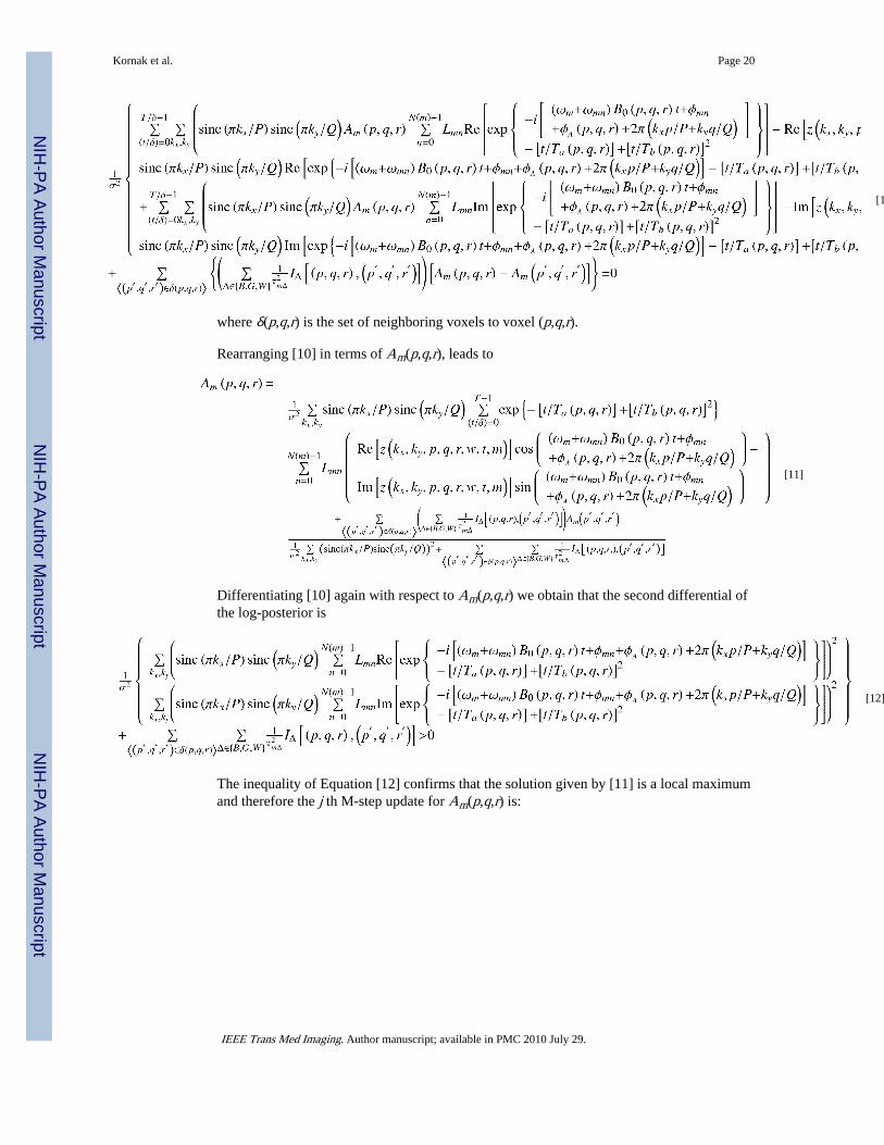
[10]
where δ(p,q,r) is the set of neighboring voxels to voxel (p,q,r).
Rearranging [10] in terms of Am(p,q,r), leads to
[11]
Differentiating [10] again with respect to Am(p,q,r) we obtain that the second differential ofthe log-posterior is
[12]
The inequality of Equation [12] confirms that the solution given by [11] is a local maximumand therefore the j th M-step update for Am(p,q,r) is:
Kornak et al. Page 20
IEEE Trans Med Imaging. Author manuscript; available in PMC 2010 July 29.
NIH
-PA Author Manuscript
NIH
-PA Author Manuscript
NIH
-PA Author Manuscript

[13]
References1. Brown TR, Kincaid BM, Ugurbil K. NMR chemical shift imaging in three dimensions. Proceedings
of the National Academy of Sciences. 1982; 79:3523–3526.
2. Maudsley AA, Hilal SK, Perman WH, Simon HE. Spatially resolved high resolution spectroscopyby four-dimensional NMR. J Magn Reson. 1983; 51:147–152.
3. Young K, Govindaraju V, Soher BJ, Maudsley AA. Automated spectral analysis I: formation of apriori information by spectral simulation. Magn Reson Med. Dec.1998 40:812–5. [PubMed:9840824]
4. Young K, Soher BJ, Maudsley AA. Automated spectral analysis II: application of wavelet shrinkagefor characterization of non-parameterized signals. Magn Reson Med. Dec.1998 40:816–21.[PubMed: 9840825]
5. Soher BJ, Young K, Govindaraju V, Maudsley AA. Automated spectral analysis III: application toin vivo proton MR spectroscopy and spectroscopic imaging. Magn Reson Med. Dec.1998 40:822–31. [PubMed: 9840826]
6. de Beer R, van den Boogaart A, van Ormondt D, Pijnappel WW, den Hollander JA, Marien AJ,Luyten PR. Application of time-domain fitting in the quantification of in vivo 1H spectroscopicimaging data sets. NMR Biomed. 1992; 5:171–178. [PubMed: 1449952]
7. Liang, Z-P.; Lauterbur, PC.; IEEE Engineering in Medicine and Biology Society. Principles ofmagnetic resonance imaging : a signal processing perspective. SPIE Optical Engineering Press;IEEE Press; Bellingham, Wash. New York: 2000.
8. Hurn MA, Mardia KV, Hainsworth TJ, Kirkbridge J, Berry E. Bayesian Fused Classification ofMedical Images. IEEE Transactions on Medical Imaging. 1996; 15:850–858. [PubMed: 18215964]
9. Miller IM, Schaewe TJ, Cohen SB, Ackerman JJH. Model-Based Maximum-Likelihood Estimationfor Phase- and Frequency-Encoded Magnetic-Resonance-Imaging Data. Journal of MagneticResonance, Series B. 1995; 107:10–221.
10. Schaewe TJ, Miller IM. Parallel Algorithms for Maximum A Posteriori Estimation of Spin Densityand Spin-spin Decay in Magnetic Resonance Imaging. IEEE Transactions on Medical Imaging.1995:362–373. [PubMed: 18215839]
11. Denney TS Jr. Reeves SJ. Bayesian image reconstruction from Fourier-domain samples using prioredge information. Journal of Electronic Imaging. 2005; 14:043009, 1–11. 2005.
12. Ouyang X, Wong WH, Johnson VE, Hu X, Chen C-T. Incorporation of Correlated StructuralImages in PET Image Reconstruction. IEEE Transactions on Medical Imaging. 1994; 13:627–640.[PubMed: 18218541]
13. Bowsher JE, Johnson VE, Turkington TG, Jaszczak RJ, Floyd CE Jr. Coleman RE. BayesianReconstruction and Use of Anatomical A Priori Information for Emission Tomography. IEEETransactions on Medical Imaging. 1996; 15:673–686. [PubMed: 18215949]
14. Sastry S, Carson RE. Multimodality Bayesian Algorithm for Image Reconstruction in PositronEmission Tomography: A Tissue Composition Model. IEEE Transactions on Medical Imaging.1997; 16:750–761. [PubMed: 9533576]
Kornak et al. Page 21
IEEE Trans Med Imaging. Author manuscript; available in PMC 2010 July 29.
NIH
-PA Author Manuscript
NIH
-PA Author Manuscript
NIH
-PA Author Manuscript
15. Hu X, Levin DN, Lauterbur PC, Spraggins T. SLIM: spectral localization by imaging. Magn ResonMed. 1988; 8:314–22. [PubMed: 3205158]
16. Von Kienlin M, Mejia R. Spectral localization with optimal pointspread function. Journal ofmagnetic resonance. 1991; 94:268–287.
17. Liang ZP, Lauterbur PC. A generalized series approach to MR spectroscopic imaging. MedicalImaging, IEEE Transactions on. 1991; 10:132–137.
18. Liang ZP, Lauterbur PC. An efficient method for dynamic magnetic resonance imaging. MedicalImaging, IEEE Transactions on. 1994; 13:677–686.
19. Jacob M, Zhu X, Ebel A, Schuff N, Liang ZP. Improved Model-Based Magnetic ResonanceSpectroscopic Imaging. Medical Imaging, IEEE Transactions on. 2007; 26:1305–1318.
20. Bao Y, Maudsley AA. Improved Reconstruction for MR Spectroscopic Imaging. Medical Imaging,IEEE Transactions on. 2007; 26:686–695.
21. Haldar JP, Hernando D, Song SK, Liang ZP. Anatomically constrained reconstruction from noisydata. Magnetic Resonance in Medicine. 2008; 59:810. [PubMed: 18383297]
22. Kornak J, Young K, Schuff N, Du A, Maudsley AA, Weiner MW. K-Bayes Reconstruction forPerfusion MRI I: Concepts and Application. Journal of Digital Imaging. 2008
23. Kornak J, Young K. K-Bayes Reconstruction for Perfusion MRI II: Modeling and TechnicalDevelopment. Journal of Digital Imaging. 2008
24. Geman S, German D. Stochastic Relaxation, Gibbs Distributions, and the Bayesian Restoration ofImages. IEEE Transactions on Pattern Analysis and Machine Intelligence. 1984; 6:721–741.[PubMed: 22499653]
25. Besag JE. Towards Bayesian Image Analysis. Journal of Applied Statistics. 1989; 16:395–407.
26. Winkler, G. Image Analysis, Random Fields, and Markov Chain Monte Carlo Methods: AMathematical Introduction. 2nd ed.. Springer; 2003.
27. Maudsley A, Domenig C, Govind V, Darkazanli A, Studholme C, Arheart K, Bloomer C. Mappingof brain metabolite distributions by volumetric proton MR spectroscopic imaging (MRSI).Magnetic Resonance in Medicine. 2009; 61
28. Besag JE. Spatial Interaction and The Statistical Analysis of Lattice Systems (with discussion).Journal of the Royal Statistical Society, Series B. 1974; 36:192–236.
29. Dempster AP, Laird NM, Rubin DB. Maximum Likelihood From Incomplete Data Via the EMAlgorithm (with discussion). Journal of the Royal Statistical Society, Series B. 1977; 39:1–38.
30. Ashburner J, Friston KJ. Multimodal Image Coregistration and Partitioning - A UnifiedFramework. NeuroImage. 1997; 6:209–217. [PubMed: 9344825]
31. Zhang Y, Brady M, Smith S. Segmentation of brain MR images through a hidden Markov randomfield model and the expectation-maximization algorithm. IEEE Trans Med Imaging. Jan.200120:45–57. [PubMed: 11293691]
32. Besag JE. Statistical Analysis of Non-lattice Data. The Statistician. 1975; 24:179–195.
33. Kunsch HR. Intrinsic Autoregressions and Related Models on the Two-dimensional Lattice.Biometrika. 1987; 74:517–524.
34. Besag JE, Kooperberg C. On Conditional and Intrinsic Autoregressions. Biometrika. 1995;82:733–746.
35. Green PJ. Bayesian Reconstructions From Emission Tomography Data Using A Modified EMAlgorithm. IEEE Transactions on Medical Imaging. 1990; 9:84–93. [PubMed: 18222753]
36. Cohen, L. Time-frequency analysis: theory and applications. 1995.
37. Cocosco, CA.; Kollokian, V.; Kwan, RK-S.; Evans, AC. BrainWeb: Online Interface to a 3D MRISimulated Brain Database. Proceedings of 3rd International Conference on Functional Mapping ofthe Human Brain; 1997;
38. Maudsley AA, Lin E, Weiner MW. Spectroscopic imaging display and analysis. Magn ResonImaging. 1992; 10:471–85. [PubMed: 1406098]
39. Kaiser LG, Young K, Matson GB. Elimination of spatial interference in PRESS-localized editingspectroscopy. Magnetic resonance in medicine: official journal of the Society of MagneticResonance in Medicine/Society of Magnetic Resonance in Medicine. 2007; 58:813. [PubMed:17899586]
Kornak et al. Page 22
IEEE Trans Med Imaging. Author manuscript; available in PMC 2010 July 29.
NIH
-PA Author Manuscript
NIH
-PA Author Manuscript
NIH
-PA Author Manuscript

40. Kaiser LG, Young K, Matson GB. Numerical simulations of localized high field 1H MRspectroscopy. Journal of Magnetic Resonance. 2008; 195:67–75. [PubMed: 18789736]
41. Provencher S. Automatic quantitation of localized in vivo 1H spectra with LCModel. NMR inBiomedicine. 2001; 14
Kornak et al. Page 23
IEEE Trans Med Imaging. Author manuscript; available in PMC 2010 July 29.
NIH
-PA Author Manuscript
NIH
-PA Author Manuscript
NIH
-PA Author Manuscript
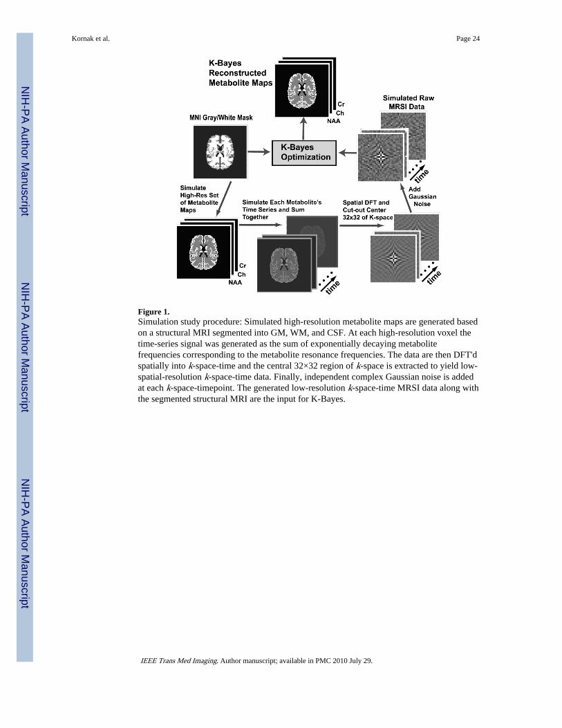
Figure 1.Simulation study procedure: Simulated high-resolution metabolite maps are generated basedon a structural MRI segmented into GM, WM, and CSF. At each high-resolution voxel thetime-series signal was generated as the sum of exponentially decaying metabolitefrequencies corresponding to the metabolite resonance frequencies. The data are then DFT'dspatially into k-space-time and the central 32×32 region of k-space is extracted to yield low-spatial-resolution k-space-time data. Finally, independent complex Gaussian noise is addedat each k-space-timepoint. The generated low-resolution k-space-time MRSI data along withthe segmented structural MRI are the input for K-Bayes.
Kornak et al. Page 24
IEEE Trans Med Imaging. Author manuscript; available in PMC 2010 July 29.
NIH
-PA Author Manuscript
NIH
-PA Author Manuscript
NIH
-PA Author Manuscript
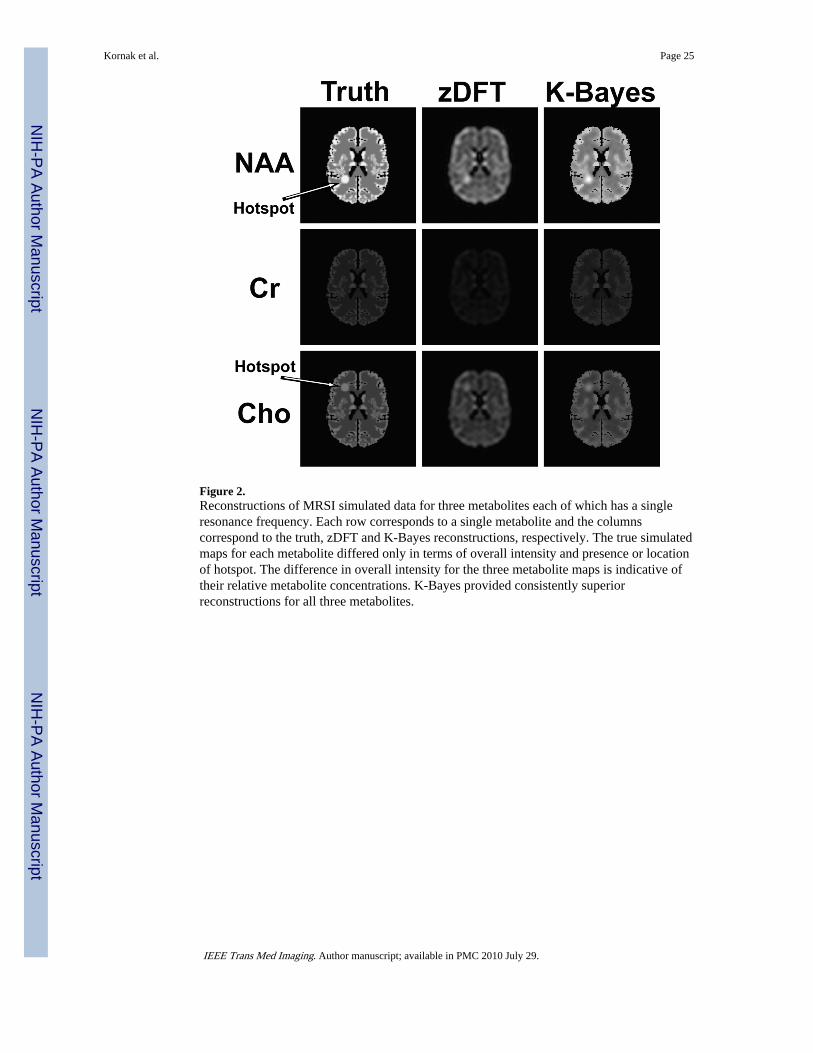
Figure 2.Reconstructions of MRSI simulated data for three metabolites each of which has a singleresonance frequency. Each row corresponds to a single metabolite and the columnscorrespond to the truth, zDFT and K-Bayes reconstructions, respectively. The true simulatedmaps for each metabolite differed only in terms of overall intensity and presence or locationof hotspot. The difference in overall intensity for the three metabolite maps is indicative oftheir relative metabolite concentrations. K-Bayes provided consistently superiorreconstructions for all three metabolites.
Kornak et al. Page 25
IEEE Trans Med Imaging. Author manuscript; available in PMC 2010 July 29.
NIH
-PA Author Manuscript
NIH
-PA Author Manuscript
NIH
-PA Author Manuscript
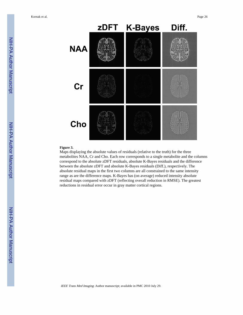
Figure 3.Maps displaying the absolute values of residuals (relative to the truth) for the threemetabolites NAA, Cr and Cho. Each row corresponds to a single metabolite and the columnscorrespond to the absolute zDFT residuals, absolute K-Bayes residuals and the differencebetween the absolute zDFT and absolute K-Bayes residuals (Diff.), respectively. Theabsolute residual maps in the first two columns are all constrained to the same intensityrange as are the difference maps. K-Bayes has (on average) reduced intensity absoluteresidual maps compared with zDFT (reflecting overall reduction in RMSE). The greatestreductions in residual error occur in gray matter cortical regions.
Kornak et al. Page 26
IEEE Trans Med Imaging. Author manuscript; available in PMC 2010 July 29.
NIH
-PA Author Manuscript
NIH
-PA Author Manuscript
NIH
-PA Author Manuscript
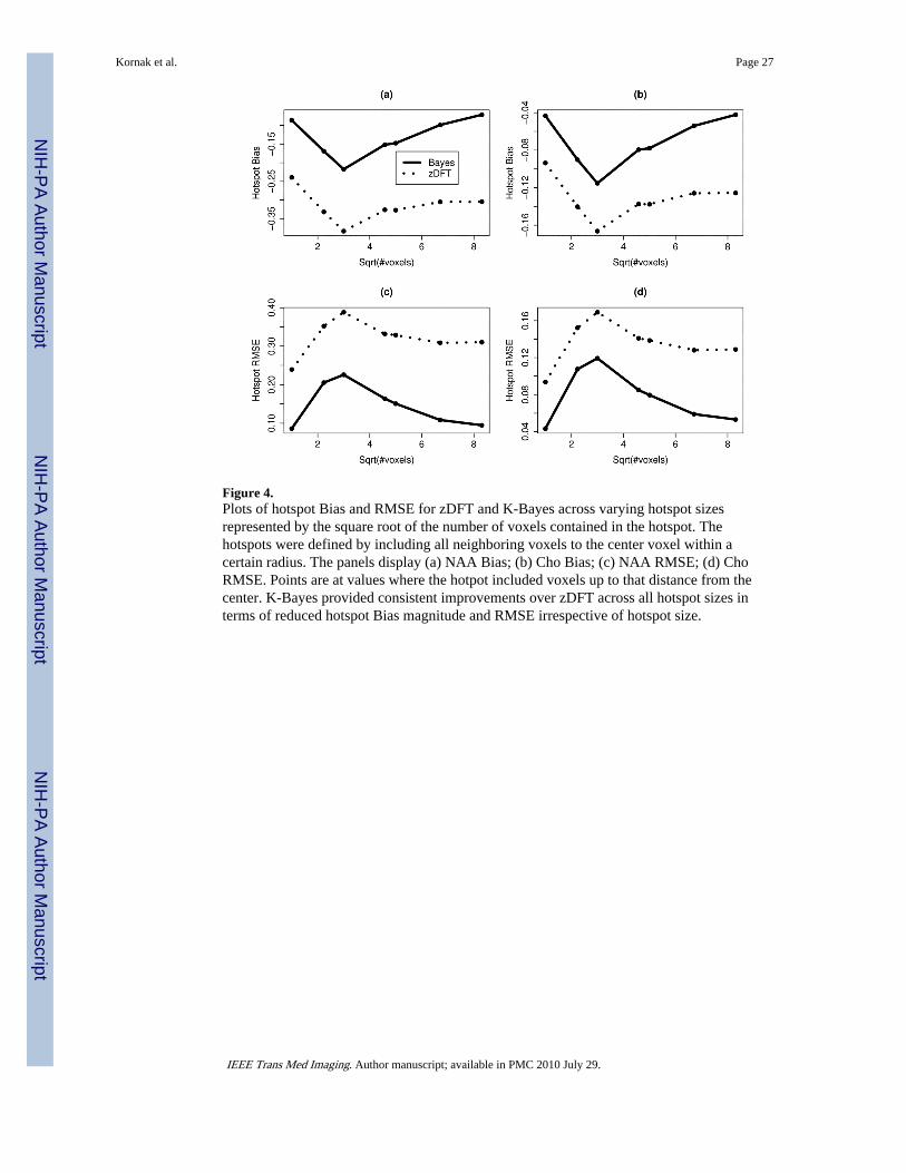
Figure 4.Plots of hotspot Bias and RMSE for zDFT and K-Bayes across varying hotspot sizesrepresented by the square root of the number of voxels contained in the hotspot. Thehotspots were defined by including all neighboring voxels to the center voxel within acertain radius. The panels display (a) NAA Bias; (b) Cho Bias; (c) NAA RMSE; (d) ChoRMSE. Points are at values where the hotpot included voxels up to that distance from thecenter. K-Bayes provided consistent improvements over zDFT across all hotspot sizes interms of reduced hotspot Bias magnitude and RMSE irrespective of hotspot size.
Kornak et al. Page 27
IEEE Trans Med Imaging. Author manuscript; available in PMC 2010 July 29.
NIH
-PA Author Manuscript
NIH
-PA Author Manuscript
NIH
-PA Author Manuscript
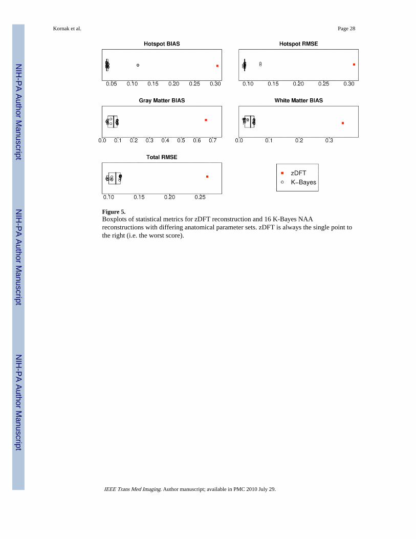
Figure 5.Boxplots of statistical metrics for zDFT reconstruction and 16 K-Bayes NAAreconstructions with differing anatomical parameter sets. zDFT is always the single point tothe right (i.e. the worst score).
Kornak et al. Page 28
IEEE Trans Med Imaging. Author manuscript; available in PMC 2010 July 29.
NIH
-PA Author Manuscript
NIH
-PA Author Manuscript
NIH
-PA Author Manuscript
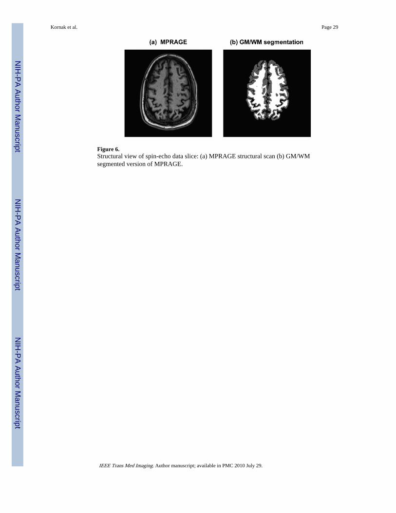
Figure 6.Structural view of spin-echo data slice: (a) MPRAGE structural scan (b) GM/WMsegmented version of MPRAGE.
Kornak et al. Page 29
IEEE Trans Med Imaging. Author manuscript; available in PMC 2010 July 29.
NIH
-PA Author Manuscript
NIH
-PA Author Manuscript
NIH
-PA Author Manuscript

Figure 7.Spin-echo metabolite map reconstructions: zDFT (left column) and K-Bayes (right column)reconstructions for NAA, Cr, and Cho.
Kornak et al. Page 30
IEEE Trans Med Imaging. Author manuscript; available in PMC 2010 July 29.
NIH
-PA Author Manuscript
NIH
-PA Author Manuscript
NIH
-PA Author Manuscript

Figure 8.Left: zDFT reconstruction. Right: eight images corresponding to a range of K-Bayesreconstructions with different parameter settings. K-Bayes reconstructions are more similarto each other than to zDFT.
Kornak et al. Page 31
IEEE Trans Med Imaging. Author manuscript; available in PMC 2010 July 29.
NIH
-PA Author Manuscript
NIH
-PA Author Manuscript
NIH
-PA Author Manuscript
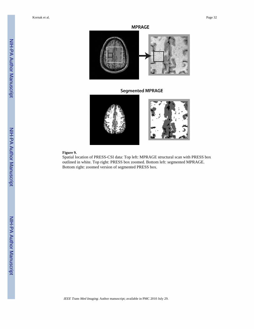
Figure 9.Spatial location of PRESS-CSI data: Top left: MPRAGE structural scan with PRESS boxoutlined in white. Top right: PRESS box zoomed. Bottom left: segmented MPRAGE.Bottom right: zoomed version of segmented PRESS box.
Kornak et al. Page 32
IEEE Trans Med Imaging. Author manuscript; available in PMC 2010 July 29.
NIH
-PA Author Manuscript
NIH
-PA Author Manuscript
NIH
-PA Author Manuscript
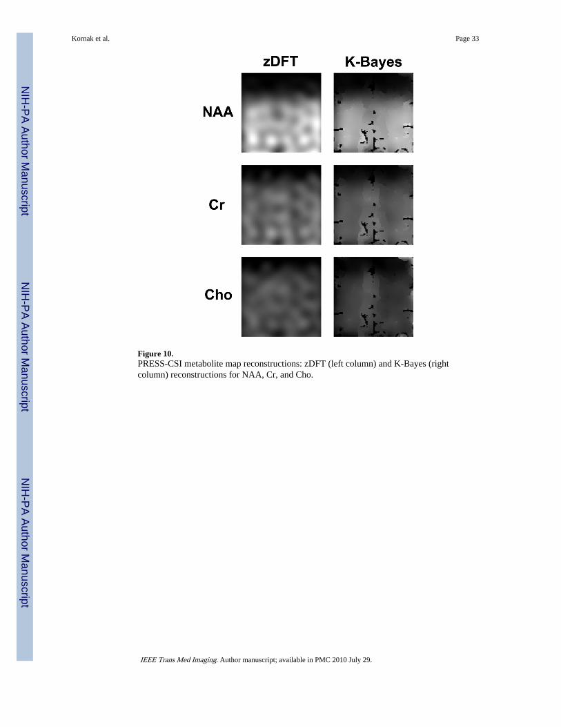
Figure 10.PRESS-CSI metabolite map reconstructions: zDFT (left column) and K-Bayes (rightcolumn) reconstructions for NAA, Cr, and Cho.
Kornak et al. Page 33
IEEE Trans Med Imaging. Author manuscript; available in PMC 2010 July 29.
NIH
-PA Author Manuscript
NIH
-PA Author Manuscript
NIH
-PA Author Manuscript
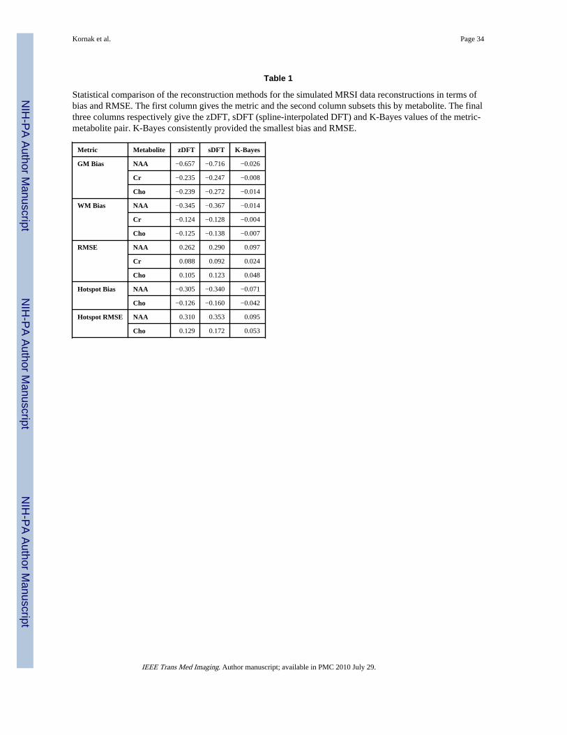
NIH
-PA Author Manuscript
NIH
-PA Author Manuscript
NIH
-PA Author Manuscript
Kornak et al. Page 34
Table 1
Statistical comparison of the reconstruction methods for the simulated MRSI data reconstructions in terms ofbias and RMSE. The first column gives the metric and the second column subsets this by metabolite. The finalthree columns respectively give the zDFT, sDFT (spline-interpolated DFT) and K-Bayes values of the metric-metabolite pair. K-Bayes consistently provided the smallest bias and RMSE.
Metric Metabolite zDFT sDFT K-Bayes
GM Bias NAA −0.657 −0.716 −0.026
Cr −0.235 −0.247 −0.008
Cho −0.239 −0.272 −0.014
WM Bias NAA −0.345 −0.367 −0.014
Cr −0.124 −0.128 −0.004
Cho −0.125 −0.138 −0.007
RMSE NAA 0.262 0.290 0.097
Cr 0.088 0.092 0.024
Cho 0.105 0.123 0.048
Hotspot Bias NAA −0.305 −0.340 −0.071
Cho −0.126 −0.160 −0.042
Hotspot RMSE NAA 0.310 0.353 0.095
Cho 0.129 0.172 0.053
IEEE Trans Med Imaging. Author manuscript; available in PMC 2010 July 29.
Related Documents