Bayesian Analysis of Mass Spectrometry Proteomic Data using Wavelet ... · Bayesian Analysis of Mass Spectrometry Proteomic Data using Wavelet Based Functional Mixed Models Jeﬁrey

Bayesian Analysis of Mass Spectrometry Proteomic Data using WaveletBased Functional Mixed Models

Jeffrey S. Morris 1

The University of Texas M.D. Anderson Cancer Center, Houston, TX, USA.

Philip J. Brown

The University of Kent, Canterbury, England.

Richard C. Herrick


Keith A. Baggerly


Kevin R. Coombes


Abstract

In this paper, we apply the recently developed Bayesian wavelet-based functional mixedmodel methodology to analyze MALDI-TOF mass spectrometry proteomic data. By modelingmass spectra as functions, this approach avoids reliance on peak detection methods. Theflexibility of this framework in modeling nonparametric fixed and random effect functionsenables it to model the effects of multiple factors simultaneously, allowing one to performinference on multiple factors of interest using the same model fit, while adjusting for clinicalor experimental covariates that may affect both the intensities and locations of peaks in thespectra. From the model output, we identify spectral regions that are differentially expressedacross experimental conditions, in a way that takes both statistical and clinical significanceinto account and controls the Bayesian false discovery rate to a prespecified level. We applythis method to two cancer studies.

Key words: Bayesian analysis; False discovery rate; Functional data analysis; Functional mixedmodels; Mass spectrometry; Proteomics.

1Address for correspondence: Jeffrey S. Morris, The University of Texas M.D. Anderson Cancer Center, 1515Holcombe Blvd, Unit 447, Houston, TX 77030-4009, USA.

Email: [email protected]

1

1 Introduction

Proteomic methods simultaneously detect and measure the expression of hundreds or thousands of

proteins present in a biological sample, and are gaining increased attention in biomedical research.

One popular proteomic method is matrix assisted laser desorption and ionization, time-of-flight

mass spectrometry (MALDI-TOF).

In a MALDI-TOF experiment, a biological sample of interest is first mixed with an energy-

absorbing matrix substance, and the mixture is placed on a steel plate. A commonly used variant of

MALDI-TOF, called surface enhanced laser desorption and ionization (SELDI-TOF), incorporates

additional chemistry on the surface of the metal plate to bind specific classes of proteins. The plate

is then placed into a vacuum chamber, where a laser strikes the plate, desorbing ionized peptides

from the sample. An electric field accelerates the particles into a potential free flight tube through

which they travel at a constant velocity until striking a detector plate.

The detector plate records the abundance of particles striking it over a series of short, fixed

intervals of time indexed by t = (t1, . . . , tT ), yielding the proteomic spectrum y(t). Using basic

physics principles, a quadratic transformation can be used to map the time axis t to a set of

corresponding mass-to-charge ratios (m/z) x. Each spectrum is characterized by numerous peaks,

which correspond to proteins or protein fragments (polypeptides) present in the sample. Depending

on the proteomic makeup of the sample, some peptides present may fail to manifest as peaks if

they are located on the shoulder of a more abundant peak (see the supplementary material for an

illustration of this phenomenon). Since most ions have equal charges (+1), the value of spectrum

y(x) at a peak is a rough measure of the abundance of some molecule in the sample having a

molecular mass of x Daltons. The first column of Figure 1 contains two raw spectra from a MALDI-

TOF instrument. In this paper, we consider two example data sets from cancer studies conducted

at the University of Texas MD Anderson Cancer Center.

2

Pancreatic Cancer Experiment: In this study, blood serum was taken from 139 pancreatic

cancer patients and 117 healthy controls. The blood serum was fractionated using 25% acetonitrile

elutions optimized using myoglobin, then run on a MALDI-TOF instrument to obtain a proteomic

spectrum for each sample. For this analysis, we consider the region of the spectra between x =

4,000 and 40,000 Daltons, containing 12,096 observations per spectrum. These 256 samples were

run in four different batches over a period of several months. More specifics of the experiment

can be found in Koomen, et al. (2005). Our primary goal is to identify regions of the spectra

that are differentially expressed between pancreatic cancer patients and healthy controls, regions

corresponding to proteins that may serve as blood serum biomarkers of pancreatic cancer.

Some recent case studies (Baggerly et al. 2003, 2004, Sorace and Zhan 2004, Hu, et al. 2005,

Coombes, et al. 2005a, Villanueva, et al. 2005, Conrads and Veenstra 2005) have demonstrated

that MALDI-TOF instruments can be very sensitive to experimental conditions, even varying over

time within the same laboratory. These differences can manifest in systematic changes in both the

intensities and locations of the peaks (i.e. both the y and x axes), and are sometimes larger in

magnitude than the biological effects of interest. Thus, it is important for us to adequately model

the block effects if we are to properly analyze these data.

Organ-by-Cell Line Experiment: In this study, a tumor from one of two cancer cell lines was

implanted into either the brain or lungs of 16 mice. The cell lines were A375P, a human melanoma

cancer cell line with low metastatic potential, and PC3MM2, a highly metastatic human prostate

cancer cell line. After a period of time, blood serum was extracted and then placed on a SELDI

chip. This chip was run on the SELDI-TOF instrument twice, once using a low laser intensity and

the other using a high laser intensity. This resulted in a total of 32 spectra, two per mouse. Here, we

considered the part of the spectrum between x = 2,000 and 14,000 Daltons, a range that included

7,985 observations per spectrum.

Our primary goals are to assess whether differential protein expression, if present, is more tightly

3

coupled to the host organ site or to the donor cell line type, and to identify regions of the spectra

differentially expressed by organ site, by cell line, and/or their interaction. Typically, spectra from

different laser intensities are analyzed separately, which is inefficient since spectra from both laser

intensities contain information on the same proteins. We want to perform these analyses combining

information across the two laser intensities, requiring us to model an effect of laser intensity on both

the location (x axis) and intensity (y axis) of the peaks, and to account for correlation between

spectra obtained from the same mouse.

It is common to use a two-step approach to analyze mass spectrometry data (Baggerly, et al.

2003, Yasui, et al. 2003, Coombes, et al. 2003, 2005b, Morris, et al. 2005c). First, some type

of feature detection algorithm is applied to identify peaks in the spectra. A quantification is then

obtained for each peak and each spectrum, e.g., by taking the intensity at a local maximum or

computing the area under the peak. Assuming there are p peaks and N spectra, this results in

a p × N matrix of protein expression levels that is somewhat analogous to the matrix of mRNA

expression levels obtained after preprocessing microarray data. Second, this matrix is analyzed

using methods similar to those used for microarrays to identify peaks differentially expressed across

experimental conditions.

This two-step approach is intuitive since it focuses on the peaks, which are theoretically the

most scientifically relevant features of the spectra, and convenient, since it can borrow from a

wide array of available methods developed for microarrays. However, it also has disadvantages.

First, important information can be lost in the reduction from the full spectrum to the set of

detected peaks. Since group comparisons are only performed after peak detection, this approach

will miss important differences in low intensity peaks or on shoulders of peaks whenever the peak

detection algorithm fails to detect them. Second, this approach affords no natural way to account

for experimental effects that impact both the x and y axes of the spectra.

An alternative to the two-step approach described above is to model the spectra as functions,

4

in the spirit of functional data analysis (Ramsay and Silverman 1997). Billheimer (2005) took this

approach, and this is the approach we take in this paper. Mass spectra are irregular functions with

many peaks, and so require flexible modeling and spatially adaptive regularization to represent

accurately. The wavelet-based functional mixed model introduced by Morris and Carroll (2006)

possesses these properties, and in this paper we use this methodology to model mass spectrome-

try data. In modeling the entire spectrum, this method has the potential to identify differences

at locations missed by peak detection algorithms. Further, the method’s flexible nonparametric

representation of the fixed and random effects allows it to model the functional effects of a number

of factors simultaneously, including factors of interest as well as nuisance factors related to the

experimental design. As we will demonstrate, these nonparametrically modeled effects can account

for differences on both the x and y axes of the spectra, allowing data to be combined across laser

intensities, blocks, or other experimental factors. The output of the method can be used to identify

regions of interest within the spectra in a way that takes both statistical and practical significance

into account, while controlling the Bayesian false discovery rate (FDR) at a specified level.

While the primary goal of this paper is to apply an existing method to the setting of mass

spectrometry, we also present some methodological advances not present in Morris and Carroll

(2006). First, we describe a systematic method for selecting an additive shrinkage constant to

apply before log transformation in a way that controls the bias for fold-change estimates at peak

intensities of a specified size. Second, we introduce a method for identifying regions of the spectra

that are differentially expressed in a way that takes both statistical and practical significance into

account, and controls the Bayesian FDR below a certain threshold. Given this threshold, we

also demonstrate how to compute the corresponding estimated false negative rate, sensitivity, and

specificity. These principles can be applied to any Bayesian setting yielding posterior samples of

effects or of some other indicator of biomarker status. To our knowledge, this is the first presentation

of FDR-based methods for the functional data setting. Third, although our method does not require

5

peak detection be done, we demonstrate how to perform peak detection from the method’s output

in case it is desired.

The remainder of the paper is organized as follows. In Section 2, we describe some preprocessing

steps that must be performed before analyzing MALDI-TOF data, and present a systematic method

for choosing an additive shrinkage constant before log transforming the spectral intensities. Section

3 describes the wavelet based functional mixed model, and explains how model specification should

proceed for MALDI-TOF data. In Section 4, we present our Bayesian-FDR based approach for

identifying significant regions of the spectra, and describe how to perform peak detection, if desired.

We present results from analysis of the example data sets in Section 5, and conclude with a discussion

of the strengths and weaknesses of this approach in Section 6.

2 Preprocessing MALDI-TOF Data

A number of preprocessing steps must be performed before modeling MALDI-TOF or SELDI-TOF

data, regardless of the ultimate approach used for inference. It has been shown that inadequate

or ineffective preprocessing can make it difficult to extract meaningful biological information from

the data (Sorace and Zhan, 2003; Baggerly et al., 2003, 2004). These steps include calibration,

baseline correction, normalization, denoising, and transformation. Calibration must be done to

align the peaks across different spectra. The baseline, frequently seen in MALDI-TOF and SELDI-

TOF spectra, is a smooth underlying function that is thought to be largely due to a large cloud

of particles striking the detector in the early part of the experiment (Malyarenko, et al. 2005).

This baseline artifact must be removed. Normalization refers to a constant multiplicative factor

that is used to adjust for spectrum-specific factors, for example to adjust for different amounts

of total protein ionized and desorbed from the sample. Denoising is used to remove white noise,

which is largely due to electronic noise from the detector, from the spectrum. In recent years,

various methods have been proposed to deal with these issues. Here, we use the methods described

6

by Coombes, et al. (2005b). The first two columns of Figure 1 contain a raw spectrum and

corresponding preprocessed MALDI spectrum from a cancer sample and a control sample, and

demonstrate the effects of preprocessing.

It is often useful to transform the spectral intensities in order to reduce the skewness in their

distribution. Some options that appear to work well include the log transformation and the cube root

transformation (Coombes, et al. 2005b, Billheimer 2005). Here, we choose the log2 transformation

since it leads to nice interpretations in terms of fold change. For example, a difference of one in

this scale corresponds to a two-fold increase in intensity.

The presence of zero intensities makes it necessary to add a small positive constant ε to each

intensity before taking the log. This constant shrinks any fold-change estimates towards 1, with

stronger shrinkage at lower intensities. Here we describe a systematic approach for choosing ε for

a given setting. Suppose we wish to control the shrinkage factor for spectral intensities of at least

γ to be no less than α, meaning that the shrunken estimate of a true fold change of δ would be

at least δα. This is accomplished by choosing ε = {(1 − α) ∗ γ ∗ δ}/{α ∗ δ − 1}. For the analyses

presented in this paper, we chose ε = 0.25. This guaranteed that given a fold-change difference of

2 at spectral locations with intensities of at least 1.0, the fold-change estimate will be no less than

1.8, and at spectral intensities of 5.0 or more, the expected fold-change estimate will be no less than

1.95. Effectively, this choice leads to very little shrinkage in regions of the spectra surrounding the

true protein peaks, but reduces the possibility that spurious differences will be detected at very low

intensities because of the log scale that was used.

3 Wavelet-Based Functional Mixed Models

In this section, we briefly overview the wavelet-based functional mixed model method introduced

by Morris and Carroll (2006) and describe how to apply it to mass spectrometry data. See that

paper for further details on its modeling assumptions and computational procedure.

7

The functional mixed model we present here is a special case of the one discussed by Morris and

Carroll (2006), and is also like the functional mixed model discussed by Guo (2002). Suppose we

observe N functions Yi(t), i = 1, . . . , N , all defined on the closed interval T ∈ <1. In MALDI-TOF

data, these functions are the preprocessed, log-transformed spectra on the time axis t. A functional

mixed model for these data is given by

Yi(t) =

p∑j=1

XijBj(t) +m∑

k=1

ZikUk(t) + Ei(t), (1)

where Xij are covariates, Bj(t) are functional fixed effects, Zik are elements of the design matrix for

functional random effects Uk(t), and Ei(t) are residual error processes. We assume that Uk(t) are

independent and identically distributed (iid) mean-zero Gaussian processes with covariance surface

Q(t1, t2), and Ei(t) are iid mean-zero Gaussian processes with covariance surface S(t1, t2), with

Uk(t) and Ei(t) assumed to be independent. A parsimonious yet flexible structure will be used

to represent Q and S, as described below. One may allow different strata, h = 1, . . . , H, to have

their own covariance matrices Qh and Sh by splitting the random effect functions and residual error

processes into blocks, for example to allow cancer and control spectra to have different covariance

surfaces.

Covariates {X.j, j = 1, . . . , p}, discrete or continuous, are specified for any factors one wants to

relate to the mass spectra. Each functional coefficient βj(t) describes the effect of the corresponding

factor at location t of the spectrum. The covariates can include a column of 1’s for an overall mean

spectrum, continuous or discrete variables of interest, clinical or experimental covariates for which

one would like to adjust, and any interactions among these factors. As in linear mixed models,

absent constraints one must take care in parameterizing the X.j so the resulting design matrix

X = (X.1, . . . , X.p) has full column rank.

When the spectra are not independent, the functional random effects provide a flexible mecha-

nism for modeling correlation among spectra. For example, individual-level random effect functions

8

can be specified when multiple spectra are obtained from the same individual, and additional ran-

dom effect functions can be specified for other clustering units such as blocks or laboratories when

the spectra are obtained over a long period of time or at many different locations.

An important feature of this model is that it places no restrictions on the form of the fixed

or random effect functions, since for MALDI-TOF data we expect their true form should be very

irregular and spiky. Although their high dimensionality precludes unstructured representation, it is

also important to allow flexibility in the forms of Q and S, as described below, since irregular and

spiky curve-to-curve deviations imply irregularity in these matrices, as well.

It is possible to write a discrete matrix version of model (1) if we have all spectra observed on

the same equally spaced grid t = (tl; l = 1, . . . , T ), as

Y = XB + ZU + E. (2)

Each row of the N × T matrix Y contains one spectrum observed on the grid t. The matrix X is

an N × p design matrix of covariates; B is a p × T matrix whose rows contain the corresponding

fixed effect functions on the grid t. Bjl denotes the effect of the covariate in column j of X on

the spectrum at clock tick tl. The matrix U is an m× T matrix whose rows contain random effect

functions on the grid t, and Z is the corresponding N ×m design matrix. Each row of the N × T

matrix E contains the residual error process for the corresponding observed spectrum. We assume

that the rows of U are iid MVN(0, Q) and the rows of E are iid MVN(0, S), independent of U ,

with Q and S being T × T covariance matrices that are discrete analogs of the covariance surfaces

in (1), defined on the grid t× t.

Morris and Carroll (2006) used a basis function approach to fit the model (2). They chose

wavelet basis functions, which possess various properties that make them well-suited for representing

MALDI-TOF data. First, their compact support allows them to efficiently model the spikes in the

data. Second, their whitening property allows us to make parsimonious yet flexible assumptions on

the covariances Q and S. Specifically, the assumed structure requires only T parameters for each

9

of these matrices, yet it accommodates various types of nonstationarities characteristic of MALDI-

TOF data, for example allowing the between-spectra variances and within-spectrum smoothness

to vary across different regions of the spectra. This point is illustrated by Figure 1 of Morris

and Carroll (2006). Third, their decomposition of the spectral energy in both the frequency and

time domains makes it possible to perform adaptive regularization on the fixed effect functions.

By adaptive regularization, we mean that the functional estimates are denoised in a manner that

tends to preserve strong peaks, which are important features that characterize these functions in

MALDI-TOF applications. Finally, given spectra sampled on an equally spaced grid of length T , the

special structure of the basis functions allows us to quickly compute a set of T wavelet coefficients

using a pyramid-based algorithm, the discrete wavelet transform (DWT), in just O(T ) operations.

Conversely, given the set of wavelet coefficients, the function can be constructed using the inverse

discrete wavelet transform (IDWT), also in O(T ) operations.

The wavelet-based approach to fitting the functional mixed model involves three steps. First,

the wavelet coefficients are computed by applying the DWT to each of the N spectra. This step

effectively projects the observed spectra into the space spanned by the chosen wavelet bases. Second,

a Markov chain Monte Carlo simulation is performed to obtain posterior samples of the model

parameters in a wavelet-space version of the functional mixed model. Third, the IDWT is applied

to the posterior samples, yielding posterior samples of the parameters B,U,Q, and S in the data-

space functional mixed model (2). These posterior samples can subsequently be used to perform

any desired Bayesian inference.

Morris and Carroll (2006) made the code for performing these steps freely available at the

following URL: http://biostatistics.mdanderson.org/Morris/papers.html. This code has

since been updated to effectively handle the extremely large data sets characteristic of MALDI-

TOF data (100’s of spectra, each on a grid of 10,000-20,000). The code is a standalone executable

that runs on a Windows-based PC, and takes Matlab data files for the required input. The required

10

input includes the matrix of log-transformed, preprocessed spectra, Y , plus a structure specifying

the model used (at a minimum, X and Z, if present, must be specified), a structure specifying the

wavelet basis to use, and another structure containing the MCMC specifications. Details are given

in the documentation provided with the code. The output of this code is Matlab files containing

the posterior samples for the model parameters resulting from the MCMC.

The third column of Figure 1 contains spectra randomly generated from the posterior predictive

distribution of the wavelet-based functional mixed model fit to the pancreatic cancer example data

set, and illustrates that the model is flexible enough to generate functional data characteristic of

MALDI-TOF.

4 Bayesian Inference for MALDI-TOF

Here, we describe how to perform Bayesian inference for MALDI-TOF experiments using the pos-

terior samples output from the wavelet-based functional mixed model. First, we describe how peak

detection can be done, if desired. Second, we describe how to identify significant regions of the

spectra while controlling the expected Bayesian FDR, and then summarize the global properties of

this significance rule.

Peak Detection: A key benefit of our functional approach is that peak detection is unnecessary.

For those who still wish to restrict attention to the peaks, however, it is straightforward to perform

peak detection from the posterior samples output from the wavelet-based functional mixed model.

Morris, et al. (2005) describe a peak detection approach and demonstrate that performing peak

detection on the mean spectrum results in greater sensitivity and specificity than the usual approach

of performing peak detection on the individual spectra. Since the mean spectrum is easily obtainable

from the functional mixed model either as a fixed effect function or a linear combination of fixed

effect functions, it is easy to adapt the procedure described in that paper to detect and quantify

peaks in this setting, as well.

11

The mean spectrum estimate from the wavelet-based functional mixed model differs from the

simple pointwise mean spectrum in several ways. First, it is denoised (adaptively regularized) as a

result of the shrinkage induced by a spike-slab prior that is assumed on the wavelet coefficients for the

fixed effect functions. The benefit of this denoising is that it reduces the number of small, spurious

bumps that are called peaks. Second, the mean spectrum estimate will adjust for other effects in

the model. For example, including a block or laser intensity effect improves the alignment across the

different groups of spectra, thus sharpening the peaks in the estimated mean spectrum and making

them easier to detect. Third, the denoising of the mean spectrum is affected by the random effect

and residual variance structure of the functional mixed model. As can be seen by the formulas

presented in Morris and Carroll (2006), both the random effect structure and residual variance

directly impact the wavelet shrinkage of the fixed effect functions. This may also lead to improved

denoising over the simple pointwise mean spectrum, especially in data sets with imbalanced designs

in terms of the number of spectra per individual.

Morris, et al. (2005) also perform a wavelet-based denoising step on the mean spectra before

detecting peaks. An important difference is that the approach described in that paper uses the

undecimated discrete wavelet transform (UDWT, also sometimes called the translation invariant

or maximum overlap discrete wavelet transform), while the wavelet-based functional mixed model

works with the decimated DWT (DDWT). The UDWT is translation invariant, while the DDWT

is not. This means that arbitrary translations in the x-axes of the spectra will result in different

wavelet coefficients for the DDWT, but not for the UDWT. It has been observed that the translation

invariant property can lead to better denoising, but at the cost of computational time and parsimony.

The calculations for the UDWT are of order up to O{T log(T )} rather than O(T ), and the full range

of translations would yield a great deal more coefficents to model, increasing the memory demands

on the procedure. While it would be possible to apply the wavelet-based functional mixed model in

the UDWT context, we choose to stick with the DDWT here because with reasonably aligned spectra

12

taken at a high sampling frequency, the differences are not great, and the increased computational

and computer memory demands from the UDWT make would make it more difficult to apply the

method to these extremely large data sets.

Identifying Significant Regions of Spectra: Our primary analysis goal in this paper is

to identify regions of the spectra that are differentially expressed across factors of interest, which

can subsequently be mapped to proteins that may serve as useful biomarkers. In microarrays,

two classical approaches for handling differential expression are (i) identify all genes with a fold-

change difference of at least δ and (ii) identify genes that differ significantly across treatment groups

according to a statistical hypothesis test. Option (i) is intuitive to many researchers but lacks

statistical rigor since it ignores the variability in the data, and option (ii) only focuses on statistical

significance, ignoring practical significance, since it is typically based on a null hypothesis of equality.

In the present MALDI-TOF context, we identify differentially expressed regions of the spectra in a

way that considers both statistical and practical significance, and controls the expected Bayesian

FDR to be no more than α.

Suppose we are interested in identifying biomarkers that have at least a δ-fold intensity change

between treatment groups. From the MCMC, supposed we have G posterior samples of the cor-

responding fixed effect function Bj = [Bj(t1), . . . , Bj(tT )] on the log2 scale, denoted by {B(g)j , g =

1, . . . , G}. From these, we compute the pointwise posterior probabilities of at least a δ-fold intensity

change at each spectral location as pj(tl) = pjl = Pr{|Bj(tl)| > log2(δ)|Y } ≈ G−1∑G

g=1 I{|B(g)j (tl)| >

log2(δ)} for (tl, l = 1, . . . , T ). We replace any pjl = 1 with 1− (2 ∗G)−1. These posterior probabili-

ties can also be computed for any contrast involving the fixed effect functions, A(g) =∑p

j=1 CjB(g)j ,

or similar posterior probabilities can be computed for linear combinations of spectral locations, e.g.

if one wanted to detect peaks and look at areas under peaks, or only consider tl that are flagged as

peaks. The quantity 1 − pjl can be considered a local false discovery rate estimate for location tl

for factor i. Global properties are described below.

13

Given a desired global FDR bound α, we flag the set of locations ψj = {tl : pjl > φα} as

significant spectral regions for factor j. In order to obtain φα, we first sort {pjl, l = 1, . . . , T} in

descending order to obtain {p(l), l = 1, . . . , T}. Then φα = p(λ), with λ = max[l∗ : (l∗)−1∑l∗

l=1{1−p(l)} ≤ α]. The threshold φα is a cutpoint on the posterior probabilities that controls the expected

Bayesian FDR at level α, in the sense that on average we expect ≤ 100α% of the locations in the set

ψj to have a true δ-fold difference in expression, as estimated by the wavelet-based functional mixed

model. That is, if N (ψj) is the cardinality of the set ψj, defined as N (ψj) =∑T

l=1 I(tl ∈ ψj), then

N (ψj)−1

∑tl∈ψj

Pr{|Bj(tl)| ≤ log2(δ)|Y } ≤ α. If p∗ factors are to be investigated simultaneously, it

is possible to either use one common threshold φα or separate thresholds for each factor, {φj,α, j =

1, . . . , p∗}. This use of Bayesian FDR is similar in principle to the approach used by Newton, et al.

(2004).

Given the set of locations ψj = {tl : pj(tl) > φα} flagged as discoveries, we can compute

model-based estimates of the false discovery rate, false negative rate, sensitivity, and specificity for

detecting differentially expressed locations. Defining ψ′j

⋃ψj = T , and N (S) as the cardinality of

set S, defined as above, the false discovery rate is estimated by {N (ψj)}−1∑

tl∈ψj{1− pj(tl)}, the

false negative rate by {N (ψ′j)}−1

∑tl∈ψ

′j{pj(tl)}, sensitivity by {∑T

l=1 pj(tl)}−1∑

tl∈ψjpj(tl), and

specificity by [∑T

l=1{1− pj(tl)}]−1∑

tl∈ψ′j{1− pj(tl)}. In the idealized functional setting, ψj is a set

of continuous regions, and the estimates given above are approximations of the continuous versions

of these quantities obtained by substituting integrals over t for the summations, and defining N (S)

as the Lebesgue measure of set S. The interpretations of these quantities in the continuous case

are also analogous. For example, if flagging a region ψj as significant results in an FDR of α, then

the expected proportion of the set of contiguous regions ψj that is truly differentially expressed at

least δ-fold is 1− α, based on Lebesgue measure.

For MALDI-TOF data, these measures do not depend heavily on the sampling frequency of the

data. To demonstrate this point, we computed the threshold φα for the pancreatic cancer example

14

while downsampling the spectra in multiples of 2, 3, 4, 6, and 8. The results are available as

supplementary material. We found nearly identical thresholds and flagged regions in each analysis.

This approach for identifying cutpoints for significance and summarizing the resulting global

properties can be used in any Bayesian context yielding a posterior probability of discovery for each

of a number of discrete units or continuous regions.

5 Analysis of Example Data

For both examples, we modeled the spectra on the time scale t but plotted results on the biologi-

cally meaningful mass-per-unit-charge scale (m/z, x). In our wavelet-space modeling, we chose the

Daubechies wavelet with vanishing 4th moments and performed the DWT down to J = 10 and J = 9

levels for the two respective examples. Other wavelet bases were examined and yielded equivalent

results. We used the modified empirical Bayes procedure described by Morris and Carroll (2006)

to estimate the shrinkage hyperparameters that guide the adaptive regularization of the fixed effect

functions. For each example, we ran 10 parallel chains, each consisting of 1000 iterations after a

burn-in of 1000, and we kept every fifth iteration for a total of G = 2000 MCMC samples for our

analyses. All chains appear to have converged, as indicated by trace plots. In the pancreatic cancer

example, the median and 99% credible interval for the Metropolis Hastings acceptance probabilities

across the roughly 12,000 covariance parameters were 0.22 and (0.11,0.31), respectively, and for

the organ-by-cell line example with roughly 8,000 covariance parameters, they were 0.17 and (0.05,

0.51), respectively.

We explored the possible protein identities of any flagged regions by running the estimated m/z

values of the corresponding peaks in the region through TagIdent, a searchable database (available

at http://us.expasy.org/tools/tagident.html) that contains the molecular masses and pH for

proteins observed in various species. For the organ by cell line example, we searched for proteins

emanating from both the source (human) and the host (mouse) whose molecular masses were within

15

the estimated mass accuracy (0.3%) of the instrument from the nearest peak or most significant

location of each flagged region. This only gives an educated guess at what the protein identity of the

peak could be; it is necessary to perform an additional MS/MS experiment in order to rigorously

validate the protein identity.

Pancreatic Cancer Example: The design matrix for this data set of N = 256 spectra was

chosen to have p = 5 columns, the first column indicating cancer (=1) or normal (= -1) status, and

corresponding to a functional cancer main effect B1(t) describing the difference between the mean

log2 intensities of cancer and normal spectra at time t. The final four columns indicate the time

blocks, and correspond to mean spectra for the respective time blocks (Bi(t), i = 2, . . . , 5). The

block effects between block i and i′ can be constructed by Bi(t) − Bi′(t). No functional random

effects were specified. The residual covariance matrix S was allowed to vary across cancer status.

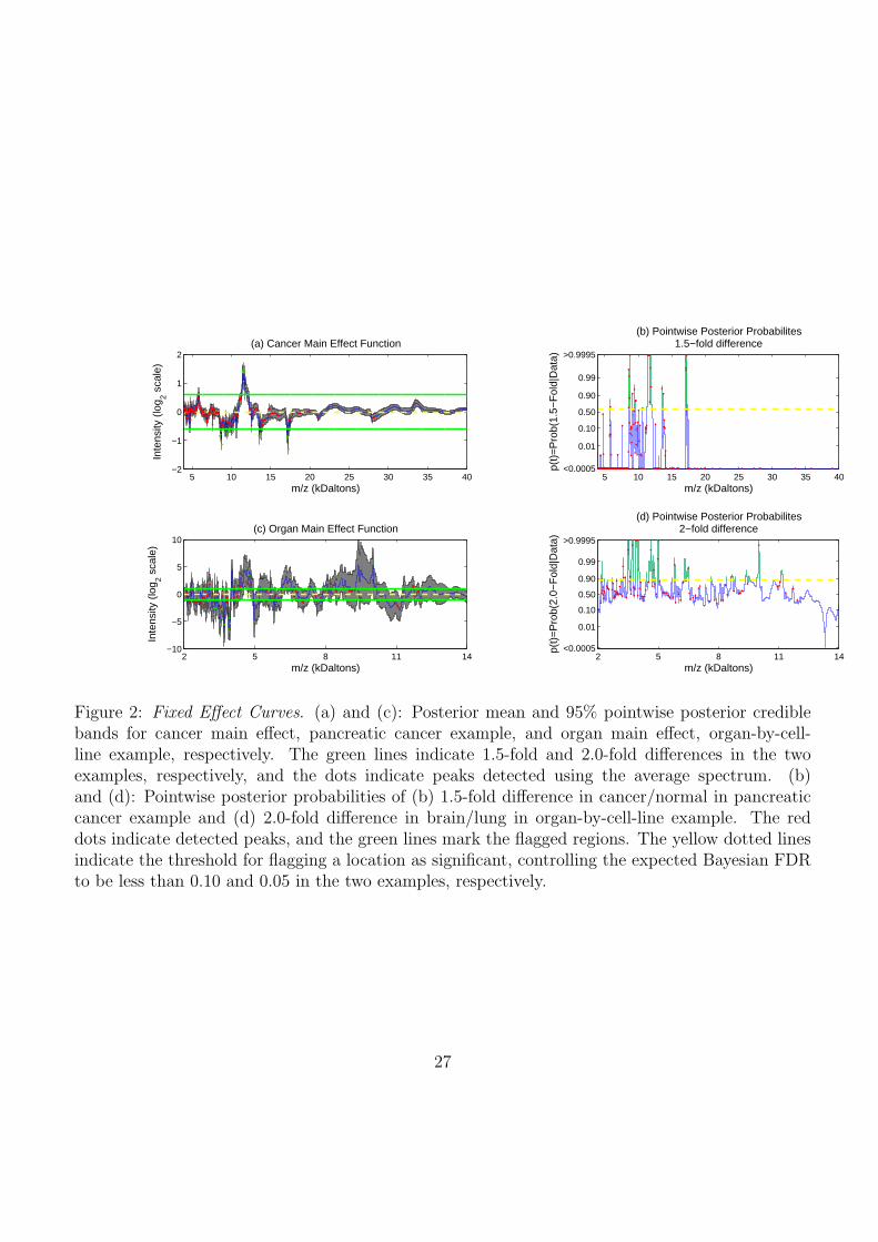
The top two panels of Figure 2 contain posterior means and 95% credible intervals for the cancer

main effect function and the corresponding pointwise posterior probabilities of at least 1.5-fold ex-

pression. The dots in the plots correspond to the 227 peaks detected on the posterior mean for the

overall mean spectrum µ̂(t) = (4G)−1∑G

g=1

∑5i=2 B

(g)i (t). The horizontal line indicates the threshold

on the posterior probabilities φ10 = 0.595 corresponding to an expected Bayesian FDR at 0.10. This

threshold yielded a false negative rate of 0.016, a sensitivity of 0.716, and specificity of 0.996. There

were a total of 506 spectral locations contained within 16 contiguous regions that were flagged as sig-

nificant. Analyzing the peaks, we found 26/227 were flagged as significant. A list containing the sig-

nificant regions and peaks, and a plot of the overall mean spectrum with detected peaks are available

as supplementary material at http://biostatistics.mdanderson.org/Morris/papers.html.

The most significant effects were observed in the regions (i) (17230D, 17311D), (ii) (8730D,

8787D), (iii) (11314D, 12037D), with maximum posterior mean fold-change differences of 1/2.46,

1/2.20, 2.77, respectively, between cancers and normals. A fold change of δ means that cancer was

overexpressed relative to normal by a factor of δ, while a fold change of 1/δ means that normal was

16

overexpressed relative to cancer by a factor of δ. The maximum fold-change differences for all three of

these regions were located at peaks. These were also all identified in Koomen, et al. (2005). In that

paper, they reported MS/MS results confirming the identity of (i) as a fragment of apolipoprotein

A-I or apolipoprotein glutamine-I, and the cluster of 7 peaks in (iii) as serum amyloid A. Based on

TagIdent, region (ii) may correspond to complement C4-A or C4-B(precursor), 8764.07D, mediators

of inflammatory processes that circulate in the blood.

One peak (4284D) found to be statistically significant and highlighted by Koomen, et al. (2005)

had a very small fold-change estimate (1.22), and was not flagged by our analysis. Also interesting

was the region (8671D, 8684D) that was on the upslope of a very abundant peak at 8688D. The

peak itself was not flagged (p=0.186), but this region was, with a maximum fold-change of 1/1.70

at 8679 (p=0.968). It is possible that this result is driven by protein at 8679D whose peak is not

visible because of its proximity to the extremely abundant peak at 8688D. An MS/MS experiment

would have to be done to investigate this possibility.

Plots of the block effects (in supplementary material) demonstrate that they affect both the

location and intensity of peaks, and are of a similar magnitude as the cancer main effect. Figure

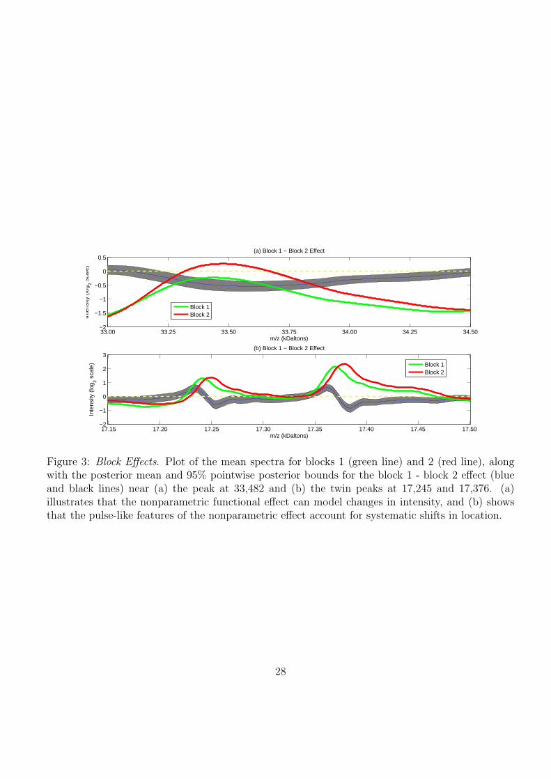
3 illustrates the block effect (block 1 - block 2) in the neighborhood of some prominent peaks.

The nonparametrically modeled block effects were able to capture both shifts in intensity {Figure

3(a)} and shifts in location {Figure 3(b)}. Note that changes in the x axis appear as pulses in the

nonparametric block effects. These features served to calibrate the x and y axes across blocks so

they were comparable, allowing spectra from different blocks to be pooled for a combined analysis.

Organ-by-Cell-Line Example: The design matrix for this set of N = 32 spectra had p = 5

columns. We used a cell means model for the factorial design, so the first four columns contained

indicators of the 4 organ-by-cell-line groups with corresponding mean functions Bi(t), i = 1, . . . , 4,

ordered brain-A375P, brain-PC3MM2, lung-A375P, and lung-PC3MM2. From these, the overall

mean spectrum 0.25∑4

i=1 Bi(t), the organ main effect function B1(t) + B2(t)−B3(t)−B4(t), cell-

17

line main effect function B1(t)−B2(t)+B3(t)−B4(t), and the organ-by-cell line interaction function

B1(t) − B2(t) − B3(t) + B4(t) were constructed. Column 5 indicated whether a low (-1) or high

(1) laser intensity setting was used in generating the given spectrum. The Z matrix had m = 16

columns, with Zik = 1 if spectrum i came from animal k, with corresponding mouse-level random

effect functions Uk(t), k = 1, . . . , 16.

The bottom two panels of Figure 2 contain the posterior means and 95% credible intervals for

the organ main effect function and the corresponding pointwise posterior probabilities of at least 2-

fold difference, respectively. Equivalent plots for the cell line and interaction effects are available as

supplementary material. The threshold on the posterior probabilities based on setting the expected

Bayesian FDR of 0.05 was φ05 = 0.874, which led to a false negative rate of 0.469, a sensitivity of

0.204, and a specificity of 0.987. We flagged 1393/7985 of the spectral locations in 41 contiguous

regions for the organ main effect, 798/7985 in 25 contiguous regions for the cell line main effect, and

594/7985 in 18 contiguous regions for the organ-by-cell line interaction effect. Of the 101 detected

peaks, we flagged 40 as significant, 13 for organ alone, 13 for cell-line, 1 for both organ and cell-line,

and 13 for the interaction. Table 1 contains information for the top 10 most significant regions, all of

which contained locations with posterior probabilities pl > 0.9995. The complete list of significant

regions and peaks is available as supplementary material.

The strongest differences observed were between organ groups. The largest estimated fold

changes were observed in the regions [3658D, 3739D] and [3866.3D, 3971.3D]. These regions each

contain a peak that is strongly present in all mice with tumors injected into their brains, but absent

from those injected in their lungs. The region [3866.3, 3971.3] is represented in figure 4(a) and (c).

This region may correspond to a calcitonin gene-related peptide II precursor (CGRP-II, 3882D),

a peptide in the mouse proteome that dilates blood vessels in the brain and has been observed

to be abundant in the central nervous system (http://www.expasy.org/uniprot/Q99MP3). The

region [3658D, 3739D] may correspond to a precursor of amyloid beta A4 protein in the mouse

18

proteome (3717.1D) that “functions as a cell surface receptor and performs physiological func-

tions on the surface of neurons relevant to neurite growth, neuronal adhesion and axonogenesis”,

and is “involved in cell mobility and transcription regulation through protein-protein interactions”

(http://www.expasy.org/uniprot/P12023). Another flagged region [10912D, 11269D] may also

correspond to a precursor of the same protein (11050.6D). These results may represent important

responses within the hosts to the tumor implantation in their brains.

There were some significant effects that would not have been detected had we restricted our

attention to the peaks. The significant organ effect in the region [3993D, 4061D], with maximum

fold change difference of 21.0, is on the upslope of a peak, but the peak value itself was not

significant. Also, the region [7618D, 7650D] was flagged for an organ effect, being specific to brain-

injected mice. Inspection of the overall mean spectrum (see black line in Figure 4(b)) reveals that

this region contains a flattening region near 7620D on the overall mean spectrum that is not a

peak, but is near the shoulder of a larger peak at 7580D that is not itself differentially expressed.

The protein neurogranin in the human proteome, with a molecular weight of 7618.5D, is active in

synaptic development and remodeling in the brain. No peak was detected in the region [7618D,

7650D], so this potential discovery would not have been made had we restricted attention to the

peaks.

Of the 25 regions flagged as significantly different across cell lines, 22 of them were overexpressed

in the metastatic PC3MM2 cell line relative to the non-metastatic A375P cell line. Plots of the laser

intensity effect (in supplementary material) reveal systematic differences between the low and high

laser intensity spectra that affect both the locations and intensities of peaks. Our nonparametric

laser intensity effect was able to model this difference, allowing us to pool data from both laser

intensities for this analysis.

19

6 Discussion

We have demonstrated how to use the recently developed Bayesian wavelet-based functional mixed

model to analyze MALDI-TOF proteomics data. This method appears well suited to this context,

for several reasons: the functional mixed model is very flexible; it is able to simultaneously model

nonparametric functional effects for multiple covariates, both factors of interest and nuisance fac-

tors such as block effects. The nonparametric functional effects for nuisance factors are flexible

enough to account for systematic changes in both the location and intensity of peaks in the spectra.

Further, the random effect functions can be used to model correlation among spectra that might

be induced by the experimental design. The wavelet-based modeling approach works well for mod-

eling functional data with many local features like MALDI-TOF peaks since it results in adaptive

regularization of the fixed effect functions, avoids attenuation of the effects at the peaks, and is

reasonably flexible in modeling the between-curve covariance structures, accommodating autoco-

variance structures induced by peaks and heteroscedasticity allowing different between-spectrum

variances for different peaks. The method is extremely adaptive in terms of the types of functions it

can represent. The example in Morris and Carroll (2006) illustrates that it can handle smooth fixed

and random effect functions and spiky residual error processes, while our examples here demonstrate

that it can also handle very spiky fixed and random effect functions as well. The use of wavelet

bases and the resulting adaptive regularization are the keys to this flexibility.

Before applying this method to mass spectra, it is important to perform adequate preprocessing,

at a minimum to remove the baseline artifact and align the spectra. Variable baselines, if not

removed, can add extra noise variability to the data, making it more difficult to identify meaningful

differences. Misalignment in the spectra will cause the fixed effect functions to be less peaked,

and will increase the variability across spectra, also decreasing power for detecting differentially

expressed regions of the spectra. In our experience, spectra obtained on a given day in a given

20

laboratory tend to be quite well aligned with each other, and require no further alignment. It

is still a good idea to use a heat map of the spectra to check, and then to perform some type

of function registration if the alignment is off. Spectra from different laboratories or obtained at

different times, however, are frequently severely misaligned. These systematic misalignments appear

to be handled quite well in the functional mixed model framework by including nonparametric

block and laboratory effects in the functional mixed model, as long as these block effects are not

completely confounded with other effects in the model. If there is complete confounding due to

poor experimental design, however, then there is little that any statistical analysis can do to factor

out the confounding effects (Baggerly, et al. 2004, 2005; Coombes, et al. 2005a)

We applied this method to two cancer proteomic studies, and identified spectral regions that

were differentially expressed and may correspond to potential biomarkers. Many of these regions

contained peaks, but several would not have been found had attention been restricted to peaks alone.

Another benefit of our approach is that both statistical and practical significance were considered

in identifying potential biomarkers.

In the pancreatic cancer example, this method was able to model nonparametric block effects

that served to calibrate the x and y axes across blocks, making spectra from the different time

blocks comparable and enabling them to be pooled for a common analysis. In a similar fashion, the

incorporation of the nonparametric laser intensity effect in the organ-by-cell line example allowed

us to account for systematic differences in spectral intensity and peak locations between the high

and low laser intensity spectra. Along with the nonparametric random effects accounting for the

correlation between spectra from the same animal, this allowed us to pool data across laser inten-

sities for a common analysis, potentially increasing our power for detecting differentially expressed

proteins.

While the method is complex, it is relatively straightforward to implement using the code freely

available at http://biostatistics.mdanderson.org/Morris/papers.html. The user only needs

21

to construct a matrix Y containing the preprocessed spectral intensities for the N spectra in the

study and specify the design matrices X and Z. Starting values, empirical Bayes and vague proper

priors, and proposal variances are all automatically computed by the program and can be used

without any user input. Default choices for wavelet basis and levels of decomposition are also

automatically computed and can be used, if desired. The code yields posterior samples and sum-

mary statistics for all quantities in the functional mixed model, from which Bayesian inference

can be done in a straightforward fashion. The method is computationally intensive, but the code

has been optimized to be able to handle very large data sets, and parallel processing can further

speed the computations when it is available. For example, on average each chain of 2000 MCMC

iterations for our pancreatic cancer example with 256 spectra and 12,096 observations per spectra

took under an hour to run. In our analysis, we ran 10 of these chains in parallel using Con-

dor (http://www.cs.wisc.edu/condor), parallel processing freeware that shared the job among

roughly 10 Pentium IV computers in a Windows network.

We also described a systematic method for choosing the additive shrinkage constant before log

transformation in settings when estimating fold-changes is the question of interest. This method

has applications outside of this work, in the setting of microarrays and other measurement tech-

nologies. We also presented a new method for identifying significant regions of a curve that takes

both statistical and practical significance into account, while controlling the Bayesian FDR at a

prespecified level. Also, we discussed how to assess the properties of these discovery rules in terms

of false discovery and false negative rates, sensitivity and specificity. These approaches can also be

applied outside the context of this paper to any situation for which posterior samples of fold-changes

are given, including Bayesian models for microarray data, as well as other Bayesian settings.

Wavelet-based functional mixed models show great promise for the analysis of MALDI-TOF

proteomic data. This approach may also prove useful for analyzing data from other biomedical

platforms that generate irregular functional data.

22

Acknowledgments

We thank Jim Abbruzzesse, Nancy Shih, Stan Hamilton, Donghui Li, John Koomen, and Ryuji

Kobayashi for the data sets used in this paper. We also thank the associate editor and two referees,

whose insightful comments have led to a much improved paper. This work was supported by a grant

from the National Cancer Institute (CA-107304), and the UK Department of Trade and Industry

Texas-UK Collaborative Initiative in Bioscience.

References

Abramovich, F., Sapatinas, T. and Silverman, B. W. (1998) Wavelet thresholding via a Bayesian

approach. Journal of the Royal Statistical Society, Series B, 60, 725–749.

Baggerly K. A., Morris, J. S., Wang, J., Gold, D., Xiao, L. C. and Coombes, K. R. (2003) A

comprehensive approach to the analysis of matrix-assisted laser desorption/ionization-time of

flight proteomics spectra from serum samples. Proteomics, 3(9): 1667-1672.

Baggerly, K. A., Morris J. S., and Coombes K. R. (2004) Reproducibility of SELDI Mass Spec-

trometry Patterns in Serum: Comparing Proteomic Data Sets from Different Experiments.

Bioinformatics, 20(5): 777-785.

Baggerly K. A., Morris, J. S., Edmonson, S., and Coombes, K. R. (2005) Signal in Noise: Evaluating

Reported Reproducibility of Serum Proteomic Tests for Ovarian Cancer. Journal of the National

Cancer Institute, 97: 307-309.

Billheimer D (2005) Functional data analysis of protein expression in matrix-assisted laser desorp-

tion/ionization time-of-flight mass spectrometry. unpublished manuscript.

Clyde, M., Parmigiani, G. and Vidakovic, B. (1998) Multiple shrinkage and subset selection in

wavelets. Biometrika, 85: 391–401.

23

Conrads TP and Veenstra TD (2005) What Have We Learned from Proteomic Studies of Serum?

Expert Review of Proteomics, 2(3): 279-281.

Coombes KR, Fritsche HA Jr., Clarke C, Cheng JN, Baggerly KA, Morris JS, Xiao LC, Hung

MC, and Kuerer HM (2003) Quality Control and Peak Finding for Proteomics Data Collected

from Nipple Aspirate Fluid Using Surface Enhanced Laser Desorption and Ionization. Clinical

Chemistry. 49(10): 1615-1623.

Coombes KR, Morris JS, Hu J, Edmonson SR, and Baggerly KA (2005a) Serum Proteomics Pro-

filing: A Young Technology Begins to Mature. Nature Biotechnology, 23(3): 291-292.

Coombes KR, Tsavachidis S, Morris JS, Baggerly KA, and Kobayashi R (2005b) Improved Peak

Detection and Quantification of Mass Spectrometry Data Acquired from Surface-Enhanced

Laser Desorption and Ionization by Denoising Spectra using the Undecimated Discrete Wavelet

Transform. Proteomics, 41: 4107-4117.

Guo, W. (2002) Functional mixed effects models. Biometrics, 58, 121–8.

Hu J, Coombes KR, Morris JS, and Baggerly KA (2005) The Importance of Experimental Design

in Proteomic Mass Spectrometry Experiments: Some Cautionary Tales. Briefings in Genomics

and Proteomics, 3(4): 322-331.

Koomen J. M., Shih L. N., Coombes K. R., Li D., Xiao L. C., Fidler I. J., Abbruzzese J. L.,

Kobayashi R. (2005) Plasma protein profiling for diagnosis of pancreatic cancer reveals the

presence of host response proteins. Clinical Cancer Research, 11(3): 1110-1118.

Malyarenko DI, Cooke WE, Adam BL, Malik G, Chen H, Tracy ER, Trosset MW, Sasinowski M,

Semmes OJ, and Manos DM (2005) Enhancement of sensitivity and resolution of SELDI TOF-

MS records for serum peptides using time series analysis techniques. Clinical Chemistry, 51(1):

65-74.

24

Misiti M., Misiti Y., Oppenheim G., and Poggi J. M. (2000), Wavelet Toolbox For Use with Matlab:

User’s Guide. Natick, MA: Mathworks, Inc.

Morris JS and Carroll RJ (2006) Wavelet-based functional mixed models. Journal of the Royal

Statistical Society, Series B. 68(2): 179-199.

Morris JS, Coombes KR, Koomen J, Baggerly KA, and Kobayashi R (2005) Feature Extraction

and Quantification for Mass Spectrometry Data in Biomedical Applications Using the Mean

Spectrum. Bioinformatics, 21(9): 1764-1775.

Morris JS, Vannucci M, Brown PJ, and Carroll RJ (2003) Wavelet-Based Nonparametric Mod-

eling of Hierarchical Functions in Colon Carcinogenesis. Journal of the American Statistical

Association, 98: 573-583.

Newton, M. A., Noueiry, A., Sarkar, D., and Ahlquist P. (2004) Detecting differential gene expression

with a semiparametric hierarchical mixture method Biostatistics, 5: 155-176.

Ramsay, J. O. and Silverman, B. W. (1997) Functional Data Analysis. Springer, New York.

Sorace JM and Zhan M (2003) A data review and re-assessment of ovarian cancer serum proteomic

profiling. BMC Bioinformatics, 2003 Jun 9, 4-24.

Vidakovic, B. (1999) Statistical Modeling by Wavelets. Wiley, New York.

Villanueva, J., Philip J., Chaparro, C. A., Li, Y., Toledo-Crow, R., DeNoyer, L., Fleisher, M.,

Robbins, R. J., and Tempst, P. (2005) Correcting common errors in identifying cancer-specific

peptide signatures. Journal of Proteome Research, 4(4): 1060-1072.

Yasui T., Pepe M., Thompson M. L., Adam B. L., Wright G. L. Jr., Qu Y., Potter J. D., Winget

M., Thornquist M. and Feng Z. (2003) A data-analytic strategy for protein biomarker discovery:

profiling of high-dimensional proteomic data for cancer detection. Biostatistics, 4(3): 449-463.

25

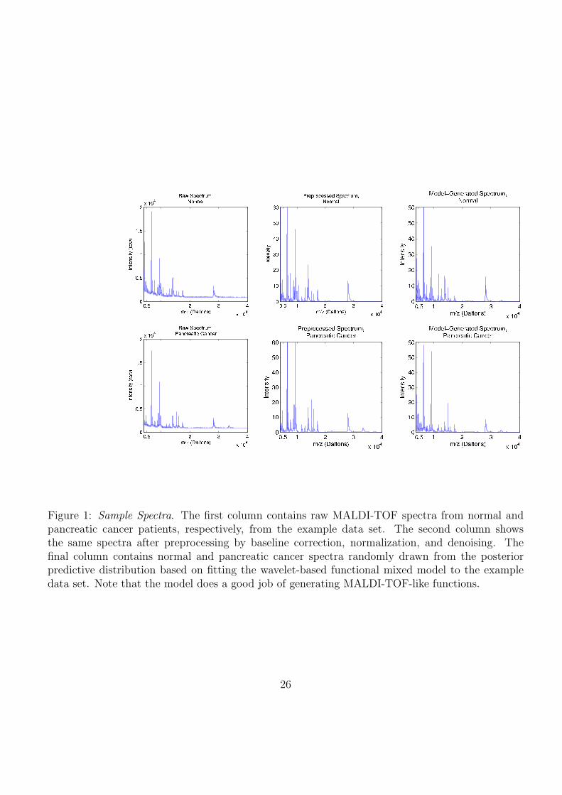
Figure 1: Sample Spectra. The first column contains raw MALDI-TOF spectra from normal andpancreatic cancer patients, respectively, from the example data set. The second column showsthe same spectra after preprocessing by baseline correction, normalization, and denoising. Thefinal column contains normal and pancreatic cancer spectra randomly drawn from the posteriorpredictive distribution based on fitting the wavelet-based functional mixed model to the exampledata set. Note that the model does a good job of generating MALDI-TOF-like functions.

26

5 10 15 20 25 30 35 40−2

−1

0

1

2

m/z (kDaltons)

Inte

nsity

(lo

g 2 sca

le)

(a) Cancer Main Effect Function

5 10 15 20 25 30 35 40<0.0005

0.01

0.10

0.50

0.90

0.99

>0.9995

m/z (kDaltons)

p(t)

=P

rob(

1.5−

Fol

d|D

ata)

(b) Pointwise Posterior Probabilites1.5−fold difference

2 5 8 11 14−10

−5

0

5

10

m/z (kDaltons)

Inte

nsity

(lo

g 2 sca

le)

(c) Organ Main Effect Function

2 5 8 11 14<0.0005

0.01

0.10

0.50

0.90

0.99

>0.9995

m/z (kDaltons)

p(t)

=P

rob(

2.0−

Fol

d|D

ata)

(d) Pointwise Posterior Probabilites2−fold difference

Figure 2: Fixed Effect Curves. (a) and (c): Posterior mean and 95% pointwise posterior crediblebands for cancer main effect, pancreatic cancer example, and organ main effect, organ-by-cell-line example, respectively. The green lines indicate 1.5-fold and 2.0-fold differences in the twoexamples, respectively, and the dots indicate peaks detected using the average spectrum. (b)and (d): Pointwise posterior probabilities of (b) 1.5-fold difference in cancer/normal in pancreaticcancer example and (d) 2.0-fold difference in brain/lung in organ-by-cell-line example. The reddots indicate detected peaks, and the green lines mark the flagged regions. The yellow dotted linesindicate the threshold for flagging a location as significant, controlling the expected Bayesian FDRto be less than 0.10 and 0.05 in the two examples, respectively.

27

33.00 33.25 33.50 33.75 34.00 34.25 34.50−2

−1.5

−1

−0.5

0

0.5

m/z (kDaltons)

Inte

nsity

(lo

g 2 sca

le)

(a) Block 1 − Block 2 Effect

17.15 17.20 17.25 17.30 17.35 17.40 17.45 17.50−2

−1

0

1

2

3

m/z (kDaltons)

Inte

nsity

(lo

g 2 sca

le)

(b) Block 1 − Block 2 Effect

Block 1Block 2

Block 1Block 2

Figure 3: Block Effects. Plot of the mean spectra for blocks 1 (green line) and 2 (red line), alongwith the posterior mean and 95% pointwise posterior bounds for the block 1 - block 2 effect (blueand black lines) near (a) the peak at 33,482 and (b) the twin peaks at 17,245 and 17,376. (a)illustrates that the nonparametric functional effect can model changes in intensity, and (b) showsthat the pulse-like features of the nonparametric effect account for systematic shifts in location.

28

3800 3850 3900 3950 4000−10

−5

0

5

10

m/z (Daltons)

Inte

nsity

(a) Organ Main Effect

7500 7550 7600 7650 7700−6

−4

−2

0

2

4

m/z (Daltons)

Inte

nsity

(b) Organ Main Effect

3800 3850 3900 3950 4000<0.0005

0.01

0.10

0.50

0.90

0.99

>0.9995

m/z (Daltons)

(c) Pointwise Posterior Probabilities, 2−fold difference

7500 7550 7600 7650 7700<0.0005

0.01

0.10

0.50

0.90

0.99

>0.9995

m/z (Daltons)

p(t)

=P

rob(

2.0−

Fol

d|D

ata)

(d) Pointwise Posterior Probabilities, 2−fold difference

Lung−InjectedBrain−Injected

Lung−InjectedBrain−InjectedOverall Mean Spectrum

Figure 4: Select Results. (a) and (b) Plot of organ main effect function in selected regions. Thegreen and red lines are the organ-specific mean spectra on the untransformed intensity scale, theblue and black lines are the posterior mean and pointwise 95% posterior bounds for the organ maineffect on the log2 intensity scale. The yellow dotted line at 0 and the cyan dotted lines at +/-1 areprovided for reference. (c) and (d) Pointwise posterior probabilities of 2-fold difference in intensity.The red dots indicate peaks detected in the mean spectrum, and the yellow dotted line indicatesthe threshold on pointwise posterior probabilities chosen so the expected Bayesian FDR<0.05. Thegreen lines in the plot indicate regions flagged as significant.

29

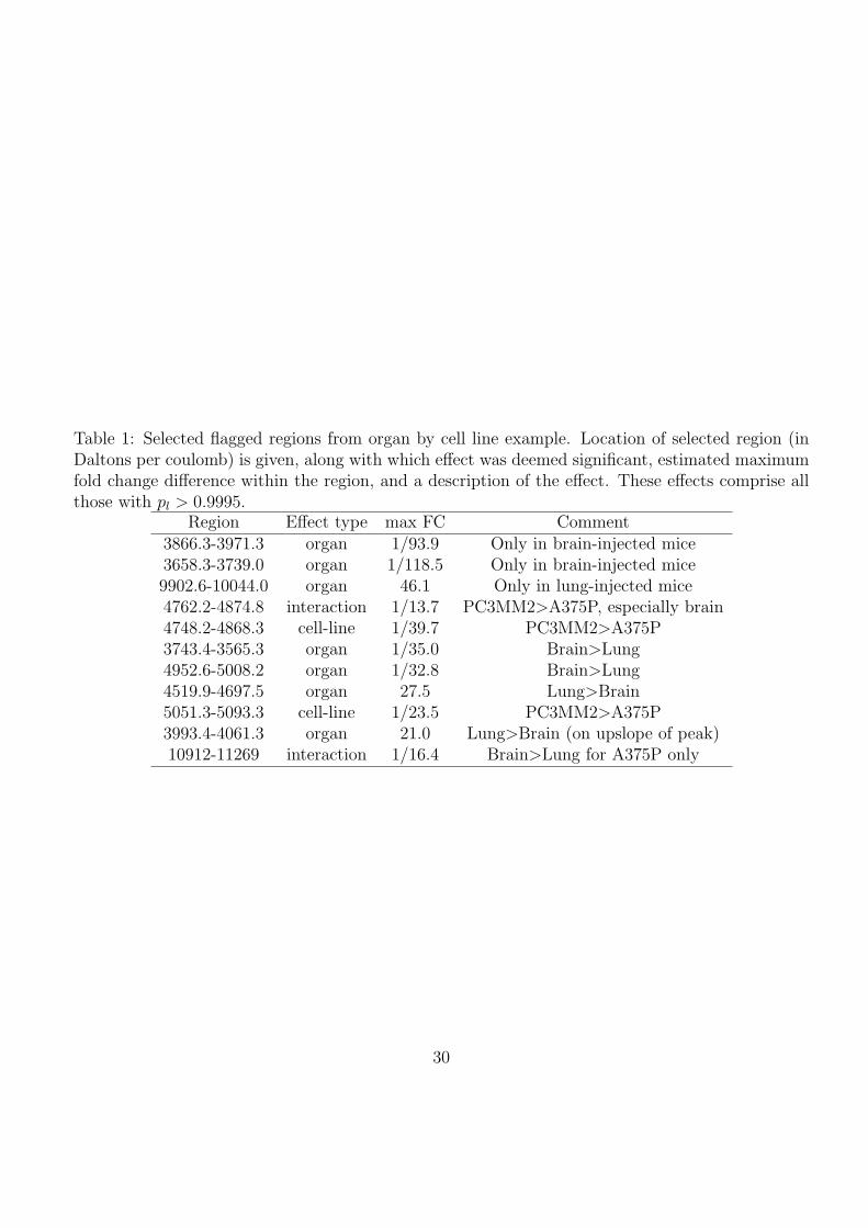
Table 1: Selected flagged regions from organ by cell line example. Location of selected region (inDaltons per coulomb) is given, along with which effect was deemed significant, estimated maximumfold change difference within the region, and a description of the effect. These effects comprise allthose with pl > 0.9995.

Region Effect type max FC Comment3866.3-3971.3 organ 1/93.9 Only in brain-injected mice3658.3-3739.0 organ 1/118.5 Only in brain-injected mice9902.6-10044.0 organ 46.1 Only in lung-injected mice4762.2-4874.8 interaction 1/13.7 PC3MM2>A375P, especially brain4748.2-4868.3 cell-line 1/39.7 PC3MM2>A375P3743.4-3565.3 organ 1/35.0 Brain>Lung4952.6-5008.2 organ 1/32.8 Brain>Lung4519.9-4697.5 organ 27.5 Lung>Brain5051.3-5093.3 cell-line 1/23.5 PC3MM2>A375P3993.4-4061.3 organ 21.0 Lung>Brain (on upslope of peak)10912-11269 interaction 1/16.4 Brain>Lung for A375P only

30

Bayesian Analysis of Mass Spectrometry Proteomic Data using Wavelet ... · Bayesian Analysis of Mass Spectrometry Proteomic Data using Wavelet Based Functional Mixed Models Jeﬁrey

Documents