1 Statistical design and analysis of quantitative mass spectrometry-based proteomic experiments Olga Vitek Department of Statistics Department of Computer Science Joint work with Susanne Ragg, Indiana University School of Medicine and Ilka Otts, Technical University of Munich

Welcome message from author
This document is posted to help you gain knowledge. Please leave a comment to let me know what you think about it! Share it to your friends and learn new things together.
Transcript

1
Statistical design and analysis of quantitative mass spectrometry-based
proteomic experiments
Olga VitekDepartment of Statistics
Department of Computer Science
Joint work with Susanne Ragg, Indiana University School of Medicine
and Ilka Otts, Technical University of Munich
Scope of the discussion
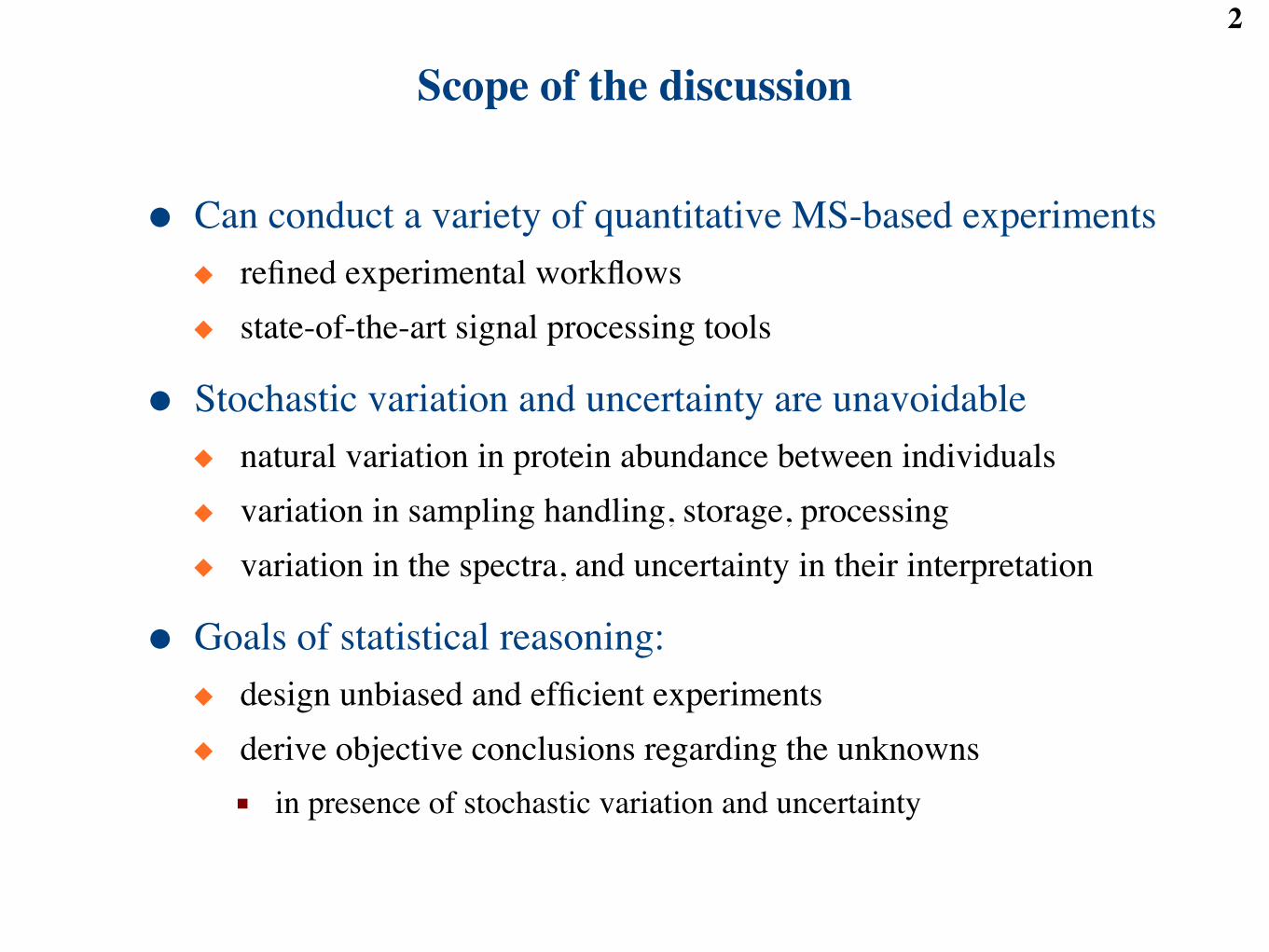
● Can conduct a variety of quantitative MS-based experiments◆ refined experimental workflows◆ state-of-the-art signal processing tools
● Stochastic variation and uncertainty are unavoidable◆ natural variation in protein abundance between individuals◆ variation in sampling handling, storage, processing◆ variation in the spectra, and uncertainty in their interpretation
● Goals of statistical reasoning:◆ design unbiased and efficient experiments◆ derive objective conclusions regarding the unknowns■ in presence of stochastic variation and uncertainty
2

Outline3
● LC-MS proteomics: a case study of coronary artery disease◆ Framing the question◆ Experimental design◆ Statistical analysis■ methods■ evaluation
◆ Enrichment of pre-defined sets in differential abundance
● Extensions◆ Planning future studies with LC-MS workflows◆ Design and analysis with labeling workflows
References4
● Case study ◆ Clough et al. Methods in Molecular Biology, in press.◆ Another example:
■ Patil et al. J. Proteome Research, 6, p.955, 2007.
● Protein-level quantification◆ T. Clough et al. J. Proteome Research, 8, p.5275, 2009.◆ Other examples:
■ J. Karpievitch et al. Bioinformatics, 25, p.2028, 2009■ A. Oberg et al. J. Proteome Research, 7, p.225, 2008.
● Experimental design◆ A. Oberg, O. Vitek. J. Proteome Research, 8, p.2144, 2009.
● Extensions (poster session) ◆ T. Clough et al. An R package for complex LC-MS experiments◆ V. Chang et al. Statistical methods for protein quantification in label-free
and labeling SRM experiments

Motivating example: a case study of coronary artery disease
5
● Collection of plasma samples of 3290 disease subjects and controls◆ treated at the Munich Heart Center between 2005 and 2006◆ collected at single time point at diagnosis◆ recorded clinical characteristics
● Focus on 5 disease groups ◆ STEMI, NSTEMI, unstable angina, stable angina, controls
● General goal: an initial quantitative LC-MS screening◆ select a subset of plasma samples◆ examine protein profiles◆ a follow-up study will focus on a subset of proteins and disease
groups

Outline6
● LC-MS proteomics: a case study of coronary artery disease◆ Framing the question◆ Experimental design◆ Statistical analysis■ methods■ evaluation
◆ Enrichment of pre-defined sets in differential abundance
● Extensions◆ Planning future studies with LC-MS workflows◆ Design and analysis with labeling workflows
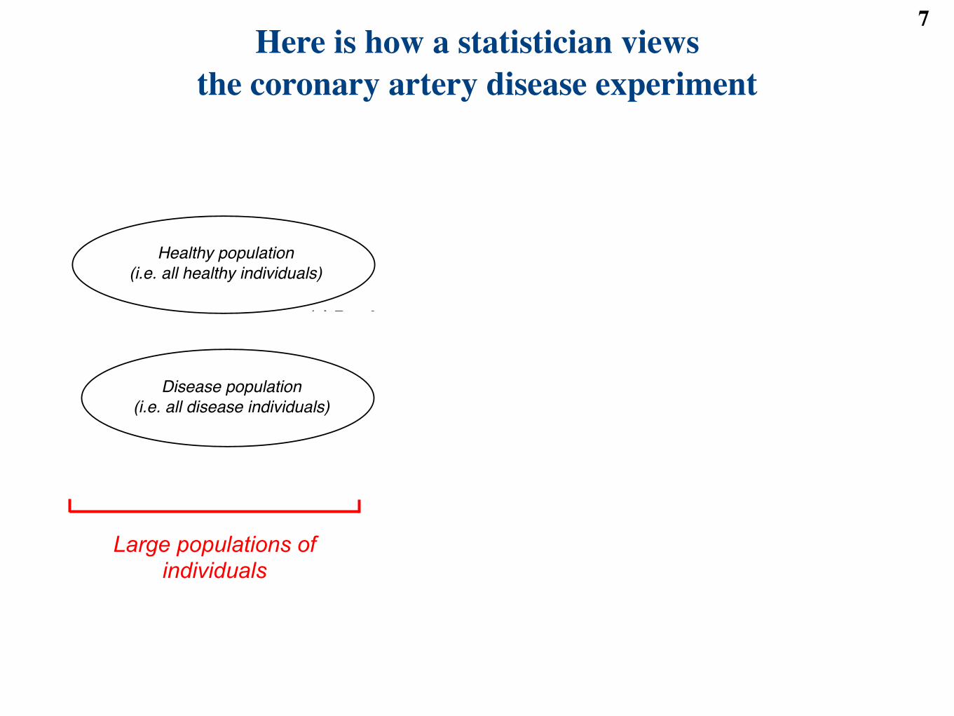
Here is how a statistician viewsthe coronary artery disease experiment
7
Large populations of individuals
Healthy population
(i.e. all healthy individuals)
Disease population
(i.e. all disease individuals)
Healthy individuals
in the study
Disease individuals
in the study
Healthy individuals
in the study
Disease individuals
in the study
(b) Noisy measurements
(b) Noisy measurements
(a) Random sample of
individuals
(a) Random sample of
individuals
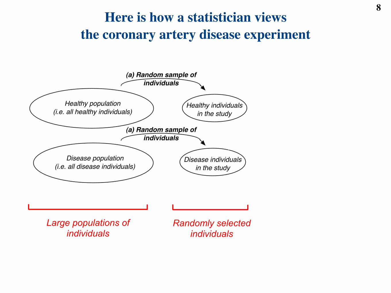
Here is how a statistician viewsthe coronary artery disease experiment
8
Large populations of individuals
Randomly selected individuals
Healthy population
(i.e. all healthy individuals)
Disease population
(i.e. all disease individuals)
Healthy individuals
in the study
Disease individuals
in the study
Healthy individuals
in the study
Disease individuals
in the study
(b) Noisy measurements
(b) Noisy measurements
(a) Random sample of
individuals
(a) Random sample of
individuals
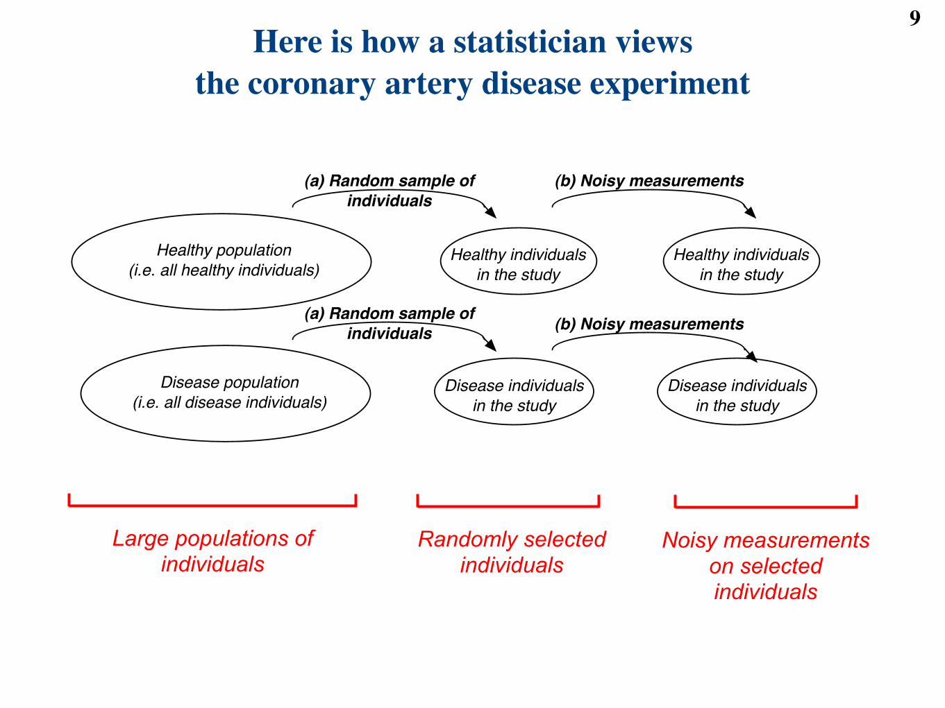
Here is how a statistician viewsthe coronary artery disease experiment
9
Large populations of individuals
Randomly selected individuals
Noisy measurements on selectedindividuals
Healthy population
(i.e. all healthy individuals)
Disease population
(i.e. all disease individuals)
Healthy individuals
in the study
Disease individuals
in the study
Healthy individuals
in the study
Disease individuals
in the study
(b) Noisy measurements
(b) Noisy measurements
(a) Random sample of
individuals
(a) Random sample of
individuals
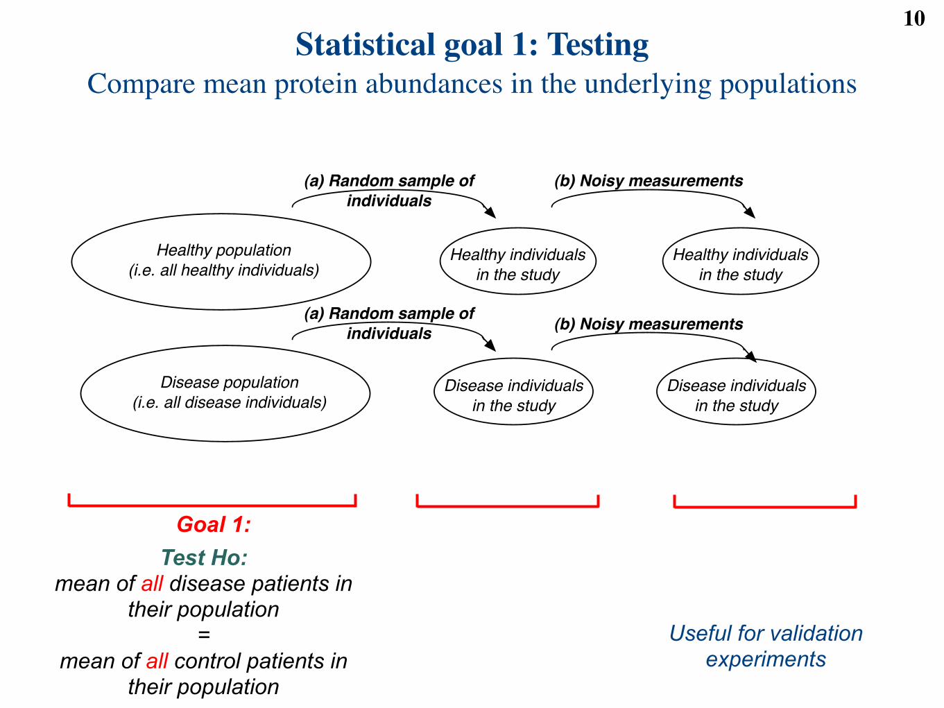
Statistical goal 1: TestingCompare mean protein abundances in the underlying populations
10
Goal 1:
Healthy population
(i.e. all healthy individuals)
Disease population
(i.e. all disease individuals)
Healthy individuals
in the study
Disease individuals
in the study
Healthy individuals
in the study
Disease individuals
in the study
(b) Noisy measurements
(b) Noisy measurements
(a) Random sample of
individuals
(a) Random sample of
individuals
Test Ho: mean of all disease patients in
their population =
mean of all control patients in their population
Useful for validation experiments
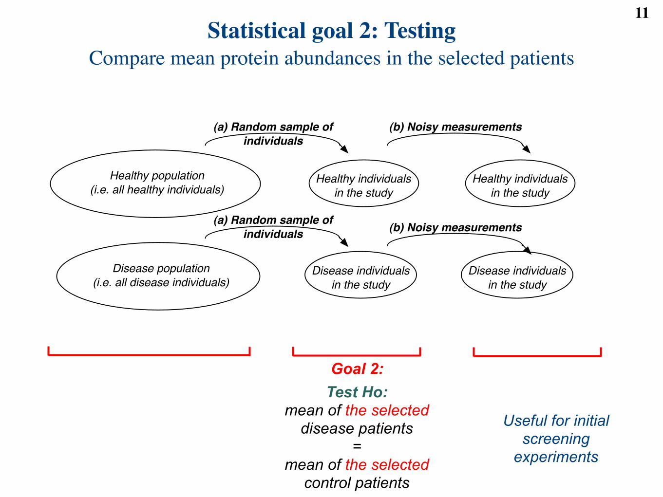
Statistical goal 2: TestingCompare mean protein abundances in the selected patients
11
Healthy population
(i.e. all healthy individuals)
Disease population
(i.e. all disease individuals)
Healthy individuals
in the study
Disease individuals
in the study
Healthy individuals
in the study
Disease individuals
in the study
(b) Noisy measurements
(b) Noisy measurements
(a) Random sample of
individuals
(a) Random sample of
individuals
Useful for initial screening
experiments
Goal 2:Test Ho:
mean of the selecteddisease patients
= mean of the selected
control patients
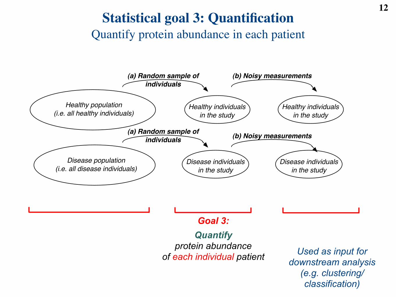
Statistical goal 3: QuantificationQuantify protein abundance in each patient
12
Healthy population
(i.e. all healthy individuals)
Disease population
(i.e. all disease individuals)
Healthy individuals
in the study
Disease individuals
in the study
Healthy individuals
in the study
Disease individuals
in the study
(b) Noisy measurements
(b) Noisy measurements
(a) Random sample of
individuals
(a) Random sample of
individuals
Quantify protein abundance
of each individual patient Used as input fordownstream analysis
(e.g. clustering/classification)
Goal 3:

Outline13
● LC-MS proteomics: a case study of coronary artery disease◆ Framing the question◆ Experimental design◆ Statistical analysis■ methods■ evaluation
◆ Enrichment of pre-defined sets in differential abundance
● Extensions◆ Planning future studies with LC-MS workflows◆ Design and analysis with labeling workflows
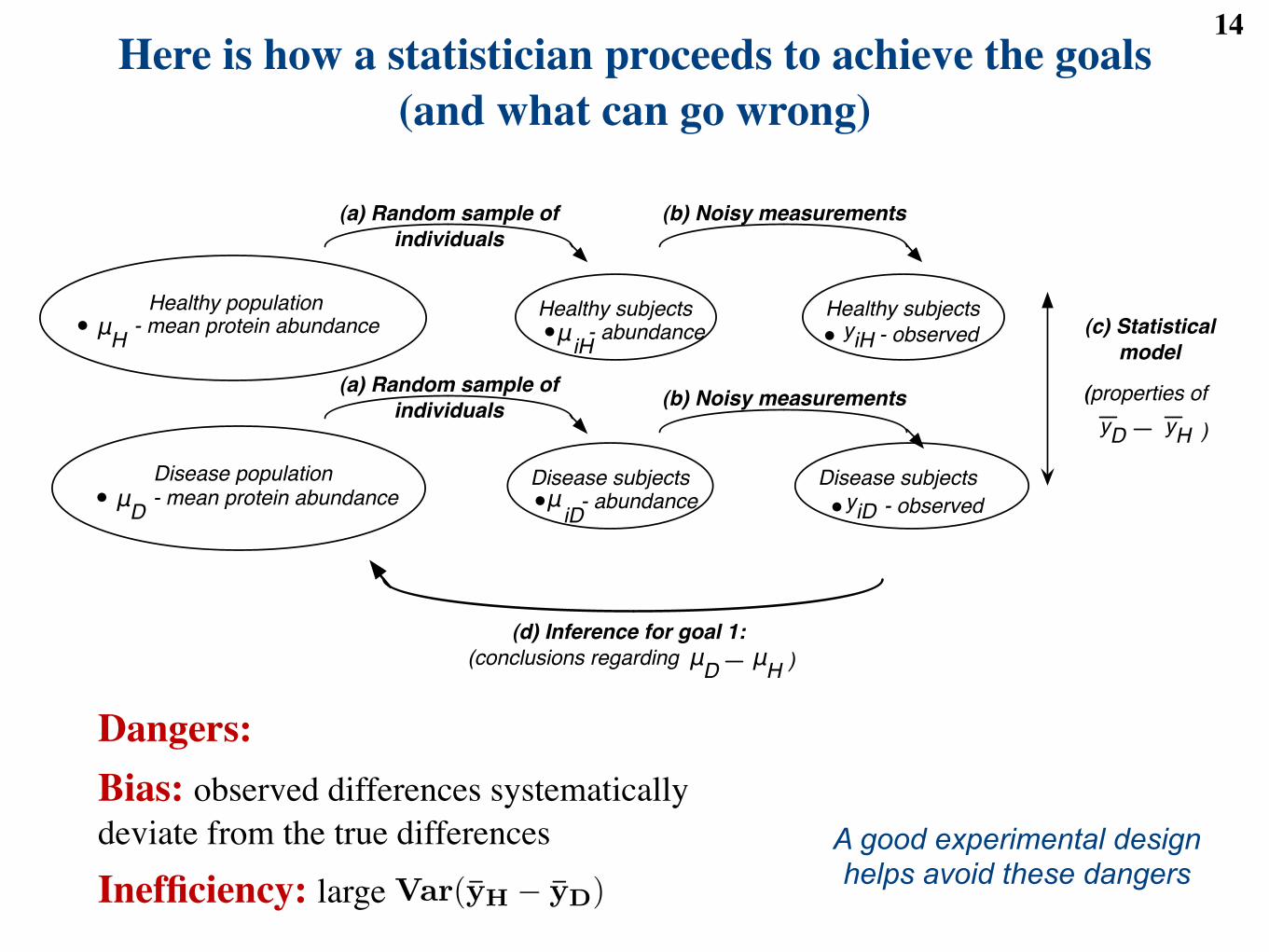
Here is how a statistician proceeds to achieve the goals(and what can go wrong)
14
Healthy population
Disease population
Healthy subjects
Disease subjects
Healthy subjects
Disease subjects
(b) Noisy measurements
(b) Noisy measurements
(a) Random sample of
individuals
(a) Random sample of
individuals
- mean protein abundance!H
!
- mean protein abundance!D
!
- observedyiH!- abundance!iH
!
- abundanceiD
!! - observedyiD!
(c) Statistical
model
(properties of
yHyD )
(d) Inference for goal 1:
(conclusions regarding !D
!H
)
Dangers:Bias: observed differences systematically deviate from the true differences
Inefficiency: large
Observed Systematic Random deviationfeature = mean signal + due to all sources
intensity of disease group of variation
yij = Group meani + Errorj(i)
! N`0, !2
´
Observed Systematic Random Random Randomfeature = mean signal + deviation due to + deviation due to + deviation due to
intensity of disease group individual sample preparation measurement error
yijkl = Group meani + Indiv(Group)j(i) + Prep(Indiv)k(ij) + Errorl(ijk)
! N`0, !2
Indiv
´! N
`0, !2
Prep
´! N
`0, !2
Error
´
Var(yH ! yD) = 2
!!2Indiv
I+
!2Prep
IJ+
!2Error
IJK
". (1)
Observed Systematic Random deviation Random Randomfeature = mean signal + due to block + deviation due to + deviation due to
intensity of disease group (e.g. plate or day) individual measurement error
yijkl = Group meani + Blockk + Indiv(Group)j(i) + Errorl(ijk)
! N`0, !2
Block
´! N
`0, !2
Indiv
´! N
`0, !2
Error
´
1
A good experimental design helps avoid these dangers

Fundamental principle 1: replication15
Healthy population
(all healthy individuals)
- mean feature abundance!H
!
(a) Random sample of individuals
Healthy individuals in study
- observed mean! yH
Disease population
(all disease individuals)
- mean feature abundance!D
!
(a) Random sample of individuals
Disease individuals in study
- observed mean! yD
(c) Inference (conclusions regarding !D
!H
)
(b) Statistical
model
(properties of
yHyD )
yH
yD
Healthy Disease
(a) No replication
Featu
re inte
nsity
yH
yD
Healthy Disease
(c) Not a significant difference
Featu
re inte
nsity
yH
yD
Healthy Disease
(b) A significant difference
Featu
re inte
nsity
yDd3
yH
Healthy Disease
(a) Sequential acquisition
Featu
re inte
nsity
d2
d2
d1
d1
d4
d4
d3
Healthy Disease
d4
d3
d2
d1
(c) Day = block
Featu
re inte
nsity
(b) Complete randomization
yH
yD
Healthy Disease
Featu
re inte
nsity
d3
d3
d2
d2
d4
d4
d1
d1
Observed Systematic Random deviationfeature = mean signal + due to all sources
intensity of disease group of variation
yij = Group meani + Errorj(i)
! N!0, !2
"
1
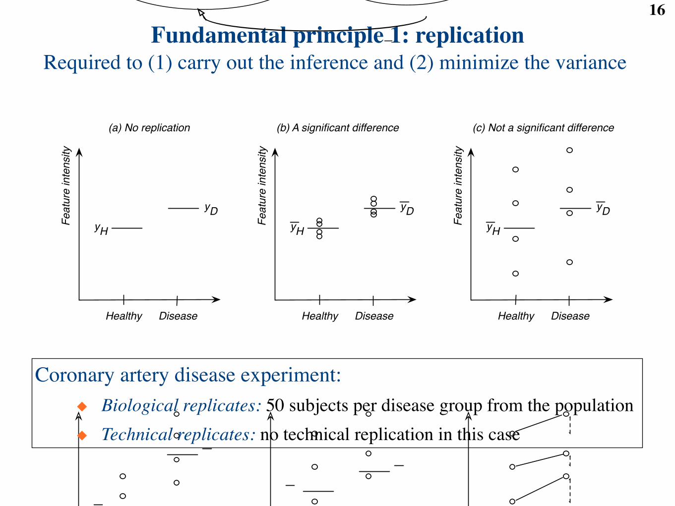
Required to (1) carry out the inference and (2) minimize the variance
Two levels of randomness imply two types of replication:◆ Biological replicates: selecting multiple subjects from the population◆ Technical replicates: multiple runs per subject
Fundamental principle 1: replication16
Healthy population
(all healthy individuals)
- mean feature abundance!H
!
(a) Random sample of individuals
Healthy individuals in study
- observed mean! yH
Disease population
(all disease individuals)
- mean feature abundance!D
!
(a) Random sample of individuals
Disease individuals in study
- observed mean! yD
(c) Inference (conclusions regarding !D
!H
)
(b) Statistical
model
(properties of
yHyD )
yH
yD
Healthy Disease
(a) No replication
Featu
re inte
nsity
yH
yD
Healthy Disease
(c) Not a significant difference
Featu
re inte
nsity
yH
yD
Healthy Disease
(b) A significant difference
Featu
re inte
nsity
yDd3
yH
Healthy Disease
(a) Sequential acquisition
Featu
re inte
nsity
d2
d2
d1
d1
d4
d4
d3
Healthy Disease
d4
d3
d2
d1
(c) Day = block
Featu
re inte
nsity
(b) Complete randomization
yH
yD
Healthy Disease
Featu
re inte
nsity
d3
d3
d2
d2
d4
d4
d1
d1
Observed Systematic Random deviationfeature = mean signal + due to all sources
intensity of disease group of variation
yij = Group meani + Errorj(i)
! N!0, !2
"
1
Required to (1) carry out the inference and (2) minimize the variance
Coronary artery disease experiment:◆ Biological replicates: 50 subjects per disease group from the population◆ Technical replicates: no technical replication in this case
17Fundamental principle 2: randomization
yDd3
yH
Healthy Disease
(a) Sequential acquisition
Fe
atu
re in
ten
sity
d2
d2
d1
d1
d4
d4
d3
Healthy Disease
d2
d2
d3
d4
(c) Day = block
Fe
atu
re in
ten
sity
(b) Complete randomization
yH
yD
Healthy Disease
Fe
atu
re in
ten
sity
d2
d2
d4
d4
d3
d3
d1
d1
No randomization = confounding
= bias
Complete randomization = no bias
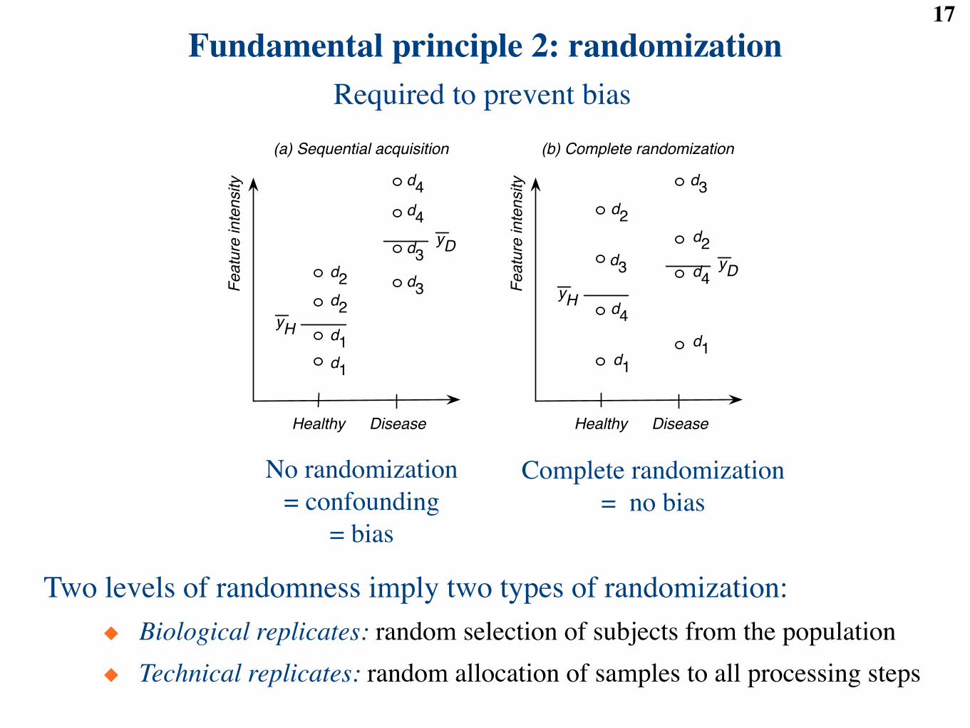
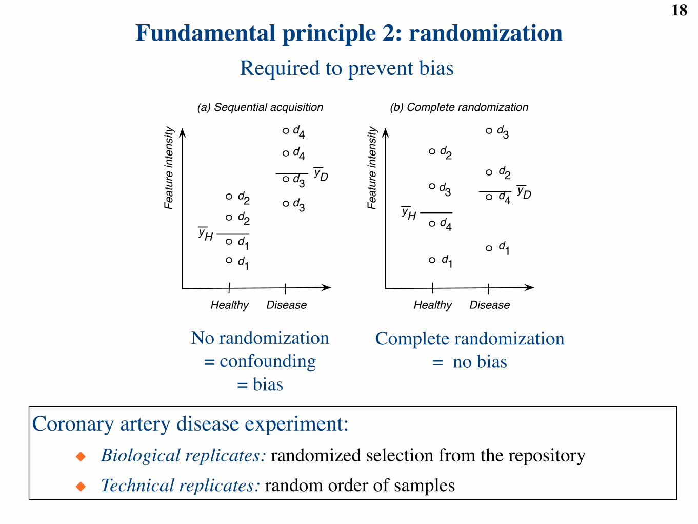
Required to prevent bias
Two levels of randomness imply two types of randomization:◆ Biological replicates: random selection of subjects from the population◆ Technical replicates: random allocation of samples to all processing steps
18Fundamental principle 2: randomization
yDd3
yH
Healthy Disease
(a) Sequential acquisition
Fe
atu
re in
ten
sity
d2
d2
d1
d1
d4
d4
d3
Healthy Disease
d2
d2
d3
d4
(c) Day = block
Fe
atu
re in
ten
sity
(b) Complete randomization
yH
yD
Healthy Disease
Fe
atu
re in
ten
sity
d2
d2
d4
d4
d3
d3
d1
d1
No randomization = confounding
= bias
Complete randomization = no bias
Required to prevent bias
Coronary artery disease experiment:◆ Biological replicates: randomized selection from the repository◆ Technical replicates: random order of samples
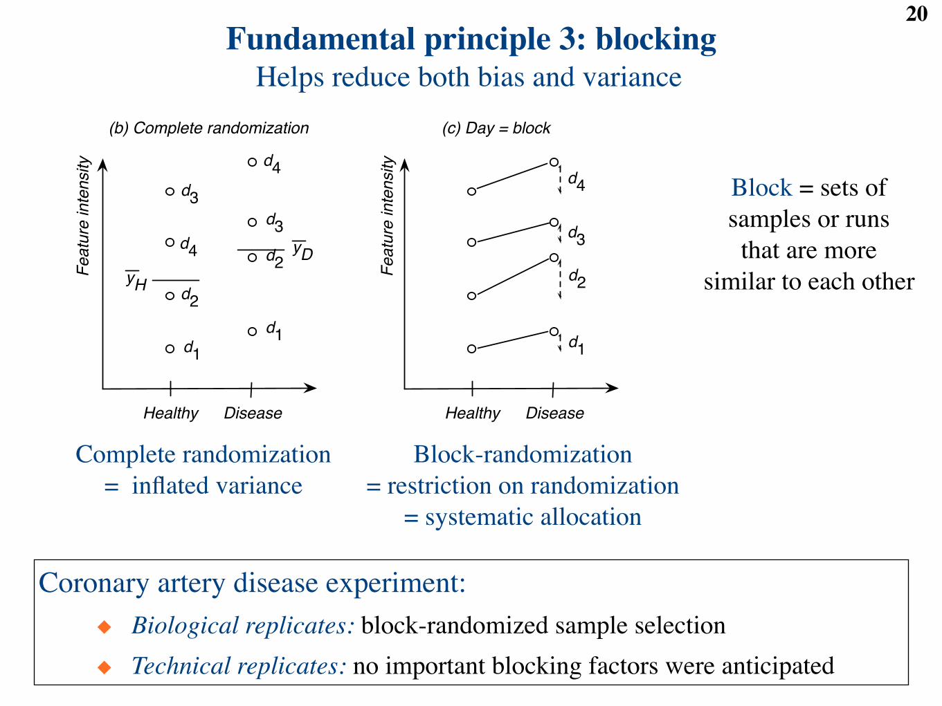
19Fundamental principle 3: blocking
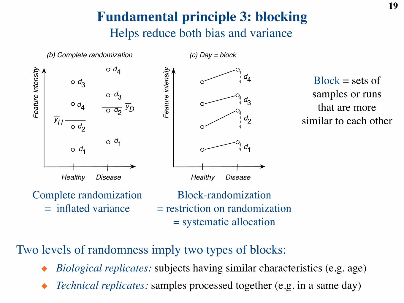
Helps reduce both bias and variance
Block = sets of samples or runs
that are more similar to each other
Complete randomization = inflated variance
Block-randomization = restriction on randomization
= systematic allocation
yDd3
yH
Healthy Disease
(a) Sequential acquisition
Fe
atu
re in
ten
sity
d2
d2
d1
d1
d4
d4
d3
Healthy Disease
d4
d3
d2
d1
(c) Day = block
Fe
atu
re in
ten
sity
(b) Complete randomization
yH
yD
Healthy Disease
Fe
atu
re in
ten
sity
d3
d3
d2
d2
d4
d4
d1
d1
Figure 3: (a) Sequential acquisition creates a confounding e!ect: the di!erence in group meanscan be due to both di!erences between groups and di!erences between days. (b) Complete ran-domization removes the confounding e!ect. The variance within each group is now a combinationof the biological di!erence and of the day-to-day variation. (c) Paired design uses day as a block ofsize 2. The design allows one to compare di!erences between individuals from two groups within ablock.
Observed Systematic Random deviationfeature = mean signal + due to all sources
intensity of disease group of variation
yij = Group meani + Errorj(i)
! N!0, !2
"
Figure 4: Statistical model for a completely randomized design with a single mass spectrumreplicate per patient. i indicates the index of a disease group, and j(i) the index of a patient withinthe group. All Errorj(i) are assumed independent.
Observed Systematic Random Random Randomfeature = mean signal + deviation due to + deviation due to + deviation due to
intensity of disease group individual sample preparation measurement error
yijkl = Group meani + Indiv(Group)j(i) + Prep(Indiv)k(ij) + Errorl(ijk)
! N!0, !2
Indiv
"! N
!0, !2
Prep
"! N
!0, !2
Error
"
Figure 5: Statistical model for a mixed e!ects analysis of variance (ANOVA). i is the index ofa disease group, j(i) the index of a patient within the group, k(ij) is the index of the samplepreparation within the patient, and l(ijk) is the replicate run. Indiv(Group)j(i), Prep(Indiv)k(ij)
and Errorl(ijk) are all independent.
40
Two levels of randomness imply two types of blocks:◆ Biological replicates: subjects having similar characteristics (e.g. age)◆ Technical replicates: samples processed together (e.g. in a same day)
20Fundamental principle 3: blocking
Helps reduce both bias and variance
Complete randomization = inflated variance
Block-randomization = restriction on randomization
= systematic allocation
yDd3
yH
Healthy Disease
(a) Sequential acquisition
Fe
atu
re in
ten
sity
d2
d2
d1
d1
d4
d4
d3
Healthy Disease
d4
d3
d2
d1
(c) Day = block
Fe
atu
re in
ten
sity
(b) Complete randomization
yH
yD
Healthy Disease
Fe
atu
re in
ten
sity
d3
d3
d2
d2
d4
d4
d1
d1
Figure 3: (a) Sequential acquisition creates a confounding e!ect: the di!erence in group meanscan be due to both di!erences between groups and di!erences between days. (b) Complete ran-domization removes the confounding e!ect. The variance within each group is now a combinationof the biological di!erence and of the day-to-day variation. (c) Paired design uses day as a block ofsize 2. The design allows one to compare di!erences between individuals from two groups within ablock.
Observed Systematic Random deviationfeature = mean signal + due to all sources
intensity of disease group of variation
yij = Group meani + Errorj(i)
! N!0, !2
"
Figure 4: Statistical model for a completely randomized design with a single mass spectrumreplicate per patient. i indicates the index of a disease group, and j(i) the index of a patient withinthe group. All Errorj(i) are assumed independent.
Observed Systematic Random Random Randomfeature = mean signal + deviation due to + deviation due to + deviation due to
intensity of disease group individual sample preparation measurement error
yijkl = Group meani + Indiv(Group)j(i) + Prep(Indiv)k(ij) + Errorl(ijk)
! N!0, !2
Indiv
"! N
!0, !2
Prep
"! N
!0, !2
Error
"
Figure 5: Statistical model for a mixed e!ects analysis of variance (ANOVA). i is the index ofa disease group, j(i) the index of a patient within the group, k(ij) is the index of the samplepreparation within the patient, and l(ijk) is the replicate run. Indiv(Group)j(i), Prep(Indiv)k(ij)
and Errorl(ijk) are all independent.
40
Coronary artery disease experiment:◆ Biological replicates: block-randomized sample selection ◆ Technical replicates: no important blocking factors were anticipated
Block = sets of samples or runs
that are more similar to each other
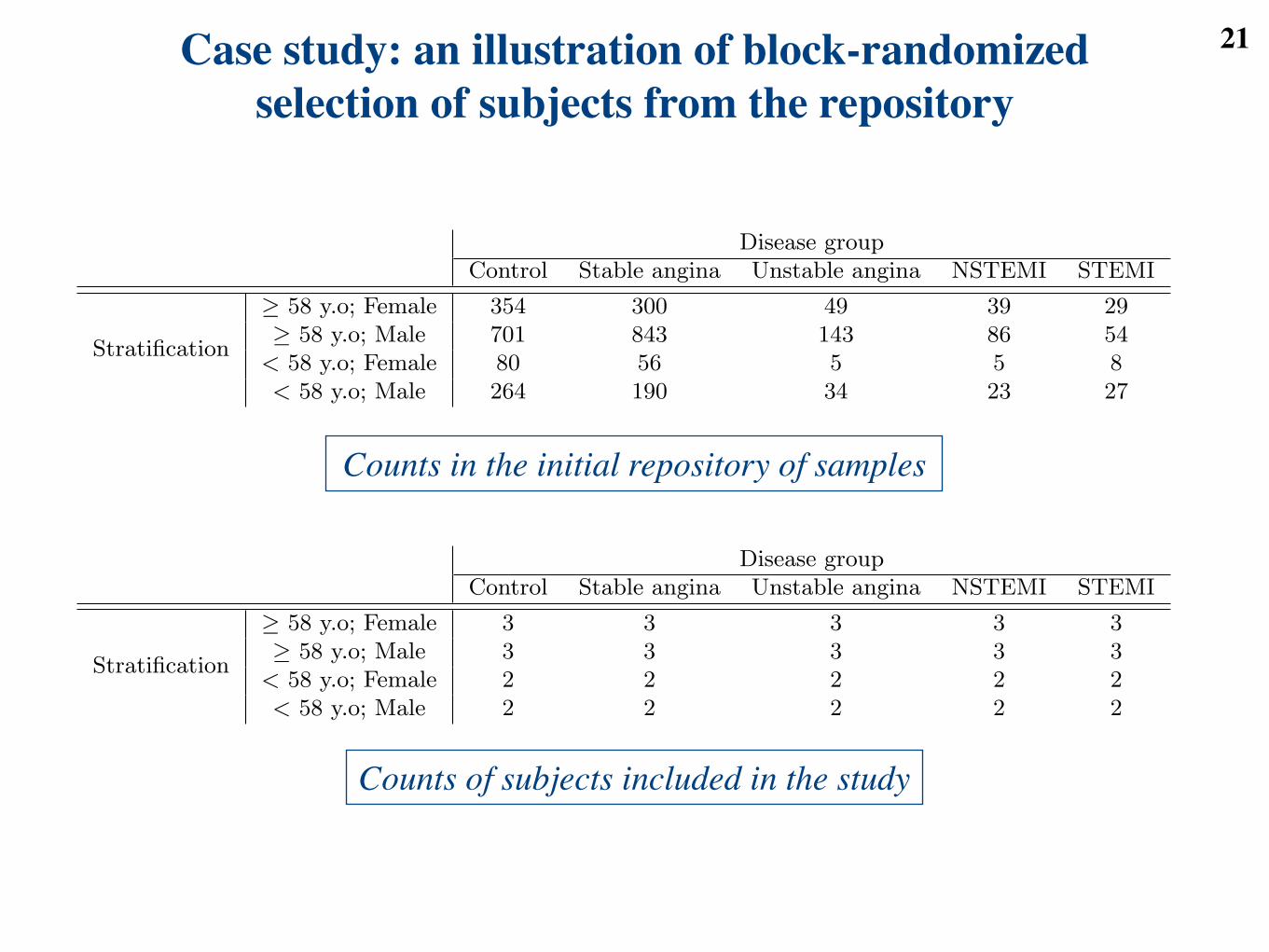
21Case study: an illustration of block-randomized selection of subjects from the repository
Disease groupControl Stable angina Unstable angina NSTEMI STEMI
Stratification
! 58 y.o; Female 354 300 49 39 29! 58 y.o; Male 701 843 143 86 54
< 58 y.o; Female 80 56 5 5 8< 58 y.o; Male 264 190 34 23 27
Table 1: Number of serum samples from subjects with coronary artery disease and controls, available foreach combination of age group, gender and disease group.
Disease groupControl Stable angina Unstable angina NSTEMI STEMI
Stratification
! 58 y.o; Female 3 3 3 3 3! 58 y.o; Male 3 3 3 3 3
< 58 y.o; Female 2 2 2 2 2< 58 y.o; Male 2 2 2 2 2
Table 2: Number of serum samples selected for the proteomic experiment. Each disease group has the samenumber of subjects for each combination of age group and gender.
# of proteins with # of proteins with Totalno detected di!erence detected di!erence
# true non-di!. proteins U V m0
# true di!. proteins T S m1 = m!m0
Total m!R R m
Table 3: Outcomes of testing m null hypotheses H0 : µH = µD simultaneously for m identified proteins. m and m0
are fixed, and R, S, T , U and V are random. Only m and R are observed.
# of proteins with # of proteins with Totalno detected di!erence detected di!erence
# of proteins in the set s!K K s# of proteins not in the set (m! s)! (R!K) R!K m! s
Total m!R R m
Table 4: Outcomes of the gene set enrichment analysis (GSEA) for one protein set. m is the total number of proteins(also called the “universe”), and s is the total number of proteins in the pre-specified set. The Hypergeometric testis conditional on the number of di!erentially abundant proteins R. It tests the null hypothesis that the number ofdi!erentially abundant proteins in the set K is as expected by random chance, against the alternative hypothesisthat K is larger than as expected by random chance.
21
Disease groupControl Stable angina Unstable angina NSTEMI STEMI
Stratification
! 58 y.o; Female 354 300 49 39 29! 58 y.o; Male 701 843 143 86 54
< 58 y.o; Female 80 56 5 5 8< 58 y.o; Male 264 190 34 23 27
Table 1: Number of serum samples from subjects with coronary artery disease and controls, available foreach combination of age group, gender and disease group.
Disease groupControl Stable angina Unstable angina NSTEMI STEMI
Stratification
! 58 y.o; Female 3 3 3 3 3! 58 y.o; Male 3 3 3 3 3
< 58 y.o; Female 2 2 2 2 2< 58 y.o; Male 2 2 2 2 2
Table 2: Number of serum samples selected for the proteomic experiment. Each disease group has the samenumber of subjects for each combination of age group and gender.
# of proteins with # of proteins with Totalno detected di!erence detected di!erence
# true non-di!. proteins U V m0
# true di!. proteins T S m1 = m!m0
Total m!R R m
Table 3: Outcomes of testing m null hypotheses H0 : µH = µD simultaneously for m identified proteins. m and m0
are fixed, and R, S, T , U and V are random. Only m and R are observed.
# of proteins with # of proteins with Totalno detected di!erence detected di!erence
# of proteins in the set s!K K s# of proteins not in the set (m! s)! (R!K) R!K m! s
Total m!R R m
Table 4: Outcomes of the gene set enrichment analysis (GSEA) for one protein set. m is the total number of proteins(also called the “universe”), and s is the total number of proteins in the pre-specified set. The Hypergeometric testis conditional on the number of di!erentially abundant proteins R. It tests the null hypothesis that the number ofdi!erentially abundant proteins in the set K is as expected by random chance, against the alternative hypothesisthat K is larger than as expected by random chance.
21
Counts in the initial repository of samples
Counts of subjects included in the study

Outline22
● LC-MS proteomics: a case study of coronary artery disease◆ Framing the question◆ Experimental design◆ Statistical analysis■ methods■ evaluation
◆ Enrichment of pre-defined sets in differential abundance
● Extensions◆ Planning future studies with LC-MS workflows◆ Design and analysis with labeling workflows
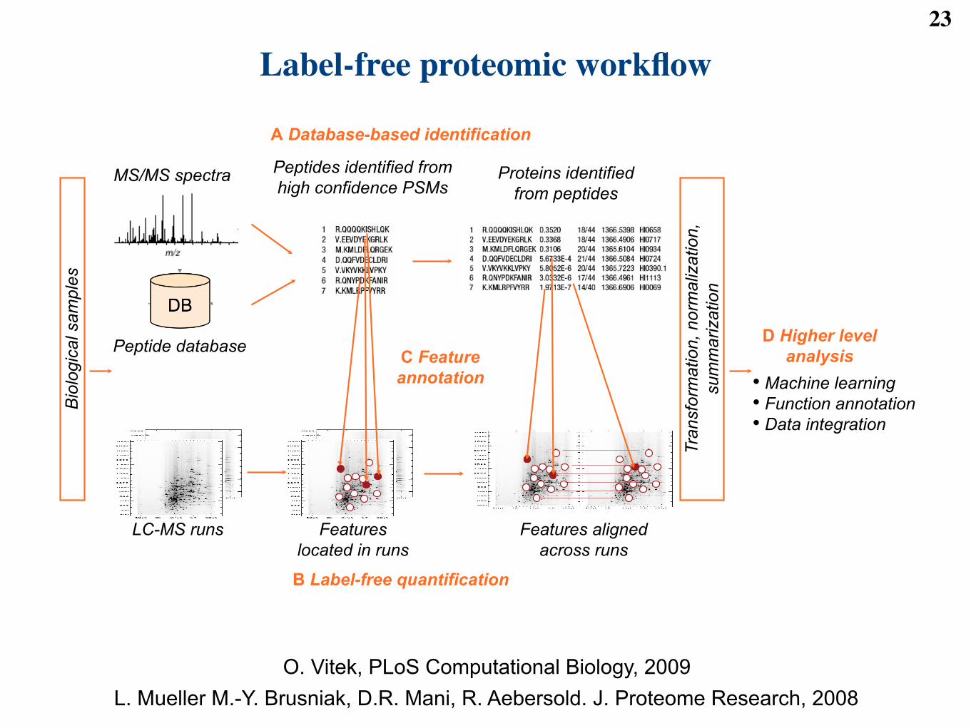
Label-free proteomic workflow23
MS/MS spectra Peptides identified from
high confidence PSMs Proteins identified
from peptides
Peptide database
LC-MS runs Features
located in runs
Features aligned
across runs
C Feature
annotation
A Database-based identification
B Label-free quantification
Tra
nsfo
rmation, norm
aliz
ation,
sum
marization
Bio
logic
al sam
ple
s
D Higher level
analysis
•! Machine learning
•! Function annotation
•! Data integration
O. Vitek, PLoS Computational Biology, 2009L. Mueller M.-Y. Brusniak, D.R. Mani, R. Aebersold. J. Proteome Research, 2008
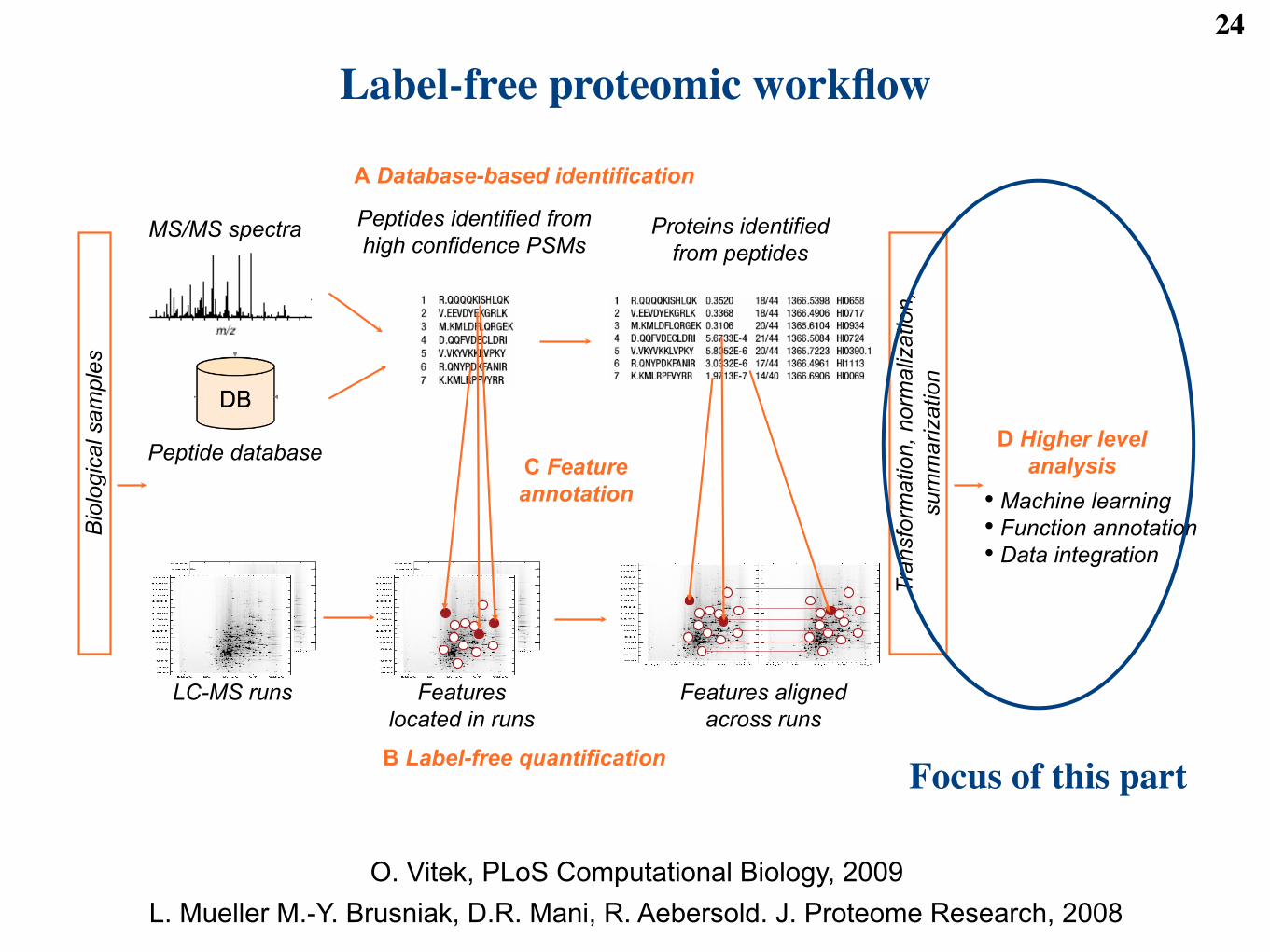
Label-free proteomic workflow24
MS/MS spectra Peptides identified from
high confidence PSMs Proteins identified
from peptides
Peptide database
LC-MS runs Features
located in runs
Features aligned
across runs
C Feature
annotation
A Database-based identification
B Label-free quantification
Tra
nsfo
rmation, norm
aliz
ation,
sum
marization
Bio
logic
al sam
ple
s
D Higher level
analysis
•! Machine learning
•! Function annotation
•! Data integration
Focus of this part
O. Vitek, PLoS Computational Biology, 2009L. Mueller M.-Y. Brusniak, D.R. Mani, R. Aebersold. J. Proteome Research, 2008
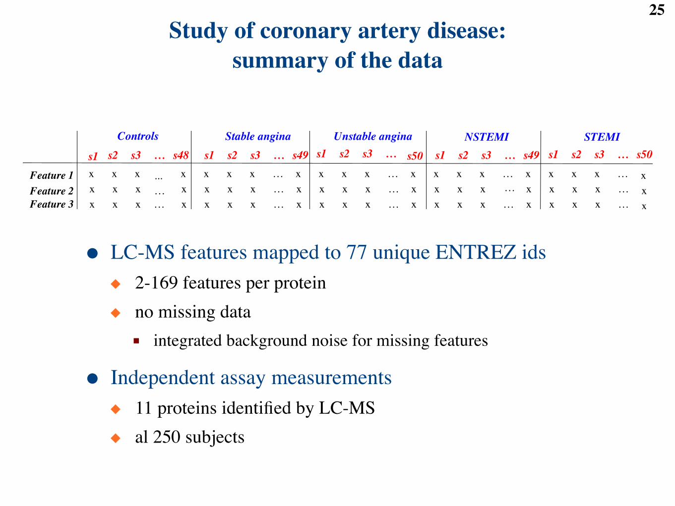
Study of coronary artery disease: summary of the data
25
!"
Controls! Stable angina! Unstable angina! NSTEMI!
x! x! x!x! x! …! x! x! x! x! …! x! x! x! x! …! x! x!x! x! …!x! ...! x!Feature 1!
x! x! x!x! x! …! x! x! x! x! …! x! x! x! x! …! x! x!x! x! …!x! …! x!Feature 2!
x! x! x!x! x! …! x! x! x! x! …! x! x! x! x! …! x! x!x! x! …!x! …! x!Feature 3!
s1 s3! s48!s2! …! s1 s3! s49!s2! …!
STEMI!
s1 s3! s50!s2! …! s1 s3! s49!s2! …! s1 s3! s50!s2! …!
x!
x!
x!
● LC-MS features mapped to 77 unique ENTREZ ids◆ 2-169 features per protein◆ no missing data■ integrated background noise for missing features
● Independent assay measurements◆ 11 proteins identified by LC-MS◆ al 250 subjects
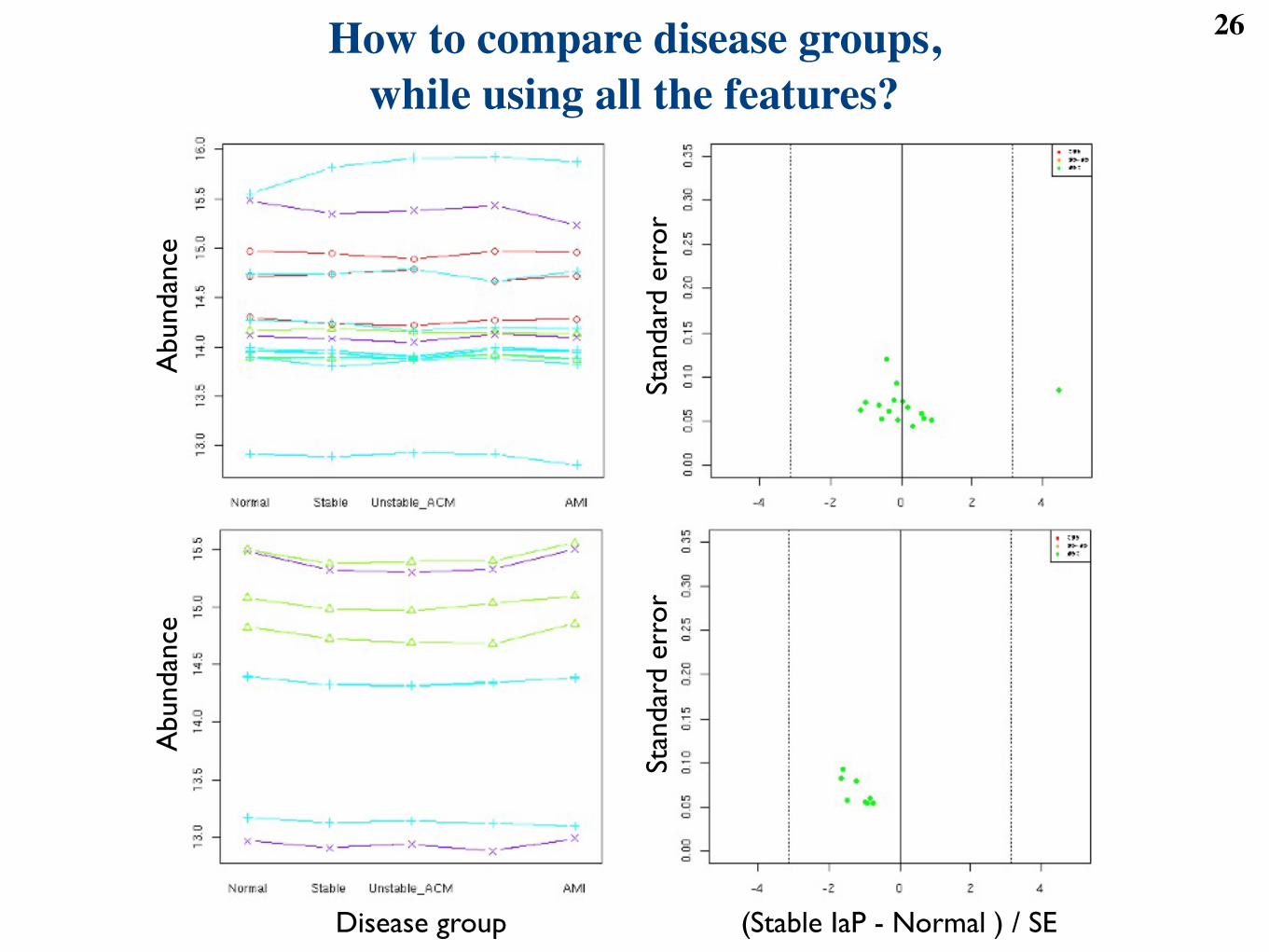
26How to compare disease groups, while using all the features?
Disease group
Abu
ndan
ceA
bund
ance
Stan
dard
err
orSt
anda
rd e
rror
(Stable IaP - Normal ) / SE
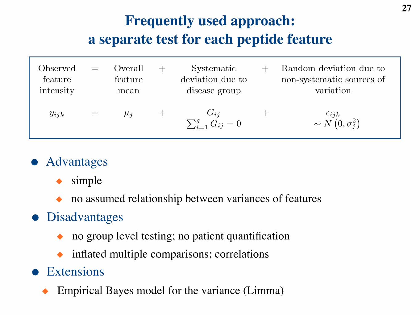
27Frequently used approach:
a separate test for each peptide feature
● Disadvantages◆ no group level testing; no patient quantification◆ inflated multiple comparisons; correlations
Observedfeature
intensity
= Overallfeaturemean
+ Systematicdeviation due todisease group
+ Random deviation due tonon-systematic sources of
variation
yijk = µj + Gij + !ijkPgi=1 Gij = 0 ! N
`0, "2
j
´
Figure 1: Per-feature ANOVA. i is the index of a disease group, j the index of a feature, and k the indexof a subject.
!gi=1 Gij = 0 is an identifiability constraint that is required for estimation of the model
parameters. !2j is the variance of the measurement error associated with feature j. All random deviations
are independent.
Averagefeature
intensity persubject
= Overallfeaturemean
+ Systematicdeviation due todisease group
+ Random deviation dueto non-systematic
sources of variation
yi·k = µ + Gi + !ikPgi=1 Gi = 0 ! N
`0, "2
´
Figure 2: Average ANOVA. i is the index of a disease group, and k the index of a subject.!g
i=1 Gi = 0is an identifiability constraint that is required for estimation of the model parameters. !2 is the variance ofthe measurement error. All random deviations are independent.
Systematic deviation due to
Observedintensity
= Overallmean
+ diseasegroup
+ fea-ture
+ interac-tion
+ sub-ject
+ Randomdeviation
yijk = µ + Gi + Fj + (G"F )ij + S(G)k(i) + !ijk
! N`0, "2
´
gX
i=1
Gi =fX
j=1
Fj =gX
i=1
(G" F )ij =fX
j=1
(G" F )ij =nX
k=1
S(G)k(i) = 0
Figure 3: Fixed e!ects ANOVA. i is the index of a disease group, j the index of a feature, and k the indexof a subject.
!gi=1 Gi =
!fj=1 Fj =
!gi=1(G ! F )ij =
!fj=1(G ! F )ij = 0 and
!nk=1 S(G)k(i) = 0 are
identifiability constraints that are required for estimation of the model parameters. !2 is the variance of themeasurement error. All random deviations are independent.
23
● Extensions◆ Empirical Bayes model for the variance (Limma)
● Advantages◆ simple◆ no assumed relationship between variances of features
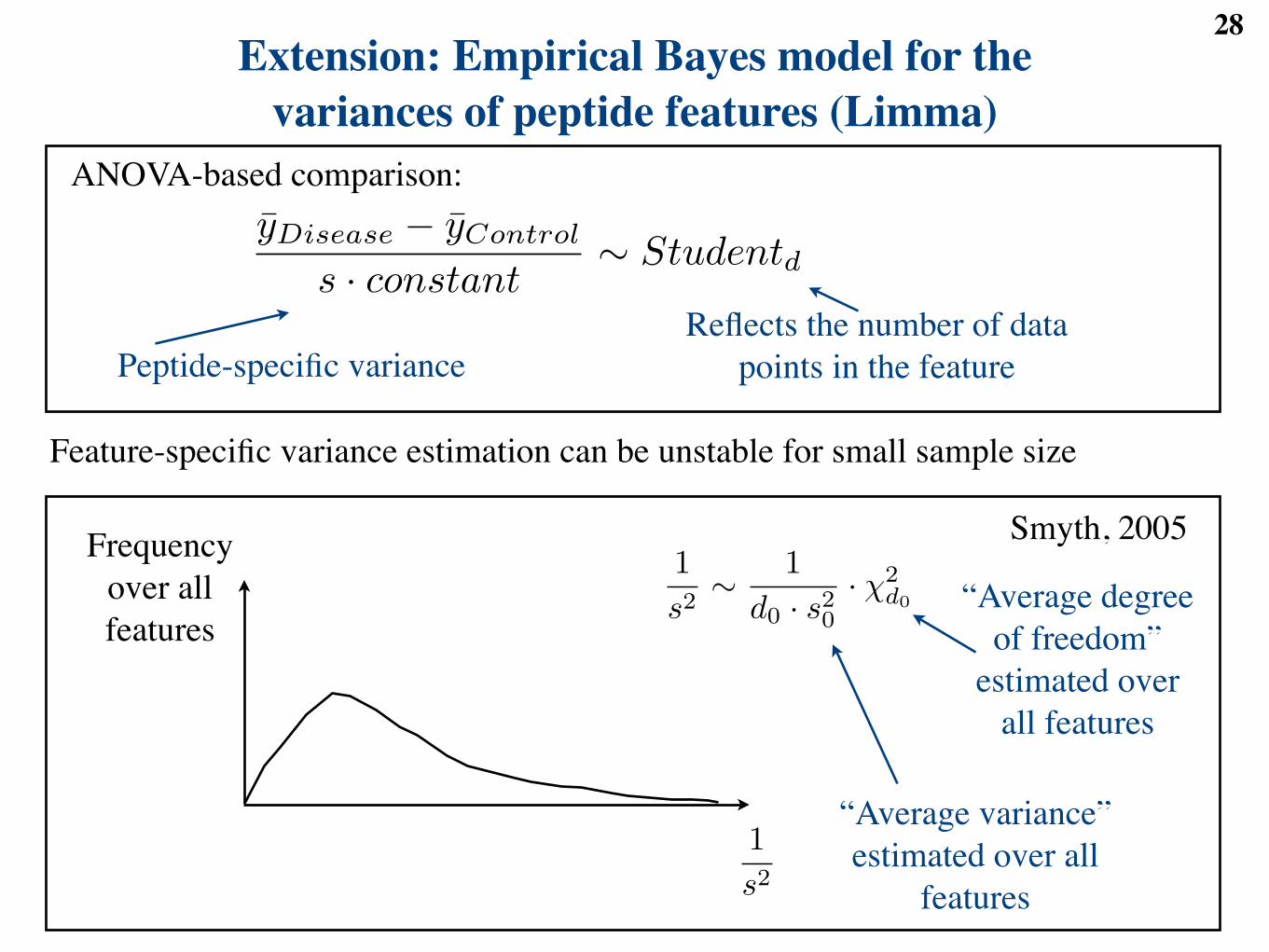
28Extension: Empirical Bayes model for the
variances of peptide features (Limma)ANOVA-based comparison:
Peptide-specific varianceReflects the number of data
points in the feature
Frequency over all features
xDiab ! xControl
s · constant" Studentd
xDiab ! xControl
s · constant" Student(d)
s2 =d0 · s2
0 + d · s2
d0 + d
d = d0 + d
1s2" 1
d0 · s20
· !2d0
1
xDiab ! xControl
s · constant" Studentd
xDiab ! xControl
s · constant" Student(d)
s2 =d0 · s2
0 + d · s2
d0 + d
d = d0 + d
1s2" 1
d0 · s20
· !2d0
1
“Average variance” estimated over all
features
“Average degree of freedom”
estimated over all features
Feature-specific variance estimation can be unstable for small sample size
yDisease ! yControl
s · constant" Studentd
yDisease ! yControl
s · constant" Student(d)
s2 =d0 · s2
0 + d · s2
d0 + d
d = d0 + d
1s2" 1
d0 · s20
· !2d0
1
Smyth, 2005
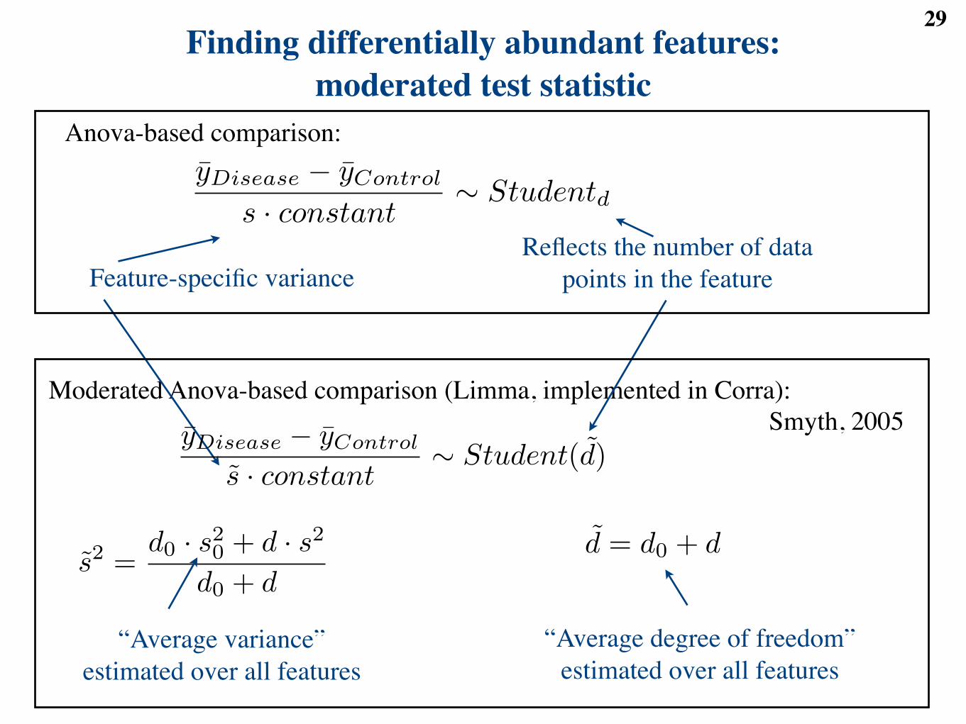
29Finding differentially abundant features:
moderated test statistic
xDiab ! xControl
s · constant" Studentd
xDiab ! xControl
s · constant" Student(d)
s2 =d0 · s2
0 + d · s2
d0 + d
1
xDiab ! xControl
s · constant" Studentd
xDiab ! xControl
s · constant" Student(d)
s2 =d0 · s2
0 + d · s2
d0 + d
d = d0 + d
1
Anova-based comparison:
Feature-specific varianceReflects the number of data
points in the feature
Moderated Anova-based comparison (Limma, implemented in Corra):
“Average variance” estimated over all features
“Average degree of freedom” estimated over all features
Smyth, 2005
yDisease ! yControl
s · constant" Studentd
yDisease ! yControl
s · constant" Student(d)
s2 =d0 · s2
0 + d · s2
d0 + d
d = d0 + d
1s2" 1
d0 · s20
· !2d0
1
yDisease ! yControl
s · constant" Studentd
yDisease ! yControl
s · constant" Student(d)
s2 =d0 · s2
0 + d · s2
d0 + d
d = d0 + d
1s2" 1
d0 · s20
· !2d0
1
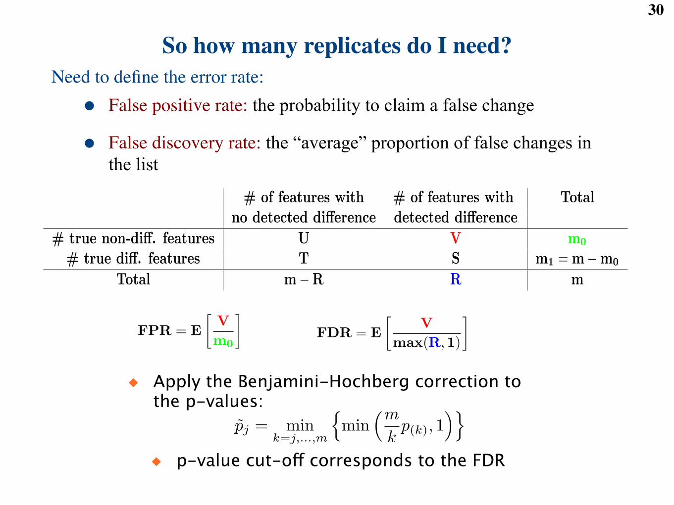
So how many replicates do I need?30
Need to define the error rate:● False positive rate: the probability to claim a false change
● False discovery rate: the “average” proportion of false changes in the list
# of features with # of features with Totalno detected di!erence detected di!erence
# true non-di!. features U V m0
# true di!. features T S m1 = m!m0
Total m!R R m
Table 1: Outcomes of testing m null hypotheses H0 : µH = µD simultaneously for m experimental features,conditionally on the features detected and quantified by a signal processing procedure. R, S, T , U and Vare random quantities, but only R is observed.
!
"
!
FDR = E!
Vmax(R,1)
". (1)
FPR = E!
Vm0
". (2)
!ave ! (1" ")ave · q 11 + (1" q) · m0/m1
, (3)
Var(yH " yD) !#
!z1!! + z1!"/2
$2
, (4)
where z1!! and z1!"/2 are respectively the 100(1" ")th and the 100(1" !/2)th percentiles of the
standard Normal distribution. The formula can be applied to variances of c
Var(yH " yD) = 2#
#2Indiv + #2
Error
I
$!
#!
z1!! + z1!"/2
$2
(5)
1
◆ Apply the Benjamini-Hochberg correction to the p-values:
◆ p-value cut-off corresponds to the FDR
Frequentist approaches to controlling multivariate type I error 7
Procedure
1. Order the p-valuesp(1) ! p(2) ! . . . ! p(m) (10)
2. Starting with the largest p-value, compare p(j) to a !j = f(!!, j) as follows
p" value p(m) p(m"1) . . . p(K+1) p(K) p(K"1) . . . p(1)
! mm!! m"1
m !! . . . K+1m !! K
m!! K"1m !! . . . 1
m!!
p ! ! No No . . . No Yes ? . . . ?(11)
Once the first statistic is encountered such that p ! !, reject that null hypothesiss, and all others witha lower p-value.
This is equivalent to adjusting each p-value by
pj = mink=j,...,m
!min
"m
kp(k), 1
#$(12)
The outer minimization ensures that the order of the p-values is preserved, while the inside minimizationensures that all p-values remain below 1.
Comments
In 2001, Benjamini and Yekutieli showed that this procedure tolerates positive regression dependence, butnot general dependence. However, they were able to modify it such that it does control the FDR undergeneral dependence, using
pj = mink=j,...,m
%min
&m
'mt=1 1/t
kp(k), 1
()(13)
This is generally considered too conservative unless the dependence structure of the data requires it.
References
[Benjamini1995] Benjamini Y and Y. Hochberg. Controlling the false discovery rate. Journal of the RoyalStatistical Society Series B., 57(1): 289-300 1995
[Benjamini2001] Benjamini, Y and D. Yekutieli. The Control of the false discovery rate in multiple testingunder dependency. Annals of Statistics, 29(4): 1165-1188, Aug 2001.
[Xu2004] N. Zhong and J. Liu (Ed.), Intelligent Technologies for Infomration Analysis, Springer, pp615-659,2004.
[Westfall1993] Westfall, P.H. and S.S Young. Resampling-Based Multiple Testing. John Wiley & Sons, Inc.,New York 1993.
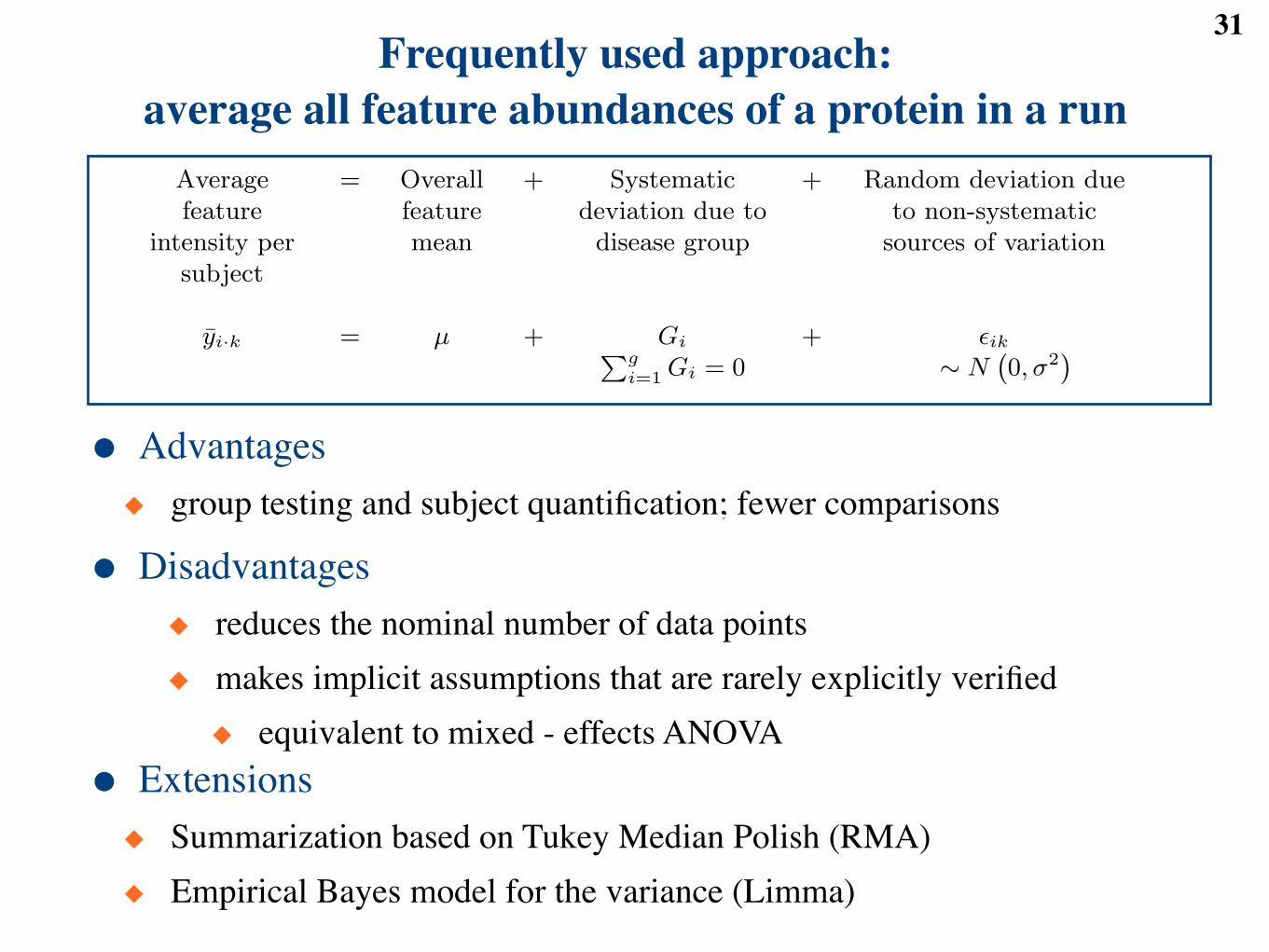
31Frequently used approach:
average all feature abundances of a protein in a run
Observedfeature
intensity
= Overallfeaturemean
+ Systematicdeviation due todisease group
+ Random deviation due tonon-systematic sources of
variation
yijk = µj + Gij + !ijkPgi=1 Gij = 0 ! N
`0, "2
j
´
Figure 1: Per-feature ANOVA. i is the index of a disease group, j the index of a feature, and k the indexof a subject.
!gi=1 Gij = 0 is an identifiability constraint that is required for estimation of the model
parameters. !2j is the variance of the measurement error associated with feature j. All random deviations
are independent.
Averagefeature
intensity persubject
= Overallfeaturemean
+ Systematicdeviation due todisease group
+ Random deviation dueto non-systematic
sources of variation
yi·k = µ + Gi + !ikPgi=1 Gi = 0 ! N
`0, "2
´
Figure 2: Average ANOVA. i is the index of a disease group, and k the index of a subject.!g
i=1 Gi = 0is an identifiability constraint that is required for estimation of the model parameters. !2 is the variance ofthe measurement error. All random deviations are independent.
Systematic deviation due to
Observedintensity
= Overallmean
+ diseasegroup
+ fea-ture
+ interac-tion
+ sub-ject
+ Randomdeviation
yijk = µ + Gi + Fj + (G"F )ij + S(G)k(i) + !ijk
! N`0, "2
´
gX
i=1
Gi =fX
j=1
Fj =gX
i=1
(G" F )ij =fX
j=1
(G" F )ij =nX
k=1
S(G)k(i) = 0
Figure 3: Fixed e!ects ANOVA. i is the index of a disease group, j the index of a feature, and k the indexof a subject.
!gi=1 Gi =
!fj=1 Fj =
!gi=1(G ! F )ij =
!fj=1(G ! F )ij = 0 and
!nk=1 S(G)k(i) = 0 are
identifiability constraints that are required for estimation of the model parameters. !2 is the variance of themeasurement error. All random deviations are independent.
23
● Advantages◆ group testing and subject quantification; fewer comparisons
● Disadvantages◆ reduces the nominal number of data points◆ makes implicit assumptions that are rarely explicitly verified◆ equivalent to mixed - effects ANOVA
● Extensions◆ Summarization based on Tukey Median Polish (RMA)◆ Empirical Bayes model for the variance (Limma)
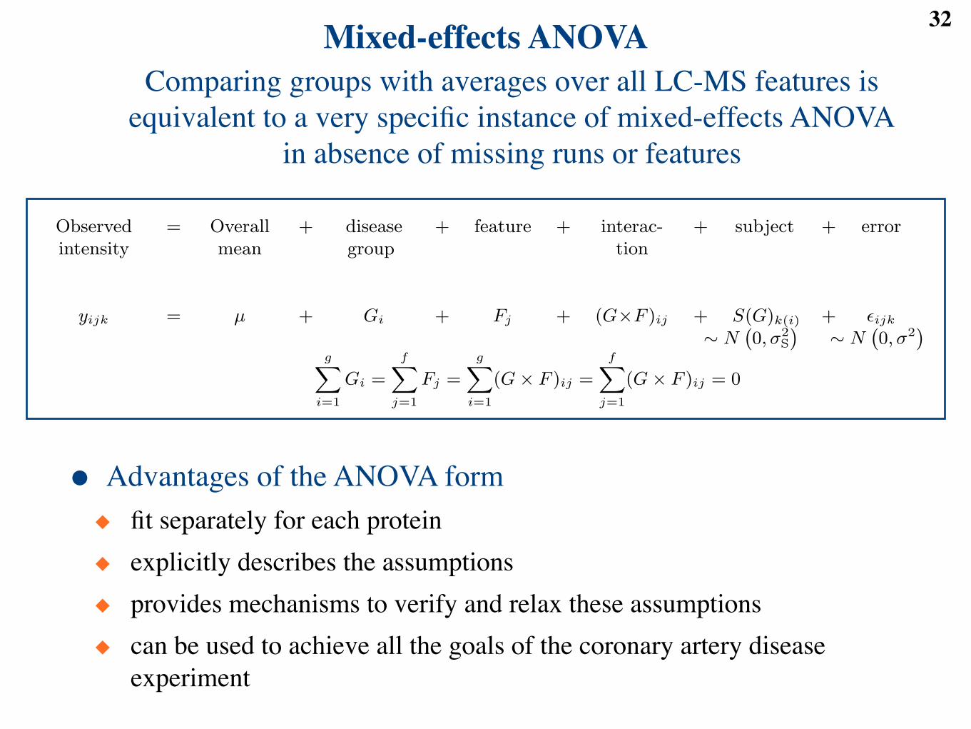
Mixed-effects ANOVA 32
● Advantages of the ANOVA form◆ fit separately for each protein◆ explicitly describes the assumptions◆ provides mechanisms to verify and relax these assumptions◆ can be used to achieve all the goals of the coronary artery disease
experiment
Comparing groups with averages over all LC-MS features is equivalent to a very specific instance of mixed-effects ANOVA
in absence of missing runs or features Systematic deviation due to Random deviation due to
Observedintensity
= Overallmean
+ diseasegroup
+ feature + interac-tion
+ subject + error
yijk = µ + Gi + Fj + (G!F )ij + S(G)k(i) + !ijk
" N`0, "2
S
´" N
`0, "2
´
gX
i=1
Gi =fX
j=1
Fj =gX
i=1
(G! F )ij =fX
j=1
(G! F )ij = 0
Figure 4: Mixed e!ects ANOVA. i is the index of a disease group, j the index of a feature, and k the indexof a subject.
!gi=1 Gi =
!fj=1 Fj =
!gi=1(G! F )ij =
!fj=1(G! F )ij = 0 are the identifiability constraints
that are required for estimation of the model paramaters. !2S is the between-subjects variance, and !2 is the
variance of the measurement error. All random deviations are independent.
(a) Spike-in dataset (b) Clinical dataset
1 2 3 4 5 6
16
18
20
22
24
26
28
Mixture
Avera
ge inte
nsity
0 1 2 3 4
13.0
13.5
14.0
14.5
15.0
Group
Avera
ge inte
nsity
Figure 5: Representative quantitative protein profiles in the experimental datasets. X-axis: mixture type ordisease group. Y-axis: average log-intensity of a feature, on average over the replicates. Each line representsa feature. (a) Spike-in dataset: Alcohol dehydrogenase. (b) Clinical dataset: protein 116844.
24
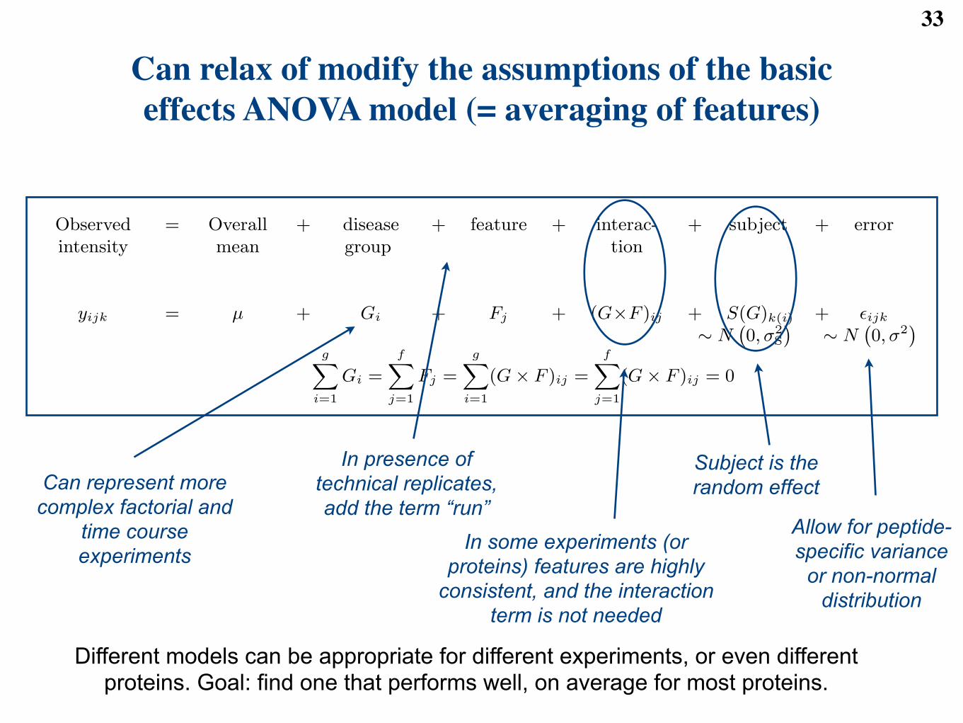
Can relax of modify the assumptions of the basic effects ANOVA model (= averaging of features)
33
Systematic deviation due to Random deviation due to
Observedintensity
= Overallmean
+ diseasegroup
+ feature + interac-tion
+ subject + error
yijk = µ + Gi + Fj + (G!F )ij + S(G)k(i) + !ijk
" N`0, "2
S
´" N
`0, "2
´
gX
i=1
Gi =fX
j=1
Fj =gX
i=1
(G! F )ij =fX
j=1
(G! F )ij = 0
Figure 4: Mixed e!ects ANOVA. i is the index of a disease group, j the index of a feature, and k the indexof a subject.
!gi=1 Gi =
!fj=1 Fj =
!gi=1(G! F )ij =
!fj=1(G! F )ij = 0 are the identifiability constraints
that are required for estimation of the model paramaters. !2S is the between-subjects variance, and !2 is the
variance of the measurement error. All random deviations are independent.
(a) Spike-in dataset (b) Clinical dataset
1 2 3 4 5 6
16
18
20
22
24
26
28
Mixture
Avera
ge inte
nsity
0 1 2 3 4
13.0
13.5
14.0
14.5
15.0
Group
Avera
ge inte
nsity
Figure 5: Representative quantitative protein profiles in the experimental datasets. X-axis: mixture type ordisease group. Y-axis: average log-intensity of a feature, on average over the replicates. Each line representsa feature. (a) Spike-in dataset: Alcohol dehydrogenase. (b) Clinical dataset: protein 116844.
24
Subject is the random effect
In presence of technical replicates, add the term “run”
In some experiments (or proteins) features are highly
consistent, and the interaction term is not needed
Allow for peptide-specific variance
or non-normal distribution
Different models can be appropriate for different experiments, or even different proteins. Goal: find one that performs well, on average for most proteins.
Can represent more complex factorial and
time course experiments
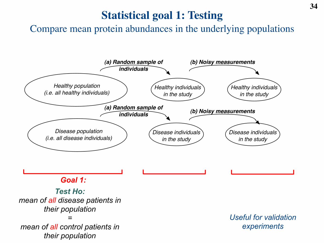
Statistical goal 1: TestingCompare mean protein abundances in the underlying populations
34
Goal 1:
Healthy population
(i.e. all healthy individuals)
Disease population
(i.e. all disease individuals)
Healthy individuals
in the study
Disease individuals
in the study
Healthy individuals
in the study
Disease individuals
in the study
(b) Noisy measurements
(b) Noisy measurements
(a) Random sample of
individuals
(a) Random sample of
individuals
Test Ho: mean of all disease patients in
their population =
mean of all control patients in their population
Useful for validation experiments
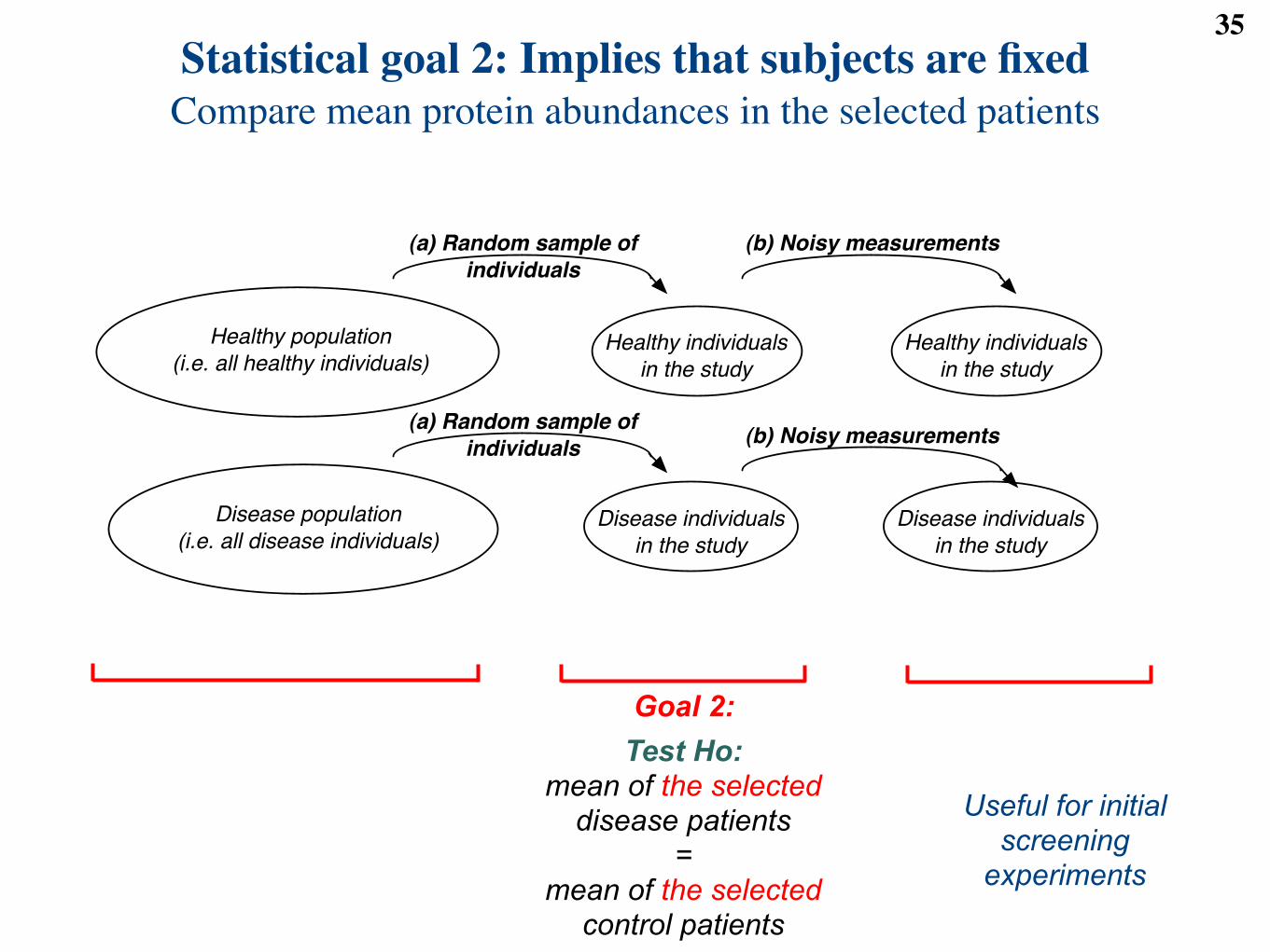
Statistical goal 2: Implies that subjects are fixedCompare mean protein abundances in the selected patients
35
Healthy population
(i.e. all healthy individuals)
Disease population
(i.e. all disease individuals)
Healthy individuals
in the study
Disease individuals
in the study
Healthy individuals
in the study
Disease individuals
in the study
(b) Noisy measurements
(b) Noisy measurements
(a) Random sample of
individuals
(a) Random sample of
individuals
Useful for initial screening
experiments
Goal 2:Test Ho:
mean of the selecteddisease patients
= mean of the selected
control patients
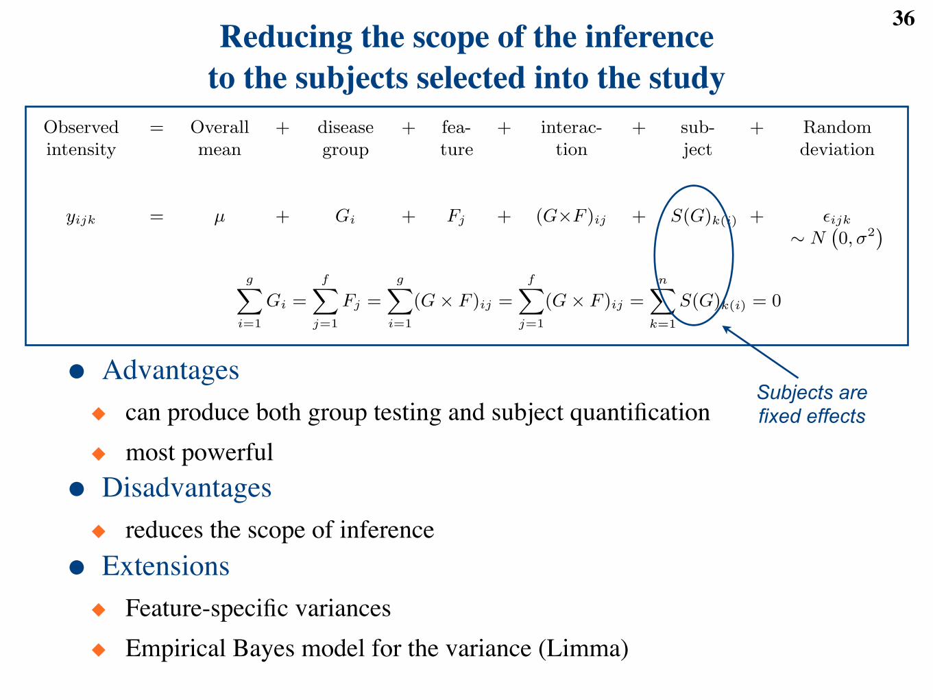
Reducing the scope of the inference to the subjects selected into the study
36
Observedfeature
intensity
= Overallfeaturemean
+ Systematicdeviation due todisease group
+ Random deviation due tonon-systematic sources of
variation
yijk = µj + Gij + !ijkPgi=1 Gij = 0 ! N
`0, "2
j
´
Figure 1: Per-feature ANOVA. i is the index of a disease group, j the index of a feature, and k the indexof a subject.
!gi=1 Gij = 0 is an identifiability constraint that is required for estimation of the model
parameters. !2j is the variance of the measurement error associated with feature j. All random deviations
are independent.
Averagefeature
intensity persubject
= Overallfeaturemean
+ Systematicdeviation due todisease group
+ Random deviation dueto non-systematic
sources of variation
yi·k = µ + Gi + !ikPgi=1 Gi = 0 ! N
`0, "2
´
Figure 2: Average ANOVA. i is the index of a disease group, and k the index of a subject.!g
i=1 Gi = 0is an identifiability constraint that is required for estimation of the model parameters. !2 is the variance ofthe measurement error. All random deviations are independent.
Systematic deviation due to
Observedintensity
= Overallmean
+ diseasegroup
+ fea-ture
+ interac-tion
+ sub-ject
+ Randomdeviation
yijk = µ + Gi + Fj + (G"F )ij + S(G)k(i) + !ijk
! N`0, "2
´
gX
i=1
Gi =fX
j=1
Fj =gX
i=1
(G" F )ij =fX
j=1
(G" F )ij =nX
k=1
S(G)k(i) = 0
Figure 3: Fixed e!ects ANOVA. i is the index of a disease group, j the index of a feature, and k the indexof a subject.
!gi=1 Gi =
!fj=1 Fj =
!gi=1(G ! F )ij =
!fj=1(G ! F )ij = 0 and
!nk=1 S(G)k(i) = 0 are
identifiability constraints that are required for estimation of the model parameters. !2 is the variance of themeasurement error. All random deviations are independent.
23
● Advantages◆ can produce both group testing and subject quantification◆ most powerful● Disadvantages◆ reduces the scope of inference● Extensions◆ Feature-specific variances◆ Empirical Bayes model for the variance (Limma)
Subjects are fixed effects
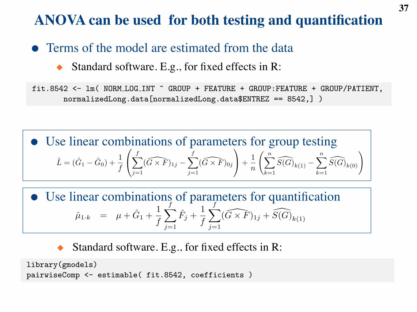
ANOVA can be used for both testing and quantification37
● Use linear combinations of parameters for group testing
● Use linear combinations of parameters for quantification
individual LC-MS features from the average profile due to both biological interferences and experimentalartifacts.
The model also specifies the deviation of each subject (i.e., biological replicate, or subject) S(G)k(i) fromthe overall group mean, which expresses the fact that some individuals have a higher natural abundance ofthe protein than others. Notation S(G)k(i) is read as “subject within a group”, indicating that in comparativeexperiments, such as this case study, each individual belongs to only one group. A di!erent model, and adi!erent notation, is necessary in experiments with repeated measurements where groups corresponds totime points, and multiple samples from the same individual are collected across time. The last term in themodel !ijk describes the remaining deviations of peak intensity, and is viewed as non-systematic replicatesof a Normally distributed measurement error with constant variance "2
Error.The “fixed e!ects” in the model name refers to the fact that the individuals selected for the study are
considered fixed, and the model limits the scope of our conclusions to these specific individuals. This isappropriate for an initial screening experiment such as this case study, and has been shown to both increasethe sensitivity and the specificity of testing, and improve the accuracy of subject quantification (12), whichwe describe in Section 3.2.3 and Section 3.2.4. A di!erent “mixed e!ects” ANOVA model will benecessary for a validation experiment where individuals in the study are viewed as random instances froma larger population of subjects, and one would like to extend the scope of the conclusions to the entirepopulation (12).
Model fit. The terms in Figure 2 are estimated from the data separately for each protein, using thestandard least squares procedure (13, 14) available in the statistical software R. Once the model is fit, weverify the appropriateness of the assumptions regarding !ijk using residual plots and Normal quantile-quantileplots.
3.2.3 Model-based testing for di!erential abundance
Specifying hypotheses of interest. We use the model to compare the mean abundance of a protein acrosspairs of disease groups, on average over all subjects and features. For example, if we denote µ0 the meanabundance of the protein among controls, and µ1 the mean protein abundance in the first disease group, thelog-fold change is defined as L = µ1 ! µ0. We test the null hypothesis H0 : L = µ1 ! µ0 = 0 against thealternative Ha : L = µ1 ! µ0 "= 0.
Testing. In the notation of Figure 2, the log-fold change is estimated from the model as
L = (G1 ! G0) +1f
!
"f#
j=1
( !G# F )1j !f#
j=1
( !G# F )0j
$
% +1n
&n#
k=1
"S(G)k(1) !n#
k=1
"S(G)k(0)
'(1)
where “(” indicates that these are model-based quantities estimated from the data. Since this experiment hasa balanced design, the model-based estimates of L simplify to the di!erence of sample averages L = y1..!y0...However, in situations where a balanced experiment cannot be achieved (e.g., when some runs or featureintensities are lost), the model-based estimates will di!er from the averages, and have been shown to becloser to the true values (12).
The fitted model is also used to estimate the standard error of L (i.e., the estimate of its variation). Inour special case of a balanced design,
SE{L} =)
2nf
"2Error (2)
where "2Error is the estimate of residual variance based on g(f!1)(n!1) degrees of freedom (i.e., data points
available after fitting the model). Using these estimates, the null hypothesis is tested with a t-test, whichcompares the test statistic ts = L
SE{L} to the Studentg(f!1)(n!1) distribution, and derives the correspondingp-value. If the p-value of a protein is below a pre-specified cuto!, we reject the null hypotheses. In otherwords, we state that the observed di!erence of protein abundance between groups is larger than what would
6
be expected by random chance. In this case study, we perform four sets of t-tests, each set comparing theabundance of the identified proteins in one of the four disease groups to the controls.
Multiple comparisons. Procedures of statistical inference allow us to select a p-value cuto! in a way tocontrol the expected error rate in our conclusions. For example, when testing the null hypothesis for a singleprotein, the p-value is typically compared to a pre-specified significance level !, where ! is the probabilityof rejecting the null hypothesis given that the null hypothesis is true. Unfortunately, this procedure is onlydesigned for a single test, and does not control the overall error rate in an experiment such as this casestudy, where we perform multiple tests for all the identified proteins. Therefore, we should select a di!erent,and more conservative, p-value cuto! that controls the experiment-wide error rate. A popular choice is tocontrol the False Discovery Rate (FDR), i.e., the expected proportion of false rejections in the reported listof di!erentially abundant proteins.
Table 3 summarizes the possible outcomes of such a procedure in an experiment with m identifiedproteins, m0 of which do not di!er in abundance between two groups. R, S, T , U , and V are randomvariables that depend on the observed data, but only R is actually observed. In the notation of Table 3,the FDR is defined as
q = E
!V
max(R, 1)
", (3)
where E denotes the expected value of the quantity in brackets, i.e., the “average” value over a large numberof repetitions of this experiment.
In this case study, we use the procedure by Benjamini and Hochberg (15), which controls the FDR ata desired level q. First, for each comparison of a disease group to controls, we order the p-values of them proteins from the largest p(m) (i.e., the least significant) to the smallest p(1) (i.e., the most significant).Next, we vary j from m to 1, and define the adjusted p-value pj as in reference (16)
pj = mink=j,...,m
#min
$m
kp(k), 1
%&
It can be shown that the list of proteins with adjusted p-values pj below a pre-defined cuto! has the FDRof at most the cuto!.
3.2.4 Model-based protein quantification in individual samples
In addition to comparing average protein abundances across groups, our goal is to obtain a separate quantifi-cation of the protein in each subject, from all peptide features, and on a continuous scale that is comparableacross runs. We call this procedure subject quantification. Results of subject quantification will be subse-quently used as input to unsupervised clustering or supervised classification of the samples. The statisticalmodel in Figure 2 can also be used to perform this task. The model views subject quantification as es-timation of the “true” abundance of the protein in each sample from noisy measurements, and helps toappropriately derive this summary. For example, if we denote µ1·k as the protein abundance of the kthsubject in the first disease group, its model-based estimation is
µ1·k = µ + G1 +1f
f'
j=1
Fj +1f
f'
j=1
( !G! F )1j + "S(G)k(1) (4)
As before “( ” indicates that the quantities in Eq. (4) are estimated from the data. In the case of a balanceddesign, the model-based quantities simplify to sample averages y1·k. In other experiments where balancecannot be achieved, the model-based estimates will di!er from sample averages, and they have been shownto be closer to the true values (12).
We confirm the accuracy of model-based quantification by means of independent protein quantification onthe same samples. In this study, 11 proteins were measured independently in all samples using nephelometry.We therefore calculate 11 Pearson coe"cients of correlation between the model-based quantifications andthe nephelometry-based values.
7
● Terms of the model are estimated from the data◆ Standard software. E.g., for fixed effects in R:
4.2.2 Model specification
To fit the fixed e!ects ANOVA model in Section 3.2.2, we restructure the normalized data into the “long”format. In this format, each row represents a feature intensity within a single run, and columns containinformation on both features and runs. We denote the R implementation of such a data structure asnormalizedLong.data, of type data.frame. In this case study, normalizedLong.data has 1643 !50 =82150 rows. The first and last three rows of the data structure are shown in Table 5. NORM LOG INT is thelog-transformed and normalized intensity, of type numeric. The remaining columns are of type factor.
The formatted data can be used to fit the model in Figure 2, separately for each protein, using standardANOVA implementations available in R. For example, the model fit for protein 8542 is obtained using
fit.8542 <- lm( NORM LOG INT ~ GROUP + FEATURE + GROUP:FEATURE + GROUP/PATIENT,normalizedLong.data[normalizedLong.data$ENTREZ == 8542,] )
summary(fit)
The summary of the model fit outputs 60 estimated parameters; the names of each are shown in the “Pa-rameter” column of Table 7.
The assumption of Normality of the error terms is visually verified using a Normal quantile-quantile plot,which can be obtained using
qqnorm( y = fit$residuals, datax = FALSE, ylab = "Residuals" )
An example of the plot for protein 8542 is shown in Figure 3. Points on the plot form approximately astraight line, indicating that the assumption is appropriate. The assumption of constant variance of the errorterms is visually verified by plotting, from the fitted model, the residual versus the predicted value for eachfeature intensity. An example of the plot for protein 8542 is shown in Figure 4. The plot can be obtainedusing
plot( fit$fitted.values, fit$residuals, xlab = "Predicted Values", ylab = "Residuals" )
The residuals are distributed roughly equally above and below the horizontal line, and have a similar spreadacross the entire range predicted values, indicating that the assumption of constant variance is appropriatein this case.
The summary also reports the standard errors of the estimated parameters, and the p-values of t-teststhat compare each estimate to 0. However, these estimates and tests are not of direct relevance to the goal ofthe case study. Instead, we are interested in model-based summaries, such as comparisons of the estimatedgroup means, that we discuss next.
4.2.3 Model-based testing for di!erential abundance
Suppose, for example, that we test H0 : µ1 " µ0 = 0 versus Ha : µ1 " µ0 #= 0, where (in notation ofTable 1) µ1 represents the mean of protein abundance of subjects in the Stable angina group, and µ0
represents the mean protein abundance among controls. We test the hypothesis for protein 8542, which hasthree features. As discussed in Section 3.2.3, the di!erence between group means can be estimated fromthe data as a linear combination of the estimated parameters. To obtain this quantity, one must explicitlyspecify the coe"cients of the linear combination. According to Eq. (1), the coe"cients of all the model-based parameters associated with group 1 are positive, and the coe"cients of the parameters associated withgroup 0 are negative. The absolute value of the coe"cients of the two disease groups is 1. Since this proteinhas three features, the absolute value of all the coe"cients of the interaction terms associated with thesedisease groups is 1
3 . Similarly, since there are ten subjects per group, the absolute value of the coe"cients ofsubjects from these disease groups is 1
10 . The remaining coe"cients are equal to 0. The full set of coe"cientsis shown in Table 7; it is applicable to all the identified proteins.
We denote a vector of the coe"cients in Table 7 as coefficients. The numeric estimate of the linearcombination, as well as its standard error and corresponding p-value, are obtained using
11
◆ Standard software. E.g., for fixed effects in R:library(gmodels)pairwiseComp <- estimable( fit.8542, coefficients )
When tests are performed for multiple proteins in parallel, the p-values must be adjusted for multiplecomparisons as discussed in Section 3.2.3. If p is a data structure of type data.frame, such that its rowsare genes and its four columns are p-values comparing each of the four disease groups to the controls, thenadjustment for multiple comparisons, separately for each type of test, can be obtained as
p.BH <- apply( p, 2, function(x) p.adjust(x, method = "BH") )
We reject the null hypothesis, and claim di!erential abundance, when an adjusted p-value is below an FDRcut-o! of 0.05. In total, 59 proteins were found to be di!erentially abundant in at least one of the fourcomparisons in this case study.
4.2.4 Model-based protein quantification in individual samples
Similarly to testing, we use the model to derive subject-level protein quantifications as discussed in Sec-tion 3.2.4. For example, to estimate the abundance of protein 8542 for the second subject in the first diseasegroup (Stable angina), we create a linear combination of the estimated parameters. According to Eq. (4),the coe"cients associated with the intercept, with the corresponding disease group, and with the corre-sponding subject, are all equal to 1. Since the protein has three features, the coe"cients associated with theinteraction term are 1
3 . The remaining coe"cients are 0. The full set of coe"cients is shown in Table 8,and it is applicable to all the identified proteins. We denote a vector of the coe"cients in Table 8 assubjectQuantCoef. The numeric estimate of the linear combination is obtained using
subjectQuant <- estimable( fit.8542, subjectQuantCoef )subjectQuant$Estimate
We further consider the 11 proteins for which independent nephelometry measurements were made foreach subject. For each protein, we calculate the Pearson correlation coe"cient between the subject-levelabundances and the nephelometry measurements. The median coe"cient of correlation over the 11 proteinsis 0.667.
4.2.5 Gene set enrichment analysis
We test the pre-defined groups of proteins for enrichment in di!erential abundance between each of the diseasegroups and controls. For example, we consider a pre-defined group of 11 proteins sharing the annotationComplement, and the comparison between the first disease group (Stable angina) and the group of controls.In this case, in the notation of Table 4, K = 4, s = 11, m! s = 66, and R = 36. We calculate the p-valueof the Hypergeometric test using
p <- phyper( K, s, m-s, R, lower.tail = FALSE )
The test yields a p-value of 0.660, which indicates an insu"cient evidence that the Complement group isenriched in proteins that are di!erentially abundant between Stable angina and the controls. Overall, twoout of the ten pre-defined protein groups were found enriched in proteins that are di!erentially abundant inat least one disease group as compared to controls.
4.3 Planning a follow-up experiment: sample size calculation
To calculate the sample size necessary for a follow-up experiment, we specify
(1) L = |µH!µD|, the minimal absolute log-fold change in protein abundance that we would like to detect.We set L = 0.3, which on the original scale corresponds to the fold change of 20.3 = 1.23.
12
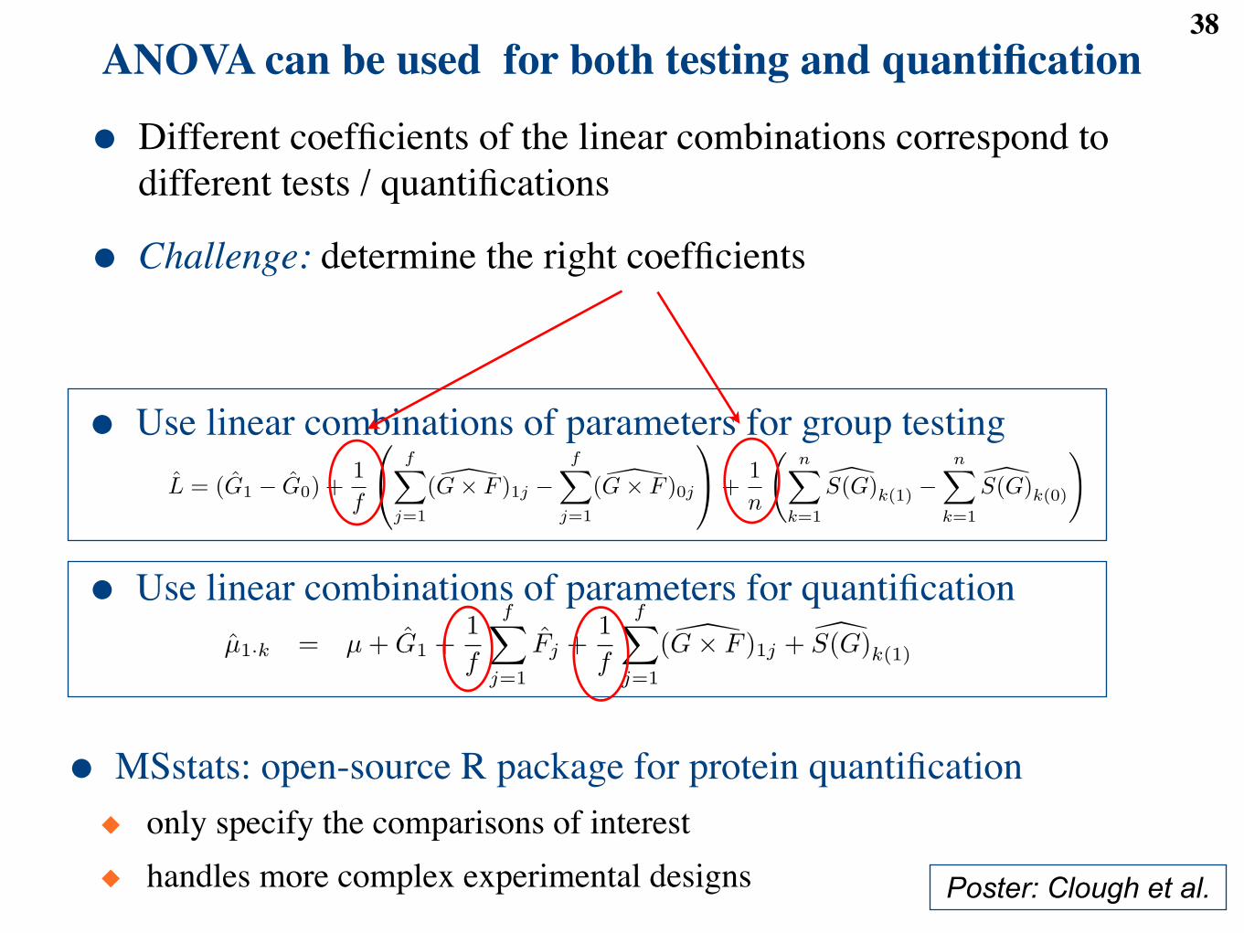
ANOVA can be used for both testing and quantification38
● Use linear combinations of parameters for group testing
● Use linear combinations of parameters for quantification
individual LC-MS features from the average profile due to both biological interferences and experimentalartifacts.
The model also specifies the deviation of each subject (i.e., biological replicate, or subject) S(G)k(i) fromthe overall group mean, which expresses the fact that some individuals have a higher natural abundance ofthe protein than others. Notation S(G)k(i) is read as “subject within a group”, indicating that in comparativeexperiments, such as this case study, each individual belongs to only one group. A di!erent model, and adi!erent notation, is necessary in experiments with repeated measurements where groups corresponds totime points, and multiple samples from the same individual are collected across time. The last term in themodel !ijk describes the remaining deviations of peak intensity, and is viewed as non-systematic replicatesof a Normally distributed measurement error with constant variance "2
Error.The “fixed e!ects” in the model name refers to the fact that the individuals selected for the study are
considered fixed, and the model limits the scope of our conclusions to these specific individuals. This isappropriate for an initial screening experiment such as this case study, and has been shown to both increasethe sensitivity and the specificity of testing, and improve the accuracy of subject quantification (12), whichwe describe in Section 3.2.3 and Section 3.2.4. A di!erent “mixed e!ects” ANOVA model will benecessary for a validation experiment where individuals in the study are viewed as random instances froma larger population of subjects, and one would like to extend the scope of the conclusions to the entirepopulation (12).
Model fit. The terms in Figure 2 are estimated from the data separately for each protein, using thestandard least squares procedure (13, 14) available in the statistical software R. Once the model is fit, weverify the appropriateness of the assumptions regarding !ijk using residual plots and Normal quantile-quantileplots.
3.2.3 Model-based testing for di!erential abundance
Specifying hypotheses of interest. We use the model to compare the mean abundance of a protein acrosspairs of disease groups, on average over all subjects and features. For example, if we denote µ0 the meanabundance of the protein among controls, and µ1 the mean protein abundance in the first disease group, thelog-fold change is defined as L = µ1 ! µ0. We test the null hypothesis H0 : L = µ1 ! µ0 = 0 against thealternative Ha : L = µ1 ! µ0 "= 0.
Testing. In the notation of Figure 2, the log-fold change is estimated from the model as
L = (G1 ! G0) +1f
!
"f#
j=1
( !G# F )1j !f#
j=1
( !G# F )0j
$
% +1n
&n#
k=1
"S(G)k(1) !n#
k=1
"S(G)k(0)
'(1)
where “(” indicates that these are model-based quantities estimated from the data. Since this experiment hasa balanced design, the model-based estimates of L simplify to the di!erence of sample averages L = y1..!y0...However, in situations where a balanced experiment cannot be achieved (e.g., when some runs or featureintensities are lost), the model-based estimates will di!er from the averages, and have been shown to becloser to the true values (12).
The fitted model is also used to estimate the standard error of L (i.e., the estimate of its variation). Inour special case of a balanced design,
SE{L} =)
2nf
"2Error (2)
where "2Error is the estimate of residual variance based on g(f!1)(n!1) degrees of freedom (i.e., data points
available after fitting the model). Using these estimates, the null hypothesis is tested with a t-test, whichcompares the test statistic ts = L
SE{L} to the Studentg(f!1)(n!1) distribution, and derives the correspondingp-value. If the p-value of a protein is below a pre-specified cuto!, we reject the null hypotheses. In otherwords, we state that the observed di!erence of protein abundance between groups is larger than what would
6
be expected by random chance. In this case study, we perform four sets of t-tests, each set comparing theabundance of the identified proteins in one of the four disease groups to the controls.
Multiple comparisons. Procedures of statistical inference allow us to select a p-value cuto! in a way tocontrol the expected error rate in our conclusions. For example, when testing the null hypothesis for a singleprotein, the p-value is typically compared to a pre-specified significance level !, where ! is the probabilityof rejecting the null hypothesis given that the null hypothesis is true. Unfortunately, this procedure is onlydesigned for a single test, and does not control the overall error rate in an experiment such as this casestudy, where we perform multiple tests for all the identified proteins. Therefore, we should select a di!erent,and more conservative, p-value cuto! that controls the experiment-wide error rate. A popular choice is tocontrol the False Discovery Rate (FDR), i.e., the expected proportion of false rejections in the reported listof di!erentially abundant proteins.
Table 3 summarizes the possible outcomes of such a procedure in an experiment with m identifiedproteins, m0 of which do not di!er in abundance between two groups. R, S, T , U , and V are randomvariables that depend on the observed data, but only R is actually observed. In the notation of Table 3,the FDR is defined as
q = E
!V
max(R, 1)
", (3)
where E denotes the expected value of the quantity in brackets, i.e., the “average” value over a large numberof repetitions of this experiment.
In this case study, we use the procedure by Benjamini and Hochberg (15), which controls the FDR ata desired level q. First, for each comparison of a disease group to controls, we order the p-values of them proteins from the largest p(m) (i.e., the least significant) to the smallest p(1) (i.e., the most significant).Next, we vary j from m to 1, and define the adjusted p-value pj as in reference (16)
pj = mink=j,...,m
#min
$m
kp(k), 1
%&
It can be shown that the list of proteins with adjusted p-values pj below a pre-defined cuto! has the FDRof at most the cuto!.
3.2.4 Model-based protein quantification in individual samples
In addition to comparing average protein abundances across groups, our goal is to obtain a separate quantifi-cation of the protein in each subject, from all peptide features, and on a continuous scale that is comparableacross runs. We call this procedure subject quantification. Results of subject quantification will be subse-quently used as input to unsupervised clustering or supervised classification of the samples. The statisticalmodel in Figure 2 can also be used to perform this task. The model views subject quantification as es-timation of the “true” abundance of the protein in each sample from noisy measurements, and helps toappropriately derive this summary. For example, if we denote µ1·k as the protein abundance of the kthsubject in the first disease group, its model-based estimation is
µ1·k = µ + G1 +1f
f'
j=1
Fj +1f
f'
j=1
( !G! F )1j + "S(G)k(1) (4)
As before “( ” indicates that the quantities in Eq. (4) are estimated from the data. In the case of a balanceddesign, the model-based quantities simplify to sample averages y1·k. In other experiments where balancecannot be achieved, the model-based estimates will di!er from sample averages, and they have been shownto be closer to the true values (12).
We confirm the accuracy of model-based quantification by means of independent protein quantification onthe same samples. In this study, 11 proteins were measured independently in all samples using nephelometry.We therefore calculate 11 Pearson coe"cients of correlation between the model-based quantifications andthe nephelometry-based values.
7
● Different coefficients of the linear combinations correspond to different tests / quantifications
● Challenge: determine the right coefficients
● MSstats: open-source R package for protein quantification◆ only specify the comparisons of interest◆ handles more complex experimental designs Poster: Clough et al.

Outline39
● LC-MS proteomics: a case study of coronary artery disease◆ Framing the question◆ Experimental design◆ Statistical analysis■ methods■ evaluation
◆ Enrichment of pre-defined sets in differential abundance
● Extensions◆ Planning future studies with LC-MS workflows◆ Design and analysis with labeling workflows
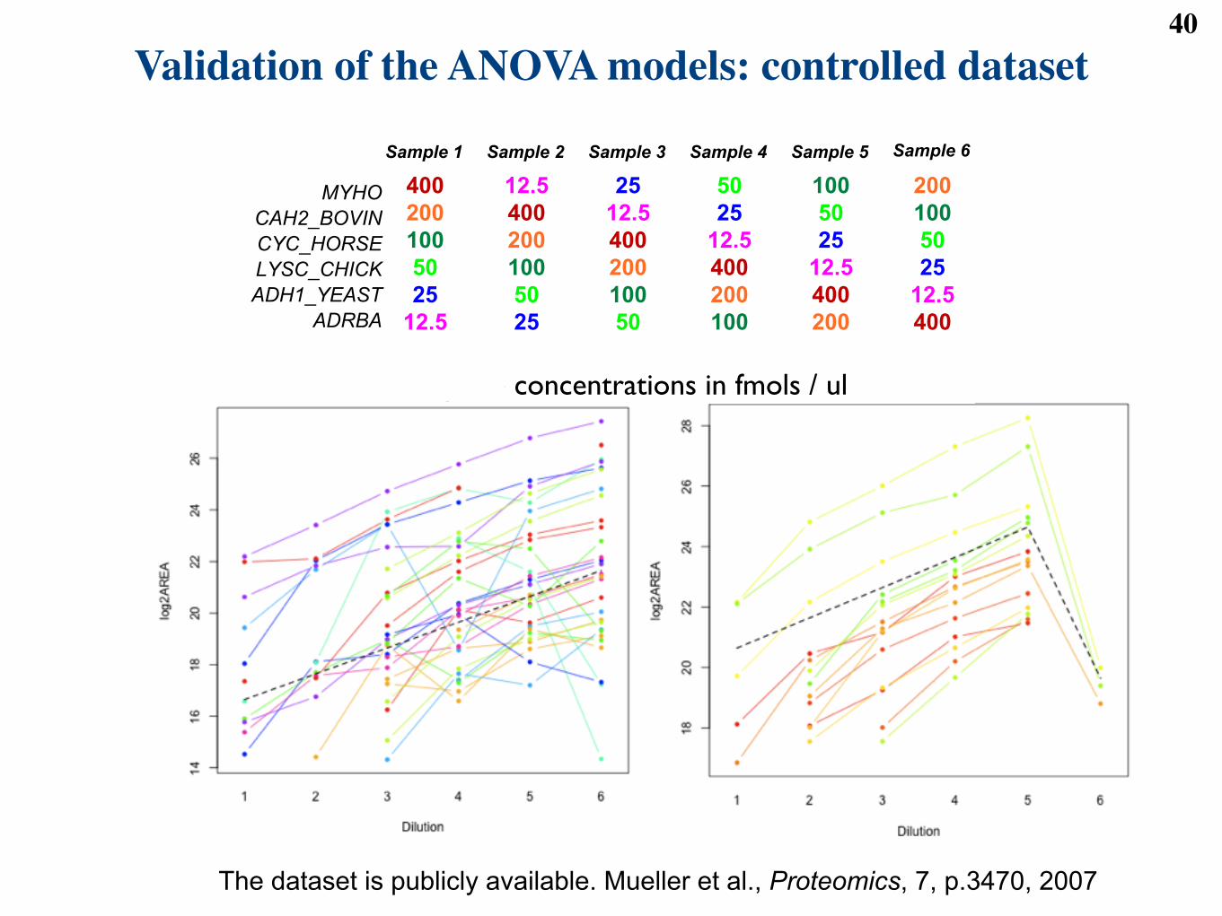
Validation of the ANOVA models: controlled dataset 40Experimental data set I:
technical variation
13
! Controlled sample: a latin square design
" commercially purified and digested proteins
" can study multiple proteins, multiple fold changes
" limited number of runs
" REPLICATION, BLOCKING, RANDOMIZATION!
Sample 6Sample 1
400
200
100
50
25
12.5
Sample 2
12.5
400
200
100
50
25
Sample 3
25
12.5
400
200
100
50
Sample 4
50
25
12.5
400
200
100
Sample 5
100
50
25
12.5
400
200
200
100
50
25
12.5
400
MYHO
CAH2_BOVIN
CYC_HORSE
LYSC_CHICK
ADH1_YEAST
ADRBA
Peptide concentrations in fmols / ul
The dataset is publicly available. Mueller et al., Proteomics, 7, p.3470, 2007
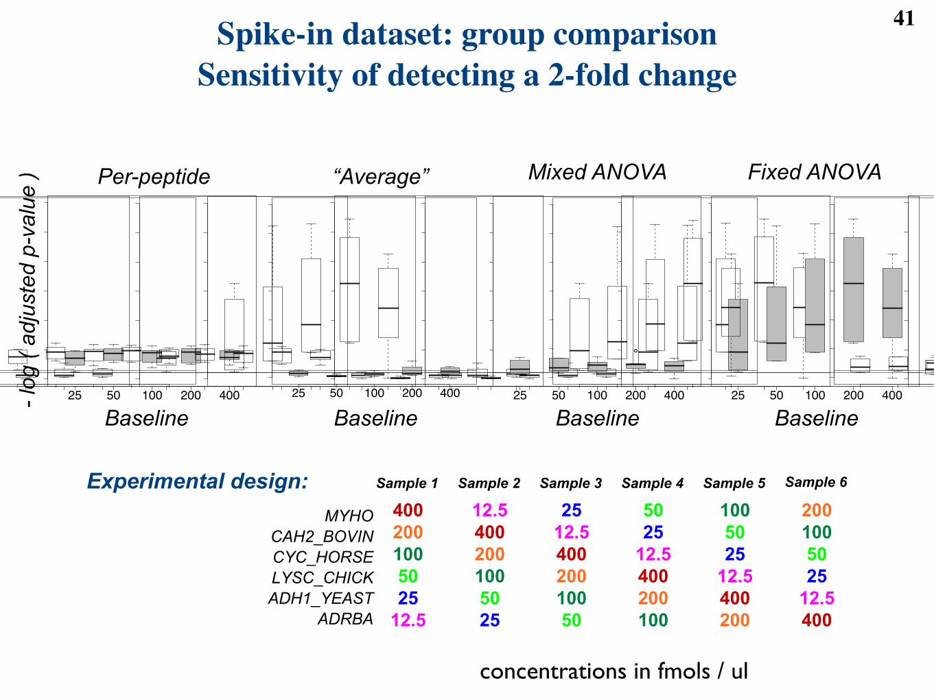
Spike-in dataset: group comparisonSensitivity of detecting a 2-fold change
41
Experimental data set I:
technical variation
13
! Controlled sample: a latin square design
" commercially purified and digested proteins
" can study multiple proteins, multiple fold changes
" limited number of runs
" REPLICATION, BLOCKING, RANDOMIZATION!
Sample 6Sample 1
400
200
100
50
25
12.5
Sample 2
12.5
400
200
100
50
25
Sample 3
25
12.5
400
200
100
50
Sample 4
50
25
12.5
400
200
100
Sample 5
100
50
25
12.5
400
200
200
100
50
25
12.5
400
MYHO
CAH2_BOVIN
CYC_HORSE
LYSC_CHICK
ADH1_YEAST
ADRBA
Peptide concentrations in fmols / ul
(a) Spike-in: (b) Spike-in: (c) Spike-in: (d) Spike-in:per-feature “average” fixed mixed
25 50 100 200 400
020
40
60
80
100
Baseline
!!log2(p!value)
25 50 100 200 400
020
40
60
80
100
Baseline
!!log2(p!value)
25 50 100 200 400
020
40
60
80
100
Baseline
!!log2(p!value)
!
25 50 100 200 400
020
40
60
80
100
Baseline
!!log2(p!value)
Figure 6: Sensitivity of the four basic models at detecting a two-fold change in the spike-in dataset, startingfrom five abundance baselines. X-axis: abundance baseline. Y-axis: -log2(FDR-adjusted p-value). Each boxcontains the middle 50% of the proteins; the line within the box is the median. The higher the value onthe y-axis, the stronger the evidence for di!erential abundance. The horizontal line corresponds to the FDRcuto! of 0.05.
(a) Clinical: subset (b) Clinical: full (c) Spike-in
per!feature average = mixed
fixed 13
60
0
1
0
1
0
2
per!feature average = mixed
fixed 10
41
3
7
0
2
0
14
0 50 100 150
0.0
0.1
0.2
0.3
0.4
0.5
Number of detected fold changes
Fals
e p
ositiv
e r
ate
Per!feature model
Average model
Fixed model
Mixed model
Figure 7: (a) and (b) Sensitivity of the four basic models at detecting changes in abundance in the clinicaldataset. Each circle shows the number of proteins with at least one detected pairwise di!erence betweendisease groups after the FDR cuto! 0.05. (a) Reduced dataset with 50 subjects. (b) Full dataset with246 subjects. (c) Specificity of the four basic models at detecting changes in abundance in the spike-indataset. X-axis: number of di!erences in a comparison between two mixtures. Y-axis: false positive rate inall pairwise comparisons of mixtures. More specific models produce lower curves.
25
(a) Spike-in: (b) Spike-in: (c) Spike-in: (d) Spike-in:per-feature “average” fixed mixed
25 50 100 200 400
020
40
60
80
100
Baseline
!!log2(p!value)
25 50 100 200 400
020
40
60
80
100
Baseline!!log2(p!value)
25 50 100 200 400
020
40
60
80
100
Baseline
!!log2(p!value)
!
25 50 100 200 400
020
40
60
80
100
Baseline
!!log2(p!value)
Figure 6: Sensitivity of the four basic models at detecting a two-fold change in the spike-in dataset, startingfrom five abundance baselines. X-axis: abundance baseline. Y-axis: -log2(FDR-adjusted p-value). Each boxcontains the middle 50% of the proteins; the line within the box is the median. The higher the value onthe y-axis, the stronger the evidence for di!erential abundance. The horizontal line corresponds to the FDRcuto! of 0.05.
(a) Clinical: subset (b) Clinical: full (c) Spike-in
per!feature average = mixed
fixed 13
60
0
1
0
1
0
2
per!feature average = mixed
fixed 10
41
3
7
0
2
0
14
0 50 100 150
0.0
0.1
0.2
0.3
0.4
0.5
Number of detected fold changes
Fa
lse
po
sitiv
e r
ate
Per!feature model
Average model
Fixed model
Mixed model
Figure 7: (a) and (b) Sensitivity of the four basic models at detecting changes in abundance in the clinicaldataset. Each circle shows the number of proteins with at least one detected pairwise di!erence betweendisease groups after the FDR cuto! 0.05. (a) Reduced dataset with 50 subjects. (b) Full dataset with246 subjects. (c) Specificity of the four basic models at detecting changes in abundance in the spike-indataset. X-axis: number of di!erences in a comparison between two mixtures. Y-axis: false positive rate inall pairwise comparisons of mixtures. More specific models produce lower curves.
25
(a) Spike-in: (b) Spike-in: (c) Spike-in: (d) Spike-in:per-feature “average” fixed mixed
25 50 100 200 400
020
40
60
80
100
Baseline
!!log2(p!value)
25 50 100 200 400
020
40
60
80
100
Baseline
!!log2(p!value)
25 50 100 200 400
020
40
60
80
100
Baseline
!!log2(p!value)
!
25 50 100 200 400
020
40
60
80
100
Baseline
!!log2(p!value)
Figure 6: Sensitivity of the four basic models at detecting a two-fold change in the spike-in dataset, startingfrom five abundance baselines. X-axis: abundance baseline. Y-axis: -log2(FDR-adjusted p-value). Each boxcontains the middle 50% of the proteins; the line within the box is the median. The higher the value onthe y-axis, the stronger the evidence for di!erential abundance. The horizontal line corresponds to the FDRcuto! of 0.05.
(a) Clinical: subset (b) Clinical: full (c) Spike-in
per!feature average = mixed
fixed 13
60
0
1
0
1
0
2
per!feature average = mixed
fixed 10
41
3
7
0
2
0
14
0 50 100 150
0.0
0.1
0.2
0.3
0.4
0.5
Number of detected fold changes
Fa
lse
po
sitiv
e r
ate
Per!feature model
Average model
Fixed model
Mixed model
Figure 7: (a) and (b) Sensitivity of the four basic models at detecting changes in abundance in the clinicaldataset. Each circle shows the number of proteins with at least one detected pairwise di!erence betweendisease groups after the FDR cuto! 0.05. (a) Reduced dataset with 50 subjects. (b) Full dataset with246 subjects. (c) Specificity of the four basic models at detecting changes in abundance in the spike-indataset. X-axis: number of di!erences in a comparison between two mixtures. Y-axis: false positive rate inall pairwise comparisons of mixtures. More specific models produce lower curves.
25
- log
( ad
just
ed p
-val
ue )
Baseline Baseline Baseline Baseline
Per-peptide “Average” Mixed ANOVA Fixed ANOVA
Experimental design:
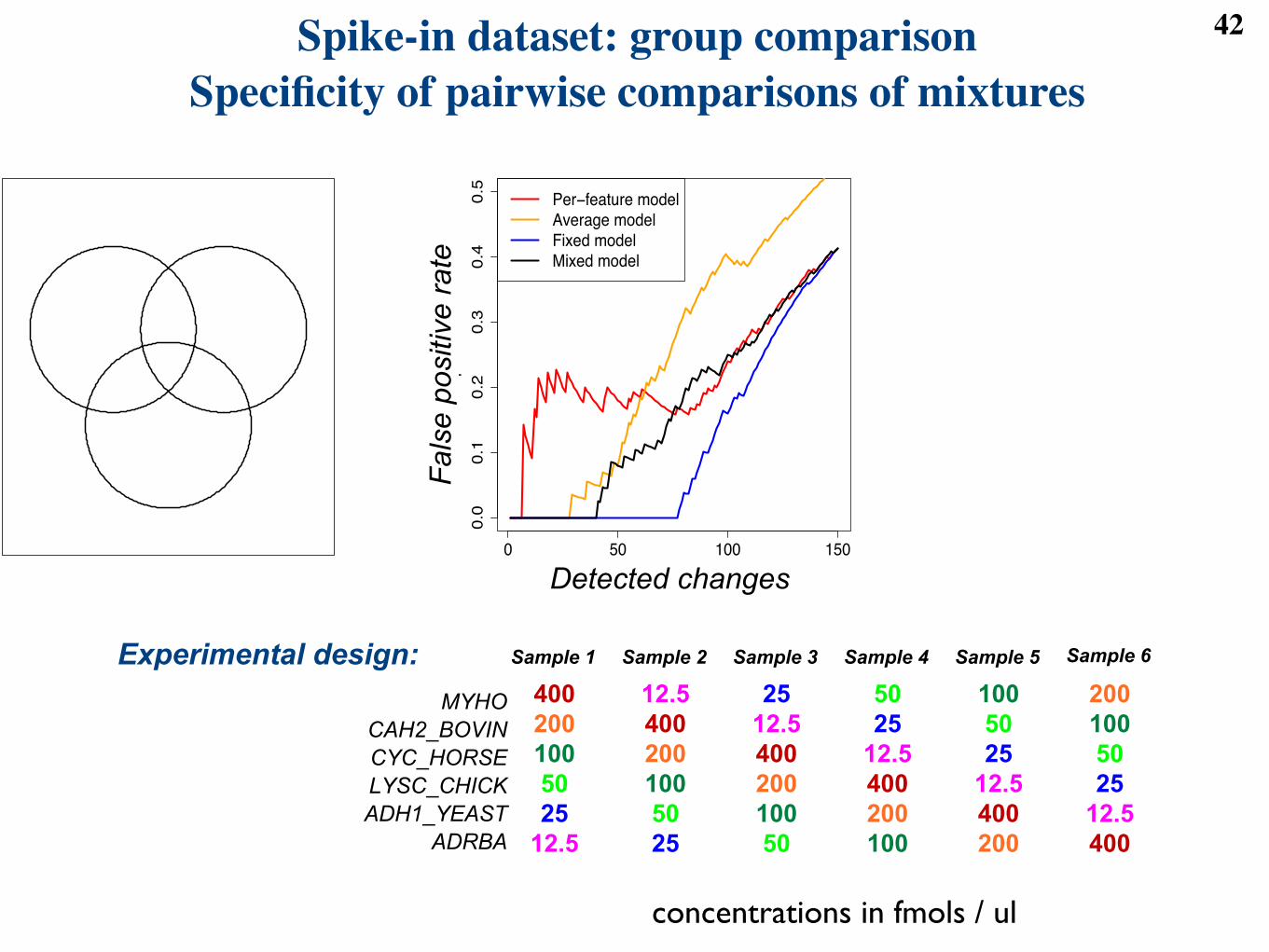
Spike-in dataset: group comparison Specificity of pairwise comparisons of mixtures
42
(a) Spike-in: (b) Spike-in: (c) Spike-in: (d) Spike-in:per-feature “average” fixed mixed
25 50 100 200 400
020
40
60
80
100
Baseline
!!log2(p!value)
25 50 100 200 400
020
40
60
80
100
Baseline
!!log2(p!value)
25 50 100 200 400
020
40
60
80
100
Baseline
!!log2(p!value)
!
25 50 100 200 400
020
40
60
80
100
Baseline
!!log2(p!value)
Figure 6: Sensitivity of the four basic models at detecting a two-fold change in the spike-in dataset, startingfrom five abundance baselines. X-axis: abundance baseline. Y-axis: -log2(FDR-adjusted p-value). Each boxcontains the middle 50% of the proteins; the line within the box is the median. The higher the value onthe y-axis, the stronger the evidence for di!erential abundance. The horizontal line corresponds to the FDRcuto! of 0.05.
(a) Clinical: subset (b) Clinical: full (c) Spike-in
per!feature average = mixed
fixed 13
60
0
1
0
1
0
2
per!feature average = mixed
fixed 10
41
3
7
0
2
0
14
0 50 100 150
0.0
0.1
0.2
0.3
0.4
0.5
Number of detected fold changes
Fals
e p
ositiv
e r
ate
Per!feature model
Average model
Fixed model
Mixed model
Figure 7: (a) and (b) Sensitivity of the four basic models at detecting changes in abundance in the clinicaldataset. Each circle shows the number of proteins with at least one detected pairwise di!erence betweendisease groups after the FDR cuto! 0.05. (a) Reduced dataset with 50 subjects. (b) Full dataset with246 subjects. (c) Specificity of the four basic models at detecting changes in abundance in the spike-indataset. X-axis: number of di!erences in a comparison between two mixtures. Y-axis: false positive rate inall pairwise comparisons of mixtures. More specific models produce lower curves.
25
Detected changes
Fals
e po
sitiv
e ra
te
Experimental data set I:
technical variation
13
! Controlled sample: a latin square design
" commercially purified and digested proteins
" can study multiple proteins, multiple fold changes
" limited number of runs
" REPLICATION, BLOCKING, RANDOMIZATION!
Sample 6Sample 1
400
200
100
50
25
12.5
Sample 2
12.5
400
200
100
50
25
Sample 3
25
12.5
400
200
100
50
Sample 4
50
25
12.5
400
200
100
Sample 5
100
50
25
12.5
400
200
200
100
50
25
12.5
400
MYHO
CAH2_BOVIN
CYC_HORSE
LYSC_CHICK
ADH1_YEAST
ADRBA
Peptide concentrations in fmols / ul
Experimental design:
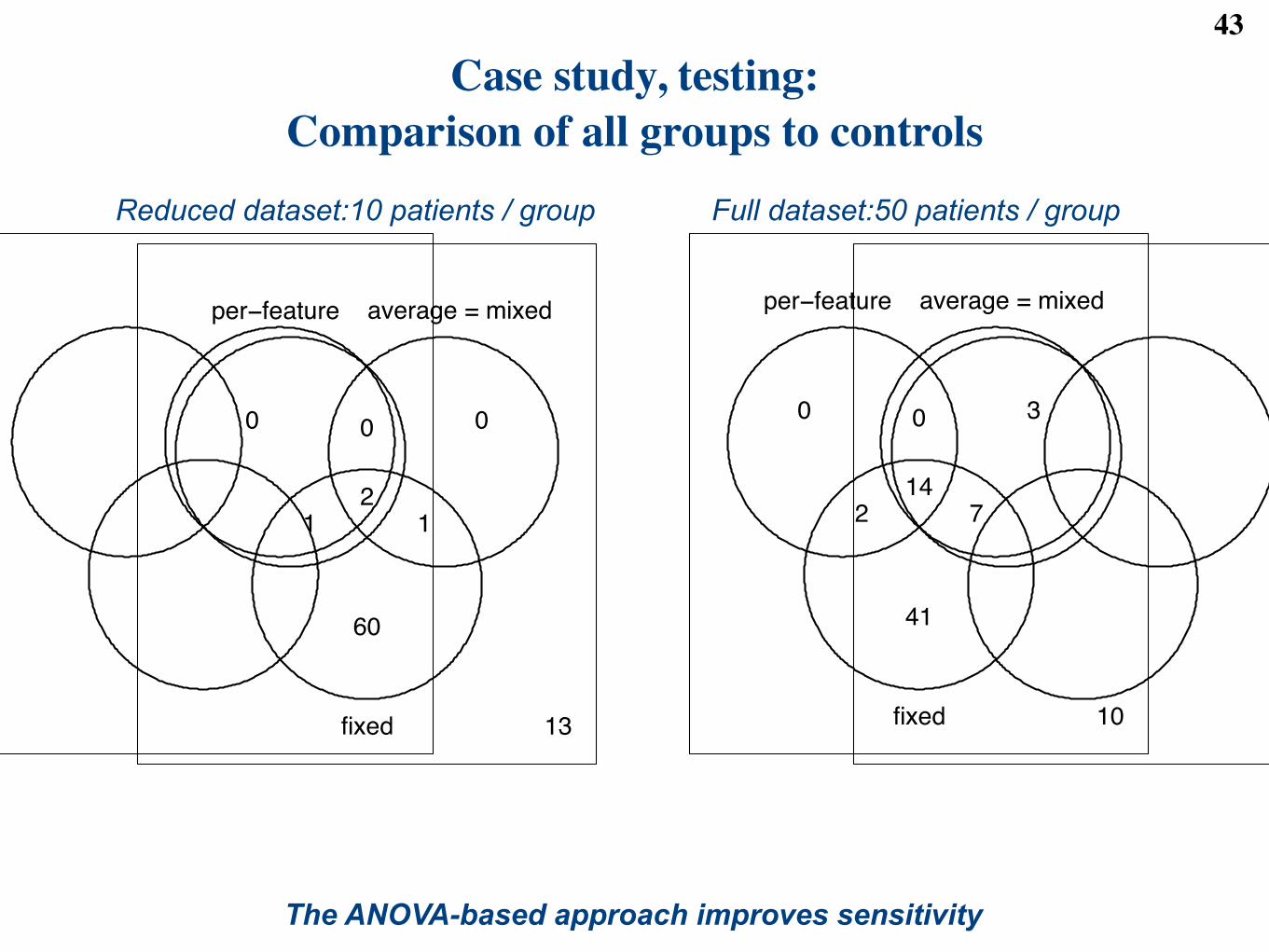
Case study, testing: Comparison of all groups to controls
43
(a) Spike-in: (b) Spike-in: (c) Spike-in: (d) Spike-in:per-feature “average” fixed mixed
25 50 100 200 400
020
40
60
80
100
Baseline
!!log2(p!value)
25 50 100 200 400
020
40
60
80
100
Baseline
!!log2(p!value)
25 50 100 200 400
020
40
60
80
100
Baseline
!!log2(p!value)
!
25 50 100 200 400
020
40
60
80
100
Baseline
!!log2(p!value)
Figure 6: Sensitivity of the four basic models at detecting a two-fold change in the spike-in dataset, startingfrom five abundance baselines. X-axis: abundance baseline. Y-axis: -log2(FDR-adjusted p-value). Each boxcontains the middle 50% of the proteins; the line within the box is the median. The higher the value onthe y-axis, the stronger the evidence for di!erential abundance. The horizontal line corresponds to the FDRcuto! of 0.05.
(a) Clinical: subset (b) Clinical: full (c) Spike-in
per!feature average = mixed
fixed 13
60
0
1
0
1
0
2
per!feature average = mixed
fixed 10
41
3
7
0
2
0
14
0 50 100 150
0.0
0.1
0.2
0.3
0.4
0.5
Number of detected fold changes
Fa
lse
po
sitiv
e r
ate
Per!feature model
Average model
Fixed model
Mixed model
Figure 7: (a) and (b) Sensitivity of the four basic models at detecting changes in abundance in the clinicaldataset. Each circle shows the number of proteins with at least one detected pairwise di!erence betweendisease groups after the FDR cuto! 0.05. (a) Reduced dataset with 50 subjects. (b) Full dataset with246 subjects. (c) Specificity of the four basic models at detecting changes in abundance in the spike-indataset. X-axis: number of di!erences in a comparison between two mixtures. Y-axis: false positive rate inall pairwise comparisons of mixtures. More specific models produce lower curves.
25
Reduced dataset:10 patients / group Full dataset:50 patients / group
The ANOVA-based approach improves sensitivity
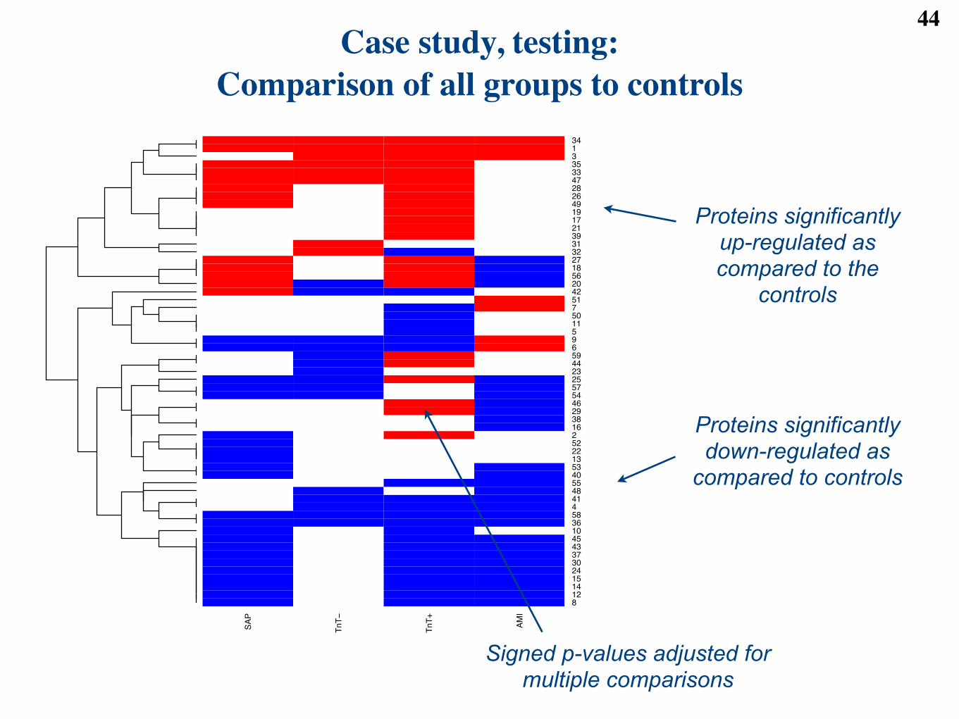
Case study, testing: Comparison of all groups to controls
44
SAP
TnT!
TnT+
AMI
8
12
14
15
24
30
37
43
45
10
36
58
4
41
48
55
40
53
13
22
52
2
16
38
29
46
54
57
25
23
44
59
6
9
5
11
50
7
51
42
20
56
18
27
32
31
39
21
17
19
49
26
28
47
33
35
3
1
34
Proteins significantly up-regulated as compared to the
controls
Proteins significantly down-regulated as
compared to controls
Signed p-values adjusted for multiple comparisons
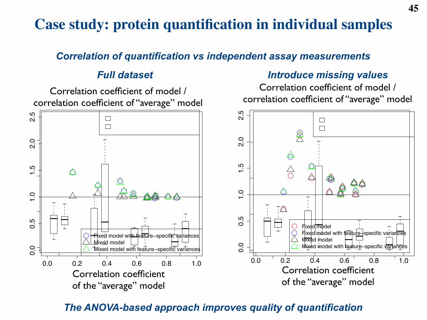
Case study: protein quantification in individual samples45
(a) Clinical: subset (b) Clinical: subset (c) Clinical: subset30% intensities missing 30% low intensities missing
!
!
!!!
! !
!
!
!
!
0.0 0.2 0.4 0.6 0.8 1.0
0.0
0.5
1.0
1.5
2.0
2.5
Corr(Average)
Corr
(AN
OV
A)
/ C
orr
(Ave
rag
e)
! Fixed model with feature!specific variances
Mixed model
Mixed model with feature!specific variances0.0
0.1
0.2
0.3
Approach
Bia
s
0.0
0.1
0.2
0.3
!
0.0
0.1
0.2
0.3
0.0
0.1
0.2
0.3
!
0.0
0.1
0.2
0.3
0.0
0.1
0.2
0.3
!
0.0
0.1
0.2
0.3
!
0.0
0.1
0.2
0.3
Per!feature Average Fixed Mixed
Missings at random
Missings at low intensities
!
!
!!
!!
!!
!
! !
0.0 0.2 0.4 0.6 0.8 1.0
0.0
0.5
1.0
1.5
2.0
2.5
Corr(Average)
Corr
(AN
OV
A)
/ C
orr
(Ave
rag
e)
!
!!!
!! !
!
!
!
!
!!
Fixed model
Fixed model with feature!specific variances
Mixed model
Mixed model with feature!specific variances
Figure 8: (a) Accuracy of subject quantification in the clinical dataset. X-axis: correlation of protein abun-dances derived from the “average model” and the nephelometry measurements. Y-axis: ratio of ANOVA-based correlations and the “average model”-based correlations. Points above the horizontal line indicateimproved quantification. (b) E!ect of missing intensities on estimates of di!erences between disease groups.X-axis: model type. Y-axis: absolute value of bias in estimation of the di!erences after removing 30% ofintensities. Lower boxes correspond to more robust models. (c) Same as (a), but after removing 30% offeature intensities, with higher probability of removal for low-abundant features.
26
Correlation coefficient of model / correlation coefficient of “average” model
Correlation coefficientof the “average” model
Correlation of quantification vs independent assay measurements
The ANOVA-based approach improves quality of quantification
(a) Clinical: subset (b) Clinical: subset (c) Clinical: subset30% intensities missing 30% low intensities missing
!
!
!!!
! !
!
!
!
!
0.0 0.2 0.4 0.6 0.8 1.0
0.0
0.5
1.0
1.5
2.0
2.5
Corr(Average)
Co
rr(A
NO
VA
) /
Co
rr(A
ve
rag
e)
! Fixed model with feature!specific variances
Mixed model
Mixed model with feature!specific variances
0.0
0.1
0.2
0.3
Approach
Bia
s
0.0
0.1
0.2
0.3
!
0.0
0.1
0.2
0.3
0.0
0.1
0.2
0.3
!
0.0
0.1
0.2
0.3
0.0
0.1
0.2
0.3
!
0.0
0.1
0.2
0.3
!
0.0
0.1
0.2
0.3
Per!feature Average Fixed Mixed
Missings at random
Missings at low intensities
!
!
!!
!!
!!
!
! !
0.0 0.2 0.4 0.6 0.8 1.0
0.0
0.5
1.0
1.5
2.0
2.5
Corr(Average)
Co
rr(A
NO
VA
) /
Co
rr(A
ve
rag
e)
!
!!!
!! !
!
!
!
!
!!
Fixed model
Fixed model with feature!specific variances
Mixed model
Mixed model with feature!specific variances
Figure 8: (a) Accuracy of subject quantification in the clinical dataset. X-axis: correlation of protein abun-dances derived from the “average model” and the nephelometry measurements. Y-axis: ratio of ANOVA-based correlations and the “average model”-based correlations. Points above the horizontal line indicateimproved quantification. (b) E!ect of missing intensities on estimates of di!erences between disease groups.X-axis: model type. Y-axis: absolute value of bias in estimation of the di!erences after removing 30% ofintensities. Lower boxes correspond to more robust models. (c) Same as (a), but after removing 30% offeature intensities, with higher probability of removal for low-abundant features.
26
Correlation coefficient of model / correlation coefficient of “average” model
Correlation coefficientof the “average” model
Full dataset Introduce missing values

Outline46
● LC-MS proteomics: a case study of coronary artery disease◆ Framing the question◆ Experimental design◆ Statistical analysis■ methods■ evaluation
◆ Enrichment of pre-defined sets in differential abundance
● Extensions◆ Planning future studies with LC-MS workflows◆ Design and analysis with labeling workflows

47
Example: P. Hu et al., Nature Reviews, 2007
Gene set enrichment: a typical application is to test the enrichment of GO terms in “interesting” genes
Size: total gene membershipColor: statistical significance of cancer genes
● Case study: test pre-defined functional terms based on clinical literature● Test for enrichment in differentially abundant genes
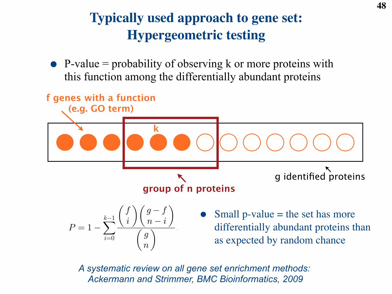
Typically used approach to gene set:Hypergeometric testing
48
● P-value = probability of observing k or more proteins with this function among the differentially abundant proteins
g identified proteins
f genes with a function (e.g. GO term)
group of n proteins
k
P -value of a cluster. In [66], Tavazoie et al. mapped thegenes in each resulting cluster to the 199 functionalcategories in the Martinsried Institute of Protein Sciencesfunction classification scheme (MIPS) database. For eachcluster, P -values were calculated to measure the statisticalsignificance for functional category enrichment. To bespecific, the authors used the hypergeometric distributionto calculate the probability of observing at least k genesfrom a functional category within a cluster of size n:
P ! 1"Xk"1
i!0
fi
! "g" fn" i
! "
gn
! " ;
where f is the total number of genes within a functionalcategory and g is the total number of genes within thegenome. Since the expectation of P within the cluster wouldbe higher than 0:05%, the authors regarded clusters withP -values smaller than 3 # 10"4 as significant. Jakt et al. [35]integrated the assessment of the potential functionalsignificance of both gene clusters and the correspondingpostulated regulatory motifs (common DNA sequencepatterns), and developed a method to estimate the prob-ability (P -value) of finding a certain number of matches to amotif in all of the gene clusters. A smaller probabilityindicates a higher significance of the clustering results.
Prediction strength. A novel approach to evaluating thereliability of sample clusters is based on the concept that if aclustering result reflects true cluster structure, then apredictor based on the resulting clusters should accuratelyestimate the cluster labels for new test samples. For geneexpression data, extra data objects are rarely used as testsamples since the number of available samples is limited.Rather, a cross-validation method is applied. The generatedclusters are assessed by repeatedly measuring the predictionstrengthwith one or a few of the data objects left out, in turn,as “test samples” while the remaining data objects are usedfor clustering.
Golub et al. introduced a method based on this idea.Suppose a clustering algorithm partitions the samples intotwo groups C1 and C2, with samples ~ss1; . . . ;~ssk belonging toC1 and samples ~ssk$1; . . . ;~ssp"1 belonging to C2, ~ssp being theleft out test sample, and G being a set of genes mostcorrelated with the current partition. Given the test sample~ssp, each gene~ggi 2 G votes for either C1 or C2, depending onwhether the gene expression level wip of ~ggi in ~ssp is closer to!1 or !2 (which denote, respectively, the mean expressionlevels of~ss1; . . . ;~ssk (C1) and~ssk$1; . . . ;~ssp"1 (C2)). The votes forC1 and C2 are summed as V1 and V2, respectively, and theprediction strength for~ssp is defined as j V1"V2
V1$V2j. Clearly, if most
of the genes in G uniformly vote ~ssp for C1 (or for C2), thevalue of the predication strength will be high. High valuesof prediction strength with respect to sufficient test samplesindicate a biologically significant clustering.
Golub’s method constructs a predictor based on derivedclusters and converts the reliability assessment of sampleclusters to a “supervised” classification problem. In [77],Yeung et al. extended the idea of “prediction strength” andproposed an approach to cluster validation for gene
clusters. Intuitively, if a cluster of genes has possiblebiological significance, then the expression levels of thegenes within that cluster should also be similar to eachother in “test” samples that were not used to form thecluster. Yeung et al. proposed a specific figure of merit(FOM), to estimate the predictive power of a clusteringalgorithm. Suppose C1; . . . ; Ck are the resulting clustersbased on samples 1; . . . ; %e" 1&; %e$ 1&; . . . ;m, and sample eis left out to test the prediction strength. Let R%g; e& be theexpression level of gene g under sample e in the raw datamatrix. Let !Ci%e& be the average expression level in samplee of the genes in cluster Ci. The figure of meritwith respect toe and the number of clusters k is defined as
FOM%e; k& !
##############################################################1
n#Xk
i!1
X
x2Ci
%R%x; e& " !Ci%e&&2
vuut :
Each of the m samples can be left out, in turn, and theaggregate figure of merit is defined as
FOM%k& !Xm
e!1
FOM%e; k&:
The FOM measures the mean deviation of the expressionlevels of genes in e relative to their corresponding clustermeans. Thus, a small value of FOM indicates a strongprediction strength and, therefore, a high-level reliability ofthe resulting clusters. Levine and Domany [41] proposedanother figure of merit M based on a resampling scheme.The basic idea is that the cluster structure derived from thewhole data set should be able to “predict” the clusterstructure of subsets of the full data. M measures the extentto which the clustering assignments obtained from theresamples (subsets of the full data) agree with those fromthe full data. A high value of M against a wide range ofresampling indicates a reliable clustering result.
4 CURRENT AND FUTURE RESEARCH DIRECTIONS
Recent DNA microarray technologies have made it possibleto monitor transcription levels of tens of thousands of genesin parallel. Gene expression data generated by microarrayexperiments offer tremendous potential for advances inmolecular biology and functional genomics. In this paper,we reviewed both classical and recently developed cluster-ing algorithms, which have been applied to gene expressiondata, with promising results.
Gene expression data can be clustered on both genes andsamples. As a result, the clustering algorithms can bedivided into three categories: gene-based clustering, sam-ple-based clustering, and subspace clustering. Each cate-gory has specific applications and present specificchallenges for the clustering task. For each category, wehave analyzed its particular problems and reviewed severalrepresentative algorithms.
Given the variety of available clustering algorithms, oneof the problems faced by biologists is the selection of thealgorithm most appropriate to a given gene expression dataset. However, there is no single “best” algorithmwhich is the“winner” in every aspect. Researchers typically select a fewcandidate algorithms and compare the clustering results.Nevertheless, we have shown that there are three aspects ofcluster validation and, for each aspect, various approaches
JIANG ET AL.: CLUSTER ANALYSIS FOR GENE EXPRESSION DATA: A SURVEY 1383
● Small p-value = the set has more differentially abundant proteins than as expected by random chance
A systematic review on all gene set enrichment methods: Ackermann and Strimmer, BMC Bioinformatics, 2009
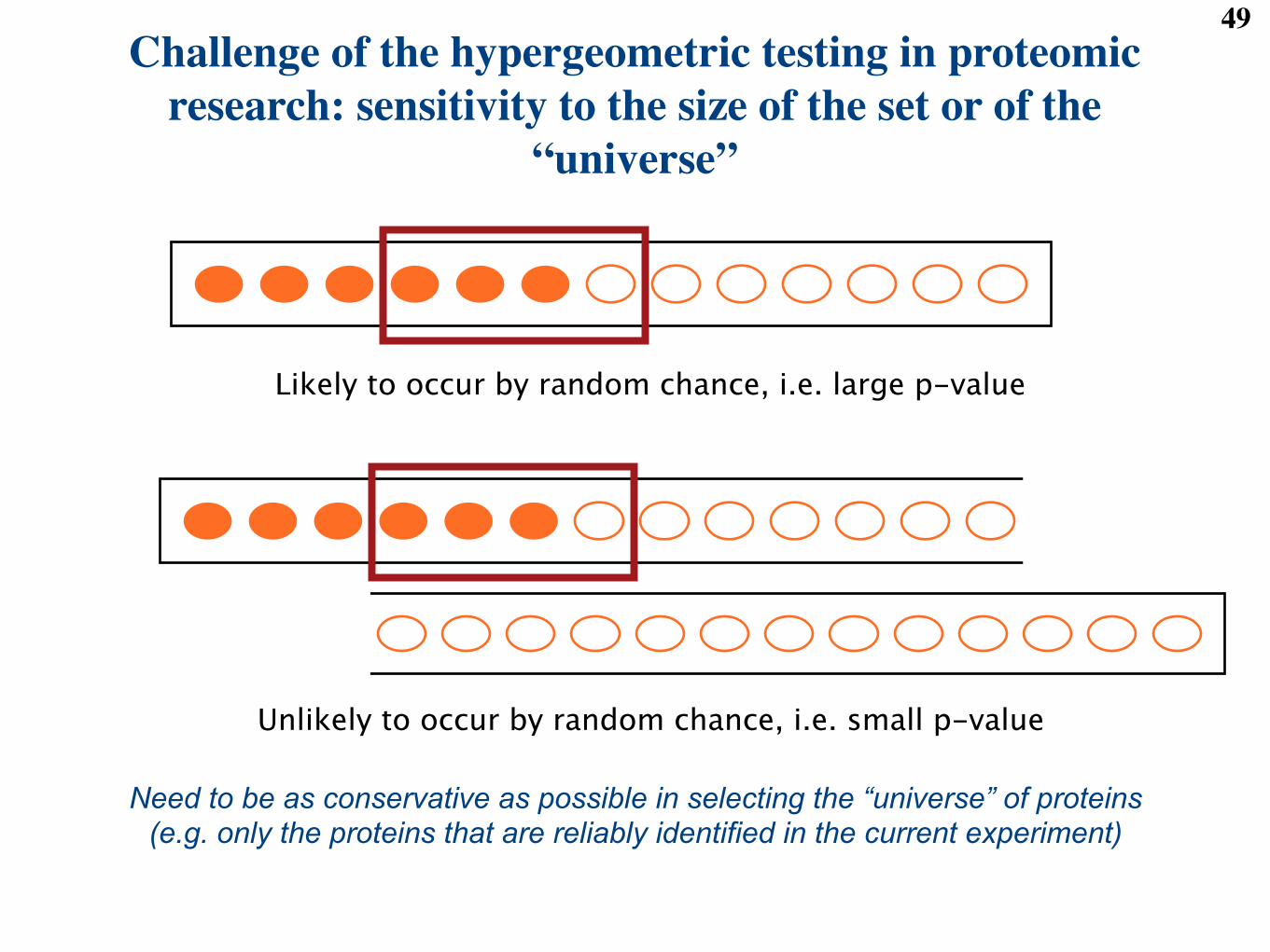
49Challenge of the hypergeometric testing in proteomic
research: sensitivity to the size of the set or of the “universe”
Likely to occur by random chance, i.e. large p-value
Unlikely to occur by random chance, i.e. small p-value
Need to be as conservative as possible in selecting the “universe” of proteins(e.g. only the proteins that are reliably identified in the current experiment)
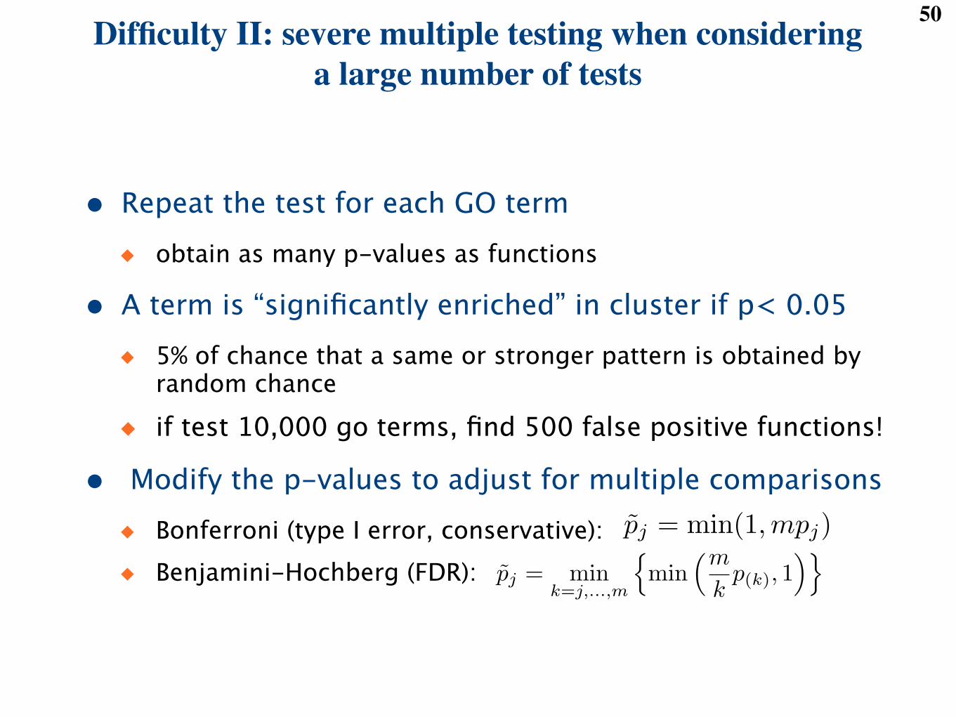
50Difficulty II: severe multiple testing when considering
a large number of tests
● Repeat the test for each GO term◆ obtain as many p-values as functions
● A term is “significantly enriched” in cluster if p< 0.05◆ 5% of chance that a same or stronger pattern is obtained by
random chance◆ if test 10,000 go terms, find 500 false positive functions!
● Modify the p-values to adjust for multiple comparisons◆ Bonferroni (type I error, conservative): ◆ Benjamini-Hochberg (FDR):
Frequentist approaches to controlling multivariate type I error 5
Consequently, to control the multivariate type I error at the level !!, we need to set
! =!!
m(4)
Procedure
Adjust each p-value such thatpj = min(1, mpj) (5)
Example
Suppose there are 100 genes, and we wish to control the FWER such that it is no larger than 0.05.
1. Set !! = 0.05.
2. (a) Calculate the p-value, pj corresponding to each test statistic, t(j)s .(b) Transform pj = min(1, 100pj).
3. Reject H(j)0 if pj < !! = 0.05.
alternatively,
1. Set !! = 0.05.
2. Calculate the p-value, pj corresponding to each test statistic, t(j)s .
3. Reject H(j)0 if pj < !!
m = 0.05100 = 0.0005.
Comments
• Even for methods controlling FWER, Bonferroni is extremely conservative. The e!ect is that inforcing that no type I errors occur, the rejection region is extremely small. Although we are (almost)guaranteed no false discoveries, it is extremely unlikely for there to be any true discoveries either.
• Suppose that m0 null hypotheses are true. Then it is true that
P{V ! 1} "m0!
j=1
P {reject H0 |H0 true} (6)
Since!!
m0>
!!
m, this would gain power. This means that Bonferroni assumes that as many as m null
hypotheses may be true. If we knew m0, we could make adjustments, however m0 is unknown.
4.2 minP - Westfall & Young (1993)
Description
• Single Step.
Frequentist approaches to controlling multivariate type I error 7
Procedure
1. Order the p-valuesp(1) ! p(2) ! . . . ! p(m) (10)
2. Starting with the largest p-value, compare p(j) to a !j = f(!!, j) as follows
p" value p(m) p(m"1) . . . p(K+1) p(K) p(K"1) . . . p(1)
! mm!! m"1
m !! . . . K+1m !! K
m!! K"1m !! . . . 1
m!!
p ! ! No No . . . No Yes ? . . . ?(11)
Once the first statistic is encountered such that p ! !, reject that null hypothesiss, and all others witha lower p-value.
This is equivalent to adjusting each p-value by
pj = mink=j,...,m
!min
"m
kp(k), 1
#$(12)
The outer minimization ensures that the order of the p-values is preserved, while the inside minimizationensures that all p-values remain below 1.
Comments
In 2001, Benjamini and Yekutieli showed that this procedure tolerates positive regression dependence, butnot general dependence. However, they were able to modify it such that it does control the FDR undergeneral dependence, using
pj = mink=j,...,m
%min
&m
'mt=1 1/t
kp(k), 1
()(13)
This is generally considered too conservative unless the dependence structure of the data requires it.
References
[Benjamini1995] Benjamini Y and Y. Hochberg. Controlling the false discovery rate. Journal of the RoyalStatistical Society Series B., 57(1): 289-300 1995
[Benjamini2001] Benjamini, Y and D. Yekutieli. The Control of the false discovery rate in multiple testingunder dependency. Annals of Statistics, 29(4): 1165-1188, Aug 2001.
[Xu2004] N. Zhong and J. Liu (Ed.), Intelligent Technologies for Infomration Analysis, Springer, pp615-659,2004.
[Westfall1993] Westfall, P.H. and S.S Young. Resampling-Based Multiple Testing. John Wiley & Sons, Inc.,New York 1993.

Outline51
● LC-MS proteomics: a case study of coronary artery disease◆ Framing the question◆ Experimental design◆ Statistical analysis■ methods■ evaluation
◆ Enrichment of pre-defined sets in differential abundance
● Extensions◆ Planning future studies with LC-MS workflows◆ Design and analysis with labeling workflows
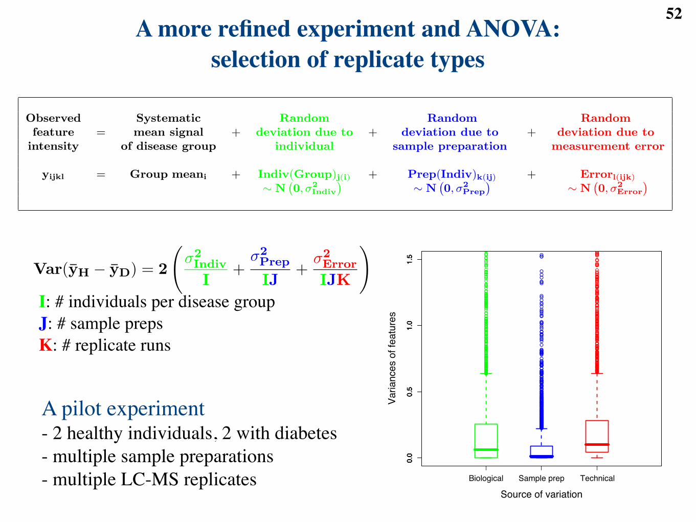
A more refined experiment and ANOVA: selection of replicate types
52
Observed Systematic Random deviationfeature = mean signal + due to all sources
intensity of disease group of variation
yij = Group meani + Errorj(i)
! N`0, !2
´
Observed Systematic Random Random Randomfeature = mean signal + deviation due to + deviation due to + deviation due to
intensity of disease group individual sample preparation measurement error
yijkl = Group meani + Indiv(Group)j(i) + Prep(Indiv)k(ij) + Errorl(ijk)
! N`0, !2
Indiv
´! N
`0, !2
Prep
´! N
`0, !2
Error
´
Var(yH ! yD) = 2
!!2Indiv
I+
!2Prep
IJ+
!2Error
IJK
". (1)
Observed Systematic Random deviation Random Randomfeature = mean signal + due to block + deviation due to + deviation due to
intensity of disease group (e.g. plate or day) individual measurement error
yijkl = Group meani + Blockk + Indiv(Group)j(i) + Errorl(ijk)
! N`0, !2
Block
´! N
`0, !2
Indiv
´! N
`0, !2
Error
´
1
0.0
0.5
1.0
1.5
Biological Sample prep Technical
Source of variation
Variances o
f fe
atu
res
!
!
!
!
!
!
!
!
!
!
!!
!
!
!
!
!
!
!
!
!!
!
!
!
!
!
!
!
!
!
!!
!
!
!
!
!
!
!
!
!
!
!
!
!
!
!
!
!
!
!
!
!
!!!
!
!
!
!
!
!
!
!
!
!
!
!
!
!
!
!
!
!
!
!
!
!
!
!
!
!
!
!
!
!
!
!
!
!
!
!
!
!
!
!
!
!
!
!
!
!
!
!
!
!
!
!
!
!
!
!
!
!
!
!
!
!
!
!
!
!
!
!
!
!
!
!
!
!
!
!
!
!
!
!
!
!
!
!
!
!
!
!
!
!
!
!
!
!
!
!
!
!
!
!!
!
!
!
!
!
!
!
!
!
!
!!
!
0.0
0.5
1.0
1.5
!
!
!!
!
!!
!
!
!
!
!
!
!
!
!!!
!!
!
!
!
!
!
!
!
!
!
!
!
!!
!
!
!
!
!
!
!
!
!
!
!!
!
!
!
!
!
!
!!
!
!
!
!
!
!
!
!
!!
!
!
!
!
!
!
!
!
!!
!
!
!
!
!
!
!
!
!
!
!
!
!!
!
!!
!
!
!
!!
!
!
!
!!!
!
!
!!
!
!
!
!
!
!
!
!
!
!
!!
!
!
!
!
!
!
!
!
!
!!!
!
!
!
!
!
!
!
!
!
!
!
!
!
!
!
!
!
!
!
!
!!
!
!
!
!
!
!
!
!
!
!
!
!
!
!!
!
!
!
!
!
!
!
!
!
!
!
!
!
!
!!!
!
!
!
!
!
!
!
!
!
!!!
!
!
!
!
!
!
!
!!
!
!
!
!
!
!
!
!
!
!
!
!
!
!
!
!
!
!
!
!
!
!
!
!
!
!
!
!
!
!
!
!
!
!
!!
!
!
!
!
!
!!
!
!
!
!!
!
!
!
!
!
!
!
!
!
!
!
!!
!
!
!
!
!
!
!
!
!!!
!
!
0.0
0.5
1.0
1.5
!
!
!
!
!
!
!
!
!
!
!
!
!
!
!
!
!
!
!
!
!
!
!
!
!
!
!
!
!
!
!
!
!!
!
!
!
!
!
!
!
!
!
!
!
!
!
!
!
!
!
!
!
!
!
!
!
!!
!
!
!
!
!
!
!
!
!
!
!
!
!
!
!
!
!
!
!
!
!
!
!
!
!
!
!
!
!
!
!
!
!
!
!
!
!
!
!
!
!
!
!
!
!
!!
!
!
!
!
!
!
!
!
!
!
!
!
!
!
!
!
!!
!
!
!
!
!!!
!
!
!
!
!
!
!
!
!
!
!!
!
!
!
!
!
!
!
!
!
!
!
!
!
!
!
!
!
!
!
!
!
!
!
!
!
!
!
!
!
!
!
!
!
!
!
!
!
!
!
!!
!
!
!
!
!
!
!
!
!
!
!
!
!
0.0
0.5
1.0
1.5
A pilot experiment- 2 healthy individuals, 2 with diabetes- multiple sample preparations- multiple LC-MS replicates
I: # individuals per disease groupJ: # sample prepsK: # replicate runs
Observed Systematic Random deviationfeature = mean signal + due to all sources
intensity of disease group of variation
yij = Group meani + Errorj(i)
! N`0, !2
´
Observed Systematic Random Random Randomfeature = mean signal + deviation due to + deviation due to + deviation due to
intensity of disease group individual sample preparation measurement error
yijkl = Group meani + Indiv(Group)j(i) + Prep(Indiv)k(ij) + Errorl(ijk)
! N`0, !2
Indiv
´! N
`0, !2
Prep
´! N
`0, !2
Error
´
Var(yH ! yD) = 2
!!2Indiv
I+
!2Prep
IJ+
!2Error
IJK
". (1)
Observed Systematic Random deviation Random Randomfeature = mean signal + due to block + deviation due to + deviation due to
intensity of disease group (e.g. plate or day) individual measurement error
yijkl = Group meani + Blockk + Indiv(Group)j(i) + Errorl(ijk)
! N`0, !2
Block
´! N
`0, !2
Indiv
´! N
`0, !2
Error
´
1
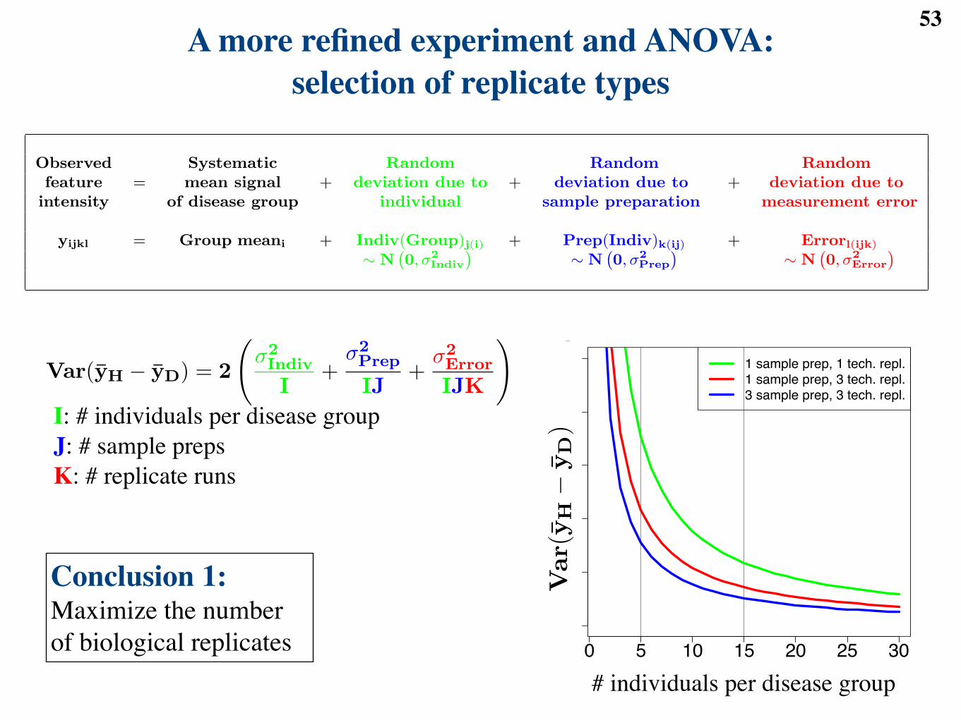
A more refined experiment and ANOVA: selection of replicate types
53
Observed Systematic Random deviationfeature = mean signal + due to all sources
intensity of disease group of variation
yij = Group meani + Errorj(i)
! N`0, !2
´
Observed Systematic Random Random Randomfeature = mean signal + deviation due to + deviation due to + deviation due to
intensity of disease group individual sample preparation measurement error
yijkl = Group meani + Indiv(Group)j(i) + Prep(Indiv)k(ij) + Errorl(ijk)
! N`0, !2
Indiv
´! N
`0, !2
Prep
´! N
`0, !2
Error
´
Var(yH ! yD) = 2
!!2Indiv
I+
!2Prep
IJ+
!2Error
IJK
". (1)
Observed Systematic Random deviation Random Randomfeature = mean signal + due to block + deviation due to + deviation due to
intensity of disease group (e.g. plate or day) individual measurement error
yijkl = Group meani + Blockk + Indiv(Group)j(i) + Errorl(ijk)
! N`0, !2
Block
´! N
`0, !2
Indiv
´! N
`0, !2
Error
´
1
I: # individuals per disease groupJ: # sample prepsK: # replicate runs
Observed Systematic Random deviationfeature = mean signal + due to all sources
intensity of disease group of variation
yij = Group meani + Errorj(i)
! N`0, !2
´
Observed Systematic Random Random Randomfeature = mean signal + deviation due to + deviation due to + deviation due to
intensity of disease group individual sample preparation measurement error
yijkl = Group meani + Indiv(Group)j(i) + Prep(Indiv)k(ij) + Errorl(ijk)
! N`0, !2
Indiv
´! N
`0, !2
Prep
´! N
`0, !2
Error
´
Var(yH ! yD) = 2
!!2Indiv
I+
!2Prep
IJ+
!2Error
IJK
". (1)
Observed Systematic Random deviation Random Randomfeature = mean signal + due to block + deviation due to + deviation due to
intensity of disease group (e.g. plate or day) individual measurement error
yijkl = Group meani + Blockk + Indiv(Group)j(i) + Errorl(ijk)
! N`0, !2
Block
´! N
`0, !2
Indiv
´! N
`0, !2
Error
´
1
0 5 10 15 20 25 30
0.0
00
.02
0.0
40
.06
0.0
80
.10
1 sample prep, 1 tech. repl.
1 sample prep, 3 tech. repl.
3 sample prep, 3 tech. repl.
# individuals per disease group
Obse
rved
Syst
emat
icR
andom
dev
iation
feat
ure
=m
ean
sign
al+
due
toal
lso
urc
esin
tensi
tyof
dis
ease
grou
pof
vari
atio
n
y ij
=G
roup
mea
ni
+E
rror
j(i
)
!N
` 0,!
2´
Obse
rved
Syst
em
ati
cR
andom
Random
Random
featu
re=
mean
signal
+devia
tion
due
to+
devia
tion
due
to+
devia
tion
due
toin
tensi
tyofdis
ease
gro
up
indiv
idual
sam
ple
pre
para
tion
measu
rem
ent
err
or
yijkl
=G
roup
mean
i+
Indiv
(Gro
up) j
(i)
+P
rep(I
ndiv
) k(ij)
+Err
or l
(ijk
)
!N
` 0,!
2 Indiv
´!
N` 0
,!2 Prep
´!
N` 0
,!2 Error
´
Var
(yH!
y D)
=2
!!
2 Indiv
I+
!2 Pre
p
IJ+
!2 Err
or
IJK
".
(1)
Obse
rved
Syst
emat
icR
andom
dev
iation
Ran
dom
Ran
dom
feat
ure
=m
ean
sign
al+
due
toblo
ck+
dev
iation
due
to+
dev
iation
due
toin
tensi
tyof
dis
ease
grou
p(e
.g.
pla
teor
day
)in
div
idual
mea
sure
men
ter
ror
y ijk
l=
Gro
up
mea
ni
+B
lock
k+
Indiv
(Gro
up)
j(i
)+
Err
orl(
ijk)
!N
` 0,!
2 Blo
ck
´!
N` 0,
!2 In
div
´!
N` 0,
!2 E
rror
´
1
Conclusion 1:Maximize the number of biological replicates
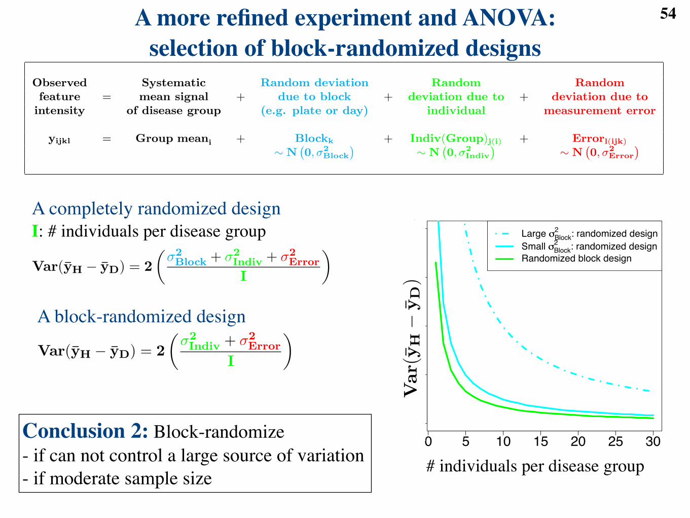
54A more refined experiment and ANOVA: selection of block-randomized designs
Observed Systematic Random deviationfeature = mean signal + due to all sources
intensity of disease group of variation
yij = Group meani + Errorj(i)
! N`0, !2
´
Observed Systematic Random Random Randomfeature = mean signal + deviation due to + deviation due to + deviation due to
intensity of disease group individual sample preparation measurement error
yijkl = Group meani + Indiv(Group)j(i) + Prep(Indiv)k(ij) + Errorl(ijk)
! N`0, !2
Indiv
´! N
`0, !2
Prep
´! N
`0, !2
Error
´
Var(yH ! yD) = 2
!!2Indiv
I+
!2Prep
IJ+
!2Error
IJK
". (1)
Observed Systematic Random deviation Random Randomfeature = mean signal + due to block + deviation due to + deviation due to
intensity of disease group (e.g. plate or day) individual measurement error
yijkl = Group meani + Blockk + Indiv(Group)j(i) + Errorl(ijk)
! N`0, !2
Block
´! N
`0, !2
Indiv
´! N
`0, !2
Error
´
1
Observed Systematic Random deviationfeature = mean signal + due to all sources
intensity of disease group of variation
yij = Group meani + Errorj(i)
! N`0, !2
´
Observed Systematic Random Random Randomfeature = mean signal + deviation due to + deviation due to + deviation due to
intensity of disease group individual sample preparation measurement error
yijkl = Group meani + Indiv(Group)j(i) + Prep(Indiv)k(ij) + Errorl(ijk)
! N`0, !2
Indiv
´! N
`0, !2
Prep
´! N
`0, !2
Error
´
Var(yH ! yD) = 2
!!2Indiv
I+
!2Prep
IJ+
!2Error
IJK
". (1)
Var(yH ! yD) = 2#
!2Indiv + !2
Indiv + !2Error
I
$(2)
Var(yH ! yD) = 2#
!2Indiv + !2
Error
I
$(3)
Observed Systematic Random deviation Random Randomfeature = mean signal + due to block + deviation due to + deviation due to
intensity of disease group (e.g. plate or day) individual measurement error
yijkl = Group meani + Blockk + Indiv(Group)j(i) + Errorl(ijk)
! N`0, !2
Block
´! N
`0, !2
Indiv
´! N
`0, !2
Error
´
1
A completely randomized design I: # individuals per disease group
A block-randomized design
Conclusion 2: Block-randomize - if can not control a large source of variation- if moderate sample size
Observed Systematic Random deviationfeature = mean signal + due to all sources
intensity of disease group of variation
yij = Group meani + Errorj(i)
! N`0, !2
´
Observed Systematic Random Random Randomfeature = mean signal + deviation due to + deviation due to + deviation due to
intensity of disease group individual sample preparation measurement error
yijkl = Group meani + Indiv(Group)j(i) + Prep(Indiv)k(ij) + Errorl(ijk)
! N`0, !2
Indiv
´! N
`0, !2
Prep
´! N
`0, !2
Error
´
Var(yH ! yD) = 2
!!2Indiv
I+
!2Prep
IJ+
!2Error
IJK
". (1)
Var(yH ! yD) = 2#
!2Block + !2
Indiv + !2Error
I
$(2)
Var(yH ! yD) = 2#
!2Indiv + !2
Error
I
$(3)
Observed Systematic Random deviation Random Randomfeature = mean signal + due to block + deviation due to + deviation due to
intensity of disease group (e.g. plate or day) individual measurement error
yijkl = Group meani + Blockk + Indiv(Group)j(i) + Errorl(ijk)
! N`0, !2
Block
´! N
`0, !2
Indiv
´! N
`0, !2
Error
´
1
0 5 10 15 20 25 30
0.0
0.1
0.2
0.3
0.4
Large !!Block2
: randomized design
Small !!Block2
: randomized design
Randomized block design
# individuals per disease group
Obse
rved
Syst
emat
icR
andom
dev
iation
feat
ure
=m
ean
sign
al+
due
toal
lso
urc
esin
tensi
tyof
dis
ease
grou
pof
vari
atio
n
y ij
=G
roup
mea
ni
+E
rror
j(i
)
!N
` 0,!
2´
Obse
rved
Syst
em
ati
cR
andom
Random
Random
featu
re=
mean
signal
+devia
tion
due
to+
devia
tion
due
to+
devia
tion
due
toin
tensi
tyofdis
ease
gro
up
indiv
idual
sam
ple
pre
para
tion
measu
rem
ent
err
or
yijkl
=G
roup
mean
i+
Indiv
(Gro
up) j
(i)
+P
rep(I
ndiv
) k(ij)
+Err
or l
(ijk
)
!N
` 0,!
2 Indiv
´!
N` 0
,!2 Prep
´!
N` 0
,!2 Error
´
Var
(yH!
y D)
=2
!!
2 Indiv
I+
!2 Pre
p
IJ+
!2 Err
or
IJK
".
(1)
Obse
rved
Syst
emat
icR
andom
dev
iation
Ran
dom
Ran
dom
feat
ure
=m
ean
sign
al+
due
toblo
ck+
dev
iation
due
to+
dev
iation
due
toin
tensi
tyof
dis
ease
grou
p(e
.g.
pla
teor
day
)in
div
idual
mea
sure
men
ter
ror
y ijk
l=
Gro
up
mea
ni
+B
lock
k+
Indiv
(Gro
up)
j(i
)+
Err
orl(
ijk)
!N
` 0,!
2 Blo
ck
´!
N` 0,
!2 In
div
´!
N` 0,
!2 E
rror
´
1

So how many replicates do I need?55
Fix:
# of features with # of features with Totalno detected di!erence detected di!erence
# true non-di!. features U V m0
# true di!. features T S m1 = m!m0
Total m!R R m
Table 1: Outcomes of testing m null hypotheses H0 : µH = µD simultaneously for m experimental features,conditionally on the features detected and quantified by a signal processing procedure. R, S, T , U and Vare random quantities, but only R is observed.
!
"
!
q = E!
Vmax(R,1)
". (1)
!ave ! (1" ")ave · q 11 + (1" q) · m0/m1
, (2)
Var(yH " yD) !#
!z1!! + z1!"/2
$2
, (3)
where z1!! and z1!"/2 are respectively the 100(1" ")th and the 100(1" !/2)th percentiles of the
standard Normal distribution. The formula can be applied to variances of c
Var(yH " yD) = 2#
#2Indiv + #2
Error
I
$!
#!
z1!! + z1!"/2
$2
(4)
Var(yH " yD) = 2
%#2Indiv
I+
#2Prep
IJ+
#2Error
IJK
&. (5)
1
- probability of a false positive discovery (False Positive Rate)
- probability of a true positive discovery
- anticipated fold change- anticipated variability
Var(yH ! yD) "!
!z1!! + z1!"/2
"2
, (1)
where z1!! and z1!"/2 are respectively the 100(1! !)th and the 100(1! "/2)th percentiles of the
standard Normal distribution. The formula can be applied to variances of c
Var(yH ! yD) = 2!
#2Indiv + #2
Error
I
""
!!
z1!! + z1!"/2
"2
(2)
Var(yH ! yD) = 2
##2Indiv
I+
#2Prep
IJ+
#2Error
IJK
$. (3)
Var(yH ! yD) = 2!
#2Block + #2
Indiv + #2Error
I
"(4)
Var(yH ! yD) = 2!
#2Indiv + #2
Error
I
"(5)
Var(D1 ! D2) = 2nb
ngnpns
%#2Indiv + #2
Error
&(6)
Reference:
Var(D1 ! D2) = 2!
#2Indiv + 2#2
Error
I
"(7)
1
and
Var(yH ! yD) "!
!z1!! + z1!"/2
"2
, (1)
where z1!! and z1!"/2 are respectively the 100(1! !)th and the 100(1! "/2)th percentiles of the
standard Normal distribution. The formula can be applied to variances of c
Var(yH ! yD) = 2!
#2Indiv + #2
Error
I
""
!!
z1!! + z1!"/2
"2
(2)
Var(yH ! yD) = 2
##2Indiv
I+
#2Prep
IJ+
#2Error
IJK
$. (3)
Var(yH ! yD) = 2!
#2Block + #2
Indiv + #2Error
I
"(4)
Var(yH ! yD) = 2!
#2Indiv + #2
Error
I
"(5)
Var(D1 ! D2) = 2nb
ngnpns
%#2Indiv + #2
Error
&(6)
Reference:
Var(D1 ! D2) = 2!
#2Indiv + 2#2
Error
I
"(7)
1
Write:
Var(yH ! yD) "!
!z1!! + z1!"/2
"2
, (1)
where z1!! and z1!"/2 are respectively the 100(1! !)th and the 100(1! "/2)th percentiles of the
standard Normal distribution. The formula can be applied to variances of c
Var(yH ! yD) = 2!
#2Indiv + #2
Error
I
""
!!
z1!! + z1!"/2
"2
(2)
Var(yH ! yD) = 2
##2Indiv
I+
#2Prep
IJ+
#2Error
IJK
$. (3)
Var(yH ! yD) = 2!
#2Block + #2
Indiv + #2Error
I
"(4)
Var(yH ! yD) = 2!
#2Indiv + #2
Error
I
"(5)
Var(D1 ! D2) = 2nb
ngnpns
%#2Indiv + #2
Error
&(6)
Reference:
Var(D1 ! D2) = 2!
#2Indiv + 2#2
Error
I
"(7)
1
andwhere are quantiles of the Normal distribution
If we only had one feature:
# of features with # of features with Totalno detected di!erence detected di!erence
# true non-di!. features U V m0
# true di!. features T S m1 = m!m0
Total m!R R m
Table 1: Outcomes of testing m null hypotheses H0 : µH = µD simultaneously for m experimental features,conditionally on the features detected and quantified by a signal processing procedure. R, S, T , U and Vare random quantities, but only R is observed.
!
"
!
q = E!
Vmax(R,1)
". (1)
!ave ! (1" ")ave · q 11 + (1" q) · m0/m1
, (2)
Var(yH " yD) !#
!z1!! + z1!"/2
$2
, (3)
where z1!! and z1!"/2 are respectively the 100(1" ")th and the 100(1" !/2)th percentiles of the
standard Normal distribution. The formula can be applied to variances of c
Var(yH " yD) = 2#
#2Indiv + #2
Error
I
$!
#!
z1!! + z1!"/2
$2
(4)
Var(yH " yD) = 2
%#2Indiv
I+
#2Prep
IJ+
#2Error
IJK
&. (5)
1
solve for the number of individuals I
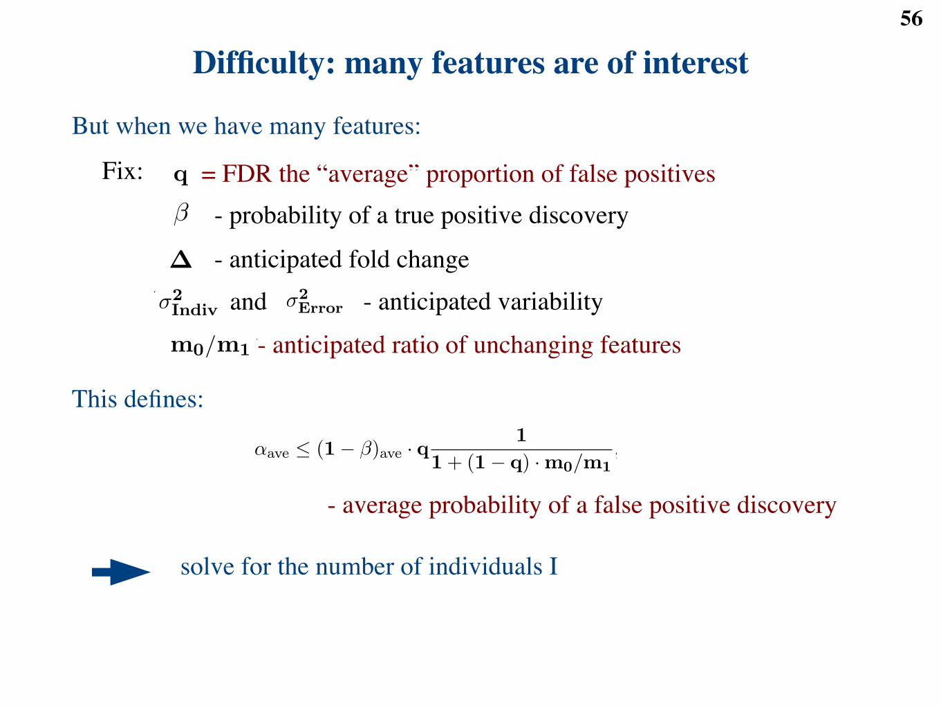
Difficulty: many features are of interest56
Fix:
# of features with # of features with Totalno detected di!erence detected di!erence
# true non-di!. features U V m0
# true di!. features T S m1 = m!m0
Total m!R R m
Table 1: Outcomes of testing m null hypotheses H0 : µH = µD simultaneously for m experimental features,conditionally on the features detected and quantified by a signal processing procedure. R, S, T , U and Vare random quantities, but only R is observed.
!
"
!
q = E!
Vmax(R,1)
". (1)
!ave ! (1" ")ave · q 11 + (1" q) · m0/m1
, (2)
Var(yH " yD) !#
!z1!! + z1!"/2
$2
, (3)
where z1!! and z1!"/2 are respectively the 100(1" ")th and the 100(1" !/2)th percentiles of the
standard Normal distribution. The formula can be applied to variances of c
Var(yH " yD) = 2#
#2Indiv + #2
Error
I
$!
#!
z1!! + z1!"/2
$2
(4)
Var(yH " yD) = 2
%#2Indiv
I+
#2Prep
IJ+
#2Error
IJK
&. (5)
1
# of features with # of features with Totalno detected di!erence detected di!erence
# true non-di!. features U V m0
# true di!. features T S m1 = m!m0
Total m!R R m
Table 1: Outcomes of testing m null hypotheses H0 : µH = µD simultaneously for m experimental features,conditionally on the features detected and quantified by a signal processing procedure. R, S, T , U and Vare random quantities, but only R is observed.
!
"
!
q = E!
Vmax(R,1)
". (1)
!ave ! (1" ")ave · q 11 + (1" q) · m0/m1
, (2)
Var(yH " yD) !#
!z1!! + z1!"/2
$2
, (3)
where z1!! and z1!"/2 are respectively the 100(1" ")th and the 100(1" !/2)th percentiles of the
standard Normal distribution. The formula can be applied to variances of c
Var(yH " yD) = 2#
#2Indiv + #2
Error
I
$!
#!
z1!! + z1!"/2
$2
(4)
Var(yH " yD) = 2
%#2Indiv
I+
#2Prep
IJ+
#2Error
IJK
&. (5)
1
- probability of a true positive discovery
- anticipated fold change- anticipated variability
Var(yH ! yD) "!
!z1!! + z1!"/2
"2
, (1)
where z1!! and z1!"/2 are respectively the 100(1! !)th and the 100(1! "/2)th percentiles of the
standard Normal distribution. The formula can be applied to variances of c
Var(yH ! yD) = 2!
#2Indiv + #2
Error
I
""
!!
z1!! + z1!"/2
"2
(2)
Var(yH ! yD) = 2
##2Indiv
I+
#2Prep
IJ+
#2Error
IJK
$. (3)
Var(yH ! yD) = 2!
#2Block + #2
Indiv + #2Error
I
"(4)
Var(yH ! yD) = 2!
#2Indiv + #2
Error
I
"(5)
Var(D1 ! D2) = 2nb
ngnpns
%#2Indiv + #2
Error
&(6)
Reference:
Var(D1 ! D2) = 2!
#2Indiv + 2#2
Error
I
"(7)
1
and
Var(yH ! yD) "!
!z1!! + z1!"/2
"2
, (1)
where z1!! and z1!"/2 are respectively the 100(1! !)th and the 100(1! "/2)th percentiles of the
standard Normal distribution. The formula can be applied to variances of c
Var(yH ! yD) = 2!
#2Indiv + #2
Error
I
""
!!
z1!! + z1!"/2
"2
(2)
Var(yH ! yD) = 2
##2Indiv
I+
#2Prep
IJ+
#2Error
IJK
$. (3)
Var(yH ! yD) = 2!
#2Block + #2
Indiv + #2Error
I
"(4)
Var(yH ! yD) = 2!
#2Indiv + #2
Error
I
"(5)
Var(D1 ! D2) = 2nb
ngnpns
%#2Indiv + #2
Error
&(6)
Reference:
Var(D1 ! D2) = 2!
#2Indiv + 2#2
Error
I
"(7)
1
solve for the number of individuals I
But when we have many features:
# of features with # of features with Totalno detected di!erence detected di!erence
# true non-di!. features U V m0
# true di!. features T S m1 = m!m0
Total m!R R m
Table 1: Outcomes of testing m null hypotheses H0 : µH = µD simultaneously for m experimental features,conditionally on the features detected and quantified by a signal processing procedure. R, S, T , U and Vare random quantities, but only R is observed.
q = E!
Vmax(R,1)
". (1)
!ave ! (1" ")ave · q 11 + (1" q) · m0/m1
, (2)
Var(yH " yD) !#
!z1!! + z1!"/2
$2
, (3)
where z1!! and z1!"/2 are respectively the 100(1" ")th and the 100(1" !/2)th percentiles of the
standard Normal distribution. The formula can be applied to variances of c
Var(yH " yD) = 2#
#2Indiv + #2
Error
I
$!
#!
z1!! + z1!"/2
$2
(4)
Var(yH " yD) = 2
%#2Indiv
I+
#2Prep
IJ+
#2Error
IJK
&. (5)
1
= FDR the “average” proportion of false positives
- anticipated ratio of unchanging features!ave ! (1" ")ave · q 1
1 + (1" q) · m0/m1, (1)
Var(yH " yD) !!
!z1!! + z1!"/2
"2
, (2)
where z1!! and z1!"/2 are respectively the 100(1" ")th and the 100(1" !/2)th percentiles of the
standard Normal distribution. The formula can be applied to variances of c
Var(yH " yD) = 2!
#2Indiv + #2
Error
I
"!
!!
z1!! + z1!"/2
"2
(3)
Var(yH " yD) = 2
##2Indiv
I+
#2Prep
IJ+
#2Error
IJK
$. (4)
Var(yH " yD) = 2!
#2Block + #2
Indiv + #2Error
I
"(5)
Var(yH " yD) = 2!
#2Indiv + #2
Error
I
"(6)
Var(D1 " D2) = 2nb
ngnpns
%#2Indiv + #2
Error
&(7)
1
!ave ! (1" ")ave · q 11 + (1" q) · m0/m1
, (1)
Var(yH " yD) !!
!z1!! + z1!"/2
"2
, (2)
where z1!! and z1!"/2 are respectively the 100(1" ")th and the 100(1" !/2)th percentiles of the
standard Normal distribution. The formula can be applied to variances of c
Var(yH " yD) = 2!
#2Indiv + #2
Error
I
"!
!!
z1!! + z1!"/2
"2
(3)
Var(yH " yD) = 2
##2Indiv
I+
#2Prep
IJ+
#2Error
IJK
$. (4)
Var(yH " yD) = 2!
#2Block + #2
Indiv + #2Error
I
"(5)
Var(yH " yD) = 2!
#2Indiv + #2
Error
I
"(6)
Var(D1 " D2) = 2nb
ngnpns
%#2Indiv + #2
Error
&(7)
1
- average probability of a false positive discovery
This defines:
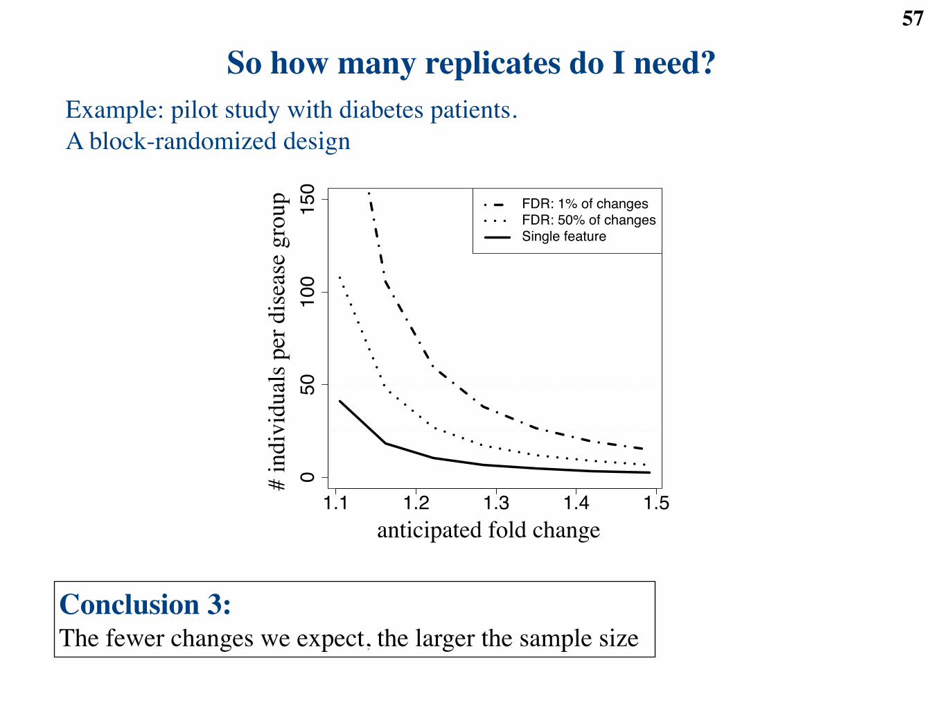
So how many replicates do I need?57
anticipated fold change
# in
divi
dual
s per
dise
ase
grou
p
1.1 1.2 1.3 1.4 1.5
050
100
15
0
FDR: 1% of changesFDR: 50% of changesSingle feature
Conclusion 3: The fewer changes we expect, the larger the sample size
Example: pilot study with diabetes patients. A block-randomized design
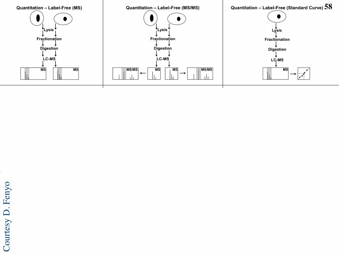
Cour
tesy
D. F
enyo
58
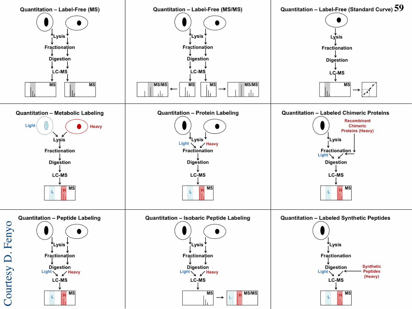
Cour
tesy
D. F
enyo
59
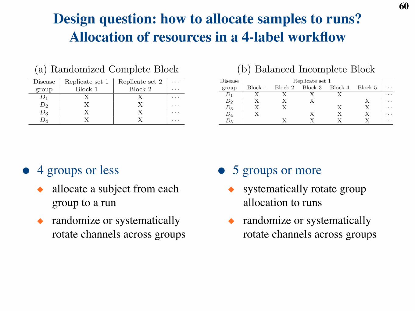
60
(a) (b) (c)
0.0
0.5
1.0
1.5
Biological
replicate
Sample
preparation
Technical
replicate
Source of variation
Variances o
f fe
atu
res
!
!
!
!
!
!
!
!
!
!
!!
!
!
!
!
!
!
!
!
!!
!
!
!
!
!
!
!
!
!
!!
!
!
!
!
!
!
!
!
!
!
!
!
!
!
!
!
!
!
!
!
!
!!!
!
!
!
!
!
!
!
!
!
!
!
!
!
!
!
!
!
!
!
!
!
!
!
!
!
!
!
!
!
!
!
!
!
!
!
!
!
!
!
!
!
!
!
!
!
!
!
!
!
!
!
!
!
!
!
!
!
!
!
!
!
!
!
!
!
!
!
!
!
!
!
!
!
!
!
!
!
!
!
!
!
!
!
!
!
!
!
!
!
!
!
!
!
!
!
!
!
!
!
!!
!
!
!
!
!
!
!
!
!
!
!!
!
0.0
0.5
1.0
1.5
!
!
!!
!
!!
!
!
!
!
!
!
!
!
!!!
!!
!
!
!
!
!
!
!
!
!
!
!
!!
!
!
!
!
!
!
!
!
!
!
!!
!
!
!
!
!
!
!!
!
!
!
!
!
!
!
!
!!
!
!
!
!
!
!
!
!
!!
!
!
!
!
!
!
!
!
!
!
!
!
!!
!
!!
!
!
!
!!
!
!
!
!!!
!
!
!!
!
!
!
!
!
!
!
!
!
!
!!
!
!
!
!
!
!
!
!
!
!!!
!
!
!
!
!
!
!
!
!
!
!
!
!
!
!
!
!
!
!
!
!!
!
!
!
!
!
!
!
!
!
!
!
!
!
!!
!
!
!
!
!
!
!
!
!
!
!
!
!
!
!!!
!
!
!
!
!
!
!
!
!
!!!
!
!
!
!
!
!
!
!!
!
!
!
!
!
!
!
!
!
!
!
!
!
!
!
!
!
!
!
!
!
!
!
!
!
!
!
!
!
!
!
!
!
!
!!
!
!
!
!
!
!!
!
!
!
!!
!
!
!
!
!
!
!
!
!
!
!
!!
!
!
!
!
!
!
!
!
!!!
!
!
0.0
0.5
1.0
1.5
!
!
!
!
!
!
!
!
!
!
!
!
!
!
!
!
!
!
!
!
!
!
!
!
!
!
!
!
!
!
!
!
!!
!
!
!
!
!
!
!
!
!
!
!
!
!
!
!
!
!
!
!
!
!
!
!
!!
!
!
!
!
!
!
!
!
!
!
!
!
!
!
!
!
!
!
!
!
!
!
!
!
!
!
!
!
!
!
!
!
!
!
!
!
!
!
!
!
!
!
!
!
!
!!
!
!
!
!
!
!
!
!
!
!
!
!
!
!
!
!
!!
!
!
!
!
!!!
!
!
!
!
!
!
!
!
!
!
!!
!
!
!
!
!
!
!
!
!
!
!
!
!
!
!
!
!
!
!
!
!
!
!
!
!
!
!
!
!
!
!
!
!
!
!
!
!
!
!
!!
!
!
!
!
!
!
!
!
!
!
!
!
!
0.0
0.5
1.0
1.5
0 5 10 15 20 25 30
0.0
00.0
20.0
40.0
60.0
80.1
0
Number of individuals per group
Variance o
f a d
iffe
rence b
etw
een tw
o g
roups 1 sample prep, 1 tech. repl.
1 sample prep, 3 tech. repl.3 sample prep, 3 tech. repl.
0 5 10 15 20 25 30
0.0
0.1
0.2
0.3
0.4
Number of blocks (= number of individuals per group)
Variance o
f a d
iffe
rence b
etw
een tw
o g
roups Large !!Block
2: randomized design
Small !!Block2
: randomized design
Randomized block design
Figure 6: The pilot label-free experiment of patients with diabetes. (a) Variance components!2
Indiv, !2Prep and !2
Error over all quantified features. Each box contains the middle 50% of thefeatures, the horizontal line within a box is the median, dots are the outliers. (b) V ar(yH ! yD) ofa complete randomized design in Eq. (2). (c) V ar(yH ! yD) for randomized block design in Eq. (3)and completely randomized design in Eq. (4), with no technical replicates. “Large” !2
Block =5(!2
Indiv + !2Error), and “small” !2
Block = 0.5(!2Indiv + !2
Error).
Observed Systematic Random deviation Random Randomfeature = mean signal + due to block + deviation due to + deviation due to
intensity of disease group (e.g. plate or day) individual measurement error
yijkl = Group meani + Blockk + Indiv(Group)j(i) + Errorl(ijk)
" N!0, !2
Block
"" N
!0, !2
Indiv
"" N
!0, !2
Error
"
Figure 7: Statistical model for a mixed ANOVA with random blocks. i is the index of a diseasegroup, j(i) the index of a patient within the group, k is the index of the block, and l(ijk) is thereplicate run. Blockk, Indiv(Group)j(i) and Errorl(ijk) are all independent.
(a) Randomized Complete Block (b) Balanced Incomplete Block
Disease Replicate set 1 Replicate set 2 · · ·group Block 1 Block 2 · · ·D1 X X · · ·D2 X X · · ·D3 X X · · ·D4 X X · · ·D5 X X · · ·
Disease Replicate set 1 Replicate set 2 · · ·group Block 1 Block 2 · · ·D1 X X · · ·D2 X X · · ·D3 X X · · ·D4 X X · · ·
Disease Replicate set 1group Block 1 Block 2 Block 3 Block 4 Block 5 · · ·D1 X X X X · · ·D2 X X X X · · ·D3 X X X X · · ·D4 X X X X · · ·D5 X X X X · · ·
Disease Replicate set 1group Block 1 Block 2 Block 3 Block 4 Block 5 · · ·
R X X X X X · · ·D1 X · · ·D2 X · · ·D3 X · · ·D4 X · · ·D5 X · · ·
Disease Replicate set 1group Block 1 Block 2 Block 3 Block 4 Block 5 · · ·D1 X X · · ·D2 X X · · ·D3 X X · · ·D4 X X · · ·D5 X X · · ·
Disease Replicate set 1group Block 1 Block 2 Block 3 Block 4 Block 5 Block 6 Block 7 Block 8 Block 9 Block 10 · · ·D1 X X X X · · ·D2 X X X X · · ·D3 X X X X · · ·D4 X X X X · · ·D5 X X X X · · ·
1
Statistical issues in LC-MS based biomarker discovery:summary of discussion with Xiao-jun and suggestions.
September 7, 2008
Disease Replicate set 1 Replicate set 2 · · ·group Block 1 Block 2 · · ·D1 X X · · ·D2 X X · · ·D3 X X · · ·D4 X X · · ·
Disease Replicate set 1group Block 1 Block 2 Block 3 Block 4 Block 5 · · ·D1 X X X X · · ·D2 X X X X · · ·D3 X X X X · · ·D4 X X X X · · ·D5 X X X X · · ·
Disease Replicate set 1group Block 1 Block 2 Block 3 Block 4 · · ·
H X X X X · · ·D1 X X X · · ·D2 X X X · · ·D3 X X X · · ·D4 X X X · · ·
Disease Replicate set 1group Block 1 Block 2 Block 3 Block 4 · · ·
H X X X X · · ·D1 X · · ·D2 X · · ·D3 X · · ·D4 X · · ·
1
Figure 8: Experiments with a four-label workflow; “X” indicates a unique biological sample. (a)Randomized complete block design with four disease groups: each block contains one individualfrom each disease group. (b) Balanced incomplete block design with four labels and five diseasegroups: individuals from each pair of groups appear in the same block an equal number of times.
40
Design question: how to allocate samples to runs?Allocation of resources in a 4-label workflow
● 4 groups or less◆ allocate a subject from each
group to a run◆ randomize or systematically
rotate channels across groups
● 5 groups or more◆ systematically rotate group
allocation to runs◆ randomize or systematically
rotate channels across groups
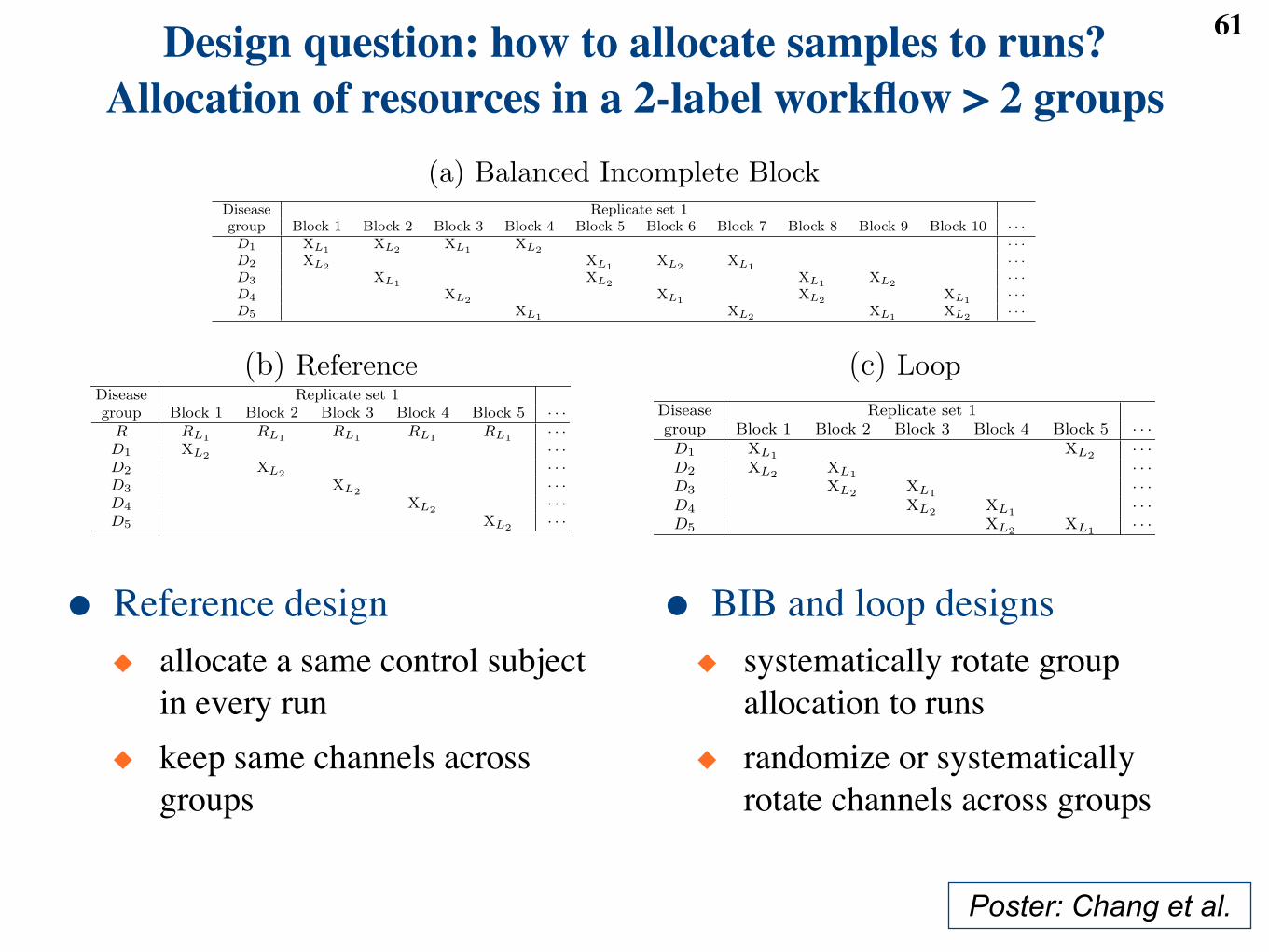
61
(a) Balanced Incomplete Block
Disease Replicate set 1group Block 1 Block 2 Block 3 Block 4 Block 5 · · ·
R XL1 XL1 XL1 XL1 XL1 · · ·D1 XL2 · · ·D2 XL2 · · ·D3 XL2 · · ·D4 XL2 · · ·D5 XL2 · · ·
Disease Replicate set 1group Block 1 Block 2 Block 3 Block 4 Block 5 · · ·D1 XL1 XL2 · · ·D2 XL2 XL1 · · ·D3 XL2 XL1 · · ·D4 XL2 XL1 · · ·D5 XL2 XL1 · · ·
Disease Replicate set 1group Block 1 Block 2 Block 3 Block 4 Block 5 Block 6 Block 7 Block 8 Block 9 Block 10 · · ·D1 XL1 XL2 XL1 XL2 · · ·D2 XL2 XL1 XL2 XL1 · · ·D3 XL1 XL2 XL1 XL2 · · ·D4 XL2 XL1 XL2 XL1 · · ·D5 XL1 XL2 XL1 XL2 · · ·
2
(b) Reference (c) LoopDisease Replicate set 1group Block 1 Block 2 Block 3 Block 4 Block 5 · · ·
R RL1 RL1 RL1 RL1 RL1 · · ·D1 XL2 · · ·D2 XL2 · · ·D3 XL2 · · ·D4 XL2 · · ·D5 XL2 · · ·
Disease Replicate set 1group Block 1 Block 2 Block 3 Block 4 Block 5 · · ·D1 XL1 XL2 · · ·D2 XL2 XL1 · · ·D3 XL2 XL1 · · ·D4 XL2 XL1 · · ·D5 XL2 XL1 · · ·
Disease Replicate set 1group Block 1 Block 2 Block 3 Block 4 Block 5 Block 6 Block 7 Block 8 Block 9 Block 10 · · ·D1 XL1 XL2 XL1 XL2 · · ·D2 XL2 XL1 XL2 XL1 · · ·D3 XL1 XL2 XL1 XL2 · · ·D4 XL2 XL1 XL2 XL1 · · ·D5 XL1 XL2 XL1 XL2 · · ·
2
Disease Replicate set 1group Block 1 Block 2 Block 3 Block 4 Block 5 · · ·
R XL1 XL1 XL1 XL1 XL1 · · ·D1 XL2 · · ·D2 XL2 · · ·D3 XL2 · · ·D4 XL2 · · ·D5 XL2 · · ·
Disease Replicate set 1group Block 1 Block 2 Block 3 Block 4 Block 5 · · ·D1 XL1 XL2 · · ·D2 XL2 XL1 · · ·D3 XL2 XL1 · · ·D4 XL2 XL1 · · ·D5 XL2 XL1 · · ·
Disease Replicate set 1group Block 1 Block 2 Block 3 Block 4 Block 5 Block 6 Block 7 Block 8 Block 9 Block 10 · · ·D1 XL1 XL2 XL1 XL2 · · ·D2 XL2 XL1 XL2 XL1 · · ·D3 XL1 XL2 XL1 XL2 · · ·D4 XL2 XL1 XL2 XL1 · · ·D5 XL1 XL2 XL1 XL2 · · ·
2
Figure 9: Five-group experiments with a two-label workflow; “X” indicates a unique biologicalsample, “R” indicates a reference sample, and “L1” and “L2” indicate the (optional) systematiclabeling scheme. (a) Balanced incomplete block: individuals from each pair of groups appear in asame block once. (b) Reference design: each block contains a reference sample which is the same inall blocks, and one additional unique individual. (c) Loop design: pairs of individuals from di!erentgroups cycle through blocks.
(a) (b) (c)
0 5 10 15 20 25 30
0.0
00.0
20.0
40.0
60.0
80.1
0
Number of individuals per group
Variance o
f a d
iffe
rence b
etw
een tw
o g
roups 2 label: BIB
4 label: BIB5 label: RCB
0 5 10 15 20 25 30
0.0
00.0
20.0
40.0
60.0
80.1
0
!
!
!
!
!
!
!
!!
!!
!!
!
!
!
!
!
!
!
!
!
!
!!
!!
!
Number of individuals per group
Variance o
f a d
iffe
rence b
etw
een tw
o g
roups
!
!
2 label: REF2 label: loop, disconnect2 label: loop, connect2 label: BIB
0 20 40 60 80
0.0
00.0
20.0
40.0
60.0
80.1
0
!
!
!
!
!
!
!
!!
!!
!!
! ! ! ! !
!
!
!
!
!
!
!
!
!
!!
!!
!!
!! !
Number of runs
Variance o
f a d
iffe
rence b
etw
een tw
o g
roups
!
!
2 label: REF2 label: loop, disconnect2 label: loop, connect2 label: BIB
Figure 10: Variances V ar(D1 ! D2) of a comparison between two disease groups in a 5-groupexperiment. (a) 5-label workflow with a randomized complete block design in Eq. (4), and 4-and 2-label workflows with a balanced incomplete block design in Eq. (5). (b) and (c) 2-labelworkflow with a balanced incomplete block in Eq. (5), reference design in Eq. (6) and loop designin Eq. (7)-Eq. (8).
41
Poster: Chang et al.
● Reference design◆ allocate a same control subject
in every run◆ keep same channels across
groups
● BIB and loop designs◆ systematically rotate group
allocation to runs◆ randomize or systematically
rotate channels across groups
Design question: how to allocate samples to runs?Allocation of resources in a 2-label workflow > 2 groups
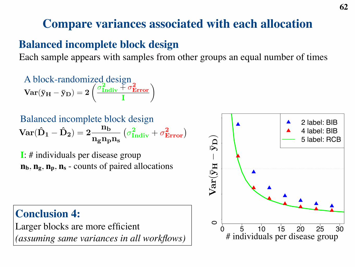
Compare variances associated with each allocation62
Observed Systematic Random deviationfeature = mean signal + due to all sources
intensity of disease group of variation
yij = Group meani + Errorj(i)
! N`0, !2
´
Observed Systematic Random Random Randomfeature = mean signal + deviation due to + deviation due to + deviation due to
intensity of disease group individual sample preparation measurement error
yijkl = Group meani + Indiv(Group)j(i) + Prep(Indiv)k(ij) + Errorl(ijk)
! N`0, !2
Indiv
´! N
`0, !2
Prep
´! N
`0, !2
Error
´
Var(yH ! yD) = 2
!!2Indiv
I+
!2Prep
IJ+
!2Error
IJK
". (1)
Var(yH ! yD) = 2#
!2Block + !2
Indiv + !2Error
I
$(2)
Var(yH ! yD) = 2#
!2Indiv + !2
Error
I
$(3)
Var(D1 ! D2) = 2nb
ngnpns
%!2Indiv + !2
Error
&(4)
1
Observed Systematic Random deviationfeature = mean signal + due to all sources
intensity of disease group of variation
yij = Group meani + Errorj(i)
! N`0, !2
´
Observed Systematic Random Random Randomfeature = mean signal + deviation due to + deviation due to + deviation due to
intensity of disease group individual sample preparation measurement error
yijkl = Group meani + Indiv(Group)j(i) + Prep(Indiv)k(ij) + Errorl(ijk)
! N`0, !2
Indiv
´! N
`0, !2
Prep
´! N
`0, !2
Error
´
Var(yH ! yD) = 2
!!2Indiv
I+
!2Prep
IJ+
!2Error
IJK
". (1)
Var(yH ! yD) = 2#
!2Indiv + !2
Indiv + !2Error
I
$(2)
Var(yH ! yD) = 2#
!2Indiv + !2
Error
I
$(3)
Observed Systematic Random deviation Random Randomfeature = mean signal + due to block + deviation due to + deviation due to
intensity of disease group (e.g. plate or day) individual measurement error
yijkl = Group meani + Blockk + Indiv(Group)j(i) + Errorl(ijk)
! N`0, !2
Block
´! N
`0, !2
Indiv
´! N
`0, !2
Error
´
1
A block-randomized design
Balanced incomplete block design
I: # individuals per disease groupnb, ng, np, ns - counts of paired allocations
Conclusion 4: Larger blocks are more efficient (assuming same variances in all workflows)
0 5 10 15 20 25 30
0.0
0.1
0.2
0.3
0.4
2 label: BIB
4 label: BIB
5 label: RCB
# individuals per disease group
Obse
rved
Syst
emat
icR
andom
dev
iation
feat
ure
=m
ean
sign
al+
due
toal
lso
urc
esin
tensi
tyof
dis
ease
grou
pof
vari
atio
n
y ij
=G
roup
mea
ni
+E
rror
j(i
)
!N
` 0,!
2´
Obse
rved
Syst
em
ati
cR
andom
Random
Random
featu
re=
mean
signal
+devia
tion
due
to+
devia
tion
due
to+
devia
tion
due
toin
tensi
tyofdis
ease
gro
up
indiv
idual
sam
ple
pre
para
tion
measu
rem
ent
err
or
yijkl
=G
roup
mean
i+
Indiv
(Gro
up) j
(i)
+P
rep(I
ndiv
) k(ij)
+Err
or l
(ijk
)
!N
` 0,!
2 Indiv
´!
N` 0
,!2 Prep
´!
N` 0
,!2 Error
´
Var
(yH!
y D)
=2
!!
2 Indiv
I+
!2 Pre
p
IJ+
!2 Err
or
IJK
".
(1)
Obse
rved
Syst
emat
icR
andom
dev
iation
Ran
dom
Ran
dom
feat
ure
=m
ean
sign
al+
due
toblo
ck+
dev
iation
due
to+
dev
iation
due
toin
tensi
tyof
dis
ease
grou
p(e
.g.
pla
teor
day
)in
div
idual
mea
sure
men
ter
ror
y ijk
l=
Gro
up
mea
ni
+B
lock
k+
Indiv
(Gro
up)
j(i
)+
Err
orl(
ijk)
!N
` 0,!
2 Blo
ck
´!
N` 0,
!2 In
div
´!
N` 0,
!2 E
rror
´
1
Balanced incomplete block designEach sample appears with samples from other groups an equal number of times
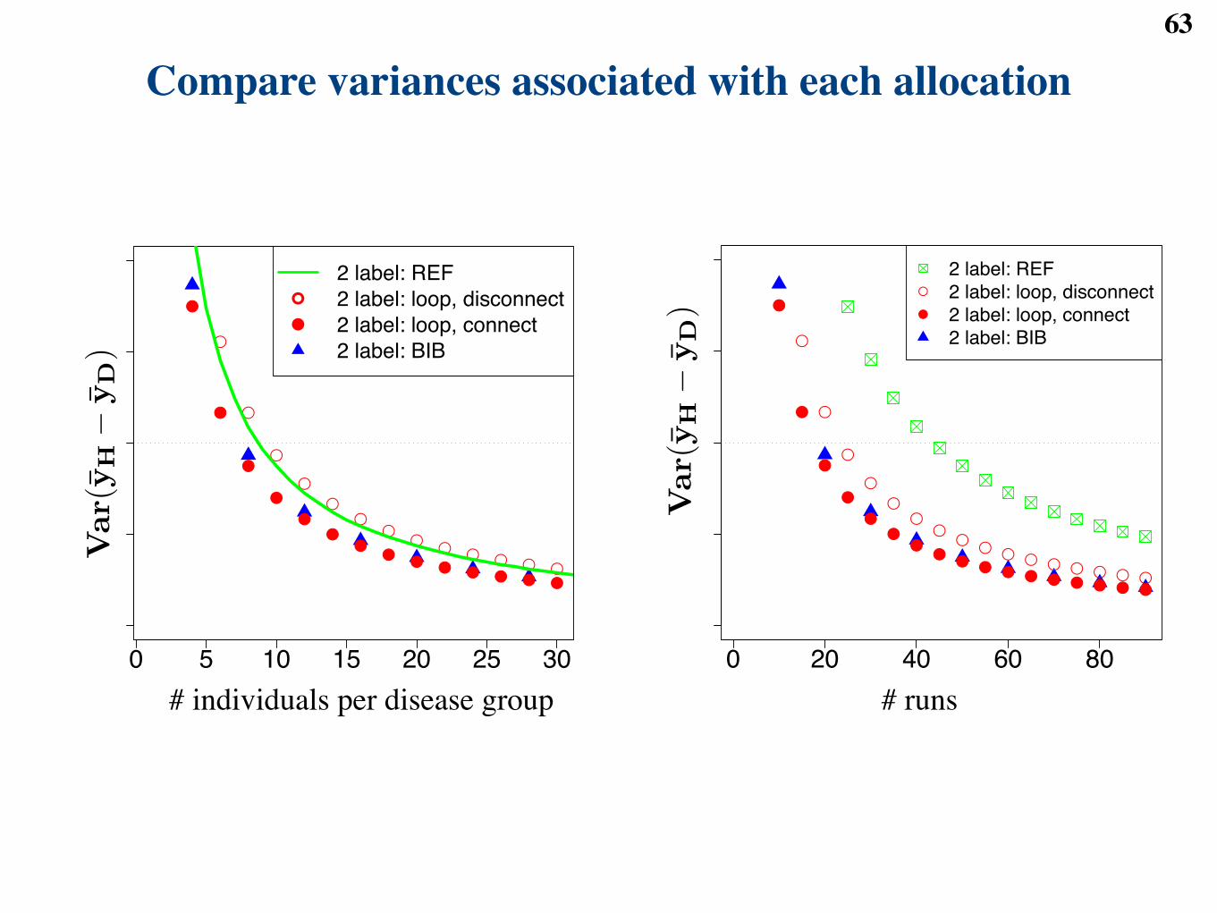
Compare variances associated with each allocation63
0 5 10 15 20 25 30
0.0
0.1
0.2
0.3
0.4
!
!
!
!
!!
!!
! ! ! ! ! ! !
!
!
!
!
!
!!
!!
! ! ! ! ! !
!
!
2 label: REF
2 label: loop, disconnect
2 label: loop, connect
2 label: BIB
0 20 40 60 80
0.0
0.1
0.2
0.3
0.4
!
!
!
!
!!
!!
! ! ! ! ! ! ! ! ! ! !
!
!
!
!
!
!!
!!
! ! ! ! ! ! ! ! ! !
!
!
2 label: REF
2 label: loop, disconnect
2 label: loop, connect
2 label: BIB
Obse
rved
Syst
emat
icR
andom
dev
iation
feat
ure
=m
ean
sign
al+
due
toal
lso
urc
esin
tensi
tyof
dis
ease
grou
pof
vari
atio
n
y ij
=G
roup
mea
ni
+E
rror
j(i
)
!N
` 0,!
2´
Obse
rved
Syst
em
ati
cR
andom
Random
Random
featu
re=
mean
signal
+devia
tion
due
to+
devia
tion
due
to+
devia
tion
due
toin
tensi
tyofdis
ease
gro
up
indiv
idual
sam
ple
pre
para
tion
measu
rem
ent
err
or
yijkl
=G
roup
mean
i+
Indiv
(Gro
up) j
(i)
+P
rep(I
ndiv
) k(ij)
+Err
or l
(ijk
)
!N
` 0,!
2 Indiv
´!
N` 0
,!2 Prep
´!
N` 0
,!2 Error
´
Var
(yH!
y D)
=2
!!
2 Indiv
I+
!2 Pre
p
IJ+
!2 Err
or
IJK
".
(1)
Obse
rved
Syst
emat
icR
andom
dev
iation
Ran
dom
Ran
dom
feat
ure
=m
ean
sign
al+
due
toblo
ck+
dev
iation
due
to+
dev
iation
due
toin
tensi
tyof
dis
ease
grou
p(e
.g.
pla
teor
day
)in
div
idual
mea
sure
men
ter
ror
y ijk
l=
Gro
up
mea
ni
+B
lock
k+
Indiv
(Gro
up)
j(i
)+
Err
orl(
ijk)
!N
` 0,!
2 Blo
ck
´!
N` 0,
!2 In
div
´!
N` 0,
!2 E
rror
´
1
Obse
rved
Syst
emat
icR
andom
dev
iation
feat
ure
=m
ean
sign
al+
due
toal
lso
urc
esin
tensi
tyof
dis
ease
grou
pof
vari
atio
n
y ij
=G
roup
mea
ni
+E
rror
j(i
)
!N
` 0,!
2´
Obse
rved
Syst
em
ati
cR
andom
Random
Random
featu
re=
mean
signal
+devia
tion
due
to+
devia
tion
due
to+
devia
tion
due
toin
tensi
tyofdis
ease
gro
up
indiv
idual
sam
ple
pre
para
tion
measu
rem
ent
err
or
yijkl
=G
roup
mean
i+
Indiv
(Gro
up) j
(i)
+P
rep(I
ndiv
) k(ij)
+Err
or l
(ijk
)
!N
` 0,!
2 Indiv
´!
N` 0
,!2 Prep
´!
N` 0
,!2 Error
´
Var
(yH!
y D)
=2
!!
2 Indiv
I+
!2 Pre
p
IJ+
!2 Err
or
IJK
".
(1)
Obse
rved
Syst
emat
icR
andom
dev
iation
Ran
dom
Ran
dom
feat
ure
=m
ean
sign
al+
due
toblo
ck+
dev
iation
due
to+
dev
iation
due
toin
tensi
tyof
dis
ease
grou
p(e
.g.
pla
teor
day
)in
div
idual
mea
sure
men
ter
ror
y ijk
l=
Gro
up
mea
ni
+B
lock
k+
Indiv
(Gro
up)
j(i
)+
Err
orl(
ijk)
!N
` 0,!
2 Blo
ck
´!
N` 0,
!2 In
div
´!
N` 0,
!2 E
rror
´
1
# individuals per disease group # runs
Key points64
● Statistical reasoning should be applied before and after collecting the data:◆ A good experimental design:■ avoids bias■ improves efficiency (i.e. reduces the variation)
◆ A good statistical model:■ states and verifies the assumptions■ improves sensitivity and specificity
● Methodological framework is already in place◆ Traditional statistical methods go a long way, if used correctly◆ Recent methods developed for high-dimensional data are useful◆ However new specialized methods for MS-based proteomics are
needed■ e.g. to account for uncertainty in feature identification

Acknowledgment65
Corra development team
Institute for Systems Biology, SeattleInstitute for Molecular Systems Biology, ETH Zurich, Switzerland
Indiana University and Regenstrief Institute, IndianapolisVladimir Fokin
Purdue University
Aebersold lab
Susanne Ragg
German Heart Center, MünichIlka Ott Sigmund-Lorenz Braun
Gunther Schadow
Tim Clough Veavi Chang Melissa KeyKelvin Ma
Related Documents