Available - DTIC

BestAvailable

Copy

REPORT DOCUMENTATION PAt AD-A275 c039

1. ~ ~ ~ ~ ~ ~ ~ ~ S AecUsOny(ev LRprDo&Report TypesandDatesCovere.

4. Tis HI Sbtile.19921 Fal Proeedngs5. Fundlng Numbers.Determination of the Time of Energy Return from Beanformed Data PW'9M" EbIM~f 0602436N

A40aft. 3585

L A1111110rKTask Ib. O

E. J. Kaminsky', A. B. Martinezt , B. S. Bourgeois. C. ZabounidisP. and W. J. CapeiP AcebnA. DN255031

V&A W Ab. 13512D7. performing Organinaton Name(s) mnd Addressl~es). S. Performing Organization

Naval Research Laboratory Report Numnber.Mapping, Charting and Geodesy Branch PR 92:111:351Stennis Space Center, MS 39529-5004

9. SpnolgoholgAgency Namne(s) and Addrssa(e*.t. 10. Sponsoringlionkmirng AgencyReport Number.

Uploator Deelopent rogam GoupPR 92:111:351

11. Supplemnentary Notes.Published in Proc. Institute of Acoustics.'Sverdrup Tech., Stennis Space Center, MS, tmTulane Univ. Now Orleans, LA, 3SeaBeam Instruments, Inc. Westwood, MA

12s. DistulbutionlAvelabbllty StatemmiLt 12b. Distribution Code.Approved for public release; distribution is unlimited.

1I& Abstract (Maximum 200 words).Muftibeamn bathymetric sonar systems such as the Sonar Array Survey System (SASS), the Sea Beam, and the Sea Beam

2000, are capable of collecting data which, after proper processing, may be used to map the bottom of the ocean. The sonar energyfrom the projector array impinges the ocean bottom as a narrow swath perpendicular to the ship's heading. The echo from thisswath is received by an array of hydrophones mounted athwartships. Beanforming permits good reception of energy propagatingIn a certain direction while attenuating energy propagating in other directions, and may be performed in hardware or software.Beamformed data gives a time history of the energy received from each look direction 9a,, This data must be further processedto determine the time corresponding to the center of the beam. t., The peak of the envelope corresponds to the intersection ofthe Maximum Response Axis (MRA) of the beam and the area ensonified. Once the time t, has been determined, the bathymetryof the area surveyed can be obtained.

94 1 2 6 052 94- 02585114. Subject Terms. 15. Number of pages.

Hydrography. bathymetry. optical poperties. remote sensing, reverberation 816. price code.

17. Seu~yClasslfication 1IL Security Clesslflcaon 19. Security ClassIfication 20. Umliatio of Abstract.of Report. of This Pags. of Abstract.

Unclassified Unclassified Unclassified SARNSN 7S4001 -805500 Stwtdd Formi 296 (Rev. 2469)

Pwrbsend by ANSI Sid. Z30-182MI02

' MUMWIUON or mI TIoo (N inGY orwURK fRoM azAM ADATA7

E J Kami y (), A B Martia (2), SBouroi (3), C Zabouid (4) W Cp (4)

(1) Sverdrup Technology, Stennis Space Centa, US, USA.(2) Tlaane University, EE Dept., New Orleans, LA, USA.(3) Naval Research Lab., Stennis Space Center, MS, USA.(4) SeaBeam Instruments, Inc., Westwood, MA, USA.

I1. INTRODUCTION

Multibeam bathymetric sonar systems such as the Sonar Array Survey System (SASS), the Sea Beam, andthe Sea Beam 2000, are capable of collecting data which, after proper processing, may be used to map thebottom of the ocean. The tonar energy from the projector array impinges the ocean bottom as a narrowswath perpendicular to the ship's heading. The echo from this swath is received by an array of hydrophonesmounted athwartships. Beamforming permits good reception of energy propagating in a certain directionwhile attenuating energy propagating in other directions, and may be performed in hardware or software.Beamformed data gives a time history of the energy received from each look direction #i. This data mustbe further processed to determine the time corresponding to the center of the beam, t,. The peak of theenvelope corresponds to the intersection of the Maximum Response Axis (MRA) of the beam and the areaensonified. Once the time t, has been determined, the bathymetry of the area surveyed -an be obtained.

In (11 simulation was used to determine the performance of recursive filters matched to a Gaussian bottomreturn signal to find t.. A Rician model for the bottom return signals and nonrecursive digital matchedfilters were used in (21. In this paper, we study several methods that might be used for determining thetime t. of energy return for each bin. These methods are matched filtering detection, peak detection andWeighted Mean Time (WMT). Synthetic data generated using Morgera's models for the bottom returnsignal are used to compare the performance of these methods as regards accuracy, bias, angular depen-dency of their performance, and computational efficiency. Comparisons of the algorithms applied to actualsurvey data collected by SASS are also presented, and show acceptable performance of all algorithms tested.

2. BEAM CENTER DETECTION

The area ensonified by the intersection of the transmit and receive beams produces an echo return fromwhich bathymetry must be extracted. This area typically increases with increasing steering angle 0, andthe returned energy spans a finite time. The acoustic signals reflected from a wide swath beneath theship are spatially separated into beams by the beamformer. Time-of-arrival data are obtained from thebeam signals. A detector is used to determine which point in the time envelope corresponds to the bottom.Determination of this time should be easier for the narrow high Signal-to-Noise Ratio (SNR) nadir returnsthan for the noisier and wider pulses from higher angles. If ideal conditions were present the peak of theenergy signal returned for each beam would correspond to the MRA of the beam. Actual conditions includenoise and signal fluctuations. Weighted Mean Time (WMT) algorithms (center of mass) have been usedby Sea Beam and Sea Beam 2000. Matched filtering has been used for SASS [3]. Simple peak detectionmay also be used. These methods are reviewed in this section.

The simplest way of determining the time corresponding to the MRA of the bottom return signal is to usea peak detector. It finds the largest amplitude of the signal and then determines the sample time for whichthis return occurred.

With matched filtering, filters loosely matched to the return signal are generated, a filtering operation is

* Proc. I.O.A. Vol. 15 Part 2 (1993)

* 303

I

4v

TIME OF ENERGY RETURN

performed, and the peak of the signal at the output of the filter is then detected. Observation of datacollected by SASS indicate a roughly Gaussian shape of the returned signal for all steering angles. Theimpulse response of the filters generated are made Gaussian as well to provide a relatively close match tothe returned energy. The width w of the filter can be predetermined or computed from the data collected.The Gaussian matched filter is created from samples of

y -- exp [--. (!)2] (1)

The signal obtained for each beamformer bin is convolved with its matched filter, and a smoother signalis obtained. Filtering also emphasizes the peak so that peak detection can then be used. The maindisadvantage of using Gaussian filters is that convolutions must be performed; this is very time consumingand might theiefore preclude its use for real-time pro.essing. If the Gaussian filter is replaced by a filterwith a rectangular impulse response, a much simpler filter is obtained at the expense of a worse match tothe return signal. When rectangular filters are used convolutions are not required.

In Sea Beam's operation, the echo processor digitizes the echo envelopes and applies ray bending, roll andgain corrections, and sidelobe suppression. A time of arrival is then determined at the center of mass ofeach of the 16 corrected echoes [4, 5]. Sea Beam weighs every time sample by its amplitude (the voltage1') as in (2), while Sea Beam 2000 uses powers as in (3). The Sea Beam systems use exclusively the WMTalgorithm for bottom detection on the entire swath. The Sea Beam 2000 uses WMT only on the portionsof the swath that correspond to near vertical returns; for the rest of the swath an interferometric detectionprocess is applied. The interferometric detection method is in general more accurate than WMT, but isnot discussed in this paper.

t ' V i t i( 2 )

t.= Pt, (3)

SP

Adaptive thresholdingl is performed prior to the determination of the time corresponding to the MRA ofthe beam, in order to separate actual responses from dropouts and noise. This should be done regardlessof the detection method used to avoid processing useless data, but is specially important for the WMTalgorithms. The window used determines i,,• and ,

3. SIMULATIONS

Numerous Monte Carlo simulations were performed to reliably (at least 90% confidence) compare thedifferent MRA time detection methods. The algorithms were applied both to the voltage signals and to 771the intensity (power) signals. Although sufficient survey data from operating systems are available for thisstudy,.the actual location of the peaks, t., is unknown. For simulation purposes, then, Gaussian and Rician :models from [1, 2J were used to generate the simulated bottom return of which the actual peak time isknown. In both cases the generated smooth-bottom return is corrupted by multiplicative and additive 'low-pass filtered white Gaussian noises. The models were presented in (1, 21 and are simply summarizedhere for continuity.

1Sea Beam's thresholding method is proprietary information.

ity 004d@

Proc. I.O.A. Vol. I5 Part2 (1993) ,

W#ALrry UINB= 5

304 ±UJX m

IWM OF ENERY RETUN

The simulated bottom return signal at time sample k, is

b(k) = s(k) -s n(k) + n2(k) (4)

where n, and n3 are the output of digital third order Butterworth filters with cutoff frequencies W, and W2Hs, respectively, when the inputs are white Gaussian noise sequences of mean zero and standard deviationsel and v2. The variance o-2 of the multiplicative noise controls the level of the signal and the bandwidthW, sets the fluctuation rate of the signal b(k). The variance a,] controls the additive noise level, while W2determines its bandwidth. The parameters combine to determine the SNR as given in (5).

SNR=°20log10 [Y W(

Morgera first modelled the noiseless signal s(k) from (4) as a Gaussian signal and then as an approximationto the functional form of the Rician pdf. These signals are given in (6) and (7), respectively.

s(k) = exp n2 (M)

(k)- { exp~..,) 7H•T .) ,- 1

where S= . The parameters E and a in (7) werechosen to be

E, = r [exp (cos ) - 1] (8)

a = T(O, d) (9)

where the approximate values of a used are 0.6 close to nadir and 0.8 off nadir. T is the expected echoduration given by

T(•,d) r •d-tan÷sec÷+ r (10)C

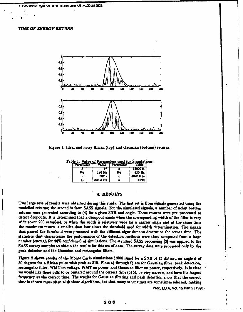
with d the depth, 0 the steering angle, c the speed of sound in water, r the time duration of the transmittedsignal, and 9 the receive beamwidth in radians. The parameters in Morgera's models were chosen to resemblethose of SASS data and are given in Table I.Figure I shows normalized Rician and Gaussian signals s(k)and the noisy bottom returns 6(k) for a SNR of 15 dB and angle # of 30 degrees.

A major difference between Morgera's work and ours is that we maintain a constant sampling rate regardlessof the angle 0. Morgera uses a constant number of samples per "hump", therefore using a much highersampling rate for angles close to nadir than for angles close to endfire; actual operating systems typicallymaintain a constant sampling rate.

We chose to define the width wi of the matched filters from o - , where w needs to be determined. Itcan either be based on the SNR (data dependent threshold) or on the expected width of the return, which

* is easily computed from (10) where a flat bottom assumption was made. In our simulations we compute was the number of samples that exceed a threshold set to twice the standard deviation of the returned, noisy

0• signal for the Gaussian filters, and 2.5 times the standard deviation in the case of the rectangular filters., When using (1), the independent variable ranged from -100 to 100.

0 Proc. I.O.A. Vol. 15 Part 2 (1993)

* 305I

I

* ,•..a•.,- e vo us~ 11 obULtUtW U1 .GOUSMS

iMWE OF ENERGY RETURN

OA : "

G o0 40 s0 o0 100 120 140 160 140 200

0.5J

0 20 40 60 80 10 120 140 140 I1O 200

Figure 1: Ideal and noisy Rician (top) and Gaussian (bottom) returns.

Tabt :V l eofP r m t r used fi r Simulatio sF value Parawte" Value

[ W,. 140sI Hs W2 420Hs.007a I C 489 / I

fe 1 1333.3 Rio n 110241

4. RESULTS

Two large sets of results were obtained during this study. The first set is from signals generated using themodelled returns; the second is from SASS signals. For the simulated signals, a number of noisy bottomreturns were generated according to (4) for a given SNR and angle. These returns were pre-processed todetect dropouts. It is determined that a droupout exists when the corresponding width of the filter is verywide (over 200 samples), or when the width is relatively wide for a narrow angle and at the same timethe maximum return is smaller than four times the threshold used for width determination. The signalsthat passed the threshold were processed with the different algorithms to determine the center time. Thestatistics that characterize the performance of the detection methods were then computed from a largenumber (enough for 90% confidence) of simulations. The standard SASS processing [3] was applied to theSASS survey samples to obtain the results for this set of data. The survey data were processed only by thepeak detector and the Gaussian and rectangular filters.

Figure 2 shows results of the Monte Carlo simulations (1000 runs) for a SNR of 15 dB and an angle 4 of30 degrees for a Rician pulse with peak at 515. Plots a) through f) are for Gaussian filter, peak detection,rectangular filter, WMT on voltage, WMT on power, and Gaussian filter on power, respectively. It is clearwe would like these pdfs to be centered around the correct time (516), be very narrow, and have the largestfrequency at the correct time. The results for Gaussian filtering and peak detection show that the correcttime is chosen most often with those algorithms, but that many other times are sometimes selected, making

Proc. I.O.A. Vol. 15 Part 2 (1993)

3306o

21MBW OF ENERGY RETURN

the variance relatively large. The results obtained with the WMT algorithms show a very small variance,but a marked (and expected) bias of the results. From Fig. 2 we also see that the rectangular filters yieldsmall biases (*1) with large variances, while the results of the Gaussian filters and peak detection areunbiased with similar variances. Notice, though, that the correct center time is chosen less than 20% ofthe time.Results for the Gaussian-shaped pulses at 30 degrees and for all SNR tested generate Gaussian-like pdfscentered at the correct time, and with variances smaller than those obtained for Rician pulses. The WMT

algorithm applied to the voltage signal detects the correct time over 50% of the time for a SNR as low as5 dB, with a very small variance. A large number of combinations of angles and SNR were simulated. In

Table 2: Beam Center Time Results for € 150

Signa SNR -20d] SNH= 10 dBAlgorithm Shape t, ext 0, MA t. ext -7 M

Gaussan on H--Mn 1.0 22 1.6 1,24 1 .5 1T 1.8 1.26sigpal. Gaussian 0.0 24 1.7 0,24 0.1 28 1.7 0,28

Rectaga ii 1.2 21 1.3 1,32 2.2 8 4.0 2,13on signal Gaussian -0.3 23 1.6 0,23 -0.2 16 3.5 0,16

Peak Rician 0.6 13 3 , 0.7 15 2.6 0,15detection Gaussian 0.1 15 2.7 0,15 -0.1 12 2.8 0.12

Gausian on R 1.6 I1 2.3 1,15 0.8 20 1.8 1,21Power Gaussian 0.1 15 2.4 0,15 0.0 20 2.0 0,20

Rec tanu .a 22 1.8 0,22 0.8 2 1.9 1,21Power Gaussian -0.3 21 1.9 0,21 -0.2 20 2.0 0,20

WMT on Rician 1.3 11 0.T 1,47 1.0 21 0.73 1,53signal Gaussian 0.0 30 0.76 0,50

WMT on 1 m 1.1 24 1.1 1,3 1.0 22 1.1 1,38power Gaussian 0.0 35 1.1 0,35

Table 3: Beam Center Time Results for € = 450Signal =NR 20 SNR= 10

Algorithm Shape t. ext , m,% t. ext I a :AGausian on Ri 1.8 7 6.4 2,8 2.2 8 5.7 2,7

signal. Gaussian -. 4 6 6.0 0,6 0.0 7 5.1 0,7ReZTmjt r RGnI 2.1 -T -T 5.4 2,6 2.0 6 5.9 2,6

on signal Gaussian -0.2 8 5.5 0,8 -0.2 7 5.9 0,7Peak Ricia 1.5 4 9.7 1,3 1.3 4 10.1 1,4

detection Gaussian -0.3 5 8.7 0,s 0.0 4 9.1 0,4Gausian on Rian 1.3 5 8.1 1,4 1.6 4 8.5 2,4

Power Gaussian -0.5 6 7.7 0,6 0.1 5 7.5 0,5Rectangular Rican 1.0 5 7.2 1,6 1.2 5 7.3 2,4

Power Gaussian -0.5 5 6.8 0,5 -0.3 5 6.8 0,5WMT on Rician 5. 0 173 6,1A 4.4 0 1.5 4,

signal Gaussian 0.0 25 1.5 0,25 0.1 25 1.6 0,25WMT an Ri1'an 4. 3 2.3 4,NA 4.1 4 2.4 4,NA

power Gaussian 0.0 20 2.3 0,20 0.1 17 2.3 0,17

Tables 2 and 3 we show the difference (in sample counts) between the time of the peak, tf, and the timeselected as the MRA time by the various algorithms for look directions of 15 and 45 degrees, rdspectively,and SNR of 20 and 10 dB. Results for both Rician- and Gaussian-shaped pulses are given. The percentageof time the exact peak time was correctly detected (ext), the standard deviation (or), and the median value(m) together with the percentage of time the median value occurred are also shown.


* 307


1 56 M M s 3 n L s IS ps i I A s

II

- -

30-

____ s S.1___

SS1 21 35 41 )6 1 52 14 ie 1 - I U 18 61 1 11 12 3

e) F

16116581 •1 3 31 Ill 54 -

Figure 2: Pdfs for Rician signal with SNR of 15 dB and angle of 30 degrees.

Proc. I.O.A. Vol 15 Part 2 (1993)

308

c) d)


A

The reults are somewhat dependent upon parameters such an the threshold level used to determine thewidth of the filter, but we tried to minimize these dependencies. Windowing to reduce sidelobes also hassome effect on the results obtained. When no windowing was used and therefore the sidelobes of the specularreturn appeared as a high intensity at other angles, the Gaussian matched filter algorithm performed betterthan peak detection, selectin the (erroneous) sidelobe less frequently.

Cerer limes vs. Bin Number

140C 'Gw i n

0 40 60 80 100 120 140 160 160 200

Difference in Center Tiimes

20 - -eaG-P

14'

40 60 80 100 120 140 160 180 200Beamformer bin number

Figure 3: Comparison results on survey data from SASS. i

.G-P

In Fig. 3 we show some results for peak detection, Gaussian and rectangular filtering when applied to a,'typical ping of SASS data. The center times, in sample number, are plotted at the top of Fig. 3. The i

difference between meulti from the three algorithms are too small to be seen in this plot. In the bottom of IFig. 3 the difference, also in number of samples, is plotted vesus the beamformer bin number. We see that

although the differences are small for angles close to nadir, these increase as the steering angle aproachesthe extremes. The average difference in the resulting bathymetry for the data shown in Fig. 3 is about.25% of the depth with the worst case difference being about 1.5% of the depth. Remember that for thisdata we don't have the actual correct t,, and only comparison between the yielded results are possible.

5. CONCLUSIONS AND SUGGESTIONS

Results show that the actual shape of the energy pulses discriminated angularly markedly P'ffects the results,and must therefore be investigated further. The noise characteristics and statistics must also be studied.

We showed here that all algorithms presented perform well, including simple peak detection, especiallyif some pre-processing is performed to determine dropouts and eliminate sidelobes. The Weighted MeanTime algorithms were shown to yield results with very narrow distributions, although they produce biased

Proc. I.O.A. Vol. 15 Pan 2 (1993)

309


estimates if the return pulse is not symmetric. We suggest that if very accurate determination of the centerof the peak must be made, the estimate produced by a peak detector can be used to place the window andthen the Weighted Mean Time algorithm can be applied to the windowed data to obtain the final centertime; this estimate might need to be de-biased.

Another area that needs to be investigated is the accuracy of the velocity profiles and the effect that er-rors in them cause on the resulting bathymetry. If errors caused by lack of exact profiles for ray bendingcalculations are considerable, it might be senseless to try to obtain an exact MRA time. If this is the case,simple peak detection is certainly a method to consider.

6. ACKNOWLEDGMENTS

The authors acknowledge the Office of Naval Technology, project element 602435N, managed by Dr. HerbertC. Eppert, Jr., NRL, Stennis Space Center, MS. This paper, NRL Contribution Number NRL/PP/7441-93-0011, is approved for public release; distribution is unlimited.

References

[1] S. D. Morgera, "Signal processing for precise ocean mapping," IEEE J. Oceanic Engineering, vol. O-1,pp. 49-52, November 1976.

12] S. D. Morgera and R. Sankar, "Digital signal processing for precision wide-swath bathymetry," IEEEJ. Oceanic Engineering, vol. OE-9, pp. 73-84, April 1984.

(3] E. J. Kaminsky, B. S. Bourgeois, A. B. Martinez, and H. Barad, "SASS imagery development," TechnicalReport in process, NRL, Code 351, Sept. 1992.

[41 H. K. Farr, "Multibeam bathymetric sonar: Sea Beam and Hydrochart," Marine Geodesy, vol. 4, no. 2,pp. 289-298, 1980.

[5] C. de Moustier, "Beyond bathymetry: Mapping acoustic backscattering from the deep seafloor withSea Beam," Journal of the Acoustical Society of America, vol. 79, pp. 316-331, February 1986.


310

Available - DTIC

Documents