ASAP 2020 Accelerated Surface Area and Porosimetry System Operator’s Manual V4.00 202-42801-01 March 2011

ASAP2020 Operator's Manual
Sep 06, 2014
Welcome message from author
This document is posted to help you gain knowledge. Please leave a comment to let me know what you think about it! Share it to your friends and learn new things together.
Transcript

ASAP 2020
Accelerated Surface Area and Porosimetry System
Operator’s Manual
V4.00
202-42801-01March 2011

Kalrez is a registered trademark of DuPont Dow Elastomers L.L.C.Teflon is a registered trademark of E.I. DuPont de Nemours CompanyWindows is a registered trademark of Microsoft Corporation
© Micromeritics Instrument Corporation 2004-2011. All rights reserved. Printed in the U.S.A.
The software described in this manual is furnished under a license agreement and may be used or copied only in accordance with the terms of the agreement.

Form No. 008-42104-00
WARRANTYMICROMERITICS INSTRUMENT CORPORATION warrants for one year from the date of shipment eachinstrument manufactured by it to be free from defects in material and workmanship impairing its usefulnessunder normal use and service conditions except as noted herein.
Our liability under this warranty is limited to repair, servicing and adjustment, free of charge at our plant, of anyinstrument or defective parts, when returned prepaid to us, and which our examination discloses to have beendefective. The purchaser is responsible for all transportation charges involving the shipment of materials forwarranty repairs. Failure of any instrument or product due to operator error, improper installation, unauthorizedrepair or alteration, failure of utilities, or environmental contamination will not constitute a warranty claim. Thematerials of construction used in MICROMERITICS instruments and other products were chosen after extensivetesting and experience for their reliability and durability. However, these materials cannot be totally guaranteedagainst wear and/or decomposition by chemical action (corrosion) as a result of normal use.
Repair parts are warranted to be free from defects in material and workmanship for 90 days from the date ofshipment.
No instrument or product shall be returned to MICROMERITICS prior to notification of alleged defect andauthorization to return the instrument or product. All repairs or replacements are made subject to factoryinspection of returned parts.
MICROMERITICS shall be released from all obligations under its warranty in the event repairs or modificationsare made by persons other than its own authorized service personnel unless such work is authorized in writing byMICROMERITICS.
The obligations of this warranty will be limited under the following conditions:
1. Certain products sold by MICROMERITICS are the products of reputable manufacturers, sold under theirrespective brand names or trade names. We, therefore, make no express or implied warranty as to suchproducts. We shall use our best efforts to obtain from the manufacturer, in accordance with his customarypractice, the repair or replacement of such of his products that may prove defective in workmanship ormaterials. Service charges made by such manufacturer are the responsibility of the ultimate purchaser. Thisstates our entire liability in respect to such products, except as an authorized person of MICROMERITICSmay otherwise agree to in writing.
2. If an instrument or product is found defective during the warranty period, replacement parts may, at thediscretion of MICROMERITICS, be sent to be installed by the purchaser, e.g., printed circuit boards, checkvalves, seals, etc.
3. Expendable items, e.g., sample tubes, detector source lamps, indicator lamps, fuses, valve plugs (rotor) andstems, seals and O-rings, ferrules, etc., are excluded from this warranty except for manufacturing defects.Such items which perform satisfactorily during the first 45 days after the date of shipment are assumed to befree of manufacturing defects.
Purchaser agrees to hold MICROMERITICS harmless from any patent infringement action brought againstMICROMERITICS if, at the request of the purchaser, MICROMERITICS modifies a standard product ormanufactures a special product to the purchaser’s specifications.
MICROMERITICS shall not be liable for consequential or other type damages resulting from the use of any ofits products other than the liability stated above. This warranty is in lieu of all other warranties, express orimplied, including, but not limited to the implied warranties of merchantability or fitness for use.
4356 Communications Drive Norcross, GA 30093-1877 Fax (770) 662-3696
Domestic Sales - (770) 662-3633 Domestic Repair Service - (770) 662-3666International Sales - (770) 662-3660 Customer Service - (770) 662-3636
Rev. 12/95


ASAP 2020 Operator’s Manual Table of Contents
TABLE OF CONTENTS
1. GENERAL INFORMATION
Organization of the Manual . . . . . . . . . . . . . . . . . . . . . . . . . . . . . . . . . . . . . . . . . . . . . . . . . . . . . 1-1Conventions . . . . . . . . . . . . . . . . . . . . . . . . . . . . . . . . . . . . . . . . . . . . . . . . . . . . . . . . . . . . . . . . . 1-3Online Manual . . . . . . . . . . . . . . . . . . . . . . . . . . . . . . . . . . . . . . . . . . . . . . . . . . . . . . . . . . . . . . . 1-4
Using Bookmarks. . . . . . . . . . . . . . . . . . . . . . . . . . . . . . . . . . . . . . . . . . . . . . . . . . . . . . . . . 1-4Using the Table of Contents, Index, and other Links. . . . . . . . . . . . . . . . . . . . . . . . . . . . . . 1-6
Table of Contents . . . . . . . . . . . . . . . . . . . . . . . . . . . . . . . . . . . . . . . . . . . . . . . . . . . . . 1-6Index. . . . . . . . . . . . . . . . . . . . . . . . . . . . . . . . . . . . . . . . . . . . . . . . . . . . . . . . . . . . . . . 1-7Cross References . . . . . . . . . . . . . . . . . . . . . . . . . . . . . . . . . . . . . . . . . . . . . . . . . . . . . 1-7
Using the Find Command . . . . . . . . . . . . . . . . . . . . . . . . . . . . . . . . . . . . . . . . . . . . . . . . . . 1-8Printing . . . . . . . . . . . . . . . . . . . . . . . . . . . . . . . . . . . . . . . . . . . . . . . . . . . . . . . . . . . . . . . . . 1-9
Equipment Description. . . . . . . . . . . . . . . . . . . . . . . . . . . . . . . . . . . . . . . . . . . . . . . . . . . . . . . . . 1-10Gas Requirements . . . . . . . . . . . . . . . . . . . . . . . . . . . . . . . . . . . . . . . . . . . . . . . . . . . . . . . . . . . . 1-11Analysis Program. . . . . . . . . . . . . . . . . . . . . . . . . . . . . . . . . . . . . . . . . . . . . . . . . . . . . . . . . . . . . 1-11
Report System . . . . . . . . . . . . . . . . . . . . . . . . . . . . . . . . . . . . . . . . . . . . . . . . . . . . . . . 1-11Specifications . . . . . . . . . . . . . . . . . . . . . . . . . . . . . . . . . . . . . . . . . . . . . . . . . . . . . . . . . . . . . . . . 1-12
2. INSTALLATION
Unpacking and Inspection . . . . . . . . . . . . . . . . . . . . . . . . . . . . . . . . . . . . . . . . . . . . . . . . . . . . . . 2-1Lifting the Analyzer . . . . . . . . . . . . . . . . . . . . . . . . . . . . . . . . . . . . . . . . . . . . . . . . . . . . . . . 2-1Equipment Damage or Loss During Shipment . . . . . . . . . . . . . . . . . . . . . . . . . . . . . . . . . . 2-1Equipment Return . . . . . . . . . . . . . . . . . . . . . . . . . . . . . . . . . . . . . . . . . . . . . . . . . . . . . . . . 2-2
Setting up the Analyzer . . . . . . . . . . . . . . . . . . . . . . . . . . . . . . . . . . . . . . . . . . . . . . . . . . . . . . . . 2-3Installing the Vacuum Pumps . . . . . . . . . . . . . . . . . . . . . . . . . . . . . . . . . . . . . . . . . . . . . . . 2-3
Oil-Based Systems . . . . . . . . . . . . . . . . . . . . . . . . . . . . . . . . . . . . . . . . . . . . . . . . . . . . 2-3Dry Systems . . . . . . . . . . . . . . . . . . . . . . . . . . . . . . . . . . . . . . . . . . . . . . . . . . . . . . . . . 2-4
Verifying Line Voltage Selection . . . . . . . . . . . . . . . . . . . . . . . . . . . . . . . . . . . . . . . . . . . . 2-5Installing the Cold Trap Tubes. . . . . . . . . . . . . . . . . . . . . . . . . . . . . . . . . . . . . . . . . . . . . . . 2-5Installing Saturation Pressure (Psat) Tube . . . . . . . . . . . . . . . . . . . . . . . . . . . . . . . . . . . . . . 2-6Selecting the Computer Power Input . . . . . . . . . . . . . . . . . . . . . . . . . . . . . . . . . . . . . . . . . . 2-7Connecting the Gas Supply . . . . . . . . . . . . . . . . . . . . . . . . . . . . . . . . . . . . . . . . . . . . . . . . . 2-8
Connecting a Regulator to the Gas Bottle . . . . . . . . . . . . . . . . . . . . . . . . . . . . . . . . . . 2-8Connecting the Gas Delivery Tubing to the Analyzer . . . . . . . . . . . . . . . . . . . . . . . . . 2-9
Connecting Cables and Power Cords . . . . . . . . . . . . . . . . . . . . . . . . . . . . . . . . . . . . . . . . . . 2-10Turning On the System . . . . . . . . . . . . . . . . . . . . . . . . . . . . . . . . . . . . . . . . . . . . . . . . . . . . 2-11Turning Off the System . . . . . . . . . . . . . . . . . . . . . . . . . . . . . . . . . . . . . . . . . . . . . . . . . . . . 2-11
Installing the Analysis Program. . . . . . . . . . . . . . . . . . . . . . . . . . . . . . . . . . . . . . . . . . . . . . . . . . 2-12Initial Installation . . . . . . . . . . . . . . . . . . . . . . . . . . . . . . . . . . . . . . . . . . . . . . . . . . . . . . . . . 2-12Using the Setup Program for Other Functions . . . . . . . . . . . . . . . . . . . . . . . . . . . . . . . . . . . 2-15Installing Subsequent Software Versions. . . . . . . . . . . . . . . . . . . . . . . . . . . . . . . . . . . . . . . 2-16
Adding an Analyzer . . . . . . . . . . . . . . . . . . . . . . . . . . . . . . . . . . . . . . . . . . . . . . . . . . . 2-17Moving an Analyzer from one PC to another PC . . . . . . . . . . . . . . . . . . . . . . . . . . . . 2-18
Mar 2011 i

Table of Contents ASAP 2020 Operator’s Manual
Removing an Analyzer . . . . . . . . . . . . . . . . . . . . . . . . . . . . . . . . . . . . . . . . . . . . . . . . . 2-21Changing an Analyzer Setup . . . . . . . . . . . . . . . . . . . . . . . . . . . . . . . . . . . . . . . . . . . . 2-22Reinstalling the Calibration Files . . . . . . . . . . . . . . . . . . . . . . . . . . . . . . . . . . . . . . . . . 2-23Uninstalling the Analysis Program . . . . . . . . . . . . . . . . . . . . . . . . . . . . . . . . . . . . . . . . 2-24
Specifying Gas Ports. . . . . . . . . . . . . . . . . . . . . . . . . . . . . . . . . . . . . . . . . . . . . . . . . . . . . . . 2-25
3. USER INTERFACE
Controls, Indicators, and Connectors . . . . . . . . . . . . . . . . . . . . . . . . . . . . . . . . . . . . . . . . . . . . . . 3-1Front Panel . . . . . . . . . . . . . . . . . . . . . . . . . . . . . . . . . . . . . . . . . . . . . . . . . . . . . . . . . . . . . . 3-1Side Panel . . . . . . . . . . . . . . . . . . . . . . . . . . . . . . . . . . . . . . . . . . . . . . . . . . . . . . . . . . . . . . . 3-4
Upper. . . . . . . . . . . . . . . . . . . . . . . . . . . . . . . . . . . . . . . . . . . . . . . . . . . . . . . . . . . . . . . 3-4Lower . . . . . . . . . . . . . . . . . . . . . . . . . . . . . . . . . . . . . . . . . . . . . . . . . . . . . . . . . . . . . . 3-5
Rear Panel . . . . . . . . . . . . . . . . . . . . . . . . . . . . . . . . . . . . . . . . . . . . . . . . . . . . . . . . . . . . . . . 3-6Using the Software . . . . . . . . . . . . . . . . . . . . . . . . . . . . . . . . . . . . . . . . . . . . . . . . . . . . . . . . . . . . 3-7
Shortcut Menus . . . . . . . . . . . . . . . . . . . . . . . . . . . . . . . . . . . . . . . . . . . . . . . . . . . . . . . . . . . 3-7Shortcut Keys . . . . . . . . . . . . . . . . . . . . . . . . . . . . . . . . . . . . . . . . . . . . . . . . . . . . . . . . . . . . 3-7Dialog Boxes. . . . . . . . . . . . . . . . . . . . . . . . . . . . . . . . . . . . . . . . . . . . . . . . . . . . . . . . . . . . . 3-9Selecting Files. . . . . . . . . . . . . . . . . . . . . . . . . . . . . . . . . . . . . . . . . . . . . . . . . . . . . . . . . . . . 3-11File Name Conventions . . . . . . . . . . . . . . . . . . . . . . . . . . . . . . . . . . . . . . . . . . . . . . . . . . . . 3-13
Menu Structure . . . . . . . . . . . . . . . . . . . . . . . . . . . . . . . . . . . . . . . . . . . . . . . . . . . . . . . . . . . . . . . 3-14Windows Menu. . . . . . . . . . . . . . . . . . . . . . . . . . . . . . . . . . . . . . . . . . . . . . . . . . . . . . . . . . . 3-15Help Menu . . . . . . . . . . . . . . . . . . . . . . . . . . . . . . . . . . . . . . . . . . . . . . . . . . . . . . . . . . . . . . 3-15
4. OPERATIONAL PROCEDURES
Specifying Sample File Defaults . . . . . . . . . . . . . . . . . . . . . . . . . . . . . . . . . . . . . . . . . . . . . . . . . 4-1Basic Format . . . . . . . . . . . . . . . . . . . . . . . . . . . . . . . . . . . . . . . . . . . . . . . . . . . . . . . . . . . . . 4-2Advanced Format . . . . . . . . . . . . . . . . . . . . . . . . . . . . . . . . . . . . . . . . . . . . . . . . . . . . . . . . . 4-4
Creating Sample Information Files. . . . . . . . . . . . . . . . . . . . . . . . . . . . . . . . . . . . . . . . . . . . . . . . 4-6Advanced Format . . . . . . . . . . . . . . . . . . . . . . . . . . . . . . . . . . . . . . . . . . . . . . . . . . . . . . . . . 4-6Basic and Restricted Formats . . . . . . . . . . . . . . . . . . . . . . . . . . . . . . . . . . . . . . . . . . . . . . . . 4-8
Defining Parameter Files . . . . . . . . . . . . . . . . . . . . . . . . . . . . . . . . . . . . . . . . . . . . . . . . . . . . . . . 4-9Sample Tube . . . . . . . . . . . . . . . . . . . . . . . . . . . . . . . . . . . . . . . . . . . . . . . . . . . . . . . . . . . . . 4-9Degas Conditions . . . . . . . . . . . . . . . . . . . . . . . . . . . . . . . . . . . . . . . . . . . . . . . . . . . . . . . . . 4-10Analysis Conditions . . . . . . . . . . . . . . . . . . . . . . . . . . . . . . . . . . . . . . . . . . . . . . . . . . . . . . . 4-11Adsorptive Properties . . . . . . . . . . . . . . . . . . . . . . . . . . . . . . . . . . . . . . . . . . . . . . . . . . . . . . 4-13Report Options . . . . . . . . . . . . . . . . . . . . . . . . . . . . . . . . . . . . . . . . . . . . . . . . . . . . . . . . . . . 4-14
Preparing Samples . . . . . . . . . . . . . . . . . . . . . . . . . . . . . . . . . . . . . . . . . . . . . . . . . . . . . . . . . . . . 4-16Choosing Sample Tubes . . . . . . . . . . . . . . . . . . . . . . . . . . . . . . . . . . . . . . . . . . . . . . . . . . . . 4-16Cleaning and Labeling Sample Tubes . . . . . . . . . . . . . . . . . . . . . . . . . . . . . . . . . . . . . . . . . 4-17Determining Amount of Sample to Use . . . . . . . . . . . . . . . . . . . . . . . . . . . . . . . . . . . . . . . . 4-20Determining the Mass of the Sample . . . . . . . . . . . . . . . . . . . . . . . . . . . . . . . . . . . . . . . . . . 4-20Degassing the Sample. . . . . . . . . . . . . . . . . . . . . . . . . . . . . . . . . . . . . . . . . . . . . . . . . . . . . . 4-22Transferring the Degassed Sample to the Analysis Port. . . . . . . . . . . . . . . . . . . . . . . . . . . . 4-24
Installing Dewars . . . . . . . . . . . . . . . . . . . . . . . . . . . . . . . . . . . . . . . . . . . . . . . . . . . . . . . . . . . . . 4-26Precautions . . . . . . . . . . . . . . . . . . . . . . . . . . . . . . . . . . . . . . . . . . . . . . . . . . . . . . . . . . . . . . 4-26Cold Trap Dewar . . . . . . . . . . . . . . . . . . . . . . . . . . . . . . . . . . . . . . . . . . . . . . . . . . . . . . . . . 4-26Analysis Dewar. . . . . . . . . . . . . . . . . . . . . . . . . . . . . . . . . . . . . . . . . . . . . . . . . . . . . . . . . . . 4-28
ii Mar 2011

ASAP 2020 Operator’s Manual Table of Contents
Performing an Analysis . . . . . . . . . . . . . . . . . . . . . . . . . . . . . . . . . . . . . . . . . . . . . . . . . . . . . . . . 4-29Printing File Contents . . . . . . . . . . . . . . . . . . . . . . . . . . . . . . . . . . . . . . . . . . . . . . . . . . . . . . . . . 4-31Listing File Statistics . . . . . . . . . . . . . . . . . . . . . . . . . . . . . . . . . . . . . . . . . . . . . . . . . . . . . . . . . . 4-32Exporting Isotherm Data . . . . . . . . . . . . . . . . . . . . . . . . . . . . . . . . . . . . . . . . . . . . . . . . . . . . . . . 4-33Generating Graph Overlays . . . . . . . . . . . . . . . . . . . . . . . . . . . . . . . . . . . . . . . . . . . . . . . . . . . . . 4-34
Multiple Samples Overlay . . . . . . . . . . . . . . . . . . . . . . . . . . . . . . . . . . . . . . . . . . . . . . . . . . 4-34Multiple Graphs Overlay . . . . . . . . . . . . . . . . . . . . . . . . . . . . . . . . . . . . . . . . . . . . . . . . . . . 4-37
5. FILE MENU
Description . . . . . . . . . . . . . . . . . . . . . . . . . . . . . . . . . . . . . . . . . . . . . . . . . . . . . . . . . . . . . . . . . . 5-1Open . . . . . . . . . . . . . . . . . . . . . . . . . . . . . . . . . . . . . . . . . . . . . . . . . . . . . . . . . . . . . . . . . . . . . . . 5-3
Sample Information . . . . . . . . . . . . . . . . . . . . . . . . . . . . . . . . . . . . . . . . . . . . . . . . . . . . . . . 5-5Advanced Format . . . . . . . . . . . . . . . . . . . . . . . . . . . . . . . . . . . . . . . . . . . . . . . . . . . . . 5-6Basic Format. . . . . . . . . . . . . . . . . . . . . . . . . . . . . . . . . . . . . . . . . . . . . . . . . . . . . . . . . 5-9Restricted Format . . . . . . . . . . . . . . . . . . . . . . . . . . . . . . . . . . . . . . . . . . . . . . . . . . . . . 5-11
Sample Tube. . . . . . . . . . . . . . . . . . . . . . . . . . . . . . . . . . . . . . . . . . . . . . . . . . . . . . . . . . . . . 5-12Degas Conditions . . . . . . . . . . . . . . . . . . . . . . . . . . . . . . . . . . . . . . . . . . . . . . . . . . . . . . . . . 5-14Analysis Conditions . . . . . . . . . . . . . . . . . . . . . . . . . . . . . . . . . . . . . . . . . . . . . . . . . . . . . . . 5-16Adsorptive Properties. . . . . . . . . . . . . . . . . . . . . . . . . . . . . . . . . . . . . . . . . . . . . . . . . . . . . . 5-31Report Options . . . . . . . . . . . . . . . . . . . . . . . . . . . . . . . . . . . . . . . . . . . . . . . . . . . . . . . . . . . 5-35
Summary Report. . . . . . . . . . . . . . . . . . . . . . . . . . . . . . . . . . . . . . . . . . . . . . . . . . . . . . 5-38Isotherm Report Options . . . . . . . . . . . . . . . . . . . . . . . . . . . . . . . . . . . . . . . . . . . . . . . 5-40BET/Langmuir Surface Area Report Options . . . . . . . . . . . . . . . . . . . . . . . . . . . . . . . 5-42Freundlich Isotherm . . . . . . . . . . . . . . . . . . . . . . . . . . . . . . . . . . . . . . . . . . . . . . . . . . . 5-45Temkin Isotherm . . . . . . . . . . . . . . . . . . . . . . . . . . . . . . . . . . . . . . . . . . . . . . . . . . . . . 5-47t-Plot Report Options . . . . . . . . . . . . . . . . . . . . . . . . . . . . . . . . . . . . . . . . . . . . . . . . . . 5-49Alpha-S Plot . . . . . . . . . . . . . . . . . . . . . . . . . . . . . . . . . . . . . . . . . . . . . . . . . . . . . . . . . 5-55f-Ratio Plot . . . . . . . . . . . . . . . . . . . . . . . . . . . . . . . . . . . . . . . . . . . . . . . . . . . . . . . . . . 5-58BJH Adsorption/Desorption Report Options . . . . . . . . . . . . . . . . . . . . . . . . . . . . . . . . 5-60Dollimore-Heal Adsorption/Desorption Report Options . . . . . . . . . . . . . . . . . . . . . . . 5-69Horvath-Kawazoe Report Options . . . . . . . . . . . . . . . . . . . . . . . . . . . . . . . . . . . . . . . . 5-70DFT Pore Size . . . . . . . . . . . . . . . . . . . . . . . . . . . . . . . . . . . . . . . . . . . . . . . . . . . . . . . 5-77Surface Energy . . . . . . . . . . . . . . . . . . . . . . . . . . . . . . . . . . . . . . . . . . . . . . . . . . . . . . . 5-80Dubinin Report Options . . . . . . . . . . . . . . . . . . . . . . . . . . . . . . . . . . . . . . . . . . . . . . . . 5-81MP-Method Report Options. . . . . . . . . . . . . . . . . . . . . . . . . . . . . . . . . . . . . . . . . . . . . 5-86Options Report . . . . . . . . . . . . . . . . . . . . . . . . . . . . . . . . . . . . . . . . . . . . . . . . . . . . . . . 5-90Sample Log Report. . . . . . . . . . . . . . . . . . . . . . . . . . . . . . . . . . . . . . . . . . . . . . . . . . . . 5-90Validation Report . . . . . . . . . . . . . . . . . . . . . . . . . . . . . . . . . . . . . . . . . . . . . . . . . . . . . 5-91
Collected/Entered Data . . . . . . . . . . . . . . . . . . . . . . . . . . . . . . . . . . . . . . . . . . . . . . . . . . . . 5-92Save . . . . . . . . . . . . . . . . . . . . . . . . . . . . . . . . . . . . . . . . . . . . . . . . . . . . . . . . . . . . . . . . . . . . . . . 5-94Save As. . . . . . . . . . . . . . . . . . . . . . . . . . . . . . . . . . . . . . . . . . . . . . . . . . . . . . . . . . . . . . . . . . . . . 5-95
Sample and Parameter Files . . . . . . . . . . . . . . . . . . . . . . . . . . . . . . . . . . . . . . . . . . . . . . . . . 5-95t-Curve and Alpha-S Files . . . . . . . . . . . . . . . . . . . . . . . . . . . . . . . . . . . . . . . . . . . . . . . . . . 5-96
Save All . . . . . . . . . . . . . . . . . . . . . . . . . . . . . . . . . . . . . . . . . . . . . . . . . . . . . . . . . . . . . . . . . . . . 5-96Close. . . . . . . . . . . . . . . . . . . . . . . . . . . . . . . . . . . . . . . . . . . . . . . . . . . . . . . . . . . . . . . . . . . . . . . 5-96Close All. . . . . . . . . . . . . . . . . . . . . . . . . . . . . . . . . . . . . . . . . . . . . . . . . . . . . . . . . . . . . . . . . . . . 5-97Print . . . . . . . . . . . . . . . . . . . . . . . . . . . . . . . . . . . . . . . . . . . . . . . . . . . . . . . . . . . . . . . . . . . . . . . 5-98List . . . . . . . . . . . . . . . . . . . . . . . . . . . . . . . . . . . . . . . . . . . . . . . . . . . . . . . . . . . . . . . . . . . . . . . . 5-99
Mar 2011 iii
Table of Contents ASAP 2020 Operator’s Manual
Export . . . . . . . . . . . . . . . . . . . . . . . . . . . . . . . . . . . . . . . . . . . . . . . . . . . . . . . . . . . . . . . . . . . . . . 5-100Format of Data Output . . . . . . . . . . . . . . . . . . . . . . . . . . . . . . . . . . . . . . . . . . . . . . . . . . . . . 5-101
Convert . . . . . . . . . . . . . . . . . . . . . . . . . . . . . . . . . . . . . . . . . . . . . . . . . . . . . . . . . . . . . . . . . . . . . 5-102Exit . . . . . . . . . . . . . . . . . . . . . . . . . . . . . . . . . . . . . . . . . . . . . . . . . . . . . . . . . . . . . . . . . . . . . . . . 5-104
6. UNIT MENU
Description . . . . . . . . . . . . . . . . . . . . . . . . . . . . . . . . . . . . . . . . . . . . . . . . . . . . . . . . . . . . . . . . . . 6-1Sample Analysis . . . . . . . . . . . . . . . . . . . . . . . . . . . . . . . . . . . . . . . . . . . . . . . . . . . . . . . . . . . . . . 6-3Start Degas . . . . . . . . . . . . . . . . . . . . . . . . . . . . . . . . . . . . . . . . . . . . . . . . . . . . . . . . . . . . . . . . . . 6-8Enable Manual Control. . . . . . . . . . . . . . . . . . . . . . . . . . . . . . . . . . . . . . . . . . . . . . . . . . . . . . . . . 6-9Show Instrument Schematic . . . . . . . . . . . . . . . . . . . . . . . . . . . . . . . . . . . . . . . . . . . . . . . . . . . . . 6-12Show Status . . . . . . . . . . . . . . . . . . . . . . . . . . . . . . . . . . . . . . . . . . . . . . . . . . . . . . . . . . . . . . . . . 6-13Show Instrument Log . . . . . . . . . . . . . . . . . . . . . . . . . . . . . . . . . . . . . . . . . . . . . . . . . . . . . . . . . . 6-14Unit Configuration . . . . . . . . . . . . . . . . . . . . . . . . . . . . . . . . . . . . . . . . . . . . . . . . . . . . . . . . . . . . 6-16Diagnostics . . . . . . . . . . . . . . . . . . . . . . . . . . . . . . . . . . . . . . . . . . . . . . . . . . . . . . . . . . . . . . . . . . 6-18Calibration . . . . . . . . . . . . . . . . . . . . . . . . . . . . . . . . . . . . . . . . . . . . . . . . . . . . . . . . . . . . . . . . . . 6-20
Vacuum Gauge . . . . . . . . . . . . . . . . . . . . . . . . . . . . . . . . . . . . . . . . . . . . . . . . . . . . . . . . . . . 6-20Pressure Zero . . . . . . . . . . . . . . . . . . . . . . . . . . . . . . . . . . . . . . . . . . . . . . . . . . . . . . . . . . . . 6-21Pressure Scale . . . . . . . . . . . . . . . . . . . . . . . . . . . . . . . . . . . . . . . . . . . . . . . . . . . . . . . . . . . . 6-21Temperature . . . . . . . . . . . . . . . . . . . . . . . . . . . . . . . . . . . . . . . . . . . . . . . . . . . . . . . . . . . . . 6-22Volume . . . . . . . . . . . . . . . . . . . . . . . . . . . . . . . . . . . . . . . . . . . . . . . . . . . . . . . . . . . . . . . . . 6-22Save to File . . . . . . . . . . . . . . . . . . . . . . . . . . . . . . . . . . . . . . . . . . . . . . . . . . . . . . . . . . . . . . 6-25Load from File . . . . . . . . . . . . . . . . . . . . . . . . . . . . . . . . . . . . . . . . . . . . . . . . . . . . . . . . . . . 6-25
Degas . . . . . . . . . . . . . . . . . . . . . . . . . . . . . . . . . . . . . . . . . . . . . . . . . . . . . . . . . . . . . . . . . . . . . . 6-26Enable Manual Control . . . . . . . . . . . . . . . . . . . . . . . . . . . . . . . . . . . . . . . . . . . . . . . . . . . . . 6-26Show Instrument Schematic . . . . . . . . . . . . . . . . . . . . . . . . . . . . . . . . . . . . . . . . . . . . . . . . . 6-27Show Status. . . . . . . . . . . . . . . . . . . . . . . . . . . . . . . . . . . . . . . . . . . . . . . . . . . . . . . . . . . . . . 6-28Calibrate Pressure Zero. . . . . . . . . . . . . . . . . . . . . . . . . . . . . . . . . . . . . . . . . . . . . . . . . . . . . 6-29Calibrate Pressure Scale . . . . . . . . . . . . . . . . . . . . . . . . . . . . . . . . . . . . . . . . . . . . . . . . . . . . 6-29Calibrate Vacuum Gauge . . . . . . . . . . . . . . . . . . . . . . . . . . . . . . . . . . . . . . . . . . . . . . . . . . . 6-30Calibrate Servo . . . . . . . . . . . . . . . . . . . . . . . . . . . . . . . . . . . . . . . . . . . . . . . . . . . . . . . . . . . 6-30
Service Test . . . . . . . . . . . . . . . . . . . . . . . . . . . . . . . . . . . . . . . . . . . . . . . . . . . . . . . . . . . . . . . . . 6-31
7. REPORTS MENU
Description . . . . . . . . . . . . . . . . . . . . . . . . . . . . . . . . . . . . . . . . . . . . . . . . . . . . . . . . . . . . . . . . . . 7-1Start Report. . . . . . . . . . . . . . . . . . . . . . . . . . . . . . . . . . . . . . . . . . . . . . . . . . . . . . . . . . . . . . . . . . 7-3Close Reports . . . . . . . . . . . . . . . . . . . . . . . . . . . . . . . . . . . . . . . . . . . . . . . . . . . . . . . . . . . . . . . . 7-5Open Report . . . . . . . . . . . . . . . . . . . . . . . . . . . . . . . . . . . . . . . . . . . . . . . . . . . . . . . . . . . . . . . . . 7-5SPC Report Options . . . . . . . . . . . . . . . . . . . . . . . . . . . . . . . . . . . . . . . . . . . . . . . . . . . . . . . . . . . 7-6Regression Report. . . . . . . . . . . . . . . . . . . . . . . . . . . . . . . . . . . . . . . . . . . . . . . . . . . . . . . . . . . . . 7-7Control Chart . . . . . . . . . . . . . . . . . . . . . . . . . . . . . . . . . . . . . . . . . . . . . . . . . . . . . . . . . . . . . . . . 7-11Heat of Adsorption . . . . . . . . . . . . . . . . . . . . . . . . . . . . . . . . . . . . . . . . . . . . . . . . . . . . . . . . . . . . 7-14Rate of Adsorption (ROA) . . . . . . . . . . . . . . . . . . . . . . . . . . . . . . . . . . . . . . . . . . . . . . . . . . . . . . 7-17Printed Reports . . . . . . . . . . . . . . . . . . . . . . . . . . . . . . . . . . . . . . . . . . . . . . . . . . . . . . . . . . . . . . . 7-18
Header . . . . . . . . . . . . . . . . . . . . . . . . . . . . . . . . . . . . . . . . . . . . . . . . . . . . . . . . . . . . . . . . . . 7-18Onscreen Reports . . . . . . . . . . . . . . . . . . . . . . . . . . . . . . . . . . . . . . . . . . . . . . . . . . . . . . . . . 7-18
Tool Bar . . . . . . . . . . . . . . . . . . . . . . . . . . . . . . . . . . . . . . . . . . . . . . . . . . . . . . . . . . . . 7-19
iv Mar 2011

ASAP 2020 Operator’s Manual Table of Contents
Shortcut Menus. . . . . . . . . . . . . . . . . . . . . . . . . . . . . . . . . . . . . . . . . . . . . . . . . . . . . . . 7-23Zoom Feature . . . . . . . . . . . . . . . . . . . . . . . . . . . . . . . . . . . . . . . . . . . . . . . . . . . . . . . . . . . . 7-27Axis Cross Hair . . . . . . . . . . . . . . . . . . . . . . . . . . . . . . . . . . . . . . . . . . . . . . . . . . . . . . . . . . 7-27
Report Examples . . . . . . . . . . . . . . . . . . . . . . . . . . . . . . . . . . . . . . . . . . . . . . . . . . . . . . . . . . . . . 7-27Summary Report - Silica Alumina. . . . . . . . . . . . . . . . . . . . . . . . . . . . . . . . . . . . . . . . . . . . . . . . 7-28Isotherm Report - Silica Alumina . . . . . . . . . . . . . . . . . . . . . . . . . . . . . . . . . . . . . . . . . . . . . . . . 7-29BET Surface Area Report - Silica Alumina. . . . . . . . . . . . . . . . . . . . . . . . . . . . . . . . . . . . . . . . . 7-32t-Plot - Silica Alumina . . . . . . . . . . . . . . . . . . . . . . . . . . . . . . . . . . . . . . . . . . . . . . . . . . . . . . . . . 7-34BJH Adsorption Report - Silica Alumina . . . . . . . . . . . . . . . . . . . . . . . . . . . . . . . . . . . . . . . . . . 7-36BJH Desorption Report - Silica Alumina. . . . . . . . . . . . . . . . . . . . . . . . . . . . . . . . . . . . . . . . . . . 7-39DFT Surface Energy Report - Silica Alumina . . . . . . . . . . . . . . . . . . . . . . . . . . . . . . . . . . . . . . . 7-54Options Report - Silica Alumina . . . . . . . . . . . . . . . . . . . . . . . . . . . . . . . . . . . . . . . . . . . . . . . . . 7-61Options Report (cont’d) - Silica Alumina . . . . . . . . . . . . . . . . . . . . . . . . . . . . . . . . . . . . . . . . . . 7-62Summary Report - Y Zeolite . . . . . . . . . . . . . . . . . . . . . . . . . . . . . . . . . . . . . . . . . . . . . . . . . . . . 7-63Isotherm Report - Y Zeolite . . . . . . . . . . . . . . . . . . . . . . . . . . . . . . . . . . . . . . . . . . . . . . . . . . . . . 7-64Horvath-Kawazoe Report - Y Zeolite . . . . . . . . . . . . . . . . . . . . . . . . . . . . . . . . . . . . . . . . . . . . . 7-68DFT Pore Size Report - Y Zeolite . . . . . . . . . . . . . . . . . . . . . . . . . . . . . . . . . . . . . . . . . . . . . . . . 7-72DFT Surface Energy Report. . . . . . . . . . . . . . . . . . . . . . . . . . . . . . . . . . . . . . . . . . . . . . . . . . . . . 7-77Options Report - Y Zeolite. . . . . . . . . . . . . . . . . . . . . . . . . . . . . . . . . . . . . . . . . . . . . . . . . . . . . . 7-85Options Report (cont’d) - Y Zeolite. . . . . . . . . . . . . . . . . . . . . . . . . . . . . . . . . . . . . . . . . . . . . . . 7-86
8. OPTIONS MENU
Description . . . . . . . . . . . . . . . . . . . . . . . . . . . . . . . . . . . . . . . . . . . . . . . . . . . . . . . . . . . . . . . . . . 8-1Option Presentation . . . . . . . . . . . . . . . . . . . . . . . . . . . . . . . . . . . . . . . . . . . . . . . . . . . . . . . . . . . 8-2
Advanced . . . . . . . . . . . . . . . . . . . . . . . . . . . . . . . . . . . . . . . . . . . . . . . . . . . . . . . . . . . . . . . 8-2Basic . . . . . . . . . . . . . . . . . . . . . . . . . . . . . . . . . . . . . . . . . . . . . . . . . . . . . . . . . . . . . . . . . . . 8-3Restricted . . . . . . . . . . . . . . . . . . . . . . . . . . . . . . . . . . . . . . . . . . . . . . . . . . . . . . . . . . . . . . . 8-3
Sample Defaults . . . . . . . . . . . . . . . . . . . . . . . . . . . . . . . . . . . . . . . . . . . . . . . . . . . . . . . . . . . . . . 8-4Basic Format . . . . . . . . . . . . . . . . . . . . . . . . . . . . . . . . . . . . . . . . . . . . . . . . . . . . . . . . . . . . 8-5Advanced Format . . . . . . . . . . . . . . . . . . . . . . . . . . . . . . . . . . . . . . . . . . . . . . . . . . . . . . . . . 8-7
Units . . . . . . . . . . . . . . . . . . . . . . . . . . . . . . . . . . . . . . . . . . . . . . . . . . . . . . . . . . . . . . . . . . . . . . . 8-12Graph Grid Lines . . . . . . . . . . . . . . . . . . . . . . . . . . . . . . . . . . . . . . . . . . . . . . . . . . . . . . . . . . . . . 8-12Live Graph . . . . . . . . . . . . . . . . . . . . . . . . . . . . . . . . . . . . . . . . . . . . . . . . . . . . . . . . . . . . . . . . . . 8-13Parameter Files Directory . . . . . . . . . . . . . . . . . . . . . . . . . . . . . . . . . . . . . . . . . . . . . . . . . . . . . . 8-13Service Test Mode . . . . . . . . . . . . . . . . . . . . . . . . . . . . . . . . . . . . . . . . . . . . . . . . . . . . . . . . . . . . 8-14
9. TROUBLESHOOTING AND MAINTENANCE
Troubleshooting . . . . . . . . . . . . . . . . . . . . . . . . . . . . . . . . . . . . . . . . . . . . . . . . . . . . . . . . . . . . . . 9-1Preventive Maintenance . . . . . . . . . . . . . . . . . . . . . . . . . . . . . . . . . . . . . . . . . . . . . . . . . . . . . . . . 9-3
Lubricating the Elevator Screw . . . . . . . . . . . . . . . . . . . . . . . . . . . . . . . . . . . . . . . . . . . . . . 9-4Checking the Analysis Port Dewar . . . . . . . . . . . . . . . . . . . . . . . . . . . . . . . . . . . . . . . . . . . 9-4Replacing the Sample Tube O-ring . . . . . . . . . . . . . . . . . . . . . . . . . . . . . . . . . . . . . . . . . . . 9-5Replacing the Port Filters. . . . . . . . . . . . . . . . . . . . . . . . . . . . . . . . . . . . . . . . . . . . . . . . . . . 9-6
Analysis Port . . . . . . . . . . . . . . . . . . . . . . . . . . . . . . . . . . . . . . . . . . . . . . . . . . . . . . . . 9-6Degas Port . . . . . . . . . . . . . . . . . . . . . . . . . . . . . . . . . . . . . . . . . . . . . . . . . . . . . . . . . . 9-7
Replacing the Vacuum Pump Exhaust Filter . . . . . . . . . . . . . . . . . . . . . . . . . . . . . . . . . . . . 9-7Inspecting and Changing Vacuum Pump Fluid . . . . . . . . . . . . . . . . . . . . . . . . . . . . . . . . . . 9-9
Mar 2011 v
Table of Contents ASAP 2020 Operator’s Manual
Inspecting Fluid . . . . . . . . . . . . . . . . . . . . . . . . . . . . . . . . . . . . . . . . . . . . . . . . . . . . . . 9-9Changing Fluid . . . . . . . . . . . . . . . . . . . . . . . . . . . . . . . . . . . . . . . . . . . . . . . . . . . . . . . 9-9
Replacing the Alumina in the Oil Vapor Traps . . . . . . . . . . . . . . . . . . . . . . . . . . . . . . . . . . 9-11Cleaning the Cold Trap Tubes . . . . . . . . . . . . . . . . . . . . . . . . . . . . . . . . . . . . . . . . . . . . . . . 9-14Calibrating the Manifold Temperature Sensor . . . . . . . . . . . . . . . . . . . . . . . . . . . . . . . . . . . 9-15Performing a Leak Test. . . . . . . . . . . . . . . . . . . . . . . . . . . . . . . . . . . . . . . . . . . . . . . . . . . . . 9-16Cleaning and Verifying the Gas Line . . . . . . . . . . . . . . . . . . . . . . . . . . . . . . . . . . . . . . . . . . 9-19
Routine Maintenance . . . . . . . . . . . . . . . . . . . . . . . . . . . . . . . . . . . . . . . . . . . . . . . . . . . . . . . . . . 9-22Cleaning the Analyzer . . . . . . . . . . . . . . . . . . . . . . . . . . . . . . . . . . . . . . . . . . . . . . . . . . . . . 9-22Calibrating the Pressure Offset . . . . . . . . . . . . . . . . . . . . . . . . . . . . . . . . . . . . . . . . . . . . . . . 9-22Calibrating the Pressure Scale . . . . . . . . . . . . . . . . . . . . . . . . . . . . . . . . . . . . . . . . . . . . . . . 9-23
10. ORDERING INFORMATION
Analysis System Components and Accessories . . . . . . . . . . . . . . . . . . . . . . . . . . . . . . . . . . . . . . 10-1Sample Tubes and Components . . . . . . . . . . . . . . . . . . . . . . . . . . . . . . . . . . . . . . . . . . . . . . . . . . 10-4
1/4-in., 3/8-in, and 1/2-in Sample Tubes . . . . . . . . . . . . . . . . . . . . . . . . . . . . . . . . . . . . . . . 10-422-mm Sample Tube Kit. . . . . . . . . . . . . . . . . . . . . . . . . . . . . . . . . . . . . . . . . . . . . . . . . . . . 10-5
Cold Trap Tubes and Components . . . . . . . . . . . . . . . . . . . . . . . . . . . . . . . . . . . . . . . . . . . . . . . . 10-6
A. FORMS
ASAP Series Sample Data Worksheet . . . . . . . . . . . . . . . . . . . . . . . . . . . . . . . . . . . . . . . . . . . . . A-3
B. ERROR MESSAGES
2200 and 2400 Series . . . . . . . . . . . . . . . . . . . . . . . . . . . . . . . . . . . . . . . . . . . . . . . . . . . . . . . . . . B-12500 Series . . . . . . . . . . . . . . . . . . . . . . . . . . . . . . . . . . . . . . . . . . . . . . . . . . . . . . . . . . . . . . . . . . B-134000 Series . . . . . . . . . . . . . . . . . . . . . . . . . . . . . . . . . . . . . . . . . . . . . . . . . . . . . . . . . . . . . . . . . . B-196200 Series . . . . . . . . . . . . . . . . . . . . . . . . . . . . . . . . . . . . . . . . . . . . . . . . . . . . . . . . . . . . . . . . . . B-376500 Series . . . . . . . . . . . . . . . . . . . . . . . . . . . . . . . . . . . . . . . . . . . . . . . . . . . . . . . . . . . . . . . . . . B-41
C. CALCULATIONS
Saturation Pressure (Po) . . . . . . . . . . . . . . . . . . . . . . . . . . . . . . . . . . . . . . . . . . . . . . . . . . . . . . . . C-1Relative Pressure . . . . . . . . . . . . . . . . . . . . . . . . . . . . . . . . . . . . . . . . . . . . . . . . . . . . . . . . . . . . . C-1Free Space. . . . . . . . . . . . . . . . . . . . . . . . . . . . . . . . . . . . . . . . . . . . . . . . . . . . . . . . . . . . . . . . . . . C-3Equations of State . . . . . . . . . . . . . . . . . . . . . . . . . . . . . . . . . . . . . . . . . . . . . . . . . . . . . . . . . . . . . C-4Quantity Adsorbed . . . . . . . . . . . . . . . . . . . . . . . . . . . . . . . . . . . . . . . . . . . . . . . . . . . . . . . . . . . . C-5Equilibration . . . . . . . . . . . . . . . . . . . . . . . . . . . . . . . . . . . . . . . . . . . . . . . . . . . . . . . . . . . . . . . . . C-6Thermal Transpiration Correction . . . . . . . . . . . . . . . . . . . . . . . . . . . . . . . . . . . . . . . . . . . . . . . . C-7BET Surface Area. . . . . . . . . . . . . . . . . . . . . . . . . . . . . . . . . . . . . . . . . . . . . . . . . . . . . . . . . . . . . C-8Langmuir Surface Area. . . . . . . . . . . . . . . . . . . . . . . . . . . . . . . . . . . . . . . . . . . . . . . . . . . . . . . . . C-9t-Plot . . . . . . . . . . . . . . . . . . . . . . . . . . . . . . . . . . . . . . . . . . . . . . . . . . . . . . . . . . . . . . . . . . . . . . . C-11BJH Pore Volume and Area Distribution . . . . . . . . . . . . . . . . . . . . . . . . . . . . . . . . . . . . . . . . . . . C-13
Explanation of Terms . . . . . . . . . . . . . . . . . . . . . . . . . . . . . . . . . . . . . . . . . . . . . . . . . . . . . . C-13Calculations . . . . . . . . . . . . . . . . . . . . . . . . . . . . . . . . . . . . . . . . . . . . . . . . . . . . . . . . . . . . . C-14Compendium of Variables . . . . . . . . . . . . . . . . . . . . . . . . . . . . . . . . . . . . . . . . . . . . . . . . . . C-21
vi Mar 2011
ASAP 2020 Operator’s Manual Table of Contents
Horvath-Kawazoe . . . . . . . . . . . . . . . . . . . . . . . . . . . . . . . . . . . . . . . . . . . . . . . . . . . . . . . . . . . . C-22Slit Pore Geometry (original HK) . . . . . . . . . . . . . . . . . . . . . . . . . . . . . . . . . . . . . . . . . . . . C-22Cylinder Pore Geometry (Saito/Foley) . . . . . . . . . . . . . . . . . . . . . . . . . . . . . . . . . . . . . . . . C-23Sphere Pore Geometry (Cheng/Yang) . . . . . . . . . . . . . . . . . . . . . . . . . . . . . . . . . . . . . . . . . C-24Cheng/Yang Correction . . . . . . . . . . . . . . . . . . . . . . . . . . . . . . . . . . . . . . . . . . . . . . . . . . . . C-25Interaction Parameter . . . . . . . . . . . . . . . . . . . . . . . . . . . . . . . . . . . . . . . . . . . . . . . . . . . . . . C-26
Additional Calculations . . . . . . . . . . . . . . . . . . . . . . . . . . . . . . . . . . . . . . . . . . . . . . . . C-27Interaction Parameter Components . . . . . . . . . . . . . . . . . . . . . . . . . . . . . . . . . . . . . . . . . . . C-28
Dubinin-Radushkevich. . . . . . . . . . . . . . . . . . . . . . . . . . . . . . . . . . . . . . . . . . . . . . . . . . . . . . . . . C-30Dubinin-Astakhov . . . . . . . . . . . . . . . . . . . . . . . . . . . . . . . . . . . . . . . . . . . . . . . . . . . . . . . . . . . . C-32MP-Method . . . . . . . . . . . . . . . . . . . . . . . . . . . . . . . . . . . . . . . . . . . . . . . . . . . . . . . . . . . . . . . . . C-36Freundlich Isotherm . . . . . . . . . . . . . . . . . . . . . . . . . . . . . . . . . . . . . . . . . . . . . . . . . . . . . . . . . . . C-38Temkin Isotherm . . . . . . . . . . . . . . . . . . . . . . . . . . . . . . . . . . . . . . . . . . . . . . . . . . . . . . . . . . . . . C-39DFT (Density Functional Theory) . . . . . . . . . . . . . . . . . . . . . . . . . . . . . . . . . . . . . . . . . . . . . . . . C-40
The Integral Equation of Adsorption . . . . . . . . . . . . . . . . . . . . . . . . . . . . . . . . . . . . . . . . . . C-40Application to Surface Energy Distribution. . . . . . . . . . . . . . . . . . . . . . . . . . . . . . . . . C-41Application to Pore Size Distribution . . . . . . . . . . . . . . . . . . . . . . . . . . . . . . . . . . . . . C-41
Performing the Deconvolution . . . . . . . . . . . . . . . . . . . . . . . . . . . . . . . . . . . . . . . . . . . . . . . C-41Regularization . . . . . . . . . . . . . . . . . . . . . . . . . . . . . . . . . . . . . . . . . . . . . . . . . . . . . . . C-42
Heat of Adsorption. . . . . . . . . . . . . . . . . . . . . . . . . . . . . . . . . . . . . . . . . . . . . . . . . . . . . . . . . . . . C-43Summary Report . . . . . . . . . . . . . . . . . . . . . . . . . . . . . . . . . . . . . . . . . . . . . . . . . . . . . . . . . . . . . C-43SPC Report Variables . . . . . . . . . . . . . . . . . . . . . . . . . . . . . . . . . . . . . . . . . . . . . . . . . . . . . . . . . C-45
Regressions Chart Variables . . . . . . . . . . . . . . . . . . . . . . . . . . . . . . . . . . . . . . . . . . . . . . . . C-45Control Chart Variables . . . . . . . . . . . . . . . . . . . . . . . . . . . . . . . . . . . . . . . . . . . . . . . . . . . . C-46
D. TESTING FOR LEAKS
Testing Individual Valves . . . . . . . . . . . . . . . . . . . . . . . . . . . . . . . . . . . . . . . . . . . . . . . . . . . . . . D-1Analysis Valves . . . . . . . . . . . . . . . . . . . . . . . . . . . . . . . . . . . . . . . . . . . . . . . . . . . . . . . . . . D-1
Valves 3 and P1 through P6 . . . . . . . . . . . . . . . . . . . . . . . . . . . . . . . . . . . . . . . . . . . . . D-4Valves PS, 5, and 7. . . . . . . . . . . . . . . . . . . . . . . . . . . . . . . . . . . . . . . . . . . . . . . . . . . . D-4Valves 1, 2, 8, 9, 10, 11, and PV . . . . . . . . . . . . . . . . . . . . . . . . . . . . . . . . . . . . . . . . . D-5
Degas Valves . . . . . . . . . . . . . . . . . . . . . . . . . . . . . . . . . . . . . . . . . . . . . . . . . . . . . . . . . . . . D-7What To Do If You Detect a Leaking Valve . . . . . . . . . . . . . . . . . . . . . . . . . . . . . . . . . . . . . . . . D-8
Removing Differential Pressure from a Leaking Valve. . . . . . . . . . . . . . . . . . . . . . . . . . . . D-8Repairing or Replacing a Leaking Valve . . . . . . . . . . . . . . . . . . . . . . . . . . . . . . . . . . . . . . . D-8
Repairing Valves on the Analysis Manifold . . . . . . . . . . . . . . . . . . . . . . . . . . . . . . . . D-8Replacing Valves on the Degas and Gas Inlet Manifold . . . . . . . . . . . . . . . . . . . . . . . D-10
Valve Data Test Sheet . . . . . . . . . . . . . . . . . . . . . . . . . . . . . . . . . . . . . . . . . . . . . . . . . . . . . . . . . D-11
E. CALCULATING FREE-SPACE VALUESFOR MICROPORE ANALYSES
F. DEFAULT FILES AND SYSTEM FILES
Mar 2011 vii

Table of Contents ASAP 2020 Operator’s Manual
G. DFT MODELS
Models Based on Statistical Thermodynamics. . . . . . . . . . . . . . . . . . . . . . . . . . . . . . . . . . . . . . . G-1Theoretical Background . . . . . . . . . . . . . . . . . . . . . . . . . . . . . . . . . . . . . . . . . . . . . . . . . . . . G-1Molecular Simulation Methods . . . . . . . . . . . . . . . . . . . . . . . . . . . . . . . . . . . . . . . . . . . . . . G-2
Molecular Dynamics Method . . . . . . . . . . . . . . . . . . . . . . . . . . . . . . . . . . . . . . . . . . . . G-2Monte Carlo Method. . . . . . . . . . . . . . . . . . . . . . . . . . . . . . . . . . . . . . . . . . . . . . . . . . . G-2
Density Functional Formulation . . . . . . . . . . . . . . . . . . . . . . . . . . . . . . . . . . . . . . . . . . . . . . G-3Models Included . . . . . . . . . . . . . . . . . . . . . . . . . . . . . . . . . . . . . . . . . . . . . . . . . . . . . . . . . . G-7
Non-Local Density Functional Theory with Density-Independent Weights . . . . . . . . G-7Non-Local Density Functional Theory with Density-Dependent Weights. . . . . . . . . . G-7
Models Based on Classical Theories . . . . . . . . . . . . . . . . . . . . . . . . . . . . . . . . . . . . . . . . . . . . . . G-13Surface Energy . . . . . . . . . . . . . . . . . . . . . . . . . . . . . . . . . . . . . . . . . . . . . . . . . . . . . . . . . . . G-13Pore Size . . . . . . . . . . . . . . . . . . . . . . . . . . . . . . . . . . . . . . . . . . . . . . . . . . . . . . . . . . . . . . . . G-13Models Included . . . . . . . . . . . . . . . . . . . . . . . . . . . . . . . . . . . . . . . . . . . . . . . . . . . . . . . . . . G-14
Kelvin Equation with Halsey Thickness Curve . . . . . . . . . . . . . . . . . . . . . . . . . . . . . . G-14Kelvin Equation with Harkins and Jura Thickness Curve . . . . . . . . . . . . . . . . . . . . . . G-14Kelvin Equation with Broekhoff-de Boer Thickness Curve. . . . . . . . . . . . . . . . . . . . . G-15
References. . . . . . . . . . . . . . . . . . . . . . . . . . . . . . . . . . . . . . . . . . . . . . . . . . . . . . . . . . . . . . . . . . . G-16
INDEX
viii Mar 2011

ASAP 2020 Operator’s Manual Organization of the Manual
1. GENERAL INFORMATION
This manual describes how to install and operate the ASAP (Accelerated Surface Area and Porosimetry) 2020 System. It includes instructions for the following ASAP 2020 systems:
• Standard Physisorption System• Multigas System• Micropore System• 1-mmHg System• 0.1-mmHg System
Organization of the Manual
The manual is divided into the following chapters:
Chapter 1 General InformationProvides a general description of the ASAP 2020 system as well as its specifications.
Chapter 2 INSTALLATIONDescribes how to unpack, inspect, and install the ASAP 2020 analyzer.
Chapter 3 USER INTERFACEProvides basic instrument and software interface.
Chapter 4 OPERATIONAL PROCEDURESProvides step-by-step instructions for operating the ASAP 2020.
Chapter 5 FILE MENUProvides a description of the commands on the File menu.
Chapter 6 UNIT MENUProvides a description of the commands on the Unit menu.
Chapter 7 REPORTS MENUProvides a description of the commands on the Reports menu and samples of reports.
Mar 2011 1-1

Organization of the Manual ASAP 2020 Operator’s Manual
Chapter 8 OPTIONS MENUProvides a description of the commands on the Options menu.
Chapter 9 TROUBLESHOOTING AND MAINTENANCEProvides instructions for troubleshooting hardware problems and for performing routine maintenance procedures
Chapter 10 ORDERING INFORMATIONProvides part numbers and descriptions of the ASAP 2020 System components and accessories.
Appendix A ASAP Series Sample Data WorksheetContains a form to assist you in determining the sample mass.
Appendix B ERROR MESSAGESLists the error messages that may be displayed in the analysis program; includes a cause and action for each.
Appendix C CALCULATIONSContains the calculations used by the system to produce reports.
Appendix D TESTING FOR LEAKSDescribes the procedure for manually testing each valve for leaks.
Appendix E CALCULATING FREE-SPACE VALUES FOR MICROPORE ANALYSESProvides instructions for obtaining free-space values to use in micropore analyses.
Appendix F DEFAULT FILES AND SYSTEM FILESProvides default files shipped with the software.
Appendix G DFT MODELSProvides information on DFT models.
Index INDEXProvides quick access to a subject matter.
1-2 Mar 2011
ASAP 2020 Operator’s Manual Conventions
Conventions
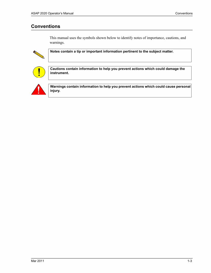
This manual uses the symbols shown below to identify notes of importance, cautions, and warnings.
Notes contain a tip or important information pertinent to the subject matter.
Cautions contain information to help you prevent actions which could damage the instrument.
Warnings contain information to help you prevent actions which could cause personal injury.
Mar 2011 1-3
Online Manual ASAP 2020 Operator’s Manual
Online Manual
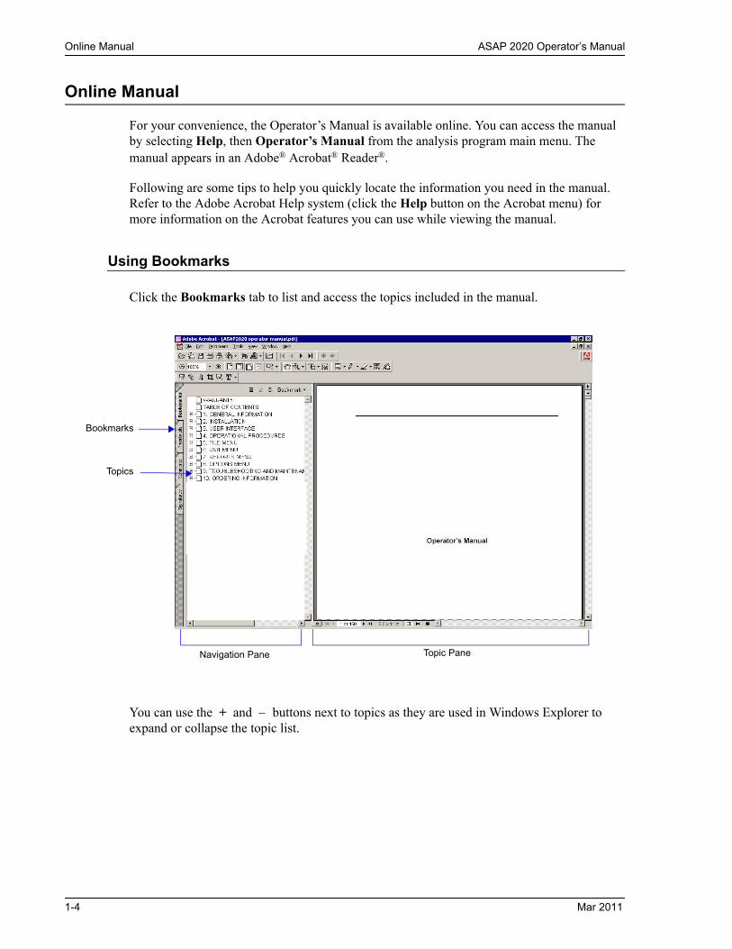
For your convenience, the Operator’s Manual is available online. You can access the manual by selecting Help, then Operator’s Manual from the analysis program main menu. The manual appears in an Adobe® Acrobat® Reader®.
Following are some tips to help you quickly locate the information you need in the manual. Refer to the Adobe Acrobat Help system (click the Help button on the Acrobat menu) for more information on the Acrobat features you can use while viewing the manual.
Using Bookmarks
Click the Bookmarks tab to list and access the topics included in the manual.
You can use the + and buttons next to topics as they are used in Windows Explorer to expand or collapse the topic list.
Navigation Pane Topic Pane
Bookmarks
Topics
1-4 Mar 2011
ASAP 2020 Operator’s Manual Online Manual
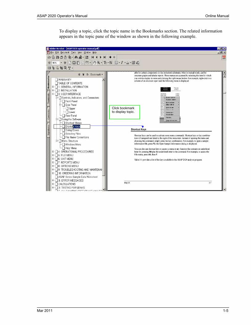
To display a topic, click the topic name in the Bookmarks section. The related information appears in the topic pane of the window as shown in the following example.
Click bookmarkto display topic.
Mar 2011 1-5

Online Manual ASAP 2020 Operator’s Manual
Using the Table of Contents, Index, and other Links
Links provide direct access to selected information. All links appear in blue type. Links are contained in:
• the table of contents• index entries• cross-references within the manual
Table of Contents
To display the table of contents, click Table of Contents in the Bookmarks section. When the table of contents is displayed, you can click an entry to display its associated page. For example, clicking Using the Software in the table of contents, displays the page containing information about the software.
Click topic name in table of contents to display topic.
1-6 Mar 2011

ASAP 2020 Operator’s Manual Online Manual
Index
To use the index in the online manual, click the Bookmarks tab, scroll down to INDEX (the last topic in Bookmarks), then click the + button to expand the index. The letters A through Z are displayed. Click a letter to display its corresponding index entries as shown in the following example.
After you display the entries, locate the item of interest and click on the page reference to access the information.
Cross References
Cross-references work in the same manner. In the example below, clicking on the cross-reference, FILE MENU (shown on the screen in blue type) will display the first page of the chapter describing the commands found on the File menu.
FILE MENU
Provides a description of the commands available on the File menu.
Click a letter to display its index entries.
Mar 2011 1-7

Online Manual ASAP 2020 Operator’s Manual
Using the Find Command
The Adobe Acrobat Find command provides another method of easily accessing specific information. For example, suppose you want to know how the Save as command works. You could select Edit > Find from the Adobe Acrobat menu, then enter Save as in the Find dialog. The following example shows the results.
1-8 Mar 2011

ASAP 2020 Operator’s Manual Online Manual
Printing
You can print the entire manual, a selected page, or range of pages. There are several options for printing. You can:
• Select the printer icon ( ) on the Adobe Acrobat toolbar.
A standard Print dialog is displayed. Select the page(s) to print, then click OK. When using this option (or the next one), be sure to enter the page number(s) displayed in Adobe Acrobat; do not use the page number(s) listed in the footer(s) of the manual.
• Select File > Print.
A standard Print dialog is displayed. Select the page(s) to print, then click OK.
• Click the Thumbnails tab.
Thumbnails of manual pages are displayed.
a. Click the pages you want to print.
b. Right-click to display a shortcut menu, then select Print Pages.
c. A standard Print dialog is displayed; click OK.
Enter this number.
Do not use number in footer of the manual.
Thumbnails tab
Mar 2011 1-9

Equipment Description ASAP 2020 Operator’s Manual
Equipment Description
The ASAP 2020 analyzer is equipped with two independent vacuum systems — one for sample preparation and one for sample analysis. Having two separate systems, as well as separate preparation ports, allows sample preparation and sample analysis to occur concurrently without interruption. Inline cold traps are located between the vacuum pump and the manifold in both the analysis and the degas systems.The sample saturation pressure (Psat) tube is located next to the sample analysis port. Gas inlet ports and cable connections are located conveniently on the side panel of the analyzer for easy access.
The ASAP 2020 is equipped with an elevator that raises and lowers the analysis bath fluid Dewar automatically. A removable shield to enclose the Dewar is also included for safety purposes.
The ASAP 2020 system includes Micromeritics’ Isothermal Jackets for the sample tube. The Isothermal Jacket maintains a stable thermal profile along the full length of the sample and Psat tubes.
1-10 Mar 2011

ASAP 2020 Operator’s Manual Gas Requirements
Gas Requirements
Compressed gases are required for analyses performed by the ASAP 2020 analyzer. Gas bottles or an outlet from a central source should be located near the analyzer.
Appropriate two-stage regulators which have been leak-checked and specially cleaned are required. Pressure relief valves should be set to no more than 30 psig (200 kPag). Gas regulators are available from Micromeritics; refer to Ordering Information, page 10-1.
Analysis Program
The ASAP 2020 analysis program is designed to operate in a Windows Vista, Windows XP, or Windows 7 Professional environment. The Windows environment provides a user-friendly interface for performing analyses and generating reports.
The ASAP 2020 System software monitors and controls the analyzer. It enables you to perform automatic analyses with just a few key strokes, and collects and reports analysis data. You can choose from a variety of reports, which can be printed automatically after an analysis or stored and printed later.
Report System
The ASAP 2020 software includes a report system which allows you to manipulate and customize reports. You can zoom in on portions of the graphs or shift the axes to examine fine details. Scalable graphs can be copied to the clipboard and pasted into other applications. Reports can be customized with your choice of fonts and a company logo added to the report header for an impressive presentation. Refer to REPORTS MENU for the options available for reports.
Mar 2011 1-11

Specifications ASAP 2020 Operator’s Manual
Specifications
The ASAP 2020 system has been designed and tested to meet theses specifications.
Characteristic Specification
—————— PRESSURE MEASUREMENT ——————
Range: 0 to 950 mmHg
Resolution:
1000-mmHg Transducer 0.001 mmHg (Analysis system)1 mmHg (Degas system)
10-mmHg Transducer* 0.00001 mmHg
1-mmHg Transducer** (optional for high stability)
0.000001 mmHg
0.1-mmHg Transducer (optional for high stability)
0.0000001 mmHg
Accuracy (Analysis system only):
Includes nonlinearity, hysteresis, and nonrepeatability. Transducer manufacturer’s specifications.
1000-mmHg Range 10-mmHg Range* 1-mmHg Range** 0.1-mmHg Range***
Within 0.15% of readingWithin 0.15% of readingWithin 0.12% of reading Within 0.15% of reading
—————— VACUUM SYSTEM ——————
Vacuum Pump: Mechanical, two-stage, for analysis; optional
for degas. Ultimate vacuum 5 x 10⁻³ mmHg. Dry pumps available for systems equipped with optional High Vacuum pump.
High Vacuum Pump(if installed):
Less than 3.8 x 10⁻⁹ mmHg
* High Vacuum systems**Micropore systems***Micropore systems with 0.1 mmHg transducer
Ultimate vacuum measured by pump manufacturer according to Pneurop Standard 5608.
1-12 Mar 2011

ASAP 2020 Operator’s Manual Specifications
Characteristic Specification
—————— MANIFOLD TEMPERATURE TRANSDUCER ——————
Type: Platinum resistance device (RTD)
Accuracy: + 0.02 oC (by keyboard entry)
—————— DEGAS SYSTEM (Optional) ——————
Temperature Range: Ambient to 450 oC
Selection: 1 oC increments
Accuracy: Deviation less than +10 oC of set point at thermocouple
Backfill Gas: User-selectable, typically helium or nitrogen
Pressure Range: Accuracy:
0 to 950 mmHg1% best fit straight line
—————— SYSTEM CAPACITY ——————
Sample Preparation: 2 degas ports (optional)
Analysis: 1 sample port and 1 saturation pressure tube
Total Operating Capacity: Up to two complete analysis units can be controlled independently by one computer
—————— CRYOGEN SYSTEM ——————
Special Features: Isothermal Jackets effectively maintain cryogen level constant on sample tube and Po tube during analysis while evaporation of cryogen occurs.
Capacity: 3-Liter Dewar, which typically provides greater than 91 hours of unattended analysis.
Mar 2011 1-13

Specifications ASAP 2020 Operator’s Manual
Characteristic Specification
Analysis Time: Unlimited. Cryogen Dewars may be refilled without affecting the accuracy of results.
—————— SAMPLE SIZE ——————Sample tubes are available for various size pellets, cores and powders. Sample tube stems are normally 1.27-cm (1/2-in.) OD with 9-cc bulbs. Also available are 0.635- (1/4-) or 0.953-cm (3/8-in.) OD with 9-cc bulbs. A 22-mm (0.87-in.) ID, 25-mm (1.0-in) OD sample tube kit is also available. Special tubes can be designed to accommodate unusual samples.
—————— ELECTRICAL ——————
Voltage: 100, 115, 230 VAC +10%
Frequency: 50/60 Hz
Power: 700 VA, operating
—————— ENVIRONMENT ——————
Temperature: 10 to 30 oC, operating-10 to 55 oC, storing or shipping
Humidity 20 to 80% relative, noncondensing
—————— GASES ——————
Normal: Argon, carbon dioxide, nitrogen, krypton (Multigas system), and other suitable gases
—————— PHYSICAL ——————
Height 99 cm (39 in.)
Width: 85 cm (33.5 in.)
Depth: 61 cm (24 in.)
Weight: 115 kg (250 lbs)
1-14 Mar 2011

ASAP 2020 Operator’s Manual Specifications
Characteristic Specification
—————— COMPUTER ——————
Minimum requirements: CD-ROM drive512 megabytes of main memory20-gigabyte hard driveSVGA monitor (1024 x 768 min. resolution)Windows Vista, Windows XP, or Windows 7 Professional.
Mar 2011 1-15

Specifications ASAP 2020 Operator’s Manual
1-16 Mar 2011

ASAP 2020 Operator’s Manual Unpacking and Inspection
2. INSTALLATION
This chapter contains instructions for the following:
• Unpacking and Inspection• Setting Up the Analyzer• Installing the Analysis Program
Initially, your ASAP 2020 analyzer will be installed and verified for operation by an authorized Micromeritics service representative or a representative of a Micromeritics distributor. If your analyzer is moved to a different location in your laboratory, use the instructions provided in this chapter for reinstallation.
Unpacking and Inspection
When you receive the shipping cartons, carefully compare the packing list with the equipment actually received while checking for equipment damaged during shipment. Be sure to sift through all packing materials before declaring equipment missing.
Lifting the Analyzer
The ASAP 2020 analyzer weighs 115 kg (250 lbs) and requires the use of two people to lift it from its shipping carton. One person should not attempt to lift the analyzer. With one person on each side of the analyzer, lift it upright from its shipping carton. Place the analyzer on a table top of sufficient space.
Equipment Damage or Loss During Shipment
When equipment is damaged or lost in transit, you are required to make note of the damage or loss on the freight bill. The carrier, not the shipper, is responsible for all damage or loss. In the event of equipment damage or loss during shipment, contact the carrier of the equipment immediately.
Save the shipping cartons if equipment or parts have been damaged or lost. The inspector or claim investigator must examine the cartons prior to completion of the inspection report.
Use proper lifting techniques to prevent back injury.
Mar 2011 2-1

Unpacking and Inspection ASAP 2020 Operator’s Manual
Equipment Return
Micromeritics strives to ensure that all items arrive safely and in working order. Occasionally, due to circumstances beyond our control, equipment is received which is not in working condition. When it is necessary to return equipment (damaged either during shipment or while in use) to Micromeritics for repair or replacement, use the following procedure:
1. Pack the instrument in its original shipping carton if possible. If the original carton is unavailable, for a nominal fee, Micromeritics can provide another carton for your use.
2. Tag or identify the defective equipment, noting the defect and circumstances, if any, under which the defect is observed.
3. Make reference to the sales order or purchase order for the equipment, and provide the date the equipment was received.
4. Notify the Micromeritics Service Department of the defect and request shipping instructions. The service department will assign a Returned Materials Authorization (RMA) number. Write the RMA number on the outside of the shipping carton.
Failure to package your instrument properly may result in shipping damage.
2-2 Mar 2011

ASAP 2020 Operator’s Manual Setting up the Analyzer
Setting up the Analyzer
The ASAP 2020 System should be installed correctly and tested to ensure that it is operating properly before actual analyses are attempted.
Installing the Vacuum Pumps
Two vacuum pumps are required for operating the ASAP 2020 analyzer when equipped with a degas system: one for degas operations and one for analysis. A recessed cavity is provided on the rear side of the analyzer for placement of the vacuum pumps The analysis pump (facing the rear of the analyzer) is on the left side and the degas pump on the right side.
Two types of vacuum pumps are available, the oil-based vacuum pump and the dry vacuum pump. Typically the dry vacuum pump is used when a mass spectrometer is attached to the analyzer and for chemisorption analyses.
Oil-Based Systems
1. Remove the vacuum pump from its shipping carton.
2. Prepare the alumina and oil vapor trap (refer to Replacing the Alumina in the Oil Vapor Trap on page 9-11), then install the trap onto the intake port of the vacuum pump.
Oil vapor traps reduce the amount of oil vapor that collects in the hoses leading to the instrument.
3. Add fluid to the vacuum pump (refer to Inspecting and Changing Vacuum Pump Fluid on page 9-9).
4. Install the vacuum pump exhaust filter (refer to Replacing the Vacuum Pump Exhaust Filter on page 9-7).
5. Place the vacuum pump onto its drip tray and slide the tray into the right side of the vacuum pump cavity. Be sure the power cord is facing outward; do not connect the power cord to a power source at this time.
Mar 2011 2-3

Setting up the Analyzer ASAP 2020 Operator’s Manual
6. Connect the flexible tubing from the analyzer to the connector on the topside of the pump. The following illustration shows orientation of a typical vacuum pump and its components attached to the flexible tubing of the analyzer.
Dry Systems
1. Remove the vacuum pump from its shipping carton.
2. Slide the vacuum pump into the left side of the vacuum pump cavity. Be sure the power cord is facing outward; do not connect the cord to a power source at this time.
3. Set the voltage selector switch on the vacuum pump to suit the voltage of your local power source.
4. Connect the flexible tubing from the analyzer to the connector on the topside of the pump.
Flexible Tubing
Clamp
Oil Vapor Trap
Clamp
Centering Ring
Centering RingHose Fitting
Intake
2-4 Mar 2011
ASAP 2020 Operator’s Manual Setting up the Analyzer
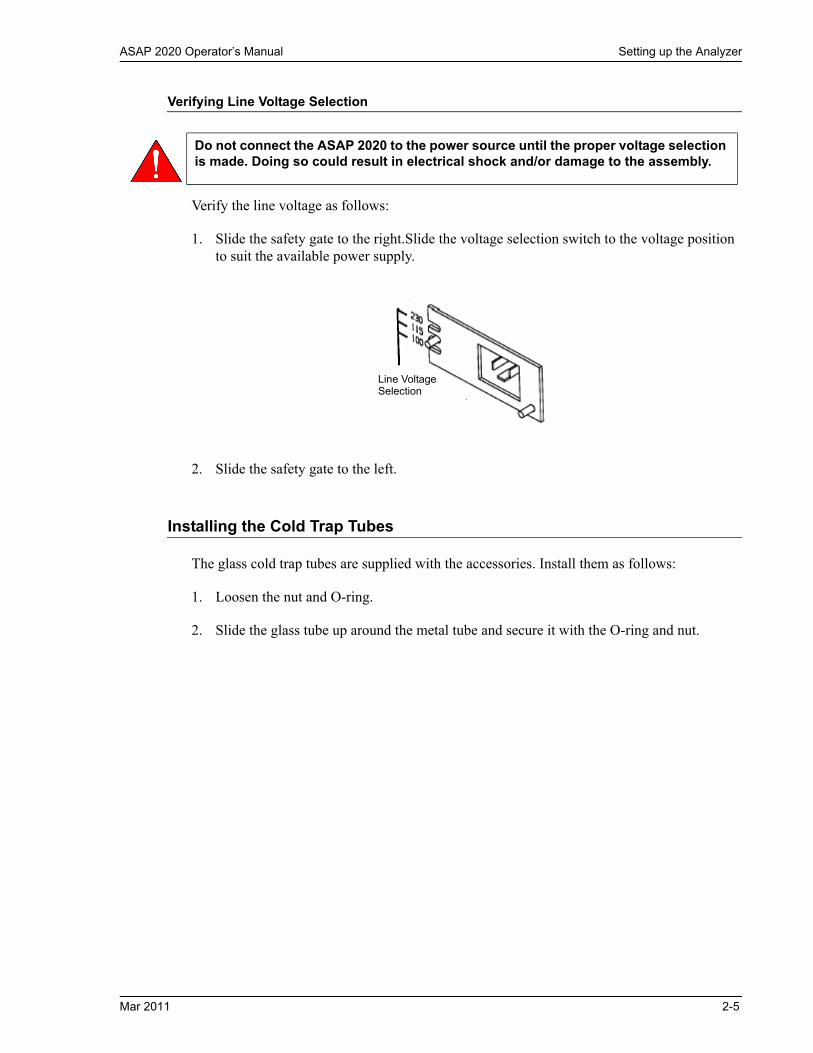
Verifying Line Voltage Selection
Verify the line voltage as follows:
1. Slide the safety gate to the right.Slide the voltage selection switch to the voltage position to suit the available power supply.
2. Slide the safety gate to the left.
Installing the Cold Trap Tubes
The glass cold trap tubes are supplied with the accessories. Install them as follows:
1. Loosen the nut and O-ring.
2. Slide the glass tube up around the metal tube and secure it with the O-ring and nut.
Do not connect the ASAP 2020 to the power source until the proper voltage selection is made. Doing so could result in electrical shock and/or damage to the assembly.
Line VoltageSelection
Mar 2011 2-5

Setting up the Analyzer ASAP 2020 Operator’s Manual
3. Repeat for the second cold trap port.
Installing Saturation Pressure (Psat) Tube
The saturation pressure tube is packaged separately. This tube must be mounted onto the Po port located just behind the sample analysis port.
1. Remove the plastic protective cover from the saturation pressure port by turning it counterclockwise, then pull downward.
Port
Glass Tube
O-ring
Nut
Po Port
Plastic Protective Cap
2-6 Mar 2011

ASAP 2020 Operator’s Manual Setting up the Analyzer
2. Ensure that the O-ring is in place on the end of the saturation pressure tube. Rotate the tube so that the isothermal jacket is closest to the analysis port. Secure the tube in place by turning the connector nut clockwise. Tighten by hand.
Selecting the Computer Power Input
The power input selection on the computer must be set to match the input power source. The computer operates with either 100-120 VAC or 200-240 VAC at 50 or 60 Hz. Refer to the instruction manual supplied with your computer for instructions on selecting power input.
Sample PortPo Port
O-ring
Saturation Pressure Tube
Do not connect the computer power cord to a power source until the proper voltage selection is made. Doing so could result in electrical shock and/or damage to the computer.
Mar 2011 2-7

Setting up the Analyzer ASAP 2020 Operator’s Manual
Connecting the Gas Supply
Delivery tubes for connecting the gases used with the ASAP 2020 system are supplied with the instrument. A regulator is required for each gas bottle connected to the analyzer. Appropriate regulators are available from Micromeritics. Refer to Ordering Information on page 10-1 for part numbers.
Connecting the gas supply involves three procedures; you must:
• connect a regulator to each gas bottle that is being attached to the analyzer • connect the gas bottle(s) to the analyzer’s gas inlet(s)• specify (using the software) which gas is attached to the inlet(s)
The first two procedures are found below; refer to Specifying Gas Ports on page 2-25 to perform the third procedure, which cannot be performed until after software installation.
Connecting a Regulator to the Gas Bottle
1. Leave the gas bottle shut-off valve closed until instructed otherwise.
2. If the regulator has a 1/8-in. outlet, proceed to the next step. If the regulator has a 1/4-in. outlet, attach the reducer fitting to the outlet of the regulator shut-off valve.
3. Close the regulator shut-off valve.
4. Attach the copper delivery tubing to the regulator or reducer fitting. Do not connect the other end of the tubing.
Bottle Shut-Off ValveTwo-stage Pressure Reducing Regulator
Regulator Shut-Off
Gas Bottle
Pressure Control knob
Tubing
Brass Reducer Fitting
Shut-Off Valve Nut
Do not overtighten the fittings. Doing so could collapse the tubing and cause a leak.
2-8 Mar 2011

ASAP 2020 Operator’s Manual Setting up the Analyzer
5. Purge the regulator as follows:
a. Close the regulator shut-off valve by turning it fully clockwise.
b. Turn the pressure regulator control knob fully counterclockwise.
c. Open the gas bottle valve by turning it counterclockwise, then close the gas bottle valve.
d. Observe the high pressure gauge. If the pressure decreases, tighten the nut connecting the regulator to the gas bottle. If the pressure is stable, proceed to Step e.
e. Turn each pressure regulator control knob clockwise until the outlet pressure gauge indicates 10 psig (0.7 bar). Open each regulator shut-off valve by turning it counterclockwise briefly. Then close each valve.
f. Make sure the gas bottle valve is completely closed.
6. Repeat steps 2 through 5 for each gas bottle to be attached to the analyzer.
7. Proceed to the next section to attach the other end of the copper delivery tubing to the analyzer.
Connecting the Gas Delivery Tubing to the Analyzer
The ASAP 2020 analyzer allows for connection of up to six physisorption gases, a gas for degassing, a helium port for the free-space gas, and a Vapor port for water vapor analyses. The helium gas bottle is connected to the analyzer for use in free-space measurements. Other gases can also be used as the analysis gas. Nitrogen or helium (or other suitable gas) can be used as the degas backfill gas.
Gas inlet connections, located on the right side panel of the analyzer, are labeled 1 through 6 for the physisorption gases, Degas for the backfill gas, and helium for the free-space measurement. A vapor gas inlet is also provided for water vapor analyses.
Degas Backfill
FreespaceHelium
These ports are available for chemisorptionanalyses. Refer to Chapter 10 for orderinginformation on the Chemi upgrade.
Mar 2011 2-9

Setting up the Analyzer ASAP 2020 Operator’s Manual
A typical hook-up for gases is as follows:
1 Nitrogen2 Argon3 Carbon dioxide4 Krypton5 As desired6 As desiredDegas Backfill NitrogenFreespace Helium Helium
Attach the other end of the copper tubing (from the regulator) to the appropriate gas port on the side of the analyzer.
Connecting Cables and Power Cords
All cables must be connected securely to their respective connectors for proper operation of the analyzer and its peripheral equipment.
1. Connect the keyboard cable, the monitor cable, the printer cable, and the mouse cable into their respective connectors on the rear panel of the computer. Refer to the manual provided with your computer if you are unsure of connector locations.
2. Plug one end of the instrument communications cable into the connector labeled RS232 on the right side of the analyzer. Plug the other end into the communications port on the computer.
3. Insert one end of the analyzer power cord into the input power connector on the right side of the analyzer and the other end into an appropriate power source.
4. Plug all other power cords, including the vacuum pumps, into an appropriate power source.
5. Turn on the power to the vacuum pumps, but do not turn on the instrument power at this time.
Be sure to specify which gas is attached to the ports you are using. Refer to Specifying Gas Ports on page 2-25.
Some monitors and printers shipped from the United States must be connected to a 100-120 VAC power source. Connecting this equipment to a 200-240 VAC power source could result in electrical shock and/or damage to the equipment.
2-10 Mar 2011

ASAP 2020 Operator’s Manual Setting up the Analyzer
Turning On the System
1. Place the ON/OFF switches for the computer and all peripheral devices in the ON position.
2. Place the analyzer ON/OFF switch in the ON position; verify that the green power indicator on the front panel is illuminated.
Turning Off the System
1. Select Close from the System Menu or Exit from the File menu.
2. If you exit the ASAP 2020 program with analyses in progress, you will be warned of the operation. If desired, you can continue with exiting the application and the analyses will proceed and continue to collect data. Reports that are queued under the Print Manager will print. If, however, a power failure occurs and an uninterruptible power supply (UPS) is not attached to the computer, the data collected after exiting the ASAP 2020 System program are lost.
3. Place the computer, monitor, printer, and plotter (if used) ON/OFF switches in the OFF position.
4. Place the analyzer Main Power switch in the OFF position.
Always exit the ASAP 2020 program and/or Windows before turning off the computer. Failure to do so could result in loss of data.
Mar 2011 2-11
Installing the Analysis Program ASAP 2020 Operator’s Manual
Installing the Analysis Program
Your system must meet or exceed the following requirements before you can install the software:
• CD-ROM drive• 128 megabytes of main memory• 1-gigabyte hard drive• SVGA monitor (800 x 600 minimum resolution)• Windows Vista, Windows XP, or Windows 7 Professional
The ASAP 2020 program is also available as a standalone option so that you can install it on a computer other than the one controlling the analyzer. This allows you to create or edit sample and parameter files, as well as generate reports on completed sample files. Review the Micromeritics PROGRAM License Agreement for restrictions on the use of additional copies.
Initial Installation
The ASAP 2020 System program is supplied on a CD. Perform the following steps to install the program:
1. Turn on the analyzer.
2. Insert the program CD into your CD-ROM drive.
3. Select Start from the Status bar, then Run from the Start menu.
4. Enter the name of the drive designator, followed by setup. For example:
e:setup
Power Management features should be disabled so that the Micromeritics application can communicate properly with the instrument during operation. These features can be disabled in the computer Setup configuration through Windows NT or through a utility supplied by the computer manufacturer.
2-12 Mar 2011

ASAP 2020 Operator’s Manual Installing the Analysis Program
5. Click OK; the New Installation dialog is displayed.
The Destination Folder group box displays the amount of current disk space, the amount of disk space required for the analysis program, and the directory into which the application will be installed. If you wish to install the application into a different directory, click Browse to choose the directory.
6. If you want to run the application from the desktop, select the check box just below the Destination Folder group box to add an icon.
7. The ASAP 2020 icon is added to the Micromeritics folder by default. If you prefer a different folder, enter or select one from the drop-down list.
8. The Install this application for All Users check box enables you to allow or prohibit users other than the installer to access the application.
• Select the check box to allow access for all users logged onto Windows.
• Deselect the check box to allow access for only the user installing the application.
9. Click Next; the Analyzer Configuration dialog is displayed.
Displays the amount of currentdisk space and the amountrequired for installation of theapplication. Also displays thedirectory into which theapplication will be installed.
Select this option to add theASAP 2020 icon to your desktopfor quick access to the application.
You may cancel the installation at any time by selecting Exit. If you do so, you must start the installation program from the beginning to install the analysis program.
Mar 2011 2-13
Installing the Analysis Program ASAP 2020 Operator’s Manual
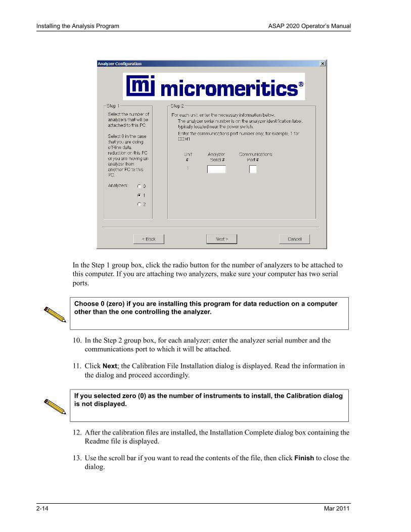
In the Step 1 group box, click the radio button for the number of analyzers to be attached to this computer. If you are attaching two analyzers, make sure your computer has two serial ports.
10. In the Step 2 group box, for each analyzer: enter the analyzer serial number and the communications port to which it will be attached.
11. Click Next; the Calibration File Installation dialog is displayed. Read the information in the dialog and proceed accordingly.
12. After the calibration files are installed, the Installation Complete dialog box containing the Readme file is displayed.
13. Use the scroll bar if you want to read the contents of the file, then click Finish to close the dialog.
Choose 0 (zero) if you are installing this program for data reduction on a computer other than the one controlling the analyzer.
If you selected zero (0) as the number of instruments to install, the Calibration dialog is not displayed.
2-14 Mar 2011

ASAP 2020 Operator’s Manual Installing the Analysis Program
14. Remove the Setup CD and store in a safe place. The original Setup CD contains the calibration files specific to your instrument. Upgrade CDs do not contain calibration files. Therefore, it is important that you maintain your original Setup CD in a secure location in the event calibration files need to be reinstalled.
Using the Setup Program for Other Functions
After initial installation of the ASAP 2020 analysis program, the application setup program can be used to:
• Upgrade software• Add an analyzer• Move an analyzer from one computer to another computer• Remove an analyzer from the computer• Change the analyzer setup• Reinstall calibration files• Uninstall the analysis program
To start the application setup program:
1. Ensure that the analysis program is not operating.
2. Insert the CD into your CD-ROM drive.
3. Select Start from the Status bar.
4. Select Run from the start menu.
5. Enter the drive designator of the CD-ROM drive, followed by setup. For example: e:setup.
Alternatively, you can click Browse, navigate to your CD-ROM drive, and select setup.exe.
Mar 2011 2-15
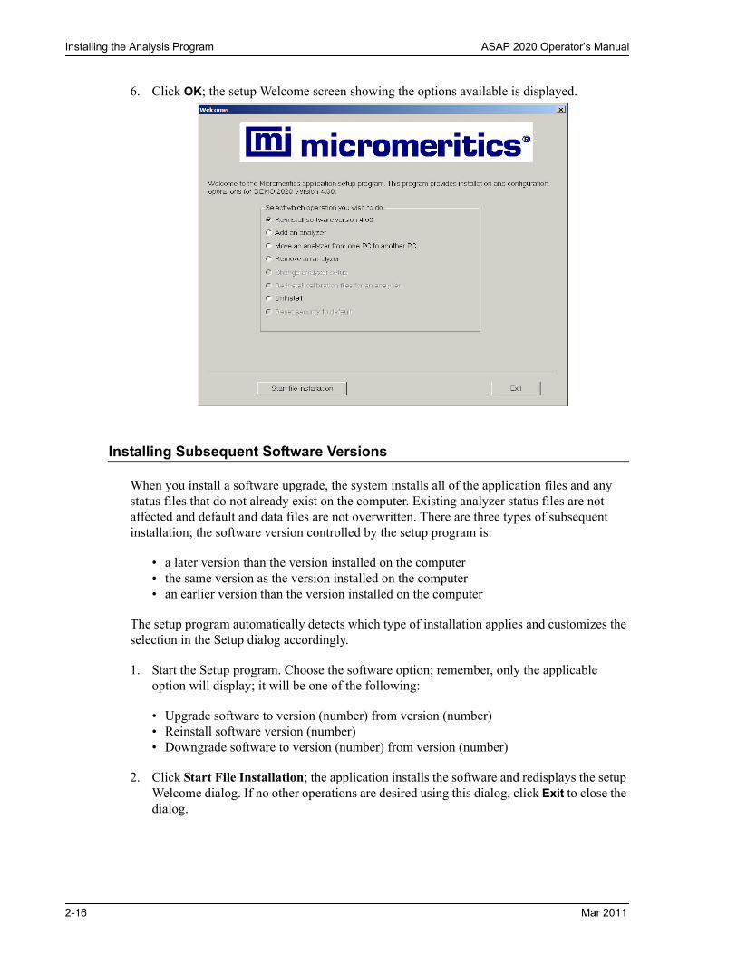
Installing the Analysis Program ASAP 2020 Operator’s Manual
6. Click OK; the setup Welcome screen showing the options available is displayed.
Installing Subsequent Software Versions
When you install a software upgrade, the system installs all of the application files and any status files that do not already exist on the computer. Existing analyzer status files are not affected and default and data files are not overwritten. There are three types of subsequent installation; the software version controlled by the setup program is:
• a later version than the version installed on the computer• the same version as the version installed on the computer• an earlier version than the version installed on the computer
The setup program automatically detects which type of installation applies and customizes the selection in the Setup dialog accordingly.
1. Start the Setup program. Choose the software option; remember, only the applicable option will display; it will be one of the following:
• Upgrade software to version (number) from version (number)• Reinstall software version (number)• Downgrade software to version (number) from version (number)
2. Click Start File Installation; the application installs the software and redisplays the setup Welcome dialog. If no other operations are desired using this dialog, click Exit to close the dialog.
2-16 Mar 2011

ASAP 2020 Operator’s Manual Installing the Analysis Program
Adding an Analyzer
Add an analyzer to the existing application as follows:
1. Start the Setup program. Select Add an analyzer, then click Next; the Setup analyzer dialog is displayed.
2. Enter the serial number of the analyzer being added, then the communications port to which it is to be connected.
3. Click Next; the Calibration Installation dialog is displayed.
4. Select the location of the calibration source files. If the calibration files are located in a directory other than the one displayed, click Browse to select the directory. Click Finish; a media change dialog is displayed.
5. Click OK to install the calibration files. A dialog containing the Readme file is displayed after the calibration files are installed.
6. Click Exit to close the dialog.
Mar 2011 2-17

Installing the Analysis Program ASAP 2020 Operator’s Manual
Moving an Analyzer from one PC to another PC
You can move an analyzer, along with its status and calibration files, from one computer (Source PC) to another computer (Destination PC).
1. Install the application program on the destination computer. Refer to Installing the Analysis Program on page 2-12.
If the analysis program is already installed on the destination computer, proceed to Step 2.
2. Start the application setup program on the source computer. Refer to Using the Setup Program for Other Functions on page 2-15.
3. In the Setup dialog, select Move an analyzer from one PC to another PC, then click Next; the Move analyzer operation dialog is displayed.
This operation does not move sample or parameter files. To move these files, use a file management program such as Explorer or a backup/restore utility.
2-18 Mar 2011
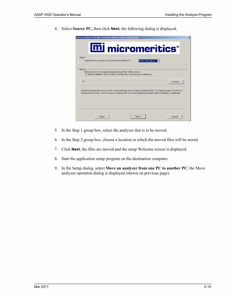
ASAP 2020 Operator’s Manual Installing the Analysis Program
4. Select Source PC, then click Next; the following dialog is displayed.
5. In the Step 1 group box, select the analyzer that is to be moved.
6. In the Step 2 group box, choose a location in which the moved files will be stored.
7. Click Next; the files are moved and the setup Welcome screen is displayed.
8. Start the application setup program on the destination computer.
9. In the Setup dialog, select Move an analyzer from one PC to another PC; the Move analyzer operation dialog is displayed (shown on previous page).
Mar 2011 2-19

Installing the Analysis Program ASAP 2020 Operator’s Manual
10. Select Destination PC, then click Next; the following dialog is displayed.
11. In the Step 1 group box, enter the serial number of the analyzer being moved and the communications port to which it will be attached.
12. In the Step 2 group box, click Browse and choose the location of the moved files.
13.Click Finish; the files are moved and the setup Welcome dialog is displayed.
2-20 Mar 2011

ASAP 2020 Operator’s Manual Installing the Analysis Program
Removing an Analyzer
You can remove an analyzer from the computer as follows. When you remove an analyzer, the status files are removed as well.
1. Start the Setup program. Refer to Using the Setup Program for Other Functions on page 2-15.
2. From the Setup dialog, select Remove an analyzer, then click Next; the Remove an analyzer dialog is displayed.
3. From the drop-down list, choose the serial number of the analyzer you want to remove.
4. Click Remove; the analyzer is removed and the Welcome screen is again displayed.
5. Click Exit to close the dialog.
Mar 2011 2-21

Installing the Analysis Program ASAP 2020 Operator’s Manual
Changing an Analyzer Setup
Change the analyzer setup as follows:
1. Start the Setup program. Refer to Using the Setup Program for Other Functions on page 2-15.
2. From the Setup dialog, select Change analyzer setup, then click Next; the Change analyzer setup dialog is displayed.
3. From the drop-down list, choose the analyzer you want to change.
4. Enter the new port number in the space provided.
5. Click Finish; the change is completed and the Welcome dialog is again displayed.
6. Click Exit to close the dialog.
2-22 Mar 2011

ASAP 2020 Operator’s Manual Installing the Analysis Program
Reinstalling the Calibration Files
You can reinstall the files containing an analyzer’s factory calibration data as follows:
1. Start the Setup program.
2. From the Setup dialog, select Re-install calibration files for an analyzer, then click Next; the Re-install calibration files dialog is displayed.
If .... Then ....
you have only one analyzer installed
the calibration files are installed and the Welcome screen is displayed.
you have multiple ana-lyzers installed, a dialog enabling you to choose the desired analyzer is displayed.
select the appropriate analyzer, then click Next; the cali-bration files are installed and the Welcome screen is displayed.
Mar 2011 2-23

Installing the Analysis Program ASAP 2020 Operator’s Manual
Uninstalling the Analysis Program
When you uninstall the ASAP 2020 analysis program, the application removes the analysis program, status files, analyzer setup files, and resulting empty directories. It does not remove data files. Perform the following steps to uninstall the program:
1. Start the Setup program. From the Setup dialog, select Uninstall, then click Next; the Uninstall dialog is displayed.
2. Click Uninstall; the Select Uninstall Method dialog is displayed.
2-24 Mar 2011
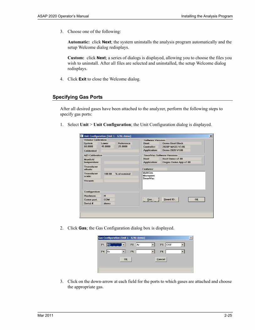
ASAP 2020 Operator’s Manual Installing the Analysis Program
3. Choose one of the following:
Automatic: click Next; the system uninstalls the analysis program automatically and the setup Welcome dialog redisplays.
Custom: click Next; a series of dialogs is displayed, allowing you to choose the files you wish to uninstall. After all files are selected and uninstalled, the setup Welcome dialog redisplays.
4. Click Exit to close the Welcome dialog.
Specifying Gas Ports
After all desired gases have been attached to the analyzer, perform the following steps to specify gas ports:
1. Select Unit > Unit Configuration; the Unit Configuration dialog is displayed.
2. Click Gas; the Gas Configuration dialog box is displayed.
3. Click on the down-arrow at each field for the ports to which gases are attached and choose the appropriate gas.
Mar 2011 2-25

Installing the Analysis Program ASAP 2020 Operator’s Manual
Gases may be added to the drop-down list using the Adsorptive Properties dialog. Refer to Adsorptive Properties on page 4-13.
4. Click OK to close the dialog box, and then again to close the Unit Configuration dialog.
2-26 Mar 2011

ASAP 2020 Operator’s Manual Controls, Indicators, and Connectors
3. USER INTERFACE
This chapter contains information to familiarize you with the hardware and software of the ASAP 2020 system. It is recommended that you read this chapter before attempting to operate the ASAP 2020 system.
Controls, Indicators, and Connectors
This section contains a description of the controls, indicators, and connectors located on the front, side, and rear panels of the ASAP 2020 system.
Front Panel
Green indicator light Illuminated when power is applied to the analyzer.
Indicator Light
Vacuum Pump Panel
Elevator
Mar 2011 3-1

Controls, Indicators, and Connectors ASAP 2020 Operator’s Manual
Vacuum pump panel Allows access to the vacuum pumps. Remove this panel when you need to service the pumps.
It is not necessary to remove the panel to inspect the condi-tion of the oil or the oil level (oil-sealed forepump). To accomplish either of these tasks, remove (or fold over to the right) the protective rubber mat from the work surface and lift off the metal cover; this exposes the vacuum pump sight win-dow.
Vacuum pump sight window
The vacuum pump sight windows enable you to inspect the oil levels in the degas and analysis pumps.
Vacuum pump drain Provides a convenient method of draining fluid from the pump when service is required.
High vacuum pump A high vacuum pump is used on all but the basic nitrogen instrument. A second high vacuum pump is installed as an option on the degas system.
Connections, as well as an on/off (breaker) switch, are located on the front right side of the analyzer beneath the work surface. Remove (or fold over to the left) the rubber mat from the work surface and lift off the metal cover.
Indicator lights (located on the underside of the upper exten-sion of the front panel) illuminate when the high vacuum pump is operating. Left light = degas; right light = analysis.
Elevator Allows placement of the Dewar around the sample tube.
3-2 Mar 2011

ASAP 2020 Operator’s Manual Controls, Indicators, and Connectors
The components listed here are located on the underside of the upper extension of the front panel.
Po PortHeating Mantle Power Connector
Degas Port
Heating Mantle Thermocouple Connector
Sample PortHigh Vacuum Pump indicators
Heating Mantle Breaker
Cold Traps
Four hangers are provided for place-ment of safety shields.
Degas ports Allow you to degas up to two samples. Each degassing port has connections for a heating mantle.
Heating mantle thermocouple
Allows connection of a heating mantle thermocouple (one for each degas port).
Heating mantle power connec-tor
Allows connection of the heating mantle power cord (one for each heating mantle).
Heating mantle breaker Protects the circuitry for the heating mantle in the event of a failure (one for each heating mantle). If the circuit breaker trips (pops out), call your Micromeritics service representa-tive.
Cold Traps Two cold traps are provided; one for degassing and one for analysis.
Mar 2011 3-3

Controls, Indicators, and Connectors ASAP 2020 Operator’s Manual
Side Panel
Upper
High vacuum pump indicators
Illuminate when the high vacuum pumps are operating at nor-mal speed. The left indicator is for degas operations and the right one for analysis.
Sample port For installing the sample tube containing the material you wish to analyze.
Po port For installing a Po (saturation pressure) tube when perform-ing physisorption analyses.
Gas Inlet Ports
Degas Backfill PortVapor Gas Port
Freespace HeliumPort
Chemisorption Ports(available if upgraded toChemisorption capability)
Gas inlet ports Used to connect gas supplies to the analyzer.
Vapor gas port For attaching the water vapor option, or connecting a vapor gas. Refer to “ORDERING INFORMATION” on page 10-1 for the part number of the water vapor option.
Degas Backfill port Allows connection of a gas to use for degassing the sample.
Freespace Helium port Allows connection of helium to use for measuring the free space.
3-4 Mar 2011

ASAP 2020 Operator’s Manual Controls, Indicators, and Connectors
Lower
On/Off switch For turning the analyzer on and off. This switch also serves as the main breaker for the analyzer; it switches off automati-cally in the event of an electrical fault.
Power connector For connecting the analyzer to the electrical supply.
RS232 port For connecting the analyzer to a computer.
Valve circuit breaker Protects the circuitry for the valves in the event of a failure. If the circuit breaker trips (pops out), call your Micromeritics service representative.
Voltage selector switch For setting the analyzer to the correct incoming AC line volt-age.
On/Off Switch
Power Connector
Voltage Selector
Valve Circuit Breaker
RS 232 Port
Mar 2011 3-5

Controls, Indicators, and Connectors ASAP 2020 Operator’s Manual
Rear Panel
Vacuum Pump Location
Vacuum pump recess Provides for placement of the vacuum pumps. Vacuum pumps can be serviced from the front of the instrument by removing the vacuum pump panel located on the lower left side of the front panel (see Front Panel described previ-ously).
3-6 Mar 2011

ASAP 2020 Operator’s Manual Using the Software
Using the Software
The analysis program operates in the Windows environment and requires familiarity with stan-dard Windows operations such as using the mouse, menus, and dialog boxes. While this manual provides brief instructions for such standard operations, you may have to refer to your Windows documentation or to its online help system to clarify functions which are specific to Windows.
Shortcut Menus
Shortcut menus (sometimes referred to as context-sensitive menus or pop-up menus) are avail-able for certain components on the instrument schematic when in manual mode, and for onscreen graphs and tabular reports. These menus are accessed by selecting the item for which you wish to display its menu and clicking the right mouse button. For example, right-click in a column of an onscreen report and the following menu is displayed.
Shortcut Keys
Shortcut keys can be used to activate some menu commands. Shortcut keys or key combina-tions (if assigned) are listed to the right of the menu item. Instead of opening the menu and choosing the command, simply press the key combination. For example, to open a sample information file, press F2; the Open Sample Information dialog is displayed.
You can also use shortcut keys to access a menu or any function that contains an underlined letter by pressing Alt plus the underlined letter in the command. For example, to access the File menu, press Alt, then F.
Table 3-1 provides a list of the keys available in the ASAP 2020 analysis program.
Mar 2011 3-7

Using the Software ASAP 2020 Operator’s Manual
Table 3-1. Shortcut Keys
Key(s) Function
F1 Access online operator’s manual
F2 Open a sample information file
Clear the field of existing date (Select Dates dialog)
F3 Open an analysis conditions file
Insert the current date (Select Dates dialog)
F4 Open an adsorptive properties file
Display a calendar from which to choose a date (Select Dates dialog)
F5 Open a report options file
F6 Tile open windows
F7 Cascade open windows
F8 Start report
F9 Close all open reports
F10 Generate a Heat of Adsorption report
Alt + F4 Exit the ASAP 2020 program
Shift + F2 List sample information files
Shift + F3 List analysis conditions files
Shift + F4 List adsorptive properties files
Shift + F5 List report options files
Shift + F9 Access shortcut menu of (1) selected component on instrument schematic, or (2) onscreen reports
3-8 Mar 2011

ASAP 2020 Operator’s Manual Using the Software
Dialog Boxes
Dialog boxes are displayed when a menu item followed by an ellipsis (...) is selected. Subdia-log boxes are displayed when certain push buttons are selected. Both types of boxes may contain one or more of the items listed below.
The following describes elements that are often included in dialog boxes. If an element is shown in gray instead of black, the element is currently unavailable.
Data Entry Fields A Data Entry field is used to enter text; either numeric (num-bers only) or alphanumeric (numbers, letters, or printable characters).
If an invalid entry is made, an error message is displayed; for example, if you attempt to enter text in a numeric field or a number outside of the range shown in the information bar.
Information Bar Some dialog boxes contain information pertinent to the selected field in an information bar across the bottom of the dialog. For example, a range is shown for fields in which numeric entries are required.
Radio buttons Radio buttons are provided in groups of two or more and are used to make a choice; only one radio button can be selected. Simply click the desired option with your mouse pointer. A black dot indicates the item is selected.
Check boxes Check boxes allow you to choose multiple options from a group of options. Click the desired options with your mouse pointer. An X in the box indicates the item is selected; remove the X in the same manner.
Grayed Item(indicates unavailable)
Check Box
Radio Button
Data Entry Field
Push ButtonInformation Bar
Mar 2011 3-9

Using the Software ASAP 2020 Operator’s Manual
Push Buttons A push button is used to display a subdialog box in which to enter additional information about the subject matter, or to invoke an action.
For example, if you click Date Range on the Open Sample Information dialog box, the Select Dates subdialog box is dis-played. If you click Cancel on the Open Sample Information dialog box, you invoke the action of canceling and closing the dialog box.
Close Closes the active dialog. If the dialog box contains unsaved changes, you will be prompted to save them before the dialog box closes.
Any information entered in subdialog boxes (refer to the next section of this chapter), is discarded also.
Save Saves the information entered in the current session; the dia-log box remains open.
Replace Allows you to replace the contents of the current file with those from an existing file. For example, if you are creating an analysis conditions file, you can save time by clicking and choosing the file containing the values you wish to use. These values are copied into the current file automatically. And since the values are actually just copied into the file, you can edit them in any way you wish. The file from which they were copied remains intact and ready for the next use.
Cancel Discards everything you entered in the dialog box and any subdialog boxes, and closes the dialog box. A warning mes-sage is displayed before closing.
Drop-down list A drop-down list contains a list of options and is indicated by a down arrow to the right of the field. If there are more items than can fit in the box, a scroll bar is provided for navigating through the list.
3-10 Mar 2011

ASAP 2020 Operator’s Manual Using the Software
Selecting Files
Sample information is stored in files and saved under file names. Certain dialog boxes contain a Files list box which displays a list of files available for that particular operation. For exam-ple, the Open Sample Information File dialog.
A default string appears in the File name field. To select a file, simply move the mouse pointer to the desired file in the list and double-click.
You can limit the list of files displayed by choosing one or more of the following options:
• Use wildcard characters in the path name entered in the File name field. Standard and wildcard characters (such as * and ?) can be used to filter file names. For example, you could limit the list of files shown in the dialog above to those beginning with 13x by enter-ing 13x*.SMP in the file name field.
• Enter a range of dates. Click Date Range; the Select Dates dialog is displayed.
Select Show Date Range to enable the From and To fields, then enter a beginning and ending date. Or you can double-click in each field to display a calendar to select a date. The range of dates remains the default until you change the dates or select Show All Dates.
The Status drop-down list does not appear on the Open dialog boxes for parameter files.
Displays all files of the type in the Status field.
Displays the current directory.
Mar 2011 3-11

Using the Software ASAP 2020 Operator’s Manual
For convenience, the following shortcut keys are available when the Select Dates dialog is displayed:
F2 Clears the dateF3 Inserts the current dateF4 Displays a calendar from which you may select a date
• Select a file status from the Status drop-down list. For example, choose Complete from the drop-down list and only files that have been used in an analysis are displayed. The table shown below describes each file status.
Table 3-2. File Status and Description
• Navigate to a different directory. The current directory is displayed just above the Directo-ries list box. You can change directories by double-clicking a directory in the Directories list box, double-clicking [..] to move up one level, or by entering the desired directory in the File Name field. For example, enter C:\2020files\sample\*.smp to display sample files in the 2020files\sample directory on your local drive.
The Status drop-down list does not appear on the File, Open dialogs for parameter files.
Status Description
All All sample information files in the specified directory and within the specified range of dates
Analyzing Sample information files that are currently being used with an analysis
Complete Sample information files that have been used with an analysis
Entered Sample information files that contain manually entered data
No analysis Sample information files that have not been used in a degassing operation or an analysis
Prepared Sample information files that have been used in an automatic degassing operation and are ready for analysis
Preparing Sample information files that are currently being used in an automatic degassing operation
3-12 Mar 2011

ASAP 2020 Operator’s Manual Using the Software
File Name Conventions
For sample information and parameter files, a wildcard character (*) and a default extension display.
The following table shows the file name extensions for the ASAP 2020 program.
Table 3-3. Default File Name Extensions
File Type Extension
Sample Information SMP
Sample Tube STB
Degas Conditions DEG
Analysis Conditions ANC
Report Options RPO
Adsorptive Properties ADP
Export to disk (ASCII) ISO
Sample information files from the ASAP 2000 analyzers; may be converted to an ASAP 2020-compatible format
DAT
Report to disk RPT
List to disk LST
Thickness curve THK
Alpha-s curve ALS
The following types are available for reports saved from the Report window
Report REP
Spreadsheet XLS
ASCII TXT
Mar 2011 3-13

Menu Structure ASAP 2020 Operator’s Manual
Menu Structure
All functions for the ASAP 2020 are located on menus which are accessed from the Menu bar. Each menu contains commands, and in some cases a submenu. A submenu is indicated when the command is followed by an arrow.
Brief descriptions of each menu are provided below; refer to the chapter given in parentheses for a detailed description of the commands contained on that menu.
Menu Name
Menu Bar
Submenu
Command
File Enables you to maintain system files. (Chapter 5, FILE MENU)
Unit [n] Enables you to perform analyses and other instrument operations. (Chapter 6, UNIT MENU)
Reports Enables you to generate, customize, and close reports. Also pro-vides examples of reports. (Chapter 7, REPORTS MENU)
Options Enables you select data presentation formats, and enter system default values. (Chapter 8, OPTIONS MENU)
Windows Enables you to arrange the windows and icons on your screen. It also displays the names of all open files. (this chapter, page 3-15)
Help Displays Help information. (this chapter, page 3-15)
3-14 Mar 2011

ASAP 2020 Operator’s Manual Menu Structure
Windows Menu
Help Menu
Tile Resizes all open windows and arranges them side by side so that the contents of all open windows are visible.
Cascade Resizes all open windows and arranges them in a stacked fashion. The active window is positioned on top of the stack. Each window’s title remains visible, making it easy to select other windows.
Arrange Icons Arranges the symbols for all minimized windows in an orderly manner.
Open Files Displays all open files; the active window is preceded with a check mark.
Operator’s Manual Displays the operator’s manual in PDF format.
Micromeritics on the Web Accesses the Micromeritics Web site.
About ASAP 2020 Displays information about the ASAP 2020 analysis pro-gram
Mar 2011 3-15

Menu Structure ASAP 2020 Operator’s Manual
3-16 Mar 2011

ASAP 2020 Operator’s Manual Specifying Sample File Defaults
4. OPERATIONAL PROCEDURES
This chapter contains brief step-by-step instructions on how to:
• specify sample file defaults, this page • create sample information files, page 4-6• define parameter files, page 4-9 • prepare the sample, page 4-16• perform an analysis, page 4-29• generate a list of information on a sample or parameter file, page 4-32• print contents of a sample or parameter file, page 4-31• export data in a sample information file to an ASCII file, page 4-33• overlay graphs, page 4-34
This chapter does not contain detailed descriptions of the dialogs used to perform these procedures. Refer to Chapters 5 through 8 for dialog descriptions. Use the index to assist you in locating the appropriate dialog.
Specifying Sample File Defaults
You can specify sample defaults in the Basic or Advanced format. The defaults you specify are the ones you see when you create a new sample file in the respective format. Therefore, it is best to specify (or enter) parameters that you plan to use most frequently. For example; specify defaults for your most commonly analyzed sample material. You can always edit parameters in the sample file when it is created. The ASAP 2020 system automatically generates sample information file names and uses the values you specify as the defaults.
Mar 2011 4-1

Specifying Sample File Defaults ASAP 2020 Operator’s Manual
Basic Format
Perform the following steps to define defaults for a sample information file in the Basic format.
1. Select Options > Sample Defaults; the default Basic Sample Information dialog is displayed.
2. In the Sequence field, specify a default string. This is the number that is incrementally sequenced and displays in the File name field when you select File, Open, Sample information. You can use up to eight characters.
3. In the field on the right of the Sample line, enter a format for the sample identification. Be sure to include the $ symbol if you want the sample file number included as part of the identification. You can use up to 42 alphanumeric characters.
Select Option Presentation on the Options menu and ensure that Basic is selected as the format.
You also can edit the word Sample. For example, you may prefer to use Material or Test. You can enter up to 15 characters in this field.
4-2 Mar 2011

ASAP 2020 Operator’s Manual Specifying Sample File Defaults
4. You can enter a sample mass or have it calculated automatically; choose the desired method.
• Enter: enter a default value in the Mass field.
• Calculate: enter default values in the Empty tube and Sample+tube fields
Regardless of which method you choose, the choice can be changed when you create a sample file.
5. The sample density is used when free space is calculated; enter a default for your sample’s density if you typically use a calculated free space. Otherwise, this value is ignored.
6. Select the down arrow to the right of the parameter fields to choose default parameter files:
• Sample tube• Degas conditions• Analysis conditions• Adsorptive properties• Report options
7. Click Save, then Close.
Mar 2011 4-3
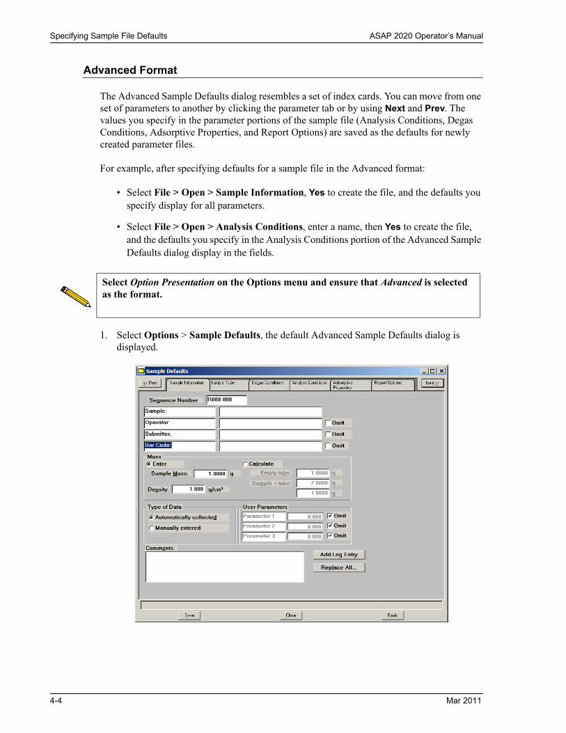
Specifying Sample File Defaults ASAP 2020 Operator’s Manual
Advanced Format
The Advanced Sample Defaults dialog resembles a set of index cards. You can move from one set of parameters to another by clicking the parameter tab or by using Next and Prev. The values you specify in the parameter portions of the sample file (Analysis Conditions, Degas Conditions, Adsorptive Properties, and Report Options) are saved as the defaults for newly created parameter files.
For example, after specifying defaults for a sample file in the Advanced format:
• Select File > Open > Sample Information, Yes to create the file, and the defaults you specify display for all parameters.
• Select File > Open > Analysis Conditions, enter a name, then Yes to create the file, and the defaults you specify in the Analysis Conditions portion of the Advanced Sample Defaults dialog display in the fields.
1. Select Options > Sample Defaults, the default Advanced Sample Defaults dialog is displayed.
Select Option Presentation on the Options menu and ensure that Advanced is selected as the format.
4-4 Mar 2011

ASAP 2020 Operator’s Manual Specifying Sample File Defaults
2. In the Sequence field, specify a default string for the sample file number; you can use up to eight characters. This is the number that appears in the File name field when you select File > Open > Sample information.
3. In the right-side field of the Sample line, enter a format for the sample’s identification. You can enter up to 42 characters. Be sure to include the $ symbol if you want the sample file number (Sequence) included as part of the identification.
4. Edit the Operator and Submitter lines as desired. Or have them omitted entirely by selecting Omit.
5. If bar code information is not applicable, select Omit to omit this field from the sample information dialog. Or, if you prefer to use this line for some other type of information, edit the label.
6. You can enter a sample mass or have it calculated automatically; choose the desired method.
• Enter: enter a default value in the Mass field.
• Calculate: enter default values in the Empty tube and Sample+tube fields
Regardless of which method you choose, the choice can be changed when you create a sample file.
7. If you plan to use a calculated free space, enter the sample’s density in the Density field.
8. Choose whether you wish to have data collected automatically or if you plan to enter the data. This option can be changed (if desired) before the analysis.
9. If you plan to report statistical process control (SPC) information, enter appropriate information. These are user-definable parameters that can be entered and tracked along with other statistical process control data; refer to Sample Defaults, page 8-4 for additional information on these parameters.
10. Click the Sample Tube tab. Enter criteria for the sample tube you most commonly use, then click Save.
11. Click the Analysis Conditions tab. Choose the analysis conditions appropriate for your most commonly analyzed material, then click Save.
12. Click the Degas Conditions tab. Specify degassing criteria, then click Save.
13. Click the Adsorptive Properties tab. Specify gas characteristics, then click Save.
You can click Save on each dialog as you specify parameters, or you can click Save on any dialog after all parameters have been specified. All dialog defaults will be saved.
Mar 2011 4-5

Creating Sample Information Files ASAP 2020 Operator’s Manual
14. Click the Report Options tab. Choose desired reports, using Edit to specify details; then click Save.
15. Click Close to close the dialog.
Creating Sample Information Files
A sample information file must be assigned to every sample that is analyzed. When you create a sample file, you can accept the default values specified using Sample Defaults, or you can edit them as desired. You can create a sample information file using the Advanced, Basic, or Restricted format.
Advanced Format
The Advanced format allows you to customize the parameters of a sample information file. Chapter 5 provides a description of the fields associated with creating sample information files.
1. Select File > Open > Sample information; the Open Sample Information File dialog is displayed.
2. Accept the next sequenced file number or enter a new name in the File name field.
3. Click OK, then Yes to create the file; the Sample Information dialog is displayed.
The defaults that appear in the fields are the ones specified in Sample Defaults.
4-6 Mar 2011

ASAP 2020 Operator’s Manual Creating Sample Information Files
4. Accept the default identification in the Sample field or change it to an appropriate one. The dialog box above shows the sample file number because the dollar ($) symbol was used when specifying sample defaults.
5. Edit the Operator, Submitter and/or Bar Code fields as needed. If these fields are not displayed, they were selected to be omitted in Sample Defaults.
6. Select Enter to enter a value for the sample’s mass (if different from the default value), or Calculate to have the mass calculated automatically. If you select Calculate, you must enter weights for the Empty tube and the Tube + sample.
7. Enter a value in the Density field (or accept the default). This value is applicable only when using a calculated free space.
8. Choose whether you want data automatically collected by the system or whether you wish to enter the data.
9. Unless you are gathering statistical process control information, it is unnecessary to enter parameter values. These are user-definable parameters that can be entered and tracked along with other statistical process control data; refer to Sample Defaults, page 8-4 for information on user parameters.
10. Click Save to save the information you entered.
11. The steps for completing the remaining parameters of the sample information file are explained in subsequent sections:
• Specifying Sample Tube Criteria • Defining Degas Conditions• Defining Analysis Conditions• Defining Adsorptive Properties• Defining Report Options
Simply click on the tabs to open the associated dialog.
If a sample information file already exists containing the values you want to use in this file, you can click Replace all to copy those values into this one. You can still edit the values after they are loaded.
Use the Comments window to record specifics of the analysis or its conditions. Anything you enter in this window is displayed in the report header.
Mar 2011 4-7
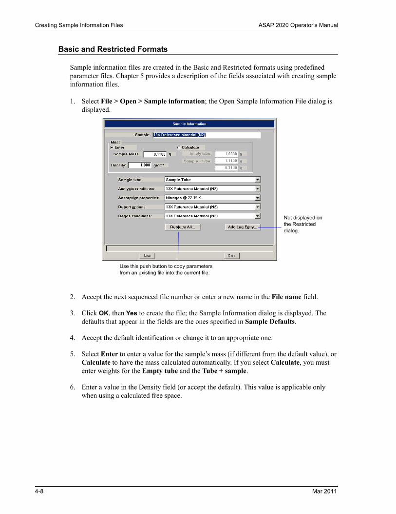
Creating Sample Information Files ASAP 2020 Operator’s Manual
Basic and Restricted Formats
Sample information files are created in the Basic and Restricted formats using predefined parameter files. Chapter 5 provides a description of the fields associated with creating sample information files.
1. Select File > Open > Sample information; the Open Sample Information File dialog is displayed.
2. Accept the next sequenced file number or enter a new name in the File name field.
3. Click OK, then Yes to create the file; the Sample Information dialog is displayed. The defaults that appear in the fields are the ones specified in Sample Defaults.
4. Accept the default identification or change it to an appropriate one.
5. Select Enter to enter a value for the sample’s mass (if different from the default value), or Calculate to have the mass calculated automatically. If you select Calculate, you must enter weights for the Empty tube and the Tube + sample.
6. Enter a value in the Density field (or accept the default). This value is applicable only when using a calculated free space.
Use this push button to copy parameters from an existing file into the current file.
Not displayed on the Restricted dialog.
4-8 Mar 2011
ASAP 2020 Operator’s Manual Defining Parameter Files
7. Using the down arrows to the right of each parameter field, select an appropriate file (or accept the defaults). You can review or edit the contents of these files by switching to the Advanced format if desired.
8. Click Save, then Close.
Defining Parameter Files
The following file types can exist as part of the sample information file or as an individual parameter file:
• Sample tube• Degas conditions• Analysis conditions• Adsorptive properties• Report options
Having these files exist independently allows you to use them over and over again.Several predefined parameter files (located in the params directory) are included with the ASAP 2020 analysis program. Although these files may come close to the needs of your laboratory, you may wish to define additional ones. Or you can use a predefined file as a starting point. This is easily accomplished by creating a new file and then selecting Replace. A dialog is displayed so that you can select the existing file containing the values you wish to use. After the values are copied into the current file, you can edit the values as desired; the original file remains intact and ready for the next use.
If you wish to have parameter files display in the drop-down list on the Basic Sample Information dialog, be sure to save them to the directory specified as the Parameter Files Directory. (Refer Parameter Files Directory on page 8-13 for additional information.)
Sample Tube
1. Select File >Open > Sample Tube; the Sample tube dialog is displayed.
2. Enter a name in the File name field, then click OK.
If you are using the Restricted format, you cannot switch to the Advanced format.
Be sure the directory specified is the Parameter files directory if you wish to have it display in the drop-down list in the Basic Sample Information dialog. (Refer to Parameter Files Directory on page 8-13 for additional information.)
Mar 2011 4-9

Defining Parameter Files ASAP 2020 Operator’s Manual
3. Click Yes to create the file; the Sample Tube dialog is displayed.
4. Enter a description in the Sample Tube field. Be sure to use an intuitive description so that you can recognize it easily.
5. Click Load from Sample File; the Open Sample Information File dialog is displayed.
6. Select the file you used in the blank run with this sample tube, then click Open to copy the warm and cold free space values into the Sample Tube dialog.
7. If a vacuum seal of some type was used, select the appropriate option or leave the default of None selected.
8. Click Save, then Close.
Degas Conditions
Degas Conditions files contain degassing information for preparing samples. These files are appropriate only if your ASAP 2020 analyzer is equipped with the SmartVac degassing system.
Perform the following steps to define a degas conditions file:
1. Select File > Open > Degas Conditions; the Degas Conditions dialog is displayed.
2. Enter a name in the File name field, then click OK.
Be sure the directory specified is the Parameter files directory if you wish to have it display in the drop-down list in the Basic Sample Information dialog. (Refer to Parameter Files Directory on page 8-13 for additional information.)
4-10 Mar 2011

ASAP 2020 Operator’s Manual Defining Parameter Files
3. Click Yes to create the file; the Degas Conditions dialog is displayed.
4. Enter a description in the Description field. Be sure to use an intuitive description so that you can recognize it easily.
5. Specify values for the evacuation and heating phases for degassing the sample
6. Click Save, then Close.
Analysis Conditions
Analysis conditions specify the data used to guide an analysis. An analysis conditions file may be assigned a unique name, and you can direct any sample to be analyzed according to the conditions in any existing analysis conditions file. Chapter 5 provides a detailed description of the fields on this dialog.
1. Select File > Open > Analysis Conditions; the Open Analysis Conditions File dialog is displayed.
2. Enter a name (up to eight characters) in the File name field, then click OK.
Be sure the directory specified is the Parameter files directory if you wish to have it display in the drop-down list in the Basic Sample Information dialog. (Refer to Parameter Files Directory on page 8-13 for additional information.)
Mar 2011 4-11

Defining Parameter Files ASAP 2020 Operator’s Manual
3. Click Yes to create the file; the Analysis Conditions dialog is displayed.
4. Enter a description (up to 42 characters) in the Description field. Use an intuitive description, one that will help you identify the type of sample you plan to analyze using these analysis conditions.
5. Specify points for your pressure table. Use the push buttons adjacent to the table to assist you in creating your table.
6. Click Preparation to specify evacuation and leak test values.
7. Click Free Space to specify how the free space is to be measured.
8. Click Po and T to specify how the saturation pressure (Po) is to be measured, and the analysis bath temperature. If you select Absolute pressure dosing, options 1 through 5 are disabled. The Po will be calculated using the analysis bath temperature; enter the appropriate temperature in the field provided.
9. Click Dosing to specify dosing options.
10. Click Equilibration to specify the equilibration interval and its delay time.
11. Click Backfill to specify backfill options.
12. If you wish to use absolute dosing, click the Absolute pressure dosing option.
13. Click Save, then Close.
4-12 Mar 2011

ASAP 2020 Operator’s Manual Defining Parameter Files
Adsorptive Properties
Adsorptive properties specify the characteristics of the gases used in the ASAP 2020 System. Chapter 5 provides a detailed description of the fields on this dialog.
1. Select File > Open > Adsorptive properties; the Open Adsorptive Properties File dialog box is displayed.
2. Enter a name (up to eight characters) in the File name field, then click OK.
3. Click Yes to create the file; the Adsorptive Properties dialog is displayed.
4. Enter the name of the adsorptive gas in the Adsorptive field, then enter its mnemonic.
5. Click Psat vs T to edit the Psat vs Temperature table. Edit any other field(s) on this dialog as required, then click OK.
6. Select Non-condensing Adsorptive if the gas is non-condensing.
7. Enter the appropriate information (or accept the defaults) in the following fields.
Maximum manifold pressureDensity conversion factorTherm. tran. hard-sphere diameterMolecular cross-sectional area
8. Choose your preferred dosing method; choose Normal for gases under pressure.
Be sure the directory specified is the Parameter files directory if you wish to have it display in the drop-down list in the Basic Sample Information dialog. (Refer to Parameter Files Directory on page 8-13 for additional information.)
Mar 2011 4-13

Defining Parameter Files ASAP 2020 Operator’s Manual
9. Click one of the following:
• Real gas equation of state, then use Open to select a table.
Adsorbed molecules occupy volume in the sample tube reducing the cold free space. Select the Adsorbed-phase free-space correction box to adjust the reported quantity adsorbed to correct for this effect. This option is appropriate for all sample analyses that use the real gas equation of state. It should be deselected for blank tube analyses.
• Ideal gas law with non-ideality correction, then enter a Non-idealty factor.
Report Options
Report options specify the types of reports to be generated from an analysis or manually entered data. They also help you customize details of reports such as axis scale, axis range, column headings, and components of thickness curve equations.
You can tailor report options files to accommodate the requirements of your analyses. For example, you can generate a simple report that lets you determine the basic characteristics of the sample. Then use that report to make choices about the variables you want to include in lengthier, more sophisticated reports. You can specify for reports to be generated automatically after each analysis, or you can generate reports at any time during or after an analysis. However, a report generated during an analysis only includes data collected up to the time of the report. Chapter 5 provides a detailed description of the fields on this dialog.
Define report options as follows:
1. Select File > Open > Report Options; the Open Report Options File dialog is displayed.
2. Enter a name (up to eight characters) in the File name field, then click OK.
Be sure the directory specified is the Parameter files directory if you wish to have it display in the drop-down list in the Basic Sample Information dialog. (Refer t Parameter Files Directory on page 8-13 for additional information.)
4-14 Mar 2011

ASAP 2020 Operator’s Manual Defining Parameter Files
3. Click Yes to create the file; the Report Options dialog is displayed.
4. Enter a description (up to 42 characters) in the Description field. Enter an identifier that gives a more intuitive description of the file’s contents. For example, BJH Adsorption Report Options.
5. Select Show report title and enter the title you wish to appear at the top of the report. Or deselect this option if you prefer not to have a report title.
6. If you wish to compare the same type of graph from multiple files, click Overlays and choose the files. Then be sure you edit the graph from the Selected Reports window and choose Samples from the Overlay drop-down list.
7. Select Thermal transpiration correction if you want correction made for thermal transpiration in the sample tube, then enter the inside diameter of the sample tube.
8. The reports that may be generated are listed in the Selected Reports list. Select reports by double-clicking on the desired report. Reports are deselected in the same manner. A report is selected when it is preceded by a check mark.
9. You can edit some reports by highlighting the desired report and clicking Edit.
10. Click Save, then Close to save the information and close the dialog.
If your company logo exists as a bitmap (bmp) or enhanced metafile (emf), you can have it display in the report header by selecting Show graphic. Click Browse to select the file; use the Height and Width fields to specify the size.
Mar 2011 4-15

Preparing Samples ASAP 2020 Operator’s Manual
Preparing Samples
Care should be taken in choosing, conditioning, and filling sample tubes. The following guidelines help ensure accurate, reproducible results.
Choosing Sample Tubes
A sample tube set consists of the following parts:
• Sample tube• Stopper or seal frit• Filler rod
Standard sample tubes for the ASAP 2020 degas and analysis stations have a 1.27-cm (1/2-in.) outside diameter (OD). Two other sizes are available: 0.64 cm and 0.95 cm (1/4 in. and 3/8 in.) OD. Stepped ferrules, smaller O-rings, isothermal jackets, and filler rods are available for adapting the smaller stems to the degas or analysis ports (refer to Ordering Information on page 10-1 for part numbers). The stem diameter selected for use is a matter of accuracy and precision requirements, as well as personal preference and convenience in loading the sample.
A rubber stopper may be used with all size sample tubes; however, seal frits are recommended for 1.27-cm (1/2-in.) OD sample tubes (refer to Ordering Information on page 10-1 for part numbers).
Filler rods help to ensure accuracy in samples with lower total surface areas by reducing the free-space volume. It is generally a good practice to use filler rods for samples having less than 100 square meters of total surface area. Filler rods are unnecessary for samples with total surface areas greater than 100 square meters.
The weight of the empty sample tube should be determined after it has been cleaned (refer to Cleaning and Labeling Sample Tubes, page 4-17), degassed, and filled with backfill gas. The sample tube should be allowed to cool to room temperature before backfilling. After the sample tube has cooled, remove it from the degas port and weigh it.
The weight of the isothermal jacket may vary slightly and cannot be considered as constant; therefore, do not weigh it with the sample tube set.
Filler rods can interfere with thermal transpiration correction and, therefore, should not be used when performing micropore analyses.
If a seal frit is not used, insert a stopper immediately after removing the sample from the degas port.
4-16 Mar 2011
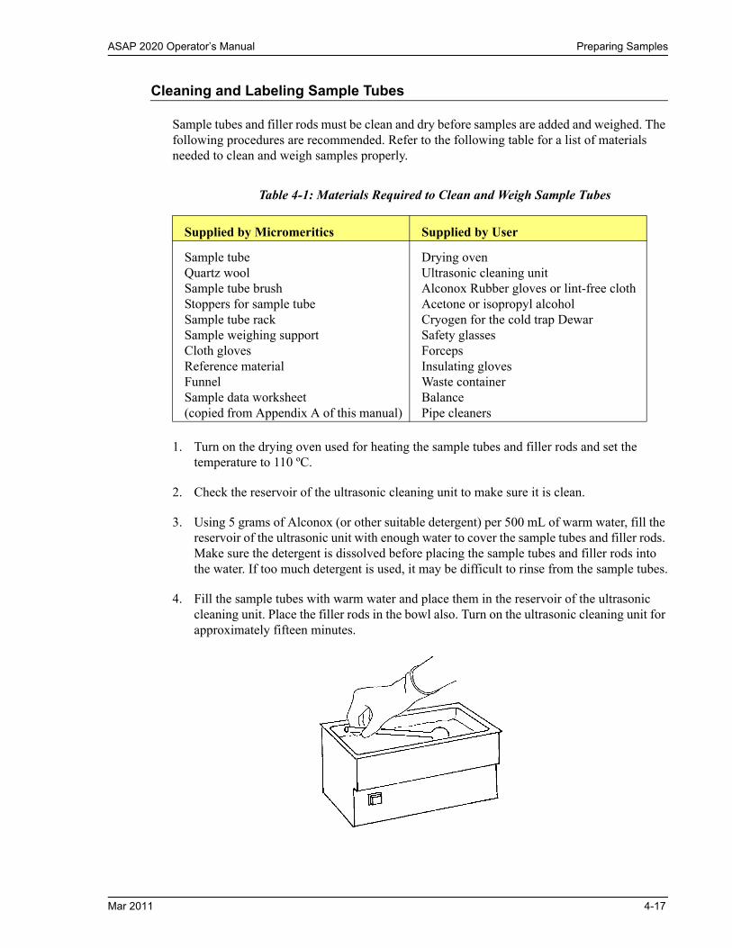
ASAP 2020 Operator’s Manual Preparing Samples
Cleaning and Labeling Sample Tubes
Sample tubes and filler rods must be clean and dry before samples are added and weighed. The following procedures are recommended. Refer to the following table for a list of materials needed to clean and weigh samples properly.
Table 4-1: Materials Required to Clean and Weigh Sample Tubes
1. Turn on the drying oven used for heating the sample tubes and filler rods and set the temperature to 110 ºC.
2. Check the reservoir of the ultrasonic cleaning unit to make sure it is clean.
3. Using 5 grams of Alconox (or other suitable detergent) per 500 mL of warm water, fill the reservoir of the ultrasonic unit with enough water to cover the sample tubes and filler rods. Make sure the detergent is dissolved before placing the sample tubes and filler rods into the water. If too much detergent is used, it may be difficult to rinse from the sample tubes.
4. Fill the sample tubes with warm water and place them in the reservoir of the ultrasonic cleaning unit. Place the filler rods in the bowl also. Turn on the ultrasonic cleaning unit for approximately fifteen minutes.
Supplied by Micromeritics Supplied by User
Sample tubeQuartz woolSample tube brushStoppers for sample tubeSample tube rackSample weighing supportCloth glovesReference materialFunnelSample data worksheet (copied from Appendix A of this manual)
Drying ovenUltrasonic cleaning unitAlconox Rubber gloves or lint-free clothAcetone or isopropyl alcoholCryogen for the cold trap DewarSafety glassesForcepsInsulating glovesWaste containerBalancePipe cleaners
Mar 2011 4-17

Preparing Samples ASAP 2020 Operator’s Manual
5. Using rubber gloves, remove the sample tubes and filler rods from the reservoir.
6. Clean the interior of the sample tubes with the brush supplied with the ASAP 2020 System.
7. Rinse the sample tubes and filler rods thoroughly with hot water. Then rinse them with isopropyl alcohol or acetone using a waste container to collect used solvent.
8. Using nitrogen, dry the interior of the sample tubes and filler rods under a vent hood. Use a tubing extension long enough and small enough in diameter to fit inside the tubes.
If isopropyl alcohol or acetone is not available, deionized water may be used to rinse the sample tubes.
4-18 Mar 2011

ASAP 2020 Operator’s Manual Preparing Samples
9. Stand the sample tubes on the sample tube rack and place the filler rods in a basket or in the rack. Bake for two hours.
10. Remove the sample tubes from the oven and allow them to cool.
11. Using either rubber gloves or a lint-free cloth (but not bare hands), place a filler rod (if used) in each sample tube by holding the sample tube horizontally and sliding the filler rod into the sample tube slowly.
12. Wipe a rubber stopper (or seal frit, if used with 1.27-cm (1/2-in.) tubes) with a lint-free cloth.
13. Label the sample tube and stopper or seal frit for identification.
14. Fill the tube with the selected backfill gas; then insert the stopper or seal frit quickly to avoid releasing the gas.
If helium is used as the degas backfill gas, seal frits are recommended. Refer to Ordering Information on page 10-1 or seal frit part numbers.
To obtain the accurate mass of a degassed sample, the gas in both the empty sample tube and in the tube with the sample must be the same.
Mar 2011 4-19

Preparing Samples ASAP 2020 Operator’s Manual
Determining Amount of Sample to Use
Clean, dry sample tubes are essential for accurate results. How much sample to use can be determined best by experiment. In general, a sample providing 40 to 120 square meters of total surface area is recommended for nitrogen analysis. Less than this may cause variability of results; considerably more than this extends unnecessarily the time required for analysis.
Smaller quantities are required for samples having high surface areas. These samples require careful weighing after degassing because a small error may represent a considerable percent of total weight. Proper weighing techniques are most important in this case. Use no less than 100 mg to reduce the effect of weighing errors.
Care should be taken when loading powders; the accessory funnel is useful for this purpose. Large granules or chunks may be loaded with forceps.
Determining the Mass of the Sample
Analysis results are expressed in units of surface area per gram of sample; therefore, the true mass of the sample must be known. Carefully weigh each sample tube set and sample as described below.
1. Write the Sample Tube number on the Sample Data Worksheet. (A Sample Data Worksheet, which you may copy, is included in Appendix A.)
2. Place the sample weighing support on the balance. Tare the balance and allow it to stabilize at zero (0).
3. Place the sample tube set (sample tube, stopper or seal frit, and filler rod, if used) on the sample support. Record the stabilized weight on the Sample Data Worksheet as Mass of empty sample tube. Remove the sample support and sample tube set from the balance.
4. Place a sample container onto the balance. Tare the balance and allow it to stabilize at zero (0).
5. Slowly add the sample to the sample container.
6. Remove the rubber stopper or seal frit and filler rod from the sample tube.
Avoid touching the sample with your fingers because oils may be transferred to the sample and can alter results or create degassing problems.
Do not touch the sample or filler rod with bare hands while performing the next six steps. Doing so could affect the accuracy of results.
4-20 Mar 2011

ASAP 2020 Operator’s Manual Preparing Samples
7. Using a funnel, pour sample from the container into the sample tube.
If some sample clings to the inside of the sample tube above the last 3 in. (7.5 cm) of the tube, use a pipe cleaner or lint-free wipe to remove it.
8. Replace the filler rod and insert the rubber stopper or seal frit.
9. Weigh the sample tube set containing the sample and record the weight on the Sample Data Worksheet as Mass of sample tube plus sample (Before Degas).
10. Subtract the Mass of empty sample tube from the Mass of sample tube plus sample; record this value as the Mass of sample.
Mar 2011 4-21
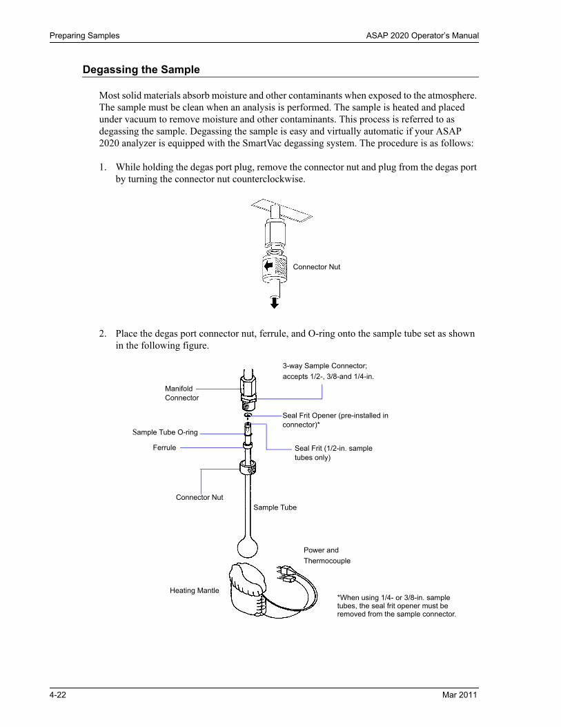
Preparing Samples ASAP 2020 Operator’s Manual
Degassing the Sample
Most solid materials absorb moisture and other contaminants when exposed to the atmosphere. The sample must be clean when an analysis is performed. The sample is heated and placed under vacuum to remove moisture and other contaminants. This process is referred to as degassing the sample. Degassing the sample is easy and virtually automatic if your ASAP 2020 analyzer is equipped with the SmartVac degassing system. The procedure is as follows:
1. While holding the degas port plug, remove the connector nut and plug from the degas port by turning the connector nut counterclockwise.
2. Place the degas port connector nut, ferrule, and O-ring onto the sample tube set as shown in the following figure.
Connector Nut
Manifold Connector
Sample Tube O-ring
Connector Nut
Seal Frit Opener (pre-installed in connector)*
Ferrule
3-way Sample Connector;
accepts 1/2-, 3/8-and 1/4-in.
Seal Frit (1/2-in. sample tubes only)
Sample Tube
Heating Mantle
Power and
Thermocouple
*When using 1/4- or 3/8-in. sample tubes, the seal frit opener must beremoved from the sample connector.
4-22 Mar 2011
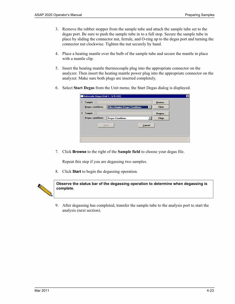
ASAP 2020 Operator’s Manual Preparing Samples
3. Remove the rubber stopper from the sample tube and attach the sample tube set to the degas port. Be sure to push the sample tube in to a full stop. Secure the sample tube in place by sliding the connector nut, ferrule, and O-ring up to the degas port and turning the connector nut clockwise. Tighten the nut securely by hand.
4. Place a heating mantle over the bulb of the sample tube and secure the mantle in place with a mantle clip.
5. Insert the heating mantle thermocouple plug into the appropriate connector on the analyzer. Then insert the heating mantle power plug into the appropriate connector on the analyzer. Make sure both plugs are inserted completely.
6. Select Start Degas from the Unit menu; the Start Degas dialog is displayed.
7. Click Browse to the right of the Sample field to choose your degas file.
Repeat this step if you are degassing two samples.
8. Click Start to begin the degassing operation.
9. After degassing has completed, transfer the sample tube to the analysis port to start the analysis (next section).
Observe the status bar of the degassing operation to determine when degassing is complete.
Mar 2011 4-23

Preparing Samples ASAP 2020 Operator’s Manual
Transferring the Degassed Sample to the Analysis Port
The sample tube must be removed from the degas port, weighed and then installed onto the analysis port for analysis.
1. Allow the sample tube to cool.
2. Carefully remove the heating mantle clip and the heating mantle from the sample tube and allow the sample tube to cool to room temperature (approximately fifteen minutes).
3. While holding the sample tube, loosen the port connector nut and remove the sample tube from the degas port. If you are not using a seal frit, insert a stopper immediately. Remove the connector nut, ferrule, and O-ring from sample tube stem.
4. Weigh the sample tube set. Enter the weight on the Sample Data Worksheet as Mass of sample tube plus sample (After Degas).
5. Subtract the Mass of empty sample tube (Before Degas) from the Mass of sample tube plus sample (After Degas) to determine the mass of the sample. Record this value as the Mass of sample (After Degas).
6. Slide an isothermal jacket down over the sample tube stem until it touches the sample tube bulb.
7. Place the connector nut, ferrule, and O-ring onto the sample tube stem.
8. Remove the stopper and immediately attach the sample tube to the analysis port, pushing it fully up into the port. Secure it in place by screwing the connector nut onto the analysis port connector; hand-tighten the connector nut.
9. Place the sample tube Dewar cover over the sample tube stem just above the isothermal jacket as shown in the following illustration.
If the sample tube is not mounted to the analysis port immediately, either leave it on the degas port or remove it and insert the rubber stopper (unless you are using a seal frit) into the sample tube opening.
Do not touch the sample tube or the heating mantle until they have reached room temperature. Touching the sample tube, heating mantle, or heating mantle clip could result in burns.
You do not have to remove the seal frit (if used).
4-24 Mar 2011
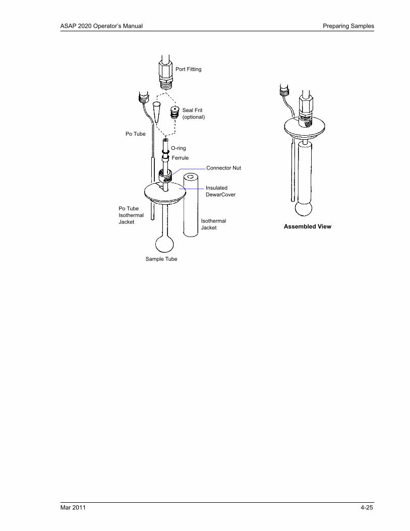
ASAP 2020 Operator’s Manual Preparing Samples
Port Fitting
Seal Frit (optional)
Connector Nut
Insulated DewarCover
Isothermal Jacket
Sample Tube
Po Tube Isothermal Jacket
Po Tube
Ferrule
O-ring
Assembled View
Mar 2011 4-25

Installing Dewars ASAP 2020 Operator’s Manual
Installing Dewars
Precautions
Always handle Dewars with care. Any product with a glass vacuum flask is a potential safety hazard and should be treated with caution.
We recommend the following be observed when handling Dewars containing liquefied gases:
• Protect yourself by wearing 1) goggles (or a face shield), 2) an insulated or rubber apron, and 3) insulated gloves.
• When pouring liquefied gases from one container to another: 1) cool the receiving container gradually to minimize thermal shock, 2) pour the liquefied gas slowly to prevent splashing, and 3) vent the receiving container to the atmosphere.
• Use a plastic stirring rod when stirring substances in a Dewar containing liquefied gases (or other materials of extremely low temperature). Do not use a glass or metal stirring rod unless it is coated with some form of protective coating.
• Do not handle heavy objects above the Dewar. If unavoidable, place a protective cover over the Dewar’s opening. If an object of sufficient weight is accidentally dropped into the Dewar, shattering may occur.
• Always install the Dewar cover before performing an analysis. The cover reduces the accumulation of ice. Accumulated ice could cause the Dewar to bond to the sample tube.
Cold Trap Dewar
1. Fill the cold trap Dewar with a cryogen such as liquid nitrogen to about 5 cm (2 in.) from the top.
Cryogens can cause frostbite injury. Wear safety glasses and insulating gloves when handling cryogens.
4-26 Mar 2011

ASAP 2020 Operator’s Manual Installing Dewars
2. Hang the cold trap Dewar around the cold trap port as shown below.
3. Place the insulator/stopper over the Dewar opening as shown below.
Cold Trap
Cold Trap Dewar
Mar 2011 4-27
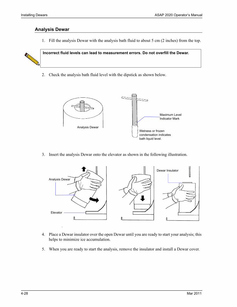
Installing Dewars ASAP 2020 Operator’s Manual
Analysis Dewar
1. Fill the analysis Dewar with the analysis bath fluid to about 5 cm (2 inches) from the top.
2. Check the analysis bath fluid level with the dipstick as shown below.
3. Insert the analysis Dewar onto the elevator as shown in the following illustration.
4. Place a Dewar insulator over the open Dewar until you are ready to start your analysis; this helps to minimize ice accumulation.
5. When you are ready to start the analysis, remove the insulator and install a Dewar cover.
Incorrect fluid levels can lead to measurement errors. Do not overfill the Dewar.
Maximum Level Indicator Mark
Wetness or frozen condensation indicates bath liquid level.
Analysis Dewar
Elevator
Analysis Dewar
Dewar Insulator
4-28 Mar 2011

ASAP 2020 Operator’s Manual Performing an Analysis
Performing an Analysis
After the sample has been degassed and transferred to an analysis port, you may begin an analysis.
Ensure that the analysis gas and the Psat gas specified in the sample file match the system configuration gases; if they do not, correct the sample information file or correct the unit configuration gas.
Perform the following steps to begin an analysis:
1. Select Unit > Start Analysis; the Analysis dialog is displayed with the Start Analysis dialog positioned on top.
2. Choose a file for your analysis and click OK; the Analysis dialog containing the parameters of the selected file is displayed.
3. Verify parameters and make any changes you feel necessary.
4. To generate a report automatically after the analysis, click Report after Analysis and choose report output options. You can generate reports to the screen or directly to a printer.
You cannot perform an analysis while calibration is in progress.
Before beginning an analysis, make sure the tank pressure for the gas regulator is at least 200 psig. Pressures less than 200 psig may cause the sample to be inadequately saturated, resulting in inaccurate data or termination of analysis.
Mar 2011 4-29

Performing an Analysis ASAP 2020 Operator’s Manual
5. Click Export after Analysis to have isotherm data generated automatically after the analysis if finished.
6. Click Start to begin the analysis; as data are collected, the graph will be drawn in the window.
7. Click Next to perform another analysis; the first view of the Analysis dialog is displayed.
Before clicking Start, make sure the elevator is all the way down. If it is not all the way down, hazardous conditions can result.
After the elevator rises, do not place any items under the elevator platform. Objects under the platform will prevent the elevator from fully lowering, and could cause damage to the elevator mechanism.
4-30 Mar 2011

ASAP 2020 Operator’s Manual Printing File Contents
Printing File Contents
You can print the contents of one or more sample or parameter files.
1. Select File > Print; a drop-down list containing file types is displayed.
2. Choose the file type; a dialog similar to this one is displayed.
3. From the Files list box, select the desired file. If you plan to print multiple files, hold down Ctrl while clicking on the desired files.
4. Choose whether you wish to print the contents to the screen (Preview) or to a printer (Print). If you choose Print, the Copies field is enabled allowing you to print up to four copies.
5. Click OK; the file is printed to the specified destination.
You can use the Status drop-down list and/or the Date Range push button to limit the files displayed in the Files list.
Mar 2011 4-31

Listing File Statistics ASAP 2020 Operator’s Manual
Listing File Statistics
You can generate a list of the following information on a sample file or parameter file.
• File name• Date the file was created (or last edited)• Time the file was created (or last edited)• File identification• File status
Perform the following steps to list file statistics:
1. Select File > List.
2. From the List drop-down menu, select the type of file on which you wish information. A dialog similar to the one shown below is displayed:
3. From the Files list box, choose the desired file(s). If you wish to include all files, leave all files deselected.
4. Choose whether you wish to print statistics to the screen (Preview) or to a printer (Print). If you choose Print, the Copies field is enabled allowing you to print up to four copies.
5. Click OK, a list for the requested file(s) is sent to the specified destination.
Displays the type of fileon which you requestedinformation; in thisexample, a sampleinformation file
4-32 Mar 2011

ASAP 2020 Operator’s Manual Exporting Isotherm Data
Exporting Isotherm Data
The Export option on the File menu allows you to copy the isotherm data in the sample information file and reformat it in ASCII text. If saved to a File, the data can be imported into applications, such as spreadsheets. The output file consists of five columns containing the elapsed time, absolute pressure, relative pressure, and specific volume adsorbed (refer to Format of Data Output, page 5-101 for an example of exported data).
Perform the following steps to export a sample information file or ASCII data:
1. Select File > Export; the Export Sample Information dialog is displayed.
2. From the Files list box, choose the file(s) you wish to export. You can select multiple files by holding down Ctrl while clicking on the desired files.
3. In the Settings group box, choose a Destination for your exported file.
a. If you choose File as the destination, select the file type. Then enter a name in the File name field or accept the default. If you have selected multiple files, individual files are exported as their file name. You can also change the destination path if desired.
b. If you choose Printer, the Copies field is enabled; you can print up to four copies.
4. Click OK; the file(s) is exported to the specified destination.
Use the Status drop-down list and/or the Date Range push button to limit the files displayed in the Files list.
Mar 2011 4-33

Generating Graph Overlays ASAP 2020 Operator’s Manual
Generating Graph Overlays
Use graph overlays when you wish to compare graphically results for multiple samples or multiple graphs for one sample. Graphical lines are differentiated by the use of varying symbols and reported in a legend on the report. If color output capability is available, different colors are used instead of symbols.
Graph overlays can be implemented in two ways:
• Multiple Sample Overlays Overlay results for up to eight samples on top of a previously selected sample.
• Multiple Graph OverlaysOverlay two different types of graphs from one sample. The multiple graph overlay capability exists for:
BJH Adsorption/DesorptionDFT Pore Size/Surface EnergyDollimore-Heal Adsorption/DesorptionHorvath-KawazoeMP-Method
You cannot overlay graphs if your sample file presentation is in the Basic format. You must switch to the Advanced format before proceeding.
Multiple Samples Overlay
1. Select File > Open > Sample Information to display the Open Sample Information File dialog box.
2. Select a sample on which to overlay graphs of other samples, then click OK; the Sample Information dialog is displayed.
3. Click the Report Options tab to display the Report Options dialog.
4-34 Mar 2011

ASAP 2020 Operator’s Manual Generating Graph Overlays
4. Make your report selections (or deselect any you do not wish to generate).
5. Choose the type of report for which you wish to generate overlays, click Edit, and perform the steps listed for that report:
If you are overlaying this type of report.... Then ....
Isotherm Select the desired plot(s) from the Select Reports group box.
Click Options (becomes enabled when the plot is selected) adjacent to the selected plot
Select the Overlay samples check box, then click OK.
Click OK again to return to the Report Options dialog.
BET Surface AreaLangmuir Surface AreaFreundlichTemkint-PlotAlpha-Sf-Ratio
Select the Overlay Samples check box.
Click OK.
Mar 2011 4-35

Generating Graph Overlays ASAP 2020 Operator’s Manual
6. Click Overlays; the Graph Overlay Samples dialog is displayed.
7. Click Browse to the right of the Sample 1 field; the Plot Overlay Sample Selection dialog is displayed.
8. Choose a sample file, then click OK. You may choose up to eight files in this manner.
9. After selecting the desired number of sample files, click OK to return to the Report Options dialog.
10. Click Save if you wish to save your Selected Reports list. Even if you don’t save, all of the options regarding overlays and anything else are available as your reports are generated.
11. Select Reports > Start Report; the Start Report screen is displayed with the name of your primary file highlighted.
12. Click OK; the Select Reports dialog is displayed.
13. Ensure that the desired graph is selected (preceded with a check mark), then click OK.
If you are overlaying this type of report.... Then ....
BJH AdsorptionBJH DesorptionDollimore-Heal AdsorptionDollimore-Heal DesorptionDFT Pore SizeDFT Surface EnergyMP-Method
Choose the report variable from the Selected Reports window, then click Edit.
Click on the down arrow at the Overlay field and choose Samples; then click OK.
Click OK again to close the report variable’s dialog and return to the Report Options dialog.
4-36 Mar 2011

ASAP 2020 Operator’s Manual Generating Graph Overlays
Multiple Graphs Overlay
Remember that multiple graph overlays can be done only for:
• BJH Adsorption• BJH Desorption• DFT Pore Size• DFT Surface Energy• Dollimore-Heal Adsorption• Dollimore-Heal Desorption• Horvath-Kawazoe • MP-Method
1. Select File > Open > Sample Information to display the Open Sample Information File dialog.
2. Select a sample for which you want to overlay two graphs; then select Edit; the Sample Information dialog box is displayed.
3. Click the Report Options tab to display the Report Options dialog.
4. Make your report selections (or deselect any you do not wish to generate).
Mar 2011 4-37

Generating Graph Overlays ASAP 2020 Operator’s Manual
5. From the Selected Reports list, select the report for which you want multiple graph overlays, then select Edit; a Report Options dialog for that report (or graph) is displayed (this example shows BJH Adsorption).
6. Select a report type, then click Edit; an options dialog for that specific item is displayed (this example shows Cumulative Pore Volume).
7. Click the down arrow at the Overlay field and select a graph type from the list. This selection will be overlaid on the graph selected in the Variable field.
8. Select OK to return to the BJH Adsorption Report Options dialog; do any editing you wish.
9. Click OK to return to the main Report Options dialog.
These two graphswill be overlaid
4-38 Mar 2011

ASAP 2020 Operator’s Manual Generating Graph Overlays
10. Click Save to save your Selected Reports list. Even if you don’t save, all of the options regarding overlays and anything else are available as your reports are run.
11. Select Reports > Start Report; the Start Report screen is displayed with the name of your primary file highlighted.
12. Click OK; the Select Reports dialog is displayed.
13. Ensure that the desired graph is selected (preceded with a check mark), then click OK.
Mar 2011 4-39

Generating Graph Overlays ASAP 2020 Operator’s Manual
4-40 Mar 2011

ASAP 2020 Operator’s Manual Description
5. FILE MENU
The File menu contains commands which allow you to manage sample and parameter files.
Description
Listed below are brief descriptions of the File menu commands. Detailed descriptions follow this section.
Open Opens an existing sample information or parameter file. Page 5-3.
Save Saves the file in the active window. Page 5-94.
Save As Saves the file in the active window as a different name. You also can use this option to save a subset of the sample file as a parameter file. Page 5-95.
Save All Saves all open files. Page 5-96.
Close Closes the file in the active window. Page 5-96.
Close All Closes all open files. Page 5-97.
Mar 2011 5-1

Description ASAP 2020 Operator’s Manual
Print Prints the contents of a sample or parameter file. Page 5-98.
List Generates a list of certain information for sample or parameter files. Page 5-99.
Export Copies the isotherm data in a sample information file and exports it in ASCII format. Page 5-100.
Convert Allows you to convert a sample file in the MICMOS 2000 or 2000 micropore format to a format compatible with the ASAP 2020 program. Page 5-102.
Exit Exits the analysis program. Page 5-104.
5-2 Mar 2011
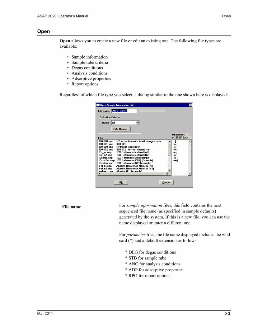
ASAP 2020 Operator’s Manual Open
Open
Open allows you to create a new file or edit an existing one. The following file types are available:
• Sample information• Sample tube criteria• Degas conditions• Analysis conditions• Adsorptive properties• Report options
Regardless of which file type you select, a dialog similar to the one shown here is displayed:
File name For sample information files, this field contains the next sequenced file name (as specified in sample defaults) generated by the system. If this is a new file, you can use the name displayed or enter a different one.
For parameter files, the file name displayed includes the wild card (*) and a default extension as follows:
*.DEG for degas conditions*.STB for sample tube *.ANC for analysis conditions*.ADP for adsorptive properties*.RPO for report options
Mar 2011 5-3
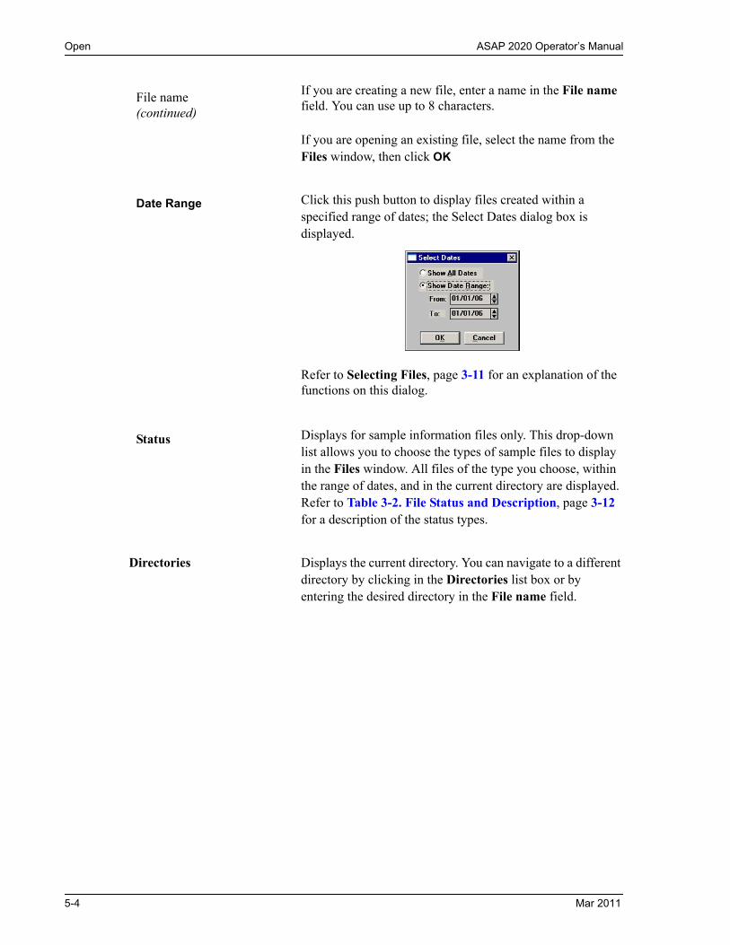
Open ASAP 2020 Operator’s Manual
File name(continued)
If you are creating a new file, enter a name in the File name field. You can use up to 8 characters.
If you are opening an existing file, select the name from the Files window, then click OK
Date Range Click this push button to display files created within a specified range of dates; the Select Dates dialog box is displayed.
Refer to Selecting Files, page 3-11 for an explanation of the functions on this dialog.
Status Displays for sample information files only. This drop-down list allows you to choose the types of sample files to display in the Files window. All files of the type you choose, within the range of dates, and in the current directory are displayed.Refer to Table 3-2. File Status and Description, page 3-12 for a description of the status types.
Directories Displays the current directory. You can navigate to a different directory by clicking in the Directories list box or by entering the desired directory in the File name field.
5-4 Mar 2011
ASAP 2020 Operator’s Manual Open
Sample Information
Sample information files contain information used to control the analysis. Therefore, an analysis cannot proceed until it has been assigned a sample information file. A sample information file consists of the following:
• sample identification• sample tube criteria• analysis conditions• adsorptive properties• report options• collected (after an analysis has been completed) or entered data
Portions of the sample information file can also exist as standalone parameter files. Having these files exist independently allows you to use them as many times as you wish. For example, if you typically use the same analysis conditions for many of your analyses, you can create an analysis conditions file containing the desired conditions. Then when you create your sample file, select that file for your analysis conditions; the values will be copied into the current sample file. After it becomes part of the new sample file, you can edit it as desired. The file from which the values were copied remains intact and ready for the next use.
Sample information files reside in a folder, more commonly referred to as a directory. The more files in a directory, the longer it may take to access a file. Therefore, it is a good practice to limit the number of files in a directory to approximately 200. You may create additional directories as needed.
Sample information files can be created and presented in the Advanced, Basic, or Restricted format.
• AdvancedPresents all parts of the sample information file in a tabbed dialog. Each tab opens its associated dialog, allowing you to edit conditions. You can also switch to the Basic format if desired.
• BasicPresents all parts of the sample information file as a single dialog. This format allows you to quickly create a sample information file using predefined parameter files. You can also switch to the Advanced format if desired.
• RestrictedIdentical to the Basic format except that you cannot switch to the Advanced format for editing; certain functions are also disabled.
Mar 2011 5-5

Open ASAP 2020 Operator’s Manual
Advanced Format
The Advanced format displays all parts of the sample file in a tabbed dialog. This format allows you to customize your sample file, moving easily among the parameters simply by clicking on the tabs; alternatively, you can use Prev and Next. Refer to Advanced Format, page 4-6 for step-by-step instructions for creating a sample information file using the Advanced format.
Sample Contains the description of the current sample file. If this is a new file, this field contains the file description specified in Sample Defaults. The above dialog shows the sample file number because the dollar ($) symbol was included when sample defaults were specified.
You can enter a new description or edit the existing one if desired.
Maximum number of characters: 50
These fields can be edited to display a different label if desired.
5-6 Mar 2011
ASAP 2020 Operator’s Manual Open
OperatorSubmitter
Displays the operator and submitter names of the current sample file.
If this is a new file, these fields contain the names specified in Sample Defaults. You can enter a different name or edit the current one if desired. You can use up to 40 characters.
Either (or both) of these fields can be prevented from displaying on this dialog by selecting Omit in Sample Defaults (Chapter 8). The labels also can be edited in Sample Defaults.
Bar Code This field enables you to enter bar code information. If bar code information is not used, you can use this field to enter additional information about the sample; for example, you may wish to enter the lot number of your sample. This field can also be omitted in Sample Defaults if it is not needed.
This field will also accept data from a bar code reader.
Range: 40 characters
Mass You can enter a sample mass or have the mass calculated automatically.
Enter Enables the Sample Mass field allowing you to enter a value.
Calculate Enables the Empty tube and Sample + tube fields, allow-ing you to enter appropriate values. These values are used to calculate the mass of the sample,
You should always use the same gas (typically nitrogen) for degassing and analysis. If different gases are used, the sample mass after degas and after analysis will not be equal. For example; if you use helium to backfill after degassing and nitrogen after analysis, you can get as much as a 0.02-gram difference.
Masssample Masssample tube+ Masstube–=
Mar 2011 5-7
Open ASAP 2020 Operator’s Manual
Density If you plan to use a calculated free space, enter the sam-ple’s density in this field. A value in this field is ignored for measured or entered free spaces.
Type of Data Displays the type of data for the current sample file.
If this is a new file, choose whether you wish to have data collected automatically or if you plan to enter data col-lected from another source.
User Parameters These fields are used primarily for SPC (Statistical Process Control) reporting. However, they can be used for other data as well. You may wish to enter specific analysis con-ditions or sample criteria. These parameters print on the Options report. Select Options > Sample Defaults to specify the parameters you wish to report. The parameters you specify replace the User Parameter labels.
If desired, you can have these fields omitted from the sam-ple information file (refer to Sample Defaults, page 8-4).
Comments Allows you to enter pertinent information about the sam-ple or analysis. The information you enter in this window is displayed in the report header. You may enter up to 500 characters in this window
Replace All Use this push button to replace all parameters of the cur-rent file with those from an existing one. You can edit the parameters after they have been copied into the current file; editing the current file does not affect the file from which they were copied.
Save Saves all parameters of the current file; the dialog remains open.
Close Closes the dialog. If the file contains unsaved changes, you are prompted to save before the dialog closes.
Basic Switches the sample editor to the Basic format.
5-8 Mar 2011

ASAP 2020 Operator’s Manual Open
Basic Format
The Basic format displays all parts (parameters) of the file on a single dialog. With this format, you can quickly create a sample information file using predefined parameter files. You can also switch to the Advanced format if a specific parameter requires editing. Refer to Basic and Restricted Formats on page 4-8 for step-by-step instructions for creating a sample information file using the Basic format.
If you are creating a new file, this dialog displays the defaults you specified in Sample Defaults. Chapter 8 explains how to establish sample defaults.
Sample Contains the description of the current sample file.
If this is a new file, this field contains the next sequenced file description based on the format specified in Sample Defaults (see Chapter 8). The above dialog box shows the sample file number because the dollar ($) symbol was included when sample defaults were specified.
You can enter a new description or edit the existing one if desired.
Maximum number of characters: 50
Mar 2011 5-9

Open ASAP 2020 Operator’s Manual
Mass You can enter a sample mass or have the mass calculated automatically.
Enter Enables the Sample Mass field allowing you to enter a value.
Calculate Enables the Empty tube and Sample + tube fields, allow-ing you to enter appropriate values. These values are used to calculate the mass of the sample,
Density If you plan to use a calculated free space, enter the sam-ple’s density in this field. A value in this field is ignored for measured or entered free spaces.
Sample TubeDegas ConditionsAnalysis ConditionsAdsorptive PropertiesReport Options
Each parameter field contains the description of the current parameter file.
If this is a new sample file, these fields contain the descriptions of the files chosen as the defaults.
Click on the down arrow to the right of each field to choose a different file. File parameters can be viewed or edited by switching to the Advanced format.
Replace All Use this push button to replace all parameters of the current file with those copied from an existing one. A dialog box is displayed allowing you to choose the desired file.
Save Saves all parameters of the current file; the dialog remains open.
Close Closes the dialog.
Advanced Switches the sample editor to the Advanced format, allowing you to view or edit parameters of the current file.
Masssample Masssample tube+ Masstube–=
5-10 Mar 2011

ASAP 2020 Operator’s Manual Open
Restricted Format
The Restricted format is used when analysis parameters must remain constant. For example, in the pharmaceutical industry where consistency and accuracy are crucial. A password is required to enter and exit this format. Refer to Restricted, page 8-3 for additional information on the Restricted format.
When you open an existing sample information file or create a new one using the Restricted format, all parts of the sample file are displayed in the same manner as the Basic format. Some menu functions, however, are disabled and you cannot switch to the Advanced format to edit file parameters.
Mar 2011 5-11

Open ASAP 2020 Operator’s Manual
Sample Tube
The fields on this dialog are used for storing sample tube information. Before creating a sample tube file, you should perform a blank analysis (no sample) using the sample tube.
Sample Tube Contains the description of the current file.
If this is a new file, this field contains the name (descrip-tion) you specified as the default. You can enter a new description or add to the existing one if desired.
Maximum number of characters: 40
Replace Use this push button to replace the values of the current file with those from an existing Sample Tube file. The Open Sample Tube dialog is displayed, allowing you to choose a file. After the values are copied into the current file, you can edit them as desired.
Warm free space Displays the warm free space used for the blank analysis.
Cold free space Displays the cold free space used for the blank analysis.
Use isothermal jacket Select this option if an isothermal jacket is to be used in the analysis.
Use filler rod Select this option if a filler rod is to be used in the sample tube.
5-12 Mar 2011

ASAP 2020 Operator’s Manual Open
Vacuum seal type If the sample is to be transferred under vacuum to the anal-ysis port, select the seal type to be used. If not, leave None selected.
Load From Sample File Click this push button to choose the sample file that was used in the blank analysis. The values for the Warm and Cold free spaces, and the non-ideality factor will be copied into the sample tube file.
Save Saves all parameters of the current dialog.
Close Closes the dialog box. If the file contains unsaved changes, you are prompted to save before the dialog box closes.
Mar 2011 5-13

Open ASAP 2020 Operator’s Manual
Degas Conditions
The fields on this dialog are used for specifying degas conditions when your ASAP 2020 is equipped with the SmartVac degas option. If you do not have the SmartVac, the values you enter are meaningless.
Description Contains the description of the current Degas Conditions file.
If this is a new file, this field contains the name (descrip-tion) you specified as the default. You can enter a new description or add to the existing one if desired.
Maximum number of characters: 40
Replace Use this push button to replace the parameters of the cur-rent file with those from an existing Degas Conditions file. The Open Degas Conditions File dialog is displayed, allowing you to choose a file. After the values are copied into the current file, you can edit them as desired.
Evacuation Phasegroup box
The options in this group box allow you to specify condi-tions for the evacuation phase of the degassing operation.
Temperature ramp rate
Allows you to specify the rate at which the temperature is to change while advancing to the target temperature during evacuation.
5-14 Mar 2011
ASAP 2020 Operator’s Manual Open
Target temperature Allows you to specify a temperature at which the sample will be held for the remainder of the evacuation.
Evacuation rate Enables you to specify an evacuation rate for initial evacu-ation.
Unrestricted evac.from
Enables you to specify a pressure at which unrestricted sample evacuation will begin.
Vacuum setpoint Enables you to specify the vacuum level to be achieved before evacuation begins.
Evacuation time Enables yo to specify how long the sample is to be evacu-ated prior to the second stage of heating.
Heating Phasegroup box
The options in this group box allow you to specify condi-tions for the heating phase of the degassing operation.
Ramp rate Enables you to specify the rate at which the temperature will change after evacuation while advancing to the hold temperature.
Hold temp Enables you to specify a temperature at which the sample is to be held during degassing.
Hold time Enables you to specify how long the sample is to be held at the specified temperature before beginning to cool down.
Hold Pressure If during the temperature ramp the pressure exceeds the value you enter in this field, the ramp will be suspended until the pressure returns to a safe level.
Backfill Sample Tube Select this option to have the sample tube backfilled. You should deselect this option if you are using the TranSeal; this allows the sample to remain under vacuum while transferring to the analysis port.
Mar 2011 5-15

Open ASAP 2020 Operator’s Manual
Analysis Conditions
The Analysis Conditions dialog allows you to specify the data used to guide the analysis. You can create an Analysis Conditions file as an independent parameter file or include it as part of the sample information file.
Refer to Analysis Conditions, page 4-11 for step-by-step instructions on creating an analysis conditions file.
Save Saves all parameters of the current dialog.
Close Closes the dialog box. If the file contains unsaved changes, you are prompted to save before the dialog box closes.
Description Contains the description of the current Analysis Conditions file.
If this is a new file, this field contains the name you specified as the default. You can enter a new description or add to the existing one if desired.
Maximum number of characters: 40
The ROA group boxand column displayonly if the ROA optionis installed
5-16 Mar 2011
ASAP 2020 Operator’s Manual Open
Replace Use this push button to replace the parameters in the cur-rent file with those from an existing Analysis Conditions file. After you choose the file and the values are copied into the current file, you can edit them in any way desired. Editing in the current file will not change anything in the file from which they were copied.
Collect ROA Data Allows you to collect Rate of Adsorption (ROA) data. When this option is selected, its related fields become enabled. An ROA column is also added to the Pressure table, allowing you to select pressures at which to collect ROA data. See the ROA operator’s manual for additional information.
This group box is displayed only if the ROA option is installed.
Interval Enter a value which represents the length of time from one reading to the next.
Dose amount Enter the amount of gas to be applied.
Max. readings Enter a value which represents the maximum number of readings to record.
Pressures selected Displays the number of pressure points selected for ROA data.
Pressure Table A pressure table is a list of pressure points (with calcula-tion assignments) at which data are to be collected. The pressures may span the entire range from the lowest rela-tive value of 0.00000001 to the maximum value of 0.995 P/Po. (The maximum recommended value for krypton is 0.5 P/Po.) In addition, one saturation point may be entered with relative pressure of 1.0.
Mar 2011 5-17

Open ASAP 2020 Operator’s Manual
Pressure Table(continued)
The minimum absolute pressure for desorption is 0.050 mmHg. For example, if Po = 760 mmHg, a relative pressure less than 0.050 / 760.0 = 0.0000658 will result in an error. The analysis will terminate.
Several analysis conditions files containing complete pres-sure tables are included with the ASAP 2020 software and can be found in the PARAMS subdirectory.
The pressure table for automatically collected data includes the pressure points for data collection and identifies calcula-tions through which the data are processed.
Edit existing values by highlighting the field and entering the desired values. Use Insert to add rows for additional values. To append to the beginning or to the end of the table, use Ctrl + Up Arrow and Ctrl + Down Arrow.
The pressure table must contain one sequence of strictly ascending relative pressures, optionally followed by one sequence of strictly descending relative pressures. You can enter a maximum of one thousand pressure points.
To specify the calculations performed at a given relative pres-sure, click in the field of the desired calculation type; an X in the field indicates the calculation is selected.
Insert Range Displays the Insert Pressure Range dialog box.
This dialog allows you to specify the starting pressure, the ending pressure, the number of points to insert within the specified range, and whether you wish to have linear or geometric progression.
Linear Inserts evenly spaced points into your table.
5-18 Mar 2011

ASAP 2020 Operator’s Manual Open
Geometric from low pressure
Inserts geometrically spaced points from the low pressure range. For example, to insert 5 points with a 0.01 starting pressure and a 0.16 ending pressure, the following points are inserted into the table:
0.010.020.040.080.16
Geometric towards saturation
Inserts geometrically spaced points from the saturation pressure. For example, to insert 5 points with a 0.99 start-ing pressure and a 0.84 ending pressure, the following points are inserted into the table:
0.990.980.960.920.84
Insert predefined Displays the Insert Predefined Pressures dialog.
Choose predefined pressure points for surface area, t-Plot micropore, and/or BJH adsorption/desorption.
Click on the down arrow for each field to choose the desired set of points. You can also specify Adsorption/ Desorption total pore volume and Saturation.
Mar 2011 5-19

Open ASAP 2020 Operator’s Manual
Insert Inserts a row into the table above the selected line.
Delete Deletes the selected row.
Clear Removes all but one required entry from the table. The rows do not have to be selected. A warning message appears requesting confirmation before the table is cleared.
Absolute pressure dosing Select this option to specify pressure targets in mmHg, mbar, or kPa instead of relative pressure. This option is typically selected when using adsorptives at analysis con-ditions above the critical point of the gas; for example, H2 adsorption on carbon at liquid nitrogen temperature.
Use calculation assignments Select this option to assign the points to be collected for each type of report.
If this option is not selected, each report (with the excep-tion of Langmuir and BET) uses a range of pressures as selected in the report options. The Langmuir and BET reports interpolate to entered relative pressures on the report options.
The outlier points can be selected so that they will not be reported.
Preparation Displays the Analysis Preparation dialog box.
5-20 Mar 2011

ASAP 2020 Operator’s Manual Open
Fast evacuation Select this option for samples (such as pellets) that do not fluidize or shed particles during evacuation.
Unrestricted evac. from Enabled when Fast evacuation is not desired. This field allows you to enter the pressure at which unrestricted sam-ple evacuation is to begin.
Vacuum setpoint Allows you to specify the vacuum level to be achieved before timed evacuation begins.
Evacuation time Enables you to enter the length of time for preliminary evacuation, which takes place prior to the free-space mea-surement.
Leak test Enables the system to check for leaks or sample outgassing before the analysis. The leak test allows sample pressure to rise during the test. If the pressure rises more than 0.15 mmHg, the analysis does not proceed and you are notified. While leak testing slightly increases analysis time, it pre-vents the continuation of analysis and collection of errone-ous data if a leak exists.
Leak test duration Enables you to specify how long the pressure is to be mon-itored.
Use TranSeal Select this option if you are using the TranSeal to transfer the sample from the preparation port to the analysis port under vacuum.
Mar 2011 5-21

Open ASAP 2020 Operator’s Manual
Free Space Allows you to specify free-space measurement conditions; the Free Space dialog is displayed.
Measure Select this option to have free space measured automati-cally by the system.
Typically, it is best to measure the free space when analyz-ing macro- and mesoporous samples, and for routine sur-face area measurements.
Select Lower dewar for evacuation to lower the dewar following free-space measurements.
Evacuation time enables you to specify how long evacua-tion is to take place following the measured free space.
Select Outgas test to check for system leaks or sample out-gassing. After free space is measured, the Dewar is low-ered and the sample evacuated for 30 minutes. The leak test is performed after evacuation. If a leak is found, the leak test repeats nine times, with 30 minutes evacuation between tests. If the 10th leak check fails, the analysis stops and you are notified. While leak testing slightly increases analysis time, it prevents the continuation of analysis and collection of erroneous data if a leak occurs.
Outgas test duration indicates the number of seconds the leak test is performed.
5-22 Mar 2011

ASAP 2020 Operator’s Manual Open
Enter Select this option to enter values for the warm and cold free spaces. You may need to use this option if the sample retains helium and measurement of very low micron range pressures are required.
If you change the entered free-space value after the preliminary analysis stage is 50% complete, the change does not affect the analysis.
Warm free space is the sample tube gas capacity measured at room temperature.
Cold free space is the sample tube gas capacity measured with the Dewar raised.
Calculate Select this option to have the free-space calculated using the mass, density, and sample tube parameters entered in the Sample Information and Sample Tube files. Calculated free space measurement takes less time than measured free space, so if you know the mass and density of the sample and the sample tube parameters, you may wish to use this choice of free space methods. If you do not know the parameters, you may wish to use measured free space.
Po and T Displays the Po and Temperature Options dialog box, allowing you to choose saturation pressure and analysis bath temperature. It also provides a field for entering the ambient temperature.
Mar 2011 5-23

Open ASAP 2020 Operator’s Manual
This dialog provides six options for obtaining the satura-tion pressure (Po) and analysis bath temperature. Clicking on each option prompts you for the entry of related param-eters in the lower portion of the dialog box.
Option Prompts for...
1 a measurement interval (how often dur-ing analysis the Po is to be measured)
2 a measurement interval and the analysis bath temperature
3 a Po; the analysis bath temperature is calculated at the time of analysis
4 a Po and analysis bath temperature an analysis bath temperature only (when Absolute pressure dosing is selected on the Analysis conditions dialog)
Displays as Analysis Bath Temperature only when Absolute dosing is selected (Analysis conditions dialog)
5-24 Mar 2011

ASAP 2020 Operator’s Manual Open
5 a psat gas other than the adsorptive; the temperature and pressure ranges for the chosen gas are displayed. Click Psat vs.T to edit the values if desired. Editing the values in the current table do not affect the ones of the original table
6 an analysis bath temperature
Ambient Temperature Enables you to enter the ambient temperature of the labo-ratory to be used in calculations.
Dosing Displays the Dosing Options dialog.
Mar 2011 5-25

Open ASAP 2020 Operator’s Manual
First Pressure Fixed Dose
The most frequent use of this option is when you are per-forming a standard nitrogen analysis of mesoporous mate-rials such as catalysts. If the first pressure table point is low and you expect the gas uptake of the sample to be high, this option can shorten the time required to reach the first point on the pressure table.
The sample is dosed repeatedly at low pressures with a specified amount of gas until the first pressure point is reached. This initial dosing quickly meets the adsorptive demand of the sample.
The first point on the pressure table is the threshold value, triggering the transition from the Fixed Dose Mode to Pressure Table Mode. When the first pressure table value is reached, Fixed Dose Mode is disabled, and points are equilibrated and recorded in accordance with the specified pressure table.
In the field adjacent to this option, enter the amount of gas that is to be added to the sample for each dose cycle.
This option is disabled if Low pressure incremental dose mode is selected.
Maximum volume increment
Select this option to determine when additional data points are collected between target pressures in regions of adsorption. When the maximum increment has been adsorbed since the last collected data point, another point is equilibrated and collected.
During desorption, this field is treated as a maximum vol-ume “decrement” value.
5-26 Mar 2011

ASAP 2020 Operator’s Manual Open
Absolute and Relative pressure tolerance
The values entered in these fields are used to determine how close the actual pressure must be to each target pres-sure from the pressure table. At lower pressures the rela-tive tolerance value is smaller, and at higher pressures the absolute tolerance value is smaller. The lesser (or more stringent) of these two criteria are used to determine the tolerance.
For example, with relative tolerance = 5% and absolute tolerance = 5 mmHg, the relative tolerance at 40 mmHg target pressure is 5% of 40 mmHg, or 2 mmHg; 2 mmHg is smaller than the absolute tolerance of 5 mmHg, so 2 mmHg is used. At 200 mmHg target pressure, the relative tolerance is 5% of 200 mmHg, or 10 mmHg; in this case, the absolute tolerance of 5 mmHg is smaller and is used.
In the above example, a minimum pressure of 40 - 2 = 38 mmHg must be attained to collect data for a target pressure of 40 mmHg. For a target of 200 mmHg, 200 - 5 = 195 mmHg must be attained.
Normally, surface area measurement points are widely spaced, and the resulting measurement is not very sensi-tive to the precise location of points so wider tolerances may be used. Unnecessarily tight tolerances lengthen the analysis.
Low pressure incrementaldose mode
Enabled only if the MicroPore option is installed. Choose this option when you are performing an analysis of micro-porous materials. At low pressures on Type 1 isotherms, the pressure points are very closely spaced, making a use-ful pressure table difficult to define. Choosing this mode enables you to measure equilibrium points at approxi-mately equal intervals on the quantity adsorbed axis. Each dose is fully equilibrated and recorded as a data point.
Mar 2011 5-27

Open ASAP 2020 Operator’s Manual
Low pressure incrementaldose mode(continued)
In this mode, the sample is successively dosed with a spec-ified amount of gas until the first pressure point is reached. The first point is the threshold value, triggering the transi-tion from Incremental Dose Mode to Pressure Table Mode. When the first pressure table value is reached, Incremental Dose Mode is disabled, and points are recorded in accor-dance with the specified pressure table. Because the data points recorded during Incremental Dose Mode may define most of the analysis, one point on the pressure table can be sufficient and serve as the end point for the analysis.
This field is disabled if First Pressure Fixed Dose Mode is selected.
Dose amount Enter the amount of gas to be added to the sample for each data point until the first point on the pressure table is reached.
Enabled when Low pressure incremental dose mode is selected.
Equilibration delay Enabled when Low pressure incremental dose mode is selected.
Minimum: Prevents premature equilibration caused by reduced percentage sensitivity to pressure changes at the lowest pressures.
Maximum: Prevents the effects of long term temperature or pressure drift, which may cause the instrument to wait an excessive length of time for equilibration.
5-28 Mar 2011

ASAP 2020 Operator’s Manual Open
Equilibration Displays the Equilibration dialog.
Equilibration interval
The number of seconds between successive pressure read-ings during equilibration. Long equilibration intervals tend to lengthen analyses, however, they do improve data integ-rity. Short equilibration intervals produce a faster analysis but may reduce the accuracy of data.
Minimum equilibration delay at P/Po> = 0.995
The value entered in this field determines the minimum number of seconds required before equilibration can occur for a relative pressure greater than or equal to 0.995.
This field does not display if you select Absolute pressure dosing on the analysis conditions dialog.
Does not display when Absolute dosing is selected.
Mar 2011 5-29
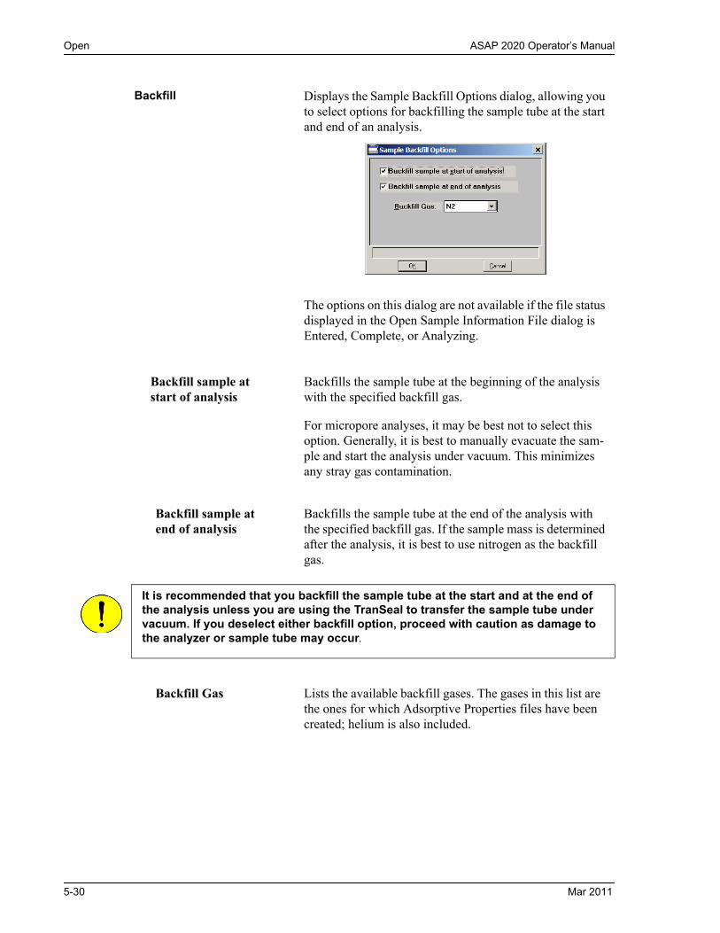
Open ASAP 2020 Operator’s Manual
Backfill Displays the Sample Backfill Options dialog, allowing you to select options for backfilling the sample tube at the start and end of an analysis.
The options on this dialog are not available if the file status displayed in the Open Sample Information File dialog is Entered, Complete, or Analyzing.
Backfill sample at start of analysis
Backfills the sample tube at the beginning of the analysis with the specified backfill gas.
For micropore analyses, it may be best not to select this option. Generally, it is best to manually evacuate the sam-ple and start the analysis under vacuum. This minimizes any stray gas contamination.
Backfill sample at end of analysis
Backfills the sample tube at the end of the analysis with the specified backfill gas. If the sample mass is determined after the analysis, it is best to use nitrogen as the backfill gas.
It is recommended that you backfill the sample tube at the start and at the end of the analysis unless you are using the TranSeal to transfer the sample tube under vacuum. If you deselect either backfill option, proceed with caution as damage to the analyzer or sample tube may occur.
Backfill Gas Lists the available backfill gases. The gases in this list are the ones for which Adsorptive Properties files have been created; helium is also included.
5-30 Mar 2011

ASAP 2020 Operator’s Manual Open
Adsorptive Properties
This dialog allows you to specify the characteristics of the gases used in the ASAP 2020 system. An Adsorptive Properties file can be created as an independent parameter file or included as part of the sample information file.
Refer to Adsorptive Properties, page 4-13 for step-by-step instructions on creating adsorptive properties files.
Adsorptive If this is a new file, this field contains either the name of the default adsorptive gas or is blank. Enter the name of the desired adsorptive gas.
Maximum number of characters: 40 alphanumeric
Replace Click this push button to choose an Adsorptive Properties file containing parameters you wish to copy and use in the current file. After the values have been copied into the file, you can edit them as desired. It does not affect the values of the file from which they were copied.
Mnemonic The mnemonic for the adsorptive gas.
Maximum number of characters: 5 alphanumeric
Mar 2011 5-31

Open ASAP 2020 Operator’s Manual
Non-condensing Adsorptive
Select this option if this file is for a non-condensing gas (adsorptive). When you select this option, the Density conversion factor field and the Psat vs. T push button become disabled.
Maximum manifold pressure
The maximum gas pressure allowed in the manifold.
Density conversion factor
This value is used to convert the gas volume at STP to liq-uid volume for the adsorptive. It is the ratio of gas density at STP to liquid density.
Therm. tran. hard-sphere diameter
The thermal transpiration hard-sphere diameter.
Molecular cross-sectional area
The molecular cross-sectional area.
Dosing Method Select the manner in which the sample tube is dosed. Select Normal for gases under pressure.
Select From Psat tube for krypton analyses.
Select Vapor source for vapors. Vapor source is disabled if the maximum manifold pressure is greater than 800.00 mmHg.
Real gas equation of state This radio button and the one below it let you choose how to account for non-ideal behavior of the adsorptive.
The real gas equation of state (EoS) calculations correct for non-ideal behavior at all pressures and temperatures. There are some adsorptives (like butane) that are signifi-cantly non-ideal even at the pressures used in the 2020. The real EoS calculations are necessary for analyses with these gases. But even for nitrogen, these calculations pro-vide some improvement. Tables containing compressibil-ity factors for several gases are installed with the ASAP 2020 software. Click Open to choose a table.
5-32 Mar 2011

ASAP 2020 Operator’s Manual Open
Real gas equation of state(continued)
The real EoS should be used whenever a table for the adsorptive is present. The gases included in the tables are: argon, carbon dioxide, carbon monoxide, ethane, ethylene, helium, hexane, hydrogen, isobutane, krypton, methane, nitrous oxide, n-butane, neon, ammonia, nitrogen, oxygen, pentane, propane, propene, sulfur hexaflouride, and xenon.
You can use the Save button to save the table under a dif-ferent name.
Adsorbed-phase free-space correction
This option is appropriate for all sample analyses that use the real gas equation of state. Adsorbed molecules occupy volume in the sample tube reducing the cold free space. If you select this option, the reported quantity adsorbed will be adjusted to correct for this effect. This check box should be deselected for blank tube analyses.
Ideal gas law with non-ideality correction
The non-ideality correction can be used if there is no com-pressibility table for the gas you are using or if you want to match existing data.
This factor adjusts the ideal gas law for calculating the quantity of gas in the cold free space. Most gases are nearly ideal near room temperature and at pressures not much above atmospheric pressure, so the cold free space is where the correction is most important. If you choose this option, enter the Non-ideality factor.
Mar 2011 5-33
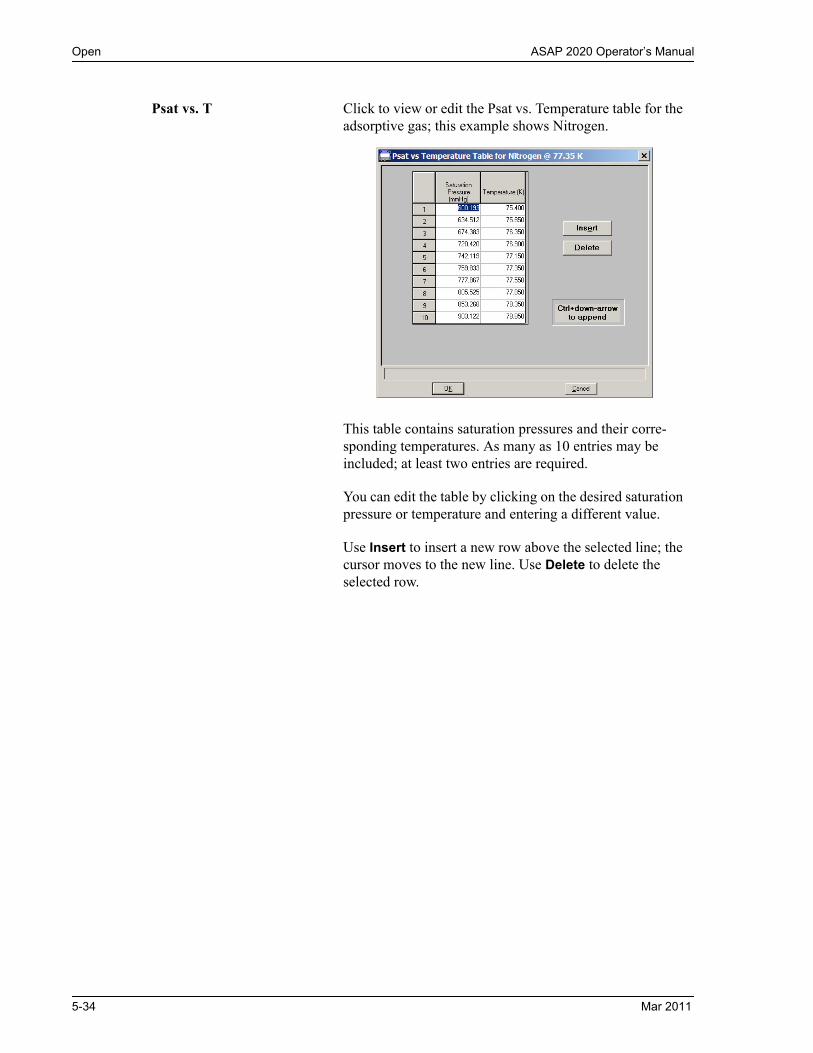
Open ASAP 2020 Operator’s Manual
Psat vs. T Click to view or edit the Psat vs. Temperature table for the adsorptive gas; this example shows Nitrogen.
This table contains saturation pressures and their corre-sponding temperatures. As many as 10 entries may be included; at least two entries are required.
You can edit the table by clicking on the desired saturation pressure or temperature and entering a different value.
Use Insert to insert a new row above the selected line; the cursor moves to the new line. Use Delete to delete the selected row.
5-34 Mar 2011

ASAP 2020 Operator’s Manual Open
Report Options
This dialog allows you to specify report options. A report options file can be created as an independent parameter file or included as part of the sample information file.
Refer to Report Options on page 4-14 for instructions on creating report options files.
Description Displays a description of the current Report Options file.
If this is a new file, this field contains the description you specified as the default. You can enter a new description or add to the existing one if desired.
Maximum number of characters: 40
Replace Click this push button to choose an existing Report Options file containing parameters you wish to copy and use in the current file. After the values have been copied into the file, you can edit them as desired. It does not affect the values of the file from which they were copied.
Show report title This option allows you to enter a title for your report.
If this is a new file, the title you specified as the default is displayed. Accept the default title or enter a different one.
Deselect this option to omit the report title.
Range: 40 characters
Mar 2011 5-35

Open ASAP 2020 Operator’s Manual
Show graphic Select this option to have a graphic display above the report title.
The graphic can be in a bitmap (bmp) or an enhanced metafile (emf) format. For example, you may wish to dis-play your company logo.
Click Browse to choose the graphic, then use the height and width fields to specify the size. The image can also be edited from the report window.
Overlays Displays the Graph Overlay Samples dialog so that you can choose the sample files containing the data you wish to overlay onto a selected plot.
Click Browse to the right of the sample number field to choose the desired file. Use Clear to clear a field of its entry. You can select up to eight files.
After choosing the desired files, select the Overlay sam-ples option for each report type you plan to overlay.
Edit Allows you to edit parameters of the selected report. This push button is disabled for the Options report.
5-36 Mar 2011

ASAP 2020 Operator’s Manual Open
Thermal transpiration cor-rection
Select this option to correct for the temperature-induced pressure difference between the manifold and the chilled sample tube. This option is most significant for pressures less than approximately 1.0 mmHg. Never use filler rods in the sample tube when applying correction for thermal transpiration.
You should always use thermal transpiration when per-forming micropore analyses.
Inside diameter of sample tube
Enabled when you select Thermal transpiration correc-tion, so that you may enter the inside diameter of the sam-ple tube.
Selected Reports Contains a list of available reports. Choose reports by dou-ble-clicking on the desired reports. Alternatively, you can highlight the desired report and press the Spacebar. A report is selected when it is preceded with a check mark. You may deselect reports in the same manner.
The following reports are available:
SummaryIsothermBET Surface AreaLangmuir Surface AreaFreundlichTemkin t-PlotAlpha-S Methodf-Ratio MethodBJH Adsorption BJH DesorptionDollimore-Heal AdsorptionDollimore-Heal DesorptionHorvath-Kawazoe DFT Pore SizeDFT Surface EnergyDubininMP-MethodOptionsSample LogValidation
You can find printed examples of some reports in Chapter 7, beginning on page 7-27.
Mar 2011 5-37

Open ASAP 2020 Operator’s Manual
Summary Report
The Summary report provides a condensed listing of analysis statistics and data results. The Summary Report Options dialog allows you to choose the type of information to include in the report.
The choices on this dialog allow you to choose the types of data to include in the Summary report.
If you choose Adsorption or Desorption total for Pore Volume data, the P/Po field is enabled so that you can enter the relative pressure at which to calculate the total pore volume. If Use calculation assignments (Collected Data screen) is not selected, the isotherm is interpolated to this value and that point used for the Total pore volume calculation. Otherwise, the point selected with calculation assignment is used.
This dialog also enables you to specify Pass/Fail criteria for up to four parameters.
Select All Selects all choices on the dialog.
Deselect All Deselects all choices on the dialog.
Pass/Fail Selection Displays the parameter you selected on the Pass/Fail Options dialog.
5-38 Mar 2011

ASAP 2020 Operator’s Manual Open
Pass/Fail Displays the Pass/Fail Options dialog so that you can choose a parameter on which to specify pass/fail criteria.
Upper/Lower Select these options to specify upper and lower limits for the selected parameter; a valid range for the selected field is displayed in the information bar.
You can leave the range open by deselecting one of the limits. For example; if you wish to leave the upper limit open, deselect the Upper check box and specify a value only for the Lower limit.
Each of these fields has a message line in which you can enter advice to the operator if a failure occurs. You may enter up to 120 characters in each field.
Mar 2011 5-39

Open ASAP 2020 Operator’s Manual
Isotherm Report Options
The isotherm report indicates adsorption (up to saturation pressure) and desorption (down from saturation pressure) of a gas by a solid held at constant temperature.
Select Reports Lists the types of reports offered.
Choices: Tabular Report, Linear plot, Logarithmic plot, Linear Absolute plot, Logarithmic Absolute plot, Pressure Composition plot
When you select Pressure Composition plot, the Adsor-bate Molecular Weight field is enabled so that you can enter a value for the adsorbate. This plot is useful for plot-ting pressure as a function of Weight % adsorbed; for example, H2 adsorbed on carbon.
Options Displays the related Plot Options dialog; this example shows the dialog for the Linear plot.
All plot dialogs contain the same options.
5-40 Mar 2011

ASAP 2020 Operator’s Manual Open
Options (continued)
You can plot the graphs as a curve, points, or both.
Select Overlay samples to overlay data from the current plot with data from other samples. The other sample files are selected by clicking Overlays on the Report Options dialog.
Autoscale options enable you to have the X- and/or Y-axes automatically scaled.
Linear X-axes begin at zero, and logarithmic X-axes begin at an appropriate value. Y-axes begin at zero. The system uses the highest values collected during analysis as the ending points for axes ranges.
If you choose not to autoscale data, the From and To fields are enabled, allowing you to specify a range. Data col-lected outside these ranges are not included in the plot.
The value entered in the To field must be greater than the value entered in the From field.
The X-axis fields show the relative pressure.The Y-axis fields show the quantity of gas adsorbed
Tabular Options Enables you to have Run Time and/or Time Between Points reported. Run time reports the time elapsed from the beginning of the analysis to the finish. Time between points reports the time relapsed between each point.
Also enables you to report Weight % when plotting pres-sure composition.
Plot Options Enables you to choose the type of isotherm you wish to plot. You can plot the adsorption and/or the desorption iso-therm.
Volume Adsorbed Enables you to choose the manner in which the volume adsorbed is reported. These data are reported by default as
Per Gram (cm3/g). However, you can choose to report
data Per BET Surface Area (cm3/m2) or Per Other Sur-
face Area (m2/g). If the latter field is selected, a field is enabled allowing you to enter a value.
Mar 2011 5-41

Open ASAP 2020 Operator’s Manual
BET/Langmuir Surface Area Report Options
• The BET calculation obtains the sample surface area value by determining the monolayer volume of adsorbed gas from the isotherm data.
• The Langmuir calculation determines the surface area of a sample by relating the surface area to the volume of gas adsorbed as a monolayer.
Weight The Adsorbate Molecular Weight field is enabled when you choose Pressure Composition plot, allowing you to enter the molecular weight of the adsorbate.
Displays as LangmuirSurface Area Report Optionsif the Langmuir report is being edited.
The Langmuir and BET Surface Area dialogs include the same fields; the operating instructions for both are the same.
Tabular report Select this option to have a tabular report of the plotted data.
BET transform plot Generates a traditional BET (Langmuir) surface area plot that is used to determine monolayer volume and BET C constant.
5-42 Mar 2011

ASAP 2020 Operator’s Manual Open
BET Isotherm plot Uses the BET (Langmuir) monolayer volume and constant to produce an isotherm.
Overlay samples Allows you to overlay data of the selected type from the current plot with data from other samples. The other sam-ples are selected by clicking Overlays on the main Report Options screen.
Autoscale x-axis Autoscale y-axis
Select these options to have the X- and/or Y-axes scaled automatically.
Both X- and Y-axes begin at zero; the system uses the highest values collected during analysis as the ending points. If you choose not to autoscale data, the From and To fields are enabled, allowing you to enter the ranges.
From/To fields Enabled when you choose not to autoscale data (deselect the Autoscale option), allowing you to specify the begin-ning and ending ranges of the X- and/or Y-axis. Data col-lected outside these ranges are not included in the plot. The values entered in the To field must be greater than the value entered in the From field.
The X-Axis Range fields show the relative pressure. The Y-Axis Range fields show the quantity of gas adsorbed.
Mar 2011 5-43

Open ASAP 2020 Operator’s Manual
Pressures Displays the Report Pressure Table dialog so that you may edit or enter relative pressure points
If Use calculation assignments is not selected on the Col-lected/Entered dialog, the isotherm is interpolated to these pressure points, and those interpolated values are used in the BET calculations.
If Use calculation assignments is selected, the collected data are used.
Insert predefined Displays the Surface Area Report Pressure Selection dia-log, allowing you to select predefined points.
Choices: 1 Point, 3 Point, 5 Point, 5 Point Low Pressure
Insert Inserts a row into the table above the selected line.
Delete Deletes the selected row.
Clear Removes all but one entry from the table; one entry is required. The rows do not have to be selected. A warning message requesting confirmation is displayed before the table is cleared.
5-44 Mar 2011
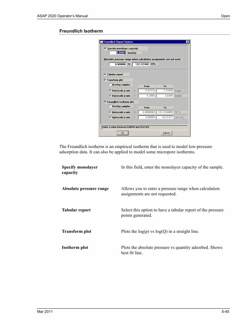
ASAP 2020 Operator’s Manual Open
Freundlich Isotherm
The Freundlich isotherm is an empirical isotherm that is used to model low-pressure adsorption data. It can also be applied to model some micropore isotherms.
Specify monolayer capacity
In this field, enter the monolayer capacity of the sample.
Absolute pressure range Allows you to enter a pressure range when calculation assignments are not requested.
Tabular report Select this option to have a tabular report of the pressure points generated.
Transform plot Plots the log(p) vs log(Q) in a straight line.
Isotherm plot Plots the absolute pressure vs quantity adsorbed. Shows best fit line.
Mar 2011 5-45

Open ASAP 2020 Operator’s Manual
Overlay samples Choose this option to overlay Freundlich isotherm data from the current file with the same type of data from other samples (files). The desired files are chosen by clicking Overlays on the Report Options dialog.
Autoscale x-axisAutoscale y-axis
Select these options to have the X- and/or Y-axis scaled automatically.
Both X- and Y-axes begin at zero; the system uses the highest values collected during analysis as the ending points.
If you choose not to autoscale data, the From and To fields are enabled, allowing you to enter the ranges.
The X-axis shows the log of absolute pressure and the Y-axis shows the quantity of gas adsorbed.
From/To fields Enabled when you choose not to autoscale data (deselect the Autoscale option), allowing you to specify the begin-ning and ending ranges of the X- and/or Y-axis. Data col-lected outside these ranges are not included in the plot.
5-46 Mar 2011
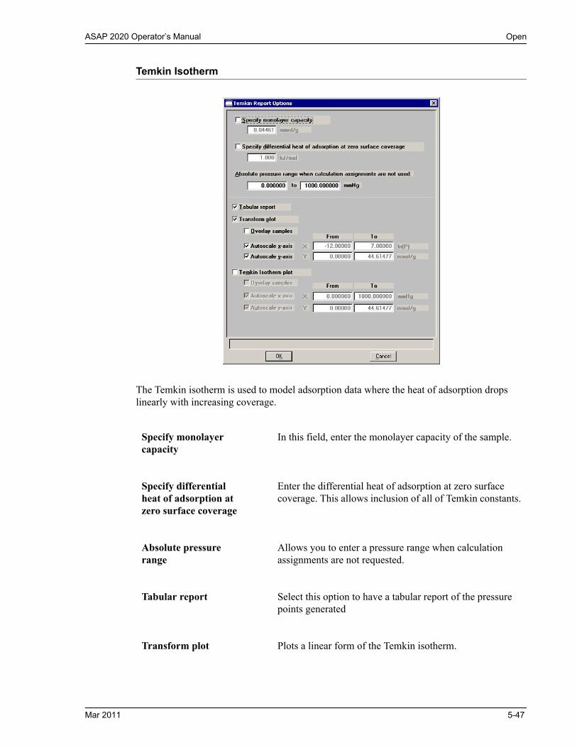
ASAP 2020 Operator’s Manual Open
Temkin Isotherm
The Temkin isotherm is used to model adsorption data where the heat of adsorption drops linearly with increasing coverage.
Specify monolayer capacity
In this field, enter the monolayer capacity of the sample.
Specify differential heat of adsorption atzero surface coverage
Enter the differential heat of adsorption at zero surface coverage. This allows inclusion of all of Temkin constants.
Absolute pressure range
Allows you to enter a pressure range when calculation assignments are not requested.
Tabular report Select this option to have a tabular report of the pressure points generated
Transform plot Plots a linear form of the Temkin isotherm.
Mar 2011 5-47

Open ASAP 2020 Operator’s Manual
Temkin Isotherm plot Overlays the Temkin isotherm with the analysis data.
Overlay samples Choose this option to overlay Temkin isotherm data from the current file with the same type of data from other sam-ples (files). The desired files are chosen by selecting Over-lays on the Report Options dialog.
Autoscale x-axisAutoscale y-axis
Select these options to have the X- and/or Y-axis scaled automatically.
Both X- and Y-axes begin at zero; the system uses the highest values collected during analysis as the ending points.
The X-axis shows the natural log of absolute pressure and the Y-axis shows the quantity of gas adsorbed.
If you choose not to autoscale data, the From and To fields are enabled, allowing you to enter the ranges.
From/To fields Enabled when you choose not to autoscale data (deselect the Autoscale option), allowing you to specify the begin-ning and ending ranges of the X- and/or Y-axis. Data col-lected outside these ranges are not included in the plot.
5-48 Mar 2011

ASAP 2020 Operator’s Manual Open
t-Plot Report Options
The t-Plot calculation allows quantitative analysis of the area and total volume ascribed to micropores. Matrix area, the area external to micropores, is directly determined and often proves to be a valuable way of characterizing complex mixed materials.
Thickness Curve Presents the type of thickness curves available.
• Reference• Kruk-Jaroniec-Sayari• Halsey• Harkins and Jura• Broekhoff-de Boer• Carbon Black STSA
You can also apply the Frenkel-Halsey-Hill thickness curve using the Halsey option, and entering the appropri-ate values in the equation. Use Edit to edit the values in the equation.
Edit Displays the equation for the type of thickness curve selected so that you may view or edit the values.
Mar 2011 5-49

Open ASAP 2020 Operator’s Manual
Reference Displays the Entered t-Curve dialog allowing you to define a t-curve by entering the relative pressure and thickness values.
This table can also be created in another application if desired and imported into this dialog using Open. When creating the table in another application, the file must be saved as ASCII text with a. THK extension. Use a two-col-umn format with the relative pressures in the first column and the thickness values in the second column. Columns must be separated by a space (or a tab).
InsertInserts a row above the selected row. A row cannot be inserted if the value in the selected row is at its lowest value; values must be strictly increasing. For example, in the table shown above the default value is 0.000000001. Therefore, you must use Ctrl + Down Arrow to insert rows.
Enables you to save the current table of values under a dif-ferent name.
5-50 Mar 2011
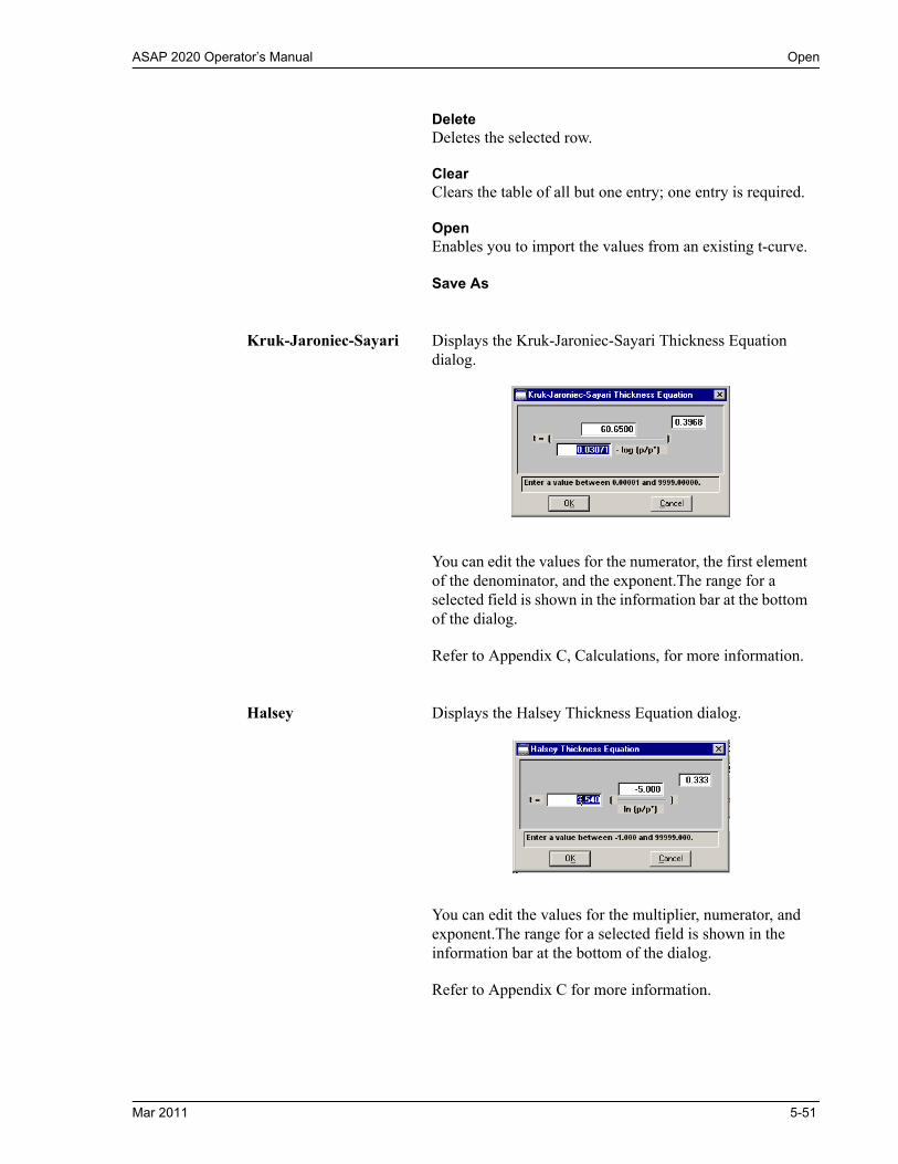
ASAP 2020 Operator’s Manual Open
DeleteDeletes the selected row.
ClearClears the table of all but one entry; one entry is required.
OpenEnables you to import the values from an existing t-curve.
Save As
Kruk-Jaroniec-Sayari Displays the Kruk-Jaroniec-Sayari Thickness Equation dialog.
You can edit the values for the numerator, the first element of the denominator, and the exponent.The range for a selected field is shown in the information bar at the bottom of the dialog.
Refer to Appendix C, Calculations, for more information.
Halsey Displays the Halsey Thickness Equation dialog.
You can edit the values for the multiplier, numerator, and exponent.The range for a selected field is shown in the information bar at the bottom of the dialog.
Refer to Appendix C for more information.
Mar 2011 5-51
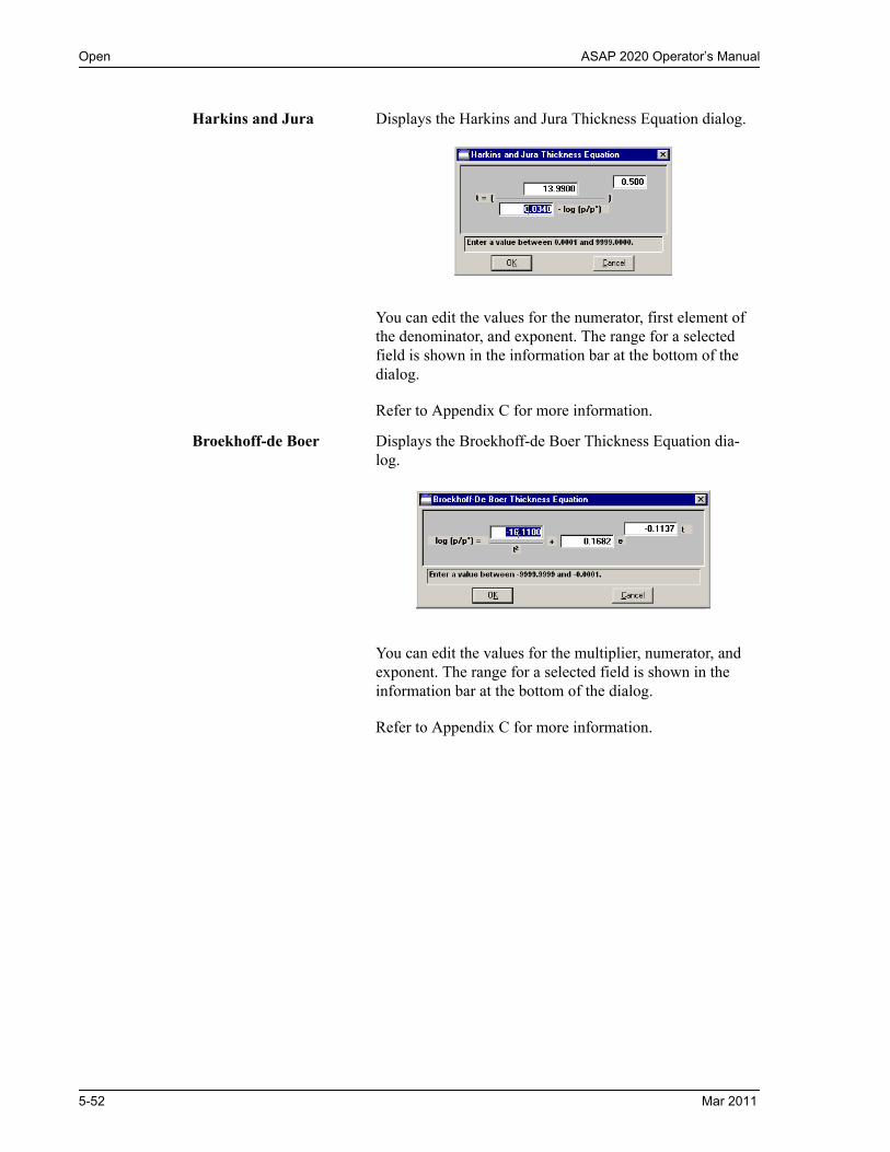
Open ASAP 2020 Operator’s Manual
Harkins and Jura Displays the Harkins and Jura Thickness Equation dialog.
You can edit the values for the numerator, first element of the denominator, and exponent. The range for a selected field is shown in the information bar at the bottom of the dialog.
Refer to Appendix C for more information.
Broekhoff-de Boer Displays the Broekhoff-de Boer Thickness Equation dia-log.
You can edit the values for the multiplier, numerator, and exponent. The range for a selected field is shown in the information bar at the bottom of the dialog.
Refer to Appendix C for more information.
5-52 Mar 2011

ASAP 2020 Operator’s Manual Open
Carbon Black STSA Displays the STSA Thickness Equation dialog.
All coefficients can be edited. The range for a selected field is shown in the information bar at the bottom of the dialog.
Refer to Appendix C for more information.
Surface Area group box Allows you to choose the surface area value used for thick-ness calculations. You can use BET (most commonly used), Langmuir, or enter one of preference.
Pressure Range Displays the Report Relative Pressure Range dialog so that you may specify minimum and maximum relative pres-sures to use with this report.
• If Use calculation assignments is not selected on the Collected/Entered dialog, all of the nonoutlier points of the collected data within the specified range are used for calculating the data for this report.
• If Use calculation assignments is selected, collected data points which are assigned to this report type are used.
Mar 2011 5-53

Open ASAP 2020 Operator’s Manual
Surface area correction factor
This value corrects for surface areas that are not smooth and brings the values for BET surface area and micropore surface area into accordance. For most samples, the default value of 1.000 is adequate.
Fitted Thickness Range Provides two fields, allowing you to enter the minimum and maximum thicknesses you wish to include in the thickness curve.
Tabular report Select this option to generate a table of collected data.
t-Plot Select this option to generate a graphical representation of the collected data.
Overlay samples Allows you to overlay data from the current sample file with data from other sample files. The other sample files are chosen by clicking Overlays on the main Report Options screen.
Autoscale x-axis Autoscale y-axis
Select these options to have the X- and/or Y-axes scaled automatically.
Both X- and Y-axes begin at zero; the system uses the highest values collected during analysis as the ending points.
If you choose not to autoscale data, the From and To fields are enabled, allowing you to enter the ranges.
From/To fields Enabled when you choose not to autoscale data (deselect the Autoscale option), allowing you to specify the begin-ning and ending ranges of the X- and/or Y-axis.
Data collected outside these ranges are not included in the plot.
The X-Axis Range fields show the relative pressure.
The Y-Axis Range fields show the quantity of gas adsorbed
5-54 Mar 2011
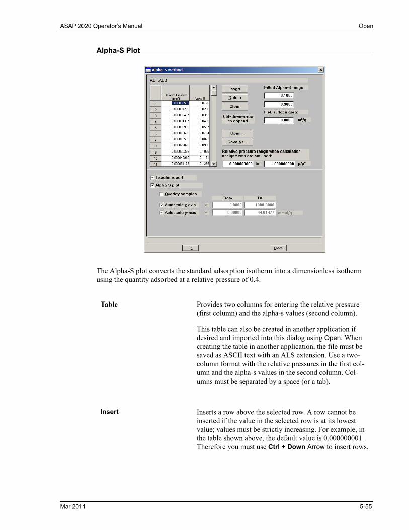
ASAP 2020 Operator’s Manual Open
Alpha-S Plot
The Alpha-S plot converts the standard adsorption isotherm into a dimensionless isotherm using the quantity adsorbed at a relative pressure of 0.4.
Table Provides two columns for entering the relative pressure (first column) and the alpha-s values (second column).
This table can also be created in another application if desired and imported into this dialog using Open. When creating the table in another application, the file must be saved as ASCII text with an ALS extension. Use a two-column format with the relative pressures in the first col-umn and the alpha-s values in the second column. Col-umns must be separated by a space (or a tab).
Insert Inserts a row above the selected row. A row cannot be inserted if the value in the selected row is at its lowest value; values must be strictly increasing. For example, in the table shown above, the default value is 0.000000001. Therefore you must use Ctrl + Down Arrow to insert rows.
Mar 2011 5-55

Open ASAP 2020 Operator’s Manual
Delete Deletes the selected row.
Clear Clears the table of all but one entry; one entry is required.
Open Allows you to import the values from an existing alpha-s curve (ALS) into the table. One predefined curve is shipped with the analysis program. After the values are copied into the table, you may edit them if desired. Editing these values will not affect the file from which they were copied.
Save As Enables you to save the current table of values under a file name.
Fitted Alpha-S range Provides two fields for entering the minimum and maxi-mum relative pressures from which the fit will be deter-mined.
Ref. surface area Enables you to enter the surface area from the reference curve. This value is used to calculate the sample surface area.
Relative pressure range Provides two fields for entering a pressure range when cal-culation assignments are not used.
Tabular report Select this option to generate collected data in a tabular manner.
Alpha-S plot Select this option to generate collected data graphically.
Overlay samples Allows you to overlay data from the current sample file with data from other sample file(s). The other sample file(s) are chosen by clicking Overlays on the main Report Options screen.
5-56 Mar 2011

ASAP 2020 Operator’s Manual Open
Autoscale x-axis Autoscale y-axis
Select these options to have the X- and/or Y-axes scaled automatically.
Both X- and Y-axes begin at zero; the system uses the highest values collected during analysis as the ending points.
If you choose not to autoscale data, the From and To fields are enabled, allowing you to enter the ranges.
From/To fields Enabled when you choose not to autoscale data (deselect the Autoscale option), allowing you to specify the begin-ning and ending ranges of the X- and/or Y-axis.
Data collected outside these ranges are not included in the plot.
The X-Axis Range fields show the relative pressure.
The Y-Axis Range fields show the quantity of gas adsorbed.
Mar 2011 5-57

Open ASAP 2020 Operator’s Manual
f-Ratio Plot
The f-Ratio report allows you to take the measured isotherm and normalize it using a reference isotherm.
Reference Isotherm Displays the sample file you choose as a reference. You should always choose a file containing an isotherm mea-sured from a non-porous sample of the same material as the current sample.
Browse Click to choose the sample file you wish to use as a refer-ence for the isotherm.
Relative pressure range Allows you to enter a pressure range when calculations assignments are not used.
Tabular report Choose this option to have a tabular report generated The tabular report contains four columns: relative pressure, quantity adsorbed for the isotherm of interest, quantity adsorbed for the reference isotherm, and the ratio of the quantities adsorbed.
f-Plot Choose this option to have the data plotted as a graph.
5-58 Mar 2011
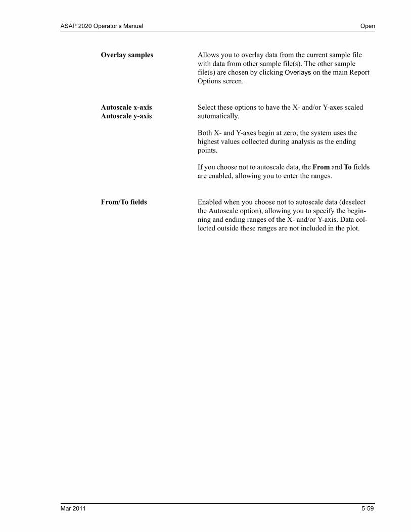
ASAP 2020 Operator’s Manual Open
Overlay samples Allows you to overlay data from the current sample file with data from other sample file(s). The other sample file(s) are chosen by clicking Overlays on the main Report Options screen.
Autoscale x-axis Autoscale y-axis
Select these options to have the X- and/or Y-axes scaled automatically.
Both X- and Y-axes begin at zero; the system uses the highest values collected during analysis as the ending points.
If you choose not to autoscale data, the From and To fields are enabled, allowing you to enter the ranges.
From/To fields Enabled when you choose not to autoscale data (deselect the Autoscale option), allowing you to specify the begin-ning and ending ranges of the X- and/or Y-axis. Data col-lected outside these ranges are not included in the plot.
Mar 2011 5-59

Open ASAP 2020 Operator’s Manual
BJH Adsorption/Desorption Report Options
The BJH calculation determines the mesopore volume/area distribution which accounts for both the change in adsorbate layer thickness and the liquid condensed in pore cores. You can generate BJH reports from adsorption and desorption data.
This field does not display on the BJH Desorption dialog
The BJH Adsorption and Desorption dialogs include the same fields; the operating instructions for both are the same.
Thickness Curve Type Presents the type of thickness curves available.
• Reference• Kruk-Jaroniec-Sayari• Halsey• Harkins-Jura• Broekhoff-de Boer• Carbon Black STSA (ASTM D-6556-0lA)
You can also apply the Frenkel-Halsey-Hill thickness curve using the Halsey option, and entering the appropriate values in the equation. Use Edit to edit the values in the equation. Halsey is the default thickness curve and typically is used for BJH calculations.
5-60 Mar 2011

ASAP 2020 Operator’s Manual Open
If you select a thickness curve which is not a good match for the sample being analyzed, an incomplete pore distribution may be generated.
Edit Displays the equation for the type of thickness curve selected.
Refer to t-Plot Report Options, page 5-49 for information on the equations for thickness curves.
Minimum/Maximum BJH Provides fields for entering the minimum and maximum size pore to be included in BJH reports.
The size can be reported in width (default), radius, or diameter. Select Options > Units to specify the desired unit.
Fraction of pores open at both ends
(not displayed on desorption dialog)
During calculations, the software assumes that all pores are closed at one end. Sometimes a percentage of pores may be open at both ends, causing disagreement in the adsorption and desorption data or in the values for total volume and total BJH pore volume. Enter a value in this field to compensate for this error.
This field does not display on the BJH Desorption Report Options dialog.
Due to normal hysteresis, data may disagree even after applying this corrective factor.
Mar 2011 5-61

Open ASAP 2020 Operator’s Manual
Adsorptive Displays the BJH Adsorptive Options dialog, allowing you to specify up to ten adsorptive/adsorbate property factor combinations.
The recommended adsorptives and their values are shown. You may specify up to six additional adsorptive/adsorbate property factor combinations.
The adsorbate property factor is the combination of con-stants in the numerator of the BJH equation which is spe-cific to the type of gas used. Adsorbate property factors may be specified in angstroms or nanometers. Select Options > Data Presentation > Units to specify desired units.
Smooth differentials Smooths all of the differential calculations, eliminating variations in the differential computation caused by noise in the input data.
Cumulative Reports Select Larger to report the total volume found in pores larger than the current pore size. This is the traditional way in which BJH data are displayed.
Select Smaller to report the total volume found in pores smaller than the current pore size.
5-62 Mar 2011
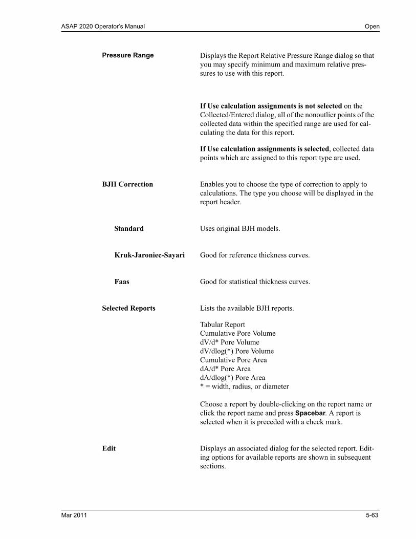
ASAP 2020 Operator’s Manual Open
Pressure Range Displays the Report Relative Pressure Range dialog so that you may specify minimum and maximum relative pres-sures to use with this report.
If Use calculation assignments is not selected on the Collected/Entered dialog, all of the nonoutlier points of the collected data within the specified range are used for cal-culating the data for this report.
If Use calculation assignments is selected, collected data points which are assigned to this report type are used.
BJH Correction Enables you to choose the type of correction to apply to calculations. The type you choose will be displayed in the report header.
Standard Uses original BJH models.
Kruk-Jaroniec-Sayari Good for reference thickness curves.
Faas Good for statistical thickness curves.
Selected Reports Lists the available BJH reports.
Tabular Report Cumulative Pore VolumedV/d* Pore VolumedV/dlog(*) Pore VolumeCumulative Pore AreadA/d* Pore AreadA/dlog(*) Pore Area* = width, radius, or diameter
Choose a report by double-clicking on the report name or click the report name and press Spacebar. A report is selected when it is preceded with a check mark.
Edit Displays an associated dialog for the selected report. Edit-ing options for available reports are shown in subsequent sections.
Mar 2011 5-63
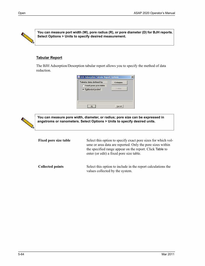
Open ASAP 2020 Operator’s Manual
Tabular Report
The BJH Adsorption/Desorption tabular report allows you to specify the method of data reduction.
You can measure port width (W), pore radius (R), or pore diameter (D) for BJH reports. Select Options > Units to specify desired measurement.
You can measure pore width, diameter, or radius; pore size can be expressed in angstroms or nanometers. Select Options > Units to specify desired units.
Fixed pore size table Select this option to specify exact pore sizes for which vol-ume or area data are reported. Only the pore sizes within the specified range appear on the report. Click Table to enter (or edit) a fixed pore size table.
Collected points Select this option to include in the report calculations the values collected by the system.
5-64 Mar 2011

ASAP 2020 Operator’s Manual Open
Columns Displays the BJH Adsorption (or Desorption) Tabular Report column Options dialog, allowing you to select up to six columns of data for the tabular report.
The default column title appears next to the column num-ber. Each column includes a pull-down list of the data types to include in the report; the pore width, radius, or diameter can be measured (select Options > Units to choose the desired unit).
Mar 2011 5-65
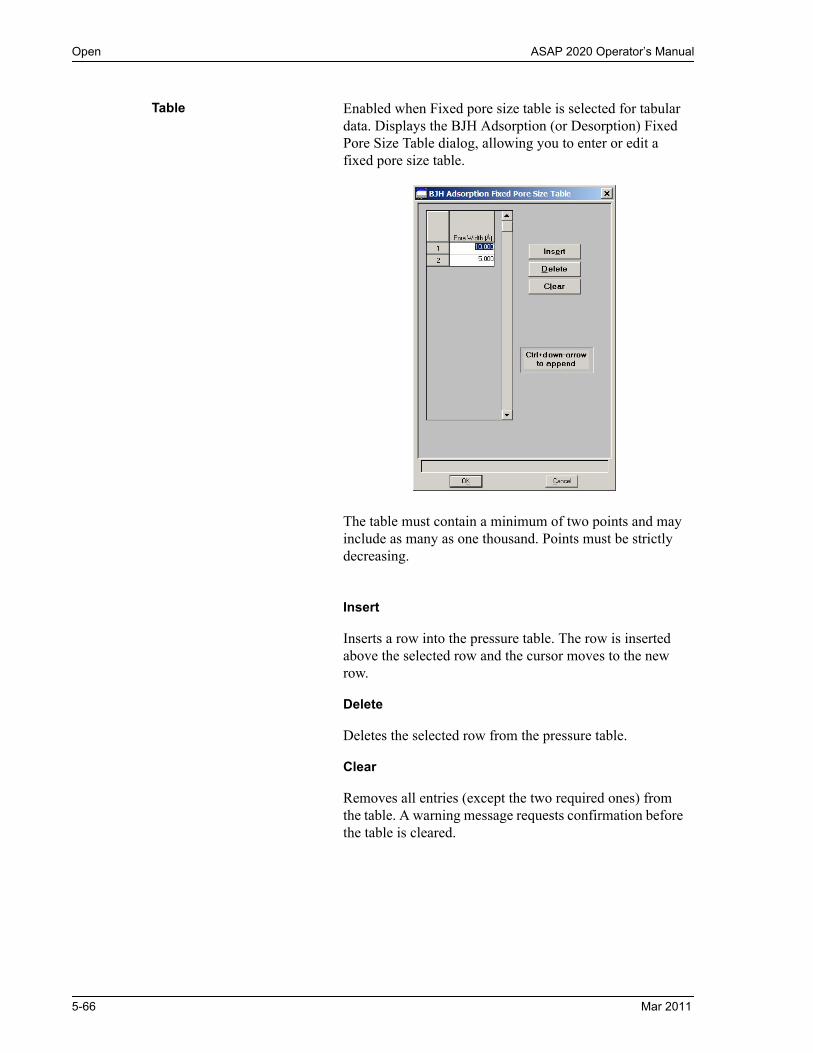
Open ASAP 2020 Operator’s Manual
Table Enabled when Fixed pore size table is selected for tabular data. Displays the BJH Adsorption (or Desorption) Fixed Pore Size Table dialog, allowing you to enter or edit a fixed pore size table.
The table must contain a minimum of two points and may include as many as one thousand. Points must be strictly decreasing.
Insert
Inserts a row into the pressure table. The row is inserted above the selected row and the cursor moves to the new row.
Delete
Deletes the selected row from the pressure table.
Clear
Removes all entries (except the two required ones) from the table. A warning message requests confirmation before the table is cleared.
5-66 Mar 2011

ASAP 2020 Operator’s Manual Open
Plot Options
Selecting a BJH plot option from the BJH Adsorption or Desorption Report Options dialog enables you to specify the plotting method used for your report and to customize the plot.
When you edit a BJH Adsorption or Desorption plot, a dialog similar to the following is displayed.
You can measure pore width, diameter, or radius; pore size can be expressed in angstroms or nanometers. Select Options > Units to specify desired units.
Plot Options Allows you to have data plotted as a curve, points, or both.
X-Axis Lists the scale options for the x-axis
Linear/Logarithmic Choose whether you wish to have the X-axis on a logarith-mic or linear scale. Unless you are performing micropore analyses, use the logarithmic option.
Mar 2011 5-67

Open ASAP 2020 Operator’s Manual
Autoscale Choose this option to have the x-axis scaled automatically. Linear X-axes begin at zero, and logarithmic X-axes begin at an appropriate value. The system uses the highest values collected during analysis as the ending points.
If you deselect this option, the corresponding fields are enabled so that you may enter a beginning and ending value. Data collected outside the specified ranges are not included in the plot.
X-axis range fields show pore radius or diameter in ang-stroms or nanometers.
Data ranges are displayed in the information bar across the bottom of the dialog when the cursor is in a numerical data entry field.
Y-axis Lists the options for the Y-axis.
Variable Click on the down-arrow to choose a variable for the Y-axis.
Overlay Displays a list of overlay choices. You can choose a differ-ent type of plot to overlay with the current plot. Or, you can choose Samples to overlay the current type of plot with the same type from other sample files. If you choose Samples, you select the other files using Overlays on the Report Options dialog box.
Autoscale Choose this option to have the y-axis scaled automatically. Y-axes begin at zero. The system uses the highest values collected during analysis as the ending points.
If you deselect this option, the corresponding fields are enabled so that you may enter a beginning and ending value. Data collected outside the specified ranges are not included in the plot.
Y-axis range fields show the quantity of gas adsorbed.
Data ranges are displayed in the information bar across the bottom of the dialog when the cursor is in a numerical data entry field.
5-68 Mar 2011

ASAP 2020 Operator’s Manual Open
Dollimore-Heal Adsorption/Desorption Report Options
You can generate DH reports from both adsorption and desorption data.
The options for Dollimore-Heal reports are the same as those for the BJH reports with the exception of BJH Correction and Adsorptive properties; this item is not applicable to DH reports. Refer to BJH Adsorption/Desorption Report Options, page 5-60 for a description of the fields on this dialog.
Or Dollimore-Heal Desorption Report Options
Mar 2011 5-69

Open ASAP 2020 Operator’s Manual
Horvath-Kawazoe Report Options
Pore Geometry Select the option in this group box which best represents the physical geometry of the micropores in the sample material. Refer to Appendix C for additional information on calculations used for these parameters.
Apply Cheng/Yang correction
Allows you to apply the Cheng/Yang correction to the pore size analysis. This correction substitutes the Langmuir equation of state for Henry’s Law in the Horvath-Kawazoe derivation (see Appendix C).
Smooth differentials Smooths the differential calculations, eliminating varia-tions in the differential computation caused by noise in the input data.
5-70 Mar 2011

ASAP 2020 Operator’s Manual Open
Pressure Range Displays the Report Relative Pressure Range dialog so that you may specify minimum and maximum relative pres-sures to use with this report.
• If Use calculation assignments is not selected on the Collected/Entered dialog, all of the nonoutlier points of the collected data within the specified range are used for calculating the data for this report.
• If Use calculation assignments is selected, collected data points which are assigned to this report type are used.
Interaction Parameter Select one of the options in this group box to determine which interaction parameter is used during report genera-tion.
Computed The interaction parameter is calculated using the parame-ters on the Horvath-Kawazoe Physical Properties dialog. You can click Properties to view or edit these parameters. Each time you change one of the parameters, the interac-tion parameter is recalculated. The formula for computing the interaction parameter is given in Appendix C.
Entered The value you enter in the adjacent field will be used.
Mar 2011 5-71

Open ASAP 2020 Operator’s Manual
Properties Use this push button to view or edit the constants (used during report generation) describing the physical proper-ties of the adsorbent and adsorptive; the Horvath-Kawazoe Physical Properties dialog box is displayed.
Adsorbent Group Box Contains the parameters for the sample. If you select Computed for the interaction parameter, all fields are enabled and can be edited if desired. If you select Entered, only the values in the Diameter and Diameter at zero energy fields may be edited.
DescriptionThe name of the adsorbent used in the analysis.
Click on the down arrow to make a new selection. Each time you change the selection, the values for that adsor-bent are displayed in the appropriate fields.
DiameterThe diameter of the sample atom.
Diameter at zero energyThe diameter of an atom at zero interaction energy,
(2/5)1/6 x diameter.
5-72 Mar 2011

ASAP 2020 Operator’s Manual Open
Adsorbent Group Box (continued)
PolarizabilityThe polarizability of the adsorbent.
Magnetic susceptibilityThe magnetic susceptibility of the adsorbent.
DensityThe density per unit area of the adsorbent.
Adsorptive Group Box Contains the parameters for the adsorptives (provided with the software and/or user-defined). If you select Computed for the interaction parameter, all fields are enabled and can be edited if desired. If you select Entered, only the values in the Diameter and Diameter at zero energy fields may be edited.
MnemonicThe mnemonic name of the adsorptive gas in use.
Click on the down arrow to make a new selection. Each time you change the selection, the values for that adsorp-tive display in the appropriate fields. If no parameters have been defined, the default values are displayed.
DiameterThe diameter of the adsorptive atom.
Diameter at zero energyThe diameter of an atom at zero interaction energy,
(2/5)1/6 x diameter.
PolarizabilityThe polarizability of the adsorptive.
Magnetic susceptibilityThe magnetic susceptibility of the adsorptive.
DensityThe density per unit area of the adsorptive.
Mar 2011 5-73

Open ASAP 2020 Operator’s Manual
Tabular Report Options
Displays the Horvath-Kawazoe Tabular Report Column Options dialog so that you can select the type of data to display in each column.
The default column title displays next to the column number. Each column includes a drop-down list of the types of data to include in the report.
Selected Reports Lists the available Horvath-Kawazoe reports. Choose a report by double-clicking on the report name or highlight the report name and press the Spacebar. A report is selected when it is preceded with a check mark.
The following reports are available:
Tabular ReportCumulative Pore VolumedV/dw Pore Volume
Edit Allows you to edit the selected report.
5-74 Mar 2011

ASAP 2020 Operator’s Manual Open
Plot Options
Selecting a Horvath-Kawazoe plot option from the Horvath-Kawazoe Report Options dialog enables you to specify the plotting method used for your report and to customize the plot. Plots for Cumulative Pore Volume and dV/dw Pore Volume are available.
When you select either of these plots from the Horvath-Kawazoe Report Options dialog, a dialog like the following is displayed.
Plot Options Lists the data presentation styles available; you must choose to plot a curve, points, or both.
X-axis options Choose Autoscale to have the x-axis scaled automatically. The X-axis begins at zero and the system uses the highest value collected during analysis as the ending point.
If you deselect Autoscale, the adjacent fields are enabled so that you may enter a beginning and ending value. Data collected outside these ranges are not included in the plot.
X-axis range fields show pore radius or diameter in ang-stroms or nanometers.
Data ranges are displayed in the information bar across the bottom of the dialog when the cursor is in a numerical data entry field.
Mar 2011 5-75

Open ASAP 2020 Operator’s Manual
Y-axis options Click on the down-arrow at the Variable field to choose a variable for the Y-axis.
Click on the down-arrow at the Overlay field to overlay the plot with data from other samples.
Choose Autoscale to have the y-axis scaled automatically. Y-axes begin at zero. The system uses the highest value collected during analysis as the ending point.
If you deselect Autoscale, the corresponding fields are enabled so that you may enter a beginning and ending value. Data collected outside these ranges are not included in the plot.
Y-axis range fields show the quantity of gas adsorbedData ranges are displayed in the information bar across the bottom of the dialog when the cursor is in a numerical data entry field.
5-76 Mar 2011

ASAP 2020 Operator’s Manual Open
DFT Pore Size
Type Drop-down list containing the types of models available; DFT or Classical.
DFT models are based on the density functional theory. Classical models are based on the Kelvin equation and thickness for determining the pore size distribution. Refer to Appendix G for a discussion on models.
Geometry Drop-down list containing pore shapes available; Slit or Cylinder.
Models Lists the models that meet the criteria specified and which match the adsorbate and temperature of the sample data.
The models display in alphabetical order with the first one automatically selected; you may select any one desired.
If the list is empty, there were no models that meet the selected criteria.
Link to Micromeritics Web Site
Provides access to the Micromeritics Web page containing the DFT models.
Mar 2011 5-77
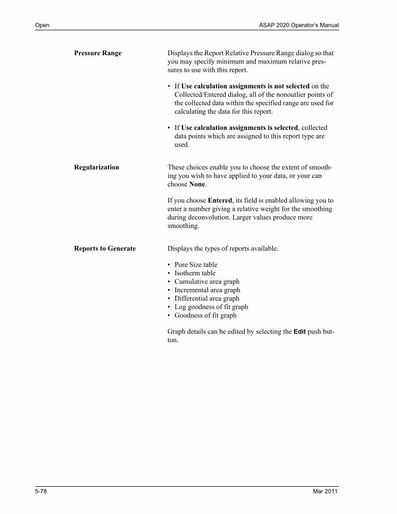
Open ASAP 2020 Operator’s Manual
Pressure Range Displays the Report Relative Pressure Range dialog so that you may specify minimum and maximum relative pres-sures to use with this report.
• If Use calculation assignments is not selected on the Collected/Entered dialog, all of the nonoutlier points of the collected data within the specified range are used for calculating the data for this report.
• If Use calculation assignments is selected, collected data points which are assigned to this report type are used.
Regularization These choices enable you to choose the extent of smooth-ing you wish to have applied to your data, or your can choose None.
If you choose Entered, its field is enabled allowing you to enter a number giving a relative weight for the smoothing during deconvolution. Larger values produce more smoothing.
Reports to Generate Displays the types of reports available.
• Pore Size table• Isotherm table• Cumulative area graph• Incremental area graph• Differential area graph• Log goodness of fit graph• Goodness of fit graph
Graph details can be edited by selecting the Edit push but-ton.
5-78 Mar 2011

ASAP 2020 Operator’s Manual Open
Edit Use this push button to edit details of a selected graph; a dialog like the following is displayed.
This push button is disabled for tables and Goodness of Fit graphs.
Plot Type Enables you to choose the manner in which you wish to display plotted data.
Autoscale Options Select these options to have the axes scaled automatically.
If you deselect one or both of these options, you must enter a range in the related Axis Range fields which become enabled automatically.
Overlay This drop-down list contains the type of overlays available for the current graph.
Choose Samples to overlay the same type of graph as the current one from other data reductions. Then select Over-lays on the Report Options dialog to choose your files (explained on page 5-35).
Axis Range The fields in this group box become enabled when you deselect Autoscale, allowing you to specify beginning and ending values for the X- and/or Y-axis. Data collected out-side these ranges are not included in the plot.
Valid ranges for a selected field are displayed in the infor-mation bar across the lower portion of the dialog. The X-axis displays the energy and the Y-axis displays the area.
Displays the type of graph you are editing.
Mar 2011 5-79

Open ASAP 2020 Operator’s Manual
Surface Energy
The fields on the Surface Energy dialog are identical to those on the DFT Pore Size dialog with the following exceptions:
Refer to the previous section for the DFT Pore Size report beginning on page 5-77 for information on the fields contained on this dialog.
Geometry drop-down list Is not applicable to the Surface Energy report and, there-fore, does not display on its dialog.
Reports to Generate Displays the types of reports available.
• Surface energy table• Isotherm table• Cumulative area graph• Incremental area graph• Differential area graph• Log goodness of fit graph• Goodness of fit graph
Graph details can be edited by selecting the Edit push but-ton.
5-80 Mar 2011

ASAP 2020 Operator’s Manual Open
Dubinin Report Options
Report Type Allows you to specify the type of report you want. At least one type of report must be selected.
Select Radushkevich to generate the Radushkevich report.
Select Astakhov to generate the Astakhov report. With this choice, you may select Optimize Astakhov exponent. If you do not select this option, the Exponent value field is enabled so that you can enter a value.
Refer to Appendix C for more information.
Fitted relative pressure range
Allows you to specify minimum and maximum limits on relative pressures included in the line fit. Data collected outside these limits are not included.
Mar 2011 5-81
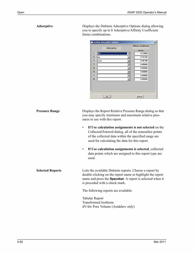
Open ASAP 2020 Operator’s Manual
Adsorptive Displays the Dubinin Adsorptive Options dialog allowing you to specify up to 8 Adsorptive/Affinity Coefficient (beta) combinations.
Pressure Range Displays the Report Relative Pressure Range dialog so that you may specify minimum and maximum relative pres-sures to use with this report.
• If Use calculation assignments is not selected on the Collected/Entered dialog, all of the nonoutlier points of the collected data within the specified range are used for calculating the data for this report.
• If Use calculation assignments is selected, collected data points which are assigned to this report type are used.
Selected Reports Lists the available Dubinin reports. Choose a report by double-clicking on the report name or highlight the report name and press the Spacebar. A report is selected when it is preceded with a check mark.
The following reports are available:
Tabular ReportTransformed IsothermdV/dw Pore Volume (Astakhov only)
5-82 Mar 2011

ASAP 2020 Operator’s Manual Open
Tabular Report
The Tabular report enables you to customize your report with one to six columns of data for Astakhov reports and one to five columns of data for Radushkevich reports. The Dubinin Tabular Report Column Options dialog is displayed.
The default column title appears next to the column number. Each column includes a drop-down list of the data types to include in the report.
Transformed Isotherm
The Transformed Isotherm report allows you to restrict the line fit to a portion of the isotherm. The Dubinin Transformed Isotherm Plot Options dialog box is displayed.
Overlay Samples Select this option to overlay the current plot with data from other samples. Then click Overlays on the Report Options dialog to choose the sample files.
Autoscale x-axisAutoscale y-axis
Select these options to have the X- and/or Y-axes automat-ically scaled. Both X- and Y-axes begin at zero, and the system uses the highest values collected during analysis as the ending points for axes ranges.
Mar 2011 5-83

Open ASAP 2020 Operator’s Manual
Pore Volume
When you select the dV/dw Pore Volume plot from the Dubinin Report Options dialog, the Dubinin dV/dw Pore Volume Options dialog is displayed.
Autoscale x-axisAutoscale y-axis(continued)
If you choose not to autoscale data for either (or both) axis, the adjacent fields are enabled so that you may enter a beginning and ending value. Data collected outside these ranges are not included in the plot.
The X-Axis Range fields show the quantity of gas adsorbed at standard temperature and pressure.
The Y-Axis Range fields show the log of relative pressure.
Data ranges are displayed in the information bar across the bottom of the dialog when the cursor is in a numerical data entry field.
The Pore Volume report is unavailable if you choose Radushkevich as the type of report.
Plot options You can plot data with a curve, points, or both.
Overlay Samples Select this option to overlay data from other samples. Then click Overlays on the Report Options dialog to choose the files.
5-84 Mar 2011
ASAP 2020 Operator’s Manual Open
Autoscale x-axisAutoscale y-axis
Select these options to have the X- and/or Y-axes auto-matically scaled. Both X- and Y-axes begin at zero, and the system uses the highest values collected during analy-sis as the ending points for axes ranges.
If you choose not to autoscale data for either (or both) axis, the adjacent fields are enabled so that you may enter a beginning and ending value. Data collected outside these ranges are not included in the plot.
The X-axis Range fields show pore width, radius, or diameter in angstroms or nanometers.
The Y-axis Range fields show the quantity of gas adsorbed.
Data ranges are displayed in the information bar across the bottom of the dialog when the cursor is in a numerical data entry field.
Mar 2011 5-85
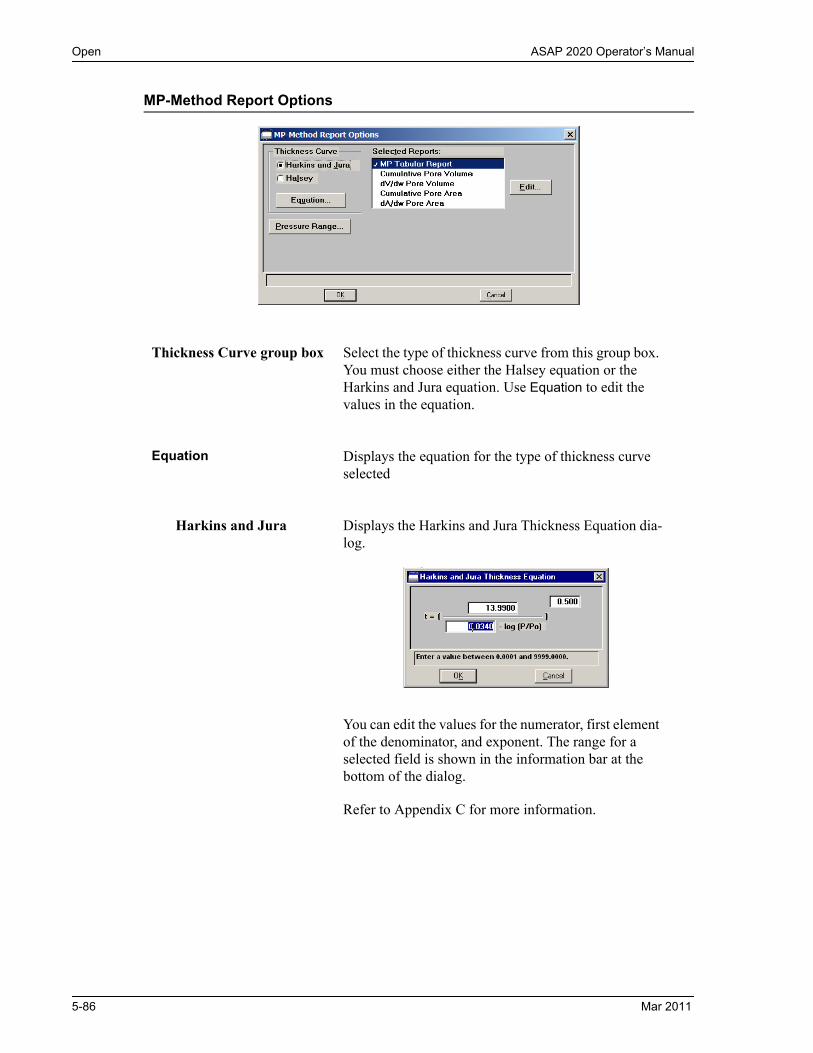
Open ASAP 2020 Operator’s Manual
MP-Method Report Options
Thickness Curve group box Select the type of thickness curve from this group box. You must choose either the Halsey equation or the Harkins and Jura equation. Use Equation to edit the values in the equation.
Equation Displays the equation for the type of thickness curve selected
Harkins and Jura Displays the Harkins and Jura Thickness Equation dia-log.
You can edit the values for the numerator, first element of the denominator, and exponent. The range for a selected field is shown in the information bar at the bottom of the dialog.
Refer to Appendix C for more information.
5-86 Mar 2011

ASAP 2020 Operator’s Manual Open
Halsey Displays the Halsey Thickness Equation dialog.
You can edit the values for the multiplier, numerator, and exponent.The range for a selected field is shown in the information bar at the bottom of the dialog.
Refer to Appendix C for more information.
Pressure Range Displays the Report Relative Pressure Range dialog so that you may specify minimum and maximum relative pressures to use with this report.
• If Use calculation assignments is not selected on the Collected/Entered dialog, all of the nonoutlier points of the collected data within the specified range are used for calculating the data for this report.
• If Use calculation assignments is selected, col-lected data points which are assigned to this report type are used.
Selected Reports Lists the available MP-Method reports. Choose a report by double-clicking on the report name or high-light the report name and press the Spacebar. A report is selected when it is preceded with a check mark.
The following reports are available:
• Tabular Report • Cumulative Pore Volume• dV/dw Pore Volume • Cumulative Pore Area• dA/dw Pore Area
Mar 2011 5-87

Open ASAP 2020 Operator’s Manual
Tabular Report
The Tabular report enables you to customize your report with one to six columns of data. (The data types in the first and second columns cannot be changed.) The MP-Method Tabular Report Column Options dialog is displayed.
The default column title appears next to the column number for columns three through six. Each of these columns includes a drop-down list of the data types to include in the report. Columns 1 and 2 are fixed and cannot be edited.
Pore Volume/Pore Area Plot
MP-Method plot options enable you to specify the plotting method used for your report and to customize the plot. A dialog box like the following is displayed. The fields on all dialogs are the same.
The MP-Method reports hydraulic radius only. If you select Pore size in diameter from the Units dialog, the MP-Method still reports pore size in radius.
5-88 Mar 2011

ASAP 2020 Operator’s Manual Open
Plot options You can plot data with a curve, points, or both.
X-axis options Choose Autoscale to have the x-axis scaled automatically. The X-axis begins at zero and the system uses the highest value collected during analysis as the ending point.
If you deselect Autoscale, the adjacent fields are enabled so that you may enter a beginning and ending value. Data collected outside these ranges are not included in the plot.
X-axis range fields show pore radius or diameter in ang-stroms or nanometers.
Data ranges are displayed in the information bar across the bottom of the dialog when the cursor is in a numerical data entry field.
Y-axis options Allows you to choose Y-axis options.
Variable Click on the down-arrow to choose a variable for the Y-axis.
Overlay You can use the choices in this drop-down list to overlay plots. You can choose a different type of plot for the cur-rent sample to overlay with the listed Variable, or you can choose Samples to overlay the Variable plot with the same type of plot from other samples.
Autoscale Choose this option to have the y-axis scaled automatically. Y-axes begin at zero. The system uses the highest value collected during analysis as the ending point.
If you deselect Autoscale, the adjacent fields are enabled so that you may enter a beginning and ending value. Data collected outside these ranges are not included in the plot.
Y-axis range fields show the quantity of gas adsorbed
Data ranges are displayed in the information bar across the bottom of the dialog when the cursor is in a numerical data entry field.
Mar 2011 5-89
Open ASAP 2020 Operator’s Manual
Options Report
The Options report provides pertinent information for the following:
• Degas conditions• Adsorptive properties• Analysis conditions• Sample tube criteria• Free space• Po and temperature• Equilibration• Isotherm collection
The Options report cannot be edited.
Sample Log Report
The Sample Log report displays the following:
• Manual control operations performed during analysis• Information entered using Add Log Entry on the sample file editor• Warnings and/or errors which occurred during analysis
The Sample Log report is a new feature with the ASAP 2020 program. Therefore, if you request a Sample Log report on a file that was used with the ASAP 2010 program, no information will be available.
The Sample Log report cannot be edited.
5-90 Mar 2011

ASAP 2020 Operator’s Manual Open
Validation Report
Use this report to have your data examined by the software to determine if the results are within typical ranges.
If the data for any report you selected for validation are determined to be out of range, a warn-ing is displayed and suggestions are given for corrective action. This information is also detailed in the report and plotted on the graph as a unique plot symbol.
Mar 2011 5-91

Open ASAP 2020 Operator’s Manual
Collected/Entered Data
If you choose Manually entered as the type of data in the Sample Information dialog, an Entered tab is added allowing you to enter the data.
If you choose Automatically collected as the type of data in the Sample Information dialog, a Collected Data tab is added when analysis is complete. The Collected Data dialog will contain the data points collected during analysis and the specified calculation assignments.
This example shows the Collected Data dialog from a completed sample information file; the Entered dialog is identical except the data is entered and the tab displays as Entered Data.
Pressure table For collected data, columns for the following are dis-played:
• absolute pressure
• relative pressure
• quantity adsorbed
• outliers (if Use calculation assignments is not selected)
• calculation assignments for each requested report option (if Use calculation assignments is selected)
5-92 Mar 2011

ASAP 2020 Operator’s Manual Open
Pressure table(continued)
For entered data, columns for the following are dis-played:
• absolute or relative pressure (depending on the selec-tion in the Pressures group box)
• quantity adsorbed
Insert Enabled for entered data; inserts a row into the pressure table.
Delete Enabled for entered data; deletes the selected row.
Clear Enabled for entered data; clears the entire table of all entries except one (one is required).
Use calculationassignments
If selected, allows you to assign the points to be collected for each report type.
If deselected, each report (with the exception of Langmuir and BET) uses a range of pressures as selected in Report Options. The Langmuir and BET reports interpolate to entered relative pressures on Report Options.
The outlier points can be selected so that they will not be reported.
Po and T Displays the Po and T dialog, allowing you to edit the sat-uration pressure and temperature. Only the applicable options are enabled.
Mar 2011 5-93

Save ASAP 2020 Operator’s Manual
Save
Save enables you to save any changes you have made to the file in the active window. The file is saved under its current name.
Free Space Displays the Free Space dialog, allowing you to edit the cold and warm free spaces.
Also allows you to choose how to account for non-ideal behavior of the adsorptive (refer to "Real gas equation of state" on page 5-33).
This dialog also includes the plotted isotherm. The iso-therm is redrawn each time you edit the values in either field.
Also available for the isotherm is a shortcut menu contain-ing options allowing you to edit the curve and axes. You also can zoom in for finer detail. Refer to Onscreen Reports, page 7-18 for the options available.
5-94 Mar 2011

ASAP 2020 Operator’s Manual Save As
Save As
Save As enables you to:
• save a sample or parameter file in the active window under a different name. This option is useful for making a duplicate copy of a file that you can modify as desired without chang-ing the original one. The original file remains open when you use this function, so be sure to open the new file before making any changes.
• save a subset (parameter) of the sample file in the active window as a standalone parame-ter file. For example, select Analysis Conditions from the Save As menu to create a stand-alone parameter file of the analysis conditions portion of the active sample file.
• save as an ASCII file the relative pressures and corresponding thicknesses (t-Curve) from the collected data. These data are derived by dividing the condensed volume of adsorptive by the selected surface area. The density conversion factor in the adsorptive properties file is used to convert quantity adsorbed to volume of condensed adsorptive.
• save as an ASCII file the relative pressures and resulting quantities adsorbed (Alpha-S) from the collected data. These data are derived by taking the isotherm and dividing it by the quantity adsorbed at 0.4 relative pressure.
Sample and Parameter Files
A dialog similar to the one shown below is displayed when you select Sample Information, Sample Tube, Degas Conditions, Analysis Conditions, Adsorptive Properties, or Report Options.
Enter a file name (up to eight characters) in the File name field; the appropriate extension is appended automatically when you click OK. The new file is saved as specified, but does not remain in the active window. Be sure to open the new file before making any changes to the file.
Indicates the type of file being saved
Mar 2011 5-95

t-Curve and Alpha-S Files
The same type of dialog box shown above is also displayed when you select t-Curve or Alpha-S. However, before you receive this dialog for t-Curve, the Save As t-Curve dialog is displayed. This dialog allows you to choose the surface area for the sample.
Save All
Save All enables you to save all open files under their current names. This option provides a faster way to save all open files at one time and avoids having to perform a Save operation on each individual file.
Close
Close enables you to close the file in the active window. If the file contains changes that have not been saved, the following message is displayed:
(file name) has been changed. Save changes before closing?
Yes No Cancel
Click Yes to close the file and save the changes.Click No to close the file without saving the changes.Click Cancel to return to the active file.

ASAP 2020 Operator’s Manual Close All
Close All
Close All enables you to close all open files under their current names. The following message displays for every file containing changes that have not been saved:
(file name) has been changed. Save changes before closing?
Yes No Cancel
Click Yes to close the file and save the changes.loses.Click No to close the file without saving the changes.Click Cancel to return to the active file.
Mar 2011 5-97

Print ASAP 2020 Operator’s Manual
Print enables you to print the contents of one or more files to the screen, a printer, or a file. For example, if you choose Analysis Conditions, you will receive the parameters used for all analysis conditions associated with the file(s). The print dialog is common to all file types.
Select the desired file type from the drop-down menu; a dialog similar to the following is displayed:
File name The name of the file you choose to print is copied to this field. If you choose multiple files, the name of the last one selected is displayed.
Copies Enabled when Printer is selected as the print destination. You may print up to four copies
Destination Select the destination. You may print to a printer, the screen, or to a file.
File name Enabled when you select File as the destination. A default file name (the same name as the sample file) appears if you choose only one file; you can use the default name or enter another one.
Indicates the type printingof report you are
5-98 Mar 2011
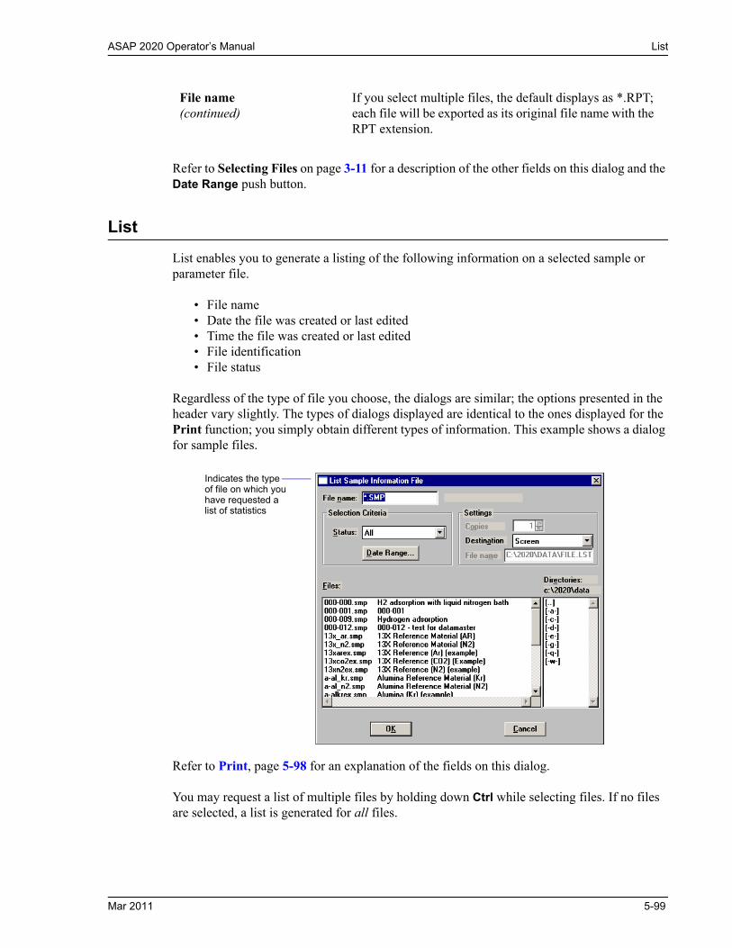
ASAP 2020 Operator’s Manual List
Refer to Selecting Files on page 3-11 for a description of the other fields on this dialog and the Date Range push button.
List
List enables you to generate a listing of the following information on a selected sample or parameter file.
• File name• Date the file was created or last edited• Time the file was created or last edited• File identification• File status
Regardless of the type of file you choose, the dialogs are similar; the options presented in the header vary slightly. The types of dialogs displayed are identical to the ones displayed for the Print function; you simply obtain different types of information. This example shows a dialog for sample files.
Refer to Print, page 5-98 for an explanation of the fields on this dialog.
You may request a list of multiple files by holding down Ctrl while selecting files. If no files are selected, a list is generated for all files.
File name(continued)
If you select multiple files, the default displays as *.RPT; each file will be exported as its original file name with the RPT extension.
Indicates the typeof file on which youhave requested alist of statistics
Mar 2011 5-99

Export ASAP 2020 Operator’s Manual
Export
Export copies the isotherm data in the sample information file and reformats it in a text format acceptable to other programs, such as spreadsheets. The output file consists of five columns containing the elapsed time, absolute pressure, relative pressure, and specific quantity absorbed, and quantity dosed (see example on next page).
File Name The name of the file you choose to export is copied to this field. If you choose multiple files, the name of the last one selected is displayed.
Destination You can export data to a printer, to the screen, or to a File.
If you select Printer, the Copies field is enabled allowing you to print up to four copies.
If you select File, the File Type and File name fields are enabled.
File Type You can export data in a spreadsheet format (XLS) or as a text file (TXT).
5-100 Mar 2011

ASAP 2020 Operator’s Manual Export
Format of Data Output
This example shows the format of the output file for exported data.
File Name Allows you to specify a name for your exported file, or you may accept the default. The default name is the name of the sample file appended with the appropriate exten-sion.
DescriptionOperator
SubmitterSample massType of Data*
*0 = automatically collected 1 = entered (relative pressures) 2 = entered (absolute pressures)
Elapsed Absolute Relative Spedific Quantitytime pressure pressure quantity adsorbed dosed
Mar 2011 5-101

Convert ASAP 2020 Operator’s Manual
Convert
Convert allows you to convert sample information files used with the ASAP 2000 to files compatible with the ASAP 2020 analysis program. You do not have to use the Convert function for ASAP 2010 files. You can open ASAP 2010 files using the Open command on the File menu. After an ASAP 2010 file is saved in the ASAP 2020 program, it is no longer compatible with the ASAP 2010 program. You will be warned of this and given the opportunity to save under a different name if desired.
The only files displayed are standard MICMOS 2000 files (SI*.DAT) and 2000 Micropore files (SM*.DAT).
Destination File name This field enables you to specify different names for the converted files. You may choose one of the following options:
• Accept the default for the converted file name. If you accept this option, the converted files will retain their original names; only the extension will change. For example, if you choose si0140.dat from the Files list box, it is converted as si0140.smp.
• Type the name for the converted file. For example, if you wish to convert the following file on the C drive:
From: C:\DATA1\SI0010.DATTo: C:\DATA2\SAMP90.SMPThen type: C:\DATA2\SAMP90.SMP
5-102 Mar 2011

ASAP 2020 Operator’s Manual Convert
Refer to Selecting Files on page 3-11 for a description of the other fields on this dialog and the Date Range push button.
The following message is displayed when the first file containing a fixed pore size table is encountered:
Fixed pore size tables will not be converted. If a sample file to be converted uses a fixed pore size table, the fixed pore size table can be entered after conversion is complete.
This message informs you that fixed pore size tables are not converted to the new format. You must enter a fixed pore size table after conversion if you desire to use one with the sample information file. Click OK to clear the message.
Destination File name(continued)
If you wish to convert the following file on the D drive:
From: D:\SI0010.DATTo: C:\DATA2\SAMP90.SMPThen enter C:\DATA2\SAMP90.SMP
If you wish to convert more than one file, enter wildcard characters. For example, the following chart shows the selected files and converted file names resulting when you enter the following:
C:\NEWDIR\*.SMP.
Selected Files Export Names
C:\DATA1\S1001.DAT C:\NEWDIR\S1001.SMP
C:\DATA1\S1002.DAT C:\NEWDIR\S1002.SMP
C:\DATA1\S1003.DAT C:\NEWDIR\S1003.SMP
Mar 2011 5-103
Exit ASAP 2020 Operator’s Manual
Exit
Exit enables you to exit (close) the ASAP 2020 program.
• If an analysis is in progress, the following message is displayed:
CAUTION: Sample analysis is in progress. If you exit the program analysis will continue to completion, but the data are not saved to disk until the program is restarted. Do you want to exit the program?
Yes No
Click Yes to close the ASAP 2020 program. The analysis continues and data are collected.Click No to allow the program to remain active.
• If a report is in progress, you are cautioned that reports are being generated, and given the opportunity to either cancel the print job or allow the reports to print before exiting.
Although data are stored in the analyzer when you exit the program during analysis, they are not saved in the file until the program is restarted. At that time the data are saved automatically. If a power failure occurs in the interim and you do not have an Uninterruptible Power Supply (UPS) attached, loss of data will result.
Observe the Status area of the instrument schematic; it indicates when an analysis is complete.
5-104 Mar 2011

Description ASAP 2020 Operator’s Manual
6. UNIT MENU
The Unit menu contains the options for the operations that can be performed with the ASAP 2020 analyzer. The main menu will contain a Unit menu for each attached analyzer. For example, if you have two attached analyzers, the main menu contains two Unit menus. The appropriate unit number and serial number display in the title bar of the operational windows. The status windows also display in different colors. This feature is especially useful when you have more than one analyzer attached to the same computer.
Description
Listed below are brief descriptions of the Unit menu options. Detailed descriptions are found in subsequent sections.
The Unit menu does not display on the menu bar if the analysis program is being used for offline data manipulation on a computer other than the one controlling the analyzer.
Sample Analysis Starts an analysis. This option is disabled if analyses are in progress. Page 6-3.
Start Degas Allows you to start the degassing operation on one or two samples. Page 6-8.
Enable Manual Control Allows you to control the system manually. Page 6-9.
Mar 2011 6-1

ASAP 2020 Operator’s Manual Description
Show Instrument Schematic
Displays a schematic of the analyzer components. Page 6-12.
Show Status Shows the status window of the operation in progress. Page 6-13.
Show Instrument Log Displays a log of recent analyses, calibrations, and error mes-sages. Page 6-14.
Unit Configuration Displays the configuration of the analyzer. Page 6-16.
Diagnostics Enables you to perform certain diagnostic tests. Page 6-18
Calibration Enables you to calibrate certain components of the analyzer. Page 6-20.
Degas Allows you to perform sample degassing operations. Enabled only if the SmartVac is installed. Page 6-26.
Service Test Enables you to perform certain troubleshooting procedures. This option is enabled only with the direction of a Micromer-itics service representative. Page 6-31.
6-2 Mar 2011

Sample Analysis ASAP 2020 Operator’s Manual
Sample Analysis
When you select this option from the Unit menu, the Sample Analysis dialog is displayed with all fields disabled (grayed) and the Start Analysis dialog positioned on top. This allows you to select a sample file for your analysis or to create a new one.
After a sample file has been designated, the Analysis dialog is displayed. The fields now con-tain the values for the selected file or, if creating a new file, the specified defaults.
View Allows you to view one of the following in the current win-
dow:
• the current operation• the instrument schematic• the instrument log
Refer to Show Instrument Schematic on page 6-12 and Show Instrument Log on page 6-14.
Browse Displays the Start Analysis dialog allowing you to choose a different sample file for the current analysis.
Sample Displays an identification of the sample file.
Mass Enables you to enter the sample’s mass.
Mar 2011 6-3

ASAP 2020 Operator’s Manual Sample Analysis
Sample Tube Displays the name of the Sample Tube file for the current sample file.
If this is a new file, this field contains the file you specified as the default.
The drop-down list contains a list of predefined parameter files that were saved to the Parameter Files Directory (refer to Parameter Files Directory on page 8-13), as well as those included with the analysis program. You may choose a dif-ferent file from this list if desired.
Analysis Conditions Displays the name of the Analysis Conditions file for the cur-rent sample file.
If this is a new file, this field contains the file you specified as the default.
The drop-down list contains a list of predefined parameter files that were saved to the Parameter Files Directory (refer to Parameter Files Directory on page 8-13), as well as those included with the analysis program. You may choose a dif-ferent file from this list if desired.
Adsorptive Properties Displays the name of the Adsorptive Properties file for the current sample file.
If this is a new file, this field contains the file you specified as the default.
The drop-down list contains a list of predefined parameter files that were saved to the Parameter Files Directory (refer to Parameter Files Directory on page 8-13), as well as those shipped with the analysis program. You may choose a differ-ent file from this list if desired.
6-4 Mar 2011

Sample Analysis ASAP 2020 Operator’s Manual
Report Options Displays the name of the Report Options file for the current sample file.
If this is a new file, this field contains the file you specified as the default.
The drop-down list contains a list of predefined parameter files that were saved to the Parameter Files Directory (refer to Parameter Files Directory on page 8-13), as well as those shipped with the analysis program. You may choose a differ-ent file from this list if desired.
Po Enabled if you have chosen to enter the Po measurement. Enter (or confirm) the saturation pressure of the adsorptive, or edit the current one if desired.
Bath temperature Enabled if you have chosen to enter the bath temperature (Po and T option on the Analysis Conditions dialog). Enter (or confirm) the temperature for the analysis bath.
Ambient Temperature Enter the temperature of the air outside of the instrument.
Warm and Cold Free space
Enabled if you have chosen to enter the free space values (Free Space option on the Analysis Conditions dialog). Enter (or confirm) the appropriate values.
Report After Analysis Displays the Report Settings dialog so that you may specify report output options. If you choose Screen, reports have many options for being customized and manipulated. (Refer to Onscreen Reports on page 7-18 for details about onscreen reports.)
Mar 2011 6-5
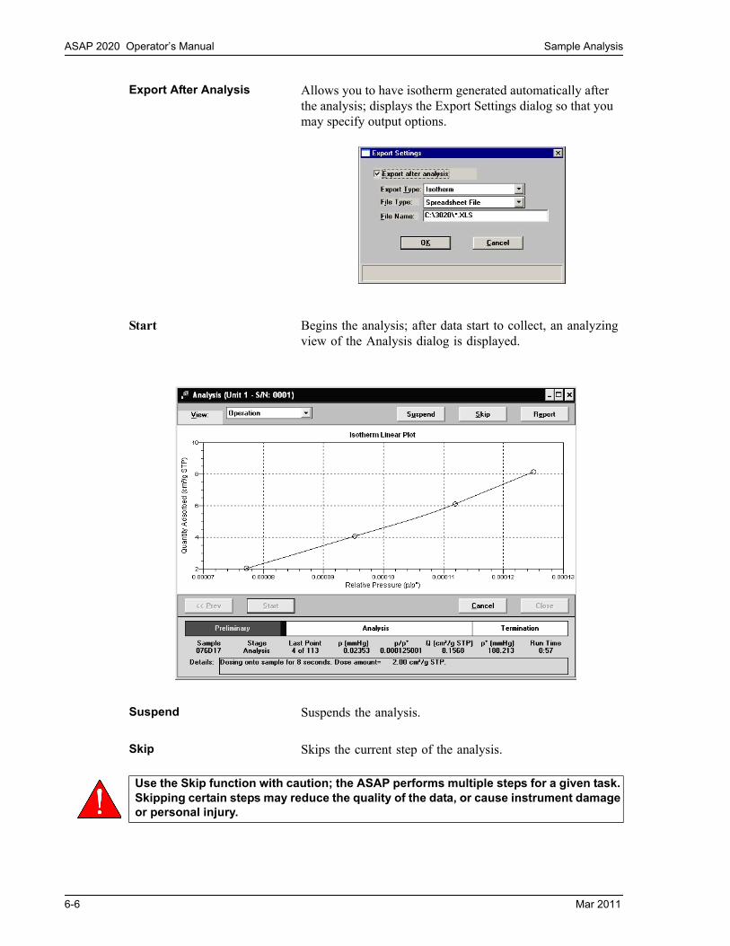
ASAP 2020 Operator’s Manual Sample Analysis
Export After Analysis Allows you to have isotherm generated automatically after the analysis; displays the Export Settings dialog so that you may specify output options.
Start Begins the analysis; after data start to collect, an analyzing view of the Analysis dialog is displayed.
Suspend Suspends the analysis.
Skip Skips the current step of the analysis.
Use the Skip function with caution; the ASAP performs multiple steps for a given task. Skipping certain steps may reduce the quality of the data, or cause instrument damage or personal injury.
6-6 Mar 2011

Sample Analysis ASAP 2020 Operator’s Manual
Resume Resumes a suspended analysis.
Cancel Cancels the analysis.
Start On this view of the analysis dialog, this push button changes to Next when the analysis is finished.
Next Enabled at the completion of the analysis. Returns you to the first view of the Analysis dialog so that you may schedule another analysis.
Close Enabled at the completion of analysis. Closes the dialog.
Mar 2011 6-7

ASAP 2020 Operator’s Manual Start Degas
Start Degas
This option allows you to choose the file and start degas operations on one or two samples; the Automatic Degas dialog is displayed.
Sample Click Browse to the right of this field to select a sample file that will be used with the current sample.
Degas Conditions Displays the Degas Conditions file designated as the default. After you choose a sample file, this field displays the file associated with the sample file.
You can choose a different Degas Conditions file from the drop-down list if desired. If you choose a different file, the values in the current file will be overwritten with the values of the new one.
Clear Clears the sample file from the port assignment. Click Browse to choose a different file.
Start Starts the degassing operation
Cancel Closes the dialog, cancelling the degassing operation.
6-8 Mar 2011

Enable Manual Control ASAP 2020 Operator’s Manual
Enable Manual Control
Select this option to control certain components of your system manually. If the instrument schematic is not displayed, select Instrument Schematic from the View drop-down list.
When manual control is enabled, the valve symbols change color on the monitor screen to indicate their status.
Green = openYellow = closed
Use the mouse pointer to select a component. A component is selected when it is surrounded by a thin line. Each component has a shortcut menu displaying the operations available for that particular component. These menus may be accessed by right-clicking on the desired component, or by using the shortcut keys Shift + F9.
You can open and close valves, and raise or lower the elevator by using one of the following methods:
• right-click on the valve or elevator symbol to access the shortcut menu and select the appropriate action
• double-click on the valve or elevator symbol
• select the valve or elevator symbol and press the Spacebar
Mar 2011 6-9

ASAP 2020 Operator’s Manual Enable Manual Control
Table 6-1. System Valves
Valves System valves and their functions are listed in Table 6-1.
Actions: Open, Close, Pulse
Pulse briefly opens and closes (or vice versa) the valve.
Valve Description
1 Unrestricted vacuum
2 Restricted vacuum
3 Free-space measurement gas (helium)
4 Restricted analysis gas
5 Unrestricted analysis gas
7 Lower manifold isolation
8 Vapor
9 Sample port
10 Restricted Psat tube port
11 Unrestricted Psat tube port
P1 through P6 Gas inlet port valves
PS Supply valve for physisorption gases
PV Vacuum valve for physisorption gases
Dewar positions The Dewar can be raised, lowered, or stopped.
Indicates the Dewar is being raised; note the position of the arrow in the center of the Dewar symbol.
Indicates the Dewar is being lowered; note the position of the arrow in the center of the Dewar symbol.
Indicates the Dewar is stopped in the raised position.
Open Closed
6-10 Mar 2011

Enable Manual Control ASAP 2020 Operator’s Manual
The remainder of the components are displayed for informational purposes only; they cannot be controlled manually.
Indicates the Dewar is stopped in the lowered position.
Represents the sample tube.
Represents the Psat tube.
This group of rectangles on the left side of the schematic dis-plays the temperature, the vacuum gauge pressure, and the transducer(s) currently installed. This representation shows all three transducers installed.
Transducers
Vacuum Gauge
Temperature
Mar 2011 6-11

ASAP 2020 Operator’s Manual Show Instrument Schematic
Show Instrument Schematic
Select this option to display a schematic of the ASAP 2020 analyzer. The schematic is a graphical representation of the plumbing system including system valves, the analysis station, and the Dewar position. The valves and Dewar can be controlled from the schematic when Manual control is enabled. Refer to Enable Manual control on page 6-9 for an explanation of the components displayed on the instrument schematic.
The state of the valves can be determined quickly by color representation even when manual control is not enabled:
• Green = open• White = closed
If you wish to change the state of a valve, you must enable manual control.
6-12 Mar 2011

Show Status ASAP 2020 Operator’s Manual
Show Status
A status window is shown across the bottom of all operational dialogs as well as the instru-ment schematic. The Show Status option enables you to show only the status window. This frees up your computer screen allowing you to perform other tasks (such as creating or edit-ing sample files), while still monitoring the progress of your analysis.
If you have multiple instruments attached to your computer, the status bar for each instrument is displayed in a different color.
Analysis status bar Shows the progression of the analysis. This bar contains three stages:
• Preliminary: warm and cold free spaces are determined; displays green during progression
• Analysis: data are collected; displays blue during progres-sion
• Termination: the dewar lowers, and the sample tube is warmed and backfilled; displays gray during progression
All stages are displayed in red if the analysis has been suspended.
Analysis details The following analysis details are displayed:
Sample: Sample file numberStage: Stage of the analysis (as in status bar)Last Point: Last point and number of points requestedP: Absolute pressure of last pointP/Po: Relative pressure of last pointQ Quantity adsorbedPo: Absolute pressure of last measured or
calculated saturation pressure (Po)Run Time: Elapsed time since the start of analysis
Step details Provides details of the current step of the analysis.
Mar 2011 6-13
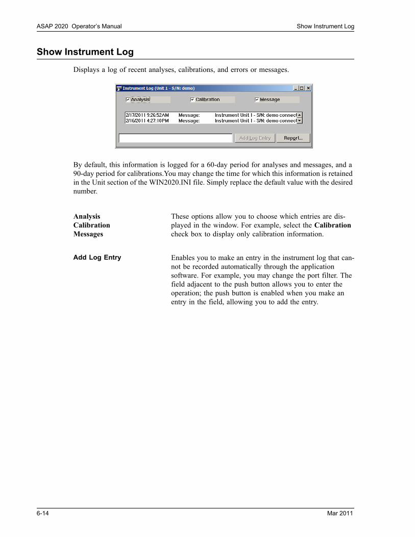
ASAP 2020 Operator’s Manual Show Instrument Log
Show Instrument Log
Displays a log of recent analyses, calibrations, and errors or messages.
By default, this information is logged for a 60-day period for analyses and messages, and a 90-day period for calibrations.You may change the time for which this information is retained in the Unit section of the WIN2020.INI file. Simply replace the default value with the desired number.
Analysis Calibration Messages
These options allow you to choose which entries are dis-played in the window. For example, select the Calibration check box to display only calibration information.
Add Log Entry Enables you to make an entry in the instrument log that can-not be recorded automatically through the application software. For example, you may change the port filter. The field adjacent to the push button allows you to enter the operation; the push button is enabled when you make an entry in the field, allowing you to add the entry.
6-14 Mar 2011

Show Instrument Log ASAP 2020 Operator’s Manual
Report Displays the Log Report Settings dialog allowing you to generate the log contents to a specified destination.
Use the Start Date field to specify the date at which to start the printout. This date does not limit the entries that display in the window, it is only pertinent to the entries that will be printed on the report.
You can specify a date using one of the following methods:
• Highlight the field (or press F2 to clear the field) and type in the desired date.
• Double-click in the field (or press F4) to display a calendar to choose a date.
• Press F2 to clear the field, then F3 to insert the current date.
Enter the number of copies desired in the Copies field; you may print up to 4. This field is disabled if you are printing to a File or to the Screen.
Choose the report destination from the drop-down list in the Destination field. If you choose File, the File name field is enabled, allowing you to enter a name for the printed file (or you may accept the default).
Mar 2011 6-15

ASAP 2020 Operator’s Manual Unit Configuration
Unit Configuration
Select this option to view the current calibration settings, the date on which calibration was performed, and the software and hardware configuration of your system.
Volume Calibration Displays the system, lower, and reference volumes from the most recent calibration. It also displays the date and time the calibration was completed.
A/D Calibration Displays the following:
• The date and time the manifold temperature was last cali-brated.
• The date and time the transducer offsets were last cali-brated.
• The percent of nominal transducer scale in use, and the date and time the transducer scale was last calibrated.
• The date and time the vacuum gauge was calibrated.
6-16 Mar 2011

Unit Configuration ASAP 2020 Operator’s Manual
Configuration Displays the following:
• The hardware code specifying the hardware components (for example transducers) present in your analyzer. This code is provided so the Service Department may quickly identify your hardware configuration and provide prompt assistance. Hardware codes translate as follows:E = 1000-mmHg transducerG = 10- and 1000-mmHg transducers H = 1-, 10-, and 1000-mmHg transducers
• The identification number of the port being used to control the analyzer.
• The serial number of the attached analyzer (active unit).
Software Versions The software versions of the MIC BIOS, Controller, and ASAP 2020 System software.
SmartVacSoftware Versions
The software versions of the MIC BIOS and SmartVac software. This group box is not displayed if the SmartVac is not installed.
Features The options currently enabled on your system (for example, MicroPore or MultiGas).
Gas Displays the Gas Configuration dialog.
This dialog allows you to choose the gases attached to each port of the analyzer.
Mar 2011 6-17

ASAP 2020 Operator’s Manual Diagnostics
Diagnostics
This option enables you to clean and verify gas lines when connecting or changing a gas. This option also allows you to perform diagnostic tests which your service representative may request. The data generated from these tests may be insignificant to you as a user, but can be very helpful to your service representative. Your service representative can view the results and may be able to resolve the problem, eliminating downtime and repair costs.
Diagnostic tests generate files to the 2020\Service\userdiag directory. Your service represen-tative will request that you E-mail the files to him so that he may examine them.
When you select Unit [n] > Diagnostics, the Service Test dialog is displayed:
Board ID Displays the Board ID dialog so that you can view the sta-tistics of the board contained in the requested slot of the card cage in the instrument.
6-18 Mar 2011

Diagnostics ASAP 2020 Operator’s Manual
View Allows you to view the current operation, the instrument schematic, or the instrument log in the Service Test dialog. Operation is the appropriate choice for tests.
Test Contains a list of diagnostic tests. These tests will always include the latest revision letter at the end of the test name.
Sequence Displays the test file name. This name is assigned automati-cally and incrementally sequenced by the software each time a test is performed. This also serves as the name of the file that is generated to the userdiag directory, and will be appended with SVT.
Report after test Select this option to have a report generated automatically after the test.
If you do not select this option, you can still have a report generated from the report window.
Cancel Cancels the test.
Next Begins the test; displays the next view of the Service test dialog. The second view of the Service test dialog may con-tain a single pane or two panes, depending on the test selected.
Mar 2011 6-19

ASAP 2020 Operator’s Manual Calibration
The following push buttons become enabled when the test is complete.
Calibration
This option allows you to calibrate the vacuum gauge, pressure gauge, pressure scale, mani-fold temperature, and system volume. You can also save the current calibrations to a file or load a different calibration file.
Vacuum Gauge
Displays the Calibration Vacuum Gauge dialog containing the current vacuum level.
This dialog also allows you to enter a new value (if necessary) after calibration using an external reference gauge.
Report (field) Contains a list of the reports that will be generated during this test.
Item [n] Lists the data in the two panes. Item 1 is the upper pane and Item 2, the lower pane.
Report (push button) Enables you to generate a report.
Cancel Cancels the test.
Repeat Repeats the test; not applicable for this test.
Next Returns you to the first view of the Service Test window.
Close Closes the dialog.
6-20 Mar 2011

Calibration ASAP 2020 Operator’s Manual
Pressure Zero
Displays the Calibrate Pressure Offset dialog.
This dialog allows you to evacuate the manifold and zero all pressure transducers in the system.
Pressure Scale
A Pressure Scale option is available for each type of transducer you have installed. For exam-ple, if you have the 1000-mmHg, 10-mmHg, and 1-mmHg transducers installed, a Pressure Scale option is displayed for the adjustment of each one.
Use these options to adjust the scale of a transducer to match a reference standard; the Cal-ibrate Pressure Scale dialog is displayed.
Reset to nominal Restores factory calibration settings for all transducers.
Match to entered pressure Select this option to enter a value obtained using a reference pressure gauge to determine the actual manifold pressure.
Mar 2011 6-21

ASAP 2020 Operator’s Manual Calibration
Temperature
Use this option to adjust the offset of the manifold temperature sensor to agree with a value obtained using a calibration device. The Calibrate Manifold Temperature dialog is displayed so that you may enter the measured value.
Volume
Use this option to enter a predetermined system volume in the event of data loss.
The system volume typically is calibrated after servicing valves, transducers, or any part of the analysis plumbing. The ASAP 2020 must be idle to calibrate system volume. Before sys-tem volume is calibrated, the manifold temperature sensor and the master pressure gauge must be calibrated.
Previous Retains the values currently in use.
Entered Allows you to enter values to use.
Measured This field is used by authorized service personnel when mea-suring the system and lower manifold volumes. A special Service Kit is required to perform these procedures.
Displays as Next if you choose Measured.
6-22 Mar 2011

Calibration ASAP 2020 Operator’s Manual
Done Closes the dialog (displays for the Previous and Entered selections).
Next Appears only when Measured was selected; displays a dia-log that enables service personnel to enter measured volumes.
Reference Volume Enter the volume in cubic centimeters for the reference vol-ume you are using in this calibration.
Reference Volume Temp. Enter the temperature of the reference volume. Since the ref-erence volume should be submerged in an ice bath, this value should remain at 0.0 oC for best accuracy.
Perform measurement Choose the number of measurements you wish to perform; you may choose up to 9.
Mar 2011 6-23
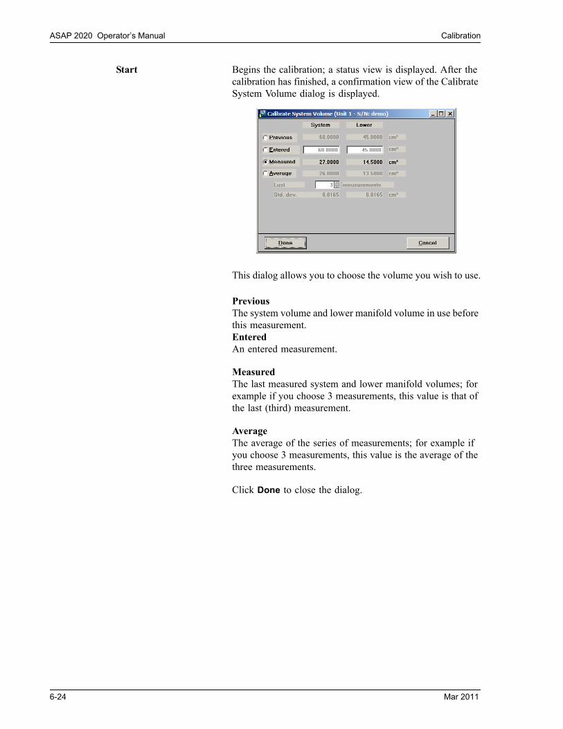
ASAP 2020 Operator’s Manual Calibration
Start Begins the calibration; a status view is displayed. After the calibration has finished, a confirmation view of the Calibrate System Volume dialog is displayed.
This dialog allows you to choose the volume you wish to use.
PreviousThe system volume and lower manifold volume in use before this measurement.EnteredAn entered measurement.
MeasuredThe last measured system and lower manifold volumes; for example if you choose 3 measurements, this value is that of the last (third) measurement.
AverageThe average of the series of measurements; for example if you choose 3 measurements, this value is the average of the three measurements.
Click Done to close the dialog.
6-24 Mar 2011

Calibration ASAP 2020 Operator’s Manual
Save to File
Use this option to save the current calibration settings to a file; the Select Calibration File dia-log is displayed.
Load from File
Displays the Select Calibration File dialog (shown above) so that you can load a previously saved calibration file.
File name Defaults to the next sequence number for calibration files. The sequence number consists of: xxx-yyy.CAL, where xxx = serial number of unit and yyy = sequence number. For example, the number listed in the above dialog represents the first calibration file for unit serial number 202.
Mar 2011 6-25

ASAP 2020 Operator’s Manual Degas
Degas
This option on the Unit menu is enabled if your ASAP 2020 is equipped with the SmartVac degassing option. The choices on this cascading menu allow you to select operations for the SmartVac degasser.
Enable Manual Control
Select this option to control manually certain components of the degas operation. If the instrument schematic for the SmartVac is not displayed, select Show Instrument Schematic from the Degas menu.
Valves D1, D2, D5, D6, D7 Degasser valves and their functions are listed in Table 6-2.
Actions: Open, Close
Servo Valve
6-26 Mar 2011

Degas ASAP 2020 Operator’s Manual
Table 6-2. Degasser Valves
Show Instrument Schematic
Displays the schematic (shown in the previous section) for the SmartVac.
Valve Description
D1 and D2 Sample port valves
D5 Vacuum valve
D6 Servo isolation valve
D7 Gas inlet port valve
Servo Valve Actions: Set, Close
Set displays the Servo Valve Settings dialog so that you can enter a target pressure for sample evacuation. This feature enables you to use the software to bring down the sample pressure slowly and incrementally.
Close closes the servo valve.
Heaters Actions: Set, Disable
Set displays the Port [n] Heater Settings dialog so that you can specify a ramp rate and target temperature. After you click and close the dialog, the settings are displayed directly below the heater symbol.
Disable cancels the settings.
Status window Displays the status of the current degassing operation(s).
Mar 2011 6-27

ASAP 2020 Operator’s Manual Degas
Show Status
This option allows you to monitor the degassing operation.
Sample Displays the sample file being used with the degassing oper-ation for each port.
Status Displays the current stage of the degassing operation for each port.
Check Allows you to check the outgassing rate of the sample on the related port; the following actions occur:
• current degassing step is suspended (on both ports). Degassing can be checked after the vacuum setpoint has been attained, or during a temperature ramp and hold. If you choose this option during any other step, a message indicating the SmartVac is not in a valid state is displayed.
• vacuum valves are closed and the vacuum level moni-tored.
• the Status window is displayed (if not already displayed). The Status window will indicate that the degassing opera-tion is being checked and will display the outgassing rate as it becomes available.
During the degas check, this push button changes to Con-tinue. When Continue is clicked, the valves open, the tem-perature ramp or hold continues, and the degassing operation resumes. If your outgassing rate indicated that contaminants have been removed from the sample (minimal pressure increase), you can click Skip to advance to the next state of the degassing operation. For example, if you check degas-sing after the setpoint is attained, Skip advances you to the ramping stage.
Skip Skips the current stage of the degassing operation for the port associated with this push button.
6-28 Mar 2011

Degas ASAP 2020 Operator’s Manual
Calibrate Pressure Zero
Use this option to evacuate the manifold and zero the transducer.
Calibrate Pressure Scale
Use this option to adjust the scale of the pressure transducer.
Cancel Cancels the degassing operation for the port associated with this push button.
Start Begins the calibration.
Status messages are displayed during this procedure, then the dialog closes automatically.
Current Pressure Enter the current pressure of the degasser manifold.
Mar 2011 6-29

ASAP 2020 Operator’s Manual Degas
Calibrate Vacuum Gauge
Displays the Calibration Vacuum Gauge dialog containing the current vacuum level.
This dialog also allows you to enter a new calibration value (if necessary) obtained using an external reference gauge.
Calibrate Servo
Use this option to calibrate the servo valve to the manifold pressure transducer. The servo valve should always be recalibrated after a pressure calibration has been performed. The Cal-ibrate Servo Valve dialog is displayed.
Start Begins the calibration. The servo valve is used to evacuate and equilibrate the manifold. The pressure transducer read-ings are used to calibrate the servo set point. Status messages are displayed during this procedure, then the dialog closes automatically.
6-30 Mar 2011

Service Test ASAP 2020 Operator’s Manual
Service Test
Various service tests are included in the ASAP 2020 operating program. These tests can be enabled and performed only with the assistance of a trained Micromeritics service represen-tative. These tests are designed to provide your service representative with instrument readouts, as well as to assist him in troubleshooting potential problems and, perhaps, elimi-nating unnecessary repair services. This service strategy allows you to conduct expert tests in less time than it would take to be trained in servicing the instrument properly.
Mar 2011 6-31

ASAP 2020 Operator’s Manual Service Test
6-32 Mar 2011

ASAP 2020 Operator’s Manual Description
7. REPORTS MENU
This chapter describes the commands on the Reports menu; it also contains examples of reports.
Reports can be generated for data:
• collected on a sample that has completed analysis
• collected on a sample that is currently being analyzed (includes only the information col-lected up to the time of the report)
• that is manually entered
Description
Listed below are brief descriptions of the commands contained on the Reports menu. Detailed descriptions follow this section.
Start Report Allows you to generate a report on a completed sample analysis or on the data collected thus far for an analysis in progress. Page 7-3.
Close Reports Closes all open report windows. Page 7-5.
Open Report Enables you to open a report that was saved from the report window. Page 7-5.
SPC Report Options Allows you to specify the sample data to be included in SPC reports. Page 7-6.
Mar 2011 7-1
Description ASAP 2020 Operator’s Manual
Regression Report Allows you to generate a regression report. Page 7-7.
Control Chart Allows you to generate a control chart report. Page 7-11.
Heat of Adsorption Allows you to generate a Heat of Adsorption report. Page 7-14.
Rate of Adsorption Invokes the Rate of Adsorption program, allowing you to generate ROA reports. Page 7-17.
7-2 Mar 2011

ASAP 2020 Operator’s Manual Start Report
Start Report
Select this option to generate a report on a sample analysis. Select Start report from the Reports menu to display the Start Report dialog.
File name The name you select from the Files list box is copied to this field. If you select multiple files, only the last one selected is displayed. If you have a sample file open when you select this option, its name is displayed.
Status This drop-down list determines what type of sample files are displayed in the Files list window in the specified directory for all dates, or within the specified range of dates (using push button).
Choices: All, Analyzing, Complete, Entered
Refer to Table 3-2. File Status and Description, page 3-12 for a description of the status types.
Date Range Displays the Select Dates dialog so that you may specify a range of dates. Refer to Selecting Files on page 3-11 for a description of this push button.
Copies Enabled when the Printer or Printer/Plotter destination is chosen. This option allows you to print up to four copies of the selected report(s).
Mar 2011 7-3

Start Report ASAP 2020 Operator’s Manual
Destination Displays a drop-down list of output destinations.
Choices: File, Printer, Screen
If you select Printer, requested reports are printed to the selected printer.
If you select Screen, many options are available for manipulating and customizing reports. Refer to Printed reports on page 7-18.
If you select File, the tabular reports of the requested file are converted to a text file which can be viewed with a text editor or other text file manipulation tool. Graphical data cannot be generated to a File.
File name Enabled when you select File as the destination. Allows you to enter a name, or you may accept the default.
Files list box Displays a list of the available sample files for the choice shown in the Status field and within the range of dates specified in the Dates dialog.
Directories Displays a list of available drives and directories. The drive and directory last accessed is displayed immediately above the Directories list box.
If you choose a single sample file, the Reports to Generate dialog is displayed. The reports selected are the ones you specified in the sample file. This dialog allows you to deselect reports or select additional ones.
7-4 Mar 2011
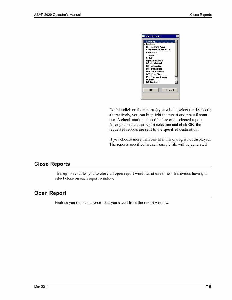
ASAP 2020 Operator’s Manual Close Reports
Close Reports
This option enables you to close all open report windows at one time. This avoids having to select close on each report window.
Open Report
Enables you to open a report that you saved from the report window.
Double-click on the report(s) you wish to select (or deselect); alternatively, you can highlight the report and press Space-bar. A check mark is placed before each selected report. After you make your report selection and click OK, the requested reports are sent to the specified destination.
If you choose more than one file, this dialog is not displayed. The reports specified in each sample file will be generated.
Mar 2011 7-5

SPC Report Options ASAP 2020 Operator’s Manual
SPC Report Options
When you select SPC Report Options, the SPC Report Options dialog is displayed.
The SPC Report Options dialog lists the variables that are most frequently used for SPC reporting. You can check as many as desired. All variables selected are computed for each sample file used in an SPC report.
Click More for additional SPC calculations for the detailed reports.
7-6 Mar 2011

ASAP 2020 Operator’s Manual Regression Report
Regression Report
Select this option to generate a regression report. The regression report is used to determine the interdependency between two variables. Up to three dependent variables (Y-axis) may be plotted against a single independent variable (X-axis). The degree of correlation between the variables also is reported. The graphs for the regression report are scaled so that all three fit on a single page. If you choose less than three, the graphs are scaled to fill most of the page.
Show report title Select this option to have a title display on your report. Accept the default or enter a new title. You can enter up to 40 alphanumeric characters.
Deselect this option to omit the report title.
Show graphic Select this option to have a graphic display above your report title. For example, you may wish to display your company logo. The graphic must be a bitmap (bmp) or enhanced metafile (emf).
Click Browse to choose the file, then use the Height and Width fields to specify a size. This image can be edited in the report window (when printed to the screen), or removed if desired.
Mar 2011 7-7

Regression Report ASAP 2020 Operator’s Manual
X- and Y-Axes Variable fields
Allows you to designate the X- and Y-axes variables. Click on the down arrow to display a list of variables. The variables in this list are the ones you specified in the SPC report options.
With this option, you can plot the regression of up to three Y-axis variables against the X-axis variable. The X-axis specifies the independent variable for the regression, while the Y-axes provide the dependent variables.
Axis Range Enables you to specify the beginning and ending values for the X- and Y-axis ranges. Data collected outside these ranges are not included in the plot. These fields are disabled if you choose Autoscale.
Autoscale Allows you to have the X- and/or Y-axes scaled automatically. When scaled automatically, both axes begin at zero. The analysis program uses the highest values collected during analysis as the ending points.
Recalculate archived SPC results
Select this option to have archived SPC values recalculated. This ensures that any changes made to the SPC Report Options are included in the new report; however, it does lengthen the time required to generate the report.
Tabular report Enables you to generate tabular, as well as graphical, data of the included samples. A tabular report contains the numeric values contributed by each sample.
Label data Allows you to label the points on the plot to correspond with the values in the sample files.
Samples Displays the Regression Report Sample Selection dialog, allowing you to choose the sample files you wish to have reported.
7-8 Mar 2011
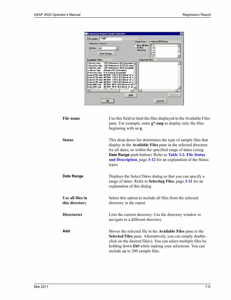
ASAP 2020 Operator’s Manual Regression Report
File name Use this field to limit the files displayed in the Available Files pane. For example; enter g*.smp to display only the files beginning with an g.
Status This drop-down list determines the type of sample files that display in the Available Files pane in the selected directory for all dates, or within the specified range of dates (using Date Range push button). Refer to Table 3-2. File Status and Description, page 3-12 for an explanation of the Status types.
Date Range Displays the Select Dates dialog so that you can specify a range of dates. Refer to Selecting Files, page 3-11 for an explanation of this dialog.
Use all files inthis directory
Select this option to include all files from the selected directory in the report.
Directories Lists the current directory. Use the directory window to navigate to a different directory.
Add Moves the selected file in the Available Files pane to the Selected Files pane. Alternatively, you can simply double-click on the desired file(s). You can select multiple files by holding down Ctrl while making your selections. You can include up to 200 sample files.
Mar 2011 7-9

Regression Report ASAP 2020 Operator’s Manual
Remove Removes the selected file from the Selected Files pane and places it back into the Available Files pane.
Save As Default Saves the current definition of the report as the default.
Report Settings The options in this group box enable you to choose output criteria.
The Copies field is enabled when you choose Printer as the destination, enabling you to print up to four copies of the report.
Report Generates the report.
7-10 Mar 2011

ASAP 2020 Operator’s Manual Control Chart
Control Chart
This option enables you to generate a control chart report which plots the changes in a statistic.
Show report title Select this option to have a title display on your report. Accept the default or enter a new title. You can enter up to 40 alphanumeric characters.
Deselect this option to omit the report title.
Show graphic Select this option to have a graphic display above your report title. For example, you may wish to display your company logo. The graphic must be a bitmap (bmp) or enhanced metafile (emf).
Click Browse to choose the file, then use the Height and Width fields to specify a size. This image can be edited in the report window (when printed to the screen), or removed if desired.
X-axis Order By Enables you to choose the order in which X-axis statistics are placed. You can have them placed by Time, File name, Date, Minutes, or Days.
Mar 2011 7-11

Control Chart ASAP 2020 Operator’s Manual
Graph [n] Displays the Control Chart Graph [n] Options dialog, allowing you to define the Y-axis of each graph.
Statistic This drop-down list displays the SPC variables selected on the SPC Report Options dialog. The variable you choose will be plotted against time.
Autoscale Allows you to have the Y-axis scaled automatically. If you wish to specify a range, deselect this option and enter a range in the From and To fields.
Center Line Displays placement options for the variable’s optional value. Choose Entered to specify placement of the line.
Limit Lines Displays the options available for limiting lines. You can have the lines placed at some multiple of the standard deviation or at specified positions (Entered).
When you select Entered, the High limit and Low limit fields are enabled, allowing you to enter appropriate values.
Tabular report Allows you to generate tabular, as well as graphical, data of the included samples. A tabular report contains the numeric values contributed by each sample.
Recalculate archived SPC results
Select this option to have archived SPC values recalculated. This ensures that any changes made to the SPC Report Options are included in the new report. It also lengthens the time required to generate the report.
7-12 Mar 2011

ASAP 2020 Operator’s Manual Control Chart
Samples Displays the Control Chart Sample Selection dialog, allowing you to choose the sample files on which you wish to report.
This dialog functions in the same manner as the Regression Report Sample Selection Dialog explained on page 7-8.
Save as Default Saves the current definition of the report as the default.
Report Settings The options in this group box enable you to choose output criteria.
The Copies field is enabled when you choose Printer as the destination, enabling you to print up to four copies of the report.
Report Generates the report.
Mar 2011 7-13

Heat of Adsorption ASAP 2020 Operator’s Manual
Heat of Adsorption
The isosteric heat of adsorption is an important parameter for characterizing the surface heterogeneity, providing information about the adsorbent and the adsorption capacity. Multiple adsorption isotherms are obtained on the same sample using the same adsorptive but at different temperatures to obtain the heat of adsorption.
This option allows you to choose the sample files, define the quantities, and generate a Heat of Adsorption report; the Heat of Adsorption dialog is displayed.
Table Contains the files you choose; also lists the quantity adsorbed.
Add Samples Displays the Select Samples dialog so that you can choose desired files.
Remove Samples Removes the selected sample from the list. If no samples are selected, the last one is removed.
Clear Samples Removes all samples from the list.
7-14 Mar 2011

ASAP 2020 Operator’s Manual Heat of Adsorption
Edit Quantities Displays the Edit Quantities Adsorbed dialog so that you can specify the range of surface coverage to include in the heat of adsorption report.
Quantity Adsorbed table
Allows you to enter the points.
Insert Range Displays the Insert Quantity Range dialog.This dialog allows you to specify the starting and ending quantities adsorbed, as well as the number of points to insert within the specified range.
Insert Inserts a row above the selected row.
Delete Deletes the selected row.
Mar 2011 7-15

Heat of Adsorption ASAP 2020 Operator’s Manual
Clear Clears the entire table of all entries except one; one is required.
Load Table Allows you to import a previously saved table.
Save Table Allows you to save the current table as a file (QNT extension).
Apply Applies the quantities in the table to the current Heat of Adsorption report.
Report Settings The options in this group box allow you to choose report criteria.
Show report title Choose this option to have a title display in the header of your report, then use the adjacent field to enter the title.
Show graphic This option allows you to have a graphic appear in your title; for example, you may wish to show your company logo. You can use a bitmap or an enhanced metafile.
Use the Height and Width fields to define a size.
Tabular report Select this option to have data generated in a tabular format.
Isostere plot Select this option to generate a graph showing quantities of gas adsorbed vs. the temperature.
Heat of adsorption plot
Select this option to generate the Heat of Adsorption data in a graphical format.
Copies Enabled when you choose Printer as the destination, allowing you to print up to four copies of your report(s).
Destination Enables you to choose a destination for your report.
File name Enabled when you choose File as the destination, allowing you to enter a name (or you can accept the default).
Open Enables you to open a previously saved report.
7-16 Mar 2011
ASAP 2020 Operator’s Manual Rate of Adsorption (ROA)
Rate of Adsorption (ROA)
Rate of Adsorption is enabled only if this option is installed.
Select Rate of Adsorption to start the ROA program. Refer to your Rate of Adsorption operator’s manual for operating instructions.
Save Saves the current report.
Report Generates the report.
Close Closes the dialog.
Mar 2011 7-17

Printed Reports ASAP 2020 Operator’s Manual
Printed Reports
Header
All printed reports (either to the screen or to a printer) contain a header displaying file statistics.
• Tabular and graphical reports contain sample and instrument statistics such as when the file was created and by whom, date and time of analysis, analysis conditions, and so forth.
The headers for these reports also contain notes of any changes to the sample file that occur after analysis.
• Summary report headers contain the same type of information displayed in tabular and graphical reports with the exception of notes.
Onscreen Reports
The report window containing onscreen reports provides many options for customizing and manipulating reports:
• a tool bar• shortcut menus• zoom feature• axis cross-hairs
When reports are printed to the screen, they are printed in a window like the one shown below. Each requested report is listed in the Reports window on the tool bar; they are also indicated by selectable tabs across the top of the report header. To view a specific report, select its tab or select the report in the Reports window and click Show.
7-18 Mar 2011
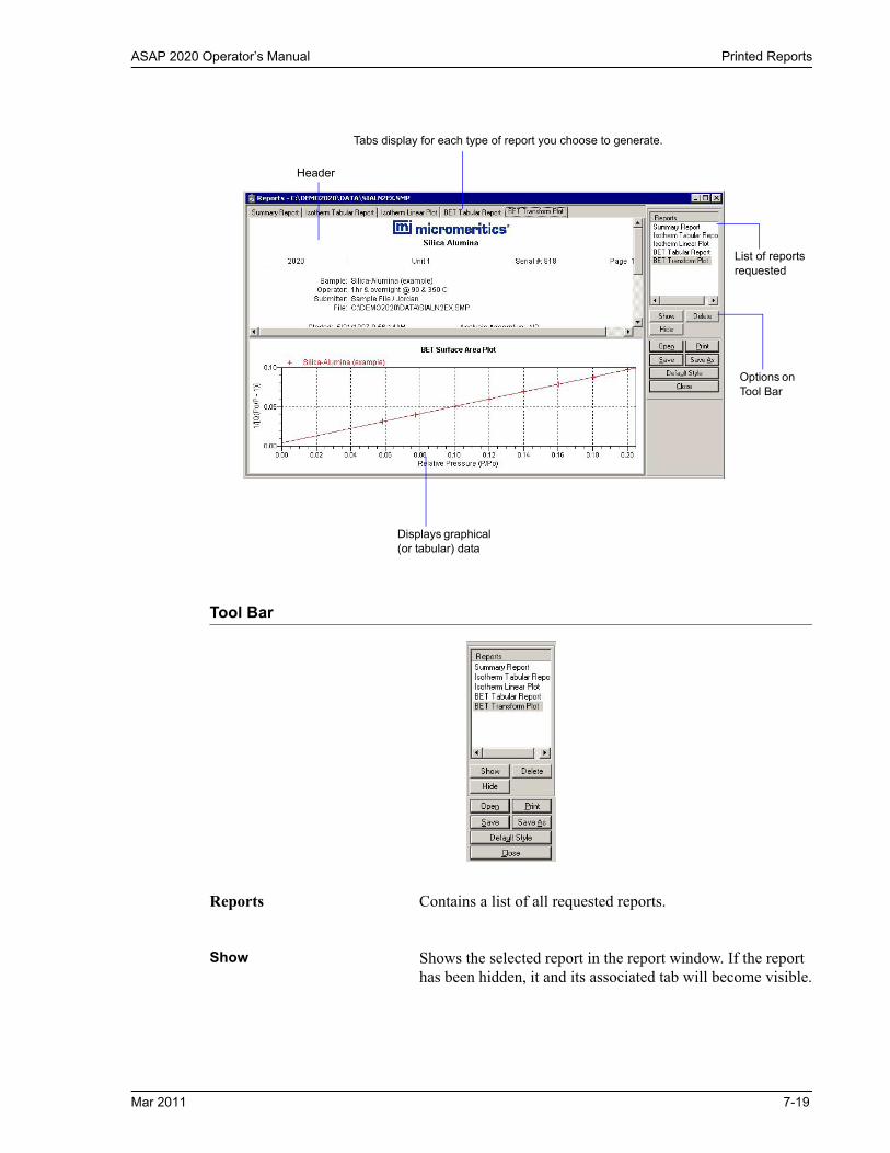
ASAP 2020 Operator’s Manual Printed Reports
Tool Bar
Reports Contains a list of all requested reports.
Show Shows the selected report in the report window. If the report has been hidden, it and its associated tab will become visible.
Displays graphical (or tabular) data
Options on Tool Bar
List of reports requested
Tabs display for each type of report you choose to generate.
Header
Mar 2011 7-19

Printed Reports ASAP 2020 Operator’s Manual
Delete Deletes the selected report. A deletion confirmation dialog is displayed since this function cannot be undone. The deleted report(s) will have to be regenerated if deleted in error.
Hide Hides (removes) the selected report from the report window. The report’s associated tab is also removed.
Open Allows you to open a previously saved report file.
Print Displays a print dialog so that you can choose an appropriate printer for report output. A list of available reports is displayed in the window on the right side of the dialog.
For convenience in selecting which reports to print, push buttons are provided beneath the report window. Or, you can make your selection by clicking on the desired reports.
Current selects the report displayed in the report window.
Shown selects only the shown reports; any non-highlighted reports indicate they are hidden. You can still select hidden reports from this window to print.
All selects all reports, including those that may have been hidden.
Clear clears all selections.
7-20 Mar 2011

ASAP 2020 Operator’s Manual Printed Reports
Save Saves all reports of the currently open file in a report format using the same name as the sample file, only with an rep extension. If you wish to specify a name and/or specific reports to save, use the Save As push button.
Save As Saves all or specified reports from the currently open file. The push buttons displayed on this dialog perform in the same manner as the print dialog (explained above).
Reports can be saved in three different formats:
Report system (*.rep): Saved in a format which allows you to reopen the file using the push button on the Report window tool bar.
Spreadsheet (*.xls): Saved in a format which can be imported into most spreadsheet programs.
Ascii Text (*.txt): Saved in ASCII text which can be imported into programs accepting this type of file.
Default Style Displays the Default Style dialog so that you can specify default parameters for report fonts and curve properties.
Fonts Contains a list of report elements for which the font can be edited. Simply highlight the desired element and click Edit; a font dialog is displayed so that you can specify the desired font and attributes.
Curve The items in this group box enable you to specify a thickness for report curves and, when using histograms, the type of fill to apply.
Mar 2011 7-21

Printed Reports ASAP 2020 Operator’s Manual
Graph border linethickness
Enables you to specify a thickness for the border of the graph.
Load Loads the last saved defaults.
Save Saves the changes as the defaults. If you do not click Save, the changes will apply to the current report set only. The next reports will revert to the defaults.
Close Closes the dialog and applies the changes. If you clicked Save, the changes become the defaults. If you did not click Save, the changes apply to the current report only.
Close Closes the report window.
7-22 Mar 2011

ASAP 2020 Operator’s Manual Printed Reports
Shortcut Menus
Shortcut menus are accessed when you right-click on the tabular or graphical portion of a report.
Tabular Reports
Resize column Displays a dialog so that you can specify the width of the selected column (in inches).
Rename column Displays a dialog so that you can edit the name of the selected column. Use Ctrl + Enter to insert line feeds.
Move column Allows you to move the location of the selected column to the left or to the right.
Align column Enables you to right-align, left-align, or center the data in the selected column.
Hide column Displays a list of the columns that have not been hidden, enabling you to select the one you wish to hide.
Show column Displays a list of all hidden columns, enabling you to select the one you wish to have shown again.
Column font Displays a Font dialog, allowing you to change font attributes for the tabular data in the current report.
Mar 2011 7-23
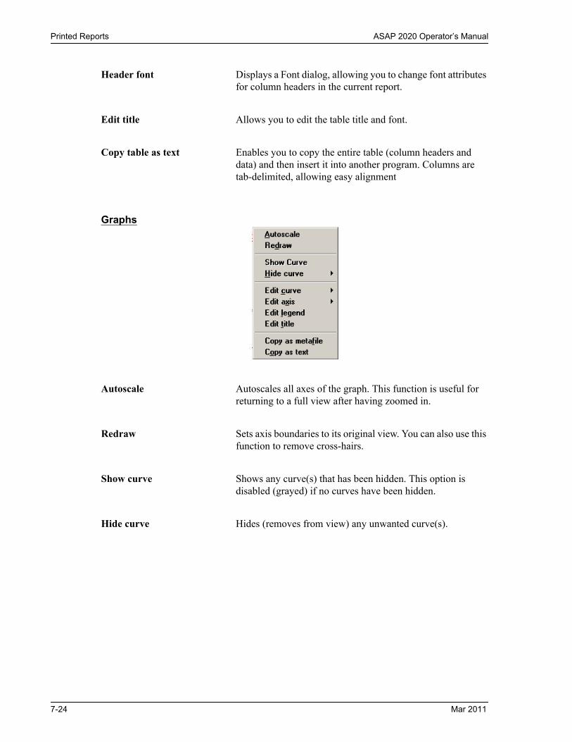
Printed Reports ASAP 2020 Operator’s Manual
Graphs
Header font Displays a Font dialog, allowing you to change font attributes for column headers in the current report.
Edit title Allows you to edit the table title and font.
Copy table as text Enables you to copy the entire table (column headers and data) and then insert it into another program. Columns are tab-delimited, allowing easy alignment
Autoscale Autoscales all axes of the graph. This function is useful for returning to a full view after having zoomed in.
Redraw Sets axis boundaries to its original view. You can also use this function to remove cross-hairs.
Show curve Shows any curve(s) that has been hidden. This option is disabled (grayed) if no curves have been hidden.
Hide curve Hides (removes from view) any unwanted curve(s).
7-24 Mar 2011
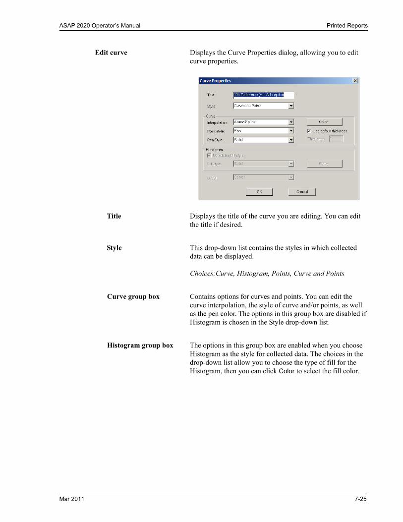
ASAP 2020 Operator’s Manual Printed Reports
Edit curve Displays the Curve Properties dialog, allowing you to edit curve properties.
Title Displays the title of the curve you are editing. You can edit the title if desired.
Style This drop-down list contains the styles in which collected data can be displayed.
Choices:Curve, Histogram, Points, Curve and Points
Curve group box Contains options for curves and points. You can edit the curve interpolation, the style of curve and/or points, as well as the pen color. The options in this group box are disabled if Histogram is chosen in the Style drop-down list.
Histogram group box The options in this group box are enabled when you choose Histogram as the style for collected data. The choices in the drop-down list allow you to choose the type of fill for the Histogram, then you can click Color to select the fill color.
Mar 2011 7-25

Printed Reports ASAP 2020 Operator’s Manual
Edit axis Displays the Axis Properties dialog, allowing you to edit axis properties.
Edit legend Displays the Legend Properties dialog, allowing you to edit the placement of the legend. You can also edit the font if desired.
Edit title Displays the Title Properties dialog, allowing you to edit the current graph’s title and font.
Copy as metafile Copies the graph and places it on the clipboard, allowing you to paste it into other applications accepting Windows metafiles.
7-26 Mar 2011

ASAP 2020 Operator’s Manual Report Examples
Zoom Feature
A zoom feature is included with the report system so that you can zoom in to examine fine details. To use this feature, simply hold down the left mouse button and drag the mouse cursor (drawing a box) across the area you wish to view; then release the button. The enlarged area immediately fills the graph area. Right-click in the graph area and choose Autoscale from the shortcut menu to return to the normal view
Axis Cross Hair
A cross-hair function is available so that you can view axis coordinates. To use this feature, simply left-click in the desired area of the graph.
Right-click in the graph area and choose Autoscale or Redraw from the shortcut menu to remove cross-hair lines and return to the normal view. Alternatively, you can click outside of the graph area.
Report Examples
The remainder of this chapter contains samples of reports produced by analyses of two different materials:
• Silican Alumina reference material analyzed with N2 at 77 K• Y Zeolite reference material analyzed with N2 at 77.35 K
Copy as text Copies the data used to generate the graph as a series of tab-delimited columns of text.
Point of CoordinationY-axis position
X-axis position
Mar 2011 7-27
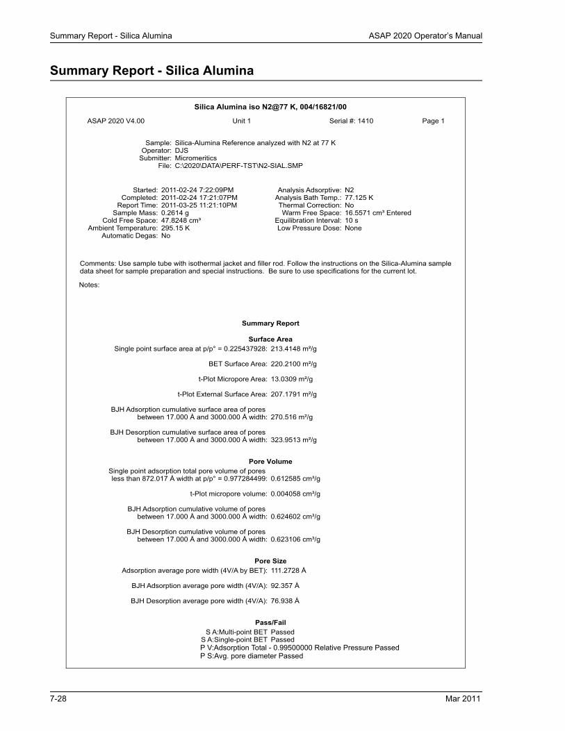
Summary Report - Silica Alumina ASAP 2020 Operator’s Manual
Summary Report - Silica Alumina
Silica Alumina iso N2@77 K, 004/16821/00
ASAP 2020 V4.00 (V3.05 H) Unit 1 Serial #: 1410 Page 1
Sample: Silica-Alumina Reference analyzed with N2 at 77 KOperator: DJS
Submitter: MicromeriticsFile: C:\2020\DATA\PERF-TST\N2-SIAL.SMP
Started: 2011-02-24 7:22:09PM Analysis Adsorptive: N2Completed: 2011-02-24 17:21:07PM Analysis Bath Temp.: 77.125 K
Report Time: 2011-03-25 11:21:10PM Thermal Correction: NoSample Mass: 0.2614 g Warm Free Space: 16.5571 cm³ Entered
Cold Free Space: 47.8248 cm³ Equilibration Interval: 10 sAmbient Temperature: 295.15 K Low Pressure Dose: None
Automatic Degas: No
Comments: Use sample tube with isothermal jacket and filler rod. Follow the instructions on the Silica-Alumina sample data sheet for sample preparation and special instructions. Be sure to use specifications for the current lot.
Notes:
Summary Report
Surface AreaSingle point surface area at p/p° = 0.225437928: 213.4148 m²/g
BET Surface Area: 220.2100 m²/g
t-Plot Micropore Area: 13.0309 m²/g
t-Plot External Surface Area: 207.1791 m²/g
BJH Adsorption cumulative surface area of pores
between 17.000 Å and 3000.000 Å width: 270.516 m²/g
BJH Desorption cumulative surface area of pores between 17.000 Å and 3000.000 Å width: 323.9513 m²/g
Pore VolumeSingle point adsorption total pore volume of pores less than 872.017 Å width at p/p° = 0.977284499: 0.612585 cm³/g
t-Plot micropore volume: 0.004058 cm³/g
BJH Adsorption cumulative volume of pores
between 17.000 Å and 3000.000 Å width: 0.624602 cm³/g
BJH Desorption cumulative volume of pores between 17.000 Å and 3000.000 Å width: 0.623106 cm³/g
Pore SizeAdsorption average pore width (4V/A by BET): 111.2728 Å
BJH Adsorption average pore width (4V/A): 92.357 Å
BJH Desorption average pore width (4V/A): 76.938 Å
Pass/FailS A:Multi-point BET Passed
S A:Single-point BET Passed P V:Adsorption Total - 0.99500000 Relative Pressure Passed P S:Avg. pore diameter Passed
7-28 Mar 2011

ASAP 2020 Operator’s Manual Isotherm Report - Silica Alumina
Isotherm Report - Silica Alumina
Silica Alumina iso N2@77 K, 004/16821/00
ASAP 2020 V4.00 (V3.05 H) Unit 1 Serial #: 1410 Page 3
Sample: Silica-Alumina Reference analyzed with N2 at 77 KOperator: DJS
Submitter: MicromeriticsFile: C:\2020\DATA\PERF-TST\N2-SIAL.SMP
Started: 2011-02-24 7:22:09PM Analysis Adsorptive: N2Completed: 2011-02-24 17:21:07PM Analysis Bath Temp.: 77.125 K
Report Time: 2011-03-25 11:21:10PM Thermal Correction: NoSample Mass: 0.2614 g Warm Free Space: 16.5571 cm³ Entered
Cold Free Space: 47.8248 cm³ Equilibration Interval: 10 sAmbient Temperature: 295.15 K Low Pressure Dose: None
Automatic Degas: No
Comments: Use sample tube with isothermal jacket and filler rod. Follow the instructions on the Silica-Alumina sample data sheet for sample preparation and special instructions. Be sure to use specifications for the current lot.
Notes:
Isotherm Tabular ReportRelative
Pressure (p/p°)AbsolutePressure(mmHg)
QuantityAdsorbed
(cm³/g STP)
Elapsed Time(h:min)
SaturationPressure(mmHg)
00:41 743.1268310.009531209 7.080653 36.0245 01:040.033702750 25.035069 43.1510 01:110.069312916 51.482746 48.5056 01:170.081949977 60.865673 49.9859 01:210.118880333 88.288406 53.7985 01:260.140710115 104.493446 55.8419 01:310.186214229 138.275955 59.8815 01:360.225437928 167.390518 63.2936 01:410.277756514 206.220673 67.8903 01:470.326988938 242.753265 72.4267 01:530.376592638 279.555420 77.2896 01:590.425275617 315.668060 82.4824 02:050.474365209 352.071655 88.3683 02:120.522801435 387.983337 95.0697 02:190.570348466 423.222412 102.9292 02:270.599440995 444.767334 108.6925 02:340.646909533 479.914734 120.3034 02:45
02:47 741.8370970.695583996 515.918579 137.1353 02:590.754458542 559.387817 172.1878 03:230.803352647 595.358398 230.9460 03:550.818816439 606.666016 259.0634 04:120.855473657 633.506958 329.6220 04:460.879826475 651.377197 356.5463 05:03
05:05 740.3254390.907384285 671.489868 371.8145 05:210.932766033 690.099731 382.2773 05:310.947137652 700.609253 387.4319 05:380.977284499 722.745789 396.0335 05:470.998767570 738.447876 400.5519 05:570.965605668 713.857544 398.5429 06:010.924130039 683.109375 395.8252 06:060.876983917 648.145264 390.7455 06:130.857717903 633.810852 387.4625 06:190.852194791 629.666199 386.3166 06:230.829198788 612.567139 381.0485 06:30
Mar 2011 7-29

Isotherm Report - Silica Alumina ASAP 2020 Operator’s Manual
Silica Alumina iso N2@77 K, 004/16821/00
ASAP 2020 V4.00 (V3.05 H) Unit 1 Serial #: 1410 Page 4
Sample: Silica-Alumina Reference analyzed with N2 at 77 KOperator: DJS
Submitter: MicromeriticsFile: C:\2020\DATA\PERF-TST\N2-SIAL.SMP
Started: 2011-02-24 7:22:09PM Analysis Adsorptive: N2Completed: 2011-02-24 17:21:07PM Analysis Bath Temp.: 77.125 K
Report Time: 2011-03-25 11:21:10PM Thermal Correction: NoSample Mass: 0.2614 g Warm Free Space: 16.5571 cm³ Entered
Cold Free Space: 47.8248 cm³ Equilibration Interval: 10 sAmbient Temperature: 295.15 K Low Pressure Dose: None
Automatic Degas: No
Comments: Use sample tube with isothermal jacket and filler rod. Follow the instructions on the Silica-Alumina sample data sheet for sample preparation and special instructions. Be sure to use specifications for the current lot.
Notes:
Isotherm Tabular ReportRelative
Pressure (p/p°)AbsolutePressure(mmHg)
QuantityAdsorbed
(cm³/g STP)
Elapsed Time(h:min)
SaturationPressure(mmHg)
0.805018739 594.554626 373.4363 06:4007:11 737.983887
0.756437482 558.074768 265.0066 07:300.699072862 515.473999 157.2673 08:050.635931970 468.792633 121.2898 08:220.592357948 436.596680 108.6831 08:330.534731256 394.068115 97.4256 08:420.479370390 353.231873 89.1965 08:490.426910874 314.542145 82.6950 08:560.375251524 276.454559 77.0545 09:020.324421734 238.985138 72.0226 09:080.273687848 201.596436 67.3259 09:13
09:15 736.5697630.223387277 164.540314 62.8633 09:200.172815469 127.290649 58.4314 09:250.112054097 82.535660 52.8082 09:31
7-30 Mar 2011

ASAP 2020 Operator’s Manual Isotherm Report - Silica Alumina
Silica Alumina iso N2@77 K, 004/16821/00
ASAP 2020 V4.00 (V3.05 H) Unit 1 Serial #: 1410 Page 5
Sample: Silica-Alumina Reference analyzed with N2 at 77 KOperator: DJS
Submitter: MicromeriticsFile: C:\2020\DATA\PERF-TST\N2-SIAL.SMP
Started: 2011-02-24 7:22:09PM Analysis Adsorptive: N2Completed: 2011-02-24 17:21:07PM Analysis Bath Temp.: 77.125 K
Report Time: 2011-03-25 11:21:10PM Thermal Correction: NoSample Mass: 0.2614 g Warm Free Space: 16.5571 cm³ Entered
Cold Free Space: 47.8248 cm³ Equilibration Interval: 10 sAmbient Temperature: 295.15 K Low Pressure Dose: None
Automatic Degas: No
Comments: Use sample tube with isothermal jacket and filler rod. Follow the instructions on the Silica-Alumina sample data sheet for sample preparation and special instructions. Be sure to use specifications for the current lot.
Notes:
Relative Pressure (p/p°)0.00.0 0.1 0.2 0.3 0.4 0.5 0.6 0.7 0.8 0.9 1.0
Qua
ntity
Ads
orbe
d (c
m³/g
STP
)
00
50
100
150
200
250
300
350
400
Isotherm Linear PlotSilica-Alumina Reference analyzed with N2 at 77 K - AdsorptionSilica-Alumina Reference analyzed with N2 at 77 K - Desorption
Mar 2011 7-31

BET Surface Area Report - Silica Alumina ASAP 2020 Operator’s Manual
BET Surface Area Report - Silica Alumina
Silica Alumina iso N2@77 K, 004/16821/00
ASAP 2020 V4.00 (V3.05 H) Unit 1 Serial #: 1410 Page 6
Sample: Silica-Alumina Reference analyzed with N2 at 77 KOperator: DJS
Submitter: MicromeriticsFile: C:\2020\DATA\PERF-TST\N2-SIAL.SMP
Started: 2011-02-24 7:22:09PM Analysis Adsorptive: N2Completed: 2011-02-24 17:21:07PM Analysis Bath Temp.: 77.125 K
Report Time: 2011-03-25 11:21:10PM Thermal Correction: NoSample Mass: 0.2614 g Warm Free Space: 16.5571 cm³ Entered
Cold Free Space: 47.8248 cm³ Equilibration Interval: 10 sAmbient Temperature: 295.15 K Low Pressure Dose: None
Automatic Degas: No
Comments: Use sample tube with isothermal jacket and filler rod. Follow the instructions on the Silica-Alumina sample data sheet for sample preparation and special instructions. Be sure to use specifications for the current lot.
Notes:
BET Surface Area ReportBET Surface Area: 220.2100 ± 0.2949 m²/g
Slope: 0.019590 ± 0.000026 g/cm³ STPY-Intercept: 0.000178 ± 0.000004 g/cm³ STP
C: 111.058215Qm: 50.5858 cm³/g STP
Correlation Coefficient: 0.9999964Molecular Cross-Sectional Area: 0.1620 nm²
RelativePressure
(p/p°)
QuantityAdsorbed
(cm³/g STP)
1/[Q(p°/p - 1)]
0.069312916 48.5056 0.0015350.081949977 49.9859 0.0017860.118880333 53.7985 0.0025080.140710115 55.8419 0.0029320.186214229 59.8815 0.0038210.225437928 63.2936 0.004598
7-32 Mar 2011

ASAP 2020 Operator’s Manual BET Surface Area Report - Silica Alumina
Silica Alumina iso N2@77 K, 004/16821/00
ASAP 2020 V4.00 (V3.05 H) Unit 1 Serial #: 1410 Page 7
Sample: Silica-Alumina Reference analyzed with N2 at 77 KOperator: DJS
Submitter: MicromeriticsFile: C:\2020\DATA\PERF-TST\N2-SIAL.SMP
Started: 2011-02-24 7:22:09PM Analysis Adsorptive: N2Completed: 2011-02-24 17:21:07PM Analysis Bath Temp.: 77.125 K
Report Time: 2011-03-25 11:21:10PM Thermal Correction: NoSample Mass: 0.2614 g Warm Free Space: 16.5571 cm³ Entered
Cold Free Space: 47.8248 cm³ Equilibration Interval: 10 sAmbient Temperature: 295.15 K Low Pressure Dose: None
Automatic Degas: No
Comments: Use sample tube with isothermal jacket and filler rod. Follow the instructions on the Silica-Alumina sample data sheet for sample preparation and special instructions. Be sure to use specifications for the current lot.
Notes:
Relative Pressure (p/p°)0.000.00 0.02 0.04 0.06 0.08 0.10 0.12 0.14 0.16 0.18 0.20 0.22
1/[Q
(p°/
p - 1
)]
0.00000.0000
0.0005
0.0010
0.0015
0.0020
0.0025
0.0030
0.0035
0.0040
0.0045
BET Surface Area PlotSilica-Alumina Reference analyzed with N2 at 77 K
Mar 2011 7-33

t-Plot - Silica Alumina ASAP 2020 Operator’s Manual
t-Plot - Silica Alumina
Silica Alumina iso N2@77 K, 004/16821/00
ASAP 2020 V4.00 (V3.05 H) Unit 1 Serial #: 1410 Page 8
Sample: Silica-Alumina Reference analyzed with N2 at 77 KOperator: DJS
Submitter: MicromeriticsFile: C:\2020\DATA\PERF-TST\N2-SIAL.SMP
Started: 2011-02-24 7:22:09PM Analysis Adsorptive: N2Completed: 2011-02-24 17:21:07PM Analysis Bath Temp.: 77.125 K
Report Time: 2011-03-25 11:21:10PM Thermal Correction: NoSample Mass: 0.2614 g Warm Free Space: 16.5571 cm³ Entered
Cold Free Space: 47.8248 cm³ Equilibration Interval: 10 sAmbient Temperature: 295.15 K Low Pressure Dose: None
Automatic Degas: No
Comments: Use sample tube with isothermal jacket and filler rod. Follow the instructions on the Silica-Alumina sample data sheet for sample preparation and special instructions. Be sure to use specifications for the current lot.
Notes:
t-Plot ReportMicropore Volume: 0.004058 cm³/g
Micropore Area: 13.0309 m²/gExternal Surface Area: 207.1791 m²/g
Slope: 13.394044 ± 0.046845 cm³/g·Å STPY-Intercept: 2.623340 ± 0.196363 cm³/g STP
Correlation Coefficient: 0.999976Surface Area Correction Factor: 1.000
Density Conversion Factor: 0.0015468Total Surface Area (BET): 220.2100 m²/g
Thickness Range: 3.5000 Å to 5.0000 ÅThickness Equation: Harkins and Jura
t = [ 13.99 / ( 0.034 - log(p/p°) ) ] ^ 0.5
RelativePressure (p/p°)
StatisticalThickness (Å)
QuantityAdsorbed
(cm³/g STP)
Fitted
0.009531209 2.6093 36.02450.033702750 3.0475 43.15100.069312916 3.4242 48.50560.081949977 3.5336 49.9859 *0.118880333 3.8197 53.7985 *0.140710115 3.9744 55.8419 *0.186214229 4.2792 59.8815 *0.225437928 4.5326 63.2936 *0.277756514 4.8681 67.8903 *0.326988938 5.1896 72.42670.376592638 5.5261 77.28960.425275617 5.8750 82.48240.474365209 6.2522 88.36830.522801435 6.6573 95.06970.570348466 7.0957 102.92920.599440995 7.3888 108.69250.646909533 7.9178 120.30340.695583996 8.5439 137.1353
7-34 Mar 2011
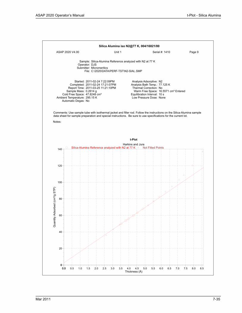
ASAP 2020 Operator’s Manual t-Plot - Silica Alumina
Silica Alumina iso N2@77 K, 004/16821/00
ASAP 2020 V4.00 (V3.05 H) Unit 1 Serial #: 1410 Page 9
Sample: Silica-Alumina Reference analyzed with N2 at 77 KOperator: DJS
Submitter: MicromeriticsFile: C:\2020\DATA\PERF-TST\N2-SIAL.SMP
Started: 2011-02-24 7:22:09PM Analysis Adsorptive: N2Completed: 2011-02-24 17:21:07PM Analysis Bath Temp.: 77.125 K
Report Time: 2011-03-25 11:21:10PM Thermal Correction: NoSample Mass: 0.2614 g Warm Free Space: 16.5571 cm³ Entered
Cold Free Space: 47.8248 cm³ Equilibration Interval: 10 sAmbient Temperature: 295.15 K Low Pressure Dose: None
Automatic Degas: No
Comments: Use sample tube with isothermal jacket and filler rod. Follow the instructions on the Silica-Alumina sample data sheet for sample preparation and special instructions. Be sure to use specifications for the current lot.
Notes:
Thickness (Å)0.00.0 0.5 1.0 1.5 2.0 2.5 3.0 3.5 4.0 4.5 5.0 5.5 6.0 6.5 7.0 7.5 8.0 8.5
Qua
ntity
Ads
orbe
d (c
m³/g
STP
)
00
20
40
60
80
100
120
140
t-PlotHarkins and Jura
Silica-Alumina Reference analyzed with N2 at 77 K Not Fitted Points
Mar 2011 7-35
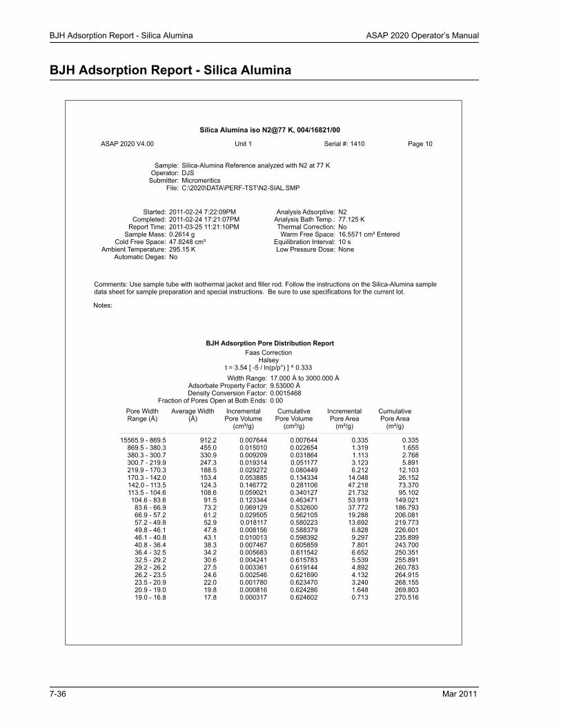
BJH Adsorption Report - Silica Alumina ASAP 2020 Operator’s Manual
BJH Adsorption Report - Silica Alumina
Silica Alumina iso N2@77 K, 004/16821/00
ASAP 2020 V4.00 (V3.05 H) Unit 1 Serial #: 1410 Page 10
Sample: Silica-Alumina Reference analyzed with N2 at 77 KOperator: DJS
Submitter: MicromeriticsFile: C:\2020\DATA\PERF-TST\N2-SIAL.SMP
Started: 2011-02-24 7:22:09PM Analysis Adsorptive: N2Completed: 2011-02-24 17:21:07PM Analysis Bath Temp.: 77.125 K
Report Time: 2011-03-25 11:21:10PM Thermal Correction: NoSample Mass: 0.2614 g Warm Free Space: 16.5571 cm³ Entered
Cold Free Space: 47.8248 cm³ Equilibration Interval: 10 sAmbient Temperature: 295.15 K Low Pressure Dose: None
Automatic Degas: No
Comments: Use sample tube with isothermal jacket and filler rod. Follow the instructions on the Silica-Alumina sample data sheet for sample preparation and special instructions. Be sure to use specifications for the current lot.
Notes:
BJH Adsorption Pore Distribution ReportFaas Correction
Halseyt = 3.54 [ -5 / ln(p/p°) ] ^ 0.333Width Range: 17.000 Å to 3000.000 Å
Adsorbate Property Factor: 9.53000 ÅDensity Conversion Factor: 0.0015468
Fraction of Pores Open at Both Ends: 0.00Pore WidthRange (Å)
Average Width(Å)
IncrementalPore Volume
(cm³/g)
CumulativePore Volume
(cm³/g)
IncrementalPore Area
(m²/g)
CumulativePore Area
(m²/g)
15565.9 - 869.5 912.2 0.007644 0.007644 0.335 0.335869.5 - 380.3 455.0 0.015010 0.022654 1.319 1.655380.3 - 300.7 330.9 0.009209 0.031864 1.113 2.768300.7 - 219.9 247.3 0.019314 0.051177 3.123 5.891219.9 - 170.3 188.5 0.029272 0.080449 6.212 12.103170.3 - 142.0 153.4 0.053885 0.134334 14.048 26.152142.0 - 113.5 124.3 0.146772 0.281106 47.218 73.370113.5 - 104.6 108.6 0.059021 0.340127 21.732 95.102104.6 - 83.6 91.5 0.123344 0.463471 53.919 149.021
83.6 - 66.9 73.2 0.069129 0.532600 37.772 186.79366.9 - 57.2 61.2 0.029505 0.562105 19.288 206.08157.2 - 49.8 52.9 0.018117 0.580223 13.692 219.77349.8 - 46.1 47.8 0.008156 0.588379 6.828 226.60146.1 - 40.8 43.1 0.010013 0.598392 9.297 235.89940.8 - 36.4 38.3 0.007467 0.605859 7.801 243.70036.4 - 32.5 34.2 0.005683 0.611542 6.652 250.35132.5 - 29.2 30.6 0.004241 0.615783 5.539 255.89129.2 - 26.2 27.5 0.003361 0.619144 4.892 260.78326.2 - 23.5 24.6 0.002546 0.621690 4.132 264.91523.5 - 20.9 22.0 0.001780 0.623470 3.240 268.15520.9 - 19.0 19.8 0.000816 0.624286 1.648 269.80319.0 - 16.8 17.8 0.000317 0.624602 0.713 270.516
7-36 Mar 2011

ASAP 2020 Operator’s Manual BJH Adsorption Report - Silica Alumina
Silica Alumina iso N2@77 K, 004/16821/00
ASAP 2020 V4.00 (V3.05 H) Unit 1 Serial #: 1410 Page 11
Sample: Silica-Alumina Reference analyzed with N2 at 77 KOperator: DJS
Submitter: MicromeriticsFile: C:\2020\DATA\PERF-TST\N2-SIAL.SMP
Started: 2011-02-24 7:22:09PM Analysis Adsorptive: N2Completed: 2011-02-24 17:21:07PM Analysis Bath Temp.: 77.125 K
Report Time: 2011-03-25 11:21:10PM Thermal Correction: NoSample Mass: 0.2614 g Warm Free Space: 16.5571 cm³ Entered
Cold Free Space: 47.8248 cm³ Equilibration Interval: 10 sAmbient Temperature: 295.15 K Low Pressure Dose: None
Automatic Degas: No
Comments: Use sample tube with isothermal jacket and filler rod. Follow the instructions on the Silica-Alumina sample data sheet for sample preparation and special instructions. Be sure to use specifications for the current lot.
Notes:
Pore Width (Å)10 50 100 500
Pore
Vol
ume
(cm
³/g)
0.00.0
0.1
0.2
0.3
0.4
0.5
0.6
BJH Adsorption Cumulative Pore Volume (Larger)Halsey : Faas Correction
Silica-Alumina Reference analyzed with N2 at 77 K
Mar 2011 7-37

BJH Adsorption Report - Silica Alumina ASAP 2020 Operator’s Manual
Silica Alumina iso N2@77 K, 004/16821/00
ASAP 2020 V4.00 (V3.05 H) Unit 1 Serial #: 1410 Page 12
Sample: Silica-Alumina Reference analyzed with N2 at 77 KOperator: DJS
Submitter: MicromeriticsFile: C:\2020\DATA\PERF-TST\N2-SIAL.SMP
Started: 2011-02-24 7:22:09PM Analysis Adsorptive: N2Completed: 2011-02-24 17:21:07PM Analysis Bath Temp.: 77.125 K
Report Time: 2011-03-25 11:21:10PM Thermal Correction: NoSample Mass: 0.2614 g Warm Free Space: 16.5571 cm³ Entered
Cold Free Space: 47.8248 cm³ Equilibration Interval: 10 sAmbient Temperature: 295.15 K Low Pressure Dose: None
Automatic Degas: No
Comments: Use sample tube with isothermal jacket and filler rod. Follow the instructions on the Silica-Alumina sample data sheet for sample preparation and special instructions. Be sure to use specifications for the current lot.
Notes:
Pore Width (Å)10 50 100 500 1,000
dV/d
log(
w) P
ore
Volu
me
(cm
³/g·Å
)
0.00.0
0.2
0.4
0.6
0.8
1.0
1.2
1.4
1.6
BJH Adsorption dV/dlog(w) Pore VolumeHalsey : Faas Correction
Silica-Alumina Reference analyzed with N2 at 77 K
7-38 Mar 2011

ASAP 2020 Operator’s Manual BJH Desorption Report - Silica Alumina
BJH Desorption Report - Silica Alumina
Silica Alumina iso N2@77 K, 004/16821/00
ASAP 2020 V4.00 (V3.05 H) Unit 1 Serial #: 1410 Page 13
Sample: Silica-Alumina Reference analyzed with N2 at 77 KOperator: DJS
Submitter: MicromeriticsFile: C:\2020\DATA\PERF-TST\N2-SIAL.SMP
Started: 2011-02-24 7:22:09PM Analysis Adsorptive: N2Completed: 2011-02-24 17:21:07PM Analysis Bath Temp.: 77.125 K
Report Time: 2011-03-25 11:21:10PM Thermal Correction: NoSample Mass: 0.2614 g Warm Free Space: 16.5571 cm³ Entered
Cold Free Space: 47.8248 cm³ Equilibration Interval: 10 sAmbient Temperature: 295.15 K Low Pressure Dose: None
Automatic Degas: No
Comments: Use sample tube with isothermal jacket and filler rod. Follow the instructions on the Silica-Alumina sample data sheet for sample preparation and special instructions. Be sure to use specifications for the current lot.
Notes:
BJH Desorption Pore Distribution ReportFaas Correction
Halseyt = 3.54 [ -5 / ln(p/p°) ] ^ 0.333Width Range: 17.000 Å to 3000.000 Å
Adsorbate Property Factor: 9.53000 ÅDensity Conversion Factor: 0.0015468
Fraction of Pores Open at Both Ends: 0.00Pore WidthRange (Å)
Average Width(Å)
IncrementalPore Volume
(cm³/g)
CumulativePore Volume
(cm³/g)
IncrementalPore Area
(m²/g)
CumulativePore Area
(m²/g)
15564.3 - 577.4 596.3 0.003480 0.003480 0.233 0.233577.4 - 265.6 317.2 0.004807 0.008287 0.606 0.840265.6 - 164.8 191.7 0.009538 0.017825 1.990 2.829164.8 - 142.6 152.0 0.006374 0.024199 1.677 4.506142.6 - 137.3 139.8 0.002257 0.026455 0.645 5.152137.3 - 118.7 126.6 0.010515 0.036971 3.323 8.475118.7 - 103.9 110.2 0.015582 0.052553 5.655 14.129103.9 - 82.6 90.7 0.235321 0.287874 103.830 117.959
82.6 - 66.1 72.4 0.235614 0.523488 130.183 248.14266.1 - 53.7 58.5 0.065587 0.589075 44.839 292.98153.7 - 47.3 50.0 0.016589 0.605664 13.265 306.24647.3 - 40.4 43.3 0.010129 0.615793 9.367 315.61340.4 - 35.2 37.4 0.004607 0.620401 4.928 320.54135.2 - 31.0 32.8 0.002019 0.622420 2.462 323.00431.0 - 27.5 29.0 0.000687 0.623106 0.948 323.951
Mar 2011 7-39

BJH Desorption Report - Silica Alumina ASAP 2020 Operator’s Manual
Silica Alumina iso N2@77 K, 004/16821/00
ASAP 2020 V4.00 (V3.05 H) Unit 1 Serial #: 1410 Page 14
Sample: Silica-Alumina Reference analyzed with N2 at 77 KOperator: DJS
Submitter: MicromeriticsFile: C:\2020\DATA\PERF-TST\N2-SIAL.SMP
Started: 2011-02-24 7:22:09PM Analysis Adsorptive: N2Completed: 2011-02-24 17:21:07PM Analysis Bath Temp.: 77.125 K
Report Time: 2011-03-25 11:21:10PM Thermal Correction: NoSample Mass: 0.2614 g Warm Free Space: 16.5571 cm³ Entered
Cold Free Space: 47.8248 cm³ Equilibration Interval: 10 sAmbient Temperature: 295.15 K Low Pressure Dose: None
Automatic Degas: No
Comments: Use sample tube with isothermal jacket and filler rod. Follow the instructions on the Silica-Alumina sample data sheet for sample preparation and special instructions. Be sure to use specifications for the current lot.
Notes:
Pore Width (Å)40 60 80 100 200 400 600
Por
e V
olum
e (c
m³/g
)
0.00.0
0.1
0.2
0.3
0.4
0.5
0.6
BJH Desorption Cumulative Pore Volume (Larger)Halsey : Faas Correction
Silica-Alumina Reference analyzed with N2 at 77 K
7-40 Mar 2011
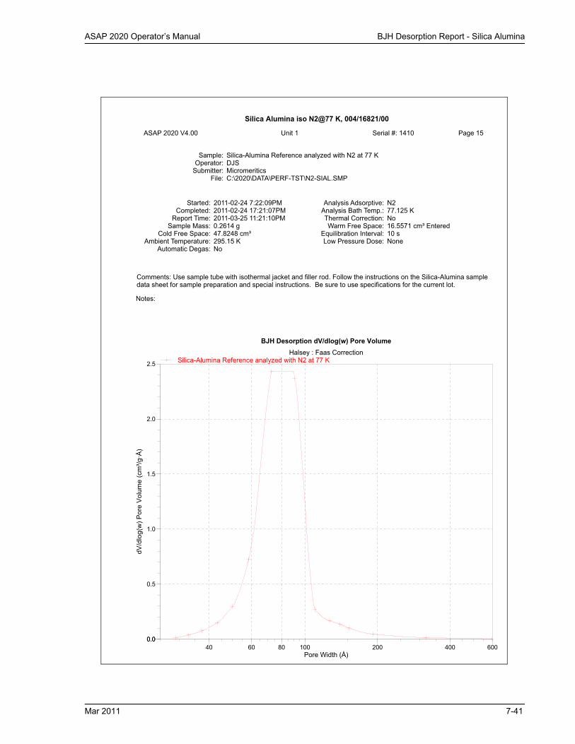
ASAP 2020 Operator’s Manual BJH Desorption Report - Silica Alumina
Silica Alumina iso N2@77 K, 004/16821/00
ASAP 2020 V4.00 (V3.05 H) Unit 1 Serial #: 1410 Page 15
Sample: Silica-Alumina Reference analyzed with N2 at 77 KOperator: DJS
Submitter: MicromeriticsFile: C:\2020\DATA\PERF-TST\N2-SIAL.SMP
Started: 2011-02-24 7:22:09PM Analysis Adsorptive: N2Completed: 2011-02-24 17:21:07PM Analysis Bath Temp.: 77.125 K
Report Time: 2011-03-25 11:21:10PM Thermal Correction: NoSample Mass: 0.2614 g Warm Free Space: 16.5571 cm³ Entered
Cold Free Space: 47.8248 cm³ Equilibration Interval: 10 sAmbient Temperature: 295.15 K Low Pressure Dose: None
Automatic Degas: No
Comments: Use sample tube with isothermal jacket and filler rod. Follow the instructions on the Silica-Alumina sample data sheet for sample preparation and special instructions. Be sure to use specifications for the current lot.
Notes:
Pore Width (Å)40 60 80 100 200 400 600
dV/d
log(
w) P
ore
Vol
ume
(cm
³/g·Å
)
0.00.0
0.5
1.0
1.5
2.0
2.5
BJH Desorption dV/dlog(w) Pore VolumeHalsey : Faas Correction
Silica-Alumina Reference analyzed with N2 at 77 K
Mar 2011 7-41
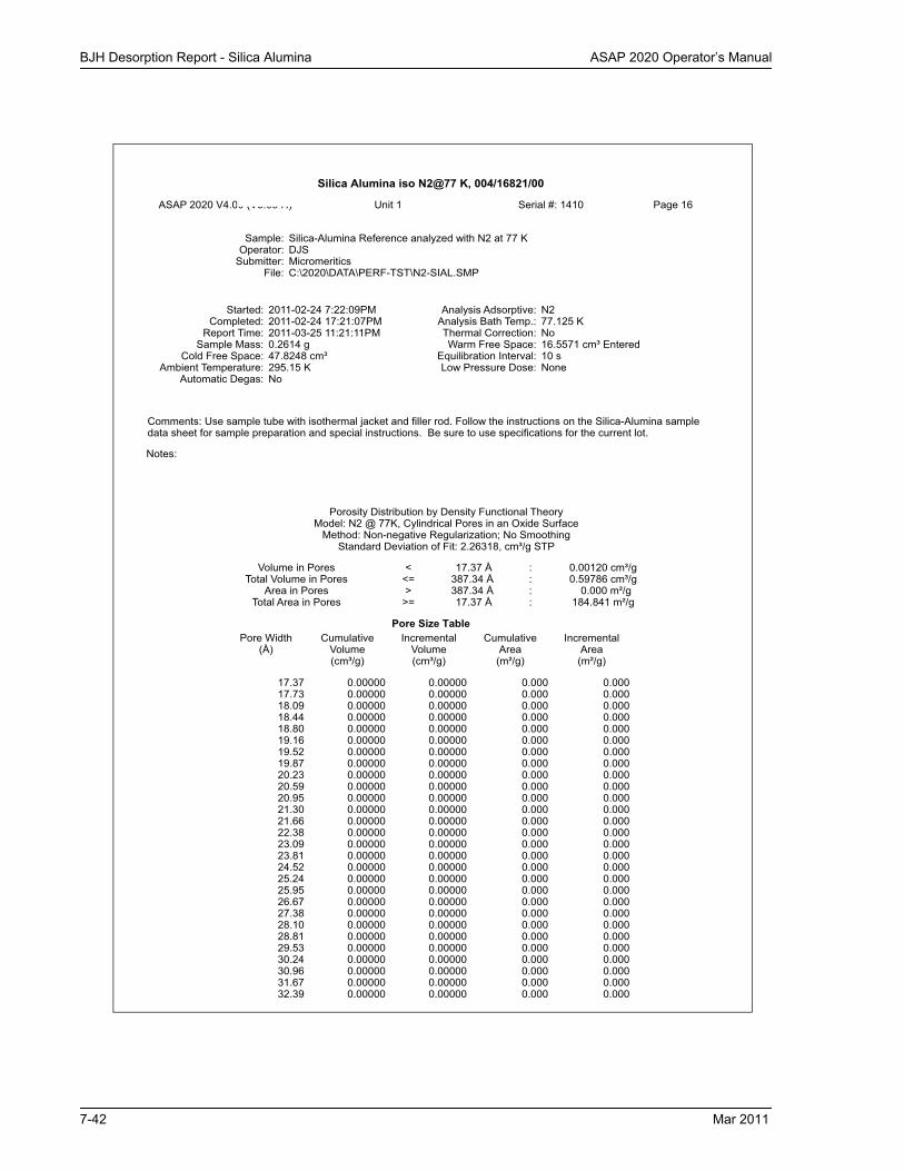
BJH Desorption Report - Silica Alumina ASAP 2020 Operator’s Manual
Silica Alumina iso N2@77 K, 004/16821/00
ASAP 2020 V4.00 (V3.05 H) Unit 1 Serial #: 1410 Page 16
Sample: Silica-Alumina Reference analyzed with N2 at 77 KOperator: DJS
Submitter: MicromeriticsFile: C:\2020\DATA\PERF-TST\N2-SIAL.SMP
Started: 2011-02-24 7:22:09PM Analysis Adsorptive: N2Completed: 2011-02-24 17:21:07PM Analysis Bath Temp.: 77.125 K
Report Time: 2011-03-25 11:21:11PM Thermal Correction: NoSample Mass: 0.2614 g Warm Free Space: 16.5571 cm³ Entered
Cold Free Space: 47.8248 cm³ Equilibration Interval: 10 sAmbient Temperature: 295.15 K Low Pressure Dose: None
Automatic Degas: No
Comments: Use sample tube with isothermal jacket and filler rod. Follow the instructions on the Silica-Alumina sample data sheet for sample preparation and special instructions. Be sure to use specifications for the current lot.
Notes:
Porosity Distribution by Density Functional TheoryModel: N2 @ 77K, Cylindrical Pores in an Oxide Surface
Method: Non-negative Regularization; No SmoothingStandard Deviation of Fit: 2.26318, cm³/g STP
Volume in Pores < 17.37 Å : 0.00120 cm³/gTotal Volume in Pores <= 387.34 Å : 0.59786 cm³/g
Area in Pores > 387.34 Å : 0.000 m²/gTotal Area in Pores >= 17.37 Å : 184.841 m²/g
Pore Size TablePore Width
(Å)Cumulative
Volume(cm³/g)
IncrementalVolume(cm³/g)
CumulativeArea(m²/g)
IncrementalArea(m²/g)
17.37 0.00000 0.00000 0.000 0.000 17.73 0.00000 0.00000 0.000 0.000 18.09 0.00000 0.00000 0.000 0.000 18.44 0.00000 0.00000 0.000 0.000 18.80 0.00000 0.00000 0.000 0.000 19.16 0.00000 0.00000 0.000 0.000 19.52 0.00000 0.00000 0.000 0.000 19.87 0.00000 0.00000 0.000 0.000 20.23 0.00000 0.00000 0.000 0.000 20.59 0.00000 0.00000 0.000 0.000 20.95 0.00000 0.00000 0.000 0.000 21.30 0.00000 0.00000 0.000 0.000 21.66 0.00000 0.00000 0.000 0.000 22.38 0.00000 0.00000 0.000 0.000 23.09 0.00000 0.00000 0.000 0.000 23.81 0.00000 0.00000 0.000 0.000 24.52 0.00000 0.00000 0.000 0.000 25.24 0.00000 0.00000 0.000 0.000 25.95 0.00000 0.00000 0.000 0.000 26.67 0.00000 0.00000 0.000 0.000 27.38 0.00000 0.00000 0.000 0.000 28.10 0.00000 0.00000 0.000 0.000 28.81 0.00000 0.00000 0.000 0.000 29.53 0.00000 0.00000 0.000 0.000 30.24 0.00000 0.00000 0.000 0.000 30.96 0.00000 0.00000 0.000 0.000 31.67 0.00000 0.00000 0.000 0.000 32.39 0.00000 0.00000 0.000 0.000
7-42 Mar 2011

ASAP 2020 Operator’s Manual BJH Desorption Report - Silica Alumina
Mar 2011 7-43

BJH Desorption Report - Silica Alumina ASAP 2020 Operator’s Manual
Silica Alumina iso N2@77 K, 004/16821/00
ASAP 2020 V4.00 (V3.05 H) Unit 1 Serial #: 1410 Page 16
Sample: Silica-Alumina Reference analyzed with N2 at 77 KOperator: DJS
Submitter: MicromeriticsFile: C:\2020\DATA\PERF-TST\N2-SIAL.SMP
Started: 2011-02-24 7:22:09PM Analysis Adsorptive: N2Completed: 2011-02-24 17:21:07PM Analysis Bath Temp.: 77.125 K
Report Time: 2011-03-25 11:21:11PM Thermal Correction: NoSample Mass: 0.2614 g Warm Free Space: 16.5571 cm³ Entered
Cold Free Space: 47.8248 cm³ Equilibration Interval: 10 sAmbient Temperature: 295.15 K Low Pressure Dose: None
Automatic Degas: No
Comments: Use sample tube with isothermal jacket and filler rod. Follow the instructions on the Silica-Alumina sample data sheet for sample preparation and special instructions. Be sure to use specifications for the current lot.
Notes:
Porosity Distribution by Density Functional TheoryModel: N2 @ 77K, Cylindrical Pores in an Oxide Surface
Method: Non-negative Regularization; No SmoothingStandard Deviation of Fit: 2.26318, cm³/g STP
Volume in Pores < 17.37 Å : 0.00120 cm³/gTotal Volume in Pores <= 387.34 Å : 0.59786 cm³/g
Area in Pores > 387.34 Å : 0.000 m²/gTotal Area in Pores >= 17.37 Å : 184.841 m²/g
Pore Size TablePore Width
(Å)Cumulative
Volume(cm³/g)
IncrementalVolume(cm³/g)
CumulativeArea(m²/g)
IncrementalArea(m²/g)
17.37 0.00000 0.00000 0.000 0.000 17.73 0.00000 0.00000 0.000 0.000 18.09 0.00000 0.00000 0.000 0.000 18.44 0.00000 0.00000 0.000 0.000 18.80 0.00000 0.00000 0.000 0.000 19.16 0.00000 0.00000 0.000 0.000 19.52 0.00000 0.00000 0.000 0.000 19.87 0.00000 0.00000 0.000 0.000 20.23 0.00000 0.00000 0.000 0.000 20.59 0.00000 0.00000 0.000 0.000 20.95 0.00000 0.00000 0.000 0.000 21.30 0.00000 0.00000 0.000 0.000 21.66 0.00000 0.00000 0.000 0.000 22.38 0.00000 0.00000 0.000 0.000 23.09 0.00000 0.00000 0.000 0.000 23.81 0.00000 0.00000 0.000 0.000 24.52 0.00000 0.00000 0.000 0.000 25.24 0.00000 0.00000 0.000 0.000 25.95 0.00000 0.00000 0.000 0.000 26.67 0.00000 0.00000 0.000 0.000 27.38 0.00000 0.00000 0.000 0.000 28.10 0.00000 0.00000 0.000 0.000 28.81 0.00000 0.00000 0.000 0.000 29.53 0.00000 0.00000 0.000 0.000 30.24 0.00000 0.00000 0.000 0.000 30.96 0.00000 0.00000 0.000 0.000 31.67 0.00000 0.00000 0.000 0.000 32.39 0.00000 0.00000 0.000 0.000
7-44 Mar 2011
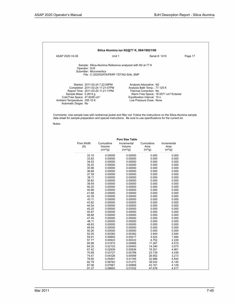
ASAP 2020 Operator’s Manual BJH Desorption Report - Silica Alumina
Silica Alumina iso N2@77 K, 004/16821/00
ASAP 2020 V4.00 (V3.05 H) Unit 1 Serial #: 1410 Page 17
Sample: Silica-Alumina Reference analyzed with N2 at 77 KOperator: DJS
Submitter: MicromeriticsFile: C:\2020\DATA\PERF-TST\N2-SIAL.SMP
Started: 2011-02-24 7:22:09PM Analysis Adsorptive: N2Completed: 2011-02-24 17:21:07PM Analysis Bath Temp.: 77.125 K
Report Time: 2011-03-25 11:21:11PM Thermal Correction: NoSample Mass: 0.2614 g Warm Free Space: 16.5571 cm³ Entered
Cold Free Space: 47.8248 cm³ Equilibration Interval: 10 sAmbient Temperature: 295.15 K Low Pressure Dose: None
Automatic Degas: No
Comments: Use sample tube with isothermal jacket and filler rod. Follow the instructions on the Silica-Alumina sample data sheet for sample preparation and special instructions. Be sure to use specifications for the current lot.
Notes:
Pore Size TablePore Width
(Å)Cumulative
Volume(cm³/g)
IncrementalVolume(cm³/g)
CumulativeArea(m²/g)
IncrementalArea(m²/g)
33.10 0.00000 0.00000 0.000 0.000 33.82 0.00000 0.00000 0.000 0.000 34.53 0.00000 0.00000 0.000 0.000 35.25 0.00000 0.00000 0.000 0.000 35.96 0.00000 0.00000 0.000 0.000 36.68 0.00000 0.00000 0.000 0.000 37.39 0.00000 0.00000 0.000 0.000 38.11 0.00000 0.00000 0.000 0.000 38.82 0.00000 0.00000 0.000 0.000 39.54 0.00000 0.00000 0.000 0.000 40.25 0.00000 0.00000 0.000 0.000 40.96 0.00000 0.00000 0.000 0.000 41.68 0.00000 0.00000 0.000 0.000 42.39 0.00000 0.00000 0.000 0.000 43.11 0.00000 0.00000 0.000 0.000 43.82 0.00000 0.00000 0.000 0.000 44.54 0.00000 0.00000 0.000 0.000 45.25 0.00000 0.00000 0.000 0.000 45.97 0.00000 0.00000 0.000 0.000 46.68 0.00000 0.00000 0.000 0.000 47.40 0.00000 0.00000 0.000 0.000 48.11 0.00000 0.00000 0.000 0.000 48.83 0.00000 0.00000 0.000 0.000 49.54 0.00000 0.00000 0.000 0.000 50.26 0.00000 0.00000 0.000 0.000 52.05 0.00382 0.00382 2.940 2.940 54.91 0.00600 0.00217 4.524 1.584 57.77 0.00922 0.00322 6.752 2.228 60.98 0.01610 0.00688 11.267 4.515 64.20 0.02103 0.00493 14.340 3.073 67.42 0.02939 0.00836 19.301 4.961 70.99 0.03727 0.00788 23.739 4.438 74.57 0.04326 0.00599 26.952 3.213 78.50 0.05491 0.01165 32.886 5.934 82.79 0.06762 0.01272 39.032 6.145 87.08 0.07661 0.00899 43.161 4.129 91.37 0.08693 0.01032 47.678 4.517
Mar 2011 7-45

BJH Desorption Report - Silica Alumina ASAP 2020 Operator’s Manual
Silica Alumina iso N2@77 K, 004/16821/00
ASAP 2020 V4.00 (V3.05 H) Unit 1 Serial #: 1410 Page 18
Sample: Silica-Alumina Reference analyzed with N2 at 77 KOperator: DJS
Submitter: MicromeriticsFile: C:\2020\DATA\PERF-TST\N2-SIAL.SMP
Started: 2011-02-24 7:22:09PM Analysis Adsorptive: N2Completed: 2011-02-24 17:21:07PM Analysis Bath Temp.: 77.125 K
Report Time: 2011-03-25 11:21:11PM Thermal Correction: NoSample Mass: 0.2614 g Warm Free Space: 16.5571 cm³ Entered
Cold Free Space: 47.8248 cm³ Equilibration Interval: 10 sAmbient Temperature: 295.15 K Low Pressure Dose: None
Automatic Degas: No
Comments: Use sample tube with isothermal jacket and filler rod. Follow the instructions on the Silica-Alumina sample data sheet for sample preparation and special instructions. Be sure to use specifications for the current lot.
Notes:
Pore Size TablePore Width
(Å)Cumulative
Volume(cm³/g)
IncrementalVolume(cm³/g)
CumulativeArea(m²/g)
IncrementalArea(m²/g)
96.37 0.10697 0.02004 55.996 8.318 101.38 0.12924 0.02226 64.781 8.785 106.38 0.14540 0.01617 70.860 6.079 112.10 0.16294 0.01753 77.116 6.256 117.82 0.19527 0.03233 88.093 10.977 123.90 0.23344 0.03817 100.416 12.324 130.33 0.26297 0.02953 109.480 9.064 136.76 0.29481 0.03184 118.793 9.313 143.91 0.32698 0.03216 127.733 8.940 151.06 0.35843 0.03145 136.061 8.328 158.93 0.40462 0.04619 147.687 11.626 167.15 0.44789 0.04327 158.043 10.355 175.73 0.47397 0.02608 163.979 5.936 184.66 0.49659 0.02261 168.877 4.898 193.96 0.51309 0.01650 172.280 3.403 203.97 0.52489 0.01180 174.594 2.314 214.33 0.53342 0.00853 176.187 1.593 225.06 0.53996 0.00654 177.350 1.163 236.50 0.54584 0.00587 178.343 0.993 248.29 0.55357 0.00773 179.588 1.245 261.16 0.56003 0.00647 180.579 0.991 274.39 0.56356 0.00353 181.093 0.514 287.97 0.56661 0.00305 181.516 0.423 302.63 0.56948 0.00287 181.895 0.379 318.00 0.57219 0.00271 182.237 0.341 334.08 0.57471 0.00252 182.539 0.302 350.88 0.57705 0.00234 182.805 0.266 368.76 0.57921 0.00216 183.039 0.234 387.34 0.59665 0.01745 184.841 1.802
7-46 Mar 2011

ASAP 2020 Operator’s Manual BJH Desorption Report - Silica Alumina
Silica Alumina iso N2@77 K, 004/16821/00
ASAP 2020 V4.00 (V3.05 H) Unit 1 Serial #: 1410 Page 19
Sample: Silica-Alumina Reference analyzed with N2 at 77 KOperator: DJS
Submitter: MicromeriticsFile: C:\2020\DATA\PERF-TST\N2-SIAL.SMP
Started: 2011-02-24 7:22:09PM Analysis Adsorptive: N2Completed: 2011-02-24 17:21:07PM Analysis Bath Temp.: 77.125 K
Report Time: 2011-03-25 11:21:11PM Thermal Correction: NoSample Mass: 0.2614 g Warm Free Space: 16.5571 cm³ Entered
Cold Free Space: 47.8248 cm³ Equilibration Interval: 10 sAmbient Temperature: 295.15 K Low Pressure Dose: None
Automatic Degas: No
Comments: Use sample tube with isothermal jacket and filler rod. Follow the instructions on the Silica-Alumina sample data sheet for sample preparation and special instructions. Be sure to use specifications for the current lot.
Notes:
Porosity Distribution by Density Functional TheoryModel: N2 @ 77K, Cylindrical Pores in an Oxide Surface
Method: Non-negative Regularization; No Smoothing
Standard Deviation of Fit: 2.26318, cm³/g STP
Isotherm TableRelativePressure
ExperimentalQuantity
Adsorbed(cm³/g STP)
Fitted QuantityAdsorbed
(cm³/g STP)
AbsoluteResidual
(cm³/g STP)
RelativeResidual
0.010000000 36.1963 33.9344 2.2619 0.0624900.012355640 37.0506 35.2667 1.7838 0.0481460.015186320 38.0505 36.6101 1.4404 0.0378550.018485530 39.1661 37.9287 1.2374 0.0315940.022294740 40.3665 39.2356 1.1309 0.0280160.026653420 41.5932 40.5226 1.0706 0.0257400.031598160 42.7486 41.8327 0.9159 0.0214250.037162240 43.7566 43.1397 0.6168 0.0140970.043374470 44.8019 44.4608 0.3412 0.0076150.050259210 45.8935 45.7872 0.1063 0.0023150.057835260 47.0073 47.0913 -0.0840 -0.0017870.066115920 48.1123 48.3730 -0.2607 -0.0054190.075109080 49.2051 49.6257 -0.4206 -0.0085480.084815920 50.2909 50.8434 -0.5525 -0.0109850.095232370 51.3960 52.0278 -0.6318 -0.0122930.106348200 52.5526 53.2136 -0.6610 -0.0125780.118147500 53.7279 54.4444 -0.7165 -0.0133360.130609100 54.9145 55.7689 -0.8545 -0.0155600.143706600 56.1102 57.1914 -1.0813 -0.0192710.157410500 57.3354 58.6579 -1.3225 -0.0230660.171685500 58.6043 60.1325 -1.5282 -0.0260760.186492100 59.9058 61.6095 -1.7037 -0.0284400.201792100 61.2372 63.0953 -1.8581 -0.0303420.217539500 62.6056 64.5869 -1.9814 -0.0316480.233689500 64.0144 66.0851 -2.0707 -0.0323470.250196100 65.4612 67.5898 -2.1286 -0.0325170.267011800 66.9415 69.0972 -2.1557 -0.0322030.284089500 68.4545 70.6092 -2.1546 -0.0314750.301380300 70.0317 72.1252 -2.0935 -0.0298930.318838200 71.6604 73.6451 -1.9847 -0.0276960.336417100 73.3228 75.1697 -1.8469 -0.025189
Mar 2011 7-47

BJH Desorption Report - Silica Alumina ASAP 2020 Operator’s Manual
Silica Alumina iso N2@77 K, 004/16821/00
ASAP 2020 V4.00 (V3.05 H) Unit 1 Serial #: 1410 Page 20
Sample: Silica-Alumina Reference analyzed with N2 at 77 KOperator: DJS
Submitter: MicromeriticsFile: C:\2020\DATA\PERF-TST\N2-SIAL.SMP
Started: 2011-02-24 7:22:09PM Analysis Adsorptive: N2Completed: 2011-02-24 17:21:07PM Analysis Bath Temp.: 77.125 K
Report Time: 2011-03-25 11:21:11PM Thermal Correction: NoSample Mass: 0.2614 g Warm Free Space: 16.5571 cm³ Entered
Cold Free Space: 47.8248 cm³ Equilibration Interval: 10 sAmbient Temperature: 295.15 K Low Pressure Dose: None
Automatic Degas: No
Comments: Use sample tube with isothermal jacket and filler rod. Follow the instructions on the Silica-Alumina sample data sheet for sample preparation and special instructions. Be sure to use specifications for the current lot.
Notes:
Isotherm TableRelativePressure
ExperimentalQuantity
Adsorbed(cm³/g STP)
Fitted QuantityAdsorbed
(cm³/g STP)
AbsoluteResidual
(cm³/g STP)
RelativeResidual
0.354071100 75.0419 76.7004 -1.6585 -0.0221010.371757900 76.8035 78.2391 -1.4356 -0.0186920.389435500 78.6074 79.7889 -1.1815 -0.0150300.407065800 80.4845 81.3548 -0.8704 -0.0108140.424610500 82.4086 82.9392 -0.5306 -0.0064380.442034200 84.4033 84.5443 -0.1410 -0.0016710.459305300 86.4897 86.1726 0.3171 0.0036660.476393400 88.6250 87.8292 0.7959 0.0089800.493271100 90.8534 90.5062 0.3472 0.0038220.509911800 93.1878 92.2003 0.9875 0.0105970.526293400 95.5924 94.5093 1.0830 0.0113300.542394700 98.1346 97.1456 0.9889 0.0100770.558200000 100.8002 100.8967 -0.0965 -0.0009570.573690800 103.5331 102.6166 0.9165 0.0088520.588853900 106.4955 105.8180 0.6776 0.0063620.603677600 109.5999 110.1203 -0.5203 -0.0047480.618153900 112.9576 111.7963 1.1612 0.0102800.632272400 116.5022 115.9740 0.5282 0.0045340.646028900 120.0740 119.5869 0.4871 0.0040570.659417100 123.9543 125.1541 -1.1998 -0.0096800.672435500 128.4107 126.7495 1.6612 0.0129370.685081600 133.1213 132.7459 0.3754 0.0028200.697355300 137.8245 137.5052 0.3192 0.0023160.709256600 143.1260 142.8095 0.3164 0.0022110.720789500 149.3008 151.8437 -2.5430 -0.0170330.731953900 156.1519 153.3167 2.8353 0.0181570.742756600 163.5096 163.2793 0.2303 0.0014090.753200000 171.2223 170.9965 0.2258 0.0013190.763289500 179.5559 179.3622 0.1937 0.0010790.773030300 189.1292 193.8378 -4.7086 -0.0248960.782430300 200.0012 195.0806 4.9206 0.0246030.791496100 212.1898 212.0294 0.1605 0.0007560.800232900 225.6826 225.5435 0.1391 0.0006160.808648700 240.3101 240.1757 0.1344 0.0005590.816752600 255.2179 255.1008 0.1171 0.0004590.824552600 269.9568 269.8444 0.1124 0.000416
7-48 Mar 2011

ASAP 2020 Operator’s Manual BJH Desorption Report - Silica Alumina
Silica Alumina iso N2@77 K, 004/16821/00
ASAP 2020 V4.00 (V3.05 H) Unit 1 Serial #: 1410 Page 21
Sample: Silica-Alumina Reference analyzed with N2 at 77 KOperator: DJS
Submitter: MicromeriticsFile: C:\2020\DATA\PERF-TST\N2-SIAL.SMP
Started: 2011-02-24 7:22:09PM Analysis Adsorptive: N2Completed: 2011-02-24 17:21:07PM Analysis Bath Temp.: 77.125 K
Report Time: 2011-03-25 11:21:11PM Thermal Correction: NoSample Mass: 0.2614 g Warm Free Space: 16.5571 cm³ Entered
Cold Free Space: 47.8248 cm³ Equilibration Interval: 10 sAmbient Temperature: 295.15 K Low Pressure Dose: None
Automatic Degas: No
Comments: Use sample tube with isothermal jacket and filler rod. Follow the instructions on the Silica-Alumina sample data sheet for sample preparation and special instructions. Be sure to use specifications for the current lot.
Notes:
Isotherm TableRelativePressure
ExperimentalQuantity
Adsorbed(cm³/g STP)
Fitted QuantityAdsorbed
(cm³/g STP)
AbsoluteResidual
(cm³/g STP)
RelativeResidual
0.832053900 284.6197 291.3352 -6.7155 -0.0235940.839267100 298.8533 292.0003 6.8530 0.0229310.846200000 312.3517 312.2606 0.0911 0.0002920.852860500 324.8806 324.7974 0.0832 0.0002560.859257900 335.8928 335.8168 0.0760 0.0002260.865398700 344.1136 344.0416 0.0719 0.0002090.871292100 350.1375 350.0720 0.0655 0.0001870.876947400 354.6217 354.5619 0.0598 0.0001690.882369700 358.1534 358.0971 0.0564 0.0001570.887569700 361.3644 361.3130 0.0514 0.0001420.892553900 364.3068 365.4654 -1.1587 -0.0031800.897328900 366.9574 365.7445 1.2129 0.0033050.901905300 369.3046 369.2597 0.0449 0.0001220.906286800 371.3407 371.2998 0.0409 0.0001100.910484200 373.1341 373.0949 0.0392 0.0001050.914501300 374.8452 374.8087 0.0365 0.0000970.918347400 376.4730 376.4391 0.0339 0.0000900.922026300 378.0092 377.9777 0.0315 0.0000830.925547400 379.4506 379.4207 0.0298 0.0000790.928915800 380.7942 380.7666 0.0276 0.0000730.932136800 382.0392 390.2888 -8.2496 -0.0215940.935218400 383.1983 390.4504 -7.2521 -0.0189250.938163200 384.2902 390.6042 -6.3140 -0.0164300.940978900 385.3120 390.7572 -5.4452 -0.0141320.943669700 386.2607 390.9145 -4.6538 -0.0120480.946242100 387.1357 391.0645 -3.9287 -0.0101480.948700000 387.9436 391.2074 -3.2639 -0.0084130.951048700 388.7077 391.3527 -2.6450 -0.0068050.953292100 389.4297 391.5019 -2.0722 -0.0053210.955435500 390.1102 391.6442 -1.5340 -0.0039320.957482900 390.7495 391.7798 -1.0303 -0.0026370.959438200 391.3488 391.9092 -0.5603 -0.0014320.961305300 391.9093 392.0503 -0.1410 -0.0003600.963088200 392.4324 392.1921 0.2403 0.0006120.964789500 392.9195 392.3274 0.5921 0.0015070.966414500 393.3726 392.4563 0.9163 0.002329
Mar 2011 7-49

BJH Desorption Report - Silica Alumina ASAP 2020 Operator’s Manual
Silica Alumina iso N2@77 K, 004/16821/00
ASAP 2020 V4.00 (V3.05 H) Unit 1 Serial #: 1410 Page 22
Sample: Silica-Alumina Reference analyzed with N2 at 77 KOperator: DJS
Submitter: MicromeriticsFile: C:\2020\DATA\PERF-TST\N2-SIAL.SMP
Started: 2011-02-24 7:22:09PM Analysis Adsorptive: N2Completed: 2011-02-24 17:21:07PM Analysis Bath Temp.: 77.125 K
Report Time: 2011-03-25 11:21:11PM Thermal Correction: NoSample Mass: 0.2614 g Warm Free Space: 16.5571 cm³ Entered
Cold Free Space: 47.8248 cm³ Equilibration Interval: 10 sAmbient Temperature: 295.15 K Low Pressure Dose: None
Automatic Degas: No
Comments: Use sample tube with isothermal jacket and filler rod. Follow the instructions on the Silica-Alumina sample data sheet for sample preparation and special instructions. Be sure to use specifications for the current lot.
Notes:
Isotherm TableRelativePressure
ExperimentalQuantity
Adsorbed(cm³/g STP)
Fitted QuantityAdsorbed
(cm³/g STP)
AbsoluteResidual
(cm³/g STP)
RelativeResidual
0.967965800 393.7934 392.5794 1.2140 0.0030830.969447400 394.1838 392.6968 1.4870 0.0037720.970860500 394.5450 392.8387 1.7063 0.0043250.972209200 394.8791 392.9925 1.8866 0.0047780.973496100 395.1876 393.1391 2.0485 0.0051840.974725000 395.4725 393.2791 2.1934 0.0055460.975897400 395.7350 393.4126 2.3225 0.0058690.977015800 395.9768 393.5398 2.4369 0.0061540.978082900 396.2014 393.6612 2.5403 0.0064120.979101300 396.4156 393.7770 2.6386 0.0066560.980072400 396.6199 393.8872 2.7327 0.0068900.980998700 396.8147 393.9901 2.8246 0.0071180.981882900 397.0007 394.0884 2.9123 0.0073360.982726300 397.1781 394.1821 2.9960 0.0075430.983530300 397.3472 394.2714 3.0758 0.0077410.984297400 397.5085 394.3565 3.1520 0.0079290.985028900 397.6623 394.6254 3.0369 0.0076370.985727600 397.8093 394.8822 2.9271 0.0073580.986392100 397.9491 395.1264 2.8227 0.0070930.987027600 398.0827 395.3599 2.7228 0.0068400.987632900 398.2100 395.5823 2.6277 0.0065990.988209200 398.3312 395.9965 2.3348 0.0058610.988760500 398.4472 396.7324 1.7148 0.0043040.989285500 398.5576 397.4332 1.1244 0.0028210.989785500 398.6628 398.1006 0.5622 0.0014100.990263200 398.7632 399.0940 -0.3308 -0.0008300.990718400 398.8590 400.3168 -1.4578 -0.0036550.991151300 398.9500 401.4798 -2.5297 -0.0063410.991565800 399.0372 402.5932 -3.5560 -0.0089110.991959200 399.1199 403.6500 -4.5300 -0.011350
7-50 Mar 2011

ASAP 2020 Operator’s Manual BJH Desorption Report - Silica Alumina
Silica Alumina iso N2@77 K, 004/16821/00
ASAP 2020 V4.00 (V3.05 H) Unit 1 Serial #: 1410 Page 23
Sample: Silica-Alumina Reference analyzed with N2 at 77 KOperator: DJS
Submitter: MicromeriticsFile: C:\2020\DATA\PERF-TST\N2-SIAL.SMP
Started: 2011-02-24 7:22:09PM Analysis Adsorptive: N2Completed: 2011-02-24 17:21:07PM Analysis Bath Temp.: 77.125 K
Report Time: 2011-03-25 11:21:11PM Thermal Correction: NoSample Mass: 0.2614 g Warm Free Space: 16.5571 cm³ Entered
Cold Free Space: 47.8248 cm³ Equilibration Interval: 10 sAmbient Temperature: 295.15 K Low Pressure Dose: None
Automatic Degas: No
Comments: Use sample tube with isothermal jacket and filler rod. Follow the instructions on the Silica-Alumina sample data sheet for sample preparation and special instructions. Be sure to use specifications for the current lot.
Notes:
Pore Width (Angstroms)20 40 60 80 100 200 400
Cum
ulat
ive
Por
e V
olum
e (c
m³/g
)
0.00.0
0.1
0.2
0.3
0.4
0.5
0.6
Cumulative Pore Volume vs. Pore WidthCumulative Pore Volume
Mar 2011 7-51
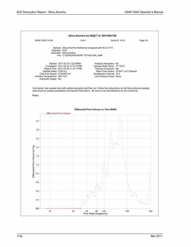
BJH Desorption Report - Silica Alumina ASAP 2020 Operator’s Manual
Silica Alumina iso N2@77 K, 004/16821/00
ASAP 2020 V4.00 (V3.05 H) Unit 1 Serial #: 1410 Page 24
Sample: Silica-Alumina Reference analyzed with N2 at 77 KOperator: DJS
Submitter: MicromeriticsFile: C:\2020\DATA\PERF-TST\N2-SIAL.SMP
Started: 2011-02-24 7:22:09PM Analysis Adsorptive: N2Completed: 2011-02-24 17:21:07PM Analysis Bath Temp.: 77.125 K
Report Time: 2011-03-25 11:21:11PM Thermal Correction: NoSample Mass: 0.2614 g Warm Free Space: 16.5571 cm³ Entered
Cold Free Space: 47.8248 cm³ Equilibration Interval: 10 sAmbient Temperature: 295.15 K Low Pressure Dose: None
Automatic Degas: No
Comments: Use sample tube with isothermal jacket and filler rod. Follow the instructions on the Silica-Alumina sample data sheet for sample preparation and special instructions. Be sure to use specifications for the current lot.
Notes:
Pore Width (Angstroms)20 40 60 80 100 200 400
Diff
eren
tial P
ore
Vol
ume
(cm
³/g)
0.00.0
0.2
0.4
0.6
0.8
1.0
1.2
1.4
1.6
1.8
2.0
Differential Pore Volume vs. Pore WidthDifferential Pore Volume
7-52 Mar 2011

ASAP 2020 Operator’s Manual BJH Desorption Report - Silica Alumina
Silica Alumina iso N2@77 K, 004/16821/00
ASAP 2020 V4.00 (V3.05 H) Unit 1 Serial #: 1410 Page 25
Sample: Silica-Alumina Reference analyzed with N2 at 77 KOperator: DJS
Submitter: MicromeriticsFile: C:\2020\DATA\PERF-TST\N2-SIAL.SMP
Started: 2011-02-24 7:22:09PM Analysis Adsorptive: N2Completed: 2011-02-24 17:21:07PM Analysis Bath Temp.: 77.125 K
Report Time: 2011-03-25 11:21:11PM Thermal Correction: NoSample Mass: 0.2614 g Warm Free Space: 16.5571 cm³ Entered
Cold Free Space: 47.8248 cm³ Equilibration Interval: 10 sAmbient Temperature: 295.15 K Low Pressure Dose: None
Automatic Degas: No
Comments: Use sample tube with isothermal jacket and filler rod. Follow the instructions on the Silica-Alumina sample data sheet for sample preparation and special instructions. Be sure to use specifications for the current lot.
Notes:
Standard Deviation of Fit: 2.26318, cm³/g STP
Silica Alumina iso N2@77 K, 004/16821/00
ASAP 2020 V4.00 (V3.05 H) Unit 1 Serial #: 1410 Page 26
Sample: Silica-Alumina Reference analyzed with N2 at 77 KOperator: DJS
Submitter: MicromeriticsFile: C:\2020\DATA\PERF-TST\N2-SIAL.SMP
Started: 2011-02-24 7:22:09PM Analysis Adsorptive: N2Completed: 2011-02-24 17:21:07PM Analysis Bath Temp.: 77.125 K
Report Time: 2011-03-25 11:21:11PM Thermal Correction: NoSample Mass: 0.2614 g Warm Free Space: 16.5571 cm³ Entered
Cold Free Space: 47.8248 cm³ Equilibration Interval: 10 sAmbient Temperature: 295.15 K Low Pressure Dose: None
Automatic Degas: No
Comments: Use sample tube with isothermal jacket and filler rod. Follow the instructions on the Silica-Alumina sample data sheet for sample preparation and special instructions. Be sure to use specifications for the current lot.
Notes:
Relative Pressure (p/p°)0.01 0.05 0.1 0.5 1
Qua
ntity
Ads
orbe
d (c
m³/g
STP
)
5050
100
150
200
250
300
350
400
Goodness of Fit
Standard Deviation of Fit: 2.26318, cm3/gSTP
Mar 2011 7-53

DFT Surface Energy Report - Silica Alumina ASAP 2020 Operator’s Manual
DFT Surface Energy Report - Silica Alumina
Silica Alumina iso N2@77 K, 004/16821/00
ASAP 2020 V4.00 (V3.05 H) Unit 1 Serial #: 1410 Page 27
Sample: Silica-Alumina Reference analyzed with N2 at 77 KOperator: DJS
Submitter: MicromeriticsFile: C:\2020\DATA\PERF-TST\N2-SIAL.SMP
Started: 2011-02-24 7:22:09PM Analysis Adsorptive: N2Completed: 2011-02-24 17:21:07PM Analysis Bath Temp.: 77.125 K
Report Time: 2011-03-25 11:21:11PM Thermal Correction: NoSample Mass: 0.2614 g Warm Free Space: 16.5571 cm³ Entered
Cold Free Space: 47.8248 cm³ Equilibration Interval: 10 sAmbient Temperature: 295.15 K Low Pressure Dose: None
Automatic Degas: No
Comments: Use sample tube with isothermal jacket and filler rod. Follow the instructions on the Silica-Alumina sample data sheet for sample preparation and special instructions. Be sure to use specifications for the current lot.
Notes:
Surface Energy Distribution by Modified Density Functional TheoryModel: N2 @ 77K, Surface Energy Distribution
Method: Non-negative Regularization; No SmoothingStandard Deviation of Fit: 0.08682, cm³/g STP
Total Area : 349.553 m²/g
Surface Energy TableEnergy
(e/k)Cumulative
Area(m²/g)
IncrementalArea(m²/g)
20.00 0.000 0.000 22.00 129.052 129.052 24.00 129.052 0.000 26.00 129.052 0.000 28.00 129.052 0.000 30.00 129.052 0.000 32.00 129.052 0.000 34.00 129.052 0.000 36.00 145.197 16.145 38.00 145.197 0.000 40.00 145.197 0.000 42.00 145.197 0.000 44.00 262.309 117.112 46.00 262.309 0.000 48.00 262.335 0.027 50.00 262.335 0.000 52.00 262.335 0.000 54.00 262.335 0.000 56.00 287.694 25.358 58.00 287.694 0.000 60.00 287.694 0.000 62.00 287.694 0.000 64.00 308.720 21.026 66.00 308.720 0.000 68.00 308.720 0.000 70.00 308.720 0.000 72.00 319.473 10.753 74.00 319.473 0.000 76.00 319.473 0.000 78.00 328.859 9.386 80.00 328.859 0.000
7-54 Mar 2011

ASAP 2020 Operator’s Manual DFT Surface Energy Report - Silica Alumina
Silica Alumina iso N2@77 K, 004/16821/00
ASAP 2020 V4.00 (V3.05 H) Unit 1 Serial #: 1410 Page 28
Sample: Silica-Alumina Reference analyzed with N2 at 77 KOperator: DJS
Submitter: MicromeriticsFile: C:\2020\DATA\PERF-TST\N2-SIAL.SMP
Started: 2011-02-24 7:22:09PM Analysis Adsorptive: N2Completed: 2011-02-24 17:21:07PM Analysis Bath Temp.: 77.125 K
Report Time: 2011-03-25 11:21:11PM Thermal Correction: NoSample Mass: 0.2614 g Warm Free Space: 16.5571 cm³ Entered
Cold Free Space: 47.8248 cm³ Equilibration Interval: 10 sAmbient Temperature: 295.15 K Low Pressure Dose: None
Automatic Degas: No
Comments: Use sample tube with isothermal jacket and filler rod. Follow the instructions on the Silica-Alumina sample data sheet for sample preparation and special instructions. Be sure to use specifications for the current lot.
Notes:
Surface Energy TableEnergy
(e/k)Cumulative
Area(m²/g)
IncrementalArea(m²/g)
82.00 328.859 0.000 84.00 328.859 0.000 86.00 336.830 7.971 88.00 336.830 0.000 90.00 336.830 0.000 92.00 341.670 4.840 94.00 341.670 0.000 96.00 341.670 0.000 98.00 341.670 0.000
100.00 349.553 7.884
Mar 2011 7-55

DFT Surface Energy Report - Silica Alumina ASAP 2020 Operator’s Manual
Silica Alumina iso N2@77 K, 004/16821/00
ASAP 2020 V4.00 (V3.05 H) Unit 1 Serial #: 1410 Page 29
Sample: Silica-Alumina Reference analyzed with N2 at 77 KOperator: DJS
Submitter: MicromeriticsFile: C:\2020\DATA\PERF-TST\N2-SIAL.SMP
Started: 2011-02-24 7:22:09PM Analysis Adsorptive: N2Completed: 2011-02-24 17:21:07PM Analysis Bath Temp.: 77.125 K
Report Time: 2011-03-25 11:21:11PM Thermal Correction: NoSample Mass: 0.2614 g Warm Free Space: 16.5571 cm³ Entered
Cold Free Space: 47.8248 cm³ Equilibration Interval: 10 sAmbient Temperature: 295.15 K Low Pressure Dose: None
Automatic Degas: No
Comments: Use sample tube with isothermal jacket and filler rod. Follow the instructions on the Silica-Alumina sample data sheet for sample preparation and special instructions. Be sure to use specifications for the current lot.
Notes:
Surface Energy Distribution by Modified Density Functional TheoryModel: N2 @ 77K, Surface Energy Distribution
Method: Non-negative Regularization; No Smoothing
Standard Deviation of Fit: 0.08682, cm³/g STP
Isotherm TableRelativePressure
ExperimentalQuantity
Adsorbed(cm³/g STP)
Fitted QuantityAdsorbed
(cm³/g STP)
AbsoluteResidual
(cm³/g STP)
RelativeResidual
0.010000000 36.1963 35.8529 0.3434 0.0094870.010592537 36.4127 36.1841 0.2286 0.0062790.011220185 36.6409 36.5104 0.1305 0.0035620.011885022 36.8813 36.8330 0.0483 0.0013100.012589254 37.1343 37.1530 -0.0187 -0.0005040.013335214 37.4004 37.4717 -0.0714 -0.0019080.014125375 37.6797 37.7903 -0.1105 -0.0029330.014962357 37.9727 38.1098 -0.1371 -0.0036110.015848932 38.2794 38.4315 -0.1521 -0.0039750.016788040 38.5998 38.7564 -0.1567 -0.0040590.017782794 38.9337 39.0855 -0.1517 -0.0038970.018836491 39.2810 39.4191 -0.1382 -0.0035180.019952623 39.6408 39.7576 -0.1168 -0.0029470.021134890 40.0123 40.1006 -0.0883 -0.0022060.022387211 40.3943 40.4474 -0.0532 -0.0013160.023713737 40.7848 40.7974 -0.0126 -0.0003090.025118864 41.1814 41.1501 0.0313 0.0007600.026607251 41.5812 41.5060 0.0752 0.0018080.028183829 41.9800 41.8665 0.1136 0.0027060.029853826 42.3730 42.2339 0.1391 0.0032820.031622777 42.7536 42.6119 0.1417 0.0033140.033496544 43.1141 43.0044 0.1097 0.0025450.035481339 43.4644 43.4118 0.0526 0.0012090.037583740 43.8292 43.8274 0.0018 0.0000410.039810717 44.2090 44.2422 -0.0332 -0.0007500.042169650 44.6036 44.6533 -0.0498 -0.0011160.044668359 45.0126 45.0639 -0.0513 -0.0011400.047315126 45.4356 45.4790 -0.0434 -0.0009550.050118723 45.8719 45.9034 -0.0314 -0.0006850.053088444 46.3205 46.3388 -0.0183 -0.0003960.056234133 46.7798 46.7836 -0.0038 -0.000081
7-56 Mar 2011
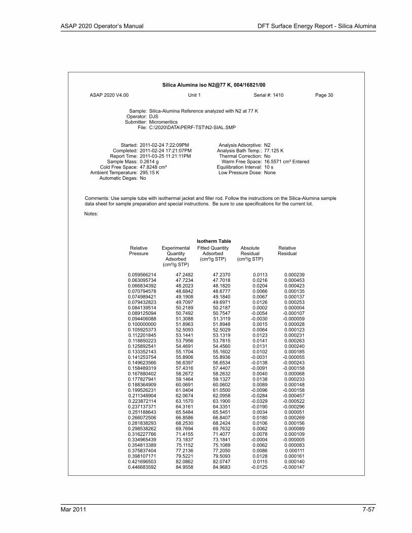
ASAP 2020 Operator’s Manual DFT Surface Energy Report - Silica Alumina
Silica Alumina iso N2@77 K, 004/16821/00
ASAP 2020 V4.00 (V3.05 H) Unit 1 Serial #: 1410 Page 30
Sample: Silica-Alumina Reference analyzed with N2 at 77 KOperator: DJS
Submitter: MicromeriticsFile: C:\2020\DATA\PERF-TST\N2-SIAL.SMP
Started: 2011-02-24 7:22:09PM Analysis Adsorptive: N2Completed: 2011-02-24 17:21:07PM Analysis Bath Temp.: 77.125 K
Report Time: 2011-03-25 11:21:11PM Thermal Correction: NoSample Mass: 0.2614 g Warm Free Space: 16.5571 cm³ Entered
Cold Free Space: 47.8248 cm³ Equilibration Interval: 10 sAmbient Temperature: 295.15 K Low Pressure Dose: None
Automatic Degas: No
Comments: Use sample tube with isothermal jacket and filler rod. Follow the instructions on the Silica-Alumina sample data sheet for sample preparation and special instructions. Be sure to use specifications for the current lot.
Notes:
Isotherm TableRelativePressure
ExperimentalQuantity
Adsorbed(cm³/g STP)
Fitted QuantityAdsorbed
(cm³/g STP)
AbsoluteResidual
(cm³/g STP)
RelativeResidual
0.059566214 47.2482 47.2370 0.0113 0.0002390.063095734 47.7234 47.7018 0.0216 0.0004530.066834392 48.2023 48.1820 0.0204 0.0004230.070794578 48.6842 48.6777 0.0066 0.0001350.074989421 49.1908 49.1840 0.0067 0.0001370.079432823 49.7097 49.6971 0.0126 0.0002530.084139514 50.2189 50.2187 0.0002 0.0000040.089125094 50.7492 50.7547 -0.0054 -0.0001070.094406088 51.3088 51.3119 -0.0030 -0.0000590.100000000 51.8963 51.8948 0.0015 0.0000280.105925373 52.5093 52.5029 0.0064 0.0001230.112201845 53.1441 53.1319 0.0123 0.0002310.118850223 53.7956 53.7815 0.0141 0.0002630.125892541 54.4691 54.4560 0.0131 0.0002400.133352143 55.1704 55.1602 0.0102 0.0001850.141253754 55.8906 55.8936 -0.0031 -0.0000550.149623566 56.6397 56.6534 -0.0138 -0.0002430.158489319 57.4316 57.4407 -0.0091 -0.0001580.167880402 58.2672 58.2632 0.0040 0.0000680.177827941 59.1464 59.1327 0.0138 0.0002330.188364909 60.0691 60.0602 0.0089 0.0001480.199526231 61.0404 61.0500 -0.0096 -0.0001580.211348904 62.0674 62.0958 -0.0284 -0.0004570.223872114 63.1570 63.1900 -0.0329 -0.0005220.237137371 64.3161 64.3351 -0.0190 -0.0002960.251188643 65.5484 65.5451 0.0034 0.0000510.266072506 66.8586 66.8407 0.0180 0.0002690.281838293 68.2530 68.2424 0.0106 0.0001560.298538262 69.7694 69.7632 0.0062 0.0000890.316227766 71.4155 71.4077 0.0078 0.0001090.334965439 73.1837 73.1841 -0.0004 -0.0000050.354813389 75.1152 75.1089 0.0062 0.0000830.375837404 77.2136 77.2050 0.0086 0.0001110.398107171 79.5221 79.5093 0.0128 0.0001610.421696503 82.0862 82.0747 0.0115 0.0001400.446683592 84.9558 84.9683 -0.0125 -0.000147
Mar 2011 7-57

DFT Surface Energy Report - Silica Alumina ASAP 2020 Operator’s Manual
Silica Alumina iso N2@77 K, 004/16821/00
ASAP 2020 V4.00 (V3.05 H) Unit 1 Serial #: 1410 Page 32
Sample: Silica-Alumina Reference analyzed with N2 at 77 KOperator: DJS
Submitter: MicromeriticsFile: C:\2020\DATA\PERF-TST\N2-SIAL.SMP
Started: 2011-02-24 7:22:09PM Analysis Adsorptive: N2Completed: 2011-02-24 17:21:07PM Analysis Bath Temp.: 77.125 K
Report Time: 2011-03-25 11:21:11PM Thermal Correction: NoSample Mass: 0.2614 g Warm Free Space: 16.5571 cm³ Entered
Cold Free Space: 47.8248 cm³ Equilibration Interval: 10 sAmbient Temperature: 295.15 K Low Pressure Dose: None
Automatic Degas: No
Comments: Use sample tube with isothermal jacket and filler rod. Follow the instructions on the Silica-Alumina sample data sheet for sample preparation and special instructions. Be sure to use specifications for the current lot.
Notes:
Energy (e/k)2020 30 40 50 60 70 80 90 100
Cum
ulat
ive
Sur
face
Are
a (m
²/g)
00
50
100
150
200
250
300
350
Cumulative Surface Area vs. EnergyCumulative Surface Area
7-58 Mar 2011

ASAP 2020 Operator’s Manual DFT Surface Energy Report - Silica Alumina
Silica Alumina iso N2@77 K, 004/16821/00
ASAP 2020 V4.00 (V3.05 H) Unit 1 Serial #: 1410 Page 33
Sample: Silica-Alumina Reference analyzed with N2 at 77 KOperator: DJS
Submitter: MicromeriticsFile: C:\2020\DATA\PERF-TST\N2-SIAL.SMP
Started: 2011-02-24 7:22:09PM Analysis Adsorptive: N2Completed: 2011-02-24 17:21:07PM Analysis Bath Temp.: 77.125 K
Report Time: 2011-03-25 11:21:11PM Thermal Correction: NoSample Mass: 0.2614 g Warm Free Space: 16.5571 cm³ Entered
Cold Free Space: 47.8248 cm³ Equilibration Interval: 10 sAmbient Temperature: 295.15 K Low Pressure Dose: None
Automatic Degas: No
Comments: Use sample tube with isothermal jacket and filler rod. Follow the instructions on the Silica-Alumina sample data sheet for sample preparation and special instructions. Be sure to use specifications for the current lot.
Notes:
Energy (e/k)2020 30 40 50 60 70 80 90 100
Diff
eren
tial S
urfa
ce A
rea
(m²/g
-K)
00
10
20
30
40
50
60
Differential Surface Area vs. EnergyDifferential Surface Area
Mar 2011 7-59

DFT Surface Energy Report - Silica Alumina ASAP 2020 Operator’s Manual
Silica Alumina iso N2@77 K, 004/16821/00
ASAP 2020 V4.00 (V3.05 H) Unit 1 Serial #: 1410 Page 35
Sample: Silica-Alumina Reference analyzed with N2 at 77 KOperator: DJS
Submitter: MicromeriticsFile: C:\2020\DATA\PERF-TST\N2-SIAL.SMP
Started: 2011-02-24 7:22:09PM Analysis Adsorptive: N2Completed: 2011-02-24 17:21:07PM Analysis Bath Temp.: 77.125 K
Report Time: 2011-03-25 11:21:11PM Thermal Correction: NoSample Mass: 0.2614 g Warm Free Space: 16.5571 cm³ Entered
Cold Free Space: 47.8248 cm³ Equilibration Interval: 10 sAmbient Temperature: 295.15 K Low Pressure Dose: None
Automatic Degas: No
Comments: Use sample tube with isothermal jacket and filler rod. Follow the instructions on the Silica-Alumina sample data sheet for sample preparation and special instructions. Be sure to use specifications for the current lot.
Notes:
Relative Pressure (p/p°)0.01 0.05 0.1 0.5 1
Qua
ntity
Ads
orbe
d (c
m³/g
STP
)
5050
100
150
200
250
300
350
400
Goodness of Fit
Standard Deviation of Fit: 0.08682, cm3/gSTP
7-60 Mar 2011

ASAP 2020 Operator’s Manual Options Report - Silica Alumina
Options Report - Silica Alumina
Silica Alumina iso N2@77 K, 004/16821/00
ASAP 2020 V4.00 (V3.05 H) Unit 1 Serial #: 1410 Page 36
Sample: Silica-Alumina Reference analyzed with N2 at 77 KOperator: DJS
Submitter: MicromeriticsFile: C:\2020\DATA\PERF-TST\N2-SIAL.SMP
Started: 2011-02-24 7:22:09PM Analysis Adsorptive: N2Completed: 2011-02-24 17:21:07PM Analysis Bath Temp.: 77.125 K
Report Time: 2011-03-25 11:21:11PM Thermal Correction: NoSample Mass: 0.2614 g Warm Free Space: 16.5571 cm³ Entered
Cold Free Space: 47.8248 cm³ Equilibration Interval: 10 sAmbient Temperature: 295.15 K Low Pressure Dose: None
Automatic Degas: No
Comments: Use sample tube with isothermal jacket and filler rod. Follow the instructions on the Silica-Alumina sample data sheet for sample preparation and special instructions. Be sure to use specifications for the current lot.
Notes:
Options Report
Sample TubeWarm free space: 1.0000 cm³
Cold free space: 1.0000 cm³Non-ideality factor: 0.0000620
Use Isothermal Jacket: YesUse Filler Rod: Yes
Vacuum seal type: Seal FritAnalysis Conditions
PreparationFast evacuation: Yes
Vacuum setpoint: 10 µmHgEvacuation time: 0.50 h
Leak test: NoUse TranSeal: No
Free SpaceFree-space type: Entered
Warm free space: 27.9452 cm³Cold free space: 89.2064 cm³
p° and Temperaturep° and T type: Measure p° at intervals during analysis. Calculate the
Analysis Bath Temperature from these values.Measurement interval: 120 minAmbient temperature: 295.15 K
DosingUse first pressure fixed dose: No
Use maximum volume increment: NoTarget tolerance: 5.0% or 5.000 mmHg
Low pressure dosing: NoEquilibration
Equilibration time (p/p° = 1.000000000): 10 sMinimum equilibration delay at p/p° >= 0.995: 600 s
Sample BackfillBackfill at start of analysis: YesBackfill at end of analysis: Yes
Backfill gas: N2
Mar 2011 7-61

Options Report (cont’d) - Silica Alumina ASAP 2020 Operator’s Manual
Options Report (cont’d) - Silica Alumina
Silica Alumina iso N2@77 K, 004/16821/00
ASAP 2020 V4.00 (V3.05 H) Unit 1 Serial #: 1410 Page 37
Sample: Silica-Alumina Reference analyzed with N2 at 77 KOperator: DJS
Submitter: MicromeriticsFile: C:\2020\DATA\PERF-TST\N2-SIAL.SMP
Started: 2011-02-24 7:22:09PM Analysis Adsorptive: N2Completed: 2011-02-24 17:21:07PM Analysis Bath Temp.: 77.125 K
Report Time: 2011-03-25 11:21:11PM Thermal Correction: NoSample Mass: 0.2614 g Warm Free Space: 16.5571 cm³ Entered
Cold Free Space: 47.8248 cm³ Equilibration Interval: 10 sAmbient Temperature: 295.15 K Low Pressure Dose: None
Automatic Degas: No
Comments: Use sample tube with isothermal jacket and filler rod. Follow the instructions on the Silica-Alumina sample data sheet for sample preparation and special instructions. Be sure to use specifications for the current lot.
Notes:
Adsorptive PropertiesAdsorptive: Nitrogen @ 77.35 K
Maximum manifold pressure: 925.00 mmHgNon-ideality factor: 0.0000660
Density conversion factor: 0.0015468Therm. tran. hard-sphere diameter: 3.860 Å
Molecular cross-sectional area: 0.162 nm²Inside diameter of sample tube: 9.53 mm
7-62 Mar 2011

ASAP 2020 Operator’s Manual Summary Report - Y Zeolite
Summary Report - Y Zeolite
Y Zeolite, N2 @ 77.35 K, 004/16844/00
ASAP 2020 V4.00 (V4.00 J) Unit 1 Serial #: 1410 Page 1
Sample: Y-Zeolite Reference Mat analyzed with N2 at 77 KOperator: AWT/JCH
Submitter: MicromeriticsFile: C:\2020\DATA\PERF-TST\N2-YZEOL.SMP
Started: 2011-03-10 17:35:46PM Analysis Adsorptive: N2Completed: 2011-03-11 23:41:34PM Analysis Bath Temp.: 77.150 K
Report Time: 2011-03-25 11:22:03PM Thermal Correction: YesSample Mass: 0.1272 g Warm Free Space: 28.5000 cm³ Entered
Cold Free Space: 90.1000 cm³ Equilibration Interval: 30 sAmbient Temperature: 295.15 K Low Pressure Dose: 3.000 cm³/g STP
Automatic Degas: Yes
Comments: Use sample tube with isothermal jacket, but no filler rod. Follow the instructions on the Y-Zeolite sample data sheet for sample preparation and special instructions. Be sure to use specifications for the current lot.
Summary Report
Horvath-KawazoeMaximum pore volume at p/p° = 0.011168820: 0.228476 cm³/g
Median pore width: 7.350 Å
Pass/FailH-K:Median pore width Passed
Mar 2011 7-63
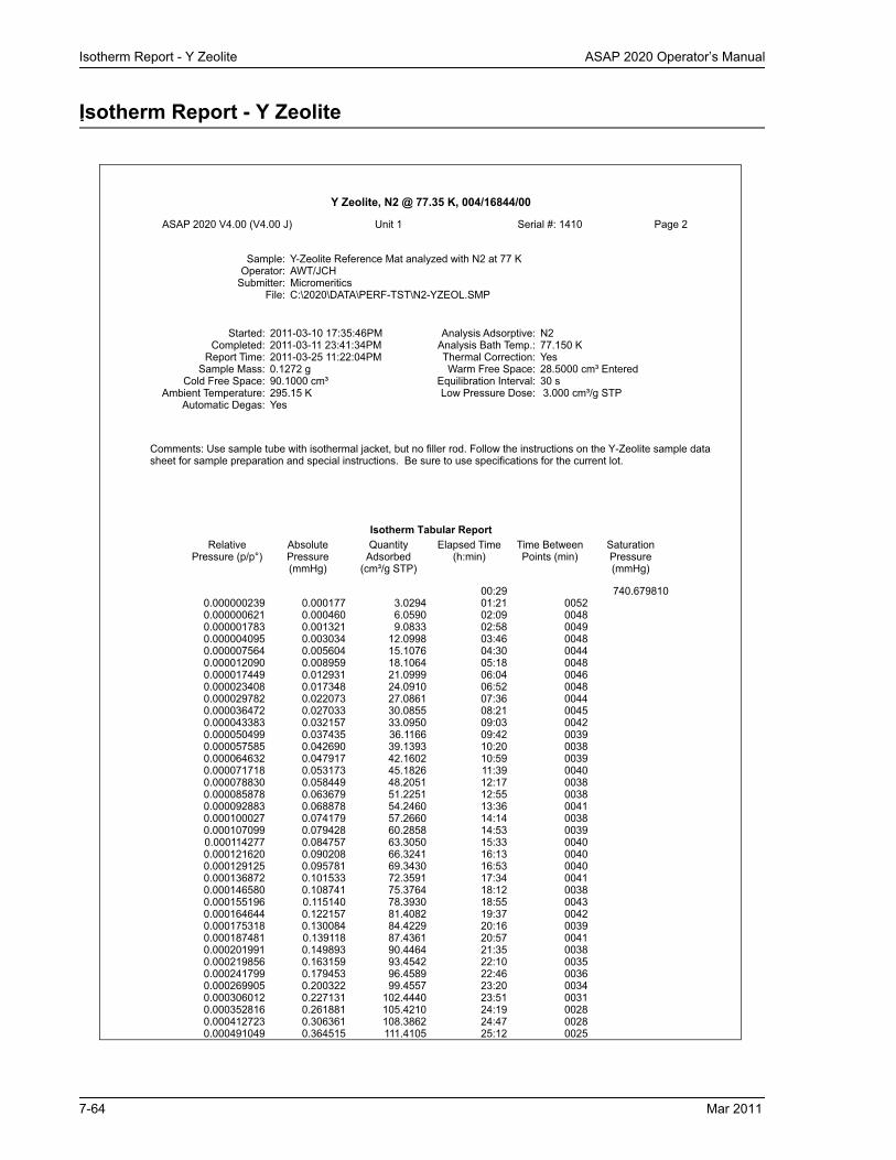
Isotherm Report - Y Zeolite ASAP 2020 Operator’s Manual
Isotherm Report - Y Zeolite
Y Zeolite, N2 @ 77.35 K, 004/16844/00
ASAP 2020 V4.00 (V4.00 J) Unit 1 Serial #: 1410 Page 2
Sample: Y-Zeolite Reference Mat analyzed with N2 at 77 KOperator: AWT/JCH
Submitter: MicromeriticsFile: C:\2020\DATA\PERF-TST\N2-YZEOL.SMP
Started: 2011-03-10 17:35:46PM Analysis Adsorptive: N2Completed: 2011-03-11 23:41:34PM Analysis Bath Temp.: 77.150 K
Report Time: 2011-03-25 11:22:04PM Thermal Correction: YesSample Mass: 0.1272 g Warm Free Space: 28.5000 cm³ Entered
Cold Free Space: 90.1000 cm³ Equilibration Interval: 30 sAmbient Temperature: 295.15 K Low Pressure Dose: 3.000 cm³/g STP
Automatic Degas: Yes
Comments: Use sample tube with isothermal jacket, but no filler rod. Follow the instructions on the Y-Zeolite sample data sheet for sample preparation and special instructions. Be sure to use specifications for the current lot.
Isotherm Tabular ReportRelative
Pressure (p/p°)AbsolutePressure(mmHg)
QuantityAdsorbed
(cm³/g STP)
Elapsed Time(h:min)
Time BetweenPoints (min)
SaturationPressure(mmHg)
00:29 740.6798100.000000239 0.000177 3.0294 01:21 00520.000000621 0.000460 6.0590 02:09 00480.000001783 0.001321 9.0833 02:58 00490.000004095 0.003034 12.0998 03:46 00480.000007564 0.005604 15.1076 04:30 00440.000012090 0.008959 18.1064 05:18 00480.000017449 0.012931 21.0999 06:04 00460.000023408 0.017348 24.0910 06:52 00480.000029782 0.022073 27.0861 07:36 00440.000036472 0.027033 30.0855 08:21 00450.000043383 0.032157 33.0950 09:03 00420.000050499 0.037435 36.1166 09:42 00390.000057585 0.042690 39.1393 10:20 00380.000064632 0.047917 42.1602 10:59 00390.000071718 0.053173 45.1826 11:39 00400.000078830 0.058449 48.2051 12:17 00380.000085878 0.063679 51.2251 12:55 00380.000092883 0.068878 54.2460 13:36 00410.000100027 0.074179 57.2660 14:14 00380.000107099 0.079428 60.2858 14:53 00390.000114277 0.084757 63.3050 15:33 00400.000121620 0.090208 66.3241 16:13 00400.000129125 0.095781 69.3430 16:53 00400.000136872 0.101533 72.3591 17:34 00410.000146580 0.108741 75.3764 18:12 00380.000155196 0.115140 78.3930 18:55 00430.000164644 0.122157 81.4082 19:37 00420.000175318 0.130084 84.4229 20:16 00390.000187481 0.139118 87.4361 20:57 00410.000201991 0.149893 90.4464 21:35 00380.000219856 0.163159 93.4542 22:10 00350.000241799 0.179453 96.4589 22:46 00360.000269905 0.200322 99.4557 23:20 00340.000306012 0.227131 102.4440 23:51 00310.000352816 0.261881 105.4210 24:19 00280.000412723 0.306361 108.3862 24:47 00280.000491049 0.364515 111.4105 25:12 0025
7-64 Mar 2011

ASAP 2020 Operator’s Manual Isotherm Report - Y Zeolite
Y Zeolite, N2 @ 77.35 K, 004/16844/00
ASAP 2020 V4.00 (V4.00 J) Unit 1 Serial #: 1410 Page 3
Sample: Y-Zeolite Reference Mat analyzed with N2 at 77 KOperator: AWT/JCH
Submitter: MicromeriticsFile: C:\2020\DATA\PERF-TST\N2-YZEOL.SMP
Started: 2011-03-10 17:35:46PM Analysis Adsorptive: N2Completed: 2011-03-11 23:41:34PM Analysis Bath Temp.: 77.150 K
Report Time: 2011-03-25 11:22:04PM Thermal Correction: YesSample Mass: 0.1272 g Warm Free Space: 28.5000 cm³ Entered
Cold Free Space: 90.1000 cm³ Equilibration Interval: 30 sAmbient Temperature: 295.15 K Low Pressure Dose: 3.000 cm³/g STP
Automatic Degas: Yes
Comments: Use sample tube with isothermal jacket, but no filler rod. Follow the instructions on the Y-Zeolite sample data sheet for sample preparation and special instructions. Be sure to use specifications for the current lot.
Isotherm Tabular ReportRelative
Pressure (p/p°)AbsolutePressure(mmHg)
QuantityAdsorbed
(cm³/g STP)
Elapsed Time(h:min)
Time BetweenPoints (min)
SaturationPressure(mmHg)
0.000590797 0.438577 114.4263 25:38 00260.000716280 0.531748 117.4310 26:02 00240.000873058 0.648157 120.4220 26:24 00220.001068032 0.792932 123.3953 26:47 00230.001312099 0.974165 126.3434 27:08 00210.001620134 1.202902 129.2561 27:29 00210.002015208 1.496277 132.1076 27:49 00200.002529451 1.878152 134.8674 28:08 00190.003206058 2.380602 137.4922 28:25 00170.004090737 3.037581 139.9300 28:42 00170.005268317 3.912094 142.2017 28:59 0017
29:06 0007 742.5776980.006894097 5.119403 144.3670 29:18 00120.008813154 6.544452 146.1397 29:30 00120.011168820 8.293716 147.7088 29:41 0011
Mar 2011 7-65

Isotherm Report - Y Zeolite ASAP 2020 Operator’s Manual
Y Zeolite, N2 @ 77.35 K, 004/16844/00
ASAP 2020 V4.00 (V4.00 J) Unit 1 Serial #: 1410 Page 4
Sample: Y-Zeolite Reference Mat analyzed with N2 at 77 KOperator: AWT/JCH
Submitter: MicromeriticsFile: C:\2020\DATA\PERF-TST\N2-YZEOL.SMP
Started: 2011-03-10 17:35:46PM Analysis Adsorptive: N2Completed: 2011-03-11 23:41:34PM Analysis Bath Temp.: 77.150 K
Report Time: 2011-03-25 11:22:04PM Thermal Correction: YesSample Mass: 0.1272 g Warm Free Space: 28.5000 cm³ Entered
Cold Free Space: 90.1000 cm³ Equilibration Interval: 30 sAmbient Temperature: 295.15 K Low Pressure Dose: 3.000 cm³/g STP
Automatic Degas: Yes
Comments: Use sample tube with isothermal jacket, but no filler rod. Follow the instructions on the Y-Zeolite sample data sheet for sample preparation and special instructions. Be sure to use specifications for the current lot.
Relative Pressure (p/p°)0.0000.000 0.002 0.004 0.006 0.008 0.010
Qua
ntity
Ads
orbe
d (c
m³/g
STP
)
00
20
40
60
80
100
120
140
Isotherm Linear PlotY-Zeolite Reference Mat analyzed with N2 at 77 K - Adsorption
7-66 Mar 2011

ASAP 2020 Operator’s Manual Isotherm Report - Y Zeolite
Y Zeolite, N2 @ 77.35 K, 004/16844/00
ASAP 2020 V4.00 (V4.00 J) Unit 1 Serial #: 1410 Page 5
Sample: Y-Zeolite Reference Mat analyzed with N2 at 77 KOperator: AWT/JCH
Submitter: MicromeriticsFile: C:\2020\DATA\PERF-TST\N2-YZEOL.SMP
Started: 2011-03-10 17:35:46PM Analysis Adsorptive: N2Completed: 2011-03-11 23:41:34PM Analysis Bath Temp.: 77.150 K
Report Time: 2011-03-25 11:22:04PM Thermal Correction: YesSample Mass: 0.1272 g Warm Free Space: 28.5000 cm³ Entered
Cold Free Space: 90.1000 cm³ Equilibration Interval: 30 sAmbient Temperature: 295.15 K Low Pressure Dose: 3.000 cm³/g STP
Automatic Degas: Yes
Comments: Use sample tube with isothermal jacket, but no filler rod. Follow the instructions on the Y-Zeolite sample data sheet for sample preparation and special instructions. Be sure to use specifications for the current lot.
Relative Pressure (p/p°)10-6 10-5 10-4 10-3 10-2
Qua
ntity
Ads
orbe
d (c
m³/g
STP
)
00
20
40
60
80
100
120
140
Isotherm Log PlotY-Zeolite Reference Mat analyzed with N2 at 77 K - Adsorption
Mar 2011 7-67

Horvath-Kawazoe Report - Y Zeolite ASAP 2020 Operator’s Manual
Horvath-Kawazoe Report - Y Zeolite
Y Zeolite, N2 @ 77.35 K, 004/16844/00
ASAP 2020 V4.00 (V4.00 J) Unit 1 Serial #: 1410 Page 6
Sample: Y-Zeolite Reference Mat analyzed with N2 at 77 KOperator: AWT/JCH
Submitter: MicromeriticsFile: C:\2020\DATA\PERF-TST\N2-YZEOL.SMP
Started: 2011-03-10 17:35:46PM Analysis Adsorptive: N2Completed: 2011-03-11 23:41:34PM Analysis Bath Temp.: 77.150 K
Report Time: 2011-03-25 11:22:04PM Thermal Correction: YesSample Mass: 0.1272 g Warm Free Space: 28.5000 cm³ Entered
Cold Free Space: 90.1000 cm³ Equilibration Interval: 30 sAmbient Temperature: 295.15 K Low Pressure Dose: 3.000 cm³/g STP
Automatic Degas: Yes
Comments: Use sample tube with isothermal jacket, but no filler rod. Follow the instructions on the Y-Zeolite sample data sheet for sample preparation and special instructions. Be sure to use specifications for the current lot.
Horvath-Kawazoe ReportCylinder Pore Geometry (Saito-Foley)
Maximum Pore Volume: 0.228476 cm³/gat Relative Pressure: 0.011168820Median Pore Width: 7.350 Å
Relative Pressure Range: 2.393e-07 to 1.117e-02
Diameter of Adsorptive Molecule: 3.000 ÅDiameter of Sample Atom: 2.760 Å
Interaction Parameter: 1.68e-43 erg·cm^4
Density Conversion Factor: 0.0015468AbsolutePressure(mmHg)
RelativePressure (p/p°)
QuantityAdsorbed
(cm³/g STP)
Pore Width (Å) CumulativePore Volume
(cm³/g)
SmoothedDifferential Pore
Volume(cm³/g·Å)
0.00018 0.000000239 3.02941 5.065 0.0047 0.02160.00046 0.000000621 6.05896 5.299 0.0094 0.01800.00132 0.000001783 9.08332 5.586 0.0141 0.01680.00303 0.000004095 12.09979 5.840 0.0187 0.02030.00560 0.000007564 15.10761 6.045 0.0234 0.02510.00896 0.000012090 18.10640 6.215 0.0280 0.03010.01293 0.000017449 21.09987 6.356 0.0326 0.03620.01735 0.000023408 24.09103 6.474 0.0373 0.04260.02207 0.000029782 27.08609 6.576 0.0419 0.04900.02703 0.000036472 30.08552 6.666 0.0465 0.05600.03216 0.000043383 33.09500 6.744 0.0512 0.06330.03743 0.000050499 36.11664 6.814 0.0559 0.07110.04269 0.000057585 39.13934 6.877 0.0605 0.07930.04792 0.000064632 42.16020 6.933 0.0652 0.08690.05317 0.000071718 45.18257 6.985 0.0699 0.09480.05845 0.000078830 48.20512 7.033 0.0746 0.10250.06368 0.000085878 51.22509 7.077 0.0792 0.10980.06888 0.000092883 54.24596 7.118 0.0839 0.11660.07418 0.000100027 57.26600 7.157 0.0886 0.12310.07943 0.000107099 60.28585 7.194 0.0933 0.12830.08476 0.000114277 63.30503 7.230 0.0979 0.13140.09021 0.000121620 66.32415 7.264 0.1026 0.13310.09578 0.000129125 69.34298 7.298 0.1073 0.13430.10153 0.000136872 72.35906 7.330 0.1119 0.13410.10874 0.000146580 75.37638 7.369 0.1166 0.13210.11514 0.000155196 78.39297 7.403 0.1213 0.1290
7-68 Mar 2011

ASAP 2020 Operator’s Manual Horvath-Kawazoe Report - Y Zeolite
Y Zeolite, N2 @ 77.35 K, 004/16844/00
ASAP 2020 V4.00 (V4.00 J) Unit 1 Serial #: 1410 Page 7
Sample: Y-Zeolite Reference Mat analyzed with N2 at 77 KOperator: AWT/JCH
Submitter: MicromeriticsFile: C:\2020\DATA\PERF-TST\N2-YZEOL.SMP
Started: 2011-03-10 17:35:46PM Analysis Adsorptive: N2Completed: 2011-03-11 23:41:34PM Analysis Bath Temp.: 77.150 K
Report Time: 2011-03-25 11:22:04PM Thermal Correction: YesSample Mass: 0.1272 g Warm Free Space: 28.5000 cm³ Entered
Cold Free Space: 90.1000 cm³ Equilibration Interval: 30 sAmbient Temperature: 295.15 K Low Pressure Dose: 3.000 cm³/g STP
Automatic Degas: Yes
Comments: Use sample tube with isothermal jacket, but no filler rod. Follow the instructions on the Y-Zeolite sample data sheet for sample preparation and special instructions. Be sure to use specifications for the current lot.
AbsolutePressure(mmHg)
RelativePressure (p/p°)
QuantityAdsorbed
(cm³/g STP)
Pore Width (Å) CumulativePore Volume
(cm³/g)
SmoothedDifferential Pore
Volume(cm³/g·Å)
0.12216 0.000164644 81.40818 7.437 0.1259 0.12400.13008 0.000175318 84.42292 7.475 0.1306 0.11740.13912 0.000187481 87.43611 7.515 0.1352 0.10850.14989 0.000201991 90.44636 7.561 0.1399 0.09670.16316 0.000219856 93.45420 7.614 0.1446 0.08430.17945 0.000241799 96.45890 7.674 0.1492 0.07230.20032 0.000269905 99.45574 7.745 0.1538 0.06130.22713 0.000306012 102.44401 7.829 0.1585 0.05170.26188 0.000352816 105.42100 7.926 0.1631 0.04450.30636 0.000412723 108.38621 8.037 0.1677 0.03910.36452 0.000491049 111.41055 8.165 0.1723 0.03480.43858 0.000590797 114.42627 8.307 0.1770 0.03140.53175 0.000716280 117.43103 8.462 0.1816 0.02870.64816 0.000873058 120.42204 8.630 0.1863 0.02650.79293 0.001068032 123.39527 8.810 0.1909 0.02450.97416 0.001312099 126.34338 9.005 0.1954 0.02241.20290 0.001620134 129.25610 9.215 0.1999 0.02031.49628 0.002015208 132.10764 9.446 0.2043 0.01781.87815 0.002529451 134.86744 9.705 0.2086 0.01532.38060 0.003206058 137.49222 9.994 0.2127 0.01293.03758 0.004090737 139.92998 10.317 0.2164 0.01073.91209 0.005268317 142.20172 10.680 0.2200 0.00875.11940 0.006894097 144.36696 11.106 0.2233 0.00716.54445 0.008813154 146.13971 11.534 0.2260 0.00578.29372 0.011168820 147.70882 11.988 0.2285 0.0052
Mar 2011 7-69

Horvath-Kawazoe Report - Y Zeolite ASAP 2020 Operator’s Manual
Y Zeolite, N2 @ 77.35 K, 004/16844/00
ASAP 2020 V4.00 (V4.00 J) Unit 1 Serial #: 1410 Page 8
Sample: Y-Zeolite Reference Mat analyzed with N2 at 77 KOperator: AWT/JCH
Submitter: MicromeriticsFile: C:\2020\DATA\PERF-TST\N2-YZEOL.SMP
Started: 2011-03-10 17:35:46PM Analysis Adsorptive: N2Completed: 2011-03-11 23:41:34PM Analysis Bath Temp.: 77.150 K
Report Time: 2011-03-25 11:22:04PM Thermal Correction: YesSample Mass: 0.1272 g Warm Free Space: 28.5000 cm³ Entered
Cold Free Space: 90.1000 cm³ Equilibration Interval: 30 sAmbient Temperature: 295.15 K Low Pressure Dose: 3.000 cm³/g STP
Automatic Degas: Yes
Comments: Use sample tube with isothermal jacket, but no filler rod. Follow the instructions on the Y-Zeolite sample data sheet for sample preparation and special instructions. Be sure to use specifications for the current lot.
Pore Width (Å)00 1 2 3 4 5 6 7 8 9 10 11 12
Por
e V
olum
e (c
m³/g
)
0.000.00
0.02
0.04
0.06
0.08
0.10
0.12
0.14
0.16
0.18
0.20
0.22
Horvath-Kawazoe Cumulative Pore Volume PlotCylinder Pore Geometry (Saito-Foley)
Y-Zeolite Reference Mat analyzed with N2 at 77 K
7-70 Mar 2011

ASAP 2020 Operator’s Manual Horvath-Kawazoe Report - Y Zeolite
Y Zeolite, N2 @ 77.35 K, 004/16844/00
ASAP 2020 V4.00 (V4.00 J) Unit 1 Serial #: 1410 Page 9
Sample: Y-Zeolite Reference Mat analyzed with N2 at 77 KOperator: AWT/JCH
Submitter: MicromeriticsFile: C:\2020\DATA\PERF-TST\N2-YZEOL.SMP
Started: 2011-03-10 17:35:46PM Analysis Adsorptive: N2Completed: 2011-03-11 23:41:34PM Analysis Bath Temp.: 77.150 K
Report Time: 2011-03-25 11:22:04PM Thermal Correction: YesSample Mass: 0.1272 g Warm Free Space: 28.5000 cm³ Entered
Cold Free Space: 90.1000 cm³ Equilibration Interval: 30 sAmbient Temperature: 295.15 K Low Pressure Dose: 3.000 cm³/g STP
Automatic Degas: Yes
Comments: Use sample tube with isothermal jacket, but no filler rod. Follow the instructions on the Y-Zeolite sample data sheet for sample preparation and special instructions. Be sure to use specifications for the current lot.
Pore Width (Å)00 1 2 3 4 5 6 7 8 9 10 11 12
Sm
ooth
ed d
V/d
w (c
m³/g
·Å)
0.000.00
0.02
0.04
0.06
0.08
0.10
0.12
Horvath-Kawazoe Differential Pore Volume PlotCylinder Pore Geometry (Saito-Foley)
Y-Zeolite Reference Mat analyzed with N2 at 77 K
Mar 2011 7-71
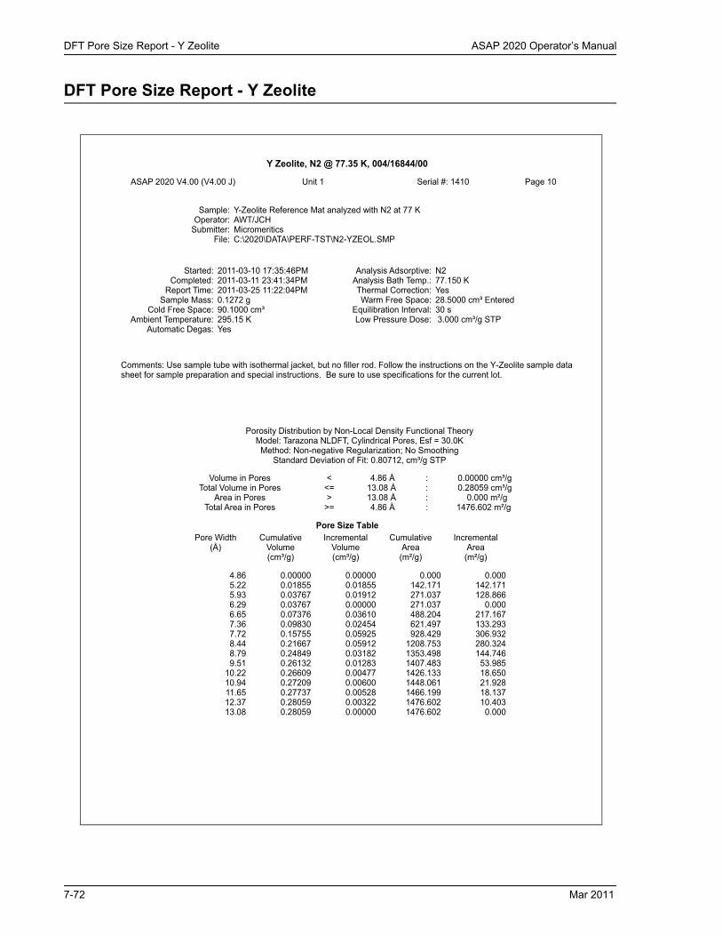
DFT Pore Size Report - Y Zeolite ASAP 2020 Operator’s Manual
DFT Pore Size Report - Y Zeolite
Y Zeolite, N2 @ 77.35 K, 004/16844/00
ASAP 2020 V4.00 (V4.00 J) Unit 1 Serial #: 1410 Page 10
Sample: Y-Zeolite Reference Mat analyzed with N2 at 77 KOperator: AWT/JCH
Submitter: MicromeriticsFile: C:\2020\DATA\PERF-TST\N2-YZEOL.SMP
Started: 2011-03-10 17:35:46PM Analysis Adsorptive: N2Completed: 2011-03-11 23:41:34PM Analysis Bath Temp.: 77.150 K
Report Time: 2011-03-25 11:22:04PM Thermal Correction: YesSample Mass: 0.1272 g Warm Free Space: 28.5000 cm³ Entered
Cold Free Space: 90.1000 cm³ Equilibration Interval: 30 sAmbient Temperature: 295.15 K Low Pressure Dose: 3.000 cm³/g STP
Automatic Degas: Yes
Comments: Use sample tube with isothermal jacket, but no filler rod. Follow the instructions on the Y-Zeolite sample data sheet for sample preparation and special instructions. Be sure to use specifications for the current lot.
Porosity Distribution by Non-Local Density Functional TheoryModel: Tarazona NLDFT, Cylindrical Pores, Esf = 30.0K
Method: Non-negative Regularization; No SmoothingStandard Deviation of Fit: 0.80712, cm³/g STP
Volume in Pores < 4.86 Å : 0.00000 cm³/gTotal Volume in Pores <= 13.08 Å : 0.28059 cm³/g
Area in Pores > 13.08 Å : 0.000 m²/gTotal Area in Pores >= 4.86 Å : 1476.602 m²/g
Pore Size TablePore Width
(Å)Cumulative
Volume(cm³/g)
IncrementalVolume(cm³/g)
CumulativeArea(m²/g)
IncrementalArea(m²/g)
4.86 0.00000 0.00000 0.000 0.000 5.22 0.01855 0.01855 142.171 142.171 5.93 0.03767 0.01912 271.037 128.866 6.29 0.03767 0.00000 271.037 0.000 6.65 0.07376 0.03610 488.204 217.167 7.36 0.09830 0.02454 621.497 133.293 7.72 0.15755 0.05925 928.429 306.932 8.44 0.21667 0.05912 1208.753 280.324 8.79 0.24849 0.03182 1353.498 144.746 9.51 0.26132 0.01283 1407.483 53.985
10.22 0.26609 0.00477 1426.133 18.650 10.94 0.27209 0.00600 1448.061 21.928 11.65 0.27737 0.00528 1466.199 18.137 12.37 0.28059 0.00322 1476.602 10.403 13.08 0.28059 0.00000 1476.602 0.000
7-72 Mar 2011
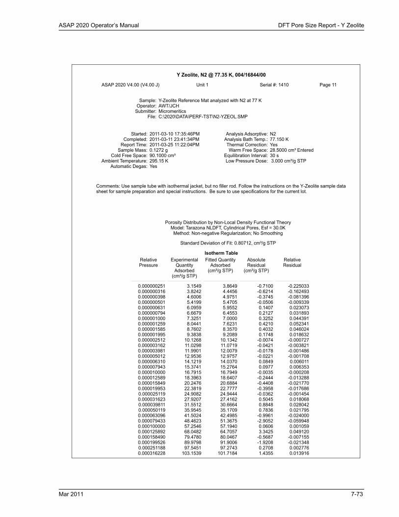
ASAP 2020 Operator’s Manual DFT Pore Size Report - Y Zeolite
Y Zeolite, N2 @ 77.35 K, 004/16844/00
ASAP 2020 V4.00 (V4.00 J) Unit 1 Serial #: 1410 Page 11
Sample: Y-Zeolite Reference Mat analyzed with N2 at 77 KOperator: AWT/JCH
Submitter: MicromeriticsFile: C:\2020\DATA\PERF-TST\N2-YZEOL.SMP
Started: 2011-03-10 17:35:46PM Analysis Adsorptive: N2Completed: 2011-03-11 23:41:34PM Analysis Bath Temp.: 77.150 K
Report Time: 2011-03-25 11:22:04PM Thermal Correction: YesSample Mass: 0.1272 g Warm Free Space: 28.5000 cm³ Entered
Cold Free Space: 90.1000 cm³ Equilibration Interval: 30 sAmbient Temperature: 295.15 K Low Pressure Dose: 3.000 cm³/g STP
Automatic Degas: Yes
Comments: Use sample tube with isothermal jacket, but no filler rod. Follow the instructions on the Y-Zeolite sample data sheet for sample preparation and special instructions. Be sure to use specifications for the current lot.
Porosity Distribution by Non-Local Density Functional TheoryModel: Tarazona NLDFT, Cylindrical Pores, Esf = 30.0K
Method: Non-negative Regularization; No Smoothing
Standard Deviation of Fit: 0.80712, cm³/g STP
Isotherm TableRelativePressure
ExperimentalQuantity
Adsorbed(cm³/g STP)
Fitted QuantityAdsorbed
(cm³/g STP)
AbsoluteResidual
(cm³/g STP)
RelativeResidual
0.000000251 3.1549 3.8649 -0.7100 -0.2250330.000000316 3.8242 4.4456 -0.6214 -0.1624930.000000398 4.6006 4.9751 -0.3745 -0.0813960.000000501 5.4199 5.4705 -0.0506 -0.0093390.000000631 6.0959 5.9552 0.1407 0.0230730.000000794 6.6679 6.4553 0.2127 0.0318930.000001000 7.3251 7.0000 0.3252 0.0443910.000001259 8.0441 7.6231 0.4210 0.0523410.000001585 8.7602 8.3570 0.4032 0.0460240.000001995 9.3838 9.2089 0.1748 0.0186320.000002512 10.1268 10.1342 -0.0074 -0.0007270.000003162 11.0298 11.0719 -0.0421 -0.0038210.000003981 11.9901 12.0079 -0.0178 -0.0014860.000005012 12.9536 12.9757 -0.0221 -0.0017080.000006310 14.1219 14.0370 0.0849 0.0060110.000007943 15.3741 15.2764 0.0977 0.0063530.000010000 16.7915 16.7949 -0.0035 -0.0002080.000012589 18.3963 18.6407 -0.2444 -0.0132880.000015849 20.2476 20.6884 -0.4408 -0.0217700.000019953 22.3819 22.7777 -0.3958 -0.0176860.000025119 24.9082 24.9444 -0.0362 -0.0014540.000031623 27.9207 27.4162 0.5045 0.0180680.000039811 31.5512 30.6664 0.8848 0.0280420.000050119 35.9545 35.1709 0.7836 0.0217950.000063096 41.5024 42.4985 -0.9961 -0.0240000.000079433 48.4623 51.3675 -2.9052 -0.0599480.000100000 57.2546 57.1940 0.0606 0.0010590.000125892 68.0482 64.7057 3.3425 0.0491200.000158490 79.4780 80.0467 -0.5687 -0.0071550.000199526 89.9798 91.9006 -1.9208 -0.0213480.000251188 97.5451 97.2743 0.2708 0.0027760.000316228 103.1539 101.7184 1.4355 0.013916
Mar 2011 7-73
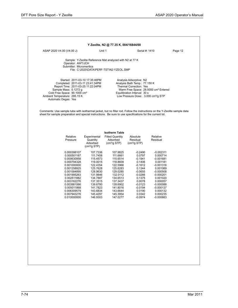
DFT Pore Size Report - Y Zeolite ASAP 2020 Operator’s Manual
Y Zeolite, N2 @ 77.35 K, 004/16844/00
ASAP 2020 V4.00 (V4.00 J) Unit 1 Serial #: 1410 Page 12
Sample: Y-Zeolite Reference Mat analyzed with N2 at 77 KOperator: AWT/JCH
Submitter: MicromeriticsFile: C:\2020\DATA\PERF-TST\N2-YZEOL.SMP
Started: 2011-03-10 17:35:46PM Analysis Adsorptive: N2Completed: 2011-03-11 23:41:34PM Analysis Bath Temp.: 77.150 K
Report Time: 2011-03-25 11:22:04PM Thermal Correction: YesSample Mass: 0.1272 g Warm Free Space: 28.5000 cm³ Entered
Cold Free Space: 90.1000 cm³ Equilibration Interval: 30 sAmbient Temperature: 295.15 K Low Pressure Dose: 3.000 cm³/g STP
Automatic Degas: Yes
Comments: Use sample tube with isothermal jacket, but no filler rod. Follow the instructions on the Y-Zeolite sample data sheet for sample preparation and special instructions. Be sure to use specifications for the current lot.
Isotherm TableRelativePressure
ExperimentalQuantity
Adsorbed(cm³/g STP)
Fitted QuantityAdsorbed
(cm³/g STP)
AbsoluteResidual
(cm³/g STP)
RelativeResidual
0.000398107 107.7336 107.9825 -0.2490 -0.0023110.000501187 111.7458 111.6661 0.0797 0.0007140.000630958 115.4573 115.6514 -0.1941 -0.0016810.000794328 119.0015 118.8609 0.1406 0.0011810.001000000 122.4354 122.5966 -0.1612 -0.0013160.001258925 125.7628 125.6283 0.1344 0.0010690.001584895 128.9630 129.0285 -0.0655 -0.0005080.001995263 131.9846 132.0112 -0.0266 -0.0002010.002511882 134.7887 134.6513 0.1375 0.0010200.003162276 137.3515 137.3437 0.0078 0.0000570.003981066 139.6780 139.6902 -0.0123 -0.0000880.005011868 141.7823 141.8016 -0.0194 -0.0001370.006309579 143.6834 143.6644 0.0190 0.0001320.007943276 145.4297 145.3954 0.0342 0.0002350.010000000 146.9303 147.0277 -0.0974 -0.000663
7-74 Mar 2011
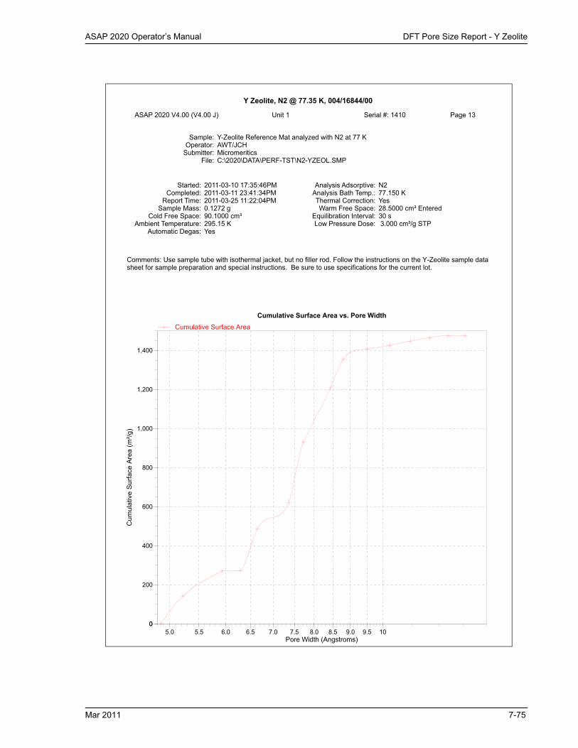
ASAP 2020 Operator’s Manual DFT Pore Size Report - Y Zeolite
Y Zeolite, N2 @ 77.35 K, 004/16844/00
ASAP 2020 V4.00 (V4.00 J) Unit 1 Serial #: 1410 Page 13
Sample: Y-Zeolite Reference Mat analyzed with N2 at 77 KOperator: AWT/JCH
Submitter: MicromeriticsFile: C:\2020\DATA\PERF-TST\N2-YZEOL.SMP
Started: 2011-03-10 17:35:46PM Analysis Adsorptive: N2Completed: 2011-03-11 23:41:34PM Analysis Bath Temp.: 77.150 K
Report Time: 2011-03-25 11:22:04PM Thermal Correction: YesSample Mass: 0.1272 g Warm Free Space: 28.5000 cm³ Entered
Cold Free Space: 90.1000 cm³ Equilibration Interval: 30 sAmbient Temperature: 295.15 K Low Pressure Dose: 3.000 cm³/g STP
Automatic Degas: Yes
Comments: Use sample tube with isothermal jacket, but no filler rod. Follow the instructions on the Y-Zeolite sample data sheet for sample preparation and special instructions. Be sure to use specifications for the current lot.
Pore Width (Angstroms)5.0 5.5 6.0 6.5 7.0 7.5 8.0 8.5 9.0 9.5 10
Cum
ulat
ive
Sur
face
Are
a (m
²/g)
00
200
400
600
800
1,000
1,200
1,400
Cumulative Surface Area vs. Pore WidthCumulative Surface Area
Mar 2011 7-75

DFT Pore Size Report - Y Zeolite ASAP 2020 Operator’s Manual
Y Zeolite, N2 @ 77.35 K, 004/16844/00
ASAP 2020 V4.00 (V4.00 J) Unit 1 Serial #: 1410 Page 14
Sample: Y-Zeolite Reference Mat analyzed with N2 at 77 KOperator: AWT/JCH
Submitter: MicromeriticsFile: C:\2020\DATA\PERF-TST\N2-YZEOL.SMP
Started: 2011-03-10 17:35:46PM Analysis Adsorptive: N2Completed: 2011-03-11 23:41:34PM Analysis Bath Temp.: 77.150 K
Report Time: 2011-03-25 11:22:04PM Thermal Correction: YesSample Mass: 0.1272 g Warm Free Space: 28.5000 cm³ Entered
Cold Free Space: 90.1000 cm³ Equilibration Interval: 30 sAmbient Temperature: 295.15 K Low Pressure Dose: 3.000 cm³/g STP
Automatic Degas: Yes
Comments: Use sample tube with isothermal jacket, but no filler rod. Follow the instructions on the Y-Zeolite sample data sheet for sample preparation and special instructions. Be sure to use specifications for the current lot.
Pore Width (Angstroms)5.0 5.5 6.0 6.5 7.0 7.5 8.0 8.5 9.0 9.5 10
Incr
emen
tal S
urfa
ce A
rea
(m²/g
)
00
50
100
150
200
250
300
Incremental Surface Area vs. Pore WidthIncremental Surface Area
7-76 Mar 2011
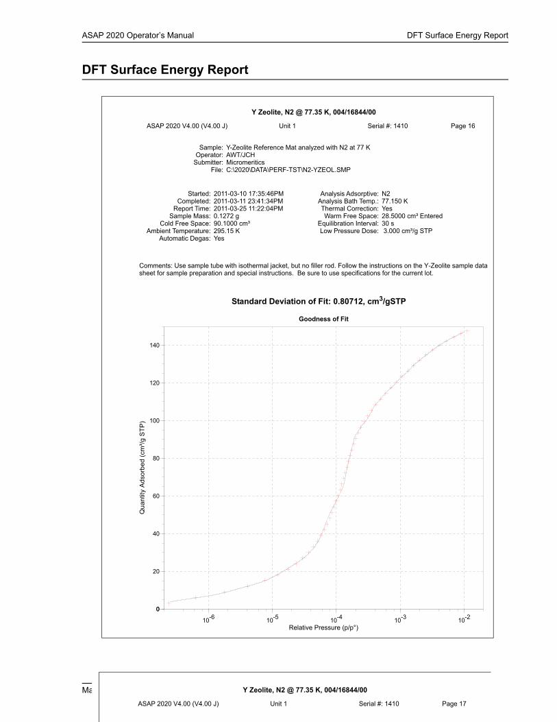
ASAP 2020 Operator’s Manual DFT Surface Energy Report
DFT Surface Energy Report
Y Zeolite, N2 @ 77.35 K, 004/16844/00
ASAP 2020 V4.00 (V4.00 J) Unit 1 Serial #: 1410 Page 16
Sample: Y-Zeolite Reference Mat analyzed with N2 at 77 KOperator: AWT/JCH
Submitter: MicromeriticsFile: C:\2020\DATA\PERF-TST\N2-YZEOL.SMP
Started: 2011-03-10 17:35:46PM Analysis Adsorptive: N2Completed: 2011-03-11 23:41:34PM Analysis Bath Temp.: 77.150 K
Report Time: 2011-03-25 11:22:04PM Thermal Correction: YesSample Mass: 0.1272 g Warm Free Space: 28.5000 cm³ Entered
Cold Free Space: 90.1000 cm³ Equilibration Interval: 30 sAmbient Temperature: 295.15 K Low Pressure Dose: 3.000 cm³/g STP
Automatic Degas: Yes
Comments: Use sample tube with isothermal jacket, but no filler rod. Follow the instructions on the Y-Zeolite sample data sheet for sample preparation and special instructions. Be sure to use specifications for the current lot.
Relative Pressure (p/p°)10-6 10-5 10-4 10-3 10-2
Qua
ntity
Ads
orbe
d (c
m³/g
STP
)
00
20
40
60
80
100
120
140
Goodness of Fit
Standard Deviation of Fit: 0.80712, cm3/gSTP
Mar 2011 7-77 Y Zeolite, N2 @ 77.35 K, 004/16844/00
ASAP 2020 V4.00 (V4.00 J) Unit 1 Serial #: 1410 Page 17
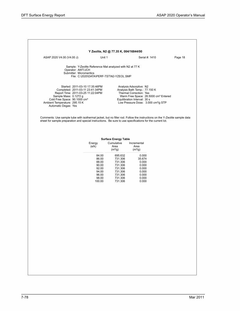
DFT Surface Energy Report ASAP 2020 Operator’s Manual
Y Zeolite, N2 @ 77.35 K, 004/16844/00
ASAP 2020 V4.00 (V4.00 J) Unit 1 Serial #: 1410 Page 18
Sample: Y-Zeolite Reference Mat analyzed with N2 at 77 KOperator: AWT/JCH
Submitter: MicromeriticsFile: C:\2020\DATA\PERF-TST\N2-YZEOL.SMP
Started: 2011-03-10 17:35:46PM Analysis Adsorptive: N2Completed: 2011-03-11 23:41:34PM Analysis Bath Temp.: 77.150 K
Report Time: 2011-03-25 11:22:04PM Thermal Correction: YesSample Mass: 0.1272 g Warm Free Space: 28.5000 cm³ Entered
Cold Free Space: 90.1000 cm³ Equilibration Interval: 30 sAmbient Temperature: 295.15 K Low Pressure Dose: 3.000 cm³/g STP
Automatic Degas: Yes
Comments: Use sample tube with isothermal jacket, but no filler rod. Follow the instructions on the Y-Zeolite sample data sheet for sample preparation and special instructions. Be sure to use specifications for the current lot.
Surface Energy TableEnergy
(e/k)Cumulative
Area(m²/g)
IncrementalArea(m²/g)
84.00 695.632 0.000 86.00 731.306 35.674 88.00 731.306 0.000 90.00 731.306 0.000 92.00 731.306 0.000 94.00 731.306 0.000 96.00 731.306 0.000 98.00 731.306 0.000
100.00 731.306 0.000
7-78 Mar 2011

ASAP 2020 Operator’s Manual DFT Surface Energy Report
Y Zeolite, N2 @ 77.35 K, 004/16844/00
ASAP 2020 V4.00 (V4.00 J) Unit 1 Serial #: 1410 Page 19
Sample: Y-Zeolite Reference Mat analyzed with N2 at 77 KOperator: AWT/JCH
Submitter: MicromeriticsFile: C:\2020\DATA\PERF-TST\N2-YZEOL.SMP
Started: 2011-03-10 17:35:46PM Analysis Adsorptive: N2Completed: 2011-03-11 23:41:34PM Analysis Bath Temp.: 77.150 K
Report Time: 2011-03-25 11:22:04PM Thermal Correction: YesSample Mass: 0.1272 g Warm Free Space: 28.5000 cm³ Entered
Cold Free Space: 90.1000 cm³ Equilibration Interval: 30 sAmbient Temperature: 295.15 K Low Pressure Dose: 3.000 cm³/g STP
Automatic Degas: Yes
Comments: Use sample tube with isothermal jacket, but no filler rod. Follow the instructions on the Y-Zeolite sample data sheet for sample preparation and special instructions. Be sure to use specifications for the current lot.
Surface Energy Distribution by Modified Density Functional TheoryModel: N2 @ 77K, Surface Energy Distribution
Method: Non-negative Regularization; No Smoothing
Standard Deviation of Fit: 0.45744, cm³/g STP
Isotherm TableRelativePressure
ExperimentalQuantity
Adsorbed(cm³/g STP)
Fitted QuantityAdsorbed
(cm³/g STP)
AbsoluteResidual
(cm³/g STP)
RelativeResidual
0.000001000 7.3251 7.3867 -0.0616 -0.0084070.000001059 7.5007 7.5380 -0.0373 -0.0049770.000001122 7.6797 7.6957 -0.0160 -0.0020850.000001189 7.8611 7.8587 0.0024 0.0003100.000001259 8.0441 8.0260 0.0182 0.0022580.000001334 8.2273 8.1961 0.0312 0.0037890.000001413 8.4091 8.3680 0.0410 0.0048810.000001496 8.5875 8.5408 0.0467 0.0054340.000001585 8.7602 8.7141 0.0461 0.0052600.000001679 8.9243 8.8878 0.0365 0.0040840.000001778 9.0763 9.0623 0.0140 0.0015480.000001884 9.2249 9.2381 -0.0132 -0.0014290.000001995 9.3838 9.4160 -0.0322 -0.0034290.000002113 9.5533 9.5967 -0.0434 -0.0045450.000002239 9.7336 9.7812 -0.0476 -0.0048880.000002371 9.9248 9.9703 -0.0455 -0.0045820.000002512 10.1268 10.1649 -0.0381 -0.0037620.000002661 10.3393 10.3658 -0.0265 -0.0025660.000002818 10.5614 10.5734 -0.0120 -0.0011360.000002985 10.7921 10.7879 0.0042 0.0003880.000003162 11.0298 11.0093 0.0205 0.0018560.000003350 11.2721 11.2371 0.0349 0.0030990.000003548 11.5159 11.4709 0.0449 0.0039030.000003758 11.7570 11.7102 0.0468 0.0039780.000003981 11.9901 11.9549 0.0352 0.0029370.000004217 12.2126 12.2048 0.0077 0.0006330.000004467 12.4454 12.4604 -0.0150 -0.0012060.000004732 12.6925 12.7219 -0.0294 -0.0023180.000005012 12.9536 12.9896 -0.0360 -0.0027790.000005309 13.2284 13.2638 -0.0355 -0.0026830.000005623 13.5158 13.5448 -0.0290 -0.0021480.000005957 13.8143 13.8326 -0.0183 -0.001326
Mar 2011 7-79

DFT Surface Energy Report ASAP 2020 Operator’s Manual
Y Zeolite, N2 @ 77.35 K, 004/16844/00
ASAP 2020 V4.00 (V4.00 J) Unit 1 Serial #: 1410 Page 20
Sample: Y-Zeolite Reference Mat analyzed with N2 at 77 KOperator: AWT/JCH
Submitter: MicromeriticsFile: C:\2020\DATA\PERF-TST\N2-YZEOL.SMP
Started: 2011-03-10 17:35:46PM Analysis Adsorptive: N2Completed: 2011-03-11 23:41:34PM Analysis Bath Temp.: 77.150 K
Report Time: 2011-03-25 11:22:04PM Thermal Correction: YesSample Mass: 0.1272 g Warm Free Space: 28.5000 cm³ Entered
Cold Free Space: 90.1000 cm³ Equilibration Interval: 30 sAmbient Temperature: 295.15 K Low Pressure Dose: 3.000 cm³/g STP
Automatic Degas: Yes
Comments: Use sample tube with isothermal jacket, but no filler rod. Follow the instructions on the Y-Zeolite sample data sheet for sample preparation and special instructions. Be sure to use specifications for the current lot.
Isotherm TableRelativePressure
ExperimentalQuantity
Adsorbed(cm³/g STP)
Fitted QuantityAdsorbed
(cm³/g STP)
AbsoluteResidual
(cm³/g STP)
RelativeResidual
0.000006310 14.1219 14.1277 -0.0059 -0.0004150.000006683 14.4353 14.4305 0.0048 0.0003350.000007079 14.7505 14.7415 0.0090 0.0006130.000007499 15.0619 15.0613 0.0007 0.0000430.000007943 15.3741 15.3903 -0.0162 -0.0010540.000008414 15.7036 15.7286 -0.0250 -0.0015950.000008913 16.0504 16.0763 -0.0259 -0.0016160.000009441 16.4135 16.4332 -0.0196 -0.0011970.000010000 16.7915 16.7991 -0.0076 -0.0004550.000010593 17.1819 17.1744 0.0075 0.0004360.000011220 17.5816 17.5598 0.0218 0.0012390.000011885 17.9861 17.9565 0.0296 0.0016460.000012589 18.3963 18.3660 0.0302 0.0016440.000013335 18.8280 18.7904 0.0376 0.0019960.000014125 19.2816 19.2319 0.0497 0.0025760.000014962 19.7556 19.6931 0.0625 0.0031650.000015849 20.2476 20.1765 0.0711 0.0035130.000016788 20.7541 20.6848 0.0693 0.0033410.000017783 21.2717 21.2206 0.0511 0.0024020.000018836 21.8129 21.7860 0.0269 0.0012310.000019953 22.3819 22.3824 -0.0006 -0.0000250.000021135 22.9773 23.0101 -0.0329 -0.0014310.000022387 23.5967 23.6681 -0.0714 -0.0030250.000023714 24.2373 24.3541 -0.1168 -0.0048200.000025119 24.9082 25.0651 -0.1569 -0.0063000.000026607 25.6137 25.7982 -0.1845 -0.0072020.000028184 26.3517 26.5512 -0.1995 -0.0075710.000029854 27.1189 27.3236 -0.2047 -0.0075470.000031623 27.9207 28.1160 -0.1954 -0.0069970.000033497 28.7640 28.9309 -0.1669 -0.0058030.000035481 29.6484 29.7717 -0.1234 -0.0041610.000037584 30.5745 30.6430 -0.0684 -0.0022380.000039811 31.5512 31.5499 0.0013 0.0000420.000042170 32.5753 32.4987 0.0766 0.0023510.000044668 33.6419 33.4962 0.1457 0.0043300.000047315 34.7642 34.5501 0.2142 0.0061610.000050119 35.9545 35.6688 0.2857 0.007947
7-80 Mar 2011

ASAP 2020 Operator’s Manual DFT Surface Energy Report
Y Zeolite, N2 @ 77.35 K, 004/16844/00
ASAP 2020 V4.00 (V4.00 J) Unit 1 Serial #: 1410 Page 21
Sample: Y-Zeolite Reference Mat analyzed with N2 at 77 KOperator: AWT/JCH
Submitter: MicromeriticsFile: C:\2020\DATA\PERF-TST\N2-YZEOL.SMP
Started: 2011-03-10 17:35:46PM Analysis Adsorptive: N2Completed: 2011-03-11 23:41:34PM Analysis Bath Temp.: 77.150 K
Report Time: 2011-03-25 11:22:04PM Thermal Correction: YesSample Mass: 0.1272 g Warm Free Space: 28.5000 cm³ Entered
Cold Free Space: 90.1000 cm³ Equilibration Interval: 30 sAmbient Temperature: 295.15 K Low Pressure Dose: 3.000 cm³/g STP
Automatic Degas: Yes
Comments: Use sample tube with isothermal jacket, but no filler rod. Follow the instructions on the Y-Zeolite sample data sheet for sample preparation and special instructions. Be sure to use specifications for the current lot.
Isotherm TableRelativePressure
ExperimentalQuantity
Adsorbed(cm³/g STP)
Fitted QuantityAdsorbed
(cm³/g STP)
AbsoluteResidual
(cm³/g STP)
RelativeResidual
0.000053088 37.2203 36.8621 0.3582 0.0096240.000056234 38.5622 38.1403 0.4218 0.0109390.000059566 39.9880 39.5154 0.4726 0.0118200.000063096 41.5024 41.0000 0.5024 0.0121060.000066834 43.1006 42.6077 0.4929 0.0114360.000070795 44.7890 44.3526 0.4364 0.0097440.000074989 46.5727 46.2479 0.3248 0.0069740.000079433 48.4623 48.3046 0.1577 0.0032540.000084140 50.4787 50.5286 -0.0499 -0.0009880.000089125 52.6262 52.9178 -0.2916 -0.0055410.000094406 54.8939 55.4589 -0.5650 -0.0102920.000100000 57.2546 58.1261 -0.8715 -0.0152220.000105925 59.7862 60.8824 -1.0962 -0.0183350.000112202 62.4381 63.6848 -1.2467 -0.0199670.000118850 65.1929 66.4916 -1.2987 -0.0199210.000125893 68.0483 69.2682 -1.2199 -0.0179270.000133352 71.0192 71.9898 -0.9706 -0.0136670.000141254 73.7685 74.6410 -0.8725 -0.0118280.000149624 76.4391 77.2130 -0.7739 -0.0101240.000158489 79.4779 79.7004 -0.2225 -0.0028000.000167880 82.3641 82.0994 0.2647 0.0032130.000177828 85.0813 84.4060 0.6752 0.0079370.000188365 87.6373 86.6167 1.0206 0.0116450.000199526 89.9798 88.7295 1.2503 0.0138950.000211349 92.0996 90.7440 1.3556 0.0147190.000223872 94.0512 92.6623 1.3889 0.0147680.000237137 95.8811 94.4881 1.3930 0.0145280.000251189 97.5451 96.2262 1.3189 0.0135210.000266073 99.0948 97.8821 1.2127 0.0122380.000281838 100.5246 99.4615 1.0631 0.0105760.000298538 101.8934 100.9700 0.9234 0.0090620.000316228 103.1539 102.4130 0.7409 0.0071820.000334965 104.3770 103.7955 0.5815 0.0055710.000354813 105.5298 105.1222 0.4076 0.0038630.000375837 106.6423 106.3972 0.2451 0.0022980.000398107 107.7336 107.6245 0.1091 0.0010130.000421697 108.7661 108.8075 -0.0414 -0.000381
Mar 2011 7-81

DFT Surface Energy Report ASAP 2020 Operator’s Manual
Y Zeolite, N2 @ 77.35 K, 004/16844/00
ASAP 2020 V4.00 (V4.00 J) Unit 1 Serial #: 1410 Page 24
Sample: Y-Zeolite Reference Mat analyzed with N2 at 77 KOperator: AWT/JCH
Submitter: MicromeriticsFile: C:\2020\DATA\PERF-TST\N2-YZEOL.SMP
Started: 2011-03-10 17:35:46PM Analysis Adsorptive: N2Completed: 2011-03-11 23:41:34PM Analysis Bath Temp.: 77.150 K
Report Time: 2011-03-25 11:22:04PM Thermal Correction: YesSample Mass: 0.1272 g Warm Free Space: 28.5000 cm³ Entered
Cold Free Space: 90.1000 cm³ Equilibration Interval: 30 sAmbient Temperature: 295.15 K Low Pressure Dose: 3.000 cm³/g STP
Automatic Degas: Yes
Comments: Use sample tube with isothermal jacket, but no filler rod. Follow the instructions on the Y-Zeolite sample data sheet for sample preparation and special instructions. Be sure to use specifications for the current lot.
Energy (e/k)2020 30 40 50 60 70 80 90 100
Cum
ulat
ive
Sur
face
Are
a (m
²/g)
00
100
200
300
400
500
600
700
Cumulative Surface Area vs. EnergyCumulative Surface Area
7-82 Mar 2011

ASAP 2020 Operator’s Manual DFT Surface Energy Report
Y Zeolite, N2 @ 77.35 K, 004/16844/00
ASAP 2020 V4.00 (V4.00 J) Unit 1 Serial #: 1410 Page 25
Sample: Y-Zeolite Reference Mat analyzed with N2 at 77 KOperator: AWT/JCH
Submitter: MicromeriticsFile: C:\2020\DATA\PERF-TST\N2-YZEOL.SMP
Started: 2011-03-10 17:35:46PM Analysis Adsorptive: N2Completed: 2011-03-11 23:41:34PM Analysis Bath Temp.: 77.150 K
Report Time: 2011-03-25 11:22:04PM Thermal Correction: YesSample Mass: 0.1272 g Warm Free Space: 28.5000 cm³ Entered
Cold Free Space: 90.1000 cm³ Equilibration Interval: 30 sAmbient Temperature: 295.15 K Low Pressure Dose: 3.000 cm³/g STP
Automatic Degas: Yes
Comments: Use sample tube with isothermal jacket, but no filler rod. Follow the instructions on the Y-Zeolite sample data sheet for sample preparation and special instructions. Be sure to use specifications for the current lot.
Energy (e/k)2020 30 40 50 60 70 80 90 100
Incr
emen
tal S
urfa
ce A
rea
(m²/g
)
00
50
100
150
200
250
300
350
400
450
Incremental Surface Area vs. EnergyIncremental Surface Area
Mar 2011 7-83
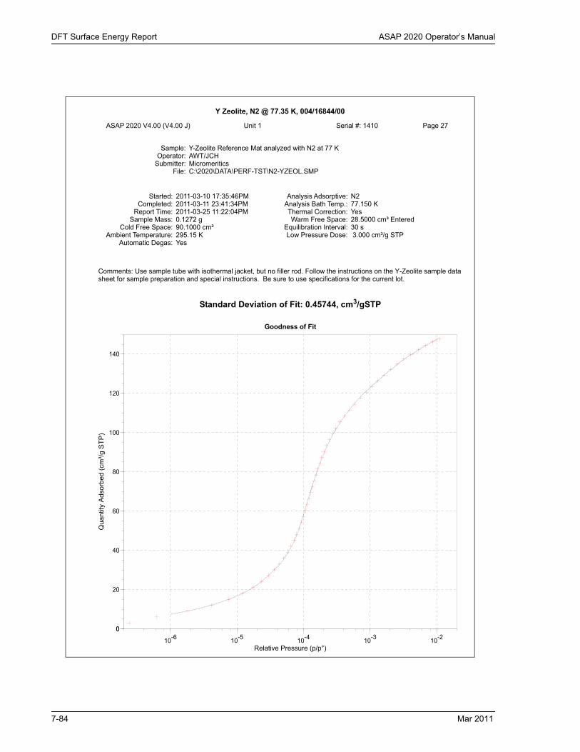
DFT Surface Energy Report ASAP 2020 Operator’s Manual
Y Zeolite, N2 @ 77.35 K, 004/16844/00
ASAP 2020 V4.00 (V4.00 J) Unit 1 Serial #: 1410 Page 27
Sample: Y-Zeolite Reference Mat analyzed with N2 at 77 KOperator: AWT/JCH
Submitter: MicromeriticsFile: C:\2020\DATA\PERF-TST\N2-YZEOL.SMP
Started: 2011-03-10 17:35:46PM Analysis Adsorptive: N2Completed: 2011-03-11 23:41:34PM Analysis Bath Temp.: 77.150 K
Report Time: 2011-03-25 11:22:04PM Thermal Correction: YesSample Mass: 0.1272 g Warm Free Space: 28.5000 cm³ Entered
Cold Free Space: 90.1000 cm³ Equilibration Interval: 30 sAmbient Temperature: 295.15 K Low Pressure Dose: 3.000 cm³/g STP
Automatic Degas: Yes
Comments: Use sample tube with isothermal jacket, but no filler rod. Follow the instructions on the Y-Zeolite sample data sheet for sample preparation and special instructions. Be sure to use specifications for the current lot.
Relative Pressure (p/p°)10-6 10-5 10-4 10-3 10-2
Qua
ntity
Ads
orbe
d (c
m³/g
STP
)
00
20
40
60
80
100
120
140
Goodness of Fit
Standard Deviation of Fit: 0.45744, cm3/gSTP
7-84 Mar 2011
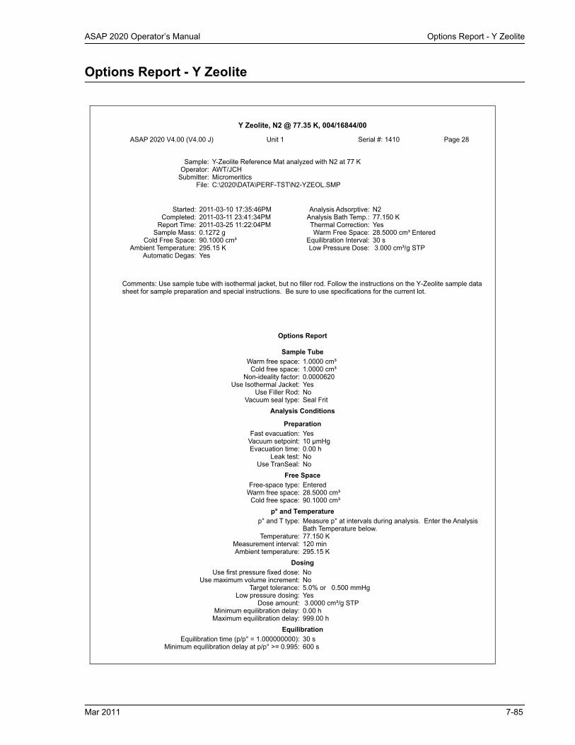
ASAP 2020 Operator’s Manual Options Report - Y Zeolite
Options Report - Y Zeolite
Y Zeolite, N2 @ 77.35 K, 004/16844/00
ASAP 2020 V4.00 (V4.00 J) Unit 1 Serial #: 1410 Page 28
Sample: Y-Zeolite Reference Mat analyzed with N2 at 77 KOperator: AWT/JCH
Submitter: MicromeriticsFile: C:\2020\DATA\PERF-TST\N2-YZEOL.SMP
Started: 2011-03-10 17:35:46PM Analysis Adsorptive: N2Completed: 2011-03-11 23:41:34PM Analysis Bath Temp.: 77.150 K
Report Time: 2011-03-25 11:22:04PM Thermal Correction: YesSample Mass: 0.1272 g Warm Free Space: 28.5000 cm³ Entered
Cold Free Space: 90.1000 cm³ Equilibration Interval: 30 sAmbient Temperature: 295.15 K Low Pressure Dose: 3.000 cm³/g STP
Automatic Degas: Yes
Comments: Use sample tube with isothermal jacket, but no filler rod. Follow the instructions on the Y-Zeolite sample data sheet for sample preparation and special instructions. Be sure to use specifications for the current lot.
Options Report
Sample TubeWarm free space: 1.0000 cm³
Cold free space: 1.0000 cm³Non-ideality factor: 0.0000620
Use Isothermal Jacket: YesUse Filler Rod: No
Vacuum seal type: Seal FritAnalysis Conditions
PreparationFast evacuation: Yes
Vacuum setpoint: 10 µmHgEvacuation time: 0.00 h
Leak test: NoUse TranSeal: No
Free SpaceFree-space type: Entered
Warm free space: 28.5000 cm³Cold free space: 90.1000 cm³
p° and Temperaturep° and T type: Measure p° at intervals during analysis. Enter the Analysis
Bath Temperature below.Temperature: 77.150 K
Measurement interval: 120 minAmbient temperature: 295.15 K
DosingUse first pressure fixed dose: No
Use maximum volume increment: NoTarget tolerance: 5.0% or 0.500 mmHg
Low pressure dosing: YesDose amount: 3.0000 cm³/g STP
Minimum equilibration delay: 0.00 hMaximum equilibration delay: 999.00 h
EquilibrationEquilibration time (p/p° = 1.000000000): 30 s
Minimum equilibration delay at p/p° >= 0.995: 600 s
Mar 2011 7-85

Options Report (cont’d) - Y Zeolite ASAP 2020 Operator’s Manual
Options Report (cont’d) - Y Zeolite
Y Zeolite, N2 @ 77.35 K, 004/16844/00
ASAP 2020 V4.00 (V4.00 J) Unit 1 Serial #: 1410 Page 29
Sample: Y-Zeolite Reference Mat analyzed with N2 at 77 KOperator: AWT/JCH
Submitter: MicromeriticsFile: C:\2020\DATA\PERF-TST\N2-YZEOL.SMP
Started: 2011-03-10 17:35:46PM Analysis Adsorptive: N2Completed: 2011-03-11 23:41:34PM Analysis Bath Temp.: 77.150 K
Report Time: 2011-03-25 11:22:04PM Thermal Correction: YesSample Mass: 0.1272 g Warm Free Space: 28.5000 cm³ Entered
Cold Free Space: 90.1000 cm³ Equilibration Interval: 30 sAmbient Temperature: 295.15 K Low Pressure Dose: 3.000 cm³/g STP
Automatic Degas: Yes
Comments: Use sample tube with isothermal jacket, but no filler rod. Follow the instructions on the Y-Zeolite sample data sheet for sample preparation and special instructions. Be sure to use specifications for the current lot.
Sample BackfillBackfill at start of analysis: NoBackfill at end of analysis: Yes
Backfill gas: N2Adsorptive PropertiesAdsorptive: Nitrogen
Maximum manifold pressure: 925.00 mmHgNon-ideality factor: 0.0000570
Density conversion factor: 0.0015468Therm. tran. hard-sphere diameter: 3.860 Å
Molecular cross-sectional area: 0.162 nm²Inside diameter of sample tube: 9.53 mm
7-86 Mar 2011

ASAP 2020 Operator’s Manual Description
8. OPTIONS MENU
The commands on the Options menu enable you to configure the system to your laboratory’s requirements and establish sample defaults.
Description
Option Presentation Allows you to display the sample file dialog in Advanced, Basic, or Restricted mode. Page 8-2.
Sample Defaults Enables you to specify default values for sample and parameter files. Page 8-4.
Units Enables you to choose the way in which data are presented on the screen and in printed reports. Page 8-12.
Graph Grid Lines Enables you to choose the type(s) of grid lines to show on your report. Page 8-12.
Live Graph Enables you to choose the variable for the X-axis during data collection. Page 8-13.
Parameter Files Directory Allows you to specify a location for the parameter files used in the Basic sample file editor. Page 8-13.
Service Test Mode Enables you to perform certain troubleshooting procedures. This option is available only under the direction of a Micromeritics service representative. Page 8-14.
Mar 2011 8-1

Option Presentation ASAP 2020 Operator’s Manual
Option Presentation
The sample editing dialogs for the ASAP 2020 analysis program may be presented in three modes: Restricted, Basic, and Advanced. Each format displays sample information dialogs differently.
• Advanced: displays all parts of the sample information file in a tabbed dialog as in an index card file. You just click on the tab of the desired parameter. This format also allows you to switch to the Basic mode.
• Basic: displays all parts of the sample file as a single dialog. in which you select from pre-defined parameter files. This format also allows you to switch to the Advanced mode if editing of parameters is desired.
• Restricted: displays in the same manner as the Basic format. Certain menu options, how-ever, become disabled and you cannot switch to the Advanced mode. You also must enter a password to access and exit this format.
Advanced
The Advanced format presents all parts of the sample information file in a tabbed dialog. Each tab opens its associated dialog. For example, if you are using the Advanced format and you open or create a sample information file, the following dialog is displayed.
The Advanced format can be used to edit sample parameters and customize files.
8-2 Mar 2011

ASAP 2020 Operator’s Manual Option Presentation
Basic
The Basic format presents the sample information file and its parameter files as a single dialog. You also have access to all menu options. For example, if you are using the Basic format and open or create a sample information file, the dialog is displayed in this manner.
The Basic format is used to quickly create sample information files using previously defined parameter files. You also can switch easily to the Advanced format to view or edit details of parameter files.
Restricted
The Restricted format is identical to the Basic format, except that certain options are disabled. You also cannot switch to the Advanced format. This format is password-protected and typically is used in laboratories where analysis conditions must remain constant, for example, in the pharmaceutical industry.
When you select Restricted, a dialog requesting a password is displayed.
You can enter any password (up to 31 characters) to enable the Restricted mode. You must enter the same password to exit the Restricted mode. For example, if you enter “password” to enable the Restricted format, then you must enter “password” to exit. If you forget the
Predefined parameter fileare selected from drop-down lists.
Mar 2011 8-3

Sample Defaults ASAP 2020 Operator’s Manual
password, open the application INI file and navigate to the Private section. The current password is shown immediately following “OptionPresentationPassword.” Make a note of the password, exit the INI file, and enter the password where requested. Deleting the password from the INI file will not disable the Restricted mode; you must enter the password using the Password dialog to exit the Restricted format.
Sample Defaults
Sample defaults are the values you see in the sample information editors when you create a new sample file. This option allows you to specify the default values. This feature makes it easy for you to apply the same conditions to many samples.
For efficiency, it is best to specify defaults for materials you most commonly analyze. You can always edit the values in the sample file when it is created. Sample defaults can be specified using the Basic or Advanced format.
The analysis program contains one complete default sample information file. When you select Open, Sample information from the Main Menu, a new file with these default values is generated. Default files for degas conditions, analysis conditions, adsorptive properties, and report options also are included. Appendix F, Default Files and System Files lists details on system default files.
Sample defaults can be specified using the Advanced or Basic format. The Advanced or Basic format is chosen by selecting Options > Option presentation from the main menu.
8-4 Mar 2011
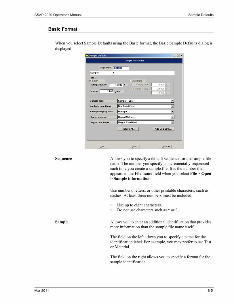
ASAP 2020 Operator’s Manual Sample Defaults
Basic Format
When you select Sample Defaults using the Basic format, the Basic Sample Defaults dialog is displayed.
Sequence Allows you to specify a default sequence for the sample file name. The number you specify is incrementally sequenced each time you create a sample file. It is the number that appears in the File name field when you select File > Open > Sample information.
Use numbers, letters, or other printable characters, such as dashes. At least three numbers must be included.
• Use up to eight characters.• Do not use characters such as * or ?.
Sample Allows you to enter an additional identification that provides more information than the sample file name itself.
The field on the left allows you to specify a name for the identification label. For example, you may prefer to use Test or Material.
The field on the right allows you to specify a format for the sample identification.
Mar 2011 8-5

Sample Defaults ASAP 2020 Operator’s Manual
Sample(continued)
Use numbers, letters, or other printable characters, such as dashes.
• Use up to 20 characters for the prompt.
• Use up to 43 characters (including the $ symbol).
• Include the automatically generated file name as part of the identification by using the $ symbol where you want the sequence number to appear.
For example, if the sequence number is 000-001, enter the identification as follows:
Lab #25 - $
The resulting sample identification for the first sample information file would be:
Lab #25 - 000-001
for the second file:
Lab #25 - 000-002, and so on.
Mass You can choose to enter a sample mass or have the mass automatically calculated. Regardless of which option you choose for your default, you can change it in the sample file.
Enter Enables the Sample Mass field allowing you to enter a default value.
Calculate Enables the Empty tube and Sample + tube fields, allowing you to enter default values. These values are used to calcu-late the mass of the sample,
Density The sample density is used when using a calculated free space. The default value is appropriate unless you typically use a calculated free space. This field can always be edited in the sample file.
Masssample Masssample tube+ Masstube–=
8-6 Mar 2011

ASAP 2020 Operator’s Manual Sample Defaults
Advanced Format
When you select Sample Defaults while using the Advanced format, the Advanced Sample Defaults dialog is displayed.
Sample TubeDegas ConditionsAnalysis ConditionsAdsorptive PropertiesReport Options
Each parameter has a drop-down list containing files included with the software, as well as any you may have created and saved to the Parameter Files Directory.
Choose from the list provided for each parameter the file you wish to use as the default.
Replace All Use this push button to replace the current default values with those from an existing sample file.
Save Saves the current definition as the defaults
Close Closes the dialog box.
Advanced Switches the sample editor to the Advanced format.
The defaults you specify for the parameters in the Advanced format display as the defaults for newly created standalone parameter files
Mar 2011 8-7
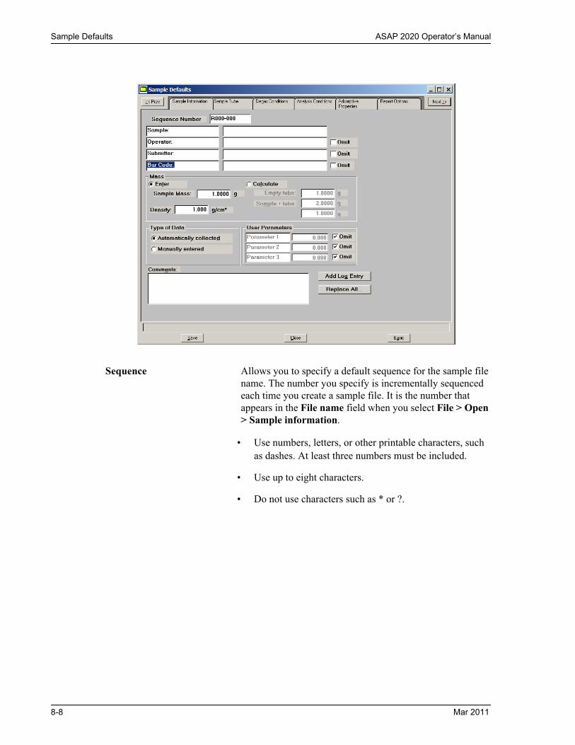
Sample Defaults ASAP 2020 Operator’s Manual
Sequence Allows you to specify a default sequence for the sample file name. The number you specify is incrementally sequenced each time you create a sample file. It is the number that appears in the File name field when you select File > Open > Sample information.
• Use numbers, letters, or other printable characters, such as dashes. At least three numbers must be included.
• Use up to eight characters.
• Do not use characters such as * or ?.
8-8 Mar 2011

ASAP 2020 Operator’s Manual Sample Defaults
Sample Allows you to enter an additional identification that provides more information than the sample file name itself.
The field on the left allows you to specify a name for the identification label. For example, you may prefer to use Test or Material.
The field on the right allows you to specify a format for the sample identification.
• Use numbers, letters, or other printable characters, such as dashes.
• Use up to 20 characters for the prompt.
• Use up to 43 characters (including the $ symbol).
• Include the automatically generated file name as part of the identification by using the $ symbol where you want the sequence number to appear.
For example, if the sequence number is 000-001, enter the identification as follows:
Lab #25 - $
The resulting sample identification for the first sample information file would be:
Lab #25 - 000-001
for the second file:
Lab #25 - 000-002, and so on.
Mar 2011 8-9

Sample Defaults ASAP 2020 Operator’s Manual
OperatorSubmitter
These fields contain the name (or other identification) of the operator and submitter.
The fields on the left can be edited to display a different label if desired.
The fields on the right allow you to specify default names or titles.
• Include the automatically generated file number as part of the identification by using the symbol $ where you want the sequence number to appear. Refer to the exam-ple in the previous section.
• Use up to 20 characters for the prompt.
• Use up to 43 characters (including the $ symbol).
• Omit either (or both) item entirely from the sample infor-mation file by selecting Omit.
Bar Code This field can be used to enter bar code information or to accept data from a bar code reader. If bar code information is not used, this field can be used to enter additional information about the sample. The field can also be omitted if it is not needed.
Use up to 40 characters.
Mass You can choose to enter a sample mass or have the mass auto-matically calculated. Regardless of which option you choose for your default, you can change it in the sample file.
Enter Enables the Sample Mass field allowing you to enter a default value.
Calculate Enables the Empty tube and Sample + tube fields, allowing you to enter default values. These values are used to calculate the mass of the sample,
Density Enter a default density. If there is a material you analyze quite often, you may wish to use its default in this field. This value can be edited in the sample information file.
Masssample Masssample tube+ Masstube–=
8-10 Mar 2011

ASAP 2020 Operator’s Manual Sample Defaults
Type of Data Choose whether you wish to enter data or have it collected automatically by the system.
User Parameters The fields in this group box are used primarily for SPC (Sta-tistical Process Control) reporting. They are used to specify characteristics of the sample or its manufacturing process.
Once specified, these parameters display on the sample edi-tor and in the SPC Sample Options dialog (accessed through the SPC Report Options dialog).
These fields can also be used to record analysis conditions or sample information so that it can be printed on the Summary report.
Select Omit if you do not wish to use these fields; this will prevent them from displaying on the sample information dia-log.
Comments Use this window to enter sample characteristics, analysis conditions, etc. Anything you type in this window is printed in the report header.
Add Log Entry Allows you to enter comments about the sample or its analysis conditions. Anything you enter using this option appears in the Instrument Log Report; it does not display in the report header.
Replace All Use this push button to replace the current default values with those from an existing sample file.
Save Saves the current definition as the defaults
Close Closes the dialog.
Basic Switches the sample editor to the Basic format.
Mar 2011 8-11

Units ASAP 2020 Operator’s Manual
Units
This menu command displays the Units Selections dialog which allows you to choose the manner in which to display data on reports.
Graph Grid Lines
Graph Grid Lines enables you to choose the type(s) of grid lines to show on your reports; the Graph Grid Lines dialog is displayed.
X-AxisY-Axis
Enables you to choose Major and/or Minor lines to display in printed reports for the Logarithmic and Linear scales.
If you deselect these items (remove the check marks), your report will not display grid lines.
Grid Line Style Allows you to choose the type of grid line to display if grid lines are being shown.
8-12 Mar 2011
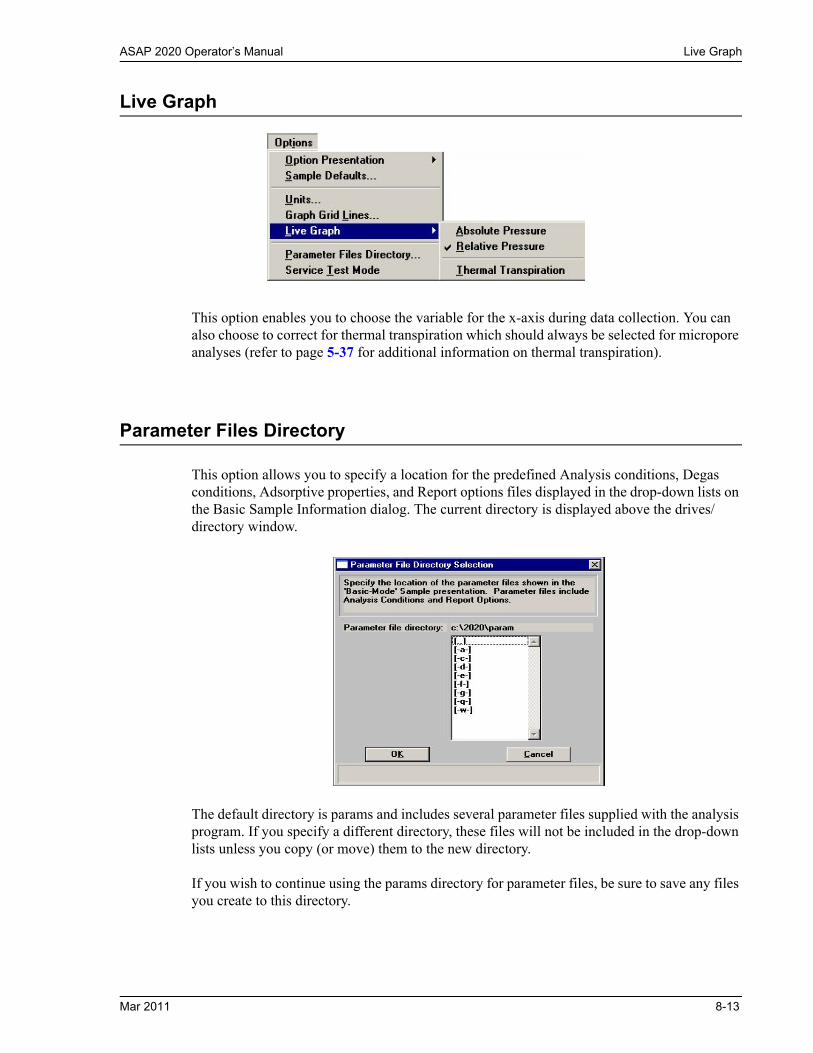
ASAP 2020 Operator’s Manual Live Graph
Live Graph
This option enables you to choose the variable for the x-axis during data collection. You can also choose to correct for thermal transpiration which should always be selected for micropore analyses (refer to page 5-37 for additional information on thermal transpiration).
Parameter Files Directory
This option allows you to specify a location for the predefined Analysis conditions, Degas conditions, Adsorptive properties, and Report options files displayed in the drop-down lists on the Basic Sample Information dialog. The current directory is displayed above the drives/directory window.
The default directory is params and includes several parameter files supplied with the analysis program. If you specify a different directory, these files will not be included in the drop-down lists unless you copy (or move) them to the new directory.
If you wish to continue using the params directory for parameter files, be sure to save any files you create to this directory.
Mar 2011 8-13

Service Test Mode ASAP 2020 Operator’s Manual
Service Test Mode
Various service tests are included in the ASAP 2020 operating program. These tests can be performed only with the assistance of a trained Micromeritics service representative. When you select Service Test Mode from the Options menu, a dialog box prompting you to enter a password is displayed. This password is coded to change on a regular basis and is known only by your service representative. You will not be able to perform these tests without his guidance.
8-14 Mar 2011

ASAP 2020 Operator’s Manual Troubleshooting
9. TROUBLESHOOTING AND MAINTENANCE
The ASAP 2020 system has been designed to provide efficient and continuous service. However, to get the best results over the longest period of time, certain maintenance procedures must be followed. This chapter includes troubleshooting information, recommended preventive maintenance procedures, and routine maintenance procedures.
Troubleshooting
Most operational problems are caused by leaks (commonly around the sample tube O-ring at the analysis port), sample weighing errors, use of too much analysis bath fluid in the Dewar at the start of an analysis, or entry of incorrect system volume for analysis. Always check these first when expected analysis results are not obtained. Some common operational problems, which are not indicated on the video monitor screen, and their respective causes and solutions are provided in the following table.
What Happened Why What To Do
Analysis Dewar cannot be raised (or lowered).
Elevator that moves dewar stuck in up position, down position, or somewhere in between.
Check for possible obstruction to elevator movement.
Vacuum pump gurgles continuously.
Sample tube or cold trap tube O-ring or fitting loose.
Tighten fitting. Replace O-ring.
Sample tube cracked. Replace with new sample tube.
No sample tube loaded on a selected port.
Install plug or empty sample tube.
Gas inlet valve open while vacuum valve open.
With manual control enabled, use the instrument schematic to close gas inlet valve.
Vacuum gauge shows reading above 20 mHg, even after extended pumping through unrestricted valve with analysis or degas ports closed.
Vacuum pump oil is low, causing ineffective evacuation.
Add or change vacuum pump oil. Be sure to add oil to proper level according to indicator window on the pump.
Mar 2011 9-1

Troubleshooting ASAP 2020 Operator’s Manual
What Happened Why What To Do
Vacuum gauge shows reading above 20 mHg, even after extended pumping through unrestricted valve with analysis or degas ports closed.(continued)
Cold trap obstructed by condensation.
Clean the cold trap tubes. Refer to Cleaning the Cold Trap Tubes on page 9-14.
Filter in port being used is dirty. Replace filter in port. Refer to Replacing the Port Filters on page 9-6.
Leak in vacuum plumbing. Check and tighten all connections in vacuum plumbing, including cold traps.
Vacuum pump turned off or unplugged.
Check pump power plug and power switch.
The alumina in the oil vapor trap is holding moisture.
Replace or dry the alumina. Refer to Replacing the Alumina in the Oil Vapor Traps on page 9-11.
Analysis valves cannot be operated.
Circuit opened by circuit breaker. Reset breaker (depress breaker button) located on the right side of the instrument near (page 3-4 shows location). If it does not stay in or if it continues to trip, contact appropriate service personnel.
Cable from computer to the instrument is loose.
Make sure the cable is seated properly.
9-2 Mar 2011

ASAP 2020 Operator’s Manual Preventive Maintenance
Preventive Maintenance
The table below lists the preventive maintenance procedures you should perform to keep your analyzer operating at peak performance. Instructions for each procedure follow the table. Micromeritics recommends that you perform these procedures as indicated, as well as by one of our service representatives every 12 months.
Maintenance Required Frequency
Clean the analyzer, page 9-22 As required or every 6 months
Lubricate elevator screw, page 9-4 As required or every 6 months
Check analysis port Dewar, page 9-4 Weekly
Replace sample tube O-ring, page 9-5 As required or every 3 months
Replace port filters, page 9-6 Every 30 days
Replace vacuum pump exhaust filter*, page 9-7 Annually (Heavy use may require more frequent maintenance.)
Inspect and change vacuum pump fluid*, page 9-9 As required or every 3 months
Replace alumina in oil vapor traps*, page 9-11(if installed)
As required or every 3 months
Replace diaphragm in vacuum pump (oil-free pump only)**
Every 12 months
Clean cold trap tubes, page 9-14 As required or every 3 months
Calibrate manifold temperature sensor, page 9-15 Every 12 months
Calibrate system volume Every 12 months
Check analyzer outgassing rate Every 6 months
Test analyzer for leaks, page D-1 As required or every 12 months
*Oil-based vacuum pumps only.**After about 12 to 18 months of operation, the diaphragm in the pump will wear out and
become completely inoperable. To prevent any instrument downtime due to an inoperable pump, it is recommended that you have the diaphragm replaced by a Micromeritics Service Representative every 12 months.
Mar 2011 9-3

Preventive Maintenance ASAP 2020 Operator’s Manual
Lubricating the Elevator Screw
Apply a light coat of lithium grease to the elevator screw, accessed from the rear of the instrument, as needed.
Checking the Analysis Port Dewar
Ice and suspended frost particles may accumulate in the bottom of the analysis port Dewar. Particles or deposits exceeding 1/4 in. (0.64 cm) in depth may jam between the bottom of the sample tube and the bottom of the Dewar, causing the Dewar not to raise fully. Accumulations of fine particles impede liquid nitrogen circulation around the bottom of the sample tube. This causes the sample temperature to be slightly higher which, in turn, can cause pore volume measurement errors in those samples exhibiting high isotherm slope above 0.97 relative pressure. Accumulated ice is likely to melt and form a pool of water in the Dewar if all liquid nitrogen evaporates. The water must be removed; otherwise it will solidify when liquid nitrogen is added and could press on the bottom of the sample tube causing breakage.To ensure problems do not develop due to ice accumulation, check the Dewar after each use. Clean on a weekly basis as follows:
1. Lift out the entire analysis port Dewar.
2. Pour out liquid nitrogen into an appropriate cryogenic container.
3. Rinse the Dewar with warm water to melt any ice accumulation which may remain in the Dewar, then dry thoroughly.
4. Replace the Dewar.
When handling Dewars, be sure to observe the Dewar precautions outlined in Installing Dewars in Chapter 3.
Do not pour liquid nitrogen directly into a sink. Doing so may cause drain pipes to burst.
9-4 Mar 2011
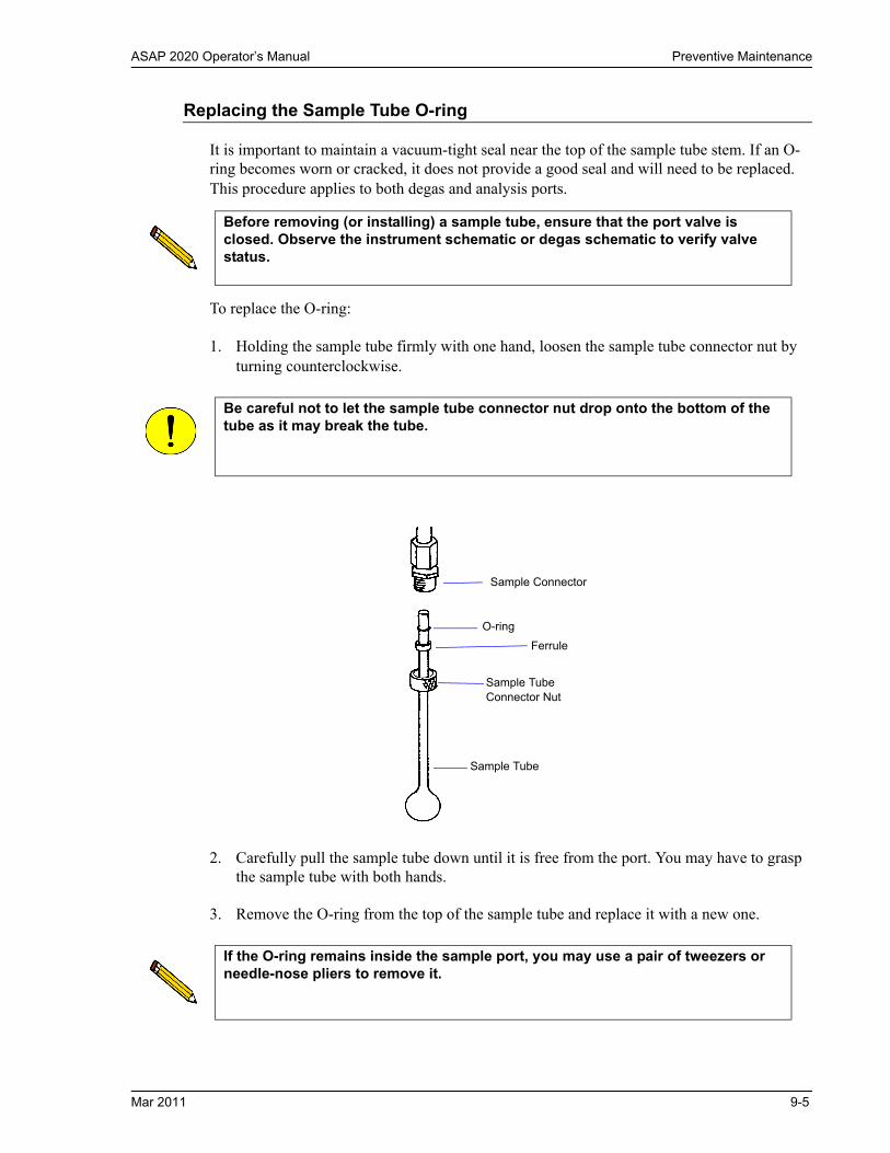
ASAP 2020 Operator’s Manual Preventive Maintenance
Replacing the Sample Tube O-ring
It is important to maintain a vacuum-tight seal near the top of the sample tube stem. If an O-ring becomes worn or cracked, it does not provide a good seal and will need to be replaced. This procedure applies to both degas and analysis ports.
To replace the O-ring:
1. Holding the sample tube firmly with one hand, loosen the sample tube connector nut by turning counterclockwise.
2. Carefully pull the sample tube down until it is free from the port. You may have to grasp the sample tube with both hands.
3. Remove the O-ring from the top of the sample tube and replace it with a new one.
Before removing (or installing) a sample tube, ensure that the port valve is closed. Observe the instrument schematic or degas schematic to verify valve status.
Be careful not to let the sample tube connector nut drop onto the bottom of the tube as it may break the tube.
Sample Connector
O-ring
Ferrule
Sample Tube Connector Nut
Sample Tube
If the O-ring remains inside the sample port, you may use a pair of tweezers or needle-nose pliers to remove it.
Mar 2011 9-5

Preventive Maintenance ASAP 2020 Operator’s Manual
4. After the new O-ring is in place, insert the sample tube back into the sample port until it is fully seated.
5. Slide the sample tube connector nut up the tube (the ferrule and O-ring will move along with the connector nut). Then, turning clockwise, hand-tighten the connector nut to the sample connector.
Replacing the Port Filters
A porous metal filter is located in the analysis port and in each degas port of the analyzer. If a filter on a degas port is contaminated, the contaminant may adsorb atmospheric gases when the port is not plugged (with either a sample tube or plug), resulting in extended degassing time for samples on that port. Using a contaminated filter on the analysis port may extend the time required to achieve a vacuum at that port. More importantly, the contaminant may adsorb or desorb during analysis, affecting the analysis results. A contaminated filter on the analysis port may be detected by a leak test (if the contaminant outgasses) or by a free space reading much lower than normal.
Perform the following steps to replace the filters:
Analysis Port
1. Make sure the Dewar and sample tube (or plug) are removed. Make sure the analysis port (sample valve) is closed.
2. Using a wrench, remove the sample tube fitting from the manifold connector and remove the filter and O-ring.
O-ring
Filter
Sample Tube Fitting
9-6 Mar 2011
ASAP 2020 Operator’s Manual Preventive Maintenance
3. Replace the filter and the O-ring. Carefully reassemble the sample tube fitting, filter, O-ring and manifold connector, and tighten by hand. Then tighten with a wrench to prevent leaks when evacuated.
Degas Port
1. Using a wrench, remove the degas port fitting and remove the filter and O-ring.
2. Replace the filter and the O-ring. Carefully reassemble the sample tube fitting, filter, O-ring and manifold connector, and tighten by hand. Then tighten with the wrenches to prevent leaks when evacuated.
Replacing the Vacuum Pump Exhaust Filter
The gases used by the ASAP 2020 are exhausted by vacuum pumps. An exhaust filter is installed on the exhaust port of each vacuum pump. The filter minimizes the release of oil vapor and should be replaced when it becomes so saturated with oil that it is ineffective.
1. Using a flat-head screwdriver, remove the screws from the vacuum pump panel on the front of the analyzer, then remove the panel to access the pump.
To avoid analysis problems, the new filter and O-ring must be clean. Do not touch them with bare hands.
To avoid degassing problems, the new filter and O-ring must be clean. Do not touch them with bare hands.
This procedure does not apply, and is not required, for dry vacuum pumps.
Exhaust filters are used on the vacuum pump to minimize the release of oil vapors. The gases used are diluted substantially upon being released from the vacuum pumps. However, it may be desirable in some locations to provide a fume hood for added protection from hazardous gases and vapors released into the work area.
Mar 2011 9-7

Preventive Maintenance ASAP 2020 Operator’s Manual
2. Loosen the wing nut of the vacuum clamp at the vacuum pump exhaust port. Swing the clamp fastening screw away from the exhaust port. Open the clamp to remove it from the port.
3. Make sure the dust cover has been removed. Lift the exhaust filter from the exhaust port and discard it. Install a new filter on the exhaust port and push the filter against the O-ring.
4. Open the clamp and place it around the flange of the exhaust port and the flange of the exhaust filter. Swing the clamp fastening screw toward the exhaust port until it fits into the slot in the other half of the clamp. Tighten the wing nut.
5. Reinstall the vacuum pump panel.
Filter
Clamp
9-8 Mar 2011
ASAP 2020 Operator’s Manual Preventive Maintenance
Inspecting and Changing Vacuum Pump Fluid
The fluid in the vacuum pump should be changed every three months or when the efficiency of the vacuum pump declines (requiring increased time to reach vacuum levels). The fluid can first be inspected to determine if a change is necessary.
Use oil supplied by Micromeritics, or refer to the manual for the vacuum pump for other acceptable oils.
Inspecting Fluid
Inspect the fluid as follows:
1. Remove the vacuum pump panel (located on the left front side of the analyzer).
2. View the vacuum pump fluid through the oil level indicator window. Fluid in good condition is clean, clear or light in color, and transparent. If the color of the fluid is darkened, the fluid should be changed.
Changing Fluid
Change the fluid as follows:
1. Place the analyzer ON/OFF switch in the OFF position.
2. Remove the vacuum pump panel (if not already removed).
3. Disconnect the vacuum pump power cord from its power source.
4. Disconnect the vacuum pump hose from the top of the vacuum pump.
5. Grasp the handle on top of the vacuum pump and lift it out of the analyzer; place the vacuum pump on a work table.
This procedure does not apply, and is not required, for dry vacuum pumps.
If the high vacuum pump is installed, wait for it to stop completely (approximately 10 minutes).
Always drain the vacuum pump while the pump is warm and switched off (unplugged).
Mar 2011 9-9

Preventive Maintenance ASAP 2020 Operator’s Manual
6. Drain the used oil:
a. Place a waste container under the drain fitting.
b. Remove the plug from the drain spout.
c. Allow the oil to drain into the waste container.
d. Replace the drain plug.
7. Remove the Oil-fill plug; add fresh fluid to the oil-fill port until the level is midway between the two indicator lines.
8. Check the washer or O-ring used at the oil-filling port; replace if necessary. Replace the oil-fill plug.
9. Place the vacuum pump back into the analyzer onto the drip tray and reconnect the vacuum pump hose.
10. Reconnect the vacuum pump power cord.
11. Replace the vacuum pump panel.
12. Place the analyzer ON/OFF switch in the ON position. The pump must run a few hours (or overnight) to eliminate air and moisture from the fresh fluid and to produce efficient vacuum operations.
Badly contaminated fluid requires flushing of the pump once or twice with fresh fluid to wash out contaminants.
Adding fluid above the midway position on the fluid level indicator may cause fluid to splash into the vacuum hoses and leak from the internal vacuum pump.
OIl-Fill Plug
Indicator Lines
Oil-Level Indicator Window
9-10 Mar 2011

ASAP 2020 Operator’s Manual Preventive Maintenance
Replacing the Alumina in the Oil Vapor Traps
The activated alumina in the oil vapor traps becomes saturated during use. The alumina should be replaced if any of the following conditions exist:
• The alumina has been used for a three-month period.• Oil has accumulated in the cold trap.• Most of the alumina pellets are no longer white.
Perform the following steps to replace the alumina:
1. Remove the vacuum pump panel.
2. Turn off power to the vacuum pump
3. Prepare fresh alumina as follows:
a. Heat an oven between 250 °C and 350 °C.
b. Pour about 180 grams of alumina into a glass or metal container for each trap (approximately 250 mL if a graduated beaker is used). Place the container in the oven.
c. Bake the alumina for two hours; turn off the oven.
d. Allow the alumina to cool in the oven before pouring it into the traps.
4. Display the Instrument Schematic and select Enable Manual Mode.
5. Open the vacuum valve (P1 on analysis schematic and D5 on degas schematic) and an inlet valve (nitrogen or helium) until the pressure stabilizes around atmospheric pressure. Then, close all valves. This step fills the vacuum section before disconnecting.
When you replace the alumina, you may also need to change the vacuum pump oil if the interval between changes of alumina has been short.
Do not perform the following procedure on used alumina. The resultant oil vapors may cause a fire or an explosion.
Mar 2011 9-11

Preventive Maintenance ASAP 2020 Operator’s Manual
6. Remove the traps by opening both vacuum clamps and separating the trap from the vacuum pump and hose connections.
7. Remove one end fitting from each trap body.
8. Remove the used alumina from the trap body and dispose of it in an appropriate manner.
Hose Fitting
Hose
Centering Ring
Intake
Centering Ring
Oil Vapor Trap
Clamp
Clamp
End Fitting
End Fitting
Body
O-ring
O-ring
9-12 Mar 2011

ASAP 2020 Operator’s Manual Preventive Maintenance
9. If the trap body interior appears oily or dirty, wash it with isopropyl alcohol or ethyl alcohol and dry it thoroughly.
10. Pour the new activated alumina pellets into each trap until they are level with the tops of the trap bodies.
11. Screw the end fittings back onto the trap bodies and tighten securely by hand.
12. Replace the traps on the vacuum pump.
13. Reconnect the hose.
14. Turn on power to the vacuum pump.
15. Replace the vacuum pump access panel.
Exposure of the trap body to oil vapor may cause small cracks on the inside surface of the trap body. Under normal circumstances, these cracks will not cause problems or leaks.
Ensure adequate ventilation when using solvents for cleaning purposes.
Fill Level
Mar 2011 9-13

Preventive Maintenance ASAP 2020 Operator’s Manual
Cleaning the Cold Trap Tubes
Oil vapor from the vacuum pumps accumulates in the cold trap. Clean the tubes as follows:
1. Remove the vacuum pump panel.
2. Disconnect the vacuum pump power cord from its power source.
3. Display the [unit] Instrument Schematic and select Enable Manual Control.
4. Open analysis valves in the following order: P1, PS, 5, 7, and 1. Allow the pressure to stabilize until around atmospheric. Then, close the valves in the same order as they were opened. This step fills the analysis vacuum section before disconnecting.
5. Display the Degas Instrument Schematic and select Enable Manual Control.
6. Open degas valves in the following order: D5 and D7. Allow the pressure to stabilize until around atmospheric. Then, close valve D7 and D5. This step fills the degas vacuum section before disconnecting.
7. Remove the connector nut from the glass tube and inspect the O-ring. Replace the O-ring if it is cracked or worn.
8. Carefully slide the glass tube down over the metal tube and remove the glass tube.
9. Rinse the tube with acetone; then dry it.
If the high vacuum pump is installed, wait for it to completely stop (approximately 10 minutes).
O-ring
Connector Nut
9-14 Mar 2011

ASAP 2020 Operator’s Manual Preventive Maintenance
10. Reinstall the cold trap tube. Make sure the O-rings are in place.
11. Repeat Steps 2 through 10 for the other cold trap.
12. Reconnect the vacuum pump power cord
13. Replace the vacuum pump access panel.
Calibrating the Manifold Temperature Sensor
You should calibrate the manifold temperature on an annual basis. This allows you to correct for any changes in the manifold temperature sensor that occur with time.
You will need a small diameter probe, such as a 1/16-in. (1.5-mm) thermocouple to calibrate the manifold temperature sensor.
1. Insert the thermocouple probe into the opening located to the left of the sample port connector.
2. Move the thermocouple back and forth until you locate the small opening on the underside of the manifold. Push the thermocouple through the white insulation into the opening until the thermocouple stops.
3. Allow the temperature gauge reading to stabilize.
Manifold Probe Hole (to the left of the analysis port)
You may have to scrape the insulation to locate the opening on the underside of the manifold.
Mar 2011 9-15

Preventive Maintenance ASAP 2020 Operator’s Manual
4. Select Unit > Calibration > Temperature; the Calibrate Manifold Temperature dialog is displayed.
5. Enter the manifold temperature indicated on the reference temperature gauge. Click OK to store the new value.
6. Remove the thermocouple probe.
Performing a Leak Test
This procedure may be performed at the request of your service representative to determine if there is a leak in your system This test generates a report that your service representative will request that you send to him for observation.
The following types of information are displayed during the test:
• Prompts on preparing the instrument for the test• Approximate time period of the test• Prompts in which an operator response is required
A manual procedure for checking leaks is also available. Refer to Appendix D, page D-1.
9-16 Mar 2011

ASAP 2020 Operator’s Manual Preventive Maintenance
1. Select Unit [n] > Diagnostics; the Service Test dialog is displayed.
2. Click the down arrow to the right of the Test field and select System Leak Test Rev. [latest revision letter].
3. Ensure that Report after test is selected and that Screen is chosen as the destination.
4. Click Next; the second view of the Service Test dialog is displayed.
Mar 2011 9-17

Preventive Maintenance ASAP 2020 Operator’s Manual
Data will be inserted into the pane as collected.
5. After the test is finished, a dialog stating the test is complete is displayed.
6. Click OK to close the dialog, then click Close on the test dialog to close the test.
7. When you close the test, a report is generated automatically to the screen.
8. Click Save as; the Save As dialog is displayed.
9. Accept the default name displayed in the File name field, then click Save to return to the report window.
10. Click Close to close the report window.
11. An additional report file named with the same file name and the extension ECD will be automatically created.
12. E-mail the report file and the ECD file to your service representative.
9-18 Mar 2011
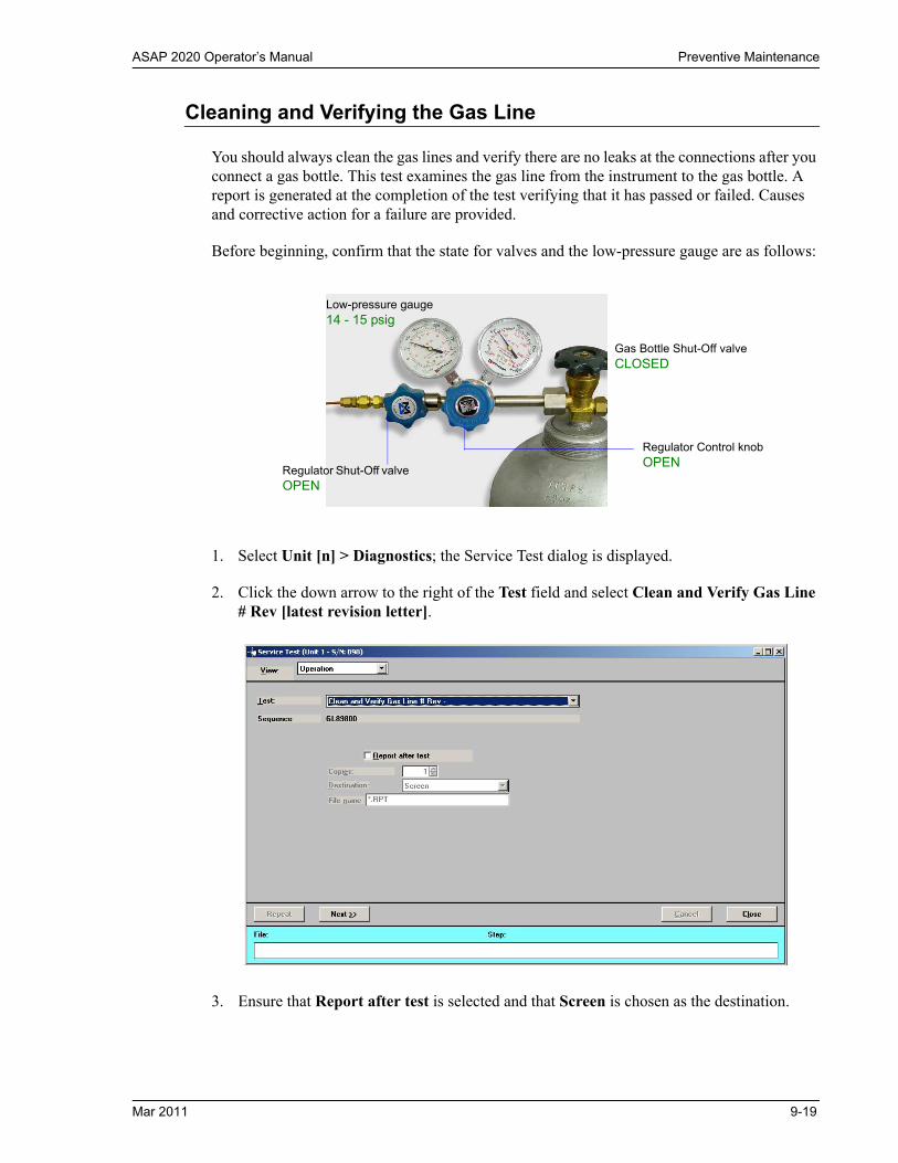
ASAP 2020 Operator’s Manual Preventive Maintenance
Cleaning and Verifying the Gas Line
You should always clean the gas lines and verify there are no leaks at the connections after you connect a gas bottle. This test examines the gas line from the instrument to the gas bottle. A report is generated at the completion of the test verifying that it has passed or failed. Causes and corrective action for a failure are provided.
Before beginning, confirm that the state for valves and the low-pressure gauge are as follows:
1. Select Unit [n] > Diagnostics; the Service Test dialog is displayed.
2. Click the down arrow to the right of the Test field and select Clean and Verify Gas Line # Rev [latest revision letter].
3. Ensure that Report after test is selected and that Screen is chosen as the destination.
Regulator Control knobOPEN
Gas Bottle Shut-Off valve CLOSED
Regulator Shut-Off valve OPEN
Low-pressure gauge14 - 15 psig
Mar 2011 9-19

Preventive Maintenance ASAP 2020 Operator’s Manual
4. Click Next; the second view of the Service Test dialog is displayed. On this dialog a series of messages is displayed. These messages are of the following types:
• Informative; for example, advising how long the test will take or how long before you will be required to open or close a valve. Read the message and click OK to proceed.
• Operator response; for example, you will be asked to open and close regulator and gas bottle valves (depicted below). Perform the task first, then click OK.
5. After the test is finished, a dialog stating the test is complete is displayed; click OK to close the dialog.
6. A report is generated automatically to the screen.
Observe the Rate of Change on the Outgas/Leak Rate of the Gas Line report; it should display Passed, indicating that the gas line from the instrument to the gas bottle is clean and leak-free.
Regulator Control knob
Gas Bottle Shut-Off valve
Regulator Shut-Off valve
Low-pressure gauge
9-20 Mar 2011

ASAP 2020 Operator’s Manual Preventive Maintenance
If Failed is shown, a leak is indicated between this connection. Check the connections from the instrument to the gas bottle. Tighten as necessary, then try the test again.
7. Click the Gas Pressure Test - 2 tab to display its report.
Passed should display in the Maximum field, indicating that all valves are in the proper state for operation.
If Failed is shown, one or more valves is not in the proper position; set the valves as shown below and ensure the appropriate pressure is displayed on the low-pressure gauge.
If you wish to run the test again, close the gas bottle valve before starting the test.
8. Click Close to close the test report.
9. Click Close on the test dialog to close the test.
Regulator Control knobOPEN
Gas Bottle Shut-Off valve OPEN
Regulator Shut-Off valve OPEN
Low-pressure gauge14 - 15 psig
Mar 2011 9-21

Routine Maintenance ASAP 2020 Operator’s Manual
Routine Maintenance
The procedures in this section are performed as needed.
Cleaning the Analyzer
The ASAP 2020 should be cleaned every six months, or sooner if required. Clean the outside casing of the analyzer (except for the shields) with a clean cloth dampened with isopropyl alcohol (IPA), a mild detergent in water, or a 3% hydrogen peroxide solution. It is not necessary to remove any switches or screws to clean the outside casing. Use only a mild detergent in water to clean the shields.
Calibrating the Pressure Offset
When operating the system in manual mode, Calibration > Pressure Zero enables you to evacuate the manifold and zero all the transducers. Your system may contain up to three transducers.
The system automatically zeros the transducers before an analysis begins. Therefore, you do not need to use this feature unless you are operating the system in manual mode.Perform the following steps to calibrate the pressure gauge:
1. Select Unit > Calibration > Pressure Zero; the Calibrate Pressure Offset dialog is displayed.
2. Click Start to evacuate the manifold and zero the pressure gauge(s).
3. When the calibration is complete, click OK to close the dialog.
Use only a mild detergent in water to clean the shields. Do not use isopropyl alcohol. Isopropyl alcohol could damage the surface of the shield.
You may cancel a calibration at any time by selecting Cancel. If you cancel a calibration, no new calibration data are saved.
9-22 Mar 2011

ASAP 2020 Operator’s Manual Routine Maintenance
Calibrating the Pressure Scale
Calibration > Pressure Scale allows the software to adjust the gain of the selected transducer to match a reference standard.
1. Attach a reference pressure gauge to the sample port of the analyzer.
2. With manual control enabled:
a. Dose the manifold with helium or nitrogen to 760 mmHg.
b. Open the sample port to expose the reference pressure gauge to the same pressure as the analyzer’s transducer.
3. Select Unit > Calibration > Pressure Scale; the Calibrate Pressure Scale dialog is displayed.
4. Select Match to entered pressure.
5. Enter the pressure reported by the reference pressure gauge, then click OK.
6. Close the sample port and evacuate the manifold.
7. Remove the reference pressure gauge.
Mar 2011 9-23

Routine Maintenance ASAP 2020 Operator’s Manual
9-24 Mar 2011

ASAP 2020 Operator’s Manual Analysis System Components and Accessories
10. ORDERING INFORMATION
The ASAP2020 system components and accessories can be ordered using one of the following methods:
• Call our Customer Service Department at (770) 662-3636• Access our web site at www.micromeritics.com• Contact your local sales representative
When ordering, please use the information provided in this chapter to place your order:.
Analysis System Components and Accessories
Part Number Item and Description
Peripheral Accessories
060-00030-00 FlowPrep 060, degasses up to six samples at up to 400 ºC with flowing gas
061-00030-00 VacPrep 061, degasses up to six samples at up to 400 ºC with either flowing gas or by evacuation (evacuation requires a vacuum pump)
021-00000-00 Model 021 LN2 transfer system, for easy filling of sample Dewars; includes 47-L Dewar, mobile platform, and pump with 100-cm discharge line
202-33050-00 Water vapor option; allows water vapor adsorption studies
System Components
202-25849-00 Dewar, 3 liter, cold trap
202-25850-00 Dewar, 3 liter, analysis
200-25928-00 Dewar, 1 liter, analysis (wide mouth)
202-33053-00 Stainless Steel Dewar Kit, 4 liter, wide mouth, includes analysis Dewar, cold trap Dewar, and elevator adapter. Typically provides greater than 40 hours of unattended analysis.
240-25901-00 Dewar depth gauge
202-31708-00 Dewar cover, cold trap
202-31707-00 Dewar cover, analysis
200-25929-00 Dewar stopper, sample port, 1-liter Dewar
004-25103-00 Ferrule, front, Teflon 1/4 in.
004-25104-00 Ferrule, rear, Nylon 1/4 in.
Mar 2011 10-1

Analysis System Components and Accessories ASAP 2020 Operator’s Manual
Part Number Item and Description
290-25846-00 Copper tube, for gas inlet, 1/8-in. diameter, 6 ft. long
290-25846-01 Same as 290-25846-00, but uses 16-ft. (5m) tubing
201-25818-00 Same as 290-25846-00, but uses stainless steel tubing
201-25818-01 Same as 290-25846-00, but uses stainless steel 16-ft. (5m) tubing
004-25549-00 Reducer, 1/8-in. tube x 1/4-in. tube, accepts 1/8-in. tube, connects to 1/4-in. swage fittings
004-62230-35 Gas pressure regulator, CGA 350 fitting (CO, H2), 30 psig
004-62230-54 Gas pressure regulator, CGA 540 fitting (O2), 30 psig
004-62230-32 Gas pressure regulator, CGA 320 fitting (CO2), 30 psig
004-62230-326 Gas pressure regulator, CGA 326 fitting (N2O), 30 psig
004-62230-705 Gas pressure regulator, CGA 705 fitting (NH3), 30 psig
004-33601-00 Expansion Kit; adds an additional outlet to the gas regulator, includes fittings and instructions
004-33602-00 Pressure Relief Kit; prevents excessive gas pressure in the event of regulator failure (not to be used with noxious gases)
003-26043-00 Heating mantle with type K thermocouple, 450 ºC maximum, 24 V
003-26045-00 Heating mantle with type K thermocouple, 450 ºC maximum, 24 V, side-laced to accommodate monolithic & nonstandard sample tubes
230-25808-00 Heating mantle clip
202-42801-00 Operator’s manual
004-25006-00 O-ring, size 006, Buna-N, for Po tube
004-16821-00 Reference material, high surface area
004-16816-00 Reference material, low surface area (krypton)
004-16843-00 Reference material, micropore, 13X
004-16844-00 Reference material, micropore, Y-zeolite
004-54609-00 Sample tube brush
240-25853-00 Sample tube funnel
240-14855-00 Sample tube rack
240-32805-00 Sample tube support, assists sample weighing
004-54618-00 Tool, for removing sample port O-ring
200-25840-00 Saturation pressure tube, includes isothermal jacket
10-2 Mar 2011
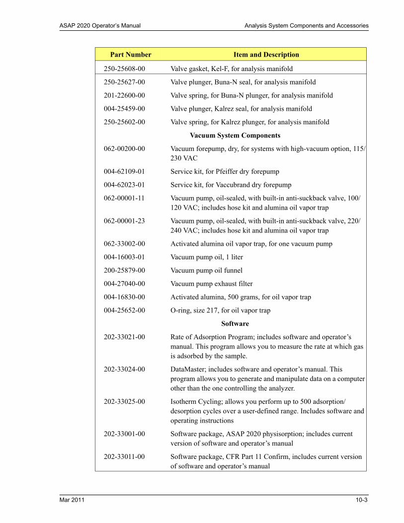
ASAP 2020 Operator’s Manual Analysis System Components and Accessories
Part Number Item and Description
250-25608-00 Valve gasket, Kel-F, for analysis manifold
250-25627-00 Valve plunger, Buna-N seal, for analysis manifold
201-22600-00 Valve spring, for Buna-N plunger, for analysis manifold
004-25459-00 Valve plunger, Kalrez seal, for analysis manifold
250-25602-00 Valve spring, for Kalrez plunger, for analysis manifold
Vacuum System Components
062-00200-00 Vacuum forepump, dry, for systems with high-vacuum option, 115/230 VAC
004-62109-01 Service kit, for Pfeiffer dry forepump
004-62023-01 Service kit, for Vaccubrand dry forepump
062-00001-11 Vacuum pump, oil-sealed, with built-in anti-suckback valve, 100/120 VAC; includes hose kit and alumina oil vapor trap
062-00001-23 Vacuum pump, oil-sealed, with built-in anti-suckback valve, 220/240 VAC; includes hose kit and alumina oil vapor trap
062-33002-00 Activated alumina oil vapor trap, for one vacuum pump
004-16003-01 Vacuum pump oil, 1 liter
200-25879-00 Vacuum pump oil funnel
004-27040-00 Vacuum pump exhaust filter
004-16830-00 Activated alumina, 500 grams, for oil vapor trap
004-25652-00 O-ring, size 217, for oil vapor trap
Software
202-33021-00 Rate of Adsorption Program; includes software and operator’s manual. This program allows you to measure the rate at which gas is adsorbed by the sample.
202-33024-00 DataMaster; includes software and operator’s manual. This program allows you to generate and manipulate data on a computer other than the one controlling the analyzer.
202-33025-00 Isotherm Cycling; allows you perform up to 500 adsorption/ desorption cycles over a user-defined range. Includes software and operating instructions
202-33001-00 Software package, ASAP 2020 physisorption; includes current version of software and operator’s manual
202-33011-00 Software package, CFR Part 11 Confirm, includes current version of software and operator’s manual
Mar 2011 10-3

Sample Tubes and Components ASAP 2020 Operator’s Manual
Sample Tubes and Components
1/4-in., 3/8-in, and 1/2-in Sample Tubes
AB
C
D EFG
H
JK L
N Q T
O
P
R U
SV
I
Part Number Item and Description
004-25466-00 A004-25465-00
O-ring, size 010, Buna-N, for 1/4-in. sample tubeO-ring, size 010, Kalrez, for 1/4-in. sample tube
004-25022-00 B004-25022-01
O-ring, size 012, Buna-N, for 3/8-in. sample tubeO-ring, size 012, Kalrez, for 3/8-in. sample tube
260-25891-00 C Opener, seal frit, for 1/2-in. sample tube
240-25803-00 D Ferrule, 1/4 in.
240-25802-00 E Ferrule, 3/8 in.
004-25044-00 F004-25474-00
O-ring, size 013, Buna-N, for 1/2-in. sample tubeO-ring, size 013, Kalrez, for 1/2-in. sample tube
260-25843-00 G Ferrule, 1/2 in.
300-25824-00 H Nut, sample tube
10-4 Mar 2011

ASAP 2020 Operator’s Manual Sample Tubes and Components
22-mm Sample Tube Kit
Part Number Item and Description
004-32604-00 I Cap (stopper) for 1/4-in. sample tube (not shown)
004-32004-00 J Stopper, for 3/8-in. sample tubes
240-32000-00 K Stopper, for 1/2-in. sample tube
260-25890-00 L Seal Frit with built-in check valve for air-sensitive samples
202-25901-00 N Isothermal jacket, 1/4 in.
240-61001-00 O Sample tube, 1/4 in.
240-61014-00 P Volume displacement insert, 1/4 in.
202-25902-00 Q Isothermal jacket, 3/8 in.
240-61002-00 R Sample tube, 3/8 in.
240-61015-00 S Volume displacement insert, 3/8 in.
202-25903-00 T Isothermal jacket, 1/2-in. sample tube
240-61003-00 U Sample tube, 1/2 in.
240-61016-00 V Volume displacement insert, 1/2 in.
Part Number Item and Description
202-33052-00 22mm ID Sample Tube Kit
004-25609-02 O-ring, -022, 70 Buna-N
004-32240-00 Stopper, rubber, for 22mm ID Tube
202-25868-00 Fitting, sample port, 25mm sample tube
202-25869-00 Nut, for 25-mm sample tube
202-25870-00 Ferrule for 25-mm sample tube
202-25871-00 Fitting, degas port, 25-mm sample tube
202-25904-00 Isothermal jacket, for 25-mm OD sample tube
202-31709-00 Dewar cover, 25-mm OD sample tube
202-61022-00 Sample tube, 22-mm ID, 25-mm OD
202-61022-01 Filler rod for 22-mm ID sample tube
Mar 2011 10-5

Cold Trap Tubes and Components ASAP 2020 Operator’s Manual
Cold Trap Tubes and Components
A
B
C
Part Number Item and Description
004-25469-00 A O-ring, Buna-N, size 014
004-25979-00 B Nut, cold trap
004-61063-00 C Tube, 1/2-in. OD stem, cold trap
10-6 Mar 2011

ASAP 2020 Operator’s Manual Appendix A
A. FORMS
This appendix contains the following form:
• Sample Data Worksheet
Copy and use this form as needed.
Mar 08 A-1

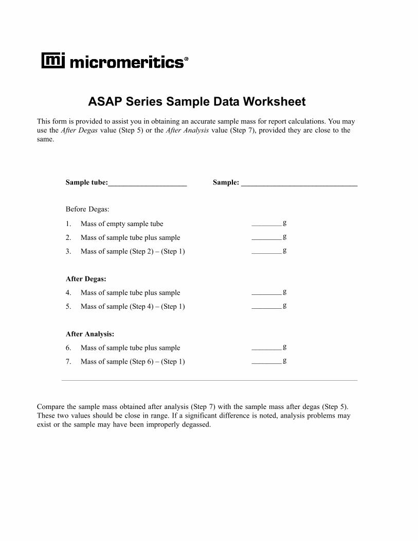
ASAP Series Sample Data Worksheet
This form is provided to assist you in obtaining an accurate sample mass for report calculations. You may use the After Degas value (Step 5) or the After Analysis value (Step 7), provided they are close to the same.
Compare the sample mass obtained after analysis (Step 7) with the sample mass after degas (Step 5). These two values should be close in range. If a significant difference is noted, analysis problems may exist or the sample may have been improperly degassed.
Sample tube:_____________________ Sample: _______________________________
Before Degas:
1. Mass of empty sample tube ________ g
2. Mass of sample tube plus sample ________ g
3. Mass of sample (Step 2) – (Step 1) ________ g
After Degas:
4. Mass of sample tube plus sample ________ g
5. Mass of sample (Step 4) – (Step 1) ________ g
After Analysis:
6. Mass of sample tube plus sample ________ g
7. Mass of sample (Step 6) – (Step 1) ________ g


Appendix B ASAP 2020 Operator’s Manual
B. ERROR MESSAGES
Error messages are listed numerically. If the Action response instructs you to contact your service representative, record the error message and make backup copies of any files involved in the operation.
2200 and 2400 Series
2201- Cannot execute report subsystem.
2401- FATAL ERROR: (error message).
2430- Error accessing file (file name), error code = (number).
The 1000-series error messages (used primarily for software testing) are not included in this appendix. These errors should not occur during normal operation. If you receive a 1000 series error message or an error message not listed in this appendix: record the error message, make backup copies of any files involved, then contact your service representative.
Cause: Start Report failed to execute the report subsystem (which is a separate process).
Action: Restart the computer. If the problem persists, reinstall the application (this will not affect any of your sample files). If the problem continues, contact a Micromeritics service representative.
Cause: An internal processing and/or hardware error has occurred.
Action: Contact your service representative if you continue to receive this error message.
Cause A: A computer or network problem occurred.
Action A: Check the performance of your computer devices or network.
Cause B: A software error occurred when the file was accessed.
Action B: Contact your service representative.
Mar 2011 B-1

ASAP 2020 Operator’s Manual Appendix B
2431- Error writing file (file name), error code = (number).
2432- Invalid response from MMI ‘FILE_READ’ request.
2433- New entries have been found in this directory. Refresh the directory information?
2434- File (file name) — Subset # (number) wrote wrong amount of data.
Cause: The hard disk does not have enough space left to perform the opera-tion.
Action: Copy files not used regularly from the hard disk to a diskette, CD, or network directory, delete them from the hard disk, and then try the operation again.
Cause: An internal processing and/or hardware error has occurred.
Action: Contact your service representative if you continue to receive this error message.
Cause: Several ASAP 2020 files (sample information, analysis conditions, adsorptive properties, or report options) have been added to this direc-tory by some function other than the ASAP 2020 program.
Action: Select Yes to update the directory information with data from each new file. This operation may take a minute.
Select No if you do not want to spend the time updating the directory information. This option may be feasible if a large number of files have been copied into the directory and you know the name of the file you wish to access.
Cause: An internal processing and/or hardware error has occurred.
Action: Contact your service representative if you continue to receive this error message.
B-2 Mar 2011

Appendix B ASAP 2020 Operator’s Manual
2436- Path specification (path name) is invalid.
2437- File (file name) does not exist.
2438- Disk drive (letter): is inaccessible.
2439- Could not register file.2440- Subset not found.2441- Seek within file failed.2442- Bad header in subset file.2443- Subset owner denied access.2444- Not a valid file format.2445- Subset wrote the wrong amount of data.2446- Error reading data.2447- Error writing data.
2448- File directory (path name) is invalid. Resetting to the installation directory.
Cause: You entered an invalid path name and/or extension.
Action: Type a valid path name (including the proper extension) and press Enter.
Cause: You entered a file specification that does not exist.
Action: Enter an existing file specification or select a file name from the list box.
Cause: You selected a disk drive that is not presently accessible.
Action: Ensure that the disk is not write-protected.
Cause: An unexpected error occurred when you tried to access a data file.
Action: Contact your service representative.
Cause: A working directory specified in the .INI file is invalid. The directory may have been deleted or moved to a different location.
Action: The installation directory will be substituted. The next time you open a file, use the Directories: list to move to the correct directory.
Mar 2011 B-3
ASAP 2020 Operator’s Manual Appendix B
2449- This field does not contain a valid file specification.
2450- Sample Defaults may not be edited while this operation is in progress. Do you wish to save and close the Sample Defaults edit session?
2452- Attempt to write MICATTR.DIR in read only mode. (file name)2453- Attempt to append MICATTR.DIR in read only mode. (file name)
2454- Too many selections for a print-to-file operation. Only the first (number) selec-tions will be processed. Please reselect the remainder.
2455- Too many selections for an export-to-file operation. Only the first (number) selections will be processed. Please reselect the remainder.
Cause: You entered an invalid file name.
Action: See the description of file naming conventions in your DOS or Win-dows manual and re-enter the name.
Cause: You are in the process of initiating an automatic analysis (an analysis in which sample files are created using the defaults) while editing the defaults.
Action: Finish your edit session of the defaults and close the dialog. Then restart the automatic analysis.
Cause: The Read-Only attribute is turned on in the application’s MICATTR.DIR file (this file exists in each folder containing sample or parameter files).
Action: Use Windows Explorer to access the folder containing the MICATTR.DIR file and disable the Read-Only option.
Cause: You selected too many files for this operation.
Action: Select only the number of files specified in the message.
B-4 Mar 2011

Appendix B ASAP 2020 Operator’s Manual
2456- Insufficient file handles available. Application cannot continue.
2457- Results cannot be displayed. More than (number) windows are currently dis-playing or printing results.
2458- An instrument is performing a critical operation. Wait a few moments before exiting the application.
2459- An instrument is busy. A delay in restarting this application could result in loss of new data. Continue with program Exit?
Cause: You have more than 50 files open at the same time.
Action: Refer to the manual for your operating system and set the limit for open files to 50 or greater.
Cause: You have too many windows open in the application.
Action: Close some of the open windows.
Cause: You attempted to exit the application while the analyzer is performing a critical operation. This operation must be completed before the appli-cation can be stopped.
Action: Wait a few minutes before attempting to exit the application again.
Cause: You attempted to exit the application while the analyzer was perform-ing an operation.
Action: Rather than exiting the application you may choose to minimize it.
Mar 2011 B-5

ASAP 2020 Operator’s Manual Appendix B
2460- Fatal Communications error on (unit n).
2461- No instruments are in operation. This application will unconditionally terminate.
2471- Unit n - S/N; nn has an invalid communications port specified. It cannot be initialized.
Cause: Repeated attempts to maintain communication with the analyzer have failed.
Action: Check the communications cable connecting the analyzer to the com-puter. Confirm that the analyzer is turned on and that the status light is not blinking.
If these checks are okay, exit the analysis program and then restart the application. If this error persists, contact your service representative.
Cause: At least one analyzer must be active for the application to operate. The initialization of the analyzers configured with the Setup program has failed. The application stops.
Action A: Usually this message is preceded by another message giving the reason for the analyzer’s failure to initialize. See the instructions for that mes-sage.
Action B: Check the cable connection between the analyzer and the computer. Verify that the analyzer has the power switch in the ON position and that the light on the front panel is illuminated. If the application con-tinues to fail in its attempts to initialize the analyzer, contact your ser-vice representative.
Cause: The communications port specified for this analyzer during installation (or configuration) is invalid.
Action: Use the setup program to change the analyzer configuration.
B-6 Mar 2011
Appendix B ASAP 2020 Operator’s Manual
2474- (Unit n) Communications port COM (port number) specified in the program con-trol files is already in use. Unit cannot initialize.
2475- (Unit n) Communications port COM (port number) specified in the program con-trol files cannot be accessed. Unit cannot initialize.
2476- Unit startup failed. Cannot initialize the communications port.
2477- (Unit n; Serial nn) did not properly initialize.
Cause: The communications port assigned to the indicated unit is in use by another program.
Action: End the program using the busy port or use the Setup program to change the communications port assigned to this program.
Cause: The operating system has prevented the application from accessing the communications port.
Action: Review the hardware configuration of the computer, ensure that no other application is using the port. Contact your service representative if you continue to receive this error message.
Cause: The communications port specified during installation is invalid.
Action: Use the setup program to change the analyzer configuration. Contact your service representative if you continue to receive this error mes-sage.
Cause: The software was unable to initialize the analyzer.
Action A: Run the Setup program and ensure that a valid port is specified; if not, specify a valid one when prompted.
Action B: Reinstall the software, then restart application.
Action C: Contact your Micromeritics service representative if you continue to get this message.
Mar 2011 B-7

ASAP 2020 Operator’s Manual Appendix B
2478- Error copying sequential data segment.
2479- (Unit n; Serial nn) The instrument is busy performing an operation of which this application is unaware. Do you want to cancel? (Yes, No)
2480- File (file name) cannot be analyzed. It is currently being edited.
2481- Error accessing the sample information file (file name).
Cause: An internal processing and/or hardware error occurred while accessing a portion of a sample file.
Action: Confirm that the media being accessed does not contain errors; for example, you may wish to use a utility such as ScanDisk. Contact your service representative if you continue to receive this error message.
Cause: During initialization of the application, the status of the analyzer was found to be in a different state than expected.
Action: Click Yes to cancel the operation in process, allowing the analyzer to reset and continue with initialization.
Click No to cancel the initialization process.
If you continue to get this message, verify that files in the application directory structure are not being changed or removed.
Cause: You attempted an analysis using a sample file that is being edited.
Action: Save the changes and close the dialog box.
Cause A: You attempted to open a file that is already open, possibly minimized.
Action A: View the minimized icons, locate and maximize the file.
Cause B: A computer or network problem occurred.
Action B: Check the performance of your computer devices or network.
B-8 Mar 2011

Appendix B ASAP 2020 Operator’s Manual
2482- File cannot be opened for writing. It is already in use.
2483- An analysis cannot be performed on (file name). It is open for editing and con-tains errors.
2484- The edit session for (file name) must be saved before the analysis. Save changes and continue with the analysis.
2485- The service test file has an invalid status and cannot be used for this analysis.
Cause C: A software error occurred when the file was accessed.
Action C: Contact your service representative.
Cause: You are attempting to open a file that is currently being used (either by this application or another).
Action: Locate the application using the file (in the Micromeritics application, use the Windows menu item to get a list of all windows, one of which may contain this file).
Cause: You attempted to use a sample file containing errors that is currently open.
Action: Go to the window containing the file, correct the errors, and save it.
Cause: You attempted an analysis using a sample file that contains unsaved changes.
Action: Select Yes to save the changes and continue with the analysis.
Select No to abort the analysis and return to the sample file.
Cause: The selected service test file has a status other than No Analysis.
Action: Select a different service test file or create a new one and use Replace All to copy parameters from the file you originally selected.
Mar 2011 B-9

ASAP 2020 Operator’s Manual Appendix B
2486- Cannot construct (name) report type. Program will terminate.2487- Cannot start report generator. Error code (number). Program will terminate.
2488- File (file name) cannot be opened for editing. It is already in use.
2490- No ‘.INI’ file present. Application will terminate.
2491- Highlighted fields contain errors. Please correct the errors before closing dia-log box.
Cause A: You may not have full rights to the application’s folders and files.
Action A: Contact your system administrator and have him grant you full rights.
Cause B: An internal processing and/or hardware error has occurred.
Action B: Contact your service representative if you continue to receive this error message.
Cause: The file you specified is being used in another edit operation.
Action: Check the Windows list to locate the other edit session.
Cause: The ASCII (.INI) file containing initialization and system options information cannot be found. The .INI file may have become cor-rupted. The application cannot operate without this file.
Action: Use the Setup CD to uninstall the ASAP 2020 application. When you uninstall the application, only the application files are deleted; data files remain intact.
After the uninstall operation is complete, reinstall the ASAP 2020 application.
Cause: The highlighted fields contain invalid entries. You will not be able to close the dialog box until you correct the errors.
Action: Check the entries, correct the errors, and close the dialog.
B-10 Mar 2011
Appendix B ASAP 2020 Operator’s Manual
2492- This field’s entry is invalid.
2493- An entry is required for this field.
2494- Value is out of the valid range.2495- Value is out of the valid range. Enter a value between (value) and (value).
2496- Invalid number.
2497- This field contains an invalid character.
Cause: The highlighted field contains an invalid entry.
Action: Check the entry and correct the error.
Cause: This field requires a valid entry for you to proceed.
Action: Enter or select an appropriate value.
Cause: The value you entered in the highlighted field is outside the valid range of values.
Action: Check the entry and enter or select an appropriate value.
Cause: The number you entered in the highlighted field is invalid.
Action: Check the entry and enter or select a valid number.
Cause: You entered an invalid character in the highlighted field.
Action: Check the entry and enter valid characters.
Mar 2011 B-11

ASAP 2020 Operator’s Manual Appendix B
2498- The requested change to the Sample’s status is invalid at this time.
2499- Sequence number must contain at least 3 digits.
Cause: A request to change the file’s status (for example, from automatically collected to manually entered) could not be done.
Action: Contact your service representative if you continue to receive this error message. Record the name of the sample file in which the problem occurred.
Cause: You tried to enter a sequence number that did not contain at least three digits.
Action: Enter a sequence number that contains at least three digits.
B-12 Mar 2011

Appendix B ASAP 2020 Operator’s Manual
2500 Series
2500- All sample file names that can be created using the sequence number pattern already exist. You may want to modify the next sequence number.
2501- System resources have reached a dangerously low level. Please close some windows to avoid the loss of data.
2502- Error writing to file (name) during print. Error code: (number).
2503- Error converting file (file name). Could not create DIO intermediate file.
Cause: No more sample information files can be created using the currently entered file name sequence number.
Action: Select Options > Sample Defaults from the Main Menu and enter a new sequence number.
Cause: A large number of windows are open and consuming the system resources available to all applications.
Action: Close one or more windows on the screen. Contact your service rep-resentative if you continue to receive this error message.
Cause: An error occurred in the file being written to during a print operation.
Action: Ensure that there is sufficient space on the drive containing the file.
Cause A: Insufficient space is available on the hard disk. The DIO file is placed in the directory specified by the TEMP environment variable.
Action A: Determine if there is sufficient space on the drive where the TEMP directory is located.
Cause B: An internal processing and/or hardware error has occurred.
Action B: Contact your service representative if you continue to receive this error message.
Mar 2011 B-13
ASAP 2020 Operator’s Manual Appendix B
2504- Cannot create output file for sample (sample name).
2505- Error Logger cannot be initialized! Error code (number). Program will exit.
2506- (sample file) Output device (name) is not installed. Printing cannot be accomplished.
2508- (sample file) Overlay file (name) was not found. It will not be included in the reports.
2509- (sample file) Error opening file (name): (error). Reports cannot be produced.
Cause: Insufficient space may be available on the hard disk.
Action: Ensure that sufficient space is available. Contact your service repre-sentative if you continue to receive this error message.
Cause: An internal processing and/or hardware error has occurred.
Action: Contact your service representative.
Cause: The selected output device is not installed in Windows.
Action: Select a different output device in the System Configuration dialog box. Install the device using the Control Panel, Printers operation.
Cause: The specified overlay file could not be found.
Action: Ensure that the file specified as an overlay does exist.
Cause: An error occurred while the program was opening a file necessary to the report operation.
Action: Use the name given in the error message to investigate. Contact your service representative if you continue to receive this error message.
B-14 Mar 2011

Appendix B ASAP 2020 Operator’s Manual
2510- (sample file) Error parsing reports from file (name). Reports cannot be produced.
2511- Print job (name) has been cancelled due to insufficient disk space. Delete unnecessary files and restart the report.
2512- Print job (name) has been cancelled.
Cause A: One or more data entry fields in the sample file may contain an invalid character (such as a single quote or double quotes).
Action A: Review the data entry fields (for example, the Sample field) and remove the invalid character.
Cause B: The system was unable to create the usual temporary files during the report, possibly due to insufficient disk space.
Action B: Check the space available on the hard disk.
Cause C: An internal processing error occurred.
Action C: Contact your service representative.
Cause: The disk drive does not have enough space for the temporary file required by the Windows Print Manager. Therefore, printing of the requested report has been canceled.
Action: Delete unnecessary files from the disk. You will require at least five megabytes of free space for normal operation.
Cause: The requested print job was canceled at your request.
Action: None required.
Mar 2011 B-15

ASAP 2020 Operator’s Manual Appendix B
2513- Unable to read the calibration file (file name).
2514- Unable to write the calibration file (file name).
2515- Warning: Changing the calibration information will affect the performance of the instrument. Only qualified service personnel should do this. Do you wish to proceed?
2516- Warning: Keeping a backup copy of the calibration data is recommended by Micromeritics. Would you like to do so now?
2517- Canceling this dialog will reset the calibration state to what it was when this dialog was first opened. Are you sure you want to cancel?
Cause: You selected an invalid calibration file or one that cannot be read.
Action: Be sure the media containing the calibration file has no problems.
Cause: An attempt to Save calibration data has failed due to possible media problems.
Action A: Be sure the media you want to Save the file to has no problems.
Action B: Choose an alternate media to Save the calibration data.
Cause: You have started the process of performing a calibration operation.
Action: Calibration operations should only be done by or under the direction of qualified service personnel.
Cause: You have performed a calibration operation; a backup copy is recom-mended.
Action: Perform a calibration Save operation.
Cause: You have not accepted the calibration you performed.
Action: If the calibration operation was successful, press Accept.
B-16 Mar 2011
Appendix B ASAP 2020 Operator’s Manual
2521- Unable to program controller.
2522- Invalid controller application file.
2523- Programming the controller failed.2524- CRC check failed on programming controller.2525- Unknown error programming controller.2526- Controller download was not successful.2527- Controller CRC error on boot block.2528- Controller DRAM error.2529- Controller Com1: error.2530- Controller Com2: error.2531- Controller debug port error.
2532- The instrument contains a different software version. Do you want to reset it?
2533- Analyzer initialization failed.
Cause: A hardware malfunction has occurred.
Action: Contact your local Micromeritics service representative.
Cause: The application’s control file has been corrupted or deleted.
Action: Reinstall the ASAP 2020 analysis program.
Cause: An internal processing and/or hardware error has occurred.
Action: Contact your service representative if you continue to receive this error message.
Cause: The application has discovered a different version of software operat-ing in the analyzer.
Action: If there are no analyzers other than the ASAP 2020 connected to the computer, select Yes and allow the updated software to load.
Cause: An internal processing and/or hardware error has occurred.
Action: Contact your service representative if you continue to receive this error message.
Mar 2011 B-17

ASAP 2020 Operator’s Manual Appendix B
2534- Error opening file (name) for printing. Error code: (number).
Cause: An error occurred in the selected file for print output.
Action: Ensure that sufficient space is available on the drive containing the file.
B-18 Mar 2011

Appendix B ASAP 2020 Operator’s Manual
4000 Series
4000- Memory Allocation Error.
4002- Thermal Transpiration correction had no effect.
4003- Error Converting Pressures.4004- Error Computing Volume Adsorbed.
4005- Pressures were not smoothed. Not enough pressures below 0.10 P/Po.
Cause: An internal processing and/or hardware error occurred during report generation.
Action: Contact your service representative if you continue to receive this error message.
Cause: The Thermal transpiration correction option was selected on the Report Options dialog box. However, the correction did not change any pres-sure by more than one percent.
Action: De-select this option to disable this message. This correction is only meaningful for very low pressures.
Cause: An internal processing and/or hardware error occurred during report generation.
Action: Contact your service representative if you continue to receive this error message.
Cause: The Smooth pressures below 0.10 P/Po option was selected on the Report Options dialog. There must be at least 10 pressures within this range for smoothing to occur.
Action: Deselect this option to disable this message.
Mar 2011 B-19

ASAP 2020 Operator’s Manual Appendix B
4006- Report Type Not Found.4007- Error Processing Report.
4008- Report requested on sample file with no data points.
4009- Error, No Reports Selected.
4010- Summary Report was not included in the Selected Reports.
Cause: An internal processing and/or hardware error occurred during report generation.
Action: Contact your service representative if you continue to receive this error message.
Cause: You selected a file for reporting which contains no collected data.
Action: Select another file which contains collected data and restart the report.
Cause: You attempted to generate reports for a sample that has no reports selected in its report options.
Action: Select the desired reports in the sample’s report options and save the sample file.
Cause: You did not select a plot or a table for any of the Selected Reports in the Report Options dialog; you selected the reports only to generate an entry in the summary. However, the Summary was not included in the Selected Reports.
Action: Select a plot or table in one or more of the Selected Reports, and/or add the Summary to the Selected Reports.
B-20 Mar 2011

Appendix B ASAP 2020 Operator’s Manual
4011- Analysis gas in sample file does not match analysis gas in unit.
4012- Psat gas in sample file does not match Psat gas in unit.
4013- The ‘Incremental Dosing’ option is not available on the selected unit.
4014- File (name) is not a valid file for conversion.
Cause: You attempted to start an analysis using a sample information file in which the analysis gas specified does not match the analysis gas entered in the unit configuration.
Action: If necessary, attach the appropriate gas bottle, then enter the gas in the Unit Configuration dialog box.
Cause: You attempted to start an analysis using a sample information file in which the Psat gas does not match the Psat gas entered in the unit con-figuration.
Action: If necessary, attach the appropriate gas bottle, then enter the gas in the Unit Configuration dialog box.
Cause: The MicroPore option is not installed.
Action: Install the MicroPore option before starting the analysis.
Cause: The file selected for conversion is not a MICMOS 2000 or 2000 MicroPore file.
Action: Select only files that have been created by MICMOS 2000 or 2000 MicroPore programs.
Mar 2011 B-21
ASAP 2020 Operator’s Manual Appendix B
4015- Error creating export file for sample <sample file name>.
4016- Sample (file name) has no data for export.
4017- Damage to the instrument will result if the sample has not been manually evac-uated. Have you evacuated the sample?
Cause: A file error occurred during creation of an export output file.
Action: The output file name may be invalid. Ensure that the target directory exists. Ensure that the target diskette is not full or write protected. The target disk drive may be damaged or inoperative. Verify that other files may be created on the same drive. Contact your service representative if you continue to receive this error message.
Cause: The file selected for export has a status of No Analysis. No export file will be created.
Action: Select a file which contains analysis data.
Cause: You did not select Backfill sample at start of analysis on the Sample Backfill Options dialog box. The sample tube is normally at atmo-spheric pressure when an analysis is started, and it must be backfilled before the analysis begins to prevent sample material from being drawn into the manifold.
Action: If you have manually evacuated the sample tube, select Yes. If you have not, select No and then either perform a manual evacuation or go to the Sample Backfill Options dialog box and select Backfill sample at start of analysis.
B-22 Mar 2011

Appendix B ASAP 2020 Operator’s Manual
4020- Disabling this option may damage the instrument. Are you sure that the sample should not be backfilled?
4021- The entered Po value (Po and Temperature Options of the Analysis Conditions) is outside the range of the pressures listed in the Psat vs. Temperature Table (Adsorptive Properties).
4022- The entered bath temperature value (Po and Temperature Options of the Anal-ysis Conditions) is outside the range of the temperatures listed in the Psat vs. Temperature Table (Adsorptive Properties).
Cause: You did not select Backfill sample at start of analysis on the Sample Backfill Options dialog. The sample tube is normally at atmospheric pressure when an analysis is started; it must be backfilled before the analysis begins to prevent sample material from being drawn into the manifold.
Action: If you want to manually evacuate the sample prior to the start of the analysis, select Yes. Otherwise, select No, go to the Sample Backfill Options dialog, and select Backfill sample at start of analysis.
Cause: The temperature that corresponds to the entered Po cannot be found because the entered Po is outside of the range of values in the Psat vs. T table.
Action A: Enter a Po that is within the range of the table.
Action B: Use a different Psat vs. T table.
Cause: The Po that corresponds to the entered temperature cannot be found because the entered temperature is outside of the range of values in the Psat vs. T table.
Action A: Enter a temperature that is within the range of the table.
Action B: Use a different Psat vs. T table.
Mar 2011 B-23

ASAP 2020 Operator’s Manual Appendix B
4023- The file (sample file) cannot be prepared for analysis. It is open for editing and contains errors.
4024- Backfill gas in sample file does not match any gas in unit.
4025- There is no Helium attached to the unit.
4026- Cannot calculate Dubinin-Astkahov: bad least squares data.
4027- Fewer than two sample files have data suitable for heat of adsorption reports.
Cause: You attempted an analysis using a sample file that is being edited and has invalid values in one or more of its fields.
Action: Enter valid values into the fields that have errors, save the changes, and close the dialog box.
Cause: You selected a backfill gas that is not included in the gas configuration.
Action: Make sure that gas selections match the gases that are attached to the instrument. Choose one of the gases as the backfill gas, or edit the sam-ple file and choose one of the existing gases as the backfill gas.
Cause: A measured free space has been requested but Helium does not appear to be available.
Action: Make sure the helium cylinder is attached to the unit at its designated port.
Cause: Less than two selected data points are within the fitted pressure range.
Action: Edit the calculation assignments on the Collected Data dialog, or change the fitted pressure range on the Dubinin report options dialog.
Cause: Less than two of the sample files you selected for heat of adsorption reports contain appropriate data.
Action: Edit the Quantity Adsorbed table, or select other sample files.
B-24 Mar 2011
Appendix B ASAP 2020 Operator’s Manual
4028- Dubinin calculations cannot be performed because the affinity coefficient of the analysis gas is zero.
4029- At least two fitted data points are needed for Alpha-S calculations.
4030- Preparations failed in primary data.
4031- Not enough points with a relative pressure in the range (n,n)
4032- Some summary reports could not be produced because they require the Micro-pore option.
Cause: Dubinin values could not be calculated because the affinity coefficient of the analysis gas is zero.
Action: Access the Dubinin Report Adsorptive options in the sample file and enter an appropriate value for the analysis gas.
Cause: Fewer than two data points fall within the selected Alpha-s range.
Action: Edit the calculation assignments or the fitted Alpha-s range, or use a different reference curve.
Cause: Appropriate data were not available to generate the report.
Action: This message was preceded by a different error message; refer to the cause/action of the preceding message.
Cause: Fewer than two data points selected for the Dubinin report falls within the selected relative pressure range.
Action: Edit the calculation assignments or the fitted relative pressure range.
Cause: Some of the summary reports you requested were not produced because you do not have the micropore option installed.
Action: Edit the summary report and deselect the micropore options.
Mar 2011 B-25

ASAP 2020 Operator’s Manual Appendix B
4033- Not enough points to generate Dubinin Tabular Report.
4034- Fewer than 2 points available for Dubinin calculations.
4035- Cannot calculate optimized Astakhov exponent: Not enough points with a rel-ative pressure in the range [(pressure), (pressure)].
4036- Fewer than 2 points available for Horvath-Kawazoe calculations.
Cause: There are fewer than two valid data points available for the Dubinin tabular reports.
Action: Examine the calculation assignments in the Collected Data dialog of the sample file. You must have at least two micropore pressures selected for inclusion in the Dubinin report.
Cause: There are fewer than two valid data points available for Dubinin reports in one of the sample files selected for overlaying.
Action: Examine the calculation assignments in the Collected Data dialog of the sample file. You must have at least two micropore pressures selected for inclusion in the Dubinin report.
Cause: There are fewer than two valid data points in the relative pressure range specified. Astakhov reports will not be produced.
Action: Examine the calculation assignments in the Collected Data dialog for the sample file. You must have at least two pressures in the given range selected for inclusion in the Dubinin report.
Cause: You must select at least two data points for inclusion in the Horvath-Kawazoe analysis on the Collected Data dialog. No report will be pro-duced.
Action: From the Collected Data dialog, select the data points to be analyzed.
B-26 Mar 2011

Appendix B ASAP 2020 Operator’s Manual
4037- Computations failed while processing the primary data set. No reports will be produced.
4038- Fewer than 2 points available for the Langmuir Qm computation. Cheng/Yang correction will not be applied.
4039- The isotherm does not meet the constraints of the Cheng/Yang assumption. Cheng/Yang correction will not be applied.
Cause: The preparation of data for reporting could not be successfully com-pleted. No Horvath-Kawazoe reports will be produced. This message will always be preceded with another one containing additional infor-mation.
Action: Refer to the number of the error message which preceded this one for an explanation.
Cause: The Cheng/Yang correction to the Horvath-Kawazoe equation requires the value of the monolayer volume as calculated from the Langmuir equation. The isotherm must include at least two points above 0.02 rel-ative pressure for the Langmuir equation to be applied.
Action: The analysis will be performed without the Cheng/Yang correction. Deselect Apply Cheng/Yang correction on the Horvath-Kawazoe Report Options dialog to prevent this message from appearing on future reports.
Cause: The Cheng/Yang correction to the Horvath-Kawazoe equation requires the value of the monolayer volume as calculated from the Langmuir equation. The isotherm does not correlate to the Langmuir assumption with a coefficient of 0.98 or more. The correction is not applicable to this isotherm or to the range of the data points selected.
Action A: The analysis will be performed without the Cheng/Yang correction. Deselect Apply Cheng/Yang correction on the Horvath-Kawazoe Report Options dialog to prevent this message from appearing on future reports.
Action B: Generate the Langmuir report for the same data points selected for the Horvath-Kawazoe report. If the Langmuir correlation coefficient can be brought above 0.98 by removing some points at high relative pres-sure, remove them and reproduce the Horvath-Kawazoe reports.
Mar 2011 B-27

ASAP 2020 Operator’s Manual Appendix B
4040- The value of Qm computed from the Langmuir equation is too low. The pore size will not be computed for all data points.
4041- Cheng/Yang correction is inappropriate for some P/Po.
4042- 0.0 cannot be a starting or ending pressure for a geometric progression from low pressure.
Cause: The Cheng/Yang correction to the Horvath-Kawazoe equation requires the value of the monolayer volume as calculated from the Langmuir equation. The computed value is less than the volume adsorbed at the largest relative pressure included in the analysis. The correction is not applicable to this isotherm or to the range of the data points selected.
Action: The analysis will be performed and the Cheng/Yang correction will be applied to all points with a volume adsorbed less than the value of Vm. The pore size will not be calculated for data points with an invalid vol-ume adsorbed. Deselect Apply Cheng/Yang correction on the Horvath-Kawazoe Report Options dialog to clear this message.
Cause: The Cheng/Yang correction is usually inappropriate for any P/Po above the isotherm knee. In some instances, the computed pore sizes may decrease above the knee. While it is possible to include these relative pressures (usually above 0.1 P/Po) in the analysis, the computed pore sizes for these pressures are usually meaningless.
Action: Change the data points selected for the Horvath-Kawazoe report to include only relative pressures at or below the knee of the isotherm, or change the Horvath-Kawazoe report options so that the Cheng/Yang correction is not applied.
Cause: You selected to generate a pressure table from a geometrically pro-gressing range.
Action: Change the 0.0 entered value.
B-28 Mar 2011

Appendix B ASAP 2020 Operator’s Manual
4043- 1.0 cannot be a starting or ending pressure for a geometric progression toward saturation.
4044- Points in the Langmuir report pressure table lie outside the collected data.
4045- Points in the report pressure table lie outside the collected data.
4046- (file name) could not be opened for reading.
4047- Warning: An error occurred while reading (file name).
Cause: You selected to generate a pressure table from a geometrically pro-gressing range.
Action: Change the 1.0 entered value.
Cause: Calculation assignments are not being used and more than one of the report pressure table points is above the range of the collected data, and more than one is below.
Action: Change the report pressure table to be more consistent with the col-lected data.
Cause: Calculation assignments are not being used and more than one of the report pressure table points is above the range of the collected data, and more than one is below.
Action: Change the report pressure table to be more consistent with the col-lected data.
Cause: A thickness curve file could not be opened.
Action: If the problem persists, restart your computer and optionally perform a media integrity check (using ScanDisk).
Cause: An error happened during a read operation of a thickness curve file.
Action: If the problem persists, restart your computer and optionally perform a media integrity check (using ScanDisk).
Mar 2011 B-29

ASAP 2020 Operator’s Manual Appendix B
4048- Warning: An error occurred while restoring the heat of adsorption report editor.
4049- The sample (file name) does not have enough data. A minimum of two adsorp-tion points is required.
4050- None of the requested quantities adsorbed is within the range of the collected data of more than one sample file.
4051- The sample (file name) does not have any data in the range of the requested quantities adsorbed.
4052- Fewer than two points are selected for this report.
Cause: The state of the heat of adsorption report editor could not be restored. Default settings will be used.
Action: No action.
Cause: A sample file has been included in the Heat of Adsorption report that does not have enough data.
Action: Remove the file from the selected file list.
Cause: The Heat of Adsorption report failed because the specified quantities are not within the range of the collected data.
Action A: Edit the quantities adsorbed so that they are within the range of the col-lected data, or select other sample files.
Cause: The sample’s data cannot be interpolated to any of the quantities adsorbed.
Action: Edit the quantities adsorbed so that they are within the range of the col-lected data.
Cause: At least two points are required for the BET calculations.
Action: Edit the calculation assignments for the BET report.
B-30 Mar 2011

Appendix B ASAP 2020 Operator’s Manual
4053- At least two data points must be selected for t-Plot calculations.
4054- Fewer than two data points are inside the fitted thickness range.
4055- The BET surface area could not be calculated.
4056- The Langmuir surface area could not be calculated.
Cause: At least two points are required for the t-Plot calculations.
Action: Edit the calculation assignments for the t-Plot report.
Cause: At least two points must be within the fitted thickness range for the t-Plot calculations.
Action A: Edit the calculation assignments for the t-Plot report.
Action B: Edit the fitted thickness range in the t-Plot report editor.
Cause: Fewer than two points were assigned to the requested surface area cal-culation in the collected data table.
Action A: Assign more points to the surface area calculation.
Action B: Select a different surface area in the t-Plot report editor.
Cause: Fewer than two points were assigned to the requested surface area cal-culation in the collected data table.
Action A: Assign more points to the surface area calculation.
Action B: Select a different surface area in the t-Plot report editor.
Mar 2011 B-31

ASAP 2020 Operator’s Manual Appendix B
4057- At least two data points are needed for Freundlich calculations.
4058- At least two data points are needed for Temkin calculations.
4059- Fewer than 2 points available for MP-Method calculations.
4060- Sample (file name) contains no data points.
Cause: Less than two data points have been selected for the Freundlich report; at least two are required.
Action: Select Freundlich points on the Collected Data dialog. If calculation assignments are not being used, edit the Freundlich Report options, Absolute pressure range in the sample file.
Cause: Less than two data points have been selected for the Temkin report; at least two are required.
Action: Select Temkin points on the Collected Data dialog. If calculation assignments are not being used, edit the Temkin Report options, Absolute pressure range in the sample file.
Cause: You have selected at least one point with a negative pressure value to include in the Temkin report.
Action: Negative pressure points void Temkin calculations. Open the sample file and click the Collected Data tab. Locate the negative value(s) in the Temkin column and deselect it (them).
Cause: At least two points are required for the MP-Method calculations.
Action: Edit the calculation assignments for the MP-Method report.
Action: An attempt was made to save a sample without collected data as a t-curve or alpha-S curve.
Cause: Repeat the save as t-curve or save as alpha-S operation after opening a sample that has collected data.
B-32 Mar 2011

Appendix B ASAP 2020 Operator’s Manual
4061- The t-curve must contain at least 2 points.
4062- Error during report generation.
4063- The data requested on this report are not available.
4064- This report cannot be produced without the Micropore option.
4067- No data points are within the range of pressures in the reference isotherm.
Cause: At least two points are required in a thickness curve definition.
Action: Edit the thickness curve.
Cause: An internal processing error has occurred.
Action: Contact your Micromeritics service representative.
Cause: There is no information in the sample log to report.
Action: You selected a sample file for which no instrument operations have been used. Select a sample file with a status of Prepared, Preparing, Analyzing, or Complete to obtain a valid sample log report.
Cause: You requested a report that requires the micropore option.
Action: Deselect the report. Order the Micropore option to install on the ana-lyzer.
Cause: There are no collected data points within the range of pressures in the reference isotherm.
Action: Select data points that are in the range of the reference isotherm, or select a more appropriate reference isotherm.
Mar 2011 B-33

ASAP 2020 Operator’s Manual Appendix B
4068- No points were selected for the f-Ratio report.
4069- Dosing method choice is invalid. The Analysis Conditions choice of Absolute pressure dosing requires that the Adsorptive Properties (Dosing Method) is set to Normal.
4070- Unable to load deconvolution model (name).
4071- The selected pressures points do not form a valid set for deconvolution.
Cause: The collected data column for the f-Ratio report does not have any points selected.
Action: Edit the collected data dialog and select points for the f-Ratio report.
Cause: There is an incompatibility between the analysis conditions choice of Absolute pressure dosing and the adsorptive properties dosing method.
Action: Edit one of the choices.
Cause: For some reason, the list of available models was corrupted, therefore, the model selected could not be loaded for the deconvolution.
Action: Exit the program and reinstall the software, then try again.
Cause: The data points selected for analysis do not contain enough informa-tion to allow a DFT data reduction.
Action A: Edit data points in the table of the Collected Data dialog, or select another sample file. At least two points with strictly increasing pres-sures and volumes adsorbed are required for a DFT Plus data reduc-tion.
Action B: Edit the pressure range on the DFT report options dialog.
B-34 Mar 2011

Appendix B ASAP 2020 Operator’s Manual
4072- The range of pressures selected is too small to deconvolute using this model.
4073- The analysis gas (name) does not match the model gas (name).
4074- The analysis temperature (nn) does not match the model temperature (nn).
4075- The models cannot be located in the models folder. Reinstall the software.
Cause: A null result was found using the selected model.
Action: Edit data points in the table of the Collected Data dialog, or select another sample file. At least two points with strictly increasing pres-sures and volumes adsorbed are required for a DFT data reduction.
Cause: The model assumes a specific gas and the sample file uses a different one.
Action: Select a model that assumes the same gas.
Cause: The temperature for the selected model did not match the analysis tem-perature.
Action: Select a different model.
Cause: The models could not be located. They may have been inadvertently deleted or moved.
Action: Reinstall the software.
Mar 2011 B-35

ASAP 2020 Operator’s Manual Appendix B
4076- Invalid sample file - Adsorptive Properties “Non-condensing adsorptive” can-not be used unless Analysis Conditions “Absolute pressure dosing” is selected.
4077- Cannot get surface area for: (file name)
4078- Slope and Y-Intercept cannot be determined from the selected points.
4079- Points found with negative pressure values will not appear on the graph.
Cause: You selected a sample file that has Non-condensing adsorptive selected in the Adsorptive Properties but does not have Absolute pres-sure dosing selected in Analysis Conditions.
Action A: If you plan to use a non-condensing adsorptive, select Absolute pres-sure dosing on the Analysis Conditions dialog.
Action B: If you are not using a non-condensing adsorptive, deselect the Non-condensing adsorptive option on the Adsorptive Properties dialog, or choose an adsorptive that you are sure in not non-condensing.
Cause: The Isotherm report for the named overlay file has Per gram selected for the Volume Adsorbed, and the Isotherm report for the primary file has a surface area option selected for the Volume Adsorbed.
Action A: Edit the Isotherm report for the named overlay file and select a surface area option for Volume Adsorbed.
Action B: Click Overlays on the Report options dialog of the primary file and remove the named overlay file from the list.
Cause: The Langmuir report cannot be generated from the selected points.
Action: Edit the calculation assignments in the Langmuir column on the Collected Data dialog.
Cause: Collected data contains negative pressure values.
Action: Negative pressure points are automatically removed from isotherm graphs. If you wish to have negative pressure values appear on the graph: Open the sample file and click the Collected Data tab. Deselect Use calculation assignments and then select the points with negative pressures as Outliers.
B-36 Mar 2011

Appendix B ASAP 2020 Operator’s Manual
6200 Series
6201- ‘GetOpenFile()’ reports error code (number). File selection cannot be made.
6202- Invalid communications port (port name) specified in the application’s config-uration settings. Unit cannot initialize.
6203- No serial number available. Unit cannot initialize.
6204- The disk does not have enough room for the ROA data. The space required is (number) megabytes.
Cause: You specified a file name which does not exist.
Action: Confirm that the file name used is valid and that the file exists.
Cause A: The communications port assigned to the ASAP 2020 cannot be made available for proper communications.
Action A: Run the ASAP 2020 Setup program, select Change analyzer setup, and enter the correct port information. If the message continues, contact your service representative.
Cause B: The ASAP 2020 control file was manually modified and an invalid communications port was specified.
Action B: Use the ASAP 2020 Setup program to change the communications port assigned to the ASAP 2020.
Cause: The ASAP 2020 control file does not contain a serial number for the unit.
Action: Run the ASAP 2020 Setup program, select Change analyzer setup, and define the serial number for the instrument.
Cause: The computer’s disk is almost out of disk space.
Action: Delete unwanted files.
Mar 2011 B-37

ASAP 2020 Operator’s Manual Appendix B
6209- Analysis startup failed. (Secondary message number and text.)
6212- Calibrating. This action must be completed before the application exits.
6216- Instrument could not initialize. Reason: (reason).
6235- (Unit [number]) Analysis canceled: Time limit exceeded while dosing Psat tube to 925 mmHg.
Cause: The ASAP 2020 Program was unable to start an analysis with the indi-cated unit.
Action: Refer to the specified error number and text for instructions.
Cause: The unit is calibrating.
Action: Do not exit the application until the calibration is complete.
Cause: An internal processing and/or hardware error has occurred.
Action: The specific reason given may identify a possible corrective action. Contact your service representative if you continue to receive this error message.
Cause A: A pressure of 925 mmHg was not attained within the allowed time. The Psat gas regulator may be set too low or turned off.
Action A: Set the Psat gas regulator to 10 psig (0.7 bar). Then restart the analysis.
Cause B: The Psat gas bottle is empty.
Action B: Connect a new Psat gas bottle. Then restart the analysis.
Cause C: The Psat tube fitting is loose.
Action C: Check the Psat tube fittings and ensure that the tube is attached securely to the port. Then restart the analysis.
B-38 Mar 2011

Appendix B ASAP 2020 Operator’s Manual
6237- (Unit [number]) Analysis canceled: Time limit exceeded while evacuating Psat tube.
6240- Leak test failed.
6241- (Unit [number]) Analysis canceled: Maximum time exceeded before the elevator reached the UP (or DOWN) position.
Cause: The maximum time for evacuating the Psat tube was exceeded before the vacuum set point was achieved.
Action: Check the Psat tube fittings. Tighten the connector nut if necessary; then restart the analysis.
Cause: With the sample port valve closed, the sample pressure increased by 0.15 mmHg before the leak test duration was completed.
Action: Check sample tube fitting and ensure that it is securely attached to the port. Then restart the analysis.
Cause A: The maximum time for the analysis was exceeded before the elevator reached the UP (or DOWN) position. Ice may be present in the bottom or the neck of the Dewar.
Action A: Check the Dewar and remove ice if necessary. Refer to Checking the Analysis Port Dewar in Chapter 8. Then restart the analysis.
Cause B: The Psat tube is interfering with elevator movement.
Action B: Make sure the Psat tube is close to the sample tube and the Dewar cover is over both the sample and Psat tubes. Then restart the analysis.
Mar 2011 B-39

ASAP 2020 Operator’s Manual Appendix B
6244- (Unit [number]) Analysis canceled: Time limit exceeded while storing analysis gas in Psat tube.
Cause A: The time limit (10 minutes) was exceeded while storing the analysis gas in the Psat tube. The Psat gas regulator may be set too low or turned off.
Action A: Set the Psat gas regulator to 10 psig (0.7 bar). Then restart the analysis.
Cause B: The Psat gas bottle is empty.
Action B: Connect a new Psat gas bottle. Then restart the analysis.
Cause C: The Psat tube fitting is loose.
Action C: Check the Psat tube fittings and ensure that the tube is attached securely to the port. Then restart the analysis.
B-40 Mar 2011

Appendix B ASAP 2020 Operator’s Manual
6500 Series
6500- Failed to evacuate manifold to VAC SET in (number of) seconds. Calibration canceled.
6501- The 1000 mmHg transducer offset exceeds recommended limits: (number)
6502- The 10 mmHg transducer offset exceeds recommended limits: (number)
Cause A: The vacuum set point is set too low.
Action A: Ensure that the vacuum set point is at 5.0 mmHg. If the set point is already at 5.0 mmHg or above, the vacuum gauge may need servicing.
Cause B: Leak in manifold.
Action B: Locate the leak and repair it. Refer to Chapter 9, Troubleshooting and Maintenance. Restart calibration.
Cause C: Valve failure.
Action C: Identify the leaking valve. Contact your service representative.
Cause: The Pressure Gauge Calibration operation showed the transducer offset exceeds the recommended limit.
Action: Repeat the Pressure Gauge Calibration operation, if this message occurs again contact a Micromeritics service representative.
Cause: The Pressure Gauge Calibration operation showed the transducer offset exceeds the recommended limit.
Action: Repeat the Pressure Gauge Calibration operation, if this message occurs again contact a Micromeritics service representative.
Mar 2011 B-41

ASAP 2020 Operator’s Manual Appendix B
6503- The 1 mmHg transducer offset exceeds recommended limits: (number)
6504- Unable to write the calibration file (name).
6505- Unable to read the calibration file (name).
6506- Calibration file for (file name) is invalid.
6509- The sample has an invalid status and cannot be used for degassing.
Cause: The Pressure Gauge Calibration operation showed the transducer offset exceeds the recommended limit.
Action: Repeat the Pressure Gauge Calibration operation, if this message occurs again contact a Micromeritics service representative.
Cause: A Save to File operation failed.
Action: Confirm there is sufficient free space on the media receiving the file and that the media is not corrupted (run ScanDisk). If the problem per-sists contact a Micromeritics service representative.
Cause: A Load from File operation failed.
Action: Confirm there is sufficient free space on the media receiving the file and that the media is not corrupted (run ScanDisk). If the problem per-sists contact a Micromeritics service representative.
Cause: A Load From File operation failed due to invalid information in the file.
Action: Confirm there is sufficient free space on the media receiving the file and that the media is not corrupted (run ScanDisk). If the problem per-sists contact a Micromeritics service representative.
Cause: A file selected for degassing has a status other then No Analysis or Pre-pared.
Action: Select a different file.
B-42 Mar 2011
Appendix B ASAP 2020 Operator’s Manual
6510- Error evacuating.
6511- Error dosing.
6512- Error calibrating the servo.
6513- Error waiting for pressure to drop.
6514- Problem encountered dosing to target [PR2] [PR-U], last pressure = [PR4] [PR-U], elapsed time = [0]:[0].
Cause: An evacuation error occurred during a degas operation.
Action: If the problem persists, contact a Micromeritics service representative.
Cause: A dosing error occurred during a degas operation.
Action: If the problem persists, contact a Micromeritics service representative.
Cause: An error occurred while calibrating the servo valve.
Action: If the problem persists, contact a Micromeritics service representative.
Cause: A pressure error occurred during a degas operation.
Action: If the problem persists, contact a Micromeritics service representative.
Cause: Dosing during an analysis did not come within the allowed range of the target.
Action: Check that the outlet stage of the gas regulator is within specification. If the problem occurs frequently contact a Micromeritics service rep-resentative.
Mar 2011 B-43

ASAP 2020 Operator’s Manual Appendix B
6516- (Unit n]) Analysis canceled: Sample pressure greater than (pressure) mmHg is not allowed.
6517- (Unit n) Analysis canceled: Total volume dosed greater than (volume) cm3 is not allowed.
6518- (Unit n) Analysis canceled: Pressure of (pressure point) mmHg exceeds the maximum manifold pressure of (pressure point) mmHg.
Cause: An absolute pressure greater than (pressure) mmHg was attained dur-ing Low pressure dosing (either fixed dose mode or incremental dose mode).
Action: The analysis was canceled. All previously collected data were stored.
Cause A: More than (volume) cm3 has been dosed onto the sample, possibly due to leaks in the system.
Action A: Perform leak checks on the system. Refer to Appendix E, Testing for Leaks.
Cause B: The value for the Po may be too low, causing the instrument to mistake condensation for actual adsorption.
Action B: Change the analysis variables to directly measure the value of Po dur-ing the experiment.
Cause C: The amount of sample you used may be too large. Multiply the max-imum value from the Volume Adsorbed column of the Isotherm Report by the sample weight. If the result exceeds (volume) cm3, the amount of sample is too large.
Action C: Reduce the amount of sample.
Cause: An absolute pressure greater than (pressure) mmHg was attained that exceeded the specified maximum manifold pressure.
Action: The analysis was canceled. All previously collected data were stored. Change the maximum manifold pressure value in the Adsorptive Prop-erties file.
B-44 Mar 2011
Appendix B ASAP 2020 Operator’s Manual
6519- (Unit n) Analysis canceled: Psat gas is not condensing.
6520- Power failure detected.
Cause A: The working Dewar does not contain enough bath liquid.
Action A: Retry the operation after filling the Dewar.
Cause B: The Psat gas is contaminated.
Action B: Replace the Psat gas supply.
Cause C: The Psat tubing from the regulator to the instrument is contaminated.
Action C: Pump out the tubing.
Cause A: Main power failed but UPS (if attached) is working.
Action A: Restore power to the analyzer.
Cause B: The value for the Po may be too low, causing the instrument to mistake condensation for actual adsorption.
Action B: Change the analysis variables to directly measure the value of Po dur-ing the experiment.
Cause C: The amount of sample you used may be too large. Multiply the max-imum value from the Volume Adsorbed column of the Isotherm Report by the sample weight. If the result exceeds (volume) cm3, the amount of sample is too large.
Action C: Reduce the amount of sample.
Mar 2011 B-45

ASAP 2020 Operator’s Manual Appendix B
6521- Transducer overrange detected.
6522- (Unit n) Analysis canceled: Time limit exceeded while evacuating manifold.
6523- (Unit n) Analysis canceled: Time limit exceeded while evacuating sample (unrestricted).
Cause: A manifold pressure over 1000 mmHg was detected.
Action: Observe caution when operating the analyzer manually. If the problem persists contact a Micromeritics service representative.
Cause A: Maximum manifold evacuation time was exceeded before the vacuum set point was achieved. Vacuum pump may be turned off.
Action A: Turn on vacuum pump switch. Then restart the analysis.
Cause B: The vacuum pump oil level is low.
Action B: Check the vacuum pump oil level and add more oil if necessary. Then restart the analysis.
Cause C: The manifold is contaminated or leaking.
Action C: Correct the problem. Refer to Appendix D, Testing for Leaks. Then restart the analysis.
Cause: The maximum time for evacuating the sample through the unrestricted valve was exceeded. Possible causes are a leak in the sample tube fit-ting or a crack in the sample tube.
Action: Check the sample tube and the sample tube fitting; ensure that the tube is securely attached to the port. Then restart the analysis.
B-46 Mar 2011

Appendix B ASAP 2020 Operator’s Manual
6524- (Unit n) Analysis canceled: Time limit exceeded while evacuating sample (restricted).
6525- Power failure lasted too long.
6526- Time limit exceeded while backfilling manifold to [PR4] [PR-U] with [G].
Cause: The maximum time for evacuating the sample through the restricted valve was exceeded. Possible causes are a leak in the sample tube fit-ting, a crack in the sample tube, or a poorly degassed sample.
Action: Check the sample tube and the sample tube fitting; ensure that the tube is securely attached to the port. Verify that the sample is properly degassed; then restart the analysis
Cause: A power failure on an analyzer which has an Uninteruptible Power Supply attached has lasted for an hour or more; therefore, the analysis has been canceled.
Action: Determine the cause of the power failure and correct it.
Cause A: The maximum time was exceeded before the target pressure point was reached. The gas regulator may be set too low or turned off.
Action A: Set the gas regulator to 10 psig (0.7 bar). Then resume the analysis.
Cause B: The gas bottle is empty.
Action B: Connect a new gas bottle. Then resume the analysis.
Mar 2011 B-47
ASAP 2020 Operator’s Manual Appendix B
6527- (Unit n) Analysis suspended: Time limit exceeded while dosing manifold to (tar-get pressure point) mmHg with (gas name).
6528- Low pressure gauge offset too high - [PR4] [PR-U].
6529- Master pressure gauge offset is too high - [PR1] [PR-U].
6530- Volume calibration canceled due to failure (code [0]).
Cause A: The maximum time was exceeded before the target pressure point was reached. The nitrogen regulator may be set too low or turned off.
Action A: Set the analysis gas regulator to 10 psig (0.7 bar). Then resume the analysis.
Cause B: The analysis gas bottle is empty.
Action B: Connect a new analysis gas bottle. Then resume the analysis.
Cause: A check of the 1000 mmHg gauge’s offset during an automatic oper-ation indicated it was too high.
Action: If this message occurs repeatedly, contact a Micromeritics service rep-resentative
Cause: A check of the 10 mmHg or 1 mmHg gauge’s offset during an auto-matic operation indicated it was too high.
Action: If this message occurs repeatedly contact a Micromeritics service rep-resentative.
Cause: A problem occurred during volume calibration.
Action: Contact a Micromeritics service representative.
B-48 Mar 2011

Appendix B ASAP 2020 Operator’s Manual
6531- The gas configuration file for (unit number) is invalid.
6532- The instrument is currently running the Physi software. Do you want to reset it?
6533- The instrument is currently running the Chemi software. Do you want to reset it?
6534- Instrument (unit number) is not calibrated.
Cause: The contents of the gas configuration file are not valid.
Action A: Exit the application, navigate to the application hardware directory, and delete the <S/N>.SST file. Then restart the application and reas-sign gasses.
Action B: Confirm there is sufficient free space on the media receiving the file and that the media is not corrupted (run ScanDisk). If the problem per-sists, contact a Micromeritics service representative.
Cause: The analyzer is under the control of the 2020 Physisorption software.
Action: Selecting Yes will reset the analyzer and download the 2020 Chemi-sorption control software.
Cause: The analyzer is under the control of the 2020 Chemisorption software.
Action: Selecting Yes will reset the analyzer and download the 2020 Physisorption control software.
Cause: Calibration information for various analyzer components are missing.
Action: Run the application setup program and reinstall calibration information for the specified unit.
Mar 2011 B-49

ASAP 2020 Operator’s Manual Appendix B
6535- Problem encountered evacuating.
6536- There is no Nitrogen attached to the unit.
6537- Error reading SmartVac ADC.
6538- Power failure detected. The sample is in an unknown condition. A run termina-tion will be performed for safety.
6539- Error overheating Current = (no.), Target = (no.), Limit = (no.)
Cause: Evacuation during the manifold dosing operation did not come within the allowed range of the target.
Action: Check that the outlet stage of the gas regulator is within specification. If the problem occurs frequently, contact a Micromeritics service rep-resentative.
Cause: A volume calibration has been requested but N2 is not one of the gases selected in the unit/gas configuration.
Action: Make sure the nitrogen cylinder is attached to the unit and edit unit configuration to match the gases that are present.
Cause: There was a problem reading one of the signals on the SmartVac board.
Action: Exit the application, turn off the power switch on the analyzer, then turn the power back on. Restart the application and the degas opera-tion. If the problem persists, contact your service representative.
Cause: A total power failure occurred (a UPS was not connected) while an analysis was in progress.
Action: Allow the analysis to terminate.
Cause A: The heating mantle is reporting a higher temperature than expected.
Action A: Ensure that the heating mantle and thermocouple cables are plugged in fully on the port(s).
B-50 Mar 2011
Appendix B ASAP 2020 Operator’s Manual
6540- Error thermocouple unplugged. Current= (no.), Target = (no.)
6541- Error: SmartVac is not in a valid state to check degas.
6546- Error: Desorption sample pressure less than 0.050 mmHg is not allowed.
Cause B: An internal failure of the degas system may have occurred.
Action B: Unplug the heating mantle power connector; do not unplug the ther-mocouple. Allow the heating mantle to cool down (approximately 15-30 minutes). Then exit the analysis program and turn off the analyzer. Wait a couple of minutes, then turn the instrument on and restart the program. If the problem recurs, contact your Micromeritics service representative.
Cause: The heater was enabled, but the thermocouple was unplugged.
Action: Plug in the thermocouple and try again.
Cause: You clicked Check to check degassing but the sample was not in an appropriate state. You can only check the degassing operation after the vacuum setpoint has been attained, or during a temperature ramp or hold.
Action: Wait until an appropriate time during the degassing operation and check the degassing operation again.
Cause: A desorption target pressure less than 0.050 mmHg was requested. A target absolute pressure less than 0.050 mmHg can correspond to var-ious target relative pressures depending on the value of p0. For exam-ple, if p0 = 760 mmHg, a relative pressure less than 0.050 / 760.0 = 0.0000658 will result in an error. The analysis will terminate.
Action: Remove the low target relative pressure from the pressure table.
Mar 2011 B-51

ASAP 2020 Operator’s Manual Appendix B
B-52 Mar 2011
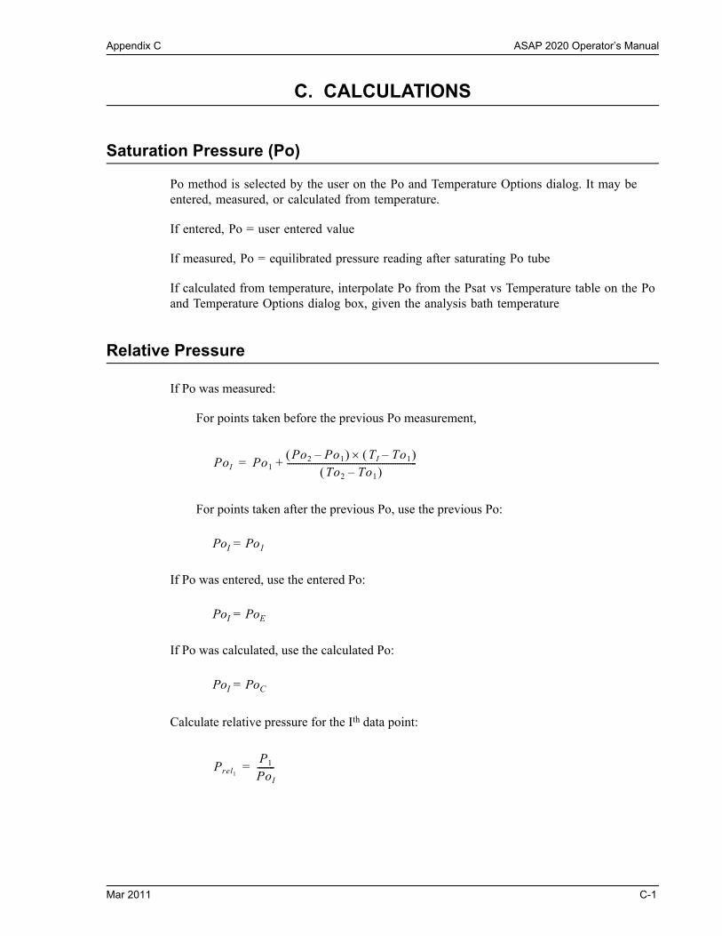
Appendix C ASAP 2020 Operator’s Manual
C. CALCULATIONS
Saturation Pressure (Po)
Po method is selected by the user on the Po and Temperature Options dialog. It may be entered, measured, or calculated from temperature.
If entered, Po = user entered value
If measured, Po = equilibrated pressure reading after saturating Po tube
If calculated from temperature, interpolate Po from the Psat vs Temperature table on the Po and Temperature Options dialog box, given the analysis bath temperature
Relative Pressure
If Po was measured:
For points taken before the previous Po measurement,
For points taken after the previous Po, use the previous Po:
PoI = Po1
If Po was entered, use the entered Po:
PoI = PoE
If Po was calculated, use the calculated Po:
PoI = PoC
Calculate relative pressure for the Ith data point:
PoI Po1Po2 Po1– TI To1–
To2 To1– ------------------------------------------------------------+=
Prel1
P1
PoI
--------=
Mar 2011 C-1

ASAP 2020 Operator’s Manual Appendix C
where
PoI = saturation pressure for the Ith data point (mmHg)
Po1 = most previous measured saturation pressure before Ith data point (mmHg)
Po2 = first measured saturation pressure after the Ith data point (mmHg)PoC = calculated PoPoE = entered saturation pressure (mmHg)
TI = time when the Ith data point was taken (minutes)To1 = time when Po1 was measured (minutes)To2 = time when Po2 was measured (minutes)
PrelI= relative pressure for the Ith data point (mmHg)
PI = absolute pressure for the Ith data point, taken at equilibrium (mmHg)
C-2 Mar 2011
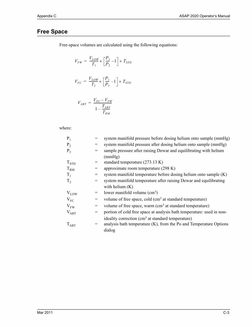
Appendix C ASAP 2020 Operator’s Manual
Free Space
Free-space volumes are calculated using the following equations:
where:
P1 = system manifold pressure before dosing helium onto sample (mmHg)P2 = system manifold pressure after dosing helium onto sample (mmHg)P3 = sample pressure after raising Dewar and equilibrating with helium
(mmHg)TSTD = standard temperature (273.13 K)TRM = approximate room temperature (298 K)T1 = system manifold temperature before dosing helium onto sample (K)T2 = system manifold temperature after raising Dewar and equilibrating
with helium (K)VLOW = lower manifold volume (cm3)
VFC = volume of free space, cold (cm3 at standard temperature)
VFW = volume of free space, warm (cm3 at standard temperature)VABT = portion of cold free space at analysis bath temperature: used in non-
ideality correction (cm3 at standard temperature)TABT = analysis bath temperature (K), from the Po and Temperature Options
dialog
VFW
VLOW
T1
------------P1
P2
----- 1– TSTD=
VFC
VLOW
T2
------------P1
P3
----- 1– TSTD=
VABTVFC VFW–
1TABT
TRM
----------–------------------------=
Mar 2011 C-3

ASAP 2020 Operator’s Manual Appendix C
Equations of State
The ideal gas law relates pressure, volume, temperature, and quantity of gas.
where
P = pressureV = volumeT = temperatureR = a constant that depends on the units of n.
For n in cm3STP, R = PSTD / TSTD
For n in moles, R = 8.3145 J mol-1 K-1
The non-ideality correction is made by replacing P with P(1 + P), where is the non-ide-altiy factor. This gives
The real gas equation of state uses
where z(P,T) is the compressibility factor for the gas at the given pressure and temperature.
n PVRT-------=
nPVRT------- (1 P +=
n PVRTz P T -------------------------=
C-4 Mar 2011

Appendix C ASAP 2020 Operator’s Manual
Quantity Adsorbed
For the Ith dose, the quantity dosed is:
The real gas equation of state is used to calculate n if compressibility information is available. Otherwise, the ideal gas law is used. The pressure, volume, and temperature are those of the lower manifold before and after expanding into the sample tube.
The quantity of gas in the free space is either
if the non-ideality correction is used, or
with the real gas equation of state. Here, Ps is the sample pressure.
The specific quantity adsorbed is
where m is the sample mass.
ndosed i ndosed i 1– n P1 Vm T1 n P2 Vm T2 –+=
nads i ndosed i nFS i–=
nFS iPS i
TSTD
---------- VFC PS i VABT+ =
nFS iPS i
TSTD
---------- VFA
z PS i TFA ---------------------------
VABT
z PS i TABT ------------------------------+
=
Qads inads i
m------------=
Mar 2011 C-5

ASAP 2020 Operator’s Manual Appendix C
Equilibration
Equilibration is reached when the pressure change per equilibration time interval (first derivative) is less than 0.01% of the average pressure during the interval. Both the first derivative and average pressure are calculated using the Savitzky-Golay1 convolution method for polynomial functions. The equations below are those used to compute weighted average and first derivative, respectively, for the 6th point of an 11-point window.
where the numerical constants are from the Savitzky-Golay convolution arrays, and
PAVG = average pressure (mmHg)PCHG = change in pressure (mmHg)
PI = Ith pressure reading taken at equilibrium intervals (mmHg)
After equilibration has been reached, if the user-entered minimum equilibration time from the Low Pressure Options dialog box has not elapsed, the equilibration continues until the entered time has elapsed.
If the user entered a non-zero maximum equilibration time from the Low Pressure Options dialog box, and this time period has elapsed before equilibration has been reached, the equilibration ends as if equilibration had been reached, and the point is collected.
1. Savitzky, A. and Golay, M.J.E., Anal. Chem. 36, 1627 (1964).
PAVG36 P11 P1+ – 9 P10 P2+ 44 P9 P3+ 69 P8 P4+ 84 P7 P5+ 89 P6 + + + + +
429--------------------------------------------------------------------------------------------------------------------------------------------------------------------------------------------------------=
PCHG5 P11 P1– 4 P10 P2– 3 P9 P3– 2 P8 P4– P7 P5– + + + +
110-----------------------------------------------------------------------------------------------------------------------------------------------------------=
If a non-zero value that is too small is entered for the maximum equilibration time, the points are collected before equilibration is reached.
If PAVG is greater than 0.995 times the current Po, equilibration will not take place until the Minimum equilibration delay for P/Po 0.995 has expired, in addition to the standard equilibration criteria.
C-6 Mar 2011

Appendix C ASAP 2020 Operator’s Manual
Thermal Transpiration Correction
During data reduction, thermal transpiration correction is applied to the data if the user selected Thermal transpiration correction from the Report Options dialog. Starting with the first collected pressure, the following calculations are performed until the pressure ratio (PC/P) is greater than or equal to 0.99.
where:
P = equilibrated collected pressure measured by gauge at temp TRM (mmHg)
SD = inside diameter of sample tube (mm), from the Report Optionsdialog
MD = thermal transpiration hard sphere diameter of gas (Å), from the Adsorptive Properties dialog
T = average temperature [TABT + TRM] / 2 (K) = Weber’s coefficient, 0.033 = Weber’s coefficient, 0.245G = Weber’s coefficient, 2.5H = Weber’s coefficient, 2 TABT = analysis bath temperature (K), from the Po and Temperature Options
dialog TRM = room temperature (298 K) PC = corrected equilibrated pressure at temperature TABT (mmHg)F,Y, = intermediate values for subsequent calculations
YP SD MD2
2.33 T----------------------------------- 103=
1 G Y+1 H Y+-----------------------=
F 1
Y2 Y + +------------------------------------------------------=
PC 1 F FTABT
TRM
----------
0.5
P
––
=
Mar 2011 C-7

ASAP 2020 Operator’s Manual Appendix C
BET Surface Area
For each point designated for surface area calculations, the BET1 transformation is calculated as follows:
where BI is in units of g/cm3 STP.
A least-squares fit is performed on the (PrelI ,BI) designated pairs where PrelI is the independent variable and BI is the dependent variable. The following are calculated:
a. Slope (S g/cm3 STP)
b. Y-intercept (YINT g/cm3 STP)
c. Error of the slope (SERR g/cm3 STP)
d. Error of the y-intercept (YIERR g/cm3 STP)
e. Correlation coefficient (Cc)
Using the results of the above calculations, the following can be calculated:
BET Surface Area (m2/g):
where
CSA = analysis gas molecular cross-sectional area (nm2), user-entered on the Adsorptive Properties dialog box
BET C value:
1. Brunauer, S.; Emmett, P.H.; and Teller, E., J. Am. Chem. Soc. 60, 309 (1938).
B1
Prel1
1.0 Prel1– Nads1
----------------------------------------------=
SABETCSA 6.023 1023
22414 cm3 STP 1018 nm2/m2 S YINT+ ---------------------------------------------------------------------------------------------------------------------=
CS YINT+
YINT
-------------------=
C-8 Mar 2011

Appendix C ASAP 2020 Operator’s Manual
Volume of the Monolayer (cm3/g STP):
Error of the BET Surface Area (m2/g):
Langmuir Surface Area
For each point designated for surface area calculations, the Langmuir1 transformation is cal-culated as follows:
where LI is in units of g/cm3 STP
A least-squares fit is performed on the (PrelI ,LI) designated pairs where PrelI is the inde-
pendent variable and LI is the dependent variable. The following are calculated:
a. Slope (S g/cm3 STP)
b. Y-intercept (YINT g/cm3 STP)
c. Error of the slope (SERR g/cm3 STP)
d. Error of the y-intercept (YIERR g/cm3 STP)
e. Correlation coefficient (Cc)
Using the results of the above calculations, the following can be calculated:
VM1
C YINT-------------------- 1
S YINT+-------------------= =
BETERRSABET SERR 2 YIERR 2+
0.5
YINT S+---------------------------------------------------------------------=
1. Langmuir, I., J. Am. Chem. Soc. 38, 2267 (1916); J. Am. Chem. Soc. 40, 1361 (1918); Phys. Rev 8, 149 (1916).
LI
PrelI
NadsI
-----------=
Mar 2011 C-9

ASAP 2020 Operator’s Manual Appendix C
Langmuir Surface Area (m2/g):
where
CSA = analysis gas molecular cross-sectional area (nm2), user-entered on the Adsorptive Properties dialog
Volume of the Monolayer (cm3/g STP):
Langmuir b Value:
Error of the Langmuir Surface Area (m2/g):
SALANCSA 6.023 1023
22414 cm3 STP 1018 nm2/m2 S-----------------------------------------------------------------------------------------------=
VM1S---=
b YINT VM =
LANERRSALAN SERR
S-------------------------------=
C-10 Mar 2011

Appendix C ASAP 2020 Operator’s Manual
t-Plot
For each point designated for t-Plot1 calculations, the following calculations are done:
Thickness for the Ith point (Å):
(Halsey2)
(Harkins and Jura3)
(STSA Carbon Black4)
(Broekhoff-deBoer5)
where:
tI = thickness for Ith point HP1 = Halsey parameter #1 HP2 = Halsey parameter #2 HP3 = Halsey parameter #3HJP1 = Harkins and Jura parameter #1 HJP2 = Harkins and Jura parameter #2 HJP3 = Harkins and Jura parameter #3 STSA1 = statistical thickness surface area parameter #1 STSA2 = statistical thickness surface area parameter #2 STSA3 = statistical thickness surface area parameter #3 BdB1 = Broekhoff-de Boer parameter #1 BdB2 = Broekhoff-de Boer parameter #2 BdB3 = Broekhoff-de Boer parameter #3
1. deBoer, J.H., et al, J. Catalysis 3, 32, 38, 44, 268 (1964); J. Catalysis 4, 319, 643, 649 (1965); Cranston, R. and Inkley, F., Adv. Catalysis 9, 143 (1957).
2. Halsey, G., J. Chem. Phys. 16, 931-937 (1948).3. Harkins, W.D. and Jura, G., J. Chem. Phys. 11, 431 (1943).4. Magee, R.W., Rubber Chemistry and Technology, Vol 68, No 4, 1995, p. 590; ASTM Standard D65565. Broekhoff, J.C.P. and de Boer, J.H., “The Surface Area in Intermediate Pores,” Proceedings of the International
Symposium on Surface Area Determination, D.H. Everett, R.H. Ottwill, eds., U.K. (1969).
tI HP1HP2
PrelI ln
--------------------HP3
=
tIHJP1
HJP2 PrelI log–
-------------------------------------------HJP3
=
tI STSA1 STSA2 PrelI STSA3Prel
2+ +=
PrelI log BdB1
tI 2
-------------- BdB2 BdB3*tI exp+=
tKJS1
KJS2 Prellog–------------------------------------ KJS3
=
Mar 2011 C-11

ASAP 2020 Operator’s Manual Appendix C
KJS1 = Kruk-Jaroniec-Sayari parameter #1 KJS2 = Kruk-Jaroniec-Sayari parameter #2 KJS3 = Kruk-Jaroniec-Sayari parameter #3 PrelI = relative pressure for the Ith point
A least-squares analysis fit is performed on the (tI, NadsI) data pairs where tI is the indepen-dent variable and NadsI is the dependent variable. Only the values of tI between tMIN and tMAX, the minimum and maximum thickness, are used. The following are calculated:
a. Slope (S cm3/g-Å STP)
b. Y-intercept (YINT cm3/g STP)
c. Error of the slope (SERR cm3/g-Å STP)
d. Error of the Y-intercept (YIERR cm3/g STP)
e. Correlation coefficient (Cc)
Using the results of the above calculations, the following can be calculated:
External Surface Area (m2/g):
where
F = surface area correction factor, user-entered on the t-Plot Report Options dialog
D = density conversion factor, user-entered on the Adsorptive Properties dialog
Micropore Surface Area (m2/g):
where SATOT is the BET surface area if the user enabled the BET report, or Langmuir surface area if the user enabled the Langmuir report. If neither report has been selected, SATOT is the BET surface area value calculated using a set of default parameters.
Micropore Volume (cm3 liquid/g):
SAEXTS cm3/g A STP– 1010 A/m D cm3 liquid/cm3 STP
F 106 cm3/m3 --------------------------------------------------------------------------------------------------------------------------------------------------------=
SAP SATOT SAEXT+=
VP YINT cm3/g STP D cm3 liquid/cm3 STP =
C-12 Mar 2011

Appendix C ASAP 2020 Operator’s Manual
BJH Pore Volume and Area Distribution
For adsorption data, the relative pressure and volume adsorbed data point pairs collected dur-ing an analysis must be arranged in reverse order from which the points were collected during analysis. All calculations are performed based on a desorption model, regardless of whether adsorption or desorption data are being used.
The data used in these calculations must be in order of strictly decreasing numerical value. Points which do not meet this criterion are omitted. The remaining data set is composed of relative pressure (Pr), volume adsorbed (Va) pairs from (Pr1, Va1) to (PrN, VaN) where (PrN = 0, VaN = 0) is assumed as a final point. Each data pair represents an interval boundary (or desorption step boundary) for intervals i=1 to i=N-1 where N = total number of (Pr, Va) pairs.
Generally, the desorption branch of an isotherm is used to relate the amount of adsorbate lost in a desorption step to the average size of pores emptied in the step. A pore loses its con-densed liquid adsorbate, known as the core of the pore, at a particular relative pressure related to the core radius by the Kelvin1 equation. After the core has evaporated, a layer of adsorbate remains on the wall of the pore. The thickness of this layer is calculated for a particular rel-ative pressure from the thickness equation. This layer becomes thinner with successive decreases in pressure, so that the measured quantity of gas desorbed in a step is composed of a quantity equivalent to the liquid cores evaporated in that step plus the quantity desorbed from the pore walls of pores whose cores have been evaporated in that and previous steps. Barrett, Joyner, and Halenda2 developed the method (known as the BJH method) which incor-porates these ideas. The algorithm used on the ASAP 2020 is an implementation of the BJH method.
Explanation of Terms
A pore filled with condensed liquid nitrogen has three zones:
a. The core - evaporates all at once when the critical pressure for that radius is reached; the relationship between the core radius and the critical pressure is defined by the Kelvin equation.
b. The adsorbed layer - composed of adsorbed gas that is stripped off a bit at a time with each pressure step; the relationship between the thickness of the layer and the relative pressure is defined by the thickness equation.
1. Kelvin, J. (published under the name of Sir William Thomson), Phil. Mag. 42, 448-452 (1871).2. Barrett, E.P.; Joyner, L.S.; and Halenda, P.P., J. Am. Chem. Soc. 73, 373-380 (1951).
Mar 2011 C-13

ASAP 2020 Operator’s Manual Appendix C
c. The walls of the cylindrical pore - the diameter of the empty pore is required to determine the pore volume and pore area. End area is neglected.
Calculations
The volumes adsorbed (Va) are converted to the liquid equivalent volumes (V1, cm3/g):
where D is the Density Conversion Factor from the Adsorptive Properties dialog box.
The relative pressure (Pr1) is assumed to be close to unity so that substantially all the pores in the sample are filled.
The corresponding Kelvin core radius is calculated. Only pores smaller than this size will be included:
where
A = adsorbate property factor (the BJH Adsorptive Options dialog box)F = fraction of pores open at both ends (from the BJH Adsorption Report
Options dialog box or the BJH Desorption Report Options dialog box); assumed to be zero for desorption
This radius will be adjusted for the thickness of the adsorbed layer during subsequent calcu-lation steps.
adsorbed
layer
wall
core
Insignificant compared to core length
pore
VII VaI D =
RcIA–
1 F+ PrI ln -----------------------------------------=
C-14 Mar 2011
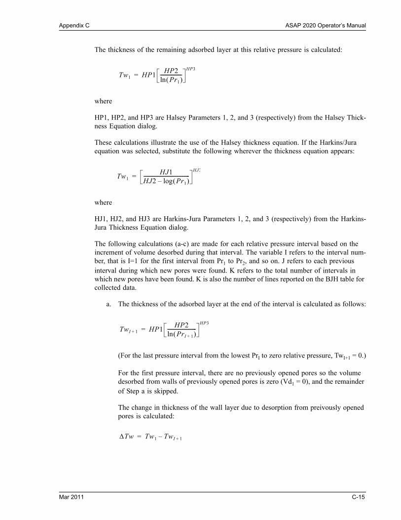
Appendix C ASAP 2020 Operator’s Manual
The thickness of the remaining adsorbed layer at this relative pressure is calculated:
where
HP1, HP2, and HP3 are Halsey Parameters 1, 2, and 3 (respectively) from the Halsey Thick-ness Equation dialog.
These calculations illustrate the use of the Halsey thickness equation. If the Harkins/Jura equation was selected, substitute the following wherever the thickness equation appears:
where
HJ1, HJ2, and HJ3 are Harkins-Jura Parameters 1, 2, and 3 (respectively) from the Harkins-Jura Thickness Equation dialog.
The following calculations (a-c) are made for each relative pressure interval based on the increment of volume desorbed during that interval. The variable I refers to the interval num-ber, that is I=1 for the first interval from Pr1 to Pr2, and so on. J refers to each previous interval during which new pores were found. K refers to the total number of intervals in which new pores have been found. K is also the number of lines reported on the BJH table for collected data.
a. The thickness of the adsorbed layer at the end of the interval is calculated as follows:
(For the last pressure interval from the lowest PrI to zero relative pressure, TwI+1 = 0.)
For the first pressure interval, there are no previously opened pores so the volume desorbed from walls of previously opened pores is zero (Vd1 = 0), and the remainder of Step a is skipped.
The change in thickness of the wall layer due to desorption from preivously opened pores is calculated:
Tw1 HP1HP2
Pr1 ln------------------
HP3
=
Tw1HJ1
HJ2 Pr1 log–--------------------------------------
HJ3
=
TwI 1+ HP1HP2PrI 1+ ln
------------------------HP3
=
Tw Tw1 TwI 1+–=
Mar 2011 C-15

ASAP 2020 Operator’s Manual Appendix C
The annular cross-sectional area of the wall layer desorbed is calculated for all pre-viously opened pores:
The total volume of gas desorbed from walls of previously opened pores is calculated:
for all previously opened pores
where LPJ = length of previously opened pores as calculated in Step b(2).
b. The physical processes occurring for this pressure interval are determined as follows:
(1) If VdI is greater than the current increment of volume desorbed (VlI - VlI+1), desorption from walls only is occurring. Total surface of walls exposed thus far (cm2/g) is calculated as follows:
for all previously opened pores
where
DavgJ = weighted average pore diameter calculated below in Step b(2).
A new layer thickness (Tw) that will not overcompensate for the actual volume desorbed in this interval is calculated:
Since no cores are evaporated in this pressure interval, no new pores are revealed. Thus no ending Kelvin radius and average pore diameter are calculated for this interval. Note that this means the report may have fewer tabulated intervals on the collected data report than experimental pressure intervals.
(2) If VdI is less than the volume increment desorbed during this interval, the remaining volume is due to new pores with core evaporation taking place in this interval. K, the number of intervals with new pores exposed, is increased by 1. (For the interval from the lowest to zero relative pressure, no new pore volume is calculated and the rest of Step b is skipped.)
The volume desorbed from newly opened pores in this interval is calculated as follows:
CSAJ Rcj Tw+ 2 Rcj 2– 10 16– cm2/A2 =
VdI LpJ CSAaJ =
SAW LPJ DavgJ 10 8– cm/A =
TwV1I V1I 1+– 108 A/cm
SAwI
--------------------------------------------------------------=
VcI VII VII 1+– VdI–=
C-16 Mar 2011

Appendix C ASAP 2020 Operator’s Manual
The Kelvin radius for the end of the interval is calculated as follows:
All new pores opened in this interval are represented by one pore having a length-weighted average pore diameter and a corresponding length sufficient to account for the required volume of adsorbate. The weighted average pore diam-eter is calculated as follows:
DavgK is the diameter of a pore which would have a surface area that is the aver-age of the areas for pores with radius and , if its length was the mean of the lengths at those radii.
The relative pressure corresponding to is calculated as follows:
The thickness of the adsorbed layer at this pressure is calculated as follows:
The decrease in thickness of the wall layer by desorption from the walls of new pores during the lower portion of the pressure interval is calculated as follows:
The cross-sectional area of the newly opened pores is calculated as follows:
The length of the newly opened pores is calculated as follows:
RcK 1+A–
1 F+ PrI 1+ ln -----------------------------------------------=
DavgK
2 RcK RcK 1++ RcK RcK 1+
RcK 2 RcK 1+ 2+-------------------------------------------------------------------------------=
PavgK 1– 2A–
1 F+ DavgK
-----------------------------------ln=
TwavgKHP1
HP2PavgK ln
----------------------HP3
=
Td TwavgKTWI 1+–=
CSAcKDavgK
2---------------- Td+
2
10 16– cm2/A2 =
LPKVcI
CSAcK
-----------------=
Mar 2011 C-17

ASAP 2020 Operator’s Manual Appendix C
c. Pore diameters and radii are adjusted for the change in thickness of the adsorbed wall layer during this interval. If new pores were opened during this interval, the average diameter is adjusted by the change in layer thickness during the second portion of the desorption interval as follows:
The layer thickness change during the whole interval is added to diameters of previ-ously opened pores as follows:
(not including DavgK)
The layer thickness change desorbed during this interval also is added to the radii corresponding to the ends of the pressure intervals as follows:
for all except RcK+1.
Steps a to c are repeated for each pressure interval.
After the above calculations have been performed, the diameters corresponding to the ends of the intervals are calculated as follows:
for all RcJ including RcK+1.
The remaining calculations are based on DP(I), Davg(I), and LP(I). These calculations are only done for values that fall between the Minimum BJH diameter and the Max-imum BJH diameter specified by the operator on the BJH Adsorption Report Options dialog box or the BJH Desorption Report Options dialog box.
1) Incremental Pore Volume (VpI, cm3/g):
2) Cumulative Pore Volume (VpCUM(1), cm3/g):
DavgKnewDavgKold
2 Td +=
DavgJnewDavgJold
2 Tw +=
RcJnew RcJold Tw+=
DpJ 2 rcJ =
VpI LpI DavgI
2-----------
2
1016 cm2/A2=
VPCUM 1 VpJ for J 1 =
C-18 Mar 2011
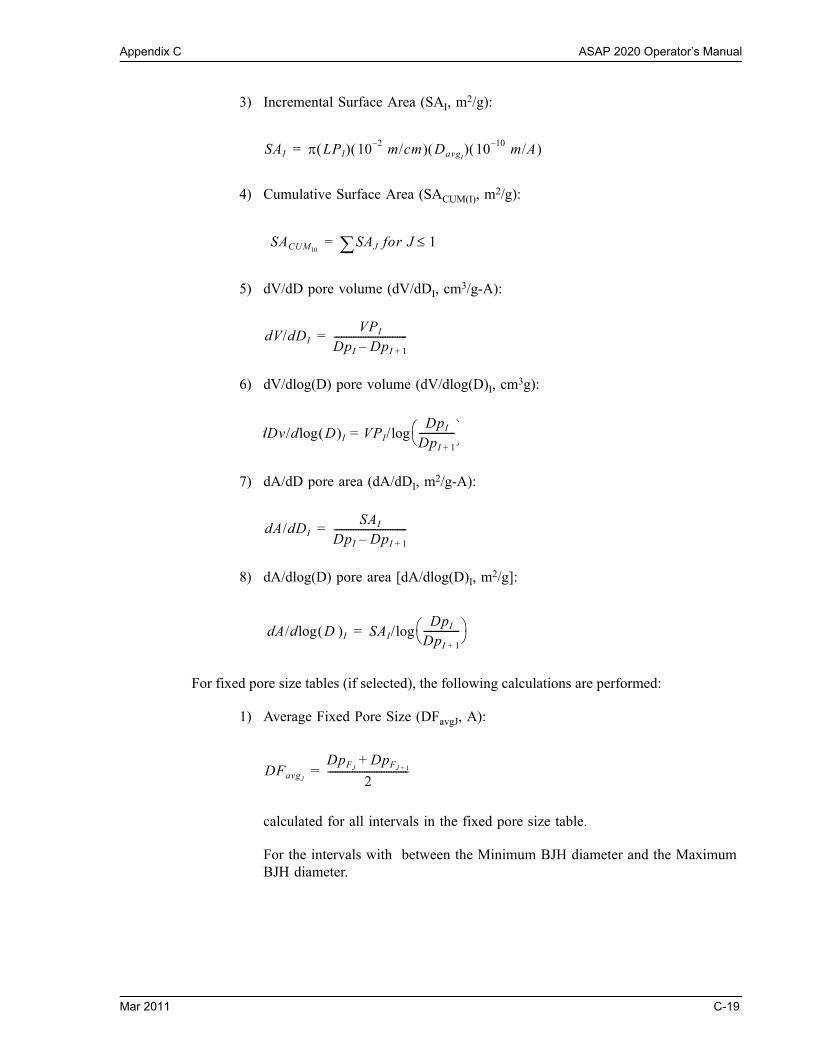
Appendix C ASAP 2020 Operator’s Manual
3) Incremental Surface Area (SAI, m2/g):
4) Cumulative Surface Area (SACUM(I), m2/g):
5) dV/dD pore volume (dV/dDI, cm3/g-A):
6) dV/dlog(D) pore volume (dV/dlog(D)I, cm3g):
7) dA/dD pore area (dA/dDI, m2/g-A):
8) dA/dlog(D) pore area [dA/dlog(D)I, m2/g]:
For fixed pore size tables (if selected), the following calculations are performed:
1) Average Fixed Pore Size (DFavgJ, A):
calculated for all intervals in the fixed pore size table.
For the intervals with between the Minimum BJH diameter and the Maximum BJH diameter.
SAI LPI 10 2– m/cm DavgI 10 10– m/A =
SACUM10SAJ for J 1=
dV/dDIVPI
DpI DpI 1+–------------------------------=
dDv/d D I VPI/DpI
DpI 1+
--------------- log=log
dA/dDISAI
DpI DpI 1+–------------------------------=
dA/d D Ilog SAI/DpI
DpI 1+
--------------- log=
DFavgJ
DpFJDpFJ 1+
+
2---------------------------------=
Mar 2011 C-19

ASAP 2020 Operator’s Manual Appendix C
2) Cumulative Pore volume (VpFCUMI, cm3/g):
where INTERP(x) is the value interpolated from the function X = DpJ+1 and Y = VPCUMJ, using an AKIMA semi-spline interpolation.
3) Incremental Pore Volume (VpFI, cm3/g):
where VpFCUM0 = 0.
4) Cumulative Surface Area (SAFCUMI, m2/g):
where INTERP(x) is the value interpolated from the function X = DpJ+1 and Y = SACUMJ.
5) Incremental Surface Area (SAFI, m2/g):
where SAFCUM0 = 0.
6) dV/dD pore volume (dV/dDpFI, cm3/g-A)):
where INTERP(x) is the value interpolated from the function X = DavgJ and Y = dV/dDJ.
7) dV/dlog(D) pore volume [dV/dlog(DpF)I, cm3/g]:
where INTERP(x) is the value interpolated from the function X = DavgJ and Y = dV/dlog(D)J.
VpFCUMIINTERP DpFI 1+ =
VpFI VpFCUMIVpFCUMI 1–
–=
SAFCUMIINTERP DpFI 1+ =
SAFI SAFCUMISAFCUMI 1–
–=
dV/dDpFI INTERP DpFI 1+ =
dV/d D pFI log INTERP DpFI 1+ =
C-20 Mar 2011

Appendix C ASAP 2020 Operator’s Manual
8) dA/dD pore area (dA/dDpFI, m2/g-A):
where INTERP(x) is the value interpolated from the function X = DavgJ and Y = dA/dDJ.
9) dA/dlog(D) pore area [dA/dlog(DpFI), m2/g]:
where INTERP(x) is the value interpolated from the function X = DavgJ and Y = dA/dlog(D)J.
Compendium of Variables
Va = quantity adsorbed expressed as a volume (cm3/g STP)Vl = liquid equivalent volume of volume adsorbed (cm3/g)D = density conversion factor from the Adsorptive Properties dialog box
(cm3/cm3 STP)Pr = relative pressureDp = pore (or core) diameter (A)Rc = Kelvin radius (A) of coreA = adsorbate property factor; from the BJH Adsorptive Options dialog
boxF = fraction of pores open at both ends; from the BJH Adsorption Report
Options dialog box or the BJH Desorption Report Options dialog boxTw = thickness of adsorbed layer desorbed during interval (A)Tw = thickness of remaining adsorbed wall (A)
HP1, HP2, and HP3 are Halsey Parameters from the Halsey Thickness Equation dialog.
HJ1, HJ2, and HJ3 are Harkins and Jura Parameters from the Harkins/Jura Thickness Equa-tion dialog.
Vd = volume of gas desorbed from walls of previously opened pores (cm3/g)
Davg = average pore diameter (A)CSAa = annular cross-sectional area of the desorbed layer (cm2)CSAc = cross-sectional area of opening of newly opened pores (cm2)SAw = total surface area of walls exposed (cm2/g)Td = thickness of layer desorbed from walls of newly opened pores (A)Vc = volume desorbed from cores of newly opened pores (cm3/g)Lp = length of pore (cm/g)
dA/dDpFI INTERP DpFI 1+ =
dA/d D pFI log INTERP DpFI 1+ =
Mar 2011 C-21

ASAP 2020 Operator’s Manual Appendix C
Horvath-Kawazoe
A relative pressure lower limit is determined such that L-d0 never equals zero. All pressure points less than this limit are discarded. For each collected relative pressure point, values of L are chosen in an iterative manner, and the relative pressure (P/Po) determined by solving one of the following equations:
• Slit Pore Geometry (original Horvath-Kawazoe)• Cylinder Pore Geometry (Saito/Foley)• Sphere Pore Geometry (Cheng/Yang)
Slit Pore Geometry (original HK)
When you use the original Horvath-Kawazoe1 method, the following equation is solved for each value of P. The value of L is determined when the solved-for relative pressure is within 0.1% of the collected absolute pressure.
where
K = Avogadro’s number (6.023 x 10²³)R = gas constant (8.31441 x 10⁷ ergs/mole K)T = analysis bath temperature (K), from an entered or calculated
value on the Po and Temperature Options dialog
= gas solid nuclear separation at zero interaction energy (Å),
where:
ZS = sample equilibrium diameter at zero interaction energy (Å) from the Horvath-Kawazoe Physical Properties dialog
ZA = zero interaction energy diameter from the Horvath-Kawazoe Physical Properties dialog
1. Horvath, G. and Kawazoe, K., J. Chem. Eng. Japan 16(6), 470 (1983).
PPo-------ln
KRT------- IP 1032 JA4/J cm4
4 L 2 d0– -------------------------------------------------- 4
3 L d0– 3------------------------------ 10
9 L d0– 9------------------------------– 4
3 d0 3
---------------– 10
9 d0 9
---------------+=
ZS ZA+2
-----------------
C-22 Mar 2011
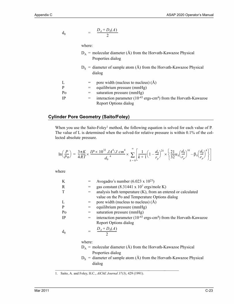
Appendix C ASAP 2020 Operator’s Manual
d0 =
where:
DA = molecular diameter (Å) from the Horvath-Kawazoe PhysicalProperties dialog
DS = diameter of sample atom (Å) from the Horvath-Kawazoe Physical dialog
L = pore width (nucleus to nucleus) (Å)P = equilibrium pressure (mmHg)Po = saturation pressure (mmHg)IP = interaction parameter (10-43 ergs-cm4) from the Horvath-Kawazoe
Report Options dialog
Cylinder Pore Geometry (Saito/Foley)
When you use the Saito-Foley1 method, the following equation is solved for each value of P. The value of L is determined when the solved-for relative pressure is within 0.1% of the col-lected absolute pressure.
where
K = Avogadro’s number (6.023 x 10²³)R = gas constant (8.31441 x 10⁷ ergs/mole K)T = analysis bath temperature (K), from an entered or calculated
value on the Po and Temperature Options dialogL = pore width (nucleus to nucleus) (Å)P = equilibrium pressure (mmHg)Po = saturation pressure (mmHg)IP = interaction parameter (10-43 ergs-cm4) from the Horvath-Kawazoe
Report Options dialog
d0 =
where:DA = molecular diameter (Å) from the Horvath-Kawazoe Physical
Properties dialog DS = diameter of sample atom (Å) from the Horvath-Kawazoe Physical
dialog
DA DS A +2
------------------------------
1. Saito, A. and Foley, H.C., AlChE Journal 37(3), 429 (1991).
PPo------- ln
34---K
RT------- IP 1032 JA4/J cm4
d0 4-------------------------------------------------- 1
k 1+------------ 1
d0
rp
-----– 2k 21
32------k
d0
rp
-----
10
k
d0
rp
-----
4
–
k 0=
=
DA DS A +2
----------------------------
Mar 2011 C-23

ASAP 2020 Operator’s Manual Appendix C
k =
k =
rp = radius of the cylindrical pore,
Sphere Pore Geometry (Cheng/Yang)
When you use the Cheng/Yang1 method, the following equation is solved for each value of P. The value of L is determined when the solved-for relative pressure is within 0.1% of the col-lected absolute pressure.
where
R = gas constant (8.31441 x 10⁷ ergs/mole K)T = analysis bath temperature (K), from an entered or calculated
value on the Po and Temperature Options dialog
d0 =
where:DA = molecular diameter (Å) from the Horvath-Kawazoe Physical
Properties dialog DS = diameter of sample atom (Å) from the Horvath-Kawazoe Physical
dialog L = pore width (nucleus to nucleus) (Å)P = equilibrium pressure (mmHg)Po = saturation pressure (mmHg)N1 = 4 L2 NS, where NS = number of sample atoms/cm2 at monolayer
N2 = 4 (L - d0)2 NA, where Ns = number of gas molecules/cm2
e*12 = , where
4.5– k–k
--------------------
2
k 1– ,0 1.0=
1.5– k–k
--------------------
2
k 1– ,0 1.0=
L2---
1. Cheng, Linda S. and Yang, Ralph T., Chemical Engineering Science 49(16), 2599-2609 (1994).
PPo------- n
6 N1* 12 N2
* 22+ L3 1032 J A4/J cm4
RT L d0– 3----------------------------------------------------------------------------------------------------=
d0
L-----
6 112------T1
18---T2+
–d0
L-----
12 190------T3
180------+ T4
+
DA DS A +2
----------------------------
AS
4dS 6------------ AS
6 MC2 S AS
S
-----A
A
------+---------------------------------------------=
C-24 Mar 2011

Appendix C ASAP 2020 Operator’s Manual
*22 = , where
T1 =
T2 =
T3 =
T4 =
where
Cheng/Yang Correction
This factor corrects for the nonlinearity of the isotherm. It adds an additional term to the equations for the different geometrics:
where
G(L) = one of the Horvath-Kawazoe equations given above = degree of void filling; is estimated by first computing the
monolayer capacity (Vm) with the Langmuir equation over the range of data points from relative pressure 0.02 to 0.2 or the maximum relative pressure included in the Horvath-Kawazoe analysis. is computed as the volume adsorbed over Vm.
AA
4DA 6-------------- AA
3 MC2 A A2
---------------------------------------------=
1
1 S– 3------------------- 1
1 S+ 3-------------------–
1
1 S+ 2------------------- 1
1 S– 2-------------------–
1
1 S– 9------------------- 1
1 S+ 9-------------------–
1
1 S+ 8------------------- 1
1 S– 8-------------------–
SL d0–
L--------------=
PPo------- ln G L 1
1--- 1
1 –------------ ln––=
Mar 2011 C-25

ASAP 2020 Operator’s Manual Appendix C
Interaction Parameter
The interaction parameter (IP) results from the following calculations:
The Kirkwood-Muller dispersion coefficients -
where
MC2 = kinetic energy of electron (0.8183 x 10⁻⁶ erg)S = polarizability of sample atoms (cm3)
A = polarizability of gas molecule (cm3)
S = diamagnetic susceptability of sample atom (cm3)
A = diamagnetic susceptability of gas molecule (cm3)
where:
NA = number of gas molecules/cm2 at monolayer from the Horvath-Kawazoe Physical Properties dialog box
NS = number of sample atoms/cm2 from the Horvath-Kawazoe Physical Properties dialog box
Refer to Interaction Parameter Components later in this Appendix for recommended values.
AS6 MC2 S A
S
S
-----A
A
------+---------------------------------------------=
AA3 MC2 A A
2---------------------------------------------=
IP NA A A NS AS +=
C-26 Mar 2011
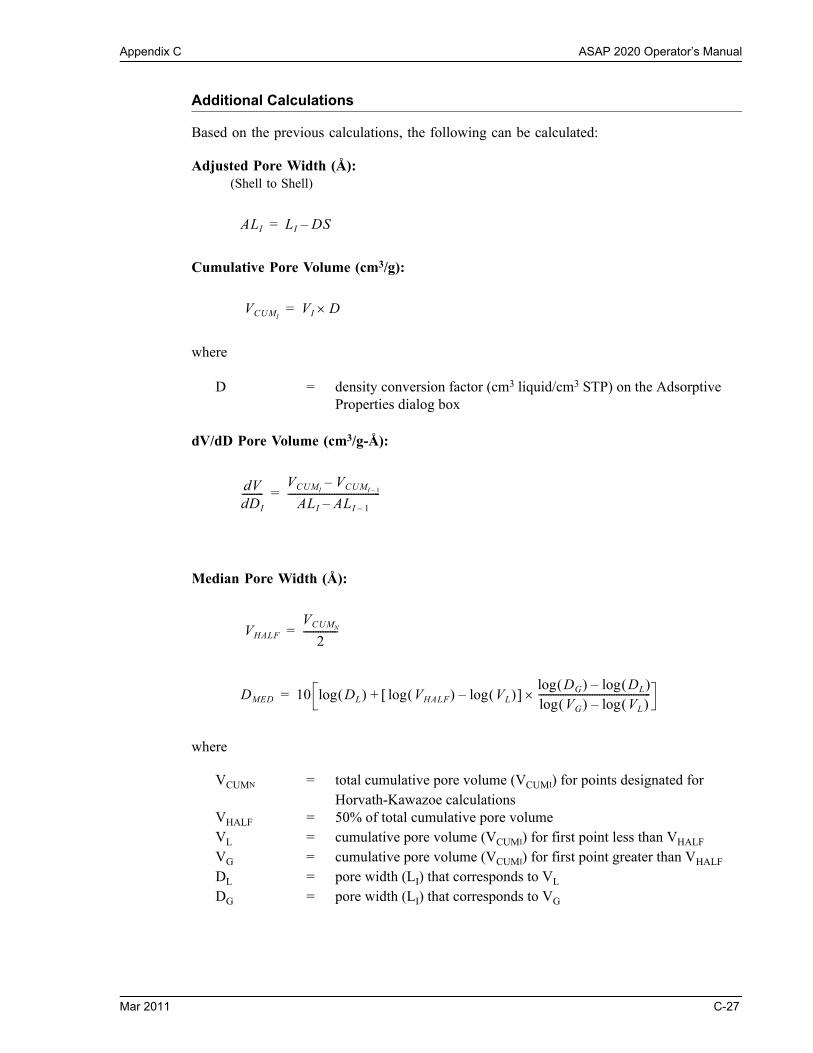
Appendix C ASAP 2020 Operator’s Manual
Additional Calculations
Based on the previous calculations, the following can be calculated:
Adjusted Pore Width (Å): (Shell to Shell)
Cumulative Pore Volume (cm3/g):
where
D = density conversion factor (cm3 liquid/cm3 STP) on the Adsorptive Properties dialog box
dV/dD Pore Volume (cm3/g-Å):
Median Pore Width (Å):
where
VCUMN = total cumulative pore volume (VCUMI) for points designated for Horvath-Kawazoe calculations
VHALF = 50% of total cumulative pore volume VL = cumulative pore volume (VCUMI) for first point less than VHALF
VG = cumulative pore volume (VCUMI) for first point greater than VHALF
DL = pore width (LI) that corresponds to VL DG = pore width (LI) that corresponds to VG
ALI LI DS–=
VCUMIVI D=
dVdDI
---------VCUMI
VCUMI 1––
ALI ALI 1––--------------------------------------=
VHALF
VCUMN
2--------------=
DMED 10 DL log VHALF VL log–log DG DL log–logVG VL log–log
----------------------------------------------+=
Mar 2011 C-27

ASAP 2020 Operator’s Manual Appendix C
Interaction Parameter Components
Table C-1. Interaction Parameters
The following values were used to calculate the values in Table C-1.
Gas
Bath Temperature
(K) Sample Type
Interaction Parameter Calculated
Value*
Argon 87.3 Carbon (Ross/Olivier value)Carbon (Horvath/Kawazoe value)Zeolite
2.615.893.19
Carbon Dioxide
298.15 Carbon (Ross/Olivier value)Carbon (Horvath/Kawazoe value)Zeolite
4.209.205.08
273.15 Carbon (Ross/Olivier value)Carbon (Horvath/Kawazoe value)Zeolite
4.349.355.22
194.65 Carbon (Ross/Olivier value)Carbon (Horvath/Kawazoe value)Zeolite
4.729.725.60
Nitrogen 77.15 Carbon (Ross/Olivier value)Carbon (Horvath/Kawazoe value)Zeolite
2.846.533.49
*The interaction parameter is entered in the Horvath-Kawazoe Report Options dialog in the following field:
Interaction parameter: (calculated value) x 10-43 ergs-cm4
Carbon-Graphite ZeoliteDS = 3.40 DS = 3.04NS = 3.845 x 10¹⁵ NS = 3.75 x 10¹⁵
S = 1.05 x 10⁻²⁹ (Ross/Olivier) S = 1.94 x 10⁻²⁹
13.5 x 10⁻²⁹ (Horvath/Kawazoe, implicit) S = 0.85 x 10⁻²⁴
S = 1.02 x 10⁻²⁴
Nitrogen ArgonDA = 3.00 DA = 2.95A = 6.71 x 10¹⁴ A = 7.608 x 10¹⁴
A = 3.6 x 10⁻²⁹ A = 3.22 x 10⁻²⁹
A = 1.76 x 10⁻²⁴ A = 1.63 x 10⁻²⁴
C-28 Mar 2011

Appendix C ASAP 2020 Operator’s Manual
DA values are from van der Waal’s constant.NA values are from liquid densities.
and values are derived from data found in Ross and Olivier1.
The physical parameters referenced in Saito/Foley are as follows:
Carbon DioxideDA = 3.23NA = 4.567 x 10¹⁴ (25 ºC)
5.45 x 10¹⁴ (0 ºC)7.697 x 10¹⁴ (-78 ºC)
A = 5.0 x 10⁻²⁹
A = 2.7 x 10⁻²⁴
1. Ross and Olivier, J.P., “On Physical Adsorption,” J. Wiley and Sons, New York (1964).
Aluminophosphate AluminosilicateDS = 2.60 DS = 2.76NS = 1.48 x 10¹⁵ Ns = 1.31 x 10¹⁵
S = 1.3 x 10⁻²⁹ S = 1.3 x 10⁻²⁹
S = 2.5 x 10⁻²⁴ S = 2.5 x 10⁻²⁴
Mar 2011 C-29

ASAP 2020 Operator’s Manual Appendix C
Dubinin-Radushkevich
The Dubinin-Radushkevich1 equation is as follows:
where:
V = volume adsorbed at equilibrium pressure (cm3/g STP)Vo = the micropore capacity (cm3/g STP)Po = saturation vapor pressure of gas at temperature T (mmHg) P = equilibrium pressure (mmHg)B = a constant = the affinity coefficient of analysis gas relative to Po gas
(for this application is taken to be 1)T = analysis bath temperature (K), from the Po and Temperature
Options dialog For each point designated for Dubinin-Radushkevich calculations, the following calculations are done:
LV = log (V)
The intercept, log(Vo) can be found by performing a least-squares fit on the (LP,LV) desig-nated pairs where LP is the independent variable and LV is the dependent variable. Assuming the adsorption of gas is restricted to a monolayer, Vo is the monolayer capacity. Based on this assumption, the following are calculated:
a. Slope (S cm3/g STP)
b. Y-intercept (YI cm3/g STP)
c. Error of the slope (SERR cm3/g STP)
d. Error of the y-intercept (YIERR cm3/g STP)
e. Correlation coefficient (Cc)
1. Dubinin, M., Carbon 21, 359 (1983); Dubinin, M., Progress in Surface and Membrane Science 9, 1, Academic Press, New York (1975); Dubinin, M. and Astakhov, V., Adv. Chem. Ser. 102, 69 (1971); Lamond, T. and Marsh, H., Carbon 1, 281, 293 (1964); Medek, J., Fuel 56, 131 (1977); Polanyi, M., Trans. Faraday Soc. 28, 316 (1932); Radushkevich, L., Zh. fiz. Kemi. 33, 2202 (1949); Stoeckli, H., et al, Carbon 27, 125 (1989).
V log Vo B T2
--------------- PoP
-------log2
–log=
LPPoP
-------
2
log=
C-30 Mar 2011
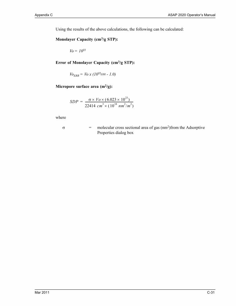
Appendix C ASAP 2020 Operator’s Manual
Using the results of the above calculations, the following can be calculated:
Monolayer Capacity (cm3/g STP):
Vo = 10YI
Error of Monolayer Capacity (cm3/g STP):
VoERR = Vo x (10YIERR - 1.0)
Micropore surface area (m2/g):
where
= molecular cross sectional area of gas (nm2)from the Adsorptive Properties dialog box
SDP Vo 6.023 1023 22414 cm3 1018 nm2/m2 --------------------------------------------------------------------=
Mar 2011 C-31

ASAP 2020 Operator’s Manual Appendix C
Dubinin-Astakhov
The Dubinin-Astakhov equation is a follows:
where
V = volume adsorbed at equilibrium pressure (cm3/g STP)Vo = the micropore capacity (cm3/g STP)Po = saturation vapor pressure of gas at temperature T (mmHg) P = equilibrium pressure (mmHg)T = analysis bath temperature (K) R = the gas constant (0.0083144 kJ/mol)E0 = characteristic energy (kJ/mole)N = Astakhov exponent, may be optimized or user entered from the
Dubinin Report Options dialog box = the affinity coefficient of the analysis gas relative to the Po gas, from
the Dubinin Adsorptive Options dialog boxFor each point designated for Dubinin-Astakhov calculations, the following calculations are done:
LV = log(V)
A least-squares fit is performed on the (LP,LV) designated pairs where LP is the independent variable and LV is the dependent variable. If the user selected yes for the Optimize Astakhov Exponent prompt, a systematic search for the optimum value of N is conducted by recalcu-lating the linear regression and selecting the value of N that gives the smallest standard error of the y-intercept. The exponent N is optimized to within 10-4. If the optimum value for N is not found in this range, an exponent of 2 is used. The following are calculated:
a. Slope (S cm3/g STP)
b. Y-intercept (YI cm3/g STP)
c. Error of the slope (SERR cm3/g STP)
d. Error of the y-intercept (YIERR cm3/g STP)
e. Correlation coefficient (Cc)
f. Optimized Astakhov exponent (N)
V log Vo RTE0
---------N Po
P-------log
N
–log=
LP PoP
-------logN
=
C-32 Mar 2011

Appendix C ASAP 2020 Operator’s Manual
Using the results of the above calculations, the following can be calculated:
Monolayer Capacity (cm3/g STP):
V0 = 10YI
Micropore Volume (cm3/g):
WI = (VI x D)
where
D = density conversion factor (cm3 liquid/cm3 STP) from the Adsorptive Properties dialog box
Limiting Micropore Volume (cm3/g):
W0 = (V0 x D)
where
D = density conversion factor (cm3 liquid/cm3 STP) from the Adsorptive Properties dialog box
Error of Limiting Micropore Volume (cm3/g):
W0ERR = W0 x (10YIERR - 1.0)
Characteristic Energy (KJ/mole):
Modal Equivalent Pore Width (nm):
where
k = the interaction constant for benzene, 8.969 kJ•nm3/mol
E 2.303 R T 2.303 S 1/N-------------------------------------=
wmode 23N
3N 1+----------------
1/N kE0
-----
1/3
=
Mar 2011 C-33
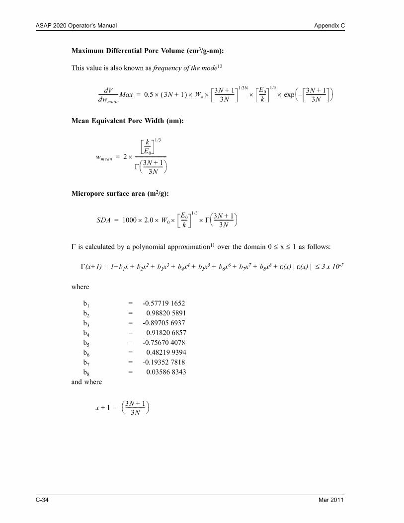
ASAP 2020 Operator’s Manual Appendix C
Maximum Differential Pore Volume (cm3/g-nm):
This value is also known as frequency of the mode12
Mean Equivalent Pore Width (nm):
Micropore surface area (m2/g):
is calculated by a polynomial approximation11 over the domain 0 x 1 as follows:
(x+1) = 1+b1x + b2x2 + b3x3 + b4x4 + b5x5 + b6x6 + b7x7 + b8x8 + (x) | (x) | 3 x 10⁻⁷
where
b1 = -0.57719 1652b2 = 0.98820 5891b3 = -0.89705 6937b4 = 0.91820 6857b5 = -0.75670 4078b6 = 0.48219 9394b7 = -0.19352 7818b8 = 0.03586 8343
and where
dVdwmode
----------------Max 0.5 3N 1+ Wo 3N 1+3N
----------------1/3N
E0
k-----
1/3 3N 1+3N
----------------– exp=
wmean 2
kE0
-----1/3
3N 1+3N
----------------
--------------------------=
SDA 1000 2.0 W0E0
k-----
1/3
3N 1+3N
---------------- =
x 1+3N 1+
3N---------------- =
C-34 Mar 2011

Appendix C ASAP 2020 Operator’s Manual
Equivalent Pore Width (nm):
dV/dw Pore Volume (cm3/g-nm):
wi 2
kE0
----- N
–
W i W0 ln–ln-----------------------------------------
1/3N
=
dVdwi
-------- 0.5 W0 3Nk
E0
-----N
wi
2-----
3N 1+ –
kE0
----- N
wi
2-----
3N–
–exp=
Mar 2011 C-35

ASAP 2020 Operator’s Manual Appendix C
MP-Method
For each point designated for MP-method1 calculations, the following calculations are done:
Thickness for the Ith point (Å):
(Halsey6)
or
(Harkins and Jura7)
where:
tI = thickness for Ith point HP1 = Halsey parameter #1HP2 = Halsey parameter #2HP3 = Halsey parameter #3HJP1 = Harkins and Jura parameter #1HJP2 = Harkins and Jura parameter #2HJP3 = Harkins and Jura parameter #3PrelI = relative pressure for the Ith point (mmHg)
With the (tI,VI) data pairs, the Akima semi-spline interpolation method is used to interpolate volume adsorbed values based on thickness values that are evenly spaced 0.2 Angstrom apart starting at the first outlier point. Outliers are defined as those points have the maximum instantaneous slope within an iteratively shrinking subset of all points. The remaining pore surface area calculation result is the slope of the line defined by two consecutive interpolated points. The slopes of each pair of consecutive points from the origin to the last point must be monotonically decreasing and non-negative. With the interpolated points set the following can be calculated:
Average pore hydraulic radius (Å):
1. Mikhail, R., Brunauer, S. and Bodor, E., J. Colloid and Interface Sci. 24, 45 (1968).
tI HP1HP2
PrelI ln
--------------------HP3
=
tIHJP1
HJP2 PrelI log–
-------------------------------------------HJP3
=
RItI tI 1–+
2------------------=
C-36 Mar 2011
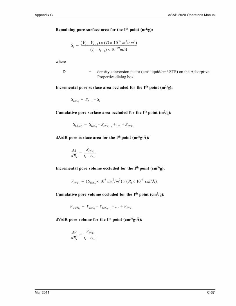
Appendix C ASAP 2020 Operator’s Manual
Remaining pore surface area for the Ith point (m2/g):
where
D = density conversion factor (cm3 liquid/cm3 STP) on the Adsorptive Properties dialog box
Incremental pore surface area occluded for the Ith point (m2/g):
Cumulative pore surface area occluded for the Ith point (m2/g):
dA/dR pore surface area for the Ith point (m2/g-Å):
Incremental pore volume occluded for the Ith point (cm3/g):
Cumulative pore volume occluded for the Ith point (cm3/g):
dV/dR pore volume for the Ith point (cm3/g-Å):
SIVI VI 1–– D 10 6– m3/cm3
tI tI 1–– 10 10– m/A-------------------------------------------------------------------------------=
SINCISI 1– SI–=
SCUMISINCI
SINCI 1– SINC1
+ + +=
dAdRI
--------SINCI
tI tI 1––------------------=
VINCISINCI
104 cm2/m2 RI 10 8– cm/Å =
VCUMIVINCI
VINCI 1– VINC1
+ + +=
dVdRI
--------VINCI
tI tI 1––------------------=
Mar 2011 C-37
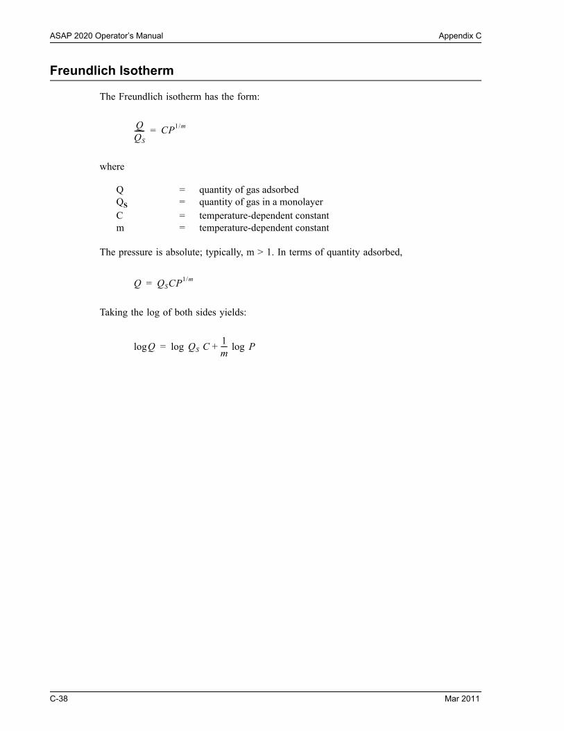
ASAP 2020 Operator’s Manual Appendix C
Freundlich Isotherm
The Freundlich isotherm has the form:
where
Q = quantity of gas adsorbedQS = quantity of gas in a monolayerC = temperature-dependent constantm = temperature-dependent constant
The pressure is absolute; typically, m > 1. In terms of quantity adsorbed,
Taking the log of both sides yields:
QQS
------ CP1/m=
Q QSCP1/m=
Qlog QS C1m---- Plog+log=
C-38 Mar 2011
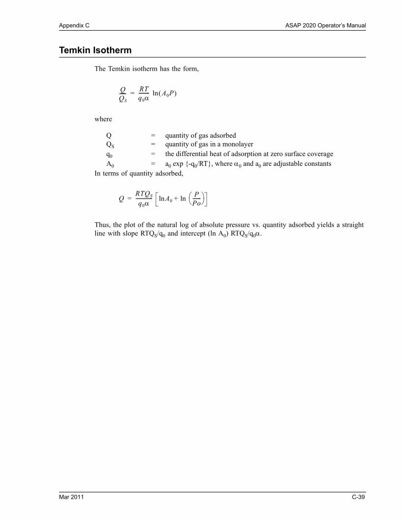
Appendix C ASAP 2020 Operator’s Manual
Temkin Isotherm
The Temkin isotherm has the form,
where
Q = quantity of gas adsorbedQS = quantity of gas in a monolayerq0 = the differential heat of adsorption at zero surface coverageA0 = a0 exp {-q0/RT}, where 0 and a0 are adjustable constants
In terms of quantity adsorbed,
Thus, the plot of the natural log of absolute pressure vs. quantity adsorbed yields a straight line with slope RTQS/q0 and intercept (ln A0) RTQS/q0.
QQS
------RTq0--------- A0P ln=
QRTQS
q0-------------- A0
PPo------- ln+ln=
Mar 2011 C-39

ASAP 2020 Operator’s Manual Appendix C
DFT (Density Functional Theory)
The adsorption isotherm is known to convey a great deal of information about the energetic heterogeneity and geometric topology of the sample under study. The data of physical adsorp-tion have been used for many years as the basis for methods to characterize the surface area and porosity of adsorbents. Real solid surfaces rarely approach ideal uniformity of structure. It is accepted that in general, the surface of even a nonporous material presents areas of greater or lesser attraction for adsorbed molecules.
This energetic heterogeneity greatly affects the shape of the adsorption isotherm with the result that simple theories such as the Langmuir and BET formulas can, at best, give only approximate estimates of surface area. Porous solids virtually are never characterized by a single pore dimension, but instead exhibit a more or less wide distribution of sizes. The observed adsorption isotherm for a typical material is therefore the convolution of an adsorp-tion process with the distribution of one or more properties which affect that process. This was first stated mathematically by Ross and Olivier13 for the case of surface energy distribu-tion and has become known as the integral equation of adsorption.
The Integral Equation of Adsorption
In a general form for a single component adsorptive, the integral equation of adsorption can be written as
(1)
where
Q(p) = the total quantity adsorbed per unit weight at pressure p,a,b,c,... = a set of distributed properties,f(a,b,c,...) = the distribution function of the properties, andq(p,a,b,c,...) = the kernel function describing the adsorption isotherm on unit
surface of material with fixed properties a,b,c,...
Equation (1), a Fredholm integral of the first kind, is a member of a class of problems known as ill-posed, in that there are an infinite number of functional combinations inside the integral that will provide solutions. Even when the kernel function is known, experimental error in the data can make solving for even a single distribution function a difficult task. Solving for mul-tiple distribution functions requires more data than provided by a single adsorption isotherm.
Q p a d b d cq p a b c f a b c d=
C-40 Mar 2011

Appendix C ASAP 2020 Operator’s Manual
Application to Surface Energy Distribution
Under certain conditions, an energetically heterogeneous surface may be characterized by a distribution of adsorptive energies. The conditions are that the sample is not microporous, i.e., that adsorption is taking place on essentially a free surface with no pore filling processes at least to about 0.2 relative pressure. Secondly, that each energetically distinct patch contributes independently to the total adsorption isotherm in proportion to the fraction of the total surface that it represents. This condition is satisfied if the patches are relatively large compared to an adsorptive molecule, or if the energy gradient along the surface is not steep. In mathematical terms, this concept is expressed by the integral equation of adsorption in the following form.
(2)
where
Q(p) = the experimental quantity adsorbed per gram at pressure p,q(p,e) = the quantity adsorbed per unit area at the same pressure, p, on
an ideal free surface of energy e, and f(e) = the total area of surface of energy e in the sample
The exact form of the energy-dependent term depends on the form of the model isotherms expressed in the kernel function and is provided in the library model description in Chapter 5.
Application to Pore Size Distribution
Similarly, a sample of porous material may be characterized by its distribution of pore sizes. It is assumed in this case that each pore acts independently. Each pore size present then con-tributes to the total adsorption isotherm in proportion to the fraction of the total area of the sample that it represents. Mathematically, this relation is expressed by
(3)
where
Q(p) = the experimental quantity adsorbed at pressure p,q(p,H) = the quantity adsorbed per unit area at the same pressure, p, in
an ideal pore of size H, and f(H) = the total area of pores of size H in the sample.
Numerical values for the kernel functions in the form of model isotherms can be derived from modern statistical mechanics such as density functional theory or molecular simulations, or can be calculated from one of various classical theories based on the Kelvin equation. Several types are found in the models library.
Performing the Deconvolution
The integrations in equations (2) and (3) are carried out over all surface energies or pore sizes
Qp q p f d=
Q p H q p H f H d=
Mar 2011 C-41

ASAP 2020 Operator’s Manual Appendix C
in the model. The functions q(p,e) and q(p,H), which we call the kernel functions, are con-tained in numeric form as model isotherms. Because, in general, there is no analytic solution for equation (1), the problem is best solved in a discrete form; the integral equation for any distributed property Z becomes a summation:
(4)
Given a set of model isotherms, q(p,Z), from a model chosen from the models library and an experimental isotherm, Q(p), contained in a sample information file, the software determines the set of positive values f(Z) that most nearly, in a least squares sense, solves equation (4). The distributed property, surface energy or pore size, is then displayed on the Report Options dialog box as a selection of tables or graphs.
Regularization
DFT reports allow a selectable regularization (also referred to as smoothing) constraint to be applied during the deconvolution process to avoid over-fitting in the case of noisy data or ill-fitting models. The method used is based on co-minimization of the second derivative of the distribution. The relative weight given to this term is determined by the value of the regular-ization parameter, which is set on the DFT Pore Size or Surface Energy dialog box and also is shown in the header of reports. The value of the regularization parameter varies from zero (for no second derivative constraint) to ten (indicating a weight equal to minimizing the resid-uals), or even larger. When the distribution and residuals obtained change little with the value of the regularization parameter, it indicates that the chosen model provides a good represen-tation of the data. Conversely, a large sensitivity to the regularization parameter might indicate inadequate data or a poor choice of model to represent the data.
Q p q p Zi f Zi i
=
C-42 Mar 2011

Appendix C ASAP 2020 Operator’s Manual
Heat of Adsorption
The adsorption isostere is represented by
where
qi = isosteric heat of adsorptionC = unknown constant
The isosteric heat of adsorption, q,i is determined by finding the slope of ln (P/P0) as a func-tion of 1/RT for a set of isotherms measured at different temperatures.
Summary Report
The following calculations and the results of previous calculations (as noted) are used to gen-erate the summary report:
a. BET Surface Area
See BET Surface Area Calculations
b. Langmuir Surface Area
See Langmuir Surface Area Calculations
c. Single Point Surface Area (m2/g)
where
Pr = pressure closest to 0.3 of the relative pressure points designated for surface area calculations.
Va = volume corresponding to Pr
d. Micropore Area
See t-Plot calculations.
PP0
----- qi
RT------- C+=ln
S1PTVa 1 Pr– CSA 6.023 1023
22414 cm3 STP 1018 nm2/m2-------------------------------------------------------------------------------------------------=
Mar 2011 C-43

ASAP 2020 Operator’s Manual Appendix C
e. Micropore Volume
See t-Plot calculations.
f. Horvath-Kawazoe Maximum Pore Volume
See Horvath-Kawazoe Calculations
g. Horvath-Kawazoe Median Pore Diameter
See Horvath-Kawazoe Calculations
h. Dubinin-Radushkevich Micropore Surface Area
See Dubinin-Radushkevich Calculations
i. Dubinin-Radushkevich Monolayer Capacity
See Dubinin-Radushkevich Calculations
j. Dubinin-Astakhov Micropore Surface Area
See Dubinin-Astakhov Calculations
k. Dubinin-Astakhov Micropore Volume
See Dubinin-Astakhov Calculations
l. MP-Method Cumulative Surface Area of Pores
MPSTOT = SCUMI, (see MP-method Calculations) for the last collected data point used in the MP-method Calculations, and the range of hydraulic pore radii over which the cumulative surface area was computed.
m. MP-Method Cumulative Pore Volume of Pores
MPVTOT = VCUMI, (see MP-method Calculations) for the last collected data point used in the MP-method Calculations, and the range of hydraulic pore radii over which the cumulative pore volume was computed.
n. Average Pore Hydraulic Radius (A)
MPDAVER
MPVTOT
MPSTOT
-------------------- 10 6– m3/cm 1010 Å/m=
C-44 Mar 2011

Appendix C ASAP 2020 Operator’s Manual
SPC Report Variables
Regressions Chart Variables
The line of best fit for the Regression Chart is calculated by the usual Least Squares methd. (Refer to BASIC Scientific Subroutines Vol II, by F.R. Ruckdeschel, Copyright 1981 BYTE Publications/McGraw Hill, p. 16.) If there is only a single point or all N points have the same x-value, there can be no line of best fit in the standard form.
The coefficient of Correlation for this line is also calculated in the usual way. (Refer to Math-ematical Handbook for Scientists and Engineers, by Granino A. Korn and Theresa M. Korn, Copyright 1961, 1968 McGraw Hill, Sec. 18.4.)
XAve xi
N---------=
XAve yi
N---------=
Slope xi XAve– yi XAve–
xi XAve– 2---------------------------------------------------------------=
x xi XAve– 2
N------------------------------------=
y yi XAve– 2
N------------------------------------=
Cov x y xi XAve– yi XAve–
N---------------------------------------------------------------=
Correlation Coefficient Cov x y xy
-----------------------=
Mar 2011 C-45

ASAP 2020 Operator’s Manual Appendix C
Control Chart Variables
Mean yi
N---------=
StdDev y Mean– 2
N 1–------------------------------------=
CoefVar StdDevMean
-------------------=
PlusNSig Mean n StdDev+=
MinusNSig Mean n StdDev–=
C-46 Mar 2011

Appendix D ASAP 2020 Operator’s Manual
D. TESTING FOR LEAKS
This appendix contains general instructions for testing the ASAP 2020 and the SmartVac degasser (if installed) for leaks. If the analyzer successfully performs a blank tube analysis using nitrogen, you do not need to test for leaks.
These procedures may be performed individually or sequentially. Record pressure readings on the Valve Test Data Sheet included at the end of this appendix. After you finish testing for leaks, replace any leaking valves.
You will need the following items to perform tests:
• Stopwatch• Valve Test Data Sheet (included in this appendix)
Testing Individual Valves
Analysis Valves
This procedure removes differential pressure from all valves in the analysis system and estab-lishes that there are no leaks in the analysis system. It should be performed before testing for individual valves.
1. Ensure that the analyzer is idle.
2. Close the regulator outlet valve for each gas supply line to the analyzer.
3. Attach the Po tube to the Po port.
4. Insert a plug (or attach a clean, empty sample tube) into the analysis port.
5. Insert a plug into the vapor inlet (if the vapor option is not installed).
An automated method of performing a leak test can be found in “Performing a Leak Test” on page 9-16.
Mar 2011 D-1

ASAP 2020 Operator’s Manual Appendix D
6. Select Show Instrument Schematic, then Enable Manual Control from the Unit menu. (For clarity, this illustration shows only the valve portion of the schematic.) Table D-1 lists descriptions of the analysis valves.
Table D-1. Analysis Valve Descriptions
7. Open valves 1, 2, 4, 5, and 7; close all other manifold valves.
8. Open valve PS.
9. Open valve 3 and allow the pressure to drop below 1000 mHg (1 mmHg).
10. Repeat Step 9 for valves P1 through P6.
11. Open valve 9.
Valve Description
1 Unrestricted vacuum
2 Restricted vacuum
3 Helium inlet port valve
4 Restricted analysis gas
5 Unrestricted analysis gas
7 Lower manifold isolation
8 Vapor inlet port
9 Sample port
10 Restricted Psat tube port
11 Unrestricted Psat tube port
P1 through P6 Gas inlet port valves
PS Supply valve for physisorption gases
PV Vacuum valve for physisorption gases
D-2 Mar 2011

Appendix D ASAP 2020 Operator’s Manual
12. Open valves 10 and 11.
13. Open valve 8.
14. Open valve PV.
15. Allow the system to evacuate for a minimum of one hour; a four-hour or overnight evacuation is preferred.
16. Obtain the manifold outgassing rate:
a. Close valves 3, 4, 5, 8, 9, 10, 11, and P1 through P6.
b. Evacuate manifold for another 30 minutes.
c. Take a pressure reading; record it as P1 for the manifold.
d. Close valves 1 and 2.
e. Wait 10 minutes and take another pressure reading; record it as P2 for the manifold.
f. Subtract P1 from P2 and divide the difference by 10 to obtain the outgassing rate per minute;
Outgassing rate =
Record this value as the outgassing rate for the manifold. This value should be less than 0.5 mHg/min. for the lower manifold alone and less than 0.7 mHg/min. for the upper and lower manifolds combined.
17. Obtain the gas inlet valve outgassing rate:
a. Open valves PS and 5; valve 7 should still be open.
b. Take a pressure reading; record it as P1 for the gas inlet valve.
c. Wait 10 minutes and take another pressure reading; record it as P2 for the gas inlet valve.
d. Subtract P1 from P2 and divide the difference by 10; record this value as the outgas-sing rate for the gas inlet valve. This value should be less than 10 mHg/min.
Use the pressure transducer with the lowest range. For example, if you have a 1 mmHg transducer, it is the first choice. Next is the 10 mmHg transducer. If you have neither, use the Vacuum Gauge.
P2 P1–10
--------------------
Mar 2011 D-3
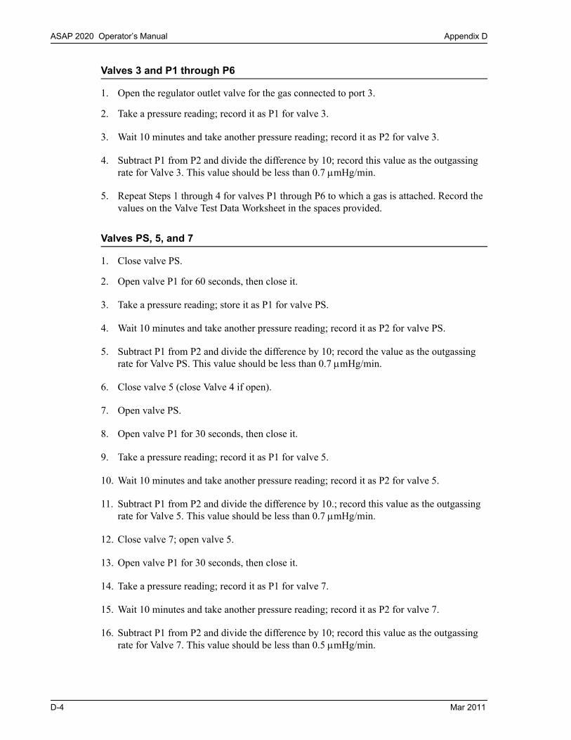
ASAP 2020 Operator’s Manual Appendix D
Valves 3 and P1 through P6
1. Open the regulator outlet valve for the gas connected to port 3.
2. Take a pressure reading; record it as P1 for valve 3.
3. Wait 10 minutes and take another pressure reading; record it as P2 for valve 3.
4. Subtract P1 from P2 and divide the difference by 10; record this value as the outgassing rate for Valve 3. This value should be less than 0.7 mHg/min.
5. Repeat Steps 1 through 4 for valves P1 through P6 to which a gas is attached. Record the values on the Valve Test Data Worksheet in the spaces provided.
Valves PS, 5, and 7
1. Close valve PS.
2. Open valve P1 for 60 seconds, then close it.
3. Take a pressure reading; store it as P1 for valve PS.
4. Wait 10 minutes and take another pressure reading; record it as P2 for valve PS.
5. Subtract P1 from P2 and divide the difference by 10; record the value as the outgassing rate for Valve PS. This value should be less than 0.7 mHg/min.
6. Close valve 5 (close Valve 4 if open).
7. Open valve PS.
8. Open valve P1 for 30 seconds, then close it.
9. Take a pressure reading; record it as P1 for valve 5.
10. Wait 10 minutes and take another pressure reading; record it as P2 for valve 5.
11. Subtract P1 from P2 and divide the difference by 10.; record this value as the outgassing rate for Valve 5. This value should be less than 0.7 mHg/min.
12. Close valve 7; open valve 5.
13. Open valve P1 for 30 seconds, then close it.
14. Take a pressure reading; record it as P1 for valve 7.
15. Wait 10 minutes and take another pressure reading; record it as P2 for valve 7.
16. Subtract P1 from P2 and divide the difference by 10; record this value as the outgassing rate for Valve 7. This value should be less than 0.5 mHg/min.
D-4 Mar 2011

Appendix D ASAP 2020 Operator’s Manual
Valves 1, 2, 8, 9, 10, 11, and PV
Valves 10 and 11
1. Open valve PV; wait 5 minutes (Valves PS and 5 should be open.).
2. Open valve 7; allow the system to evacuate to below 10 mHg.
3. Close valves PV, PS, and 5.
4. Open valves 1 and 2; allow the system to evacuate for 30 minutes.
Valves 1, 2, and 7 should be the only valves open at this time.
5. Remove the Po tube.
6. Take a pressure reading; record it as P1 for valves 10 and 11.
7. Wait 10 minutes and take another pressure reading; record it as P2 for valves 10 and 11.
8. Subtract P1 from P2 and divide the difference by 10; record this value as the outgassing rate for Valves 10 and 11. This value should be less than 0.7 mHg/min.
Valve 9
9. Remove the sample tube from the analysis port.
10. Take a pressure reading; record it as P1 for valve 9.
11. Wait 10 minutes and take another pressure reading; record it as P2 for valve 9.
12. Subtract P1 from P2 and divide the difference by 10; record this value as the outgassing rate for valve 9. This should be less than 0.7 mHg/min.
Valve 8
13. With valve 8 closed, remove the plug from the vapor inlet port on the side of the analyzer.
If the vapor accessory is installed, disconnect it from the analyzer.
14. Take a pressure reading; record it as P1 for valve 8.
15. Wait 10 minutes and take another pressure reading; record it as P2 for valve 8.
16. Subtract P1 from P2 and divide the difference by 10; record this value as the outgassing rate for valve 8. This value should be less than 0.7 mHg/min.
17. Before proceeding, reinstall the sample tube, the Po tube, and the plug from the vapor inlet (or the vapor accessory).
Mar 2011 D-5

ASAP 2020 Operator’s Manual Appendix D
Valves 1, 2, and PV
18. Open valves 1 and 2.
19. Open valves 4, 5, and PS.
20. Allow the system to evacuate for 15 minutes.
21. Close valves 1 and 2. Valve PV should be closed; if not, close it.
22. Take a pressure reading; record it as P1 for valves 1, 2, and PV.
23. Wait 10 minutes and take another pressure reading; record it as P2 for valves 1, 2, and PV.
24. Subtract P1 from P2 and divide the difference by 10; record this value as the outgassing rate for valves 1, 2, and PV. This value should be less than 0.7 mHg/min.
25. Fill the manifold to 800 mmHg with N2, then close the nitrogen port valve.
26. Close valve 4.
27. Take a pressure reading; record it as P1 for valve PV.
28. Wait 10 minutes and take another pressure reading; record it as P2 for valve PV.
29. Subtract P1 from P2 and divide the difference by 10; record this value as the outgassing rate for valve PV. This value should be less than 50 mHg/min.
If the pressure drops more than 0.05 mmHg, close valve 5, the PV valve may be leaking.
30. Take another pressure reading; record it as P1 for valves 1 and 2.
31. Wait 10 minutes and take another pressure reading; record it as P2 for valves 1 and 2.
32. Subtract P1 from P2 and divide the difference by 10; record this value as the outgassing rate for valves 1 and 2. This value should be less than 50 mHg/min.
If the pressure drops more than 0.05 mmHg, close valve 7, valves 1 or 2 may be leaking.
33. Take another pressure reading; record it as P1 for valve 1.
34. Wait 10 minutes and take another pressure reading; record it as P2 for valve 1.
35. Subtract P1 from P2 and divide the difference by 10; record this value as the outgassing rate for valve 1. This value should be less than 50 mHg/min.
If the pressure drops more than 0.05 mmHg, valve 1 may be leaking.
D-6 Mar 2011
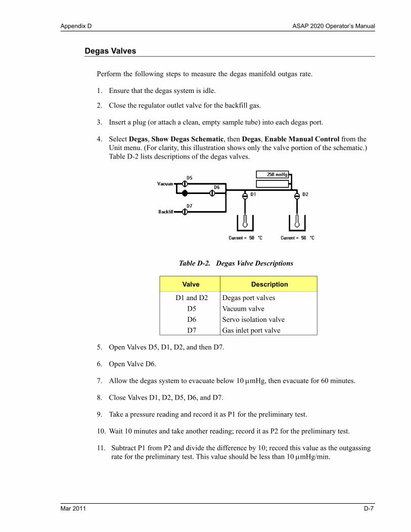
Appendix D ASAP 2020 Operator’s Manual
Degas Valves
Perform the following steps to measure the degas manifold outgas rate.
1. Ensure that the degas system is idle.
2. Close the regulator outlet valve for the backfill gas.
3. Insert a plug (or attach a clean, empty sample tube) into each degas port.
4. Select Degas, Show Degas Schematic, then Degas, Enable Manual Control from the Unit menu. (For clarity, this illustration shows only the valve portion of the schematic.) Table D-2 lists descriptions of the degas valves.
Table D-2. Degas Valve Descriptions
5. Open Valves D5, D1, D2, and then D7.
6. Open Valve D6.
7. Allow the degas system to evacuate below 10 mHg, then evacuate for 60 minutes.
8. Close Valves D1, D2, D5, D6, and D7.
9. Take a pressure reading and record it as P1 for the preliminary test.
10. Wait 10 minutes and take another reading; record it as P2 for the preliminary test.
11. Subtract P1 from P2 and divide the difference by 10; record this value as the outgassing rate for the preliminary test. This value should be less than 10 mHg/min.
Valve Description
D1 and D2 Degas port valves
D5 Vacuum valve
D6 Servo isolation valve
D7 Gas inlet port valve
Mar 2011 D-7
ASAP 2020 Operator’s Manual Appendix D
What To Do If You Detect a Leaking Valve
If you determine that a specific valve is leaking, remove differential pressure from the valve and continue testing the remaining valves for leaks.
Removing Differential Pressure from a Leaking Valve
1. Select either of the following actions:
• Close the regulator outlet valve for the gas supply line to the valve.• Reinstall the plug that was removed to test the valve.
2. Open the leaking valve.
3. Evacuate the analyzer until you obtain an outgas rate of less than 0.7 mHg per minute. Refer to Testing Individual Valves on page D-1 for detailed instructions on determining the outgas rate for specific valves.
Repairing or Replacing a Leaking Valve
Whether you repair or replace a valve depends on the type of valve that is leaking.
• Valves on the Analysis manifold should be repaired• Valves on the Degas and inlet manifold should be replaced.
Repairing Valves on the Analysis Manifold
1. Backfill the manifold with nitrogen to approximately 800 mmHg.
• Close off the helium gas supply if you are repairing the helium inlet valve.• Turn off the vacuum pump system if you are repairing a vacuum valve.
2. Remove and replace the plunger and the thin gasket on the leaking valve.
As an alternative, you may repair or replace the leaking valve after removing the differential pressure on the valve. However, opening the analysis system to replace or repair a valve exposes the analyzer manifold to atmospheric gases and moisture. These gases and moisture greatly increase the time required to evacuate the analyzer and prepare it for further testing or operation.
D-8 Mar 2011

Appendix D ASAP 2020 Operator’s Manual
3. Closely inspect the valve seat area for any debris which may cause another leak.
4. Reassemble the valve.
• Reopen the helium supply if you are repairing the helium inlet valve.• Turn on the vacuum pump system if you are repairing a vacuum valve.
5. Open and close the repaired valve approximately 20 to 30 times; this allows the valve to seat properly.
6. Evacuate the analyzer until the outgas rate is less than 0.7 mHg per minute. Refer to Testing Individual Valves on page D-1 for detailed instructions.
Plunger
Gasket
Mar 2011 D-9

ASAP 2020 Operator’s Manual Appendix D
Replacing Valves on the Degas and Gas Inlet Manifold
1. Backfill the manifold with nitrogen to approximately 800 mmHg.
2. Turn off the gas supply for the gas inlet valves.
3. Turn off the vacuum pump system for degas valves D5 and D6.
4. Carefully remove the wires to the valve coil.
5. Unscrew and remove the valve from the manifold.
6. Install the new valve, then reconnect the wiring.
7. Turn on the gas supply and vacuum pump system.
8. Evacuate the analyzer until the outgas rate is less than 0.7 mHg/min. for inlet valves or 10 mHg/min. for degas valves. Refer to Testing Individual Valves on page D-1 for detailed instructions.
D-10 Mar 2011

Appendix D ASAP 2020 Operator’s Manual
Valve Data Test Sheet
Make a copy of this form to record pressure readings and outgassing rates when leak-testing system valves.
VALVE(s)P1
(1st pressure reading)P2
(2nd pressure reading) OUTGASSING RATE
Analysis Valves
Manifold
Gas inlet valve
3
P1
P2
P3
P4
P5
P6
PS
5
7
10 and 11
9
8
1, 2, and PV
1, 2, and PV
1 and 2
1
Degas Valves
Manifold
Mar 2011 D-11

ASAP 2020 Operator’s Manual Appendix D
D-12 Mar 2011

Appendix E ASAP 2020 Operator’s Manual
E. CALCULATING FREE-SPACE VALUESFOR MICROPORE ANALYSES
Many microporous materials, such as zeolites and activated carbons, trap and hold helium in their complex pore structures for many hours after being exposed to helium. Helium trapped in micropores can interfere with the analysis at low pressures, causing an “S”-shaped curve at the lower end of the isotherm. For this reason, it is recommended that you enter the warm and cold free-space volumes when performing micropore analyses, therefore avoiding exposure of the sample to helium. Two techniques can be used for determining warm and cold free-space values.
The first method is to perform a short analysis on the sample after partial degassing (one pres-sure point with no incremental dosing), but prior to final sample preparation. Measure the free space during this analysis. The measured free-space values will be printed on the report and may then be entered into the sample file after more thorough sample preparation.
The second method requires prior tests using empty tubes that will be employed later for the sample analyses. The measured free-space data can be used thereafter on every analysis per-formed using these sample tubes. This small initial investment of time will save considerable time later. Perform an empty tube analysis on each sample tube you intend to use for micro-pore analysis. Measure the free space of each sample tube, taking only one pressure point. Four important things to remember are: 1) be consistent in using seal frits; for example, use the same seal frits for the analysis as you did for the empty tube test; 2) since the cold free space is dependent on bath temperature, perform a test for each bath temperature to be used; 3) the isothermal jacket must be in the same position for the sample analysis as it was for the empty tube test; and 4) correct the free-space volumes obtained for the volume displaced by the sample when you use them.
To make the correction, subtract the amount of gas displaced by the sample. The calculations are simple and are given here with a brief explanation of their derivation. Remember to employ the appropriate free-space values for each bath temperature used, stating all temper-atures in Kelvin.
To correct warm free space:
where
Vws = calculated warm free space with sample present (in standard cm3)
Vwm = warm free space measured for the empty tube (in standard cm3)Ms = mass of sample to be analyzed (in grams)
rs = approximate sample true density (in grams/cm3)Tamb = ambient temperature (in Kelvin)Tstd = standard temperature (273.15 Kelvin)
Vws Vwm
Ms
s-------
Tstd
Tamb------------
–=
Aug 04 E-1

ASAP 2020 Operator’s Manual Appendix E
To correct cold free space:
whereVcs = calculated cold free space with sample present (in standard cm3)
Vcm = cold free space measured for the empty tube (in standard cm3)Ms = mass of the sample to be analyzed (in grams)
rs = approximate sample true density (in grams/cm3)Tbath = analysis bath temperature (in Kelvin)Tstd = standard temperature (273.15 Kelvin)
When you later analyze a sample, select Enter Free Space, and use the values calculated above.
Example:The sample is 0.2345 grams of activated carbon with a density of 2.0000 g/cm3. The room temperature is 22 ºC or 295.15 K. The analysis tube has been measured previously in an argon bath. The measured warm and cold free spaces are 29.1234 and 89.4567 cm3 STP atm-1, respectively. The analysis will be performed with argon at liquid argon temperature, 87.3 K.
With this information, enter the corrected warm free space as follows:
and enter the corrected cold free space as follows:
Vws 29.1234 cm3 STP
0.2345 g
2.0000 g/cm3
---------------------------------- 273.2 K295.2 K-------------------
29.0149 cm3 STP atm
1–=
–=
Vcs 89.4567 cm3 STP
0.2345 g
2.0000 g/cm3
---------------------------------- 273.2 K87.3 K
------------------- 89.0898 cm
3 STP atm
1–=
–=
E-2 Mar 05

Appendix F ASAP 2020 Operator’s Manual
F. DEFAULT FILES AND SYSTEM FILES
The following table describes the default analysis conditions files provided with the ASAP 2020 software. The values in these files may not be universally accepted. You may change them if necessary.
File Description
13XARLAR.ANC 13x reference material, argon, @ 87.29 K
13XARLN2.ANC 13x reference material, argon, @ 77.35 K
ALUMINA.ANC Alumina reference material, krypton, @ 77.35 K
BJHADS42.ANC BJH 42-point adsorption
BJHDES43.ANC BJH 43-point desorption
CHARCOAL.ANC Charcoal reference material, carbon dioxide, @ 273.15 K
KBLANK.ANC Krypton blank tube run
KSTDRD.ANC Krypton standard
NBLANK.ANC Nitrogen blank tube run
NSTDRD.ANC Nitrogen standard
SILALUMF.ANC Silica-alumina reference material, nitrogen; adsorption/desorp-tion
SILALUMS.ANC Silica-alumina reference material, nitrogen; adsorption only
SURF1.ANC One-point surface area, nitrogen
SURF3.ANC Three-point surface area, nitrogen
SURF5.ANC Five-point surface area, nitrogen
SURF5lOW.ANC Five-point low surface area, nitrogen
T-PLOT.ANC 19-point t-Plot using nitrogen, nitrogen
VOLUME.ANC Volume ball run
Mar 05 F-1
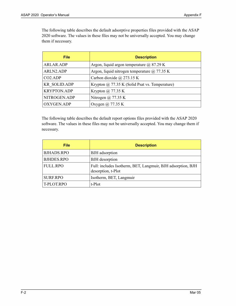
ASAP 2020 Operator’s Manual Appendix F
The following table describes the default adsorptive properties files provided with the ASAP 2020 software. The values in these files may not be universally accepted. You may change them if necessary.
The following table describes the default report options files provided with the ASAP 2020 software. The values in these files may not be universally accepted. You may change them if necessary.
File Description
ARLAR.ADP Argon, liquid argon temperature @ 87.29 K
ARLN2.ADP Argon, liquid nitrogen temperature @ 77.35 K
CO2.ADP Carbon dioxide @ 273.15 K
KR_SOLID.ADP Krypton @ 77.35 K (Solid Psat vs. Temperature)
KRYPTON.ADP Krypton @ 77.35 K
NITROGEN.ADP Nitrogen @ 77.35 K
OXYGEN.ADP Oxygen @ 77.35 K
File Description
BJHADS.RPO BJH adsorption
BJHDES.RPO BJH desorption
FULL.RPO Full: includes Isotherm, BET, Langmuir, BJH adsorption, BJH desorption, t-Plot
SURF.RPO Isotherm, BET, Langmuir
T-PLOT.RPO t-Plot
F-2 Mar 05

Appendix F ASAP 2020 Operator’s Manual
The following table describes the files created by the ASAP 2020 software.
File Description
* ASAP2020.INI ASCII file containing initialization information used during pro-gram startup as well as system options information.
* ASAP2020.SMP Binary file containing 2020 sample defaults.
2020-N.STS Binary file containing 2020 instrument status information and calibration data. The letter N in the file name represents the unit number of the instrument for which information applies.
Do not attempt to edit this file. Personal injury or damage to the ASAP 2020 could result because the operator may be given erroneous status information.
* ASAP 2020.LOG ASCII file containing a recorded log of all error messages dis-played on the screen.
* N.LOG Binary log file for analyzer with serial number contents acces-sible using the Show Instrument Log option on the Unit menu.
*Back up these files periodically to ensure data integrity. You may want to store each backup set on a separate CD so you have access to different versions of the files. For example, ASAP 2020.SMP contains the default sample information. Any time the sample defaults are changed, an updated ASAP2020.SMP is created. Keeping version backups of this file by storing each on a separate CD allows restoration of any version desired.
Mar 05 F-3

ASAP 2020 Operator’s Manual Appendix F
F-4 Mar 05

ASAP 2020 Operator’s Manual Appendix G
G. DFT MODELS
Theories are developed by scientists in an attempt to explain a class of observed behavior. In the experimental physical sciences, theories are often expressed in terms of a model that can be visualized and described mathematically. Early models of physical adsorption were quite simple, both conceptually and mathematically, for very practical reasons — hand computa-tions were required. Today we can explore complex models that describe adsorption systems on the atomic scale of size and sub-picosecond time frame. This is not because scientists are smarter, but because of available tools. The DFT models are created by classical approaches to adsorption as well as models based on modern statistical thermodynamics.
Models Based on Statistical Thermodynamics
Included in this group are methods that model the adsorption system in terms of forces acting between individual molecules.
Theoretical Background
Traditional adsorption theories attempt to describe experimental adsorption isotherms with an isotherm equation containing a small number of parameters. At a minimum, these parameters include the extent of the surface, such as the monolayer capacity (Vm), and the molar inten-sity of the gas-surface interaction, such as the Langmuir “K” constant or the BET “C” constant. In some equations, additional parameters take into account the lateral interaction of adsorbed molecules with each other. Other theories, such as the Dubinin-Astakhov approach, also include parameters for the effect of adsorbent porosity.
Instead of this classical kinetic or phenomenological approach, we can use a molecular-based statistical thermodynamic theory that allows us to relate the adsorption isotherm to the micro-scopic properties of the system: the fluid-fluid and fluid-solid interaction energy parameters, the pore size, the pore geometry, and the temperature.
The following example is given so that you may understand how such a theory is constructed.
A clean sample of a solid material containing slit-shaped pores of a single width is placed in an evacuated space. It is kept at a fixed temperature as a known quantity of pure argon gas is admitted into the space surrounding the sample. The pressure within the space is recorded over time. In this situation, the pressure falls rapidly from its initial value and gradually approaches a steady reading, called the equilibrium pressure. The amount adsorbed corre-sponds to the quantity of gas effectively removed from the gas phase by the solid surface. A graph that plots amount adsorbed versus equilibrium pressure is called an adsorption isotherm.
Under such conditions, the argon atoms that randomly enter the pore space feel the presence of the solid surface as the action of an external attractive force (the dispersion forces or Van der Waal’s forces) and spend more time near the surface. As a result, the space near the sur-face acquires a greater average density of argon atoms than regions farther removed.
Mar 2011 G-1

Appendix G ASAP 2020 Operator’s Manual
If the equilibrium distribution of the gas atoms near the surface could be described as a func-tion of pressure and the molecular properties of the components of the system, then a model could be constructed for the adsorption isotherm for the system. Modern physical chemistry provides several ways to calculate this distribution. All these methods are based on the fun-damental thermodynamic law that such a system adopts a configuration of minimum free energy at equilibrium. Also needed is a description of the pairwise interaction energy between atoms, U(s), commonly given by a Lennard-Jones potential:
where
= a characteristic energy of the adsorptive, = the diameter of the adsorptive molecule, ands = the separation distance.
Molecular Simulation Methods
Two simulation techniques are commonly used to determine the distribution of gas molecules in a system in equilibrium: the molecular dynamics method and the Monte Carlo method. Both of these are used as reference methods because their results are considered exact.
Molecular Dynamics Method
In the molecular dynamics method, the position and velocity of individual gas particles are calculated over time at very short intervals. This method takes into account both the forces acting between the gas particles themselves and those acting between the gas particles and the atoms of the simulated surface. As the simulated particles collide with each other and with the surface, the average concentration of particles in the space near the surface is calculated; this calculation yields the amount of gas adsorbed.
This method can be thought of as a way to determine the chronological record of the move-ment of each particle in the system using time steps of 10-14 seconds. Although the mathematics are simple, the number of calculations required for a system of even a few hun-dred particles is astronomical and challenges even the fastest computers.
Monte Carlo Method
In the Monte Carlo method, determination of the system equilibrium distribution begins with an assumption (which may be only approximate) about the initial configuration of particles in the system. The system is “equilibrated” through a process of randomly selecting one particle and conditionally moving it a random distance in a random direction.
If the move results in a configuration of lower total energy, then the move is completed and another particle is randomly selected to be moved.
U s s--- 12
s--- 6
–=
G-2 Mar 2011

ASAP 2020 Operator’s Manual Appendix G
If the move results in a configuration of higher energy, a probability for that event is calcu-lated, and a random number between zero and one is generated. If the generated number is smaller than the probability of the event, then the move is accepted; otherwise, another par-ticle is selected and the process is repeated. This process continues until the average total energy of the system no longer decreases; at this point, average configuration data are accu-mulated to yield the mean density distribution of particles in the system.
Monte Carlo simulations require considerably less computation time than molecular dynamic simulations and can yield the same results; however, neither method provides a really prac-tical way to calculate complete isotherms.
Density Functional Formulation
Density functional theory offers a practical alternative to both molecular dynamic and Monte Carlo simulations. When compared to reference methods based on molecular simulation, this theory provides an accurate method of describing inhomogeneous systems yet requires fewer calculations. Because the density functional theory provides accuracy and a reduced number of calculations, it is the basis embodied in the DFT models.
The system being modeled consists of a single pore represented by two parallel walls sepa-rated by a distance H. The pore is open and immersed in a single component fluid (adsorptive) at a fixed temperature and pressure. Under such conditions, the fluid responds to the walls and reaches an equilibrium distribution. In this condition (by the definition of equi-librium), the chemical potential at every point equals the chemical potential of the bulk fluid. The bulk fluid is a homogenous system of constant density; its chemical potential* is deter-mined by the pressure of the system using well-known equations. The fluid near the walls is not of constant density; its chemical potential is composed of several position-dependent con-tributions that must total at every point to the same value as the chemical potential of the bulk fluid.
As noted previously, at equilibrium, the whole system has a minimum (Helmholtz) free energy, known thermodynamically as the grand potential energy (GPE). Density functional theory describes the thermodynamic grand potential as a functional of the single-particle den-sity distribution; therefore, calculating the density profile that minimizes the GPE yields the equilibrium density profile. The calculation method requires the solution of a system of com-plex integral equations that are implicit functions of the density vector. Since analytic solutions are not possible, the problem must be solved using iterative numerical methods. Although calculation using these methods still requires supercomputing speed, the calculation of many isotherm pressure points for a wide range of pore sizes is a feasible task. The com-plete details of the theory and the mathematics can be found in the papers listed under References at the end of this appendix.
The following graphs and accompanying text illustrate the results of using density functional theory to predict the behavior of a model system.
*Chemical potential may be thought of as the energy change felt by a probe particle when it is inserted into the system from a reference point outside the system. It can also be defined as the partial derivative of the grand potential energy with respect to density (or concentration).
Mar 2011 G-3

Appendix G ASAP 2020 Operator’s Manual
Figure G-1 shows the density profile for argon at a carbon surface as calculated by density functional theory for a temperature of 87.3 K and a relative pressure of about 0.5.
Figure G-1. Density Profile for Argon on Carbon at 87.3 K and a Relative Pressure of 0.5
This figure represents a cross-section of the region near the surface. Note the layerwise dis-tribution of adsorbate; the first monolayer is sharply defined and a third layer can be distinguished. The area under the profile curve represents the amount adsorbed per unit area at this pressure. The positions of the maxima are separated by a distance determined by the size of the adsorptive atom.
Given the density profile, the amount adsorbed at the stated pressure can be easily calculated as the integral over the profile. Repeating this calculation over a range of pressures yields the adsorption isotherm for the model. If the value of H is very large, the isotherm obtained cor-responds to that of an external, or free, surface. If H is smaller, a range of pressures is reached where two minima exist for the grand potential, showing the presence of two metastable phases having different density distributions but the same chemical potential. The phase with the lower GPE is the stable one. As the pressure is increased, a point is reached where the other phase becomes the stable one. This phase transition reflects condensation of adsorbate in the pore; the pressure at which it occurs is called the critical pore-filling pressure. This pressure is analogous to the condensation pressure predicted by the Kelvin equation in the classical model of pore filling.
Figure G-2 shows how the profiles change with pressure for a model pore with H = 40 ang-stroms. The insets show the density profiles for the corresponding points of the isotherm.
G-4 Mar 2011
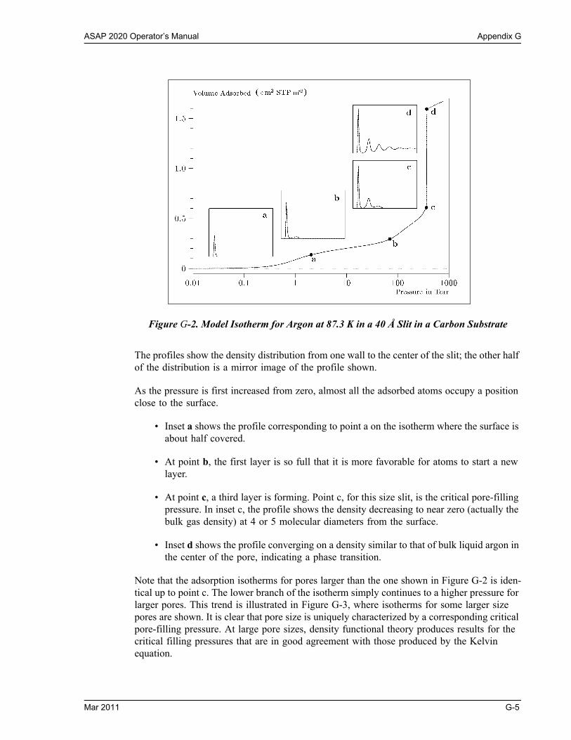
ASAP 2020 Operator’s Manual Appendix G
Figure G-2. Model Isotherm for Argon at 87.3 K in a 40 Å Slit in a Carbon Substrate
The profiles show the density distribution from one wall to the center of the slit; the other half of the distribution is a mirror image of the profile shown.
As the pressure is first increased from zero, almost all the adsorbed atoms occupy a position close to the surface.
• Inset a shows the profile corresponding to point a on the isotherm where the surface is about half covered.
• At point b, the first layer is so full that it is more favorable for atoms to start a new layer.
• At point c, a third layer is forming. Point c, for this size slit, is the critical pore-filling pressure. In inset c, the profile shows the density decreasing to near zero (actually the bulk gas density) at 4 or 5 molecular diameters from the surface.
• Inset d shows the profile converging on a density similar to that of bulk liquid argon in the center of the pore, indicating a phase transition.
Note that the adsorption isotherms for pores larger than the one shown in Figure G-2 is iden-tical up to point c. The lower branch of the isotherm simply continues to a higher pressure for larger pores. This trend is illustrated in Figure G-3, where isotherms for some larger size pores are shown. It is clear that pore size is uniquely characterized by a corresponding critical pore-filling pressure. At large pore sizes, density functional theory produces results for the critical filling pressures that are in good agreement with those produced by the Kelvin equation.
Mar 2011 G-5
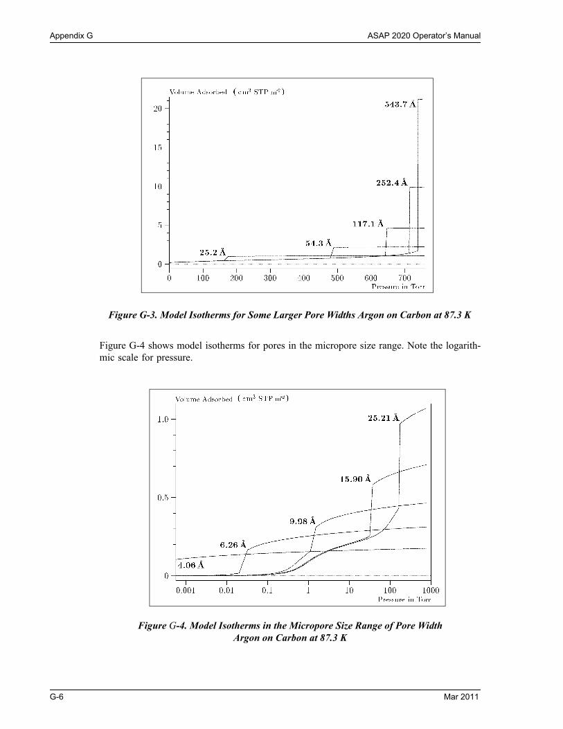
Appendix G ASAP 2020 Operator’s Manual
Figure G-3. Model Isotherms for Some Larger Pore Widths Argon on Carbon at 87.3 K
Figure G-4 shows model isotherms for pores in the micropore size range. Note the logarith-mic scale for pressure.
Figure G-4. Model Isotherms in the Micropore Size Range of Pore WidthArgon on Carbon at 87.3 K
G-6 Mar 2011

ASAP 2020 Operator’s Manual Appendix G
Pores of 4 Å width, barely larger than the argon atom (3.38 Å), fill at pressures below 1 mil-litorr. Pores below 15 Å fill before a monolayer is completed on the surface of the larger pores. In the micropore size range, the pore volume fills more gradually with pressure and the total shape of the isotherm is important in characterizing the pore size.
Models Included
Non-Local Density Functional Theory with Density-Independent Weights
N2 - DFT ModelAR - DFT Model
Using the methods of non-local density functional theory, two sets of isotherms have been calculated to serve as kernel functions for the characterization of porous solids from adsorp-tion data. The model isotherms are stored in binary format files. These models assume a slit-like pore geometry. The pore size range from 4.0 to 4000 Å is covered in 91 classes in a geo-metric progression. The class intervals are rounded to the nearest 0.02 molecular diameters. A model for the free or external surface is included to account for unfilled pores. Each of the 92 model isotherms has been calculated at 181 pressure points from near 1x10⁻⁶ to near 1.00 rel-ative pressure.
These models are identical to those supplied with the original DOS version of DFT software. Some slight difference from the DOS results may be noted when they are applied to the same data due to improvements in the deconvolution algorithm and better regularization of the cur-rent software.
Non-Local Density Functional Theory with Density-Dependent Weights
N2 - Modified Density Functional
Using the modified Tarazona prescription described by Olivier (refer to References, refer-ences 3 and 4), model isotherms were calculated for a wide range of adsorptive energies to a relative pressure of 0.6. The model makes no provision for pore filling in the micropore region. If the sample solid contains small mesopores, the isotherm data should be truncated (using the Select Data Points dialog box) to a suitably low relative pressure to avoid trying to fit this region; mesopore filling reports as a large area of low energy in the calculated distri-bution of adsorptive potential.
Geometry: SlitSubstrate: Carbon (graphite)Category: PorosityMethod: Nitrogen at 77 K; Argon at 87 K
Geometry: Free surfaceSubstrate: Surface energyMethod: Nitrogen at 77K
Mar 2011 G-7

Appendix G ASAP 2020 Operator’s Manual
The surface energy is reported in terms of the effective Lennard-Jones interaction parameter, e, for the adsorptive/adsorbent pair divided by Boltzmann’s constant. The units are therefore Kelvins.
N2 - Cylindrical Pores - Oxide SurfaceAR - Cylindrical Pores - Oxide Surface
Model isotherms were calculated using a combination of statistical mechanical calculations and experimental observations for macroporous silicas and MCM-41 mesoporous silicas as well as zeolites. The pore-filling pressures were determined as a function of the pore size from adsorption isotherms on MCM-41 materials characterized by X-ray and other tech-niques. The variation of the pore fluid density with pressure and pore size has been accounted for by density functional theory calculations. The N2 model reports pore sizes ranging from 3.8 to 387 angstroms and the AR model from 3.8 to over 500 angstroms.
N2 – Cylindrical Pores – Pillared Clay Surface (Montmorillionite)
Model isotherms were calculated using a combination of statistical thermodynamic Non-Local Density Functional Theory (NLDFT) calculations and experimental isotherms for ref-erence samples of montmorillionite.The construction method for the hybrid models was analogous to that described in the first reference below (Jaroniec et al,1999). The additional references add additional theoretical details as well as examples of the application of the model to pillared clay catalysts.This model reports pore widths from 3.8 to 387 angstroms.
Geometry: CylinderSubstrate: OxideCategory: PorosityMethod: Nitrogen at 77 K; Argon at 87 K
Reference: M. Jaroniec, M. Kruk, J.P. Olivier, and S. Koch, “A New Method for the Accurate Pore Size Analysis of MCM-41 and Other Silica-Based Mesoporous Materials,” Proceedings of COPS-V, Heidelberg, Germany (1999)
Geometry: CylinderSubstrate: Crystalline SilicateCategory: PorosityMethod: Nitrogen at 77 K
G-8 Mar 2011

ASAP 2020 Operator’s Manual Appendix G
C02 - DFT Model
Model isotherms were calculated, using the non-local prescription of Tarazona, employing molecular parameters derived from the known bulk properties of carbon dioxide.
AR - Modified Density Functional Model
This model was produced in the same manner as the N2 Modified Density Functional model listed earlier, except applicable to argon adsorbed at 87.3 K.
References: Mietec Jaroniec, Michal Kruk, James P. Olivier and Stefan Koch, “A New Method for the Characterization of Mesoporous Silicas,” Proceedings of COPS-V, 1999, Studies in Surface Science, Vol 128, Characterization of porous Solids V , Unger, et al, Eds, Elsevier, Amsterdam, 2000.
James P. Olivier and Mario L. Occell, “Surface Area and Microporosity of a Pillared Interlayered Clay (PILC) from a Hybrid Density Functional Theory (DFT) Method,” The Journal of Physical Chemistry B; 2001, 105(3), 623-629.
M. L. Occelli, J. P. Olivier, J. A. Perdigon-Melon, and A. Auroux, “Surface Area, Pore Volume Distribution, and Acidity in Mesoporous Expanded Clay Catalysts from Hybrid Density Functional Theory (DFT) and Adsorption Microcalorimetry Methods,” Langmuir 2002, 18, 9816-9823.9b
James P. Olivier, “The Importance of Surface Heterogeneity in Developing Characterization Methods.” 6th International Symposium on the Character-ization of Porous Solids, Studies in Surface Science and Catalysis 144, Elsevier, 2002.
James P. Olivier and Mario L. Occelli, “Surface Area and Microporosity of Pillared Rectorite Catalysts from a Hybrid Density Functional Theory Method,” Microporous and Mesoporous Materials 2003, 57, 291-296.
Geometry: SlitSubstrate: CarbonCategory: PorosityMethod: Carbon dioxide at 273 K
Geometry: Free SurfaceSubstrate: AnyCategory: Surface energyMethod: Argon at 87 K
Mar 2011 G-9

Appendix G ASAP 2020 Operator’s Manual
N2 - Tarazona NLDFT, Esf = 30.0K
Model isotherms were calculated using the prescriptions of Tarazona for density dependent weighting functions and a cylindrical pore geometry. The wall potential used is k = 30 K, typ-ical for a silica or alumina surface.
This model file is particularly useful for sizing zeolites or zeolite containing materials that have substantial micropore volume. The reported pore size range is 3.8 to 387 angstroms.
N2 - Carbon Slit Pores by NLDFTAr - Carbon Slit Pores by NLDFT
Model isotherms were calculated using the prescriptions of Tarazona for density dependent weighting functions and a slit-like pore geometry. These models are slightly different from N2-DFT and Ar-DFT models that were calculated using NLDFT with density independent weighting functions.
The reported pore size range is from 3.5 to 1000 angstroms.
N2 - Carbon Finite Pores, As=6, 2D-NLDFTAr - Carbon Finite Pores, As=6, 2D-NLDFT
Model isotherms were calculated using the prescriptions of Tarazona for density dependent weighting functions assuming 2D model of finite slit pores having a diam-eter-to-width aspect ratio of 6.
Geometry: CylinderSubstrate: OxideCategory: PorosityMethod: Nitrogen at 77 K
Reference: P. Tarazona, Phys. Rev. A 31: 2672 (1985).Idem, Phys. Rev. A 32: 3148 (1985).P. Tarazona, U. M. B. Marconi, and R. Evans, Mol. Phys. 60: 573 (1987).
Geometry: SlitSubstrate: CarbonCategory: PorosityMethod: Nitrogen at 77 K; Argon at 87 K
Reference: P. Tarazona, Phys. Rev. A 31: 2672 (1985).Idem, Phys. Rev. A 32: 3148 (1985).P. Tarazona, U. M. B. Marconi, and R. Evans, Mol. Phys. 60: 573 (1987).
Geometry: Finite SlitSubstrate: CarbonCategory: PorosityMethod: Nitrogen at 77 K; Argon at 87 K
G-10 Mar 2011

ASAP 2020 Operator’s Manual Appendix G
This model is particularly useful for microporous carbon materials. The reported pore size range is from 3.5 to 250 angstroms.
N2 - Carbon Finite Pores, As=12, 2D-NLDFTAr - Carbon Finite Pores, As=12, 2D-NLDFT
Model isotherms were calculated using the same methods and assumptions that were used in the model above except in this model, the aspect ratio is equal to 12.
These two finite pore models may be used as a research tool in conjunction with independent analytical techniques such as high-resolution transmission electron microscopy (HRTEM) and/or X-ray diffraction (XRD) to obtain comprehensive information about the structure of studied carbon material.
N2 - Carbon Cylinder, single-wall nanotube by NLDFTAr - Argon Cylinder, single-wall nanotube by NLDFT
Model isotherms were calculated using the prescriptions of Tarazona for density dependent weighting functions and cylindrical pore geometry. The pore wall potential is described by the Lennard-Jones potential of interaction between a gas molecule and the graphitic surface of an infinitely long cylinder.
This model is particularly useful for characterizing carbon single-wall nanotubes. The reported pore size range is from 3.5 to 1000 angstroms.
Reference: Jacek Jagiello and James P. Olivier. “A simple two-dimensional NLDFT model of gas adsorption in finite carbon pores. Application to pore structure analysis.,” The Journal of Physical Chemistry C, 113(45):19382-19385, 2009.
Geometry: Finite SlitSubstrate: CarbonCategory: PorosityMethod: Nitrogen at 77 K; Argon at 87 K
Reference: See above reference.
Geometry: CylinderSubstrate: CarbonCategory: PorosityMethod: Nitrogen at 77 K; Argon at 87K
Reference: P. Tarazona, Phys. Rev. A 31: 2672 (1985).Idem, Phys. Rev. A 32: 3148 (1985).P. Tarazona, U. M. B. Marconi, and R. Evans, Mol. Phys. 60: 573 (1987).
Mar 2011 G-11

Appendix G ASAP 2020 Operator’s Manual
N2 - Carbon Cylinder, multi-wall nanotube by NLDFTAr - Argon Cylinder, multi-wall nanotube by NLDFT
Model isotherms were calculated using the prescriptions of Tarazona for density dependent weighting functions and cylindrical pore geometry. The pore wall potential is described by the Lennard-Jones potential of interaction between a gas molecule and multiple concentric graphitic surfaces of infinitely long cylinders.
This model is particularly useful for characterizing carbon multi-wall nanotubes. The reported pore size range is from 3.5 to 1000 angstroms.
Ar - Zeolites H-Form by NLDFT
Model isotherms were calculated using the prescriptions of Tarazona for density dependent weighting functions and cylindrical pore geometry. The pore wall potential is described by the Lennard-Jones potential of interaction between a gas molecule and the oxide surface of an infinitely long cylinder.
This model is particularly useful for characterizing oxides and H+ and (NH4)+ exchanged zeo-lites. The reported pore size range is from 3.5 to 300 angstroms.
Ar - Zeolites Me-Form by NLDFT
Model isotherms were calculated using the prescriptions of Tarazona for density dependent weighting functions and cylindrical pore geometry. The pore wall potential is described by the Lennard-Jones potential of interaction between a gas molecule and the oxide surface of an infinitely long cylinder.
This model is similar to the model above but it more appropriate is for characterizing alkali metal exchanged zeolites. The reported pore size range is from 3.5 to 300 angstroms.
Geometry: CylinderSubstrate: CarbonCategory: PorosityMethod: Nitrogen at 77 K; Argon at 87K
Reference: See above reference.
Geometry: CylinderSubstrate: ZeoliteCategory: PorosityMethod: Argon at 77K
Geometry: CylinderSubstrate: ZeoliteCategory: PorosityMethod: Argon at 77K
G-12 Mar 2011

ASAP 2020 Operator’s Manual Appendix G
Models Based on Classical Theories
Both surface energy distribution and pore size distribution may be evaluated using classical approaches to model kernel functions for use with equation (1) of the DFT Theory in the cal-culations appendix. Be aware that the deconvolution method only provides a fitting mechanism; it does not overcome any inherent shortcomings in the underlying theory.
Surface Energy
The use of classical theories to extract adsorptive potential distribution is mostly of historical interest. At a minimum, the equation must contain a parameter dependent on adsorption energy and another dependent on monolayer capacity, or surface area. This is sufficient to permit the calculation of the set of model isotherms that is used to create a library model. The Langmuir equation has been used in the past, as have the Hill-de Boer equation and the Fowler-Guggenheim equation. All of these suffer from the fact that they only describe mono-layer adsorption, whereas the data may include contributions from multilayer formation.
Pore Size
It is well established that the pore space of a mesoporous solid fills with condensed adsorbate at pressures somewhat below the prevailing saturated vapor pressure of the adsorptive. When combined with a correlating function that relates pore size with a critical condensation pres-sure, this knowledge can be used to characterize the mesopore size distribution of the adsorbent. The correlating function most commonly used is the Kelvin equation. Refinements make allowance for the reduction of the physical pore size by the thickness of the adsorbed film existing at the critical condensation pressure. Still further refinements adjust the film thickness for the curvature of the pore wall.
The commonly used practical methods of extracting mesopore distribution from isotherm data using Kelvin-based theories, such as the BJH method, were for the most part developed decades ago and were designed for hand computation using relatively few experimental points. In general, these methods visualize the incremental decomposition of an experimental isotherm, starting at the highest relative pressure or pore size. At each step, the quantity of adsorptive involved is divided between pore emptying and film thinning processes and exactly is accounted for. This computational algorithm frequently leads to inconsistencies when carried to small mesopore sizes. If the thickness curve used is too steep, it finally will predict a larger increment of adsorptive for a given pressure increment than is actually observed; since a negative pore volume is non-physical, the algorithm must stop. Conversely, if the thickness curve used underestimates film thinning, accumulated error results in the cal-culation of an overly large volume of (possibly nonexistent) small pores.
The use of equation (1) represents an improvement over the traditional algorithm. Kernel functions corresponding to various classical Kelvin-based methods have been calculated for differing geometries and included in the list of models.
Mar 2011 G-13
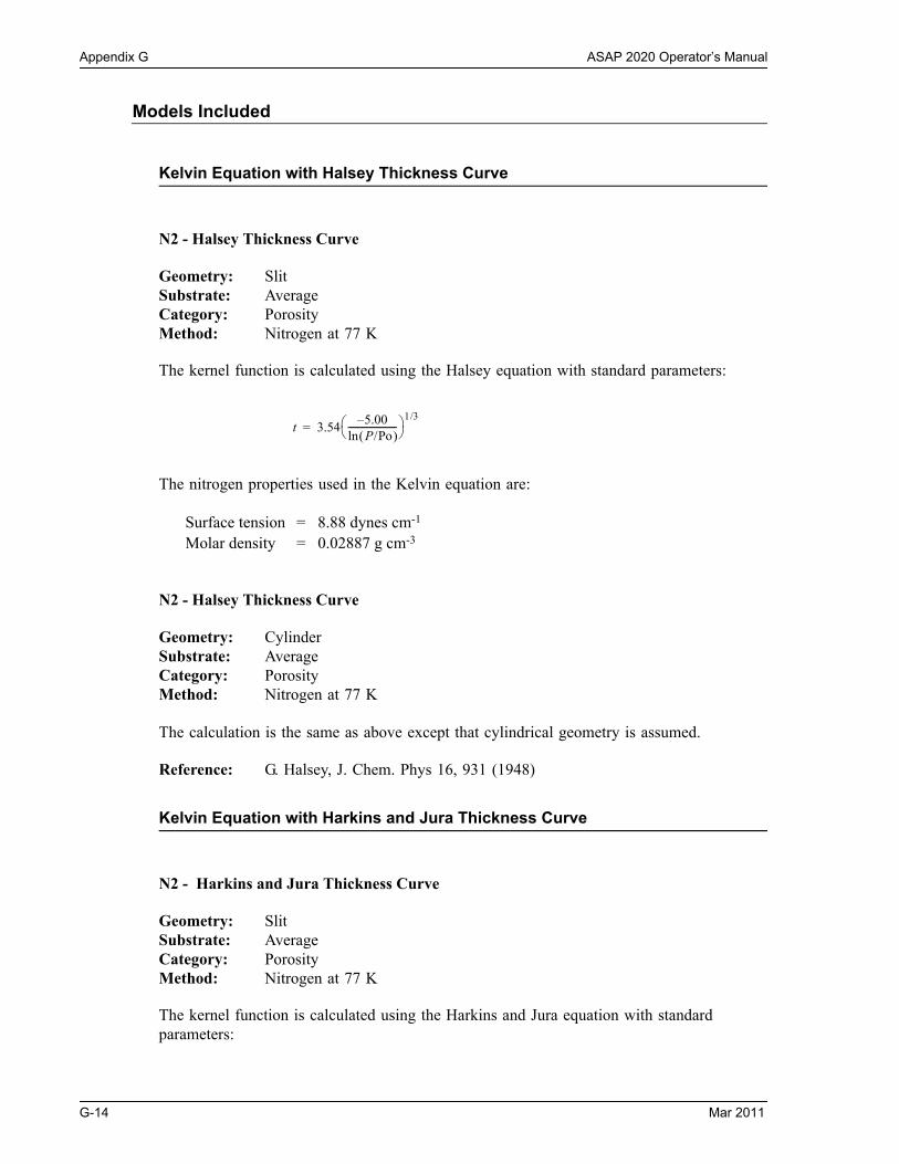
Appendix G ASAP 2020 Operator’s Manual
Models Included
Kelvin Equation with Halsey Thickness Curve
N2 - Halsey Thickness Curve
The kernel function is calculated using the Halsey equation with standard parameters:
The nitrogen properties used in the Kelvin equation are:
Surface tension = 8.88 dynes cm-1
Molar density = 0.02887 g cm-3
N2 - Halsey Thickness Curve
The calculation is the same as above except that cylindrical geometry is assumed.
Kelvin Equation with Harkins and Jura Thickness Curve
N2 - Harkins and Jura Thickness Curve
The kernel function is calculated using the Harkins and Jura equation with standard parameters:
Geometry: SlitSubstrate: AverageCategory: PorosityMethod: Nitrogen at 77 K
Geometry: CylinderSubstrate: AverageCategory: PorosityMethod: Nitrogen at 77 K
Reference: G. Halsey, J. Chem. Phys 16, 931 (1948)
Geometry: SlitSubstrate: AverageCategory: PorosityMethod: Nitrogen at 77 K
t 3.545.00–P/Po ln
---------------------- 1/3
=
G-14 Mar 2011

ASAP 2020 Operator’s Manual Appendix G
The nitrogen properties used in the Kelvin equation are:
Surface tension = 8.88 dynes cm-1
Molar density = 0.02887 g cm-3
N2 - Harkins and Jura Thickness Curve
The calculation is the same as above except that cylindrical geometry is assumed.
Kelvin Equation with Broekhoff-de Boer Thickness Curve
N2 - Broekhoff-de Boer Model
The kernel function is calculated using the Broekhoff-de Boer equation with standard parameters:
The nitrogen properties used in the Kelvin equation are:
Surface tension = 8.88 dynes cm-1
Molar density = 0.02887 g cm-3
N2 - Broekhoff-de Boer Model
Geometry: CylinderSubstrate: AverageCategory: PorosityMethod: Nitrogen at 77 K
References: W. D. Harkins and G. Jura, J.A.C.S. 66, 1366 (1944)
J. H. DeBoer et al., J. Colloid and Interface Sci. 21, 405 (1966)
Geometry: SlitSubstrate: AverageCategory: PorosityMethod: Nitrogen at 77 K
Geometry: CylinderSubstrate: AverageCategory: PorosityMethod: Nitrogen at 77 K
t13.99
0.034 P/Po log–--------------------------------------------- 1/2
=
Mar 2011 G-15

The calculation is similar to the above except that cylindrical geometry is assumed, and the film thickness depends on pore size (see reference).
References
The papers listed below provide additional information on DFT models:
1. “Determination of Pore Size Distribution from Density Functional Theoretic Models of Adsorption and Condensation within Porous Solids,” J.P. Olivier and W.B. Conklin, Micromeritics Instrument Corp; presented at the International Symposium on the Effects of Surface Heterogeneity in Adsorption and Catalysts on Solids, Kazimierz Dolny, Poland (July 1992).
2. “Classification of Adsorption Behavior: Simple Fluids in Pores of Slit-shaped Geometry,” Perla B. Balbuena and Keith E. Gubbins, Fluid Phase Equilibria, 76, 21-35, Elsevier Science Publishers, B.V., Amsterdam (1992).
3. “Modeling Physical Adsorption on Porous and Nonporous solids Using Density Functional Theory,” J.P. Olivier, Journal of Porous Materials, 3, 9-17 (1995).
4. “The Determination of Surface Energetic Heterogeneity Using Model Isotherms Calculated by Density Functional Theory,” J.P. Olivier; presented at the Fifth International Conference on the Fundamentals of Adsorption, Pacific Grove, CA (1995).
Reference: Specifically, equations 20 and 21 in: J.C.P. Broekhoff and J.H. de Boer, “The Surface Area in Intermediate Pores,” Proceedings of the International Sym-posium on Surface Area Determination, D.H. Everett, R.H. Ottwill, eds., U.K. (1969)

ASAP 2020 Operator’s Manual Index
INDEX
Symbols$ symbol, 8-6, 8-9
AAbsolute pressure tolerance, 5-27Add log entry, 8-11Adding an analyzer, 2-17Adsorption isotherm, G-1Adsorptive Properties dialog, 5-31Adsorptive properties file, 5-31
defining, 4-13listing file statistics, 4-32, 5-99printing contents, 4-31
Advanced format, 8-2creating sample file, 4-6establishing sample defaults, 4-4Sample information file, 5-6
Alpha-S curve, saving, 5-96Alpha-S Method dialog, 5-55Alpha-S report, 5-55Alumina, replacing in oil vapor traps, 9-11Ambient temperature, 5-23Analysis
bath, 4-28details, 6-13Dewar, checking, 9-4Dewar, installing, 4-28dialog, 6-3performing, 4-29, 6-3program, installing, 2-12skipping steps, 6-6status, 6-13suspending, 6-6viewing options, 6-3
Analysis Conditions dialog, 5-16Analysis conditions file, 5-16
defining, 4-11identification, 5-16listing file statistics, 4-32, 5-99printing contents, 4-31
Analysis programexiting, 5-104installing upgrade, 2-16subsequent installation, 2-16uninstalling, 2-24
Analyzeradding another, 2-17changing setup, 2-22cleaning, 9-22
description, 1-10front panel, 3-1lifting, 2-1moving to a different computer, 2-18removing, 2-21
Ar Carbon Finite Pores, As=12, 2D-NLDFT model,G-11
Ar Carbon Finite Pores, As=6, 2D-NLDFT model, G-10Ar Carbon Slit Pores by NLDFT model, G-10AR Cylindrical Pores - Oxide Surface model, G-8AR DFT model, G-7AR Modified Density Functional Model, G-9Argon Cylinder, multi-wall nanotube by NLDFT model,
G-12Argon Cylinder, single-wall nanotube by NLDFT model,
G-11ASAP 2000 files, converting for 2020 program, 5-102ASAP 2010 sample files, opening, 5-102ASCII text
saving reports, 7-21Automatic Degas dialog, 6-8Autoscale x- and y-axis, 5-46Avogadro's number, C-22Axis
coordinates, viewing, 7-27properties, editing, 7-26
Axis Properties dialog, 7-26
BBackfill
gas, 5-30options, 5-30
Backfill gas, 4-19Bar code, 4-5, 5-7, 8-10Basic format, 8-2, 8-3
creating sample file, 4-8Sample information file, 5-9specifying sample defaults, 4-1, 8-5
Bath temperature, 6-5BET Surface Area report, 5-42BET surface area report
calculations, C-8BET Surface Area Report, example, 7-32BJH Adsorption Report, example, 7-36BJH Adsorption/Desorption plot options dialog, 5-67BJH Adsorption/Desorption report, 5-60
calculations, C-13plot, 5-67tabular, 5-64
Mar 2011 Index-1

Index ASAP 2020 Operator’s Manual
BJH Adsorption/Desorption Report Options dialog, 5-60BJH Adsorptive Options dialog, 5-62BJH correction, 5-63BJH Desorption Report, example, 7-39Boltzmann’s constant, G-8Bookmarks tab, 1-4Broekhoff-de Boer equation, 5-52Broekhoff-de Boer thickness curve, C-11
CCables, connecting, 2-10Calculated free space, 5-23Calculated mass, 4-3, 4-5, 5-7, 5-10, 8-6, 8-10Calibrate Manifold Temperature dialog box, 9-16Calibrate Pressure Scale dialog box, 6-21Calibrate Servo Valve dialog box, 6-30Calibration
details, 6-16file, loading, 6-25files, reinstalling, 2-23Load from File, 6-25pressure offset, 6-21, 9-22pressure scale, 6-21, 9-23settings, saving, 6-25temperature, 6-22, 9-15Vacuum gauge, 6-20Volume, 6-22
Calibration command, 6-20Calibration Manifold Temperature dialog box, 6-22Calibration Vacuum Gauge dialog box, 6-30Cancel push button, 3-10Carbon Black STSA equation, 5-53Carbon Cylinder, multi-wall nanotube by NLDFT
model, G-12Carbon Cylinder, single-wall nanotube by NLDFT
model, G-11Cascade windows, 3-15Cautions, 1-3Check box, 3-9Chemical potential, G-3Cheng/Yang
calculations, C-25correction, 5-70Pore Geometry, C-24
Circuit breaker, valve, 9-2location, 3-5
Cleaninganalyzer, 9-22filler rods, 4-17sample tubes, 4-17
Close All command, 5-97Close command, 5-96Close push button, 3-10
Close Reports command, 7-5CO2 DFT Model, G-9Cold free space
for micropore analyses, E-2Cold trap, 1-10
Dewar, installing, 4-26location, 3-3tubes, cleaning, 9-14tubes, installing, 2-5
Collected Data dialog, 5-92Columns, editing on onscreen reports, 7-23Computer
power input, 2-7requirements, 1-15
Control Chart command, 7-11Control Chart Graph Options dialog, 7-12Control Chart Options dialog, 7-11Control Chart report, 7-11
defining the Y-axis, 7-12recalculating archived results, 7-12
Control Chart Sample Selection dialog, 7-13Controls, indicators, and connectors, 3-1
front panel, 3-1rear panel, 3-6side panel, 3-4
Conventionsoperator’s manual, 1-3
Convert command, 5-102Cross-hair, axis, 7-27Cross-references, 1-7Cryogen, 4-26Cumulative Reports, 5-62Curve Properties dialog, 7-25
DData
isotherm, exporting, 5-100selecting display options, 8-12type, 5-8
Date Range push button, 3-11Dates dialog box, 3-11Dates push button, 5-4Default Basic Sample Information dialog, 8-5Default files
adsorptive properties, F-2analysis conditions, F-1report options, F-2
DegasCalibrate pressure offset, 6-29Calibrate servo, 6-30Calibrate vacuum gauge, 6-30dialog, 6-8Enable manual control, 6-26
Index-2 Mar 2011

ASAP 2020 Operator’s Manual Index
monitoring, 6-28sample, 6-26Show instrument Schematic, 6-27Show status, 6-28
Degas command, 6-26Degas conditions file, 5-14
creating, 4-10listing file statistics, 4-32printing contents, 4-31
Degas portlocation, 3-3replacing filter, 9-7
Degassingsample, 4-22
Densitysample, 5-8, 5-10
Density Functional theory, G-3Destination, 5-98Dewar
analysis, installing, 4-28checking, 9-4cold trap, installing, 4-26precautions, 4-26raising and lowering, 6-10
DFT models, G-1See Models
DFT Pore Size Report Options dialog, 5-77DFT report
Pore size, 5-77surface energy, 5-80
DFT Surface Energy Report Options dialog, 5-80Diagnostics
gas line test, 9-19Diagnostics command, 6-18Dialog box, 3-9
closing, 3-10Directory, 5-4
limitations, 5-5Dollimore-Heal Adsorption/Desorption report, 5-69Dosing Options dialog, 5-25Dubinin report, 5-81
pore volume, 5-84tabular, 5-83transformed isotherm, 5-83
Dubinin Report Options dialog, 5-81Dubinin Transformed Isotherm Plot Options dialog, 5-83Dubinin-Astakhov
calculations, C-32, C-34, C-35Dubinin-Radushkevich
calculations, C-30
EElectrical requirements, 1-14
Elevator, 3-2, 6-10lubricating, 9-4raising and lowering, 6-9
Enable Manual Control commandanalyzer, 6-9degasser, 6-26
Entered mass, 4-3, 4-5, 5-7, 5-10, 8-6, 8-10Equilibration
calculations, C-6Equilibration dialog, 5-29Equipment
analyzer, 1-10damage and loss, 2-1description, 1-10returns, 2-2
Exit command, 5-104Exiting the analysis program, 3-8, 5-104Export
format, 5-101Export command, 5-100Export Sample File dialog box, 5-100Export Settings dialog, 6-6
FFile
listing statistics, 3-8name, including with file identification, 8-6, 8-9opening, 3-8printing to, 7-4See also Sample information filestatus, 3-12, 5-4
File menu, 5-1Close All command, 5-97Close command, 5-96Convert command, 5-102Exit command, 5-104Export command, 5-100List command, 5-99Open command, 5-3Print command, 5-98Save All command, 5-96Save As command, 5-95Save command, 5-94
File name default extensions, 3-13Filler rod, 4-16
cleaning, 4-17inserting into sample tube, 4-19
Find command, 1-8Fixed pore size table
conversion, 5-103Folder
directory, 5-5Format of exported data, 5-101
Mar 2011 Index-3
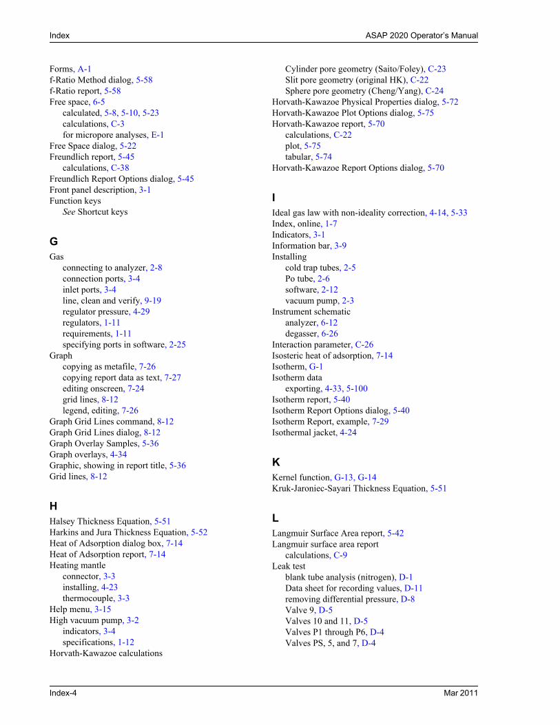
Index ASAP 2020 Operator’s Manual
Forms, A-1f-Ratio Method dialog, 5-58f-Ratio report, 5-58Free space, 6-5
calculated, 5-8, 5-10, 5-23calculations, C-3for micropore analyses, E-1
Free Space dialog, 5-22Freundlich report, 5-45
calculations, C-38Freundlich Report Options dialog, 5-45Front panel description, 3-1Function keys
See Shortcut keys
GGas
connecting to analyzer, 2-8connection ports, 3-4inlet ports, 3-4line, clean and verify, 9-19regulator pressure, 4-29regulators, 1-11requirements, 1-11specifying ports in software, 2-25
Graphcopying as metafile, 7-26copying report data as text, 7-27editing onscreen, 7-24grid lines, 8-12legend, editing, 7-26
Graph Grid Lines command, 8-12Graph Grid Lines dialog, 8-12Graph Overlay Samples, 5-36Graph overlays, 4-34Graphic, showing in report title, 5-36Grid lines, 8-12
HHalsey Thickness Equation, 5-51Harkins and Jura Thickness Equation, 5-52Heat of Adsorption dialog box, 7-14Heat of Adsorption report, 7-14Heating mantle
connector, 3-3installing, 4-23thermocouple, 3-3
Help menu, 3-15High vacuum pump, 3-2
indicators, 3-4specifications, 1-12
Horvath-Kawazoe calculations
Cylinder pore geometry (Saito/Foley), C-23Slit pore geometry (original HK), C-22Sphere pore geometry (Cheng/Yang), C-24
Horvath-Kawazoe Physical Properties dialog, 5-72Horvath-Kawazoe Plot Options dialog, 5-75Horvath-Kawazoe report, 5-70
calculations, C-22plot, 5-75tabular, 5-74
Horvath-Kawazoe Report Options dialog, 5-70
IIdeal gas law with non-ideality correction, 4-14, 5-33Index, online, 1-7Indicators, 3-1Information bar, 3-9Installing
cold trap tubes, 2-5Po tube, 2-6software, 2-12vacuum pump, 2-3
Instrument schematicanalyzer, 6-12degasser, 6-26
Interaction parameter, C-26Isosteric heat of adsorption, 7-14Isotherm, G-1Isotherm data
exporting, 4-33, 5-100Isotherm report, 5-40Isotherm Report Options dialog, 5-40Isotherm Report, example, 7-29Isothermal jacket, 4-24
KKernel function, G-13, G-14Kruk-Jaroniec-Sayari Thickness Equation, 5-51
LLangmuir Surface Area report, 5-42Langmuir surface area report
calculations, C-9Leak test
blank tube analysis (nitrogen), D-1Data sheet for recording values, D-11removing differential pressure, D-8Valve 9, D-5Valves 10 and 11, D-5Valves P1 through P6, D-4Valves PS, 5, and 7, D-4
Index-4 Mar 2011

ASAP 2020 Operator’s Manual Index
Legend Properties dialog, 7-26Lennard-Jones, G-2, G-8Links, 1-6List command, 5-99Listing file statistics, 5-99Load from File command, 6-25
MMain Menu bar, 3-14Maintenance, 9-1Manifold
temperature transducer, 1-13Manifold temperature
calibrating, 6-22, 9-15Manual control, 6-9
enabling for analyzer, 6-9Mass, 4-3, 5-7, 5-10, 8-6, 8-10MCM-41 materials, G-8Menu structure, 3-14Metafile, copying graph as, 7-26Micropore analyses, 5-27
free-space values, E-1Models, G-1
Ar Carbon finite pores by NLDFT, As=12, G-11Ar Carbon finite pores by NLDFT, As=6, G-10Ar Carbon slit pores by NLDFT, G-10AR Cylindrical Pores - Oxide Surface, G-8AR DFT model, G-7AR Modified Density Functional, G-9Argon Cylinder, multi-wall nanotube by NLDFT,
G-12Argon Cylinder, single-wall nanotube by NLDFT
model, G-11based on classical theories, G-13based on statistical thermodynamics, G-1Carbon Cylinder, multi-wall nanotube by NLDFT,
G-12CO2 DFT Model, G-9N2 Broekhoff-de Boer Model, G-15N2 Carbon Cylinder, single-walled nanotube by
NLDFT model, G-11N2 Carbon finite pores by NLDFT, As=12, G-11N2 Carbon finite pores by NLDFT, As=6, G-10N2 Carbon slit pores by NLDFT, G-10N2 Cylindrical Pores - Oxide Surface, G-8N2 Cylindrical Pores - Pillared Clay Surface, G-8N2 DFT model, G-7N2 Halsey Thickness Curve, G-14N2 Harkins and Jura Thickness Curve, G-14, G-15N2 Harkins and Jura Thickness Curve model, G-14N2 Modified Density Functional, G-7N2 Tarazona NLDFT, Esf = 30.0K, G-10Zeolites H-Form by NLDFT, G-12
Molecular dynamics, G-2Molecular simulation methods, G-2Monolayer capacity, 5-45Monte Carlo, G-2Montmorillionite, G-8MP-Method Plot Options dialog, 5-88MP-Method report, 5-86
calculations, C-36plot, 5-88tabular, 5-88
MP-Method Report Options dialog, 5-86MP-Method Tabular Report Column Options dialog,
5-88
NN2 Broekhoff-de Boer model, G-15N2 Broekhoff-de Boer Model model, G-15N2 Carbon Finite Pores, As=12, 2D-NLDFT model,
G-11N2 Carbon Finite Pores, As=6, 2D-NLDFT model, G-10N2 Carbon Slit Pores by NLDFT model, G-10N2 Cylindrical Pores - Oxide Surface model, G-8N2 Cylindrical Pores - Pillared Clay Surface model, G-8N2 DFT model, G-7N2 Halsey Thickness Curve model, G-14N2 Harkins and Jura Thickness Curve model, G-15N2 Modified Density Functional model, G-7N2 Tarazona NLDFT, Esf = 30.0K model, G-10Notes, 1-3
OOil vapor traps
replacing alumina, 9-11Online manual
cross references, 1-7index, 1-7printing options, 1-9using, 1-4See also Operator’s manual
Open Adsorptive Properties File dialog box, 4-13Open Analysis Conditions File dialog box, 4-11Open command, 5-3Open Report Options File dialog box, 4-14Open Sample Information File dialog, 4-6Open Sample Information File dialog box, 4-6, 4-8Operator’s manual
conventions, 1-3online, 1-4organization, 1-1
Option Presentation command, 8-2Options menu, 8-1
Graph Grid Lines command, 8-12
Mar 2011 Index-5

Index ASAP 2020 Operator’s Manual
Option Presentation command, 8-2Parameter Files Directory, 8-13Sample Defaults command, 8-4
Options report, 5-90Ordering information, 10-1Overlays
for multiple samples, 4-34generating, 4-34
PParameter files, 4-9
Adsorptive properties, 5-31Adsorptive properties, creating, 4-13Analysis conditions, 5-16Degas conditions, 5-14Degas conditions, creating, 4-10listing file statistics, 4-32, 5-99printing contents, 4-31printing contents of, 5-98Report options, 5-35Report options, creating, 4-14Sample tube, 5-12
Parameter files directory, 8-13Parameters, user, 8-11Parts, ordering, 10-1Pass/Fail Options dialog, 5-39Password, 8-3
Restricted format, 8-3Po and Temperature Options dialog, 5-24Po port, 3-4Po tube, installing, 2-6Pore filling pressure, G-4Pore Geometry
cylinder (Saito-Foley), C-23slit (original Horvath-Kawazoe), C-22sphere (Cheng/Yang), C-24
Pore size, G-13Port filter, degas, 9-7Ports
gas connection, 3-4Preparing samples, 4-16Pressure
measurement, 1-12relative, calculations, C-1, C-2table, 5-17
Pressure offsetcalibrating, 6-21, 9-22calibrating (Degasser), 6-29
Pressure scalecalibrating, 6-21, 9-23calibrating (Degasser), 6-29
Preventive maintenance schedule, 9-3Print command, 5-98
Printing file contents, 4-31Psat vs. Temperature Table dialog, 5-34Push buttons, 3-10
RRadio button, 3-9Rate of Adsorption, 7-17
Pressure table entries, 5-17Real gas equation of state, 4-14, 5-32, 5-33Regression report, 7-7
recalculating SPC values, 7-8selecting X- and Y-Axes variables, 7-8
Regression Report command, 7-7Regression Report Options dialog, 7-7Regression Report Sample Selection dialog, 7-8Regularization, 5-78Regulators
Gas, 1-11Relative pressure tolerance, 5-27Removing an analyzer, 2-21Replace push button, 3-10, 5-17Report
closing, 3-8, 7-5Control Chart, 7-11displaying company logo in title, 5-36Dollimore-Heal, 5-69examples, 7-27generated automatically, 6-5generating, 7-3generating automatically after analysis, 4-29graphs, editing onscreen, 7-24header, 7-18Heat of Adsorption, 7-14legend, editing, 7-26onscreen, shortcut menus for, 7-23Regression, 7-7saving in other formats, 7-21selecting, 7-5starting, 3-8Statistical Process Control (SPC), 7-6title, 5-35Validation, 5-91zoom feature, 7-27
Report button, 7-10Report options dialog, 5-35Report options file, 5-35
creating, 4-14listing file statistics, 4-32, 5-99printing contents, 4-31
Report Pressure Table dialog, 5-44Reports menu, 7-1
Close Reports command, 7-5Control Chart command, 7-11
Index-6 Mar 2011

ASAP 2020 Operator’s Manual Index
Rate of Adsorption command, 7-17Regression Report command, 7-7SPC Report Options command, 7-6Start Report command, 7-3
Reports to Generate dialog, 7-4Restricted format, 8-2, 8-3
creating sample file, 4-8password, 8-3Sample information file, 5-11specifying sample defaults, 8-5
Returned Materials Authorization (RMA), 2-2ROA data, collecting, 5-17RS232 port, 3-5
SSaito-Foley
calculations, C-23Pore Geometry, C-23
Sampledegassing, 4-22, 6-26determining amount to use, 4-20determining weight, 4-20information, defining, 4-6preparing, 4-16
Sample Analysis command, 6-3Sample Backfill Options, 5-30Sample defaults, 8-4
establishing for Advanced format, 8-7establishing for Basic format, 8-5
Sample information fileconverting 2000 files to 2020 files, 5-102creating, 4-6default values, 4-1exporting isotherm data, 4-33listing file statistics, 4-32, 5-99printing contents, 4-31, 5-98specifying defaults, 4-1
Sample Log report, 5-90Sample port, 3-4Sample tube
choosing, 4-16cleaning, 4-17displayed on schematic, 6-11installed, 4-24installing on sample port, 4-24labeling, 4-17replacing O-ring, 9-5set, 4-16
Sample Tube dialog, 5-12Sample tube file, 5-12
listing file statistics, 4-32printing contents, 4-31
Saturation pressure
calculations, C-1tube, installing, 2-6
Save All command, 5-96Save As command, 5-95Save as Default button, 7-13Save command, 5-94Save push button, 3-10Save to File command, 6-25Schematic
analyzer, 6-12degasser, 6-26
Select Dates dialog, 5-4Service Test command, 6-31Servo valve, calibrating (Degasser), 6-30Setup program
adding an analyzer, 2-17changing an analyzer setup, 2-22moving an analyzer to a different computer, 2-18reinstalling analysis program, 2-16reinstalling calibration files, 2-23removing an analyzer from the computer, 2-21uninstalling the software, 2-24using for other functions, 2-15
Shortcut keys, 3-7list of, 3-8
Shortcut menu, 3-7for graphs, 7-24for tabular reports, 7-23
Show Instrument Log command, 6-14Show Instrument Schematic command
analyzer, 6-12degasser, 6-27
Show Status commandanalyzer, 6-13degasser, 6-28
Softwareinstalling, 2-12installing upgrade, 2-16
SPC reportuser parameters, 5-8, 8-11
SPC Report Options command, 7-6SPC Report Options dialog, 7-6Specifications
ASAP 2020, 1-12SmartVac degas system, 1-13
Spreadsheet formatsaving reports in, 7-21
Start Degas command, 6-8Start Report command, 7-3Start Report dialog box, 7-3Status drop-down list, 3-12Status list, 7-3STSA thickness curve, C-11STSA Thickness equation, 5-53
Mar 2011 Index-7
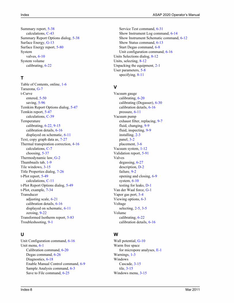
Index ASAP 2020 Operator’s Manual
Summary report, 5-38calculations, C-43
Summary Report Options dialog, 5-38Surface Energy, G-13Surface Energy report, 5-80System
valves, 6-10System volume
calibrating, 6-22
TTable of Contents, online, 1-6Tarazona, G-7t-Curve
entered, 5-50saving, 5-96
Temkim Report Options dialog, 5-47Temkin report, 5-47
calculations, C-39Temperature
calibrating, 6-22, 9-15calibration details, 6-16displayed on schematic, 6-11
Text, copy graph data as, 7-27Thermal transpiration correction, 4-16
calculations, C-7choosing, 5-37
Thermodynamic law, G-2Thumbnails tab, 1-9Tile windows, 3-15Title Properties dialog, 7-26t-Plot report, 5-49
calculations, C-11t-Plot Report Options dialog, 5-49t-Plot, example, 7-34Transducer
adjusting scale, 6-21calibration details, 6-16displayed on schematic, 6-11zeroing, 9-22
Transformed Isotherm report, 5-83Troubleshooting, 9-1
UUnit Configuration command, 6-16Unit menu, 6-1
Calibration command, 6-20Degas command, 6-26Diagnostics, 6-18Enable Manual Control command, 6-9Sample Analysis command, 6-3Save to File command, 6-25
Service Test command, 6-31Show Instrument Log command, 6-14Show Instrument Schematic command, 6-12Show Status command, 6-13Start Degas command, 6-8Unit configuration command, 6-16
Units Selections dialog, 8-12Units, selecting, 8-12Unpacking the equipment, 2-1User parameters, 5-8
specifying, 8-11
VVacuum gauge
calibrating, 6-20calibrating (Degasser), 6-30calibration details, 6-16pressure, 6-11
Vacuum pumpexhaust filter, replacing, 9-7fluid, changing, 9-9fluid, inspecting, 9-9installing, 2-3panel, 3-2placement, 3-6
Vacuum system, 1-12Validation report, 5-91Valves
degassing, 6-27description, D-2failure, 9-2opening and closing, 6-9system, 6-10testing for leaks, D-1
Van der Waal force, G-1Vapor gas port, 3-4Viewing options, 6-3Voltage
selecting, 2-5, 3-5Volume
calibrating, 6-22calibration details, 6-16
WWall potential, G-10Warm free space
for micropore analyses, E-1Warnings, 1-3Windows
Cascade, 3-15tile, 3-15
Windows menu, 3-15
Index-8 Mar 2011

ASAP 2020 Operator’s Manual Index
ZZeolites H-Form by NLDFT model, G-12Zeolites Me-Form by NLDFT model, G-12Zoom feature, 7-27
Mar 2011 Index-9

Index ASAP 2020 Operator’s Manual
Index-10 Mar 2011
Related Documents