1990 - inis.iaea.org

BARC-151300

33O

_>w

ISSUES IN DEVELOPING PARALLEL ITERATIVE ALGORITHMSFOR SOLVING PARTIAL DIFFERENTIAL EQUATIONS

ON A\ TRANSPUTER - BASED ) DISTRIBUTED PARALLEL COMPUTING SYSTEM

by

S. Kajagopalan. A. Jcthra. A. N. Kharc and M. D. GhodgaonkarElectronics Division

ami

R. Srivenkateshan and S. V. G. MenonTheoretical Physics Division

1990

B.A.R.C. - 1513

GOVERNMENT OF INDIAATOMIC ENERGY COMMISSION

oa:

ISSUES IN DEVELOPING PARALLEL ITERATIVE ALGORITHMS FOR SOLVING

PARTIAL DIFFERENTIAL EQUATIONS ON A (TRANSPUTER-BASED)

DISTRIBUTED PARALLEL COMPUTING SYSTEM

by

S. Rajagopalan*, A. Jethra*, A.N. Khare*, M.D. Ghodgaonkar*,R. Srivenkateshan and S.V.G. Menon

*Electronics Division, Theoretical Physics Division

BHABHA ATOMIC RESEARCH CENTREBOMBAY, INDIA

1990

B.A.R.C-1513

10

BIBLIOGRAPHIC DESCRIPTION SHEET FOR TECHNICAL REPORT

(as per IS : 9400 - 1980)

01

02

03

04

05

06

07

08

Security classification :

Distribution :

Report status :

Series :

Report type :

Report No. :

Part No. or Volume No. :

Contract No. :

Unclassified

External

New

B.A.R.C. External

Technical Report

B.A.R.C.-1513

Title and subtitle : Issues in developing parallel iterativealgorithms for solving partial differ-ential equations on a (transputer—based)distributed parallel Computing system

11 Collation :

13 Project No. :

20 Personal author(s) :

29 p., 4 tabs., 2 figs., 3 appendixes

(1) S. Rajagopalan; A. Jethra;A.N. Khare; M.D. Ghodgaonkar;(2) R. Srivenkateshan; S.V.G. Menon

21 Affiliation of author(s) (1) Electronics Division,Bhabha AtomicResearch Centre, Bombay(2) Theoretical Physics Division,Bhabha Atomic Research Centre, Bombay

22

23

24

30

31

Corporate author(s) :

Originating unit :

Sponsor(s) Name :

Type :

Date of submission :

Publication/Issue date :

Bhabha Atomic Research Centre,Bombay-400 085

Electronics Division, B.A.R.C.,Bombay

Department of Atomic Energy

Government

June 1990

July 1990

Contd... (ii)

4O

42

50

51

52

53

Publisher/Distributor :

Form of distribution :

Language of text :

Language of summary :

No. of references :

Gives data on :

(ii)

Head, Library and InformationDivision, Bhabha Atomic ResearchCentre, Bombay-400 O85

Hard copy

English

English

7 refs.

60 Abstract : Issues relating to implementing iterative procedures,

for numerical solution of elliptic partial differential

equations, on a distributed parallel computing system are

discussed. Preliminary investigations show that a speed—up of

about 3.85 is achievable on a four transputer pipeline network.

70 Keywords/Descriptors : ALGORITHMS; PARALLEL PROCESSING; PARTIALDIFFERENTIAL EQUATIONS; HELMHOLTZ THEOREM; EIGENVALUES; COMPUTERCALCULATIONS; PROGRAMMING LANGUAGES; COMPUTER NETWORKS; REACTORPHYSICS; NEUTRON FLUX; TOPOLOGY; NEUTRON DIFFUSION EQUATION;NUMERICAL SOLUTION; ITERATIVE METHODS; MESH GENERATION; P CODES; SCODES; TWO-DIMENSIONAL CALCULATIONS; THREE-DIMENSIONALCALCULATIONS; DATA PROCESSING

71 Class No. : INIS Subject Category : F51.OO

99 Supplementary elements :

CONTENTS

1. INTRODUCTION 2

2. SOLVING PDEs BY DIFFERENCE EQUATIONS 3

3. GENERAL IMPLEMENTATION STRATEGY 5

4. HELMHOLZ EQUATION: PARALLEL IMPLEMENTATION & RESULTS 10

5. THE REACTOR PHYSICS PROBLEM 12

6. THE REACTOR PHYSICS PROBLEM: SOLUTION STRATEG Y 13

7. THE REACTOR PHYSICS PROBLEM: IMPLEMENTATION & RESULTS 14

8. CONCLUSION 16

ACKNOWLEDGEMENTS 1«

REFERENCES 17

APPENDIX A: CONCEPTS IN PARALLELISM 18

APPENDIX B: THE PARALLEL COMPUTING SYSTEM 20

APPENDIX C: CODES FOR SELECTED PROGRAMS 23

ISSUES IN DEVELOPING PARALLEL ITERATIVE ALGORITHMS

FOR SOLVING PARTIAL DIFFERENTIAL EQUATIONS

ON A

(TRANSPUTER BASED) DISTRIBUTED PARALLEL COMPUTING SYSTEM

1. INTRODUCTION

Efforts to solve partial differential equations (of the elliptic type) on the transputer-based

parallel computing system being developed by the Electronics Division of BARC are

described in this report. The results are encouraging with efficiencies of upto 96.25%

being achieved.

Elliptic partial differential equations occur in many areas of Physics and Engineering. We

study two problems: the solution of the Helmholz equation and an eigenvalue problem of

two Helmholz equations. The former has applications in electrostatics, wave propagation

etc., while the latter is an important problem arising in reactor physics.

The most common numerical scheme for solving partial differential equations (PDEs)

employ finite difference methods and iterative procedures. These methods are gener-

ally time-consuming (especially when the domain is three dimensional) and hence our

interest in parallel computing and iterative methods.

The. target machine is a transputer-based parallel system. Each node is an Inmos T809

transputer. The target language is Occam. Since the transputer was developed in con-

junction with the concurrent programming language Occam, some of the usual problems

faced by a programmer (working in a parallel environment) are manageable. The proce

dures we have developed on the available system is such that it can be ported to more

sophisticated systems as they are developed.

We digress for a moment to give the general layout of this report. Section 2 describes

iterative methods based on finite difference equations for solving PDEs. In Section 3, a

strategy (based on Geometric Parallelism) for solving PDEs on a tranputer-based system is

described. Section 4 contains the results of our attempts at solving the Helmholz equations.

Section 5 states the reactor physics problem and sections 6 and 7 explains the solution

strategy and results for this problem. Finally, in Section 8 we present our conclusions.

For those not familiar with parallel architectures, APPENDIX A may provide a brief

insight into such concepts. APPENDIX B describes the parallel distributed computing

system being developed at our division. Some of the phrases which appear in bold are ex-

plained in these appendices. APPENDIX C contains the codes of some of the programs.

The times listed in tables 1 and 3 do not include time for reading data from the hard

disk or writing onto the hard disk.

2. Solving PDEs by Difference Equations

We consider the two dimensional Helmholz equation,

V20 - K<p = -f.

For simplicity, we shall assume that x: and f are independent of the position co-ordinates

and set them equal to 1.0. Further, we shall assume that the domain of the problem is a

rectangular region and <j> vanishes at the boundaries. We map the domain onto a nixnj

rectangular grid of evenly spaced points, and we calculate the unknown $ at these

points.

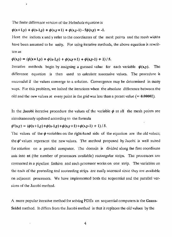
The finite difference version of the Helmholz equation is

(p(x+l,y) + 4>(x-l#) + tf>(x,y+l) + (p(x,y-l) - 50(x,y) = -1.

Here the indices x and y refer to the coordinates of the mesh points and the mesh widths

have been assumed to be unity. For using iterative methods, the above equation is rewrit-

ten as

Iterative methods begin by assigning a guessed value for each variable #(x,y). The

difference equation is then used to calculate successive values. The procedure is

successful if the values converge to a solution. Convergence may be determined in many

ways. For this problem, we halted the iterations when the absolute difference between the

old and the new values at every point in the grid was less than a preset value (= 0.00001).

In the Jacobi iterative procedure the values of the variable <p at all the mesh points are

simultaneously updated according to the formula

The values of the <p variables on the right-hand side of the equation are the old values;

the 0 ' values represent the new values. The method proposed by Jacobi is well suited

for solution on a parallel computer. The domain is divided along the first coordinate

axis into nt.(the number of processors available) rectangular strips. The processors are

connected in a pipeline fashion and each processor works on one strip. The variables on

the ends of the preceding and succeeding strips are easily accessed since they are available

on adjacent processors. We have implemented both the sequential and the parallel ver-

sions of the Jacobi method.

A more popular iterative method for solving PDEs on sequential computers is the Gauss-

Seidel method. It differs from the Jacobi method in that it replaces the old values by the

new values as soon as they are computed. This increases the rate of convergence (as

can be seen from our results) and reduces the storage requirements. On the other

hand, parallel implementations require slight modifications of the procedure. Our

parallel variant retains its high rate of convergence.

The modification we have affected to the Gauss-Seidel method is the following:

Sweep over the "odd" rows downwards (1, 3,..., (ni - 3));

Sweep over the "even" rows upwards ((ni - 2),..., 2);

(Note: In Occam, indexing starts from 0. We have assumed the number of rows to be a

power of 2. This is because the number of nodes in any expanded version of the current

system will be a power of 2 and our parallel codes may then be ported to these systems

with changes only in the configuration files. If there is no such restriction, then minor

changes will have to be made in some of the programs.

This version will be referred to as the Gauss-Seidel method with odd-even ordering. For a

variant of this modification, refer [4]. This ordering and the natural ordering (in which the

rows are swept successively) have asymptotically the same convergence properties.

In table 1 we have listed the times for solving the Helmholz equation with the Gauss-

Seidel method with natural ordering (SEQhhGO) and with the odd-even ordering

(SEQhhGl) using sequential codes. The latter is more efficient. The reason for choosing

the odd-even ordering will be made clear in the next section.

3. General Implementation Strategy

The root transputer has been used only for interfacing between the host and the network

of T800 transputers, that is, the processes running on it accept prompts from the keyboard

or open files on the hard disk and send the data to the network processes, and accept

data from the network and either display it on the screen or store it in files. For interfacing

with the programs running on the network, we use link 2 (see Figure 2, Appendix B) to

send and receive messages from the first processor in the network, PO.

Since we have only four transputers, we restricted ourselves to the pipeline topology. This

is one of the simplest of networks and can easily be expanded. Algorithms for routing

messages from one processor to another are easily implemented. On the other hand, if

the last processor wishes to send and accept a message from the first processor (as is

required by our programs), the message must travel along 2 * (nt - 1) links (where nt is

the number of processors in pipeline). This distance may become unacceptably large for

large nt.

Conceptually, in this report we regard the leftmost processor in the network, PO, as the first

processor and the rightmost as the last. The sequential programs were run on PO. The

following figure shows tne network that has been used for all the (parallel) programs

mentioned in the report.

PC Root PO PI P2 P3

Figure 1

We need nt processes, one to run on each processor in the network. Instead of

writing nt programs (which would be unacceptable if nt were large), we used the existing

labelling of the processors (PO, PI, P2, ...) to write four programs: pO* to run on the first

processor, pN

to run on the last processor, pE* to run on processors labelled by even numbers, and pO* to

run on the odd processors. The processor PO alone communicates with the root processor.

The grid is divided along the first coordinate axis into nt blocks, with adjacent blocks

sharing one row. It is clear from the equations in Section 2 why the overlaps are necessary.

If ni is the number of rows in the grid then the top and bottom blocks have (ni / nt + 1)

rows while the remaining blocks have one additional row. Each processor processes ni /

nt number of rows of some block, with processor PO processing the top block, the last

processor processing the last block, and the intermediate' processors processing the

intermediate blocks in the same order.

The general scheme of processing is as follows: Each processor executes an iteration,

receives and sends (the order depending on the position of the processor in the pipeline) the

updated values of the overlapping rows, checks whether all processors wish to halt or not,

and if not executes another iteration.

For the Jacobi method, the above parallel scheme generates the same results after every

iteration as the sequential scheme. This is because the values are updated simultaneously

at every point of the grid.

This is not the case if the Gauss-Seidel method were to be applied in a parallel fashion.

As an illustration, consider the first row to be processed by the second processor, PI, in

the first iteration. This row is the (ni / nt)-th row (indexing starting from 0) for the entire

grid. For the sequential scheme, this row is processed using the updated values of (ni / nt -

l)-th row, while in the parallel scheme the processing would use the initial values of the

adjacent row.

This is why we have employed the odd-even ordering for the Gauss-Seidel method. The

parallel strategy is as follows:

1. The first processor PO sweeps over the odd rows (starting from 1) of its share of the data,

and the remaining processors sweep over the even rows of their share of the data (starting

from 2). This phase imitates that of the sequential scheme.

2. The processed rows of the overlapping regions are sent to the neighbouring processors

which require them. The even processors send their second-last row to their right neigh-

bour and accept their O-th row from their left neighbour; the odd processors dc the

reverse. (The reason why we need to differentiate between odd and even processors for

this message-passing is to prevent a deadlock.)

3. PO sweeps over even rows (starting from the third-last row of its share of the data) while

the other processors sweep over the odd rows (starting from the second-last row). This

phase, too, imitates that of the sequential scheme.

4. Once again data is exchanged. The even processors send the first row to their left

neighbour and accept the first row of their right neighbour, the odd processors do the

reverse.

Thus at the end of every iteration, updated values at each grid point are equal in both the

parallel and the sequential schemes.

Notice that for the message-passing scheme described above in 2. and 4., there cannot be

any advantage in using a network other than a pipeline topology.

Now each processor needs to find out when to stop the iterations. The process is halted

when a certain condition is met in each processor.

Thus we need to transmit two different types of messages along the links in the pipeline.

We have used two disjoint sets of bidirectional links for this. Since a transputer has 4

bidirectional links, a pair of disjoint sets of links as required above will be available in any

expansion of the system. Later in the section, we will explain why we felt the need for a pair

of disjoint connections.

We implemented the message passing on the other set of links as follows: If the condition

for termination is not met in a processor or on any processor to its right (its right

neighbour would inform it of this fact), it informs its left neighbour of the fact, and carries

out the next iteration; otherwise, it informs its left neighbour and waits for the neighbour

to inform it whether every processor on the left has agreed to halt or not and passes this

message to its right neighbours. The worst-case occurs when every processor except the

first wishes to halt. In which case, the message has to travel the distance mentioned

earlier. Note that in this case, the last processor has to remain idle until it is told to

continue.

To avoid this wait, link communication has to be decoupled from computation by taking

advantage of the fact that the links are autonomous direct-memory-access devices. We

attempted this in the program PARG01 (see table 1, Section 4). The results were not

discouraging and we hope that in a larger system, this may prove advantageous. We

forced each processor to execute one iteration (including transmitting/receiving the

overlapping rows). We set up the following scheme (which has been written in pidgin

Occam):

ITERATE + TRANSMIT/RECEIVE OVERLAPPING ROWS

WHILE (HALTING CONDITION IS FALSE)

PRI PAR

HALT ? ON THE BASIS OF PREVIOUS ITERATION

ITERATE + TRANSMIT/RECEIVE OVERLAPPING ROWS

9

The WHILE construct forces the succeeding statements to be executed as long as the

test result (the parenthetical condition) is true. PRI PAR is a construct in Occam which

declares that subsequent statements must be run in parallel with a higher priority given

to the first. In this way, we have kept the processor as well as the links as busy as possible.

Of course, one extra iteration is being done by the processors but this may be more than

offset by making maximum use of the tranputers. Since there is message passing in both

statements of the PRI PAR, the two sets of links handling these messages must be disjoint (a

variable cannot be accessed in parallel statements).

Other topologies may prove more useful when dealing with the halting problem

described above. Since the transputer is restricted to 4 links, the only available

topology which may prove more efficient than the pipeline is the mesh network. The

existing programs will have to be modified a little for running on a different network.

4. Helmholz Equation: Parallel Implementation and Results

The grid size was fixed at 128x128. The boundary of the grid was ^et at 0.0 while the initial

value at each of the inner points was set at 1.0. The iterations were broken off when the

absolute difference between the old and the new values at each of the grid points was less

than 0.00001.

The Jacobi method was programmed in three ways: one sequentially (SEQhhJO) and two

parallely (PARhhJO and PARhhJl). In PARhhJO a 32x128 matrix temp was used to

store new values while in PARhhJl, an array temp of size 128 was used to store the new

values of the last processed row and these were entered into <p as the new values of the next

row was generated and stored in temp. As can be seen from Table 1 below, PARhhJl

proved to be more efficient than PARhhJO. This is because accessing an entry in a matrix

10

requires one more calculation than for accessing an entry from an array.

On the other hand, comparing the parallel scheme (PARhhJO) to the sequential scheme for

this method, we have speed-ups of upto 4.5! This is because of an overlap in communica-

tion for the parallel scheme. Firstly, there is communication between the memory and the

Floating Point Unit (which executes the floating point operations). Secondly, the

sequential program, uses-two 128x128 real (4 bytes) matrices while each parallel process

handles two 32x128 real matrices (PARhhJO). Since the on-chip memory is 4Kbytes, the

sequential program requires more accesses to the external memory than the parallel

program. In fact the sequential program used 124Kbytes of external memory while each

parallel process used about 29Kbytes.

In the case of the Gauss-Seidel method, two sequential programs were coded. One

(SEQhhGO) used the natural ordering and the other (SEQhhGl) used the odd-even

ordering. The latter proved to be more efficient (table 1).

Two parallel programs (PARhhGO and PARhhGl) were developed based on the odd-even

ordering. PARhhGl attempted to take advantage of the fact that the links are autono-

mous direct memory access devices. For the present system, there was a loss in time; on

the other hand, taking the times listed in 6, 7 and 8 of table 1 into consideration and the

fact that PARhhGl was forced to do one extra iteration, the loss may be acceptable. For

a larger system, we believe that PARhhGl will be more efficient than PARhhGO. Once

again we have super linear speed-ups for same reason as above. Even though the speed-

up is maximum in the Jacobi method, we should note that PARhhGO is most efficient.

11

TABLE 1

i .

1

2

3.

4.

5}

6.

7.

8.

PROGRAM

SEQhhJO

SEQhhGO

SEQhhGl

PARhhJO

PARhhJl

PARhhGO

PARhhGl

TIME FOR

TIME (t)

12.72s

6.6s

6.3s

2.85s

2.7s

1.5s

1.57s

# OF ITERATIONS

32

21

20

32

32

20

21

ONE ITERATION IN PARGOO: 0.075s

SPEED-UP

-

-

-

tl /14 = 4.5

t l / t5 = 4.7

t3/t<5 = 4.2

t3/t7 = 4.01

5. The Reactor Physics Problem

An important reactor physics problem is the determination of the neutron flux distribution

using two group diffusion theory. The steady state diffusion equations are [7]:

+ (2 a, + 2 sl)<fiL = (vS nft + vZ n<pz) IK

Here Dg is the diffusion coefficient for the neutrons of group g (g = 1, 2), 2 a g and Zfg are

the absorbtion and fission cross-sections, 2S | is the slowing down cross-section of the

moderator and v is the mean number of fission neutrons. The neutron fluxes </>„ are

assumed to vanish at the reactor boundary and K (called the iceff eigenvalue) is the

criticality parameter. For simplicity, we assume the material properties are independent

of the position co-ordinates and that the reactor geometry is cartesian in two or three

dimensions. It will be obvious that these assumptions can very easily be relaxed and do not

affect in any manner the parallelization of

the numerical algorithms. In the calculations to be reported, we used the typical values of

the reactor properties given below:

12

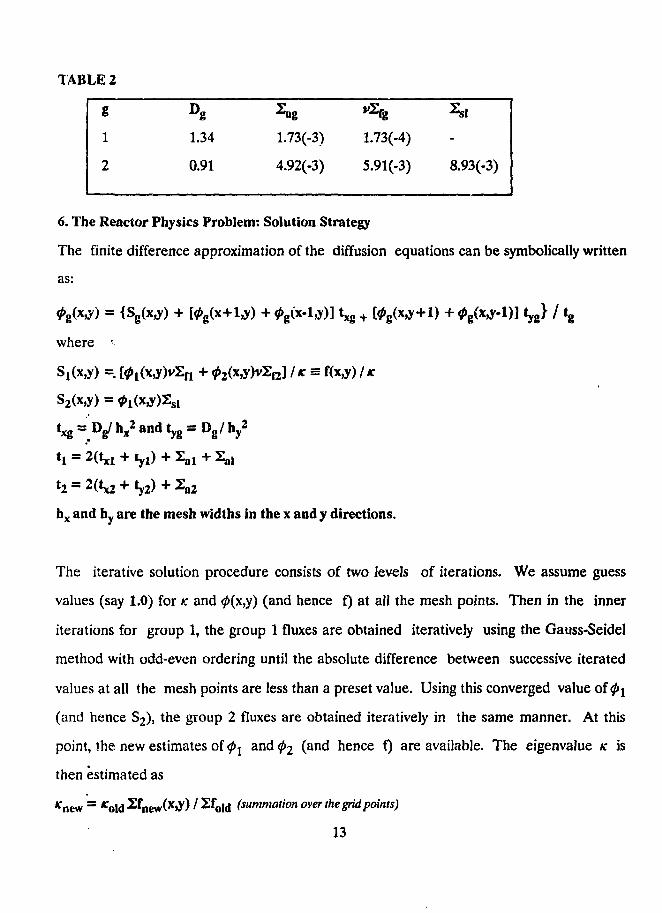
TABLE 2

g

1

2

1.34

0.91

**ng

1.73(-3)

4.92(-3)

vZtg

1.73(-4)

5.91(-3)

-

8.93(-3)

6. The Reactor Physics Problem: Solution Strategy

The finite difference approximation of the diffusion equations can be symbolically written

as:

0g(x,y) = {Sg(x,y) + [0g(x+l,y) +^g(x-l,y)] t ^ + [

w h e r e •••

S!(x,y) = [<Pi(\,y)vEn + <p2(x,y)vXn] IK = f(x,y) / *

S2(x,y) = 0i(x,y)Zsi

t ^ = Dg/ hx2 and tyg = Dg / hy

2

hx and hy are the mesh widths in the x and y directions.

The iterative solution procedure consists of two levels of iterations. We assume guess

values (say 1.0) for K and 0(x,y) (and hence f) at all the mesh points. Then in the inner

iterations for group 1, the group 1 fluxes are obtained iteratively using the Gauss-Seidel

method with odd-even ordering until the absolute difference between successive iterated

values at all the mesh points are less than a preset value. Using this converged value of 4>i

(and hence S2), the group 2 fluxes are obtained iteratively in the same manner. At this

point, the new estimates of 0j and^2 (a°d hence f) are available. The eigenvalue K is

then estimated as

*new = *old 2 fnew(x»y) / 2 fold (summation over the grid points)

13

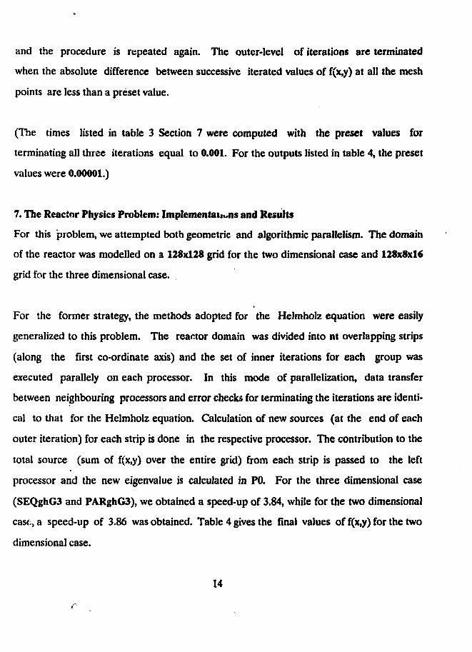
and the procedure is repeated again. The outer-level of iterations are terminated

when the absolute difference between successive iterated values of f(x,y) at all the mesh

points are less than a preset value.

(The times listed in table 3 Section 7 were computed with the preset values for

terminating all three iterations equal to 0.001. For the outputs listed in table 4, the preset

values were 0.00001.)

7. The Reactor Physics Problem: Implementations and Results

For this problem, we attempted both geometric and algorithmic parallelism. The domain

of the reactor was modelled on a 128x128 grid for the two dimensional case and 128x8x16

grid for the three dimensional case.

For the former strategy, the methods adopted for the Helmholz equation were easily

generalized to this problem. The reactor domain was divided into nt overlapping strips

(along the first co-ordinate axis) and the set of inner iterations for each group was

executed parallely on each processor. In this mode of parallelization, data transfer

between neighbouring processors and error checks for terminating the iterations are identi-

cal to that for the Helmholz equation. Calculation of new sources (at the end of each

outer iteration) for each strip is done in the respective processor. The contribution to the

total source (sum of f(x,y) over the entire grid) from each strip is passed to the left

processor and the new eigenvalue is calculated in P0. For the three dimensional case

(SEQghG3 and PARghG3), we obtained a speed-up of 3.84, while for the two dimensional

case;, a speed-up of 3.86 was obtained. Table 4 gives the final values of f(x,y) for the two

dimensional case.

14

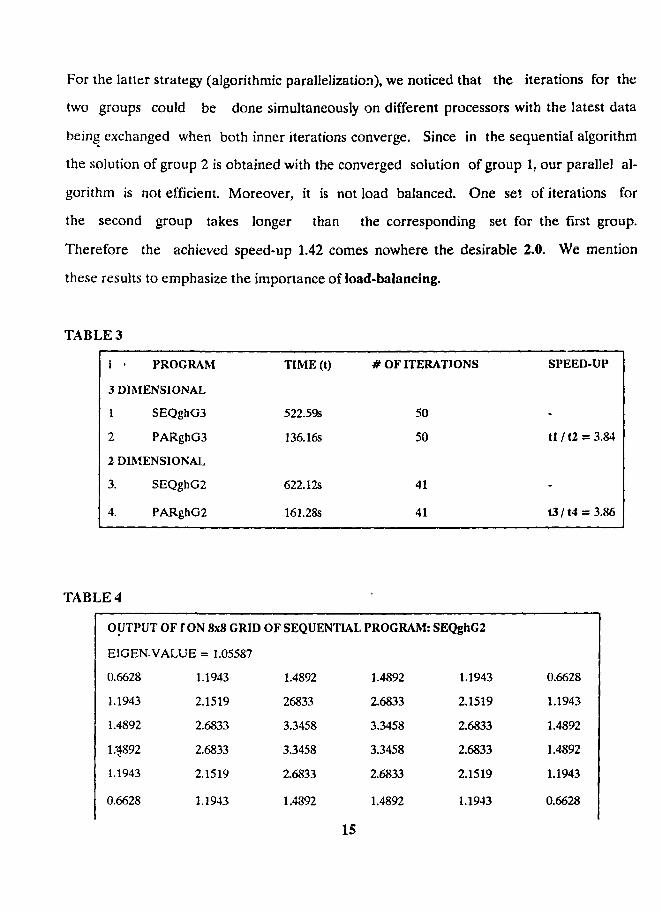
For the latter strategy (algorithmic parallelization), we noticed that the iterations for the

two groups could be done simultaneously on different processors with the latest data

being exchanged when both inner iterations converge. Since in the sequential algorithm

the solution of group 2 is obtained with the converged solution of group 1, our parallel al-

gorithm is not efficient. Moreover, it is not load balanced. One set of iterations for

the second group takes longer than the corresponding set for the first group.

Therefore the achieved speed-up 1.42 comes nowhere the desirable 2.0. We mention

these results to emphasize the importance of load-balancing.

TABLE 3

i

3

1

2

2

3.

4.

PROGRAM

DIMENSIONAL

SEQghG3

PARghG3

DIMENSIONAL

SEQghG2

PARghG2

TIME (t)

522.59s

136.16s

622.12s

161.28s

# OF ITERATIONS

50

50

41

41

SPEED-UP

-

tl/t2 = 3.84

-

!3/t4 = 3.86

TABLE 4

OUTPUT OF f ON 8x8 GRID

EIGEN. VALUE = 1.05587

0.6628

1.1943

1.4892

1.3892

1.1943

0.6628

1.1943

2.1519

2.6833

2.6833

2.1519

1.1943

OF SEQUENTIAL PROGRAM: SEQghG2

1.4892

26833

3.3458

3.3458

2.6833

1.4892

1.4892

2.6833

3.3458

3.3458

2.6833

1.4892

1.1943

2.1519

2.6833

2.6833

2.1519

1.1943

0.6628

1.1943

1.4892

1.4892

1.1943

0.6628

15

OUTPUT OF f ON 8x8 GRID

EIGEN

0.6628

1.1943

1.4892

1.4892

1.1943

0.6628

VALUE = 1.05587

1.1943

2.1519

2.6833

2.6833

2.1519

1.1943

OF PARALLEL PROGRAM

1.4892

2.6833

3.3458

3.3458

2.6833

1.4892

1.4892

2.6833

3.3458

3.3458

2.6833

1.4892

:PARghG2

1.1943

2.1519

2.6833

2.6833

2.1519

1.1943

0.6628

1.1943

1.4892

1.4892

1.1943

0.6628

8. Conclusion

The results of our investigations show that a speed-up of about 3.85 is achievable on a 4

transputer pipeline network for solving elliptic partial differential equations. We have

employed the pipeline topology and the parallel programs can be run on larger systems

(with changes only in the configuration files). We may emphasize that the Gauss-Seidel

method with odd-even ordering is necessary for parallelization, without loss of efficiency,

of existing finite-difference procedures. Without any further effort (in parallelization),

the Gauss-Seidel method may be replaced by a more efficient successive over relaxation

method [7]. Since the execution time for a sequential program on a single T800

transputer is comparable to that for an ND-570 computer, the parallel transputer

network is expected to be of considerable interest for solving problems of the type dis-

cussed in this report.

ACKNOWLEDGEMENTS

The encouragement and interest of Mr. B.R. Bairi, Head, Electronics Division, is

gratefully acknowledged.

16

References

1. K.C. Bowler and R.D. Kenway, "Physics on parallel computers",

Contemporary Physics, vol. 28, No. 6. 573- 598 (1987).

2. G.C. Fox and S.W. Otto, "Algorithms for Concurrent Processors", Physics

Today (May 1984).

3. D. Pountain and D. May, A Tutorial Introduction to Occam Programming, BSP

Professional Books, London (1987).

4. MJ. Quinn, Designing Efficient Algorithms for Parallel Computers, McGraw-

Hill Book Company, New York USA (1987).

5. Transputer Databook, Inmos Limited, UK (1989).

6. Transputer Development System, Prentice Hall Internationa], London (1988)

7. E.L. Wachspress, Iterative solution of Elliptic Systems and Applications to Neutron

Diffusion Equations of Reactor Physics, Prentice Hall International, London (1966).

17

APPENDIX A; Concepts in Parallelism

Since an iterative process is generally time-consuming, we would like to increase the power of the com-

puter. There are two options: either we increase the performance of the processor by developing newer

technologies and using the latest technology, or we apply more than one computer to solve the problem.

A.1 Types of parallelism: There are many classes of parallelism, SIMD, MIMD etc., and for details refer [1]

and [4]. For example, in the case of the Single Instruction Multiple Data (SIMD) machine, a master

control unit issues the same instruction simultaneously to many slave processors operating in lockstep,

each of which enacts it (with a limited degree of local autonomy) on its set of data. In the case of the

Multiple Instruction Multiple Data (MIMD) machine, each processor carries its own program and data

and works independently of the others until it becomes necessary to communicate with one another.

We have applied a version of the SIMD system on both problems and the MIMD for the generalized

Helmholz equation. For the latter problem, the SIMD was far superior (for atleast one obvious reason

which is mentioned in the appropriate section).

A.2 Topologies: There various topologies which may be used in networking the processors. In the

pipeline topology, each processor (except the first and last processors) are connected to a left and right

processor. They form a ring if the last processor is connected to the first. In a mesh architecture, the

processors are placed on the points of a rectangular grid with connections being mapped onto the grid lines.

A.3 Performance Evaluation: In devising parallel algorithm, we are concerned with maximizing the speed-up

and the efficiency. These parameters are defined as follows:

speed-up = tl / tp

efficiency = tl / (p * tp)

where tl is the time taken by a sequential program on one processor and tp is the time taken by a parallel

program on p processors.

Two considerations are important in discussing efficiency. First, the nodes spend some time

communicating with their neighbours. This term is minimized if the intcrnode communications

18

demanded by the algorithm always proceeds by a "hardwired" path. Load balancing is the second factor

affecting efficiency. One needs to ensure that all nodes have essentially identical computing loads.

A.4 Deadlock

A set of active concurrent processes is said to be deadlocked if each holds non-preemptible resources that

must be acquired by some other process in order for it to proceed [1]. As an example, consider two processes

AatvJB. Each has to send data and receive data from the other. If at any point during execution, both are

sending data to each other then a deadlock will occur. This is because each is waiting for the other to

receive its data but neither is receiving.

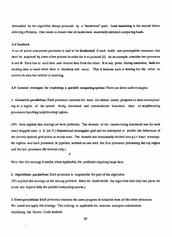
A.5 General strategies for exploiting a parallel computing system: There arc three such strategics:

1. Geometric parallelism: Each processor executes the same (or almost same) program on data correspond-

ing to a region of the system being simulated and communicate boundary data to neighbouring

processors handling neighbouring regions.

(We have applied this strategy on both problems. The domain of the system being simulated was (in each

case) mapped onto a 2- (or 3-) dimensional rectangular grid and we attempted to predict the behaviour of

the (evenly spaced) grid points at steady state. The domain was horizontally divided into p (= four) rectangu-

lar regions and each processor, in pipeline, worked on one with the first processor processing the top region

and the last processor the bottom strip.)

4

Note that this strategy is useful, when applicable, for problems requiring large data.

2. Algorithmic parallelism: Each processor is responsible for part of the algorithm.

(We applied this strategy on the secong problem. Since we could divide the algorithm into only two parts, we

could not exploit fully the parallel computing system.)

3. Event parallelism: Each processor executes the same program in isolation from all the other procesors.

We could not apply this strategy. This strategy is applicable for neutron transport calculations

employing the Monte Carlo method.

19

APPENDIX B: The Parallel Computing System

B.I Hardware

This section briefly describes the parallel system being developed by the Electronics Division of BARC.

In general terms, the system may be described as a distributed memory (that is, no shared memory) parallel

computing system.

The basic element in the system will be the Inmos T800 transputer chip (peak: 30 MIPS and 4.3 Mflops).

This is a reduced instruction set computer which integrates a 32-bit microprocessor, a 64-bit floating

poit unit, 4 Kbytes of on-chip RAM, interfaces to additional memory and I/O devices, and 4 bidirectional

serial links (2.4 Mbytes/s per link) which provide point-to-point connections to other tranputers. The links

are autonomous direct-memory-access devices that transfer data without any processor intervention.

Communication between processes is achieved by means of channels: a channel between two processes run-

ning on the same processor is implemented by a single word in the memory, while a channel between two

processes running on different transputers is implemented by means of the above links. Process

communication is synchronized and unbuffered. Therefore, communication can only begin when both

processes are ready.

The transputer supports concurrency by means of an in-built micro-seeduler. Active processes on a

processor, waiting to be executed, are held in queues. This removes the need for any software kernel.

The present system has the following features:

1. Personal computer IBM PC-AT

2. One root transputer Inmos T414

3.4 T800 transputers.

The PC acts as the host and the root transputer interfaces with the host and is networked to the othei

transputers. At present, the network is hardwired. The network is shown in Figure 2 below. For example, in

the case of the root transputer, link 0 is connected to the host PC, link 1 is connected to link 1 of the

transputer labelled P3 and Iink2 is connected to Iink3 of the tranputer labelled PO.

20

The system, when completed, will have, apart from additional T800 transputers, Inmos C004 link switches. Thenetwork may then be dynamically reconfigured into many architectures including those mentioned above.

P3 P2

PO

ROOTIN IBM PC-AT

I

FIGURE 2

For more details, refer [5].

21

B.2 Occam

As indicated earlier, the transputer was developed as a language-first type approach with the language being

Occam. Thus Occam has been specifically designed for parallel processing, and the hardware and software

architectures required for a specific program are defined by an Occam description. Although Fortran,

Pascal and C are supported, programming in Occam provides maximum performance and allows exploitation

of concurrency. It allows parallelism to be expressed explicilty. It has the PAR construct: statements following

PAR are executed concurrently.

Two Occam processes communicate with each other along channels. As mentioned earlier, the channels are

memory locations if the processes are on the same transputer and hardware links if otherwise. The

synchronization of two processes is realized by the hardware. Therefore the programmer need not worry

about this crucial issue of parallel programming.

An Occam program can be executed on one tranputcr where the validity and response times can be

checked, and if the "software network" defined by the Occam program can be realized on the actual system,

the program with, only minor modifications, can be mapped onto the hardware architecture.

For more details of the language, refer [3].

B.3 Support Software

The Transputer Development System is an Occam development system which provides a completely inte-

grated environment including the INMOS folding editor. This provides a secure development

environment with limited reliance on host services. This means that no operating system host support is

required.

B.4 Configuration Programs and Loading the Transputer Network

An application must be expressed as a number of parallel processes. Once this is done, the

programmer needs to add information describing the link topology and needs to describe the association of

each code to individual transputers. This is called configuration, and the additional code is called the

configuration program. There are two configuration files: one for the code running on the root transputer

and another for the different codes running on the network.

22

APPENDIX C: Codes for Selected Programs

1. LOGICAL NAMES OF LINKS

USED BY CONFIGURATION PROGRAMS (#USE links)

VALlinkOin IS4:

VALlinkOoutlSO:

VALlinklin IS 5:

VALlinkloutlSl:

VALlink2in IS 6:

VAL Iink2out IS 2:

VALHnk3in IS 7:

VALHnk3outIS3:

2. PREDEFINED VALUES USED BY NETWORK PROGRAMS (#USE puramS)

VALREAL32dl IS 1.34(REAL32):

VALREAL32d2 IS 0.9(REAL32):

VAL REAL32 sigal IS 0.00173(REAL32):

VAL REAL32 siga2 IS 0.00492(REAL32):

VAL REAL32 signl IS 0.000953(REAL32):

VAL REAL32 sign2 IS 0.00591 (REAL32):

VALREAL32sigl IS 0.008(REAL32):

VALREAL32zt IS 525.0(REAL32):

VALREAL32xt IS 525.0(REAL32):

VALREAL32yt IS 525.0(REAL32):

VAL REAL32 epsi IS 0.001 (REAL32):

VAL REAL32 epso IS 0.001(REAL32):

VAL INT nout IS 100: -- ITERATIONS CANNOT EXCEED nout

VALINTnil2IS126: - - N I - 2

VALINTnil lIS127: - -NI -1

VAL INT ni IS 128: - - # OF ROWS IN GRID

VAL INT nil IS 129: -- NI + 1

23

VALINTnjl2IS126: --NJ-2

VALINTnjllIS127: --NJ-1

VALINTnj IS 128: --# OF COLUMNS IN GRID

VALINTnjl IS 129: --NJ+ 1

VAL INT nt IS 4: -- # OF TRANSPUTERS IN PIPELINE

VAL INT ntl IS 3: - NT -1

VAL INT overlap IS 1: -- SHARED ROWS OF DIFFERENT PROCESSES

VAL INT overlap 1 IS 2: -- OVERLAP + 1

VAL INT blckl2 IS 30: -- BLCK - OVERLAP1

VAL INT blckll IS 31: -- BLCK - OVERLAP

VALINTblck IS 32: - (NI / NT) ROWS PROCESSED BY EACH TRANSPUTER

VAL INT blckl IS 33: - BLCK + OVERLAP

VAL INT bick2 IS 34: -- BLCK + OVERLAP1

3. CONFIGURATION FILE FOR ROOT TRANSPUTER

#USE "Iinks4.tsr"

... SCRGhlmhlz

CHAN OF ANY pipein, pipeout:

PLACE pipein AT Iink2in:

PLACE pipeout AT Iink2oui:

pghlmhlz(keyboard, screen, pipein, pipeout)

4. PROGRAM ON ROOT TRANSPUTER

#USE userio

PROC pghImhlz(CHAN OF INT keyboard, CHAN OF ANY screen, pipei, pipco)

SEQ

-- PROMPT TO SCREEN

newlinc(screen)

write.full.string(screen, "PLEASE WAIT. ")

newline(screen)

24

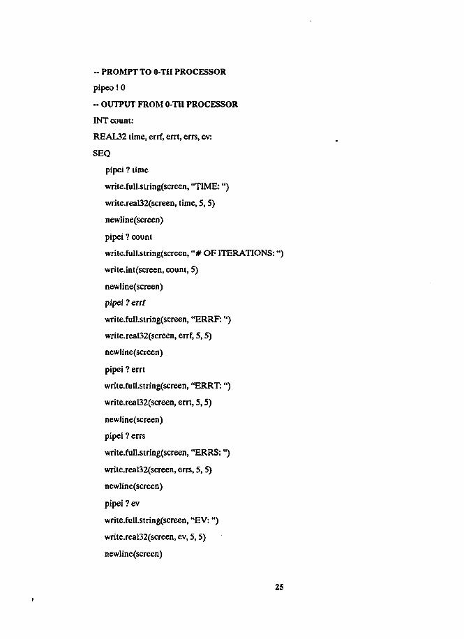
-- PROMPT TO 0-TII PROCESSOR

pipeo! 0

•- OUTPUT FROM 0-TH PROCESSOR

INT count:

REAL32 time, errf, errt, errs, ev:

SEQ

pipei ? time

write.full.siring(screen, "TIME:")

write.real32(screen, time, 5, S)

newline(screen)

pipei ? count

write.full.siring(screen, "# OF ITERATIONS:")

write.int(screen, count, 5)

newline(screen)

pipei ? errf

write.full.string(screen, "ERRF:")

write.reaO2(screen, errf, 5,5)

newline(screen)

pipei ? errt

write.full.string(screen, "ERRT:")

write.rea!32(screen, errt, 5,5)

newline(screen)

pipei ? errs

write.full.string(screen, "ERRS:")

write.real32(screen, errs, 5,5)

newline(screen)

pipei ? ev

write.full.string(screen, "EV:")

write.real32(screen, ev, 5,5)

newline(screen)

25

» PROMPT TO USER

wriie.full.string(screcn, "HIT ANY KEY TO RETURN TO TDS")

INTl:

keyboard ? t

5. CONFIGURATION FILE FOR NETWORK PROGRAM

#USE "Iinks8.tsr" -- LIBRARY OF LOGICAL NAMES FOR LINKS

... SCpOPRGhz2 --0-TH PROCESSOR

... SC pOPRGhz2 -- INTERMEDIATE PROCESSOR (ODD)

... SC pEPRGhz2 -- INTERMEDIATE PROCESSOR (EVEN)

... SCpNPRGhz2 -- LAST PROCESSOR IN PIPELINE

-- piperw: RTWARD PIPELINE LINK FOR UPDATING SHARED REGION

-- pipeiw: LTWARD PIPELINE LINK FOR UPDATING SHARED REGION

[4]CHAN OF ANY piperw, pipeiw:

-- piperw 1 : RIGHTWARDS PIPELINE LINK FOR IULTING CHECK

•- pipelwl: LEFrWARDS PIPELINE LINK FOR HALTING CHECK

[3JCHAN OF ANY piperwl, pipelwl:

PLACED PAR

PROCESSOR 0T8

PLACE piperw[0] AT Iink3in:

PLACE piperw[l] AT Iink2out:

PLACE pipelw[2] AT Iink2in:

PLACE pipclw[3] ATlink3out:

PLACE piperwl [0] AT linkOout:

PLACE pipclwl[2] AT linkOin:

pOGhmhlz(piperw[O], pipenv[l], pipelw[2], pipelw[3], piperwl[0], pipelwl[2], 0)

26

PROCESSOR 1 T8

PLACE piperwfl] AT linkOin:

PLACE piperw[2] AT linklout:

PLACE pipelwfl] AT linklin:

PLACE pipe] w[2] AT linkOout:

PLACE piperwlfO] AT Iink2in:

PLACE piperwlfl] ATlink3out:

PLACE pipelwl[l] AT Hnk3in:

"PLACE pipelwl[2] ATHnk2out:

pOGhmhlz(piperw[l], piperw[2], pipelw[l], pipelw[2],

piperwl[0], pipetwl[l], pipelwl[l], pipelwl[2J, 1)

PROCESSOR 2 T8

PLACE piperw[2] AT Iink3in:

PLACE piperw[3] AT linkOout:

PLACE pipelw[0] AT linkOin:

PLACE pipelw[l] AT Hnk3out:

PLACE piperwl[l] AT linklin:

PLACE piperwl[2] AT Iink2out:

PLACE pipelwlJO] AT Iink2in:

PLACE pipelwl[l] AT linklout:

pEGhmhlz(piperw[2], pipetw[3], pipelw[0], pipelwfl],

piperwl[l], piperwl[2], pipelwl[0], pipelwl[l], 2)

PROCESSOR 3 T8

PLACE piperw[3J AT Iink2in:

PLACE pipelw[0] AT Hnk2out:

PLACE piperwl[2] AT linkOin:

PLACE pipclwl[0] AT linkOout:

pNGhmhlz(piperw[31, pipclwfO], pipenvl[2], pipclwl[0]3)

27

Published by : M. R. Balakrishnan Head, Library & Information Services DivisionBhabha Atomic Research Centre Bombay 400 085