You are lost without a map: Navigating the sea of protein structures
Audrey L. Lamba,*, T. Joseph Kappockb, and Nicholas R. Silvaggic,**
aDepartment of Molecular Biosciences, University of Kansas, Lawrence, KS 66045, United States
bDepartment of Biochemistry, Purdue University, West Lafayette, IN 47907, United States
cDepartment of Chemistry and Biochemistry, University of Wisconsin—Milwaukee, Milwaukee, WI 53211, United States
Abstract
X-ray crystal structures propel biochemistry research like no other experimental method, since
they answer many questions directly and inspire new hypotheses. Unfortunately, many users of
crystallographic models mistake them for actual experimental data. Crystallographic models are
interpretations, several steps removed from the experimental measurements, making it difficult for
nonspecialists to assess the quality of the underlying data. Crystallographers mainly rely on
“global” measures of data and model quality to build models. Robust validation procedures based
on global measures now largely ensure that structures in the Protein Data Bank (PDB) are largely
correct. However, global measures do not allow users of crystallographic models to judge the
reliability of “local” features in a region of interest. Refinement of a model to fit into an electron
density map requires interpretation of the data to produce a single “best” overall model. This
process requires inclusion of most probable conformations in areas of poor density. Users who
misunderstand this can be misled, especially in regions of the structure that are mobile, including
active sites, surface residues, and especially ligands. This article aims to equip users of
macromolecular models with tools to critically assess local model quality. Structure users should
always check the agreement of the electron density map and the derived model in all areas of
interest, even if the global statistics are good. We provide illustrated examples of interpreted
electron density as a guide for those unaccustomed to viewing electron density.
Keywords
Protein structure; X-ray crystallography; Molecular models; Electron density maps; Atomic coordinate files; Atomic displacement parameters
1. Introduction
Advances in crystallization, data collection, and computers have made macromolecular
crystal structures commonplace. Biochemists, medicinal chemists, chemical biologists and
*Corresponding author. Tel.: +1 785 864 5075. **Corresponding author. Tel.: +1 414 229 2647. [email protected] (A.L. Lamb), [email protected] (N.R. Silvaggi).
HHS Public AccessAuthor manuscriptBiochim Biophys Acta. Author manuscript; available in PMC 2016 October 05.
Published in final edited form as:Biochim Biophys Acta. 2015 April ; 1854(4): 258–268. doi:10.1016/j.bbapap.2014.12.021.
Author M
anuscriptA
uthor Manuscript
Author M
anuscriptA
uthor Manuscript

many others have come to rely on macromolecular structural data as never before, and it has
become routine to read, write, and review manuscripts that contain crystal structures.
Furthermore, advances in the field have made it possible for scientists with limited training
in crystallography to determine protein structures. Thus, even scientists with no formal
background in crystallography need to know how to critically evaluate these complex
experiments. While it has been noted recently that poorly determined structures have a
negative impact on the drug design community [2], the focus here is on how to avoid the
improper use of well-determined structural models. The first step is to understand how
crystallographic models are made.
Every atom in the repeating unit of a crystal (the unit cell) contributes to the intensity of
every reflection in the diffraction pattern. The measured intensity for each diffraction spot is
the result of scattering from the entire model. Particular data points cannot be associated
with specific parts of a model. For example, there is no “metal spot” in data collected from a
metalloprotein crystal; the metal contributes to the intensity of every reflection (see Box A
for a description of the crystallographic experiment). While crystallographic statistics
reported in structure papers provide numerical indications of the overall quality of the
diffraction data (for an excellent review, see [3]), these do not report on how well-
determined individual parts of a model are. The Protein Data Bank (PDB)1 has recently
adopted a new structure report format that gives a graphical representation of how a given
model compares with others in the PDB in terms of five statistical measures of model quality
[4–7]. These reports are based on the excellent work of numerous leaders in the field of X-
ray structure determination [6]. As good as these reports are, they are focused on the global
quality of the structure.
Even in the best cases, there are areas of the electron density map that are poorly defined
(Fig. 1). Thus, even a crystal structure that is based on high quality diffraction data and was
carefully and competently built and refined will have local areas of the model that are less
reliable than the rest. Very often, these regions are on the surface of a protein, and for most
users, will not be important in drawing conclusions about molecular structure and function.
Of course, if one is interested in protein–protein interactions, these regions are relevant.
One’s interests determine which parts of the electron density map to inspect.
Regions of the electron density map that are poorly defined due to mobile, disordered
sections of the polypeptide frequently have important functions. For example, an enzyme
may adopt multiple conformations associated with substrate entry, catalysis, and product
egress. In addition, no protein model is produced entirely objectively, since human judgment
always plays a role. Recognizing where uncertainty and bias may intrude is an important
skill for a structure user who wishes to extract meaningful biological or chemical
conclusions from a structure model. To assess which parts of a model are strongly supported
by the data and which are less so, one cannot rely on statistical indicators, but should instead
examine the electron density maps in regions of functional interest. Fortunately, most
journals now require authors to deposit structure factors (the processed experimental data
1The current Protein Data Bank is a cooperation of three different organizations, RCSB PDB, PDBe, and PDBj which all contribute entries to the wwPDB (wwpdb.org) [1].
Lamb et al. Page 2
Biochim Biophys Acta. Author manuscript; available in PMC 2016 October 05.
Author M
anuscriptA
uthor Manuscript
Author M
anuscriptA
uthor Manuscript

with associated phase estimates) along with the atomic coordinates in the PDB, making it
easy to generate maps. The only way for users of macromolecular structures to evaluate the
quality of the electron density maps used to build a model is to actually look at them. To
avoid basing important experiments on weak structural data, users of macromolecular
models must judge which parts of a model are relevant and trustworthy. The information
content of the model might not support every idea the structure user has about the molecule.
2. Understanding macromolecular models
2.1. The coordinate file
Scientists who work with protein structures routinely download PDB coordinate files from
the Protein Data Bank and view models in a graphics program such as COOT [8,9], PyMOL
[10], Chimera [11], or JMOL [12]. The coordinate file is actually a simple text file that can
be inspected with any text editor (Box B). Model users are encouraged to inspect the file in
this way, because the header of the PDB file contains important information regarding the
protein sample, the experimental setup, and ways to assess the final model. Every atom
listed in a PDB file is associated with at least five parameters: x, y, and z coordinates and
two highly correlated terms, the atomic displacement parameter (ADP) and occupancy (Q),
that modulate the contribution of that atom to the overall diffraction pattern.
2.1.1. Atomic displacement parameters (B-factors)—ADPs are historically known
and most often referred to in the literature as B-factors or temperature factors. These
parameters describe the vibration of an atom around a mean position specified by the atomic
coordinates. B-factors are typically low (5–20 Å2) for the well-ordered atoms of the
backbone in well-defined secondary structures like an α-helix or a β-sheet. Loops tend to be
more mobile than α-helices and β-sheets and thus have higher B-factors. Likewise, side
chains can have considerably higher B-factors than main chain atoms. Atoms with high B-
factors are found in poorly defined electron density. In Fig. 2, notice the poorer fit to the
electron density of the aliphatic chain, which has higher B-factors, than the fused ring
system where the B-factors are lower. It is unlikely that this is due to an error in structure
determination or model building. Consistent with chemical intuition, the aliphatic chain is
not interacting with the protein and is neither rigid nor constrained by the protein, and so is
more mobile than the fused ring system.
In high-resolution structures (better than 1.5 Å), anisotropic B-factors are used to describe
the non-spherical atomic shapes that result from partially restricted motion. Lower-
resolution datasets do not contain enough observations to justify the addition of five extra
parameters per atom: six values define an ellipsoid versus one for a sphere [13]. Anisotropic
B-factor records are interdigitated in the coordinate section of a PDB file, and are only
obvious by looking at the coordinate file in a text editor (see Box B).
An alternative way of describing atomic displacements, Translation, Libration, Screw (TLS),
is based on the assumption that groups of atoms in a large molecule undergo correlated,
rigid-body motions [14]. In TLS refinement, protein atoms are placed in several groups and
the parameters defining the anisotropic motion of each group are refined. Since there are
significantly fewer TLS groups than atoms, fewer additional parameters are required to fit
Lamb et al. Page 3
Biochim Biophys Acta. Author manuscript; available in PMC 2016 October 05.
Author M
anuscriptA
uthor Manuscript
Author M
anuscriptA
uthor Manuscript
the data than with full anisotropic B-factor refinement. Whereas individual TLS motions can
be visualized [15], they may or may not correspond to real macromolecular dynamics [16].
2.1.2. Occupancy—Occupancies (or Q-values) are comparable to mole fractions for
different molecular configurations. They indicate if an atom is found in a single location in
the model (occupancy of 1.0) or multiple locations (fractional occupancies). Occupancies
can be refined, to a value that approximates the proportion of unit cells that contain the
molecule in each conformation. For example, a crystal soaked with ligand at an insufficient
concentration or for too short a time may not contain a ligand in every binding site and will
therefore have a fractional occupancy. As another example, side chains can be present in two
(sometimes three) different conformations. To be visible in the electron density map, and
thus included in the model, an alternate conformation of a residue must be present in at least
20% of the molecules in the crystal (fractional occupancy 0.2). Conformations with
occupancies that refine to less than 0.2 are generally not included in a model (Fig. 3).
2.2. Electron density maps
Scientists who work with protein structures routinely download PDB coordinate files from
the Protein Data Bank (http://www.wwpdb.org) and view models in a graphics program such
as COOT [8,9], PyMOL [10], or Chimera [11]. It is just as easy to download the structure
factors from the same PDB page, or pre-calculated electron density maps from the Electron
Density Server (EDS; http://eds.bmc.uu.se/eds/) (Box C) [17]. The PDB entry even includes
hyperlinks to the EDS to facilitate use of these electron density maps. The diffraction spots
measured during a crystallographic experiment (see Box A) arise due to scattering of the X-
rays by the electrons associated with the protein atoms. The electron density map derived
from the diffraction data is a three dimensional plot that shows wherein space electrons are
concentrated within the repeating unit of the crystal. The areas of high electron density mark
the positions of the protein atoms.
There are a number of ways to calculate electron density maps, and the map types most
frequently mentioned in the literature are: Fo – Fc, 2Fo – Fc, the maximum likelihood-
weighted versions of these (mFo – DFc and 2mFo – DFc), and various flavors of “omit”
maps. The maximum likelihood weights, ‘m’ and ‘D’, effectively reduce the contributions of
poorly estimated structure factors to the electron density calculation. This has the effect of
making the maps more interpretable by reducing model bias (see [18,19] for more detailed
discussion). The EDS allows one to choose both the format (CCP4 [20] format is the most
widely accepted by crystallographic software) and type of map (either 2mFo – DFc or mFo –
DFc). Since the structure factor file that can be downloaded from the PDB cannot be directly
displayed in molecular visualization software, we strongly suggest that users download the
pre-calculated maps from the EDS. It is also worth noting that the EDS provides per-residue
plots of the real space correlation coefficient (RSCC) [21], which provides a statistical
measure of how well each residue fits within the electron density. The RSCC values can thus
be used to guide visual inspection of the model.
2.2.1. Fo–Fc or mFo – DFc maps—To calculate an electron density map, the structure
factor amplitudes are combined with corresponding phase estimates (see Box A) in a Fourier
Lamb et al. Page 4
Biochim Biophys Acta. Author manuscript; available in PMC 2016 October 05.
Author M
anuscriptA
uthor Manuscript
Author M
anuscriptA
uthor Manuscript
series. The direct experimental map calculated from the observed structure factor amplitudes
(Fo) is relatively difficult to interpret, especially for incomplete models. This is why
crystallographers calculate difference maps. An Fo – Fc or mFo – DFc map is calculated by
subtracting the observed structure factor amplitudes from those calculated from the current
model (Fc). In areas where there is good agreement between the experimental data and the
model, there is no density. In areas where the model is missing atoms, there will be a peak in
the Fo – Fc map. Where the model contains atoms that should not be there, the Fo – Fc map
will have a hole (i.e. a negative “peak”). Thus, the Fo – Fc map shows where the model and
experimental data differ. It can aid interpretation of the 2Fo – Fc map (see below). Fo – Fc
maps are contoured at (+) and (−) 3.0 σ to show areas for which the model does not
adequately account for the electron density (positive) or where atoms are partially disordered
or have been incorrectly placed (negative). Typically the peaks in the Fo – Fc map are
colored green and the minima are colored red. The sigma level is an estimate of the noise in
the map, and is analogous to setting a minimum elevation on a topographical map, such that
only peaks above a certain threshold are drawn. Some graphics programs set the map
contour in units of electrons per Å3, but the idea is the same: only regions with electron
density above the threshold value are drawn.
2.2.2. 2Fo – Fc or 2mFo – DFc maps—The 2Fc – Fc or 2mFo – DFc map, where the
model-derived structure factor amplitudes are subtracted from twice the observed structure
factor amplitudes, can be thought of as a combination of the direct Fo map and the Fo – Fc
difference map. The observed structure factor amplitudes are weighted more heavily, so that
even areas where the model and data agree will be covered by the electron density. Atoms
that should not be at their current positions in the model will have little to no electron
density, while empty peaks mark positions where atoms must be added to the model to agree
with the data. To inspect a completed structure, set the 2mFo – DFc map contour level
between 1.0 and 1.5 σ. The 2mFo – DFc map should be fairly continuous (occasional breaks
are normal, especially at lower resolutions) and should cover most of the atoms in the model.
One expects less well-defined maps at low resolution, and thus more discontinuities in the
main chain electron density and “naked” atoms than would be tolerated at higher resolution
(see below).
2.2.3. Omit maps—Model bias is the result of how maps are calculated: because the phase
estimates for the calculation come from the model, maps will tend to show electron density
for an atom in the model whether it is truly there or not. A simple omit map is normally a
difference (Fo – Fc) map calculated after omitting specific atoms from a model, like a ligand
or a functionally important loop. While simple to do, the drawback to this approach is that
leaving out a small percentage of the model does little to remove model bias. A more
rigorous (and computation/time-intensive) approach is the composite omit map, where
sections of a model (5–10%) are omitted in a series of map calculations, and the relevant
regions of each calculation are stitched together to give an electron density map with much
less bias, since the entire model has been omitted. For further bias removal, a round of
simulated annealing refinement is done at each omit step during the composite omit
calculation to give the simulated annealing composite omit map. This type of omit map has
minimal model bias and is the gold standard for figures designed to confirm the electron
Lamb et al. Page 5
Biochim Biophys Acta. Author manuscript; available in PMC 2016 October 05.
Author M
anuscriptA
uthor Manuscript
Author M
anuscriptA
uthor Manuscript
density of protein·ligand complex structures, especially if the 2mFo – DFc density is not
solid for every atom of the ligand. If the published electron density images or 2Fo – Fc map
from the EDS lead one to question the validity of a region in the model, calculating the
simulated annealing composite omit map may be worth the small additional effort.
Simulated annealing composite omit maps are not available directly for download from
EDS, but can be calculated without too much effort by a friendly crystallographer from the
deposited structure factor and coordinate files using PHENIX [22] or other software.
2.3. Resolution
High-resolution data add detail to electron density maps (Fig. 4). A 4 Å-resolution map
shows the location of secondary structure elements, but not necessarily their orientation–
helices can go in either direction and the directionality of β-sheets is similarly hard to
determine. A 3 Å-resolution map clearly shows secondary structure and some side chains. A
2 Å-resolution map will show most side chains. At resolutions of 1 Å and better, the map
shows individual atoms. At the highest resolutions (0.7 Å and better), it becomes possible to
see electron density between covalently bonded atoms in stable regions of the molecule.
Diffraction data at almost any resolution can provide valuable information. After all,
Rosalind Franklin’s fiber diffraction images contained enough information to construct a
hugely influential model of DNA that was in no way a “solved” structure [23–25]. Likewise,
Roderick MacKinnon’s 4 Å-resolution Rb+ or Cs+ soaked potassium channel crystals
provided evidence for the selectivity filter [26]. The resolution of the data–the detail
available in the electron density map–dictates the conclusions that can be drawn from a
crystallographic model.
Higher resolution data provide more observations against which the parameters of the model
(the x,y,z of atomic locations and B-factors and occupancies) can be refined. Model
refinement is conceptually similar to non-linear least squares fitting, where the fit can be
improved simply by increasing the complexity of the equation used to fit the data. When the
number of parameters grows too large, a least-squares fit may look perfect but the model it
represents has no basis in reality. While crystallographic models are more complex,
refinement is similarly vulnerable to overfitting and over-parameterization. Parameters are
added to a macromolecular model in the form of additional atoms (e.g. water molecules,
ligands, residues in mobile loops), or by using more realistic models of atomic behavior (B-
factors, occupancies). The number of observations in the diffraction data set must be greater
than the number of refined parameters to support a robust model refinement. Models can
also be overfit by violating chemical (e.g. poor stereo-chemical restraints) or physical (e.g.
steric clashes) principles.
At low resolution, the electron density is simply too ill-defined for the side chains, especially
the longer ones, to be well-modeled, and the many waters that are part of the hydrogen bond
network are not visible. As a rule of thumb, a model built using 3 Å-resolution diffraction
data is usually sufficient for determining the overall fold of the protein (e.g. for comparison
to proteins with similar structure and/or function). A model determined at 2 Å-resolution can
support detailed arguments about the roles of enzyme active site residues, the binding mode
of an inhibitor, or analysis of the solvent and hydrogen bond network. A model determined
Lamb et al. Page 6
Biochim Biophys Acta. Author manuscript; available in PMC 2016 October 05.
Author M
anuscriptA
uthor Manuscript
Author M
anuscriptA
uthor Manuscript
at 1 Å-resolution allows visualization of individual non-hydrogen atoms and a detailed
biophysical analysis.
3. All parts of a model are not of the same quality
3.1. The protein
Structural data consumers should remember that structural models are not as rigid as they
might seem. The ability to “measure” interatomic distances in hundredths of Ångstroms
from a model using a graphics program does not mean they are actually known to anywhere
near that level of accuracy. A molecular dynamics movie of a protein in solution shows them
to be incredibly dynamic, bouncing and vibrating crazily (and anisotropically). It is
entropically “expensive” to immobilize a floppy molecule like a protein in a crystal, and the
most flexible regions are the hardest to constrain.
Crystals are snap-cooled in cryoprotectant agents to minimize the formation of crystalline
ice that can obscure protein diffraction data or destroy the protein crystal. Snap-cooling does
not typically serve as a kinetic trap, since even at room temperature the crystalline lattice
confines the protein to a relatively small ensemble of conformations. (Unstable chemical
intermediates can sometimes be trapped by snapcooling crystals undergoing an enzymatic
reaction.) If protein crystal structures represent a thermodynamic minimum, they should be
reproducible. Independently determined high-resolution models for the same protein tend to
agree [27]. At moderate resolution, different structure models may be equally plausible since
the electron density may represent an ensemble of conformations [28]. A protein crystallized
in multiple space groups may adopt different conformations [29–31]. In addition, minor
conformational substates with disproportionate functional significance may be thermal
“excited states” that are not populated at cryogenic X-ray data collection temperatures
[32,33]. A single consensus structure is typically reported, not the ensemble it represents
[34]. These motions may be studied using complementary experimental and computational
approaches [35,36].
Low temperatures further limit conformational ensembles in the crystalline lattice. Proteins
undergo a “glass transition” as the temperature drops below 160–200 K that restricts internal
motions [37]. At cryogenic data collection temperatures (100 K), molecular motions are
almost entirely “frozen out”; even methyl rotation is suppressed [38]. In relatively
unconstrained regions of the crystal, multiple conformations that have similar energies can
be trapped by snap-cooling. These often correspond to regions that are flexible in solution,
like loops, and they are colloquially referred to as flexible in a crystal, even though they
cannot “move” (interconvert) at cryogenic temperatures. Disordered regions give weaker
electron density maps and higher B-values than other parts of the protein. In many cases, the
density is so weak that there is no justification for including part of the protein in the final
model (Fig. 1B).
It is often possible to discern mobility in crystal structures, despite the stabilizing influences
of the crystal lattice and cryogenic temperatures. As discussed above, the B-factors give an
approximation of the degree of mobility of atoms in the model. In practice, it is difficult to
tell if high B-factors are due to thermal motions, lattice displacements (slight misalignment
Lamb et al. Page 7
Biochim Biophys Acta. Author manuscript; available in PMC 2016 October 05.
Author M
anuscriptA
uthor Manuscript
Author M
anuscriptA
uthor Manuscript
of the repeating units of the crystal), or the existence of a large number of possible
conformations. In all three cases, the electron density blurs and eventually disappears for
very mobile parts of the structure. Mobile side chains can be modeled with alternate
conformations in structures of higher resolution (~2 Å resolution or better), when there is
sufficient crystallographic evidence (density in the map) to warrant more than one
orientation. In favorable cases, only two conformations of a residue or region contribute to
the observed electron density and both conformations can be built into the model (Fig. 3B).
Occupancy values for each contributor are optimized during refinement. In unfavorable
cases, the flexible bits of the molecule adopt so many conformations that there is no
information on where they are (no density).
Unfortunately, molecular visualization programs are not designed to alert the casual user to
the use of alternate conformations or high B-factors. If a model contains two conformations
of a side chain, both will be displayed by most graphics programs. Most of the time, the
smaller partial occupancy should be at least 20% for inclusion in the model, since they are
distracting and often do not add much to what can be gleaned from common sense and B-
factors. It is usually easy to color a model by relative B-factor to insure that a region of
interest is not associated with weak electron density. Weak electron density is often
associated with surface-exposed residues since they have no chemical reason to adopt a
particular conformation (Fig. 1A).
Crystallographers disagree about how to handle disordered side chains. The first group omits
atoms that have no electron density from the model. Their rationale is that if there is no
evidence to place an atom at a specific point, then no atom should be placed there in the
model. This approach, however, leads to confusion about residue identity (i.e. glutamate
winds up looking exactly like alanine). The second group assumes that the visible portion of
a residue constrains where the invisible (mobile) atoms can be. A somewhat-disordered
residue can be placed intact in the most stereochemically plausible pose and the B-factors
allowed to refine to high values. This avoids confusing residue truncations, but it obliges
structure users to check B-factors and maps in any interesting region of the model [39]. The
third group models a side chain that has no electron density in the most stable rotamer and
sets the occupancy values to zero for atoms with no electron density. This obliges structure
users to inspect occupancies closely. Unfortunately, most molecular viewers do not
automatically alert the user to occupancies less than 1. Most of the ambiguity disappears
when one looks at the maps. So, if one is interested in a particular active site residue or a
surface patch that may be involved in a protein-protein interaction, one must look carefully
at the electron density map to decide if there is sufficient density to support the modeled side
chain orientation.
In addition to making decisions about what to do with surface side chains, there are several
residues (Asn, Gln, and His) with side chain functional groups that have flat, symmetrical
shapes in electron density maps. In the final rounds of refinement, crystallographers decide
how to orient these side chains based on the surrounding hydrogen bonding network.
Sometimes this is straightforward (Fig. 5), and sometimes it is not. This is a particular
concern in enzyme active sites, where a His side chain, for example, might participate in
Lamb et al. Page 8
Biochim Biophys Acta. Author manuscript; available in PMC 2016 October 05.
Author M
anuscriptA
uthor Manuscript
Author M
anuscriptA
uthor Manuscript

catalysis. Model users should always check the surrounding network of hydrogen bonding
interactions to judge if it supports the modeled pose and the proposed function.
Molecular motions discerned by comparing crystal structures are only meaningful if the
positional uncertainty (coordinate error) of each structure is known. However, coordinate
error is seldom included in the information contained within the PDB header section. It is
not un-usual to see small movements of, for example, a helixorloop when multiple structures
of the same protein in different states (e.g. ligand bound vs unbound) are compared.
Unfortunately, it is difficult to estimate the precision of atomic positions [40] and thereby to
determine if an apparent motion is significant. An apparent movement of 0.4 Å that is based
on a comparison between two structures with coordinate errors of 0.3 Å could be real but it
is unlikely to be biochemically relevant. Recall that most deposited protein structures
represent only the most stable state among the ensemble of states present in the crystal.
Claims that tiny structural shifts have catalytic relevance should be treated with skepticism
except when based on comparison of ultra-high resolution data sets. Ultimately, any
assertion that a minor motion has functional significance requires additional biochemical or
biophysical data.
3.2. Buffer components and solvent
Protein molecules are solvated and contain “ordered” water molecules that are integral to the
structure. These ordered water molecules are modeled as single oxygens (hydrogens cannot
be seen at the resolution of most structures), found on the exterior of the protein molecule or
in any cavity, but must obey simple rules of hydrogen bonding. The number of water
molecules in a crystallographic model depends on resolution, with few at 3 Å and as many
as two per amino acid at high resolution. There is some danger in comparing water
molecules between different protein structures unless the structures are determined to
sufficient resolution and the water molecules have appropriate B-factors.
Most protein crystals form in solutions containing organic precipitants (e.g., polyethylene
glycol) and/or Hofmeister “salting-out” ions (e.g., ammonium sulfate) that stabilize proteins
and favor controlled crystal nucleation and growth. Even though the mother liquor contains
high concentrations of these additives, they appear less often in electron density maps than
might be supposed. Those that do appear often look very odd, as a consequence of local
disorder: for instance, sulfate is a tetrahedral oxyanion that shows up bound to enzyme
active sites where a phosphate group might normally bind. Sulfate can also appear on the
surface of a protein as a smaller, spherical blob near a positively charged region, and is
identified primarily on the basis of knowledge of which chemicals are present and a strong
peak of electron density that is inadequately modeled as water. Alternatively, sulfate may be
spotted first as a water molecule with an unrealistically low B-factor.
What about the ammonium ions provided by ammonium sulfate, which are twice as
abundant as the sulfates? About a quarter of deposited X-ray crystal structures contain
sulfate, which is almost two orders of magnitude more common than structures containing
ammonium (NH4+) or ammonia. Many water molecules adjacent to a negative charge may
be ammonium ions. However, neither X-ray crystallography nor chemical plausibility can
Lamb et al. Page 9
Biochim Biophys Acta. Author manuscript; available in PMC 2016 October 05.
Author M
anuscriptA
uthor Manuscript
Author M
anuscriptA
uthor Manuscript
support that assignment. One should nevertheless keep an open mind about whether a
solvent molecule could be something other than water [41].
3.3. The ligands
Ligands, which we define as interesting buffer components, can be danger zones. Ligands
are noncovalently associated with the protein (Fig. 6A) so are likely to be present with high
B-factors or fractional occupancy. Flexible parts of the ligand are often incompletely
immobilized in a macromolecular complex, to lessen the entropic cost of binding the parts of
the molecule that make specific interactions with the protein. In favorable cases, flexible
loops of an enzyme active site become ordered in the presence of a ligand. It can be difficult
to saturate all of the binding sites in a protein crystal, even when the dissociation constant is
small. In cases of fractional ligand occupancy, only a fraction of the protein molecules
making up the crystal lattice bind to the ligand (simply, only some active sites have ligand
bound) or only a fraction of ligands bind in the same orientation.
One of the few ways to distinguish fractional occupancies from high B-factors is to compare
B-factors within a ligand. In general, only atoms that contact the protein directly have B-
factors comparable to surrounding protein atoms. If B-factors range from low to high (partly
disordered) within a ligand molecule, the ligand is probably present at full occupancy but it
is less ordered at one end. If B-factors are consistently high, the ligand is probably not
present at full occupancy; occupancies may be refined as a group (e.g., all atoms in a
ligand). In either case, we prefer to set all ligand atom occupancies to 1, to force B-factors
higher and thereby to alert the structure user. A good example is found in the 1.6 Å structure
of the yeast oxysterol binding protein Osh4 bound to cholesterol (PDB ID: 1ZHY) [42]. The
ring system (Fig. 2) is rigid relative to the alkyl side chain, thanks to interactions with the
protein and conformational constraints imposed by the fused rings. The increase in disorder
correlates well with the expected decrease in rigidity. The chemical stability of cholesterol
disfavors the alternate hypothesis, that side chain atoms are present at fractional occupancy
due to breakdown of the ligand.
Overzealous interpretation of solvent components as ligands is particularly hazardous in
structure-based drug design [10,43]. A serious problem arises when a buffer component or a
decomposition product is mistaken for a ligand that was desired to be present [44]. Unless
heavy atoms are part of the ligand, it can be hard to distinguish ligands from solvent or
buffer components. There are a number of tools available to crystallographers and model
users alike for validating the fit of a ligand to the electron density. Most of these rely wholly
or in part on statistical measures of map-model agreement like the real space R value (RSR),
the real space correlation coefficient, or a difference density Z score [7,45,46]. One tool, the
Twilight script [21], flags ligands with low RSCC values and ranks ligand plausibility.
Another piece of software, VHELIBS [47] allows even novice users to visually assess both
the ligand and binding site.
Covalent adducts are physically linked to the protein (Fig. 6B) and the occupancy is of ten
known from separate analysis. Small covalent adducts, such as an acetylated lysine residue,
often have B-factors similar to unmodified residues. Large covalent adducts, like the sugar
Lamb et al. Page 10
Biochim Biophys Acta. Author manuscript; available in PMC 2016 October 05.
Author M
anuscriptA
uthor Manuscript
Author M
anuscriptA
uthor Manuscript

moieties in glycoproteins, are often rather mobile and can be as difficult to model as ligands.
Polysaccharide adducts are often represented by partial models with high B-factors.
4. Conclusions
Coordinate files downloaded from the PDB contain three dimensional models that are built
to approximate electron density maps derived from crystallographic data. All areas of the
map are not equally well-drawn, so structure users must be careful not to base their
hypothesis on areas of the map that ancient mapmakers would have labeled “Here Be
Dragons.” Nevertheless, all areas of the model appear at first glance to be equally sound
when looking at the coordinate file in a graphical viewer. In order to know where the
dragons lurk, the savvy scientist must examine the map. Critical assessment of the data (in
the form of electron density maps) will assure model users that their hypotheses and future
experiments are supported by crystallographic evidence.
Acknowledgments
Funding sources
This work was supported by the Purdue University College of Agriculture and MB-22 from the Pacific Enzyme Science Trust (T.J.K.), K02 AI093675 from the National Institute for Allergy and Infectious Disease of the National Institutes of Health (A.L.L), and MCB7171573 from the National Science Foundation, Directorate of Biological Sciences (N.R.S.). Use of the Advanced Photon Source was supported by the U. S. Department of Energy, Office of Science, Office of Basic Energy Sciences, under Contract No. DE-AC02-06CH11357. Use of the LS-CAT Sector 21 was supported by the Michigan Economic Development Corporation and the Michigan Technology Tri-Corridor for the support of this research program (Grant 085P1000817). Use of the Stanford Synchrotron Radiation Light source, SLAC National Accelerator Laboratory, is supported by the U.S. Department of Energy, Office of Science, Office of Basic Energy Sciences under Contract No. DE-AC02-76SF00515. The SSRL Structural Molecular Biology Program is supported by the DOE Office of Biological and Environmental Research, and by the National Institutes of Health, National Institute of General Medical Sciences (including P41GM103393). The contents of this publication are solely the responsibility of the authors and do not necessarily represent the official views of NIGMS or NIH.
We thank Drs. Aron Fenton, Andy Gulick, Joe Jez, Graham Moran, Jeramia Ory, Emily Scott, and Courtney Starks for comments on the manuscript and synchrotron beamline scientists across the country for their help and advice. TJK thanks Drs. Paul Harkins, Courtney Starks, and I. I. Mathews for encouraging an interest in crystallography. ALL thanks Drs. Marcia Newcomer, Paula Flicker and Amy Rosenzweig for crystallographic training. NRS thanks Drs. Judith Kelly, Karen Allen, and Michael McDonough for training in crystallography. TJK and NRS thank Dr. Robert Sweet and the staff of the RapiData course for providing a solid foundation in crystallographic theory and practice.
References
1. Berman H, Henrick K, Nakamura H. Announcing the worldwide Protein Data Bank. Nat. Struct. Biol. 2003; 10:980–980. [PubMed: 14634627]
2. Dauter Z, Wlodawer A, Minor W, Jaskolski M, Rupp B. Avoidable errors in deposited macromolecular structures: an impediment to efficient data mining. IUCrJ. 2014; 1:179–193.
3. Wlodawer A, Minor W, Dauter Z, Jaskolski M. Protein crystallography for non-crystallographers, or how to get the best (but not more) from published macromolecular structures. FEBS J. 2008; 275:1–21. [PubMed: 18034855]
4. Chen VB, Arendall WB 3rd, Headd JJ, Keedy DA, Immormino RM, Kapral GJ, Murray LW, Richardson JS, Richardson DC. MolProbity: all-atom structure validation for macromolecular crystallography. Acta Crystallogr. Sect. D: Biol. Crystallogr. 2010; 66:12–21. [PubMed: 20057044]
5. Kleywegt GJ. Validation of protein crystal structures. Acta Crystallogr. D Biol. Crystallogr. 2000; 56:249–265. [PubMed: 10713511]
Lamb et al. Page 11
Biochim Biophys Acta. Author manuscript; available in PMC 2016 October 05.
Author M
anuscriptA
uthor Manuscript
Author M
anuscriptA
uthor Manuscript

6. Read RJ, Adams PD, Arendall WB 3rd, Brunger AT, Emsley P, Joosten RP, Kleywegt GJ, Krissinel EB, Lutteke T, Otwinowski Z, Perrakis A, Richardson JS, Sheffler WH, Smith JL, Tickle IJ, Vriend G, Zwart PH. A new generation of crystallographic validation tools for the protein data bank. Structure. 2011; 19:1395–1412. [PubMed: 22000512]
7. Tickle IJ. Statistical quality indicators for electron-density maps. Acta Crystallogr. D Biol. Crystallogr. 2012; 68:454–467. [PubMed: 22505266]
8. Emsley P, Cowtan K. Coot: model-building tools for molecular graphics. Acta Crystallogr. Sect. D: Biol. Crystallogr. 2004; 60:2126–2132. [PubMed: 15572765]
9. Emsley P, Lohkamp B, Scott WG, Cowtan K. Features and development of Coot. Acta Crystallogr. D Biol. Crystallogr. 2010; 66:486–501. [PubMed: 20383002]
10. Davis AM, Teague SJ, Kleywegt GJ. Application and limitations of X-ray crystallographic data in structure-based ligand and drug design. Angew. Chem. 2003; 42:2718–2736. [PubMed: 12820253]
11. Pettersen EF, Goddard TD, Huang CC, Couch GS, Greenblatt DM, Meng EC, Ferrin TE. UCSF Chimera–a visualization system for exploratory research and analysis. J. Comput. Chem. 2004; 25:1605–1612. [PubMed: 15264254]
12. Herraez A. Biomolecules in the computer: Jmol to the rescue. Biochem. Mol. Biol. Educ. 2006; 34:255–261. [PubMed: 21638687]
13. Ringe D, Petsko GA. Study of protein dynamics by X-ray diffraction. Methods Enzymol. 1986; 131:389–433. [PubMed: 3773767]
14. Winn MD, Isupov MN, Murshudov GN. Use of TLS parameters to model anisotropic displacements in macromolecular refinement. Acta Crystallogr. D Biol. Crystallogr. 2001; 57:122–133. [PubMed: 11134934]
15. Painter J, Merritt EA. A molecular viewer for the analysis of TLS rigid-body motion in macromolecules. Acta Crystallogr. D Biol. Crystallogr. 2005; 61:465–471. [PubMed: 15809496]
16. Moore PB. On the relationship between diffraction patterns and motions in macromolecular crystals. Structure. 2009; 17:1307–1315. [PubMed: 19836331]
17. Kleywegt GJ, Harris MR, Zou JY, Taylor TC, Wahlby A, Jones TA. The Uppsala Electron-Density Server. Acta Crystallogr. D Biol. Crystallogr. 2004; 60:2240–2249. [PubMed: 15572777]
18. Terwilliger TC, Grosse-Kunstleve RW, Afonine PV, Moriarty NW, Adams PD, Read RJ, Zwart PH, Hung LW. Iterative-build OMIT maps: map improvement by iterative model building and refinement without model bias. Acta Crystallogr. D. 2008; 64:515–524. [PubMed: 18453687]
19. Hodel A, Kim SH, Brunger AT. Model bias in macromolecular crystal-structures. Acta Crystallogr. A. 1992; 48:851–858.
20. N. Collaborative Computational Project. The CCP4 suite: programs for protein crystallography. Acta Crystallogr. Sect. D: Biol. Crystallogr. 1994; 50:760–763. [PubMed: 15299374]
21. Weichenberger CX, Pozharski E, Rupp B. Visualizing ligand molecules in Twilight electron density. Acta Crystallogr. Sect. F: Struct. Biol. Cryst. Commun. 2013; 69:195–200.
22. Adams PD, Afonine PV, Bunkoczi G, Chen VB, Davis IW, Echols N, Headd JJ, Hung LW, Kapral GJ, Grosse-Kunstleve RW, McCoy AJ, Moriarty NW, Oeffner R, Read RJ, Richardson DC, Richardson JS, Terwilliger TC, Zwart PH. PHENIX: a comprehensive Python-based system for macromolecular structure solution. Acta Crystallogr. Sect. D: Biol. Crystallogr. 2010; 66:213–221. [PubMed: 20124702]
23. Franklin RE, Gosling RG. Molecular configuration in sodium thymonucleate. 1953. Nature. 2003; 421:400–401. (discussion 396). [PubMed: 12569939]
24. Watson JD, Crick FH. A structure for deoxyribose nucleic acid. 1953. Nature. 2003; 421:397–398. (discussion 396). [PubMed: 12569935]
25. Wilkins MH, Stokes AR, Wilson HR. Molecular structure of deoxypentose nucleic acids. Nature. 1953; 171:738–740. [PubMed: 13054693]
26. Doyle DA, Morais Cabral J, Pfuetzner RA, Kuo A, Gulbis JM, Cohen SL, Chait BT, MacKinnon R. The structure of the potassium channel: molecular basis of K+ conduction and selectivity. Science. 1998; 280:69–77. [PubMed: 9525859]
27. Burroughs AM, Hoppe RW, Goebel NC, Sayyed BH, Voegtline TJ, Schwabacher AW, Zabriskie TM, Silvaggi NR. Structural and functional characterization of MppR, an enduracididine
Lamb et al. Page 12
Biochim Biophys Acta. Author manuscript; available in PMC 2016 October 05.
Author M
anuscriptA
uthor Manuscript
Author M
anuscriptA
uthor Manuscript

biosynthetic enzyme from streptomyces hygroscopicus: functional diversity in the acetoacetate decarboxylase-like super-family. Biochemistry. 2013; 52:4492–4506. [PubMed: 23758195]
28. DePristo MA, de Bakker PI, Blundell TL. Heterogeneity and inaccuracy in protein structures solved by X-ray crystallography. Structure. 2004; 12:831–838. [PubMed: 15130475]
29. Best RB, Lindorff-Larsen K, DePristo MA, Vendruscolo M. Relation between native ensembles and experimental structures of proteins. Proc. Natl. Acad. Sci. U. S. A. 2006; 103:10901–10906. [PubMed: 16829580]
30. Burra PV, Zhang Y, Godzik A, Stec B. Global distribution of conformational states derived from redundant models in the PDB points to non-uniqueness of the protein structure. Proc. Natl. Acad. Sci. U. S. A. 2009; 106:10505–10510. [PubMed: 19553204]
31. Kondrashov DA, Zhang W, Aranda RT, Stec B, Phillips GN Jr. Sampling of the native conformational ensemble of myoglobin via structures in different crystalline environments. Proteins. 2008; 70:353–362. [PubMed: 17680690]
32. Fraser JS, Clarkson MW, Degnan SC, Erion R, Kern D, Alber T. Hidden alternative structures of proline isomerase essential for catalysis. Nature. 2009; 462:669–673. [PubMed: 19956261]
33. Fraser JS, van Phillipsden Bedem H, Samelson AJ, Lang PT, Holton JM, Echols N, Alber T. Accessing protein conformational ensembles using room-temperature X-ray crystallography. Proc. Natl. Acad. Sci. U. S. A. 2011; 108:16247–16252. [PubMed: 21918110]
34. Furnham N, Blundell TL, DePristo MA, Terwilliger TC. Is one solution good enough? Nat. Struct. Mol. Biol. 2006; 13:184–185. (discussion 185). [PubMed: 16518382]
35. Fenwick RB, van den Bedem H, Fraser JS, Wright PE. Integrated description of protein dynamics from room-temperature X-ray crystallography and NMR. Proc. Natl. Acad. Sci. U. S. A. 2014; 111:E445–E454. [PubMed: 24474795]
36. Ramanathan A, Savol A, Burger V, Chennubhotla CS, Agarwal PK. Protein conformational populations and functionally relevant substates. Acc. Chem. Res. 2014; 47:149–156. [PubMed: 23988159]
37. Iben IE, Braunstein D, Doster W, Frauenfelder H, Hong MK, Johnson JB, Luck S, Ormos P, Schulte A, Steinbach PJ, Xie AH, Young RD. Glassy behavior of a protein. Phys. Rev. Lett. 1989; 62:1916–1919. [PubMed: 10039803]
38. Miao Y, Yi Z, Glass DC, Hong L, Tyagi M, Baudry J, Jain N, Smith JC. Temperature-dependent dynamical transitions of different classes of amino acid residue in a globular protein. J. Am. Chem. Soc. 2012; 134:19576–19579. [PubMed: 23140218]
39. Rupp B. Detection and analysis of unusual features in the structural model and structure-factor data of a birch pollen allergen. Acta Crystallogr. Sect. F: Struct. Biol. Cryst. Commun. 2012; 68:366–376.
40. Cruickshank, DWJ. Protein precision re-examined: Luzzati plots do not estimate final errors. In: Dodson, E.; Moore, M.; Ralph, A.; Bailey, S., editors. Proceedings of the CCP4 Study. UK: WeekendDaresbury Laboratory; 1996.
41. Werbeck ND, Kirkpatrick J, Reinstein J, Hansen DF. Using N-ammonium to characterise and map potassium binding sites in proteins by NMR spectroscopy. Chembiochem. 2014; 15(4):543–548. [PubMed: 24520048]
42. Im YJ, Raychaudhuri S, Prinz WA, Hurley JH. Structural mechanism for sterol sensing and transport by OSBP-related proteins. Nature. 2005; 437:154–158. [PubMed: 16136145]
43. Davis AM, St-Gallay SA, Kleywegt GJ. Limitations and lessons in the use of X-ray structural information in drug design. Drug Discov. Today. 2008; 13:831–841. [PubMed: 18617015]
44. Pozharski E, Weichenberger CX, Rupp B. Techniques, tools and best practices for ligand electron-density analysis and results from their application to deposited crystal structures. Acta Crystallogr. D Biol. Crystallogr. 2013; 69:150–167. [PubMed: 23385452]
45. Branden C-I, Alwyn Jones T. Between objectivity and subjectivity. Nature. 1990; 343:687–689.
46. Jones TA, Zou JY, Cowan SW, Kjeldgaard M. Improved methods for building protein models in electron density maps and the location of errors in these models. Acta Crystallogr. Sect. A: Found. Crystallogr. 1991; 47(Pt 2):110–119.
Lamb et al. Page 13
Biochim Biophys Acta. Author manuscript; available in PMC 2016 October 05.
Author M
anuscriptA
uthor Manuscript
Author M
anuscriptA
uthor Manuscript
47. Cereto-Massague A, Ojeda MJ, Joosten RP, Valls C, Mulero M, Salvado MJ, Arola-Arnal A, Arola L, Garcia-Vallve S, Pujadas G. The good, the bad and the dubious: VHELIBS, a validation helper for ligands and binding sites. J. Cheminform. 2013; 5:36. [PubMed: 23895374]
48. Cowtan K. The Buccaneer software for automated model building. 1. Tracing protein chains. Acta Crystallogr. D Biol. Crystallogr. 2006; 62:1002–1011. [PubMed: 16929101]
49. Terwilliger TC, Grosse-Kunstleve RW, Afonine PV, Moriarty NW, Zwart PH, Hung LW, Read RJ, Adams PD. Iterative model building, structure refinement and density modification with the PHENIX AutoBuild wizard. Acta Crystallogr. D Biol. Crystallogr. 2008; 64:61–69. [PubMed: 18094468]
50. Langer G, Cohen SX, Lamzin VS, Perrakis A. Automated macromolecular model building for X-ray crystallography using ARP/wARP version 7. Nat. Protoc. 2008; 3:1171–1179. [PubMed: 18600222]
51. Schrodinger LLC. The PyMOL Molecular Graphics System. Version. 2010; 1.3r1
52. Hartshorn MJ. AstexViewer: a visualisation aid for structure-based drug design. J. Comput. Aided Mol. Des. 2002; 16:871–881. [PubMed: 12825620]
53. C.C.G. Inc. Molecular Operating Environment (MOE), 1010 Sherbooke St. West, Suite #910, Montreal, QC, Canada, H3A 2R7. 2013.
54. Silvaggi NR, Wilson D, Tzipori S, Allen KN. Catalytic features of the botulinum neurotoxin A light chain revealed by high resolution structure of an inhibitory peptide complex. Biochemistry. 2008; 47:5736–5745. [PubMed: 18457419]
55. Silvaggi NR, Boldt GE, Hixon MS, Kennedy JP, Tzipori S, Janda KD, Allen KN. Structures of Clostridium botulinum Neurotoxin Serotype A Light Chain complexed with small-molecule inhibitors highlight active-site flexibility. Chem. Biol. 2007; 14:533–542. [PubMed: 17524984]
56. Gu S, Rumpel S, Zhou J, Strotmeier J, Bigalke H, Perry K, Shoemaker CB, Rummel A, Jin R. Botulinum neurotoxin is shielded by NTNHA in an interlocked complex. Science. 2012; 335:977–981. [PubMed: 22363010]
Lamb et al. Page 14
Biochim Biophys Acta. Author manuscript; available in PMC 2016 October 05.
Author M
anuscriptA
uthor Manuscript
Author M
anuscriptA
uthor Manuscript

Box A
From X-ray dataset to finished model
The figure below highlights the steps in X-ray data collection and refinement. A single
oscillation image (panel A) is obtained by rotating the crystal through a small rotation
angle while it is illuminated by X-rays. Hundreds of these images comprise a data set that
completely samples the entire three-dimensional diffraction pattern. The resolution of the
data increases from the center to the edge of the image. The highest resolution where the
diffraction spots still have measurable intensity gives some idea of the resolution of the
data set, about 1.7 Å in this example. The diffuse grey ring near 3.5 Å is background
scattering from solvent surrounding the crystal in the sample holder.
In order to calculate an electron density map, a crystallographer requires both the
amplitudes of the diffracted X-ray waves and their relative phase angles. The amplitudes
are measured as the intensities of the diffraction spots in the experiment, but the phase
information is lost. This is the crystallographic phase problem. The missing phase
information can be obtained from using the structure of a homologous protein (molecular
replacement) or by a number of experimental methods involving incorporation of heavy
atoms (e.g. Hg, Se) into the ordered array of the crystal. There are a number of excellent
introductory and advanced texts that provide excellent explanations of phasing methods2.
However the initial estimates of the phases are obtained, they typically have large errors,
and the resulting electron density maps are relatively noisy and ill-defined (Panel B).
Once this imperfect electron density map is calculated, the process of building a
crystallographic model begins. A macromolecular crystallographer working on a new
structure begins with either a molecular replacement model that likely contains
significant portions that need to be rebuilt, or an empty map into which they build the
polypeptide chain from scratch or using an automated algorithm [48–50]. In either case,
the initial model is never an optimal match to the electron density. The initial model is
iteratively altered to improve its fit to the electron density by refining some or all atomic
parameters (Panel C). When adjustments to the model no longer improve the phase
estimates, refinement is stopped and the model is said to be finished.
Lamb et al. Page 15
Biochim Biophys Acta. Author manuscript; available in PMC 2016 October 05.
Author M
anuscriptA
uthor Manuscript
Author M
anuscriptA
uthor Manuscript
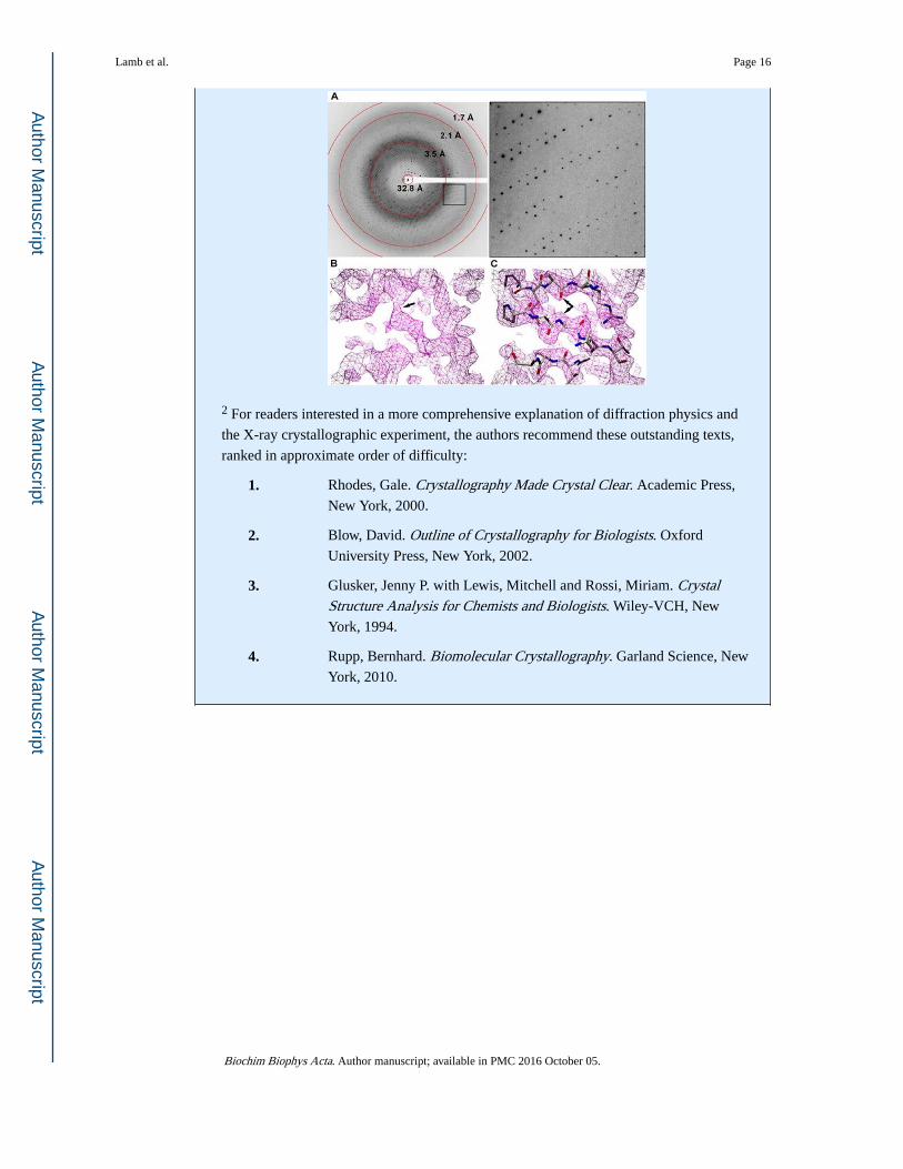
2 For readers interested in a more comprehensive explanation of diffraction physics and
the X-ray crystallographic experiment, the authors recommend these outstanding texts,
ranked in approximate order of difficulty:
1. Rhodes, Gale. Crystallography Made Crystal Clear. Academic Press,
New York, 2000.
2. Blow, David. Outline of Crystallography for Biologists. Oxford
University Press, New York, 2002.
3. Glusker, Jenny P. with Lewis, Mitchell and Rossi, Miriam. Crystal Structure Analysis for Chemists and Biologists. Wiley-VCH, New
York, 1994.
4. Rupp, Bernhard. Biomolecular Crystallography. Garland Science, New
York, 2010.
Lamb et al. Page 16
Biochim Biophys Acta. Author manuscript; available in PMC 2016 October 05.
Author M
anuscriptA
uthor Manuscript
Author M
anuscriptA
uthor Manuscript
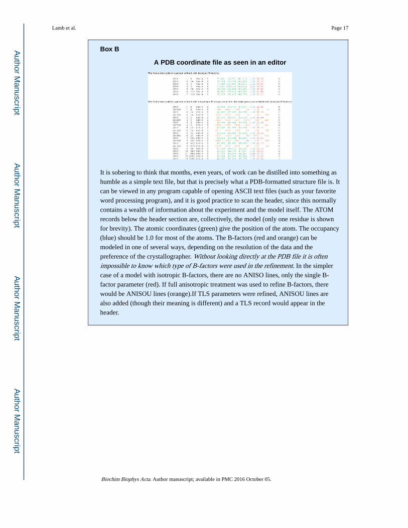
Box B
A PDB coordinate file as seen in an editor
It is sobering to think that months, even years, of work can be distilled into something as
humble as a simple text file, but that is precisely what a PDB-formatted structure file is. It
can be viewed in any program capable of opening ASCII text files (such as your favorite
word processing program), and it is good practice to scan the header, since this normally
contains a wealth of information about the experiment and the model itself. The ATOM
records below the header section are, collectively, the model (only one residue is shown
for brevity). The atomic coordinates (green) give the position of the atom. The occupancy
(blue) should be 1.0 for most of the atoms. The B-factors (red and orange) can be
modeled in one of several ways, depending on the resolution of the data and the
preference of the crystallographer. Without looking directly at the PDB file it is often impossible to know which type of B-factors were used in the refinement. In the simpler
case of a model with isotropic B-factors, there are no ANISO lines, only the single B-
factor parameter (red). If full anisotropic treatment was used to refine B-factors, there
would be ANISOU lines (orange).If TLS parameters were refined, ANISOU lines are
also added (though their meaning is different) and a TLS record would appear in the
header.
Lamb et al. Page 17
Biochim Biophys Acta. Author manuscript; available in PMC 2016 October 05.
Author M
anuscriptA
uthor Manuscript
Author M
anuscriptA
uthor Manuscript
Box C
Downloading and displaying electron density
The Electron Density Server hosted at Uppsala University (http://eds.bmc.uu.se/eds)
allows users to generate and download the model and map files for any structure in the
Protein Data Bank for which the structure factor data have been deposited. The
downloaded map files can then be opened in a number of programs, including COOT
[8,9], PyMol [51], Jmol [12], AstexViewer [52], Chimera [11], and MOE [53]. The
authors prefer to examine electron density in COOT, since it is capable of automatically
downloading and displaying the model, 2Fo – Fc map and Fo – Fc map with no input
beyond the PDB accession code. Displaying electron density is a simple matter of
choosing “ Get PDB & map using EDS…” from the file menu, entering the PDB
accession code for the structure of interest, and pressing the “Get it” button. That is all
there is to it. The contour level of the map can be changed using the scroll wheel on a
PC-style mouse. For more detailed instructions, see the COOT documentation at http://
www2.mrc-lmb.cam.ac.uk/personal/pemsley/coot. COOT can be downloaded free of
charge for Linux, Windows and Mac and is straightforward to install.
Lamb et al. Page 18
Biochim Biophys Acta. Author manuscript; available in PMC 2016 October 05.
Author M
anuscriptA
uthor Manuscript
Author M
anuscriptA
uthor Manuscript
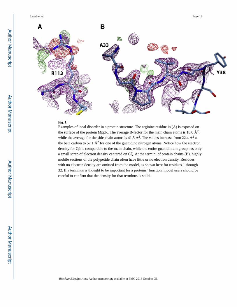
Fig. 1. Examples of local disorder in a protein structure. The arginine residue in (A) is exposed on
the surface of the protein MppR. The average B-factor for the main chain atoms is 18.0 Å2,
while the average for the side chain atoms is 41.5 Å2. The values increase from 22.4 Å2 at
the beta carbon to 57.1 Å2 for one of the guanidino nitrogen atoms. Notice how the electron
density for Cβ is comparable to the main chain, while the entire guanidinium group has only
a small scrap of electron density centered on Cζ. At the termini of protein chains (B), highly
mobile sections of the polypetide chain often have little or no electron density. Residues
with no electron density are omitted from the model, as shown here for residues 1 through
32. If a terminus is thought to be important for a proteins’ function, model users should be
careful to confirm that the density for that terminus is solid.
Lamb et al. Page 19
Biochim Biophys Acta. Author manuscript; available in PMC 2016 October 05.
Author M
anuscriptA
uthor Manuscript
Author M
anuscriptA
uthor Manuscript
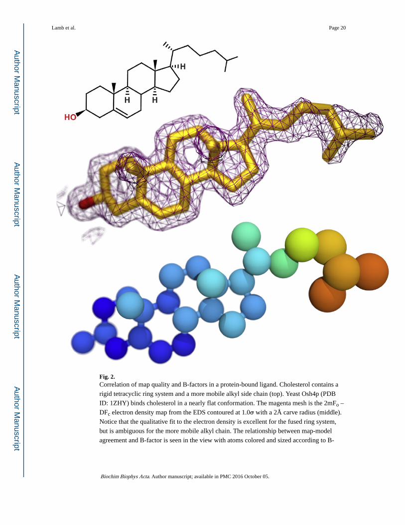
Fig. 2. Correlation of map quality and B-factors in a protein-bound ligand. Cholesterol contains a
rigid tetracyclic ring system and a more mobile alkyl side chain (top). Yeast Osh4p (PDB
ID: 1ZHY) binds cholesterol in a nearly flat conformation. The magenta mesh is the 2mFo –
DFc electron density map from the EDS contoured at 1.0σ with a 2Å carve radius (middle).
Notice that the qualitative fit to the electron density is excellent for the fused ring system,
but is ambiguous for the more mobile alkyl chain. The relationship between map-model
agreement and B-factor is seen in the view with atoms colored and sized according to B-
Lamb et al. Page 20
Biochim Biophys Acta. Author manuscript; available in PMC 2016 October 05.
Author M
anuscriptA
uthor Manuscript
Author M
anuscriptA
uthor Manuscript

factor (bottom; ramp from blue [15 Å2] to red [35 Å2]). The atoms with weaker electron
density have higher B-factors.
Lamb et al. Page 21
Biochim Biophys Acta. Author manuscript; available in PMC 2016 October 05.
Author M
anuscriptA
uthor Manuscript
Author M
anuscriptA
uthor Manuscript
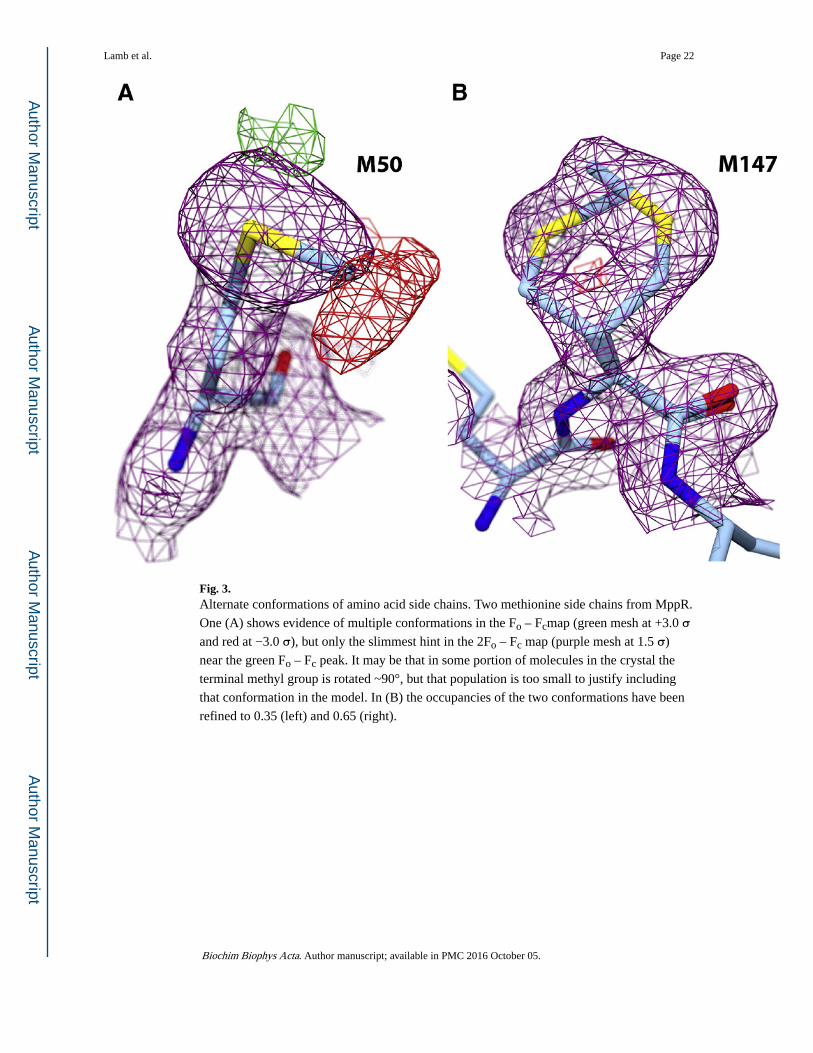
Fig. 3. Alternate conformations of amino acid side chains. Two methionine side chains from MppR.
One (A) shows evidence of multiple conformations in the Fo – Fcmap (green mesh at +3.0 σ and red at −3.0 σ), but only the slimmest hint in the 2Fo – Fc map (purple mesh at 1.5 σ)
near the green Fo – Fc peak. It may be that in some portion of molecules in the crystal the
terminal methyl group is rotated ~90°, but that population is too small to justify including
that conformation in the model. In (B) the occupancies of the two conformations have been
refined to 0.35 (left) and 0.65 (right).
Lamb et al. Page 22
Biochim Biophys Acta. Author manuscript; available in PMC 2016 October 05.
Author M
anuscriptA
uthor Manuscript
Author M
anuscriptA
uthor Manuscript

Fig. 4. The effect of increasing resolution on electron density maps. The panels show the active site
of the Clostridium botulinum serotype A neurotoxin with various ligands bound at 4.3 Å
(A), 2.4Å(B), 1.9 Å (C), 1.4 Å (D), and 1.2 Å (E). The 2mFo – DFc electron density maps
are contoured at 1.0 σ (blue) and 3.0 σ(yellow) within a 2.0 Å radius around each atom. The
catalytic Zn(II) ion is shown as a silver sphere. Notice the clear differences in the level of
detail in moving from 4.3 to 2.4 Å (A and B), and from 2.4 to 1.9Å (B and C). Notice also
that as the resolution increases, small differences in resolution give diminishing returns in
Lamb et al. Page 23
Biochim Biophys Acta. Author manuscript; available in PMC 2016 October 05.
Author M
anuscriptA
uthor Manuscript
Author M
anuscriptA
uthor Manuscript
terms of map detail (e.g. compare 1.4 and 1.2 Å in D and E). The structures shown are PDB
ID 3V0C, 2IMB, 2IMA, 3BOO, and 3BON [54–56].
Lamb et al. Page 24
Biochim Biophys Acta. Author manuscript; available in PMC 2016 October 05.
Author M
anuscriptA
uthor Manuscript
Author M
anuscriptA
uthor Manuscript

Fig. 5. Hydrogen bonding patterns should make chemical sense. An ultra-high resolution electron
density map (0.75 Å) of the Streptomyces strain R61 D-alanyl-D-alanine carboxy-peptidase/
transpeptidase showing His37, on the protein surface, making hydrogen bonding interactions
with a water molecule and an adjacent aspartate residue (unpublished data). The modeled
conformation of the imidazole ring of His37 agrees with the surrounding network of
hydrogen bonds and is further supported by the larger electron density peaks of the two N
atoms (N has one more electron than C, and at very high resolutions this difference in visible
for well-ordered atoms). The 2mFo - DFc electron density maps are contoured at 1.5 (blue)
and 4.0 σ (yellow).
Lamb et al. Page 25
Biochim Biophys Acta. Author manuscript; available in PMC 2016 October 05.
Author M
anuscriptA
uthor Manuscript
Author M
anuscriptA
uthor Manuscript
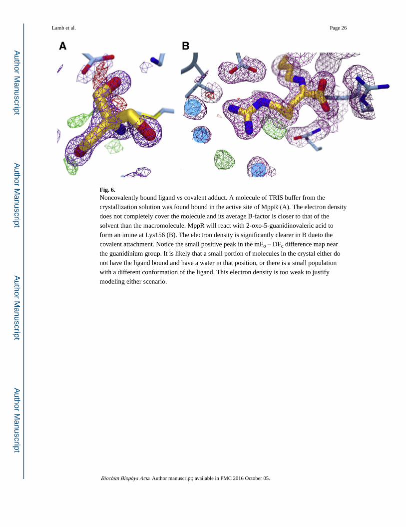
Fig. 6. Noncovalently bound ligand vs covalent adduct. A molecule of TRIS buffer from the
crystallization solution was found bound in the active site of MppR (A). The electron density
does not completely cover the molecule and its average B-factor is closer to that of the
solvent than the macromolecule. MppR will react with 2-oxo-5-guanidinovaleric acid to
form an imine at Lys156 (B). The electron density is significantly clearer in B dueto the
covalent attachment. Notice the small positive peak in the mFo – DFc difference map near
the guanidinium group. It is likely that a small portion of molecules in the crystal either do
not have the ligand bound and have a water in that position, or there is a small population
with a different conformation of the ligand. This electron density is too weak to justify
modeling either scenario.
Lamb et al. Page 26
Biochim Biophys Acta. Author manuscript; available in PMC 2016 October 05.
Author M
anuscriptA
uthor Manuscript
Author M
anuscriptA
uthor Manuscript