


Performance analysis of the multi-user system
by
Wing Kwan, NG
A Thesis Submitted to
The Hong Kong University of Science and Technology
in partial Fulfillment of the Requirements for
the Degree of Master of Philosophy
in the Department of Electronic and Computer Engineering
July 2008, Hong Kong
Dedicated to my parents, elder sister, younger brother.
Special thanks to Yvonne Chan and Rachel Au-Yeung.
iv

Acknowledgements
I would like to thank my supervisor, Dr. Vincent Lau, not only for his unfailing
encouragement, support and guidance but also for his belief in me. He has given
me numerous chances in projects and research which has strengthened my multi-
tasking ability. Besides academic supervision, I would like to give thanks for
his nomination, I have received serval scholarships during my study which have
alleviated the financial burden from my family.
I am also indebted to Dr. Roger Shu-Kwan Cheng, it has been my pleasure to
be his TA in the last two years. His good lecturing skill and his patience and great
efforts in explaining things have helped me to develop interests in researching the
wireless world.
I truly appreciate the friendship of my friends for having a pleasant working
environment and for their helpful discussions. My appreciation goes to: Ernest Lo,
Roderick Luo, Zuleita Ho, Big Henry, Henry Cheung, P.D, Tin, Kelvin Lai, Lilian,
Herbert Chan, Adam Man, Sherlock Chan, Hailing Meng , Bao, Karama Hamdi,
Li Tao, S.Y. Chan, Edward Au, Ray, Tianyu, LED, Jane, David, Cui Ying, Sun
Liang and Eddy.
In additional, i would like to say a big thank you to Yvonne Chan and Rachel
Au-Yeung. With their guidance, I learned to understand myself deeply in the last
two years, and I am ready to leave Hong Kong to pursue my PHD degree.
v

Lastly, but most importantly, I wish to thank my family who have been sup-
porting me in every possible way.
vi

Table of Contents
Title Page i
Authorization Page ii
Signature Page iii
Acknowledgements v
Table of Contents vii
List of Tables ix
List of Figures x
Abstract xiii
Abbreviations xv
Notation xviii
1 Introduction 1
1.1 Wireless Communication . . . . . . . . . . . . . . . . . . . . . . . . 1
1.2 Literature Survey - Downlink . . . . . . . . . . . . . . . . . . . . . 3
1.3 Literature Survey - uplink . . . . . . . . . . . . . . . . . . . . . . . 6
1.4 Problem Statement . . . . . . . . . . . . . . . . . . . . . . . . . . . 7
1.5 Thesis Contributions . . . . . . . . . . . . . . . . . . . . . . . . . . 9
1.6 Thesis Outline . . . . . . . . . . . . . . . . . . . . . . . . . . . . . . 11
1.7 Author’s Publications List . . . . . . . . . . . . . . . . . . . . . . . 12
2 Background 14
2.1 Introduction . . . . . . . . . . . . . . . . . . . . . . . . . . . . . . . 14
2.1.1 Wireless Channel . . . . . . . . . . . . . . . . . . . . . . . . 14
2.1.2 Orthogonal frequency division multiple access-OFDMA . . . 19
2.1.3 Cross-layer scheduling . . . . . . . . . . . . . . . . . . . . . 22
2.1.4 Successive interference cancellation . . . . . . . . . . . . . . 24
3 Cross-Layer optimization and analysis 27
3.1 Introduction . . . . . . . . . . . . . . . . . . . . . . . . . . . . . . . 27
3.1.1 System model . . . . . . . . . . . . . . . . . . . . . . . . . . 30
vii
3.1.2 Frequency Selective Fading Channel Model and Delayed CSIT
Model . . . . . . . . . . . . . . . . . . . . . . . . . . . . . . 30
3.1.3 Instantaneous Mutual Information and System Goodput . . 33
3.2 Cross-Layer Design for OFDMA Systems . . . . . . . . . . . . . . . 35
3.2.1 Cross-Layer Design Optimization Formulation . . . . . . . . 36
3.2.2 Closed-form Solutions for Power and Rate Allocation Policies 38
3.2.3 Low Complexity User Selection and Subcarrier Allocation
Policies . . . . . . . . . . . . . . . . . . . . . . . . . . . . . 39
3.3 Asymptotic Performance Analysis for Cross-Layer Design . . . . . 43
3.3.1 Frequency Diversity at Small Target Packet Outage Proba-
bility ε . . . . . . . . . . . . . . . . . . . . . . . . . . . . . . 45
3.3.2 Cross-Layer Goodput Gains at Large K and fixed Nd . . . . 45
3.3.3 Asymptotic System Goodput at Large Nd and fixed K . . . 48
3.4 Summary . . . . . . . . . . . . . . . . . . . . . . . . . . . . . . . . 50
4 Uplink multi-user detection analysis 53
4.1 Introduction . . . . . . . . . . . . . . . . . . . . . . . . . . . . . . . 53
4.2 System Model . . . . . . . . . . . . . . . . . . . . . . . . . . . . . . 58
4.2.1 Multi-access Channel Model . . . . . . . . . . . . . . . . . . 59
4.2.2 MUD-SIC Processing and Per-User Packet Error Model . . . 59
4.2.3 Optimal Decoding Order Policy . . . . . . . . . . . . . . . . 62
4.3 Performance Analysis . . . . . . . . . . . . . . . . . . . . . . . . . . 64
4.3.1 System Goodput and Per-User Packet Outage Probability
for MUD-SIC . . . . . . . . . . . . . . . . . . . . . . . . . . 65
4.3.2 Asymptotic Expressions on Average System Goodput and
Per-User Packet Error Probability . . . . . . . . . . . . . . . 69
4.4 Results and Discussions . . . . . . . . . . . . . . . . . . . . . . . . 70
4.4.1 Results on the Average System Goodput . . . . . . . . . . . 72
4.4.2 Results on Average Per-User Packet Error Probability . . . . 75
4.5 Summary . . . . . . . . . . . . . . . . . . . . . . . . . . . . . . . . 76
5 Conclusions 79
6 Appendix 81
6.0.1 Proof of Lemma 6.0.1 in Chapter 3 . . . . . . . . . . . . . . 81
6.0.2 Proof of Lemma 2 in Chapter 3 . . . . . . . . . . . . . . . . 84
6.0.3 Proof of Theorem 1 in Chapter 3 . . . . . . . . . . . . . . . 85
6.0.4 Proof of Lemma 4 in Chapter 3 . . . . . . . . . . . . . . . . 85
6.0.5 Proof of Lemma 3 in Chapter 3 . . . . . . . . . . . . . . . . 86
6.0.6 Proof of Theorem 2 in Chapter 3 . . . . . . . . . . . . . . . 87
6.0.7 Proof of Lemma 5 in Chapter 4 . . . . . . . . . . . . . . . . 87
6.0.8 Proof of Lemma 6 in Chapter 4 . . . . . . . . . . . . . . . . 88
6.0.9 Proof of Lemma 7 in Chapter 4 . . . . . . . . . . . . . . . . 89
References 90
viii
List of Tables
2.1 general trends of different multiuser receivers, with spreading factor
N, number of users K, and P receiver stages . . . . . . . . . . . . . 25
ix
List of Figures
2.1 Basic mitigation types . . . . . . . . . . . . . . . . . . . . . . . . . 19
2.2 OFDM system base-band implementation . . . . . . . . . . . . . . 20
2.3 OFDMA scheduling block diagram . . . . . . . . . . . . . . . . . . 21
2.4 International Standard Organization (ISO)’s Open System Inter-
connect (OSI) reference model . . . . . . . . . . . . . . . . . . . . . 22
2.5 OFDMA scheduling block diagram . . . . . . . . . . . . . . . . . . 23
3.1 A comparison of the average system goodput versus SNR with CSIT
error σ2e = 0.01. . . . . . . . . . . . . . . . . . . . . . . . . . . . . . 41
3.2 A flow chart of the Greedy cross-layer scheduling algorithm. . . . . 42
3.3 Average system goodput versus number of users with Nd=2, differ-
ent CSIT error (σ2e=0.01,0.05,0.1,1) at high SNR(20dB). . . . . . . 46
3.4 Average system goodput versus number of users with Nd=2, differ-
ent CSIT error (σ2e=0.01,0.05,0.1,1) at low SNR(0dB). . . . . . . . . 47
3.5 Average system goodput versus packet diversity order (Nd) with
different CSIT error σ2e at high SNR(20dB) and K=20. . . . . . . . 49
3.6 Average system goodput versus packet diversity order (Nd) with
different CSIT error σ2e at low SNR(0dB) and K=20. . . . . . . . . 50
3.7 Inverse CDF of non central chi square random variable versus non-
centrality parameter s2 for ε=0.001 with degrees of freedom equal
to 6. . . . . . . . . . . . . . . . . . . . . . . . . . . . . . . . . . . . 51
x

3.8 Inverse CDF of non central chi square random variable versus ε with
degree of freedom 6 and non central parameter s2 = 1. . . . . . . . 52
4.1 Illustration of the mutual coupling (error propagation) of packet
outage events and the importance of decoding order in MUD-SIC
for system goodput considerations in quasi-static multiaccess fad-
ing channels. Rate vector ~rA, which is outside the instantaneous
capacity region, may contribute to non-zero system goodput if user
1 is decoded first. Rate vector ~rB, which is inside the instantaneous
capacity region, may contribute to zero system goodput if a wrong
decoding order is used. . . . . . . . . . . . . . . . . . . . . . . . . . 56
4.2 System model of multi-user network with multi-user detection . . . 58
4.3 Illustration of the MUD-SIC decoding tree for random decoding
order. The decoding process continues even there is packet error in
the current iteration. This is because there is still a possibility that
subsequent decoding iterations will be successful given the current
decoding iteration fails. . . . . . . . . . . . . . . . . . . . . . . . . . 71
4.4 System goodput vs SNR(dB) with different outage (n=5). The solid
line represent the theoretical expression and the dotted solid repre-
sent the simulated result of the system goodput respectively. The
double sided arrow represent the performance gain of the optimal
SIC over the random SIC. . . . . . . . . . . . . . . . . . . . . . . . 72
4.5 System goodput against number of users with different SNR (packet
error probability=10%) . . . . . . . . . . . . . . . . . . . . . . . . 74
xi
4.6 Average packet error probability against SNR with different trans-
mitted rate(r) (Number of users(n)=5). The solid line represent the
theoretical expression and the dotted solid represent the simulated
packet error expression respectively. Different curve represent dif-
ferent transmitted rate with the same user. The double sided arrow
represent the performance gain of the optimal SIC over the random
SIC. . . . . . . . . . . . . . . . . . . . . . . . . . . . . . . . . . . . 75
4.7 Average packet error probability against SNR with different trans-
mitted rate(r) (Number of users(n)=10) . . . . . . . . . . . . . . . 76
4.8 Average packet error probability against number of users with dif-
ferent transmitted rate(r) (SNR=5dB). The solid line represent the
theoretical expression and the dotted solid represent the simulated
packet error expression respectively. Different curve represent dif-
ferent transmitted rate with the same SNR(dB). The double sided
arrow represent the performance gain of the optimal SIC over the
random SIC. . . . . . . . . . . . . . . . . . . . . . . . . . . . . . . . 77
4.9 Average packet error probability against number of users with dif-
ferent transmitted rate(r) (SNR=10dB) . . . . . . . . . . . . . . . . 78
xii
Performance analysis of multi-user system
by
Wing Kwan, NG
The Department of Electronic and Computer Engineering
The Hong Kong University of Science and Technology
Abstract
Cross-layer design has been shown to offer high spectral efficiency which benefits
from the inherent multi-user diversity in wireless fading channels. In cross-layer
OFDMA systems with perfect CSIT, it is well known that the system through-
put (ergodic capacity) scales in the order of O(log logK) due to the MuDiv gain.
However, with imperfect CSIT, it is still not clear whether we can get the same
performance as that of the perfect case.
In the first part of this thesis, we shall consider the cross-layer OFDMA schedul-
ing design under various practical PHY layer and MAC layer constraints for a
wireless system with one base station and K mobile users . We study the cross-
layer scheduling design with imperfect channel state information (CSI) at the base
station for delay-tolerant applications. The imperfectness of CSI is assumed to
be the result of feedback or duplexing delay. With imperfect CSI at transmit-
ter (CSIT), there exists a potential packet transmission error when the scheduled
data rate exceeds the instantaneous channel capacity referring to packet outage.
The OFDMA cross-layer design with delayed CSIT is modeled as an mixed integer
and convex optimization problem where the rate adaptation, power adaptation and
subcarrier allocation policies are designed to optimize the system goodput (b/s/Hz
successfully received by the mobiles). At the time same time, we are interested to
xiii
know the trade-off between packet outage diversity gain and multi-user diversity
gain. Therefore, by using extreme value theorem, we are able to show the trade-off
analytically.
In the second part of this thesis, we would like to evaluate the performance
of a uplink multiaccess channel with successive interference cancellation receiver
equipped in the base-station. We derive analytically the per-user packet outage
probability and the total system goodput for multi-access systems using multiuser
detector with adaptive successive interference cancellation (MUD-SIC). Slow fad-
ing channel is assumed where packet transmission error (outage) is the primary
concern even if strong channel coding is applied. To capture the effect of potential
packet error, goodput should be used as performance measure. Unlike previous
works, our analysis focuses on the error-propagation effects in MUD-SIC detector
where the packet outage event for a single user is depending on the other users.
Also, we derive the optimal SIC decoding order (to maximize system goodput)
and evaluate the closed-form per-user packet outage probabilities for the n users
for MUD-SIC. Simulation results are used to verify the analytical expressions.
xiv

Abbreviations
AMPS Advanced mobile phone service
AWGN Additive white Gaussian noise
B3G Beyond third generation cellular system
BER Bit error rate
BPSK Binary phase shift keying
BSC Base station controller
cdf Cumulative distribution function
CDMA Code division multiple access
CSCG Circularly symmetric complex Gaussian
CSI Channel state information
CSIR Channel state information at receiver
CSIT Channel state information at transmitter
D-AMPS Digital advanced mobile phone service
D-BLAST Diagonal Bell layered space-time
DFE Decision feedback equalization
DFT Discrete Fourier transform
DS/SS Direct sequence spread spectrum
DVB Digital video broadcasting
EV-DO Evolution-data optimized
EV-DV Evolution-data and video
FDD Frequency division duplex
FDMA Frequency division multiple access
FER Frame error rate
xv

FFT Fast Fourier transform
GSM Global system for mobile communications
HSDPA High-speed downlink packet access
i.i.d. Independent and identically distributed
ISI Inter-symbol interference
ISO International Standard Organization
ICI Inter-carrier interference
LAN Local area network
LDPC Low-density parity-check code
MAC Media access control
MAI Multiple access interference
MAN Metropolitan area network
MC-CDMA Multiple carrier-code division multiple access
ML Maximum likelihood
MMSE Minimum mean square error
MUD Multiuser detection
NLOS Non line of sight
OFDM Orthogonal frequency division multiplexing
OFDMA Orthogonal frequency division multiple access
OSI Open System Interconnect
p.d.f Probability density function
PER Packet error rate
PHY Physical layer
QoS Quality of service
xvi
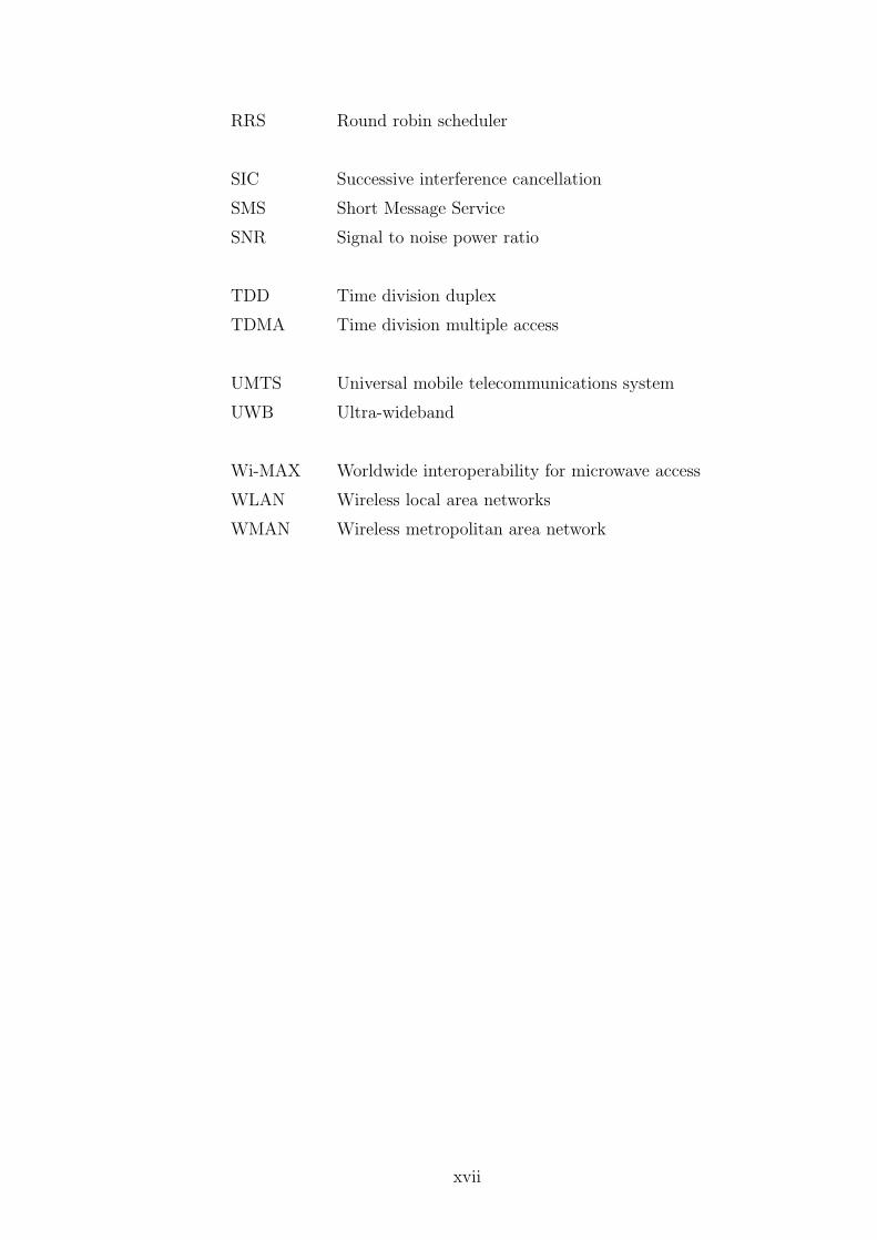
RRS Round robin scheduler
SIC Successive interference cancellation
SMS Short Message Service
SNR Signal to noise power ratio
TDD Time division duplex
TDMA Time division multiple access
UMTS Universal mobile telecommunications system
UWB Ultra-wideband
Wi-MAX Worldwide interoperability for microwave access
WLAN Wireless local area networks
WMAN Wireless metropolitan area network
xvii

Notation
≈ approximately equal to
logx(y) the log, base x of y
E[.] expectation operator
E[.|.] Conditional expectation operator
(.)∗ complex conjugate
(.)T transpose
F(.) Fourier transform operator
F−1(.) Inverse Fourier transform operator
φx(s) Characteristic function of random variable X
xviii

Chapter 1
Introduction
1.1 Wireless Communication
Wireless Communication has been one of the most active research areas over
the past decades, the fruits of these research works have benefited human be-
ings through different wireless products. They penetrates our offices, homes and
even in our pocket, they become an essential part of our life.
The first wireless communication system can be traced back to the last century.
In 1895, Guglielmo Marconi [1] demonstrated the first radio transmission system
by using a free propagating electromagnetic wave as a carrier. Since then, tere has
been rapid progress in the wireless technology.
A century after the invention of Marconi, in the 1980s, the first generation (1G)
cellular system, AMPS( advanced mobile phone service) system was developed in
American and the other system TACS (Total Access Communication system) was
developed in the European countries. These systems suffered from some weaknesses
when compared to today’s digital technologies. Since it is an analog standard, it
1

is very susceptible to static noise and has no protection from eavesdropping using
a scanner.
The second generation (2G) digital cellular systems development is due to the
incompatibly of 1G system standards and the increasing demand of a mobile phone
service. These factors lead to a quickly converged uniform standard (GSM) in
Europe and was first implemented in Finland in 1991. Later on, IS-136 and IS-95
were implemented in the U.S which provided more options to terminal users. These
kind of systems have significantly improved the spectral efficiency and network
capacity to support more than voice service such as Short Message Service (SMS)
and photo transmission.
Fueled by the exposition of demand for high data rate multimedia applica-
tion such as video streaming and video conferencing, researcher developed a lot
of high speed and high quality communication system. This includes the devel-
opment of 3G systems(CDMA 2000, UMTS), 3.5G systems (HSDPA,EV-DO,EV-
DV), B3G systems (Beyond 3G), wireless LAN (IEEE 802.11 a/b/g/n), ultra-
wideband(UWB) systems, and WiMAX (IEEE 802.16) as well as Wi-Man (IEEE
802.20) systems. Although the listed above advance wireless technology provided
much higher quality than that of the old days, the need for higher data rate grows
ever faster, therefore new technology needs to be implemented in the future system.
In order to provide reliable and efficient communication over the wireless chan-
nel, researchers have been trying very hard to explore this topic since the 1950s.
The reason of unreliable communication is mainly due to fading and interference.
Fading refers to the time variation of the channel signal strength due to multi-
path effect as well as large scaling fading [2]. On the other hand, unlike point to
2

point wired channel, users communicate over the air and share the same channel ,
therefore significant interference does exist in the wireless channel.
Traditionally, various diversity techniques such as frequency diversity, time
diversity are used to mitigate deep-fade situations. In addition, multiple access
techniques such TDMA , FDMA together with cell sectoring are used to reduce
co-channel interference in partial systems. However, these techniques can not
satisfy our future need due to lack of spectral efficiently. Recent research works
[3–7] have shown that cross-layer scheduling with OFDMA systems can boost up
the capacity of downlink while using multi-user detection (MUD) in the uplink can
achieve any points in the multiuser capacity region.
Therefore, we shall investigate the performance advantages of these two promis-
ing technologies throughout this thesis.
1.2 Literature Survey - Downlink
In [8, 9], a joint design of the MAC layer and link layer has been shown to
achieve significant gains over the isolated design approach within each layer for
single antenna systems as a result of multiuser diversity gain, which is achieved by
scheduling transmissions (through power and rate adaption) to users when their
instantaneous channel quality is near the peak. However, most of the existing
literatures about cross-layer design, perfect channel state information (CSIT) is
assumed to be available in the transmitter(basestation)[10–12]. The information
is further assumed to be up-to-update of the scheduler finishes the scheduling of
power,rate and user selection. In the above works, since CSIT is assumed to be
perfect, by carefully adapting the power and rate, channel outage can be avoided
3

as long as the error correcting code is sufficiently long and strong. As a result,
ergodic capacity is a meaningful performance measure although it does not capture
the outage effect.
However, with imperfect CSIT (channel state is a random variables to the
transmitter) there is finite probability that the scheduled data exceeds the channel
capacity and causes the packet corrupted. Furthermore, in slow fading channel,
there is no significant channel variation across the encoding frame and there may
be no classical Shannon meaning attached to the capacity in this situation. There-
fore, ergodic capacity is no longer a suitable performance measure. Furthermore,
the imperfectness of CSIT would cause ‘mis-scheduling” which would degrade the
system performance significantly. All in all, imperfectness of CSIT should be taken
into consideration in the system design.
Besides, in the modern wireless communication system, it is a mix of real-time
traffic (voice,multimedia teleconferencing, and games) and data traffic(file transfer
and email). All of these applications require widely varying and very diverse quality
of service (QoS) guarantees for the different types of offered traffic. In [13], a cross-
layer scheduler desgin for multimedia applications in adaptive wireless networks is
developed, novel admission and scheduling police is introduced to provide useful
analytical results in terms of throughput, packet loss rate and average delay. In
[14], the authors first introduce a theoretical framework for cross-layer optimization
for orthogonal frequency division multiplexing(OFDM), necessary and sufficient
conditions for optimal subcarrier assignment and power allocation are discussed.
Then they further develop effective and practical algorithms for efficient and fair
resource allocation in OFDM wireless networks[15] such as sorting-search dynamic
4

subcarrier assignment, greedy bit loading, and power allocation, as well as objective
aggregation algorithms, all of these algorithms provide useful tools in the future
OFDM base scheduling based system.
On the other hand, scheduling have been implemented in practical 3G systems
(CDMA based system), there are four basic types of traffic classes supported by
UMTS Rel 99,the scheduler is responsible for the dynamic allocation of the radio
resources in terms of data rate, time duration and power levels based on the class
of users (QoS requirement) over a macroscopic time scale[16].
Thus, scheduling not only has great impact in academic areas, but also have
evolutional effect in the practical system.
5

1.3 Literature Survey - uplink
Nowadays, the performance of cellular systems are limited by interference more
than by any other single effect. Unlike traditional channel noise (thermal noise),
interference is caused by human-designed device, mostly from devices designed
to use the same spectrum. This kind of interference is called multiple access
interference (MAI). It is a main factor which limits the capacity and performance.
Unfortunately, the conventional detector does not take into account the existence
of MAI. It follows a single-user detection strategy in which each user is detected
separately without regard for other users. For example, in practical systems such as
IS-95 and 3G cellular, an interference limited system is willfully created in order
to achieve capacity and universal frequency reuse. The most common receiver
uses match filter for the desired user and treats all the signal of other users as
noise[17], however it is strictly suboptimal in most situations from an information
theory perspective[4]. Therefore, multi-user receiver(detection) is needed to further
improve system capacity.
Multiuser detection (MUD) have been studied over 20 years since the mid
1980.The optimal multi-user receiver for CDMA was first introduced by Verdu in
his P.H.D thesis [18]. Although MUD provides a promising result in multiaccess
channel, it has not found widespread acceptance in commercial systems because
the major problem with multiuser detectors is the maintenance of simplicity. Over
the past two decades of study, researchers have come up with the idea of inter-
ference cancellation [19]. In [20–23], iterative interference cancellation with turbo
coding have been shown to have near-single-user performance which is very attrac-
tive. However, the complexity of order of turbo MUD increases with the number
6

of users exponentially, which is not practical. On the other hand, successive in-
terference cancellation (SIC) has complexity only proportional to the number of
users which has the same complexity order as the conventional single user detec-
tor.Furthermore, it has been shown that commercial CDMA power control algo-
rithm can be directly applied to SIC without any modification[24]. Therefore, SIC
receivers have been considered as a candidate in the future communication sys-
tem. In the early works of SIC receiver [25, 26], channel estimation is assumed to
be perfect and the interference is completely cancellated in each decoding stage,
but this assumption is never achievable in practice. In [24], researchers begin to
consider the effect of error propagation together with power control. Nevertheless
, decoding order in the receiver have not been considered.
To conclude, either in both uplink MUD and downlink cross-layer scheduling,
we still need more research works to bridge the gap between theoretical and prac-
tical implementation such that the next generation of communication system can
fulfill the future need of users.
1.4 Problem Statement
Cross-layer design is a revolutionary technology in wireless commination system
which increases the system capacity substantially. However, most existing research
works assume either perfect CSI estimation or perfect feedback. Scheduler can
based on the perfect information to perform user selection, power adaption and
rate adaption such that multi-user diversity is fully exploited. However, perfect
CSIT is difficult to obtain in practice,especially in FDD systems in which explicit
feedback is required. On the other hand, in TDD systems, feedback may be delayed
7

and therefore the estimation no longer accurate since the channel is changing. With
imperfect CSIT, channel outage would occur even strong error correction code is
applied to the transmission frame. To take account of the potential packet outage,
we define the average system goodput the performance measure metric, which
measures the average total bit/s/Hz and successfully deliverers to the receivers.
In the cross-layer design, we would like to solve the following open issues in the
downlink multiuser system:
• There are two important aspects of cross-layer gains in multiuser OFDMA
systems with slow fading channels. They are the system goodput gain (by
scheduling a strongest user per subband) as well as the packet diversity gain
(by scheduling a user to transmit on multiple independent subbands). Due to
the delayed CSIT, packet outage diversity is important to protect the packet
from potential packet outage. Yet, it is not clear how the asymptotic system
goodput gain and the packet outage diversity tradeoff with each other.
• How would the system goodput be affected by CSIT errors and the number
of resolvable multipaths in the frequency selective fading channel?
On the other hand, in the uplink transmission, optimal MUD is a well-known
technology that allows us to achieve any points in the multi-access capacity region
from the information theory perspective. Due to the exponential complexity in the
implementation of optimal MUD, successive interference cancellation have been
proposed which has only linear complexity. Furthermore, it can be shown that
MMSE-SIC is able to achieve corner points of the multi-access capacity region.
However, this attractive technology comes with other research problems such as
optimal power control, rate adaption , error propagation effect and decoding order.
8

In the uplink multiuser system with successive interference cancellation receiver
, we would like to address the following issues:
• In slow fading channel without CSIT, outage occurs with non-zero probabil-
ity. With the consideration of error-propagation effects and per user outage
constraint, what is the maximum achievable capacity in the multiuser sys-
tem?
1.5 Thesis Contributions
The central subject of interest of this thesis is the performance analysis in the
future uplink and downlink transmission technologies. In the first part, we would
like to focus on the downlink OFDMA scheduling system design, a systematic
framework to address the scheduling where the presence of outdated CSIT is pro-
posed. Because of the imperfect CSIT , outage occurs with non-zero probability.
To address this problem, one way is to take into account the estimation error, and
the other way is to schedule a user with multiple independent sub-bands such that
the transmit information has diversity protection. This is further explained in the
following:
• Tradeoff between Cross-Layer Goodput Gain and Outage Diver-
sity: The OFDMA cross-layer design with delayed CSIT is modeled as
an optimization problem where the rate adaptation, power adaptation and
subcarrier allocation policies are designed to optimize the system goodput
(b/s/Hz successfully received by the mobiles). We derive simple closed-form
expressions for the power and rate allocations as well as the asymptotic or-
der of growth in system goodput for general CSIT error. From the analytical
9
asymptotic analysis, tradeoff between the system goodput gain and the packet
outage diversity gain in cross-layer OFDMA systems with delayed CSIT is
illustrated.
In the second part, we aim at deriving a analytical expression to calculate the
system performance for an uplink environment with multi-user detector equipped
in the basestation. Optimal MUD is a promising technology which allows us to
achieve any points in the multi-access capacity region from the information theory
point of view. However, due to high complexity in the implementation, researchers
have been searching for the past two decades for sub-optimal solutions but with
guaranteed performance. In all of the substitutes, successive interference is shown
to be optimal in the sense that it can achieve the corner point of the multi-access
capacity region, and it only has linear complexity with the number of users. There-
fore, in practice, we would like to find out the system performance when we con-
sider some implementations details such as decoding order. The construction of
the uplink parts is summarized as follows:
• Per user outage analysis with Multiuser detection - successive in-
terference cancellation : We analytically derive the per-user packet out-
age probability and the total system goodput for multi-access systems using
multiuser detector with adaptive successive interference cancellation (MUD-
SIC). We consider a multiuser wireless system with n mobile users and a
base station. We assume slow fading channels where packet transmission er-
ror (outage) is the primary concern even if strong channel coding is applied.
To capture the effect of potential packet error, we consider the average packet
error probability and the total system goodput of the n users, which measures
10

the average b/s/Hz successfully delivered to the base station. Unlike previous
works, our analysis focus on the error-propagation effects in MUD-SIC detec-
tor where the packet outage event for the i-th decoded user is coupled with
that in the i− 1, .., 1-th decoding attempts. We shall derive the optimal SIC
decoding order (to maximize system goodput) and evaluate the closed-form
per-user packet outage probabilities for the n users for MUD-SIC. Simulation
results are used to verify the analytical expressions.
1.6 Thesis Outline
The remainder of the thesis is organized as follows.
Chapter 2 introduces the background material, including the basic theory of
wireless communication, general cross-layer scheduling model and the multiuser
detection technology.
Chapter 3 presents the downlink scheduling and rate adaptation and inves-
tigates the system performance with imperfect CSIT consideration. Asymptotic
analysis is used to investigate the trade-off between system goodput gain and
packet outage diversity in the cross-layer OFDMA design.
Chapter 4 describes a multiuser wireless system with n mobile users and a base
station. We derive an analytical upper bound of per user outage probability and a
lower bound of average system goodput which provides useful insight in the future
system design.
Finally, we give some concluding remarks in Chapter 5.
11
1.7 Author’s Publications List
Journal paper:
1. V. K. N. Lau, W.K. Ng,” Per-User Packet Outage Analysis in Slow Multi-
access Fading Channels with Successive Interference Cancellation for Equal
Rate Applications ” IEEE Transactions on Wireless Communications, ac-
cepted, Sep 2007.
2. V. K. N. Lau, W.K. Ng , David S. W. Hui , ”Asymptotic Tradeoff between
Cross-Layer Goodput Gain and Outage Diversity in OFDMA Systems with
Slow Fading and Delayed CSIT”,IEEE Transactions on Wireless Communi-
cations, accepted, January 2008.
3. M.Z, W.K. Ng, V.K.N Lau and C.T Lea, ”Cross-Layer Scheduling under
Mobility”, submitted to IEEE Transactions on Wireless Communication,
under review, March 2008.
4. W.K. Ng, V.K.N Lau, Design and Analysis of Outage-Limited Multi-access
Cellular Systems with Macro-diversity. , drafting. May 2008.
Conference paper:
1. V. K. N. Lau, W.K. Ng , David S. W. Hui ,”Asymptotic Tradeoff between
Cross-Layer Goodput Gain and Outage Diversity in OFDMA Systems with
Slow Fading and Delayed CSIT”, in Proceedings of the 2007 IEEE Interna-
tional Symposium on Information Theory (ISIT 2007), Nice, France, June
2007, pp 2756-2760
12

2. V. K. N. Lau, W.K. Ng , David S. W. Hu, Bin Chen ,”Cross-Layer Op-
timization for OFDMA System with Imperfect CSIT in Quasi Static Chan-
nel”, International Conference on Communications and Networking in China
2008, accepted March 2008.
Patent:
1. Ming Y. Tsang, Chi-Tin Luk, Wing-Kwan Ng, Vincent K. N. Lau , C.Y.Tsui
and Roger S. K. Cheng, ”Robust timing Synchronizations in MB-OFDM Fre-
quency hopping System in SOP environment”,filed in Sep. 2007
13

Chapter 2
Background
2.1 Introduction
The goal of this chapter is to give an overview of the wireless channel character-
ization and the modern technology to achieve high data rate communication. In
particular, we would like to introduce the fundamental theory of OFDMA, cross-
layer scheduling and successive interference cancellation as well as the difficulties
in practical application.
2.1.1 Wireless Channel
The wireless channel poses a challenge as a medium for reliable high-speed-communication.
Not only are noise and interference harmful to the transmission link, but also the
unpredictable nature of channel variation. Modelling the radio channel has histori-
cally been one of the most difficult parts of mobile system design, and it is typically
done in a statistical manner. To have a good understanding of the wireless channel,
we would like to introduce the following two types of fading:
14

Large scale fading
Traditional path loss models are aimed on predicting the average received signal
power at a given distance from the transmitter, and used to approximate the wave
propagation according to Maxwell’s equation. Conventional model such as free-
space path loss does not consider the shadowing effect which is caused by obstacles
between the transmitter and the receiver.
Measurements have shown that at any value d, the path loss at a practical
location is random and with log-normal distribution above the mean path loss
value. The statical equation which combines the path loss and shadowing effect is
given in the following equation and can be found in reference [27]:
PL(d) = PL(d0) + 10n log
(d
d0
)+ Xσ, (2.1.1)
where d0 is the reference distance; n is the path loss exponent which indicate the
rate of signal power drop beyond the reference distance; Xσ is a zero-mean Gaussian
distributed random variable (in dB) with standard deviation σ (in dB), which is
called log-normal shadowing. The log-normal distribution describes the random
shadowing effects which occur over a larger number of measurement locations which
have the same transmitter and receiver distance, but have different levels of clutter
on the propagation path. The combined path loss and shadowing information
provides the system designer with a useful reference to calculate the cell coverage
and also the link budget (frequency reuse factor).
Small scale fading
In the small scale fading, the signal strength fluctuates over 30dB within a
short period of time(in the order of milli-second) or travel distance (length of a
15

few wavelengths). Small scale fading is caused by interference between two or
more versions of the transmitted signal which arrive at the receiver ar slightly
different times. These multipaths combined at the receiver antenna and result in
either constructive or destructive interference and cause the fluctuation of received
signal. There are two independent dimensions in small scale fading, they are listed
below:
• Multipath dimension: To quantify the multipath dimension in micro-
scopic fading, we can either look at the delay spread or coherence band-
width. Root mean square (rms) delay spread (στ ) is defined as the range of
multipath components with significant power. A linearly modulated signal
with symbol period Ts experiences significant intersymbol interference (ISI)
if Ts << στ . Conversely, when Ts >> στ the system experiences negligible
ISI.
On the other hand, the multipath can also characterize in frequency domain
by introducing the concepts of coherence bandwidth Bc.
In general, if we are transmitting a narrow-band signal with bandwidth
BW << Bc, then the fading across the entire signal bandwidth is highly
correlated. This is usually referred to as the flat fading. On the other hand,
if the signal bandwidth BW >> Bc, the the channel amplitude values at
frequencies separated by more than the coherence bandwidth are roughly
independent. In this case the fading is called frequency selective fading .It
is found that for 0.5 correlation coefficient between two separated frequency
amplitudes, the coherence bandwidth is related to delay spread by:
Bc =1
στ
(2.1.2)
16

• Time-varying dimension: To characterize the time variation dimension,
we can have either the Doppler spread or the coherence time. The time
variation nature of channel that arise form transmitter, receiver or mobility
of the surrounding obstacles cause a doppler shift in the received signal and
result in a doppler spread. The maximum Doppler spread is given by:
fD =v
λ(2.1.3)
where λ is the wavelength of the signal and v is the maximum speed be-
tween the mobile and the base station. Similar with the case of multipath
dimension, we have an equivalent parameter to quantify the time variation
dimension of microscopic fading which is coherence time Tc. It can be shown
that, with 0.5 correlation coefficient, the coherence time can be approximated
by:
Tc ≈ 9
16πfd
(2.1.4)
A signal with symbol period Ts experiences fast fading if Ts >> Tc and the
signal experiences slow fading if Ts << Tc.
Practical consideration
In this sub-section, we would like to give an overview on how the large scale
fading as well as small scale fading affect the system design. Actually, system per-
formance of wireless communication is heavily depends on the channel condition.
For example, path loss exponent indicate the rate of signal decrease as the distance
between transmitter and receiver increase. Intuitively, high path loss exponent is
bad because the transmitter has to increase it’s transmit power to main the re-
ceived power level as the distance increases, which result in extra power usage and
17
shortens the transmission range. This intuition is generally hold in noise limited
communication such as point to point digital link. However, it’s not the case in
interference limited system such as cellular CDMA and GSM. In the interference
limited system, high path loss exponent although results in weaker received signal
in the deserved receiver. This also reduce the co-channel interference for the users
in other cells. Because of this, aggressive frequency resource reuse can be realized
in the cell planning which turns out to be of benefit in term of system capacity.
On the other hand, shadowing introduces randomness in the coverage of cellular
systems. If the standard derivation of the shadowing component is large, the
average received signal power at the cell edge will have large fluctuations. In order
to maintain a certain QoS to the users, we have to transmit a higher power or
shorten the cell radius to allow for some shadowing margins.
Finally, the effects of microscopic fading have high impact on the physical
design of communication systems. In order to support high data rate transmission
, signal may transmit with larger bandwidth in order to maintain the system
performance. As the signal bandwidth increases, it will likely see a frequency
selective fading channel rather than a flat fading channel. Frequency selective
fading will introduce intersymbol interference (ISI) and this induces irreducible
error floor. Hence, complex equalization at the receiver is needed.
To overcome the combined effect of fading, noise and signal interference, various
18

Figure 2.1: Basic mitigation types
techniques have been proposed [28]. The typical mitigation methods are summa-
rized in Figure 2.1.
2.1.2 Orthogonal frequency division multiple access-OFDMA
In this sub-section, we would like to introduce a modern wireless communica-
tion technology - OFDMA. OFDMA is a multiaccess scheme which is based on Or-
thogonal frequency division multiplexing (OFDM). Nowadays, many applications
have adopted OFDM(A) technique to improve spectral efficiency such as IEEE
802.11a/g/n and 802.16e (WiMax). Although the technologies are new to termi-
nal users, the principle for multi-channel transmission over a bandlimited channel
was proposed in 1966 [29]. Thanks to Weinstein and Ebert who introduced Dis-
crete Fourier Transform (DFT) [30], nowadays OFDM can be implemented in a
efficient way byadvance VLSI technology.
The idea of OFDM is to split a high-rate data stream into a number of low
rate stream that are transmitted simultaneously over the number of subcarrier.
19

Figure 2.2: OFDM system base-band implementation
20

Unlike the traditional frequency division multiplexing, overlapping in the subcar-
riers(subbands) are allowed in the orthogonal way to improve spectral efficiency.
Since a wide-band frequency selected channel is divided into many small pieces
of sub-channels, each sub-channel experiences a flat fading channel. In order to
prevent inter-symbol interference (ISI) and inter-carrier interference(ICI), a cyclic
prefix of suffix is usually attached to each OFDM symbol. A typical OFDM system
with IFFT/FFT implementation is shown in Figure 2.2.
Based on the structure of OFDM, we can define the multiple access scheme
by assigning subsets of subcarriers to individual users as shown in the Figure 2.3.
This allows simultaneous low data rate transmission from several users.
The main advantages of OFDMA are summarized below:
• Enables adaptive modulation for every user.
• Frequency diversity can be achieved by spreading the carriers over all the
used spectrum (OFDM-CDMA).
• Enables orthogonality in the uplink by synchronizing users in time and fre-
quency.
• Multiuser diversity can be achieved if subcarriers allocation is based on the
Figure 2.3: OFDMA scheduling block diagram
21

channel state information.
2.1.3 Cross-layer scheduling
A communication link can be viewed as a hierarchy of layers as shown in
Figure2.4. Traditionally, each layer performs a well-defined task and communi-
cation system design is based on an isolated approach of each layer. This isolated
approach work well for the time invariant channel. However, for the time-varying
channel such as wireless channel, cooperation of each layers is needed to exploit the
time-varying nature of the channel and enhance the wireless system performance.
Figure 2.4: International Standard Organization (ISO)’s Open System Intercon-nect (OSI) reference model
In this thesis, we would like to investigate the cross-layer scheduling which
involve physical layer and MAC layer joint design. The role of the physical layer
is to deliver information bits across a wireless channel in an efficient and reliable
manner given a limited resource. Resource in this context refers to the bandwidth
22

Figure 2.5: OFDMA scheduling block diagram
and transmit power; performance refers to the bit rate (bits per second) and the
frame error rate. The design objective is generally to increase the bit rate at a
given target frame error rate with fixed bandwidth and power budget. On the
other hand, MAC layer is responsible for the rate and power allocation of each
user. By the conventional optimization on MAC, the power and rate allocation is
independent of the actual channel condition, which is obviously sub-optimal since
the channel capacity is not fixed and not time-varying.
To illustrate the concept of scheduling, let’s consider an OFDMA system with
scheduling capability which is shown in Figure 2.5. We have different scheduling
strategies, depending on the quality of channel state information available at the
transmitter, buffer state of each user and system requirement. In general, cross-
layer is typically designed to maximize the average system throughput or propor-
tional fairness throughput with users’s QoS requirement. Output of the scheduler
23

consist of serval resource allocation policies which satisfy the objective and con-
straint(s). The sub-carriers allocation policy, is based on feedback information of
the channel conditions and change the user-to-subcarrier assignment adaptively. If
the assignment is done sufficiently fast, this further improves the OFDM robust-
ness to fast fading and narrow-band co-channel interference, and makes it possible
to achieve even better system spectral efficiency. Besides, the selected transmission
power level and transmission rate policy will also be adapted to achieve the system
objective. The magic behind the cross-layer scheduling is multi-user diversity(Mu-
Div). It improves system performance by exploiting channel fading1[31], allocating
all the system resources to the strongest user, the benefit of this strong channel
is fully capitalized. Unlike the traditional diversity technique which increase the
realizability of transmit information, Mu-Div provide a gain in the total system
throughput. Furthermore, it is not a technique to reduce the effect of fading, but
to take advantage on the fluctuation of channel.
2.1.4 Successive interference cancellation
Conventional single user detectors operate by enhancing a desired user while
suppressing other users, considered as interference multiple access interference
(MAI) or noise. A different viewpoint is to consider other users not as noise
but to jointly detect all users’ signals (multiuser detection). This has significant
potential of increasing capacity and near/far resistance.[32]
Multi-user detection (MUD) is one of the most important recent advances in
communication technology. This is used to deal with demodulation of the mutually
1Channel fluctuations due to fading assume that, if the fading condition of all users areindependent, then with high probability there is a user with a channel strength much larger thanthe mean level.
24

interfering digital streams of information that occurs in wireless communication.
The optimal design of CDMA multi-user receiver can be dated back to 1980. How-
ever, the complexity of this kind of multi-user detector is very high and it stills
not practical to employ in commercial systems. Therefore, researcher have been
working very hard over the past two decades and some important substitutes have
been invented . They are listed in table 2.1 with illustration of complexity:
MUD type Complexity Latency Error-correction codeOptimal max. likelihood 2K 1 SeparateLinear K to K3 1 SeparateTurbo PK to 2K 2P IntegratedParallel IC PK P IntegratedSuccessive IC K K IntegratedNonorth. matched fiter K 1 SeparateOrth. matched filter K 1 Separate
Table 2.1: general trends of different multiuser receivers, with spreading factor N,number of users K, and P receiver stages
Although there are a lot of multi-user detectors, we would like to focus on
successive interference cancellation. SIC is a promising future multi-user detection
technique. Unlike the exponential complexity in the optimal detector, it provides
a linear complexity with the number of users. The approach of successive decoding
is to decode a user first, then re-encoding the decoded bits and after making an
estimate of the channel, the interfering signal is recreated at the receiver and
subtracted from the received waveform. SIC benefits users who are in the later
decoding stage as the MAI from the previous users are cancellated. Because users
in the later stage do not experience MAI, they can transmit less power to maintain
the same system performance and cause less MAI for the initial users. Therefore,
SIC can reduce the interference from all perspective users .
25

Even though SIC provide a promising gain in terms of system performance,
there are some technique issues that need to solved before we can apply them
to practical system. First, we need to find out to implement SIC into existing
system with existing power control. Convectional concept of power control, equal
received power of all users in the receiver antenna, may not be optimal for SIC
receiver since this kind of receiver takes advantage of the disparity of received
powers. Second, we want to identify the error propagation. Decoding errors are
cumulative, therefore users in the last decoding stage may face the largest decoding
error and the imperfect cancellation may create extra interference . Last but not
the least, the signal in each stage may induce correlations and colored noise because
of uncancelled interference. Therefore, further research works are needed before
applying this technology in practice.
26

Chapter 3
Cross-Layer optimization and
analysis
In this chapter, we would like to present a cross-layer design as an optimization
problem where rate adaptation, power adaptation and subcarrier allocation policies
are designed to optimize the system objective. Furthermore, we should discuss the
trade-off between cross-layer goodput gain and packet outage diversity gain.
3.1 Introduction
In OFDMA systems, it is well-known [6, 7] that cross-layer scheduling (by selecting
a set of users with the best channel condition for each subcarrier) can substantially
increase the system spectral efficiency due to multiuser diversity gain (MuDiv) on
system throughput.
However, in all these works, the channel state knowledge at the base station
(CSIT) is assumed to be perfect. When we have perfect CSIT, packet errors can be
ignored even in slow fading channels by careful rate adaptation as well as applying
27
strong channel coding for the transmitted packets. Hence, system performance
is usually evaluated based on ergodic capacity. In [33], it is shown that system
throughput (ergodic capacity) in cross-layer systems scales with O(log log K) for
multi-users systems with perfect knowledge of CSIT at the base station where K
is the number of users in the system.
However, in practice, the CSIT can never be perfect due to either the CSIT
estimation noise in Time Division Duplex(TDD) systems or the outdate of CSIT
due to feedback delay. When the CSIT is imperfect, there will be potential packet
transmission error because of channel outage (packet outage). This happens even
if powerful error correction coding is applied. Because of delayed CSIT, the instan-
taneous mutual information is not known precisely at the base station and hence,
there is finite probability that the scheduled data rate exceeds the instantaneous
mutual information, causing the transmitted packet to be corrupted. Hence, con-
ventional performance measure by throughput (ergodic capacity) fails to account
for the penalty of packet outage. The cross-layer design with delayed CSIT is a
relatively new topic. In [34], cross-layer scheduling for OFDMA systems is an-
alyzed using limited feedback in the CSIT. The authors also show that system
throughput scales in the order of O(log log K) with one bit feedback. In [35], an
opportunistic scheduling approach is proposed with rate feedbacks from the mo-
biles. Yet, in all these cases, due to the perfect (but partial) feedback1 assumption,
packet error (packet outage) is not an issue as long as the error correction code
is sufficiently strong and hence, these works also considered ergodic capacity as
the performance objective. However, when we have delayed CSIT in slow fading
1Partial feedback here refers to the limited feedback. Perfect feedback here refers to theassumption that there is no feedback errors or feedback delay in the limited feedback.
28

channels, packet outage is a key issue and must not be ignored in the cross-layer
design or performance analysis. In this case, the cross-layer packet outage diver-
sity is important to protect the packet errors due to channel outage and there is
a natural tradeoff between the system goodput gain and packet outage diversity in
cross-layer systems. In [36], the authors established a theoretical framework for
the fundamental tradeoff of spatial diversity and spatial multiplexing gain in point-
to-point MIMO systems. In [37], the authors extended the framework to consider
multiuser (uplink) systems. However, in all these works, no knowledge of CSIT is
assumed at the base station. Furthermore, flat fading channel is considered and
hence, the results cannot be applied in our case with delayed CSIT and frequency
selective fading channels. As far as we are aware, the followings are some open
fundamental questions remained to be answered for cross-layer OFDMA systems
with delayed-CSIT.
• There are two important aspects of cross-layer gains in multiuser OFDMA
systems with slow fading channels. They are the system goodput gain (by
scheduling a strongest user per subband) as well as the packet diversity gain
(by scheduling a user to transmit on multiple independent subbands). Due to
the delayed CSIT, packet outage diversity is important to protect the packet
from potential packet outage. Yet, it is not clear how the asymptotic system
goodput gain and the packet outage diversity tradeoff with each other.
• How would the system goodput be affected by CSIT errors and the number
of resolvable multipaths in the frequency selective fading channel?
In this chapter, asymptotic tradeoff analysis between the system goodput gain
29

and the packet outage diversity gain in cross-layer OFDMA 2 systems with slow
frequency selective fading and delayed CSIT are focused. The OFDMA cross-
layer design with delayed CSIT is modeled as an optimization problem where the
rate adaptation, power adaptation and subcarrier allocation policies are designed
to optimize the system goodput (b/s/Hz successfully received by the mobiles).
We derived simple closed-form expressions for the power and rate allocations as
well as the asymptotic order of growth in system goodput for general CSIT error
σ2e ∈ [0, 1).
3.1.1 System model
In this chapter, we shall adopt the following convention. X denotes a matrix
and x denotes a vector. X† denotes matrix transpose and XH denotes matrix
hermitian.
3.1.2 Frequency Selective Fading Channel Model and De-
layed CSIT Model
We consider a downlink transmission in OFDMA system. The channel is assumed
to be time-invariant, frequency selective channel model. The number of resolvable
paths are approximately L =⌊
W∆fc
⌋, where W is the signal bandwidth and ∆fc
is the coherence bandwidth. Consider a time-invariant L-tap delay line channel
model, the channel impulse response between the base station and the k-th user
is given by:
h(τ ; k) =L−1∑n=0
h(k)n δ(τ − n
W) (3.1.1)
2The OFDMA system in our chapter is a concrete example to demonstrate the idea of thechapter. Actually, our analysis technique and concept in the trade-off between diversity andgoodput can be generalized and applied to many systems which support scheduling.
30
where {h(k)n } are modeled as independent identically distributed (i.i.d. ) complex
Gaussian circularly symmetric random variables with zero mean and variance 1L.
Therefore, the received signal of the k-th user can be represented as the follow:
yk(t) =L−1∑n=0
h(k)n x(t− n
W) + n(t) (3.1.2)
where x(t) is the transmitted signal from the base station and n(t) is complex
white Gaussian noise with density N0.
Using nF -point IFFT and FFT in the OFDMA system, the equivalent discrete
channel model in the frequency domain (after removing the cyclic prefix with length
L) is:
yk = Hkx + nk (3.1.3)
where x and yk are nF × 1 transmit and receive vectors and nk is the nF × 1 i.i.d.
complex Gaussian channel noise vector with zero mean and normalized covariance
E[nknHk ] = 1/nF (so that the total noise power across the nF subcarriers is unity).
Hk is the nF × nF diagonal channel matrix between the base station and the k-th
user Hk = diag[H
(k)0 , ..., H
(k)nF−1
], where H
(k)m =
∑L−1l=0 h
(k)l e
−j2πlmnF ,∀m ∈ {0, ..., nF−
1} are the FFT of the time-domain channel taps {h(k)0 , ..., h
(k)L−1}. Since H
(k)m is a
linear combination of Gaussian random variables, {H(k)0 , .., H
(k)nF−1} are circularly
symmetric complex Gaussian random variables with zero mean and the correlation
between H(k)m and H
(k)n is
E[H(k)
m H(k)n
H]
=1
L
1− e−2jπL(m−n)
nF
1− e−2jπ(m−n)
nF
= ηk,m,n (3.1.4)
Observe that ηk,m,n = 0 when (m − n)L is integer multiple of nF . Hence, we
can divide {H(k)0 , .., H
(k)nF−1} into Ls = nF /L groups, where each group has L i.i.d.
31
elements, as follows:
H(k)0
H(k)Ls
...
H(k)(L−1)Ls
︸ ︷︷ ︸H
(k)0
H(k)1
H(k)Ls+1...
H(k)(L−1)Ls+1
︸ ︷︷ ︸H
(k)1
· · ·
H(k)Ls−1
H(k)2Ls−1...
H(k)LLs−1
︸ ︷︷ ︸H
(k)Ls−1
In other words, there are L independent subbands (labelled as m = 0, 1, 2, ..., L−1)
in the nF -subcarriers with Ls correlated subcarriers in each subband.
The CSI at the base station transmitter (CSIT) is obtained from either explicit
feedback (FDD systems) or implicit feedback (TDD systems) using channel reci-
procity between uplink and downlink. Yet, in either case, the CSIT is outdated
which resulted from feedback or duplexing delay. Hence, for simplicity, we consider
TDD systems (with channel reciprocity) and assume the CSIR is perfect but the
CSIT is outdated. The estimated CSIT (time domain) at the base station for the
k-th user is given by:
h(k)l = h
(k)l + ∆h
(k)l ∆h
(k)l ∼ CN(0, σ2
e) l ∈ {0, 1, .., L− 1}
Hence, the estimated CSIT in frequency domain (m-th subcarrier) H(k)m after nF -
point FFT of {h(k)0 , ..., h
(k)L−1} is given by:
H(k)m = H(k)
m + ∆H(k)m ∆H(k)
m ∼ CN(0, σ2e) (3.1.5)
where H(k)m is the actual CSIT of the m-th subcarrier for the k-th user, ∆H
(k)m
represents the CSIT error which is circular symmetric complex Gaussian (CSCG)
random variable with zero mean and variance σ2e . The correlation of the CSIT
error between the m-th and n-th subcarriers of user k is given by:
E[∆H(k)
m ∆H(k)n
H]
= σ2e
1− e−2jπL(m−n)
nF
1− e−2jπ(m−n)
nF
(3.1.6)
Finally, the CSI between the K users are i.i.d.
32

3.1.3 Instantaneous Mutual Information and System Good-
put
The instantaneous mutual information between the base station and the k−th user
is given by the maximum mutual information of the channel input x and channel
output yk. Let Bk denotes the set of subband indices m = {0, 1, ..., L−1} assigned
to the k-th user. Hence, the instantaneous mutual information between the base
station and the k-th mobile (given the CSIR Hk) is given by:
Ck =Ls−1∑n=0
∑m∈Bk
log2
1 +
nF pk
∣∣∣H(k)mLs+n
∣∣∣2
LsNd
(3.1.7)
where Ls is the number of correlated subcarriers in one subband, Nd is the number
of independent subbands allocated to the k−th user and pk is the transmit power
allocated to the k-th user.
In general, packet error is contributed by two factors, namely channel noise and
the channel outage. In the former case, as long as we can provide sufficient strong
channel coding (e.g. LDPC) with sufficiently long block length (e.g. 10Kbytes)
to protect the information, it can be shown in [38] that Shannon’s capacity can
be approached to within 0.04 dB for a target FER of 10−6. Hence, packet errors
due to the first factor is practically negligible. On the other hand, the channel
outage effect is systematic and cannot be eliminated by simply using strong channel
coding. This is because the instantaneous mutual information3 Ck(Hk) between
the base station and k-th user is a function of actual CSI Hk, which is unknown to
the base station. Hence, the packet will be corrupted whenever the scheduled data
rate rk exceeds the instantaneous mutual information Ck. Hence, for simplicity,
3The instantaneous mutual information represents the maximum achievable data rate for errorfree transmissions.
33

we shall model the packet error solely by the probability that the scheduled data
rate exceeding the instantaneous mutual information (i.e. packet error due to the
channel outage only).
Traditionally, in most existing cross-layer designs, the system performance is
mostly measured by ergodic capacity and the potential packet errors (due to chan-
nel outage) is completely ignored. While this is a meaningful measure when we
have perfect CSIT or when we have fast fading channels (ergodic realizations of CSI
within an encoding frame), ergodic capacity fails to capture the potential packet
errors, which is a very critical issue in slow fading channels (non-ergodic chan-
nel) with outdated CSIT. In order to account for potential packet errors, we shall
consider the system goodput (b/s/Hz successfully delivered to the mobile station)
as our performance measure. Since packet errors (due to channel outage) is very
important to the overall goodput performance, we shall require diversity to protect
the information from channel outage to enhance the chance of successful packet
delivery to the mobile receivers in the presence of outdated CSIT. By assigning
Nd independent subbands to a mobile user, we sacrifice the cross-layer goodput
gain to trade for Nd order diversity protection on the packet outage probability.
We first define the instantaneous goodput [39] of a packet transmission for user k
(b/s/Hz successfully delivered to the k-th mobile) as
ρk =rk
nF
1(rk ≤ Ck) (3.1.8)
where 1(.) is an indicator function which is 1 when the event is true and 0 otherwise.
The average total goodput4 is defined as the total average b/s/Hz successfully
4The utility function can incorporate fairness, we can modify the system utility tobe another function of average goodputs such as UPF (ρ1, ρ2, ..., ρk) =
∑Ki=1 log(ρi) or
Uweight(ρ1, ρ2, ..., ρk) =∑K
i=1 αiρi . Then we can follow the same procedure of this chapterto a derive the scheduling algorithm which consider fairness.
34

delivered to the K mobiles (averaged over multiple scheduling slots) and is given
by:
Ugoodput(A,B,P ,R) = E
[K∑
k=1
ρk
]=
1
nF
EH
{K∑
k=1
rkEH
[1(rk ≤ Ck|H)
]}
=1
nF
EH
K∑
k=1
rk Pr[rk ≤ Ck|H]︸ ︷︷ ︸Conditional outage prob. Pout
where R = {r1, ..., rK} is the rate allocation policy, P = {p1, ..., pK :∑
k pk ≤ P0}
is the power allocation policy , {A} is the user selection policy with respect to
the outdated CSIT H, {B} is the set of subband allocation policy with respect
to Nd independent subbands and EH{X} denotes the expectation of the random
variable X w.r.t H. These policies are formally defined in the next section.
3.2 Cross-Layer Design for OFDMA Systems
In this section, we shall formulate the cross-layer scheduling design as an optimiza-
tion problem. We shall first introduce the following definitions.
Definition 3.2.1 (Rate Allocation Policy R). Let rk(H) be the scheduled data
rate of the k-th user and R = {rk(H) : k ∈ A(H)} be the rate allocation policy.
Definition 3.2.2 (Power Allocation Policy P). Let pk(H) be the transmitted
power of the k-th user and P = {pk(H) :∑
k∈A( bH) pk(H) = P0} be the power
allocation policy with respect to a total transmit power P0.
Definition 3.2.3 (Admitted User Set Policy A). Let A(H) = {k ∈ {1, K} :
pk > 0} be the set of admitted users (users that are assigned downlink subbands
for transmitting payload) and A = {A(H)} be the admitted user set allocation
policy.
35

Definition 3.2.4 (Subcarrier Allocation Policy B ). Let Bk(H) ⊂ {0, 1, 2, .., L−
1} be the set of subband indices assigned to the k-th user for k ∈ A(H) such that
each selected user is assigned Nd independent subbands5 and B = {Bk(H)} be the
subcarrier allocation policy with respect to Nd independent subbands.
Definition 3.2.5 (Exponential Equality). “.= ” denotes exponential equal-
ity. Specifically, f(x).= g(x) with respect to the limit x → a,a = {0,∞}, if
limx→alog f(x)log g(x)
= 1.“.≥ ” and “
.≤ ” are defined in similar manner.
Definition 3.2.6 (Asymptotic Upper Bound). O(g(x)) denotes asymptotic
upper bound. Specifically, f(x) = O(g(x)) if f(x) ≤ Mg(x) ∀x > x0 for some x0
and M > 0.
3.2.1 Cross-Layer Design Optimization Formulation
The cross-layer scheduling algorithm is responsible for the allocation of channel
resource at every scheduling slot. The base station collects the delayed CSIT from
the K mobile users at the beginning of the scheduling slot and deduces the user
selection (admitted set A(H)), the subband allocation {Bk(H), k ∈ A(H)}, the
power allocation {pk(H) ≥ 0, k ∈ A(H)} and the rate allocation {rk(H), k ∈ A(H)}
so as to optimize the total average system goodput Ugoodput(A,R,P ,B) at a target
packet outage probability ε. This can be written into the following optimization
problem.
5In the optimization problem , we impose a fixed diversity order constraint Nd into the problemand study the asymptotic performance. This is because we are interested in the asymptoticperformance rather than absolute performance, although the system performance of constrainedNd will be inferior to that with dynamic Nd (changing Nd on a frame-by-frame basis), they willhave the same order of growth and that’s why we impose Nd as a constraint to make the systemanalytically tractable and study how the system performance changes with Nd.
36
Problem 1 (Cross-Layer Optimization Problem ). The optimal power allo-
cation policy P∗, rate allocation policy R∗, user selection policy A∗ and subband
allocation policy B∗ are given by:
(P∗,R∗,A∗,B∗) = arg maxP,R,A,B
Ugoodput(A,R,P ,B) such that
Pout(k, H) = Pr
[rk >
Ls−1∑n=0
∑m∈Bk
log2
(1 +
nF pk
LsNd
|H(k)mLs+n|2
)|H
]= ε
(3.2.1)
where Ls is the number of correlated subcarriers in one subband.
The key to solve the above optimization problem is on the modeling of the con-
ditional packet outage probability Pout(k, H). The cumulative distribution func-
tion (cdf) of the random variable Ik =Ls−1∑n=0
∑m∈Bk
log2
(1 + nF pk
NdLs|H(k)
mLs+n|2)
(con-
ditioned on the delayed CSIT H) is in general very tedious and it is virtually
impossible to obtain closed-form rate and power solutions by brute force optimiza-
tion on top of the complicated expression. To obtain first order design insight and
simple closed-form solutions, we shall consider asymptotic Pout(k, H) for high and
low SNR. We shall summarize the results in the following lemmas.
Lemma 1 (Asymptotic Packet Outage Probability for High and Low
SNR). For both high and low SNR (P0 → ∞ or P0 → 0), the asymptotic condi-
tional packet outage probability Pout(k, H) is given by:
Pout(k, H) = Pr
[1
Ls
Ls−1∑n=0
∑m∈Bk
log2
(1 +
nF pk
LsNd
|H(k)mLs+n|2
)< rk/Ls|H
]
.= Fχ2
k;s2(Bk);σ2e/Nd
((2
rkLsNd − 1)LsNd
nF pk
)(3.2.2)
where Fχ2k;s2(Bk);σ2
e/Nd(x) is the cdf of non-central chi-square random variable χ2
k =
1Nd
∑m∈Bk
|H(k)mLs
|2 with 2Nd degrees of freedom, non-centrality parameter s2(Bk) =
37

1Nd
∑m∈Bk
|H(k)mLs
|2 and variance σ2e/Nd.
Proof 1. Please refer to Appendix 6.0.1.
The optimization Problem 1 consists of a mixture of combinatorial variables
(A, {Bk}) and real variables ({rk}, {pk}). We shall first obtain closed-form solu-
tion for rate and power allocation for a given admitted user set A and subcarrier
allocation {Bk}.
3.2.2 Closed-form Solutions for Power and Rate Allocation
Policies
In this section, we shall focus on deriving the asymptotically optimal power and
rate allocation solution that optimize the system goodput for a given admitted user
set A and subcarrier allocation {Bk}. Using Lemma 1, the target packet outage
constraint in (3.2.1) for high and low SNR is equivalent to the following:
Pout(k, H) = ε ⇐⇒ rk = LsNd log2
(1 +
nF pk
NdLs
F−1χ2
k;s2(Bk);σ2e/Nd
(ε)
)(3.2.3)
Substituting the equivalent constraint (3.2.3) into the system goodput, the
objective function in (3.2.1) is given by:
Ugoodput(A,R,P ,B) =(1− ε)
nF
EH
[∑
k∈A
LsNd log2
(1 +
nF pk
NdLs
F−1χ2
k;s2(Bk);σ2e/Nd
(ε)
)].
(3.2.4)
Taking into consideration of the total transmit power constraint P0, the Lagrangian
function of the optimization problem in (3.2.1) is given by:
L({pk}, λ) =(1− ε)LsNd
nF
∑
k∈A
log2
(1 +
nF pk
NdLs
F−1χ2
k;s2(Bk);σ2e/Nd
(ε)
)− λpk
38

where λ > 0 is the Lagrange multiplier with respect to the total transmit power
constraint. Using standard optimization techniques, the optimal power allocation
is given by:
p∗k =LsNd
nF
(1− ε
λ− 1
F−1χ2
k;s2(Bk);σ2e/Nd
(ε)
)+
∀k ∈ A(H) (3.2.5)
Substituting (3.2.5) into the equivalent packet outage constraint in (3.2.3), the
optimal rate allocation r∗k is given by:
r∗k =
[LsNd log2
((1− ε)F−1
χ2k;s2(Bk);σ2
e/Nd(ε)
λ
)]+
∀k ∈ A(H) (3.2.6)
3.2.3 Low Complexity User Selection and Subcarrier Allo-
cation Policies
In this section, we focus on the combinatorial algorithm for user selection and
subcarrier allocation given a delayed CSIT H. Using the optimal power alloca-
tion solution in (3.2.5) and for sufficiently large average SNR constraint P0, the
Lagrange multiplier λ is given by:
λ =|A| (1− ε)
nF P0/NdLs +∑
k∈A1
F−1
χ2k;s2(Bk);σ2
e/Nd(ε)
(3.2.7)
Substituting into the rate allocation solution in (3.2.6), the conditional system
goodput is given by:
G∗goodput(A, {Bk}) =
(1− ε)NdLs
nF
∑
k∈A
log2
(F−1
χ2k;s2(Bk);σ2
e/Nd(ε)
|A|
(P0nF
NdLs
+∑i∈A
1
F−1χ2
i ;s2(Bi);σ2e/Nd
(ε)
))
(3.2.8)
The conditional system goodput G∗goodput(A, {Bk}) is a function of A and {Bk}
which are combinatorial variables. The optimal A∗ and {B∗k} can be obtained by
39

exhaustive search over all possible combinations that maximizes G∗goodput(A, {Bk}).
However, such procedure has huge complexity because of two factors. Firstly, the
objective function G∗goodput(A, {Bk}) in (3.2.8) is difficult to compute and with
coupled dependency on A and {Bk}. Secondly, the combinatorial search itself is
coupled between the nF subcarriers.
Yet, we observe that for large average SNR P0, the term
F−1
χ2k;s2(Bk);σ2
e/Nd(ε)P
i∈A1
F−1
χ2i;s2(Bi);σ
2e/Nd
(ε)
|A|
is of order O(1) (constant order) and does not scale with P0. Hence, for large P0,
the first term shall dominate and the conditional system goodput can be approxi-
mated by:
G∗goodput(A, {Bk}) ≈ (1− ε)NdLs
nF
∑
k∈A
log2
(F−1
χ2k;s2(Bk);σ2
e/Nd(ε)P0nF
NdLs|A|
)(3.2.9)
Observe that F−1χ2
k;s2;σ2e/Nd
(x) is a increasing function of s2 for a given x. Hence, the
equivalent combinatorial search problem for A and {Bk} is given by:
(A∗, {B∗k}) = arg max
A,{Bk}|Bk|=Nd
∏
k∈A
[ ∑m∈Bk
|H(k)mLs
|2]
(3.2.10)
However, even with the simplified searching objective in (3.2.10), the search
for A and {Bk} are still coupled among the nF subcarriers due to the constraint
that each Bk should contain Nd independent subbands. To address the complexity
issue, we shall propose a low complexity greedy combinatorial search algorithm
to obtain the admitted user set A∗ and the subcarrier allocation sets {B∗k}. The
proposed algorithm is shown to achieve close-to-optimal performance by numerical
simulation which is illuistrated in Figure 3.1. The greedy algorithm is summarized
below with flow chart illustration in Figure 3.2.
40
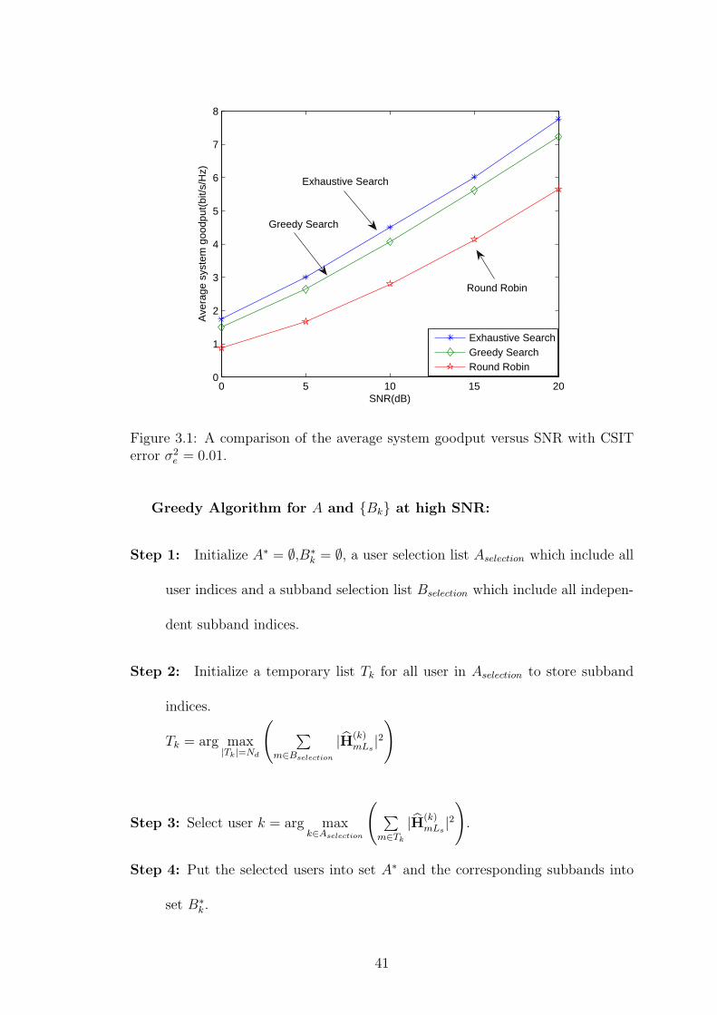
0 5 10 15 200
1
2
3
4
5
6
7
8
SNR(dB)
Ave
rage
sys
tem
goo
dput
(bit/
s/H
z)
Exhaustive SearchGreedy SearchRound Robin
Exhaustive Search
Greedy Search
Round Robin
Figure 3.1: A comparison of the average system goodput versus SNR with CSITerror σ2
e = 0.01.
Greedy Algorithm for A and {Bk} at high SNR:
Step 1: Initialize A∗ = ∅,B∗k = ∅, a user selection list Aselection which include all
user indices and a subband selection list Bselection which include all indepen-
dent subband indices.
Step 2: Initialize a temporary list Tk for all user in Aselection to store subband
indices.
Tk = arg max|Tk|=Nd
(∑
m∈Bselection
|H(k)mLs
|2)
Step 3: Select user k = arg maxk∈Aselection
(∑
m∈Tk
|H(k)mLs
|2)
.
Step 4: Put the selected users into set A∗ and the corresponding subbands into
set B∗k.
41
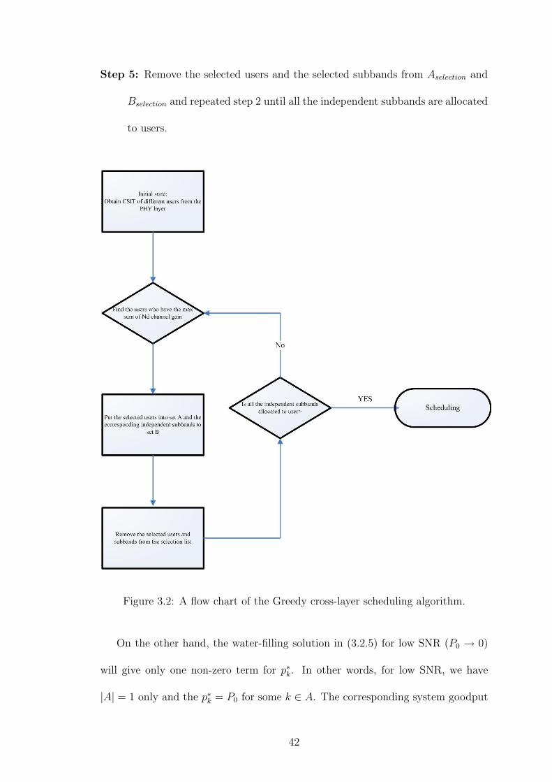
Step 5: Remove the selected users and the selected subbands from Aselection and
Bselection and repeated step 2 until all the independent subbands are allocated
to users.
Figure 3.2: A flow chart of the Greedy cross-layer scheduling algorithm.
On the other hand, the water-filling solution in (3.2.5) for low SNR (P0 → 0)
will give only one non-zero term for p∗k. In other words, for low SNR, we have
|A| = 1 only and the p∗k = P0 for some k ∈ A. The corresponding system goodput
42

for low SNR is given by:
G∗goodput(A,Bk) ≈ (1− ε)NdLs
nF
log2
(1 +
F−1χ2
k;s2(Bk);σ2e/Nd
(ε)P0nF
NdLs
)for k ∈ A
(3.2.11)
Observe that F−1χ2
k;s2(Bk);σ2e/Nd
(x) is a increasing function of s2 for a given x. Hence,
the equivalent combinatorial search problem for A and Bk is given by:
(A∗, B∗k) = arg max
k,Bk
|Bk|=Nd
[ ∑m∈Bk
|H(k)mLs
|2]
(3.2.12)
In this case, the optimal combinatorial search algorithm for A and Bk in low SNR
is similar to the one in high SNR, except that we only select one user with the
corresponding subbbands and stop the algorithm after the first iteration.
3.3 Asymptotic Performance Analysis for Cross-
Layer Design
In this section, we shall analysis asymptotically the order of growth of the average
system goodput with respect to some important system parameters such as the
average SNR P0, the number of users K and the CSIT quality (CSIT error variance)
σ2e . We shall first introduce the following important lemma based on extreme value
theorem.
Lemma 2 (Extreme Value Theorem). Let {X1, ..., XK} be a set of K i.i.d.
central chi-square random variables with 2n degrees of freedom and variance σ2X
and X∗ = maxk Xk. We have
Pr{σ2
X log K + σ2X (n− 2) log log K ≤ X∗ ≤ σ2
X log K + σ2Xn log log K
}
≥ 1−O(
1
log K
)(3.3.1)
43

for large K.
In other words, X∗ ≈ O (σ2X log K + σ2
Xn log log K) with probability one for
sufficiently large K.
Proof 2. Please refer to appendix 6.0.2.
As a result, the average system goodput is given by:
Theorem 1 (Asymptotic System Goodput for High and Low SNR).
ρ∗ = EH[G∗∗goodput(H)] =
O[(1− ε) log
(F−1
χ2k∗ ;es2;σ2
e/Nd
(ε)P0
)]for high SNR,
O[(1− ε)P0F
−1
χ2k∗ ;es2;σ2
e/Nd
(ε)
]for low SNR.
(3.3.2)
for sufficiently large K where s2 =(
1−σ2e
Nd(log K + Nd log log K)
).
Proof 3. Please refer to appendix 6.0.3.
Hence, the order of growth in the cross-layer throughput gain is contained en-
tirely in the inverse non-central chi-square cdf via the non-centrality parameter s2.
Yet, there is no closed form for F−1χ2
k;s2;σ2e/Nd
(x) in general case. We shall discuss the
asymptotic tradeoff between cross-layer goodput gain and the packet outage diver-
sity Nd in the following asymptotic cases.In addition to the asymptotic analysis,
we shall also simulate the system performance in term of average system goodput
and compare the result with asymptotic performance in different scenarios. In our
simulation, frequency selective fading channel is considered with uniform power-
delay profile for simplicity. The number of subcarriers Nf is 1024 and the total
number of independent taps L = 16. Hence, the 1024 subcarriers are grouped into
16 subbands, each containing Ls = 64 correlated subcarriers. The target packet
44

error probability ε is set to 0.01. Each point in the figure is obtained by 5000
realizations.
3.3.1 Frequency Diversity at Small Target Packet Outage
Probability ε
We shall first introduce the following lemma about F−1χ2
k;s2;σ2e/Nd
(x) for small x.
Lemma 3 (Order of Growth for small ε). Let X be a non-central random
variable with 2n degrees of freedom, noncentral parameter s2 and variance σ2X . For
a given s2, the inverse cdf of X can be expressed as below for asymptotically small
ε.
F−1X (ε)
.= ε1/nσ2
X(n!)1/n exp
(s2
nσ2X
)(3.3.3)
Proof 4. Please refer to appendix 6.0.4.
Thus, the average outage probability Pout(k) is given by the following theorem:
Theorem 2 (Frequency Diversity at Small Target Packet Outage Prob-
ability ε ). For sufficiently small ε, the average packet outage probability Pout(k)
scales with the SNR P0 (at a given average goodput) in the order of:
Pout(k) = EH
[Pout(k, H)
]= O
(P−Nd
0
)(3.3.4)
Hence, Nd is the order of frequency diversity protection against packet outage.
Proof 5. Please refer to Appendix 6.0.6.
3.3.2 Cross-Layer Goodput Gains at Large K and fixed Nd
We have the following lemma about the order of growth of inverse non-central
chi-square cdf F−1χ2
k;s2;σ2X(x) with respect to s2 for large s2.
45

Lemma 4 (Order of Growth for large s). Let X be a non-central random
variable with 2n degrees of freedom, noncentrality parameter s2 > 0 and variance
σ2X . For a given ε, the inverse cdf of X can be expressed as F−1
X (ε).= O(s2σ2
X)
asymptotically for large s2.
Proof 6. Please refer to appendix 6.0.4.
Using the results of Lemma 2 and Lemma 4 for large K and σ2e < 1, we have
the following Theorem:
Theorem 3 (Asymptotic System Goodput at Large K for High and Low
SNR at fixed Nd ).
ρ∗ = EH[G∗∗goodput(H)] =
O{(1− ε) log [P0 (1− σ2e) (log K)]} for high SNR, σ2
e < 1,
O{(1− ε)P0(1− σ2e) (log K)} for low SNR, σ2
e < 1.
(3.3.5)
20 30 40 50 60 70 80 90 1003.5
4
4.5
5
5.5
6
6.5
7
7.5
Number of users
Ave
rage
sys
tem
goo
dput
(bit/
s/H
z)
σe2=0.01
Asymptotic trend
σe2=0.05
Asymptotic trend
σe2=0.1
Asymptotic trend
σe2=1
Asymptotic trendσ
e2=1
σe2=0.1
σe2=0.05
σe2=0.01
Figure 3.3: Average system goodput versus number of users with Nd=2, differentCSIT error (σ2
e=0.01,0.05,0.1,1) at high SNR(20dB).
46

20 30 40 50 60 70 80 90 1000.2
0.4
0.6
0.8
1
1.2
1.4
1.6
Number of users
Ave
rage
sys
tem
goo
dput
(bit/
s/H
z)
σe2=0.01
Asymptotic trend
σe2=0.05
Asymptotic trend
σe2=0.1
Asymptotic trend
σe2=1
Asymptotic trend
σe2=0.01
σe2=0.05
σe2=0.1
σe2=1
Figure 3.4: Average system goodput versus number of users with Nd=2, differentCSIT error (σ2
e=0.01,0.05,0.1,1) at low SNR(0dB).
Figure 3.3 depicts the average system goodput performance(bit/s/Hz) of the
proposed scheduling schemes as a function of the number of users in high SNR (20
dB) and various frequency diversity order Nd = 2. It can be seen that when the
number of user K increases, the system goodput grows as O{log [(1− σ2e) log K]}
due to multi-user diversity. Figure 3.4 shows the average system goodput perfor-
mance(bit/s/Hz) of the proposed scheduling schemes as a function of the number
of users K in low SNR (0 dB) and Nd = 2. The average system goodput grows in
the order of O{(1− σ2e) (log K)} which matches the predicted asymptotic trend
quite closely.
Remark 3.3.1. Theorem 3 is valid for estimation error σ2e ∈ [0, 1). When going
from equation (3.3.2) to (3.3.5), we used Lemma 4: F−1
χ2k∗ ;es2;σ2
e/Nd
(ε).= O(s2σ2
e), but
47

this holds only for non-zero and sufficiently large non central parameter s2. Hence,
the results in equation (3.3.5) holds only for σ2e < 1. For the case when σ2
e = 1 and
s2 = 0 ,the F−1
χ2k∗ ;es2;σ2
e/Nd
(ε) in Theorem 1 becomes inverse cdf of central chi square.
In that case, the average goodput is given by equation (3.3.2). As a result, the
average goodput does not growth with the number of users as illustrated in Figure
3.3 and 3.4.
3.3.3 Asymptotic System Goodput at Large Nd and fixed
K
From equation (3.3.1) in Lemma 2, there exists K0 > 0 such that for K0 > 0, the
non-central parameter
[1−σ2
e
Nd(log K + (Nd − 2) log log K)
]≤ s2(H) ≤
[1−σ2
e
Nd(log K + Nd log log K)
]
with probability one for all Nd. As a result, consider the case for large Nd and fixed
K > K06. From equation (3.3.2), the first term in the equation
(1−σ2
e
Nd(log K + Nd log log K)
)
will trend to zero as Nd increases faster than log K while the second term will be
bounded by log log K . In this case, we have the non central parameter s2 which
is bounded by:
s2 = O {[(1− σ2
e) (log log K)]}
(3.3.6)
for some K > K0 > 0 such that Nd
log K→∞.
The asymptotic goodput at Large Nd for High and Low SNR for K > K0 is
6In general, the results will hold if we allow K to grow as Nd increase as long as Nd/ log K →∞.
48

given by :
ρ∗ = EH[G∗∗goodput(H)] =
O[(1− ε) log
(F−1
χ2k∗ ;es2;σ2
e/Nd
(ε)P0
)]for high SNR,
O[(1− ε)P0F
−1
χ2k∗ ;es2;σ2
e/Nd
(ε)
]for low SNR.
(3.3.7)
There is a factor (1 − σ2e) in s2 outside the log log K in equation (3.3.6) and
F−1χ2
k;s2;σ2X(x) in equation (3.3.7) is an increasing function of s2. Hence, we need
double exponentially more users K to compensate the penalty due to (1 − σ2e) in
the system goodput (via s2).
0 2 4 6 8 10 12 14 161
2
3
4
5
6
7
8
9
Nd
Ave
rage
sys
tem
goo
dput
Perfect CSIT
Asymptotic trend
σe2=0.05
Asymptotic trend
σe2=0.1
Asymptotic trend
σe2=0.15
Asymptotic trend
σe2=1
Asymptotic trend
σe2=1
Perfect CSIT
σe2=0.05
σe2=0.15 σ
e2=0.1
Figure 3.5: Average system goodput versus packet diversity order (Nd) with dif-ferent CSIT error σ2
e at high SNR(20dB) and K=20.
Figure 3.5 illustrates the average system goodput performance versus Nd in high
SNR (20dB) at different CSIT errors σ2e = 0, 0.05, 0.1, 0.15, 1. Figure 3.6 shows the
same scenario for low SNR (0 dB) regime. The system goodput is shown to be a
49
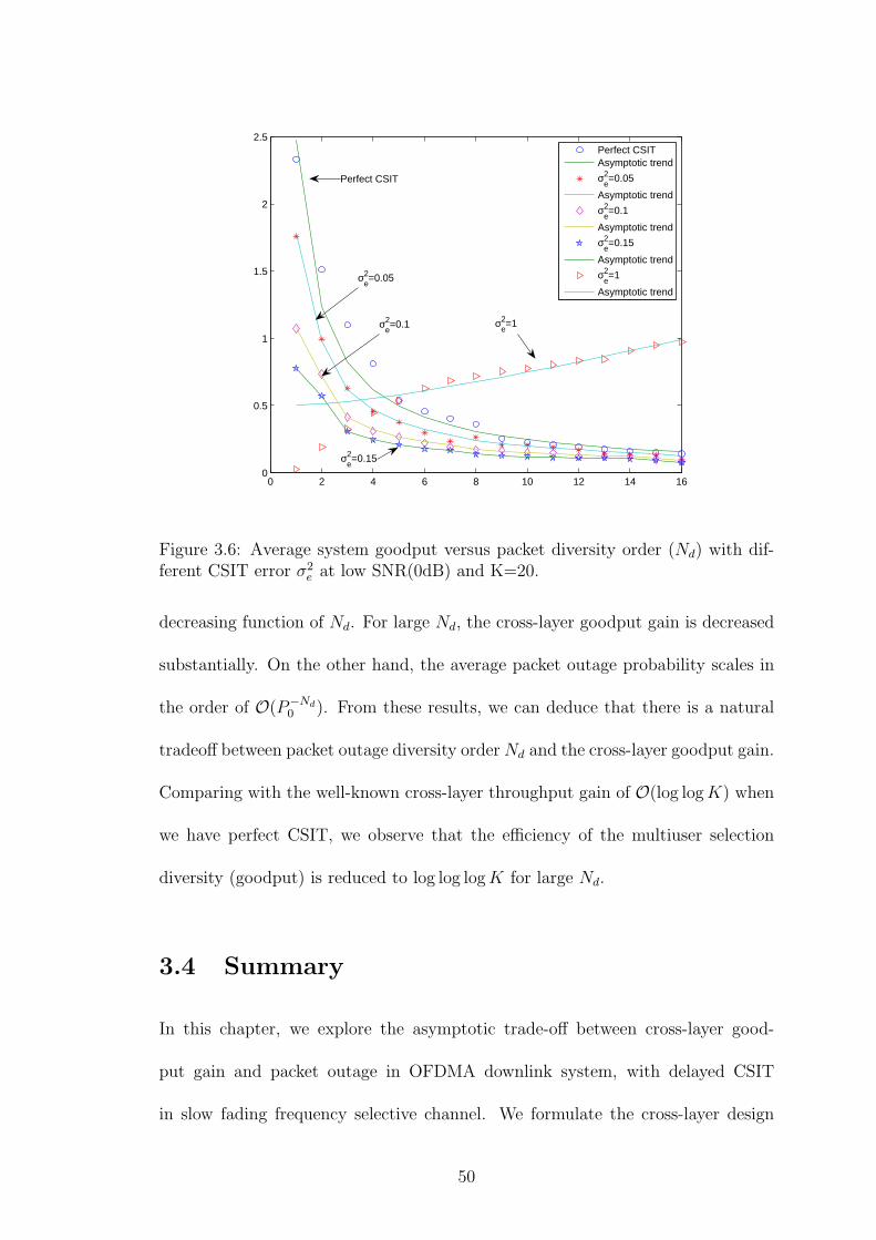
0 2 4 6 8 10 12 14 160
0.5
1
1.5
2
2.5
Perfect CSITAsymptotic trend
σe2=0.05
Asymptotic trend
σe2=0.1
Asymptotic trend
σe2=0.15
Asymptotic trend
σe2=1
Asymptotic trend
σe2=1
Perfect CSIT
σe2=0.05
σe2=0.1
σe2=0.15
Figure 3.6: Average system goodput versus packet diversity order (Nd) with dif-ferent CSIT error σ2
e at low SNR(0dB) and K=20.
decreasing function of Nd. For large Nd, the cross-layer goodput gain is decreased
substantially. On the other hand, the average packet outage probability scales in
the order of O(P−Nd0 ). From these results, we can deduce that there is a natural
tradeoff between packet outage diversity order Nd and the cross-layer goodput gain.
Comparing with the well-known cross-layer throughput gain of O(log log K) when
we have perfect CSIT, we observe that the efficiency of the multiuser selection
diversity (goodput) is reduced to log log log K for large Nd.
3.4 Summary
In this chapter, we explore the asymptotic trade-off between cross-layer good-
put gain and packet outage in OFDMA downlink system, with delayed CSIT
in slow fading frequency selective channel. We formulate the cross-layer design
50

as a mixed convex and combinational optimization problem. Due to the de-
layed CSIT, it is critical to account for potential packet errors (due to chan-
nel outage) and we consider total system goodput as our optimization objec-
tive. By allocating Nd independent subbands to a user, the packet outage prob-
ability drops in the order of SNR−Nd . On the other hand, the system goodput
scales in the order of O[(1− ε) log
(F−1
χ2k∗ ;es2;σ2
e/Nd
(ε)P0
)]at high SNR where s2 =
O{(1− σ2e) (log log K)} and O{(1− σ2
e) (log K)} for large Nd [K > K0] and large
K [fixed Nd] respectively.
0 5 10 15 200
0.5
1
1.5
2
2.5
3
3.5
4
4.5
5
s2
Fχ−
1 (ε)
O(s2)Actual inverse CDF
Acutal inverse CDF
O(s2)
Figure 3.7: Inverse CDF of non central chi square random variable versus non-centrality parameter s2 for ε=0.001 with degrees of freedom equal to 6.
51

0 0.2 0.4 0.6 0.8 1
x 10−3
10−0.7
10−0.6
10−0.5
10−0.4
ε
Fχ−
1 (ε)
Approx. inverse CDFActual inverse CDF
Actual inverse CDF
Approx. inverse CDF
Figure 3.8: Inverse CDF of non central chi square random variable versus ε withdegree of freedom 6 and non central parameter s2 = 1.
52

Chapter 4
Uplink multi-user detection
analysis
In this chapter, we will present an analytical framework on uplink multiple access
channel with successive interference cancellation receiver. We would like to show
how error propagation affect system performance and what is the optimal decoding
order to maximize the achievable capacity.
4.1 Introduction
The uplink of wireless cellular system, where many mobile users communicate to a
single base station, can be modeled by the multi-access channel. The multi-access
channel is characterized by a capacity region, which is the set of achievable rate vec-
tor[40] and multi-user detection with successive interference cancellation (MUD-
SIC) is one receiver scheme that can achieve the corner points in the dominant
face of the multiaccess capacity region1. Most of the existing works on multiaccess
1In general, joint detection is needed to achieve the multi-access capacity region.
53

channel are either focused on signal processing algorithms or performance analysis
for multi-user detection. In [41], signal design for multiaccess channel is discussed.
In [42], multiuser detection algorithm for overloaded CDMA system is discussed.
Conventional performance analysis of multi-access fading channel is usually based
on the ergodic capacity[43, 44]. Uplink power adaptation for multiaccess channel
is addressed in [9] where the transmit power of mobile users are optimized with
respect to a system objective function of user capacities. In all these works, ergodic
capacity is the key performance measure and optimization objective. However, the
ergodic capacity is a reasonable performance measure only for fast ergodic fading
channels where a transmitted packet spans across ergodic realizations of channel
fading. In this case, the transmitted packets from the mobile users can be guar-
anteed to be successfully received by the base station as long as powerful channel
coding such as LDPC code[45] with sufficiently long block length is applied and the
transmitted data rate is less than the ergodic channel capacity. However, for slow
fading channels (non-ergodic channels), in which the channel fading is quasi-static
within the entire encoding frame, the transmitted packets cannot be guaranteed to
be always successfully received even if powerful channel coding is applied. In this
case, the instantaneous mutual information of the channel appears as a random
variable to the transmitters. The packet transmitted will be corrupted if the data
rate is larger than the instantaneous mutual information (despite the use of error
correction code) and this is called packet outage. Hence, in slow fading channels,
ergodic capacity is no longer a useful performance measure because it does not take
into account potential packet outage. To include the effects of potential packet er-
rors due to channel outage, we should analyze the packet outage probability and
54

system goodput (which is defined as the average bits/sec/Hz successfully delivered
to the receiver).
In this chapter, our focus is to evaluate the per-user packet error (outage) prob-
abilities and the system goodput for multi-access slow fading channel with adaptive
MUD-SIC. We consider a system with a base station and n mobile users where
there is no channel state knowledge (CSIT) at the transmitters of the mobiles. We
assume adaptive successive interference cancellation (MUD-SIC) processing at the
base station where the decoding order among the n mobile users is adaptive based
on the channel state information at the base station (CSIR) so as to maximize the
total system goodput. In [9, 46, 47], the delay-limited capacity of the multi-access
channel with perfect CSIT is analyzed without considering packet outage events.
In [48, 49], the authors analyzed the system goodput for multiaccess channels with
optimal (maximal likelihood (ML)) multiuser detection and linear multiuser de-
tection (MMSE). Yet, the results from these works cannot be applied in our case
with MUD-SIC in quasi-static fading channels. In the case of ML detector (joint
detection), the outage event is defined as the event that the rate vector is outside
the instantaneous capacity region2 of the multiaccess channel and there is no ”no-
tion” of per-user packet outage or error-propagation effects. In the case of MMSE
detectors, the outage event is completely decoupled among the n users. However,
when we consider MUD-SIC detector, there is mutual coupling (error propagation)
of the packet error events between the n users in the SIC decoding process. For
example, the packet error event of the user decoded in the k-th iteration depends
not only on the packet transmitted by user k but also on all the users decoded in
2Instantaneous capacity region refers to the multiaccess capacity region for a given channelfading realization.
55
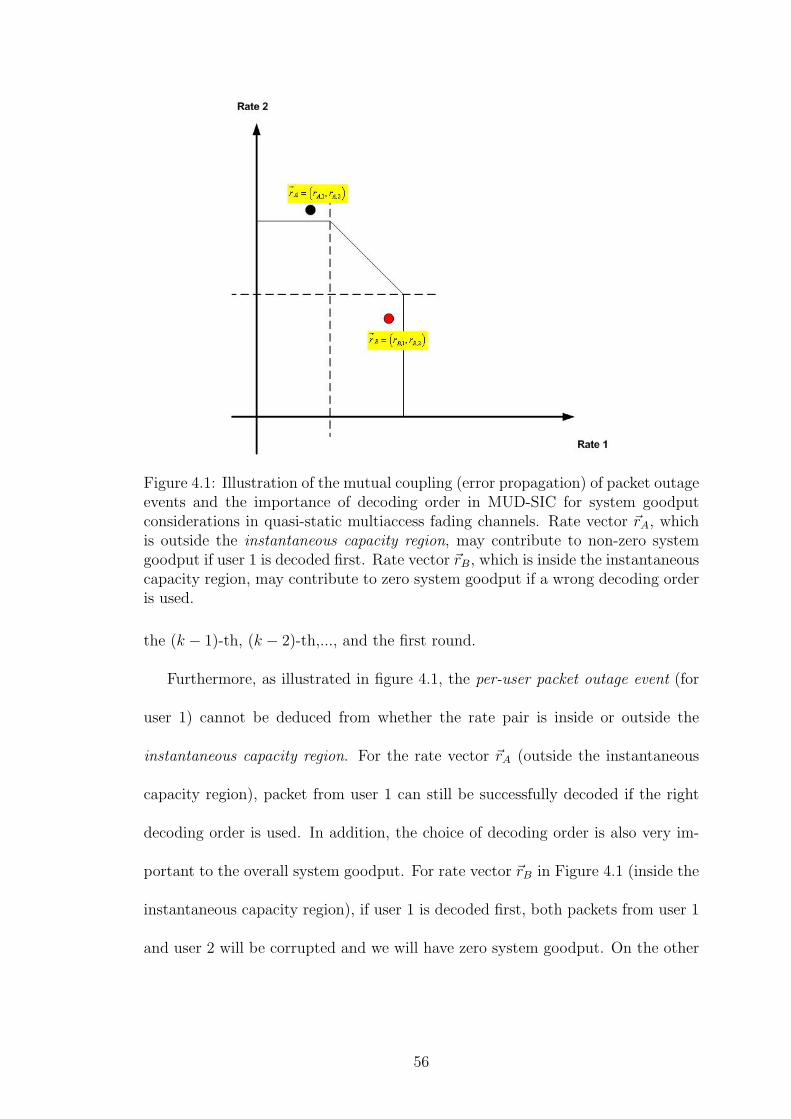
Figure 4.1: Illustration of the mutual coupling (error propagation) of packet outageevents and the importance of decoding order in MUD-SIC for system goodputconsiderations in quasi-static multiaccess fading channels. Rate vector ~rA, whichis outside the instantaneous capacity region, may contribute to non-zero systemgoodput if user 1 is decoded first. Rate vector ~rB, which is inside the instantaneouscapacity region, may contribute to zero system goodput if a wrong decoding orderis used.
the (k − 1)-th, (k − 2)-th,..., and the first round.
Furthermore, as illustrated in figure 4.1, the per-user packet outage event (for
user 1) cannot be deduced from whether the rate pair is inside or outside the
instantaneous capacity region. For the rate vector ~rA (outside the instantaneous
capacity region), packet from user 1 can still be successfully decoded if the right
decoding order is used. In addition, the choice of decoding order is also very im-
portant to the overall system goodput. For rate vector ~rB in Figure 4.1 (inside the
instantaneous capacity region), if user 1 is decoded first, both packets from user 1
and user 2 will be corrupted and we will have zero system goodput. On the other
56

hand, if user 2 is decoded first, both packets can be successfully received. Further-
more, the packet outage event of user 1 depends not only on the channel state of
user 1 but also on that of user 2 as well due to the coupling of the adaptive MUD-
SIC. As far as we are aware, the issues of coupled per-user packet outage events
or error-propagation for MUD-SIC detection have not been addressed previously.
In this chapter, we shall address two important issues associated with MUD-SIC
detection in quasi-static multi-access fading channels where we have homogeneous
users with equal data rate3.
• Optimal Decoding Order in MUD-SIC: While there are some works on
finding the optimal decoding order in MUD systems, they did not consider
the per-user outage event (error propagation) in MUD-SIC. For example, the
optimal decoding order is found in[9] to maximize a general utilize function of
ergodic capacity. In [49], joint detection is used and hence, the outage event
is defined by whether the rate vector is outside the instantaneous capacity
region and this is very different from the per-user packet outage event we
considered here.
• Closed-Form Analysis of Per-user Packet Outage Probability and
System Goodput: Based on the optimal decoding order obtained, we shall
derive the closed-form per-user packet outage probability for MUD-SIC, tak-
ing care of the coupled per-user outage event in the SIC decoding process.
The chapter is organized as follows. In Section 4.2, the multi-user system
model is described. In Section 4.3, we shall derive the packet error probability
of the n users and the overall system goodput. In Section 4.4, simulation results
3Equal data rate represents an important class of voice applications in wireless networks
57
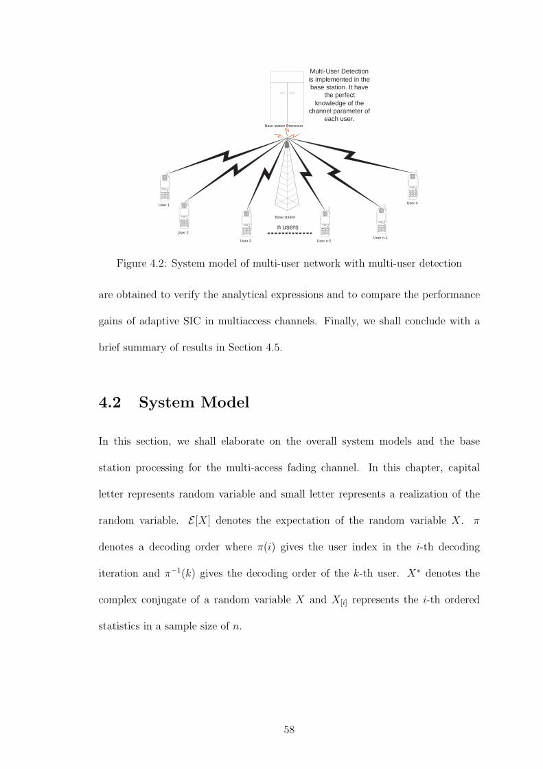
Base station
User 1
User n-1 User n-2 User 3
User 2
User n
Base station Processor
Multi-User Detection is implemented in the base station. It have
the perfect knowledge of the
channel parameter of each user.
n users
Figure 4.2: System model of multi-user network with multi-user detection
are obtained to verify the analytical expressions and to compare the performance
gains of adaptive SIC in multiaccess channels. Finally, we shall conclude with a
brief summary of results in Section 4.5.
4.2 System Model
In this section, we shall elaborate on the overall system models and the base
station processing for the multi-access fading channel. In this chapter, capital
letter represents random variable and small letter represents a realization of the
random variable. E [X] denotes the expectation of the random variable X. π
denotes a decoding order where π(i) gives the user index in the i-th decoding
iteration and π−1(k) gives the decoding order of the k-th user. X∗ denotes the
complex conjugate of a random variable X and X[i] represents the i-th ordered
statistics in a sample size of n.
58

4.2.1 Multi-access Channel Model
Figure 4.2 illustrates the overall system model. We have a base station and n
mobile users. The uplink transmissions of the n mobiles are synchronous so that
successive interference cancellation (SIC) is applied at the base station with perfect
channel state information (CSIR). On the other hand, the mobile transmitters
do not have any channel state information (CSIT). We consider slow flat fading
multi-access channels where the channel fading remains quasi-static within the
entire transmitted packet. This is a realistic assumption for pedestrian mobility
( 10km/hr) in most systems such as HSDPA, 3G1X and WiFi, where the coherence
time is around 20ms and the frame duration is less than 2ms.
Let Xi be the transmitted symbol from the i-th user with average transmit SNR
E[|Xi|2] = σ2i and Hi be the channel fading coefficient between the i−th mobile
and the base station (which is modelled as zero-mean complex Gaussian random
variable with covariance E[|Hi|2] = 1) and H = [H1, ..., Hn] be the aggregate
channel fading. The received signal at the base station is given by
Y =n∑
i=1
HiXi + Z (4.2.1)
where Z denotes channel noise, which is modelled as zero mean complex Gaussian
with normalized variance E[|Z|2] = 1.
4.2.2 MUD-SIC Processing and Per-User Packet Error Model
The base station has to detect the signal transmitted by the n users based on the
received signals Y . In this chapter, we assume the base station is equipped with
synchronous multi-user detection with successive interference cancellation (MUD-
SIC) and perfect channel state information (CSIR). Given a particular decoding
59

order π = (π(1), ..., π(n)) where π(i) is the user index of the user decoded in
the i-th decoding iteration, the instantaneous mutual information (using Gaussian
random codebook) of the π(i)−th user is given by
Cπ(i)(H, π, i) = log2
1 +|Hπ(i)|2σ2
π(i)
n∑p=i+1
(|Hπ(p)|2σ2π(p)) + 1
(4.2.2)
where σ2k is the transmit SNR of the k−th user.
In this chapter, we consider a homogeneous system where the n users transmit
information with the same data rate (r1 = ... = rn = r). This represents an
important case such as voice applications in the cellular systems. Since the channel
fading is quasi-static within the transmitted packets and the mobile transmitters
do not have knowledge of the channel states H1, .., Hn, the instantaneous mutual
information of the n users {C1, ..., Cn} appears as random variables to the mobile
transmitters. The transmitted packet of the π(i)-th user will be corrupted if the
data rate of the transmitted packet r exceeds the instantaneous mutual information
Cπ(i) of individual users. This refers to packet outage. In fact, the packet error
probability is contributed by two factors, namely the packet outage and the channel
noise. The second factor is due to the finite block length effect of channel coding.
Suppose strong enough channel coding is applied and the channel coherence time
is much longer than the symbol duration (so that sufficiently long block length can
be used), the packet outage will be the dominant factor that contributes to packet
error. Note that the packet outage is due to the slow fading channels (non-ergodic
channels) and cannot be eliminated even if capacity achieving codes are used at
the transmitter. Hence, we shall assume packet error probability is mainly due to
the packet outage only and shall use the two words interchangeably in the chapter.
60

In this chapter, we consider multiaccess channel with adaptive SIC and hence,
the decoding order π is a function of the CSIR H. Let P = {πH} denotes the
decoding order policy, which is a set of decoding order πH with respect to every
realization of CSIR H. Given a decoding order policy P , we are interested to
find the average PER (averaged over ergodic realization of CSI) of the user k,
Pout(r,P , k). However, the analysis of per-user PER is not trivial due to the
coupling of decoding events in SIC. For example, when user k is decoded in the
3-rd iteration, the success of packet delivery depends not only on the instantaneous
mutual information of user k but also on the success/failure in the 1st and 2nd
decoding iterations. In fact, the success or failure of a packet transmission of a
user cannot be simply told from whether the rate vector is inside the multiaccess
capacity region. As illustrated in Figure 4.1, rate vector ~rA, which is outside the
capacity region, may contribute to non-zero system goodput if the correct decoding
order is used. To take care of the intrinsic coupling of the adaptive SIC in the PER
analysis, we define the effective instantaneous mutual information4 of user k = π(i)
in the i-th decoding iteration as:
Ck(H, π, i) = log2
(1 +
∑nj=i σ
2π(j)|Hπ(j)|2 + W π
i
1 +∑n
j=i+1 σ2π(j)|Hπ(j)|2 + W π
i
)(4.2.3)
where Wi denotes the accumulated undecodable interference after i − 1 decoding
iterations and it is given by:
W πi =
i−1∑j=1
σ2π(j)
∣∣Hπ(j)
∣∣2 I[r ≥ Cπ(j)(H, π, j)] (4.2.4)
where I[.] represents the indicator function5, r is the transmitted data rate and
W π1 = 0.
4The effective mutual information here is different from the mutual information in (4.2.2) inthe sense that the success/failure events in the i−1, i−2, ..., 1 decoding attempts are taken care.
5I[A] = 1 if the event A is true and zero otherwise.
61

Hence, the average PER of the user k (averaged over CSIR) is given by:
PER(r,P , k) ≈ Pout(r,P , k) = 1−∑π∈P
Pr[r < Ck
(H, π, π−1(k)
) |π]Pr[π] (4.2.5)
In order to capture the effect of potential packet error due to channel outage,
we define the average system goodput under a given decoding order policy (P),
ρ(r,P), to be the total bits/sec/Hz that successfully delivered to the base station.
That is,
ρ(r,P) =n∑
k=1
r {1− Pout(r,P , k)} (4.2.6)
Note that both system goodput and the PER are functions of the decoding
order policy P . In the next section, we shall deduce the optimal decoding order
policy to maximize the average system goodput.
4.2.3 Optimal Decoding Order Policy
Note that existing literature that discusses about the optimal decoding order are
all based on some utility functions of ergodic capacity [9, 46] in which potential
packet errors (outage) of the n users are not taken into consideration. In this
section, we shall derive the optimal decoding order (per fading slot) to maximize
the system goodput ρ(r,P) as defined in (4.2.6). The results are summarized in
the lemma below.
Lemma 5 (Optimal Decoding Order). Given the instantaneous receive SNR
{γ1, .., γn} where γk = σ2k|Hk|2, the optimal decoding order that maximize the sys-
tem goodput ρ(r,P) is given by
π(j) = arg maxk∈(S\T )
(γk
)(4.2.7)
62

where S = {1..n}, T = {π(1), .., π(j − 1)} and the pdf of γk is given by
fγk(xk) =
1
σ2k
e− xk
σ2k (4.2.8)
Proof 7. Please refer to Appendix 6.0.7.
Define ξi ∈ {0, 1} as the event that the i-th decoded user is decoded successfully
(ξi = 1 denotes successful decoding and ξi = 0 denotes decoding failure). The event
ξi is given by:
ξi = I{
r < log
(1 +
γπ(i)
1 +∑
j<i γπ(j)(1− ξj) +∑
j>i γπ(j)
)}∈ {0, 1} (4.2.9)
where I(A) is the indicator function. Define
Ii = I{
r < log
(1 +
γπ(i)
1 +∑
j>i γπ(j)
)}. (4.2.10)
Given the optimal decoding order policy P∗ in (4.2.7) and the associated opti-
mal decoding order π, we have Cπ(i)(H, π, i) > Cu(H, π, i) for all u 6= π(i). Hence,
for user π(i) in the i-th decoding iteration, packet error for user π(i) can be declared
whenever packet error occurs in any of the j = 1, 2, .., i-th decoding iterations. In
other words, we have
ξi = 0 ⇒ I1 ∪ I2 ∪ .... ∪ Ii = 0 (4.2.11)
Hence, the average packet outage probability of user k transmitting at a rate r in
(4.2.5) can be simplified as:
Pout(r,P∗, k) =∑π∈P∗
π−1(k)∑i=1
Pr[ξi = 0|π]
Pr[π]
=∑π∈P∗
π−1(k)∑i=1
Pr[I1 ∪ I2 ∪ .... ∪ Ii = 0|π]
Pr[π] ≤
∑π∈P∗
π−1(k)∑i=1
i∑j=1
Pr[Ij = 0|π]
Pr[π]
(4.2.12)
63

where the final upper bound is due to union bound and Pr[Ij = 0|π] is the condi-
tional packet outage probability in the j-th iteration under the decoding order π.
From (4.2.10), Pr[Ij = 0|π] is given by:
Pr(Ij = 0|π) = Pr[r > Cπ(i)(H, π, i)|π] (4.2.13)
and Pr[π] is the probability for the decoding order π in the optimal policy P∗ to
be selected in the current time slot and is given by
Pr(π) = Pr(γπ(1) ≥ γπ(2) ≥ γπ(3).. ≥ γπ(n)). (4.2.14)
In other words, the average outage probability is the average of the occurrence of
all the packet outage events that happen prior to the current decoding iteration
(average over every possible decoding order π in the policy P∗).
Similarly, the average system goodput under the optimal decoding order policy
P∗ is given by:
ρ(r,P∗) =∑π∈P∗
( n∑i=1
r Pr[ξi = 1|π]
)Pr(π)
=∑π∈P∗
( n∑i=1
r (1− Pr[I1 ∪ I2 ∪ .... ∪ Ii = 0|π])
)Pr(π)
≥∑π∈P∗
( n∑i=1
r
(1−
i∑j=1
Pr[Ij = 0|π]
))Pr(π)
(4.2.15)
4.3 Performance Analysis
In this section, we shall derive the analytical expressions on the per-user packet
outage probability and the system goodput for MUD-SIC detector under the optimal
decoding order policy P∗.
64

4.3.1 System Goodput and Per-User Packet Outage Prob-
ability for MUD-SIC
From equations (4.2.15) and (4.2.12), both the average system goodput ρ and
the average packet error probability of user k, Pout(r,P∗, k), are determined by
averaging over all the possible decoding order π under the optimal policy P∗. To
obtain the analytical expressions of the average system goodput and the average
packet error probability, we have to determine the conditional outage probability
of the j-th iteration Pr(Ij = 0|π) in (4.2.13) and the probability of choosing the
decoding order Pr(π). Given a decoding order π and from (4.2.2), Pr(Ij = 0|π)
can be expressed as
Pr(Ij = 0|π) = 1− Pr[r ≤ Cπ(j)(H, π, j)|π] = 1− Pr
[γπ(j) − η
n∑p=j+1
γπ(p) ≥ η
∣∣∣∣π]
(4.3.1)
where η = 2r − 1. Without loss of generality, we consider a decoding order π =
(1, 2, .., n). From P∗, the optimal decoding order is in descending order of γi.
Hence, conditional on π = (1, 2, ..., n), we have γ1 ≥ γ2 ≥ ... ≥ γn. By [50], the
joint pdf of the γj is then given by
fγ1,γ2,...γn(x1, x2...xn|π) =
1Pr(π)
Qni=1 σ2
i
∏ni=1 e
−xiσ2
i if 0 ≤ xn ≤ xn−1 ≤ xn−2... ≤ x1 < ∞,
0 otherwise.(4.3.2)
where Pr(π) = Pr(γ1 ≥ γ2 ≥ γ3.. ≥ γn)). Hence, from the above equations,
the computation of Pr(Ij = 0|π) and Pr[π] involved multi-dimensional nested
integrals which are cumbersome and complicated. To obtain a tractable analytical
expression for the average system goodput, we shall derive the following lemma.
65

Lemma 6. The ordered channel gains (γ[1] ≥ γ[2] ≥ ... ≥ γ[n]) can be trans-
formed into independent (but not necessarily identical) exponential random vari-
ables {Z1, ..., Zn} by the following transformation
Zi = i[γ[i] − γ[i+1]] (4.3.3)
where 0 ≤ Zi < ∞ for all i ∈ {1, 2, .., n} and γ[n+1] = 0. {Zi} is a set of
independent exponential random variables with p.d.f. given by:
fZi(z) = φie
−zφi
where the parameter φi given by
φi =
∑iu=1 σ−2
u
i(4.3.4)
Proof 8. Please refer to Appendix 6.0.8.
The implication of the above lemma is that the original ordered random vari-
ables {γ[i]} can be transformed6 into a set of ”virtual user” statistics (Zv) which is
independent. By making use of this lemma, the joint pdf of Zv is then given by
fz1,z2,...zn(z1, z2...zn|π) =1
n!
1
Pr(π)∏n
i=1 σ2i
n∏i=1
e−ziφi (4.3.5)
where φi is given by the equation(4.3.4). Hence, from (4.3.1), the conditional
outage probability Pr(Ij = 0|π) in j− th iteration conditioned on a given decoding
order π can be expressed as
Pr(Ij = 0|π) = 1− Pr
[ n∑v=j
λvZv ≥ η
∣∣∣∣π]
= 1− Pr
[Γj ≥ η|π
](4.3.6)
6Yet, unlike the standard ordered-statistics transformation[50], the transformed variables {Zv}are independent but not necessarily identical due to potentially different transmit SNR σ2
i amongthe n users.
66

where η = 2r−1, Γj =∑n
v=j λvZv is a linear combination of (n−j+1) independent
exponential random variables ({Zv}) and λv = 1−(v−j)ηv
. Now, the conditional
outage probability is expressed in terms of a single random variable Γj and nested
multi-dimensional integration can be avoided.
Making use of the characteristic function of the exponential random variable
and the partial fraction theorem, the p.d.f. of the random variable Γj is found and
summarized in the following lemma.
Lemma 7. The p.d.f. of Γj is given by
fΓj(x) =
n∑v=j
Av
|λv|Bv (4.3.7)
where xj ∈ < and
λv = λv/φv , Av =
( n∏
u=j,u6=v
λv
(λv − λu)
), Bv =
e−x
|λv |u(x) if λv ≥ 0
ex|λv |u(−x) otherwise
(4.3.8)
where φv is given by the equation(4.3.4) and u(x) is the unit step function.
Proof 9. Please refer to Appendix 6.0.9.
From above lemma, Pr(Ij = 0|π) is found to be
Pr(Ij = 0|π) = 1−∫ ∞
η
fΓj(xj)dxj
= 1−n∑
v=j
Ave−η
λv I(λv ≥ 0) (4.3.9)
The indicator function I(λv ≥ 0) is due to the integration over the region 0 ≤ η <
∞.
After obtaining the closed-form expression for Pr(Ij = 0|π), we have to obtain the
closed form expression for Pr(π). From the p.d.f. expression in equation (4.3.2),
the probability of the optimal decoding order π can be derived from the fact that
67

the integration of the joint p.d.f., fz1,z2,...zn(z1, z2...zn|π), over the entire space of
Z1, .., Zn equals to 1. Hence, Pr(π) is given by
Pr(π) =1
n!
n∏i=1
1
φiσ2i
(4.3.10)
Note that the probability of optimal decoding order depend on the average received
SNR (σ2i ) of every user. If all user have the same received SNR (σ2
1 = σ22...σ
2n), the
probability of decoding order become
Pr(π) =1
n!(4.3.11)
Hence, under the special case of equal SNR, every optimal decoding order is sta-
tistically equiprobable.
Based on the analytical expressions for Pr(Ij = 0|π) and Pr(π), the average sys-
tem goodput and the average packet error probability of user k under the optimal
decoding order policy P∗ are summarized in the following two theorem.
Theorem 4 (Lower Bound for Average System Goodput of MUD-SIC
with Optimal Decoding Order). The average system goodput (ρ)(r,P∗) with
optimal decoding order policy P∗ is given by
ρ(r,P∗) ≥ 1
n!
∑π∈P∗
[n∑
i=1
r
(1−
i∑j=1
(1−
n∑v=j
Ave−η
λv I(λv ≥ 0)
))]n∏
i=1
1
φiσ2π(i)
(4.3.12)
where η = 2r − 1.
From the above expression, the first term inside the summation represent the
system goodput corresponds to each decoding permutation in the optimal decoding
policy. The second term outside the summation correspond to the probability of
each permutation inside the decoding policy.
68

Theorem 5 (Upper Bound for Average Per-User Packet Outage Prob-
ability of MUD-SIC with Optimal Decoding Order). The average packet
error probability of user k under the optimal decoding order policy P∗ is given by
Pout(r,P∗, k) ≤ 1
n!
∑π∈P∗
( π−1(k)∑i=1
i∑j=1
[1−
n∑v=j
Ave−η
λv I(λv ≥ 0)
])n∏
i=1
1
φiσ2π(i)
(4.3.13)
4.3.2 Asymptotic Expressions on Average System Good-
put and Per-User Packet Error Probability
In this section, we consider the asymptotic expressions of the average system good-
put and the packet error probability under the optimal decoding order policy at
large SNRs. Specifically, when the average SNR of all the users σ21 = ... = σ2
n →∞,
the channel capacity of j-th iteration with the optimal decoding order π becomes
Cπ(j)(H, π, j) = log2
1 +|Hπ(j)|2
n∑p=j+1
|Hπ(p)|2
(4.3.14)
From the above expression, we observe that the channel capacity Cπ(j)(H, π, j) is
independent of the average transmit SNRs. Hence, by symmetry, all the decoding
order π in P∗ is statistically equiprobable (Pr(π) = 1n!
). The analytical expression
for the system goodput (ρ(r,P∗)) under the optimal decoding policy P∗ is given
by
ρ(r,P∗) ≥[
n∑i=1
r
(1−
i∑j=1
(1−
n∑v=j
AvI(λv ≥ 0)
))](4.3.15)
Similarly, the average packet error probability of user k becomes
Pout(r,P∗, k) ≤ 1
n!
∑π∈P∗
π−1(k)∑i=1
i∑j=1
[1−
n∑v=i
AvI(λv ≥ 0)
](4.3.16)
where λv is given by the equations (4.3.4) and (4.3.8).
69
4.4 Results and Discussions
In this section, we shall present the numerical results obtained from the analytical
expressions and verify them with respect to the simulation results on the average
packet error probability and the average system goodput. In the simulation, we
consider a single cell uplink wireless communicated system with n single-antenna
users. All the channel fading coefficients {H1, ..., Hn} are generated as i.i.d. com-
plex Gaussian random realizations with zero mean and unit variance.
To obtain the average system goodput, we count the number of successfully
decoded packets for the n users and average it over multiple fading realizations. To
obtain the average packet error probability, we count the number of packet errors
of a user k and average it over multiple fading realizations. In the simulation, each
point of the system goodput and packet error probability are obtained by 20000
fading realizations. We consider two different successive interference cancellation
policies, namely the optimal policy and the random policy.
• Adaptive SIC with Optimal Decoding Order: For every CSIR realiza-
tion, the optimal decoding order is given by the descending order of the user
received SNR (γi = σ2i |Hi|2). The decoding process stops and all undecoded
packets are declared corrupted as soon as there is any packet error in any
decoding iteration because the subsequent iterations will surely be failed.
• SIC with Random Decoding Order: For every fading realization, a
random permutation order is obtained and used as the decoding order. On
each iteration, the base station attempts to decode the user using different
possible paths as illustrated in figure 4.3. Different from the SIC with optimal
70

Correct
Error
Correct
Error
Correct
Error
Correct
Correct
Error
Correct
Error
Correct
Error
Correct
Error Decoding event
Possible decoding event
Figure 4.3: Illustration of the MUD-SIC decoding tree for random decoding order.The decoding process continues even there is packet error in the current iteration.This is because there is still a possibility that subsequent decoding iterations willbe successful given the current decoding iteration fails.
decoding order, the decoding process continues even there is packet error in
the current iteration. This is because in the tree processing as illustrated in
figure 4.3, there is still a possibility that subsequent decoding iterations will
be successful given the current decoding iteration fails. Finally, number of
error packets for a user k will be counted and averaged over multiple fading
realizations.
Under these two decoding order policies, we would like to compare the perfor-
mance gains on the average system goodput and average packet error probability.
Note that all solid lines represent the theoretical result and dotted markers repre-
sent the simulated result. Besides, units of all goodput measurements will be in
bits/sec/Hz.
71

0 2 4 6 8 10 12 14 16 18 200
1
2
3
4
5
6
SNR(dB)
Sys
tem
Goo
dput
(bi
t/sec
/Hz)
TDMA(10%)
Optimal SIC,(per user outage=10%)
Optimal SIC,(per user outage=5%)
Performance gain
Random SIC(per user outage=10%)
Random SIC(per user outage=5%)
TDMA(5%)
Joint detection(common outage=5%)
Joint detection(common outage=10%)
Figure 4.4: System goodput vs SNR(dB) with different outage (n=5). The solidline represent the theoretical expression and the dotted solid represent the simu-lated result of the system goodput respectively. The double sided arrow representthe performance gain of the optimal SIC over the random SIC.
4.4.1 Results on the Average System Goodput
Figure 4.4 shows the average system goodput versus the average user SNR (dB) for
n = 5 users. Each curve in the graph represent different detection methods with
same target average packet error probability (10% and 5%). It can be observed
that the system goodput with optimal decoding order increases with SNR but with
a diminishing return. This is because at high SNR, the SNR term in the MUD-
SIC will cancel out each other in (4.2.2). As a result, the system goodput will be
limited by the SINR rather than SNR7. Besides, a huge performance gain is found
in SIC with the optimal decoding order over the SIC with random decoding order.
With random SIC, the average system goodput suffers from the frequent packet
decoding error. In order to achieve the same average packet error probability
level, each user has to transmit at a lower data rate and this reduces the average
7Note that for joint detection, the system goodput will not be limited by SINR anymore. Yet,our focus in the chapter is to study the performance of MUD-SIC.
72
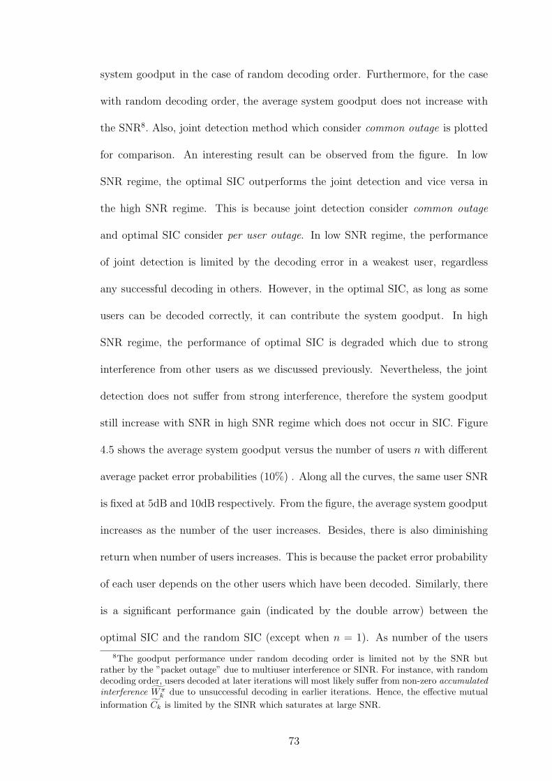
system goodput in the case of random decoding order. Furthermore, for the case
with random decoding order, the average system goodput does not increase with
the SNR8. Also, joint detection method which consider common outage is plotted
for comparison. An interesting result can be observed from the figure. In low
SNR regime, the optimal SIC outperforms the joint detection and vice versa in
the high SNR regime. This is because joint detection consider common outage
and optimal SIC consider per user outage. In low SNR regime, the performance
of joint detection is limited by the decoding error in a weakest user, regardless
any successful decoding in others. However, in the optimal SIC, as long as some
users can be decoded correctly, it can contribute the system goodput. In high
SNR regime, the performance of optimal SIC is degraded which due to strong
interference from other users as we discussed previously. Nevertheless, the joint
detection does not suffer from strong interference, therefore the system goodput
still increase with SNR in high SNR regime which does not occur in SIC. Figure
4.5 shows the average system goodput versus the number of users n with different
average packet error probabilities (10%) . Along all the curves, the same user SNR
is fixed at 5dB and 10dB respectively. From the figure, the average system goodput
increases as the number of the user increases. Besides, there is also diminishing
return when number of users increases. This is because the packet error probability
of each user depends on the other users which have been decoded. Similarly, there
is a significant performance gain (indicated by the double arrow) between the
optimal SIC and the random SIC (except when n = 1). As number of the users
8The goodput performance under random decoding order is limited not by the SNR butrather by the ”packet outage” due to multiuser interference or SINR. For instance, with randomdecoding order, users decoded at later iterations will most likely suffer from non-zero accumulatedinterference Wπ
k due to unsuccessful decoding in earlier iterations. Hence, the effective mutualinformation Ck is limited by the SINR which saturates at large SNR.
73

0 5 10 150
0.5
1
1.5
2
2.5
3
Number of users
Sys
tem
goo
dput
(bit/
sec/
Hz)
Joint detection(SNR=10dB, common outage=10%)
Joint detection(SNR=5dB, common outage=10%)
Optiam SIC,(SNR=5dB, per user outage=10%)
Random SIC,(SNR=10dB, per user outage=10%)
Random SIC,(SNR=5dB, per user outage=10%)
Optimal SIC,(SNR=10dB, per user outage=10%)
Performance gain
Figure 4.5: System goodput against number of users with different SNR (packeterror probability=10%)
increases, the importance of the decoding order increases and this contributes to
the performance gains. Similar to the above case, the average system goodput in
the random SIC case does not scale with number of the users due to the failure
of the interferers cancellation. Hence, the optimal decoding order for SIC is very
important especially for high SNR cases. Furthermore, joint detection method
which consider common outage is plotted for comparison. It is also very interesting
that the system goodput of joint detection (which consider common outage) does
not increase with the number of user for a fixed SNR. This counter intuitive result
can be explained by the performance of joint detection is always limited by the
weakest user. If we don’t increase the SNR to help the weakest user, the system
goodput can’t increase with the number or user.
In all cases, the simulation results match with the analytical results. This
74
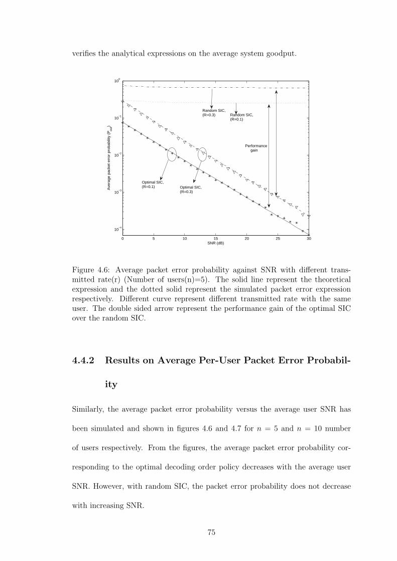
verifies the analytical expressions on the average system goodput.
0 5 10 15 20 25 30
10−4
10−3
10−2
10−1
100
SNR (dB)
Ave
rage
pac
ket e
rror
pro
babi
lity
(Pou
t)Random SIC,(R=0.3) Random SIC,
(R=0.1)
Performance gain
Optimal SIC,(R=0.1) Optimal SIC,
(R=0.3)
Figure 4.6: Average packet error probability against SNR with different trans-mitted rate(r) (Number of users(n)=5). The solid line represent the theoreticalexpression and the dotted solid represent the simulated packet error expressionrespectively. Different curve represent different transmitted rate with the sameuser. The double sided arrow represent the performance gain of the optimal SICover the random SIC.
4.4.2 Results on Average Per-User Packet Error Probabil-
ity
Similarly, the average packet error probability versus the average user SNR has
been simulated and shown in figures 4.6 and 4.7 for n = 5 and n = 10 number
of users respectively. From the figures, the average packet error probability cor-
responding to the optimal decoding order policy decreases with the average user
SNR. However, with random SIC, the packet error probability does not decrease
with increasing SNR.
75

0 5 10 15 20 25 30
10−4
10−3
10−2
10−1
100
SNR (dB)
Ave
rage
pac
ket e
rror
pro
babi
lity
(Pou
t)
Performance gain
Random SIC,(R=0.3)
Random SIC,(R=0.1)
Optimal SIC,(R=0.3)
Optimal SIC,(R=0.1)
Figure 4.7: Average packet error probability against SNR with different transmit-ted rate(r) (Number of users(n)=10)
On the other hand, the average packet error probability versus the number of
users at the same average user SNR (5dB and 10dB) and the same transmit data
rate R is shown in figures 4.8 and 4.9. It can be observed that with the optimal
decoding order policy, the packet error probability increases at a slower rate as
the number of users increases. Similarly, in all cases, the simulation results match
the analytical results closely, verifying the analytical expressions on the average
outage probabilities.
4.5 Summary
In this chapter, we have derived the analytical expressions for the average system
goodput and the per-user packet outage probability for multiacces channel with
MUD-SIC. We consider a system with n users and a base station and derive the
76
0 5 10 15
10−1
100
Number of User
Ave
rage
pac
ket e
rror
pro
babi
lity
P out
R=0.2Random SIC
R=0.3Random SIC
R=0.2Optimal SIC
R=0.3Optimal SIC
Figure 4.8: Average packet error probability against number of users with differenttransmitted rate(r) (SNR=5dB). The solid line represent the theoretical expressionand the dotted solid represent the simulated packet error expression respectively.Different curve represent different transmitted rate with the same SNR(dB). Thedouble sided arrow represent the performance gain of the optimal SIC over therandom SIC.
optimal decoding order at the base station so as to maximize the total average
goodput (which measures the b/s/Hz successfully delivered to the base station).
Based on the optimal decoding order, we obtain the per-user packet outage prob-
ability and the system goodput based on ordered statistics. Numerical result and
simulation results are obtained to verify the analytical expressions. The analytical
expressions are found to be of close match with the simulations.
77

0 5 10 15
10−1
100
Number of Users
Ave
rage
pac
ket e
rror
pro
babi
lity
P out
R=0.1,Optimal SIC
R=0.2,Optimal SIC
R=0.2,Random SIC
R=0.1,Random SIC
Figure 4.9: Average packet error probability against number of users with differenttransmitted rate(r) (SNR=10dB)
78
Chapter 5
Conclusions
In this thesis, we first investigate the performance of cross-layer scheduling with im-
perfect CSIT consideration in downlink OFDMA system. We formulate the cross-
layer design as a mixed convex and combinational optimization problem. With im-
perfect CSIT, packet outage occurs even powerful error correction code is used for
protection. To account for the packet outage effect, we define average system good-
put, which measures the average b/s/Hz successfully delivered to the K mobiles, as
the performance objective. Since the system performance suffers a significant loss
on the system throughput in the presence of outdated CSI, we introduce certain
degrees of diversity to protect the transmitted information. We are interested to
find out the asymptotic performance on how the diversity order improve the system
performance when there is CSIT error. By allocating Nd independent subbands to
a user, the packet outage probability drops in the order of SNR−Nd . On the other
hand, the system goodput scales in the order of O[(1− ε) log
(F−1
χ2k∗ ;es2;σ2
e/Nd
(ε)P0
)]
at high SNR where s2 = O{(1− σ2e) (log log K)} and O{(1− σ2
e) (log K)} for large
Nd [K > K0] and large K [fixed Nd] respectively.
79

In the second part of thesis, we shifted our focus to uplink multi-access channel
with successive interference cancellation receiver. We consider a system with n
users and a base station and derive the optimal decoding order in the MUD based
on the CSIR per fading slot at the base station. Based on the optimal decoding
order, the analytical expressions for the packet outage probability and the system
goodput are derived based on ordered statistics. From the results, the system
goodput increases with the average SNR and the number of users with diminishing
returns since interference is dominated in each decoding stage and results in un-
cancellated error.
80

Chapter 6
Appendix
6.0.1 Proof of Lemma 6.0.1 in Chapter 3
Consider the low SNR case when P0 → 0. The mutual information between the
base station and the k-th mobile user with perfect CSIR is given by:
1
Ls
Ls−1∑n=0
∑m∈Bk
log2
1 +
∣∣∣H(k)mLs+n
∣∣∣2
pknF
LsNd
=
1
Ls
Ls−1∑n=0
log2
( ∏m∈Bk
(1 +
|H(k)mLs+n|2pknF
LsNd
))
.=
1
Ls
Ls−1∑n=0
log2
1 +
∑m∈Bk
∣∣∣H(k)mLs+n
∣∣∣2
pknF
LsNd
(a)
= Nd log2
1 +
∑m∈Bk
∣∣∣H(k)mLs
∣∣∣2
pknF
LsN2d
where the.= is due to the fact that
∏m∈Bk
(1 +
|H(k)mLs+n|2pknF
LsNd
).= 1+ pknF
LsNd
∑m∈Bk
∣∣∣H(k)mLs+n
∣∣∣2
and the equality in (a) is due to the fact that:
∑m∈Bk
∣∣∣H(k)mLs+n
∣∣∣2
= tr(H(k)
m H(k)m
H)
= tr
{1
Nd
FLDnFHL H
(k)0 H
(k)0
H(
1
Nd
FLDnFHL
)H}
= tr(H
(k)0 H
(k)0
H)
=∑
m∈Bk
∣∣∣H(k)mLs
∣∣∣2
(6.0.1)
81
where FL is the L×L L-point FFT matrix (unitary) andDn = diag[1, e− j2πn
nF , . . . , e− j2πn(L−1)
nF ].
Hence, the packet outage probability for low SNR is given by:
Pout(k, H) = Pr
[1
Ls
Ls−1∑n=0
∑m∈Bk
log2
(1 +
nF pk
LsNd
|H(k)mLs+n|2
)< rk/Ls|H
]
.= Pr
[Nd log2
(1 +
nF pk
LsN2d
∑m∈Bk
|H(k)mLs
|2)
< rk/Ls|H]
On the other hand, for high SNR, we first consider a lower bound of the packet
outage probability in (3.1.9). From (6.0.1), the mutual information can be ex-
pressed as:
1
Ls
Ls−1∑n=0
∑m∈Bk
log2
1 +
∣∣∣H(k)mLs+n
∣∣∣2
pknF
LsNd
=
1
Ls
Ls−1∑n=0
log2
∏m∈Bk
1 +
∣∣∣H(k)mLs+n
∣∣∣2
pknF
LsNd
(a)
≤ 1
Ls
Ls−1∑n=0
log2
1
Nd
∑m∈Bk
1 +
∣∣∣H(k)mLs+n
∣∣∣2
pknF
LsNd
Nd
(b)= Nd log2
1 +
∑m∈Bk
∣∣∣H(k)mLs
∣∣∣2
pknF
LsN2d
(6.0.2)
where (a) is due to geometric mean less than or equal to the arithmetic mean and
(b) is due to (6.0.1). Hence, we have
Pout(k, H)¦= Pr
Nd log2
1 +
∑m∈Bk
∣∣∣H(k)mLs
∣∣∣2
pknF
LsN2d
< rk/Ls|H
(6.0.3)
Next, we shall consider an upper bound of the packet for the packet outage
probability in (3.1.9). Let I(k)n =
∑m∈Bk
log2
(1 +
|H(k)mLs+n|2pknF
LsNd
). Since the outage
event{
1Ls
∑Ls−1n=0 I
(k)n ≤ rk/Ls
}is a subset of
⋃Ls−1n=0
{I
(k)n ≤ rk/Ls
}, we have
Pout(k, H) = Pr
[1
Ls
Ls−1∑n=0
I(k)n ≤ rk/Ls|H
]≤ Pr
[Ls−1⋃n=0
{I(k)n ≤ rk/Ls
} |H]
≤Ls−1∑n=0
Pr[I(k)n ≤ rk/Ls|H
](a)= Ls Pr
[I
(k)0 ≤ rk/Ls|H
](6.0.4)
82
where (a) is because I(k)n are identically distributed. Given the CSIT H, the random
variables Hk,n inside the probability operator in (6.0.4) are non-central chi-square
distributed with 2Nd degrees of freedom, variance 1−σ2e and non-centrality param-
eter s2 = ‖H(k)n ‖2. Let γk,n = |H(k)
n |2 , αγ(k)n be the SNR of the n-th subcarrier and
define a transformation y = log(1+αγ)log α
where α = pknF /(NdLs). The joint p.d.f. of
the random variables {y(k)n } after transformation from the random variables {γ(k)
n }
is given by:
f(yk) =(log α)Ndα
Pm∈Bk
y(k)mLs
αNd(1− σ2e)
Ndexp
−
∑m∈Bk
(αy
(k)mLs
−1 − 1α
+ s(k)mLs
2)
2(1− σ2e)
×∏
m∈Bk
I0
s
√αy
(k)mLs
−1 − 1/α
1− σ2e
where yk = {y(k)m }m∈Bk
.
From (6.0.4), the upper bound can be expressed as:
Pr[I
(k)0 ≤ rk/Ls|H
]= Pr
[ ∑m∈Bk
y(k)mLs
≤ rk
Ls log α|H
]=
∫P
m∈Bky(k)mLs
≤rk/(Ls log α)
f(y)dy
(a).=
(log α)Nd
αNd(1− σ2e)
Nd
∫
GαP
m∈Bky(k)mLs dyk ≤ (log α)Nd
αNd(1− σ2e)
Nd
∫
Gαrk/(Ls log α)dyk ≤ (log α)Nd
(1− σ2e)
Nd
erk/Ls
αNd
¦≤ erk/Ls
(pknF /(NdLs))Nd
.= Pr
Nd log2
1 +
∑m∈Bk
∣∣∣H(k)mLs
∣∣∣2
pknF
LsN2d
< rk/Ls|H
(6.0.5)
where (a) is due to the fact that when yk,mLs > 1,
exp
−P
m∈Bk
α
y(k)mLs
−1− 1α
+s(k)mLs
2!
2(1−σ2e)
∏m∈Bk
I0
s
rα
y(k)mLs
−1−1/α
1−σ2e
decays with α
exponentially. Hence, at high SNR, we can ignore the integration region with
any yk,mLs > 1 and replace with the integration region G = {∑m∈Bky
(k)mLs
≤
rk/(Ls log α)}⋂{y(k)mLs
≤ 1,∀m ∈ Bk}. Thus, using equation (6.0.4) and (6.0.5),
we have
Pout(k, H).= Pr
Nd log2
1 +
∑m∈Bk
∣∣∣H(k)mLs
∣∣∣2
pknF
LsN2d
< rk/Ls|H
for large SNR.
83

6.0.2 Proof of Lemma 2 in Chapter 3
Consider a sequence of i.i.d. random variable xk, having central chi-square dis-
tribution with degree of freedom 2n. Formally, xk is characterized by the CDF
of F (x) = 1 − e− x
σ2X
n−1∑m=0
1m!
(x
σ2X
)m
; the PDF of f (x) = 1σ2n
X Γ(n)xn−1e
− xσn
X , x ≥ 0,
where σ2X is the variance of the underlying complex Gaussian random variables.
Define the growth function g(x) = 1−F (x)f(x)
. It is obvious that
limx→∞
g(x) = 1 (6.0.6)
From [51] and [52], we have the following expression
log[− log FK (bK + yg (bK)) = −y + y2
2!g′(bK) + y3
3!
[g (bK) g(2) (bK)− 2g
′2 (bK)]... + ...
+ e−y+...2K
+ 5e−2y+...
2K+ ...− e−3y
8K3 + ... + ...
(6.0.7)
where bK is given by F (bK) = 1− 1K
, i.e. e− bK
σ2X
n−1∑m=0
1m!
(bK
σ2X
)m
= 1K
.
In the other words, bK is the solution of bK
σ2X− log
n−1∑m=0
1m!
(bK
σ2X
)m
= log K.
So bK
σ2X− log
(1
(n−1)!
(bK
σ2X
)n−1)−O
(log
(1
(n−2)!
(bK
σ2X
)n−2))
.= log K and bK
σ2X−
(n− 1) log(
bK
σ2X
)− (n− 2)O
(log
(bK
σ2X
)).= log K.
Thus, bK = σ2X (log K + (n− 1) log log K) satisfies the above equation for large
K. Note that the CDF of x = max1≤k≤K
xk is given by FK (x) substituting y as
± log log K in equation (6.0.7) and from equation (6.0.6),
Pr
{− log log K ≤ max
1≤k≤Kxk − bK ≤ log log K
}≥ 1−O
(1
log K
).
Therefore,
Pr{
σ2X log K + σ2
X (n− 2) log log K ≤ max1≤k≤K
xk ≤ σ2X log K + σ2
Xn log log K
}
≥ 1−O(
1log K
)(6.0.8)
84

6.0.3 Proof of Theorem 1 in Chapter 3
Given the CSIT H, the conditional average goodput of the k-th user (k ∈ A∗(H))
for high SNR P0 after cross-layer scheduling is given by:
G∗∗goodput(H) =
(1− ε)LsNd
nF
∑
k∈A∗log2
(F−1
χ2k;s2(Bk);σ2
e/Nd(ε)P0nF
NdLs|A∗|
)(6.0.9)
where s2(H; B∗k) = 1
Nd
∑m∈B∗k
|H(k)mLs
|2. The average system goodput is given by
ρ∗ = EH[G∗∗goodput(H)]. Observe that F−1
χ2k;s2;σ2
e/Nd(x) is an increasing function of s2
for a given x.Consider selecting one user with the largest s2(H; B∗k) from K users.
Using the result in Lemma 2, we have s2(H; B∗k) = O
(1−σ2
e
Nd(log K + Nd log log K)
)
with probability 1 (for sufficiently large K). Assume that K À |A| and if we ignore
the inter-dependency (or coupling constraint) in the user selection result between
different users, we have s2(H; B∗k) = O
(1−σ2
e
Nd(log K + Nd log log K)
)with proba-
bility 1 for all other users k ∈ A∗. Hence, the result follows by direct substitution
into (6.0.9).
Similarly, for low SNR (P0 → 0), the conditional average goodput of the k-th
user (k ∈ A∗(H)) for low SNR P0 after cross-layer scheduling is given by:
G∗∗goodput(H) =
(1− ε)LsNd
nF
log2
(1 +
F−1χ2
k∗ ;s2(B∗k);σ2
e/Nd(ε)P0nF
NdLs
).= (1−ε)F−1
χ2k∗ ;s
2(B∗k);σ2e/Nd
(ε)P0
where k∗ is obtained by selecting one user with the largest s2(H; Bk) from the K
users. Using the result in Lemma 2, we have s2(H; B∗k) = O
(1−σ2
e
Nd(log K + Nd log log K)
)
with probability 1.
6.0.4 Proof of Lemma 4 in Chapter 3
For a non-central chi-square random variable X (with 2n degrees of freedom, non-
centrality parameter s2 and variance σ2). Given a constant x, the asymptotic CDF
85

of X for large s is given by:
Fx(x) =
x∫
0
1
2σ2
( u
s2
)(2n−2)/4
exp
(−(s2 + u)
2σ2
)In
(s√
u
σ2
)du
.=
1
2σ2
x∫
0
( u
s2
)(2n−2)/4
exp(− [
s−√u]2
/2σ2)du
.= exp
[−(s−√x)2
2σ2
]
where In(x) is the n−th order modified Bessel function of the first kind . Therefore
the inverse cdf of a non-central chi square random variable X can be approximated
asymptotically as
F−1X (x)
.= O(s2σ2) (6.0.10)
Figure 3.7 illustrates a comparison between the actual and asymptotic F−1χ2;s2;σ2
X(x)
versus s2 for a given x.
6.0.5 Proof of Lemma 3 in Chapter 3
The CDF of a non-central chi-square random variable X (with 2n degrees of free-
dom, non-centrality parameter s2 and variance σ2)for small x can be expressed
as:
Fx(x) =
x∫
0
1
2σ2
( u
s2
)(2n−2)/4
exp
(−(s2 + u)
2σ2
)In
(s√
u
σ2
)du
=∞∑i=0
aixi .=
1
σ2nn!exp
(−s2
σ2
)xn (6.0.11)
where In(x) is the n−th order modified Bessel function of the first kind and
ai = 1i!
∂F(i)X (x)
∂xi
∣∣∣∣x=0
is the Taylor series coefficient. The.= line is obtained for asymp-
totically small x by taking the first non-zero term in the Taylor series, which is an.
Then the inverse CDF of X can be approximated as :
F−1x (x)
.= x1/nσ2(n!)1/n exp
(s2
nσ2
)(6.0.12)
86
for small x. Figure 3.8 illustrates the actual and asymptotic F−1χ2;s2(Bk);σ2
X(x) versus
x for a given s2. We can observe that the asymptotic inverse CDF in (3.3.3)
matches the actual inverse CDF closely for small x.
6.0.6 Proof of Theorem 2 in Chapter 3
Using the result of Lemma 3, the average system goodput ρ∗ in (3.3.2) can be
expressed as:
ρ∗ = O(
(1− ε) log2
(σ2
e
Nd
(εNd!)1/Nd exp
(s2
σ2e
)P0
))
As a result, the average packet outage probability Pout(k) scales with the SNR P0
(at a given average goodput) in the order of:
Pout(k) = EH
[Pout(k, H)
]= O
(P−Nd
0
)
for sufficiently small ε.
6.0.7 Proof of Lemma 5 in Chapter 4
Consider a given CSIR realization H, the optimal decoding order (w.r.t. good-
put) is the one that has the largest number of successfully decoded users because
the transmit data rate of all the n users are the same. Consider the first itera-
tion, the accumulated undecodable interference W π1 = 0 and hence, the effective
instantaneous mutual information in (4.2.3) for the first iteration is given by:
Cπ(1)(H, π, 1) = Cπ(1)(H, π, 1) = log2
(1 +
γπ(1)
1 +∑n
j=2 γπ(j)
)
Let π∗(1) = arg maxk∈[1,n] γk be the user with the largest instantaneous SNR and
j 6= π∗(1) be some other user. If the j-th user can be decoded in the first it-
eration (i.e. r < Cj(H, π, 1)), so can the π∗(1)−th user because Cj(H, π, 1) ≤
87
Cπ∗(1)(H, π, 1). Hence, we should decode user π∗(1) in the first iteration because
otherwise, (say decoding user j rather than user π∗(1) in the first iteration), such
decoding order will result in potentially higher accumulated undecodable interfer-
ence W π2 = γπ(1)I[r ≥ Cπ(1)(H, π, 1)]. As a result, the optimal decoding order
(given a CSIR realization) is given by always picking users with the highest SNR.
i.e.
π∗(i) = arg maxk∈[1,n]\{π∗(1),π∗(2),..π∗(i−1)}
γk. (6.0.13)
6.0.8 Proof of Lemma 6 in Chapter 4
Without loss of generality, consider a particular optimal decoding order π =
(1, ...., n). Hence, we have γ1 ≥ γ2 · · · ≥ γn. Applying probability transforma-
tion theory for the 1− 1 transformation in (4.3.3), the joint pdf of {Z1, ..., Zn} is
given by:
fZ1,...,Zn(z1, ..., zn|π) = J fγ1,γ2,...γn (x1, ..., xn|π)|xi=Pn
j=i Zj/j,i∈{1,2,..,n}
= J1
Pr(π)∏n
i=1 σ2i
n∏i=1
e−φizi (6.0.14)
where J denotes the Jacobian of the transformation which is given by 1n!
and φi is
defined in (4.3.4). From equation (6.0.14), the joint p.d.f. can then be expressed
as:
fZ1,...,Zn(z1, ..., zn|π) =1
n!
1
Pr(π)∏n
i=1 σ2i
n∏i=1
e−φizi
=n∏
i=1
G(zi) (6.0.15)
where G(zi) = kie−φizi and ki can be chosen to satisfy
∫∞0
G(zi) = 1. Hence,
Z1, Z2...Zn are independent (not necessary identical) random variable. By choos-
ing ki equal to φi, all Zi are exponential random variables but with a different
88
parameter φi which is given by the equation(4.3.4).
6.0.9 Proof of Lemma 7 in Chapter 4
The characteristic function of the random variable Γm =∑n
v=m λvZv is given by:
ΦΓm(ω) =n∏
v=m
1
(1− λvjω)(6.0.16)
By the partial fraction theorem[53], equation (4.3.7) can be expressed as:
ΦΓm(ω) =n∑
v=m
Av
(1− λvjω)where Av =
n∏
u=m,u 6=v
λv
λv − λu
(6.0.17)
Hence, the characteristic function can be further expressed as the sum of charac-
teristic function of several exponential random variable. After doing the inverse
Fourier transform[54], the probability density function is given by:
fΓj(x) =
n∑v=j
Av
|λv|Bv (6.0.18)
where xj ∈ < and
λv = λv/φv , Av =
( n∏
u=j,u6=v
λv
(λv − λu)
), Bv =
e−x
|λv |u(x) if λv ≥ 0
ex
|λv |u(−x) otherwise(6.0.19)
for x ∈ < and the results in the equation (4.3.7) follows.
89

References
[1] G. Corazza, “Proceedings of the ieee,” Studies in Mathematics and Mechanics
Presented to Richard von Mises, pp. 1307–1311, Jul 1998.
[2] T. Rappaport, Wireless Communication: Principle and practice. Prentice
Hall, 2002.
[3] V. K. Lau and R. Y. Kwok, Channel Adaptive Technologies and Cross Layer
Designs for Wireless Systems with Multiple Antennas, 1st ed. John Wiley
Sons, 2006.
[4] J. Andrews, “Interference cancellation for cellular systems: A contemporary
overview,” IEEE Wireless Commun. Mag., vol. 12, pp. 19–29, Apr. 2005.
[5] Y. Kim, B. J. Jeong, J. Chung, C.-S. Hwang, J. Ryu, K.-H. Kim, and Y. K.
Kim, “Beyond 3g: vision, requirements, and enabling technologies,” IEEE
Commun. Mag., vol. 41, pp. 120– 124, Mar. 2003.
[6] P. Svedman, “Multiuser diversity orthogonal frequency division multiple ac-
cess systems,” Master’s thesis, Signal Processing Laboratory KTH Signals,
Sensors and Systems Royal Institute of Technology, 2004.
90
[7] R. Knopp and P. A. Humblet, “Information capacity and power control in
single-cell multiusercommunications,” in Proc. IEEE Int. Conf. Comm.1995,
vol. 1, June 1995, pp. 331–335.
[8] K. N. Lau and Y. K. Kwok, “On the synergy between adaptive physical layer
and multiple-access control for integrated voice and data services in cellular
networks,” IEEE Trans. on Vehicular Technologies, pp. 1338–1351, November
2002.
[9] D. Tse and S. Hanly, “Multi-access fading channels: Part i: Polymatroid struc-
ture, optimal resource allocation and throughput capacities,” IEEE Transac-
tions on Information Theory, vol. 44, pp. 2796–2815, 1998.
[10] M. Realp, A. Perez-Neira, and C. Mecklenbrauker, “A cross-layer approach
to multi-user diversity in heterogeneous wireless systems,” in Proc. IEEE In-
ternational Conference on Communications, 2005. ICC ’05, vol. 4, 2005, pp.
2791– 2796.
[11] A. Sali, A. Widiawan, S. Thilakawardana, R. Tafazolli, and B. Evans, “Cross-
layer design approach for multicast scheduling over satellite networks,” in
Proc. IEEE International Symposium on Wireless Communication Systems,
Sep 2005, pp. 701– 705.
[12] Q. Liu, S. Zhou, and G. Giannakis, “ Cross-layer scheduling with prescribed
QoS guarantees in adaptive wireless networks,” IEEE J. Select. Areas Com-
mun., pp. 1056– 1066, Nov 2005.
91
[13] S. Z. Qingwen Liu and G. Giannakis, “Cross-layer scheduling with prescribed
QoS guarantees in adaptive wireless networks,” Selected Areas in Communi-
cations, IEEE Journal on, vol. 23, pp. 1056–1066, May 2005.
[14] G. Song and Y. Li, “Cross-layer optimization for OFDM wireless networks-
part I: theoretical framework,” IEEE Trans. Wireless Commun., pp. 614–624,
Mar 2005.
[15] ——, “Cross-layer optimization for OFDM wireless networks-part II: Algo-
rithm Development,” IEEE Trans. Wireless Commun., pp. 625–634, Mar
2005.
[16] R. Y. Kwok and V. K. Lau, Wireless Internet and Mobile Computing: Inter-
operability and Performance, 1st ed. Wiley-IEEE Press, 2007.
[17] A. J. Viterbi, CDMA: principles of spread spectrum communication. Red-
wood City, CA, USA: Addison Wesley Longman Publishing Co., Inc., 1995.
[18] P. Svedman, “optimal multiuser signal detection,” Ph.D. dissertation, De-
partment of Electrical and Computer Engineering, University of Illinois at
Urbana-Champaign, Aug 1984.
[19] T. M.Cover and J. A. Thomas, Elements of Information Theory. Wiley, 1991.
[20] M. Reed, C. Schlegel, P. Alexander, and J. Asenstorfer, “Iterative multiuser
detection for CDMA with FEC: near-single-user-performance,” IEEE Trans.
Commun., pp. 1693–1699, Jun 1998.
92
[21] P. Alexander, M. Reed, J. Asenstorfer, and C. Schlegel, “ Iterative multiuser
interference reduction: turbo CDMA,” IEEE Trans. Commun., pp. 1008–
1014, Jul 1999.
[22] X. Wang and H. Poor, “ Iterative (turbo) soft interference cancellation and
decoding for coded CDMA,” IEEE Trans. Commun., pp. 1046–1061, Jul 1999.
[23] P. Jung and M. Nasshan, “ Results on turbo-codes for speech transmission in
a joint detectionCDMA mobile radio system with coherent receiver antenna
diversity,” IEEE Transactions on Vehicular Technology, pp. 862–870, Nov
1997.
[24] J. C. J. T. M. Agrawal, A. Andrews, “iterative power control for imperfect
successive interference cancellation,” IEEE Trans. Wireless Commun., vol. 4,
pp. 878– 884, May 2005.
[25] D. Warrier and U. Madhow, “The capacity of cellular cdma with controlled
power disparities,” in Proc. EEE Vehicular Technology Conference, May 1998,
pp. 1873–1878.
[26] R. Siu Man Shum Cheng, “Power control for multirate cdma systems with
interferencecancellation,” in Proc. IEEE Global Telecommunications Confer-
ence, 2000. GLOBECOM ’00, vol. 2, 2000, pp. 895–900.
[27] W. C. Jakes and D. C. Cox, Eds., Microwave Mobile Communications. Wiley-
IEEE Press, 1994.
[28] B. Sklar, “Rayleigh fading channels in mobile digital communication sys-
tems.ii. mitigation,” IEEE Commun. Mag., vol. 35, pp. 102–109, July 1997.
93

[29] R. W. Chang, “Synthesis of band-limited orthogonal signals for multichannel
data transmission,” Bell System Tech. J., vol. 45, pp. 1775–1796, Dec. 1966.
[30] S. Weinstein and P. Ebert, “Data transmission by frequency-division multi-
plexing using the discrete fourier transform,” IEEE Trans. Commun., vol. 19,
pp. 628– 634, Oct. 1966.
[31] D. Tse, Ed., Fundamentals of Wireless Communication. Cambridge Univer-
sity Press, 2005.
[32] J. Holtzman, “Ds/cdma successive interference cancellation,” in Proc. IEEE
Third International Symposium on Spread Spectrum Techniques and Applica-
tions, 1994. IEEE ISSSTA ’94, Jul 1994, pp. 69–78.
[33] J. Chen, A.Berry, and L. Honig, “Large system performance of downlink
OFDMA,” Proc. IEEE Int. Symposium on Information Theory ISIT, pp.
1399–1403, July 2006.
[34] S. Sanayei and A.Nosratinia, “Exploiting multiuser diversity with only 1-bit
feedback,” in IEEE Wireless Communications and Networking Conference,
vol. 2, 2005, pp. 978–983.
[35] P. Svedmane, S. Wilson, L. Cimini, and B. Ottersten, “Opportunistic beam-
forming and scheduling for OFDMA systems,” IEEE Trans. Commun., Oct.
2004.
[36] L. Zheng and D. Tse, “Diversity and multiplexing: a fundamental tradeoff
in multiple-antenna channels,” IEEE Personal Commun. Mag., vol. 49, pp.
1073– 1096, May 2003.
94

[37] D. Tse, P.Viswanath, and L.Zheng, “Diversity-multiplexing tradeoff in
multiple-access channels,” IEEE Trans. Inform. Theory, vol. 10, pp. 1859–
1874, Sept. 2004.
[38] S. Chung, G.D.Jr.Forney, T. Richardson, and R. Urbanke, “On the design of
low-density parity-check codes within 0.0045 db of the shannon limit,” IEEE
Commun. Lett., vol. 5, pp. 58–60, Feb. 2001.
[39] Z. K. M. Ho, V. K. N.Lau, and R. S. Cheng, “Closed loop cross layer
scheduling for goodput maximization in frequency selective environment with
no csit,” in IEEE Wireless Communications and Networking Conference
(WCNC), 2007, pp. 299–303.
[40] T.Cover, Elements of information theory. John Wiley and Sons Inc.,, 1991.
[41] T. Guess and M. K. Varanasi, “Signal design for bandwidth efficient multiple-
access communications based on eigenvalue optimization,” IEEE Transactions
on Information Theory, vol. 46, pp. 2045–2058, 2000.
[42] A. Kapur and M. K. Varanasi, “Multiuser detection for overloaded cdma
systems,” IEEE Transactions on Information Theory, vol. 49, pp. 1728–1742,
2003.
[43] S. Shamai and A. Wyner, “Information theoretic considerations for symmet-
ric cellular, multiple-access fading channels- part i,” IEEE Transaction on
Information Theory, vol. 43, pp. 1877–1894, 1997.
95
[44] ——, “Information-theoretic consideration for symmetric, cellular, multiple-
access fading channels-part ii,” IEEE Transaction on Information Theory,
vol. 43, pp. 1895–1911, 1997.
[45] R. Gallager, “Low density parity check codes,” Number 21 in Research Mono-
graph Series, MIT Press, 1962.
[46] D. Tse and S. Hanly, “Multi-access fading channels: Part ii: Delay-limited
capacities,” IEEE Transactions on Information Theory, vol. 44, pp. 2816–
2831, 1998.
[47] L. Li, N. Jindal, and A. Goldsmith, “Outage capacities and optimal power
allocation for fading multiple-access channels,” IEEE Transactions on Infor-
mation Theory, vol. 41, no. 4, pp. 1326 – 1347, Apr 2005.
[48] I. Bettesh and S. Shamai, “Outages, expected rates and delays in multiple-
users fading channels,” Proceedings Conference on Information Science and
Systems, vol. I, Mar 2000.
[49] D. Tuninetti and G. Caire, “The throughput of some wireless multiaccess
systems,” IEEE Transactions on Information Theory, vol. 48, no. 10, Oct
2002.
[50] N. B. Barry C. Arnold and H. Nagaraja, A first course in order statistics.
John Wiley and Sons, INC., 1992.
[51] Q. Zhou and H.Dai, “Asymptotic analysis in MIMO MRT/MRC systems,”
European Journal on Wireless Communications and Networking, pp. 1–8,
Aug. 2006.
96

[52] N. T. Uzgoren, “The asymptotic development of the distribution of the ex-
treme values of a sample,” Studies in Mathematics and Mechanics Presented
to Richard von Mises, pp. 346–353, Academic Press, New York, NY, USA,
1954.
[53] Oppenheim and Wilsky, Signal and System. Prentice-Hall, 1993.
[54] A. Leon-Garcia, Probability and random processess for electrical engineering.
Addison Wesley, 1994.
97


![Avalokitesvara [Kwan Im]](https://static.cupdf.com/doc/110x72/577c7b031a28abe05496ed08/avalokitesvara-kwan-im.jpg)


![[a1] Kwan Joseph](https://static.cupdf.com/doc/110x72/577ce4791a28abf1038e6ef5/a1-kwan-joseph.jpg)


