WP5 – Standards and Best Practice
- VERSION 1.1 -
- Ljubljana, 2014 -
2
WP5.4– Practice Guidelines on Monitoring and Warning
Technology for Debris Flow
- VERSION 1.1 -
Project: State-of-the-Art in Risk Management Technology: Implementation and Trial for
Usability in Engineering Practice and Policy
Institution: Geological Survey of Slovenia
External expert: University of Ljubljana, Faculty of Civil and Geodetic Engineering
Date: November 2014

3
DELIVERABLE SUMMARY
1.1.1. 1.1.2. PROJECT INFORMATION
Project acronym: START_it_up
Project title: State-of-the-Art in Risk Management Technology: Implementation and Trial for
Usability in Engineering Practice and Policy
Contract number: 11-5-3-AT
Starting date: September 2013
Ending date: November 2014
Project website address: http://startit-up.eu/
Lead partner organisation: Federal Ministry of Agriculture, Forestry, Environment and Water Management,
Dep. IV/5 - Torrent and Avalanche Control Service, Austria
Address: Marxergasse 2, 1030 Vienna
Project manager: Florian Rudolf-Miklau
E-mail: [email protected]
1.1.3. 1.1.4. DELIVERABLE INFORMATION
Title of the deliverable: Practice Guideline on Monitoring and Warning Technology for Debris Flow
WP/activity WP5.4
related to the deliverable: Handbook (Practice Guideline) on Monitoring and Warning Technology for
Debris Flow
Type: Internal
Activity leader: Geological Survey of Slovenia
External expert: Faculty of Civil and Geodetic Engineering, University of Ljubljana, Ljubljana,
Slovenia
Author(s): Matjaž Mikoš, Matej Maček, Jošt Sodnik
E-mail: [email protected]
External expert: Institute of Mountain Risk Engineering, University of Natural Resources and Life
Sciences, Vienna, Austria
Author(s): Johannes Hübl
E-mail: [email protected]
Keywords: debris flows, landslides, monitoring
Final Report
4
CONTENT
LANDSLIDE MONITORING TECHNIQUES DATABASE 6
1 INTRODUCTION 6
2 LANDSLIDE MONITORING DATABASE 8
3 REFERENCES 11
MONITORING AND WARNING TECHNOLOGY FOR DEBRIS FLOWS 12
1 INTRODUCTION 12
2 DEFINITION AND AIMS OF MONITORING 12
3 CHAIN OF PERCEPTION, MONITORING AND WARNING 12
4 SIGNALS 14
5 POSITIONING OF MEASURING DEVICES 15
5.1. DEBRIS-FLOW TRIGGERING 16
5.2. DEBRIS-FLOW PATHWAY 16
5.2.1. Changes in torrent channel morphology (erosion) 16
5.2.2. Changes in debris-flow behavior 17
5.2.3. Wire sensors 17
5.2.4. Inclinometers 17
5.2.5. Debris-flow depths 17
5.2.6. Ultrasound 18
5.2.7. Radar 18
5.2.8. Laser 19
5.2.9. Debris-flow velocities 19
5.2.10. Shear stresses 20
5.2.11. Debris-flow densities 20
5.2.12. Impact forces 20
5.2.13. Seismic waves 20
5.2.14. Infrasound 20
5.2.15. Debris-flow dynamics 21
5.3. DEBRIS-FLOW DEPOSITION AREA 22

Final Report
5
6 MONITORING DATA RECORDING 22
7 MONITORING DATA COMMUNICATION 23
8 ENERGY SUPPLY 24
9 MONITORING DATA ARCHIVING 24
10 DEBRIS-FLOW MONITORING SYSTEMS IN EUROPE 24
11 DEBRIS-FLOW WARNING SYSTEMS 24
12 CONCLUSIONS 25
13 REFERENCES 25
Final Report
6
LANDSLIDE MONITORING TECHNIQUES DATABASE
1 INTRODUCTION
In recent years, monitoring of landslides has improved by the development of new monitoring equipment, automatic
measurements done by computerized equipment and a decrease in equipment costs. However, together with these
newly developed techniques, old techniques still remain in everyday use by geotechnical engineers. Thus, results of
both new and old techniques for landslide monitoring are reported in the literature. The techniques used for landslide
monitoring depend on the type and size of a landslide, as well as the risks involved from its movements. There are
also differences between countries, due to their gross domestic product, past experiences with landslide monitoring
and other factors.
The first step towards an overview of landslide monitoring techniques is to critically compare different monitoring
techniques and early warning systems (EWS) from an international point of view, together with the possible transfer
of technologies and experiences using them. In this regard, a web page is proposed to be set up showing selected but
advanced landslide monitoring techniques and providing a short but comprehensive overview of installed
monitoring systems on active landslides around the world and to prepare review papers covering different landslide
monitoring techniques and early warning systems.
Monitoring of landslides presents a challenge for geotechnical engineers, in part due to a lack of definition and due
to their usually large scale (Mikkelsen 1996). Before the monitoring of a landslide is executed, careful plans should
be made that consider topography, geology, ground water levels, material properties, possible mass movements, and
reasons for monitoring. Typical monitoring tasks include determination of the slip surface, rate of movements,
monitoring of marginally stable slopes before, during and after new construction, and evaluation of the effectiveness
of mitigation works and EWS. The most important parameters for successful description of the landsliding should
be recognized during planning, as well as the precision needed and time scale of the measurements. Usually the
most important parameters are also the ones which will change significantly during the possible mass movement
event. The selected parameters are thus problem dependent and in general depend on landslide types and reasons for
landslide observation. The quality and the quantity of measurements are also dependent on economic constraints,
which are dependent on the risk imposed by possible landslide movement. In the case of historic sites, the
monitoring system is more comprehensive and innovative (e.g. Vlcko 2004; Chelli et al. 2006; Greif et al. 2006;
Coppola et al. 2006).
The distinction should also be made between landslide monitoring and landslide survey. Landslide survey is done by
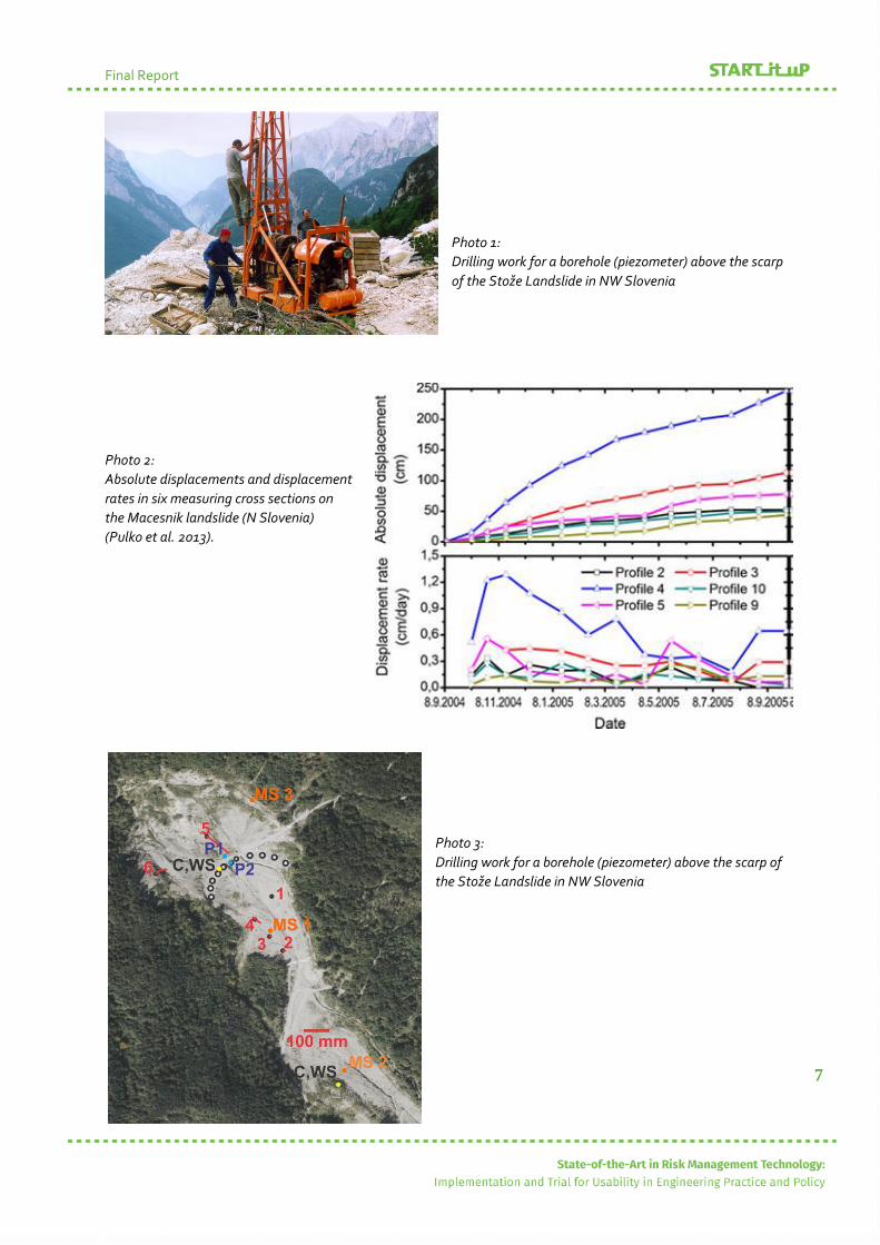
surface survey and subsurface exploration (boreholes, geologic mapping, Photo 1) and the landslide monitoring is
carried out at regular time intervals by different measurement techniques, such as piezometers, inclinometers and
extensometers.
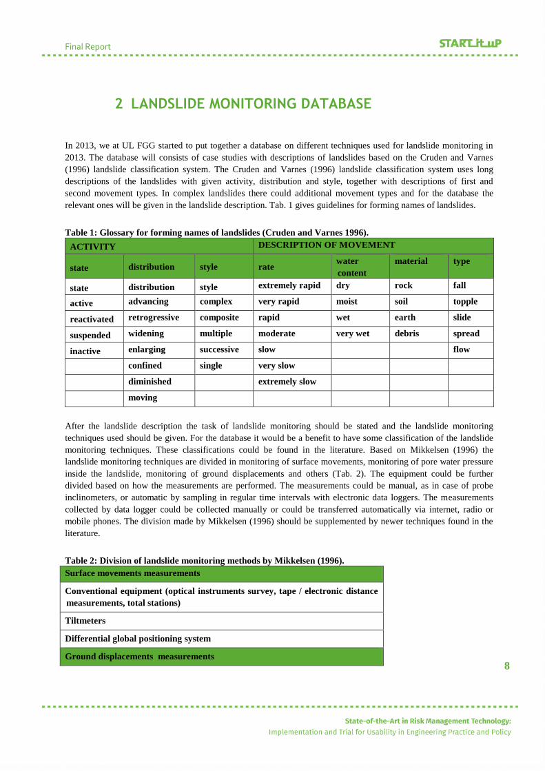
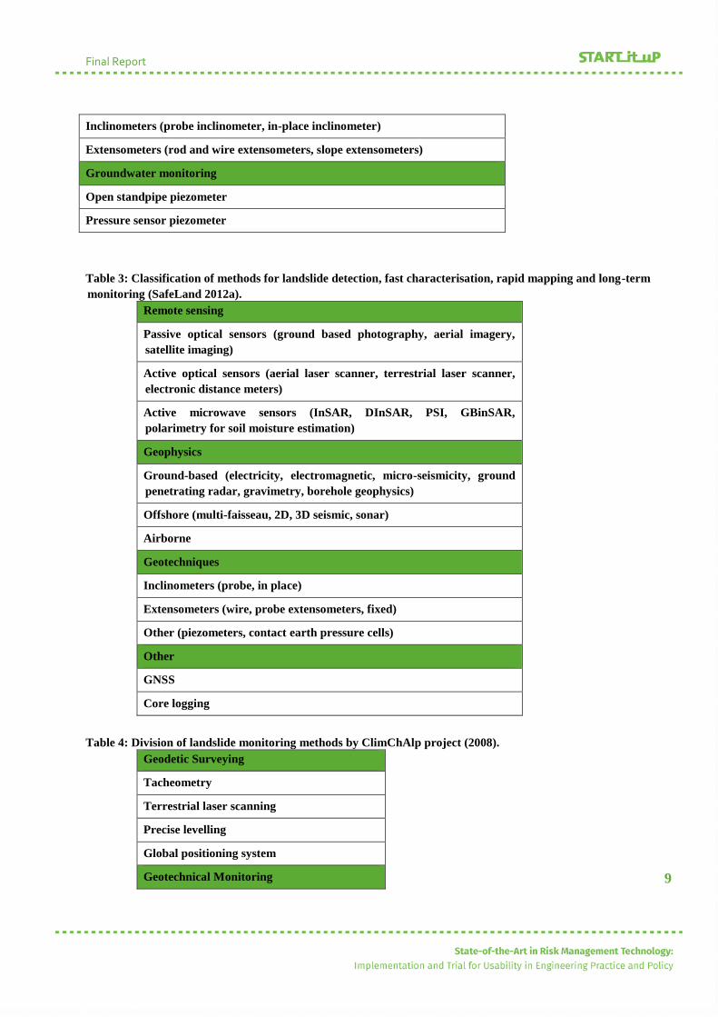
However, there are known examples of using landslide surface surveys (e.g. Photo 2) and subsurface exploration
techniques for landslide monitoring, as in case of the Slano Blato landslide (Logar et al. 2005; Pulko et al. 2013;
Photo 3). The equipment used for landslide monitoring should also be reliable, being capable of functioning for long
periods of time without maintenance or replacement. The response time should be short, and the sensitivity should
be high enough for the given problem.
Final Report
7
Photo 1:
Drilling work for a borehole (piezometer) above the scarp
of the Stože Landslide in NW Slovenia
Photo 2:
Absolute displacements and displacement
rates in six measuring cross sections on
the Macesnik landslide (N Slovenia)
(Pulko et al. 2013).
Photo 3:
Drilling work for a borehole (piezometer) above the scarp of
the Stože Landslide in NW Slovenia
Final Report
8
2 LANDSLIDE MONITORING DATABASE
In 2013, we at UL FGG started to put together a database on different techniques used for landslide monitoring in
2013. The database will consists of case studies with descriptions of landslides based on the Cruden and Varnes
(1996) landslide classification system. The Cruden and Varnes (1996) landslide classification system uses long
descriptions of the landslides with given activity, distribution and style, together with descriptions of first and
second movement types. In complex landslides there could additional movement types and for the database the
relevant ones will be given in the landslide description. Tab. 1 gives guidelines for forming names of landslides.
Table 1: Glossary for forming names of landslides (Cruden and Varnes 1996).
ACTIVITY DESCRIPTION OF MOVEMENT
state distribution style rate water
content
material type
state distribution style extremely rapid dry rock fall
active advancing complex very rapid moist soil topple
reactivated retrogressive composite rapid wet earth slide
suspended widening multiple moderate very wet debris spread
inactive enlarging successive slow flow
confined single very slow
diminished extremely slow
moving
After the landslide description the task of landslide monitoring should be stated and the landslide monitoring
techniques used should be given. For the database it would be a benefit to have some classification of the landslide
monitoring techniques. These classifications could be found in the literature. Based on Mikkelsen (1996) the
landslide monitoring techniques are divided in monitoring of surface movements, monitoring of pore water pressure
inside the landslide, monitoring of ground displacements and others (Tab. 2). The equipment could be further
divided based on how the measurements are performed. The measurements could be manual, as in case of probe
inclinometers, or automatic by sampling in regular time intervals with electronic data loggers. The measurements
collected by data logger could be collected manually or could be transferred automatically via internet, radio or
mobile phones. The division made by Mikkelsen (1996) should be supplemented by newer techniques found in the
literature.
Table 2: Division of landslide monitoring methods by Mikkelsen (1996).
Surface movements measurements
Conventional equipment (optical instruments survey, tape / electronic distance
measurements, total stations)
Tiltmeters
Differential global positioning system
Ground displacements measurements
Final Report
9
Inclinometers (probe inclinometer, in-place inclinometer)
Extensometers (rod and wire extensometers, slope extensometers)
Groundwater monitoring
Open standpipe piezometer
Pressure sensor piezometer
Table 3: Classification of methods for landslide detection, fast characterisation, rapid mapping and long-term
monitoring (SafeLand 2012a).
Remote sensing
Passive optical sensors (ground based photography, aerial imagery,
satellite imaging)
Active optical sensors (aerial laser scanner, terrestrial laser scanner,
electronic distance meters)
Active microwave sensors (InSAR, DInSAR, PSI, GBinSAR,
polarimetry for soil moisture estimation)
Geophysics
Ground-based (electricity, electromagnetic, micro-seismicity, ground
penetrating radar, gravimetry, borehole geophysics)
Offshore (multi-faisseau, 2D, 3D seismic, sonar)
Airborne
Geotechniques
Inclinometers (probe, in place)
Extensometers (wire, probe extensometers, fixed)
Other (piezometers, contact earth pressure cells)
Other
GNSS
Core logging
Table 4: Division of landslide monitoring methods by ClimChAlp project (2008).
Geodetic Surveying
Tacheometry
Terrestrial laser scanning
Precise levelling
Global positioning system
Geotechnical Monitoring
Final Report
10
Crack monitoring
Tiltmeters extensometers
Borehole inclinometers
Borehole extensometers
Piezometers
Time domain reflectometry
Fibre optics
Geophysical Methods
Direct current geoelectric
Microseismic monitoring
Remote sensing
Photogrammetry
Airborne laser scanning
Satellite-born radar interferometry
Ground-based radar interferometry
In the recent years the project SafeLand: Living with landslide risk in Europe: Assessment, effects of global change,
and risk management strategies) (SafeLand 2012a) produced several reports dealing with landslide detection, fast
characterisation, rapid mapping, monitoring and early warning systems. In these reports a slightly different division
of landslide monitoring techniques is given (Tab. 3).
The division of landslide monitoring techniques is more based on who performs the tests and not the physical
quantity. Report D4.4 of the SafeLand project (SafeLand 2012b) gives a comprehensive review of remote sensing
techniques and also guidelines for their selection for long-term landslide monitoring, based on landslide rate,
movement type, and for different phases of the risk management cycle. Report D4.5 (SafeLand 2012c) describes
some new methods for landslide monitoring. The results of these two reports should be included in the database.
Similar to the SafeLand project the ClimChAlp project (ClimChAlp – Climate Change, Impacts and adaptation
strategies in the Alpine Space) divides monitoring methods into four main categories: geodetic, geotechnical,
geophysical and remote sensing (Tab. 4).
As seen from Tabs. 2, 3 and 4, there are different divisions of landslide observation techniques and a combination of
these should be used.
It is important to note that usually only one part of a landslide monitoring system is described in a publication (e.g. a
journal paper), and it is thus problematic to get an integrated picture of the whole landslide monitoring system.
Publications mainly describe new measurement equipment, compare two different measurements (e.g. water level
and landslide movements), or compare measured and predicted data.
To obtain a better understanding of which field measurements are important for a specific type of landslide and if
there are differences between landslide monitoring techniques in different countries, a web questionnaire will be
prepared to be filled in on-line by landslide experts.
Final Report
11
3 REFERENCES
Chelli A, Mandrone G, Truffelli G (2006) Field investigations and monitoring as tools for modelling the Rossena
castle landslide (Northern Appennines, Italy). Landslides. 3(3): 252–259. doi: 10.1007/s10346-006-0046-z.
ClimChAlp (2008) Slope Monitoring Methods, A State of the Art Report. pp. 179. http://www.lfu.bayern.de
/geologie/massenbewegungen/projekte/climchalp/doc/engl_report_6.pdf [Last accessed 30.8.2013].
Coppola L, Nardone R, Rescio P, Bromhead E (2006) Reconstruction of the conditions that initiate landslide
movement in weathered silty clay terrain: effects on the historic and architectural heritage of Pietrapertosa,
Basilicata, Italy. Landslides. 3(4): 349–359. doi: 10.1007/s10346-006-0064-x.
Cruden DM, Varnes DJ (1996) Landslide types and processes. in: Turner AK, Schuster RL (eds). Landslides
investigation and mitigation; Special report 247, National Academy Press, Washington D.C., pp. 36-75.
Greif V, Sassa K, Fukuoka H (2006) Failure mechanism in an extremely slow rock slide at Bitchu-Matsuyama castle
site (Japan). Landslides 3(1): 22-38, doi: 10.1007/s10346-005-0013-0.
Logar J, Fifer Bizjak K, Kočevar M, Mikoš M, Ribičič M, Majes B (2005) History and present state of the Slano
Blato landslide. Natural Hazards and Earth System Sciences. 5: 1-11.
Mikkelsen PE (1996) Filed Instrumentation. in: Turner AK, Schuster RL (eds). Landslides investigation and
mitigation; Special report 247, National Academy Press, Washington D.C., pp. 278-316.
Petkovšek A, Maček M, Majes B (2013) Lessons learned from the 6 years matrix suction monitoring on the Slano
Blato landslide (Slovenia). Mediterranean Workshop on Landslides. Napoli, 2013: 1-4
http://www.mwl.unina2.it/Download/Petkovsek%20et%20al.pdf [Last accessed 15.9.2013]
Pulko B, Majes B, Mikoš M (2013) Reinforced concrete shafts for the structural mitigation of large deep-seated
landslides: an experience from the Macesnik and the Slano blato landslides (Slovenia). Landslides.
doi:10.1007/s10346-012-0372-2
SafeLand (2012a) SafeLand–FP7, Deliverable 4.1, Review of Techniques for Landslide Detection, Fast
Characterization, Rapid Mapping and Long-Term Monitoring. 401p. http://www.safeland-fp7.eu/
results/Pages/wa4.aspx [Last accessed 30.8.2013].
SafeLand (2012b) SafeLand–FP7, Deliverable 4.4, Guidelines for the selection of appropriate remote sensing
technologies for monitoring different types of landslides. 91p. http://www.safeland-fp7.eu/results/
Pages/wa4.aspx [Last accessed 30.8.2013].
SafeLand (2012c) SafeLand–FP7, Deliverable 4.5, Evaluation report on innovative monitoring and remote sensing
methods and future technology. 280p., http://www.safeland-fp7.eu/results/ Pages/wa4.aspx [L ast accessed
30.8.2013].
Vlcko J (2004) Extremely slow slope movements influencing the stability of Spis Castle, UNESCO site. Landslides.
1(1): 67-71, doi: 10.1007/s10346-003-0007-8.
This chapter was published in the conference proceedings of the 3rd
World Landslide Forum, held in Beijing in June
2014: Maček, M., Petkovšek, A., Majes, B., Mikoš, M. (2014): Landslide monitoring techniques database. In: Sassa,
K., Canuti, P., Yin, Y. (Eds.): Landslide science for a safer geoenvironment. Vol. 1, Springer International
Publishing Switzerland, 193-197.
Final Report
12
MONITORING AND WARNING TECHNOLOGY FOR
DEBRIS FLOWS
1 INTRODUCTION
In recent years, monitoring of landslides has improved by the development of new monitoring equipment, automatic
measurements done by computerized equipment and a decrease in equipment
Within the last two decades several debris flow catchments in Europa were equipped with monitoring systems for a
continuous measurement of important parameters describing debris flow initiation and flow dynamic. These systems
are mainly operated by scientific institutions and therefore the main focus is laid on investigations about different
aspects of the debris flow process itself. Further development to warning systems took place in the last years,
because of the availability of cost-efficient and reliable sensors, the rapid enhancement of data transmission and the
derivation of characteristic factors of already recorded debris flow events. Nowadays parameters of triggering
(precipitation) and transport (flow depth, acoustic signals) are recorded, stored and transmitted in a more or less
standardized way.
2 DEFINITION AND AIMS OF MONITORING
Monitoring (of "monitor": observe, supervise) is a systematic observation of a process or a system. Depending on
the objectives and applied technical means such an observation (surveillance) may be executed for certain limited
periods of time or permanently resp. continuosly.
For monitoring one can defines different aims, i.e. as follows:
1. The observations to better understand the processes within the system, to obtain data and to develop, test
and calibration of models. Eventhough this goal is primarily of a scientific interest, it also forms the basis
for all further practical applications.
2. The detection of thresholds in order to be able to intervene into the running process and cause changes in
the process flow. For debris flows one can say that these processes in fact cannot be directly controled,
field applications for such a preventive goal for the debris-flow control can be for example performed via
the control of flood retention basins.
3. The recognition of the exceedance of thresholds to initiate further actions that cannot change the process
itself. The applications can be found especially in the area of early warning or alarming, but also in
surveillance of structures.
3 CHAIN OF PERCEPTION, MONITORING AND WARNING
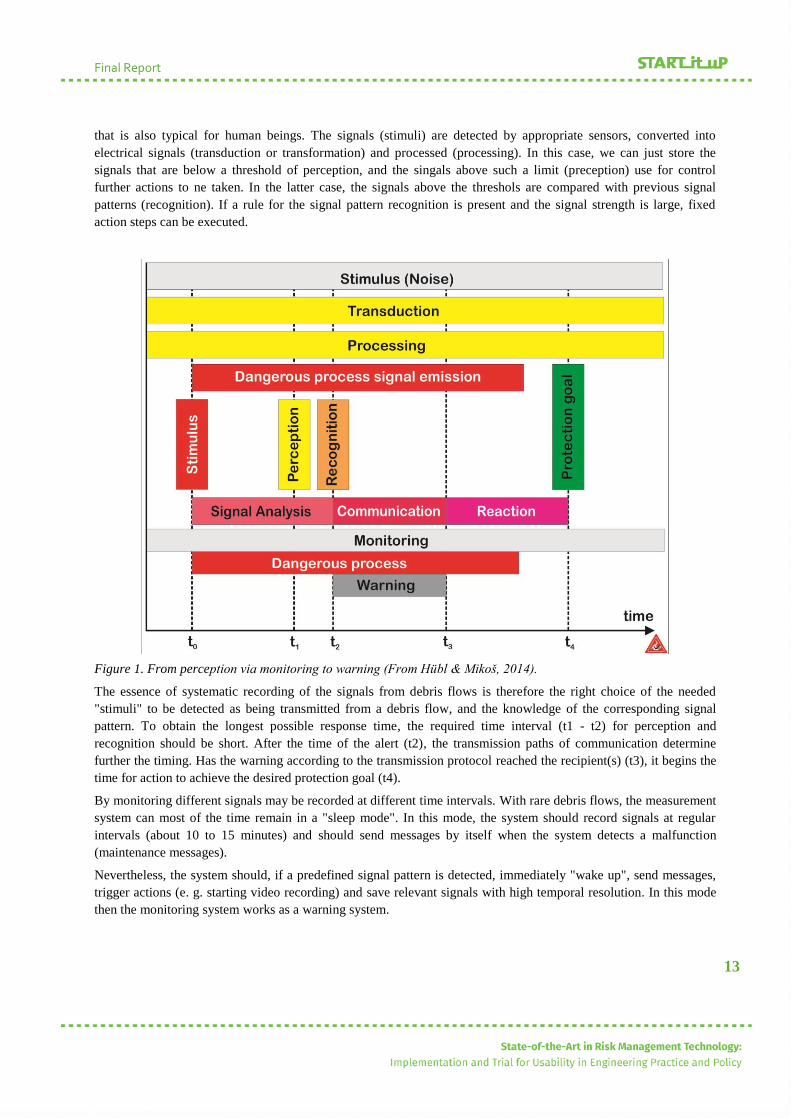
The systematic observation using technical means follows a chain of perception, monitoring and warning (Fig. 1)
Final Report
13
that is also typical for human beings. The signals (stimuli) are detected by appropriate sensors, converted into
electrical signals (transduction or transformation) and processed (processing). In this case, we can just store the
signals that are below a threshold of perception, and the singals above such a limit (preception) use for control
further actions to ne taken. In the latter case, the signals above the threshols are compared with previous signal
patterns (recognition). If a rule for the signal pattern recognition is present and the signal strength is large, fixed
action steps can be executed.
Figure 1. From perception via monitoring to warning (From Hübl & Mikoš, 2014).
The essence of systematic recording of the signals from debris flows is therefore the right choice of the needed
"stimuli" to be detected as being transmitted from a debris flow, and the knowledge of the corresponding signal
pattern. To obtain the longest possible response time, the required time interval (t1 - t2) for perception and
recognition should be short. After the time of the alert (t2), the transmission paths of communication determine
further the timing. Has the warning according to the transmission protocol reached the recipient(s) (t3), it begins the
time for action to achieve the desired protection goal (t4).
By monitoring different signals may be recorded at different time intervals. With rare debris flows, the measurement
system can most of the time remain in a "sleep mode". In this mode, the system should record signals at regular
intervals (about 10 to 15 minutes) and should send messages by itself when the system detects a malfunction
(maintenance messages).
Nevertheless, the system should, if a predefined signal pattern is detected, immediately "wake up", send messages,
trigger actions (e. g. starting video recording) and save relevant signals with high temporal resolution. In this mode
then the monitoring system works as a warning system.
Final Report
14
4 SIGNALS
To detect the signals (input variables, mostly physical parameters) of debris flows, different sensors can be used. In
the measuring instruments occurs the conversion into a measured value, the output signal, which is presented mostly
as mVs. On the basis of calibration functions, this measured value within the measurement range can be
backcalculated into the desired measured value.
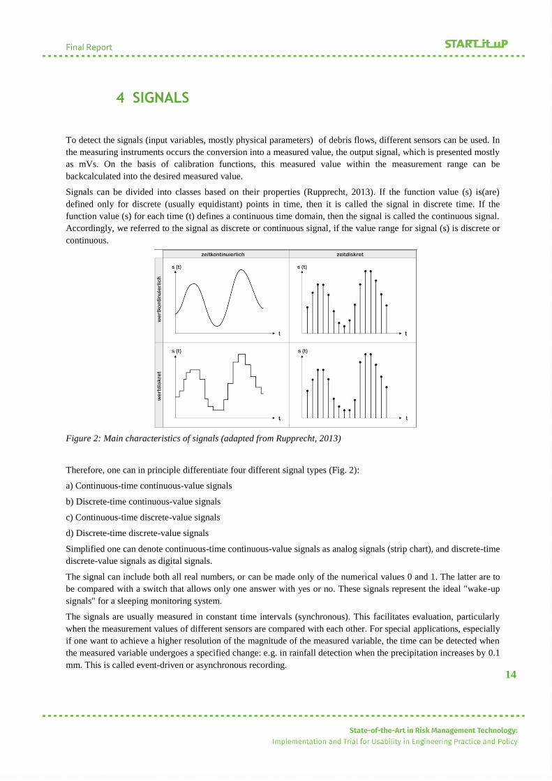
Signals can be divided into classes based on their properties (Rupprecht, 2013). If the function value (s) is(are)
defined only for discrete (usually equidistant) points in time, then it is called the signal in discrete time. If the
function value (s) for each time (t) defines a continuous time domain, then the signal is called the continuous signal.
Accordingly, we referred to the signal as discrete or continuous signal, if the value range for signal (s) is discrete or
continuous.
Figure 2: Main characteristics of signals (adapted from Rupprecht, 2013)
Therefore, one can in principle differentiate four different signal types (Fig. 2):
a) Continuous-time continuous-value signals
b) Discrete-time continuous-value signals
c) Continuous-time discrete-value signals
d) Discrete-time discrete-value signals
Simplified one can denote continuous-time continuous-value signals as analog signals (strip chart), and discrete-time
discrete-value signals as digital signals.
The signal can include both all real numbers, or can be made only of the numerical values 0 and 1. The latter are to
be compared with a switch that allows only one answer with yes or no. These signals represent the ideal "wake-up
signals" for a sleeping monitoring system.
The signals are usually measured in constant time intervals (synchronous). This facilitates evaluation, particularly
when the measurement values of different sensors are compared with each other. For special applications, especially
if one want to achieve a higher resolution of the magnitude of the measured variable, the time can be detected when
the measured variable undergoes a specified change: e.g. in rainfall detection when the precipitation increases by 0.1
mm. This is called event-driven or asynchronous recording.

Final Report
15
5 POSITIONING OF MEASURING DEVICES
One can assess the tendency of a catchment area to produce debris flows by systematic observations of debris flows
in it. If debris flows in a selected torrent channel do not occur often, in principle a debris-flow monitoring system
monitors the status I, in which predominate fluvial processes (Huebl, 2009). If one wants to draw conclusions about
the changes in a torrent system, especially to conclude about the changing tendecies with regard to debris flow
initiation, of course, the parameters that reflect this tendencies are of paramount importance. A key parameter in
this regard is soil moisture. To get conclusions about the change of the torrent system into the state II, characterized
by debris-flow processes, of course, data on a triggering event is necessary. First and foremost, the rainfall
(precipitation) data collection is needed, which is measured locally, but also spatially by means of weather radar.
After a debris flow has been already triggered, measurements that detect its movement are in one’s focus. Typical
for debris flows is sharp increase in their flow depths and they usually last only a short time. In case of debris-flow
pulses, their duration can be limited to only a few seconds, somewhat longer pulses can last a few minutes, but very
rarely a debris-flow event exceeds a period of half an hour.
If one wishes to detect a single debris-flow event with the aim to send this information to a decision point in a
monitoring resp. warning system, or also to other gauges along the torrent channel in order to "wake them up", one
is faced with the following problem (Fig. 3, Kienholz, 1998).
Figure 3: Reliability and time for identification based on the localisation of the alarm devices or on the phase of
process (Kienholz, 1998).
If the observation of the variable tendency for debris flows inititation is included into a debris-flow monitoring
system, i.e. the time prior to the initiation of a debris flow, this will result in a high reaction time, but also the chance
for "false alarms" is then very large. If a debris flow has already been triggered, any measruments (readings) can be
recorded with high reliability, but then the reaction time is reduced. Next question with regard to a monitoring
system is the question, where in the torrent catchment the debris-flow monitoring system should be placed. If it is
situated in the upper part of the torrent catchment, i.e. close resp. within the triggering/initiation area, one saves time
for the reaction at the expense of the uncertainty of its perception and recognition. If the debris-flow monitoring
system is placed at the apex of the torrent fan, we get very trustworthy signals, but the reaction time is extremely
short.
Therefore, from the very beginning we should clearly communicate to the users of any debris-flow monitoring
system (e.g. local residents) the goal of debris-flow monitoring not to raise wrong hopes. You should also take as the
rule the fact that the sooner you want to record a measurement, the greater the uncertainty of the signal.
Final Report
16
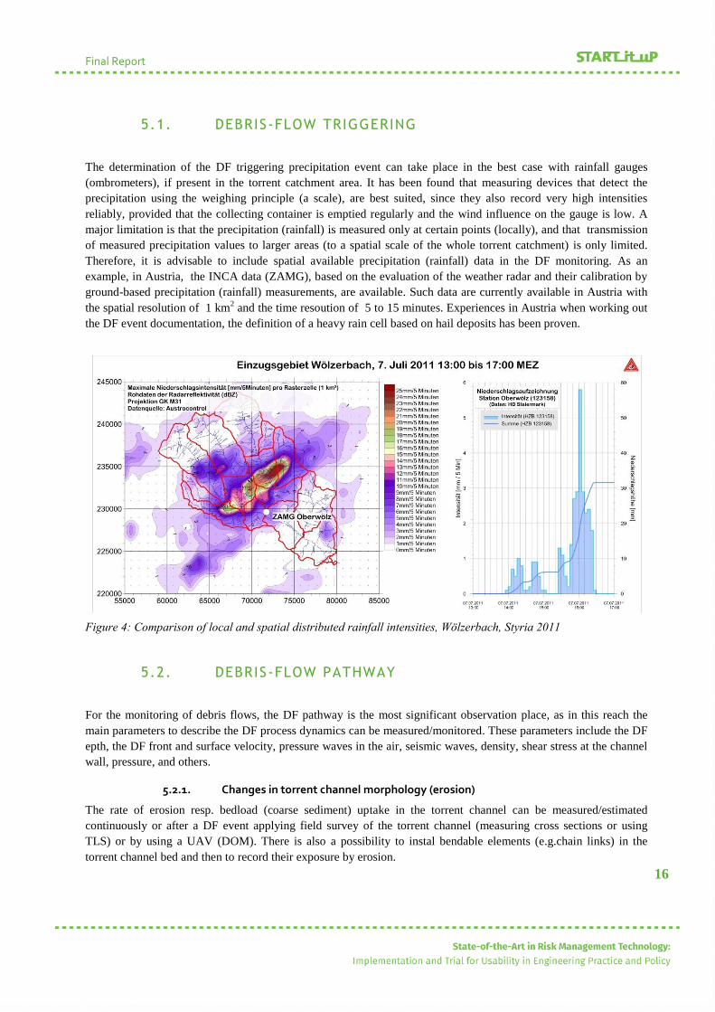
5.1. DEBRIS-FLOW TRIGGERING
The determination of the DF triggering precipitation event can take place in the best case with rainfall gauges
(ombrometers), if present in the torrent catchment area. It has been found that measuring devices that detect the
precipitation using the weighing principle (a scale), are best suited, since they also record very high intensities
reliably, provided that the collecting container is emptied regularly and the wind influence on the gauge is low. A
major limitation is that the precipitation (rainfall) is measured only at certain points (locally), and that transmission
of measured precipitation values to larger areas (to a spatial scale of the whole torrent catchment) is only limited.
Therefore, it is advisable to include spatial available precipitation (rainfall) data in the DF monitoring. As an
example, in Austria, the INCA data (ZAMG), based on the evaluation of the weather radar and their calibration by
ground-based precipitation (rainfall) measurements, are available. Such data are currently available in Austria with
the spatial resolution of 1 km2 and the time resoution of 5 to 15 minutes. Experiences in Austria when working out
the DF event documentation, the definition of a heavy rain cell based on hail deposits has been proven.
Figure 4: Comparison of local and spatial distributed rainfall intensities, Wölzerbach, Styria 2011
5.2. DEBRIS-FLOW PATHWAY
For the monitoring of debris flows, the DF pathway is the most significant observation place, as in this reach the
main parameters to describe the DF process dynamics can be measured/monitored. These parameters include the DF
epth, the DF front and surface velocity, pressure waves in the air, seismic waves, density, shear stress at the channel
wall, pressure, and others.
5.2.1. Changes in torrent channel morphology (erosion)
The rate of erosion resp. bedload (coarse sediment) uptake in the torrent channel can be measured/estimated
continuously or after a DF event applying field survey of the torrent channel (measuring cross sections or using
TLS) or by using a UAV (DOM). There is also a possibility to instal bendable elements (e.g.chain links) in the
torrent channel bed and then to record their exposure by erosion.

Final Report
17
5.2.2. Changes in debris-flow behavior
In principle, two different groups of sensors can be used (Jingri, 1989): those who come into contact with the debris
flow (contact detection) and those that deliver measured data without a direct contact with the debris flow
(contactless detection).
The contact detection of debris flows (Fig. 5) represents the beginning of the automated detection of debris flows in
the past, and has been used in in many parts of China and Japan. But even today, this not technically sophisticated
technique is an inexpensive and practical possibility for the detection of DF dynamics. The biggest benefit of this
technique is its simple integration into DF warning systems, but also in the triggering of DF monitoring facilities.
The disadvantages of these systems are in their maintenance. Parts of the system need to be replaced after each DF
detection. A continuous measurement is not possible, generally, only the first DF pulse can be detected. The
measured cross sections must be stabilized, because after each lowering or rising of the torrent channel the DF
triggering criteria are changed. In addition, a disorder of the measurement system by people (vandalism, playing) or
animals (game) can be a problem, and a certain protection is therefore necessary.
Figure 5: Examples for contact monitoring by check-line and mercury inclinometer
5.2.3. Wire sensors
In this system, one or more (n) horizontal wire sensors are used as a triggering device. If a DF surge exceeds the
level of a certain control wire sensor at given elevation, this wire will be dissmantled since a preset tensile force of
an anchor (e.g. magnetic) has been reached. A wire pull from its position triggers a change of the signal (0, 1). This
system also works in a vertical position. If on a tether in a cross section multiple wire sensors (pull ropes) are
distributed in a vertical position, also wide cross-sections can be easily monitored. At the lower end of each pull
rope counterweights are mounted, possibly at different heights, so that they can be caught and pulled off when a
debris flow flows through the control cross section, and thereby switching signals for each known elevation of the
counterweigth.
5.2.4. Inclinometers
The system with inclinometers works similarly to wire sensors. When an object undergoes a deflection by a DF
surge, a circuit will be closed by a switch (mercury switch, principle DLT).
5.2.5. Debris-flow depths
In stable torrent channel reaches, the DF depths can be measured contacless, withiut coming into contact with the
moving material. One may apply ultrasonic, radar and laser sensors, most of which are centered over the torrent
channel (Fig. 6). During installation, one should ensure an appropriate working distance from the presumed
maximum DF surface to secure proper data acquisition. Currently applied sensors can detect without problems
distances up to 30 meters. In natural torrent channels with high channel roughness and small discharges, the
measurement signal shows a high level of noise, since pure water runoff can usually not be easily measured at the
DF measurement point because the effective torrent channel width and the current water flowline is constantly
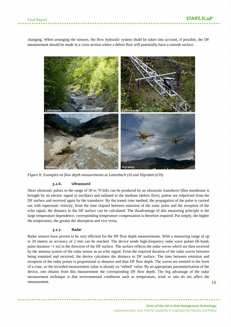
Final Report
18
changing. When arranging the sensors, the flow hydraulic system shuld be taken into account, if possible, the DF
measurement should be made in a cross section where a debris flow will potentially have a smooth surface.
Figure 6: Examples on flow depth measurements at Lattenbach (A) and Illgraben (CH)
5.2.6. Ultrasound
Short ultrasonic pulses in the range of 30 to 70 kHz can be produced by an ultrasonic transducer (thin membrane is
brought by an electric signal to oscillate) and radiated to the medium (debris flow), pulese are refpelcted from the
DF surface and received again by the transducer. By the transit time method, the propagation of the pulse is carried
out with supersonic velocity, from the time elapsed between emission of the sonic pulse and the reception of the
echo signal, the distance to the DF surface can be calculated. The disadvantage of this measuring principle is the
large temperature dependence, corresponding temperature compensation is therefore required. Put simply, the higher
the temperature, the greater the absorption and vice versa.
5.2.7. Radar
Radar sensors have proven to be very efficient for the DF flow depth measurements. With a measuring range of up
to 20 meters an accuracy of 2 mm can be reached. The device sends high-frequency radar wave pulses (K-band,
pulse duration ~1 ns) in the direction of the DF surface. The surface reflects the radar waves which are then received
by the antenna system of the radar sensor as an echo signal. From the required duration of the radar waves between
being emmited and received, the device calculates the distance to DF surface. The time between emission and
reception of the radar pulses is proportional to distance and thus DF flow depth. The waves are emitted in the form
of a cone, so the recorded measurement value is already an "edited" value. By an appropriate parameterization of the
device, one obtains from this measurement the corresponding DF flow depth. The big advantage of the radar
measurement technique is that environmental conditions such as temperature, wind or rain do not affect the
measurement.
Final Report
19
5.2.8. Laser
The distance measurement by laser is kind of an optical methods, the measurement is either performed using the
transit time method, or measuring the phase position. One can apply point as well as 2D laser devices. The
advantage of a 2D laser is that the entire cross section of a torrent channel can be measured (laser opening angle of
190°). Laser measurement applications are independent of weather conditions but fail when measuring pure water
(no particles for reflection of waves).
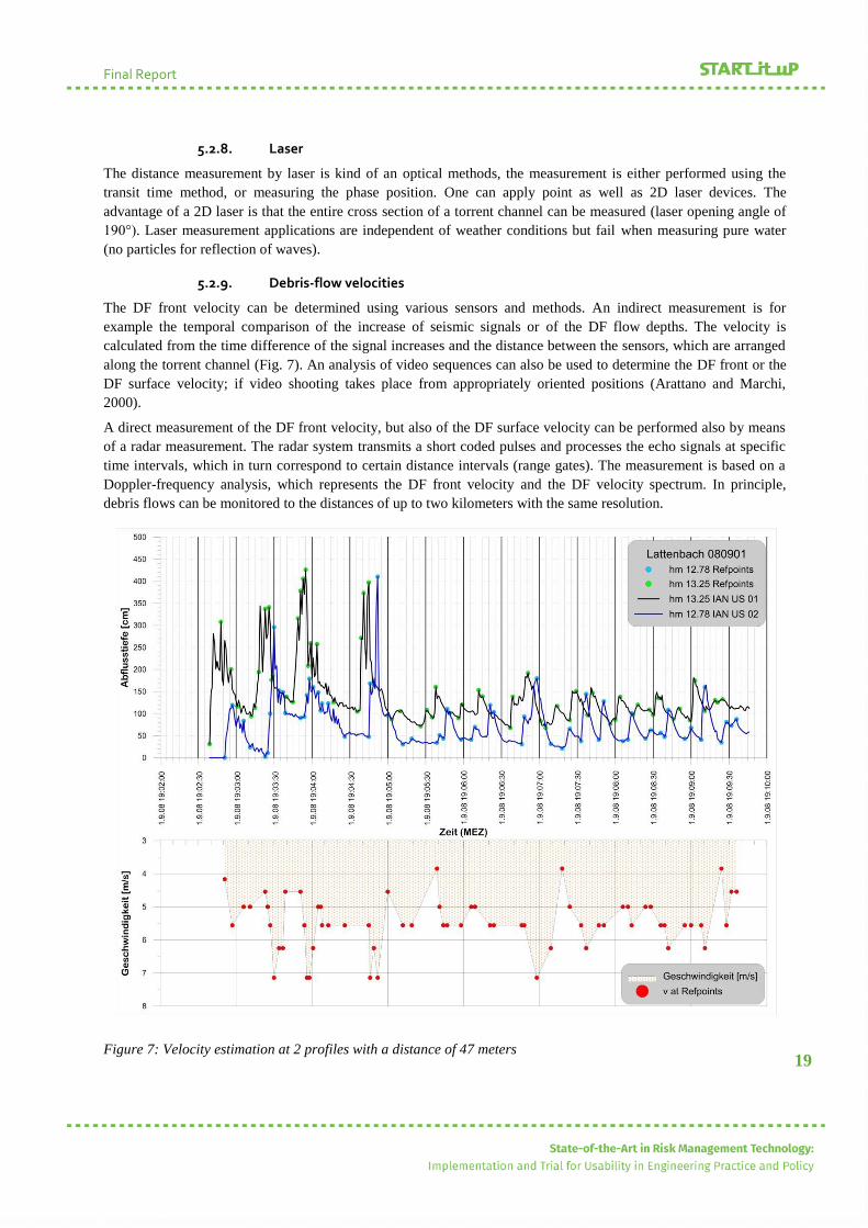
5.2.9. Debris-flow velocities
The DF front velocity can be determined using various sensors and methods. An indirect measurement is for
example the temporal comparison of the increase of seismic signals or of the DF flow depths. The velocity is
calculated from the time difference of the signal increases and the distance between the sensors, which are arranged
along the torrent channel (Fig. 7). An analysis of video sequences can also be used to determine the DF front or the
DF surface velocity; if video shooting takes place from appropriately oriented positions (Arattano and Marchi,
2000).
A direct measurement of the DF front velocity, but also of the DF surface velocity can be performed also by means
of a radar measurement. The radar system transmits a short coded pulses and processes the echo signals at specific
time intervals, which in turn correspond to certain distance intervals (range gates). The measurement is based on a
Doppler-frequency analysis, which represents the DF front velocity and the DF velocity spectrum. In principle,
debris flows can be monitored to the distances of up to two kilometers with the same resolution.
Figure 7: Velocity estimation at 2 profiles with a distance of 47 meters
Final Report
20
5.2.10. Shear stresses
The shear stress excerted by a debris flow can be detected directly or indirectly by means of a mechanical translation
by force transducer, mounted in the torrent channel bottom or on its banks. Such a measuring device is installed only
in Illgraben, Switzerland.
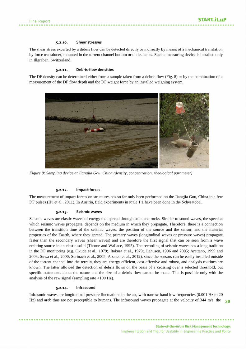
5.2.11. Debris-flow densities
The DF density can be determined either from a sample taken from a debris flow (Fig. 8) or by the combination of a
measurement of the DF flow depth and the DF weight force by an installed weighing system.
Figure 8: Sampling device at Jiangjia Gou, China (density, concentration, rheological parameter)
5.2.12. Impact forces
The measurement of impact forces on structures has so far only been performed on the Jiangjia Gou, China in a few
DF pulses (Hu et al., 2011). In Austria, field experiments in scale 1:1 have been done in the Schesatobel.
5.2.13. Seismic waves
Seismic waves are elastic waves of energy that spread through soils and rocks. Similar to sound waves, the speed at
which seismic waves propagate, depends on the medium in which they propagate. Therefore, there is a connection
between the transition time of the seismic waves, the position of the source and the sensor, and the material
properties of the Eaarth, where they spread. The primary waves (longitudinal waves or pressure waves) propagate
faster than the secondary waves (shear waves) and are therefore the first signal that can be seen from a wave
emitting source in an elastic solid (Thorne and Wallace, 1995). The recording of seismic waves has a long tradition
in the DF monitoring (e.g. Okuda et al., 1979;. Itakura et al., 1979;. Lahusen, 1996 and 2005; Arattano, 1999 and
2003; Suwa et al., 2000; Surinach et al., 2005; Abanco et al., 2012), since the sensors can be easily installed outside
of the torrent channel into the terrain, they are energy efficient, cost-effective and robust, and analysis routines are
known. The latter allowed the detection of debris flows on the basis of a crossing over a selected threshold, but
specific statements about the nature and the size of a debris flow cannot be made. This is possible only with the
analysis of the raw signal (sampling rate >100 Hz).
5.2.14. Infrasound
Infrasonic waves are longitudinal pressure fluctuations in the air, with narrow-band low frequencies (0.001 Hz to 20
Hz) and areb thus are not perceptible to humans. The infrasound waves propagate at the velocity of 344 m/s, the

Final Report
21
same velocity as the audible sound. The propagation velocity depends on the properties of the air (temperature,
density) and not on the frequency or amplitude of the wave. They can propagate thousands of kilometers and can
still be detected. If one monitors infrasound over short distances (<5 km), particularly scattering losses must be
taken into account, since the energy loss due to absorption in the atmosphere is relatively small (Albert and Orcutt,
1990; Johnson, 2003; Zhang, 1993; Zhang et al., 2004; Huebl et al., 2008).
The debris flows cause by the inter-collision of stones insode the DF mass and the collision of the DF mass with the
torrent channel both infrasound and seismic waves. The characteristic frequency range in which the largest
amplitudes occur varies depending on the viscosity from 5-10 Hz for debris flows with high coarse sediment content
to 15-30 Hz for debris-flow like events with low viscosity. The fact that debris flows exhibit in the frequency-time
domain a characteristic pattern of infrasound and seismic signals, permits an early detection of such events, even
before a DF pulse reaches the sensor location (Kogelnig et al., 2011). Fig. 9 depicts the infrasonic and the seismic
signal of a debris flow that occurred on September 1, 2008 at Lattenbach in Tirol, Austria.
Figure 9: Infrasound and seismic signal of a debris flow of 01.09.2008 at Lattenbach, Tyrol. Infrasound signal (a),
seismic signal (b), time-frequency spectrum of the infrasound signal (c), time-frequency spectrum of the seismic
signal (d)
5.2.15. Debris-flow dynamics
The dynamics of a debris flow in a torrent channel reach can be best seen (recognized) by means of a video camera
(webcam) that was activated by a trigger. In order to make geometric statements about the debris flow, one should
place markers in the video image area that are also visible during the DF event (during video footage). The video
time resolution should not be less than 10 frames per second so that also still pictures contain enough image
information. In order to assure video footage even at night, the use of day/night cameras is required. As an
additional light source at night infrared emitters are preferable because they have no light pollution as a normal
Final Report
22
headlight. The recording time of the video footage can be process-based determined or by a timer.
5.3. DEBRIS-FLOW DEPOSITION AREA
In a DF deposition area, spreading and twodimensionally propagating debris flows is very difficult to measure. If
video sequences are available, they can be evaluated with respect to the DF propagation direction, DF velocity and
DF flow depth. After a debris flow has deposited (after a DF event), for DF monitoring purposes are essential the
determinantion of the DF deposition area, the DF deposition heights, but also sampling of the DF deposits in order
to determine the concentration of solids and DF granulometric composition.
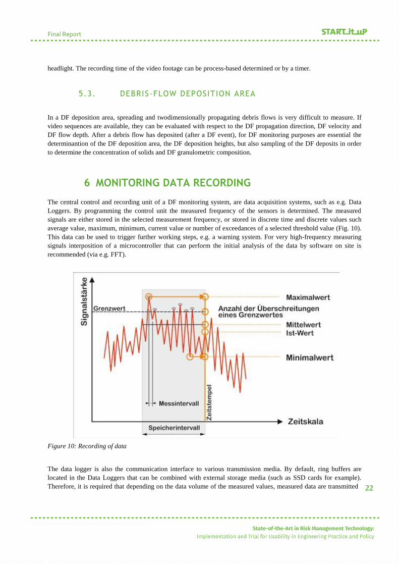
6 MONITORING DATA RECORDING
The central control and recording unit of a DF monitoring system, are data acquisition systems, such as e.g. Data
Loggers. By programming the control unit the measured frequency of the sensors is determined. The measured
signals are either stored in the selected measurement frequency, or stored in discrete time and discrete values such
average value, maximum, minimum, current value or number of exceedances of a selected threshold value (Fig. 10).
This data can be used to trigger further working steps, e.g. a warning system. For very high-frequency measuring
signals interposition of a microcontroller that can perform the initial analysis of the data by software on site is
recommended (via e.g. FFT).
Figure 10: Recording of data
The data logger is also the communication interface to various transmission media. By default, ring buffers are
located in the Data Loggers that can be combined with external storage media (such as SSD cards for example).
Therefore, it is required that depending on the data volume of the measured values, measured data are transmitted
Final Report
23
to a different storage medium (such as a database). This data transmission can in principle be done in 2 ways: either
sends the Data Logger in a set time intervals data packets (hourly, daily) or a server requests the data from the Data
Logger in the desired time intervals. It is important to ensure that at the selected times, the communication between
server and Data Logger is also guaranteed.
Regardless of the data recording, Data Logger should be able to send service messages, such as when the battery
level drops below a threshold value. Of course, a closed ground system for the measurement system (sensors, data
logger, power supply) must be installed (lightning protection).
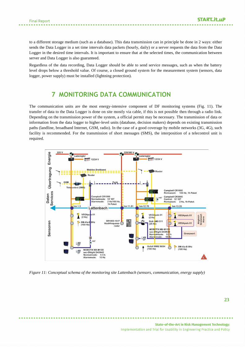
7 MONITORING DATA COMMUNICATION
The communication units are the most energy-intensive component of DF monitoring systems (Fig. 11). The
transfer of data to the Data Logger is done on site mostly via cable, if this is not possible then through a radio link.
Depending on the transmission power of the system, a official permit may be necessary. The transmission of data or
information from the data logger to higher-level units (database, decision makers) depends on existing transmission
paths (landline, broadband Internet, GSM, radio). In the case of a good coverage by mobile networks (3G, 4G), such
facility is recommended. For the transmission of short messages (SMS), the interposition of a telecontrol unit is
required.
Figure 11: Conceptual schema of the monitoring site Lattenbach (sensors, communication, energy supply)
Final Report
24
8 ENERGY SUPPLY
If a DF monitoring system can be limited to the summer months (or rainy season – monsoon season), the devices
can be put into a hybernation status. Very advantageous was proven the use a 230/240 V power supply (in Europe),
at least for the central unit of the DF monitoring system. Nevertheless, additional buffering by a 12/24 V battery is
required. If no electricity network connection can be established, must the entire DF monitoring system be operated
via solar units or in combination with fuel cells. The (sloar) supply unit must be designed and positioned in such a
way that a full-day operation is guaranteed, if possible. The energy reserves should be able to efficiently bridge
some days of "bad weather".
9 MONITORING DATA ARCHIVING
For a permanent DF monitoring system, the archiving of data in a database is essential. In addition to storing the raw
data, the data quality control must be carried out in order to identify in due time faulty recordings and to be able to
replace defective components of the system.
10 DEBRIS-FLOW MONITORING SYSTEMS IN EUROPE
Professional literature (Genevois et al., 2000; Marchi et al., 2002; Huebl and Moser, 2006; Hürlimann et al, 2011;
Navratil et al., 2012) contains descriptions of catchments that are equipped with field facilities for long-term DF
monitoring. The main criterion for selection of interesting DF monitoring systems can be the frequency of DF events
in these areas. In Europe, DF monitoring systems are in:
a) Austria: Lattenbach, warden's Bach, and other
b) Switzerland: Illgraben, village Bach, Spreitgraben, and others
c) Italy: Rio Moscardo, Aquabona, Gadria
d) France: Manival Torrent, Torrent Réal
e) Spain: Rebaixader torrent, and others
11 DEBRIS-FLOW WARNING SYSTEMS
Early warning system (EWS) is “the set of capacities needed to generate and disseminate timely and meaningful
warning information to enable individuals, communities and organizations threatened by a hazard to prepare and to
act appropriately and in sufficient time to reduce the possibility of harm or loss«. There are 5 key elements of the
human-centred EWS:
a) Knowledge of the debris-flow risk;
b) Monitoring, analysis, and forecasting of debris-flow hazards;
c) Operational centres;
d) Communication or dissemination of alerts and warnings;
e) Local capabilities to respond to the warnings received.
The EWS are usually based on:
a) debris-flow hazard maps (hazard zones within the maximum run-out zone);
b) meteorological forecasts (rainfall forecasts, rain radars), and
Final Report
25
c) monitoring data from hazard areas,
d) issuing debris-flow pre-trigger warnings (using different empirical thresholds) or
e) post-trigger warnings (event triggered warnings).
12 CONCLUSIONS
A Debris Flow Montoring System consists of different components, such as sensors, data acquisition units, control
unit, communications equipment, power supply and storage unit for data archiving. Due to the lasting rapid
technological development constantly new sensors, memory chips, etc. are available, so that the possibilities of DF
monitoring is steadily improving. In the meantime, industrial standard solutions (e.g. radar, ultrasonic, ..) can be
integrated into a DF monitoring system, so that the equipment costs can be reduced. Experiences have shown that an
optimal matched combination of the components of a DF monitoring system is an essential criterion for success. A
clear definition of DF monitoring system objectives, an excellent knowledge of the characteristics of the DF
processes to be detected, and the acceptance of local and technical conditions are the main requirements for
operation of a DF monitoring system.
13 REFERENCES
Abancó, C., Hürlimann, M., Fritschi, B., Graf, Ch., Moya, J. (2012): Transformation of Ground Vibration Signal for
Debris-Flow Monitoring and Detection in Alarm Systems; Sensors (Basel) 12(4): 4870– 4891
Albert, D. and Orcutt, J. (1990): Acoustic pulse propagation above grassland and snow: Comparison of theoretical
and experimental waveforms, Journal of the Acoustical Society of America, 87 (1), 93-100 Arattano, M. (1999):
On the use of seismic detectors as monitoring and warning systems for debris flows, Natural Hazards and Earth
System Sciences, 20,197–213
Arattano, M. and Marchi, L. (2000): Video-derived velocity distribution along a debris flow surge, Physics and
Chemistry of the Earth, Part B, 25, 781–784
Arattano, M. (2003): Monitoring the presence of the debris-flow front and its velocity through ground vibrations
detectors, Proceedings of the Third International Conference on Debris-Flow Hazards Mitigation: Mechanics,
Prediction and Assessment, Millpress, Rotterdam, 2, 731-743
Comiti, F., L. Marchi, L., Macconi, P., Arattano, M., Bertoldi, G., Borga, M., Brardinoni, F., Cavalli, M.,
D’Agostino, V., Penna, D., Theule, J. (2014): A new monitoring station for debris flows in the European Alps:
first observations in the Gadria basin, Natural Hazards, Springer-link, DOI 10.1007/s11069-014-1088-5, 1-
24
Genevois, R., Tecca, P., Breti, M. and Simoni, A. (2000): Debris-flow in the Dolomites: Experimental data from a
monitoring system, in: Debris-Flow Hazards Mitigation: Mechanics, Prediction, and Assessment, edited by:
Wieczorek, G. F. and Naeser, N. D., Proc. 2nd Intern. Conf., Taipei, Taiwan, 16–18 August 2000, Rotterdam,
Balkema Press, 283–291
Hu, K., Wei, F., Li, Y. (2011): Real-time measurement and preliminary analysis of debris-flow impact forces at
Jiangjia Ravine, China. Earth Surface Processes and Landforms, 36, 1628-1278, Wiley Online Library, DOI:
10.1002/esp.2155
Hübl, J. and Moser, M. (2006): Risk management in Lattenbach: a case study from Austria. In: Lorenzi G, Brebbia
C, Emmanouloudis D (eds.) Monitoring, Simulation, Prevention and Remediation of Dense and Debris Flows,
WIT Press, Southamption, 333-342

Final Report
26
Hübl, J., Zhang, S. and Kogelnig, A. (2008): Infrasound measurements of debris flow, In: De Wrachien, D.,
Brebbia, C.A., Lenzi, M.A. (Eds.), WIT Transactions on Engineering Sciences, Second International Conference
on Monitoring, Simulation, Prevention and Remediation of Dense and Debris Flows II, 60, 3-12 ISSN 1743-
3533, doi: 10.2495/DEB080011
Hübl, J (2009): Hochwässer in Wildbacheinzugsgebieten, Wiener Mitteilungen - Wasser, Abwasser, Gewässer, Bd.
216, 45-58;
Hürlimann, M., Abancó, C., Moya, J., Raimat, C., Luis-Fonseca R. (2011) Debris-flow monitoring stations in the
Eastern Pyrenees. Description of instrumentation, first experiences and preliminary results. In: Genevois R,
Hamilton DL, Prestininzi A (eds) 5th international conference on debris-flow hazards mitigation: mechanics,
prediction and assessment. Casa Editrice Universita` La Sapienza, Roma, pp 553–562
Itakura, Y., Koga, Y., Takahama, J. and Nowa, Y. (1997): Acoustic detection sensor for debris-flow, in: Debris-
Flow Hazards Mitigation: Mechanics, Prediction, and Assessment, edited by: Chen, C. L., Proc. First Intern.
Conf., San Francisco, USA, 7–9 August 1997, New York, ASCE, 747–756
Jingri, C. (1989): A Study on Debris Flow Warning in China, in: The Japan – China Symposium on Landslides and
Debris Flows; Niigata, Tokyo, Japan; S 177 – 182.
Johnson, J. (2003): Generation and propagation of infrasonic airwaves from volcanic explosions, Journal of
Volcanology and Geothermal Research, 121,1–14
Kienholz, H. (1998): Early warning systems related to mountain hazards; Manuskript hand-out; In: International
Conference on Early Warning Systems for Natural Disaster Reduction, Postdam
Kogelnig, A., Hübl, J., Suriñach, E., Vilajosana, I. and McArdell, B. (online first): Infrasound produced by debris
flow: propagation and frequency content evolution, Natural Hazards, doi:10.1007/s11069-011- 9741-8
LaHusen, R. (1996): Detecting debris flows using ground vibrations. USGS Fact Sheet 236-96, USGS (ed)
LaHusen (2005): Debris flow instrumentation; In: Jakob, M., Hungr, O., Debris-flow hazards and related
phenomena, 291 - 304; Springer, Chichester; ISBN 3-540-20726-0
Marchi L., Arattano M. and Deganutti, A. (2002): Ten years of debris-flow monitoring in the Moscardo Torrent
(Italian Alps), Geomorphology, 46(1-2), 1-17
Navratil, O., Liébault, F., Bellot, H., Theule, J., Travaglini, X., Ravanat, X., Ousset, F., Laigle, D., Segel, V., Fiquet,
M. (2012): High-frequency monitoring of debris flows in the French Alps, preliminary results of a starting
program, Conference Proc. Interpraevent
Okuda, S., Suwa, H., Okunishi, K., Yokoyama, K., Ogawa, K. and Hamana, S. (1979): Synthetic observation on
debris-flow, Part 5, Observation at Valley Kamikamihorisawa of Mt. Yakedade in 1978, Annuals of Disaster
Prevention Research Institute, Kyoto University, 22B-1, 157–204
Rupprecht, W. (2013): Signale und Übertragungssysteme – Modelle und Verfahren; Skriptum zur Vorlesung
Grundlagen der Informationsübertragung, Fachbereich Elektrotechnik und Informationstechnik, Universität
Kaiserslautern (http://nt.eit.uni-kl.de/fileadmin/lehre/guet/skript)
Suriñach, E., Vilajosana, I., Khazaradze, G., Biescas, B., Furdada, G. and Vilaplana, J. (2005): Seismic detection
and characterization of landslides and other mass movements, Natural Hazards and Earth System Sciences, 5,
791–798
Suwa, H., Yamakoshi, T. and Sato, K. (2000): Relationship between debris-flow discharge and ground vibration, in:
Debris-Flow Hazards Mitigation: Mechanics, Prediction, and Assessment, edited by: Wieczorek, G. F. and
Naeser, N. D., Proceedings 2nd International Conference, Taipei, Taiwan, 16-18 August 2000, Rotterdam,
Balkema Press, 311–318
Thorne, L. and Wallace, T. (1995): Modern Global Seismology, Academic Press, San Diego, USA
Zhang, S. (1993): A Comprehensive Approach to the Observation and Prevention of Debris Flow in China, Natural

Final Report
27
Hazards, 7, 1-23
Zhang, S., Hong, Y. and Yu, B. (2004): Detecting infrasound emission of debris flow for warning purposes,
International Symposium Interpraevent VII, Riva, Trient, 359–364
The main content of these practice guideline was published by Prof. Johannes Hübl and Prof. Matjaž Mikoš as a
paper in German language titled “Monitoring von Murgängen” in Journal für Wildbach-, Lawinen-, Erosions- und
Steinschlagschutzes (Journal of Torrent, Avalanche, Landslide and Rock Fall Engineering) in July 2014 in Heft 173,
Vol. 78, “Naturgefahrenbeobachtungen und Monitoring – Monitoring of Natural Hazard processes”.