Chinese Journal of Aeronautics, (2016), 29(5): 1294–1301
Chinese Society of Aeronautics and Astronautics& Beihang University
Chinese Journal of Aeronautics
Using PoF models to predict system reliability
considering failure collaboration
* Corresponding author. Tel.: +86-10-82338236.
E-mail addresses: [email protected], zengzhiguo@
buaa.edu.cn (Z. Zeng), [email protected] (R. Kang),
[email protected] (Y. Chen).
Peer review under responsibility of Editorial Committee of CJA.
Production and hosting by Elsevier
http://dx.doi.org/10.1016/j.cja.2016.08.0141000-9361 � 2016 Chinese Society of Aeronautics and Astronautics. Production and hosting by Elsevier Ltd.This is an open access article under the CC BY-NC-ND license (http://creativecommons.org/licenses/by-nc-nd/4.0/).
Zhiguo Zeng a,*, Rui Kang b, Yunxia Chen b
aChair on Systems Science and Energetic Challenge, Fondation Electricite de France (EDF), CentraleSupelec,Universite Paris-Saclay, Chatenay-Malabry 92290, FrancebSchool of Reliability and Systems Engineering, Beihang University, Beijing 100083, China
Received 29 January 2016; revised 16 March 2016; accepted 12 May 2016Available online 26 August 2016
KEYWORDS
Dependency;
Failure collaboration;
Physics-of-failure;
Reliability modeling;
Reliability prediction
Abstract Existing Physics-of-Failure-based (PoF-based) system reliability prediction methods are
grounded on the independence assumption, which overlooks the dependency among the compo-
nents. In this paper, a new type of dependency, referred to as failure collaboration, is introduced
and considered in reliability predictions. A PoF-based model is developed to describe the failure
behavior of systems subject to failure collaboration. Based on the developed model, the
Bisection-based Reliability Analysis Method (BRAM) is exploited to calculate the system reliabil-
ity. The developed methods are applied to predicting the reliability of a Hydraulic Servo Actuator
(HSA). The results demonstrate that the developed methods outperform the traditional PoF-based
reliability prediction methods when applied to systems subject to failure collaboration.� 2016 Chinese Society of Aeronautics and Astronautics. Production and hosting by Elsevier Ltd. This is
an open access article under theCCBY-NC-ND license (http://creativecommons.org/licenses/by-nc-nd/4.0/).
1. Introduction
Reliability prediction plays a significant role in reliability engi-neering. Since the Reliability Analysis Center (RAC) proposed
the first known reliability prediction method in 1956,1 enor-mous effort has been dedicated to developing more accuratereliability prediction methods. According to Goel and Graves,2
the existing reliability prediction methods can be categorized
into the empirical-based (or handbook-based) and Physics-of-Failure-based (PoF-based) methods. Empirical-based meth-ods, such as those in MIL-HDBK-217F, use historical data
from handbooks to make predictions. PoF-based methods,however, are based on the Time-To-Failures (TTFs) predictedby deterministic PoF models.3,4
Since the 1990s, increasing doubts have been cast over theaccuracy and validity of the empirical-based reliability predic-tion methods.5 Thus, Pecht et al.5 first proposed to use deter-
ministic PoF models to predict reliability of electronicproducts, which comprises three steps: first, a deterministicmodel is developed based on PoF models to predict the TTFof the system; then, parametric uncertainties of the system
TTF model are identified and represented by their ProbabilityDensity Functions (PDFs); finally, system reliability ispredicted by propagating the parametric uncertainties based
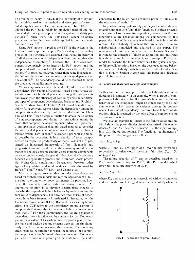
Fig. 1 Schematic of power divider.
Using PoF models to predict system reliability considering failure collaboration 1295
on probability theory.6 CALCE at the University of Marylandfurther elaborated on the method and developed software toaid its application in electronic equipment.7 In 2003, IEEE
adopted the PoF-based reliability prediction method and rec-ommended it as a general procedure for system reliability pre-dictions.8,9 Since then, the PoF-based system reliability
prediction method has been widely applied in both academiaand industries.10–14
Using PoF models to predict the TTF of the system is the
first and most important step in PoF-based system reliabilityprediction. In literature, it is assumed that the failure behaviorof all the components is independent from one another (theindependence assumption).6 Therefore, the TTF of each com-
ponent is completely determined by its PoF models, and thecomponent with the shortest TTF determines the TTF of thesystem.3,4 In practice, however, rather than being independent,
the failure behavior of the components is always dependent onone another.15 The dependency should be considered to makethe predicted reliability more accurate.
Various approaches have been developed to model thedependency. For example, Kotz et al.16 used a multivariate dis-tribution to describe the dependency among the components
and investigated the efficiency of parallel systems under differ-ent types of component dependencies. Navarro and Rychlik17
calculated Mean Time To Failure (MTTF) and bounds of reli-ability for a coherent system where the dependency among its
components is described by multivariate distributions. Ebra-himi and Hua18 used a copula function to assess the reliabilityof a nanocomponent considering the interactions among the
atoms that compose the nanocomponent. Mo et al.19 presenteda multiple-value decision diagram based method to considerthe statistical dependence of component states in a phased-
mission system. Levitin et al.20 developed a probabilistic modelto describe the dependent failure behavior of some compo-nents with respect to productivity or loads. Vasan et al.21 pre-
sented an integrated framework of fault diagnostic andprognostic to monitor and predict the remaining useful perfor-mance of analog electronic circuits where multiple componentsdegrade simultaneously. Peng et al.22 described the dependency
between a degradation process and a random shock processvia Monte-Carlo simulations. Dependency between othertypes of degradation and random shocks is also discussed by
Rafiee,23 Fan,24 Song,25,26 Lin,27 and Zhang et al.28
Most existing approaches that consider dependency arebased on probabilistic models and rely on large amount of fail-
ure data to estimate the model parameters. In practice, how-ever, the available failure data are always limited. Analternative solution is to develop deterministic models todescribe the dependent failure behavior by understanding the
root cause of dependency. Till now, two root causes of depen-dency have been frequently investigated in literature, i.e., theCommon-Cause-Failure (CCF) effect and the cascading failure
effect. The CCF refers to the dependency among a group ofcomponents that are subject to common failure causes or com-mon loads.29 For these components, the failure behavior is
dependent since it is influenced by common factors. For exam-ple, in the accident of Fukushima nuclear power plant,30 boththe main and backup cooling systems were cut off simultane-
ously due to a common cause, the tsunami. The cascadingeffect refers to the situation in which the failure of one compo-nent might cause the failure of other components.31 For exam-ple, when a node in a power grid network fails, the nodes
connected to the failed node are more prone to fail due tothe rebalance of loads.32,33
In practice, many systems rely on the joint contribution of
several components to fulfill their functions. For these systems,a new kind of root cause for dependency arises from the col-laborative failure behavior among the components. In this
paper, this kind of dependency is referred to as failure collab-oration. The reliability of systems that are subject to failurecollaboration is modeled and analyzed in this paper. The
remainder of this paper is structured as follows. Section 2introduces the concept of failure collaboration and illustratesit with an example. In Section 3, we develop a PoF-basedmodel to describe the failure behavior of the systems subject
to failure collaboration. Based on the developed failure behav-ior model, a reliability prediction method is developed in Sec-tion 4. Finally, Section 5 concludes this paper and discusses
possible future work.
2. Failure collaboration: concepts and examples
In this section, the concept of failure collaboration is intro-duced and illustrated with an example. When a group of com-ponents collaborates to fulfill a system’s function, the failure
behavior of one component might be influenced by the othercomponents, which causes dependency among the compo-nents. This kind of dependency is referred to as failure collab-
oration, since it is caused by the joint effect of components ona common function.
We give an example to illustrate the failure collaboration.Fig. 1 shows the power divider circuit. Comprised of two impe-
dances X1 and X2, the circuit transfers Uin, the input voltage,into Uout, the output voltage. The functional requirements ofthe power divider are given as follows:
UL < Uout < UU ð1Þ
where UU and UL are upper and lower failure thresholds,respectively. In other words, the circuit fails when Uout > UU
or Uout < UL.
The failure behavior of X1 can be described based on itsPoF model. According to Ref.34, the PoF model whichdescribes the failure behavior of X1 is
X1ðtÞ ¼ X0;1 þ k1t ð2Þ
where X0;1 and k1 are constants associated with environmental
and use conditions. Let Xth;1 denote the value of X1 when the
1296 Z. Zeng et al.
system fails (Uout > UU or Uout < UL). Then, the TTF of X1 is
determined by calculating the moment when X1ðtÞ ¼ Xth;1:
TTF1 ¼ ðXth;1 � X0;1Þ=k1 ð3ÞEqs. (2) and (3) describe the failure behavior of X1.
Based on circuit laws, Uout is determined by X1 and X2:
Uout ¼ X1
X1 þ X2
Uin ð4ÞIt can be seen from Eq. (4) that X1 and X2 work together to
ensure the normal functioning of the circuit. Thus, the value ofX2 would influence the failure threshold of X1. Supposet ¼ TTF, and the circuit fails. From Eqs. (1) and (4), we have
Xth;1 ¼UUX2ðTTFÞUin �UU
k1 P 0
ULX2ðTTFÞUin �UL
k1 < 0
8>><>>:
ð5Þ
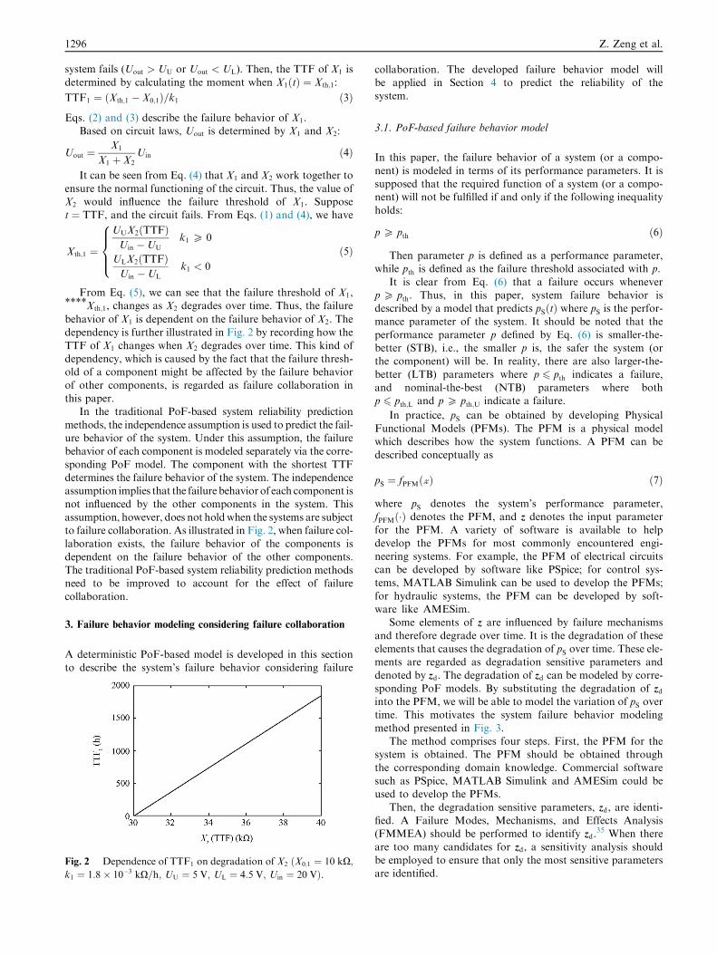
From Eq. (5), we can see that the failure threshold of X1,****Xth;1, changes as X2 degrades over time. Thus, the failure
behavior of X1 is dependent on the failure behavior of X2. Thedependency is further illustrated in Fig. 2 by recording how the
TTF of X1 changes when X2 degrades over time. This kind ofdependency, which is caused by the fact that the failure thresh-old of a component might be affected by the failure behavior
of other components, is regarded as failure collaboration inthis paper.
In the traditional PoF-based system reliability prediction
methods, the independence assumption is used to predict the fail-ure behavior of the system. Under this assumption, the failurebehavior of each component is modeled separately via the corre-
sponding PoF model. The component with the shortest TTFdetermines the failure behavior of the system. The independenceassumption implies that the failurebehaviorof each component isnot influenced by the other components in the system. This
assumption, however, does not holdwhen the systems are subjectto failure collaboration. As illustrated in Fig. 2, when failure col-laboration exists, the failure behavior of the components is
dependent on the failure behavior of the other components.The traditional PoF-based system reliability prediction methodsneed to be improved to account for the effect of failure
collaboration.
3. Failure behavior modeling considering failure collaboration
A deterministic PoF-based model is developed in this sectionto describe the system’s failure behavior considering failure
Fig. 2 Dependence of TTF1 on degradation of X2 ðX0;1 ¼ 10 kX;k1 ¼ 1:8� 10�3 kX=h; UU ¼ 5 V; UL ¼ 4:5 V; Uin ¼ 20 VÞ.
collaboration. The developed failure behavior model willbe applied in Section 4 to predict the reliability of thesystem.
3.1. PoF-based failure behavior model
In this paper, the failure behavior of a system (or a compo-
nent) is modeled in terms of its performance parameters. It issupposed that the required function of a system (or a compo-nent) will not be fulfilled if and only if the following inequality
holds:
p P pth ð6ÞThen parameter p is defined as a performance parameter,
while pth is defined as the failure threshold associated with p.
It is clear from Eq. (6) that a failure occurs wheneverp P pth. Thus, in this paper, system failure behavior isdescribed by a model that predicts pSðtÞ where pS is the perfor-mance parameter of the system. It should be noted that the
performance parameter p defined by Eq. (6) is smaller-the-better (STB), i.e., the smaller p is, the safer the system (orthe component) will be. In reality, there are also larger-the-
better (LTB) parameters where p 6 pth indicates a failure,and nominal-the-best (NTB) parameters where bothp 6 pth;L and p P pth;U indicate a failure.
In practice, pS can be obtained by developing Physical
Functional Models (PFMs). The PFM is a physical modelwhich describes how the system functions. A PFM can bedescribed conceptually as
pS ¼ fPFMðzÞ ð7Þwhere pS denotes the system’s performance parameter,fPFMð�Þ denotes the PFM, and z denotes the input parameterfor the PFM. A variety of software is available to help
develop the PFMs for most commonly encountered engi-neering systems. For example, the PFM of electrical circuitscan be developed by software like PSpice; for control sys-tems, MATLAB Simulink can be used to develop the PFMs;
for hydraulic systems, the PFM can be developed by soft-ware like AMESim.
Some elements of z are influenced by failure mechanisms
and therefore degrade over time. It is the degradation of theseelements that causes the degradation of pS over time. These ele-ments are regarded as degradation sensitive parameters and
denoted by zd. The degradation of zd can be modeled by corre-sponding PoF models. By substituting the degradation of zdinto the PFM, we will be able to model the variation of pS overtime. This motivates the system failure behavior modeling
method presented in Fig. 3.The method comprises four steps. First, the PFM for the
system is obtained. The PFM should be obtained through
the corresponding domain knowledge. Commercial softwaresuch as PSpice, MATLAB Simulink and AMESim could beused to develop the PFMs.
Then, the degradation sensitive parameters, zd, are identi-fied. A Failure Modes, Mechanisms, and Effects Analysis(FMMEA) should be performed to identify zd.
35 When there
are too many candidates for zd, a sensitivity analysis shouldbe employed to ensure that only the most sensitive parametersare identified.
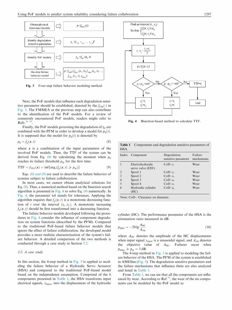
Fig. 3 Four-step failure behavior modeling method.
Fig. 4 Bisection-based method to calculate TTF.
Table 1 Components and degradation sensitive parameters of
HSA.
Index Component Degradation
sensitive parameter
Failure
mechanisms
1 Electrohydraulic
servo valve (ESV)
CoD x1 Wear
2 Spool 1 CoD x2 Wear
3 Spool 2 CoD x3 Wear
4 Spool 3 CoD x4 Wear
5 Spool 4 CoD x5 Wear
6 Hydraulic cylinder
(HC)
CoD x6 Wear
Note: CoD—Clearance on diameter.
Using PoF models to predict system reliability considering failure collaboration 1297
Next, the PoF models that influence each degradation sensi-tive parameter should be established, denoted by the fFMð�Þ inFig. 3. The FMMEA at the previous step can also contributeto the identification of the PoF models. For a review ofcommonly encountered PoF models, readers might refer to
Refs.36–39.Finally, the PoF models governing the degradation of zd are
combined with the PFM in order to develop a model for pSðtÞ.It is supposed that the model for pSðtÞ is denoted by
pS ¼ fpðx; tÞ ð8Þwhere x is a combination of the input parameters of theinvolved PoF models. Then, the TTF of the system can be
derived from Eq. (8) by calculating the moment when pSreaches its failure threshold pth for the first time:
TTF ¼ fTTFðxÞ ¼ inffargtðfpðx; tÞ P pthÞg ð9ÞEqs. (8) and (9) are used to describe the failure behavior of
systems subject to failure collaboration.In most cases, we cannot obtain analytical solutions for
Eq. (9). Thus, a numerical method based on the bisection search
algorithm is presented in Fig. 4 to solve Eq. (9) numerically. InFig. 4, the parameter tol stands for tolerances. Applying thealgorithm requires that fpðx; tÞ is a monotonic decreasing func-
tion of t over the interval ðtL; tUÞ. A monotonic increasingfpðx; tÞ should be first transformed into a decreasing function.
The failure behavior models developed following the proce-dures in Fig. 4 consider the influence of component degrada-tion on system functions (described by the PFM). Comparedto the traditional PoF-based failure behavior models that
ignore the effect of failure collaboration, the developed modelprovides a more realistic characterization of the system’s fail-ure behavior. A detailed comparison of the two methods is
conducted through a case study in Section 3.2.
3.2. A case study
In this section, the 4-step method in Fig. 3 is applied to mod-eling the failure behavior of a Hydraulic Servo Actuator(HSA) and compared to the traditional PoF-based model
based on the independence assumption. Comprised of the 6components presented in Table 1, the HSA transforms inputelectrical signals, xinput, into the displacement of the hydraulic
cylinder (HC). The performance parameter of the HSA is theattenuation ratio measured in dB:
pHSA ¼ �20 lgAHC
Aobj
ð10Þ
where AHC denotes the amplitude of the HC displacementswhen input signal xinput is a sinusoidal signal, and Aobj denotes
the objective value of AHC. Failures occur whenpHSA P pth ¼ 3 dB.
The 4-step method in Fig. 3 is applied to modeling the fail-
ure behavior of the HSA. The PFM of the system is establishedin AMESim (Fig. 5). The degradation sensitive parameters andthe failure mechanisms that influence them are also analyzed
and listed in Table 1.From Table 1, we can see that all the components are influ-
enced by wear. According to Ref.39, the wear of the six compo-
nents can be modeled by the PoF model as
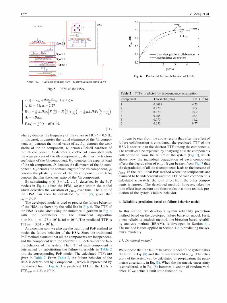
Fig. 5 PFM of the HSA.
Fig. 6 Predicted failure behavior of HSA.
Table 2 TTFs predicted by independence assumption.
Component Threshold (mm) TTF (105 h)
1 0.0015 4:23
2 0.770 355
3 0.070 29:2
4 0.065 26:4
5 0.070 16:2
6 0.050 9:77
1298 Z. Zeng et al.
xiðtÞ ¼ x0;i þ KiLm;iWa;i
Hitfi 1 6 i 6 6
lg Ki ¼ 5 lg li � 2:27
Wa;i ¼ 130AiHiwi F3
2ðhiriÞ � F3
2
hiriþ 1
wi2
� �h iþ 1
10pAiHiF1
hiriþ 1
wi2
� �Ai ¼ pDiLj;i
FnðuÞ ¼R1uðt� uÞne�t2
2 dt
8>>>>>>><>>>>>>>:
ð11Þwhere f denotes the frequency of the valves or HC (f ¼ 0:5 Hz
in this case), xi denotes the radial clearance of the ith compo-nent, x0;i denotes the initial value of xi, Lm;i denotes the wear
stroke of the ith component, Hi denotes Brinell hardness ofthe ith component, Ki denotes a coefficient associated withthe wear process of the ith component, li denotes the frictioncoefficient of the ith component, Wa;i denotes the asperity load
of the ith component, Di denotes the diameters of the ith com-
ponent, Lj;i denotes the contact length of the ith component, wi
denotes the plasticity index of the ith component, and hi=ri
denotes the film thickness ratio of the ith component.By substituting xiðtÞ ði ¼ 1; 2; . . . ; 6Þ described by the PoF
models in Eq. (11) into the PFM, we can obtain the model
which describes the variation of pHSA over time. The TTF ofthe HSA can then be calculated by Eq. (9), given thatpth ¼ 3 dB.
The developed model is used to predict the failure behavior
of the HSA, as shown by the solid line in Fig. 6. The TTF ofthe HSA is calculated using the numerical algorithm in Fig. 4with the parameters of the numerical algorithm
tL ¼ 0 h; tU ¼ 1:75� 109 h; tol ¼ 10�3. The predicted TTF is
TTFFC ¼ 3:04� 105 h.As a comparison, we also use the traditional PoF method to
model the failure behavior of the HSA. Since the traditional
PoF method assumes that all the components are independent,and the component with the shortest TTF determines the fail-ure behavior of the system. The TTF of each component isdetermined by substituting the failure thresholds in Table 2
into the corresponding PoF model. The calculated TTFs aregiven in Table 2. From Table 2, the failure behavior of theHSA is determined by Component 1, which is represented by
the dashed line in Fig. 6. The predicted TTF of the HSA is
TTFIND ¼ 4:23� 105 h.
It can be seen from the above results that after the effect offailure collaboration is considered, the predicted TTF of the
HSA is shorter than the shortest TTF among the components.The results can be explained by analyzing how the componentscollaborate to cause the failure of the system (Fig. 7), which
shows how the individual degradation of each componentaffects the degradation of pHSA. It can be seen from Fig. 7 thatthe degradation of all the 6 components leads to the increase of
pHSA. In the traditional PoF method where the components areassumed to be independent and the TTF of each component iscalculated separately, the joint effect from the other compo-nents is ignored. The developed method, however, takes the
joint effect into account and thus results in a more realistic pre-diction of the system’s failure behavior.
4. Reliability prediction based on failure behavior model
In this section, we develop a system reliability predictionmethod based on the developed failure behavior model. First,
a new reliability analysis method, the bisection-based reliabil-ity analysis method (BRAM), is developed in Section 4.1.The method is then applied in Section 4.2 to predicting the sys-
tem’s reliability.
4.1. Developed method
We suppose that the failure behavior model of the system takesthe form of Eq. (8) and the failure threshold is pth. The relia-bility of the system can be calculated by propagating the para-metric uncertainty in Eq. (8). When the parametric uncertainty
is considered, x in Eq. (8) becomes a vector of random vari-ables. If we define a limit state function as
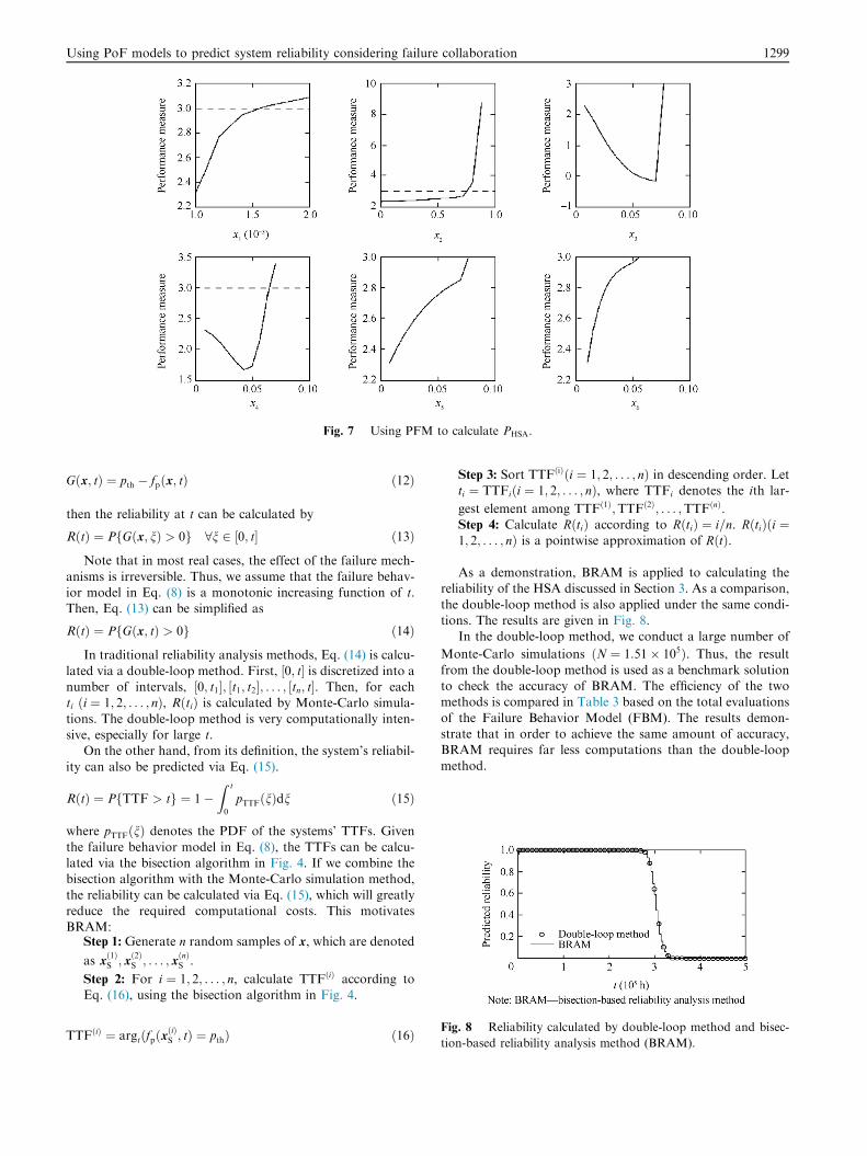
Fig. 7 Using PFM to calculate PHSA.
Using PoF models to predict system reliability considering failure collaboration 1299
Gðx; tÞ ¼ pth � fpðx; tÞ ð12Þ
then the reliability at t can be calculated by
RðtÞ ¼ PfGðx; nÞ > 0g 8n 2 ½0; t� ð13ÞNote that in most real cases, the effect of the failure mech-
anisms is irreversible. Thus, we assume that the failure behav-ior model in Eq. (8) is a monotonic increasing function of t.Then, Eq. (13) can be simplified as
RðtÞ ¼ PfGðx; tÞ > 0g ð14ÞIn traditional reliability analysis methods, Eq. (14) is calcu-
lated via a double-loop method. First, ½0; t� is discretized into anumber of intervals, ½0; t1�; ½t1; t2�; . . . ; ½tn; t�. Then, for eachti ði ¼ 1; 2; . . . ; nÞ, RðtiÞ is calculated by Monte-Carlo simula-
tions. The double-loop method is very computationally inten-sive, especially for large t.
On the other hand, from its definition, the system’s reliabil-
ity can also be predicted via Eq. (15).
RðtÞ ¼ PfTTF > tg ¼ 1�Z t
0
pTTFðnÞdn ð15Þ
where pTTFðnÞ denotes the PDF of the systems’ TTFs. Given
the failure behavior model in Eq. (8), the TTFs can be calcu-lated via the bisection algorithm in Fig. 4. If we combine thebisection algorithm with the Monte-Carlo simulation method,
the reliability can be calculated via Eq. (15), which will greatlyreduce the required computational costs. This motivatesBRAM:
Step 1: Generate n random samples of x, which are denoted
as xð1ÞS ; x
ð2ÞS ; . . . ; x
ðnÞS .
Step 2: For i ¼ 1; 2; . . . ; n, calculate TTFðiÞ according toEq. (16), using the bisection algorithm in Fig. 4.
Fig. 8 Reliability calculated by double-loop method and bisec-
tion-based reliability analysis method (BRAM).
TTFðiÞ ¼ argtðfpðxðiÞS ; tÞ ¼ pthÞ ð16Þ
Step 3: Sort TTFðiÞði ¼ 1; 2; . . . ; nÞ in descending order. Letti ¼ TTFiði ¼ 1; 2; . . . ; nÞ, where TTFi denotes the ith lar-
gest element among TTFð1Þ;TTFð2Þ; . . . ;TTFðnÞ.Step 4: Calculate RðtiÞ according to RðtiÞ ¼ i=n. RðtiÞði ¼1; 2; . . . ; nÞ is a pointwise approximation of RðtÞ.
As a demonstration, BRAM is applied to calculating thereliability of the HSA discussed in Section 3. As a comparison,
the double-loop method is also applied under the same condi-tions. The results are given in Fig. 8.
In the double-loop method, we conduct a large number of
Monte-Carlo simulations ðN ¼ 1:51� 105Þ. Thus, the result
from the double-loop method is used as a benchmark solutionto check the accuracy of BRAM. The efficiency of the twomethods is compared in Table 3 based on the total evaluations
of the Failure Behavior Model (FBM). The results demon-strate that in order to achieve the same amount of accuracy,BRAM requires far less computations than the double-loop
method.
Table 3 Computational costs of double-loop method and BRAM.
Double-loop method BRAM
Number of ti Samples to calculate RðtiÞ Total samples Numbers of FBM evaluations Total samples Numbers of FBM evaluations
51 3000 1:53� 105 1:53� 105 1000 6845
1300 Z. Zeng et al.
4.2. System reliability prediction based on FBM
Based on the FBM and BRAM, the reliability of systems sub-ject to failure collaboration can be predicted following a three-step procedure: first, the FBM of the system is developed fol-
lowing the PoF-based method presented in Section 3; next, thePDFs of the input parameter x are identified to account for theeffect of parametric uncertainty; finally, the system’s reliability
is calculated using BRAM.For some elements in x, the parametric uncertainty can be
controlled in design and manufacturing processes by assigning
tolerance requirements. The tolerance requirements for theseparameters can be transformed into a normal distribution,
Nðl; r2Þ, according to the 3-r principle:
l ¼ ULþ LL
2
r ¼ UL� LL
3
8><>: ð17Þ
where l and r are the parameters of the normal distributionand UL and LL are the upper and lower limits of the tolerancerequirements. For these parameters, the PDFs can be deter-
mined according to Eq. (17) based on the tolerance require-ments. For other parameters that do not have tolerancerequirements, e.g., environment temperature or vibration, thePDFs should be determined by measuring the variations of
the parameters.The three-step procedure is applied to predicting the relia-
bility of the HSA, whose failure behavior model has been
developed in Section 3. The result of the reliability predictionis given in Fig. 9. We also calculate the MTTF based on the
predicted reliability, which is MTTFFC ¼ 3:04� 105 h.As a comparison, the traditional PoF-based reliability pre-
diction method which is based on the independence assump-tion is also used to predict the reliability of the HSA. Theresult is given as the dashed line in Fig. 9. The predicted
MTTF based on the independence assumption is
MTTFIND ¼ 3:92� 105 h.
Fig. 9 Results of reliability predictions.
It can be seen from Fig. 9 that the reliability curve predictedby the developed method lies to the left of the one predicted by
the traditional PoF method. Besides, the predicted MTTFobtained from the developed method is shorter than the onefrom the traditional method. The results indicate that the tra-
ditional method overestimates the reliability of the HSA. Thereason is that, as demonstrated in Section 3, the failure collab-oration among the components in the HSA accelerates its fail-
ure processes. The traditional PoF-based reliability predictionmethod is based on the independence assumption and does notconsider the effect of failure collaboration. The developedmethod, however, takes the effect into account and thus pro-
vides a more realistic prediction of the system’s reliability.
5. Conclusions
In this paper, a new type of dependency, the failure collabora-tion, is introduced. A PoF-based model was developed todescribe the failure behavior of systems subject to failure col-
laboration. Based on the developed failure behavior model, asystem reliability prediction method was developed. An actualcase study demonstrates that the developed methods outper-
form the traditional one in predicting the reliability of systemssubject to failure collaboration.
The developed reliability prediction method mainly focuses
on the dependency among components. In fact, when a com-ponent is subject to several failure mechanisms, dependencymight also exist among the failure mechanisms. In the future,the dependency among the failure mechanisms should also be
considered in order to develop a more accurate reliability pre-diction method.
Acknowledgements
This work has been performed within the initiative of the Cen-
ter for Resilience and Safety of Critical Infrastructures(CRESCI, http://cresci.cn). The researches of Dr. Zeng andProf. Kang are supported by the National Natural Science
Foundation of China (No. 61573043). The research of Prof.Chen is supported by National Natural Science Foundationof China (No. 51675025). The authors would like to thankMiss Xiao Ying, Mr. Fan Kejia from Beihang University for
their help in developing the AMESim model for the HSA,and Mr. Liao Xun from Beihang University for his generousdiscussions and suggestions.
References
1. Denson W. The history of reliability prediction. IEEE Trans
Reliab 1998;47(3):321–8.
2. Goel A, Graves RT. Electronic system reliability: Collating
prediction models. IEEE Trans Dev Mater Reliab 2006;6
(2):258–65.
Using PoF models to predict system reliability considering failure collaboration 1301
3. Pecht M, Jaai R. A prognostics and health management roadmap
for information and electronics-rich systems. Microelectron Reliab
2010;50(3):317–23.
4. White M, Bernstein JB. Microelectronics reliability: Physics-of-
failure based modeling and lifetime evaluation [Internet]. 2008
[cited 2014 October 17]. Available from: https://nepp.nasa.gov/
files/16365/08_102_4_%20JPL_White.pdf.
5. Pecht M, Dasgupta A, Barker D, Leonard CT. Reliability physics
approach to failure prediction modelling. Qual Reliab Eng Int
1990;6(4):267–73.
6. Pecht M, Dasgupta A. Physics-of-failure: An approach to reliable
product development. J IES 1995;38(5):30–4.
7. CALCE Electronic Products and Systems Center, University of
Maryland. Introducing CalcePWA 4.0 [Internet]. 2003 [cited 2014
October 17]. Available from: http://www.calce.umd.edu/gen-
eral/software/calcePWA/calcePWA.pdf.
8. Elerath JG, Pecht M. IEEE 1413: A standard for reliability
predictions. IEEE Trans Reliab 2012;61(1):125–9.
9. IEEE guide for selecting and using reliability predictions based on
IEEE 1413. IEEE Std 14131–2002. Piscataway (NJ); IEEE Press;
2003.
10. Thaduri A, Verma AK, Gopika V, Gopinath R, Kumar U.
Reliability prediction of semiconductor devices using modified
physics of failure approach. Int J Syst Assur Eng Manage 2013;4
(1):33–47.
11. Hava A, Qin J, Bernstein JB, Bot Y. Integrated circuit reliability
prediction based on physics-of-failure models in conjunction with
field study. Proceedings – annual of reliability and maintainability
symposium 2013. 2013 January 28–31. Orlando (FL). Piscataway
(NJ): IEEE Press; 2013. p. 1–6.
12. Bernstein JB, Gurfinkel M, Li X, Walters J, Shapira Y, Talmor M.
Electronic circuit reliability modeling. Microelectron Reliab
2006;46(12):1957–79.
13. Zeng Z, Chen Y, Kang R. Failure behavior modeling: towards a
better characterization of product failures. Chem Eng Trans 2013;1
(33):571–6.
14. Hu C, Zhou Z, Zhang J, Si X. A survey on life prediction of
equipment. Chin J Aeronaut 2015;28(1):25–33.
15. Zeng Z, Chen Y, Zio E, Kang R. A compositional method to
model dependent failure behaviors based on PoF models [Inter-
net]. [Cited 2015 December 20]. Available from: http://dx.doi.org/
10.13140/RG.2.1.4365.6562.
16. Kotz S, Lai CD, Xie M. On the effect of redundancy for systems
with dependent components. IIE Trans 2003;35(12):1103–10.
17. Navarro J, Rychlik T. Comparisons and bounds for expected
lifetimes of reliability systems. Eur J Operat Res 2010;207
(1):309–17.
18. Ebrahimi N, Hua L. Assessing the reliability of a nanocomponent
by using copulas. IIE Trans 2014;46(11):1196–208.
19. Mo YC, Xing LD, Amari SV. A multiple-valued decision diagram
based method for efficient reliability analysis of non-repairable
phased-mission systems. IEEE Trans Reliab 2014;63(1):320–30.
20. Levitin G, Xing LD, Dai YS. Optimal completed work dependent
loading of components in cold standby systems. Int J Gener Syst
2015;44(4):471–84.
21. Vasan ASS, Long B, Pecht M. Diagnostics and prognostics
method for analog electronic circuits. IEEE Trans Ind Electron
2013;60(11):5277–91.
22. Peng H, Feng QM, Coit DW. Reliability and maintenance
modeling for systems subject to multiple dependent competing
failure processes. IIE Trans 2011;43(1):12–22.
23. Rafiee K, Feng QM, Coit DW. Reliability modeling for dependent
competing failure processes with changing degradation rate. IIE
Trans 2014;46(5):483–96.
24. Fan M, Zeng Z, Zio E, Kang R. Modeling dependent competing
failure processes with degradation-shock dependence [Internet].
[Cited 2015 Decmber 20]. Available from: http://dx.doi.org/10.
13140/RG.2.1.4837.4641.
25. Song SL, Coit DW, Feng QM, Peng H. Reliability analysis for
multi-component systems subject to multiple dependent competing
failure processes. IEEE Trans Reliab 2014;63(1):331–45.
26. Song SL, Coit DW, Feng QM. Reliability for systems of degrading
components with distinct component shock sets. Reliab Eng Syst
Saf 2014;132:115–24.
27. Lin YH, Li YF, Zio E. Integrating random shocks into multi-state
physics models of degradation processes for component reliability
assessment. IEEE Trans Reliab 2015;64(1):154–66.
28. Zhang Q, Zeng Z, Zio E, Kang R. Probability box as a tool to
model and control the effect of epistemic uncertainty in multiple
dependent competing failure processes. Appl Soft Comput 2016.
http://dx.doi.org/10.1016/j.asoc.2016.06.016 [in press].
29. Coolen FPA, Coolen-Maturi T. Predictive inference for system
reliability after common-cause component failures. Reliab Eng
Syst Saf 2015;135:27–33.
30. Labib A, Harris MJ. Learning how to learn from failures: the
Fukushima nuclear disaster. Eng Fail Anal 2015;47:117–28.
31. Fang Y, Pedroni N, Zio E. Comparing network-centric and power
flow models for the optimal allocation of link capacities in a
cascade-resilient power transmission network. IEEE Syst J
2014;99:1–12.
32. Zhu YH, Yan J, Sun Y, He HB. Revealing cascading failure
vulnerability in power grids using risk-graph. IEEE Trans Paral
Distrib Syst 2014;25(12):3274–84.
33. Xing LD, Morrissette BA, Dugan JB. Combinatorial reliability
analysis of imperfect coverage systems subject to functional
dependence. IEEE Trans Reliab 2014;63(1):367–82.
34. Deng A. Reliability assessment based on accelerated degradation
data. J Project, Rock, Miss Guid 2006;26(2):808–15 [Chinese].
35. Pecht M, Cu J. Physics-of-failure-based prognostics for electronic
products. Trans Inst Meas Control 2009;31(3–4):309–22.
36. Tinga T. Principles of loads and failure mechanisms: applications in
maintenance, reliability and design. London: Springer Science &
Business Media; 2013, p. 1–26.
37. McPherson JW. Reliability physics and engineering: time-to-failure
modeling. New York: Springer; 2010, p. 108–135.
38. Collins JA, Busby HR, Staab GH. Mechanical design of machine
elements and machines: a failure prevention perspective. New
York: John Wiley & Sons; 2010, p. 58–69.
39. Liao X. Research on the wear mechanism and life modeling
method of aero-hydraulic spool valve[dissertation]. Beijing:
Beihang University; 2014.
Zeng Zhiguo received his bachelor’s degree in 2011 and Ph.D. degree in
2015 both from Beihang University. Currently, he is a post-doc
researcher in Centralesupelec, Universite Paris Saclay. His research
interests include modeling dependent failure behavior, uncertainty
quantification and belief reliability theory.
![Dependable Systems Reliability Prediction · • Procedure of system reliability prediction [Misra] • Define system and its operating conditions • Define system performance](https://static.cupdf.com/doc/110x72/5e1a77ce89782215020e022d/dependable-systems-reliability-prediction-a-procedure-of-system-reliability-prediction.jpg)
![RELIABILITY PREDICTION FORwiki.solid-run.com/...clearfog_base-rev1.1-mtbf.pdf · The reliability prediction was performed in accordance with: Telcordia SR-332 [Ref. 1] Reliability](https://static.cupdf.com/doc/110x72/5f2c74ebfe515469053bf545/reliability-prediction-the-reliability-prediction-was-performed-in-accordance-with.jpg)