University of Palestine
Faculty of Applied Engineering and Urban Planning
GIS Course
Spatial Analysis
Eng. Osama Dawoud
1st Semester 2009/2010

Content
Retrieval, classification and measurement• Measurement• Spatial selection queries• Classification
Overlay functions• Vector overlay operators• Raster overlay operators
Neighbourhood functions• Proximity computation• Spread computation• Seek computation
Network analysis
Analytical GIS Capabilities
There are many ways to classify the analytic functions of a GIS. The classification used for this lecture makes the following distinctions in function classes:
•Measurement, retrieval, and classification functions
•Overlay functions
•Neighbourhood functions
•Connectivity functions
Retrieval, classification and measurement
Measurement:
•Measurements on vector data
•Measurements on raster data
Retrieval, classification and measurement
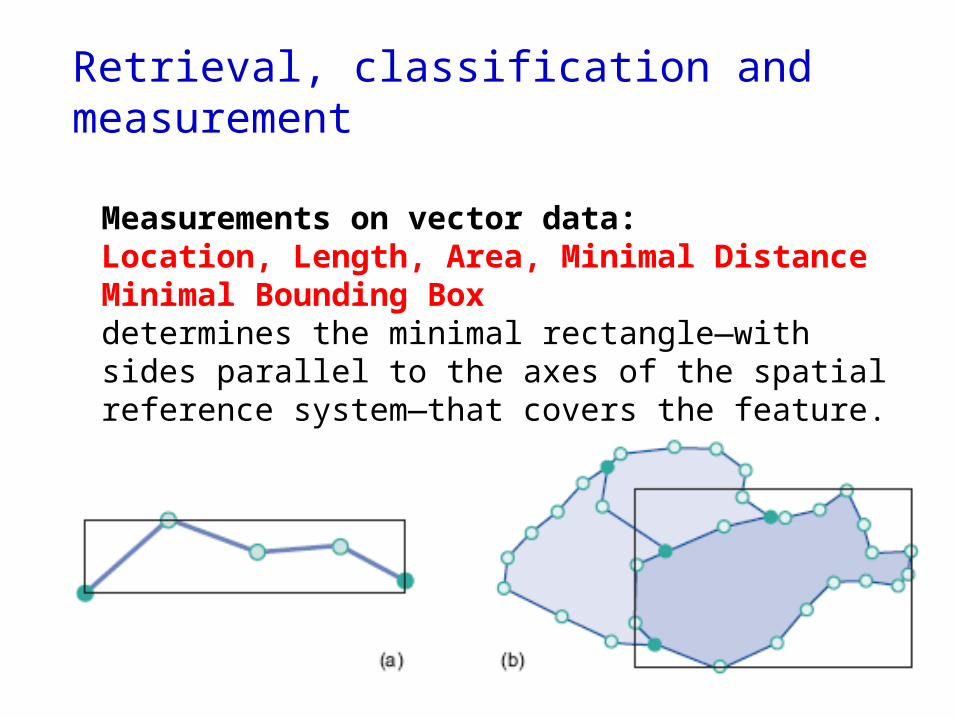
Measurements on vector data:Location, Length, Area, Minimal DistanceMinimal Bounding Boxdetermines the minimal rectangle—with sides parallel to the axes of the spatial reference system—that covers the feature.

Measurement
Length (Lines)
by Pythagorean theorem
Area (Polygons)
by dividing the polygon into triangles whose areas can easily be calculated
212
212 yyxxD
1
2
D

Retrieval, classification and measurement
Measurements on raster data:
The geometric information stored with the raster data is:Horizontal and vertical resolution, and the location of an anchor point so all other measurements by the GIS are computed.
The anchor point is fixed by convention to be the lower left (or sometimes upper left) location of the raster.

Spatial selection queries
• Spatial selection by attribute conditions

Spatial selection queries
• Spatial selection using topological relationships
InsideIntersectAdjacentIn distance with
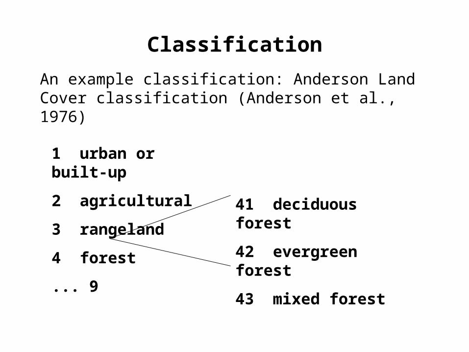
Classification
An example classification: Anderson Land Cover classification (Anderson et al., 1976)
1 urban or built-up
2 agricultural
3 rangeland
4 forest
... 9
41 deciduous forest
42 evergreen forest
43 mixed forest
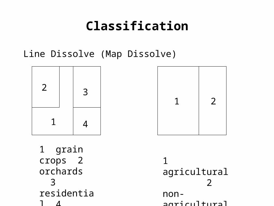
Classification
Line Dissolve (Map Dissolve)
1 grain crops 2 orchards 3 residential 4 commercial
1 agricultural 2 non-agricultural
2
1
3
4
1 2
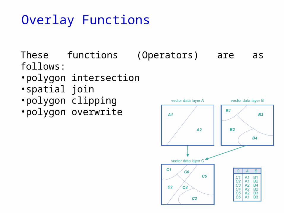
Overlay Functions
These functions (Operators) are as follows:•polygon intersection•spatial join•polygon clipping•polygon overwrite

Overlay
A series of registered data layers ‘overlaying’ each other
Arguably the most important GIS analysis function

Overlay
Derived from manual cartographic overlay using Mylar sheets (transparent plastic) that were physically overlaid on top of one another.

Overlay
An overlay operation takes two or more data layers as input and results in an output data layer
Three types of overlay:
Point in polygon
Line in polygon
Polygon (polygon on polygon)

Point in Polygon Overlay
A
BC
ID Tree
A Elm B Maple C Elm
Point Table
ID Tree Cover
A Elm Rural B Maple Rural C Elm Urban
Point Table
ID Cover
1 Rural 2 Urban
Poly Table
1 2
+ A
BC=
Land CoverTrees NewTrees
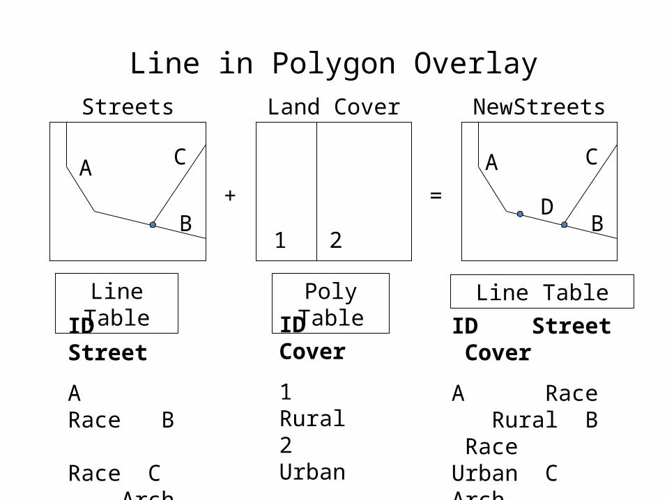
Line in Polygon Overlay
A
B
C
ID Street
A Race B Race C Arch
Line Table
ID Street Cover
A Race Rural B Race Urban C Arch Urban D Race Urban
Line Table
ID Cover
1 Rural 2 Urban
Poly Table
1 2
+ =
Land CoverStreets NewStreets
A
B
C
D

Polygon Overlay
Intersection (and) Union (or) Identity

Polygon Overlay: Intersection
Agriculture
A
B
A
Land Cover
ID Owner
A Brown B Smith
ID Cover
A commercial B industrial
B
Area of intersection
New node
<Intermediate>

Polygon Overlay: Intersection
Output
ID Owner Cover
A Brown commercial
B Smith industrial
A
B
Area of intersection
New node
<Intermediate>
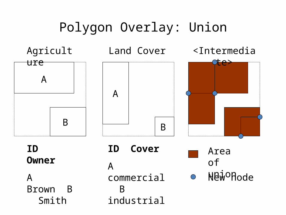
Polygon Overlay: Union
Agriculture
A
B
A
ID Owner
A Brown B Smith
ID Cover
A commercial B industrial
B
Area of union
New node
<Intermediate>Land Cover

Polygon Overlay: Union
Area of union
New node
<Intermediate>
Output
ID Owner Cover
A commercial B Brown commercial C Brown D Smith E Smith industrial
A
B C
D E

Polygon Overlay: Identity
Agriculture (input layer)
A
B
A
Land Cover (identity layer)
ID Owner
A Brown B Smith
ID Cover
A commercial B industrial
B
Area of identity
New node
<Intermediate>

Polygon Overlay: Identity
Area of identity
New node
<Intermediate>
Output
ID Owner Cover
A Brown commercial B Brown C Smith D Smith industrial
A B
C D
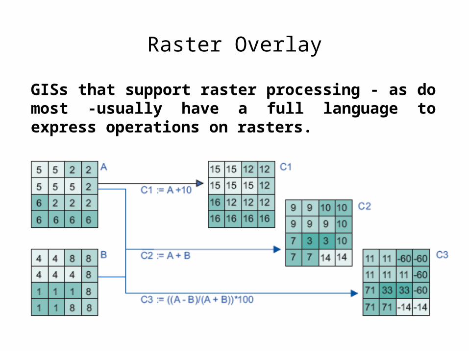
Raster Overlay
GISs that support raster processing - as do most -usually have a full language to express operations on rasters.

Neighbourhood functions
To perform neighbourhood analysis, we must:
1.state which target locations are of interest to us, and what is their spatial extent,
2.define how to determine the neighbourhood for each target,
3.define which characteristic(s) must be computed for each neighbourhood.

Neighbourhood functions
Proximity computation:
1.Buffer zone generation
2.Thiessen polygon generation

Neighbourhood functions
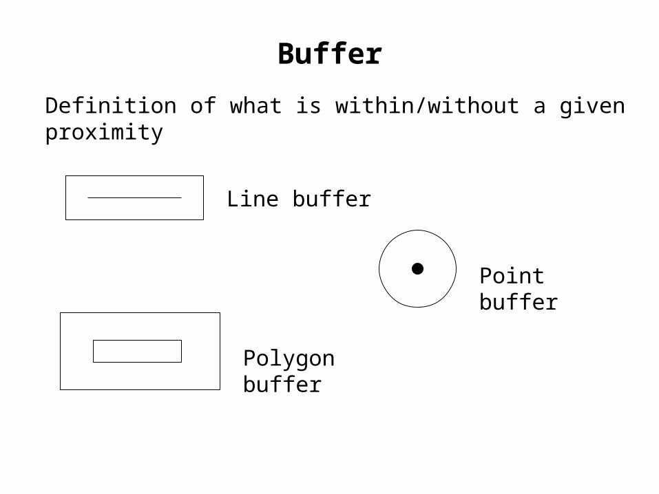
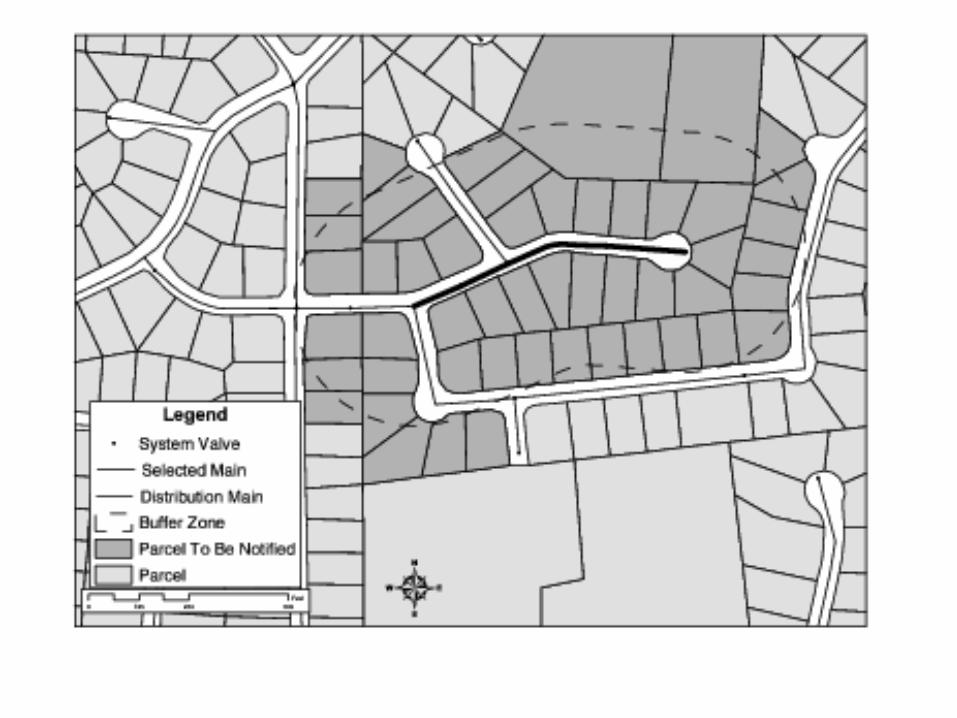
Buffer
Definition of what is within/without a given proximity
Point buffer
Line buffer
Polygon buffer
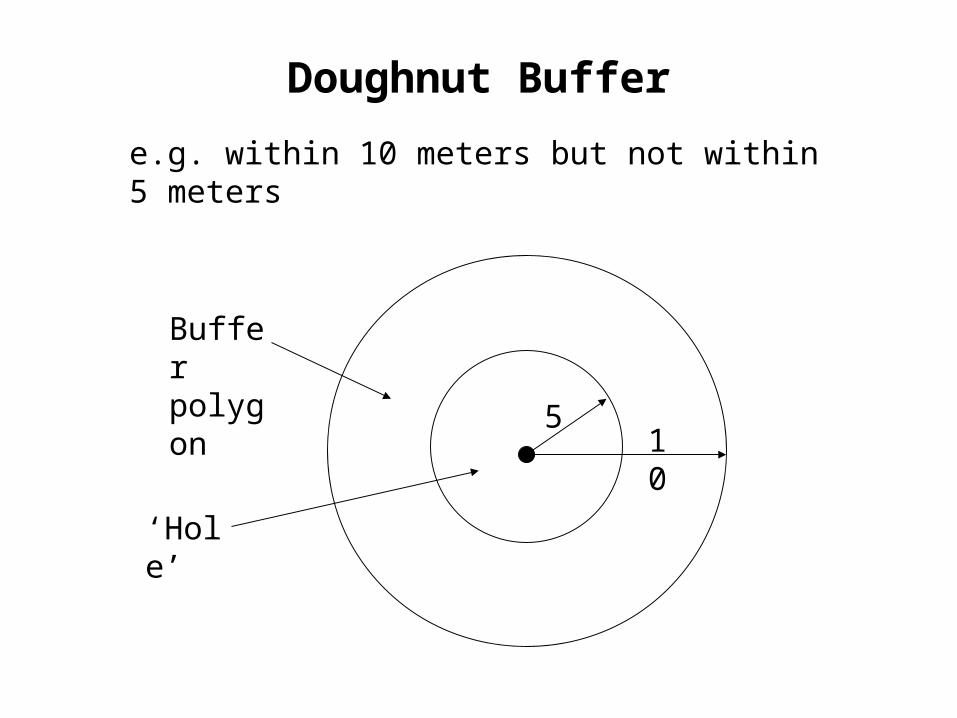
Doughnut Buffer
e.g. within 10 meters but not within 5 meters
105
Buffer polygon
‘Hole’

Variable Buffer
Buffer distance varies by some feature attribute or friction surface

Variable Buffer
Buffer polygon
A B
C
ID Dist
A 3 B 2 C 5
6 4
10
Original line

Neighbourhood functions

Table 12.3 Computing water use based on land-use area
Node
Total Node Area (ha)
Land Use Type
Land Use
Area (ha)
Unit Demand
(l/day/ha)
Demand
(l/day)
Node Total
(l/day)
J-1 6.88 Industrial 6.88 11,200 77,100 77,100
J-2 7.69 IndustrialCommercialResidential
1.380.925.38
11,2004,7007,500
15,5004,30040,400
60,200
J-3 7.69 CommercialResidentialUndeveloped
1.315.151.23
4,7007,5000
6,10038,6000
44,800
J-4 8.50
IndustrialCommercialResidentialUndeveloped
0.170.102.455.78
11,2004,7007,5000
1,90047018,4000
20,800
J-5 8.09 IndustrialCommercial
6.481.62
11,2004,700
72,5007,600
80,100
J-6 4.86 IndustrialCommercialResidential
0.201.363.30
11,2004,7007,500
2,2006,40024,800
33,400

Network Analysis
A network is a connected set of lines, representing some geographic phenomenon, typically of the transportation type.
Network analysis can be done using either raster or vector data layers, but they are more commonly done in the latter, as line features can be associated with a network naturally, and can be given typical transportation characteristics like capacity and cost per unit.

Network Analysis